optimal portfolio selection with transaction costs and

Optimal Portfolio Selection withTransaction Costs and Finite Horizons

Hong LiuWashington University

Mark LoewensteinBoston University

We examine the optimal trading strategy for a CRRA investor who maximizes theexpected utility of wealth on a finite date and faces transaction costs. Closed-form solu-tions are obtained when this date is uncertain. We then show a sequence of analyticalsolutions converge to the solution to the problem with a deterministic finite horizon.Consistent with the common life-cycle investment advice, the optimal trading strategyis found to be horizon dependent and largely buy and hold. Moreover, it might be opti-mal for the investor in our model not to buy any stock, even when the risk premium ispositive. Further analysis of the optimal policy is also provided.

Financial advisers typically recommend that younger investors should allo-cate a greater share of wealth to stocks than older investors and all investorsshould follow a largely buy-and-hold strategy. Representative of this conven-tional wisdom, Malkiel (2000), in his popular book A Random Walk DownWall Street, states that “The longer period over which you can hold on toyour investments, the greater should be the share of common stocks in yourportfolio. � � � [M]oreover, these returns are gained by the steady strategy ofbuying and holding your diversified portfolio.” To be consistent with thisclearly horizon-dependent portfolio rule, a model must be of finite horizonby definition. Moreover, when an investor invests for a specific event, such asbequest or retirement, his horizon is also clearly finite. However, the finite-ness of the horizon alone is not sufficient to justify the horizon-dependentinvestment strategy. For example, in Samuelson (1969) and Merton (1971),even though the investor has a finite horizon, his optimal fraction of wealthinvested in the stock is still horizon independent.

Assuming time-varying investment opportunities or other time-varyingparameters would imply horizon-dependent portfolio rules [Kim andOmberg (1996), Brennan, Schwartz, and Lagnado (1997), Liu (1999)]. How-ever, these models do not produce buy-and-hold rules and it is still hard

Much of this work was completed while M. Loewenstein was at Washington University in St. Louis. We aregrateful to an anonymous referee for useful suggestions. We also thank Jerome Detemple, Phil Dybvig, GaryGorton (the editor), Tao Li, Guofu Zhou, and seminar participants at Fudan University, Hong Kong Univer-sity of Science and Technology, Tsinghua University, University of Science and Technology of China, andUniversity of Utah for helpful comments. All errors are our responsibility. Address correspondence to HongLiu, Olin School of Business, Washington University, St. Louis, MO 63130, or e-mail: [email protected] [email protected].

The Review of Financial Studies Summer 2002 Vol. 15, No. 3, pp. 805–835© 2002 The Society for Financial Studies

The Review of Financial Studies / v 15 n 3 2002

to explain in general why, as an investor gets older, he should invest asmaller fraction of wealth in stock. Introduction of labor income can poten-tially explain the inverse relationship between age and the fraction of wealthinvested in stocks [Bodie, Merton, and Samuelson (1992), Jagannathan andKocherlakota (1996), Campbell and Viceira (1999)]. However, these modelsgenerally do not produce buy-and-hold strategies either.

Jagannathan and Kocherlakota (1996) examine several possible explana-tions of the above life-cycle investment advice. In particular, they show thatif investors with constant relative risk aversion (CRRA) preferences overterminal wealth are restricted to buy-and-hold strategies due to transactioncosts, the optimal portfolio choice is largely horizon independent. However,they do not account for the transaction costs incurred by an investor, and inthis case whether an investor optimally chooses to engage in a buy-and-holdstrategy should depend on the time interval over which the portfolio is held.

In this article, instead of assuming time-varying parameters or labor in-come or buy and hold as in the above articles, we show that the presenceof transaction costs (which are certainly present in most financial markets)together with a finite horizon would imply a time-varying and largely buy-and-hold trading strategy which is consistent with the above life-cycle invest-ment advice.1 In particular, we examine the optimal transaction policy fora CRRA investor who has a finite horizon and is subject to proportionaltransaction costs in stock trading. Our analysis reveals that an investor witha longer horizon would tend to hold more stock in his portfolio. Thus thehorizon becomes an important element of the investor’s optimal decision pro-cess. Moreover, even small transaction costs lead to dramatic changes in theoptimal behavior for an investor: from continuous trading to virtually buy-and-hold strategies. For example, an investor whose horizon is 10 years mayexpect to hold a position in the asset subject to transaction costs for 5 years.In addition, for the first time in the literature (as far as we know), we deriveexplicit bounds on the transaction boundaries. Our analysis also shows thatan investor might optimally never buy the stock subject to transaction costs,even when there is a positive risk premium. We provide explicit necessaryand sufficient conditions for this to happen in all the cases we analyze. Intu-itively, an investor who does not expect to live long enough for the excessreturn on the asset to overcome the transaction costs would optimally neverbuy the asset.

There are a large number of articles studying the optimal transaction policyfor an agent facing transaction costs in the financial markets. Constantinides(1979, 1986), Davis and Norman (1990), and Shreve and Soner (1994) studyan infinite horizon problem where the investor maximizes discounted utilityof intermediate consumption. Dumas and Luciano (1991) study the problem

1 Adding labor income to our model would clearly reinforce the main results in the article in the same manneras in Jagannathan and Kocherlakota (1996).

806

Optimal Portfolio Selection

of maximizing terminal utility of wealth in the limit as the horizon gets verylarge. For these analyses, the investor’s horizon is infinite and, as a result,if the risk premium is positive the investor always optimally invests in thestock, even with transaction costs. Davis, Panas, and Zariphopoulou (1993)show the existence and uniqueness of the solution to a deterministic finitehorizon problem and provide a discretization scheme to numerically solve theproblem. Cvitanic and Karatzas (1996) and Loewenstein (2000) also studya deterministic finite horizon problem but do not provide specific solutions.Gennotte and Jung (1994) and Balduzzi and Lynch (1999) use binomial ordiscrete approximations to numerically compute the optimal trading strategyfor an investor with a finite horizon. While a numerical approach may allowmore flexible specifications of the form of the asset market, it provides lit-tle insight into the global properties of the optimal solutions. Moreover, theoptimal solutions in these approaches can be sensitive to the choice of dis-cretization. In contrast, this article proposes a methodology to analyticallyapproximate the optimal strategy. It shows that this approach is indeed validand provides approximations that are less prone to approximation error.

In order to focus on the effect of the horizon on an investor’s investmentdecision in the presence of transaction costs, we restrict our attention tothe case where the investor wishes to maximize the utility of wealth on afinite date, although much of our analysis is applicable to the case withintermediate consumption. This choice of objective function is appropriatefor an individual who is investing for a specific event in the future. A directattack on solving the transaction cost problem with a deterministic horizoninvolves solving a partial differential equation with two free boundaries; thisis difficult because these two free boundaries also change through time.2 Herewe propose a different approach, based on an idea in Carr (1998).

We first examine the optimization problem for an investor maximizingexpected CRRA utility of wealth at an uncertain time, which is assumed tobe the first jump time of an independent Poisson process (thus the horizonis exponentially distributed). This analysis is of independent interest sincemany lifetime events such as disability or retirement occur at an uncertaintime.3 This case bears some resemblance, although with important economicdifferences, to the analysis in Dumas and Luciano (1991), where they exam-ine the limiting strategy as the investor’s horizon becomes large. In particular,the optimal trading strategy is also time independent in this case. However,in contrast to the asymptotic analysis in Dumas and Luciano (1991), whofound no bias in favor of cash in the optimal portfolio, a finite horizon caninduce a bias in favor of cash; our investor may optimally never buy the assetsubject to transaction costs if the expected horizon is short.

2 Recall that there is only one moving boundary for an American put option with finite maturity.3 Previous asset pricing literature has explored portfolio optimization in frictionless markets with uncertain

lifetime such as Cass and Yaari (1967), Merton (1971), and Richard (1975).

807


As in most of the literature on optimal investment with transaction costs[e.g., Davis and Norman (1990), Grossman and Laroque (1990), Cuoco andLiu (2000)], the optimization problem in this case amounts to a singularstochastic control problem. We obtain analytic expressions for the value func-tion as the closed form solution to an ordinary differential equation subjectto certain free boundary conditions. We find that the optimal transaction pol-icy is to maintain the ratio of the dollar amount in the risk-free asset to theamount in the risky asset within a wedge, represented by the buy boundaryand the sell boundary.

We also derive explicit, horizon-independent bounds on the boundaries.We show that the ratio at the buy boundary is always greater than the ratioin the absence of transaction costs (the Merton line). However, the ratio atthe sell boundary could also be greater than the Merton line, which meansthat the entire no-transaction region could be above the Merton line.

We then extend the above analysis to the case where the terminal dateoccurs at the time of the nth (n > 1) jump of an independent Poisson process(thus the horizon is Erlang distributed). As expected, the optimal transactionboundaries become state dependent and jump each time the Poisson processjumps. We also demonstrate that the bounds on the transaction boundariesobtained in the previous case still apply.

Finally, we show that the value function and transaction boundaries inthe Erlang distributed case converge to the value function and transactionboundaries, respectively, for an investor with a deterministic finite horizon.This implies that the bounds on boundaries derived in the previous cases arealso valid for the deterministic horizon case. We also show that the tradingboundaries for the exponentially distributed horizon case can be regarded asapproximations to the trading boundaries for the deterministic finite horizoncase.

Since the optimal trading boundaries for investors with exponentially dis-tributed horizons approximate those for the Erlang distributed and deter-ministic horizons, we provide detailed analysis of the trading behavior ofinvestors with exponentially distributed horizons. In particular, we examinehow the optimal transaction boundaries change as the coefficients of themodel change. In general, the comparative statics follow those known in thefrictionless case. However, we find that the buy boundary is more sensitiveto parameter changes than the sell boundary. Furthermore, the sensitivity ofthe buy boundary increases as the horizon decreases. We also examine theexpected time to sale after purchase and find that the optimal trading strat-egy is indeed largely buy and hold, consistent with much of the conventionalwisdom.

The remainder of the article is organized as follows. In Section 1 wedescribe the basic model where an investor has a finite deterministic horizon.In Section 2 we solve the problem for an investor with an exponentiallydistributed horizon. In Section 3 we extend the problem to the case where

808


the investor’s horizon is Erlang distributed, and in Section 4 we show thatthe solutions in Section 3 converge to those for the basic model specifiedin Section 1. Section 5 provides comparative statics and further analysis ofoptimal trading policies. Section 6 concludes with some possible extensionsof the model and applications of the methodology.

1. The Basic Model

1.1 The asset marketThroughout this article we are assuming a probability space �� P� anda filtration �t�. Uncertainty in the model is generated by a standard one-dimensional Brownian motion w. We will assume that wt is adapted.

There are two assets our investor can trade. The first asset (“the bond”)is a money market account growing at a continuously compounded, constantrate r . The second asset (“the stock”) is a risky investment. The investor canbuy the stock at the ask price, SA

t = St , and sell the stock at the bid price,SB

t = �1−��St ,4 where 0 ≤ � < 1 represents the proportional transaction cost

rate5 and St is given by

St = S0e��−�2/2�t+�wt � (1)

where we assume all parameters are positive constants and � > r .When � > 0, the above model gives rise to equations governing the evo-

lution of the amount invested in the bond, xt , and the amount invested in thestock, yt:

dxt = rxt dt−dIt + �1−��dDt� (2)

dyt = �yt dt+�yt dwt +dIt −dDt� (3)

where the processes D and I represent the cumulative dollar amount of salesand purchases of the stock, respectively. These processes are nondecreasing,right continuous adapted processes with D�0� = I�0� = 0. Let x0 and y0 bethe given initial positions in the bond and the stock, respectively. We let��x0� y0� denote the set of admissible trading strategies �D� I� such thatEquations (2) and (3) are satisfied and the investor is always solvent, that is,

xt + �1−��yt ≥ 0�∀ t ≥ 0� (4)

4 We choose the ask price SAt instead of the midpoint [as in Davis and Norman (1990)] as the numeraire for

notational simplicity without any loss of generality. This does not imply no transaction costs when purchasingthe stock. In fact, SA

t should be interpreted as the stock price inclusive of the transaction cost for purchasing.5 In our model, the case where � = 1 is a trivial case since no investor with monotonic preferences would ever

buy the stock.

809


1.2 The investor’s problemIn order to highlight the role of the horizon, we assume the utility of aninvestor only depends on the market value of his portfolio at a determin-istic time T . This is consistent with earlier models in the literature [e.g.,Dumas and Luciano (1991), Brennan, Schwartz, and Lagnado (1997)]. Theinvestor’s problem is to choose trading strategies D and I so as to maximizeE u�xT + �1−��yT �" subject to Equations (2), (3), and (4). We assume thatthe investor has CRRA preference, that is, u�W� = W 1−$

1−$for $ > 0, $ �= 1.6

To solve this problem, we define the value function at time t as

V �x� y� t� = sup�D� I�∈��x� y�

E

[�xT + �1−��yT �1−$

1−$

∣∣∣∣�t

]� (5)

1.3 Optimal policies with no transaction costsFor the purpose of comparison we present results, due to Merton (1971),for the case when there are no transaction costs (� = 0) without proof. Inthis case, the cumulative purchases and sales of the stock can be of infinitevariation. The investor’s problem can be written as

V �x� y�0� = supyt &t≥0�

E

[�xT +yT �1−$

1−$

]�

subject to

d�xt +yt� = r�xt +yt�dt+ ��− r�yt dt+�yt dwt� (6)

In this case, it is well known that the optimal policy involves investinga constant fraction of wealth in the stock and the fraction is independentof the investor’s horizon. It is important to note that as long as � > r , theinvestor always optimally holds some of the risky asset. Here we will sketchthe solution and define parameters which will be used in the sequel. Withouttransaction costs, the optimal stock investment policy can be shown to be

y∗t =

1r∗ +1

�x∗t +y∗

t � (7)

for all 0 < t < T , where the “Merton line” r∗ is given by

r∗ = $�2

�− r−1� (8)

The lifetime expected utility is

V �x� y�0� = e'T �x+y�1−$

1−$� (9)

6 Similar results for $ = 1 (i.e., log utility) can be derived.

810


where

' = �1−$�

(r + (

$

)(10)

and

( = ��− r�2

2�2� (11)

1.4 The transaction cost caseIn the case where � > 0, the problem is considerably more complicated.Here we outline a direct approach: first, we postulate that the region wherethe investor has positive wealth, the solvency region,

� = �y� x� & x+ �1−��y > 0��

at each point in time splits into a “buy” region, a “no-transaction” region,and a “sell” region, as in Davis and Norman (1990). Under regularity condi-tions on the value function, we have the following Hamilton–Bellman–Jacobi(HJB) equation,

12�2y2Vyy + rxVx +�yVy +Vt = 0�

in the no-transaction region. In the buy region, the marginal cost of decreas-ing the amount in the bond is equal to the marginal benefit of increasing theamount in the stock, that is,

Vx = Vy�

Similarly, in the sell region, the marginal benefit of increasing the amount inthe bond must be equal to the marginal cost of decreasing the amount in thestock, that is,

�1−��Vx = Vy�

In addition, we must have the terminal condition

limt→T

V �x� y� t� = �x+ �1−��y�1−$

1−$�

It follows immediately from the homogeneity of the utility function u, theconvexity of the set of admissible strategies, and the fact that ��)x�)y� =)��x� y� for all ) > 0 that the value function V is concave and homogeneousof degree 1−$ in �x� y� [cf. Fleming and Soner (1993), Lemma VIII.3.2].This homogeneity implies

V �x� y� t� = y1−$*

(x

y� t

)�

for some function *& ��−1��× 0� T " → �. Let

811


z = x

y(12)

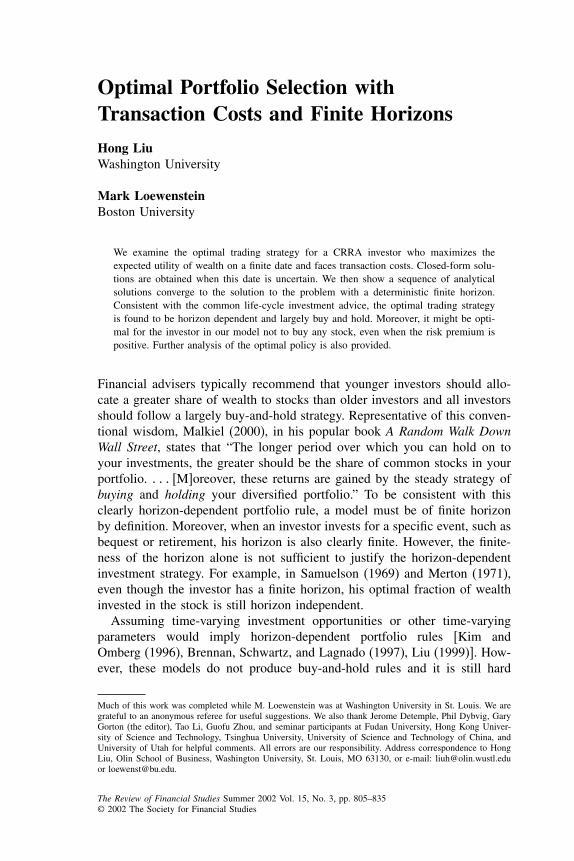
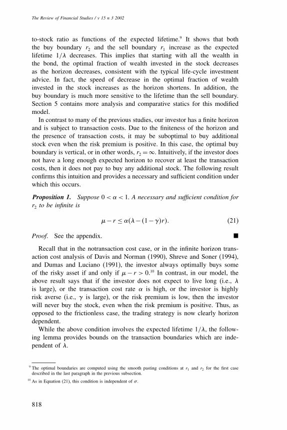
denote the ratio of the amount invested in the bond to the amount invested inthe stock. The homogeneity property then implies that the buy, no-transaction,and sell regions can be described by two functions of time r1�t� and r2�t�.The buy region corresponds to z ≥ r2�t�, the sell region to z ≤ r1�t�, and theno-transaction region to r1�t� < z < r2�t�, as depicted in Figure 1.

Using these properties, we obtain a partial differential equation for * inthe no-transaction region (r1�t� < z < r2�t�):

12�2z2*zz + �$�2 − ��− r��z*z − �1−$��$�2/2−��*+*t = 0�

In the buy region (z ≥ r2�t�), we have

�z+1�*z�z� t� = �1−$�*�z� t��

Similarly, in the sell region (z ≤ r1�t�), we have

�z+1−��*z�z� t� = �1−$�*�z� t��

In addition, * must also satisfy the terminal condition

limt→T

*�z� t� = �z+1−��1−$

1−$�

This system of equations involves finding a pair of moving boundaries r1�t�and r2�t� and is difficult to solve. In the subsequent sections we develop an

Figure 1The solvency region

812


alternative methodology which can circumvent this difficulty and lead to asolution for the optimal trading policy.

2. Exponentially Distributed Horizon

In this section, as a first step toward solving the problem, we modify the opti-mization problem so that our investor has an uncertain horizon. In particular,the investor’s problem is now to choose admissible trading strategies D andI so as to maximize E u�x, + �1−��y,�" for an event which occurs at thefirst jump time , of a standard, independent Poisson process with intensity-. , is thus exponentially distributed with parameter -, that is,

P, ∈ dt� = -e−-t dt�

This modified model yields a closed-form solution for the value functionand serves as a foundation for solving the basic model specified in the pre-vious section. Moreover, it can also be of independent interest. For example,bequest, accidents, retirement, and many other events happen on uncertaindates.

If , is interpreted to represent the investor’s uncertain lifetime [as inMerton (1971) and Richard (1975)], the investor’s average lifetime is then1/- and the variance of his lifetime is accordingly 1/-2.

We can then write the value function as

v�x� y� = sup�D� I�∈��x� y�

E

[�x, + �1−��y,�

1−$

1−$

]� (13)

In light of our assumptions on , and the asset market, this can be rewrittenas [see Merton (1971), Carr (1998)]

v�x� y� = sup�D� I�∈��x� y�

-E

[∫ �

0e−-t �xt + �1−��yt�

1−$

1−$dt

]� (14)

Thus the investor’s problem [Equation (13)] can be solved by solving thetransformed problem [Equation (14)]. The critical difference from the basicmodel is the absence of the time dimension, which significantly simplifiesthe problem.

2.1 Optimal policies with no transaction costsAgain, for purpose of comparison, let us first consider the case without trans-action costs (� = 0). In this case, the investor’s problem becomes

v�x� y� = supyt &t≥0�

-E

[∫ �

0e−-t �xt +yt�

1−$

1−$dt

]�

subject to the self-financing condition [Equation (6)].

813


The above problem is formally similar to the one studied by Merton(1971). As in Merton (1971), a condition on the parameters is required forthe existence of the optimal solution.7

Assumption 1. The investor’s expected horizon parameter - satisfies

- > �1−$�

(r + (

$

)�

where ( is as defined in Equation (11).

Assumption 1 is necessary because if the investor expects to live a longtime (- is small) then the risk-free rate must be low enough and the stockcannot deliver too high a risk premium ��− r� with low risk (�), otherwisethe investor can obtain bliss levels of utility by investing in either the stock(if ( is too high) or the bond (if r is too high). We summarize the main resultfor this case of no transaction costs without proof in the following lemma.

Lemma 1. Suppose that � = 0. Then the optimal stock investment policy isEquations (7) and (8) for 0 ≤ t ≤ , . Moreover, the lifetime expected utility is

v�x� y� = -

-−'

�x+y�1−$

1−$�

where ' is as defined in Equation (10).

Thus, without transaction costs, the optimal policy involves investing thesame horizon-independent, constant fraction of total wealth in the stock andthe bond as in the deterministic horizon case in Section 1.3. This is similarin spirit to the observation in Samuelson (1969) that the optimal portfoliodoes not depend on the investor’s horizon. Moreover, it is always optimal toinvest some in the stock if the expected return in the stock is greater than theinterest rate. We will see later that all these features disappear in the presenceof even small transaction costs.

2.2 Optimal policies with transaction costsSuppose now that � > 0. As in Section 1.4, the value function is homoge-neous of degree 1−$ in �x� y�. This implies that

v�x� y� = y1−$/

(x

y

)(15)

for some concave function /& ��−1�� → �.

7 Introducing time discounting in the preference or restricting to the case with $ > 1 would make this assump-tion unnecessary or automatically satisfied and all the subsequent results still hold with, at most, minormodifications.

814


Similar to Section 1.4, the solvency region splits into three regions: buyregion, sell region, and no-transaction region. In contrast to Section 1.4, how-ever, because of the time homogeneity of the value function, these regionscan be identified by two critical numbers (instead of functions of time) r1 andr2. The buy region corresponds to z ≥ r2, the sell region to z ≤ r1, and theno-transaction region to r1 < z < r2, where z is as defined in Equation (12).

Under regularity conditions on v, we have the following HJB equation:

12�2y2vyy + rxvx +�yvy −-v+ -�x+ �1−��y�1−$

1−$= 0 (16)

in the no-transaction region, with the associated conditions

vx = vy

in the buy region, and�1−��vx = vy

in the sell region.Using Equation (15), we can simplify the PDE in Equation (16) to get the

following ordinary differential equation in the no-transaction region:

z2/zz +)2z/z +)1/+)0

�z+1−��1−$

1−$= 0� (17)

where )2 = 2�$�2−��−r��/�2, )1 =−2�-+�1−$��$�2/2−��/�2, and)0 = 2-/�2. The associated boundary conditions are transformed into

�z+1�/z�z� = �1−$�/�z�

for all z ≥ r2 and�z+1−��/z�z� = �1−$�/�z�

for all z ≤ r1. Define

n1�2 =�1−)2�±

√�1−)2�

2 −4)1

2�

Assumption 1 implies that �1−)2�2−4)1 > 0. The solutions to the homoge-

neous part of Equation (17) can therefore be characterized by the fundamentalsolutions /1 and /2, where

/1�z� = �z�n1� /2�z� = �z�n2 �

The general solution to Equation (17) can thus be written as

C1/1�z�+C2/2�z�+/p�z��

815


where C1 and C2 are integration constants and the particular solution [seeBoyce and DiPrima (1969)]

/p�z� = )0

∫ z

r∗

/1�2�/2�z�−/1�z�/2�2�

/′1�2�/2�2�−/1�2�/′

2�2�

�2+1−��1−$

�1−$�22d2�

The above discussions imply that

/�z� =

A�z+1�1−$

1−$if z ≥ r2

C1/1�z�+C2/2�z�+/p�z� if r1 ∨0 < z < r2 ∨0

�C1/1�z�+ �C2/2�z�+/p�z� if r1 ∧0 < z < r2 ∧0

B �z+1−��1−$

1−$if �−1 < z ≤ r1�

(18)

for some constants A�B�C1�C2� �C1� �C2� r1, and r2.We have the following result on the existence of the value function and

the optimal trading strategy for the modified model.

Theorem 1. There exist constants A, B, C1, C2, �C1, �C2, r1, and r2 such that

1. /�z� is a C2 function on ��−1�0� and �0��,2. /�z� satisfies the following: if r2 =�, then

limy→0�x>0

y1−$/

(x

y

)= -

-− �1−$�r

x1−$

1−$(19)

and if r1 ≤ 0 ≤ r2, then

limx→0

y1−$/

(x

y

)

= -

�1−$��-− �1−$��+$�1−$��2

2 ��1−��y�1−$� (20)

3. v�x� y� = y1−$/(

xy

)is the value function.

Moreover, the optimal transaction policy is to transact the minimal amountin order to maintain z between r1 and r2.

Proof. The proof is similar to the references below. Since this is not thefocus of our analysis, we refer the interested reader to these sources fordetails. The basic idea is to note that the value function in Equation (14) is apiecewise C2 solution of Equation (16).8 This, combined with convex analysis

8 Here we need to allow for the fact that the value function may not be a C2 function at z = 0 (and thus not aclassic solution) if the x axis is contained in the no-transaction region. This really causes no problem, sincethe optimal policy will never cross the axis in this case. Proposition 5 formally demonstrates this fact.

816


of the value function along the lines of Shreve and Soner (1994), reveals thatthe value function itself will satisfy the conditions stated in the theorem.Thus we are assured of the existence of the function above. The existence ofan optimal transaction policy then follows directly from Fleming and Soner(1993), Theorem VIII.4.1. �

In order to solve for the value function and the optimal trading strategy, weneed to consider three cases. If r2 is finite and the no-transaction region doesnot contain 0, then we need to determine six constants A�B�C1�C2� r1, andr2 using Equation (18) and the C2 property (the “smooth pasting conditions”)of / across r1 and r2. If r2 is finite but the no-transaction region contains0, then we need to determine eight constants A�B�C1�C2� �C1� �C2� r1, and r2

using Equation (18), the C2 property of / across r1 and r2 and the condition[Equation (20)] at z = 0. If r2 is infinite, then the only boundary conditionat r2 would be Equation (19), but other boundary conditions apply as in theprevious two cases. For the first case, algebraic manipulation can reduce thesix equations to two nonlinear equations for r1 and r2, which can be solvednumerically. Of course this search is easier if we can find bounds on r1 andr2 and conditions which tell us when r2 is infinite. The next section providesthis information.

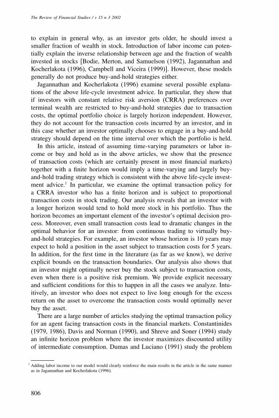
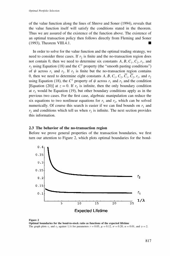
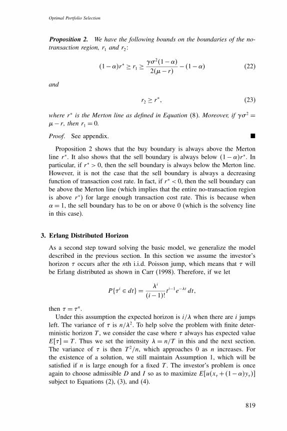
2.3 The behavior of the no-transaction regionBefore we prove general properties of the transaction boundaries, we firstturn our attention to Figure 2, which plots optimal boundaries for the bond-

Figure 2Optimal boundaries for the bond-to-stock ratio as functions of the expected lifetimeThe graph plots r1 and r2 against 1/- for parameters r = 0�05, � = 0�12, � = 0�20, � = 0�01, and $ = 2.

817


to-stock ratio as functions of the expected lifetime.9 It shows that boththe buy boundary r2 and the sell boundary r1 increase as the expectedlifetime 1/- decreases. This implies that starting with all the wealth inthe bond, the optimal fraction of wealth invested in the stock decreasesas the horizon decreases, consistent with the typical life-cycle investmentadvice. In fact, the speed of decrease in the optimal fraction of wealthinvested in the stock increases as the horizon shortens. In addition, thebuy boundary is much more sensitive to the lifetime than the sell boundary.Section 5 contains more analysis and comparative statics for this modifiedmodel.

In contrast to many of the previous studies, our investor has a finite horizonand is subject to transaction costs. Due to the finiteness of the horizon andthe presence of transaction costs, it may be suboptimal to buy additionalstock even when the risk premium is positive. In this case, the optimal buyboundary is vertical, or in other words, r2 =�. Intuitively, if the investor doesnot have a long enough expected horizon to recover at least the transactioncosts, then it does not pay to buy any additional stock. The following resultconfirms this intuition and provides a necessary and sufficient condition underwhich this occurs.

Proposition 1. Suppose 0 < � < 1. A necessary and sufficient condition forr2 to be infinite is

�− r ≤ ��-− �1−$�r�� (21)

Proof. See the appendix. �

Recall that in the notransaction cost case, or in the infinite horizon trans-action cost analysis of Davis and Norman (1990), Shreve and Soner (1994),and Dumas and Luciano (1991), the investor always optimally buys someof the risky asset if and only if �− r > 0.10 In contrast, in our model, theabove result says that if the investor does not expect to live long (i.e., -is large), or the transaction cost rate � is high, or the investor is highlyrisk averse (i.e., $ is large), or the risk premium is low, then the investorwill never buy the stock, even when the risk premium is positive. Thus, asopposed to the frictionless case, the trading strategy is now clearly horizondependent.

While the above condition involves the expected lifetime 1/-, the follow-ing lemma provides bounds on the transaction boundaries which are inde-pendent of -.

9 The optimal boundaries are computed using the smooth pasting conditions at r1 and r2 for the first casedescribed in the last paragraph in the previous subsection.

10 As in Equation (21), this condition is independent of � .

818


Proposition 2. We have the following bounds on the boundaries of the no-transaction region, r1 and r2:

�1−��r∗ ≥ r1 ≥$�2�1−��

2��− r�− �1−�� (22)

and

r2 ≥ r∗� (23)

where r∗ is the Merton line as defined in Equation (8). Moreover, if $�2 =�− r , then r1 = 0.

Proof. See appendix. �

Proposition 2 shows that the buy boundary is always above the Mertonline r∗. It also shows that the sell boundary is always below �1−��r∗. Inparticular, if r∗ > 0, then the sell boundary is always below the Merton line.However, it is not the case that the sell boundary is always a decreasingfunction of transaction cost rate. In fact, if r∗ < 0, then the sell boundary canbe above the Merton line (which implies that the entire no-transaction regionis above r∗) for large enough transaction cost rate. This is because when� = 1, the sell boundary has to be on or above 0 (which is the solvency linein this case).

3. Erlang Distributed Horizon

As a second step toward solving the basic model, we generalize the modeldescribed in the previous section. In this section we assume the investor’shorizon , occurs after the nth i.i.d. Poisson jump, which means that , willbe Erlang distributed as shown in Carr (1998). Therefore, if we let

P,i ∈ dt� = -i

�i−1�! ti−1e−-t dt�

then , = ,n.Under this assumption the expected horizon is i/- when there are i jumps

left. The variance of , is n/-2. To help solve the problem with finite deter-ministic horizon T , we consider the case where , always has expected valueE ," = T . Thus we set the intensity - = n/T in this and the next section.The variance of , is then T 2/n, which approaches 0 as n increases. Forthe existence of a solution, we still maintain Assumption 1, which will besatisfied if n is large enough for a fixed T . The investor’s problem is onceagain to choose admissible D and I so as to maximize E u�x, + �1−��y,�"subject to Equations (2), (3), and (4).

819


3.1 Optimal policies with no transaction costsIn this subsection we present results without proof for the case when there areno transaction costs (�= 0) and the investor’s horizon , is Erlang distributed.The investor’s problem can be written as

vn�x� y� = supyt &t≥0�

E

[�x, +y,�

1−$

1−$

]�

subject to the budget constraint in Equation (6).

Lemma 2. Suppose that � = 0. The optimal stock investment policy is then

y∗t =

1r∗ +1

�x∗t +y∗

t ��

Moreover, the lifetime expected utility is

vn�x� y� = -n

�-−'�n

�x+y�1−$

1−$�

where ' is as defined in Equation (10). Moreover, with - = n/T , we have

limn→�vn�x� y� = e'T �x+y�1−$

1−$= V �x� y�0��

where V �x� y�0� is as defined in Equation (9).

Once again, without transaction costs, the optimal policy involves investinga constant fraction of total wealth in the stock and the bond, and this isindependent of the investor’s horizon. Also, notice that as we make n verylarge, the value function converges to the value function for the deterministichorizon case. We will show in Section 4 that this convergence result alsoholds in the presence of transaction costs.

3.2 Optimal policies with transaction costsLet vi�x� y� be the value function when there are i jumps left until the hori-zon,

vi�x� y� = sup�D� I�∈��x� y�

E

[�x�,i�+ �1−��y�,i��1−$

1−$

]�

and thus v0�x� y� = �x+�1−��y�1−$

1−$. Then to compute vi�x� y�, we can solve the

following recursive structure:

vi�x� y� = -E

[∫ �

0e−-tvi−1�xt� yt� dt

]� i = 1� � � � � n� (24)

820


As before, because of the homogeneity of vi�x� y�, there exists some function/i such that

vi�x� y� = y1−$/i

(x

y

)�

Solving Equation (24) reduces to finding functions /i�z� such that

z2/izz +)2z/

iz +)1/

i +)0/i−1 = 0� i = 1� � � � � n (25)

with the associated boundary conditions

�z+1�/iz�z� = �1−$�/i�z�� (26)

for all z ≥ r i2 and

�z+1−��/iz�z� = �1−$�/i�z�� (27)

for all z ≤ r i1, where )2, )1, and )0 are the same as in Equation (17) and r i

1

and r i2 represent the sell and buy boundaries, respectively, when there are i

jumps left. Moreover, the homogeneous solutions to Equation (25) are alsothe same as those for Equation (17). This leads to the general solution toEquation (25),

Ci1/1�z�+Ci

2/2�z�+/ip�z�� (28)

where Ci1 and Ci

2 are integration constants and the particular solution

/ip�z� = )0

∫ z

r∗

/1�2�/2�z�−/1�z�/2�2�

/′1�2�/2�2�−/1�2�/′

2�2�

/i−1�2�

22d2�

Equations (25)–(28) imply that

/i�z� =

Ai �z+1�1−$

1−$if z ≥ r i

2

Ci1/1�z�+Ci

2/2�z�+/ip�z� if r i

1 ∨0 < z < ri2 ∨0

�Ci1/1�z�+ �Ci

2/2�z�+/ip�z� if r i

1 ∧0 < z < ri2 ∧0

Bi �z+1−��1−$

1−$if �−1 < z ≤ r i

1�

for some constants Ai,Bi,Ci1,Ci

2, �Ci1, �Ci

2 and the boundaries r i1 and r i

2.As in the previous section, we need to find coefficients that make /i�z� a

C2 function on ��0� and �0�� and satisfy the appropriate limiting condi-tions when r i

2 is infinite or r i2 ≥ 0 ≥ r i

1. Notice that in this case the coefficientsAi,Bi,Ci

1,Ci2, �Ci

1, �Ci2, and the boundaries r i

1 and r i2 change each time the Pois-

son jump occurs. To save space, we omit the analogue of Theorem 1 for theErlang distributed horizon, but we are assured of the existence of a solutionto these equations by such a result.

821


To compute the optimal boundaries when there are i > 1 jumps left, wefirst compute r1

1 and r12 using the approach described in the last paragraph of

Section 2.2. We then iterate i−1 times using the same approach to obtain r i1

and r i2.

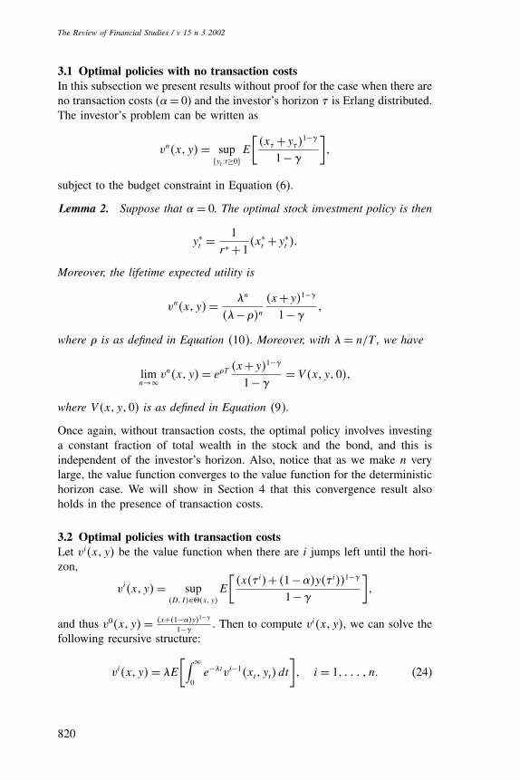
3.3 Behavior of the no-transaction regionFigure 3 plots r i

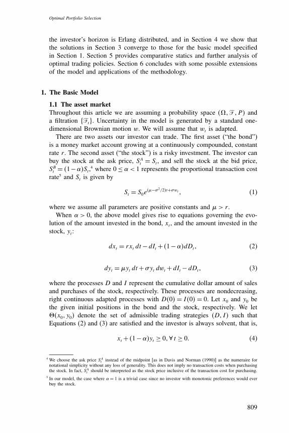
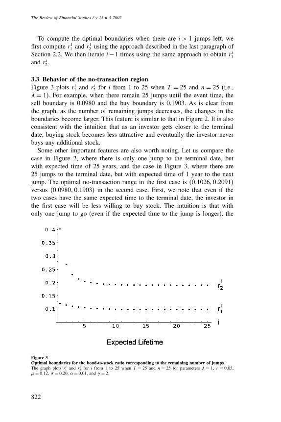
1 and r i2 for i from 1 to 25 when T = 25 and n = 25 (i.e.,

- = 1). For example, when there remain 25 jumps until the event time, thesell boundary is 0.0980 and the buy boundary is 0.1903. As is clear fromthe graph, as the number of remaining jumps decreases, the changes in theboundaries become larger. This feature is similar to that in Figure 2. It is alsoconsistent with the intuition that as an investor gets closer to the terminaldate, buying stock becomes less attractive and eventually the investor neverbuys any additional stock.

Some other important features are also worth noting. Let us compare thecase in Figure 2, where there is only one jump to the terminal date, butwith expected time of 25 years, and the case in Figure 3, where there are25 jumps to the terminal date, but with expected time of 1 year to the nextjump. The optimal no-transaction range in the first case is �0�1026�0�2091�versus �0�0980�0�1903� in the second case. First, we note that even if thetwo cases have the same expected time to the terminal date, the investor inthe first case will be less willing to buy stock. The intuition is that withonly one jump to go (even if the expected time to the jump is longer), the

Figure 3Optimal boundaries for the bond-to-stock ratio corresponding to the remaining number of jumpsThe graph plots r i

1 and r i2 for i from 1 to 25 when T = 25 and n = 25 for parameters - = 1, r = 0�05,

� = 0�12, � = 0�20, � = 0�01, and $ = 2.

822


uncertainty in the first case is much greater. In the second case, the investorhas a better idea along the way about how much time is left. It is this higheruncertainty that makes the investor in the first case less willing to buy stock.We also note that even though the first case has a much coarser grid than thesecond case, the differences between the initial trading boundaries in thesetwo cases are small, only 0.0046 and 0.0188, respectively, for the sell andbuy boundary. Thus we conjecture that the analysis in Section 2 will producea fairly accurate description of the initial trading boundaries for reasonableparameter values.

Next we provide the analogues to Propositions 1 and 2 for the investorwho has an Erlang distributed horizon:

Proposition 3. Suppose 0 < � < 1. A necessary and sufficient condition forr i

2 to be infinite is

�1−��1i �-− �1−$�r� ≤ �-−�+$r��

We also have the following bounds:

�1−��r∗ ≥ r i1 ≥

$�2�1−��

2��− r�− �1−��

andr i

2 ≥ r∗�

Moreover, if $�2 = �− r , then r i1 = 0.

Proof. Similar to Propositions 1 and 2. �

4. Deterministic Horizon

The deterministic finite horizon case in Section 1 can now be dealt withby using the model of the previous section. Suppose that in the previousmodel we make n very large and always maintain E ," = T (i.e., - = n/T ).Intuitively we should expect that the limiting value function would convergeto the value function of the case with a deterministic horizon T , since thevariance of , goes to zero as n gets large. This is indeed the case in the notransaction cost case as shown in Lemma 2 of Section 3.1. The followingtheorem confirms that this is also the case with the presence of transactioncosts.

Theorem 2. Let V �x� y� t� be as defined in Equation (5). Then

limn→�vn�x� y� = V �x� y�0��


This result shows that to approximate the value function for the prob-lem with finite deterministic horizon, one can solve the case with Erlangdistributed horizon with a large n.

823


4.1 Behavior of the no-transaction regionA natural question is whether the optimal transaction boundaries converge.Theorem 25.5 in Rockafellar (1970) implies that the value function will bedifferentiable on a dense set of the solvency region, and the homogene-ity property of the value function implies this dense set can be written asthe union of open convex cones. Theorem 25.7 in Rockafellar (1970) thenimplies that the derivatives of the value functions for the Erlang distributedhorizon will converge to those of the value function for the deterministichorizon on this union. Thus the transaction boundaries (which are defined bythe ratio of the derivatives) must also converge. In addition, the necessaryand sufficient condition for not buying any additional stock will converge tothe condition for the deterministic finite horizon case. Moreover, since thebounds in Proposition 3 are independent of -, they are still valid for thedeterministic horizon case. In particular, this shows that in the deterministic,finite horizon case, the time-varying buy boundary will always be above theMerton line r∗, and if r∗ > 0, the time-varying sell boundary will always bebelow the Merton line. We summarize the preceding remarks in the followingproposition.

Proposition 4. Let r1�t� and r2�t� be the optimal no-transaction boundariesat t ∈ 0� T " for the deterministic horizon problem as defined in Equation (5).A necessary and sufficient condition for r2�t� to be infinite is

�− r ≤− 1T − t

log�1−��

We also have the following bounds: ∀ t ∈ 0� T ",

�1−��r∗ ≥ r1�t� ≥$�2�1−��

2��− r�− �1−��

andr2�t� ≥ r∗�

Moreover, if $�2 = �− r , then ∀ t ∈ 0� T "� r1�t� = 0.

Proof. This is summarized in the discussion preceding the proposition. �

As far as we know, this is the first time explicit bounds for the opti-mal no-transaction boundaries are derived in the deterministic finite hori-zon case. Some articles, for example, Gennotte and Jung (1994), have useddiscrete approximations to solve the deterministic horizon investor problemwith transaction costs. However, these approximations can produce no traderegions which violate the above bounds due to discretization.

Theorem 2 and Figure 3 suggest that �0�0980�0�1903� is a good approxi-mation to the initial optimal range for the case with a deterministic horizon

824


of 25 years. According to Theorem 2, Figure 3 also approximates the behav-ior of the transaction boundaries as a function of remaining time in the casewith a deterministic horizon of 25 years.

Also, if we compare Figure 2 with Figure 3, we see that we can closelyapproximate the initial trading boundaries for an investor with a deterministichorizon T by the boundaries for an investor with an exponentially distributedhorizon with mean T . In addition, Propositions 4 and 2 imply that the buyboundary in the deterministic finite horizon case is infinite for a remaininglifetime of less than 0.1436, while the buy boundary is infinite in the expo-nentially distributed horizon case for an expected lifetime of less than 0.1439,which is only 0.0003 away. We thus conjecture that the trading boundariesfor exponentially distributed horizons produce a reasonable approximation ofthe trading boundaries for the deterministic horizon for reasonable parametervalues.

5. Further Analysis of the Exponential Horizon Case

In the previous section we showed that we can regard the optimal tradingboundaries for the exponentially distributed horizon case in Section 2 asa good approximation of the initial trading boundaries in the deterministichorizon case. In this section we provide further analysis of the optimal poli-cies for an investor with an exponentially distributed horizon. This analysisshould provide a fairly accurate description of the trading behavior of aninvestor with a deterministic horizon.

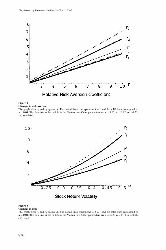
5.1 Changes in risk aversionFigure 4 shows the effect of the coefficient of relative risk aversion, $, onthe optimal trading boundaries for expected horizons of 1 year and 25 years.As $ increases, both r1 and r2 increase and the width of the no-transactionregion increases. Essentially a more risk-averse investor holds more of therisk-free asset. Of interest is that the sell boundary r1 is not sensitive tohorizon, even as risk aversion increases, but the buy boundary r2 increasesat a faster rate as the horizon decreases.

5.2 Changes in riskFigure 5 shows how the optimal transaction boundaries change as we changethe riskiness of the stock � for investors with expected horizons of 1 yearand 25 years. As stock return volatility increases, we see that not only r1

and r2, but also the width of the no-transaction region increase. Intuitivelythe risk-averse investor tends to invest less in the stock on average as therisk rises and he needs to widen the no-transaction region in order to avoidtransacting too frequently as the volatility increases. Also note that the sellboundary is not sensitive to the horizon as � increases. The buy boundary, onthe other hand, increases at a significantly higher rate for a shorter-horizoninvestor as the risk increases.

825


Figure 4Changes in risk aversionThe graph plots r1 and r2 against $. The dotted lines correspond to - = 1 and the solid lines correspond to- = 0�04. The thin line in the middle is the Merton line. Other parameters are r = 0�05, � = 0�12, � = 0�20,and � = 0�01.

Figure 5Changes in riskThe graph plots r1 and r2 against � . The dotted lines correspond to - = 1 and the solid lines correspond to- = 0�04. The thin line in the middle is the Merton line. Other parameters are r = 0�05, � = 0�12, � = 0�01,and $ = 2.

826


Figure 6Changes in expected return of the stockThe graph plots r1 and r2 against �. The dotted lines correspond to - = 1 and the solid lines correspond to- = 0�04. The thin line in the middle is the Merton line. Other parameters are r = 0�05, � = 0�2, � = 0�01,and $ = 2.

5.3 Changes in the expected return of the stockFigure 6 shows how the buy and sell boundaries change as the expectedstock return changes for expected horizons of 1 year and 25 years. We seethat as the expected return increases both r1 and r2 decrease. Naturally, asthe expected return on the stock becomes more attractive, an investor wouldwant to hold more stock, all else being equal. However, this relationshipis also affected by the horizon of the investor. We see that for investorswith shorter horizons the buy boundary moves much farther up for smallerexpected returns than for investors with longer horizons. Once again, the sellboundary is much less sensitive to the horizon than the buy boundary.

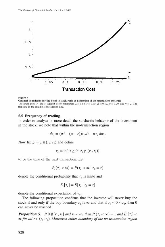
5.4 Changes in transaction costsFigure 7 shows how the transaction boundaries change as the transaction costrate � changes. The sell boundary is much less sensitive to the change inthe transaction cost rate than the buy boundary. When � = 1%, the investorwould let the ratio of the bond to the stock fluctuate between 0.1032 and0.2037 before adjusting. In the absence of transaction costs, the investorwould constantly keep the ratio at 0.1428. In contrast to Dumas and Luciano(1991), who found no bias toward cash in the optimal portfolio, here wesee that as transaction cost rate increases, there is a clear bias toward cashin the optimal portfolio caused by the finiteness of the horizon. Notice theconvexity of the buy boundary when � gets large enough (about 2%). In fact,this has to be the case because by Proposition 1, as the transaction cost rate� increases to 77.8%, the buy boundary has to approach infinity.

827


Figure 7Optimal boundaries for the bond-to-stock ratio as a function of the transaction cost rateThe graph plots r1 and r2 against � for parameters - = 0�04, r = 0�05, � = 0�12, � = 0�20, and $ = 2. Thethin line in the middle is the Merton line.

5.5 Frequency of tradingIn order to analyze in more detail the stochastic behavior of the investmentin the stock, we note that within the no-transaction region

dzt = ��2 − ��− r��zt dt−�zt dwt�

Now fix z0 = z ∈ �r1� r2� and define

,e = inft ≥ 0 & zt � �r1� r2��

to be the time of the next transaction. Let

Pz�,e < �� = P�,e < � � z0 = z�

denote the conditional probability that ,e is finite and

Ez ,e" = E ,e � z0 = z"

denote the conditional expectation of ,e.The following proposition confirms that the investor will never buy the

stock if and only if the buy boundary r2 is � and that if r1 ≤ 0 ≤ r2, then 0can never be reached.

Proposition 5. If 0 �∈ r1� r2" and r2 <�, then Pz�,e <��= 1 and Ez ,e" <� for all z ∈ �r1� r2�. Moreover, either boundary of the no-transaction region

828


can be reached with positive probability. On the other hand, if 0 ∈ r1� r2"(r2 =�, respectively), 0 (�, respectively) is never reached from within theinterior of the first and the fourth orthants in the �y� x� plane.

Proof. This follows immediately from propositions in Section 5.5 ofKaratzas and Shreve (1988). �

The previous analysis implies that if 0 ∈ r1� r2", then zt can never crossthe x-axis, which shows that the value function might not be C2 at 0 in thiscase as pointed out in note 8. However, if 0 �∈ r1� r2" and r2 < �, then bothboundaries can be reached in finite expected time and we can compute aset of measures of trading frequency, for example, expected time to the nexttrade, expected time to the next sale after a purchase, etc. In this section weare going to focus on the expected time to the next sale after a purchase tomeasure the average turnover time. To do this we utilize the following result.

Proposition 6. Suppose 0 �∈ r1� r2" and r2 < �. Then

E ,s ∧ ,�x0 = x� y0 = y" = F �x/y��

where

,s ≡ inft ≥ 0 & zt = r1��

F �z� = k1�r2�k1 �z�k2 −k2�r2�k2 �z�k1

-�k2�r1�k1 �r2vertk2 −k1�r1�k2 �r2�k1�

+ 1-

�

and

k1�2 =−( 1

2�2 − ��− r�

)±√( 12�

2 − ��− r�)2 +2-�2

�2�


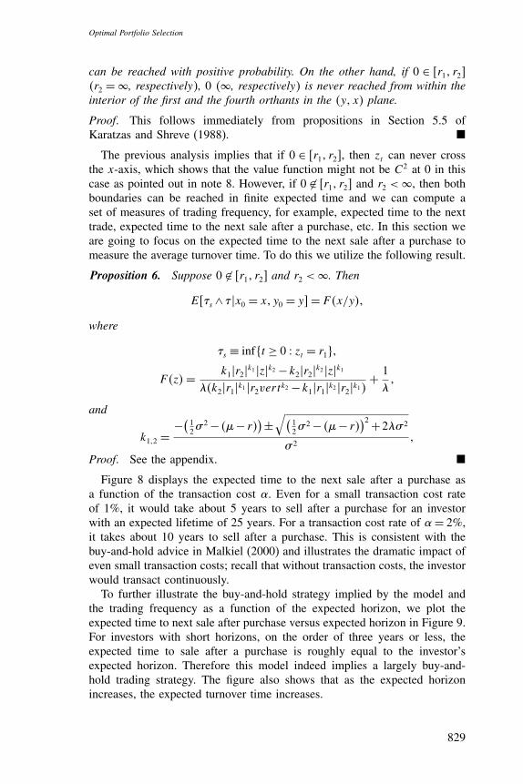
Figure 8 displays the expected time to the next sale after a purchase asa function of the transaction cost �. Even for a small transaction cost rateof 1%, it would take about 5 years to sell after a purchase for an investorwith an expected lifetime of 25 years. For a transaction cost rate of � = 2%,it takes about 10 years to sell after a purchase. This is consistent with thebuy-and-hold advice in Malkiel (2000) and illustrates the dramatic impact ofeven small transaction costs; recall that without transaction costs, the investorwould transact continuously.

To further illustrate the buy-and-hold strategy implied by the model andthe trading frequency as a function of the expected horizon, we plot theexpected time to next sale after purchase versus expected horizon in Figure 9.For investors with short horizons, on the order of three years or less, theexpected time to sale after a purchase is roughly equal to the investor’sexpected horizon. Therefore this model indeed implies a largely buy-and-hold trading strategy. The figure also shows that as the expected horizonincreases, the expected turnover time increases.

829


Figure 8Expected time to the next sale after purchase as a function of transaction costThe graph plots E ,s ∧ ," against � for parameters - = 0�04, r = 0�05, � = 0�12, � = 0�20, and $ = 2.

Figure 9Expected time to the next sale after purchase as a function of expected horizonThe graph plots E ,s ∧ ," against 1/- for parameters r = 0�05, � = 0�12, � = 0�20, � = 0�01, and $ = 2.

830


6. Conclusion

In this article we propose a methodology to study the optimal transactionpolicy for an investor with a finite horizon who is also subject to transactioncosts. In particular, we show that, in contrast to the frictionless case, thereis a clear link between the investor’s horizon and the optimal portfolio trad-ing strategy: investors with shorter horizons will buy relatively less of therisky asset and basically follow a buy-and-hold strategy. This is consistentwith the conventional wisdom on life-cycle investing. Our analysis derivesexplicit solutions for investors whose horizons are exponential and Erlangdistributed. We then show that the solution to the case with an Erlang dis-tributed horizon converges to the solution to the deterministic finite horizonproblem. We demonstrate that the optimal trading boundaries for the casewith an exponentially distributed horizon can be a good approximation forthose for the case with a deterministic horizon. In addition, we derive explicitbounds on the transaction boundaries for all the cases we consider. More-over, we obtain the necessary and sufficient conditions under which it is notoptimal to buy any stock, even when the risk premium is positive.

Our approach could be exploited to give approximate solutions for agreater range of transaction cost problems with finite horizons. First, wecan generalize our model to allow for a dividend paying stock and still haveclosed-form solutions for the exponentially distributed horizon case. Second,the analysis in this article can be further generalized to cover the case wherethe coefficients (including -) change at each jump of the Poisson process.From our analysis, we can conjecture that these value functions will convergeto the value function for an economy where the coefficients are time varying.Such generalizations could lead to interesting market microstructure studiesin the future.

Our approach should also find applications in a greater range of optimalconsumption/investment problems with time-varying components. To employthis methodology, one could first derive a modified problem with time invari-ant solution and then solve a series of such problems whose solutions con-verge to the optimal solution to the original problem.

Appendix

In this appendix, we collect the proofs for Propositions 1, 2, 6, and Theorem 2.

Proof of Proposition 1. The proof relies on the inequality

u�x�−u�y� ≥ u′�x��x−y�� (A.1)

which is valid for differentiable concave functions [see Rockafellar (1970), Theorem 25.1].Suppose our investor starts with initial endowments x0 > 0 and y0 = 0. For convenience, we

831


take S0 = 1. To show necessity, notice that if it is optimal not to buy stock, we must have forx� y corresponding to any feasible �D� I� ∈ ��x0� y0�,

E u′�x, + �1−��y,��x, + �1−��y, −x0er, �" ≤ 0�

In particular, letting x, = �1−a�x0er, and y, = ax0S, for 0 < a < 1, we have

E u′��1−a�x0er, +ax0�1−��S,��1−��S, − er, �" ≤ 0�

Choose a sequence 0 < an < 1 which goes down to 0. Taking limits as an ↓ 0 and interchangingthe limit and expectation, which is justified from using dominated convergence, since u′�x0�e

r, +S,�� ≤ u′��1−an�x0e

r, +anx0�1−��S,� ≤ u′�x0�1−a0�er, �, we then have

E u′�x0er, ��1−��S, − er, �" ≤ 0�

which leads to ∫ �

0�x0e

rt�−$��1−��E St"− ert�-e−-t dt ≤ 0�

Recalling E St" = e�t , we can integrate the above equations to get Equation (21). To provesufficiency, if we can show

E u′�x0er, ��x0e

r, −x, − �1−��y,�" ≥ 0 (A.2)

for x� y corresponding to any �D� I� ∈ ��x0� y0�, then from Equation (A.1), it is not optimal tobuy stock. Note that Equation (A.2) is equivalent to

∫ �

0x0e

�−-+�1−$�r�t dt ≥∫ �

0e�−-−$r�tE �xt + �1−��yt�" dt� (A.3)

By Equation (21), it is easy to check that

∫ s

0e�−-−$r�t�1−��E St" dt ≤

∫ s

0e�−-−$r�tert dt (A.4)

for all s ≥ 0. This implies that the right-hand side of Equation (A.3) is maximized by lendingx0 and not buying any stock. �

Proof of Proposition 2. If r1 �= 0�/ is C2 at r1 and

/�z� = B�z+1−��1−$

1−$� ∀ z ≤ r1�

Notice B > 0, since v�x� y� is strictly increasing in x and y. Putting this expression evaluated atr1 into Equation (16), we get (after simplification)

− 12$� 2�1−��2B+ ��− r��1−��r1 +1−��B

+[− �-− �1−$�r�

B

1−$+ -

1−$

]�r1 +1−��2 = 0� (A.5)

If r1 = 0, then B = -

-−�1−$��+$�1−$� �22

by Equation (20) and direct substitution shows that Equa-

tion (A.5) still holds. In either case we know that B �x+y�1−��1−$

1−$≥ -�x+y�1−��1−$

�1−$��-−�1−$�r�, since the

investor must do at least as well as liquidating his stock holdings and lending until the horizon.

832


Applying this inequality to the last term in Equation (A.5) leads to the lower bound in Equa-tion (22). For the upper bound in Equation (22), let us first define [recalling the definition of (

in Equation (11)]

f �z� =−B

(√(

$�z+1−��−��1−��

√$

2

)2

and

g�z� =(− �-− �1−$��r + (

$��B

1−$+ -

1−$

)�z+1−��2�

Notice f �z� ≤ 0 and y1−$�f �z�+g�z�� is equal to the left-hand side of Equation (16) evaluatedat z ≤ r1. The supermartingale property of v�xt� yt� then implies

f �z�+g�z� ≤ 0� ∀ z ≤ r1

and Equation (A.5) implies

f �r1�+g�r1� = 0� (A.6)

If f �r1� = 0, then r1 = $�2�1−��

�−r− �1−�� = �1−��r∗. If f �r1� < 0, then g�r1� > 0 by Equa-

tion (A.6). This implies g�z� > 0, ∀ z ≤ r1, which in turn implies that f �z� < 0, ∀ z ≤ r1. Sincef ��1−��r∗�= 0, we must have r1 < �1−��r∗. The lower bound for r2 can be similarly derived.

Finally, if �− r = $� 2 (i.e., r∗ = 0), then from above we must have r1 ≤ 0. Comparingthe optimal strategy for some z ≤ r1 to the strategy of immediately closing out the short bondposition and holding stock until the horizon gives

B

1−$≥ -

�1−$�(-− �1−$��+$�1−$� �2

2

) = -

�1−$�(-− �1−$�

(r + (

$

)) �or in other words,

− �-− �1−$��r + ($��B

1−$+ -

1−$≤ 0�

This implies that g�r1� ≤ 0. Equation (A.6) and the fact that f �r1� ≤ 0 implies in fact thatg�r1� = f �r1� = 0. As a result,

(√(

$�r1 +1−��−��1−��

√$

2

)2

= 0�

which implies r1 = 0. �

Proof of Theorem 2. Let xt� yt correspond to any feasible strategy �D� I� ∈ ��x� y� with theproperties that t → E u�xt + �1−��yt�" is continuous and for all t, xt + �1−��yt > : for somefixed constant : > 0. Notice that this ensures u�xt +�1−��yt� is bounded uniformly from belowfor all t ≤ T . We can modify each strategy in ��x� y� to be feasible for horizon , by liquidatingat , if , ≤ T and otherwise liquidating at T and leaving all wealth in the bond until , . LetV t�x� y�0� be the value function corresponding to the optimization problem of Equation (5), butwith the deterministic horizon t. Then from the feasibility of the above strategy for horizon , ,we deduce

E[u(�xT∧, + �1−��yT∧, �e

r�,−T �1,>T �)]≤ vn�x� y� ≤

∫ �

0V t�x� y�0�

(nT

)n�n−1�! t

n−1e− nT t dt�

833


Notice that V t�x� y�0� is bounded above by the Merton (1971) frictionless value function fora deterministic horizon t, as in Equation (9), and bounded below by the value function cor-responding to the strategy which liquidates all wealth and lends until the horizon t. In otherwords,

u��x+ �1−��y�ert� ≤ V t�x� y�0� ≤ e'tu�x+y��

where ' is defined in Equation (10). Moreover, using Theorem 2 of Davis, Panas, andZariphopoulou (1993), it is easy to verify that the conditions for a variant of the Helly–Braytheorem hold. As a result [see Chow and Teicher (1988), Theorem 8.1.2],

E u�xT + �1−��yT �" ≤ limn→�

vn�x� y� ≤ V T �x� y�0�� (A.7)

The theorem then follows from the fact that Equation (A.7) holds for any : > 0 and by takingthe supremum over all feasible strategies on the left-hand side. �

Proof of Proposition 6. Let *�x� y�=E �,s ∧,��x0 = x� y0 = y". Since , follows the exponen-tial distribution, we have

*�x� y� = E

[∫ �

0-e−-t�,s ∧ t�dt

∣∣∣x0 = x� y0 = y

]= E

[∫ ,s

0e−-t dt

∣∣∣x0 = x� y0 = y

]�

It is easily verified that * is homogeneous of degree 0 in �x� y�, so that *�x� y� = F �x/y� forsome function F . By Itô’s lemma and the fact that the process

e−-t*�xt� yt�+∫ t

0e−-s ds

is a martingale ∀ t < ,s , F must be the unique solution to the ordinary differential equation

12� 2z2Fzz + �� 2 − ��− r��zFz −-F +1 = 0

on �r1� r2�, with boundary conditions F �r1� = 0 and Fz�r2� = 0. It is straightforward to checkthat the function F defined in the proposition solves the above ODE. �

ReferencesBalduzzi, P., and A. Lynch, 1999, “Transaction Costs and Predictability: Some Utility Cost Calculations,”Journal of Financial Economics, 52, 47–78.

Bodie, Z., R. C. Merton, and W. F. Samuelson, 1992, “Labor Supply Flexibility and Portfolio Choice in aLife Cycle Model,” Journal of Economic Dynamics and Control, 16, 427–449.

Boyce, W. E., and R. C. DiPrima, 1969, Elementary Differential Equations and Boundary Value Problems,John Wiley & Sons, New York.

Brennan, M., E. Schwartz, and R. Lagnado, 1997, “Strategic Asset Allocation,” Journal of Economic Dynamicsand Control, 21, 1377–1403.

Campbell, J. Y., and L. M. Viceira, 1999, “Consumption and Portfolio Decisions When Expected Returns AreTime Varying,” Quarterly Journal of Economics, 11, 597–626.

Carr, P., 1998, “Randomization and the American Put,” Review of Financial Studies, 11, 597–626.

Cass, D., and M. Yarri, 1967, “Individual Saving, Aggregate Capital Accumulation, and Efficient Growth,” inK. Shell (ed.), Essays on the Theory of Optimal Economic Growth. MIT Press, Cambridge, MA, pp. 233–268.

Chow, Y. S., and H. Teicher, 1988, Probability Theory, Springer-Verlag, New York.

834


Constantinides, G. M., 1979, “Multiperiod Consumption and Investment Behavior with Convex TransactionCosts,” Management Science, 25, 1127–1137.

Constantinides, G. M., 1986, “Capital Market Equilibrium with Transaction Costs,” Journal of Political Econ-omy, 94, 842–862.

Cuoco, D., and H. Liu, 2000, “Optimal Consumption of a Divisible Durable Good,” Journal of EconomicDynamics and Control, 24, 561–613.

Cvitanic, J., and I. Karatzas, 1996, “Hedging and Portfolio Optimization Under Transaction Costs: A Martin-gale Approach,” Mathematical Finance, 6, 133–165.

Davis, M. H. A., and A. R. Norman, 1990, “Portfolio Selection with Transaction Costs,” Mathematics ofOperations Research, 15, 676–713.

Davis, M. H. A., V. G. Panas, and T. Zariphopoulou, 1993, “European Option Pricing with Transaction Costs,”SIAM Journal of Control and Optimization, 31, 470–493.

Dumas B., and E. Luciano, 1991, “An Exact Solution to a Dynamic Portfolio Choice Problem Under Trans-action Costs,” Journal of Finance, 46, 577–595.

Fleming, W. H., and H. M. Soner, 1993, Controlled Markov Processes and Viscosity Solutions, Springer-Verlag, New York.

Gennotte, G., and A. Jung, 1994, “Investment Strategies Under Transaction Costs: The Finite Horizon Case,”Management Science, 40, 385–404.

Grossman, S. J., and G. Laroque, 1990, “Asset Pricing and Optimal Portfolio Choice in the Presence ofIlliquid Durable Consumption Goods,” Econometrica, 58, 23–51.

Jagannathan, R., and N. R. Kocherlakota, 1996, “Why Should Older People Invest Less in Stocks ThanYounger People?” Federal Reserve Bank of Minneapolis Quarterly Review, Summer, 11–20.

Karatzas, I., and S. E. Shreve, 1988, Brownian Motion and Stochastic Calculus, Springer-Verlag, New York.

Kim, T. S., and E. Omberg, 1996, “Dynamic Nonmyopic Portfolio Behavior,” Review of Financial Studies, 9,141–161.

Liu, J., 1999, “Portfolio Selection in Stochastic Environments,” working paper, Stanford University.

Loewenstein, M., 2000, “On Optimal Investment Strategies for an Investor Facing Transaction Costs in aContinuous Trading Market,” Journal of Mathematical Economics, 33, 209–228.

Malkiel, B. G., 2000, A Random Walk Down Wall Street, W.W. Norton, New York.

Merton, R. C., 1971, “Optimum Consumption and Portfolio Rules in a Continuous Time Model,” Journal ofEconomic Theory, 3, 373–413.

Richard, S., 1975, “Optimal Consumption, Portfolio and Life Insurance Rules for an Uncertain Lived Indi-vidual in a Continuous Time Model,” Journal of Financial Economics, 2, 187–203.

Rockafellar, R. T., 1970, Convex Analysis, Princeton University Press, Princeton, NJ.

Samuelson, P. A., 1969, “Lifetime Portfolio Selection by Dynamic Stochastic Programming,” Review of Eco-nomics and Statistics, 51, 239–246.

Shreve, S. E., and H. M. Soner, 1994, “Optimal Investment and Consumption with Transaction Costs,” Annalsof Applied Probability, 4, 609–692.

835

optimal portfolio selection with transaction costs and

Documents