optimal pricing and delayed incentives in a heterogeneous consumer market
DESCRIPTION
TRANSCRIPT
Optimal pricing and delayed incentivesin a heterogeneous consumer market
Moutaz Khouja�, Stephanie S. Robbins and Hari K. RajagopalanReceived (in revised form): 10th July, 2007
�Business Information Systems and Operations Management Department, The Belk College of BusinessAdministration, The University of North Carolina — Charlotte, Charlotte, NC 28223, USATel: þ 1 704 687 3242; Fax: þ 1 704 687 6330; E-mail: [email protected]
Moutaz Khouja received a BS in Mechanical
Engineering, an MBA from the University of
Toledo and a PhD in Operations Management
from Kent State University. Currently, he is a
Professor of Operations Management in the
Belk College of Business Administration at the
University of North Carolina at Charlotte. His
research interests are in the areas of inventory
management, production planning and control,
pricing and forecasting. His publications have
appeared in many leading journals including
Computers and Operations Research, Deci-
sion Sciences, IIE Transactions, European
Journal of Operational Research, International
Journal of Production Research, International
Journal of Production Economics, Journal
of the Operational Research Society, and
Omega.
Stephanie S. Robbins received a PhD in
Management from Louisiana State University.
She is currently a Professor of MIS/OM at
The University of North Carolina at Charlotte.
Dr Robbins does research in the areas of
management information systems, marketing
management and strategy development for
non-profit organisations. Her publications have
appeared in journals such as International
Journal of Electronic Commerce, European
Journal of Operations Research, International
Journal of Production Economics, Information
and Management, The Journal of Computer
Information Systems, Behavioral Science and
the Journal of the Academy of Marketing
Science. She has also presented numerous
papers at international, national and regional
professional meetings.
Hari K. Rajagopalan earned his PhD in
Information Technology from the University of
North Carolina at Charlotte in 2006. Apart from
his PhD, he also has an MBA in Finance and
an MS in Computer Science. His research
interests include locating emergency response
systems, pricing of digital products and ob-
solescence in the high-technology industry.
His research has published in the European
Journal of Operational Research, Computers
and Operations Research and other journals.
He is also an active participant at INFORMS,
Decision Sciences, and European Working
Group in Transportation Meeting and Mini
EURO Conferences. He is currently the
Assistant Professor in Management at Francis
Marion University.
ABSTRACT
KEYWORDS: pricing, delayed incentives,
mail-in cash rebates
Delayed incentives in the form of cash mail-in rebates
have become very popular. We develop and solve a
model for jointly determining optimal price and rebate
value for a heterogeneous consumer market. Con-
sumers are divided into three segments: rebate
independent, fully rebate dependent, and partially
rebate dependent. Partially rebate-dependent consu-
mers’ redemption probability depends on the value of
www.palgrave-journals.com/rpm
& 2008 Palgrave Macmillan Ltd, 1476-6930 $30.00 Vol. 7, 1 85–105 Journal of Revenue and Pricing Management 85

the rebate relative to a reference value. Data show
that the probability of redemption increases linearly in
rebate value for small rebate values and at a
decreasing rate as the rebate value becomes large.
The model shows that two consumer attributes
are critical in determining the effectiveness of rebates.
The first is the reference value. The larger the
reference value, the larger the optimal rebate
value and the higher the profit. The second is the
distribution of consumers among the three segments.
Profit decreases as the proportion of consumers in the
probabilistic redeemers segment decreases. There is,
however, a threshold value where profit increases
as the proportion of consumers in the partially
rebate-dependent segment decreases. This occurs
because as the rebate-independent and fully rebate-
dependent consumers are priced out of the market, a
seller can increase both price and rebate value
substantially without having to be burdened by
the heavy cost of rebates for the fully rebate-dependent
segment. If the reference value for the partially
rebate-dependent segment is high, such a strategy
may prove profitable.
Journal of Revenue and Pricing Management (2008) 7,
85–105. doi:10.1057/palgrave.rpm.5160111
INTRODUCTION
Some researchers in marketing contend that
mail-in rebates present a great opportunity for
firms to increase their profit (Mouland, 2004).
Two main advantages of rebates are that few
consumers redeem them and that they do not
lower consumers’ future price expectations of
the product. Manufacturers mail-in rebates are
the most common type of rebates. Lately many
retailers are, however, offering store rebates.
The main focus of research has been on
consumer attitudes and behaviour with respect
to mail-in cash rebates and there has been
little research on determining the optimal
rebate strategy for sellers. Furthermore, there
is less research on joint optimal pricing
and rebate strategy. Like pricing, rebates are
used to manipulate demand. Therefore, deter-
mining optimal rebate strategy cannot be
accomplished without simultaneously deter-
mining product price.
In this paper, we develop a profit-max-
imisation model for jointly determining the
optimal price and rebate value. Based on survey
data, consumers are divided into three seg-
ments: rebate independent, fully rebate depen-
dent, and partially rebate dependent. The data
also indicate that the redemption rate is
increasing and is linear or slightly convex for
low rebate value and becomes concave at high
rebate values. Therefore, the model is solved
for linear and convex redemption rates that
apply for small ticket items for which the rebate
is less than $20. Results of the model indicate
that three consumer attributes are critical in
determining the profitability of rebates. First is
the reference value, which can be thought of as
the value consumers place on the time required
to redeem the rebate. The larger the reference
value, the larger the optimal rebate value and
the higher the profit. Second is the distribution
of consumers among the three segments. Profit
decreases as the proportion of consumers in the
partially rebate-dependent segment decreases.
There is, however, a threshold value where
profit increases as the proportion of consumers
in the partially rebate-dependent segment
decreases. This occurs because as the rebate-
independent and fully rebate-dependent con-
sumers are priced out of the market, a seller can
increase both price and rebate value substan-
tially without having to be burdened by the
heavy cost of rebates for the fully rebate-
dependent consumers. If the reference value for
the partially rebate-dependent segment is high,
rebates may prove profitable. Third is the ratio
of the increase in demand due to a $1 increase
in rebate value to the increase in demand due
to $1 decrease in price. The closer the amount
is to a $1, the more profitable the rebate
programme. This ratio, termed rebate attrac-
tiveness, is in part determined by the distribu-
tion of consumers among the three segments
and approaches zero as the proportion of
consumers in the rebate-independent segment
approaches 100 per cent.
In the next section, the literature on mail-in
rebates is reviewed. In a further section, results
Journal of Revenue and Pricing Management Vol. 7, 1 85–105 & 2008 Palgrave Macmillan Ltd, 1476-6930 $30.0086
Optimal pricing and delayed incentives

from the data are discussed and the linear
redemption model is formulated and solved
and then the convex redemption model is
formulated and solved followed by numerical
examples and sensitivity analysis. We close with
conclusions and suggestions for future research
in the last section.
LITERATURE REVIEW
One marketing tool that has received little
attention in the production-marketing inter-
face literature is cash mail-in rebates. The use
rebates has become very popular among
manufacturers and retailers (Bulkeley, 1998;
McGinn, 2003). Most rebates are offered by
manufacturers, but rebates are also becoming
popular among retailers. While many of the
studies on delayed incentives focus on con-
sumer perceptions and behaviour, little has
been done to determine their optimal value, or
to examine their impact on inventory policy
and profit.
Several studies have examined consumer
perception and response to delayed incentives
(Soman, 1998; Folkes and Wheat, 1995; Tat et
al., 1988; Jolson et al., 1987). The literature
suggests a few reasons for the popularity of
mail-in rebates (Jolson et al., 1987) which
include negligible accumulation requirements
by the consumer, ease of scheduling by
manufacturers and retailers, minimal risk by
consumers, and slippage. Slippage refers to the
proportion of consumers who purchase the
product because of the rebate but never redeem
it. Preliminary evidence indicates that most
consumers never redeem the rebate offers. For
example, Jolson et al. (1987) reports that 70 per
cent of consumers whose buying decisions are
influenced by rebate offers never redeem them.
Some estimates of the total proportions of
consumers who redeem their rebates are in the
range of 5–10 per cent (Bulkeley, 1998). Even
for rebates as high as $100, some experts
suggest that 50 per cent of consumers do not
make an effort to collect them (McGinn,
2003). A fifth reason suggested for the popular-
ity of mail-in rebates among manufacturers is
that they allow them to offer price discounts
directly to the consumers whereas with tradi-
tional price cuts, retailers may not fully pass the
price reductions to the consumer (Bulkeley,
1998). A sixth reason which makes rebates
preferable to using coupons or sales is that
consumers’ price expectations are higher for
products with rebates than the same products
with sales or coupons (Folkes and Wheat,
1995). In other words, when the promotions
are offered using coupons or sales, empirical
evidence indicate that the savings are likely to
be integrated into the regular price, which
means consumers will have future price
expectations closer to the promoted price
(Folkes and Wheat, 1995). This integration
and decrease in future price expectations are
much less likely to occur when the promotion
is delivered using mail-in rebates.
Based on an empirical experiment, Soman
(1998) tested and found support for two
hypotheses. The first hypothesis is that con-
sumer choice behaviour is more sensitive to the
rebate face value at the time of purchase than it
is to the level of effort required for redemption.
The second hypothesis is that the redemption
rate after purchase is more sensitive to the level
of effort than the rebate face value. In other
words, consumers underestimate the effort
required for redemption at the time of
purchase. Therefore, mail-in rebates provide
retailers with an excellent opportunity for
increasing profit, especially when the optimal
rebate face value is determined jointly with
price and order quantity. A retailer can increase
the per unit price but at the same time can
increase the mail-in rebate face value to offset
the impact of the price increase on demand. If
the redemption rate is low enough, then the
net impact will be an increase in profit. Silk
(2005) conducted a series of experiments that
tracked the purchase and redemption of a real
rebate offer. The experiments showed that
increasing the rebate value or the length of the
period for which it is valid make consumers
more confident that they will redeem the
rebate and increase the likelihood of purchasing
& 2008 Palgrave Macmillan Ltd, 1476-6930 $30.00 Vol. 7, 1 85–105 Journal of Revenue and Pricing Management 87
Khouja, Robbins and Rajagopalan

the product. This increased confidence did
not result in significant increase in actual
redemption later on. Therefore, increasing
rebate value has much less impact on redemp-
tion behaviour than purchase behaviour.
Furthermore, contrary to expectations, increas-
ing the length of valid redemption period
decreases redemptions.
Tat (1994) investigated three consumer
motives for rebate redemption: price con-
sciousness, perceived time and efforts associated
with rebate redemption, and perceived satisfac-
tion from using rebates to obtain the savings.
All three factors were found to be significant
predictors of consumers’ decisions to redeem
rebates. Perceived satisfaction was the most
significant, followed by price consciousness,
and then perceived time and efforts. The study
confirmed earlier results reported by Tat et al.
(1988) on the negative relationship between
the perceived effort and the difficulty of
redemption and redemption rates. Tat and
Schwepker (1998) empirically investigated the
relationships between rebate redemption mo-
tives. The authors found that perceived price
consciousness was positively related to rebate
redemption; however, the relationship was not
statistically significant, which implies that more
price conscious consumers do not redeem
rebates more frequently than consumers
who are not as price conscious. Similarly,
the authors found a negative, but statistically
insignificant, relationship between time and
effort required for redemption and rebate
redemption. In other words, the time and
effort needed to redeem a rebate offer does not
seem to directly decrease its probability of
being redeemed.
Ali et al. (1994) developed a model for
determining the optimal refund rate of rebates
as a proportion of the retail price. Their model
considered four ways by which rebates con-
tribute to incremental sales: brand switching,
repeat purchases, purchase acceleration, and
category expansion. The authors developed a
myopic model that considers incremental profit
due to sales during the rebate period only. The
authors also developed a long-term model that
also considers the repeat purchases in subse-
quent cycles due to brand switching and
showed that an optimal long-term rebate value
exists. Soman (1998) took another step toward
establishing optimal rebate value by formulat-
ing a profit maximisation model in which
demand and redemptions are linear functions
of rebate value. The model is developed for a
pre-determined price and under the assump-
tion that total redemptions depend only on
rebate face value and are independent of the
quantity sold. Gilpatric (2003), using the
present-biased preference model, identified
market conditions under which a rebate
programme is profitable. In this model, some
consumers assume that their preferences will be
unchanged in the future and buy the product
thinking they will redeem the rebate. Later on,
because their preferences change, they do not
redeem it. Chen et al. (2005) introduced an
explanation of rebate usage based on the idea of
‘utility arbitrage’. In this model, rebates are
viewed as state-dependent discounts. As re-
demption occurs after purchase, the rebate
utility to the consumer will depend on their
income utility at that time, which can be
low or high. The authors compared a rebate
policy with no rebate policy and presented
a set of necessary conditions for an optimal
rebate policy for the performance of utility
arbitrage.
Mail-in cash rebates have not received as
much research attention as other sales incentives
such as coupons (see Anderson and Song (2004)
for a brief review). Dhar et al. (1996) analysed
the profit impact of package coupons on profit.
They compared three types of package coupons:
Peel-off coupons that are redeemed at time of
purchase of the item, on-pack coupons that can
be redeemed at future purchases of the item, and
in-pack coupons that are similar to on-pack
coupons except consumers are unaware of their
presence at purchase. Other researchers dealt
with the impact of other types of coupons.
A distinguishing characteristic of mail-in rebates
is that they require an additional effort for
Journal of Revenue and Pricing Management Vol. 7, 1 85–105 & 2008 Palgrave Macmillan Ltd, 1476-6930 $30.0088
Optimal pricing and delayed incentives
redemption over coupons, which may reduce
their redemption rates.
Our review of the literature did not identify
any models that analyse the pricing and rebate
value decisions while taking into account the
diverse behaviour of consumers regarding
rebates. In this paper, we develop a model for
determining the optimal price and rebate value
of a manufacturer operating in a market with
three consumer segments. Based on empirical
evidence, consumers are divided into three
segments with different demand sensitivity to
price and rebate value and redemption behaviour.
MODEL 1: LINEAR REDEMPTION
FUNCTION
Data on actual rebate redemptions are closely
guarded and firms are reluctant to release it. We
relied on exploratory data gathered from 204
graduate students using a questionnaire.
Summary of the data is shown in Appendix
A. In designing the questionnaire, we relied on
literature from the present biased preferences
model (O’Donoghue and Rabin, 1999, 2001).
In this model, consumers are aware that they
may have self-control problems in the future. In
the case of rebates, this self-control problem is
whether they will have the discipline to expend
the time and effort required to redeem the
rebate offer. Individuals are classified into one
of two groups: sophisticated individuals who
have full knowledge of their future selves and
preferences, albeit different from their current
selves and preferences, and naı̈ve individuals
who assume that their preferences will not
change over time. Naı̈ve consumers may find
that after purchase of the product, their
preferences have changed and they do not
redeem the rebate. We therefore divide
consumers into three segments with the first
two making up the sophisticated consumers
and the third making up the naı̈ve consumers.
1. Rebate-independent (RI) consumers. These con-
sumers do not redeem rebates and their
demand is unaffected by rebate value. They
may have been adversely affected by negative
past redemption experience or realise
from past redemption failures that they do
not redeem rebates. The existence of this
consumer segment is supported by earlier
research (Oldenburg, 2005).
2. Fully rebate-dependent (FRD) consumers. These
are consumers who are very sensitive to the
net cost of the product and always redeem
the rebate offer.
3. Partially rebate-dependent (PRD) consumers.
These are consumers who are sensitive to
rebates and intend to redeem them at the
time of purchase, but may not act on their
intentions.
The data from the questionnaire were used to
provide three characteristics of the consumers:
(1) The distribution among the three segments:
RI, FRD, and PRD, (2) the propensity of PRD
to redeem rebates, and (3) how do the PRD
and FRD trade-off price decrease versus
rebate increase. The data are used to identify
reasonable values for the model parameters.
Obviously, values of these parameters will
depend on the type of product as it determines
the consumer base, the ease of the redemption
process, the time allowed for redemption, etc.
The following notation is defined:
t, f, p denote rebate-independent consumers,
fully rebate-dependent consumers, and
partially rebate-dependent consumers
P price per unit, a decision variable
R value of the rebate, which does not
include its processing cost if it is
redeemed, a decision variable
r processing cost per rebate redeemed,
which is incurred in addition to
rebate value
h cost per unit of the product
xi demand for the product by consumer
segment i, (i¼ t, f, p)
X total demand for the product and
p profit, an effectiveness measure.
RI consumers are sensitive to only price and,
therefore, their demand can be written as
xt ¼ at � btP ð1Þ
& 2008 Palgrave Macmillan Ltd, 1476-6930 $30.00 Vol. 7, 1 85–105 Journal of Revenue and Pricing Management 89
Khouja, Robbins and Rajagopalan
FRD consumers are sensitive to both price and
rebate value and, therefore, their demand can
be written as
xf ¼ af � bf P þ cf R ð2ÞPRD consumers are also sensitive to both price
and rebate value but in different degrees than
FRD consumers. Therefore, their demand can
be written as
xp ¼ ap � bpP þ cpR ð3ÞEquations (1)–(3) imply that demand decreases
(btþ bfþ bp) units for each $1 increase in price
and increases (cfþ cp) units for each $1 increase
in the value of the rebate. The ratio
L ¼ ðcf þ cpÞðbt þ bf þ bpÞ
ð4Þ
is a measure of the effect of a $1 increase in
rebate value relative to a $1 decrease in price on
demand and will be referred to as ‘rebate
attractiveness’. An L¼ 1 indicates that there
are no RI consumers and as many consumers
buy the product because of a $1 increase in
rebate value as those who will buy it because of a
$1 decrease in price. An L value close to zero
indicates that most consumers are RI or
insensitive to rebates and that increasing rebate
value is much less effective in increasing demand
than decreasing price by the same amount.
Total rebate redemptions depend on the total
number of FRD and PRD consumers who
purchase the product. All FRD consumers will
redeem the rebate. For PRD consumers, the
proportion of rebates redeemed depends on
rebate value relative to a reference value, denoted
by V, resulting in xpR/V redemptions. The use
of the linear function for the proportion of PRD
who redeem the rebate results in a reasonably
good fit for the self-reported data for values of up
to $20 with adjusted R2 value of 0.93. Therefore,
the total number of rebate offers redeemed is
g ¼ xf þ xp
R
Vð5Þ
A reference value is used instead of unit price
because as observed by Soman (1998), redemp-
tion occurs after purchase and at that time the
redemption probability is no longer influenced
by the price paid for the product.
To simplify the analysis, we introduce the
following assumption with respect to the
parameters of the demand functions:
For all non-negative P and R such that
0pRoP; xtoxf oxp ð6Þ
which implies that the demand of the RI
segment vanishes first, followed by the FRD
segment, and finally the PRD segment. Let
S1 ¼ ðP;RÞ : RX0 and hoPoat
bt
;
� �ð7Þ
S2 ¼ ðP;RÞ : RX0 andat
bt
oPoaf þ cf R
bf
� �ð8Þ
S3 ¼(ðP;RÞ : RX0 and
af þ cf R
bf
oPoap þ cpR
bp
) ð9Þ
All three consumer segments are served
If the demand for all three consumer segments
are positive, the profit, which is revenue minus
cost, is given by
Z ¼ XðP � hÞ � gðR þ rÞ ð10Þ
Using the expressions for xi and g from equations
(1–3) and (5) in equation (10) and simplifying
gives the following expression for profit:
Z ¼ ðP � hÞðA � BP þ CRÞ � ðr þ RÞ
� af � bf P þ cf R þ Rðap � bpP þ cpRÞV
� �ð11Þ
where A¼P
iai, B¼P
ibi, and C¼P
ici.
Appendix B shows the conditions under which
the Hessian matrix is negative semi-definite.
Journal of Revenue and Pricing Management Vol. 7, 1 85–105 & 2008 Palgrave Macmillan Ltd, 1476-6930 $30.0090
Optimal pricing and delayed incentives
Under those conditions, the sufficient condi-
tions for optimality are given by
P� ¼
ðA þ Bh þ bf rÞV þ ½ðbf þ CÞVþbprR þ bpR2
2BVð12Þ
and
R� ¼
bpP � aþ
ffiffiffiffiffiffiffiffiffiffiffiffiffiffiffiffiffiffiffiffiffiffiffiffiffiffiffiffiffiffiffiffiffiffiffiffiffiffiffiffiffiffiffiffiffiffiffiffiffiffiffiffiffiffiffiffiffiffiffiffiffiffiffiffiffiffiffiffiffiffiffiða� bpPÞ2 � 3cpV ½af þ Ch
�ðbf þ CÞP � 3cprðap � bpP þ cf V Þ
s
3cp
ð13Þwhere
a ¼ ap þ cpr þ cf V ð14ÞAt convergence, the values of P� and R� should
be used to compute xp, xf, and xt. If a consumer
segment’s demand is negative, then as shown
later, the optimal price and rebate value may
result in no sales to that consumer segment.
Not all consumer segments are served
Let Zfp be the profit if only the FRD and PRD
consumers are served with a maximum at Pfp�
and Rfp� (the subscript fp denotes only the FRD
and PRD segments). Zfp is obtained from
equation (11) with bt¼ at¼ 0, which should
also be used in computing A and B. Equations
(12) and (13) can be used to compute Pfp� and
Rfp� . The conditions under which the profit
function without the RI segment is concave are
shown in Appendix B.
Let Zp be the profit if only PRD consumers
are served with a maximum at Pp� and Rp
� (the
subscript p denotes only the PRD segment). Zp
is obtained from equation (11) with
bt¼ at¼ bf¼ af¼ cf¼ 0, which should also be
used in computing A, B, and C. Lemma 1
shows the optimal rebate value.
Lemma 1. A solution is optimal if and only if
R�p ¼ cpV � bpr
2bp
ð15Þ
Proof. The proof is shown in Appendix B.
Substituting for Rp� from equation (15) into
equation (12) gives
P�p ¼
½4bpðap þ bphÞ þ 3c2p V V � bprð2cpV � bprÞ8b2
pV
ð16ÞThe sufficiency of equation (16) is proven in
Appendix B. The global optimal solution may
occur when all three consumer segments are
served, only two segments are served, or only
one segment is served.
Identifying the global optimal solution
is based on the following properties of the
profit function which derive from assumption
in (6).
Property 1. For all P and R in S1,
Z >Zpf >Zp.
Proof. The proof is shown in Appendix B.
Property 2. For all P and R in S2 and
P>hþ rþR, ZoZfp and Zfp>Zp.
Proof. The proof is shown in Appendix B.
Property 3. For all P and R in S3, ZfpoZp
and Zp >Z.
Proof. The proof is shown in Appendix B.
Lemmas 2–4 are used to develop an algorithm
for identifying the global optimal solution.
Lemma 2 If equations (12) and (13) with all
three consumer segments converge to P� and
R� in S2 or S3 then it is optimal not to serve the
RI consumer segment.
Proof. The proof is shown in Appendix B.
Lemma 3. If equations (12) and (13) with only
the FRD and PRD segments converge to Pfp�
and Rfp� in S1 or S3 then it is not optimal to serve
only the FRD and PRD consumer segments.
Proof. The proof is shown in Appendix B.
& 2008 Palgrave Macmillan Ltd, 1476-6930 $30.00 Vol. 7, 1 85–105 Journal of Revenue and Pricing Management 91
Khouja, Robbins and Rajagopalan

Lemma 4. If equations (12) and (13) with
only the PRD segment converge to Pp� and Rp
�
in S1 or S2 then it is not optimal to serve only
the PRD consumer segment.
Proof. The proof is shown in Appendix B.
Boundary solutions
If the optimal solution occurs at the boundary
between S1 and S2 where P¼ at/bt (ie the
demand of the RI segment is zero), then
substituting P¼ at/bt into equation (11) and
differentiating with respect to (w.r.t.) R, yields
the following necessary condition, which is
sufficient under the condition shown in
Appendix B, for R to be optimal:
R� ¼ �b1 þ
ffiffiffiffiffiffiffiffiffiffiffiffiffiffiffiffiffiffiffiffiffiffib2
1 � 4b0b2
q2b2
ð17Þ
where
b0 ¼ atbf � af V þ Cðat � bthÞþ rðap þ atbp=bt � cf V Þ ð18Þ
b1 ¼ 2atbp=bt � 2ðap þ cpr þ Vcf Þ ð19Þ
b2 ¼ �3cp ð20Þ
If the solution occurs at the boundary between
S2 and S3 where P¼ (afþ cfR)/bf (ie the demand
of the FRD segment is zero), then substituting
P¼ (afþ cfR)/bf and at¼ bt¼ 0 into equation
(11) and differentiating w.r.t. R, yields (17) with
b0 ¼ bf ½V ðapcf � bf cph þ bpcf hÞ � apbf rþ af ½V ðbf cp � 2bpcf Þ þ bpbf r
ð21Þb1 ¼ �2½ðbf cp � bpcf Þðbf r � cf V Þ
� af bpbf þ apb2f ð22Þ
b2 ¼ 3bf ðbpcf � bf cpÞ ð23Þ
as the necessary condition for optimality, which
is also sufficient under the condition shown in
Appendix B.
Algorithm to identify the optimal solution
Step 1. Using all three consumer segments
in equations (12) and (13) compute
P� and R�.If P� and R� are in S1 then P� and R�
are a local maximum.
If P� and R� are in S2 or S3 then R�
is given by equations (17)–(20) and
P� ¼ at/bt.
Compute the maximum profit in S1
denoted Z1� using equation (11).
Step 2. Using only the FRD and PRD
segments in equations (12) and (13)
compute Pfp� and Rfp
� .
If Pfp� and Rfp
� are in S2 Pfp� and Rfp
� are
a local maximum. Compute Zfp�
If Pfp� and Rfp
� are in S3 then use
equations (17) and (21–23) to com-
pute Rfp1� which should be used to
compute Pfp1� ¼ (afþ cfRfp1
� )/bf and
then Zfp1�
Step 3. Using only the PRD consumer
segment in equations (15) and (16)
compute Pp� and Rp
�.If Pp
� and Rp� are in S3 then Pp
� and Rp�
are a local maximum. Compute Zp�.
If Pp� and Rp
� are in S2 then use
equations (17) and (21)–(23) to
compute Rp1� which should be used
to compute Pp1� ¼ (af þ cfRp1
� )/bf and
then Zp1�
Step 4. Compare all local maximum profits
and select the largest.
MODEL 2: REDEMPTIONS INCREASE
AT AN INCREASING RATE IN REBATE
VALUE
As described by Soman (1998), one of the
problems with the linear redemption function
is that it does not reflect actual consumer
behaviour at extreme values of the rebate
where very few or very many consumers
redeem them. This observation is supported
by the collected data especially at large values of
the rebate exceeding $25 where the redemp-
tion function clearly increases at an increasing
Journal of Revenue and Pricing Management Vol. 7, 1 85–105 & 2008 Palgrave Macmillan Ltd, 1476-6930 $30.0092
Optimal pricing and delayed incentives

rate. As we are restricting our attention to small
ticket items, we assume proportion of rebate
offers that are redeemed by the PRD is an
increasing convex function in the value of the
rebate and is given by:
g ¼ R
u � Rð24Þ
where u is an empirically determined constant.
Equation (24) implies that 100 per cent of
consumers redeem the rebate (ie g¼ 1) when
its value is R¼ u/2. In other words, u/2 has the
same meaning as the reference value in the
linear redemption function. A graph of the
linear redemption function versus the redemp-
tion function given by equation (24) for V¼u/
2¼ $50 is shown in Figure 1.
Using the expressions for xi and g from
equations (1)–(3) and (24) in equation (10)
and simplifying gives the following expression
for profit:
Z ¼ðP � hÞðA � BP þ CRÞ � ðr þ RÞ
� af � bf P þ cf R þ Rðap � bpP þ cpRÞu � R
� �ð25Þ
Let
o0 ¼ u½rðbpP � apÞ � ðaf � CðP � hÞ� bf P þ cf rÞu ð26Þ
o1 ¼ 2u½af � ap � CðP � hÞ þ Pðbp � bf Þþ rðcf � cpÞ � cf u ð27Þ
o2 ¼ af � ap þ Pðbf � bpÞ þ CðP � hÞþ rðcp � cf Þ þ uð4cf � 3cpÞ
ð28Þ
o3 ¼ 2ðcp � cf Þ ð29Þ
Appendix B shows the conditions under which
the Hessian matrix is negative semidefinite.
Under those conditions, the sufficient condi-
tions for optimality are given by
P� ¼
½A þ Bh þ bf r þ ðbp þ CÞRðu � RÞþbpRðr þ RÞ
2Bðu � RÞð30Þ
and
o3R3 þ o2R
2 þ o1R þ o0 ¼ 0 ð31Þ
At convergence, the values of P� and R� should
be used to compute xp, xf, and xt. If a segment’s
demand becomes negative, then as shown later,
the optimal price and rebate values may result
in no sales to that consumer segment.
1
0.8
0.6
0.4
Pro
prtio
n of
reb
ates
red
eem
ed
0.2
10 20 30R ($)
40 50
Figure 1: Linear versus nonlinear redemption functions for the PRD consumer segment
& 2008 Palgrave Macmillan Ltd, 1476-6930 $30.00 Vol. 7, 1 85–105 Journal of Revenue and Pricing Management 93
Khouja, Robbins and Rajagopalan
NOT ALL CONSUMER SEGMENTS
ARE SERVED
Let Zfp be the profit if only the FRD and PRD
consumers are served (ie its demand is greater
than zero) with a maximum at Pfp� and Rfp
� . Zfp is
obtained from equation (25) with bt¼ at¼ 0,
which should also be used in computing A and
B. Equations (30) and (31) can be used to
compute Pfp� and Rfp
� . The conditions under
which the profit function without the RI
segment is concave are shown in Appendix B.
Let Zp be the profit if only PRD consumers
are served with a maximum at Pp� and Rp
�. Zp is
obtained from equation (25) with bt¼ at¼ bf¼af¼ cf¼ 0, which should also be used in
computing A, B, and C. Lemma 5 shows the
optimal rebate value.
Lemma 5. A solution is optimal if and only if
R�p ¼ u �
ffiffiffiffiffiffiffiffiffiffiffiffiffiffiffiffiffiffiffiffiffiffiffiffiffiffiffiffiffiffiffiffiffiffiffiffibpuðbp þ cpÞðr þ uÞ
pbp þ cp
ð32Þ
Proof. The proof is shown in Appendix B.
Substituting for Rp� from equation (32) into
equations (26) gives
P�p ¼ 1
2
2ffiffiffiffiffiffiffiffiffiffiffiffiffiffiffiffiffiffiffiffiffiffiffiffiffiffiffiffiffiffiffiffiffiffiffiffibpuðbp þ cpÞðr þ uÞ
pbp þ cp
þbp þ cpu
b2
þ h � 2u � r
�ð33Þ
The sufficiency of equation (33) for optim-
ality is proven in Appendix B. The global
optimal solution may occur when all three
consumer segments are served, only two
segments are served, or when only one segment
is served.
Properties 1–3 and Lemmas 2–4 also hold
for this redemption function. Therefore, the
same algorithm can be used to find the optimal
solution after replacing equations (12, 13), (15,
16), (17) (18–20), and (21–23) with equations
(30, 31), (32, 33) (31), (34–37) (38–41),
respectively.
Boundary solutions
Similar to the linear redemption function, if
the optimal solution occurs at the boundary
between S1 and S2, then substituting P¼ at/bt
into equation (15) and differentiating w.r.t. R,
yields equation (31) with
o0 ¼ u½apbtr þ btðaf þ cph þ cf ðh þ rÞÞu� apðbpr þ ðbf þ CÞuÞ
ð34Þ
o1 ¼� 2u½apbt þ atðbf � bp þ CÞ� btðaf þ cpðh � rÞ þ cf ðh þ r � uÞÞ
ð35Þo2 ¼ apbt þ atðbf � bp þ CÞ
� bt½af þ cf ðh þ r � 4uÞ þ cpðh � r þ 3uÞð36Þ
o3 ¼ 2btðcp � cf Þ ð37Þ
as the necessary condition for R to be optimal,
which is also sufficient under the condition
shown in Appendix B. If the solution occurs
at the boundary between S2 and S3 where
P¼ (afþ cfR)/bf, then substituting P¼ (afþ cfR)/
bf and at¼ bt¼ 0 into equation (25) and
differentiating w.r.t. R yields equation (31)
with
o0 ¼ u½af ðbpbf r þ bf cpu � 2bpcf uÞþ bf ðbpcf hu � apbf r � cpbf hu þ apcf uÞ
ð38Þ
o1 ¼� 2u½apbf ðbf þ cf Þ þ cf ðbf cp � bpðbf þ 2cf ÞÞ� ðbf cp � bpcf Þðbf h � bf r þ cf uÞ ð39Þ
o2 ¼ apbf ðbf þ cf Þ þ af ½bf cp � bpðbf þ 2cf Þ� ðbf cp � bpcf Þ½bf ðh � r þ 3uÞ þ 4cf u
ð40Þ
o3 ¼ 2ðbf þ cf Þðbf cp � bpcf Þ ð41Þ
as the necessary condition for optimality, which
is also sufficient under the condition shown in
Appendix B.
Journal of Revenue and Pricing Management Vol. 7, 1 85–105 & 2008 Palgrave Macmillan Ltd, 1476-6930 $30.0094
Optimal pricing and delayed incentives
NUMERICAL EXAMPLES AND
SENSITIVITY ANALYSIS
Numerical Example 1
Based on the collected data, we use the
consumer distribution among segments shown
in Table A1. We assume a total market of
50,000 consumers. In addition, we assume a
loss of the consumer base of 5.5 per cent, 5.0
per cent, and 4.5 per cent for each $1 increase
in price for the RI, FRD, and PRD segments,
respectively. Based on the data, PRD con-
sumers are assumed to be indifferent between
$1.72 increase in rebate and $1.00 decrease in
price whereas FRD consumers are assumed to
be indifferent between $1.69 increase in rebate
and $1.00 decrease in price. The resulting
demand functions are: xt¼ 3,450�189.75P,
xf¼ 20,350�1017.50Pþ 602.78R, xp¼ 26,250�1181.25Pþ 686.37R, and regression analysis of
the data for rebate value up to $20 indicate that
V¼ $24.64. The curve has a better fit at the
lower values of R while the fit becomes poor as
R becomes larger. At unit cost of h¼ $5, the
product is sold to all three segments (ie the
solution is in S1) with P� ¼ $14.55, R� ¼ $2.62,
and Z� ¼ $148,373. Also, 10.6 per cent of the
PRD consumers redeem the rebate offer and
44.3 per cent of all consumers redeem the
rebate offer. At unit cost of h¼ $10, the
product is sold to all three segments (ie the
solution is in S1) with P� ¼ $17.09, R� ¼ $2.69,
and Z� ¼ $69,936. Also, 10.9 per cent of the
PRD consumers redeem the rebate offer and
42.9 per cent of all consumers redeem the
rebate offer. At unit cost of h¼ $15, the
product is sold to only the FRD and PRD
segments (ie the solution is in S2) with
P� ¼ $21.10, R� ¼ $4.72, and Z� ¼ $23,502.
Also, 19.2 per cent of the PRD consumers
redeem the rebate offer and 41.3 per cent of all
consumers redeem the rebate offer. At unit cost
of h¼ $20, the product is sold to only the PRD
segment (ie the solution is in S3) with
P� ¼ $24.08, R� ¼ $6.66, and Z� ¼ $4,776.
Also, 27 per cent of the PRD consumers
redeem the rebate.
Numerical Example 2
To illustrate the impact of different parameters
on pricing and rebates, we consider another
example of a product with demand functions
xt¼ 40,000�3,000P, xf¼ 40,000�3,000Pþ2,500R, and xp¼ 100,000�6,000Pþ 2,000R
for the RI, FRD, and PRD consumer
segments, respectively. The cost of the product
is h¼ $4 per unit, r¼ $1 per redemption, and
the proportion of consumers who redeem
the rebate offer is linear in its value with a
reference value of V¼ $50. Equation (B.9)
shows that the profit function is concave for all
prices below $21.00 and rebates up to 100 per
cent of price. The algorithm results in an
optimal price of P� ¼ $10.45 per unit and
optimal rebate value of R� ¼ $2.49, which is in
S1. Equation (11) yields an optimal profit of
Z� ¼ $365,180. The demand for the three
consumer segments are xp¼ 42,300 units,
xf¼ 14,883 units, and xt¼ 8,662 units. The
rebates redeemed by the FRD and PRD
consumer segments are 14,883 and 2,105,
respectively.
If bt is changed from 3,000 to 4,000, then it
is optimal not to serve the RI segment
Pfp� ¼ $11.75 and Rfp
� ¼ $4.01, which is in S2,
and the optimal profit is Zfp� ¼ $316,188. If, in
addition to the change in bt, bf is changed from
3,000 to 5,000, then it is optimal to serve only
the PRD segment in S3 with Pp� ¼ $12.33 and
Rp� ¼ $7.33 and Zp
� ¼ $289,560.
For the case in which the proportion of
consumers who redeem the rebate offers is an
increasing nonlinear convex function given by
equation (24), we use u¼ $100, which results
in 100 per cent redemptions at R¼ $50 (the
same as the value of V in the linear redemption
function). Equation (B.25) shows that the profit
function is concave for all prices below $16.41
and rebates up to 60 per cent of price. The
algorithm results in an optimal price of
P� ¼ $10.65 per unit and an optimal rebate
value of R� ¼ $3.16, which is in S1. Equation
(25) yields an optimal profit of Z� ¼ $369,583.
The demand for the three consumer segments
is xp¼ 42,441 units, xf¼ 15,964 units, and
& 2008 Palgrave Macmillan Ltd, 1476-6930 $30.00 Vol. 7, 1 85–105 Journal of Revenue and Pricing Management 95
Khouja, Robbins and Rajagopalan

xt¼ 8,058 units. The rebates redeemed by the
FRD and PRD consumer segments are 15,964
and 1,386, respectively. Even though both the
linear and nonlinear redemption functions
reach 100 per cent redemption rate at $50,
the nonlinear case has an optimal price, rebate
value, and profit which are $0.21, $0.71, and
$4,404 larger, respectively.
If bt is changed from 3,000 to 4,000, then
the optimal solution is in S2 where the RI
consumers are not served with Pfp� ¼ $12.21,
Rfp� ¼ $5.17, and Zfp
� ¼ $325,196. Unlike the
linear redemption case, if, in addition to the
change in bt, bf is changed from 3,000 to 5,000,
then it is optimal to only serve the PRD
segment with Pp� ¼ $13.87 and Rp
� ¼ $11.75,
which are given by equation (31) with
equations (38)–(41), and Zp� ¼ 329,141. The
results of the last case are counter-intuitive as
the demand of the FRD consumers becomes
more sensitive to price, profit increases. This is
explained by the fact that if it is not profitable
to serve the FRD segment (because the sum of
the optimal rebate value, rebate processing
cost, and unit cost exceeds the optimal
price, any sales to this segment result in a loss),
then an increased sensitivity to price of the
FRD consumers will allow a firm to drive
that segment’s demand to zero at smaller
values of price. Therefore, the solution space
of focusing on the PRD consumers alone, that
is S3, is enlarged and the optimal profit
increases.
Numerical sensitivity analysis
Numerical analysis indicate that there are three
key consumer/market attributes that determine
the effectiveness of a rebate programme. First is
the reference value, V. Figures 2 and 3 show the
optimal profit, rebate value, and price and for
values of V up to $100. Figures 2–5 are
constructed based on the distribution of
consumers shown in Table A1 with unit cost
of h¼ $10. As the figures shows, optimal profit,
price, and rebate value increase with V. The
rate of increase in the optimal profit, price, and
rebate value changes at a value of V between
$20 and $30 and becomes larger. This is due to
the optimal solution moving from region S1,
where all three consumer segments are served
to region S2, where only the FRD and
PRD segments are served. As the RI segment
is only sensitive to price, when it is priced out,
the optimal price increases and so does the
optimal rebate value. As price can be increased
without losing as many consumers, the rate of
increase in the optimal profit with V becomes
even larger.
The second key consumer/market attribute
is the rebate attractiveness defined in equation
(4). As Figure 4 shows, as rebate attractiveness
increases, the optimal profit increases at an
increasing rate. Figure 5 shows the optimal
price and rebate value, which are both
increasing in rebate attractiveness. As the figure
shows, there is a jump in both optimal rebate
value and price at L of about 0.52 as the RI
$67,000
$69,000
$71,000
$73,000
$75,000
$77,000
$79,000
$81,000
$83,000
$85,000
$- $20 $40 $60 $80 $100 $120
Reference value (V)
Opt
imal
Pro
fit (
Z*)
Figure 2: Optimal profit as a function of reference value
Journal of Revenue and Pricing Management Vol. 7, 1 85–105 & 2008 Palgrave Macmillan Ltd, 1476-6930 $30.0096
Optimal pricing and delayed incentives

consumer segment is priced out of the market.
An important conclusion from Figure 4 is that
having a large RI segment can have a negative
impact on profit. The reason is that even if
consumers in the PRD and FRD segments are
indifferent between $1 increase in rebate value
and $1 decrease in price but the RI segment is
large, the rebate attractiveness will be small.
$(3.00)
$2.00
$7.00
$12.00
$17.00
$22.00
$27.00
$- $20 $40 $60 $80 $100 $120
Reference value V
Uni
t pric
e an
d re
bate
val
ue
P*
R*
Figure 3: Optimal price and rebate value as a function of reference value
Opt
imal
pro
fit (
Z*)
$-
$50,000
$100,000
$150,000
$200,000
$250,000
$300,000
$350,000
0.49 0.54 0.59 0.64 0.69 0.74 0.79 0.84 0.89 0.94Rebate attractiveness (L)
Figure 4: Optimal profit as a function of rebate attractiveness, V¼ $100
$-
$10.00
$20.00
$30.00
$40.00
$50.00
$60.00
0.49 0.54 0.59 0.64 0.69 0.74 0.79 0.84 0.89 0.94Rebate attractiveness (L)
Pric
e an
d re
bate
val
ue
P*
R*
Figure 5: Optimal price and rebate value as a function of rebate attractiveness
& 2008 Palgrave Macmillan Ltd, 1476-6930 $30.00 Vol. 7, 1 85–105 Journal of Revenue and Pricing Management 97
Khouja, Robbins and Rajagopalan

This is an important motive for firms to
simplify the redemption process and ensure
prompt refunds upon redemption to avoid
causing consumers becoming RI due to
negative redemption experience.
The third key consumer/market attribute is
the distribution of consumers among the three
consumer segments. To analyse the impact of
different consumer demographics that may
exist for different products on rebate profit-
ability, we again use a market of 500,000
consumers and a product with a unit cost of
h¼ $10.00. For each consumer segment, 5 per
cent of the demand is lost for each $1 increase
in price. PRD consumers are assumed to be
indifferent between $1.72 increase in rebate
value and $1.00 decrease in price, whereas
FRD consumers are assumed to be indifferent
between $1.25 increase in rebate value and
$1.00 decrease in price. Figures 6 and 7 show
the optimal profit, optimal rebate value, and
optimal price and for V values of $75 and $100.
Figure 6 shows that as the relative size of the RI
and FRD increase, profit tends to decrease but
not over all ranges. For V¼ $75 there is a region
around (RI¼ 3 per cent, FRD¼ 38 per cent,
16.00
18.00
20.00
22.00
24.00
26.00
28.00
30.00
1,36,63 2,37,61 3,38,59 4,39,57 5,40,55 6,41,53 7,42,51 8,43,49 9,44,47 10,45,45Market Segments (%RI, %FRD, %PRD)
Pric
es a
nd r
ebat
e va
lue
R*, V = $75
R*, V = $100P*, V = $100
P*, V = $75
Figure 7: Optimal price and rebate value as a function of consumer distribution among segments
Pro
fit (
Z*)
$68,000
$73,000
$78,000
$83,000
$88,000
$93,000
$98,000
$103,000
$108,000
$113,000
$118,000
1,36,63 2,37,61 3,38,59 4,39,57 5,40,55 6,41,53 7,42,51 8,43,49 9,44,47 10,45,45
Market segments (%RI, %FRD, %PRD)
V=$100
V=$75
Figure 6: Optimal profit as a function of consumer distribution among segments
Journal of Revenue and Pricing Management Vol. 7, 1 85–105 & 2008 Palgrave Macmillan Ltd, 1476-6930 $30.0098
Optimal pricing and delayed incentives
PRD¼ 59 per cent) where the profit shows
an increase. A more significant increase occurs
for V¼ $100 around (RI¼ 5 per cent,
FRD¼ 40 per cent, PRD¼ 55 per cent). Both
of these increases in profit occur when the
optimal solution moves from the boundary of
regions S2 and S3 into region S3. Such a
phenomena is counter-intuitive as it implies
that as the proportion of consumers who are RI
and FRD increase, there is a threshold where
the optimal profit increases. The explanation is
that at a certain threshold in terms of the
distribution of consumers among the three
segments, it becomes optimal to price the FRD
out of the market. As Figure 7 shows, at this
threshold distribution of consumers among
segments, optimal prices show a sudden
increase to price the FRD out of the market.
As FRD are 100 per cent redeemers, having
them priced out of the market causes the
optimal rebate value to also increase. In some
cases, such as for V¼ $100, optimal rebate
value becomes even larger than the optimal
price.
Figures 6 and 7 have an important implica-
tion in terms of the time dimension. As
consumers gain better understanding of their
behaviour with respect to rebates over time,
they may move from the PRD segment to
the RI or the FRD segments. A consumer
who finds that she/he did not redeem any
rebates, in spite of intending to at the time of
purchase, may decide that they will no longer
take rebates into account in making the
purchase decision and becomes part of the RI
segment. Similarly, a consumer who finds
that she/he have successfully redeemed all
rebate offers over time may place more
emphasis on rebates in making a purchase
decision and becomes part of the FRD
segment. As Figure 6 shows, this change in
the relative size of the consumer segments in
favor of the RI and FRD segments will cause
rebate effectiveness to decrease over time,
which may be a contributing factor to some
retailers eliminating cash mail-in-rebates alto-
gether (Albright, 2005).
CONCLUSIONS AND SUGGESTIONS
FOR FUTURE RESEARCH
In this paper, we have developed a profit-
maximisation model for a firm using mail-in
cash rebates. The model takes into account the
presence of three heterogeneous consumer
groups: a RI segment whose demand is
unaffected by the rebate and whose consumers
do not redeem rebates, an FRD segment whose
consumers always redeem rebates, and a PRD
segment whose consumers intend to redeem
rebate offers at the time of purchase but may
not do so later. The proposed model is solved
for a demand that is linearly increasing in rebate
value and decreasing in price and for redemp-
tion functions that are increasing (linear or
convex) in rebate value. These redemption
functions are valid for rebate values up to about
$20 beyond which the redemption function
becomes concave.
Our analysis indicates that there are three
consumer/market characteristics that deter-
mine the profitability of a rebate programme:
The first is the reference value of the consu-
mers in the PRD segment. The reference
value can be thought of as the value at which
consumers believe that the rebate is fully
sufficiently large to compensate for the time
and effort they will spend on redeeming it. The
larger the reference price, the larger the
increase in profit a rebate programme brings
about. This suggests that rebate programmes
may be more profitable for products targeted
toward consumers with relatively large dispo-
sable income since these consumers may
place a larger value on their time. The second
characteristic is the rebate attractiveness
which is given by the ratio of the increase in
demand due to a $1.00 increase in rebate
value to the increase in demand due to a
$1.00 decrease in price. The larger the rebate
attractiveness, the larger the increase in profit.
The third characteristic, which partially deter-
mines the second characteristic, is the distribu-
tion of consumers among the three segments.
The larger the proportion of consumers in the
PRD consumers, the larger the increase in
& 2008 Palgrave Macmillan Ltd, 1476-6930 $30.00 Vol. 7, 1 85–105 Journal of Revenue and Pricing Management 99
Khouja, Robbins and Rajagopalan

profit from using rebates. This observation,
however, is not true in certain regions of the
solution space where the optimal solution
changes in terms of the composition of the
served market.
There are several important research ques-
tions that remain. A very important question in
light of the increased negative perception of
rebates among consumers (Oldenburg, 2005;
Chuang, 2003, Spencer, 2002) is the effect
of simplifying the rebate redemption pro-
cess and requirements on redemption rates.
The negative perception of rebates has even
caused some retailers such as Best Buy to
phase-out mail-in rebates altogether (Smith,
2005) and causing many consumers to become
RI. If simplifying the redemption process
has only a small effect on the redemption
rates, then manufacturers and retailers may be
able to avoid the negative perceptions that is
overtaking the market place and may be
causing many consumers to become RI while
maintaining profitable rebate programmes.
Another area or research involves determining
reference values of customer groups and its
relationship to disposable income. Obviously,
the reference value of consumers may be
positively correlated with their disposable income.
While some products are targeted to a broad
consumer market, some products are targeted to
only higher disposable income consumers. Dif-
ferent pricing and rebate strategy may greatly
enhance the profitability of these products.
REFERENCES
Albright, M. (2005) ‘Best buy phasing out mail-in
rebate offers’, St. Petersburg Times (South Pinellas
Edition), April 2, p. 1.D.
Ali, A., Jolson, M. A. and Darmon, R. Y. (1994) ‘A
model for optimizing the refund value in rebate
promotions’, Journal of Business Research, 29, 3,
239–245.
Anderson, E. T. and Song, I. (2004) ‘Coordinating
price reductions and coupon events’, Journal of
Marketing Research, 41, 411–422.
Bulkeley, W. M. (1998) ‘Rebates’ secret appeal to
manufacturers: few consumers actually redeem
them’, Wall Street Journal (Eastern edition),
February 10, B1.Chen, Y., Moorthy, S. and Zhang, Z. J. (2005)
‘Price discrimination after the purchase? A note
on rebates as state-dependant discounts’, Manage-
ment Science, 51, 1131–1140.
Chuang, T. (2003) ‘Manufacturer, retailer rebates
grow even more popular, despite disappoint-
ments’, Orange County Register, November 17.
Dhar, S. K., Morisson, D. G. and Raju, J. S. (1996)
‘The effect of package coupons on brand choice:
an epilogue on profits’, Marketing Science, 15,
192–203.
Folkes, V. and Wheat, R. D. (1995) ‘Consumers’
price perceptions of promoted products’, Journal
of Retailing, 71, 3, 317–328.
Gilpatric, S. M. (2003) Present-biased Preferences,
Self-awareness and Shirking in a Principal-agent
Setting, Department of Economics, University
of Tennessee, Knoxville.
Jolson, M. A., Wiener, J. L. and Rosecky, R. (1987)
‘Correlates of rebate proneness’, Journal of
Advertising Research, 27, 33–43.
McGinn, D. (2003) ‘Let’s make a (tough) deal’,
Newsweek, 141, 25, 48–49.
Mouland, W. (2004) ‘Rebates rule!’, Marketing
Magazine, 109, 33, 1196–4650.
Oldenburg, D. (2005) ‘The rebate check may not be
in the mail’, Washington Post, February 1.
O’Donoghue, T. and Rabin, M. (2001) ‘Choice
and procrastination’, Quarterly Journal of Econom-
ics, 116, 1, 121–160.
O’Donoghue, T. and Rabin, M. (1999) ‘Doing It now
or later’, American Economic Review, 89, 1, 103–124.
Silk, T. G. (2005) Why Do We Buy But Fail to
Redeem? Department of Marketing, University of
South Carolina, Columbia, SC.
Smith, Z. (2005) ‘Complaints prompt Best Buy to
phase out mail-in rebates’, The New & Advance
(Lynchburg, VA), April 17.
Soman, D. (1998) ‘The illusion of delayed incentives:
Evaluating future effort-money transactions’, Jour-
nal of Marketing Research, 35, 4, 427–437.
Spencer, J. (2002) ‘Rejected! rebates get harder to
collect’, Wall Street Journal, 6/11 (Eastern ed) pg. D.1.
Tat, P., Cunningham III, W. A. and Babakus, E.
(1988) ‘Consumer perceptions of rebates’, Jour-
nal of Advertising Research, 28, 4, 47–53.
Tat, P. K. (1994) ‘Rebate usage: a motiva-
tional perspective’, Psychology & Marketing, 11,
1, 15–26.
Journal of Revenue and Pricing Management Vol. 7, 1 85–105 & 2008 Palgrave Macmillan Ltd, 1476-6930 $30.00100
Optimal pricing and delayed incentives

Tat, P. K. and Schwepker Jr., C. H. (1998)
‘An empirical investigation of the relation-
ships between rebate redemption motives:
Understanding how price consciousness, time
and effort, and satisfaction affect consumer’,
Journal of Marketing Theory and Practice, 6, 2,
61–71.
APPENDIX A
A pilot study was conducted in order to
develop a profile of consumer behaviour
relative to redeeming manufacturers’ mail-in
cash rebates. A brief four-part questionnaire
was designed and distributed to graduate
students over a three-week period during the
spring semester of 2005. Of the 204 ques-
tionnaires collected, consumers fell into the
three categories as shown in Table A1.
Respondents indicating they always or
sometimes redeem mail-in cash rebates were
asked the following question: ‘If you were
willing to purchase a product priced at $40 that
has a $10 mail-in cash rebate, how much would
the rebate have to be if the price were raised to
$50?’ The average responses were $17.21,
$16.88, and $17.07 for the PRD, FRD, and
the PRD and FRD combined, respectively.
PRD consumers were asked to indicate their
future probability of redemption based on nine
dollar amounts ranging from $1.00 to $100.
After collecting 147 questionnaires, it became
clear that the rebate increments were too large
to estimate redemption rates for rebates that fall
below $20. Therefore, in the next 57 ques-
tionnaires, the increment in mail-in cash rebate
values were reduced to seven, ranging from
$1.00 to $20. Figures A1 and A2 represent the
data from the two parts of the survey. Both
graphs indicate that for rebate value up to $20,
the rebate redemption function is well approxi-
mated by a linear function. Actually, regression
analysis for the second group of respondents
using a linear regression model results in an
adjusted R2 of 93 per cent and a reference value
of $24.64. While this value may be a good
estimate for rebate values up to about $20,
beyond this value, Figure A1 shows that the
redemption function becomes concave. Further-
more, Figure A2 shows that at smaller rebate
values, of up about $10, there may be slight
0
0.1
0.2
0.3
0.4
0.5
0.6
0.7
0.8
0.9
1
0 20 40 60 80 100Rebate value (R)
Pro
babi
lity
of r
edem
ptio
n
Figure A1: Self-reported redemption probability as a function of rebate values up to $100
Table A1: Manufacturer’s mail-in cash rebate
survey responses
Consumer category Number of
responses
Percentage
Rebate independent: RI 14 6.9
Partially rebate dependent:
PRD (sometimes redeem)
107 52.5
Fully rebate dependent:
FRD (always redeem)
83 40.7
& 2008 Palgrave Macmillan Ltd, 1476-6930 $30.00 Vol. 7, 1 85–105 Journal of Revenue and Pricing Management 101
Khouja, Robbins and Rajagopalan
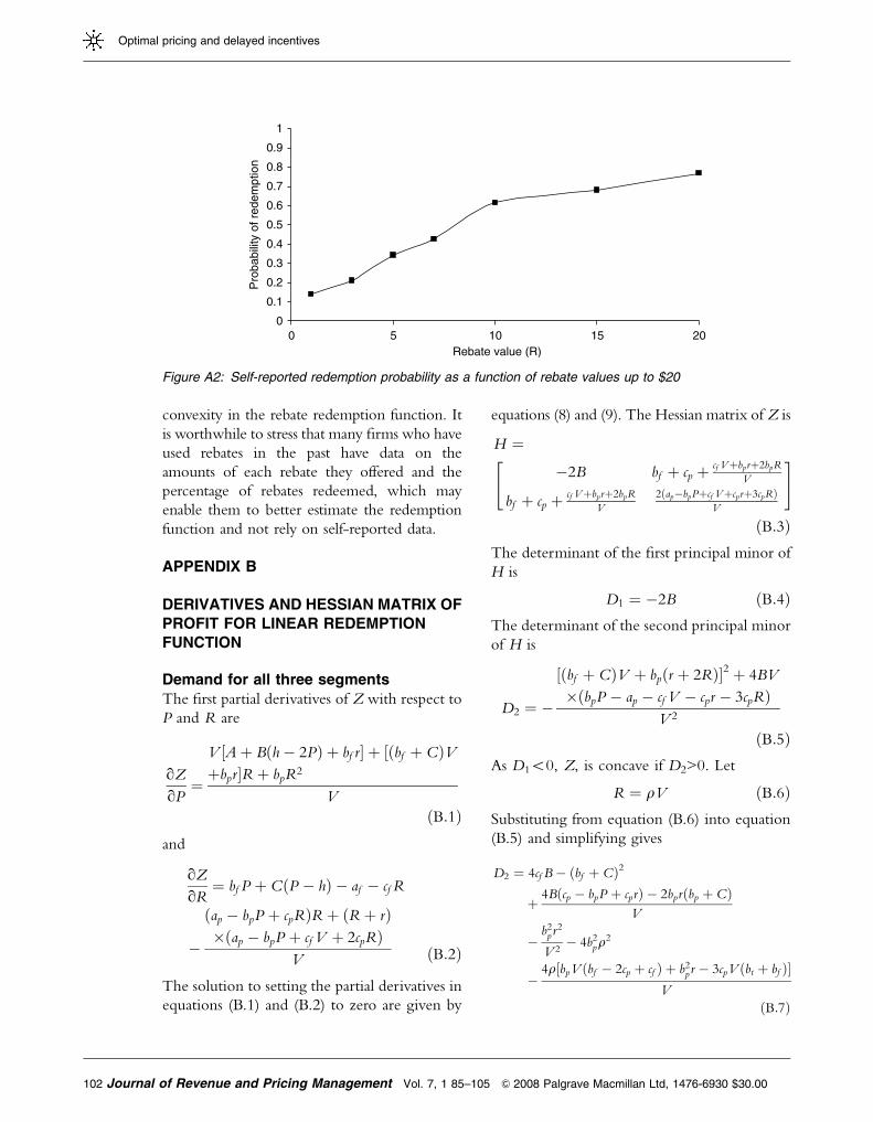
convexity in the rebate redemption function. It
is worthwhile to stress that many firms who have
used rebates in the past have data on the
amounts of each rebate they offered and the
percentage of rebates redeemed, which may
enable them to better estimate the redemption
function and not rely on self-reported data.
APPENDIX B
DERIVATIVES AND HESSIAN MATRIX OF
PROFIT FOR LINEAR REDEMPTION
FUNCTION
Demand for all three segments
The first partial derivatives of Z with respect to
P and R are
qZ
qP¼
V ½A þ Bðh � 2PÞ þ bf r þ ½ðbf þ CÞVþbprR þ bpR2
V
ðB:1Þand
qZ
qR¼ bf P þ CðP � hÞ � af � cf R
�
ðap � bpP þ cpRÞR þ ðR þ rÞ�ðap � bpP þ cf V þ 2cpRÞ
V ðB:2Þ
The solution to setting the partial derivatives in
equations (B.1) and (B.2) to zero are given by
equations (8) and (9). The Hessian matrix of Z is
H ¼�2B bf þ cp þ cf Vþbprþ2bpR
V
bf þ cp þ cf Vþbprþ2bpR
V
2ðap�bpPþcf Vþcprþ3cpRÞV
" #
ðB:3ÞThe determinant of the first principal minor of
H is
D1 ¼ �2B ðB:4ÞThe determinant of the second principal minor
of H is
D2 ¼ �
½ðbf þ CÞV þ bpðr þ 2RÞ2 þ 4BV
�ðbpP � ap � cf V � cpr � 3cpRÞV 2
ðB:5ÞAs D1o0, Z, is concave if D2>0. Let
R ¼ rV ðB:6ÞSubstituting from equation (B.6) into equation
(B.5) and simplifying gives
D2 ¼ 4cf B � ðbf þ CÞ2
þ 4Bðcp � bpP þ cprÞ � 2bprðbp þ CÞV
�b2
pr2
V 2� 4b2
pr2
�4r½bpV ðbf � 2cp þ cf Þ þ b2
pr � 3cpV ðbt þ bf ÞV
ðB:7Þ
0
0.1
0.2
0.3
0.4
0.5
0.6
0.7
0.8
0.9
1
0 5 10 15 20Rebate value (R)
Pro
babi
lity
of r
edem
ptio
n
Figure A2: Self-reported redemption probability as a function of rebate values up to $20
Journal of Revenue and Pricing Management Vol. 7, 1 85–105 & 2008 Palgrave Macmillan Ltd, 1476-6930 $30.00102
Optimal pricing and delayed incentives
equation (B.7) has a single root at
Ps ¼� V
"ðbf þ CÞ2 � 4cf B
� 4Bðap þ cprÞ � 2bprðbf þ CÞV
þb2
p r2
V 2þ 4b2
pr2
þ4r½bpV ðbf � 2cp þ cf Þ þ b2
p r � 3cpV ðbt þ bf ÞV
#
=ð4bpBÞ ðB:8ÞD2 switches signs at Ps. Let e be a small positive
number. For P¼Ps�e, D2¼ 4Bbpe/V>0.
Therefore, Z is concave for PoPs. A plot of
Ps for 0prp1 shows the values of P for which
Z is concave for all positive rebate values up to
price.
Demand from only the FRD and PRD
segments
Following the same analysis for the three-
segment case, Zfp is concave for PoPs, where
Ps is given by equation (B.8) with at¼ bt¼ 0. A
plot of Ps for 0prp1 shows the values of P for
which Zfp is concave for all rebate values up to
price.
Demand from only the PRD segment
Substituting from equation (15) into the profit
function and taking the first and second
derivative w.r.t. P gives d2Zp/dP2¼�2bpo0.
Therefore, Zp is concave and equation (16) is a
sufficient condition for optimality.
Proof of Lemma 1. 1. By contradiction, suppose
R1¼ (cpV�bpr)/2bpþD is optimal. Then de-
creasing the rebate by D and decreasing the
price by Dcp/bp will leave demand unchanged.
The change in revenue is:
xp P � Dcp
bp
� �� P
� �¼ � xpDcp
bp
ðB:9Þ
The change in total rebates paid is
xp
R1 � DV
ðR1 � Dþ rÞ
� xp
R1
VðR1 þ rÞ ¼ � xpDðbpDþ cpV Þ
bpV
ðB:10Þ
As the revenue decreases and rebate cost also
decreases, the net change in total profit is
� xpDcp
bp
� � xtDðbpDþ cpV ÞbpV
� �
¼ xpD2
V40 ðB:11Þ
Therefore, R1 cannot be optimal.
2. By contradiction, suppose R2¼ (cpV�bpr)/
(2bp)�D is optimal. Then increasing the rebate
by D and increasing the price by Dcp/bp will
leave demand unchanged. The change in
revenue is
xp P þ Dcp
bp
� �� P
� �¼ þ xpDcp
bp
ðB:12Þ
The change in total rebates paid is
xp
R2 þ DV
ðR2 þ Dþ rÞ
� xp
R2
VðR2 þ rÞ ¼ xpDðcpV � bpDÞ
bpV
ðB:13ÞThe net change in total profit is
xpDcp
bp
� xpDðc2V � bpDÞbpV
¼ xpD2
V40 ðB:14Þ
Therefore, R2 cannot be optimal.
Proof of Property 1. Subtracting Zfp from Z gives
Z � Zfp ¼ ðP � hÞðat � btPÞ40 for all P and R in S1
ðB:15Þ
Subtracting Zp from Zfp gives
Zfp � Zp ¼ ½P � ðh þ r þ RÞðaf � bf P þ cf RÞ40
for all P and R in S1 ðB:16ÞFrom equations (B.15) and (B.16), Z>Zfp and
Zfp>Zp.
Proof of Property 2. From equation (B.15),
Z�Zfpo0 for all P and R in S2. Therefore,
ZoZfp. From equation (B.16), Zfp�Zp>0 for
all P and R in S2 and P>hþ rþR. Therefore,
Zfp>Zp.
& 2008 Palgrave Macmillan Ltd, 1476-6930 $30.00 Vol. 7, 1 85–105 Journal of Revenue and Pricing Management 103
Khouja, Robbins and Rajagopalan

Proof of Property 3. From equation (B.16),
Zfp�Zpo0 for all P and R in S3 and
P>hþ rþR. Therefore, ZfpoZp. Subtracting
Zp from Z gives
Z � Zp ¼ ðP � hÞðat � btPÞþ ½P � ðh þ r þ RÞðaf � bf P þ cf RÞo0 for all P and R in S3 ðB:17Þ
From equation (B.17), ZoZp.
Proof of Lemma 2. By Property 1, if P� and R�
are in S2, then Z(P�, R�)oZfp(P�, R�). There-
fore, there is a P2 and R2 in S2 such thatZ(P�, R�)oZfp(P
�, R�)pZfp(P2, R2) and P� andR� cannot be optimal. By Property 2, if P� andR� are in S3, then Z(P�, R�)oZp(P
�, R�).Therefore, there is a P3 and R3 in S3 such thatZ(P�, R�)oZp(P
�, R�)pZp(P3, R3) and P� andR� cannot be optimal.
Proof of Lemma 3. By Property 3, if Pfp� and Rfp
�
are in S3, then Zfp(Pfp� , Rfp
� )oZp(Pfp� , Rfp
� ).Therefore, there is a P3 and R3 in S3 such thatZfp(Pfp
� , Rfp� )oZp(Pfp
� , Rfp� )pZp(P3, R3) and Pfp
�
and Rfp� cannot be optimal. By Property 1, if
Pfp� and Rfp
� are in S1, then Z(Pfp� , Rfp
� )>Zfp(Pfp
� , Rfp� ). Therefore, there is a P1 and R1
in S1 such that Z(P1, R1)>Z(Pfp� , Rfp
� )>Zfp(Pfp
� , Rfp� ) and Pfp
� and Rfp� cannot be optimal.
Proof of Lemma 4. By Property 1, if Pp� and Rp
�
are in S1, then Zp(Pp�, Rp
�)oZ(Pp�, Rp
�). There-fore, there is a P1 and R1 in S1 such thatZp(Pp
�, Rp�)oZ(Pp
�, Rp�)pZ(P1, R1) and Pp
� andRp� cannot be optimal. By Property 1, if Pp
� andRp� are in S2, then Zp(Pp
�, Rp�)oZfp(Pp
�, Rp�).
Therefore, there is a P2 and R2 in S2 such thatZfp(P2, R2)XZfp(Pp
�, Rp�)>Zp(Pp
�, Rp�) and Pp
� andRp� cannot be optimal.
DERIVATIVES AND HESSIAN MATRIX OF
PROFIT FOR NONLINEAR REDEMPTION
FUNCTION
The first partial derivatives of Z with respect to
P and R are
qZ
qP¼
½A þ Bðh � 2PÞ þ bf r þ ðbf þ CÞR�ðu � RÞ þ bpRðr þ RÞ
ðu � RÞðB:18Þ
and
qZ
qR¼ �
ðap � bpP þ cpRÞRðu � RÞ þ ðR þ rÞ½uðap � bpPÞ þ cf ðu � RÞ2 þ cpRð2u � RÞ
ðu � RÞ2
þ bf P þ CðP � hÞ � af � cf R ðB:19Þ
The solution to setting the partial derivatives in
equations (B.18) and (B.19) to zero are given by
equations (30) and (31). The elements of the
Hessian matrix of Z are
q11 ¼ �2B ðB:20Þ
q12 ¼ q12 ¼ bf þ C þ bp½uð2R þ rÞ � R2ðu � RÞ2
ðB:21Þ
and
q22 ¼2½ðap � bpPÞðr þ uÞu þ cpðR2ðR � 3uÞ
þu2ð3R þ rÞÞðR � uÞ3
ðB:22Þ
The determinant of the second principal minor of
H is
D2 ¼1
ðu � RÞ4½½ðbf þ CÞðu � RÞ2
þ bpðRð2u � RÞ þ ruÞ2
þ 4BðR � uÞ½cf ðR � uÞ3
þ uðbpP � apÞðr þ uÞ � cp½R2ðR � 3uÞþ u2ðr þ 3RÞ ðB:23Þ
As q11o0, Z is concave if D2>0. As (u�R)4>0, it is
sufficient that the term inside the brackets be
positive. Let
R ¼ km ðB:24Þ
Substituting from (B.24) into (B.23) and simplifying
gives
D2 ¼u2½�½uðbf þ CÞðk� 1Þ2
þ bpðr � uðk� 2ÞkÞ2
þ 4Bðk� 1Þ½cf u2ðk� 1Þ3
þ ðbpP � apÞðr þ uÞ� cpu½r þ ukð3 þ kðk� 3ÞÞ ðB:25Þ
Journal of Revenue and Pricing Management Vol. 7, 1 85–105 & 2008 Palgrave Macmillan Ltd, 1476-6930 $30.00104
Optimal pricing and delayed incentives
equation (B.25) has a single root at
Pc ¼1
4bpBðr þ uÞð1 � kÞ ½4apBðr þ uÞð1 � kÞ
þ 4Bcf u2ðk� 1Þ4 þ 4Bð1 � kÞcpu
�½r þ ukð3 þ ðk� 3ÞkÞ� ½ðbf þ CÞuð1 � kÞ2
þ bpðr � uðk� 2ÞkÞ2 ðB:26ÞD2 switches signs at Pc. Let e be a small positive
number. For P¼ Pc�e, D2¼�4bpBu2(rþ u)
(1�k)e. Therefore, as long as ko1 (ie rebate values
less than price), D2o0 for PoPc and Z is concave.
A plot of Pc for 0pko1 shows the values of P for
which Z is concave for all rebate values up to price.
Demand for the FRD and PRD only
Following the same analysis for the three-
segment case, Zfp is concave for PoPc, where
Pc is given by equation (B.26) with at¼ 0 and
bt¼ 0. A plot of Pc for 0prp1 shows the
values of P for which Zfp is concave for all
rebate values up to price.
Demand for the PRD only
Substituting from equation (32) into the profit
function and taking the first and second
derivative w.r.t. P gives d2Zp/dP2¼�2bpo0.
Therefore, Zp is concave and equation (33) is a
sufficient condition for optimality.
Proof of Lemma 5. The proof of Lemma 5 can
be established in the same way as Lemma 1
using and
R1 ¼ u �ffiffiffiffiffiffiffiffiffiffiffiffiffiffiffiffiffiffiffiffiffiffiffiffiffiffiffiffiffiffiffiffiffiffiffiffiffiffibpu ðbp þ cpÞð r þ uÞ
pbp þ cp
þ D
and
R2 ¼ u �ffiffiffiffiffiffiffiffiffiffiffiffiffiffiffiffiffiffiffiffiffiffiffiffiffiffiffiffiffiffiffiffiffiffiffiffiffiffibpu ðbp þ cpÞð r þ uÞ
pbp þ cp
� D
ðB:27Þ
Solution at boundary — Linear
redemption
At P¼ at/bt, d2Z/dR2o0 for R>[atbp�bt(apþcfVþ cpr)]/(3btcp) and Z is concave. At P¼
(afþ cf R)/bf, d2Z/dR2o0 for Ro(bpaf�apbf)/
[3(bc cp�bpcf )]þ (cfV–bfr)/(3bf) and Z is concave.
Solution at boundary — Nonlinear
redemption
At P¼ at/bt,
d2Z=dR2 ¼ k0 þ 6k1u2R � 6k1uR2
þ 2k1R3 ðB:28Þ
where
k0 ¼� 2u½ðapbt � atbpÞðr þ uÞþ btuðcpr þ cf uÞ
ðB:29Þ
k1 ¼ btðcp � cf Þ ðB:30Þ
For k0o0 (which holds for realistic problems)
and R>0, d2Z/dR2 switches sign at
Rc ¼ mþ
ffiffiffiffiffiffiffiffiffiffiffiffiffiffiffiffiffiffiffiffiffiffiffiffiffiffiffiffiffiffiffiffið�2k3
1u3 � k2
1k0Þ2k3
1
3
sðB:31Þ
If k1o0 then d 2Z/dR2o0 for all R>Rc and Z
is concave. If k1>0, then d2Z/dR2o0 for all
RoRc and Z is concave.
At P¼ (afþ cfR)/bf, d2Z/dR2 is given by
(B.28) where
k0 ¼� 2u½ðcf bp � cpbf Þðbf r � cf uÞu
þ bf ðaf bp � apbf Þðr þ uÞ ðB:32Þ
k1 ¼ ðbf þ cf Þðbf cp � bpcf Þ ðB:33Þ
If k0>0 and k1o0, k0o0 and k1>0,
or k0o0 and k1o0, then d2Z/dR2 switches
sign at Rc given by equation (B.31) and
for all RoRc, d2Z/dR2o0 and Z is
concave. If k0>0 and k1>0 then d2Z/dR2
switches sign at Rc given by equation (B.31)
and for all R>Rc, d2Z/dR2o0 and Z is
concave.
& 2008 Palgrave Macmillan Ltd, 1476-6930 $30.00 Vol. 7, 1 85–105 Journal of Revenue and Pricing Management 105
Khouja, Robbins and Rajagopalan