optimal recharging strategy for battery-switch...

Interdisciplinary Institute for Innovation

Optimal Recharging Strategy for

Battery-Switch Stations for Electric

Vehicles in France

Margaret Armstrong

Charles El Hajj Moussa

Jérôme Adnot

Alain Galli

Philippe Rivière

Working Paper 12-ME-07

November 2012

CERNA, MINES ParisTech

60 boulevard Saint Michel

75006 Paris, France

Email: [email protected]

1

Optimal Recharging Strategy for Battery-Switch Stations for Electric

Vehicles in France

M Armstrong1, C El Hajj Moussa2, J Adnot2, A Galli1 & P Riviere2

1. Cerna, Mines-ParisTech, 60 Boulevard Saint-Michel, Paris France

2. Centre Energétique et Procédés, Mines-ParisTech, 60 Boulevard

Saint-Michel, Paris France

Corresponding author: Margaret Armstrong

Date: 27 June 2012

Abstract

Most papers that study the recharging of electric vehicles focus on charging

the batteries at home and at the work-place. The alternative is for owners to

exchange the battery at a specially equipped battery switch station (BSS).

This paper studies strategies for the BSS to buy and sell the electricity

through the day-ahead market. We determine what the optimal strategies

would have been for a large fleet of EVs in 2010 and 2011, for the V2G and

the G2V cases. These give the amount that the BSS should offer to buy or

sell each hour of the day. Given the size of the fleet, the quantities of

electricity bought and sold will displace the market equilibrium. Using the

aggregate offers to buy and the bids to sell on the day-ahead market, we

compute what the new prices and volumes transacted would be. While

buying electricity for the G2V case incurs a cost, it is possible to generate

revenue in the V2G case, if the arrivals of the EVs are evenly spaced during

the day. We compare the total cost of implementing the strategies proposed

with the cost of buying the same quantity of electricity from EDF.

Keywords: day-ahead auction market, vehicle-to-grid, grid-to-vehicle

2

Introduction

Over the next 10-15 years most European countries are planning to introduce

electric vehicles (EV) in order to reduce greenhouse gas emissions and to

cut pollution levels in urban areas. According to Hacker et al (2009), the

German government plans to have 1 million EVs by 2020 and 5 million by

2025; the Irish government aims for 10% of the national fleet to be electric by

2020 while the Spanish government has committed to having 1 million

electric or hybrid cars on Spanish roads by 2014. The French grid operator

has developed two scenarios for the introduction of EVs (RTE, 2009). In the

reference scenario there will be 1 million EVS in 2020 and 2.7 million in 2025;

the second scenario is more ambitious: it envisages 3.5 million EVs in 2020

and 6.7 million in 2025. In both cases the demand for electricity will increase

considerably. The impact on the system will depend on when the batteries

are recharged. Schneider et al (2011) studied three scenarios for recharging

the batteries of one million EVs in the Washington-Baltimore Metropolitan

Area:

• unmanaged charging,

• consumer-price incentivized recharging where price differentials

in electricity tariffs are designed to dissuade car owners from

recharging their batteries during peak periods,

• getting a central network operator (CNO) to coordinate the

charging of a large number of batteries in response to real-time

prices.

They concluded that the third option would lead to lower wholesale electricity

prices as well as reducing load peaks. So in this paper we only consider the

case where the charging of the batteries is coordinated.

Broadly speaking there are two ways of charging batteries: by

plugging the EVs into a smart plug at the owner’s home or workplace, or by

exchanging the depleted battery for a fully charged one at a battery switch

station (BSS). The impact of the first option has been studied by many

authors including Rousselle (2009) for France, and Hadley and Tsvetkova

(2009) and Lyon et al (2012) for the USA. In a study sponsored by the

French grid operator RTE, Rousselle (2009) simulated the recharge times

3

and the state of charge in the battery, in order to estimate the total load

curve. Her analysis highlighted the impact of unmanaged charging on the

load curves. She did not study the impact on electricity prices. Hadley &

Tsvetkova (2009) determined the marginal generation type in 12 regions in

the USA, and hence the impact on wholesale prices for different recharging

scenarios.

A recent study of the economic impact of smart meters by Lyon et al

(2012) was motivated by a decision by the Colorado Public Utility

Commission to disallow part of the costs of the “Smart Grid City” project in

Boulder, Co, on the grounds that the benefits of the smart meters had not

been adequately established. Using data from two different independent

system operators, MISO in the Midwest and PJM on the east coast, they

demonstrated that shifting charging from daytime to off-peak periods could

lead to billions of dollars of savings. They concluded that while “time-of-use”

pricing is worthwhile in both systems, the economic benefits of optimal

charging of EVs did not appear to justify the costs of investing in the smart

grid infrastructure required to implement real time pricing. To take advantage

of the “time-of-use” pricing homeowners only need an appliance timer costing

between $12 and $60 whereas they need a smart meter worth $150 to

respond to the real-time pricing.

As the option to recharge batteries at home or at the workplace has

already been studied thoroughly, this paper focuses on the battery exchange

option, and uses France to illustrate how the strategies could work. Initially

we assumed that the BSS operator captured 10% of a fleet of 3 million EVs

as its clients and that these 300,000 vehicles were recharged twice per week,

giving 85,700 batteries to recharge per day on average. This corresponds to

the usage pattern for the second family car in urban areas. But it rapidly

became clear that the economics of the BSS depends on the number of

batteries to be recharged per day and the number of spare batteries held by

the BSS but not on the total number of EVs. For example, if 10,000 taxis sign

up for a battery exchange contract, they would require an exchange battery

at the end of each driver’s shift (and possibly another while waiting for a fare

at the airport). This alone would account for 20,000 to 30,000 batteries per

day.

4

The number of spare batteries held by the BSS has a marked

influence on when the batteries are recharged. If the BSS has only a small

number of batteries, it would be obliged to recharge them as soon as they

arrive in order to have fully charge batteries available as clients arrive. As this

would put a strain on the power supply at peak periods, we assume that the

BSS has enough spare batteries to recharge them in off-peak periods.

Another important choice for the BSS operator is whether to provide

power to the grid during peak hours (that is, operate in vehicle-to-grid mode,

V2G) or just to buy power (that is, grid-to-vehicle G2V mode). The positive

effects of vehicle-to-grid power transfers (V2G) are well-known: it lowers

wholesale electricity prices and reduces the load at peak hours (Kempton

and Tomic, 2005; Denholm and Short, 2006; Tomic and Kempton, 2007;

Scott et al 2007). So we develop strategies for both the V2G and G2V

operations.

In contrast to the PJM area which uses real-time locational marginal

prices, few countries in Europe currently use nodal pricing, Poland being an

exception (Sivorski, 2011), even though a recent study (Neuhoff et al, 2011)

advocated it to reduce congestion. At present the day-ahead auction market

is the main wholesale electricity market in western European countries. In

some countries such as Ireland (Finn et al, 2012) and the Iberian Peninsula

(Tomé Saraiva, 2007; Camus et al, 2011) there is a pool, but in Scandinavia

and in the Central West Europe market (Benelux, France and Germany) only

part of the electricity is sold through the organized market.

To buy/sell through the day-ahead auction market interested parties

must send firm offers specifying prices and quantities for each 1-hour period

(30 minutes in Ireland), before 11am or 12 noon on the day prior to delivery.

The electricity bourse compiles the aggregate curves of bids to buy electricity

and of offers to sell for each hour and computes the intersection of the two

curves to determine the market fixing price. This price applies to all buyers

and sellers provided that the interconnection capacity is sufficient to allow the

required transfers. Within France, the transmission and distribution grids are

dense enough so that the same price applies throughout the country.

If a BSS were to set up business in France, the management could

negotiate a contract to buy power directly from the historic utility, EDF, or one

5

of its competitors. Alternatively the BSS could trade through the day-ahead

market run by the bourse, Epexspot, but in order to trade, it would need a

strategy for deciding how much to offer for each hour of the day1. This paper

proposes strategies for buying and selling power through bourse, which have

been optimized assuming that the management of the BSS aims to maximize

corporate profits in the long-term by minimizing the operating costs of

recharging the EVs in the short-term. Finally we compare the cost of using

these strategies to recharge the batteries of the EVs with the cost of

purchasing the same quantity of electricity at the price specified by the new

NOME law2: 40 € in 2011 and 42 € per MWh in 2012.

This is not the first paper to propose algorithms for charging EVs.

Taheri et al (2011) developed a demand response service for a fleet of

around 10,000 PHEVs. They assume that vehicles plug in periodically over a

given period of time (say 12 hours) and report their driving schedule for the

next n hours. To ensure that the total amount of electricity supplied to EVs

stays within limits that are acceptable to utilities they put an hourly cap on

charging. Earlier on, Han et al (2011) and Wu et al (2011) had constructed

decision-making algorithms for minimum-cost recharging schedules which

considered the vehicles individually rather than collectively as a fleet. Ma et

al (2010) optimised the recharging to fill up the “overnight” valley. But none of

these papers considered buying and selling via the day-ahead auction

market.

The paper is structured is follows. The next section describes the

methodology used and explains the assumptions that have been made. The

results are presented in Section 3: firstly, the schedules for recharging the

batteries; secondly, the cost of carrying out these schedules and thirdly their

impact on the day-ahead market (i.e. on prices and on the volumes

transacted). The conclusions follow in Section 4.

1 We assume that the BSS operator is a price-taker who offers to buy/sell a certain quantity whatever the price. In the future we plan to work on optimising the price at which the BSS offers to buy/sell power. 2 The French government recently passed the NOME law (short for Nouvelle Organisation des Marchés de l’Electricité) which requires the historic utility, EDF, to provide base-load electricity from nuclear power plants to new entrants at a regulated tariff (40 € in 2011 and 42 € per MWh in 2012). This price was designed to cover the full cost of nuclear energy including investments, production, decommissioning and the long-term storage of nuclear waste, as a benchmark for evaluating the cost of charging the batteries.

6

Research methodology

The first step when optimising the schedules for recharging batteries is to

decide what data to use. One possibility would be to use the data over a long

period of time (e.g. several years). Three factors made us think that this is

not appropriate. Firstly data from before the creation of the CWE market in

November 2010 comes from a time when the market structure was different.

Secondly, the markets are evolving gradually because of the introduction of

renewable energy. The production mix is changing and so will the strategies

of buyers and sellers on the bourse. Thirdly, electricity consumption is

inherently seasonal, with marked differences between summer and winter, as

well as between the different days of the week. For all these reasons we

think that more robust strategies can be developed by using a relatively short

training set that reflects the current market structure and trading practices.

We chose a moving training set consisting of the aggregated offers to

buy/sell electricity on the day-ahead auction market during the previous 4

weeks. As the usage patterns vary from one day of the week to another,

different strategies are developed for each day of the week and the training

set consists of same day of the week over the previous four weeks. Public

holidays are taken into account because electricity consumption is different

on holidays compared to working days. Care is also required with the day in

spring when Europe changes over from winter time to summer time and

again in autumn with the change back to winter time3.

Market data for the past two years, 2010 and 2011, were used in the

study. Over the past 5 years several important changes have been made to

the structure of electricity markets in Western Europe. Firstly in 2007 the

markets in France, Belgium and the Netherlands were coupled. This means

that provided the transmission capacity was sufficient, the three countries

had a common price. In November 2010 the Central Western European

market was formed by coupling Germany with those three countries. So our

study covers the period before and after a major structural change in the

French electricity market. One of our objectives was to see how much the

3 On the Saturday night in March of the change-over to day-light saving, there are only 23 hours, whereas in autumn there is a day with 25 hours.

7

optimal strategies changed because of the market coupling with Germany,

and whether there were problems just after the change-over when the

training set uses data before the market coupling to determine the strategies

applied afterwards.

The next point to decide was when the clients were likely to arrive and

when the batteries would be charged. To simplify the computations we

assumed that no clients arrive between 10pm and 6am. In G2V mode, the

batteries are recharged from 10pm until 6am4 and all vehicles must be fully

charged by 6am when clients start arriving. The G2V strategy gives the

optimal amount to buy for each of these 8 hours. In V2G mode, all the

batteries must also be fully charged by 6am but as the BSS can buy or sell at

any time during the 24 hour period, the optimal strategy gives the amounts to

buy or sell for each of the 24 hours. In contrast to the G2V case, the arrival

times during the day have a marked effect on the V2G strategy. Two extreme

scenarios are considered: (A) all EVs arrive at 6am and (B) the arrival of the

EVs is spread evenly from 6am until 10pm.

It is assumed that on arrival batteries contain 10% of the nominal

charge (24KWh). Secondly due to technical losses between the grid and the

battery, 5% is lost each time a battery is charged or discharged (Badey, 2012

p13; Dang et al, 2010). By way of comparison, Lyon et al (2012) considered

a battery capacity of 16 KWh and a charging efficiency of 88% based on the

specifications of the 2011 Chevy Volt. Like them we do not take account of

the wear and tear on batteries due to charging and discharging.

The key step in the study is to determine the impact of buying or

selling more power on the day-ahead market. Figure 1 shows a schematic

representation of the offers to buy and the bids to sell electricity for a given

hour5. As we have assumed that the BSS operator is a price-taker, an offer to

buy power would shift the aggregate offers to buy to the right, leading to a

higher price (Figure 2 left). Figure 2 (right) illustrates the effect of selling

electricity, which drops the price.

4 The times 10pm and 6am correspond to a cheap tariff proposed by EDF for heating hot water systems. 5 In this figure the minimum price is 0. This was the case before the market coupling with Germany. Since then the market has adopted the German convention of having a minimum

8

Figure 1: Aggregate offers to buy and sell electricity during a given hour. The

intersection of the two curves gives the market fixing price and volume.

Figure 2: Aggregate offers. If the BSS wishes to buy power, the aggregate curve of

offers to purchase would be shifted to right leading to a higher price (left);

conversely if the BSS wishes to sell power, the aggregate curve of offers to sell

would be shifted to right, leading to a lower price (right).

Optimisation procedure

Our objective is to determine the quantities qi of electricity to charge into or

discharge from the batteries in the ith hour for i=1, …24, to ensure that all the

batteries are fully charged by 6am the next day. By convention qi is positive

when the battery is being charged and negative when it is being discharged.

The quantities to be bought or sold on the bourse depend on the extent of

losses when charging and discharging the batteries. If the quantity qi is

charged into the batteries after losing 5% of energy during the charging

process, then the quantity bought on the bourse was 1.05qi; and conversely if

qi is discharged from the batteries, then 0.95qi will be available for sale on

the bourse.

price of -3000 €. It may seem unnatural to sell electricity for a negative price but some producers prefer to pay to continue to produce rather than having to stop.

Price

Volume Volume

Price

Price

Volume

9

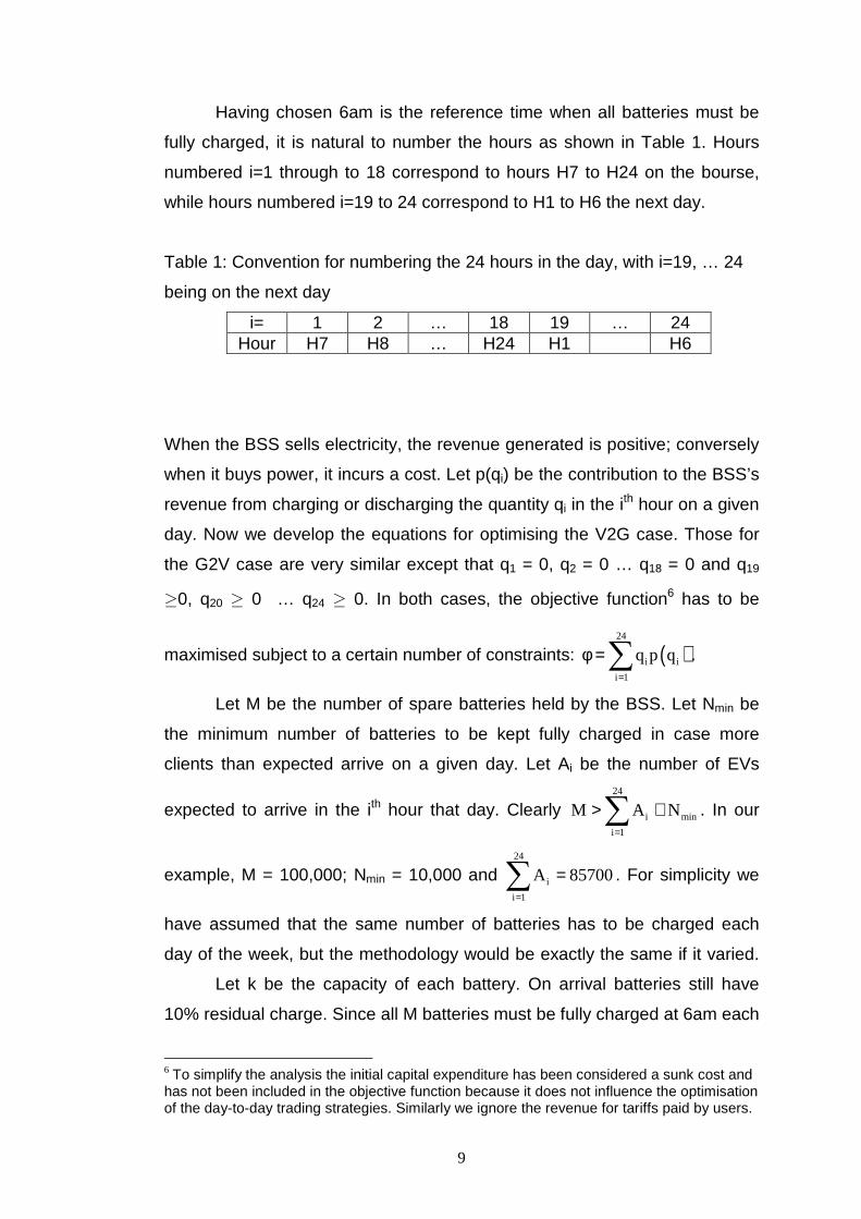
Having chosen 6am is the reference time when all batteries must be

fully charged, it is natural to number the hours as shown in Table 1. Hours

numbered i=1 through to 18 correspond to hours H7 to H24 on the bourse,

while hours numbered i=19 to 24 correspond to H1 to H6 the next day.

Table 1: Convention for numbering the 24 hours in the day, with i=19, … 24

being on the next day

i= 1 2 … 18 19 … 24 Hour H7 H8 … H24 H1 H6

When the BSS sells electricity, the revenue generated is positive; conversely

when it buys power, it incurs a cost. Let p(qi) be the contribution to the BSS’s

revenue from charging or discharging the quantity qi in the ith hour on a given

day. Now we develop the equations for optimising the V2G case. Those for

the G2V case are very similar except that q1 = 0, q2 = 0 … q18 = 0 and q19

≥0, q20 ≥ 0 … q24 ≥ 0. In both cases, the objective function6 has to be

maximised subject to a certain number of constraints: ( )24

i i

i 1

q p q=

φ =∑ .

Let M be the number of spare batteries held by the BSS. Let Nmin be

the minimum number of batteries to be kept fully charged in case more

clients than expected arrive on a given day. Let Ai be the number of EVs

expected to arrive in the ith hour that day. Clearly 24

i min

i 1

M A N=

> +∑ . In our

example, M = 100,000; Nmin = 10,000 and 24

i

i 1

A 85700=

=∑ . For simplicity we

have assumed that the same number of batteries has to be charged each

day of the week, but the methodology would be exactly the same if it varied.

Let k be the capacity of each battery. On arrival batteries still have

10% residual charge. Since all M batteries must be fully charged at 6am each

6 To simplify the analysis the initial capital expenditure has been considered a sunk cost and has not been included in the objective function because it does not influence the optimisation of the day-to-day trading strategies. Similarly we ignore the revenue for tariffs paid by users.

10

day, the first constraint concerns the net increase in the charge in the

batteries: 24 24

i i

i 1 i 1

q 0.9k A= =

= ×∑ ∑

As the charge in the batteries cannot be less than zero or more than 100% of

the capacity, there are also limits on the quantity that can be physically

charged into the batteries or discharged from them in any given hour, and

hence on the quantities that can be bought or sold. For the V2G case, these

depend on the expected hourly arrivals Ai. During the first hour, A1 EVs are

expected to arrive. After those batteries have been exchanged and the

quantity q1 is charged into the batteries, the total charge left in the M

batteries in the BSS will be

1 1Mk 0.9A k q− +

This amount must be greater than Nmin k and less than Mk:

( )min 1 1

min 1 1

N k Mk 0.9A k q

0 M N 0.9A k q

≤ − +⇒ ≤ − − +

1 1

1 1

Mk 0.9A k q Mk

q 0.9A k

− + ≤⇒ ≤

By the ith hour in the day, a total of (A1+…+Ai) EVs should have arrived. The

cumulative amount put into the batteries and discharged from the batteries

will be (q1 +…+qi), so the total charge left in the batteries in the BSS will be i i

j j

j 1 j 1

Mk 0.9k A q= =

− +∑ ∑

This gives the inequalities

i i

min i j

j 1 j 1

0 M N 0.9 A k q= =

≤ − − +

∑ ∑ for i =1, … 23

i i

j j

j 1 j 1

q 0.9k A= =

≤∑ ∑ for i =1, … 23

Because all the batteries must be fully charged by 6am, the constraint on the

24th hour of the day is: 24 24

i i

i 1 i 1

q 0.9k A= =

=∑ ∑

11

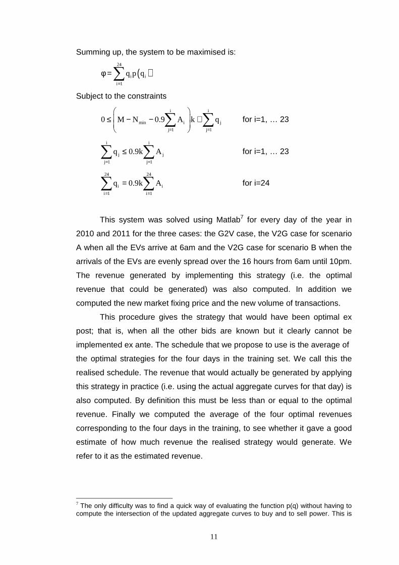
Summing up, the system to be maximised is:

( )24

i i

i 1

q p q=

φ =∑

Subject to the constraints

i i

min i j

j 1 j 1

0 M N 0.9 A k q= =

≤ − − +

∑ ∑ for i=1, … 23

i i

j j

j 1 j 1

q 0.9k A= =

≤∑ ∑ for i=1, … 23

24 24

i i

i 1 i 1

q 0.9k A= =

=∑ ∑ for i=24

This system was solved using Matlab7 for every day of the year in

2010 and 2011 for the three cases: the G2V case, the V2G case for scenario

A when all the EVs arrive at 6am and the V2G case for scenario B when the

arrivals of the EVs are evenly spread over the 16 hours from 6am until 10pm.

The revenue generated by implementing this strategy (i.e. the optimal

revenue that could be generated) was also computed. In addition we

computed the new market fixing price and the new volume of transactions.

This procedure gives the strategy that would have been optimal ex

post; that is, when all the other bids are known but it clearly cannot be

implemented ex ante. The schedule that we propose to use is the average of

the optimal strategies for the four days in the training set. We call this the

realised schedule. The revenue that would actually be generated by applying

this strategy in practice (i.e. using the actual aggregate curves for that day) is

also computed. By definition this must be less than or equal to the optimal

revenue. Finally we computed the average of the four optimal revenues

corresponding to the four days in the training, to see whether it gave a good

estimate of how much revenue the realised strategy would generate. We

refer to it as the estimated revenue.

7 The only difficulty was to find a quick way of evaluating the function p(q) without having to compute the intersection of the updated aggregate curves to buy and to sell power. This is

12

Results

The results will be presented in the following order: firstly the optimal and

realised schedules for recharging the batteries; secondly, the values

generated by carrying out these schedules and thirdly the impact that

recharging the batteries would have on the day-ahead market (i.e. on prices

and on the volumes transacted).

Optimal and Realised Schedules

The schedules give the quantity of electricity in MW to buy or sell each hour

of the day on the day-ahead market. The optimal schedules were averaged

over periods of 13 weeks in winter and summer 2010 (Figure 3) and in 2011

(Figure 4). Figures 5 and 6 present the corresponding averages of the

realised schedules. In each case the solid black line is for the V2G case for

scenario A (when all EVs arrive at 6am), while the thick black dotted line is

for the V2G case for scenario B (when the arrivals of EVs are evenly spread

from 6am until 10pm) and the solid red line is for the G2V case.

Both the optimal and the realised schedules vary from one day of the

week to another but the main differences are between the weekend and the

other five working days. To save space only two typical cases are presented:

the schedules for 6am Sunday to 6am Monday, and for 6am Tuesday to 6am

Wednesday. Looking at these figures we see that:

done by pre-calculating the intersections for a set of 100 evenly spaced points above and below the original market fixing and interpolating linearly in between these points.

13

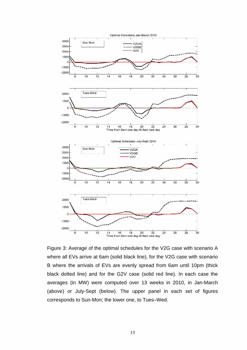
Figure 3: Average of the optimal schedules for the V2G case with scenario A

where all EVs arrive at 6am (solid black line), for the V2G case with scenario

B where the arrivals of EVs are evenly spread from 6am until 10pm (thick

black dotted line) and for the G2V case (solid red line). In each case the

averages (in MW) were computed over 13 weeks in 2010, in Jan-March

(above) or July-Sept (below). The upper panel in each set of figures

corresponds to Sun-Mon; the lower one, to Tues–Wed.

14

Figure 4: Average of the optimal schedules for the V2G case with scenario A




averages (in MW) were computed over 13 weeks in 2011, in Jan-March

(above) or July-Sept (below). The upper panel in each set of figures

corresponds to Sun-Mon; the lower one, to Tues–Wed

15

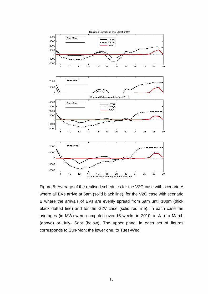
Figure 5: Average of the realised schedules for the V2G case with scenario A




averages (in MW) were computed over 13 weeks in 2010, in Jan to March

(above) or July- Sept (below). The upper panel in each set of figures

corresponds to Sun-Mon; the lower one, to Tues-Wed

16

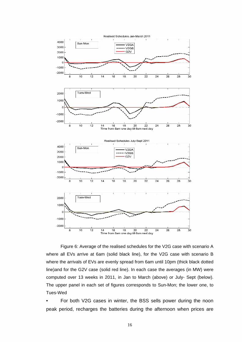
Figure 6: Average of the realised schedules for the V2G case with scenario A

where all EVs arrive at 6am (solid black line), for the V2G case with scenario B

where the arrivals of EVs are evenly spread from 6am until 10pm (thick black dotted

line)and for the G2V case (solid red line). In each case the averages (in MW) were

computed over 13 weeks in 2011, in Jan to March (above) or July- Sept (below).

The upper panel in each set of figures corresponds to Sun-Mon; the lower one, to

Tues-Wed

• For both V2G cases in winter, the BSS sells power during the noon

peak period, recharges the batteries during the afternoon when prices are

17

lower, then sells power again during the evening peak period and recharges

the batteries during the night; in summer, the evening peak price is not as

high so less power is sold on the market.

• The recharging schedule for the V2G case scenario A when all the

EVs arrive at 6am is quite different from scenario B when the arrivals are

spread evenly from 6am until 10pm. Much more power is bought and sold in

scenario B.

• The recharging schedule for the G2V is almost the same as for

scenario A of the V2G case during the night-time (10pm to 6am). This is why

the solid red line has almost covered up the solid black line.

• The optimal schedules are quite similar to the realised schedules, but

both vary from winter to summer because of different usage patterns

because electrical heating is widely used in winter in France.

Values generated by carrying out these schedules

The value generated by implementing these strategies can be either negative

(i.e. a cost that the BSS must pay) or positive (i.e. revenue for the BSS).

Three sets of values were computed for each case:

• the estimated value obtained by averaging the optimal values for the

days in the training set;

• the optimal value (obtained by optimising the schedule ex post)

• the realised value obtained using the proposed schedule and the

actual information for the day.

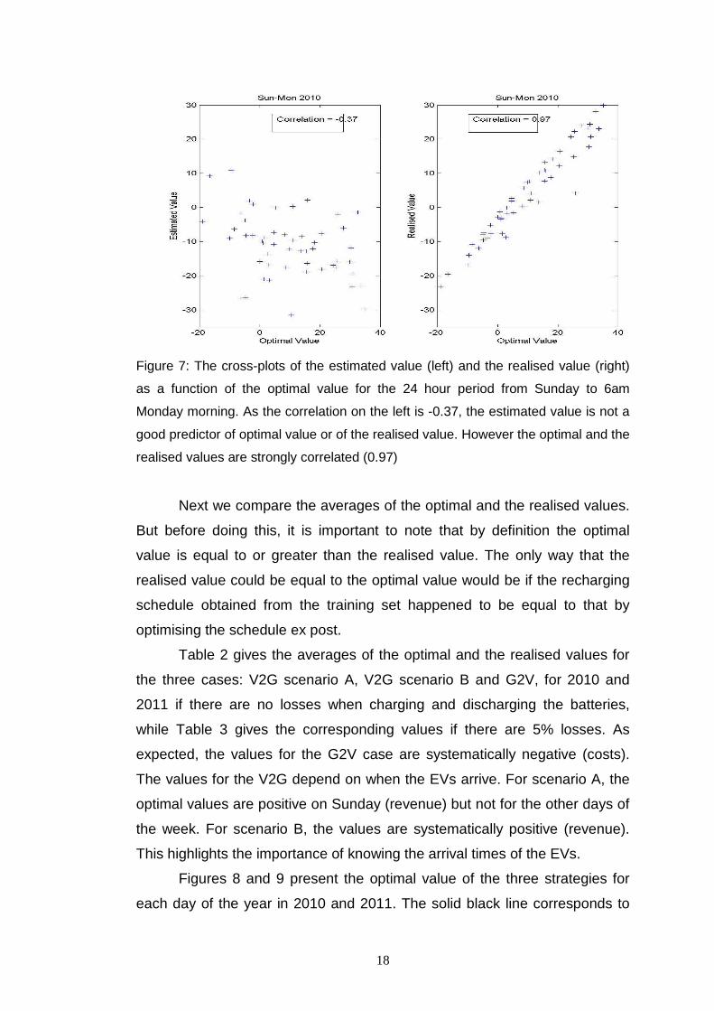
We had expected the estimated value to be a good predictor of the

future value but this turned out to be incorrect. To illustrate this point, Figure

7 shows the cross-plot of the estimated value (left) and the realised value

(right) as a function of the optimal value for the 24 hour period Sunday to

Monday in 2010. The correlation coefficient in the left panel is -0.37

compared 0.97 in the right one. That is, there is a strong correlation between

the realised value and the optimal value, but virtually none between the

estimated value and the optimal one. Consequently the estimated value will

not be considered in the rest of the study.

18

Figure 7: The cross-plots of the estimated value (left) and the realised value (right)

as a function of the optimal value for the 24 hour period from Sunday to 6am

Monday morning. As the correlation on the left is -0.37, the estimated value is not a

good predictor of optimal value or of the realised value. However the optimal and the

realised values are strongly correlated (0.97)

Next we compare the averages of the optimal and the realised values.

But before doing this, it is important to note that by definition the optimal

value is equal to or greater than the realised value. The only way that the

realised value could be equal to the optimal value would be if the recharging

schedule obtained from the training set happened to be equal to that by

optimising the schedule ex post.

Table 2 gives the averages of the optimal and the realised values for

the three cases: V2G scenario A, V2G scenario B and G2V, for 2010 and

2011 if there are no losses when charging and discharging the batteries,

while Table 3 gives the corresponding values if there are 5% losses. As

expected, the values for the G2V case are systematically negative (costs).

The values for the V2G depend on when the EVs arrive. For scenario A, the

optimal values are positive on Sunday (revenue) but not for the other days of

the week. For scenario B, the values are systematically positive (revenue).

This highlights the importance of knowing the arrival times of the EVs.

Figures 8 and 9 present the optimal value of the three strategies for

each day of the year in 2010 and 2011. The solid black line corresponds to

19

Scenario A for the V2G case, the dotted black corresponds to Scenario B of

the V2G case while the solid red line is for the G2V case. In each figure the

case where there are no losses is in the upper panel, while the lower panels

corresponds to the case where there are 5% losses. The optimal value for

G2V case is almost always less than the other two; the optimal value for

scenario B of the V2G case is almost always higher than the other two.

Table 2: Optimal values (OptVal) and realised values (RVal) for the V2G

case scenario A (where all EVS arrive at 6am), for the V2G case scenario B

(where the arrivals of the EVs are evenly spread from 6am until 10pm) and

for the G2V case, for 2010 and 2011 when there are no losses transferring

power to and from the batteries.

2010 Sun Mon Tues Wed Thu Fri Sat

OptValA 9.83 -10.90 -9.60 -13.36 -11.87 -12.19 -1.54

RValA 3.95 -18.04 -17.58 -19.85 -21.92 -18.20 -7.71

OptValB 51.00 60.76 75.60 57.91 57.95 50.05 46.01

RValB 32.37 41.03 53.96 39.00 36.86 33.09 7.94

OptValG2V -26.81 -32.91 -31.32 -32.39 -31.86 -31.87 -24.43

RValG2V -27.70 -33.53 -32.24 -33.35 -32.90 -32.71 -25.08


OptValA 4.71 -14.70 -16.92 -16.16 -18.63 -16.89 -3.41

RValA -6.06 -24.91 -23.71 -23.03 -26.40 -24.32 -14.27

OptValB 34.36 41.06 38.74 44.31 30.05 33.25 33.23

RValB -3.22 6.41 15.18 22.63 9.53 12.01 1.96

OptValG2V -27.60 -32.83 -33.66 -31.38 -33.76 -32.77 -25.56

RValG2V -28.84 -34.03 -34.44 -32.60 -35.12 -33.98 -27.07

20

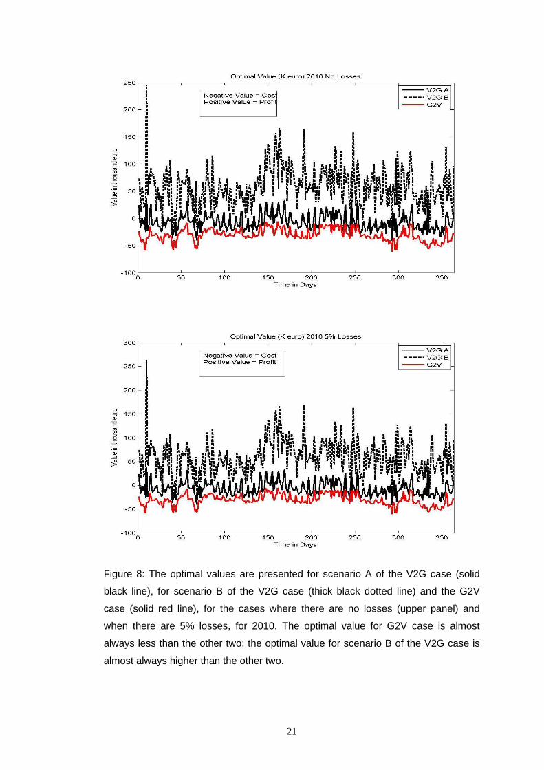
We had wondered to what extent the creation of the CWE market would

perturb the strategies since the data from before the change was being used

afterwards. In particular we had been expecting to see changes in the

realised values, or a discontinuity in the optimal value. Looking at Figure 8,

there are no obvious differences toward the end of that year. So the

strategies are quite stable – even when confronted with a major structural

change in the market.

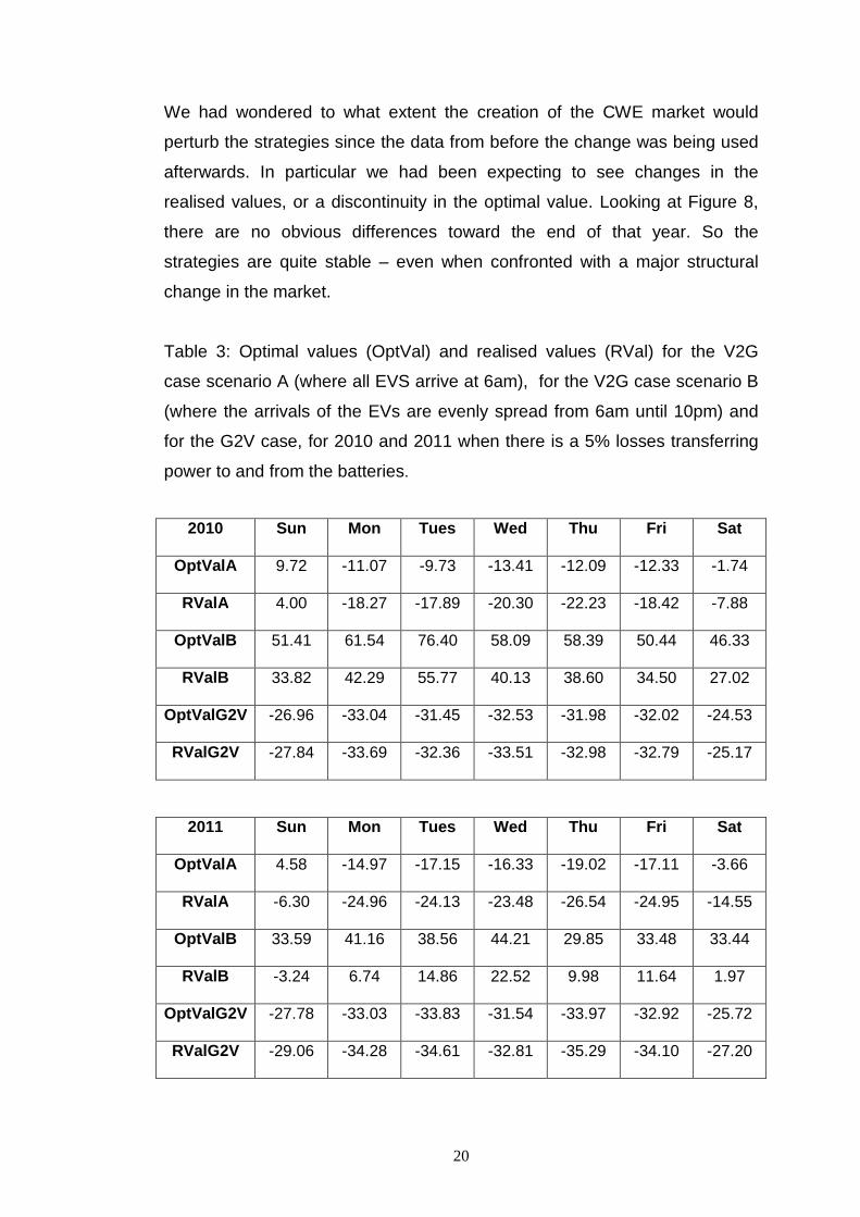
Table 3: Optimal values (OptVal) and realised values (RVal) for the V2G

case scenario A (where all EVS arrive at 6am), for the V2G case scenario B

(where the arrivals of the EVs are evenly spread from 6am until 10pm) and

for the G2V case, for 2010 and 2011 when there is a 5% losses transferring

power to and from the batteries.


OptValA 9.72 -11.07 -9.73 -13.41 -12.09 -12.33 -1.74

RValA 4.00 -18.27 -17.89 -20.30 -22.23 -18.42 -7.88

OptValB 51.41 61.54 76.40 58.09 58.39 50.44 46.33

RValB 33.82 42.29 55.77 40.13 38.60 34.50 27.02

OptValG2V -26.96 -33.04 -31.45 -32.53 -31.98 -32.02 -24.53

RValG2V -27.84 -33.69 -32.36 -33.51 -32.98 -32.79 -25.17


OptValA 4.58 -14.97 -17.15 -16.33 -19.02 -17.11 -3.66

RValA -6.30 -24.96 -24.13 -23.48 -26.54 -24.95 -14.55

OptValB 33.59 41.16 38.56 44.21 29.85 33.48 33.44

RValB -3.24 6.74 14.86 22.52 9.98 11.64 1.97

OptValG2V -27.78 -33.03 -33.83 -31.54 -33.97 -32.92 -25.72

RValG2V -29.06 -34.28 -34.61 -32.81 -35.29 -34.10 -27.20

21

Figure 8: The optimal values are presented for scenario A of the V2G case (solid

black line), for scenario B of the V2G case (thick black dotted line) and the G2V

case (solid red line), for the cases where there are no losses (upper panel) and

when there are 5% losses, for 2010. The optimal value for G2V case is almost

always less than the other two; the optimal value for scenario B of the V2G case is

almost always higher than the other two.

22

Figure 9 The optimal values are presented for scenario A of the V2G case (solid

black line), for scenario B of the V2G case (thick black dotted line) and the G2V

case (solid red line), for the cases where there are no losses (upper panel) and

when there are 5% losses, for 2011. The optimal value for G2V case is almost

always less than the other two; the optimal value for scenario B of the V2G case is

almost always higher than the other two.

23

Impact of the strategies for recharging the batteries on the day-ahead market

As the strategies were designed to optimise the revenue for the BSS, we

want to find out what effect this will have on the wholesale electricity market.

To be more precise, we are interested in their impact on the hourly day-

ahead prices for electricity and on the volumes of transactions.

The average prices were computed over a 13 week period in winter

and again in summer, in 2010 and 2011. Figures 10 and 11 show these for

winter and summer 2010, and winter and summer 2011, respectively. As

before the averages are shown for the 24 hour period from 6am Sunday until

6 am Monday, and from 6 am Tuesday until 6 am Wednesday. Four curves

are shown in each figure: a solid black line for scenario A for the V2G case, a

thick black dotted line for scenario B for the V2G case, a solid red line for the

G2V case and finally a fine black line showing the original prices (that is, the

observed prices). The red line corresponding to the G2V case is only shown

from 10pm until 6am because it does not affect prices or volumes during the

daytime.

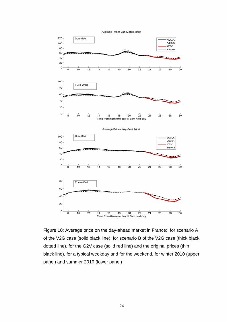
As expected the original prices are higher than those for the two V2G

cases during the evening peak hour especially in winter. Scenario B in the

V2G case leads to a greater drop at peak hours and to a correspondingly

higher price in the early morning off-peak period. In contrast to electricity

prices which drop during peak hours in the V2G cases, the volumes of

electricity bought and sold through the auction market rise in both peak hours

and off peak periods. This is particularly marked for scenario B in the V2G

case. In the case studied where 300,000 EVs have signed up with the BSS,

the impact on the market prices and volumes are not very marked. But the

French government has plans to have 10 times as many EVs on the roads. In

that case the impact of coordinated changing would lead to a much more

pronounced drop in peak prices.

24

Figure 10: Average price on the day-ahead market in France: for scenario A

of the V2G case (solid black line), for scenario B of the V2G case (thick black

dotted line), for the G2V case (solid red line) and the original prices (thin

black line), for a typical weekday and for the weekend, for winter 2010 (upper

panel) and summer 2010 (lower panel)

25

Figure 11: Average volumes on the day-ahead market in France: for

scenario A of the V2G case (solid black line), for scenario B of the V2G case

(thick black dotted line), for the G2V case (solid red line) and the original

prices (thin black line), for a typical weekday and for the weekend, for winter

2010 (upper panel) and summer 2010 (lower panel)

26

Discussion and Conclusions

Most papers that study the recharging of electric vehicles focus on charging

the batteries at home and in the work-place. The alternative is for owners to

exchange the battery at a specially equipped battery switch station (BSS).

This paper proposes strategies for the BSS to buy and sell the electricity

through the day-ahead auction market. To do this the BSS would have to

submit firm offers specifying the amounts of electricity that it is offering to buy

or sell during each hour of the day, before noon on the day prior to delivery.

So the management needs a procedure for determining those quantities.

We determined what the optimal strategies would have been for a

large fleet of EVs each day in 2010 and 2011, for the V2G and the G2V

cases. As one of the key factors influencing the optimal strategies for the

V2G case is the expected arrival time of the EVs, two fairly extreme

possibilities were considered: firstly an unfavourable case where all the EVs

arrive first thing in the morning and secondly when their arrivals are spread

evenly throughout the day. Another factor that was taken into account was

losses when charging and discharging batteries. Table 4 gives the annual

revenue in millions of euros from buying and selling on the day-ahead

market, for the three scenarios considered with and without losses. Positive

values correspond to revenue while negative ones are costs. These can be

compared with the amount (27 M euro) that it would cost to buy the same

quantity of electricity at the benchmark base-load price of 40 € per MWh at

which the government obliges EDF to sell nuclear power to competitors.

27

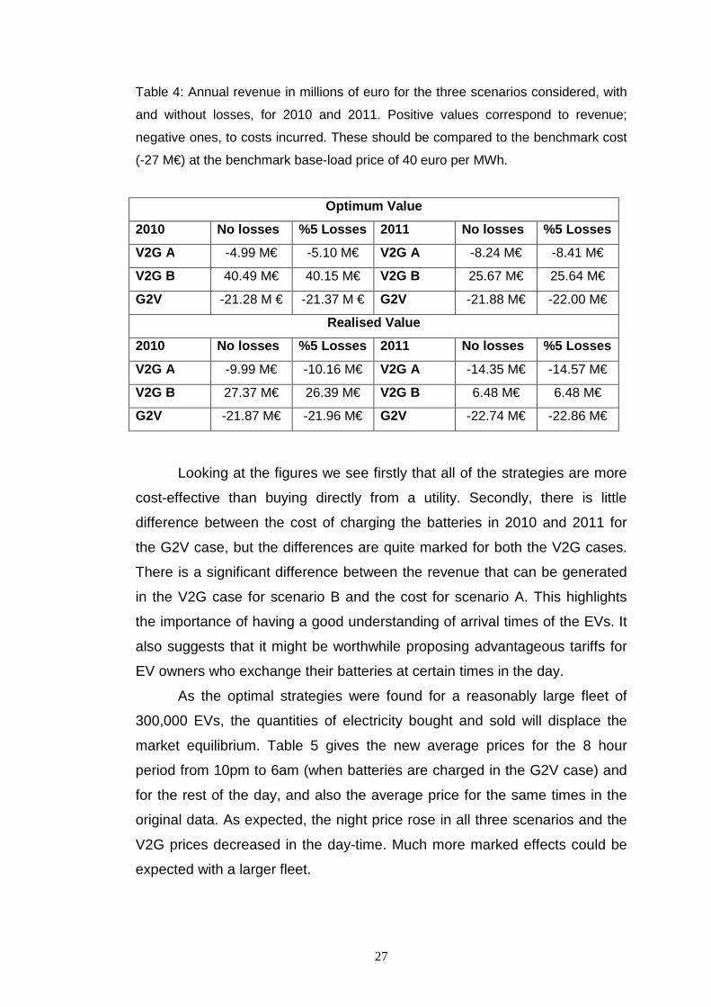
Table 4: Annual revenue in millions of euro for the three scenarios considered, with

and without losses, for 2010 and 2011. Positive values correspond to revenue;

negative ones, to costs incurred. These should be compared to the benchmark cost

(-27 M€) at the benchmark base-load price of 40 euro per MWh.

Optimum Value

2010 No losses %5 Losses 2011 No losses %5 Losses

V2G A -4.99 M€ -5.10 M€ V2G A -8.24 M€ -8.41 M€

V2G B 40.49 M€ 40.15 M€ V2G B 25.67 M€ 25.64 M€

G2V -21.28 M € -21.37 M € G2V -21.88 M€ -22.00 M€

Realised Value


V2G A -9.99 M€ -10.16 M€ V2G A -14.35 M€ -14.57 M€

V2G B 27.37 M€ 26.39 M€ V2G B 6.48 M€ 6.48 M€

G2V -21.87 M€ -21.96 M€ G2V -22.74 M€ -22.86 M€

Looking at the figures we see firstly that all of the strategies are more

cost-effective than buying directly from a utility. Secondly, there is little

difference between the cost of charging the batteries in 2010 and 2011 for

the G2V case, but the differences are quite marked for both the V2G cases.

There is a significant difference between the revenue that can be generated

in the V2G case for scenario B and the cost for scenario A. This highlights

the importance of having a good understanding of arrival times of the EVs. It

also suggests that it might be worthwhile proposing advantageous tariffs for

EV owners who exchange their batteries at certain times in the day.

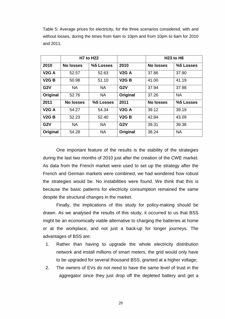
As the optimal strategies were found for a reasonably large fleet of

300,000 EVs, the quantities of electricity bought and sold will displace the

market equilibrium. Table 5 gives the new average prices for the 8 hour

period from 10pm to 6am (when batteries are charged in the G2V case) and

for the rest of the day, and also the average price for the same times in the

original data. As expected, the night price rose in all three scenarios and the

V2G prices decreased in the day-time. Much more marked effects could be

expected with a larger fleet.

28

Table 5: Average prices for electricity, for the three scenarios considered, with and

without losses, during the times from 6am to 10pm and from 10pm to 6am for 2010

and 2011.

H7 to H22 H23 to H6


V2G A 52.57 52.63 V2G A 37.86 37.90

V2G B 50.98 51.10 V2G B 41.00 41.19

G2V NA NA G2V 37.94 37.98

Original 52.76 NA Original 37.26 NA


V2G A 54.27 54.34 V2G A 39.12 39.19

V2G B 52.23 52.40 V2G B 42.84 43.09

G2V NA NA G2V 39.31 39.38

Original 54.28 NA Original 38.24 NA

One important feature of the results is the stability of the strategies

during the last two months of 2010 just after the creation of the CWE market.

As data from the French market were used to set up the strategy after the

French and German markets were combined, we had wondered how robust

the strategies would be. No instabilities were found. We think that this is

because the basic patterns for electricity consumption remained the same

despite the structural changes in the market.

Finally, the implications of this study for policy-making should be

drawn. As we analysed the results of this study, it occurred to us that BSS

might be an economically viable alternative to charging the batteries at home

or at the workplace, and not just a back-up for longer journeys. The

advantages of BSS are:

1. Rather than having to upgrade the whole electricity distribution

network and install millions of smart meters, the grid would only have

to be upgraded for several thousand BSS, granted at a higher voltage;

2. The owners of EVs do not need to have the same level of trust in the

aggregator since they just drop off the depleted battery and get a

29

fully charged battery in exchange. No one is charging/discharging the

battery in THEIR car. The batteries remain anonymous;

3. From a mathematical point of view it is much simpler to optimize the

charging/discharging of a large set of anonymous batteries. There is

no need to know the owners’ travel details individually, or to store and

process vast quantities of private information;

4. Most interesting of all, no new special incentives are needed to

convince the BSS operator to charge the batteries in a socially

optimal way during offpeak periods. It is in his/her interest to reduce

the cost of charging the EVs to increase the profitability of the

business, and as we have shown, in V2G mode this achieves the

socially desirable outcome of having the BSS sell power to the grid

during peak hours (thereby reducing prices and the need for new

peaking power plants) and buying during off-peak periods when

some of the generation capacity is under-used.

This is why we think that if the cost of the batteries drops sufficiently

and if they resist the additional wear-and-tear due to the additional

charging/ discharging cycles, a pure BSS business might actually be a

viable economic proposition - as well as being socially useful.

References

Badey, Q. (2012) Etude des mécanismes et modélisation du vieillissement des

batteries lithium-ion dans le cadre d’un usage automobile, PhD Thesis,

Université Paris-Sud, 260pp available from http://tel.archives-

ouvertes.fr/docs/00/69/33/44/PDF/VA2_BADEY_QUENTIN_22032012.pdf

Camus C., T. Farias,and J. Esteves 2011 Potential impacts assessment of plug-in

electric vehicles on the Portuguese energy market, Energy Policy, 39 (10)

Oct 2011 pp5883-5897

Dang V.T.T., C. Fournier, S. Morel, J. Adnot & J. Oostebaan (2010) Batteries

Management for Minimization of Electric Vehicles’ Environmental Impacts in

A Life Cycle Assessment Framework, EcoBalance2010, 9th International

Conference on EcoBalance, 9-12 Nov, 2010, Tokyo

30

Denholm, P., and W. Short, 2006 An Evaluation of Utility System Impacts and

Benefits of Optimally Dispatched Plug-In Hybrid Electric Vehicles. Technical

Report NREL/TP-620-40293. National Renewable Energy Laboratory,

Golden, CO.

Finn, P., C. Fitzpatrick and D. Connolly, (2012) Demand side management of

electric car charging: Benefits for consumer and grid, Energy (42 (2012) 358-

363

Hacker, F., R. Harthan, F. Matthes & W. Zimmer, (2009), Environmental impacts

and impact on the electricity market of a large scale introduction of electric

cars in Europe – Critical Review of Literature, ETC/ACC Technical Paper

2009/4

Hadley S.W. and A. Tsvetkova (2008) Potential impacts of plug-in electric vehicles

on regional power generation, 71pp, available from

http://www.ornl.gov/info/ornlreview/v41_1_08/regional_phev_analysis.pdf

Han, SE, SO Han and K. Sezaki (2010) Development of an optimal vehicle-to-grid

aggregator for frequency regulation, IEEE Transaction on Smart Grid, 1:65-

72, June, 2010

Kempton W. and J. Tomic, (2005) Vehicle-to-grid power fundamentals: calculating

capacity and net revenue, J. Power Sources 144(1) 280-294

Lyon, T., M. Michelin, A. Jongejan and T. Leahy, (2012) Is “smart-charging” policy

for electric vehicles worthwhile?, Energy Policy 41 (2012) 259-268

Ma Z., D. Callaway and I. Hiskens (2010) Decentralized charging control for large

populations of plug-in electric vehicles: Application of the Nash certainty

equivalence principle. IEEE International Conference on Control

Applications, pp191-195, Sept 2010

Neuhoff, K., R. Boyd, T. Grau, B. Hobbs, D. Newbery, F. Borggrefe, J. Barquin, F.

Echavarren, J. Bialek, C. Dent, C. von Hirschhausen, F. Kunz, H. Weight, C.

Nabe, G. Papaefthymiou, and C. Weber, (2011) Reshaping: Shaping an

effective and efficient European renewable energy market, D20 Report:

Consistency with other EU policies, System and Market Integration- A Smart

Power Market at the Centre of a Smart Grid, 110pp

Rousselle, M. (2009) Impact of the Electric Vehicle on the electric system, MSc

Thesis KTH

31

RTE (2009) Generation Adequacy Report on the electricity supply-demand balance

in France, 172pp available from www.rte-france.fr

Schneider, S.J., R. Bearman, H. McDermott, X. Xu, S. Benner & K. Huber (2011) An

assessment of the price impact of electric vehicles on PJM market: A joint

study by PJM & Better Place, 30pp available from

http://www.betterplace.com/uploads/ckfinder/files/Press%20Kits/An_Assess

ment_of_the_Price_Impacts_of_Electric_Vehicles_on_the_PJM_Market.pdf?

awesm=btrp.lc_fXd&utm_campaign=&utm_medium=btrp.lc-

copypaste&utm_source=direct-btrp.lc&utm_content=awesm-publisher

Scott M.J., M. Kintner-Meyer, D.B. Elliott and W.M. Warwick (2007) Impacts

assessment of plug-in hybrid vehicles on electric utilities and regional U.S.

power grids: Part 2: Economic assessment, 18pp available from

http://www.roguevalleycleancities.org/images/news.html/PNNL%20Articles/P

HEV_Economic_Analysis_Part2_Final.pdf

Sivorski, T. (2011) Nodal pricing project in Poland, presented at the 34th IAEE

International Conference, Stockholm, 21 June 2011

Taheri, N., R. Entriken and Y. Ye, (2011) A dynamic algorithm for facilitated

charging of plug-in electric vehicles, 16pp

Tomic, J., and W. Kempton, (2007) Using fleets of electric-drive vehicles for grid

support, J. Power Sources 168(2) 459-468

Tomé Saraiva, J., (2007) Iberian Electricity market: Difficulties, advantages and

challenges, 37pp, available from

http://www.cefes.untz.ba/pdf/3_CEFES_Tuzla_JTS_Final.pdf

Wu, D., D.C. Aliprantis and L. Ying (2011) Load scheduling and dispatch for

aggregators of plug-in electric vehicles. IEEE Transactions on Smart Grid,

Special Issue on Transportation Electricification and Vehicle-to-Grid

Applications, May 2011

optimal recharging strategy for battery-switch...

Documents