optimal sample size allocation for multi-stress tests ...faculty.smu.edu/ngh/erpre2.pdf · optimal...
TRANSCRIPT

Optimal Sample Size Allocation forMulti-Stress Tests using
Extreme Value RegressionH. K. Tony Ng
Department of Statistical Science
Southern Methodist University, Dallas, Texas
Co-authored with N. Balakrishnan (McMaster University)
& P. S. Chan (Chinese University of Hong Kong)
Optimal Sample Size Allocation for Multi-Stress Tests using Extreme Value Regression – p.1/51
Outline1. Introduction - Multi-stress Experiments
Optimal Sample Size Allocation for Multi-Stress Tests using Extreme Value Regression – p.2/51

Outline1. Introduction - Multi-stress Experiments
2. Introduction - Extreme value regression
Optimal Sample Size Allocation for Multi-Stress Tests using Extreme Value Regression – p.2/51

Outline1. Introduction - Multi-stress Experiments
2. Introduction - Extreme value regression
3. Likelihood Inference
Optimal Sample Size Allocation for Multi-Stress Tests using Extreme Value Regression – p.2/51

Outline1. Introduction - Multi-stress Experiments
2. Introduction - Extreme value regression
3. Likelihood Inference
4. Optimal Sample Size Allocation for Estimation
Optimal Sample Size Allocation for Multi-Stress Tests using Extreme Value Regression – p.2/51

Outline1. Introduction - Multi-stress Experiments
2. Introduction - Extreme value regression
3. Likelihood Inference
4. Optimal Sample Size Allocation for Estimation• Two-stress levels
Optimal Sample Size Allocation for Multi-Stress Tests using Extreme Value Regression – p.2/51

Outline1. Introduction - Multi-stress Experiments
2. Introduction - Extreme value regression
3. Likelihood Inference
4. Optimal Sample Size Allocation for Estimation• Two-stress levels• k-stress levels
Optimal Sample Size Allocation for Multi-Stress Tests using Extreme Value Regression – p.2/51
Outline1. Introduction - Multi-stress Experiments
2. Introduction - Extreme value regression
3. Likelihood Inference
4. Optimal Sample Size Allocation for Estimation• Two-stress levels• k-stress levels
5. Optimal Sample Size Allocation for Prediction
Optimal Sample Size Allocation for Multi-Stress Tests using Extreme Value Regression – p.2/51

Outline1. Introduction - Multi-stress Experiments
2. Introduction - Extreme value regression
3. Likelihood Inference
4. Optimal Sample Size Allocation for Estimation• Two-stress levels• k-stress levels
5. Optimal Sample Size Allocation for Prediction• Two-stress levels
Optimal Sample Size Allocation for Multi-Stress Tests using Extreme Value Regression – p.2/51
Outline1. Introduction - Multi-stress Experiments
2. Introduction - Extreme value regression
3. Likelihood Inference
4. Optimal Sample Size Allocation for Estimation• Two-stress levels• k-stress levels
5. Optimal Sample Size Allocation for Prediction• Two-stress levels• k-stress levels
Optimal Sample Size Allocation for Multi-Stress Tests using Extreme Value Regression – p.2/51

Outline1. Introduction - Multi-stress Experiments
2. Introduction - Extreme value regression
3. Likelihood Inference
4. Optimal Sample Size Allocation for Estimation• Two-stress levels• k-stress levels
5. Optimal Sample Size Allocation for Prediction• Two-stress levels• k-stress levels
6. Numerical Illustration
7. Monte Carlo Study for Small Sample Sizes
Optimal Sample Size Allocation for Multi-Stress Tests using Extreme Value Regression – p.2/51

Multi-stress Experiments• In industrial experiments, the lifetime of an unit
may be affected by one or more factors/covariates(such as voltage, load, temperature, etc.)
Optimal Sample Size Allocation for Multi-Stress Tests using Extreme Value Regression – p.3/51

Multi-stress Experiments• In industrial experiments, the lifetime of an unit
may be affected by one or more factors/covariates(such as voltage, load, temperature, etc.)
• The purpose of a life-testing experiment is then tostudy the effect of these covariates on the failuretime distribution and predict the reliability undersome other operating conditions.
• Nowadays, products that are tested are oftenextremely reliable with long life under normaloperating conditions.
Optimal Sample Size Allocation for Multi-Stress Tests using Extreme Value Regression – p.3/51

Multi-stress Experiments• To overcome these problems, the experimenter
may resort to accelerated testing wherein theunits are subjected to higher stress levels thannormal.
Optimal Sample Size Allocation for Multi-Stress Tests using Extreme Value Regression – p.4/51
Multi-stress Experiments• To overcome these problems, the experimenter
may resort to accelerated testing wherein the unitsare subjected to higher stress levels than normal.
• The accelerated tests may be performed usingconstant stress or increasing stress levels.
• Assessing the effects of the acceleratingvariables(e.g. temperature, voltage, load,vibration etc.) on the lifetimes of the product.
• Information from tests at high-levels of one ormore accelerating variables is extrapolated,through a reasonable statistical model, to obtainestimates of life or long-term performance atlower, normal levels of the acceleratingvariable(s).
Optimal Sample Size Allocation for Multi-Stress Tests using Extreme Value Regression – p.4/51
Multi-stress Experiments –Example
• Such testing provides a saving in time and costcompared with testing at normal conditions.
Optimal Sample Size Allocation for Multi-Stress Tests using Extreme Value Regression – p.5/51

Multi-stress Experiments –Example
• Such testing provides a saving in time and costcompared with testing at normal conditions.
• Refrigerator door open/close test:
Optimal Sample Size Allocation for Multi-Stress Tests using Extreme Value Regression – p.5/51

Multi-stress Experiments –Example
• Such testing provides a saving in time and costcompared with testing at normal conditions.
• Refrigerator door open/close test:• Consider the reliability of a refrigerator door,
which is designed for a median open/closecycles of 200,000 times, assuming a normalusage force is used.
• Increase the force of open/close test, therefrigerator door fail more rapidly than itwould have failed at the normal usage force.
• The open/close tests are done under higherforces, the data may then be extrapolated toestimate the mean lifetime under normalcondition.
Optimal Sample Size Allocation for Multi-Stress Tests using Extreme Value Regression – p.5/51

Multi-stress Experiments –Example
• The insulating fluidin a power transformer performs two
major functions:
Optimal Sample Size Allocation for Multi-Stress Tests using Extreme Value Regression – p.6/51

Multi-stress Experiments –Example
• The insulating fluidin a power transformer performs two
major functions:
• electrical insulation to withstand the high voltages
present inside the transformer.
Optimal Sample Size Allocation for Multi-Stress Tests using Extreme Value Regression – p.6/51

Multi-stress Experiments –Example
• The insulating fluidin a power transformer performs two
major functions:
• electrical insulation to withstand the high voltages
present inside the transformer.
• heat transfer medium to dissipate heat generated within
the transformer windings.
• Dielectric Breakdown Voltage - a measure of the ability of
the liquid to withstand electric stress without failure.
• The general accepted minimum dielectric strength is 30kV
for transformers with a high-volatage rating≥ 287.5 kV
and 25kV for transformers with a high-voltage rating<
287.5kV.
Optimal Sample Size Allocation for Multi-Stress Tests using Extreme Value Regression – p.6/51

Multi-stress Experiments
-
-
-
-
-
-
-
26 kV
28 kV
30 kV
32 kV
34 kV
36 kV
38 kV
Voltage (Stress)
s ss
s s ss s
s s s ss ss ss
s s sss ss s ss s
s s s s s s s ss s s s s s
ss ss ss s
s s s s s
Example: Life-testing experiment of insulating fluid at seven stress
levels
• Lifetime = function of factors or covariates
Optimal Sample Size Allocation for Multi-Stress Tests using Extreme Value Regression – p.7/51
Extreme Value Regression• To study the effect of these covariates on the
failure time distribution, a regression model isused to incorporate the covariates in the analysis.
Optimal Sample Size Allocation for Multi-Stress Tests using Extreme Value Regression – p.8/51

Extreme Value Regression• To study the effect of these covariates on the
failure time distribution, a regression model isused to incorporate the covariates in the analysis.
• If the life data are taken under differentenvironmental conditions, the Weibull (Extremevalue) model will be useful as it has moreflexibility.
• Suppose the survival timeT has a Weibulldistribution with probability density function
fT (t; α, δ) =δ
α
(
t
α
)δ−1
exp
[
−
(
t
α
)δ]
, t > 0,
whereα > 0 is the scale parameter andδ > 0 isthe shape parameter.
Optimal Sample Size Allocation for Multi-Stress Tests using Extreme Value Regression – p.8/51

Extreme Value Regression• In this discussion, we will focus on the case with
a single covariate.
Optimal Sample Size Allocation for Multi-Stress Tests using Extreme Value Regression – p.9/51

Extreme Value Regression• In this discussion, we will focus on the case with
a single covariate.• Assume that the covariatex affects only the scale
parameterα; then, we have a proportional hazardmodel for the survival timeT (Kalbfleisch andPrentice, 1980).
Optimal Sample Size Allocation for Multi-Stress Tests using Extreme Value Regression – p.9/51

Extreme Value Regression• Making a logarithmic transformation on the
survival timeT , we have an extreme value(Gumbel Type I) distribution forY = ln T withp.d.f.
fY (y; µ(x), σ) =1
σexp
[(
y − µ(x)
σ
)
− exp
(
y − µ(x)
σ
)]
, −∞ < y < ∞,
whereµ(x) = ln α(x) andσ = 1δ.
Optimal Sample Size Allocation for Multi-Stress Tests using Extreme Value Regression – p.10/51

Extreme Value Regression• Making a logarithmic transformation on the
survival timeT , we have an extreme value(Gumbel Type I) distribution forY = ln T withp.d.f.
fY (y; µ(x), σ) =1
σexp
[(
y − µ(x)
σ
)
− exp
(
y − µ(x)
σ
)]
, −∞ < y < ∞,
whereµ(x) = ln α(x) andσ = 1δ.
• We can writeY in a location-scale form as
Y = µ(x) + σZ,
whereZ has a standard extreme valuedistribution with p.d.f.
fZ(z) = exp (z − exp z) , −∞ < z < ∞.
Optimal Sample Size Allocation for Multi-Stress Tests using Extreme Value Regression – p.10/51

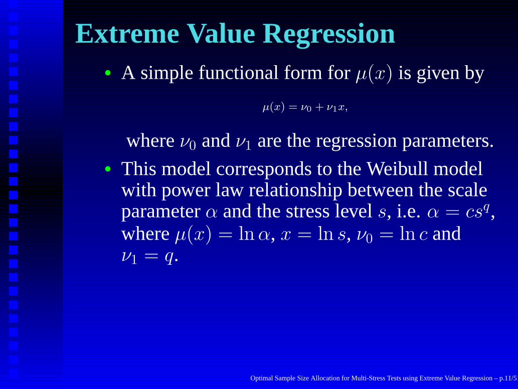
Extreme Value Regression• A simple functional form forµ(x) is given by
µ(x) = ν0 + ν1x,
whereν0 andν1 are the regression parameters.
Optimal Sample Size Allocation for Multi-Stress Tests using Extreme Value Regression – p.11/51
Extreme Value Regression• A simple functional form forµ(x) is given by
µ(x) = ν0 + ν1x,
whereν0 andν1 are the regression parameters.• This model corresponds to the Weibull model
with power law relationship between the scaleparameterα and the stress levels, i.e. α = csq,whereµ(x) = ln α, x = ln s, ν0 = ln c andν1 = q.
Optimal Sample Size Allocation for Multi-Stress Tests using Extreme Value Regression – p.11/51

Multi-stress Experiments
-
-
...
-
-
Stress
x1
x2
...
xk−1
xk
n1
n2
...
nk−1
nk
• Suppose we haveN items available for the test atk oredered
stress level, sayx1 < x2 < . . . < xk.
• We assignnl items for testing at stress levelxl (l = 1, 2, . . . , k)
withk∑
l=1
nl = N
• In planning such a life-testing experiment, we have the flexibility
in the choice of (n1, n2, . . . , nk) for a pre-fixed value ofN and
the stress levelsxl, l = 1, 2, . . . , k.
Optimal Sample Size Allocation for Multi-Stress Tests using Extreme Value Regression – p.12/51

Likelihood Inference• One of the approaches to analyze extreme value (Weibull)
regression model is based on the asy. theory of MLEs.
Optimal Sample Size Allocation for Multi-Stress Tests using Extreme Value Regression – p.13/51

Likelihood Inference• One of the approaches to analyze extreme value (Weibull)
regression model is based on the asy. theory of MLEs.
• Let Zli = (Yli − ν0 − ν1xl) /σ for l = 1, 2, . . . , k,
i = 1, 2, . . . , nl, Zli follows a standard extreme value dist.
Optimal Sample Size Allocation for Multi-Stress Tests using Extreme Value Regression – p.13/51

Likelihood Inference• One of the approaches to analyze extreme value (Weibull)
regression model is based on the asy. theory of MLEs.
• Let Zli = (Yli − ν0 − ν1xl) /σ for l = 1, 2, . . . , k,
i = 1, 2, . . . , nl, Zli follows a standard extreme value dist.• The likelihood function based on thek-stress level model is
then
L(ν0, ν1, σ) =
k∏
l=1
1
σnl
nl∏
i=1
exp (zli − ezli ) ,
so that the log-likelihood function is
ln L(ν0, ν1, σ) = −N ln σ +
k∑
l=1
nl∑
i=1
zli −
k∑
l=1
nl∑
i=1
ezli ,
whereN =k∑
l=1
nl is the total number of units on life-test.
Optimal Sample Size Allocation for Multi-Stress Tests using Extreme Value Regression – p.13/51

Likelihood Inference• We then have the likelihood equations as
∂ ln L(ν0, ν1, σ)
∂ν0= −
1
σ
(
N −
k∑
l=1
nl∑
i=1
ezli
)
= 0,
∂ ln L(ν0, ν1, σ)
∂ν1= −
1
σ
(
k∑
l=1
nlxl −
k∑
l=1
xl
nl∑
i=1
ezli
)
= 0,
∂ ln L(ν0, ν1, σ)
∂σ= −
1
σ
(
N +
k∑
l=1
nl∑
i=1
zli −
k∑
l=1
nl∑
i=1
zliezli
)
= 0,
Optimal Sample Size Allocation for Multi-Stress Tests using Extreme Value Regression – p.14/51

Likelihood Inference• We then have the likelihood equations as
∂ ln L(ν0, ν1, σ)
∂ν0= −
1
σ
(
N −
k∑
l=1
nl∑
i=1
ezli
)
= 0,
∂ ln L(ν0, ν1, σ)
∂ν1= −
1
σ
(
k∑
l=1
nlxl −
k∑
l=1
xl
nl∑
i=1
ezli
)
= 0,
∂ ln L(ν0, ν1, σ)
∂σ= −
1
σ
(
N +
k∑
l=1
nl∑
i=1
zli −
k∑
l=1
nl∑
i=1
zliezli
)
= 0,
• The corresponding MLEs ofν0, ν1 andσ(denoted byν0, ν1 andσ, respectively) can beobtained by solving the above non-linearequations simultaneously by some numericalprocedures, such as the Newton-Raphson method.
Optimal Sample Size Allocation for Multi-Stress Tests using Extreme Value Regression – p.14/51

Likelihood Inference• Let pl = nl
Nbe the proportion of units (of a total
of N units under test) to be assigned to stresslevelxl.
Optimal Sample Size Allocation for Multi-Stress Tests using Extreme Value Regression – p.15/51

Likelihood Inference• Let pl = nl
Nbe the proportion of units (of a total
of N units under test) to be assigned to stresslevelxl.
• The Fisher information matrix in terms ofpl’s is
I(ν0, ν1, σ) =N
σ2I∗(ν0, ν1, σ)
=N
σ2
1k∑
l=1
xlpl (1 − γ)
k∑
l=1
xlpl
k∑
l=1
x2l pl (1 − γ)
k∑
l=1
xlpl
(1 − γ) (1 − γ)k∑
l=1
xlplπ2
6+ (1 − γ)2
.
Optimal Sample Size Allocation for Multi-Stress Tests using Extreme Value Regression – p.15/51

Likelihood Inference• The asymptotic variance-covariance matrix of
(ν0, ν1, σ) is then
I−1 =
σ2
N
Q1 +6(1−γ)2
π2−Q2 −
6(1−γ)
π2
Q3 0
6π2
,
where
Q1 =
k∑
l=1
x2l pl
k∑
l=1
x2lpl −
(
k∑
l=1
xlpl
)2, Q2 =
k∑
l=1
xlpl
k∑
l=1
x2lpl −
(
k∑
l=1
xlpl
)2,
Q3 =1
k∑
l=1
x2lpl −
(
k∑
l=1
xlpl
)2.
Optimal Sample Size Allocation for Multi-Stress Tests using Extreme Value Regression – p.16/51
OPTIMAL SAMPLE SIZE ALLOCATION
FOR ESTIMATION
Optimal Sample Size Allocation for Multi-Stress Tests using Extreme Value Regression – p.17/51

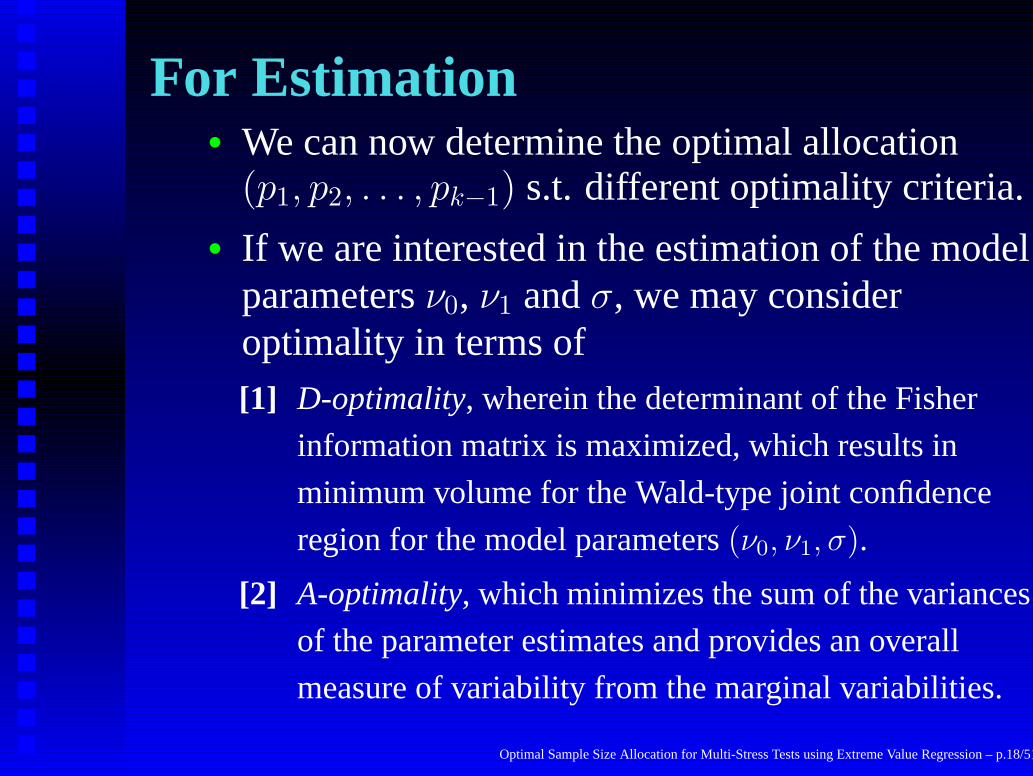
For Estimation• We can now determine the optimal allocation
(p1, p2, . . . , pk−1) s.t. different optimality criteria.
Optimal Sample Size Allocation for Multi-Stress Tests using Extreme Value Regression – p.18/51

For Estimation• We can now determine the optimal allocation
(p1, p2, . . . , pk−1) s.t. different optimality criteria.
• If we are interested in the estimation of the modelparametersν0, ν1 andσ, we may consideroptimality in terms of
Optimal Sample Size Allocation for Multi-Stress Tests using Extreme Value Regression – p.18/51

For Estimation• We can now determine the optimal allocation
(p1, p2, . . . , pk−1) s.t. different optimality criteria.
• If we are interested in the estimation of the modelparametersν0, ν1 andσ, we may consideroptimality in terms of[1] D-optimality, wherein the determinant of the Fisher
information matrix is maximized, which results in
minimum volume for the Wald-type joint confidence
region for the model parameters(ν0, ν1, σ).
Optimal Sample Size Allocation for Multi-Stress Tests using Extreme Value Regression – p.18/51
For Estimation• We can now determine the optimal allocation
(p1, p2, . . . , pk−1) s.t. different optimality criteria.
• If we are interested in the estimation of the modelparametersν0, ν1 andσ, we may consideroptimality in terms of[1] D-optimality, wherein the determinant of the Fisher
information matrix is maximized, which results in
minimum volume for the Wald-type joint confidence
region for the model parameters(ν0, ν1, σ).
[2] A-optimality, which minimizes the sum of the variances
of the parameter estimates and provides an overall
measure of variability from the marginal variabilities.
Optimal Sample Size Allocation for Multi-Stress Tests using Extreme Value Regression – p.18/51

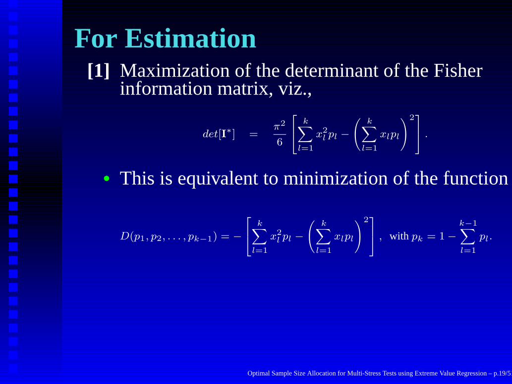
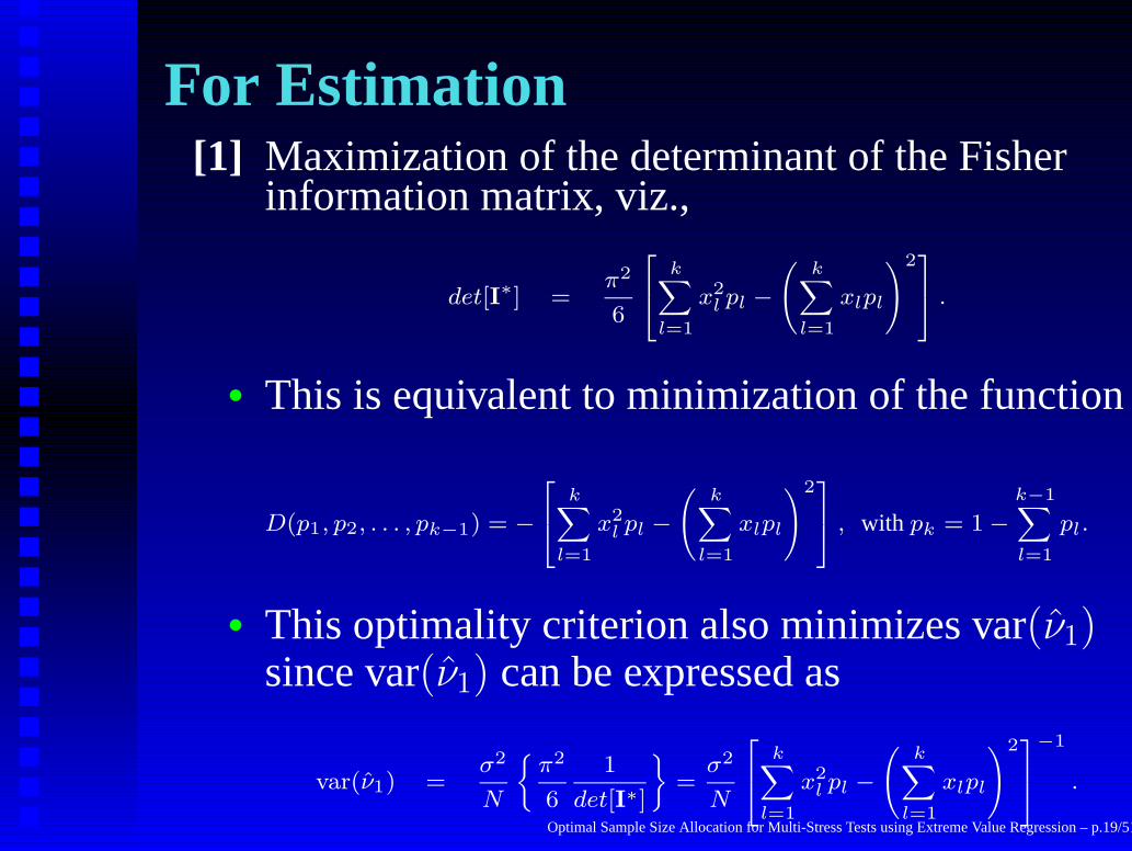
For Estimation[1] Maximization of the determinant of the Fisher
information matrix, viz.,
det[I∗] =π2
6
k∑
l=1
x2l pl −
(
k∑
l=1
xlpl
)2
.
Optimal Sample Size Allocation for Multi-Stress Tests using Extreme Value Regression – p.19/51
For Estimation[1] Maximization of the determinant of the Fisher
information matrix, viz.,
det[I∗] =π2
6
k∑
l=1
x2l pl −
(
k∑
l=1
xlpl
)2
.
• This is equivalent to minimization of the function
D(p1, p2, . . . , pk−1) = −
k∑
l=1
x2l pl −
(
k∑
l=1
xlpl
)2
, with pk = 1 −
k−1∑
l=1
pl.
• This optimality criterion also minimizes var(ν1)since var(ν1) can be expressed as
var(ν1) =σ2
N
{
π2
6
1
det[I∗]
}
=σ2
N
k∑
l=1
x2l pl −
(
k∑
l=1
xlpl
)2
−1
.
Optimal Sample Size Allocation for Multi-Stress Tests using Extreme Value Regression – p.19/51

For Estimation[2] Minimization of the trace of the
variance-covariance matrix (I−1) of the MLE’s,
viz.
tr[I∗−1] = 1 +6[(γ − 1)2 + 1]
π2+
1 +
(
k∑
l=1
xlpl
)2
k∑
l=1
x2lpl −
(
k∑
l=1
xlpl
)2.
Optimal Sample Size Allocation for Multi-Stress Tests using Extreme Value Regression – p.20/51

For Estimation[2] Minimization of the trace of the
variance-covariance matrix (I−1) of the MLE’s,
viz.
tr[I∗−1] = 1 +6[(γ − 1)2 + 1]
π2+
1 +
(
k∑
l=1
xlpl
)2
k∑
l=1
x2lpl −
(
k∑
l=1
xlpl
)2.
• This is equivalent to minimization of the function
T (p1, p2, . . . , pk−1) =
1 +
(
k∑
l=1
xlpl
)2
k∑
l=1x2
lpl −
(
k∑
l=1xlpl
)2, with pk = 1 −
k−1∑
l=1
pl.
Optimal Sample Size Allocation for Multi-Stress Tests using Extreme Value Regression – p.20/51

Estimation – Two-stress Levels• Theorem 1.Whenk = 2, the functionD(p1) is
minimized atp∗1 = 12.
Optimal Sample Size Allocation for Multi-Stress Tests using Extreme Value Regression – p.21/51

Estimation – Two-stress Levels• Theorem 1.Whenk = 2, the functionD(p1) is
minimized atp∗1 = 12.
• Theorem 2.Whenk = 2, the functionT (p1) isminimized at
p∗1 =1
1 + d, whered2 =
x21 + 1
x22 + 1
.
Optimal Sample Size Allocation for Multi-Stress Tests using Extreme Value Regression – p.21/51

Estimation – Two-stress Levels• Theorem 1.Whenk = 2, the functionD(p1) is
minimized atp∗1 = 12.
• Theorem 2.Whenk = 2, the functionT (p1) isminimized at
p∗1 =1
1 + d, whered2 =
x21 + 1
x22 + 1
.
• Remark: Sincex1 < x2, d =√
x2
1+1
x2
2+1
< 1 and
consequentlyp∗1 = 11+d
> 12. This means that the
trace-optimal design allocates more units fortesting at the lower stress level than does thedeterminant optimal design.
Optimal Sample Size Allocation for Multi-Stress Tests using Extreme Value Regression – p.21/51
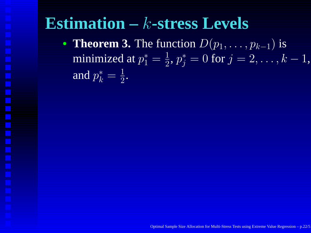
Estimation – k-stress Levels• Theorem 3.The functionD(p1, . . . , pk−1) is
minimized atp∗1 = 12, p∗j = 0 for j = 2, . . . , k − 1,
andp∗k = 12.
Optimal Sample Size Allocation for Multi-Stress Tests using Extreme Value Regression – p.22/51

Estimation – k-stress Levels• Theorem 3.The functionD(p1, . . . , pk−1) is
minimized atp∗1 = 12, p∗j = 0 for j = 2, . . . , k − 1,
andp∗k = 12.
• Theorem 4.The functionT (p1, p2, . . . , pk−1) isminimized at
p∗1 =1
1 + d, whered2 =
x21 + 1
x2k + 1
,
p∗j = 0 for j = 2, . . . , k − 1, andp∗k = d1+d
.
Optimal Sample Size Allocation for Multi-Stress Tests using Extreme Value Regression – p.22/51

Estimation – k-stress Levels• Proof of Theorem 3: We havek − 1 equations,
of which the first equation is
−(x21 − x2
k) + 2(x1 − xk)
(
k∑
l=1
xlpl
)
= 0
=⇒
k∑
l=1
xlpl =x1 + xk
2.
Optimal Sample Size Allocation for Multi-Stress Tests using Extreme Value Regression – p.23/51

Estimation – k-stress Levels• Proof of Theorem 3: We havek − 1 equations,
of which the first equation is
−(x21 − x2
k) + 2(x1 − xk)
(
k∑
l=1
xlpl
)
= 0
=⇒
k∑
l=1
xlpl =x1 + xk
2.
• Now, consider the first derivative of the functionD with respect topj (for j = 2, 3, . . . , k − 1)
∂D(p1, . . . , pk−1)
∂pj
= −(x2j − x2
k) + 2(xj − xk)
(
k∑
l=1
xlpl
)
= (xj − x1)(xk − xj) > 0.
Optimal Sample Size Allocation for Multi-Stress Tests using Extreme Value Regression – p.23/51
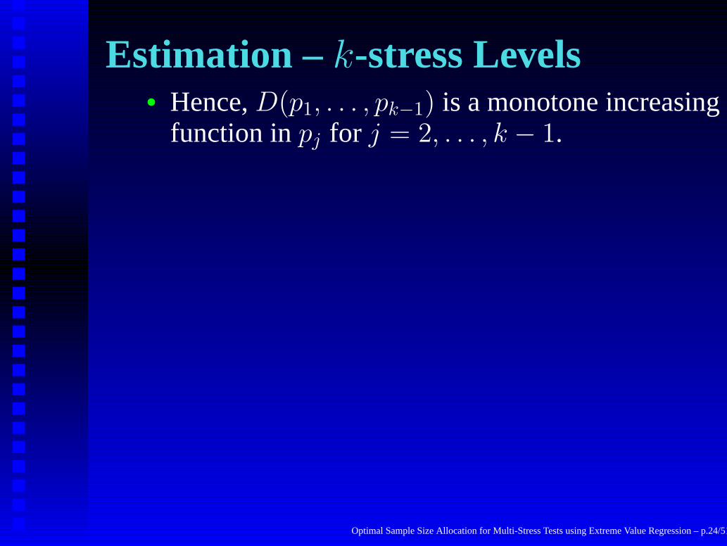
Estimation – k-stress Levels• Hence,D(p1, . . . , pk−1) is a monotone increasing
function inpj for j = 2, . . . , k − 1.
Optimal Sample Size Allocation for Multi-Stress Tests using Extreme Value Regression – p.24/51

Estimation – k-stress Levels• Hence,D(p1, . . . , pk−1) is a monotone increasing
function inpj for j = 2, . . . , k − 1.
• Since0 ≤ pj ≤ 1, D(p1, . . . , pk−1) is minimizedatp∗j = 0 for j = 2, 3, . . . , k − 1.
• As a result, the only non-zeropj forj = 1, 2, . . . , k − 1 is p1 and from Theorem 1,p∗1 = 1
2 minimizes the functionD(p1, . . . , pk−1),and consequentlyp∗k = 1 − p∗1 = 1
2.
Optimal Sample Size Allocation for Multi-Stress Tests using Extreme Value Regression – p.24/51

Estimation – k-stress Levels• In conclusion, in planning ak-stress level
experiment, we do not have to assign units at anystress level other than the lowest (x1) and thehighest (xk) levels.
Optimal Sample Size Allocation for Multi-Stress Tests using Extreme Value Regression – p.25/51

Estimation – k-stress Levels• In conclusion, in planning ak-stress level
experiment, we do not have to assign units at anystress level other than the lowest (x1) and thehighest (xk) levels.
• If optimality criterion [1] is considered, then oneshould allocate50% of the units to stress levelx1
and the remaining50% of the units to stress levelxk.
Optimal Sample Size Allocation for Multi-Stress Tests using Extreme Value Regression – p.25/51
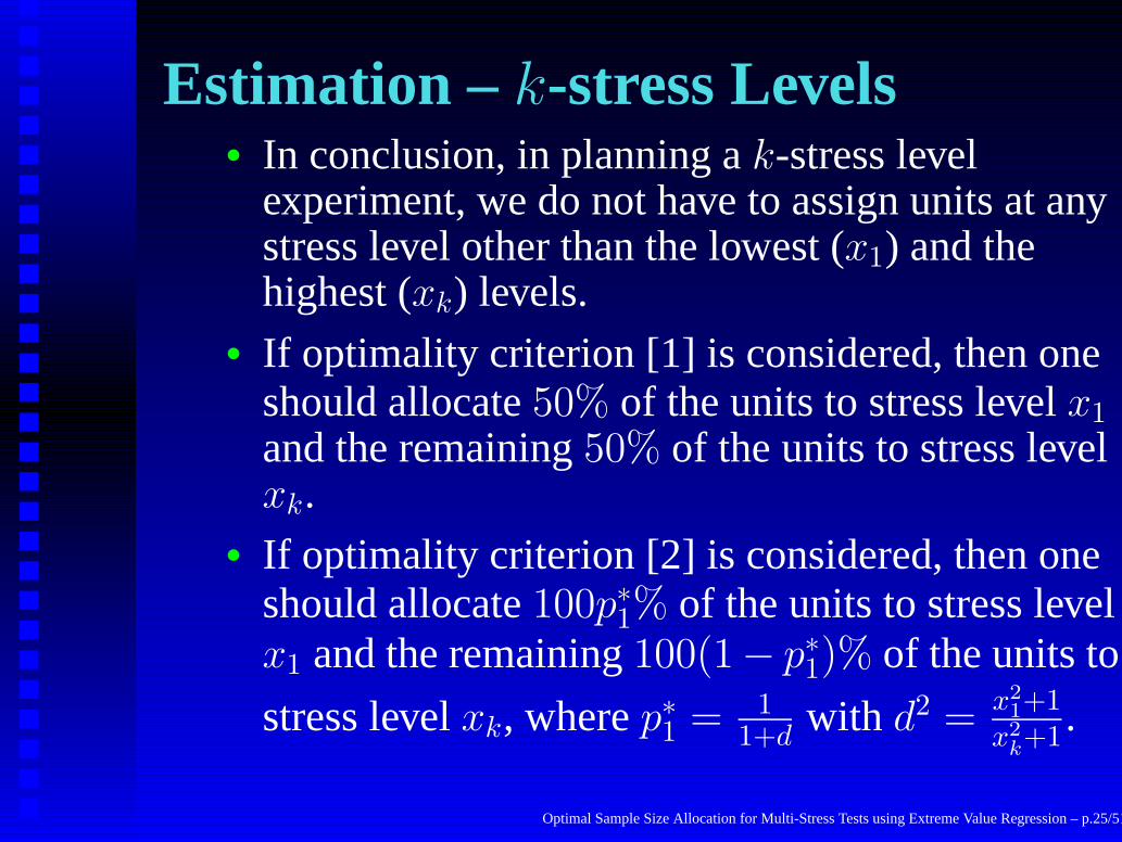
Estimation – k-stress Levels• In conclusion, in planning ak-stress level
experiment, we do not have to assign units at anystress level other than the lowest (x1) and thehighest (xk) levels.
• If optimality criterion [1] is considered, then oneshould allocate50% of the units to stress levelx1
and the remaining50% of the units to stress levelxk.
• If optimality criterion [2] is considered, then oneshould allocate100p∗1% of the units to stress levelx1 and the remaining100(1− p∗1)% of the units to
stress levelxk, wherep∗1 = 11+d
with d2 = x2
1+1
x2
k+1
.
Optimal Sample Size Allocation for Multi-Stress Tests using Extreme Value Regression – p.25/51

OPTIMAL SAMPLE SIZE ALLOCATION
FOR PREDICTION
Optimal Sample Size Allocation for Multi-Stress Tests using Extreme Value Regression – p.26/51

For prediction• Our goal is to estimate a parameter
θ = ν0 + ν1x + hσ at a pre-specified stress levelx.
Optimal Sample Size Allocation for Multi-Stress Tests using Extreme Value Regression – p.27/51

For prediction• Our goal is to estimate a parameter
θ = ν0 + ν1x + hσ at a pre-specified stress levelx.
• Note that this general parameterθ can include thequantiles and the mean of the lifetime distributionat stress levelx.
• Specifically, ifθ is the mean, thenh = −γ; if θ istheq-th quantile, thenh = ln[− ln(1 − q)].
• With this goal in mind, we may then be interestedin the optimal sample size allocation for theestimation ofθ (for a givenh).
Optimal Sample Size Allocation for Multi-Stress Tests using Extreme Value Regression – p.27/51
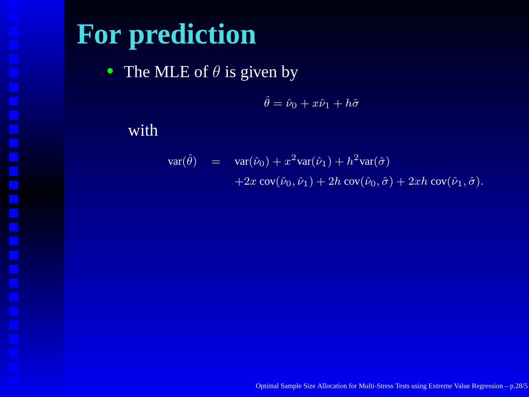
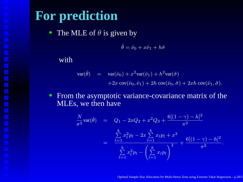
For prediction• The MLE ofθ is given by
θ = ν0 + xν1 + hσ
with
var(θ) = var(ν0) + x2var(ν1) + h2var(σ)
+2x cov(ν0, ν1) + 2h cov(ν0, σ) + 2xh cov(ν1, σ).
Optimal Sample Size Allocation for Multi-Stress Tests using Extreme Value Regression – p.28/51
For prediction• The MLE ofθ is given by
θ = ν0 + xν1 + hσ
with
var(θ) = var(ν0) + x2var(ν1) + h2var(σ)
+2x cov(ν0, ν1) + 2h cov(ν0, σ) + 2xh cov(ν1, σ).
• From the asymptotic variance-covariance matrix of theMLEs, we then have
N
σ2var(θ) = Q1 − 2xQ2 + x2Q3 +
6[(1 − γ) − h]2
π2
=
k∑
l=1
x2l pl − 2x
k∑
l=1
xlpl + x2
k∑
l=1
x2lpl −
(
k∑
l=1
xlpl
)2+
6[(1 − γ) − h]2
π2.
Optimal Sample Size Allocation for Multi-Stress Tests using Extreme Value Regression – p.28/51

For predictionIn this case, optimality can simply be defined in termsof minimizing the variance of the MLE ofθ for apre-specified stress levelx, or equivalently,[3] Minimization of
V (p1, p2, . . . , pk−1) =
k∑
l=1
x2l pl − 2x
k∑
l=1
xlpl + x2
k∑
l=1
x2lpl −
(
k∑
l=1
xlpl
)2
with pk = 1 −k−1∑
l=1
pl.
Optimal Sample Size Allocation for Multi-Stress Tests using Extreme Value Regression – p.29/51
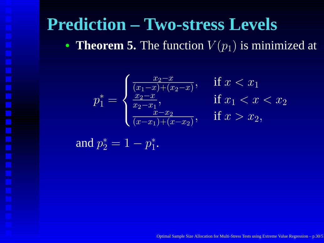
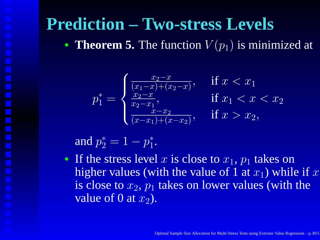
Prediction – Two-stress Levels• Theorem 5.The functionV (p1) is minimized at
p∗1 =
x2−x(x1−x)+(x2−x) , if x < x1x2−xx2−x1
, if x1 < x < x2x−x2
(x−x1)+(x−x2), if x > x2,
andp∗2 = 1 − p∗1.
Optimal Sample Size Allocation for Multi-Stress Tests using Extreme Value Regression – p.30/51
Prediction – Two-stress Levels• Theorem 5.The functionV (p1) is minimized at
p∗1 =
x2−x(x1−x)+(x2−x) , if x < x1x2−xx2−x1
, if x1 < x < x2x−x2
(x−x1)+(x−x2), if x > x2,
andp∗2 = 1 − p∗1.• If the stress levelx is close tox1, p1 takes on
higher values (with the value of 1 atx1) while if xis close tox2, p1 takes on lower values (with thevalue of 0 atx2).
Optimal Sample Size Allocation for Multi-Stress Tests using Extreme Value Regression – p.30/51

Prediction – Two-stress Levels• Theorem 5.The functionV (p1) is minimized at
p∗1 =
x2−x(x1−x)+(x2−x) , if x < x1x2−xx2−x1
, if x1 < x < x2x−x2
(x−x1)+(x−x2), if x > x2,
andp∗2 = 1 − p∗1.• If the stress levelx is close tox1, p1 takes on
higher values (with the value of 1 atx1) while if xis close tox2, p1 takes on lower values (with thevalue of 0 atx2).
• As x tends to either−∞ or +∞, p1 tends to12 .
Optimal Sample Size Allocation for Multi-Stress Tests using Extreme Value Regression – p.30/51

Prediction – k-stress Levels• Theorem 6.The functionV (p1, p2, . . . , pk−1) is
minimized at
p∗1 =
{
xk−x(x1−x)+(xk−x) , if x < x1,
x−xk
(x−x1)+(x−xk) , if x > xk.
p∗j = 0 for j = 2, . . . , k − 1, andp∗k = 1 − p∗1.
Optimal Sample Size Allocation for Multi-Stress Tests using Extreme Value Regression – p.31/51
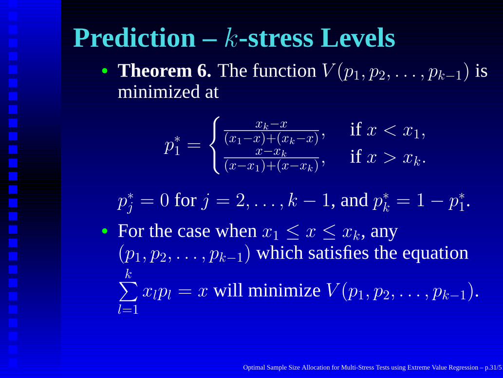
Prediction – k-stress Levels• Theorem 6.The functionV (p1, p2, . . . , pk−1) is
minimized at
p∗1 =
{
xk−x(x1−x)+(xk−x) , if x < x1,
x−xk
(x−x1)+(x−xk) , if x > xk.
p∗j = 0 for j = 2, . . . , k − 1, andp∗k = 1 − p∗1.
• For the case whenx1 ≤ x ≤ xk, any(p1, p2, . . . , pk−1) which satisfies the equationk
∑
l=1
xlpl = x will minimize V (p1, p2, . . . , pk−1).
Optimal Sample Size Allocation for Multi-Stress Tests using Extreme Value Regression – p.31/51

NUMERICAL ILLUSTRATION
Optimal Sample Size Allocation for Multi-Stress Tests using Extreme Value Regression – p.32/51

Numerical Illustration• Nelson and Meeker (1978) considered the
following data on insulating fluids in anaccelerated test that was conducted in order todetermine the relationship between time tobreakdown and voltage (which is the stressfactor).
Optimal Sample Size Allocation for Multi-Stress Tests using Extreme Value Regression – p.33/51

Numerical Illustration• Nelson and Meeker (1978) considered the
following data on insulating fluids in anaccelerated test that was conducted in order todetermine the relationship between time tobreakdown and voltage (which is the stressfactor).
• 76 units were tested at seven stress levels, equallyspaced between 26kV and 38kV
Optimal Sample Size Allocation for Multi-Stress Tests using Extreme Value Regression – p.33/51

Numerical IllustrationTime to breakdown for insulating fluids at seven stress levels
Stress ni Breakdown Times
26kV 3 5.79, 1579.52, 2323.70
28kV 5 68.85, 426.07, 110.29, 108.29, 1067.60
30kV 11 17.05, 22.66, 21.02, 175.88, 139.07, 144.12, 20.46, 43.40,194.90, 47.30,
7.74
32kV 15 0.40, 82.85, 9.88, 89.29, 215.10, 2.75, 0.79, 15.93, 3.91, 2.7,
0.69, 100.58, 27.80, 13.95, 53.24
34kV 19 0.96, 4.15, 0.19, 0.78, 8.01, 31.75, 7.35, 6.50, 8.27, 33.91,
32.52, 3.16, 4.85, 2.78, 4.67, 1.31, 12.06, 36.71, 72.89
36kV 15 1.97, 0.59, 2.58, 1.69, 2.71, 25.50, 0.35, 0.99, 3.99, 3.67,
2.07, 0.96, 5.35, 2.90, 13.77
38kV 8 0.47, 0.73, 1.40, 0.74, 0.39, 1.13, 0.09, 2.38
We havex1 = ln 26 = 3.2581, x2 = ln 28 = 3.3322, x3 = ln 30 = 3.4012, x4 = ln 32 =
3.4657, x5 = ln 34 = 3.5264, x6 = ln 36 = 3.5835 andx7 = ln 38 = 3.6376.
Optimal Sample Size Allocation for Multi-Stress Tests using Extreme Value Regression – p.34/51
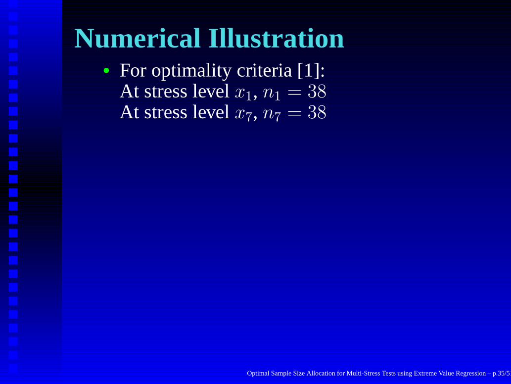
Numerical Illustration• For optimality criteria [1]:
At stress levelx1, n1 = 38At stress levelx7, n7 = 38
Optimal Sample Size Allocation for Multi-Stress Tests using Extreme Value Regression – p.35/51

Numerical Illustration• For optimality criteria [1]:
At stress levelx1, n1 = 38At stress levelx7, n7 = 38
• For optimality criterion [2], we would obtain
d =
√
(3.2581)2 + 1
(3.6376)2 + 1= 0.9034,
p∗1 =1
1 + d= 0.5254 and p∗7 = 0.4746.
At stress levelx1, n1 = 40At stress levelx7, n2 = 36
Optimal Sample Size Allocation for Multi-Stress Tests using Extreme Value Regression – p.35/51

Numerical Illustration• Prediction the mean lifetime at stress level at
20kV (x∗ = ln(20) = 2.99573):
p∗1 =3.63759 − 2.99573
(3.25810 − 2.99573) + (3.63759 − 2.99573)= 0.70984.
At stress levelx1, n1 = 54At stress levelx7, n2 = 22
Optimal Sample Size Allocation for Multi-Stress Tests using Extreme Value Regression – p.36/51

Numerical Illustration• Prediction the mean lifetime at stress level at
20kV (x∗ = ln(20) = 2.99573):
p∗1 =3.63759 − 2.99573
(3.25810 − 2.99573) + (3.63759 − 2.99573)= 0.70984.
At stress levelx1, n1 = 54At stress levelx7, n2 = 22
• Prediction the mean lifetime at stress level at40kV (x∗∗ = ln(40) = 3.68888):
p∗1 =3.68888 − 3.63759
(3.68888 − 3.25810) + (3.68888 − 3.63759)= 0.10640
At stress levelx1, n1 = 8At stress levelx7, n2 = 68
Optimal Sample Size Allocation for Multi-Stress Tests using Extreme Value Regression – p.36/51

Numerical IllustrationComparison of the allocation scheme of Nelson and Meeker (1978) and the optimal allocations
(n1, n2, n3, n4) det[I∗](RE) (N/σ2)var(ν1) (N/σ2)tr[I∗−1](RE)
Example (3,5,11,15,19,15,8) .0154(0.259) 107.1449 1418.3173(0.253)
[1] (38,0,0,0,0,0,38) .0592(1.000) 27.7754 359.6750(0.997)
[2] (40,0,0,0,0,0,36) .0591(0.997) 27.8525 358.7541(1.000)
[3] (54,0,0,0,0,0,22) .0487(0.823) 33.7607 418.4271(0.857)
[4] (8,0,0,0,0,0,68) .0223(0.377) 73.7273 1029.6976(0.348)
(n1, n2, n3, n4) (N/σ2) var [θ|x∗] (RE) (N/σ2) var [θ|x∗∗] (RE)
Example (3,5,11,15,19,15,8) 28.4127(0.221) 5.3953(0.374)
[1] (38,0,0,0,0,0,38) 7.2853(0.863) 3.0191(0.669)
[2] (40,0,0,0,0,0,36) 7.0523(0.891) 3.1605(0.639)
[3] (54,0,0,0,0,0,22) 6.2853(1.000) 4.8826(0.414)
[4] (8,0,0,0,0,0,68) 28.3188(0.222) 2.0191(1.000)
Optimal Sample Size Allocation for Multi-Stress Tests using Extreme Value Regression – p.37/51

MONTE CARLO STUDY FOR
SMALL SAMPLE SIZES
Optimal Sample Size Allocation for Multi-Stress Tests using Extreme Value Regression – p.38/51

Monte Carlo Study for SmallSample Sizes
• As the results are based on asymptotic theory ofMLEs, Monte Carlo simulations are used toexamine that if the optimal allocations hold forsmall sample sizes (as small as 20 even).
Optimal Sample Size Allocation for Multi-Stress Tests using Extreme Value Regression – p.39/51

Monte Carlo Study for SmallSample Sizes
• As the results are based on asymptotic theory ofMLEs, Monte Carlo simulations are used toexamine that if the optimal allocations hold forsmall sample sizes (as small as 20 even).
• Under different settings, we simulated
Optimal Sample Size Allocation for Multi-Stress Tests using Extreme Value Regression – p.39/51

Monte Carlo Study for SmallSample Sizes
• As the results are based on asymptotic theory ofMLEs, Monte Carlo simulations are used toexamine that if the optimal allocations hold forsmall sample sizes (as small as 20 even).
• Under different settings, we simulated• The Fisher information matrix
Optimal Sample Size Allocation for Multi-Stress Tests using Extreme Value Regression – p.39/51

Monte Carlo Study for SmallSample Sizes
• As the results are based on asymptotic theory ofMLEs, Monte Carlo simulations are used toexamine that if the optimal allocations hold forsmall sample sizes (as small as 20 even).
• Under different settings, we simulated• The Fisher information matrix• The variance-covariance matrix of the MLEs
ν0, ν1 andσ.
Optimal Sample Size Allocation for Multi-Stress Tests using Extreme Value Regression – p.39/51

Monte Carlo StudySetting (1):k = 2, ν0 = 0.0, ν1 = 1.0, σ = 1.0
Stress
-3.5 θ1 = E(Y |x = −3.5)
x1 = −2.5 -
-1.0 θ3 = E(Y |x = −1.0)
x2 = 0.5 -
1.5 θ2 = E(Y |x = 1.5)
Optimal Sample Size Allocation for Multi-Stress Tests using Extreme Value Regression – p.40/51

Monte Carlo StudyComparison of different allocation schemes for setting (1), N = 20
(Relative Efficiency in parenthesis)
Asymptotic
(n1, n2) det[I] tr[I−1] var(θ1) var(θ2) var(θ3)
(12,8) 28424.5(0.96) .148(0.787) .192(0.880) .262(0.646) .083(0.975)
(10,10)[1][5] 29608.8(1.00) .130(0.894) .219(0.772) .219(0.772) .080(1.000)
(6,14)[2] 24871.4(0.84) .117(1.000) .335(0.506) .176(0.962) .090(0.894)
(16,4)[3] 18949.6(0.64) .246(0.474) .169(1.000) .482(0.351) .109(0.741)
(4,16)[4] 18949.6(0.64) .121(0.964) .482(0.351) .169(1.000) .109(0.741)
Simulated
(12,8) 60725.6(0.99) .156(0.773) .197(0.857) .280(0.627) .081(1.014)
(10,10)[1][5] 61543.3(1.00) .135(0.895) .234(0.721) .227(0.773) .082(1.000)
(6,14)[2] 51262.4(0.83) .121(1.000) .350(0.483) .184(0.958) .090(0.913)
(16,4)[3] 37331.6(0.61) .278(0.434) .169(1.000) .556(0.316) .120(0.685)
(4,16)[4] 39605.7(0.64) .125(0.969) .522(0.323) .176(1.000) .111(0.742)
Optimal Sample Size Allocation for Multi-Stress Tests using Extreme Value Regression – p.41/51
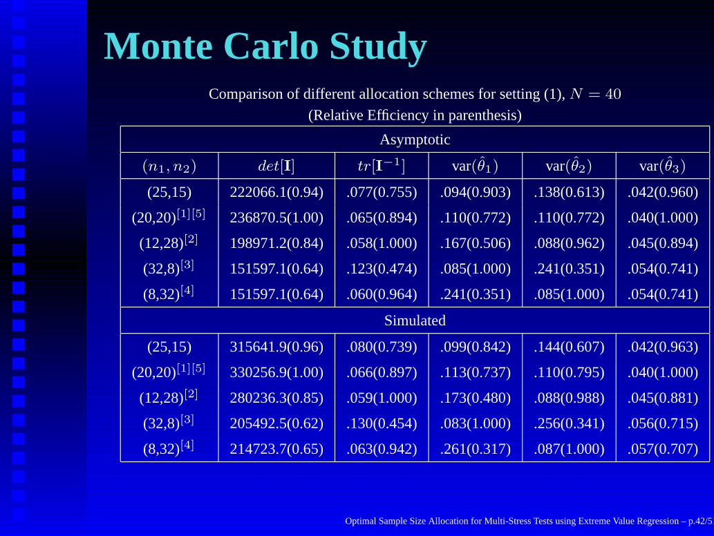
Monte Carlo StudyComparison of different allocation schemes for setting (1), N = 40
(Relative Efficiency in parenthesis)
Asymptotic
(n1, n2) det[I] tr[I−1] var(θ1) var(θ2) var(θ3)
(25,15) 222066.1(0.94) .077(0.755) .094(0.903) .138(0.613) .042(0.960)
(20,20)[1][5] 236870.5(1.00) .065(0.894) .110(0.772) .110(0.772) .040(1.000)
(12,28)[2] 198971.2(0.84) .058(1.000) .167(0.506) .088(0.962) .045(0.894)
(32,8)[3] 151597.1(0.64) .123(0.474) .085(1.000) .241(0.351) .054(0.741)
(8,32)[4] 151597.1(0.64) .060(0.964) .241(0.351) .085(1.000) .054(0.741)
Simulated
(25,15) 315641.9(0.96) .080(0.739) .099(0.842) .144(0.607) .042(0.963)
(20,20)[1][5] 330256.9(1.00) .066(0.897) .113(0.737) .110(0.795) .040(1.000)
(12,28)[2] 280236.3(0.85) .059(1.000) .173(0.480) .088(0.988) .045(0.881)
(32,8)[3] 205492.5(0.62) .130(0.454) .083(1.000) .256(0.341) .056(0.715)
(8,32)[4] 214723.7(0.65) .063(0.942) .261(0.317) .087(1.000) .057(0.707)
Optimal Sample Size Allocation for Multi-Stress Tests using Extreme Value Regression – p.42/51

Monte Carlo StudyComparison of different allocation schemes for setting (1), N = 60
(Relative Efficiency in parenthesis)
Asymptotic
(n1, n2) det[I] tr[I−1] var(θ1) var(θ2) var(θ3)
(35,25) 777231.4(0.97) .048(0.807) .065(0.863) .084(0.668) .027(0.983)
(30,30)[1][5] 799438.0(1.00) .043(0.894) .073(0.772) .073(0.772) .027(1.000)
(18,42)[2] 671527.9(0.84) .039(1.000) .112(0.506) .059(0.962) .030(0.894)
(48,12)[3] 511640.3(0.64) .082(0.474) .056(1.000) .161(0.351) .036(0.741)
(12,48)[4] 511640.3(0.64) .040(0.964) .161(0.351) .056(1.000) .036(0.741)
Simulated
(35,25) 971381.4(0.96) .049(0.820) .067(0.815) .087(0.669) .027(0.997)
(30,30)[1][5] 1010361.9(1.00) .045(0.907) .074(0.742) .075(0.776) .027(1.000)
(18,42)[2] 855098.1(0.85) .040(1.000) .114(0.480) .061(0.951) .031(0.864)
(48,12)[3] 619924.6(0.61) .088(0.460) .055(1.000) .174(0.332) .038(0.704)
(12,48)[4] 642403.0(0.64) .041(0.985) .166(0.330) .058(1.000) .036(0.737)
Optimal Sample Size Allocation for Multi-Stress Tests using Extreme Value Regression – p.43/51

Monte Carlo StudySetting (2):k = 4, ν0 = 0.0, ν1 = 1.0, σ = 1.0
Stress
-2.5 θ1 = E(Y |x = −2.5)
x1 = −1.5 -
x2 = −0.5 -
x3 = 0.1 -
x4 = 0.66 -
-1.0 θ2 = E(Y |x = 1.5)
Optimal Sample Size Allocation for Multi-Stress Tests using Extreme Value Regression – p.44/51
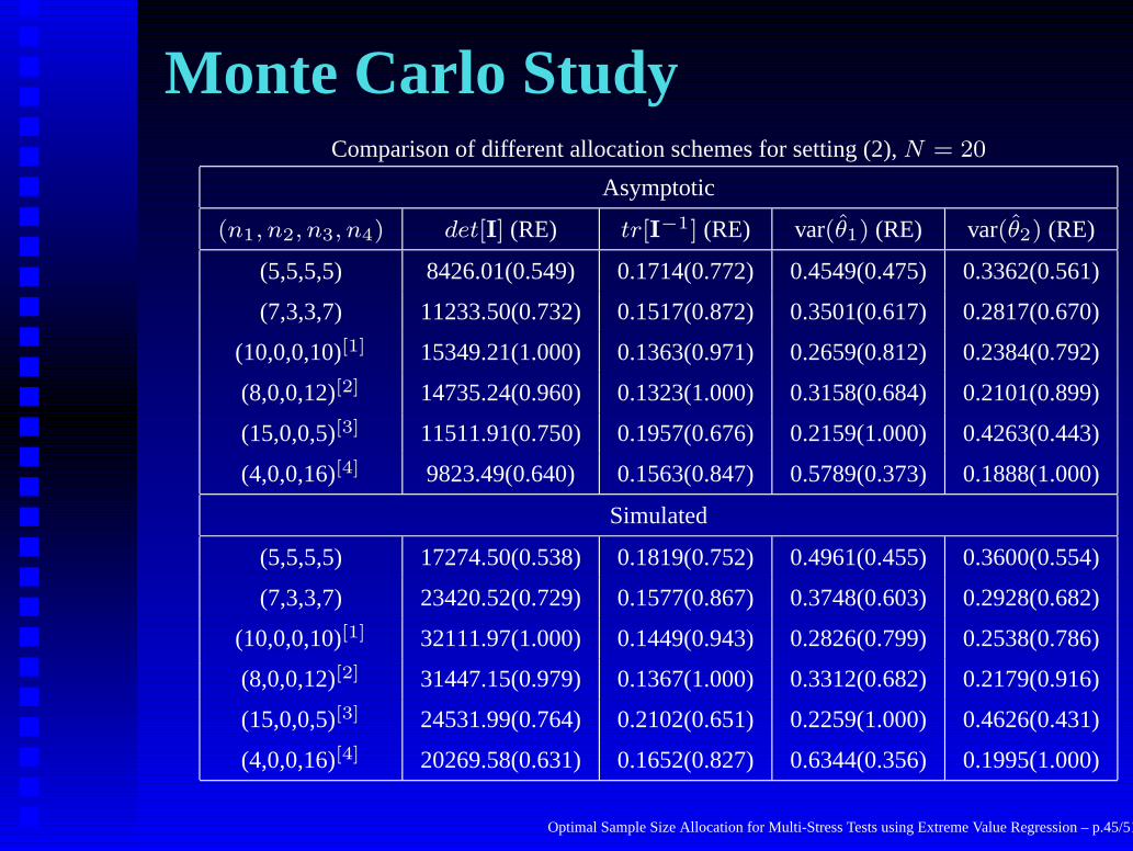
Monte Carlo StudyComparison of different allocation schemes for setting (2), N = 20
Asymptotic
(n1, n2, n3, n4) det[I] (RE) tr[I−1] (RE) var(θ1) (RE) var(θ2) (RE)
(5,5,5,5) 8426.01(0.549) 0.1714(0.772) 0.4549(0.475) 0.3362(0.561)
(7,3,3,7) 11233.50(0.732) 0.1517(0.872) 0.3501(0.617) 0.2817(0.670)
(10,0,0,10)[1] 15349.21(1.000) 0.1363(0.971) 0.2659(0.812) 0.2384(0.792)
(8,0,0,12)[2] 14735.24(0.960) 0.1323(1.000) 0.3158(0.684) 0.2101(0.899)
(15,0,0,5)[3] 11511.91(0.750) 0.1957(0.676) 0.2159(1.000) 0.4263(0.443)
(4,0,0,16)[4] 9823.49(0.640) 0.1563(0.847) 0.5789(0.373) 0.1888(1.000)
Simulated
(5,5,5,5) 17274.50(0.538) 0.1819(0.752) 0.4961(0.455) 0.3600(0.554)
(7,3,3,7) 23420.52(0.729) 0.1577(0.867) 0.3748(0.603) 0.2928(0.682)
(10,0,0,10)[1] 32111.97(1.000) 0.1449(0.943) 0.2826(0.799) 0.2538(0.786)
(8,0,0,12)[2] 31447.15(0.979) 0.1367(1.000) 0.3312(0.682) 0.2179(0.916)
(15,0,0,5)[3] 24531.99(0.764) 0.2102(0.651) 0.2259(1.000) 0.4626(0.431)
(4,0,0,16)[4] 20269.58(0.631) 0.1652(0.827) 0.6344(0.356) 0.1995(1.000)
Optimal Sample Size Allocation for Multi-Stress Tests using Extreme Value Regression – p.45/51
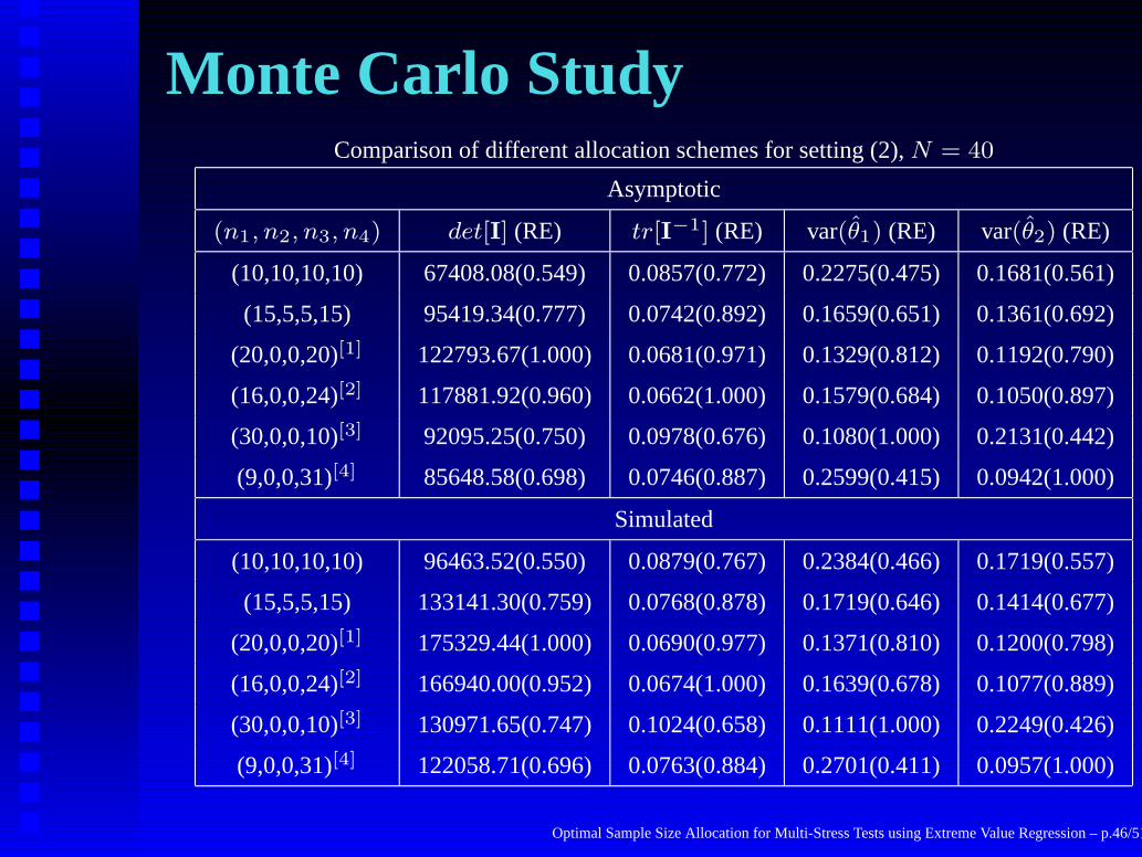
Monte Carlo StudyComparison of different allocation schemes for setting (2), N = 40
Asymptotic
(n1, n2, n3, n4) det[I] (RE) tr[I−1] (RE) var(θ1) (RE) var(θ2) (RE)
(10,10,10,10) 67408.08(0.549) 0.0857(0.772) 0.2275(0.475) 0.1681(0.561)
(15,5,5,15) 95419.34(0.777) 0.0742(0.892) 0.1659(0.651) 0.1361(0.692)
(20,0,0,20)[1] 122793.67(1.000) 0.0681(0.971) 0.1329(0.812) 0.1192(0.790)
(16,0,0,24)[2] 117881.92(0.960) 0.0662(1.000) 0.1579(0.684) 0.1050(0.897)
(30,0,0,10)[3] 92095.25(0.750) 0.0978(0.676) 0.1080(1.000) 0.2131(0.442)
(9,0,0,31)[4] 85648.58(0.698) 0.0746(0.887) 0.2599(0.415) 0.0942(1.000)
Simulated
(10,10,10,10) 96463.52(0.550) 0.0879(0.767) 0.2384(0.466) 0.1719(0.557)
(15,5,5,15) 133141.30(0.759) 0.0768(0.878) 0.1719(0.646) 0.1414(0.677)
(20,0,0,20)[1] 175329.44(1.000) 0.0690(0.977) 0.1371(0.810) 0.1200(0.798)
(16,0,0,24)[2] 166940.00(0.952) 0.0674(1.000) 0.1639(0.678) 0.1077(0.889)
(30,0,0,10)[3] 130971.65(0.747) 0.1024(0.658) 0.1111(1.000) 0.2249(0.426)
(9,0,0,31)[4] 122058.71(0.696) 0.0763(0.884) 0.2701(0.411) 0.0957(1.000)
Optimal Sample Size Allocation for Multi-Stress Tests using Extreme Value Regression – p.46/51

Monte Carlo StudyComparison of different allocation schemes for setting (2), N = 60
Asymptotic
(n1, n2, n3, n4) det[I] (RE) tr[I−1] (RE) var(θ1) (RE) var(θ2) (RE)
(15,15,15,15) 227502.28(0.549) 0.0571(0.772) 0.1516(0.475) 0.1121(0.560)
(20,10,10,20) 290766.44(0.702) 0.0514(0.858) 0.1212(0.594) 0.0963(0.653)
(30,0,0,30)[1] 414428.64(1.000) 0.0454(0.971) 0.0886(0.812) 0.0795(0.790)
(24,0,0,36)[2] 397851.49(0.960) 0.0441(1.000) 0.1053(0.684) 0.0700(0.897)
(46,0,0,14)[3] 296546.71(0.716) 0.0684(0.645) 0.0720(1.000) 0.1512(0.415)
(13,0,0,47)[4] 281351.00(0.679) 0.0504(0.875) 0.1793(0.401) 0.0628(1.000)
Simulated
(15,15,15,15) 288524.21(0.557) 0.0580(0.767) 0.1554(0.463) 0.1131(0.556)
(20,10,10,20) 365622.05(0.706) 0.0524(0.850) 0.1231(0.585) 0.0987(0.636)
(30,0,0,30)[1] 517988.16(1.000) 0.0461(0.966) 0.0893(0.806) 0.0819(0.768)
(24,0,0,36)[2] 502820.78(0.971) 0.0445(1.000) 0.1062(0.678) 0.0706(0.890)
(46,0,0,14)[3] 374893.37(0.724) 0.0696(0.639) 0.0720(1.000) 0.1545(0.407)
(13,0,0,47)[4] 351866.54(0.679) 0.0512(0.870) 0.1833(0.393) 0.0628(1.000)
Optimal Sample Size Allocation for Multi-Stress Tests using Extreme Value Regression – p.47/51

Monte Carlo Study• The optimal allocation of units for optimality
criterion [1] actually increases the determinant ofthe Fisher information matrix and reduces thevariance ofν1 compared to all other allocation ofunits for sample sizes as small as 20.
Optimal Sample Size Allocation for Multi-Stress Tests using Extreme Value Regression – p.48/51

Monte Carlo Study• The optimal allocation of units for optimality
criterion [1] actually increases the determinant ofthe Fisher information matrix and reduces thevariance ofν1 compared to all other allocation ofunits for sample sizes as small as 20.
• The optimal allocation of units for optimalitycriterion [2] similarly reduces the trace of thevariance-covariance matrix.
• For largeN andk (k at least as large as 3 or 4),the difference between optimality criterion [1]and [2] is negligible (which means that either ofthese criteria can be used in practice, since theywill give nearly full efficiency).
Optimal Sample Size Allocation for Multi-Stress Tests using Extreme Value Regression – p.48/51

Monte Carlo Study• The allocations based on optimality criterion [3]
can change dramatically depending on what levelof stress we are interested in predicting at, andthe corresponding relative efficiencies will alsocritically depend on those allocations.
Optimal Sample Size Allocation for Multi-Stress Tests using Extreme Value Regression – p.49/51

Monte Carlo Study• The allocations based on optimality criterion [3]
can change dramatically depending on what levelof stress we are interested in predicting at, andthe corresponding relative efficiencies will alsocritically depend on those allocations.
• We have shown by means of Monte Carlosimulations that the optimal allocations hold notonly for large sample sizes but also for smallsample sizes (as small as 20 even).
Optimal Sample Size Allocation for Multi-Stress Tests using Extreme Value Regression – p.49/51
References1. Bugaighis, M. M. (1993). Percentiles of pivotal ratios for the MLE of the parameters of a
Weibull regression model,IEEE Transactions on Reliability, 42, 97-99.
2. Cox, D. R. (1964). Some applications of exponential orderedscores,Journal of the Royal
Statistical Society, Series B, 26, 103-110.
3. Elperin, T. and Gertsbakh, I. (1987). Maximum likelihood estimation in a Weibull
regression model with Type-I censoring: a Monte Carlo study, Communications in
Statistics – Simulation and Computation, 16, 349-371.
4. Feigl, P. and Zelen, M. (1965). Estimation of exponential survival probabilities with
concomitant information,Biometrics, 21, 826-838.
5. Gaylor, D. W. and Sweeny, H. C. (1965). Design for optimal prediction in simple linear
regression,Journal of the American Statistical Association, 60, 205-216.
6. Glasser, M. (1967). Exponential survival with covariance,Journal of the American
Statistical Association, 62, 561-568.
7. Kalbfleisch, J. D. and Prentice, R. L. (1980).The Statistical Analysis of Failure Time
Data, New York: John Wiley & Sons.
8. Lawless, J. F. (1982).Statistical Models and Methods for Lifetime Data, New York: John
Wiley & Sons.
Optimal Sample Size Allocation for Multi-Stress Tests using Extreme Value Regression – p.50/51
References9. McCool, J. I. (1980). Confidence limits for Weibull regression with censored data,IEEE
Transactions on Reliability, 29, 145-150.
10. Meeker, W. Q. and Escobar, L. A. (1998).Statistical Methods for Reliability Data, New
York: John Wiley & Sons.
11. Nelson, W. (1982).Applied Life Data Analysis, New York: John Wiley & Sons.
12. Nelson, W. and Kielpinski, T. J. (1976). Theory for optimum censored accelerated life
tests for normal and lognormal life distributions,Technometrics, 18, 105-114.
13. Nelson, W. and Meeker, W. Q. (1978). Theory for optimum accelerated censored life
tests for Weibull and extreme value distributions,Technometrics, 20, 171-177.
14. Paul, S. R. and Thiagarajah, K. (1996). Approximate variance covariance of maximum
likelihood estimators for the parameters of extreme value regression models for censored
data,Sankhya, Series B, 58, 28-37.
15. Paula, G. A. and Rojas, O. V. (1997). On restricted hypotheses in extreme value
regression models,Computational Statistics & Data Analysis, 25, 143-157.
16. Silvey, S. D. (1980).Optimal Design, New York: Chapman and Hall.
17. Zhou, Q. J. (2002).Inferential Methods for Extreme Value Regression Models,
Unpublished Ph.D. Thesis, McMaster University, Hamilton,Ontario, Canada.
Optimal Sample Size Allocation for Multi-Stress Tests using Extreme Value Regression – p.51/51