optimal scheduling for biocide dosing and heat …
TRANSCRIPT

OPTIMAL SCHEDULING FOR BIOCIDE DOSING AND HEAT
EXCHANGERS MAINTENANCE TOWARDS ENVIRONMENTALLY
FRIENDLY SEAWATER COOLING SYSTEMS
A Dissertation
by
ABDULLAH S. O. BINMAHFOUZ
Submitted to the Office of Graduate Studies ofTexas A&M University
in partial fulfillment of the requirements for the degree of
DOCTOR OF PHILOSOPHY
August 2011
Major Subject: Chemical Engineering

OPTIMAL SCHEDULING FOR BIOCIDE DOSING AND HEAT
EXCHANGERS MAINTENANCE TOWARDS ENVIRONMENTALLY
FRIENDLY SEAWATER COOLING SYSTEMS
A Dissertation
by
ABDULLAH S. O. BINMAHFOUZ
Submitted to the Office of Graduate Studies ofTexas A&M University
in partial fulfillment of the requirements for the degree of
DOCTOR OF PHILOSOPHY
Approved by:
Chair of Committee, Mahmoud El-HalwagiCommittee Members, Bill Batchelor
Juergen HahnM. Sam Mannan
Head of Department, Michael Pishko
August 2011
Major Subject: Chemical Engineering

iii
ABSTRACT
Optimal Scheduling for Biocide and Heat Exchangers Maintenance Towards
Environmentally Friendly Seawater Cooling Systems. (August 2011)
Abdullah S. O. Binmahfouz, B.S., King Fahd University of Petroleum & Minerals;
M.B.A., Indiana University of Pennsylvania;
M.S., Texas A&M University
Chair of Advisory Committee: Dr. Mahmoud El-Halwagi
Using seawater in cooling systems is a common practice in many parts of the
world where there is a shortage of freshwater. However, biofouling is one of the major
operational problems associated with the usage of seawater in cooling systems.
Microfouling is caused by the activities of microorganisms, such as bacteria and algae,
producing a very thin layer that sticks to the inside surface of the tubes in heat
exchangers. This thin layer has a tremendously negative impact on heat transferred
across the heat exchanger tubes in the system. In some instances, even a 250 micrometer
thickness of fouling film can reduce the heat exchanger’s heat transfer coefficient by
50%. On the other hand, macrofouling is the blockage caused by relatively large marine
organisms, such as oysters, mussels, clams, and barnacles. A biocide is typically added
to eliminate, or at least reduce, biofouling. Typically, microfouling can be controlled by
intermittent dosages, and macrofouling can be controlled by continuous dosages of
biocide.
iv
The aim of this research work is to develop a systematic approach to the optimal
operating and design alternatives for integrated seawater cooling systems in industrial
facilities. A process integration framework is used to provide a holistic approach to
optimizing the design and operation of the seawater cooling system, along with the
dosage and discharge systems. Optimization formulations are employed to systematize
the decision-making and to reconcile the various economic, technical, and environmental
aspects of the problem. Building blocks of the approach include the biocide water
chemistry and kinetics, process cooling requirements, dosage scenarios and dynamic
profiles, biofilm growth, seawater discharge, and environmental regulations.
Seawater chemistry is studied with emphasis on the usage of biocide for seawater
cooling. A multi-period optimization formulation is developed and solved to determine.
The optimal levels of dosing and dechlorination chemicals
The timing of maintenance to clean the heat-exchange surfaces
The dynamic dependence of the biofilm growth on the applied doses, the
seawater-biocide chemistry, the process conditions, and seawater
characteristics for each time period.
The technical, economic, and environmental considerations of the system are
accounted for and discussed through case studies.

v
DEDICATION
I would like to devote my academic work to the spirit of my late father, Salmeen,
who taught me that knowledge is the best way to raise one’s qualifications, and who
helped me set my essential goals for my life. I am deeply grateful to my mother,
Fatimah, whose strength and faith show me how to stand with confidence through all of
the ups and downs of life; she has taught me that even the largest task can be
accomplished if it is done one step at a time.
Many thanks to my mother-in-law, Victoria, who has never stopped praying for
my success in life and who has supported me with all means throughout my studies.
Special thanks are due to my wife, Nouf, who has always been there for me and has
never failed to give me encouragement and emotional support along with unconditional
love. My wife believed in me before I started believing in myself and helped me to make
my dreams come true.
Also, this research work is dedicated to my daughters: Mariam, who wants to be
a great eye doctor, and Doha, who wants to be a famous interior designer. Both of them
continuously admire my accomplishments and show that they are always proud of their
father. These feelings inspire and motivate me to rise above any difficulties.
Finally, I also dedicate this work with much love to my two-year-old twins,
Liane and Sultan, who are my future dreams and my joy. Having Liane and Sultan
waiting for me at the end of every day charges me up and gives me the hope to
overcome any challenging tasks in my work.

vi
ACKNOWLEDGEMENTS
First and foremost, I would like to express my deepest gratitude to God, Allah,
for blessing me with the ability to gain knowledge and for helping me throughout my life
with his mercy and grace to make the impossible possible.
Though only my name appears on the cover of this written research, many people
have contributed to its production, without whom it might not have been completed. I
cherish and owe my gratitude to all those who have helped to make this research work
possible.
My deepest gratitude is to my advisor, mentor, and scientist model, Professor El -
Halwagi. I am amazingly fortunate to have an advisor who has given me such
thoughtful, patient guidance and support. I hope that one day I will become as good of
an advisor for my students as Professor El-Halwagi has been to his students.
Dr. El-Halwagi is one of the best teachers that I have had in my life. He sets very
high expectations for his students, then he encourages and guides them to meet or exceed
those standards. His teaching continuously inspired me to work hard.
I am tremendously appreciative for the support and aid Professor El-Halwagi
gave my family during the difficulties that I faced in the last year of my Ph.D. studies at
Texas A&M University.
I would also like to extend my gratitude to the members of my committee,
including Professors Batchelor, Mannan, and Hahn for their helpful comments and
suggestions at all stages of my research work at Texas A&M.

vii
I am deeply grateful to Dr. Batchelor for introducing me to the seawater
chemistry world and for putting me on the right track toward fundamental resources. Dr.
Batchelor has always listened to my concerns and continuously advised me in my
research and publications.
Dr. Mannan and Dr. Hahn’s insightful comments during my seminars and oral
exams helped me focus my ideas as they held me to high research standards. I would like
to further express my gratitude to both Dr. Mannan and Dr. Hahn for writing me very
strong recommendation letters that definitely helped me obtain the best job I could have
dreamed of.
Additionally, I would like to acknowledge Dr. Abdel-Wahab and Dr. Linke from
Texas A&M University at Qatar for their many valuable comments and insightful ideas
that helped me understand the most complicated areas of my research. I am grateful to
both Dr. Abdel-Wahab and Dr. Linke for their contribution to various domains. I would
also like to acknowledge Dr. Jimenez for our numerous discussions on related topics that
helped to improve my knowledge in my research area.
I would like to thank the professors at Indiana University of Pennsylvania who
taught me during my MBA studies and encouraged me to continue my education in
engineering through graduate school. Special thanks are due to Professor Krishnan, my
academic advisor, for his kind advice and help, and to Professor Al-Bohali who
introduced me to the field of optimization and made it one of the most interesting
subjects to me. This interest introduced me to Process Integration, my current research
area in my chemical engineering graduate studies.

viii
I appreciate the cooperative research with Selma that resulted in my published
research work. I am especially grateful to several past and current members of Dr. El-
Hawlagi’s group, including Nasser, Musaed, Houssein, Younas, Ian, Mohamed, Denny,
Fabrecio and many others, whose support and friendship helped me to stay focused on
my research and provided me with encouragement.
Finally, I appreciate the financial support from the Ministry of Higher Education
(MOHE) for sponsoring my graduate studies and giving me the opportunity to study at
one of the best schools in the United States, Texas A&M University. Additionally, I
would like to acknowledge the funding from King Abdullah University of Science and
Technology (KAUST) and the Qatar National Research Fund (QNRF).

ix
TABLE OF CONTENTS
Page
ABSTRACT .............................................................................................................. iii
DEDICATION .......................................................................................................... v
ACKNOWLEDGEMENTS ...................................................................................... vi
TABLE OF CONTENTS .......................................................................................... ix
LIST OF FIGURES................................................................................................... xii
LIST OF TABLES .................................................................................................... xv
1. INTRODUCTION............................................................................................... 1
1.1 Fouling ................................................................................................. 21.2 Antifouling ........................................................................................... 51.3 Environmental Problems of Chlorine................................................... 61.4 Dechlorination ...................................................................................... 7
2. BACKGROUND AND LITERATURE REVIEW............................................. 10
2.1 Overview .............................................................................................. 102.2 Introduction .......................................................................................... 102.3 Characteristics of Seawater Impacting Biocide Chemistry .................. 122.4 Seawater Salinity and Density.............................................................. 142.5 Problems from Using Seawater for Cooling ........................................ 162.6 Avoiding Seawater Problems ............................................................... 182.7 Commonly Used Biocides.................................................................... 19
2.7.1 Chlorine ....................................................................................... 192.7.2 Bromine ....................................................................................... 212.7.3 Ozone .......................................................................................... 212.7.4 Loop Experiments of Treating Seawater..................................... 22
2.8 Halogen Chemistry in Seawater ........................................................... 232.8.1 Chlorine Reaction........................................................................ 232.8.2 Bromine Reaction........................................................................ 392.8.3 Chlorine/Bromine Combined ...................................................... 46
2.9 Factors Impacting the Effectiveness of the Biocide ............................. 51

x
Page
2.9.1 Factors Impacting Effectiveness of Chlorine Compounds.......... 512.9.2 Factors Impacting Effectiveness of Bromine Compounds.......... 55
2.10 Other Biocides...................................................................................... 612.11 Measurement of Halogen Species ........................................................ 622.12 Treatment of Biocide Discharges ......................................................... 66
2.12.1 Typical Regulations................................................................... 662.12.2 Source of Halogen ..................................................................... 702.12.3 Dose Control ............................................................................. 702.12.4 Biocide Removal ....................................................................... 73
2.12.4.1 High Resolution Redox (HRR)....................................... 752.12.4.2 UV Radiation .................................................................. 792.12.4.3 Chemical Removal.......................................................... 812.12.4.4 Activated Carbon ............................................................ 832.12.4.5 Chlorine-Active Carbon Reactions ................................. 842.12.4.6 Carbon-Sulfite System.................................................... 882.12.4.7 Combination of Removal Systems ................................. 882.12.4.8 Mixing............................................................................. 95
2.13 Conclusions .......................................................................................... 96
3. PROBLEM STATEMENT ................................................................................. 97
4. DEVELOPMENT OF A SHORTCUT PROCESS-INTEGRATIONAPPROACH TO THE OPTIMIZATION OF SEAWATER COOLINGSYSTEMS WITH ECONOMIC AND ENVIRONMENTALCONSIDERATIONS .......................................................................................... 99
4.1 Overview .............................................................................................. 994.2 Problem Statement ............................................................................... 994.3 Challenges and Specifications of the Proposed Design ....................... 1014.4 Summarized Procedure Steps ............................................................... 1034.5 Biocide Chemistry................................................................................ 1074.6 Objective Function for Optimum Dosage ............................................ 1174.7 Case Study............................................................................................ 125
5. OPTIMAL SCHEDULING OF BIOCIDE FOR SEAWATER-COOLEDPOWER AND DESALINATION PLANTS....................................................... 127
5.1 Overview .............................................................................................. 1275.2 Introduction .......................................................................................... 1285.3 Problem Statement ............................................................................... 1385.4 Approach .............................................................................................. 1405.5 Case Study............................................................................................ 151

xi
Page
5.6 Results .................................................................................................. 164
6. A SYSTEMS INTEGRATION APPROACH TO THE OPTIMUMOPERATION AND SCHEDULING OF BIOCIDE USAGE ANDDISCHARGE FOR SEAWATER COOLING SYSTEMS ................................ 168
6.1 Overview .............................................................................................. 1686.2 Introduction .......................................................................................... 1696.3 Problem Statement ............................................................................... 1756.4 Approach and Challenges..................................................................... 1766.5 Biocide Chemistry................................................................................ 1816.6 Modeling of Heat-Transfer Reduction Due to Biofilm Growth........... 1906.7 Biocide Kinetics ................................................................................... 200
6.7.1 Reaction Kinetics ........................................................................ 2006.7.2 Decay Kinetics ............................................................................ 200
6.8 Objective Function for Optimum Dosage ............................................ 2086.9 Environmental and Quality Constraints ............................................... 2106.10 Case Study............................................................................................ 2126.11 Results .................................................................................................. 2266.12 Conclusions .......................................................................................... 230
7. CONCLUSIONS AND RECOMMENDATIONS.............................................. 231
8. RECOMMENDATIONS FOR FUTURE WORK.............................................. 233
REFERENCES.......................................................................................................... 234
VITA ......................................................................................................................... 246

xii
LIST OF FIGURES
FIGURE ..................................................................................................... Page
1.1 Diagram Summarizing the Biofilm Formation and Detachment Processes(Adapted from Characklis, 1979) ............................................................... 4
2.1 Diagram Summarizing the Biofilm Accumulation and DetachmentProcesses (Characklis et al., 1979)............................................................. 17
2.2 Reaction Mechanism for Sea Water Reactors Upon Chlorination (BinMahfouzet al., 2009) .................................................................................. 29
2.3 Chlorine Breakpoint Model Calculations at T = 200C, pH = 7.0, [NH3]0= 1.01 mg/l, and Molar Ratio of Cl2/NH3 = 2.63 After One Hour (BasedOn Results By Lietzke, 1977). .................................................................. 35
2.4 Chlorine Demand as a Fraction of Chlorine Dose at 200C (Wong et al.,1984)........................................................................................................... 38
2.5 Dependence of Bromine Ratio at Equilibrium on Excess Ammonia(Johnson, 1982) .......................................................................................... 44
2.6 Second-Order Plots Comparing 1:1 Stoichiometry for NHBr2Formation to 2:1 Stoichiometry for NHBrCl Formation (Johnson et al.,1982)........................................................................................................... 48
2.7 Active Chlorine Decay Rate Dependence on Temperature at pH 7(Initial Active Chlorine Concentration 29.5mg Dm-1, Initial ChlorideConcentration 134 Mg Dm-1, Electrolyte Volume 250 Cm2) (Rennauet al., 1990)................................................................................................. 53
2.8 The Equilibrium Point at the Existence of Different Bromine SpeciesCan Be Determined From the Ratio of N/Br and pH (Johnson Et Al.,1979)........................................................................................................... 56
2.9 Relative Disinfection Efficiency of Some Chlorination Products.............. 59
2.10 Monochloramine Interference in the Determination of Free Chlorineby DPD Colorimetric (Spectrophotometric) Method as a Function ofTime (Temp 210C) (Strupler, 1985). ......................................................... 63

xiii
FIGURE ..................................................................................................... Page
2.11 The Reduction of Residual Chlorine in Tap Water at Different FlowRates Through an Ultraviolet Dechlorinator (Brooks et al., 1978). ........... 80
4.1 Diagram Summarizing the Problem Statement .......................................... 100
4.2 A Flowchart Summarizing the Proposed Procedure Steps......................... 107
4.3 Variation of Chlorine Distribution in Sea Water With pH (Based onOldfield and Todd, 1981 ............................................................................ 108
4.4 Concentration of Bromide and Ammonia in Natural Water ...................... 111
4.5 Summarizes the Reaction Mechanism of Chlorine in Seawater ................ 116
4.6 Typical Once-Through Cooling Using Seawater and Treatment. .............. 125
5.1 The Primary Inorganic Reaction Pathways of Chlorine in Saline Waters . 135
5.2 Representation of a Once-Thorough Cooling System................................ 141
5.3 An Overall Representation of the Power/Desalination Plant ..................... 152
5.4 The Cooling System for the Case Study .................................................... 153
5.5 Monthly Average Biocide and EOP Chemical Dosing .............................. 165
5.6 Monthly Cost of the Optimal Dosing of the Biocide EOT Treatment ....... 166
6.1 Representation of the Problem Statement .................................................. 176
6.2 Overview of the Proposed Procedure ......................................................... 180
6.3 Distribution of Chlorine Species in Seawater (Based on the Data byOldfield and Todd, 1981) ........................................................................... 182
6.4 Concentration of Bromide Ammonia in Natural Water ............................. 184
6.5 Summary of the Reaction Mechanism of Chlorine in Seawater ................ 189
6.6 Segment Representation of the Process ..................................................... 191

xiv
FIGURE ..................................................................................................... Page
6.7 Seawater Cooling System for the Acrylonitrile Plant ................................ 213
6.8 Comparison Between Current and Natural Heating and Cooling UtilitiesIncluding Seawater Usage .......................................................................... 227
6.9 Annual Savings From Current to Proposed Schedule in Millions ofDollars ........................................................................................................ 228
6.10 Proposed Monthly Biocide and EOP Chemical Dosing for theAcrylonitrile Plant ...................................................................................... 229
6.11 Biofilm Thickness with the Corresponding Biocide Dosing for theProposed Schedule ..................................................................................... 229

xv
LIST OF TABLES
TABLE ....................................................................................................... Page
2.1 Relative Conductivity Contribution of Seawater Salt Composition at1 atm, 356 salinity, and 230C (Drumeva, 1986) ........................................ 14
2.2 Experimental Results of Treating Seawater (Obo et al., 2000).................. 23
2.3 Halflives of Monochloramine for 1.0 mg/1-1 as Cl2 Dose with ChangingpH and Salinity........................................................................................... 49
2.4 Monochloramine Interference in the Determination of Free Chlorine byDPD Visual Comparator ............................................................................ 64
2.5 Comparison of the Results Obtained with Standard and Non-StandardReagents for Monochloramine Interference in the Determination ofChlorine by DPD Colorimetic (Spectrophotometric) Method ................... 65
2.6 Free Chlorine Reaction with Activated Carbon (Young et al., 1974) ........ 85
2.7 Bacterium Concentration at Different Flow Rates (Young et al, 1974)..... 91
2.8 Reducing Free Chlorine in Municipal Water (Danell et al, 1983) ............. 95
5.1 Substance of Seawater Samples Collected at Halfmoon Bay Beach inSaudia Arabia (Fayad et al, 1987) .............................................................. 138
5.2 The Cooling System for the Case Study .................................................... 154
5.3 Summary of the Solution Results of the Case Study ................................. 155
5.4 Table Showing the Summary of the Solution Results of the Case Study .. 166
6.1 Heating and Cooling Utilities Required for the Acrylonitrile Plant........... 212
6.2 Comparison of Current and Achieved Heating and Cooling UtilitiesRequired for the Acrylonitrile Plant ........................................................... 226

1
1. INTRODUCTION
The use of seawater in industrial cooling is a common practice in many parts of
the world that have limited freshwater resources. One of the primary operational
problems of using seawater in cooling is biofouling, though there are other problems
such as scaling and corrosion. The formation of biofilm is caused by the biological
activities of microorganisms in the seawater. Biofilms are very thin layer s that stick to
the inside surface of heat exchanger tubes that use seawater. As small as a 250
micrometer biofilm thickness is enough to reduce the heat transfer coefficient by 50%.
Therefore, biofouling is a serious problem (Goodman 1987).
In some cases, excessive biofouling can obstruct the heat exchangers. To prevent
this, biocides are used to control the biological activities of the microorganisms and
lessen the effect of fouling. Controlling microbial growth is usually achieved by using an
oxidizing agent, such as chlorine, in an easy-to-disperse form, such as a hypochlorous
acid or a hypochlorite ion, or in a gaseous form like chlorine gas or chlorine dioxide. An
intermittent chlorine dosage of 2–5 mg/L for 10 minutes per day can control
microfouling, and a continuous dosage of 0.5 mg/L during the second to fourth week of
breeding season can control the blockage caused by macrofouling. Under a continuous
biocide dosage, aquatic organisms like oysters and mussels tightly close their shells and
often die of asphyxiation. These chlorine forms are most widely used due to cost and
effectiveness factors.
____________This dissertation follows the style of Chemical Engineering Science.

2
Chlorine is a nonselective oxidant (it reacts with organics and inorganics), and it
deactivates microbes. Also, chlorine reacts with natural organic matter (NOM), leading
to the formation of numerous by-products (Ben Waren, 2006). Some of these by-
products are hazardous to aquatic life and human health. While there are other means of
preventing biofouling, such as periodic cleaning with sponge balls, tube heating and
drying, and antifouling paint, nonetheless, chlorine dosing is the most widely-used
method because of its cost-effectiveness and efficiency in controlling different
organisms that cause fouling.
Because of the strong interaction between the process cooling demand, operating
conditions, and biocide needs and performance, it is important to develop an integrated
approach to optimizing biocide usage and discharge by understanding the key process
factors and seawater chemistry aspects, then reconciling them in an effective manner.
The objective of this paper is to develop a systematic approach to the optimization of
biocide usage and discharge by integrating seawater chemistry and process performance
issues. This includes modeling the mechanism and kinetics of the biocide, relating the
biocide kinetics to process conditions, and reducing biocide usage by lowering the
cooling needs of the process via heat integration. The usage and discharge of seawater is
linked to the process requirements, including cooling duties. So, any reduction in cooling
duties will have a direct impact on the usage and discharge of both seawater and biocide.
1.1. FOULING
Fouling refers to the process of attaching any preventable, unnecessary deposit of
organics and/or inorganics onto a wetted tube surface. The unwanted consequences of

3
fouling include directly reducing the amount of heat flowing across the surface and
enhancing both the rate of corrosion on the tube and the friction resistance of fluid.
There are different types of fouling:
Crystalline fouling is the precipitation of CaCO3, CaSO4, silicates or
other solids.
Corrosion fouling is the process of oxidizing the metal of the tube surface
Particulate fouling is the result of the adhesion of particulate matters to
the surface.
Chemical reaction fouling is the deposition caused by chemical reaction
that occurs in the fluid or at the fluid/wall interface influenced by
autoxidation of the fluid, thermal decomposition process and controlling
chemical reaction.
Biological fouling is the process of attachment and growth of microbial
organisms on a surface.
There are three sources where biological fouling takes place:
Microbial fouling occurs as a result of the development of
microorganisms and their products.
Macrobial fouling is a result of the deposit and growth of
macroorganisms like barnacles and mussels.
Biological fouling is a result of a collection of detritus.
Typically, the development of microbial fouling precedes any macroorganism
colonization. Therefore, controlling microbial fouling has a great advantage of avoiding

4
microbial fouling development. Biofouling usually develops over a few steps including
biological, chemical, and physical processes. These processes may happen in a series
and/or parallel steps. Figure 1.1. shows all of the steps of biofilm accumulation
(Characklis, 1979).
Figure 1.1. Diagram Summarizing the Biofilm Formation and DetachmentProcesses (Adapted from Characklis, 1979).
These steps can be described as follows:
Transportation: the process of transporting the organic molecules and
microbial cells in the fluid from bulk to the tube surface; this happens
within the first minutes.
Adsorption: mainly the process of organic molecule adsorption and
sedimentation on the surface of the tube.
Adhesion: the microbial cell adhesion to the tube surface and started with
reversible followed by irreversible adhesion.
Surface
Organic
MicrobialCell
Biofilm
OrganicTransport
MicrobialCellTransport
DetachedBiofilm
BiofilmDetachment

5
Production: the attached microbial cells start producing, which is the
major factor of biofilm development.
Detachment: the sheer stress of the fluid plays a major role in detaching
some of the developed biofilm from the beginning, but now the rates of
attachment and growth of microbial cells are higher (up to a certain level
of biofilm thickness which is called viscous sublayer). Then, detachment
due to sheer stress will control the thickness of the biofilm.
1.2. ANTIFOULING
Antifouling agents are used in order to control the growth of biological
organisms that play a great role in biofouling. Biocides are applied as disinfectants to
eliminate, or at least reduce, the biological activities that contribute to biofouling and
blocking of the cooling systems. Chlorine and chlorine products are among the most
common biocides because of their relatively low cost and high effectiveness. Seawater
may be chlorinated by diffusing chlorine gas, electrolyzing the seawater to produce
chlorine, or adding a chlorinated solution such as sodium hypochlorite. Other forms of
chlorinated disinfectants include chloramines (e.g., NH2Cl, NHCl2, and NCl3) and
chlorine dioxide.
Other biocides include ozone and ultraviolet radiation, but both are relatively
high in cost compared to chlorine. Ozone has not been commercially utilized due to the
high risk of possible leakage. A low concentration of ozone, i.e. 0.3 ppm, is considered
to be harmful to workers and to the surrounding environment. Ultraviolet radiation is a n
effective disinfection method; however, its applicability is limited to cases when the

6
water has little turbidity and suspended matter. Also, there is no residual disinfection
effect after the radiation.
Preventing biofouling can be alternatively achieved by hydromechanical and
chemical methods. The primary chemical method is using surfactants to reduce the
adhesion forces of the biofilm to the surface of heat exchangers. This method is used to
reduce the development of the biofilm on the inside surface of the heat exchangers’ tube.
Other methods use mechanical means (e.g., rotating brushes and sponge balls) for
regular scheduled cleaning, either on- or off-line (Langford, 1977). Other mechanical
means include pulsating hot solutions (e.g. hot seawater) on a regular basis. The hot
solution should be at a temperature hot enough to deactivate the microorganisms. But, by
far, biocide dosing (primarily chlorination) is the most widely-used approach in
industries. This is attributed to industrial reliability, large –scale applicability,
effectiveness in disinfecting various forms of microorganisms in seawater, and cost -
effectiveness.
1.3 ENVIRONMENTAL PROBLEMS OF CHLORINE
Using chlorine is not trouble-free. Discharging chlorine and its by-products back
into natural bodies of waters with no treatment would definitely create some
environmental problems. Chlorine is a nonselective oxidant. In seawater, chlorine and its
various forms may react with organic species that exist in natural water, producing
hazardous compounds. Examples of these compounds are trihalomethanes (THMs),
halogenated acetic acids (HAAs), and halophenols (HPs), which are carcinogenic for
human health and aquatic life. THMs are formed from a reaction of chlorine with natural
7
organic matter. THMs are chemical compounds of methane, replacing the three
hydrogen atoms with halogens like tri-chlorinated/ brominated methane demonstrated as
(CHX3):(CHCl3), (CHBr3). THMs are environmental pollutants and they may cause
damage to the liver, kidneys, and central nervous system. HAAs are acetic acids with H -
atoms (fixed to a COOH-group) replaced by halogen atoms. HAAs are suspected to raise
the risk of cancer. HAAs could form THMs during biological decomposition. THM and
HAA concentrations are higher during the summer season than in winter. Also, THM
and HAA concentrations increase in that water comes from the surface, rather than from
groundwater.
1.4 DECHLORINATION
With no chlorine compound removal treatment, the effects of chlorine and its by-
products will carry on disinfecting microorganisms, and they are very toxic to aquatic
life when discharged back to the environment at a level higher than the safe level.
Chlorine compounds are always maintained at a certain level throughout the cooling
system to control biofouling. Proper treatment is required to keep a sustainable
surrounding environment and to prevent the aquatic life from any damages.
Dechlorination is a process designed to remove, or at lease reduce, the
concentrations of chlorine and its products at the discharged point. Chemical reduction
using sulfur compounds has been used as a dechlorination agent to remove free and
combined residual chlorine. Sulfur compounds like sulfur dioxide (SO2), sodium
sulphite (Na2SO4), bisulfite (NaHSO3), or bisulphate (NaHSO4) and sodium thiosulphate
(Na2S2O3), or sodium metabisulfite (Na2S2O5), have been used to dechlorinate seawater

8
in industrial cooling systems before discharging to the sea. Different dechlorination
methods have been utilized in the industry, including activated carbon, activated carbon
combined with ozonation, and photochemical reduction with ultraviolet irradiation.
Pyle (1960) and Beeton (1976) found that sodium sulfite (Na2SO3) was the most
economically effective, the safest, and the most capable of eliminating the toxicity of
residual chlorine for the aquatic life. Sodium sulfite is added at a 2:1 ratio by weight
with residual chlorine in order to completely and instantaneously eliminate chloramines.
However, the disadvantage of using sodium sulfite is that it requires an accurate
injection system and a periodic follow-up with chlorine fluctuating in influent water.
In the industry, it was found that sulfur dioxide is the most cost-effective
dechlorinating agent. Sulfur dioxide is added at a weight ratio of 0.9 of sulfur dioxide for
every 1.0 of chlorine to be removed. But, practically a 10% excess amount of sulfur
dioxide is always added to make sure that the dechlorination process is completed.
Sulfur dioxide is the most widely used in the industry because of its high effectiveness in
removing both free and combined residual chlorine in a very cost-effective way. Also,
sulfur dioxide can be fed using similar equipment as is used for chlorination with a
simple control scheme.
Sulfur dioxide hydrolysis happens in water rapidly and completely to form
sulfuric acid, as shown in the following reaction:
SO2 +H2OH2SO3 Equation 1.1

9
The oxidation number of the aqueous sulfur (SO3-2) is four, which means it will
react with free and combined chlorine rapidly and completely, as shown in the following
equations:
SO3-2 +HOCl SO4
-2 + Cl- + H+ Equation 1.2
SO3-2 +NH2Cl + H2O SO4
-2 + Cl- + NH4+ Equation 1.3

10
2. BACKGROUND AND LITERATURE REVIEW
2.1. OVERVIEW
Using seawater in cooling systems is a common practice in many parts of the
world where there is a shortage of freshwater. However, biofouling is one of the major
operational problems associated with the usage of seawater in cooling systems, beside
other problems like corrosion and scaling. A biocide is typically added to eliminate or
reduce biofouling. This work provides a critical review of the usage, chemistry, and
discharge of biocides for seawater cooling systems. The following categories are
covered:
Characteristics of seawater impacting biocide chemistry
Reaction pathways
Factors impacting biocide performance
Measurement of biocides
Treatment of biocide discharges
The work focuses on information and data that are particularly useful in the
modeling, design, and operation of seawater cooling systems.
2.2. INTRODUCTION
The scarcity of freshwater resources in particular industrial regions of the world
leads to extensive use of seawater for industrial cooling. One of the primary operational
problems of using seawater in cooling is biofouling, though there are other problems
such as scaling and corrosion (Freese et al., 2007). The formation of bioflim is caused by

11
the biological activities of microorganisms in the seawater. Biofilms are very thin layers
of bacteria and algae that stick to the inside surface of heat exchanger tubes that use
seawater and can cause serious operational problems (Goodman, 1987). As small as a
250 micrometer biofilm thickness is enough to reduce the heat transfer coefficient by
50% (Goodman, 1987). There are two broad categories of biofouling: macroscopic and
microscopic. In macrofouling or macroinvertebrate fouling, clams, barnacles, and
mussels block the seawater from properly flowing through the heat exchangers. On the
other hand, microbiologic fouling or microfouling is caused by the growth of slime and
algae.
Biofouling results in major operating costs for cleaning, repairing, and additional
utilities (Nadine, 1984). There are several methods for preventing biofouling, such as
periodic cleaning with sponge balls, tube heating and drying, and antifouling paint.
Nonetheless, biocide (e.g., chlorine) dosing is the most widely-used method because of
its cost-effectiveness and efficiency in disinfecting different microbial forms. Owing to
the strong interaction between the process cooling demand, operating conditions, and
biocide needs and performance, it is important to develop an integrated approach to
optimizing biocide usage and discharge by understanding the key process factors and
seawater chemistry aspects, then reconciling them in an effective manner. While much
work has been done in the area of biocide usage and the associated chemistry, there is a
major literature gap in a single source providing a comprehensive and an integrated view
of this important topic. The objective of this work is to provide a critical and integrated
review of biocide usage and discharge for industrial seawater cooling systems and the

12
associated water chemistry and biofilm characteristics (Kim et al., 2001). This work
focuses on critical data, information, and models that can be effectively used to guide the
design, operation, troubleshooting, and optimization of seawater cooling systems. The
review is categorized into the following sections:
Characteristics of seawater impacting biocide chemistry
Reaction pathways
Factors impacting biocide performance
Measurement of biocides
Treatment of biocide discharges
2.3. CHARACTERISTICS OF SEAWATER IMPACTING BIOCIDE
CHEMISTRY
Several seawater characteristics impact the biocide chemistry. These include
concentration of ammonia, bromide, and organic carbon, pH, and salinity. Ammonia
concentration in seawater typically ranges from 1.0 ppb to 1.0 ppm, and as the salinity
increases, the ammonia concentration decreases (Lietzke, 1977). As the ammonia
concentration decreases, it causes a shift from combined oxidants to free oxidants (e.g.,
HOBr) (Lietzke, 1977). Bromide concentration is very low in freshwater, but can go up
to 65 ppm in high salinity seawater (Lietzke, 1977; Minear et al., 2004). As organic
carbon content decreases, there is a corresponding reduction in demand for the biocide
dosage. There are un-reactive chemical constituents in marine or estuarine waters from
chlorination. These constituents, such as sulfur, manganese ion, and iodide, play a key
part in the chlorination of seawater. Components such as (Org-C, NO2-N, S, Mn, Fe) are

13
oxidized to inert products like carbon dioxide and carboxylic acids, which help chlorine
residuals disappear. Components such as (NH3-N, Org-N, Br, I) react to produce
oxidative products or biocide. Chlorine-produced oxidants are mainly formed from
chlorinating bromide, inorganic amino-nitrogen and organic amino-nitrogen (Helz et al.,
2005).
A low oxidant level means low chlorinity at the transition from chlorine to
bromine dominance. At a low ratio of ammonia-nitrogen to total oxidant, the free
bromine species, HOBr and OBr-, are predominant. On the other hand, halogenation
happens to the aminated compounds in a high ammonia concentration.
At low ammonia-nitrogen concentration and pH 6-8, the important oxidant
species are HOBr, OBr-, and NBr3. But at high ammonia-nitrogen levels and same pH
range (6-8), the important oxidant species is first NHBr2 and then NH2Br and NH2Cl
(Helz et al., 2005). Chlorination of river water produces predominantly CHCl3, while,
chlorination of sea or estuarine water would produce mainly CHBr3. Chlorination of
seawater, with NaCl to 5 mg/liter as Cl2, at pH 8.1 and 0.01 mg/liter of natural ammonia-
nitrogen, would produce CHBr3 in one hour as the only trihalomethane. This shows that
chloramines do not react with organic matter during water treatments (Helz et al., 2005).
Chlorination of marine water with more than 3 g/Kg and at pH range 6-8 would produce
five important oxidants (HOBr, OBr-, NH2Br, NHBr2, NBr3). At conditions where NH4
is rich in seawater, trihalomethane yield would become less, and bromamines would
replace HOBr to reach equilibrium, and NH2Cl would become dominant (Helz et al.,
2005). Residual oxidants decay slowly in high salinity water (Richardson et al., 1981).

14
2.4. SEAWATER SALINITY AND DENSITY
The salinity of any seawater can be calculated by the sum of salts. Conductivity
of seawater, one of the important characteristics, can be used to determine its salinity. Cl
has 64% and Na has 25% contribution in seawater conductivity, as shown in Table 2.1.
Table 2.1. Relative Conductivity Contribution of Seawater Salt Composition at1 atm, 356 Salinity, and 230C (Drumeva, 1986).
Ion Cl Na 2Mg 24SO K 2Ca Br
4HCO
Contribution
%64 29 2.7 2.3 1.1 0.77 0.12 0.06
The conductivity-density-salinity-chlorinity relationships for estuarine waters
were also examined. The difference between the actual salinity and the salinity measured
from conductivity was 0.047. Also, the difference between measured and calculated
salinity was 35 x 10-6 g/cm3. The limitation of using the Practical Salinity Scale is to
determine the conductivity-density-salinity-chlorinity relationships for estuarine waters.
River water has 105.7 g of salt, and the chlorinity is 0.008 g for every 1 Kg. Therefore,
assuming seawater has the same composition, the total salt in grams as a function of
chlorinity is represented as:
gT (est) = 0.092 + 1.80271 Cl Equation 2.1

15
where Cl is grams of chlorinity in 1 Kg of solution. Chlorinity in this mathematical
expression is the mass of chlorine representing the equivalent total mass of halogen
contained in one kilo of seawater.
Total salinity of estuarine water is St = gt / 1.00488:
ST = 0.092 + 1.80183 Cl Equation 2.2
From the conductivity ratios (R24) at 240C, conductivity salinity (SCOND) is
measured as shown in this equation (Millero, 1984):
SCOND = 0.044 + 1.803898 Cl Equation 2.3
Millero and Poisson (1981) developed an expression relating seawater density to
salinity as shown below:
SDENS = 0.092 + 1.80186 Cl Equation 2.4
For low chlorinity (below 2.0) the result shows that the conductivity is 0.94 times
lower. So the true salinity can be measured as (Millero, 1984):
ST = 0.131 + 1.78982 Cl Equation 2.5

16
Also, SCOND and SDENS can be measured by the Practical Salinity Scale and
International Equation of State (Millero, 1984):
SCOND = 0.084 + 1.8028 Cl Equation 2.6
SDENS = 0.092 + 1.7996 Cl Equation 2.7
with errors of +/- 0.004 in salinity and 50 x 10-6 g.cm-3 .
These errors can be accepted. Therefore, the estuarine density and conductivity
can be calculated without the detailed knowledge of ionic composition. Total salt
concentration varies from ocean to ocean, but the composition of its constituents and the
ratio of principal ions to chlorinity are constants. Salinity as a function of chlorinity is
defined with this expression (Millero, 1984):
Salinity = chlorinity x 1.805 + 0.03 Equation 2.8
2.5. PROBLEMS FROM USING SEAWATER FOR COOLING
Seawater is typically used in industry as once-through systems or by using
cooling towers. If the ambient temperature drops below 10o C, the fouling problem is
significantly reduced (Helz et al., 2005). The kind and number of the microorganisms
that colonize on the metal surface are determined by the type and electrical potential

17
induced by the electrochemical polarization of the metal. There are two main factors
impacting microorganism adhesion to surfaces (Wagner et al., 2004):
Surface characteristics of the cell (e.g., hydrophobicity)
Substratumnature including composition and chemistry.
Substratum can be defined as the material in which an organism grows
and attached.
It is not clear what metal characteristics have key influence on the adhesion force of
microorganisms to metal surface (Wagner et al., 2004).
Typically, the development of microbial fouling precedes any macroorganism
colonization. Therefore, controlling microbial fouling has a great advantage of avoiding
macrobial fouling development. Biofouling usually develops over a few steps including
biological, chemical, and physical processes. These processes may happen in a series
and/or parallel steps. Figure 2.1 from Characklis et al., (1979) shows all of the steps of
biofilm accumulation.
Figure 2.1. Diagram Summarizing the Biofilm Accumulation and DetachmentProcesses (Characklis et al., 1979).
18
The steps can be described as follows:
Transportation: the process of transporting the organic molecules and
microbial cells in the fluid from bulk to the tube surface; this happens
within the first minutes.
Adsorption: mainly the process of organic molecule adsorption and
sedimentation on the surface of the tube.
Adhesion: the microbial cell adhesion to the tube surface, started with
reversible adhesion and followed by irreversible adhesion.
Production: the attached microbial cells start producing, which is the
major factor of biofilm development.
Detachment: the sheer stress of the fluid plays a major role in detaching
some of the developed biofilm from the beginning, but now the rates of
attachment and growth of microbial cells are higher (up to a certain level
of biofilm thickness which is called viscous sublayer). Then, detachment
due to sheer stress will control the thickness of the biofilm.
2.6. AVOIDING SEAWATER PROBLEMS
Controlling microbial growth is usually achieved by using an oxidizing agent,
such as chlorine, in an easy-to-disperse form, such as a hypochlorous acid or a
hypochlorite ion, or in a gaseous form, like chlorine gas or chlorine dioxide. An
intermittent chlorine dosage of 2–5 mg/L for 10 minutes per day can prevent
microfouling, and a continuous dosage of 0.5 mg/L during the second to fourth week of
breeding season can prevent the blockage caused by macrofouling (Characklis et al.,

19
1979). Under a continuous biocide dosage, aquatic organisms like oysters and mussels
tightly close their shells for weeks at a time, but they often die of asphyxiation
(Macdonald et al., 2009). These chlorine forms are most widely used due to cost and
effectiveness factors. Chlorine is a nonselective oxidant (it reacts with organics and
nonorganics), and it deactivates microbes (Venkatesan et al.; Verween et al., 2009).
Also, chlorine reacts with natural organic matter (NOM), leading to the formation of
numerous by-products (Ben Waren et al. 2006). Some of these by-products are
hazardous to aquatic life and human health.
2.7. COMMONLY USED BIOCIDES
This section provides basic information on the following commonly used
biocides:
Chlorine
Bromine
Ozone
2.7.1. CHLORINE
To avoid slime accumulation, corrosion, and reduction in heat transfer efficiency,
chlorine is typically used in doses of 0.5-10 mg/l for 30 minutes to several hours.
Chlorine and its organic and inorganic byproducts are used as antifouling control agents
(Helz et al., 2005; Shiga et al., 1995).
Another way of getting chlorine into water is by electrochlorination (Lattemann
et al., 2008). Producing chlorine and hypochlorite by electrolytic cells has been a
commonly used method in the industry. Anodic oxidation, electrochemical disinfection,

20
or electrochemical treatments are typically used in water treatment processes for
disinfection. (Nagarajan et al., 2010) These processes produce hypochlorous acid or
hypochlorite as the main disinfecting agents from the chloride ion which naturally exists
in water at 10 – 250 mg dm-3 or more (Rennau et al., 1990).
The electrochemical disinfection process has advantages over chlorination by
using chlorine gas or a hypochlorite solution. Advantages include not requiring
chemicals to be added and staying away from the risk of transporting and storing
chemicals. Ultraviolet radiation and ozonation treatments are very effective but do not
have any disinfecting residual byproducts (Rennau et al., 1990).
In order to obtain an accurate measurement of hypochlorite production rate, it is
required to consider chlorine decay or chlorine consumption due to the rapid chlorine
reaction with oxidizable agents in water and the apparatus. Hypochlorite is produced in
electrolytic in the following two steps and then dissociation (Rennau et al., 1990):
Oxidizing chloride to chlorine at the anode surface:
2 Cl- Cl2 + 2 e- Equation 2.9
Solution phase reaction:
Cl2(aq) + H2O HClO + Cl- + H+ Equation 2.10

21
Dissociation of hypochlorous acid to form hypochlorite and H+ which
depends on water pH:
HOCl ClO- + H+ Equation 2.11
2.7.2. BROMINE
Bromine is used as a disinfectant for drinking water, wastewater, swimming
pools, and cooling water (Inman 1984). Bromide concentration and contact time are the
main factors for bromate formation in non-photolyzed ozonation of seawater
(Richardson et al., 1981). Oxidant decay and bromate production may vary according to
the natural existence of organic or nitrogenous compounds (Richardson et al., 1981).
2.7.3. OZONE
Ozonation of seawater leads to oxidation of Br- to OBr-, which competes with
hydroxide-catalyzed decay of ozone through production of free radicals:
O3 + Br- OBr- + B2 Equation 2.12
The half-life of O3 is 30 seconds at 00C and less than 30 seconds at higher
temperatures (Richardson et al., 1981). Bromide exists in nature and can be oxidized to
form bromate. The free bromine (HOBr/OBr-) reacts with ozone to eventually form
bromate. Ammonia reacts with free bromine to form bromamines. This ammonia
reaction decreases bromate concentration (Freese et al., 2009).

22
2.7.4. LOOP EXPERIMENTS OF TREATING SEAWATER
This experiment was conducted with four loops. One loop, the control, had no
treatment; the other three were pulsed discharge, continuous NaClO injection, and
pulsed NaClO injection. The pulsed discharged loop used shockwaves, UV light, the
electric field, and radicals. Each loop consisted of three sections of different flow rates:
1.1, 1.8, 3.0 m/s. Each section was composed from three different pipe materials (Poly-
Ethylene, FRP, and Nylon) of 50 cm length. The pulsed injection was 3 ppm for the
duration of one hour, repeated three times a day. The continuous injection was made at
0.6 ppm and measured 0.2 ppm by the end of the cooling loop. The results were checked
after a period of two months (Obo et al., 2000). The conclusion of this experiment was
that the flow rate of water of 3.0 m/s or higher will prevent the growth of sludge and
barnacles in the pipes. However, at flow rates lower than 3.0 m/s, the water has to be
treated. Therefore, it is found from Obo’s experiments that adding NaClO by way of
continuous dosing will prevent the growth of both sludge and barnacles. The results of
these experiments are summarized in Table 2.2.

23
Table 2.2. Experimental Results of Treating Seawater (Obo et al., 2000).
2.8. HALOGEN CHEMISTRY IN SEAWATER
The next two subsections provide a description of the chemical path ways
involved when chlorine and bromine are used as biocide.
2.8.1. CHLORINE REACTION
Let us first start with some of the overall reactions involved when chlorine is
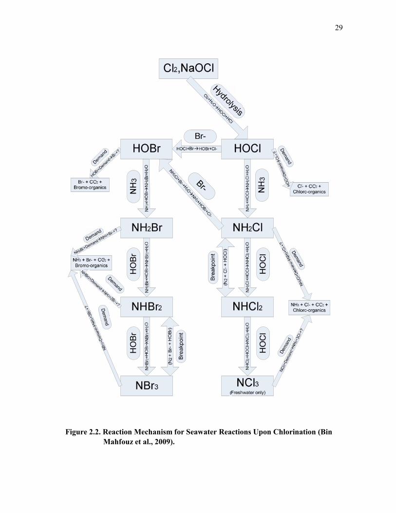
added as a gas to seawater. Bin Mahfouz et al. (2009) have constructed the reaction
mechanism shown in Figure 2.2. On this diagram, starting species and intermediate and
final byproducts are represented in boxes. Arrows correspond to reaction steps. Boxes on
the arrows represent reactive species that contribute to that reaction. First, chlorine will
dissolve and hydrolyze rapidly and completely to HOCl (hypochlorous) acid:
Loops
Flow (m/s)
1.1 1.8 3.0
Control
Thick sludge film
& many barnacles
Same as in
1.1 m/s
No attachmentPulsed Discharged
Thin sludge film
& no barnacles
Pulsed NaClO
No sludge film
& small # of barnacles
Continuous NaClO No sludge & no barnacles

24
Cl2 H2O HOCl HCl Equation 2.13
Hypochlorous acid is a strong biocide, but it is a weak acid that will dissociate to
hydrogen and hypochlorite ions:
HOCl H OCl Equation 2.14
where OCl- is the hypochlorite ion. In terms of disinfection effectiveness, hypochlorous
acid is much stronger (almost two orders of magnitude) than the hypochlorite ion. Since,
the hydrogen ion appears on the right side, this reaction is pH-dependent. Hypochlorous
acid will reach its maximum concentration at pH ranges between 4 and 6 (Hostgaard-
Jensen et al. 1977). However, the effectiveness of a chemical as a disinfectant may not
be the same as its effectiveness in removing biofilms. Controlling biofilm is achieved by
weakening the polysaccharide matrix of microbial cells. There is experimental evidence
that shows that chlorination is more effective in causing biofilm detachment at pH values
greater than pH 8, where OCl- concentration is more dominant than HOCl (Characklis et
al., 1979).
Usually, seawater contains organic and non-organic species. Of particular
importance are ammonia and bromide species. Ammonia, as well as other reactive
nitrogenous compounds, will be chlorinated to yield monochloramine (NH2Cl),
dichloramine (NHCl2), and trichloramine (NCl3). by replacing the hydrogen atom of the
25
ammonia molecule with a chlorine atom while maintaining its positive charge according
to the following reactions:
HOCl + NH3 NH2Cl (monochloramine) + H2O Equation 2.15
NH2Cl + HOCl NHCl2 (dichloramine) + H2O Equation 2.16
NHCl2 + HOCl NCl3 (trichloramine) + H2O Equation 2.17
These reactions depend on pH, temperature, contact time, but mainly on chlorine
to ammonia ratio. All of the free chlorine (hypochlorous acid) will be converted to
monochloramine at pH 7-8 (fastest conversion is at pH 8.3) when there is 1:1 molar ratio
of chlorine to ammonia (5:1 by wt.) or less. Then, within the same range of pH,
dichloramine is produced at a molar ratio of 2:1 of chlorine to ammonia (10:1 by wt.).
This reaction is relatively slow, so it may take an hour. Also, within the same range of
pH, trichloramine will be produced at a molar ratio of 3:1 of chlorine to ammonia (15:1
by wt.) and at equal molar ratios but at pH 5 or less. The two reactions producing di -
and tri-chloramine are known as the breakpoint reactions where the chloramines are
reduced suddenly to the lowest level. The significance of breakpoint reaction is that
chlorine reaches its highest concentration and germicidal efficiency (at 1:1 molar ratio of
chlorine to ammonia) just before reaching this point. Also, at the breakpoint

26
monochloramine and dichloramine react together (which reduces chlorine residuals) to
produce nitrogen gas, nitrate, and trichloramine.
Dichloramine decomposes to an intermediate reactive product (NOH) which
consumes mono-, di-chloramine, and hypochlorous acid producing nitrogen gas and
nitrate. Also, excessive chlorine will form trichloramine.
NHCl2 + H2O NOH + 2 H+ + 2 Cl- Equation 2.18
NOH + NH2Cl N2 + H2O + H+ + Cl Equation 2.19
NOH + NHCl2 N2 + HOCl + H+ + Cl- Equation 2.20
NOH + 2 HOCl NO3- + 3 H+ + 2 Cl- Equation 2.21
NCl3 + H2O NHCl2 + HOCl Equation 2.22
The reaction of chlorine into these forms steer it away from the disinfection
function and render the biocide less effective. Consequently, it is important to
understand such side reactions.
Hypochlorous acid rapidly reacts with bromide producing hypobromous acid,
which also can be produced from the reaction of bromide with monochloramine as
follows:

27
HOCl Br HOBr Cl Equation 2.23
NH2Cl + Br- + H2O HOBr + Cl- + NH3 Equation 2.24
where HOBr is hypobromous acid. Additionally, the hypochlorite ion may undergo a
slow reaction with the bromide ion as follows:
OCl Br OBr Cl Equation 2.25
where OBr- is the hypobromite ion. Bromide in seawater may also react directly with
added chlorine to give bromine and chloride:
ClBrBrCl 22 22 Equation 2.26
It is worth noting that the presence of ammonia and other nitrogenous
compounds in the seawater will react with HOBr to yield monobromamine (NH2Br),
dibromamine (NHBr2), and tribromamine (NBr3):
HOBr + NH3 NH2Br (monobromamine) + H2O Equation 2.27
HOBr + NH2Br NHBr2 (dibromamine) + H2O Equation 2.28

28
HOBr + NHBr2 NBr3 (tribromamine) + H2O Equation 2.29
The bromine breakpoint happens when the dibromamines are produced rapidly,
leading to the formation of nitrogen gas:
NHBr2 + H2O NOH + 2 H+ + 2 Br- Equation 2.30
NOH + NHBr2 N2 + HOBr + H+ + Br- Equation 2.31
It is also important to consider the effect of bromide which naturally exists in
seawater at (50 – 70 mg/l). This is in stoichiometric excess of chlorine dosage as well as
ammonia concentration don’t exceed 2 to 3 mg/L. The relative produced amount of
bromine species to ammonia species is proportional to bromide concentration over
ammonia concentration if we assume both reactions are rapid and simultaneous.
29
Figure 2.2. Reaction Mechanism for Seawater Reactions Upon Chlorination (BinMahfouz et al., 2009).

30
The following is a more detailed analysis of the key reaction steps which may be
broken down into:
1) Hydrolysis
Chlorine as gas (Cl2) is added to water to form hypochlorous acid (HOCl), or by
adding a solution containing caustic producing hypochlorite which reacts with water to
form hypochlorous acid (HOCl). This reaction is called hydrolysis of chlorine gas
(White, 1999):
Cl2 H 2O HOCl H Cl Equation 2.32
Hydrolysis of chlorine gas needs a few tenths of a second at 64F and a few
seconds at 32F.
Cl2 Equation 2.33
Free chlorine residual is the total chlorine residual. Available chlorines are
double the amount of existing chlorine by weight, reflecting the oxidation power of the
compound. Total chlorine is simply the sum of the combined and free levels (White,
1999).
2) Formation of chloramines
At ammonia nitrogen levels greater than 0.5 mg/l and with a chlorine dose less
than 2.5mg/l, dibromamine and monochloramine become the predominants. At a higher
OH HOCl Cl

31
ammonia concentration with a longer time, monochloramine will be the main
component. However, at a lower ammonia nitrogen concentration (less than 0.4mg/l)
with a high chlorine dose, tribromamine and hypobromous acid are going to be the major
products (Johnson et al., 1982). The main factors determining the predominance of either
chloramines or bromamines are bromide concentration or salinity, ammonia nitrogen
concentration, and pH. If pH is decreased from 8.0 to 7.5, the concentration of ammonia
would decrease by a factor of 3, as would the formation of monochloramine (Johnson et
al., 1982). The critical ammonia nitrogen to bromide ratio is 0.008 at pH of 8.1. At
higher than the critical ratio, monochloramine would be predominant after 30 minutes to
one hour; at lower than the critical ratio, dibromamine would be the predominant and
there would be a small amount of monochloramine remaining after the bromamine
decomposes. One way to avoid forming monochloramine is to add excess chlorine
because of its toxicity and low oxidant level. .In cases where there is high salinity,
excess bromide exists of more than 100 fold, so only bromamine and bromine would be
produced (Johnson et al., 1982).
The inorganic reaction between chlorine and ammonia nitrogen forms
monochloramine, dichloramine, and trichloramine in three reactions as chlorine
concentration increases up to 50 mg/L. Each reaction involves a chlorine -substituting
hydrogen atom in the ammonia. The reactions are dependent of pH, temperature, time
contact, initial ratio of chlorine-to-ammonia, and initial concentrations of chlorine and
ammonia nitrogen (White, 1999).

32
HOClNH3NH2Cl (monochloramine)H2O Equation 2.34
HOCl NH2ClNHCl2 (dichlora min e) H 2O Equation 2.35
HOClNHCl2 NCl3 (trichloramine) H2O Equation 2.36
The first reaction is to convert free chlorine to monochloramine at equimolar (5:1
by weight) of chlorine to ammonia or less. The highest conversion (99%) occurs at 8.3
pH at 25 C (White, 1999). The second reaction is to form dichloramine, which is slower
than the first reaction at a pH of 7 to 8 with a ratio of 2 moles of chlorine to 1 mole of
ammonia. This reaction takes five hours for 90% conversion at pH 8.5, and the reaction
speeds up as the pH increases (White 1999). The third reaction is to form nitrogen
trichloride at pH 7-8 with the chlorine to ammonia nitrogen mole ratio at 3:1 (15:1 by
wt.). Nitrogen trichloride can be formed at an equimolar of chlorine to ammonia
nitrogen, but only at 5 pH or less. Also, nitrogen trichloride can be formed at a high pH,
such as 9 pH, when the mole ratio of chlorine to ammonia nitrogen is 5:1 (25:1 by wt.)
(White, 1999).
Halamine formation reactions are rapid and completed in less than one minute,
and they increase as the basicity of amine increases. The hydrolysis of the bond in N -Cl
is slower compared to the bond in N-Br, which is very fast. It was assumed that the first
order for calculating ammonia level NH2Br formation has to be measured for only

33
inorganic bromamines (Lietzke, 1977). The NHBr2 rate is 200 times slower than NHCl2
formation, and the latter is 1.8 x 10⁴, which is slower than that of NH2Cl (Lietzke,
1977). The NBr3 rate is 500 times slower than the NCl3 formation, and the latter is 2.5 x
106 times slower than NH2Cl (Lietzke, 1977). Unmeasured halogenation rates are based
on these assumptions:
The formation of bromamines from hydrolysis is faster than chloramines
(Lietzke, 1977).
The halogenation of organic amines and halamine is faster than inorganic
ones.
Chlorination of bromine is slower than bromination of chloramine and
slower than bromination of bromine.
3) Destruction of chloramines
When the ratio of chlorine to ammonia nitrogen exceeds 1:1, monochloramine
reacts to the excess free chlorine to form dichloramine, which is twice as germicidal as
monochloramine. Zone 3 starts from the dip, or the breakpoint at the curve, which
happens when free chlorine starts to appear. There is a lack of understanding of the
breakpoint reaction behavior due to many competing reactions of high active chlorine
(White, 1999). Breakpoint reactions are caused by the oxidation of ammonia by halogen
to produce nitrogen, which simultaneously reduces halogen to halides. Those reactions
are considered to be the most rapid reactions at a molar ratio of 1.5 halogen to ammonia
because forming trihalamines are more stable. On the other hand, at a lower molar ratio,
this reaction would be slower because the oxidant would be limited (Lietzke, 1977).

34
3HOX + 2NH3 N2 + 3H2O + 3H+ + 3X- Equation 2.37
where X is bromine or chlorine.
These are the reactions representing chlorine breakpoint.
NHCl2 H 2 O HNO 2HCl Equation 2.38
NH 2 Cl HNO N 2 H 2 O HCl Equation 2.39
NHCl2 HNO N 2 HOCl HCl Equation 2.40
HNO 2HOCl HNN3 2HCl Equation 2.41
An additional dosage of chlorine is needed to oxidize ammonia beyond nitrogen
to a nitrate. NHCl2 decomposes slowly at a ratio of Cl/N below 1.5. NHCl2 rarely exists
in the total oxidant residual in the case of any Br- presence. It is very difficult to
precisely predict the required dose of chlorine with other amines existent and an unstable
demand (Lietzke, 1977).

35
Figure 2.3. Chlorine Breakpoint Model Calculations at T = 200C, pH = 7.0, [NH3]0= 1.01 mg/l, and Molar Ratio of Cl2/NH3 = 2.63 After One Hour(Based On Results By Lietzke, 1977).
The model shown in Figure 2.3 assumes that there is no chlorine demand and that
the only nitrogenous compound that exists is ammonia. When chlorine is added at equal
molar or less than ammonia, only NH2Cl and no (or merely a trace) of NHCl2 are
produced. NH2Cl is more stable with the higher ammonia molar than when chlorine is
added, and after one hour, all total residual chlorine is NH2Cl and equal to the initial
chlorine added. If the chlorine dose exceeds the required amount to produce NH2Cl,
NHCl2 will be produced and will decompose to react with NH2Cl and reduce the total
oxidants proportional to NHCl2 formed. The breakpoint is at an equal mixture of both
NH2Cl and NHCl2 and chlorine will be reduced by oxidizing ammonia to nitrogen. After
passing the breakpoint, it takes only a few hours to oxidize ammonia. A chlorine dose

36
beyond the breakpoint will remain as a hypochlorite, and the chlorine residual increases
with increasing chlorine doses (Lietzke, 1977).
Monochloramine is toxic and persistent, while dibromamine is toxic and not
persistent. The natural compounds that exist in seawater play a role in reducing
haloamines. Monochloramine is stable in seawater for about 8 months at pH 8. On the
other hand, there is a dibromamine decomposition rate of 700 L/mol/min at pH 8, 200 C
with a half-life of four hours and a bromine concentration of 1 mg/L (Johnson et
al.,1977).
4) Formation of organic byproducts
Some chlorination byproducts are carcinogenic and are formed from organic
halogenated compounds like THMs, HAAs, HANs, haloketones, chlorophenols, chloral
hydrate and chloropicrin (Sayato et al., 1995). Chlorination of seawater produces
compounds that are toxic to aqueous life. These compounds’ concentrations and
lifetimes are functions of pH, temperature, salinity, dissolved organic matter and
nitrogen, inorganic nitrogen and the amount of chlorine and mixing efficiency (Freese et
al., 2006). The two major components that determine chlorination are bromine and
ammonia . Direct toxicity of hypohalites and/or halamines from chlorination is thought
to be affecting the aquatic ecosystem. Even low chlorine concentration (0.005 mg/l)
would affect fish (Lietzke, 1977). Chlorination of seawater at a Kuwait desalination-
power plant results in forming halomethanes, which at high concentration, measures up
to 90 ug/l, near the outfalls. 95% of the total halomethanes are made up of bromoform,
and the remains are mostly dibromochloromethane. Some of these volatile halogenated

37
hydrocarbons, such as CCl4 , CHCl3 , andCHBr3 , are harmful to aquatic life (Riley et al.,
1986).
Chlorine has an effect on marine life when it is dumped into costal and estuarine
waters from sewage treatment plants, electric power plants, and industrial plants. Fish
have to migrate to avoid the water area that is polluted with halogenated organic
compounds and has ecological effects from chlorination (Helz et al., 2005).
An estimated 0.5-3.0 % of chlorine added to freshwater is transferred to
chlorinated organics and mostly is chloroform. With higher salinity, chlorine is
converted into more reactive bromine forming bromo-organics and brominated
trihalomethanes, such as (CHCl2Br, CHClBr2, and CHBr3). Chloroform and bromoform
are carcinogen products and have direct toxicity with rapid bioaccumulation in fish and
fish eggs. Peter and his colleagues found a model for trihalomethane concentration at the
end of the contact period in freshwater treated with chlorine (Lietzke, 1977):
Total haloforms (M) = 0.01307 (CDO) (1 + 14[Br-]0.25) Equation 2.42
where CDO is the molar concentration of Cl2 that is consumed by organic demand. [Br-]
is the initial molar concentration of bromide. The last term, 14[Br-]0.25 is for rapid
production of haloform at bromide presence.
The model shows that about 13 mmol of chloroform is produced for every mole
of chlorine consumed in freshwater. Generally, kinetics of haloform do not apply when

38
there is with chlorine consumption. Total haloform production does not depend on pH
(Lietzke, 1977).
5) Consumption by non-organic compounds
The total chlorine demand is due to nitrogenous compounds and anything that
consumes chlorine. Chlorine demand is a non-nitrogenous demand.
The objective of a chlorine demand (CD) model is to relate it to chlorine dosage
(CL) at a certain temperature and for given seawater conditions. For example, the
following expression is based on the work of Wong et al. at for doses from 0-30 mg/l,
shown in Figure 2.4. (Wong et al., 1984):
CD = 0.2468 + 0.989CL – 0.02522CL2 + 9.897 X 10⁻⁴ CL3 – 1.35 X 10⁻⁵ CL4
Equation 2.43
Figure 2.4. Chlorine Demand as a Function of Chlorine Dose at 200 C (Wong et al.,1984).

39
For freshwater there is no existence of HOBr. Figure 2.4 shows ultimate, non-
nitrogenous, chlorine demand as a function of dose and temperature in seawater
(Lietzke, 1977).
6) Bromide oxidation
Hypobromous acid is an active chemical constituent and is formed from
oxidizing a bromine ion with chlorine in a very fast reaction. Reactions of hypochlorous
acid with ammonia and a natural existence of bromide determines domination of
bromine compounds or monochloramine (Johnson et al., 1982). Formation of
hypobromous acid in open seawater occurs when chlorine oxidizes bromide and converts
to chloride in absence of ammonia. But in estuarine or coastal sea water, ammonia
concentration increases and bromide concentration decreases, so bromamine is first
produced and followed by monochloramine (Johnson et al., 1982). More on the bromide
reactions are given in the following subsection.
2.8.2. BROMINE REACTION
The bromine reactions typically proceed through the following steps:
Formation of acid
Formation of bromamines
Destruction of bromamines
Formation of organic products
Consumption of non-organic byproducts
More information on these steps follows:

40
1) Acid-base
Bromine is used as a disinfectant and may be used with chlorine and iodine (I2).
The hydrolysis of bromine in water will produce hypobromous acid and bromide ions.
Free available bromine is the concentration of both hypobromous acid and hypobromite
ions. Then, hypobromous acid will dissociate into hypobromite and hydrogen ions
according to the following equations (Johanneson, 1960):
Br2 H2 O HOBr H Br Equation 2.44
HOBrH OBr Equation 2.45
2) Formation of bromamines
Hypobromous acid reacts with the ammonia that already exists in most treated
waters to produce bromamines (Johnson et al., 1982). Bromamine formation depends on
bromide ions as well as ammonia concentration, pH, natural organic content, and
chlorine dosage (Minear et al.,. 2004). Inman and John found out that mixing
hypobromous acid (HOBr) with ammonia at a pH range of 7.0 to 8.4 would produce
monobromamine (NH2Br). Bromamines including monobromamine, dibromamine, and
tribromamine are formed by adding bromine to ammonia as shown in the following
reactions (Hofmann et al., 2001):

41
molKJBrNHGKOHBrNHNHHOBr
feq /1.77,100.3 210
223
Equation 2.46
molKJNHBrGKOHNHBrBrNHHOBr
feq /181,107.4 28
222
Equation 2.47
molKJNBrGKOHNBrNHBrHOBr
feq /296,103.5 36
232
Equation 2.48
3) Destruction of bromamines
Inorganic bromamine will exchange bromine rapidly with pH dependence, while
chloramines, mainly monochloramine, do the exchange of chlorine very slow at pH a
range from 6 to 9. The breakpoint reaction, which is the oxidation of ammonia to
nitrogen gas, of halamines occurs when the molar ratio of halogen to ammonia is 3:2.
The breakpoint for chlorine is the reaction between NH2Cl and NHCl2, while for
bromine it is the reaction between NHBr2 and NBr3. Organic halamines are more stable
than inorganic ones. The bromine-ammonia breakpoint is the reaction between di- and
tribromamine, whereas in chlorine-ammonia it was between mono- and dichloramine.
The bromine-ammonia system is shown as follows (Lietzke, 1977):
H 2 O 2HNBr2 N 2 HOBr 3HBr Equation 2.49
42
2H 2 O HNBr2 NBr3 N2 2HOBr 3HBr Equation 2.50
3H 2 O 2NBr3 N2 3HOBr 3HBr Equation 2.51
The rate constant of reaction (32) is 1000 times larger than reaction (31), and
reaction (33) is kinetically insignificant at a pH above 6. It is very difficult to expect
which bromamine species exist initially because the breakpoint occurs very rapidly at
equal concentration of di- & tri-bromamine.
The differences between all chlorine and all bromine systems are (Lietzke, 1977):
Bromamine decomposition residuals are so rapid.
When NHBr2 and NBr3 exist at a significant amount below breakpoint, it
helps decomposition to occur at lower doses; and at a halogen/N ratio
of 1.0, the peak would become flat.
Formation and decomposition of NBr3 above the breakpoint without
evolving N2, not like NCl3.
Nitrate formation is insignificant.
Dibromamine decay rate is the second order with respect to NHBr2 and the half-
life is 10-15 hours. There is no specific mechanism of tribromamine formation. But,
tribromamine decomposition was studied by LaPoite et al. in 1975 and the result was as
follows (Hofmann et al., 2001):
2NBr3 + 3H2O N2 + 3HOBr + 3H+ + 3Br- Equation 2.52
43
At high ammonia to bromine ratios, tribromamine concentration is very low.
Bromine decay occurs at the reaction between tribromamine and dibromamine, with an
N:Br ratio of 2:3 according to this reaction (Hofmann et al., 2001):
2NH3 + 3OBr- N2 + 3Br- + 3H2O Equation 2.53
To oxidize all chlorine, 3.2-3.6 mol of chlorine must be added to every 2 mol of
ammonia to reach the breakpoint, according to White’s study in 1992 (Hofmann et al.,
2001):
4HOCl + NH4+ NH3
- H2O + H+ + 4Cl- Equation 2.54
Adding an excess amount of chlorine, more than the theoretical, is due to side
reactions in which bromamines do not decay to form nitrate (Hofmann et al., 2001).
Figure 2.5. shows NH 2 Breq/NHBr2 eq against excess ammonia (Johnson et al., 1982).

44
Figure 2.5. Dependence of Bromine Ratio at Equilibrium on Excess Ammonia(Johnson, 1982).
Dibromamine, NHBr2 , and tribromamine, NBr3 , are formed at a pH lower than
8.5 and a bromine molar concentration of at least five times the concentration of
ammonia (Guy W. Inman 1984). Dibromamine decomposition occurred less than a
minute after its formation. At a pH above 7, the rate of formation of monobromamine is
much higher than rate of formation of dibromamine. Dibromamine formation was first
order in hydrogen ion and second order in monobromamine or an initial bromine in a
case with an excess amount of ammonia (Inman et al., 1984).
dNH 2Br/ dt k1 NH3HOBrwhere, k1 4 1 10 Msat pH 7-8 Equation 2.55
45
With an excess amount of ammonia, monobromamine is still present even after
the dibromamine reaction reached completion. The phosphate is affecting the stability
and formation of dibromamine (Inman et al., 1984). Inman and Johnson found out that
the chloride ion does not affect bromamine decomposition; however, the bromide ion
has no effect at pH 8.48, but at pH 6.71, the bromide ion increases the rate of the
reaction of decomposition of NH2Br to NHBr2 and NH3. The bromamine decomposition
at pH 6.71 and the different initial bromide ion concentrations has been studied by
Minear (Minear et al., 2004). There are similarities between bromamine decomposition
and the chloramine system.
4) Formation of organic byproducts
The organic byproducts are produced by the reaction of hypobromous acid
(HOBr) with natural organic matters to produce compounds with bromine attached to a
carbon atom. There are many examples of bromo-organic byproducts such as
bromoform, bromopicrin, dibromoacetonitrile, bromoacetone,bromoacetic acid,
bromoalkanes, bromohydrins, etc. (Gunten, 2003). Then, these intermediate compounds
can go further in halogenations to bond three bromine to the carbon atom forming tri -
halogenated intermediates. Since the bromine atom is greater than chlorine, the bro mine
compound CBr-3 is more stable than chlorine CCl-
3 (Greca et al., 2008). The higher the
concentration of bromite, the higher the formation of trihaloginated methane and
halogenated aitic acid while they can be reduced at higher concentration of ammonia
(Chang et al., 2008).

46
CX3 R OHCX3 ROHCHX3 OH Equation 2.56
5) Consumption by non-organic compounds
The N-Br bond is relatively unstable compared to the N-Cl bond. Therefore,
inorganic bromamine disproportionation is rapid compared to inorganic chloramine. The
latter is disregarded at a pH above 6. NH2Cl disproportiation does not depend on pH at
ranges of 6-9. NHCl2 formation is negligible in organic amines’ presence. NHBr2 is less
stable and reacts four times faster than NH2Br and eight times faster than NH2Cl
(Lietzke et al., 1977).
2.8.3. CHLORINE/ BROMINE COMBINED
1) Competition for Chlorine
Most organic nitrogen does not react with chlorine, and its concentration is
higher than free ammonia and has less correlation to salinity. Also, the organic nitrogen
formation of halamines is much faster than NH2Cl, which competes with ammonia to
react with halogen. Methylamine is the simplest organic amine (Lietzke et al., 1977).
Chlorine hydrolyzes rapidly and completely to produce HOCl and HCl. Then, HOCl
reacts with three items: bromide, ammonia, and non-amine “demand”. Non-amine
consists of inorganic and organic reducing agents and autodecomposition reactions.
HOCl reacts with ammonia to form monochloramine and a small amount of
dichloramine. A reaction of HOCl with bromide produces HOBr. Then, HOBr would
react with any available amines to form bromamines. Halamines are unstable and
ultimately decay to nitrogen gas or ammonia. Halamine intermediates are part of the
47
oxidant residual. HOCl and HOBr are the non-nitrogenous oxidants (free halogens)
(Lietzke, 1977). Chlorination of polluted seawater (which contains ammonia) could form
monochloramine, bromochloramine, and bromamines depending on the water’s pH,
temperature, salinity, ammonia concentration, and chlorine dosages (Johnson et al.,
1982). In case of low halogen in seawater containing ammonia, only NH 2 Br , NHBr2 ,
NH 2 Cl and NHCl2 are observed.
The monochloramine formation rate is higher in low salinity water which has
more ammonia. Ammonia is competing with bromide to react with chlorine. The
reaction of ammonia and chlorine is forming monochloramine not bromine or
bromamine at these conditions: pH 8.1 and weight ratio of NH3 : Br 0.008 . Morris
and Weil found out that the mechanism of monochloramine formation in low ionic
solution is as follows (Johnson et al., 1982):
HOCl OCl H Equation 2.57
HOCl NH3 NH2 Cl H 2 O Equation 2.58
2) Mixed Bromochloramines
Monochloramine is formed when chlorine is added to saline water, regardless of
bromide presence. The two passable reactions of monochloramine with bromide are as
follows:

48
2NH2Cl 2Br- NHBr2 2Cl- NH3 Equation 2.59
2NH2Cl Br- NHBrCl Cl NH3 Equation 2.60
Dibromamine will be produced at stoichiometry of 1:1 (monochloramine and
bromide) and bromochloramine will be produced a stoichiometry of 2:1
(monochloramine and bromide). From the plot of lnBr /NH2 Cl vs. time, the 2:1
stoichiometry is a better fit (Johnson et al., 1982).
Figure 2.6. Second-Order Plots Comparing 1:1 Stoichiometry for NHBr2
Formation to 2:1 Stoichiometry for NHBrCl Formation (Johnson etal., 1982).
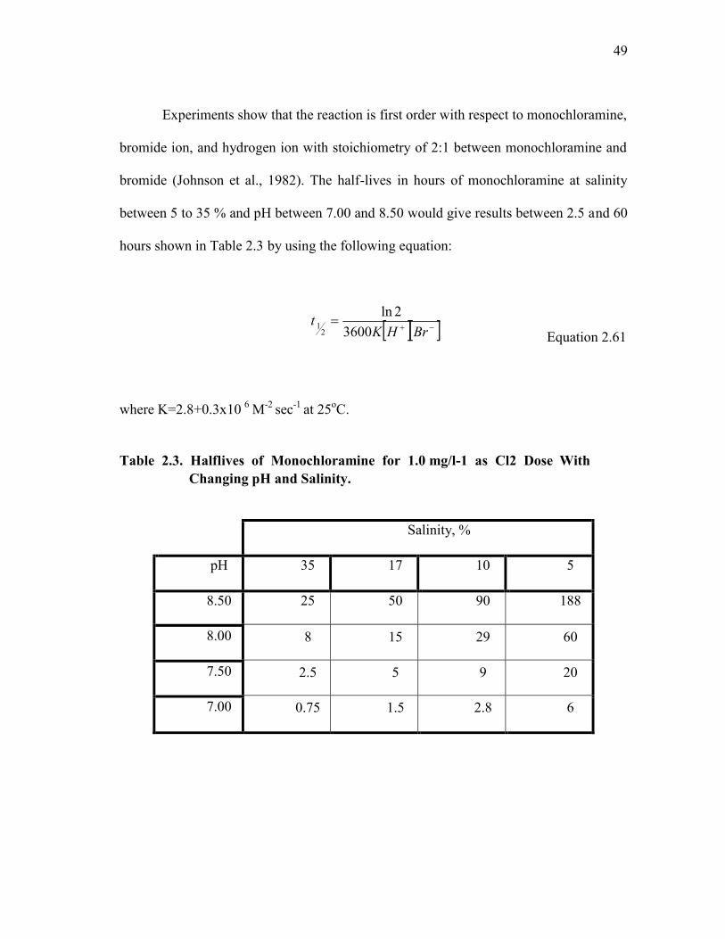
49
Experiments show that the reaction is first order with respect to monochloramine,
bromide ion, and hydrogen ion with stoichiometry of 2:1 between monochloramine and
bromide (Johnson et al., 1982). The half-lives in hours of monochloramine at salinity
between 5 to 35 % and pH between 7.00 and 8.50 would give results between 2.5 and 60
hours shown in Table 2.3 by using the following equation:
BrHK
t3600
2ln2
1Equation 2.61
where K=2.8+0.3x10 6 M-2 sec-1 at 25oC.
Table 2.3. Halflives of Monochloramine for 1.0 mg/l-1 as Cl2 Dose WithChanging pH and Salinity.
Salinity, %
pH 35 17 10 5
8.50 25 50 90 188
8.00 8 15 29 60
7.50 2.5 5 9 20
7.00 0.75 1.5 2.8 6

50
For resident time of less than one hour, the oxidation of Br- by NH2Cl is out of
consideration because it is not for generating bromamine from chloramine by
bromochloramine (Lietzke et al., 1977):
NH2 Cl- Br H2O NH3 HOBr Cl Equation 2.62
The HOBr can react with NH2Cl to produce NHBrCl, and also HOBr reacts with amines,
halamine, and demand to produce other products. This would show the conversion from
NH2Cl into NHBrCl (Lietzke et al., 1977).
There is not enough information about the breakpoint in systems which consist of
both active chlorine and bromine. It is not clear whether chloramines react with
bromamine or with bromochloramines, and there is no prediction of how
bromochloramines species react as a function of pH, Br-, or as chlorine dose. This model
combines all chlorine and bromine breakpoint reactions, plus bromochloramines
formation reactions. Bromochloramine interacts with the bromine breakpoint system, but
not with the chlorine one, and it has a lower rate constant than bromine reactio ns
(Lietzke et al., 1977).
Two experimental breakpoint curves are above the theoretical 1.5 Cl/N molar
ratio because extra chlorine is required to satisfy the organic need (Jenner et al., 1997).
An extra chlorine dose will shift the breakpoint to a higher ratio (Allonier et al., 1999 &
2000). Khalanski 1977 proved that adding an ammonia solution to seawater would give
51
a higher breakpoint than predicted due to oxidation of NH3 to N2 (Lietzke et al., 1977;
Rajagopal et al., 2005; Viveau et al., 1980; Shaw et al., 2006).
Demand has an effect on shifting the breakpoint. Dominant compounds below
the breakpoint for NH2Cl, are NHBrCl, and NHBr2; above the breakpoint, HOBr,
NBr2Cl, and NBr3 are dominants. At equal concentrations of dihalamines (NHBr2 and
NHBrCl) and trihalamines (NBr3 and NBr2Cl), the decomposition is rapid (Lietzke et al.,
1977).
2.9. FACTORS IMPACTING THE EFFECTIVENESS OF THE
BIOCIDE
This section discusses the key factors impacting the effectiveness of the biocide.
Four factors are considered: free versus combined form, pH, temperature, and other
factors such as ammonia concentration. The following discussion focuses on chlorine
and bromine compounds because of their widespread use.
2.9.1. FACTORS IMPACTING EFFECTIVENESS OF CHLORINE
COMPOUNDS
1) Free/Combined Forms
Optimization of chlorination is done to achieve disinfection efficiencies through
predicting species distribution. Hypochlorous acid (HOCl) is 80 times more effective
than hypochlorite OCl-. HOCl is 80 times more effective than the hypochlorite ion
OCl for reducing E Coli. A comparison between the use of bromine species and
other halogens has been studied in literature (Goodenough et al., 1969 and Kristoffersen,
1958). This shows that HOX and X 2 are much more effective than X3-, OX , and

52
chloramines. Johnson, by contrast, shows that monochloramine (NH2Cl) and
monobromamine (NH2Br) are very effective as disinfectants (Overby, 1971).
Free chlorine is more effective in bacteria inactivation wastewater treatment than
monochloramine. The study here was for inactivation of E Coli by free chlorine and
monochloramine simultaneously and separately in a continuous flow system (CSTR).
The highest inactivation of E Coli bacteria is when both free chlorine and
monochloramine coexist at conditions close to the breakpoint. The result shows that
there is a synergistic interaction between free chlorine and monochloramine in killing E
Coli bacteria (Yukselen et al. 2003).
Maintaining 1-2 mg/L of chlorine residual was not enough to reduce the bacterial
growth. But a 3-5 mg/L level will reduce biofilm by 2 logs. It is required to keep
chlorine residual at 15-20 mg/L to control biofouling (White, 1999). Monochloramine
residual at a level of 2.0 mg/L is more effective to reduce biofilming than free chlorine.
Chloramine dosages are increased from 2.0 to 40 mg/L to maintain 2-3 mg/L of residual
to ensure that there is no a coliform bacterium or nitrification in the distribution system.
Biofilm growth can be controlled by maintaining 2-4 mg/L of chlorine residual (White,
1999).
2) Effect of pH
Free residual chlorine is twice as effective in chlorinated water at pH 7.2 as it is
at 7.8 (White 1999). Free chlorine vs. combined chlorine residual: It is preferred to
have combined chlorine predominantly monochloramine residual if entering a clean

53
system. If the system is dirty, then free residual chlorine must be added to clean the
system to produce nitrogen trichloride NCl3 (White 1999).
3) Effect of temperature
It is crucial to determine the chlorine demand (chlorine consumed by inorganic
and organic impurities in water) in order to measure the chlorine production rate.
Chlorination Breakpoint occurs when chlorine demand is satisfied; then free chlorine can
be formed. Figure 2.7. shows chlorine decay dependence on temperature with an
exponential increase in decay with a temperature increase, but no dependence on pH
(Rennau et al., 1990).
Figure 2.7. Active Chlorine Decay Rate Dependence o n Temperature a t pH 7(Initial Active Chlorine Concentration 29.5mg Dm-1, Initial ChlorideConcentration 134 Mg Dm-1, Electrolyte Volume 250 Cm2) (Rennauet al., 1990).

54
4) Calcareous deposits on the cathode surface
Electrochemical disinfection for water faces calcareous deposits on cathode
surface due to pH changes. Calcium and HCO3—
ions are responsible for deposits. pH
changes come from OH- ion according to this reaction at the cathode (Rennau et al.,
1990):
2 H2O + 2 e- H2 + 2 OH- Equation 2.63
Calcareous layers increase with temperature and reduce the current efficiency
and therefore hypochlorite production. Producing chlorate from hypochlorite and
hypochlorous acid with rate constant k is as follows (Rennau et al., 1990):
ClO- 2 HClO ClO3- + 2 HCl Equation 2.64
Production of hypochlorite from much diluted chloride solution can be lower in
natural water due to chlorine decay. Iridium oxide electrode showed high performance
more than platinum electrode. Chlorate production is very negligible. The chlorine
demand can be targeted by increasing current density which has linear relation with
active chlorine production. Water disinfection can be achieved by electrolytic
hypochlorite production (Rennau et al., 1990). Wong and Davidson found that
decomposition of HOBr for long time is in the third decay phase (Lietzke, 1977).

55
HOBr ½ O2 + HBr Equation 2.65
5) Other effects
Residual-oxidants concentration is calculated by a computer program as a
function of time. In the function, time can be converted to distance in case of a constant
water flow through the cooling system. Typical chlorine doses (for unpolluted water
only) change from below breakpoint for freshwater to near breakpoint for estuarine
water to above breakpoint for seawater. Ammonia concentration increases as pollution
increases in water and may prevent breakpoint chlorination (Lietzke, 1977).
2.9.2. FACTORS IMPACTING EFFECTIVENESS OF BROMINE
COMPOUNDS
1) Free/Combined Form
Monobromamine is less efficient, but bromamines are effective as HOBr and
HOCl. Hypobromous acid (HOBr) is a better disinfectant than hypochlorous acid
(HOCl) at the pH range of 6-9. Hypobromous acid (free available bromine) is used as a
disinfectant to control biofouling. Bromamines are formed immediately by the reaction
of hypobromous acid with ammonia. The disinfection capability of bromine compounds
is as strong as the chlorine compounds for the toxicity of biofouling organism s
(Pinkernell et al. 2000).
2) Effect of pH
From the log (NH3/Br2) ratio versus pH, it is known that forming tribromamine
from dibromamine and reverse can be achieved by altering pH. Those reactions are

56
assumed to occur rapidly, and the equilibrium of bromamine species is established as a
result. Therefore, at equilibrium, the existence of different bromine species can be
determined from the ratio of N/Br and pH. Figure 2.8. shows the equilibrium of
bromamines as reported by Johnson and Overby (1979) (Hofmann et al., 2001).
Figure 2.8. The Equilibrium Point at the Existence of Different Bromine SpeciesCan Be Determined From the Ratio of N/Br and pH (Johnson et al.,1979).

57
At a high pH, such as 9, hypobromous acid is a more effective disinfectant than
hypochlorous acid. Bromine is a more effective disinfectant than iodine in a case of high
bromide concentration and low pH. Bromine and bromamines are more effective
disinfectants than chloramines. Bromine reacts faster than chlorine with ammonia at
high pH. The breakpoint is reached quickly with a 2:3 molar ratio of ammonia to
bromine (Overby et al., 1971). Bromate has a high formation rate at low salinity in
water, but there is no formation in darkness (Richardson et al., 1981).
Ammonia reacts with bromine to form monobromamine. This reaction happens
most rapidly at pH of 9, and it takes several seconds at 6-8 pH values. Monobromamine
decomposition and dibromamine formation occurs as shown in this reaction (Hofmann et
al., 2001):
2NH2Br + OBr- + 2OH- N2 + 3Br- + 3H2O Equation 2.66
Monobromamine is oxidized by free bromine and becomes more unstable at high
pH values (such as 12) and at a high bromine:ammonia ratio, and it may
formdibromamine (Hofmann et al., 2001). Dibromamine, NHBr2 , is an intermediate
product of chlorination of seawater containing ammonia. Dibromamine is toxic,
unstable, and its formation is an optimizing disinfection and antibiofouling process.
The rate formation of dibromamine is a second order with respect to bromine and
becomes faster at low pH. At a pH 8.5 and if the molar ratio of bromine: ammonia is
equal or greater than 5, dibromamine, NHBr2 , and tribromamine, NBr3 , are the main

58
products (J. D. Johnson 1982). There is an assumption that monobromamine stays in
equilibrium with dibromamine and never goes completely disproportionate.
Monobromamine, NH 2 Br , formation rate is 4 1 10 7 M 1 sec 1 where K1 is defined
based on this equation (Johnson et al., 1982):
HOBrNHKdt
BrNHd31
2 Equation 2.67
It is found that the formation rate of monobromamine is much larger than the
formation of dibromamine at pH 7-8.5. With a high ammonia concentration, and after
dibromamine reaction completion, monobromamine can still be observed. At pH of 7.0
and excess ammonia K eq 2.02 10 10M , at 25 0 C for the reaction:
NHBr2 NH4 Keq 2NH 2 Br H Equation 2.68
3) Other effects
Bromine is preferable as a disinfectant because it is less affected by either pH or
ammonia concentration, and the decomposition of bromine oxidant species is very fast
(Lietzke, 1977). As shown in Figure 2.9., Bromamines were found to be stronger and
more stable disinfectants for drinking water than chloramines (1-3) (Minear et al., 2004).

59
Figure 2.9. Relative Disinfection Efficiency of Some Chlorination Products.
59
Figure 2.9. Relative Disinfection Efficiency of Some Chlorination Products.
59
Figure 2.9. Relative Disinfection Efficiency of Some Chlorination Products.

60
Bromamine formation is enhanced by high salinities and high bromide
concentrations. Bromide is oxidized by chlorine or hypochlorous acid, producing
hypobromous acid and a hypobromite ion. Also, ammonia reacts with chlorine to
produce monochloramine. Chlorination chemistry is significantly affected by a low
concentration of ammonia (Johnson, et al. 1982):
1) Bromamines are produced from hypobromous acid at a low concentration
of ammonia. At low ammonia concentration, tribromamine and
hypobromous acid are predominant. In case of a low concentration of
ammonia, the formation of dibromamine and hypobromous acid is high
(Johnson et al., 1982).
2) At an intermediate level of ammonia concentration, a mixture of
monochloramine and dibromamine are formed (Johnson et al., 1982).
3) At high concentrations of ammonia, forming monochloramine competes
with bromide oxidation, so only monochloramine is formed.
Monochloramine is undesirable because it does not assist fouling control
and has a high toxicity to marine life. However, at high ammonia
concentration, monobromamine and dibromamine are coexistent (Johnson
et al., 1982).
Each mM of phosphate speeds dibromamine formation so that it is four times
faster (Hofmann et al., 2001). Also, the presence of an acetate buffer would have the
same effect as a phosphate buffer. The equilibrium would be reached in one second in
the presence of either buffer; otherwise, it would take several minutes. Both phosphate

61
and acetone do not naturally exist in sizeable amounts. On the other hand, bicarbonate
exists in nature and has the same effect as phosphate and acetone (Hofmann et al., 2001).
2.10. OTHER BIOCIDES
Biocides are chemical substances used to control biofouling in heat exchangers
by killing the living organisms. However, chlorine is the most widely used chemical for
disinfecting in water treatment, but there is a high risk of the potential production of
hazardous halogenated byproducts. There are other alternatives for treating water, like
ozone, chlorine dioxide, and chloramines. On the other hand, there are some
disinfectants that are less commonly used, like ultraviolet light, hydrogen peroxide,
permanganate and other halogens (Fiessinger et al., 1985).
Ozonation is used in the disinfection of water and is widely used in Canad a,
Europe, and the Soviet Union (Bruijs et al., 1988). Applying ozone will oxidize
inorganic and organic materials. Also, ozonation is used to reduce the turbidity or to
suspended solids by flocculation and microflocculation. The decomposition of ozone
will form higher-oxidizing power radical intermediates. There is a high risk of using
ozone when there is a leakage. Even a low concentration (3 ppm) of ozone is considered
to be harmful to the workers and to the surrounding environment. The efficiency of
ozone is limited because its decay rate is so high (half-life is less than one hour), and it
reacts with a natural organic substance that will allow the bacteria regrowth.
Hydrogen peroxide is a disinfectant for a wide range of bacteria. It is used to
disinfect the Pseudomonas aeruginosa bacteria, which can resist chlorine-based
chemicals. Hydrogen peroxide is used widely with other disinfectants, like UV

62
irradiation and ozone. The bactericidal is not the hydrogen peroxide, but the formed
hydroxyl radical that can impinge the membrane surface by reacting with the cell
component.
Ultraviolet irradiation is water disinfection without the use of chemicals. It has
been developed so that it is cheaper and more reliable to be used in drinking water. The
wavelength of the Ultraviolet irradiation used for this purpose is in the range of 200nm
to 280 nm. The advantage of using Ultraviolet irradiation compared to other methods is
that it does not produce any unwanted substances or byproducts. The efficiency of
Ultraviolet irradiation method is guided by the quality of the water in terms of the
turbidity, and it dissolves organic as well as inorganic substances. The transmittance of
water is reduced due to the absorbance of UV irradiation by suspended matters (Freese
et al., 2007).
2.11. MEASUREMENT OF HALOGEN SPECIES
Several methods are used to measure halogen species. Here, we cover the
following methods:
DPD testing
Amperometric titration
Iodine
1) Diethyl-P-Phenylene Diamine (DPD) Testing
Determining the amount of free available chlorine (FAC) and combined chlorine
by using the Diethyl-P-Phenylene Diamine (DPD) titrimetric and colorimetric methods
has been recognized as a standard method. This method quantitatively determines FAC

63
and different forms of combined chlorine (monochloramine, dichloramine, and
trichloramine). The variation of the intensity of the red color produced from the reaction
of chlorine with DPD reagent determines each chlorine residual fraction. DPD reacts
with FAC, and the addition of potassium iodide would react with combined chlorine
(Strupler, 1985). Moore et al. found out that the interface of monochloramine on FAC by
using DPD at 250C in one minute was 5.6% and 6.0% of 3.5 and 7.0 mg/L Cl2,
respectively (Strupler, 1985). Figure 2.10. shows the determination of free chlorine by
DPD as a function of time in minutes.
Figure 2.10. Monochloramine Interference in the Determination of Free Chlorineby DPD Colorimetric (Spectrophotometric) Method as a Function ofTime (Temp 210C) (Strupler, 1985).

64
Apparent FAC readings as percentage of monochloramine after 1 minute at two
temperatures 100C and 200C are shown in Table 2.4.
Table 2.4. Monochloramine Interference in the Determination of Free Chlorine byDPD Visual Comparator.
Monochloraminemg/l Cl2
Apparent FAC readings as percentage ofmonochloramine after 1 minute
Temp. 100C Temp. 200C2 1.0 2.55 1.2 2.210 1.2 3.125 1.4 2.050 0.8 2.9
Apparent FAC readings as a percentage of monochloramine after 1 minute at
different temperatures at reagents standard and non-standard are shown in Table 2.5:

65
Table 2.5. Comparison of the Results Obtained With Standard and Non-Standard Reagents for Monochloramine Interference in theDetermination of Chlorine by DPD Colorimetric(Spectrophotometric) Method.
Apparent FAC readings as a percentage of monochloramine after 1minute
Reagents standard Non-standard100C 190C 60C 80C 180C
2 1.0 2.9 3.8 6.5 9.0
5 1.5 2.6 3.4 4.6 5.1
10 1.9 2.8 3.1 6.9 4.6
20 1.4 2.4 3.0 4.0 4.2
In any dyehouse, the consistency of water quality is an important factor in
influencing the color application regardless of the quality variations of the water supply
(Bowman 1998).
2) Amperometric titration
The amperometric titration method for identifying free or combined chlorine is
one of the most precise methods, which needs a lot of skills and portable power in the
field. This method has the ability to identify different chlorine residuals, like free
chlorine, and chloramines, such as mono-, di-, and tri-chloramine. This method is lightly
influenced by common oxidizing agents, temperature changes, turbidity and color (W,
2000). Measurement from both DPD and amperometric methods showed comparable
results, including TRC & FRC readings, whereas ion-selective electrode results were
much lower, particularly in TRC values than the other two methods (W, 2000). No major

66
changes were found in the TRC boundary measurement during heating water or passage.
The DPD method, which is EPA-approved, was found to be easy and fast for measuring
both TRC and FRC in the field or at the lab (W, 2000).
3) Iodine
Disinfecting seawater would help increase the efficiency of cooling systems.
Chlorine reacts with natural compounds that exist in seawater to produce residuals.
Iodine cannot measure the chlorine residual accurately in seawater because it measures
all oxidizing agents, such as iodine, bromine, and manganese. The toxic chlorine
residuals can be found in bromine, chloro-, and bromo-amines (Johnson, 1977).
2.12. TREATMENT OF BIOCIDE DISCHARGES
2.12.1. TYPICAL REGULATIONS
An Oxidation Reduction Potential (ORP) system is used to evaluate water
treatment disinfection. ORP would eliminate errors of chlorine measurements by organic
compounds. ORP is a method for controlling the chlorination process in a qualitative,
not quantitative, appearance of chlorine residuals. If there is any amount of combined
chlorine residual alone, the response is very rapid. Whereas, in the case of the presence
of combined chlorine residual with free chlorine, the response takes longer, about 30
minutes, to return back to the base potential when the reducing agent is added. White
found out that the breakpoint reaction depends on the OH ion. The oxidation power of
the hydroxyl radical OH , not the ion, is more important to the disinfection chemistry.
In order to have a complete chlorination, the solution should have free residual
that is 85% HOCl. Unsatisfactory results with the orthotolidine method for measuring

67
chlorine residuals guided research to the oxidation reduction potential method. ORP or
“redox systems” measures the electrode potential readings for different chlorine
residuals to estimate their germicidal efficiency. The main factor affecting the
disinfection power of free chlorine (HOCl) is the pH of the solution.
In 1933, Schmelkes found that the germicidal efficiency is affected by pH,
chlorine concentration, and the amount of chlorine relative to ammonia. The germicidal
efficiency of chloramines is less than that of free chlorine (White, 1999).
The Stranco system, also called the “High Resolution Redox Control System”, is
a very successful automatic chlorination control system in cooling water systems.
Calibrating water is important by measuring ORP before adding chlorine. Maintaining
close control of pH guarantees a constant value of free chlorine (HOCl), which is the
most effective disinfectant of the chlorine residual species. A higher pH would give
lower ORP readings for the same free chlorine residual content. This is about 60 mV of
the ORP and it shifts down for every one-point increase in pH. For a constant pH at 7.5
solution, ORP readings shift 37mV for every 0.5 mg/L in free chlorine residual (White,
1999). ORP is the only method that can precisely determine the changing in the
oxidation profile throughout the distribution system while keeping the required
restrictions of the ORP control system (White, 1999).Water treatment systems that use
ORP control systems are saving 25-50% of chemical costs. This redox system has the
ability to measure the oxidation reduction potentials for chlorine and sulfite groups
(White, 1999). Considerable microbial activity in the distribution system is at 15 C or
higher (White, 1999).

68
Chlorination is widely used because it is economically feasible and efficiently
disinfects microorganisms in seawater. In the chlorination process, chlorines are used in
different forms such as chlorine gas, sodium hypochlorite, calcium hypochlorite, and
chlorine dioxide. The residual chlorine from chlorination has to be reduced before
discharging in order to protect aquatic life. This kind of process is known as
dechlorinating the treated water using an agent such as SO2 , HSO3 , and SO2
to
consume the residual chlorine.
Traditionally, chlorine and sulfite dosages are determined by manual titration at
certain scheduled intervals. But, due to dynamic characteristics of the water, the changes
are continuous in this process. An insufficient chlorine dosage would allow
microorganisms to survive, whereas excess chlorine would add to the operating cost for
chlorination and dechlorination. Also, an excess amount of sulfite would cause
consumption of dissolved oxygen in the treated water. There is a high cost for the
instrumentation of frequent and rapid determination of the total residual chlorine and
sulfite amounts before discharge (Kim et al., 2006).
The new approach is to determine the dosage by monitoring oxidation-reduction
potential (ORP) and/or pH. This is much cheaper compared to the old method. ORP was
proposed by Kim and Hensley in 1997. Water ORP varies with the dominant specie.
Water that is chlorine-free shows an ORP over 700mV, while water with
monochloramine as the dominant specious has an ORP of about 450mV. Also, ORP was
used by Bossard et al. in 1995 to determine the dechlorination dosages for agents such as
sulfite. The ORP of water with sulfites is much lower than with chlorine specious (Kim

69
et al., 2006). In 2005, Kim et al came up with a new pH/ORP method to determine
chlorine and sulfite dosages. The bending point of ORP and pH profiles is the second
derivative of ORP,2
during chlorination titration, and it is22 2 3 during
dechlorination; the first derivative of pH is
during chlorination titration, and it is 2 3 during dechlorination (Kim et al.,
2006).
As chlorine is added, ORP is increased from 300mV to 400mV, then stabilizes
due to domination of the NH2Cl which comes from N4H+ oxidation. Accordingly, the pH
profile is increased due to the hydroxyl ion generated from NaOCl. At this point, more
chlorine is added, so the ORP is going to increase due to the fact that monochloramine is
oxidized to dichloramine and produces H+, which lowers the pH and shows the “hill” on
the pH profile. The second increase in ORP is from the oxidation of dichloramine and
the further oxidation to trichloramine. At the second increase of ORP, you can see a drop
in the pH profile (Yebra et al., 2006). The free chlorine appears after all dichloramine is
oxidized (Sugita et al., 1992). The third ORP increase is when free chlorine appears and
ORP is raised to an 800mV level; this is the ending point of titration. Adding more
NaOCl would result in increasing pH, due to the hydroxyl ion, showing a V-shape on the
pH profile. After the breakpoint there were no total coliforms, and free chlorine, which is
more efficient to kill microbes, was available. The breakpoint is the third increase in the
ORP profile, where22Na = 0, and the V-shape of the pH profile is represented by
=0 (Kim et al., 2006).

70
2.12.2. SOURCE OF HALOGEN
There are three sources for halogen, depending on the size of the usage and cost
effectiveness. In smaller water treatment facilities, calcium hypochlorite is commonly
used in a powder form (Lee et al., 2004). This form is more expensive than using the gas
or liquid form, but it is more convenient to use as a powder. The least expensive form of
halogen is liquefied gas. This option is more cost effective for larger amounts of treated
water. However, the gas form of chlorine requires more sophisticated equipment for
dosing. It also has high risks of problems caused by uncontrolled leakages. The third
option is that chlorine can be generated on-site by using electricity on brine; this is more
convenient in remote areas (Freese et al., 2007).
2.12.3. DOSE CONTROL
Chlorine produces an oxidant species with small fractions of the total residual
oxidant. In order to determine each species, an oxidant reduction agent is measured with
an indicator dye or potassium iodide. Inorganic chloramines can be deducted by
watching pH and iodide concentration in the reduction stage (Helz et al., 2005). Chlorine
toxicity that affects aquatic organisms is controlled by optimizing dosing for a longer
exposure (Helz et al., 2005). There are two mathematical models, kinetics and
thermodynamic, to predict species distribution in water treatment. The kinetics model
requires the initial species and rate of equation, and the computer calculates the changes
through time. The thermodynamic model gives species distribution at a metastable
equilibrium with no dependence on initial concentration (Helz et al., 2005).
71
Saunier’s model shows that the chlorine residual vs. an initial chlorine dose at
NH3 N is 0.5 mg/L, and contact time is 2.5 minutes and also 20 minutes (White, 1999).
Adding sufficient chlorine to water distributing systems to maintain enough residual
throughout the system is important to insure continuous treatment. In order to meet
system requirements, it is essential to develop a model for optimal chlorine dosages
(Haas, 1999). It is possible to estimate the inactivation for an open system by obtaining
information from batch systems used in laboratories. It is important to pay attention to
avoid duplicating errors when extrapolating from the batch system in the laboratory to
full scale treatment (Anmangandla et al., 1998).
The Chick-Watson relationship describes the microorganisms’ inactivation
process by chlorine and chloramines. Chlorine demand is available and has effect on the
disinfection process by either consuming some of the chlorine residuals or reacting with
free chlorine to produce organic and inorganic forms. Selleck in 1978 and White in 1972
developed this model (Karra et al., 1984):
Ln(N/No)=-n ln(1+bct) Equation 2.69
where N and No are the microorganisms survived and are represented as follows:
C = Chlorine residuals
t = contact time
b and n = experimental constants.

72
By using the Chick-Watson relationship with the assumption that the free and
combined chlorine are additives and are functions of time, the inactivation equation can
be:
dN/dt = - N (k1Cn1f + k2Cn2
c) Equation 2.70
where k1, k2, n1, n2 are the constants of Chick-Watson.
Assuming that the rate of chlorine demand is relatively slow and the weight ratio
of chlorine dose to available ammonia is below the required amount for the breakpoint,
then monochloramine is going to be the dominant form (Karra et al., 1984). The
equation below describes the decay of free chlorine in the short time between adding
chlorine and the conversion of free to combined chlorine (Karra et al., 1984):
Cf = Co exp (- k”t) Equation 2.71
where Co is the chlorine dose.
The decomposition of combined chlorine happens in two phases -- slow and fast
(x is fraction in fast):
Cc = Co [x exp ( - k1‘t ) + (1 – x) exp (- k2
‘t) – exp (- k” t)] Equation 2.72

73
Solving Equation 2.71 and Equation 2.72 in Equation 2.70 would give a
differential equation to disrobe the inactivation of microorganisms with existence of
chlorine demand (Karra et al., 1984).
2.12.4. BIOCIDE REMOVAL
The highly chlorinated phenol derivatives, like 2,4,6-trichlorophenol (TCP) and
pentachlorophenol (PCP), are highly toxic and carcinogenic. Hydrogen peroxide is
commonly used as an oxidant for wastewater treatment. The optimized conditions were
studied under the manipulation of pH, temperature, and concentrations of MoO42and
H2O2. At 15C the removal efficiency was 65%; at 25C and above, the efficiency was
found to be more than 95%. The highest removal efficiency was found to be in the 9 to
11 range of pH. The higher concentrations of MoO42and H2O2 have higher removal
efficiency (Jiang, 2005).
Hexachlorobenxene (HCB) was taken as a model compound of polychlorinated
aromatic hydrocarbons. HCB removed about 98% in about thirty minutes at 300C in the
existence of CaO and Fe2O3(CaO / Fe2O3 ) , which is more efficient than CaO or
Fe2O3 (CaO / Fe2O3 ) by itself. Removal of HCB, by CaO only, at about 300C,
was 52% efficient after one hour. On the other hand, removal of HCB by Fe2O3 on
temperature ranges between 400 and 620C was less efficient, about 8.4%. This is
attributed to the fact that the CaO has more alkalinity than Fe2O3 (Xiaodong et al,.
2005).

74
The removal efficiency (DE) was calculated by:
Equation 2.73
where Ni is the molar number of chlorinated benzene containing i chlorine atoms in the
molecule. N0 is the initial molar number of HCB (Xiaodong et al., 2005). Discharging
seawater is regulated to be less than 0.02ppm of chlorine (Shiga et al., 1995).
Decomposition of residual chlorine can be achieved by three methods:
1) Adding raw seawater to water after passing a condenser.
2) Adding ozone to seawater, which has residual chlorine greater than 3 ~ 4
ppm, before discharging in order to degrade hypochlorite.
3) Exposing seawater to ultraviolet light (254 nm) to decompose residual
chlorine.
The addition of seawater with UV irradiation would give better results for
decomposing residual chlorine to meet regulations (Shiga et al., 1995).
In wastewater disinfection by chlorine, residual chlorine was found to be 3 M
(0.2 ppm) when sulfite (SO2(g) or HSO-3(aq)) was used as a removal agent. The
experiment used four other removal agents: ascorbic acid, iron, sulfite plus an iodide
mediator, and thiosulfate (Helz et al., 2005). A typical chlorine dosage is 14 – 56 M (1 –
4 ppm). The study was meant to identify the removal agent to reduce the chlorine
residual and remove the harm of chlorine disinfection to the aquatic life. At the lab,

75
seawater is treated with hypochlorite; after one hour of reaction, 26 % of the dosed
chlorine is found. Then sulfite is added to reduce 67 % of chlorine residual chlorine in
the first two minutes, and the rest remains after 2 hours (Helz et al., 2005).
The removal agents were ranked as follows: iron metal >> sulfite plus iodide =
thiosulfate > sulfite >> ascorbic acid. Thiosulfate as a reducing agent is very effective
after one hour. Sulfite plus iodide is more effective and would reduce residual chlorine
completely after one hour. Iron metal is highly effective for reducing residual chlorine
with larger moral excess than other reducing agents. Iron reacts quickly, has low cost,
and has less of an impact on the environment (Helz et al., 2005).
2.12.4.1. High Resolution Redox (HRR)
Using high resolution redox (HRR), the automated removal system, is to remove
all chlorine or at least the oxidation/oxidation activities. A setpoint procedure in
millivolts is used to accurately determine the dosage. The automated removal process
decreases the defective products and increases efficiency (Bowman, 1998). Re-dyeing
may take half of the machine time. One of the main factors that affects the performance
of the dyeing process is the water chemistry. The water supply contains chlorine at
different ranges, from <1.0 to 3.0 ppm, and it reaches 6.0 ppm at times. In order to avoid
chlorine impairing the action of some dyes, chlorine must be removed by sodium
thiosulfate (Na2S2O3) or sodium bisulfite (Na2HSO4) (Bowman, 1998). The water is
manually tested for residual chlorine and passes through carbon filters. Then, the water
is tested once again, and a reducing agent is added as needed, like thiosulfate (Na 2S2O3)
(Bowman, 1998).

76
Flow pacing is basically the process when the water passes through the flow
meter and gives signals to the chemical meter pump to distribute the required amount
accordingly. This method will fail if the residual chlorine is fluctuating (Bowman, 1998).
Automatically analyzing residual chlorine will take several minutes, which will not
accommodate the quick variation in water flow. Such analysis should be more frequent
and accurate (Bowman, 1998). Using the compound loop is to combine flow pacing and
chlorine analysis for more precise results (Bowman, 1998). Many dyehouses decide to
overfeed the dechlorine agent to avoid chlorine residual damage in the dyeing process
(Bowman, 1998).
Using a high resolution redox (HRR) removal system is to instantaneously and
accurately measure the oxidation reduction potential (ORP or redox) in millivolts.
downstream and send signals to the removal agent feed controller. The oxidation
reduction potential (ORP) is measuring the electromotive force in millivolts of the
oxidizing agent, which is transferring electrons. The electromotive force goes higher
with increases in concentration of the oxidizing agent and decreases with high
concentration of the reducing agent.
Chlorine activity is a function of residual chlorine, pH, load, flow, and
temperature. The high resolution redox (HRR) measures the chlorine activity, represents
all variables (Bowman, 1998). The system’s sensitivity is higher when the water has zero
activity because the system responses are logarithmic. This system can be programmed
to alert workers of pump problems or when they run out of chemicals.

77
A major textile plant in south Texas is processing 1500 dyebatches per month.
This plant uses recycled wastewater with 0.1-0.3 ppm and may reach up to 2.0 ppm Cl2,
and sometimes uses potable water with as high as 6.0 ppm Cl2. Workers will test
residual chlorine manually on a regular basis, which causes overfeeding the amount of
dechlorination agent or chlorine to breakthrough. At any dye defect, a worker will either
use a flawed bath for a few seconds or re-bleach; both are expensive options (Bowman,
1998). After considering the HRR system with a setpoint at 450 mV, total removal
without overfeeding was achieved. The amount of thiosulfate reduced by 33% and made
$6,000 savings. This savings was accounted for in 16 months’ payout by the initial
investments in the HRR system. Also, reducing chlorine breakthrough made savings in
materials, bleach, and two hours of manpower per shift (Bowman, 1998).
Jaunty Textile in Pennsylvania adopted the HRR removing strategy to avoid any
variation in water flow. This system helped the company to save costs of reprocessing
and dyeing with consistency and high quality (Bowman, 1998). Over a million gallons of
water per day was filtered by carbon, and then sodium thiosulfate was added. The water
was softened before it was used for dyeing. Conventional manual residual chlorine
testing is not appropriate with water flow fluctuating from 0 to 600 gpm (Bowman,
1998). The first try was connecting a water flow meter to a dechlorination injection
pump to reduce residual chlorine from 2.2 to 0.05 ppm. But this try did not help to
balance with the sudden changes in water flow (Bowman, 1998). Carbon filter
effectiveness is reduced in water containing high chlorine. Also, the resin in softeners is
damaged by chemicals from overfeeding (Bowman, 1998).

78
Chlorine residual contributes in reprocessing and delays in deliveries. Customer
dissatisfaction cost the company thousands of dollars in revenue loss (Bowman, 1998).
The previous arrangement was that the water was filtered by carbon and then sodium
thiosulfate was added based on manual residual chlorine testing (Bowman,1998).
Optimal operation was by installing an HRR system, including a dechlorination
injection pump, a flow meter, an HRR sensor, and a system controller to modulate the
dechlorination feed according to the redox and flow data. This setting is to insure
residual chlorine is in the range of 0.02-0.08 ppm (Bowman, 1998). The HRR system
reduces inefficiencies. Carbon filters remove traces of residual chlorine, whereas before,
there was a 2.2 ppm of Cl2. This system helps the carbon filter to last longer—from
three to ten years. Each filter replacement costs $18,500. Overfeeding the dechlorination
agent helped to maintain the softening media (Bowman, 1998). The cost of installing the
HRR system was recovered after a few months of operation. Other savings were in
materials and an increase in both labor efficiencies and customer satisfaction (Bowman,
1998).
Operators identify variables affecting process performance, like chemistry and
flow volume and others. The HRR automated removal system is used to reach optimal
operation conditions including savings in chemical treatment, carbon filter replacement,
and production cost (Bowman, 1998). There were three methods used to detect the
chlorine residuals in standard solutions and in the Savannah River. The methods are
DPD, amperometric, and ion-selective electrode. The DPD and amperometric methods
showed comparable results, whereas the ion-selective method electrode presented lower

79
values. The recommendation is assigned for DPD method for its simplicity and
suitability in usage in the lab and field. Also, the DPD method has the capability to
measure both total residual chlorine (TRC) and free residual chlorine (FRC) (Wilde,
1991). This study was conducted to study chlorination and removal of chlorine using
Savannah River water at Aiken, South Caroline for their cooling nuclear reactor. This
study should design chlorination to fight biofouling in the cooling tower and removal to
meet the environmental regulation in limiting the load of discharging the residua l
chlorine in the receiving water (Wilde, 1991).
2.12.4.2. U V Radiation
By using a UV sterilizer, the residual chlorine of 0.6 ug/L was reduced to 50%,
then 90%, then 99% at flow rates of 4, 0.9, and 0.2 L/min respectively as shown in
Figure 2.11. (Brooks et al., 1978).
Reduction of monochloramine follows first order kinetics at flow rate of 0.5-50
L/min as shown in Figure 2.11. according to the following equation:
tCCK lnln 0
Equation 2.74
where C0 = initial chlorine concentration; C = chlorine concentration at time t; t = time
in UV chamber (Brooks et al., 1978).

80
Figure 2.11. The Reduction of Residual Chlorine in Tap Water at Different FlowRates Through an Ultraviolet Dechlorinator (Brooks et al., 1978).
Activated carbon was able to remove 100% of residual chlorine at a few hours of
operation and would allow 10-20 ug/L of residual chlorine to pass through after few
days. Atkins et al. 1973; Bauer and Snoeyink 1973; Snoeyink et al. 1974 showed that
activated carbon is capable to remove residual carbon 100%. These findings are different
from the previous result due to the fact that techniques for measuring residual chlorine
were not adequate to measure residual chlorine below 0.1 mg/L. Also, activated carbon
is ten times slower to remove monochloramine compared to free chlorine (Kim et al.,
1978). Residual chlorine in wastewater treatment contains 1-5 mg/L with a high portion
of monochloramine. Another factor is that previous work was done on short term and
extrapolated into long term (Brooks et al., 1978). Free chlorine is reduced by exposure to
UV radiation according to the following reaction (Brooks et al., 1978):

81
221 OClHHOCl
(Hancil et al., 1971). Equation 2.75
Chloramines and chlororganics have been reported to be reduced by UV
radiation. Armstrong and Scott showed that UV is capable of 100% removal of residual
chlorine as proven in this study. Most municipal treated water contains about 500 ug/L
of residual chlorine. Armstrong and Scott (1974) showed that 90% of residual free
chlorine was removed by two 1200-W sterilizers at a flow rate of 50 L/min, whereas in
this study 99% removal was at 0.2 L/min flow rate (Brooks et al., 1978).
Two 1200-W sterilizers (Xodar XO-260) cost $14,000 and $2,000 as two lamps
replacement in a year time. The electricity costs $850/year ($0.04 kW/h) (Brooks et al.,
1978). Armstrong and Scott (1974) described continuation of removing after irradiation.
The explanation for this phenomena is that UV lamps can produce hydrogen peroxide,
which is a removal agent that reacts slowly with hypochlorous acid according to the
following reaction (Brooks et al., 1978):
OHClOOHHOCl 2222
Equation 2.76
2.12.4.3. Chemical Removal
Activated carbon, ultraviolet radiation and sodium sulfite as removal agents are
evaluated. There were always from 5 to 70 ug/L of chlorine not being able to be
removed due to service life of the carbon and flow rate. Ultraviolet radiation is more

82
effective but very costly. Sodium sulfite was very effective, but requires a safety
protection in case of failure (Brooks et al., 1978). Most laboratories use chlorinated
wastewater for culturing aquatic organisms which provides a good disinfection
environment. But removal might be needed to maintain very residual chlorine level to
assure non-toxicity to aquatic life. Environmental regulations sometimes require residual
chlorine to be less than 3 ug/L, but it is recommended to be less than 0.5 ug/L, which is
below the deduction limit in most labs (Brooks et al., 1978).
Three methods for residual chlorine removal were considered: activated carbon,
chemical reduction, and photochemical degradation. Snoeyink et al. (1974) and Atkins et
al. (1973) claimed that activated carbon is most effective. Armstrong and Scott (1974)
and Beeton et al. (1976) claimed that ultraviolet and chemical reductions are sufficient.
The objective of this study to find out which method has the ability to completely
(100%) remove all residual chlorine and to design a removal system for large quantities
of culturing aquatic organisms (Brooks et al., 1978). Residual chlorine was determined
by amperometric titration to as low values as 1 ug/L. Distinguishing between free
chlorine and mono- and dio-chloramine was done by using the DPD method with low
concentration as 20 ug/L (Brooks et al., 1978). This experiment is for Milwaukee
municipal water which contains 0.3-0.6 mg/L residual chlorine and 90% of it is
monochloramine. The ultraviolet radiation system was used on residual chlorine in 13.7
L and one single 91-cm lamp rated at 39 W at 2537 oA (Brooks et al., 1978).
Some sulfur compounds like Na2S2O3, Na2SO3, SO2 have been used as removal
agents (Pyle, 1960; Beeton et al., 1976). It was found in 1976 that sodium sulfite,

83
Na2SO3, was the most economically effective, safest, and capable of eliminating t
oxicity of residual chlorine for the aquatic life. Sodium sulfite is added at a 2:1 ratio by
weight with residual chlorine in order to eliminate chloramines completely and
instantaneously (Brooks et al., 1978). The disadvantage of using sodium sulfite is that it
requires an accurate injection system and periodic follow up with chlorine fluctuating in
influent water (Brooks et al., 1978).
2.12.4.4. Activated Carbon
Chlorine is added to water to defeat odor and taste or to disinfect. Excess
chlorine has to be removed to avoid chlorine-destroying ion exchange resins or to avoid
the harm of chlorine compounds to receiving water or crops in irrigation (Young et al.,
1974). Chlorine can be reduced by reacting with carbon which can also destroy NH2Cl
and NHCl2. Also, organic compounds receive attention as well as chlorine (Young et al.,
1974). The result of the experiment of Unit 1 with new carbon and Unit 2 with about 3
months in service at a flow rate of about 12 L/min. In Unit 1, completed removal is only
for one day at a flow rate of 7 L/min, but residual chlorine increased to 23 ug/L in 23
days (Brooks et al., 1978). At the same flow rate of 4.5 L/min unit 2 in 105 days service
remove all residual chlorine except 37 ug/L However, in Unit 1, after 23 days, service
removed all residual chlorine except 19 ug/L residual chlorine (Brooks et al., 1978).
Two units in series at 4.5 L/min flow rate will form only 9 ug/L of residual
chlorine while passing similar flow rate through unit 1 would result in only 10 ug/L of
residual chlorine. A higher flow rate of about 17 L/min had little effect (Brooks et al.,
1978). From observation, the same set up of units in a series at range of 4-7 L/min flow

84
rate only 10-15 ug/L of residual chlorine would pass through at about 2 days of
operation. Eight months later, at a flow rate of 2 L/min, about 20-30 ug/L of residual
chlorine could pass through (Brooks et al., 1978). After a large capacity observation, it
was shown that at 60 L/min of flow rate, 5, 10, 15 ug/L of residual chlorine would pass
through after 1, 2, 24 hours, respectively. Six months later, 40-50 ug/L of residual
chlorine would pass through at 38 L/min of flow rate. After three years, 70 ug/L of
residual chlorine would pass from an original 560 ug/L (Brooks et al., 1978).
2.12.4.5. Chlorine-Active Carbon Reactions
Magee and others show that hypochlorous acid reacts with active carbon, a
reducing agent, producing H+, Cl-, and oxidized carbon surface. But with the case of
hypochlorite, OCl-, no hydrogen ion, H+, is produced (Young et al., 1974):
HOCl C(activecarbon) H Cl CO(surfaceoxide) Equation 2.77
When gaseous chlorine is added to water, hydrolysis takes place and produces
H+, Cl-, and hydrochlorous acid (Young et al., 1974):
Cl2(g) + H2OHOCl + Cl- + H+ Equation 2.78
Magee found out that the rate of reaction occurs in two phases. First, there is a
diffusion controlled step where the rate is very fast due to higher concentration of HOCl
in a column more influent than effluent, and HOCl is starting to build up at the carbon

85
site. The second phase happens near the saturation when the reaction rate is slower and
the limiting step is carbon surface reduction of HOCl. At this phase, the amount of Cl-
produced is equal to the HOCl removed (Young et al., 1974).
Magee discovered that rate of reaction is slower at the second phase, when OCl-
becomes dominant. This reaction is first order with respect to the concentration of
HOCl+ OCl- and the reaction rate constant at pH 5-6 is four times the value at pH 8.5-
10. The ionization constant of HOCl is 3.7 x 10⁻⁸ and reaction rate at high pH (8.5-
10) is four times the value at low pH (5-6) (Young et al., 1974). These findings are
summarized in Table 2.6.
Table 2.6. Free Chlorine Reaction with Activated Carbon (Young et al., 1974).
Free Chlorine (HOCl & OCl-) reaction with Active Carbon
pH Dominant ChlorineSpecies
Reaction Rate1st order [HOCl]+[ OCl-]
About 7.4 (8.5-10) OCl- K
Below 7.4 (5-6) HOCl 4 x K
NH2Cl H2O C activecarbon NH3 Cl H COcarbonoxide
Equation 2.79
2 NH2 Cl CO carbon oxide N 2 HO 2 H 2Cl C active carbon
Equation 2.80

86
Dichloramine is also destroyed at active carbon to produce oxidized ammonia
(Young 1974):
2NHCl2 H 2 O C activecarbon N 2 4H 4Cl CO carbonoxide
Equation 2.81
Some of the oxides accumulate on the carbon surface, poisoning and blocking
carbon sites. Boehm and Puri showed that heating carbon to 1000oC would release all
fixed oxides, but at a lower temperature, like 500-700oC, the carbon removal capacity
can be restored 100%. The adsorption decrease of carbon is due to surface acidity and
BET-nitrogen decrease in surface area (Young et al., 1974). The experiment was
conducted by adding 100 ml deionized water with a certain amount of NaOCl solution to
0.2 g carbon. The pH is decreased from 9.5-10.5 to 5-7. Chlorine was determined by the
DPD Ferrous Titrimetric Method and Cl- by the Argentometric procedure (Young et al.,
1974). The experiment data shows the relationship between acidic surface oxides and the
extent of free chlorine treatment. At high concentration of free chlorine, more than 15
mmoles/g, a brown color is observed. This is an indication that the carbon has been
oxidized completely which is in agreement to Boehm (Young et al., 1974).
The capacity of carbon decreased by about 35%, at equilibrium concentration of
3 x 10⁻⁴ M, when free chlorine concentration increased from 0 to 15 mmoles/g. The
carbon capacity also was decreased for p-nitrophenol after each cycle. The adsorption

87
capacity of carbon is decreased of about 75% at equilibrium concentration of 3 x 10 -4 M
(Young et al., 1974).
It is known that there is a carbon surface plateau at about 1.7 mmoles/g and this
is due to surface capacity limits for oxygen (Young et al., 1974). It was found that in
titration, there is about 1:1 of chlorine and Ba(OH)2 and 15:0.5-1 mmoles of chlorine
with NaOH. Hagar and Flentje estimated the life time of the bed is 2-3 years for free
concentration of 2-4 mg/L and rate of 1 gpm/ft3. This estimation is for 10-15 mmoles of
free chlorine and reacts with every gram of carbon for complete dechlorination (Young
et al., 1974).
There is a relationship between an acidic carbon surface and a carbon bed
dechlorination efficiency. Most of the oxides that build up on the carbon surface are
volatile, which gives the carbon a longer removal life. The brown color appearance
occurs when the carbon bed goes beyond its life’s usefulness (Young et al., 1974).
Carbon capacity for aromatics adsorption does not vary much by oxides, which can be
easily washed or volatilized by drying. But fixed oxides on the carbon surface have to be
taken into account when the dissolved organic removal process is considered as well as
removal of chlorine species (Young et al., 1974). The more polar compounds adsorption
to acidic carbon surface can be increased by studying the interaction between dipole-
dipole molecule and surface interactions. It is necessary to study the rate of oxide
buildup at low free chlorine concentration. Also, it is required to investigate the effect of
the removal rate and life of carbon bed by organic compounds on carbon surface. It is
important to study the characteristics of acidic reaction products which can be removed

88
by heating. It is required to study the alteration in surface area and pore size to the effect
of acidic surface on organic compounds adsorption.
2.12.4.6. Carbon-Sulfite System
Each system has its own drawbacks: carbon effectiveness, UV cost, Sulfite
injection system. A combination of carbon and sulfite is made to build effective
reliability, and it is relatively inexpensive. A flow rate of up to 60 L/min is passed
through activated carbon to remove 90-95% of chlorine and then sodium sulfite is added
at 6:1 weight ratio to the remaining residual chlorine. It is assumed that the remaining
residual chlorine is about 0.05 ug/L and sodium sulfite is added at 0.3 ug/L (about 6 g of
sodium sulfite at 60 L/min flow rate). An excess amount of sodium sulfite has no effect
on fish or on oxygen content (Brooks et al., 1978).
Any failure on the sodium sulfite injector would also have a removal result of
90%. This carbon-sulfite system is provided hassle-free, and the effectiveness in
removing chlorine by-products species is high (Brooks et al., 1978).
Installing an active carbon bed and sodium sulfite pump would cost around
$2065 and $2290 respectively. The annual operating cost is $150 and $21 for carbon and
sulfite respectively (Brooks et al., 1978).
2.12.4.7. Combination of Removal Systems
This study was to evaluate chlorine species removal by activated carbon
filtration, U.V. irradiation and sodium sulphite. Activated carbon couldn’t totally remove
all residual chlorine but was not insensitive to the chlorine level and water flow rates.
Activated carbon reduces organic carbon to 65 % and halogenated methane derivatives

89
to 97-100%. By using ultraviolet irradiation, residual chlorine was reduced to 99% in
municipal water with sensitivity to flow rates in the range of 10 – 271 min-1.
Temperature from 7.5 to 20.6 0C has no effect on the removal process by neither
activated carbon nor UV. All chlorine was totally removed by using sodium sulphite at
3:1 molar ratio to chlorine in municipal water or at 6:1 molar ratio after filtered by active
carbon (Danell et al., 1983).
Chlorine is often used to disinfect municipal water. Chlorine is very toxic to
aquatic life except at low levels of 2 and 10 ugl-1. Normally, municipal water is two to
three orders of magnitude higher than the safe level (2 and 10 ugl-1). Sulphur compounds
in +4 oxidation state [like sulphur dioxide (SO2), sodium sulphite (Na2SO4) or bisulphate
(NaHSO4) and sodium thiosulphate (Na2S2O3)] have been used to remove chlorine
species from municipal water and industrial wastewater (Danell et al., 1983). Different
removal methods have been studied, including activated carbon, activated carbon
combined with ozonation, and photochemical reduction with ultraviolet irradiation
(Danell et al., 1983).
The experiments used the tap water of the city of Winnipeg, which has a residual
chlorine of 81 ug/L at 190C in summer and 750 ug/L at 30C in winter (Danell et al.,
1983). The removal process was examined by combining carbon filtration and with UV
irradiation at two times: March –April period with 300-550 ug/L of residual chlorine and
August-September of 81-124 of residual chlorine (Danell et al., 1983).
Also, the removal process was tested for municipal water by using sodium
sulphite in sand-filtered and in sand followed by carbon-filtered water at 50C and 150C

90
(Danell et al., 1983). The water treatment consisted of a series of sand filters, plastic
contact columns for ozone, and carbon filter (Danell et al., 1983). Total residual chlorine
was tested by using the o-tolidine method (APHA et al., 1971). Dissolved ozone was
tested by potassium iodide. Organic compounds were measured by the Stainton et al.
(1977) method (Danell et al., 1983).
When the carbon filter was first, the efficiency was changed by less than 10%.
When UV was first in the configuration, efficiency was decreased from 98% to 75%
when the flow rate was increased from 5 L/min to 20 L/min. The second carbon filter did
not do so much in chlorine removal so it was removed from any further experiments
Danell et al., 1983). For municipal water containing 80-110 ug/L of total chlorine at
flow rate ranges between 5 and 27 L/min, the increase of 0.8 ug/L of chlorine breaking
through the filter is for every L/min increase in flow rate (Danell et al., 1983). At a low
flow rate of about 1-2 L/min residual chlorine at post-carbon was 25-29 ug/L and at
higher flow rate residual chlorine was as high as 40 ug/L (Danell et al., 1983).
Initial concentration variation between 40 to 500 ug/L of residual chlorine has no
effect on removal process results by UV. Removal process relation with flow rate ranges
between 5 to 28 L/min is a first order kinetics with rate constant of K = 2.02 /min
according to K = (ln Co – ln C)/ t. For higher efficiency, more than one UV system is
used in parallel rather than in series (Danell et al., 1983). As shown in Table 2.7., a water
flow rate of 4L/min and chlorine residual of 306-676 ug/L that water temperature (6.2-
25.5oC) has negligible effect on % removal either by UV irradiation or activated carbon
filters (Danell et al., 1983).

91
In city water the bacterial content was less than 1bacterium/ml. In chlorine
species removal by activated carbon filters, the bacterium was 8000, 5000, 2000 at flow
rates of 5, 10, 20 L/min respectively. Whereas, after the UV process, the bacteria was
observed as 5, 60, 200 per ml, respectively. It was shown from the data that the carbon
bed was a good environment for bacterial growth. On the other hand, UV kills 90-99%
of bacteria but has decreased as the flow rate increases due to less exposure to the UV
light (Danell et al., 1983).
Table 2.7. Bacterium Concentration at Different Flow Rates (Young et al., 1974).
City Water(Bacterium/ ml)
Flow Rate(L/min)
(Bacterium/ml)After
activatedcarbonfilters
After UVirradiation
< 1/ml5 8000 5
10 5000 6020 2000 200
Dechlorination efficiency by sodium sulphite to untreated municipal water (200-
450 ug/L TR-chlorine) and filtered water (40-90 ug/L TR-chlorine) with activated
carbon at both 5 and 15oC are shown on the below figures. The relation between
dechlorination % and the molar ratio of sulphite and chlorine is hyperbolic and very
similar for both temperatures (Danell et al., 1983).
The efficiency of removal for untreated water is higher than the filtered water. At
3:1 sulphite to chlorine molar ratio the removal is 100% for untreated water while only

92
70% for filtered water. It is required 6:1 molar ratio for 100% removal the filtered water
(Danell et al., 1983).
After the diatomaceous earth filter (DE filter), 30% of the residual chlorine was
removed at all incoming different chlorine concentration of range 315-750 ug/L. Since
the chlorine concentration was not measured, the chlorine reduction was not determined
from reducing chlorine to chloride or from adsorption to filter. Another 35% removal
after passing through the ozonation system and water leaves with total residual chlorine
of 110-31- ug/L. After just 30 cm of carbon filter, the total oxidant residual was reduced
to 97%, and this is due to the fact that most of the oxidant residual is chlorine. No
significant further removal was made by other activated carbon filters (Danell et al.,
1983).
Total dissolved organic carbon (TDOC) was reduced by 5.3% by DE filters and
no reduction during ozonation. 58% of TDOC was removed in the first 30 cm of carbon
filter and 13 % reduction in 60 cm carbon filters (Danell et al., 1983). Halogenated
methane derivatives (chloroform CHCl3, dichloromonobromomethane CHCl2Br,
dibromomonochloromethane CHClBr2) were not removed in diatomaceous earth filters
and ozonation. However, in the 30 cm carbon filter, 97% of CHCl3 was reduced and
CHCl2Br and CHClBr2 was reduced to less than 0.2ug/L. Chloroform was reduced in 30
cm carbon filter from high 67.8 and low 33.0 to .7 ug/L. Carbon filter of 60 cm did not
reduce chloroform any further.

93
In sand filtration, 2.0-10.08 um particulate is 45-50% reduced and low efficiency
for 10.08-40.3 um particulate. At DE filters, particulates of less than 10.08 um are 87 -
95% reduced and low efficiency for larger particulate (Danell et al., 1983).
This study shows that activated carbon filters are capable of reducing total
residual chlorine (TRC) from 80-530 ug/L 40-70 ug/L at a flow rate of 5-27 L/min
and also reduce TRC to 15-25 ug/L at a low flow rate of 100-200 L/min. Ozonation prior
to carbon filtration would increase the efficiency of removal by AC filters, as suggested
by Lacy & Rice in 1978. A second carbon filtration in the series would not have any
further reduction in chlorine, as proved by Seegert & Brooks in 1978 (Danell et al.,
1983).
Suidan et al. (1977) showed that the removal process was reduced by 50% when
the temperature was decreased from 23 to 20C by using active carbon filters at 5 mg/L
chlorine concentration and 758 L min-1m-3 of carbon. In the current study, the chlorine
concentration and flow rate used are 10 and 30 % respectively of Suidan et al. which
explains that the carbon sites were beyond thermodynamic limits over 6 – 250C
temperature range. The size of the carbon bed does not constrain the removal rate
reflected in the small increase in chlorine concentration after the carbon filter with an
increase of flow rate from 5 to 27 L/min (Danell et al., 1983).
The decrease in removal rate over time by carbon filters is not directly related to
the amount of chlorine contacting the carbon. There were some propositions made in
1975 by Snoeyink and Suidan, but the results are still unambiguous. A carbon filter’s
functional life can be increased by several times when water is ozonated before filtering

94
by carbon (Danell et al., 1983). A carbon filter can remove 65% of total dissolved
organiccarbon and 97-100% of chloroform, dichlorobromomethane and
dibromochloromethane. In 1978, Seegert and Brooks recommended that adding sodium
sulphite at 6:1 weight ratio for carbon-filtered water would lead to complete removal of
chlorine (Danell et al., 1983).
Sulfite was added to the Winnipeg city water supply after carbon filters were at a
6:1 weight ratio and resulted in only 85% of chlorine removed and 100% at 10.7 weight
ratio. Also, Sulfite was added to unfiltered water at a 5:1 weight ratio to remove all
chlorine because an organochlorine complex was generated at the carbon bed which
cannot be reduced by sulfite. An excess of sulphite is not desirable for aquatic organisms
(Danell et al., 1983). Another alternative that is similar for chlorine species removal after
carbon filtration is ultraviolet irradiation, which has the same result when chlorine
concentration is at a range of 40-525 ug/L and temperature is at a range of 6-25oC
(Danell et al., 1983).
A higher removal rate can be achieved by functioning two UV units in a series
rather than in parallel. Chlorine concentration of 60 ug/L at 20 L/min flow rate can be
reduced to 4.9 and 6.2 ug/L by series and parallel, respectively of UV units. Carbon
filters are environmentally friendly to grow bacteria while the UV irradiation knocks
down them (Danell et al., 1983). A system was built for treating municipal water
containing 100-900 ug/L free chlorine and has a flow rate of 120 L/min. This system,
which has incorporated a series sand filter, has an activated carbon filter and uses
ultraviolet irradiation, was constructed at the Freshwater Institute Department of

95
Fisheries and Oceans in Winnipeg, Manitoba to reduce free chlorine to 4-8 ug/L. The
capital and annual operating costs are shown in Table 2.8. (Danell et al., 1983).
Table 2.8. Reducing Free Chlorine in Municipal Water (Danell et al., 1983).
Municipal water containing 100-900 ug/L free chlorine and flow rate of 120 L/min
Aiming to reduce free chlorine to 4-8 ug/L
Dechlorination System Equipment (Canadian $, 1980)
Type Size Capital Cost Annual Operating Cost
Sand Filter 300 L $ 840 -- --
Activated Carbon
Filter340 L $ 2,640
Activated Carbon
Replacement$ 400
Ultraviolet 1200-W $ 19,700 Ultraviolet Lamps $ 1,730
Sterilizers 12-tube
Associated Pluming $1,850Electricity 2,233 KWh
($ 0.30 KWh)$ 670
Total Capital Cost $ 25,030 Total Operating Cost $ 2,800
2.12.4.8. Mixing
The unchlorinated tempering water is mixed with a condenser discharge to meet
regulations temperature discharge. The decay rate in daylight is faster than in nighttime.
It is desirable to take samples at different point though the cooling system. The time
(transit) for the water from intake to discharge is about 3 minutes (Helz et al., 1984).
2.13. CONCLUSIONS
This section covered the overview of the chemistry of seawater with biocide
focusing on the reaction of chlorine. The reaction of chlorine is very difficult to be
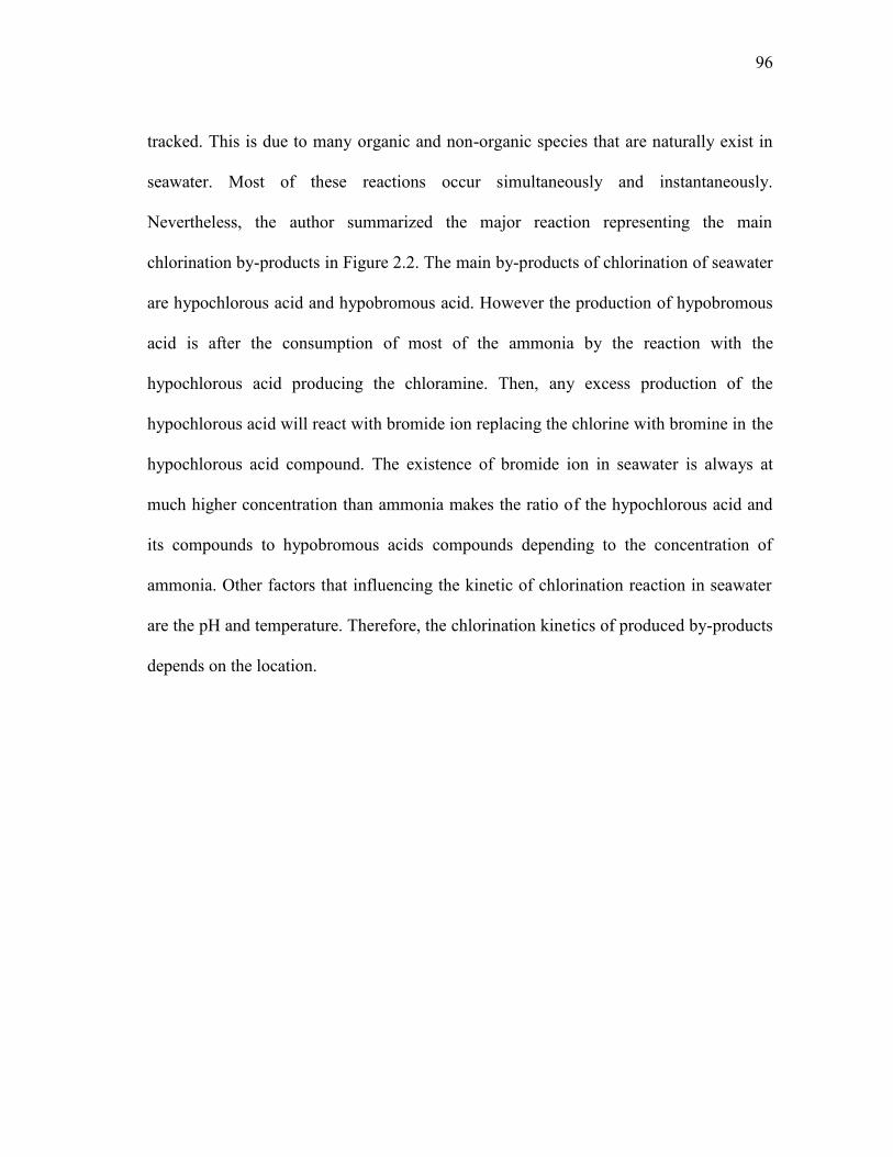
96
tracked. This is due to many organic and non-organic species that are naturally exist in
seawater. Most of these reactions occur simultaneously and instantaneously.
Nevertheless, the author summarized the major reaction representing the main
chlorination by-products in Figure 2.2. The main by-products of chlorination of seawater
are hypochlorous acid and hypobromous acid. However the production of hypobromous
acid is after the consumption of most of the ammonia by the reaction with the
hypochlorous acid producing the chloramine. Then, any excess production of the
hypochlorous acid will react with bromide ion replacing the chlorine with bromine in the
hypochlorous acid compound. The existence of bromide ion in seawater is always at
much higher concentration than ammonia makes the ratio of the hypochlorous acid and
its compounds to hypobromous acids compounds depending to the concentration of
ammonia. Other factors that influencing the kinetic of chlorination reaction in seawater
are the pH and temperature. Therefore, the chlorination kinetics of produced by-products
depends on the location.

97
3. PROBLEM STATEMENT
Consider an industrial facility which uses seawater for cooling. The
characteristics of seawater vary throughout the year leading to dynamic variations in the
growth of biofilms on the surfaces of the heat exchangers. Biofilm growth is controlled
through the use of biocide and regular maintenance. It is desired to identify an optimal
scheduling policy for the use of biocide and heat-exchange maintenance to minimize the
cost while accounting for the technical performance of the plant and the environmental
discharge of the biocide and its byproducts.
The aforementioned problem statement entails several challenges to be addressed
including:
How should the biocide dosages be varied during the year?
How does the biocide react and decay in the dosing basin and throughout
the process?
How is the biofilm growth in several exchangers related to biocide usage,
reactions, and the characteristics of the process and the seawater?
How to account for the heat-exchanger performance throughout the
process as a function of the time?
When is maintenance necessary?
How to meet the environmental regulations on the discharge of the
biocide and its byproducts throughout the year?
The following systems will be addressed in the ensuing sections:

98
Industrial plants with seasonal variation in seawater temperature
Integrated power plants and thermal desalination facilities
Processing facilities with solar-driven biocide manufacturing

99
4. DEVELOPMENT OF A SHORTCUT PROCESS-INTEGRATION APPROACH
TO THE OPTIMIZATION OF SEAWATER COOLING SYSTEMS WITH
ECONOMIC AND ENVIRONMENTAL CONSIDERATIONS
4.1. OVERVIEW
The aim of this section is to develop a systematic approach to the optimal
operating and design alternatives for integrated seawater cooling systems in industrial
facilities. A shortcut process-integration framework is used to provide a holistic
approach to optimizing the design and operation of the seawater cooling system, along
with the dosage and discharge systems. Optimization formulations are employed to
systematize the decision-making and to reconcile the various economic, technical, and
environmental aspects of the problem. Building blocks of the approach include the
biocide water chemistry and kinetics, process cooling requirements, dosage scenarios
and dynamic profiles, biofilmgrowth, seawater discharge and environmental regulations.
4.2. PROBLEM STATEMENT
The problem is that a given process which uses seawater in a once through
cooling system can experience fouling due to biofilm development in heat exchanger
tubes. In order to prevent biofouling in coolers, an antifouling agent (i.e., chlorine) is
added to the incoming seawater. A certain load of chemicals is added to the process
intake of seawater flow, FS.W.Intake . Currently, the process discharges a flow rate,
FS.W.Discharge of used seawater and a chemical concentration of CChemical
Discharge, leading to
a discharge laod of chemicals, L ChemicalDischarge. Due to environmental regulations, it is

100
desired to minimize the load of the discharged chemicals. Conventionally, the residual
biocide problem in the seawater used in the cooling system before the discharge is
solved by end-of-pipe treatment. This will solve the problem of excess residual chlorine,
but the question can be raised whether there is a more cost-effective solution.
Implementing the proposed holistic approach is one such solution. Figure 4.1
summarizes the problem statement and shows the conventional approach for biocide
treatment.
Figure 4.1. Diagram Summarizing the Problem Statement.
The objectives of this section are to:
Develop a systematic procedure for understanding the chemical and Use
shortcut input-output relations to represent the kinetics of biocide
usage and their reactions with different species in seawater.

101
Relate the formation of by-products to the characteristics of the seawater,
the biocide, and the process.
Identify the most effective by-product to control biofouling development.
Develop optimal policies for process modification and biocide dosing to
optimize biocide usage and discharge.
The ultimate goal is to develop a cost-effective procedure that integrates the process
resources, revises the process design and/or operation, and determines the optimal
scheduling of chemical dosage load and timing, along with implementing chemical
removal at the minimum number of heat exchanger cleaning cycles per year. This
approach might incorporate new technologies to meet the new regulations.
4.3. CHALLENGES AND SPECIFICATIONS OF THE PROPOSED
DESIGN
Applying the proposed approach has some challenges. The complexity of a
biocide reaction with different species that exist naturally in seawater is that it produces
different by-products. It is necessary to identify the most effective by-product in
controlling biofilm development. In the meantime, any hazardous compounds produced
throughout the cooling system until the discharge point must be monitored. Sometimes
there are regulations on the propagation of the compounds at a certain radius from the
discharge point. On the other hand, the usage of seawater is linked to the process
requirements, including cooling utilities. Therefore, any reduction in cooling
requirements will have a direct impact on the amount of seawater used and discharged,
along with the usage and discharge of biocide. In order to successfully achieve that

102
reduction in seawater and biocide, several design and operational changes must be made.
The last step is to consider new biocide removal units (e.g., dechlorination) as required
to meet the environmental regulations. These units have to be screened according to
techno-economic criteria. All of these challenges help to identify and allocate for the
development of an applicable integrated approach deal with interactive tasks while
aiming for the cost-effective solutions. The development of this approach and its
application will be explained in the following sections.
The proposed approach starts with understanding the chemistry of the biocide in
seawater and integrating it with the performance of the process. Also, we must try to
integrate process units and streams in order to reduce seawater usage and discharge
along with the usage and discharge of biocide and its by-products. Finally, if necessary,
the end-of-pipe treatment must be integrated with the in-process modification.
Specifically, this approach can be achieved by starting with the development of the
biocide kinetic models, then using the heat integration techniques as a tool to make the
most feasible possible reduction in cooling duty, and consequently on heating duties.
Any optimal changes on design and operating conditions must be made to reach that
approach. Then, based on the biocide kinetics and the optimal conditions for the biocide
to be effectively controlling biofouling, a model for biocide dosing must be constructed.
The biocide dosing amount and scheduling on different seasons must be identified. The
last step is always to use the appropriate load of end-of-pipe treatment as required to
meet the environmental regulations.
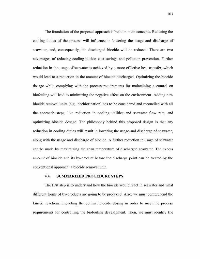
103
The foundation of the proposed approach is built on main concepts. Reducing the
cooling duties of the process will influence in lowering the usage and discharge of
seawater, and, consequently, the discharged biocide will be reduced. There are two
advantages of reducing cooling duties: cost-savings and pollution prevention. Further
reduction in the usage of seawater is achieved by a more effective heat transfer, which
would lead to a reduction in the amount of biocide discharged. Optimizing the biocide
dosage while complying with the process requirements for maintaining a control on
biofouling will lead to minimizing the negative effect on the environment. Adding new
biocide removal units (e.g., dechlorination) has to be considered and reconciled with all
the approach steps, like reduction in cooling utilities and seawater flow rate, and
optimizing biocide dosage. The philosophy behind this proposed design is that any
reduction in cooling duties will result in lowering the usage and discharge of seawater,
along with the usage and discharge of biocide. A further reduction in usage of seawater
can be made by maximizing the span temperature of discharged seawater. The excess
amount of biocide and its by-product before the discharge point can be treated by the
conventional approach: a biocide removal unit.
4.4. SUMMARIZED PROCEDURE STEPS
The first step is to understand how the biocide would react in seawater and what
different forms of by-products are going to be produced. Also, we must comprehend the
kinetic reactions impacting the optimal biocide dosing in order to meet the process
requirements for controlling the biofouling development. Then, we must identify the

104
most effective biocide by-product for controlling the biofilm and utilize that piece of
information in making any design and/or operational changes to satisfy the criteria.
The next step is to reduce the cooling duty of the process by using heat
integration instruments. Heat integration is carried out by using a graphical thermal
pinch analysis, algebraic techniques, or optimization formulations (e.g., (Smith 2005; El-
Halwagi 2006; Kemp 2007)). The objective of this step is to minimize cooling and
heating utilities of the process. The biocide dosage is proportional to the cooling duty.
As such, reducing the cooling utility of the process leads to reducing the usage and
discharge of the biocide. The rationale behind starting with heat integration is that it will
generate a cost savings from the reduction of cooling utilities. Heat integration is the
synthesis between process streams to feasibly exchange heat between hot process
streams and cold process streams. Thus, the outsources for heat and cooling are reduced.
This approach is superior to the end-of-pipe treatment because it does not start with
investment in biocide removal units without considering other options for running the
process at optimal design and operating conditions. Therefore, heat integration creates an
economic advantage by the savings made from fewer dependents on the outside source
of heating and cooling. At the same time, this is a more environmentally-friendly
process. The heat integration thermal pinch analysis will define the minimum amount
heating and cooling duties that can be achieved. Those amounts will be the targets that
are required for feasibly implementing the heat exchangers’ retrofitting using the
synthesis of the heat exchanger network and the process’ hot and cold streams. Using the
synthesis of the heat exchanger network to perform the retrofitting for the process hot

105
and cold streams. Normally, an inspection technique is preformed to find the best match
between the process streams to meet the minimum heating and cooling duties. Then, all
of the annualized cost data are calculated for the new required units to implement the
heat exchanger synthesis that will meet the minimum heating and cooling utilities. How
much was saved from introducing the new unit as a reduction of heating and cooling
utilities out of that match can also be calculated. Then, the return on investment (ROI) of
the proposed new unit can be calculated and compared with the ROI of the company.
Then, the decision of installing the new unit will be made based on the ROI policy of the
company. Accordingly, the reduced seawater flow rate can be calculated.
The next step is to make a further reduction in seawater flow rate by enhancing
the efficiency of seawater utilization. The least complicated technique to reach that
reduction is to maximize the discharged seawater temperature while complying with the
environmental thermal pollution regulations. Then, the new seawater flow rate from the
heat balance equation can be calculated after the reduction has been made from
increasing the discharged temperature. After the reduction has been achieved in the
seawater flow rate, the revised calculation can be performed by recalculating the reduced
amount of biocide required for the seawater flow rate. The following step is to optimize
the dosage of biocide, while meeting the requirements of the process of the minimum
residual biocide remains in the cooling system to insure the control over any biofouling
development. At the same time, reducing the amount of biocide and its by-products that
are discharged back to the seawater saves the aquatic live. The optimal biocide dosage is
chosen based on mathematical model incorporating the knowledge of biocide chemistry
106
in seawater and utilizing the lab data of the biocide kinetics inside the used seawater
because seawater characterization is based on the location. On top of that, the effect of
biocide on bioflim development changes seasonally. This is one of the factors that need
to be considered in modeling the biocide dosages to reach the optimal biocide -dosing
scheme. In order to keep the heat exchangers effectively operating at their optimal
conditions, the maintenance schedule for cleaning needs to be considered in the
evaluation of biocide dosing amount and scheduling.
The previous steps generate cost savings while reducing the biocide usage and
discharge. If the environmental target has not been achieved through all of the previous
steps, end-of-pipe treatment can be used to reach that target. For instance, biocide
removal units (e.g., dechlorination devices) are added to treat the seawater leaving the
plant and to reduce the biocide load prior to environmental discharge. When there are
multiple end-of-pipe alternatives, they should be screened in order to select the cheapest
alternative. The economic driver for scheduling the biocide dosages should also consider
the cost of removing any excess amount of biocide before discharging. Therefore, the
solution should have the most effective cost, including the cost of removing the excess
biocide and cleaning the heat exchangers. The proposed flowchart is shown by Figure
4.2.

107
Figure 4.2. A Flowchart Summarizing the Proposed Procedure Steps.
4.5. BIOCIDE CHEMISTRY
It is necessary to develop a mechanistic model for the reaction pathways
involving the biocide and the various species in the seawater. First of all, start with the
reaction of chlorine when it is added to seawater as a gas or solution of a chlorine
compound (e.g., sodium hypochlorite). Chlorine will dissolve and hydrolyze rapidly
(almost instantaneous) and completely to HOCl (hypochlorous) acid with a reaction rate
constant of 5X10¹⁴. When chlorine is added to seawater, it produces hypochlorous acid

108
and hydrochloric acid, HCl. The latter is a relatively strong acid, and it will dissociate
completely to a hydrogen ion and a chloride ion, while hydrochlorous acid, HOCl, is a
relatively weaker acid, and it will dissociate slightly to a hydrogen ion and a
hypochlorite OCl-. Since the hydrogen ion appears in this reaction, this equilibrium is pH
dependent. The distribution of the various species (HOCl, OCl-) at equilibrium is a
function of pH. Hypochlorous acid is the most germicidal species, but it is a weak acid
that will dissociate to hydrogen and hypochlorite ions with pKa of 7.5 at 30oC, as shown
in Figure 4.3:
Figure 4.3. Variation of Chlorine Distribution in Seawater with pH (Based onOldfield and Todd, 1981).
Cl2+H2OHOCl + HCl Equation 4.1
V a r ia t io n o f C h lo r in e D is t r ib u t io n in S e a w a t e r w it h p H : a f t e rO ld f ie ld a n d T o d d ( 1 9 8 1 )
-2 0
0
2 0
4 0
6 0
8 0
1 0 0
1 2 0
0 2 4 6 8 1 0 1 2
S e a w a te r p H
Sp
ec
ies
Dis
trib
uti
on
%
H C lOC l2C lO -

109
HOClH++ OCl- Equation 4.2
In terms of disinfection effectiveness, hypochlorous acid is much stronger
(almost two orders of magnitude) than the hypochlorite ion. Hypochlorous acid will
reach its maximum concentration at pH ranges between 4 and 6 (Hostgaard-Jensen,
Klitgaard et al. 1977). However, the effectiveness of a chemical species as a disinfectant
does not necessary correlate with its effectiveness in removing biofilms. Weakening the
polysaccharide matrix of microbial cells is one way to control the development of
biofilms on the tube surface of heat exchangers. There is experimental evidence that
shows that chlorination is more effective in causing biofilm detachment at pH values
greater than pH 8, where OCl- concentration is more dominant than HOCl (Characklis
W. G. 1979). Naturally, seawater contains organic and nonorganic species.
Of particular importance are ammonia and bromide species. Their concentrations
are varied depending on the nature of the water. For instance, seawater contains bromide
with concentrations as high as 65 mg/l, but it will go as low as a negligible amount in
fresh waters. Ammonia concentrations depend on pollutants of the water. In highly
polluted water, ammonia concentration is as high as 15 ppm, while in unpolluted water
the concentration is lower than 0.05 mg/l. At full strength salinity, seawater ammonia
concentration ranges between 0.001 and 1.0 ppm. Ammonia, as well as other reactive
nitrogenous compounds, will be chlorinated to yield monochloramine (NH 2Cl), and will
react further to produce dichloramine (NHCl2). In freshwater, and a very traceable
amount in seawater, dichloramine will react further with hypochlorous acid, producing
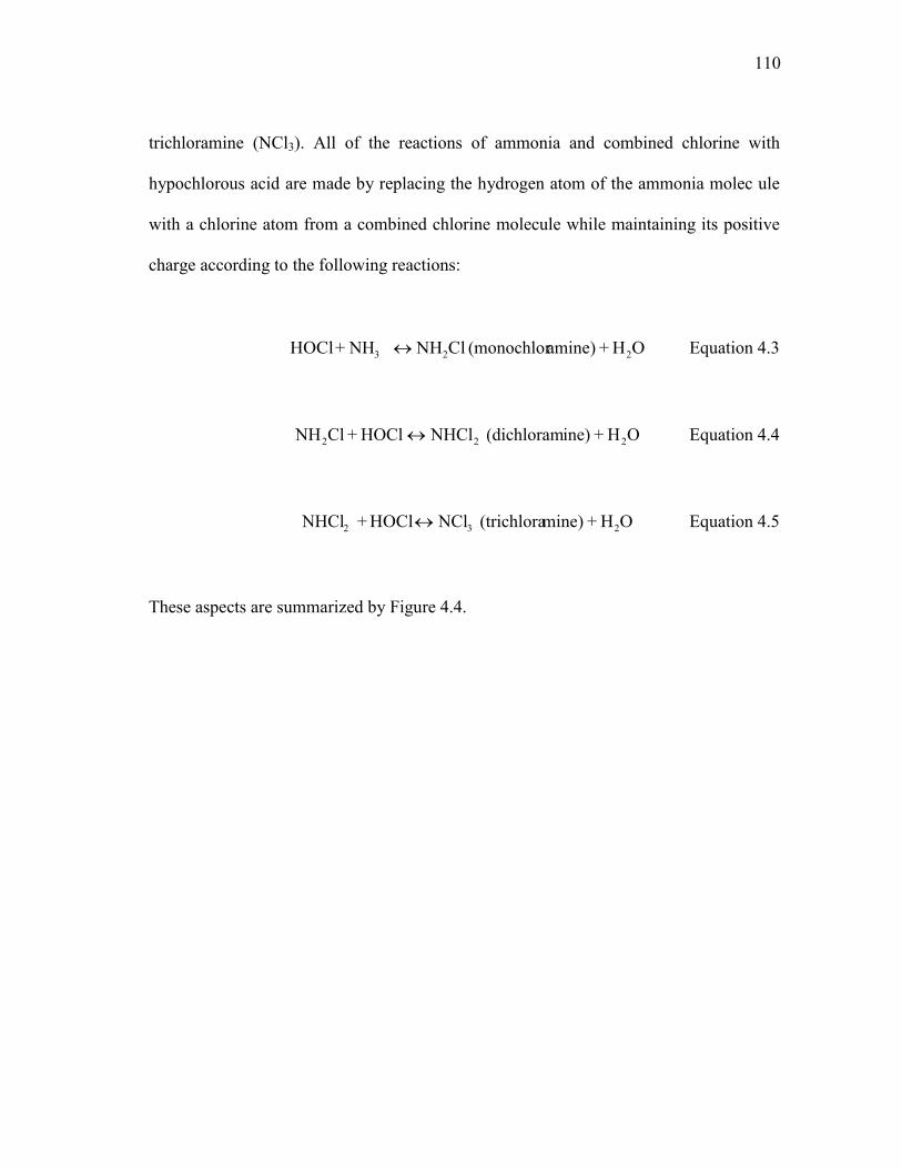
110
trichloramine (NCl3). All of the reactions of ammonia and combined chlorine with
hypochlorous acid are made by replacing the hydrogen atom of the ammonia molec ule
with a chlorine atom from a combined chlorine molecule while maintaining its positive
charge according to the following reactions:
HOCl+ NH3 NH2Cl (monochloramine) + H2O Equation 4.3
NH2Cl + HOCl NHCl2 (dichloramine) + H2O Equation 4.4
NHCl2 + HOClNCl3 (trichloramine) + H2O Equation 4.5
These aspects are summarized by Figure 4.4.

111
Br-
Con
c.
Negligible
65 mg/lFull
strengthseawater
Freshwater (0.1-2.0) ppm
NH
3C
onc.
(< 0.001-1.0) ppm
Pollutedwater
Unpollutedwater < 0.05 mg/l
15 ppm
Br- & NH3 Conc.
Figure 4.4. Concentrations of Bromide and Ammonia in Natural Water

112
These reactions depend on pH, temperature and contact time, but mainly on the
chlorine to ammonia ratio. All of the free chlorine (hypochlorous acid) will be converted
to monochloramine at pH 7-8 (the fastest conversion is at pH 8.3) when there is 1:1
molar ratio of chlorine to ammonia (5:1 by weight) or less. Then, within the same range
of pH, dichloramine is produced at a molar ratio of 2:1 of chlorine to ammonia (10:1 by
wt.). This reaction is relatively slow, so it may take up to an hour. Also, within t he same
range of pH, trichloramine will be produced at a molar ratio of 3:1 of chlorine to
ammonia (15:1 by wt.) and at equal molar ratios, but at pH 5 or less. The two reactions
producing di- and tri-chloramine are known as the breakpoint reactions where the
chloramines are reduced suddenly to the lowest level. The significance of the breakpoint
reaction is that chlorine reaches its highest concentration and germicidal efficiency (at
1:1 molar ratio of chlorine to ammonia) just before reaching this point. Also, at the
breakpoint, monochloramine and dichloramine react together (which reduces chlorine
residuals) to produce nitrogen gas, nitrate, and trichloramine. Dichloramine decomposes
to an intermediate reactive product (NOH) which consumes mono-, di-chloramine, and
hypochlorous acid, producing nitrogen gas and nitrate. Also, excessive chlorine will
form trichloramine. These processes are shown in the following equations:
NHCl 2 + H 2 O NOH + 2 H + 2 Cl- Equation 4.6
NOH+ NH2Cl N2 + H2O + H+ + Cl- Equation 4.7

113
NOH + NHCl2 N2 + HOCl + H + Cl - Equation 4.8
NOH+ 2 HOClNO3- +3H+ + 2 Cl- Equation 4.9
NCl3 + H2O NHCl2 + HOCl Equation 4.10
The reaction of chlorine into these forms steers it away from the disinfection
function and renders the biocide less effective. Consequently, it is important to
understand such side reactions. Hypochlorous acid rapidly reacts with bromide,
producing hypobromous acid, which can also be produced from the reaction of bromide
with monochloramine, as follows:
HOCl Br - HOBr Cl - Equation 4.11
NH2 Cl + Br- + H2O HOBr+ Cl- + NH3 Equation 4.12
where HOBr is hypobromous acid. Additionally, the hypochlorite ion may undergo a
slow reaction with the bromide ion, as follows:
OCl - Br - OBr - Cl - Equation 4.13

114
where OBr- is the hypobromite ion. Bromide in seawater may also react directly with
added chlorine to give bromine and chloride:
Cl2 2Br- Br2 2Cl- Equation 4.14
It is worth noting that the presence of ammonia and other nitrogenous
compounds in the seawater will react with HOBr to yield monobromamine (NH2Br),
dibromamine (NHBr2), and tribromamine (NBr3):
HOBr + NH3 NH2 Br (monobromamine) + H2O Equation 4.15
HOBr + NH2 Br NHBr2 (dibromamine) + H2O Equation 4.16
HOBr+ NHBr2 NBr3 (tribromamine) + H2O Equation 4.17

115
The bromine breakpoint happens when the dibromamines are produced rapidly,
leading to the formation of nitrogen gas:
NHBr2 + H2O NOH + 2H+ 2 Br- Equation 4.18
NOH + NHBr2 N2 + HOBr + H+ + Br- Equation 4.19
It is also important to consider the effect of the bromide that naturally exists in
seawater at (50–70 mg/l). Bromide is typically in stoichiometric excess over the chlorine
dosage, whereas ammonia concentration doesn’t exceed 2 to 3 mg/L. The relative
amount of bromine species to ammonia species produced is proportional to bromide
concentration over ammonia concentration if we assume both reactions are rapid and
simultaneous. In order to understand the various species interactions and reaction
pathways, we have constructed the reaction mechanism shown in Figure 4.5. On these
diagrams, the starting species and intermediate and final by-products are represented in
boxes. The arrows correspond to reaction steps, and the boxes on the arrows represent
the reactive species that contribute to that reaction.

116
Figure 4.5. Summarizes the Reaction Mechanism of Chlorine in Seawater.
Cl2,NaOCl
HOCl+Br- HOBr+Cl-
Br-
Cl2+H2O
HOCl+HCl
Deman
d
Br- + CO2 +Bromo-organics
HOBr+Deman
dBr-+
?
Hydrolysis
NH2Cl
HOCl
NH
3+H
OC
lN
H2C
l+H
2O
NH
3
NH
Cl2+
HO
Cl
NC
l3+H
2ON
H2C
l+H
OC
lN
HC
l2+H
2O
NHCl2
NCl3(Freshwater only)
HO
Cl
HO
Cl
Demand
Cl- + CO2 +Chloro-organics
HO
Cl+
Dem
and
Cl-+
?
NH3 + Cl- + CO2 +Chloro-organics
NH2C
l+De
man
dNH
3+Cl
-+?
NCl3+
Dem
and
NH3+
3Cl-+
?
Demand
Dem
and
(N2
+C
l-+
HO
Cl)
Brea
kpoi
nt
HOBrN
H3+
HO
Br
NH
2Br+
H2O
NH2Br
NBr3
NHBr2
NH
2Br+
HO
Br
NH
Br2
+H2O
NH
Br2
+HO
Br
NB
r3+H
2O
NH
3H
OB
rH
OB
r
Demand
NH3 + Br- + CO2 +Bromo-organics
Demand
Dem
and
NH2Br+DemandNH3+Br-+?
NHBr2+DemandNH3+2Br-+?
NBr3
+Dem
and
NH3+
3Br-+
?
(N2
+B
r-+
HO
Br)
Bre
akpo
int
NH2Cl+Br-+H
2ONH
3+HOBr+Cl-
Br-
117
4.6. OBJECTIVE FUNCTION FOR OPTIMUM DOSAGE
Based on the proposed holistic approach, all scenarios from the chemical dosing
of treatment and post-treatment, and all of the costs incurred from heating loss due to
fouling and heat exchanger cleaning, have to be incorporated in the decision for any
design or operation changes. The objective function is built on the economic criterion. It
will permit the most feasible solution that would also cost the least to operate the plant.
This approach might allow for biofilm growth and removal by periodic heat exchanger
cleaning at the minimum overall operating cost. On top of that, there are a variety of
options for chemical dosing. For each dosing course, the response of biofouling
development will vary accordingly. Thus, there will be an impact on the other operating
costs. Also, the nitration and the ambient temperature variations through different
seasons of the year will govern the microorganisms’ behavior inside the cooling system.
All of the different aspects have to be integrated to make one plan that considers the
impact on all of the related design and operation changes. The dynamics of the process
itself will add difficulty to selecting the optimal scenario among the options.
The objective function is to minimize the annual total cost that is incurred
directly and indirectly from fouling. It will include the annual operating cost of
chemicals (chlorine) used to treat the cooling water against biofouling, the annual fixed
and operating costs of removing chemical residuals from the effluent water, the cost of
cleaning heat exchanger units, the cost of the loss incurred by biofouling, and the annual
gross profit loss from shutting down the operation for cleaning the heat exchangers:

118
Annual Total Cost = Operating Cost of Chemicals to Treat the Water +
Annualized Fixed and Operating Costs of Chemicals for Removing Residuals +
Annual Heat Exchanger Cleaning Cost +
Cost of Heat Loss Due to Fouling +
Gross Profit Loss Due to Shutting Down the Process for Heat Exchanger
Cleaning
AnnualTotalCost ChemCost Chem RemovCost HxgCleaningCost HeatLossCost
Gross ProfitLoss Equation 4.20
dayLV
: is the volumetric flow rate of water
yrcyltCyl
: is the number of cleaning cycles per year
cyldaytOpr
: is the number of days that the process operates per cleaning cycle
yrcylt
cyldayt cylOpr
: is the number operating days per year, excluding the shutting
down for cleaning heat exchangers

119
ChemCost: is the annual operating cost of chemicals for treating the water
yrcylt
cyldayt
mgCost
dayLV
LmgCChemCost cylOprChCh
$
Equation 4.21
LmgCCh
: is the chemical residual concentration
mg
CostCh$
: is the cost of chemicals used
movCostChem Re : is the total annualized cost for removing residuals
yrcylt
cyldayt
mgCost
dayLV
LmgLmg
CC
LmgC
YrostAnnualFixC
movCostChem
cylOprChRmChRs
ChRmChRs *
$//$
Re
Equation 4.22
YrostAnnualFixC $
: is the annualized fixed cost for removing the residuals

120
LmgCChRs
: is the concentration of residuals
Lmg
LmgCC
ChRs
ChRm
//
: is the ratio of adding chemicals for removing residuals
mg
CostChRm$
: is the cost of chemicals to remove the residuals
: is the cost for cleaning heat exchangers per cycle
Yrcylt
cylHxggCostHxgCleanin cylC
$ln
Equation 4.23
stHeatLossCo : is the cost of the lost heating due to fouling in heat exchangers
yrcylt
cyldayt
KJHtCst
daySec
KWSecKJKWQKWQ
stHeatLossCo
cylOprFldC$86400/
ln
Equation 4.24
KWQKWQ FldC &ln : is the heat transfer rate for clean and fouled heat exchangers,
respectively.
gCostHxgCleanin

121
The heat transfer rate would be decreasing from KWQC ln to KWQFld as the
biofilm is accumulating.
KJHtCst $
: is the cost of heating
Gross profit is the revenue or sales after deducting all directed costs like
manufacturing expenses, feed, labor, and selling/marketing expenses. The gross profit
loss is how much of the gross profit would have been generated if the production had not
been stopped for heat changer cleaning. The daily gross profit (DGPft) can be calculated
by taking the revenue of a company over a period of time, with no shutdown in
production, and dividing it by the number of days of that period:
yrcylt
cyldayt
dayDGPftofitLossGross cylopr
$PrEquation 4.25
The relationship between the chemical added to the influence on how it controls
the fouling can be shown in the following model. The biofilm thickness is a function of
chemical concentration and scheduled dosage:
Dsgd
d
ttt eeXX Pr
Pr 0 Equation 4.26
where dtXPr : is the biofilm thickness at the end of the period

122
0X : is the initial biofilm thickness
: is the biofilm growth rate constant
: is the biofilm destruction rate constant
Dsgt: is chemical dosage schedule in hours per day
The biofilm growth rate constant, , can be calculated on the plant itself by
letting the biofilm grow for some time with no chemical added to control it. Then, a
graph is generated for the biofilm thickness versus time in days. By using regression
analysis, the growth rate can be calculated from the exponential kinetic growth. This
kind of experiment can be repeated at different months/seasons to generate at each
month/season.
The biofilm destruction rate constant, , is based on the relationship between the
kinetic of biofilm destruction by chemicals and disinfection kinetics of suspended
bacterial systems. Then, a graph is constructed to show different disinfection rate
constants, K , for bacteria that dies off versus different chemical concentration CCh
dosages. The mathematical relation, which can be linear, that represents the relationship
between the rate constants with chemical concentration is:
bCa Ch Equation 4.27

123
The disinfection rate constant, K, has to be c alibrated by , which can be
determined by dosing the plant that is going to use this model with a certain chemical
concentration for one hour per day and developing a graph from the data collected to
represent the biofilm thickness versus time in days. By using a regression analysis for
the curve, the destruction rate constant can be determined. From the disinfection rate
constant K and destruction rate constant at the same dosage, can be calculated as
follows:
Equation 4.28
The chemical residual concentration, C ChRs , at the effluent before discharge or
treatment can be determined by developing a kinetic model of the process. The
consumption of chemicals is due to the reaction with organic and nonorganic
compounds, biofilm, and corrosion. The chemical decay in kinetics in a batch cooling
system (Xin et al. 2003) may be described as follows:
CKrW
rCK
dtdC
bhh
WW
Op
Ch
Equation 4.29
Based on examining numerous experimental results for the kinetics of seawater
treated with a chemical (i.e. chlorine), decay kinetics have been correlated to several
factors, including temperature, pH, and contact time, but mainly on the ratio of chlorine

124
dosage to ammonia (Haag 1981). The reduction or decay of chlorine in seawater is due
to reactions with organic and nonorganic compounds in seawater. The chlorine decay
occurs in three stages, starting with a very fast rate during the first the two minutes, due
to a reaction with inorganic reducing agents. The second phase is slower and usually
does not last more than two hours. It mainly involves reactions with the organic
compounds that started in the first phase. Then, chlorine decays continuously via a very
slow rate.
Of particular importance is the dependence on residence time and temperature.
Given the specific path of seawater inside the process, the following model is developed
to account for chlorine decay throughout the process. The seawater goes through a
number of pipes and units. The process is discretized into a number of segments. Each
segment, i, represents a portion of the seawater pipeline or a heat exchanger (e.g., cooler,
coil in a hot unit, cooling jacket of a unit, etc.). Consider the N key species and refer to
their concentrations in segment i as: Nijiii CCCC ,,2,1, ,...,,...,, . For the jth species, in the ith
segment, the following kinetic expression may be written as:
iiNijiiijji pHTCCCCC ,,,...,,...,, ,,2,1,,1 Equation 4.30
Figure 4.6. shows the typical once-through cooling using seawater and treating
the influent and effluent with chemicals.

125
Figure 4.6. Typical Once-Through Cooling Using Seawater and Treatment.
4.7. CASE STUDY
Consider a Urea process described by Bin Mahfouz (2006). The current usage of
a seawater cooling utility is 89.2 MM Btu/hr and it employs a continuous dosage of 0.75
mg/L. For maintaining the appropriate biocide effect, the residual chlorine should be
kept at levels higher than 0.05 mg/L throughout the system. By carrying out heat
integration, the cooling utility is reduced to 77.1 MM Btu/hr, which corresponds to about
14% reduction in the biocide usage. Next, shortcut kinetic modeling is used to track the
biocide and its key reaction by-products. The experimental data of Ben Waren (2006) of
residual chlorine at different chlorine dosages at 25oC are used to develop the following
simplified dynamic decay functions for the three continuous dosages (1.0, 5.0, and 10
mg/L, respectively) as:

126
)*0015.(1 *42.0 toeC Equation 4.31
)*00004.(2 *80.3 toeC Equation 4.32
)*00003.(3 *55.8 toeC Equation 4.33
where C is chlorine concentration in mg/L and t is the residence time in minutes. A
regression analysis was carried out with the experimental data for a residence time of 20
minutes for the case study. A linear expression was derived to relate the residual chlorine
(Cout) to the chlorine dosage (Cin) through:
52.0*9.0 ChChRs CC Equation 4.34
In order to maintain 0.05 mg/l concentration of residual chlorine at the discharge,
we need a dosage concentration of no more than 0.63 mg/L, which provides 19%
reduction in biocide usage from the current practice, which is 0.78 mg/L (in addition to
the 14% reduction in biocide load already achieved via heat integration.

127
5. OPTIMAL SCHEDULING OF BIOCIDE DOSING FOR SEAWATER-
COOLED POWER AND DESALINATION PLANTS
5.1. OVERVIEW
Thermal desalination systems are typically integrated with power plants to
exploit the excess heat resulting from the power generation units. Using seawater in
cooling the power plant and the desalination system is a common practice in many parts
of the world where there is a shortage of freshwater. Biofouling is one of the major
problems associated with the usage of seawater in cooling systems. Because of the
dynamic variation in the power and water demands as well as the changes in the
characteristics of seawater and the process, there is a need to develop an optimal policy
for scheduling biocide usage and cleaning maintenance of the heat exchangers.
The objective of this paper is to introduce a systematic procedure for the
optimization of scheduling the dosing of biocide and dechlorination chemicals as well as
cleaning maintenance for a power production/thermal desalination plant. A multi -period
optimization formulation is developed and solved to determine:
The optimal levels of dosing and dechlorination chemicals
The timing of maintenance to clean the heat-exchange surfaces
The dynamic dependence of the biofilm growth on the applied doses, the
seawater-biocide chemistry, the process conditions, and seawater
characteristics for each time period.

128
The technical, economic, and environmental considerations of the system are accounted
for. A case study is solved to elucidate the applicability of the developed optimization
approach.
5.2. INTRODUCTION
In many regions that lack freshwater, it is common to integrate power production
and desalination whereby the exhaust steam from the power-generation turbines is used
to drive thermal-desalination systems (Lijesen, 2007). These cooling duties of the
power-desalination processes are usually provided by seawater cooling. The cooling
duties vary seasonally depending on the need for power and desalinated water. Such
variations determine the various flow rates of seawater required for the cooling system at
throughout the year. As a result of using seawater for cooling, biofilms grow on the heat-
transfer areas of the process heat exchangers (de Beer et al., 2006). Such growth is
impacted by the varying temperature of the seawater and the process and the
characteristics of the seawater The biofilm negatively affects the performance of the heat
exchangers as it lowers the overall heat transfer coefficient. Therefore, the incoming
seawater is typically treated with a biocide to control the growth of the biofilm. The
extent of biocide dosage should be tied to the seawater characteristics, the cooling tasks,
and the need to maintain the level of biocide and biocide byproducts within an
environmentally acceptable level prior to discharge back into the sea.
This paper is aimed at identifying optimal scheduling policies for the timing and
dosing levels of biocides used for seawater cooling of power and desalination plants.
The time-based variations in the characteristics of the seawater, the process, and the

129
demands for power and desalinated water are addressed in the optimization scheme.
Seasonal maintenance is also considered in the optimization framework. The technical,
economic, and environmental considerations are accounted for and traded off.
Seawater stimulates the growth of aquatic species that are attached to solid
surfaces by using planktonic larvae for spreading and growing films that causing fouling
of heat-exchanger surfaces. Electric power plants require the usage of large amounts of
water to run electric turbines by steam. Accumulating slime on condenser tubes consists
of planktonic of young barnacles and mussels (Jenner et al., 1998). The large area of
pipelines inside heat exchangers makes it a good environment for bacteria to attach and
grow. Biofilm consists of single or multiple species of microorganisms, organic, and
inorganic solids distributed heterogeneously on the attached surface (Characklis et al.,
1983; Characklis et al., 1982). The development of biofilm depends on nutrients and the
oxygen content of the water, as well as the cell metabolism. Fouling of heat exchangers
at power plants can be referred to as trash, biological microfouling, biological
macrofouling, siltation, and scaling. Other factors that influence biofilm developm ent
are the physical conditions of the seawater flowing in the cooling system such as water
flow and temperature, and the nature of the surface of the tube (Sriyutha Murthy et al.,
2004). Some of the problems that are caused by biofouling in the cooling systems are:
1) Increased rate of corrosion of the tubes by creating a potential charge
difference across the surface.
2) Increased heat transfer resistance due to fouling.

130
3) Increased friction resistance of the seawater flow by changing the tube
surface’s roughness when the biofilm thickness is higher than the
monolayer and consequently the flow rate of seawater is reduced (Cloete
et al., 1998).
Controlling the growth of biofilm in industrial cooling systems can be achieved by using
chemical treatment that is primarily intended to:
1) Reduce the number of microbes by using biocides
2) Remove microbes by using:
• Oxidizing biocides (e.g. chlorine) by weakening biofilms.
• Synthetic dispersants
• Enzymes
Biocides, also called antimicrobial agents, aim to reduce the growth of microbes. There
are two types of biocides:
1) Antibiotics which are formed from the prokaryotic organisms
2) Antiseptics, disinfectants, sanitizers or biocides which do not naturally
exist
Biocides are commonly used in controlling biofilm development. It is important to
consider these essential aspects in treating seawater with a biocide:
1) Identify the type of organisms in the seawater
2) Use the right biocide or combination of biocides
3) Determine the required concentration of biocide and dosing scenarios
4) Observe the growth of the microorganisms and their attachment

131
5) Determine the contact time required for killing the bacteria
Biocides act by putting the components in the bacterial cells under stress to hinder their
functionality.
Chlorine and chlorinated compounds are typically used as biocides. Chlorine is
very toxic and human exposure for more than an hour to chlorine fumes with
concentration as 4 ppm or higher can cause respiratory problems. Chlorine can be
generated by:
Electrolysis of saline water, typically sodium chloride, to produce
chlorine gas
Salt process which causes the reaction between sodium chloride and nitric
acid
)()(3)(3)( gSss HClNaNOHNONaCl Equation 5.1
Oxidation of hydrochloric acid
Electrolysis of hydrochloric acid solutions.
Chlorine in pure water will hydrolyze immediately and completely to form
hypochlorous acid (HOCl) and hydrochloric acid (HCl) (Bin Mahfouz, 2010).
HClHOClOHCl 22 Equation 5.2

132
OClHHCl Equation 5.3
The hydrochloric acid is a strong acid that will dissociate into chlorine and
hydrogen ions. Whereas, hypochlorous acid is a relatively weaker acid that will
dissociate slightly into hydrogen and hypochlorous ions. The concentration distribution
of hypochlorite ions and hypochlorous acid at equilibrium is pH dependent. Chlorine
demand is the difference between the amount of chlorine added and the available
chlorine, either as free or combined chlorine. The consumed chlorine is due to the
oxidation or substitution reactions with organic and inorganic species like: H2S, Fe2+,
Mn2+, NH3, phenols, amino acids, proteins, and carbohydrates. After the amount of
chlorine has been consumed according to the demand, the rest will be available for
oxidation to treat the water. The available chlorine is computed from a half-cell reaction
of reducing chlorine gas (Cl2) to a chloride ion by consuming two electrons. Only a half
mole of chlorine gas will dissociate, forming one mole of chloride ion.
eHHOClOHCl 2222 22 Equation 5.4
In saline waters, bromide which exists naturally at a much higher concentration
(about 65 ppm) and ammonia will compete to react with hypochlorous acid.
Chloramines are formed from the reaction of hypochlorous acid with ammonia, forming
monochloramine (NH2Cl), dichloramine (NHCl2), and trichloramine, which is also

133
called nitrogen trichloride (NCl3). The formation of chloramines depends on water
temperature, pH, and the relative amount of chlorine added to the amount of ammonia
available prior to treatment. Typically, at higher pH (around 7 and above) there is a
higher formation of monochloramine (NH2Cl). Whereas, at lower pH (around 4 and
lower) the formation of trichloramine is higher (Bin Mahfouz et al., 2006).
OHClNHNHHOCl 223 Equation 5.5
OHClNHNHHOCl 223 Equation 5.6
OHNClNHNHCl 2332 Equation 5.7
The breakpoint reaction of chlorine is the reaction that satisfies the demand and
eliminates all the ammonia, including nitrogen-containing organic compounds, and
produces free available chlorine. The weight ratio of chlorine to be added to the
available ammonia nitrogen should be 8:1 or higher to ensure formation of free available
residual chlorine. These types of reactions have a higher rate at high pH (7-8) and at high
temperatures. The first immediate consumption of chlorine is made by the immediate
demand associated with non-nitrogenous compounds. Then, if there is enough chlorine,
the reaction with ammonia will form chloramines. After consumption of all of the
ammonia nitrogen, an extra amount of chlorine is added to form free available residual

134
chlorine. Hypochlorous acid reacts with bromide, producing hypobromous acid, by
replacing the chlorine atom with bromine. Hypobromous acid will react with ammonia
in the same way as hypochlorous acid, producing monobromamine (NH2Br),
dibromamine (NHBr2), and tribromamine, or nitrogen tribromide (NBr3).
ClHOBrBrHOCl Equation 5.8
OHBrNHNHHOBr 223 Equation 5.9
OHCBrNHNHHOBr 223 Equation 5.10
OHNBrNHNHBr 2332 Equation 5.11
Figure 5.1. is a schematic representation of the key reaction steps in the
chlorination of seawater. These reactions may happen concurrently, depending on
seawater characteristics (Bin Mahfouz et al., 2009). Monochloramine (NH2Cl) formation
will dominate over HOBr formation when bromide concentration is 65 ppm and
ammonia is above about 0.4 ppm. At higher concentrations of ammonia, NH2Cl will
dominate. On the other hand, in relatively uncontaminated seawater, the ammonia
concentration is very low and the bromide concentration is usually higher than the
chlorine dose, which results in a residual that consists mainly of HOBr. The most

135
important products of chlorine reaction with seawater are NH2Cl, HOBr, and the
bromamines (Lietzke et al., 1979).
Figure 5.1. The Primary Inorganic Reaction Pathways of Chlorine in SalineWaters.

136
Chlorine is typically added at a concentration of 1.0 ppm to control biological
growth in receiving water at the basin before entering the cooling system (Eppley et al.,
1976). Chlorination is the process of adding chlorine to the treated water to kill germs. It
is highly effective at pH ranges of 6.5–9.5. Using chlorine is widespread in the industry
because of its high reliability, low cost, and easy application. Addition of chlorine will
produce hypochlorous acid (HOCl), which has the disinfection effect on both bacteria
and viruses. Hypochlorous acid will react with all types of biological molecules because
it is non-selective. The existence of ammonia will reduce the effectiveness of the
chlorination process because ammonia will react with hypochlorous acid, producing
inorganic and organic chloramines. Hypochlorous acid aimed to control the growth of
biofilm but it also will attack the cell membrane of Escherichia coli, causing chemical
and physical changes of the porosity and leakage of macromolecules. Also, the residual
chlorine can be simply measured to assess the required concentration of the dosing to
avoid excessive dosing and regrowth of the bacteria. A concentration of residual chlorine
is as low as 1.5 mg/l can allow bacterial regrowth. The negative aspects of chlorine are
that its major byproducts (such as HOBr, chloramines and bromamines) can react with
organic substances, such as humic acid and fulvine acid, that naturally exists in seawater,
producing organohalogenated, hazardous, compounds such as chloroform, and
trihalomethanes. Increase in seawater temperature will inhibit carbon uptake, which will
consequently stimulate the development of biofilms. But if the temperature gets too high,
it will decrease microbial activity and eventually kill the microbes. On the other hand,
microbes can be destroyed by chlorination. The physiological activities of the algae
137
population are increased during the summer (Morgan et al., 1969). The most accurate
and sensitive method to measure the chlorine residual is the amperometric method. The
potentiometric method is rapid and sensitive to be used in automated and in-line
observations (Eppley et al., 1976). Intermittent chlorine dosing was used in plate heat
exchangers at the Ocean Thermal Energy Conversion power plant on the east coast of
India. This intermittent chlorine dosing at a residual concentration of 1.2 ppm showed a
significant reduction in biofilm thickness, bacterial density, and diversity (Macdonald et
al., 2008). When the primary problem of fouling is slime formation or microfouling, the
intermittent dosing of chlorine has been the most commonly used technique to fix it.
But if macrofouling is the main problem, then continuous dosing of chlorine
proves to be more effective (Jenner et al., 1998). Another technique of chlorine addition
includes a pulsed dosing, which has proven to give better results in controlling
biofouling with a 36% reduction in the mass of chlorine applied. An example of this
kind of result was shown in a 10 month operation at Qatargas, the first major liquefied
natural gas (LNG) company located in Doha, Qatar. The pulsing of chlorine dosing
resulted in reducing the power consumption, as well as operational and maintenance
costs. It also improved the discharged seawater quality by reducing chlorination by-
products. In 2005, the Qatari Ministry of the Environment lowered the allowable
discharge concentration of free residual halogen from 0.1 to 0.05 mg/l. The
environmental agencies’ regulations for the biocide residual concentration discharge will
add complexity to the industrial development in reducing the environmental footprint of
cooling seawater systems. End- of-pipe treatment can be used to protect the environment
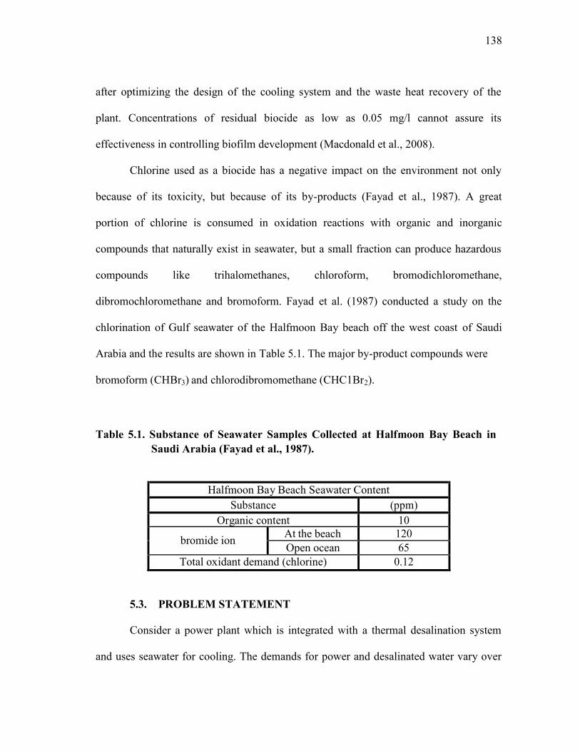
138
after optimizing the design of the cooling system and the waste heat recovery of the
plant. Concentrations of residual biocide as low as 0.05 mg/l cannot assure its
effectiveness in controlling biofilm development (Macdonald et al., 2008).
Chlorine used as a biocide has a negative impact on the environment not only
because of its toxicity, but because of its by-products (Fayad et al., 1987). A great
portion of chlorine is consumed in oxidation reactions with organic and inorganic
compounds that naturally exist in seawater, but a small fraction can produce hazardous
compounds like trihalomethanes, chloroform, bromodichloromethane,
dibromochloromethane and bromoform. Fayad et al. (1987) conducted a study on the
chlorination of Gulf seawater of the Halfmoon Bay beach off the west coast of Saudi
Arabia and the results are shown in Table 5.1. The major by-product compounds were
bromoform (CHBr3) and chlorodibromomethane (CHC1Br2).
Table 5.1. Substance of Seawater Samples Collected at Halfmoon Bay Beach inSaudi Arabia (Fayad et al., 1987).
Halfmoon Bay Beach Seawater ContentSubstance (ppm)
Organic content 10
bromide ion At the beach 120Open ocean 65
Total oxidant demand (chlorine) 0.12
5.3. PROBLEM STATEMENT
Consider a power plant which is integrated with a thermal desalination system
and uses seawater for cooling. The demands for power and desalinated water vary over

139
the year. Therefore, the process operation and the used rates of seawater change
accordingly. The characteristics of seawater vary throughout the year leading to dynamic
variations in the growth of biofilms on the surfaces of the heat exchangers. Biofilm
growth is controlled through the use of biocide and regular maintenance. It is desired to
identify an optimal scheduling policy for the use of biocide and heat-exchange
maintenance to minimize the cost while accounting for the technical performance of the
plant and the environmental discharge of the biocide and its byproducts.
The aforementioned problem statement entails several challenges to be addressed
including:
How should the biocide dosages be varied during the year?
How does the biocide react and decay in the dosing basin and throughout
the process?
How is the biofilm growth in several exchangers related to biocide
usage, reactions, and the characteristics of the process and the seawater?
How to account for the heat-exchanger performance throughout the
process as a function of the time?
When is maintenance necessary?
How to meet the environmental regulations on the discharge of the
biocide and its byproducts throughout the year?
The next section introduces a systematic approach to addressing these challenges.

140
5.4. APPROACH
The cooling system in the plant is divided into Ni segments. Each segment (e.g.,
a pipeline or a heat exchanger unit) is denoted by the index i. The annual operation is
discretized into Nt time intervals and t is used to designate an operational period. The
coolant (seawater) average daily temperature varies depending on the time of the year.
The variations in the power and water demand, the plant, and the seawater characteristics
affect the required amount of biocide for treating the seawater before it enters the
cooling system. Therefore, the seawater flow rate (SW
tF ) and biocide dosage (B
tF ) are to
be optimized over the Nt operational periods. The biofilms growth is tracked over time
for all the process segments (Ni) and is related to the biocide usage and decay
throughout the process. Figure 5.2 is a schematic representation of the discretized
process segments with the time-based variations in seawater flow rate and biocide usage
and discharge.

141
Figure 5.2. Representation of a Once-Through Cooling System.
Figure 5.2. sketches the cycle of the reaction of the biocide inside a once-through
cooling system. It starts by adding the biocide solution to seawater in a basin before it
enters the cooling system. Seawater is pumped from the body of the sea and is screened
from large objects to be ready for cooling use. The biocide reacts and decays depending
on many factors including residence time, temperature, initial concentration of biocide,
and characterization of the seawater, including pH, salinity, and nutrients.
The annual operation is discretized into Nt time intervals (where t = 1,2, …, Nt).
Within each interval (period), t, the operation is taken to be the overage over that period.
The number of intervals is selected in a way that balances accuracy (e.g., the intervals
must capture seasonal variations, action points such as changes in biocide dosage,

142
operational variations such as increases in flow rate of product and/or seawater) versus
computational effort (size of the optimization problem and computing time).
Let us use the index j to denote the key components to be tracked in the system.
These include the biocide (given an index j = 1) as well as the biocide residuals (which
impact biofouling development) and other byproducts (which also contribute to the
consumption of biocide, but do not affect the biofilm). These residuals and byproducts
are described by the index j (where j = 2, 3, …, Nc). The following terms are defined:
Time Intervals:
N t : the annual operation time is discretized into Nt time intervals.
t : is the time interval
Key Components:
j : is an index denoted to a key component, j=1 for the biocide.
NC : is the number of key components tracked in the cooling system.
Process Segments:
i: is an index denoted to a process segment, i=1 for the basin.
SN : is the number of the process segments (a portion of pipeline or a heat exchanger) in
the cooling system.

143
Seawater Influent:
SWtjC , : Composition of the, j, key component of the biocide in fresh seawater as a
function of, t, time interval.
SWtF : Flow rate of fresh seawater into the basin as a function of, t, time interval.
SWtpH : the pH of the seawater at the influent at time interval t.
SWtT : the temperature of the seawater at the influent at time interval t.
Biocide Storage:
BtjC ,1 : Composition of biocide in the added biocide solution from the biocide storage
into the basin as a function of, t, time interval.
BtF : Flow rate of the biocide solution into the basin as a function of, t, time interval.
Basin:
sin,
BatjC : Composition of the, j, key component of the biocide in the basin as a function
of, t, time interval.
sinBatpH : the pH of the treated seawater at the basin at time interval t.
sinBatT : the temperature of the treated seawater at the basin at time interval t.
sinBat : is the residence time at the basin at time interval t.
sinBatV : Volume of the water inside the basin as a function of, t, time interval.

144
Inlet of Cooling System:
i = 1.
Process Segment (i):
tjiC ,, : Composition of the, j, key component of biocide in the process segment, i, of the
cooling system as a function of, t, time interval.
tiF , : Flow rate of the treated seawater through the process segment, i, of the cooling
system as a function of, t, time interval.
tipH , : the pH of the treated seawater inside the process segment, i, of the cooling system
at time interval t.
tiT , : the temperature of the treated seawater inside the process segment, i, of the cooling
system at time interval t.
ti , : is the residence time inside the process segment, i, of the cooling system at time
interval t.
ti
titi F
V
,
,,
tiV , : Volume of the seawater inside the process segment, i, of the cooling system as a
function of, t, time interval.

145
Outlet of Cooling System:
i = Ns-2
End Of Pipe Treatment (EOP):
ChemtN s
C ,1 : Composition of the key component of chemicals at the end of pipe treatment
unit as a function of, t, time interval.
i = Ns-1
Chemical Storage:
ChemtC : Composition of the chemicals out of the storage and going to the end of pipe
treatment unit as a function of, t, time interval.
ChemtF : Flow rate of the chemicals to the end of pipe treatment unit as a function of, t,
time interval.
Seawater Effluent:
ChemtNs
C , : Composition of the key component of chemicals out to the environment as a
function of, t, time interval.
i = Ns
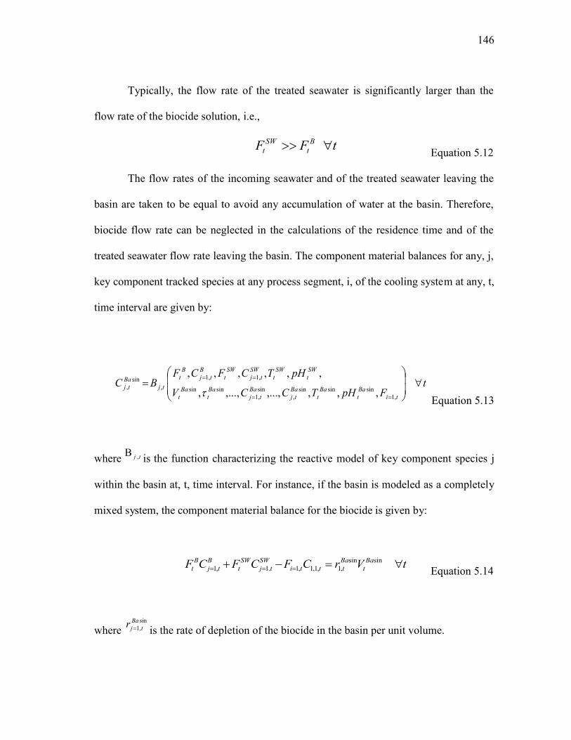
146
Typically, the flow rate of the treated seawater is significantly larger than the
flow rate of the biocide solution, i.e.,
tFF Bt
SWt Equation 5.12
The flow rates of the incoming seawater and of the treated seawater leaving the
basin are taken to be equal to avoid any accumulation of water at the basin. Therefore,
biocide flow rate can be neglected in the calculations of the residence time and of the
treated seawater flow rate leaving the basin. The component material balances for any, j,
key component tracked species at any process segment, i, of the cooling system at any, t,
time interval are given by:
tFpHTCCV
pHTCFCFBC
tiBat
Bat
Batj
Batj
Bat
Bat
SWt
SWt
SWtj
SWt
Btj
Bt
tjBa
tj
,1sinsinsin
,sin,1
sinsin
,1,1,
sin, ,,,,...,,...,,
,,,,,,
Equation 5.13
where j ,t is the function characterizing the reactive model of key component species j
within the basin at, t, time interval. For instance, if the basin is modeled as a completely
mixed system, the component material balance for the biocide is given by:
tVrCFCFCF Bat
Battti
SWtj
SWt
Btj
Bt
sinsin,1,1,1,1.1,1 Equation 5.14
wheresin,1
Batjr is the rate of depletion of the biocide in the basin per unit volume.

147
Within the process, given the specific path of seawater inside the process, a
“path” model is developed to account for the biocide reaction kinetics throughout the
process. The seawater goes through a number of pipes and units. The process is
discretized into a number of segments. Each segment, i, represents a portion of the
seawater pipeline or a heat exchanger (e.g., cooler, coil in a hot unit, cooling jacket of a
unit, etc.). Consider the Nc key species and refer to the concentration of key component j
in segment i during period t as Cj,i,t . For the jth species, in the ith segment, and at tth
period, the following kinetic expression may be written as:
tipHTVCCCFC tititititNpitjpitpititjitjiC
,,,,,,...,,...,, ,,,,,,,,,1,,,,,,
Equation 5.15
where the subscript, i-p, is referring to the previous process segment of the cooling
system before process segment i. The thickness of the biofilm in the i th segment at the
end of the tth period is given by the following equation:
Equation 5.16
where is a binary integer variable defined as:
= 1 if maintenance/cleaning is carried out at the end of period t-1
= 0 if no maintenance/cleaning is carried out at the end of period t-1

148
The effect of the binary in the previous equation is to set the thickness of the
biofilm to zero (i.e., a clean surface) after the cleaning is carried out. The biofilm growth
function is described in terms of the compositions of the biocide and residual
byproducts, as well as the average temperature and pH of the seawater in segment i.
In addition to the economic aspects of determining when cleaning is scheduled,
there is also mandatory cleaning if the biofilm thickness reaches a maximum allowable
level:
tidd titi ,max,, Equation 5.17
tid , : the biofilm thickness at process segment i and at time interval t.
max,tid : the maximum allowable biofilm thickness at process segment i and time interval t.
tid , : the highest level of biofilm thickness at process segment i at time interval t.
The biofilm thickness grows seasonally up to a certain level defined as , This
thickness depends on the biological and process conditions. The loss in performance of
the ith heat exchanger resulting from the cumulative formation of the biofilm at the end
of period t is given by:
Equation 5.18

149
is the function characterizing the heat transfer reduction model in the process
segment i at, t, time interval.
The objective function is to minimize the total annualized cost incurred from
biofouling development. That cost includes all direct and indirect costs.
Annual Total Cost = Annual Cost of Biocide to Treat the Seawater
+ Annual Costs of Chemicals at EOP Treatment Unit for Removing the effect
of Biocide Residuals
+ Annual Costs of Heat Exchanger Cleaning, Heat Loss Due to Fouling, and
Gross Profit Loss Due to Shutting Down the Process for Heat Exchanger Cleaning.
Mathematically, the objective function is described by:
Equation 5.19
The cost of biocide during period t is expressed as:
),(_ Bt
Bt
Bt CFBiocideCostCost Equation 5.20
The cost of end-of-pipe treatment during period t is given by:
t SN
t
N
iti
Cleaningi
LPt
EOPt
Bt ICostCostCostCostCostAnnualizedTotalMinimize
1 1, )*(

150
),...,,...,,,,(_ ,,2,,2,1,2,2 tNNtjNtNtNiChemt
Chemt
EOPt cssss
CCCFCFEOPCostCost
Equation 5.21
Loss of production can be defined as loss due to reduction in heat transfer in the
heat exchanger units, as well as the loss of production due to shutting down the process
for maintenance. The cost of loss of production is given by:
),(_ ,, titiLPt IQLPCostCost Equation 5.22
Environmental and quality constraints:
In addition to the aforementioned technical constraints, the minimization of the
cost objective function is also subject to environmental and quality constraints from the
process and from the environment. There is a minimum requirement from the process
technical specification of the plant on the concentration of biocide residual to insure
minimum biofouling development. Also, another constraint on the thickness of biofilm is
to not exceed a certain thickness,max,tid .
TechtjC ytjN s ,,,2
Equation 5.23

151
max,, titi dd Equation 5.24
The concentration of key component j of biocide residual must comply with the
environmental regulations. Also, the concentration of chemicals added to reduce the
effect of the biocide residuals is regulated by the environmental requirements. Hence,
EnvtjC ytjN s ,,,
Equation 5.25
EnvChemC yChem
tjNs ,,
Equation 5.26
5.5. CASE STUDY
Consider an integrated power production/desalination plant. The power plant has
a maximum capacity to produce 427 MW of electricity using natural gas and turbines
with steam extraction. Figures 5.3. and 5.4. provide the schematic flow diagrams of the
power/desalination plant and the cooling system. The multi-stage flash (MSF)
desalination plant has a maximum production capacity of 11,400 m 3/hr of desalinated
water from three units, each producing 3,800 m3/hr. The seawater ambient temperature
varies from 24oC to 35oC. The maximum allowable temperature difference of seawater
from the inlet to the outlet of the plant is 8oC. The total seawater intake is designed to
take a capacity of up to 67,500 m3/hr in four pipes of 2.2 m diameter and about 1.2 km

152
long. For maximum capacity, the flow rates of seawater used for the MSF units cooling
system, the steam turbines, and the steam generators (boilers) are 36,822, 12,600, and
1,800 m3/hr, respectively (Abdul-Wahab et al., 2009).
Figure 5.3. An Overall Representation of the Power/Desalination Plant.
The seawater cooling system of the power desalination plant is simplified and
shown in Figure 5.4. (Abdul-Wahab et al., 2009). The production of power and the
usage of seawater cooling vary monthly as shown by Table 5.2 and Table 5.3.
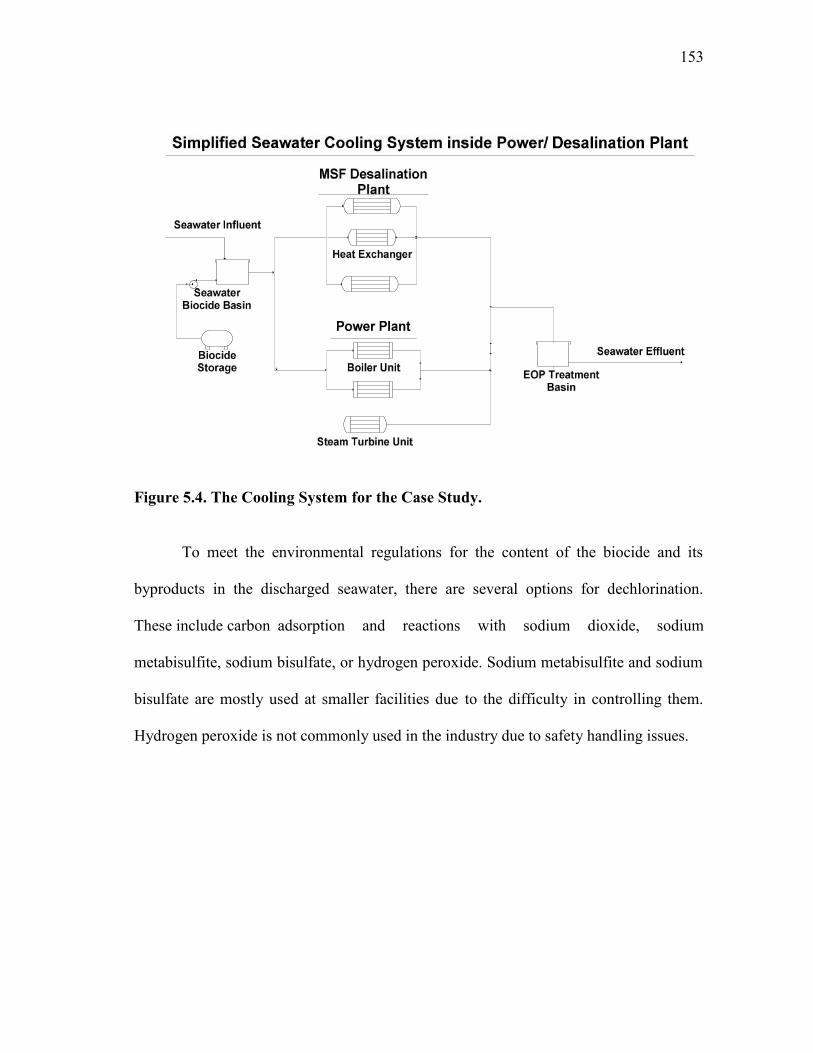
153
Figure 5.4. The Cooling System for the Case Study.
To meet the environmental regulations for the content of the biocide and its
byproducts in the discharged seawater, there are several options for dechlorination.
These include carbon adsorption and reactions with sodium dioxide, sodium
metabisulfite, sodium bisulfate, or hydrogen peroxide. Sodium metabisulfite and sodium
bisulfate are mostly used at smaller facilities due to the difficulty in controlling them.
Hydrogen peroxide is not commonly used in the industry due to safety handling issues.

154
Table 5.2. The Cooling System for the Case Study.
Base-Case Amount of Seawater Used in the Cooling System of thePower/ Desalination Plant
PlantSection Unit Number
of Units
Seawaterused/Unit
Total Seawaterusage Heat Load
m3/Hr m3/Hr MM Btu/hr
Desalination MSF3
12274 463
12274 46312274 463
36822
PowerBoilers
2900 34
900 341800
SteamTurbine 1 12600 12600 476
Total 51222
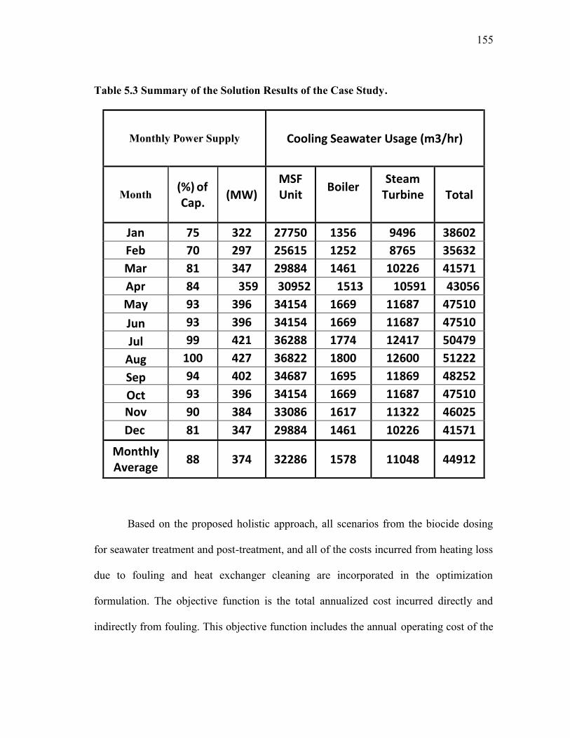
155
Table 5.3 Summary of the Solution Results of the Case Study.
Monthly Power Supply Cooling Seawater Usage (m3/hr)
Month (%) ofCap. (MW)
MSFUnit Boiler Steam
Turbine Total
Jan 75 322 27750 1356 9496 38602Feb 70 297 25615 1252 8765 35632Mar 81 347 29884 1461 10226 41571Apr 84 359 30952 1513 10591 43056May 93 396 34154 1669 11687 47510Jun 93 396 34154 1669 11687 47510Jul 99 421 36288 1774 12417 50479
Aug 100 427 36822 1800 12600 51222Sep 94 402 34687 1695 11869 48252Oct 93 396 34154 1669 11687 47510Nov 90 384 33086 1617 11322 46025Dec 81 347 29884 1461 10226 41571
MonthlyAverage 88 374 32286 1578 11048 44912
Based on the proposed holistic approach, all scenarios from the biocide dosing
for seawater treatment and post-treatment, and all of the costs incurred from heating loss
due to fouling and heat exchanger cleaning are incorporated in the optimization
formulation. The objective function is the total annualized cost incurred directly and
indirectly from fouling. This objective function includes the annual operating cost of the

156
biocide (chlorine) used to treat the cooling seawater against biofouling, the annual cost
of removing chemicals used for removing residuals from the effluent seawater before
discharge, the cost of cleaning the heat exchanger units, the cost of the loss of production
incurred by biofouling, and the annual gross profit loss from shutting down the plant
operation for cleaning the heat exchangers. The objective of the optimization model here
is to directly minimize the cost for treating seawater for cooling purposes and any loss
occurred due to biofouling development from an untransferred heat load below the
required cooling duty due to the growth of the biofilm which may affect the yield of the
plant. Also, the objective function considers the cost of maintaining the cooling units on
a regular basis throughout the year to clean the heat-transfer surface of the coolers.
The annual operating time is discretized into Nt = 365 time intervals (i.e., the
optimization formulation is developed on a daily basis). The key components are tracked
in the cooling system for an accumulation of biocide residuals. The cooling system is
discretized into numbers of segments i = 1, 2,…, Ns. Those segments are portions of the
pipelines or heat exchanger units.
t SN
t
N
iti
Lt
EOPt
Bt ICostCostCostCostAnnualizedTotalMinimize
1 1, )*(
Equation 5.27
Total Annual Cost of Biocide:BiocideFCost
tN
t
Bt
Bt
Equation 5.28

157
The total annual cost of biocide is the summation of the volumetric flow rate of
biocideB
tF over all time intervals Nt, multiplied by the duration of each time interval .
This total is multiplied by the cost of biocide ($/m3).
Total annual cost of end-of-pipe treatment is calculated as follows:
ChemicalsFCosttN
t
Chemt
EOPt
Equation 5.29
Total annual cost of end of pipe treatment is equal to the summation of the
volumetric flow rate of chemicals (m3/hr) multiplied by the duration of each time
interval over all time intervals, Nt. The total summation is multiplied by the cost of
chemicals ($/m3).
Total annual cost for production loss due to heat reduction in heat exchangers
caused by fouling and shutting down the process for heat exchangers cleaning is given
by:
tenanceMaCost i
N
i
Lt
S
int1 Equation 5.30
where Maintenancei is the cost for maintaining process segment I with a loss of
production due to the reduction in heat transfer and being out of the process for cleaning.
The total annual cost for heat exchangers’ maintenance is the summation of the

158
multiplication of binary number Ii,t by the cost of the maintenance of a single process
segment over all process segments Ni and over all time intervals Nt.
Determining the amount of residual chlorine [CCl2 ] after time t in minutes
requires the result of the kinetic study depending on water quality and the time of the
year. Also, for different temperatures, the changes in decay rate constants are considered.
The models of Wang et al. (2008) and Xin et al. (2003) were used in developing
the kinetic model for chlorine. The general form of chlorine decay in seawater is as
follows:
C = A e-kt Equation 5.31
It was considered that the first chlorine decay was very rapid in the first few minutes
(Characklis et al., 1980). After the first five minutes, the data are fitted to the exponential
form shown above (Xin et al., 2003).
The decay of biocide inside the cooling system for this case study follows this
function:
titktjpitji eCC ,*
,,,,
Equation 5.32
where:

159
tijC ,, :is the concentration of biocide key component j at process segment, i, at time
interval t in (mg/l).
tpijC ,, :is the concentration of biocide key component j at process segment, i-p, which
precedes process segment i at time interval t.
The decay constant (1/min) has a proportional relationship with temperature
(Nebot et al., 2007). As temperature increases, the decay of chlorine increases following
this equation:
titi Tk ,, * Equation 5.33
where T is measured in Celsius
tj , :is the disinfection kinetics rate constant for key component j at time interval t.
: is the coefficient of the decay constant of biocide by-products
)min./1(108.6 4 Co .
tiT , the temperature in (oC) at process segment i and time interval t.
Data for the residual chlorine is in seawater at temperature range from 20 to 24C
were extracted from Hostgaard-Jensen et al. (1977).
tpiSWp
SWti
titi T
CFQ
T ,,
,,
Equation 5.34

160
tpiT , :is the temperature of seawater at process segment i-p, preceding segment i at time
interval t
tiQ , : the heat transfer at process segment (in the heat exchanger) i and at time interval t.
qtiQ Re
, :is the heat transfer required for process segment i at time interval t (Btu/hr).
The heat transfer rate would decrease from tiq
ti QtoQ ,Re, as the biofilm
accumulates. The required output of the plant required an operational schedule to
maintain certain operational conditions. Thus, the heat load required to be transferred at
each process segment (in the heat exchanger) is assigned accordingly. This amount of
heat load for each process segment i at time interval t is calledq
tiQ Re, . At the same time,
the heat load transferred, tiQ , , has to be within the designed margin after any reduction
due to fouling according to the equation below (Nebot et al., 2007). From the percentage
reduction in heat transfer in the heat exchanger, the heat transferred can be calculated
from the designed value.
100..%
1* ,Re,,
tiqtiti
RTHQQ
Equation 5.35
therefore, tiQ , is the actual heat load transferred at unit i and time interval t, which has to
be less than or equal to the unit i is designed for.Desiti QQ , where %HTRi,t is the
percentage of heat transfer reduced at heat exchanger i at time interval t. The reduction
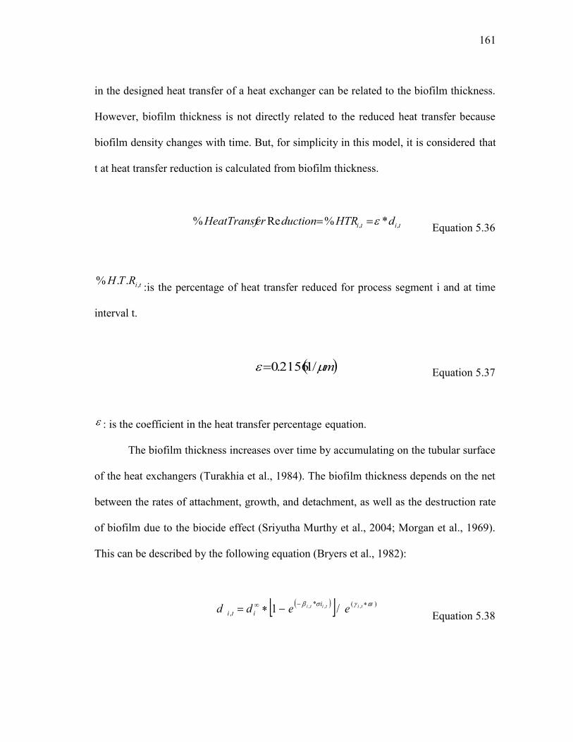
161
in the designed heat transfer of a heat exchanger can be related to the biofilm thickness.
However, biofilm thickness is not directly related to the reduced heat transfer because
biofilm density changes with time. But, for simplicity in this model, it is considered that
t at heat transfer reduction is calculated from biofilm thickness.
titi dHTRductionerHeatTransf ,, *%Re% Equation 5.36
tiRTH ,..% :is the percentage of heat transfer reduced for process segment i and at time
interval t.
m /12156.0 Equation 5.37
: is the coefficient in the heat transfer percentage equation.
The biofilm thickness increases over time by accumulating on the tubular surface
of the heat exchangers (Turakhia et al., 1984). The biofilm thickness depends on the net
between the rates of attachment, growth, and detachment, as well as the destruction rate
of biofilm due to the biocide effect (Sriyutha Murthy et al., 2004; Morgan et al., 1969).
This can be described by the following equation (Bryers et al., 1982):
)(*,
,,, /1 tititi eedd iiti Equation 5.38

162
titi T ,, Equation 5.39
di,t= net development from growth and destruction
ti , : is the biofilm growth rate constant for process segment i at time interval t (1/min)
(phi) ).min/1(10*909.2 7 Co
: is the coefficient of biofilm growth rate constant [1/ (min.oC)].
: is the duration of a single time interval (day).
i
titi
titi d
dI 1,1,
1,,
*1ln*1
, Equation 5.40
ti , : is the biofilm growth rate constant considering the growth from the previous time
interval for process segment i and at time interval t (min).
min0225.0 m
Equation 5.41
where is the coefficient of biofilm growth from the previous time segment.
When the biofilm thickness reaches the maximum allowable thickness, a decision
for maintaining that unit has to be made. Here, this has been accounted for by
multiplying the maximum allowable thickness by a binary number Ii,t. When biofilm

163
thickness di,t-1 of unit i at time interval t-1 exceeds the allowable level diMax , then Ii,t for
unit i and time interval t-1 is equal to zero. Otherwise, Ii,t is always equal to one. The
maximum allowable level of the biofilm thickness has to be less thanid :
MaxitiMaxiti
ddwhenddwhentiI
1,
1,
011.
Equation 5.42
tiMaxi
Maxititi
Maxi IdddId ,,, 1*10000*0
Equation 5.43
iMaxi dd Equation 5.44
mdi 250 Equation 5.45
ti , : is a binary number for making decisions in order to maintain process segment i at
time interval t.
The destruction rate of the biofilm due to the biocide depends on the biofilm
thickness of the same unit i at the pervious time interval t-1 and the concentration of
biocide residual coming from the previous process segment pi at the pervious time
interval t-1 (Platon et al., 1985).

164
1,, * tpti iC , min/1: Equation 4.56
lmg /.min110*829.2 4
Equation 4.57
ti , : is the biofilm destruction rate constant for process segment i and time interval t
(1/min).
: is the coefficient of biofilm destruction rate constant (Gamma) of biocide residual
Additional constraints used in the case study:
The maximum allowable biofilm thickness is 70um.
Cleaning (maintenance) of heat exchangers is only considered at the end
of each month and no more than three maintenances are allowed per year.
5.6. RESULTS
The optimization formulation for the 365 daily periods was solved
simultaneously using the software LINGO. The key optimization results are summarized
by Figures 5.5. and 5.6. as well as Table 5.4., which show the amount of biocide and
chemical dosing each month as well as the total annual cost for treating seawater before
it enters the cooling system and before it is discharged back to the sea. The importance
of the results emerging from this work is holistic approach with respect to the whole
plant and the simultaneous consideration of the whole annual operation. The discharges
conform to the environmental regulations after enforcing the new limit which reduces
the allowable residual chlorine limit from 0.10 to 0.05 ppm. The biocide dosing was on a

165
continuous dosing on monthly basis instead of semiannual basis. The focus was on an
optimal biocide dosing to meet the minimum technical process requirements. The end-
of-pipe treatment was used to treat the biocide residual beyond the environmental
regulations. In most of the time, the average biocide residual is below 0.002 ppm at the
discharge. Heat-exchanger cleaning was carried out at the end of July. All these results
were achieved while the total cost of the biocide and the chemicals used for the end-of-
pipe treatment were reduced from $ 4.9 MM/yr to $3.5 MM/yr.
Figure 5.5. Monthly Average Biocide and EOP Chemical Dosing.

166
Figure 5.6. Monthly Cost of the Optimal Dosing of the Biocide and EOP TreatmentChemical.
Table 5.4. Table Showing the Summary of the Solution Results of the Case Study.
Biocide Used MaintenanceChemicalsUsed for
Dechlorination
CoolingSeawater Used
TotalCost
M3/yr MM$/yr #/yr MM
$/yr m3/yr MM$/yr m3/yr MM
$/yrMM$/yr
600 1.620 1 0.3 523 1.621 394 0.039 3.541
There are many operating practices that impact the efficiency, performance, and
cost of the plant. Adding more than the required amount of biocide would result in a
higher performance of the heat exchanger units, but it would require additional treatment
for seawater before it is discharged. Using less than the optimal doses of the biocide lead
to reduction in heat transfer and process performance. Furthermore, there is a critical

167
need to determine the timing of the cleaning maintenance of the heat exchangers. A
systematic procedure has been developed for the optimization of scheduling the dosing
of biocide and dechlorination chemicals as well as cleaning maintenance for a power
production/thermal desalination plant. The annual operation is discretized into
operational periods and the process is discretized into operating segment. A multi -
period optimization formulation was developed to determine the optimal levels of
dosing, the relationship between the applied doses, the process conditions, and seawater
characteristics for each time period. The technical and environmental considerations
were also accounted for and a case study has been solved to demonstrate the
applicability of the devised procedure.

168
6. A SYSTEMS INTEGRATION APPROACH TO THE OPTIMUM OPERATION
AND SCHEDULING OF BIOCIDE USAGE AND DISCHARGE FOR
SEAWATER COOLING SYSTEMS
6.1. OVERVIEW
Using seawater in cooling systems is a common practice in many parts of the
world where there is a shortage of freshwater. Biofouling is one of the major problems
associated with the usage of seawater in cooling systems. Therefore, a biocide is
typically added to seawater to control the growth of biofilms. There are numerous
challenges in the design and operation of seawater cooling systems. Specifically, it is
important to determine optimal strategies for the use of biocide to address the technical
objectives of the process while complying with the environmental regulations for the
discharge of the biocide and its byproducts. The objective of this work is to develop a
systematic approach to the optimal design and integration of seawater cooling systems in
industrial facilities along with the usage and discharge of biocides. The key building
blocks of the approach include the chemistry and kinetics of the biocide, process cooling
requirements and prospects for heat integration, dosage scenarios and dynamic profiles,
biofilm growth, seawater discharge, and environmental regulations. Specifically, the
paper will address the following tasks:
1) Identification of the reaction pathways for the biocide from the mixing
basin to the discharge points.
2) Kinetic modeling of the biocide and byproducts throughout the process.
169
3) A process integration framework to provide a holistic approach to
optimizing the design and operation of the seawater cooling systems, along
with the dosage and discharge systems.
Scheduling chemical dosing to minimize the total annual cost of the system
includes considering the cost of the biocide, the value of lost heat transfer resulting from
the biofilm, the cost of cleaning and maintenance, and the cost of treating the biocide
and byproducts in the discharged seawater. A hierarchical procedure is developed to first
identify design modifications for heat integration and energy efficiency. Then, a multi -
period, multi-segment optimization formulation is developed and solved to identify the
optimal operation and scheduling of biocide usage and discharge. The formulation
includes the biocide chemistry and kinetics, the time-based variations in seawater and
process characteristics, the relationship between the biocide usage, the process
conditions, and the rate of biofilm growth, and the environmental regulations for the
discharge of seawater. A case study is solved to illustrate the applicability of the devised
approach.
6.2. INTRODUCTION
The use of seawater in industrial cooling is a common practice in many parts of
the world that have limited freshwater resources. One of the primary operational
problems of using seawater in cooling is biofouling. Other problems include scali ng and
corrosion. The formation of bioflim is caused by the biological activities of
microorganisms in the seawater. Biofilms are very thin layers that stick to the inside
surface of heat exchanger tubes that use seawater. As small as a 250 micrometer biofilm

170
thickness is enough to reduce the heat transfer coefficient by 50%. Therefore, biofouling
is a serious problem (Goodman 1987). In some cases, excessive biofouling can obstruct
the heat exchangers.
There are three major types of biofouling:
Microbial fouling, which occurs as a result of the development of
microorganisms and their products
Macrobial fouling, which is a result of the deposit and growth of
macroorganisms like barnacles and mussels
Biological fouling, which is a result of a collection of detritus.
Typically, the development of microbial fouling precedes any macroorganism
colonization. Therefore, controlling microbial fouling has a great advantage of avoiding
macrobial fouling development. Biofouling usually develops over a few steps, including
biological, chemical, and physical processes. These processes may happen in a series
and/or parallel steps (Characklis, 1979). These steps include:
Transportation of organic molecules and microbial cells from the bulk of
the seawater coolant to the surface of the tubes of the heat exchangers.
Adsorption of the organic molecule and sedimentation on the surface of
the tubes of the heat exchangers.
Adhesion of the microbial cells surface of the heat-exchange tubes.
Growth whereby the attached microbial cells start producing more cells
leading to the formation of the biofilm.

171
Detachment of some cells of the formed biofilm due to sheer stress of the
flowing seawater.
To prevent the harmful effects of biofouling, biocides are used to control the
biological activities of the microorganisms and lessen the effect of fouling. Controlling
microbial growth is usually achieved by using an oxidizing agent, such as chlorine, in an
easy-to-disperse form, such as a hypochlorous acid or a hypochlorite ion, or in a gaseous
form like chlorine gas or chlorine dioxide. An intermittent chlorine dosage of 2 –5 mg/L
for 10 minutes per day can prevent microfouling, and a continuous dosage of 0.5 mg/L
during the second to fourth week of breeding season can prevent the blockage caused by
macrofouling. Under a continuous biocide dosage, aquatic organisms like oysters and
mussels tightly close their shells for weeks at a time, but they often die of asphyxiation.
These chlorine forms are most widely used due to cost and effectiveness factors.
Chlorine is a nonselective oxidant (it reacts with organics and nonorganics) and it
deactivates microbes. Also, chlorine reacts with natural organic matter (NOM), leading
to the formation of numerous by-products (Ben Waren 2006). Some of these by-products
are hazardous to aquatic life and human health. While there are other means of
preventing biofouling, such as periodic cleaning with sponge balls, tube heating and
drying, and antifouling paint, nonetheless, chlorine dosing is the most widely-used
method because of its cost-effectiveness and efficiency in slowing down or eliminating
different forms of microbial growth.
Other forms of chlorinated biocides include chloramines (e.g., NH2Cl, NHCl2,
and NCl3) and chlorine dioxide. Other biocides include ozone and ultraviolet radiation,

172
but both are relatively high in cost compared to chlorine. Ozone has not been
commercially utilized due to the high risk of possible leakage. A low concentration of
ozone, i.e. 0.3 ppm, is considered to be harmful to workers and to the surrounding
environment. Ultraviolet radiation is an effective disinfection method; however, its
applicability is limited to cases when the water has little turbidity and suspended matter.
Also, there is no residual disinfection effect after the radiation.
Using chlorine as a biocide is not trouble-free. Discharging chlorine and its by-
products back into natural bodies of waters with no treatment would definitely create
some environmental problems. Chlorine is a nonselective oxidant. In seawater, chlorine
and its various forms may react with organic species that exist in natural water,
producing hazardous compounds. Examples of these compounds are trihalomethanes
(THMs), halogenated acetic acids (HAAs), and halophenols (HPs), which are
carcinogenic for human health and aquatic life. THMs are formed from a reaction of
chlorine with natural organic matter. THMs are chemical compounds of methane,
replacing the three hydrogen atoms with halogens like tri-chlorinated/ brominated
methane demonstrated as (CHX3):(CHCl3), (CHBr3). THMs are environmental
pollutants and they may cause damage to the liver, kidneys, and central nervous system.
HAAs are acetic acids with H-atoms (fixed to a COOH-group) replaced by halogen
atoms. HAAs are suspected to raise the risk of cancer. HAAs could form THMs during
biological decomposition. THM and HAA concentrations are higher during the summer
season than in winter. Also, THM and HAA concentrations increase in that water comes
from surface, rather than groundwater.

173
Since the seawater discharge of biocides and their reaction byproducts poses
environmental and public health problems, there is a need to add end -of-pipe biocide
treatment (e.g., dechlorination) units to reduce the concentrations of the biocid e and its
byproducts at the discharged point. Chemical reduction using sulfur compounds has
been used as a dechlorination agent to remove free and combined residual chlorine.
Sulfur compounds like sulfur dioxide (SO2), sodium sulphite (Na2SO4), bisulfite
(NaHSO3), or bisulphate (NaHSO4) and sodium thiosulphate (Na2S2O3), or sodium
metabisulfite (Na2S2O5), have been used to dechlorinate seawater in industrial cooling
systems before discharging to the sea. Different dechlorination methods have been
utilized in the industry, including activated carbon, activated carbon combined with
ozonation, and photochemical reduction with ultraviolet irradiation.
Sodium sulfite (Na2SO3) was recommended for use as a dechlorinating agent by
(Pyle 1960; Beeton 1976) based on economic and safety uses. It was the most
economically effective, the safest, and the most capable of eliminating the toxicity of
residual chlorine for the aquatic life. Sodium sulfite is added at a 2:1 ratio by weight
with residual chlorine in order to completely and instantaneously eliminates
chloramines. However, the disadvantage of using sodium sulfite is that it requires an
accurate injection system and a periodic follow-up with chlorine fluctuating in influent
water. Sulfur dioxide is another cost-effective dechlorinating agent. Sulfur dioxide is
added at a weight ratio of 0.9 of sulfur dioxide for every 1.0 of chlorine to be removed.
But, practically a 10% excess amount of sulfur dioxide is always added to make sure that
the dechlorination process is completed. Sulfur dioxide is effective in removing both free

174
and combined residual chlorine. Also, sulfur dioxide can be fed using similar equipment
as is used for chlorination with a simple control scheme. Sulfur dioxide hydrolysis
happens in water rapidly and completely to form sulfuric acid, as shown in the following
reaction:
SO2 +H2OH2SO3 Equation 6.1
The oxidation number of the aqueous sulfur (SO3-2) is four, which means it
will react with free and combined chlorine rapidly and completely, as shown in the
following equations:
SO3-2 +HOCl SO4-2 + Cl- + H+ Equation 6.2
SO3-2 +NH2Cl + H2O SO4-2 + Cl- + NH4+ Equation 6.3
Because of the strong interaction between the process cooling demand, operating
conditions, and biocide needs and performance, it is important to develop an integrated
approach to optimizing biocide usage and discharge by understanding the key process
factors and seawater chemistry aspects, then reconciling them in an effective manner.
The objective of this paper is to develop a systematic approach to the optimization of
biocide usage and discharge by integrating seawater chemistry and process performance
175
issues. This includes modeling the mechanism and kinetics of the biocide, relating the
biocide kinetics to process conditions, and reducing biocide usage by lowering the
cooling needs of the process via heat integration. The usage and discharge of seawater is
linked to the process requirements, including cooling duties.
6.3. PROBLEM STATEMENT
The problem addressed in this paper can be stated as follows: given is a process
which uses seawater in a once-through cooling system via a number of segments that
include heat exchangers (coolers) and connecting pipelines. The heat duties of
the process coolers and the temperature of the incoming seawater vary throughout the
year. A typical dynamic profile for such variations is known. In order to prevent
biofouling in the coolers, a biocide is added to the incoming seawater The added
biocide undergoes various water chemistry reactions leading to the discharge of
chemical pollutants (e.g., residual biocide, reaction byproducts). The composition and
load of the pollutants as well as the temperature of the discharged seawater must meet a
given set of environmental regulations. An end-of-pipe (EOP) treatment system may
be added to assist in meeting the environmental regulations. Figure 6.1. is a schematic
representation of the problem statement.

176
Figure 6.1. Representation of the Problem Statement.
The process resources, revises the process design and operation, and determines
the optimal scheduling of chemical dosage load and timing, along with the heat -
exchanger cleaning cycles per year.
6.4. APPROACH AND CHALLENGES
A systematic approach is to be developed to include the following specific tasks:
Develop an appropriate level of modeling the chemical and kinetic
aspects of biocide usage and their reactions with different species in
seawater.
Relate the usage of biocide, the generation of byproducts, the
characteristics of the seawater, and the characteristics of the process to
the formation of the biofilm on the heat-exchange surfaces.

177
Account for the time-based variation in seawater temperature and process
requirements.
Incorporate the effect of regular maintenance activities to clean the heat-
exchanger surfaces and end-of-pipe treatment to meet the environmental
regulations.
Develop optimal policies for process modification and dynamic dosing to
optimize biocide usage and discharge.
Develop an optimum scheduling strategy which determine the optimal
frequency and timing of the maintenance service for cleaning the heat
exchangers.
Developing the systematic approach involves several challenges. There is
complexity in describing the reaction mechanism and kinetics for the biocide with the
different species that exist naturally in seawater. It is necessary to identify the effective
byproducts in controlling the biofilm development and to track these species. The
developed models must also account for the time-based variations in the seawater
characteristics (e.g., temperature) because of the impact on the reaction kinetics and the
rate of biofilm growth. Additionally, any hazardous compounds produced throughout the
cooling system until the discharge point must also be tracked. Appropriate levels of
details should be obtained to be representative enough of the chemical behavior while
avoiding too many details that will increase the size of the developed optimization
formulation or complicate it mathematical nature.

178
Since the usage of seawater is linked to the process cooling requirements, any
reduction in cooling requirements will have a direct impact on the amount of seawater
used and discharged, along with the usage and discharge of the biocide. In order to
successfully achieve this reduction in seawater and biocide, several design and
operational changes must be made. It is also important to consider the impact of biocide-
removal units (e.g., dechlorination) as required to meet the environmental regulations.
The first step in the proposed approach is to discretize the annual operation into
Nt periods (e.g., days or months). For each period, the seawater characteristics are taken
as the average during that period. To track the biocide chemistry and biofilm growth
throughout the plant, the process is broken down into Ni segments (e.g., portion of a
pipeline, heat exchanger, process unit). The next step is to reduce the cooling duty of the
process by using heat integration tools such as thermal pinch analysis (e. g., (Smith
2005; El-Halwagi 2006; Kemp 2007)).
The objective of this step is to minimize cooling and heating utilities of the
process. The biocide dosage is proportional to the cooling duty. As such, reducing the
cooling utility of the process leads to reducing the usage and discharge of the biocide.
The rationale behind starting with heat integration is that it will generate a cost savings
from the reduction of cooling utilities.

179
The next step is to make a further reduction in seawater flow rate by enhancing
the efficiency of seawater utilization. A practical technique to reach that reduction is to
maximize the temperature of the discharged seawater while complying with the thermal
pollution regulations. Then, the new seawater flow rate from the heat balance equation
can be calculated after the reduction has been made from increasing the discharged
temperature. After the reduction has been achieved in the seawater flow rate, the revised
calculation can be performed by recalculating the reduced amount of biocide required
for the seawater flow rate. Next, the chemical pathways and kinetics of the biocide
reactions are modeled at the appropriate level of details. The following step is to
optimize the dosage of biocide, while meeting the requirements of the process of the
minimum residual biocide remains in the cooling system to insure the control over any
biofouling development. The optimal biocide dosage is chosen based on an optimization
formulation that includes the relationship between the biocide usage and the bio film
growth, the impact of seawater characteristics, the effect of process conditions, the
performance of the end-of-pipe biocide-removal unit, regular maintenance to clean the
surfaces of the heat exchangers, and the impact of biofilm growth on the performance of
the individual heat exchangers. Figure 6.2. is a schematic representation of the proposed
procedure. The following sections provide more details on the key steps.
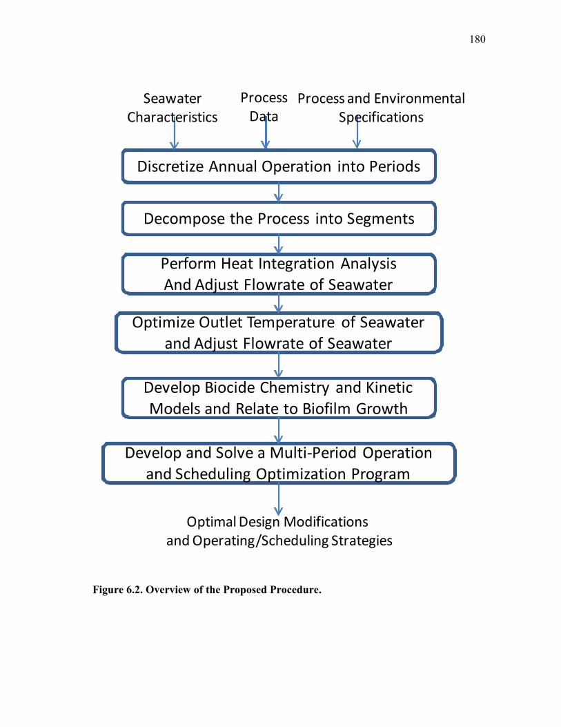
180
Figure 6.2. Overview of the Proposed Procedure.
Discretize Annual Operation into Periods
Decompose the Process into Segments
Develop Biocide Chemistry and KineticModels and Relate to Biofilm Growth
Perform Heat Integration AnalysisAnd Adjust Flowrate of Seawater
Optimize Outlet Temperature of Seawaterand Adjust Flowrate of Seawater
Develop and Solve a Multi-Period Operationand Scheduling Optimization Program
SeawaterCharacteristics
ProcessData
Process and EnvironmentalSpecifications
Optimal Design Modificationsand Operating/Scheduling Strategies
181
6.5. BIOCIDE CHEMISTRY
It is necessary to develop a mechanistic model for the reaction pathways
involving the biocide and the various species in the seawater. First of all, start with the
reaction of chlorine when it is added to seawater as a gas or solution of a chlorine
compound (e.g., sodium hypochlorite). Chlorine will dissolve and hydrolyze rapidly
(almost instantaneous) and completely to HOCl (hypochlorous) acid with a reaction rate
constant of 5X10¹⁴. When chlorine is added to seawater, it produces hypochlorous acid
and hydrochloric acid, HCl. The latter is a relatively strong acid, and it will dissociate
completely to a hydrogen ion and a chloride ion, while hydrochlorous acid, HOCl, is a
relatively weaker acid, and it will dissociate slightly to a hydrogen ion and a
hypochlorite OCl-. Since the hydrogen ion appears in this reaction, this equilibrium is pH
dependent. The distribution of the various species (HOCl, OCl-) at equilibrium is a
function of pH. Hypochlorous acid is the most germicidal species, but it is a weak acid
that will dissociate to hydrogen and hypochlorite ions with pKa of 7.5 at 30 oC. Figure
6.3 shows the distribution of the species over the pH range.

182
Figure 6.3. Distribution of Chlorine Species in Seawater (Based on the Data byOldfield and Todd, 1981).
Cl2+H2OHOCl + HCl Equation 6.4
HOClH++ OCl- Equation 6.5
In terms of disinfection effectiveness, hypochlorous acid is much stronger
(almost two orders of magnitude) than the hypochlorite ion. Hypochlorous acid will
reach its maximum concentration at pH ranges between 4 and 6 (Hostgaard-Jensen,
Klitgaard et al. 1977). However, the effectiveness of a chemical species as a disinfectant
does not necessary correlate with its effectiveness in removing biofilms. Weakening the
polysaccharide matrix of microbial cells is one way to control the development of
biofilms on the tube surface of heat exchangers. Experimental evidence shows that
V a r ia t io n o f C h lo r in e D is t r ib u t io n in S e a w a t e r w it h p H : a f t e rO ld f ie ld a n d T o d d ( 1 9 8 1 )
- 2 0
0
2 0
4 0
6 0
8 0
1 0 0
1 2 0
0 2 4 6 8 1 0 1 2
S e a w a t e r p H
Sp
ec
ies
Dis
trib
uti
on
%
H C lOC l2C lO -
183
chlorination is more effective in causing biofilm detachment at pH values greater than
pH 8, where OCl- concentration is more dominant than HOCl (Characklis,1979).
Seawater naturally contains organic and nonorganic species, particularly
ammonia and bromide species. Their concentrations vary depending on the nature of the
water. For instance, seawater contains bromide with concentrations as high as 65 mg/l,
but there may be a negligible amount in fresh waters. Ammonia concentrations depend
on pollutants of the water. In highly polluted water, ammonia concentration is as high as
15 ppm, while in unpolluted water the concentration is lower than 0.05 mg/l. At full
strength salinity, seawater ammonia concentration ranges between 0.001 and 1.0 ppm.
Ammonia, as well as other reactive nitrogenous compounds, will be chlorinated to yield
monochloramine (NH2Cl), and will react further to produce dichloramine (NHCl2). In
freshwater, and a very traceable amount in seawater, dichloramine will react further
with hypochlorous acid, producing trichloramine (NCl3). All of the reactions of
ammonia and combined chlorine with hypochlorous acid are made by replacing the
hydrogen atom of the ammonia molecule with a chlorine atom from a combined chlorine
molecule while maintaining its positive charge according to the following reactions:
OH+amine)(monochlorClNHNH+HOCl 223 Equation 6.6
OH+ine)(dichloramNHClHOCl+ClNH 222 Equation 6.7

184
OH+mine)(trichloraNClHOCl+NHCl 232 Equation 6.8
Figure 6.4. Concentration of Bromide and Ammonia in Natural Water.
Br-
Con
c.
Negligible
65 mg/lFull
strengthseawater
Freshwater (0.1-2.0) ppm
NH
3C
onc.
(< 0.001-1.0) ppm
Pollutedwater
Unpollutedwater < 0.05 mg/l
15 ppm
Br- & NH3 Conc.

185
These reactions depend on pH, temperature and contact time, but mainly on the
chlorine to ammonia ratio. All of the free chlorine (hypochlorous acid) will be converted
to monochloramine at pH 7-8 (the fastest conversion is at pH 8.3) when there is 1:1
molar ratio of chlorine to ammonia (5:1 by weight) or less. Then, within the same range
of pH, dichloramine is produced at a molar ratio of 2:1 of chlorine to ammonia (10:1 by
wt.). This reaction is relatively slow, so it may take up to an hour. Also, within the same
range of pH, trichloramine will be produced at a molar ratio of 3:1 of chlorine to
ammonia (15:1 by wt.) and at equal molar ratios, but at pH 5 or less. The two reactions
producing di- and tri-chloramine are known as the breakpoint reactions where the
chloramines are reduced suddenly to the lowest level. The significance of the breakpoint
reaction is that chlorine reaches its highest concentration and germicidal efficiency (at
1:1 molar ratio of chlorine to ammonia) just before reaching this point. Also, at the
breakpoint, monochloramine and dichloramine react together (which reduces chlorine
residuals) to produce nitrogen gas, nitrate, and trichloramine. Dichloramine decomposes
to an intermediate reactive product (NOH) which consumes mono-, di-chloramine, and
hypochlorous acid, producing nitrogen gas and nitrate. Also, excessive chlorine will
form trichloramine. These processes are shown in the following equations:
_
Cl2++H2+NOHOH+NHCl 22 Equation 6.9
-222 Cl+H+OH+NClNH+NOH Equation 6.10

186
-Cl+H+HOCl+N2NHCl2+NOH Equation 6.11
-+-3 Cl2+H3+NOHOCl2+NOH Equation 6.12
HOCl+NHClOH+NCl 223 Equation 6.13
The reaction of chlorine into these forms steers it away from the disinfection
function and renders the biocide less effective. Consequently, it is important to
understand such side reactions. Hypochlorous acid rapidly reacts with bromide,
producing hypobromous acid, which can also be produced from the reaction of bromide
with monochloramine, as follows:
-- ClHOBrBrHOCl Equation 6.14
3-
2-
2 NH+Cl+HOBrOH+Br+ClNH Equation 6.15
where HOBr is hypobromous acid. Additionally, the hypochlorite ion may undergo a
slow reaction with the bromide ion, as follows:
---- ClOBrBrOCl Equation 6.16

187
where OBr- is the hypobromite ion. Bromide in seawater may also react directly with
added chlorine to give bromine and chloride:
-2
-2 Cl2BrBr2Cl Equation 6.17
It is worth noting that the presence of ammonia and other nitrogenous
compounds in the seawater will react with HOBr to yield monobromamine (NH2Br),
dibromamine (NHBr2), and tribromamine (NBr3).
OH+mine)(monobromaBrNHNH+HOBr 223 Equation 6.18
OH+ne)(dibromamiNHBrBrNH+HOBr 222 Equation 6.19
OH+ine)(tribromamNBrNHBr+HOBr 232 Equation 6.20

188
The bromine breakpoint happens when the dibromamines are produced rapidly,
leading to the formation of nitrogen gas:
-22 Br2+2H+NOHOH+NHBr Equation 6.21
-+22 Br+H+HOBr+NNHBr+NOH Equation 6.22
It is also important to consider the effect of the bromide that naturally exists in
seawater at (50–70 mg/l). Bromide is typically in stoichiometric excess over the chlorine
dosage, whereas ammonia concentration doesn’t exceed 2 to 3 mg/L. The relative
amount of bromine species to ammonia species produced is proportional to bromide
concentration over ammonia concentration if we assume both reactions are rapid and
simultaneous. In order to understand the various species interactions and reaction
pathways, we have constructed the reaction mechanism shown in Figure 6.5. On these
diagrams, the starting species and intermediate and final by-products are represented in
boxes. The arrows correspond to reaction steps, and the boxes on the arrows represent
the reactive species that contribute to that reaction.

189
Figure 6.5. Summary of the Reaction Mechanism of Chlorine in Seawater.
Cl2,NaOCl
HOCl+Br- HOBr+Cl-
Br-
Cl2+H2O
HOCl+HCl
Deman
d
Br- + CO2 +Bromo-organics
HOBr+Deman
dBr-+
?
Hydrolysis
NH2Cl
HOCl
NH
3+H
OC
lN
H2C
l+H
2O
NH
3
NH
Cl2+
HO
Cl
NC
l3+H
2ON
H2C
l+H
OC
lN
HC
l2+H
2O
NHCl2
NCl3(Freshwater only)
HO
Cl
HO
Cl
Demand
Cl- + CO2 +Chloro-organics
HO
Cl+
Dem
and
Cl-+
?
NH3 + Cl- + CO2 +Chloro-organics
NH2C
l+De
man
dNH
3+Cl
-+?
NCl3+
Dem
and
NH3+
3Cl-+
?
Demand
Dem
and
(N2
+C
l-+
HO
Cl)
Brea
kpoi
nt
HOBrN
H3+
HO
Br
NH
2Br+
H2O
NH2Br
NBr3
NHBr2
NH
2Br+
HO
Br
NH
Br2
+H2O
NH
Br2
+HO
Br
NB
r3+H
2O
NH
3H
OB
rH
OB
r
Demand
NH3 + Br- + CO2 +Bromo-organics
Demand
Dem
and
NH2Br+DemandNH3+Br-+?
NHBr2+DemandNH3+2Br-+?
NBr3
+Dem
and
NH3+
3Br-+
?
(N2
+B
r-+
HO
Br)
Bre
akpo
int
NH2Cl+Br-+H
2ONH
3+HOBr+Cl-
Br-

190
6.6. MODELING OF HEAT-TRANSFER REDUCTION DUE TO
BIOFILM GROWTH
The cooling system in the plant is divided into Ni segments. Each segment
represents a pipe or a heat exchanger unit and is denoted by a subscript i. Figure 6.6. is a
schematic representation of the segments included in the analysis. Also, for simplicity
the annual operation is discretized into Nt time intervals. The values are taking as
average during each time interval t. The ambient temperature of seawater (the coolant)
varies depending on the time of the year. On the other hand, the scheduling changes for
the operational conditions depend on the seasonal demand on the plant output. The
climate changes affect the required amount of biocide because of its impact on the
reaction kinetics and the rate of biofilm growth. The seasonal demand on the plant
output add another variation that is making the model for optimizing the cooling system
has to be more responsive to all those variations. The rate of biofilm growth depends on
the temperature, nutrients, time of the year, flow rate, etc. Furthermore, the biofilm
develops through a number of physical, chemical, and biological steps which happen in
series and/or parallel. The biofilm begins with the attachment, then growth. Detachment
is due to the sheer stress of the fluid flow and starts from early stages of the
development. However, growth continues only up to a certain level where the
detachment rate becomes higher than the attachment and growth rate. This limits the
biofilm thickness from exceeding certain level.

191
Basin
BiocideStorage
Seawater Influent
Heat ExchangerNetwork
Seawater Discharge
Seawater Effluent
Typical Once-Through seawater Cooling System
EOP Treatment
Seawater Body
Figure 6.6. Segment Representation of the Process.
The segmented diagram starts by adding the biocide solution to seawater in a
basin before entering the cooling system. Seawater is pumped from the body of the sea
and screened from large objects to be ready for cooling use. At the basin seawater is well
mixed with the biocide. The assumption is that the reaction of biocide and seawater is
immediate and complete instantaneously. The flow of seawater is much larger the flow
rate of biocide. The flow rate of seawater is constant and therefore the volume of
seawater inside the basin is constant. The products of the reaction of biocide with
seawater are some byproducts (Seawater demand) and biocide residuals. Since, biocide
is added to natural water like this case seawater, biocide will be reacting with organic
materials and metals that are naturally exist before treatment. The assumption of biocide
192
residuals is that has the capability of controlling the biofouling development. Therefore,
the concern of the concentration of biocide residuals is taking under consi deration to
determine its influence on biofouling control. The biocide residuals are going to decay
depending on many factors including residence time, temperature, initial concentration
of biocide, and characterization of seawater including pH, salinity, nutrients, etc.
The annual operating time is discretized into Nt time intervals. Within each
interval (period), t, the operation is assumed to be steady state. The number of intervals
is selected in a way that balances accuracy (e.g., the intervals must capture seasonal
variations, action points such as changes in biocide dosage, operational variations such
as increases in flow rate of product and/or seawater) versus computational effort (size of
the optimization problem and computing time).
Let us use the index j to denote the key components to be tracked in the system.
These include the biocide (given an index j = 1) as well as the biocide residuals (which
impact biofouling development) and other byproducts (which are also contribute to the
consumption of biocide but do not affect the biofilm. These residuals and byproducts are
described by the index j (where j = 2, 3, …, Nc).
Time Intervals:
tN : Number of time periods to which the annual operation is discretized
t: is the time interval

193
Key Components:
j : is an index denoted to a key component, j=1 for the biocide.
CN : is the number of key components tracked in the cooling system.
Process Segments:
i: is an index denoted to a process segment, i=1 for the basin.
SN : is the number of the process segments (a portion of pipeline or a heat exchanger) in
the cooling system.
The following terms are used for each time interval t:
Seawater Influent:
SWtjC , : Composition of the, j, key component of the biocide in fresh seawater as a
function of, t, time interval.
SWtF : Flow rate of fresh seawater into the basin as a function of, t, time interval.
SWtpH : the pH of the seawater at the influent at time interval t.
SWtT : the temperature of the seawater at the influent at time interval t.

194
Biocide Storage:
BtjC ,1 : Composition of biocide in the added biocide solution from the biocide storage
into the basin as a function of, t, time interval.
BtF : Flow rate of the biocide solution into the basin as a function of, t, time interval.
Basin:
sin,
BatjC : Composition of the, j, key component of the biocide in the basin as a function of,
t, time interval.
sinBatpH : the pH of the treated seawater at the basin at time interval t.
sinBatT : the temperature of the treated seawater at the basin at time interval t.
sinBat : is the residence time at the basin at time interval t.
sinBatV : Volume of the water inside the basin as a function of, t, time interval.
Inlet of Cooling System:
i = 1.
Process Segment (i):
tjiC ,, : Composition of the, j, key component of biocide in the process segment, i, of the
cooling system as a function of, t, time interval.
195
tiF , : Flow rate of the treated seawater through the process segment, i, of the cooling
system as a function of, t, time interval.
tipH , : the pH of the treated seawater inside the process segment, i, of the cooling system
at time interval t.
tiT , : the temperature of the treated seawater inside the process segment, i, of the cooling
system at time interval t.
ti , : is the residence time inside the process segment, i, of the cooling system at time
interval t.
ti
titi F
V
,
,,
tiV , : Volume of the seawater inside the process segment, i, of the cooling system as a
function of, t, time interval.
Outlet of Cooling System:
i = Ns-2
End Of Pipe Treatment (EOP):
ChemtN s
C ,1 : Composition of the key component of chemicals at the end of pipe treatment
unit as a function of, t, time interval.
i = Ns-1

196
Chemical Storage:
ChemtC : Composition of the chemicals out of the storage and going to the end of pipe
treatment unit as a function of, t, time interval.
ChemtF : Flow rate of the chemicals to the end of pipe treatment unit as a function of, t,
time interval.
Seawater Effluent:
ChemtNs
C , : Composition of the key component of chemicals out to the environment as a
function of, t, time interval.
i = Ns
Typically, the flow rate of the treated seawater is significantly larger than the
flow rate of the biocide solution, i.e.,
tFF Bt
SWt Equation 6.23
The flow rates of the incoming seawater and of the treated seawater leaving the basin are
taken to be equal to avoid any accumulation of water at the basin. Therefore, biocide
flow rate can be neglected in the calculations of the residence time and of the treated
197
seawater flow rate leaving the basin. The component material balances for any key
component tracked species, j, at any process segment, i, of the cooling system at any, t,
time interval are given by:
Equation 6.24
where tj , is the function characterizing the reactive model of key component species, j,
within the basin at, t, time interval. For instance, if the basin is modeled as a completely
mixed system, the component material balance for the biocide is given by:
tVrCFCFCF Bat
Battti
SWtj
SWt
Btj
Bt
sinsin,1,1,1,1.1,1 Equation 6.25
wheresin,1
Batjr is the rate of depletion of the biocide in the basin per unit volume.
Within the process, given the specific path of seawater inside the process, a
“path” model is developed to account for the biocide reaction kinetics throughout the
process. The seawater goes through a number of pipes and units. The process is
discretized into a number of segments. Each segment, i, represents a portion of the
seawater pipeline or a heat exchanger (e.g., cooler, coil in a hot unit, cooling jacket of a
unit, etc.). Consider the Nc key species and refer to the concentration of key component j
tFpHTCCV
pHTCFCFBC
tiBat
Bat
Batj
Batj
Bat
Bat
SWt
SWt
SWtj
SWt
Btj
Bt
tjBa
tj
,1sinsinsin
,sin,1
sinsin
,1,1,
sin, ,,,,...,,...,,
,,,,,,
198
in segment i during period t as Cj,i,t . For the jth species, in the ith segment, and at tth
period, the following kinetic expression may be written as:
Equation 6.26
where the subscript, i-p, is referring to the previous process segment of the cooling
system before process segment i. The thickness of the biofilm in the i th segment at the
end of the tth period is given by the following equation:
Equation 6.27
where is a binary integer variable defined as:
= 1 if maintenance/cleaning is carried out at the end of period t-1
= 0 if no maintenance/cleaning is carried out at the end of period t-1
The effect of the binary in the previous equation is to set the thickness of the
biofilm to zero (i.e., a clean surface) after the cleaning is carried out. The biofilm growth
function is described in terms of the compositions of the biocide and residual
byproducts, as well as the average temperature and pH of the seawater in segment i.
tipHTVCCCFC tititititNpitjpitpititjitjiC
,,,,,,...,,...,, ,,,,,,,,,1,,,,,,
199
In addition to the economic aspects of determining when cleaning is scheduled,
there is also mandatory cleaning if the biofilm thickness reaches a maximum allowable
level:
tidd titi ,max,, Equation 6.28
tid , : the biofilm thickness at process segment i and at time interval t.
max,tid : the maximum allowable biofilm thickness at process segment i and time interval t.
tid , : the highest level of biofilm thickness at process segment i at time interval t.
The biofilm thickness grows seasonally up to a certain level defined as , This
thickness depends on the biological and process conditions. The loss in performance of
the ith heat exchanger resulting from the cumulative formation of the biofilm at the end
of period t is given by:
Equation 6.29
is the function characterizing the heat transfer reduction model in the process
segment i at, t, time interval.

200
6.7. BIOCIDE KINETICS
6.7.1. REACTION KINETICS
Biocide + Seawater Biocide Residuals + Byproducts (Seawater demand)
Equation 6.30
B + SW BR + BP Equation 6.31
BRr : Rate of appearance (reaction) of biocide residuals (mass/ [time. Volume]n)
)( nBIBR Ckr
BPr : Rate of appearance (reaction) of biocide byproducts (mass/ [time. volume]n)
)( nBIIBP Ckr
where n is the order of the reaction.
6.7.2. DECAY KINETICS
Biocide residuals + Seawater Byproducts Equation 6.32
BR + SW BP Equation 6.33

201
BRr : Rate of disappearance/ decay of biocide residuals (mass/ [time. Volume]m)
)( mBRDBR Ckr
Dk : Reaction rate constant (time-1 [mass/ Volume]-m)
mn & : Reaction orders
There are some assumptions considered:
1) BBSW VFF therefore, the volume of the basin can be considered as a
constant
2) Therefore, the reaction inside the basin considered to be as a plug flow
reactor
3) The reaction of seawater with biocide in the basin is a single irreversible
complete and instantaneous reaction:
Biocide + Seawater Biocide Residuals + Byproducts Equation 6.34
B + SW BR + BP Equation 6.35
4) There is no change in the number of moles
5) There is no change in temperature inside the basin
6) The products of the reaction are biocide residuals (BR), which have major
effects on biofouling development

202
7) Other products are called byproducts (BP) which are considered as
consumption of biocide or seawater demand
8)sinBa
jC is biocide residuals and byproducts’ concentrations are uniform
inside the basin
9) Water is well-mixed with biocide inside the basin, so there is no
accumulation
10) iSW FF & the volumetric flow rate of seawater and treated seawater in and
out of the basin are constants, therefore the volume of the water inside the
basin is constant
The mass balance on biocide residuals around the basin is represented by:
[Flow into the basin] + [Rate of generation] = [Rate of consumption/ decay] + [Rate of
accumulation] + [Flow out of the basin] Equation 6.36
After considering the assumptions:
[Rate of generation] = [Rate of consumption/ decay] + [Flow out of the basin]
Equation 6.37
tim
BRDBRBn
BIIBPSW
t FCkrVCkrF ,1** Equation 6.38

203
tim
BRDBn
BIISW
t FCkVCkF ,1** Equation 6.39
Mass balance on biocide residuals around Heat exchangers network (HEN):
[Flow in to HEN] + [Rate of generation] = [Rate of consumption/ decay] + [Rate of
accumulation] + [Flow out of HEN] Equation 6.40
After considering the assumptions:
There will be a slight change in temperature of seawater trough HEN
The residence time τ of seawater inside HEN
VHEN is the volume of seawater inside the HEN
tNiti SFF ,2,1 & are volumetric flow rate of treated water out of the basin
and out of HEN respectively.
[Flow in to HEN] = [Rate of consumption/ decay] + [Flow out of HEN]
Equation 6.41
tjitim
tiDBRtitjiti CFCkrFCF ,,1,1,1,1,,1,1 *** Equation 6.42
tjitim
tiDtitjiti CFCkFCF ,,1,1,1,1,,1,1 *** Equation 6.43

204
After considering the assumptions:
1) There will be no change in temperature of seawater through EOP
2) The residence time τ of seawater inside EOP equals flow rate/EOP volume
3) tjNi SF ,,1 is the volume of seawater inside the EOP
4) tjNitjNi SSFF ,,,,2 & are volumetric flow rates of effluent water out of HEN
and out of EOP respectively.
5) Decay kinetics:
Biocide residuals + EOP Agent Byproducts Equation 6.44
BR + RA BP Equation 6.45
BRr : Rate of removing of biocide residuals (mass/ [time. volume]o)
)( ,,2o
tjNiRBR SCkr
Rk : Removing rate constant (time-1 [mass/ Volume]-o)
o : Reaction orders
6) [Flow in to EOP] = [Rate of consumption/ decay] + [Flow out of EOP]
Equation 6.46

205
Equation 6.47
tjNitjNio
tjNiRtjNitjNitjNi SSSSSSCFCkFCF ,,,,,,2,,1,,1,,2 ***
Equation 6.48
The relation between the chemical added to seawater at the basin and its
influence on how it controls the fouling can be shown in the following model. The
thickness of biofilm inside the heat exchangers tubes is a function of chemical
concentration and scheduled dosage:
Dsgd
d
ttt eeXX Pr
Pr 0 Equation 6.49
where dtXPr : is the biofilm thickness at the end of the period
0X : is the initial biofilm thickness
: is the biofilm growth rate constant
: is the biofilm destruction rate constant from the influence of biocide
Dsgt : is chemical dosage schedule in hours per day
The biofilm growth rate constant, , can be calculated by letting the biofilm
grow for some time with no chemical added to control it. Then, a graph is generated for
tjNitjNio
tjNiRBRtjNitjNitjNi SSSSSSCFCkrFCF ,,,,,,2,,1,,1,,2 ***

206
the biofilm thickness versus time in days. By using regression analysis, the growth rate
can be calculated from the exponential kinetic growth. This kind of experiment can be
repeated at different months/ seasons to generate at each month/season.
The biofilm destruction rate constant, , is based on the relationship between the
kinetic of biofilm destruction by chemicals and disinfection kinetics of suspended
bacterial systems. Then, a graph is constructed to show different disinfection rate
constants, K , for bacteria that dies off versus different biocide concentration BC
dosages. The mathematical relation, which can be linear, that represents the relationship
between the rate constants with chemical concentration is:
bCa B Equation 6.50
The disinfection rate constant, K, has to be calibrated by , which can be
determined by dosing the plant that is going to use this model with a certain chemical
concentration for one hour per day and developing a graph from the data collected to
represent the biofilm thickness versus time in days. By using a regression analysis for
the curve, the destruction rate constant can be determined. From the disinfection rate
constant K and destruction rate constant at the same dosage, can be calculated as
follows:
Equation 6.51

207
The biocide residual concentration, tjNi SC ,,2 , at the effluent before discharge
or biocide removal treatment can be determined by developing a kinetic model of the
process. The consumption of chemicals is due to the reaction with organic and
nonorganic compounds, biofilm, and corrosion. The chemical decay in kinetics in a
batch cooling system (Xin et al. 2003) may be described as follows:
CKrW
rCK
dtdC
bhh
WW
Equation 6.52
Based on examining numerous experimental results for the kinetics of seawater
treated with a chemical (e.g., chlorine), decay kinetics have been correlated to several
factors, including temperature, pH, and contact time, but mainly on the ratio of chlorine
dosage to ammonia (e.g., Haag 1981). The reduction or decay of chlorine in seawater is
due to reactions with organic and nonorganic compounds in seawater. The chlorine
decay occurs in three stages, starting with a very fast rate during the first the two
minutes, due to a reaction with inorganic reducing agents. The second phase is slower
and usually does not last more than two hours. It mainly involves reactions with the
organic compounds that started in the first phase. Then, chlorine decays continuously via
a very slow rate.
Of particular importance is the dependence on residence time and temperature.
Given the specific path of seawater inside the process, the following model is developed
to account for chlorine decay throughout the process. The seawater goes through a
208
number of pipes and units. The process is discretized into a number of segments. Each
segment, i, represents a portion of the seawater pipeline or a heat exchanger (e.g., cooler,
coil in a hot unit, cooling jacket of a unit, etc.). Consider the NS key species and refer to
their concentrations in segment i as: SNijiii CCCC ,,2,1, ,...,,...,, .
6.8. OBJECTIVE FUNCTION FOR OPTIMUM DOSAGE
Based on the proposed holistic approach, all scenarios from the chemical dosing
of treatment and post-treatment, and all of the costs incurred from heating loss due to
fouling and heat exchanger cleaning, have to be incorporated in the decision for any
design or operation changes. The objective function is built on the economic criterion. It
will permit the most feasible solution that would also cost the least to operate the plant.
This approach might allow for biofilm growth and removal by periodic heat
exchanger cleaning at the minimum overall operating cost. On top of that, there are a
variety of options for chemical dosing. For each dosing course, the response of
biofouling development will vary accordingly. Thus, there will be an impact on the other
operating costs. Also, the nitration and the ambient temperature variations through
different seasons of the year will govern the microorganisms’ behavior inside the cooling
system. All of the different aspects have to be integrated to make one plan that considers
the impact on all of the related design and operation changes. The dynamics of the
process itself will add difficulty to selecting the optimal scenario among the options.
The objective function is to minimize the annual total cost that is incurred
directly and indirectly from fouling. It will include the annual operating cost of
chemicals (chlorine) used to treat the cooling water against biofouling, the annual fixed

209
and operating costs of removing chemical residuals from the effluent water, the cost of
cleaning heat exchanger units, the cost of the loss incurred by biofouling, and the annual
gross profit loss from shutting down the operation for cleaning the heat exchangers.
The annual operating time in discretized into Nt time intervals t = 1, 2,….., Nt
under the assumption of steady state at each t (time interval). The key components are
tracked in the cooling system as j = 1,2,…, Nc with j=1 for biocide added. The cooling
system is discretized into number of segments i = 1, 2,…, Ns. Those segments are
portions of pipeline or heat exchanger unit. The objective function is to minimize the
total annualized cost which includes all direct and indirect costs. Hence:
Annual Total Cost = Annual Cost of Biocide to Treat the Seawater +
Annual Costs of Chemicals at EOP Treatment Unit for Removing the effect of
Biocide Residuals +
Annual Costs of Heat Exchanger Cleaning, Heat Loss Due to Fouling, and Gross
Profit Loss Due to Shutting Down the Process for Heat Exchanger Cleaning.
Mathematically, the objective function is described by:
t SN
t
N
iti
Cleaningi
LPt
EOPt
Bt ICostCostCostCostCostAnnualizedTotalMinimize
1 1, )*(
Equation 6.53
The cost of biocide during period t is expressed as:
210
),(_ Bt
Bt
Bt CFBiocideCostCost Equation 6.54
The cost of end-of-pipe treatment during period t is given by:
),...,,...,,,,(_ ,,2,,2,1,2,2 tNNtjNtNtNiChemt
Chemt
EOPt cssss
CCCFCFEOPCostCost
Equation 6.55
Loss of production can be defined as loss due to reduction in heat transfer in the
heat exchanger units, as well as the loss of production due to shutting down the process
for maintenance. The cost of loss of production is given by:
),(_ ,, titiLPt IQLPCostCost Equation 6.56
6.9 ENVIRONMENTAL AND QUALITY CONSTRAINTS
In addition to the aforementioned technical constraints, the minimization of the
cost objective function is also subject to environmental and quality constraints from the
process and from the environment. There is a minimum requirement from the process
technical specification of the plant on the concentration of biocide residual to insure
minimum biofouling development. Also, another constraint on the thickness of biofilm is
to not exceed a certain thickness,max,tid .

211
TechtjC ytjN s ,,,2
Equation 6.57
max,, titi dd Equation 6.58
The concentration of key component, j, of biocide residual must comply with the
environmental regulations. Also, the concentration of chemicals added to reduce the
effect of the biocide residuals is regulated by the environmental requirements. Hence,
EnvtjC ytjN s ,,,
Equation 6.59
EnvChemC yChem
tjNs ,,
Equation 6.60
Gross profit is the revenue or sales after deducting all directed costs like
manufacturing expenses, feed, labor, and selling/marketing expenses. The gross profit
loss is how much of the gross profit would have been generated if the production had not
been stopped for heat changer cleaning. The daily gross profit (DGPft) can be calculated
by taking the revenue of a company over a period of time, with no shutdown in
production, and dividing it by the number of days of that period.

212
6.10.CASE STUDY
The case study is for a plant producing Acrylonitrile from propane with annual
capacity of 200 million pounds. The discharged amount of biocide residuals is higher
than newly enacted environmental regulations of 0.002 ppm of total residual chlorine.
This problem is normally solved by a conventional end-of-pipe treatment approach. The
purpose of the case study is to develop optimal design modifications and operating and
scheduling strategies for biocide usage and cleaning maintenance. The current usage of
seawater and the heating and cooling utilities of the process are given in Table 6.1. First,
thermal pinch analysis is carried out to minimize the heating and cooling utilities. The
results of heat integration lead to a targeted reduction of 92% and % 60% in heating and
cooling utilities, respectively. The amount of seawater and utilities for the target
reduction by heat integration tools is compared to the current usage and shown in Table
6.1. A simplified diagram depicting the cooling system is shown by Figure 6.7.
Table 6.1. Heating and Cooling Utilities Required for the Acrylonitrile Plant.
Heating & Cooling Utilities
Utility
Current Heat IntegrationTarget
% ofRed.Seawater Heat
Load Seawater HeatLoad
m3/hr MMBtu/hr m3/hr MM
Btu/hr
CoolingSeawater 9328 228 4337 91 60Refrigeration --- 39 --- 39 0
Heating --- 173 --- 36 79

213
Figure 6.7. Seawater Cooling System for the Acrylonitrile Plant.
The next step is to develop the biocide kinetic model and the biofilm growth
model for the heat exchangers in the plant. The objective is to develop chlorine residual
model to predict the chlorine concentration over a period of time throughout the process.
Chlorine is used as the biocide and the original plan is to introduce chlorine dosing at 5
mg/L three times for about 30 minutes and to switch to continuous chlorination to
prevent mussels during 2-4 week of breeding season at residual chlorine not less than 0.5
mg/L. Decay of chlorine is due to volatilization to the atmosphere and reaction with
ammonia-nitrogen in natural water. This reaction takes place when the ratio of the
concentration of free available chlorine to chloramines ([HOCl]/[ NH2Cl + NHCl2]) is 8
to 10. This reaction is known as a breakpoint reaction as shown in the following
reaction.

214
NH2Cl + NHCl2 + HOCl N2O + 4H+ + 4Cl- Equation 6.61
Other factors participating in reducing chlorine residual to chloride is reacting
chlorine with in-organic species like S--, Fe++, and NO2-. Also, chlorine can be reduced
to chloride by reaction with organic species to produce higher level compounds or
decomposed to CO2 and H2O. Moreover, hypochlorous acid is decomposed at very low
rate to produce oxygen.
HOCl1/2 O2 + H+ + Cl- Equation 6.62
Chlorine residual is detected by diethyl-p-phenylenediamine DPD method at
range of 0.05 to 5.00 mg/L chlorine. This method is the titration of Fe++ ions at the
presence of iodide and diethyl-p-phenylenediamine. The samples from the seawater are
examined at different points of time with known initial chlorine dosing. The results then
plotted in graphs of residual chlorine concentrations versus time. These data are used in
building a kinetic model of chlorine residual over time.
Due to the complexity of the reaction of chlorine with seawater, the consideration
is just for one reactant which is chlorine residual. The kinetics of chlorine residual
disappearance happens in two phases. It starts with a very fast decay rate, then it moves
to a slow rate. The following reactions are considered: The first equation is dominant
until organic species are consumed, then the second reaction becomes dominant.

215
Cl2 + Organics products Equation 6.63
r1 = - k1 CCl2 COrg Equation 6.64
Cl2 products Equation 6.65
r2 = k2 CCl2 Equation 6.66
There is a limitation of this model. It cannot be used for long periods (over 18
hours) nor can it be used for very small periods of time and low initial chlorine
concentrations. Alternatively, a second order kinetic model is used for the second
reaction:
Cl2 products Equation 6.67
r = dCCl2 /dt = - k C2Cl2 Equation 6.68
1/[CCl2 ] = k t + 1/[CCl2 ]o Equation 6.69
The collected data were graphed as reciprocal residual chlorine 1/ C2Cl2 versus
time. A linear relationship indicating that this reaction is indeed a second order reaction.
The assumption is that the instantaneous disappeared amount of chlorine is [CCl2]d.

216
For low initial chlorine concentrations [CCl2]o, the disappearing concentration is equal
to the remaining concentration [CCl2]o = [CCl2]r.
Amount of disappeared chlorine = Initial chlorine – remaining chlorine Equation 6.70
[CCl2 ]d = [CCl2 ]o – [CCl2 ]r Equation 6.71
Therefore, the concentration of remaining chlorine [CCl2 ]r after the initial
instantaneous disappearance [CCl2 ]d will be considered as the initial chlorine
concentration for the second order kinetic reaction:
1/[CCl2 ] = k t + 1/[CCl2 ]r Equation 6.72
There is a linear relationship between disappeared chlorine with initial chlorine
concentration. As the initial chlorine increases, the pH of seawater increases slightly.
Thus, the value of k changes as appears from the obtained data from the experiment of
Wang 2008. The data for [CCl2 ]r and k are obtained from the graph with the
corresponding initial chlorine concentration [CCl2 ]o:
k = 0.6925 e-0.8124[Ccl2]o Equation 6.73
The temperature effect on the k value was accounted for using the work of Wang, 2008.

217
It is important to track the biocide residuals concentration inside the cooling
system through each process segment. The biofilm growth is controlled by biocide
residual concentration. Determining the amount of residual chlorine [CCl2 ] after time t
in minutes requires the result of the kinetic study depending on water quality and the
time of the year. Also, for different temperatures, the changes in decay rate constants are
considered. The works of Wang et al. (2008) and Xin et al. (2003) were used in
developing the kinetic model for chlorine. The general form of chlorine decay in
seawater was taken as follows:
C = A e-kt Equation 6.74
It was considered that the first chlorine decay was very rapid in the first few minutes
(Characklis et al., 1980). After the first five minutes, the data are fitted to the
exponential form shown above (Xin et al., 2003).
The decay of biocide inside the cooling system for this case study follows this
function:
titktjpitji eCC ,*
,,,,
Equation 6.75
where:
tijC ,, :is the concentration of biocide key component j at process segment, i, at
time interval t in (mg/l).
218
tpijC ,, :is the concentration of biocide key component j at process segment, i-p,
which precedes process segment i at time interval t.
The decay constant (1/min) has a proportional relationship with temperature
(Nebot et al., 2007). As temperature increases, the decay of chlorine increases following
this equation:
titi Tk ,, * Equation 6.76
where T is measured in Celsius.
tj , : is the disinfection kinetics rate constant for key component j at time interval t.
: is the coefficient of the decay constant of biocide by-
products )min./1(108.6 4 Co .
tiT , the temperature in (oC) at process segment i and time interval t.
Data for the residual chlorine is in seawater at temperature range from 20 to 24C were
extracted from Hostgaard-Jensen et al. (1977).
The biofilm development model is integrated in the optimization model to track
the thickness of biofilm on the inside surface of the tubes of the heat exchanger. The
biofilm development is influenced by many factors including the variation in
temperature through the cooling systems after passing through heat exchanger units. The
other factor is the seasonal temperature variations of fresh seawater. This factor
influences the biological activities of microorganisms that contribute to the development

219
of the biofilms. Therefore, the optimization model includes constraints that track the
biofilm thickness which reduces the heat transferred across the tube surface. The influent
seawater temperature varies and after passing through heat exchanger units. It becomes:
tpiSWp
SWti
titi T
CFQ
T ,,
,,
Equation 6.77
tpiT , : is the temperature of seawater at process segment i-p, preceding segment i at time
interval t
tiQ , : the heat transfer at process segment (in the heat exchanger) i and at time interval t.
qtiQ Re
, : is the heat transfer required for process segment i at time interval t (Btu/hr).
The heat transfer rate would decrease from tiq
ti QtoQ ,Re, as the biofilm accumulates.
The required output of the plant requires an operational schedule to maintain
certain process conditions. Thus, the heat load required to be transferred at each process
segment (in the heat exchanger) is assigned accordingly. This amount of heat load for
each process segment i at time interval t is calledq
tiQRe, . The transferred heat load, tiQ , ,
must be kept e within the designed margin after any reduction due to fouling according
to the equation below (Nebot et al., 2007). From the percentage reduction in heat transfer
in the heat exchanger, the heat transferred can be calculated from the designed value.

220
100..%
1* ,Re,,
tiqtiti
RTHQQ
Equation 6.78
Therefore, tiQ , is the actual heat load transferred at unit i and time interval t, which has
to be less than or equal to the unit i is designed for.Desiti QQ , where %HTRi,t is the
percentage of heat transfer reduced at heat exchanger i at time interval t. The reduction
in the designed heat transfer of a heat exchanger can be related to the biofilm thickness.
However, biofilm thickness is not directly related to the reduced heat transfer because
biofilm density changes with time. But, for simplicity in this model, it is considered that
heat transfer reduction is calculated from biofilm thickness.
titi dHTRductionerHeatTransf ,, *%Re% Equation 6.79
tiRTH ,..% :is the percentage of heat transfer reduced for process segment i and at time
interval t.
m /12156.0 Equation 6.80
: is the coefficient in the heat transfer percentage equation.
The biofilm thickness increases over time by accumulating on the tubular surface
of the heat exchangers (Turakhia et al.1984). The biofilm thickness depends on the net

221
between the rates of attachment, growth, and detachment, as well as the destruction rate
of biofilm due to the biocide effect (Sriyutha Murthy et al., 2004; Morgan et al., 1969).
This complex relation is expressed through a function that takes care of the biofilm
growth over the variation of seawater condition with the destruction effect of biocide
residuals. This can be described by the following equation (Bryers et al., 1982):
di,t= net development from growth and destruction
)(*,
,,, /1 tititi eedd iiti Equation 6.81
titi T ,, Equation 6.82
ti , : is the biofilm growth rate constant for process segment i at time interval t (1/min);
(phi) ).min/1(10*909.2 7 Co Equation 6.83
: is the coefficient of biofilm growth rate constant [1/ (min.oC)].
: is the duration of a single time interval (day).
i
titi
titi d
dI 1,1,
1,,
*1ln*1
, Equation 6.84

222
ti , : is the biofilm growth rate constant considering the growth from the previous time
interval for process segment i and at time interval t (min).
min0225.0 m
Equation 6.85
where : is the coefficient of biofilm growth from the previous time segment.
When the biofilm thickness reaches the maximum allowable thickness, a decision
for maintaining that unit has to be made. Here, this has been accounted for by
multiplying the maximum allowable thickness by a 0/1 binary integer variable, Ii,t.
When biofilm thickness di,t-1 of unit i at time interval t-1 exceeds the allowable level
diMax , then Ii,t for unit i and time interval t-1 is equal to zero. Otherwise, Ii,t is always
equal to one. The maximum allowable level of the biofilm thickness has to be less
thanid .
MaxitiMaxiti
ddwhenddwhentiI
1,
1,
011. Equation 6.86
tiMaxi
Maxititi
Maxi IdddId ,,, 1*10000*0
Equation 6.87

223
iMaxi dd Equation 6.88
mdi 250 Equation 6.89
ti , : is a binary integer variable for making decisions in order to maintain process
segment i at time interval t.
The destruction rate of the biofilm due to the biocide depends on the biofilm
thickness of the same unit i at the pervious time interval t-1 and the concentration of
biocide residual coming from the previous process segment pi at the pervious time
interval t-1 (Platon et al., 1985):
1,, * tpti iC , min/1: Equation 6.90
lmg /.min110*829.2 4
Equation 6.91
ti , : is the biofilm destruction rate constant for process segment i and time interval t
(1/min).
: is the coefficient of biofilm destruction rate constant (Gamma) of biocide residual
Additional constraints used in the case study:
The maximum allowable biofilm thickness is 70um.

224
Cleaning (maintenance) of heat exchangers is only considered at the end
of each month and no more than three maintenances are allowed per year.
The objective function is considering all costs directly or indirectly
incurred by biofilm developments. Those costs include biocide and EOP
chemical dosing. The optimal solution would include also the heat
exchanger maintenance schedules. The maximum allowable biofilm
thickness is 70 micrometer.
The annual operating time is discretized into Nt = 365 time intervals (i.e.,
the optimization formulation is developed on a daily basis). The key
components are tracked in the cooling system for an accumulation of
biocide residuals. The cooling system is discretized into numbers of
segments i = 1, 2,…, Ns. Those segments are portions of the pipelines or
heat exchanger units.
t SN
t
N
iti
Lt
EOPt
Bt ICostCostCostCostAnnualizedTotalMinimize
1 1, )*(
Equation 6.92
Total Annual Cost of Biocide:BiocideFCost
tN
t
Bt
Bt
Equation 6.93
The total annual cost of biocide is the summation of the volumetric flow rate of
biocideB
tF over all time intervals Nt, multiplied by the duration of each time

225
interval . This total is multiplied by the cost of biocide ($/m3). Total annual cost of
end-of-pipe treatment is calculated as follows:
ChemicalsFCosttN
t
Chemt
EOPt
Equation 6.94
Total annual cost of end of pipe treatment is equal to the summation of the volumetric
flow rate of chemicals (m3/hr) multiplied by the duration of each time interval over all
time intervals, Nt. The total summation is multiplied by the cost of chemicals ($/m3).
Total annual cost for production loss due to heat reduction in heat exchangers
caused by fouling and shutting down the process for heat exchangers cleaning is given
by:
tenanceMaCost i
N
i
Lt
S
int1 Equation 6.95
where maintenance is the cost for maintaining process segment I with a loss of
production due to the reduction in heat transfer and being out of the process for cleaning.
The total annual cost for heat exchangers’ maintenance is the summation of the
multiplication of binary number Ii,t by the cost of the maintenance of a single process
segment over all process segments Ni and over all time intervals Nt.

226
6.11. RESULTS
The optimal schedule is for continuous monthly chlorine dosing that depends on
seasonal variations. In response, the chemical dosing at the EOP treatment unit is
eliminating or reducing the effect of biocide on aquatic life in the seawater. The
achieved reduction in heating and cooling utilities was 79 % and 51 %, respectively,
which is shown in Table 6.2. This is the most economically feasible reduction of the
utilities.
Table 6.2. Comparison of Current and Achieved Heating and Cooling UtilitiesRequired for the Acrylonitrile Plant.
Heating & Cooling Utilities
Utilities
Heating Cooling
MM Btu/hr MM Btu/hr
Current 173.4 266.90
H.I. Target 14.05 107.55
% of Current 91.8973 59.70
Achieved 36.4 129.90
% of Current 79.0 51.3

227
The comparison between the current and the proposed reduction in the usages of
heating and seawater cooling utilities as well as the amount of seawater is shown in
Figure 6.8. A significant reduction (percentagewise) was made for the heating utilities.
Figure 6.8. Comparison Between Current and Achieved Heating and CoolingUtilities Including Seawater Usage.
The majority of annual savings is attained through the reduction of heating
utilities of $3.5 MM. Then, the next annual savings is achieved from the reduction in
biocide dosing of $ 2.7 MM. Furthermore, savings is about $ 1 MM in usage of
seawater. There is a small annual savings in EOP chemical dosing because the aim was
to lower the biocide residual concentration beyond well below the current discharge to
reach 0.002 ppm. There is no saving in the maintenance of heat exchangers because the
current maintenance although the timing has changed. A summary of these savings is
shown in Figure 6.9.
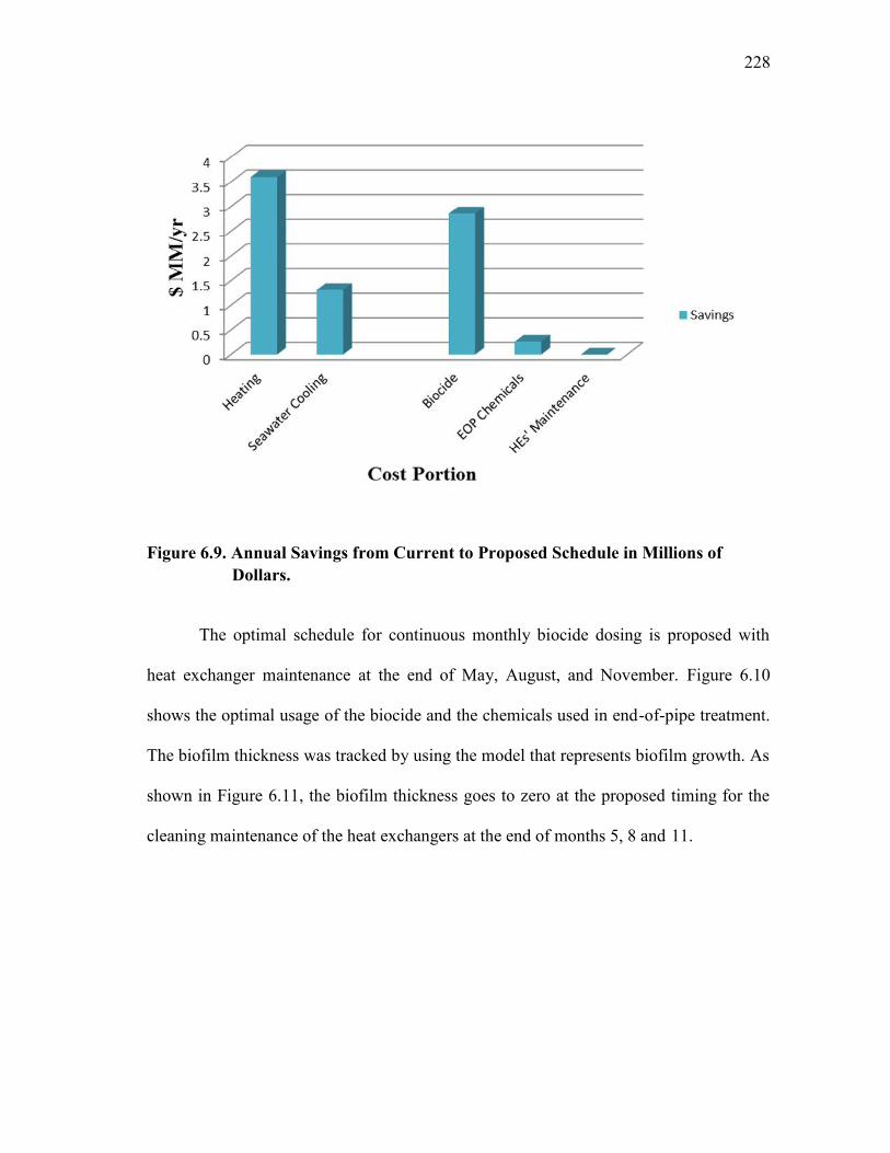
228
Figure 6.9. Annual Savings from Current to Proposed Schedule in Millions ofDollars.
The optimal schedule for continuous monthly biocide dosing is proposed with
heat exchanger maintenance at the end of May, August, and November. Figure 6.10
shows the optimal usage of the biocide and the chemicals used in end-of-pipe treatment.
The biofilm thickness was tracked by using the model that represents biofilm growth. As
shown in Figure 6.11, the biofilm thickness goes to zero at the proposed timing for the
cleaning maintenance of the heat exchangers at the end of months 5, 8 and 11.
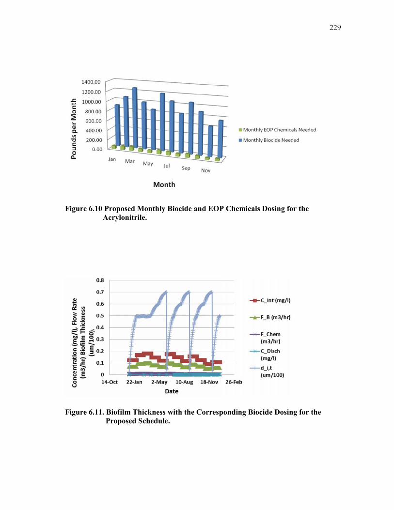
229
Figure 6.10 Proposed Monthly Biocide and EOP Chemicals Dosing for theAcrylonitrile.
Figure 6.11. Biofilm Thickness with the Corresponding Biocide Dosing for theProposed Schedule.

230
6.12. CONCLUSIONS
A systematic procedure has been developed for the optimization of biocide usage
and discharge for seawater cooling systems. The devised procedure includes design
modifications using heat integration and optimization of temperature profile. A kinetic
model is developed for the reaction mechanism of biocide and its byproducts and is
linked to the biofilm growth. A multi-period, multi-segment optimization model has also
been developed to account for the various cost item, the technical performance, and the
desired specifications and constraints. The case study of the plant for acrylonitrile from
propane showed how the procedure can be effectively applied to determine optimal
design changes and operating and scheduling strategies.

231
7. CONCLUSIONS AND RECOMMENDATIONS
This work has introduced systematic tools for the optimization of seawater
cooling systems. Emphasis has been given to the use and discharge of biocide and the
associated technical, economic, and environmental aspects. A comprehensive survey has
been presented for the biocide-seawater chemistry to understand the key relations
governing the effectiveness of the biocide dosing and the residual components exiting
the plant.
There are many operating practices that impact the efficiency, performance, and
cost of the plant. Adding more than the required amount of biocide would result in a
higher performance of the heat exchanger units, but it would require additional treatment
for seawater before it is discharged. Using less than the optimal doses of the biocide lead
to reduction in heat transfer and process performance. Furthermore, there is a critical
need to determine the timing of the cleaning maintenance of the heat exchangers.
Systematic procedures have been developed for the optimization of scheduling
the dosing of biocide and dechlorination chemicals as well as cleaning maintenance for a
power production/thermal desalination plant. A shortcut methods has been proposed to
include simplified biocide kinetics in a process-integration scheme. Next, more detailed
analysis of biocide chemistry and process characteristics were included. The annual
operation has been discretized into operational periods and the process is discretized into
two operating segments. A multi-period optimization formulation has been developed to
determine the optimal levels of dosing, the relationship between the applied doses, the

232
process conditions, and seawater characteristics for each time period. Applications were
shown for general facilities and for combined power plants and thermal desalination
systems. The technical and environmental considerations were also accounted for
through case studies that have been solved to demonstrate the applicability of the
devised procedures.

233
8. RECOMMENDATIONS FOR FUTURE WORK
The following topics are recommended for future work:
Inclusion of process-modification changes: This work has focused on the
seawater cooling system while accepting the process design and operation
in their current form. It will be useful to allow changes in process design
and operation to establish tradeoffs with the seawater cooling system.
Molecular design of biocide: This work has assumed the selection of a
specific biocide. Future research should include the problem of the
molecular design and selection of biocides that provide the necessary
controlling effect to the biofilms while exhibiting desirable technical,
economic, and environmental performance.
Integration with seawater dispersion models: This work has accepted a
certain set of environmental regulations for biocide discharge. Future
work should include dispersion models for the discharged biocide and
relate such dispersion to the impact on aquatic lives.
Inclusion of safety metrics: This work has focused on techno-economic
and environmental criteria. It is important to include safety metrics in the
assessment and screening of the design and operational strategies.

234
REFERENCES
Abdul-Wahab S.A., Juppb, B.P., 2009. Levels of heavy metals in subtidal sediments inthe vicinity of thermal power/desalination plants: a case study. Desalination 244,12.
Allonier, A., Khalanski, M., Bermond, A., Camel, V., 2000. Determination oftrihalomethanes in chlorinated sea water samples using a purge-and-trap system
coupled to gas chromatrography. Talanta 51, (3), 467-477.
Allonier, A., Khalanski, M., Camel, V., Bermond, A., 1999. Charactrization ofchlorination by-products in cooling effluents of coastal nuclear power stations.Marine Pollution Bulletin,. 38, 12, 1232-1241.
Anmangandla, U., Haas, C. N., Joffe, J., Heath, M., Jacangelo, J., 1998 Predictingdisinfection performance in continuous flow systems from batch disinfectionkinetics. Water Science and Technology 38(6); 171-179.
Becker , C., Thatcher, T, 1973. Toxicity of power plant chemicals to aquatic life. UnitedStates Atomic Energy Commission, Richland, WA.
Beeton, A. M., Kovacic, P. K., Brooks, A. S., 1976. Effect of chlorine and sulfitereduction on Lake Michigan invertebrates. Environment Protection Agency.Milwaukee, WI.
Ben Waren, A., Heitz, A., Joll, C., Kagi, R. 2006. A new method for calculation of thechlorine demand of natural and treated waters. Water Research 40(8), 2877.
Bin Mahfouz, A., Atilhan, S., El-Halwagi, M., Batchelor, B., Linke, P., Abdel-Wahab,A., 2009. Process integration and kinetic analysis of seawater cooling inindustrial facilities: Design for energy and the environment, Proceedings of the7th International Conference on the Foundations of Computer Aided ProcessDesign. El-Halwagi, M., Linninger, A., Taylor and Francis, London, England;223-231.

235
Bin Mahfouz, A., 2010. Process Integration Techniques for Optimizing SeawaterCooling Systems. LP Lambert Academic Publishing, Saarbrücken.
Bin Mahfouz, A., El-Halwagi, M., Batchelor, Bill, Atilhan, S., Linke, P., Abdel-Wahab,A., 2009. Process integration and kinetic analysis of seawater cooling inindustrial facilities, In: El-Halwagi, M., Linninger, A. (Ed.), Design for Energyand the Environment, Water Chlorination: Environmental Impact andHealth Vol. 3, Ann Arbor Science, Ann Arbor, MI, , pp. 349–368.
Characklis W. G., Trulear, M. G., Lin-Chiang, Chang, 1979 . Oxidation and Disinfectionof Microbial Films. Ann Arbor Science, Ann Arbor, MI.
Characklis, W.G., Cooksey, K.E., 1983. Biofilms and microbial fouling, In: I.L. Allen(Ed.), Advances in Applied Microbiology. Academic Press, Maryland Heights,MO; 93-138.
Characklis, W.G., Trulear, M.G., Bryers, J.D., Zelver, N., 1982. Dynamics of biofilmprocesses: methods. Water Research 16, 1207-1216.
Danell, R., Giles, M., 1983. Water dechlorination by activated carbon ultravioletradiation and sodium sulphite . Water Research 17(6): 667-676.
Drumeva, L. B., 1986. Determination and calculation of seawater salinity. WaterResources 13, 2, 173-177.
El-Halwagi, M. M.1997. Pollution prevention through process integration. SystematicDesign Tools. Academic Press, San Diego, CA.
El-Halwagi, M. M. 2006 . Process Integration. Academic Press, San Diego, CA.
El-Halwagi, M. M., Srinivas, B. K., Dunn, R. F. (1995). Synthesis of optimal heat-induced separation networks. Chemical Engineering Science 50: 81-97.
236
Eppley, R.W., Renger, E.H., Williams, P.M., 1976. Chlorine reactions with seawaterconstituents and the inhibition of photosynthesis of natural marinephytoplankton. Estuarine and Coastal Marine Science 4, 147-161.
Fayad, N.M., Iqbal, S., 1987. Chlorination byproducts of Arabian Gulf seawater.Bulletin of Environmental Contamination and Toxicology 38, 475-482.
Fiessinger, F., Rook, J. J. Duguet, J. P., 1985. Alternative methods for chlorination. TheScience of the Total Environment 47; 299-315.
Freese, S.D., Nozaic, D.J., 2004. Chlorine:– Is it really so bad and what are thealternatives?, In: P.W. SA (Ed.), The Water Institute of Southern Africa BiennialConference, Cape Town, South Africa, 18-24.
Freese, S. D., Nozaic, D.J., 2007. Chlorine: Is it really so bad and what are thealternatives? Water South Africa 30(5); 18-24.
Freese, S. D., Genthe, B. 2006. Just how toxic is chlorine, or any other disinfectants forthat matter? The Water Institute of Southern Africa Biennial Conference,Durban, South Africa 1906 (31); 150 - 157 .
Freese, S. D., Nozaic, D. J. 2007 . Chlorine Based Disinfectants: How Do TheyCompare? Water Science & Technology 55 (10); 403-411.
George R., Helz, G., Sugam, R., Sigleo, A. 1984. Chemical modification of estuairnewater by a power plant using continuous chlorination. Environmental ScienceTechnology 18 (3): 192-199.
Goodenough, R.D., Mills, J.F., Place, J., 1969. Anion exchange resin (polybromideform) as a source of active bromine for water disinfection. EnvironmentalScience Technology 3 (9): 854-856.
Goodman, P. D. (1987). Effect of chlorine on materials for sea water cooling systems: areview of chemical reactions. British Corrosion Journal 22(1): 56-62.

237
Greca, G. D., Fabbricino, M. (2008). DBP formation in drinking water: kinetics andlinear modelling. Water Science and Technology 8(2), 161-166.
Gunten, U. V. 2003. Ozonation of drinking water: Part II. Disinfection and by-productformation in presence of bromide, iodide or chlorine. Water Research 37(7):1469-1487.
Haag, W. R., Lietzke, M.H. 1981. A Kinetics model for predicting the concentrations ofactive halogens species in chlorinated saline cooling waters. Oak Ridge NationalLaboratory. Technical Report, Oak Ridge, TN.
Haag, W.R., Lietzke, M.H., 1981. Kinetic model for predicting the concentrations ofactive halogens species in chlorinated saline cooling waters. Technical Report,Oak Ridge National Laboratory, Oak Ridge, TN.
Haas, C. N. 1999. Benefits of using a disinfectant residual. American Water WorksAssociation 91(1): 65-69.
Hampel, C. A. 1950. Densities and boiling points of seawater concentrates. Industrial& Engineering Chemistry 42(2); 383-386.
Hancil, V., Smith, J.M., 1991. Chlorine-sensitized photochemical oxidation of solubleorganics in municipal waste water. Industrial Engineering for Chemical ProcessDesign and Development 10 (4), 515-524.
Hela, G.R., Sugam, R., Sigleo, A.C., 1984. Chemical modification of estuarine water bya power plant using continuous chlorination. Environmental Science Technology18 (3); 192-199.
Helz, R., SUgam, R., 2005. Chlorine specification in seawater. Chemosphere 10 (1); 41-57.
Helz, G., Bender, M., MacCrehan, W. 2005. Making chlorine greener: performance ofalternative dechlorination agents in wastewater: Chemosphere 60 (3); 381-388.

238
Hofmann, R., Andrews, R. C. 2001. Ammonical bromamines: a review of their influenceon bromate formation during ozonation. Water Research 35(3); 599 – 604.
Høstgaard-Jensen, P., Klitgaard, J., Pedersen, K.M., 1977. Chlorine decay in coolingwater and discharge into seawater. Journal Water Pollution Control Federation 49(8); 1832-1841.
Inman, G.W., Donald Johnson, J. 1984. Kinetics of monobromamine disproportionation-dibromamine formation in aqueous ammonia solutions, Environmental Science& Technology 8(4); 219-224
Jenner, H.A., Taylor, C.J.L., Donk, M.D., Khalanski, M., 1997. Chlorination by-products in chlorinated cooling water of some European coastal power stations.Marine Environmental Research 43, 4; 279-293
Jenner, H.A., Whitehouse, J.W., Taylor, C.J.L., Khalanski, M., 1998. Cooling watermanagement in European power stations Biology and control of fouling,Hydroecologie appliqué 10 (1/2) ; 225-245.
Jian-hua, Z., Gang, X.U.E., Hong-bin, Z., Yong-hui, W., Mei-fang, G.U.O., 2004.Kinetics of chlorine decay in water distribution systems. Journal of DonghuaUniversity 21; 140-145.
Jiang., C. T. G. 2005. Dechlorination and destruction of 2 4 6 trichlorophenol andpentachlorophenol using hydrogen peroxide as the oxidant catalyzed molybdateions under basic condition. Chemosphere 59; 321-326.
Johanneson, J. K. 1960. The bromination of swimming pools. American Journal PublicHealth 50; 1731–1736.
Johnson, J.D., Inman, G.W., Trofe, T.W., 1982. Cooling Water Chlorination: TheKinetics of Chlorine, Bromine, and Ammonia in Sea Water, National TechnicalInformation Service. Springfield, VA.

239
Johnson, J. D. 1977. Analytical problems in chlorination of saline water. ChesapeakeScience 18(1); 116-118.
Karra, B. S., Haas, C N., 1984. Kinetics of microbial inactivation by chlorine II kineticsin the presence of chlorine demand. Water Research 18(11); 1443-1449.
Kemp, I. 2007. Pinch analysis and process integration: a User Guide on ProcessIntegration for the Efficient Use of Energy. Butterworth-Heinemann, Burlington,MA.
Kim, B.R., Schmitz, R.A., Snoeyink, V.L., Tauxe, G.W., 1978. Analysis of models fordichloramine removal by activated carbon in batch and packed-bed reactorsusing quasilinearization and orthogonal collocation methods. Water Research,12; 347-326.
Kim, J., Smith, R., 2001. Cooling water system design. Chemical Engineering Science,56; 3641-3658.
Kim, H., Kwon, S., Han, S., Yu, M., Kim, J., Gong, S., Colosimo, M. F. 2006. NewORP pH based control strategy for chlorination and dechlorination ofwastewater-pilot scale application". Water Science and Technology 53(6); 145-151.
Kouame, Y., Haas, C.N., 2003. Inactivation of E Coli by Combined Action of FreeChlorine and Monochloramine. Water Research 25 (9); 1027-1032.
Kristoffersen, T., 1958. Mode of action of hypochlorite sanitizers with and withoutsodium bromide. Journal of Dairy Science 41 (7); 942-949.
Langford, T. 1977. Environmental management of coastal cooling discharges in HongKong. Chemistry & Industry 16; 612-616.
Lattemann, S., Hopner, T., 2008. Impacts of seawater desalination plants on themarine environment of the gulf, Protecting the Gulf’s Marine Ecosystems fromPollution, 191-205. Birkhauser Verlag, Switzerland.

240
Lee, Y., Kim, H., Lee, U., 2004. Formation of chlorite and chlorate from chlorinedioxide with Han River Water. Korean Journal of Chemical Engineering 21 (3);647-653.
Lei, H., Marinas, B.J., Minear, R.A., 2004. Bromamine Decomposition Kinetics inAqueous Solutions. Environmental Science Technology 38 (7); 2111-2119.
Leopold, P., Freese, S. D. 2009. A simple guide to the chemistry , SELECTION ANDUSE OF CHEMICALS FOR WATER AND WASTEWATER TREATMENT.Report to the Water Research Commission. Gezina, South Africa.
Li, X., Gu, D.M., Qi, J.Y., 2003. Modeling of residual chlorine in water distributionsystem. Journal of Environmental Science 15 (1); 136-144.
Lietzke, M.H., 1977. A Kinetic Model for Predicting the Composition of ChlorinatedWater Discharged from Power Plant Cooling Systems, Oak Ridge NationalLaboratory. Technical Report, Oak Ridge, TN.
Lietzke, M.H., Haag, W.R., 1979. Kinetic model for predicting the concentrations ofactive halogen species in chlorinated saline cooling waters. Oak Ridge NationalLab., Tennessee University, Knoxville , TN. Department of Chemistry.
Lijesen, M.G., 2007. The real-time price elasticity of electricity. Energy Economics 29,249-258.
MacCrehan, W. A., Bedner, M., Helz, G.R., 2005. Making chlorine greener Performanceof alternative dechlorination agents in wastewater. Chemosphare 60; 381-388.
Macdonald, I.A., Polman, H.J., Jenner, H.A., Quyam, S., 2009. Industrial coolingseawater antifouling optimization through the adoption of pulsed-chlorination.Gas processing in Doha, Boca Raton, FL; 537- 554.
M.H. Lietzke, Haag, W. R., 1977. A Kinetic Model for Predicting the Concentrations ofActive Halogens Species in Chlorinated Saline Cooling Water. Technical Report,Oak Ridge, TN.

241
Millero, F. J. 1984. The conductivity-density-salinity-chlorinity relationships forestuarine waters. Limnology and Oceanography 29; 1317-1321.
Millero, F.J., Gounzalez, A., Ward, G.K.,1976. Density of seawater solutions at oneatmosphere as a function of temperature and salinity. 34 (1), 61-93
Minear., R. A., Lie, H., Marinas, B. J., 2004. Bromamine decomposition kinetics inaqueous solutions. Environmental Science & Technology 38 (7); 2111- 2119.
Morgan, R.P., II, Stross, R.G., 1969. Destruction of phytoplankton in the cooling watersupply of a steam electric station. Chesapeake Science 10, 165-171.
Nada, N., Lwahashi, H., Umemori, F., 1994. Test result of the intermittent chlorineinjection method in Jeddah 1 plant. Desalination 96 (3); 283-290.
Nadine, L. 1984. Keeping biofouling at bay. Electric Power Research Institute Journal4(6); 22-27.
Nagarajan, B. , Jaiparakash, G.B., 2010. A study on microbial disinfection of drinkingwater using Nano Silver, Indian Electronic Thesis and Dissertation Repository,Bharath University, Tamil Nadu, India; 241-260.
Nebot, E., Casanueva, J.F., Casanueva, T., Sales, D., 2007. Model for fouling depositionon power plant steam condensers cooled with seawater: effect of water velocityand tube material. International Journal of Heat and Mass Transfer 50, 3351-3358.
Obo, T., Kunitomo, S., 2003. Biofouling Prevention with a Pulsed Discharge. IEEETransactions on Plasma Science 2(2); 1286-1289.
Overby, R., Johnson, J., 1971. Bromine and Bromamine Disinfection Chemistry.American Society of Civil Engineers 97 (5); 617-628.

242
Philip, Y. B. C., Vincent, K. C. T., David, P. L. Y., 1986. Using seawater for cooling.American Society of Heating, Refrigerating and Air-Conditioning Engineers28(9); 18-24.
Pinkernell, U., Nowack, B., Gallard, H., Gunten, U., 2000. Methods for the photometricdetermination of reactive bromine and chlorine species with ABTS. WaterResearch 34(18); 4343-4350.
Platon, M., Waite, T.D., A predictive model for destruction of biofilms with chlorine. In:R. Jolly, Editor, Water Chlorination: Chemistry, Environmental Impact andHealth Effects 5, Lewis Publishers Inc., Chelsea, MI (1985), pp. 1435–1445.
Pyle, E. A. (1960). Neutralizing Chlorine in City Water for Use in Fish-DistributionTank. The Progressive Fish-Culturist 22: 30-33.
Rajagopal, S., Velde, G.V.D., Venugopalan, V.P., Jenner, H.A., 2005. Chlorine andChlorine Residuals, Water Encyclopedia, John Wiley & Sons, New York, NY.
Rennau, J., Schroder, F., Sandt, B., Kreysig, D., Blaschke, M., Stadelmann, Kraft, A.,1990. Electrochemical water disinfection Part I Hypochlorite production fromvery dilute chloride solutions. Journal of Applied Electrochemistry 29 (7); 859-866.
Richardson, L.B., Burton, D. T., Helz, G. R., Rhoderick, J. C., 1981. Residual oxidantdecay and bromate formation in chlorinated and ozonation sea-water. WaterResearch 15 (9); 1067-1074.
Riley., J. P., Ali, M. 1986. The distribution of Halomethanes in the Coastal Waters ofKuwait. Marine Pollution Bulletin 17(9); 409-414.
Sayato., Y., Moto, T., Ueno, H., 1995. Disinfection by products in the chlorination oforganic nitrogen compounds, Water Supply 13(3); 171-176.

243
Shaw, R.F., Baggett, K.W., 2006. Annotated Bibliography of the PotentialEnvironmental Impacts of Chlorination and Disinfection Byproducts Relevant toOffshore Liquefied Natural Gas Port Facilities, Coastal Marine Institute. BatonRouge, LA.
Shiga., A., Yoshinaga, T., Kawano, K., Yanagase, 1995. Decomposition of DiluteResidual Active Chlorine in Sea Water Basic Study for the prevention of Growthof Marine Organisms. Water Research 26 (8); 110.
Smith, R. 2005. Chemical Process Design and Integration. New York, Wiley.
Sriyutha Murthy, P., Venkatesan, R., Nair, K.V.K., Ravindran, M., 2004. Biofilmcontrol for plate heat exchangers using surface seawater from the open ocean forthe OTEC power plant. International Biodeterioration & Biodegradation 53 (1);133-140.
Strupler, N. 1985. The extent of monochloramine interference in the DPD colorimetricmethod for free chlorine in water. Journal of the Institution of Water Engineersand Scientists 39(2); 134-136.
Sugita, H., Hayashi, K., Asai, T., Mitsuya, T., Amanuma, K., Maruyama, C., Deguchi,Y., 1992. Spectrophotometric method for determination of total residual oxidantsin seawater. Suisanzoshoku. H4; 45-49.
Tai, C., Jiang, G., 2005. Dechlorination and destruction of 2 4 6 trichlorophenol andpentachlorophenol using hydrogen peroxide as the oxidant catalyzed molybdateions under basic condition. Chemosphere 59 (3); 321-327.
Turakhia, M., Characklis, W., Zelver, N., 1984. Fouling of heat exchanger surface:measurement and diagnosis. Heat Transfer Engineering 5, 93-101.
Venkatesan, R., Murthy, P.S., 2009. Macrofouling control in power plants. Marine andIndustrial Biofouling 4 ( II), 265-291.

244
Verween, A., Vincx, M., Degraer, S., 2009. Comparative toxicity of chlorine andperacetic acid in the biofouling control of Mytilopsis leucophaeata and Dreissenapolymorpha embryos, International Biodeterioration & Biodegradation, 63, (4) ,523-528.
Videau, C., Khalanski, M., Penot, M., 1980. Physiological response to chlorination ofthe unicellular marine alga Dunaliella primolecta Butcher, 1980. Journal ofExperimental Marine Biology and Ecology 47, ( 2), 113-126
Wang, T.X., Margerum, D.W., 1994. Kinetics of reversible chlorine hydrolysis:Temperature dependence and general-acid/base-assisted mechanisms. InorganicChemistry 33 (1); 1050-1055.
Wagner, P., Little, B. J., Maki, J. S., Welch, M., Mitchell, R., 2004. Factors Influencingthe Adhesion of Microorganisms to Surfaces. Journal of Adhesion 20 (3); 187-210.
White, G. C. 1999. Handbook of Chlorination and Alternative Disinfectants, John Wiley& Sons Inc; San Francisco, CA.
Wilde, E.W., 1991. Technical note comparison of three methods for measuring residualchlorine". Water Research. 25, (10); 1303-1305.
Wong, G.T.F., Oatts, T.J., 1983. Chlorine demand in deep sea-water. Water Research,17, (11): 1533-1535.
Wong, G.T.F., Oatts, T.J., 1984. Dissolved organic matter and the dissipation of chlorinein estuarine water and seawater. Water Research. 18, ( 4); 501-504.
Xiaodong, M., Zheng, M. 2005. Synergic effect of calcium oxide and iron III oxide onthe dechlorination of hexachlorobenzene. Chemosphere 60 (6); 796-801.
Xin, L., Da-ming, GU., Jing-yao, QI., Ukita, M., Hong-bin, Zhao, Y., et al. 2003.Modeling of residual chlorine in water distribution system. Journal ofEnvironmental Science 15(1): 136-144.

245
Xin, L., Da-ming, G., Jing-yao, Q., Ukita, M., Hong-bin, Z., 2003. Modeling of residualchlorine in water distribution system. Journal of Environmental Sciences 15 (1);136-144.
Xu, X., Zhou, H., Wang, D., 2005. Structure relationship for catalytic dechlorination rateof dichlorobenzenes in water. Chemosphere 58 (11); 1497-1502.
Yebra, D.M., Kiil, S., Weinell, C.E., Dam-Johnson, K., 2006. Effects of marinemicrobial biofilms on the biocide release rate from antifouling paints- a model-based analysis. Progress in Organic Coatings 57 (1); 56-66.
Young, J. F., Snoeyink, V. L., Lai, H. T., Johnson, J. H., 1974. Chapter 11 active carbondechlorination and adsorption of organic compounds. American ChemicalSociety Symposium on the Chemistry of Water Supply, Treatment, andDistribution. Springfield, VA; 233-252.
Yukselen, M. A., Calli, B., Gokyay, O., Saatci, A., 2003. Inactivation of coliformbacteria in Black Sea waters due to solar radiation. Environment International 29(1); 45-50.
Zhou, J., Xue, G., Zhao, H.B., Wang, Y.H., Guo, M.F., 2004. Kinetics of chlorine decayin water distribution systems, Journal of Donghua University 21 (1); 140-145.

246
VITA
Abdullah S. O. BinMahfouz was born in Makkah, Saudi Arabia in 1968, and he
grew up in Abha, Saudi Arabia. Abdullah is married and was blessed with three
daughters, Mariam, Doha and Liane, and one son, Sultan.
In 1991, Abdullah graduated from the King Fahd University of Petroleum &
Minerals with a Bachelor of Science in applied chemical engineering. He worked at the
Saudi ARAMCO Oil Company based in Dhahran, Saudi Arabia from 1991 until 1994.
Abdullah then joined a family business.
In 2001, Abdullah enrolled at the Indiana University of Pennsylvania (IUP) in
Indiana, Pennsylvania, where he graduated with a Master’s in Business Administration
in 2003. In the fall of 2003, Abdullah joined the Department of Chemical Engineering at
Texas A&M University and graduated in 2005 with his Master of Science degree.
Abdullah went on to pursue doctoral studies in chemical engineering at Texas A&M
University and graduated with his Ph.D. in 2011.
Abdullah’s research is aimed at resource conservation and the environment in the
process industries with an emphasis on water conservation and management, under the
supervision of Professor El-Halwagi. His specific focus is on optimizing industrial
seawater cooling and minimizing environmental problems caused by biocide.
Dr. Bin-Mahfouz may be reached at: Texas A&M University, Artie McFerrin
Department of Chemical Engineering, College Station, TX 77843-3122. His email
address is: [email protected].