optimal soaring via hamilton-jacobi-bellman equationsalmgren/papers/glider.pdf · optimal soaring...

Optimal Soaringvia Hamilton-Jacobi-Bellman Equations

Robert Almgren∗and Agnès Tourin†

February 20, 2014

Abstract

Competition glider flying is a game of stochastic optimization, in which mathematicsand quantitative strategies have historically played an important role. We addressthe problem of uncertain future atmospheric conditions by constructing a nonlinearHamilton-Jacobi-Bellman equation for the optimal speed to fly, with a free boundarydescribing the climb/cruise decision. We consider two different forms of knowledgeabout future atmospheric conditions, the first in which the pilot has complete fore-knowledge and the second in which the state of the atmosphere is a Markov processdiscovered by flying through it. We compute an accurate numerical solution by de-signing a robust monotone finite difference method. The results obtained are of directapplicability for glider flight.

1 Introduction

Competition glider flying, like other outdoor sports such as sailboat racing, is a gameof probabilities, and of optimization in an uncertain environment. The pilot must makea continuous series of strategic decisions, with imperfect information about the likelyconditions to be encountered further along the course and later in the day. In a com-petition, these decisions are made in order to maximize cross-country speed, and hencefinal score in the contest; even in non competition flying the pilot is under pressure tocomplete the chosen course before the end of the day.

Optimal control under uncertainty is, of course, an area of extremely broad applica-tion, not only of sport competition, but for many practical problems, in particular in thegeneral area of finance and investments.

Another area of broad mathematical interest is that of free boundary problems. Theseare common in optimal control problems, where the boundary delineates a region of statespace where it is optimal to take a different action: exercise an option, sell an asset, etc.The glider problem also has an optimal exercise boundary, corresponding to the decisionwhether to stop and climb in a thermal.

∗Quantitative Brokers LLC and New York University Courant Institute of Mathematical Sciences,[email protected]

†New York University Polytechnic School of Engineering, Department of Finance and Risk Engineering,[email protected]

1

Almgren/Tourin Optimal Soaring 2

An entire area of mathematical research—viscosity solutions—has been developed inorder to solve these problems with various forms of nonsmooth constraints. In thispaper, we do not justify rigorously the applicability of these mathematical techniques.However, the theoretical results available provide important insight into this problem,which in turn gives a very concrete example to illustrate the techniques in practice. Foran introduction to the theory and some of its applications, we recommend Fleming andSoner [1993] and Touzi [2013].

1.1 How a glider flies

A modern glider, or sailplane, is a remarkably sophisticated machine.1 It has a stream-lined fiberglass fuselage, and carefully shaped wings, to cruise at speeds in the rangeof 100–150 km/hr, with a glide ratio approaching 40: with 1000 meters of altitude theaircraft can glide 40 km in still air. Cross-country flights of 300–500 km are routinelyattained in ordinary conditions. With this level of performance human intuition and per-ception are not adequate to make strategic decisions, and today most racing gliders carrysophisticated computer and instrument systems to help optimize in-flight decisions. Butthe inputs to these systems still come largely from the pilot’s observations of weatherconditions around him and conditions to be expected on the course ahead.

The glider is launched into the air by a tow from a powered airplane (most frequently—launching on a ground-based cable is also possible). Once aloft, the pilot needs to findrising air in order to stay up, and to progress substantial distances cross-country. In themost common type of soaring, this rising air is generated by thermal convection in theatmospheric boundary layer: no hills and no wind is necessary. (Soaring on ridges, andon mountain waves, is also possible but is not discussed here.)

Thermal lift happens when a cold air mass comes in over warm ground. Instability inthe air is triggered by local hot spots, and once released, the air parcels continue to riseuntil they meet a thermal inversion layer. If the air contains moisture, the water vaporcondenses at an altitude determined by the initial humidity and the temperature profile;this condensation forms the puffy cumulus clouds typical of pleasant spring and summerdays. From the pilot’s point of view, these clouds are useful as markers of the tops ofthermals, and they also impose an upper altitude limit since flight in clouds is illegal.This altitude is typically 1–2000 m above ground in temperate regions, and as much as3–4000 m in the desert. By flying in circles within the rising air, the glider can climbright up to this maximum altitude, although of course while climbing no cross-countryprogress is being made. Clearly, in order to complete a 300 km flight, the glider willneed to climb in many different thermals, and one of the biggest determinants of cross-country speed is the proper choice of thermals to use: different individual thermals havedifferent strengths.

In such unstable conditions, nearly the entire air mass is in vertical motion of onesign or another; the organized structures described as thermals are only the largest andmost conspicuous features. The air is of course moving down at some points in betweenthe rising masses, but in addition, there are vertical motions of smaller magnitude both

1More information about gliders and the sport of soaring is available from the Soaring Society of America,http://www.ssa.org.


A

B

C

D

Figure 1: Gliding between thermals. Four gliders leave the thermal on the right at thesame time; the trajectories shown cover the same length of elapsed time. Glider A stopsin every weak thermal; he has low probability of landout but achieves a low total speed.Glider B heads toward the strong thermal at the speed of best glide angle, with minimumloss of height. Glider C flies faster: although he loses more height in the glide, the rapidclimb more than compensates. Glider D flies even faster; unfortunately he is forced toland before he reaches the thermal. (Modeled on an original in Reichmann [1975].)

up and down. By exploiting these smaller motions during the “cruise” phase of flight,the pilot can greatly extend the distance of glide before it is again necessary to stop andclimb. Generally speaking, the pilot slows down when passing through rising air andspeeds up in sinking air; if the fluctuations are large enough then it can be possible toadvance with almost no loss of altitude.

Since the air motion encountered in a particular flight is largely random, there isno guarantee that lift of the needed strength will be encountered soon enough. It isperfectly possible, and happens frequently, that the pilot will wind up landing in a farmfield and will retrieve his aircraft by car. The probability of this happening is affected bythe pilot’s strategy: a cautious pilot can greatly reduce his risk of landout, but at the costof a certain substantial reduction in cross-country speed.

Soaring competitions are organized around the general objective of flying large dis-tances at the fastest possible speed. Although the details of the rules are bewilderinglycomplex, for the mathematics it will be enough to assume that the task is to complete acircuit around a given set of turn points, in the shortest possible time. Furthermore, apenalty for landout is specified, which we crudely approximate in Section 3.1 below.


ï60 ï50 ï40 ï30 ï20 ï10 0 10ï50

ï40

ï30

ï20

ï10

0

10

Rockton AP

Tillsonburg Waterford

New Hamburg Rockton AP

x (km)

y (k

m)

Figure 2: GPS trace from the 2001 Canadian Nationals competition, in xy projection. Thecourse started at Rockton Airport, and rounded turnpoints at Tillsonburg, Waterford,and New Hamburg, before returning to Rockton. The glider does not follow precisely thestraight lines of the course, but deviations are not too extreme (except on the last leg).

1.2 Mathematics in soaring

Soaring is an especially fruitful area for mathematical analysis, much more than othersports such as sailing or sports that directly involve the human body, for two reasons:First, as mentioned above, the space and time scales are beyond direct human perception,and as a consequence the participants already carry computing equipment.

Second, the physical aspects can be characterized unusually well. Unlike a sailboat,a sailplane operates in a single fluid whose properties are very well understood. Theperformance of the aircraft at different speeds can be very accurately measured and isvery reproducible. The largest area of uncertainty is the atmosphere itself, and the way inwhich this is modeled determines the nature of the mathematical problem to be solved.

Indeed, in addition to vast amounts of research on traditional aeronautical subjectssuch as aerodynamics and structures, there have been a few important contributions tothe mathematical study of cross-country soaring flight itself.

In the 1950’s, Paul MacCready, Jr., solved a large portion of the problem describedabove: in what conditions to switch from cruise to climb, and how to adjust cruise speedto local lift/sink. In 1956, he used this theory to become the first American to win aworld championship. His theory was presented in a magazine article [MacCready, 1958]and is extensively discussed and extended in many books [Reichmann, 1975].

This theory involves a single number, the “MacCready setting”, which is to be setequal to the rate of climb anticipated in the next thermal along the course. By a simpleconstruction described in Section 2.1 below, this gives the local speed to fly in cruise


0 50 100 150 200 250 300 350600

800

1000

1200

1400

1600

Rock

ton

AP

Tills

onbu

rg

Wat

erfo

rd

New

Ham

burg

Rock

ton

AP

Distance to finish (km)

Alti

tude

(m)

Figure 3: The same trajectory as in Figure 2, with altitude. The horizontal axis x isdistance remaining on course, around the remaining turn points. Vertical segments rep-resent climbs in thermals; not all climbs go to the maximum altitude. In the cruise phasesof flight, the trajectories are far from smooth, representing response to local up/downair motion.

mode, and is simultaneously the minimum thermal strength that should be accepted forclimb. MacCready showed how the necessary speed calculation could be performed bya simple ring attached to one of the instruments, and now of course it is done digitally.Indeed, modern flight computers have a knob for the pilot to explicitly set the MacCreadyvalue, and as a function of this setting and the local lift or sink a needle indicates theoptimal speed.

The defect, of course, is that the strength of the next thermal is not known withcertainty. Of course, one has an idea of the typical strength for the day, but it is notguaranteed that one will actually encounter such a thermal before reaching ground. As aresult, the optimal setting depends on altitude: when the aircraft is high it is likely thatit may meet a strong thermal before being forced to land. As altitude decreases, thisprobability decreases, and the MacCready setting should be decreased, both to lower thethreshold of acceptable thermals and to fly more conservatively and slower in the cruise.

Various attempts have been made to incorporate probability into MacCready theory.Edwards [1963] constructed an “efficient frontier” of optimal soaring. In his model, ther-mals were all of the same strength, and were independently distributed in location; airwas still in between. As a function of cruise speed, he could evaluate the realized average


speed, as well as the probability of completing a flight of a specified length. His conclu-sion was that by slowing down slightly from the MacCready-optimal speed, a first-orderreduction in landout probability could be obtained with only a second-order reduction inspeed.

Cochrane [1999] has performed the most sophisticated analysis to date, which was theinspiration for the present paper. He performs a discrete-space dynamic programmingalgorithm: the horizontal axis is divided into one-mile blocks, and in each one the liftis chosen randomly and independently. For each mile, the optimal speed is chosen tominimize the expectation of time to complete the rest of the course.

In this model, the state variables are only distance remaining and altitude; since thelift value is chosen independently in each block, the current lift has no information con-tent for future conditions. MacCready speed optimization is automatically built in. Solv-ing this model numerically, he obtains specific quantitative profiles for the optimumMacCready value as a function of altitude and distance: as expected, the optimal valueincreases with altitude.

1.3 Outline of this paper

Our model may be viewed as a continuous version of Cochrane’s. We model the liftas a continuous Markov process in the horizontal position variable: the lift profile isdiscovered as you fly through it. As a consequence, the local value of lift appears as anexplicit state variable in our model, and the MacCready construction is independentlytested. We find that it is substantially verified, with small corrections which are likely anartifact of our model.

The use of a Markov process represents an extremely strong assumption, representingalmost complete ignorance about the patterns to be encountered ahead. In reality, thepilot has some form of partial information, such as characteristic thermal spacings, etc.But this is extremely difficult to capture in a mathematical model. Further, our modelhas only a single horizontal dimension: it does not permit the pilot to deviate from thecourse line in search of better conditions. This is likely our largest source of unrealism.

In Section 2 we present our mathematical model. We explain the basic features ofthe aircraft performance, and the MacCready construction, which are quite standard andquite reliable. Then we describe our Markov atmosphere model, which is chosen forsimplicity and robustness.

In Section 3 we consider an important simplification of this model, in which the entirelift profile is known in advance. This case represents the opposite extreme of our trueproblem; it yields a first-order PDE which gives important insight into the behavior ofsolutions to the full problem.

In Section 4 we solve the full problem: we define the objective, which is the expecta-tion of time to complete the course and derive, using the Bellman Dynamic ProgrammingPrinciple, a degenerate second-order parabolic partial differential equation (PDE) that de-scribes the optimal value function and the optimal control. Boundary conditions at theground come from the landout penalty and at cloud base a state constraint is neces-sary. This nonlinear Hamilton-Jacobi-Bellman equation is surprisingly difficult to solvenumerically, but numerical techniques based on the theory of viscosity solutions give


very good methods [Barles and Souganidis, 1991]. We exhibit solutions and assess theextent to which MacCready theory is satisfied.

2 Model

In this section, the first and most straightforward part discusses the performance of theglider itself. Second, we present the MacCready optimization problem and its solution.Finally, we introduce our extremely simplified probabilistic model for the structure ofthe atmosphere; this model is the bare minimum that has any hope of capturing thepartial information which is such an essential part of the problem.

2.1 The glider and its performance

The pilot can control the horizontal speed v of the glider by varying its pitch angle. Foreach speed v , the sink rate, or downwards vertical velocity, is given by a function s(v)as in Figure 4. (In a powered aircraft, the rate of sink or climb is controlled by the enginethrottle.)

The function s is positive and convex, with a minimum value smin at speed vmin. Asv decreases below vmin the sink rate s(v) increases, down to a minimum speed that theaircraft needs to sustain flight. In the rest of this paper we will consider v to be the netforward speed of the aircraft over the ground, which may be less than its instantaneousairspeed if it is not flying straight. We view forward speeds 0 < v < vmin as being attainedby an alternation of flying in a straight line at speed vmin, with circling at airspeed vmin

but net forward speed v = 0. Thus we set s(v) = smin for 0 ≤ v ≤ vmin, although belowwe show that such speeds are never optimal. In practice the sink rate is slightly higherin circling flight than in straight, but we neglect this effect.

The glide ratio, or slope of the flight path, is r(v) = v/s(v), which achieves its max-imum value r0 at speed v0 > vmin. As v increases beyond v0, the glide ratio decreases,but in strong conditions it may be optimal to accept this poorer slope in exchange forthe faster speed.

Beyond a maximum speed vmax, flight becomes unsafe due to unstable oscillations ofthe control surfaces; the corresponding sink rate smax = s(vmax) is finite. At any speed v ,one can achieve sink rates larger than s(v) by opening spoilers on the wings; this can beimportant near cloud base in strong lift, when flying at vmax does not yield enough sinkto keep the glider from climbing into clouds. Thus the accessible region of horizontaland vertical speeds is the gray shaded area in Figure 4, rather than just its boundarycurve.

For vmin ≤ v ≤ vmax, the function s(v) is reasonably well approximated by a quadratic,and hence is fully specified by any three of the parameters smin vmin, r0, and v0:

s(v) = vr0+ α(v − v0)2, α = 1

4r 20 (s0 − smin)

= smin + α(v − vmin)2, vmin = r0(2smin − s0).


0 10 20 30 40 50 60 70ï4

ï3

ï2

ï1

0

1

2

v0=v

(0)m = 0 v

*(2)

m = 2

vmin

vvmax

Horizontal speed v (m/sec)

Ver

tical

spee

d ïs

(v) (

m/s

ec)

Figure 4: The sink rate, or “polar” function s(v), with parameters as described in thetext. Speed vmin is the speed at which sink rate is minimal; slower speeds correspondto circling flight. The tangent lines illustrate the MacCready construction: each valuem ≥ −smin plotted on the vertical axis gives a MacCready speed v∗(m) ≥ vmin.

Reasonable values are those for a Pegasus (formerly owned by the first author): smin =1.16 kt = 0.60 m/sec, v0 = 57 kt = 29.3 m/sec, r0 = 41, and vmin = 38 kt = 19.5 m/sec.2

Also, vmax = 133 kt = 68.6 m/sec. See Figure 4.

2.2 MacCready Optimization

The speed v0 that maximises the glide angle v/s(v) gives the maximum glide distancefor a given altitude loss, but it says nothing about time.

MacCready posed the following question: Suppose the aircraft is gliding through stillair towards a thermal that will give realized climb rate m (upwards air velocity minussink rate of glider). What glide speed v will give the largest final cross-country speed,after the glider has climbed back to its starting altitude?

The answer is given by the graphical construction in Figure 4. For any speed v , thefinal average cross country speed is given by the intersection with the horizontal axis ofthe line between (0,m) and (v, s(v)). This speed is maximised by the tangent line.

We denote by v∗(m) the MacCready value

v∗(m) = arg minvmin≤v≤vmax

m+ s(v)v

for m ≥ −smin. (1)

2kt denotes “knot,” one nautical mile per hour. Aviation in North America involves a confusing mix ofstatute, nautical, and metric units, but we shall consistently use SI units.


For the quadratic polar, this function is easily determined explicitly:

v∗(m) =√v 2

0 +mα

for m ≥ α(v 2min − v 2

0 ).

This v∗(m) is an increasing function: the stronger conditions you expect in the future,the more willing you are to burn altitude to gain time now.

The function v∗(m) also answers the following two related questions. First, Supposethe glider is flying through air that is rising at rate ` (sinking, if ` < 0). What speed vgives the flattest glide angle, relative to the ground? The effect of the local lift or sink isto shift the polar curve up or down, and the optimal speed is v∗(−`).

Second, combining the above two interpretations, suppose that the glider is flyingtoward a thermal that will give lift m, through air with varying local lift/sink `(x). Theoptimal speed is v∗

(m − `(x)

). Each unit of time spent gliding in local lift `(x) is

separately matched with a unit of time spent climbing at ratem, so the optimization canbe carried out independently at each x.

Thus, under the key assumption that future climb rate is known, the MacCready pa-rameter m, and the associated function v∗(m), give the complete optimal control. Toemphasize the centrality of the parameter m, let us point out one more interpretation:m is the time value of altitude: each meter of additional altitude at the current locationtranslates directly into 1/m seconds less of time on course. This is a direct consequenceof the assumption of a final climb at rate m.

A consequence of this interpretation is that m is also the threshold for accepting athermal. Suppose you are cruising towards an expected climb rate m, but you unexpect-edly encounter a thermal giving climb ratem′. You should stop and climb in this thermalif m′ ≥m.

The subject of this paper is how to determine optimal cruise speeds and climb deci-sions when future lift is uncertain. Thus the interpretation ofm as a certain future climbrate will no longer be valid. Butm will still be the time value of altitude, and local cruisespeeds will still be determined by the MacCready function v∗(m). The outcome of theanalysis will be a rule for determining m in terms of local state variables.

As a final note, let us mention one extension: If the glider is cruising in a headwindof strength w, then the speed for flattest glide angle is

v∗(m,w) = arg minvmin≤v≤vmax

s(v)+mv −w . (2)

It is an increasing function of both m and w: you speed up when penetrating against aheadwind. This function will become important when landout is inevitable, as a conse-quence of the time penalties assigned there.

2.3 Atmosphere

The model we propose is the simplest possible one that contains the essential featuresof fluctuating lift/sink, and of uncertainty about the conditions to be discovered ahead.

We assume that the glider moves in a two-dimensional vertical plane, whose hori-zontal coordinate x represents distance to the finish. Thus x decreases as the glider


advances. The air is moving up and down with local vertical velocity (lift) `(x), indepen-dent of altitude.

We take the lift to be a continuous Markov process, satisfying a stochastic differentialequation (SDE) with x as the time-like variable, with the difference that x is decreasingrather than increasing. We choose the simplest possible Ornstein-Uhlenbeck model

d`x = a(`x) (−dx) + bdWx, (3)

where W is a time-reversed Wiener process, a, is the drift coefficient, and b is the stan-dard deviation of the process. These are further specified by setting

a(`) = `ξ, b2 = 2`

2

ξ.

Here ` is an average amplitude, or in other words, the standard deviation of the wholelift time history, and ξ is a correlation length (or alternately 1/ξ is often called the speedof mean reversion).

This model should not be taken too seriously. The true vertical motion of the atmo-sphere within its convective boundary layer has an extremely complicated structure thatis not well understood. For example, rising air tends to be concentrated in narrow “ther-mals”, often driven by condensation at the top (puffy fair-weather cumulus clouds) whilesink is spread across broad areas, in contrast to our model which is symmetric betweenlift and sink. Also, the strength of lift generally increases with height, in contrast to ourmodel in which ` depends only on x. Thus this model is only a crude approximation.

In principle, it might be possible to determine plausible estimates ξ, ` empiricallyby analyzing flight data. In practice, noise in the data and other difficulties such aswind, three-dimensional effects, and the need to subtract the glider sink rate, make thisextremely difficult. But based on experience, reasonable values are on the order of ξ =1 km and ` = 1.5 m/sec for good conditions.

The choice of a Markov process imposes very strict constraints on the nature of theinformation discovery. We shall consider two extreme forms of information.

First, in Section 3 below, we consider the following completely deterministic problem:we suppose that the entire profile `(x) is known at the beginning; the randomness entersonly in the initial determination of the profile, before the start of the flight and the pilotseeks to minimize his time to finish. If the lift is not strong enough, the pilot may not beable to complete the race. When an unavoidable landout occurs, we apply a penalty tothe objective function. The model gives us a first-order Hamilton-Jacobi equation in thetwo variables (x, z), with `(x) appearing as a parameter. Its solutions can be completelydescribed in terms of characteristics, and it allows us to reproduce the classic MacCreadytheory [Cochrane, 1999].

Second, in Section 4, we consider the opposite extreme in which the pilot has infor-mation about what lies ahead. He discovers lift only by flying through it, though thecontinuity of the process (3) gives some information over distances less than ξ. Al-though in practice the pilot does have some ability to evaluate atmospheric conditionsahead, this version is more realistic than the fully deterministic problem, especially on


the large length scales characteristic of competitions. It gives rise to a degenerate non-linear second-order parabolic equation in two space-like variables (z, `) and a time-likevariable x.

3 Deterministic problem

3.1 Control problem

As described above, we suppose that the entire lift profile `(x) is known to the pilot. Theglider is in x > 0, flying inwards along a line toward a goal at x = 0; z denotes altitudewhich will vary between z = 0 and z = zmax (see below). The pilot’s objective is to reachthe goal as quickly as possible. In this version of the problem there is no uncertainty, sothe pilot simply seeks to minimize the deterministic time.

Dynamics The control variables are the horizontal velocity v ∈ [0, vmax] and the sinkrate s ≥ s(v), from which the vertical velocity is determined as `(x) − s. If the pilotadvances at speed v and sink rate s, then his distance x and height z change by

dx = −v dt, dz =(`(x)− s

)dt.

Away from the cloud base, there is no reason to sink faster than the minimum, so thepreferred sink rate is s = s(v) = smin +α(v − vmin)2. The realized glide angle is then

dzdx

= s(v)− `(x)v

.

The pilot “cruises” if v > 0. As a special case of the above with v = 0, if ` ≥ smin, thenhe has the option to “climb” without advancing, and his position updates according to

dx = 0, dz =(` − smin

)dt.

State constraint As noted in the introduction, the cloud bases define a maximum heightfor safe flight. We let z = zmax denote the altitude of the cloud bases. At z = zmax, evenwhen the lift `(x) is very strongly positive and the condition v ≤ vmax becomes binding,the pilot can always avoid being drawn upwards into the clouds by opening the spoilersto increase the sink rate to a value greater or equal to `(x). We thus impose the conditionthat the trajectories are forbidden to exit the domain even when it would otherwise beoptimal to do so:

z(t) ≤ zmax

and the admissible controls at z = zmax must satisfy the extra condition s ≥ `(x).

Landout penalty Let z = 0 denote the height at which the pilot must stop trying to soar,and land in whatever field is available (typically ∼ 300 m above actual ground level). Atz = 0, it is impossible to impose the conditions that trajectories may not exit; “landouts”


may become inevitable when `(x) < smin, and when z is close to zero so that the pilotdoes not have room to advance toward a possible climb.

In this first-order problem, it would be possible to impose an infinite cost on trajec-tories that exit the domain, which would not affect nearby trajectories that do not exit.But since this would lead to an infinite value function for the second-order problem dis-cussed in Section 4, and since it is incompatible with actual practice, we impose a finitevalue.

Contest rules impose a complicated set of penalties for failure to complete the course;these penalties are deliberately less than drastic, in order to encourage competitors tomake safe landings with adequate preparation rather than to search for lift until the lastpossible moment. The penalty rules generally have two features: a discontinuity at theend, so landing one meter short of the finish is substantially worse than finishing; and agraduated reward for completing as much distance as possible.

Since we want a formula that can be simply expressed in terms of time, we supposethat when you land out, your aircraft is put onto a conveyer belt. This belt transportsyou to the finish in a time which depends only on the position on which you landed onthe belt, not on the time at which you landed: the belt’s speed is a function only of itsown position, not of time. Thus the time at which you reach the goal is the time at whichyou landed, plus the time of transport; each minute in the air is always worth exactly oneminute in final arrival time.

Thus we impose the penalty

Ψ(x) = Tpen +xVpen

where Tpen is the discontinuity at x = 0, and Vpen represents the distance penalty. In thispaper, we use the more or less realistic values Tpen = 600 sec, Vpen = 17 m/sec.

Value function Let u(x, z) denote the time needed to reach x = 0 from position (x, z).It is defined for x ≥ 0 and 0 ≤ z ≤ zmax by

u(x, z) = inf(v,s)∈Ax,z

τ +φ

(x(τ), z(τ)

)where Ax,z is the set of admissible controls, and τ is the first exit time from the openset Ω = x > 0, z > 0 (recall that we forbid exit through z = zmax):

τ = inft ≥ 0 :

(x(t), z(t)

)∉ Ω

.

Here φ is the discontinuous function defined on ∂Ω by

φ(x, z) =

0 if x = 0Ψ(x) if x > 0 and z = 0 (4)

where Ψ is the penalty defined above. In other words, the trajectories exit the domain,either when the glider reaches the finish line (x = 0), or else when it lands out beforereaching the finish line (x > 0, z = 0); in the latter case, a strictly positive penalty applies.


The value function is nonnegative and grows linearly in the variable x. Since theglider can reach the goal from position x only by passing through smaller values of x atfinite velocity, u is a strictly increasing function of x. Furthermore, u is a non increasingfunction of z. Consider indeed two different values of z; starting from the higher altitude,the pilot may always apply the strategy that would be optimal at the lower altitude andreach the finish line in the same amount of time. Furthermore, he may have access toa better strategy that would have led to a landout at the lower altitude but does not atthe higher altitude. Finally, u may not be continuous when climbing is not an option(`(x) ≤ smin) because the penalty resulting from a landout causes a discontinuity.

3.2 Hamilton-Jacobi-Bellman equation

We do not expect the value function to be smooth and we present an informal derivationof the Variational Inequalities, assuming that the value function has continuous firstderivatives. The theory of viscosity solutions tells us how to extend the formulation tonon-smooth solutions.

Climb From height z < zmax in lift ` > smin, the glider can access a new height z′ =z + (` − smin)∆t > z by circling (v = 0) for time ∆t = (z′ − z)/(` − smin). Therefore, bythe Dynamic Programming Principle,

u(x, z) ≤ u(x, z′) + z′ − z` − smin

for all 0 ≤ z ≤ z′ ≤ zmax,

oru(x, z′)−u(x, z)

z′ − z ≥ − 1` − smin

.

Letting ∆t go to 0, we obtain the gradient constraint

uz(x, z) ≥ −1

`(x)− sminwherever `(x) > smin, (5)

with uz = ∂u/∂z. As noted above, we have uz ≤ 0 even when `(x) ≤ smin. Below weshall identify m = −1/uz, and then this may be written

m ≥ max` − smin, 0

. (6)

Cruise Because the pilot has the option to fly forward at any speed v with 0 < v ≤ vmax,

u(x, z) ≤ ∆xv+ u

(x −∆x, z −∆z

)≈ ∆x

v+ u(x, z) −

(ux +

s(v)− `v

uz

)∆x,

with ` = `(x) and ∆z = ∆x(s(v)− `(x)

)/v . Canceling the common u(x, z) and retain-

ing only the terms of size O(∆x), we have

0 ≤ −ux + min0<v≤vmax

(1v− s(v)− `

vuz

).


Next, we use the fact that uz ≤ 0 and the MacCready index m = − 1uz to derive

0 ≤ −ux −uz min0<v≤vmax

(m− ` + s(v)

v

).

The minimum is attained at v = v∗(m− `(x)

)from (1), so this is

0 ≤ −ux −uzm− ` + s(v∗)

v∗.

The minimum in (1) is indeed well defined thanks to (6), which guarantees that whether`(x) ≤ smin or `(x) > smin, there is a minimum v with vmin ≤ v ≤ vmax. Values 0 < v <vmin are never optimal: the glider either climbs or it cruises.

We thus obtain the partial differential inequality

ux + H(`(x),uz

)≤ 0 (7)

where

H(`,p) = − minv∈[vmin,vmax]

(1v− s(v)− `

vp)

= m− ` + s(v∗(m− `)

)v∗(m− `)

p

= −m− ` + s(v∗(m− `)

)mv∗(m− `)

with m = −1/p.

Hamilton-Jacobi Variational Inequalities Finally, let xmax > 0 be the length of the race.The value function u of the deterministic control problem is (at least formally) a boundedand nonnegative viscosity solution of the following HJB equation in (0, xmax]× (0, zmax)

maxux +H

(`(x),uz

), −uz −

1`(x)− smin

= 0 in

`(x) > smin

(8)

ux +H(`(x),uz

)= 0 in

`(x) ≤ smin

associated with the state constraint

ux +H(`(x),uz

)= 0 on

x > 0, z = zmax

, (9)

the initial condition

u(0, z) = 0 onx = 0, 0 ≤ z ≤ zmax

, (10)

and the weak Dirichlet condition

u(x,0) = Ψ(x) onx > 0, z = 0

. (11)


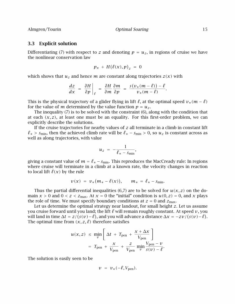
3.3 Explicit solution

Differentiating (7) with respect to z and denoting p = uz, in regions of cruise we havethe nonlinear conservation law

px + H(`(x),p

)z = 0

which shows that uz and hence m are constant along trajectories z(x) with

dzdx

= ∂H∂p

∣∣∣∣∣`= ∂H∂m

∂m∂p

= s(v∗(m− `)

)− `

v∗(m− `).

This is the physical trajectory of a glider flying in lift `, at the optimal speed v∗(m− `)for the value of m determined by the value function p = uz.

The inequality (7) is to be solved with the constraint (6), along with the condition thatat each (x, z), at least one must be an equality. For this first-order problem, we canexplicitly describe the solutions.

If the cruise trajectories for nearby values of z all terminate in a climb in constant lift`∗ > smin, then the achieved climb rate will be `∗ − smin > 0, so uz is constant across aswell as along trajectories, with value

uz = −1

`∗ − smin,

giving a constant value ofm = `∗− smin. This reproduces the MacCready rule: In regionswhere cruise will terminate in a climb at a known rate, the velocity changes in reactionto local lift `(x) by the rule

v(x) = v∗(m∗ − `(x)

), m∗ = `∗ − smin.

Thus the partial differential inequalities (6,7) are to be solved for u(x, z) on the do-main x > 0 and 0 < z < zmax. At x = 0 the “initial” condition is u(0, z) = 0, and x playsthe role of time. We must specify boundary conditions at z = 0 and zmax.

Let us determine the optimal strategy near landout, for small height z. Let us assumeyou cruise forward until you land; the lift ` will remain roughly constant. At speed v , youwill land in time ∆t = z/

(s(v)−`

), and you will advance a distance ∆x = −zv/

(s(v)−`

).

The optimal time from (x, z, `) therefore satisfies

u(x, z) ≤ minv

[∆t + Tpen +

x +∆xVpen

]

= Tpen +xVpen

+ zVpen

minv

Vpen − vs(v)− `.

The solution is easily seen to be

v = v∗(−`,Vpen).


with v∗(m,`) from (2). When landout is inevitable, you should fly at the MacCreadyspeed for the local sink rate, and as though you had a headwind of speed Vpen. The finalresult for u is

u(x, z) ≤ Tpen +xVpen

− v∗ − Vpen

s(v∗)− `zVpen

for z small.

The inequality recognizes the possibility that this strategy may be superseded by theability to climb away from the bottom boundary. But when z is small, this possibility isnegligible, and we may treat this as an equality.

3.4 Numerical solutions

Here we simply exhibit example solutions; the scheme is a simplification of the second-order one introduced below.

Figure 5 shows the trajectories and MacCready values for one realization of the lift,with values as described above. The trajectory starts 200 km from the finish, at an al-titude half of the maximum thermal height zmax = 1500 m. The upper panel shows theactual trajectory in x and z. The black regions indicate the “maximum thermal height:”the height to which it is optimal to climb in lift. At the top of the black region, the opti-mal trajectories leave the lift and cruise. The trajectories go right down to z = 0, sincethe pilot has perfect knowledge that the lift will be there.

The lower panel shows the local climb rate `(x) − smin, and the MacCready value m.By virtue of the constraint (6), the former is a lower bound for the latter. The MacCreadyvalue is approximately constant in regions of cruise. In contrast to classic MacCreadytheory, the value of this coefficient is typically equal to the climb rate experienced in theprevious thermal, when the previous one is weaker than the one ahead. This is becausewith perfect foreknowledge, the optimal strategy when approaching a strong thermal isto enter it exactly at ground level. There is a collection of paths that all converge at thispoint. The physical analogy would be a rarefaction fan in compressible gas dynamics.

The increase in MacCready number shown when the trajectories approach groundlevel, for example at around x = 80 km is due to a computational artifact known as “nu-merical viscosity,” well-known in the numerical solution of hyperbolic partial differentialequations [LeVeque, 1992]. For each trajectory that reaches a thermal at ground level atmaximum glide, there is a neighboring trajectory just below that misses the thermal andpays the landout penalty. For the landing trajectory, the optimal strategy is to increasethe MacCready value as though flying into a headwind, as discussed above. The truesolution is discontinuous along this division line, and the discretization on a finite gridcauses the landout value to diffuse upwards and affect solutions that do not land.

A really accurate solution of this problem would require explicit tracking of charac-teristics and trajectories, and would be extremely complicated geometrically. Since ourreal purpose is to solve the second-order problem below, in which numerical viscosity isdominated by the true uncertainty, we accept these minor errors.


020

4060

8010

012

014

016

018

020

00

500

1000

1500

Dis

tanc

e x

(km

)

Height (m)Tr

ajec

tory

Ther

mal

hei

ght

020

4060

8010

012

014

016

018

020

0−1012345

Dis

tanc

e x

(km

)

Speed (m/sec)

Mac

Cre

ady

setti

ngC

limb

rate

Figu

re5:

Op

tim

altr

ajec

tory

and

corr

esp

on

din

gM

acC

read

yva

lues

for

on

ere

aliz

atio

nof

lift

for

the

firs

t-ord

erp

rob

-le

m,w

ith

com

ple

tekn

ow

led

ge

of

futu

reli

ft.

Inth

eu

pp

erp

anel

,th

eth

ick

lin

eis

the

traj

ecto

ry;ve

rtic

alse

gm

ents

are

wh

ere

the

gli

der

stop

sto

clim

bin

lift

.T

he

vert

ical

lin

esb

elow

the

traj

ecto

ryd

enote

the

hei

gh

tto

wh

ich

itis

op

tim

alto

clim

bin

each

ther

mal

;if

on

een

ters

the

ther

mal

above

that

alti

tud

eit

isop

tim

alto

con

tin

ue

wit

hou

tst

op

pin

g.

Th

elo

wer

pan

elsh

ow

sth

eli

ft`(x)

(bla

ckre

gio

n),

wh

ich

isfu

lly

kn

ow

nto

the

pil

ot

atth

eb

egin

nin

g,

and

the

op

tim

alM

acC

read

yco

effici

ent

alon

gth

etr

ajec

tory

.R

eali

zed

aver

age

spee

dis

139

km

/hr.


4 Stochastic problem

We now address the much more realistic “stochastic” problem. The lift profile is againgenerated by the process (3); the only difference is that the pilot does not know theprofile in advance. He or she learns it by flying through it, so his or her informationstructure is the filtration generated by the Brownian motion Wx in decreasing x.

Now the desire to finish “as quickly as possible” is more ambiguous. US and interna-tional contest rules give a bewilderingly complex definition of this criterion. Briefly, thepilot is awarded a number of points equal to his speed divided by the fastest speed flownby any competitor on that day.

A fully realistic model would take into account all of these effects, by introducing asmany state variables as necessary. For example, elapsed time would need to be a statevariable, since speed depends on that in addition to remaining time. Also, the uncertaintyof the winner’s speed would need to be incorporated, as an extrinsic random variable,with special consideration if this pilot believes himself to be the leader. Finally, a suitableobjective function would need to be specified, taking proper account of the various waysto assess contest performance. Cochrane [1999] discusses these issues in detail.

To avoid these complexities, we define the objective function to be simply

u = minimum expectation of time to reach x = 0,

where the conditional expectation is taken over potentially uncertain future atmosphericconditions, and the minimum is taken over control strategies described below. Thisquantity depends on the starting position x, z, and the local atmospheric conditions asrepresented by the locally observed lift `(x). Since `(x) is Markovian, no past informa-tion is needed, and the value function depends on (x, z, `).

4.1 Stochastic control problem

The state variables, xt, zt, `x are solutions of the controlled stochastic differential equa-tions (3) and

dxt = −vt dt, dzt =(`xt − st

)dt, (12)

with st = s(vt), where, as before, the sink rate s(v) = smin + α(v − vmin)2 for v > vmin

and s(0) = smin.We apply the same state constraint and impose the same landout penalty as for the

first-order case. The value function is defined by

u(x, z, `) = inf(vt ,st)∈Ax,z,`

Ex,z,`[τ +φ(xτ , zτ)

]where τ is the first exit time of the pair (xt, zt) from the open set Ω = (0,+∞)2:

τ = inft ≥ 0 : (xt, zt) ∉ Ω

,

Ex,z,` denotes the expectation for the initial condition x0 = x, z0 = z, `x0 = `, and φ isthe function defined in (4).


As in the first-order problem, the value function is nonnegative and bounded on[0, xmax], is strictly increasing in x, nonincreasing in z; it is also nonincreasing in `because stronger lift cannot be detrimental. As in the deterministic case, u may fail tobe continuous when ` ≤ smin.

4.2 Second-order Hamilton-Jacobi-Bellman equation

Constraint (5) applies just as before, since the lift does not change while the glider doesnot advance in x:

uz ≥ −1

` − smin. (13)

The Dynamic Programming Principle and Itô’s Lemma give the partial differential inequal-ity

ux + H(`,uz) + a(`)u` −12b2u`` ≤ 0 (14)

with

H(`,p) = − minv∈[vmin,vmax]

(1v− s(v)− `

vp).

Boundary conditions The domain is now 0 ≤ x ≤ xmax, 0 ≤ z ≤ zmax, and −∞ < ` <∞.At x = 0 and at z = 0, zmax, we have the same boundary conditions as we gave for thefirst-order problem in Section 3.2.

Furthermore, at every point, one and only one of the equations (13,14) holds, that is,we now are to solve the system of Variational Inequalities

maxux +H

(`,uz

)+ a(`)− 1

2b2u``, −uz −

1` − smin

= 0 in ` > smin (15)

ux +H(`,uz

)+ a(`)− 1

2b2u`` = 0 in ` ≤ smin (16)

associated with the state constraint

ux +H(`,uz)+ a(`)−12b2u`` = 0 on z = zmax, (17)

the initial condition

u(0, z, `) = 0 on x = 0 (18)

and the weak Dirichlet condition

u(x,0, `) = Ψ(x) on x > 0, z = 0. (19)

We will denote the finite limits in the variable ` by ±`max, which are an approximationto the infinitely distant boundaries in the PDE. In the computation, we impose someNeumann conditions at ±`max. Specifically, we set them arbitrarily equal to 0:

u`(±`max) = 0.


Because the characteristics of the first-order part flow strongly out of the domain (as xincreases), errors at the boundary will have an effect confined to a thin boundary layer,and the exact numerical boundary conditions are not too important [LeVeque, 1992].

4.3 Numerical approximation

We continue with a detailed description of the finite difference numerical scheme we im-plemented. In 1991, Barles and Souganidis [1991] established the convergence of a classof numerical approximations toward the viscosity solution of a degenerate parabolic orelliptic fully nonlinear equation (see also Crandall and Lions [1984], Souganidis [1985]for earlier results). Although the second-order equation (15–19) is slightly different fromthe one considered by Barles and Souganidis [1991], it is appropriate to seek an approx-imation belonging to this class and we verify its convergence to a reasonable solutionexperimentally.

We apply two operator splitting techniques: the first one, which consists in splittingthe parabolic operator into an operator in the z variable and an operator in the variable `,is the nonlinear analogue of the well-known Alternate Directions method and is justifiedby Barles and Souganidis [1991]. The second one, which consists of treating separatelythe parabolic operator and the gradient constraint is specific to Variational Inequalitiesand has been applied in a variety of situations [Barles, 1997, Barles et al., 1995, Tourinand Zariphopoulou, 1994] .

4.4 Semi-discretization in “time”

Recall that distance x is our time-like variable. It is approximated by the meshn∆x|0 ≤

n ≤ N, where ∆x > 0 is the discretization step, N∆x = x, and the approximation of

the value function at the point n∆x is denoted by Un(z, `), i.e. Un(z, `) ≈ u(n∆x, z, `).Here we want to compute Un+1(z, `) in terms of Un(z, `).

• Initialize U0 = 0.

• Given Un, solve for every `,

ux +H(`,uz)=0, for z > 0, x∈(n∆x,(n+1)∆x], (20)

u(n∆x, z, `) = Un(z, `), for z > 0, (21)

u(x,0, `) = Ψ(x), (22)

and denote its computed solution at (n+ 1)∆x by Un∗.

• Given Un∗, solve for every z > 0,

ux−12b2u`` + a(`)u`=0, for ` ∈ R, x∈(n∆x,(n+1)∆x], (23)

u(n∆x, z, `) = Un∗(z, `), (24)

and denote its computed solution at (n+ 1)∆x by Un∗∗.

• Form Cn+1 =(z, `) : ` > smin and Un∗∗z < − 1

`−smin

.


• Compute the solution v of

uz = −1

` − smin, on Cn+1, (25)

u = Un∗∗ on ∂Cn+1. (26)

• Set

Un+1(z, `) =Un∗∗(z, `) if (z, `) ∈ [0,+∞)× (−∞,+∞)\Cn+1

v(z, `) if (z, `) ∈ Cn+1

4.5 Fully discretized Finite Difference scheme

We now turn to the fully discretized scheme. The approximation that will be appliedwhen cruising in the interior of the domain is explicit in the variable z and implicit in thevariable `.

Specifically, let Uni,j be the approximation of the value function at the grid point(xn, zj, ì) with xn = n∆x, zj = j∆z and ì = −`max + i∆`, where 0 ≤ i ≤ 2L, 0 ≤ j ≤ M ,M∆z = zmax and L∆` = `max.

Step 1: explicit upwind difference in z For z < zmax, we apply the following explicitupwind (monotone) Finite Difference scheme:

Un∗i,j −Uni,j∆x

= minvmin≤v≤vmax

1v−max

s(v)− ì

v,0D−zU

ni,j

− min

s(v)− ì

v,0D+zU

ni,j

,0 < j < M.

where D±z denote the standard one-sided differences, with ∆z in the denominator so thatthey approximate derivatives.

We also impose the Dirichlet boundary condition

Un∗i,j = Ψ(xn+1) = Tpen +xn+1

Vpen, for all i, j.

In practice, we solve in closed form the above minimization problem. We d not showthis computation which is straightforward. We compute the optimal control v∗ usingthe upwind difference construction

v∗ =

s(v−) < ì s(v−) ≥ ì

s(v+) ≤ ì v+

arg min

1v+− s(v+)− ì

v+D+zU

ni,j,

1v−− s(v−)− ì

v−D−zU

ni,j

s(v+) > ì vmin +√ì − smin

αv−


with

v± =min

√√√√v2

0 −1

αD±zUni,j− 1αì

, vmax

.Then we determine Un∗ by the explicit difference formula

Un∗i,j −Uni,j∆x

= 1v∗− s(v

∗)− ìv∗

D−zU

ni,j, if s(v∗) ≥ ì

D+zUni,j, else.

At the boundary z = zmax, there is a state constraint and we have to modify thescheme accordingly: we do not assume any longer that s = s(v) but we require s ≥ s(v)and s ≥ ` instead. In addition, we drop the forward finite difference in the variable z atthis boundary.

Un∗i,M −Uni,M∆x

= minvmin≤v≤vmax

1v− maxs(v), ì − ì

vD−zU

ni,M

where the optimization problem above is solved explicitly in a similar manner as in theinterior of the domain.

Step 2: Implicit upwind difference in ` For every 0 < j ≤ M , we apply the FiniteDifference scheme:

Un∗∗i,j −Un∗i,j∆x

= 12b2D2

Ùn∗∗i,j − a(ì)

D−` U

n∗∗i,j if ì > 0

D+` Un∗∗i,j if ì < 0,

where D−` Un∗∗i,j ,D+` U

n∗∗i,j are the standard implicit one sided differences divided by ∆`

and D2Ù is the usual implicit difference approximation for the second derivative Un∗∗``

D2Ù =

Un+1i+1,j +Un+1

i−1,j − 2Un+1i,j

∆`.

The above scheme inside the domain is complemented by the Neuman boundary condi-tions at ±`max

Un∗∗1,j −Un∗∗0,j = 0, Un∗∗2L−1,j −Un∗∗2L,j = 0, 0 < j ≤ M.

Step 3: Climb (gradient constraint): For ì > smin, we apply the gradient constraint atthe points at which it is violated, from top to bottom in the variable j, using an implicitscheme. Let j∗i be the smallest indice j for a given i, such that Un∗∗i,j satisfy the gradientconstraint, i.e.,

D+zUn∗∗i,j ≥ − 1

ì − smin, for all j ≥ j∗i .

Then

Un+1i,j =

Un∗∗i,j , for j ≥ j∗i ,

Un+1i,j+1 +

∆zì − smin

, for j = j∗i − 1, . . . ,1.


It is easy to verify that the scheme is consistent, stable and monotone, in the sense ofBarles and Souganidis [1991], provided ∆x is small enough. Checking its consistency isstraightforward. A sufficient condition for the monotonicity is provided by the condition

∆x ≤ ∆z · minvi,j>0

vni,j|sni,j − `i|

(27)

where vni,jand sni,j are respectively the approximations for the optimal speed and the sinkrate at (xn, zj, `i). Under the above condition, the scheme is also stable.

Finally, we mentioned earlier the first-order problem where the lift is a known func-tion of the distance to the target. An alternate method for solving this problem numeri-cally is to use a modified version of the algorithm we described above. We just eliminatethe partial derivatives with respect to ` and replace the variable ` by the given func-tion `(x). We can compare the results obtained with those coming from the explicitcalculations carried out in Section 3, and this helps us validate our algorithm.

4.6 Numerical solutions

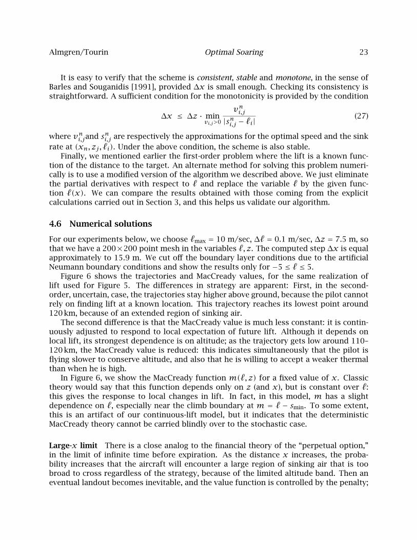
For our experiments below, we choose `max = 10 m/sec, ∆` = 0.1 m/sec, ∆z = 7.5 m, sothat we have a 200×200 point mesh in the variables `, z. The computed step ∆x is equalapproximately to 15.9 m. We cut off the boundary layer conditions due to the artificialNeumann boundary conditions and show the results only for −5 ≤ ` ≤ 5.

Figure 6 shows the trajectories and MacCready values, for the same realization oflift used for Figure 5. The differences in strategy are apparent: First, in the second-order, uncertain, case, the trajectories stay higher above ground, because the pilot cannotrely on finding lift at a known location. This trajectory reaches its lowest point around120 km, because of an extended region of sinking air.

The second difference is that the MacCready value is much less constant: it is contin-uously adjusted to respond to local expectation of future lift. Although it depends onlocal lift, its strongest dependence is on altitude; as the trajectory gets low around 110–120 km, the MacCready value is reduced: this indicates simultaneously that the pilot isflying slower to conserve altitude, and also that he is willing to accept a weaker thermalthan when he is high.

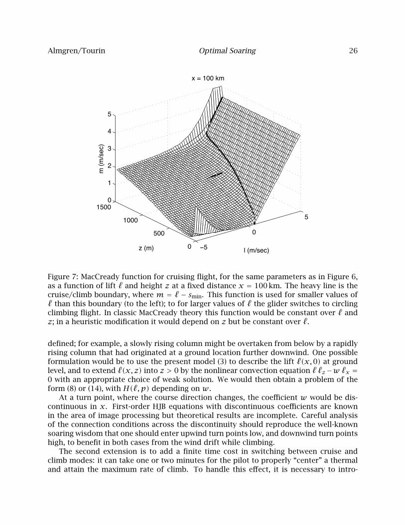
In Figure 6, we show the MacCready function m(`, z) for a fixed value of x. Classictheory would say that this function depends only on z (and x), but is constant over `:this gives the response to local changes in lift. In fact, in this model, m has a slightdependence on `, especially near the climb boundary at m = ` − smin. To some extent,this is an artifact of our continuous-lift model, but it indicates that the deterministicMacCready theory cannot be carried blindly over to the stochastic case.

Large-x limit There is a close analog to the financial theory of the “perpetual option,”in the limit of infinite time before expiration. As the distance x increases, the proba-bility increases that the aircraft will encounter a large region of sinking air that is toobroad to cross regardless of the strategy, because of the limited altitude band. Then aneventual landout becomes inevitable, and the value function is controlled by the penalty;


020

4060

8010

012

014

016

018

020

00

500

1000

1500

Dis

tanc

e x

(km

)

Height (m)Tr

ajec

tory

Ther

mal

hei

ght

020

4060

8010

012

014

016

018

020

0−10123

Dis

tanc

e x

(km

)

Speed (m/sec)

Mac

Cre

ady

setti

ngC

limb

rate

Figu

re6:

Op

tim

altr

ajec

tory

and

corr

esp

on

din

gM

acC

read

yva

lues

for

on

ere

aliz

atio

nof

lift

for

the

seco

nd

-ord

erp

rob

lem

,wit

hn

okn

ow

led

ge

of

futu

reli

ft.

As

inFi

gu

re5,i

nth

eu

pp

erp

anel

the

thic

kli

ne

isth

etr

ajec

tory

,in

clu

din

gve

rtic

alse

gm

ents

wh

ere

the

gli

der

stop

sto

clim

b,an

dth

eve

rtic

alli

nes

bel

ow

show

the

max

imu

mcl

imb

hei

gh

t.T

he

low

erp

anel

show

sth

eli

ftp

rofi

le,w

hic

his

the

sam

eas

inFi

gu

re5

bu

th

ere

dis

cove

rdb

yth

ep

ilot

on

lyw

hen

he

flie

sth

rou

gh

it.

Rea

lized

aver

age

spee

dis

105

km

/hr,

less

than

wit

hp

erfe

ctkn

ow

led

ge.


mathematically this corresponds to an Ansatz of the form u(x, z, `) = U(z, `)+ x/Vpen,where the function U is independent of x, and m(x,z, `) =m(z, `). From its maximumheight zmax, through still air the glider can travel a distance on the order of r0zmax, wherer0 is the maximum glide ratio from Section 2.1. The number of independent lift samplesencountered is therefore r0zmax/ξ ≈ 60, where ξ is the correlation length (Section 2.3).The sample distance required before encountering such a stretch of sinking air is thuson the order of ∼ exp(r0zmax/ξ) which is extremely large, and hence the large-x limit isnot relevant in practice.

Nonetheless, our computed profiles for the control variables do appear to be ap-proximately stable after 50–100 km, and Figure 7 is thus a reasonable illustration of the“generic” case for long-distance cross-country flight.

5 Conclusions

Many real-world problems involve the choice of optimal strategy in uncertain conditions.Among these, problems arising from finance play a central role, because of their prac-tical importance as well as their intrinsic interest. In financial settings, the principleof efficient markets suggests that price changes are pure Markov processes as well asmartingales, which enables the use of a set of powerful mathematical techniques.

For problems in which the randomness comes from the physical world, there is noprinciple of efficient markets. Part of the modeling challenge is to correctly incorporatethe appropriate degree of partial information. In this paper we have attempted to illumi-nate this difficulty by considering two extreme cases: one in which the agent has perfectforeknowledge, and the Markov setting in which he has none. The real situation is be-tween these, and a true optimal strategy should incorporate elements of both solutions.

The sport of soaring provides a natural laboratory for this sort of modeling: theaircraft performance is very accurately known, the cockpits are equipped with ampleinstrumentation and recording capability, and the distances and angles are such thatdirect human perception is an inadequate guide for competitive performance. For thesereasons, the sport has a history of incorporating mathematical optimizations, and wehope that these results may be useful in real competitions.

In the course of developing the mathematical model and in constructing the numer-ical solutions, we needed to draw on some common but relatively subtle aspects of themathematical theory of Hamilton-Jacobi-Bellman equations. We hope that this problemcan serve as a concrete example to stimulate further development of the theory.

5.1 Future work

Following suggestions by John Cochrane, we would like to propose two extensions of thismodel as possible subjects for future work.

The first extension is the role of wind. With a component w along the direction ofthe course, the first dynamic equation in (12) is modified to dx = −(v + w)dt; wewould neglect the crosswind component. Description of the lift is more complicatedsince the thermals also drift with the wind as they rise, and their angle of climb dependson the local vertical velocity `. This would cause the local lift to no longer be uniquely


−5

0

5

0

500

1000

15000

1

2

3

4

5

l (m/sec)

x = 100 km

z (m)

m (m

/sec

)

Figure 7: MacCready function for cruising flight, for the same parameters as in Figure 6,as a function of lift ` and height z at a fixed distance x = 100 km. The heavy line is thecruise/climb boundary, where m = ` − smin. This function is used for smaller values of` than this boundary (to the left); to for larger values of ` the glider switches to circlingclimbing flight. In classic MacCready theory this function would be constant over ` andz; in a heuristic modification it would depend on z but be constant over `.

defined; for example, a slowly rising column might be overtaken from below by a rapidlyrising column that had originated at a ground location further downwind. One possibleformulation would be to use the present model (3) to describe the lift `(x,0) at groundlevel, and to extend `(x, z) into z > 0 by the nonlinear convection equation ` `z−w `x =0 with an appropriate choice of weak solution. We would then obtain a problem of theform (8) or (14), with H(`,p) depending on w.

At a turn point, where the course direction changes, the coefficient w would be dis-continuous in x. First-order HJB equations with discontinuous coefficients are knownin the area of image processing but theoretical results are incomplete. Careful analysisof the connection conditions across the discontinuity should reproduce the well-knownsoaring wisdom that one should enter upwind turn points low, and downwind turn pointshigh, to benefit in both cases from the wind drift while climbing.

The second extension is to add a finite time cost in switching between cruise andclimb modes: it can take one or two minutes for the pilot to properly “center” a thermaland attain the maximum rate of climb. To handle this effect, it is necessary to intro-


duce a binary state variable describing whether the aircraft is currently in cruise modeor climbing. There may be locations in the state space (x, z, `) where it is optimal tocontinue climbing if one is already in the thermal, but not to stop if one is cruising. Itwould be necessary to solve for two different value functions, one for the cruise modeand one for the climb mode.

5.2 Conclusion

In this paper, we propose a stochastic control approach to compute the optimal speed-to-fly and we test the classic MacCready theory. We find that it is verified to a large extent,with small corrections, namely some slight dependence on the value of the lift, which arelikely an artifact of our model.

The remaining question is how to use these mathematical results to optimize soar-ing contest performance. Even with modern mobile computing, it is likely unrealisticto repeatedly solve a nonlinear PDE in two space-like variables, continually updating asconditions change. More plausibly, one could attempt to parameterize the computed so-lution shown in Figure 7 so as to rapidly evaluate it. This would likely be difficult becauseit is a function of three variables as well as several parameters. But more fundamentallythe details of the mathematical solution depend on the exact model used for the atmo-sphere, which is realistic only in a qualitative sense. The penalization for landout is alsonot consistent with actual contest rules.

We expect the value of this work to be in the qualitative lessons one can draw from it.The surface in Figure 7 may be approximately summarized as a function of z, constantover `; in practice this works out roughly to “MacCready equals altitude” (altitude inthousands of feet and speeds in knots). But understanding the theory and solutions pre-sented here can give the pilot confidence and a rational basis for adjusting this strategyas conditions change.


References

G. Barles. Convergence of numerical schemes for degenerate parabolic equations arisingin finance theory. In L. C. G. Rogers and D. Talay, editors, Numerical Methods in Finance,pages 1–21. Cambridge University Press, 1997.

G. Barles and P. E. Souganidis. Convergence of approximation schemes for fully nonlinearsecond order equations. Asymptot. Anal., 4:271–283, 1991.

G. Barles, C. Daher, and M. Romano. Convergence of numerical schemes for parabolicequations arising in finance theory. Math. Models Methods Appl. Sci., 5:125–143, 1995.

J. H. Cochrane. MacCready theory with uncertain lift and limited altitude.Technical Soaring, 23:88–96, 1999.Available at http://faculty.chicagobooth.edu/john.cochrane/soaring.

M. G. Crandall and P. L. Lions. Two approximations of solutions of Hamilton-Jacobiequations. Math. Comp., 43:1–19, 1984.

A. W. F. Edwards. A stochastic cross-country or festina lente. Sailplane and Gliding, 14:12–14, 1963. Reprinted in Stochastic Geometry, E. F. Harding and D. G. Kendall, editors,John Wiley & Sons 1974.

W. H. Fleming and H. M. Soner. Controlled Markov Processes and Viscosity Solutions.Springer-Verlag, 1993.

R. J. LeVeque. Numerical Methods for Conservation Laws. Springer (Birkhäuser Basel),2nd edition, 1992.

P. B. MacCready, Jr. Optimum airspeed selector. Soaring, pages 10–11, 1958.

H. Reichmann. Streckensegelflug. Motorbuch Verlag, 1975. Reprinted as Cross-CountrySoaring by the Soaring Society of America, 1978.

P. E. Souganidis. Existence of viscosity solutions of Hamilton-Jacobi equations. J. Differ-ential Equations, 56:345–390, 1985.

A. Tourin and T. Zariphopoulou. Numerical schemes for investment models with singulartransactions. Comput. Econom., 7:287–307, 1994.

N. Touzi. Optimal Stochastic Control, Stochastic Target Problems and Backward SDE,volume 29 of Fields Institute Monographs. Springer, 2013.

optimal soaring via hamilton-jacobi-bellman equationsalmgren/papers/glider.pdf · optimal soaring...

Documents