OPTIMAL STORAGE AND TRANSMISSION INVESTMENTSIN A BILEVEL ELECTRICITY MARKET MODEL

MARTIN WEIBELZAHL∗ AND ALEXANDRA MÄRTZ∗∗

Keywords: Bilevel Problem, Multistage Game, Congestion Management, Zonal Pricing, Storage Facilities,Long-Run Investments.

ABSTRACT. This paper analyzes the interplay of transmission and storage investments in a multistage gamethat we translate into a bilevel market model. In particular, on the first level we assume that a transmissionsystem operator chooses an optimal line investment and a corresponding optimal network fee. On the secondlevel we model competitive firms that trade energy on a zonal market with limited transmission capacities anddecide on their optimal storage facility investments. To the best of our knowledge, we are the first to analyzeinterdependent transmission and storage facility investments in a zonal market environment that accounts for thedescribed hierarchical decision structure. As a first best benchmark, we also present an integrated, single-levelproblem that may be interpreted as a long-run nodal pricing model. Our numerical results show that adequatestorage facility investments of firms may in general have the potential to reduce the amount of line investments ofthe transmission system operator. However, our bilevel zonal pricing model may yield inefficient investments instorages, which may be accompanied by suboptimal network facility extensions as compared to the nodal pricingbenchmark. In this context, the chosen zonal configuration of the network as well as the planning objective ofthe transmission system operator will highly influence the equilibrium investment outcomes including the sizeand location of the newly invested facilities. As zonal pricing is used for instance in Australia or Europe, ourmodels may be seen as valuable tools for evaluating different regulatory policy options in the context of long-runinvestments in storage and network facilities.

1. INTRODUCTION

Modern electricity markets are typically characterized by a spatial or regional divergence of energy supplyand demand. One example is the German electricity market with substantial wind production in the northand a high South-German consumption; see Bucksteeg et al. (2015). Given transmission capacity shortages,as a direct result of the regional divergence of demand and supply corresponding network congestion arisesin many situations, where power flows between nodes are restricted by binding technical constraints; see alsoDijk and Willems (2011) or Neuhoff et al. (2013). In this context, long-run transmission investments and theimplementation of different short-run congestion management regimes are frequently discussed as possiblesolutions to network congestion; see for instance Jenabi et al. (2013), Grimm et al. (2016a), or Grimm et al.(2016b). Besides the described regional divergence of supply and demand, intermittent renewable energysupply yields additionally a temporal divergence of the produced and consumed energy. Obviously, boththe regional and temporal dimension are highly interdependent, as for instance an extended inter-regionalnetwork may simultaneously contribute to a better adjustment of the inter-temporal divergence of demandand intermittent supply; see also Steinke et al. (2013). On the other side, storage facilities that typicallysmoothen inter-temporal demand spikes may also have the potential to lower the necessity for large networkinvestments. To the best of our knowledge, we are the first to analyze such interdependencies of storageand network investments under different congestion management regimes in a multistage game that wetranslate into a bilevel market model. As we will demonstrate, in such a framework the chosen congestionmanagement mechanism will highly influence long-run investments in both transmission lines and storagefacilities.

In particular, this paper assumes a transmission system operator (TSO) that decides on optimal lineinvestments as well as on a corresponding network fee on the first level. The TSO anticipates marketoutcomes of the second level, where competitive firms trade energy and invest in storage facilities giventhe realized network extensions of the TSO. Thus, energy trading on the second level directly accountsfor possibly scare network capacities that may result in a regionally differentiated price structure. Withinour model, we also study the effects of different zonal designs as well as the effects of different planning

Date: March 30, 2017.1

objectives of the TSO including welfare and profit maximization. In this context we will evaluate bothabsolute investment levels as well as the locations of the corresponding facility investments. Given that zonalpricing is applied in different European countries as well as in Australia (see for instance Bjørndal et al.(2003), Glachant and Pignon (2005), and Dijk and Willems (2011)), our analyses may directly contribute tothe current policy discussion on the design of efficient market structures that account for adequate long-runinvestment incentives in both storage facilities and network lines. In addition, in times of growing importanceof storage facilities the proposed models may also be seen as tools for a meaningful evaluation of the needfor huge network extension plans that typically involve billions of euros like in Germany; for more detailssee German-Transmission-System-Operators (2017).

As our numerical results show, both under nodal and zonal pricing storage investments may in generalhave the potential to reduce network extensions as compared to the no-storage case. However, our bilevel,zonal-pricing-market model may yield inefficient storage facility investments that may be accompanied bysuboptimal line investments as compared to a nodal pricing model. Moreover, invested storage facilitiesmay affect inter-regional price and demand structures in a way that requires a complete reconfiguration ofoptimal zonal boundaries, i.e., in the case of storage facilities the welfare-maximizing zone configurationmay change as compared to the no-storage case. Finally, if planning objectives of the TSO are not alignedwith a maximization of welfare, the described investment inefficiencies may further be aggravated.

Our work directly contributes to various strands of the energy market literature. In particular, we elaborateon different congestion management regimes. In the context of congestion management, nodal pricesare know to yield a first best outcome, as they simultaneously reflect all relevant economic and technicalrestrictions between the different nodes of the network; see Bohn et al. (1984), Hogan (1992), or Chao andPeck (1996). In contrast, zonal pricing assumes identical prices within given zonal boundaries, which directlyyield a simplified price structure; see Bjørndal et al. (2014). Even though, zonal pricing may in general beaccompained by a welfare loss as compared to a system of nodal prices, it is sometimes seen as being moreattractive from an administratively and politically point of view. For this reason, various studies have focusedon properties of zonal pricing systems that ensure a comparatively small welfare loss. Such propertiesrelate for instance to the number of price zones and their respective boundaries; see Bjørndal and Jørnsten(2001), Ehrenmann and Smeers (2005), or Oggioni and Smeers (2013). In addition, we also contribute to theincreasing literature on transmission investments. Traditionally, reference investment solutions were derivedfor integrated, single-level optimization problems as in Gallego et al. (1998), Hirst and Kirby (2001), orAlguacil et al. (2003). However, in recent years transmission investments were also analyzed in multistagegames and corresponding multilevel optimization problems; see for instance Sauma and Oren (2006), Fanet al. (2009), Garcés et al. (2009), Baringo and Conejo (2012), or Jenabi et al. (2013). As pointed out byGrimm et al. (2016b), in such games the market environment and the chosen congestion management regimewill highly influence optimal transmission expansions of the TSO. In particular, hierarchical market modelsmay yield suboptimal line investments as compared to an integrated network expansion plan. Finally, we linkthe two above stands of congestion management and transmission investment literature to existing studies onprice and welfare effects of storage facilities. Most of the latter studies including Sioshansi et al. (2009),Sioshansi (2010), Gast et al. (2013), and Sioshansi (2014) mainly abstract from transmission constraintsand the network management regime. Only recently, Weibelzahl and Märtz (2017) study storage facilitiesand their effects in a zonal electricity market. However, the authors only consider the short-run perspective,where both the transmission network and storage facilities are given. It is the aim of the present paper toanalyze the interplay of transmission and storage facility investments in a multilevel market environmentfrom a long-run perspective.

This paper is organized as follows. Our model framework is introduced in Section 2. Then, Section 3and Section 4 present the nodal pricing reference model and the bilevel zonal pricing model with storage,respectively. The main solution strategy for our multistage game and for the corresponding bilevel optimiza-tion model is then discussed in Section 5. Numerical results of our long-run investment analysis regardingstorage facility investments and network extensions are presented in Section 6. Finally, Section 7 concludesand highlights main policy implications.

2. NOTATION AND ECONOMIC QUANTITIES

This section introduces the main model framework that is used in our paper. All sets, parameters, andvariables are summarized in Tables 5, 6, and 7 in the appendix.

2.1. Electricity Network and Time Horizon. In order to keep our analysis simple, we only consider anoff-peak period t1 and an on-peak period t2, i.e, we assume that the time period set is given by T = {t1, t2};

wl

Il(wl)

1binvl

ainvl

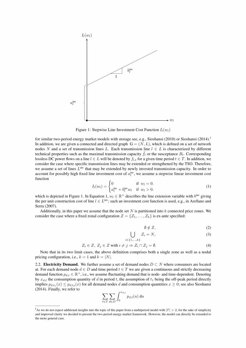
Figure 1: Stepwise Line Investment Cost Function Il(wl)

for similar two-period energy market models with storage see, e.g., Sioshansi (2010) or Sioshansi (2014).1

In addition, we are given a connected and directed graph G = (N ,L), which is defined on a set of networknodes N and a set of transmission lines L. Each transmission line l ∈ L is characterized by differenttechnical properties such as the maximal transmission capacity f̄l or the susceptance Bl. Correspondinglossless DC power flows on a line l ∈ L will be denoted by fl,t for a given time period t ∈ T . In addition, weconsider the case where specific transmission lines may be extended or strengthened by the TSO. Therefore,we assume a set of lines Linv that may be extended by newly invested transmission capacity. In order toaccount for possibly high fixed line investment cost of ainv

l , we assume a stepwise linear investment costfunction

Il(wl) ={

0 if wl = 0.ainvl + binv

l wl if wl > 0.(1)

which is depicted in Figure 1. In Equation 1, wl ∈ R+ describes the line extension variable with binv givingthe per unit construction cost of line l ∈ Linv; such an investment cost function is used, e.g., in Arellano andSerra (2007).

Additionally, in this paper we assume that the node set N is partitioned into k connected price zones. Weconsider the case where a fixed zonal configuration Z = {Z1, . . . ,Zk} is ex-ante specified:

∅ /∈ Z, (2)⋃i∈{1,...,k}

Zi = N , (3)

Zi ∈ Z, Zj ∈ Z with i 6= j ⇒ Zi ∩ Zj = ∅. (4)

Note that in its two limit cases, the above definition comprises both a single zone as well as a nodalpricing configuration, i.e., k = 1 and k = |N |.

2.2. Electricity Demand. We further assume a set of demand nodes D ⊂ N where consumers are locatedat. For each demand node d ∈ D and time period t ∈ T we are given a continuous and strictly decreasingdemand function pd,t ∈ R+, i.e., we assume fluctuating demand that is node- and time-dependent. Denotingby xd,t the consumption quantity of d in period t, the assumption of t1 being the off-peak period directlyimplies pd,t1(x) ≤ pd,t2(x) for all demand nodes d and consumption quantities x ≥ 0; see also Sioshansi(2014). Finally, we refer to ∑

t∈T

∑d∈D

∫ xd,t

0pd,t(u) du

1As we do not expect additional insights into the topic of this paper from a multiperiod model with |T | > 2, for the sake of simplicityand improved clarity we decided to present the two-period energy market framework. However, the model can directly be extended tothe more general case.

as the gross consumer surplus that is aggregated over all demand nodes and time periods. This grossconsumer surplus measures the sum of all monetary consumer benefits.

2.3. Electricity Generation. Throughout this paper, we will denote by G the set of all ex-ante givengeneration facilities. Gn ⊂ G describes the generators, which are located at a node n. In addition, we denoteproduction of a generator g in a time period t by yg,t. Production is further described by a continuous andstrictly increasing marginal cost function Vg,t ∈ R+ that gives the respective variable production costs of agenerator; see also Chao and Peck (1998), Bjørndal and Jørnsten (2001), Ehrenmann and Smeers (2005), orOggioni and Smeers (2013).

We will assume that all firms act in a perfectly competitive environment as price takes. Such an assumptionhas been established as a standard in order to keep complex electricity market models computationallytractable, see, e.g., Boucher and Smeers (2001), Daxhelet and Smeers (2007), Grimm et al. (2016b), orWeibelzahl (2017). We further note that such models may also serve as a benchmark for evaluating deviationsfrom perfect competition, i.e., market power.

2.4. Storage Facilities. Finally, we assume a set of storage facilities S that may be invested in. The non-storage scenario is captured by the limit case S = ∅. As above, by Sn ⊂ S we denote the subset of storagefacilities that are located at node n. Storage facilities are described by their (roundtrip) storage efficiencyρs ∈ [0, 1]; see for instance Sioshansi et al. (2014). Storage investment costs are given by a continuous andstrictly increasing function Is(z̄s) ∈ R+, with z̄s denoting the invested storage capacity. An example isan affine investment function with a positive slope.2 Further note that our framework allows to explicitlyanalyze both the size and location of storage facility investment within the electricity network G. For eachstorage facility we additionally introduce the variables z+

s,1 and z−s,2 that describe the amount of electricitythat is stored in or stored out in period 1 and 2, respectively. The latter two variables are obviously limited bythe invested storage capacity z̄s.

2.5. Network Fees. In order to recover network investment cost, the TSO charges a network fee. Inparticular, we consider the case of a production-based fee that is paid for each unit of produced electricity.The corresponding fee is denoted by ϕTSO. Income ITSO of the TSO is given by

ITSO =∑t∈T

∑n∈N

∑g∈Gn

ϕTSOyg,t. (5)

Analogously, expenses of the TSO in form of line investments can be written as

ETSO =∑l∈Linv

Il(wl), (6)

with the difference P TSO = ITSO − ETSO describing profits of the TSO.

3. INTEGRATED PLANNING WITH STORAGE FACILITIES AS AN OVERALL INVESTMENT OPTIMUM

As a first best benchmark, we present an integrated planning model, which may alternatively be interpretedas a nodal pricing model similar to Jenabi et al. (2013), Grimm et al. (2016a), Grimm et al. (2016b), orWeibelzahl and Märtz (2017). We add storage facility investments to these standard models in order toderive welfare-maximizing line and storage capacities that account for all relevant technical and economicrestrictions in a single-level optimization problem. Therefore, this reference investment solution can be usedto assess and evaluate inefficiencies of our zonal market model in Section 4, where investments are made ina complex hierarchical environment based on the expectations of the optimal decision response of marketplayers.

In line with Section 2, we assume fully competitive firms that have no market power. This assumptiondirectly implies that nodal pricing may be modeled as a welfare maximization problem:

W i :=∑t∈T

∑d∈D

∫ xd,t

0pd,t(u) du−

∑n∈N

∑g∈Gn

∫ yg,t

0Vg,t(u) du

−∑s∈S

∫ z̄s

0Is(u) du−

∑l∈Linv

Il(wl).

(7)For each storage facility s ∈ S, the storage level in period 1 is described by the amount of stored in

electricity less than the storage loss (1− ρs)z+s,1. Assuming an adequate planning in terms of an optimal end

of horizon inventory, we additionally require each storage facility to be empty in period 2, i.e.,

ρsz+s,1 − z

−s,2 = 0 ∀ s ∈ S. (8)

2Observe that for an infinitely small slope such an affine investment cost function will converge to a constant investment cost function.

Denoting by δinn (L) and δout

n (L) the set of in- and outgoing lines of node n ∈ N , Kirchhoff’s First Lawensures power balance at every node and in each of the two time periods, i.e., demand, generation, chargingand discharging activities as well as power flows in and out of a given node are balanced:

xn,1 =∑g∈Gn

yg,1 +∑

l∈δinn(L)

fl,1 −∑

l∈δoutn (L)

fl,1 −∑s∈Sn

z+s,1 ∀ n ∈ N . (9)

xn,2 =∑g∈Gn

yg,2 +∑

l∈δinn(L)

fl,2 −∑

l∈δoutn (L)

fl,2 +∑s∈Sn

z−s,2 ∀ n ∈ N . (10)

For all lines, the following set of constraints ensures that no transmission capacities are exceeded:

− f l ≤ fl,t ≤ f l ∀ l ∈ L \ Linv, t ∈ T . (11)

−(f l + wl) ≤ fl,t ≤ (f l + wl) ∀ l ∈ Linv, t ∈ T . (12)

Power flows fl,t on each line l = (n,m) are further characterized by Kirchhoff’s Second Law, whichlinks line flows to the corresponding phase angles Θn,t, and Θm,t:

fl,t = Bl (Θn,t −Θm,t) ∀ l = (n,m) ∈ L, t ∈ T . (13)

We additionally set the phase angle of the reference node 1 to zero, which will ensure unique phase anglevalues (see also Section 5):

Θ1,t = 0 ∀ t ∈ T . (14)

Moreover, we assume that storage investment is nonnegative

z̄s ≥ 0 ∀ s ∈ S, (15)

and that all charging and discharging variables will not violate their lower nonnegativity bounds as well astheir upper storage capacity investment bounds, respectively:

0 ≤ z+s,1 ≤ z̄s, 0 ≤ z−s,2 ≤ z̄s ∀ s ∈ S. (16)

In analogy, demand and generation are restricted by the following nonnegativity constraints:

0 ≤ xn,t ∀ n ∈ N , t ∈ T . (17)0 ≤ yg,t ∀ n ∈ N , g ∈ Gn, t ∈ T . (18)

Finally, we use some simple variable bounds on the line investment quantities:

wl ∈ R+ ∀ l ∈ Linv. (19)

Thus, the complete nodal-pricing problem can be stated as:

max Welfare : (7), (20a)s.t. Storage Level Constraints: (8), (20b)

Kirchoff’s First Law: (9), (10), (20c)Flow Restrictions: (11), (12), (20d)Kirchhoff’s Second Law: (13), (20e)Reference Phase Angle: (14), (20f)Variable Restrictions: (15), (16), (17), (18), (19). (20g)

Let us conclude this section with an observation: The well-known concept of congestion cost measure thewelfare loss of a network-constrained model (20) as compared to a non-network model, where transmissionconstraints and power flows do not play a relevant role. Obviously, we could relax all power flow restrictionsin Problem (20) to derive the optimal welfare under such a non-network model. Given the optimal welfarelevel of such a non-network model, our network-based (nodal pricing) model (20) with its welfare maximiza-tion objective (7) can be equivalently rewritten as the minimization of the derived optimal objective functionvalue of the model without network restrictions and the corresponding network-restricted objective. Thedifference of these two quantities measures congestion costs.

Observation 1. The nodal pricing model (20) does not only maximize welfare, but also minimizes congestioncost.

4. BILEVEL ZONAL PRICING MODEL WITH STORAGE

4.1. Structure of the Hierarchical Game and the Corresponding Bilevel Optimization Problem. Eventhough, an integrated, nodal pricing system ensures welfare maximizing investments, such a first bestmechanism is not a realistic policy option for different countries and regions including for instance Europe;see Oggioni and Smeers (2013) or Bucksteeg et al. (2015). In contrast, in liberalized electricity marketsdecisions of independent market players are typically made in a highly complex market environment, whichoften uses a system of zonal prices. In such an interdependent market structure, the extent of optimalline investment of the TSO highly depends on optimal storage facility investments and vice versa. Whiletransmission line extensions base on the respective regulatory structures, investments in storage facilitiesare driven by future profits of firms and corresponding structures of the (zonal) market. As we will see inour numerical results that are presented in Section 6, such a complex market environment will yield a quitedifferent equilibrium investment solution as compared to our integrated benchmark model.

In this section we assume that the TSO decides on an optimal transmission expansion and on a correspond-ing network fee before firms invest in their storage facilities. In this hierarchical game the TSO is the leaderthat is the first to make an optimal investment decision with competitive firms reacting as followers in anoptimal way to the leader’s investment choice; see also the vast literature including Gil et al. (2002), Saumaand Oren (2006), Fan et al. (2009), Garcés et al. (2009), Baringo and Conejo (2012), Jenabi et al. (2013),and Grimm et al. (2016b) that also consider multistage games with the TSO acting as the leader. Our gamedirectly relates to the classical problem of Von Stackelberg (2010), where a leader and different followersinteract in an anticipative environment. Note that in our setting the sequential investment decisions of theTSO and of the firms are followed by trading on two zonal spot markets, which determine the profitabilityand efficiency of the respective investment decisions; see also Figure 2. As in Sauma and Oren (2006),we assume that at each stage all (investment) decisions of the previous stage(es) can be observed by therational players, which allows a correct expectation formation. Therefore, our game can be translated intoa bilevel programming problem with a network-extending TSO on the first level that anticipates storageinvestments and competitive market outcomes on the second level. Observe that storage investment andspot market trading may be analyzed jointly on the second level, as we assume a competitive market, wherestorage investments directly determine the stored amounts of energy in the two trading periods; for detailssee Section 5.1. The two problem levels will be described in more detail in the following two sections.

t

line expansion(TSO)

storage facilityinvestment (firms)

|T | = 2 periods of zonal spotmarket trading (firms)

Figure 2: Timing of the Underlying Multistage Game

4.2. First Level Problem: Network Extension. On the first level, we assume that the TSO chooses aline expansion plan, i.e., the TSO decides, which line to extend by which amount. Such a long-termnetwork development of the grid is a very challanging task, as in principle the TSO should eliminate all thetransmission capacity shortages that are welfare diminishing; see also Hornnes et al. (2000), David and Wen(2001), or Rious et al. (2008). Despite this theoretical aim, in practice the TSO must both have an incentiveand the responsibility to implement such a welfare maximizing extension plan. As a main drawback, theconcept of welfare may not directly be measured and observed by the TSO, which will make it difficult forthe TSO to decide on an efficient network expansion plan. As pointed out by Hirst and Kirby (2001), for thisreason there may be quite different objectives that the TSO can pursue. A summary of objectives that arediscussed in the literature can be found in Table 1. However, as some of the objectives presented in Table1 will either be difficult to quantify or will be outside the scope of our model framework, in this paper wefocus on the three extreme cases where the TSO maximizes (i) social welfare W , (ii) its own profits P TSO,or (iii) tries to eliminate as much transmission obstacles O as possible, i.e., aims at a maximization of lineextensions in order to reduce transmission limitations in the network. The corresponding objectives can bestated as:

TABLE 1. Different Transmission Expansion Objectives of the TSO

Objective Reference

Welfare maximization Sauma and Oren (2006), Torre et al. (2008), Garcés et al. (2009);Network reliability Hirst and Kirby (2001), Jenabi et al. (2013);Elimination of transmission obstacles/ Buygi et al. (2004);Robust networkMaximization of competition Motamedi et al. (2010), Zhao et al. (2011);Profit maximization of the TSO Jenabi et al. (2013), Fan et al. (2009);Investment cost minimization Oliveira et al. (1995), Gallego et al. (1998), Gil et al. (2002);Cheap electricity prices Hirst and Kirby (2001), Zhao et al. (2011);Facilitation of trade/ Motamedi et al. (2010);Maximization of consumption

W f :=∑t∈T

(∑d∈D

∫ xd,t0 pd,t(u) du−

∑n∈N

∑g∈Gn

∫ yg,t0 Vg,t(u) du

)(21)

−∑s∈S

∫ z̄s

0 Is(u) du−∑l∈Linv Il(wl).

P TSO :=∑t∈T

∑n∈N

∑g∈Gn

ϕTSOyg,t −∑l∈Linv Il(wl). (22)

O :=∑l∈Linv wl. (23)

In all three model variants, we will assume that the TSO uses a production-based network fee in order torecover its network investment costs. The following budget constraint ensures that investment costs of theTSO are covered by its income in form of network fees:∑

t∈T

∑n∈N

∑g∈Gn

ϕTSOyg,t ≥∑l∈Linv

Il(wl). (24)

Finally, we use some simply variable bounds on the line investment quantities:

wl ∈ R+ ∀ l ∈ Linv. (25)

Altogether, the first-level problem can be written as:

max Objective : (21), (22), or (23) (26a)s.t. Budget Constraint: (24), (26b)

Investment Variable Restrictions: (25). (26c)

4.3. Second Level Problem: Storage Investment and Energy Trading. On the second level firms investin new storage technologies and trade energy on a competitive market. Note that the decision behaviour ofthe firms on the second level is part of the constraint set of the TSO on the first level.

As in Jenabi et al. (2013), the assumption of full competition allows to model profit maximizationbehaviour of firms as a welfare maximization problem, where costs in form of the transmission fee ϕTSO aredirectly taken into account:

W s :=∑t∈T

∑d∈D

∫ xd,t

0pd,t(u) du−

∑n∈N

∑g∈Gn

(ϕTSOyg,t +

∫ yg,t

0Vg,t(u) du

)−∑s∈S

∫ z̄s

0Is(u) du.

(27)As in Section 2, we consider a given zonal configuration Z, which satisfies the connectivity conditions (2)

to (4). We will use the zonal pricing formulation introduced by Bjørndal and Jørnsten (2001), which requiresthat consumer and producer prices at network nodes that belong to a given zone Zi ∈ Z must be equal forevery time period t ∈ T 3:

pn,t = pm,t, ∀ i ∈ {1, . . . , |Z|}, {(n,m) : n,m ∈ Zi ∩D, n < m} , (28)

Vg,t + ϕTSO = pm,t, ∀ i ∈ {1, . . . , |Z|},{(n,m) : n ∈ Zi ∩DC, m ∈ Zi ∩D, n < m

}, g ∈ Gn, (29)

3For applications of this zonal pricing formulation see Bjørndal et al. (2003), Ehrenmann and Smeers (2005), Bjørndal and Jørnsten(2007), Weibelzahl (2017), or Weibelzahl and Märtz (2017).

pn,t = Vg,t + ϕTSO, ∀ i ∈ {1, . . . , |Z|},{(n,m) : n ∈ Zi ∩D, m ∈ Zi ∩DC, n ≤ m

}, g ∈ Gm, (30)

Vg,t + ϕTSO = Vg̃,t + ϕTSO, ∀ i ∈ {1, . . . , |Z|},{(n,m) : n,m ∈ Zi ∩DC, n ≤ m

}, g ∈ Gn, g̃ ∈ Gm, (31)

where we explicitly distinguish between demand and production nodes and account for the transmission feeof the TSO.

As all equilibrium quantities must be both technically and economically feasible, on the second levelall power flow, production, storage, and market clearing constraints discussed in Section 3 are taken intoaccount. Therefore, the second level problem can be written as:

max Welfare : (27), (32a)s.t. Zonal Pricing: (28), (29), (30), (31), (32b)

Storage Level Constraints: (8), (32c)Kirchoff’s First Law: (9), (10), (32d)Flow Restrictions: (11), (12), (32e)Kirchhoff’s Second Law: (13), (32f)Reference Phase Angle: (14), (32g)Variable Restrictions: (15), (16), (17), (18). (32h)

Let us conclude this section with the following observation, which states that welfare under the integratedplanning model (20) yields an upper bound for the bilevel model (26) and (32):

Observation 2. For all variants of the bilevel model (26) and (32), its optimal welfare level can not exceedwelfare of the integrated planning model in (20), i.e., welfare of the integrated model is at least as high aswelfare of the bilevel model.

5. SOLUTION STRATEGY AND PROBLEM REFORMULATION

Our market model introduced in the previous section can be seen as a special instance of a general bilevelmodel. Being non-convex and non-differentiable, bilevel models are known to be NP hard, which impliesthat this class of optimization problem is in gereral very challenging and hard to solve; see for instanceJeroslow (1985). In this section we present a single-level problem reformulation and discuss our mainsolution strategy.

5.1. Uniqueness of the Second Level Problem and KKT Reformulation. Given that the second level isa convex and continous optimization problem with only linear constraints, we can use a Karush-Kuhn-Tucker(KKT) reformulation in order to replace the bilevel problem by a single-level problem; see for instanceDempe (2002), Boyd and Vandenberghe (2004), or Colson et al. (2007). From a mathematical point of view,such a reformulation strategy yields a mathematical program under equilibrium constraints (MPEC); seeHuppmann and Egerer (2015). However, a KKT reformulation is only valid, as the second-level problemhas a unique optimal solution. In particular, in the case of nonuniqueness of lower-level optimal solutions,the TSO cannot anticipate the optimal storage investment choice of firms. On the other hand, the TSO canalso not force the implementation of specific investments out of the set of multiple optimal storage facilityextension plans. Ultimately, it will be impossible for the TSO to assess the value of an optimal transmissionexpansion on the first level; for details and further discussions see, e.g., Dempe (2003) or Zugno et al. (2013).From a policy persepctive, such ambiguities will also make it hard to compare different policy regulationsand market designs, as it is unclear which equilibrium investments will be realized; see also Hu and Ralph(2007).

Being a prerequisite for meaningful bilevel policy analyses, we first prove uniqueness of the optimalsolution of the second-level problem, before we present our KKT reformulation.

Theorem 1. The second level problem (32) has a unique optimal solution.

Proof. By assumption, all demand functions pd,t are continuous and strictly decreasing. In addition, boththe variable cost functions Vg,t and the storage investment functions Is are continuous and strictly increasing.As a direct consequence, the second-stage objective is strictly concave in all demand, production, and storage

investment variables, with

∂2W s

∂x2d,t

= p′d,t ∀ d ∈ D, t ∈ T , ∂2W s

∂y2g,t

= −V ′g,t ∀ n ∈ N , g ∈ Gn, t ∈ T ,

∂2W s

∂z̄2s

= −I ′s ∀ n ∈ N , s ∈ Sn.

This strict concavity directly implies uniqueness of these variables; see Mangasarian (1988).We next show that for each storage facility s, the amount of stored-in electricity z+

s,1 in period 1 equals theuniquely determined storage capacity z̄s. To see this, assume the contrary, i.e., consider the case z+

s,1 < z̄s.Obviously, z̄∗s := z+

s,1 is also a feasible solution. However, as z̄∗s yields a welfare increase as compared to z̄s,with M W = W (·, z̄∗s )−W (·, z̄s) =

∫ z̄s

z̄∗sIs(u)du > 0, the original investment level z̄s cannot be optimal.

Obviously, this yields a contradiction. In addition, for each storage facility s ∈ S, the amount of stored outelectricity is uniquely determined by Constraint (8), which readily implies z−s,2 = z+

s,1.To show uniqueness of power flows, we finally consider Kirchhoff’s First Laws (9) and (10). For all

nodes n ∈ N we set

Fn,1 := xn,1 −∑g∈Gn

yg,1 +∑s∈Sn

z+s,1, (33)

Fn,2 := xn,2 −∑g∈Gn

yg,2 −∑s∈Sn

z−s,2, (34)

and rewrite Constraints (9) and (10) for both periods t ∈ {t1, t2} as:

Fn,t =∑

l∈δinn(L)

Bl (Θn,t −Θm,t)−∑

l∈δoutn (L)

Bl (Θn,t −Θm,t) . (35)

Using (35), we see that for the unique optimal demand, production, and storage variable values captured byFn,t, all phase angles are determined by a system of linear equations, which can equivalently be stated as thefollowing matrix representation

Ft = BΘt, ∀ t ∈ T , (36)

where Θt denotes the vector of phase angles in period t, Ft is the vector of optimal nodal net injections inperiod t, and B is the corresponding matrix of (aggregated) susceptances. As

∑n∈N Fn,t = 0 holds for all

time periods t, it directly follows that B is singular. However, in Constraint (14) we have set the phase anglevalue of the (arbitrarily chosen) reference node to zero, which yields non-singularity. Ultimately, optimalphase angles will be uniquely determined. By using the relation between phase angles and power flows givenby Constraint (13), in each period and on each line optimal power flows will also be unique. �

Given the above result, we equivalently describe the second-level problem by its KKT formulation, whichcomprises primal and dual feasibility as well as complementary slackness. We first state the correspondingprimal-dual pairs of complementarity, where the symbol ⊥ denotes orthogonality:

0 ≤ fl,t + f l ⊥ δlowl,t ≥ 0 ∀ l ∈ L \ Linv, t ∈ T , (37)

0 ≤ −fl,t + f l ⊥ δupl,t ≥ 0 ∀ l ∈ L \ Linv, t ∈ T , (38)

0 ≤ fl,t + (f l + wl) ⊥ εlowl,t ≥ 0 ∀ l ∈ Linv, t ∈ T , (39)

0 ≤ −fl,t + (f l + wl) ⊥ εupl,t ≥ 0 ∀ l ∈ Linv, t ∈ T , (40)

0 ≤ xd,t ⊥ υd,t ≥ 0 ∀ d ∈ D, t ∈ T , (41)0 ≤ yg,t ⊥ νg,t ≥ 0 ∀ n ∈ N , g ∈ Gn, t ∈ T , (42)

0 ≤ z+s,1 ⊥ ρs,1 ≥ 0 ∀ n ∈ N , s ∈ Sn, (43)

0 ≤ z−s,2 ⊥ ϕs,2 ≥ 0 ∀ n ∈ N , s ∈ Sn, (44)0 ≤ z̄s ⊥ χs ≥ 0 ∀ n ∈ N , s ∈ Sn, (45)

0 ≤ −z+s,1 + z̄s ⊥ ζs,1 ≥ 0 ∀ n ∈ N , s ∈ Sn, (46)

0 ≤ −z−s,2 + z̄s ⊥ ηs,2 ≥ 0 ∀ n ∈ N , s ∈ Sn. (47)

Note that these complementarity pairs correspond exclusively to inequalities of the primal problem, whileprimal equality constraints are only equipped with unrestricted dual variables:

0 =∑g∈Gn

yg,1 +∑

l∈δinn(L)

fl,1 −∑

l∈δoutn (L)

fl,1 −∑s∈Sn

z+s,1 − xn,1 and α1

n,1 ∈ R ∀ n ∈ N , (48)

0 =∑g∈Gn

yg,2 +∑

l∈δinn(L)

fl,2 −∑

l∈δoutn (L)

fl,2 +∑s∈Sn

z−s,2 − xn,2 and α2n,2 ∈ R ∀ n ∈ N , (49)

0 = Bl (Θn,t −Θm,t)− fl,t and βl,t ∈ R ∀ l ∈ L, t ∈ T , (50)0 = Θ1,t and γt ∈ R ∀ t ∈ T , (51)

0 = ρsz+s,1 − z

−s,2 and ι2s ∈ R ∀ s ∈ S, (52)

0 = pm,t − pn,t and ω1t,n,m ∈ R (53)

∀ i ∈ {1, . . . , |Z|}, t ∈ T ,{(n,m) : n,m ∈ Zi ∩D, n < m},

0 = pm,t − Vg,t − ϕTSO and ω2t,m,g ∈ R (54)

∀ i ∈ {1, . . . , |Z|}, t ∈ T ,{(n,m) : n ∈ Zi ∩DC,m ∈ Zi ∩D, n < m}, g ∈ Gn,

0 = Vg,t + ϕTSO − pn,t and ω3t,n,g ∈ R (55)

∀ i ∈ {1, . . . , |Z|}, t ∈ T ,{(n,m) : n ∈ Zi ∩D,m ∈ Zi ∩DC, n ≤ m}, g ∈ Gm,

0 = Vg,t − Vg̃,t and ω4t,g,g̃ ∈ R (56)

∀ i ∈ {1, . . . , |Z|}, t ∈ T ,{(n,m) : n,m ∈ Zi ∩DC,n ≤ m}, g ∈ Gn, g̃ ∈ Gm.

We complement the KKT system with the set of dual feasibility requirements that correspond to thepartial derivates with respect to the primal variables

− δlowl,1 + δup

l,1 +∑

n∈N :l∈δinn(L)

α1n,1 −

∑n∈N :l∈δout

n (L)

α1n,1 − βl,1 = 0 ∀ l ∈ L \ Linv, (57)

−δlowl,2 + δup

l,2 +∑

n∈N :l∈δinn(L)

α2n,2 −

∑n∈N :l∈δout

n (L)

α2n,2 − βl,2 = 0 ∀ l ∈ L \ Linv, (58)

−εlowl,1 + εup

l,1 +∑

n∈N :l∈δinn(L)

α1n,1 −

∑n∈N :l∈δout

n (L)

α1n,1 − βl,1 = 0 ∀ l ∈ Linv, (59)

−εlowl,2 + εup

l,2 +∑

n∈N :l∈δinn(L)

α2n,2 −

∑n∈N :l∈δout

n (L)

α2n,2 − βl,2 = 0 ∀ l ∈ Linv, (60)

∑l∈δout

n (L)

Blβl,t −∑

l∈δinn(L)

Blβl,t + γt = 0 ∀ n ∈ N : n = 1, t ∈ T , (61)

∑l∈δout

n (L)

Blβl,t −∑

l∈δinn(L)

Blβl,t = 0 ∀ n ∈ N : n ≥ 2, t ∈ T , (62)

−ρs,1 + ζs,1 + ρsι2s −

∑n∈N :s∈Sn

α1n,1 = 0 ∀ s ∈ S, (63)

−ϕs,2 + ηs,2 − ι2s +∑

n∈N :s∈Sn

α2n,2 = 0 ∀ s ∈ S, (64)

Is − χs − ζs,1 − ηs,2 = 0 ∀ s ∈ S, (65)

in addition to the derivatives with respect to demand and generation quantities that we skip given their hugenumber of different cases.

5.2. Linearization of Complementary Slackness Conditions and Final Single-Level Problem Refor-mulation. In the above KKT reformulation, all constraints except the complementariy slackness conditionsare linear. Exploiting the disjunctive structure of these complementary slackness conditions, in this sectionwe use a Fortuny-Amat-like linearization to handle these nonconvexities in Equations (37) to (47); seeFortuny-Amat and McCarl (1981). For example, KKT condition (41) can be linearized as

0 ≤ xd,t ≤ Md,tmd,t ∀ d ∈ D, t ∈ T , (66)0 ≤ υd,t ≤ Md,t(1−md,t) ∀ d ∈ D, t ∈ T , (67)

where md,t ∈ {0, 1} is a binary auxiliary variable and Md,t, Md,t are sufficiently large constants denoted as"big-M". Note that from a computational point of view it is important to choose adequate big-M parametersthat are as large as necessary but as small as possible. For instance, in the above example we could setMd,t = pd,t(0), which gives the maximum consumption possible at demand node d in period t.

In an analogous way we also linearize and reformulate all complementarity constraints in (37) to (47),which yields a more tractable problem formulation. Applying the results of the present and the previoussection, the single-level reformulation of our bilevel model is given by the first-level objective that is subjectto

(1) the original first-level constraints,(2) the primal constraints of the second-level problem,(3) the linearized complementary slackness conditions, and(4) the dual feasibility constraints.

We implemented this single-level mixed-integer program in Zimpl (see Koch (2004)) and used SCIP (seeAchterberg (2009)) as a solver.

6. ON THE EFFECTS OF STORAGE FACILITIES ON OPTIMAL PRICING:A CASE STUDY BASED ON CHAO AND PECK (1996)

6.1. Six-Node Network. In this section we analyze the economic interdependencies of transmission andstorage facility investments under different market environments including the integrated planning referencecase as well as various variants of our bilevel market model. We consider the standard six-node example ofChao and Peck (1998) that has frequently been used for various policy-related analysis including Ehrenmannand Smeers (2005), Oggioni and Smeers (2013), or Grimm et al. (2016b). As can be seen in Figure 3, thenetwork consists of three demand nodes (node 3, node 5, and node 6) and three production nodes (node 1,node 2, and node 4) that are interconnected by 8 transmission lines. Storage facilities with constant losses of10% may be built at the three demand nodes, respectively. Only the two lines that interconnect the north withthe south have a limited capacity of 200 MWh and 250 MWh, respectively. As the three nodes in the north(node 1 to node 3) are characterized by relatively low generation cost and a low demand with the south (node4 to node 6) having the opposite characteristics, trade will naturally take place from the north to the south. Inline with our theoretical framework introduced in the previous sections, we consider a two-period modelwith period 1 being the low demand period. All relevant demand and production input data that characterizesthe respective market participants is given in Figure 3.

3

1 2

6 5

4

f 13 =∞ MWhB13 = 1 MWh

f 12 =∞ MWhB12 = 1 MWh

f 16 = 200 MWhB16 = 0.5 MWh

Il(wl) =

0 if wl = 0.300 + 10 wl if wl > 0.

f 23 =∞ MWhB23 = 1 MWh

f 25 = 250 MWhB25 = 0.5 MWh

Il(wl) =

0 if wl = 0.300 + 10 wl if wl > 0.

f 56 =∞ MWhB56 = 1 MWh

f 64 =∞ MWhB64 = 1 MWh

f 45 =∞ MWhB45 = 1 MWh

Demand:t1 : p(x) = 28.125− 0.05xt2 : p(x) = 37.5− 0.05xStorage:Is(z̄) = 2 + 0.005 z̄

Production:V (y) = 42.5 + 0.025y

Production:V (y) = 10 + 0.05y

Demand:t1 : p(x) = 60− 0.1xt2 : p(x) = 80− 0.1xStorage:Is(z̄) = 2 + 0.005 z̄

Production:V (y) = 15 + 0.05y

Demand:t1 : p(x) = 56.25− 0.1xt2 : p(x) = 75− 0.1xStorage:Is(z̄) = 2 + 0.005 z̄

Figure 3: Six-Node Network of Chao and Peck (1998)

6.2. Integrated Planning. Let us first consider the nodal pricing, reference solution; see also Table 2. In theno-storage case, the TSO invests in both transmission lines in the amount of 159.38 MWh and 90.63 MWh,respectively. As expected, demand in the off-peak period is almost 200 MWh lower than in the on-peakperiod. Welfare amounts to 38626.56 $. In the case where storage facility investments are possible, storagesare built at the two southern demand nodes. Investment at node 5 amounts to 66.36 MWh, while at node6 storage facility investment of 72.43 MWh takes place. However, given the relatively low northern zonedemand, in the north no storage facility is invested in. Ultimately, the invested storage facilities in the southreduce line extensions of the TSO to 137.19 MWh and 69.18 MWh, respectively. As the invested storagefacilities allow to significantly increase consumption in the on-peak period as compared to the no-storagecase, welfare rises to 39370.85 $.

TABLE 2. Nodal Pricing Solution

storages no yes

welfare 38626.56 39370.85

network fee - -TSO revenues - -TSO expenses - -TSO profits - -

line investment (1,6) 159.38 137.19line investment (2,5) 90.63 69.18

storage investment 3 - 0storage investment 5 - 66.36storage investment 6 - 72.43

aggr. demand t1 612.5 517.59aggr. demand t2 800 895.82

aggr. production t1 612.5 656.37aggr. production t2 800 770.91

aggr. stored-in energy t1 - 138.78aggr. stored-out energy t2 - 124.90

6.3. Bilevel Zonal Market Model. In the case of our bilevel zonal market model, similar to Oggioniand Smeers (2013), we evaluate both a 3-3 and 4-2 configuration, i.e., we consider the two cases ofZ3−3 = {{1, 2, 3}, {4, 5, 6}} and Z4−2 = {{1, 2, 3, 6}, {4, 5}}. Note that under the two zonal designs atleast one inter-zonal line has a limited transmission capacity, which directly yields a regional differentiateddemand and generation structure; see also the thick lines in Figure 4. In this section we will further assumethat the TSO exclusively aims at a welfare maximizing line extension, which may be interpreted as a situationwhere the TSO and the regulator constitute and act as a single public entity; see also Jenabi et al. (2013).The subsequent section will then compare these results to the case of profit maximization of the TSO and aminimization of transmission obstacles.

(i) Zonal Design Z3−3 (ii) Zonal Design Z4−2

3

1 2

6 5

4

3

1 2

6 5

4

Figure 4: Zonal Designs Taken From Oggioni and Smeers (2013)

Again, under both zonal configurations storage facilities allow a welfare increase of 7.27 % and 3.05 % ascompared to the no-storage case, respectively; see also Table 3. Similar to the nodal pricing reference case, inthe north no storage facility is built. In addition, under the two zonal designs the storage facility investments

in the southern zone reduce the need for line capacity extension of the TSO. As a direct consequence of thesereduced line investments in the storage case, network fees decrease as compared to the no-storage model.However, given the strictly positive network fees, production (and consumption) decreases in all scenarios ascompared to the (integrated) nodal pricing case.

As can further be seen from Table 3, under the 4-2 configuration storage investments are relatively low,with investment levels of only 56.08 MWh and 56.08 MWh, respectively. These low storage investments areaccompanied by relatively high line extension of the TSO in the amount of 136.18 MWh and 51.85 MWh. Incontrast, under the 3-3 configuration, investments in storage facilities increase to 57.08 MWh and 137.63MWh, respectively. As a direct consequence of these increased storage investments, there is no need forlarge network extensions of the TSO as in the 4-2 configuration. Instead, only investment in the eastern linetakes place in the amount of 59.69 MWh.

Let us finally note that in the no-storage case the 4-2 zonal configuration is welfare maximizing. Incontrast, in the case of storage facility investments the 3-3 zonal design yields a higher welfare level as the4-2 configuration. This underlies that markets with increased storage facility investments may require anadjustment and reconfiguration of the current zonal design in order to ensure and maintain efficient marketstructures.

TABLE 3. Solutions of the Zonal Pricing Model: Welfare Maximization of the TSO

zonal design Z3−3 Z4−2

storages no yes no yes

welfare 35148.97 37705.81 36438.60 37550.54

network fee 0.84 0.75 2.62 1.89TSO revenues 987.5 896.88 3329.57 2480.32TSO expenses 987.5 896.88 3329.57 2480.32TSO profits 0 0 0 0

line investment (1,6) 68.75 59.69 177.78 136.18line investment (2,5) 0 0 95.18 51.85

storage investment 3 - 0 - 0storage investment 5 - 57.08 - 56.08storage investment 6 - 137.63 - 56.08

aggr. demand t1 394.19 331.66 468.78 437.39aggr. demand t2 777.53 838.30 804.13 866.42

aggr. production t1 394.19 526.36 468.78 549.55aggr. production t2 777.53 663.07 804.13 765.47

aggr. stored-in energy t1 - 194.70 - 112.17aggr. stored-out energy t2 - 175.23 - 100.95

6.4. Regulatory Incentive Structures: Comparison of Different Planning Objectives of the TSO. Inthis section we analyze and compare different objectives that the TSO may pursue in practice when decidingon a network development. As we will see below, regulatory incentive structures that relate to the planningobjectives of the TSO will significantly influence the size and location of both transmission and storageinvestments. As a direct consequence, welfare will considerably vary under different regulatory environments.In particular, private interest like profit maximization may yield severe welfare losses. Note that similarconflicts of interests between public (welfare-driven) interests and private interests were previously reflectedin Wu et al. (2006). Therefore, adequate regulations of the TSO are highly important for every well-designedand well-functioning electricity market.

In Section 6.3 we have seen that a welfare-maximizing TSO extends at least one of the two transmissionlines that interconnect the northern zone with the southern zone. However, in the case where the TSOmaximizes its own profits, in all four zonal model variants the TSO refrains from any network extension;see Table 4. This observation is in line with the results of Jenabi et al. (2013), where a profit maximization-oriented TSO does not have an adequate incentive to extent the network. As a direct consequence of theabsence of line investments, demand decreases for all four zonal pricing model variants as compared to thewelfare-maximization case. Further note that the TSO charges relatively high networks fees with valuesof more than 10 $, which ultimately yield large profits for the TSO. These high network fees only allow aprofitable storage facility investment of 86.10 MWh at node 6 in the 3-3 configuration, i.e., we observe asevere underinvestment in storage facilities. As compared to the welfare-maximization case, welfare losses

between 27.85% and 32.15% can be observed. Obviously, these losses underline the importance of anadequate regulation of TSOs, as profit maximization of the TSO may be at the expense of welfare.

TABLE 4. Solutions of the Zonal Pricing Model: Profit Maximization of the TSO

zonal design Z3−3 Z4−2

storages no yes no yes

welfare 25165.19 27206.37 25479.88 25479.88

network fee 11.41 11.32 10.70 10.70TSO revenues 6938.80 7003.38 10778.23 10778.23TSO expenses 0 0 0 0TSO profits 6938.80 7003.38 10778.23 10778.23

line investment (1,6) 0 0 0 0line investment (2,5) 0 0 0 0

storage investment 3 - 0 - 0storage investment 5 - 0 - 0storage investment 6 - 86.10 - 0

aggr. demand t1 112.50 86.13 318.75 318.75aggr. demand t2 495.83 524.01 688.27 688.27

aggr. production t1 112.50 172.23 318.75 318.75aggr. production t2 495.83 446.49 688.27 688.27

aggr. stored-in energy t1 - 86.10 - 0aggr. stored-out energy t2 - 77.52 - 0

We finally consider the case where the TSO aims at minimizing transmission obstacles in the network,i.e., we assume that the TSO focuses on maximizing its line extensions in order to reduce transmissionrestrictions of the network. Such an objective of the TSO may also be interpreted as some kind of a naiveplanning approach that aims at a more robust network with an increased system reliability. Interestingly,assuming a TSO that minimizes transmission obstacles gives identical production, consumption, network fee,storage investment, and storage operation results as compared to a profit maximizing TSO. This can be seen,as the TSO will try to maximize its income in order to being able to finance its huge network extensions.In particular, (aggregated) line investments in the amount of 663.88 MWh, 670.34 MWh, 1047.82 MWh,and 1047.82 MWh take place in the four model variants, respectively. As these additional transmissioncapacities cannot be used in a welfare-enhancing way, the increased line investment costs directly yield afurther welfare reduction to 19957.78 $, 20203.03 $, 14700.68 $, and 14700.68 $ for the four consideredscenarios. These results underline that a naive network planning in terms of constructing networks as largeas possible may even yield a lower welfare as compared to a TSO that exclusively focuses on its own profits.As a main reason, not the pure amount of network investments but the interplay of grid extensions withconsumption, production, and storage determines efficient investments. Obviously, this calls for a carefulanalysis of huge real-world grid development plans in order to avoid inefficiently large network extensions,which may also lower investment incentives in potentially efficient storage facilities.

7. CONCLUSIONS AND POLICY IMPLICATIONS

In this paper we are the first to analyze the interplay of network extensions and storage facility investmentsin a multistage game. We translate the investment game into a mathematical bilevel model. In particular, onthe first level we assume a transmission system operator (TSO) that decides on optimal network extensionsand on a corresponding optimal network fee. On the second level we consider competitive firms that tradeenergy on zonal spot markets and invest in new storage facilities.

As we show, adequate storage investments of firms may in general have the potential to reduce lineinvestments of the TSO. However, investments in a (zonal) market environment may yield suboptimal resultsas compared to an integrated planning (nodal pricing) solution. In addition, we demonstrate that planningobjectives of the TSO that are not aligned with a maximization of welfare as well as different zonal designsmay aggravate these investment inefficiencies. As zonal pricing is currently applied in different regionsand countries all around the world (see, e.g., Australia or Europe), these results call for a careful design ofmarket structures that ensure efficient investments incentives of the different market players including theTSO as well as private firms. In addition, cost-intense network extension plans that are currently developed

in various countries including Germany should account for the interdependencies of line and storage facilityinvestments in order to avoid inefficiently large grid investment.

APPENDIX A. SETS, PARAMETERS, AND VARIABLES

Tables 5, 6, and 7 summarize the main sets, parameters, and variables used in this paper.

TABLE 5. Sets

Symbol Description

G Electricity networkN Set of network nodesD Set of demand nodesL Set of transmission linesLinv Set of transmission lines that can be extendedT Set of time periodsZ Price zone configurationG Set of generatorsGn ⊂ G Set of generators located at node nS Set of storage facilitiesSn ⊂ S Set of storage facilities located at node n

TABLE 6. Parameters

Symbol Description Unit

ainvl Intercept of line investment function l $/MWhbinvl Slope of line investment function l $ /MWh2

ρs Storage efficiency of facility s %f l Transmission capacity of line l MWhBl Susceptance of line l MWhk Number of price zones 1

TABLE 7. Variables and Derived Quantities

Symbol Description Unit

xd,t Electricity demand at d in period t MWhpd,t Electricity price at d in period t $/MWhyg,t Electricity generation of g in period t MWhz+s,1 Amount of electricity stored in at s in period 1 MWhz−s,2 Amount of electricity stored out of s in period 2 MWhz̄s Invested storage capacity of facility s MWhfl,t Power flow on line l MWhΘn,t Phase angle value at node n in period t radwl Line extension variable for candidate line l ∈ Linv MWhϕTSO Network fee $/MWhITSO Income of TSO $ETSO Expenses of TSO $P TSO Profits of TSO $Il Line investment cost function $Is Storage investment cost function $ /MWVg,t Marginal generation cost function $ /MWhW Aggregated welfare $O Aggregated line investments MWh

ACKNOWLEDGEMENT

We thank Claudia Ehrig, Arie M.C.A. Koster, Katja Kutzer, and Nils Spiekermann for their valuablecomments and discussions. In addition, we highly acknowledge the good cooperation with Veronika Grimm,Alexander Martin, Martin Schmidt, Christian Sölch, and Gregor Zöttl at the Friedrich-Alexander-UniversityErlangen-Nuremberg in the past years.

REFERENCES

Achterberg, T. (2009). “SCIP: Solving Constraint Integer Programs.” In: Mathematical ProgrammingComputation 1.1, pp. 1–41. DOI: 10.1007/s12532-008-0001-1.

Alguacil, N., A. L. Motto, and A. J. Conejo (2003). “Transmission expansion planning: A mixed-integerLP approach.” In: IEEE Transactions on Power Systems 18.3, pp. 1070–1077. DOI: 10.1109/TPWRS.2003.814891.

Arellano, M. S. and P. Serra (2007). “Spatial peak-load pricing.” In: Energy economics 29.2, pp. 228–239.Baringo, L. and A. J. Conejo (2012). “Transmission and wind power investment.” In: IEEE Transactions on

Power Systems 27.2, pp. 885–893. DOI: 10.1109/TPWRS.2011.2170441.Bjørndal, E., M. Bjørndal, and H. Cai (2014). “Nodal pricing in a coupled electricity market.” In: European

Energy Market (EEM), 2014 11th International Conference on the. IEEE, pp. 1–6.Bjørndal, M. and K. Jørnsten (2001). “Zonal pricing in a deregulated electricity market.” In: The Energy

Journal, pp. 51–73.Bjørndal, M. and K. Jørnsten (2007). “Benefits from coordinating congestion management—The Nordic

power market.” In: Energy policy 35.3, pp. 1978–1991.Bjørndal, M., K. Jørnsten, and V. Pignon (2003). “Congestion management in the Nordic power market:

Counter purchasers and zonal pricing.” In: Journal of Network Industries 4.3, pp. 271–292.Bohn, R. E., M. C. Caramanis, and F. C. Schweppe (1984). “Optimal pricing in electrical networks over

space and time.” In: The Rand Journal of Economics, pp. 360–376. JSTOR: 2555444.Boucher, J. and Y. Smeers (2001). “Alternative models of restructured electricity systems, part 1: No market

power.” In: Operations Research 49.6, pp. 821–838. DOI: 10.1287/opre.49.6.821.10017.Boyd, S. and L. Vandenberghe (2004). Convex optimization. Cambridge: Cambridge University Press.Bucksteeg, M., K. Trepper, and C. Weber (2015). “Impacts of RES-generation and demand pattern on

net transfer capacity: Implications for effectiveness of market splitting in Germany.” In: Generation,Transmission and Distribution 9.12.

Buygi, M. O., G. Balzer, H. M. Shanechi, and M. Shahidehpour (2004). “Market-based transmissionexpansion planning.” In: IEEE Transactions on Power Systems 19.4, pp. 2060–2067.

Chao, H.-P. and S. Peck (1996). “A market mechanism for electric power transmission.” In: Journal ofregulatory economics 10.1, pp. 25–59.

Chao, H.-P. and S. Peck (1998). “Reliability management in competitive electricity markets.” In: Journal ofRegulatory Economics 14.2, pp. 189–200. DOI: 10.1023/A:1008061319181.

Colson, B., P. Marcotte, and G. Savard (2007). “An overview of bilevel optimization.” In: Annals of operationsresearch 153.1, pp. 235–256.

David, A. and F. Wen (2001). “Transmission planning and investment under competitive electricity marketenvironment.” In: Power Engineering Society Summer Meeting, 2001. Vol. 3. IEEE, pp. 1725–1730.

Daxhelet, O. and Y. Smeers (2007). “The EU regulation on cross-border trade of electricity: A two-stageequilibrium model.” In: European Journal of Operational Research 181.3, pp. 1396–1412. DOI: 10.1016/j.ejor.2005.12.040.

Dempe, S. (2002). Foundations of bilevel programming. Springer.Dempe, S. (2003). “Annotated Bibliography on Bilevel Programming and Mathematical Programs with

Equilibrium Constraints.” In: Optimization 52.3, pp. 333–359.Dijk, J. and B. Willems (2011). “The effect of counter-trading on competition in electricity markets.” In:

Energy Policy 39.3, pp. 1764–1773.Ehrenmann, A. and Y. Smeers (2005). “Inefficiencies in European congestion management proposals.” In:

Utilities policy 13.2, pp. 135–152. DOI: 10.1016/j.jup.2004.12.007.Fan, H., H. Cheng, and L. Yao (2009). “A bi-level programming model for multistage transmission network

expansion planning in competitive electricity market.” In: Power and Energy Engineering Conference,2009. APPEEC 2009. Asia-Pacific. IEEE, pp. 1–6.

Fortuny-Amat, J. and B. McCarl (1981). “A representation and economic interpretation of a two-levelprogramming problem.” In: Journal of the operational Research Society 32.9, pp. 783–792.

Gallego, R. A., A. Monticelli, and R. Romero (1998). “Transmission system expansion planning by anextended genetic algorithm.” In: IEEE Proceedings – Generation, Transmission and Distribution 145.3,pp. 329–335. DOI: 10.1049/ip-gtd:19981895.

Garcés, L. P., A. J. Conejo, R. García-Bertrand, and R. Romero (2009). “A bilevel approach to transmissionexpansion planning within a market environment.” In: Power Systems, IEEE Transactions on 24.3,pp. 1513–1522.

Gast, N., J.-Y. Le Boudec, A. Proutière, and D.-C. Tomozei (2013). “Impact of storage on the efficiency andprices in real-time electricity markets.” In: Proceedings of the fourth international conference on Futureenergy systems. ACM, pp. 15–26.

German-Transmission-System-Operators (2017). “Grid Development Plan Electricity 2030.” In: Accessed:March 2017. URL: https://www.netzentwicklungsplan.de/sites/default/files/paragraphs-files/NEP_2030_1_Entwurf_Teil1.pdf.

Gil, H. A., E. L. Da Silva, and F. D. Galiana (2002). “Modeling competition in transmission expansion.” In:IEEE Transactions on Power Systems 17.4, pp. 1043–1049.

Glachant, J.-M. and V. Pignon (2005). “Nordic congestion’s arrangement as a model for Europe? Physicalconstraints vs. economic incentives.” In: Utilities policy 13.2, pp. 153–162.

Grimm, V., A. Martin, M. Weibelzahl, and G. Zöttl (2016a). “On the long-run effects of market splitting:Why more price zones might decrease welfare.” In: Energy Policy 94, pp. 453–467.

Grimm, V., A. Martin, M. Schmidt, M. Weibelzahl, and G. Zöttl (2016b). “Transmission and generationinvestment in electricity markets: The effects of market splitting and network fee regimes.” In: EuropeanJournal of Operational Research 254.2, pp. 493–509.

Hirst, E. and B. Kirby (2001). “Key transmission planning issues.” In: The Electricity Journal 14.8, pp. 59–70.

Hogan, W. (1992). “Contract networks for electric power transmission.” In: Journal of Regulatory Economics4.3, pp. 211–242.

Hornnes, K. S., O. S. Grande, and B. H. Bakken (2000). “Main grid development planning in a deregulatedmarket regime.” In: Power Engineering Society Winter Meeting, 2000. IEEE. Vol. 2. IEEE, pp. 845–849.

Hu, X. and D. Ralph (2007). “Using EPECs to model bilevel games in restructured electricity markets withlocational prices.” In: Operations Research 55.5, pp. 809–827. DOI: 10.1287/opre.1070.0431.

Huppmann, D. and J. Egerer (2015). “National-strategic investment in European power transmission capacity.”In: European Journal of Operational Research 247.1, pp. 191–203.

Jenabi, M., S. M. T. F. Ghomi, and Y. Smeers (2013). “Bi-level game approaches for coordination ofgeneration and transmission expansion planning within a market environment.” In: IEEE Transactions onPower Systems 28.3, pp. 2639–2650. DOI: 10.1109/TPWRS.2012.2236110.

Jeroslow, R. G. (1985). “The polynomial hierarchy and a simple model for competitive analysis.” In:Mathematical Programming 32.2, pp. 146–164. DOI: 10.1007/BF01586088.

Koch, T. (2004). “Rapid mathematical programming.” PhD thesis. Technische Universität Berlin. URL:http://opus.kobv.de/zib/volltexte/2005/834/.

Mangasarian, O. (1988). “A simple characterization of solution sets of convex programs.” In: OperationsResearch Letters 7.1, pp. 21–26.

Motamedi, A., H. Zareipour, M. O. Buygi, and W. D. Rosehart (2010). “A transmission planning frameworkconsidering future generation expansions in electricity markets.” In: IEEE Transactions on Power Systems25.4, pp. 1987–1995.

Neuhoff, K., J. Barquin, J. W. Bialek, R. Boyd, C. J. Dent, F. Echavarren, T. Grau, C. von Hirschhausen,B. F. Hobbs, F. Kunz, et al. (2013). “Renewable electric energy integration: Quantifying the value ofdesign of markets for international transmission capacity.” In: Energy Economics 40, pp. 760–772.

Oggioni, G. and Y. Smeers (2013). “Market failures of market coupling and counter-trading in Europe: Anillustrative model based discussion.” In: Energy Economics 35, pp. 74–87. DOI: 10.1016/j.eneco.2011.11.018.

Oliveira, G., A. Costa, and S. Binato (1995). “Large scale transmission network planning using optimizationand heuristic techniques.” In: Power Systems, IEEE Transactions on 10.4, pp. 1828–1834.

Rious, V., J.-M. Glachant, Y. Perez, and P. Dessante (2008). “The diversity of design of TSOs.” In: EnergyPolicy 36.9, pp. 3323–3332.

Sauma, E. E. and S. S. Oren (2006). “Proactive planning and valuation of transmission investments inrestructured electricity markets.” In: Journal of Regulatory Economics 30.3, pp. 261–290.

Sioshansi, R. (2010). “Welfare impacts of electricity storage and the implications of ownership structure.” In:The Energy Journal, pp. 173–198.

Sioshansi, R. (2014). “When energy storage reduces social welfare.” In: Energy Economics 41, pp. 106–116.

Sioshansi, R., P. Denholm, T. Jenkin, and J. Weiss (2009). “Estimating the value of electricity storage inPJM: Arbitrage and some welfare effects.” In: Energy economics 31.2, pp. 269–277.

Sioshansi, R., S. H. Madaeni, and P. Denholm (2014). “A dynamic programming approach to estimate thecapacity value of energy storage.” In: IEEE Transactions on Power Systems 29.1, pp. 395–403.

Steinke, F., P. Wolfrum, and C. Hoffmann (2013). “Grid vs. storage in a 100% renewable Europe.” In:Renewable Energy 50, pp. 826–832.

Torre, S. de la, A. J. Conejo, and J. Contreras (2008). “Transmission expansion planning in electricitymarkets.” In: IEEE transactions on power systems 23.1, pp. 238–248.

Von Stackelberg, H. (2010). Market structure and equilibrium. Springer Science & Business Media.Weibelzahl, M. (2017). “Nodal, Zonal, or Uniform Electricity Pricing: How to Deal with Network Conges-

tion?” In: Frontiers in Energy. Forthcoming.Weibelzahl, M. and A. Märtz (2017). On the Effects of Storage Facilities on Optimal Zonal Pricing in

Electricity Markets. Tech. rep.Wu, F., F. Zheng, and F. Wen (2006). “Transmission investment and expansion planning in a restructured

electricity market.” In: Energy 31.6, pp. 954–966.Zhao, J. H., J. Foster, Z. Y. Dong, and K. P. Wong (2011). “Flexible transmission network planning

considering distributed generation impacts.” In: IEEE Transactions on Power Systems 26.3, pp. 1434–1443.

Zugno, M., J. M. Morales, P. Pinson, and H. Madsen (2013). “A bilevel model for electricity retailers’participation in a demand response market environment.” In: Energy Economics 36, pp. 182–197.

∗ RWTH AACHEN UNIVERSITY, DISCRETE OPTIMIZATION & ADVANCED ANALYTICS, PONTDRIESCH 10-12, 52062 AACHEN,GERMANY, ∗∗ FRIEDRICH-ALEXANDER-UNIVERSITÄT ERLANGEN-NÜRNBERG, DISCRETE OPTIMIZATION, CAUERSTR. 11,91058 ERLANGEN, GERMANY

E-mail address: ∗weibelzahl@math2.rwth-aachen.deE-mail address: ∗∗alexandra.maertz@fau.de