Optimisation under uncertainty: software tools for modelling and solver

support

Christian Valente, Gautam Mitra, Victor Zverovich

ICSP 2013, Bergamo

Motivation

Architecture

SP

CCP

ICCP

Robust Optimisation

Solver

Conclusions

Agenda

• Background and motivation

• Modelling & computational architecture

• SAMPL:

– Stochastic Programming

– Chance Constraints

– Integrated Chance Constraints

– Robust Optimization

• Solver support

• Conclusions

Motivation

Architecture

SP

CCP

ICCP

Robust Optimisation

Solver

Conclusions

Positioning of Tools

• Introduction

• We are preoccupied with tools…

• Financial analytics tools..as important as finance itself…!

• View SP today as at the beginning of Gold Rush of analytics…!!

Motivation

Architecture

SP

CCP

ICCP

Robust Optimisation

Solver

Conclusions

Donald Rumsfeld sets out uncertainty……….!!

Motivation

Architecture

SP

CCP

ICCP

Robust Optimisation

Solver

Conclusions

Analytics comes of age: modelling paradigms

• Donald Rumsfeld’s utterances:

• Known Known…deterministic world{ Time tabling , TV advert scheduling…air line scheduling }

• Known Unknown… uncertain world …but can model

uncertainty >> scenario generation{ All BFSI applications

supply chain logistics, energy systems….}

• Unknown Unknown… information is not revealed

Optimisation = Decision Making

Optimisation under uncertainty >> focus on BFSI

Motivation

Architecture

SP

CCP

ICCP

Robust Optimisation

Solver

Conclusions

The Message

• The embedding of analytics within IS based solutions is becoming necessary…gaining acceptance

• Analytics = Application of ( Models + Software realisations)

• In order to sell analytics it is necessary to understand the different categories of models and how these are integrated in a total solution.

Motivation

Architecture

SP

CCP

ICCP

Robust Optimisation

Solver

Conclusions

Analytics comes of age: modelling paradigms

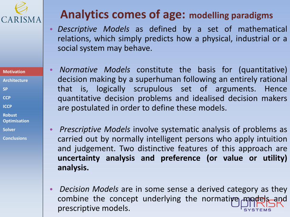
• Descriptive Models as defined by a set of mathematical relations, which simply predicts how a physical, industrial or a social system may behave.

• Normative Models constitute the basis for (quantitative) decision making by a superhuman following an entirely rational that is, logically scrupulous set of arguments. Hence quantitative decision problems and idealised decision makers are postulated in order to define these models.

• Prescriptive Models involve systematic analysis of problems as carried out by normally intelligent persons who apply intuition and judgement. Two distinctive features of this approach are uncertainty analysis and preference (or value or utility) analysis.

• Decision Models are in some sense a derived category as they combine the concept underlying the normative models and prescriptive models.

Motivation

Architecture

SP

CCP

ICCP

Robust Optimisation

Solver

Conclusions

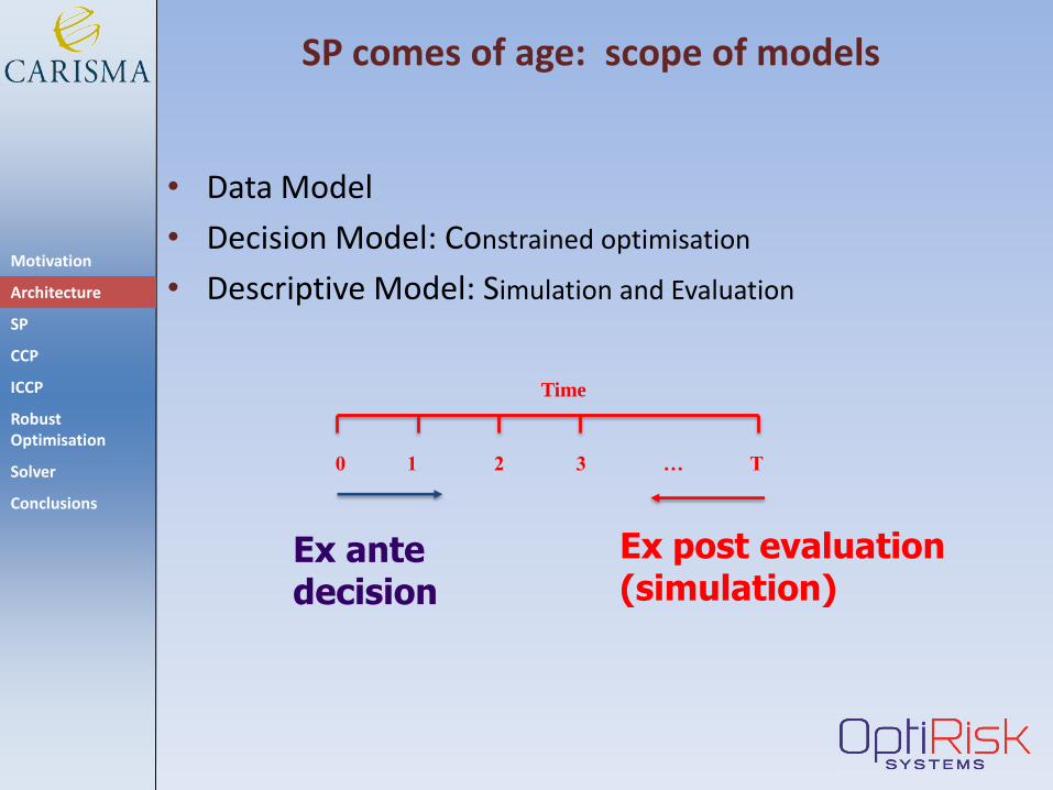
Time

0 1 2 3 … T

Ex ante decision

Ex post evaluation (simulation)

SP comes of age: scope of models

• Data Model

• Decision Model: Constrained optimisation

• Descriptive Model: Simulation and Evaluation

Motivation

Architecture

SP

CCP

ICCP

Robust Optimisation

Solver

Conclusions

Models of (parameter) randomness

Scenario Generator 1

Scenario Generator 2

Simulation

and

Decision evaluation

Performance measures

Statistical measures: mean, variance, skewness, kurtosis

Stochastic measures: EVPI, VSS

Risk measures: VaR, CVaR, standard deviation

Performance measures: Solvency ratio, Sharpe ratio, Sortino ratio

Ex-ante decision models

Two-stage SP - recourse

Multistage SP- recourse

Chance-constrained SP

Expected value LP

Integrated chance constraints

Robust optimisation

SP comes of age: decision…simulation…evaluation engine

Motivation

Architecture

SP

CCP

ICCP

Robust Optimisation

Solver

Conclusions

Research problems • Mathematical Programming is a useful and

widely used paradigm for decision making

• A few approaches are now established for quantitative decision making under uncertainty:

– Dynamic Stochastic Programming

– Stochastic Programming

– Robust Optimisation

• These differ in respect of :

– their formulation

– assumptions and models for uncertain parameters

Motivation

Architecture

SP

CCP

ICCP

Robust Optimisation

Solver

Conclusions

Focus of the development

• To simplify the formulation of SP and RO problems with a modelling language

• To facilitate the investigation of a given decision problem under alternative modelling frameworks

• To automate the steps necessary for their solution

• To connect scalable solution algorithms which match the models

Motivation

Architecture

SP

CCP

ICCP

Robust Optimisation

Solver

Conclusions

Modelling phase

SP modelling process

Runtime phase

SG Parameters Algebraic model Solver Controls

Scenario Generator

Modelling System

Solver

Which scenario generators?

Model(s) of randomness

Which decision model?

Decision Model

Which solution method?

Solution algorithm

Modelling System

Algebraic model

Motivation

Architecture

SP

CCP

ICCP

Robust Optimisation

Solver

Conclusions

Modelling Languages

• Algebraic Modelling Languages conveniently express MPs in a format both easy to understand and that can be processed by a solver (i.e. AMPL, GAMS, AIMMS, MPL, OPL, …)

• Both SP and RO problems have different requirements

– in language constructs

– in specification of parameters uncertainty

– in interacting with the solver

• SAMPL extends AMPL adding syntax to support such problem classes

Motivation

Architecture

SP

CCP

ICCP

Robust Optimisation

Solver

Conclusions

Supported problems classes

SP Problems

Distribution Problems

Wait and See

Expected Value

Recourse Problems

Distribution based

Scenario based Problems with

Chance Constraints

Problems with ICC

Sto

chas

tic

Mea

sure

s: E

VP

I an

d V

SS

Robust Optimisation

Dynamic Stochastic

Programming

SP Problems

Distribution Problems

Wait and See

Expected Value

Recourse Problems

Distribution based

Scenario based Problems with

Chance Constraints

Problems with ICC

Sto

chas

tic

Mea

sure

s: E

VP

I an

d V

SS

Robust Optimisation

Recourse Problems

Motivation

Architecture

SP

CCP

ICCP

Robust Optimisation

Solver

Conclusions

Modelling Languages • Sometimes it is not practical or not possible to

find distributions of the random parameters -> no scenarios

• A robust model can be formulated using the Robust Optimisation framework

DECISION MODEL

Optimum Allocation

Modelling

SCENARIO GENERATION

Modelling distribution of

random parameters

UNCERTAINTY not revealed

Parameters defined by uncertainty

sets (Soyster, Bertsimas and Sim,

Ben-Tal and Nemirovski)

Stochastic

Programming

Robust

Optimisation

Motivation

Architecture

SP

CCP

ICCP

Robust Optimisation

Solver

Conclusions

Introducing ALM Example

• ALM model:

– individual has incomes to invest in the stock market

– In various time periods, he has liabilities to match

– Asset prices are uncertain

• Objective: maximise terminal wealth of investor

• Constraints:

– Asset inventory constraints

– Cash balance constraints (buys and sales subject to transaction costs)

Motivation

Architecture

SP

CCP

ICCP

Robust Optimisation

Solver

Conclusions

Example: entities Type Name Notation Description Range//Dimensions

Indices

(sets)

ASSETS I Assets classes i = 1 ... I;

TIME T Time periods t = 1 ... T;

Parameters

(data)

price Pi t Price of asset i at time period t ASSETS,TIME,

liabilities Lt Liability at time period t TIME

Incomes Ft Incomes at time period t INCOMES

Tcost G Transaction cost as % of trade value

hold0 H0 Initial holdings of each asset ASSETS

Variables

hold Hit Quantity of assets i to hold in time

period t

ASSETS,TIME

sell Sit Quantity of assets i to sell in time

period t

ASSETS,TIME

buy Bit Quantity of assets i to buy in time

period t

ASSETS,TIME

Motivation

Architecture

SP

CCP

ICCP

Robust Optimisation

Solver

Conclusions

Deterministic version set ASSETS; set TIME; param NT; param Tcost; param liabilities{TIME}; param income{TIME}; param hold0{ASSETS}; param price{TIME, ASSETS};

var hold{TIME, ASSETS} >=0; var buy{TIME, ASSETS} >=0; var sell{TIME, ASSETS} >=0;

maximize wealth: sum{a in ASSETS} price[NT,a]*hold[NT,a];

subject to sinv1{a in ASSETS}: hold[1,a]=hold0[a]+buy[1,a]-sell[1,a]; sinv2{a in ASSETS,t in 2..NT}: hold[t,a]=hold[t-1,a]+buy[t,a]-sell[t,a]; cashbalance{t in TIME}: (1-Tcost)*(sum{a in ASSETS}price[t,a]*sell[t,a]) + income[t] - (1+Tcost)*(sum{a in ASSETS}price[t,a]*buy[t,a]) >= liabilities[t];

Motivation

Architecture

SP

CCP

ICCP

Robust Optimisation

Solver

Conclusions

Example: entities stochastic Type Name Notation Description Range//Dimensions

Indices

(sets)

ASSETS I Assets classes i = 1 ... I;

TIME T Time periods t = 1 ... T;

SCENARIO S Scenarios S= 1..NS;

Parameters

(data)

price Pi t s Price of asset i at time period t in

each SCENARIO

ASSETS,TIME,

SCENARIO

liabilities Lt Liability at time period t TIME

Incomes Ft Incomes at time period t INCOMES

Tcost G Transaction cost as % of trade value

hold0 H0 Initial holdings of each asset ASSETS

Variables

hold Hits Quantity of assets i to hold in time

period t in each SCENARIO

ASSETS,TIME,

SCENARIO

sell Sits Quantity of assets i to sell in time

period t in each SCENARIO

ASSETS,TIME,

SCENARIO

buy Bits Quantity of assets i to buy in time

period t in each SCENARIO

ASSETS,TIME,

SCENARIO

Motivation

Architecture

SP

CCP

ICCP

Robust Optimisation

Solver

Conclusions

Introducing Scenarios

t

Deterministic (EV) Multiple scenarios (WS)

t

t

Multiple scenarios (TSSP)

Motivation

Architecture

SP

CCP

ICCP

Robust Optimisation

Solver

Conclusions

Non anticipativity

• Example: Variable hold(asset, time, scenario)

t 1 2 3 4

Hold(a,2,1) Hold(a,3,1) Hold(a,4,1)

Scenario 1

Scenario 2 Hold(a,2,2) Hold(a,3,2) Hold(a,4,2)

Scenario S

Hold(a,2, S) Hold(a,3,S) Hold(a,4,S)

Hold(a,1,1)

Hold(a,1,2)

Hold(a,1,S)

The variables of the first time period represent all the same decision -> Fix their values to be the same with a constraint (NON ANTICIPATIVITY)

Hold(a,1,1)

Hold(a,1,2)

Hold(a,1,S)

Motivation

Architecture

SP

CCP

ICCP

Robust Optimisation

Solver

Conclusions

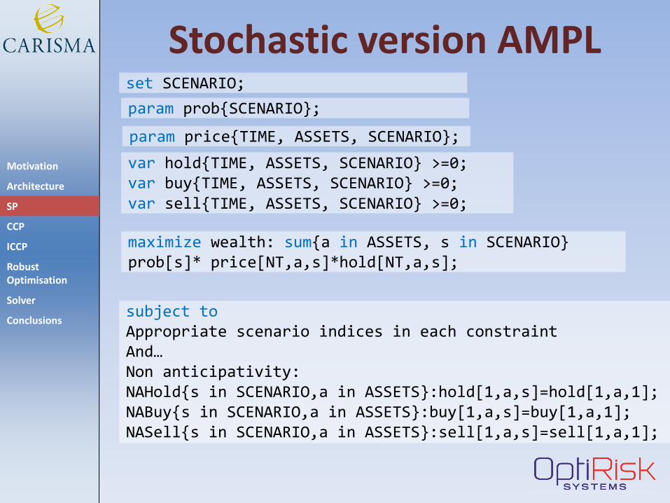
Stochastic version AMPL set SCENARIO;

var hold{TIME, ASSETS, SCENARIO} >=0; var buy{TIME, ASSETS, SCENARIO} >=0; var sell{TIME, ASSETS, SCENARIO} >=0;

maximize wealth: sum{a in ASSETS, s in SCENARIO} prob[s]* price[NT,a,s]*hold[NT,a,s];

subject to Appropriate scenario indices in each constraint And… Non anticipativity: NAHold{s in SCENARIO,a in ASSETS}:hold[1,a,s]=hold[1,a,1]; NABuy{s in SCENARIO,a in ASSETS}:buy[1,a,s]=buy[1,a,1]; NASell{s in SCENARIO,a in ASSETS}:sell[1,a,s]=sell[1,a,1];

param price{TIME, ASSETS, SCENARIO};

param prob{SCENARIO};

Motivation

Architecture

SP

CCP

ICCP

Robust Optimisation

Solver

Conclusions

Stochastic version SAMPL set SCENARIO;

var hold{TIME, ASSETS, SCENARIO} >=0; var buy{TIME, ASSETS, SCENARIO} >=0; var sell{TIME, ASSETS, SCENARIO} >=0;

maximize wealth: sum{a in ASSETS, s in SCENARIO} prob[s]* price[NT,a,s]*hold[NT,a,s];

subject to Appropriate scenario indices in each constraint And… Non anticipativity: NAHold{s in SCENARIO,a in ASSETS} hold[1,a,s]=hold[1,a,1]; NABuy{s in SCENARIO,a in ASSETS} buy[1,a,s]=buy[1,a,1]; NASell{s in SCENARIO,a in ASSETS} sell[1,a,s]=sell[1,a,1];

param price{TIME, ASSETS, SCENARIO};

param prob{SCENARIO};

scenarioset SCENARIO;

probability prob{SCENARIO};

random param price{TIME, ASSETS, SCENARIO};

var hold{TIME, ASSETS, SCENARIO} >=0, suffix stage if t=1 then 1 else 2; var buy{TIME, ASSETS, SCENARIO} >=, suffix stage if t=1 then 1 else 2; var sell{TIME, ASSETS, SCENARIO} >=0 , suffix stage if t=1 then 1 else 2;

maximize wealth: sum{a in ASSETS, s in SCENARIO} prob[s]* price[NT,a,s]*hold[NT,a,s];

subject to Appropriate scenario indices in each constraint tree thetree := twostage; and.. no non-anticipativity!!

Motivation

Architecture

SP

CCP

ICCP

Robust Optimisation

Solver

Conclusions

Chance Constraints

Motivation

Architecture

SP

CCP

ICCP

Robust Optimisation

Solver

Conclusions

Integrated Chance Constraints

•

Motivation

Architecture

SP

CCP

ICCP

Robust Optimisation

Solver

Conclusions

(Integrated) Chance Constraints subject to cashbalance{t in TIME} : probability{s in SCENARIO: (1-Tcost)*(sum{a in ASSETS} price[t,a,s]*sell[t,a,s])+income[t] -(1+Tcost)*(sum{a in ASSETS} price[t,a,s]*buy[t,a,s]) >= liab[t] }>= reliability;

CCP

subject to cashbalance{t in TIME} : expectation{s in SCENARIO} ( (liab[t]+(1+Tcost)*(sum{a in ASSETS} price[t,a,s]*buy[t,a,s])) less ((1-Tcost)*(sum{a in ASSETS} price[t,a,s]*sell[t,a,s])+income[t]) ) <= level;

ICCP

Motivation

Architecture

SP

CCP

ICCP

Robust Optimisation

Solver

Conclusions

Robust Optimisation

Motivation

Architecture

SP

CCP

ICCP

Robust Optimisation

Solver

Conclusions

Robust Optimisation • There are three well known formulations:

Motivation

Architecture

SP

CCP

ICCP

Robust Optimisation

Solver

Conclusions

Robust Optimisation

Motivation

Architecture

SP

CCP

ICCP

Robust Optimisation

Solver

Conclusions

Robust Optimisation

Motivation

Architecture

SP

CCP

ICCP

Robust Optimisation

Solver

Conclusions

Robust Optimisation

param eprice{t in TIME, a in ASSETS}; param amplitude{t in TIME, a in ASSETS}; param Rob{t in TIME};

• SAMPL: same as deterministic model but

subject to cashbalance{t in TIME} suffix robustness Rob[t]: (1-Tcost)*(sum{a in ASSETS}randomprice[t,a]*sell[t,a]) + income[t] – (1+Tcost)*(sum{a in ASSETS}randomprice[t,a]*buy[t,a]) >= liab[t];

random param randomPrice{t in TIME, a in ASSETS} dist symmetric(eprice[t,a] - amplitude[t,a], eprice[t,a] + amplitude[t,a]);

option RobustForm BenTal_Nemirovski;

Motivation

Architecture

SP

CCP

ICCP

Robust Optimisation

Solver

Conclusions

Robust extensions

Motivation

Architecture

SP

CCP

ICCP

Robust Optimisation

Solver

Conclusions

Robust Optimisation

Motivation

Architecture

SP

CCP

ICCP

Robust Optimisation

Solver

Conclusions

Robust Optimisation

Motivation

Architecture

SP

CCP

ICCP

Robust Optimisation

Solver

Conclusions

Solution methods

• Scenario based problems are characterized by finite discrete distributions

• Deterministic equivalent is a large-scale LP with a specific structure

• Solution methods:

– LP methods directly applied to deterministic equivalent: Simplex, IPM

– Decomposition methods: Benders’, regularized, level decomposition, integer L-shaped

• Information about the model type and its structure is retained during modelling -> automatic selection of solution method

Motivation

Architecture

SP

CCP

ICCP

Robust Optimisation

Solver

Conclusions

FortSP architecture

FortSP executable

FortSP library

CPLEX plugin

CPLEX library

GUROBI plugin

GUROBI library

FORTMP plugin

FORTMP library

AMPL Solvers

API

plugin interface

nl interface

Motivation

Architecture

SP

CCP

ICCP

Robust Optimisation

Solver

Conclusions

Solution methods

Two stage SP

Multi stage SP

Chance Constrained

Integrated CCPs

ROBUST

Soyster’s

ROBUST

Bertsimas

Benders

Nested Benders

Level

ICCP cutting plane

Deterministic Equivalent

ROBUST

Ben-Tal

QP

MIP

LP

SOCP

Motivation

Architecture

SP

CCP

ICCP

Robust Optimisation

Solver

Conclusions

Linear Programming

Quadratic Programming

Mixed Integer Programming

Second Order Cone Programming

Solution methods

Motivation

Architecture

SP

CCP

ICCP

Robust Optimisation

Solver

Conclusions

Conclusions • The advantages of this AML tools approach are:

– Simplification of the syntax to express these models (both SP and RO)

– Easy to investigate and introduce a comprehensive modelling framework

– Conveys the structure of the problem to the solver (permits the exploitation of appropriate solution methods)

Motivation

Architecture

SP

CCP

ICCP

Robust Optimisation

Solver

Conclusions

References • Erickson, J. and Fourer, R., 2010. Second-Order Cone

Program (SOCP) Detection and Transformation Algorithms for Optimization Software INFORMS Annual meeting 2010, Available at http://www.ampl.com/MEETINGS/TALKS/2010_11_Austin_MC33.pdf

• Valente, C., Mitra, G., Sadki, M. & Fourer, R., 2009. Extending algebraic modelling languages for Stochastic Programming. INFORMS Journal on Computing, 21, pp.107--122.

• Valente, C. et al., 2002-2010. SAMPL/SPInE User Manual. [Online] Available at: http://www.optirisk-

systems.com/manuals/SpineAmplManual.pdf.