optimization an introduction

OPTIMIZATION

An introduction

A. Astolfi

First draft – September 2002

Last revision – September 2006

Contents

1 Introduction 11.1 Introduction . . . . . . . . . . . . . . . . . . . . . . . . . . . . . . . . . . . . 21.2 Statement of an optimization problem . . . . . . . . . . . . . . . . . . . . . 3

1.2.1 Design vector . . . . . . . . . . . . . . . . . . . . . . . . . . . . . . . 41.2.2 Design constraints . . . . . . . . . . . . . . . . . . . . . . . . . . . . 41.2.3 Objective function . . . . . . . . . . . . . . . . . . . . . . . . . . . . 4

1.3 Classification of optimization problems . . . . . . . . . . . . . . . . . . . . . 61.4 Examples . . . . . . . . . . . . . . . . . . . . . . . . . . . . . . . . . . . . . 6

2 Unconstrained optimization 92.1 Introduction . . . . . . . . . . . . . . . . . . . . . . . . . . . . . . . . . . . . 102.2 Definitions and existence conditions . . . . . . . . . . . . . . . . . . . . . . 102.3 General properties of minimization algorithms . . . . . . . . . . . . . . . . . 17

2.3.1 General unconstrained minimization algorithm . . . . . . . . . . . . 172.3.2 Existence of accumulation points . . . . . . . . . . . . . . . . . . . . 182.3.3 Condition of angle . . . . . . . . . . . . . . . . . . . . . . . . . . . . 192.3.4 Speed of convergence . . . . . . . . . . . . . . . . . . . . . . . . . . . 22

2.4 Line search . . . . . . . . . . . . . . . . . . . . . . . . . . . . . . . . . . . . 232.4.1 Exact line search . . . . . . . . . . . . . . . . . . . . . . . . . . . . . 242.4.2 Armijo method . . . . . . . . . . . . . . . . . . . . . . . . . . . . . . 242.4.3 Goldstein conditions . . . . . . . . . . . . . . . . . . . . . . . . . . . 262.4.4 Line search without derivatives . . . . . . . . . . . . . . . . . . . . . 272.4.5 Implementation of a line search algorithm . . . . . . . . . . . . . . . 29

2.5 The gradient method . . . . . . . . . . . . . . . . . . . . . . . . . . . . . . . 292.6 Newton’s method . . . . . . . . . . . . . . . . . . . . . . . . . . . . . . . . . 31

2.6.1 Method of the trust region . . . . . . . . . . . . . . . . . . . . . . . 352.6.2 Non-monotonic line search . . . . . . . . . . . . . . . . . . . . . . . . 362.6.3 Comparison between Newton’s method and the gradient method . . 37

2.7 Conjugate directions methods . . . . . . . . . . . . . . . . . . . . . . . . . . 372.7.1 Modification of βk . . . . . . . . . . . . . . . . . . . . . . . . . . . . 402.7.2 Modification of αk . . . . . . . . . . . . . . . . . . . . . . . . . . . . 412.7.3 Polak-Ribiere algorithm . . . . . . . . . . . . . . . . . . . . . . . . . 41

2.8 Quasi-Newton methods . . . . . . . . . . . . . . . . . . . . . . . . . . . . . 42

iii

iv CONTENTS

2.9 Methods without derivatives . . . . . . . . . . . . . . . . . . . . . . . . . . . 45

3 Nonlinear programming 493.1 Introduction . . . . . . . . . . . . . . . . . . . . . . . . . . . . . . . . . . . . 503.2 Definitions and existence conditions . . . . . . . . . . . . . . . . . . . . . . 51

3.2.1 A simple proof of Kuhn-Tucker conditions for equality constraints . 533.2.2 Quadratic cost function with linear equality constraints . . . . . . . 54

3.3 Nonlinear programming methods: introduction . . . . . . . . . . . . . . . . 543.4 Sequential and exact methods . . . . . . . . . . . . . . . . . . . . . . . . . . 55

3.4.1 Sequential penalty functions . . . . . . . . . . . . . . . . . . . . . . . 553.4.2 Sequential augmented Lagrangian functions . . . . . . . . . . . . . . 573.4.3 Exact penalty functions . . . . . . . . . . . . . . . . . . . . . . . . . 593.4.4 Exact augmented Lagrangian functions . . . . . . . . . . . . . . . . 61

3.5 Recursive quadratic programming . . . . . . . . . . . . . . . . . . . . . . . . 623.6 Concluding remarks . . . . . . . . . . . . . . . . . . . . . . . . . . . . . . . 64

4 Global optimization 654.1 Introduction . . . . . . . . . . . . . . . . . . . . . . . . . . . . . . . . . . . . 664.2 Deterministic methods . . . . . . . . . . . . . . . . . . . . . . . . . . . . . . 66

4.2.1 Methods for Lipschitz functions . . . . . . . . . . . . . . . . . . . . . 664.2.2 Methods of the trajectories . . . . . . . . . . . . . . . . . . . . . . . 684.2.3 Tunneling methods . . . . . . . . . . . . . . . . . . . . . . . . . . . . 70

4.3 Probabilistic methods . . . . . . . . . . . . . . . . . . . . . . . . . . . . . . 714.3.1 Methods using random directions . . . . . . . . . . . . . . . . . . . . 714.3.2 Multistart methods . . . . . . . . . . . . . . . . . . . . . . . . . . . . 724.3.3 Stopping criteria . . . . . . . . . . . . . . . . . . . . . . . . . . . . . 72

List of Figures

1.1 Feasible region in a two-dimensional design space. Only inequality con-straints are present. . . . . . . . . . . . . . . . . . . . . . . . . . . . . . . . 4

1.2 Design space, objective functions surfaces, and optimum point. . . . . . . . 51.3 Electrical bridge network. . . . . . . . . . . . . . . . . . . . . . . . . . . . . 6

2.1 Geometrical interpretation of the anti-gradient. . . . . . . . . . . . . . . . . 132.2 A saddle point in IR2. . . . . . . . . . . . . . . . . . . . . . . . . . . . . . . 162.3 Geometrical interpretation of Armijo method. . . . . . . . . . . . . . . . . . 252.4 Geometrical interpretation of Goldstein method. . . . . . . . . . . . . . . . 27

2.5 The function√

ξξ − 1ξ + 1

. . . . . . . . . . . . . . . . . . . . . . . . . . . . . . 30

2.6 Behavior of the gradient algorithm. . . . . . . . . . . . . . . . . . . . . . . . 312.7 The simplex method. The points x(1), x(2) and x(3) yields the starting

simplex. The second simplex is given by the points x(1), x(2) and x(4). Thethird simplex is given by the points x(2), x(4) and x(5). . . . . . . . . . . . . 47

4.1 Geometrical interpretation of the Lipschitz conditions (4.2) and (4.3). . . . 664.2 Geometrical interpretation of Schubert-Mladineo algorithm. . . . . . . . . . 684.3 Interpretation of the tunneling phase. . . . . . . . . . . . . . . . . . . . . . 704.4 The functions f(x) and T (x, x�

k). . . . . . . . . . . . . . . . . . . . . . . . . 71

v

vi LIST OF FIGURES

List of Tables

1.1 Properties of the articles to load. . . . . . . . . . . . . . . . . . . . . . . . . 7

2.1 Comparison between the gradient method and Newton’s method. . . . . . . 37

vii

viii LIST OF TABLES

Chapter 1

Introduction

2 CHAPTER 1. INTRODUCTION

1.1 Introduction

Optimization is the act of achieving the best possible result under given circumstances.In design, construction, maintenance, ..., engineers have to take decisions. The goal of allsuch decisions is either to minimize effort or to maximize benefit.The effort or the benefit can be usually expressed as a function of certain design variables.Hence, optimization is the process of finding the conditions that give the maximum or theminimum value of a function.It is obvious that if a point x� corresponds to the minimum value of a function f(x), thesame point corresponds to the maximum value of the function −f(x). Thus, optimizationcan be taken to be minimization.There is no single method available for solving all optimization problems efficiently. Hence,a number of methods have been developed for solving different types of problems.Optimum seeking methods are also known as mathematical programming techniques,which are a branch of operations research. Operations research is coarsely composedof the following areas.

• Mathematical programming methods. These are useful in finding the minimum of afunction of several variables under a prescribed set of constraints.

• Stochastic process techniques. These are used to analyze problems which are de-scribed by a set of random variables of known distribution.

• Statistical methods. These are used in the analysis of experimental data and in theconstruction of empirical models.

These lecture notes deal mainly with the theory and applications of mathematical program-ming methods. Mathematical programming is a vast area of mathematics and engineering.It includes

• calculus of variations and optimal control;

• linear, quadratic and non-linear programming;

• geometric programming;

• integer programming;

• network methods (PERT);

• game theory.

The existence of optimization can be traced back to Newton, Lagrange and Cauchy. Thedevelopment of differential methods for optimization was possible because of the contri-bution of Newton and Leibnitz. The foundations of the calculus of variations were laid byBernoulli, Euler, Lagrange and Weierstrasse. Constrained optimization was first studiedby Lagrange and the notion of descent was introduced by Cauchy.

1.2. STATEMENT OF AN OPTIMIZATION PROBLEM 3

Despite these early contributions, very little progress was made till the 20th century, whencomputer power made the implementation of optimization procedures possible and this inturn stimulated further research methods.The major developments in the area of numerical methods for unconstrained optimizationhave been made in the UK. These include the development of the simplex method (Dantzig,1947), the principle of optimality (Bellman, 1957), necessary and sufficient conditions ofoptimality (Kuhn and Tucker, 1951).Optimization in its broadest sense can be applied to solve any engineering problem, e.g.

• design of aircraft for minimum weight;

• optimal (minimum time) trajectories for space missions;

• minimum weight design of structures for earthquake;

• optimal design of electric networks;

• optimal production planning, resources allocation, scheduling;

• shortest route;

• design of optimum pipeline networks;

• minimum processing time in production systems;

• optimal control.

1.2 Statement of an optimization problem

An optimization, or a mathematical programming problem can be stated as follows.Find

x = (x1, x2, ...., xn)

which minimizesf(x)

subject to the constraintsgj(x) ≤ 0 (1.1)

for j = 1, . . . ,m, andlj(x) = 0 (1.2)

for j = 1, . . . , p.The variable x is called the design vector, f(x) is the objective function, gj(x) are theinequality constraints and lj(x) are the equality constraints. The number of variables nand the number of constraints p + m need not be related. If p + m = 0 the problem iscalled an unconstrained optimization problem.


xxxxxxxxxxxxxxxxxxxxxxxxxxxxxxxxxxxxxxxxxxxxxxxxxxxxxxxxxxxxxxxxxxxxxxxxxxxxxxxxxxxxxxxxxxxxxxxxxxxxxxxxxxxxxxxxxxxxxxxxxxxxxxxxxxxxxxxxxxxxxxxxxxxxxxxxxxxxxxxxxxxxxxxxxxxxxxxxxxxxxxxxxxxxxxxxxxxxxxxxxxxxxxxxxxxxxxxxxxxxxxxxxxxxxxxxxxxxxxxxxxxxxxxxxxxxxxxxxxxxxxxxxxxxxxxxxxxxxxxxxxxxxxxxxxxxxxxxxxxxxxxxxxxxxxxxxxxxxxxxxxxxxxxxxxxxxxxxxxxxxxxxxxxxxxxxxxxxxxxxxxxxxxxxxxxxxxxxxxxxxxxxxxxxxxxxxxxxxxxxxxxxxxxxxxxxxxxxxxxxxxxxxxxxxxxxxxxxxxxxxxxxxxxxxxxxxxxxxxxxxxxxxxxxxxxxxxxxxxxxxxxxxxxxxxxxxxxxxxxxxxxxxxxxxxxxxxxxxxxxxxxxxxxxxxxxxxxxxxxxxxxxxxxxxxxxxxxxxxxxxxxxxxxxxxxxxxxxxxxxxxxxxxxxxxxxxxxxxxxxxxxxxxxxxxxxxxxxxxxxxxxxxxxxxxxxxxxxxxxxxxxxxxxxxxxxxxxxxxxxxxxxxxxxxxxxxxxxxxxxxxxxxxxxxxxxxxxxxxxxxxxxxxxxxxxxxxxxxxxxxxxxxxxxxxxxxxxxxxxxxxxxxxxxxxxxxxxxxxxxxxxxxxxxxxxxxxxxxxxxxxxxxxxxxxxxxxxxxxxxxxxxxxxxxxxxxxxxxxxxxxxxxxxxxxxxxxxxxxxxxxxxxxxxxxxxxxxxxxxxxxxxxxxxxxxxxxxxxxxxxxxxxxxxxxxxxxxxxxxxxxxxxxxxxxxxxxxxxxxxxxxxxxxxxxxxxxxxxxxxxxxxxxxxxxxxxxxxxxxxxxxxxxxxxxxxxxxxxxxxxxxxxxxxxxxxxxxxxxxxxxxxxxxxxxxxxxxxxxxxxxxxxxxxxxxxxxxxxxxxxxxxxxxxxxxxxxxxxxxxxxxxxxxxxxxxxxxxxxxxxxxxxxxxxxxxxxxxxxxxxxxxxxxxxxxxxxxxxxxxxxxxxxxxxxxxxxxxxxxxxxxxxxxxxxxxxxxxxxxxxxxxxxxxxxxxxxxxxxxxxxxxxxxxxxxxxxxxxxxxxxxxxxxxxxxxxxxxxxxxxxxxxxxxxxxxxxxxxxxxxxxxxxxxxxxxxxxxxxxxxxxxxxxxxxxxxxxxxxxxxxxxxxxxxxxxxxxxxxxxxxxxxxxxxxxxxxxxxxxxxxxxxxxxxxxxxxxxxxxxxxxxxxxxxxxxxxxxxxxxxxxxxxxxxxxxxxxxxxxxxxxxxxxxxxxxxxxxxxxxxxxxxxxxxxxxxxxxxxxxxxxxxxxxxxxxxxxxxxxxxxxxxxxxxxxxxxxxxxxxxxxxxxxxxxxxxxxxxxxxxxxxxxxxxxxxxxxxxxxxxxxxxxxxxxxxxxxxxxxxxxxxxxxxxxxxxxxxxxxxxxxxxxxxxxxxxxxxxxxxxxxxxxxxxxxxxxxxxxxxxxxxxxxxxxxxxxxxxxxxxxxxxxxxxxxxxxxxxxxxxxxxxxxxxxxxxxxxxxxxxxxxxxxxxxxxxxxxxxxxxxxxxxxxxxxxxxxxxxxxxxxxxxxxxxxxxxxxxxxxxxxxxxxxxxxxxxxxxxxxxxxxxxxxxxxxxxxxxxxxxxxxxxxxxxxxxxxxxxxxxxxxxxxxxxxxxxxxxxxxxxxxxxxxxxxxxxxxxxxxxxxxxxxxxxxxxxxxxxxxxxxxxxxxxxxxxxxxxxxxxxxxxxxxxxxxxxxxxxxxxxxxxxxxxxxxxxxxxxxxxxxxxxxxxxxxxxxxxxxxxxxxxxxxxxxxxxxxxxxxxxxxxxxxxxxxxxxxxxxxxxxxxxxxxxxxxxxxxxxxxxxxxxxxxxxxxxxxxxxxxxxxxxxxxxxxxxxxxxxxxxxxxxxxxxxxxxxxxxxxxxxxxxxxxxxxxxxxxxxxxxxxxxxxxxxxxxxxxxxxxxxxxxxxxxxxxxxxxxxxxxxxxxxxxxxxxxxxxxxxxxxxxxxxxxxxxxxxxxxxxxxxxxxxxxxxxxxxxxxxxxxxxxxxxxxxxxxxxxxxxxxxxxxxxxxxxxxxxxxxxxxxxxxxxxxxxxxxxxxxxxxxxxxxxxxxxxxxxxxxxxxxxxxxxxxxxxxxxxxxxxxxxxxxxxxxxxxxxxxxxxxxxxxxxxxxxxxxxxxxxxxxxxxxxxxxxxxxxxxxxxxxxxxxxxxxxxxxxxxxxxxxxxxxxxxxxxxxxxxxxxxxxxxxxxxxxxxxxxxxxxxxxxxxxxxxxxxxxxxxxxxxxxxxxxxxxxxxxxxxxxxxxxxxxxxxxxxxxxxxxxxxxxxxxxxxxxxxxxxxxxxxxxxxxxxxxxxxxxxxxxxxxxxxxxxxxxxxxxxxxxxxxxxxxxxxxxxxxxxxxxxxxxxxxxxxxxxxxxxxxxxxxxxxxxxxxxxxxxxxxxxxxxxxxxxxxxxxxxxxxxxxxxxxxxxxxxxxxxxxxxxxxxxxxxxxxxxxxxxxxxxxxxxxxxxxxxxxxxxxxxxxxxxxxxxxxxxxxxxxxxxxxxxxxxxxxxxxxxxxxxxxxxxxxxxxxxxxxxxxxxxxxxxxxxxxxxxxxxxxxxxxxxxxxxxxxxxxxxxxxxxxxxxxxxxxxxxxxxxxxxxxxxxxxxxxxxxxxxxxxxxxxxxxxxxxxxxxxxxxxxxxxxxxxxxxxxxxxxxxxxxxxxxxxxxxxxxxxxxxxxxxxxxxxxxxxxxxxxxxxxxxxxxxxxxxxxxxxxxxxxxxxxxxxxxxxxxxxxxxxxxxxxxxxxxxxxxxxxxxxxxxxxxxxxxxxxxxxxxxxxxxxxxxxxxxxxxxxxxxxxxxxxxxxxxxxxxxxxxxxxxxxxxxxxxxxxxxxxxxxxxxxxxxxxxxxxxxxxxxxxxxxxxxxxxxxxxxxxxxxxxxxxxxxxxxxxxxxxxxxxxxxxxxxxxxxxxxxxxxxxxxxxxxxxxxxxxxxxxxxxxxxxxxxxxxxxxxxxxxxxxxxxxxxxxxxxxxxxxxxxxxxxxxxxxxxxxxxxxxxxxxxxxxxxxxxxxxxxxxxxxxxxxxxxxxxxxxxxxxxxxxxxxxxxxxxxxxxxxxxxxxxxxxxxxxxxxxxxxxxxxxxxxxxxxxxxxxxxxxxxxxxxxxxxxxxxxxxxxxxxxxxxxxxxxxxxxxxxxxxxxxxxxxxxxxxxxxxxxxxxxxxxxxxxxxxxxxxxxxxxxxxxxxxxxxxxxxxxxxxxxxxxxxxxxxxxxxxxxxxxxxxxxxxxxxxxxxxxxxxxxxxxxxxxxxxxxxxxxxxxxxxxxxxxxxxxxxxxxxxxxxxxxxxxxxxxxxxxxxxxxxxxxxxxxxxxxxxxxxxxxxxxxxxxxxxxxxxxxxxxxxxxxxxxxxxxxxxxxxxxxxxxxxxxxxxxxxxxxxxxxxxxxxxxxxxxxxxxxxxxxxxxxxxxxxxxxxxxxxxxxxxxxxxxxxxxxxxxxxxxxxxxxxxxxxxxxxxxxxxxxxxxxxxxxxxxxxxxxxxxxxxxxxxxxxxxxxxxxxxxxxxxxxxxxxxxxxxxxxxxxxxxxxxxxxxxxxxxxxxxxxxxxxxxxxxxxxxxxxxxxxxxxxxxxxxxxxxxxxxxxxxxxxxxxxxxxxxxxxxxxxxxxxxxxxxxxxxxxxxxxxxxxxxxxxxxxxxxxxxxxxxxxxxxxxxxxxxxxxxxxxxxxxxxxxxxxxxxxxxxxxxxxxxxxxxxxxxxxxxxxxxxxxxxxxxxxxxxxxxxxxxxxxxxxxxxxxxxxxxxxxxxxxxxxxxxxxxxxxxxxxxxxxxxxxxxxxxxxxxxxxxxxxxxxxxxxxxxxxxxxxxxxxxxxxxxxxxxxxxxxxxxxxxxxxxxxxxxxxxxxxxxxxxxxxxxxxxxxxxxxxxxxxxxxxxxxxxxxxxxxxxxxxxxxxxxxxxxxxxxxxxxxxxxxxxxxxxxxxxxxxxxxxxxxxxxxxxxxxxxxxxxxxxxxxxxxxxxxxxxxxxxxxxxxxxxxxxxxxxxxxxxxxxxxxxxxxxxxxxxxxxxxxxxxxxxxxxxxxxxxxxxxxxxxxxxxxxxxxxxxxxxxxxxxxxxxxxxxxxxxxxxxxxxxxxxxxxxxxxxxxxxxxxxxxxxxxxxxxxxxxxxxxxxxxxxxxxxxxxxxxxxxxxxxxxxxxxxxxxxxxxxxxxxxxxxxxxxxxxxxxxxxxxxxxxxxxxxxxxxxxxxxxxxxxxxxxxxxxxxxxxxxxxxxxxxxxxxxxxxxxxxxxxxxxxxxxxxxxxxxxxxxxxxxxxxxxxxxxxxxxxxxxxxxxxxxxxxxxxxxxxxxxxxxxxxxxxxxxxxxxxxxxxxxxxxxxxxxxxxxxxxxxxxxxxxxxxxxxxxxxxxxxxxxxxxxxxxxxxxxxxxxxxxxxxxxxxxxxxxxxxxxxxxxxxxxxxxxxxxxxxxxxxxxxxxxxxxxxxxxxxxxxxxxxxxxxxxxxxxxxxxxxxxxxxxxxxxxxxxxxxxxxxxxxxxxxxxxxxxxxxxxxxxxxxxxxxxxxxxxxxxxxxxxxxxxxxxxxxxxxxxxxxxxxxxxxxxxxxxxxxxxxxxxxxxxxxxxxxxxxxxxxxxxxxxxxxxxxxxxxxxxxxxxxxxxxxxxxxxxxxxxxxxxxxxxxxxxxxxxxxxxxxxxxxxxxxxxxxxxxxxxxxxxxxxxxxxxxxxxxxxxxxxxxxxxxxxxxxxxxxxxxxxxxxxxxxxxxxxxxxxxxxxxxxxxxxxxxxxxxxxxxxxxxxxxxxxxxxxxxxxxxxxxxxxxxxxxxxxxxxxxxxxxxxxxxxxxxxxxxxxxxxxxxxxxxxxxxxxxxxxxxxxxxxxxxxxxxxxxxxxxxxxxxxxxxxxxxxxxxxxxxxxxxxxxxxxxxxxxxxxxxxxxxxxxxxxxxxxxxxxxxxxxxxxxxxxxxxxxxxxxxxxxxxxxxxxxxxxxxxxxxxxxxxxxxxxxxxxxxxxxxxxxxxxxxxxxxxxxxxxxxxxxxxxxxxxxxxxxxxxxxxxxxxxxxxxxxxxxxxxxxxxxxxxxxxxxxxxxxxxxxxxxxxxxxxxxxxxxxxxxxxxxxxxxxxxxxxxxxxxxxxxxxxxxxxxxxxxxxxxxxxxxxxxxxxxxxxxxxxxxxxxxxxxxxxxxxxxxxxxxxxxxxxxxxxxxxxxxxxxxxxxxxxxxxxxxxxxxxxxxxxxxxxxxxxxxxxxxxxxxxxxxxxxxxxxxxxxxxxxxxxxxxxxxxxxxxxxxxxxxxxxxxxxxxxxxxxxxxxxxxxxxxxxxxxxxxxxxxxxxxxxxxxxxxxxxxxxxxxxxxxxxxxxxxxxxxxxxxxxxxxxxxxxxxxxxxxxxxxxxxxxxxxxxxxxxxxxxxxxxxxxxxxxxxxxxxxxxxxxxxxxxxxxxxxxxxxxxxxxxxxxxxxxxxxxxxxxxxxxxxxxxxxxxxxxxxxxxxxxxxxxxxxxxxxxxxxxxxxxxxxxxxxxxxxxxxxxxxxxxxxxxxxxxxxxxxxxxxxxxxxxxxxxxxxxxxxxxxxxxxxxxxxxxxxxxxxxxxxxxxxxxxxxxxxxxxxxxxxxxxxxxxxxxxxxxxxxxxxxxxxxxxxxxxxxxxxxxxxxxxxxxxxxxxxxxxxxxxxxxxxxxxxxxxxxxxxxxxxxxxxxxxxxxxxxxxxxxxxxxxxxxxxxxxxxxxxxxxxxxxxxxxxxxxxxxxxxxxxxxxxxxxxxxxxxxxxxxxxxxxxxxxxxxxxxxxxxxxxxxxxxxxxxxxxxxxxxxxxxxxxxxxxxxxxxxxxxxxxxxxxxxxxxxxxxxxxxxxxxxxxxxxxxxxxxxxxxxxxxxxxxxxxxxxxxxxxxxxxxxxxxxxxxxxxxxxxxxxxxxxxxxxxxxxxxxxxxxxxxxxxxxxxxxxxxxxxxxxxxxxxxxxxxxxxxxxxxxxxxxxxxxxxxxxxxxxxxxxxxxxxxxxxxxxxxxxxxxxxxxxxxxxxxxxxxxxxxxxxxxxxxxxxxxxxxxxxxxxxxxxxxxxxxxxxxxxxxxxxxxxxxxxxxxxxxxxxxxxxxxxxxxxxxxxxxxxxxxxxxxxxxxxxxxxxxxxxxxxxxxxxxxxxxxxxxxxxxxxxxxxxxxxxxxxxxxxxxxxxxxxxxxxxxxxxxxxxxxxxxxxxxxxxxxxxxxxxxxxxxxxxxxxxxxxxxxxxxxxxxxxxxxxxxxxxxxxxxxxxxxxxxxxxxxxxxxxxxxxxxxxxxxxxxxxxxxxxxxxxxxxxxxxxxxxxxxxxxxxxxxxxxxxxxxxxxxxxxxxxxxxxxxxxxxxxxxxxxxxxxxxxxxxxxxxxxxxxxxxxxxxxxxxxxxxxxxxxxxxxxxxxxxxxxxxxxxxxxxxxxxxxxxxxxxxxxxxxxxxxxxxxxxxxxxxxxxxxxxxxxxxxxxxxxxxxxxxxxxxxxxxxxxxxxxxxxxxxxxxxxxxxxxxxxxxxxxxxxxxxxxxxxxxxxxxxxxxxxxxxxxxxxxxxxxxxxxxxxxxxxxxxxxxxxxxxxxxxxxxxxxxxxxxxxxxxxxxxxxxxxxxxxxxxxxxxxxxxxxxxxxxxxxxxxxxxxxxxxxxxxxxxxxxxxxxxxxxxxxxxxxxxxxxxxxxxxxxxxxxxxxxxxxxxxxxxxxxxxxxxxxxxxxxxxxxxxxxxxxxxxxxxxxxxxxxxxxxxxxxxxxxxxxxxxxxxxxxxxxxxxxxxxxxxxxxxxxxxxxxxxxxxxxxx

x1

x2

g = 04

g = 03

g = 02

g = 01

Infeasible region

Feasible region

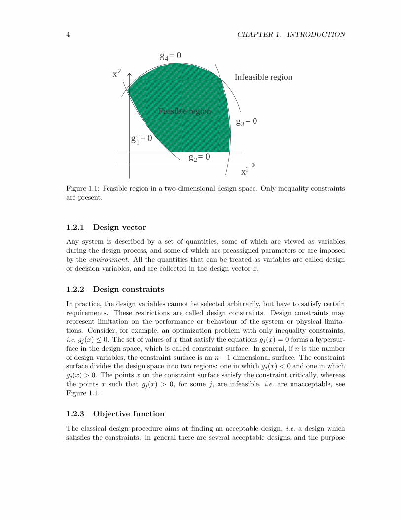
Figure 1.1: Feasible region in a two-dimensional design space. Only inequality constraintsare present.

1.2.1 Design vector

Any system is described by a set of quantities, some of which are viewed as variablesduring the design process, and some of which are preassigned parameters or are imposedby the environment. All the quantities that can be treated as variables are called designor decision variables, and are collected in the design vector x.

1.2.2 Design constraints

In practice, the design variables cannot be selected arbitrarily, but have to satisfy certainrequirements. These restrictions are called design constraints. Design constraints mayrepresent limitation on the performance or behaviour of the system or physical limita-tions. Consider, for example, an optimization problem with only inequality constraints,i.e. gj(x) ≤ 0. The set of values of x that satisfy the equations gj(x) = 0 forms a hypersur-face in the design space, which is called constraint surface. In general, if n is the numberof design variables, the constraint surface is an n− 1 dimensional surface. The constraintsurface divides the design space into two regions: one in which gj(x) < 0 and one in whichgj(x) > 0. The points x on the constraint surface satisfy the constraint critically, whereasthe points x such that gj(x) > 0, for some j, are infeasible, i.e. are unacceptable, seeFigure 1.1.

1.2.3 Objective function

The classical design procedure aims at finding an acceptable design, i.e. a design whichsatisfies the constraints. In general there are several acceptable designs, and the purpose

1.2. STATEMENT OF AN OPTIMIZATION PROBLEM 5

x1

x2 Feasible region

f=af=b

f=c

f=d

a<b<c<d

Optimum point

Figure 1.2: Design space, objective functions surfaces, and optimum point.

of the optimization is to single out the best possible design. Thus, a criterion has to beselected for comparing different designs. This criterion, when expressed as a function ofthe design variables, is known as objective function. The objective function is in generalspecified by physical or economical considerations. However, the selection of an objectivefunction is not trivial, because what is the optimal design with respect to a certain criterionmay be unacceptable with respect to another criterion. Typically there is a trade offperformance–cost, or performance–reliability, hence the selection of the objective functionis one of the most important decisions in the whole design process. If more than onecriterion has to be satisfied we have a multiobjective optimization problem, that maybe approximately solved considering a cost function which is a weighted sum of severalobjective functions.

Given an objective function f(x), the locus of all points x such that f(x) = c forms ahypersurface. For each value of c there is a different hypersurface. The set of all thesesurfaces are called objective function surfaces.

Once the objective function surfaces are drawn, together with the constraint surfaces, theoptimization problem can be easily solved, at least in the case of a two dimensional decisionspace, as shown in Figure 1.2. If the number of decision variables exceeds two or three,this graphical approach is not viable and the problem has to be solved as a mathematicalproblem. Note however that more general problems have similar geometrical properties oftwo or three dimensional problems.


R1

R2

R3

R4

R5

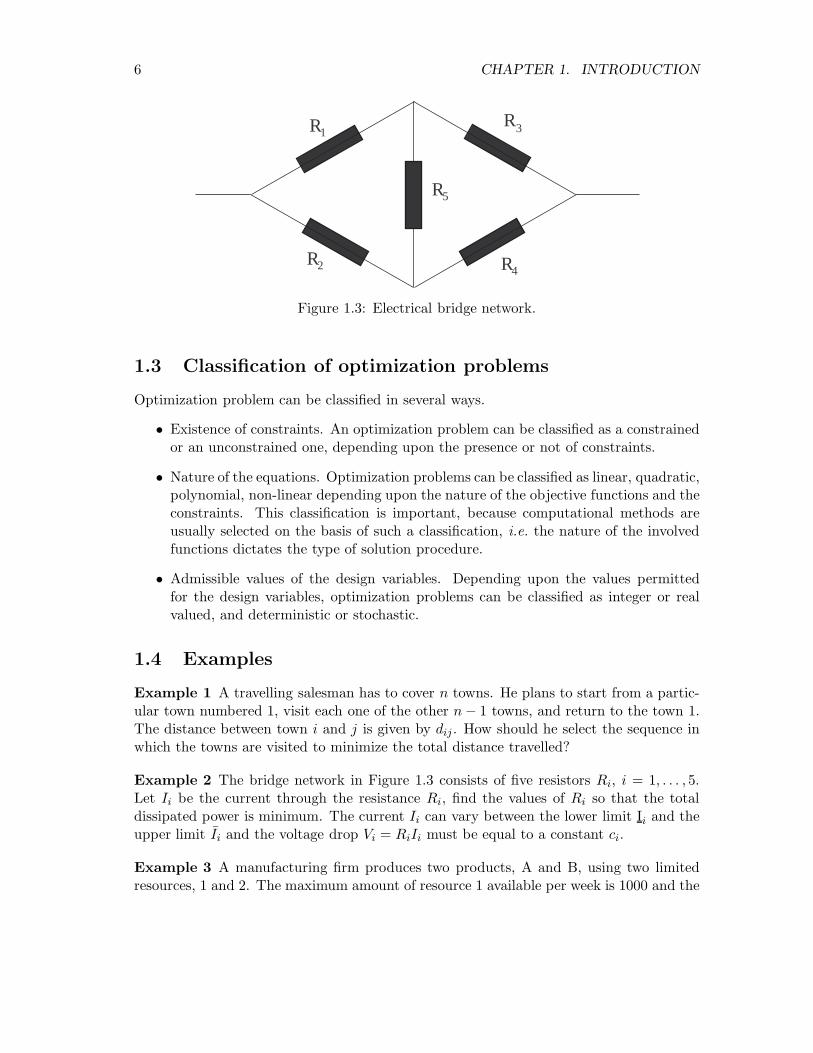
Figure 1.3: Electrical bridge network.

1.3 Classification of optimization problems

Optimization problem can be classified in several ways.

• Existence of constraints. An optimization problem can be classified as a constrainedor an unconstrained one, depending upon the presence or not of constraints.

• Nature of the equations. Optimization problems can be classified as linear, quadratic,polynomial, non-linear depending upon the nature of the objective functions and theconstraints. This classification is important, because computational methods areusually selected on the basis of such a classification, i.e. the nature of the involvedfunctions dictates the type of solution procedure.

• Admissible values of the design variables. Depending upon the values permittedfor the design variables, optimization problems can be classified as integer or realvalued, and deterministic or stochastic.

1.4 Examples

Example 1 A travelling salesman has to cover n towns. He plans to start from a partic-ular town numbered 1, visit each one of the other n − 1 towns, and return to the town 1.The distance between town i and j is given by dij . How should he select the sequence inwhich the towns are visited to minimize the total distance travelled?

Example 2 The bridge network in Figure 1.3 consists of five resistors Ri, i = 1, . . . , 5.Let Ii be the current through the resistance Ri, find the values of Ri so that the totaldissipated power is minimum. The current Ii can vary between the lower limit Ii and theupper limit Ii and the voltage drop Vi = RiIi must be equal to a constant ci.

Example 3 A manufacturing firm produces two products, A and B, using two limitedresources, 1 and 2. The maximum amount of resource 1 available per week is 1000 and the

1.4. EXAMPLES 7

Article type wi vi ci

1 4 9 52 8 7 63 2 4 3

Table 1.1: Properties of the articles to load.

maximum amount of resource 2 is 250. The production of one unit of A requires 1 unit ofresource 1 and 1/5 unit of resource 2. The production of one unit of B requires 1/2 unitof resource 1 and 1/2 unit of resource 2. The unit cost of resource 1 is 1−0.0005u1, whereu1 is the number of units of resource 1 used. The unit cost of resource 2 is 3/4−0.0001u2 ,where u2 is the number of units of resource 2 used. The selling price of one unit of A is

2 − 0.005xA − 0.0001xB

and the selling price of one unit of B is

4 − 0.002xA − 0.01xB ,

where xA and xB are the number of units of A and B sold. Assuming that the firm is ableto sell all manufactured units, maximize the weekly profit.

Example 4 A cargo load is to be prepared for three types of articles. The weight, wi,volume, vi, and value, ci, of each article is given in Table 1.1.Find the number of articles xi selected from type i so that the total value of the cargo ismaximized. The total weight and volume of the cargo cannot exceed 2000 and 2500 unitsrespectively.

Example 5 There are two types of gas molecules in a gaseous mixture at equilibrium. Itis known that the Gibbs free energy

G(x) = c1x1 + c2x

2 + x1log(x1/xT ) + x2log(x2/xT ),

with xT = x1 + x2 and c1, c2 known parameters depending upon the temperature andpressure of the mixture, has to be minimum in these conditions. The minimization ofG(x) is also subject to the mass balance equations:

x1ai1 + x2ai2 = bi,

for i = 1, . . . ,m, where m is the number of atomic species in the mixture, bi is the totalweight of atoms of type i, and aij is the number of atoms of type i in the molecule of typej. Show that the problem of determining the equilibrium of the mixture can be posed asan optimization problem.

Chapter 2

Unconstrainedoptimization

10 CHAPTER 2. UNCONSTRAINED OPTIMIZATION

2.1 Introduction

Several engineering, economic and planning problems can be posed as optimization prob-lems, i.e. as the problem of determining the points of minimum of a function (possibly inthe presence of conditions on the decision variables). Moreover, also numerical problems,such as the problem of solving systems of equations or inequalities, can be posed as anoptimization problem.We start with the study of optimization problems in which the decision variables aredefined in IRn: unconstrained optimization problems. More precisely we study the problemof determining local minima for differentiable functions. Although these methods areseldom used in applications, as in real problems the decision variables are subject toconstraints, the techniques of unconstrained optimization are instrumental to solve moregeneral problems: the knowledge of good methods for local unconstrained minimization isa necessary pre-requisite for the solution of constrained and global minimization problems.The methods that will be studied can be classified from various points of view. Themost interesting classification is based on the information available on the function to beoptimized, namely

• methods without derivatives (direct search, finite differences);

• methods based on the knowledge of the first derivatives (gradient, conjugate direc-tions, quasi-Newton);

• methods based on the knowledge of the first and second derivatives (Newton).

2.2 Definitions and existence conditions

Consider the optimization problem:

Problem 1 Minimizef(x) subject to x ∈ F

in which f : IRn → IR and1 F ⊂ IRn.

With respect to this problem we introduce the following definitions.

Definition 1 A point x ∈ F is a global minimum2 for the Problem 1 if

f(x) ≤ f(y)

for all y ∈ F .A point x ∈ F is a strict (or isolated) global minimum (or minimiser) for the Problem 1if

f(x) < f(y)1The set F may be specified by equations of the form (1.1) and/or (1.2).2Alternatively, the term global minimiser can be used to denote a point at which the function f attains

its global minimum.

2.2. DEFINITIONS AND EXISTENCE CONDITIONS 11

for all y ∈ F and y �= x.A point x ∈ F is a local minimum (or minimiser) for the Problem 1 if there exists ρ > 0such that

f(x) ≤ f(y)

for all y ∈ F such that ‖y − x‖ < ρ.A point x ∈ F is a strict (or isolated) local minimum (or minimiser) for the Problem 1 ifthere exists ρ > 0 such that

f(x) < f(y)

for all y ∈ F such that ‖y − x‖ < ρ and y �= x.

Definition 2 If x ∈ F is a local minimum for the Problem 1 and if x is in the interiorof F then x is an unconstrained local minimum of f in F .

The following result provides a sufficient, but not necessary, condition for the existence ofa global minimum for Problem 1.

Proposition 1 Let f : IRn → IR be a continuous function and let F ⊂ IRn be a compactset3. Then there exists a global minimum of f in F .

In unconstrained optimization problems the set F coincides with IRn, hence the abovestatement cannot be used to establish the existence of global minima. To address theexistence problem it is necessary to consider the structure of the level sets of the functionf . See also Section 1.2.3.

Definition 3 Let f : IRn → IR. A level set of f is any non-empty set described by

L(α) = {x ∈ IRn : f(x) ≤ α},with α ∈ IR.

For convenience, if x0 ∈ IRn we denote with L0 the level set L(f(x0)). Using the conceptof level sets it is possible to establish a simple sufficient condition for the existence ofglobal solutions for an unconstrained optimization problem.

Proposition 2 Let f : IRn → IR be a continuous function. Assume there exists x0 ∈ IRn

such that the level set L0 is compact. Then there exists a point of global minimum of f inIRn.

Proof. By Proposition 1 there exists a global minimum x� of f in L0, i.e. f(x�) ≤ f(x) forall x ∈ L0. However, if x �∈ L0 then f(x) > f(x0) ≥ f(x�), hence x� is a global minimumof f in IRn. �

It is obvious that the structure of the level sets of the function f plays a fundamentalrole in the solution of Problem 1. The following result provides a necessary and sufficientcondition for the compactness of all level sets of f .

3A compact set is a bounded and closed set.


Proposition 3 Let f : IRn → IR be a continuous function. All level sets of f are compactif and only if for any sequence {xk} one has

limk→∞

‖xk‖ = ∞ ⇒ limk→∞

f(xk) = ∞.

Remark. In general xk ∈ IRn, namely

xk =

⎡⎢⎢⎢⎢⎣x1

k

x2k...

xnk

⎤⎥⎥⎥⎥⎦ ,

i.e. we use superscripts to denote components of a vector. �

A function that satisfies the condition of the above proposition is said to be radiallyunbounded.

Proof. We only prove the necessity. Suppose all level sets of f are compact. Then,proceeding by contradiction, suppose there exist a sequence {xk} such that limk→∞ ‖xk‖ =∞ and a number γ > 0 such that f(xk) ≤ γ < ∞ for all k. As a result

{xk} ⊂ L(γ).

However, by compactness of L(γ) it is not possible that limk→∞ ‖xk‖ = ∞. �

Definition 4 Let f : IRn → IR. A vector d ∈ IRn is said to be a descent direction for fin x� if there exists δ > 0 such that

f(x� + λd) < f(x�),

for all λ ∈ (0, δ).

If the function f is differentiable it is possible to give a simple condition guaranteeing thata certain direction is a descent direction.

Proposition 4 Let f : IRn → IR and assume4 ∇f exists and is continuous. Let x� and dbe given. Then, if ∇f(x�)′d < 0 the direction d is a descent direction for f at x�.

Proof. Note that ∇f(x�)′d is the directional derivative of f (which is differentiable byhypothesis) at x� along d, i.e.

∇f(x�)′d = limλ→0+

f(x� + λd) − f(x�)λ

,

4We denote with ∇f the gradient of the function f , i.e. ∇f = [ ∂f∂x1 , · · · , ∂f

∂xn ]′. Note that ∇f is acolumn vector.


f increasing

f(x) = f(x )*

descent direction

anti-gradient

f(x) = f(x ) > f(x )*1

f(x) = f(x ) > f(x )12

Figure 2.1: Geometrical interpretation of the anti-gradient.

and this is negative by hypothesis. As a result, for λ > 0 and sufficiently small

f(x� + λd) − f(x�) < 0,

hence the claim. �

The proposition establishes that if ∇f(x�)′d < 0 then for sufficiently small positive dis-placements along d and starting at x� the function f is decreasing. It is also obvious thatif ∇f(x�)′d > 0, d is a direction of ascent, i.e. the function f is increasing for sufficientlysmall positive displacements from x� along d. If ∇f(x�)′d = 0, d is orthogonal to ∇f(x�)and it is not possible to establish, without further knowledge on the function f , what isthe nature of the direction d.From a geometrical point of view (see also Figure 2.1), the sign of the directional derivative∇f(x�)′d gives information on the angle between d and the direction of the gradient atx�, provided ∇f(x�) �= 0. If ∇f(x�)′d > 0 the angle between ∇f(x�) and d is acute. If∇f(x�)′d < 0 the angle between ∇f(x�) and d is obtuse. Finally, if ∇f(x�)′d = 0, and∇f(x�) �= 0, ∇f(x�) and d are orthogonal. Note that the gradient ∇f(x�), if it is notidentically zero, is a direction orthogonal to the level surface {x : f(x) = f(x�)} and it isa direction of ascent, hence the anti-gradient −∇f(x�) is a descent direction.

Remark. The scalar product x′y between the two vectors x and y can be used to definethe angle between x and y. For, define the angle between x and y as the number θ ∈ [0, π]such that5

cos θ =x′y

‖x‖E‖y‖E.

If x′y = 0 one has cos θ = 0 and the vectors are orthogonal, whereas if x and y have thesame direction, i.e. x = λy with λ > 0, cos θ = 1. �

5‖x‖E denotes the Euclidean norm of the the vector x, i.e. ‖x‖E =√

x′x.


We are now ready to state and prove some necessary conditions and some sufficient con-ditions for a local minimum.

Theorem 1 [First order necessary condition] Let f : IRn → IR and assume ∇f exists andis continuous. The point x� is a local minimum of f only if

∇f(x�) = 0.

Remark. A point x� such that ∇f(x�) = 0 is called a stationary point of f . �

Proof. If ∇f(x�) �= 0 the direction d = −∇f(x�) is a descent direction. Therefore, in aneighborhood of x� there is a point x� + λd = x� − λ∇f(x�) such that

f(x� − λ∇f(x�)) < f(x�),

and this contradicts the hypothesis that x� is a local minimum. �

Theorem 2 [Second order necessary condition] Let f : IRn → IR and assume6 ∇2f existsand is continuous. The point x� is a local minimum of f only if

∇f(x�) = 0

andx′∇2f(x�)x ≥ 0

for all x ∈ IRn.

Proof. The first condition is a consequence of Theorem 1. Note now that, as f is twotimes differentiable, for any x �= x� one has

f(x� + λx) = f(x�) + λ∇f(x�)′x +12λ2x′∇2f(x�)x + β(x�, λx),

wherelimλ→0

β(x�, λx)λ2‖x‖2

= 0,

or what is the same (note that x is fixed)

limλ→0

β(x�, λx)λ2

= 0.

6We denote with ∇2f the Hessian matrix of the function f , i.e.⎡⎢⎣∂2f

∂x1∂x1 · · · ∂2f∂x1∂xn

.... . .

...∂2f

∂xn∂x1 · · · ∂2f∂xn∂xn

⎤⎥⎦ .

Note that ∇2f is a square matrix and that, under suitable regularity conditions, the Hessian matrix issymmetric.


Moreover, the condition ∇f(x�) = 0 yields

f(x� + λx) − f(x�)λ2

=12x′∇2f(x�)x +

β(x�, λx)λ2

. (2.1)

However, as x� is a local minimum, the left hand side of equation (2.1) must be non-negative for all λ sufficiently small, hence

12x′∇2f(x�)x +

β(x�, λx)λ2

≥ 0,

andlimλ→0

(12x′∇2f(x�)x +

β(x�, λx)λ2

)=

12x′∇2f(x�)x ≥ 0,

which proves the second condition. �

Theorem 3 (Second order sufficient condition) Let f : IRn → IR and assume ∇2fexists and is continuous. The point x� is a strict local minimum of f if

∇f(x�) = 0

andx′∇2f(x�)x > 0

for all non-zero x ∈ IRn.

Proof. To begin with, note that as ∇2f(x�) > 0 and ∇2f is continuous, then there is aneighborhood Ω of x� such that for all y ∈ Ω

∇2f(y) > 0.

Consider now the Taylor series expansion of f around the point x�, i.e.

f(y) = f(x�) + ∇f(x�)′(y − x�) +12(y − x�)′∇2f(ξ)(y − x�),

where ξ = x� + θ(y − x�), for some θ ∈ [0, 1]. By the first condition one has

f(y) = f(x�) +12(y − x�)′∇2f(ξ)(y − x�),

and, for any y ∈ Ω such that y �= x�,

f(y) > f(x�),

which proves the claim. �

The above results can be easily modified to derive necessary conditions and sufficient con-ditions for a local maximum. Moreover, if x� is a stationary point and the Hessian matrix


−2

−1

0

1

2

−2

−1

0

1

2−4

−3

−2

−1

0

1

2

3

4

Figure 2.2: A saddle point in IR2.

∇2f(x�) is indefinite, the point x� is neither a local minimum neither a local maximum.Such a point is called a saddle point (see Figure 2.2 for a geometrical illustration).If x� is a stationary point and ∇2f(x�) is semi-definite it is not possible to draw anyconclusion on the point x� without further knowledge on the function f . Nevertheless, ifn = 1 and the function f is infinitely times differentiable it is possible to establish thefollowing necessary and sufficient condition.

Proposition 5 Let f : IR → IR and assume f is infinitely times differentiable. The pointx� is a local minimum if and only if there exists an even integer r > 1 such that

dkf(x�)dxk

= 0

for k = 1, 2, . . . , r − 1 anddrf(x�)

dxr> 0.

Necessary and sufficient conditions for n > 1 can be only derived if further hypotheses onthe function f are added, as shown for example in the following fact.

Proposition 6 (Necessary and sufficient condition for convex functions) Let f :IRn → IR and assume ∇f exists and it is continuous. Suppose f is convex, i.e.

f(y) − f(x) ≥ ∇f(x)′(y − x) (2.2)

for all x ∈ IRn and y ∈ IRn. The point x� is a global minimum if and only if ∇f(x�) = 0.

2.3. GENERAL PROPERTIES OF MINIMIZATION ALGORITHMS 17

Proof. The necessity is a consequence of Theorem 1. For the sufficiency note that, byequation (2.2), if ∇f(x�) = 0 then

f(y) ≥ f(x�),

for all y ∈ IRn. �

From the above discussion it is clear that to establish the property that x�, satisfying∇f(x�) = 0, is a global minimum it is enough to assume that the function f has thefollowing property: for all x and y such that

∇f(x)′(y − x) ≥ 0

one hasf(y) ≥ f(x).

A function f satisfying the above property is said pseudo-convex. Note that a differentiableconvex function is also pseudo-convex, but the opposite is not true. For example, thefunction x + x3 is pseudo-convex but it is not convex. Finally, if f is strictly convex orstrictly pseudo-convex the global minimum (if it exists) is also unique.

2.3 General properties of minimization algorithms

Consider the problem of minimizing the function f : IRn → IR and suppose that ∇f and∇2f exist and are continuous. Suppose that such a problem has a solution, and moreoverthat there exists x0 such that the level set

L(f(x0)) = {x ∈ IRn : f(x) ≤ f(x0)}is compact.General unconstrained minimization algorithms allow only to determine stationary pointsof f , i.e. to determine points in the set

Ω = {x ∈ IRn : ∇f(x) = 0}.Moreover, for almost all algorithms, it is possible to exclude that the points of Ω yieldedby the algorithm are local maxima. Finally, some algorithms yield points of Ω that satisfyalso the second order necessary conditions.

2.3.1 General unconstrained minimization algorithm

An algorithm for the solution of the considered minimization problem is a sequence {xk},obtained starting from an initial point x0, having some convergence properties in relationwith the set Ω. Most of the algorithms that will be studied in this notes can be describedin the following general way.

1. Fix a point x0 ∈ IRn and set k = 0.


2. If xk ∈ Ω STOP.

3. Compute a direction of research dk ∈ IRn.

4. Compute a step αk ∈ IR along dk.

5. Let xk+1 = xk + αkdk. Set k = k + 1 and go back to 2.

The existing algorithms differ in the way the direction of research dk is computed andon the criteria used to compute the step αk. However, independently from the particularselection, it is important to study the following issues:

• the existence of accumulation points for the sequence {xk};

• the behavior of such accumulation points in relation with the set Ω;

• the speed of convergence of the sequence {xk} to the points of Ω.

2.3.2 Existence of accumulation points

To make sure that any subsequence of {xk} has an accumulation point it is necessary toassume that the sequence {xk} remains bounded, i.e. that there exists M > 0 such that‖xk‖ < M for any k. If the level set L(f(x0)) is compact, the above condition holds if{xk} ∈ L(f(x0)). This property, in turn, is guaranteed if

f(xk+1) < f(xk),

for any k such that xk �∈ Ω. The algorithms that satisfy this property are denominateddescent methods. For such methods , if L(f(x0)) is compact and if ∇f is continuous onehas

• {xk} ∈ L(f(x0)) and any subsequence of {xk} admits a subsequence converging toa point of L(f(x0));

• the sequence {f(xk)} has a limit, i.e. there exists f ∈ IR such that

limk→∞

f(xk) = f ;

• there always exists an element of Ω in L(f(x0)). In fact, as f has a minimum inL(f(x0)), this minimum is also a minimum of f in IRn. Hence, by the assumptionsof ∇f , such a minimum must be a point of Ω.

Remark. To guarantee the descent property it is necessary that the research directions dk

be directions of descent. This is true if

∇f(xk)′dk < 0,


for all k. Under this condition there exists an interval (0, α�] such that

f(xk + αdk) < f(xk),

for any α ∈ (0, α�]. �

Remark. The existence of accumulation points for the sequence {xk} and the convergenceof the sequence {f(xk)} do not guarantee that the accumulation points of {xk} are localminima of f or stationary points. To obtain this property it is necessary to impose furtherrestrictions on the research directions dk and on the steps αk. �

2.3.3 Condition of angle

The condition which is in general imposed on the research directions dk is the so-calledcondition of angle, that can be stated as follows.

Condition 1 There exists ε > 0, independent from k, such that

∇f(xk)′dk ≤ −ε‖∇f(xk)‖‖dk‖,for any k.

From a geometric point of view the above condition implies that the cosine of the anglebetween dk and −∇f(xk) is larger than a certain quantity. This condition is imposed toavoid that, for some k, the research direction is orthogonal to the direction of the gradient.Note moreover that, if the angle condition holds, and if ∇f(xk) �= 0 then dk is a descentdirection. Finally, if ∇f(xk) �= 0, it is always possible to find a direction dk such that theangle condition holds. For example, the direction dk = −∇f(xk) is such that the anglecondition is satisfied with ε = 1.

Remark. Let {Bk} be a sequence of matrices such that

mI ≤ Bk ≤ MI,

for some 0 < m < M , and for any k, and consider the directions

dk = −Bk∇f(xk).

Then a simple computation shows that the angle condition holds with ε = m/M . �

The angle condition imposes a constraint only on the research directions dk. To makesure that the sequence {xk} converges to a point in Ω it is necessary to impose furtherconditions on the step αk, as expressed in the following statements.

Theorem 4 Let {xk} be the sequence obtained by the algorithm

xk+1 = xk + αkdk,

for k ≥ 0. Assume that


(H1) ∇f is continuous and the level set L(f(x0)) is compact.

(H2) There exists ε > 0 such that

∇f(xk)′dk ≤ −ε‖∇f(xk)‖‖dk‖,

for any k ≥ 0.

(H3) f(xk+1) < f(xk) for any k ≥ 0.

(H4) The property

limk→∞

∇f(xk)′dk

‖dk‖ = 0

holds.

Then

(C1) {xk} ∈ L(f(x0)) and any subsequence of {xk} has an accumulation point.

(C2) {f(xk)} is monotonically decreasing and there exists f such that

limk→∞

f(xk) = f .

(C3) {∇f(xk)} is such thatlim

k→∞‖∇f(xk)‖ = 0.

(C4) Any accumulation point x of {xk} is such that ∇f(x) = 0.

Proof. Conditions (C1) and (C2) are a simple consequence of (H1) and (H3). Note nowthat (H2) implies

ε‖∇f(xk)‖ ≤ |∇f(xk)′dk|‖dk‖ ,

for all k. As a result, and by (H4),

limk→∞

ε‖∇f(xk)‖ ≤ limk→∞

|∇f(xk)′dk|‖dk‖ = 0

hence (C3) holds. Finally, let x be an accumulation point of the sequence {xk}, i.e. thereis a subsequence that converges to x. For such a subsequence, and by continuity of f , onehas

limk→∞

∇f(xk) = ∇f(x),

and, by (C3),∇f(x) = 0,

which proves (C4). �


Remark. Theorem 4 does not guarantee the convergence of the sequence {xk} to a uniqueaccumulation point. Obviously {xk} has a unique accumulation point if either Ω∩L(f(x0))contains only one point or x, y ∈ Ω ∩ L(f(x0)), with x �= y implies f(x) �= f(y). Finally,if the set Ω ∩ L(f(x0)) contains a finite number of points, a sufficient condition for theexistence of a unique accumulation point is

limk→∞

‖xk+1 − xk‖ = 0.

�

Remark. The angle condition can be replaced by the following one. There exists η > 0and q > 0, both independent from k, such that

∇f(xk)′dk ≤ −η‖∇f(xk)‖q‖dk‖.�

The result illustrated in Theorem 4 requires the fulfillment of the angle condition or of asimilar one, i.e. of a condition involving ∇f . In many algorithms that do not make useof the gradient it may be difficult to check the validity of the angle condition, hence it isnecessary to use different conditions on the research directions. For example, it is possibleto replace the angle condition with a property of linear independence of the researchdirections.

Theorem 5 Let {xk} be the sequence obtained by the algorithm

xk+1 = xk + αkdk,

for k ≥ 0. Assume that

• ∇2f is continuous and the level set L(f(x0)) is compact.

• There exist σ > 0, independent from k, and k0 > 0 such that, for any k ≥ k0 thematrix Pk composed of the columns

dk

‖dk‖ ,dk+1

‖dk+1‖ , . . . ,dk+n−1

‖dk+n−1‖ ,

is such that|detPk| ≥ σ.

• limk→∞ ‖xk+1 − xk‖ = 0.

• f(xk+1) < f(xk) for any k ≥ 0.

• The property

limk→∞

∇f(xk)′dk

‖dk‖ = 0

holds.


Then

• {xk} ∈ L(f(x0)) and any subsequence of {xk} has an accumulation point.

• {f(xk)} is monotonically decreasing and there exists f such that

limk→∞

f(xk) = f .

• Any accumulation point x of {xk} is such that ∇f(x) = 0.

Moreover, if the set Ω ∩ L(f(x0)) is composed of a finite number of points, the sequence{xk} has a unique accumulation point.

2.3.4 Speed of convergence

Together with the property of convergence of the sequence {xk} it is important to studyalso the speed of convergence. To study such a notion it is convenient to assume that {xk}converges to a point x�.If there exists a finite k such that xk = x� then we say that the sequence {xk} has finiteconvergence. Note that if {xk} is generated by an algorithm, there is a stopping conditionthat has to be satisfied at step k.If xk �= x� for any finite k, it is possible (and convenient) to study the asymptotic propertiesof {xk}. One criterion to estimate the speed of convergence is based on the behavior ofthe error Ek = ‖xk − x�‖, and in particular on the relation between Ek+1 and Ek.We say that {xk} has speed of convergence of order p if

limk→∞

(Ek+1

Epk

)= Cp

with p ≥ 1 and 0 < Cp < ∞. Note that if {xk} has speed of convergence of order p then

limk→∞

(Ek+1

Eqk

)= 0,

if 1 ≤ q < p, and

limk→∞

(Ek+1

Eqk

)= ∞,

if q > p. Moreover, from the definition of speed of convergence, it is easy to see that if{xk} has speed of convergence of order p then, for any ε > 0 there exists k0 such that

Ek+1 ≤ (Cp + ε)Epk ,

for any k > k0.In the cases p = 1 or p = 2 the following terminology is often used. If p = 1 and 0 < C1 ≤ 1the speed of convergence is linear; if p = 1 and C1 > 1 the speed of convergence is sublinear;if

limk→∞

(Ek+1

Ek

)= 0

2.4. LINE SEARCH 23

the speed of convergence is superlinear, and finally if p = 2 the speed of convergence isquadratic.Of special interest in optimization is the case of superlinear convergence, as this is the kindof convergence that can be established for the efficient minimization algorithms. Note thatif xk has superlinear convergence to x� then

limk→∞

‖xk+1 − xk‖‖xk − x�‖ = 1.

Remark. In some cases it is not possible to establish the existence of the limit

limk→∞

(Ek+1

Eqk

).

In these cases an estimate of the speed of convergence is given by

Qp = lim supk→∞

(Ek+1

Eqk

).

�

2.4 Line search

A line search is a method to compute the step αk along a given direction dk. The choiceof αk affects both the convergence and the speed of convergence of the algorithm. In anyline search one considers the function of one variable φ : IR → IR defined as

φ(α) = f(xk + αdk) − f(xk).

The derivative of φ(α) with respect to α is given by

φ(α) = ∇f(xk + αdk)′dk

provided that ∇f is continuous. Note that ∇f(xk + αdk)′dk describes the slope of thetangent to the function φ(α), and in particular

φ(0) = ∇f(xk)′dk

coincides with the directional derivative of f at xk along dk.From the general convergence results described, we conclude that the line search has toenforce the following conditions

f(xk+1) < f(xk)

limk→∞

∇f(xk)′dk

‖dk‖ = 0


and, whenever possible, also the condition

limk→∞

‖xk+1 − xk‖ = 0.

To begin with, we assume that the directions dk are such that

∇f(xk)′dk < 0

for all k, i.e. dk is a descent direction, and that it is possible to compute, for any fixed x,both f and ∇f . Finally, we assume that the level set L(f(x0)) is compact.

2.4.1 Exact line search

The exact line search consists in finding αk such that

φ(αk) = f(xk + αkdk) − f(xk) ≤ f(xk + αdk) − f(xk) = φ(α)

for any α ≥ 0. Note that, as dk is a descent direction and the set

{α ∈ IR+ : φ(α) ≤ φ(0)}is compact, because of compactness of L(f(x0)), there exists an αk that minimizes φ(α).Moreover, for such αk one has

φ(αk) = ∇f(xk + αkdk)′dk = 0,

i.e. if αk minimizes φ(α) the gradient of f at xk + αkdk is orthogonal to the direction dk.From a geometrical point of view, if αk minimizes φ(α) then the level surface of f throughthe point xk + αkdk is tangent to the direction dk at such a point. (If there are severalpoints of tangency, αk is the one for which f has the smallest value).The search of αk that minimizes φ(α) is very expensive, especially if f is not convex. More-over, in general, the whole minimization algorithm does not gain any special advantagefrom the knowledge of such optimal αk. It is therefore more convenient to use approximatemethods, i.e. methods which are computationally simple and which guarantee particularconvergence properties. Such methods are aimed at finding an interval of acceptable valuesfor αk subject to the following two conditions

• αk has to guarantee a sufficient reduction of f ;

• αk has to be sufficiently distant from 0, i.e. xk + αkdk has to be sufficiently awayfrom xk.

2.4.2 Armijo method

Armijo method was the first non-exact linear search method.Let a > 0, σ ∈ (0, 1) and γ ∈ (0, 1/2) be given and define the set of points

A = {α ∈ R : α = aσj , j = 0, 1, . . .}.

2.4. LINE SEARCH 25

α

φ(α)

φ(0)α.

γ φ(0)α.

aaσφ(0)

Figure 2.3: Geometrical interpretation of Armijo method.

Armijo method consists in finding the largest α ∈ A such that

φ(α) = f(xk + αdk) − f(xk) ≤ γα∇f(xk)′dk = γαφ(0).

Armijo method can be implemented using the following (conceptual) algorithm.

Step 1. Set α = a.

Step 2. Iff(xk + αdk) − f(xk) ≤ γα∇f(xk)′dk

set αk = α and STOP. Else go to Step 3.

Step 3. Set α = σα, and go to Step 2.

From a geometric point of view (see Figure 2.3) the condition in Step 2 requires that αk

is such that φ(αk) is below the straight line passing through the point (0, φ(0)) and withslope γφ(0). Note that, as γ ∈ (0, 1/2) and φ(0) < 0, such a straight line has a slopesmaller than the slope of the tangent at the curve φ(α) at the point (0, φ(0)).For Armijo method it is possible to prove the following convergence result.

Theorem 6 Let f : IRn → IR and assume ∇f is continuous and L(f(x0)) is compact.Assume ∇f(xk)′dk < 0 for all k and there exist C1 > 0 and C2 > 0 such that

C1 ≥ ‖dk‖ ≥ C2‖∇f(xk)‖q,

for some q > 0 and for all k.Then Armijo method yields in a finite number of iterations a value of αk > 0 satisfyingthe condition in Step 2. Moreover, the sequence obtained setting xk+1 = xk + αkdk issuch that

f(xk+1) < f(xk),


for all k, and

limk→∞

∇f(xk)′dk

‖dk‖ = 0.

Proof. We only prove that the method cannot loop indefinitely between Step 2 andStep 3. In fact, if this is the case, then the condition in Step 2 will never be satisfied,hence

f(xk + aσjdk) − f(xk)aσj

> γ∇f(xk)′dk.

Note now that σj → 0 as j → ∞, and the above inequality for j → ∞ is

∇f(xk)′dk > γ∇f(xk)′dk,

which is not possible since γ ∈ (0, 1/2) and ∇f(xk)′dk �= 0. �

Remark. It is interesting to observe that in Theorem 6 it is not necessary to assume thatxk+1 = xk + αkdk. It is enough that xk+1 is such that

f(xk+1) ≤ f(xk + αkdk),

where αk is generated using Armijo method. This implies that all acceptable values of αare those such that

f(xk + αdk) ≤ f(xk + αkdk).

As a result, Theorem 6 can be used to prove also the convergence of an algorithm basedon the exact line search. �

2.4.3 Goldstein conditions

The main disadvantage of Armijo method is in the fact that, to find αk, all points in theset A, starting from the point α = a, have to be tested till the condition in Step 2 isfulfilled. There are variations of the method that do not suffer from this disadvantage. Acriterion similar to Armijo’s, but that allows to find an acceptable αk in one step, is basedon the so-called Goldstein conditions.Goldstein conditions state that given γ1 ∈ (0, 1) and γ2 ∈ (0, 1) such that γ1 < γ2, αk isany positive number such that

f(xk + αkdk) − f(xk) ≤ αkγ1∇f(xk)′dk

i.e. there is a sufficient reduction in f , and

f(xk + αkdk) − f(xk) ≥ αkγ2∇f(xk)′dk

i.e. there is a sufficient distance between xk and xk+1.From a geometric point of view (see Figure 2.4) this is equivalent to select αk as any pointsuch that the corresponding value of f is included between two straight lines, of slope

2.4. LINE SEARCH 27

α

φ(α)

φ(0)

φ(0)α.

γ φ(0)α.

1

α

γ φ(0)α.

2

α

Figure 2.4: Geometrical interpretation of Goldstein method.

γ1∇f(xk)′dk and γ2∇f(xk)′dk, respectively, and passing through the point (0, φ(0)). As0 < γ1 < γ2 < 1 it is obvious that there exists always an interval I = [α,α] such thatGoldstein conditions hold for any α ∈ I.Note that, a result similar to Theorem 6, can be also established if the sequence {xk} isgenerated using Goldstein conditions.The main disadvantage of Armijo and Goldstein methods is in the fact that none ofthem impose conditions on the derivative of the function φ(α) in the point αk, or whatis the same on the value of ∇f(xk+1)′dk. Such extra conditions are sometimes usefulin establishing convergence results for particular algorithms. However, for simplicity, weomit the discussion of these more general conditions (known as Wolfe conditions).

2.4.4 Line search without derivatives

It is possible to construct methods similar to Armijo’s or Goldstein’s also in the case thatno information on the derivatives of the function f is available.Suppose, for simplicity, that ‖dk‖ = 1, for all k, and that the sequence {xk} is generatedby

xk+1 = xk + αkdk.

If ∇f is not available it is not possible to decide a priori if the direction dk is a descentdirection, hence it is necessary to consider also negative values of α.We now describe the simplest line search method that can be constructed with the con-sidered hypothesis. This method is a modification of Armijo method and it is known asparabolic search.Given λ0 > 0, σ ∈ (0, 1/2), γ > 0 and ρ ∈ (0, 1). Compute αk and λk such that one of thefollowing conditions hold.

Condition (i)


• λk = λk−1;

• αk is the largest value in the set

A = {α ∈ IR : α = ±σj, j = 0, 1, . . .}

such thatf(xk + αkdk) ≤ f(xk) − γα2

k,

or, equivalently, φ(αk) ≤ −γα2k.

Condition (ii)

• αk = 0, λk ≤ ρλk−1;

• min (f(xk + λkdk), f(xk − λkdk)) ≥ f(xk) − γλ2k.

At each step it is necessary to satisfy either Condition (i) or Condition (ii). Note that thisis always possible for any dk �= 0. Condition (i) requires that αk is the largest numberin the set A such that f(xk + αkdk) is below the parabola f(xk) − γα2. If the functionφ(α) has a stationary point for α = 0 then there may be no α ∈ A such that Condition(i) holds. However, in this case it is possible to find λk such that Condition (ii) holds. IfCondition (ii) holds then αk = 0, i.e. the point xk remains unchanged and the algorithmscontinues with a new direction dk+1 �= dk.For the parabolic search algorithm it is possible to prove the following convergence result.

Theorem 7 Let f : IRn → IR and assume ∇f is continuous and L(f(x0)) is compact.If αk is selected following the conditions of the parabolic search and if xk+1 = xk + αkdk,with ‖dk‖ = 1 then the sequence {xk} is such that

f(xk+1) ≤ f(xk)

for all k,lim

k→∞∇f(xk)′dk = 0

andlim

k→∞‖xk+1 − xk‖ = 0.

Proof. (Sketch) Note that Condition (i) implies f(xk+1) < f(xk), whereas Condition (ii)implies f(xk+1) = f(xk). Note now that if Condition (ii) holds for all k ≥ k, then αk = 0for all k ≥ k, i.e. ‖xk+1 − xk‖ = 0. Moreover, as λk is reduced at each step, necessarily∇f(xk)

′d = 0, where d is a limit of the sequence {dk}. �

2.5. THE GRADIENT METHOD 29

2.4.5 Implementation of a line search algorithm

On the basis of the conditions described so far it is possible to construct algorithms thatyield αk in a finite number of steps. One such an algorithm can be described as follows.(For simplicity we assume that ∇f is known.)

• Initial data. xk, f(xk), ∇f(xk), α and α.

• Initial guess for α. A possibility is to select α as the point in which a parabolathrough (0, φ(0)) with derivative φ(0) for α = 0 takes a pre-specified minimum valuef�. Initially, i.e. for k = 0, f� has to be selected by the designer. For k > 0 it ispossible to select f� such that

f(xk) − f� = f(xk−1) − f(xk).

The resulting α is

α� = −2f(xk) − f�

∇f(xk)′dk.

In some algorithms it is convenient to select α ≤ 1, hence the initial guess for α willbe min (1, α�) .

• Computation of αk. A value for αk is computed using a line search method. Ifαk ≤ α the direction dk may not be a descent direction. If αk ≥ α the level setL(f(xk)) may not be compact. If αk �∈ [α,α] the line search fails, and it is necessaryto select a new research direction dk. Otherwise the line search terminates andxk+1 = xk + αkdk.

2.5 The gradient method

The gradient method consists in selecting, as research direction, the direction of the anti-gradient at xk, i.e.

dk = −∇f(xk),

for all k. This selection is justified noting that the direction7

− ∇f(xk)‖∇f(xk)‖E

is the direction that minimizes the directional derivative, among all direction with unitaryEuclidean norm. In fact, by Schwartz inequality, one has

|∇f(xk)′d| ≤ ‖d‖E‖∇f(xk)‖E ,

and the equality sign holds if and only if d = λ∇f(xk), with λ ∈ IR. As a consequence,the problem

min‖d‖E=1

∇f(xk)′d

7We denote with ‖v‖E the Euclidean norm of the vector v, i.e. ‖v‖E =√

v′v.


has the solution d� = − ∇f(xk)‖∇f(xk)‖E

. For this reason, the gradient method is sometimescalled the method of the steepest descent. Note however that the (local) optimality ofthe direction −∇f(xk) depends upon the selection of the norm, and that with a properselection of the norm, any descent direction can be regarded as the steepest descent.The real interest in the direction −∇f(xk) rests on the fact that, if ∇f is continuous, thenthe former is a continuous descent direction, which is zero only if the gradient is zero, i.e.at a stationary point.The gradient algorithm can be schematized has follows.

Step 0. Given x0 ∈ IRn.

Step 1. Set k = 0.

Step 2. Compute ∇f(xk). If ∇f(xk) = 0 STOP. Else set dk = −∇f(xk).

Step 3. Compute a step αk along the direction dk with any line search method suchthat

f(xk + αkdk) ≤ f(xk)

and

limk→∞

∇f(xk)′dk

‖dk‖ = 0.

Step 4. Set xk+1 = xk + αkdk, k = k + 1. Go to Step 2.

By the general results established in Theorem 4, we have the following fact regarding theconvergence properties of the gradient method.

Theorem 8 Consider f : IRn → IR. Assume ∇f is continuous and the level set L(f(x0))is compact. Then any accumulation point of the sequence {xk} generated by the gradientalgorithm is a stationary point of f .

1 2 3 4 5 6 7 8 9 100

0.5

1

1.5

2

2.5

3

Figure 2.5: The function√

ξξ − 1ξ + 1

.

2.6. NEWTON’S METHOD 31

To estimate the speed of convergence of the method we can consider the behavior of themethod in the minimization of a quadratic function, i.e. in the case

f(x) =12x′Qx + c′x + d,

with Q = Q′ > 0. In such a case it is possible to obtain the following estimate

‖xk+1 − x�‖ ≤√

λM

λm

√λMλm

− 1√λMλm

+ 1‖xk − x�‖,

where λM ≥ λm > 0 are the maximum and minimum eigenvalue of Q, respectively. Notethat the above estimate is exact for some initial points x0. As a result, if λM �= λm thegradient algorithm has linear convergence, however, if λM/λm is large the convergence canbe very slow (see Figure 2.5).Finally, if λM/λm = 1 the gradient algorithm converges in one step. From a geometricpoint of view the ratio λM/λm expresses the ratio between the lengths of the maximumand the minimum axes of the ellipsoids, that constitute the level surfaces of f . If this ratiois big there are points from which the gradient algorithm converges very slowly, see e.g.Figure 2.6.

.. ..Figure 2.6: Behavior of the gradient algorithm.

In the non-quadratic case, the performance of the gradient method are unacceptable,especially if the level surfaces of f have high curvature.

2.6 Newton’s method

Newton’s method, with all its variations, is the most important method in unconstrainedoptimization. Let f : IRn → IR be a given function and assume that ∇2f is continuous.Newton’s method for the minimization of f can be derived assuming that, given xk, thepoint xk+1 is obtained minimizing a quadratic approximation of f . As f is two timesdifferentiable, it is possible to write

f(xk + s) = f(xk) + ∇f(xk)′s +12s′∇2f(xk)s + β(xk, s),

in whichlim

‖s‖→0

β(xk, s)‖s‖2

= 0.


For ‖s‖ sufficiently small, it is possible to approximate f(xk + s) with its quadratic ap-proximation

q(s) = f(xk) + ∇f(xk)′s +12s′∇2f(xk)s.

If ∇2f(xk) > 0, the value of s minimizing q(s) can be obtained setting to zero the gradientof q(s), i.e.

∇q(s) = ∇f(xk) + ∇2f(xk)s = 0,

yielding

s = −[∇2f(xk)

]−1 ∇f(xk).

The point xk+1 is thus given by

xk+1 = xk −[∇2f(xk)

]−1 ∇f(xk).

Finally, Newton’s method can be described by the simple scheme.


Step 1. Set k = 0.

Step 2. Compute

s = −[∇2f(xk)

]−1 ∇f(xk).

Step 3. Set xk+1 = xk + s, k = k + 1. Go to Step 2.

Remark. An equivalent way to introduce Newton’s method for unconstrained optimizationis to regard the method as an algorithm for the solution of the system of n non-linearequations in n unknowns given by

∇f(x) = 0.

For, consider, in general, a system of n equations in n unknown

F (x) = 0,

with x ∈ IRn and F : IRn → IRn. If the Jacobian matrix of F exists and is continuous,then one can write

F (x + s) = F (x) +∂F

∂x(x)s + γ(x, s),

with

lim‖s‖→0

γ(x, s)‖s‖ = 0.

Hence, given a point xk we can determine xk+1 = xk + s setting s such that

F (xk) +∂F

∂x(xk)s = 0.


If ∂F∂x (xk) is invertible we have

s = −[∂F

∂x(xk)]−1

F (xk),

hence Newton’s method for the solution of the system of equation F (x) = 0 is

xk+1 = xk −[∂F

∂x(xk)]−1

F (xk), (2.3)

with k = 0, 1, . . .. Note that, if F (x) = ∇f , then the above iteration coincides withNewton’s method for the minimization of f . �

To study the convergence properties of Newton’s method we can consider the algorithm forthe solution of a set of non-linear equations, summarized in equation (2.3). The followinglocal convergence result, providing also an estimate of the speed of convergence, can beproved.

Theorem 9 Let F : IRn → IRn and assume that F is continuously differentiable in anopen set D ⊂ IRn. Suppose moreover that

• there exists x� ∈ D such that F (x�) = 0;

• the Jacobian matrix ∂F∂x (x�) is non-singular;

• there exists L > 0 such that8∥∥∥∥∂F

∂x(z) − ∂F

∂x(y)∥∥∥∥ ≤ L‖z − y‖,

for all z ∈ D and y ∈ D.

Then there exists and open set B ⊂ D such that for any x0 ∈ B the sequence {xk} generatedby equation (2.3) remains in B and converges to x� with quadratic speed of convergence.

The result in Theorem 9 can be easily recast as a result for the convergence of Newton’smethod for unconstrained optimization. For, it is enough to note that all hypotheseson F and ∂F

∂x translate into hypotheses on ∇f and ∇2f . Note however that the resultis only local and does not allow to distinguish between local minima and local maxima.To construct an algorithm for which the sequence {xk} does not converge to maxima,and for which global convergence, i.e. convergence from points outside the set B, holds,it is possible to modify Newton’s method considering a line search along the directiondk = − [∇2f(xk)

]−1 ∇f(xk). As a result, the modified Newton’s algorithm

xk+1 = xk − αk

[∇2f(xk)

]−1 ∇f(xk), (2.4)

8This is equivalent to say that ∂F∂x

(x) is Lipschitz continuous in D.


in which αk is computed using any line search algorithm, is obtained. If ∇2f is uni-formly positive definite, and this implies that the function f is convex, the directiondk = − [∇2f(xk)

]−1 ∇f(xk) is a descent direction satisfying the condition of angle. Hence,by Theorem 4, we can conclude the (global) convergence of the algorithm (2.4). Moreover,it is possible to prove that, for k sufficiently large, the step αk = 1 satisfies the conditionsof Armijo method, hence the sequence {xk} has quadratic speed of convergence.

Remark. If the function to be minimized is quadratic, i.e.

f(x) =12x′Qx + c′x + d,

and if Q > 0, Newton’s method yields the (global) minimum of f in one step. �

In general, i.e. if ∇2f(x) is not positive definite for all x, Newton’s method may be in-applicable because either ∇2f(xk) is not invertible, or dk = − [∇2f(xk)

]−1 ∇f(xk) is nota descent direction. In these cases it is necessary to further modify Newton’s method.Diverse criteria have been proposed, most of which rely on the substitution of the matrix∇2f(xk) with a matrix Mk > 0 which is close in some sense to ∇2f(xk). A simplermodification can be obtained using the direction dk = −∇f(xk) whenever the directiondk = − [∇2f(xk)

]−1 ∇f(xk) is not a descent direction. This modification yields the fol-lowing algorithm.

Step 0. Given x0 ∈ IRn and ε > 0.

Step 1. Set k = 0.

Step 2. Compute ∇f(xk). If ∇f(xk) = 0 STOP. Else compute ∇2f(xk). If ∇2f(xk)is singular set dk = −∇f(xk) and go to Step 6.

Step 3. Compute Newton direction s solving the (linear) system

∇2f(xk)s = −∇f(xk).

Step 4. If|∇f(xk)′s| < ε‖∇f(xk)‖‖s‖

set dk = −∇f(xk) and go to Step 6.

Step 5. If∇f(xk)′s < 0

set dk = s; if∇f(xk)′s > 0

set dk = −s.

Step 6. Make a line search along dk assuming as initial estimate α = 1. Computexk+1 = xk + αkdk, set k = k + 1 and go to Step 2.


The above algorithm is such that the direction dk satisfies the condition of angle, i.e.

∇f(xk)′dk ≤ −ε‖∇f(xk)‖‖dk‖,

for all k. Hence, the convergence is guaranteed by the general result in Theorem 4.Moreover, if ε is sufficiently small, if the hypotheses of Theorem 9 hold, and if the linesearch is performed with Armijo method and with the initial guess α = 1, then the abovealgorithm has quadratic speed of convergence.Finally, note that it is possible to modify Newton’s method, whenever it is not applicable,without making use of the direction of the anti-gradient. We now briefly discuss two suchmodifications.

2.6.1 Method of the trust region

A possible approach to modify Newton’s method to yield global convergence is to set thedirection dk and the step αk in such a way to minimize the quadratic approximation off on a sphere centered at xk and of radius ak. Such a sphere is called trust region. Thisname refers to the fact that, in a small region around xk we are confident (we trust) thatthe quadratic approximation of f is a good approximation.The method of the trust region consists in selecting xk+1 = xk+sk, where sk is the solutionof the problem

min‖s‖≤ak

q(s), (2.5)

withq(s) = f(xk) + ∇f(xk)′s +

12s′∇2f(xk)s,

and ak > 0 the estimate at step k of the trust region. As the above (constrained) optimiza-tion problem has always a solution, the direction sk is always defined. The computation ofthe estimate ak is done, iteratively, in such a way to enforce the condition f(xk+1) < f(xk)and to make sure that f(xk + sk) ≈ q(sk), i.e. that the change of f and the estimatedchange of f are close.Using these simple ingredients it is possible to construct the following algorithm.

Step 0. Given x0 ∈ IRn and a0 > 0.

Step 1. Set k = 0.

Step 2. Compute ∇f(xk). If ∇f(xk) = 0 STOP. Else go to Step 3.

Step 3. Compute sk solving problem (2.5).

Step 4. Compute9

ρk =f(xk + sk) − f(xk)

q(sk) − f(xk). (2.6)

9If f is quadratic then ρk = 1 for all k.


Step 5. If ρk < 1/4 set ak+1 = ‖sk‖/4. If ρk > 3/4 and ‖sk‖ = ak set ak+1 = 2ak.Else set ak+1 = ak.

Step 6. If ρk ≤ 0 set xk+1 = xk. Else set xk+1 = xk + sk.

Step 7. Set k = k + 1 and go to Step 2.

Remark. Equation (2.6) expresses the ratio between the actual change of f and the esti-mated change of f . �

It is possible to prove that, if L(f(x0)) is compact and ∇2f is continuous, any accumulationpoint resulting from the above algorithm is a stationary point of f , in which the secondorder necessary conditions hold.The update of ak is devised to enlarge or shrink the region of confidence on the basis ofthe number ρk. It is possible to show that if {xk} converges to a local minimum in which∇2f is positive definite, then ρk converges to one and the direction sk coincides, for ksufficiently large, with the Newton direction. As a result, the method has quadratic speedof convergence.In practice, the solution of the problem (2.5) cannot be obtained analytically, hence ap-proximate problems have to be solved. For, consider sk as the solution of the equation(

∇2f(xk) + νkI)

sk = −∇f(xk), (2.7)

in which νk > 0 has to be determined with proper considerations. Under certain hypothe-ses, the sk determined solving equation (2.7) coincides with the sk computed using themethod of the trust region.

Remark. A potential disadvantage of the method of the trust region is to reduce the stepalong Newton direction even if the selection αk = 1 would be feasible. �

2.6.2 Non-monotonic line search

Experimental evidence shows that Newton’s method gives the best result if the step αk = 1is used. Therefore, the use of αk < 1 along Newton direction, resulting e.g. from theapplication of Armijo method, results in a degradation of the performance of the algorithm.To avoid this phenomenon it has been suggested to relax the condition f(xk+1) < f(xk)imposed on Newton algorithm, thus allowing the function f to increase for a certainnumber of steps. For example, it is possible to substitute the reduction condition ofArmijo method with the condition

f(xk + αkdk) ≤ max0≤j≤M

[f(xk−j)] + γαk∇f(xk)′dk

for all k ≥ M , where M > 0 is a fixed integer independent from k.

2.7. CONJUGATE DIRECTIONS METHODS 37

Gradient method Newton’s method

Information required ateach step

f and ∇f f , ∇f and ∇2f

Computation to findthe research direction

∇f(xk)∇f(xk), ∇2f(xk),

−[∇2f(xk)]−1∇f(xk)

ConvergenceGlobal if L(f(x0))compact and ∇f

continuous

Local, but may berendered global

Behavior for quadraticfunctions

Asymptoticconvergence

Convergence in onestep

Speed of convergence Linear for quadraticfunctions

Quadratic (underproper hypotheses)

Table 2.1: Comparison between the gradient method and Newton’s method.

2.6.3 Comparison between Newton’s method and the gradient method

The gradient method and Newton’s method can be compared from different point of views,as described in Table 2.1. From the table, it is obvious that Newton’s method has betterconvergence properties but it is computationally more expensive. There exist methodswhich preserve some of the advantages of Newton’s method, namely speed of convergencefaster than the speed of the gradient method and finite convergence for quadratic functions,without requiring the knowledge of ∇2f . Such methods are

• the conjugate directions methods;

• quasi-Newton methods.

2.7 Conjugate directions methods

Conjugate directions methods have been motivated by the need of improving the con-vergence speed of the gradient method, without requiring the computation of ∇2f , asrequired in Newton’s method.A basic characteristic of conjugate directions methods is to find the minimum of a quadraticfunction in a finite number of steps. These methods have been introduced for the solutionof systems of linear equations and have later been extended to the solution of unconstrainedoptimization problems for non-quadratic functions.


Definition 5 Given a matrix Q = Q′, the vectors d1 and d2 are said to be Q-conjugate if

d′1Qd2 = 0.

Remark. If Q = I then two vectors are Q-conjugate if they are orthogonal. �

Theorem 10 Let Q ∈ IRn×n and Q = Q′ > 0. Let di ∈ IRn, for i = 0, · · · , k, be non-zerovectors. If di are mutually Q-conjugate, i.e.

d′iQdj = 0,

for all i �= j, then the vectors di are linearly independent.

Proof. Suppose there exists constants αi, with αi �= 0 for some i, such that

α0d0 + · · ·αkdk = 0.

Then, left multiplying with Q and d′j yields

αjd′jQdj = 0,

which implies, as Q > 0, αj = 0. Repeating the same considerations for all j ∈ [0, k] yieldsthe claim. �

Consider now a quadratic function

f(x) =12x′Qx + c′x + d,

with x ∈ IRn and Q = Q′ > 0. The (global) minimum of f is given by

x� = −Q−1c,

and this can be computed using the procedure given in the next statement.

Theorem 11 Let Q = Q′ > 0 and let d0, d1, · · ·, dn−1 be n non-zero vectors mutuallyQ-conjugate. Consider the algorithm

xk+1 = xk + αkdk

with

αk = −∇f(xk)′dk

d′kQdk= −(x′

kQ + c′)dk

d′kQdk.

Then, for any x0, the sequence {xk} converges, in at most n steps, to x� = −Q−1c, i.e. itconverges to the minimum of the quadratic function f .


Remark. Note that αk is selected at each step to minimize the function f(xk + αdk) withrespect to α, i.e. at each step an exact line search in the direction dk is performed. �

In the above statement we have assumed that the directions dk have been preliminarilyassigned. However, it is possible to construct a procedure in which the directions arecomputed iteratively. For, consider the quadratic function f(x) = 1

2x′Qx + c′x + d, withQ > 0, and the following algorithm, known as conjugate gradient method.

Step 0. Given x0 ∈ IRn and the direction

d0 = −∇f(x0) = −(Qx0 + c).

Step 1. Set k = 0.

Step 2. Letxk+1 = xk + αkdk

with

αk = −∇f(xk)′dk

d′kQdk− (x′

kQ + c′)dk

d′kQdk.

Step 3. Compute dk+1 as follows

dk+1 = −∇f(xk+1) + βkdk,

with

βk =∇f(xk+1)′Qdk

d′kQdk.


Remark. As already observed, αk is selected to minimize the function f(xk + αdk). More-over, this selection of αk is also such that

∇f(xk+1)′dk = 0. (2.8)

In fact,Qxk+1 = Qxk + αkQdk

hence∇f(xk+1) = ∇f(xk) + αkQdk. (2.9)

Left multiplying with d′k yields

d′k∇f(xk+1) = d′k∇f(xk) + d′kQdkαk = d′k∇f(xk) − d′kQdk∇f(xk)′dk

d′kQdk= 0.

�


Remark. βk is such that dk+1 is Q-conjugate with respect to dk. In fact,

d′kQdk+1 = d′kQ

(−∇f(xk+1) +

∇f(xk+1)′Qdk

d′kQdkdk

)= d′kQ (−∇f(xk+1) + ∇f(xk+1)) = 0.

Moreover, this selection of βk yields also

∇f(xk)′dk = −∇f(xk)′∇f(xk). (2.10)

�

For the conjugate gradient method it is possible to prove the following fact.

Theorem 12 The conjugate gradient method yields the minimum of the quadratic func-tion

f(x) =12x′Qx + c′x + d,

with Q = Q′ > 0, in at most n iterations, i.e. there exists m ≤ n − 1 such that

∇f(xm+1) = 0.

Moreover∇f(xj)′∇f(xi) = 0 (2.11)

andd′jQdi = 0, (2.12)

for all [0,m + 1] � i �= j ∈ [0,m + 1].

Proof. To prove the (finite) convergence of the sequence {xk} it is enough to show that thedirections dk are Q-conjugate, i.e. that equation (2.12) holds. In fact, if equation (2.12)holds the claim is a consequence of Theorem 11. �

The conjugate gradient algorithm, in the form described above, cannot be used for theminimization of non-quadratic functions, as it requires the knowledge of the matrix Q,which is the Hessian of the function f . Note that the matrix Q appears at two levels inthe algorithm: in the computation of the scalar βk required to compute the new directionof research, and in the computation of the step αk. It is therefore necessary to modify thealgorithm to avoid the computation of ∇2f , but at the same time it is reasonable to makesure that the modified algorithm coincides with the above one in the quadratic case.

2.7.1 Modification of βk

To begin with note that, by equation (2.9), βk can be written as

βk =∇f(xk+1)′

∇f(xk+1) −∇f(xk)αk

d′k∇f(xk+1) −∇f(xk)

αk

=∇f(xk+1)′ [∇f(xk+1) −∇f(xk)]

d′k [∇f(xk+1) −∇f(xk)],


and, by equation (2.8),

βk = −∇f(xk+1)′ [∇f(xk+1) −∇f(xk)]d′k∇f(xk)

. (2.13)

Using equation (2.13), it is possible to construct several expressions for βk, all equivalentin the quadratic case, but yielding different algorithms in the general (non-quadratic) case.A first possibility is to consider equations (2.10) and (2.11) and to define

βk =∇f(xk+1)′∇f(xk+1)∇f(xk)′∇f(xk)

=‖∇f(xk+1)‖2

‖∇f(xk)‖2, (2.14)

which is known as Fletcher-Reeves formula.A second possibility is to write the denominator as in equation (2.14) and the numeratoras in equation (2.13), yielding

βk =∇f(xk+1)′ [∇f(xk+1) −∇f(xk)]

‖∇f(xk)‖2, (2.15)

which is known as Polak-Ribiere formula. Finally, it is possible to have the denominatoras in (2.13) and the numerator as in (2.14), i.e.

βk = −‖∇f(xk+1)‖2

d′k∇f(xk). (2.16)

2.7.2 Modification of αk

As already observed, in the quadratic version of the conjugate gradient method also thestep αk depends upon Q. However, instead of using the αk given in Step 2 of thealgorithm, it is possible to use a line search along the direction αk. In this way, analgorithm for non-quadratic functions can be constructed. Note that αk, in the algorithmfor quadratic functions, is also such that dk∇f(xk+1) = 0. Therefore, in the line search, itis reasonable to select αk such that, not only f(xk+1) < f(xk), but also dk is approximatelyorthogonal to ∇f(xk+1).

Remark. The condition of approximate orthogonality between dk and ∇f(xk+1) cannot beenforced using Armijo method or Goldstein conditions. However, there are more sophisti-cated line search algorithms, known as Wolfe conditions, which allow to enforce the aboveconstraint. �

2.7.3 Polak-Ribiere algorithm

As a result of the modifications discussed in the last sections, it is possible to construct analgorithm for the minimization of general functions. For example, using equation (2.15)we obtain the following algorithm, due to Polak-Ribiere, which has proved to be one ofthe most efficient among the class of conjugate directions methods.



Step 1. Set k = 0.

Step 2. Compute ∇f(xk). If ∇f(xk) = 0 STOP. Else let

dk =

⎧⎪⎪⎨⎪⎪⎩−∇f(x0), if k = 0

−∇f(xk) +∇f(xk)′ [∇f(xk) −∇f(xk−1)]

‖∇f(xk−1)‖2dk−1, if k ≥ 1.

Step 3. Compute αk performing a line search along dk.

Step 4. Set xk+1 = xk + αkdk, k = k + 1 and go to Step 2.

Remark. The line search has to be sufficiently accurate, to make sure that all directionsgenerated by the algorithm are descent directions. A suitable line search algorithm is theso-called Wolfe method, which is a modification of Goldstein method. �

Remark. To guarantee global convergence of a subsequence it is possible to use, every nsteps, the direction −∇f . In this case, it is said that the algorithm uses a restart procedure.For the algorithm with restart it is possible to have quadratic speed of convergence in nsteps, i.e

‖xk+n − x�‖ ≤ γ‖xk − x�‖2,

for some γ > 0. �

Remark. It is possible to modify Polak-Ribiere algorithm to make sure that at each stepthe angle condition holds. In this case, whenever the direction dk does not satisfy theangle condition, it is sufficient to use the direction −∇f . Note that, enforcing the anglecondition, yields a globally convergent algorithm. �

Remark. Even if the use of the direction −∇f every n steps, or whenever the angle condi-tion is not satisfied, allows to prove global convergence of Polak-Ribiere algorithm, it hasbeen observed in numerical experiments that such modified algorithms do not perform aswell as the original one. �

2.8 Quasi-Newton methods

Conjugate gradient methods have proved to be more efficient than the gradient method.However, in general, it is not possible to guarantee superlinear convergence. The mainadvantage of conjugate gradient methods is in the fact that they do not require to constructand store any matrix, hence can be used in large scale problems.

2.8. QUASI-NEWTON METHODS 43

In small and medium scale problems, i.e. problems with less then a few hundreds decisionvariables, in which ∇2f is not available, it is convenient to use the so-called quasi-Newtonmethods.Quasi Newton methods, as conjugate directions methods, have been introduced for qua-dratic functions. They are described by an algorithm of the form

xk+1 = xk − αkHk∇f(xk),

with H0 given. The matrix Hk is an approximation of [∇2f(xk)]−1 and it is computediteratively at each step.If f is a quadratic function, the gradient of f is given by

∇f(x) = Qx + c,

for some Q and c, hence for any x ∈ IRn and y ∈ IRn one has

∇f(y) −∇f(x) = Q(y − x),

or, equivalently,Q−1[∇f(y) −∇f(x)] = y − x.

It is then natural, in general, to construct the sequence {Hk} such that

Hk+1[∇f(xk+1) −∇f(xk)] = xk+1 − xk. (2.17)

Equation (2.17) is known as quasi-Newton equation.There exist several update methods satisfying the quasi-Newton equation. For simplicity,set

γk = ∇f(xk+1) −∇f(xk),

andδk = xk+1 − xk.

As a result, equation (2.17) can be rewritten as

Hk+1γk = δk.

One of the first quasi-Newton methods has been proposed by Davidon, Fletcher and Powell,and can be summarized by the equations

DFP

⎧⎪⎪⎨⎪⎪⎩H0 = I

Hk+1 = Hk +δkδ

′k

δ′kγk− Hkγkγ

′kHk

γ′kHkγk

.(2.18)

It is easy to show that the matrix Hk+1 satisfies the quasi-Newton equation (2.17), i.e.

Hk+1γk = Hkγk +δkδ

′k

δ′kγkγk − Hkγkγ

′kHk

γ′kHkγk

γk

= Hkγk +δ′kγk

δ′kγkδk − γ′

kHkγk

γ′kHkγk

Hkγk

= δk.


Moreover, it is possible to prove the following fact, which gives conditions such that thematrices generated by DFP method are positive definite for all k.

Theorem 13 Let Hk = H ′k > 0 and assume δ′kγk > 0. Then the matrix

Hk +δkδ

′k


′kHk

γ′kHkγk

is positive definite.

DFP method has the following properties. In the quadratic case, if αk is selected tominimize

f(xk − αHk∇f(xk)),

then

• the directions dk = −Hk∇f(xk) are mutually conjugate;

• the minimum of the (quadratic) function is found in at most n steps, moreoverHn = Q−1;

• the matrices Hk are always positive definite.

In the non-quadratic case

• the matrices Hk are positive definite (hence dk = −Hk∇f(xk) is a descent direction)if δ′kγk > 0;

• it is globally convergent if f is strictly convex and if the line search is exact;

• it has superlinear speed of convergence (under proper hypotheses).

A second, and more general, class of update formulae, including as a particular case DFPformula, is the so-called Broyden class, defined by the equations

Broyden

⎧⎪⎪⎨⎪⎪⎩H0 = I

Hk+1 = Hk +δkδ

′k


′kHk

γ′kHkγk

+ φvkv′k,

(2.19)

with φ ≥ 0 and

vk = (γ′kHkγk)1/2

(δk

δ′kγk− Hkγk

γ′kHkγk

).

If φ = 0 then we obtain DFP formula, whereas for φ = 1 we have the so-called Broyden-Fletcher-Goldfarb-Shanno (BFGS) formula, which is one of the preferred algorithms inapplications. From Theorem 13 it is easy to infer that, if H0 > 0, γ′

kδk > 0 and φ ≥ 0,then all formulae in the class of Broyden generate matrices Hk > 0.

2.9. METHODS WITHOUT DERIVATIVES 45

Remark. Note that the condition δ′kγk > 0 is equivalent to

(∇f(xk+1) −∇f(xk))′ dk > 0,

and this can be enforced with a sufficiently precise line search. �

For the method based on BFGS formula, a global convergence result, for convex functionsand in the case of non-exact (but sufficiently accurate) line search, has been proved.Moreover, it has been shown that the algorithm has superlinear speed of convergence.This algorithm can be summarized as follows.


Step 1. Set k = 0.

Step 2. Compute ∇f(xk). If ∇f(xk) = 0 STOP. Else compute Hk with BFGSequation and set

dk = −Hk∇f(xk).

Step 3. Compute αk performing a line search along dk.

Step 4. Set xk+1 = xk + αkdk, k = k + 1 and go to Step 2.

In the general case it is not possible to prove global convergence of the algorithm. However,this can be enforced verifying (at the end of Step 2), if the direction dk satisfies an anglecondition, and if not use the direction dk = −∇f(xk). However, as already observed, thismodification improves the convergence properties, but reduces (sometimes drastically) thespeed of convergence.

2.9 Methods without derivatives

All the algorithms that have been discussed presuppose the knowledge of the derivatives(first and/or second) of the function f . There are, however, also methods which do notrequire such a knowledge. These methods can be divided in two classes: direct researchmethods and methods using finite difference approximations.Direct search methods are based upon the direct comparison of the values of the functionf in the points generated by the algorithm, without making use of the necessary conditionof optimality ∇f = 0. In this class, the most interesting methods, i.e. the methods forwhich it is possible to give theoretical results, are those that make use cyclically of nlinearly independent directions. The simplest possible method, known as the method ofthe coordinate directions, can be described by the following algorithm.


Step 1. Set k = 0.

Step 2. Set j = 1.


Step 3. Set dk = ej , where ej is the j-th coordinate direction.

Step 4. Compute αk performing a line search without derivatives along dk.

Step 5. Set xk+1 = xk + αkdk, k = k + 1.

Step 6. If j < n set j = j + 1 and go to Step 3. If j = n go to Step 2.

It is easy to verify that the matrix

Pk =[

dk dk+1 · · · dk+n−1

]is such that

|detPk| = 1,

hence, if the line search is such that

limk→∞

∇f(xk)′dk

‖dk‖ = 0

andlim

k→∞‖xk+1 − xk‖ = 0,

convergence to stationary points is ensured by the general result in Theorem 5. Notethat, the line search can be performed using the parabolic line search method describedin Section 2.4.4.The method of the coordinate directions is not very efficient, in terms of speed of conver-gence. Therefore, a series of heuristics have been proposed to improve its performance.One such heuristics is the so-called method of Jeeves and Hooke, in which not only thesearch along the coordinate directions is performed, but also a search along directionsjoining pairs of points generated by the algorithm. In this way, the search is performedalong what may be considered to be the most promising directions.An alternative direct search method is the so-called simplex method (which should notbe confused with the simplex method of linear programming). The method starts withn + 1 (equally spaced) points x(i) ∈ IRn (these points give a simplex in IRn). In each ofthese points the function f is computed and the vertex where the function f attains themaximum value is determined. Suppose this is the vertex x(n+1). This vertex is reflectedwith respect to the center of the simplex, i.e. the point

xc =1

n + 1

n+1∑i=1

x(i).

As a result, the new vertex

x(n+2) = xc + α(xc − x(n+1))

where α > 0, is constructed, see Figure 2.7. The procedure is then repeated.

2.9. METHODS WITHOUT DERIVATIVES 47

xxxxxxxxxxxxxxxxxxxxxxxxxxxxxxxxxxxxxxxxxxxxxxxxxxxxxxxxxxxxxxxxxxxxxxxxxxxxxxxxxxxx

xxxxxxxxxxxxxxxxxxxxxxxxxxxxxxxxxxxxxxxxxxxxxxxxxxxxxxxxxxxxxxxxxxxxxxxxxxxxxxxxxxxxxxxxxxxxxxxxxxxxxxxxxxxxxxxxxxxxxxxxxxxxxxxxxxxxxxxxxxxxxxxxxxxxxxxxxxxxxxxxxxxxxxxxxxxxxxxxxxxxxxxxxxxxxxxxxxxxxxxxxxxxxxxxxxxxxxxxxxxxxxxxxxxxxxxxxxxxxxxxxxxxxxxxxxxxxxxxxxxxxxxxxxxxxxxxxxxxxxxxxxxxxxxxxxxxxxxxxxxxxxxxxxxxxxxxxxxxxxxxxxxxxxxxxxxxxxxx

xxxxxxxxxxxxxxxxxxxxxxxxxxxxxxxxxxxxxxxxxxxxxxxxxxxxxxxxxxxxxxxxxxxxxxxxxxxxxxxxxxxxxxxxxxxxxxxxxxxxxxxxxxxxxxxxxxxxxxxxxxxxxxxxxxxxxxxxxxxxxxxxxxxxxxxxxxxxxxxxxxxxxxxxxxxxxxxxxxxxxxxxxxxxxxxxxxxxxxxxxxxxxxxxxxxxxxxxxxxxxxxxxxxxxxxxxxxxxxxxxxxxxxxxxxxxxxxxxxxxxxxxxxxxxxxxxxxxxxxxxxxxxxxxxxxxxxxxxxxxxxxxxxxx

x(4)

x(2)

x(1)

x(3)

x*

x(5)

Figure 2.7: The simplex method. The points x(1), x(2) and x(3) yields the starting simplex.The second simplex is given by the points x(1), x(2) and x(4). The third simplex is givenby the points x(2), x(4) and x(5).

It is possible that the vertex that is generated by one step of the algorithm is (again) theone where the function f has its maximum. In this case, the algorithm cycles, hence thenext vertex has to be determined using a different strategy. For example, it is possible toconstruct the next vertex by reflecting another of the remaining n vertex, or to shrink thesimplex.As a stopping criterion it is possible to consider the condition

1n + 1

n+1∑i=1

(f(x(i)) − f

)2< ε (2.20)

where ε > 0 is assigned by the designer, and

f =1

n + 1

n+1∑i=1

f(x(i)),

i.e. f is the mean value of the f(x(i)). Condition (2.20) implies that the points x(i) are allin a region where the function f is flat.As already observed, direct search methods are not very efficient, and can be used only forproblems with a few decision variables and when approximate solutions are acceptable. Asan alternative, if the derivatives of the function f are not available, it is possible to resortto numeric differentiation, e.g the entries of the gradient of f can be computed using theso-called forward difference approximation, i.e.

∂f(x)∂xi

≈ f(x + tei) − f(x)t

,


where ei is the i-th column of the identity matrix of dimension n, and t > 0 has to befixed by the user. Note that there are methods for the computation of the optimal valueof t, i.e. the value of t which minimizes the approximation error.

Chapter 3

Nonlinearprogramming

50 CHAPTER 3. NONLINEAR PROGRAMMING

3.1 Introduction

In this chapter we discuss the basic tools for the solution of optimization problems of theform

P0

⎧⎪⎪⎨⎪⎪⎩min

xf(x)

g(x) = 0

h(x) ≤ 0.

(3.1)

In the problem P0 there are both equality and inequality constraints1. However, sometimesfor simplicity, or because a method has been developed for problems with special structure,we will refer to problems with only equality constraints, i.e. to problems of the form

P1

{min

xf(x)

g(x) = 0,(3.2)

or to problems with only inequality constraints, i.e. to problems of the form

P2

{min

xf(x)

h(x) ≤ 0.(3.3)

In all the above problems we have x ∈ IRn, f : IRn → IR, g : IRn → IRm, and h : IRn → IRp.From a formal point of view it is always possible to transform the equality constraintgi(x) = 0 into a pair of inequality constraints, i.e. gi(x) ≤ 0 and −gi(x) ≤ 0. Hence,problem P1 can be (equivalently) described by

P1

⎧⎪⎨⎪⎩min

xf(x)

g(x) ≤ 0−g(x) ≤ 0,

which is a special case of problem P2. In the same way, it is possible to transform theinequality constraint hi(x) ≤ 0 into the equality constraint hi(x) + y2

i = 0, where yi isan auxiliary variable (also called slack variable). Therefore, defining the extended vectorz = [x′, y′]′, problem P2 can be rewritten as

P2

{min

zf(x)

h(x) + Y = 0,

with

Y =

⎡⎢⎢⎢⎢⎣y21

y22...

y2p

⎤⎥⎥⎥⎥⎦ ,

which is a special case of problem P1.1The condition h(x) ≤ 0 has to be understood element-wise, i.e. hi(x) ≤ 0 for all i.


Note however, that the transformation of equality constraints into inequality constraintsyields an increase in the number of constraints, whereas the transformation of inequalityconstraints into equality constraints results in an increased number of variables.Given problem P0 (or P1, or P2), a point x satisfying the constraints is said to be anadmissible point, and the set of all admissible points is called the admissible set and it isdenoted with X . Note that the problem makes sense only if X �= ∅.In what follows it is assumed that the functions f , g and h are two times differentiable,however we do not make any special hypothesis on the form of such functions. Notehowever, that if g and h are linear there are special algorithms, and linear/quadraticprogramming algorithms are used if f is linear/quadratic and g and h are linear. We donot discuss these special algorithms, and concentrate mainly on algorithms suitable forgeneral problems.

3.2 Definitions and existence conditions

Consider the problem P0 (or P1, or P2). The following definitions are instrumental toprovide a necessary condition and a sufficient condition for the existence of local minima.

Definition 6 An open ball with center x� and radius θ > 0 is the set

B(x�, θ) = {x ∈ IRn | ‖x − x�‖ < θ}.

Definition 7 A point x� ∈ X is a constrained local minimum if there exists θ > 0 suchthat

f(y) ≥ f(x�), (3.4)

for all y ∈ X ∩ B(x�, θ).A point x� ∈ X is a constrained global minimum if

f(y) ≥ f(x�), (3.5)

for all y ∈ X .If the inequality (3.4) (or (3.5)) holds with a strict inequality sign for all y �= x� then theminimum is said to be strict.

Definition 8 The i-th inequality constraints hi(x) is said to be active at x if hi(x) = 0.The set Ia(x) is the set of all indexes i such that hi(x) = 0, i.e.

Ia(x) = {i ∈ {1, 2, · · · , p} | hi(x) = 0}.The vector ha(x) is the subvector of h(x) corresponding to the active constraints, i.e.

ha(x) = {hi(x) | i ∈ Ia(x).

Definition 9 A point x is a regular point for the constraints if at x the gradients of theactive constraints, i.e. the vectors ∇gi(x), for i = 1, · · · ,m and ∇hi(x), for i ∈ Ia(x), arelinearly independent.


The definition of regular point is given because, the necessary and the sufficient conditionsfor optimality, in the case of regular points are relatively simple. To state these conditions,and with reference to problem P0, consider the Lagrangian function

L(x, λ, ρ) = f(x) + λ′g(x) + ρ′h(x) (3.6)

with λ ∈ IRm and ρ ∈ IRp. The vectors λ and ρ are called multipliers.With the above ingredients and definitions it is now possible to provide a necessary con-dition and a sufficient condition for local optimality.

Theorem 14 [First order necessary condition] Consider problem P0. Suppose x� is alocal solution of the problem P0, and x� is a regular point for the constraints.Then there exist (unique) multipliers λ� and ρ� such that2

∇xL(x�, λ�, ρ�) = 0g(x�) = 0h(x�) ≤ 0ρ� ≥ 0(ρ�)′h(x�) = 0.

(3.7)

Conditions (3.7) are known as Kuhn-Tucker conditions.

Definition 10 Let x� be a local solution of problem P0 and let ρ� be the corresponding(optimal) multiplier. At x� the condition of strict complementarity holds if ρ�

i > 0 for alli ∈ Ia(x�).

Theorem 15 [Second order sufficient condition] Consider the problem P0. Assume thatthere exist x�, λ� and ρ� satisfying conditions (3.7). Suppose moreover that ρ� is suchthat the condition of strict complementarity holds at x�. Suppose finally that

s′∇2xxL(x�, λ�, ρ�)s > 0 (3.8)

for all s �= 0 such that ⎡⎢⎢⎣∂g(x�)

∂x∂ha(x�)

∂x

⎤⎥⎥⎦ s = 0.

Then x� is a strict constrained local minimum of problem P0.

Remark. Necessary and sufficient conditions for a global minimum can be given underproper convexity hypotheses, i.e. if the function f is convex in X , and if X is a convexset. This is the case, for example if there are no inequality constraints and if the equalityconstraints are linear. �

2We denote with ∇xf the vector of the partial derivatives of f with respect to x.


Remark. If all points in X are regular points for the constraints then conditions (3.7) yielda set of points P, i.e. the points satisfying conditions (3.7), and among these points thereare all constrained local minima (and also the constrained global minimum, if it exists).However, if there are points in X which are not regular points for the constraints, thenthe set P may not contain all constrained local minima. These have to be searched in theset P and in the set of non-regular points. �

Remark. In what follows, we will always tacitly assume that the conditions of regularityand of strict complementarity hold. �

3.2.1 A simple proof of Kuhn-Tucker conditions for equality constraints

Consider problem P1, i.e. a minimization problem with only equality constraints, and apoint x� such that g(x�) = 0, i.e. x� ∈ X . Suppose that3

rank∂g

∂x(x�) = m

i.e. x� is a regular point for the constraints, and that x� is a constrained local minimum.By the implicit function theorem, there exist a neighborhood of x�, a partition of thevector x, i.e.

x =

[uv

],

with u ∈ IRm and v ∈ IRn−m, and a function φ such that the constrains g(x) = 0 can be(locally) rewritten as

u = φ(v).

As a result (locally){min

xf(x)

g(x) = 0⇔{

minu,v

f(u, v)

u = φ(v)⇔ min

vf(φ(v), v),

i.e. problem P1 is (locally) equivalent to a unconstrained minimization problem. Therefore

0 = ∇f(φ(v�), v�) =(

∂f

∂u

∂φ

∂v+

∂f

∂v

)x�

=

(−∂f

∂u

(∂g

∂u

)−1 ∂g

∂v+

∂f

∂v

)x�

.

Setting

λ� =

(−∂f

∂u

(∂g

∂u

)−1)′

x�

yields (∂f

∂v+ (λ�)′

∂g

∂v

)x�

= 0 (3.9)

3Note that m is the number of the equality constraints, and that, to avoid trivial cases, m < n.


and (∂f

∂u+ (λ�)′

∂g

∂u

)x�

= 0. (3.10)

Finally, letL = f + λ′g,

note that equations (3.9) and (3.10) can be rewritten as

∇xL(x�, λ�) = 0,

and this, together with g(x�) = 0, is equivalent to equations (3.7).

3.2.2 Quadratic cost function with linear equality constraints

Consider the functionf(x) =

12x′Qx,

with x ∈ IRn and Q = Q′ > 0, the equality constraints

g(x) = Ax − b = 0,

with b ∈ IRm and m < n, and the Lagrangian function

L(x, λ) =12x′Qx + λ′(Ax − b).

A simple application of Theorem 14 yields the necessary conditions of optimality

∇xL(x�, λ�) = Qx� + A′λ� = 0g(x�) = Ax� − b = 0.

(3.11)

Suppose now that the matrix A is such that AQ−1A′ is invertible4. As a result, the onlysolution of equations (3.11) is

x� = Q−1A′(AQ−1A′)−1b λ� = −(AQ−1A′)−1b.

Finally, by Theorem 15, it follows that x� is a strict constrained (global) minimum.

3.3 Nonlinear programming methods: introduction

The methods of non-linear programming that have been mostly studied in recent yearsbelong to two categories. The former includes all methods based on the transformationof a constrained problem into one or more unconstrained problems, in particular the so-called (exact or sequential) penalty function methods and (exact or sequential) augmentedLagrangian methods. Sequential methods are based on the solution of a sequence ofproblems, with the property that the sequence of the solutions of the subproblems converge

4This is the case if rankA = m.

3.4. SEQUENTIAL AND EXACT METHODS 55

to the solution of the original problem. Exact methods are based on the fact that, undersuitable assumptions, the optimal solutions of an unconstrained problem coincides withthe optimal solution of the original problem.The latter includes the methods based on the transformation of the original problem intoa sequence of constrained quadratic problems.From the above discussion it is obvious that, to construct algorithms for the solution ofnon-linear programming problems, it is necessary to use efficient unconstrained optimiza-tion routines.Finally, in any practical implementation, it is also important to quantify the complexityof the algorithms in terms of number and type of operations (inversion of matrices, differ-entiation, ...), and the speed of convergence. These issues are still largely open, and willnot be addressed in these notes.

3.4 Sequential and exact methods

3.4.1 Sequential penalty functions

In this section we study the so-called external sequential penalty functions. This name isbased on the fact that the solutions of the resulting unconstrained problems are in generalnot admissible. There are also internal penalty functions (known as barrier functions) butthis can be used only for problems in which the admissible set has a non-empty interior.As a result, such functions cannot be used in the presence of equality constraints.The basic idea of external sequential penalty functions is very simple. Consider problemP0, the function

q(x) =

⎧⎨⎩0, if x ∈ X

+∞, if x �∈ X(3.12)

and the functionF = f + q. (3.13)

It is obvious that the unconstrained minimization of F yields a solution of problem P0.However, because of its discontinuous nature, the minimization of F cannot be performed.Nevertheless, it is possible to construct a sequence of continuously differentiable functions,converging to F , and it is possible to study the convergence of the minima of such asequence of functions to the solutions of problem P0.For, consider a continuously differentiable function p such that

p(x) =

⎧⎨⎩0, if x ∈ X

> 0, if x �∈ X ,(3.14)

and the function

Fε = f +1εp,


with ε > 0. It is obvious that5

limε→0

Fε = F.

The function Fε is known as external penalty function. The attribute external is due tothe fact that, if x is a minimum of Fε in general p(x) �= 0, i.e. x �∈ X . The term 1

ε p is calledpenalty term, as it penalizes the violation of the constraints. In general, the function phas the following form

p =m∑

i=1

(gi)2 +p∑

i=1

(max(0, hi))2. (3.15)

Consider now a strictly decreasing sequence {εk} such that limk→∞ εk = 0. The sequentialpenalty function method consists in solving the sequence of unconstrained problems

minx

Fεk(x),

with x ∈ IRn. The most important convergence results for this methods are summarizedin the following statements.

Theorem 16 Consider the problem P0. Suppose that for all σ > 0 the set6

X σ = {x ∈ IRn | |gi(x)| ≤ σ, i = 1, · · · ,m} ∩ {x ∈ IRn | hi(x) ≤ σ, i = 1, · · · , p}

is compact. Suppose moreover that for all k the function Fεk(x) has a global minimum xk.

Then the sequence {xk} has (at least) one converging subsequence, and the limit of anyconverging subsequence is a global minimum for problem P0.

Theorem 17 Let x� be a strict constrained local minimum for problem P0. Then thereexist a sequence {xk} and an integer k > 0 such that {xk} converges to x� and, for allk ≥ k, xk is a local minimum of Fεk

(x).

The construction of the function Fε is apparently very simple, and this is the main ad-vantage of the method. However, the minimization of the function Fε may be difficult,especially for small values of ε. In fact, it is possible to show, even via simple examples,that as ε tends to zero the Hessian matrix of the function Fε becomes ill conditioned. Asa result, any unconstrained minimization algorithm used to minimize Fε has a very slowconvergence rate. To alleviate this problem, it is possible to use, in the minimization ofFεk+1

, as initial point the point xk. However, this is close to the minimum of Fεk+1only if

εk+1 is close to εk, i.e. only if the sequence {εk} converges slowly to zero.We conclude that, to avoid the ill conditioning of the Hessian matrix of Fε, hence the slowconvergence of each unconstrained optimization problem, it is necessary to slow down theconvergence of the sequence {xk}, i.e. slow convergence is an intrinsic property of themethod. This fact has motivated the search for alternatives methods, as described in thenext sections.

5Because of the discontinuity of F , the limit has to be considered with proper care.6The set X σ is sometimes called the relaxed admissible set.


Remark. It is possible to show that the local minima of Fε describe (continuous) trajectoriesthat can be extrapolated. This observation is exploited in some sophisticated methods forthe selection of initial estimate for the point xk. However, even with the addition of thisextrapolation procedure, the convergence of the method remains slow. �

Remark. Note that, if the function p is defined as in equation (3.15), then the functionFε is not two times differentiable everywhere, i.e. it is not differentiable in all points inwhich an inequality constraints is active. This property restricts the class of minimizationalgorithms that can be used to minimize Fε. �

3.4.2 Sequential augmented Lagrangian functions

Consider problem P1, i.e. an optimization problem with only equality constraints. Forsuch a problem the Lagrangian function is

L = f + λ′g,

and the first order necessary conditions require the existence of a multiplier λ� such that,for any local solution x� of problem P1 one has

∇xL(x�, λ�) = 0∇λL(x�, λ�) = g(x�) = 0.

(3.16)

The first of equations (3.16) is suggestive of the fact that the function L(x, λ�) has aunconstrained minimum in x�. This is actually not the case, as L(x, λ�) is not convex in aneighborhood of x�. However it is possible to render the function L(x, λ�) convex with theaddition of a penalty term, yielding the new function, known as augmented Lagrangianfunction7,

La(x, λ�) = L(x, λ�) +1ε‖g(x)‖2, (3.17)

which, for ε sufficiently small, but such that 1/ε is finite, has a unconstrained minimumin x�. This intuitive discussion can be given a formal justification, as shown in the nextstatement.

Theorem 18 Suppose that at x� and λ� the sufficient conditions for a strict constrainedlocal minimum for problem P1 hold. Then there exists ε > 0 such that for any ε ∈ (0, ε)the point x� is a unconstrained local minimum for the function La(x, λ�).Vice-versa, if for some ε and λ�, at x� the sufficient conditions for a unconstrained localminimum for the function La(x, λ�) hold, and g(x�) = 0, then x� is a strict constrainedlocal minimum for problem P1.

The above theorem highlights the fact that, under the stated assumptions, the functionLa(x, λ�) is an (external) penalty function, with the property that, to give local minima

7To be precise we should write La(x, λ�, ε), however we omit the argument ε.


for problem P1 it is not necessary that ε → 0. Unfortunately, this result is not of practicalinterest, because it requires the knowledge of λ�. To obtain a useful algorithm, it is possibleto make use of the following considerations.By the implicit function theorem, applied to the first of equation (3.16), we infer thatthere exist a neighborhood of λ�, a neighborhood of x�, and a continuously differentiablefunction x(λ) such that (locally)

∇xLa(x(λ), λ) = 0.

Moreover, for any ε ∈ (0, ε), as ∇2xxLa(x�, λ�) is positive definite also ∇2

xxLa(x, λ) is locallypositive definite. As a result, x(λ) is the only value of x that, for any fixed λ, minimizesthe function La(x, λ). It is therefore reasonable to assume that if λk is a good estimate ofλ�, then the minimization of La(x, λk) for a sufficiently small value of ε, yields a point xk

which is a good approximation of x�.On the basis of the above discussion it is possible to construct the following minimizationalgorithm for problem P1.

Step 0. Given x0 ∈ IRn, λ1 ∈ IRm and ε1 > 0.

Step 1. Set k = 1.

Step 2. Find a local minimum xk of La(x, λk) using any unconstrained minimizationalgorithm, with starting point xk−1.

Step 3. Compute a new estimate λk+1 of λ�.

Step 4. Set εk+1 = βεk, with β = 1 if ‖g(xk+1)‖ ≤ 14‖g(xk)‖ or β < 1 otherwise.


In Step 3 it is necessary to construct a new estimate λk+1 of λk. This can be done withproper considerations on the function La(x(λ), λ), introduced in the above discussion.However, without providing the formal details, we mention that one of the most usedupdate laws for λ are described by the equations

λk+1 = λk +2εk

g(xk), (3.18)

orλk+1 = λk −

[∇2La(x(λk), λk)

]−1g(xk), (3.19)

whenever the indicated inverse exists.Note that the convergence of the sequence {xk} to x� is limited by the convergence of thesequence {λk} to λ�. It is possible to prove that, if the update law (3.18) is used then thealgorithm as linear convergence, whereas if (3.19) is used the convergence is superlinear.

Remark. Similar considerations can be done for problem P2. For, recall that problem P2 canbe recast, increasing the number of variables, as an optimization problem with equality


constraints, i.e. problem P2. For such an extended problem, consider the augmentedLagrangian

La(x, y, ρ) = f(x) +p∑

i=1

ρi

(hi(x) + y2

i

)+

1ε

p∑i=1

(hi(x) + y2

i

)2,

and note that, in principle, it would be possible to make use of the results developed withreference to problem P1. However, the function La can be analytically minimized withrespect to the variables yi. In fact, a simple computation shows that the (global) minimumof La as a function of y is attained at

yi(x, ρ) =

√−min

(0, hi(x) +

ε

2ρi

).

As a result, the augmented Lagrangian function for problem P2 is given by

La(x, ρ) = f(x) + ρ′h(x) +1ε‖h(x)‖2 − 1

ε

p∑i=1

(min(0, hi(x) +

ε

2ρi))2

.

�

3.4.3 Exact penalty functions

An exact penalty function, for a given constrained optimization problem, is a function ofthe same variables of the problem with the property that its unconstrained minimizationyields a solution of the original problem. The term exact as opposed to sequential indicatesthat only one, instead of several, minimization is required.Consider problem P1, let x� be a local solution and let λ� be the corresponding multi-plier. The basic idea of exact penalty functions methods is to determine the multiplier λappearing in the augmented Lagrangian function as a function of x, i.e. λ = λ(x), withλ(x�) = λ�. With the use of this function one has8

La(x, λ(x)) = f(x) + λ(x)′g(x) +1ε‖g(x)‖2.

The function λ(x) is obtained considering the necessary condition of optimality

∇xLa(x�, λ�) = ∇f(x�) +∂g(x�)′

∂xλ� = 0 (3.20)

and noting that, if x� is a regular point for the constraints then equation (3.20) can besolved for λ� yielding

λ� = −(

∂g(x�)∂x

∂g(x�)′

∂x

)−1 ∂g(x�)∂x

∇f(x�).

8As in previous sections we omit the argument ε.


This equality suggests to define the function λ(x) as

λ(x) = −(

∂g(x)∂x

∂g(x)′

∂x

)−1 ∂g(x)∂x

∇f(x),

and this is defined at all x where the indicated inverse exists, in particular at x�.It is possible to show that this selection of λ(x) yields and exact penalty function forproblem P1. For, consider the function

G(x) = f(x) − g(x)′(

∂g(x)∂x

∂g(x)′

∂x

)−1 ∂g(x)∂x

∇f(x) +1ε‖g(x)‖2,

which is defined and differentiable in the set

X = {x ∈ IRn ‖ rank∂g(x)∂x

= m}, (3.21)

and the following statements.

Theorem 19 Let X be a compact subset of X . Assume that x� is the only global minimumof f in X ∩ X and that x� is in the interior of X . Then there exists ε > 0 such that, forany ε ∈ (0, ε), x� is the only global minimum of G in X .

Theorem 20 Let X be a compact subset of X . Then there exists ε > 0 such that, for anyε ∈ (0, ε), if x� is a unconstrained minimum of G(x) and x� ∈ X , then x� is a constrainedlocal minimum for problem P1.

Theorems 19 and 20 show that it is legitimate to search solutions of problem P1 minimizingthe function G for sufficiently small values of ε. Note that it is possible to prove strongerresults, showing that there is (under certain hypotheses) a one to one correspondencebetween the minima of problem P1 and the minima of the function G, provided ε issufficiently small.For problem P2 it is possible to proceed as discussed in Section 3.4.2, i.e. transformingproblem P2 into problem P2 and then minimizing analytically with respect to the newvariables yi. However, a different and more direct route can be taken. Consider problemP2 and the necessary conditions

∇xL(x�, ρ�) = ∇f(x�) +∂h(x�)′

∂xρ� = 0 (3.22)

andρ�

i hi(x�) = 0, (3.23)

for i = 1, · · · , p. Premultiplying equation (3.22) by ∂h(x�)∂x and equation (3.23) by γ2hi(x�),

with γ > 0, and adding, yields(∂h(x�)

∂x

∂h(x�)′

∂x+ γ2H2(x�)

)ρ� +

∂h(x�)∂x

∇f(x�) = 0,


whereH(x�) = diag(h1(x�), · · · , hp(x�)).

As a result, a natural candidate for the function ρ(x) is

ρ(x) = −(

∂h(x)∂x

∂h(x)′

∂x+ γ2H2(x)

)−1 ∂h(x)∂x

∇f(x),

which is defined whenever the indicated inverse exists, in particular in the neighborhoodof any regular point. With the use of this function, it is possible to define an exact penaltyfunction for problem P2 and to establish results similar to those illustrated in Theorems19 and 20.The exact penalty functions considered in this section provide, in principle, a theoreticallysound way of solving constrained optimization problem. However, in practice, they havetwo major drawbacks. Firstly, at each step, it is necessary to invert a matrix with dimen-sion equal to the number of constraint. This operation is numerically ill conditioned ifthe number of constraints is large. Secondly, the exact penalty functions may not be suf-ficiently regular to allow the use of unconstrained minimization methods with fast speedof convergence, e.g. Newton method.

3.4.4 Exact augmented Lagrangian functions

An exact augmented Lagrangian function, for a given constrained optimization problem, isa function, defined on an augmented space with dimension equal to the number of variablesplus the number of constraint, with the property that its unconstrained minimization yieldsa solution of the original problem. Moreover, in the computation of such a function it isnot necessary to invert any matrix.To begin with, consider problem P1 and recall that, for such a problem, a sequentialaugmented Lagrangian function has been defined adding to the Lagrangian function aterm, namely 1

ε ‖g(x)‖2, which penalizes the violation of the necessary condition g(x) = 0.This term, for ε sufficiently small, renders the function La convex in a neighborhood ofx�. A complete convexification can be achieved adding a further term that penalizes theviolation of the necessary condition ∇xL(x, λ) = 0. More precisely, consider the function

S(x, λ) = f(x) + λ′g(x) +1ε‖g(x)‖2 + η‖∂g(x)

∂x∇xL(x, λ)‖2, (3.24)

with ε > 0 and η > 0. The function (3.24) is continuously differentiable and it is such that,for ε sufficiently small, the solutions of problem P1 are in a one to one correspondencewith the points (x, λ) which are local minima of S, as detailed in the following statements.

Theorem 21 Let X be a compact set. Suppose x� is the unique global minimum of f inthe set X ∩ X and x� is an interior point of X . Let λ� be the multiplier associated tox�. Then, for any compact set Λ ⊂ IRm such that λ� ∈ Λ there exists ε such that, for allε ∈ (0, ε), (x�, λ�) is the unique global minimum of S in X × Γ.


Theorem 22 Let9 X × Λ ⊂ X × IRm be a compact set. Then there exists ε > 0 suchthat, for all ε ∈ (0, ε), if (x�, λ�) is a unconstrained local minimum of S, then x� is aconstrained local minimum for problem P1 and λ� is the corresponding multiplier.

Theorems 21 and 22 justify the use of a unconstrained minimization algorithm, applied tothe function S, to find local (or global) solutions of problem P1.Problem P2 can be dealt with using the same considerations done in Section 3.4.2.

3.5 Recursive quadratic programming

Recursive quadratic programming methods have been widely studied in the past years. Inthis section we provide a preliminary description of such methods. For, consider problemP1 and suppose that x� and λ� are such that the necessary conditions (3.7) hold. Considernow a series expansion of the function L(x, λ�) in a neighborhood of x�, i.e.

L(x, λ�) = f(x�) +12(x − x�)′∇2

xxL(x�, λ�)(x − x�) + ....

a series expansion of the constraint, i.e.

0 = g(x) = g(x�) +∂g(x�)

∂x(x − x�) + ...

and the problem

PQ1

⎧⎪⎪⎪⎨⎪⎪⎪⎩min

xf(x�) +

12(x − x�)′∇2

xxL(x�, λ�)(x − x�)

∂g(x�)∂x

(x − x�) = 0.

Note that problem PQ1 has the solution x�, and the corresponding multiplier is λ = 0,which is not equal (in general) to λ�. This phenomenon is called bias of the multiplier,and can be avoided by modifying the objective function and considering the new problem

PQ1

⎧⎪⎪⎪⎨⎪⎪⎪⎩min

xf(x�) + ∇f(x�)′(x − x�) +

12(x − x�)′∇2

xxL(x�, λ�)(x − x�)

∂g(x�)∂x

(x − x�) = 0,(3.25)

which has solution x� with multiplier λ�. This observation suggests to consider the se-quence of quadratic programming problems

PQk+11

⎧⎪⎪⎪⎨⎪⎪⎪⎩min

δf(xk) + ∇f(xk)′δ +

12δ′∇2

xxL(xk, λk)δ

∂g(xk)∂x

δ = 0,(3.26)

9The set X is defined as in equation (3.21).

3.5. RECURSIVE QUADRATIC PROGRAMMING 63

where δ = x − xk, and xk and λk are the current estimates of the solution and of themultiplier. The solution of problem PQk+1

1 yields new estimates xk+1 and λk+1. To assessthe local convergence of the method, note that the necessary conditions for problem PQk+1

1

yields the system of equations⎡⎢⎣ ∇2xxL(xk, λk)

∂g(xk)′

∂x∂g(xk)

∂x0

⎤⎥⎦[ δλ

]= −[∇f(xk)g(xk)

], (3.27)

and this system coincides with the system arising from the application of Newton methodto the solution of the necessary conditions for problem P1. As a consequence, the solutionsof the problems PQk+1

1 converge to a solution of problem P1 under the same hypothesesthat guarantee the convergence of Newton method.

Theorem 23 Let x� be a strict constrained local minimum for problem P1, and let λ�

be the corresponding multiplier. Suppose that for x� and λ� the sufficient conditions ofTheorem 15 hold. Then there exists an open neighborhood Ω ⊂ IRn × IRm of the point(x�, λ�) such that, if (x0, λ0) ∈ Ω, the sequence {xk, λk} obtained solving the sequence ofquadratic programming problems PQk+1

1 , with k = 0, 1, · · ·, converges to (x�, λ�).Moreover, the speed of convergence is superlinear, and, if f and g are three times differ-entiable, the speed of convergence is quadratic.

Remark. It is convenient to solve the sequence of quadratic programming problems PQk+11 ,

instead of solving the equations (3.27) with Newton method, because, for the former it ispossible to exclude converge to maxima or saddle points. �

In the case of problem P2, using considerations similar to the one above, it is easy toobtain the following sequence of quadratic programming problems

PQk+12

⎧⎪⎪⎪⎨⎪⎪⎪⎩min

δf(xk) + ∇f(xk)′δ +

12δ′∇2

xxL(xk, λk)δ

∂h(xk)∂x

δ + h(xk) ≤ 0.(3.28)

This sequence of problems has to be solved iteratively to generate a sequence {xk, λk}that, under hypotheses similar to those of Theorem 23, converges to a strict constrainedlocal minimum of problem P2.The method described are the basis for a large class of iterative methods.A first disadvantage of the proposed iterative schemes is that it is necessary to computethe second derivatives of the functions of the problem. This computation can be avoided,using the same philosophy of quasi-Newton methods.A second disadvantage is in the fact that, being based on Newton algorithm, only localconvergence can be guaranteed. However, it is possible to combine the method with globalconvergent methods: these are used to generate a pair (x, λ) sufficiently close to (x�, λ�)


and then recursive quadratic programming methods are used to obtain fast convergenceto (x�, λ�).A third disadvantage is in the fact that there is no guarantee that the sequence of admis-sible sets generated by the algorithm is non-empty at each step.Finally, it is worth noting that, contrary to most of the existing methods, quadraticprogramming methods do not rely on the use of a penalty term.

Remark. There are several alternative recursive quadratic programming methods whichalleviate the drawbacks of the methods described. These are (in general) based on theuse of quadratic approximation of penalty functions. For brevity, we do not discuss thesemethods. �

3.6 Concluding remarks

In this section we briefly summarize advantages and disadvantages of the nonlinear pro-gramming methods discussed.Sequential penalty functions methods are very simple to implement, but suffer from theill conditioning associated to large penalties (i.e. to small values of ε). As a result, thesemethods can be used if approximate solutions are acceptable, or in the determination ofinitial estimates for more precise, but only locally convergent, methods. Note, in fact, thatnot only an approximation of the solution x� can be obtained, but also an approximationof the corresponding multiplier λ�. For example, for problem P1, a (approximate) solutionx is such that

∇Fεk(x) = ∇f(x) +

2εk

∂g(x)∂x

g(x) = 0,

hence, the term 2εk

g(x) provides an approximation of λ�.Sequential augmented Lagrangian functions do not suffer from ill conditioning, and yieldfaster speed of convergence then that attainable using sequential penalty functions.The methods based on exact penalty functions do not require the solution of a sequenceof problems. However, they require the inversion of a matrix of dimension equal to thenumber of constraints, hence their applicability is limited to problems with a small numberof constraints.Exact augmented Lagrangian functions can be built without inverting any matrix. How-ever, the minimization has to be performed in an extended space.Recursive quadratic programming methods require the solution, at each step, of a con-strained quadratic programming problem. Their main problem is that there is no guaran-tee that the admissible set is non-empty at each step.We conclude that it is not possible to decide which is the best method. Each method has itsown advantages and disadvantages. Therefore, the selection of a nonlinear programmingmethod has to be driven by the nature of the problem: and has to take into considerationthe number of variables, the regularity of the involved functions, the required precision,the computational cost, ....

Chapter 4

Globaloptimization

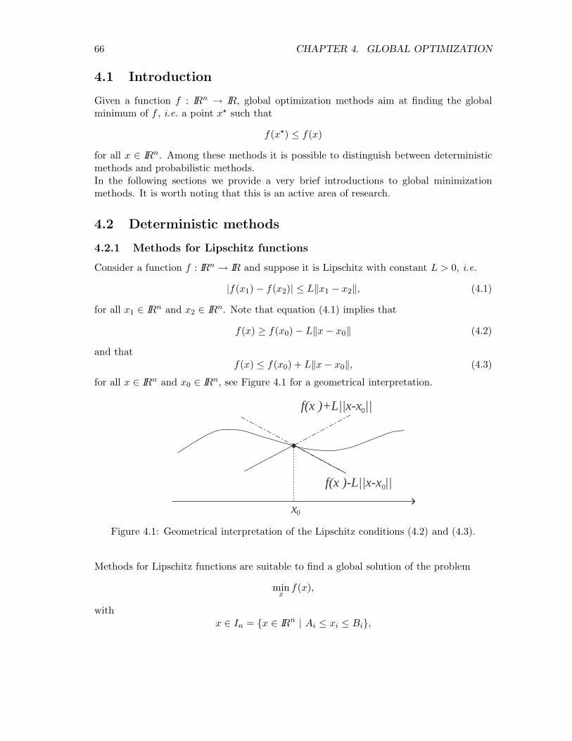
66 CHAPTER 4. GLOBAL OPTIMIZATION

4.1 Introduction

Given a function f : IRn → IR, global optimization methods aim at finding the globalminimum of f , i.e. a point x� such that

f(x�) ≤ f(x)

for all x ∈ IRn. Among these methods it is possible to distinguish between deterministicmethods and probabilistic methods.In the following sections we provide a very brief introductions to global minimizationmethods. It is worth noting that this is an active area of research.

4.2 Deterministic methods

4.2.1 Methods for Lipschitz functions

Consider a function f : IRn → IR and suppose it is Lipschitz with constant L > 0, i.e.

|f(x1) − f(x2)| ≤ L‖x1 − x2‖, (4.1)

for all x1 ∈ IRn and x2 ∈ IRn. Note that equation (4.1) implies that

f(x) ≥ f(x0) − L‖x − x0‖ (4.2)

and thatf(x) ≤ f(x0) + L‖x − x0‖, (4.3)

for all x ∈ IRn and x0 ∈ IRn, see Figure 4.1 for a geometrical interpretation.

.

x0

f(x )+L||x-x ||0

f(x )-L||x-x ||0

Figure 4.1: Geometrical interpretation of the Lipschitz conditions (4.2) and (4.3).

Methods for Lipschitz functions are suitable to find a global solution of the problem

minx

f(x),

withx ∈ In = {x ∈ IRn | Ai ≤ xi ≤ Bi},

4.2. DETERMINISTIC METHODS 67

and Ai < Bi given, under the assumptions that the set In contains a global minimum off , the function f is Lipschitz in In and the Lipschitz constant L of f in In is known.Under these assumptions it is possible to construct a very simple global minimizationalgorithm, known as Schubert-Mladineo algorithm, as follows.

Step 0. Given x0 ∈ In and L > L.

Step 1. Set k = 0.

Step 2. LetFk(x) = max

j=0,···,k{f(xj) − L‖x − xj‖}

and compute xk+1 such that

Fk(xk+1) = minx∈In

Fk(x).


Remark. The functions Fk in Step 2 of the algorithm have a very special form. This canbe exploited to construct special algorithms solving the problem

minx∈In

Fk(x)

in a finite number of iterations. �

For Schubert-Mladineo algorithm it is possible to prove the following statement.

Theorem 24 Let f� be the minimum value of f in In, let x� be such that f(x�) = f� andlet F �

k be the minima of the functions Fk in In. Let

Φ = {x ∈ In | f(x) = f�}

and let {xk} be the sequence generated by the algorithm. Then

• limk→∞

f(xk) = f�;

• the sequence {F �k } is non-decreasing and lim

k→∞F �

k = f�;

• limk→∞

infx∈Φ

‖x − xk‖ = 0;

• f(xk) ≥ f� ≥ Fk−1(xk).

Schubert-Mladineo algorithm can be given, if x ∈ I1 ⊂ IR, a simple geometrical interpre-tation, as shown in Figure 4.2.The main advantage of Schubert-Mladineo algorithm is that it does not require the com-putation of derivatives, hence it is also applicable to functions which are not everywhere


f(x).

x =A1 x0

.

B

F (x)0

. f(x).

x =A1 x0

.

B

F (x)1

..

x2

Figure 4.2: Geometrical interpretation of Schubert-Mladineo algorithm.

differentiable. Moreover, unlike other global minimization algorithms, it is possible toprove the convergence of the sequence {xk} to the global minimum. Finally, it is possibleto define a simple stopping condition. For, note that if {xk} and {F �

k } are the sequencesgenerated by the algorithm, then

f(xk) ≥ f� ≥ F �k

andf(xk) ≥ f� ≥ f(xk) + rk,

where rk = F �k − f(xk) and limk→∞ rk = 0. As a result, if |rk| < ε, for some ε > 0, the

point xk gives a good approximation of the minimum of f .The main disadvantage of the algorithm is in the assumption that the set In containsa global minimum of f in IRn. Moreover, it may be difficult to compute the Lipschitzconstant L.

4.2.2 Methods of the trajectories

The basic idea of the global optimization methods known as methods of the trajectoriesis to construct trajectories which go through all local minima. Once all local minimaare determined, the global minimum can be easily isolated. These methods have beenoriginally proposed in the 70’s, but only recently, because of increased computer powerand of a reformulation using tools from differential geometry, they have proved to beeffective.The simplest and first method of the trajectories is the so-called Branin method. Considerthe function f and assume ∇f is continuous. Fix x0 and consider the differential equations

d

dt∇f(x(t)) = ±∇f(x(t)) x(0) = x0. (4.4)

The solutions x(t) of such differential equations are such that

∇f(x(t)) = ∇f(x0)e±t,

i.e. ∇f(x(t)) is parallel to ∇f(x0) for all t. Using these facts it is possible to describeBranin algorithm.

4.2. DETERMINISTIC METHODS 69

Step 0. Given x0.

Step 1. Compute the solution x(t) of the differential equation

d

dt∇f(x(t)) = −∇f(x(t))

with x(0) = x0.

Step 2. The point x� = limt→∞x(t) is a stationary point of f , in fact lim

t→∞∇f(x(t)) = 0.

Step 3. Consider a perturbation of the point x�, i.e. the point x = x� + ε andcompute the solution x(t) of the differential equation

d

dt∇f(x(t)) = ∇f(x(t)).

Along this trajectory the gradient ∇f(x(t)) increases, hence the trajectory escapesfrom the region of attraction of x0.

Step 4. Fix t > 0 and assume that x(t) is sufficiently away from x0. Set x0 = x(t)and go to Step 1.

Note that, if the perturbation ε and the time t are properly selected, at each iteration thealgorithm generates a new stationary point of the function f .

Remark. If ∇2f is continuous then the differential equations (4.4) can be written as

x(t) = ±[∇2f(x(t))

]−1 ∇f(x(t)).

Therefore Branin method is a continuous equivalent of Newton method. Note howeverthat, as ∇2f(x(t)) may become singular, the above equation may be meaningless. In sucha case it is possible to modify Branin method using ideas borrowed from quasi-Newtonalgorithms. �

Branin method is very simple to implement. However, it has several disadvantages.

• It is not possible to prove convergence to the global minimum.

• Even if the method yields the global minimum, it is not possible to know how manyiterations are needed to reach such a global minimum, i.e. there is no stoppingcriterion.

• The trajectories x(t) are attracted by all stationary points of f , i.e. both minimaand maxima.

• There is not a systematic way to select ε and t.


x0*x1

Figure 4.3: Interpretation of the tunneling phase.

4.2.3 Tunneling methods

Tunneling methods have been proposed to find, in an efficient way, the global minimumof a function with several (possibly thousands) of local minima.Tunneling algorithms are composed of a sequence of cycles, each having two phases. Thefirst phase is the minimization phase, i.e. a local minimum is computed. The second phaseis the tunneling phase, i.e. a new starting point for the minimization phase is computed.

Minimization phase

Given a point x0, a local minimization, using any unconstrained optimization algorithm,is performed. This minimization yields a local minimum x�

0.

Tunneling phase

A point x1 �= x�0 such that

f(x1) = f(x�0)

is determined. See Figure 4.3 for a geometrical interpretation.

In theory, tunneling methods generate a sequence {x�k} such that

f(x�k+1) ≤ f(x�

k)

4.3. PROBABILISTIC METHODS 71

xk*

x

T(x, )xk*

f(x)

Figure 4.4: The functions f(x) and T (x, x�k).

and the sequence {x�k} converges to the global minimum without passing through all

local minima. This is the most important advantage of tunneling methods. The maindisadvantage is the difficulty in performing the tunneling phase. In general, given a pointx�

k a point x such that f(x) = f(x�k) is constructed searching for a zero of the function

(see Figure 4.4)

T (x, x�k) =

f(x) − f(x�k)

‖x − x�k‖2λ

,

where the parameter λ > 0 has to be selected such that T (x�k, x

�k) > 0.

Finally, it is worth noting that tunneling methods do not have a stopping criterion, i.e.the algorithm attempts to perform the tunneling phase even if the point x�

k is a globalminimum.

4.3 Probabilistic methods

4.3.1 Methods using random directions

In this class of algorithms at each iteration a randomly selected direction, having unitynorm, is selected. The theoretical justification of such an algorithm rests on Gavianotheorem. This states that the sequence {xk} generated using the iteration

xk+1 = xk + αkdk,


where dk is randomly selected on a unity norm sphere and αk is such that

f(xk + αkdk) = minα

f(xk + αdk),

is such that for any ε > 0 the probability that

f(xk) − f� < ε,

where f� is a global minimum of f , tends to one as k → ∞.

4.3.2 Multistart methods

Multistart methods are based on the fact that for given sets D and A, with measuresm(D) and m(A), and such that

1 ≥ m(A)m(D)

= α ≥ 0,

the probability that, selecting N random points in D, one of these points is in A is

P (A,N) = 1 − (1 − α)N .

As a resultlim

N→∞P (A,N) = 1.

Therefore, if A is a neighborhood of a global minimum of f in D, we conclude that, selectinga sufficiently large number of random points in D, one of these will (almost surely) beclose to the global minimum. Using these considerations it is possible to construct a wholeclass of algorithms, with similar properties, as detailed hereafter.

Step 0. Set f� = ∞.

Step 1. Select a random point x0 ∈ IRn.

Step 2. If f(x0) > f� go to Step 1.

Step 3. Perform a local minimization starting from x0 and yielding a point x�0. Set

f� = f(x�0).

Step 4. Check if x�0 satisfies a stopping criterion. If not, go to Step 1.

4.3.3 Stopping criteria

The main disadvantage of probabilistic algorithms is the lack of a theoretically soundstopping criterion. The most promising and used stopping criterion is based on the con-struction of a probabilistic approximation P (w) of the function

P (w) =m({x ∈ D | f(x) ≤ w})

m(D).

Once the function P (w) is known, a point x� is regarded as a good approximation of theglobal minimum of f if

P (f(x�)) ≤ ε � 1.

optimization an introduction

Documents