optimization and performance analysis of high speed mobile access
TRANSCRIPT

Communication Networks
University of Bremen
Prof. Dr. rer. nat. habil. C. Görg
Optimization and Performance Analysis
of High Speed Mobile Access Networks
Dissertation
submitted to the Faculty of
Electrical Engineering and Information Technology
to achieve the degree of a
Doktor der Ingenieurwissenschaften (Dr.-Ing.)
by
Thushara Lanka Weerawardane, M.Sc. B.Sc.
From
Hambantota, Sri Lanka
First Examiner: Prof. Dr. rer. nat. habil. C. Görg
Second Examiner: Prof. Dr.-Ing. Andreas Timm-Giel
Date of submission: 12th October 2010
Date of oral exam: 17th November 2010

ii

ACKNOWLEDGEMENT
This thesis was written during my work as a research scientist at the
Communication Networks Group (ComNets) of the Center for Computer
Science and Information Technology (TZI) at the University of Bremen,
Germany.
It has been a great pleasure to have worked throughout these years at
ComNets with a cooperative group of colleagues who are supportive of each
other, sharing their knowledge. I have gained considerably from the
experiences I had in our scientific and others interactions.
I sincerely thank and appreciate Prof. Carmelita Görg for giving me this great
opportunity just after finishing my master studies at the University of
Bremen. As the head of the Communication Networks Group she provided
excellent guidance and gave valuable advice and directions throughout my
studies. Also, I am deeply grateful to Prof. Andreas Timm-Giel who supplied
me with invaluable knowledge, encouragement and supervision of my project
and research work at ComNets.
I am really thankful to Prof. Ranjit Perera who gave me great support, advice
and guidance for the analytical and research work. I also thank Stephan
Hauth, Dr. Gennaro Malafronte and Thomas Reim for giving me great advice
and valuable support in performing the scientific work as well as on many
other technical matters. In addition, I am grateful to Dr. Andreas Könsgen
who provided me with not only valuable knowledge on scientific and
technical matters but also supported me on other non-technical matters
throughout my studies at the University of Bremen.
Further, I would like to thank the colleagues from my project group Yasir
Zaki, Dr. Xi Li and Umar Toseef who are OPNET experts, for giving
valuable input to my work and for having many technical discussions. I thank
Asanga Udugama who supported me to solve the programming issues that I
had during my project and thesis work. I would also like to thank all the other
colleagues, Dr. Koojana Kuladinithi, Markus Becker, Dr. Bernd-Ludwig
Wenning, Liang Zhao, Chen Yi, Mohammad Siddique, Amanpreet Singh,
Gulshanara Singh and Vo Que Son who gave me their support to successfully
finalize my thesis work.

iv
My non-academic life has many people who have helped me in different
ways. The first of these people is my loving wife, Ureka Weerawardane who
gave me great encouragement and invaluable support throughout my studies.
She took away a lot of the family responsibilities from me during difficult
moments and also shared life with me in all happy and difficult situations. I
never forget my lovely son, Deshabhi Weerawardane who had to offer his
playing time for my studies on many occasions. Last but not least, I
remember with respect my loving parents who are living far away from me
now but gave me the foundation and the encouragement to reach the stars.

ABSTRACT
Cost-effective end-to-end performance is one of the key objectives which
should be optimised for any broadband wireless network. Even though the
radio channel is an important scarce resource, the rest of the mobile access
network must respond according to the time variant radio channel capacity,
otherwise a good overall performance cannot be achieved effectively. The
packet traffic of high speed mobile access networks often has a bursty nature
which causes a severe impact on the performance. For the reasons given
above, a proper control of data flows over the access network is required. In a
modern mobile access network not only the throughput optimization has to
be considered, but also the QoS for different service requirements should be
guaranteed at a minimum cost.
The main focus of this work is the performance evaluation of High Speed
Packet Access (HSPA) networks. In addition, the effects of the Long Term
Evolution (LTE) transport network (S1and X2 interfaces) on the end user
performance are investigated and analysed by introducing a novel
comprehensive MAC scheduling scheme and a novel transport service
differentiation model.
In order to achieve the aforementioned goals, new transport technologies and
features are introduced within the focus of this work. Novel adaptive flow
control and enhanced congestion control algorithms are proposed,
implemented, tested and validated using a comprehensive HSPA system
simulator which is developed by the author. In addition to the development
of HSPA network protocols, novel scheduling approaches are introduced and
developed in the HSPA system simulator for the downlink and the uplink.
Therefore, the system simulator provides great flexibility and enhanced
scalability for the analysis of the overall network performance for all
protocol layers from the applications to the physical layer. Effects of the
adaptive flow control and the congestion control algorithms on the end-to-
end performance have been investigated and analysed using detailed HSPA
system simulations. These analyses confirm that aforementioned algorithms
do not only enhance the end user performance by providing guaranteed QoS
but also optimise the overall network utilisation and performance. Further,
the algorithms are able to provide for both the network operators and the end
users reliable and guaranteed services cost-effectively.
To overcome issues related to the detailed simulation approach of analysing
the performance of adaptive flow control and enhanced congestion control

vi
such as time consuming development and long lasting simulations, two novel
analytical models – one for congestion control and the other for the combined
flow control and congestion control – which are based on Markov chains, are
designed and developed. The effectiveness and correctness of these analytical
models are validated by comparing them to the results of the detailed system
simulator. The proposed analytical models provide exceptional efficiency
regarding the speed of the analysis along with a high accuracy compared to
the detailed HSPA simulator. Therefore, the analytical models can be used to
evaluate the performance of adaptive flow control and enhanced congestion
control algorithms effectively within a shorter period of time compared to the
simulation based analysis.

KURZFASSUNG
Ein kosteneffektives Ende-zu-Ende-Leistungsverhalten ist eines der
wesentlichen Kriterien, das für jedes drahtlose Breitbandnetz optimiert
werden sollte. Auch wenn der Funkkanal eine wesentliche, knappe Ressource
ist, muss der Rest des mobilen Zugangsnetzes entsprechend der
zeitveränderlichen Kapazität des Funkkanales reagieren, da sonst ein gutes
Gesamtleistungsverhalten nicht erreicht werden kann. Der Paketverkehr von
mobilen Hochgeschwindigkeits-Zugangsnetzen weist oft eine burstartige
Natur auf, die starke Auswirkungen auf das Leistungsverhalten hat. Aus den
oben genannten Gründen ist eine sorgfältige Steuerung der Datenflüsse über
das Zugangsnetz erforderlich. In einem modernen mobilen Zugangsnetz
muss nicht nur die Optimierung des Durchsatzes betrachtet werden, sondern
es sollten auch verschiedene Dienstgüteanforderungen bei minimalen Kosten
garantiert werden.
Schwerpunkt dieser Arbeit sind High Speed Packet Access (HSPA)-Netze.
Desweiteren werden die Auswirkungen des Long Term Evolution (LTE)-
Transportnetzes (S1 und X2- Schnittstelle) auf das Leistungsverhalten beim
Endbenutzer untersucht und ausgewertet, und zwar durch Einführung eines
neuartigen umfassenden MAC-Schedulingverfahrens und eines neuartigen
Modells zur Unterscheidung von Transportdiensten.
Um die zuvor erwähnten Ziele zu erreichen, werden als Schwerpunkt dieser
Arbeit neue Transporttechnologien und -funktionen eingeführt. Neuartige
adaptive Algorithmen zur Flusssteuerung und zur verbesserten
Überlastvermeidung zwecks Optimierung des Leistungsverhaltens im
Transportnetz werden mit Hilfe eines umfassenden vom Autor entwickelten
HSPA-Systemsimulators, vorgestellt, implementiert, getestet und validiert.
Zusätzlich zur Entwicklung der HSPA-Netzprotokolle werden neuartige
Scheduling-Ansätze im HSPA-Simulator für den Up- und den Downlink
eingeführt. Daher bietet der Systemsimulator große Flexibilität und
erweiterte Skalierbarkeit für die Auswertung des gesamten Netz-
Leistungsverhaltens für alle Protokollschichten von der Anwendungs- bis zur
physikalischen Schicht. Auswirkungen der Algorithmen für die adaptive
Flusssteuerung und die Überlastvermeidung auf das Ende-zu-Ende-
Leistungsverhalten werden mit Hilfe von ausführlichen HSPA-
Systemsimulationen untersucht und analysiert. Diese Analysen bestätigen,
dass die zuvor erwähnten Algorithmen nicht nur das Endbenutzer-
Leistungsverhalten unter Einhaltung der Dienstgüteanforderungen
verbessern, sondern auch die Auslastung und das Leistungsverhalten des

viii
Gesamtnetzes optimieren. Desweiteren sind die Algorithmen in der Lage,
sowohl für die Netzbetreiber als auch für die Endbenutzer zuverlässige und
kosteneffektive Dienste bereitzustellen.
Um Schwierigkeiten bei der detaillierten Simulation des Leistungsverhaltens
der adaptiven Flusssteuerung und Überlastvermeidung zu überwinden, etwa
die zeitintensive Entwicklung und lang andauernde Simulationen, werden
zwei neuartige analytische Modelle – eines für die Überlastvermeidung und
eines für die Kombination aus letzterem und der Flusssteuerung – auf der
Basis von Markov-Ketten entworfen und implementiert. Die Effektivität und
Richtigkeit dieser analytischen Modelle wird durch Vergleich mit den
Ergebnissen des detaillierten Systemsimulators validiert. Die
vorgeschlagenen analytischen Modelle ermöglichen im Vergleich mit dem
detaillierten HSPA-Simulator eine außerordentliche Effizienz bezüglich der
Analysegeschwindigkeit, zusammen mit einer hohen Genauigkeit. Daher
können die analytischen Modelle verwendet werden, um das
Leistungsverhalten der Algorithmen für die adaptive Flussssteuerung und die
verbesserte Überlastvermeidung effektiv in einer kürzeren Zeitperiode im
Vergleich zu der simulationsbasierten Analyse auszuwerten.

TABLE OF CONTENTS
1 INTRODUCTION ................................................................................... 1
2 HIGH SPEED BROADBAND MOBILE NETWORKS .................................. 7
2.1 UMTS broadband technology ...................................................... 8
2.1.1 Wideband code division multiple access ................................ 8
2.1.2 UMTS network architecture .................................................... 9
2.1.3 UMTS quality of service ........................................................ 12
2.2 High speed packet access .......................................................... 13
2.2.1 Adaptive modulation and coding .......................................... 14
2.2.2 Hybrid ARQ............................................................................ 15
2.2.3 Fast scheduling ...................................................................... 15
2.2.4 High speed downlink packet access ...................................... 16
2.2.5 High speed uplink packet access ........................................... 19
2.3 UMTS transport network ........................................................... 25
2.3.1 ATM based transport network .............................................. 25
2.3.2 DSL based transport network ............................................... 31
2.4 Long term evolution .................................................................. 34
2.4.1 LTE targets............................................................................. 34
2.4.2 LTE technology ...................................................................... 35
2.4.3 LTE architecture and protocols ............................................. 36
2.4.4 Quality of service and bearer classification .......................... 45
2.4.5 LTE handovers ....................................................................... 49
3 HSPA NETWORK SIMULATOR ............................................................ 57
3.1 Simulation environment ............................................................ 57
3.2 HSPA network simulator design ................................................ 58
3.2.1 HSDPA network simulator model design and development . 59
3.2.2 HSUPA network simulator model design and development . 63
3.3 HSDPA MAC-hs scheduler design and implementation .............. 64
3.3.1 Proposed scheduling disciplines ........................................... 65
3.3.2 Round robin scheduling procedure ....................................... 66

x
3.3.3 Channel dependent scheduling procedure ........................... 66
3.3.4 HSDPA scheduler architecture .............................................. 67
3.4 E-DCH scheduler design and implementation ............................ 68
3.4.1 E-DCH scheduler design and development ........................... 69
3.4.2 Modelling HARQ .................................................................... 77
3.4.3 Modelling soft handover ....................................................... 78
3.5 TNL protocol developments ...................................................... 80
3.5.1 ATM based transport network .............................................. 81
3.5.2 DSL based transport network ............................................... 83
3.5.3 ATM and DSL based transport deployment .......................... 92
3.6 Radio link control protocol ........................................................ 93
3.6.1 Overview of RLC protocol ..................................................... 93
3.6.2 RLC AM mode implementation in HSPA simulator ............... 94
4 HSDPA FLOW CONTROL AND CONGESTION CONTROL ...................... 97
4.1 HSDPA TNL flow control ............................................................ 98
4.1.1 HSDPA ON/OFF flow control ................................................. 99
4.1.2 HSDPA adaptive credit-based flow control ......................... 100
4.1.3 Traffic models and simulation configurations .................... 104
4.1.4 Simulation analysis-1: FTP traffic ....................................... 106
4.1.5 Simulation analysis 2: ETSI traffic ....................................... 110
4.1.6 TNL bandwidth recommendation ....................................... 115
4.1.7 Conclusion ........................................................................... 118
4.2 TNL congestion control ............................................................ 119
4.2.1 Overview of the HSDPA congestion control schemes ......... 120
4.2.2 Preventive and reactive congestion control ....................... 121
4.2.3 Congestion control algorithms ............................................ 125
4.2.4 Congestion control schemes ............................................... 126
4.2.5 Traffic models and simulation configurations .................... 129
4.2.6 Simulation results and analysis ........................................... 131
4.2.7 Conclusion ........................................................................... 137

xi
5 ANALYTICAL MODELS FOR FLOW CONTROL AND CONGESTION CONTROL ................................................................................................ 139
5.1 Analytical model for congestion control .................................. 140
5.1.1 Modelling of the CI arrival process ..................................... 141
5.1.2 States and steps definition for the analytical modelling..... 143
5.1.3 A discrete-time Markov model with multiple departures .. 145
5.1.4 Average transmission rate .................................................. 146
5.1.5 Simulation and analytical results analysis ........................... 147
5.1.6 Summary and conclusion .................................................... 161
5.2 Analytical modelling of flow control and congestion control ... 161
5.2.1 Joint Markov model ............................................................ 163
5.2.2 Analytical and simulation parameter configuration ........... 172
5.2.3 Input distribution of radio user throughput ....................... 173
5.2.4 Simulation results analysis .................................................. 174
5.2.5 Fast queuing simulator ....................................................... 179
5.2.6 Analytical results analysis ................................................... 187
5.2.7 Result comparison and conclusion ..................................... 189
5.2.8 Conclusion ........................................................................... 194
6 CONCLUSION, OUTLOOK AND SUMMARY ....................................... 195
6.1 Conclusion and outlook ........................................................... 195
6.2 Summary of the thesis contributions ....................................... 198
A. EFFECT OF DSL TRANSPORT ON HSPA PERFORMANCE .................... 201
A.1 Effects of DSL default mode on HSPA performance ................. 201
A.2 Effects of the DSL fast mode on HSPA performance ................ 208
B. LTE NETWORK SIMULATOR ............................................................. 215
B.1. LTE reference architecture ....................................................... 215
B.2. LTE model architecture ............................................................ 217
B.3. LTE protocol development ....................................................... 222
B.4. LTE mobility and handover modelling ..................................... 235

xii
C. IMPACT OF LTE TRANSPORT FOR END USER PERFORMANCE .......... 249
C.1. Traffic models .......................................................................... 250
C.2. Simulation configuration ......................................................... 252
C.3. Simulation results analysis ...................................................... 256

CHAPTER 1
1 Introduction
High Speed Packet Access (HSPA) is introduced within the broadband
wireless network paradigm as an extension of the Universal Mobile
Telecommunication System (UMTS) which is standardised by the 3rd
Generation Partnership Project (3GPP). The main objective of this
technology is to enhance the data rate in the up- and downlink, and also
reduce the latency in both directions. In recent years, usage of real time and
multimedia applications is rapidly increasing worldwide by demanding
higher capacity and lower latency. In order to fulfil such requirements, 3GPP
steps in by introducing the Long-Term Evolution (LTE) along with the
System Architecture Evolution (SAE) as the foreseen broadband wireless
access technologies.
Currently broadband wireless technologies are becoming a part of people’s
life style and a key requirement for every business worldwide. Therefore,
high reliability of various services with different Quality of Service (QoS)
requirements is vitally important. To fulfil such requirements, the complete
system from end user to end user needs to be controlled in a cost-effective
manner. If any part of the network does not comply with the rest, the overall
performance degrades by wasting a large part of the valuable resources. From
the end user perspective, the performance which can be measured in terms of
user data throughput and QoS is the final outcome. To achieve such
objectives, all parts of the networks should be properly dimensioned and
controlled. The radio part of the broadband network which is widely in the
research focus [17, 18] is the main bottleneck of such achievements.
However, in order to utilise the scarce radio resources efficiently, the rest of
the network protocols should be adapted accordingly. The achievable
capacity of the radio resources is time variant and also dependent on several
other real time issues such as the traffic types and their QoS requirements,
number of users and mobility, the environmental conditions etc. Such time
varying radio capacity fluctuations have a huge impact on the rest of the
network which reduces the cost-effectiveness and the overall performance
Introduction
2
[42, 43, 44]. Since such issues regarding the overall performance are rarely
addressed within the literature [24, 25], one part of this work is focused on
this area of investigations.
The proper dimensioning of the transport network is one of the key areas in
mobile access networks to gain the aforementioned benefits for the end users.
All transport and network protocols have to be parameterized in a suitable
way in which they operate efficiently and cost-effectively, coexisting with
the broadband mobile access network. For example, a limited transport
network can cause congestion due to the unpredictable bursty nature of the
traffic [3]. In such a situation, there is a requirement of an adaptive feedback
flow control algorithm [4, 7] which can closely monitor the time varying
wireless capacity and control the input traffic to the transport network. Since
the cost-efficient operation is vitally important for the mobile network
operators (MNOs), often the transport network is dimensioned based on
average network utilisation [32, 33]. Therefore congestion can occur during
peak demands which are highly unpredictable in real scenarios. Depending
on the severity, congestion can cause a significant impact on the overall
performance and even obstruct the demanded services for a certain period of
time. There are several protocols such as the Transmission Control Protocol
(TCP) which are sensitive to these abrupt fluctuations [27, 29, 30]. Since the
customer satisfaction is one of the primary goals of the mobile network
operators, such situations should be minimized or if possible avoided. It is
identified that there is a clear requirement of the transport network flow
control and congestion control for effective utilisation of scarce radio
resources to provide the optimum end user performance. Therefore, during
the focus of this dissertation, issues related to the UTRAN network that can
severely impact the end user performance and QoS experience are
investigated and analysed. As one of the main contributions of the author,
this work introduces novel flow and congestion control algorithms for high
speed packet access systems that can overcome all aforementioned issues and
provide service guarantees to the end users while optimizing overall network
performance cost-effectively. The comprehensive detailed HSPA system
simulation models have been developed by the author in the focus of the
thesis and according to the requirements of the industrial research project
managed by Nokia Siemens Network (NSN) to test, validate and analyse the
above findings.

Introduction
3
Investigations and analyses using a detailed simulator along with the
validation of the simulator itself are always time consuming activities which
are sometimes unacceptably long. Therefore, often analytical approaches can
provide faster investigation and analyses along with a good accuracy
compared to a simulation approach. For this reason, two analytical models
are designed and developed by the author to evaluate the performance of the
aforementioned flow control and congestion control algorithms in high speed
broadband access networks.
Apart from the HSPA transport network, the work further extends the
investigation and analyses to the network and end user performance of the
LTE transport network. Dimensioning the latter which completely operates
on IP based packet networks for different QoS requirements is a key
challenge for mobile network operators. For example, during LTE handovers,
the traffic load over the S1 interface between the enhanced Node-B (eNB)
and the Evolved Packet Core (EPC) network and the X2 interface between
two eNBs has to be efficiently controlled without degrading the end user QoS
performance. Further, the forwarding data over the X2 interface has to be
transferred without long delays in order to provide seamless mobility to the
end users. The traffic prioritization over the transport network should be done
carefully and effectively to meet the required QoS at the end users for
different services. In such cases, the transport level congestion can worsen
the impact on the end user performance wasting overall network resources.
Therefore, LTE transport network congestion should also be avoided by
considering proper congestion control triggers. Further, an effective traffic
differentiation model is deployed at the transport level in order to resolve the
aforementioned issues. All these investigations and analyses are performed
by deploying suitable traffic models within the LTE system simulator which
are designed and developed by the author. The effects of the LTE transport
network (mainly the S1/X2 interface) during the intra-LTE handovers on the
end-to-end performance are widely investigated and analysed by introducing
proper traffic differentiation models at the transport network level along with
a comprehensive QoS aware MAC scheduling approach within the
framework of this thesis.
This thesis work is organized as follows. Chapter 2 provides an overview of
high speed broadband wireless networks such as UMTS, HSPA and LTE.
First, the technological advancements of UMTS are discussed along with an
architectural overview. Next, high speed access technologies are described by

Introduction
4
introducing the key enhancements in the down- and uplink. Several transport
technologies such as ATM, IP and DSL which can be deployed for the high
speed packet access network are also described in this chapter. New
technological advancements of future broadband wireless networks are
considered as well by introducing LTE along with the architecture overview.
Further, all architectural changes to the previous technologies are presented
in this chapter by highlighting the prominent changes. The description about
user mobility and LTE handovers are also presented in this chapter.
Chapter 3 describes the design and development of a comprehensive HSPA
simulator. The simulator development is performed in two steps: first the
HSDPA simulation model is developed and then the HUSPA part is added.
The chapter further discusses the challenges of developing a system
simulator which is suitable for analyzing the transport and end-to-end
performance. Apart from general protocol developments, novel MAC
scheduling approaches for the downlink MAC-hs and uplink E-DCH are
introduced and implemented within the simulator whose details are given in
this chapter. All UTRAN network entities along with the underlying transport
technologies such as ATM and DSL are implemented according to the
guideline and specification given by the 3GPP standards.
A new credit-based flow control algorithm is introduced in chapter 4. The
technical and implementation aspects of the algorithm are described in detail.
After defining appropriate traffic models and simulation scenarios, the
performance of the algorithm is investigated and analysed using the HSPA
simulator. All achievements are given in the results analysis and the
conclusion. In addition to the credit-based flow control algorithm a novel
congestion control algorithm is also presented within the chapter. Different
congestion detection principles are discussed along with implementation
details. Variants of the congestion control algorithm are described by
providing extensive investigations and analyses using the simulator. The
simulation results present the effectiveness of these novel approaches from
the performance point of view. Finally the conclusion of the chapter
summarizes the valuable findings about these new approaches.
Chapter 5 presents two novel analytical models which are based on the
Markov property: first, a model for congestion control and second, a joint
model for flow control and congestion control is developed. The theoretical
backgrounds of both models are discussed in detail within the chapter. The

Introduction
5
outcome of these analytical models is compared with the simulation results.
The chapter concludes by highlighting all achievements of the analytical
models in comparison to the simulations.
Chapter 6 presents the conclusion of this work where all achievements are
summarised.
Appendix A presents effects of the DSL based UTRAN network on the
performance of the HSPA network. The analysis is focused to investigate the
impact of DSL packet losses, delay and delay variations – which are caused
due to impairments of the DSL connections – on the HSPA network and the
end user performance.
A description of the LTE network simulator is given in Appendix B. The
main node models such as User Equipment (UE), enhanced Node-B (eNB)
and the access Gateway (aGW) are designed and developed including the
peer-to-peer protocols such as TCP. The design of a proper IP DiffServ
model and MAC scheduler is crucial for such simulator development since
they have a great impact on the overall network performance. By considering
all these challenges, the detailed implementation procedures of these network
entities and the LTE handover modelling are presented in this chapter.
Appendix C presents an extensive analysis and investigation about the effects
of the LTE transport network on the end user performance. For this analysis,
a comprehensive LTE system simulator which includes a novel MAC
scheduler and a novel traffic differentiation module are described in this
chapter. The end user performance is evaluated for different overload
situations at the transport network level by deploying appropriate traffic
models. Further, the inter-eNB and intra-eNB user handover mobility is
considered with different transport priorities for the forwarded traffic. The
impact of all above transport effects on the different services at the end user
is discussed in the results analyses. The conclusion of the chapter
summarizes all achievements of this investigation and analysis.


CHAPTER 2
2 High speed broadband mobile networks
At the beginning of 1990, GSM with digital communication commenced as
the 2nd generation mobile network and achieved staggering popularity of
mobile cellular technology. With the evolution of wideband 3G UMTS, the
usage of broadband wireless technology was further enhanced for many day
to day applications. UMTS was primarily oriented with dedicated channel
allocation to support circuit-switched services however it was also designed
with the motivation to provide better support for the IP based application
than the GPRS (General Packet Radio Service). Later, the 3GPP standard
evolved into high-speed packet access technologies for downlink and uplink
transmission [22]. They were popular in practice as HSDPA (High Speed
Downlink Packet Access) and HSUPA (High Speed Uplink Packet Access).
The latest step being investigated and developed in 3GPP is EPS (Evolved
Packet System) which represents an evolution of 3G into an evolved radio
access referred to as Long Term Evolution (LTE) and an evolved packet
access core network in the System Architecture Evolution (SAE) [46].
Currently, the first deployment of LTE is entering the market [54].
As mentioned above, UMTS, HSPA and LTE are the main broadband
wireless technologies in the 3rd
and 4th
generation mobile networks. The use
of the Internet booms among the world population rapidly. In many cases, the
Internet is accessed by handheld devices, using a large number of
applications and services such as music downloads, online TV, and video
conferencing. The trend of the most of these multimedia applications is a
demand for high speed broadband access [54]. On the other hand, today the
basic platform for many activities such as business and marketing, daily
routines and lifestyle of the people, medical activities and most of the social,
cultural and religious activities are based on broadband wireless technology.
In short, the technology becomes part of everyone’s lifestyle.

UMTS broadband technology
8
The chapter is organised as follows. First, UMTS and related technologies
are discussed along with the network architecture. Then new enhancements
in the downlink and in the uplink are described under the heading of HSDPA
and HSUPA respectively. Lastly the details about the LTE technology and its
achievements are presented.
2.1 UMTS broadband technology
There is a huge change in the wireless paradigm after the introduction of the
UMTS network. GSM is the first digital mobile radio standard developed for
mobile voice communications. As an extension of GSM networks, GPRS has
been introduced to provide packet switched data communications. UMTS
triggers a phased approach towards an all-IP network by improving second
generation (2G) GSM/GPRS networks based on Wideband Code Division
Multiple Access (WCDMA) technology. UMTS supports backward
compatibility with GSM/GPRS netowrks. GPRS is the convergence point
between the 2G technologies and the packet-switched domain of the 3G
UMTS [23].
Within this section, a brief overview of the UMTS technology, network
architecture and its supported services are presented.
2.1.1 Wideband code division multiple access
The key enhancement of the radio technology from 2G mobile
telecommunication networks to 3G mobile telecommunication networks
(UMTS) is the introduction of WCDMA. It uses Direct Sequence (DS)
CDMA channel access and Frequency Division Duplex (FDD) to access the
radio channel among a number of users for the uplink and the downlink
transmission. WCDMA transmits on a pair of radio channels with a
bandwidth of 5 MHz each [17]. Further, WCDMA provides a significantly
improved spectral efficiency and higher data rates compared to the 2G GSM
network for both packet and circuit switched data. However, apart from these
achievements, WCDMA also faces many challenges due to its complexity
such as high computational effort at the receiver. Theoretically, it supports
data rates up to 2 Mbit/sec in indoor/small cell out-door, and up to 384 kbps
for the wide-area coverage [17, 18].

UMTS broadband technology
9
2.1.2 UMTS network architecture
The UMTS architecture consists of User Equipment (UE), the Universal
Terrestrial Radio Access Network (UTRAN) and the Core Network (CN).
The UMTS architectural overview is shown in Figure 2-1.
Figure 2-1: UMTS network overview
Figure 2-1illustrates the hierarchical structure of UMTS starting from the
Core Network to the User Equipment in the cell. The Core Network is the
backbone of the UMTS network. The user equipments represent the lowest
level of the hierarchy; UEs are connected to the Node-B (also called UMTS
base station) via the radio channels. Several NodeBs are connected to a Radio
Network Controller (RNC) through the transport network which includes a
number of ATM based routers in between. The RNC is directly connected
with the backbone network via the Iu interface. Further details about the
UMTS network architecture are described by categorising it into two main
groups, the Core Network and the UTRAN.
2.1.2.1 UMTS Core Network and Internet Access
As shown in Figure 2-2, the core network provides the connection between
the UMTS network and the external network such as the Public Switched
Telephone Network (PSTN) and the Public Data Network (PDN). In order to

UMTS broadband technology
10
perform a connection to the external networks with appropriate QoS
requirements, the CN operates in two domains: circuit switched and packet
switched. The circuit switched part of the CN network mainly consists of a
Mobile service Switching Centre (MSC), a Visitor Location Register (VLR)
and Gateway MSC (GMSC) network entities. All circuit switched calls
including roaming, inter-system handovers and the routing functionalities are
controlled by these main circuit switched network elements.
Figure 2-2: UMTS network architecture
In contrast to circuit switched domain activities, the packet switched domain
mainly controls the data network. The packet switched part of the Core
Network consists of the Serving GPRS Support Node (SGSN) and the
Gateway GPRS support Node (GGSN). The SGSN performs the functions
related to the packet relaying between the radio network and the Core
Network along with the mobility and session management. The GGSN entity
provides the gateway access control functionality to the outside world.
Apart from the above described network elements, there are several other
network elements such as the Home Location Register (HLR), the Equipment
Identity Register (EIR) and the Authentication Centre (AuC) in the Core
Network. These network elements provide services to both packet-switched
and circuit-switched domains. All subscriber related information such as
associated telephone numbers, supplementary services, security keys and
access priorities are stored in the HLR. EIR and AuC are also acting as

UMTS broadband technology
11
databases which keep identity information of the mobile equipment and
security information such as authentication keys respectively.
2.1.2.2 UMTS radio access network
The UTRAN consists of one or more radio network subsystems (RNS) and is
shown in Figure 2-2. A radio network subsystem includes a radio network
controller (RNC), several Node-Bs (or UMTS base stations) and many UEs.
The radio network controller is responsible for the control of radio resources
of UTRAN [44] and plays a very important role in power control (PC),
handover control (HC), admission control (AC), load control (LC) and packet
scheduling (PS) algorithms. The RNC has three interfaces: the Iu interface
which connects to the core network, the Iub interface which connects to
Node-B entities and the Iur interface which connects with peer RNC entities.
The Node-B is comparable to the GSM base station (BS/BTS), and it is the
physical unit for radio transmission and reception within the cells. The Node-
B performs the air interface functions which include mainly channel coding,
interleaving, rate adaptation, spreading, modulation and transmission of data.
The interface which provides the connection with the user equipment is
called the Uu interface. This radio interface is based on the WCDMA
technology [56]. The Node-B is also responsible for softer handovers in
which the UE is connected to a single Node-B with more than one
simultaneous radio links whereas for the soft handovers the UE is connected
with two Node-Bs with more than one simultaneous radio links [44]. During
the process of softer handover, the Node-B is responsible of adding or
removing the radio links which are connected with the UE who is located in
the overlapping area of adjacent sectors of the same Node-B [44, 45]. The
user equipment is based on the same principles as the GSM mobile station
(MS), and it consists of two parts: mobile equipment (ME) and the UMTS
subscriber identity module (USIM). Mobile equipment is the device that
provides radio transmission, and the USIM is the smart card holding the user
identity and personal information. The UTRAN user plane and the control
plane [55] protocols are shown in Figure 2-3.
The user plane includes the Packet Data Convergence Protocol (PDCP), the
Radio Link Control (RLC) protocol, the Medium Access Control (MAC)
Protocol and the physical layer whereas the control plane includes all these
protocols except the PDCP and the Radio Resource Control (RRC). The RRC

UMTS broadband technology
12
is a signalling protocol which is used to set up and maintain the dedicated
radio bearers between the UE and the RNC. The physical layer provides
transport channels to the MAC layer at the interface. The MAC layer maps
logical channels to transport channels and also performs multiplexing and
scheduling functionalities. The RLC layer is responsible for error protection
and recovery. The PDCP works in the user plane providing IP header
compression and decompression functions [57].
Figure 2-3: UTRAN control plane and user plane protocols
2.1.3 UMTS quality of service
UMTS has been designed to support a variety of quality of service (QoS)
requirements that are set by end user applications. 3G services does vary
from simple voice telephony to more complex data applications including
voice over IP (VoIP), video conferencing over IP (VCoIP), video streaming,
interactive gaming, web browsing, email and file transfer. The 3GPP has
identified four different main traffic classes for UMTS networks according to

High speed packet access
13
the nature of traffic and services. They are termed conversational class,
streaming class, interactive class and background class [17].
Real time conversation is always performed between peers of human end
users. This is the only traffic type where the required characteristics are
strictly imposed by human perception. Real time conversations are mainly
characterized by the transfer time (or delay) and time variation (or jitter).
These two QoS parameters should be kept within the human perception. The
streaming class is mainly characterized by the preserved time variation (or
jitter) between information entities of the stream, but it does not have tight
requirements on low transfer delay as required by the voice applications.
Therefore, the acceptable delay variation over transmission media is much
higher than required by the applications of the conversational class. An
example of this scheme is the user looking at a real time video or listening to
real time audio.
The interactive class of the UMTS QoS is applied when an end user (either
human or a machine) is requesting data online from a remote entity such as a
server or any other equipment. The basic requirements for this QoS class are
characterised by the low RTD (Round Trip Delay), low response time and
low bit error rate which preserves the payload contents. Web browsing,
database retrieval and server data access are some examples for the
interactive class. As the last category of this QoS classification, there is the
background traffic class which includes applications such as email and Short
Message Services (SMS) as well as download of files. The RTD and
response time are not that critical for this QoS class but the data integrity
must be preserved during the delivery of the data therefore it demands for a
low bit error rate for the transmission.
2.2 High speed packet access
As discussed in the previous section, the UMTS implementation supports
data rates up to 2 Mbit/s. However this is a theoretical limit; the practically
feasible data rate is much smaller than the theoretical maximum. Therefore
UMTS is suitable for most of the normal voice based applications and some
of the Internet based applications such as simple web browsing and the large
file downloads. The usage of current Internet based applications is vastly
growing worldwide among all age segments of people [20]. Traffic over any

High speed packet access
14
network becomes more bursty demanding high data rates. Applications such
as high quality video downloads, online TV and video conferencing require
higher data rates and also lower delays. Furthermore, the quality perceived by
the end user for interactive applications is largely determined by the latency
(or delay) of the system. In order to satisfy these ongoing and future
demands, the WCDMA air interface is improved in the 3GPP Rel’5 (Rel’5)
and Rel’6 (Rel’6) of the 3GPP specifications by introducing high speed
downlink packet access (HSDPA) and high speed uplink packet access
(HSUPA) respectively. HSUPA is officially referred to as E-DCH (Enhanced
Dedicated Channel) in the 3GPP specification but industry widely uses the
term HSUPA as a counterpart for HSDPA. To achieve a very high data rate
and low latency both in the uplink and the downlink, WCDMA introduces
three main fundamental technologies: fast link adaptation using Adaptive
Modulation and Coding (AMC), fast Hybrid ARQ (HARQ) and fast
scheduling [22]. These rely on the rapid adaptation of the transmission
parameters to the instantaneous radio channel conditions in an effective
manner in order to achieve higher spectral efficiency for the transmission.
Before getting into the detailed discussion of the high speed downlink packet
access (HSDPA) and high speed uplink packet access (HSUPA), a brief
overview of these key enhancements of the above technologies is discussed
in the following sections.
2.2.1 Adaptive modulation and coding
The basic principle of Adaptive Modulation and Coding (AMC) is to offer a
link adaptation method which can dynamically adapt the modulation scheme
and coding scheme to current radio link conditions for each UE. The
modulation and coding schemes can be selected to optimise user performance
in the downlink and the uplink when the instantaneous channel conditions are
known. The users who are close to the Node-B usually have a good radio link
and are typically assigned to higher-order modulation schemes with higher
code rates (e.g. 64 QAM with R=3/4 turbo codes). The modulation order
and/or code rate will decrease as the distance of a user from the Node-B
increases. Higher-order modulation such as 64-QAM, provides higher
spectral efficiency in terms of bit/s/Hz compared to QPSK or BPSK based
transmissions. Such schemes can be used to provide instantaneous high peak
data rates especially in the downlink, when the channel quality is sufficiently
good with high signal-to-noise-ratio (S/N). WCDMA systems are typically
interference limited and rely on the processing gain to be able to operate at a

High speed packet access
15
low signal-to-interference ratio. The use of a higher order modulation
becomes impossible in practise in multi-user environments due to the fact
that it has limited robustness against interference. However, in the downlink,
a large part of the power is allocated to a single user at a time, and therefore a
large signal-to-interference ratio can be experienced by allowing higher-order
modulation to be advantageously used. Hence, higher-order modulation
combined with fast link adaptation is able to adapt the instantaneous channel
condition effectively mainly for the downlink transmissions rather than the
uplink transmission.
2.2.2 Hybrid ARQ
The principle of Hybrid ARQ (HARQ) is to combine retransmission data
with its previous transmissions which were not successful prior to the
decoding process at the receiver. Such HARQ mechanisms greatly improve
the performance and add robustness to link adaptation errors [23]. For the
packet-data services, the receiver typically detects and requests a
retransmission of erroneously received data units. Combining the soft
information from both the original transmission and any subsequent
retransmissions prior to decoding will reduce the number of required
retransmissions. This results in a reduction of the delay and robustness
against link adaptation errors. The link adaptation serves the task of selecting
a good initial estimate of the amount of required redundancy in order to
minimize the number of retransmissions needed, while maintaining a good
system throughput. The hybrid ARQ mechanism serves the purpose of fine-
tuning the effective code rate and compensates for any errors in the channel
quality estimates used by the link adaptation. However HARQ will also
introduce redundancy into the system which causes a lower utilisation of
radio resources. Proper link adaptation together with HARQ mechanisms will
help to achieve effective bandwidth utilisation as a total.
2.2.3 Fast scheduling
The scheduler which moves from the RNC to the Node-B for HSPA is an
important element in the base station that can effectively allocate the radio
resources for the users by considering various aspects such as QoS
requirements, instantaneous channel quality etc. The design of a proper base
station scheduler is a complex task due to the different user requirements and

High speed packet access
16
also mobile network operators. However, designing a fast scheduler in any
system has to primarily consider the radio channel. It has to change the
resource allocation depending on the varying channel conditions. Therefore a
small scheduling interval such as 2 milliseconds is often chosen to keep this
flexibility of channel adaptation. Another important aspect which should be
considered when designing a fast scheduler is to achieve high data rates for
each UE satisfying delay requirements. The throughput and the fairness
become a clear trade-off situation for any scheduler design. When one feature
is optimised, the other is reversely affected. For example if a scheduler is
designed to optimise the throughput, it selects the user with best channel
quality and allocates full resources to that particular UE. If the UE has
sufficient data in the transmission buffer, it can use even total radio resources
during the period of best channel condition. This type of scheduling approach
is commonly named Maximum C/I (MaxC/I) or channel dependent
scheduling in the literature [44, 54]. The opposite of this approach is the fair
scheduling approach which considers the fairness among the users and
provides guaranteed delay for each connection [44]. Often current mobile
operators consider both aspects of this trade-off and design a scheduler which
provides high throughput while providing required QoS guarantees to users.
2.2.4 High speed downlink packet access
HSDPA is an extension for the UMTS network that provides fast access for
the downlink by introducing advanced techniques which were described
above. Therefore, from the architectural point of view it uses the same
architecture as UMTS Rel’99. In addition to the techniques such as fast link
adaptation, fast hybrid ARQ and fast scheduling, there are some functional
changes in UE, Node-B and RNC for the downlink. HSDPA introduces a
new type of transport channel called High Speed Downlink Shared Channel
(HS-DSCH) [22]. The HS-DSCH transport channel is mapped onto one or
more High Speed Physical Downlink Shared Channels (HS-PDSCHs)
depending on the instantaneous data rate.
The HS-PDSCHs operate on 2 millisecond transmission time intervals (TTIs)
or sub-frame rather than the standard 10 milliseconds TTI which is used in
UMTS Rel’99 and have a fixed spreading factor of sixteen [22]. Shorter TTIs
have a better adaptation to the varying radio channel conditions, can achieve
high interleaving gain and also provide much better delay performance.

High speed packet access
17
Further, this helps to provide better scheduling flexibility and granularity for
HSDPA.
Figure 2-4: WCDMA channel and layer hierarchy for HSDPA
Figure 2-4 shows the WCDMA channels and layer hierarchy for an HSDPA
system. Logical channels operate between Radio Link Control (RLC) and
Medium Access Control (MAC). Transport channels are defined between
MAC level and PHY level. Finally, physical channels are defined over the
radio interface. Mobile stations in a cell share the same set of HS-PDSCHs,
so a companion set of High Speed Shared Control Channels (HS-SCCHs) are
used to indicate which mobile station should read which HS-PDSCH during a
particular 2ms TTI. On call establishment of each mobile station a unique
identifier called the H-RNTI (HS-DSCH Radio Network Transaction

High speed packet access
18
Identifier) and a set of HS-SCCHs are assigned. Whenever the network
wishes to send some data to the mobile station it will setup the HS-SCCH
using that mobile station's identity and also other network information which
is required by the mobile station such as number of HS-PDSCHs, their
channelization codes and the HARQ process number.
Figure 2-5: HSDPA UTRAN protocol architecture
Further, a new Node-B entity introduced at the MAC layer is called MAC-hs
[59]. Most of the scheduling functions are shifted to this layer in the Node-B
compared to standard UMTS. Further, the HARQ process runs at this level
providing acknowledgement (ACK) and negative acknowledgement (NACK)
for correctly and incorrectly received MAC PDUs respectively. Depending
on whether the Transport Block (TB) was received correctly or not, the
HARQ process of the mobile station will request its physical layer to transmit
an ACK or NACK on the uplink HS-DPCCH channel for HSDPA DL
transmission. There are between 1 and 8 HARQ processes running in parallel
on any given HSDPA connection process.
The basic HSDPA UTRAN protocol architecture is shown in the Figure 2-5
[22]. It shows both Uu and Iub interfaces and respective protocols. In order to
High speed packet access
19
send the data over the Uu interface, data has to be delivered from RNC to
Node-B appropriately. The UE demands over the radio channel vary rapidly
and therefore adequate data should be available at MAC-hs buffers to cater
such varying demands. Data packets which are sent by the MAC (MAC-d)
layer in the RNC are called MAC-d PDUs. They are transmitted through the
Iub interface as MAC-d flows or HS-DSCH data streams on the HS-DSCH
transport channels. These HSDPA transport channels are controlled by the
MAC-hs entity in the Node-B. Further, the HS-DSCH Frame Protocol (FP)
mainly handles the data transport through the Iub interface, the interface
between the RNC and the Node-B. All other protocols in the RNC still
provide the same functionalities as used in UMTS. Ciphering of the data is
one example of such functionality provided by the RNC that is still needed
for HSDPA.
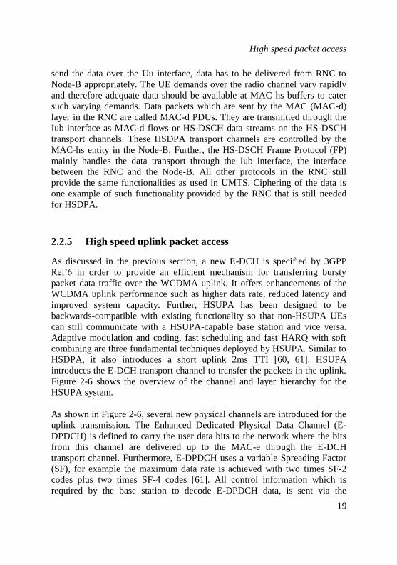
2.2.5 High speed uplink packet access
As discussed in the previous section, a new E-DCH is specified by 3GPP
Rel’6 in order to provide an efficient mechanism for transferring bursty
packet data traffic over the WCDMA uplink. It offers enhancements of the
WCDMA uplink performance such as higher data rate, reduced latency and
improved system capacity. Further, HSUPA has been designed to be
backwards-compatible with existing functionality so that non-HSUPA UEs
can still communicate with a HSUPA-capable base station and vice versa.
Adaptive modulation and coding, fast scheduling and fast HARQ with soft
combining are three fundamental techniques deployed by HSUPA. Similar to
HSDPA, it also introduces a short uplink 2ms TTI [60, 61]. HSUPA
introduces the E-DCH transport channel to transfer the packets in the uplink.
Figure 2-6 shows the overview of the channel and layer hierarchy for the
HSUPA system.
As shown in Figure 2-6, several new physical channels are introduced for the
uplink transmission. The Enhanced Dedicated Physical Data Channel (E-
DPDCH) is defined to carry the user data bits to the network where the bits
from this channel are delivered up to the MAC-e through the E-DCH
transport channel. Furthermore, E-DPDCH uses a variable Spreading Factor
(SF), for example the maximum data rate is achieved with two times SF-2
codes plus two times SF-4 codes [61]. All control information which is
required by the base station to decode E-DPDCH data, is sent via the

High speed packet access
20
Enhanced Dedicated Physical Control Channel (E-DPCCH). E-DPDCH and
E-DPCCH are main physical channels which are added in the uplink whereas
three other new physical channels are defined in downlink direction. They are
the Enhanced Hybrid Indicator Channel (E-HICH) which carries the ACKs
and NACKs to the UE, Enhanced Absolute Grant Channel (E-AGCH) which
is a shared channel that signals absolute values for the Grant for each UE
with a unique E-RNTI identity, Enhanced Relative Grant Channel (E-RGCH)
which signals the incremental up/down/hold adjustments to the UE's Serving
Grant. The E-RGCH and E-HICH share the same code space in the
Orthogonal Variable Spreading Factor (OVSF) tree [61]. Orthogonality
between the two channels is provided by the use of orthogonal 40 bit
signatures which are the limited resources for the uplink transmission,
because up to 40 different signatures can be encoded.
Figure 2-6: WCDMA channel and layer hierarchy for HSUPA
In contrast to HSDPA, HSUPA does not utilise a shared channel for data
transfer in the uplink. Each UE has a dedicated uplink connection which is
realised by a unique scrambling code. In contrast to this, Node-B uses a
single scrambling code and then assigns different OVSF channelization codes
to differentiate UEs in the downlink [22].

High speed packet access
21
2.2.5.1 Uplink shared resource and grants
The main shared resource in the uplink is the interference level in a cell.
Managing the interference is done via a fast closed loop power control
algorithm. The primary shared resource on the uplink is the total power
received at the Node-B for a particular cell. Hence HSUPA scheduling is
performed by directly controlling the maximum amount of power that a UE
can use to transmit at any given point in time. Therefore, one of the primary
goals of HSUPA is to achieve effective fast scheduling which allows
adapting to rapidly changing radio channels with different data rates [18]. On
the other hand, with 2 ms TTIs, the overall transmission delay is greatly
reduced. The transmission delay performance is further improved by
introducing HARQ technique as used in the HSDPA network.
HSUPA mainly uses two types of resource grants in order to control the UE’s
transmit power: non-scheduled grants and scheduled grants. The non-
scheduled grant is most suited for constant-rate delay-sensitive applications
such as voice-over-IP. In the non-scheduled grant which is mapped to a
certain power level at the UE, the Node-B simply tells the UE the maximum
Transport Block Size (TBS) that it can transmit on the E-DCH during the
next TTI. The TBS is signalled at call setup and the UE can then transmit a
transport block of that size or less in each TTI until the call ends or the Node-
B modifies the non-scheduled grant via an RRC reconfiguration procedure.
For scheduled grants, the UE maintains a serving grant that it updates based
on information received from the Node-B via E-AGCH or E-RGCH
downlink channels [61]. E-AGCH signals the absolute serving grants and the
UE can adjust its maximum power level in order to determine maximum
transport block size for the current transmission. E-RGCH signals the relative
grants to the UE and based on this information the UE adjusts its serving
grant up or down from its current value. At any given point in time the UE
will be listening to a single E-AGCH from its serving cell and to one or more
E-RGCHs. The E-RGCH is shared by multiple UEs but on this channel the
UE is listening for a particular orthogonal signature which is 40 bit code in
same code space of OVSF (Orthogonal Variable Spreading Factor) tree. If it
does not detect its signature in a given TTI it interprets this as a "Hold"
command, and thus makes no change to its serving grants. In summary, both
grants, absolute and relative directly specify the maximum power that the UE
can use on the E-DPDCH in the current TTI. As E-DCH block sizes map
High speed packet access
22
deterministically to power levels [18], the UE can translate its Serving Grant
to the maximum E-DCH transport block size which can be used in a TTI.
2.2.5.2 Serving radio link set and non-serving radio link set
The concept of a Serving Radio Link Set (S-RLS) and a Non-Serving Radio
Link Set (Non-SRLS) is defined in combination with soft handover for
HSUPA [18, 43]. The group of cells from which the UE can soft combine E-
RGCH commands, create the serving RLS. The serving RLS by definition
includes the serving cell from which the UE is receiving the E-AGCH.
Further, the cells in the serving RLS must all transmit the same E-RGCH
command in each TTI, which means the cells that are belonging to the same
RLS should be controlled by the same Node-B. Apart from this, UE can also
receive the E-RGCH information of any other cell which belongs to another
RLS. All such cells that transmit an E-RGCH to the UE form the non-serving
RLS by definition [43].
The cells which are in the serving RLS can issue E-RGCH commands to
raise, hold or lower the current UE serving grants. However, the cells in the
Non-Serving RLS can only issue “HOLD” or “DOWN” commands. This is a
kind of control measure which informs the current cell about an overloading
situation at neighbour cells. Therefore, out of all E-RGCH commands, the
“DOWN” command has the highest priority and the UE must reduce its
serving grants regardless of any other grants it receives. The “HOLD”
command has the second highest priority and lastly the “UP” command has
the lowest priority to increase the UE’s serving grants if no other command is
received. Although the 3GPP standards define how the network
communicates a serving grant to a UE, the algorithm by which the network
determines which commands should be sent on the E-AGCH/E-RGCH is not
defined and is left to the mobile network operators [61].
2.2.5.3 UE status report for scheduling
The measurement reporting functionality is defined in the 3GPP standards to
allow the UEs to communicate their current status. UE status reporting takes
two forms, scheduling information transmitted on the E-DCH along with the
user data, and a “happy” bit transmitted on the E-DPCCH channel. The
scheduling information provides an indication of how much data is waiting to
be transmitted in the UE and how much additional network capacity the UE
could make use of. For example if the UE is already transmitting at full

High speed packet access
23
power then it would be a wastage of resources to increase its serving grant as
the UE would be unable to make use of the additional power [60].
The other status reporting mechanism is the “happy” bit information. This is
a single bit that is transmitted on the E-DPCCH physical channel. A UE
considers itself to be unhappy if it is not transmitting at maximum power and
it cannot empty the transmit buffer with the current serving grant within a
certain period of time. The period of time is known as the Happy Bit Delay
Condition (HBDC) and is signalled by the RRC layer during call setup. Thus
the “happy” bit is a crude indication of whether the UE could make good use
of additional uplink power.
2.2.5.4 Uplink HARQ functionality
The basic functionality of HARQ is described in section 2.2.2. The HARQ
scheme runs in Node-B for the uplink transmission. The functionality is
similar to the HARQ in HSDPA. There are 8 HARQ processes that run in
parallel for 2 ms TTI and for each connection. Each time when the UE
transmits, the receiving HARQ process in the Node-B will attempt to decode
the transport block. If the decoding is successful, the Node-B transmits an
ACK to the UE over the E-HICH channel and that HARQ process in the UE
will advance onto the next transport block. If the decoding of the transport
block fails then the Node-B transmits a NACK to the UE on the E-HICH.
The UE retransmits the transport block until the maximum number of
retransmissions is met. After reaching the maximum number of
retransmissions, the HARQ process which runs in the UE will advance to the
next transport block. The UE will either use chase combining which means
the transmission of exactly the same bits again or incremental redundancy
which is a transmission of a different set of bits, depending on how the RRC
layer configured the link at call setup.
2.2.5.5 HSUPA protocol architecture
Figure 2-7 shows the UTRAN protocols which are used for the uplink
transmissions. There are uplink related specific layers which are added to the
standard UMTS layered architecture [61]. They are MAC-es/e at the UE
entity, the MAC-e at the Node-B and MAC-es at the RNC. In the UE MAC-
es/e are considered as one single layer and in the network side MAC-e and
MAC-es are considered as separate layers. The new E-DCH transport
channel connects up to the new MAC-e, MAC-es and the MAC-es/e layer.

High speed packet access
24
The MAC-es/e in the UE contains the HARQ processes and it performs the
selection of the uplink data rate based on maintaining the current serving
grant and also provides the status reporting. Further this layer creates a
transport block based on the scheduling grants received by the MAC-e layer
in Node-B. The latter layer contains the HARQ processes, some de-
multiplexing functionality and the fast scheduling algorithm. The MAC-es
layer in RNC primarily provides reordering, combining and also disassembly
of MAC-es PDUs into individual MAC-d PDUs.
Figure 2-7: UTRAN protocol architecture for the uplink
Since HSUPA supports soft handover, it is possible to receive more than one
MAC-e PDU at the RNC from the same UE via different routes (via different
Node-Bs). This results in duplicate PDU arrivals. MAC-es detects such
duplicates and deletes them before sending the PDUs to the upper layer in the
RNC. Further, due to the parallel nature of the HARQ processes it is also
possible for MAC-e PDUs to arrive out of order at the MAC-es layer in the
RNC. Therefore, the latter layer also does the reordering and provides in-
sequence delivery to the upper layer.

UMTS transport network
25
2.3 UMTS transport network
The UMTS transport network mainly consists of the Iub interface which
connects the Node-B with the RNC. Often this network is also named
Transport Network Layer (TNL) in scientific reports. Asynchronous Transfer
Mode (ATM) is the prime technology introduced in UMTS 3GPP Rel’99
(Rel’99) and release 4 (Rel’4). The ATM technology provides several service
priorities which support different QoS requirements of various traffic types
and it achieves a very good multiplexing gain for bursty traffic. With the
improvement of the QoS support and the transport capacity requirements
from Rel’5 (Rel’5) onward, other transport technologies such as IP or IP over
DSL have been introduced into the standards. Therefore apart from the main
ATM technology, DSL based transport technology is also described in this
chapter.
The Iub interface allows the RNC and the Node-B to communicate about
radio resources. It is the most critical interface in the UTRAN from the
terrestrial transport network point of view. The designing and dimensioning
of this expensive Iub network should be done as cost effectively as possible.
Therefore traffic over this network should be controlled in order to provide
optimum utilisation while achieving the required Quality of Service (QoS)
guarantees for each service. The trade-off between optimisation of bandwidth
(low cost transmission) and provision of QoS is a major challenge for Mobile
Network Operates (MNOs).
2.3.1 ATM based transport network
Due to the tremendous growth of Internet and multimedia traffic at the start
of 3G mobile communications, scientific research focuses on finding cost
effective solutions. ATM (Asynchronous Transfer Mode) is one of the key
technologies which is used for high speed transmissions. ATM is designed as
a cell switching and multiplexing technology to combine the benefits of
circuit switching and packet switching techniques [62]. The term cell in the
context of ATM means a small packet with constant size. Circuit switching
provides constant transmission delay and guaranteed capacity whereas packet
switching provides high flexibility and a bandwidth efficient way of
transmission. Due to the short fixed length cells transmitted over the network,

UMTS transport network
26
it can be used for the traffic integration of all services including voice, video
and data.
The basic format of the cell which has the size of 53 bytes [62] is shown in
Figure 2-8. The cell consists of five bytes header and 48 bytes user or control
data. Two different header code structures can be defined in the header
depending on the transmission: User Network Interface (UNI) and Network
Node Interface (NNI).
Figure 2-8: ATM PDU format
For the purpose of routing cells over the network, VPI (Virtual Path
Identifier, 8 bits) and VCI (Virtual Channel Identifier, 16 bits) are defined in
the header. The Payload Type (PT) is used to identify the type of data –
control or user data – whereas the CLP bit field is used to set the priority.
When congestion occurs, the cell discarding technique is applied based on
the priority assigned to the cell by the CLP field. For example, packets with
CLP = 1 are discarded first while preserving CLP = 0 packets. Finally 8 bits
are assigned to the HEC field to monitor header correctness and perform
single bit error correction.
Payload (48 bytes)

UMTS transport network
27
After the ATM connection has been set up, cells can be independently
labelled and transmitted on demand across the network. Therefore the ATM
layer can be divided into VP and VC sub-layers [62] as shown in Figure 2-9.
The connections supported at the VP sub-layers, i.e. the Virtual Path
Connections (VPC) do not require call control, bandwidth management, or
processing capabilities. The connection at the VC sub layer, i.e. the Virtual
Channel Connection (VCC) may be permanent, semi-permanent or switched
connections. The switched connections require signalling to support
establishment, tearing down and capacity management. The permanent and
semi-permanent virtual paths are denoted as PVPs and SPVPs throughout
this thesis.
Figure 2-9: VP and VC sub-layers details
ATM technology is intended to support a wide variety of services and
applications. The control of ATM network traffic is fundamentally related to
the ability of the network to provide appropriately differentiated Quality of
Service (QoS) for network applications. A set of six service categories is
specified. For each one, a set of parameters is given to describe both the
traffic presented to the network and the Quality of Service (QoS) which is
required from the network. A number of traffic control mechanisms are
defined which the network may utilise to meet the QoS objectives. The six

UMTS transport network
28
service categories which are specified in the ATM forum 99 release are listed
as follows.
Constant Bit Rate (CBR),
Real time Variable Bit Rate (rt-VBR),
Non-Real time Variable Bit Rate (nrt-VBR),
Unspecified Bit Rate (UBR),
Available Bit Rate (ABR),
Guaranteed Frame Rate (GFR).
Service categories are distinguished as being real time or non-real time. The
categories belonging to real time are CBR and rt-VBR support real time
application services depending on the traffic descriptor specifications such as
peak cell rate (PCR) or sustainable cell rate (SCR). The other four services
categorise the support of non-real time services under the requirements of the
traffic descriptor parameters. All service categories except GFR apply to both
VPCs and VCCs. GFR is a frame aware service category which can only be
applied to VC connections since frame delineation is usually not visible at
the virtual path level.
2.3.1.1 ATM adaptation layer
When considering the OSI reference protocol architecture ATM belongs to
data link layer. In general, services or applications cannot be mapped directly
to ATM cells. This is done through the ATM adaptation layer (AAL). The
AAL protocols perform functions of adapting services to the ATM layer and
are also responsible for making the network behaviour transparent to the
application. It represents the link between particular functional requirements
of a service and the generic service-independent nature of ATM transport.
Depending on the type of service, the AAL layer can be used by either end
users or the network. Figure 2-10 depicts the AAL layer architecture. The
layer can be divided into two main sub-layers: Segmentation and Reassembly
(SAR) and Convergences Sub-layer (CS) [62]. The CS is further divided into
two sub-layers: Service Specific Convergence Sub-layer (SSCS) and
Common Part Convergence Sub-layer (CPCS). The SSCS part is specially
designed for connection oriented services which support connection
management purposes whereas CPCS can be shared by both connection-
oriented as well as connectionless services. The function of the SAR is to
segment the protocol data units from the CS layer which are fitted to the
payload of the ATM cell.

UMTS transport network
29
Figure 2-10: AAL architectural overview
There are four types of AAL protocols defined by the ITU standard for the
ATM network [ITU I.363]: AAL1, AAL2, AAL3/4 and AAL5 [62]. AAL1
is used to support CBR connections over the ATM network on a per user
basis; it is not optimised for bandwidth efficient transmissions. AAL3/4 is an
obsolete adaptation standard used to deliver connectionless and connection
oriented data over the ATM network. It has a substantial overhead consisting
of sequence numbers and multiplexing indicators, and it is rarely used in
practice. AAL5 has been developed by the data communication industry; it is
optimised for data transport. The AAL2 protocol is the enhanced version of
AAL1 which is designed to overcome the limitation experienced from AAL1
and also used in practice. AAL2 is also the adaptation protocol used by the
UTRAN Iub interface in the UMTS implementation. This is the most suitable
transport layer protocol for real time, variable bit rate services like voice and
video. Therefore more details about the architecture and packet formats of the
AAL2 protocol are discussed in the next section.
AAL2 is an adaptation layer that is designed to multiplex more than one low
bit rate user data stream on a single ATM virtual connection. This AAL
provides bandwidth-efficient transmission of low-rate, short, and variable
length packets in delay sensitive applications. In situations where multiple
low Constant Bit Rate data streams need to be connected to end systems, a lot
of precious bandwidth is wasted in setting up conventional VCs for each of
the connections. Moreover, most network carriers charge on the basis of
number of open Virtual Connections, hence it is efficient both in terms of

UMTS transport network
30
bandwidth and cost to multiplex as many of these as possible on a single
connection.
2.3.1.2 ATM QoS and traffic descriptor parameters
A set of parameters are negotiated when a connection is set up on ATM
networks. These parameters are also used to measure the Quality of Service
(QoS) of a connection and quantify end-to-end network performance at the
ATM layer. The QoS parameters are described as follows.
Cell Transfer Delay (CTD): The delay experienced by a cell
between the first bit of the cell transmitted by the source and the last
bit of the cell received by the destination. Maximum Cell Transfer
Delay (Max CTD) and Mean Cell Transfer Delay (Mean CTD) are
used.
Peak-to-peak Cell Delay Variation (CDV): The difference of the
maximum and minimum CTD experienced during the connection.
Peak-to-peak CDV and Instantaneous CDV are used.
Cell Loss Ratio (CLR); The percentage of cells that are lost in the
network due to error or congestion and are not received by the
destination.
The ATM traffic descriptor is defined by four parameters which are
Peak Cell Rate (PCR): The PCR specifies an upper bound on the
rate at which traffic can be submitted on an ATM connection. By
knowing this parameter, the network performance objectives can be
ensured at the design stage by allocating sufficient transport
resources to the network.
Sustainable Cell Rate (SCR): The SCR is an upper bound on the
average rate of the conforming cells of an ATM connection.
Defining this parameter is also a good measure to ensure the
performance objective of the network. However, this depends on the
type of network and the QoS criteria.
Burst Tolerance (BT): The maximum burst size that can be sent at
the peak rate.
Maximum Burst Size (MBS): The maximum numbers of back-to-
back cells that can be sent at the peak cell rate. MBS is related as
follows with the other parameters.

UMTS transport network
31
Burst Tolerance = (MBS-1) (1/SCR – 1/PCR)
Minimum Cell Rate (MCR): The minimum cell rate is the rate at
which a source is always allowed to send. MCR is useful for
network elements in order to allocate bandwidth among the
connections.
2.3.1.3 ATM traffic control and congestion control
The objectives of traffic control and congestion control for ATM are
supporting a set of QoS parameters and classes for all ATM services and
minimize network and end-system complexity while maximizing network
utilisation. Designing a congestion control scheme appropriate for ATM
networks is mainly guided by scalability and fairness criteria. On the other
hand the design of the network is done in such a way that it should react to
congestion in order to minimise its intensity, spread and duration. Three main
factors have to be examined for the congestion control: burstiness of the data
traffic, the unpredictability of the resource demand and the large propagation
delay vs. the large bandwidth. Different levels of network performance may
be provided on connections by proper routing, traffic scheduling, priority
control and resource allocation to meet the required QoS for the connections.
2.3.2 DSL based transport network
The Digital Subscriber Line (DSL) technology is one of the key technologies
used in modern data communication. It uses existing twisted-pair telephone
lines (Plan Old Telephony System, POTS) to transmit high bandwidth data.
Commonly it is also called xDSL where “x” distinguishes variants of DSL.
Mainly there are two types: Symmetric DSL (also called Single pair High bit-
rate Digital Subscriber Loop, SHDSL´, [65]) or Asymmetric DSL (ADSL)
[64]. The latter has different data rates in downstream and upstream whereas
SDSL supports equal data rates in both directions. Both ADSL and SHDSL
services provides dedicated, point to point, public network access using
existing telecommunication infrastructure on the local loop which is
commonly known as “last mile”, the connection between the network service
provider’s switching center and the customer’s site.
The twisted-pair copper wire supports the frequency spectrum up to 1MHz
for the transmission. However the normal voice telephony signal utilises the

UMTS transport network
32
spectrum below 4 kHz whereas the rest is not used. Therefore, DSL
technology uses this leftover spectrum almost completely for high-speed data
transmissions. In general ADSL shares the BW with voice signals whereas
the SHDSL uses the complete spectrum without sharing the spectrum with
voice telephony [64, 65].
When it comes to performance of the DSL technology, there is a number of
factors that can affect frequencies in the DSL spectrum differently which
reduce the effectiveness of the available BW.
Attenuation: depends on the length and the gauge of the line. The
higher the length is, the higher the attenuation becomes, and also
narrowing the gauge increases the attenuation as well.
Reflection and noise: When bridging the lines, reflection and noise
can be introduced.
Cross-talk: bundling results in cross-talk which also depends on the
relative position of the line.
Radio frequency interference: RF interference can occur from
external sources, e.g. any nearby station which transmits RF.
ADSL uses the DMT (Discrete Multi-Tone, [64]) modulation scheme at the
transmitter so that it can effectively cope with the above mentioned
impairment conditions. DMT splits the available frequency spectrum into
several sub-bands. There are 224 subcarriers in the downstream, each
occupying a 4 kHz portion of the spectrum. SHDSL uses the Trellis Coded
Pulse Amplitude Modulation (TC-PAM, [65]) to provide adaptive
performance over the long links.
The ADSL and SHDSL frame formats are given in Figure 2-11. In addition
to the normal frame of ADSL, a super frame is also used for synchronisation
purposes. After sending 68 normal frames, a super frame or synchronous
frame is sent. Each frame starts on a 250 microsecond time boundary; the
timing of the frame is kept constant. Depending on prevailing transport
conditions, the actual size and content can vary.

UMTS transport network
33
Fast Byte Fast Data FEC Interleaved Data
ADSL frame format
Over
head
Payload
BlockFrame Sync.
Stuff
bits
SHDSL frame format
Over
head
Payload
Block
Over
head
Payload
Block
Over
head
Payload
Block
Figure 2-11: ADSL and SHDSL frame formats
The Fast Byte is used to super frame related processing and Fast Data
transmits sensitive data such as audio. The accuracy of the data is ensured by
the FEC. Interleaved data is the user data such as Internet data.
The first field of the SHDSL frame is a frame synchronisation word used to
align the frames. The payload blocks carry the user data; each of them is pre-
pended by a corresponding header field for error checking and further
synchronisation. Each payload block is divided into 12 sub-blocks. The last
stuffing bits are also used to support the frame synchronisation.
2.3.2.1 ADSL network
Figure 2-12 shows the main entities in the ADSL network [63, 64]. The last
mile network, i.e. the network between the switching center and the
subscriber's premises is shown along with the relevant components in Figure
2-12. The central-switching unit connects to the PSTN and the data network.
The central switching unit consists of a DSL splitter and a DSL Access
Multiplexer (DSLAM). The latter is a collection of ATU-C units where each
of them is the termination point of a local loop at the central switching unit.
Further it connects to the ATU-R unit (also called ADSL Modem) at the
subscriber premises. The splitter is a passive filter which is located at both
sides of the local loop. It separates the voice frequencies from the data
frequencies when receiving the signals whereas when transmitting it
combines the voice and data signals together into one line. The external data
network of the Internet Service Provider (ISP) is connected to the central
switching unit via the DSLAM; the PSTN network is directly connected via
the splitter.

Long term evolution
34
Figure 2-12: ADSL network
2.4 Long term evolution
Traffic demand in modern days is growing exponentially with usage of
numerous applications in both real time and best effort domains. In order to
be prepared for such demands in the future, 3GPP Rel’8 defines a new
mobile broadband access technology often referred to as Long-Term
Evolution (LTE) including the development of an evolved core network
which is known as System Architecture Evolution (SAE). The bandwidth
capability for a UE is expected to be 20 MHz for both the uplink and the
downlink [48]. The main targets of these technologies are high peak data
rates, low latency, flexible bandwidth support, improved system capacity,
reduced UE and system complexities and also reduced network cost. LTE
technology is designed to rely on IP based packet networks. Therefore, the
main challenge from the view of mobile network operators is to achieve
target data rates and latency by meeting the end user QoS requirements and
throughput performance.
2.4.1 LTE targets
The 3GPP activity regarding 3G evolution fixed the requirements, objectives
and targets in the spring of 2005. These targets are documented in 3GPP TR

Long term evolution
35
25.913 [40]. When operating in a 20MHz spectrum allocation, the targets for
downlink and uplink peak data-rates are 100Mbit/s and 50Mbit/s respectively
[42]. The latency requirements consist of control-plane requirements and
user-plane requirements separately. The user-plane latency means the time it
spends to transmit a IP packet from the terminal to the RAN edge node or
vice versa which is measured on the IP layer. The requirement for the one-
way transmission time should not exceed 5 ms [44]. The control-plane
latency requires the delay less than 100 ms.
The global demands for bandwidth increase rapidly and network operators
obtain an increasing amount of scattered spectrum, spread over various bands
with different bandwidth. Under such circumstances, LTE is targeted to
operate in different frequency bands for the spectrum allocation. The 3GPP
standardised LTE to operate in channels with 1.25, 1.6, 2.5, 5, 10, 15, and
20MHz bandwidths [47, 48]. The mobility requirements focus on the speed
of the mobile stations. The best performance for LTE is realized at low
speeds around 0-15 km/h [43]. However, LTE systems should ensure high
performance for speeds above 120km/h as well [43]. The maximum speed
which LTE is designed to manage acceptable performance is in the range
from 300 to 400 km/h which is mainly dependent on the selected frequency
band as well.
2.4.2 LTE technology
LTE introduces a new air interface technology based on Orthogonal
Frequency Division Multiplex (OFDM) which uses closely spaced carriers
that are modulated with low data rates. Since carrier spacing is equal to the
reciprocal of the symbol period, carriers are orthogonal to each other which
leads to a simple equalisation effort at the receiver. Therefore, the OFDM
based transmission is not only robust against multipath fading effects but also
avoids mutual interference [44]. Since due to frequency selective fading only
a small number of carriers are affected, the forward error correction is able to
effectively recover the corrupted data from the remaining subcarriers. In
contrast to the LTE downlink which deploys OFDM, the uplink uses Single-
Carrier Frequency Division Multiple Access (SC-FDMA) which provides a
lower peak-to-average ratio for the transmitted signal. Saving power in the
mobile station in order to keep a long battery life is one of the main
considerations to select SC-FDMA in the LTE uplink. The small peak-to-
average ratio of the transmitted signal allows a high transmission power,

Long term evolution
36
while achieving more efficient usage of the power amplifier in the uplink
transmission. The implementation of the modulation and the demodulation
functionalities in the LTE uplink and the downlink transmission is
computationally efficient due to usage of FFT techniques. The supported
modulation schemes for the individual carriers in the downlink and uplink are
QPSK, 16QAM and 64QAM [43].
Shared-channel transmission is vital for LTE transmission technique. In such
a scheme, the time-frequency resource which is used as the main shared
resource is dynamically allocated among different users. The scheduler is
responsible for allocating resources for each user for the downlink
transmission. When compared to HSPA channel dependent scheduling, it
selects the UE with best the channel condition in the frequency domain
whereas the LTE scheduler considers channel variations in both time and
frequency domain. It can make decisions to track channel variations as often
as every 1 ms with a 180 kHz granularity in the frequency domain [46].
As in HSPA, fast HARQ with soft combining is deployed in LTE as well
which enables the UE to request retransmissions to quickly recover
erroneously received data blocks. The soft combining of HARQ exploits
incremental redundancy to increase the successful decoding capabilities [48].
Another key technique applied in LTE is the multiple antenna technique
which is also called Multiple-Input Multiple-Output (MIMO). This method is
the one of the key technologies to achieve the targets of LTE performance. It
can enhance the diversity for reception and transmission. Further, beam-
forming can be effectively used at the LTE base station with the usage of
multiple antennas.
2.4.3 LTE architecture and protocols
The LTE architecture with all network entities is shown as a bock diagram in
Figure 2-13. As described above, the LTE network consists of two main
parts: Evolved UMTS Terrestrial Radio Access Network (E-UTRAN) and
the Evolved Packet Core (EPC). The UE and enhanced Node-B (also referred
to as eNB or eNode-B) are the main functional elements which are located in
the E-UTRAN whereas the Serving Gateway (SGW), Mobility Management
entity (MME) and SGSN are the main functional elements which are located
in the EPC. The serving gateway is the main router for an LTE network

Long term evolution
37
which connects the E-UTRAN and the PDN (Packet Domain Controller)
networks.
Figure 2-13: LTE architecture with main network entities
From the functional point of view, it routes and forwards packet data to the
external network via the PDN. Further it acts as the mobility anchor for the
inter-eNB handovers at user-plane and also for other handovers between LTE
network and the other 3GPP based broadband wireless networks. The MME
is the key control element of the LTE access network at the control-plane.
Many control-plane functionalities, such as activation and deactivation of
bearers, UE tracking and paging procedures, authentication and security key
management of UEs, providing initial user identity and selecting the SGW
during handovers are performed by this node. Further, Non-Access Stratum
(NAS) signals terminate at the MME node as well [43]. The PDN gateway
provides connectivity between the LTE network and the external packet data
network and performs policy enforcement, packet filtering for each user,
charging support, lawful interception and packet screening.
2.4.3.1 E-UTRAN architecture
The E-UTRAN has a simple flat architecture compared to the HSPA UTRAN
architecture and has only two main network elements: UE and eNB, whereas
the UTRAN consists of three main network entities: UE, Node-B and RNC
[40]. The comparison between the two architectures UTRAN and E-UTRAN
is shown in Figure 2-14. The eNB in LTE is directly connected with the core
network whereas the Node-B in the UTRAN connects through the RNC to
the core network. The RNC is the main control entity in UTRAN network,
however in the E-UTRAN, this entity is dropped and most of its
functionalities are distributed among the enhanced Node-B entity, the MME

Long term evolution
38
and the serving GW. The figure shows that the E-UTRAN and UTRAN
connectivity to their core networks are done via different interfaces as well.
For an E-UTRAN network, the UE is connected to the eNB via the LTE Uu
interface and eNB is connected to the EPC via the S1 interface. The
additional X2 interface connects the eNBs with each other. All interfaces of
the UTRAN have been discussed in the UMTS network architecture.
Figure 2-14: UTRAN (left) and E-UTRAN architectures
2.4.3.2 LTE user-plane protocol architecture
The LTE user plane architecture mainly consists of the LTE access network
and the core network. However in order to have a better overview, Figure
2-15 shows the end-to-end user-plane protocol architecture from the
application layer of the LTE mobile terminal to the application layer of the
remote server. Even though it is called user-plane protocol architecture, all
application based signalling such as SIP, RTCP and SDP are also routed via
this network. The complete architecture uses IP as the transport network
protocol. Depending on the services, different end user protocols are
involved during data transmissions between end-nodes. For example, best
effort traffic uses TCP as the transport protocol whereas the most of the real
time applications use UDP as the transport protocol.

Long term evolution
39
Figure 2-15: LTE user-plane protocol architecture
As shown in Figure 2-15, S1, X2 and S5/S8 interfaces use the 3GPP specific
tunnelling protocol, the GPRS Tunnelling Protocol (GTP). The protocol stack
of these interfaces consists of the GTP-user plane (GTP-U), User Datagram
Protocol (UDP), IP, data link layer and PHY layer. Transport bearers are
identified by the GTP tunnel endpoints and IP based information such as
source address, destination address etc. Apart from routing the user-plane
data, IP transport performs service differentiation at the E-UTRAN network
entities in order to meet the end user QoS requirements. Further security
protection is also provided for user-plane data at this layer using the IPSec
security protocol according to the IETF in RFC 2401 [66].
The LTE radio interface, the interface between UE and eNode-B is called Uu
interface. This interface consists of four main protocol layers in order to
transfer the data between eNB and UE securely. They are Packet Data
Convergence Protocol (PDCP) layer, Radio Link Control (RLC) layer,
Medium Access Control (MAC) layer and Physical (PHY) layer.
The PDCP layer processes the IP packets in the user plane. Each radio bearer
has one PDCP entity that performs header compression/decompression,
security including mainly integrity/verification and ciphering/deciphering,
and also reordering during handovers. Further details about the PDCP
protocol can be found in 3GPP [49].

Long term evolution
40
According to 3GPP [45], the RLC also has one entity per radio bearer and
performs a reliable transmission over the air interface, segmentation and
reassembly based on the transport block size allowed by the radio interface
and also in-sequence packet delivery to the upper layers. The in-sequence
delivery is required due to the HARQ process in MAC layer which can
receive out of order arrivals due to retransmissions.
Figure 2-16: Uu interface protocols functionalities
The MAC layer provides one MAC entity per UE, not per radio bearer. The
MAC layer provides data multiplexing of different radio bearers which
belong to the same UE. It indicates the transport block size to the RLC
bearers by considering QoS aspects of the services. There are two very
important functional units which are located in this layer: the MAC scheduler
and the HARQ processes. The MAC scheduler is in the MAC layer of the
eNB. The scheduler allocates the radio resources for each UE based on the
agreed QoS criteria. For this process, the user buffer occupancy and service
priorities are taken into account. The common set of guidelines which should
be agreed by all vendors for scheduling is given in 3GPP [48], however the
implementation is vendor specific who are able to apply different algorithms
such as different priority schemes for different services within the given
frame work of the 3GPP specification. As in HSPA, the HARQ processes

Long term evolution
41
provide efficient error recovery at the MAC layer which increases the
spectral efficiency for the cost of additional delay due to retransmissions.
The physical layer transmits data over the radio channel using the Orthogonal
Frequency Division Multiplex (OFDM) and Multiple Input Multiple Output
(MIMO) technologies. In the downlink, Orthogonal Frequency Division
Multiple Access (OFDMA) allows multiple users to access the medium on
sub carrier basis. In the uplink, Single Carrier Frequency Division Multiple
Access (SC-FDMA) is used for the medium access. Extensive details about
modelling the PHY layer are provided by 3GPP [47].
2.4.3.3 Control-plane protocol architecture
The control-plane protocol stack between UE and MME and also for the X2
interface is shown in Figure 2-17.
Figure 2-17: LTE control-plane protocol architecture
This protocol stack includes most of the protocols which are described in the
user-plane. From the functional point of view they work in the same manner
with one exception at the PDCP layer. In this case, there is no PDCP header
compression functionality for the control plane.
The Non-Access Stratum (NAS) is the key application layer protocol which
provides signalling between UE and MME that are not processed by the eNB.
NAS messages are encapsulated into the Radio Resource Control (RRC)
protocol and the S1-Application Protocol (S1-AP) in order to provide direct
transport of NAS signalling between MME and UE. The eNB is responsible
for mapping NAS messages between RRC and S1-AP protocols. NAS
supports authentication, tracking area updates, paging, Public Land Mobile

Long term evolution
42
Network (PLMN) selection and bearer management (EPS bearer
establishment, modification and release). The RRC provides the means to
transfer NAS signalling information between UE and eNB entities whereas
the S1-AP is responsible for transferring signalling information between the
eNB and MME over the S1-MME reference point. The S-AP is carried using
the Stream Control Transmission Protocol (SCTP) [41]. Furthermore the S1-
AP supports QoS bearer management, S1 signalling bearer management, S1
interface management, paging signalling, mobility signalling and tracking
area control signalling.
The X2-Application Protocol (X2-AP) is used to transfer signalling
information between neighbouring eNBs over the X2 interface. It is also
carried over the SCTP protocol by providing handover signalling, inter-cell
RRM signalling and X2 interface management functionalities.
2.4.3.4 Logical channels and transport channels
The data is exchanged between the MAC layer and the RLC layer using the
logical traffic channels. The dedicated traffic channel (DTCH) is used to
transmit dedicated user data for both uplink and downlink directions whereas
the Multicast Traffic Channel (MTCH) is used to transmit MBMS services
for the downlink. The transport channel is used to transfer data between
MAC layer and PHY layer.
Figure 2-18: Mapping between logical channels and transport channels for
uplink and downlink transmission

Long term evolution
43
Data is multiplexed into transport channels depending on air interface bearer
allocation. There are four transport channels for the downlink. They are
Downlink Shared Channel (DL-SCH) which is used to transport user data,
Broadcast Channel (BCH) which is used to transport system information for
the DL-SCH channel, Paging Channel (PCH) which is used for paging
information and Multicast Channel (MCH) which transports some user and
control information. The mapping between logical channels and transport
channels for the downlink and the uplink is shown in Figure 2-18.
There are two transport channels which are used for the uplink: the Uplink
Shared Channel (UL-SCH) is used to transport user data over the uplink and
the Random Access Channel (RACH), is used for network access if the UE
does not have accurate time synchronisation or allocated uplink resources.
2.4.3.5 LTE MAC scheduler
The LTE MAC scheduler is located in eNB. Radio resources at the Uu
interface are scarce and have to be distributed among the users in the cell in
order to achieve optimum throughput while meeting QoS requirements for
different services. Due to many factors, such as throughput, fairness and
limited resources, designing an appropriate scheduler is a real challenge for
mobile network operators. Many advanced PHY technologies such as OFDM
provide great flexibility and support such achievements in LTE. The
scheduler implementation itself is not standardised but signalling to support
scheduling is standardised by the 3GPP specification.
The basic resource unit is the Physical Resource Block (PRB) which is
defined in both the time and the frequency domain. In the latter domain it has
a size of 180 kHz and in the time domain, a sub-frame or transmission time
interval (TTI) is 1 ms for both the uplink and the downlink. The radio
resources in a cell are dynamically allocated to the UEs in terms of resource
blocks through UL-SCH and DL-SCH channels in the uplink and the
downlink respectively. Such resource allocation for individual users is
performed by mainly considering three factors: current channel condition,
UE buffer status (buffer status report, BSR) and QoS requirements. Figure
2-19 shows the scheduler overview in eNB.
Since OFDM is used as the PHY technology, there is great flexibility of
selecting frequency blocks which have the optimum channel performance for
certain UEs that provide higher spectral efficiency for the selected frequency

Long term evolution
44
range in which high modulation schemes such as 64 QAM can be deployed.
In this manner, the scheduler can select users who provide the best channel
conditions in different frequencies and utilise the complete frequency band
effectively for the scheduling among the selected users.
Figure 2-19: LTE MAC scheduler overview
This means the LTE scheduler is able to use the benefit of multi-user
diversity by using frequency-time resource allocation based on best channel
conditions among active users during the scheduling process. The channel

Long term evolution
45
information of each connection is provided by the UE Channel Quality
Indicators (CQIs) for the downlink. For the uplink, the eNB uses Sounding
Reference Signals (SRSs). To have channel information for every TTI
requires a large signalling overhead for the scheduler. Therefore this is again
a critical design criterion which leads to a trade-off between the signalling
overhead and the availability of up-to-date channel information. When
accurate channel information is available before the scheduling decision,
optimum performance can be achieved at the cost of higher signalling
overhead and vice versa.
The buffer Status Report (BSR) provides information about the buffer status,
including details about the filling level for each bearer. For the uplink, the
UE sends the BSR report to the eNB whereas for DL, the eNB itself gets the
BSR information from its PDCP layer.
The different types of scheduling techniques can be used to distribute
resource among the users from fully fair scheduling scheme such as Round-
Robin (RR) to opportunistic scheduling schemes such as exhaustive
scheduling. The latter optimises the throughput by allocating even full
resources for a particular UE who has the best channel conditions currently
while having a full buffer. The fair scheduler considers not only the channel
status but also the distribution of available radio resources among current
active users.
All above listed facts can be used to design an effective MAC scheduler
selecting appropriate scheduling parameters is completely dependent on the
vendor specific based on its individual goals.
2.4.4 Quality of service and bearer classification
In general, QoS is the concept of providing particular quality guarantees for a
specific service. By nature, different applications need different QoS
requirements. One user may run more than one application at any time in the
UE device or the mobile. The network should guarantee the required QoS for
each application individually which is a real challenge for mobile network
operators. To cater such demands, LTE introduces the services into different
service categories and defines a common framework to differentiate such
services in the packetized network [45].

Long term evolution
46
In general, all applications can be divided into two main categories: real time
applications and best effort applications. The real time applications such as
VoIP require stringent delay and delay variation (jitter) guarantees whereas
the best effort applications such as web browsing and FTP require low packet
loss rate guarantees. In a similar manner, the LTE network also distinguishes
two types of bearers in a broader view, which are GBR bearers and non-GBR
bearers. GBR bearers provide a guaranteed data rate within an acceptable
packet delay budget whereas non-GBR bearers are concerned about the
reliable packet delivery by providing low packet loss rates.
Figure 2-20: EPS bearer mapping in LTE network:
In order to support multiple QoS requirements, Evolved Packet System (EPS)
in LTE introduces the EPS bearer concepts which establish the bearer
connection between UE and PDN gateway (P-GW). Within the LTE
network, the EPS bearer is realised by three subsidiary bearers: S5/S8 bearer,
S1 bearer and radio bearer. Figure 2-20 shows the overall QoS mapping and
bearer mapping between end-to-end entities through the LTE network [47].
The end-to-end services are defined between end networks, in this case
between the LTE UE and the external network. The end-to-end QoS
requirements of application flows are realised by the EPS bearers in the LTE
network. As shown in Figure 2-20, the EPS bearer consists of three bearers:

Long term evolution
47
S5/S8 bearer between P-GW and S-GW, the S1 bearer between the S-GW
and the eNB and radio bearer between eNB and UE in the LTE network. All
these bearers are mapped one-to-one through each interface and keep a
unique bearer identity to guarantee the QoS targets through the networks.
From the view of services, the EPS bearer is a sequence of IP flows with the
same QoS profile established between UE and P-GW. There are five QoS
parameters which are defined by 3GPP standards [46]. They are
QoS class identifier (QCI),
Allocation and retention priority (ARP),
Guaranteed bit rate (GBR),
Maximum bit rate (MBR),
Aggregate maximum bit rate (AMBR).
Each of these QoS parameters provides different tasks in the IP based packet
network. The QCI is a scalar value which is used for bearer level packet
forwarding over the network whereas ARP supports admission control
procedures for the connection establishment and release functionalities based
on congestion in the radio network. As the definition states, the GBR
parameter provides guaranteed bit rates for the service and is only used for
GBR bearers. The MBR parameter specifies the maximum bit rate which can
be provided by the bearer whereas AMBR specifies the limit of the aggregate
bit rate that can be expected to be provided by all non-GBR bearers
associated with a PDN connection (e.g. excess traffic may get discarded by a
rate-shaping function).
End application is specified with QoS parameters before packets are sending
to the IP based packet network. QCI is one of the important parameters
which provide information about how the packet of a particular service type
should be treated in the packet network concerning QoS. The QCI value is
mapped into Differentiated Service Code Points (DSCP) and is included in
the Type of Service (ToS) field of the IP packet header. Therefore, any IP
packet which traverses the network carries the QoS information along with
the packet itself. When a network node processes the packets, it can
differentiate packets regarding QoS and can provide the required QoS
guarantee for a particular service flow. In order to handle traffic uniformly
throughout the LTE network, some of the QCIs are standardised by 3GPP.

Long term evolution
48
Therefore all vendors and mobile network operators have to agree on these
service requirements. They are listed in Table 2-1.
Table 2-1: LTE QoS classes defined by 3GPP
QCI Resource type
Priority Packet delay
budget (ms)
Packet error loss
rate
Example services
1 GBR 2 100 10-2 Conversational video
2 GBR 4 150 10-3 Conversational video (Live streaming)
3 GBR 5 300 10-6 Non-conversational video
(buffered streaming)
4 GBR 3 50 10-3 Real time gaming
5 Non-GBR 1 100 10-6 IMS signalling
6 Non-GBR 7 100 10-3 Voice, live streaming,
interactive gaming
7 Non-GBR 6 300 10-6 Video (buffer streaming)
8 Non-GBR 8 300 10-6 TCP based best effort applications (web, email)
9 Non-GBR 9 300 10-6 TCP based best effort
( a large file downloads)
For each QoS flow, a separate EPS bearer is required to be established
between the UE and the PDN gateway. Therefore IP packets must be
categorised into different EPS bearers. This is done based on Traffic Flow
Templates (TFTs) which use the IP header information such as ToS, TCP
port numbers, source and destination addresses to select packets from
different service flows such VoIP and web browsing.
This TFT based packet filtering procedure is defined by 3GPP [46] and is
shown in Figure 2-21 for the uplink and downlink service data flows
separately. When the UE is attached to the LTE network, it is assigned an IP
address by the P-GW by establishing at least one EPS bearer. This bearer is
called “default” EPS bearer and it is kept throughout the life-time of the
connection with the PDN network. Since the default EPS bearer is
permanently established, it always has to be a non-GBR bearer. Any
additional EPS bearer which is established by the UE is called “dedicated”
EPS bearer. Depending on different application flows, any number of
dedicated bearers can be established between the UE and the P-GW at any
time.

Long term evolution
49
Figure 2-21: TFT based packet filtering procedure defined by 3GPP [46]
2.4.5 LTE handovers
LTE is designed to provide seamless mobility. UE handovers occur with
imperceptible delay and an acceptable number of packet losses which can be
recovered by the upper layers. In contrast to HSPA there is no centralised
controller in LTE [46]. All centralised functions are performed at the eNB.
Therefore soft handover is not possible for LTE. Whenever UE performs a
handover, buffered data in eNB has to be forwarded to the corresponding cell
in eNB. Data protection during the HOs is handled by the PDCP layer. UE
mobility can be categorised into intra-LTE mobility and inter-RAT (Radio
Access Technologies, such as UMTS and CDMA200) mobility. During this
work only intra-LTE mobility is considered, which occurs either between
eNBs or between cells. Based on this, handovers within E-UTRAN can be
also categorised into two types: inter-eNB handovers which occur between
two eNBs and intra-eNB handovers which occurs between cells within the
same eNB. In both cases the main data handling is performed by the eNB.
For the first case, the buffered data in the source eNB, where the UE is
currently located has to be forwarded via the X2 interface to the target eNB
where the UE is moving to. In this case data should be protected and a fast
transmission between two eNBs should be executed. Not only the data but
also the load or interference related information also has to be forwarded to
the target eNB. In the latter case, the eNB handles the data and signalling
information within its own entity and forwards data to the target cell from the
source cell based on the new UE connectivity.

Long term evolution
50
2.4.5.1 Inter-eNB handovers
As mentioned above, inter-eNB handovers occur between two eNBs which
are called source eNB and target eNB. Since data is forwarded over the X2
interface during HOs, the X2 protocol architecture has to be considered in
detail. The X2 user-plane protocol stack is given in Figure 2-22 according to
the 3GPP specification [47].
Figure 2-22: X2 protocols and inter-eNB HOs
The PDCP layer takes care of the data protection and the GTP establishes a
tunnel through the transport network between source and target eNBs. The
transport network guarantees the QoS aspects and provides the required
priority to the forwarded data. To minimise the packet losses, data
forwarding is performed on a per bearer basis. Minimising delay for
forwarding data is required for the real time applications such as VoIP

Long term evolution
51
whereas a very low loss probability is required for best effort applications
such as email and web browsing which mainly use the TCP protocol. In the
context of an HO, the “lossless”, means a very low loss probability and is
performed by the PDCP layer which can use an ARQ scheme. Further, PDCP
layer also provides in-sequence delivery functionalities for forwarded data.
Once the UE has established the connection with the target eNB, the MME is
notified for path switching procedures by the target eNB. In this case, the
Late Path Switching (LPS) or the backward handover is used to minimise the
losses and also minimise the interruption during HOs.
Figure 2-23: starting phases of the inter-eNB handover process
As shown in Figure 2-23, first the UE is connected to the source eNB (SeNB)
and they communicate with each other. Once UE reaches the tracking area of
the target eNB, it initiates an HO by informing the MME via the source eNB.
Before the UE disconnects from the source eNB, internal bearers are set up
between the target eNB and the source eNB. This is done using inter-eNB
signalling over the X2 interface. Then the UE starts a new connection process
with the target eNB and meanwhile all data including unacknowledged data
is buffered and newly arriving data is forwarded to the target eNB.
The target eNB buffers the forwarded data until the UE finalises the new
connection process with the target eNB. The Figure 2-24 shows that the
buffered data of the source eNB is forwarded and then incoming data to the
source eNB is also forwarded via the X2 interface.
As mentioned above, all data received from the source eNB via the X2
interface is stored in the target eNB PDCP buffer sequentially. Once the UE
has completed the connection process with the target eNB, the buffered data
in the latter is transmitted immediately to the UE and all incoming data is

Long term evolution
52
transmitted to UE afterwards. For the uplink, during the UE interruption
period, the UL data is stored in the UE PDCP layer and after the new
connection is completed with the target eNB, the UE immediately starts a
communication with the target eNB and sends the data via the S1 to the
respective end nodes.
Figure 2-24: Data forwarding during HO over process via X2 interface
For DL path switching, information about the new UE connection to the
target eNB is sent to the S-GW via the MME. This is the reason why this
method is called late path switching. Once the path is switched to the target
eNB, new data arriving from the PDN uses the new path via the S1 interface.
Figure 2-25: Path switched procedures and last stage of HO activities
To indicate path switching functionality to intermediate nodes, an end-
marker PDU is used. The last PDU before the path switch is the end marker
PDU which indicates the end of the transmission via the source eNB. When
eNB receives the end-marker it assumes that the handover is completed and
no further data will come along this route. Then the source eNB releases the
resources for that UE and passes the end mark transparently to the target

Long term evolution
53
eNB. The complete HO procedure according to the 3GPP specification is
given in the flow chart in Figure 2-26. The red arrows show the control plane
signalling whereas the blue arrows show the user plane messages and data
handling. There are 18 steps which are shown in the flow chart with different
signalling messages.
At step 1, the source eNB configures the UE measurement procedures
according to the area tracking information whereas in step 2, the UE is
triggered to send a Measurement Report. The source eNB makes the decision
to handover UE to the target eNB based on the received Measurement Report
at step 3. Next, the source eNB issues a Handover Request message to the
target eNB which passes necessary information to prepare the handover at the
target eNB. At step 5, Admission Control will be performed by the target
eNB dependent on the received radio bearer QoS information and the S1
connectivity to increase the likelihood of a successful handover.
At step 6, the target eNB prepares the handover with L1/L2 and sends a
Handover Request Acknowledge message to the source eNB. This message
includes a transparent container which includes the new C-RNTI and the
value of the dedicated preamble to be sent to the UE as part of the Handover
Command. The source eNB sends an RRC Handover Command message
towards the UE at step 7. Next the SN Status Transfer message is used to
transfer PDCP layer information from the source eNB to the target eNB to
ensure UL and DL PDCP SN continuity for every bearer that requires PDCP
status preservation. Afterwards, DL data forwarding is started from the
source eNB to the target eNB.
After the UE receives the Handover Command which is sent by the source
eNB to perform the handover immediately to the target eNB. When the UE
has successfully accessed the target cell, it sends the Handover Confirm
message to the target eNB to indicate that the handover procedure is
completed for the UE and starts sending downlink data forwarded from the
source eNB to UE, and UE can begin sending uplink data to the target eNB
as well.

Long term evolution
54
Figure 2-26: Inter-eNB handover procedures
At step 12, the target eNB sends a Path Switch Request message to the MME
to inform it that the handover has been completed. The new TNL information
is then passed to the MME and to the target eNB in step 16. The resources at
the S-GW are then released some time after step 16.The MME sends a User

Long term evolution
55
Plane Update Request message to the S-GW. The S-GW switches the
downlink data path to the target eNB and sends a User Plane Update
Response message to the MME to confirm that it has switched the downlink
data path. The MME confirms the Path Switch Request message with the
Path Switch Request Ack message. By sending a Release Resource message,
the target eNB informs the source eNB of the success of the handover and
triggers the release of resources.
2.4.5.2 Intra-eNB handovers
Intra-eNB handovers are performed among the cells within the same eNB. In
this case, there is no signalling with EPC and the HO procedures are very
simple compared to inter-eNB HOs and shown in Figure 2-27.
Figure 2-27: Intra-eNB handover procedures
All HO procedures are completely done within the eNB. The HO procedure
from one cell to another in the same eNB is shown Figure 2-27. Based on the
measurement report received from the UE, the eNB takes the decision for

Long term evolution
56
handover to the target cell. Admission Control will be performed in the target
cell and the resources are granted by setting up the required radio bearers for
that UE. During this HO process DL data is buffered at eNB and UL data is
buffered at the UE. Once the HO process is successful, the UE sends a
Handover Confirm message to the eNB to indicate that the handover
procedure is completed. Then both the UE and the eNB immediately start
transmitting data for UL and DL respectively.

CHAPTER 3
3 HSPA Network Simulator
The implementation of a real world system is a time consuming and costly
working process. Still, after implementing such a complex system, it might
not provide the expected behaviour or performance at last. This can result in
wastage of resources and huge financial downturns for any institution. For
this reason, these systems have to be realised with a low probability of risk.
Therefore, before the real implementation, there should be ways to estimate
the risks of behaviour and performance of such systems. To fill this gap,
imitation of such complex systems can be modelled in simulations and also
analysed with respect to the focused requirements. Understanding the
requirements and the objectives are the key elements of designing a
simulation model. A model cannot be more accurate than the understanding
of the corresponding real-world system. Many approaches of such as
simulation and analytical considerations are introduced to cater for such real
world scenarios. The analytical approaches are more theoretical and use
mathematical modelling. They are efficient in analysing simplified models.
However, today real world systems are very complex having many dependent
and independent parameters and cannot be easily described using analytical
models. Therefore, in order to analyse the performance and evaluate
behavioural aspects, computer based simulation models are introduced. Such
computer based simulation models can realise many complex systems and
can also evaluate the performance in a wider scope. However depending on
the complexity, these systems require longer processing time and longer
implementation time than some analytical approaches require.
3.1 Simulation environment
For the HSPA network design and development, the OPNET software is used
as the simulation environment. It is a discrete event simulation tool and
provides a comprehensive development environment mainly supporting the

HSPA network simulator design
58
modelling of communication networks and distributed systems. It supports a
user friendly environment for all phases of system modelling including
model design, simulation, data collection, and analysis.
Key features of the OPNET simulator are object orientation, specialised in
communication networks and information systems, hierarchical models,
graphical models, flexibility to develop detailed custom models, application
program interface (API), application specific statistics, integrated post-
simulation analysis tools, interactive analysis, animation and co-simulation.
For the design and development of the HSPA network simulator, the basic
OPNET modeller is used. It includes the basic communication protocols and
their basic functionalities. Further, there are many kernel procedures and
dynamic link libraries (DLL) which can be effectively utilised to develop
new protocols. Further details about the OPNET simulator are given in the
OPNET web page [67].
3.2 HSPA network simulator design
To investigate the performance of HSPA broadband technologies, simulation
models have been developed by the author. It is difficult to focus all the
aspects of the above technologies in detail for such complex systems.
Therefore, focus of these simulators is concentrated on transport network
performance and its optimisation aspects. The end user performance is
evaluated by considering the possible effects on the transport network such as
congestion, traffic differentiation and handover. As mentioned above, the
OPNET simulator is used to design the HSPA network simulator. The basic
modeller models from the OPNET simulator are taken as the basis for the
network simulator development. All required new protocol functionalities for
transport network investigations have been added on top of these basic
models. Further a link level simulator traces were used to get the relevant
properties of physical layer characteristic for the development of HSPA
network simulator which has the main focus of transport network and system
level performance analysis.
The HSPA network simulator has been designed in two steps. First, the
HSDPA part was designed and later the HSUPA part was added. Based on
the investigation requirements, the HSDPA or HSUPA units can be used
separately or combined. Therefore, the HSPA network simulator has a great

HSPA network simulator design
59
flexibility for different aims of investigation. This chapter mainly describes
the design and development of the two simulator units as a summary. In
addition to the implementation, some of the main features of few protocols
are elaborated in a bit more detail.
3.2.1 HSDPA network simulator model design and development
A comprehensive HSDPA simulation model has been developed by using the
OPNET simulation environment. The main protocols and network structure
for this simulator are shown in Figure 3-1 which shows the simplified
protocol architecture specifically designed for the transport network based
performance analysis. However, it also provides broader coverage of
performance analysis for HSDPA due to the implementation of all UTRAN
and end user protocols. Therefore, in addition to the transport network layer
(TNL) performance analysis, it allows Radio Link Controller (RLC),
Transmission Control Protocol (TCP) and application layer protocols
performance analyses and thus provides better overview about the end user
performance.
Figure 3-1: simplified HSDPA network simulator overview
When the proposed network and the real system are compared, many
network entities and relevant protocol functionalities are modelled in a

HSPA network simulator design
60
simplified manner since they are not the main focus of the investigation. For
example, the Internet nodes and the core network protocol functionalities are
simplified and added to the RNC node itself. The Radio Access Bearer
(RAB) connections are provided by the three upper layers (Application,
TCP/UDP and IP) of the proposed RNC protocol stack. They are
representing the load generated by the core network and the Internet nodes to
the transport network. The rest of the protocols in the RNC protocol stack are
the transport network protocols, namely Radio Network Control (RLC),
Medium Access Controller in downlink (MAC-d), Frame Protocol (FP) and
the ATM based transport layers.
Figure 3-2: Detailed HSDPA network node models’ protocol stack
The user and cell classification are done in Node-B. The HSDPA simulator
was designed in such a way that one Node-B can support up to 3 cells – each
with a maximum of up to 20 users. In addition to the transport layers, the
Node-B consists of MAC-hs and FP layers as shown in Figure 3-1. The
physical layer of Node-B is not modelled in detail within the simulator. The
physical layer data rate for each UE is considered in the MAC layer as a
statistical approach. They are statistically analysed and emulated at MAC
level as the relevant per-user data rates. With the help of the MAC-hs

HSPA network simulator design
61
scheduler, individual user data rates which emulate the wireless channel
behaviour are scheduled on TTI basis. The number of MAC PDUs is selected
for each user from the corresponding MAC-d probability distributions taken
from dedicated radio simulation traces. Further details about the HSDPA
scheduler implementation and related functionalities are given in the section
3.3.
Figure 3-2 shows the more detailed network node model of the HSDPA
simulator. As depicted in the figure, the network entities and UTRAN
protocols are implemented on top of the OPNET ATM node modules. ATM
advanced server and workstation modules are selected from the existing
OPNET modeller modules and modified in such a way that they complete the
simplified HSDPA protocol architecture. The protocols RLC, MAC-d and FP
are added to the ATM server node model. The key Node-B protocols FP and
MAC-hs and the user equipment protocols MAC and RLC, are implemented
in the ATM workstation node model. In order to analyse the effects of the
transport network for the end user performance, all above newly added
protocols were implemented according to the specification given by 3GPP
and ATM forum [22, 62].
The overview of the detailed implementation of the MAC-d user data flow is
shown in Figure 3-3. The main functionalities of RNC and Node-B protocols
are shown in this figure. In summary, the user downlink data flow works as
follows. The IP packets received from the radio bearer connection in the
RNC entity are segmented into fixed sized RLC PDUs by the RLC protocol.
Then these RLC PDUs are stored in the RLC transmission buffers until they
are served to the transport network. The FP protocol handles the data flows
within the transport network for each connection and this is done based on
the flow control and congestion control inputs. The flow control and
congestion control provide the information about the granted data rates
(credits/interval) over the transport network for each UE flow independently.
The FP protocol transmits the data packets from the RLC transmission
buffers to the transport network based on the receipt of these flow control
triggers at the RNC entity. All ATM based transport protocols transfer the
data from RNC to Node-B over the Iub interface. The received data at the
Node-B are stored in the MAC-hs buffers until they are served to the
corresponding users in the cell by the Node-B scheduler. Once packets are
received by the UE entity, they will be sent to the upper layers after taking
protocol actions at the respective layers.

HSPA network simulator design
62
Figure 3-3: HSDPA user-plane data flow

HSPA network simulator design
63
When the packets reach the UE protocols, the user data flow from RNC to
UE is completed. For each RAB connection, the same procedure is applied
from RNC to UE. The simulation model implements the data flow of the
HSDPA user-plane. The control-plane protocols are not modelled within the
simulator. Further details about the HSDPA simulator can be found in [3, 5].
3.2.2 HSUPA network simulator model design and development
The HSUPA network simulator is designed by adding the uplink protocols to
the existing HSDPA simulator. Both simulators together form the HSPA
simulator.
Figure 3-4: simplified HSUPA protocol stack
Some of the protocols which are already implemented in the HSDPA
simulator can be used for new uplink simulator as well. The new protocols
which should be added to the existing downlink simulator for the uplink data
flow are shown in Figure 3-4. It can be seen that RLC, MAC-d, MAC-es and
MAC-e protocols are implemented in the UE entity, MAC-e and FP

HSDPA MAC-hs scheduler design and implementation
64
protocols are implemented in the Node-B, and the corresponding peer to peer
functionalities of RLC, MAC-d, MAC-es and FP protocols are in the RNC
entity. All these protocols were also implemented in the simulator based on
the 3GPP specification [22]. All the above HSUPA related protocols are
implemented in a separate layer module (between IP and IPAL=IP adaptation
Layer) in the workstation node and in the server node. The separate process
module is named the HSUPA process module or HSUPA layer for the
simulator.
The E-DCH scheduler is the main entity which models the air interface
functionality in HSUPA. It is implemented in the MAC-e protocol of the
Node-B. Further details about the MAC modelling are given in 3.3.So far, a
brief overview about the model design and development of HSUPA and
HSDPA has been discussed. Providing complete details about the
implementation of all protocols in the simulator is not the focus of this
dissertation. The idea is to provide a good understanding about the simulators
for transport network analysis. However, some details about the key
protocols which are directly related to the transport network are elaborated in
the next section of this chapter.
3.3 HSDPA MAC-hs scheduler design and implementation
The exact modelling of the air interface is a very complex topic. There are
several main considerations such as propagation environments with short and
long term fading as well as interference which is caused by other users of the
same cell and of other cells (inter-cell interference) have to be considered
during this part of modelling. Further, besides the radio propagation
modelling, the complete W-CDMA air interface with scrambling and
spreading codes, power control etc. needs also to be modelled within the
physical layer. Modelling of such detailed radio interface is a part of the link
level simulator. From the system level simulator point of view, modelling the
complete air interface is not practicable, so it only uses an abstract model of
the air interface with certain accuracy of the system level performance.
Therefore, the complete WCDMA radio interface for HSDPA is modelled in
combination with the MAC-hs scheduler modelling.

HSDPA MAC-hs scheduler design and implementation
65
3.3.1 Proposed scheduling disciplines
Depending on the QoS requirements of the HSDPA system, the different
scheduling disciplines can be deployed as shown in Figure 3-5. Allocating
users in round robin manner gains a high degree of fairness among the active
users in the cell at the cost of less overall throughput compared to unfair
schedulers. When the scheduler employs channel dependent scheduling, i.e.
the scheduler prioritizes transmissions to users with favourable instantaneous
channel conditions (max C/I). This is a kind of unfair exhaustive scheduling
method which achieves a high overall throughput, but with lower fairness
among active users.
Figure 3-5: Scheduling discipline overview
For the HSDPA TNL analysis, both the round-robin based fair scheduling
scheme and the channel dependent based exhaustive scheduling scheme are
modelled in the simulator. The per-user throughput over the radio interface
was analysed using the traces which were taken from the radio simulator. The
radio simulation output is used as the input to the MAC-hs scheduler. The
traces were provided by the radio simulator for 27 cells, each with 20 users.
These traces were analysed and investigated thoroughly to understand the
user channel behaviour over the radio interface. Since radio traces are taken
for 20 users/cell scenarios, the TNL simulation is also performed with a
group of 20 users per cell. Scheduling is performed per TTI basis and during
the investigation of the traces the following key observations have been
identified.
Always two users were scheduled for every TTI and
HSDPA MAC-hs scheduler design and implementation
66
those two users occupy a certain number of TTIs consecutively
which means the scheduling has a bursty characteristic.
The per-user throughput over the radio interface is represented by the number
of MAC-ds per TTI in the traces. Therefore, two probability distributions
were derived from the user traces: one gives the probability for the number of
MAC-d PDUs per TTI and the other one the number of consecutive TTIs
inside a burst. These two probability distributions were used for the
scheduling decisions in every TTI.
3.3.2 Round robin scheduling procedure
For the TNL Round Robin (RR) scheduling, at each TTI, two users are
selected. At the first TTI, they are chosen independently with two random
values for the number of MAC-ds/TTI and burst of consecutive TTIs. These
parameters are taken from the probability distributions which are derived
from the corresponding UE traces. The scheduled user transmits the data with
the amount of the selected number of MAC-ds during consecutive TTIs. The
next user who is to be scheduled according to the RR service discipline is
selected based on either one of the current scheduling UEs elapses its
consecutive TTIs or finishes its data in the transmission and retransmission
buffers. Each time when a new user is selected for transmitting, the
corresponding number of MAC-ds and burst of TTI are also selected
randomly from the probability distribution. This procedure continues until
the end of the simulation. The RR scheduler always selects two users for
every transmission if they have data in their transmission buffers.
3.3.3 Channel dependent scheduling procedure
The TNL simulator also provides the exhaustive scheduling approach which
is based on the best channel quality. In this approach, two best channel
quality UEs are selected for the transmission in every TTI. Since there is a
direct relationship between the best channel quality and the number of MAC-
ds/TTI, two UEs who have the highest number of MAC-ds/TTI are selected
for the scheduling for each TTI. Selecting the two best UEs is done in
following manner. First active users who have data in their transmission
buffers are chosen as an eligible user list for the current transmission. Next,
the number of MAC-ds and burst TTIs are randomly selected from individual

HSDPA MAC-hs scheduler design and implementation
67
distributions for each of these UEs who are in the eligible list. Within the list,
these selected UEs are prioritised based on number of MAC-ds/TTI from
higher to lower. Therefore the user who is on the top of the list has the
highest number of MAC-d/TTI and also corresponds to the best channel
quality for the current TTI. In order to start scheduling, at the very beginning,
the two best priority UEs (top two) are chosen from the priority list for
scheduling. Whenever one out of two finishes its transmissions or the
duration of consecutive TTIs elapses, the next user is selected for scheduling
by applying the same procedure again from the beginning. First prioritisation
procedure is started and then the best prioritised user who has the highest
number of MAC-ds/TTI is selected.
3.3.4 HSDPA scheduler architecture
Figure 3-6 shows the block diagram of the MAC-hs scheduler which contains
the MAC-hs transmission buffers and the retransmission buffers.
Figure 3-6: overview of the MAC scheduler
The per-user transmission buffer is the main buffering point in the Node-B.
Buffer capacity at the Node-B should be maintained at an adequate level in
order to avoid underutilisation of radio channel capacities and also to
minimise data losses during UE Handovers (HOs). Flow control is developed

E-DCH scheduler design and implementation
68
for this purpose and the flow over the transport network is controlled based
on the changing radio channel capacity. As shown in Figure 3-6, two buffer
thresholds are maintained at the Node-B user buffers. More details about the
flow control are discussed in chapter 4. In addition to the transmission buffer,
each user has a separate HARQ process. More details about the HARQ are
discussed later in this chapter.
3.4 E-DCH scheduler design and implementation
HSUPA uses the E-DCH scheduler for the uplink transmission. This is a
scheduler of its own and there is no relation to downlink scheduler
functionalities. It uses, however, downlink control channels such as E-AGCH
and E-RGCH to receive the information about the user scheduling grants in
the uplink. Further, the uplink control channels indicate what the UE
transmits as a "request for transmission", which includes the scheduling
information (SI), as well as the happy bit. The E-DCH scheduler is
implemented in the Node-B. In the decision making process, it uses QoS
information acquired from the RNC and scheduling information gathered in
Node-B. A simple overview of downlink and uplink control information
exchange between UE and eNB is shown in Figure 3-7.
Figure 3-7: DL and UL information channels for the E-DCH scheduler
The E-DCH scheduler the implementation procedures are not specified in the
3GPP specification except some main guide line for the implementation.

E-DCH scheduler design and implementation
69
Therefore, implementation is mostly vender specific. The detailed HSUPA
scheduler implementation is discussed next.
3.4.1 E-DCH scheduler design and development
The HSUPA scheduler decides when and how many UEs are allowed and in
which order to transmit during the next transmission opportunity based on
their requests and the individual channel knowledge. The UE request mainly
includes the amount of data to be transmitted in terms of transmission buffer
level information and UE power information. By considering the
aforementioned requests and gathered information, the uplink scheduler
effectively distributes the available uplink resources among the UEs in every
TTI.
The main uplink resource which is taken into consideration is the interference
level, or, more precisely, the noise rise (NR) which is mostly in the range of
4dB to 8dB. In the real system the value of the NR is given by the RNC and
changes over time. However for this implementation, the NR is assumed to
be a constant value over the whole simulation run. The scheduler uses the
"uplink load factor" to maintain the interference level within the cell. A direct
relationship between the NR and the uplink load factor is given by equation
3-1 [18].
equation 3-1
Where the NR is Noise Rise and is the total uplink load factor.
The total uplink load factor can be formulated using individual load factors
which are user specific and the interference ratio, α from other cells to its
own.
equation 3-2
where represents the load factor for user j. This user specific load factor
can be derived as follows ([17] [18]).

E-DCH scheduler design and implementation
70
equation 3-3
where is the carrier to interference ratio. It can be taken from prior link
level simulations, which depend on the UE speed as well as the BLER.
is the ratio between the bit energy and noise energy, Rj is the data rate
of jth
UE and W is the chip rate of HSUPA which is equal to 3.84 Mcps [18].
The users in uplink transmission are categorised into two main groups based
on their resource grants which they receive from the Node-B: primary
absolute grant (PAG) and secondary absolute grant (SAG) UEs. The current
implementation always gives the priority to the SAG UEs over PAG UEs.
Therefore, first resources are given to the SAG UEs and then the residual
resources are allocated to the PAG UEs. The key features which were taken
into consideration for the E-DCH scheduler implementation are listed below.
1. The absolute grant (AG) channel carries PAG or SAG of the UE.
2. The relative grants (RG) channel carries “up”, “down” and “hold”
scheduling information.
3. The scheduler considers RLC buffer occupancies of the UEs as the
input buffers for the scheduling.
4. The scheduler uses the multi-level SAG grants and the TNL
congestion control inputs in order to make scheduling decisions.
The absolute grants for the scheduler are limited due to a limited number of
AG channels. Since these channels are downlink channels, they use the same
resources that HSDPA uses. During the E-SCH development those aspects
are taken into consideration.
So far, the main features and main entities required by the uplink scheduler
such as uplink throughput for WCDMA have been discussed. Next the
procedure of the uplink scheduler is discussed.
Figure 3-8 shows the main flow chart which describes the overall HSUPA
scheduler functionality in detail for every TTI. Each procedure of this flow
chart is described separately.

E-DCH scheduler design and implementation
71
Initialisation 1
(at start of simulation)
Initialisation 2
Data collection, AG-channel = 1,
Unlock all UEs
Creation of scheduling UE list
(data in the buffer)
Process 1
Categorising PAG and SAG
in different lists
Process 2
Allocating Resources for PAG
and SAG
AG channels>0
PAG UEs < n
SAG UEs > 0
Total Upload factor
calculation, UL
> ULtarget
Assign the highest buffer SAG
UE to AG
- Lock UE
Update PAG and SAG UE lists
Issue Grants for
all selected UEs
No
yes
TTI based
Process 3
No
yes
Figure 3-8: Uplink scheduler functionality
Initialisation procedures
At the beginning of the simulation, the target noise rise (NR) of the Node-B
is initialised and all the HSUPA users are initialised with minimum SAG (for
example 32kbps). At the start of each TTI, the data collection phase is also
started in which the scheduler collects and updates all the required
information, mainly the current UE RLC buffer occupancy, the last UE
transmission data rate and the congestion control inputs. All these
initialisation procedures are performed in the block "Initialisation process 1
and process 2".
If a UE does not have any data in the RLC buffer, it set the initial grant with
SAG. This is a simplified way of allocating SAGs without sending explicit
signalling. Therefore, whenever a UE gets data it can directly transmit with

E-DCH scheduler design and implementation
72
this SAG based on the grants allocation by the Node-B. At the second phase
of the initialisation, an internal variable of unlock status is set in order to
protect a UE being selected twice in a single TTI. Further, the total number
of AG channels is also initialised in this phase.
Process 1: Splitting grants and handling congestion control input
The process 1 flow chart can be seen in Figure 3-9.
UE had PAG?
UE AG = SAG_current
Reduce #AG_channels
Lock UE
Add UE to SAG list
UE Sch_period <=0
AG_channels >0
Add UE to PAG list
UE RG = DOWN
Lock UE
UE causes congestion
yes
No
No
No
No
yes
yes
yes
Process 1
Figure 3-9: splitting grants and handling CC inputs
The main function of this process is to split the PAG and SAG UEs
according to the last allocated TTI grants. Further it checks if the scheduling

E-DCH scheduler design and implementation
73
period of the PAG UE is completed in order to change the grant of this UE
into the secondary mode. This change is also performed using an AG
channel. Therefore, the number of AG channels is reduced by one at each
change. Since the number of AG channels is limited, a few users can only be
changed from PAG grant to SAG grant and the rest has to wait for the next
TTI. For example, if the number of available channels in this TTI is one and
two UEs are eligible for changing from PAG to SAG in the current TTI, then
only one user can be changed from PAG to SAG while other has to wait for
the next TTI.
Another function inside process 1 is the congestion control action that the
scheduler is supposed to take based on the congestion indication. The
congestion control is done only against PAG users. If there is a congestion
indication due to a PAG user then the scheduler reduces the UE grant by one
step down using RG = Down. Even though the congestion control module
signals to the scheduler a grant limit for that UE which is more than one step
lower than the previous grant, the scheduler cannot reduce the scheduling
grants within one step or one TTI. It will decrease the grant in a stepwise
manner, one step in each TTI (by using the RG = Down) until the grants are
equal to the recommended value by the CC module. This recommended CC
grant limit is also called Reference Congestion Limit (RCL). At the end of
process 1, the scheduler will have two user lists, one corresponds to the PAG
UEs and the other corresponds to the SAG UEs
Process 2: Interference and scheduler grants handling
After the scheduler finishes the initial splitting of HSUPA users into primary
and secondary categories, it starts executing process 2 which is shown in
Figure 3-10. In this process, grants are allocated to UEs. In order to perform
such allocation of grants for users, the scheduler maintains the target
interference level of the cell. As mentioned at the beginning, the noise rise
(NR) is the main resource and by calculating individual user specific load
factors according to equation 3-3, these resources are quantified in the grants
allocation process.
At the beginning of process 2 the current total uplink load factor is calculated
using equation 3-1 and equation 3-2. To perform this calculation, PAG and
SAG UEs are compared with their previous grants (previous data rates). The
current uplink load factor is compared to the target uplink load factor which
is calculated using equation 3-2. After this comparison there are two
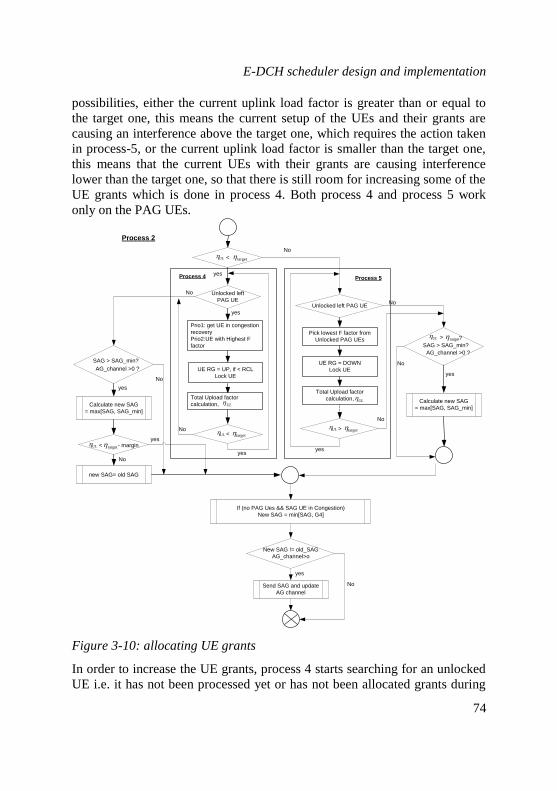
E-DCH scheduler design and implementation
74
possibilities, either the current uplink load factor is greater than or equal to
the target one, this means the current setup of the UEs and their grants are
causing an interference above the target one, which requires the action taken
in process-5, or the current uplink load factor is smaller than the target one,
this means that the current UEs with their grants are causing interference
lower than the target one, so that there is still room for increasing some of the
UE grants which is done in process 4. Both process 4 and process 5 work
only on the PAG UEs.
New SAG != old_SAG
AG_channel>o
No
yes
yes
< targetUL
Unlocked left
PAG UE Unlocked left PAG UE
Pick lowest F factor from
Unlocked PAG UEs
UE RG = DOWN
Lock UE
Total Upload factor
calculation, UL
> targetUL
Prio1: get UE in congestion
recovery
Prio2:UE with Highest F
factor
UE RG = UP, if < RCL
Lock UE
< targetUL
Total Upload factor
calculation, UL
> targetUL
SAG > SAG_min?
?
AG_channel >0 ?
Calculate new SAG
= max[SAG, SAG_min]
SAG > SAG_min?
AG_channel >0 ?
Calculate new SAG
= max[SAG, SAG_min]
new SAG= old SAG
< - margintargetUL
If (no PAG Ues && SAG UE in Congestion)
New SAG = min[SAG, G4]
Send SAG and update
AG channel
No
yes
No
yes
No
No
No
No
yes
yes
No
yesyes
No
Process 5Process 4
Process 2
Figure 3-10: allocating UE grants
In order to increase the UE grants, process 4 starts searching for an unlocked
UE i.e. it has not been processed yet or has not been allocated grants during

E-DCH scheduler design and implementation
75
process 1. The grant allocation for an unlocked user is performed based on
two priorities. First a UE who is in congestion recovery phase requires to
increase the grants, and second a UE with the highest F factor does so. The F
factor is defined as the relation between the RLC buffer occupancy and the
UE data rate. It is a mechanism to offer fairness for the users who have large
buffer occupancies with lowest data rates during previous TTIs.
When a UE is chosen, it is given a RG = “up” to increase its grant by one
step of E-TFCI which provides the transport block size set information [61].
With the new UE grant assignment, the total uplink load factor is calculated
and compared with the target load factor. Each turn, by giving grants for a
new unlocked UE, this recursive procedure of load factor calculation and
comparison is performed until it meets the target load factor requirement
which represents the optimum cell capacity for the current TTI. If there is no
unlocked UE to be given the grants, then the recursive procedure exits
without meeting the requirement of the target load factor. In that case some
part of the left resources can be used to increase the SAG grants of SAG UEs
if only multilevel SAGs are enabled and supported by the scheduler.
The support of multilevel SAG is a configurable parameter for this scheduler.
The remaining portion of the left resources is used to promote the SAG UEs
to the primary mode by allocating the PAG grants. Setting up resource
allocation for the above two categories is dependent on the vender specific
system requirements of the scheduler design. For example, the scheduler
discussed here uses 30% of left resources for the promoting process from
SAG to PAG.
Handling multi level SAG in case of congestion
Handling multi-level SAG in case of transport congestion is shown in process
5 of the flow chart in Figure 3-10. It is similar to the procedure of process 4
but works in the opposite way. The scheduler starts executing this process
when the current total load factor is higher than the target one. In this case, in
order to reduce the total load factor, the scheduler decreases UEs grants by
issuing RG “down” commands for some of the UEs. In this process, the UEs
are prioritised based on the lowest F-factor which is the opposite action to
process 4. It might also be the case when the scheduler exits process 5, and
the total load factor is still above the target value. If the multi level SAG is

E-DCH scheduler design and implementation
76
enabled, the scheduler decreases the SAG by one step to reduce the current
total load factor.
At the end of process 2, the scheduler checks the occurrence of a congestion
indication from SAG UEs. The scheduler also reacts for such indications if
there is no PAG UE in the system. Then new grants for SAG users are
calculated as the minimum value between the current SAG and G4. The latter
is the minimum reference congestion limit (RCL) between all SAG UEs
causing congestion. The RCL value is provided by the transport congestion
control mechanism and is discussed in chapter 4.
Process-3: Handling the promotion of a SAG to a PAG UE
By finishing the process 2 functionality, the scheduler enters the grant
promoting phase, which is represented by process 3 as shown in Figure 3-10.
To promote one of the SAG UEs into the primary mode, there are several
conditions that must be fulfilled as listed below.
At least one AG channel should be available in order to provide the
new grant.
At least one SAG UE should be in the SAG UEs list.
The total number of PAG should not exceed a predefined upper
limit.
The left resources should be sufficient to provide primary grants.
At the promoting process, the load factor is calculated by taking the target
value into consideration. For this calculation, a factor K is defined as the
difference between the maximum possible numbers of PAG UEs and the
currently available number of PAG UEs. Therefore left resources are divided
by this value K in order to provide fair resource allocation when promoting
users. In addition to the fair resource allocation, priorities are also considered
among eligible users based on their current buffer occupancies. This is
maintained by another factor to consider fairness when it comes to delay
constraints. By using the above consideration the first promoting user from
SAG to PAG is selected and granted resources for the primary mode.
After scheduling grants allocation procedures, all SAG and PAG UEs
transmit the data with their allowed grants in this TTI and the scheduler
moves to the next TTI processing. After elapsing the TTI period, the whole

E-DCH scheduler design and implementation
77
scheduling process is again started from the beginning and continued until
end of the simulation.
3.4.2 Modelling HARQ
The modelling approaches of HARQ for HSDPA and HSUPA are similar in
general. However, HARQ mechanism for HSDPA is not modelled within the
system simulator but modelled in the radio simulator. The traces, per-user
data rates (in term of number of MAC-ds) were taken from the radio
simulator after the outcome of the HARQ functionality. Therefore, when
deploying traces for the downlink, effects of HARQ for the transmission over
the radio channel were already considered.
For the uplink scheduler, no traces were used, therefore the HARQ
functionality has to be modelled in the HSUPA network simulator according
to the 3GPP specification [60, 62]. A simplified approach of HARQ
functionality was taken into consideration for this implementation; the main
functional features are listed below.
Each UE has 4 HARQ processes and works based on a stop-and-
wait protocol.
Retransmissions of MAC-e PDU are performed based on the air
interface Block Error Rate (BLER).
The following table shows the selected BLER with the number of
retransmissions. It uses the concept of incremental redundancy and
the following retransmissions have the higher recovery and hence
lower BLER for second and third retransmissions.
Table 3-1: HARQ retransmission probabilities
1st transmission 2
nd transmission 3
rd transmission
BLER 10 % 1 % 0 %
The simplified HARQ procedure can be summarised as follows. When the
MACe packet is transmitted, a copy of the packet is inserted in the HARQ
process. Based on the BLER, for each packet, it is determined whether the
transmission is a successful transmission or an unsuccessful transmission. If
the latter is the case (assuming that a NACK is received), the same packet is
retransmitted after elapsing of an RTT period. If the packet is transmitted

E-DCH scheduler design and implementation
78
successfully (assuming an ACK is received), the packet is removed from the
HARQ process after the RTT period has elapsed. The RTT is set to “n”
number of TTIs. For the current implementation, n is set to 4 based on
allowed vender specific maximum delay limits. When a UE has a scheduling
opportunity, it prioritises retransmissions over new transmissions.
3.4.3 Modelling soft handover
Soft Handover (SHO) has some negative influences on the network
performance. Especially, the influence of SHO on the network performance
and the individual end user performance are significant at overload situations.
SHO leads to additional load inside the transport network. Therefore it causes
blocking of certain parts of the BW for these additional overheads. The
transport congestion control algorithm also has to handle such HO situations
effectively. Therefore within the focus of the TNL feature development in the
network simulator, it is important to consider the effect of the SHO load on
the transport network. This leads to modelling of SHO effects in the uplink
simulator.
For uplink transmission, the E-DCH scheduler has to control the offered load
to the transport network. In a congestion situation, the scheduler should
reduce the offered load to the transport network for some greedy connection
in the uplink. These actions are performed combined with the transport
network congestion control algorithm. Since SHO is causing additional load
over the transport network, the E-DCH scheduler has to manage the uplink
transport resources among user connections during the soft handovers.
However SHO is not critical for the downlink since the Node-B is centrally
managing the resources among connections and the flow control scheme
along with the downlink transport congestion control scheme decides the
offered load to the transport network. An overload situation is completely
controlled by the DL congestion control schemes and further, in this case, the
main buffering for the connections is located at the RNC entity. Therefore,
for transport analysis, DL Soft handover does not play a significant role on
the network and end user performance. Within the discussion of this section
mainly the effect of the soft handover for uplink transmission is modelled.
For uplink transmission, two different SHO cases can be distinguished: the
first case represents the soft handover that some of the Serving Radio Link
Set (S-RLS) UEs are experiencing, in which those UEs will have their
packets carried over the N-SRLS Iub link to the RNC. The second case

E-DCH scheduler design and implementation
79
represents the UEs from the neighbouring cells that are in soft handover with
the current cell which belongs to the considered Node-B. Those UEs are
referred to as N-SRLS UEs, and some of their packets have to be carried by
its Iub link.
Add RLC
headers
RLC segmentation
process
AAL2
ATM
Application
TCP/UDP
IP
Air Interface
PerUE RLC
buffers
MAC-es
buffers
N*MAC-d
MAC-e Txn and
Retxn buffers
High Loss probability
(ex. 40%-60%)
X% traffic
NRLS UEs
AAL2
ATM
FP header
processing
MAC-es
buffers
MAC-es header
processing
PerUE RLC
buffers
Application
TCP/UDP
IP
Iub Link
NSRLS
UEs
FPIub
delay
SHO Ues
Transmitting via the NSRLS
Emulating the delay
between the other
Node-B and RNC
MAC-es
MAC-d
RLC
MAC-e
MAC-e
EDCH-FP
EDCH-FP
MAC-es
MAC-d
RLC
Node-B
UE
RNC
Figure 3-11: architectural overview of UL UE modelling with SHO
functionality
Figure 3-11 shows the architectural overview of the UL UE modelling with
SHO functionality. Further, it is shown that the SHO UE data is transmitted
via neighbouring Iub link and the N-SRLS UE data is transmitted over the

TNL protocol developments
80
considered Iub link. The first case (S-RLS UEs in SHO) is modelled in the
following way:
a) The number of SHO UEs is chosen as a percentage of the total
number of the HSUPA UEs.
b) The SHO UEs are considered to be in handover during the whole
simulation time. This is done in order to emulate the additional load
on the transport network.
When SHO UEs are transmitting a MACe PDU over the air interface, a copy
of the packet is also transmitted via the Iub of the neighbouring cells. Since
these neighbouring cells are not modelled in this simulator however, they are
modelled in following way to counter the impact of the load offered.
A direct link was created in the model that links the HSUPA layer of the
Node-B with the corresponding layer of the RNC. This link is used to
emulate the effects of the N-SRLS Iub links, where the packets are
transmitted over this link directly to the RNC by emulating a certain packet
error rate (for example 40% – 60%) and a certain delay variation (for
example, 10 ms – 40 ms). Therefore SHO UEs get the duplicate arrivals at
RNC and they are filtered at the MAC-es layer in RNC.
The N-SRLS UEs that are in soft handover with the cell in consideration are
modelled in the simulator as well. Since the N-SRLS UEs are not the main
concern of this analysis, and also the per-UE evaluation is not intended for
them there is no need of modelling the full protocol architecture for those N-
SRLS UEs to generate their traffic, instead a simplified approach is used to
generate the traffic for those UEs according to the following guide lines. The
N-SRLS UEs are needed to block some of the Iub link capacity with their
traffic to have the realistic scenarios for the simulations, so those UEs should
only generate MACe PDUs to be carried over the Iub (after being
encapsulated as FP PDUs) and then discarded on the RNC when they are
received.
3.5 TNL protocol developments
The network between the RNC and the Node-B is considered as the transport
network and also the Iub interface for the UMTS based UTRAN network. As

TNL protocol developments
81
mentioned in chapter 2.3, it has been initially designed with a high speed
ATM based transport network later using other technologies such as IP over
DSL based transport. Supporting QoS guarantees for different services at
minimum cost over the transport network is the main challenge for many
broadband wireless network operators. With the development of high speed
core network technologies in recent years, the delay over the transport
network significantly reduced and created many opportunities to use packet
based transport networks with service differentiation in order to meet the end
user service guarantees.
In the focus of HSPA traffic (HSDPA and HSUPA best effort services) the
end user and network performance are investigated using ATM based and
DSL based transport network technologies. These two transport technologies
are modelled in the HSPA network simulator for the uplink and the
downlink. Next, details about the implementation of these two transport
technologies are presented separately.
3.5.1 ATM based transport network
Rel’99 UMTS based real time traffic requires strict delay requirements
whereas the HSPA based best effort traffic is more concerned on data
integrity in comparison to strict delay constraints. ATM is one of the key
technologies which uses the cell based packet transmission in high speed
wired network to guarantee the required QoS for different services. Since the
cells are relatively small, this leads to a significantly higher overhead
compared to the IP based data transmission. This effect is significant for the
transmission of the best effort traffic over the wired network compared to the
real time traffic which has often small packets in nature. For example Rel’99
UMTS traffic, mainly the voice traffic has small data packets which can be
effectively multiplexed within a cell and can achieve the best network
performance due to a very high statistical multiplexing gain.
3.5.1.1 ATM traffic separation
ATM traffic separation is the key technique which is achieved through virtual
paths (VPs) and Virtual Circuits (VCs). When cells are transmitted over the
ATM network, connections and routing are set up based on virtual path
identifiers (VPIs) and virtual channel identifiers (VCIs). Several traffic
separation approaches have been investigated for the traffic over the transport

TNL protocol developments
82
network in order to investigate end user performance by evaluating packet
loss ratio, delay, delay variation and throughputs [14]. Selecting a proper
traffic separation is completely vendor specific and can be chosen based on
service requirements. For the HSPA simulation analysis, a 3 VP based traffic
separation approach is deployed and the basic architecture is shown in the
following figure.
Figure 3-12: 3VP based traffic separation approach
The three VPs are used for the traffic separation based on their QoS
requirements. VP1 is based on the CBR category which carries the Rel’99
UMTS based traffic, VP2 is based on UBR+ which carries the HSDPA best
effort traffic and VP3 is also based on UBR+ which carries the HSUPA best
effort traffic. Mostly Rel’99 real time services are symmetric services which
require equal capacity in both directions with strict delay requirements.
Therefore such services are mapped into the CBR VP with a guaranteed peak
cell rate. In contrast to that, best effort services are asymmetric services
which have a high demand in one direction in comparison to the other
direction. For example, HSDPA mainly uses the downlink to transmit data
and therefore requires a higher BW in the downlink compared to the uplink.
The latter is mostly used to transmit the signalling information which is
required by the downlink data flow. However, it is necessary to allocate a
certain minimum guarantee for these signalling messages (mainly for in-band

TNL protocol developments
83
signalling). Therefore, the VPs which are assigned for HSDPA and HSUPA
services are deployed using the UBR+ ATM service category.
3.5.1.2 AAL2 buffer management
AAL2 is used as the layer 2 adaptation layer for both Rel’99 and HSPA
traffic services. The RNC side of the Iub interface consists of an RNC ATM
switch which connects the Rel’99 traffic flows to the ATM multiplexer. The
task of this intermediate MUX is to combine CBR and UBR PVCs at the
RNC side of the transport network. This ATM MUX is designed together
with a WRR (Weighted Round Robin) scheduler that guarantees specific
service rates with the appropriate traffic configuration parameters.
AAL2 uses class based limited buffers to store the data. These buffers are
implemented in the RNC and Node-B for the downlink and the uplink
respectively. The AAL2 buffers are limited by the maximum delay limit
which is a configurable value for the HSPA network simulator. For example,
the maximum buffering delay can be set to 50 milliseconds and therefore all
packets exceeding this maximum delay limit are discarded at the AAL2
buffers. In order to implement the simulation efficiently, a timer based
discarding procedure with a packet trigger is applied. That means, whenever
a packet is taken out from the AAL2 buffer for transmission, the packet
waiting time is measured. If the packet waiting time is lower than the
configured delay limit, the packet is sent. Otherwise the packet is discarded
and the next packet is checked from the buffer. This procedure applies until
the transmission trigger gets a valid packet to be transmitted over the
transport network. This simplified discarding approach is efficient for
simulations since it uses a transmission trigger to identify the delayed packets
in the AAL2 buffer and also to send packets to the lower layer without
having any additional frequent event triggers.
3.5.2 DSL based transport network
Digital Subscriber Line (DSL) technology is widely deployed for fast data
transmission for industry, business and home usage. The great advantage of
DSL is that it can use the existing telephone network by utilising left
frequencies above the voice telephony spectrum. This technology is one of
the cheapest ways for fast data transmission which can be effectively
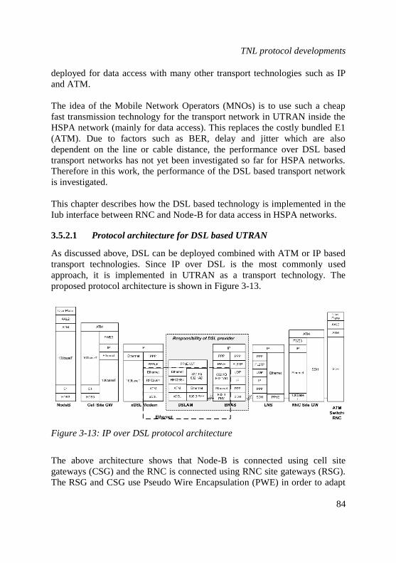
TNL protocol developments
84
deployed for data access with many other transport technologies such as IP
and ATM.
The idea of the Mobile Network Operators (MNOs) is to use such a cheap
fast transmission technology for the transport network in UTRAN inside the
HSPA network (mainly for data access). This replaces the costly bundled E1
(ATM). Due to factors such as BER, delay and jitter which are also
dependent on the line or cable distance, the performance over DSL based
transport networks has not yet been investigated so far for HSPA networks.
Therefore in this work, the performance of the DSL based transport network
is investigated.
This chapter describes how the DSL based technology is implemented in the
Iub interface between RNC and Node-B for data access in HSPA networks.
3.5.2.1 Protocol architecture for DSL based UTRAN
As discussed above, DSL can be deployed combined with ATM or IP based
transport technologies. Since IP over DSL is the most commonly used
approach, it is implemented in UTRAN as a transport technology. The
proposed protocol architecture is shown in Figure 3-13.
Figure 3-13: IP over DSL protocol architecture
The above architecture shows that Node-B is connected using cell site
gateways (CSG) and the RNC is connected using RNC site gateways (RSG).
The RSG and CSG use Pseudo Wire Encapsulation (PWE) in order to adapt

TNL protocol developments
85
the ATM layer to the IP layer. The DSL line is connected in between the
xDSL modem and the Broadband Remote Access Server (BRAS). The traffic
aggregation occurs at BRAS which connects the broadband network to the
access network and vice versa. Further it performs the Point-to-Point
Protocol (PPP) termination and tunnelling. The Layer 2 Tunnelling Protocol
(L2TP) network server (LNS) which is located between BRAS and RSG
provides the layer 2 tunnelling.
The protocol architecture described above is implemented in the HSPA
simulator while keeping the existing ATM based transport technology. The
basic structure for all network entities is shown in Figure 3-14.
Figure 3-14: Overview HSDPA simulator with DSL based transport
It is shown that the new IP over DSL based transport network is implemented
between Node-B and RNC in the HSPA simulator in parallel to the native
ATM based transport. The model is designed in such a way that both
transport technologies can be deployed independently. Figure 3-14 shows
that the DSL based transport network is added between the RNC switch and

TNL protocol developments
86
NodeB_UL_Mux. The RNC Site Gateway (RSG) is connected to the RNC
via a switch. The LNS and BRAS are network entities in the service provider
network and the DSL modem and BRAS are directly connected. Further,
DSLAM is included within the DSL network and the Cell Site Gateway is
connected to the Node-B via NodeB_UL_Mux. In the model, the RNC
switch and the NodeB_UL_Mux are the switchable devices which can turn
ON and OFF DSL based UTRAN based on the usage of ATM based
technology.
The DSL protocol functionality is emulated between the xDSL modem and
the BRAS by deploying a trace file which was taken from the field test. The
trace file is applied at Ethernet packet level; it includes all behavioural
aspects such as BER, delay and jitter of the DSL line including the DSLAM
functionality. The main functionality of RSG and CSG is connecting two
different transport technologies using the Pseudo Wire Emulation (PWE).
The details about the generic network entities such as LNS, BRAS and DSL
modem can be found in the respective product specifications, therefore
further details will not be discussed here. This section focuses on more
details about the implementation of DSL based UTRAN in the HSPA
simulator.
3.5.2.2 CSG and RSG protocol implementation
The CSG and the RSG gateways are connected to Node-B and RNC
respectively through the E1 based ATM links. To connect the ATM based
network to the IP based Packet Switch Network (PSN), the Pseudo Wire
Emulation Edge-to-Edge (PWE3) technology is proposed by the Internet
Engineering Task Force (IETF). In this implementation, PWE3 is used to
couple the two transport technologies, ATM and Ethernet via an IP
backbone. The peer-to-peer protocols for the CSG and the RSG are shown in
the Figure 3-15.
IP is the base media in between the two main transport technologies
mentioned above. Both sides use a 100BaseT Ethernet link to connect to the
other entities in the DSL network.
The basic PWE3 technology is described by the IETF standards. This
protocol is implemented in the CSG and the RSG entities. The OPNET
simulator uses the same node model for both entities and the required

TNL protocol developments
87
protocol functionalities are added into the process model of each node model.
The node model is shown in Figure 3-16.
IP
Ethernet
100BaseT
PWE3
ATM
IP
Ethernet
100BaseT
PWE3
ATM
RSG CSG
Node B
side
RNC
side
Figure 3-15: Peer-to-peer protocols in CSG and RSG
The node model mainly consists of ATM, PWE IP and MAC (Ethernet)
protocols. The IP and MAC protocols are used as transport for the PWE3
encapsulation. ATM is the base transport technology that is used by the
UMTS/HSPA networks.
Figure 3-16: PWE, IP and MAC protocols in CSG and RSG
The above node model shows the main protocol entities with their respective
functionalities. When packets are received by the ATM protocol then they are

TNL protocol developments
88
delivered to the PWE process model where all PWE protocol functionality is
implemented. The PWE process model is shown in Figure 3-17.
Figure 3-17: PWE protocol process model
The PWE packet is sent to the IP protocol which consists of two process
models: the IP routing process model and the IP encapsulation process
model. After adding all functionalities (IP transport information) to the PWE
packets at IP level, the IP PDU is sent to the Ethernet protocol layer which
consists of ARP and MAC protocol processes. By adding all header
information into IP packets, the Ethernet frames are generated by the MAC
protocol process and then the packet is sent to the output port for delivery.
3.5.2.3 LNS, BRAS and xDSL modem implementation
The connections among LNS, BRAS and the xDSL modem are shown in
Figure 3-18. The effect of the DSL link is modelled between BRAS and
xDSL modem by deploying a real trace file as it was discussed in the
previous chapter. In the OPNET simulator, all three network nodes use a
single advanced node model which is shown in the following figure. All
protocol functionalities such as PPP, PPPoE, L2TP, UDP, etc. are
implemented between the IP and MAC protocol nodes in the advanced node

TNL protocol developments
89
model. The standard main IP process model is modified and a child process
which performs most of the protocol activities when the connection is
activated between respective nodes is added. The newly created child process
model along with all states is shown in Figure 3-19.
Figure 3-18: An advanced node model for LNS, BRAS and xDSL_modem
The protocol descriptions are coded inside the states of the child process. The
upper and lower states in the process model describe the packet arrival and
departure processes respectively, whereas the middle states describe the
processing and routing functionalities for the network entities. All other
protocols are coded inside each state appropriately. More details about the
protocols and their specifications are listed in Figure 3-20.
The PPP protocol uses two specification formats. When PPP is used over a
direct link, it uses a format according to the IETF RFC 1662 [69] which
specifies additional fields such as address, control, and flags etc., compared
to the PPP protocol specified in the specification IETF RFC 1661 [68].

TNL protocol developments
90
The L2TP protocol is implemented in the simulation model according to the
IETF RFC 2661. This protocol runs over UDP; the OPNET default
implementation is deployed in the simulator. However, the newest version of
L2TP call L2TPv3, defined by the IETF RFC 3931 [70] includes additional
safety features compared to the current RFC 2661 [71].
Figure 3-19: Process model for PPP, PPPoE, L2TP and UDP
The protocols which are newly implemented between BRAS and the xDSL
modem are listed in Figure 3-19. They are mainly PPP, PPPoE and the MAC
protocols. As in the previous implementation, IP and MAC use the default
OPNET implementation and rest is implemented according to the
specification given Figure 3-20.

TNL protocol developments
91
Figure 3-20: PPP, PPPoE, L2TP and UDP protocols specifications
The PPP is implemented according to the IETF RFC 1661 [71] which was
discussed in the previous section. The PPPoE protocol is implemented
according to the IETF RFC 2516 [72]. The header which causes an overhead
of 6 bytes includes version/type, code, session_id and length fields.
Figure 3-21: added protocols between BRAS and xDSL model

TNL protocol developments
92
3.5.2.4 DSL trace deployment
As discussed in the beginning of this report, the DSL line of the HSPA
simulator is emulated using a real trace file taken at the Ethernet layer which
records the absolute value and the variation of the delay for each packet
arriving at the receiver. It also includes the details about lost packets. The
real traces are often short in length. Therefore, in order to use these traces in
the network simulator, the raw data of approx. 100 traces are analysed and
the probability distribution (CDF) is created. The delay and delay variation
characteristics over the DSL line are simulated according to the derived real
distribution.
To include bit errors for the DSL transmission, the following approach is
deployed. In general, for the DSL network, bit errors can be experienced in
two forms, random bit errors and bursty bit errors. The burst errors which
cannot be eliminated even with interleaving are due to impulse noise and
impairments of neighbouring CPEs. Therefore these packet errors should be
included within the model of the DSL line along with the delay and the delay
variation distributions. To perform this, the following simple approach is
used to emulate the packet errors in the system level simulator which
provides sufficient accuracy for the end user performance analysis.
The main assumption of this method is that the total number of lost packets
(or burst of lost packet events) is uniformly distributed over the given length
of the trace file. First, all numbers of bit errors which create a corrupted
packet and bursty errors which cause the loss of more than one packet are
extracted from trace files based on their lengths. Then from these extracted
details, the average packet and burst error rates are calculated. According to
these average error rates, the packets are discarded when sending data over
the DSL network. At the end, RLC or TCP has to recover those lost packets
by resending them over the network. In order to analyse the end user
performance, the average packet and burst loss rates are important and also
provide sufficient accuracy for HSDPA and HSUPA networks.
3.5.3 ATM and DSL based transport deployment
In the focus of this thesis, mainly ATM and DSL based transport
technologies have been implemented, tested and validated in the HSPA
simulator in order to analyse the end user performance. Since ATM is the

Radio link control protocol
93
most widely used transport technology, all TNL flow control and the
congestion control analyses which are described in chapter 5 and chapter 6
are performed using the ATM transport technology in the HSPA simulator.
The DSL based HSPA analysis shows a similar performance to ATM based
analyses. Therefore some of the analyses are given in appendix A which
mainly summarises the impact of the DSL transport technology on the HSPA
end user performance.
3.6 Radio link control protocol
The radio link control (RLC) protocol is implemented between RNC and UE
entities in the UTRAN. The Acknowledge Mode (AM) RLC protocol
provides a reliable data transmission in the HSPA network for the best effort
traffic. The packet losses over the Uu and the Iub interface need to be
recovered using the RLC protocol and that avoids long retransmission delays
by TCP which is located at the end entities. In this way, a minimum loss rate
for the best effort traffic in the UTRAN network can be guaranteed and the
required number of TCP retransmissions by the end entities is also
minimised. Any retransmissions at TCP level do not only cause additional
delay but also consume additional network resources. Further, by hiding
packet losses at the UTRAN network, TCP can provide effective flow control
between end nodes to maximise the throughput and optimise the network
utilisation. In short, having RLC AM mode for best effort traffic within the
UTRAN enhances the overall end-to-end performance. The following section
briefly describes the RLC protocol implementation within the HSPA network
simulator.
3.6.1 Overview of RLC protocol
The RLC protocol does not only provide the AM mode operation but also
two other modes: Transparent Mode (TM) and Unacknowledged Mode
(UM). In TM mode, data will be sent to the lower layer without adding any
header information. In UM mode, data will be sent to the lower layer with the
header information, however similar to UDP, there is no recovery scheme.
Hence it is recommended to use this mode of operation for most of the real
time services which do not require strict constraints for the loss but which
have critical limits for the delay. In AM mode, as described above, the RLC
protocol works like TCP. In this mode of operation, a reliable data

Radio link control protocol
94
transmission is guaranteed between peer RLC entities by using an ARQ
based recovery scheme. Further details about the RLC protocol are given in
the 3GPP specification [22].
The RLC protocol is implemented in the HSPA network simulator. The main
focus of this implementation is to protect the overall HSPA performance
from few packet losses occurred at the transport network for the best effort
traffic. Packet losses occur either due to unreliable wireless channels or
congestion caused by the transport network and they can be recovered by the
RLC protocol without affecting the upper layer protocols such as TCP. The
summary of the implemented protocol functionalities within the HSPA
simulator is described in the next sections.
3.6.2 RLC AM mode implementation in HSPA simulator
To achieve the objectives described above, some of the RLC AM
functionalities specified in 3GPP [22] are implemented in the HSPA
simulator. The implemented functionalities are marked with () whereas
others are marked with () in the list given below. The RLC AM mode is
applied to each user flow separately between RNC and UE.
Segmentation and reassembly: function performs segmentation and
reassembly of variable-length upper layer PDUs into/from RLC PDUs.
Concatenation: if the contents of an RLC SDU cannot be carried by one
RLC PDU, the first segment of the next RLC SDU may be put into the
RLC PDU in concatenation with the last segment of the previous RLC
SDU. A PDU containing the last segment of a RLC SDU will be padded.
The effectiveness of this functionality is not significant for a network
which uses a large packet sizes such as best effort IP packets. Therefore,
this function is not necessary for the HSPA model.
Padding: If concatenation is not applicable and the remaining data to be
transmitted does not fill an entire RLC PDU of given size, the remainder
of the data field shall be filled with padding bits.
Transfer of user data: this function is used for conveyance of data
between users of RLC services.
Radio link control protocol
95
Error correction: function provides error correction by retransmission
(e.g. Selective Repeat) in acknowledged data transfer mode.
In-sequence delivery of upper layer PDUs and duplicate detection:
the data will be sent between peer RLC entities in a sequential order. The
function detects any arrival of duplicated RLC PDUs and ensures in-
sequence delivery to the upper layer.
Flow control: this function allows an RLC receiver to control the rate at
which the peer RLC transmitting entity may send.
Sequence number check: this function is used in acknowledged mode.
It guarantees the integrity of reassembled PDUs and provides a
mechanism for the detection of corrupted RLC SDUs through checking
the sequence number in RLC PDUs when they are reassembled into a
RLC SDU. A corrupted RLC SDU will be discarded.
Protocol error detection and recovery: this function detects and
recovers errors in the AM operation of the RLC protocol.
Ciphering: this function prevents unauthorised acquisition of data.
Ciphering is performed in the RLC layer when the non-transparent RLC
mode is used. In this simulation, ciphering is not used because the model
is implemented in order to evaluate the RLC performance for the data
traffic without considering the security aspects.
According to the RLC functionalities specified above, both RLC transmitter
and the receiver entities are implemented in the UE and RNC nodes in the
uplink and the downlink.


CHAPTER 4
4 HSDPA flow control and congestion control
The flow control and congestion control are the key TNL features which
have been developed to enhance the overall end-to-end performance for the
downlink of the HSPA network. The motivation and theoretical aspects of
flow control are described in this section. A new adaptive credit-based flow
control algorithm is introduced for HSDPA. This enhanced flow control
scheme has been implemented, tested and validated using the HSPA
simulator. Comprehensive simulation results of the flow control are
presented here. Since the flow control scheme itself cannot avoid congestion
in the transport network, a new congestion control concept has been
introduced combined with the adaptive flow control scheme. First the
concept of congestion control is described in detail and next different variants
of congestion control algorithms are presented which have been
implemented, tested and validated within the HSPA simulator for the
downlink. Finally a comprehensive simulation investigation and analysis has
been performed in order to analyse the end user performance. These two
congestion and flow control algorithms address and overcome the two
separate issues in the transport network by significantly improving the end-
to-end performance. Further these schemes optimise the usage of transport
network resources for the HSDPA network while providing aforementioned
achievements.
HSUPA also uses the same congestion control scheme as HSDPA. There is
no requirement of implementing a flow control scheme since the Node-B
scheduler has full control over the transport and radio resources, and further
there is no bottleneck behind the RNC in the uplink direction. However a
congestion control scheme is required to avoid congestion at the transport
level and to optimise the radio resource utilisation. The congestion control
input is taken into account in the implementation of the uplink scheduler as
described in chapter 3.4.

HSDPA TNL flow control
98
4.1 HSDPA TNL flow control
Due to the bursty nature of the (HSDPA) packet-switched traffic, the accurate
dimensioning of the TNL bandwidth is a difficult task. The mobile network
Operators (MNOs) are facing many challenges to optimise the performance
of the TNL network to achieve best end user performance at minimum cost.
Reducing the burstiness of the traffic over the TNL network and handling
adequate buffer requirements at the Node-B buffers can optimise the capacity
requirement at the Iub interface [1, 2, 3, 4, 32, 33]. When compared to
Rel’99, HSDPA uses two buffering points at the Node-B and at the RNC. To
optimise the transport capacity, the data flow over the Iub interface should be
handled effectively to cope with varying capacities at the air interface [1, 24].
Thus, adequate queuing in the Node-B buffers is required. Due to large
fluctuations of the time varying channel at the air interface, the Node-B
buffers are frequently empty if less buffer capacity is used and such
situations can cause wastage of the scarce radio resource [24, 25, 32]. On the
other hand, large buffer levels at the Node-B can result in large delays and
also a large capacity requirement at the Node-B [26]. Further, a large amount
of data buffering at Node-B leads to high packet losses during handovers
resulting in poor mobility performance as well [24, 26, 27, 28]. Therefore
this is a clear trade-off which has to be handled carefully for the optimum
network and the end user performance. As a solution to this issue, some of
the literature discusses the need of flow control techniques [24, 25, 27, 29,
34] that closely monitors the time varying radio channel demands and
estimates Node-B buffer requirements in advance for each connection.
However, the data flow handling over the transport network should be
performed adaptively along with a feedback channel between RNC and
Node-B. Therefore, an intelligent credit-based flow control mechanism has
been introduced in this thesis which addresses all above requirements to
achieve the best end-to-end performance at minimum cost while providing
optimum network utilisation.
The credit-based flow control scheme operates on a per flow basis and adapts
the transport network flow rate to the time varying radio channel capacity.
The estimated capacity requirements feedback to the RNC through the in-
band signalling channels in an effective manner to minimised the signalling
overhead over the uplink. The mechanism is further optimised to reduce the
burstiness over the transport network that efficiently utilise the transport

HSDPA TNL flow control
99
network providing minimum cost for the usage of network resources. By
deploying different HSDPA traffic models, the overall network and end-to-
end performance are analysed using the HSDPA simulator which is discussed
in chapter 3. During these analyses and investigations, the performance of the
developed credit-based flow control schemes is compared with the generic
flow control scheme.
All the aforementioned aspects are described in this chapter in detail and the
chapter is organised as follows. First, the generic flow control schemes
(ON/OFF) and the adaptive credit-based scheme are discussed in detail and
next, the performances of the two algorithms are presented and analysed
using the HSDPA network simulator. Finally, the conclusion is provided by
summarizing the achievements at the end of the chapter.
4.1.1 HSDPA ON/OFF flow control
The ON/OFF flow control mechanism is considered to be the most simple
mechanism which can be applied for the purpose of flow control for HSDPA
traffic on the Iub link. The flow control mechanism monitors the filling levels
of the MAC-hs buffers for each user flow. It uses an upper and a lower
threshold to control the MAC-d flow rate over the Iub. The MAC-hs buffer
with the two thresholds is shown in Figure 4-1.
Figure 4-1: MAC buffer per flow basis
It is assumed that the incoming data rate to the MAC-hs buffer is λS (source
rate) and the outgoing flow rate from the MAC-hs buffer is λD (drain rate).

HSDPA TNL flow control
100
The upper and lower buffer limits are determined by an approximated value
of the round trip time (RTT) between Node-B and RNC and by the
Source/Drain rate as shown in equation 4-1.
RTTth
i
RTTith
DLower
SUpper
10 ...., 4, 3, where
1
equation 4-1
The per-user ON/OFF flow control mechanism assigns credits to each
individual user in the Node-B based on the maximum achievable data rate
over the air interface. If the upper limit of the buffer is exceeded, the data
flow over the Iub link is stopped and if the buffer limit reaches the lower
limit, data is transmitted over the Iub. This ON/OFF flow control mechanism
protects the MAC-hs buffers from overflowing as well as emptying.
However, when the incoming traffic has bursty nature, the delay variation
significantly fluctuates from a lower to a higher value and vice versa. For
such situations, the ON/OFF flow control mechanism turns out to be unstable
[3], hence it becomes difficult to meet the requirements at the radio interface.
On the other hand the ON/OFF flow control mechanism increases the
burstiness of the traffic rather than mitigating it [4].
4.1.2 HSDPA adaptive credit-based flow control
The adaptive credit-based flow control mechanism is developed to optimise
the Iub utilisation while providing required QoS to the end user in the
HSDPA network. It smoothes down the HSDPA traffic and reduces the
burstiness over the Iub interface. This flow control mechanism introduces
two new aspects with respect to the ON/OFF flow control algorithm. First,
the frame protocol capacity allocation message is sent periodically from the
Node-B to the RNC. Second, the credit allocation algorithm is based on the
provided bit rate (PBR) of the per-user queues in the Node-B. Since the
credits are sending periodically, the PBR is also calculated at the same
frequency which is called cycle time or cycle period.

HSDPA TNL flow control
101
Figure 4-2: PBR calculation procedure
The HS-DSCH Provided Bit Rate (PBR) measurement is defined as follows
in the 3GPP specification [22]: “For each priority class the MAC-hs entity
measures the total number of MAC-d PDU bits whose transmission over the
radio interface has been considered successful by MAC-hs in Node-B during
the last measurement period (cycle time), divided by the duration of the
measurement period ”. Figure 4-2 shows the calculation of the PBR based
credit allocation which is sent periodically after the cycle time. The PBR
calculation is done at time t for the next allocation message sent after one
cycle time considering the current and the previous successful transmissions.
PBR(t) is the average number of MAC-d PDUs for each priority successfully
sent over the air interface during a cycle time. Then, the average PBR rate,
)(PBR t is calculated using the following formula with w being the weighting
factor (for example default w = 0.7).
)(PBR)1()1(PBR)(PBR twtwt equation 4-2
The filling level of the Node-B priority queue is calculated using the
measured MAC-hs queue size qs(t) and the calculated PBR average
according to the given formula below.
)ms(
)(PBR
)(_
t
qs(t)tflevelFilling equation 4-3

HSDPA TNL flow control
102
Figure 4-2 shows the overview of the buffer management for the credit-based
flow control scheme. As in the ON/OFF flow control mechanism, there is an
upper and a lower threshold that are maintained to control the flow over the
Iub interface. Both the upper and the lower buffer limits are set according to
the estimated value of the RTT. The credits to be sent over the Iub interface
are calculated by using the MAC-hs filling levels and the upper/lower limit
of the Node-B user priority queues. With the employment of the upper and
lower queue thresholds, the filling level can be in three regions: less than the
lower limit, higher than the upper limit or between these two thresholds. The
number of credits allocated to the RNC for data transfer is calculated
according to the three active regions of the MAC-hs buffer fillings and is
given by the following three cases.
Case 1:
If then Credits = (MAC-d/TTI) equation 4-4
Case 2:
If then Credits = (MAC-d/TTI) equation 4-5
Where the factor is a value between 0 and 2 which changes based on the
variation of the filling level in MAC-hs buffer
Case 3:
If , then Credits = 0 (MAC-d/TTI) equation 4-6
The initial credit/interval calculation is performed using the Channel Quality
Indicator (CQI) and is sent to the RNC as a Capacity Allocation (CA)
message to regulate the data transfer over the Iub interface.
So the number of MAC-d PDUs transferred to each Node-B priority queue
can be regulated in periodic instants of the cycle time according to their
individual buffer occupancy levels. A user queue with less priority or a user
with bad radio channel quality gets no MAC-d PDUs from the RNC, which
otherwise would have been an unnecessary usage of the precious Iub
bandwidth.

HSDPA TNL flow control
103
Figure 4-3: Credit-based buffer management technique
The credit-based flow control mechanism is implemented at FP and MAC-hs
layers in the HSPA network simulator. Since flow control is only applied for
the downlink data flow which can be centrally controlled by the node-B, the
credit-based and generic ON/OFF flow mechanisms are implemented to
control the downlink user flows. The credit-based buffer management is
implemented in Node-B and the traffic regulation is implemented in the RNC
layer. The FP is the main protocol which handles all flow control related
functionalities.
The basic functional diagram of downlink flow control is shown in Figure
4-4. The flow data rate is determined using the calculated PBR and the filling
level of the MAC-hs buffer in the Node-B. The credits/interval information
or capacity allocations which are calculated according to the flow data rate at
the Uu interface are sent to the RNC to calculate the frame size and the frame
interval. The Node-B sends these HS-DSCH credits allocation messages
periodically to the RNC in order to regulate the downlink data flow to the
transport network. According to the allocated credits, the FP PDU is formed
and sent to the Node-B by the RNC. All this flow control is performed on a
per user flow basis separately and independently.

HSDPA TNL flow control
104
Figure 4-4: Credit-based flow control scheme functional overview
4.1.3 Traffic models and simulation configurations
The most common type of HSDPA packet traffic consists of web and FTP
traffic using TCP (Transmission Control Protocol) as a reliable end-to-end
transport layer protocol. The web traffic model, defined by the ETSI
standards [1, 19], is selected to evaluate the performance of HSDPA traffic
under moderate network load. The FTP traffic model is the worst case traffic
scenario. It is used to overload the network in order to analyse the impact of
the flow control features on the end user performance as well as the overall
network performance. Under this traffic configuration, all users in the cell are
downloading a large file and utilizing the network resources up to the
maximum available capacity.
The parameters of the web traffic model defined by ETSI and the FTP traffic
models [19, 22] are given in Table 4-1. These traffic models are configured
and deployed at the application layer of the end user entity so that all the
other protocol effects can be included into the overall analysis. Especially,
RLC and TCP protocols effects are investigated.
The simulation scenarios are defined based on two main analyses to
investigate the effect of the adaptive flow control algorithms on the
performance of HSDPA network. Further investigations are performed to

HSDPA TNL flow control
105
find the bandwidth recommendations for the Iub interface for these two
different flow control schemes. Simulation analyses provide detailed results
to elaborate the effect of the adaptive flow control algorithm in comparison
to the ON/OFF flow control algorithm.
Table 4-1: Traffic models
ETSI traffic model parameters
Parameters Distribution and values
Packet Call Interarrival Time Geometric distribution
μIAT = 5 seconds
Packet Call Size Pareto Distribution
Parameters:
α=1.1, k=4.5 Kbytes, m=2 Mbytes
μMPS = 25 Kbytes
Packet sizes within a Packet Call Constant (MTU size)
Constant (1500 bytes)
Number of packets in a packet call Based on packet call size and the packet
MTU
FTP traffic model parameters
File Size Constant Distribution
μMFS = 12 Mbytes
(No reference, Only for testing purpose)
As shown in Table 4-2, the simulation analysis 1 is performed based on the
FTP traffic model whereas the simulation analysis 2 is done based on the
ETSI traffic model which offers a moderate load compared the FTP traffic
model.
Table 4-2: Simulation configuration
Simulation Analysis
Analysis Simulation Configuration TNL flow control
Simulation Analysis -1
(using FTP)
Configuration-1 ON/OFF FC
Configuration-2 Credit-based FC
Simulation Analysis -2
(using ETSI)
Configuration-3 ON/OFF FC
Configuration-4 Credit-based FC
Each simulation analysis consists of two simulation configurations which are
defined according to the selected flow control algorithm, either credit-based

HSDPA TNL flow control
106
FC or ON/OFF FC. The simulation analysis 1 is used to study the effect of
the two flow control mechanisms under the worst network load situation and
whereas simulation, analysis-2 analyses the above-mentioned effect under
moderate HSDPA network load which is normally bursty in nature. For TCP,
the widely used NewReno flavour is configured and the RLC protocol is set
to run in acknowledge mode with its default settings in the HSDPA network
simulator. Each cell is configured with 20 users being active in the cell until
the end of the simulation time. The simulation model time is 2000 seconds
which is sufficient to achieve steady state results for the analysis.
4.1.4 Simulation analysis-1: FTP traffic
As mentioned above, the HSDPA network simulator is configured with a
very high offered load for this analysis. All users are downloading very large
files simultaneously in the system utilising full radio and network resources.
Under these conditions, the effect of different flow control schemes is
analysed for the network and end user performance. The Iub ATM link,
between RNC and Node-B is configured with 4 Mbit/s bandwidth. Only one
cell in the Node-B is configured with 20 UEs performing FTP downloads.
The simulation results are analysed from system level to application level.
4.1.4.1 ATM link throughput
The downlink ATM throughput between RNC and Node-B is shown in
Figure 4-5. The actual variations of the link throughput for both FC schemes
are elaborated along with model time. Figure 4-5 depicts that the ON/OFF
flow control shows a very high burstiness over the transport network whereas
the adaptive credit-based flow scheme yields a low burstiness over the
transport link. The adaptive credit-based flow control scheme effectively
mitigates the burstiness over the transport network compared to the ON/OFF
flow control scheme. This effect can be further seen from Figure 4-6 which
shows the cumulative distribution of the ATM link throughput.
The high burstiness leads to a high congestion probability at bandwidth
limited networks. Further it requires high bandwidth and large buffers in the
TNL network in order to meet the end user QoS.

HSDPA TNL flow control
107
Figure 4-5: Iub ATM link throughput, between RNC and Node-B
Figure 4-6: CDF of ATM link throughput between RNC and Node-B

HSDPA TNL flow control
108
By introducing the adaptive credit-based flow control algorithm, required
BW can be even reduced less than 3Mbit/sec without any packet losses at the
transport network compared to ON/OFF flow control. Therefore, the
adaptive-credit based flow control mechanism can significantly increases the
efficient use of network resources by reducing the cost for the operator.
4.1.4.2 TNL delay performance
The cumulative distribution of the end-to-end delay of the FP PDUs between
RNC and Node-B for the downlink is shown in Figure 4-7. This statistic is
measured from the point of time when an FP PDU is sent from the FP layer
in the RNC to the point of time when it is received by the FP layer in the
Node-B for the downlink data flow.
Figure 4-7: CDF of FP end-to-end delay
Figure 4-7 shows that adaptive credit-based flow control scheme provides a
significantly lower FP end-to-end delay compared to ON/OFF flow control.
Further the delay variation of the FP PDUs between RNC and Node-B is
greatly reduced by providing excellent application performance.

HSDPA TNL flow control
109
4.1.4.3 MAC-d end-to-end delay
Figure 4-8 shows the cumulative distribution of the MAC-d end-to-end delay
for the adaptive credit-based and the ON/OFF flow control schemes. The
credit-based flow control shows significantly lower MAC-d delay compared
to the latter. The ON/OFF flow control mechanism has a very high buffer
occupancy at the MAC-hs and ATM buffers which is due to high bursts at
the TNL network. All these facts lead to a very high MAC-d end-to-end
delay which includes all intermediate buffering delays as well. The credit-
based flow mechanism has very efficient buffer management mechanism. It
allows sending data from RNC based on the demand of the available channel
capacity. Hence the MAC-d end-to-end delay is significantly reduced.
Figure 4-8: CDF of MAC-d end-to-end delay
4.1.4.4 End-to-end performance
The overall IP throughput is shown in Figure 4-9. It is measured between end
user entities and averaged over all users. It reflects the overall end-to-end
performance of the UTRAN.

HSDPA TNL flow control
110
Figure 4-9: overall IP throughput
The above figure shows that the achieved IP throughputs for both flow
control mechanisms are similar and even slightly higher for the adaptive
credit-based flow mechanism. That means both configurations achieve the
same end user performance for different TNL conditions. Due to the reduced
burstiness at the transport network, Figure 4-5 and Figure 4-6 show that the
TNL bandwidth can be significantly reduced when applying the adaptive
credit-based flow control mechanism compared to ON/OFF flow mechanism
while achieving same end user performance which is shown in Figure 4-9.
4.1.5 Simulation analysis 2: ETSI traffic
This section presents simulation results for the simulation analysis 2 which
deploys the moderate ETSI traffic model. The Node-B is connected to a cell
with 20 users. Since the ETSI traffic model provides the moderate load to
transport network compared to the worst FTP traffic model, the ATM link is
configured to 3 Mbit/s bandwidth capacity for this analysis.
0
200
400
600
800
1000
1200
1400
ON/OFF FC Credit-based FC
thro
ugh
pu
t (k
bit
/se
c)
flow control schemes
Overall IP throughput
ON/OFF FC
Credit-based FC

HSDPA TNL flow control
111
4.1.5.1 ATM link throughput
The downlink ATM throughput (in bit/s) is shown in Figure 4-10. As in the
previous analysis, there is a clear reduction of the burstiness over the TNL
network when the adaptive credit-based flow control mechanism is used.
However, this traffic model is bursty by nature. Therefore the burstiness on
the TNL network cannot be eliminated completely. Figure 4-11 shows the
corresponding cumulative distribution function (CDF) of the ATM link
throughput which exhibits the variations of the ATM throughput distribution.
Figure 4-10: Iub ATM link throughput between RNC and Node-B
It shows a large number of zero occurrences in the throughput distribution.
This means, the link is idle for a long period of time due to the frequent
bursty fluctuations of the traffic. In comparison to the ON/OFF scheme, the
adaptive credit-based scheme mitigates the idle periods over the transport
network and also tries to optimise the link utilisation by controlling traffic
over the transport network.

HSDPA TNL flow control
112
Figure 4-11: CDF of ATM link throughput between RNC and Node-B
4.1.5.2 TNL delay performance
The cumulative distribution of the end-to-end FP delay for the downlink is
shown in Figure 4-12. It shows that the adaptive credit-based flow control
configuration provides lower burstiness compared to the ON/OFF flow
control algorithm. The latter also shows higher delay and higher delay
variation compared to the credit-based flow algorithm.

HSDPA TNL flow control
113
Figure 4-12: CDF of FP end-to-end delay
4.1.5.3 MAC-d end-to-end performance
The cumulative distribution of the MAC-d end-to-end delay is shown in
Figure 4-13 for the ON/OFF and the adaptive credit-based simulations. The
latter flow control shows significantly lower delay compared to the ON/OFF
flow control at MAC level which is measured between RNC and the UE
entity. The adaptive flow control provides an enhanced MAC level delay
performance.

HSDPA TNL flow control
114
Figure 4-13: CDF of MAC-d end-to-end delay
4.1.5.4 End user performance
The average IP throughputs for the ON/OFF flow control and the adaptive
credit-based flow control are shown in Figure 4-14. This statistic shows the
overall end user performance of the UTRAN. The achieved IP throughput is
approximately equal for both simulations and even slightly higher for the
adaptive credit-based flow mechanism. A lower burstiness of the carried
traffic over the transport network was clearly shown in Figure 4-11 by the
adaptive credit-based flow control mechanism compared to the ON/OFF flow
control mechanism. Therefore, the adaptive credit-based flow control
achieved the same application throughput with less congestion probability
and also indicates that TNL has lower capacity requirement due to the
reduced burstiness compared to ON/OFF flow control.

HSDPA TNL flow control
115
Figure 4-14: Overall IP throughput
4.1.6 TNL bandwidth recommendation
The TNL bandwidth recommendation is issued by deploying the ETSI traffic
model which is the most moderate traffic for the HSDPA networks. The main
quality of service criterion for the BW recommendation is 1% of the packet
loss rate experienced at the TNL network. This means, that the maximum
packet loss rate should be less than 1% at the bottleneck of the transport
network. Two air interface scheduler types, Round Robin (RR) and channel-
dependent have been deployed for the simulation analysis along with 3 cells
attached to a single Node-B. In each cell there are 20 active users who
provide offered traffic to the UTRAN network throughout the simulation
time.
The selected simulation scenarios are listed in Table 4-3. The Round Robin
scheduler is considered as the fair scheduler which distributes the fair share
of the available capacity among the active users whereas the channel-
dependent scheduler is an unfair scheduler which is used to optimise the
throughput in the HSDPA network. The bandwidth recommendation is
0
100
200
300
400
500
600
ON/OFF FC Credit-based FC
Thro
ugh
pu
t (k
bit
/s)
Flow control mechanisms
Average IP throughput
ON/OFF FC
Credit-based FC

HSDPA TNL flow control
116
determined by varying the configured Iub ATM capacity and achieving the
same QoS for two different flow control algorithms and applying two types
of schedulers.
Table 4-3: simulation configurations for BW recommendation
Traffic model MAC-hs
Scheduler type #cell
Flow control
type
ETSI based
web traffic
model
Round robin
1 cell ON/OFF
Credit-based
2 cells ON/OFF
Credit-based
3 cells ON/OFF
Credit-based
Channel
dependent
1 cell ON/OFF
Credit-based
2 cells ON/OFF
Credit-based
3 cells ON/OFF
Credit-based
Figure 4-15 shows the bandwidth recommendations when the round robin
scheduler is used for three different cell configurations (1 cell, 2 cells and 3
cells) and two different flow control mechanisms. The required bandwidths
are 2.9Mbit/s, 4.3Mbit/s and 5.7Mbit/s for one cell, two and three cell
configurations respectively when ON/OFF flow control is used. These results
also confirm the multiplexing gain of the ATM network. To add one
additional cell with 20 users under this configuration requires approximately
an additional half of the capacity being added to the previous cell capacity.
This means approximately 50% of statistical multiplexing gain can be
achieved for ON/OFF based simulations. The required bandwidths applying
the credit-based flow control are 1.9 Mbit/s, 3.2 Mbit/s and 4.3 Mbit/s for one
cell, two and three cell configurations respectively. These results show that
by applying the adaptive credit-based flow control algorithm the required
BW at the TNL network can be reduced about 33%.

HSDPA TNL flow control
117
Figure 4-15: TNL bandwidth recommendations when RR MAC scheduler is
used
Figure 4-16 shows the BW recommendations with the channel dependent
scheduler used for three different cell configurations. The bandwidth
requirements are 3.0 Mbit/s, 4.6 Mbit/s and 6.1Mbit/s for ON/OFF based
simulation configuration for the one cell, two and three cell configurations
respectively. The bandwidth recommendations when adaptive credit-based
flow control is used are 2.2 Mbit/s, 3.9 Mbit/s and 5.2 Mbit/s for one cell,
two cells and three cells configurations respectively. These results also
confirm that by applying the adaptive credit-based flow control algorithm the
TNL BW requirement at the TNL network can be significantly reduced.
TNL Bandwidth Recommandation for RR MAC-hs scheduler
2.9
4.3
5.7
1.9
3.2
4.5
0
1
2
3
4
5
6
1 cell 2 cells 3 cell
# Cells
Req
uir
ed
BW
(M
bp
s)
ON/OFF FC Credit-based FC

HSDPA TNL flow control
118
Figure 4-16: TNL bandwidth recommendations when channel dependent
MAC scheduler is used
4.1.7 Conclusion
Within the flow control analysis, the theoretical and modelling aspects of the
ON/OFF and the adaptive credit-based flow control mechanisms were
discussed in detail. The performance of both mechanisms was presented,
simulated and validated using an HSDPA network simulator.
When evaluating the simulation results for both simulation models which are
based on the ETSI and the FTP traffic models, it is confirmed that the
adaptive credit-based flow control mechanism achieves lower burstiness over
the Iub link, lower buffer occupancy, lower FP delay and also the lower delay
variation at the TNL network in comparison to the ON/OFF flow control
mechanism. Based on above achievements, the required capacity for
bandwidth recommendations is significantly reduced when credit-based flow
control is used. The Iub bandwidth requirement and the utilisation of
TNL BW recommendations for channel dependent MAC-hs scheduler

TNL congestion control
119
resource at the transport network layer of the UTRAN can be optimised
while achieving the same end user performance.
If the Iub capacity is limited in comparison to the cell capacity, congestion on
the TNL network may occur. Congestion control techniques for the TNL
network are addressed in the next section.
4.2 TNL congestion control
In the previous section, the effects of the flow control on the HSDPA
performance were discussed in detail. Reducing the burstiness of the traffic
over the transport network can greatly minimise the required transport
capacity while providing required QoS for the end user. The flow control
adapts the transport flow to the varying air interface channel capacity in such
a way that it minimizes the burstiness over the transport network. However,
the flow control mechanism does not consider the limitation at the last mile
of the transport network. Therefore, congestion can occur at the transport
network when it tries to send data at a rate which is higher than the available
last mile capacity.
The required Iub TNL (Transport Network Layer) bandwidth for the HSDPA
capable Node-B depends on the traffic engineering strategy pursued by the
Network Operators (MNO), but one key aspect that MNOs always take into
great consideration is that the “last mile” Iub connectivity is usually a major
cost factor (e.g. large OPEX in case of leased lines). From all of the above, it
follows that a typical TNL deployment for an HSDPA RAN foresees quite
often transient situations in which the last mile Iub link is congested.
Congestion at any level can cause severe performance degradation and major
impact on the end user QoS requirements. For example, when congestion
arises at transport level, a number of RLC PDUs may be lost and the RLC
protocol triggers retransmissions to recover those lost packets. Such
retransmissions also introduce additional load to the transport network and
can further enhance the congestion at the TNL network. In such situations,
the end-to-end application throughput can be low if an appropriate Iub
congestion control mechanism is not applied between the Node-B and the
RNC. Therefore the HSDPA Iub congestion control feature is an important
feature for PS (Packet Switched) RAB (Radio Access Bearer) using RLC
acknowledged mode. According to 3GPP Rel-5 [22] the congestion control

TNL congestion control
120
algorithm mainly consists of two parts: congestion detection (preventive and
reactive) and congestion control. Two main congestion detection mechanisms
implemented at the FP layer which means they are transport media
independent, frame loss detection (reactive) by means of FSN (Frame
Sequence Number) supervision and delay build up detection (preventive) by
means of DRT (Delay Relative Time) supervision. In addition to these, a
third congestion detection mechanism which is based on the checksum of the
HSDPA data frames (reactive) is also considered. All these detection
mechanisms work independently and produce indication triggers to the
congestion control algorithm. This chapter introduces a complete solution for
a suitable transport network layer congestion control mechanism which
enhances the end user performance and Iub link utilisation.
4.2.1 Overview of the HSDPA congestion control schemes
The congestion control mechanism consists of two main functional entities as
mentioned above: the congestion detection and the congestion control. The
congestion detection identifies a congestion situation in the network before or
while it occurs.
Figure 4-17: HSDPA flow control and congestion control functional
overview
The congestion control works based on the input of congestion detection
triggers. Depending on the severity of the congestion, the congestion control

TNL congestion control
121
module takes relevant measures to avoid congestion in the TNL network by
regulating the output data rates. The granted data rates which are called
“credits” are sent to the RNC as a capacity allocation message via the uplink
in-band signalling channels. When the MAC-d flow is not in congestion, the
granted credits are completely decided by the flow control mechanism; in this
case, regular congestion avoidance (CA) messages are sent to RNC. In this
HSDPA TNL implementation, the credit-based flow control, the congestion
detection and the congestion control work together; they are shown in the
functional block diagram of the Node-B in Figure 4-17.
Figure 4-17 shows that both congestion detection and congestion control
algorithms are implemented in a cascade with the credit-based flow control
mechanism which is effectively used to estimate the current air interface
capacity in the Node-B for HSDPA. The congestion detection is triggered
based on each arrival of an FP PDU at the Node-B. The figure also shows the
two inputs to the congestion control algorithm: one is provided by the FC
(Flow Control) module and the other by the congestion detection module.
The FC and the congestion detection algorithms work independently and
provide detection information to the congestion control module which
processes all input information and triggers the capacity allocation messages
to the RNC. The details about each algorithm which is shown in the block
diagram are separately discussed in the next sections.
4.2.2 Preventive and reactive congestion control
The preventive congestion detection schemes can detect a congestion
situation with high probability before it occurs in the network. Such
detections can adapt the offered load according to the available transport
capacity. Therefore, a prevailing congestion situation is mitigated and QoS is
preserved. However, preventive congestion control schemes are not able to
completely avoid congestion in the networks which experience bursty traffic.
In such networks, in addition to the preventive congestion detection
mechanism, the reactive congestion detection mechanisms are deployed to
recover the congestion in the network. The combined effort of preventive and
reactive mechanisms is also able to mitigate the congestion situation in the
network. However, the effectiveness of all these schemes has to be tested
and validated through proper investigations and analyses which will be
addressed in this chapter.

TNL congestion control
122
The preventive DRT based delay build-up algorithm monitors the FP PDU
delay variation for the correctly received FP frames through the transport
network for each MAC-d flow. High delay variation is often an indication for
future congestion in the network. Figure 4-18 below shows the delay
variation for several FP PDU transmissions with respect to the RNC and the
Node-B reference counters.
Figure 4-18: DRT delay build-up calculation procedures
According to Figure 4-18, the delay build-up algorithm monitors the TNL
delay variations for each arrival of an FP frame at the RNC. For example, the
delay variation between frame i and frame i+1 is given in the following
formula.
1i 1),i(i,TNL)t( DELAYi equation 4-7
where )t( i is the delay variation between i and i+1.
The accumulated delay variation is calculated using these build-up delay
variations and is given by R(ti),
1i 1),i(i,ΔTNL)t()R(t
2i
DELAYi
2i
i
equation 4-8

TNL congestion control
123
Once the accumulated delay variation exceeds a certain user defined
threshold within a certain time window, congestion detection is triggered to
indicate foreseen congestion in the network.
Packet loss at transport level is a clear indication for a system overload.
Therefore, the data flow over the transport network should be immediately
controlled once a packet has been dropped. Such loss detection mechanism is
called reactive congestion detection which is performed at the FP layer in the
RNC of the HSDPA network. Since the TNL uses ATM as the transport
technology between Node-B and RNC, ATM cells can be dropped when the
system is overloaded. This can cause either generation of corrupted frames or
loss of complete frames which is mostly due to bursty losses. When the
header CRC check fails, the packet cannot be identified and is discarded. In
many situations, the FP layer receives frames with a valid header but invalid
payload. Such errors are identified as payload CRC errors. The most
common frame errors can be categorised as follows.
Error type 1: Missing a last segment or tail of the FP frame
When the last segment or the tail of the FP PDU is lost, the receiver waits
until it receives the last segment of the next frame to be reassembled. This
results in creating a large invalid frame during the reassembly process. The
following figure illustrates the effect of such invalid frame creation.
Figure 4-19: Invalid FP frame reassembly due to a missing tail of a frame

TNL congestion control
124
Error type 2: Missing segment except the tail of a frame
The receiver can reassemble a FP frame which is invalid due to a missing
segment or due to an insertion of a foreign segment. Since the tail segment of
the frame is preserved, the FP frame is reassembled by generating an invalid
frame. A replacement of a foreign segment is a rare occurrence for the
HSDPA network compared to a missing segment. Figure 4-20 illustrates such
errors.
Figure 4-20: Invalid FP frame reassembly due to a missing any of the
segments except tail
Error type 3: Loss of complete frame(s)
When a burst of cell losses occurs at the transport network, one FP frame or
several FP frames can be lost. These kind of bursty losses are common for
HSDPA PS networks when congestion persists for a long period of time.
Another important reason for CRC errors besides Iub congestion is PHY
layer errors; therefore a mechanism for discriminating between rare PHY
errors and real Iub congestion conditions is needed. This mechanism can be a
probabilistic discriminator that discards PHY layer errors by taking into
account typical BER figures of physical lines. This probabilistic
discriminator is not implemented in the current HSDPA simulator for
simplicity.

TNL congestion control
125
The above first two error types can be easily identified by the FP payload
CRC check. The last error type can be identified by using a frame sequence
number (FSN). All these loss indications are identified by the reactive
congestion detection mechanisms which provide detection signals to the
congestion control module. The next section discusses the congestion control
process in general which acts based on these detection inputs.
4.2.3 Congestion control algorithms
The congestion control algorithm is triggered by the congestion detection
events. A MAC-d flow mainly operates in two states: flow control and
congestion control that are shown in the MAC-d flow state machine in the
Figure 4-21. When there is no congestion in the network, the MAC-d flow is
operating in flow control state. In this state the credits are updated
periodically based on the air interface capacity changes. However, when
congestion detection is triggered, credit calculation is completely handled by
the congestion control algorithm which also takes the flow control output into
account. The preventive congestion indications are considered to be light
congestion indication inputs whereas the reactive congestion indications are
considered to be severe congestion inputs by the congestion control module.
FC State CC StateStart
Congestion
detection
Congestion
detection
Congestion
condition
expiry
Figure 4-21: MAC-d flow state machine for congestion control
Once the congestion detection events are triggered by the detection module,
the MAC-d flow goes to CC state by immediately sending a CA message to
the RNC. At the congestion control state, the MAC-d flow is controlled by
the Additive Increase Multiplicative Decrease, AIMD algorithm with
parameters (a, b) [26, 28]. The credits allocation is done on top of the flow
control credits whereas the amount of credit reduction is done according to
the severity of the congestion detection trigger which is received by the CC
module. The AIMD rate control mechanism with parameters (a, b) is used to

TNL congestion control
126
reduce the rate by b% at each congestion detection and subsequently the rate
is increased by “a” credits at the end of a user defined time interval in the
recovery phase. The timer which is used to calculate the credits in congestion
control state is also called congestion control step timer. Since the FC and
CC algorithm work independently, the FC continuously monitors the air
interface channel capacity and calculates the new credits at FC timer expiry,
the timer which calculates the credits at the expiry in the flow control state.
The congestion control module always compares both FC credits and CC
credits, and only the minimum credit is sent to the RNC as a CA message.
The condition for the MAC-d flow to exit the CC state is the value of credits
calculated by AIMD (a, b) which either reaches again the value of credits
when the MAC-d Flow entered the CC state or is exceeded by the flow
control credits.
4.2.4 Congestion control schemes
Up to now, all principle aspects of the congestion detection and congestion
control have been discussed in detail. In order to improve the HSPA
performance by the best CC configuration along with the adaptive credit
based FC scheme, several combinations of congestion detection and
congestion control algorithms are selected and analysed for different HSDPA
traffic deployments. Mainly, three schemes which are defined depending on
the functionality have been selected.
(a) Reactive congestion control scheme (R_CC)
(b) Per MAC-d flow based reactive and preventive congestion control
scheme (RP_CC)
(c) A common rate control based reactive and preventive congestion
control scheme (RP_CC_Common)
The first two schemes (a) and (b) works per flow basis and are expected to be
the appropriate CC schemes since they affects the individual flows which
making congestion at the transport network due to overloading. On the other
hand these schemes are designed to work fairly by distributing the available
transport resources among the users. However, in order to further validate
this expected behaviour, the CC scheme (c) is selected for the analysis. All
these investigation results are presented in chapter 4.2.6. Each of the above
congestion control schemes and their functionalities are discussed in detail in
the following sections.

TNL congestion control
127
4.2.4.1 Reactive congestion control scheme (R_CC)
The FP payload errors are a common type of error in the HSDPA network.
The first congestion control mechanism is built by deploying the FP payload
CRC error based congestion detection mechanism and the congestion control
mechanism. Both detection and control mechanisms work independently on a
per MAC-d flow basis. This is a pure reactive congestion detection
mechanism which detects congestion after it occurs. Since this is a severe
congestion detection event, the congestion control module immediately
activates the rate reduction procedures to avoid growing congestion in the
network. As described in the previous section, the congestion control module
uses the AIMD (a, b) control and recovery mechanism. In this scheme, FSN
(Frame Sequence Number) based and delay variation based congestion
detection mechanisms are ignored.
4.2.4.2 Per MAC-d flow based congestion control scheme (RP_CC)
Since traffic has bursty nature, a complete frame or many frames together can
be lost at any time. A high packet delay variation in the network is also a
prior indication for such bursty losses. Therefore, a DRT based preventive
congestion detection algorithm is used along with the reactive scheme.
Figure 4-22: Reactive and preventive congestion control scheme
Furthermore, the reactive congestion detection scheme is also enhanced by
adding the FSN based loss detection algorithm. Therefore, the reactive
congestion detection scheme can detect both FP payload based CRC errors
and bursty losses. All congestion detection triggers have been considered by
the preventive and reactive algorithm during this implementation, therefore it

TNL congestion control
128
is a comprehensive congestion control mechanism which is also called
RP_CC in this context.
The reactive and preventive congestion detection algorithms and the
congestion control algorithm work independently per MAC-d flow. Figure
4-22 shows the block diagram of the Node-B congestion control mechanism
for a single MAC-d flow. All three types of congestion detection events are
independently generated by the congestion detection modules. They are
named as follows: event A is due to the detection of payload CRC errors,
event B due to the detection of high delay variation and event C due to the
detection of FSN based loss detection. Event A and event C are considered to
be severe congestion indications whereas event B is not a severe congestion
event. The congestion control activates the rate reduction procedures
according to the AIMD (a,b) algorithm based on the detection of above
events for that particular MAC-d flow. The amount of rate reduction is
changed depending on the severity of the congestion which is indicated by
the three detection events.
4.2.4.3 Common rate control based congestion control scheme
(RP_CC_Common)
Figure 4-23 shows an alternative congestion control algorithm for the RP_CC
algorithm. The principle is similar since it uses the same congestion detection
algorithms, however the way how the congestion control is applied and the
ways how it reacts are different. Mainly, the rate reduction in the CC
algorithm is applied on a per cell basis or per Node-B basis instead of a per
MAC-d flow basis. When a congestion detection trigger is received by the
CC module from one MAC-d flow, the congestion control activity is
triggered for all MAC-d flows in the cell irrespective of the flow in which the
congestion is detected. This means, when a MAC-d flow detects a congestion
event, it immediately propagates this information to all other flows in the cell
(or Node-B). Then congestion control is immediately applied to all MAC-d
flows.
Figure 4-23 shows that there are “N” MAC-d flows in the cell. All detection
events are connected in parallel to the congestion control modules of all
MAC-d flows. Therefore, any congestion detection trigger or event (A, B or
C) from one MAC-d flow is multicast to all congestion control modules and
the rate reduction triggers are activated in parallel for all MAC-d flows as

TNL congestion control
129
shown in Figure 4-23. Except for this behaviour, all other functionalities are
the same as in the RP_CC algorithm. For example, the congestion recovery
and control activity are independently continued for each flow according to
their current updated settings such as capacity limit, reference congestion
limits etc.
Adaptive
credit-based FC
Congestion
Control
Congestion Detection
Eve
nt A
trig
ge
r
Eve
nt B
trig
ge
r
Eve
nt C
trig
ge
r
Prio
rity
Qu
eu
e
filli
ng
sta
tus
Cre
dit/in
terv
al in
fo
Capacity
Allocation
messages to
RNC
MAC-d Flow 1
Eve
nt A
de
tectio
n
Eve
nt B
de
tectio
n
Eve
nt C
de
tectio
n
Adaptive
credit-based FC
Congestion
Control
Congestion Detection
Eve
nt A
trig
ge
r
Eve
nt B
trig
ge
r
Eve
nt C
trig
ge
r
Prio
rity
Qu
eu
e
filli
ng
sta
tus
Cre
dit/in
terv
al in
fo
Capacity
Allocation
messages to
RNC
MAC-d Flow 2
Eve
nt A
de
tectio
n
Eve
nt B
de
tectio
n
Eve
nt C
de
tectio
n
Adaptive
credit-based FC
Congestion
Control
Congestion Detection
Eve
nt A
trig
ge
r
Eve
nt B
trig
ge
r
Eve
nt C
trig
ge
r
Prio
rity
Qu
eu
e
filli
ng
sta
tus
Cre
dit/in
terv
al in
fo
Capacity
Allocation
messages to
RNC
MAC-d Flow N
Eve
nt A
de
tectio
n
Eve
nt B
de
tectio
n
Eve
nt C
de
tectio
n
Figure 4-23: A common rate control based reactive and preventive
congestion control scheme mechanism
4.2.5 Traffic models and simulation configurations
The HSDPA congestion control analysis also uses the same traffic models
which were deployed in the HSDPA flow control analysis. The ETSI and the
FTP traffic models which are given in chapter 4.1.3 are used for the
simulation analysis. This section mainly highlights the simulation
configurations which are used for the HSDPA congestion control analysis.

TNL congestion control
130
There are four scenarios used for the simulations. Three scenarios R_CC,
RP_CC and RP_CC_common are defined according to the three congestion
control schemes which were explained in the previous section; the remaining
scenario does not deploy any congestion control scheme (without_CC).
Further, all four scenarios are configured with 2 different traffic models
(chapter 4.1.3). The FTP traffic model is used with two different user
constellations and two different MAC-hs scheduler configurations: 3 FTP
users/cell with the Proportional Fair (PF) scheduler at MAC-hs and 20 FTP
users/cell with a channel dependent (Max C/I) scheduler at MAC-hs. Further,
the ETSI based web traffic model is configured with a 20 user constellation
and the channel dependent scheduler at MAC-hs. All simulation scenarios
which are defined are shown in Table 4-4 with their relevant configurations.
The scenarios listed in Table 4-4 are selected by considering two traffic
models, FTP and ETSI which exhibit the worst and the moderate offered load
to the transport network respectively. Further two different schedulers are
also used to investigate different fairness behaviours among the users when
the system is running together with the CC functionality.
Table 4-4: simulation configuration for CC analysis
Scenarios (#users) Traffic models
Without_CC 3 FTP
(PF)
20 FTP
(Max C/I)
20 ETSI
(Max C/I)
R_CC 3 FTP
(PF)
20 FTP
(Max C/I)
20 ETSI
(Max C/I)
RP_CC 3 FTP
(PF)
20 FTP
(Max C/I)
20 ETSI
(Max C/I)
RP_CC_Co 3 FTP
(PF)
20 FTP
(Max C/I)
20 ETSI
(Max C/I)
The key results presented in this section are used to evaluate the effect of the
TNL congestion control algorithm on the performance of the HSDPA
network. For the link level as well as the end user level, the performance is
analysed. The ATM throughput statistics explain the utilisation at the
transport network whereas the IP throughput statistics show the performance
at the end user entities. The delay statistics and the loss ratio statistics show
the impact of the congestion control scheme on the TNL network.

TNL congestion control
131
4.2.6 Simulation results and analysis
In this section, all simulation results are presented and analysed separately.
All simulation scenarios are configured with the same parameters for all
other protocols except the above mentioned changes. The ATM bandwidth is
configured with 2Mbit/s for all simulation scenarios.
4.2.6.1 ATM link utilisation
The average downlink ATM link utilisation is shown in Figure 4-24 which
illustrates link utilisations for the 3 FTP user scenario, the 20 FTP user
scenario and the 20 ETSI user scenario under the effects of the three
congestion control schemes mentioned before in comparison with no
congestion control (without_CC). The link utilisation is measured by
dividing the average ATM link throughput by the configured link capacity
which is shown in the following formula.
Link Utilisation =
Average Throughput
Configured Iub W
equation 4-9
As expected, the FTP traffic model based simulations exhibit a higher
average link utilisation than the ETSI traffic model based simulations.
The link utilisation figures for all CC algorithm based scenarios show less
utilisation compared to the without_CC scenario. Two arguments can be
made on this indication. One is that high utilisation is due to no control of the
input traffic flow to the TNL network and the second is that the CC
algorithms throttle down the input traffic unnecessarily causing less offered
load to the TNL network. In order to clarify these issues further results at the
higher layer protocols such as application layer throughputs are analysed at
the end of this section.

TNL congestion control
132
Figure 4-24: ATM link utilisation
4.2.6.2 Loss ratio at TNL network
The loss ratio (LR) is measured in the AAL2 layer at the AAL2 buffers. The
AAL2 discard mechanism is delay based which means the packets which
have been waiting longer than 50 milliseconds in the AAL2 buffers are
discarded. The LR at the TNL network is shown in Figure 4-25. From the
figure, it can be noticed that there is a clear advantage of having RP_CC or
RP_CC_common congestion control algorithms which significantly reduce
the loss ratio by reducing the number of packet losses at the transport
network whereas the simulation scenarios without any CC scheme experience
significantly higher losses at the transport network.

TNL congestion control
133
Figure 4-25: TNL loss ratio
The loss ratios under no congestion algorithm are 15.67%, 29.27% and
25.45% for the 3 FTP users scenario, 20 FTP users scenario and 20 ETSI
users scenario respectively. The 20 FTP users scenario shows the highest loss
ratio due to the worst case traffic model which offers heavy load to the
network. Since the losses at the TNL network are significantly higher for
without_CC simulation scenarios, the higher layer retransmissions such as
RLC and TCP are consequently also high. These subsequent effects yield an
increase of the offered load to the TNL network. This additional load is a
wastage of network resources and prone to a congestion-induced collapse of
the HSDPA network if it persists long in the system.
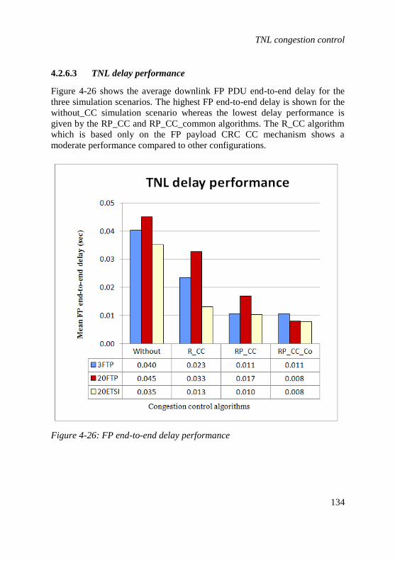
TNL congestion control
134
4.2.6.3 TNL delay performance
Figure 4-26 shows the average downlink FP PDU end-to-end delay for the
three simulation scenarios. The highest FP end-to-end delay is shown for the
without_CC simulation scenario whereas the lowest delay performance is
given by the RP_CC and RP_CC_common algorithms. The R_CC algorithm
which is based only on the FP payload CRC CC mechanism shows a
moderate performance compared to other configurations.
Figure 4-26: FP end-to-end delay performance

TNL congestion control
135
4.2.6.4 Required in-band signalling capacity over uplink
Figure 4-27 shows the required uplink signalling capacity for each simulation
configuration.
Figure 4-27: required in-band signalling capacity
The highest signalling capacity is required by the without_CC simulation
scenario which completely operates under the credit-based flow control
algorithm. When the system is in flow control state the CA messages are
being sent periodically based on the expiry of the FC timer which has a
shorter duration than the AIMD recovery timer. Therefore these CA
messages create the highest in-band signalling load on uplink compared to
other scenarios as shown in Figure 4-27. However, when the system is in
congestion control state, the number of CA messages which are sent over the

TNL congestion control
136
uplink is reduced due to two main reasons. One is that the recovery timer
period in the congestion control is higher than the flow control timer period.
Therefore, the number of periodically generated CA messages is reduced
when the flow is in CC state. On the other hand, the CA messages are only
being updated if either the currently calculated credits are different from the
previously sent credits or based on detection of new congestion events.
Since the FP payload based CRC CC algorithm detects the lowest number of
CD events compared to the combined CC algorithm, it requires the lowest
number of uplink in-band signalling bandwidth. The combined
RP_CC_common algorithm shows a bit lower amount of signalling capacity
compared to RP_CC algorithm. This is mainly due to fact that the congestion
control activity for the RP_CC based configuration is only initiated for the
MAC-d flow which detects the CD event while the other flows are still in the
FC state.
4.2.6.5 End user performance
The effective Iub utilisation, shown in Figure 4-24 is the ratio between the
effective application throughput which is measured at application layer and
the theoretically achievable maximum application throughput with the
configured Iub bandwidth.
The theoretically achievable maximum application throughput can be
calculated by taking into account the overheads of the RLC and ATM
protocols. In this evaluation, the theoretically achievable maximum
application throughput is estimated by multiplying the configured Iub
capacity with a constant factor of 0.76 which is taken as a rough estimation
of the overhead from ATM to application layer. From Figure 4-28, it can be
seen that the highest effective Iub utilisation is achieved by the RP_CC
configuration for all simulation scenarios whereas the lowest effective
utilisation is achieved by the no congestion control based configuration for
all simulation scenarios. The RP_CC_common scenarios show a slightly less
effective utilisation for the 20 FTP and 20 ETSI users constellation compared
to the RP_CC based configuration. The FP payload based configuration
shows less end user performance compared to the combined CC
configurations but a significantly higher performance compared to the
without_CC configuration.

TNL congestion control
137
Figure 4-28: Effective Iub utilisation
4.2.7 Conclusion
The theoretical and modelling aspects of the preventive and reactive
congestion control schemes have been discussed in detail within this chapter.
There are several combinations of congestion control algorithms which have
been widely investigated, tested and validated for the performance of the
HSDPA network. The simulation results confirm that the combined usage of
preventive and reactive congestion control algorithms achieves a
significantly better overall performance for HSDPA networks compared to
other configurations. Such combined congestion control mechanisms
optimise the effective link utilisation by minimising the higher layer
retransmissions and also achieve high end user throughputs.

TNL congestion control
138

CHAPTER 5
5 Analytical models for flow control and
congestion control
Chapter 4 discusses the congestion control (CC) and the flow control
(FC) algorithms in detail. Such algorithms are very complex in nature due to
the dependency on many parameters. Therefore, analytical modelling of these
algorithms has to be done carefully in a stepwise manner. During this
investigation, first the behaviour of the congestion control functionality is
modelled and second, in a combined analytical model, flow control and
congestion control are modelled together. Before getting into the detailed
discussion of the analytical model, an overview of the two mechanisms is
given.
The flow control and congestion control is done per MAC-d flow (user
flow). The two states FC state and CC state are defined based on the flow
activity whether the user flow is controlled by the FC algorithm or by the CC
algorithm. The user flow stays in the flow control state when there is no
congestion [3, 4] in the network.
FC State CC State
Cong. Detection
Max. permitted bit
rate level reached
Cong.
Detection
Normal
arrival
Figure 5-1: User flow state diagram, the user flow (MAC-d flow) stays in the
FC state if there is no congestion at the transport network otherwise it stays
in the CC state

Analytical model for congestion control
140
When the transport network is congested, the congestion control algorithm
takes over the control of the data flow of the users and hence, user flows are
rather staying in CC state than in the flow control state. The flow state
diagram for a single user flow is shown in Figure 5-1.
The flow control algorithm estimates the capacity over the air interface and
grants are provided to the RNC controller to send the data over the transport
network on a per-flow basis. Even with the functionality of a proper flow
control scheme, a user flow often gets into congestion at the transport
network level due to limited transport capacity and bursty traffic.
The analysis of the transport network was performed using the simulations in
chapter 5. However, it is a real challenge to investigate all the analyses such
as sensitivity analyses and optimisation parameters for the CC and FC
algorithms using the detailed system simulations which require a
considerable long simulation time, often in the order of days, for each
simulation run. Therefore, from this perspective it is necessary to have an
analytical model which can perform these investigations and analyses faster
than the detailed system simulation does. Such an analytical model is
addressed in this chapter which is structured into two main subchapters.
Chapter 5.1 discusses the analytical modelling of congestion control,
compares the analytical results and simulation results and finally provides a
conclusion. Chapter 0 presents the combined analytical model of flow control
and congestion control, compares the results with the simulation results and
lastly gives a conclusion.
5.1 Analytical model for congestion control
In today’s Internet, many users who are connected via broadband access
network consistently overload the system by downloading very large files.
Such greedy users often create heavy congestion at the transport network
level. The congestion control function in the HSDPA system controls such
user flows in order to provide a fair share of the resources for all users. Due
to the congestion control, most of the time, these flows are staying in the
congestion control state and the CC algorithm adaptively allocates the grants
based on the fair share of the available transport capacity. Investigation of
such greedy user behaviour at the transport level is the focus of this analysis.

Analytical model for congestion control
141
The modelling approach of the congestion control is shown in Figure 5-2 for
a single flow. The congestion control process which has an input and an
output is shown. For the simplicity, this can be considered as a black box
approach in which all CC functions are included. The input is described by
the congestion indication (CI) interarrival process and the output can be
described by granted data rate from the RNC according to the CC evaluation.
Since all the processing for the CC is performed at the Node-B, the signalling
transmission delay over the uplink is assumed to be constant.
Figure 5-2: block diagram of the CC modelling approach includes input,
output and CC process. All CC functionalities are modelled within the CC
process. The input process can be described by a CI arrival distribution and
the output is the per user transmission data rate which can be described by
the service distribution.
The CI interarrival distribution depends on the current load at the transport
network which again depends on several factors such as radio conditions, the
number of users in the system and the type of user traffic. Modelling of the
CI arrival process is discussed next.
5.1.1 Modelling of the CI arrival process
The traffic burstiness in the transport network is mainly due to the HSDPA
best effort traffic. All the user flows (MAC-d flows) are considered as
independent and are modelled per flow basis. The behaviour of the traffic
over the transport network mainly depends on the bursty nature of the
independent traffic flows and the time varying channel capacity at the air
interface for each connection. Congestion often occurs randomly when
several user flows which are operating at the same time try to transmit a bulk
amount of data over the transport network simultaneously. This is a random
process in which the current transmissions do not depend on the past actions
but on the prevailing transport and radio channel conditions. Therefore, the

Analytical model for congestion control
142
congestion detection process for each flow can be assumed as a Poisson
process in which the interarrival time is modelled using the negative
exponential distribution in the continuous time domain.
The interarrival time between the arrival of the nth
and the (n+1)th
CI signals
is denoted by a random variable Tn. The CI interarrival distribution, )(tAn
can then be defined as follows.
t TtA nn Pr)( equation 5-1
However, this analytical model considers the time in discrete intervals (or
steps) since the data reduction procedures of the CC are activated in discrete
time intervals as discussed in chapter 4. Therefore, all multiple occurrences
within a single step are assumed to occur at the end of the time step and those
multiple occurrences in a single discrete time step are also a Poisson
distributed processes due to the memory less property of CI arrival process.
When the system is in recovery phase, the transmission data rate is increased
at the end of each step timer period. Any congestion indications received
during the step timer period are considered as received at the end of the
relevant time step with zero interarrival time. Figure 5-3 shows the CI
occurrence over time.
Figure 5-3: Modelling of CI interarrival process.
First the CI interarrival distribution is modelled without considering multiple
basic CI arrivals and then the basic CI arrivals are modelled separately.
Since the multiple arrivals within a single step are a Poisson process, they
can be modelled using the geometric distribution. The random variable K

Analytical model for congestion control
143
represents the number of CI arrivals in a single step. The probability of k CI
arrivals in a single step can be represented by the following probability mass
function.
ppkK k 1)1()Pr( equation 5-2
where p is the success probability of exactly one CI arrival within a step.
5.1.2 States and steps definition for the analytical modelling
Each CI arrival causes the current data rate to be reduced by a factor β which
is equivalent to the parameter “b” of the AIMD algorithm which was
described in chapter 4.2. When the MAC-d flow is in recovery phase and also
further CI indications are not received then this indicates that the system can
recover from the congestion. This means further data can be sent to the
system to optimise the utilisation. Therefore the data rate increases at a
constant rate per AIMD step time which is called step time or step which is
measured in seconds. At the end of each step, the data rate is increased by
one step height which is “a” kbit/sec (discussed in chapter 4.2 as the AIMD
parameter “a”). The terminology of steps and states is used throughout this
analytical model. The CC functionality is shown in Figure 5-4, where the
transmission rate is displayed versus the elapsed time. Further all CA
messages are sent to the RNC through a dedicated uplink signalling channel,
therefore the uplink in-band signalling (CA messages) delay is assumed as
constant and it is also assumed that there are no packet losses during uplink
signalling.
The state of the analytical model is defined as the transmission rate
immediately after the CI arrival which means just after the CC decision has
been taken. The discrete state which occurs due to CI arrivals is denoted by a
random variable X.
321 n X, , X, XXX for all n equation 5-3
The discrete state space or the set of possible values that X can take ranges
from 0 to , then corresponds to the maximum possible step height that
can be achieved by a single flow. [kbit/s] is the maximum possible
data rate which is equal to the configured Iub capacity and α = 1–β.

Analytical model for congestion control
144
Figure 5-4: User flow behaviour in CC state. Figure shows the transmission
rate versus the elapsed time. At the arrival of the CI, the transmission rate is
reduced by factor β and the state changes to a new one. If CI arrivals do not
occur within a step time, the transmission rate increases to the next level.
As discussed above, the multiple CI events occurring within the same time
step are modelled as simultaneous CI arrivals at the end of the corresponding
step where the CC action is taken. Those multiple CI arrivals cause a
multiple reduction of the data rate which is also called multiple drops. These
multiple drops of the data rate are modelled as multiple departures in the
analytical model.
For example, in Figure 5-4, there are two CI arrivals which are received by
the CC process at the end of the step τn+1 and the current rate is reduced by
the factor β twice. If the state after processing CI is , then the
corresponding step before CI processing is given by , where α = 1-β.

Analytical model for congestion control
145
The complete behaviour is described by the Discrete-time Markov Model
with Multiple Departures and the next section describes this model in detail.
5.1.3 A discrete-time Markov model with multiple departures
In this analytical model, the number of states mainly depends on the
maximum network capacity and the step size. Assuming that the maximum
number of possible states is m+1, then the random variable X can take state
values from 0 to m. All possible state transitions from state are
shown in the state transition diagram in Figure 5-5.
Since CI interarrival time has Markov property, the transition probability
from state i to state j is denoted by which can be defined as follows.
equation 5-4
The transition probability pij can be expressed in terms of step probabilities
which are derived from the CI interarrival distribution. In this calculation, the
step probability corresponding to the one just before the drop is to be taken.
0 1 i1i 1i j 1m ml
ijp
Figure 5-5: The state transition diagram shows the possible state transitions
from state i. The maximum possible state which can be reached is m.
For example if the state at the nth
CI arrival is then the step just
before the CI arrival would be “j/α” where α = 1- β. By considering
probabilities for multiple arrivals of CIs the final transition probabilities are
expressed as given below.
equation 5-5

Analytical model for congestion control
146
Pr(k) represents the probability of exactly k CI arrivals within a step and Pr(y)
is the probability of the CI interarrival time with exactly y steps where
and dmax represents the maximum number of CI arrivals
within a step.
The transition probability matrix is a square matrix of dimension m+1 and
can be given as follows:
equation 5-6
In general, when the transition matrix is known at the steady states, the
stationary state probabilities π can be calculated by using the well known
equation 5-7. The simple matrix calculation principles are used to evaluate
vector π in equation 5-7.
Pππ equation 5-7
where π denotes the state vector, [π0, π1, π2, π3 ,… , πm ].
5.1.4 Average transmission rate
The performance is evaluated as average throughput or average transmission
rate. The average throughput can be calculated by taking the area under the
curve of the transmission rate divided by the total time (see Figure 5-6).
The area under the curve gives the volume of the data which is transferred
over the period of time. Normally, the time is assumed to be a very long
period for the average calculations. Using the trapezoidal rule, the average
throughput (volume under the curve / duration) can be calculated using the
following formula.
max
1 121
1121
.....
...2/))/((...2/))/((XE
d
k nn
nk
k
nnk
k
tttt
triitrii
max
1
123122211
1
.............5.0
XE d
kk
knnnn
j
n
rtitititititi
t

Analytical model for congestion control
147
m
i
i
d
kk
km
i
m
i
d
kk
kii i
rrtNitNi
tN 1
max
11 1
max
1
_
_15.0).()(
5.0XE
The final average throughput calculation formula is as follows:
Average Throughput
m
i
i
d
kk
k ir
11
max
15.0
equation 5-8
1nt
/ni
(kbps) RateTxn
Time
nt
1nn2n1n
nn iX 2nX
11 nn iX
/1ni
nCI 1nCI
2
1/ni
11 nn iX
Figure 5-6: Flow behaviour in CC, the shaded area under the curve
represents the total data volume which has been transferred during model
time.
5.1.5 Simulation and analytical results analysis
The simulation results and the analytical results are presented and compared
in this section. First, all configurations of the input parameters are described
in detail for both models and then the results for each model are discussed

Analytical model for congestion control
148
individually. Secondly, the analytical results are compared with the
simulation results in order to validate the analytical approach for different
configurations. Finally some of the sensitivity analyses are done using both
models and the performance is compared.
5.1.5.1 Parameter configuration
The HSPA simulation model which was described in chapter 3 is used for the
simulation analysis. The presented analytical model focuses on the
congestion control functionality. In order to compare the performance
between analytical model output and simulation output, the simulation model
is also required to be configured in such a way that at least a single user flow
is always in the congestion control phase all the time. The general user flow
behaviour is that when the system is congested, the user is in congestion
control state, otherwise the user is in flow state. An off-period user does not
transfer any data and is in neither congestion control nor flow control state.
However, in order to compare the analytical model results with the
simulation results, one user flow is required to be in CC state always. Some
greedy flows may have a lot of data always to be transmitted and can be used
for this analysis. The simulation scenario is configured in such a way that one
UE flow always stays in the CC state for this analysis. The simulation
scenario is configured including 20 users with two different traffic models.
One user is configured with the FTP traffic model while all the remaining 19
users are configured with the ETSI traffic model [23]. Since the FTP user is
downloading a large file he always stays in the congestion control phase until
he finishes the download. In this application configuration, the FTP user is
configured with very large files with zero interarrival time between two
consecutive files so that the user always has data to be transmitted and stays
in the CC phase.
The common congestion control parameters which were used for the
analytical and the simulation model (in chapter 4) are listed below:
AIMD CC step duration = 500 ms
Step size of data rate changes = 33.6 kbps (1 RLC packet/10 ms)
Congestion reduction factor β = 0.25
Safe timer = 80 ms
Link bandwidth = 2 Mbit/sec

Analytical model for congestion control
149
In addition to the above, the simulation is configured with various other
default parameters for other protocols such as TCP, RLC, MAC etc. The
simulation is run for about 4000 sec.
The analytical model assumes the geometrically distributed CI arrival process
with a mean CI interarrival time of 0.2 CIs/step. The mean value is derived
using a trace taken from the detailed system simulator. However, a fast
queuing simulator which has been described in chapter 5.2.5 can be deployed
to get this input parameter instead of using the detailed system simulation
The fast queuing simulator provides faster results in comparison to the
detailed system simulator which requires a long period of time in order to
perform the same analysis. The step size is equal to the AIMD CC step
duration, i. e. 500 ms as given in the configuration. Next, the simulation and
analytical results are described separately and compared at the end of this
section.
5.1.5.2 Analytical results
First, all transition probabilities were calculated using equation 5-5. It is a
square matrix of 37 states for the given scenario. Figure 5-7 shows the
graphical overview of the transition probability matrix. The y-axis and x-axis
shows the state i and j respectively. Figure 5-7 depicts that when the flow is
in a lower state, the transition probabilities to higher states are high. That
means, there are more opportunities of jumping to the higher states from the
lower states. However, when the flow is in the higher states then there are
more opportunities to jump to the lower states. This phenomenon completely
agrees with the real behaviour of the HSDPA system. This means, the system
at higher states is more short-lived and jumps occur to lower states due to
high congestion probability. When flows stay at higher states, more data is
transmitted to the network which leads to a network overload situation
Therefore, there are more CI signals that cause rate reduction at the
congestion control module in order to reduce the MAC-d flow data rate and
to overcome congestion situations in the transport network.
On the other hand, when the user data rate is reduced too much, the system is
relaxed and the user is allowed to again send more data. Therefore, there are
more opportunities to go for the higher states. Since the HSDPA traffic is
bursty in nature and varies over time, the congestion control always tries to
optimise the transport capacity. Further, the figure shows that a balance of

Analytical model for congestion control
150
transition between higher and lower states is achieved at the states between
12 and 18. At these states, the user transmits at data rates close to the average
capacity which is allowed by the network share. However, when more
capacity is available to transmit because the other users send less traffic for a
particular period of time, then the flow rate is increased by the CC algorithm
to utilise the unused capacity. The situation is reversed when all users have
data to transmit over the network. Therefore user flows always fluctuate
according to the available transport capacity.
Figure 5-7: Graphical overview of the transition probability matrix, y-axis
and x-axis show the state i and j respectively. The figure indicates when the
flow is in a lower state, the transition probabilities from lower to higher
states are high whereas when the flow is in a higher state, it more often
transits from higher state to lower state due to high congestion probability.
Figure 5-8 shows all stationary state probabilities from the analytical model
that are calculated using equation 5-7. The figure illustrates that the middle
states (12–18) have high state probabilities, indicating that the user is more
often granted data at those transmission rates.
This indicates the average transmission rate which is allowed by the transport
network, based on the shared capacity of the network. As described above,

Analytical model for congestion control
151
the user is allowed to transmit with higher and lower data rates based on the
available current capacity of the network. These opportunities are quantified
by lower and upper state probabilities.
Figure 5-8: Stationary state probabilities, x-axis and y-axis show the states
and its probabilities respectively. The stationary state probability shows the
regular pattern of high state probabilities for some states compared to
others. This is mainly due to the configured value of β which is 0.25, and
multiple CI arrivals.
Further, the state probability shows a regular pattern of high state
probabilities for some states compared to others. This is indicated by the high
bars relative to the neighbour states in Figure 5-8, which is mainly due to the
configured value of β set to 0.25 and multiple CI arrivals. The current state
can change by a factor of 0.25 for each CI arrival. For example if the current
step is 20, then based on the arrival of a CI, it jumps down to 15 and based on
two consecutive arrivals to 12 etc. For multiple departures, some regular
states get a slightly higher probability compared to others which depends on
the configured β value. During the simulations, it is observed that if the value

Analytical model for congestion control
152
of β changes, the pattern of the state probability peaks is also altered.
However, these results are shown for the default β of 0.25. Later in this
analysis more results are compared for different β values
Using equation 5-8 the average throughput for the analytical model is
calculated. The average throughput is 552.52 kbps for the given analytical
model scenario. Later these analytical results are compared with the
simulation results in chapter 5.1.5.4 for both the stationary state probabilities
and the average throughputs.
5.1.5.3 Simulation results analysis
The simulations were performed using the parameters specified in the
previous section 5.1.5. One simulation run is selected to illustrate the results
in detail. Figure 5-9 shows the simulation results of the FTP user who is
continuously in the congestion control state. Figure 5-9 depicts the
instantaneous output data rate or transmission data rate with its time average
values over the simulation time.
In order to understand the exact behaviour of the output data rate when the
user flow is in the congestion control state, the zoomed view of the
instantaneous throughput is shown in Figure 5-9. It clearly illustrates the
stepwise increment of the output transmission rate between two CI arrivals.
The CC functionality works according to the AIMD principle as explained in
the chapter 4. When the CI is received the transmission data rate of the user
is reduced by a factor of β from its current value.
In one occasion, it is indicated that there are two CI arrivals (multiple
arrivals) within a single step. The safe timer is configured with 80 ms to
protect the flow’s data rate being reduced too rapidly due to bursty CI
arrivals, and any arrival during that time period is not subject to the
transmission rate reduction. However, at the end of the 80 ms time period,
one rate reduction is applied if one or more arrivals present during this time
period. The step timer is about 500 ms for this simulation therefore the
maximum number of multiple arrivals is limited to 6 in this consideration.

Analytical model for congestion control
153
Figure 5-9: Instantaneous output data rate (red curve) and its average value
(blue curve) over simulation time are shown in the figure.
To investigate the confidence level of the simulation results, 30 replications
of the simulation were performed. Before explaining all the results, the next
section elaborates the way that confidence intervals are calculated for
replications.
Zoomed view
Flow is in
recovery state
Rate reduction
due to CI arrivals
tran
smis
sio
n r
ate
(kb
ps)

Analytical model for congestion control
154
Figure 5-10: Average transmission rate over simulation time for 30
replications of simulation runs. These replications were performed with
different random seeds for 4000 seconds model time.
The confidence interval is calculated by taking the means of independent
simulation replications. 30 simulation runs were performed with different
random seeds for the 4000 sec model time. During the CI calculation, the
warm-up period is not considered for the replications. The instantaneous
output data rate (simulation output) from 500 sec to 4000 sec was chosen for
each replication to calculate the mean value. The mean of the replication is
called the replication mean in this context. The replication means coincide
with the principle of batch means. The latter is taken from a single simulation
run whereas the replications are taken from simulation runs with different
random seeds. Each individual run is independent; therefore replications lead
to less correlation effects compared to batches of a single run. Figure 5-10
Avera
ge tra
nsm
issio
n r
ate
(kbps)
Model time (sec)

Analytical model for congestion control
155
shows the replication means for all simulation runs and Table 5-1 depicts the
replication means for 30 simulations.
Table 5-1: the replication means for 30 simulations, the replication means
are calculated by taking the time average of the instantaneous transmission
rate over simulation time.
All replications use different simulation seeds. Therefore, by construction,
the replications are independent and are assumed as identically distributed
which means that they are normally distributed with unknown mean and
variance.
The point estimates such as the expected mean, variance and the confidence
interval for all replications can be calculated as follows [78].
Mean
kbit s
Where is the ith
replication mean and n is the number of replications
Variance
kbit s
The 95% of confidence interval, CfI
CfI
CfI 535.28 kbit s, 556.85 kbit s where 100 CfI
The value, tα/2, n-1 is taken from Student t-distribution which is used when
sample size is relatively small and distribution of the mean is unknown. “n-1”
is the degree of freedom and 1-α is the confidence level [78].
The average throughput and the 95% confidence interval of the simulation
results are 547.07 kbps and (535.28, 556.85) respectively.

Analytical model for congestion control
156
Further, the probability distribution for each replication is calculated and
shown in Figure 5-11 which provides a broader overview of the
instantaneous transmission rates.
5.1.5.4 Comparison of simulation and analytical results
The analytical and simulation results are compared in this section. First, an
analysis of the CI arrival distributions obtained by the simulation results is
given in order to validate the assumption that was taken for the analytical
approach. A trace from a simulation was taken for the CI arrivals and
compared with the geometric distribution in logarithmic scale which is
shown in Figure 5-12. The results show the close agreement of selecting a
geometrically distributed arrival process for the analytical results.
CD
F
transmission rate (kbps)
Figure 5-11: cumulative probability distribution of instantaneous
transmission rate for 30 replications.

Analytical model for congestion control
157
Figure 5-12: CI arrivals probability distribution (blue curve) is compared
with the geometric distribution (red curve) in logarithmic scale. A trace for
CI arrivals is taken from the simulation and used for the above validation.
Secondly, the stationary state probabilities are compared between the
simulation and the analytical results as shown in Figure 5-13. One peak of
the state probability (state 36) which does not occur in the analytical results
appears in the simulation. It is mainly due to the fact that the UE tends to
transmit with a very high transmission rate at the beginning of the simulation
and receives a congestion indication due to the arrival of other users in to the
system. Therefore, at the transient phase of the simulation, the UE often tends
to stay in higher states compared to the UE movement is in the steady state
phase. However, Figure 5-13 confirms that both the simulation results and
the analytical results have a good match for all other state probabilities.
At last, the average throughput of the analytical model is compared with the
simulation results with the 95% confidence interval. The average throughput
calculated by the analytical model lies within the given confidence interval
and is shown in Figure 5-14.

Analytical model for congestion control
158
Figure 5-13: Comparison of the stationary state probabilities between
simulation and the analytical results
Figure 5-14: comparison between the analytical results and the simulation
results for the average throughput is shown in the figure.

Analytical model for congestion control
159
The above comparison confirms a close agreement between simulation and
analytical results.
5.1.5.5 Effect of the reduction factor β
All the above analyses were performed using default parameters for the CC
algorithm which were listed in the simulation configuration of the previous
section. When considering the performance, the parameters for the CC
algorithm have to be well tuned. In this section, the effect of the rate
reduction factor which is the key parameter for the CC algorithm is
investigated using the simulation and the analytical model. The analysis is
carried out by changing the β value from 0.15 to 0.25 in steps of 0.05.
Figure 5-15: Average throughputs of the simulation results with 95%
confidence interval for different β values are compared with the analytical
results. The x-axis and the y-axis show the different β values and average
throughput respectively.
The average simulation throughputs with the 95% confidence interval for
each β value were compared with the analytical results. Figure 5-15 shows
Average Throughput
400
450
500
550
600
650
0.15 0.20 0.25 0.30 0.35
beta values
thro
ug
hp
ut
(kb
it/s
ec)
Simulation results Analytical results

Analytical model for congestion control
160
the average throughput of the simulation results and the analytical results for
different β.
At the beginning of the graph, for lower β values, the simulation and
analytical results deviate from each other significantly. The average
throughput of the simulation is lower compared to the analytical model. The
reason is that from the simulation point of view, the congestion control data
reduction is not sufficient for small β values in order to control the
congestion of the transport network promptly. Therefore, a large number of
packet losses occur at the transport network and the higher layers such as
RLC and TCP start reacting to the transport congestion. Due to the additional
retransmissions triggered by the RLC layer, the offered load is further
increased in a short period of time which results in worsening congestion at
the transport network. Lastly TCP congestion control starts controlling the
data flow by limiting the offered load to the network. As a result of these
subsequent effects in the higher layers, the achievable effective user
throughput is significantly reduced for the simulation. However, in the
analytical model such higher layer protocol effects are not considered. Hence,
the average throughput differs from the simulation results.
For the range of β values from 0.20 to 0.30, both the analytical and
simulation results are in close agreement. When the β value increases (such
as 0.30 or 0.35), the effect of the congestion control is very aggressive and
the offered load is controlled tightly. Since the offered load is reduced by a
large factor, the network load is reduced significantly and the packet losses at
the transport network are minimised. The offered network traffic load for the
simulation is controlled by the TCP flow control algorithm in order to
optimise the transport utilisation whereas in the analytical model
consideration, there are no such effects from higher layers which can
optimise the available capacity at the transport network. Hence the analytical
model provides a slightly lower offered load compared to the simulation
analysis for higher β values. However, the usage of a large β values causes a
large reduction of the network load causing two key effects in any system:
one is, the congestion in the network is suppressed and the second is, the
usage of the transport capacity is underutilised. This is a trade-off situation
when the overall network performance is considered. Therefore, it is very
important to choose appropriate β values for such scenarios to achieve
optimum overall performance. The simulation results show the optimum

Analytical modelling of flow control and congestion control
161
effect of the CC activity in combination with all other protocol effects
whereas the analytical model shows only the CC functionality.
5.1.6 Summary and conclusion
An analytical model which is based on the Markov property has been
developed in order to analyse effects of the comprehensive TNL congestion
control algorithm. It has been tested and validated by using the HSDPA TNL
simulator. The results closely match with an acceptable error margin. The
error is mainly due to the fact that the simulation model consists of all higher
layer protocol effects in addition to the congestion control functionality.
In general, the user MAC-d flow is not always in the congestion control state
throughout the simulation time. The MAC-d flow alternates between the flow
control phase and the congestion control phases depending on the availability
of the network capacity and on the bursty nature of the user traffic.
Therefore, the flow control state functionality should also be included in the
analytical model in order to model the general behaviour of MAC-d flow in
the HSDPA network. The next section presents a comprehensive analytical
model that includes both the flow control and the congestion control
algorithms functionalities.
5.2 Analytical modelling of flow control and congestion
control
The complete functionality of the congestion control has been analytically
modelled, analysed and validated using simulation results. In this chapter,
both the flow control and the congestion control functionalities are modelled
for each user flow. In the most general case, a user flow over a limited Iub
interface fluctuates between flow control and congestion control states
depending on the varying network capacity which is shown in Figure 5-16.
According to the explanation given in chapter 4, the flow control is an
independent algorithm which estimates the average data rate over the air
interface periodically for each user in the cell. The algorithm considers the
channel state of the UE over a period of time which is called cycle time. The
default value of the FC cycle time for the given HSDPA system is 100 ms

Analytical modelling of flow control and congestion control
162
which exhibits the optimum performance during simulation analysis and field
tests [12]. Figure 5-16 shows an example scenario of the user flow behaviour
in FC and CC phases. It depicts the estimated FC credits for each cycle time.
Figure 5-16: The FC and CC functionalities are shown in the figure. FC
credits are calculated at the end of each FC cycle time. If the congestion
indication (CI) signal is received then the user flow goes from the FC state to
the CC state. When the flow is in CC state, new credits are updated either at
the end of the CC step timer or at the arrival of another CI event.
The HSDPA credits which are sent from RNC to eNB alternate between FC
credits and CC credits. FC credits are the data rate estimated by the FC
algorithm whereas CC credits are calculated by the CC algorithm. When
there is no congestion in the system, all MAC flows operate in the flow
control state and the FC algorithm grants credits over the transport network.
The transport network congestion occurs due to the bursty nature of the
HSDPA traffic. The congestion control algorithm detects and controls the
input traffic flows to the transport network in order to minimise adverse
effects of the congestion. Each user flow operates in congestion control state
until the congestion is eliminated. During this period, user input data flow is
regulated according to the CC credits which are determined by the CC

Analytical modelling of flow control and congestion control
163
algorithm. More details about these algorithms flow control, congestion
detection and congestion control have been discussed in chapter 4.
The flow control and congestion detection modules issue independent signals
to the congestion control module and the CC module decides the allowed
credits for the congested MAC-d flow. The CC module immediately sends a
Capacity Allocation (CA) message which includes the credits and interval
information to the RNC in order to control the data transmission to the
transport network. This CA message sending is performed periodically. The
data rate of a particular user flow is constant within this period and hence the
burstiness over the transport network is also significantly reduced. When a
flow is in the CC state, the data rate increases by a lower rate than in the FC
state. Therefore, during the periods which the CC module calculates credits
are larger than the flow control cycle time which is called CC step time or
CC cycle time.
5.2.1 Joint Markov model
The CC and FC functionalities are modelled using a discrete Markov chain.
The flow control step times are taken as time points at which state changes
occur. The flow control timer is the smallest timer at which the air interface
credits are estimated whereas the CC timer is used to estimate the CC credits.
The CC timer step is an integer multiple of the flow control timer step. The
example in Figure 5-16 shows that the CC cycle time step is five times larger
than the FC time step.
The flow in CC state can exit only when the state reaches the FC state at
which the CC was initially triggered. This is the state at which the MAC-d
flow received the first congestion indication signal just before entering to the
CC state for the current CC session. The following list highlights the basic
assumptions and the simplifications that are taken into consideration during
this analytical modelling and analysis.
The interarrival times of CI signals are independent and identically
distributed.
The number of users in the system is constant.

Analytical modelling of flow control and congestion control
164
Constant transmission delay is assumed for capacity allocation (CA)
messages which indicate the credits to the RNC (for HSDPA) to
trigger the offered load to the transport network.
Per-user buffer management at eNB is not considered for the FC
algorithm.
When there are many users in the HSDPA system, the offered load varies
significantly. Furthermore, the user air interface channel quality also changes
with the ongoing time. There are many other factors such as TCP and RLC
protocol functionalities which influence the load at the transport network
level. The congestion can occur at any time in the limited Iub network due to
the bursty nature of the offered traffic. Therefore, the first assumption is that
the interarrival time of CI detection signals can be considered as independent
and identical. The second assumption is mainly due to the design of the MAC
scheduler. The capacity allocation messages are sent through the uplink
control channel and it is assumed that UL signalling has sufficient capacity
and also a higher priority compared to the other flows of the UL traffic.
Therefore, the delay for this uplink transmission can be assumed as constant
which is listed as the third assumption. During this analytical modelling, it is
assumed that sufficient data is in the Node-B buffer to satisfy the demanded
data rate of each user flow at the air interface. Therefore, the Node-B buffer
management is not considered for this analysis. The FC and CC algorithms
work independently and the flow control considers the air interface
fluctuation by determining the FC credits whereas the congestion control
monitors the load over the transport network. Therefore, the FC and CC
functionalities are modelled independently during this analytical approach.
5.2.1.1 States representation
The state of the Markov model are represented by three non-negative integers
i, j, and k which are defined below. The notation [i, j, k] is used to represent
individual states throughout this chapter.
1. The bit rate level in the FC state denoted by i: when a MAC-d flow
is completely in flow control state, the FC can vary from the lowest
to the highest bit rate level based on the credit estimation of the
radio interface. There are “m” such levels, thus i = 1, 2, 3,….., m.
This remains constant throughout a CC session at the last FC bit rate
level corresponding to the preceding FC session.

Analytical modelling of flow control and congestion control
165
2. The bit rate levels in the CC state denoted by j: the CC state bit rate
levels can theoretically achieve all FC state bit rate levels from the
lowest to the highest. Thus, j is taken as 0 if the state is within a FC
session and is equal to the CC bit rate level for states within a CC
session Thus, j = 0, 1, 2, 3,…., m.
3. The time step count denoted by k: the CC timer is selected as an
integral multiple of the FC timer. The largest value of k (denoted as
n) is defined by dividing the CC timer by the FC timer. In the state
representation, k spans from 1 to n with integer values. k=0 is a
specific state that represents the state within the FC session whereas
all other integer k represent states within the CC session. For the
given analysis, n is set to 5.
5.2.1.2 Markov state model
The state representation of the Markov model for the HSDPA CC and FC
functionalities is shown in the following Figure 5-17 along with the state
transitions. There are four categories of state transitions.
FC to FC transition:
FC to FC transitions occur when there is no congestion in the
system. States represent the UE credits which are allocated based on
the varying air interface capacity. Only the state variable i changes
in such a transition.
FC to CC transitions:
When congestion starts, a CI signal arrives and the state changes
from FC state to CC state. This action always causes a rate reduction
by jumping into a lower state from a higher state in the model. In a
transition of this nature, the state variable i remains unchanged, j
changes from 0 to a value less than or equal to i and k changes from
0 to 1.
CC to CC transitions:
During the MAC-d flow in the CC, the current state can only change
based on another CI arrival or at the CC timer expiry. In the first
case, state changes occur from the higher state to the lower state (j
changes to a lower value) and in the second case, state changes from
the current state to the next higher state (if k is less than 5, j remains

Analytical modelling of flow control and congestion control
166
unchanged. k increases by1untill it equals to 5 otherwise j increases
by 1 and k is again reset to 1).
CC to FC transitions:
This is the transition that changes the state from CC to FC (occurs
after reaching the CC state of [i,i,5]). This transition occurs when
the system overcomes congestion in the Iub network. Here i changes
to a value within the range 1,…,m and both j and k are reset to zero.
When the MAC-d flow is in the FC state, all state transitions occur between
state [1,0,0] to [m,0,0] along the horizontal axis and the system does not
experience any congestion in the transport network. Any FC state in the
model can be reached from any other FC state in the horizontal axis. Self-
transitions are possible at each FC state; they occur due to equal credits
estimation in consecutive cycle times.
The vertical transitions represent the CC state transitions. The second number
of the state representation gives the notation for the CC bit rate level. For
each bit rate level there are k step transitions. When no congestion indication
signals are received, the CC state transitions occur due to the timer expiry
and the CC bit rate levels are incremented until they reach the bit rate level
corresponding to the last FC state immediately prior to the transition to CC
session. After reaching this level, the MAC-d flow immediately exits from
the CC state to a FC state.
The third number of the state representation denotes the step transitions for a
single CC bit rate. During these step transitions, there are no changes of the
bit rate levels but only the step advancements to the next step if no further CI
arrivals are received. When the CC state reaches the FC state and all five
steps in the considered example have been completed within the given CC
state then a state transition occurs from the CC state to the FC state as
explained above.

Analytical modelling of flow control and congestion control
167
Figure 5-17: State representation of the Markov model for the HSDPA CC
and FC functionalities. The states of the Markov model are represented by
three non-negative integers: i FC state, j CC state and k time steps. Each
column shows the CC state transitions. After the flow reaches 5th
step (k = 5)
in the CC state, it changes to the next higher level (j+1). When i and j are
equal and k reaches 5, then the exit condition is met and the flow transits
from CC to FC state which can be any state in the lowest row in the
horizontal axis.

Analytical modelling of flow control and congestion control
168
5.2.1.3 Size of the state space
Within this section, the total number states in the state space is determined.
The FC states and the CC states are represented by finite lists of numbers that
represent the simple sequences. The numbers in the sequence are known as
“terms” of the sequence. The finite sequences for the FC and the CC states
can be derived as follows.
The FC state finite sequences:
equation 5-9
The CC state finite sequences:
equation 5-10
Each of above finite sequences is an arithmetic progression (AP) where the
next element is obtained from the previous one by adding a constant common
difference. For the first sequence, the first element is 1 and the common
difference is also 1 whereas for the second sequence, the first element is 5
and the common difference is 5 as well.
There are exactly m possible discrete states corresponding to FC sessions. A
CC session starting from the ith
FC bit rate level can have upto 5i different
CC states. According to the sum of the arithmetic series, the total number of
FC and CC states can be calculated for the state model.
The total number of states
equation 5-11
For example, if m is 48 (eff_BW/step = 2.0*106*0.8/33.6*10
3, where BW =
2Mbit/s, effective BW is 80% of total BW without protocol overhead and
step height is 33.6 kbit/s) then the total number of states is 5928. This means
for a single MAC-d flow, there are 48 bit rates which can be calculated
according to the air interface capacity of the user channel which leads to the
total number of 5928 states. The transition probability matrix is square matrix
of this size.

Analytical modelling of flow control and congestion control
169
5.2.1.4 Input parameters of the analytical model
The analytical model uses two input parameters for the evaluation. One is the
FC state stationary probability distribution and the other is the CI arrival
probability distribution.
As explained in chapter 4, the exact air interface modelling is not the main
focus of this work. Therefore, a trace of UE air capacity in terms of the
number of MAC-d packets per TTI was taken from a dedicated radio
simulation. From the traces, the stationary state probabilities are derived for
the flow control states for both simulation and analytical models.
The stationary probability matrix can be written as
equation 5-12
where m is the total number of bit rate levels for the FC and PBRm represents
the flow control bit rate level stationary probability matrix. pbrj is the jth
state
probability.
The second input parameter is the CI arrival probability. This represents the
probability of CI arrivals for a given interval (FC cycle time). The CC cycle
time is always greater than the FC cycle time. The maximum number of CI
arrivals for a given FC interval is restricted by the safe timer which is used to
avoid frequent signalling over the uplink channel during congestion in the
transport network. It is assumed that dmax is the maximum number of CI
arrivals within a given FC interval. The CI arrival probability matrix for a
given FC interval can be represented by Aci:
Where exactly CI signals during
equation 5-13
5.2.1.5 Transition probability calculation
The transition probabilities of the Markov model are derived using above
input parameters. There are four transition domains which are analysed

Analytical modelling of flow control and congestion control
170
during the state modelling. Each of these transition probabilities is calculated
in this section.
The state transition probabilities for state changes within a FC session
can be represented by Pfctofc.
equation 5-14
According to the Markov property, all the past history is represented by
the previous state, i. Further, the relationship between past and current
states depends on the equation 4-2.
A FC session continues as long as no CI signal arrives. This is taken into
account by multiplying pij by the probability for zero CI arrivals within
the time step. The state transition probabilities within the FC session are
represented by P(i,0,0)(j,0,0)
interval FCgiven a within occurs
arrivals CI no ofy probabilit theis where,
0
0)0,0,)(0,0,(
q
pqp ijji
equation 5-15
The transitions from a state within a FC session to a state within a CC
session occur due to the arrival of a congestion indication. The number
of CI arrivals can be more than one. The maximum number of CI
arrivals is dmax and the state transition probabilities, P(i,0,0)(i,l,0) can be
derived.
max
1
)1,,)(0,0,(
1;
max
dnil
qp
n
d
n
nlii
equation 5-16
where, α=1-β, β is the reduction factor, qn is the probability of n CI
arrivals within a given FC interval.
Two types of transitions can occur within a CC session. If there are no
CI arrivals, state transitions can occur due to timer expiry (step timer has

Analytical modelling of flow control and congestion control
171
the same interval as the FC timer, however a different term is used in CC
states). The transition probabilities are represented by the transition
probability matrix P(i,j,k)(i,j,k+1). Here, the steps which are represented by k
can change from 1 to 5. Up to step 4, there is no change in bit rate levels.
At step 5, state changes occur to the next higher level of the CC bit rate
level.
5for
4,3,2,1for
0)1,1,)(,,(
0)1,,)(,,(
kqp
kqp
jikji
kjikji
equation 5-17
The second type of transition is caused by an arrival of a CI signal. The
state can change from the current CC state to a CC state with lower bit
rate level due to the arrival of the CI signals. When multiple CI arrivals
occur in a single step time period, the current state can fall back to a CC
state which has much lower bit rates. It is now considered that it fell
back from the CC state j to the CC state l due to the n CI arrivals.
51 and 1;
max
1
)1,,)(,,(
max
kdnjl
qp
n
d
n
nlikji
equation 5-18
where, α=1-β, β is the reduction factor, qn is the probability of n CI
arrivals within a given FC interval.
The state transitions from the CC state to the FC state occur due to the
absence of CI arrivals for a long period of time. When the CC bit rate
level reaches the FC bit rate level at which the MAC-d flow started to
move from FC session to the CC session, the current CC state changes to
a FC state. It is assumed that i is the FC bit rate level at which the current
CC session started and l is the next FC bit rate level which is entered to.
The new FC bit rate level can be any level that is selected based on the
current air interface channel capacity. All these transition probabilities
can be represented by the transition probability matrix P(i,i,5)(l,0,0).
illii pqp 0)0,0,)(5,,(
equation 5-19

Analytical modelling of flow control and congestion control
172
state CC theenters flow d-MAC thebefore
state FC starting theis and state FCnext theis il
After completing the calculation of all state transition probabilities, the
transition probability matrix is given below.
where
equation 5-20
The stationary state probabilities are calculated using the following formula
which has been explained in section 5.1.3.
equation 5-21
where πdenotes the state vector, [π0, π1, π2, π3 ,... , πnt ].
The throughput is calculated using the following equation 5-22. The bit rate
steps are defined in terms of 33.6 kbps.
equation 5-22
5.2.2 Analytical and simulation parameter configuration
The simulation and the analytical models use the same set of parameters.
FC cycle time = 100 ms
CC AIMD cycle time = 500 ms
FC and CC step size = 33.6 kbps (1packet/10ms)
β = 0.25
Safe timer = 80 ms
ATM bandwidth = 2Mbit/sec
In addition to the above, two input parameters which will be discussed next
are taken from two separate simulation models. They are the probability

Analytical modelling of flow control and congestion control
173
distribution of the radio channel capacities in terms of MAC-d/TTI and the
mean CI arrival rate per step. The radio traces are taken from the dedicated
radio simulation model whereas the mean CI arrivals are taken from a fast
queuing simulator which will be discussed in chapter 5.2.5.
For the system simulation, a comprehensive OPNET-based HSPA simulator
(chapter-3) which has been designed and developed by the author is used.
The simulation specific parameters are listed as follows.
Traffic models: FTP and HTTP traffic models [23].
User constellation: 18 users, 1 FTP user who downloads a large file
during the simulation time and uses the probability distribution used for
the analytical model. All other 17 users generate HTTP traffic.
The simulation duration is 2000 sec and 32 replications are used to
determine the confidence intervals.
5.2.3 Input distribution of radio user throughput
The input probability distribution of the radio throughput is derived from the
common trace file which includes the air interface channel capacity in terms
of number of MAC-ds/TTI. This input distribution is used both for the
simulation and the analytical model. The probability mass function of the
input is given in Figure 5-18.
The average air capacity of the user considered in the figure is about 907
kbps. This is the case without considering the HSPA access network. When
such a user operates in a real system with limited Iub capacity shared with
other users, the achievable data rate of the users is further reduced due to
transport congestion. The next section presents the simulation results in
which FC and CC algorithms are included within the detailed system
simulator in order to achieve the aforementioned achievable user throughput
over the transport network.

Analytical modelling of flow control and congestion control
174
Figure 5-18: Probability mass function of the number of MAC-ds (bit rate
levels).This input distribution is derived from a trace file which is used by
both the system level simulator and the analytical model. The bit rate levels
represent the air interface channel capacity for the selected user flow.
5.2.4 Simulation results analysis
The HSPA OPNET simulator is configured with the above common set of
parameters as well as simulation specific parameters. 32 simulations were run
using different random seeds. The instantaneous transmission rate (in green)
and the average transmission rate (in blue) over the model time of a single
simulation run are shown in Figure 5-19 as an example scenario. It is shown
that at 1500 seconds of model time, the average throughput variation
becomes stable and the system approximately achieves steady state
behaviour. Due to the bursty nature of the HSDPA traffic over the transport
network (Iub), the output data rate fluctuates inside a large range.
Furthermore, Figure 5-19 also presents a zoomed version of the relevant
portion from the figure giving a closer look. The user flow fluctuates between
two domains, the flow control domain and the CC domain. At the beginning
of the zoomed window in Figure 5-19, the MAC-d flow follows the saw-
tooth-like regular pattern which is typical for a CC session.

Analytical modelling of flow control and congestion control
175
Mostly UE is in CC mode in this region: stair case represents the CC state
Mostly UE is in FC mode in this region:
Average transmission rate
Zoomed view
Figure 5-19: Instantaneous transmission rate (green curve) and time
averaged transmission rate (blue) over the model time.
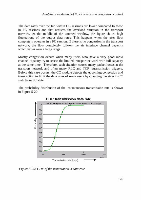
Analytical modelling of flow control and congestion control
176
The data rates over the Iub within CC sessions are lower compared to those
in FC sessions and that reduces the overload situation in the transport
network. At the middle of the zoomed window, the figure shows high
fluctuations of the output data rates. This happens when the user flow
completely operates in a FC session. If there is no congestion in the transport
network, the flow completely follows the air interface channel capacity
which varies over a large range.
Mostly congestion occurs when many users who have a very good radio
channel capacity try to access the limited transport network with full capacity
at the same time. Therefore, such situation causes many packet losses at the
transport network and often many RLC and TCP retransmission triggers.
Before this case occurs, the CC module detects the upcoming congestion and
takes action to limit the data rates of some users by changing the state to CC
state from FC state.
The probability distribution of the instantaneous transmission rate is shown
in Figure 5-20.
Pro
babili
ty
CDF: transmission data rate
Transmission rate (kbps)
Figure 5-20: CDF of the instantaneous data rate

Analytical modelling of flow control and congestion control
177
In order to analyse the statistical quantities such as the confidence interval for
the simulation results, 32 replications of the simulations were done. The
average throughput and the probability distribution (cumulative probability
distributions) of throughputs for those simulation runs are shown in Figure
5-21 and Figure 5-22 respectively.
Figure 5-21: Average transmission rate for 32 replications of the simulation
results.
The time average figure shows that at the starting phase of the simulation
(warm-up phase), the system is unstable and the average throughput varies
over a large range. During this period all protocols (network and end-to-end
protocols) are initialised and further flows are adapted to the available system
capacity. However, with the long simulation run, the system gets stable and
the results converge to stable average values.
Model time (sec)
Avera
ge tra
nsm
issio
n r
ate
(kbps)
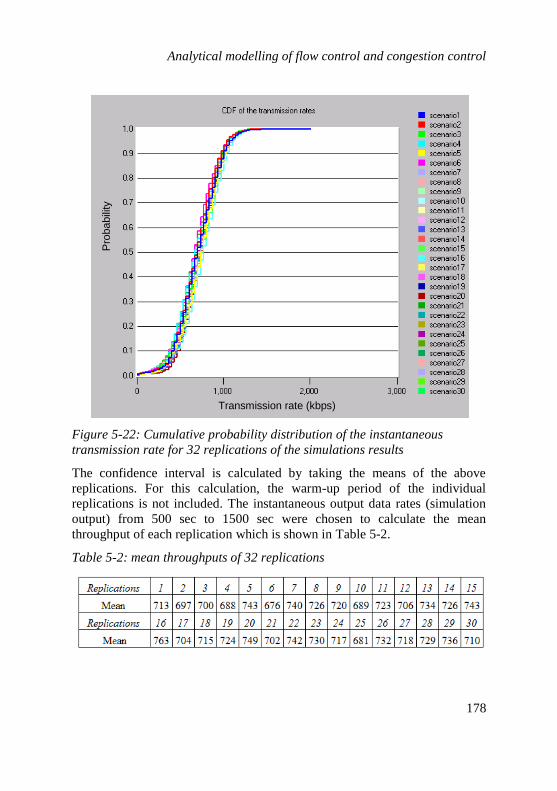
Analytical modelling of flow control and congestion control
178
Figure 5-22: Cumulative probability distribution of the instantaneous
transmission rate for 32 replications of the simulations results
The confidence interval is calculated by taking the means of the above
replications. For this calculation, the warm-up period of the individual
replications is not included. The instantaneous output data rates (simulation
output) from 500 sec to 1500 sec were chosen to calculate the mean
throughput of each replication which is shown in Table 5-2.
Table 5-2: mean throughputs of 32 replications
Transmission rate (kbps)
Pro
babili
ty

Analytical modelling of flow control and congestion control
179
The mean and standard deviations of the transmission data rate are 719.60
kbps and 21.13 kbps respectively. The 95% confidence interval is [713.05
kbps, 726.16 kbps].
So far detailed analysis of the simulation results has been discussed. Before
the analytical results analysis, the design and implementation procedures of
the fast queuing simulator are described in the next section.
5.2.5 Fast queuing simulator
A fast queuing simulator was developed in order to determine the mean CI
arrival rate. For the previous analysis, this input parameter is taken from the
system simulator and then applied in the analytical model. However, this
approach cannot be taken as a solution since it requires a long simulation run
time. To provide an approximation for this input parameter within a short
period of time, a fast simplified queuing simulator which mainly focuses on
the transport congestion is used.
5.2.5.1 Design overview of the queuing simulator
The queuing simulator was built using the CNCL simulation library which is
widely used for modelling communication network protocols and provides a
large number of built-in functions [79]. The CNCL simulator is a discrete
event simulator which is based on the concept of object orientation using the
C++ programming language as the basic programming tool. The overview of
the queuing simulation model is shown in the following Figure 5-23.
Figure 5-23 shows two main parts of the simulation model: the TNL source
manager network and the transport network. The TNL source manager
generates traffic to the transport network. The user traffic flows are
independent and are provided by a large number of TCP sources depending
on the configured application profile. For example, FTP uses a separate TCP
connection for each file download whereas web traffic uses one TCP
connection for the download of each page. Each data flow which consists of
one or many TCP sources or connections uses one RLC buffering unit with a
sufficiently large capacity in the RNC entity. Since there are “n” user flows,
Figure 5-23 shows “n” RLC buffers in the RNC. In many cases RLC buffer
occupancy rapidly increases when congestion occurs in the transport
network. The maximum RLC buffer capacity is directly controlled by the

Analytical modelling of flow control and congestion control
180
TCP end-to-end flow control scheme and also depends on the number of
simultaneous connections. All application data is stored at the RLC buffer
until they are transmitted to the transport network.
Figure 5-23: queuing simulation model
Data is sent from the RLC buffer to the transport network according to the
trigger from the CC module. As described in chapter 4, the CC module takes
two input triggers: flow control and congestion indication, and decides the
output data rate by considering the transport utilisation. All these input
triggers are independent within each data flow.
The transport network is modelled with a queue and a server. The serving
rate is determined by the last mile link capacity which is the bottleneck of the
transport network. The buffer unit which has a limited capacity represents all
buffers in the transport network. In general, the transport network is
dimensioned to keep the packet loss ratio under a certain maximum limit
which is for example 1% of the total packet transmission. The congestion
control algorithm minimises the transport packet losses while optimising the
transport utilisation. The complete congestion control procedures are
described in chapter 4.

Analytical modelling of flow control and congestion control
181
A large number of frame protocol data packets from independent application
sources arrives at the transport buffer. The decision regarding the next
transmission opportunity of these packets is taken using independent
transport triggers.
5.2.5.2 Queuing simulator implementation
Figure 5-24 shows the block diagram of the queuing model implementation
overview in the queuing simulator. As shown in Figure 5-24 the
implementation is performed by dividing the complete model into two parts:
the TNL source manager module which generates and controls the traffic
sources, and the transport network.
Figure 5-24: Queuing simulator implementation overview
When RLC and congestion control work together, all transport effects such
as a small number of losses are hidden to the TCP layer. All lost packets at
the transport network are recovered by the RLC layer before TCP notices
them whereas the CC minimises the congestion situation at the transport
network. Further the RLC buffers receive the data packets which come from
several TCP connections. The packets are stored in the RLC queue until they
get a transmission opportunity. Therefore the TCP slow start effects are
mirrored by the RLC controller unit to the transport network. The modelling
of the complete TCP protocol functionality creates again a complexity to the
fast queuing simulator and it may require a longer simulation time for the
simulations as the detailed system simulator does. On the other hand, when
the aforementioned details are considered, the modelling of TCP protocol
does not have a significant impact to the output of the fast queuing simulator.
Therefore, the modelling of the complex TCP protocol is excluded within the

Analytical modelling of flow control and congestion control
182
source modelling of the fast queuing simulator. However during application
modelling all other parameters such as file size and interarrival distributions
are correctly modelled in the fast queuing simulator which is similar to the
traffic modelling in the detailed system simulator.
The flow chart of the TNL source manager is shown in Figure 5-25 and
Figure 5-26. All user traffic flows start with the initialisation process and
start generating application packets (APP_JOB) with a random offset. The
user flow can be either in ACTIVE state or INACTIVE state. When UEs
have data to be sent to an application input queue, then the user is in
ACTIVE state otherwise they are in INACTIVE state.
The size of the FP JOB (or FP PDU) is determined according to the credits
which have been granted by the CC controller in the RNC. The FP JOBs are
transmitted at the expiry of every RNC time interval which is set by the
EV_Timer_RNC event trigger. For example the default value of the timer
event is set to 10 ms. The credits are updated every FC cycle time if the user
flow is not in congestion. This cycle timer expiry is also triggered by
EV_Timer_PBR in the TNL source manager module, the default value is set
to100 ms. When a user flow is causing congestion in the transport network,
the CC instead of the FC starts to control the sending data flow. In this case,
the credits are calculated by the CC algorithm with longer cycle time in order
to reduce input traffic to the transport network. The default CC time is set to
500 ms for this analysis which is triggered by EV_Timer_CC event. When
the UE flow is in ACTIVE state, there are three timer events and one Job
event: App_JOB, EV_Timer_RNC, EV_Timer_PBR and EV_Timer_CC
which occur in the TNL source manager block as shown in Figure 5-26.
All above event triggers are activated on a per flow basis and continuously
run when the flow is in ACTIVE state of the TNL source manager.
Depending on the timer events the respective algorithms start processing the
input data. For example if the EV_Timer_PBR timer arrives, the FC
algorithm starts the calculation procedures in order to update the credits.
Similarly when EV_Timer_CC timer is received, credits are calculated
according to the CC algorithm.
All FC and CC algorithm functionalities are depicted as blocks in the flow
chart in Figure 5-26. The FP JOBs (or FP PDUs) are sent to the transport
network continuously until the application input buffer is empty throughout
the simulation period. Figure 5-27 shows the transport network (or server)

Analytical modelling of flow control and congestion control
183
functionality. It has two states: WAITING and SERVING. Based on the
arrival of FP job events, the transport network starts sending data by
changing the flow state from waiting to serving.
Figure 5-25: TNL source manager (part 1)
Any arrival of a packet when the server is busy (or during transmission) is
stored in the buffer. When the transmission duration is over based on the
arrival of the EV_Timer_Txn event, the next packet in the buffer is served

Analytical modelling of flow control and congestion control
184
and the EV_Timer_Txn timer is rescheduled. In this manner transmission
continues until all packets in the buffer are served.
Figure 5-26: TNL source manager (part 2)
Within the transport network, congestion detection triggers are also activated
as shown in Figure 5-27. Congestion in the transport network is detected
either due to lost packets or high delay variation of the FP packet
transmission. It is assumed to be a maximum percentage of packet losses (for
example 1%) in the transport network. A lost packet causes an additional
RLC retransmission which triggers a new delayed FP JOB as shown in
Figure 5-27. The delay build-up process [chapter 4] is also continuously
running within the transport network in order to prevent forthcoming
congestion situations. All these congestion detection functionalities are
shown as blocks in the flow chart in Figure 5-27.

Analytical modelling of flow control and congestion control
185
Figure 5-27: transport network (server) functionality

Analytical modelling of flow control and congestion control
186
5.2.5.3 Mean CI arrival rate
The queuing simulator is configured with the same set of parameters which is
used in the system simulator. All congestion detection triggers are recorded
during queuing simulation. Since the latter is fast it can model a long period
of time in order to provide a large number of CI indications to achieve stable
results of computing mean CI arrival rates. Since the FC cycle and safe
timers are set to 100 ms and 80 ms respectively for the given example
configuration, the maximum number of CI indications to the CC module is
limited to one indication within a step time. The CI arrival process is
approximated by a Poisson process, hence the probability of no CI arrival
within a single step can be derived as 95.83% from the fast queuing simulator
whereas this value is 94.74% from the detailed system simulator. There are
many factors such as traffic modelling, higher layer protocol effects and
transport network settings which have an influence on the above difference of
CI arrival probabilities between the detailed system simulator and the fast
queuing simulator. Due to the trade-off between time efficiency and model
complexity, all above approximations have been applied to the fast queuing
simulator which can produce stable CI trace results within the order of
minutes compared to the detailed system simulator which requires the order
of days for the same outcome. The analytical model which uses the fast
queuing simulation trace results is able to produce final results of the impact
of transport flow control and congestion control on the transport performance
in a short period of time which is also in order of minutes. For this reason,
the analytical model along with the fast queuing simulator can achieve a very
high overall efficiency compared to the detailed system simulator. More
details about the analytical model results and the fast queuing simulation
aspects are also discussed in the results comparison chapter 5.2.7 by
highlighting the key differences.
According to the equation 5-13, the probability of CI arrivals within a single
step (q1) and the maximum number of CI arrivals within a single step (dmax)
parameters which are given by the fast queuing simulator are 0.0417 and 1
whereas the comparison values of 0.0526 and 1 are provided by the system
simulator respectively. There are several reasons for difference of the
probability of CI arrivals between the simulation and the fast queuing
simulator which will be discussed in chapter 5.2.7.

Analytical modelling of flow control and congestion control
187
5.2.6 Analytical results analysis
In order to evaluate the analytical model results, the MatLab tool is used. The
analytical model uses fast queuing simulation results as input parameters
along with the common set of parameters which have been discussed in
chapter 5.2.2. For this analysis, the CC timer which is configured to 500 ms
is selected 5 times larger than the FC timer (number of steps k = 1, 2, 3, 4 and
5). The FC timer of 100 ms is considered as the smallest time interval. There
are 5 steps of FC triggers within one CC trigger. According to these
configurations, the transition probabilities of the Markov model have been
calculated. For example, the transition probabilities from FC state to FC state
are shown in Figure 5-28.
Figure 5-28: Transition probabilities from FC to FC. These are the
transition probabilities if the user stays in the flow control. The averaging
formula is taken into consideration for the calculation of these transition
probabilities therefore there is a very low probability of a state changing
from a lower state to higher state and vice versa.
The state changes from lower to higher states have a very rare probability due
to the averaging equation 4-2. During the PBR calculation, all values of the

Analytical modelling of flow control and congestion control
188
past states are considered to be part of the previous state, therefore when the
average value is calculated, a large portion of the previous values is taken for
the current state calculation. Furthermore, the figure shows that higher state
transitions occur between states 15 to 40, in which the range of the average
radio throughput lies for this particular MAC-d flow.
The complete transition probability matrix (equation 5-20) for the given
example scenario is a square matrix with the dimension of 5928×5928. Due
to its large size no attempts are made to represent it graphically.
The average throughputs for the analytical model which are calculated using
the equation 5-21 are depicted in
Figure 5-29. The analytical-Q setup uses the mean CI arrival rate from the
fast queuing simulator whereas the analytical-S setup uses the CI output from
the system simulator. The respective average throughput values are 722.63
kbit/sec for analytical-S and 748.48 kbit/sec for analytical-Q.
Figure 5-29: Average throughput calculated using analytical model. The
analytical-Q setup uses the output of the queuing simulation for the mean CI
arrival rate whereas analytical-S uses the system simulation output.

Analytical modelling of flow control and congestion control
189
5.2.7 Result comparison and conclusion
Under this section both simulation results and analytical results are compared
for two example scenarios. First, the aforementioned simulation and
analytical results are compared together and the performance is discussed in
detail. Secondly, for further validation of the analytical approach, another
configuration by adding 10 more bursty web users to the current system is
analysed and compared with the simulation results.
5.2.7.1 Results comparison and analysis 1
Figure 5-30 shows the average throughputs which also include all transport
overheads and RLC retransmissions for both the analytical and the simulation
results. As discussed previously, the analytical model provides the average
throughput for two different configurations analytical-S which uses the trace
from the detailed system simulator and analytical-Q which uses the CI
probability from the fast queuing simulator.
Figure 5-30 depicts that the analytical-S scenario provides the results within
the 95% confidence interval of the simulation outcome whereas the results of
the analytical-Q scenario slightly deviates from the confidence interval. This
deviation is mainly due to the various assumptions made during the
modelling of the fast queuing simulator such as that the CI arrival processes
is assumed as a Poisson process. Despite this, the model simplifications such
as the effect of the TCP sources have been neglected. Further, 1% packet loss
probability was assumed at the transport in which the lost events are
uniformly distributed among the packet arrivals whereas often packet losses
are experienced in bursty nature in the detailed system simulator. For the
traffic modelling, the fast queuing simulator assumes one object which is
negative exponentially distributed for each web page by considering its
average page size whereas detailed system simulator considers five separate
objects which are Pareto distributed for each page.
Even though all aforementioned differences cause some influence to the final
outcome, only some of them can be quantified due to the complexity of the
system. For example, the fast queuing simulator assumes a fixed packet loss
probability of 1% for all analysis. However, during the simulation run, the
detailed simulator experiences 0.43% loss probability at the transport level
for the given configuration. This clearly indicates that the fast queuing

Analytical modelling of flow control and congestion control
190
simulator increases the throughput at the transport network level due to a
higher number of additional retransmissions triggered by the RLC layer to
recover transport packet losses in comparison to the detailed system
simulation. The average overhead due to RLC retransmissions can be
quantified and is approximately 6.8 kbps in case of the fast queuing
simulation for the given scenario.
Figure 5-30: Average throughputs for both simulation and analytical results.
The analytical-S setup which uses the CI arrival probability from the system
simulator provides accurate results within the 95% confidence interval of the
simulation results. However, the analytical-Q results are not located within
the confidence interval
It is shown that all above overheads cause a large difference in the
throughput comparison but fewer effects on the goodput which is the
throughput without transport overheads. Therefore, the goodput comparison
between the detailed system simulation and the analytical-Q model shown in
Figure 5-31 exhibits a closer agreement in contrast to the throughput

Analytical modelling of flow control and congestion control
191
comparison. The goodput is calculated by excluding both the general
transport packet overhead which is approximately 24% and additional RLC
retransmissions. In addition to the comparison of limited transport results,
Figure 5-31 shows an additional result in which the ideal transport is
considered. In the limited transport based scenarios, all analyses were
performed with a load factor of more than 100% to exhibit the effectiveness
of the FC and CC algorithms. Therefore, the achievable goodput performance
for the limited transport scenarios is greatly reduced compared to the ideal
transport consideration.
Figure 5-31: Goodput comparison among all simulation scenarios
The goodput is 907 kbit/sec when ideal transport is used and all three limited
transport analyses – analytical-S, analytical-Q and simulation – show a close
agreement of the goodput performances which are 545 kbit/sec, 558 kbit/sec
and 543 kbit/sec respectively as depicted in Figure 5-31. Therefore the results
confirm that the analytical model along with the fast queuing simulator

Analytical modelling of flow control and congestion control
192
provides a very good outcome and is able to perform FC and CC analysis in a
very short period of time which is in the order of minutes compared to the
full featured detailed system simulator which requires some days for the
same analysis.
5.2.7.2 Results comparison and analysis 2
As mentioned above, another example scenario is added to validate the
analytical model results using detailed system simulation analysis. In order to
compare with the previous analysis, this example scenario is configured by
adding 10 more web users to the previous system leading to an increase of
the average offered load approximately by 400 kbps. Therefore, this example
scenario causes severe transport congestion which has to be minimised by
further CC and FC activities.
The simulation was run with 12 replications; the average throughputs for all
simulations are shown in Table 5-3. The overall average throughput and the
95% confidence interval are 457.08 kbit/sec and (442.55 kbit/sec, 471.60
kbit/sec) respectively.
Table 5-3: Average throughputs of 12 replications
The Analytical-Q model also uses the same parameters and number of users
for the analysis. By configuration 10 additional web users in the fast queuing
simulator, the simulations are performed to achieve the CI arrival probability
distribution. The mean CI arrival probability within a step time is 20.0%
given by the fast queuing simulator compared to the mean CI rate of 20.79%
given by the detailed system simulator. The average loss ratio for the detailed
system simulator is ~ 0.91% which is much closer to the value of 1% which
is assumed by the fast queuing simulator. Therefore, in both cases the total
number of RLC retransmissions is nearly equal and has no significant impact
on the final results in contrast to the previous analysis. The results confirm
that the transport level congestion is severe for this configuration compared
to the previously analysed configuration, leading to many losses and CI

Analytical modelling of flow control and congestion control
193
triggers equally in both simulators. Therefore the transport level throughputs
are in close agreement similar to the goodput comparison. Both throughput
and goodput results are shown in Figure 5-32.
Figure 5-32: Average throughput and goodput comparison between
analytical and simulation results. The analytical-S and analytical-Q models
are within the 95% confidence interval of the simulation results.
The average throughputs for simulation, Analytical-S and analytical-Q
configurations are 457 kbit/sec, 459 kbit/sec and 469 kbit/sec respectively.
Both the analytical-Q and analytical-S results lie within the 95% confidence
interval (442.55 kbit/sec, 471.60 kbit/sec) of the simulation results. This
shows a good match between the simulation and the analytical results even at
a very high congestion level in the transport network.

Analytical modelling of flow control and congestion control
194
5.2.8 Conclusion
Within this chapter an analytical model along with the fast queuing simulator
has been implemented, tested and validated. The aforementioned analysis
shows that a fast queuing simulator can perform a complete FC and CC
analysis within an order of minutes compared to the detailed system
simulator which requires an order to days for the same analysis. Further
results of the fully analytical approach (the analytical model along with the
fast queuing simulator) show a good match with simulation results. Therefore
the analytical model can be effectively used to analyse the effect of the FC
and CC parameter optimisation providing a great flexibility along with
acceptable accuracy within a short period of time. Further the model can also
be efficiently used to emulate different bursty traffic environments for the
performance analysis of the aforementioned algorithms. Therefore, the
analytical model can be used as a cost-effective alternative solution to the
time consuming detailed system simulations.

CHAPTER 6
6 Conclusion, outlook and summary
6.1 Conclusion and outlook
This thesis work commenced focusing on the optimization of high speed
mobile access networks to achieve best end-to-end performance. Several
novel approaches have been proposed to achieve the above objectives. All
novel algorithms have been implemented, tested, validated and analysed
using comprehensive simulation and analytical tools. A prominent
enhancement is achieved not only for the end user performance but also for
the overall network performance. The proposed solutions significantly
improve the high speed mobile access network utilisation by providing cost-
effective benefits to the mobile network operators and the end users.
The key challenges such as developing comprehensive simulations and
analytical models for high speed mobile access networks have been
successfully achieved during this work. The comprehensive HSPA and LTE
simulators which have been designed and developed by the author are able to
test, validate and analyse all scenarios which focus on transport network
performance. In addition to the thesis work, these simulators have also been
used by the industrial projects managed by Nokia Siemens Network to
investigate and analyse the UTRAN and the E-UTRAN performance
respectively. All peer-to-peer protocols such as TCP, RLC and PDCP, and
other protocol layers such as MAC-hs and the E-DCH scheduler for HSPA
and the transport diffserv model and the time-frequency domain MAC
scheduler for LTE have been implemented in the respective simulators
according to the common framework specified by the 3GPP specification.
These simulators are able to perform an extensive analysis from the
application to the physical layer by providing detailed statistics. Both
simulators were constructed using a modularised approach in order to enable
extensions with great flexibility and enhanced scalability, adjust the required
granularity for different levels of investigations, optimise for long simulation
runs and select the appropriate statistics for different analyses.

196
The impact of the credit-based flow control on the overall network and the
end user performance was investigated and analysed using both simulation
and analytical tools. The results confirm that the algorithms achieve lower
burstiness over the Iub link, lower buffer occupancy at eNB, lower FP delay
and lower delay variation at the transport network in comparison to the
generic ON/OFF flow control mechanism. Based on above achievements, the
transport network utilisation has been significantly enhanced by reducing the
required capacity for bandwidth recommendations on the Iub interface of the
HSPA network. Hence the end user and the overall network performance are
greatly improved by optimising the goodput (throughput at the application
layer) of the network.
High speed packet traffic often has a bursty nature and leads to inefficient
usage of resources for both the radio and the broadband access networks. The
proposed congestion control algorithms work jointly with the credit-based
flow control in an effective manner to solve the aforementioned issues.
Several variants of congestion detection algorithms such as preventive,
reactive and combined have been investigated and analysed to find which of
them are able to provide the best overall performance. All these algorithms
have been tested and validated for the performance of the high speed mobile
access network using simulation and analytical approaches. The results
confirm that the combined usage of the preventive and the reactive
congestion control algorithms can achieve a significantly better overall
performance compared to other configurations. Such algorithms can protect
the transport network from any transient behaviour due to bursty traffic by
increasing the reliability of the system in order to guarantee the end user and
overall network performance. Furthermore, the analysis confirms that these
algorithms optimise the effective transport network utilisation and thus
provide cost-effective benefits for both the network operators and the mobile
users.
Two novel analytical models which are based on Markov chains were
developed within the focus of this thesis in order to overcome issues such as
long timing requirements not only for the development of the simulator but
also of the simulation itself, related to the simulation approach. Out of these
analytical models, one is designed to analyse the congestion control and the
other is to analyse both the flow control and the congestion control
functionalities. In a real system, there are some users who try to exploit the

197
system capacity by downloading a large amount of data continuously for a
long period of time. These flows are completely handled by the congestion
control algorithm covered by the first analytical model in order to monitor
and control their offered load to the transport network during the entire
connection period. In contrast to that, the moderate users who do not greedily
use the network vary their offered load in a discontinuous manner based on
their time dependent requirements. Therefore such a flow is operated under
both the flow control and the congestion control schemes which are
investigated and analysed by using the second analytical model. Since the
analytical models require an input parameter about the congestion behaviours
of the transport network, a fast simplified queuing simulation was also
developed by modelling the transport network part of the access network
along with the required other protocols. Due to the simplicity of the fast
queuing simulator, the latter is able to provide the required input to the
analytical model significantly faster than the detailed system simulator. It is
shown that by applying these congestion indication inputs, the analytical
model is able to perform the complete analysis of the flow control and the
congestion control to evaluate the end user performance and overall network
performance efficiently. The main advantage of the analytical models is that
they can perform the same analysis as the detailed system simulator does
within a shorter period of time, i.e. in the order of minutes compared to an
order of days required by the detailed system simulator. Further results
confirm that there is a good match between the analytical and the simulation
approaches. Therefore, the analytical models can be effectively used to
perform fast and efficient analyses with a good accuracy compared to the
detailed system simulation.
The LTE investigations were mainly focused on evaluating the end-to-end
performance under different transport effects such as transport level QoS
classification, transport congestion, LTE handovers and bandwidth
dimensioning. By deploying suitable real time traffic models such as VoIP
and best effort traffic models such as FTP and HTTP, the end user
performance was evaluated. All the analyses confirm that LTE requires an
enhanced traffic differentiation methodology at the transport network in order
to guarantee the end user QoS effectively. For example, a very good speech
quality for the end users can be achieved when the VoIP traffic is assigned a
higher priority over the best effort traffic at the transport network. Further, it
is observed that when HTTP traffic is mixed with large file downloads over
the transport network, the web page response time is significantly increased

198
and provides a very poor end-to-end performance. Therefore, the optimum
HTTP performance is obtained when the HTTP traffic is separated and given
higher priority than large file downloads at the transport network. Simulation
results further emphasize that seamless mobility for end users can be
provided during LTE handovers even without prioritizing the forwarded data
over the transport network if RLC and TCP work appropriately recovering
packet losses at the transport network.
The LTE deployment has been recently started in several countries such as
Norway, Sweden and Germany. However, there are many performance issues
regarding the optimum usage of the E-UTRAN network resources which are
not yet being addressed. During this thesis work, the transport network
investigation and analysis have been performed using few bearer types along
with the service differentiation mainly at the transport network for the uplink
traffic. There is no flow control mechanism considered to optimise the
network performance between the MAC scheduler and the transport
scheduler and to guarantee the QoS of different bearers in the packetized
network. Further, such a flow mechanism should be able to provide load
balancing between cells by optimizing the usage of the available transport
capacity while minimizing the inter-cell interference. It is also necessary to
build an adaptive congestion control technique by applying back pressured
feedback – the information about varying transport capacity – from the
transport scheduler to the MAC scheduler for the uplink. By deploying above
improvements, the end-to-end performance and overall network performance
should be investigated and analysed in an environment where both radio and
transport aspects are considered at the same time.
6.2 Summary of the thesis contributions
The conclusion provides the main contributions of the thesis which can be
summarised as follows.
Two comprehensive detailed system simulators are designed and
developed to investigate and analyse the performance of HSPA and
LTE networks.
The impact of traffic burstiness, transient congestion and traffic
differentiation on the HSPA transport network performance has
been investigated and analysed.

199
Novel adaptive flow control and congestion control algorithms have
been introduced where the author provided the main contribution.
The end-to-end performance and the overall network performance
have been investigated and analysed by applying the aforementioned
transport features/algorithms to the HSPA access networks.
In order to perform cost-effective HSPA transport investigations and
analyses efficiently, two novel analytical models for the adaptive
flow control and congestion control have been designed and
developed. The performance of the HSPA access network has been
investigated and analysed using these novel analytical approaches.
Transport technologies such as IP over ATM and IP over DSL have
been implemented in the detailed HSPA simulator and the end-to-
end performance has been investigated and analysed. Some of the
achievements are given in Appendix A.
Impact of intra-LTE handovers, traffic burstiness, transport level
traffic differentiation and transient congestion situations on the LTE
transport network (S1and X2 interfaces) have been investigated and
analysed with respect to the end-to-end performance (Appendix C).
All the aforementioned achievements have been completed during the past
years of research work which have been done in collaboration with industry
projects and some achievements such as flow control and congestion control
schemes have already been implemented and used in the currently deployed
HSPA network.


APPENDIX
A. Effect of DSL transport on HSPA performance
Several investigations and analyses have been performed in order to
understand the effect of the DSL based UTRAN on the HSPA performance.
Out of all these analyses, two main investigations "Effect of DSL delay and
delay variation on HSPA performance" and "Effects of the DSL fast mode
operation on HSPA performance" are presented in the thesis.
The main traffic models – ETSI based web traffic and FTP traffic – that are
described in chapter 4 are used for the downlink analysis whereas a moderate
FTP traffic model which is described in the standard (3GPP TS 2525.319
V7.2.0) is used for the uplink analysis. The main parameters for 3GPP uplink
FTP is described in Table A 1.
FTP traffic model parameters
File Size Truncated Lognormal Distribution
Mean: 2 Mbytes, Max: 5 Mbytes
Std. Dev.: 0.722 Mbytes
Inter Arrival
Time
Exponential Distribution
Mean: 180 sec
Table A 1: 3GPP FTP traffic model parameters
Next, all the DSL investigations and analyses for the aforementioned two
considerations are described.
A.1 Effects of DSL default mode on HSPA
performance
The following analyses are carried out to characterise the effect of the DSL
transport delay and delay variation on the HSPA performance. A trace file,
taken from a DSL normal mode operation in which the bit errors are
randomly distributed along the DSL data stream are deployed for this

Effect of DSL transport on HSPA performance
202
analysis. This configuration is also named as the DSL default mode of
operation.
Three simulation configurations are selected to analyse the performance.
Configuration 1: Idle DSL transport and idle DSL delay
In this method, a high BW is allocated to the transport network
which simulates a negligible delay and delay variation in the
transport network.
Configuration 2: Idle DSL BW and limited DSL delay
In this configuration, the idle BW is configured for the DSL link but
static DSL delay and delay variation is emulated using the given
ADSL2+ trace file.
Configuration 3: Limited DSL BW and Limited DSL delay
Under this configuration, the DSL uplink BW is configured to 1.23
Mbit/sec and DSL downlink BW is configured to 13 Mbit/sec.
All three configurations use 6 uplink users and 14 downlink users who are
downloading large FTP files all the time. The users are configured with the
FTP worst traffic model which has been discussed at the beginning of this
study. In addition to the HSPA users, there are Rel’99 users in the downlink
and the uplink who occupy ~2 Mbit/sec BW from each link.
According to the above configurations, no effect is expected for
configuration 1 and configuration 2 for the downlink due to sufficient
capacity in the downlink transport network which can fulfil the radio BW
requirements. However, configuration 3 which has a limited uplink may
block higher layer downlink signalling which can reduce the achievable
throughput for the end users. In order to clarify above effects, important
statistics for the simulation results are presented. The simulation scenarios
(configurations) use the following naming: the configurations 1, 2 and 3 are
respectively called “ideal”, “delay_ideal” and “delay_limited”.
Uplink application throughput
Figure A-1 shows the per user application throughput. The throughput is
measured at the application layer, therefore all the effects of the lower layer
are included in these throughputs. The idle scenario (configuration 1) has the
best throughputs whereas the delay limited scenario has the lowest

Effect of DSL transport on HSPA performance
203
throughputs which are due to the limited uplink capacity. The fairness
between the end user throughputs is excellent for the delay limited simulation
scenario. The results of the configuration 2 show that there is no significant
impact having small static delays over the DSL network.
Figure A-1: Uplink per-user application throughputs
Overall application throughputs and fairness
The total application throughput and fairness are shown in the left and the
right of Figure A-2 respectively. The overall throughput follows the same
argument which is given in the per-user throughput results.
The unfairness factor is determined by using per-user application throughputs
and the formula is given.
100/%UF_
TN
1T withTT
N
1 UF
Tavg
1
iavg
1
i
avg
N
i
N
i
avg
TUF
equation A 1
where Ti is the individual per-user throughput and Tavg is the average of all
per user throughputs. UF is the unfairness factor.

Effect of DSL transport on HSPA performance
204
The unfairness factors are very small values for three scenarios. The
configuration 3 has the best fairness among them. However, there is no
significant impact on the unfairness due to the DSL transport.
Figure A-2: Uplink overall throughputs and unfairness factors for the DSL
scenarios with and without delay and throughput constraints
DSL uplink throughput between DSL Modem and BRAS
The average and the cumulative distribution of the DSL uplink throughput
between the DSL Modem and the BRAS are shown in Figure A-3. The
average throughput is approximately 1.15 Mbit/sec for simulation
configuration 3. This corresponds to the maximum BW value of 1.23
Mbit/sec over the DSL link. The configuration 2 and configuration 1 show
the higher throughput over the DSL link and it is corresponding to the radio
interface capacity.

Effect of DSL transport on HSPA performance
205
Figure A-3: Uplink throughputs (average and CDF) between DSL Modem
and BRAS
Uplink cell throughput
The left and right of Figure A-4 show the air interface throughput and its
CDF for all three configurations respectively.
Figure A-4: Uplink cell throughputs for DSL scenarios
The configuration 1 (blue curve) shows lower throughput compared to other
two configurations due to the DSL transport bottleneck. The CC algorithm

Effect of DSL transport on HSPA performance
206
adapts the capacity of the air interface according to the available transport
capacity and thus avoids the congestion situation in the network.
DSL end-to-end delay
Figure A-5 shows the cumulative distribution of the DSL delay and its
zoomed view. This corresponds to the given trace file. The uplink delay
varies in a small range between 26 ms and 27 ms which is a very small jitter.
The above results confirm that those small DSL jitter and static delays do not
impact the HSPA end-to-end performance.
Figure A-5: Uplink DSL delay CDF (taken from trace file)
FP end-to-end delay
The FP end-to-end delays for the three configurations are shown in Figure A-
6. The highest FP delay is shown for the configuration 3 with the limited
DSL transport capacity. The delays for the other two scenarios are very small
and a major part of these delays are due to DSL network.
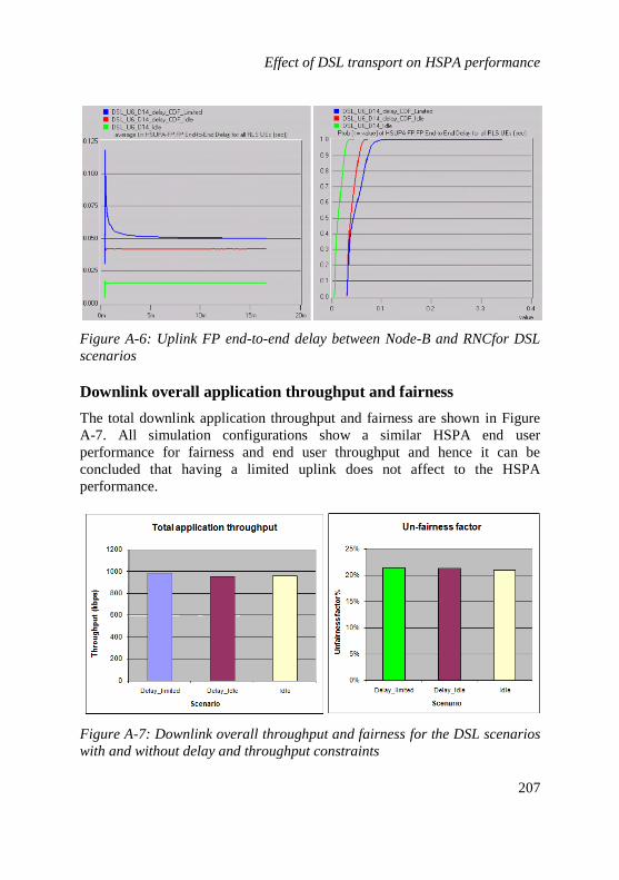
Effect of DSL transport on HSPA performance
207
Figure A-6: Uplink FP end-to-end delay between Node-B and RNCfor DSL
scenarios
Downlink overall application throughput and fairness
The total downlink application throughput and fairness are shown in Figure
A-7. All simulation configurations show a similar HSPA end user
performance for fairness and end user throughput and hence it can be
concluded that having a limited uplink does not affect to the HSPA
performance.
Figure A-7: Downlink overall throughput and fairness for the DSL scenarios
with and without delay and throughput constraints

Effect of DSL transport on HSPA performance
208
A.2 Effects of the DSL fast mode on HSPA
performance
This investigation is performed to analyse the effect of burst errors on the
performance of the HSPA networks. A trace taken from the DSL fast mode
operation is deployed in the simulator as described in chapter 2.3.2
The DSL fast mode operation simulation results are compared with the
default configuration which is described in appendix A.1. The DSL default
configuration uses random errors without considering the effects of impulse
noise and impairment due to neighbouring CPEs (Customer Premises
Equipments). oth “default” and “fast mode” simulation scenarios are
configured with the same FTP traffic model and the same CC configuration.
Per-user application throughput
The per-user throughputs for the uplink and the downlink are shown in the
following left and right of Figure A-8 respectively. From the figures, it can
be observed that there is no significant change in per-user throughputs for
both configurations. The results summaries that DSL burst errors do not have
a significant impact on the HSPA performance.
Figure A-8: Uplink and downlink per-user application throughputs for the
fast-mode DSL scenario
Uplink Downlink

Effect of DSL transport on HSPA performance
209
Total application throughput
The uplink and the downlink total application throughputs are shown in the
left and the right of Figure A-9 respectively. As corresponding to the
previous argument, both configurations show the same performance for the
overall application throughput.
Figure A-9: Uplink and downlink total application throughputs for the
default and the fast mode DSL scenarios
Unfairness factor
The unfairness factors for the uplink and the downlink are showing in left
and right of Figure A-10 respectively. The uplink fast mode shows better
fairness compare to the default mode. However, the unfairness values are not
significant and they both show a very good fairness. The fairness factors for
the downlink are equal for both configurations. In all, there is no significant
impact on fairness for both configurations.

Effect of DSL transport on HSPA performance
210
Figure A-10: Uplink and downlink total unfairness factor for the default and
fast mode DSL scenarios
DSL uplink and downlink throughputs
The DSL link throughputs for uplink and downlink are shown in left and
right of Figure A-11 respectively for both simulation configurations.
Figure A-11: Uplink and downlink total DSL throughputs for the default and
fast mode scenarios
Uplink Downlink

Effect of DSL transport on HSPA performance
211
A bit higher uplink utilisation is shown by the DSL fast mode compared to
default mode, but the overall effect is not significant. The small difference is
due to more retransmissions at RLC layer for the fast mode simulation which
has some bursty losses at the DSL transport network.
DSL end-to-end delay
The uplink and the downlink DSL end-to-end delays for both simulation
configurations are shown in Figure A-12. The fast mode based configuration
has a very low end-to-end delay compared to default configuration for both,
the uplink and the downlink. This is mainly due to that the default
configuration includes the interleaving delay where as the fast mode
configuration does not include it. However, delay variation is same for both
configurations.
Figure A-12: Uplink and downlink total DSL end-to-end delays for the
default and fast mode scenarios
FP end-to-end delay
The FP end-to-end delays for the uplink and the downlink are shown in the
left and the right of Figure A-13 respectively. These statistics show the
overall transport delay between RNC and Node-B. The major part of the
uplink and downlink FP delay is contributed by the DSL end-to-end delay.
Therefore those FP delays correspond to the respective DSL end-to-end
delays.
Uplink Downlink

Effect of DSL transport on HSPA performance
212
Figure A-13: Uplink and downlink total FP end-to-end delays
TCP segment delay
The left and right of Figure A-14 show the end-to-end TCP delay for the
uplink and the downlink respectively. There is no significant difference
between the TCP delays for the default and fast modes. Both configurations
show the same performance at the TCP layer.
Figure A-14: Uplink and downlink TCP delays for the default and fast mode
scenarios
Uplink
Uplink
Downlink
Downlink

Effect of DSL transport on HSPA performance
213
Packet losses at DSL transport network
The left graph of Figure A-15 shows the lost packet numbers over the time.
The packet sequence numbers are reinitialised after they reach the trace
length. The right figure shows the cumulative distribution of the lost packets
for entire simulation run for the downlink for fast mode simulation
configuration. These simulation results match with trace analysis.
Figure A-15 Downlink lost packets at the transport network for the default
and fast mode scenarios
Conclusion
During this investigation, effects of the DSL transport for HSPA end user
performance have been studied. Different QoS parameters such as BER,
delay and jitter have been analysed for the two modes of DSL operations:
DSL default mode and fast mode. The DSL bit errors causes the arrival of
invalid packets whereas the DSL burst errors result in complete packet
losses. All these DSL based packet errors can easily be recovered by the RLC
layer without having impact on the TCP performance. Therefore, simulation
results confirm that neither DSL random bit errors nor burst errors have a
significant impact on the HSPA performance. Further analysis also confirms
that the DSL delay and the jitter not affect the overall HSPA performance. In
summary, the limited DSL network based simulations show similar
Downlink
Lost packets CDF for fast
mode in the downlink

Effect of DSL transport on HSPA performance
214
performance which was achieved by the ATM based transport based
simulations and therefore the expensive ATM transport links can be replaced
by the cheap DSL links without having a severe impact on HSPA
performance.

APPENDIX
B. LTE network simulator
The main objective of the development of the LTE system simulator is to
analyse the end-to-end performance and the S1/X2 interface performance.
The LTE network simulator is implemented in the OPNET simulation
environment. By the time of LTE system network development, there were
no LTE based OPNET models. Therefore, the simulator development was
started with the basic OPNET modeller modules which consist of standard
protocols and network models. As in the HSPA simulator, the LTE network
simulator is also used for some of the standard node entities; it modifies them
according to the LTE protocol architecture. In this chapter, the LTE system
simulator design and development are discussed in detail.
B.1. LTE reference architecture
To achieve the aforementioned objectives, the LTE reference network
architecture which is shown in Figure B-1 is chosen for the LTE simulator
development within the focus of this investigation and analysis. The LTE
transport network of the reference model consists of three routers (R1, R2
and R3) in the reference architecture shown in Figure 1-1. There are four
eNBs that are connected with the transport network via last mile links. EPC
user plane and EPC control plane network entities are represented by the
Access Gateway (aGW) network entity. The aGW includes the
functionalities of the eGSN-C (evolved SGSN-C) and eGSN-U (evolved
SGSN-U). The remote node represents an Internet server or any other
Internet node which provides one of the end node representations. The
average delay for the data transmission between the Internet and aGW is
assumed to be approximately 20 ms. Since the network between these entities
is mainly wired, a lower delay and negligible packet loss ratio can be
experienced.

LTE reference architecture
216
Remote Server (VOIP,
HTTP, FTP, Video)
aGW = eGSN-U, + eGSN-C
R1
R3
R2
eNB4eNB3
eNB2eNB1
Last m
ile link
UEUE UE UE
Figure B-1 LTE reference architecture
The transport network between aGW and eNBs is represented by the network
which includes the three routers: R1, R2 and R3. This network is not owned
by the Mobile Network Operators (MNOs). Therefore, MNOs do not have
complete control over these router functionalities. This is an important issue
which should be considered at the packet level service differentiations.
Mostly MNOs have to control service differentiation for packetized data
traffic mainly at the entrance point of the transport network, which means
service differentiation should be applied at the aGW for the downlink and at
the eNB for the uplink. However, for the downlink direction, the last mile is
the bottleneck which is located between the eNB and the end router, the
router which is closest to the eNB. The transport network DL and UL data
flows are shown in Figure B-2. Any overload situation at the last mile link
causes packet losses mostly at the end router which is directly connected with
the last mile link. Therefore, a certain degree of service level guarantees also
have to be provided by the routers in the transport network. Since the last

LTE model architecture
217
mile in the uplink is directly located at eNB, traffic differentiation can be
more effectively controlled at eNB by MNOs for the uplink transmission.
eNB1aGW
ULDL
ULDL
Last mile router
Last mile link
Transport network
Figure B-2: LTE transport network DL and UL data flows
Inside the reference LTE architecture used in this investigation, there are four
eNBs where each of them controls three cells. As mentioned in chapter 2.4,
the eNB is one of the key elements in the E-UTRAN network. It connects to
the transport network through the S1 and X2 interfaces at one side of the
network; at the other end, it connects with users through the Uu interface.
Therefore it includes all radio interface related protocols such as PHY, MAC,
RLC, PDCP etc. and all transport protocols such as GTP, UDP, IP, Layer 2
and Layer 1 (Figure 2-15). At the transport side of the eNB it provides
service differentiation for the uplink data flow when it sends data to the
transport network. Any congestion situation at the last mile has to be
controlled by eNB for the uplink and therefore the uplink service
differentiation along with traffic shaping plays a significant role for data
handling. These aspects of eNB are discussed in detail in this chapter.
B.2. LTE model architecture
Based on the above reference protocol architecture, Figure B-3 shows a
simulator overview of the LTE system simulator in the OPNET environment.
Each eNB can be configured with a variable numbers of users. For example,
the proposed simulator overview shows a 10 UEs/cell configuration however
simulation model is flexible of configuring any user constellation along with
the mobility based on requirements of the analysis. Required applications for
each user and also the servers are configured in the application configuration
(upper left corner) and user configuration profiles. In OPNET, profiles group

LTE model architecture
218
the users according to their selected application these configured user profiles
have to be activated at each UE entity.
Figure B-3: LTE simulation model overview
Any mobility model can be included within the mobility network and can
activate any user based on their individual mobility requirements. Currently
most generic mobility models such as Random Way Point (RWP) and
Random Directional (RD) are implemented and readily available for the
configuration. As mentioned above, all UE mobility information is stored and
updated regularly in the central database (also called global user list) where it
can be accessed at any time.
Three main node models have been developed with respective user plane
protocols within the simulator. They are
UE node model,
eNB node model,

LTE model architecture
219
aGW node model.
Next, the details about these node models are discussed.
UE node-model
The UE node model is created according to the layered hierarchy shown in
Figure B-4.
Figure B-4: UE node model
When creating a UE in the network simulator, one instance of this node
model is created. All the attributes related to the layers can be configured
individually. The node model includes two sets of protocols: the LTE air
interface related protocols and the end user application protocols. The LTE
Uu protocols include PDCP, RLC, MAC and PHY layers. Except for the
PHY layer protocol, all other protocols have been implemented according to
the 3GPP specification [47] in the respective layers. The physical layer is
modelled to transmit the transport blocks of user data between eNB and UE

LTE model architecture
220
entities in order to model physical layer characteristics from the system
simulator point of view without having explicit detailed modelling. This is
done by the MAC scheduler which has been designed to emulate the PHY
layer characteristics in terms of data rate or TB size/TTI for each UE entity.
More details about the MAC scheduler and the MAC layer protocol
functionalities are discussed in chapter 2.4.3.
eNB node-model
The protocol layers of the eNB node model are shown in Figure B-5. The
creation of any eNB includes the instance of this node model. It includes all
the protocols which are required by the standard eNB entity. The attributes of
each layer in the eNB can be configured independently..
Figure B-5: eNB node model
The right hand side protocols of the node model in Figure B-5, the PDCP,
RLC and MAC layers represent the Uu related functionalities whereas the
left hand side protocols of the node model, the GTP, UDP, IP and Ethernet
layers represent the transport related functionalities. The MAC scheduler is
located at the MAC layer in the eNB. It is the key functional element which
interacts with all other Uu protocols. There are three schedulers which are
implemented on a cell basis within a single eNB node model. Each scheduler

LTE model architecture
221
works independently based on the cell configuration. The core controller
which connects the data flows from three cells combines and forwards the
data flows to the upper layers. IPsec and the service differentiation are
performed at the IP layer in the eNB. The diffserv model is implemented in
the eNB node model mainly for the uplink and partly for the downlink. The
model includes traffic differentiation and scheduling in the IP layer and
shaping functionalities at the Ethernet layer. More details about those
functionalities are given in the chapter 2.4.3.2.
aGW node model
aGW user plane transport protocols which are implemented in the simulator
are shown in Figure B-6.
Figure B-6: aGW node model
One part of the peer to peer transport protocols, GTP, UDP, IP and Ethernet,
are at the side of the transport network whereas the other part is at the side of
the remote server side. Figure B-6 shows the two GTP process models, GTP0

LTE protocol development
222
and GTP1, which can be used for the uplink and downlink separately if two
end nodes are connected for those traffic flows. If one server is used for the
downlink and the uplink applications then either GTP0 or GTP1 can be used
for both functionalities. In addition to the diffserv model, the IPSec
functionality (according to specification [46]) is also implemented within the
IP layer in both aGW and eNB node entities in order to provide data security
over the transport network. There are two Ethernet interfaces which can be
linked to the transport network based on the connectivity. Currently one
interface is connected to the transport network. The other interface is left for
any other extension of the model further investigations.
So far, an overview about the LTE system simulator has been discussed.
During the LTE simulator development, most of the standard protocols such
as application, TCP, UDP and all adaptation layer protocols were used
without any modifications. However some of the protocols such as IP and
Ethernet are modified according to the LTE requirements. There is another
set of protocols which is newly added to the simulator based on the specific
requirement of the 3GPP LTE network and it has been discussed in chapter
2.4.3. The next section discusses the modified and new protocols in detail.
Further it provides an overall protocol user plane architecture which is the
main focus of the simulator development.
B.3. LTE protocol development
Figure B-7 shows the overall LTE user plane protocol architecture which is
used to develop the LTE simulator. All protocols can be categorised into
three groups, radio (Uu), transport and end user protocols. The radio (Uu)
protocols include the peer-to-peer protocols such as PDCP, RLC, MAC and
PHY between the UE and eNB entity. The detailed physical layer modelling
is not considered in this simulator. However, effects of radio channels and
PHY characteristics are modelled at the MAC layer in terms of the data rates
of individual physical channel performance. The modelling of PHY layer
characteristics within the MAC layer is discussed later in this section.
The RLC is used to recover any losses over the air interface which cannot be
recovered by the MAC HARQ mechanism. The RLC protocol is
implemented in the simulator according to the 3GPP specification [73]. Since
the LTE RLC protocol functionalities are not different from the HSPA

LTE protocol development
223
implementation, the detailed implementation procedure is not discussed in
this chapter.
PDCP
RLC
MAC
L1
End User
Application
TCP/UDP
IP
Uu
PDCP
RLC
MAC
L1
GTP
UDP
IP (Diffserv)
L1
L2
IPSec
L2
L1
GTP
UDP
IP (Diffserv)
L1
L2
IPSec
L2
L1
Application
servers
Application
(server)
TCP/UDP
IP
S1/X2
aGWeNodeB
Figure B-7: overall LTE protocol architecture
The PDCP protocol is used to process the data from different IP flows based
on protocol specification. This protocol is used not only for data handling in
the radio interface but also for the data handling in the transport network
when UE performs the inter-eNB handovers. More details about this protocol
are discussed in the following section.
Figure B-7 also shows the user plane transport protocols which are a
common set of protocols that are used in both the S1 and X2 interface. It
includes the GTP, UDP, IP and L2 protocols. Ethernet is used as the layer 2
protocol for the current implementation; however the model is implemented
in such a way that it can use any other transport protocol with a slight
modification to the node model. IP is one of the key protocols which handle
routing, security (IPsec), service differentiation and scheduling
functionalities at the transport network. The default OPNET IP layer is
largely modified by adding the above-mentioned functionalities IPsec and
Diffserv based on the specific LTE requirements [49].

LTE protocol development
224
All control-plane protocol development is not directly considered within the
LTE simulator. However effects of the signalling such as overhead and delay
are taken into consideration at the respective design of the user-plane
protocols.
PDCP protocol development
The PDCP layer user-plane protocol is also implemented according to the
3GPP specification [49] in the UE and the eNB entities. The state process
model of the PDCP protocol implementation is shown in Figure B-8.
The main PDCP functionalities which are implemented in this protocol can
be summarised as follows:
bearer identification and packet classification based on the traffic
QoS,
per-bearer based PDCP buffer management,
encapsulation and de-capsulation of PDCP PDUs and packet
forwarding techniques,
data handling during inter-eNB handovers (X2 packet forwarding, reordering
and error control etc.).
Figure B-8: peer-to-peer process model for PDCP protocol
After setting up initial bearers, based on IP packet arrivals, each bearer
connection is identified and classified using IP header information. Each
bearer connection has individual PDCP buffers and data is stored in these
buffers until it is served.
For the LTE network, the main data buffers are located at the PDCP layer.
The PDCP buffers have been implemented on a per-bearer basis. However

LTE protocol development
225
they use common shared memory space in the eNB entity. In contrary to this,
at the UE side, the shared buffer capacity is allocated on a per-user basis. The
timer based discard, RED (Random Early Detection) and the simple drop-tail
buffer management techniques have been implemented on these per-bearer
PDCP buffers and are explained in the following.
The timer based discard mechanism discards the packets if they exceed the
configured maximum delay limit. Packets can be delayed for a long time
mostly due to two reasons: either the radio channel of the user is very bad or
some TCP connections staled or timed-out due to congestion in the network.
In the first case, since the user channel quality is bad, by discarding the
packet at PDCP, feedback is provided to the TCP source for flow control and
hence the offered user load is controlled by TCP dependent on the available
channel capacity. In the second case, packets due to an invalid TCP
connection should be discarded before they are being transferred over the Uu
interface. Not only for the best effort traffic sources but also for real time
traffic sources, such a delay-based discard mechanism can be beneficial. It
also avoids unnecessary transmissions of delayed packets over the network.
In a nutshell, this buffer management technique avoids wastage of the scarce
radio resources and enhances network resource utilisation.
The RED buffer management scheme uses a TCP friendly random discarding
approach. It maintains a lower and an upper buffer limits with two different
drop probabilities. Based on the filling level of the buffer from lower
threshold to upper threshold, the packet discarding probability increases
linearly. Due to the random discards, in-sequence multiple losses are avoided
and TCP adapts to the data flows dependent on the capacity of the network.
Further details about the RED scheme which is implemented in the simulator
can be found in [74, 75, 76].
The mechanism of the tail-drop buffer management is very simple. Whenever
the buffer exceeds its capacity, all packets are dropped. All above PDCP
related buffer management techniques have been implemented in the LTE
simulator in such a way that these parameters can be configured individually
based on specific QoS requirements for each case.
Apart from buffer management techniques, all other PDCP related protocol
functionalities such as data encapsulation, decapsulation, forwarding etc.
have been implemented according to the 3GPP specification [49]. Before

LTE protocol development
226
sending the packet to the lower layer, the PDCP layer encapsulates the IP
packets into PDCP PDUs. In contrary to this, the decapsulation of data from
PDCP PDUs is performed at the receiver PDCP entity. The PDCP protocol is
also responsible for secure X2 forwarding during handovers. Mainly, the
implementation supports the reordering, in-sequence delivery and error
handling (ARQ) during inter-eNB handovers.
GTP and UDP protocol development
At the transport side, GTP (GPRS Tunnelling Protocol) creates the transport
tunnel over the UDP protocol between eNB and other end-node which can be
either aGW or peer eNB entity. The state model of the GTP protocol is
shown in Figure B-9. At the aGW side, there are two GTP state models
GTP1 and GTP2 running in parallel which process the uplink and downlink
flows separately when flows are distinct to different end nodes. The same
processes model is used for both nodes. When the aGW is only connected to
a single server, one process, either GTP0 or GTP1, can be used for both
flows. All these GTP protocol functionalities have been implemented in the
simulator according to the 3GPP specification (46, 49).
Figure B-9: GTP protocol process model

LTE protocol development
227
IP diffserv model implementation
In addition to the generic IP routing protocol functionalities, the advanced
service differentiation model (diffserv) is implemented in the IP layer of the
eNB for the uplink. The diffserv model consists of three main functional
units, which are the packet classification unit, the scheduler unit and the
buffer management unit. According to the QoS requirements, the service
flows are differentiated and packets are classified using the Differentiated
Services Code Point (DSCP) values on the diffserv field (type of services,
ToS field) in the IP header of the IP PDU. The LTE transport network uses
the differentiated service architecture for transport network packet
classification which is defined in in RFC 2474 and RFC 2475. The DSCP
values are used to mark the per-hop behaviour (PHB) decisions about the
packet classification to provide the appropriate QoS treatment at the transport
network. After the packet identification and classification process they are
stored in the respective PHB (Per-Hop Behaviour) buffers. The complete
diffserv model with PHBs is shown in Figure B-10.
Figure B-10: diffserv model architecture

LTE protocol development
228
The PHBs can also be categorised into three distinct QoS classes, which are
Expedited Forwarding (EF), Assured Forwarding (AF) and Best effort (BE)
or default PHB. The LTE uplink diffserv model is built with 1 EF PHB, 4 AF
PHBs and 1 BE PHB which are used to classify the incoming service flows at
the IP layer. Three virtual priority queues (drop precedence) are created
within each AF PHB physical queue which further prioritises the service
flows based on their QoS requirements. The detailed classification which is
implemented in the diffserv model is shown in Table B 1.
Table B 1: Assured forwarding service classification
Drop
precedence
Assured Forwarding (AF) PHBs
PHB_AF4x PHB_AF3x PHB_AF2x PHB_AF1x
DP Level 1 PHB_AF41
(DSCP 34)
PHB_AF31
(DSCP 24)
PHB_AF21
(DSCP 18)
PHB_AF11
(DSCP 10)
DP Level 2 PHB_AF42 (DSCP 36)
PHB_AF32 (DSCP 28)
PHB_AF22 (DSCP 20)
PHB_AF12 (DSCP 12)
DP Level 3 PHB_AF43
(DSCP 38)
PHB_AF33
(DSCP 30)
PHB_AF23
(DSCP 22)
PHB_AF13
(DSCP 14)
The scheduler unit has been implemented to provide the required service
priorities for these PHBs. It consists of strict priority queuing and weighted
fair queuing disciplines. Since EF PHB handles the services which are delay,
loss and jitter sensitive such as signalling and control traffic, the scheduler
provides strict priority for this PHB class Furthermore, it provides serving
capacities for the AF classes based on their configured weights. In the
weighted fair queuing scheduler, the lowest priority is assigned to a BE PHB
class which is used to handle non-real time services such as HTTP traffic and
FTP traffic. Whenever the AF PHBs are not using the capacity based on their
assigned weights, the remaining excess capacity is always allocated to the
default (BE) PHBs.
Except EF PHB, all others use the RED or the weighted RED (WRED)
buffer management techniques which are implemented in the BE PHB and
the AF PHBs respectively [77]. The WRED combines the capabilities of the
RED algorithm to provide preferential traffic handling of higher priority
packets. It selectively discards lower priority traffic when the interface begins
getting congested and provides differentiated performance characteristics for
different classes of services. More details about the implementation of RED
and WRED is given in the reference [75, 76].

LTE protocol development
229
Ethernet shaper implementation
The L2 shaping functionality is implemented at the Ethernet layer and
provides serving triggers to the diffserv scheduler. The shaping model is a
single rate shaper which uses the token bucket principle [50]. The
configurable CIR (Committed Information Rate) rates and the CBS
(Committed Burst Size) are the two main configurable parameters for the
shaper. The basic shaper functionalities are shown in Figure B-11.
Figure B-11: Ethernet Shaper functionality
The shaper receives Ethernet frames from its input buffer, which are formed
as soon as IP packets are picked from the scheduler. The shaper’s input
buffer is treated as a FIFO, and its size is set to a configurable value (for
example 4 KB). In order to optimise the transport network utilisation, the
shaper generates a scheduling request towards the diffserv scheduler
whenever the input buffer has at least a certain empty buffer space, for
example 2 KB. Based on the CIR, arriving Ethernet frames are served to the
lower layer using a token bucket scheme which is described in [50].

LTE protocol development
230
LTE MAC scheduler
The LTE MAC scheduler is one of key elements located in the eNB entity. It
distributes the available radio resources among the active users. As discussed
in chapter 0, it operates in both time and frequency domain by sharing the
resources in small units called PRBs (Physical Resource Block). The MAC
scheduler is directly connected with the eNB Uu protocols such PDCP, RLC
and PHY through the signalling channels. All these information is used in
order to take decisions when allocating resources to the users in an effective
manner. This section summarises the eNB scheduler design and
implementation for the LTE system simulator.
The eNB maintains three cells, where each of them has two independent
MAC schedulers for the uplink and the downlink. The state process model
for the scheduler is shown in the following Figure B-12. It consists of 6
decision state models and one arrival state model. All other states are used
for the initialisation and signalling activities.
Figure B-12: eNB MAC scheduler process model
From this point onward, the common platform for the uplink and the
downlink MAC schedulers is discussed in detail in the following paragraphs.
Differences between the uplink and the downlink scheduling are highlighted
separately.

LTE protocol development
231
From the design and implementation point of view, the scheduler consists of
a time domain (TD) scheduler and a frequency domain (FD) scheduler which
are shown in Figure B-13.
Figure B-13: architecture of the eNB MAC scheduler
The TD scheduler performs the user identification, QoS classification and
bearer prioritisation as the main functions. The FD scheduler effectively
serves available radio resources among the users who have been already
prioritised and selected by the TD scheduler. In this case, depending on the
scheduling disciplines the amounts of resources which are allocated to each
user are served by the FD scheduler. For the current LTE simulator, two main
scheduling disciplines have been implemented in the LTE simulators which
are fair scheduling (Round Robin, RR) and exhaustive scheduling.
Key design considerations and assumptions
The key design principles and assumptions are described as follows.
As mentioned in chapter 2.4, the available number of PRBs depends
on the allocated BW (scalable from 1.4 MHz to 20 MHz). For
example, a 10 MHz frequency spectrum consists of 50 PRBs
whereas a 20 MHz includes 100 PRBs. The PRBs are scheduled
every TTI which is 1 millisecond.
The uplink scheduling uses the same time interval as the smallest
unit for scheduling in every TTI. However for the downlink
scheduling, a Resource Block Group (RBG) is defined as the
smallest unit by considering the overall scheduling efficiency and
the simplicity of the downlink scheduling. The relationship between
the RBG and the bandwidth is shown in the following table.

LTE protocol development
232
Table 6-1: LTE supported BWs
It is possible to allocate any number of RBGs for a particular
connection which is completely dependent on the scheduler
decision. These RBGs do not require being in consecutive order in
the frequency domain; they can be rather distributed based on their
channel characteristics with different frequencies and MCS.
However all PRBs within one RBG use the same MCS values to
achieve a high processing gain by reducing the complexity. For the
uplink scheduling, individual PRBs are allocated to users and they
are required to be in consecutive order in the frequency domain.
The signalling (SRB1, SRB2 and QCI5) has low data volume
compared to the offered traffic volume and the signalling packets
are also not as frequent during the transmission as other traffic.
Therefore the signaling overhead is neglected for the scheduling
which is one of the key assumptions for this scheduler design.
Downlink scheduling is done on a per-bearer basis whereas uplink
scheduling is done on a per-connection or per-UE basis. Further the
first phase of the scheduler design only considers a few QCI bearer
types such as QCI1, QCI7, QCI8 and QCI9.
Procedure for scheduling
The scheduling procedure can be described by three main steps. They are
bearer identification and bearer classification,
bearer prioritization and resource allocation,
Scheduling and resource assignments.
The first two steps (a and b) mainly describe the TD scheduler functionality
which considers the QoS aspects and buffer occupancies for each active
bearer connection whereas the last step focuses on the FD scheduler

LTE protocol development
233
functionality which defines the physical layer characteristics of the bearer
connection along with the resource allocation in terms of PRBs.
Bearer identification and Bearer classification
The Scheduling Candidate List (SCL) is created by listing all active users
who have data in their buffers. The BSR (buffer status report) provides the
details about the buffer occupancy for each bearer connection which indicates
the data availability at PDCP and RLC transmission and retransmission
buffers including their volume information. For the system simulator, it is
assumed that the BSR reports are received in the MAC entity with zero
delay. Depending on the QoS priorities and the pending retransmissions, the
selected bearers which are in the SCL list are grouped. For example, separate
lists can be defined based on this classification such as SCL-1 for pending
retransmission bearers, and SCL-2 for data bearers.
Bearer prioritisation and resource allocation
All users who have pending retransmissions are selected with highest priority
for the scheduling. All others are prioritised based on a common weighting
factor which is defined based on several factors such as the bearer type either
GBR or non-GBR, channel characteristics, buffer occupancy and the
accumulated data volume. This common weighting factor can be divided into
two main categories, the Proportional Fair (PF) term and the bearer QoS type
(GBR or Non-GBR) based weighting term. For the LTE system simulator,
the current channel capacity of the bearer is defined by the PF term. The
GBR-related weight factor is defined for the real time services such as the
VoIP whereas the Non-GBR related weight factor is defined for the best
effort services such as web browsing and large file downloads. Finally the
simplified version of the common weight factor (CWF) for scheduling is
defined as follows.
equation 6-1
Based on this common weight factor rating, the users in the data bearer list
are prioritised for the scheduling. The PF term includes the per-UE
throughput which is calculated based on two key parameters, which are the
number of PRBs (or RBGs) and the final MCS value for a particular
connection. The input parameters such as MCS can be taken either from

LTE protocol development
234
literature or dedicated radio simulation. The number of PRBs is selected by
the FD scheduler based on the selected scheduler discipline which is
discussed in the next section.
Scheduling and resource assignment
Two FD schedulers, the Round Robin (RR) and the exhaustive scheduler are
implemented in the simulator. The RR FD scheduler uses a fair approach
compared to the exhaustive FD scheduler. Both schedulers use maximum up
to “n” UEs for scheduling in each TTI. If the number of users who have data
in the transmission buffer is less than the maximum number (“n”), then these
users are taken for the current scheduling, otherwise always “n” UEs are
scheduled in a TTI.
For the RR scheduler, the number of PRBs for each user is calculated simply
by dividing the spectrum by the number of users, “n”.
equation 6-2
The number of PRBs for DL transmission should be determined in terms of
RBGs which depends on the configured BW as described at the beginning of
the scheduler description. Depending on the channel, users can achieve
different data rates with the same number of PRBs for the RR FD scheduler.
The exhaustive FD scheduler in UL and DL allocates full resources to the UE
who is at the top of the priority list for the current TTI. The priority list is
created by the TD scheduler. The maximum resource limit of the UL priority
user is decided either by UE power limitation and also by the input taken
from the radio simulator or the available data volume for the exhaustive FD
scheduler whereas the DL users are allowed to use even full spectrum within
the current TTI if they have sufficient data in the buffer for the current
transmission. When the MCS and the number of PRBs are known for each
bearer, the transport block size (TBS) is determined using table 36.213 of the
3GPP specifications.
Modelling HARQ
For modelling HARQ, a simplified approach is used as in HSPA. It can be
assumed that the BLER is 10% with a maximum of three retransmissions.
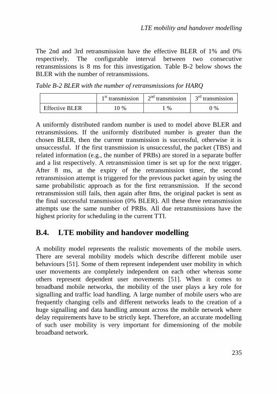
LTE mobility and handover modelling
235
The 2nd and 3rd retransmission have the effective BLER of 1% and 0%
respectively. The configurable interval between two consecutive
retransmissions is 8 ms for this investigation. Table B-2 below shows the
BLER with the number of retransmissions.
Table B-2 BLER with the number of retransmissions for HARQ
1st transmission 2nd transmission 3rd transmission
Effective BLER 10 % 1 % 0 %
A uniformly distributed random number is used to model above BLER and
retransmissions. If the uniformly distributed number is greater than the
chosen BLER, then the current transmission is successful, otherwise it is
unsuccessful. If the first transmission is unsuccessful, the packet (TBS) and
related information (e.g., the number of PRBs) are stored in a separate buffer
and a list respectively. A retransmission timer is set up for the next trigger.
After 8 ms, at the expiry of the retransmission timer, the second
retransmission attempt is triggered for the previous packet again by using the
same probabilistic approach as for the first retransmission. If the second
retransmission still fails, then again after 8ms, the original packet is sent as
the final successful transmission (0% BLER). All these three retransmission
attempts use the same number of PRBs. All due retransmissions have the
highest priority for scheduling in the current TTI.
B.4. LTE mobility and handover modelling
A mobility model represents the realistic movements of the mobile users.
There are several mobility models which describe different mobile user
behaviours [51]. Some of them represent independent user mobility in which
user movements are completely independent on each other whereas some
others represent dependent user movements [51]. When it comes to
broadband mobile networks, the mobility of the user plays a key role for
signalling and traffic load handling. A large number of mobile users who are
frequently changing cells and different networks leads to the creation of a
huge signalling and data handling amount across the mobile network where
delay requirements have to be strictly kept. Therefore, an accurate modelling
of such user mobility is very important for dimensioning of the mobile
broadband network.

LTE mobility and handover modelling
236
Within the LTE system simulator, mainly UE mobility is considered for the
intra-LTE (intra-eNB and inter-eNB) handover modelling. The details of
intra-LTE handovers have been discussed in chapter 2.4.5. The main goals of
this analysis are to evaluate the impact of the additional load due to
handovers on the transport network (X2/S1) performance and on the end user
performance. Further, in order to provide seamless mobility for end user, the
handover data must not be delayed over the transport network and is required
to be prioritised.. The intra-LTE handovers along with the user mobility are
modelled within the simulator to investigate and analyse all aforementioned
objectives. The individual handover frequency of each connection and its
carried load are the key parameters that have to be considered during
handover modelling. The UE handover frequency depends on many factors
such as the selected mobility model, the UE speed etc. Depending on the
number of users in the cell and their traffic models, the offered handover load
over the transport network also differs. Therefore by considering all these
factors, a simple, novel approach for intra-LTE handovers is designed and
implemented in the LTE simulator. The new approach provides a great
flexibility to use any mobility model or to configure any handover scenario
individually based on the focused investigation.
Within the new approach, the UE mobility which mainly provides the carried
data rates during handovers depending on the location of the UE (or distance
to eNB) and the UE handover decision are decoupled. Therefore, the model
provides a great flexibility to use any mobility model. Further the handover
frequency can be configured separately within the model and hence different
handover scenarios can be configured to analyse the impact on the transport
network individually upon the focused investigation.
The section is organised as follows. A brief overview about generic mobility
models and the design and development of an enhanced mobility model are
described in the following paragraphs. A modified random directional
mobility model is developed according to the reference architecture which
was described in appendix B.1.
This model provides the UE location details to the MAC scheduler in the
serving eNB to manage the resources among the active UEs in the cell. A
novel approach of modelling intra-LTE handovers and X2 data management
for inter-eNB handovers are described at the end of this section.

LTE mobility and handover modelling
237
Generic mobility models
The commonly used generic mobility models are the random walk [51, 52],
random way point and random direction [51]. All these three models use the
random mobility of mobile nodes within a predefined area. The speed and
direction changes occur at a reasonable time slot and the different movement
parameters are altered within predefined ranges, for example the speed
ranges between maximum and minimum values and the direction within the
range 0 and 2 . The main difference between the random walk and the
random way point mobility models is that the random walk mobility model
does not use a pause when a user changes his direction of travelling as in the
random way point mobility model. However these two mobility models have
the issue of a “density wave” in which the most of the mobile nodes are
clustered to the center of the area. To avoid such clustering effects and also to
ensure that all mobile nodes (MNs) are randomly distributed over the area,
the random direction mobility model is introduced. In this mobility model,
the mobile nodes or users change the direction of travelling at the boundaries
of the predefined area. The mobile node travels towards a selected direction
with a certain speed until it reaches the boundary of the predefined area and
then changes the direction randomly after a certain pause period. By studying
all these generic random mobility models, an enhanced mobility model is
developed for the LTE system simulator. Further the inter-LTE handovers are
also implemented within this mobility model.
Enhanced random mobility model
As described in chapter 2.4.5, the LTE system simulator is configured with 4
eNBs running 3 cells each for this investigation. Therefore users who move
among these 4 eNBs have inter-eNB and intra-eNB handovers. Figure B-14
shows the generic view of the cell architecture and user mobility within those
cells and eNBs for a certain scenario. For the modelling of the mobility
within the reference LTE architecture, the 4 eNB along with 3 cells each are
selected as marked in the Figure B-14.
Each eNB maintains three hexagonally shaped cells. Four circles are drawn
to represent the coverage of the four eNBs inside the LTE simulator. Users
randomly move from one cell to another by making inter-cell and inter-eNB
handovers which mostly occur at the edges of the cell coverage. Intra-eNB
handovers do not have a significant impact on the transport network since the

LTE mobility and handover modelling
238
main data buffering occurs at the same eNB. However the situation is more
crucial when a mobile node is performing inter-eNB handovers. As
described in chapter 2.4.5.1, the buffered user data in one eNB has to be
transferred to the other eNB where the mobile node is moving to. All this
data management within the transport network is discussed in this section.
Figure B-14: cell architecture of four eNB scenario, the mobile users marked
as blue colour
The simplified mobility modelling is considered to implement user mobility
when a UE performs intra-eNB and inter-eNB handovers within the
reference LTE architecture. Mobile nodes are moving according to the
modified random directional mobility model across the circular coverage area
of the eNB. Here, modified random directional mobility means whenever a
mobile node changes the direction by reaching the boundary, it does not stop
moving, i.e. the pausing period is zero as in the random walk mobility model.
Since the handover frequency does not depend on the user mobility for the
new apporach, the following key assumptions are taken for the development
of the LTE mobility model.

LTE mobility and handover modelling
239
The transmission range of a eNB is uniform and the coverage area is
represented by a circle.
All mobile nodes are uniformly distributed across the coverage area.
Only four eNBs are considered for this implementation and one eNB
covers three cells.
The total number of active users within these 4 eNBs is constant. All
users perform handovers and user mobility within this four eNB
constellation.
From the modelling point of view, each eNB coverage area is divided into
two zones denoted by an inner circle and an outer circle as shown in Figure
B-15. Mobile nodes in the outer zone can only perform inter-eNB handovers.
However intra-eNB handovers can be performed within both circles. The
three cells which form the coverage area are modelled by three sectors as
shown in Figure B-15.
The next section describes the statistical approach for the intra-LTE
handovers in which handover decisions are taken for each connection
independently.
Figure B-15: eNB coverage area zones
Statistical approach for intra-LTE handovers
The handover decision is taken according to the statistical approach that can
be taken from the literature for each mobile node separately. For example, a
UE handover occurs uniformly distributed between “t1” and “t2” with mean
“tm”. In this case any probability distribution can be deployed for the

LTE mobility and handover modelling
240
handover decision of each Node-Based on the probabilistic distribution or
trace. Since simulations are performed for a considerably long period of time
within the system simulator, the statistical measures of intra LTE handovers
such as handover frequency in terms of mean and variance are important for
each mobile node. In such cases, the exact load over the transport network
can be simulated based on their traffic model. According to above example
scenario, the mobile node can take a handover decision to any of the 4 eNBs
with the mean interval of “tm”. However when the handover decision is
taken, the UE may be outside of the outer circle in the eNB. In this case, the
UE cannot make the handover decision immediately and has to hold the
decision for example “Δt” time interval until it reaches the outer circle of the
eNB. Therefore, the mean inter-eNB handover duration should be calculated
according to the following equation.
equation 6-3
If the handover decision occurs when the mobile node or UE is in the outer
zone of the eN , then “Δt” is equal to zero and the handover is performed
immediately. The general concept of inter-eNB handovers can be described
according to the following example Figure B-16.
Figure B-16: Inter-eNB handovers functionality

LTE mobility and handover modelling
241
In this example scenario, the UE is moving from eNB1 to eNB3 and the
handover occurs within the outer circle area. The distance to eNB1 just
before the HO is represented by r1 and just after the handover (to eNB3) by
r2. During the inter-eNB handover process the parameters eNB_id, cell_id,
distance to transmitter and direction (eNB3 point of view) is changed.
Since there are four eNBs in the simulator, the UE can randomly perform
inter-eNB handovers to any of the other eNBs. Therefore the eNB id can be
randomly selected one out of the numbers {1, 2, 3 and 4}. The new cell id
can also be selected one out of the number {1, 2 and 3}. The distance to the
transmitter (or target eNB) can be any point in the outer zone and also the
direction can also be random. By considering all above facts, the modelling
of inter-eNB handovers is simple and efficient. Whenever the handovers
occur, these mobility parameters can be selected for each node separately
which represents the real handover situation from the system simulator point
of view. The important fact for the transport network in order to perform X2
forwarding is how often the inter-eNB handovers occur as well as the timing
and the changes of eNBs. This example handover scenario is also elaborated
in Figure B-17 with one eNB convergence zone.
Figure B-17: inter-eNB handovers mobility representation
Further, Figure B-17 on the right shows the four users’ mobility with inter-
eNB handovers within the LTE simulator. The four colours represent the four
users’ mobility behaviour separately.
As shown in the above example, the UE parameters are changed at the
handover location according to the probabilistic approach. All user
information including mobility and location information are sent and stored
in the central data base. As soon as UE makes any change about it location
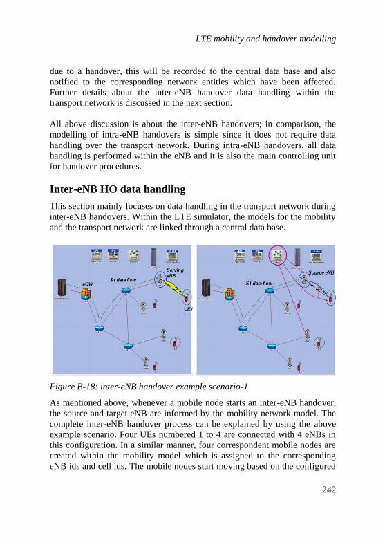
LTE mobility and handover modelling
242
due to a handover, this will be recorded to the central data base and also
notified to the corresponding network entities which have been affected.
Further details about the inter-eNB handover data handling within the
transport network is discussed in the next section.
All above discussion is about the inter-eNB handovers; in comparison, the
modelling of intra-eNB handovers is simple since it does not require data
handling over the transport network. During intra-eNB handovers, all data
handling is performed within the eNB and it is also the main controlling unit
for handover procedures.
Inter-eNB HO data handling
This section mainly focuses on data handling in the transport network during
inter-eNB handovers. Within the LTE simulator, the models for the mobility
and the transport network are linked through a central data base.
Figure B-18: inter-eNB handover example scenario-1
As mentioned above, whenever a mobile node starts an inter-eNB handover,
the source and target eNB are informed by the mobility network model. The
complete inter-eNB handover process can be explained by using the above
example scenario. Four UEs numbered 1 to 4 are connected with 4 eNBs in
this configuration. In a similar manner, four correspondent mobile nodes are
created within the mobility model which is assigned to the corresponding
eNB ids and cell ids. The mobile nodes start moving based on the configured

LTE mobility and handover modelling
243
speed in the UE configuration with random directions. When a mobile node
performs an inter-eNB handover, the following processing is performed for a
successful handover.
Figure B-18 shows that the mobile node is currently connected with eNB1
and data to the mobile node is transferred via the S1 interface through the
transport network. The UE1 is for example downloading a file from an
Internet server where the data flow is originated. The UE1 is directly mapped
to the mobile node 1 in the mobility network model. The right side of Figure
B-19 shows that UE sends the handover indication (chapter 2.4.5) to both the
target eNB and the source eNB. Once the handover starts at the source eNB,
it stops sending data to the UE and starts forwarding data to the indicated
target eNB. All these events such as handover indication, stopping the
transmission and the start of sending data over the X2 to the target eNB
occurs based on the predefined time period which was taken from a trace file
or from derived distributions. All incoming data is buffered at source eNB
and forwarded to the target eNB via the X2 interface while the mobile node
completes its handover procedure over the Uu interface (the duration is again
determined using a statistical approach or a trace).
Figure B-19: inter-eNB handover example scenario-2
Figure B-19 shows this data forwarding process over the transport network
between the source and target eNB.

LTE mobility and handover modelling
244
Figure B-20: inter-eNB handover example scenario-3
Once the UE is successfully connected with the target eNB, all buffered data
is immediately transferred to the UE. As discussed in chapter 2.4.5, the target
eNB also starts the path switching process by sending a signal to the aGW at
the same time. When the path switching process is completed, the aGW
switches the S1 data path directly to the target eNB and also triggers the end
markers to terminate the data flow through the source eNB path. When the
end marker is received by the source eNB, it transparently forwards it to the
target eNB by terminating the handover process in its own entity. When the
end marker is finally received by the target eNB, all X2 forwarding and
handover activities are terminated by the target eNB as well. Figure B-20
shows the final data flow through the S1 interface to the UE1 of the target
eNB.
During data forwarding over the X2 interface between the source and target
eNB, a new GTP tunnel over the UDP protocol is created. All in-sequence
data delivery and error handling are performed by the PDCP protocol
between the source target eNB according to the guideline highlighted by
3GPP specification [49]. All transport prioritisation and routing
functionalities are handled by the IP protocol within the transport network.
The transport priorities can be configured within the simulator as user
requirements. The complete summary of the inter-eNB handover procedures
are shown in Figure B-21.

LTE mobility and handover modelling
245
Figure B-21: Summary of the Inter-eNB handover procedure in the transport
network
It also shows the example timing triggers and periods for each handover
trigger. Further, Figure B-21 shows that the end marker arrival time is
dependent on the traffic load situation in the transport network. When the
transport is congested, the end marker traverse duration through S1 is longer
compared to non-congested transport. Therefore the overall handover
duration is determined not only by the statistical time periods but also by the
transport network loading situation as well. For the worst case scenarios,
there are expiry timers which are activated to terminate the handover process
by respective network entities. One example scenario is that if the end marker
is lost during the transmission due to the congestion in the transport network,
it will not be received by either the source eNB or target eNB. Therefore, the
end marker related timers at the source target eNB expire and all handover
processes are terminated accordingly.
Intra-eNB HO
The intra-eNB data handling is described in chapter 2.4.5.2. This section
summarises the implementation procedure within the LTE simulator. The
intra-eNB handover is explained using the following example scenario where

LTE mobility and handover modelling
246
UE1 moves from cell 1 to cell 2 within the same eNB (eNB1). Figure B-22
shows that UE is communicating with cell 1 and is moving towards the cell 2
direction.
Figure B-22: intra-eNB handover example scenario-1
The data to UE1 is received from an Internet node over the transport
network. The eNB-1 serves the UE with data based on its channel capacity.
When a handover indication is triggered, eNB-1 stops sending until the
mobile node connects to cell 2.
Figure B-23: intra-eNB handover example scenario-2
This time duration is selected based on a statistical distribution. During this
handover, the user buffer is reallocated based on the new cell number.

LTE mobility and handover modelling
247
Further, all parameters such as the data rate, are reset according to the new
handover setting at cell 2. Figure B-23 illustrates the intra-eNB handover
procedure graphically.
As in the inter-eNB handovers, all UE nobilities are performed by the
respective node in the mobility network model and provide the required
handover information to the transport network through the central database.
Summary of modelling intra-LTE handovers
In general, the intra-LTE handovers are correlated with a particular mobility
model and user movement pattern. A scenario with a very specific mobility
and propagation model cannot be generalised for all the analysis. Therefore,
the intra-LTE handover model along with the enhanced user mobility model
is developed to analyse the effects of intra-LTE handovers for the X2/S1
interface and the end user performance. Further it is designed in such a way
that any mobility model can be deployed and the aforementioned
performance can be evaluated. By decoupling the handover functionality
between the transport network and the UE mobility model, the intra-LTE
handovers can also be effectively modelled using any statistical distribution
that can be taken from the literature or from a trace taken from a dedicated
handover related simulation. Otherwise the UE mobility is restricted to a
certain mobility scenario along with a particular movement pattern of the
mobile nodes so that it does not provide the expected handover behaviours to
the transport network. The average UE handover frequency is one of the key
considerations that lead to additional bursty load to the transport network
during handovers. Such a spontaneous bursty traffic can create congestion in
the transport network resulting in a lot of packet losses if the appropriate
measures have not been taken at the design stage of the model development.
Therefore, it is necessary to estimate the handover impact on the transport
network to provide seamless mobility to the end user and also to optimise the
overall network performance. In appendix C, several investigations and
analyses are presented in order to evaluate the impact of intra-LTE handovers
for the X2/S1 interface and the end user performance.


APPENDIX
C. Impact of LTE transport for end user
performance
The main objective of this investigation is to evaluate the impact of the LTE
transport network (X2 and S1) on the end-to-end user performance. The LTE
transport network plays a key role when the user mobility along with intra-
eNB and inter-eNB handovers is considered in order to provide seamless
mobility for the end users. Traffic differentiation based on transport bearer
mapping and prioritisation of X2 data forwarding has to be provided over the
transport network to meet end user QoS requirements during handovers.
Often, a congestion situation of the transport network causes severe impact
on lower priority best effort traffic which is run on top of the TCP protocol.
To the best of the author’s knowledge, there is no literature which focuses on
this area of investigation and analysis yet.
Three main applications, VoIP, web browsing and FTP downloading are used
for the LTE transport investigation along with the inter-LTE handovers
which include inter-eNB handovers and intra-eNB handovers. By applying
the aforementioned traffic models, the impact of the LTE transport network
on the end-to-end performance is investigated by categorising the analysis
into three main considerations.
Applying different transport bearer mapping: the three different
transport bearers, BE, AF1x and EF which have different priorities
are configured at the LTE transport network and the end user
performance is evaluated.
Applying different transport priorities for X2 forwarding data: during inter-eNB handovers, buffered data at the source eNB which
is referred to as the forwarded data has to be sent to target eNB
promptly via the X2 interface in order to provide seamless mobility
for the end user. From the source eNB point of view, forwarded data
is sent in uplink direction whereas from the target eNB point of
view, forwarded data is received in downlink direction. Since the
uplink last mile is often in congestion, forwarded data may be

Traffic models
250
delayed if priorities are not allocated. Therefore, effects of such
situations are investigated by applying different transport priorities
for the forwarded data.
Applying different transport congestion situations: in the
analysis, different transport congestion situations are applied by
limiting the available capacity at the last mile network without
changing the offered load. Depending on the level of congestion at
the last mile, end user performance is investigated within the focus
of this analysis.
All the aforementioned effects are analysed together using the LTE system
simulator which was described in appendix B. The section is organised as
follows. Section C.1 presents the definition of traffic models which used for
this analysis. The simulation parameter configuration and the simulation
scenario definitions are described in section C.2. Later, the simulation results
are presented discussing the effects on the end user performance in section
C.3 and finally, a conclusion is given by summarising all LTE based
investigations and analysis.
C.1. Traffic models
Three main traffic models are used for the LTE analysis. VoIP (Voice over
IP) which is one of the popular real time applications is selected as the real
time traffic model whereas the most extensively used web browsing (HTTP)
and the FTP traffic models are selected as the best effort traffic models.
Real time traffic model (VoIP)
In this simulation analysis, one of the most commonly used voice codec, the
GSM Enhanced Full Rate (EFR) is used. GSM EFR is one of the Adaptive
Multi-Rate (AMR) codec family members with 12.2 kbps data rate at the
application layer without considering the container overhead. GSM EFR
coded frames are transported using the RTP/UDP protocol and encapsulated
as one voice frame per IP packet. Further details of the used VoIP traffic can
be summarised as follows.
Codec: AMR 12.2 kbps (GSM EFR);
no silence suppression;

Traffic models
251
50 frames/sec, 1 frame/IP packet;
codec delay: 40 ms, Transport: RTP/UDP;
Traffic idleness: 0.5 sec, Call duration: const. 90 sec;
Call inter-arrival time: const. 90 sec and neg. exp. with 50 sec mean
value.
Best effort traffic models (HTTP, FTP)
The HTTP traffic model is deployed to emulate general web browsing
applications which are vastly used in day to day applications whereas the
FTP traffic model is used for large file downloads. These two traffic models
are readily available in the default OPNET simulator environment, however
they are modified and configured in a such way that they are suitable for the
focused analysis and investigations.
The HTTP traffic model is modified in such a way that the reading time does
not include the statistics of the page download time and each web page is
downloaded by a separate TCP connection. All the objects within a page use
the already opened TCP connection which was used to download the main
part of the page. The main parameter configuration for the HTTP traffic
model is given below.
Number of pages per session = 5 pages;
Average page size = 100,000 bytes;
Number of objects in a page = 1 first Object (frame) = 1 kbyte;
1 object = 100 kbytes;
Reading time (default) = 12 sec (reading time does not include the
page downloading time. The reading timer starts after completing
the previous page).
Each page uses a separate TCP connection and all objects within the
page are downloaded via that single TCP connection.
The FTP traffic model was modified to achieve a maximum of three
simultaneously active FTP downloads per UE; furthermore, each file
download starts with a separate TCP connection. This means the UE can
download three large files simultaneously from a server in the Internet using
its broadband connection. The following parameters have been configured
for the FTP traffic models:

Simulation configuration
252
File size is 5Mbyte;
The time duration between the start of a file download and the start
of the next download is uniformly distributed between 30 and 60
sec.
C.2. Simulation configuration
This section provides the details about the simulation setup and the main
configuration parameters.
Simulation setup and user constellation
The 4 eNBs based reference simulation model which has been discussed in
appendix B.1 and appendix B.2 is used with different user constellations.
Mainly a 10 UEs / cell constellation (120 UEs / 4 eNBs) is used by deploying
different transport configurations along with aforementioned traffic models.
The LTE transport network which is the network between the aGW and the
eNBs consists of several intermediate routers. The simulator overview is
shown in Figure B-3. There are three IP based routers in the transport
network of the current LTE simulator. The last mile is the link between an
end-router which is R2 or R3 for this network and the eNBs. The last mile
routers R2 and R3 are configured with DL transport PHBs which have been
discussed in chapter 2.4 with limited transport capacities. Since the router
network is not within the responsibility of the mobile network operators, the
diffserv model which is configured in the router network cannot be controlled
and therefore, the generic diffserv model implemented in the standard
OPNET is used to configure the DL PHBs. However, the DL is also
configured with the same diffserv parameters as in the UL diffserv model
which has been developed in appendix B.
Parameter configuration and simulation scenarios
For the user mobility, the enhanced random directional (RD) mobility model
is used and the UEs are moving with a constant speed of 50 km/h. One UE is
configured with one service type throughout the simulation period. The
common simulator configuration consists of the following fixed parameter
settings.

Simulation configuration
253
PDCP layer parameters (for UL and DL):
Bearer buffer size = infinite.
Transport scheduler and shaper (only for UL):
Scheduling algorithms = SP and WRED;
Shaping rate (CIR) = 10 Mbit/sec;
CBS = 1522 bytes;
Input buffer size = 4000 bytes.
Link configurations:
All links connected to the eNB are configured as Ethernet links with
10 Mbit/sec.
All other links (mainly between routers) are configured with
Ethernet links of 100 Mbit/sec.
General MAC layer parameters (for UL and DL):
6 schedulers per eNB (2 per cell for UL and DL).
For simplicity, the simulation scenarios are defined by dividing them into
three categories which are listed below and discussed in the following.
Transport configuration based on UE bearer mapping;
X2 traffic prioritisation configuration;
Configuration based on different last mile capacities.
Transport configuration based on UE bearer mapping
The transport bearer mapping is done in the transport network of E-UTRAN
for both UL and DL. As mentioned previously, the current traffic models are
configured with one bearer per UE. Therefore one UE runs one type of
service (application) at a time and the UE traffic is assigned to one DSCP
value which shows the corresponding QCI configuration for that service.
Mainly three types of transport bearers: EF, QCI 8 (AF1x) and QCI 9 (BE)
are used for the analyses. There are four configurations named conf-1, conf-
2, conf-3 and conf-4. The detailed transport configurations in which traffic
flows are mapped into transport bearers are as follows:

Simulation configuration
254
Conf-1: All users are basic users and assigned to the default bearer with
QCI = 9 (BE).
VoIP users (basic) QCI = 9 (BE),
HTTP users (basic) QCI = 9 (BE),
FTP users (basic) QCI = 9 (BE).
Conf-2: VoIP and HTTP users are assigned to the default bearer with
QCI = 8 (AF11) and FTP users are assigned to the default bearer with QCI =
9 (BE).
VoIP users (premium) QCI= 8 (AF11),
HTTP users (premium) QCI= 8 (AF11),
FTP users (basic) QCI= 9 (BE).
Conf-3: VoIP users are assigned to the default bearer with QCI= 8 (AF11)
and HTTP and FTP users are assigned to the default bearer with QCI= 9
(BE).
VoIP users (premium) QCI = 8 (AF11),
HTTP users (basic) QCI = 9 (BE),
FTP users (basic) QCI = 9 (BE).
Conf-4: VoIP users are assigned to the highest transport priority bearer with
EF, HTTP users are assigned to the default bearer with QCI = 8 (AF11) and
FTP users are assigned to the default bearer with QCI = 9 (BE).
VoIP users (premium) QCI = 1 (EF),
HTTP users (basic) QCI = 8 (AF1x),
FTP users (basic) QCI = 9 (BE).
Transport prioritisation of the X2 data forwarding
The HO performance is analysed by applying different transport priorities at
the X2 interfaces for the forwarding traffic. The X2 interface is a part of the
LTE transport network which represents the transmission between eNBs.
Whenever a UE performs a handover from one eNB (called source eNB) to
another eNB (called target eNB), all PDCP data which is buffered at the
source eNB has to be forwarded to the target eNB within a short period of

Simulation configuration
255
time. Based on the transport priorities, the delay for forwarding data over the
X2 interface varies. During these investigations, effects on the end user
performance are analysed by applying different priorities to the forwarded
data. There are three cases which have been considered for this analysis.
All forwarded data has the same transport priority (called default
priority) as the service priority.
All forwarded data has a higher transport priority as the service
priority.
All BE (HTTP and FTP) forwarded data is discarded at the
corresponding source eNB.
All above three options are configurable in the simulator for the
corresponding investigations.
Different last mile capacities
In order to create different congestion situations in the transport network,
different last mile link capacities were configured for these simulations. For
each case, the end user and the network performance were evaluated by
setting up different simulation scenarios. Last mile capacities of 10 Mbit/sec,
8 Mbit/sec and 7 Mbit/sec were used for this analysis.
All simulation scenarios which are defined based on above three categories
are summarised in Table C 1.
Table C 1: LTE simulation scenarios
configurations
Last mile capacities
10 Mbps 8 Mbps 7 Mbps
conf-1 a, b, c a, b, c a, b, c
conf-2 a, b, c a, b, c a, b, c
conf-3 a, b, c a, b, c a, b, c
conf-4 a, b, c a, b, c a, b, c
The next section provides the simulation results for all scenarios given above.

Simulation results analysis
256
C.3. Simulation results analysis
Since simulation analyses and investigation provides a large number of
statistics at different levels, this section summarises and presents the
simulation results by focusing on the end-to-end performance.
VoIP end-to-end delay in sec
The average VoIP end-to-end delays for all users are shown in Figure C-1.
The highest VoIP end-to-end performance is shown by the simulation
scenarios with conf-4 in which the strict transport priority is allocated to the
VoIP users.
Figure C-1: VoIP end-to-end delay
It is shown that in order to achieve a satisfactory performance for VoIP, at
least a sufficient BW should be configured or otherwise the connection
should be mapped to a higher priority bearer at the transport network. All
other scenarios which are based on conf-1, conf-2 and conf-3 show a good
end-to-end performance for the VoIP traffic.

Simulation results analysis
257
HTTP page download time
Figure C-2 depicts the average HTTP response times over all users for the
different simulation configurations. In these cases, conf-1 and conf-2 show
the optimum end performance for the HTTP traffic. Even with a severe
congestion situation (the last mile is configured to 7 Mbit/sec), HTTP users
exhibit a very good end-to-end performance. This is due to the fact that
HTTP traffic has higher priority over the transport network compared to the
FTP traffic which normally downloads large files. The results of the other
two configurations which are configured with equal transport priorities for
FTP and HTTP traffic at the transport network further justify above
conclusion. The congested scenarios in which the last mile capacities are
configured to 8 Mbit/sec and 7 Mbit/sec show relatively high response times
compared to the non-congested cases.
Figure C-2: Average HTTP page response time
DL FTP downlink time
The average FTP download times over all users are shown in Figure C-3. As
expected, the figure shows that the download time increases when the last

Simulation results analysis
258
mile capacity is reduced. The last mile capacity of the 8 Mbit/sec based
simulation scenario shows a higher download time compared to the 10
Mbit/sec based scenario, however in relation to the bandwidth reduction, the
7 Mbit/sec based simulation scenario depicts a significantly higher download
time compared to other scenarios. This means, beyond a certain limit of the
last mile capacity, for example 7 Mbit/sec in comparison to the 8 Mbit/sec,
the FTP performance is severely degraded due large packet losses at the
transport network.
Figure C-3: Average FTP downloads response time
When granting priority to HTTP traffic at the transport network, conf-1 and
conf-2 have no impact on the FTP end user performance. This is mainly due
to the fact that the FTP users download very large files so that small delays of
one or several retransmitted TCP packets do not significantly affect the total
file download time. Further, the outcome of these simulation results show
that the three different X2 forwarding options (a, b and c) do not have a
significant impact on the end users performance.

Simulation results analysis
259
UL FTP upload response time
Figure C-4 shows the average FTP upload time over all users. The results are
similar to the previous FTP download time. The highest upload response time
is depicted by the scenarios with a congested last mile capacity of 7 Mbit/sec
for all configurations. There is no significant difference of the FTP end user
performance by applying different X2 forwarding priorities during UE HOs.
As discussed above, the FTP end user performance degrades when limiting
the last mile capacity.
Figure C-4: Average FTP upload response time
DL total number of packet losses
Figure C-5 shows the total number of packet losses for all users. These
statistics include all packet losses due to the buffer overflow and due to HOs
such as RLC packet losses in the eNB entity. Figure C-5 clearly depicts that
the 7 Mbit/sec last mile capacity shows the highest number of packet losses
which is mainly due to the congestion at the transport network.

Simulation results analysis
260
Figure C-5: Total number of lost packets for DL
The highest number of packet discards is shown in the simulation scenarios
which are configured with the X2 forwarding option “c” for any last mile
capacity configuration whereas the lowest number of packet discards is
shown in case of forwarding option “b” since the HTTP traffic is granted a
high priority at the transport network.
Total number of TCP retransmissions
The total number of TCP retransmissions for the DL is shown in Figure C-6.
The TCP retransmissions are either due to TCP time-outs or due to lower
layer packet losses. The configuration of 7 Mbit/sec last mile capacity causes
severe congestion at the transport network which results in a large number of
packet losses and consequently a large number of TCP retransmissions. Each
TCP retransmission always results in adding more overhead to the transport
network and reduces the achievable goodput.
A lower number of TCP retransmissions can be observed for X2 forwarding
options “a” and “b” compared to option “c” for all last mile capacities. This
is mainly due to a higher number of packet discards by activating X2
forwarding option “c” (discard timer is activated) during HOs. All other
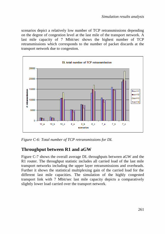
Simulation results analysis
261
scenarios depict a relatively low number of TCP retransmissions depending
on the degree of congestion level at the last mile of the transport network. A
last mile capacity of 7 Mbit/sec shows the highest number of TCP
retransmissions which corresponds to the number of packet discards at the
transport network due to congestion.
Figure C-6: Total number of TCP retransmissions for DL
Throughput between R1 and aGW
Figure C-7 shows the overall average DL throughputs between aGW and the
R1 router. The throughput statistic includes all carried load of the last mile
transport networks including the upper layer retransmissions and overheads.
Further it shows the statistical multiplexing gain of the carried load for the
different last mile capacities. The simulation of the highly congested
transport link with 7 Mbit/sec last mile capacity depicts a comparatively
slightly lower load carried over the transport network.

Simulation results analysis
262
Figure C-7: DL link throughput between aGW and R1
Figure C-8: UL link throughput between R1and aGW

Simulation results analysis
263
The average UL link throughput between the R1 router and aGW is shown
Figure C-8 which depicts a similar performance as in the DL throughput.
There is no significant difference of the carried load among the simulation
scenarios compared to the DL results.
Conclusion
A comprehensive LTE simulator which was discussed in chapter B, was used
to investigate and analyse the end-to-end performance under different
transport effects such as transport level bearer mapping, QoS classification,
transport congestion, LTE handovers and bandwidth dimensioning. Mainly
three traffic types were used with different QoS assignments for simulation
analyses and the following key findings have been achieved.
To guarantee QoS for VoIP users, it is necessary to allocate separate bearer
mapping at the transport network. Whenever a particular transport priority or
bearer mapping is assigned together with best effort traffic, the VoIP end user
performance is significantly reduced.
The optimum HTTP performance is achieved when the HTTP traffic is
separated and given a higher priority than large file downloads at the
transport network. When HTTP traffic is mixed with large file downloads in
the transport network, the web page response time is significantly increased
and provides a very poor end-to-end performance.
Simulation results show that inter-eNB handovers do not play a significant
role on the end-to-end application performance. In these analyses each UE is
performing handovers in average every 45 seconds. The number of packet
losses experienced during inter-eNB handovers can be easily recovered by
the RLC and TCP protocols even without having transport priorities for the
X2 data forwarding. When allocating transport priorities for the X2
forwarding in the transport network, a slight improvement of the end user
performance is achieved for the downlink users while having no impact on
the uplink user performance.


ABBREVIATIONS
2G The Second Generation Mobile Communication Systems
3G The Third Generation Mobile Communication Systems
3GPP 3rd Generation Partnership Project
AAL2 ATM Adaptation Layer 2
AAL5 ATM Adaptation Layer 5
ALCAP Access Link Control Application Part
ATM Asynchronous Transfer Mode
AUC Authentication Center
BCH Broadcast Channel
BER Bit Error Rate
BS Base Station
CAC Call Admission Control
DCH Dedicated Channel
DL Downlink
DSCH Downlink Shared Channel
FACH Forward Access Channel
FDD Frequency Division Duplex
FDMA Frequency Division Multiple Access
FP Frame Protocols
ETSI European Telecommunication Standards Institute
GGSN Gateway GPRS Support Node
GSM Global System for Mobile Communications
HLR Home Location Register
ID Identifier
IP Internet Protocol
ISDN Integrated Services Digital Network
ISO International Standards Organisation
ITU International Telecommunication Union
ITU-T Telecommunication Standardisation Sector of ITU
MAC Medium Access Control
ME Mobile Equipment
MM Mobility Management
MSC Mobile Services Switching Center
NBAP Node-B Application Part
NSS Network and Switching Subsystem
PCH Paging Channel
PDU Protocol Data Unit

266
PSTN Public Switched Telephone Network
QoS Quality of Service
QPSK Quadrature Phase Shift Keying
RAB Radio Access Bearer
RACH Random Access Channel
RAN Radio Access Network
RANAP Radio Access Network Application Part
RLC Radio Link Control
RNC Radio Network Controller
RNS Radio Network Subsystem
RNSAP Radio Network Subsystem Application Part
RRC Radio Resource Control
RTT Round Trip Time
SIR Signal-to-Interference Ratio
TCP Transmission Control Protocol
TDD Time Division Duplex
TDMA Time Division Multiple Access
UDP User Datagram Protocol
UE User Equipment
UL Uplink
UMTS Universal Mobile Telecommunications System
UNI User Network Interface
USIM UMTS Subscriber Identity Module
UTRAN UMTS Terrestrial Radio Access Network
VLR Visitor Location Register
VoIP Voice over Internet Protocol
WCDMA Wideband Code Division Multiple Access

LIST OF SYMBOLS
List of symbols
Probability of y
source rate
queue size
buffer filling level
Δ delay variation between and
build up delay variation between and
congestion indication interarrival time
interarrival time between nth and n 1
th CI signals
state at the nth CI arrivals
reduction factor
Pr(k): probability of exactly k CI arrivals within a step
nth stationary state probability
transition probability matrix
expected mean value of random variable X or average value of X
expected mean value of random variable Y
th drop probability
Variance
: jth
FC state probability
probability of n CI arrivals within a given FC interval
probability of no CI arrivals within a given FC interval
number of FC states
number of CC states
number of time steps (FC time steps) within a CC state
total number of states
time at nth
CI arrival


REFERENCES
[1] T.L.Weerawardane, A.Timm-Giel, C.Görg, T. Reim: Performance
Analysis of the Iub Interface in UMTS Networks for HSDPA, Mobifunk
Technologien und Anwendungen, Vorträge der 10th ITG-Fachtagung
von 1. bis 2. Juni 2005, Osnabrück.
[2] L. Zhao, Thushara Weerawardane, A.Timm-Giel, C.Görg, U.Türke,
M.Koonert: Overview on UMTS HSDPA and Enhanced Uplink
(HSUPA), Mobifunk Technologien und Anwendungen, Vorträge der
11th ITG-Fachtagung von 17. bis 18. May 2006, Osnabrück.
[3] Thushara Weerawardane, Andreas Timm-Giel, Carmelita Görg, Thomas
Reim,"UMTS Transport Network Layer: Modeling and Optimization of
HSDPA Traffic Flows", IEE conference, Sep. 2006, Sri Lanka.
[4] Thushara Weerawardane, Andreas Timm-Giel, Carmelita Görg, Thomas
Reim,"Impact of the Transport Network Layer Flow Control for HSDPA
Performance", IEE conference, Sep. 2006, Sri Lanka.
[5] Thushara Weerawardane, X. Li, A. Timm-Giel and C. Görg, "Modelling
and Simulation of UMTS HSDPA in OPNET," in Proc. OPNETWORK,
September, 2006, Washington DC, USA.
[6] M. Becker, T. L. Weerawardane, X. Li and C. Görg, Recent Advances in
Modeling and Simulation Tools for Communication Networks and
Services, "Extending OPNET Modeler with External Pseudo Random
Number Generators and Statistical Evaluation by the Limited Relative
Error Algorithm" chapter 12 (page 241-256 ), 1st edition, 2007.
[7] Thushara Weerawardane, Andreas Timm-Giel, Gennaro C. Malafronte,
Durastante Gianluca, Stephan Hauth, Carmelita Görg., “Preventive and
Reactive based TNL Congestion Control Impact on the HSDPA
Performance” VTC IEEE conference, May 2008, Singapore.
[8] Thushara Weerawardane, Andreas Timm-Giel, Gennaro C. Malafronte,
Durastante Gianluca, Stephan Hauth, Carmelita Görg., “Effective Iub
Congestion Control for the HSDPA Performance”, ICT-MobileSummit,
June 2008, Stockholm, Sweden.

270
[9] Thushara Weerawardane, Prof.Ranjit Perera, Andreas Timm-Giel,
Carmelita Görg., “A Markovian Model for HSDPA TNL Congestion
Control Performance Analysis”, VTC IEEE conference, Sep 2008,
Canada.
[10] X. Li, Y. Zaki, T. Weerawardane, A. Timm-Giel and C. Görg, "HSUPA
Backhaul Bandwidth Dimensioning," in 19th IEEE International
Symposium on Personal, Indoor and Mobile Radio Communications
(PIMRC), Sept. 15-18, 2008, Cannes France.
[11] Yasir Zaki, Thushara Weerawardane, Xi Li, Andreas Timm-Giel,
Gennaro Ciro Malafronte, Carmelita Görg: Effect of the RLC and TNL
Congestion Control on the HSUPA Network Performance, Mosharaka
International Conference on Communications, Computers and
Applications MIC-CCA 2008 in Amman-Jordan.
[12] Thushara Weerawardane, Yasir, Zaki, Andreas Timm-Giel, Gennaro C.
Malafronte, Stephan Hauth, Carmelita Görg., “Effect of the TNL
congestion control for the HSUPA performance”, IEEE International
VTC Spring in Barcelona, Spain 2009.
[13] Thushara Weerawardane, Andreas Timm-Giel, Carmelita Görg and
Gennaro Ciro Malafronte, Stephan Hauth, "Effect of TNL flow control
schemes for the HSDPA network performance", special issues-2 of
Journal of Communications 2009 (IEEE), Academy Publisher, Finland.
page(s):78-88.
[14] Xi Li, Yasir Zaki, Thushara Weerawardane, Andreas Timm-Giel,
Carmelita Görg and Gennaro Ciro Malafronte, "Use of Traffic
Separation Techniques for the Transport of HSPA and R99 Traffic in the
Radio Access Network with Differentiated Quality of Service", (5(3),
July - Sept, 2009) of IJBDCN Journal, pages(s):84-100.
[15] Thushara Weerawardane, Andreas Timm-Giel, Carmelita Görg and
Gennaro Ciro Malafronte, Stephan Hauth,: “Effect of TNL Congestion
Control Schemes on the HSDPA Network Performance” Journal
Publication, IEEE VTC magazine, Vehicular Technology Magazine,
IEEE Volume 4, Issue 4, December 2009 Page(s):54 – 63.

271
[16] Yasir Zaki, Thushara Weerawardane, Andreas Timm-Giel, Carmelita
Görg, Gennaro Ciro Malafronte, "Performance Enhancement due to the
TNL Congestion Control on the Simultaneous Deployment of both
HSDPA and HSUPA", Special Issue: Recent Advances in
Communications and Networking Technologies, JNW Journal ,Vol 5,
No 7 (2010), pages 773-781.
[17] H.Holma, A.Toskala, WCDMA for UMTS, John Wiley & Sons, Inc.,
Chichester, UK, 3rd edition, 2004.
[18] H.Holma, A.Toskala, HSDPA/HSUPA for UMTS: High Speed Radio
Access for Mobile Communications, John Wiley & Sons, Chichester,
UK, 2006.
[19] ETSI, Universal Mobile Telecommunications System (UMTS):
Selection procedures for the choice of radio transmission technologies of
the UMTS (UMTS 30.03 version 3.2.0), TR 101 112 v3.2.0, Apr. 1998.
[20] F. Agharebparast and V.C.M. Leung, QoS support in the UMTS/GPRS
backbone network using DiffServ, IEEE Global Telecommunications
Conference, vol.2, pp.1440–1444, Nov. 2002.
[21] R. Fielding, J. Gettys, J. Mogul, H. Frystyk, L. Masinter, P. Leach, and
T. Berners-Lee. Hypertext Transfer Protocol - HTTP/1.1. RFC 2616,
Internet Engineering Task Force, June 1999.
[22] 3GPP TS 25.855 High Speed Downlink Packet Access (HSDPA):
Overall UTRAN description, 3GPP TS 25.856 HSDPA: Layer 2 and 3
aspects,3GPP TS 25.876 Multiple-Input Multiple-Output Antenna
Processing for HSDPA, 3GPP TS 25.877 HSDPA - Iub/Iur Protocol
Aspects, 3GPP TS 25.890 HSDPA: User Equipment (UE) radio.
[23] ETSI, Universal Mobile Telecommunications System (UMTS): Physical
layer aspects of UTRA High Speed Downlink Packet. 3GPP, TR 25.848
v3.2.0, 2001-03.
[24] M.C. Necker and A. Weber, Impact of Iub Flow Control on HSDPA
System Performance, Proceedings of the 16th Annual IEEE International

272
Symposium on Personal Indoor and Mobile Radio Communications,
Berlin, Germany 2005.
[25] M.C. Necker and A. Weber, Parameter selection for HSDPA Iub flow
control, in Proc. 2nd International Symposium on Wireless
Communication Systems (ISWCS 2005), Siena, Italy, September 2005.
[26] G. Aniba and S. Aissa, Adaptive proportional fairness for packet
scheduling in HSDPA, in Global Telecommunications Conference,
GLOBECOM 2004, vol. 6, December 2004, pp. 4033-4037.
[27] P.J. Legg, Optimised Iub flow control for UMTS HSDPA, In Proc. IEEE
Vehicular Technology Conference (VTC 2005-Spring), Stockholm,
Sweden, June 2005.
[28] R. A. Comroe and D. J. Costello, Jr., ARQ schemes for data
transmission in mobile radio systems. IEEE Journal on Selected Areas in
Communications, vol. 2, no. 4, pp. 472-481, July 1984.
[29] S. Floyd, M. Handley, J. Padhye, A Comparison of Equation-Based and
AIMD Congestion Control, ACIRI May 12, 2000.
[30] Congestion Avoidance and Control, Van Jacobson, Lawrence Berkeley
Laboratory & Michael J. Karels, University of California at Berkeley,
November, 1988.
[31] A. Klemm, C. Lindemann, and M. Lohmann, Traffic Modeling and
Characterization for UMTS Networks, Proc. IEEE Globecom 2001, San
Antonio Texas, November 2001, USA.
[32] X. Li, R. Schelb, C. Görg and A. Timm-Giel, "Dimensioning of UTRAN
Iub Links for Elastic Internet Traffic." International Teletraffic Congress,
Beijing, Aug/Sept., 2005.
[33] X. Li, R. S. C. Görg and A. Timm-Giel, "Dimensioning of UTRAN Iub
Links for Elastic Internet Traffic with Multiple Radio Bearers," in Proc.
13th GI/ITG Conference Measuring, Modeling and Evaluation of
Computer and Communication Systems, Nürnberg, March 2006, 2006.

273
[34] X. Li, S. Li, C. Görg and A. Timm-Giel, "Traffic Modeling and
Characterization for UTRAN," in Proc. 4th International Conference on
Wired/Wireless Internet Communications, May 2006, Bern Switzerland.
[35] X. Li, S. Li, R. Schelb, A. Timm-Giel and C. Görg, "Delay in UMTS
Radio Access Networks: Analytical Study and Validation," in Proc.
Australian Telecommunication Networks and applications conference
(ATNAC), December 2006, Melbourne Australia.
[36] X. Li, L. Wang, R. Schelb, T. Winter, A. Timm-Giel and C. Görg,
"Optimization of Bit Rate Adaptation in UMTS Radio Access Network,"
in Proc. 2007 IEEE 65th Vehicular Technology Conference VTC2007-
Spring, April 2007, Dublin, Ireland.
[37] X.Li, W. Cheng, A.Timm-Giel, and C. Görg, "Modeling IP-based
UTRAN for UMTS in OPNET", distinguished paper award, in Proc.
OPNETWORK 2007, September, 2007, Washington DC, USA.
[38] X.Li, Y.Zeng, B. Kracker, R.Schelb, C.Görg and A. Timm-Giel, “Carrier
Ethernet for Transport in UMTS Radio Access Network: Ethernet
ackhaul Evolution”, (accepted for publication) 2008 IEEE 67th
Vehicular Technology Conference VTC2008-Spring, May 2008,
Singapore.
[39] 3GPP technical specification group services and system aspects,
"Evolved Universal Terrestrial Radio Access (E-UTRA) and Evolved
Universal Terrestrial Radio Access Network", 3GPP TS 36.300 V8.5.0
(2008-05): Overall description, 3GPP TS 36.300 V8.5.0 (Rel’8), June
2008.
[40] 3GPP Technical Specification Group Radio Access Network
"Requirements for Evolved UTRA (E-UTRA) and Evolved UTRAN (E-
UTRAN)", 3GPP TR 25.913 V9.0.0 (2009-12) - Release 9.
[41] R. Stewart, Ed., Network Working Group,"Stream Control Transmission
Protocol", Request for Comments: 4960, Category: Standards Track,
September 2007.

274
[42] Pierre Lescuyer and Thierry Lucidarme, "EVOLVED PACKET
SYSTEM (EPS): THE LTE AND SAE EVOLUTION OF 3G UMTS",
John Wiley & Sons, Ltd., 2008.
[43] Erik Dahlman, Stefan Parkvall, Johan Sköld and Per Beming, "3G
Evolution HSPA and LTE for Mobile Broadband", Academic Press of
Elsevier,1st edition, 2007.
[44] Harri Holma and Antti Toskala, "WCDMA FOR UMTS – HSPA
EVOLUTION AND LTE" 4th edition, John Wiley & Sons, Ltd., 2007.
[45] Stefania Sesia, Issam Toufik and Matthew Baker, "LTE – The UMTS
Long Term Evolution from Theory to Practice" 1st edition, John Wiley
& Sons Ltd., 2009.
[46] 3GPP technical specification group services and system aspects,
"General Packet Radio Service (GPRS) enhancements for Evolved
Universal Terrestrial Radio Access Network (E-UTRAN) access", 3GPP
TS 23.401 V8.2.0 (Rel’8), June 2008.
[47] 3GPP Technical Specification Group Radio Access Network, “Evolved Universal Terrestrial Radio Access (E-UTRA) and Evolved Universal
Terrestrial Radio Access Network (E-UTRAN): Radio Interface Protocol
Aspects”, 3GPP TR 25.813 v7.1.0, 2006.
[48] 3GPP technical specification group services and system aspects,
"Evolved Universal Terrestrial Radio Access (E-UTRA) Medium Access
Control (MAC) protocol specification ", 3GPP TS 36.321 V8.2.0
(Rel’8), May 2008.
[49] 3GPP technical specification group services and system aspects,
"Evolved Universal Terrestrial Radio Access (E-UTRA); Packet Data
Convergence Protocol (PDCP) specification", 3GPP TS 36.323 V8.2.1
(Rel’8), May 2008.
[50] MEF Technical specification 10.1 and MEF Technical specification
10.3, Online-web: http://metroethernetforum.org/index.php.

275
[51] T. Camp, J. Boleng, V. Davies, "A Survey of Mobility Models for Ad
Hoc Network Research", Wireless Communications & Mobile
Computing (WCMC): Special issue on Mobile Ad Hoc Networking:
Research, Trends and Applications, Vol. 2, No. 5. (2002), pp. 483-502.
[52] T.Gayathri, S.Venkadajothi, S.Kalaivani, C.Divya and C.Suresh Ghana
Dhas: "Mobility management in next-generation wireless systems",
MASAUM Journal of Computing, Volume 1 Issue 2, September 2009.
[53] J. G. Markoulidakis , G. L. Lyberopoulos , D. F. Tsirkas , E. D. Sykas,
"Mobility Modeling in Third-Generation Mobile Telecommunications
Svstems", IEEE Personal Communications, Vol. 4, No. 4, pp. 41-56,
1997.
[54] Erik Dahlman, Stefan Parkvall, Johan Sköld and Per Beming, 3G
Evolution: HSPA and LTE for Mobile Broadband , First edition, 2007.
[55] 3GPP, Technical Specification Group RAN, Synchronisation in UTRAN
Stage 2 (Release 1999), 3GPP TS 25.402 version 3.10.0, June. 2002.
[56] 3GPP, Technical Specification Group RAN, UTRAN overall description
3GPP TS 25.401 version 3.10.0, June 2002.
[57] 3GPP, Technical Specification Group RAN, Packet Data Convergence
Protocol (PDCP) specification, 3GPP TS 25.323 version 3.10.0, Sep.
2002.
[58] 3GPP, Technical Specification Group RAN, Radio Link Control (RLC)
protocol specification, 3GPP TS 25.322 version 3.18.0, June 2004.
[59] 3GPP, Technical Specification Group RAN, Medium Access Control
(MAC) protocol specification, 3GPP TS 25.321 version 3.17.0, June
2004.
[60] 3GPP, Technical Specification Group RAN, Feasibility Study for
Enhanced Uplink for UTRA FDD, 3GPP TR 25.896 version 6.0.0,
March 2004.

276
[61] 3GPP, Technical Specification Group RAN, FDD Enhanced Uplink;
Overall Description; Stage 2, 3GPP TS 25.309 version 6.6.0, Apr. 2006.
[62] ITU-T Recommendation Q.2931.1: ITU-T Recommendation I.363.1
(1996), B-ISDN ATM Adaptation Layer specification: Type 1 AAL.
ITU-T Recommendation I.363.2 (1997), B-ISDN ATM Adaptation
Layer specification: Type 2 AAL. ITU-T Recommendation I.363.3
(1996), B-ISDN ATM Adaptation Layer specification: Type 3/4
AAL.ITU-T Recommendation I.363.5 (1996), B-ISDN ATM Adaptation
Layer specification: Type 5 AAL.
[63] J.V.L. Beckers, I. Hendrawan, R.E. Kooij, and R.D. van der Mei,
Generalized Processor Sharing Performance Models for Internet Access
Lines. In Proc. of 9th IFIP Conference on Performance Modeling and
Evaluation of ATM & IP Networks, Budapest, Hungary, 2001.
[64] ITU-T Recommendation G.992.1 (1999): Asymmetric digital subscriber
line (ADSL) transceivers, G.992.2 (1999): Splitterless asymmetric
digital subscriber line (ADSL) transceivers, G.992.2 (2002): Asymmetric
digital subscriber line transceivers 2 (ADSL2), G.992.2
(2003):Asymmetric Digital Subscriber Line (ADSL) transceivers -
Extended bandwidth ADSL2 (ADSL2plus).
[65] G.992.2 (1998): High bit rate Digital Subscriber Line (HDSL)
transceivers.
[66] S. Kent, IETF Network Working Group, MPTCP : Security Architecture
for the Internet Protocol, available at http://www.ietf.org/rfc/rfc2401.txt,
accessed on April 2010.
[67] OPNET Modeler, available at http://www.opnet.com, accessed on April
2009.
[68] W. Simpson, Network Working Group: Request for Comments 1661,
The Point-to-Point Protocol (PPP), available at http://www.faqs.org/
rfcs/rfc1661.html, accessed on Nov. 2009.

277
[69] W. Simpson, Network Working Group: Request for Comments 1662,
PPP in HDLC-like Framing, available at http://www.rfc-
editor.org/rfc/rfc1662.txt, accessed on Nov. 2009.
[70] J. Lau, M. Townsley, Network Working Group: Request for Comments
3931, Layer Two Tunneling Protocol - Version 3 (L2TPv3), available at
http://www.apps.ietf.org/rfc/rfc3931.html, accessed on Nov. 2009.
[71] W. Townsley, A. Valencia, Network Working Group: Request for
Comments 2661, Layer Two Tunneling Protocol "L2TP", available at
http://www.ietf.org/rfc/rfc2661.txt, accessed on Dec. 2009.
[72] L. Mamakos, K. Lidl, J. Evarts, A. Valencia, Network Working Group:
Request for Comments 2516, A Method for Transmitting PPP Over
Ethernet (PPPoE), available at http://www.faqs.org/rfcs/rfc2516.html,
accessed on Dec. 2009.
[73] 3GPP technical specification group services and system aspects,
"Evolved Universal Terrestrial Radio Access (E-UTRA); Radio Link
Control (RLC) protocol specification", 3GPP TS 36.322 V8.2.0 (Rel’8),
May 2008
[74] B. Braden, D. Clark, J. Crowcroft, B. Davie, S. Deering, D. Estrin, S.
Floyd, V. Jacobson, G. Minshall, C. Partridge, L. Peterson, K.
Ramakrishnan, S. Shenker, J. Wroclawski, L. Zhang, RFC 2309:
Recommendations on Queue Management and Congestion Avoidance in
the Internet, April 1998. Informational.
[75] M. Christiansen, K. Jeffay, D. Ott, and F.D. Smith, Tuning RED for
Web Traffic, ACM SIGCOMM, August 2000. Or the June 2001 version
in IEEE/ACM Transactions on Networking.
[76] L. Le, J. Aikat, K. Jeffay, and F.D. Smith, The Effects of Active Queue
Management on Web Performance, ACM SIGCOMM, 2003.
[77] J. Babiarz, K. Chan, Network Working Group: Request for Comments
4594, Configuration Guidelines for DiffServ Service Classes, available
at http://tools.ietf.org/html/rfc4594, accessed on Nov. 2009.

278
[78] Harrison M Wadsworth, “The Handbook of Statistical Methods for Engineers and Scientists”, 1st edition, 1997.
[79] Communication Network Class Library, CNCL, University of Bremen,
available at http://www.comnets.uni-bremen.de/docs/cncl/, accessed on
May. 2010.