optimization and statistical learning theory for piecewise
TRANSCRIPT

HAL Id: tel-02307957https://hal.univ-lorraine.fr/tel-02307957
Submitted on 8 Oct 2019
HAL is a multi-disciplinary open accessarchive for the deposit and dissemination of sci-entific research documents, whether they are pub-lished or not. The documents may come fromteaching and research institutions in France orabroad, or from public or private research centers.
L’archive ouverte pluridisciplinaire HAL, estdestinée au dépôt et à la diffusion de documentsscientifiques de niveau recherche, publiés ou non,émanant des établissements d’enseignement et derecherche français ou étrangers, des laboratoirespublics ou privés.
Optimization and statistical learning theory forpiecewise smooth and switching regression
Fabien Lauer
To cite this version:Fabien Lauer. Optimization and statistical learning theory for piecewise smooth and switching regres-sion. Machine Learning [cs.LG]. Université de Lorraine, 2019. �tel-02307957�

Ecole doctorale IAEM Lorraine
Optimization and statistical learning theoryfor
piecewise smooth and switching regression
THÈSE
présentée et soutenue publiquement le 1er octobre 2019pour l’obtention de l’
Habilitation à Diriger des Recherchesde l’Université de Lorraine
mention informatique
par
Fabien Lauer
Composition du Jury
Rapporteurs :Stéphane Canu Professeur, INSA RouenMarius Kloft Professeur, Technische Universität KaiserslauternLiva Ralaivola Professeur, Aix-Marseille Université
Président :Marc Sebban Professeur, Université Jean Monnet Saint-Etienne
Examinateurs :Marianne Clausel Professeure, Université de LorraineYann Guermeur Directeur de Recherche, CNRS (parrain scientifique)Gilles Millérioux Professeur, Université de Lorraine
Laboratoire Lorrain de Recherche en Informatique et ses Applications — UMR 7503

Résumé/Abstract
RésuméCe manuscrit s’intéresse à différents problèmes d’apprentissage automatique. En premier lieu, nousnous concentrons sur des problèmes de régression à modèles multiples : la régression de fonctionslisses par morceaux et la régression à commutations. Deux types de contributions sont exposées.Les premières relèvent des domaines de l’optimisation et de la complexité algorithmique. Ici, ontente de savoir dans quelle mesure il est possible de minimiser exactement l’erreur empirique demodèles de régression dans les différents cadres évoqués plus haut. Dans une seconde partie, noustentons de caractériser les performances en généralisation de ces modèles. Cette partie relève dela théorie statistique de l’apprentissage dont les outils sont introduits dans un chapitre traitant dela discrimination multi-classe. Celle-ci apparaît en effet de manière naturelle lorsque l’on définitles fonctions de régression lisses par morceaux au travers d’un ensemble de modèles lisses et d’unclassifieur chargé de sélectionner un de ces modèles en fonction de l’entrée. Nous montrons dansce manuscrit qu’il existe aussi un autre lien en termes du rôle joué dans les bornes sur l’erreurde généralisation par le nombre de catégories en discrimination et par le nombre de modèles enrégression.
Techniquement, la première partie contient des preuves de NP-difficulté, des algorithmes exactspolynomiaux par rapport au nombre de données à dimension fixée et une méthode d’optimisationglobale à temps raisonnable en dimension modérée. La seconde partie repose sur l’estimation decomplexités de Rademacher, au travers de lemmes de décomposition, de chaînage "à la Dudley" etde nombres de couverture. Les bornes obtenues dans cette dernière partie sont discutées avec uneattention particulière à leur dépendance au nombre de catégories ou de modèles.
AbstractThis manuscript deals with several machine learning problems. More precisely, we study two re-gression problems involving multiple models: piecewise smooth regression and switching regression.Piecewise smooth regression refers to the case where the target function involves jumps (of valuesor derivatives) and is usually tackled by learning multiple smooth models and a classifier deter-mining the active model on the basis of the input. Switching regression refers to the case wherethe target function switches between multiple behaviors arbitrarily (and thus independently of theinput). The first part of the document focuses on optimization and computational complexityissues. Here, we try to characterize under which conditions it is possible to exactly minimize theempirical risk of these particular regression models. In the second part, we analyze the generaliza-tion performance of the models in the framework of statistical learning theory. The standard toolsof this framework are introduced in a chapter dedicated to multi-category classification, which weencounter in piecewise smooth regression and which also shares a number of characteristic featureswith switching regression regarding the analysis in generalization.
Technically, the first part contains proofs ofNP-hardness, polynomial-time exact algorithms forfixed dimensions and a global optimization method with reasonable computing time for moderatedimensions. The second part derives risk bounds by relying on the estimation of Rademachercomplexities, structural decomposition lemmas, chaining arguments and covering numbers. Theobtained risk bounds are discussed with a particular emphasis on their dependency on the numberof component models.
3

Contents
Résumé/Abstract 3
Notations 7
1 Introduction 91.1 Supervised learning . . . . . . . . . . . . . . . . . . . . . . . . . . . . . . . . . . . . 9
1.1.1 Regression . . . . . . . . . . . . . . . . . . . . . . . . . . . . . . . . . . . . . 101.1.2 Classification . . . . . . . . . . . . . . . . . . . . . . . . . . . . . . . . . . . 11
1.2 Learning heterogeneous data . . . . . . . . . . . . . . . . . . . . . . . . . . . . . . 111.2.1 Piecewise smooth regression . . . . . . . . . . . . . . . . . . . . . . . . . . . 121.2.2 Arbitrarily switching regression . . . . . . . . . . . . . . . . . . . . . . . . . 131.2.3 Bounded-error regression . . . . . . . . . . . . . . . . . . . . . . . . . . . . 141.2.4 State of the art, applications and connections with other fields . . . . . . . 16
1.3 Outline of the report and overview of the contributions . . . . . . . . . . . . . . . . 17
I Optimization 19
2 Computational complexity 232.1 Basic definitions . . . . . . . . . . . . . . . . . . . . . . . . . . . . . . . . . . . . . 232.2 Hardness of switching linear regression . . . . . . . . . . . . . . . . . . . . . . . . . 242.3 Hardness of piecewise affine regression . . . . . . . . . . . . . . . . . . . . . . . . . 272.4 Hardness of bounded-error estimation . . . . . . . . . . . . . . . . . . . . . . . . . 282.5 Conclusions . . . . . . . . . . . . . . . . . . . . . . . . . . . . . . . . . . . . . . . . 29
3 Exact methods for empirical risk minimization 313.1 Piecewise affine regression with fixed C and d . . . . . . . . . . . . . . . . . . . . . 323.2 Switching regression with fixed C and d . . . . . . . . . . . . . . . . . . . . . . . . 343.3 Bounded-error estimation with fixed d . . . . . . . . . . . . . . . . . . . . . . . . . 353.4 Conclusions . . . . . . . . . . . . . . . . . . . . . . . . . . . . . . . . . . . . . . . . 37
4 Global optimization for empirical risk minimization 394.1 General scheme . . . . . . . . . . . . . . . . . . . . . . . . . . . . . . . . . . . . . . 394.2 Switching regression . . . . . . . . . . . . . . . . . . . . . . . . . . . . . . . . . . . 394.3 Bounded-error estimation . . . . . . . . . . . . . . . . . . . . . . . . . . . . . . . . 434.4 Piecewise affine regression . . . . . . . . . . . . . . . . . . . . . . . . . . . . . . . . 444.5 Limitations of exact methods . . . . . . . . . . . . . . . . . . . . . . . . . . . . . . 454.6 Conclusions . . . . . . . . . . . . . . . . . . . . . . . . . . . . . . . . . . . . . . . . 46
II Statistical learning theory 47
5 Risk bounds for multi-category classification 515.1 Margin classifiers . . . . . . . . . . . . . . . . . . . . . . . . . . . . . . . . . . . . . 525.2 Bounds based on the Rademacher complexity . . . . . . . . . . . . . . . . . . . . . 52
5

6 CONTENTS
5.3 Decomposition of capacity measures . . . . . . . . . . . . . . . . . . . . . . . . . . 545.3.1 Decomposition at the level of Rademacher complexities . . . . . . . . . . . 545.3.2 Decomposition at the level of covering numbers . . . . . . . . . . . . . . . . 555.3.3 Covergence rates and Sauer-Shelah lemmas . . . . . . . . . . . . . . . . . . 56
5.4 Bounds dedicated to kernel machines . . . . . . . . . . . . . . . . . . . . . . . . . . 605.5 Conclusions . . . . . . . . . . . . . . . . . . . . . . . . . . . . . . . . . . . . . . . . 61
6 Risk bounds for piecewise smooth regression 636.1 General framework: error bounds in regression . . . . . . . . . . . . . . . . . . . . 636.2 Decomposition at the level of covering numbers . . . . . . . . . . . . . . . . . . . . 646.3 Application to PWS classes with linear classifiers . . . . . . . . . . . . . . . . . . . 66
6.3.1 General case . . . . . . . . . . . . . . . . . . . . . . . . . . . . . . . . . . . 676.3.2 Piecewise smooth kernel machines . . . . . . . . . . . . . . . . . . . . . . . 686.3.3 Classes of piecewise affine functions . . . . . . . . . . . . . . . . . . . . . . 69
6.4 Conclusions . . . . . . . . . . . . . . . . . . . . . . . . . . . . . . . . . . . . . . . . 70
7 Risk bounds for switching regression 717.1 Decomposition at the level of Rademacher complexities . . . . . . . . . . . . . . . 71
7.1.1 Application to linear and kernel machines . . . . . . . . . . . . . . . . . . . 727.2 Decomposition at the level of covering numbers . . . . . . . . . . . . . . . . . . . . 73
7.2.1 General case . . . . . . . . . . . . . . . . . . . . . . . . . . . . . . . . . . . 737.2.2 Kernel machines . . . . . . . . . . . . . . . . . . . . . . . . . . . . . . . . . 747.2.3 Classes with linear component functions . . . . . . . . . . . . . . . . . . . . 75
7.3 Conclusions . . . . . . . . . . . . . . . . . . . . . . . . . . . . . . . . . . . . . . . . 76
8 Research plan 77
Author’s publications 81
References 85
Notations
Vectors of Rd are written in boldface. Thus, xi denotes the ith vector x, whereas xk denotes thekth component of x. The kth component of the ith vector x is denoted by xi,k.
Random variables are written in uppercase letters and their values in lowercase. Thus, Xdenotes a random vector.
The notation tn refers to a sequence (ti)1≤i≤n of possibly nonscalar elements ti. This has tobe differentiated from the nth vector t, denoted by tn, particularly when we consider sequences ofvectors such as xn = (xi)1≤i≤n.
The set of the n first integers is written as [n] = {1, . . . , n}.In general, we use the notation 〈·, ·〉 for the inner product, except for inner products in Euclidean
spaces, where the matrix notation, a>b, is used.
Acronyms
PWA : piecewise affinePWS : piecewise smoothSVM : support vector machineM-SVM : multi-class support vector machine
References
External references are numbered as [90] and listed on page 85. My personal publications, such as[J17], are referenced with a letter indicating the type of publication and are listed on page 81.
7


Chapter 1
Introduction
The work described in this manuscript is in the field of machine learning, and more preciselysupervised learning. Here, we are interested in the two major problems of that field: classifi-
cation and regression. For classification, we concentrate on the analysis of the multi-class case andon the influence of the number of categories in the framework of statistical learning theory. Forregression, we focus on problems involving multiple models, either for piecewise smooth regressionor for switching regression. We will see in particular that these problems involve regression but alsoclassification issues related to the association of the points with the different models. The fact thatthese issues are intrinsically intertwined during training leads to novel and nontrivial optimizationproblems, more complex than those usually considered in either classification or regression. Thus,a large part of this document aims at studying the possibility of solving these problems with globaloptimality guarantees. In a second part, we will also discuss the analysis of these particular regres-sion models in the framework of statistical learning theory, where we will discover that the numberof models plays a role similar to the one of the number of categories in classification.
This chapter introduces the supervised learning framework and the classification and regressionproblems studied in this document. It starts in Sect. 1.1 with the formulations of classical problemswith a few examples of application for linear models. Then, Sect. 1.2 presents the different problemsinvolving multiple models and on which we focus. The chapter ends in Sect. 1.3 by exposing theoutline of the rest of the document and relating the contributions with my publications.
1.1 Supervised learningLet X be a set of inputs or descriptions (typically X ⊆ Rd) and Y be a set of outputs (or labels).We assume that there is a probabilistic link between inputs of X and outputs of Y encoded by thejoint probability distribution P of the random pair (X, Y ) that takes values in X ×Y. The goal oflearning is to build a model able to accurately predict the value of Y for any value of X withoutknowledge of P . The only source of information that we assume accessible is the training set: arealization ((xi, yi))1≤i≤n of the training sample ((Xi, Yi))1≤i≤n of independent copies of (X, Y ).This is the agnostic learning framework [46].
More formally, the goal of learning is to find a function f : X → Y that minimizes the risk (orgeneralization error)
L(f) = EX,Y `(Y, f(X)), (1.1)
defined as the expectation of the loss function ` : Y2 → R+, which measures what we loose whenpredicting f(X) instead of Y .
This risk cannot be computed without knowledge of P . A standard approach thus consists inminimizing an estimate of the risk: the empirical risk
Ln(f) =1
n
n∑i=1
`(Yi, f(Xi)) (1.2)
evaluated on the training set.
9
10 Chapter 1. Introduction
1.1.1 RegressionA regression problem is a learning problem with an infinite number of labels: Y = R (or, moreoften, Y = [a, b], (a, b) ∈ R2). In this case, the loss function is in general a function of the errore = y − f(x). In particular, the `p losses are defined for all p ≥ 0 by
`(y, y′) = `p(y − y′) =
{1|y−y′|>0, if p = 0
|y − y′|p, if p ∈ (0,∞).(1.3)
The case p = 0 is specific and in fact corresponds to the 0-1 loss used in classification. The mostcommon loss for regression is the squared loss (with p = 2), for which the risk corresponds to themean squared error that is minimized by the regression function
∀x ∈ X , freg(x) = EY |X [Y |X = x] .
Obviously, without access to P , this optimal model cannot be computed and the standard approachconsists in minimizing the training error:
minf∈F
1
n
n∑i=1
`(yi, f(xi)). (1.4)
Here, we note that we introduced the class of functions F ⊂ YX restricting the search space. Indeed,solving this problem without restriction, i.e., with merely f ∈ YX , does not make much sense andwould lead to an extreme case of overfitting and no guarantee that the model can generalize.
Let us consider for instance the class of linear functions of x ∈ X = Rd:
F ={f ∈ RX : f(x) = θ>x, θ ∈ Rd
}. (1.5)
For this class and the squared loss ((1.3) with p = 2), problem (1.4) corresponds to the least squaresmethod and has an well-known analytical solution of the form
f∗(x) = x>θ∗, with θ∗ =
(n∑i=1
xix>i
)−1 n∑i=1
xiyi.
Robustness to outliers
An outlier is a data point (xi, yi) that does not come from the distribution modeling the real linkbetween X and Y . A method is said to be robust to outliers when it is not too sensitive to suchoutliers.
Robustness can be obtained for instance by minimizing a saturated loss function in (1.4). Suchfunctions can be defined by plain saturation of the standard `p losses:
∀ε > 0, `p,ε(e) =
{1|e|>ε, if p = 0
(min(|e|, ε))p, if p ∈ (0,∞),(1.6)
where ε is the threshold below which the standard loss, `p(e) = |e|p, applies and above which thefunction saturates to a value determined to guarantee the continuity of the loss. The case p = 0 isspecific and corresponds here to a search for a model with an error bounded by ε for a maximumnumber of points.
Robust regression has been largely studied in statistics [78], where saturated loss functionsenter the framework of redescending M -estimators. The rationale is that such functions limit theinfluence a single outlier (xi, yi) has on the cost function of (1.4) in terms of its derivative at thispoint. Outliers typically yield large errors |yi−f(xi)|, and the aim here is to control the derivativeof the cost function so that it redescends to zero for such large errors. We can see that the saturatedlosses (1.6) totally satisfy this requirement, since we have
∀|e| > ε,d`p,ε(e)
de= 0.
1.2. Learning heterogeneous data 11
1.1.2 Classification
Classification is a learning problem in which the labels y ∈ Y are in a finite number (|Y| < ∞)and (usually) not ordered. To emphasize the difference with the regression setting, the classifiers,i.e., the models learned for classification, will be denoted by g throughout the document, whereasf refers to a real-valued function. We usually consider Y = [C] for a problem with C categories(ignoring the ordering of the integers) or Y = {−1,+1} for binary problems with C = 2.
The standard loss function for classification is the indicator of misclassification, also known asthe 0-1 loss, and corresponds to the definition (1.3) for p = 0:
`(y, y′) = 1y 6=y′ = `0(y − y′).
With this loss, the risk becomes the probability of misclassification:
L(g) = EX,Y 1g(X)6=Y = P (g(X) 6= Y ).
The optimal classifier minimizing this risk is the Bayes classifier, which outputs the most likelycategory for a given x:
∀x ∈ X , gBayes(x) = argmaxy∈Y
P (Y = y | X = x).
Linear classifiers of Rd
An important class of classifiers for X ⊆ Rd is that of linear classifiers. In the binary case, aclassifier g : Rd → {−1,+1} is said to be linear when it can be written as
∀x ∈ Rd, g(x) = sign(w>x+ b
)with parameters w ∈ Rd and b ∈ R defining a linear (actually affine) function of x. Such a classifiercan be identified with a separating hyperplane
H ={x ∈ Rd : w>x+ b = 0
}dividing the space Rd in two half-spaces, one for each category.
In the multi-class case, a classifier g : Rd → [C] is said to be linear when it can be written as
g(x) = argmaxk∈[C]
(w>k x+ bk
)(1.7)
with parameters wk ∈ Rd and bk ∈ R, 1 ≤ k ≤ C, defining a set of component functions that arelinear/affine in x. Here, the separating hyperplanes between two categories j and k are given by
Hjk ={x ∈ Rd : (wj −wk)>x+ (bj − bk) = 0
}.
Any classifier of the form (1.7) can thus be implemented as a set of binary linear classifiers.
1.2 Learning heterogeneous data
The learning problems described above are completely standard and have been largely studied. Inthis report, we will discuss more complex problems, in which classification and regression issues aremixed together and must be solved simultaneously. These problems are here gathered under thename of "learning heterogeneous data". Indeed, they amount to learning from data generated bymultiple sources while searching on the one hand to identify the source of each data (classification)and on the other hand to model the sources (regression).
12 Chapter 1. Introduction
−10 −8 −6 −4 −2 0 2 4 6 8 10−8
−6
−4
−2
0
2
4
6
−10 −8 −6 −4 −2 0 2 4 6 8 10−8
−6
−4
−2
0
2
4
6
−10 −8 −6 −4 −2 0 2 4 6 8 10−8
−6
−4
−2
0
2
4
6
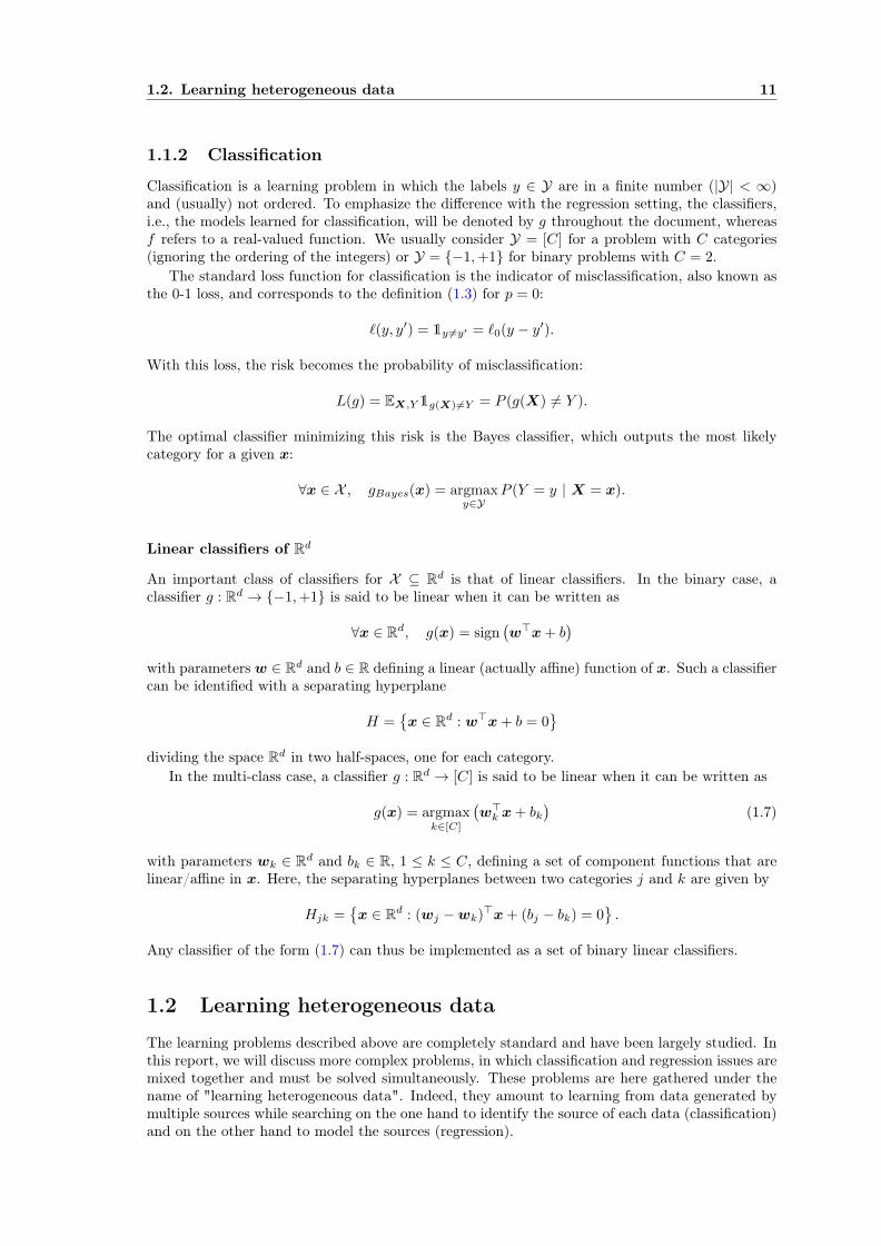
Figure 1.1: Regression of a piecewise affine function (- -) from noisy data points (•) by kernelridge regression [81] (—). Either the regularization is insufficient to limit the influence of the noise(middle plot), or it is too pronounced and the model cannot accurately learn the jump (right plot).
1.2.1 Piecewise smooth regressionThe vast majority of works on nonlinear regression concerns the case where the regression function isassumed to be smooth, i.e., infinitely differentiable. Indeed, without this assumption, the behaviorof the regression function in the vicinity of a point does not depend on its behavior at that pointand learning from a finite sample is a priori not possible.
However, it is possible to formulate less restrictive assumptions while retaining the possibility tolearn. In particular, we here consider that the regression function is smooth almost everywhere, i.e.,everywhere except on a set of zero measure. Functions including abrupt jumps of value between tworegions where they are smooth satisfy for instance this requirement. Such functions are piecewisesmooth (PWS) and can be written as
f(x) =
f1(x), if x ∈ X1
...fC(x), if x ∈ XC
with C component functions fk that are smooth and C regions Xk forming a partition of X .Alternatively, a PWS function can be defined with a classifier g : X → [C] implementing thepartition of X as
f(x) = fg(x)(x).
In the following, we shall further assume that the number C of regions is small (in particular beforethe sample size).
Piecewise smooth regression cannot be dealt with efficiently by classical methods for nonlinearregression. Indeed, because of the underlying smoothness assumption, these methods explicitlyreject solutions with abrupt changes (see Fig. 1.1). Therefore, the aim here is to design andanalyze methods dedicated to piecewise smooth regression. More precisely, we consider the numberof components (also known as the number of modes), C, as fixed. Indeed, if it was a variable, theempirical risk minimization problem would be trivial: it would suffice to take C = n and create onemodel for each data point, but this would not yield a satisfactory model from the generalizationviewpoint.
Straightforward approach to piecewise affine regression
Let us focus on piecewise affine models in Rd, for which
fk(x) = x>θk
with x = [x>, 1]> ∈ Rd+1 and a vector of parameters θk ∈ Rd+1. We additionally restrain theclassifier g to the set of linear classifiers,
G =
{g ∈ [C]X : g(x) = argmax
k∈[C]
w>k x+ bk, wk ∈ Rd, bk ∈ R
}. (1.8)

1.2. Learning heterogeneous data 13
Then, the empirical risk minimization problem (1.4), here called piecewise affine (PWA) regressionproblem, can be written as follows.
Problem 1 (PWA regression). Given a data set ((xi, yi))1≤i≤n ⊂ Rd×R and a number of modesC, find a global solution to
minθ∈RC(d+1),g∈G
1
n
n∑i=1
C∑k=1
1g(xi)=k`p(yi − x>i θk), (1.9)
where θ = [θ>1 , . . . ,θ>C ]> and G is the set of linear classifiers as in (1.8).
This problem could be solved (in principle) by a straightforward approach as follows. For allthe Cn possible classifications c ∈ [C]n of n points into C groups, test whether it is actually alinear classification, e.g., by verifying that the system
∀k ∈ [C] \ {ci}, (wci −wk)>xi + bci − bk > 0, i = 1, . . . , n,
is feasible; and for all the linear ones, solve C independent linear regression subproblems, eachusing only the data assigned to a particular mode.
However, a major issue with this approach is obviously its computational complexity as itinvolves an exponential number of iterations, Cn, wrt. n. Nonetheless, we will see in Chapter 3that this number can be reduced to a polynomial function of n.
1.2.2 Arbitrarily switching regression
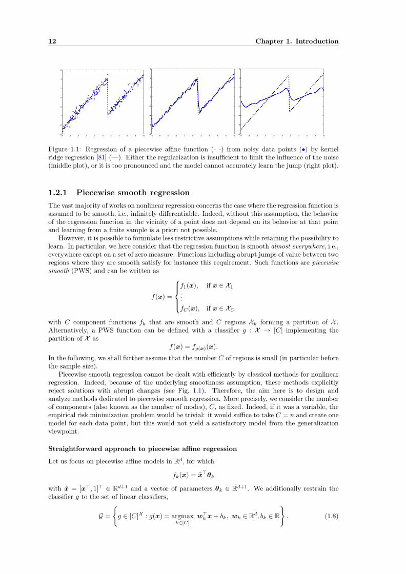
Arbitrarily switching regression is closely related to piecewise smooth regression. However, herethe switchings between the different smooth submodels are not governed by the input anymore,but merely arbitrary. This simple change, actually calls for new definitions of the loss and therisk. Indeed, here, the goal is not to learn a function f that can generalize, but to estimate acollection of models (fk)1≤k≤C such that at least one of them can accurately predict the label (seethe illustration of this setting in Figure 1.2).
Formally, this translates into a loss function that selects the component function fk among thecollection to compute the error. Thus, we define the switching `p-loss, `Cp : Y × YC → R+, by
`Cp (y, (fk)1≤k≤C) = mink∈[C]
|y − fk(x)|p.
The empirical risk minimization problem then becomes nonconvex and nondifferentiable for allp and all function classes Fk (except in trivial cases for which Fk contains a single function):
min(fk∈Fk)1≤k≤C
1
n
n∑i=1
mink∈[C]
|yi − fk(xi)|p. (1.10)
Straightforward approach to switching linear regression
In the case where the classes Fk contain linear functions on Rd, the problem can be reformulatedin a parametric form with fk(x) = θ>k x. In addition, we can introduce integer variables ci ∈ [C]to encode the assignation of the points (xi, yi) to the different component functions.
Problem 2 (Switching linear regression). Given a data set ((xi, yi))1≤i≤n ⊂ Rd×R and a numberof modes C, find a global solution to
minθ∈RCd,c∈[C]n
1
n
n∑i=1
`p(yi − x>i θci) (1.11)
with θ = [θ>1 , . . . ,θ>C ]>.
14 Chapter 1. Introduction
0 0.2 0.4 0.6 0.8 1
x
-0.5
0
0.5
1
1.5
2
y
Figure 1.2: Example of switching linear regression. The goal is to estimate the two linear functions(— and —) from data (•) mixing noisy measurements of both of them.
First, note that the only interesting values for C are in the interval [2, n/d]. Indeed, if C = 1,then the problem becomes a simple linear regression problem. On the other hand, for all C > n/d,the problem has a trivial solution based on the fact that the data can arbitrarily be classified intoC groups of less than d points. Thus, for each group, there is a d-dimensional linear model thatperfectly fits the points with zero error, which yields a zero cost and a global solution for (1.11).
In general (and in particular when C ∈ [2, n/d]), Problem 2 can be solved explicitly wrt. c fora fixed θ by assigning every data point to the submodel that best approximates it:
ci ∈ argmink∈[C]
`p(yi − x>i θk), i = 1, . . . , n. (1.12)
Conversely, for a fixed c, the problem amounts to C independent linear regression subproblems,
minθk∈Rd
∑i∈{j:cj=k}
`p(yi − x>i θk), k = 1, . . . , C, (1.13)
which easily yield the optimal θk’s.Thus, two global optimization approaches can be readily formulated.The first one tests all possible classifications c and solves the problem wrt. the θk’s for each
of them. But, this leads to s × sN linear regression subproblems (1.13) and quickly becomesintractable when N increases.
The second approach applies a continuous global optimization strategy to directly estimate{θk}Ck=1 under the optimal classification rule (1.12), which is equivalent to solving
minθ∈RCd
1
n
n∑i=1
mink∈[C]
`p(yi − x>i θk), (1.14)
and then recovering the mode estimates with (1.12). This second formulation has the advantageof being continuous and of involving only a small number of variables, Cd, which allowed us toobtain interesting results in practice [J6, J10]. However, global optimality is difficult to guarantee.For instance, the complexity remains exponential in the number of variables Cd, for a grid searchto obtain a solution with an error that is only guaranteed to be close to the global optimum.
Chapter 3 will focus on the first approach and we will show how to reduce the number ofclassifications to a polynomial function of n. The second strategy will be the basis of Chapter 4.
1.2.3 Bounded-error regression
In this report, we will consider another particular setting, the one of bounded-error regression.Here, the idea is not to minimize the error under a constraint on the number of modes, but rather

1.2. Learning heterogeneous data 15
0 0.2 0.4 0.6 0.8 1
x
-0.5
0
0.5
1
1.5
2
2.5
y
0 0.2 0.4 0.6 0.8 1
x
-0.5
0
0.5
1
1.5
2
2.5
y
Figure 1.3: Example of switching regression in dimension d = 1 dealt with by the greedy bounded-error approach. The first iteration (left) yields the first model (plain line) by considering all pointsoutside of the tube of width ε around fk as outliers (grey points). Then, the points inside the tube(black points) are removed before going through with the next iteration (right) and the estimationof the second model f2 (plain line) from the remaining points.
to minimize the number of modes under a constraint on the error. For switching regression, thisleads to
minC,(fk∈F)k≥1
C (1.15)
s.t. ∀i ∈ [n], mink∈[C]
`p(yi − fk(xi)) ≤ ε.
We shall limit the discussion here to this problem, while a similar formulation could be given forpiecewise smooth regression. Note also that all functions fk belong to the same class F , which isindeed often the case for the other settings too.
The formulation (1.15) is difficult to handle and seldom considered as such. Instead, mostworks concentrate on a greedy approach, in which the models fk are estimated one by one untilthe bound on the error is satisfied for all data. By considering points that are not assigned tothe current model as outliers, we can estimate this model with a robust regression method. Inparticular, we here consider the robust losses (1.6) to iteratively estimate the fk’s as
minfk∈F
∑i∈Ik
`p,ε(yi − fk(xi)), k = 1, 2, . . . , (1.16)
where I1 = [n] andIk = {i ∈ Ik−1 : |yi − fk−1(xi)| > ε}, k = 2, 3, . . . (1.17)
Figure 1.3 illustrates this procedure. Here, the crucial step is the estimation of each model fk witha robust method. It is clear that the first submodel can be correctly estimated only by ignoring thepoints outside of the tube (or by strongly limiting their influence). Conversely, robust estimationmethods should allow for the recovery of the dominant mode from a data set generated by severalmodes (the dominant mode is the one corresponding to the majority of the data).
Straightforward approach to robust linear regression
Let us focus on the bounded-error regression problem corresponding to the robust regression ofthe first iteration of (1.16). The next iterations can be dealt with similarly, but with a reduceddata set. We further limit the discussion here to the linear case, fk(x) = θ>k x, and `p,ε-losses forp ∈ {0, 1, 2}.
Problem 3 (Bounded-error linear estimation). Given a data set ((xi, yi))1≤i≤n ⊂ Rd × R and athreshold ε ≥ 0, find a global solution to
minθ∈Rd
n∑i=1
`p,ε(yi − x>i θ). (1.18)

16 Chapter 1. Introduction
Let I1(θ) denote the set of indexes of the points that are correctly estimated with parameterθ,
I1(θ) = {i ∈ [n] : |yi − x>i θ| ≤ ε}. (1.19)
Then, Problem (1.18) can be equivalently written as
minθ∈Rd
εp(n− |I1(θ)|) +∑
i∈I1(θ)
`p(yi − x>i θ) (1.20)
for p ∈ {1, 2} andminθ∈Rd
εp(n− |I1(θ)|) (1.21)
for p = 0.The equivalence between (1.18) and (1.20) or (1.21) comes from the definition (1.6) of the
saturated `p,ε-losses. In particular, the set I1(θ) gathers the indexes of data points that are wellapproximated by the linear model of parameter θ. Thus, n − |I1(θ)| coincides with the numberof data points for which the loss function `p,ε saturates while the loss at all points with index inI1(θ) can be computed with a standard (non-saturated) `p loss.
These equivalent formulations emphasize the connection between saturated loss minimizationand the maximization of the number of points approximated with a bounded error. Indeed, thesepoints are here marked with index in I1(θ) and maximizing their number is equivalent to minimizingthe number of points with index not in I1(θ), i.e., n− |I1(θ)|.
This also draws a connection with the classification problem of separating between points thatare approximated with a bounded error by an optimal model θ∗ and those that are not. Inparticular, given the solution to this classification problem, i.e., I1(θ∗) for some optimal θ∗, aglobal solution θ (possibly different from θ∗) can be recovered by solving (1.20) or (1.21) underthe constraint I1(θ) = I1(θ∗). Then, for p = 0, the cost in (1.21) is a mere constant and it sufficesto find a θ such that
maxi∈I1(θ∗)
|yi − x>i θ| ≤ ε
to satisfy the constraint. Conversely, for p ∈ {1, 2}, the cost in (1.20) simplifies to a constant plusa sum of errors over a fixed set of points. Hence, given I1(θ∗), these problems amount to standardregression problems with a non-saturated loss and θ can be computed as
θ = argminθ∈Rd
max
i∈I1(θ∗)|yi − x>i θ| , if p = 0∑
i∈I1(θ∗)
`p(yi − x>i θ), otherwise. (1.22)
As for switching regression, a naive algorithm can thus be devised by considering all classifica-tions of the data into two groups, those with index in I1 and the others. Then, one minimizes the`p loss over all points with index in I1 and computes the cost function value as in (1.20) or (1.21).Thus, these optimization problems can be solved via the analysis of a finite number of cases. How-ever, here again the complexity of this approach is proportional to the number of classificationsand in O(2n), thus much too large for practical purposes. Reducing this number to a polyno-mial function of n will be the topic of Sect. 3.3. The alternative approach consisting in directlytackling (1.18) with global and continuous optimization methods will be studied in Chapter 4.
1.2.4 State of the art, applications and connections with other fields
Switching regression was introduced in the 50’s by [74] and several algorithms were proposed forthe case C = 2 in [85] and [41]. The latter is based on the expectation-maximization (EM) methodand was extended to the case C > 2 by [21, 29]. It is also strongly related to the mixturesof experts [42]. Regression trees [15] and their various improvements [28, 76] are examples ofpiecewise defined regression models. The mixture of experts [42] also allows one to create suchmodels with the partition of the input space implemented by the gating network, but they mostoften consider smooth transitions between the modes.
1.3. Outline of the report and overview of the contributions 17
More recently, most works in these fields were produced by the automatic control communityin order to deal with the identification of hybrid dynamical systems [73, 31]. A hybrid system is adynamical system that switches between different operating modes. The identification of a hybridsystem from observations of its inputs ui and outputs yi at discrete time i can be formulated withxi = [yi−1, yi−2, . . . , ui, ui−1, . . . ]
> as a piecewise smooth regression problem if the switchingsdepend on xi or a switching regression problem if they are arbitrary. Seminal works in this field dateback from the start of the 2000’s and include [96, 25, 77, 9, 44]. Other original approaches were morerecently developed by building on the notion of sparsity and `1-norm minimization [4, 71, 70, 72].A more detailed review of hybrid system identification is given in the book [B1]. We here onlyadd that hybrid system identification and switching regression also have applications in computervision [95]. There is also a tighter connection between these fields via the subspace clusteringproblem [92]. Here, the goal is to cluster data {xi}ni=1 that are assumed to be distributed arounda collection of subspaces so as to recover the memberships of the data points to the subspaces.The subspaces being unknown, this problem is closely related to switching regression, with modelsthat are subspaces of Rd instead of regression models. This relationship was the source of manyworks, notably those on the algebraic method for switching regression [96] that can be seen as aparticular application of the subspace clustering method known as GPCA (for generalized principalcomponent analysis) [93] in computer vision. However, as soon as one considers noisy data, thesetwo problems are no longer quite equivalent and we will focus in this report only on the regressionviewpoint while a comprehensive overview of subspace clustering can be found in [94].
To better highlight the contributions described in this report, it might be useful to recall thatthe vast majority of the works cited above concentrate on heuristic methods for the empirical riskminimization. Some established guarantees only concern the convergence towards a local solution[43] or the case where data are noiseless [96]. Alternatively, other more recent results providingglobal optimality guarantees based on sparsity arguments and the compressed sensing literature[17, 22, 27] require specific conditions on the data that can be difficult to verify in practice [4].
From the statistical point of view, very few works establish guarantees for switching models andmost of them consider either a parametric estimation framework with strong assumptions on thedata generating process [43, 18] or rather restrictive conditions on the regression function [103].
Besides, many works consider models with smooth transitions between the modes and typicallyexpressed as convex combinations of local models, see for instance the mixtures of experts [42] orother mixture models. This formalism eases the optimization of the parameters, since the variablesencoding the association of the data to the modes become continuous instead of discrete. Thus, themodel becomes differentiable with respect to these variables. This line of work remains rather farfrom what is presented here as we concentrate on hard switchings encoded by discrete variables.
1.3 Outline of the report and overview of the contributionsThis report contains two parts, outlined and linked with my publications below.
Part I deals with the optimization of piecewise smooth or switching regression models. Byoptimization, we here mean the minimization of the error over the training set.
This part focuses on theoretical results rather than practical methods with the goal of answeringthe following question: can we exactly solve the optimization problems of interest, or, for whichproblem sizes could we obtain an exact solution? In this respect, the following chapters start byproving the NP-hardness of the problems (Chap. 2), before proposing exact algorithms with apolynomial time-complexity with respect to the number of data for fixed dimension and numberof modes (Chap. 3). Finally, Chapter 4 concludes the first part with the presentation of globaloptimization methods based on a branch-and-bound strategy. Here, our expectations are slightlyrelaxed, since these methods only yield solutions arbitrarily close to the optimum rather than trulyexact ones.
These three chapters describe my work on the optimization of switching models. In particular,Chapters 2–3 are based on [J13, J14, J19], while Chapter 4 relies on the results of [J17]. Regardingthese specific optimization problems, I also contributed to heuristic methods with the aim ofsolving a wider range of problems in practice. Among these, we can cite a black-box optimization

18 Chapter 1. Introduction
approach [J6], another one inspired by K-means [J9], one based on difference of convex functionsprogramming (DC programming) [J10], and others developed during the PhD thesis of Luong VanLe [C8, C11, J11]. Finally, we also largely contributed to the methods dedicated to the case wherethe component functions are nonlinear [C4, J8, C12, C13].
Some of these works, like [J11, C12] are inspired by compressed sensing [17, 22, 27] and thefield of sparse recovery, for which I proposed independent contributions in [J12, R1].
The works on optimization presented in Part I are also exposed in the book [B1] from theviewpoint of hybrid system identification.
Part II focuses on statistical learning theory issues. Here, we aim at obtaining guarantees notin terms of the training error (or empirical risk) minimized by an algorithm, but rather in terms ofthe generalization error (or expected risk) of a model. These so-called guaranteed risks are uniformin nature, which makes them independent of the algorithm used to learn the model. However, theyinvolve the empirical risk minimized by the methods described in Part I.
Part II starts in Chapter 5 with an introduction to the tools of statistical learning theory inthe classification setting which is most common in this field. Then, Chapters 6 and 7 show how touse these tools to derive risk bounds for piecewise smooth and switching regression.
The results described in Chapter 5 for classification were obtained in the framework of KhadijaMusayeva’s PhD thesis and published in [C16, C17, J20]. Other contributions to classificationthat are not described in this report deal with more practical issues, such as software development[J7, J16] or applications to biological [Ch2] or medical [J15, J18] data. The last two chaptersdealing with regression are based on my most recent work [J21].

Part I
Optimization
19


21
This part aims at studying the opportunity of solving the three regression problems described inthe introduction: piecewise smooth regression, switching regression and bounded-error regression.Here, we will discuss “exact" methods, meaning that these methods can solve any instance ofthe empirical risk minimization problems. Exactness is thus defined here with an optimizationviewpoint and not in statistical terms. The analysis of the statistical performance of the modelswill be the topic of Part II. However, there is a strong connection between these two parts. Indeed,the performance guarantees derived in Part II will be functions of the empirical risk minimized inPart I.


Chapter 2
Computational complexity
The aim of this chapter is to formally analyze the difficulty of the regression problems describedin Chapter 1 with a computational complexity perspective.
Since we will focus on showing hardness results, we can concentrate on the most simple cases,i.e., those with linear (or affine) submodels fk. Thus, we will discuss the complexity of Problems 1,2 and 3.
2.1 Basic definitions
We here analyze the time-complexity of the problems. We start with an introduction to conceptsfrom computational complexity before presenting the results for the regression problems of interest.This introduction shall remain brief and certainly incomplete. More details can be found in [30].
Regarding the model of computation, we consider the Turing machine with binary encoding.This standard choice allows us to perform the analysis in terms of well-defined classes of problems.However, this also implies a limitation to the rational numbers, since real numbers cannot behandled in finite time in this model. Thus, all references to problems from the preceding chaptershould be understood as variants wherein the set of rational numbers Q is substituted for all theoccurrences of the set of real numbers R.
The time complexity of an algorithm is a function T (n) of its input size n (in bits) whosevalue corresponds to the maximal number of steps occurring in its computation over all inputs ofsize n. Thus, it is a worst-case measure of the algorithm running time. In particular, under thenondeterministic model of computation, the maximal number of steps over both all inputs of sizen and all possible paths of computations on these inputs is considered.
The time complexity of a problem is defined as the smallest time complexity of an algorithmthat solves any instance of that problem.
In the following, the term “complexity" will always mean “time complexity".Here are the common classes of problems.
• A decision problem is one for which the solution (or answer) can be either “yes" or “no".
• P is the class of deterministic polynomial-time decision problems, i.e., the set of decisionproblems whose time complexity on a deterministic Turing machine is no more than polyno-mial in the input size.
• NP is the class of nondeterministic polynomial-time decision problems, i.e., the set of deci-sion problems whose time complexity on a nondeterministic Turing machine is no more thanpolynomial in the input size.
• A problem (not necessarily a decision one) isNP-hard if it is at least as hard as any problemin NP.
• A decision problem is NP-complete if it is both in NP and NP-hard.
23

24 Chapter 2. Computational complexity
The class NP can be understood as the set of problems for which a candidate solution can becertified in polynomial time.
An optimization problem, minθ∈Θ J(θ), is usually proved to be NP-hard by showing thatits decision form,
Given ε, is there some θ ∈ Θ, such that J(θ) ≤ ε?
is NP-hard. Indeed, solving the optimization problem also yields the answer to the decisionproblem and thus cannot be easier.
2.2 Hardness of switching linear regressionThe following result characterizes the hardness of the switching linear regression Problem 2 (overrational data).
Theorem 1 (After Theorem 1 in [J14]). For any p > 0, Problem 2 is NP-hard.
Theorem 1 is proved with a reduction from the “Partition" problem, which is known to beNP-hard [30].
Problem 4 (Partition). Given a multiset (a set with possibly multiple instances of its elements)of d positive integers, S = {s1, . . . , sd}, decide whether there is a multisubset S1 ⊂ S such that∑
si∈S1
si =∑
si∈S\S1
si,
or, equivalently, such that ∑si∈S1
si =1
2
∑si∈S
si.
The original proof of Theorem 1 in [J14] involves a reduction from the Partition Problem to anoiseless instance of the decision form of switching regression.
Problem 5 (Decision form of switching regression). Given a data set ((xi, yi))1≤i≤n ∈ (Qd×Q)n,an integer C ∈ [2, n/d] and a threshold ε ≥ 0, decide whether there is a set of vectors {θk}Ck=1 ⊂ Qdand a labeling c ∈ [C]n such that
1
n
n∑i=1
`p(yi − x>i θci) ≤ ε. (2.1)
However, the proof can be adapted to the restriction of the problem excluding noiseless in-stances, which is a stronger result (Theorem 2 implies Theorem 1).
Theorem 2. For any p > 0, Problem 2 is NP-hard, even when excluding noiseless instances forwhich the global minimum is zero.
The reduction used in the original proof for the noiseless case relies on a specific construction ofthe data set for switching regression from the data of the Partition problem, illustrated in Fig. 2.1.For each value si, this data set is made with two points (xi, yi) and (xi+d, yi+d) differing only inthe y-value such that each point in the pair must be fitted by a different linear regression model.Then, an additional point, (x2d+1, y2d+1) is added such that, if a linear model goes through it, thesum of si values for which this model fits one of the two previously described points equals half ofthe total sum of the si’s, hence yielding a valid partition.
We now give the formal proof of Theorem 2 for the noisy case, which is based on a similarconstruction with noise added to the y values.
Proof. To show that Problem 2 is NP-hard, it suffices to show that its decision form in Problem 5is NP-complete.
Since given a candidate solution({θk}Ck=1, c
)the condition (2.1) can be verified in polynomial
time, Problem 5 is in NP. Then, the proof of its NP-completeness proceeds by showing that the

2.2. Hardness of switching linear regression 25
0
3
0.5
1
1.5
y
2
2
2.5
x2
3
312.5
x1
21.5
10.50
0
0
2
1
1.5
2
y
x2
1 4
3
3
x1
0.52
4
10
0
Figure 2.1: Construction of the reduction (2.2) to a switching regression problem of the (toy)Partition Problem 4: with S = {s1 = 2, s2 = 2} (left) or S = {s1 = 3, s2 = 1} (right). The bluepoints are built from s1 and the red ones from s2; they are plotted with filled disks for i ≤ d andempty circles for i > d. The black point is (x5, y5). Left: a linear model can fit the blue point (•)at (2, 0, 0), the red one (◦) at (0, 2, 2) and the black one (•) at (2, 2, 2), while another linear modelfits the remaining two points (◦ and •) plus the black one. This yields a valid partition by takingin S1 the values si for which (xi, yi) with i ≤ d is fitted by one of the two models. Note that thereis no other way to perfectly fit all the points with two linear models passing through the origin.Right: the partition problem has no solution and these data points cannot be all fitted by a pairof linear models.
Partition Problem 4 has an affirmative answer if and only if a particular instance of Problem 5 hasan affirmative answer.
Given an instance of Problem 4, build an instance of Problem 5 with C = 2, n = 2d + 1,0 < ε < ε(d, p) (to be defined below) and a noisy data set such that
(xi, yi) =
(siei, si + νi), if 1 ≤ i ≤ d(si−dei−d, νi), if d < i ≤ 2d(s =
∑dj=1 sjej ,
12
∑dj=1 sj + νi
), if i = 2d+ 1,
(2.2)
where ei is the ith unit vector of the canonical basis for Qd (i.e., a vector of zeros with a single oneat the ith entry) and νi ∈ [−σ, σ] is a bounded noise term with σ > 0 chosen such that `p(σ) = ε.If Problem 4 has an affirmative answer, let I1 be the set of indexes of the elements of S in S1
and I2 the set of indexes of the remaining elements of S. Then, we can choose θ1 =∑i∈I1 ei and
θ2 =∑i∈I2 ei to obtain
x>i θ1 =
si = yi − νi, if i ≤ d and i ∈ I10, if i ≤ d and i ∈ I2si−d, if i > d and i− d ∈ I10 = yi − νi, if i > d and i− d ∈ I2∑j∈I1 sj = 1
2
∑dj=1 sj = yi − νi, if i = 2d+ 1
and
x>i θ2 =
0, if i ≤ d and i ∈ I1si = yi − νi, if i ≤ d and i ∈ I20 = yi − νi, if i > d and i− d ∈ I1si−d, if i > d and i− d ∈ I2∑j∈I2 sj = 1
2
∑dj=1 sj = yi − νi, if i = 2d+ 1.
Therefore, for all points, either x>i θ1 = yi− νi, or x>i θ2 = yi− νi, and mink∈{1,2} `p(yi−x>i θk) ≤`p(σ) = ε. Thus, (2.1) holds with c set as in (1.12) and Problem 5 has an affirmative answer.

26 Chapter 2. Computational complexity
Now, assume that Problem 5 has an affirmative answer for some ε > 0. Then, we can ensurethat mink∈{1,2} `p(x
>i θk − yi) ≤ εn for all i ∈ [n]. Since `p is strictly increasing with the absolute
value of its argument, this implies that mink∈{1,2} |x>i θk − yi| ≤ `−1p (εn) = β, where `−1
p denotesthe inverse of `p over the positive reals. Thus, for all i ∈ [n],
x>i θ1 ∈ [yi − β, yi + β] or x>i θ2 ∈ [yi − β, yi + β]. (2.3)
By construction, for i ≤ d such that x>i θ1 ∈ [yi − β, yi + β], we have x>i θ1 = siθ1,i and thus
θ1,i ∈[yisi− β
si,yisi
+β
si
]=
[1 +
νisi− β
si, 1 +
νisi
+β
si
].
On the one hand, by assuming thatβ <
si2− σ, (2.4)
this yields
θ1,i ∈(
1
2,
3
2
).
On the other hand, this also implies that x>i+dθ1 = siθ1,i is in the interval [si + νi − β, si + νi + β]whose intersection with [yi+d−β, yi+d+β] = [νi+d−β, νi+d+β] is empty if β < si/2+(νi−νi+d)/2,which is the case whenever β satisfies (2.4). In this case, under (2.4), (2.3) implies x>i+dθ2 = siθ2,i ∈[νi+d − β, νi+d + β] and
θ2,i ∈[νi+d − β
si,νi+d + β
si
]⊆[−(σ + β)
si,σ + β
si
]⊆(−1
2,
1
2
).
Similarly, for i ≤ d such that x>i θ2 ∈ [yi− β, yi + β], we can show that θ2,i ∈ [1 + νi/si− β/si, 1 +νi/si + β/si] and θ1,i ∈ [(νi+d − β)/si, (νi+d + β)/si] ⊂
(− 1
2 ,12
). This means that we can detect
which part of (2.3) holds by checking whether θ1,i ≥ 1/2.For i = 2d+ 1, we obtain at least one of the two inclusions
x>2d+1θ1 ∈
1
2
d∑j=1
sj + ν2d+1 − β,1
2
d∑j=1
sj + ν2d+1 + β
= I (2.5)
x>2d+1θ2 ∈ I. (2.6)
Assume that the first inclusion holds (a similar reasoning applies to the second one) and noticethat if β < 1/8d and σ < 1/8d, we have
I ⊂
−1
8d− σ +
1
2
d∑j=1
sj ,1
8d+ σ +
1
2
d∑j=1
sj
⊂−1
4d+
1
2
d∑j=1
sj ,1
4d+
1
2
d∑j=1
sj
while the dot product x>2d+1θ1 lives in [u, v] with (by using sj ≥ 1)
u =∑
j∈{i≤d:θ1,i≥1/2}
(sj + νj − β) +∑
j∈{i≤d:θ1,i<1/2}
(νj −
β
sj
)> −dσ − dβ +
∑j∈{i≤d:θ1,i≥1/2}
sj
>−1
4+
∑j∈{i≤d:θ1,i≥1/2}
sj
and
v =∑
j∈{i≤d:θ1,i≥1/2}
(sj + νj + β) +∑
j∈{i≤d:θ1,i<1/2}
(νj +
β
sj
)
<1
4+
∑j∈{i≤d:θ1,i≥1/2}
sj .
2.3. Hardness of piecewise affine regression 27
For the inclusion (2.5) to hold, we need [u, v] ∩ I 6= ∅ and thus∣∣∣∣∣∣∑
j∈{i≤d:θ1,i≥1/2}
sj −1
2
d∑j=1
sj
∣∣∣∣∣∣ < 1
4+
1
4d≤ 1
2.
Since the left sum is an integer and the right one is a multiple of 1/2, their distance cannot beless than 1/2 unless they are equal. Thus, we obtain a valid partition for Problem 4 by takingS1 = {si : θ1,i ≥ 1/2, i ≤ d}.
The assumption β < 1/8d amounts to `−1p (εn) < 1/8d and can be easily satisfied for n = 2d+ 1
by choosing for instance 0 < ε < ε(d, p) with
ε(d, p) =1
(8d)p(2d+ 1).
The assumption (2.4) trivially holds for all σ < 1/8d and β < 1/8d (due to si ≥ 1 et d ≥ 1).Finally, since `−1
p is an increasing function, the assumption σ < 1/8d is satisfied as σ = `−1p (ε) ≤
`−1p (εn) < 1/8d.
2.3 Hardness of piecewise affine regression
The PWA regression Problem 1 can be shown to be NP-hard by following the reasoning we appliedfor switching regression in Sect. 2.2.
Theorem 3 (After Theorem 1 in [J13]). For any p > 0, Problem 1 is NP-hard.
To prove this, we construct a reduction from the Partition Problem 4 to a PWA regression onesuch that a valid partition in the first can be found if and only if a perfect fit of the data can beobtained with a PWA model.
More precisely, given an instance of Problem 4, we set n = 2d + 3, C = 2, Q = {−1, 1}, ε = 0and build a data set with
(xi, yi) =
(siei, si), if 1 ≤ i ≤ d(−si−dei−d, si−d), if d < i ≤ 2d
(s, 0), if i = 2d+ 1
(−s, 0), if i = 2d+ 2
(0, 0), if i = 2d+ 3,
(2.7)
where ei is the ith unit vector of the canonical basis for Qd and s =∑di=1 siei. Figure 2.2 illustrates
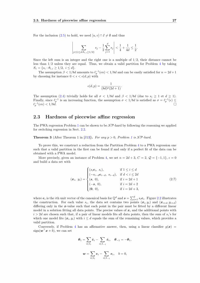
the construction. For each value si, the data set contains two points (xi, yi) and (xi+d, yi+d)differing only in the x-value such that each point in the pair must be fitted by a different linearmodel in a solution fitting all data points. The precise values of xi and the additional points withi > 2d are chosen such that, if a pair of linear models fits all data points, then the sum of si’s forwhich one model fits (xi, yi) with i ≤ d equals the sum of the remaining values, which provides avalid partition.
Conversely, if Problem 4 has an affirmative answer, then, using a linear classifier g(x) =sign(w>x+ b), we can set
θ1 =∑i∈I1
ei −∑i∈I−1
ei, θ−1 = −θ1,
w =∑i∈I1
ei −∑i∈I−1
ei, b = 0,
28 Chapter 2. Computational complexity
-2
2
-1
0
1
y
1
x2
20
2
1
x1
-1 0-1-2
-2
-3
4
-2
-1
2
0
y
1
x2
0
2
3
-2
4
x1
3210-4 -1-2-3
Figure 2.2: PWA regression data set built as in (2.7) for the reduction of the (toy) partitionproblem: with S = {s1 = 2, s2 = 2} (left) and S = {s1 = 1, s2 = 3} (right). The blue points arebuilt from s1 and the red ones from s2; they are plotted with filled disks for i ≤ d and empty criclesfor i > d. The black points are the three last ones in the data set. Left: a linear model can fitthe filled blue and empty red points on the right, while another one fits the empty blue and filledred points on the left and the black points are fitted by both models. This yields a solution to thepartition problem by taking in S1 the values si for which one of these models fits (xi, yi) with i ≤ d(filled disks). Note that there is no other way to fit all the points with two linear models. Right:the partition problem has no solution and no pair of linear models can fit all these data points.
where ei = [e>i , 0]>, I1 is the set of indexes of the elements of si in S1 and I−1 = [d] \ I1. Thisgives
x>i θ1 =
si = yi, if i ≤ d and i ∈ I1−si, if i ≤ d and i ∈ I−1
si−d = yi, if i > d and i− d ∈ I−1
−si−d, if i > d and i− d ∈ I1∑j∈I1 sj −
∑j∈I−1
sj = 0 = yi, if i = 2d+ 1∑j∈I−1
sj −∑j∈I1 sj = 0 = yi, if i = 2d+ 2
0 = yi, if i = 2d+ 3
and we can similarly show that
x>i θ−1 = yi, if i ∈ I−1 or i− d ∈ I1 or i > 2d,
while w>xi is positive if i ∈ I1 or i− d ∈ I−1 and negative if i ∈ I−1 or i− d ∈ I1. Therefore, forall points, x>i θg(xi) = yi, i = 1, . . . , 2d+ 3, and the cost function of Problem 1 is zero, yielding anaffirmative answer for its decision form.
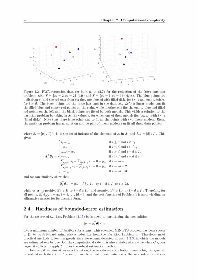
2.4 Hardness of bounded-error estimationFor the saturated `0,ε loss, Problem (1.15) boils down to partitioning the inequalities
|yi − x>i θ| ≤ ε
into a minimum number of feasible subsystems. This so-called MIN PFS problem has been shownin [3] to be NP-hard using also a reduction from the Partition Problem 4. Therefore, mostpractical methods follow the greedy iterative scheme depicted in Sect. 1.2.3, in which the modelsare estimated one by one. On the computational side, it is also a viable alternative when C growslarge: it suffices to apply C times the robust estimation method.
However, if we aim at an exact solution, the worst-case complexity remains high in general.Indeed, at each iteration, Problem 3 must be solved to estimate one of the submodels, but it can

2.5. Conclusions 29
also be shown to be NP-hard [2]. Overall, the greedy approach replaced an NP-hard problem bya sequence of NP-hard problems. Yet, the later is more amenable to practical solutions and wewill see in the following chapters that it is possible to solve such problems exactly in polynomialtime for a fixed dimension or in reasonable time in practice for small dimensions.
2.5 ConclusionsThis chapter essentially showed that all the optimization problems at the core of the consideredregression problems areNP-hard. This contribution improved our understanding of these problemsthat have been informally deemed very difficult for a long time.
The next chapter will refine these results in the case where some parameters are fixed (suchas the dimension d or the number of modes C). A remaining open issue concerns the strongNP-hardness based on a model computation with unary encoding instead of the binary encoding.Indeed, our proofs rely on reductions from the Partition problem, which is known to be only weaklyNP-hard.

Chapter 3
Exact methods for empirical riskminimization
Most works on the particular regression problems that we consider propose heuristics for theminimization of the empirical risk. Nonetheless, two types of additional contributions can bedistinguished: those that propose a new theoretical framework but only provide an algorithmthat implements an approximation of that framework (as [9]) and those that propose theoreticalguarantees for a specific heuristic (as [96, 4]). Methods from the first type are interesting as theybring a new point of view shedding light onto the problem; these often inspire other methodsdeveloped later. The second type of contribution seems stronger as it develops results that holdfor the algorithm applied in practice. However, the underlying assumptions are often violated inpractice, in which case the theoretical result does not apply anymore.
The goal of this chapter is to propose methods whose exactness can be guaranteed in a(quasi)unconditional manner.1
The complexity results presented in the preceding chapter seem to indicate that there is nohope for computing exact solutions in all circumstances. Yet, we will see here that reality is notso bad. In particular, the following questions remain open: what parameter(s) among C, d and nreally influence(s) the hardness of the problems? And, as a consequence, what parameter could befixed to make the problems exactly solvable in reasonable time?
It seems that the number of modes C plays a particular role here. On the one hand, the hardnessresults were obtained with reductions using the smallest value C = 2, implying that fixing it to asmall value will not help in overcoming the complexity. On the other hand, a larger C will typicallyincur an even larger complexity.
By a careful look at the proofs of NP-hardness, one can see that the critical parameter is thedimension d. To emphasize this more clearly, we will now derive exact algorithms with polynomialcomplexity in the last parameter, i.e., the number of data n. The existence of these algorithmsproves that with a fixed dimension, the problems can be solved in polynomial time and are notNP-hard anymore (unless P = NP). The converse is not true: by fixing n, we do not obtainpolynomial-time algorithms in d. And we shall not hope for this, since such algorithms used on thereductions of the partition problem described in Chapter 2 would contradict the famous conjectureP 6= NP.
We start this chapter in Sect. 3.1 with the case of piecewise affine regression, before extendingthe results to switching regression in Sect. 3.2 and to bounded-error estimation in Sect. 3.3.
Remark 1. In this chapter, we return in notation to real numbers. The complexity results thusobtained can be understood in terms of the number of floating-point operations (flops), which isthe standard measure of complexity in numerical analysis. Conversely, the whole chapter could bewritten with rational numbers to stick to the definitions of the preceding chapter.
1By “quasi-unconditional", we mean that the conditions are satisfied almost surely in a probabilistic framework.
31

32 Chapter 3. Exact methods for empirical risk minimization
3.1 Piecewise affine regression with fixed C and d
In the PWA regression Problem 1, one must simultaneously estimate a classifier g and a submodelfk for each mode. While these functions typically include continuous parameters, their optimizationcan be reduced to a combinatorial search over a finite (and polynomial) number of cases. To seethis, we need to focus on the classifier g and realize that g only influences the optimization problemthrough its value at the data points x1, . . . ,xn. As a result, we need not search for g in an infiniteset but merely for its output values, which belong to the finite set Q = [C]. More precisely, we canenumerate the possible classifications and determine the optimal submodels fk for each one of thefixed classifications. Yet, the number of possible classifications, Cn, remains exponential in n andtoo high to allow for a direct enumeration.
We will see now how to reduce this number to a polynomial function of n for the set of linearclassifiers G in (1.8).
Definition 1 (Trace of a function class). The trace of a set of functions G ⊂ YX on a sequence ofn points xn = (xi)1≤i≤n ⊂ X , denoted by Gxn , is the set of all labelings of xn that can be producedby a function from G:
Gxn = {(g(x1), . . . , g(xn)) : g ∈ G} ⊂ Yn.
Definition 2 (Growth function). The growth function ΠG(n) of a set of classifiers G ⊂ [C]X at nis the maximal number of labelings of n points produced by classifiers from G:
ΠG(n) = supxn∈Xn
|Gxn | ≤ Cn.
For linear classifiers, the number of classifications ΠG(n) is much smaller than Cn and classicalresults in learning theory directly lead to a polynomial bound for the binary linear classifiers ofRd:
ΠG(n) ≤(
en
d+ 1
)d+1
.
This bound results from a simple application of the Sauer–Shelah Lemma [91, 80, 83]2 to the linearclassifiers of Rd whose VC-dimension equals d + 1. However, this bound is not sufficient for ourpurposes. Indeed, its proof is not constructive and does not yield an enumeration algorithm forthe classifications, which is actually what we require to solve the PWA regression problem.
To achieve this goal, we will instead use an equivalence result that relates the linear classificationproduced by g ∈ G and the classification given by a separating hyperplane passing through a subsetxd(g) of d points of xn ⊂ Rd (see Figure 3.1). Based on this equivalence, the enumeration of thelinear classifications boils down to the enumeration of the
(nd
)= O(nd) subsets of d points among
xn.We leave some technical details aside and simply state the final result, relying on Algorithm 1
for C = 2 modes, in which we let xi = [x>i , 1]>. The case C > 2 with G as in (1.8) is dealt with bysearching for the C(C−1)/2 pairwise binary classifiers. Algorithm 1 performs two intertwined loops.As suggested above, the first one loops over all subsets xd(g) of d points to build the separatinghyperplanes. However, as the points in xd(g) lie exactly on the hyperplane, their classification isundetermined (points in xd are not in S1 nor in S2) and a second loop ensures that all classificationsof these points (into x1
d(g) and x2d(g)) are tested.
Theorem 4 (After Theorem 2 in [J13]). For any fixed number of modes C and dimension d, ifthe points {xi}ni=1 are in general position, i.e., no hyperplane of Rd contains more than d points,and if (3.1) can be solved in O(nc) time with a constant c ≥ 1 independent of n, then the timecomplexity of Problem 1 is no more than polynomial in the number of data n and in the order of
O(nc+dC(C−1)/2
).
2See also the discussion by Léon Bottou [13] on the authorship of this result.3The normal vector wxd(g)
of a hyperplane {x : w>xd(g)
x+ b = 0} passing through d points {xij }dj=1 of Rd can
be computed in O(d3) operations as a unit vector in the null space of the matrix [xi2 −xi1 , . . . , xid −xi1 ]>. Then,the offset is given by bxd(g) = −w>
xd(g)xij for any xij .

3.1. Piecewise affine regression with fixed C and d 33
−5 −4 −3 −2 −1 0 1 2 3 4 5−10
−5
0
5
Figure 3.1: The hyperplane H (—) yields the same classification (as + and ◦) of the points of R2
as the hyperplane Hxd (- - -) obtained by a translation (· · ·) and a rotation of H such that Hxd
passes exactly through xd = (x1,x2) (∗). This equivalence holds for all data points except x1 andx2 (∗) that lie exactly on the hyperplane Hxd and for which the classification is undetermined.
Algorithm 1 PWA regression in polynomial time for C = 2
Input: A data set ((xi, yi))1≤i≤n ⊂ (Rd × R)n.Initialize J∗ ← +∞.for all xd(g) ⊂ xn of cardinality |xd(g)| = d doCompute the parameters (wxd(g), bxd(g)) of a hyperplane passing through the points in xd(g).3Classify the points:
S1 = {xi ∈ xn : w>xd(g)xi + bxd(g) > 0},
S2 = {xi ∈ xn : w>xd(g)xi + bxd(g) < 0}.
for all classification of xd(g) into x1d(g) and x2
d(g) doSolve the single-mode regression subproblems:
θk ∈ argminθ∈Rd+1
∑xi∈Sk∪xkd(g)
`p(yi − x>i θ), ∀k ∈ {1, 2}. (3.1)
Compute the cost function value J =1
n
2∑k=1
∑xi∈Sk∪xkd(g)
`p(yi − x>i θk),
Update the solution (J∗,θ∗,w∗, b∗)← (J, [θ>1 ,θ>2 ]>,wxd(g), bxd(g)) if J < J∗.
end forend forreturn θ∗,w∗, b∗.
34 Chapter 3. Exact methods for empirical risk minimization
For standard loss functions, Theorem 4 guarantees that an exact solution can be computed inpolynomial time wrt. n. For instance, for the squared loss (p = 2), (3.1) corresponds to leastsquares problem that can be solved in O(d2n) operations [33], leading to c = 1 in Theorem 4.
In Algorithm 1, the inner loop over the binary classifications of the d points of xd(g) implies2d iterations. These are required because the equivalence between the classifiers of G and thecomputed hyperplanes does not hold for the points in xd(g). The general position assumption inTheorem 4 precisely bounds the number of points that can exactly lie on the hyperplanes and thusthe number of iterations required for the inner loop.
3.2 Switching regression with fixed C and d
We will now see how to extend the results of the preceding section to the switching regressionproblem introduced in Sect. 1.2.2. At first, this might not seem trivial since the polynomial-timealgorithm for PWA regression relies on the search for a linear classifier that determines the mode.Here, the switchings between the modes are arbitrary and no linear separability assumption can apriori be used. However, the groups of data pairs (xi, yi) associated with different linear modelscan be “linearly separated" in some sense.
More precisely, the classification rule (1.12) used in switching regression implicitly entails acombination of two linear classifiers: one applying to the points zi = [x>i , yi]
> in Rd+1 and anotherone applying to the regression vectors xi in Rd. The equivalence between (1.12) and these linearclassifiers will hold for all points that can be classified without ambiguity, i.e., those with indexnot in
E(θ) ={i ∈ [n] : ∃(j, k) ∈ [C]2, j 6= k, |yi − x>i θj | = |yi − x>i θk|
}. (3.2)
The cardinality of this set can be bounded as follows.
Lemma 1. Let E(θ) be defined as in (3.2). If the points {xi}ni=1 are in general position, i.e., ifno hyperplane of Rd contains more than d of these points, and if the points {zi = [x>i , yi]
>}ni=1
are also in general position in Rd+1, then |E(θ)| ≤ (2d+ 1)C(C − 1)/2.
Proposition 1 (Proposition 3 in [J14]). Given a parameter vector θ = [θ>1 , . . . ,θ>C ]> ∈ RCd, let
E(θ) be defined as in (3.2). Then, for all i /∈ E(θ), the classification (1.12) is equivalent to theclassification
ci = argmaxj∈[C]
j−1∑k=1
1qkj(xi,yi)=−1 +
C∑k=j+1
1qjk(xi,yi)=+1 (3.3)
implementing a majority vote over the C(C − 1)/2 binary classifiers (qjk)1≤j<k≤C of Rd+1, whereqjk is a product of linear classifiers defined by
∀(x, y) ∈ Rd × R, qjk(x, y) = gjk(z)hjk(x), 1 ≤ j < k ≤ C,
with linear classifiers operating in Rd+1 and Rd as
∀z ∈ Rd+1, gjk(z) = sign([−θ>jk, 1]>z), 1 ≤ j < k ≤ C,
∀x ∈ Rd, hjk(x) = sign(θ>jkx), 1 ≤ j < k ≤ C,
where θjk = (θj + θk)/2 and θjk = θj − θk.
Proposition 1, illustrated by Fig. 3.2, provides a clear connection between switching regressionand linear classification. By using this, all the consistent classifications of n points for the switchingregression problem can be formed by combining the linear classifications of the zi’s and those ofthe xi’s. According to the discussion of Sect. 3.1, for any pair (j, k), there are O(nd) possibleclassifications by a gjk and O(nd+1) possible classifications by a hjk, which make O(n2d+1) possibleclassifications by a qjk. By Proposition 1 there cannot be more classifications c ∈ [C]n consistentwith (1.12) than possible combinations of the outputs of C(C − 1)/2 classifiers qjk. Thus, thenumber of classifications to explore for switching regression is bounded by
O(n(2d+1)C(C−1)/2
)= O
(n2dC(C−1)
).
3.3. Bounded-error estimation with fixed d 35
-0.5 0 0.5
x
-1.5
-1
-0.5
0
0.5
1
y
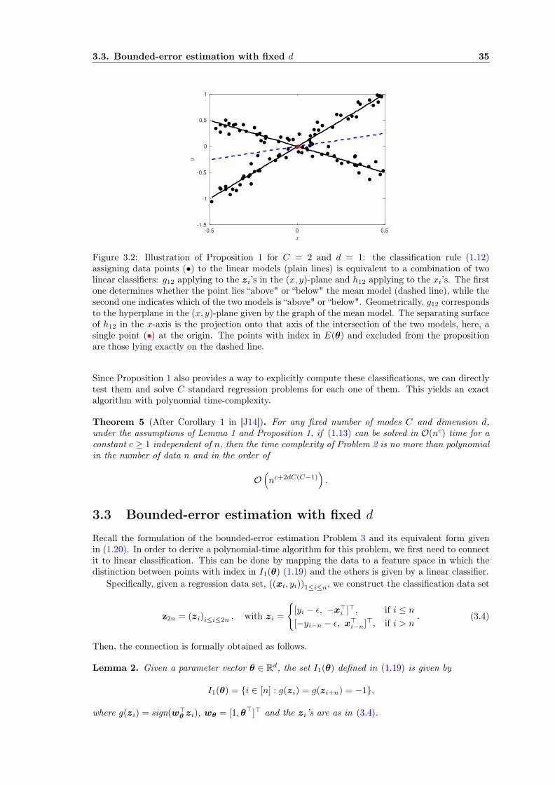
Figure 3.2: Illustration of Proposition 1 for C = 2 and d = 1: the classification rule (1.12)assigning data points (•) to the linear models (plain lines) is equivalent to a combination of twolinear classifiers: g12 applying to the zi’s in the (x, y)-plane and h12 applying to the xi’s. The firstone determines whether the point lies “above" or “below" the mean model (dashed line), while thesecond one indicates which of the two models is “above" or “below". Geometrically, g12 correspondsto the hyperplane in the (x, y)-plane given by the graph of the mean model. The separating surfaceof h12 in the x-axis is the projection onto that axis of the intersection of the two models, here, asingle point (•) at the origin. The points with index in E(θ) and excluded from the propositionare those lying exactly on the dashed line.
Since Proposition 1 also provides a way to explicitly compute these classifications, we can directlytest them and solve C standard regression problems for each one of them. This yields an exactalgorithm with polynomial time-complexity.
Theorem 5 (After Corollary 1 in [J14]). For any fixed number of modes C and dimension d,under the assumptions of Lemma 1 and Proposition 1, if (1.13) can be solved in O(nc) time for aconstant c ≥ 1 independent of n, then the time complexity of Problem 2 is no more than polynomialin the number of data n and in the order of
O(nc+2dC(C−1)
).
3.3 Bounded-error estimation with fixed d
Recall the formulation of the bounded-error estimation Problem 3 and its equivalent form givenin (1.20). In order to derive a polynomial-time algorithm for this problem, we first need to connectit to linear classification. This can be done by mapping the data to a feature space in which thedistinction between points with index in I1(θ) (1.19) and the others is given by a linear classifier.
Specifically, given a regression data set, ((xi, yi))1≤i≤n, we construct the classification data set
z2n = (zi)i≤i≤2n , with zi =
{[yi − ε, −x>i ]>, if i ≤ n[−yi−n − ε, x>i−n]>, if i > n
. (3.4)
Then, the connection is formally obtained as follows.
Lemma 2. Given a parameter vector θ ∈ Rd, the set I1(θ) defined in (1.19) is given by
I1(θ) = {i ∈ [n] : g(zi) = g(zi+n) = −1},
where g(zi) = sign(w>θ zi), wθ = [1,θ>]> and the zi’s are as in (3.4).
36 Chapter 3. Exact methods for empirical risk minimization
-0.5 0 0.5
x
-1
-0.8
-0.6
-0.4
-0.2
0
0.2
0.4
0.6
0.8
1
y
-1.2 -1 -0.8 -0.6 -0.4 -0.2 0 0.2 0.4 0.6
z1
-0.6
-0.4
-0.2
0
0.2
0.4
z2
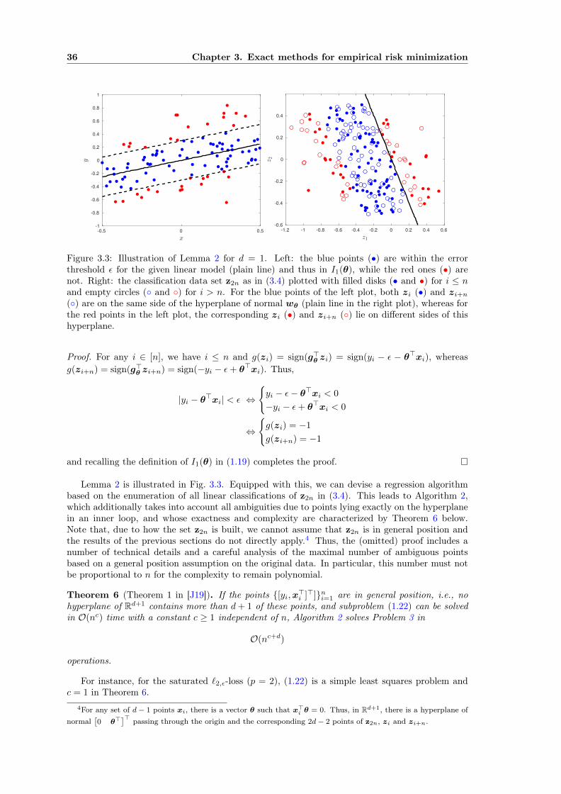
Figure 3.3: Illustration of Lemma 2 for d = 1. Left: the blue points (•) are within the errorthreshold ε for the given linear model (plain line) and thus in I1(θ), while the red ones (•) arenot. Right: the classification data set z2n as in (3.4) plotted with filled disks (• and •) for i ≤ nand empty circles (◦ and ◦) for i > n. For the blue points of the left plot, both zi (•) and zi+n(◦) are on the same side of the hyperplane of normal wθ (plain line in the right plot), whereas forthe red points in the left plot, the corresponding zi (•) and zi+n (◦) lie on different sides of thishyperplane.
Proof. For any i ∈ [n], we have i ≤ n and g(zi) = sign(g>θ zi) = sign(yi − ε − θ>xi), whereasg(zi+n) = sign(g>θ zi+n) = sign(−yi − ε+ θ>xi). Thus,
|yi − θ>xi| < ε ⇔
{yi − ε− θ>xi < 0
−yi − ε+ θ>xi < 0
⇔
{g(zi) = −1
g(zi+n) = −1
and recalling the definition of I1(θ) in (1.19) completes the proof.
Lemma 2 is illustrated in Fig. 3.3. Equipped with this, we can devise a regression algorithmbased on the enumeration of all linear classifications of z2n in (3.4). This leads to Algorithm 2,which additionally takes into account all ambiguities due to points lying exactly on the hyperplanein an inner loop, and whose exactness and complexity are characterized by Theorem 6 below.Note that, due to how the set z2n is built, we cannot assume that z2n is in general position andthe results of the previous sections do not directly apply.4 Thus, the (omitted) proof includes anumber of technical details and a careful analysis of the maximal number of ambiguous pointsbased on a general position assumption on the original data. In particular, this number must notbe proportional to n for the complexity to remain polynomial.
Theorem 6 (Theorem 1 in [J19]). If the points {[yi,x>i ]>]}ni=1 are in general position, i.e., nohyperplane of Rd+1 contains more than d+ 1 of these points, and subproblem (1.22) can be solvedin O(nc) time with a constant c ≥ 1 independent of n, Algorithm 2 solves Problem 3 in
O(nc+d)
operations.
For instance, for the saturated `2,ε-loss (p = 2), (1.22) is a simple least squares problem andc = 1 in Theorem 6.
4For any set of d− 1 points xi, there is a vector θ such that x>i θ = 0. Thus, in Rd+1, there is a hyperplane ofnormal
[0 θ>
]> passing through the origin and the corresponding 2d− 2 points of z2n, zi and zi+n.
3.4. Conclusions 37
Algorithm 2 Regression with a saturated `p,ε lossInput: a data set ((xi, yi))1≤i≤n, a threshold ε > 0.Initialize J∗ ← εpn.for all zd ⊂ z2n of cardinality |zd| = d doCompute the normal w to the hyperplane passing through zd ∪ {0} and of orientation suchthat w1 ≥ 0.if w1 6= 0 thenClassify the points while excluding those precisely on the hyperplane:
∀i ∈ [2n], ci = sign0(w>zi),
where sign0(a) returns 0 if a = 0 and sign(a) otherwise.Set I0 = {i ∈ [2n] : ci = 0} and s = |I0|.for all classification of the s points of index in I0, i.e., for all s ∈ {−1,+1}s do
Assign the values s to the entries of c with index in I0.Compute Is1 = {i ∈ [n] : ci = ci+n = −1}.if εp(n− |Is1 |) < J∗ thenCompute θ as in (1.22) with Is1 instead of I1(θ∗).Let J(θ) =
∑ni=1 `p,ε(yi − x>i θ).
if J(θ) < J∗ thenUpdate J∗ ← J(θ), θ∗ ← θ.
end ifend if
end forend if
end forreturn J∗,θ∗.
3.4 ConclusionsWe showed in this chapter the existence of algorithms with a polynomial complexity with respectto the number of data for the minimization of the empirical risk in the three regression problemsof interest. However, the complexities of the algorithms remain exponential in the dimension d.
Future work might consider developing heuristic methods inspired by the exact polynomial-time algorithms. Preliminary results in that direction were obtained in [J19]. The idea is toreplace the complete enumeration of the subsets of points used to build the classifications by arandom sampling. Doing so, a major difference with respect to RANSAC-like methods [26] isthat the subset of points is only used to determine the classification whose optimal value can berecovered according the analysis above. On the contrary, RANSAC-like methods directly estimatethe regression model from the subset of points and cannot recover the exact solution.


Chapter 4
Global optimization for empiricalrisk minimization
The applicability of the polynomial-time algorithms of the previous chapter is very limited by thedimension d, which appears as an exponent in their time complexities. In order to tackle slightlylarger-dimensional problems, we will resort to a global optimization strategy, focusing on the realparameter vectors and implicitly embedding the discrete classification in the cost function, forinstance as (1.12) was embedded in (1.14). Here, the gain in speed will be obtained thanks toheuristics. However, these heuristics only make us gain time, they do not incur a loss in accuracy(beyond the small tolerance used in the stopping criterion). Yet, they are referred to as heuristicssince they cannot be proved to yield a significant gain in speed in every circumstances: the averagecomputational time observed in practice is decreased to a reasonable amount while the worst-casecomputational time remains exponential in the dimension D of the problem (here D is the numberof optimization variables). In particular, when discussing the computational complexity of theapproach below, we will focus on the complexity of a single iteration of the algorithm, while theprecise number of iterations depends on the data.
4.1 General scheme
Branch-and-bound is a standard strategy for the global optimization of some cost function J(θ) of avector of parameters θ ∈ RD over a box Binit = [uinit,vinit] ⊂ RD. The main steps are summarizedin Algorithm 3. It relies on computing upper and lower bounds (J and J in Algorithm 3) on theglobal optimum minθ∈Binit
J(θ). Then, regions B of the search space in which the local lowerbound J(B) is larger than the global upper bound J can be discarded, reducing the volume left toexplore until the relative optimality gap, (J − J)/J , decreases below a predefined tolerance TOL.
Here, the considered regions are always boxes, i.e., hyperrectangles. Upper bounds J(B) canbe easily computed by some local optimization or heuristic method for a problem of interest.Alternatively, J(B) can be computed merely as the cost function value at the box base point uor at a random point inside the box B = [u,v]. On the other hand, lower bounds J(B) require acareful derivation, the efficiency of the approach relying mostly on the tightness of these bounds.
4.2 Switching regression
Consider the switching linear regression Problem (1.14) with the `2-loss and linear submodels, i.e.,the minimization of a cost function
J(θ) =
n∑i=1
mink∈[C]
(yi − x>i θk)2,
with θ = [θ>1 , . . . ,θ>C ]> ∈ RD and D = Cd.
39
40 Chapter 4. Global optimization for empirical risk minimization
Algorithm 3 General branch-and-bound scheme.Input: A data set {(xi, yi)}ni=1 ⊂ Rd × R, box bounds Binit = [uinit,vinit] ⊂ RD and a toleranceTOL > 0. Optionally, a first guess of θ ∈ Binit.Initialize the global bounds J ← 0, J ← +∞ or J ← J(θ) if θ is given, and the list of boxesB ← {Binit}, B ← Binit.while (J − J)/J > TOL doSplit the current box B into B1 and B2 such that B = B1 ∪B2.Compute upper bounds J(B1) and J(B2).Update J ← min{J, J(B1), J(B2)} and the best solution θ∗.Compute lower bounds J(B1) and J(B2).For j = 1, 2, append Bj to the list of active boxes B if J(Bj) ≤ J .Remove B from the list: B ← B \ {B}.Select the next box B ← argminB∈B J(B) and update J ← J(B).
end whilereturn θ∗ and J = J(θ∗) ≈ minθ∈Binit J(θ).
Note that for symmetry reasons, this cost function is invariant to permutations of the subvectorsθk in θ, hence the minimizer is not unique. Such symmetries can be broken by arbitrarily imposingan ordering on the modes, for instance as
θk,1 ≤ θk+1,1, k = 1, . . . , C − 1, (4.1)
where θk,j denotes the jth component of θk.1
The symmetry-breaking constraints (4.1) can be simply imposed at the branching level byexplicitly discarding regions of subboxes without feasible solutions. More precisely, we computeB1 = [u1,v1] and B2 = [u2,v2] from B = [u,v] by first applying a standard split along the longestside of the box:
(k∗, j∗) = argmaxk∈[C],j∈[d]
vk,j − uk,j , (4.2)
and
u1 = u, v1k,j =
{(uk,j + vk,j)/2, if (k, j) = (k∗, j∗),
vk,j , otherwise,(4.3)
v2 = v, u2k,j =
{(uk,j + vk,j)/2, if (k, j) = (k∗, j∗),
uk,j , otherwise.(4.4)
Then, in the case j∗ = 1, which is the only one concerned by (4.1), we correct the box boundsrecursively for k = k∗ − 1, . . . , 1 with
v1k,1 = min
{v1k,1, v
1k+1,1
}(4.5)
and, for k = k∗ + 1, . . . , C, with
u2k,1 = max
{u2k,1, u
2k−1,1
}. (4.6)
Figure 4.1 illustrates the splitting rule.
Lower bounds
When devising a lower bound, one always faces a trade-off between the speed with which thelower bound can be computed and its tightness. We describe below two lower bounds: one that
1Note that ties in the case θk,1 = θk+1,1 can be broken by imposing similar constraints recursively on theremaining components. However, these additional constraints might be more difficult to take into account in thebranch-and-bound approach, while they might also be of little use since the event corresponding to a tie in a globalminimizer has zero measure with noisy data.

4.2. Switching regression 41
0.5 1 1.5 2 2.5 3 3.5
θ1
0.5
1
1.5
2
2.5
3
3.5
θ2
u
v
B
0.5 1 1.5 2 2.5 3 3.5
θ1
0.5
1
1.5
2
2.5
3
3.5
θ2
u1
v2
u2
v1
B1
B2
0.5 1 1.5 2 2.5 3 3.5
θ1
0.5
1
1.5
2
2.5
3
3.5
θ2
v2
u2
B2
θ1 ≤ θ2
θ1 > θ2
Figure 4.1: Illustration of the splitting procedure when C = 2 and d = 1. Top: a box B = [u,v] isa rectangular region of the plane of axis (θ1, θ2) with bottom-left and top-right corners at u and v.Middle: B is split into B1 = [u1,v1] and B2 = [u2,v2] by application of (4.2)–(4.4). Bottom: B2
is corrected as in (4.5)–(4.6) to remove the shaded area that does not contain any feasible solutionaccording to (4.1), i.e., θ1 > θ2 for all θ in the shaded area.
42 Chapter 4. Global optimization for empirical risk minimization
can be very efficiently computed and one that is tighter. The final algorithm will result from thecombination of both.
The first lower bound is based on a pointwise decomposition of the optimization problem withrespect to the index i of data points. In particular, we use the fact that, for any i ∈ [n] and k ∈ [C],the pointwise error of a parameter vector θk at a given point (xi, yi),
ei(θk) = yi − x>i θk,
can be made smaller in magnitude if we are not trying to simultaneously minimize the errors atother points. Therefore, the global cost J(θ) must be at least as large as the sum of independentlyoptimized pointwise errors. Formally, for any i ∈ [n] and box Bk = [uk,vk] ⊂ Rd, let
eLi (Bk) = ei(uk)− (vk − uk)>(xi)− (4.7)
eUi (Bk) = ei(uk)− (vk − uk)>(xi)+,
where (xi)+ and (xi)− denote the positive and negative parts of xi, computed entrywise. Thesequantities constitute the bounds within which the error ei(θk) can be with θk ∈ Bk. Then, we candeduce the minimal value for the squared error over the box Bk as
minθk∈Bk
e2i (θk) =
(eUi (Bk)
)2+
+(eLi (Bk)
)2− . (4.8)
By applying a similar scheme to all data points, this gives a lower bound on the optimum over Bexpressed as
minθ∈B
J(θ) ≥ J(B),
where
J(B) =
n∑i=1
mink∈[C]
{(eUi (Bk)
)2+
+(eLi (Bk)
)2−
}. (4.9)
The second lower bound is based on a constant classification argument. The idea is that forsufficiently small boxes B, the parameter vectors θk can be so constrained that the classificationgiven by2
ci(θ) = argmink∈[C]
(yi − x>i θk)2
is constant over B for a certain number of points of index i. If this number is large, then thecost over all these points is at least as large as the smallest error with which these points can beestimated by a single model, independently of the rest of the problem. Let us define the set ofindexes of points constantly assigned to mode k over B as
Ik(B) = {i ∈ [n] : ∀θ ∈ B, ci(θ) = k}.
Then,
∀i ∈ Ik(B), ∀θ ∈ B, minj∈[C]
e2i (θj) = e2
i (θk)
and
∀θ ∈ B,C∑k=1
∑i∈Ik(B)
minj∈[C]
e2i (θj) =
C∑k=1
∑i∈Ik(B)
e2i (θk).
Introducing the set I0(B) = [n] \⋃Ck=1 Ik(B) of remaining indexes (for which the classification is
2Here we consider an arbitrary tie-breaking rule: ci(θ) is the smallest mode index with a minimal error.
4.3. Bounded-error estimation 43
not constant over B), we can express the cost function as
∀θ ∈ B, J(θ) =
n∑i=1
minj∈[C]
e2i (θj)
=
C∑k=0
∑i∈Ik(B)
minj∈[C]
e2i (θj)
=∑
i∈I0(B)
minj∈[C]
e2i (θj) +
C∑k=1
∑i∈Ik(B)
e2i (θk)
≥ minθ∈B
∑i∈I0(B)
minj∈[C]
e2i (θj) +
∑k∈[C]
minθk∈Bk
∑i∈Ik(B)
e2i (θk)
≥∑
i∈I0(B)
mink∈[C]
{(eUi (Bk)
)2+
+(eLi (Bk)
)2−
}+∑k∈[C]
minθk∈Bk
∑i∈Ik(B)
e2i (θk), (4.10)
where the last inequality is obtained by lower bounding the first sum in a manner similar to ourfirst lower bound, i.e., using (4.8).
In order to use (4.10) as a lower bound in the branch-and-bound algorithm, we first need todetermine the index sets Ik(B), k = 1, . . . , C. We have shown in [J17] that this can be done in acomputationally efficient manner from the quantities (4.7) as
Ik(B) ={i ∈ [n] : max
{eUi (Bk)2, eLi (Bk)2
}< min
j<k
(eUi (Bj)
)2+
+(eLi (Bj)
)2− ,
max{eUi (Bk)2, eLi (Bk)2
}≤ min
j>k
(eUi (Bj)
)2+
+(eLi (Bj)
)2−
}.
Overall procedure and complexity
We are now almost ready to apply Algorithm 3 with lower bounds computed as in (4.10). The onlyremaining part to specify is how we compute the upper bounds J(B). In practice, good resultshave been observed when using the k-LinReg algorithm [J9] every 1000 iterations and merely thecost function value J(u) at the box base point u otherwise. This is computationally very efficientand still offers enough accuracy (remember that Algorithm 3 calls the upper bounding methodmany times from different initializations).
The computational complexity of the approach is, for each iteration, mostly governed by thecomputation of the lower bounds. For the one in (4.10), the most intensive task is to solve thebox-constrained least squares problem
minθk∈Bk
∑i∈Ik(B)
e2i (θk), (4.11)
for each k ∈ [C]. Such problems are simple quadratic programs for which very efficient dedicatedsolvers can be found. In addition, it is not always necessary to solve the problems for all k ∈ [C].Since all the values of (4.11) computed one by one are accumulated in the lower bound (4.10), wecan stop as soon as the partial sum is large enough to exclude the box B from the branch-and-boundsearch, i.e., when it reaches the global upper bound J .
4.3 Bounded-error estimationWe now detail how the branch-and-bound approach above can be adapted to deal with the bounded-error estimation Problem 3. Recall that, in bounded-error estimation, we estimate a single param-eter vector θ ∈ Rd. Therefore, all the boxes B are now d-dimensional. We limit the presentationto the case p = 2, i.e., the minimization of a sum of saturated squared loss,
J(θ) =
n∑i=1
min{
(yi − x>i θ)2, ε2}. (4.12)

44 Chapter 4. Global optimization for empirical risk minimization
The idea is that bounded-error estimation can be seen as a switching regression problem with twomodes: one with a linear model approximating the points with error less than ε and another onewith a constant error of ε.
A pointwise lower bound similar to (4.9) can be derived in the bounded-error estimation setting,leading to
J(B) =
n∑i=1
min{(eUi (B)
)2+
+(eLi (B)
)2− , ε
2}≤ minθ∈B
J(θ).
A second lower bound based on a constant classification argument can also be derived. Here,we classify the points in two groups: those with squared error less than ε2 and the others. Thus,we define the index sets
I1(B) = {i ∈ [n] : ∀θ ∈ B, (yi − x>i θ)2 ≤ ε2},
I2(B) = {i ∈ [n] : ∀θ ∈ B, (yi − x>i θ)2 > ε2},
and I0(B) = [n] \ (I1(B)∪ I2(B)). These sets can be easily computed from the quantities (4.7) byusing (4.8):
I1(B) =
{i ∈ [n] : max
θ∈Be2i (θ) = max
{eLi (B)2, eUi (B)2
}≤ ε2
}and
I2(B) =
{i ∈ [n] : min
θ∈Be2i (θ) =
(eUi (B)
)2+
+(eLi (B)
)2− > ε2
}.
Clearly, for all points with index in I1(B), min{e2i (θ), ε2
}= e2
i (θ), while for those with index inI2(B), min
{e2i (θ), ε2
}= ε2. Thus, the cost function (4.12) can be lower bounded as
∀θ ∈ B, J(θ) =
2∑k=0
∑i∈Ik(B)
min{e2i (θ), ε2
}=
∑i∈I0(B)
min{e2i (θ), ε2
}+
∑i∈I1(B)
e2i (θ) + ε2|I2(B)|
≥∑
i∈I0(B)
min{(eUi (B)
)2+
+(eLi (B)
)2− , ε
2}
+ minθ∈B
∑i∈I1(B)
e2i (θ) + ε2|I2(B)|,
(4.13)
where the inequality is obtained as in (4.10) by using (4.8).
Overall procedure and complexity
Algorithm 3 can be applied for bounded-error estimation with lower bounds computed as in (4.13).For the upper bounds, the cost function value J(u) at the box base point u can be periodicallycombined with a heuristic method alternating between the classification and estimation of thelinear model (see [J17] for details).
As for switching regression, the computational complexity of the approach is, for each iteration,dominated by the (rather low) complexity of solving the box-constrained least squares problem
minθ∈B
∑i∈I1(B)
e2i (θ).
4.4 Piecewise affine regressionUnfortunately, we are not aware of a technique to generalize the methods above to the PWA case.Indeed, the need to estimate the classifier g simultaneously complicates the procedure to the pointwhere it becomes inefficient.
Historically, another global optimization strategy has been proposed in [77] to deal with thisproblem. It also relies on branch-and-bound, but with a quite different perspective. Here, binary

4.5. Limitations of exact methods 45
Table 4.1: Average and empirical standard deviation of the computing time (in seconds on a laptop)for the global optimization of a switching linear model with C modes for different dimensions dand number of data n.
C d n Time2 2 500 0.1± 0.1
1 000 0.2± 0.110 000 0.6± 0.4
3 500 0.8± 1.31 000 0.6± 0.310 000 2.3± 1.5
4 500 4.1± 2.91 000 5.8± 6.910 000 11.9± 11.9
5 500 24.0± 20.71 000 35.3± 29.910 000 66.7± 20.1
3 2 500 1.3± 0.91 000 1.8± 1.410 000 3.8± 2.2
3 500 22.8± 23.21 000 50.7± 45.310 000 72.4± 38.8
4 500 783± 6261 000 1404± 97710 000 2061± 1239
variables are introduced to encode the classification, which allows the problem to be reformulatedas a Mixed-Integer Quadratic Program (MIQP).3 The interest of this approach is that a vastamount of work has been devoted to MIQPs and generic solvers implementing efficient heuristicscan be found. However, these remain highly limited by the number of integer variables, which ishere proportional to the number of data, n. Hence, this approach is practical only for very smallproblem sizes, typically with n < 200.
4.5 Limitations of exact methods
It stems quite clearly from the preceding chapters that exact methods cannot be applied system-atically. Whenever the dimension d or the number of modes C grows too large, these become fartoo expensive computationally.
To get some intuition about these limitations, we now perform a few numerical experiments,first with the global optimization strategy of Sect. 4.2 for switching regression. Table 4.1 reportsthe computing time of Algorithm 3 for various number of data and dimensions. For each problemsize, we consider the average and empirical standard deviation of the computing time over 10 trials,in which the regression vectors xi and the true parameter vectors θk are randomly drawn from auniform distribution in [−5, 5]d.
The results in Table 4.1 show that switching regression problems with up to 10 000 pointsin dimension 4 can be solved in about one minute on a standard laptop. But, as expected, thecomputing time quickly increases with the dimension and the number of modes. Yet, these resultssupport the idea that the complexity of this global optimization approach remains reasonably lowwith respect to the number of data. In particular, Table 4.1 suggests a complexity in n that isless than linear, indicating that the number of data does not critically influences the number ofiterations and mostly affects the linear algebra and convex optimization operations.
Given the NP-hardness of the problem, the high complexity with respect to C and d appears
3In truth, this approach is only valid for a subclass of PWA models known as hinging hyperplanes.

46 Chapter 4. Global optimization for empirical risk minimization
Table 4.2: Time (in seconds for a parallel implementation on a machine with 12 cores) and numberof least squares solutions (#LS) required to solve Problem 1 exactly with the polynomial-timeAlgorithm 1 compared with the time and number of quadratic programs (#QP) required by theMIQP approach of [77]. “n/a" appears when the algorithm did not terminate in less than 10 hours.
Polynomialalgorithm
MIQP approach
d n Time #LS Time #QP1 100 0.03 400 16 5.103
1 200 0.05 800 95 4.104
1 500 0.11 2.103 n/a n/a1 1 000 0.16 4.103 n/a n/a1 10 000 3.6 4.104 n/a n/a1 50 000 110 2.105 n/a n/a2 100 0.5 4.104 10.5 3.103
2 200 0.9 2.105 32 8.104
2 500 5.6 1.106 n/a n/a2 1 000 30 4.106 n/a n/a3 100 8 2.106 15 5.103
3 200 65 2.107 81 3.104
3 500 1 536 3.108 n/a n/a3 1 000 16 870 2.109 n/a n/a4 50 23 7.106 2.2 2.103
4 100 355 1.108 12 4.103
4 200 6 506 2.109 55 1.104
hardly overcomable by any exact or global optimization approach.The same observations can be made regarding PWA regression. Table 4.2 reports the time
needed to solve PWA regression problems with C = 2 with the polynomial-time algorithm ofSect. 3.1 and the MIQP approach of [77] discussed in Sect. 4.4. On the one hand, these resultsclearly emphasize the advantages of the method of Chapter 3 over the MIQP approach. On theother hand, they show the limitations of an exact approach based on a complete enumeration ofthe classifications when d ≥ 4.
4.6 ConclusionsThis chapter presented a global optimization approach to tackle two of the three regression problemsconsidered in this report. Despite the lack of theoretical guarantees on their complexity, theresulting algorithms were shown to be rather efficient in experiments with significant problem sizes.Indeed, if the dimensions d considered here seem small, they are rather customary in applications.In particular, for hybrid dynamical system identification, such dimensions are quite common inmost studies. In this respect, we contributed to the first experimental results on thousands ofnoisy data points with global optimality guarantees.
However, a global optimization method that can be efficient with respect to the number ofpoints for piecewise affine regression remains elusive.
Part II
Statistical learning theory
47


49
The preceding Part concentrated on optimization issues in order to minimize the error over adata set. However, this is not sufficient to guarantee the quality of a predictive model and its abilityto generalize. The goal of this part is to formulate guarantees on the generalization performanceof the models. For this, we will use the framework and the tools of statistical learning theory.
Chapters 6 and 7 will derive generalization error bounds for piecewise smooth and switchingregression models. But first, we introduce the tools and techniques of learning theory in Chapter 5for the derivation of risk bounds in the more standard context of multi-category classification.Indeed, this classification problem appears in piecewise smooth regression when estimating thepartition of the input space that determines the mode. In addition, we will see that there is astrong relationship between the phenomenons observed in this setting and in switching regression,especially regarding the dependency of the bounds on the number of categories for classificationand the number of modes for switching regression.

Chapter 5
Risk bounds for multi-categoryclassification
We here briefly recall the agnostic learning framework for multi-category classification. Let X bean input space and Y a finite set of categories of cardinality C. Let (X, Y ) be a random pairtaking value in X × Y and with unknown distribution P . Given a realization ((xi, yi))1,≤i≤n of atraining sample ((Xi, Yi))1≤i≤n of n independent copies of (X, Y ), the aim of learning is to find aclassifier g ∈ G ⊂ YX minimizing, over the predefined set G, the risk
L(g) = EX,Y 1g(X)6=Y = P (g(X) 6= Y ).
This quantity cannot be computed without access to P and the standard approach is thus tobound the risk of classifiers by a function of their performance measured on the training samplevia the empirical risk,
Ln(g) =1
n
n∑i=1
1g(Xi) 6=Yi ,
and of a control term or confidence (semi-)interval. The latter depends in general on the class Gand a parameter δ quantifying the confidence with which the bound holds. Formally, we aim atderiving bounds of the form
Pn{∀g ∈ G, L(g) ≤ Ln(g) +B(n,G, δ)
}≥ 1− δ, (5.1)
where Pn denotes the joint distribution of ((Xi, Yi))1≤i≤n and the confidence interval B(n,G, δ)decreases with n. In general, the dependence on G appears through a capacity (or complexity)measure of the function class. Note that we are here interested in distribution-free (that hold forany P ) and uniform (that hold for all g ∈ G) bounds in a framework similar to that studied byVapnik [90].
In this chapter, we will particularly pay attention to the influence of the number of categoriesC on the confidence interval, which we explicit by writing B(n,C,G, δ). Indeed, the precise char-acterization of this influence is currently an active field of research [34, 68, 51, 49, 35, 55].
Note that our interest in the dependence on C of the bounds can significantly change ourperspective when considering the techniques used to derive the bounds. Indeed, in the binarycase or when C is merely considered as a constant, the standard approach is often asymptotic inthe sense that bounds are compared mostly on the basis of their convergence rate in n (in termsof a big-O of n). But whenever we are interested in the dependence on C of B(n,C,G, δ), theasymptotic notation is not always suited and bounds should be compared at fixed and finite valuesof n and C. Thus, a bound combining a weak convergence rate in n with only a mere dependenceon C could be better than another one with a faster convergence rate for specific values of n andC. In such a context, the values of the constants play a more important role than in the usualcase.
51

52 Chapter 5. Risk bounds for multi-category classification
Similar issues will arise when we will introduce an additional parameter, i.e., the dimension dof X. Indeed, we will see that it is sometimes possible to obtain very good dependencies on bothn and C but at the expanse of an exponential dependence on the dimension.
5.1 Margin classifiersA binary classifiers g : X → Y = {−1,+1} is a margin classifier when it can be expressed as
g(x) = sign (g0(x))
for a real-valued function g0. For instance, linear classifiers and support vector machines (SVMs)are margin classifiers.
In the multi-class case where Y = [C], a classifier g : X → Y is a margin classifier when it canbe expressed as
g(x) = argmaxk∈[C]
gk(x)
with C real-valued component functions (gk)1≤k≤C that compute a score for each category andan arbitrary tie-breaking rule. Multi-class SVMs, neural networks and classifiers based on a one-against-one decomposition are examples of margin classifiers.
5.2 Bounds based on the Rademacher complexityNowadays, the most common approach initiated by [48, 7] consists in deriving risk bounds of theform (5.1) with a capacity measure known as the Rademacher complexity1.
Definition 3 (Rademacher complexity). Let T be a random variable taking value in T . For anyn ∈ N∗, let Tn = (Ti)1≤i≤n be an n-sample of independent copies of T and σn = (σi)1≤i≤n be asequence of independent random variables uniformly distributed in {−1,+1}. Given a class F ofreal-valued functions on T , the empirical Rademacher complexity of F given Tn is
Rn (F) = Eσn
[supf∈F
1
n
n∑i=1
σif(Ti)
∣∣∣∣∣Tn
].
The Rademacher complexity of F is
Rn (F) = ETn
[Rn (F)
]= ETnσn
[supf∈F
1
n
n∑i=1
σif(Ti)
].
Theorem 7 (After Theorem 3.1 in [68]). Let L be a class of functions from Z into [0, 1] and(Zi)1≤i≤n a sequence of independent copies of Z ∈ Z. Then, for any fixed δ ∈ (0, 1), with probabilityat least 1− δ, uniformly for all ` ∈ L,
EZ`(Z) ≤ 1
n
n∑i=1
`(Zi) + 2Rn (L) +
√log 1
δ
2n
and
EZ`(Z) ≤ 1
n
n∑i=1
`(Zi) + 2Rn (L) + 3
√log 2
δ
2n.
To every margin multi-category classifier of
G =
{g ∈ YX : g(x) = argmax
k∈Ygk(x), gk ∈ Gk
}, (5.2)
1The Rademacher complexity is also known as the Rademacher average. It has been largely studied in the fieldof empirical processes, see, e.g., [52, 87].

5.2. Bounds based on the Rademacher complexity 53
we assign a margin function
mg(x, y) =1
2
(gy(x)−max
k 6=ygk(x)
)that allows us to estimate the 0-1 loss by
1g(x)6=y ≤ 1mg(x,y)≤0,
where the two terms are equal except when mg(x, y) = 0 (in case of a tie between two categories).Introducing this margin function allows us to take into account the real-valued outputs of theclassifier and not only their argmax. To do so, we shall not only look at the sign of mg(x, y) andreplace the indicator function in the estimation above by another loss function. Here, we considerthe saturated hinge loss parametrized by γ > 0:2
∀u ∈ R, φ(u) =
1, if u ≤ 0
1− uγ , if u ∈ (0, γ)
0, if u ≥ γ.(5.3)
Thus, 1g(x)6=y ≤ φ ◦mg(x, y) for all (x, y), and the analysis concentrates on the margin risk
Lγ(g) = EX,Y [φ ◦mg(X, Y )] , (5.4)
which upper bounds the risk L(g), and its empirical version
Lγ,n(g) =1
n
n∑i=1
φ ◦mg(Xi, Yi).
The interest of the margin risk as defined here via the function φ is to formulate the analysis interms of the computation of the Rademacher complexity of a class of Lipschitz functions whenapplying Theorem 7.
Therefore, Theorem 7 applies to the loss class
L ={`mg ∈ [0, 1]Z : `mg (x, y) = φ ◦mg(x, y), mg ∈MG
}= φ ◦MG ,
where Z = X × Y andMG denotes the class of margin functions:
MG =
{mg ∈ RZ : mg(x, y) =
1
2
(gy(x)−max
k 6=ygk(x)
), gk ∈ Gk
}. (5.5)
This leads to the bound
∀g ∈ G, Lγ(g) ≤ Lγ,n(g) + 2Rn (L) +
√log 1
δ
2n,
in which Rn (L) can be estimated from Rn (MG) thanks to the contraction principle.
Lemma 3 (Contraction principle, after Theorem 4.12 in [52]). If φ : R→ R has Lipschitz constantLφ (if ∀(u, v) ∈ R2, |φ(u)− φ(v)| ≤ Lφ|u− v|), then, for all real-valued function class F ,
Rn(φ ◦ F) ≤ LφRn(F),
where φ ◦ F is the class of functions φ ◦ f with f ∈ F .
The Lipschitz constant of φ defined in (5.3) being equal to 1γ , we obtain
Rn (L) ≤ 1
γRn (MG) .
2The choice of the saturated hinge loss is very common, but other alternatives exist. Far from being benign, thischoice actually implies the complete path of computations described in this chapter and based on the Rademachercomplexities. Alternatively, the choice φ(u) = 1u≤γ calls for an analysis based on L∞-norm covering numbers, asthe one proposed by [5] (see also [35] for the multi-class case).
54 Chapter 5. Risk bounds for multi-category classification
5.3 Decomposition of capacity measures
Given the preceding result, the next step consists in relating the Rademacher complexity of MGto the capacities of the component function classes Gk. Several approaches can be used for thisdecomposition depending on the choice of capacity measure. We here detail two main approaches.The first one presented in Sect. 5.3.1 considers the direct decomposition of Rn (MG) in terms ofthe Rademacher complexities of the classes Gk. The second approach, exposed in Sect. 5.3.2, isbased on the chaining method [87] and the estimation of the Rademacher complexity via coveringnumbers.
5.3.1 Decomposition at the level of Rademacher complexities
The decomposition at the level of Rademacher complexities relies on the following structural result.
Lemma 4 (After Lemma 8.1 in [68]3). Let (Uk)1≤k≤K be a sequence of K classes of real-valuedfunctions on Z. Then, the empirical Rademacher complexity of the class U = {u ∈ RZ : u(z) =maxk∈[K] uk(z), uk ∈ Uk} is bounded by
Rn(U) ≤K∑k=1
Rn(Uk).
With Lemma 4, we can estimate the Rademacher complexity of the margin function class fromthe component function classes with a quadratic dependence on C.
Theorem 8 (After Theorem 8.1 in [68] – itself based on Theorem 11 in [48]). Let G ⊂ [C]X be aset of margin multi-category classifiers as in (5.2) andMG be defined as in (5.5). Then
Rn (MG) ≤ CC∑k=1
Rn (Gk) .
The state of the art that improves this is originally due to [51] and leads to a linear dependencyon the number of categories C. This result considers a slightly different class: the class of marginfunctions clipped at 0 and γ:
MG,γ ={mg,γ ∈ RZ : mg,γ(x, y) = πγ ◦mg(x, y), mg ∈MG
}, (5.6)
where
∀t ∈ R, πγ(t) =
t, if t ∈ (0, γ]
γ, if t > γ
0, if t ≤ 0.
Indeed, we can focus the analysis on this class, since the margin risk (5.4) (and more precisely theloss function (5.3)) is insensitive to the variations of the margin outside of the range (0, γ].4,5
Theorem 9 (After Theorem 2 in [51]). Let G ⊂ [C]X be a set of margin multi-category classifiersas in (5.2) andMG,γ be defined as in (5.6). Then,6
Rn (MG,γ) ≤C∑k=1
Rn (Gk) .
3This result is in general attributed to [68] despite the fact that it relies on the arguments of Lemma 2 in [48]and that a similar technique was already used for pointwise minimum classes in the proof of Theorem 2.1 in [12].
4More precisely, [51] considers clipping at γ only without clipping the negative values, but the result holdssimilarly forMG,γ as defined here. The approach of [51] might thus seem less efficient, but we are not aware of anyimprovement obtained by taking into account the clipping at 0.
5A result similar to Theorem 9 up to some constant factor can be obtained by following the more recent approachof [54] with a small detour via Gaussian complexities, or the closely related one of [59].
6Actually, [51] states that Rn (MG) ≤ CRn(⋃C
k=1 Gk), but the proof also directly yields the result stated here.

5.3. Decomposition of capacity measures 55
5.3.2 Decomposition at the level of covering numbersThe relationship between component function classes and the class of margin functions can beanalyzed at the level of another capacity measure: that of covering numbers. This relationshipappears less straightforward when one aims at deriving risk bounds based on the Rademachercomplexity, but, as we will see, this can also be more efficient in terms of limiting the influence ofthe number of categories.
Definition 4 (Empirical pseudo-metrics). Given a sequence xn ∈ Xn, dq,xn is the empiricalpseudo-metric defined for all (f, f ′) ∈
(RX)2 and q ∈ [1,∞) by
dq,xn(f, f ′) =
(1
n
n∑i=1
|f(xi)− f ′(xi)|q) 1q
and for q =∞ byd∞,xn(f, f ′) = max
i∈[n]|f(xi)− f ′(xi)|.
Definition 5 (Covering numbers). Let F ⊂ RX be a function class and ρ a pseudo-metric inRX . The (external) covering number N (ε,F , ρ) at scale ε of F for the distance ρ is the smallestcardinality of an ε-net H ⊂ RX of F such that ∀f ∈ F , ρ(f,H) < ε. The internal covering numberN int(ε,F , ρ) is defined similarly but with proper ε-nets satisfying H ⊆ F .
When ρ is an empirical pseudo-metric according to Definition 4, the covering nubmers are calledLq-norm covering numbers and the uniform covering numbers are defined by
Nq(ε,F , n) = supxn∈Xn
N (ε,F , dq,xn)
andN intq (ε,F , n) = sup
xn∈XnN int(ε,F , dq,xn).
By considering covering numbers at many different scales, the chaining method developed byDudley allows one to bound the Rademacher complexity [87].
Theorem 10. Let F ⊂ RZ be a function class of diameter DF = sup(f,f ′)∈F2 d2,zn(f, f ′). Then,7
∀N ∈ N∗, Rn(F) ≤ DF2−N + 6DF
N∑j=1
2−j√
logN int(DF2−j ,F , d2,zn)
n(5.7)
and, if the entropic integral appearing below exists,
Rn(F) ≤ 12
∫ DF/2
0
√logN int(ε,F , d2,zn)
ndε. (5.8)
Decomposition at the level of covering numbers can be performed with the following lemma.
Lemma 5 (Lemma 1 in [35]8). Let G ⊂ [C]X be a set of margin multi-category classifiers asin (5.2) andMG,γ be defined as in (5.6). Then, for all ε ∈ (0, γ2 ],
∀q ∈ [1,+∞], N int (ε,MG,γ , dq,zn) ≤C∏k=1
N int( ε
C1/q,Gk, dq,xn
). (5.9)
This decomposition lemma offers a degree of freedom in the choice of the Lq norm. By intro-ducing this result with q = 2 in the chaining formula (5.7) applied to MG,γ , we observe that themain dependency on C can be radical. However, C also influences the bound via the scale, ε/
√C,
7Formula (5.7) is the standard formula, given for instance in [82], and based on dyadic weights. Other versionscan be obtained for different choices of these weights (see for instance [35]).
8A version of this result dedicated to the case q =∞ was also given in [105].
56 Chapter 5. Risk bounds for multi-category classification
of the covering numbers, which makes the dependency larger and less explicit. Indeed, based onthis approach, the study in [35] shows a final result with a closer to linear dependency.
At the other end of the spectrum, L∞-norm covering numbers allow us to obtain a truly radicaldependence on C, but in general at the expanse of a slower convergence rate in n. To use thedecomposition result with q =∞ in the chaining formula (5.7) originally based on the L2-norm, itsuffices to use the inequality
∀ε > 0, logN int(ε,Gk, d2,xn) ≤ logN int(ε,Gk, d∞,xn)
based on the ordering, d2,xn ≥ d∞,xn , of the pseudo-metrics. This directly leads to a bound witha clear and radical dependence on C:
Rn(MG,γ) ≤ γ2−N + 6γ
N∑j=1
2−j
√∑Ck=1 logN int(γ2−j ,Gk, d∞,xn)
n
≤ γ2−N + 6γ√C
N∑j=1
2−j
√maxk∈[C] logN int(γ2−j ,Gk, d∞,xn)
n, (5.10)
where the scale of the covering numbers is not touched by C during the decomposition. In addition,the dependency on C is here independent of the component function classes. Though this is anaturally desirable property of the bound, it is not obtained for other Lq norms.
5.3.3 Covergence rates and Sauer-Shelah lemmas
In order to specify the convergence rates wrt. n, we now need to estimate the covering numbersof the Gk’s. The standard approach consists in the application of a Sauer–Shelah lemma9 giving abound in terms of another capacity measure known as the fat-shattering dimension.
Definition 6 (Fat-shattering dimension [45]). Let F be a class of real-valued functions on X . Forε > 0, a set of points {xi}ni=1 ⊆ X is said to be ε-shattered by F if there is a witness b ∈ Rn suchthat for all I ⊆ [n], there is a function f I ∈ F satisfying
f I(xi)
{≥ bi + ε, if i ∈ I≤ bi − ε, if i ∈ [n] \ I.
The fat-shattering dimension at scale ε of the class F , dF (ε), is the maximal cardinality of a set ofpoints ε-shattered by F , if such a maximum exists. Otherwise, the fat-shattering dimension is saidto be infinite.
There is a whole family of Sauer–Shelah lemmas that consider for instance different pseudo-metrics to define the covering numbers. The lemmas that provide a bound that does not dependon n are said be “dimension-free", as the one of Mendelson et Vershynin for the covering numbersin L2-norm:
Lemma 6 (After Theorem 1 in [64] with constants given by [35]). Let F ⊂ [−M,M ]X be a functionclass of fat-shattering dimension dF (ε). Then, for any ε ∈ (0,M ] and n ∈ N∗,
logN int2 (ε,F , n) ≤ 20dF
( ε
96
)log
(13M
ε
).
9This name refers to the first lemma of this kind derived independently by several authors [91, 80, 83] andbounding the growth function of a binary classifier in terms of the Vapnik–Chervonenkis dimension. In this chapter,we in fact consider generalized Sauer–Shelah lemmas expressed in terms of another capacity measure. The word“generalized" will always be omitted but implicitly present.In addition, Sauer–Shelah lemmas are typically formulated to bound packing numbers instead of covering numbers.
The packing numbers correspond to the cardinality of the largest ε-separated subset of a function class and theyupper bound the covering numbers [47]. Hence we can formulate the lemmas in terms of the covering numbers.

5.3. Decomposition of capacity measures 57
Though certainly desirable, the dimension-free nature of a Sauer-Shelah lemma is not alwaysthe most relevant feature in order to optimize the convergence rate of a risk bound. In this respect,the quality of Lemma 6 is largely due to its dependence on ε in O (dF (ε) log(1/ε)) as ε→ 0.
Another lemma that applies to L∞-norm covering numbers is the following.
Lemma 7 (After Lemma 3.5 in [1]). Let F ⊂ [−M,M ]X be a function class of fat-shatteringdimension dF (ε). Then, for any ε ∈ (0,M ] and n ≥ dF ( ε4 ),
logN int∞ (ε,F , n) ≤ 2dF
( ε4
)log2
(4Men
dF(ε4
)ε
)log
(16M2n
ε2
).
Observe that this lemma is not dimension-free and leads to a metric entropy bound10 inO(dF (ε) log2(1/ε)), hence with an additional factor of log( 1
ε ) compared to Lemma 6. Another re-sult on L∞-norm covering numbers allows this factor to be reduced to logξ( 1
ε ) for a fixed ξ ∈ (0, 1)[79]. However, this gain is obtained at the cost of a decrease of the scale parameter appearing in thefat-shattering dimension which ends up being multiplied by a factor ξ. Thus, the true gain remainssmall under general assumptions as those considered below and except for the limit case n → ∞.As discussed in the introduction of this chapter, we are particularly interested in the dependenceon the number of categories C, and thus in the non-asymptotic case (n finite). Therefore, we willnot further consider the solution based on the results of [79].
Equipped with all those lemmas, we now need to bound the fat-shattering dimensions in orderto compute the convergence rates. This ultimately depends on our choice of component functionclasses Gk. But first, we will consider a very general framework in which we merely make anassumption of the growth rates of the fat-shattering dimensions wrt. ε:
Assumption 1. The classes Gk are such that there are numbers α ≥ 0 and β ≥ 0 such that
∀ε > 0, d(ε) = maxk∈[C]
dGk(ε) ≤ αε−β . (5.11)
Such an assumption was introduced in the seminal work of Mendelson [60], and further used in[63, 35, 36, C16]. As an example, support vector machines satisfy this assumption with β = 2 [8].Larger values for the degree β of the polynomial growth appear for instance if the Gk’s are sets ofneural networks: for networks with l hidden layers, we can set β = 2(l + 1) in (5.11) [5].
Results obtained with L2-norm covering numbers
By considering L2-norm covering numbers for which the most efficient Lemma 6 is available, weobtain (after Theorem 7 in [35]):
Rn(MG,γ) ≤ c√C
n
Cβ/4
√logC, if β ∈ (0, 2),√
C log3/2 n
C, if β = 2,
C1/βn1/2−1/β
√log
n
C, if β > 2,
(5.12)
for a constant c that depends only on α, β and γ. The convergence rates in n are here similar tothose obtained by Mendelson in the binary case (see Theorem 1.6 in [63]). We note that all valuesof β close to 2 lead to an almost-linear dependency on C. The values of β close to 0 actually yield aradical dependency, but these are only available for classifiers with a very low capacity (and lowerthan that of a linear classifier). Large values of β also yield a good dependence on C, but withvery slow convergence rates.
Results obtained with L∞-norm covering numbers
As seen above with (5.10), the use of the L∞-norm leads to a radical dependence on C. However,the convergence rate worsens in this case by a factor
√log n (or log n for β < 2) compared with
10The metric entropy is the logarithm of the covering number.
58 Chapter 5. Risk bounds for multi-category classification
the results obtained with the L2-norm above. More precisely, by combining Lemma 7 with (5.10)we obtain (see [C16]):
Rn(MG,γ) ≤ c√C
n
log n, if β ∈ (0, 2),
log2 n, if β = 2,
n1/2−1/β log n, if β > 2,
(5.13)
for a constant c that only depends on α, β and γ.
Towards the best of two worlds
We have seen the pros and cons of using L∞-norm covering numbers compared to those in L2-norm. We will now show that covering numbers in Lq-norm with an intermediate value of q leadto a result uniformly better that the one based on the L2-norm: a radical dependence on C (upto some logarithmic factor) with the same convergence rate. In truth, it suffices to observe thatthe scale of the covering numbers after the decomposition by Lemma 5 expressed as ε/C1/q isactually not directly influenced by C for all q ≥ log2 C. Indeed, for these values of q, we haveC1/q = 2
1q log2 C ≤ 2.
Therefore, the difficulty is now to obtain a Sauer–Shelah lemma in Lq-norm that remainsefficient wrt. ε. For instance, the dimension-free version proposed in [35] for all q ∈ (2,∞) growswith ε−1 as a O
(dF (ε) log2 1
ε
)and thus without an advantage over Lemma 7 in L∞-norm when
used in chaining.By following more closely the proof of Lemma 6 by Mendelson and Vershynin, we could derive
a more efficient result.
Lemma 8 (Sauer-Shelah Lemma in Lq-norm, after Theorem 2 in [J20]). Let F ⊂ [−M,M ]X be afunction class of fat-shattering dimension dF (ε). Then, for any ε ∈ (0,M ] and any integer q ≥ 3,we have, for n ≥ dF
(ε
15q
), the bound
logN intq (ε,F , n) < 2dF
(ε
15q
)log
39Mqn
dF
(ε
15q
)ε
, (5.14)
and, for any n ∈ N∗, the dimension-free bound
logN intq (ε,F , n) < 10q dF
(ε
36q
)log
(7Mq1/7
ε
). (5.15)
Proof sketch. The proof follows precisely the one of [64] in which we replace the equality in hisLemma 4 by the inequality
(E|X −X ′|q)1/q ≤ (E|X|q)1/q+ (E| −X ′|q)1/q
= 2 (E|X|q)1/q
derived from the Minkowski inequality and that holds for all q ∈ [1,∞), any random variable Xand independent copy X ′ of X. The rest of the proof consists in showing that there exist numbersa and b such that the probabilities
P1 = P
{X > a+
1
4(2Kq)1/q(E|X|q)1/q
}
P2 = P
{X < a− 1
4(2Kq)1/q(E|X|q)1/q
}are sufficiently large: P1 ≥ 1 − b and P2 ≥ b/2 or vice versa. To do so, we work by contradictionand show that if it was not the case, then
E|X|q =
∫ ∞0
P (|X| > λ)dλq =
∫ ∞0
P (X > λ)dλq +
∫ ∞0
P (X < −λ)dλq < E|X|q. (5.16)
5.3. Decomposition of capacity measures 59
This calls for an upper bound on these integrals obtained by partitioning R+ into intervals Ik oflength c (E|X|q)1/q such that
1
2(2Kq)1/q< c <
1
(2Kq)1/q(5.17)
with Kq defined below and
P (X ∈ Ik) = βk − βk+1, k = 0, 1, 2, . . .
where βk ≤ 1/2k+1 in the case where the Lemma does not hold. Then, the bound on the integralin Eq. (4) of [64] becomes∫ ∞
0
P (X > λ)dλq ≤ cqE|X|q∑k≥0
(k + 1)q − kq
2k+1≤ cqE|X|q
∑k≥0
(k + 1)q
2k+1= Kqc
qE|X|q,
which, combined with (5.17), leads to (5.16), and where the polylogarithm function of order −qevaluated at 1/2,
Kq = Li−q(1/2) =∑k≥1
kq
2k,
appears instead of the mere factor 4 obtained for the case q = 2 in [64].This constant Kq then enters the scales at which the subsets of functions are separated. By
following the path of [64] and after some discretizations of the class of interest, this leads to thefirst result
logN int(ε,F , dq,xn) ≤ 2dF
(ε
15K1/qq
)log
39K1/qq n
dF
(ε
15K1/qq
)ε
.
The dimension-free version of this result is obtained from a slightly different discretization andthe application of the probabilistic extraction principle as implemented by Lemma 8 in [35] (whichextends Lemma 13 in [64] to Lq-norms):
logN int(ε,F , dq,xn) ≤ 10qdF
(ε
36K1/qq
)log
(7MK
1/qq
ε
).
Thus, the conclusion comes from the fact that, for any integer q ≥ 3, Kq < qq.
Lemma 8 provides two distinct results depending on whether we wish to obtain a dimension-free bound or not. The reason is that removing the dependency on n implies an increase of theconstants, and notably the addition of a factor q in the bound (5.15) on the metric entropy. Thus,the choice of the bound can be optimized with respect to the degree β in Assumption 1 when appliedin chaining. In particular, it seems that the dimension-free nature of the bound only improves theconvergence rate for β < 2. Therefore, in the final result below, obtained with q = dlog2 Ce, we canspare a power of logC for β ≥ 2 without worsening the convergence rate by using (5.14) insteadof (5.15).
Theorem 11 (After Theorem 3 in [J20]). Let G ⊂ [C]X be a set of margin multi-category classifiersas in (5.2) andMG,γ be defined as in (5.6). Then,
Rn(MG,γ) ≤ c√C
n
log(β+1)/2(C), if β ∈ (0, 2),
log(C) log3/2(n), if β = 2,
log2−β/2(C)n1/2−1/β√
log n, if β > 2 and m ≥ C1.2,
for a constant c independent of α, β and γ.
The convergence rates in Theorem 11 are similar to those based on L2-norm covering numbersin (5.12), with generally a power of C replaced by a power of logC (a more precise comparisonshould consider the exact statement of Theorem 3 in [J20], Theorem 11 above only gives a simplifiedview of the orders of magnitude). Compared with the result in (5.13), the convergence rates havebeen improved only at the cost of a logarithmic term in C.

60 Chapter 5. Risk bounds for multi-category classification
5.4 Bounds dedicated to kernel machinesKernel machines constitute an important class of models related to support vector machines(SVMs). These are defined by considering balls in a functional space built from a kernel func-tion K. We here briefly recall the necessary definitions (see [11, 86] for more details).
Definition 7 (Positive-definite kernel). A (positive-definite) kernel is a symmetric function K :X × X → R such that
∀n ∈ N, ∀xn ∈ Xn,∀α ∈ Rn,n∑i=1
n∑j=1
αiαjK(xi,xj) ≥ 0.
Definition 8 (Reproducing kernel Hilbert space (RKHS)). A reproducing kernel Hilbert space Kis a Hilbert space (H, 〈·, ·〉H) such that
1. ∀x ∈ X , K(x, ·) ∈ H;
2. ∀x ∈ X , ∀f ∈ H, 〈f,K(x, ·)〉H = f(x) (reproducing property).
Given an RKHS H, a multi-class SVM (M-SVM) typically implements a class of functions Gwith component functions from a ball of H:
Gk = G0 = {g0 ∈ H : ‖g0‖H ≤ Λ}, k = 1, . . . , C, (5.18)
where ‖g0‖H =√〈g0, g0〉H is the norm naturally induced by the inner product in H.
For these machines, it is possible to directly and efficiently bound the Rademacher complexity.
Lemma 9 (After Lemma 22 in [7]). Let G0 be a function class as in (5.18). Then,
Rn(G0) ≤ ΛxΛ√n,
where Λx = supx∈X ‖K(x, ·)‖H = supx∈X√K(x,x).11
Thus, we can insert this result into Theorem 9 to obtain a linear dependency on C and anoptimal convergence rate: for G as in (5.18),
Rn(MG,γ) ≤ CΛxΛ√n
. (5.19)
Besides, kernel machines satisfy Assumption 1 with β = 2 [8] and Theorem 11 yields
Rn(MG,γ) ≤ c
√C log3 n
nlogC (5.20)
with a sublinear dependency on C. However, here the gain in C appears not so advantageousbefore the loss in convergence rate. This can nonetheless be slightly improved by avoiding the useof the fat-shattering dimension to bound the covering numbers. To do so, we call upon the resultsof [104] directly bounding the L∞-norm covering numbers as
logN∞(ε,G0, n) ≤ 36Λ2xΛ2
ε2log
(15ΛxΛn
ε
)(5.21)
and thus with a dependence on ε similar to the one of Lemmas 6 and 8 for the Lq-norm coveringnumbers with q < ∞. Thus, we can decrease the dependence on C of the bound (5.20) up to aradical dependency, as in Sect. 5.3.3 (see also [105]). In this case, the comparison with (5.19) showsa gain of
√C for a loss of log3/2 n; hence a range of favorable values of C and n in the order of
c1 log3 n ≤ C ≤ c2n.11A data-dependent bound on the empirical Rademacher complexity, where Λx is replaced by
√∑ni=1K(xi,xi)/n,
can also be obtained in a similar manner.
5.5. Conclusions 61
The unspecified constants c1 and c2 show that this range is not very precise, since it depends on theconstants in the bounds which are rarely determined in an optimal manner. Indeed, the literatureon risk bounds usually concentrates on convergence rates in the asymptotic sense without payingmuch attention to the constants (which are merely not expressed by some authors).
It is yet possible to further improve the bound with L∞-norm covering numbers by restrictingthe analysis to Gaussian kernels, K(x,x′) = exp(−‖x−x′‖2/2σ2), defined over an Euclidean inputspace X ⊂ Rd. In this case, [24] builds on the results of [89], themselves based on [47], to show thebound
logN∞(ε,G0, n) ≤ c(d+ 1)d+1
ε, (5.22)
where the constant c depends on the kernel parameter σ. This bound allows for the application ofthe chaining formula with the integral (5.8) and leads to
Rn(MG,γ) ≤ c√C(d+ 1)d+1
n. (5.23)
Thus, we can combine the advantages of the two approaches: an optimal convergence rate similarto the one obtained by directly decomposing the Rademacher complexity, and a radical dependenceon C obtained thanks to the chaining with L∞-norm covering numbers. However, the price to payis here expressed in terms of the dimension d of the input space. Specifically, the favorable rangeof values when compared with (5.19) must be considered in terms of C and d, and becomes
c(d+ 1)2(d+1) < C.
Note that this range is in fact very limited and corresponds in practice to data in dimension lessthan 10 for any reasonable number of categories.
5.5 Conclusions
It is difficult to conclude in a definitive manner on the most suitable approach to derive risk boundsin classification. On the one hand the approach based on covering numbers seems to yield the bestdependencies on C, including sublinear ones. On the other hand, for specific classifiers for whichthe Rademacher complexity can be easily bounded, it seems more beneficial to decompose at thislevel without using covering numbers. Besides, we have seen that it is also sometimes possible tocombine the benefits of the two approaches, but at the cost of an exponential growth with thedimension of the input space.
There is a third level at which the decomposition can operate: that of fat-shattering dimensions.A generic decomposition at that level can be obtained from the decompositions at the other levels.Indeed, it can be shown that
dMG (ε) ≤ log2N int∞ (ε,MG , dMG (ε))
and thatsup
zn∈ZnRn(MG) ≤ ε ⇒ dMG (ε) ≤ n.
However, determining the fat-shattering dimension dMG (ε) with these formulas in order to nextbound the covering numbers or the Rademacher complexity by dMG (ε) does not seem appealingand actually leads to a loss of covergence rate compared to a more direct approach.
Numerous questions thus remain open. For instance, is it possible to decompose more efficientlyat the level of fat-shattering dimensions? And, how to better take into account the specificities ofcertain classes of functions in the decomposition? Or, conversely, how to build function classes forwhich the decomposition can be optimized? A few answers to these questions can be found in therecent works of [54, 55, 59, 6].
Besides, we have seen the impact of the choice of a particular Lq-norm to define the coveringnumbers and of the associated Sauer–Shelah lemma in the general case of a polynomial growthof the fat-shattering dimension. Specifically, from the viewpoint of C, the L∞-norm seems to be

62 Chapter 5. Risk bounds for multi-category classification
the most promising choice. But to really benefit from it without altering the covergence rate wewould need to derive a new Sauer–Shelah lemma in O
(dF (ε) log 1
ε
), with a factor log 1
ε removedin comparison to Lemma 7. Some authors think that it is indeed possible [75] and an interestingpath has been opened by [79], though this is not currently sufficient to conclude.
Chapter 6
Risk bounds for piecewise smoothregression
In this chapter, we come back to regression, where the goal is to estimate a real-valued function f .
6.1 General framework: error bounds in regression
The general framework follows that described for classification in Chapter 5. In addition to thefact that the set of outputs is not countable, Y ⊆ R (with |Y| = +∞), the main change is in thedefinition of the loss function. We here consider `p-losses with p ≥ 1,
`(y, f(x)) = `p(y − f(x)) = |y − f(x)|p,
instead of the 0-1 loss.An interesting property of the 0-1 loss that is not verified here is its boundedness. To remedy
to this issue, it is common to limit the study to bounded output spaces Y and clipped functions.1For a clipping threshold M > 0, we define the following notation:
∀t ∈ R, t =
M, if t ≥Mt, if t ∈ (−M,M)
−M, if t ≤ −M.
(6.1)
In the following, we consider Y ⊆ [−M,M ] and derive risk bounds for the class
F ={f ∈ [−M,M ]X : f(x) = f(x), f ∈ F
}(6.2)
of clipped functions built from F . Indeed, in this case, the `p-loss can be clipped at M , i.e., for all(y, t) ∈ Y × R,
`(y, t) ≤ `(y, t).
Thus, for any function f ∈ F yielded by a learning algorithm, we return instead the function f ∈ Fwhose risk is always smaller than or equal to the one of f .
We fix (without loss of generality) M = 1/2 and the interval Y ⊆ [−1/2, 1/2]. This choicemerely allows us to apply Theorem 7 to the class
Lp,F ={` ∈ [0, 1]X×Y : `(x, y) = |y − f(x)|p, f ∈ F
}(6.3)
of functions with output in [0, 1]. This leads to the following general bound.
1There exist other approaches to derive risk bounds with unbounded output spaces. These are in general basedon the existence of nonconstant envelopes for the class F or bounds on the higher-order moments of Y . See also thealternative approach of [61, 62].
63
64 Chapter 6. Risk bounds for piecewise smooth regression
Theorem 12 (Theorem 2 in [J21]). Let F be a class of real-valued functions. Then, for anyδ ∈ (0, 1), with probability at least 1− δ, the `p-risk is uniformly bounded for all f ∈ F by
Lp(f) ≤ Lp,n(f) + 2pRn(F)
+
√log 1
δ
2n.
In this chapter, we are interested in the case where F is a class of piecewise smooth (PWS)functions defined from a sequence (Fk)1≤k≤C of classes of functions from X into R and a set ofclassifiers G of X with output in [C]:
F = FG ={f ∈ RX : f(x) = fg(x)(x), g ∈ G, fk ∈ Fk
}. (6.4)
To the best of our knowledge, there is no direct method to efficiently estimate the Rademachercomplexity of such a class from the ones of the classes Fk and G. Thus, we will consider the approachbased on covering numbers and chaining, as the one presented in Sect. 5.3.2 for classification.
6.2 Decomposition at the level of covering numbers
Here, we will use covering numbers as defined in Definition 5 page 55. The results will also bestated in terms of the growth function ΠG(n) of the set of classifiers G, as introduced in Definition 2page 32.
We developed two decomposition lemmas at the level of covering numbers for PWS classesexpressed as (6.4).
Lemma 10. Let FG be a PWS class as in (6.4). Then, for all q ∈ [1,∞],
N (ε, F , dq,xn) ≤ ΠG(n)
C∏k=1
N( ε
C1/q, Fk, dq,xn
).
In addition, this inequality also holds for internal covering numbers.
Lemma 11. Let FG be a PWS class as in (6.4) with classes Fk such that dFk(ε) is finite for allε > 0, 1 ≤ k ≤ C. Then,
N (ε, FG , d2,xn) ≤ ΠG(n)
C∏k=1
N2(ε, Fk, n).
In addition, this inequality also holds for internal covering numbers.
The first one is not too difficult to derive and leads to a result similar in terms of the dependenceon C to the decomposition Lemma 5 for margin classifiers.
The second one concentrates on L2-norm covering numbers while allowing us to spare the changeof scale (the switch from ε to ε/C1/q in Lemma 10). This result is specific to PWS regression anddoes not seem transferable to classification. The proof relies on the one hand on the use of acollection of L2-pseudo-metrics defined over different sets of points, and on the other hand on themonotonicity of the covering numbers with respect to the size of these sets. We here only detailthe proof of the second lemma, which leads to the best results in the following.
Proof of Lemma 11. For every possible classification c ∈ Gxn of xn, let nk =∑ni=1 1ci=k denote
the number of points classified in category k, define K(c) = {k ∈ [C] : nk > 0} as the subset ofcategories with at least one point, and consider K(c) empirical pseudo-metrics dxi:ci=k defined asd2,xn but on a restricted set of points of cardinality nk > 0:
∀(f, f ′) ∈(RX)2, dxi:ci=k(f, f ′) =
(1
nk
∑i:ci=k
(f(xi)− f ′(xi))2
) 12
.
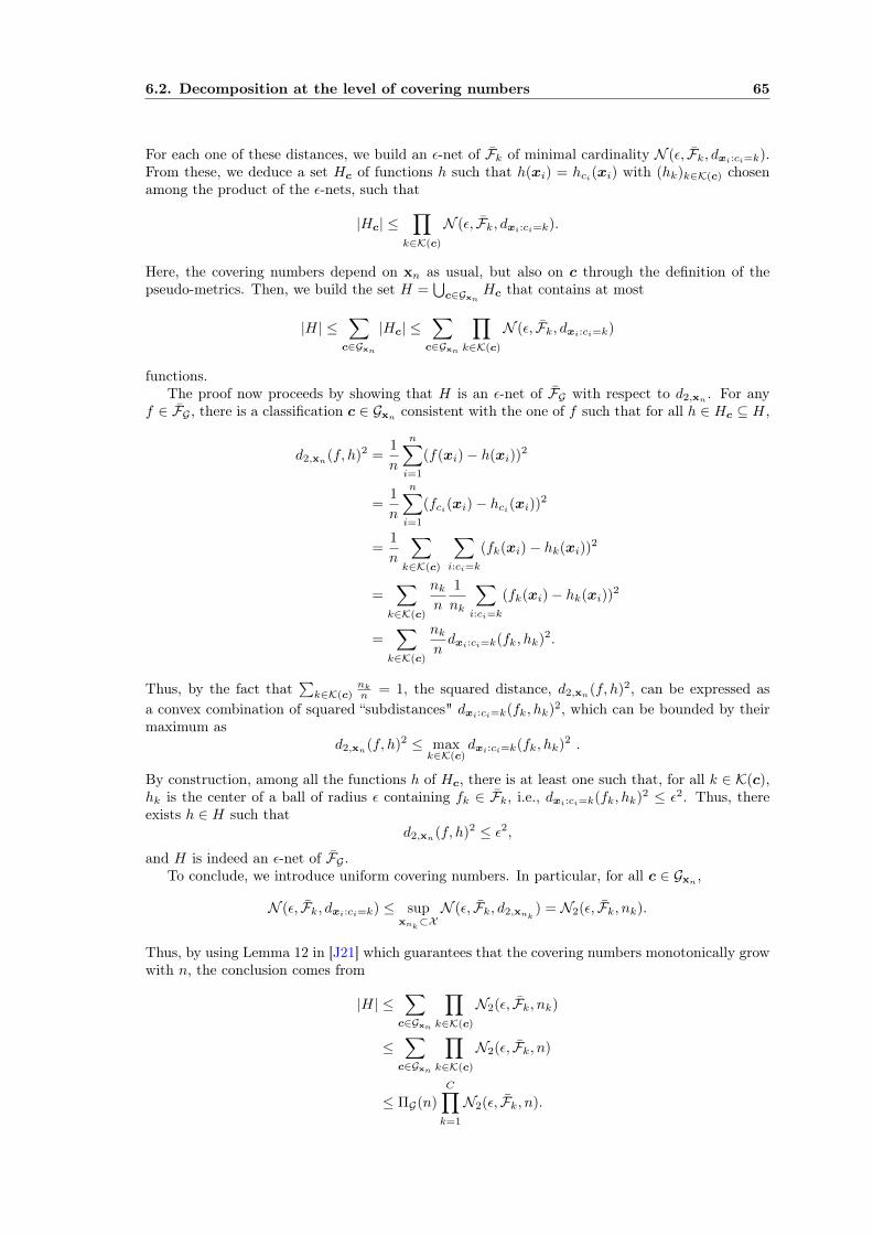
6.2. Decomposition at the level of covering numbers 65
For each one of these distances, we build an ε-net of Fk of minimal cardinality N (ε, Fk, dxi:ci=k).From these, we deduce a set Hc of functions h such that h(xi) = hci(xi) with (hk)k∈K(c) chosenamong the product of the ε-nets, such that
|Hc| ≤∏
k∈K(c)
N (ε, Fk, dxi:ci=k).
Here, the covering numbers depend on xn as usual, but also on c through the definition of thepseudo-metrics. Then, we build the set H =
⋃c∈Gxn
Hc that contains at most
|H| ≤∑c∈Gxn
|Hc| ≤∑c∈Gxn
∏k∈K(c)
N (ε, Fk, dxi:ci=k)
functions.The proof now proceeds by showing that H is an ε-net of FG with respect to d2,xn . For any
f ∈ FG , there is a classification c ∈ Gxn consistent with the one of f such that for all h ∈ Hc ⊆ H,
d2,xn(f, h)2 =1
n
n∑i=1
(f(xi)− h(xi))2
=1
n
n∑i=1
(fci(xi)− hci(xi))2
=1
n
∑k∈K(c)
∑i:ci=k
(fk(xi)− hk(xi))2
=∑
k∈K(c)
nkn
1
nk
∑i:ci=k
(fk(xi)− hk(xi))2
=∑
k∈K(c)
nkndxi:ci=k(fk, hk)2.
Thus, by the fact that∑k∈K(c)
nkn = 1, the squared distance, d2,xn(f, h)2, can be expressed as
a convex combination of squared “subdistances" dxi:ci=k(fk, hk)2, which can be bounded by theirmaximum as
d2,xn(f, h)2 ≤ maxk∈K(c)
dxi:ci=k(fk, hk)2 .
By construction, among all the functions h of Hc, there is at least one such that, for all k ∈ K(c),hk is the center of a ball of radius ε containing fk ∈ Fk, i.e., dxi:ci=k(fk, hk)2 ≤ ε2. Thus, thereexists h ∈ H such that
d2,xn(f, h)2 ≤ ε2,
and H is indeed an ε-net of FG .To conclude, we introduce uniform covering numbers. In particular, for all c ∈ Gxn ,
N (ε, Fk, dxi:ci=k) ≤ supxnk⊂X
N (ε, Fk, d2,xnk) = N2(ε, Fk, nk).
Thus, by using Lemma 12 in [J21] which guarantees that the covering numbers monotonically growwith n, the conclusion comes from
|H| ≤∑c∈Gxn
∏k∈K(c)
N2(ε, Fk, nk)
≤∑c∈Gxn
∏k∈K(c)
N2(ε, Fk, n)
≤ ΠG(n)
C∏k=1
N2(ε, Fk, n).

66 Chapter 6. Risk bounds for piecewise smooth regression
The case of internal covering numbers can be treated similarly from proper ε-nets of the Fk’s ofminimal cardinality N int(ε, Fk, dxi:ci=k). Thus, for any classification c ∈ Gxn , the functions h ∈ Hccan be defined as h(x) = hg(x)(x) with g ∈ G producing this classification and (hk)1≤k≤C chosenamong the product of the proper ε-nets. This implies that Hc ⊆ FG and thus that H is a properε-net of FG . To conclude, Lemma 12 in [J21] can be generalized to internal covering numbers in astraightforward manner.
The decomposition results above lead to general bounds on the ε-entropy,
logN int(ε, FG , d2,xn),
of a PWS class FG that can be used in the chaining formula (5.7). These general bounds are ex-pressed in terms of two combinatorial dimensions: the Natarajan dimension and the fat-shatteringdimension (Definition 6).
Definition 9 (Natarajan dimension [69]). A set xn ∈ Xn is said to be N-shattered by G ⊂ [C]X
if there are two functions a and b of X into [C] such that for all i ∈ [n], a(xi) 6= b(xi) and forall subset I ⊂ [n], there is a function g ∈ G for which ∀i ∈ I, g(xi) = a(xi) and ∀i ∈ [n] \ I,g(xi) = b(xi). The Natarajan dimension dG of G is the maximal cardinality n of a set xn ∈ XnN-shattered by G.
This dimension adopts a one-against-one approach to decompose the multi-category probleminto binary ones. It is also possible to characterize the capacity of multi-category classifiers withthe graph dimension [23], which adopts a one-against-all strategy. These dimensions are usuallydefined in the broader framework of ψ-dimensions [10]. Finally, note that margin extensions ofthese dimensions, the γ-ψ-dimensions, have also been defined [34].
The Natarajan dimension can be used to bound the growth function of a multi-category clas-sifier.
Lemma 12 (After Corollary 5 in [39] and Theorem 9 in [10]). Let dG be the Natarajan dimensionof G ⊂ [C]X . Then, for all xn ∈ Xn,
|Gxn | ≤dG∑i=1
(n
i
)(C
2
)i≤(neC
2dG
)dG.
Equipped with this result, Lemma 10 could be combined with Lemma 8 and the well-chosenvalue of q = dlogCe ensuring a trade-off between the optimization wrt. C and wrt. n. However,here, Lemma 11 provides yet a better answer and avoids the introduction of a logC.
Proposition 2 (Metric entropy bound for PWS classes). Let FG be a PWS class, dG be theNatarajan dimension of G and dF (ε) = maxk∈[C] dFk(ε) be finite for all ε > 0. Then, for allε ∈ (0, 1] and n ∈ N∗,
logN int(ε, FG , d2,xn) ≤ dG logCen
2dG+ 20CdF
( ε
96
)log
7
ε.
Proof. By application of Lemma 11, we obtain
logN int(ε, FG , d2,xn) ≤ log ΠG(n) + C maxk∈[C]
logN int2 (ε, Fk, n).
Then, we bound the first term by Lemma 12 and the last term by Lemma 6 with M = 1/2.
6.3 Application to PWS classes with linear classifiers
We here consider a few example PWS classes. In particular, we focus on Euclidean input spaces,X ⊆ Rd with d ≥ 2, and linear classifiers
G =
{g ∈ [C]X : g(x) = argmax
k∈[C]
w>k x, wk ∈ Rd}. (6.5)

6.3. Application to PWS classes with linear classifiers 67
In this case, the Natarajan dimension of G satisfies (C − 1)(d − 1) ≤ dG ≤ Cd (see for instanceCorollary 29.8 in [82]) and Lemma 12 leads to
log ΠG(n) ≤ Cd log
(neC
2(C − 1)(d− 1)
)≤ Cd log (3n) . (6.6)
6.3.1 General case
Let us start with general PWS classes FG based on linear classifiers (6.5) and component functionclasses Fk that satisfy a polynomial growth assumption of the fat-shattering dimension, similarlyto Assumption 1:
∀ε > 0, dF (ε) = maxk∈[C]
dFk(ε) ≤ αε−β (6.7)
for some positive numbers α and β. Lemma 13 below allows us to reformulate this assumptionin terms of the fat-shattering dimensions of the classes Fk in the case where those of the clippedclasses Fk are difficult to compute.
Lemma 13 (Fat-shattering dimension of clipped classes). Let F be a class of real-valued functionsand, for any interval [u, v], let F[u,v] be its clipped version:
F[u,v] ={f ∈ [u, v]X : f[u,v] = max{min{f, v}, u}, f ∈ F
}.
Then,∀ε > 0, dF[u,v]
(ε) ≤ dF (ε).
Proof. For all ε > (v − u)/2, dF[u,v](ε) = 0 and the inequality is trivial. We thus only consider the
case ε ≤ (v− u)/2. If F[u,v] ε-shatters xn, then there exists b ∈ Rn, such that for all I ⊆ [n], thereis a function f I[u,v] ∈ F[u,v] such that
f I[u,v](xi)
{≥ bi + ε, if i ∈ I≤ bi − ε, otherwise.
(6.8)
Since f I[u,v](xi) ∈ [u, v], we have bi ∈ [u+ ε, v − ε]. In addition, clipping implies
f[u,v](xi) > u ⇒ f(xi) ≥ f[u,v](xi)
andf[u,v](xi) < v ⇒ f(xi) ≤ f[u,v](xi).
Thus, for all i ∈ I, f I[u,v](xi) ≥ bi + ε ≥ u+ 2ε > u implies
f I(xi) ≥ f I[u,v](xi) ≥ bi + ε.
Conversely, for all i /∈ I, f I[u,v](xi) ≤ bi − ε ≤ v − 2ε < v implies
f I(xi) ≤ f I[u,v](xi) ≤ bi − ε.
Thus, for all n, the class F ε-shatters any set xn that is ε-shattered by F[u,v] with the same witnessb and the lemma is proved.
For instance, if the Fk’s are implemented by a neural network with l hidden layers, thendFk(ε) ≤ αε−2(l+1) [5] and assumption (6.7) holds with β = 2(l + 1).
Using the bound of Proposition 2 with (6.6) and assumption (6.7) in (5.7) leads to
Rn(FG) ≤ 2−N +6√nSN (6.9)
68 Chapter 6. Risk bounds for piecewise smooth regression
with
SN =
N∑j=1
2−j
√dG log
Cen
2dG+ 20CdF
(2−j
96
)log(7 · 2j)
≤√C
N∑j=1
2−j√d log(3n) + 20 · 96βα2jβ log(2j+3).
Thus, the dependence on the number of modes C is radical for all these classes and does notdepend on the degree β in (6.7), which only influences the convergence rate wrt. n. This rate canbe specified as follows:
SN ≤ 2β2
√C
N∑j=1
2j(β2−1)
√d log(3n)
2jβ+ 20 · 96βα log(2j+3)
≤ 2β2
√C
N∑j=1
2j(β2−1)
√d log(3n)
2jβ+ 14 · 96βα(j + 3)
≤ 2β2
√C
N∑j=1
2j(β2−1)
√d log(3n)
2β+ 14 · 96βα(j + 3)
≤ 2β2
√C
N∑j=1
2j(β2−1)
√d log(3n)
2β+ 56 · 96βαN.
By choosing N = dlog2 n1β e ≤ 1
β log2(2βn), this yields, for all β ≥ 1,
SN ≤
√C
[d+
56 · 192βα
β
]log2(2βn)
N∑j=1
2j(β2−1),
together with 2−N ≤ n−1/β for the constant (the first term in (6.9)).Therefore, for β = 2, we obtain
Rn(FG) <1√n
+3√n
√C [d+ 112 · 962α] log2(4n) log2(4n) (6.10)
and a convergence rate in
Rn(FG) = O
(log
32 n√n
)as n→∞. (6.11)
For β > 2, we have
N∑j=1
2j(β2−1) =
2( β2−1)(N+1) − 2( β2−1)
2( β2−1) − 1<
2( β2−1)(N+1)
2( β2−1) − 1≤ 4( β2−1)
2( β2−1) − 1n( 1
2−1β ), (6.12)
and a convergence rate in
Rn(FG) = O(√
log n
n1β
)as n→∞. (6.13)
Overall, these convergence rates are similar to those obtained for binary classification by [63]and multi-category classification by [35] and in Sect. 5.3.3. However, thanks to Lemma 11, thedependence on C is here more favorable since we can spare a logC factor.
6.3.2 Piecewise smooth kernel machinesWe now consider the more particular case of piecewise smooth kernel machines, i.e., classes FG (6.4)with G as in (6.5) and
Fk = {fk ∈ H : ‖fk‖H ≤ ΛH}, k = 1, . . . , C, (6.14)
6.3. Application to PWS classes with linear classifiers 69
where H is an RKHS of reproducing kernel K (see Definition 8).Since the covering numbers and the fat-shattering dimension can only decrease when switch-
ing from Fk to Fk, assumption (6.7) holds for α = Λ2xΛ2H and β = 2 [8], with Λx =
supx∈X ‖K(x, ·)‖H = supx∈X√K(x,x). Thus, the preceding results, in particular (6.10), lead
to
Rn(FG) <1√n
+3 log
322√n
(9n)√C (d+ 112 · 962Λ2
xΛ2H)
<4 log
322√n
(9n)√C (d+ 112 · 962Λ2
xΛ2H) (6.15)
= O
(log
32 n√n
)as n→∞
and a radical dependency on C.This result is of the same order as the one obtained for classification with the decomposition
at the level of the L∞-norm covering numbers and the application of the bound (5.21) from [104]on the latter (see the discussion in Sect. 5.4).
Gaussian kernel and the trade-off between n and d
As see in Sect. 5.4 for classification, with Gaussian kernels, it is possible to use the more efficientbound (5.22) on the covering numbers to obtain a convergnce rate in O(1/
√n), but at the cost of
an exponential dependency on the dimension d.
6.3.3 Classes of piecewise affine functions
Consider now a PWA class FG with G as in (6.5) and linear component functions on X ⊂ Rd:
Fk ={fk ∈ RX : fk(x) = θ>k x, ‖θk‖2 ≤ Λ
}, k = 1, . . . , C. (6.16)
Here also, the generic formulas above could apply with β = 2 to yield a result similar to (6.15).However, it is more efficient to directly estimate the covering numbers without relying on a Sauer–Shelah lemma and the fat-shattering dimension. In particular, it is here possible to call upon aclassical result2 on the covering numbers of balls in Rd, BΛ = {θ ∈ Rd : ‖θ‖2 ≤ Λ}, with respectto the Euclidean distance l2(θ,θ′) = ‖θ − θ′‖2:
∀ε ≤ Λ, logN int(ε, BΛ, l2) ≤ d log
(2 + ε
ε
)≤ d log
(2 + Λ
ε
). (6.17)
In order to transfer this result to Fk, we write, for Λx = supx∈X ‖x‖2,
d∞,xn(fk, f′k) ≤ d∞(fk, f
′k) = sup
‖x‖2≤Λx
|fk(x)− f ′k(x)|
= sup‖x‖2≤Λx
|(θk − θ′k)>x|
= ‖θk − θ′k‖2Λx.
Thus, an εΛx
-cover of BΛ in Rd yields an ε-cover of Fk in L∞-norm. Hence, by using (6.17), wehave
∀ε ≤ ΛΛx, logN int∞ (ε,Fk, n) ≤ d log
((2 + Λ)Λx
ε
), (6.18)
which also constitutes a bound on the L2-norm metric entropy of Fk, since d2,xn(fk, f′k) ≤
d∞,xn(fk, f′k)⇒ N int
2 (ε,Fk, n) ≤ N int∞ (ε,Fk, n).
2This result relies on a volumetric argument, see for instance Exercise 2.2.14 in [87].
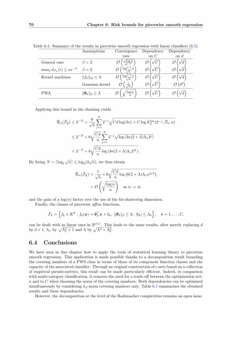
70 Chapter 6. Risk bounds for piecewise smooth regression
Table 6.1: Summary of the results in piecewise smooth regression with linear classifiers (6.5).Assumptions Convergence Dependency Dependency
rate on C on dGeneral case β > 2 O
(√lognn1/β
)O(√
C)
O(√
d)
maxk dFk(ε) ≤ αε−β β = 2 O(
log3/2 n√n
)O(√
C)
O(√
d)
Kernel machines ‖fk‖H ≤ Λ O(
log3/2 n√n
)O(√
C)
O(√
d)
Gaussian kernel O(
1√n
)O(√
C)
O(dd)
PWA ‖θk‖2 ≤ Λ O(√
lognn
)O(√
C)
O(√
d)
Applying this bound in the chaining yields
Rn(FG) ≤ 2−N +6√n
N∑j=1
2−j√Cd log(3n) + C logN int
2 (2−j , Fk, n)
≤ 2−N + 6
√Cd
n
N∑j=1
2−j√
log (3n(2 + Λ)Λx2j)
< 2−N + 6
√Cd
nlog (3n(2 + Λ)Λx2N ).
By fixing N = dlog2
√ne ≤ log2(2
√n), we thus obtain
Rn(FG) <1√n
+ 6
√Cd
nlog(6(2 + Λ)Λxn3/2
)= O
(√log n
n
)as n→∞
and the gain of a log(n) factor over the use of the fat-shattering dimension.Finally, the classes of piecewise affine functions,
Fk ={fk ∈ RX : fk(x) = θ>k x+ bk, ‖θk‖2 ≤ Λ, |bk| ≤ Λb
}, k = 1, . . . , C,
can be dealt with as linear ones in Rd+1. This leads to the same results, after merely replacing dby d+ 1, Λx by
√Λ2x + 1 and Λ by
√Λ2 + Λ2
b .
6.4 ConclusionsWe have seen in this chapter how to apply the tools of statistical learning theory to piecewisesmooth regression. This application is made possible thanks to a decomposition result boundingthe covering numbers of a PWS class in terms of those of its component function classes and thecapacity of the associated classifier. Through an original construction of ε-nets based on a collectionof empirical pseudo-metrics, this result can be made particularly efficient. Indeed, in comparisonwith multi-category classification, it removes the need for a trade-off between the optimization wrt.n and to C when choosing the norm of the covering numbers. Both dependencies can be optimizedsimultaneously by considering L2-norm covering numbers only. Table 6.1 summarizes the obtainedresults and these dependencies.
However, the decomposition at the level of the Rademacher complexities remains an open issue.
Chapter 7
Risk bounds for switching regression
We now come back to the arbitrarily switching regression setting described in Sect. 1.2.2. We willhere derive bounds on the switching `p-risk of the clipped functions f = (fk)1≤k≤C in the senseof (6.1). This risk is defined by
LCp (f) = EX,Y mink∈[C]
|Y − fk(X)|p. (7.1)
Given a sequence of real-valued function classes Fk, the learning algorithm operates within theclass of vector-valued functions F =
∏Ck=1 Fk ⊂ (RC)X . But, as in the preceding chapter, we
shall consider that the function really returned by the algorithm is a clipped function belonging toF =
∏Ck=1 Fk where Fk is defined as in (6.2).
We will thus derive bounds on the risk (7.1) that are uniform over the class F . To do this, weconcentrate on the estimation of the Rademacher complexity of the class
LCp,F =
{` ∈ [0, 1]Z : `(x, y) = min
k∈[C]|y − fk(x)|p, f ∈ F
}, (7.2)
which yields, by application of Theorem 7, with probability at least 1− δ and uniformly for all fin F , the bound
LCp (f) ≤ LCp,n(f) + 2Rn(LCp,F
)+
√log 1
δ
2n, (7.3)
where
LCp,n(f) =1
n
n∑i=1
mink∈[C]
|yi − fk(xi)|p
is the corresponding empirical risk.The next sections present two approaches to estimate this complexity: one based on the de-
composition at the level of the Rademacher complexities and another one based on chaining andthe decomposition of the covering numbers.
7.1 Decomposition at the level of Rademacher complexities
The decomposition at the level of Rademacher complexities leads to a bound linear in the numberof components C. This relies on the structural result of Lemma 4.
Theorem 13. Let F =∏Ck=1 Fk, with real-valued function classes Fk. Then, for LCp,F defined as
in (7.2),
Rn(LCp,F
)≤ p
C∑k=1
Rn (Fk) .
71
72 Chapter 7. Risk bounds for switching regression
Proof. By using the facts that for all (ak)1≤k≤C ∈ RC , mink∈[C] ak = −maxk∈[C]−ak and that σiand −σi share the same distribution, it comes:
Rn(LCp,F ) = EXnYnσn supf∈F
1
n
n∑i=1
σi mink∈[C]
|Yi − fk(Xi)|p
= EXnYnσn supf∈F
1
n
n∑i=1
−σi maxk∈[C]
−|Yi − fk(Xi)|p
= EXnYnσn supf∈F
1
n
n∑i=1
σi maxk∈[C]
−|Yi − fk(Xi)|p
= EXnYnσn sup(ek∈Ek)k∈[C]
1
n
n∑i=1
σi maxk∈[C]
−|ek(Xi, Yi)|p
≤C∑k=1
Rn(−|Ek|p),
where∀k ∈ [C], Ek = {ek ∈ RZ : ek(x, y) = y − fk(x), fk ∈ Fk} (7.4)
and where the inequality is obtained by application of Lemma 4. By taking into account theco-domain of |Ek|, i.e., [0, 1], and the Lipschitz constant of φ(u) = up for u in that interval, thecontraction principle (Lemma 3) leads to Rn(−|Ek|p) ≤ pRn(Ek). Then, we observe that, for anyk ∈ [C],
Rn(Ek) = EXnYnσn supfk∈Fk
1
n
n∑i=1
σi(Yi − fk(Xi))
≤ EYnσn
1
n
n∑i=1
σiYi + EXnσn supfk∈Fk
1
n
n∑i=1
−σif(Xi)
where
EYnσn
1
n
n∑i=1
σiYi =1
n
n∑i=1
EYiσiσiYi = 0
and (since σi and −σi share the same distribution)
EXnσn supfk∈Fk
1
n
n∑i=1
−σifk(Xi) = Rn(Fk).
Thus, we can conclude by using once more the contraction principle as Rn(Fk) ≤ Rn(Fk).
7.1.1 Application to linear and kernel machines
Here, we consider classes
Fk = {fk ∈ H : ‖fk‖H ≤ Λ} , k = 1, . . . , C, (7.5)
of functions taken in a ball of radius Λ in an RKHS H (see Sect. 5.4 for useful definitions). In thiscase, Lemma 9 can be used together with Theorem 13 to yield a result comparable to (5.19) forclassification:
Rn(LCp,F
)≤ pCΛxΛ√
n. (7.6)
A similar result can be easily deduced for classes of linear functions on X ⊂ Rd,
Fk ={fk ∈ RX : fk(x) = θ>k x, ‖θk‖2 ≤ Λ
}, k = 1, . . . , C, (7.7)
by considering the linear kernel, K(x,x′) = x>x′. This leads to (7.6) with Λx = supx∈X ‖x‖2.
7.2. Decomposition at the level of covering numbers 73
7.2 Decomposition at the level of covering numbers
We will now see how we can improve the dependency on the number of components C by decom-posing at the level of the covering numbers. This gain is similar to the one obtained in Sect. 5.3.2for classification. As in this case, the exact gain will depend on a trade-off between the values ofn, C and d.
The decomposition of the covering numbers relies on the following structural result, whichbounds the covering numbers of a class of functions defined as pointwise maximum/minimum of aset of functions. The (omitted) proof follows the path of the one of Lemma 5 (Lemma 1 in [35]).
Lemma 14. Given a sequence of C classes Ak of real-valued functions on Z, let A be either theclass of pointwise maximum functions, A = {a ∈ RZ : a(z) = maxk∈[C] ak(z), ak ∈ Ak}, or ofpointwise minimum functions, A = {a ∈ RZ : a(z) = mink∈[s] ak(z), ak ∈ Ak}. Then, for allq ∈ [1,∞],
N int(ε,A, dq,zn) ≤C∏k=1
N int( ε
C1/q,Ak, dq,zn
).
Equipped with this lemma, we obtain the following decomposition.
Lemma 15. Let F =∏Ck=1 Fk, with real-valued function classes Fk. Then, for LCp,F as in (7.2)
and any q ∈ [1,∞]:
N int(ε,LCp,F , dq,zn) ≤C∏k=1
N int
(ε
pC1/q, Fk, dq,xn
).
Proof. Let Ek be defined as in (7.4) and Epk be the class {|ek|p : ek ∈ Ek}. Then, LCp,F is the class{mink∈[C] ek : ek ∈ Epk} and Lemma 14 yields
N int(ε,LCp,F , dq,zn) ≤C∏k=1
N int( ε
C1/q, Epk , dq,zn
).
A contraction principle also applies to covering numbers. In particular, since φ : [0, 1]→ R definedby φ(u) = |u|p is p-Lipschitz, an ε-net of Ek gives a (pε)-net of Epk and
N int(ε, Epk , dq,zn) ≤ N int
(ε
p, Ek, dq,zn
).
In addition, for all pair of functions ek(x, y) = y − fk(x) and e′k(x, y) = y − f ′k(x), we have,for all (x, y) ∈ Z = X × Y, |ek(x, y) − e′k(x, y)| = |fk(x) − f ′k(x)|. Thus, for all zn ∈ Zn,dq,zn(ek, e
′k) = dq,xn(fk, f
′k) and
N int(ε, Ek, dq,zn) = N int(ε, Fk, dq,xn).
Combining all these results concludes the proof.
Note that this decomposition result is much closer to Lemma 5 that applies to classification thanto Lemmas 10–11 that aplpy to piecewise smooth regression. Therefore, as seen for classificationin Sect. 5.3.2, the dependencies on C and n will be impacted by the choice of the Lq-norm definingthe covering numbers: increasing q tends to improve the dependence on C but weakens the oneon n. In the following, we will thus favor the choice of the “nice trade-off" offered by the valueq = dlog2 Ce and Lemma 8.
7.2.1 General case
Here, we apply the chaining method to estimate the Rademacher complexity of the class LCp,F (ofdiameter 1) via the decomposition Lemma 15 and the covering numbers. For all q ∈ [2,∞], this
74 Chapter 7. Risk bounds for switching regression
gives
Rn(LCp,F
)≤ 2−N + 6
N∑j=1
2−j
√logN int(2−j ,LCp,F , dq,zn)
n
≤ 2−N + 6
√C
n
N∑j=1
2−j
√maxk∈[C]
logN int
(2−j
pC1/q, Fk, dq,xn
). (7.8)
By considering q = dlog2 Ce, we have C1/q ≤ 2 and, under assumption (6.7), Lemma 8 yields
Rn(LCp,F
)≤ 2−N + 6
√C
n
N∑j=1
2−j
√2dF
(1
30p2j log2(2C)
)log (39p log2(2C)n2j)
≤ 2−N + 6
√C
n
N∑j=1
2j(β2−1)
√2α30βpβ logβ2 (2C) log (39p log2(2C)n2j).
By choosing N =⌈log2 n
1β
⌉≤ 1
β log2(2βn), it comes
Rn(LCp,F
)≤ 1
n1β
+ 6
√C
n2α30βpβ logβ2 (2C) log
(78p log2(2C)n
1β+1
) N∑j=1
2j(β2−1)
≤ 1
n1β
+ 6
√C
n2α30βpβ logβ2 (2C) log
(78pn
1β+2
) N∑j=1
2j(β2−1),
where the second line is obtained by using C < n.For β = 2, we have
Rn(LCp,F
)≤ 1√
n+ 90p log2(2C)
√2αC
nlog(
78pn52
)log2(4n)
= O
(log3/2 n√
n
)as n→∞ (7.9)
and a dependence on C in the order of√C logC.
For β > 2, we can bound the sum as in (6.12) to obtain
Rn(LCp,F
)≤ 1
n1β
+ 32β−1α
12 30
β2 p
β2
2( β2−12 ) − 1
√C logβ2 (2C) log
(78pn
1β+2
)n
1β
= O(√
log n
n1β
)as n→∞
and a dependence on C in the order of√C logβ C.
7.2.2 Kernel machinesAs discussed in Sect. 5.4, we will use the results of [104] to bound the L∞-norm covering numbersof kernel machines. The choice of the L∞-norm is made in order to obtain a radical dependenceon C without altering the scale of the covering numbers when decomposing with Lemma 15. Moreprecisely, for classes Fk as in (7.5), we use (5.21) in (7.8) for q =∞ and obtain
Rn(LCp,F
)≤ 2−N + 36pΛxΛ
√C
n
N∑j=1
√log (15 · 2jpΛxΛn)
≤ 2−N + 36pΛxΛ
√C
nN√
log (15 · 2NpΛxΛn) (7.10)
7.2. Decomposition at the level of covering numbers 75
With N = dlog2
√ne ≤ log2 (2
√n), this gives
Rn(LCp,F
)≤ 1√
n+ 36pΛxΛ log2
(2√n)√C
nlog(30pΛxΛn3/2
)and a radical dependence on C for a convergence rate in
Rn(LCp,F
)= O
(log3/2 n√
n
)as n→∞.
In comparison with the general case above with β = 2 [8], i.e., (7.9), we can thus spare a power oflogC for a similar convergence rate.
However, note that the radical dependence on C is not the best one achievable. Indeed, wecan slightly improve it with a better balance between the two terms in the chaining formula. Forinstance, with N =
⌈log2
√n
C1/4
⌉≤ log2
(2√n
C1/4
), the inequality (7.10) leads to
Rn(LCp,F
)≤ C1/4
√n
+ 36pΛxΛ
√C
nlog2
(2
√n
C1/4
)√log
(30pΛxΛn3/2
C1/4
)and a subradical dependence on C for an unaltered convergence rate. However, the gain is herevery small.
Gaussian kernel. For Gaussian kernels, we can once again use (5.22). This yields a convergencerate in O(1/
√n) but with an exponential growth wrt. the dimension d of the input space.
7.2.3 Classes with linear component functions
For linear component function classes (7.7), we can improve the dependence on both C and nwithout introducing an exponential growth wrt. d. Indeed, we have already seen in Sect. 6.3.3that the L∞-norm covering numbers of these classes are efficiently bounded by (6.18).
Introducing this in the chaining formula with the entropic integral (5.8), we obtain
Rn(LCp,F ) ≤ 12√n
∫ 1/2
0
√logN int(ε,LCp,F , d∞,zn) dε
≤ 12
√C
n
∫ 1/2
0
√maxk∈[C]
logN int(ε/p, Fk, d∞,xn) dε
≤ 12
√Cd
n
∫ min{1/2,pΛΛx}
0
√log
(p(2 + Λ)Λx
ε
)dε
≤ 12
√Cd
n
∫ pΛΛx
0
√log
(p(2 + Λ)Λx
ε
)dε
≤ 12pΛΛx√
log (2/Λ + 1)
√Cd
n. (7.11)
The dependence is thus radical on both C and d for a convergence rate in 1/√n.
In comparison with the bound (7.6) obtained by decomposing at the level of the Rademachercomplexities, this yields a gain of
√C against a loss of
√d. More precisely, the ratio between the
two bounds is(7.6)(7.11)
=
√C
12√d log (2/Λ + 1)
,
which implies that (7.11) is more advantageous than (7.6) as soon as C > 144d log (2/Λ + 1). Buthere again, the constants are not very accurate and this only gives a rough comparison betweenthe two approaches.
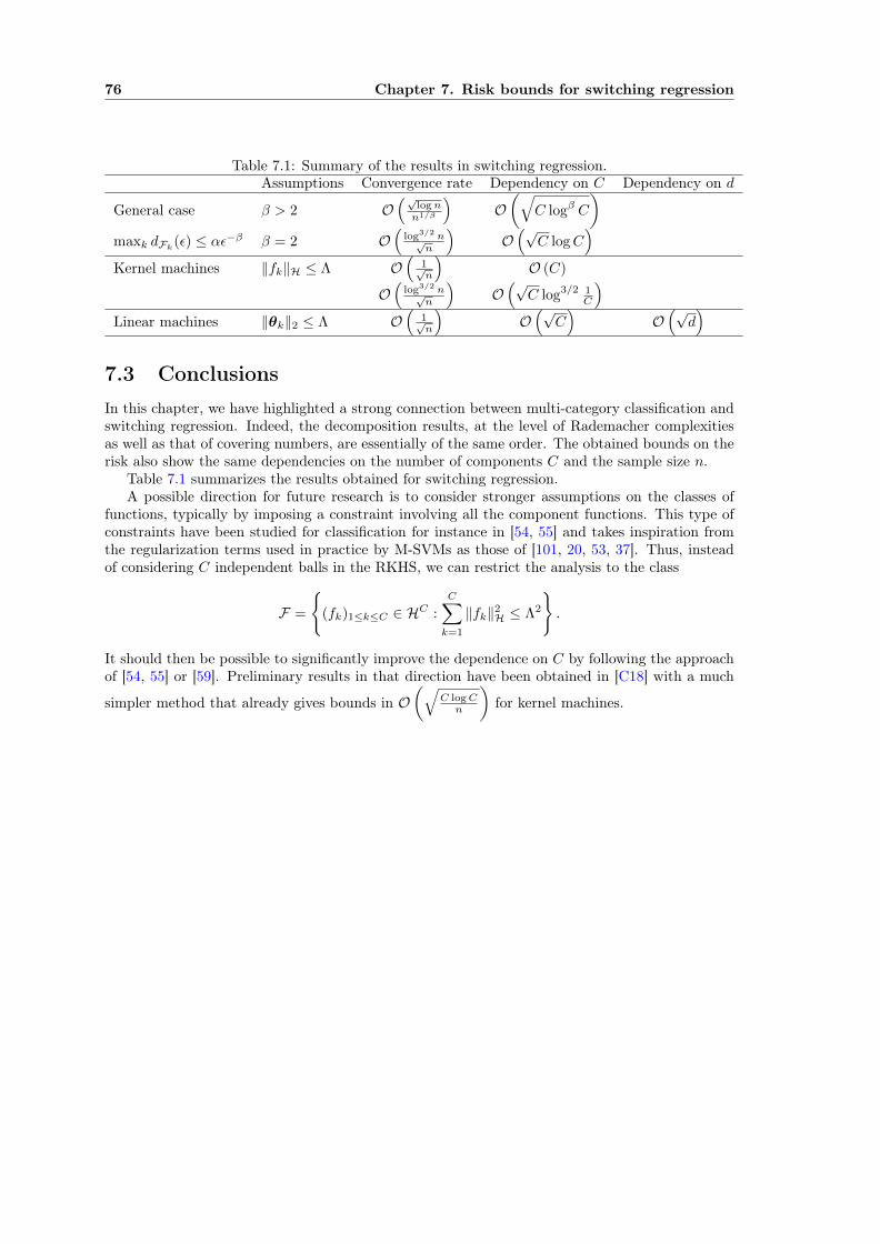
76 Chapter 7. Risk bounds for switching regression
Table 7.1: Summary of the results in switching regression.Assumptions Convergence rate Dependency on C Dependency on d
General case β > 2 O(√
lognn1/β
)O(√
C logβ C
)maxk dFk(ε) ≤ αε−β β = 2 O
(log3/2 n√
n
)O(√
C logC)
Kernel machines ‖fk‖H ≤ Λ O(
1√n
)O (C)
O(
log3/2 n√n
)O(√
C log3/2 1C
)Linear machines ‖θk‖2 ≤ Λ O
(1√n
)O(√
C)
O(√
d)
7.3 ConclusionsIn this chapter, we have highlighted a strong connection between multi-category classification andswitching regression. Indeed, the decomposition results, at the level of Rademacher complexitiesas well as that of covering numbers, are essentially of the same order. The obtained bounds on therisk also show the same dependencies on the number of components C and the sample size n.
Table 7.1 summarizes the results obtained for switching regression.A possible direction for future research is to consider stronger assumptions on the classes of
functions, typically by imposing a constraint involving all the component functions. This type ofconstraints have been studied for classification for instance in [54, 55] and takes inspiration fromthe regularization terms used in practice by M-SVMs as those of [101, 20, 53, 37]. Thus, insteadof considering C independent balls in the RKHS, we can restrict the analysis to the class
F =
{(fk)1≤k≤C ∈ HC :
C∑k=1
‖fk‖2H ≤ Λ2
}.
It should then be possible to significantly improve the dependence on C by following the approachof [54, 55] or [59]. Preliminary results in that direction have been obtained in [C18] with a much
simpler method that already gives bounds in O(√
C logCn
)for kernel machines.
Chapter 8
Research plan
Here, I describe my research plan which focuses on learning problems involving multiplecomponents. This includes the previously considered problems of multi-category classification,piecewise smooth regression and switching regression, but also entails unsupervised learning prob-lems such as center-based clustering or subspace clustering [92, 94, C6]. Switching regression andthese latter are indeed similar in the sense that they aim at learning a collection of models (orcomponents) from a data set mixing points from different sources. They differ mostly in the na-ture of the models considered: functions predicting the output for regression, points correspondingto group centers for clustering, or subspaces. Other more subtle connections also appear withmulti-category classification and piecewise smooth regression in the analysis of performances ingeneralization.
Therefore, all these problems share strong characteristics and this research plan is based on thepremise that the study of their relationships is a broad field, largely unexplored, and that shouldyield a number of advances for all these problems.
OptimizationRegarding center-based clustering, it seems possible to adapt the global optimization method de-veloped for switching regression in [J17] and described in Chap. 4 to minimize
J(θ) =
n∑i=1
mink∈[C]
‖xi − θk‖22
with respect to the concatenation θ = [θ>1 , . . . ,θ>C ]> of the C group centers θk ∈ Rd. While most
approaches develop heuristic methods, this would result in a clustering algorithm with guaranteed(optimization) accuracy for problems in small dimension d.
In [J19], I could propose an algorithm with polynomial time-complexity with respect to thenumber of points for the robust estimation of a single subspace in the presence of outliers by takinginspiration from the algorithm derived for bounded-error regression in Sect. 3.3. Specifically, fordS-dimensional subspaces of Rd, Algorithm 2 could be adapted to solve
minB∈Rd×dS
n∑i=1
`p,ε(‖xi −BB>xi ‖2), s.t. B>B = I,
where the matrix B concatenates the basis vectors of the subspace and BB>xi is the projectionof xi on the subspace. Using a similar methodology, it might be possible to extend the switchingregression results of Sect. 3.2 to subspace clustering to prove that the latter, i.e.,
min(Bk∈Rd×dS )1≤k≤C
n∑i=1
mink∈[C]
`p(‖xi −BkB>k xi ‖2), s.t. B>kBk = I, k = 1, . . . , C,
has a polynomial complexity for fixed dimensions d, dS , and number of components C.
77

78 Chapter 8. Research plan
Regarding piecewise smooth or switching regression, it seems that the next algorithmic advancesfor large dimensions would result from efficient heuristic methods, possibly inspired by those devel-oped for center-based or subspace clustering, as e.g., the one proposed in [J9]. Another directionconcerns the statistical analysis of the performance of already known heuristics. For instance, thedeterministic conditions guaranteeing the success of sparsity-based methods [4, J11] can rarelybe verified in practice. At the opposite, the compressed sensing literature [17, 22, 27] containsstatistical guarantees that could be adapted here to result in conditions on the data distribution.Lastly, other heuristic methods with original algorithmic schemes could be derived from the exactpolynomial-time algorithms of Chapter 3. Preliminary results in that direction were given in [J19].
Statistical learning theoryRegarding the analysis of generalization performance, a first question concerns the possible transpo-sition of techniques used to derive the error bounds for regression in Chapter 7 to center-based andsubspace clustering, with the hope that this can reduce the influence of the number of componentson the bounds.
Besides, all the risk bounds that we derived for classification and regression are uniform overthe model class. Other approaches allow one to derive risk bounds for the function returnedby a specific algorithm. In particular, the approach of [14] based on algorithmic stability seemspromising. Thus, we will consider analyzing the stability of the optimization algorithms proposedfor our regression problems in Part I in order to obtain dedicated bounds that could be tighterthan those currently exposed in Part II.
Another issue of interest concerns the shape of the regularization term, or, alternatively, theshape of the constrained model class. In particular, taking into account the interactions betweenthe components of the model in the definition of this class should allow us to decrease theinfluence of the number of components on the bounds. This idea, already exploited for classificationin [54, 55] or [59], also creates a greater connection between the bounds and the actual regularizationschemes implemented by practical algorithms and that are often based on a sum of complexityterms over the components. Adapting this kind of results to the regression problems with multiplecomponents or the clustering ones should yield tighter bounds, and possibly lead to the definitionof novel algorithmic schemes. Specifically, if we focus on components fk in some Hilbert space H,we could analyze the model class
F =
(fk)1≤k≤C ∈ HC :
(C∑k=1
‖fk‖pH
)1/p
≤ Λ
and the influence that the choice of `p-norm in the regularization has on the risk bound in terms ofits dependency on the number of components C. Preliminary results were obtained for regressionwith p = 2 in [C18] and current work on this topic shows that these could be significantly im-proved and extended to deal with other values of p, including values in (0, 1) related to nonconvexregularization schemes [R2].
Finally, note that these issues regarding the interactions between the components and theoptimization of error bounds with respect to the number of components are also related to recentwork on deep learning [6, 32]. Indeed, neural networks are based on the composition of a largenumber of functions and the search for bounds with a mild dependency on this number currentlyconstitutes a very active field.
Model selectionThe link between practice and theoretical guarantees in generalization lies notably at the levelof model selection [58]. For problems involving multiple components, this selection entails twolevels: the classical level of the choice of complexity for the component classes and the moreglobal level of the choice of the number of components. For the latter, the bounds derived forregression problems in Chap. 6–7 could serve as a basis to an approach based on the structural riskminimization principle. This could reveal particularly efficient to determine the number of modelsin these problems.
79
Here, it also seems natural to consider model selection techniques developed for clustering todetermine this number for switching regression or subspace clustering. In particular, recent workbased on the notion of clustering stability [100] seems promising and should be investigated.
Links with systems and control theoryThe error bounds in Chap. 6–7 are derived under the assumption that the training sample containsindependent random variables. However, this prevents the application of the bounds to hybriddynamical system identification, where the data are typically gathered from a single (or several)trajectories of the system and thus depend one on the other. Several directions can be taken toobtain bounds that hold under less restrictive conditions. Of particular interest are those based onmixing processes [102, 98, 66, 67, 38] and the more recent work of [50] or [84].
In the longer term, I would also investigate the links between learning theory and robustcontrol. These links, that have been partially explored in [97, 16, 88], rely on a probabilisticapproach to robust control. Computing the optimal control law for an uncertain dynamical systemis an optimization problem that involves an infinite number of constraints. The probabilisticapproach consists in sampling values of the uncertainty to recover a finite number of constraintsassociated with possible scenarios of the system behavior. But two essential questions spring fromthis setting: what can we guarantee on the probability that the true system satisfies the constraintsas well as in the considered scenarios? and, how many scenarios should we generate to guarantee acertain level of reliability? These questions can be cast in the learning theory language as those ofobtaining risk bounds and computing sample complexities. Doing so, an interesting link appearsbetween the number of constraints that are imposed on the system for each scenario and thenumber of model components in the learning framework. Therefore, my work on risk bounds forlearning multiple components could be the basis of efficient strategies for robust control with alarge number of constraints.
Resources
To conduct these projects, a number of human and financial resources could be used.The part dealing with statistical learning theory would naturally be aligned with my collabora-
tion with Yann Guermeur in the ABC team. We also work on these topics with Marianne Clauselat the Institut Elie Cartan de Lorraine (IECL), with whom we are involved in a Mirabelle+ project[56].
Working on subspace clustering would be the occasion to reactivate my collaboration withRené Vidal, a renown expert of this field, with a possible long-term stay in Baltimore that couldbe supported by the Widen Horizons program of the excellence initiative of my university [57].
The links with systems and control theory could be studied with members of the ResearchCenter for Automatic Control of Nancy (CRAN). Such local collaborations could typically benefitfrom the support of programs dedicated to interdisciplinary research within the Université deLorraine, such as PhD scholarships from the Fédération Charles Hermite [40] or specific projectcalls [19, 56].
Finally, the whole project is within the field of artificial intelligence (AI) as defined by theVillani report [99] and could benefit from actions and specific calls to come according to thenational strategy for AI [65].

Author’s publications
Most works listed here are available from the author’s homepage at:https://members.loria.fr/FLauer/files/papers.html .
Book
[B1] F. Lauer and G. Bloch. Hybrid System Identification: Theory and Algorithms for LearningSwitching Models. Springer, 2019.
Journal papers
[J21] F. Lauer. Error bounds for piecewise smooth and switching regression. IEEE Transactionson Neural Networks and Learning Systems, to appear, 2019.
[J20] K. Musayeva, F. Lauer, and Y. Guermeur. Rademacher complexity and generalizationperformance of margin multi-category classifiers. Neurocomputing, 342:6–15, 2019.
[J19] F. Lauer. On the exact minimization of saturated loss functions for robust regression andsubspace estimation. Pattern Recognition Letters, 112:317–323, 2018.
[J18] T.S. Illès, M. Burkus, S. Somoskeöy, F. Lauer, F. Lavaste, and J.F. Dubousset. Axialplane dissimilarities of two identical Lenke type 6C scoliosis cases visualized and analyzedby vertebral vectors. European Spine Journal, 27(9):2120–2129, 2018.
[J17] F. Lauer. Global optimization for low-dimensional switching linear regression and bounded-error estimation. Automatica, 89:73–82, 2018.
[J16] F. Lauer. MLweb: a toolkit for machine learning on the web. Neurocomputing, 282:74–77,2018.
[J15] T.S. Illés, M. Burkus, S. Somoskeöy, F. Lauer, F. Lavaste, and J.F. Dubousset. Thehorizontal plane appearances of scoliosis: what information can be obtained from top-viewimages? International Orthopaedics, 41(11):2303–2311, 2017.
[J14] F. Lauer. On the complexity of switching linear regression. Automatica, 74:80–83, 2016.
[J13] F. Lauer. On the complexity of piecewise affine system identification. Automatica, 62:148–153, 2015.
[J12] F. Lauer and H. Ohlsson. Finding sparse solutions of systems of polynomial equations viagroup-sparsity optimization. Journal of Global Optimization, 62(2):319–349, 2015.
[J11] V.L. Le, F. Lauer, and G. Bloch. Selective `1 minimization for sparse recovery. IEEETransactions on Automatic Control, 59(11):3008–3013, 2014.
[J10] T. Pham Dinh, H. A. Le Thi, H. M. Le, and F. Lauer. A difference of convex func-tions algorithm for switched linear regression. IEEE Transactions on Automatic Control,59(8):2277–2282, 2014.
81

82 Author’s publications
[J9] F. Lauer. Estimating the probability of success of a simple algorithm for switched linearregression. Nonlinear Analysis: Hybrid Systems, 8:31–47, 2013.
[J8] V.L. Le, G. Bloch, and F. Lauer. Reduced-size kernel models for nonlinear hybrid systemidentification. IEEE Transactions on Neural Networks, 22(12):2398–2405, 2011.
[J7] F. Lauer and Y. Guermeur. MSVMpack: a Multi-Class Support Vector Machine Package.Journal of Machine Learning Research, 12:2269–2272, 2011.
[J6] F. Lauer, G. Bloch, and R. Vidal. A continuous optimization framework for hybrid systemidentification. Automatica, 47(3):608–613, 2011.
[J5] G. Bloch, F. Lauer, G. Colin, and Y. Chamaillard. Support vector regression from simula-tion data and few experimental samples. Information Sciences, 178(20):3813–3827, 2008.
[J4] F. Lauer and G. Bloch. Incorporating prior knowledge in support vector regression. MachineLearning, 70(1):89–118, 2008.
[J3] F. Lauer and G. Bloch. Incorporating prior knowledge in support vector machines forclassification: a review. Neurocomputing, 71(7-9):1578–1594, 2008.
[J2] F. Lauer, C. Y. Suen, and G. Bloch. A trainable feature extractor for handwritten digitrecognition. Pattern Recognition, 40(6):1816–1824, 2007.
[J1] F. Lauer and G. Bloch. Ho–Kashyap classifier with early stopping for regularization. PatternRecognition Letters, 27(9):1037–1044, 2006.
Book chapters[Ch2] Y. Guermeur and F. Lauer. A generic approach to biological sequence segmentation prob-
lems, application to protein secondary structure prediction. In Pattern Recognition in Com-putational Molecular Biology: Techniques and Approaches, M. Elloumi, C. S. Iliopoulos,J. T. L. Wang and A. Y. Zomaya (Eds.), Wiley, 2016.
[Ch1] G. Bloch, F. Lauer, and G. Colin. On learning machines for engine control. In Compu-tational Intelligence in Automotive Applications, D. Prokhorov (Ed.), vol. 132 of Studies inComputational Intelligence, Springer, pages 125–142, 2008.
Conference papers
[C18] F. Lauer. Error bounds with almost radical dependence on the number of componentsfor multi-category classification, vector quantization and switching regression. In: FrenchConference on Machine Learning (FCML/CAp), 2018.
[C17] K. Musayeva, F. Lauer and Y. Guermeur. A sharper bound on the Rademacher complexityof margin multi-category classifiers. In: Proc. of the 26th Eur. Symp. on Artificial Neu-ral Networks, Computational Intelligence and Machine Learning (ESANN), pages 503–508,2018.
[C16] K. Musayeva, F. Lauer and Y. Guermeur. Metric entropy and Rademacher complexityof margin multi-category classifiers (abstract). In: Artificial Neural Networks and MachineLearning – Proc. of ICANN 2017, Part II, vol. 10614 of LNCS, page 767, 2017.
[C15] T. Illès, F. Lauer, F. Lavaste and J. Dubousset. A simple way to see the scoliosis in 3D:the vertebra vectors projection in horizontal plane (abstract). In: EUROSPINE 2017 andthe 38th SICOT Orthopaedic World Congress, 2017.
[C14] E. Didiot and F. Lauer. Efficient optimization of multi-class support vector machines withMSVMpack. In: Modelling, Computation and Optimization in Information Systems andManagement Sciences, Proc. of MCO 2015 – Part II, Metz, France, pages 23–34, 2015.
83
[C13] F. Lauer and G. Bloch. Piecewise smooth system identification in reproducing kernel Hilbertspace. In: Proc. of the 53rd IEEE Conf. on Decision and Control (CDC), Los Angeles, CA,USA, pages 6498–6503, 2014.
[C12] V.L. Le, F. Lauer, L. Bako, and G. Bloch. Learning nonlinear hybrid systems: from sparseoptimization to support vector regression. In: Proc. of the 16th ACM Int. Conf. on HybridSystems: Computation and Control (HSCC), Philadelphia, PA, USA, pages 33–42, 2013.
[C11] V.L. Le, F. Lauer, and G. Bloch. Identification of linear hybrid systems: a geometricapproach. In: Proc. of the American Control Conference (ACC), Washington, DC, USA,pages 830–835, 2013.
[C10] L. Bako, V.L. Le, F. Lauer, and G. Bloch. Identification of MIMO switched state-spacemodels. In: Proc. of the American Control Conference (ACC), Washington, DC, USA, pages71–76, 2013.
[C9] F. Thomarat, F. Lauer, and Y. Guermeur. Cascading discriminant and generative modelsfor protein secondary structure prediction. In: Proc. of the 7th IAPR Int. Conf. on PatternRecognition in Bioinformatics (PRIB), Tokyo, Japan, vol. 7632 of LNCS (LNBI), pages166–177, 2012.
[C8] F. Lauer, V.L. Le, and G. Bloch. Learning smooth models of nonsmooth functions viaconvex optimization. In: Proc. of the 22nd IEEE Int. Workshop on Machine Learning forSignal Processing (MLSP), Santander, Spain, 2012.
[C7] F. Lauer, G. Bloch, and R. Vidal. Nonlinear hybrid system identification with kernelmodels. In: Proc. of the 49th IEEE Int. Conf. on Decision and Control (CDC), Atlanta,GA, USA, 2010.
[C6] F. Lauer and C. Schnörr. Spectral clustering of linear subspaces for motion segmentation.In: Proc. of the 12th IEEE Int. Conf. on Computer Vision (ICCV), Kyoto, Japan, 2009.
[C5] F. Lauer, R. Vidal, and G. Bloch. A product-of-errors framework for linear hybrid systemidentification. In: Proc. of the 15th IFAC Symp. on System Identification (SYSID), Saint-Malo, France, pages 563–568, 2009.
[C4] F. Lauer and G. Bloch. Switched and piecewise nonlinear hybrid system identification.In: Proc. of the 11th Int. Conf. on Hybrid Systems: Computation and Control (HSCC), St.Louis, MO, USA, vol. 4981 of LNCS, pages 330–343, 2008.
[C3] F. Lauer and G. Bloch. A new hybrid system identification algorithm with automatictuning. In: Proc. of the 17th IFAC World Congress, Seoul, Korea, pages 10207–10212, 2008.
[C2] G. Bloch, F. Lauer, G. Colin, and Y. Chamaillard. Combining experimental data andphysical simulation models in support vector learning. In: Proc. of the 10th Int. Conf.on Engineering Applications of Neural Networks (EANN), Thessaloniki, Greece, vol. 284 ofCEUS Workshop Proceedings, pages 284–295, 2007.
[C1] F. Lauer, M. Bentoumi, G. Bloch, G. Millerioux, and P. Aknin. Ho–Kashyap with earlystopping versus soft margin SVM for linear classifiers – an application. In: Advances inNeural Networks, Proc. of the Int. Symp. on Neural Networks (ISNN), Dalian, China, vol.3173 of LNCS, pages 524–530, 2004.
Thesis[T2] F. Lauer. Machines à vecteurs de support et identification de systèmes hybrides – From sup-
port vector machines to hybrid system identification. Ph.D. thesis, Université Henri PoincaréNancy 1, France, 2008.
[T1] F. Lauer. Increasing the performance of classifiers for handwritten digit recognition. Master’sthesis, Université Henri Poincaré Nancy 1, France, also published as a Technical Report,CENPARMI, Concordia University, Canada, 2005.

84 Author’s publications
Technical reports[R2] F. Lauer. Risk bounds for learning multiple components with permutation-invariant losses.
Technical report HAL–02100779, arXiv preprint, arXiv:1904.07594, 2019.
[R1] F. Lauer and H. Ohlsson. Sparse phase retrieval via group-sparse optimization. Technicalreport HAL–00951158, arXiv preprint, arXiv:1402.5803, 2014.
Invitied communications (without proceedings)[I5] F. Lauer. A brief introduction to artificial intelligence and machine learning. Summer School
Erasmus+ DEPEND, Nancy, France, 2019.
[I4] F. Lauer. Utilisation de la parcimonie de groupe pour l’optimisation parcimonieuse souscontraintes non linéaires. Journée Parcimonie de la Fédération Charles Hermite, Nancy,France, 2014.
[I3] F. Lauer. Identification de systèmes hybrides par optimisation continue. Journée Analyse,Optimisation et Contrôle de la Fédération Charles Hermite, Nancy, France, 2010.
[I2] F. Lauer. Une approche par SVMs pour l’identification de système hybrides. GT Identificationdu GDR-MACS, Paris, France, Mars 2008, et GT Systèmes Dynamiques Hybrides (SDH) duGDR-MACS, Paris, France, Avril 2008.
[I1] F. Lauer. Support Vector Machines for handwritten digit recognition. Japan–France Seminaron Analytical and Numerical Methods for Scientific Computing in Science and Engineering,Nancy, France, 2006.
Software[S5] F. Lauer. MLweb: Machine Learning on the Web. http://mlweb.loria.fr/, également
disponible sur http://mloss.org/ (avec plus de 4000 téléchargements).
[S4] F. Lauer. SparsePoly: a Matlab toolbox for finding sparse solutions of polynomial systems.https://members.loria.fr/FLauer/files/software/
[S3] F. Lauer. k-LinReg: a simple and efficient algorithm for switched linear regression. https://members.loria.fr/FLauer/files/klinreg/
[S2] F. Lauer and Y. Guermeur. MSVMpack: a Multi-class Support Vector Machine package.https://members.loria.fr/FLauer/files/MSVMpack/, également disponible sur http://mloss.org/ (avec plus de 10000 téléchargements).
[S1] F. Lauer. COFSR: a continuous optimization framework for switched regression. https://members.loria.fr/FLauer/files/software/
References
[1] N. Alon, S. Ben-David, N. Cesa-Bianchi, and D. Haussler. Scale-sensitive dimensions, uniformconvergence, and learnability. Journal of the ACM, 44(4):615–631, 1997.
[2] E. Amaldi and V. Kann. The complexity and approximability of finding maximum feasiblesubsystems of linear relations. Theoretical Computer Science, 147(1-2):181–210, 1995.
[3] E. Amaldi and M. Mattavelli. The MIN PFS problem and piecewise linear model estimation.Discrete Applied Mathematics, 118:115–143, 2002.
[4] L. Bako. Identification of switched linear systems via sparse optimization. Automatica,47(4):668–677, 2011.
[5] P.L. Bartlett. The sample complexity of pattern classification with neural networks: Thesize of the weights is more important than the size of the network. IEEE Transactions onInformation Theory, 44(2):525–536, 1998.
[6] P.L. Bartlett, D.J. Foster, and M.J. Telgarsky. Spectrally-normalized margin bounds forneural networks. In Advances in Neural Information Processing Systems 30, pages 6240–6249, 2017.
[7] P.L. Bartlett and S. Mendelson. Rademacher and Gaussian complexities: Risk bounds andstructural results. Journal of Machine Learning Research, 3:463–482, 2002.
[8] P.L. Bartlett and J. Shawe-Taylor. Generalization performance of support vector machinesand other pattern classifiers. In B. Schölkopf, C.J.C. Burges, and A. Smola, editors, Advancesin Kernel Methods – Support Vector Learning, chapter 4, pages 43–54. The MIT Press,Cambridge, MA, 1999.
[9] A. Bemporad, A. Garulli, S. Paoletti, and A. Vicino. A bounded-error approach to piecewiseaffine system identification. IEEE Transactions on Automatic Control, 50(10):1567–1580,2005.
[10] S. Ben-David, N. Cesa-Bianchi, D. Haussler, and P.M. Long. Characterizations of learnabilityfor classes of {0, ..., N}-valued functions. Journal of Computer and System Sciences, 50(1):74–86, 1995.
[11] A. Berlinet and C. Thomas-Agnan. Reproducing Kernel Hilbert Spaces in Probability andStatistics. Kluwer Academic Publishers, Boston, 2004.
[12] G. Biau, L. Devroye, and G. Lugosi. On the performance of clustering in Hilbert spaces.IEEE Transactions on Information Theory, 54:781–790, 2008.
[13] L. Bottou. On the Vapnik-Chevonenkis-Sauer lemma. http://leon.bottou.org/news/vapnik-chervonenkis_sauer, 2017.
[14] O. Bousquet and A. Elisseeff. Stability and generalization. Journal of Machine LearningResearch, 2:499–526, 2002.
[15] Leo Breiman, Jerome H. Friedman, Richard A. Olshen, and Charles J. Stone. Classificationand Regression Trees. Chapman & Hall/CRC, 1984.
85

86 References
[16] G.C. Calafiore, F. Dabbene, and R. Tempo. Research on probabilistic methods for controlsystem design. Automatica, 47:1279–1293, 2011.
[17] E. J. Candès. Compressive sampling. In Proc. of the Int. Congress of Mathematicians,Madrid, Spain, pages 1433–1452, 2006.
[18] Y. Chen, X. Yi, and C. Caramanis. A convex formulation for mixed regression with twocomponents: Minimax optimal rates. In COLT, pages 560–604, 2014.
[19] CNRS. Appel à projets de site Mirabelle, 2017. http://www.cnrs.fr/mi/spip.php?article1065.
[20] K. Crammer and Y. Singer. On the algorithmic implementation of multiclass kernel-basedvector machines. Journal of Machine Learning Research, 2:265–292, 2001.
[21] W.S. DeSarbo and W.L. Cron. A maximum likelihood methodology for clusterwise linearregression. Journal of Classification, 5(2):249–282, 1988.
[22] D. L. Donoho. Compressed sensing. IEEE Transactions on Information Theory, 52(4):1289–1306, 2006.
[23] R.M. Dudley. Universal Donsker classes and metric entropy. The Annals of Probability,15(4):1306–1326, 1987.
[24] M. Farooq and I. Steinwart. Learning rates for kernel-based expectile regression. arXiv,1702.07552, 2017.
[25] G. Ferrari-Trecate, M. Muselli, D. Liberati, and M. Morari. A clustering technique for theidentification of piecewise affine systems. Automatica, 39(2):205–217, 2003.
[26] M. A. Fischler and R. C. Bolles. Random sample consensus: A paradigm for model fittingwith applications to image analysis and automated cartography. Communications of theACM, 24(6):381–395, 1981.
[27] S. Foucart and H. Rauhut. A Mathematical Introduction to Compressive Sensing. Springer,2013.
[28] J.H. Friedman. Multivariate adaptive regression splines. The Annals of Statistics, 19(1):1–67,1991.
[29] S. Gaffney and P. Smyth. Trajectory clustering with mixtures of regression models. In ACMSIGKDD, pages 63–72, 1999.
[30] M.R. Garey and D.S. Johnson. Computers and Intractability: a Guide to the Theory ofNP-Completeness. W.H. Freeman and Company, 1979.
[31] A. Garulli, S. Paoletti, and A. Vicino. A survey on switched and piecewise affine systemidentification. In Proc. of the 16th IFAC Symp. on System Identification (SYSID), pages344–355, 2012.
[32] N. Golowich, A. Rakhlin, and O. Shamir. Size-independent sample complexity of neuralnetworks. In Proc. of the 31st Conf. On Learning Theory (COLT), pages 297–299, 2018.
[33] G. H. Golub and C. F. Van Loan. Matrix Computations. John Hopkins University Press, 4edition, 2013.
[34] Y. Guermeur. VC theory of large margin multi-category classifiers. Journal of MachineLearning Research, 8:2551–2594, 2007.
[35] Y. Guermeur. Lp-norm Sauer-Shelah lemma for margin multi-category classifiers. Journal ofComputer and System Sciences, 89:450–473, 2017.
87
[36] Y. Guermeur. Rademacher complexity of margin multi-category classifiers. In WSOM+,2017.
[37] Y. Guermeur and E. Monfrini. A quadratic loss multi-class SVM for which a radius-marginbound applies. Informatica, 22(1):73–96, 2011.
[38] H. Hang, Y. Feng, I. Steinwart, and J.A.K. Suykens. Learning theory estimates with obser-vations from general stationary stochastic processes. Neural Computation, 28(12):2853–2889,2016.
[39] D. Haussler and P. M. Long. A generalization of Sauer’s lemma. Journal of CombinatorialTheory, Series A, 71(2):219–240, 1995.
[40] Fédération Charles Hermite. Bourse de thèse. http://www.fr-hermite.univ-lorraine.fr/these-federation-charles-hermite/.
[41] D.W. Hosmer. Maximum likelihood estimates of the parameters of a mixture of two regressionlines. Communications in Statistics, 3(10):995–1006, 1974.
[42] R.A. Jacobs, M.I. Jordan, S.J. Nowlan, and G.E. Hinton. Adaptive mixtures of local experts.Neural computation, 3(1):79–87, 1991.
[43] M.I. Jordan and L. Xu. Convergence results for the EM approach to mixtures of expertsarchitectures. Neural networks, 8(9):1409–1431, 1995.
[44] A. L. Juloski, S. Weiland, and W. Heemels. A Bayesian approach to identification of hybridsystems. IEEE Transactions on Automatic Control, 50(10):1520–1533, 2005.
[45] M.J. Kearns and R.E. Schapire. Efficient distribution-free learning of probabilistic concepts.Journal of Computer and System Sciences, 48(3):464–497, 1994.
[46] M.J. Kearns, R.E. Schapire, and L.M. Sellie. Toward efficient agnostic learning. MachineLearning, 17(2-3):115–141, 1994.
[47] A.N. Kolmogorov and V.M. Tihomirov. ε-entropy and ε-capacity of sets in functional spaces.American Mathematical Society Translations, series 2, 17:277–364, 1961.
[48] V. Koltchinskii and D. Panchenko. Empirical margin distributions and bounding the gener-alization error of combined classifiers. The Annals of Statistics, 30(1):1–50, 2002.
[49] A. Kontorovich and R. Weiss. Maximum margin multiclass nearest neighbors. In Proceedingsof the 31st Int. Conf. on Machine Learning (ICML), pages 892–900, 2014.
[50] V. Kuznetsov and M. Mohri. Theory and algorithms for forecasting time series. arXivpreprint arXiv:1803.05814, 2018.
[51] V. Kuznetsov, M. Mohri, and U. Syed. Multi-class deep boosting. In Advances in NeuralInformation Processing Systems 27, pages 2501–2509, 2014.
[52] M. Ledoux and M. Talagrand. Probability in Banach Spaces: Isoperimetry and Processes.Springer-Verlag, Berlin, 1991.
[53] Y. Lee, Y. Lin, and G. Wahba. Multicategory support vector machines: Theory and ap-plication to the classification of microarray data and satellite radiance data. Journal of theAmerican Statistical Association, 99(465):67–81, 2004.
[54] Y. Lei, U. Dogan, A. Binder, and M. Kloft. Multi-class SVMs: From tighter data-dependentgeneralization bounds to novel algorithms. In Advances in Neural Information ProcessingSystems 28, pages 2035–2043, 2015.
[55] Y. Lei, U. Dogan, D.-X. Zhou, and M. Kloft. Data-dependent generalization bounds formulti-class classification. IEEE Transactions on Information Theory, 2019.

88 References
[56] LUE. Programme mirabelle+. http://lue.univ-lorraine.fr/fr/mirabelle.
[57] LUE. Programme widen horizons. http://lue.univ-lorraine.fr/fr/widen-horizons.
[58] P. Massart. Concentration Inequalities and Model Selection. Springer, 2007.
[59] A. Maurer. A vector-contraction inequality for Rademacher complexities. In Proc. of the27th Int. Conf on Algorithmic Learning Theory (ALT), pages 3–17, 2016.
[60] S. Mendelson. Rademacher averages and phase transitions in Glivenko-Cantelli classes. IEEETransactions on Information Theory, 48(1):251–263, 2002.
[61] S. Mendelson. Learning without concentration. In Proc. of the Conference on LearningTheory (COLT), pages 25–39, 2014.
[62] S. Mendelson. Learning without concentration for general loss functions. Probability Theoryand Related Fields, 171(1-2):459–502, 2018.
[63] S. Mendelson and G. Schechtman. The shattering dimension of sets of linear functionals.Annals of Probability, 32(3A):1746–1770, 2004.
[64] S. Mendelson and R. Vershynin. Entropy and the combinatorial dimension. Inventionesmathematicae, 152:37–55, 2003.
[65] Mission Villani sur l’IA. L’intelligence artificielle au service de l’humain, 2018. https://www.aiforhumanity.fr/.
[66] M. Mohri and A. Rostamizadeh. Rademacher complexity bounds for non-iid processes. InAdvances in Neural Information Processing Systems, pages 1097–1104, 2009.
[67] M. Mohri and A. Rostamizadeh. Stability bounds for stationary ϕ-mixing and β-mixingprocesses. Journal of Machine Learning Research, 11:789–814, 2010.
[68] M. Mohri, A. Rostamizadeh, and A. Talwalkar. Foundations of Machine Learning. The MITPress, Cambridge, MA, 2012.
[69] B.K. Natarajan. On learning sets and functions. Machine Learning, 4:67–97, 1989.
[70] H. Ohlsson and L. Ljung. Identification of switched linear regression models using sum-of-norms regularization. Automatica, 49(4):1045–1050, 2013.
[71] H. Ohlsson, L. Ljung, and S. Boyd. Segmentation of ARX-models using sum-of-norms regu-larization. Automatica, 46(6):1107–1111, 2010.
[72] N. Ozay, M. Sznaier, C.M. Lagoa, and O. Camps. A sparsification approach to set mem-bership identification of switched affine systems. IEEE Transactions on Automatic Control,57(3):634–648, 2012.
[73] S. Paoletti, A. L. Juloski, G. Ferrari-Trecate, and R. Vidal. Identification of hybrid systems:a tutorial. European Journal of Control, 13(2-3):242–262, 2007.
[74] R.E. Quandt. The estimation of the parameters of a linear regression system obeying twoseparate regimes. Journal of the American Statistical Association, pages 873–880, 1958.
[75] A. Rakhlin and K. Sridharan. Statistical learning and sequential prediction, 2014. LectureNotes (Early book draft), http://www.cs.cornell.edu/~sridharan/lecnotes.pdf.
[76] A.V. Rao, D.J. Miller, K. Rose, and A. Gersho. A deterministic annealing approach forparsimonious design of piecewise regression models. IEEE Transactions on Pattern Analysisand Machine Intelligence, 21(2):159–173, 1999.
[77] J. Roll, A. Bemporad, and L. Ljung. Identification of piecewise affine systems via mixed-integer programming. Automatica, 40(1):37–50, 2004.

89
[78] P. J. Rousseeuw and A. M. Leroy. Robust regression and outlier detection. John Wiley &Sons, 2005.
[79] M. Rudelson and R. Vershynin. Combinatorics of random processes and sections of convexbodies. Annals of Mathematics, pages 603–648, 2006.
[80] N. Sauer. On the density of families of sets. Journal of Combinatorial Theory, Series A,13(1):145–147, 1972.
[81] C. Saunders, A. Gammerman, and V. Vovk. Ridge regression learning algorithm in dualvariables. In ICML, pages 515–521, 1998.
[82] S. Shalev-Shwartz and S. Ben-David. Understanding Machine Learning: From Theory toAlgorithms. Cambridge University Press, 2014.
[83] S. Shelah. A computational problem: Stability and order of models and theory of infinitarylanguages. Pacific Journal of Mathematics, 41:247–261, 1972.
[84] M. Simchowitz, H. Mania, S. Tu, M.I. Jordan, and B. Recht. Learning without mixing:Towards a sharp analysis of linear system identification. In Proc. of the 31st Conf. OnLearning Theory (COLT), pages 439–473, 2018.
[85] H. Späth. Algorithm 39: Clusterwise linear regression. Computing, 22(4):367–373, 1979.
[86] I. Steinwart and A. Christmann. Support Vector Machines. Springer, 2008.
[87] M. Talagrand. Upper and Lower Bounds for Stochastic Processes. Springer, 2014.
[88] R. Tempo, G. Calafiore, and F. Dabbene. Randomized algorithms for analysis and control ofuncertain systems: with applications. Springer, 2012.
[89] A. W. Van Der Vaart and J. H. Van Zanten. Adaptive Bayesian estimation using a Gaussianrandom field with inverse gamma bandwidth. The Annals of Statistics, pages 2655–2675,2009.
[90] V.N. Vapnik. Statistical Learning Theory. John Wiley & Sons, 1998.
[91] V.N. Vapnik and A.Y. Chervonenkis. On the uniform convergence of relative frequencies ofevents to their probabilities. Theory of Probability & Its Applications, 16(2):264–280, 1971.
[92] R. Vidal. Subspace clustering. IEEE Signal Processing Magazine, 28(2):52–68, 2011.
[93] R. Vidal, Y. Ma, and S. Sastry. Generalized principal component analysis (GPCA). IEEETransactions on Pattern Analysis and Machine Intelligence, 27(12):1945–1959, 2005.
[94] R. Vidal, Y. Ma, and S.S. Sastry. Generalized Principal Component Analysis. Springer-VerlagNew York, 2016.
[95] R. Vidal, S. Soatto, and A. Chiuso. Applications of hybrid system identification in computervision. In Proc. of the IEEE European Control Conference (ECC), pages 4853–4860, 2007.
[96] R. Vidal, S. Soatto, Y. Ma, and S. Sastry. An algebraic geometric approach to the identifi-cation of a class of linear hybrid systems. In Proc. of the 42nd IEEE Conf. on Decision andControl (CDC), Maui, Hawaï, USA, pages 167–172, 2003.
[97] M. Vidyasagar. Randomized algorithms for robust controller synthesis using statistical learn-ing theory. Automatica, 37(10):1515–1528, 2001.
[98] M. Vidyasagar and R.L. Karandikar. A learning theory approach to system identificationand stochastic adaptive control. Journal of Process Control, 18:421–430, 2008.
[99] C. Villani. Donner un sens à l’intelligence artificielle, 2018. https://www.aiforhumanity.fr/pdfs/9782111457089_Rapport_Villani_accessible.pdf.

90 References
[100] U. von Luxburg. Clustering stability: an overview. Foundations and Trends in MachineLearning, 2(3):235–274, 2010.
[101] J. Weston and C. Watkins. Multi-class support vector machines. Technical Report CSD-TR-98-04, Royal Holloway, University of London, 1998.
[102] E. Weyer. Finite sample properties of system identification of ARX models under mixingconditions. Automatica, 36(9):1291–1299, 2000.
[103] A.J. Zeevi, R. Meir, and V. Maiorov. Error bounds for functional approximation and estima-tion using mixtures of experts. IEEE Transactions on Information Theory, 44(3):1010–1025,1998.
[104] T. Zhang. Covering number bounds of certain regularized linear function classes. Journal ofMachine Learning Research, 2:527–550, 2002.
[105] T. Zhang. Statistical analysis of some multi-category large margin classification methods.Journal of Machine Learning Research, 5(Oct):1225–1251, 2004.