Optimization Methods for Big Sums of Functions

Anton Rodomanov

Higher School of Economics

p BA)yesgroup.ru|(Bayesian methods research group

(http://bayesgroup.ru)

5 June 2016Skoltech Deep Machine Intelligence Workshop, Moscow, Russia

Introduction

Consider the problem

Find f ∗ = minx∈Rd

f (x) with f (x) :=1

n

n∑i=1

fi (x),

Example (Empirical risk minimization):

I We are given observations ai (and possibly their labels βi ).

I Goal: find optimal parameters x∗ of a parametric model.

I Linear regression (ai ∈ Rd , βi ∈ R):

f (x) =1

n

n∑i=1

∥∥∥a>i x − βi∥∥∥2I Logistic regression (ai ∈ Rd , βi ∈ {−1, 1}):

f (x) =1

n

n∑i=1

ln(1 + exp(−βia>i x))

I Neural networks, SVMs, CRFs etc.

Preliminaries

Problem: f ∗ = minx∈Rd

f (x), f (x) = 1n

n∑i=1

fi (x).

Goal: Given ε > 0, find x̄ such that f (x̄)− f ∗ ≤ ε.

Assumptions:

I Each function fi is L-smooth:

‖∇fi (x)−∇fi (y)‖ ≤ L ‖x − y‖ , ∀x , y ∈ Rd .

I Function f is µ-strongly convex:

f (y) ≥ f (x)+〈∇f (x), y−x〉+µ

2‖y − x‖2 , ∀x , y ∈ Rd .

Strong convexity of f implies existence of a unique x∗ : f (x∗) = f ∗.We consider iterative methods which produce {xk}k≥0 : xk → x∗.

Gradient descent and big sums of functions

Problem: f ∗ = minx∈Rd

f (x), f (x) = 1n

n∑i=1

fi (x).

Gradient descent:xk+1 = xk − η∇f (xk)

∇f (xk) =1

n

n∑i=1

∇fi (xk)

Here η ∈ R++ is a step length.

Note:

I Computation of ∇f (xk) requires O(nd) operations.

I When n is very large, this may take a lot of time. Example:n = 108, d = 1000 ⇒ evaluating ∇f (xk) takes ≥ 2 minutes.

I We need methods with cheaper iterations.

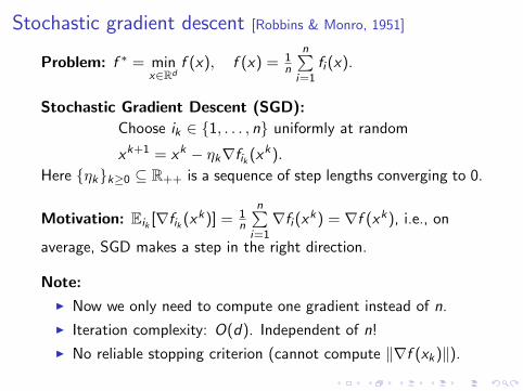
Stochastic gradient descent [Robbins & Monro, 1951]

Problem: f ∗ = minx∈Rd

f (x), f (x) = 1n

n∑i=1

fi (x).

Stochastic Gradient Descent (SGD):

Choose ik ∈ {1, . . . , n} uniformly at random

xk+1 = xk − ηk∇fik (xk).

Here {ηk}k≥0 ⊆ R++ is a sequence of step lengths converging to 0.

Motivation: Eik [∇fik (xk)] = 1n

n∑i=1∇fi (xk) = ∇f (xk), i.e., on

average, SGD makes a step in the right direction.

Note:

I Now we only need to compute one gradient instead of n.

I Iteration complexity: O(d). Independent of n!

I No reliable stopping criterion (cannot compute ‖∇f (xk)‖).

Gradient descent vs SGD: Which one is better?

Problem: f ∗ = minx∈Rd

f (x), f (x) = 1n

n∑i=1

fi (x).

Iteration cost:

I Gradient descent: O(nd).

I SGD: O(d).

Time

log(Res

idual)

sublinear

linear

Convergence rate:

I Gradient descent: linear, O(nd L

µ ln 1ε

)flops for ε-solution.

I SGD: sublinear, O( dµε) flops for ε-solution.

Discussion:

I Complexity of SGD does not depend on n.

I SGD is good for large ε and terrible for small ε.

Slow convergence of SGD: Why?

Problem: f ∗ = minx∈Rd

f (x), f (x) = 1n

n∑i=1

fi (x).

Example (Least squares): fi (x) := (a>i x − bi )2

Main reason for slow convergence of SGD is the variance

σ2k := Ei

[∥∥∥∇fi (xk)−∇f (xk)∥∥∥2] .

Note that even if xk → x∗ we have σk → σ > 0.

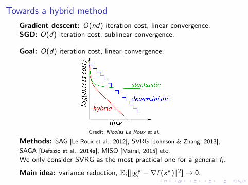
Towards a hybrid method

Gradient descent: O(nd) iteration cost, linear convergence.SGD: O(d) iteration cost, sublinear convergence.

Goal: O(d) iteration cost, linear convergence.

Credit:Nicolas Le Roux et al.

Methods: SAG [Le Roux et al., 2012], SVRG [Johnson & Zhang, 2013],

SAGA [Defazio et al., 2014a], MISO [Mairal, 2015] etc.

We only consider SVRG as the most practical one for a general fi .

Main idea: variance reduction, Ei [‖gki −∇f (xk)‖2]→ 0.

Stochastic Variance Reduced Gradient [Xiao & Zhang, 2014]

Problem: f ∗ = minx∈Rd

f (x), f (x) = 1n

n∑i=1

fi (x).

Require: x̃0: initial point; m: update frequency; η: step length.for s = 0, 1, . . . do

g̃ s := ∇f (x̃ s) = 1n

n∑i=1∇fi (x̃ s)

x0 := x̃ s

for k = 0, . . . ,m − 1 doChoose ik ∈ {1, . . . , n} uniformly at randomxk+1 := xk − η(∇fik (xk)−∇fik (x̃ s) + g̃ s)

end for

x̃ s+1 := 1m

m∑k=1

xk (or x̃ s+1 := xm)

end for

Parameters: usually m = O(n), η = O( 1L); e.g.m = 2n, η = 1

10L .

Note:I Works with a constant step length.I Reliable stopping criterion: ‖g̃ s‖2 ≤ ε̃.

Variance reduction in SVRG

Denote gi := ∇fi (x)−∇fi (x̃) +∇f (x̃).Then gi is an unbiased estimate of ∇f (x):

Ei [∇fi (x)−∇fi (x̃)+∇f (x̃)] = ∇f (x)−∇f (x̃)+∇f (x̃) = ∇f (x).

Variance:

σ2 := Ei

[‖gi −∇f (x)‖2

]= Ei

[‖(∇fi (x)−∇fi (x̃))− (∇f (x)−∇f (x̃))‖2

](‖a + b‖2 ≤ 2 ‖a‖2 + 2 ‖b‖2)

≤ 2Ei

[‖∇fi (x)−∇fi (x̃)‖2

]+ 2 ‖∇f (x)−∇f (x̃)‖2

≤ 2L2 ‖x − x̃‖2 + 2L2 ‖x − x̃‖2

= 4L2 ‖x − x̃‖2 .

Note: when x → x∗ and x̃ → x∗, then σ → 0.In plain SGD we had gi = ∇fi (x) and so σ 6→ 0 when x → x∗.

SVRG: Convergence analysis [Xiao & Zhang, 2014]

TheoremLet η < 1

4L and m is sufficiently large so that

ρ :=1

µη(1− 4Lη)m+

4Lη(m + 1)

(1− 4Lη)m< 1.

Then SVRG converges at a linear rate:

E[f (x̃ s)]− f ∗ ≤ ρs [f (x̃0)− f ∗].Discussion:

I Let us choose η = 110L and assume m� 1. Then 4Lη = 2

5 and

ρ ≈50 L

µ

3m+

2

3I To ensure ρ < 1, let us choose m = 100 L

µ . Then ρ ≈ 56 .

I To reach ε, we need to perform s = O(ln 1ε ) epochs.

I Complexity of each epoch: O((n + m)d) = O((n + Lµ)d).

I Thus total complexity is O(

(n + Lµ)d ln 1

ε

).

I Recall that for gradient descent we had O(

(n Lµ)d ln 1

ε

).

Practical performance [Allen-Zhu & Hazan, 2016]

Figure: Training Error Comparison on neural nets. Y axis: training objectivevalue; X axis: number of passes over dataset.

Conclusion

I SGD is a general method which is suitable for any stochasticoptimization problem.

I However, SGD has a sublinear rate of convergence. The mainreason for that is the large variance in estimating the gradientwhich does not decrease with time.

I For the special case of finite sums of functions it is possible todesign SGD-like methods which reduce the variance whenthey progress. This allows them to achieve a linear rate ofconvergence.

I This variance reduction has an effect only after multiplepasses through the data.

I If one can perform only a couple passes through the data,then SGD is an optimal method. If several passes through thedata are allowed, variance reducing methods (e.g. SVRG)work much better.

Thank you!

References

I Original paper on SVRG:R. Johnson & T. Zhang. Accelerating Stochastic Gradient Descent using

Predictive Variance Reduction, NIPS 2013.

I SVRG for composite functions:L. Xiao & T. Zhang. A Proximal Stochastic Gradient Method with

Progressive Variance Reduction. SIAM Journal on Optimization, 2014.

I Practical improvements for SVRG:R. Babanezhad et al.. Stop Wasting My Gradients: Practical SVRG,

NIPS 2015.

I Theory of SVRG for non-strongly convex and non-convexfunctions:

I J. Reddi et al.. Stochastic Variance Reduction for Nonconvex

Optimization, ICML 2016.I Z. Allen-Zhu & Y. Yuan. Improved SVRG for Non-Strongly-Convex

or Sum-of-Non-Convex Objectives, ICML 2016.I Z. Allen-Zhu & E. Hazan. Variance Reduction for Faster

Non-Convex Optimization, ICML 2016.