optimization model for the conjunctive use of conventional...
TRANSCRIPT
73
chapter four
Optimization modelfor the conjunctiveuse of conventionaland marginal waters
Francesca Salis, Giovanni M. Sechi, and Paola Zuddas
CINSA–University of Cagliari–Italy
Contents
4.1 Introduction ..................................................................................................744.2 Identification of the optimization algorithm...........................................77
4.2.1 Modeling approaches and software tools ...................................774.2.2 Optimization under uncertainty:
The scenario optimization .............................................................804.2.3 Hydrologic series generation for scenario optimization ..........834.2.4 Considering water quality conditions in water system
optimization .....................................................................................844.2.5 Quality indices using hydrological scenario generation ..........854.2.6 Correlation between a-chlorophyll concentration
and hydrologic contribution..........................................................884.2.6.1 Correlation between a-Chlorophyll concentration
and time .............................................................................904.2.6.2 Multiple linear regression analysis................................90
4.2.7 Evaluation of the potential use index..........................................904.3 The optimization package WARGI: Water Resources System
Optimization Aided by Graphical Interface............................................914.3.1 Problem formalization....................................................................924.3.2 Identification of network components and sets.........................964.3.3 Required Data ..................................................................................97
L1672_C004.fm Page 73 Wednesday, June 22, 2005 2:30 PM
74 Drought Management and Planning for Water Resources
4.3.4 Constraints formalization in the optimization model ............1004.3.5 Objective Function formalization
in the optimization model ...........................................................1044.4 WARGI graphical interface ......................................................................1064.5 Results applying WARGI to real cases...................................................108
4.5.1 Flumendosa–Campidano water system ....................................1084.5.2 Júcar water system........................................................................ 1124.5.3 Salso–Simeto water system.......................................................... 114
4.6 Conclusion................................................................................................... 115References............................................................................................................. 116
4.1 Introduction
There have been significant computational advances in the development ofoptimization techniques that are able to consider the inclusion of specialrisk-related system performance criteria within the analysis of different hydro-logic and demand scenarios. Advances have also been made when focusingon the water system domain and the complexity of modeling tools.
Nevertheless, mathematical optimization procedures available for largesystems are still not able to deal with all of the complexities and nonlinearitiesof the real world that can be easily incorporated in a simulation model. Opti-mization procedures can also be constructed to solve efficiently the real prob-lem and are adequate approximation to it, and simulation can greatly narrowthe search (Loucks et al., 1981). Moreover, optimization results obtained bysolving an adequately adherent model can be seen as the management reference-targets for simulation since they can be considered as obtained by anideal-manager having perfect knowledge of sources and demand behaviorin the assumed time horizon. Reflecting upon tools for water management,in one view to the future, Simonovic (2000) identified two paradigms thatwill shape tools for the future modeling of water management. The complexityparadigm states that water problems in the future are going to be more com-plex and will need to take into consideration more extended domains such asenvironmental and social impact, population growth and needs, water qualityindicators, a longer temporal horizon, large-scale water problems, etc. Theuncertain paradigm, on the other hand, is the increase in all elements of uncer-tainty in time and space. Uncertainty in water management has been dividedas reported into two basic forms: uncertainty caused by hydrologic variabilityand uncertainty due to fundamental lack of knowledge.
The main aspect of improving the practical utility of optimization inwater resources revolves around better packaging of associated computersoftware. Probably, at the moment, this is the primary requirement neededto convince decision makers to accept optimization as a real problem-solvingtool. As recently pointed out in (Nicklow, 2000), decision makers are morelikely to accept optimization if they are comfortable with their abilities toemploy the computational model and if the model has an interactive graph-ical user interface (GUI). Consequently, adequate consideration should focus
L1672_C004.fm Page 74 Wednesday, June 22, 2005 2:30 PM
Chapter four : Optimization model for the conjunctive use 75
on providing user-friendly optimization software for water systems appli-cations and additional emphasis should be given to this requirement.
Following the above-mentioned aims, in this chapter we describe a gen-eral-purpose optimization tool (Sechi and Zuddas, 2000, 2002) characterizedby considering a user-friendly interface. The proposed package, named WARGI(Water Resources System Optimization Aided by Graphical Interface), wasdeveloped to consider water quality indices under the name Water ResourcesManagement Under Drought Conditions (WAMME, 2002) European project inorder to improve opportunities in real cases for using optimization, aided bya graphical user interface in water resource systems modeling. As will beillustrated in this chapter, the package has been developed in a scenario-modeling framework and considers the possibility of conventional and marginalwater utilization for solving large-scale water system optimization problems.
As is well known, a complex regional water supply system consists ofseveral components such as reservoirs, conveyance works, treatment plants,pumping stations, hydroelectric power plants, etc. The system may includeseveral competitive water uses (urban, irrigation, hydroelectric, recreational,etc.), and the optimization model must take into account management alter-natives as well as design problems, with the aim of reaching an optimalutilization of the resource.
Optimal configurations of the water resources system will guarantee anadequate level of reliability of water supply for different uses and providemanagement assessment criteria to be adopted by the water authorities. Atthe same time emergency plans should be prepared to reduce the conse-quences of drought events by allowing the interconnection of water systemsand so on. For this purpose we need to examine very different and suffi-ciently detailed scenarios as efficiently and rapidly as possible.
In the WAMME project, the overall goal is to increase the scientificbackground and to develop technological tools for improving water resourcemanagement and environmental control in drought-prone Mediterraneanregions. In order to develop strategies for identifying the role of differentproject and management alternatives in mitigating drought impacts in com-plex water systems, including the conjunctive use of conventional and mar-ginal waters, WAMME identified an organized framework considering thefollowing phases:
1. To develop an optimization model for the conjunctive use of conven-tional and marginal waters incorporating synthetic water qualityindices;
2. To develop a simulation-based decision support system (DSS) for themanagement of integrated water resources systems focused on droughtprevention and mitigation, which could help the decision makers toface drought risk in the Mediterranean regions;
3. To verify the usefulness of the developed optimization model andDSS tools using multicriteria techniques to identify the preferablemix of long- and short-term measures for drought impacts mitigation.
AU: 2000a or 2000b?
L1672_C004.fm Page 75 Wednesday, June 22, 2005 2:30 PM

76 Drought Management and Planning for Water Resources
In this multiphase technique we need to resort to mathematical program-ming, applied to an optimization model, followed by a simulation testingprocess that limits recourse to heavy computational procedures by reducingthe gap between the solutions of the first two phases. In the optimizationphase we can examine a mathematical model representing the real physicalproblem simplified and consequently reducing its level of adherence toreality. Therefore, in the simulation phase we can only examine reducedscenarios from the dimensional and temporal points of view. On the otherhand, if the optimization model remains adherent to the real problem, in adeterministic framework mathematical programming results give us the bestmanagement (in terms of water flows in the system) obtained by an idealmanager having previous knowledge of input and demands behavior in thesystem. These results can give us a measure of the “goodness” of the simu-lation-based DSS, at least for a reduced deterministic test cases set.
It is therefore crucial to be able to solve optimization models efficientlyand with an adequate level of adherence in order to reduce the simulationphase computational effort and to have an objective measurement of DSSefficiency.
When facing droughts, the problem of the optimal dimension and man-agement of the water resource system and the related optimal flows configu-ration should take into account additional constraints and costs in the objectivefunction (OF) given by the criteria that it should operate satisfactorily duringperiods of drought. Particularly the vulnerability of the system should beconsidered when dealing with water resource shortage risk in the water systemmanagement. The vulnerability expresses the severity of drought in terms ofits consequences. The consequences of drought are generally expressed by aloss (cost) function, and the measurement estimating the severity of droughtis given considering cost functions, weighing more the shortage flows as theseverity of the drought event increases.
In the optimization model, drought vulnerability will be examined con-sidering a generalized OF expression using a standardized shortage to definethe expected losses. In this way the problem can be expressed using a linearprogramming (LP) approach. Other approaches lead to a quadratic program-ming (QP) model.
Reliability (probability that the system is of a satisfactory state) and resil-iency (recovery time from failure) indices can be evaluated in aposterior anal-ysis. The ever increasing importance of problems related to water has createdthe need to improve knowledge concerning the phenomena involving waterquality, in particular, when water resources are derived from surface waterand artificial reservoirs as is the case in the main Italian islands (Sicily andSardinia) supply systems. In a simplified frame, for river streams, reservoirs,and ground water resources, the problem of water quality can be studiedconsidering the general environmental characterization of the water-bodies,just as the recent Italian legislation has done.
On the basis of available measurements of basic macrodescriptors, sur-face water, ground water and lakes can be divided into five classes, the first
L1672_C004.fm Page 76 Wednesday, June 22, 2005 2:30 PM

Chapter four : Optimization model for the conjunctive use 77
one should be attributed with the best environmental characterization of thewater bodies, the last with the worst one.
The ecological state attribution derives from chemical and biologicalparameters. Measurement methodologies and attribution rules have beenextensively described in the recent Italian legislation.
As will be described in the following paragraphs, using this simplifiedmethod, in the optimization model WARGI we will consider the potentialuse of water sources (conventional and marginal) and the technological costsassociated with water treatment as a function of the ecological state attribu-tion of the water bodies.
4.2 Identification of the optimization algorithm
Models describing the planning and management optimization problem ofwater resource systems show a special structure that suggests some special-ized approaches in order to overcome the serious computational problemsdue to the large size of the models for complex systems.
Taking into consideration different physical situations, some specificoptimization models together with algorithms exploiting the mathematicalstructure of the problem will be examined in the following paragraphs.
4.2.1 Modeling approaches and software tools
The physical water system can be represented by a direct basic graph inwhich nodes represent sources, demands, reservoirs, etc., and arcs representthe activity connections between them.
A “basic graph” can be deduced from the schematic representation ofthe physical water system referred to a single-period. This is a static repre-sentation of the system without taking time evolution into account.
In some cases the correspondence between the physical and graphic com-ponents is not so close, at times it is even nonexistent. In fact, it may beconvenient to add “dummy” nodes and arcs to represent not only physicalcomponents but also events that may occur in the system. For example, dummyarcs can represent a shortage caused by meeting the request of the demandnodes and can prevent unfeasible solutions. This representation points outpossible deficits in the system and, as a consequence, the need to change thedimensions of the works or, alternatively, to use external water resources. Witheach node we can associate a supply or a demand representing an input flow,such as a hydrological inflow to a reservoir, or an output flow, such as a waterrequest from a demand center.
Similarly, with each arc we can associate a functional or technologicalactivity such as for pipelines, power stations, hydroelectric power plants,etc., and the transfer costs and bounds for each flow. In water resourcessystem analysis we also need to examine the evolution of flow values intime. This is done by extending the analysis to a time horizon sufficientlywide to describe the functionality of system components and the cost-benefit
L1672_C004.fm Page 77 Wednesday, June 22, 2005 2:30 PM

78 Drought Management and Planning for Water Resources
performance, which can also reach a significant representation of the vari-ability of hydrological inflows and water demands in the network nodes.
In our analysis we divide the total time horizon in time steps (periods)usually taken as equal to one month. In our Mediterranean climate, whichhas a large annual rainfall variability, the total time horizon frequently needsto be extended to several decades. In the Sardinian Island Water Plan carriedout by the Regional Authority the time horizon has been taken as equal to54 years.
In a multiperiod analysis of the water supply system we must considersurface reservoirs as well as ground water resources and other storage activ-ities that can transfer water to subsequent time periods to avoid shortage.
As a support to multiperiod planning analysis we can construct a“multiperiod graph”
R
using the “basic graph” as a multiplicative modulereproduced as many times as are the periods considered, linking the copiesby interperiod arcs between the storage nodes. Flows in these arcs representthe volume stored at the end of each period available for use during thenext period. The support network allows the use of highly efficient datastructures, reaching a significant reduction in computer storage and com-putational time during data input and processing. Modularity, moreover,allows for the automatic construction of the multiperiod network and ofdata generators.
Referring to a “static” or single-period situation, we can represent thephysical system by a direct network (the “basic graph”), derived from thephysical sketch. Figure 4.1a shows a physical sketch of a simple water sys-tem. In the figure nodes maintain the shape of the common hydraulic nota-tion in order to recall the different functions of the system components.Nodes could represent sources, demands, reservoirs, ground water, hydro-electric power station sites, etc. Nodes corresponding to storage possibilitiesrepresent the memory of the system as they can store the water resource ina period to transfer it in a successive period. A dynamic multiperiod network(the “multiperiod graph”) can be derived by replicating the basic graph foreach period (
t
= 1,
…
,
T
) to support the dynamic problem. We connect the corresponding reservoir or ground water nodes for differ-
ent consecutive periods by additional arcs (the “interperiods arcs”) carrying
Figure 4.1a
Sketch of water system.
Reservoir
Demand
Junction
(a)
L1672_C004.fm Page 78 Wednesday, June 22, 2005 2:30 PM

Chapter four : Optimization model for the conjunctive use 79
water stored at the end of each period. Figure 4.1b shows a segment of adynamic network generated by the simple basic graph of figure 4.1a. Reser-voir nodes (symbol
∇
in the figure) are connected by interperiods arcs sothey can store and transfer in time the resource. Demand nodes (symbol inthe figure) correspond to a general requirement of using and consuming theresource. Confluence nodes (symbol O in the figure) allow the resource topass without consumption.
The correspondence between physical and network components are notthat close, it is even a sham at times. Figure 4.2 shows the dynamic multi-period graph, corresponding to that of figure 4.1b, including dummy nodesand arcs marked with a dot. The basic graph is in the frame. The dummynode
U
represents a possible “external system” acting as a supposed sourceor sink. In this way each arc (
i
,
U
) represents spillway from reservoir nodes
i
,each arc (
U
,
i
) represents a supposed additional flow in case of shortage inorder to meet the request in the demand nodes
i
and prevent solutions thatare not feasible.
Flow on arcs (
U
,
i
) point out possible deficits in the system and thenecessity of modifying the dimensions of the works or, alternatively, ofmaking recourse to real external water resources.
In planning studies involving water systems characterized by a high sea-sonal and annual variation of hydrological inflows, such as in Mediterranean
Figure 4.1b
Segment of the dynamic network
Figure 4.2
Dynamic multiperiod graph with dummy nodes and arcs
(b)1st time-period 2nd time-period 3rd time-period 4th time-period
AU: please indicate which sym-bol here
AU: at this point you start using bold letters— throughout if the bold is for vector it is ok—if they are just fac-tors of equa-tions please make them italic instead
1
4 3 8
u
7 12
5 9 13
141062
11 16 15
L1672_C004.fm Page 79 Wednesday, June 22, 2005 2:30 PM
80 Drought Management and Planning for Water Resources
countries, hundreds of replicas of the basic graph need to be considered, andthis leads to a very large network model. For a given configuration of thesystem, and therefore for fixed requirements, resources, and work dimen-sions, the problem can only be viewed in an operational context, and a purenetwork flow model can adequately represent the performance of the system.In this way a network flow algorithm retrieves the best flow configuration,as if an ideal manager of the water system should take decisions knowingthe time sequence of inflows and demands beforehand.
The high efficiency of network flow programming has been well knownsince the 1960s (Ford, Fulkerson, 1966) and has been tested extensively since theend of the 1980s (Ahuja et al., 1993), (Kennington, Helgason, 1980). Concerningwater-resource systems, a comparison between commercial and public domainnetwork flow codes (RELAX, NETFLOW, EASYNET, etc.) was performed (Sechiand Zuddas, 1998) to evaluate application possibility and performances.
The formulation of a model is characterized by the usual operativeconstraints and by the determination of the optimal scaling of supplementaryworks that allows for the reduction of the system shortage to predefinedacceptable thresholds and modifies the pure-network shape of the model.Constraints that describe the links between project variables and operativevariables are in this case also present, as well as constraints that representthe control on the deficit arcs (“shortage flows”). These constraints can deter-mine, for example, that flows on deficit arcs do not exceed prefixed valuesor they can impose limits on the sums of them.
Nevertheless, in the model size a significant part of the constraints isrepresented by the flow continuity equations and by predefined lower andupper bounds on the flows. In order to exploit the model structure and theperformances of pure network programming, an expansion technique hasbeen proposed (Sechi and Zuddas, 1995) that interacts between the primaland dual mathematical optimization model. This kind of approach is veryuseful in formulating a trade-off between the dimension of water works, thereliability of the system, and the prediction of severity in demand short falls.
Regarding a more general linear programming model, the most efficientstate-of-the-art software tools (like CPLEX and X-PRESS) have been compared,when applied to water resources system optimization. Moreover, the hyper-graph approach has been considered and compared (Sechi and Zuddas, 2001)by solving the design and management problem with the ordinary LP model,using the commercial CPLEX package (CPLEX, 1993) and with the HySimpleXcode. The results obtained are very promising and show that HySimpleX canbe adopted competitively for water resource design problems.
4.2.2 Optimization under uncertainty:The scenario optimization
Water resources management problems with a multiperiod feature are usedin association with mathematical optimization models that handle thousands
AU: not on refs—add it, if this is two authors make it Ford and Fulker-son
AU: not on refs—please add it
AU: add to refs—make it Kennington and Helga-son if it is 2 authors
AU: do any of your refer-ences to pro-grams need a TM or R?
AU: not on refs—please add
AU: add to refs
AU: add to refs
L1672_C004.fm Page 80 Wednesday, June 22, 2005 2:30 PM
Chapter four : Optimization model for the conjunctive use 81
of constraints and variables depending on the level of adherence requiredin order to reach a significant representation of the system.
These models are typically characterized by a level of uncertaintyconcerning the value of hydrological exogenous inflows and demandpatterns. However, inadequate values assigned to them could invalidatethe results of the study. When the statistical information on data estima-tion is not enough to support a stochastic model or when probabilisticrules are not available, an alternative approach could be applied, that ofsetting up the scenario analysis technique. This is a general-purposemodeling framework to solve water system optimization problems underinput data uncertainty. Scenario optimization is an alternative to thetraditional stochastic approach, which is used to reach a “robust” decisionpolicy that should minimize the risk of wrong decisions. This approachleads to a huge model that includes a network submodel for each scenarioplus linking constraints, which must be treated with specialized resolu-tion techniques.
In the proposed approach, the problem is to be expanded on a set ofscenario subproblems, each of which corresponds to a possible configurationof the data series. Each scenario can be weighted to represent the “importance”assigned to the running configuration. Sometimes the weights can be viewedas the probability of occurrence of the examined scenario. A “robust-barycen-trical” optimization solution can be obtained by a procedure that minimizesthe distance between subproblems optima.
The model is usually defined in a dynamic planning horizon in whichmanagement decisions have to be made either sequentially, by adoptinga predefined scenario independently, or by following different scenariosin a “scenario-tree” context since the data characteristics change asdescribed in the next paragraph. The scenarios aggregation into a treemust be performed following the basic “implementable principle” or“principle of progressive hedging”: “If two different scenarios are iden-tical up to stage
r
on the basis of the information available about themat stage
r
, then the variables must be identical up to stage
r
” (Rockafellarand Wets, 1991, ). This condition guarantees that the solution obtainedby the model in a period is independent of the information that is notyet available; in other words model evolution is only based on the infor-mation available at the moment, a time when the future configurationmay diversify.
When the set of synthetic hydrological sequences has been generated,the principle of progressive hedging is performed by bundling the sequencesto build the scenario tree.
Data defined for the deterministic model are required for each scenarioin the chance model plus the further data:
G
set of synthetic hydrological sequences (parallel scenarios)w
g
weights assigned to a scenario
g
G
AU: add page for quote
∈
L1672_C004.fm Page 81 Wednesday, June 22, 2005 2:30 PM

82 Drought Management and Planning for Water Resources
Figure 4.3a shows a set of nine parallel scenarios before aggregation.Each dot represents the system in a time-period. Figure 4.3b shows an exam-ple of the scenario tree derived from the parallel sequences.
To perform scenario aggregation a number of stages are defined, wherestage 0 corresponds to the initial hydrological characterization of the systemup to the first branch time period. In the scenario tree this represents the root.In stage 1 a number, b
1
(3 in the figure),
of different possible hydrological
Figure 4.3a
Set G of nine parallel scenarios
Figure 4.3b
Scenario-tree aggregation
Branching times1 2
1 bundle 3 bundles(a)
1 2 3 4 5 6 7 8 9 Time-periodsScen 1
Scen 2
Scen 3
Scen 4
Scen 5
Scen 6
Scen 7
Scen 8
Scen 9
AU: please add correct symbol
(b)
Scen 1
Scen 2
Scen 3
Scen 4
Scen 5
Scen 6
Scen 7
Scen 8
Scen 92nd stage0 stage 1st stage
L1672_C004.fm Page 82 Wednesday, June 22, 2005 2:30 PM
Chapter four : Optimization model for the conjunctive use 83
configurations can occur, in stage 2 a number, b
1
*b
2
(9 in the figure), canoccur, and so on and so forth.
The figure represents a tree with two branches: the first branching timeis the 4th time period, the second is the 8th period. In time periods thatprecede the first branch, all scenarios are gathered in a single bundle andthree bundles are operated at the second branch. The zero bundle includesa group of all scenarios; in the 1st stage 3 bundles are generated including3 scenarios in each group, while in the 2nd stage the 9 scenarios run untilthey reach the end of the time horizon.
Finally, the main rules adopted to organize the set of scenarios are:
Branching
: to identify branching times
t
as time periods in which toapply bundles on parallel sequences, while identifying the stages inwhich to divide the scenario horizon.
Bundling
: to identify the number,
b
t
, of bundles at each branching-time.
Grouping
: to identify groups,
G
t
of scenarios to include in each bundle.
In this way the graph grows in size, on increasing the possible branches,and each root-to-leaf path represents a particular scenario.
Once scenarios have been generated, some general checks must be per-formed to test their statistical properties: among others, a stationary test onmean and variance in order to check process changes over time; an indepen-dence test, to look for possible relations or for a trend among subsequentstages; a time and space correlation test; etc.
4.2.3 Hydrologic series generation for scenario optimization
Scenario optimization can be used to treat uncertainty concerning the valueof hydrological exogenous inflows and demand patterns. Nevertheless, indealing with optimization under drought conditions, this approach has beenused more frequently concerning the variability in hydrological inputs. Toavoid an excess of complexity when using the WARGI optimization tool, itwas decided to adopt separate preprocessors to prepare hydrological sce-narios to be used in the scenario optimization phase.
The data preprocessor that builds scenario sequences follows proceduresthat can be developed using different approaches. Therefore, the scenarios areto be viewed as a set of synthetic hydrological series obtained from historicalsamples applying time-series modeling procedures. Mainly, three approachescould be performed to generate the series:
• The first refers to autoregressive (AR) and autoregressive with movingaverage terms (ARMA) models to generate synthetic hydrological series
• The second to a Monte Carlo (MC) generation scheme • The third to Neural Network (NN) techniques
Synthetically, the AR and ARMA models should be able to reproduce themost important statistical characteristics of observed time series generation.
AU: add cor-rect symbols here
AU: add symbol
AU: add symbolsAU: add
symbol
L1672_C004.fm Page 83 Wednesday, June 22, 2005 2:30 PM

84 Drought Management and Planning for Water Resources
Generally this technique first requires a normalization and standardizationphase. In WARGI applications, a spatial desegregating routine divides thehydrological series into two families: principal (or independent) and second-ary (or dependent). Using the normalized and standardized principal series,a hydrological series has been generated using an AR(
p
) or ARMA (
p,q
)model that can be selected for generation; for a secondary series a transfermodel has been used for the generation of synthetic series.
An example of the MC approach used for synthetic runoff series genera-tion is given in a WARGI application illustrated in a following paragraph. TheMC procedure has been used for the generation of synthetic runoff series,which rescaled the historical series in order to impose a new mean and vari-ance with respect to the historical values. Generally this generation procedurerequires a preliminary definition of time-period clusters on hydrological datain order to avoid autocorrelation components, and it synthetically consists ofthe following steps: (1) the random generation of meteorological characteriza-tion at each cluster; (2) the generation of hydrological data from predefinedsets of clusters; (3) the addition of noise components to improve the statisticalfitness.
The NN approach for scenario generations, as required by WARGI, hasbeen developed in recent papers (Cannas et al., 2000, 2001, 2002) using boththe classical multilayer perceptron scheme and the locally recurrent NNscheme. In any case, a first sensitivity analysis was carried out to evaluate thebest fitting NN configuration, the number of nodes in the layers, and thenumber of iterations to be used in model training. Subsequently (in the testingphase) the hydrological series was generated.
4.2.4 Considering water quality conditions in watersystem optimization
The ever increasing important problems related to water scarcity haveresulted in the need to improve the knowledge about the phenomena involv-ing water quality; in particular, when water resources are derived fromreservoirs, as is to be found in the Sardinia (Italy) supply systems.
The indications given by Italian legislation (Law 152/1999) for classifi-cation are different for each water body. The common characteristics concernthe discovery of two groups of parameters: one that is compulsory, the otherthat concerns dangerous substances. The choice of dangerous substances tobe examined is made by the local authorities on the base of anthropicpressure factors existing in the hydrographic basin, based on limit valuesin the norm 76/464/CEE, which allows for the evaluation of the chemicalstate.
Among the compulsory parameters, the law points out a limited numberof parameters called “macrodescriptors” used for the classification of theecological state of water bodies. The other parameters serve to give supportinformation on the principal characteristics of the water bodies or on theentity of the loads transported.
L1672_C004.fm Page 84 Wednesday, June 22, 2005 2:30 PM

Chapter four : Optimization model for the conjunctive use 85
The macrodescriptors should allow for the precise and stable measure-ment of the load caused by anthropic presence and diffused activity: theytherefore contain all those parameters that measure nutrients or organic load.
For water flows the Italian law sets out seven macrodescriptors: oxygen,ammonium nitrogen; nitrites, COD, BOD5, total phosphorous, EscherichiaColi. Moreover, for the determination of the ecological state a biological index(IBE) is also used.
The macrodescriptors for water bodies are those that define the trophicstate, considering as limiting factors respectively phosphorous and nitrogen.The law therefore sets out the following macrodescriptors for water bodies:a-chlorophyll, transparency, total phosphorous, and hypolimnion oxygen.The environmental state of the ground waters is defined in the law on thebasis of the quantitative state and the chemical state. For the evaluation ofthe latter, two sets of parameters are established: one that is compulsory andmade up of hydrochemical parameters used to characterize the aquifer, andother additional parameters relative to dangerous pollution. The parametersare based on the following: electrical conductivity, chlorides, manganese,iron, nitrates, sulphates, and ammonium ions. The quantitative state mea-sures the sustainable exploitation of the resource over a long period of timeor rather the equilibrium between the withdrawal and the natural capacityof replacement.
Under the national legislation, in the model for the optimization of thewater resources, both for surface water and for underground sources, theenvironmental state is summarized by an index which takes into consid-eration five possible values: (1) elevated; (2) good; (3) sufficient; (4) poor;(5) bad.
4.2.5 Quality indices using hydrological scenario generation
In a simplified frame for reservoirs, the problem of water quality can be studiedconsidering the trophic state of water bodies strictly related to their artificialnature. Modeling trophic conditions of water bodies needs to take into consid-eration complex phenomena that are notably related to human activities in thebasins. As is well known, a complete analysis of these phenomena needs toconsider many relations deriving from chemical, physical, and biologicalaspects. In order to study the trophic state of a water body, the populationdensity of the phytoplankton and of their limiting factors (sunlight, tempera-ture, and nutrients) has to be analyzed. This requires a great effort to understandhow these factors are related, after arranging them in a model using analyticalrelations. Of course even in a simplified approach the main characteristics ofthese relations is that they are not suitable for use in optimization modelingsuch as the WAMME project aims.
Literature presents us with various trials so that these aspects can befaced using mathematical modeling. Each one considers some factors in away to simplify relations. Some modeling approaches consider relationsinvolving many factors (Balzano et al., 1996; Gallerano et al., 1990) like
AU: for short list such as this one I am running them into regular text
AU: again I ran this into text—too short to list
AU: again too short to offset as a list
AU: neither is on refs list—please add them
L1672_C004.fm Page 85 Wednesday, June 22, 2005 2:30 PM

86 Drought Management and Planning for Water Resources
phosphorous (sometimes also in different forms), nitrogen, other chemicalelements (it depends on the specific case studied) that concern chemicalfactors, along with physical factors like temperature, wind stress, waterinflows and outflows, and also some biological factors such as the mainspecies of phytoplankton, in particular those that are the cause of eutrophica-tion. Other simplified models, on the other hand, consider only some factorsthat can be directly related to the trophic state of the water body. Frequentlythe main variables are the phosphorous concentration (Vollenweider, 1968,1975) sometimes coupled with nitrogen concentration (OCSE, 1982), thea-chlorophyll concentration (OCSE, 1982), the temperature, and others, sin-gly or coupled (Reckhov, 1981). Obviously it is a great task to carry out acomplete analysis of these phenomena in order to be able to implement andtest the model that has been chosen.
Strictly considering a real water systems management optimization toollike WARGI, it is quite difficult to take into account these evolution aspectseven if in a simplified manner. The first problem is that the time step neededto represent these phenomena is much smaller than the time step used in theoptimization models. A significant analysis of the phenomena involved needsto first study the hydrodynamic fields and the temperature fields and secondthe concentration fields, the development of which needs very small time stepsof integration (usually a few seconds). Another difficulty is related to an LPoptimization approach, since they are nonlinear relations involving waterquality evolution. Nevertheless, we tried to introduce in a very simplifiedmanner a way to consider the water quality characterization in an LP watersystem optimization. The approach allows researchers to make predictionsdefining a synthetic index that explains the trophic state of the water bodyand allows the definition of a cost associated with the use of the water.
This index is related to the macrodescriptors introduced under the recentItalian legislation. In particular, concerning water bodies, reference is madeto the a-chlorophyll concentration, which is a reliable index of the biomasspresent in the water body.
Preliminary and antecedent studies were made to consider these aspects(Carboni et al., 1998) using an index given by the rate of the a-chlorophyllconcentration on the maximum a-chlorophyll concentration admitted fordefined uses. To make previsions for the a-chlorophyll concentration, rela-tions involving the stored volume of the basin have been used. Thisapproach leads to a quadratic programming model. In the present versionof WARGI another type of modeling has been tested. In particular theprimary consideration that has been made is that the trophic state of anatural or artificial water body should depend on the hydrologic contribu-tion. The data analysis shows that it is possible to consider a periodicity inthe a-chlorophyll concentration trend, so the necessity to have linear rela-tions suggests the treatment of the chlorophyll data by multiple linearregression analysis.
The South Sardinian lakes under study are continually checked by a spe-cific EAF (Ente Autonomo del Flumendosa, the Regional Water Authority), so
AU: neither on refs—please add them
AU: not on refs—please add it
AU: not on refs—please add it
AU: not on refs—please add it
L1672_C004.fm Page 86 Wednesday, June 22, 2005 2:30 PM

Chapter four : Optimization model for the conjunctive use 87
a lot of chemical, physical, meteorological, and biological information areavailable. The following data have been considered in WARGI optimizationtool:
• Hydrologic inflows in the reservoirs• Maximum a-chlorophyll concentration• Minimum a-chlorophyll concentrations• Average a-chlorophyll concentrations
Preliminary investigations considered the following time periods’ aggre-gation: one, two, three, and six months. So, in each period we consider:
• The hydrologic inflow is the total volume flowed into the reservoir• The maximum a-chlorophyll concentration is the maximum of the
observed data in the period• The minimum a-chlorophyll concentration is the minimum of the
observed data in the period• The average a-chlorophyll concentration is the average of the ob-
served data in the period
For each water body and for each period the data at four depths has beenconsidered: at the surface, at 1 m depth, at 2.5 m depth, and at 5 m depth; thiswas in respect to the fact that the most important growth of the phytoplanktonis in the so-called photic zone (the zone interested by sunlight).
In the first phase, the regression analysis has been made considering thehydrologic contribution in the present and in the antecedent period, and theachlorophyll concentration (maximum, minimum, and average) at differentdepths.
The observed data are from four years, so at maximum we obtained 48data for the monthly period, 24 data for the two-month period, 16 data forthe three-month period, and 8 data for the six-month period.
In a second phase of data analysis a relation between a-chlorophyllconcentration and time was considered. The trend of the observed data showthat two peaks exist during the year and that these two peaks are separatedby about six months. This relation has been developed exactly betweenobserved datum and the date of the observation transformed by means ofa cycling function of the time. To measure time from six months before thedate of the peak, a sinusoidal function can be used to define a “transformeddate.”
The function used has this expression:
where:
D
transformed
is the date transformed by means of the function andreferred to the selected origin;
t
is the date of the observation;
t
0
is the date
D t tTtransformed
= − ∗
sin ( )
12
20
π
L1672_C004.fm Page 87 Wednesday, June 22, 2005 2:30 PM

88 Drought Management and Planning for Water Resources
of selected origin;
T
is the time period in a-chlorophyll concentration (oneyear). The a-chlorophyll concentrations have been averaged in each periodand dates transformed as said before. In the following analysis the averageda-chlorophyll data have been considered as centered in each period.
In this preliminary work four reservoirs were considered. All these belongto Flumendosa-Campidano-Cixerri hydraulic system situated in the south ofthe Sardinia island and managed by EAF, the Regional Water Authority. Themain characteristics of reservoirs are reported in Table 4.1. The reservoirsare: Cixerri reservoir; Mulargia reservoir; Flumendosa reservoir at NuragheArrubiu section; and Simbirizzi reservoir. For each reservoir the total hydro-logical inflow has been considered in each period. Only for the Simbirizzireservoir has it been necessary to make a balance to obtain the contributionof the reservoir. In fact, this is a small basin used as a storage reservoir thatdoes not have a significant natural hydrological contribution. Its main watercontributions or withdrawals are regulated by the Flumendosa system.
The observed a-chlorophyll concentration data for the Cixerri, Mulargia,and Flumendosa reservoirs started in January 1994 and finished in December1997. For the Simbirizzi reservoir they started in March 1992 and continueduntil November 1995.
4.2.6 Correlation between a-chlorophyll concentrationand hydrologic contribution
For all examined reservoirs, this analysis shows that the higher correlationcoefficient has been obtained for time periods of three and six months. This,of course, is in part due to the small number of the data set used to make thelinear regression analysis, but it is also possible to consider that the trophicphenomena can be related to events developing during longer time periods.
To confirm this, with the exception of the Flumendosa reservoir, usuallyfor monthly and two-month periods, the correlation coefficient between aver-age a-chlorophyll concentration and hydrologic inflow in the antecedentperiod is higher than the correlation coefficient between average a-chlorophyllconcentration and hydrologic inflow in the same period. For three-monthand six-month periods the opposite is usually true.
It is possible that, with the exception of the Mulargia reservoir, the highervalues for the correlation coefficient have been achieved for the one-meterdepth data set. For the Mulargia reservoir the higher values have beenachieved for 2.5- and five-meter depths. This is in accordance with the factthat the phytoplankton grows in the first layers of the water body and thatthe Mulargia reservoir is deeper than the others and has a lower biomass load.
Still, the correlation coefficient trend shows that the antecedent conclu-sions are true only for the correlation between hydrologic contribution andaverage a-chlorophyll concentration, whereas for correlation between hydro-logic contribution and maximum or minimum a-chlorophyll concentrationit is not possible to locate a univocal trend. In the following analysis wechose to consider only the average a-chlorophyll concentration.
L1672_C004.fm Page 88 Wednesday, June 22, 2005 2:30 PM

Chapter four : Optimization model for the conjunctive use 89
Table 4.1
Main Reservoir Data
C
ixerri Mulargia Flumendosa Simbirizzi
Total catchmentbasin [km
2
]426 1183.16 1004.51 8.50
Reservoir surfaceat maximumlevel [km
2
]
4.90 12.40 9.00 3.20
Quote at maximum level [m s.l.m.]
40.50 259.00 269.00 33.50
Quote at maximum regulation level[m s.l.m.]
39.00 258.00 267.00 32.50
Volume at maximum level [m
3
10
6
]
32.20 347.70 316.40 33.80
Volume at maximum regulation level [m
3
10
6
]
23.90 320.70 292.90 28.80
Maximum depthat maximumlevel [m]
19.00 94 119 16.50
Average depthat maximumlevel [m]
6.10 25.87 35.16 10.56
Average annual hydrological inflow [m
3
⋅
10
6
]
90.57 18.29 250.64 0.39
Average annual total phosphorus contribution[
t
/year] (*)
25 10.8 10.9 1.4
Average annual total nitrogen contribution[
t
/year] (*)
Not available 217.4 342.6 22.8
Trophic state Ipereutrophic Mesotrophic Oligotrophic- Mesotrophic
Ipereutrophic-eutrophic
Number of observations utilized
95 70 37 191
Main utilization AgriculturalIndustrial
UrbanHydro-electricalAgriculturalIndustrial
UrbanAgricultural
AU: if any tables or fig-ures need permission lines please add them
AU: please fix TCH
L1672_C004.fm Page 89 Wednesday, June 22, 2005 2:30 PM
90 Drought Management and Planning for Water Resources
4.2.6.1 Correlation between a-Chlorophyll concentration and time
This analysis shows a trend similar to the antecedent. However, for all reser-voirs not including the Mulargia reservoir, the highest correlation coefficientshave been obtained for one-meter depth. This is for all observed data sets andfor the average a-chlorophyll concentration in each period. For the Mulargiareservoir the highest correlation coefficient values have been achieved for 2.5-and five-meter depths.
4.2.6.2 Multiple linear regression analysis
The results reflect the preceding correlation analysis. The highest multiplecorrelation values have been obtained for the one-meter depth data set, withthe exception of the Mulargia reservoir. Yet, for this depth the highest valueshave been obtained for three- and six-month periods. This is, in part, to beexplained by the low number of data used to make the multiple regression.
For each basin, the multiple regression equation can be written:
chla
calculated
=
a
h
1
+
b h
2
+
c h
3
+
d
where:
chla
calculated
obtained a-chlorophyll value by the multiple linear regres-sion equation;
h
1
hydrologic contribution in the same period;
h
2
hydrologiccontribution in the antecedent period;
h
3
transformed time data as beforeillustrated; and
a, b, c, d
coefficients of the equation.The comparison between the observed average a-chlorophyll values and
those obtained by the antecedent relations remarks that it is only for six-monthperiods that there is usually a sufficient accordance between values, this inparticular for the Mulargia reservoir. Instead, for monthly and three-monthperiods only in a few cases is it possible to see an acceptable correspondence.
4.2.7 Evaluation of the potential use index
In respect to the optimization algorithm the final step is the evaluation of anindex to define the water quality state related to the final use. As made in anantecedent study considering the water quality in an optimization approach(Carboni et al., 1998), it is defined by the rate between the observed or calcu-lated average a-chlorophyll value and the maximum value admitted for eachuse. Considering south Sardinian lakes, in many cases the calculated value ofthis index (as well as the observed one) is higher than the admitted.
The effort to find an easy way to consider the quality aspects of a waterresource in a linear programming optimizations technique shows that it isdifficult to take into account all these phenomena by means of simple linearregression analysis. This is due in part to the very small amplitude of thedata set that we have, but mainly for the intrinsic complexity of these phe-nomena, which cannot be constricted in this simplified formulation.
It is possible to say that only for large time periods of data aggregation isit possible to find a satisfying correspondence between the observed values
AU: add to refs
L1672_C004.fm Page 90 Wednesday, June 22, 2005 2:30 PM

Chapter four : Optimization model for the conjunctive use 91
and those generated by the multiple regressive model. This of course is in partdue to the limited data set. Nonetheless, it is possible to think that for thesephenomena there will be a valid relation between the trophic state with thehydrologic contribution in a large time period. Of course it is necessary to testthis method with higher numbers and more complete data sets.
For eutrophic reservoirs the proposed approach can be taken as a prelim-inary way for considering these water quality aspects inside an optimizationmodel. In the same way we considered the a-chlorophyll concentrations. Amore significant index related to the most important species that generate thebiomass in each reservoir could be considered. We are on an index obtainedfrom the rate between some algae species present in the studied water body.The general purpose is to obtain an index that is more strictly referred to eachsingle reservoir (Marchetti, 1993).
4.3 The optimization package WARGI: Water Resources System Optimization Aided by Graphical Interface
As previously highlighted, the main aspect of improving the practical utilityof optimization in water resources revolves around the possibility of the userto employ efficient computational codes to deal with large-scale problems,adherent to reality, and rely on an interactive graphical user interface (GUI)managing data. Probably, at the moment, this is the primary requirementfor convincing decision makers to accept optimization as a real problem-solving tool in a DSS framework.
Consequently, when building WARGI, adequate consideration was placedon providing user-friendly optimization software for water systems applica-tions. Following the preceding aims, WARGI has been developed as a gen-eral-purpose optimization tool characterized by considering a user-friendlyinterface, developed in a scenario-optimization modeling framework alongwith water quality indices. This enables the consideration of the possibility ofconventional and marginal water utilization, which would definitely solvelarge-scale water system optimization problems.
The main features of the WARGI optimization tool, are:
• Friendly to users in the input phase and in processing output results• Prevents obsolescence of the optimizer exploiting the standard input
format in optimization codes• Easy to modify system configuration and related data to perform
sensitivity analysis and to process data uncertainty
“Preventing obsolescence” and “easy updating” are strictly connectedaspects. To prevent the risk of an early uselessness, the tool has been assem-bled as a transparent boxes collection, consisting of independent modules;in such a way each module can be easily managed.
AU: add to refs
L1672_C004.fm Page 91 Wednesday, June 22, 2005 2:30 PM
92 Drought Management and Planning for Water Resources
The main boxes inside the graphical interface are:
• System elements characterization• Topology connections and transfer constraints• Links to hydrological data and demand requirements files• Time period definition and scenario settlement• Water quality indices attribution to sources, demands, and transfer
elements• Planning and management rules definition• Benefits and costs attribution • Call to optimizers• Output processing
WARGI allows the start of the analysis from the physical system so thatan optimal solution can be reached having the possibility of controlling allthe intermediate phases. WARGI allows for an easy updating of the systemconfiguration and considers different system optimizers using standarddata-input format. The interface has been developed and tested within anHP-Unix and PC-Linux environment. The various software componentshave been coded in C++ and TCL-TK graphic language.
4.3.1 Problem formalization
Even if it is quite impossible to define a general mathematical model for-malization for water resources planning and management problem, WARGIallows the consideration of the components of a system to be as general aspossible based on the most typical characterization of this type of models.Different components can be considered or ignored updating constraints andobjective. In the following we refer to the dynamic network G = (N, A) whereN is the set of nodes and A is the set of arcs. T represents the set of timesteps t.
Following the physical-system formalization adopted in previous works(Sechi and Zuddas, 1997, 1998, 2000 ) and recently used in the EU-WARSYPproject, the water resources system can be viewed as a physical networkwhere nodes and arcs are as follows:
• Reservoir nodes: represent surface water resources with storage ca-pacity. In these nodes losses by evaporation can be considered.
• Demand nodes: such as for civil and industrial irrigation amongothers. They can be consumptive or totally nonconsumptive waterdemand nodes.
• Hydroelectric nodes: nonconsumptive nodes with hydroelectricunits.
• Confluence nodes: such as river confluence, withdraw connectionsfor demands satisfaction, etc.
AU: add refs for 1997 & 1998, is it 2000a or 2000b?
AU: explain this and add a spellout?
L1672_C004.fm Page 92 Wednesday, June 22, 2005 2:30 PM
Chapter four : Optimization model for the conjunctive use 93
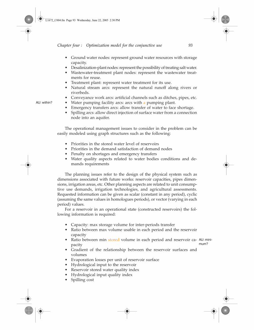
• Ground water nodes: represent ground water resources with storagecapacity.
• Desalinization-plant nodes: represent the possibility of treating salt water.• Wastewater-treatment plant nodes: represent the wastewater treat-
ments for reuse.• Treatment plant: represent water treatment for its use.• Natural stream arcs: represent the natural runoff along rivers or
riverbeds. • Conveyance work arcs: artificial channels such as ditches, pipes, etc.• Water pumping facility arcs: arcs with a pumping plant.• Emergency transfers arcs: allow transfer of water to face shortage.• Spilling arcs: allow direct injection of surface water from a connection
node into an aquifer.
The operational management issues to consider in the problem can beeasily modeled using graph structures such as the following:
• Priorities in the stored water level of reservoirs• Priorities in the demand satisfaction of demand nodes• Penalty on shortages and emergency transfers• Water quality aspects related to water bodies conditions and de-
mands requirements
The planning issues refer to the design of the physical system such asdimensions associated with future works: reservoir capacities, pipes dimen-sions, irrigation areas, etc. Other planning aspects are related to unit consump-tive use demands, irrigation technologies, and agricultural assessments.Requested information can be given as scalar (constant in any period), cyclic(assuming the same values in homologues periods), or vector (varying in eachperiod) values.
For a reservoir in an operational state (constructed reservoirs) the fol-lowing information is required:
• Capacity: max storage volume for inter-periods transfer• Ratio between max volume usable in each period and the reservoir
capacity • Ratio between min stored volume in each period and reservoir ca-
pacity• Gradient of the relationship between the reservoir surfaces and
volumes• Evaporation losses per unit of reservoir surface• Hydrological input to the reservoir• Reservoir stored water quality index • Hydrological input quality index• Spilling cost
AU: within?
AU: mini-mum?
L1672_C004.fm Page 93 Wednesday, June 22, 2005 2:30 PM

94 Drought Management and Planning for Water Resources
For a reservoir in a project state (reservoir to be constructed) the furtherfollowing information is required: max allowed capacity; min allowed capac-ity; and construction costs. For a civil demand in an operational state thefollowing information is required: population; unitary demand; request pro-gram; minimum required quality index; and deficit cost. For a civil demandin a project state the following further information is required: max popu-lation; min population; and net construction benefits. For an industrialdemand in an operational state the following information is required: indus-trial center dimension; unitary demand; request program; minimum requiredquality index; and deficit cost. For an industrial demand in a project state thefollowing further information is required: max dimension; min dimension;and net construction benefits.
For irrigation demand in an operational state the following informationis required: agriculture center dimension; unitary demand; request program;minimum required quality index; and deficit cost. For an irrigation demandin a project state the following further information is required: max area toirrigate; min area to irrigate; and net construction benefits.
For a hydroelectric power station in an operational state the followinginformation is required: production capacity; production program; energyefficiency; and production benefit. For a hydroelectric power station in aproject state the following further information is required: max productioncapacity; min production capacity; and construction cost. For a confluencenode the following information is required: hydrologic input (if arcs arenatural streams); and input quality index.
For a ground water node the following information is required: aquifercapacity; ratio between the max usable volume and the aquifer capacity;ratio between the min stored volume and the aquifer capacity, ground waterrecharge; ground water quality index; input quality index; and spilling cost.For a pump station in an operational state the following information isrequired: pumping capacity; pumping program; pumping efficiency; andpumping cost. For a pump station in a project state the following furtherinformation is required: max pumping capacity; min pumping capacity; andconstruction cost.
For a desalinization plant in an operational state the following informa-tion is required: desalinization water production; production program;treated water quality; and desalinization cost. For a desalinization plant ina project state the following further information is required: max productioncapacity; min production capacity; and construction cost.
For a wastewater treatment plant in an operational state the followinginformation is required: treatment capacity; treatment program; treatmentquota; treated water quality index; and treatment cost. For a wastewatertreatment plant in a project state the following further information isrequired: max treatment capacity; min treatment capacity; and constructioncost. For a water treatment plant in an operational state the following infor-mation is required: treatment capacity; treatment program; treated waterquality index; and treatment cost. For a water treatment plant in a project
AU: all of the lists that fol-low have been run into text—they are too small to offset
L1672_C004.fm Page 94 Wednesday, June 22, 2005 2:30 PM

Chapter four : Optimization model for the conjunctive use 95
state the following further information is required: max treatment capacity;min treatment capacity; and construction cost.
For a transfer arc in operational state the following information is required:transfer capacity; ratio between max transferred volumes and capacity; ratiobetween min transferred volumes and capacity; assured quality index; andoperating cost. For a transfer arc in a project state the following furtherinformation is required: max transfer capacity; min transfer capacity; andconstruction cost.
Consequently, variables considered in the optimization model can bedivided into flow variables (or operational variables) and project variables.The flow variables can refer to different types of water transfer such as:
• Water transfer in space along arc connecting different nodes at thesame time
• Water transfer in arc connecting homologous nodes at different times• Water transfer in arc connecting nodes to the root node• Water-losses arcs (as for evaporation) to transfer water to the root
node• Water transfer from the root node to demand nodes to face request
in drought periods (deficit transfers)
The planning variables refer to the project state and they are associated withthe dimension of future works: reservoir capacities, pipe dimensions, irriga-tion areas, etc.
Constraint equations of the optimization model can be divided into thefollowing types:
• Continuity equations for confluence nodes• Continuity equations for reservoirs and aquifers • Continuity equations for demand nodes• Continuity equations for plant nodes• Continuity for the root node• Requests evaluation for the centers of water consumption • Evaporation evaluation at reservoirs• Losses evaluation for aquifers• Production evaluation for plants• Relations between flow variables and planning works• Upper and lower bounds on spatial water transfers related to dimen-
sioned works• Upper and lower bounds on spatial water transfers related to plan-
ning works.• Upper and lower bounds on temporal transfers related to dimen-
sioned works• Upper and lower bounds on temporal transfers related to planning
works• Upper and lower bounds on project variables
L1672_C004.fm Page 95 Wednesday, June 22, 2005 2:30 PM
96 Drought Management and Planning for Water Resources
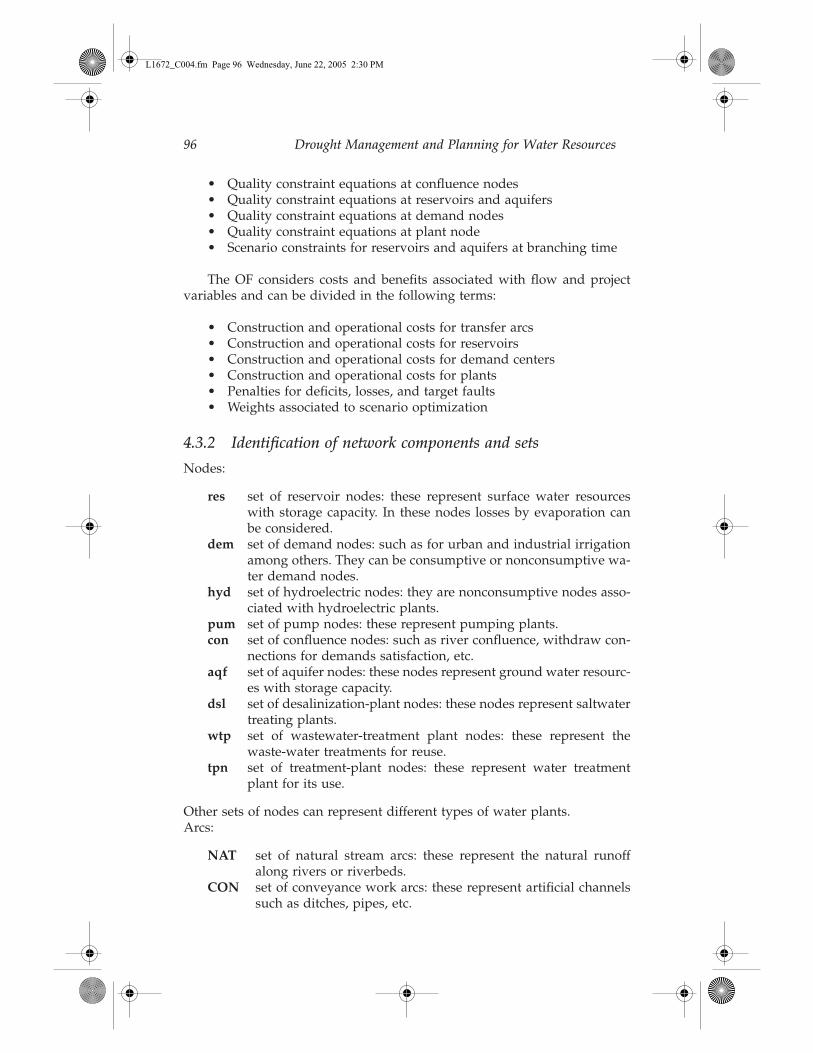
• Quality constraint equations at confluence nodes• Quality constraint equations at reservoirs and aquifers• Quality constraint equations at demand nodes• Quality constraint equations at plant node• Scenario constraints for reservoirs and aquifers at branching time
The OF considers costs and benefits associated with flow and projectvariables and can be divided in the following terms:
• Construction and operational costs for transfer arcs• Construction and operational costs for reservoirs• Construction and operational costs for demand centers• Construction and operational costs for plants• Penalties for deficits, losses, and target faults• Weights associated to scenario optimization
4.3.2 Identification of network components and sets
Nodes:
res set of reservoir nodes: these represent surface water resourceswith storage capacity. In these nodes losses by evaporation canbe considered.
dem set of demand nodes: such as for urban and industrial irrigationamong others. They can be consumptive or nonconsumptive wa-ter demand nodes.
hyd set of hydroelectric nodes: they are nonconsumptive nodes asso-ciated with hydroelectric plants.
pum set of pump nodes: these represent pumping plants.con set of confluence nodes: such as river confluence, withdraw con-
nections for demands satisfaction, etc.aqf set of aquifer nodes: these nodes represent ground water resourc-
es with storage capacity.dsl set of desalinization-plant nodes: these nodes represent saltwater
treating plants.wtp set of wastewater-treatment plant nodes: these represent the
waste-water treatments for reuse.tpn set of treatment-plant nodes: these represent water treatment
plant for its use.
Other sets of nodes can represent different types of water plants.Arcs:
NAT set of natural stream arcs: these represent the natural runoffalong rivers or riverbeds.
CON set of conveyance work arcs: these represent artificial channelssuch as ditches, pipes, etc.
L1672_C004.fm Page 96 Wednesday, June 22, 2005 2:30 PM

Chapter four : Optimization model for the conjunctive use 97
PUM set of water pumping facility arcs: these represent transfers withpumping plants activities.
EMT set of emergency transfers arcs: these arcs allow transfer of waterto face shortage.
SPL set of spilling arcs: these allow the overflow from reservoirs.REC set of recharge arcs: these allow direct injection of surface water
from a connection node into an aquifer.LOS set of water losses arcs as for evaporation from lakes, ground
water deep infiltration, etc.
4.3.3 Required Data
Some of the operational management issues to be considered in the optimi-zation problem can be easily modeled directly on the graph structures suchas priorities in the stored water level of reservoirs, priorities in the demandsatisfaction of demand nodes, and so on.
The planning issues refer to the design of the physical system such asdimensions associated with future works: reservoir capacities, pipedimensions, irrigation areas, etc. Other planning aspects are related tounit consumptive use demands, irrigation technologies, and agriculturalassessments.
Requested data can be given as scalar (constant in any period), cyclic(assuming the same values in homologues periods), or vector (varying ineach period) values. Data marked with (+) are required for an operationalstate (existing works with a known dimension) while data marked with (*)are required for a project state (works to be constructed). No marked dataare required for an operational and project state.
Required data for a reservoir j∈ res:
Yj(+) max storage volume for interperiods transfersr t
jmax ratio between max volume usable in each period t and the res-ervoir capacity
r tjmin ratio between min stored volume in each period t and reservoir
capacityd j gradient of the relationship between the reservoir surfaces and
volumeslt
j evaporation losses at time t per unit of reservoir surface areainpt
j hydrological input in each period t to the reservoirCst
j spilling cost in each period tCpt
j interperiod (t → t + 1) transfer benefit for stored waterQyt
j reservoir-stored water quality index at time tQht
j hydrological input quality index at time tYjmax (*) max allowed capacityYjmin (*) min allowed capacityg j (*) construction costs
AU: add math symbol
AU: add math symbol
AU: add math symbol
AU: add symbol
L1672_C004.fm Page 97 Wednesday, June 22, 2005 2:30 PM

98 Drought Management and Planning for Water Resources
Required data for a demand j∈ dem:
Pj (+) center dimensiondt
j unitary demandbt
j request programct
j deficit costQpt
j minimum required quality indexPjmax (*) max allowed center dimensionPjmin (*) min allowed center dimensionbj (*) net construction benefits
Required data for a hydroelectric power station j∈ hyd:
Hj (+) production capacityb t
j production programbj production benefitHjmax (*) max production capacityHjmin (*) min production capacityg j (*) construction cost
Required data for an aquifer node j∈ aqf:
Aj aquifer capacityr t
jmax ratio between the max usable volume and the aquifer capacityr t
jmin ratio between the min stored volume and the aquifer capacityLt
j deep infiltration lossesRt
j ground water rechargeClt
j loss cost in each period tCpt
j inter-period (t → t + 1) transfer benefit for aquifer-stored waterQat
j aquifer-stored water quality index at time tQrt
j ground water recharge quality index at time t
Required data for a pump station n j∈ pum:
Cj (+) pumping capacityb t j pumping programe j pumping efficiencyct
j pumping costCjmax (*) max production capacityCjmin (*) min production capacityg j (*) construction cost
Required data for a desalinization plant j∈ dsl:
Dj (+) desalinization production capacitybt j production program
AU: please add symbol
AU: please add symbol
AU: add symbol AU: add
symbol
AU: add symbols AU: add
symbols
AU: add symbol
AU: add symbols
L1672_C004.fm Page 98 Wednesday, June 22, 2005 2:30 PM

Chapter four : Optimization model for the conjunctive use 99
ctj desalinization cost
Qdtj treated water quality index
Djmax (*) max production capacityDjmin (*) min production capacityγj (*) construction cost
Required data for a wastewater treatment plant j∈ wtp:
Wj (+) treatment capacitybt
j treatment programst j treatment quotact
j treatment costQwt
j treated water quality indexWjmax (*) max treatment capacityWjmin (*) min treatment capacityγj (*) construction cost
Required data for a water treatment plant j∈ tpn:
Qj (+) treatment capacitybt j treatment programct
j treatment costQqt
j treated water quality indexQjmax (*) max treatment capacityQjmin (*) min treatment capacitycj (*) construction cost
Required data for a confluence node j∈ con:
inptj hydrologic input (if arcs are natural streams)
Qctj hydrological input water quality index
Required data for a generic transfer arc a∈TRF ≡ ∪(NAT, CON, PUM,EMT, SPL, LOS):
Fa (+) transfer capacityr t
amax ratio between max transferred volumes and capacity in eachperiod t
r tamin ratio between min transferred volumes and capacity in each
period tct
a transfer cost in each period tQft
j assured water quality index for transferred waterFamax (*) max transfer capacityFamin (*) min transfer capacityg a (*) construction cost
AU: add symbols AU: add
symbols
AU: add symbols
AU: add symbol
AU: add symbol
AU: add symbol
L1672_C004.fm Page 99 Wednesday, June 22, 2005 2:30 PM

100 Drought Management and Planning for Water Resources
4.3.4 Constraints formalization in the optimization model
As previously described, variables considered in the optimization model canbe divided into flow and project variables. Flow variables refer to differenttypes of water transfers in the multiperiod network: both in space (watertransfer along arcs connecting different nodes at the same time), and in time(water transfer in arcs connecting homologous nodes, with storage capacity,at different times), as well as along “dummy arcs” (i.e., water transfer to facedeficit at demand nodes). Project variables refer to works in a project stateand they are associated to the dimension of future works: reservoir capaci-ties, pipe dimensions, irrigation areas, etc.
Constraints in the optimization model are used to represent a large vari-ety of links and limitation in the system activities, as for example: massbalance equations concerning flow variables, demand requirements con-straints concerning flow and planning variables, transfer constraints alongarcs concerning flow and planning variables, losses (such as reservoir evap-oration) evaluation and transfer to the root node, relations between flowvariables and planning works, upper and lower bounds on flow and planningvariables, etc.
In order to deal with large-scale problems, the actual version of WARGIhas been specifically developed to treat LP and QP models.
For some system elements, related variables and corresponding con-straints are described hereafter in more detail.
Considering reservoir nodes, we can refer to Figure 4.4 to illustrate theadopted WARGI schematization and related variables and constraints: yt
j
stored water at reservoir j at the end of period t that can be used in the nextperiods. These are flow variables and they can be regarded as the waterflowing along the interperiods arcs (t → t + 1) connecting the homologous
Figure 4.4 Reservoir node schematization.
AU: ok to run this together here?
Bydrologic input(natural stream)Spatial transfer arc
Spatial transfer arc
Interperiodtransfer arc
Interperiodtransfer arc
Evaporation loss arc
Spilling arc(natural stream)
L1672_C004.fm Page 100 Wednesday, June 22, 2005 2:30 PM
Chapter four : Optimization model for the conjunctive use 101
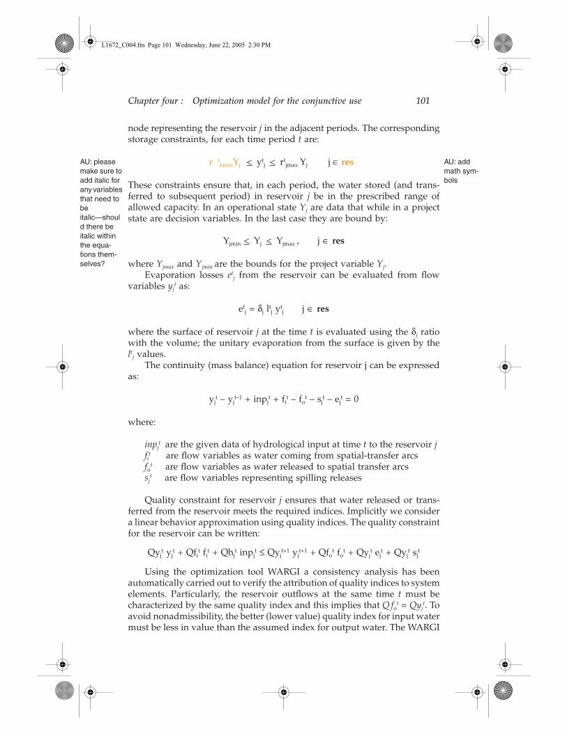
node representing the reservoir j in the adjacent periods. The correspondingstorage constraints, for each time period t are:
r tkminYj < ytj < rt
jmax Yj j ∈ res
These constraints ensure that, in each period, the water stored (and trans-ferred to subsequent period) in reservoir j be in the prescribed range ofallowed capacity. In an operational state Yj are data that while in a projectstate are decision variables. In the last case they are bound by:
Yjmin < Yj < Yjmax , j ∈ res
where Yjmax and Yjmin are the bounds for the project variable Yj.Evaporation losses et
j from the reservoir can be evaluated from flowvariables yj
t as:
etj = δj lt
j ytj j ∈ res
where the surface of reservoir j at the time t is evaluated using the δj ratiowith the volume; the unitary evaporation from the surface is given by thelt
j values.The continuity (mass balance) equation for reservoir j can be expressed
as:
yjt – yj
t–1 + inpjt + fi
t – fot – sj
t – ejt = 0
where:
inpjt are the given data of hydrological input at time t to the reservoir j
fit are flow variables as water coming from spatial-transfer arcs
fot are flow variables as water released to spatial transfer arcs
sjt are flow variables representing spilling releases
Quality constraint for reservoir j ensures that water released or trans-ferred from the reservoir meets the required indices. Implicitly we considera linear behavior approximation using quality indices. The quality constraintfor the reservoir can be written:
Qyjt yj
t + Qfit fi
t + Qhjt inpj
t ≤ Qyjt+1 yj
t+1 + Qfot fo
t + Qyjt ej
t + Qyjt sj
t
Using the optimization tool WARGI a consistency analysis has beenautomatically carried out to verify the attribution of quality indices to systemelements. Particularly, the reservoir outflows at the same time t must becharacterized by the same quality index and this implies that Q fo
t = Qyjt. To
avoid nonadmissibility, the better (lower value) quality index for input watermust be less in value than the assumed index for output water. The WARGI
AU: add math sym-bols
AU: please make sure to add italic for any variables that need to be italic—should there be italic within the equa-tions them-selves?
L1672_C004.fm Page 101 Wednesday, June 22, 2005 2:30 PM

102 Drought Management and Planning for Water Resources
consistency analysis for quality indices also considers values attributed tostored water in subsequent time periods.
Considering demand nodes, we can refer to Figure 4.5 to illustraterelated variables and constraints: pt
j water demand at civil demand center jin period t. These are flow variables associated to water transfer from thedemand node to the root node. The corresponding constraint, for pj
t evalu-ation at each time period t is:
ptj = βt
j dt j Pj , j∈ dem
where:
βjt assigned demand program
djt unitary demand
Pj demand center dimension
These constraints ensure the fulfillment of the demand in each period,regardless of whether they come from the system or from a dummy resource(deficit arc). In an operational state Pj are data that while in a project stateare project variables. In the last case they are bound by:
Pjmin < Pj < Pjmax, j∈ dem
The continuity (mass balance) equation for civil demand node j can beexpressed as:
pjt – fj
t – xjt = 0
where:
xjt is the shortage at time t for demand j as deficit flow variable
fjt are flow variables such as water coming from spatial-transfer arcs
Figure 4.5 Demand node schematization.
Spatial transfer arc
Total demand arc
Emergencytransfer arc(deficit arc)
AU: ok run together?
L1672_C004.fm Page 102 Wednesday, June 22, 2005 2:30 PM

Chapter four : Optimization model for the conjunctive use 103
Quality constraint for demand-node j ensures that water transferred byspatial transfer arcs meet the required quality index Qpj
t for the demand.The best possible quality index is implicitly attributed to the shortage arc;flows along this arc can consequently be worse than those required of thequality index in spatial water transfers coming to the demand center. Thequality constraint for the civil demand node can be written:
Qfjt fj
t + Qxjt xj
t ≤ Qpjt pj
t
Using the optimization tool WARGI, a consistency analysis was auto-matically carried out to verify the attribution of quality indices to systemelements. Variables and constraints are defined in the same way for otherdemand sets. Considering hydroelectric nodes, as they are nonconsumptivewater demand nodes: ht
j water through the plant j (hydroelectric powerplant) in period t. These are flow variables associated to hydroelectric pro-duction. The corresponding constraints, for ht
j evaluation at each time periodt is:
htj ≤ β t
ja tj Hj, j∈ hyd
where:
βjt assigned production-program
αjt unitary-production water requirement
Hj production capacity
These constraints express the dependence of flow variables htj on pro-
duction capacity. In an operational state, Hj are data that, while in a projectstate, are project variables. In the last case they are bound by:
Hjmin < Hj < Hjmax, j∈ hyd
No quality requirements are associated to hydroelectric nodes.Considering a generic spatial-transfer arc, water flows on it must be
bound to transfer capacity, determined by the dimension of the transferwork: fa
t flow on arc a in period t. These are flow variables; the corresponding
constraints for each time period t are:
r tamin Fa < fa
t <rt
amax Fa, a∈TRF
where:ρamin
t ratio between admitted min flow and capacityρamax
t ratio between admitted max flow and capacityFa transfer capacity
These constraints ensure that, in each period, the transferred volumein arc a be in the prescribed range. In an operational state Fa are data that,
AU: ok run together
AU: add math symbol
AU: ok run together?
AU: add math sym-bols
L1672_C004.fm Page 103 Wednesday, June 22, 2005 2:30 PM

104 Drought Management and Planning for Water Resources
while in a project state, are project variables. In the last case they are boundby:
Famin < Fa < Famax a∈ TRF
An assured quality index for water flowing is associated to these arcs.Quality constraints are directly associated to them. Nevertheless, using theoptimization tool WARGI, a consistency analysis is carried out to verify theattribution of quality indices to arcs when considering the composition ofsystem elements at nodes.
Variables and constraints are defined in the same way for other node andarc sets. Referring to the multiperiod dynamic network structure, mass balanceconstraints and quality constraints are defined in each node i ∈ N. Moreover,lower and upper bound constraints may be defined in some arcs a ∈ A torepresent some particular limits regarding transfer arcs in the set TRF.
4.3.5 Objective Function formalizationin the optimization model
The objective function (OF) formalization used in WARGI can be consideredas the sum of three parts: The first part concerns “weights” (costs, benefits,and penalties) on flow variables that, as previously described, are associatedwith flows in space, in time and along “dummy” arcs. Flow variables arerelated to hydrologic scenarios and they can be “weighted” in different ways.Normally the weights are to be related to the probability associated to thescenario or otherwise, especially when considering equally probable scenar-ios, and they are also related to the “preference” or “critical nature” attribu-tion of the scenario. A second part of the OF considers costs given to projectvariables and represents the “construction costs” on planned works. A thirdpart of the OF is specifically required by the scenario optimization when thescenario optimization is used to define a “barycentrical” solution. Amonghomologous flow variables in different scenarios, a flow-variable distanceminimization expression must be inserted in the OF.
Following these criteria and using the simplified notation previouslydefined, the objective function can be expressed as a minimization of thesum of the following three terms:
OF1:
wg (Σj∈ res Σt=1,T cyt yj
t + Σj∈ dem Σt=1,T cpt pj
t + Σj∈ hyd Σt=1,T cht hj
t
+ Σj∈ pum Σt=1,T cbt bj
t + Σj∈ aqf Σt=1,T cat aj
t + Σj∈ dsl Σt=1,T cdt dj
t cwt wj
t
+ Σj∈ wtp Σt=1,T + Σj∈ tpn Σt=1,T cqt qj
t Σj∈ TRF Σt=1,T cxt xj
t) = 1,G
OF2:
S j∈resgy Yj + Sj∈demgp Pj + Sj∈ hydgh Hj + Sj∈ pum gb Bj + Sj∈ dslgd Dj + Sj∈ wtpgw Wj
+ Sj∈ tpngq Qj
AU: add all maths sym-bols here
L1672_C004.fm Page 104 Wednesday, June 22, 2005 2:30 PM
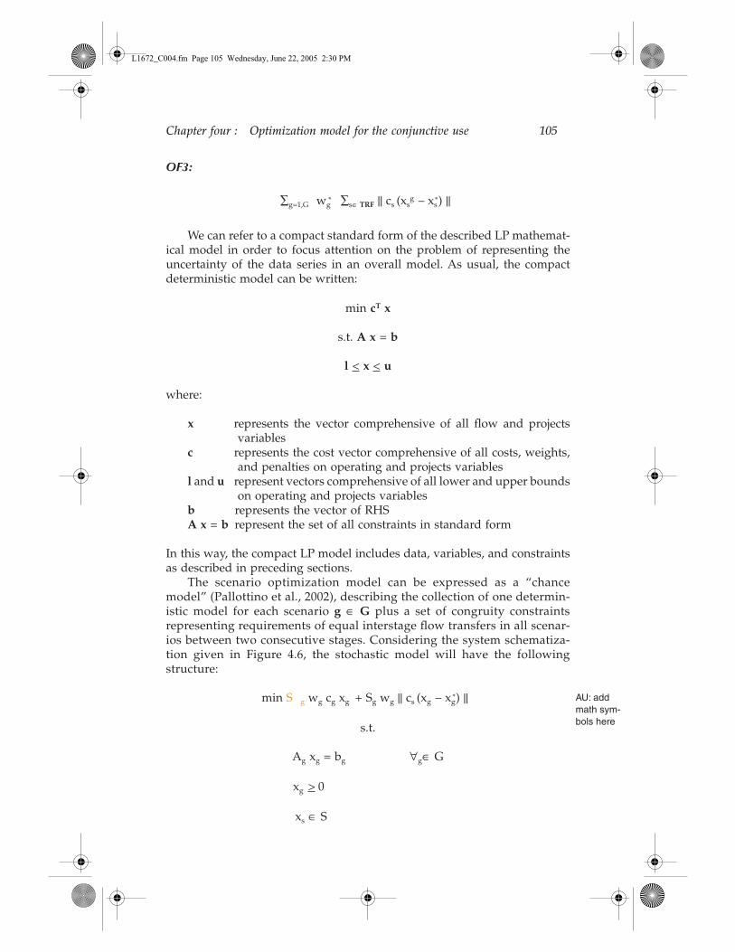
Chapter four : Optimization model for the conjunctive use 105
OF3:
∑g=1,G wg* ∑s∈ TRF || cs (xs
g – xs
*) ||
We can refer to a compact standard form of the described LP mathemat-ical model in order to focus attention on the problem of representing theuncertainty of the data series in an overall model. As usual, the compactdeterministic model can be written:
min cT x
s.t. A x = b
l < x < u
where:
x represents the vector comprehensive of all flow and projectsvariables
c represents the cost vector comprehensive of all costs, weights,and penalties on operating and projects variables
l and u represent vectors comprehensive of all lower and upper boundson operating and projects variables
b represents the vector of RHSA x = b represent the set of all constraints in standard form
In this way, the compact LP model includes data, variables, and constraintsas described in preceding sections.
The scenario optimization model can be expressed as a “chancemodel” (Pallottino et al., 2002), describing the collection of one determin-istic model for each scenario g ∈ G plus a set of congruity constraintsrepresenting requirements of equal interstage flow transfers in all scenar-ios between two consecutive stages. Considering the system schematiza-tion given in Figure 4.6, the stochastic model will have the followingstructure:
min S g wg cg xg + Sg wg || cs (xg – xg*) ||
s.t.
Ag xg = bg ∀g∈ G
xg > 0
xs ∈ S
AU: add math sym-bols here
L1672_C004.fm Page 105 Wednesday, June 22, 2005 2:30 PM

106 Drought Management and Planning for Water Resources
where xs ∈ S represents the linking constraints on interstage flows, describedin previous paragraphs, and xg* is the optimal policy (“barycentrical” flows)expected by the water manager. This kind of model can be solved by decom-position methods such as Benders decomposition techniques, which exploitthe special structure of constraints. When the size of the problem becomeshuge, it is possible to resort to parallel computing.
4.4 WARGI graphical interfaceThe WARGI graphical interface provides the possibility of inserting the basicsystem configuration components and connections between them. As shownin Figure 4.7, the main window presents an empty canvas and the programwindow consists of several parts as described below. An extended illustra-tion of WARGI features has been given in the WAMME project.
Title: The name of the current graph (NoName if the graph is new andhas not been saved).
Menu Bar: The menu bar for selecting various options and tasks. Scroll Bars: Permit scrolling the canvas in order to use a canvas larger
than the size visible on the screen. Status Bar: Multifunction bar providing information on graphic objects
and also acts as a guide during graph construction.
The tool palette is a small window containing a set of graphical objectsneeded for creating graphs. In order to open the tool palette, the user has topull up the View menu and select Drawing Tool. The tool palette windowwill open and can be dragged into a suitable position on the screen.
Figure 4.6 Segment of branch at branching time t referred to reservoir j.
τ τ+1 Time periods
Scenario g1
Scenario g2
i
i
i
AU: add math symbol
L1672_C004.fm Page 106 Wednesday, June 22, 2005 2:30 PM
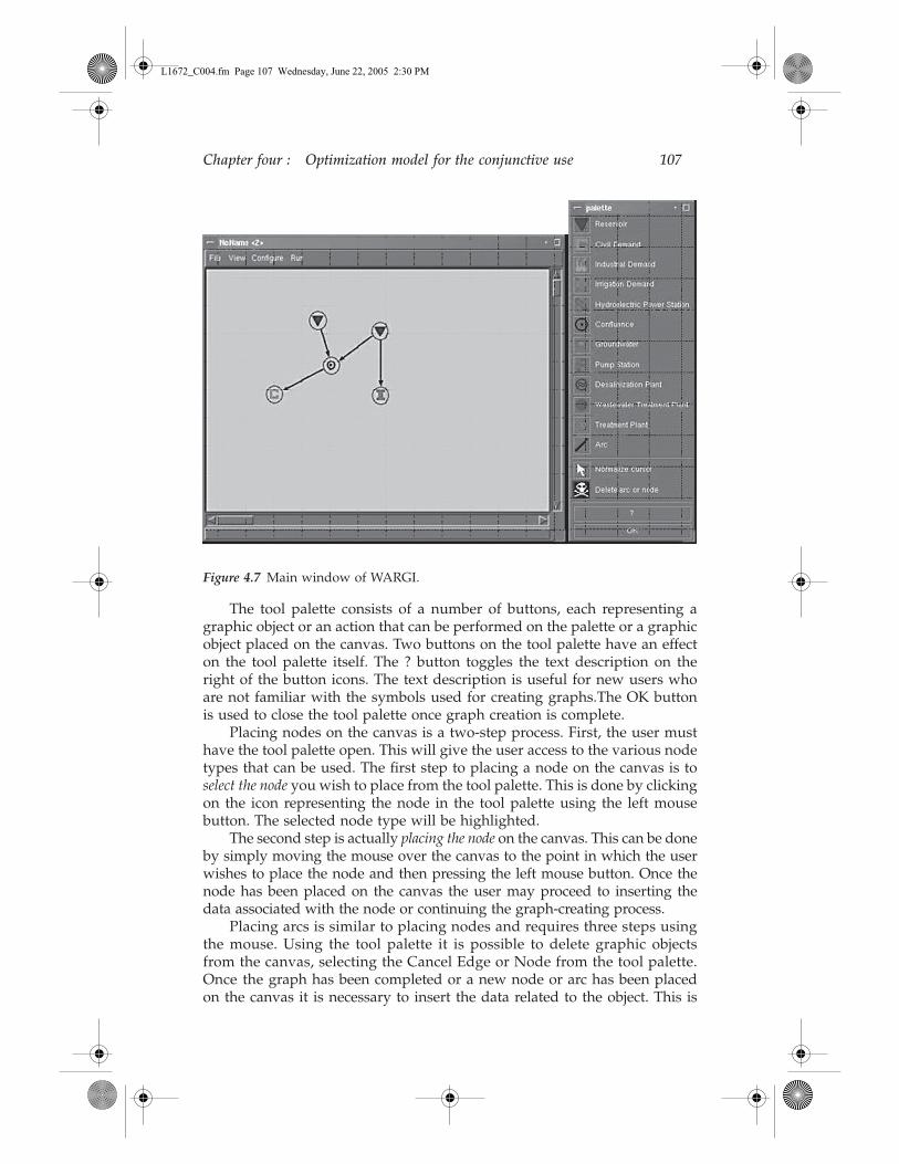
Chapter four : Optimization model for the conjunctive use 107
The tool palette consists of a number of buttons, each representing agraphic object or an action that can be performed on the palette or a graphicobject placed on the canvas. Two buttons on the tool palette have an effecton the tool palette itself. The ? button toggles the text description on theright of the button icons. The text description is useful for new users whoare not familiar with the symbols used for creating graphs.The OK buttonis used to close the tool palette once graph creation is complete.
Placing nodes on the canvas is a two-step process. First, the user musthave the tool palette open. This will give the user access to the various nodetypes that can be used. The first step to placing a node on the canvas is toselect the node you wish to place from the tool palette. This is done by clickingon the icon representing the node in the tool palette using the left mousebutton. The selected node type will be highlighted.
The second step is actually placing the node on the canvas. This can be doneby simply moving the mouse over the canvas to the point in which the userwishes to place the node and then pressing the left mouse button. Once thenode has been placed on the canvas the user may proceed to inserting thedata associated with the node or continuing the graph-creating process.
Placing arcs is similar to placing nodes and requires three steps usingthe mouse. Using the tool palette it is possible to delete graphic objectsfrom the canvas, selecting the Cancel Edge or Node from the tool palette.Once the graph has been completed or a new node or arc has been placedon the canvas it is necessary to insert the data related to the object. This is
Figure 4.7 Main window of WARGI.
L1672_C004.fm Page 107 Wednesday, June 22, 2005 2:30 PM

108 Drought Management and Planning for Water Resources
done through a template window, which is accessible by clicking on thegraphic object using the right mouse button. The template window is differentfor each type of object placed on the canvas.
Some sections of the template windows can be accessible in the case ofproject optimization, others in system management (operational) optimization.
Once the graph has been completed and all the necessary data have beeninserted, it is possible to generate the necessary MPS file to feed to the solver.MPS file generation is achieved by selecting Generate MPS from the File menu.
Graphs may be saved and previously saved graphs may be loaded byusing the File menu. When a graph becomes too large to fit on the currentlyvisible canvas, it may be helpful to scroll and zoom the canvas to have abetter understanding and vision of the graph the user is creating. This canbe done by selecting Scrolling and Zooming from the View menu.
In order to be able to launch the solver from the Graphical User Interfacethe user must first set the command line required to launch the solver. Thisis done from the Configure menu by selecting Solver. Once the requiredcommand has been inserted in the space provided clicking OK will set thecommand line for launching the solver.
At the end the user can visualize results using View results and Plotresults options from the View menu.
4.5 Results applying WARGI to real casesAs extensively reported in the WAMME project, three WARGI applicationsto real water systems in the Mediterranean area were made: the Flumendosa–Campidano (Sardinia, Italy), Júcar (Spain), and Salso-Simeto (Sicily, Italy)water systems. Application criteria and results are summarized below.
4.5.1 Flumendosa–Campidano water system
Symbols meaning can be found in the palette-window reported in Figure 4.8.The schematization carried out using WARGI for the Flumendosa–Campidanosystem is reported in Figure 4.10. The water system consists of the followingmain elements:
• Ten reservoirs with a total capacity of 723 millions of cubic meters (Mm3)• Ten civil demand centers with a total request of 116 Mm3 for year• Nine irrigation demands with a total request of 224 Mm3 for year• Two industrial demands with a total request of 19 Mm3 for year• One hydroelectric demand with request of 90 Mm3 for year• Five pumping stations• Nine water treatment plants• Three waste-water treatment plants
Therefore, the total demand of the system was estimated as equal to 449 Mm3
per year.
AU: what about Figure 4.9? need a callout
L1672_C004.fm Page 108 Wednesday, June 22, 2005 2:30 PM
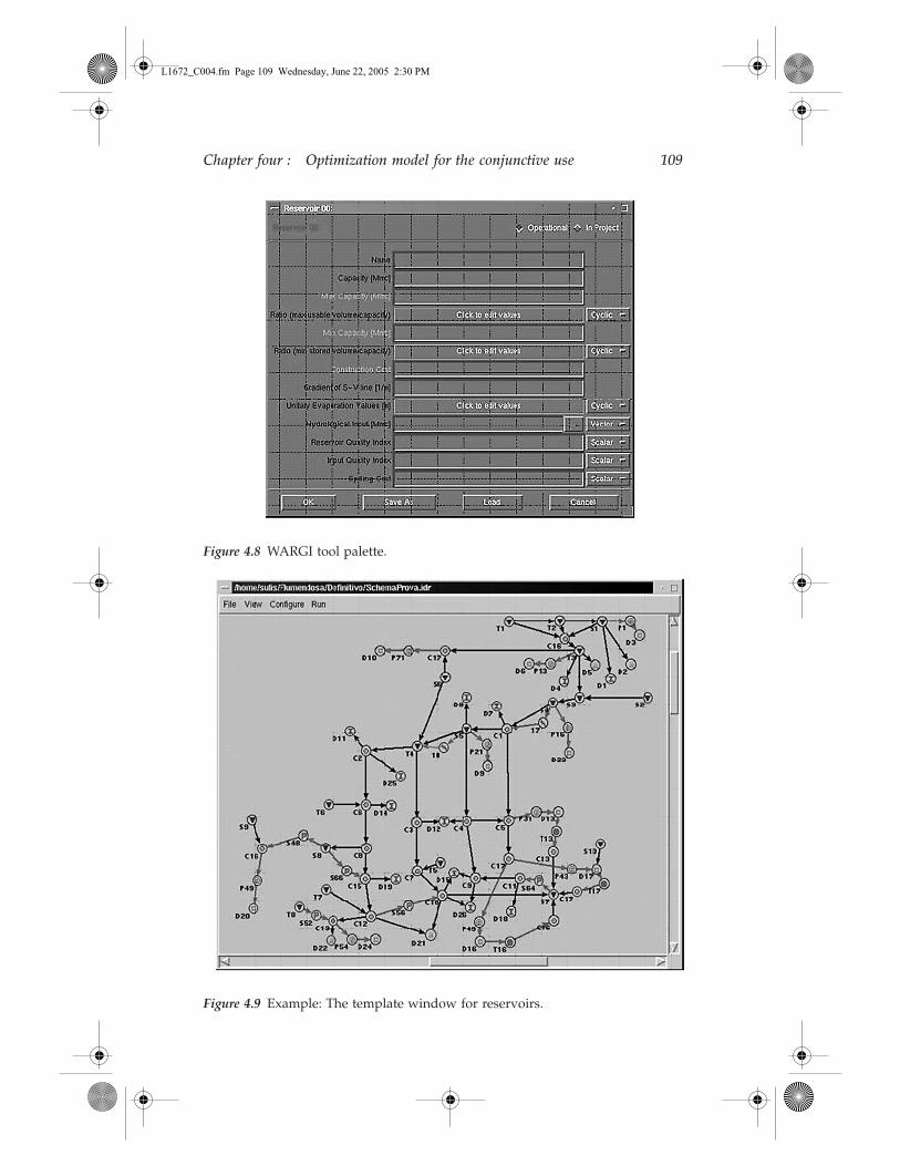
Chapter four : Optimization model for the conjunctive use 109
Figure 4.8 WARGI tool palette.
Figure 4.9 Example: The template window for reservoirs.
L1672_C004.fm Page 109 Wednesday, June 22, 2005 2:30 PM

110 Drought Management and Planning for Water Resources
The water-quality classification of the reservoirs and of the water flowsof the Flumendosa–Campidano system made use of the experience gainedduring the project and the availability of data that have been collected bythe Flumendosa Water Authority since 1985.
Preliminary hydrologic analyses took into account the marked persistenceof low runoff values in the past decade. Using WARGI, we first established theannual amount of volumes of the system to be issued considering the regionaldatabase (SISS) for the period 1922–1992. Further analysis was performed inrelation to different synthetic scenarios of runoff in the rivers under consider-ation as the necessity of considering more hydrological scenarios was evidentto characterize system performances. Nevertheless, to avoid an excess of com-plexity in the analysis, caused by the growth of examined sets, it was decidedthat investigations should be concentrated on considering two series:
A. Historical hydrological series: SISS (regional database) series1922–1992 were considered;
B. Rescaled hydrological series: series prepared for the recent regionalplan were adopted.
Thus, using the WARGI optimization tool, the results obtained using thesetwo hydrologic input configurations were reported.
Figure 4.10 The WARGI input window for the Flumendosa–Campidano water system.
AU: explain and add a spellout?
L1672_C004.fm Page 110 Wednesday, June 22, 2005 2:30 PM

Chapter four : Optimization model for the conjunctive use 111
Moreover, the application of WARGI to the Flumendosa scheme hasbeing carried out taking into consideration two phases with regard to qualityconstraint limiting water use:
1. during the first phase no quality constraints were given to limit theuse of the resource on the basis of its quality;
2. during the second phase the indices of quality referring both to theresource and the water demand were considered.
Consequently, the optimization was carried out considering four situationsgiven by the combination of two hydrologic configurations and two qualityindex attribution phases.
It was evident, however, from the analysis of the results, that maintainingthe demand equal to that totally requested would have caused a deficit thatwas not admissible, particularly concerning the irrigation demand. This factwas highlighted especially by the results obtained with the use of the rescaledhydrologic series (B1 and B2 cases), which, on average, introduced a reductionof hydrologic input of about 50% of the average of the historical series.
Therefore, was preferred to avoid the deficit reaching excessively highvalues. First, there was a reduction of the resource requested for hydroelectricuse, reduced from 90 Mm3 to 20 Mm3, which was considered strategic for theproduction of energy in the region. Finally, indices of irrigation demand reduc-tion were evaluated to annul the deficit in configuration B1. We, therefore,refer to cases B1b and B2b when reduction coefficients are applied to theoptimization model, considering rescaled hydrological series without qualityconstraints (case B1b) or with quality constraints (case B2b). The same notationis adopted when we consider historical series (case A1b and A2b).
The introduction of the indices of quality concerning the resources ofthe system has caused modifications in the optimum configuration. Even ifthese modifications were not homogeneous throughout the system, the mainimpact on it can be observed considering the total amount of deficit in thehistorical and rescaled hydrological scenarios. Small deficits were high-lighted in the Ab2 configuration. As can be expected, the rescaled hydrolog-ical (B2b) configuration shows much higher deficit values. To compareresults, Table 4.2 and Table 4.3 report the synthetic resulting values obtainedfor demand deficits in the configuration A2b and B2b.
Table 4.2 Results Obtained for Demand Deficits in the Configuration A2b
Demand DYears deficits
>25%Max year deficit
[Mm3]Year demand
[Mm3]
All demands 0 14.36 257.92Civil demand 0 2.88 93.32Irrigation demand 0 6.96 125.6Industrial demand 0 4.71 19.00Hydroelectric Demand 0 2.45 20.00
AU: word missing
L1672_C004.fm Page 111 Wednesday, June 22, 2005 2:30 PM
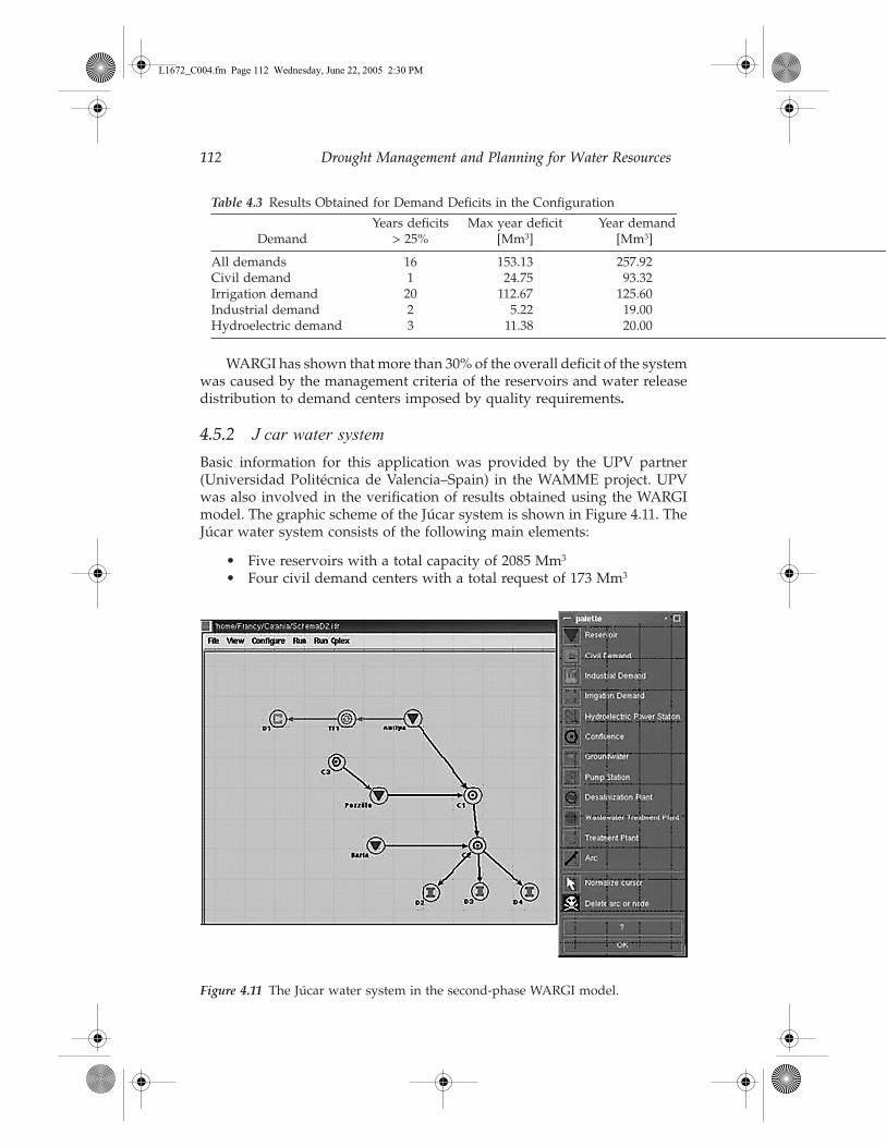
112 Drought Management and Planning for Water Resources
WARGI has shown that more than 30% of the overall deficit of the systemwas caused by the management criteria of the reservoirs and water releasedistribution to demand centers imposed by quality requirements.
4.5.2 J car water system
Basic information for this application was provided by the UPV partner(Universidad Politécnica de Valencia–Spain) in the WAMME project. UPVwas also involved in the verification of results obtained using the WARGImodel. The graphic scheme of the Júcar system is shown in Figure 4.11. TheJúcar water system consists of the following main elements:
• Five reservoirs with a total capacity of 2085 Mm3
• Four civil demand centers with a total request of 173 Mm3
Table 4.3 Results Obtained for Demand Deficits in the Configuration
Demand Years deficits
> 25%Max year deficit
[Mm3]Year demand
[Mm3]
All demands 16 153.13 257.92Civil demand 1 24.75 93.32Irrigation demand 20 112.67 125.60Industrial demand 2 5.22 19.00Hydroelectric demand 3 11.38 20.00
Figure 4.11 The Júcar water system in the second-phase WARGI model.
L1672_C004.fm Page 112 Wednesday, June 22, 2005 2:30 PM
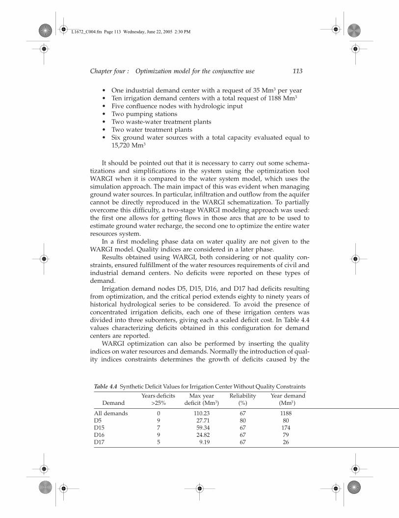
Chapter four : Optimization model for the conjunctive use 113
• One industrial demand center with a request of 35 Mm3 per year• Ten irrigation demand centers with a total request of 1188 Mm3
• Five confluence nodes with hydrologic input• Two pumping stations• Two waste-water treatment plants• Two water treatment plants• Six ground water sources with a total capacity evaluated equal to
15,720 Mm3
It should be pointed out that it is necessary to carry out some schema-tizations and simplifications in the system using the optimization toolWARGI when it is compared to the water system model, which uses thesimulation approach. The main impact of this was evident when managingground water sources. In particular, infiltration and outflow from the aquifercannot be directly reproduced in the WARGI schematization. To partiallyovercome this difficulty, a two-stage WARGI modeling approach was used:the first one allows for getting flows in those arcs that are to be used toestimate ground water recharge, the second one to optimize the entire waterresources system.
In a first modeling phase data on water quality are not given to theWARGI model. Quality indices are considered in a later phase.
Results obtained using WARGI, both considering or not quality con-straints, ensured fulfillment of the water resources requirements of civil andindustrial demand centers. No deficits were reported on these types ofdemand.
Irrigation demand nodes D5, D15, D16, and D17 had deficits resultingfrom optimization, and the critical period extends eighty to ninety years ofhistorical hydrological series to be considered. To avoid the presence ofconcentrated irrigation deficits, each one of these irrigation centers wasdivided into three subcenters, giving each a scaled deficit cost. In Table 4.4values characterizing deficits obtained in this configuration for demandcenters are reported.
WARGI optimization can also be performed by inserting the qualityindices on water resources and demands. Normally the introduction of qual-ity indices constraints determines the growth of deficits caused by the
Table 4.4 Synthetic Deficit Values for Irrigation Center Without Quality Constraints
DemandYears deficits
>25%Max year
deficit (Mm3)Reliability
(%)Year demand
(Mm3)
All demands 0 110.23 67 1188 D5 9 27.71 80 80D15 7 59.34 67 174D16 9 24.82 67 79D17 5 9.19 67 26
L1672_C004.fm Page 113 Wednesday, June 22, 2005 2:30 PM

114 Drought Management and Planning for Water Resources
unavailability of water with acceptable quality conditions for demands. Nev-ertheless, as can be seen in the WAMME report, in the Júcar case, generalconditions in behavior of quality seem quite stable: indices grow (this meansless quality) from upstream to downstream and users quality requirementsshow the same behavior. Therefore, civil demand remains completely satis-fied and only a slight growth occurs in irrigation demand deficits. Themaximum year deficit only increases from 110.2 to 131.7 Mm3 (the totalirrigation demand is equal to 1188 Mm3/year).
4.5.3 Salso–Simeto water system
Basic information for this application and verification of results obtainedusing the WARGI mode were provided by the DICA partner (University ofCatania–Italy). The graphic scheme of the Salso–Simeto system is shown inFigure 4.12.
The Salso–Simeto water system consists of the following main elements:
• Two reservoirs (Ancipa and Pozzillo) with a total capacity of 151 Mm3
• One diversion dam• One civil demand center with a total request of 12 Mm3 per year• One irrigation demand with a total request of 121 Mm3 per year• One water treatment plant
In order to take into account the transfer of the winter spills from Ancipareservoir to Pozzillo reservoir, two modeling steps have been performed: an
Figure 4.12 Final configuration of the Salso–Simeto system and WARGI tool palette.
AU: explain and provide a spellout?
Au: Provide thecorrected Figure 4.12
L1672_C004.fm Page 114 Wednesday, June 22, 2005 2:30 PM

Chapter four : Optimization model for the conjunctive use 115
initial configuration has been set, in order to determine any water spills fromAncipa reservoir; and an updated configuration has been implemented,where the water transfers within the limit of the conduit maximum capacityare input to Pozzillo through the node C3, as reported in Figure 4.12.
To avoid the presence of concentrated irrigation deficits, the irrigationdemand has been split into three equal parts: nodes D2, D3, and D4 inFigure 4.4, giving to each one a scaled deficit cost. Nevertheless, a higherpriority of municipal water supply over irrigation is guaranteed. As a con-sequence of the deficit costs imposed for the municipal and the irrigationdemands, there is no civil demand deficit during the optimization period,whereas irrigation deficits do mostly occur during the more critical historicaldrought periods. The performance of the system under the assumed conditionshas been summarized in the computed indices that are shown in Table 4.5.
4.6 ConclusionIn the present work we illustrated a general-purpose optimization tool char-acterized by considering a user-friendly graphical interface. The WARGIpackage has been developed considering the objective of the WAMMEproject, which sets out to improve opportunities for using optimization,aided by a graphical user interface in water resource systems modeling. Aspreviously highlighted, the package has been developed in a scenario-mod-eling framework and considers the possibility of conventional and marginalwater utilization for solving large-scale water system optimization problems.
The usefulness of the developed optimization approach has been con-firmed in the WARGI applications since the package allows the user an easystart to the optimization analysis by representing the physical sketch of thesystem in the main window of the toolkit. When requested information isgiven then the optimal solution can be reached. After this there is the pos-sibility of viewing main results, modifying the configuration, and checkingall the intermediate phases. WARGI allows for easy updating of the systemconfiguration and considers different system optimizers using standarddata-input format.
Table 4.5 Performance Indices of the Salso–Simeto Water System Optimization
No. of violations to min. storage
volumes(% months)
Sum of the annual squared
irrigation deficits
(106 m3)2
Maximum annual
irrigation deficit
(106 m3)
Temporal irrigation reliability
(%)
No. of years with deficit
> 25% demand
(−)
Ancipa 19.0 020,909
0 100 Municipal 0Pozzillo 14.3 74.9 61.5 Irrigation 7
L1672_C004.fm Page 115 Wednesday, June 22, 2005 2:30 PM
116 Drought Management and Planning for Water Resources
The benefit of resorting to mathematical programming, applied to opti-mization models solving real case water resources planning and manage-ment problems, seems to be confirmed in the multiphase DSS approach, asemphasized at the beginning of this chapter.
In the optimization phase we can solve a model representing the realphysical problem in an obviously simplified manner, but which does notexcessively reduce its level of adherence to reality. Consequently, in thesimulation phase, we have only to examine reduced scenario configurationsfrom the dimensional and temporal points of view. Moreover, if the opti-mization model remains adherent to the real problem, in a deterministicframework mathematical programming results give us the best manage-ment (in terms of water flows in the system) obtained by an ideal managerhaving previous knowledge of input and demands behavior in the system.These results can give us a measure of the “goodness” of the simula-tion-based DSS, at least for a reduced deterministic test-cases set.
References Cannas B., Fanni, A. Pintus, M., and Sechi, G. M. (2001a, July). Alternative neural
network models for the rainfall-runoff process. Seventh International Conferenceon Engineering Applications of Neural Networks EANN 200, Cagliari, July2001.
Cannas B., Fanni, A. Pintus, M., and Sechi, G. M. (2001b). River flow forecast for reservoirmanagement through neural networks. MODSIM 2001 Congress Proceedings,Camberra, Australia. Also published in the Proceedings of 28th Congress ofHydraulics and Hydraulic Engineering, Potenza, September 2002.
Cannas, B., Carboni, A., Fanni, A., and Sechi, G. M. (2000, July 17–19). Locally recurrentneural networks for the water flow forecasting, sixth international conference onengineering applications of neural networks. EANN 2000, Kingston UponThames, U.K.
CPLEX Optimization. (1993). Using the CPLEX callable library and CPLEX mixed integerlibrary. Incline Village, Nevada.
Loucks, D. P., Stedinger, J. R., and Haith, D A. (1981). Water resource systems planningand analysis. Englewood Cliffs, NJ: Prentice-Hall.
Nicklow J. W. (2000). Discrete-time optimal control for water resources engineeringand management. Water Int. 25(1), 89–95.
Pallottino S., Sechi G.M., and Zuddas P. (2002). A DSS for water resources managementunder uncertainty. IEMSs 2002 Conference on Integrated Assessment and De-cision Support — IEMSs: International Environmental Modelling and Soft-ware Society, Lugano, Switzerland.
Rockafellar, R. T., and Wets, R. J. B. (1991). Scenarios and policy aggregation inoptimization under uncertainty. Mathematics of Operations Research 16,119–147.
Sechi G. M., and Zuddas P. (2000a). Scenario analysis in water resources systemoptimization under uncertainty conditions. Twenty-seventh Convegno diIdraulica e Costruzioni Idrauliche, (Vol. 3, 209–216). Genova. Also publishedin R. Mehrotra, B. Soni, K. K. S. Bhatia (Eds.), Integrated water resourcesmanagement for sustainable development. Roorkee, India.
AU: to list a ref here it must be cited in text. I am deleting those not cited—to reinstate them please cite them somewhere in text
AU: pub-lisher?
L1672_C004.fm Page 116 Wednesday, June 22, 2005 2:30 PM

Chapter four : Optimization model for the conjunctive use 117
Sechi G. M., and Zuddas, P. (2000b). WARGI: Water Resources System OptimizationAided by Graphical Interface. In W. R. Blain and C. A. Brebbia (Eds.),Hydraulic engineering software. WIT-PRESS, 109–120.
Sechi, G. M., and Zuddas, P. (2002). The optimization package WARGI: Water ResourcesSystem Optimization Aided by Graphical Interface. Proceedings of 28th Congressof Hydraulics and Hydraulic Engineering, Potenza, September 2002.
Simonovic S. P. (2000). Tools for water management — A view of the future. WaterInt. 25(1), 76–88.
AU: city?
L1672_C004.fm Page 117 Wednesday, June 22, 2005 2:30 PM

L1672_C004.fm Page 118 Wednesday, June 22, 2005 2:30 PM