optimization of query streams using semantic prefetchingkmsalem/pubs/scalpeltods.pdf ·...
TRANSCRIPT
Optimization of Query Streams UsingSemantic Prefetching
IVAN T. BOWMAN and KENNETH SALEM
University of Waterloo
Streams of relational queries submitted by client applications to database servers contain pat-
terns that can be used to predict future requests. We present the Scalpel system, which detects
these patterns and optimizes request streams using context-based predictions of future requests.
Scalpel uses its predictions to provide a form of semantic prefetching, which involves combining
a predicted series of requests into a single request that can be issued immediately. Scalpel’s se-
mantic prefetching reduces not only the latency experienced by the application but also the total
cost of query evaluation. We describe how Scalpel learns to predict optimizable request patterns by
observing the application’s request stream during a training phase. We also describe the types of
query pattern rewrites that Scalpel’s cost-based optimizer considers. Finally, we present empirical
results that show the costs and benefits of Scalpel’s optimizations.
Categories and Subject Descriptors: C.2.4 [Computer-Communication Networks]: Distributed
Systems—Distributed databases; H.2.4 [Database Management]: Systems—Transactionprocessing
General Terms: Performance
Additional Key Words and Phrases: Prefetching, query streams
1. INTRODUCTION
Relational database applications establish database server connectionsthrough which they issue streams of query and update requests and fetch theresults of those requests. Although there has been a great deal of work onrelational query optimization, most of that work focuses on optimizing the pro-cessing of individual requests by the database server. Here, we consider theproblem of optimizing the stream of client/server interactions that occurs overa connection, rather than individual requests.
As an illustration of the kind of optimization we hope to achieve, consider theclient-side database application code shown in Figure 1. The code is adapted
This research was supported in part by iAnywhere Solutions and by the National Sciences and
Engineering Research Council of Canada.
Authors’ address: School of Computer Science, University of Waterloo, Waterloo, Ontario N2L 3G1,
Canada. Correspondence email: [email protected].
Permission to make digital or hard copies of part or all of this work for personal or classroom use is
granted without fee provided that copies are not made or distributed for profit or direct commercial
advantage and that copies show this notice on the first page or initial screen of a display along
with the full citation. Copyrights for components of this work owned by others than ACM must be
honored. Abstracting with credit is permitted. To copy otherwise, to republish, to post on servers,
to redistribute to lists, or to use any component of this work in other works requires prior specific
permission and/or a fee. Permissions may be requested from Publications Dept., ACM, Inc., 1515
Broadway, New York, NY 10036 USA, fax: +1 (212) 869-0481, or [email protected]© 2005 ACM 0362-5915/05/1200-1056 $5.00
ACM Transactions on Database Systems, Vol. 30, No. 4, December 2005, Pages 1056–1101.

Optimization of Query Streams Using Semantic Prefetching • 1057
Fig. 1. SQL-Ledger get openinvoices function.
Fig. 2. The join query Qopt.
from SQL-Ledger [Simader 2004], a web-based double-entry accounting sys-tem written in Perl. The get openinvoices function retrieves a list of all openinvoices for a given customer that were recorded with a given monetary cur-rency. If the given currency differs from the configured system default, then theexchange rate for each invoice is retrieved using the get exchangerate func-tion. When this application runs, it issues a series of small single-table queries(Q1, Q2, Q2, Q2, . . .) to the database server. It uses the results of these queriesto perform a two-way, nested loops join on the client side.
In this article, we present the Scalpel system, which optimizes applicationrequest streams using context-based predictions of upcoming requests. Scalpelmonitors the requests issued by the client application and learns to recognizeand optimize query patterns. For example, if Scalpel recognizes the nestedquery pattern (Q1, Q2, Q2, Q2, . . .) generated by the application in Figure 1,it can replace the entire pattern with a single, larger query similar to Qopt,which is shown in Figure 2. Query Qopt performs the join at the server andreturns all of the data that would have been returned by Q1 and the series of
ACM Transactions on Database Systems, Vol. 30, No. 4, December 2005.

1058 • I. T. Bowman and K. Salem
inner Q2 queries. Scalpel is transparent to the database client: no changes tothe application code are required.
Scalpel’s rewrites are predictive. When Scalpel sees Q1, it predicts that Q1
will be followed by a series of nested Q2 queries. Based on this prediction, itissues Qopt, rather than Q1, to the server. If the application then requests Q2
as expected, Scalpel does not pass Q2 to the server. Instead, it extracts therequired data from the result of Qopt and returns that to the application. Ifthe application behaves unexpectedly, perhaps by issuing a different query Q3,then Scalpel can simply forward Q3 to the server for execution. In this caseScalpel has done some extra work, since Qopt is a larger and more complexquery than Q1. However, Scalpel always returns correct results to the client.By replacing Q1 with Qopt, Scalpel implements a kind of prefetching. We call itsemantic prefetching because Scalpel must understand the queries Q1 and Q2
in order to generate an appropriate Qopt.There are two reasons to do semantic prefetching. First, it provides the query
optimizer at the server with more scope for optimization. For example, the ap-plication shown in Figure 1 effectively joins two tables at the client site. How-ever, the server’s optimizer will be unaware that the join is occurring. Scalpel’srewrite makes the server aware of the join, allowing its optimizer to consideralternative join methods that it may implement.
Second, by replacing many small queries with fewer larger queries, Scalpelcan reduce the latency and overhead associated with the interconnection net-work and the layers of system interface and communications software atboth ends of the connection. These costs can be quite significant, as noted byBernstein et al. [1999]. We measured the cost of fetching a single in-memory rowfrom several commercial relational database management systems. Regardlessof whether the client used local shared memory or an inter-city WAN to commu-nicate with the server, overhead was consistently over 99% of the total querytime. This excludes the cost of parsing and optimizing the query text, whichwould make the overhead even higher. For the application shown in Figure 1,this means that almost all of the time spent issuing queries Q2 to the server isoverhead.
A potential objection to Scalpel is that the problems we have illustrated canbe solved by manually rewriting the client applications. For example, the twofunctions shown in Figure 1 could be replaced by a single function that opensQopt (Figure 2). However, we claim that there is a place for both manual ap-plication tuning and automatic, run-time optimization of application requeststreams. Manual tuning can clearly improve application performance, but run-time optimization has some strengths that application tuning does not. First,run-time optimization can take advantage of information that is not known atapplication development time, or that varies from installation to installation.For example, when the monetary currency of the report differs from the de-fault currency, the implementation of the get openinvoices function shown inFigure 1 is much worse than a revised implementation based on the join queryof Figure 2. However, if the report currency and the default currency are thesame, the implementation of Figure 1 will perform best. For which of thesecircumstances should the implementation be tuned? The programmer may not
ACM Transactions on Database Systems, Vol. 30, No. 4, December 2005.

Optimization of Query Streams Using Semantic Prefetching • 1059
know the answer to this question; worse, the answer may be different for differ-ent instances of the program. Other examples of run-time information that mayhave a significant impact on the performance of the application are programparameter values, data distributions, and system parameters such as networklatency. A run-time optimizer can consider these factors in deciding how bestto interact with the database server.
A second argument in favor of run-time optimization is a software engineer-ing argument. Performance is not the only issue to be considered when design-ing and implementing an application. For example, the SQL-Ledger applicationactually calls get exchangerate from eight locations. Only one of these calls isshown in Figure 1. Rewriting get openinvoices to use the join query of Figure 2breaks the encapsulation of the exchange rate computation that was presentin the original implementation, resulting in duplication of the application’s ex-change rate logic. This kind of duplication can lead to increased developmentcost and possible maintenance issues.
Finally, there is the issue of the time and effort required to tune applications.While we do not expect Scalpel to eliminate the need for manual applicationtuning, any performance tuning that can be accomplished automatically canreduce the manual tuning effort. Scalpel may be particularly beneficial for tun-ing automatically or semi-automatically generated application programs, forwhich there may be little or no opportunity for manual tuning.
1.1 Application Request Patterns
We surveyed a set of database application programs to identify the kinds ofquery patterns they produce, and the prevalence of those patterns. We describetwo of these systems in more detail in Section 8. We considered open-sourcesystems and proprietary applications, ranging from on-line order processingsystems to report generating systems.
From our application sample, we identified three types of query patterns thatare amenable to optimization: batches, nesting, and data structure correlations.A batch is a sequence of related queries. Each query in a batch is opened,fetched, and closed before the next query is opened. The queries may be relatedin the sense that a query may provide parameter values which are used whena subsequent query is opened.
In the nesting pattern, one query is opened and then other queries areopened, executed, and closed for each row of the outer query. Figure 1 showedan example of an application that generates a nesting query pattern. The nest-ing pattern effectively implements a nested loops join in the application. Datastructure correlations are similar to nesting, in that there is an inner querythat is executed for each row fetched from an outer query. In the case of a datastructure correlation, the application opens the outer query, fetches the outerrows into a data structure, then closes the outer query. Then, an inner query isexecuted for some or all of the values stored in the data structure.
Batches were common in all of the applications we considered. Nesting ordata structure correlation also occurred in each of the applications, althoughless frequently than batches. Although nesting and data structure correlation
ACM Transactions on Database Systems, Vol. 30, No. 4, December 2005.

1060 • I. T. Bowman and K. Salem
Fig. 3. Scalpel structure during training phase. Scalpel components are shaded.
are less common than batches, the potential payoff for optimizing these patternsis greater because they usually allow more database requests to be eliminated.For example, the SQL-Ledger application in Figure 1 issues Q2 once for eachcustomer invoice. All of these queries can be replaced by a single query. Al-though both nesting and data structure correlation offer a large optimizationpayoff, nesting patterns are easier than data structure correlations to detectand optimize.
We have developed techniques for detecting and exploiting both batches andnesting patterns [Bowman 2005]. However, in this article, we will focus exclu-sively on nesting. The remainder of the paper is structured as follows. Section 2provides an overview of the Scalpel system. Section 3 describes how Scalpelmonitors application request streams and learns to predict nested query pat-terns. Sections 4 and 5 describe describe how Scalpel’s cost-based optimizerchooses effective predictive rewrites for such patterns, and Section 6 describeshow these rewrites are applied at run time to the application’s request stream.In Sections 7 and 8, we present synthetic experiments and two case studies thatillustrate the costs and benefits of Scalpel. Section 9 describes the issues thatupdates pose for semantic prefetching, and discusses how Scalpel addressesthem.
2. SCALPEL SYSTEM ARCHITECTURE
The Scalpel system is located between database client applications and thedatabase server, on the client side of the client/server interconnect. Scalpel op-erates in two phases: a training phase and a run-time phase. Figure 3 illustratesthe operation of Scalpel in the training phase. Scalpel monitors database in-terface calls that are made by the application, and passes them to the PatternDetector for analysis. The Pattern Detector, which is described in Section 3,builds a context tree, which describes the nested application request patternsthat have been generated by the client application. At the conclusion of thetraining period, the Pattern Optimizer (Section 5) analyzes the context treeand uses the Cost Model to determine whether it is worthwhile to rewrite anyof the observed patterns. If so, the Query Rewriter (Section 4) rewrites the
ACM Transactions on Database Systems, Vol. 30, No. 4, December 2005.

Optimization of Query Streams Using Semantic Prefetching • 1061
Fig. 4. Scalpel structure during run-time. Scalpel components are shaded.
patterns and annotates the context tree with them. The annotated context treeis recorded in the Scalpel’s database for use during run-time.
Scalpel’s run-time operation is illustrated in Figure 4. At run-time, Scalpelagain monitors the client application and compares the application’s requeststream against the request patterns that are encoded in the stored context tree.When the Prefetcher detects a request for which there is a rewrite, it appliesthe rewrite and issues the rewritten request to the server. Run-time operationis described in more detail in Section 6.
When client applications submit requests to a DBMS, they do so using APIcalls to a DB client library provided by the DBMS vendor. These calls are usedto prepare SQL statements for later execution, to open cursors, to fetch rowsfrom open cursors, and to close cursors. The DB client library implements thesecalls using some form of interprocess communication with the DBMS. Thereis significant variation in the details of the calls handled by different DBMSproducts. For the sake of generality, we use a simplified representation of arequest stream. By request stream, we mean the sequence of calls made by anapplication to the DB client library and monitored by Scalpel. We assume thata request stream consists of the following types of requests:
CONNECT. Initiate a connection between the client application and theDBMS.
EXECUTE. Modify the database, for example, by inserting, deleting, or updat-ing rows.
OPEN. Send a query to the DBMS, returning a cursor which can be usedto fetch the rows of the query result.
FETCH. Fetch a row from an open cursor.
CLOSE. Close an open cursor.
COMMIT. Terminate the current transaction and implicitly close any opencursors.
DISCONNECT. Terminate a connection, and implicitly close any open cursors.
Since our interest is in rewriting application queries, we will be concernedprimarily with sequences of OPEN, FETCH, and CLOSE requests. Updates are also
ACM Transactions on Database Systems, Vol. 30, No. 4, December 2005.

1062 • I. T. Bowman and K. Salem
Fig. 5. Trace example showing contexts, results, and parameter correlations.
significant, and can potentially have an effect on the correctness of Scalpel’squery rewrites. However, to simplify our presentation, we will defer discussionof EXECUTE requests until Section 9. COMMIT requests are of interest primarilybecause they implicitly close open cursors. For now, we will represent themand treat them like CLOSE. However, there is some discussion of the impacton Scalpel of transactions and SQL isolation levels in Section 9. CONNECT andDISCONNECT requests do not have a significant impact on Scalpel’s behavior (ex-cept for closing cursors) and we assume that they occur relatively infrequently,so we have not shown them explicitly in our examples.
Figure 5 shows an example of a request stream that could have been producedby an application running the program from Figure 1. The “Request” columnshows the actual sequence of requests issued by the application and monitoredby Scalpel. The “Result” column shows the result of each request. Since Scalpelis located between the DBMS client library and the application, it can alsomonitor these result values. The “Context” and “Correlations” columns willbe explained in Section 3. The example request stream illustrates a nestedquery pattern, in which Q2 is nested within Q1. This is clear because eachOPEN/CLOSE pair for Q2 occurs between the OPEN and CLOSE requests for Q1.Currently, Scalpel works only with request streams that are strictly nested,like the example. Strict nesting means that if Q1’s OPEN precedes Q2’s OPEN,then Q2’s CLOSE precedes Q1’s CLOSE.
In the rest of the article, we will assume that Scalpel is optimizing a requeststream or a sequence of request streams produced by a single client application.
ACM Transactions on Database Systems, Vol. 30, No. 4, December 2005.

Optimization of Query Streams Using Semantic Prefetching • 1063
However, it is not difficult to generalize this to multiple clients generating re-quest streams over concurrent connections. To handle that situation, Scalpelwould track multiple current contexts, one for each concurrent client. Eachmonitored request would be tagged to identify the connection over which itcame. The Pattern Detector would build a single context tree, but track multi-ple current contexts within that tree. The Pattern Detector would use the tagsto determine which of the current contexts to update.
Another potential issue is connection pooling, which is used to multiplex mul-tiple logical database connections onto a single physical connection. Pooling isirrelevant to Scalpel if the Call Monitor can be placed between the applicationand the system or library that implements pooling. For example, if connec-tion pooling is implemented in the DB Client Library (Figures 3 and 4), as isdone in some commercial DBMS, then connection pooling will be transparentto Scalpel. If pooling is implemented above the DB Client Library, for example,in an application server, then the Call Monitor should be located between thepooling implementation and the applications themselves. This should not bedifficult because a pooling implementation should present an API that is verysimilar to that of the DB Client library, with which Scalpel is designed to work.Alternatively, Scalpel can be made to monitor the pooled connection. However,in this case, it must have a way to identify the logical connection with whicheach request is associated.
3. TRAINING SCALPEL
In this section, we describe the operation of the Scalpel Pattern Detector, whichwas shown in Figure 3. The role of the Pattern Detector is to record the variousqueries that are opened in the request stream, and to track the situations,or contexts, in which each query appears. Intuitively, if a query appears ina particular context during the training period, then Scalpel may be able topredict that that query will occur when the same context occurs at run time.
Since our goal is to detect nested query patterns, we choose to define contextsin terms of query nesting. Specifically, for each request r in the request stream,we define the context at r as the ordered list of queries that are open whenr occurs. We write contexts using path-separator notation to emphasize theirnested nature. The “Context” column in Figure 5 shows the context of each ofthe requests in that stream. For example, the context of the FETCH request online 12 is /Q1/Q2, which means that queries Q1 and Q2 are both open at thetime of the FETCH, and that Q1 was opened before Q2. If /Q1/Q2/· · ·/Qn is acontext, we refer to Qn as the inner query of the context, and the remainingqueries as the outer queries.
The Pattern Detector builds a context tree, which represents the queries andcontexts that it observes during the training period. Figure 6 shows the contexttree that the Detector would construct for the trace from Figure 5. A context treeconsists of a node for each distinct context that occurs in the request stream.From each node is an edge corresponding to each query that is opened at leastonce in that context. Each edge leads to the context that results when thecorresponding query is opened.
ACM Transactions on Database Systems, Vol. 30, No. 4, December 2005.

1064 • I. T. Bowman and K. Salem
Fig. 6. Context tree for the trace from Figure 5.
Fig. 7. Part of the context tree for the SQL Ledger application.
The application snippet shown in Figure 1 is fairly simple, and so is itscontext tree. Figure 7 shows another example of a context tree, which is aportion of the context tree produced by the Pattern Detector during our casestudy of the SQL Ledger application (Section 8.2). In more realistic contexttrees like this one, several different queries may occur within a given context,for example, both Q2 and Q3 occur in context /Q1, and the same query mayoccur in multiple contexts, for example, Q5 occurs in contexts /Q4 and /Q8.
3.1 Application Predicates
The presence of an edge Q from a context C in the context tree indicates that thePattern Detector observed Q being opened at least once in context C. However,predicates in the application code may dictate that Q occurs during some oc-currences of C, but not during others. For example, the predicate (currency !=defaultcurrency) in Figure 1 determines whether query Q2 will occur in con-text /Q1. To determine whether a request rewrite is worthwhile, Scalpel’s Pat-tern Optimizer requires an estimate of how likely it is that Q will occur incontext C. For this reason, the Pattern Detector maintains two probability es-timates for each context. Section 5.2 describes how the Pattern Optimizer usesthese two probabilities to estimate the costs of potential rewrites of nestedrequest patterns.
The first estimate, called EST-P, is an estimate of the probability that an innerquery will be opened for each outer query row. Suppose that C is a context withinner query Q and that Cp is C’s parent in the context tree, that is, C is Cp/Q .EST-P(C) is defined as the number times Q is opened within Cp, divided bythe number of rows fetched from the inner query of Cp.1 For example, if C is
1At present, Scalpel assumes the inner query will be opened at most one time for each outer row,
which implies that EST-P will be no greater than 1.
ACM Transactions on Database Systems, Vol. 30, No. 4, December 2005.
Optimization of Query Streams Using Semantic Prefetching • 1065
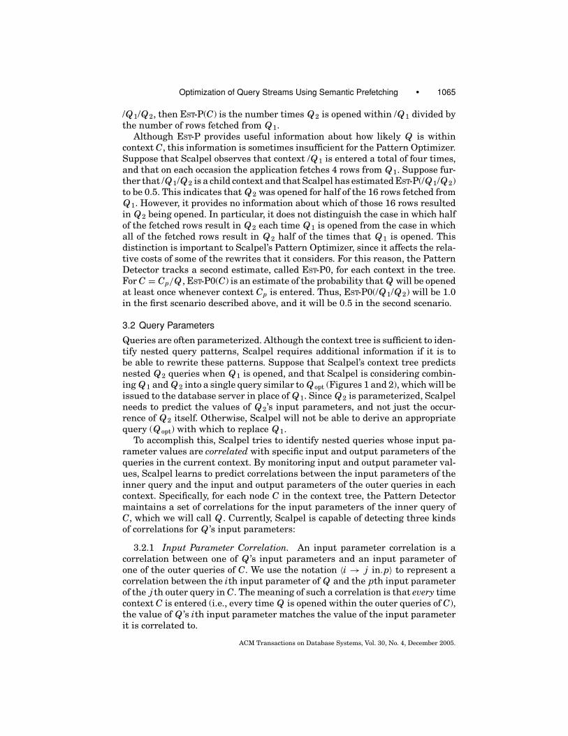
/Q1/Q2, then EST-P(C) is the number times Q2 is opened within /Q1 divided bythe number of rows fetched from Q1.
Although EST-P provides useful information about how likely Q is withincontext C, this information is sometimes insufficient for the Pattern Optimizer.Suppose that Scalpel observes that context /Q1 is entered a total of four times,and that on each occasion the application fetches 4 rows from Q1. Suppose fur-ther that /Q1/Q2 is a child context and that Scalpel has estimated EST-P(/Q1/Q2)to be 0.5. This indicates that Q2 was opened for half of the 16 rows fetched fromQ1. However, it provides no information about which of those 16 rows resultedin Q2 being opened. In particular, it does not distinguish the case in which halfof the fetched rows result in Q2 each time Q1 is opened from the case in whichall of the fetched rows result in Q2 half of the times that Q1 is opened. Thisdistinction is important to Scalpel’s Pattern Optimizer, since it affects the rela-tive costs of some of the rewrites that it considers. For this reason, the PatternDetector tracks a second estimate, called EST-P0, for each context in the tree.For C = Cp/Q , EST-P0(C) is an estimate of the probability that Q will be openedat least once whenever context Cp is entered. Thus, EST-P0(/Q1/Q2) will be 1.0in the first scenario described above, and it will be 0.5 in the second scenario.
3.2 Query Parameters
Queries are often parameterized. Although the context tree is sufficient to iden-tify nested query patterns, Scalpel requires additional information if it is tobe able to rewrite these patterns. Suppose that Scalpel’s context tree predictsnested Q2 queries when Q1 is opened, and that Scalpel is considering combin-ing Q1 and Q2 into a single query similar to Qopt (Figures 1 and 2), which will beissued to the database server in place of Q1. Since Q2 is parameterized, Scalpelneeds to predict the values of Q2’s input parameters, and not just the occur-rence of Q2 itself. Otherwise, Scalpel will not be able to derive an appropriatequery (Qopt) with which to replace Q1.
To accomplish this, Scalpel tries to identify nested queries whose input pa-rameter values are correlated with specific input and output parameters of thequeries in the current context. By monitoring input and output parameter val-ues, Scalpel learns to predict correlations between the input parameters of theinner query and the input and output parameters of the outer queries in eachcontext. Specifically, for each node C in the context tree, the Pattern Detectormaintains a set of correlations for the input parameters of the inner query ofC, which we will call Q . Currently, Scalpel is capable of detecting three kindsof correlations for Q ’s input parameters:
3.2.1 Input Parameter Correlation. An input parameter correlation is acorrelation between one of Q ’s input parameters and an input parameter ofone of the outer queries of C. We use the notation 〈i → j in.p〉 to represent acorrelation between the ith input parameter of Q and the pth input parameterof the j th outer query in C. The meaning of such a correlation is that every timecontext C is entered (i.e., every time Q is opened within the outer queries of C),the value of Q ’s ith input parameter matches the value of the input parameterit is correlated to.
ACM Transactions on Database Systems, Vol. 30, No. 4, December 2005.

1066 • I. T. Bowman and K. Salem
3.2.2 Output Parameter Correlation. An output parameter correlation isa correlation between one of Q ’s input parameters and a value fetched fromone of the outer queries of C. Scalpel only considers correlations between Q ’sinput parameters and values in the most recently fetched tuple from each of theouter queries in C. We use the notation 〈i → j .out[p]〉 to represent a correlationbetween the ith input parameter of Q and the pth attribute of the result of thej th outer query in C. As was the case for input parameter correlations, anoutput parameter correlation means Q ’s ith input parameter matches the pthattribute of the most recently fetched row of the j th outer query every timethat Q is opened in C. (However, note that each open of Q may correspond toa different row fetched from the outer query.)
3.2.3 Constant Correlation. A constant correlation indicates that an inputparameter of Q has the same value every time that Q is opened in context C.We use the notation 〈i → v〉 to represent a constant correlation for the ith inputparameter of Q , where v is the constant value of that parameter.
To detect correlations, the Pattern Detector records the values of the inputparameters of each open query, as well as the value of the most recently fetchedrow from each open query. The first time that a query Q is opened in context C,the Pattern Detector creates a new context C/Q . In addition, it compares Q ’sinput parameters to the recorded input and output parameters of the queriesin C to determine an initial list of correlations that hold for C/Q . On each sub-sequent open of Q in C, the Pattern Detector checks each of the correlations forC/Q and eliminates any that no longer hold. This ensures that any remainingcorrelations have held every time Q was opened in C.
The “Correlations” column of Figure 5 shows the correlations that hold foreach opened query after each OPEN request in the trace. For example, at line 3in Figure 5, after Q2 has opened for the first time in context /Q1, the PatternDetector initializes the set of correlations for /Q1/Q2 to include the following:
〈1 → 1.in[2]〉. This indicates that curr1, the value of the first input param-eter of Q2 (currency), matches the value of the second input parameter of thefirst (outermost) query in the current context, which is Q1.
〈2 → 1.out[2]〉. This indicates that date1, the value of Q2’s second inputparameter (transdate), matches the value of the second field in the most recenttuple fetched from Q1, at line 2.
〈1 → curr1〉,〈2 → date1〉. These constant correlations indicate that Q2’sfirst and second input parameters have been constant each time that Q2 hasbeen opened in this context. At this point, of course, Q2 has only been openedonce in context /Q1.
At line 7 of Figure 5, Q2 is opened a second time in context /Q1. After thisopen, 〈2 → date1〉 is eliminated from the set of correlations, since Q2’s sec-ond input parameter was not equal to date1. The three remaining correlationscontinue to hold at line 7, and also at line 11.
Inspection of the code in Figure 1 reveals that the observed correlations〈1 → 1.in[2]〉 and 〈2 → 1.out[2]〉 correspond to actual parameter correlationsin application that generated the trace. The third correlation, 〈1 → curr1〉, is
ACM Transactions on Database Systems, Vol. 30, No. 4, December 2005.

Optimization of Query Streams Using Semantic Prefetching • 1067
Fig. 8. An example application (a), and the corresponding context tree (b).
spurious. With a sufficiently long training period, we hope that such spuriouscorrelations will be eliminated, as the correlation 〈2 → date1〉 was. However,there is no guarantee of this: true correlations will be detected if they are ob-served at least once in the training trace, but spurious correlations are possible.Spurious correlations may cause Scalpel to generate semantic prefetches thatare not useful. Since Scalpel can recognize such prefetches at run-time, this mayimpact the system’s performance but it will not cause Scalpel to return incorrectquery results to the application. This issue is discussed further in Section 6.
4. EXECUTION ALTERNATIVES
At the conclusion of the training period, Scalpel’s pattern detector produces acontext tree annotated with probability estimates and parameter correlations.This tree is then passed to the Pattern Optimizer and the Query Rewriter,which determine whether any rewrites should be applied to the application’srequest stream at run-time. In this section, we describe the kinds of rewritesthat Scalpel considers. Section 5 describes how Scalpel determines which ap-plication requests, if any, should be rewritten, and which type of rewrite to usefor each such request.
To illustrate the types of rewrites that Scalpel considers, we will use the arti-ficial application example shown in Figure 8(a) and the corresponding contexttree shown in Figure 8(b). This is the context tree that the Pattern Detectorshould produce given a sufficiently long training trace of application requests.Scalpel considers three fundamental approaches to the execution of nested ap-plication queries like Qm, Qxy, and Qabcdef:
Nested Execution. Nested execution means that a nested query, like Qm, isexecuted as it was originally by the application program. In this case, a separateinstance of Qm will be executed for each row fetched from the outer query, Qxy.
Unified Execution. Unified execution means that an inner query is com-bined with the outer query into a single query. For example, Scalpel mightcombine Qm with Qxy, or it might combine Qabcdef with QRST. The result of
ACM Transactions on Database Systems, Vol. 30, No. 4, December 2005.

1068 • I. T. Bowman and K. Salem
Fig. 9. Fetch traces.
the combined query includes the results of the original outer query as well asthe results of all predicted instances of the inner query. When the applicationopens the original outer query, Scalpel issues the combined query instead. Eachtime the application then opens the inner query, Scalpel extracts the requiredresults from the result of the combined query. This approach was called unifiedby Fernandez et al. [2001].
Partitioned Execution. Partitioned execution also combines the inner andouter queries. The combined query encodes the results of all of the predictedinstances of the inner query. Under partitioned execution, the application’souter query is shipped unmodified to the database server. However, the firsttime the application opens the inner query (e.g., Qabcdef), Scalpel issues thecombined query instead. Subsequent opens of the inner query are answeredusing the results of the combined query. This effectively executes the nestedquery like a distributed join in which the inner table (Qabcdef) is moved to theouter table’s location and joined there, in this case by the application code.
Scalpel currently considers two different forms of unified execution and twodifferent forms of partitioned execution, in addition to nested execution. Inthe remainder of this section, these execution strategies are described in moredetail. Figure 9 illustrates the various strategies that will be discussed by show-ing how they would apply to the an execution of the application fragment fromFigure 8. In each part of the figure, each column corresponds to one of thefour application queries, and time advances from the top of the figure to thebottom. Rectangles are used to denote separately opened and fetched cursors.The letters within the cursor rectangles represent the tuples returned throughthose cursors. The various queries are named according to the tuples that theyreturn, for example, QRST returns tuples R, S, and T .
4.1 Nested Execution
Figure 9(a) illustrates the nested execution strategy. In this example, a totalof nine cursors are opened. Although fixed per-request costs are associated
ACM Transactions on Database Systems, Vol. 30, No. 4, December 2005.

Optimization of Query Streams Using Semantic Prefetching • 1069
Fig. 10. Combined nested SQL-Ledger query (not legal SQL/99).
with each of these cursors, the nested execution strategy may be appropriateif the inner query is opened infrequently. For example, this will be true forthe get openinvoices function in Figure 1 if the report currency is usually thesame as the default currency.
4.2 Unified Execution
Under the unified execution strategy, Scalpel combines the inner and outerqueries into a single query which returns all of the rows that would have beenreturned by the individual outer and inner queries. When the Prefetcher com-ponent observes the application opening the outer query (in the correct context),it submits instead the combined query. The Scalpel system then uses the cursoropened over the combined query to respond to the application’s requests to fetchrows from the inner and outer queries that were combined.
Many unified strategies are possible. Scalpel’s optimizer currently considerstwo representative unified strategies, one that combines the outer and innerqueries using an (outer) join and another which combines them using an outerunion. We describe these two strategies next. To actually combine the queries,Scalpel makes use of an SQL construct called lateral derived tables. In theremainder of this section, we first describe lateral derived tables (Section 4.2.1),and then show how they are used to perform the outer join (Section 4.2.2) andouter union (Section 4.2.3) rewrites.
4.2.1 Lateral Derived Tables. Figure 2 illustrates one way to combine theinner and outer queries from the SQL-Ledger application from Figure 1. Thequery is expressed using a join in an unnested style, and is likely to executeefficiently. However, the algorithm for combining the two queries requires aflattening of the nesting relationship that is present in the client applica-tion. This is a nontrivial procedure that has been studied extensively for thecase when the nesting is present within a single query. If we could combinethe two queries into a single nested query, we would have a relatively sim-ple way to combine queries, and we could rely on rewrite optimizations im-plemented in the DBMS optimizer to unnest the query and generate an effi-cient access plan. For example, if we could write a query such as the one inFigure 10, we could easily express the application’s query nesting, allowing theDBMS query optimizer to select the best execution strategy. Unfortunately, thequery in Figure 10 is not legal according to SQL/99. The references to O.currand O.transdate within query I are outer references, and are not within thescope of O.
ACM Transactions on Database Systems, Vol. 30, No. 4, December 2005.

1070 • I. T. Bowman and K. Salem
Fig. 11. Combined nested SQL-Ledger query using Shanmugasundaram’s approach [2001].
Shanmugasundaram et al. [2001] used a clever approach to combine queries,relying on the fact that the scope clause of a table reference includes all of thejoin conditions for joins containing the table reference. Their approach wouldresult in the query in Figure 11. This approach works adequately for queriesconsisting of select-project-join (SPJ), where the correlation value is used onlyin predicates in the WHERE clause of the inner query. As described, however,this approach does not work with cases where the correlations appear in morecomplex contexts such as an ON condition of an outer join in the FROM clause orin an expression in the SELECT list.
Galindo-Legaria and Joshi [2001] showed that, in principle, the approachdescribed by Shanmugasundaram et al. [2001] could be extended to handlearbitrary queries. However, the transformations used to decorrelate the innerquery may generate queries that are significantly more expensive than theoriginal, correlated, variant. Cost-based optimization is needed to determinewhether decorrelation is warranted; this type of optimization is best performedby the DBMS optimizer.
Fortunately, SQL/99 [International Standards Organization 1999] intro-duced a new construct called lateral derived tables, and this feature makesit easy to express nesting in the FROM clause. Using the keyword LATERAL, weare able to write a query in the style of Figure 10 that is legal. By writing aquery with nesting in the FROM clause, we directly express the original applica-tion semantics to the DBMS optimizer, allowing it to perform any decorrelationthat it estimates is beneficial. The LATERAL keyword signals that the inner de-rived table contains outer references, and it is equivalent to the algebraic applyoperator (A× ) described by Galindo-Legaria and Joshi [2001].
The syntax:
FROM <table reference list>,
LATERAL (<query expression>) <correlation name>
has the following semantics. Let TRL be the <table reference list>. Let QEbe the <query expression>. The SQL within QE can contain references to at-tributes of TRL; these are called outer references. Let TRLR be the multi-setof rows resulting from TRL. Let QE(r) represent the multiset resulting fromevaluating QE with attributes of r supplied as actual parameters to the corre-sponding outer references. The result of the FROM clause above is the followingmultiset:
{|〈r, q〉 | r ∈ TRLR, q ∈ QE(r)|},ACM Transactions on Database Systems, Vol. 30, No. 4, December 2005.

Optimization of Query Streams Using Semantic Prefetching • 1071
Fig. 12. Combined nested SQL-Ledger query using LATERAL.
where 〈r, q〉 denotes the formation of a tuple by concatenating row q with rowr. Figure 12 shows how the illegal query of Figure 10 can be corrected usingthe LATERAL keyword.
The lateral derived table construct allows Scalpel to generate a single SQLquery that directly matches the application semantics that it infers from mon-itoring the request stream, and we have used it to describe all of the rewritespresented in the remainder of this section. Of the three commercial DBMSsthat we used in our study, one supports the LATERAL construct directly. Theother two systems support the same semantics using (distinct) vendor-specificsyntax, to which we translate LATERAL expressions as necessary.
The query in Figure 12 has a shortcoming: rows from the outer query willnot be included in the result unless there is at least one row from the innerwith matching currency and transaction date. If these rows must be included,an equivalent of an outer join must be used to preserve the rows from the outerqueries (the table references that precede the lateral derived table in the FROMclause). The SQL/99 standard does not provide support for directly expressinga lateral derived table operating in an outer join with outer references to thepreserved side of the outer join. We define an extension to SQL/99, LEFT OUTERLATERAL, which provides the required outer-join semantics:
FROM <table reference list>,
LEFT OUTER LATERAL (<query expression>) <correlation name>.
The result of the FROM clause above is the following multiset:
{|〈r, q〉 | r ∈ TRLR, q ∈ QE(r)|}⊎
{|〈r, N 〉 | r ∈ TRLR, QE(r) = ∅|},where 〈r, N 〉 denotes the formation of a tuple by supplying NULL for the at-tributes of Q. The LEFT OUTER LATERAL construct is equivalent to the outerapply algebraic operator (ALOJ ) defined by Galindo-Legaria and Joshi [2001].
Of the three commercial DBMSs we considered, two provide vendor-specificsyntax supporting the use of LATERAL-style derived tables in outer joins. Wetranslate LEFT OUTER LATERAL to those vendor-specific dialects. For the remain-ing system, we can translate LEFT OUTER LATERAL to standards compliant SQLusing the LATERAL construct and an outer join.
4.2.2 The Outer Join Strategy. Figure 13 shows a simplified version of howScalpel forms a combined join query using a lateral derived table expression(we omit details such as the replacement of parameter markers with outerreferences). Given the texts of the outer and inner queries, Scalpel producesa derived table expression similar to the one shown in Figure 12, except that
ACM Transactions on Database Systems, Vol. 30, No. 4, December 2005.

1072 • I. T. Bowman and K. Salem
Fig. 13. Outer join rewrite. Syntactic substitution shown as < >.
LEFT OUTER LATERAL is used in place of LATERAL to ensure that all rows of theoriginal outer query are included in the result. In addition, the combined querycontains an ORDER BY clause matching the ORDER BY clause of the original outerquery. Thus, Scalpel would add ORDER BY O.id to the combined query shown inFigure 12 since the original outer query (from the get openinvoices functionin Figure 1) was so ordered. Although Figure 13 describes the combination ofan outer query with a single inner query, in general it is possible to combinemultiple correlated inner queries with the outer query.
Figure 9 (b) illustrates the case in which outer query QRST is combined withinner query Qxy using the outer join rewrite. When the application opens QRST,Scalpel issues the combined join query instead. When the application performsa FETCH on the outer query, Scalpel consumes the next row from the combinedquery’s cursor and extracts the values that correspond to the outer query’scolumns. When the application performs a FETCH on an inner query (Qxy),Scalpel simply extracts the attributes required by that query from the cur-rent row of the combined query. This case is distinguished from a case whereall attributes happen to be NULL by requiring that at least one non-null at-tribute of the inner query is included in the combined result (for example, a keycolumn).
Scalpel considers using the outer join strategy only if it can infer that theinner query will return at most one row for each row of the outer query. Scalpel’squery analyzer implements a support routine, AT-MOST-ONE(Q), to implementthis restriction. This function acts as an oracle that must be correct when itreturns true, but is allowed to return false for queries that can only returnone row. Currently, this is implemented by checking whether there are equalityconditions on the key attributes of the inner query, however, more elaboratechecks are certainly possible.
The AT-MOST-ONE restriction is not strictly necessary. Scalpel implements itfor two reasons. First, the restriction significantly simplifies the decoding pro-cedure used to extract the results of the original inner and outer queries fromthe result of the combined query. Without the restriction, decoding would, ingeneral, require a scrollable cursor for the combined query. Where supported,scrollable cursors are often more expensive than forward-only cursors. Fur-thermore, fetching backward may reintroduce some of the per-request latencythat the unified strategy is designed to avoid, since fetching backward may re-quire that rows be re-fetched from the server. Second, The presence of multirowinner queries can introduces redundancy into the combined query result. Forexample, Figure 9(c) illustrates the result of executing all four queries from theexample of Figure 8 as a single combined outer join query. The shaded parts ofthe join query result indicate those portions of the result that are redundant-they are computed by the combined query but should not be returned to the
ACM Transactions on Database Systems, Vol. 30, No. 4, December 2005.

Optimization of Query Streams Using Semantic Prefetching • 1073
Fig. 14. Outer union rewrite.
Fig. 15. Example queries combined using outer union.
application. Redundancy generated by the unrelated inner queries (such as Qxy
and Qabcdef) can, in general, result excessive overhead due to the duplicationof attributes and rows. This led Shanmugasundaram et al. [2001] to label theapproach “redundant relations”, and they stopped considering it after findingthat the performance was poor.
4.2.3 The Outer Union Strategy. The outer union strategy is illustratedin Figure 9(d). Each query is represented by distinct columns in the result ofthe combined query. Each row corresponds to a tuple that would have beenreturned by one of the original queries, with NULL values supplied for thecolumns corresponding to the other queries.
Figure 14 shows a simplified version of how Scalpel combines outer andinner queries using an outer union strategy.2 The Nulls function is used togenerate a NULL place-holder for each column that is not present in one branchof the outer union. Scalpel uses a more general version of this rewrite, whichallows it to combine an outer query with more than one correlated inner query.Figure 15 shows the result of applying the outer union rewrite to the transactionand exchange rate queries of our running example. The first column of thecombined query’s result is a type field, which is used to ensure that Scalpelcan unambiguously determine which of the original queries a particular row ofthe outer union result is associated with. In the example from Figure 15, rowsresulting from the original outer query are tagged with type 0, while those
2A VALUES clause results in a tuple constructed from the specified expressions.
ACM Transactions on Database Systems, Vol. 30, No. 4, December 2005.

1074 • I. T. Bowman and K. Salem
Fig. 16. Example queries combined using client hash join.
from the inner query have type 1. In the more general case, Scalpel assigns adistinct type field value to each of the inner queries. The ORDER BY clause isused to ensure that resulting rows appear in the order in which they will berequired the application. The rows are ordered first by the ordering attributesof the outer query (O.Id in this case), then by a candidate key of the outerquery, then by the type field, which ensures that all of the inner query tuplesthat correspond to a particular outer tuple are grouped together in the result,and finally by the ordering attributes of the inner query if there are any. Forsome DBMSs, it may be possible to eliminate the type field by relying on thesort order of NULL [Shanmugasundaram et al. 2001].
Unlike the join strategy, the outer union strategy can be applied regardless ofthe number of rows returned by the inner query. When the application performsa FETCH on either the outer query or the inner query, Scalpel obtains the nextrow from the combined query’s cursor and extracts the values that correspondto the original query’s columns. A change in the value of the type field (from 1to 0) indicates that there are no more inner query tuples for the current row ofthe outer.
4.3 Partitioned Execution
Under the unified execution strategies the combined query is issued when theapplication first opens the original outer query. In contrast, under a partitionedstrategy, the rewritten, combined query is issued when the application firstopens the original inner query of a query/context pair. There are many possiblepartitioned strategies, of which Scalpel’s optimizer currently considers two: theclient hash join strategy and the client merge join strategy. We describe thesetwo strategies next.
4.3.1 The Client Hash Join Strategy. Under this strategy, the inner queryis combined with the outer using a lateral derived table like the one shownin Figure 16. This gives a single statement that retrieves all of the desiredrows from the inner query for all possible outer rows. The first time that theinner query is executed by the application, the combined query is submittedinstead to the server. All result rows are fetched and stored in a hash ta-ble at the client using the parameters of the inner query from the result set(O1.curr and O1.transdate in Figure 16) as the hash key. When the applica-tion opens the inner query, the hash table is consulted, using the inner query
ACM Transactions on Database Systems, Vol. 30, No. 4, December 2005.

Optimization of Query Streams Using Semantic Prefetching • 1075
Fig. 17. Client hash join rewrite.
parameter values as the lookup key, to determine the tuple(s) that should bereturned to the application. When the outer query is closed, the hash table isdiscarded.
Figure 17 shows how Scalpel combines queries under the client hash joinstrategy. This is similar to the approach that is used under the unified outerjoin strategy (Figure 13). However, there are a few important differences. Onlythe attributes of the outer query that provide parameter values to the innerquery are included in the result. Also, each distinct set of inner query parametervalues need only be included once in the outer table. Figure 16 shows how aDISTINCT keyword can be used to achieve this. Finally, LEFT OUTER LATERAL isnot needed, since any correlation values that result in an empty inner querycan be left out of the client hash table.
Figure 9(e) illustrates the the situation in which the client hash join strategyis used for all four of the queries nested under QRST. While the nested strat-egy opens nine cursors, the partitioned client hash join strategy only opensfive. Furthermore, the number of opened cursors in the partitioned executionstrategy does not depend on the number of rows returned from outer queries.However, this strategy does require sufficient memory at the client to hold thehash table, and the CPU of the client machine may make the hash lookupsslower than the original, nested strategy. Scalpel accounts for this extra costwhen choosing an execution plan (Section 5.2).
In the example of Figure 9(e), Scalpel combines inner query Qm with outerquery Qxy. The combined query is executed at most once per instance of theparent query Qxy. Scalpel does not need to execute the combined query ifthe application never opens Qm under a particular instance of Qxy. Thus, inthe example, the combined query is executed twice, because the applicationopens Qxy three times, but in one of those cases it never opens the nestedquery Qm because Qxy returns no rows. In general, it would be possible tocombine Qm with both Qxy and QRST, so that the combined query would haveto be opened (at most) once per instance of QRST. Whether this strategy ispreferable to combining only with the immediate parent depends on costs andquery selectivities. Although it would certainly be possible to consider thesealternatives, at present Scalpel only considers the hash join combination of aquery with its immediate parent from the context tree.
4.3.2 The Client Merge Join Strategy. The client hash join strategyamounts to a distributed hash join executed at the client. Similarly, the clientmerge join strategy amounts to a distributed merge join implemented at theclient. For this to work properly, Scalpel must ensure that the inner and outertuples arrive at the client in the proper order for merging.
ACM Transactions on Database Systems, Vol. 30, No. 4, December 2005.

1076 • I. T. Bowman and K. Salem
Fig. 18. Client merge join strategy.
Fig. 19. Combined inner query for the client merge join strategy.
The merge join approach consists of opening rewritten versions of both theouter query and the inner query. The outer query is rewritten so that the resulthas a known total ordering, and so that it includes those attributes that weguess will be used as correlation parameters to the inner queries (based on ourtraining period). The inner query is rewritten by combining it with the originalouter query so that it returns matching inner rows for all of the rows of the outerquery. This is similar to the rewriting that is done to the inner query under theclient hash join strategy. However, under the client merge join strategy, therewritten inner query is ordered to match the known ordering that we imposedon the outer query results, as well as any order requirements specified in theoriginal inner query.
Figure 18 shows a simplified version of how Scalpel produces the combinedinner query, and Figure 19 shows the query that would result from combiningthe inner and outer queries from our running example. In this case, the rewrit-ten inner query is ordered by O.Id, which is the sort order of the outer query.No additional ordering constraints are imposed by the original inner query.
The first time that the inner query is opened, Scalpel submits instead thecombined query. In response to a FETCH on the inner query, Scalpel first checksthe values of the sorting and key attributes of the current row of the outerquery. It then advances the cursor of the combined inner query to the first rowfor which the corresponding attributes do not exceed the current values from theouter. If combined query’s sorting attributes match those of the current outertuple, Scalpel returns the values of the inner query attributes. If they exceedthose of the current outer tuple, this indicates the end of the application’s innerquery’s result set. Scalpel closes the combined inner query’s cursor when theouter query’s cursor is closed.
Figure 9(f) illustrates the the situation in which the client merge join strategyis used for all four of the queries nested under QRST. As was the case for theclient hash join, Scalpel only considers the merge join combination of a querywith its immediate parent from the context tree, for example, Qm is combinedwith Qxy but not with QRST. Thus, the resulting pattern of query instances is
ACM Transactions on Database Systems, Vol. 30, No. 4, December 2005.

Optimization of Query Streams Using Semantic Prefetching • 1077
Fig. 20. Examples of generated plans. Edge labels have been omitted to reduce clutter.
almost the same as that of the client hash join strategy, except for the orderingof the result of the combined inner queries. Unlike the hash join strategy, themerge join strategy does not require that the result set of the combined innerquery be stored at the client. However, the merge join strategy does impose anadditional sorting burden on the server. Scalpel’s optimizer uses its cost modelto choose between these alternatives.
5. OPTIMIZATION
Section 4 described five alternative strategies that can be employed to execute anested query. After the training phase has built a context tree, Scalpel’s PatternOptimizer and Query Rewriter decide which execution strategy should be usedin each of the contexts in the tree.
An execution plan is a context tree in which each node has been annotatedwith an execution strategy (N, J, U, H, or M) corresponding to the five strategiespresented in Section 4. For example, Figure 20 shows six plans for the context
ACM Transactions on Database Systems, Vol. 30, No. 4, December 2005.

1078 • I. T. Bowman and K. Salem
Fig. 21. Pseudo-code to annotate an execution plan with query rewrites.
tree example of Figure 8. These strategies correspond to the execution tracesshown in Figure 9.
Optimization in Scalpel works as follows: A plan generation module gener-ates candidate plans from the context tree provided by the Pattern Detector. Foreach candidate plan, the original application queries are rewritten according tothe execution strategies specified for the plan, using the rewriting techniquespresented in Section 4. The cost of the candidate plan is then estimated. Thecandidate plan with the lowest estimated cost is selected by the Pattern Opti-mizer. This plan, with its strategy annotations and rewritten queries, is storedin Scalpel’s database for use at run time. The following sections describe thesesteps in more detail. Section 5.1 describes how Scalpel generates the rewrittenqueries for a candidate plan. Section 5.2 describes how the cost of a candidateplan is estimated. Section 5.3 describes how Scalpel estimates the cost and sizeof individual queries. Finally, Section 5.4 describes how candidate plans aregenerated.
5.1 Generating Query Rewrites
Figure 21 shows the RewriteQueries algorithm, which is used to generatethe rewritten queries for an execution plan. RewriteQueries is a recursive
ACM Transactions on Database Systems, Vol. 30, No. 4, December 2005.

Optimization of Query Streams Using Semantic Prefetching • 1079
Table I. Statistics used for Ranking Plans
Quantity Source Description
ESTTOTAL(Q) Analytical Estimated total cost for Q in seconds
|Q | Analytical Estimated # of rows returned by QInterpretCost(C) Calibration The cost to interpret results for context CEST-P0, EST-P Training Selectivity of client predicates
algorithm. Scalpel generates the rewritten queries for an entire execution planby calling RewriteQueries on the plan’s root context. In Figure 21, annotate(C)represents the strategy annotation at node C of the plan, Q(C) represents theoriginal query for context C (i.e., the inner query of C), and Q’(C) is the rewrit-ten query that will be used in place of Q(C) at run-time.
When called at node C, the rewriting algorithm first recursively rewrites thesubtrees rooted at C’s children. The functions RewriteHashJoin(Q1,Q2) andRewriteMergeJoin(Q1,Q2) apply the hash join and merge join rewrites, respec-tively, to outer query Q1 and inner query Q2. If the plan calls for any of C’schildren to use partitioned strategies, the queries at those children are rewrit-ten using those two functions. If the plan calls for any of C’s children to beunified with the outer query at node C, those childrens’ queries are added tolists of queries to be unified. The RewriteOuterJoin and RewriteOuterUnionfunctions combine an outer query with a set of inner queries using the outerjoin and outer union rewrites described in Section 4. Finally, if any of the chil-dren of C use the merge join strategy, then the outer query at C must returna totally ordered result set. This is ensured by AddTotalOrdering, which addsadditional ordering constraints to Q’(C) if necessary. When RewriteQueriesis finished, each node in the execution plan will have been annotated with arewritten query.
5.2 Ranking Execution Plans
Scalpel ranks execution plans using estimates of the response time (in seconds)experienced by the client application. Clearly, other ranking functions can beused instead; for example, we could choose to rank based only on server ex-ecution costs, or we could attempt to create a more precise model of latencyby estimating the amount of overlap for server, network, and client processingcosts. In this article, we concentrate only on ranking by total latency, which isthe sum of client-side, network, and server latencies.
To estimate the cost of an execution plan, Scalpel uses the statistics shown inTable I. ESTTOTAL(Q) refers to the estimated response time for a query Q thatappears in the execution plan. (Each node in the plan is annotated with twoqueries: the original application query and a rewritten query. It is the rewrittenqueries that are used to rank the execution plans.) |Q | is the estimated numberof rows returned by Q . InterpretCost(C) is an estimate of Scalpel’s costs forinterpreting the application’s OPEN, FETCH, and CLOSE requests in context C ofthe plan. This reflects the cost of decoding the result sets of rewritten queries.InterpretCost(C) depends on the strategy annotation at C, for example, theinterpretation cost is higher at an ‘H’ node than at an ‘N’ node to reflect the costsof inserting and deleting results from the client hash table. Scalpel calibrates
ACM Transactions on Database Systems, Vol. 30, No. 4, December 2005.

1080 • I. T. Bowman and K. Salem
Table II. Statistics used to Estimate Query Costs and Sizes
Quantity Source Description
AVGTOT(Q) Training Observed average total cost for Q in seconds
AVGSRV(Q) Training Observed average server cost for Q in seconds
AVGROWS(Q) Training Observed average # of rows returned by QDBMS-COST(Q) DBMS DBMS estimate of server cost for Q in server units
U0 = AVGTOT(Q0) Calibration Query-independent overhead
AVGSRV(Q0) Calibration Query-independent server overhead
InterpretCost(C) for each strategy prior to training. Finally, EST-P0 and EST-Pare the probability estimates produced by the Pattern Detector as described inSection 3.1.
To estimate the cost of a plan, Scalpel computes a weighted sum of the esti-mated costs of the individual contexts in the plan. The contexts are weightedaccording to their estimated relative frequency of occurrence. Specifically, sup-pose that C is a plan context with rewritten query Q , and that P is the parentcontext of C. Scalpel recursively estimates ROWS(C) (the total number of resultrow produced in context C), OPENS(C) (the number of times C’s query is opened),and ONEOPENS(C) (the number of opens of P for which C’s query is opened atleast once), as
ROWS(C) = OPENS(C) × |Q | (1)
OPENS(C) = OPENS(P ) × ROWS(P ) × EST-P(C) (2)
ONEOPENS(C) = OPENS(P ) × EST-P0(C) (3)
with OPENS() and ROWS() defined to be 1 for the root context. The weighted costof each context C is then defined as
COST(C) = OPENS(C) × (ESTTOTAL(Q) + InterpretCost(C)) (4)
for contexts annotated with the nested strategy. Under the partitioned strate-gies, the rewritten inner query is issued only if the application requests opensthe inner query at least once after the outer has been opened. Therefore, forcontexts annotated with a partitioned strategy (‘H’ or ‘M’), we use
COST(C) = ONEOPENS(C) × ESTTOTAL(Q) + OPENS(C) × InterpretCost(C). (5)
If a unified strategy is used at C, then no query is issued to the server when Cis entered. Instead, Scalpel decodes prefetched results from the rewritten outerquery. So, for contexts annotated with a unified strategy (‘J’ or ‘U’), we use
COST(C) = OPENS(C) × InterpretCost(C). (6)
5.3 Estimating Query Costs and Sizes
To obtain the estimates ESTTOTAL(Q) and |Q | for each query Q in an executionplan, Scalpel relies on statistics observed during the training period, calibratedvalues, estimates provided by the DBMS, and calculations based on its own ana-lytical cost model. Table II lists the statistics that Scalpel uses for query costing,and their sources. For every query Q observed during training, Scalpel mea-sures the average total execution time, AVGTOT(Q), using a timer in Scalpel’s
ACM Transactions on Database Systems, Vol. 30, No. 4, December 2005.

Optimization of Query Streams Using Semantic Prefetching • 1081
Fig. 22. A sample communication trace.
Call Monitor. AVGTOT(Q) includes client, network, and server latencies. Inaddition, Scalpel uses DBMS timing features to measure the server latencyAVGSRV(Q) of each query. The calibrated costs AVGTOT(Q0) and AVGSRV(Q0) rep-resent the total and server execution time of a specially constructed calibrationquery, Q0, which is discussed in Section 5.3.1.
Scalpel needs to determine ESTTOTAL(Q) and |Q | for two different kinds of runtime queries that appear in execution plans. Some run time queries have beenobserved by Scalpel during its training period. Others are the results of Scalpel’srewrites, and these have not been observed. For queries that were observedduring training, query cost and query size are relatively easy to estimate, sinceScalpel measures their actual execution times during training. For such queries,execution time ESTTOTAL(Q) and number of rows |Q | are estimated using:
ESTTOTAL(Q) = AVGTOT(Q) (7)
|Q | = AVGROWS(Q) (8)
For queries that Scalpel did not observe during training, i.e., for rewrittenqueries, estimating cost is more difficult. Most DBMS systems provide a mech-anism to estimate the cost of executing an arbitrary query Q . We refer to thisestimate as DBMS-COST(Q) in Table II. One possibility is to use DBMS-COST(Q)as our required estimate ESTTOTAL(Q) for rewritten queries. In general, how-ever, DBMS estimates are not sufficient for this purpose. One problem is thatthe DBMS does not typically estimate the network and client-side costs for an-swering a query: all of the execution strategies available to the DBMS returnthe same result set and therefore share the same network and client-side costs,so there is little reason for the DBMS optimizer to include those costs in its esti-mate. Normally, DBMS-COST(Q) estimates only server execution time. Anotherproblem is that the cost units returned by the DBMS are not necessarily in thesame units that Scalpel uses. For some DBMS, the cost is returned in an undis-closed cost unit. Even where it is possible to convert the DBMS cost units toseconds, we have found the estimates used by the DBMS often are not very closeto the observed time in seconds. The goal of the DBMS optimizer is to rank ex-ecution plans, not to give a precise time estimate for a query. For these reasons,we do not use DBMS-COST(Q) as a direct estimate of the total query cost.
Instead, Scalpel estimates the costs of rewritten queries using the requestmodel shown in Figure 22. The query Q is submitted to the server (A, B, C),executed by the DBMS (D), then all result rows are returned to the client(E, F, G). This model is a simplification; in practice, there can be overlap of some
ACM Transactions on Database Systems, Vol. 30, No. 4, December 2005.

1082 • I. T. Bowman and K. Salem
of the components and other complicating factors.3 As a further simplification,we assume that durations of the intervals A, B and C are independent of therequest Q , and that the durations of E, F , and G can be written as
E = C + E ′(Q) (9)
F = B + F ′(Q) (10)
G = A + G ′(Q). (11)
In other words, the time required to return the query result from the server tothe client is equal to the time required to ship the query from the client to theserver, plus a query-dependent term that reflects the size of the query result.Larger query results take more time to return to client, which is reflected inlarger values of E ′(Q), F ′(Q), and G ′(Q).
With these simplifications, we can write:
ESTTOTAL(Q) = 2(A + B + C) + D(Q) + E ′(Q) + F ′(Q) + G ′(Q). (12)
We have written D(Q), rather than D, to emphasize the fact that the serverexecution time depends on the query being executed. For the purposes of esti-mation, we split the total time into two parts, a server processing time D(Q)and the remaining client and network time ESTOTHER(Q), defined as
ESTOTHER(Q) = 2(A + B + C) + E ′(Q) + F ′(Q) + G ′(Q). (13)
To estimate the cost of a query Q , Scalpel estimates D(Q) and ESTOTHER(Q)and sums them to obtain ESTTOTAL(Q).
As shown in Eqs. (7) and (8), Scalpel has estimates for the total cost and thesize of each original query, based on training time measurements. Training timemeasurements also provide Scalpel with an estimate (AVGSRV(Q)) of the servertime of each original query Q . However, the measured value is AVGSRV(Q) =2C + D(Q) + E ′(Q), while we would like to isolate D(Q).
D(Q) = AVGSRV(Q) − 2C − E ′(Q). (14)
To estimate D(Q), Scalpel uses a calibration step which runs prior to the train-ing period. Calibration involves measuring the total execution time (A+· · ·+G)and the server execution time (C + D + E) of a specially constructed calibra-tion query Q0. The calibration query is constructed so that server executiontime (D(Q0)) and the query dependent parts of the result return time (E ′(Q0),F ′(Q0), and G ′(G0)) are negligible. For example, we can use the following query:
SELECT 1 FROM ( VALUES(1) ) T(x) WHERE 1=0
By measuring the calibration query Q0, we find the following:
AVGTOT(Q0) = 2(A + B + C) (15)
AVGSRV(Q0) = 2C. (16)
3In this model, we assume that the actual query text is submitted to the DBMS for parsing and
optimization at some point prior to the trace of Figure 22. We do not include the cost of submitting,
parsing, and optimizing the query text in our cost model and experiments.
ACM Transactions on Database Systems, Vol. 30, No. 4, December 2005.

Optimization of Query Streams Using Semantic Prefetching • 1083
Table III. Query Constructs
Construct Description
Q1
⊎Q2 Union of Q1 and Q2 (preserving duplicates)
Q1 A× Q2 Lateral derived table with Q1 outer and Q2 inner
Q1 ALOJ Q2 Outer lateral derived table with Q1 outer and Q2 inner
S(Q) Query Q with additional ordering specification
We define quantity U0 = AVGTOT(Q0). This is the minimum cost of executing aquery.
Unfortunately, we have no available estimate that we can use to account forthe last term, E ′(Q) of Eq. (14). If Q is small, that term is likely to be negligible.If Q is larger, then that term will probably be dominated by the server executioncost (interval D). Therefore, we simply ignore the term, giving:
D(Q) ≈ AVGSRV(Q) − AVGSRV(Q0). (17)
Scalpel uses four basic constructs to rewrite queries. These four constructsare summarized in Table III. The union rewrite Q1
⊎Q2 is used when the outer
union execution strategy is chosen, as described in Section 4. Similarly, the twolateral rewrites (Q1 A× Q2 and Q1 ALOJ Q2) are used to support the outer join,client hash join, and client merge join strategies. Finally, under the client mergejoin strategy, Scalpel rewrites the outer query to ensure that its result is totallyordered. This rewrite is represented by S(Q).
For each such construct, Scalpel needs to estimate of the size and cost ofthe constructed query. It takes a compositional approach to this problem. Thismeans that we start with the size and cost estimates for the original applicationqueries. The size and cost of a constructed query are then estimated based onthe already-estimated sizes and costs of the individual queries used in theconstruction. In the remainder of this subsection, we describe how this is donefor each of the four types of combined queries shown in Table III.
5.3.1 Estimating Union Queries. Since we are using duplicate-preservingunion, we estimate the number of rows to be the sum of the rows from the twobranches.
|Q1
⊎Q2| = |Q1| + |Q2|. (18)
From Eq. (13), the nonserver cost of the union query can be written as
ESTOTHER(Q1
⊎Q2) = 2(A + B + C)
+ E ′(Q1
⊎Q2) + F ′(Q1
⊎Q2) + G ′(Q1
⊎Q2).
(19)
Since E ′, F ′ and G ′ depend only on the result size of the query, we can distributethem (for example, E ′(Q1
⊎Q2) = E ′(Q1) + E ′(Q2). Therefore, we find:
ESTOTHER(Q1
⊎Q2) = ESTOTHER(Q1) + ESTOTHER(Q2) − 2(A + B + C). (20)
With the result of our calibration queries (Eq. (15)), we can write a finalexpression for the nonserver cost of the union query:
ESTOTHER(Q1
⊎Q2) = ESTOTHER(Q1) + ESTOTHER(Q2) − U0. (21)
ACM Transactions on Database Systems, Vol. 30, No. 4, December 2005.

1084 • I. T. Bowman and K. Salem
This gives a nonserver cost estimate for the union query in terms of the non-server cost estimate of the combined queries and the calibrated value U0, asdesired.
To estimate the server execution cost D(Q1
⊎Q2), we could use the sum
of the server costs of Q1 and Q2. However, this does not take into accountthe fact that the database server may be able to execute the combined querymore efficiently than the individual queries. For example, the two branches ofthe union may refer to the same data, allowing sharing. To account for this, wemultiply the original estimate by a factor F⊎, which reflects these efficiencies:
D(Q1
⊎Q2) = (
D(Q1) + D(Q2)) × F⊎. (22)
Following an approach suggested by Zhu [1995] and Rahal et al. [2004], weuse DBMS server cost estimates to estimate the efficiency factor F⊎:
F⊎ = DBMS-COST(Q1
⊎Q2)
DBMS-COST(Q1) + DBMS-COST(Q2). (23)
Since F⊎ is a dimensionless quantity, this allows us to estimate the impact ofserver optimizations without having to worry about matching the DBMS costsunits to Scalpel’s.
5.3.2 Estimating Lateral Queries. We estimate costs and sizes for a lateralderived table (A× ) and its outer variant (ALOJ ) using an approach similar tothe approach used for unions. For laterals, we estimate the number of rowsusing the product of the outer and inner cardinalities. The estimate for theouter variant is similar except that each outer row is preserved. We account forthis using max as shown in Eq. (25).
|Q1 A× Q2| = |Q1| × |Q2| (24)
|Q1 ALOJ Q2| = |Q1| × max(1, |Q2|). (25)
For nonserver costs, we follow the approach used to develop Eq. (21), exceptthat in this case the query result size is no longer the sum of the sizes of thecombined queries. For the lateral table, this gives
ESTOTHER(Q1 A× Q2) = ESTOTHER(Q1) + |Q1| × (ESTOTHER(Q2) − U0). (26)
We estimate that the outer lateral has the same cost as the inner, ignoring thecost of generating NULL values.
To estimate server costs, we start with an estimate that assumes that theserver uses a nested loop strategy to execute the combined query. We thencorrect this using an efficiency factor (FA× ) to reflect the fact that the servermay be able to use a more efficient method of executing the query. For the lateraltable, this gives:
D(Q1 A× Q2) = (D(Q1) + |Q1| × D(Q2)
) × FA× . (27)
The efficiency factor FA× is also estimated like the efficiency factor for unionqueries:
FA× = DBMS-COST(Q1 A× Q2)
DBMS-COST(Q1) + |Q1| × DBMS-COST(Q2). (28)
ACM Transactions on Database Systems, Vol. 30, No. 4, December 2005.

Optimization of Query Streams Using Semantic Prefetching • 1085
5.3.3 Estimating the Cost of Added Ordering. When Scalpel modifies theordering characteristics of a query (e.g., because of a child annotated with clientmerge join), we estimate the number of rows based on the original query. Inorder to estimate the execution cost of S(Q), we need to know how the additionalsorting attributes affect the DBMS optimizer’s choice of execution plan. We useDBMS-COST to incorporate this cost as follows:
|S(Q)| = |Q | (29)
ESTOTHER(S(Q)) = ESTOTHER(Q) (30)
D(S(Q)) = D(Q) × FS (31)
FS = DBMS-COST(S(Q))
DBMS-COST(Q). (32)
5.4 Generating Candidate Plans
With 5 possible annotations per node, there are up to 5n possible execution plansfor a context tree with n contexts. Of these 5n plans, some are not valid. Theroot context of a tree (/) and its immediate children must be annotated with Nbecause there is no parent query that can be combined with the node. Further,we must consider whether Scalpel has predictions for all of the input parame-ters of the inner query Q of a context C from the correlation detection duringthe training period. We say that an input parameter of query Q is predictedif the context tree includes at least one correlation for that parameter. We saythat a query is predicted if all of its input parameters are predicted. If C’s queryQ is not predicted, then then C must be annotated with N because query Q cannot be rewritten. A final restriction results from the AT-MOST-ONE(Q) conditionthat Scalpel uses with the outer join rewrite. A context C with inner query Qcan be marked as J only if AT-MOST-ONE(Q) is true.
Exhaustive enumeration could become expensive if an application generateda large context tree. There are several additional techniques that can be usedto reduce the number of candidate plans to be considered, or to reduce the costof evaluating them.
First, we note that the outer join strategy is always cheaper than the outerunion strategy when the inner query returns at most one row. Because of this,we only need to consider at most one unified strategy for each context: outer joinif the inner query is known to return at most one row, otherwise outer union.
Second, we note that, if a node C in the context tree is annotated with anested or partitioned strategy, then the choice of strategy for the subtree rootedat C is independent of the rest of the context tree. This means that for anynode that is restricted to the nested execution strategy, we can optimize theassociated subtree independently of the rest of the tree. Alternatively, given anested or partitioned strategy S, we can memoize the best plan for the subtreewhen C is annotated with S. This memoization, which can be performed inO(n2) space for a tree with n nodes, reduces redundant optimization work.
These simplifications are effective at reducing the total optimization timeneeded. For the dbunload case study (Section 8.1), an exhaustive enumer-ation would require costing 535 strategies. Because Scalpel uses the above
ACM Transactions on Database Systems, Vol. 30, No. 4, December 2005.

1086 • I. T. Bowman and K. Salem
Fig. 23. Estimated execution plan cost compared to actual time.
simplifications, it computed the cost for only 1080 execution plans, with a totaloptimization time of 3.25 ms.
While these heuristics have reduced the optimization time, it is still expo-nential in the worst case. Further reductions in optimization time are possibleif we make more restrictions on the DBMS cost estimates; these simplifica-tions, however, may come at the expense of reduced plan quality. It is possibleto shrink Scalpel’s search space further by making simplifying assumptionsabout server costs. For example, in principle the DBMS may recognize datasharing opportunities for different children of a context. While we have foundin our case studies that it is common for a parent query and its children to haveshared data that benefits from executing as a shared query, we have not foundexamples where different children benefit from being combined. We can ignorethis potential for sharing and assume that the cost of a given strategy for a childC1 of C is independent of the strategies for other children of C. This restrictionon DBMS-COST restricts the number of plans that need to be considered, at theexpense of choosing a plan that does not account for data sharing opportunities.
5.5 Cost Model Validation
Figure 23 shows the estimated cost compared to the observed actual cost for theconfigurations tested in Section 7. In these experiments, we use a controlled ex-ecution environment, and Scalpel’s estimates are close to the actual quantities.This precision allows Scalpel to generate estimates that are generally close tothe actual observed cost. However, Figure 23 does show a consistent trend to-ward over-estimation of costs. Although it is not possible to see this in Figure 23,we have also observed that this over-estimation affects the rewritten strategiesmore than the nested execution strategy. One source of this over-estimation isthe overlapping of client, network, and server execution costs. Since Scalpel’scost model assumes there is no overlap, there is a tendency to overestimate,and this affects the rewritten strategies more because they expose more op-portunities to overlap work. Other simplifications in Scalpel’s request model(Figure 22) contribute to estimation errors. In some cases, these errors maylead Scalpel to select a slightly sub-optimal execution plan. However, we expect
ACM Transactions on Database Systems, Vol. 30, No. 4, December 2005.

Optimization of Query Streams Using Semantic Prefetching • 1087
that Scalpel will typically pick a reasonable plan, correctly rejecting the worstplans.
6. SCALPEL AT RUN TIME
At run-time, Scalpel uses the annotated context tree that was produced duringthe training phase. The annotations include the execution strategy that wasselected by the Pattern Optimizer for each context in the tree, as well as therewritten queries that are needed for any contexts that are to be handled usingunified or partitioned strategies.
As the application runs, Scalpel monitors its request stream and thePrefetcher tracks the current context within the saved context tree. Each timethe application enters a new context by opening a query, the Prefetcher checksthe annotations of that context to determine how to behave. The Prefetchermay pass the application’s query through to the server if the nested executionstrategy is being used. If a unified or partitioned strategy is being used, thePrefetcher may need to pass a rewritten query to the server, or it may be ableto satisfy the user’s request using the results of a rewritten query that it hadpreviously submitted.
The context tree and its annotations describe the predicted behaviour of theapplication program. However, there is no guarantee that the application willbehave as predicted. To ensure correctness, the prefetcher must be able to detectunexpected application behavior and react appropriately. One possibility is thatthe application may open a query that that Scalpel has never seen in the currentcontext. That is, if the current context is C and the application opens query Q ,there may be no child context C/Q in the context tree. When this occurs, thePrefetcher simply passes Q unmodified to the database server, and it make theroot of the context tree the new current context.
A more subtle problem involves parameter correlations. All of the unified andpartitioned rewriting strategies that Scalpel considers depend on the query pa-rameter correlations that it learns during its training phase. If these learnedcorrelations hold during the run-time phase, then Scalpel can use its rewrit-ten queries to return the appropriate values in response the the application’sFETCH requests as we have already described. However, if the predicted corre-lations do not hold at run-time, then the rewritten queries should not be used,since they may result in incorrect values being returned to the application.To ensure that this does not occur, the Prefetcher verifies predicted parame-ter correlations at run time. To do this, it records the input parameter valuesand the most recently fetched row of each open query, much as the Pattern De-tector did during training. Whenever the application opens an inner query forwhich Scalpel has determined to use a unified or partitioned execution strat-egy, Scalpel first checks the inner query’s input parameter values to determinewhether the predicted correlations actually hold. That is, it compares the innerquery’s parameter values with the stored outer query input parameters andresult attributes with which the inner query is expected to be correlated. Ifthey all match, then the correlation has held as expected and Scalpel can pro-ceed to answer the application’s subsequent FETCH requests using its prefetched
ACM Transactions on Database Systems, Vol. 30, No. 4, December 2005.
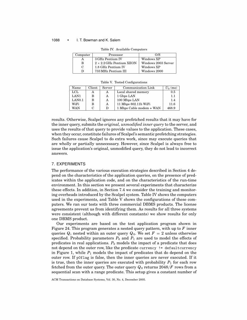
1088 • I. T. Bowman and K. Salem
Table IV. Available Computers
Computer Processor O/S
A 3 GHz Pentium IV Windows XP
B 2 × 2.2 GHz Pentium XEON Windows 2003 Server
C 1.8 GHz Pentium IV Windows XP
D 733 MHz Pentium III Windows 2000
Table V. Tested Configurations
Name Client Server Communication Link U0 (ms)
LCL A A Local shared memory 0.5
LAN1 B A 1 Gbps LAN 1.1
LAN0.1 B A 100 Mbps LAN 1.4
WiFi B A 11 Mbps 802.11b WiFi 11.6
WAN C D 1 Mbps Cable modem + WAN 468.9
results. Otherwise, Scalpel ignores any prefetched results that it may have forthe inner query, submits the original, unmodified inner query to the server, anduses the results of that query to provide values to the application. These cases,when they occur, constitute failures of Scalpel’s semantic prefetching strategies.Such failures cause Scalpel to do extra work, since may execute queries thatare wholly or partially unnecessary. However, since Scalpel is always free toissue the application’s original, unmodified query, they do not lead to incorrectanswers.
7. EXPERIMENTS
The performance of the various execution strategies described in Section 4 de-pend on the characteristics of the application queries, on the presence of pred-icates within the application code, and on the characteristics of the run-timeenvironment. In this section we present several experiments that characterizethese effects. In addition, in Section 7.4 we consider the training and monitor-ing overheads introduced by the Scalpel system. Table IV shows the computersused in the experiments, and Table V shows the configurations of these com-puters. We ran our tests with three commercial DBMS products. The licenseagreements prevent us from identifying them. As results for all three systemswere consistent (although with different constants) we show results for onlyone DBMS product.
Our experiments are based on the test application program shown inFigure 24. This program generates a nested query pattern, with up to F innerqueries Q i nested within an outer query Q0. We set F = 2 unless otherwisespecified. Probability parameters P0 and P1 are used to model the effects ofpredicates in real applications. P0 models the impact of a predicate that doesnot depend on the outer row, like the predicate currency != defaultcurrencyin Figure 1, while P1 models the impact of predicates that do depend on theouter row. If p0flag is false, then the inner queries are never executed. If itis true, then the inner queries are executed with probability P1 for each rowfetched from the outer query. The outer query Q0 returns 2048/F rows from asequential scan with a range predicate. This setup gives a constant number of
ACM Transactions on Database Systems, Vol. 30, No. 4, December 2005.

Optimization of Query Streams Using Semantic Prefetching • 1089
Fig. 24. Test application used to drive the experiments. The function RandomBoolean(p) generates
a random boolean value, returning true with probability p.
Fig. 25. Test application run times under the nested (N), outer join (J), outer union (U), client
merge join (M), and client hash join (H) strategies for varying P0 and P1 on configuration LCL.
inner query opens when varying fanout F . The inner queries Q i each returnR rows per invocation using an index range scan. R is set to 1 by default sothat the outer join strategy can be compared. Each returned row consists of Linteger columns, with L = 5 by default.
All tests were run with JDK 1.4.2 and JDBC drivers provided by the DBMSvendors. The database instance was fully cached to minimize the variance inserver costs. A prototype implementation of Scalpel was used for the exper-iments; combined queries were automatically combined using the LATERALkeyword for one of the DBMS systems, and vendor-specific equivalents for theother two systems.
In our experiments, we measure the time required to run the test applica-tion under the various execution strategies considered by Scalpel. All of thereported measurements represent the average of a number of repetitions, withthe number of repetitions selected so that the standard error of the mean (σM )is less than 5% of the mean for each measurement. The SQL statements wereprepared once for each factor combination and prepare time is not included inthe reported measurements.
7.1 Effects of Client Predicate Selectivity
Figure 25 shows the test application’s run time under the each of the executionstrategies as the selectivity of the application predicates is varied. Selectivity
ACM Transactions on Database Systems, Vol. 30, No. 4, December 2005.

1090 • I. T. Bowman and K. Salem
Fig. 26. Test application run times for the nested (N), outer union (U), outer join (J), client hash
join (H), and client merge join (M) strategies for varying query costs on configuration LCL. The
query cost factors are calibrated so that each cost factor unit adds approximately one second of
application run time.
is controlled by the probabilities P0 and P1. In Figure 25(a), P1 is fixed at 1.0and P0 is varied. In Figure 25(b), P0 is fixed at 1 and P1 is varied.
For the original nested execution strategy, mean execution time is propor-tional to the product P = P0 P1, so it has similar behaviour in both Figure 25(a)and (b). Outer query Q0 is always executed one time, and FP inner queries Q i
are executed, on average, for each row of the outer. For low values of P , thenested strategy is optimal since the inner queries are rarely executed, and noresources are wasted fetching unneeded results. However, the run time of thenested strategy grows rapidly with increasing P , as more inner queries areexecuted.
For the unified strategies, the execution time is largely independent of P0
and P1. Regardless of the results of these predicates, the combined query is ex-ecuted and all rows are fetched by the client. There is a slight linear dependenceresulting from the cost of decoding the attributes for the inner queries. If innerqueries are not executed, their attributes are not decoded from the combinedresult set, leading to slightly lower run-times.
The partitioned strategies fetch all possible rows from a rewritten innerquery when the inner query is first executed. This gives the partitioned strate-gies a strong dependence on P0, the probability that the inner queries will beopened at all.
7.2 Query Costs
We added an outer join in each query of the test queries Q0 and Q i. The outerjoins allowed us to vary the server cost of each query without affecting the num-ber of rows it returns. We used this to test the performance of Scalpel’s executionstrategies as the costs of the inner and outer queries vary. Figure 26 shows re-sults of this experiment. Predicate selectivity was fixed at P0 = 1 and P1 = 0.5.
The cost of the nested strategy increases linearly with the cost of the outerand inner queries. The cost of the unified strategies also increases linearly withthe cost of the outer query, and with the same slope as the nested strategy. This
ACM Transactions on Database Systems, Vol. 30, No. 4, December 2005.

Optimization of Query Streams Using Semantic Prefetching • 1091
Fig. 27. Run time with varying network configurations and P1 = 18
, CI = 8.
is because these strategies execute the outer query once. As the cost of the innerqueries varies, the cost of the unified strategies increases with a steeper slopethan that of the nested strategy. This is because the unified strategies computesthe result of these inner queries for all outer rows, while the nested strategyonly evaluates the inner query when the application actually requests it. Thishappens for about half of the outer rows, since P1 = 0.5. Because of this higherslope, the outer union strategy is cheaper than nested when the inner querycost is relatively low, but it becomes more expensive with increasing cost of theinner query.
The partitioned strategies effectively execute the outer query F + 1 times:once when the application issues the outer query, and once as part of the com-bined query that is issued when the application first requests each of the Finner queries. This gives the partitioned strategies a stronger dependence onthe cost of the outer query. The partitioned strategies are similar to the unifiedstrategies when we consider the cost of the inner queries.
7.3 Execution Costs
Figure 27 compares the different execution strategies under the five differentrun-time configurations listed in Table V. For these experiments, we set P0 = 1,P1 = 1
8, F = 2, and an inner cost factor of 8. One row was returned from each
invocation of the two inner queries. In this experiment, we measured clientand server CPU costs and total execution time for each strategy. Client CPUtimes were measured using client O/S functions and server CPU times weremeasured by the DBMS. The total time was measured at the client; in somecases, this total was less than the sum of the components due to overlap ofexecution costs.
There are several interesting observations that we can make from Figure 27.First, the original nested execution strategy is not significantly slower than
the optimal strategy (join) in the LCL configuration. It is reasonable for systemdevelopers to select a nested strategy for this case, especially considering thedifficulty of estimating the selectivity of local predicates and the complexity ofmanually combining queries.
Second, we observe that the join and merge strategies are faster in theLAN1 and LAN0.1 configurations than in the LCL configuration. The LAN
ACM Transactions on Database Systems, Vol. 30, No. 4, December 2005.

1092 • I. T. Bowman and K. Salem
Table VI. Training Overhead
Depth Cols Parms Original (ms) Training (ms)
1 10 1 2.64 3.15
10 10 1 2.62 3.31
10 10 10 2.88 3.34
40 100 100 14.95 198,368.17
configurations allow for overlap between server processing and client process-ing (the machine A used in LCL is a uniprocessor). The nested strategy, on theother hand, takes more than 1.5 times as long in the LAN1 configuration andmore than 2 times as long in the LAN0.1 configuration when compared to theLCL configuration.
Third, the unified and partitioned execution strategies reduce not only la-tency but also the client and server CPU costs. This cost savings results fromfewer messages that need to be formatted, sent, and interpreted. Even in theLCL configuration, all strategies but union use less server CPU time than thenested strategy, despite the selectivity P1 = 1
8.
Finally, while the savings for the LAN configuration are low in absolute terms(about 125 ms), the savings are very significant for WiFi and WAN; for example,with a wireless configuration the joined strategy saves nearly 1.5 s of elapsedtime, and the savings grows to 100 s with the WAN setup.
The original nested execution strategy is close to optimal for a local connec-tion. Even if a LAN configuration is considered, absolute benefits are modestfor an single execution of the outer and inner query (hundreds of milliseconds)so system developers might decide to use the simpler nested implementation.However, the server costs are 50% lower with the joined variant. Further, ifother deployments with higher network latency are used in the future, thenested implementation will be unsatisfactory. Finally, the predicate selectivityP1 = 1
8is quite low. If the value of P1 in particular configurations is higher,
then the nested strategy will be far from optimal.
7.4 Scalpel Overhead
The Scalpel system monitors all database requests during training. The cor-relation detection algorithm we have presented is O(n2) in n the number ofattributes for all opened cursors. A slightly more complicated O(n) algorithmexists. However, we have found that even the quadratic approach has reason-able overhead for the actual systems we examined. Table VI shows the open-time for a query with varying numbers of outer queries opened (Depth), varyingnumber of columns for each query (Cols), and varying number of parameters forthe innermost query (Parms). Testing was performed with a local client (LCL).
The overhead of the correlation detection algorithm is reasonable so long asthe product of Depth, Cols, and Parms is not greater than 1000. In the actualsystems we examined, we did not find any cases where this product exceeded100. However, the poor scalability of the quadratic algorithm indicates that alinear algorithm may be preferable in a practical implementation.
At run-time, all OPEN requests are intercepted. If a query is not being rewrit-ten, the original query is submitted to the DBMS and the result set is wrapped
ACM Transactions on Database Systems, Vol. 30, No. 4, December 2005.

Optimization of Query Streams Using Semantic Prefetching • 1093
Fig. 28. Context tree for dbunload.
in a monitor object that can detect when the cursor is closed. This monitoringis needed to maintain the current context for triggering rewrites.
We measured the overhead Scalpel adds to opening a query. With a localconfiguration (LCL), the overhead is 27 μs per query, or 7.0%. The overhead isthe same for all network setups, and drops to 1.6% in the LAN configurationdue to the higher base cost.
The overhead would be reduced if Scalpel were integrated with the vendor-provided JDBC driver (eliminating, for example, the need to use wrapper objectsto track the current context). However, the overhead seems acceptable as it islow in absolute terms, and consists entirely of client CPU time. Even withcurrent overhead levels, significant gains can be made without significantlyimpacting user interaction due to the benefits of rewrites performed by theScalpel system.
8. CASE STUDIES
As was noted in Section 1.1, we studied a set of application programs to deter-mine the kinds of request patterns that they exhibit. In this section, we presenttwo of these applications as case studies in the use of Scalpel. Our manualinspections of these applications found nested request patterns. We are inter-ested in determining whether Scalpel is able to identify and effectively exploitthose patterns. Section 8.1 describes the dbunload case study, and Section 8.2describes the SQL-Ledger.
8.1 dbunload Case Study
The first case we considered is the dbunload program. dbunload is providedwith Adaptive Server Anywhere, a relational DBMS produced by iAnywhereSolutions, a Sybase company. The dbunload program generates a text-based“unload” of a database, suitable for recreating both the schema and instancedata.
We considered only the schema portion of dbunload. Figure 28 shows thecontext tree that Scalpel detected when we trained Scalpel using a small setof artificially created databases. The context tree is relatively complex. By in-specting the source code, we found that the nesting arises because the codestructure matches the nesting structure of the output (e.g., one cursor is usedover all tables; a nested cursor is used for all columns of a table). Further, nest-ing appears because of informational functions that are called from multiplecontexts. These informational functions typically select a single row using aprovided primary key.
We measured the performance of dbunload when using Scalpel with 31 real-world databases. Figure 29 shows the run-time with and without Scalpel’s
ACM Transactions on Database Systems, Vol. 30, No. 4, December 2005.

1094 • I. T. Bowman and K. Salem
Fig. 29. Running time(s) of dbunload on LAN0.1. Original times are shown on the left in increasing
order by cost, and times with Scalpel’s optimizations are shown on the right in the opposite order.
Fig. 30. SQL-Ledger system structure.
optimizations for these 31 databases on the LAN0.1 configurations. Thesedatabases are labelled with A,B, . . . ,Z,α, β, θ λ, μ in order of increasing cost onthe LCL configuration. In these tests, all of Scalpel’s strategies were permit-ted, and we show the time to unload the entire schema. The results show thatScalpel provides significant savings. Total run-time was reduced by an averageof 60%, with a server costs reduced by an average 58% and client costs reducedby 20%.
While it is clearly cheaper to execute dbunload using the optimizations thatScalpel provides, it is daunting to consider implementing these optimizationsmanually in the code. Each of the queries is relatively complex, with a numberof variants that may be executed depending on configuration settings. It wouldbe quite difficult to manually generated the needed combined queries.
8.2 SQL-Ledger Case Study
We considered SQL-Ledger as a second case study. SQL-Ledger is a web-baseddouble-entry accounting system written in Perl. The system is configured witha DBMS storing persistent accounting entries, a web server that executes Perlscripts to implement business logic, and a web browser that presents the userinterface.
Figure 30 gives an overview of the structure of the SQL-Ledger system. Aweb browser presents a user interface, and a web server executes the businesslogic. The SQL-Ledger business logic communicates with a DBMS using thePerl DBI library and a vendor-specific DBD module. We use ‘V’ as a placeholderin Figure 30 to represent a specific DBMS implementation.
In general, the web browser, business logic, and DBMS can be placed onseparate machines. We simulated a web user and the business logic on machine
ACM Transactions on Database Systems, Vol. 30, No. 4, December 2005.

Optimization of Query Streams Using Semantic Prefetching • 1095
Table VII. Simulated User Activities
# Database Requests
Activity Frequency Original Optimized Improvement
A. Add Sales Invoice 35% 1429.9 118.5 92%
B. Add Cash Receipt 35% 46.4 28.7 38%
C. Transaction History 10% 85.0 71.5 16%
D. Tax Collected 10% 3.1 3.1 0%
E. A/R Aging 10% 63.4 4.0 94%
B, and used a commercial DBMS on machine A communicating using a 100-Mbps LAN (configuration LAN0.1 in Table V).
The web browser presents a menu of links to activities that a user can per-form, such as adding a transaction. Each of these activities may require multiplesteps. For example, when adding an invoice, a separate step is used for eachinvoice line For each step, the user presses an Update button that submits apartially completed form to the web server. The business logic scripts parse thepartially completed form, issue database requests to retrieve additional infor-mation, and format a new form to be returned to the user. The last step of auser activity consists of using a Post button to apply the requested changes tothe database server. Some of the business logic scripts that are executed dur-ing a user activity issue nested database requests that might benefit from ourproposed optimizations.
We populated the database with synthetic data and simulated the activitiesof a user working with the system. We used two scale factors, SF1 and SF10;SF1 is a small instance that we use for training of Scalpel, and SF10 representsthe data needs of a medium sized company. We simulated a user performingaccounts receivable activities with this synthetic data. Table VII shows the ac-tivities that we simulated based on the description in the SQL-Ledger manual[Simader 2004]. For each activity, we show the proportion of simulated ses-sions that perform the activity. We also show the number of database requestssubmitted for each activity in both the original setup and with Scalpel’s opti-mizations.
8.2.1 Configuring the System for Measurement. The dbunload program re-quires no human interaction, so we were able to run it with and without opti-mizations and achieve comparable results. Since the SQL-Ledger program isinteractive, we need another approach to generate repeatable results. We usedthe following procedure. First, we created a backup of the populated database.Then, we executed 500 simulated activities from a single simulated user. Wemonitored all database requests made by the business logic, and we stored theseas a trace. Then, to simulate an execution, we restored the data file from thebackup and replayed all database requests (with associated think time delays).This approach gives a repeatable setup provided that the order of the returnedrows does not change. For this reason, we restricted Scalpel to use only thenested execution (N), outer join (J), and client hash join (H) strategies. Thesestrategies do not alter the ordering of rows from outer queries so so they canbe used with replayed workloads.
ACM Transactions on Database Systems, Vol. 30, No. 4, December 2005.

1096 • I. T. Bowman and K. Salem
Table VIII. Costs of 500 User Activities
SF1 SF10
Original Training Original Optimized Improvement
Total time (s) 171.5 172.4 1,439.2 629.8 56.2%
Server CPU (s) 29.3 38.6 578.8 283.7 51.0%
Client CPU (s) 48.6 60.1 373.9 319.6 14.4%
Queries Submitted 39,909 39,909 285,913 24,982 91.3%
Top-Level 16,130 16,130 18,791 18,791 0%
Nested 23,779 23,779 267,122 6,191 97.7%
Update Requests 5,263 5,263 6,818 6,818 0.0%
Network Packets 163,223 179,181 1,200,287 160,583 86.6%
Client → Server 83,195 91,383 610,739 93,466 84.7%
Server→ Client 80,028 87,798 589,548 67,117 88.6%
Network Bytes (MB) 57.2 61.9 457.6 199.8 56.3%
Client → Server 22.2 23.5 137.2 22.1 83.9%
Server→ Client 35.1 38.4 320.5 177.7 44.6%
8.2.2 Rewrite Opportunities. After configuring the system as described,we used Scalpel’s training mode on a SF1 database to identify opportunities foroptimization. Figure 7 shows part of the context tree detected by the PatternDetector. The SQL-Ledger system dynamically generates queries with varia-tions based on input configuration; to Scalpel, these appear as distinct queries..Scalpel discovered three variants of Q1, and two variants of Q9. We collapsedthese variants for a simpler presentation. Only Q5 can be used in a join strategyas the other queries could return more than one row.
Note that query Q5 appears in two contexts, /Q4 and /Q8. In the first con-text, the input parameters of Q5 are predicted to be equal to attributes of Q4.However, in context /Q8 there is no prediction for one of the input parametersof Q5. Because of this, node /Q8/Q5 must be executed using the nested strategy(N).
8.2.3 Performance Results. Table VIII summarizes the performance re-sults when executing a stored trace of 500 user activities. During training witha SF1 database, overall time is slightly slower than running without Scalpel.However, training did increase client processing costs due to the requirementsof finding nesting patterns and identifying parameter correlations. The net-work and server costs are also slightly higher during training due to the needto retrieve catalog information from the DBMS for query analysis and costing.
When we execute the stored trace with the SF10 database using Scalpel’soptimizations, the difference is more dramatic effect. The elapsed time is re-duced by over 800s (an improvement of 56%). Further, this savings in latencyis associated with significant reductions in server and client processing costs,along with lower communication costs.
As suggested by Table VII, all of the simulated activities except D-Tax Col-lected contain some nested requests that are optimized. Figure 31(a) comparesthe optimized and unoptimized elapsed time for each of the steps performedby our simulated user. Each of these steps represents a single form submissionfrom the user, and the step may be executed multiple times within a single ac-tivity. There are four steps that benefit from Scalpel’s optimizations: A(3), B(1),
ACM Transactions on Database Systems, Vol. 30, No. 4, December 2005.

Optimization of Query Streams Using Semantic Prefetching • 1097
Fig. 31. SQL-Ledger elapsed time for unoptimized (U) and optimized (O) configurations.
C(2), and E(1). Figure 31(b) shows the elapsed time for outermost queries andinner queries for these four steps that are optimized.
8.3 Summary of Case Studies
In summary, our examination of dbunload and the SQL-Ledger system demon-strates that opportunities for our proposed optimization do appear in some sys-tems. While these opportunities are relatively rare, they can have substantialbenefit when they are optimized.
Scalpel can identify these optimization opportunities using a training pe-riod that does not excessively degrade system performance, and it is able toautomatically rewrite submitted requests to take advantage of the selectedoptimizations.
9. CONCURRENT UPDATES
When Scalpel performs a rewrite it combines an outer query with one or moreinner queries, and it issues the combined query to the server before the innerqueries have actually been requested by the application. This can potentiallylead to a data consistency problem: Prefetched results obtained from the com-bined query may not contain updates that would have been observed by theoriginal inner queries. There are two possible sources of such updates. Theymay occur on the same database connection as the queries, or they may beoccur on some other concurrent connection.
Updates performed on the same connection as the queries are observed andmonitored by the Scalpel system. If such an update is observed at run-time,and if that update could possibly affect prefetched results, Scalpel’s Prefetchercan react by simply ignoring the prefetched data, and shipping any subsequentinner queries directly to the DBMS. This is essentially the same technique thatScalpel uses to recover from mispredictions. However, determining whether anupdate conflicts with a rewritten query is, in general, a difficult task. Thattask would be further complicated by the presence of of updatable views andtriggers in the database. To avoid these problems, Scalpel takes the conservative
ACM Transactions on Database Systems, Vol. 30, No. 4, December 2005.

1098 • I. T. Bowman and K. Salem
approach of assuming that any update conflicts with prefetched query results,and ignoring the prefetched results.
Scalpel may also observe updates on the monitored connection during train-ing. If this occurs, Scalpel’s Pattern Detector marks the outermost open queryas containing an update. The Pattern Optimizer does not generate rewrites forany context tree nodes in the subtree below the marked node. Thus, Scalpelwill not prefetch in any context in which it observed an update during training.
While Scalpel can detect updates on the monitored connection, it does notobserve changes made on other, concurrent connections. If the serializable iso-lation level is used, then this does not introduce a correctness problem. Theserializability requirement means that subsequent fetches would observe thesame results as a prefetched result. However, depending on the implementa-tion of the serializable isolation, prefetching can cause extra data contentionbecause Scalpel prefetches some data that would not have been fetched by theoriginal application (because a local P0 or P1 predicate failed). Locking-basedimplementations will prevent updates to these unneeded rows until the trans-action ends. On the other hand, when using rewriting strategies the Scalpel sys-tem significantly reduces the run-time of a transaction, which can act to reducedata contention because locks are held for a shorter period. When an isolationlevel weaker than serializable is used, prefetching may introduce anomalies.These anomalies are likely acceptable to application developers that acceptthe anomalies associated with weak isolation, but they need to be carefullyconsidered.
A final, related issue is cursor sensitivity. If a cursor is currently openover prefetched results, it will not reflect any updates made after the data isprefetched. This satisfies the requirements of the INSENSITIVE and ASENSITIVEcursor types, but not SENSITIVE cursors. SENSITIVE cursors are required to re-flect relevant changes made by the same connection after the cursor is opened.Scalpel cannot use prefetched results to satisfy these types of cursors as thesensitivity requirements cannot be met using prefetched data.
10. RELATED WORK
A number of researchers have studied how to effectively execute queries thatcontain various forms of nesting [Fegaras and Maier 2000; Seshadri et al. 1996].The approaches developed in that work are effective at choosing efficient eval-uation plans for the correlated combined queries that we generate. However,the techniques are not directly applicable to the problem we consider becausethe nesting appears in the application, not the queries.
Shanmugasundaram et al. [2001] and Fernandez et al. [2001] studied effi-cient mechanisms to generate nested results from relational data sources. Theirwork differs from the current research in three ways. First, they assumed thatthe query nesting was known due to the presence of an XML view definition,while we detect nesting and correlations in the sequence of requests submit-ted by a client application. Second, our work extends the view tree reduction ofFernandez et al., a heuristic that combines all at-most-one-row queries withtheir outer query using joins. In our work, we choose the queries to join together
ACM Transactions on Database Systems, Vol. 30, No. 4, December 2005.

Optimization of Query Streams Using Semantic Prefetching • 1099
on the basis of a cost model that accounts for the effects of local predicates thatcan appear in client application.
Mayr and Seshadri [1999] also considered effective mechanisms to executequeries that contain local predicates. However, they did not consider the caseof nested queries, and assumed that the local predicate was identified in thequery. The rewrites they employ can be applied to our case. However, the localpredicates that we identified appear in application code. These predicates wouldneed to be re-expressed so that they could be exploited by the rewrites Mayr andSeshadri [1999] use. We have elected to leave the client application unchanged,which means that local predicates are always executed after fetching all therows of a combined query.
Florescu et al. [1999] discussed query simplification under preconditions,an approach to optimizing parameterized queries based on knowledge of thesource of the binding parameters. In their work, they considered queries thatwere accessed with actual parameter values drawn from different outer queries,and exploited rewrite optimizations that were safe in certain contexts. Theirwork relied on having a declarative representation of the queries and nesting,so they could be assured of knowing when a query was truly correlated.
Bernstein et al. [1999] suggested that the context in which an object wasfetched is an important factor to consider when deciding which related objectsshould be prefetched. For example, if two objects, A and B were both fetchedfrom the same query, then we fetch A’s x attribute, it is a reasonable assumptionthat we will soon fetch B’s x attribute. The solution proposed by the authorsattempts to discover operations that should be applied to multiple objects, anduses this as the basis for prefetching. In contrast to Scalpel, their system ex-amined contexts of objects not of queries.
Other researchers have considered how query results can be fetched beforethe query is actually requested. Yao and An [2003] found that there are seman-tic relationships between queries submitted by a user within a single session.They explored how a system can exploit predictions of future requests by, forexample, prefetching results before the query is submitted or caching resultsfrom previous requests. If a set of user access patterns is identified throughmining database workload traces, their work shows how these patterns can beused to reduce latency. In contrast to our work, they considered sequences ofqueries instead of nesting patterns.
Sellis [1988] investigated mechanisms for choosing an execution strategy fora stream of queries that are known ahead of time. Results for multiquery op-timization complement our results well. Scalpel derives a prediction of queriesthat will be executed together, and these could be optimized by a query opti-mizer using multiquery optimization.
11. CONCLUSIONS AND FUTURE WORK
A number of client applications generate patterns of nested, correlated queriesin the stream of requests they submit to a DBMS. This nesting pattern gen-erates a large number of small queries that contribute to high latency andserver processing costs. While it is possible in some cases to rewrite applications
ACM Transactions on Database Systems, Vol. 30, No. 4, December 2005.

1100 • I. T. Bowman and K. Salem
manually to avoid generating these patterns, such rewrites are complicated bya number of factors. One of these is the fact that a nested approach is in factoptimal for some configurations of the application program (e.g., see Figure 25).In the cases where such optimal configurations are expected to occur in the ma-jority of client deployments, it is prudent to choose the nested implementation,which is in any case easier to implement.
Although optimal in some configurations, the nested strategy can lead topoor execution performance for deployments that do not match the expectedconfiguration. Developers are thus faced with an unfortunate decision: eitheruse a more complicated implementation that is actually slower in the ma-jority of predicted deployments, duplicate development effort to use multipleimplementations that choose the optimal strategy at deployment time, or ac-cept suboptimal performance in deployments that do not match the expectedcase.
We have presented Scalpel, a system for detecting and optimizing patternsof repeated requests within a query stream. Scalpel uses a deployment-timetraining period that monitors a request stream to automatically detect nestingof queries and correlations between query parameters and attributes of outerqueries.
Once Scalpel detects nested requests and finds predicted correlation sourcesfor parameters of inner queries, it uses a cost-based optimizer to choose the opti-mal execution strategy for the particular deployed configuration. The cost-basedoptimizer minimizes response time by comparing the server, communication,and client costs of three execution strategies: nested, joined, or hash-based.
The execution strategies that we have presented give correct results evenin the case that the training phase predicted correlations that do not hold atrun-time. Further, these strategies give correct results in the face of concur-rent updates provided that serializable transactions are used. If weaker iso-lation levels are used, the presented strategies may introduce anomalies thatmay be acceptable to application developers, although they must be carefullyconsidered.
Rewriting nested patterns is only a first step toward optimizing the querystreams applications present to servers: data structure correlations and batchesalso occur frequently. Further, additional strategies such as outer unions andmerge-based rewrites may perform better in some configurations. Finally, thepatterns detected by Scalpel may be useful for tuning database servers. For ex-ample, these patterns may provide insight into appropriate materialized viewsthat can be used to answer multiple requests in a stream. Alternatively, knowl-edge of requests likely to occur in the future may aid the DBMS query optimizerto select an appropriate execution strategy using techniques such as multi-query optimization [Sellis 1988]. We plan to address these issues in futurework.
ACKNOWLEDGMENTS
Our thanks to the anonymous reviewers of an earlier version of this paper fortheir helpful suggestions.
ACM Transactions on Database Systems, Vol. 30, No. 4, December 2005.

Optimization of Query Streams Using Semantic Prefetching • 1101
REFERENCES
BERNSTEIN, P. A., PAL, S., AND SHUTT, D. 1999. Context-based prefetch for implementing objects on
relations. In Proceedings of the 25th International Conference on Very Large Databases. Morgan
Kaufmann, San Francisco, CA, 327–338.
BOWMAN, I. T. 2005. Scalpel: Optimizing query streams using semantic prefetching. Ph.D. dis-
sertation, University of Waterloo.
FEGARAS, L. AND MAIER, D. 2000. Optimizing object queries using an effective calculus. ACMTrans. Database Syst. 25, 4, 457–516.
FERNANDEZ, M., MORISHIMA, A., AND SUCIU, D. 2001. Efficient evaluation of XML middle-ware
queries. In Proceedings of the ACM SIGMOD International Conference on the Management ofData. ACM, New York, 103–114.
FLORESCU, D., LEVY, A. Y., SUCIU, D., AND YAGOUB, K. 1999. Optimization of run-time management
of data intensive web-sites. In Proceedings of the 25th International Conference on Very LargeDatabases. Morgan-Kaufmann, San Francisco, CA, 627–638.
GALINDO-LEGARIA, C. AND JOSHI, M. 2001. Orthogonal optimization of subqueries and aggregation.
In SIGMOD ’01: Proceedings of the 2001 ACM SIGMOD International Conference on Managementof Data. ACM, New York, 571–581.
INTERNATIONAL STANDARDS ORGANIZATION. 1999. Database Language SQL—Part 2: Foundation(SQL/Foundation). International Standards Organization.
MAYR, T. AND SESHADRI, P. 1999. Client-site query extensions. In Proceedings of the ACM SIGMODInternational Conference on the Management of Data (Philadelphia, PA). ACM New York.
RAHAL, A., ZHU, Q., AND LARSON, P.-A. 2004. Evolutionary techniques for updating query cost
models in a dynamic multidatabase environment. VLDB J. 13, 2, 162–176.
SELLIS, T. K. 1988. Multiple-query optimization. ACM Trans. Database Syst. 13, 1, 23–52.
SESHADRI, P., PIRAHESH, H., AND LEUNG, T. Y. C. 1996. Complex query decorrelation. In Proceedingsof the 12th International Conference on Data Engineering (Washington, DC). IEEE Computer
Society Press, Los Alamitos, CA, 450–458.
SHANMUGASUNDARAM, J., SHEKITA, E., BARR, R., CAREY, M., LINDSAY, B., PIRAHESH, H., AND REINWALD, B.
2001. Efficiently publishing relational data as XML documents. VLDB J. 10, 2–3, 133–154.
SIMADER, D. 2004. SQL Ledger Accounting: User Guide and Reference Manual for Version 2.2.
YAO, Q. AND AN, A. 2003. Using user access patterns for semantic query caching. In Proceedings ofthe 14th International Conference on Database and Expert Systems Applications (Prague, Czech
Republic).
ZHU, Q. 1995. Estimating local cost parameters for global query optimization in a multidatabase
system. Ph.D. dissertation, University of Waterloo.
Received October 2004; revised May 2005 and August 2005; accepted August 2005
ACM Transactions on Database Systems, Vol. 30, No. 4, December 2005.