optimization of variable speed chiller plants: frank … · optimization of variable speed chiller...
TRANSCRIPT

Prepared for the General Services Administration
By the Pacific Northwest National Laboratory
August 2016
Optimization of Variable Speed Chiller Plants:
Frank M. Johnson Jr. Federal Building and U.S. Courthouse,
Montgomery, Alabama
JC Hail
DD Hatley
RM Underhill

The Green Proving Ground (GPG) program leverages GSA’s real estate
portfolio to evaluate innovative sustainable building technologies and
practices. Findings are used to support the development of GSA
performance specifications and inform decision-making within GSA, other
federal agencies, and the real estate industry. The program aims to drive
innovation in environmental performance in federal buildings and help
lead market transformation through deployment of new technologies.

Control Optimization System for Chiller Plants Assessment Page i
DISCLAIMER
This document was prepared as an account of work sponsored by the United States Government. While this
document is believed to contain correct information, neither the United States Government nor any agency
thereof, nor the Pacific Northwest National Laboratory (PNNL), nor Battelle Memorial Institute, nor any of
their employees, makes any warranty, express or implied, or assumes any legal responsibility for the
accuracy, completeness, or usefulness of any information, apparatus, product, or process disclosed, or
represents that its use would not infringe privately owned rights. Reference herein to any specific
commercial product, process, or service by its trade name, trademark, manufacturer, or otherwise, does not
constitute or imply its endorsement, recommendation, or favoring by the United States Government or any
agency thereof, or PNNL, or Battelle Memorial Institute. The views and opinions of authors expressed herein
do not necessarily state or reflect those of the United States Government or any agency thereof , or PNNL, or
Battelle Memorial Institute. The work described in this report was funded by the U.S. General Services
Administration under Contract No. PX0012922. PNNL is a multi-disciplinary research laboratory operated for
the U.S. Department of Energy by Battelle Memorial Institute under contract number DE-AC05-76RL01830.
NO ENDORSEMENTS
Any hyperlink to any website or any reference to any third-party website, entity, product, or service is
provided only as a convenience and does not imply an endorsement or verification by PNNL of such website,
entity, product, or service. Any access, use or engagement of, or other dealings with, such website, entity,
product, or service shall be solely at the user's own risk.
ACKNOWLEDGEMENTS
United States General Services Administration: Kevin Powell, Michael Lowell, Christine Wu, Timothy Wisner,
Mark Moody
United States General Services Administration, Region 4
Frank M. Johnson Jr. Federal Building and U.S. Courthouse: Kevin Lear
Wilson 5 Service Company, Inc.: Mitchell Foster
Pacific Northwest National Laboratory: Jeremy Blanchard, Lorena Ruiz, Darrel Hatley, Danny Taasevigen,
John Hail, and Ron Underhill.
Tenfold Information Design Services: Andréa Silvestri, Bill Freais, Marian Mabel
For more information, contact:
Kevin Powell
Program Manager, Green Proving Ground
Office of Facilities Management, Public Buildings Service
U.S. General Services Administration
50 United Nations Plaza
San Francisco, CA 94102
Email: [email protected]

Control Optimization System for Chiller Plants Assessment Page ii
Table of Contents
I. Executive Summary .................................................................................................................................. 3
II. Introduction ........................................................................................................................................... 10
A. Problem Statement........................................................................................................................ 10
B. Opportunity .................................................................................................................................. 11
III. Methodology.......................................................................................................................................... 14
A. Technology Description.................................................................................................................. 14
B. Controls Description ...................................................................................................................... 16
C. Technical Objectives ...................................................................................................................... 17
D. Demonstration Project Location and description ............................................................................. 20
IV. M&V Evaluation Plan .............................................................................................................................. 22
A. Detailed chiller plant Equipment Description and Historical operation .............................................. 22
B. Instrumentation Plan ..................................................................................................................... 24
C. Test Plan ....................................................................................................................................... 26
V. Results ................................................................................................................................................... 27
A. Pre- And Post-Installation Chiller Plant Performance........................................................................ 27
B. Chiller Plant Post-Installation average Performance Profile .............................................................. 29
C. Chiller Plant Post-Installation Daily Performance Profile................................................................... 29
D. Ways to Further Improve Chiller Plant Performance ........................................................................ 31
VI. Summary Findings and Conclusions ......................................................................................................... 37
A. Overall Technology Assessment at the Demonstration Facility ......................................................... 37
B. Best Practices ................................................................................................................................ 38
C. Barriers and Enablers to Adoption .................................................................................................. 39
D. Market Potential within the GSA Portfolio....................................................................................... 39
E. Recommendations for Installation, Commissioning, Training, and Change Management.................... 41
F. Importance of Baseline Measurement and Documentation.............................................................. 42
VII. Appendices ............................................................................................................................................ 43
A. List of Abbreviations and Symbols .................................................................................................. 43
B. References .................................................................................................................................... 45
C. Glossary ........................................................................................................................................ 46
Control Optimization System for Chiller Plants Assessment Page 3
I. Executive Summary This report is divided into five sections. The first section describes the background and opportunity for the
Control Optimization System for Chiller Plant technology to reduce space cooling energy consumption at
U.S. General Services Administration (GSA) facilities with centrifugal chiller plants containing multiple water-
cooled chillers. The second section discusses the new technology, how it may reduce energy consumption,
and introduces the demonstration location. The third section provides a detailed description of the
demonstration facility and the configuration of the technology at the demonstration facility. The third
section also provides a detailed overview of the approach used to assess the performance of the technology
and how the chiller plant was monitored. The fourth section presents the results of the monitoring activity,
documents performance and resulting energy savings, and presents the results of a life-cycle cost analysis.
The fourth section also presents additional opportunities to further improve the performance of the chiller
plant with control optimization, based on observations and lessons learned. The final section draws
conclusions from the demonstration results and projects how GSA may best benefit from the technology’s
targeted deployment.
BACKGROUND
In the U.S., space cooling accounts for 7.4% of energy consumption in buildings (9.6% i n office buildings) (EIA
2003b). However, because space cooling is primarily driven by electricity—a higher cost energy source—
space cooling may account for more than 7.4% of a facility’s annual energy bill. Within U.S. office buildings,
chillers provide space cooling in only 2.3% of buildings (by number of buildings), but because chillers are
used more frequently in larger facilities, 18% of building floor space is cooled using chillers (32% of office
building floor space) (EIA 2003a). Therefore, a more efficient chiller plant offers significant opportunity to
reduce annual energy costs for GSA, as well as reducing annual energy consumption.
OVERVIEW OF THE DEMONSTRATION TECHNOLOGY
Control Optimization System for Chiller Plants technology claims to optimize centrifugal chiller plants to
minimize total power requirements. This technology does not require variable frequency drives (VFDs) for
chiller compressor motors, which can be expensive. However, the control strategy requires the use of VFDs
on all ancillary components such as chilled-water primary and secondary pump motors, condenser-water
pump motors, and cooling tower fan motors. For constant-speed chiller plants with a primary-secondary
configuration, the chiller plant will often be converted from a constant-volume primary system operation to
a variable-volume primary system operation when control optimization is implemented.
The optimization technology claims to optimize pressure and temperature setpoints for chilled water and
condenser water, while controlling pump and fan speeds to maximize the chiller plant efficiency.
Per documentation from the vendor, the control optimization system is expected to produce the following
outcomes:
1. Control the chilled-water system to operate at or near original design intent throughout the entire
system load requirements at all times. Condenser and chilled-water pumps, along with cooling
towers, will require VFDs for this technology to work successfully.

Control Optimization System for Chiller Plants Assessment Page 4
2. Manage chiller lift for stable refrigeration performance at virtually all tonnage loads, without the
need to install VFDs on the chillers themselves. The technology will work with chillers that have
VFDs, but it is not necessary for a chiller VFD to be in place.
3. Reset pressure and temperature setpoints on chilled and condenser water loops based on current
system dynamics to increase chiller plant deliverable tonnage while reducing chilled-water and
condenser-water pumping energy, thereby optimizing total chiller plant kW per ton.
4. The technology is customized for each site to create a variable water loop flow that reduces
pumping energy for all pumping systems (condenser-water and chilled-water).
This technology can be applied to chiller plants that serve a single building or a campus environment. The
technology extends down to individual air handler cooling coils in an attempt to create a wider temperature
difference (Delta T) between temperatures entering the coil and leaving the coil; this positively impacts the
chiller efficiency. Realization of this technology’s full benefit may require valve changes at cooling coils
(remove three-way control valves and replace with two-way control valves) and other end of line system
piping changes where bypass may exist. Therefore, some engineering of end of line piping and control valve
changes may be required, depending upon the existing designs. Isolation valves (if not existing) may also be
added to minimize flow through chillers and cooling towers that are not running. All of these potential
modifications have a net system effect of reduced pumping power when coupled to the technology.
Control system optimization is not unique among control technologies that optimize the entire chiller plant.
Another system, a variable-speed loop control logic, establishes performance algorithms for all chiller
system components and attempts to determine the most efficient operational configuration, based on load
and ambient conditions. To take advantage of part-load chiller efficiencies, compressor motors, condenser
pumps, cooling tower fans, and secondary pumps all require VFDs.
In 2012, GSA’s Green Proving Ground (GPG) program worked with researchers from the Pacific Northwest
National Laboratory (PNNL) to assess an all variable-speed (AVS) loop control technology at the Thomas F.
Eagleton U.S. Courthouse in St. Louis, MO. Researchers encountered problems with the study design and
with the technology itself, so findings were not released. Researchers did, however, find that while the
variable-speed loop control logic demonstrated energy savings, those savings did not justify installed costs.
Variable-speed loop control technology requires significant integration, and staff anticipated information
technology (IT) difficulties incorporating the technology into current GSA practices. Also, after the
assessment, but while the loop control logic was still operational, building staff reported frequent chiller
cycling, which stopped only when the control logic was turned off and the chiller was operated through the
building automation system (BAS). Because of concern that frequent cycling would damage the chiller
and/or shorten its life, use of the variable-speed loop control logic was suspended. It also is noteworthy that
the AVS loop system requires an annual service fee of approximately $20,000 for remote monitoring and
support.
Control Optimization System for Chiller Plants Assessment Page 5
STUDY DESIGN AND OBJECTIVES
GSA identified the Frank M. Johnson Jr. Federal Building and U.S. Courthouse as the demonstration location
for the chilled-water (CHW) system optimization technology assessment. The facility consists of two primary
buildings: the Frank M. Johnson Jr. U.S. Courthouse and the Frank M. Johnson Jr. Federal Building (also
known as the “Annex”).
The original courthouse was completed in 1933 and is listed in the National Register of Historic Places. The
courthouse is five stories tall, with over 135,000 gross square feet and a U-shaped footprint with an interior
light well and a red tiled roof. The most significant interior space is the U.S. District Courtroom, where Judge
Johnson presided, on the second floor. Limestone arches surround the windows. Terrazzo and marble
floors, marble wainscot, bronze elevator doors with bas-relief panels, and bronze radiator grilles are found
throughout the building. Between 2002 and 2006, the original building was renovated and the interior
spaces reconfigured to accommodate the needs of the court. Even though the courthouse was renovated,
apparently it does not have any means to economize on conditioning the building during winter and cool
spring and fall months. This drives the need to run the chiller system almost all year, but, at times, during
significantly low loads.
The five-story Annex was constructed in 2002. With over 325,000 gross square feet, it has a radial (arc)
design that is stylistically compatible with the original building. The Annex contains judges' chambers,
District Courtrooms, and bankruptcy courts. The Annex was constructed to meet current ventilation code
requirements, including economizer functionality that provides for cooling during winter, spring, and fall
months. In 2004, the two facilities were linked together.
Space cooling is provided by a central chiller plant consisting of three, 400-ton centrifugal chillers (Carrier
model number 19XR series chillers, installed circa 1998). The chillers have constant-speed compressors. Each
chiller has its own chilled-water pump and condenser-water pump. Chilled water is distributed through the
two buildings in a primary-secondary chilled-water distribution system. Along with the installation of the
control optimization system, each of the pump motors and tower fan motors was equipped with a VFD.
Differential-pressure transmitters were installed on all the pumps. Additional instrumentation was also
installed or replaced to accurately measure loop temperatures (supply/return) for each primary chilled -
water loop and the two secondary chilled-water loops, and for cross-over (bridge) temperature between the
primary and secondary piping. New current transducers were installed on all of the chiller compressor
motors and several of the pump motors to measure individual power loads. In some cases, existing VFD-
derived signals (pump and tower fan motor kW loads) were used to save on instrumentation costs. These
will be detailed in the instrumentation section.
The purpose of this demonstration was to determine the energy and cost savings associated with control
optimization in the central chiller plant serving the Frank M. Johnson Jr. Federal Building and U.S.
Courthouse.
Ideally, such energy and cost assessments include developing a pre-installation baseline (before the
technology is installed) and post-installation (after the technology has been installed and operating)
performance profile of the chiller plant, establishing a cooling load profile for the building, and comparing
the results using a weather-normalizing approach. Ideally, at least one year’s worth of baseline data is
desired to provide an accurate comparison to the post-installation technology performance, as reflected by
Control Optimization System for Chiller Plants Assessment Page 6
the data and weather-normalized. In this case, the technology was installed without GSA collecting a
monitored baseline. However, an estimated baseline was simulated over the course of one month, after the
optimization technology was installed but before it was implementated.
GSA used PNNL’s Manual Mode approach to develop an estimated baseline, whereby the chiller plant could
be operated in Manual Mode for two separate two-week periods in an attempt to simulate the baseline
behavior of the chiller plant (prior to the implementation of the optimization technology). PNNL suggested
that the monitored data provided by this approach is preferable to modeled information. Also, the site
should be able to confirm that Manual Mode reasonably represents the original chiller plant operation.
Finally, Manual Mode would use the original building automation system (BAS) operating code, which
provides better confidence than simply disabling the control optimization system algorithms.
There are many assumptions regarding whether Manual Mode accurately represents the original chiller
plant operations. This includes the pump speeds, chiller setpoints, chilled-water distribution pressure, and
actual air handler economizer performance. The short time period (20–24 days total) will not capture the
full load range of the chiller plant load profiles, which will require extrapolation of the Manual Mode data
that results in uncertainty in the energy savings results.
Additional changes may have been made to piping systems (e.g., three-way valves converted to two-way
valves, isolation valves added, etc.) which cannot be returned to original piping configuration (therefore not
simulated). Further, it is not ideal to collect monitored data after the new technology has been installed.
The site will be influenced by the control optimization system’s operating strategy and may not operate the
chiller plant or the loads served (air handling unit (AHU) cooling coils, etc.) exactly in the same manner as
they used to be operated.
PNNL cannot validate that the Manual Mode data reasonably represents the chiller plant performance
throughout the year. Therefore, results will be presented as energy and cost savings ranges, not specific
values.
The monitoring plan targeted the recording of total chilled-water plant input power (kW), chilled-water flow
rate and corresponding chilled-water supply and return temperatures, and the electric energy consumed by
the chillers, chilled- and condenser-water pumps, and cooling tower fans. Parameters required to quantify
the thermal cooling load provided by the chiller plant were also monitored. The chiller plant was monitored
from January 13, 2013 through August 31, 2013 (peak summer and cooler fall and spring load periods). The
monitored data was used to determine the operational performance of the chiller plant, as well as the
thermal cooling load profile of the building as it relates to occupancy and weather conditions.
PROJECT RESULTS/FINDINGS
Analysis of the monitored data shows that the chiller plant with control optimization is more efficient than
the baseline chiller plant. Figure 1 shows the performance profile of the chiller plant with the new
technology compared to the Manual Mode (estimated baseline). There is a noticeable difference between
the baseline chiller plant operations and the chiller plant operations with control optimization.
Control Optimization System for Chiller Plants Assessment Page 7
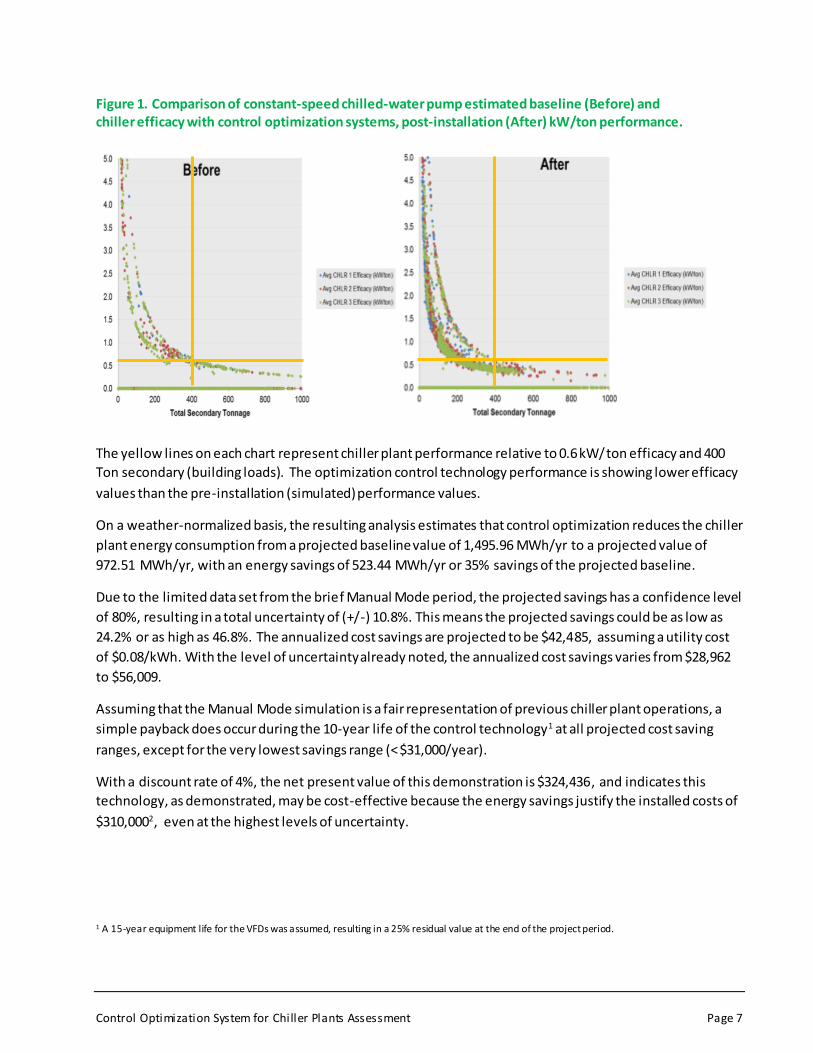
Figure 1. Comparison of constant-speed chilled-water pump estimated baseline (Before) and chiller efficacy with control optimization systems, post-installation (After) kW/ton performance.
The yellow lines on each chart represent chiller plant performance relative to 0.6 kW/ton efficacy and 400
Ton secondary (building loads). The optimization control technology performance is showing lower efficacy
values than the pre-installation (simulated) performance values.
On a weather-normalized basis, the resulting analysis estimates that control optimization reduces the chiller
plant energy consumption from a projected baseline value of 1,495.96 MWh/yr to a projected value of
972.51 MWh/yr, with an energy savings of 523.44 MWh/yr or 35% savings of the projected baseline.
Due to the limited data set from the brief Manual Mode period, the projected savings has a confidence level
of 80%, resulting in a total uncertainty of (+/-) 10.8%. This means the projected savings could be as low as
24.2% or as high as 46.8%. The annualized cost savings are projected to be $42,485, assuming a utility cost
of $0.08/kWh. With the level of uncertainty already noted, the annualized cost savings varies from $28,962
to $56,009.
Assuming that the Manual Mode simulation is a fair representation of previous chiller plant operations, a
simple payback does occur during the 10-year life of the control technology1 at all projected cost saving
ranges, except for the very lowest savings range (< $31,000/year).
With a discount rate of 4%, the net present value of this demonstration is $324,436, and indicates this
technology, as demonstrated, may be cost-effective because the energy savings justify the installed costs of
$310,0002, even at the highest levels of uncertainty.
1 A 15-year equipment life for the VFDs was assumed, resulting in a 25% residual value at the end of the project period.
Control Optimization System for Chiller Plants Assessment Page 8
SPACE GAP
CONCLUSIONS
The application of control optimization system technology offers the potential for reducing energy
consumption in space cooling applications through installation and optimization of variable-speed pumping
systems and variable-speed airflow systems (cooling tower fans) that serve a water-cooled, centrifugal
chiller plant.
The technology vendor claims that its technology can reduce annual chiller plant energy by between 20%
and 50%, with an average predicted efficiency of 0.65 kW/ton. The chiller plant efficiency throughout this
demonstration averaged 0.64 kW/ton, with an expected average annual energy savings of 35%. Therefore,
the control system optimization technology is projected to be capable of achieving the claimed energy
savings performance at the site being evaluated.
This technology is conditionally recommended for targeted deployment for locations that meet the following
recommended guidelines3:
The proposed site’s electricity rates ($/kWh) are in the top 50% of GSA’s portfolio.
The proposed site’s cooling season (or process loads) requ ire chillers to operate > 8 months/year
(or longer).
Buildings having cooling loads greater than 500 ton-hours/day, 3 million ton-hours per year.
The proposed site will undertake new construction of facilities that meet the above criteria.
The technology cost-effectiveness is related to facilities annual ton-hrs and energy costs. In general, a larger cooling load will improve the ROI in areas of the country with lower energy costs. Guidelines for targeted deployment are best expressed by combining ton-hrs and energy costs.
2 This number is provided by the vendor and cannot be itemized. During the report investigation process, PNNL was told that at least 50% of the cost noted was for labor (engineering, design, management, startup, and site customization). Most of these technology upgrade efforts have significant labor costs built into them as they are unique, customized installations. There is an assumed labor component for engineering as a team of subject matter experts is attached to the site during design, installation, and startup. Also assumed to be part of the project costs are additional efforts to integrate the existing BAS with the vendor’s technology, to customize the software, and start up/validate the new plant configuration with VFD-driven pumps and tower fans over several weeks, with additional site warranty requirements and validation of different seasonal loading that cannot be accounted for during the initial installation. There may be other costs of which PNNL was unaware. These costs (if true) would make the simple payback even longer, therefore not cost-effective.
3 Prior to giving this technology consideration, a detailed site-specific engineering analysis is recommended which should include a monitored baseline for the existing chiller plant. This is a critical first-step to determine technology applicability.

Control Optimization System for Chiller Plants Assessment Page 9
Cost-effectiveness guidelines
Energy Cost Facilities Cooling Load At or above National avg $.11 blended KW/h 3 million ton-hr or greater Below National avg $.11 blended KW/h 4 million ton-hr or greater
Variable-speed chiller plants already have variable frequency drives (VFDs), thus reducing installed costs, and should be evaluated for energy and costs savings with the control optimization system technology. However, the energy savings for variable-speed chiller plants is likely to be lower than the constant-speed chiller plant evaluated in this assessment. Therefore, it is recommended that a detailed engineering analysis, including a monitored baseline, be used to evaluate the possible application of control optimization for variable-speed chiller plants.

Control Optimization System for Chiller Plants Assessment Page 10
II. Introduction The U.S. General Services Administration (GSA) is a leader among federal agencies in aggressively pursuing
energy-efficiency opportunities for its facilities and installing renewable energy systems to provide heating,
cooling, and power to these facilities. GSA’s Public Building Services has jurisdiction, custody, or control
over more than 9,600 assets and is responsible for managing a diverse inventory of federal buildings totaling
more than 354 million square feet. This includes approximately 400 buildings listed in, or eligible for listing
in, the National Register of Historic Places and over 800 buildings that are more than 50 years old.
GSA has an abiding interest in examining the technical performance and cost-effectiveness of different
energy-efficient technologies in its existing building portfolio, as well as those buildings currently proposed
for construction. Given that a large majority of GSA buildings include office space, identifying appropriate
energy-efficient solutions has been a high priority for GSA, as well as for other United States federal
agencies. Since the enactment of the Energy Policy Act of 2005 and Executive Order 13423, “Strengthening
Federal Environmental, Energy, and Transportation Management” in 2007, other federal agencies are
looking to GSA for strategies to meet the energy efficiency and renewable energy goals mandated by statute
and Administration policy. Based on the sheer size of the building portfolio, there exists a huge opportunity
for potential energy savings.
A. PROBLEM STATEMENT
Energy consumption for space cooling accounts for 9.6% of the total energy consumption in office buildings
in the United States, according to the U.S. Energy Information Administration (EIA 2003b). This makes space
cooling the fourth largest end-use energy consumer in office buildings. Further, space cooling in office
buildings is provided by chillers in 32% of the total cooled floor space in office buildings (EIA 2003a). This
makes chillers the second largest provider of space cooling in conditioned office buildings by total floor
space. The largest provider of space cooling is packaged air conditioning units, which account for over 51%
of total floor space.
Control optimization system technology is expected to offer higher efficiency compared to conventional
constant-speed centrifugal chiller plants4, as well as reduced energy consumption, thereby assisting GSA in
achieving the energy-use intensity reduction requirements identified in the Energy Independence and
Security Act of 2007 (EISA 2007). This report will assess the energy performance from one installation of
control optimization system technology in a central centrifugal chiller plant and draw conclusions on how
the application of this technology may contribute to further reductions in space cooling energy at GSA
facilities.
The vendor-provided documentation for this technology claims that optimization control “resets pressure
and temperature setpoints of chilled water and condenser water systems based on current system dynamics
to increase chiller plant deliverable tonnage while reducing chilled water and condenser water pumping
4 This report assumes, unless stated otherwise, that any reference to a chiller plant or the chiller plant equipment refers to a centrifugal chiller plant with centrifugal equipment.

Control Optimization System for Chiller Plants Assessment Page 11
energy and reducing chiller kW per ton.” The technology utilizes variable frequency drives (VFDs) on all
major chiller plant equipment to reduce flow rates so they are commensurate with the current system
demand loads.
B. OPPORTUNITY
There are several alternatives for providing space cooling to commercial spaces. These include central
chillers (air-cooled, water-cooled, centrifugal, reciprocating, rotary-screw, scroll, and absorption); direct
expansion packaged air conditioning units (water-cooled and air-cooled); heat pumps (air-source, water-
source, ground-source, and ground-water-source); plus a few other configurations. The Commercial
Buildings Energy Consumption Survey (CBECS) estimates that chillers are used in 3.7% of commercial office
buildings (by number of buildings), but in 31.9% of commercial office building floor space (EIA 2003a). This
illustrates that chillers are predominantly used in larger (>200,000 ft2) commercial office buildings.
What makes the control optimization system technology unique is its ability to calculate the chilled-water
system’s “dynamic” Variable System Pressure Curve to maintain the most efficient loop differential pressure
for the systems (condenser water and chilled water) to operate, based on the current calculated system
load. The technology application also reviews existing piping and equipment designs and may (if
determined to be beneficial) add automatic isolation valves and convert piping loops with inherent losses to
be more efficient. This is accomplished by converting three-way valves to two-way valves and removing
bypass valves where water is flowing for no immediate benefit to the system load.
The control technology primarily reduces energy consumption at the VFD-driven pumps due to derived-
benefits from the affinity laws. The affinity laws state that power consumed by a centrifugal device (e.g.,
pump motor, fan motor, etc.) is proportional to the cube of the device’s speed (ASHRAE 2012), as shown in
Table 1.
Table 1. Affinity laws applied to a centrifugal pump and fan motor.
Relationship Affinity Law Pump Motor Fan Motor
Flow rate is proportional to
speed
(Flow) α (Speed)
Power is proportional to the cube of the speed
(Power) α (Speed)3
Since (Flow) α (Speed):
Since (Flow) α (Speed):
GPM: Pump flow rate, gallons per minute
RPM: Pump speed, revolutions per minute
Hp = Pump power, horsepower
To illustrate how this operating strategy can reduce power, assume a chiller plant has two 50-hp chilled-
water pumps and operates one pump at full load. The shaft power demand for the one pump at full load is
50 hp. However, if both pumps operate at 50% load to achieve the same combined flow rate as one pump at
full load, the shaft power demand is only 12.5 hp, representing a 75% reduction in shaft power. The same
principle is applied to the cooling tower fan motors. However, in pumping systems, this is an idealized

Control Optimization System for Chiller Plants Assessment Page 12
relationship because hydronic flow losses, due to piping frictional losses and other system effects,
contribute to the power relationship being less than a cubed relationship.
Individually, VFDs provide significant energy savings because the speed of the equipment can be decreased
when the load allows. The benefit of VFDs is illustrated graphically in Figure 2, where the power input ratio,
relative to constant-speed equipment, is compared to the centrifugal affinity law.
Control optimization may also reduce energy consumption by lowering the entering condenser water
temperature (ECWT) 5 to the chiller while managing chiller lift, thus avoiding chiller surging. In general, the
efficiency of a centrifugal chiller can be increased by 0.4% per 1°F reduction in the ECWT (Thumann 1991)6.
Control optimization system technology optimizes cooling tower fan speeds in conjunction with optimized
condenser pump speeds to maintain the required condenser water temperature and flow parameters. This
operational approach lowers the ECWT and increases the chiller plant efficiency. However, many other
building automation system (BAS) control algorithms are capable of achieving reduced condenser water
temperatures, even with constant-speed equipment.
5 The manufacturer cites condenser temperatures in the 50 degree range, though colder condenser water temperatures are limited by what the chiller manufacturer will allow.
6 Based on constant condenser pumping. Variable condenser pumping can increase chiller efficacy 1 -2%.

Control Optimization System for Chiller Plants Assessment Page 13
Figure 2. Power input ratio (relative to constant volume) for centrifugal equipment as compared to the affinity law (adapted from Doty and Turner, 2009).
0
20
40
60
80
100
120
140
0 20 40 60 80 100
Pow
er I
np
ut
Rati
o (
%)
Load Fraction (%)
Constant Speed
Variable Inlet Vane
Variable Frequency Drive
Affinity Law

Control Optimization System for Chiller Plants Assessment Page 14
III. Methodology The methodology section is divided into four subsections. First, a detailed description of the technology is
provided. Second, the controls behind the technology are described. Third, the desired technical objectives
are discussed. Finally, the demonstration location is introduced.
A. TECHNOLOGY DESCRIPTION
This report refers to the subject technology as the Control Optimization System for Chiller Plants . In this
technology, all chiller plant equipment that impacts flow of water and air (chilled water pumps, condenser
water pumps, and cooling tower fans) is required to be variable-speed. This technology is applicable only to
centrifugal chiller plants and does not apply to other chiller types ( for example, positive displacement). The
control technology is referred to as “demand flow” because the control of mass flow rates through the
different parts of the chiller plant is required to meet the real-time calculated demand for heat transfer
(chilled water flow, condenser water flow and cooling tower air flow) .
The specific technology evaluated is a network-based control strategy designed to minimize flow
requirements in the chiller plant (towers and chillers) and at the connected loads (air handling units, AHUs).
Typically, the technology can eliminate decoupling or distribution system bypasses (such as primary-
secondary distribution systems and three-way valves) and replace them with primary/boost systems and
variable-flow via variable frequency devices (VFDs). The technology will work with VFDs on chiller
compressors, but VFDs on chiller compressor motors are not required.
Control optimization system technology optimizes the chiller plant efficiency by staging all the chillers,
chilled water pumps, condenser water pumps, and cooling tower fans such that the combination of chillers
and their related ancillary systems are operated closest to their original design curves throughout the
system loading. Specifically, control optimization seeks to operate the minimum number of pumps and
cooling tower fans required at lower part-load capacity to reduce overall chiller plant power consumption,
while maintaining the required chiller lift for stable refrigeration performance at all tonnage loads. The
following technical descriptions provide some additional insight:
The technology requires a customized operating configuration (unique to each installation) to
ensure the chiller plant is always operating at its peak efficiency. The technology achieves peak
efficiency by optimizing pump speeds on the condenser, evaporator, and secondary building loops,
along with optimizing the cooling tower fan speeds.
The technology seeks to optimize flows by isolating equipment from each other (e.g., towers and
chillers) and removes or eliminates the need for bypass valves and three-way valves (at pumps),
ensuring pumping energy is used solely for moving fluid through coils and equipment that are
needed for heat transfer. Isolation of equipment (e.g., towers and chillers) may require the addition
of isolation valves (or replacement, if failed, or if check valves used for isolation are unreliable).
While no two chilled water plants are the same, if similarly sized and designed chilled water plants
existed, the cost savings of not having to create customized, control-coded sequences might exist.
This would, hopefully, provide lower design and installation costs for the prospective site. However,

Control Optimization System for Chiller Plants Assessment Page 15
given other constraints (e.g., location, climate zone, building loads, mission of the site, AHU cooling
coil designs, and level of maintenance) that exist from site to site, this may not be possible.
The optimization technology’s Variable Pressure Curve Logic algorithm is used in conjunction with a
control panel to calculate the chilled water system’s dynamic Variable System Pressure Curve.
Calculated Proportional, Integral, Derivative (PID) loop signals are delivered to the condenser and
chilled water VFD-driven pumps as well as the cooling tower VFD-driven fans. The technology
determines the speed (hertz) at which the VFDs should be dynamically operating for the calculated
system loads. The calculated Variable System Pressure Curve is continually resetting the loop
differential pressure setpoints to maintain the most efficient evaporator and condenser water-side
pumping pressures (matched to the current system load). The goal is to reduce chiller kW/ton
performance while optimizing system pumping pressures so they are matched to system loads. The
intent is to reduce or eliminate mixing of chilled water supply and chilled water return (without any
effective end-use cooling). When this unwanted mixing occurs, the results include lower Delta T
values (the difference in temperature) between leaving and entering water loops at the chiller
machine(s) than the system design intended, which can result in reduction in chiller delivered
capacity and degrading of chiller efficiency. The results often reflect movement of water with no real
benefit to the end-use cooling load(s) in the building.
System loads are calculated using chilled water plant instrumentation (temperature and flow
sensors), as well as integrating into the building automation system (BAS) for the purpose of
obtaining real-time load performance data at individual air handling units and their respective
cooling coils. Real-time load performance at individual AHUs is generally determined from cooling
coil valve positions, entering and leaving air temperatures for the cooling coils and individual space
temperature and humidity sensors (as selected). To further optimize the technology’s performance,
if a significant number of cooling coils are designed with three-way control valves, they may be
modified to be two-way control valves to ensure VFD-driven pumps can benefit from reduced valve
opening (part-load) conditions.
Based upon the AHU cooling load calculations, the primary chilled-water pumps (and secondary
chilled-water pumps, if designed as a primary/secondary pumping system) can be varied in speed to
reduce flow rates at both ends of the chiller plant (the chiller machines the AHU cooling coil loads).
This is done while still maintaining minimum evaporator flow rates through individual chiller
machine(s) and while still maintaining AHU cooling coil leaving temperatures. This translates to
higher Delta T. As a rule of thumb, this difference in leaving and entering water temperature works
to the benefit of the chiller machine life and operating efficiency when the Delta T is greater than
8oF-12oF.
Since temperature measurement is also critical to the technology application, it would not be
uncommon for existing chilled water plants with existing BAS infrastructure to have their existing
temperature sensors and flow sensors on chilled water and condenser water loops replaced with
higher accuracy (tighter precision) temperature sensors and flow meters. This sensor “optimization”
may also include relocation of sensors (if poorly located) based on the vendor’s engineering analysis.

Control Optimization System for Chiller Plants Assessment Page 16
Since water flow rates are being reduced at the chiller machines, existing safety fl ow switches in the
evaporator and condenser loops most likely will need to be replaced with switches that are sensitive
to lower flow rates (to avoid nuisance chiller tripping/shutdown actions).
B. CONTROLS DESCRIPTION
The control optimization system technology for chiller plants provides lead-lag operation for the three
chillers. On a demand for mechanical cooling, the lead chiller will be turned on by the control system. This
chiller will operate and maintain the return chilled water temperature as required by the controls algorithm.
If the desired return chilled water temperature cannot be maintained (after an adjustable time delay – 30
minutes), the lag chiller will be turned on. The lag chiller will run for a minimum of 2.5 hours and is
adjustable. If the lag chiller is not able to maintain the return chilled water temperature required by the
controls algorithm (Delta T), the third chiller will be turned on. When the Delta T is satisfied, the system will
index the lag chiller(s) off in reverse order (last chiller turned on is the first chiller turned off, after the
adjustable timer has expired).
Primary variable volume chilled water pumps and condenser water pumps will be started and stopped by
the control optimization system. When a chiller sequence is initiated, the respective chilled water pump will
be turned on after a time delay. After an additional time delay, the condenser water pump will be turned on.
After a further time delay and when water flow has been established (by the flow switches in the respective
condenser and chilled water loops), the respective chiller will be started. Since flow rates are often reduced
during the chiller operations (to optimize flow with demand), the existing flow switches are removed and
replaced with flow switches that are more sensitive to low flow rates (another project upgrade cost). When
mechanical cooling is no longer required from the chiller, the chiller will be turned off first. After a time
delay, the condenser water pump will be turned off. After a further time delay, the chilled water pump will
be turned off. If a pump failure is detected, the lag chiller system will be turned on.
The systems technology determines when to stage equipment up or down. After an adjustable time delay
(30 minutes), the lag chiller will be turned on. The lag chiller will run for a minimum of 2.5 hours
(adjustable). When a chiller sequence is initiated, the respective chilled water pump will be turned on after
a time delay. After an additional time delay, the condenser water pump will be turned on. After a further
time delay and when water flow has been established (by the flow switches in the respective condenser and
chilled water loops), the respective chiller will be started. When mechanical cooling is no longer required
from the chiller, the chiller will be turned off first. After a time delay the condenser water pump will be
turned off. After a further time delay the chilled water pump will be turned off. These delays prevent short
cycling of chiller plant equipment.
Secondary variable flow chilled water pumps will be started and stopped by the control system whenever
mechanical cooling is needed. The speed of the pumps will be controlled to satisfy the chilled water
demand, as determined by the building's chilled water control valves (located at each AHU).
On initial call for mechanical cooling, one tower fan and one condenser water pump and one chilled water
pump will be energized, along with the lead chiller. Additional cooling towers will be brought on line (tower
isolation valves will open accordingly) as needed, based upon the number of chillers in operation and the
demand for condenser water. The condenser water temperature will be maintained by modulating the
Control Optimization System for Chiller Plants Assessment Page 17
individual cooling tower fan speeds. The volume of condenser water required at each chiller will be
maintained by modulating the condenser water pump VFD speed.
Control optimization integrates with any BACnet-enabled BAS, though if the existing version of BACnet is
older than five years it will require additional programming. Also, some GSA regions are refusing to allow
any BAS-integration product to be connected to their buildings unless it meets certain design criteria. In
some cases, this means the product must be a “Tridium” BAS-compatible system/component.
C. TECHNICAL OBJECTIVES
The purpose of this demonstration is to determine the energy and cost savings associated with control
optimization in a central chiller plant serving a federal building and federal courthouse, as compared to the
baseline constant-speed chiller plant. The demonstration will monitor the operational performance of the
chiller plant with the installed technology over the full range of normal operation. The cooling-load profile
for the demonstration building also will be determined from the monitored data. The measured
performance of a chiller plant with the new optimization technology will be compared, using a weather-
normalized analysis, to assess the resulting energy savings delivered by the technology. The findings and
conclusions also will include a life-cycle cost analysis. To the extent possible, the demonstration also will
assess the technology’s broader application within the GSA portfolio.
The loop control optimization (along with the chilled- and condenser-water pump and cooling tower fan
VFDs) were installed prior to this demonstration7. Therefore, the performance of the baseline constant-
speed chiller plant could not be monitored as part of this assessment. The control optimization system
vendor provided model performance data for the baseline constant-speed chiller plant. This occurred prior
to installing the technology, installing isolation valves, modifying bypass valves, and installing VFDs for
different pumps and cooling tower fans. While the vendor modeling of proposed energy savings may be
based upon multiple installed configurations and multiple sites in various climate zones, this is not adequate
for a true measurement and verification (M&V) effort. Instead, a baseline was derived from the monitored
peak power of the chiller plant equipment when operated in a mode (referred to as Manual Mode) that was
configured to “simulate” pump operations prior to implementation of the technology.
In an attempt to develop retroactively a constant-speed chiller plant baseline performance, the control
optimization system was disabled for two separate time periods: March 18, 2013 through March 31, 2013
(winter weather demonstration), and again from August 19, 2013 through August 31, 2013 (summer
weather demonstration). It was assumed that while the control technology was disabled, the VFDs on all the
chiller plant equipment would be disabled (VFDs would be bypassed or placed at 100% speed) and the
performance of the baseline constant-speed chiller plant would be replicated. In most cases, this was
achieved without too much effort, but the control vendor had to make some modifications to the control
technology to simulate the original control responses (e.g., equipment staging), especially during low-load
periods (the March 2013 demonstration period).
7 The control optimization system , condenser water pump and primary chilled water pump VFDs and cooling tower fan VFDs were installed in 2012 as part of an American Recovery and Reinvestment Act (ARRA)-funded project. The secondary chilled water pump and cooling tower fan VFDs are assumed to be installed circa 1998 and have been replaced/upgraded only as VFDs have failed or become obsolete.
Control Optimization System for Chiller Plants Assessment Page 18
In some cases, three-way valve and bypass valve conversions, or lack of isolation valves, could not be
simulated without a significant level of effort by the on-site GSA Operations & Maintenance (O&M)
contractor staff. Simulating previous conditions that no longer exist adds a certain level of uncertainty
(which cannot be avoided), when verification of equipment and plant performance is attempted without
properly measuring the baseline system performance.
Typically, different technologies are compared on the basis of efficiency (or output energy divided by input
energy). However, refrigeration equipment does not generate output energy, but rather transfers thermal
energy from the building to the outside environment; therefore, the conventional definit ion of efficiency
(i.e., output divided by input) is irrelevant. An appropriate comparison is better defined as cooling energy
provided (or useful thermal energy) divided by energy consumed. There are several methods to convey
chiller efficiency. The most general is to use the coefficient of performance (COP), which is determined as
the ratio of useful thermal energy (in Btu) to energy consumed (also in Btu). The COP also can be calculated
using the rate of useful thermal energy (in Btu/h) divided by power demand (also in Btu/h). COP is a unitless
measure of efficiency and provides a direct comparison of how much energy is required by the chiller to
transfer thermal energy out of the building.
For industrial chilling equipment, chiller performance also may be expressed as power input per unit of
capacity. As defined by the Air Conditioning, Heating and Refrigeration Institute (AHRI), power input per
capacity is a ratio of the power input supplied to the chiller (in kilowatts, kW) to the net refrigerating
capacity (in tons of refrigeration) at any given set of rating conditions, expressed in kW/ton (AHRI Standard
550/590-2011). Also, the rated efficiency level for commercial chillers used by the Federal Energy
Management Program (FEMP)-designated products and ASHRAE Standard 90.1-2010 (ASHRAE 2010) are
expressed using the power input per capacity ratio (kW/ton). This is an inverse efficacy measure because a
smaller number implies a greater efficiency (or higher COP).
The primary objectives are to optimize flow rates by measuring the supply/return temperatures of various
flow loops (condenser water and primary and secondary chilled water loops). When the difference (Delta)
between the supply and return loop temperatures is lower than the optimum design value, this can initiate a
reduction in flow rates that results in pump horsepower (hp) savings while returning the Delta to design
levels.
Other benefits can include more reliable operations during low-load periods (cool spring and fall months,
winter months). In some climate zones (1A, 2A and 3A), ASHRAE design guidance (at the time of the
demonstration) allowed for minimum ventilation designs to be applied to buildings in such a way that they
can never optimize the use of outdoor air for cooling, even when optimal. When these designs are applied,
the greatest amount of outdoor air that can ever be introduced to the supply fan systems is often less than
20% of the total supply air. If there are minimal hours per year (most likely the winter months of
November–February) when a full economizer design would allow the building to be cooled without having
to operate the chillers, that cannot happen when the building has an economizer designed to provide only
the minimum required ventilation. In locations in the southern U.S., this is often the case. The alternative
for many of these locations is to provide some means to economize via water-side (cooling tower)
economizer systems that bypass the chiller plant, while using the cooling tower during low ambient wet-
bulb conditions.

Control Optimization System for Chiller Plants Assessment Page 19
While this analysis is not focused on other means to economize, it may be prudent to evaluate these
systems because many locations may find additional benefit from water-side economizer technology. In
some cases, it has been our observation that water-side economizers have been abandoned in place due to
poor design, poor maintenance, poor control, and other operational issues. Other low-load operations exist
as follows:
1. Systems in which full air-side economizers exist on some AHUs, but not on all AHUs. This can result
in the need to still mechanically cool (chiller operations) in cool outdoor conditions (but with lower
loads than would typically be found with working air-side economizers).
2. Systems in which all AHUs can utilize a full economizer, but the building has a year-round process
load (often 24/7) that is running inside the building. Often, this can be a data center process load,
but it may be other process loads (e.g., medical or manufacturing).
When the only option for the building O&M staff is to provide mechanical cooling, this technology has significant advantage for optimizing chiller plants that operate during low-load conditions. Data from power meters and sensors (i.e., temperature and flow) was collected through the existing
Siemens building automation system (BAS). Data from the meters and sensors was collected at 1-minute
intervals and averaged before being stored in 15-minute interval tables. The stored data was used both to
determine the performance profile for the chiller plant and to determine a thermal cooling load profile for
the building. Data was collected from January 13, 2013 through August 31, 2013.
This period of monitored data includes peak summer and cool fall and spring season loads and represents
the full range of normal operation. The chiller plant performance, building thermal load profile and typical
meteorological year (TMY) data were used to estimate weather-normalized energy savings associated with
the control technology. The results were used to develop an economic assessment of the technology.
Control Optimization System for Chiller Plants Assessment Page 20
SPACE GAP
D. DEMONSTRATION PROJECT LOCATION AND DESCRIPTION
GSA identified the Frank M. Johnson Jr. Federal Building and U.S. Courthouse as the demonstration location
for the control optimization system for chiller plants. The five-story U.S. Courthouse is a major landmark in
the city of Montgomery, Alabama. Completed in 1933 and later listed in the National Historical Register, the
Frank M. Johnson Courthouse has more than 135,000 gross square feet of space. The Federal Building
(known as the “Annex”) is a five-story plus basement building that was constructed in 2002 in the shape of
an arc and is located adjacent to the existing U.S. Courthouse. The Annex has more than 325,000 gross
square feet of space. The central chiller plant is located in a basement-level mechanical room and the
cooling towers are located outside on the street level (S. Court Street). A photograph of the building is
shown in Figure 3.
The optimization technology was installed as part of the multimillion dollar American Recovery and
Reinvestment Act of 2009 (ARRA) project. The project included advanced metering installation, BAS
graphical user interface upgrades, installation of VFDs on all primary chilled- and condenser- water pumps,
and installation of the optimization technology. See Table 3 for additional instrumentation used by the
technology.

Control Optimization System for Chiller Plants Assessment Page 21
Figure 3. Photograph of the Frank M. Johnson Jr. Federal Building and U.S. Courthouse, located in Montgomery, Alabama. The Courthouse is the upper right building (red roof) and the Federal Building (Annex) is the lower (arc/semi-circle) building. The cooling towers are located outside, just to the right of the Annex next to S. Court Street. Photo courtesy of Google Maps.
Control Optimization System for Chiller Plants Assessment Page 22
IV. M&V Evaluation Plan The measurement and verification plan section includes four subsections. The first section provides a
detailed description of the demonstration facility, including the baseline constant-speed chiller plant
operational strategy. The second subsection provides a description of the planned operation of the
technology. The third subsection identifies the analytical method that will be used to evaluate the
performance of the chiller plant with the subject technology. The fourth section identifies the
instrumentation that was installed to collect the necessary data used to evaluate the technology.
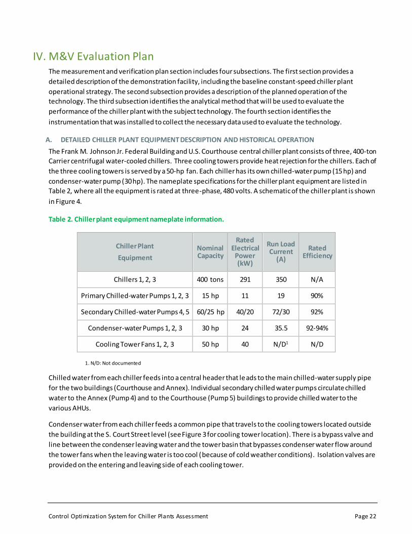
A. DETAILED CHILLER PLANT EQUIPMENT DESCRIPTION AND HISTORICAL OPERATION
The Frank M. Johnson Jr. Federal Building and U.S. Courthouse central chiller plant consists of three, 400-ton
Carrier centrifugal water-cooled chillers. Three cooling towers provide heat rejection for the chillers. Each of
the three cooling towers is served by a 50-hp fan. Each chiller has its own chilled-water pump (15 hp) and
condenser-water pump (30 hp). The nameplate specifications for the chiller plant equipment are listed in
Table 2, where all the equipment is rated at three-phase, 480 volts. A schematic of the chiller plant is shown
in Figure 4.
Table 2. Chiller plant equipment nameplate information.
Chiller Plant
Equipment
Nominal Capacity
Rated Electrical
Power (kW)
Run Load Current
(A)
Rated Efficiency
Chillers 1, 2, 3 400 tons 291 350 N/A
Primary Chilled-water Pumps 1, 2, 3 15 hp 11 19 90%
Secondary Chilled-water Pumps 4, 5 60/25 hp 40/20 72/30 92%
Condenser-water Pumps 1, 2, 3 30 hp 24 35.5 92-94%
Cooling Tower Fans 1, 2, 3 50 hp 40 N/D1 N/D
1. N/D: Not documented
Chilled water from each chiller feeds into a central header that leads to the main chilled-water supply pipe
for the two buildings (Courthouse and Annex). Individual secondary chilled water pumps circulate chilled
water to the Annex (Pump 4) and to the Courthouse (Pump 5) buildings to provide chilled water to the
various AHUs.
Condenser water from each chiller feeds a common pipe that travels to the cooling towers located outside
the building at the S. Court Street level (see Figure 3 for cooling tower location). There is a bypass valve and
line between the condenser leaving water and the tower basin that bypasses condenser water flow around
the tower fans when the leaving water is too cool (because of cold weather conditions). Isolation valves are
provided on the entering and leaving side of each cooling tower.

Control Optimization System for Chiller Plants Assessment Page 23
SPACE GAP
Figure 4. Schematic of the Frank M. Johnson Federal Building and U.S. Courthouse central chiller plant.
The chilled- and condenser-water distribution piping remained unchanged as a result of the control
technology installation, except for the automatic isolation control valves that were installed on the entering
and leaving sides of each cooling tower, as illustrated in Figure 4. It is unclear from interviews and
documents if any field-level cooling coil control valves (AHU cooling coils) or their associated piping were
replaced or modified (converted from three-way bypass piping to two-way). Field-level modifications can be
part of the control technology upgrades that are performed as part of the optimization. Figure 4 also shows
locations of new and existing VFDs and power metering, differential pressure, temperature, and flow
instrumentation.
Installation of the control technology was started in February 2012 and completed in June 2012. In addition
to the control technology, new VFDs were installed on each chiller’s primary chilled water and condenser
water pumps. VFDs already existed on the secondary chilled water pumps and the cooling tower fans
(assumed to be installed in 1998). Ultrasonic flow meters also were installed on the two secondary chilled-
water supply pipe loops that feed the Courthouse and the Annex buildings and on the primary chilled water
return loop. Additional instrumentation (i.e., temperature sensors, flow switches, and differential pressure
transducers) and isolation valves were installed as noted in Table 3. In addition, the existing Siemens BAS

Control Optimization System for Chiller Plants Assessment Page 24
software and hardware upgrades were performed to permit BAS integration with the new control
technology.
Discussions with site’s O&M operating staff and observations from site visits, mechanical print and BAS
sequence documents all highlighted the fact that the chiller plant was a constant-speed plant prior to the
installation of the control technology.
Previously, the chiller plant was controlled through the BAS to operate the number of chillers and pumps
required to satisfy the cooling loads in the two buildings. Due to legacy Heating, Ventilating, and Air
Conditioning (HVAC) design issues in the 1933-era Courthouse, the ability to economize (bring in cool
outside air) to satisfy comfort cooling requirements fully does not exist during winter and cool fall and spring
conditions (outside air temperatures < 55oF-65oF). Therefore, it is common to need mechanical cooling in
the Courthouse even during times when outdoor air temperatures are below 40oF. During cool outdoor
conditions like this, the need for chilled water is not as great or consistent, and return chilled water
temperatures can drop quickly (due to satisfied loads and cooling valves closing down). The setpoint for
supply water leaving the chiller does not always adjust automatically. As a result, the chiller(s) would short -
cycle and, in some cases, fail on any number of chiller safety trip events (typically low pressure).
The chiller plant is designed to provide a constant chilled-water supply temperature of 44°F. The secondary
chilled-water pump VFDs were operated to maintain a minimum loop differential pressure setpoint of 8–12
PSI. The VFD-driven cooling tower fans were controlled to deliver a constant Entering Condenser Water
Temperature (ECWT) of around 80oF–85oF. While this may be the expected summer operations when
outdoor wet-bulb temperatures are higher, this does not take advantage of lower wet-bulb temperatures
that often exist in the winter and cool fall and spring months. The cooling towers are equipped with basin
heaters (rated at 24 kW total capacity) to prevent freezing and allow for year-round operations.
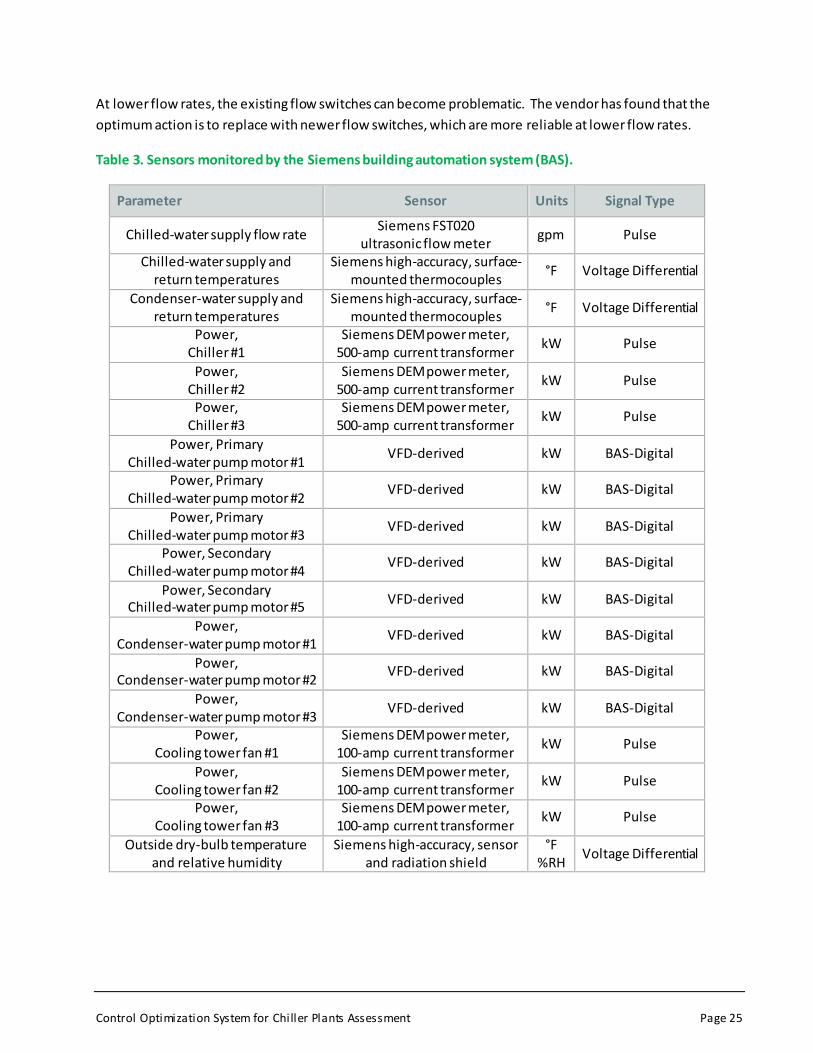
B. INSTRUMENTATION PLAN
The existing Siemens BAS was used to monitor and record data. Data collection included sensors that are
directly used in the various control loops for the chiller plant performance. A few additional sensors were
installed to validate chiller operation. Sensor data was measured every minute. Average sensor data was
recorded in 15-minute intervals. Table 3 identifies the sensors monitored and recorded by the BAS.
The primary sensors included 480-volt, three-phase Siemens digital energy monitor (DEM) power meters on
each chiller and cooling tower fan. Ultrasonic flow meters were installed on the two secondary chilled-water
supply loops to the Annex and Courthouse buildings, along with an ultrasonic flow meter in the primary
return water line. Differential pressure sensors were installed cross each condenser water pump and each
chilled water pump. In addition, newer high-accuracy temperature sensors were installed on the individual
leaving chilled water and condenser water lines from each chiller, a common return water line from the
chiller plant to the towers, a common supply water line from the towers to the chiller plant, a common
secondary loop supply temperature sensor, individual secondary return water temperature sensors, and a
secondary loop bypass temperature sensor.
Though not related to the primary instrumentation monitoring sensors and plan, new flow switches were
installed on each chiller’s condenser and evaporator piping loops. Standard flow switches are designed for
constant flow, but the addition of VFDs converted the chiller machines from constant flow to variable flow.
Control Optimization System for Chiller Plants Assessment Page 25
At lower flow rates, the existing flow switches can become problematic. The vendor has found that the
optimum action is to replace with newer flow switches, which are more reliable at lower flow rates.
Table 3. Sensors monitored by the Siemens building automation system (BAS).
Parameter Sensor Units Signal Type
Chilled-water supply flow rate Siemens FST020
ultrasonic flow meter gpm Pulse
Chilled-water supply and return temperatures
Siemens high-accuracy, surface- mounted thermocouples
°F Voltage Differential
Condenser-water supply and return temperatures
Siemens high-accuracy, surface- mounted thermocouples
°F Voltage Differential
Power, Chiller #1
Siemens DEM power meter, 500-amp current transformer
kW Pulse
Power, Chiller #2
Siemens DEM power meter, 500-amp current transformer
kW Pulse
Power, Chiller #3
Siemens DEM power meter, 500-amp current transformer
kW Pulse
Power, Primary Chilled-water pump motor #1
VFD-derived kW BAS-Digital
Power, Primary Chilled-water pump motor #2
VFD-derived kW BAS-Digital
Power, Primary Chilled-water pump motor #3
VFD-derived kW BAS-Digital
Power, Secondary Chilled-water pump motor #4
VFD-derived kW BAS-Digital
Power, Secondary Chilled-water pump motor #5
VFD-derived kW BAS-Digital
Power, Condenser-water pump motor #1
VFD-derived kW BAS-Digital
Power, Condenser-water pump motor #2
VFD-derived kW BAS-Digital
Power, Condenser-water pump motor #3
VFD-derived kW BAS-Digital
Power, Cooling tower fan #1
Siemens DEM power meter, 100-amp current transformer
kW Pulse
Power, Cooling tower fan #2
Siemens DEM power meter, 100-amp current transformer
kW Pulse
Power, Cooling tower fan #3
Siemens DEM power meter, 100-amp current transformer
kW Pulse
Outside dry-bulb temperature and relative humidity
Siemens high-accuracy, sensor and radiation shield
°F %RH
Voltage Differential
Control Optimization System for Chiller Plants Assessment Page 26
SPACE GAP
C. TEST PLAN
A monitoring plan was created to collect data on the chillers, chilled- and condenser-water pumps and
cooling tower fans. The cooling plant performance data was collected from January 2013 through August
2013. The data were used to determine the performance of the chiller plant under various load conditions.
The data for determining thermal performance were monitored and stored using the site’s BAS provided by
Siemens. This data was uploaded periodically for independent review to ensure completeness (no holes, no
“stale” data). Once the data was validated, it was stored for future analysis. Anomalies in the data were
reviewed with the site staff to ensure completeness or make provisions to account for operational issues.
Further, since the site did not provide any data for the chiller plant prior to the ARRA-funded improvements,
there was no way to validate the actual pre-technology improvement period. Therefore, it was determined
that GSA would configure the chiller plant to simulate a “winter” season and a “summer” season (to the
extent possible) by configuring equipment and controls to operate in a manner that simulated the pre -
technology operations. This simulation period was performed in March (winter operations) and August
(summer operations) of 2013. The simulation period was supposed to be 2 weeks (14 days), but, in both
cases, the simulation period was closer to 12 days. The results of this simulation will be discussed later.

Control Optimization System for Chiller Plants Assessment Page 27
V. Results The results section is divided into four sections. The first section highlights the impacts of the control
optimization system technology. The second and third sections describe the baseline (before) and post-
installation (after) performance profiles of the chiller plant resulting from the monitored data, respectively.
The fourth section extrapolates from the observed data and findings to identify additional opportunities for
improving the performance of the chiller plant both for the monitored location, as well as for potential other
applications in GSA’s portfolio.
A. PRE- AND POST-INSTALLATION CHILLER PLANT PERFORMANCE
Figure 5 highlights the improved performance (lower kW/ton) when building cooling loads are less than 400
tons.
Figure 5. Pre- and post-installation power and load comparison for 2 chillers.
In Figure 5, the green line shows performance relative to an efficacy of 0.75 kW/ton. As loads increase above
500 tons, the kW/ton efficiency of the pre-technology simulation and post-technology operations begin to
converge.
Figure 6 highlights the improved performance (lower kW/ton) when building cooling loads are less than 400
tons.

Control Optimization System for Chiller Plants Assessment Page 28
SPACE GAP
Figure 6. Pre- and post-installation power and load comparison for the entire chiller plant.
In Figure 6, the green line shows performance relative to an efficacy of 0.75 kW/ton. It is of particular
interest to see that loads less than 500 tons show the greatest improvement (reduced kW/ton).
While the data suggests some separation, things start to converge at loads greater than 500 tons. Higher
loads demand that the energy to move more chilled water and condenser-water also increases. Tower fan
speeds also increase due to higher wet-bulb temperatures when these higher-load conditions are seen.
Thus the convergence.
However, during lower-load conditions, the ability to vary pump speeds (speed reduction) is evident. This
highlights the technology’s benefit when lower-load periods prevail.

Control Optimization System for Chiller Plants Assessment Page 29
SPACE GAP
B. CHILLER PLANT POST-INSTALLATION AVERAGE PERFORMANCE PROFILE
As Figure 7 shows, between 9 AM until almost 6 PM over the 8-month monitoring period, a conservative
decrease in energy of 60 kW can be seen once the control optimization system technology was installed.
Figure 7. Pre- and post-installation power comparison for the chiller plant time averaged over the 8-month monitoring period (Jan. 2013 through Sept. 2013).
Chiller Plant average kW Red = Pre-Simulation, Blue = Post
C. CHILLER PLANT POST-INSTALLATION DAILY PERFORMANCE PROFILE
Figure 8 shows the monitored hourly chiller plant performance post-installation for each day of the week,
including holidays.
This area (green box) represents approximately 60 kW load reduction (on average) between 8 AM and 6 PM.

Control Optimization System for Chiller Plants Assessment Page 30
Figure 8. Daily performance of the chiller plant post-installation.
s
The daily profiles shown in Figure 8 should match the profile shown in Figure 7 (post-installation blue line).
When averaged together (including weekends and holidays), the results closely match Figure 7.
Figure 8 data suggests potential additional opportunities for improvement, either in the site operations or in
the control optimization system (or both).
Federal holidays show power consumption at levels approaching occupied weekday periods. The
holiday period closely represents the average for all occupied time periods (Figure 7).
Sunday nights and holiday nights indicate that energy is being consumed after 8 PM (all night), and
Monday mornings show significant energy consumption from midnight until 5 AM. This is assumed
to be related to O&M staff overrides through the BAS controls.
The holiday and weekday morning cool down period from 6 AM until 8 AM shows a higher demand
spike than the rest of the 24-hour period. This may be due to the higher demand required for
cooling down a warm loop or building, or it may be some other anomaly in the controls, etc. A
morning spike as shown is not abnormal, followed by a decline through the mid-morning period.
However, an afternoon spike also would be expected for a building with a high afternoon cooling
load (like Montgomery, Alabama), but the data does now show this.
The weekend period shows what would be expected for a typical morning cool down with an
afternoon spike, before shutting down in the early evening. These data plots may indicate extreme

Control Optimization System for Chiller Plants Assessment Page 31
over-cooling of the building during weekday morning periods. This should be evaluated for further
improvement potential if this operation is occurring without merit.
D. WAYS TO FURTHER IMPROVE CHILLER PLANT PERFORMANCE
Methods to improve chiller plan performance, discussed below, are relative to observations made of the
Frank M. Johnson Jr. Federal Building and U.S. Courthouse chiller plant. These methods also should be
considered relative to other chilled water plant operations with similar design (water-cooled chillers using
cooling towers) applications. The efficiency of a chiller plant is a relative function of three primary variables:
Cooling tower leaving water temperature setpoint reset: The optimal cooling tower water
temperature to the chillers is a function of the outdoor air wet-bulb temperature (OAWBT), which is
often overlooked in the automatic control sequences. As OAWBT increases, the cooling towers
must work harder to maintain the desired entering condenser water temperature (ECWT) setpoint.
Due to chiller designs and the need to maintain a maximum compressor lift (delta between entering
condenser water and leaving chilled water temperatures), the cooling tower fans will run at
maximum capacity, when required. This is seen in the warmer/humid summer days. However,
during cooler/dryer conditions, as the OAWBT values decrease, the cooling towers can be
automatically managed (by resetting the ECWT setpoint) to run more efficiently. In some cases, the
OAWBT is sufficiently low to allow for an automatic setpoint reset that drives the ECWT even lower,
without incurring higher costs (increased tower fan power penalties) that exceed the savings at the
chiller compressor. Unfortunately, this improvement opportunity is often overlooked.
Chilled-water supply temperature setpoint reset: When values are set too low for the actual load
requirements, the over-cooling of chilled water impacts the chilled water plant (increased tower
loading, greater refrigerant lift requirements for the compressor motors, and greater potential for
zone/space over-cooling), resulting in excess reheating and occupant complaints. Automated resets
should take into account true load conditions that reflect demand and help optimize chiller lift. It
also is imperative that humidity sensors are accurately calibrated and maintained. If not done
correctly, this strategy can transfer energy to AHU fans across the building.
Improved Optimal Equipment Runtime: Equipment run-time is often based upon automatic
scheduling for daily load requirements, automatic override for setback requirements, and finally,
operator override based upon perceived need or load, to which the BAS control did not adequately
respond or was not allowed the opportunity to respond. When chiller plants are run beyond their
“expected” hours of operations, based on “perceived” need or often for “just-in-case” scenarios,
this also results in system inefficiencies and additional energy consumption, increased wear-and-
tear, and shorter lifespans of critical and expensive equipment. Control optimization system’s
control sequences are designed to mitigate chiller and pump short-cycling. The minimum run-time
values provided in the updated control sequences may be helping to decrease equipment short
cycling, but they also could be creating added efficiency losses by running pumps longer than
needed or required (pumping systems were observed to be running when no load is apparent
before the building occupancy period begins or long after it ends). All the pumps and tower fans are
VFD-driven and VFDs offer soft-start capabilities, which should lessen impacts due to frequent
cycling of pumps. Minimum run-time values should be evaluated for possible reduction.

Control Optimization System for Chiller Plants Assessment Page 32
COOLING TOWER LEAVING WATER TEMPERATURE SETPOINT RESET
In general, lowering the ECWT will reduce the refrigerant head pressure, thereby reducing the load on the
compressor and raising the COP (Thumann 1991). The potential improvement in COP is dependent on the
type of refrigeration compressor. Further, the type of refrigeration compressor and type of load control
mechanism will limit the extent that this strategy can be employed. For conventional centrifugal chillers,
Thumann (1991, p 1538) estimates the increase in COP to be around 0.4% per 1°F reduction in the ECWT.
Cooling tower equipment designs and level of maintenance also will impact the strategy that can be used to
achieve an optimal ECWT. The cooling tower’s design approach will impact the ability to optimize the ECWT
seen by the chillers. The design approach is the difference between the OAWBT and the cooling tower’s
evaporative cooling capacity, which can be as much as 8°F–10°F. This means that OAWBT values of 70°F will
result in ECWT values of 78°F to 80°F. The design approach assumes that the tower cells, spray nozzles , and
other flow devices are properly maintained along with good water treatment and filtration.
During periods of low OAWBT conditions (< 55°F), the controls should be configured to take advantage
automatically of the opportunity to provide lower ECWT. Manufacturer specifications should be reviewed
before employing this strategy. Lowering the ECWT too much may have adverse effects on the compressor
operation with regard to head pressure and surging in certain makes and models of centrifugal compressors.
The chiller manufacturer can assist in determining the lower (and upper) limit for the ECWT. Trying to
maintain a lower condensing water temperature can be achieved (or at least attempted), but this may come
at the expense of higher tower fan speeds and increased tower fan energy consumption. This needs to be
balanced with savings that can be achieved at the chiller equipment, based upon consultation with the
chiller vendor’s recommendations.
8 8 Based on constant condenser pumping. Variable condenser pumping can increase chiller efficacy 1 -2%.

Control Optimization System for Chiller Plants Assessment Page 33
Figure 9. Post-installation monitored condenser-water temperature versus outdoor air temperature.
The orange dashed line shown in Figure 9 indicates the minimum cooling tower leaving water temperature
setpoint (assumed) as the condenser water leaving temperature (COND-ST/purple line) hovers near this
value, even during cooler OA dry-bulb (OA-TEMP/red line) conditions.
The orange box in Figure 9 indicates the optimum outdoor air temperature (OAT) value that would allow for
minimum temperature setpoint for the cooling tower leaving water (if a reset were implemented). This
would typically be during the months of October–April. Conversely, if the ECWT is not reset, based upon the
dynamic OAWBT values, the tower fans may be forced to operate at full speeds, with no benefit relative to
the actual achievable setpoint (not being reset upwards as the OAWBT value concurrently increases, as seen
in the May-September time frame).
The Frank M. Johnson buildings do not have an OAWBT sensor, but the value can be calculated from their
outdoor temperature and outdoor humidity sensors (as shown in Figure 10).

Control Optimization System for Chiller Plants Assessment Page 34
Figure 10. Post-installation monitored condenser water supply temperature versus outdoor air wet bulb
temperature.
Presently, the chiller plant with control optimization is achieving a 65°F minimum temperature value, as
illustrated in Figure 10. Occasionally, the condenser water temperature (red line) can be seen dropping
below 65°F (as low as 60°F).
However, at lower wet-bulb temperatures and lower cooling loads, the ECWT exhibits a large variance and
deviates from the 65°F temperature, as indicated by the calculated OAWBT (blue line) compared to the
assumed cooling tower leaving water temperature setpoint (solid green) in Figure 10. It may be possible to
further reduce the ECWT. As mentioned previously, the chiller manufacturer should be consulted to
determine the allowable low limit before this possible improvement is pursued.
Based on the trended condenser water temperature performance, the setpoint over the eight months of
monitored operations is assumed to be near 65oF. Only during the March pre-installation simulation testing
did the condenser ECWT drop below 60oF. This was assumed to occur because of the simulated 100% tower
fan speeds, but may have been caused by other configuration parameters that existed in the controls prior
to the optimization technology installation.
Over-cooled condenser water temperatures can lead to chiller surging and other unwanted anomalies. One
of the benefits of control optimization is the ability to run cold condenser water temperatures while
maintaining chiller lift, thus avoiding chiller surging. During warmer weather, the delta between the OAWBT
and the condenser supply temperature is between 5oF –8oF, which indicates an appropriate cooling tower
system approach design.

Control Optimization System for Chiller Plants Assessment Page 35
Figure 11 shows the fan power for the three cooling tower VFD-driven fans and peak power is noted as
approximately 20 kW per cooling tower fan. When OAWBT values are predominantly less than 60°F (Black
Box), the cooling tower fan kW consumption (red, green and purple lines) indicates lower values and less
frequent in duration. When OAWBT values are predominantly between 60°F and 70°F (yellow box), the
values increase, as well as the duration. Once the OAWBT values are consistently greater than 70°F (Light
Blue Box, June through August), the cooling tower fans all appear to be running near-simultaneously and
near their maximum load values.
Figure 11. Post-installation monitored cooling tower fan power demand versus OAWBT.
It is assumed that if the cooling tower leaving water temperature setpoint were configured to increase
automatically according to the OAWBT, this would better match the tower fan energy consumption to the
tower’s design capabilities (versus running tower fans at full speed with no benefit for the energy being
expended to meet a setpoint that is physically not attainable).
With VFD-operated tower fans and staged towers (via individual tower isolation valves), the ability to match
part-load tower capacity should be evaluated (cooling tower leaving water temperature setpoint reset). The
O&M staff on site should evaluate the cooling tower BAS or control optimization system controls for an
automatic reset of the leaving water temperature setpoint.
CHILLED-WATER SUPPLY TEMPERATURE SETPOINT RESET
Another method to improve chiller plant performance is to increase the chilled-water supply temperature
(chWST) during low-load conditions. Raising the chilled-water supply temperature will allow the evaporator
refrigerant pressure to be increased, thereby reducing the load on the compressor and raising the COP
(Thumann 1991). The potential improvement in COP is dependent on the type of refrigeration compressor.
Further, the type of refrigeration compressor and load control will limit the extent this strategy can be
employed. For conventional centrifugal chillers, Thumann (1991, p 155) estimates the increase in COP to be
around 2% per 1°F increase in the chilled-water supply temperature.

Control Optimization System for Chiller Plants Assessment Page 36
The primary concern with increasing the chilled-water temperature is the potential reduction in the ability
to dehumidify. Under design conditions, chilled-water supply temperatures are kept excessively low to allow
the cooling coil also to act as a dehumidifier by lowering the air temperature to the point where moisture
condenses out of the air stream. However, when air does not need to be dehumidified, there should be a
lower demand for excessively low chilled-water temperatures. These lower demand conditions also should
exist during cool spring and fall months (winter/heating).
As can be seen in Figure 12, the monitored period of chilled water supply temperatures indicates that the
chiller plant was producing approximately 42°F –43°F chilled water temperatures. As already noted, these
temperatures observed in the January to the April or May time frame appear to be too cold. An automatic
chilled water supply temperature setpoint reset is highly encouraged.
Figure 12. Post-installation monitored chilled water supply temperature.
p
Control Optimization System for Chiller Plants Assessment Page 37
VI. Summary Findings and Conclusions The summary findings and conclusions are discussed below, including information on best practices to assist
in optimizing chiller plants. The barriers to technology adoption and market potential also are discussed.
Finally, this section provides recommendations regarding the future installation of the technology and the
importance of a measured baseline.
A. OVERALL TECHNOLOGY ASSESSMENT AT THE DEMONSTRATION FACILITY
The application of the control optimization system technology offers the potential for reducing energy
consumption in space cooling applications by optimizing variable-speed chiller plant equipment (primarily
pumps), leading to increased chiller plant efficiency. In general, the operating efficiency of a typical water-
cooled chiller plant with the new control technology is estimated by the vendor to be around 0.6 kW/ton,
resulting in an average annual energy reduction between 25% and 50%. Factors impacting the actual
performance include climate zone, building type, hours of occupancy, and other part-load impacts.
The average chiller plant efficiency throughout this demonstration was 0.64 kW/ton, with a projected
annual energy savings of 35%. Due to the limited data set from the brief Manual Mode period, the
projected savings has a confidence level of 80%, resulting in a total uncertainty of (+/-) 10.8%. This means
the projected savings could be as low as 24.2% or as high as 46.8%.
On a weather-normalized basis, the resulting analysis estimates the data point will reduce the chiller plant
energy consumption from a projected baseline value of 1,495.96 MWh/yr to a projected value of 972.51
MWh/yr, with an energy savings of 523.44 MWh/yr, or 35%, over the projected baseline.
The annualized cost savings are projected to be $42,485. With the level of uncertainty already noted, the
annualized cost savings varies from $28,962 to $56,009. Based on the performance data collected and
evaluated from the Frank M. Johnson Jr. Federal Building and U.S. Courthouse demonstration, control
optimization is projected to be capable of achieving its performance claims.
It is recommended that the energy and cost savings associated with the technology be evaluated for
variable-speed chiller plants that already have the required VFDs installed, thereby reducing the total
installed costs (and becoming economically more viable). However, the potential energy savings for variable-
speed chiller plants is likely to be lower than for the constant-speed chiller plant evaluated in this
demonstration because it is expected that most BAS configurations applied to chiller plants will have some
energy-saving attributes (e.g., temperature and pressure resets) already embedded.
Based on the economic assessment for this demonstration, the targeted deployment of the control
optimization is recommended only where a site-specific engineering analysis determines that the
technology is likely to be life-cycle cost effective. Specific guidance for targeted deployment of this
technology is provided in Section VI.D.
This demonstration’s projected energy savings is in the mid-range of the 25% to 50% reported savings range,
so it is unlikely that additional energy savings alone will make this technology cost-effective. However,
control optimization should be evaluated for other locations where energy rates are high and installed costs
can be reduced, or where utility rebates can be obtained to help further reduce the overall installed costs. In
addition, the deployment of the technology for variable-speed chiller plants, which would not require the
Control Optimization System for Chiller Plants Assessment Page 38
costly VFD upgrades, should be evaluated for life-cycle cost-effectiveness (with the further assumption that
the variable speed chiller plants are already enjoying significant energy and cost-savings, thereby impacting
the economics).
B. BEST PRACTICES
IMPROVED LOOP DELTA-T
A chiller plant needs to be capable of meeting the building’s peak demand, as well as operating efficiently
under part-load conditions. A chiller plant with control optimization offers excellent part-load efficiency
because of the integration of VFDs into the optimized pump and cooling tower fan operations. One means
of measuring part-load efficiency is to evaluate the different pumping loop Delta T values.
Delta T has been the subject of much discussion in the HVAC industry. “Low Delta T” syndrome, in
particular, is an undesirable condition that afflicts many chilled water plants, for many reasons.
The chiller plant using control optimization in this study showed Delta T values that ranged from 8°F –18°F.
The chilled water loop Delta T values (primary and secondary) were consistently found to be operating
above 10°F, even during part-load (and low-load) conditions. This is significant because it indicates the
chiller equipment is seeing a good load and operating in a range that most likely offers the greatest
efficiency performance for the chiller(s). It is not uncommon to find chiller plants across the country
operating with Delta T values that are less than 5°F.
In addition, while the chiller plant with the new control optimization technology was highly efficient at part-
load, there is still room for additional improvement, and some of the best practices discussed below may
apply.
DASHBOARD FEEDBACK
In general, BASs provide an optional dashboard that is capable of providing considerable feedback to the
operator on the equipment’s operating conditions. GSA’s Facilities Standards for the Public Buildings Service
(P100) specifies that new chillers must provide input/output (kW/ton) information, as well as monitoring
energy consumption (GSA 2010).
The BAS system in the chiller plant evaluated in this study provides such an interface for displaying chiller
plant performance in kW/ton. However, it is recommended that the dashboard be programmed to include
trending the kW/ton versus plant load to provide long-term performance feedback. This will require minimal
effort, and no hardware procurements are required. Trending the kW/ton of the chiller plant’s chilled -water
pumps, condenser-water pumps, and cooling tower fans would provide useful insight regarding the
performance of the equipment relative to the entire chiller plant. Trending (and alarming) loop Delta T
values that persist below lower limit values (<3°F–5°F) will alert operations staff to unwanted and harmful
anomalies. This information will allow operators to better optimize the chiller plant operation, configure
alarms for “out-of-normal” operations (such as the low chilled water Delta T issues), or be alerted to
unwanted equipment configurations where a VFD-driven pump is placed in Manual Mode operations at the
VFD, resulting in lack of control from the BAS. This actually occurred at the demonstration site and ran the
pump 24/7 for over three weeks. The historical data was being reviewed when this condition was found and
restored to normal.
Control Optimization System for Chiller Plants Assessment Page 39
GSA has invested in its own dashboard of sorts. This technology is called GSALink and is part of the
Intelligent Buildings initiative. Sites like the Frank M. Johnson Federal Building and U.S. Courthouse should
be evaluated for possible inclusion into the GSALink system (if not already included). This would provide for
automatic fault detection and analysis of not only the chilled water plant (and the control optimization
system technology), but also of all the other major building HVAC systems.
C. BARRIERS AND ENABLERS TO ADOPTION
The most recognized barriers to this technology include cost, familiarity, training, and procurement
specification issues. The control optimization system requires VFDs on all chiller plant equipment for
upgrading constant-speed chiller plants, a requirement that may be costly. Some older motors that serve
pumps or tower fans may not be able to accept VFD technology, which may limit the application of the new
optimization technology when procuring newer motors is not possible. Because the technology is modular,
it can be installed on parts of the chiller plant, such as the condenser water distribution system.
Conventional constant-speed chiller plant operators are likely to be resistant to the “variable flow”
operating approach associated with this new technology and, therefore, training will be crucial to the
success of this technology’s adoption. Operators should be trained on how control optimization saves
energy, so that they fundamentally understand why operating variable-speed pumps and variable-speed
tower fans at part load is more efficient than at full load.
Procurement and specification issues may still be a potential barrier to widespread deployment. The
optimization technology is offered by only one vendor, who also happens to own and distribute its own BAS
system. It is not clear if more competition from other vendors will be forthcoming in the future. The vendor
whose technology was used in this study claims that its control optimization system will interface with
almost any other BAS vendor system. In many cases, an integration package may be required to allow the
optimization technology to communicate with (integrate to) non-Siemens BAS systems. To date, control
optimization has been installed at 27 federal sites—with two sites using Tridium controls and one site using
JCI controls.
D. MARKET POTENTIAL WITHIN THE GSA PORTFOLIO
The control optimization technology claims to be capable of integrating into almost any centrifugal chiller
plant that utilizes multiple chillers. While this analysis did not concern itself with this claim (see BARRIERS ,
above), this technology is suitable for new construction and retrofit applications alike. Thi s technology lends
itself particularly well to retrofit applications because upgrading an existing chiller plant to include the
control software and VFDs can be accomplished without waiting for the current equipment to fail or be
replaced.
GSA sites with chiller plant operating efficiency problems, low-load problems or low Delta-T syndrome
problems should all be screened initially for possible use of this technology.

Control Optimization System for Chiller Plants Assessment Page 40
This technology is recommended for potential deployment for locations that meet the following guidelines9:
Electricity rates ($/kWh) in the top 50% of GSA’s portfolio (> $0.10/kWh blended rate)
BACnet-enabled BAS (versions more than five years old will require additional programming)
Cooling season or process loads that require chillers to operate 8–10 months a year or longer
Buildings having cooling loads greater than 500 ton-hours/day, 3 million tons per year
New construction facilities that meet above criteria10
Existing central plants with three or more constant-speed centrifugal chiller flow systems
(primary/secondary pumps, condenser pumps and cooling tower fans)
In addition, deployment of control optimization at locations with the following characteristics are not likely
to be cost-effective:
Electricity rates ($/kWh) in the bottom 50% of GSA’s portfolio
The cooling season requires chiller to operate six months or less based on a typical meteorological
year (TMY)
Insufficient resources are available to identify the number of cost-effective candidates throughout GSA’s
portfolio of buildings. It is recommended that control optimization be part of a recommended suite of
possible chiller technologies for consideration during facility energy assessments, which are required by EISA
for every covered GSA facility every four years11 (EISA 2007).
It is estimated that the market potential within GSA for the application of chiller plants with the new
optimization technology could reduce annual energy consumption by around 281,275 MMBTU. Based on
GSA’s average utility pricing, this equates to annual savings of $9,008,688. This estimate is based on the
following assumptions:
9 Prior to installing the technology, a detailed site-specific engineering analysis is recommended, which should include a monitored baseline for the existing chiller plant, as well as ease-of-integration into the site’s BAS.
10 This assessment was not intended to determine if the studied optimization technology would be cost-effective for new variable-speed chiller plants. It is recommended that variable-speed chiller plants be evaluated using a detailed engineering analysis, including a monitored baseline.
11 EISA section 432 requires agencies to identify their facilities that constitute at least 75% of the agency's facility energy use, also referred to as “covered facilities,” and complete comprehensive energy and water evaluations of 25% of covered facilities each year, so that an evaluation of each facility is completed at least once every four years (Reference: FEMP web site at http://www1.eere.energy.gov/femp/regulations/eisa.html).

Control Optimization System for Chiller Plants Assessment Page 41
GSA Chilled Water Consumption – 803,643 MMBTU (10,045,532 total GSA energy use (EUAS, 02/16);
10% for Cooling (CBECS 2012) 80% for Chillers (chillers provide majority of conditioning for buildings
> 200,000 ft2, EIA 2003).
Chiller plants using the demonstrated control optimization system technology can reduce space
cooling energy consumption by an estimated 35% compared to constant-speed chiller plants
(consistent with the findings in this report).
GSA average electricity price, $0.1092 kWh, EAUS FY2015.
E. RECOMMENDATIONS FOR INSTALLATION, COMMISSIONING, TRAINING, AND CHANGE MANAGEMENT
As for any new control optimization technology, it is recommended that measurement and verification of
performance be tracked to ensure energy savings and operational claims are met and maintaine d
continually. Attention should be paid to ensure the appropriate sequencing of equipment is occurring and
that the sequence is optimized based on the particular profile of the chiller plant. A convenient dashboard is
typically provided in conjunction with this technology; the dashboard is capable of long-term trending and
performance tracking to meet this need. Since this control technology relies on sensor measurements as
input for controlling the operation of the chiller plant, it is recommended that sensors be checked for
calibration annually.
The capabilities of the technology (including chilled-water reset, condenser-water reset and maximized part-
load efficiency) need to be utilized to their full extent at each site to ensure optimum energy savings are
attained.
Control Optimization System for Chiller Plants Assessment Page 42
Generally speaking, equipment life tends to be related more to load hours than operating hours. In other
words, equipment life depends more on how hard the equipment works, as compared to how long it runs.
Therefore, although the application of the optimization technology will increase the operating hours for the
chiller plant equipment, the load hours on the individual equipment may be decreased due to reduced
speed operation of pumps and tower fans. Control optimization technology requires VFDs, which in general,
reduce wear associated with equipment start-up.
Therefore, the O&M costs associated with deploying the new optimization technology are not expected to
increase. However, equipment should be monitored periodically for unexpected degradation in
performance. Also, ongoing O&M costs should be tracked and periodically compared to historic records.
F. IMPORTANCE OF BASELINE MEASUREMENT AND DOCUMENTATION
The control optimization technology was installed prior to this demonstration. Therefore, a monitored
baseline was not available. Prior to the installation of the technology, baseline estimated data for the
constant-speed chiller plant was estimated by the vendor, based upon a snapshot of the plant’s
performance and the vendor’s internal modeling software.
The lack of a reliable and accurate monitored baseline required the development of a baseline that may vary
from the real-world baseline performance, as a result of the multiple technical assumptions, which may or
may not be completely accurate or valid. It is recommended that future evaluations include a monitored
baseline, sufficient in duration to characterize properly and fully the energy performance profile of the
system under examination, thus providing a more reliable basis for comparison and more accurately
determining energy and cost savings estimates.
Investing in a more accurate baseline (preferably developed by an independent source) likely would have
supported a better conclusion regarding the potential cost-effectiveness of this technology. The simulated
peak-power baseline developed for the assessment of the optimization technology does not likely accurately
represent the true baseline performance profile of the chiller plant prior to the installation of the
technology. The error associated with this baseline cannot be accurately determined.

Control Optimization System for Chiller Plants Assessment Page 43
VII. Appendices
A. LIST OF ABBREVIATIONS AND SYMBOLS
The following is a list of abbreviations and symbols used throughout this report.
Term Description
AHRI Air Conditioning, Heating and Refrigeration Institute
A, amp ampere (electric current)
ANSI
ASHRAE
American National Standards Institute
American Society of Heating, Refrigerating, and Air Conditioning Engineers
ARRA American Recovery and Reinvestment Act of 2009
BAS building automation system
Btu British thermal unit
Btu/h British thermal units per hour
CBECS Commercial Buildings Energy Consumption Survey
CFM cubic feet per minute
CH
CHW
CHP
ChWST
COP
Chiller
Chilled water
chilled-water pump
chilled water supply temperature
coefficient of performance, a unitless measure for efficiency
Cp specific volume, Btu/lbm-°F
CWP condenser-water pump
DEER
DOD
Database for Energy-efficient Resources
Department of Defense
DOE U.S. Department of Energy
ECIP Energy Conservation Investment Program
ECWT
EIA
entering condenser-water temperature
U.S. Energy Information Agency
EISA Energy Independence and Security Act of 2007
FEMP U.S. DOE Federal Energy Management Program
gal gallon
GPG Green Proving Ground
gpm, GPM gallons per minute
GSA U.S. General Services Administration
h, hr hour
hp, Hp horsepower
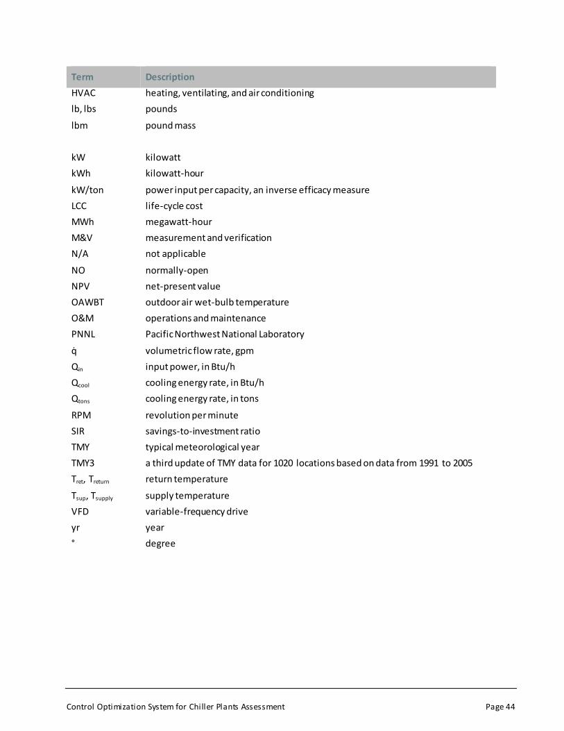
Control Optimization System for Chiller Plants Assessment Page 44
Term Description
HVAC heating, ventilating, and air conditioning
lb, lbs pounds
lbm pound mass
kW
kilowatt
kWh kilowatt-hour
kW/ton power input per capacity, an inverse efficacy measure
LCC life-cycle cost
MWh
M&V
N/A
megawatt-hour
measurement and verification
not applicable
NO
NPV
OAWBT
normally-open
net-present value
outdoor air wet-bulb temperature
O&M operations and maintenance
PNNL Pacific Northwest National Laboratory
q̇ volumetric flow rate, gpm
Qin input power, in Btu/h
Qcool cooling energy rate, in Btu/h
Qtons cooling energy rate, in tons
RPM
SIR
TMY
revolution per minute
savings-to-investment ratio
typical meteorological year
TMY3 a third update of TMY data for 1020 locations based on data from 1991 to 2005
Tret, Treturn return temperature
Tsup, Tsupply supply temperature
VFD variable-frequency drive
yr
°
year
degree
Control Optimization System for Chiller Plants Assessment Page 45
B. REFERENCES
ASHRAE 2010. Energy Standard for Buildings Except Low-Rise Residential Buildings, ASHRAE Standard 90.1-
2010, American Society of Heating, Refrigerating and Air Conditioning Engineers, Atlanta, GA.
ASHRAE 2012. 2012 ASHRAE Handbook, Heating, Ventilating, and Air-Conditioning Systems and Equipment.
American Society of Heating, Refrigerating and Air Conditioning Engineers, Atlanta, GA.
Doty, S and W Turner. 2009. Energy Management Handbook. 7th ed. The Fairmont Press, Atlanta, GA.
Energy Independence and Security Act (EISA) of 2007. Public Law 110-140.
EIA 2003a. Commercial Buildings Energy Consumption Survey. Table 8. Types of Heating Equipment Used in
Office Buildings, 2003, U.S. Energy Information Administration, Washington, DC,
http://www.eia.gov/emeu/cbecs/cbecs2003/officereport/office3.html, last accessed 10/17/2012.
EIA 2003b. Commercial Buildings Energy Consumption Survey: Energy End-Use Consumption Tables, Table
E.1. Major Fuel Consumption (Btu) by End Use for Non-Mall Buildings, 2003, U.S. Energy Information
Administration, Washington, DC, http://www.eia.gov/emeu/cbecs/cbecs2003/detailed_tables_2003/
2003set19/2003pdf/e1-e11.pdf, last accessed 10/17/2012.
FEMP 2010. Annual Report to Congress on Federal Government Energy Management and Conservation
Programs Fiscal Year 2007, U.S. Department of Energy, Washington DC,
http://www1.eere.energy.gov/femp/pdfs/annrep07.pdf, last accessed on 10/17/2012.
GSA 2010. Facilities Standards for the Public Buildings Service, P100, U.S. General Services Administration,
Washington DC, www.gsa.gov/P100, last accessed 10/17/2012.
Thumann, A. 1991. Energy Conservation in Existing Buildings Deskbook. A. Thumann, Editor. The Fairmont
Press, Atlanta, GA.
Westphalen, D. and S. Koszalinski. 2001. Energy Consumption Characteristics of Commercial Building HVAC
Systems, Volume 1: Chillers, Refrigerant Compressors, and Heating Systems. Arthur D. Little, Inc. Cambridge,
MA.
Control Optimization System for Chiller Plants Assessment Page 46
C. GLOSSARY
The following is a glossary of advanced terminology in support of this report.
Terminology Description
Affinity laws A set of three mathematical equations that define the relationship between rotational speed, flow rate, pressure rise, and brake horsepower for centrifugal systems.
Air-cooled chiller A refrigerating machine in which heat removal is accomplished entirely by heat absorption by air flowing over condensing heat exchanger surfaces (condenser is air cooled).
Air-handling unit A device used to condition and circulate air as part of a heating, ventilating, and air-conditioning (HVAC) system
Annual load profile
A measure of the time distribution of thermal or other energy loads, such as Btu/h, for a system over the course of a year.
Baseline Typically referring to an energy profile, model and/or characteristics before changes have been made to a system for the purpose of modeling the original operating condition, derived from measurements are taken over a period of time and used as a basis for comparison to one of more options or alternatives.
Bin data A data pre-processing technique used to reduce observation errors.
Building automation system (BAS)
A computerized network of electronic devices designed to monitor and control the mechanical, electronics, and lighting systems in a building.
Capacity Intended technical full-load (a.k.a., maximum) sustained output of a facility, system, or device. Typically quantified as a power rating or rate of energy transfer. May also be known as nameplate capacity, rated capacity, nominal capacity, or installed capacity.
Central chiller plant
A single or common chilled-water facility consisting of one or more chillers used to serve one or more facilities.
Centrifugal compressor
A dynamic (or non-positive-displacement) compressor that uses rotational (centrifugal) forces to raise pressure in the refrigerant system.
Chilled-water pumps
Pump and motor system used to circulate chilled water for space or process cooling distribution systems.
Chilled-water return temperature
The temperature of the chilled water entering the evaporator or returning from the facility distribution system.
Chilled-water supply temperature
The temperature of the chilled water leaving the evaporator or being supplied to the facility distribution system.

Control Optimization System for Chiller Plants Assessment Page 47
Terminology Description
Chilled-water temperature reset
An operating strategy in which the chilled water supply temperature setpoint is varied in response to a control signal or varying sensor input.
Chiller A machine that removes heat from a liquid via a vapor-compression or absorption refrigeration cycle.
Climate zone A region with similar weather characteristics.
Coefficient of Performance (COP)
The ratio of the heating or cooling provided divided by the electrical energy consumed, as a unitless measure. The COP provides a metric of performance for heat pumps that is analogous to thermal efficiency for power cycles.
Commission (commissioning process)
A quality focused process for enhancing the delivery of a project. The process focuses upon verifying and documenting that the facility and all of its systems and assemblies are planned, designed, installed, tested, operated, and maintained to meet the Owner's Project Requirements.
Condenser The part of a refrigerant system where refrigerant is liquefied by removal of heat through use of a heat sink.
Condenser-water temperature
The temperature of the water departing the cooling tower and/or entering the water-cooled condenser.
Condenser-water temperature reset
An operating strategy in which the condenser-water temperature setpoint is varied in response to a control signal or varying sensor input.
Condensing coil A heat exchanger in which the refrigerant rejects heat to the point where the refrigerant condenses from vapor to liquid.
Condenser-water pump
Motor-driven pump used to circulate water through the condensing system
Constant speed A motor system in which the motor's rotational speed remains (relatively) constant--may be applied to a pump, fan or chiller.
Constant volume (pumping system)
A pumping system in which the pump speed remains (relatively) constant.
Cooling-degree day
The difference in temperature between the outdoor mean temperature over a 24-hour period and a given base temperature. For cooling degree-days, includes data when the mean daily temperature is above the given base temperature. Unless otherwise noted, the base temperature is typically 65°F.
Cooling tower A heat removal device used to transfer (reject) heat to the atmosphere via the evaporation (mass transfer) of water.

Control Optimization System for Chiller Plants Assessment Page 48
Terminology Description
Cooling-tower-water temperature reset
An operating strategy in which the condenser-water temperature (water temperature returning from the cooling tower) setpoint is varied in response to a control signal or varying sensor input.
Current transformer
Sensor used to measure the electric current in a wire
Dashboard A display capable of providing operational data or information on a system or unit of equipment either in real time or near real time.
Design conditions
Specified environmental conditions, such as temperature and humidity, required to be produced and maintained by a system.
Design load The thermal load expected to occur under design conditions.
Dew point The temperature below which the water vapor in a volume of humid air at a constant barometric pressure will condense into liquid water.
Dry-bulb temperature
The temperature of air measured by a thermometer freely exposed to the air but shielded from radiation and moisture. Dry-bulb temperature is the temperature that is usually thought of as air temperature.
Economizer (HVAC)
A duct and damper arrangement and automatic control system that together allow a cooling system to supply outdoor air to reduce or eliminate the need for mechanical cooling during mild or cold weather.
Efficiency Typically energy output divided by energy input, but may also be defined as useful energy output divided by consumed energy input.
Energy-efficiency ratio (EER)
A ratio of the net refrigerating capacity in Btu/h to the power input value in Watts at a given set of rating conditions, expressed in Btu/(h · W).
Energy-use intensity (EUI)
A metric determined as energy consumed within an facility divided by the gross square foot of the facility, expressed as Btu/ft2-yr.
Entering water temperature
The temperature of water, or heat transfer fluid, entering the device or equipment.
Fan coil unit A small air-handling unit consisting of a heating and/or cooling coil and a fan used to serve a single space (control zone) without a ducted air distribution system. The coils are typically designed for use with heated or chilled water and used to condition air recirculated within the space.
Full load The nominal peak load that a piece of equipment is designed to carry under design conditions.
Grain (of moisture)
A unit of measure of water vapor; 7,000 grains of moisture per pound of water.

Control Optimization System for Chiller Plants Assessment Page 49
Terminology Description
Heating-degree day
The difference in temperature between the outdoor mean temperature over a 24-hour period and a given base temperature. For heating degree-days, includes data when the mean daily temperature is below the given base temperature. Unless otherwise noted, the base temperature is typically 65°F.
Heat-transfer fluid
A fluid, such as water or water-glycol solution) used to transfer heat from the heat source (equipment) to the heat sink (load).
Humidity ratio A measure of the absolute humidity in moist air, expressed as the mass of water contained per mass unit of dry air.
Impeller The device inside a pump or fan used to increase pressure, and thereby induce flow, when in rotation.
Integrated energy-efficiency ratio (IEER)
A partial-load efficiency measure, calculated with the sum of weighting factors applied to tested efficiencies at four part load conditions: (EER at 25%) X 0.125 + (EER at 50%) X 0.238 + (EER at 75%) X 0.617 + EER at 100%) X 0.02.
Integrated part-load value (IPLV)
A single-number metric based on part-load EER, COP, or kW/ton expressing part-load efficiency for air conditioning and heat pump equipment on the basis of weighted operation at specific increments of load capacities for the equipment. Typically used for ARI rating purposes
Interval data Data collected with a uniform time period.
Kilowatt An electric power term, meaning a rate of electric energy consumption.
Kilowatt-hour An electric energy term, equal to 3412 Btu and 1,000 watt-hours.
latent heat energy
Heat exchanged by a thermodynamic body based on a phase change, such as water condensing into liquid or liquid evaporating into vapor.
Least-squares regression
A statistical model that relates the dependent (y-axis) to the independent (x-axis) variable by minimizing the summed square of the difference between the observed x-y data and the regression.
Leaving water temperature
The temperature of the water, or heat transfer fluid, leaving the device or equipment.
Life-cycle cost The total discounted dollar costs of owning, operating, maintaining, and disposing of a building or building system over the study period.
Load factor Actual load or average load divided by full load, typically expressed as a percentage of full or design-full load.
Meter A sensor used for measurement.

Control Optimization System for Chiller Plants Assessment Page 50
Terminology Description
Mixed-humid climate
As defined by the U.S. DOE, a region that receives more than 20 inches (50 cm) of annual precipitation, has approximately 5,400 heating degree days (65°F basis) or fewer, and where the average monthly outdoor temperature drops below 45°F (7°C) during the winter months.
Monitoring system
A computer- or electronic-based device that observes or displays, but does not necessarily record, the results of input signals from meters and/or sensors.
Net-present value
The difference in life-cycle cost analysis of two project alternatives.
Nominal (capacity)
The capacity reported by the manufacturer for a specified device under general conditions or recorded and reported by a given test.
Non-standard part-load value (NPLV)
A seasonal average efficiency measure using kW/ton with measurements taken at non-standard conditions outside air temperature, also outdoor air temperature.
Occupied (period)
A period in which a facility is typically occupied as a result of the normal business process.
Original Equipment Manufacturer (OEM)
Refers to the company that originally manufactured the finished product. Also refers to a company that may purchase for use in its own products a component made by a second company.
Plenum According to ASHRAE, a compartment or chamber to which one or more ducts are connected, that forms a part of the air distribution system, and that is not used for occupancy or storage. A plenum often is formed in part or in total by portions of the building. An air compartment that is attached to, or is an integral part of, a forced-air furnace, which is designed to either distribute the heated air after it leaves the heat exchanger in the case of a supply plenum or collects air that enters the return inlet in the case of a return plenum. A component forming an interface between a ductwork and one or more air terminal devices; by virtue of its design or by the inclusion of accessories, it can also be used to equalize the pressure/velocity across the air terminal device.
Positive-displacement compressor
A compressor type that raises the pressure of a gas by trapping a fixed amount (volume) and forcing (displacing) that trapped volume into the discharge.
Post installation (period)
A period of time after a change to the system, typically compared or in contrast to a baseline period.
Power The rate at which energy is transferred, used, or transformed; also the rate at which this work is performed. Power is determined as energy divided by time.

Control Optimization System for Chiller Plants Assessment Page 51
Terminology Description
Power Input per Capacity
The ratio of the power input supplied to the unit in kilowatts [kW], to the net refrigerating capacity in tons refrigeration at any given set of rating conditions, expressed in kW/ton.
Primary distribution system
A chilled- or hot-water distribution system in which the circulation flow through the facility is coupled with the circulation flow through the chilled-water or hot-water generators.
Primary-boost distribution system
A (water) distribution system in which multiple circulation pumps may be installed in series.
Primary-secondary distribution system
A chilled- or hot-water distribution system in which the circulation flow through the facility is de-coupled from the circulation flow through the chilled-water or hot-water generators.
Qualified engineer
A sufficiently trained and experienced engineer; may also include certification from an accredited professional organization or registered as a licensed professional engineer through a state regulatory agency.
Rate tariff The schedule of charges and fees charged by a provider of energy services, such as a utility.
Reciprocating compressor
A positive-displacement compressor that uses pistons to raise the pressure of a gas or vapor.
Refrigerant head pressure
The pressure of a refrigerant system, typically at the discharge of the compressor.
Replace-at-end-of-life
Used in life-cycle cost analysis as a replacement alternative when the existing equipment is at the end of its useful life, so replacement in not optional. This option may also be called replace-on-failure. This type of life-cycle cost analysis is equivalent to the new construction analysis.
Retrofit Used in life-cycle cost analysis as a replacement alternative when the existing equipment has considerable useful life remaining, so replacement is optional.
Roof-top unit A packaged HVAC system designed to be mounted on the roof.
Rotary-screw compressor
A positive-displacement compressor type that uses a rotating mechanism of one or more screws to raise pressure of a vapor or gas.

Control Optimization System for Chiller Plants Assessment Page 52
Terminology Description
Scroll compressor
A positive-displacement compressor type that uses two interleaving scrolls to raise pressure of a vapor or gas. One of the scrolls may be fixed, while the other orbits eccentrically without rotating, thereby trapping and compressing pockets of fluid between the scrolls. Another method for producing the compression motion is co-rotating the scrolls, in synchronous motion, but with offset centers of rotation. The relative motion is the same as if one were orbiting.
Sensible heat energy
Heat exchanged by a thermodynamic system based solely on a change in temperature.
Sensor A device that measures a physical quantity and converts it into a signal which can be read by an observer or electronic instrument or system.
Sequencing The strategy that defines how equipment will operate, such as loading and unloading and when a piece of equipment is placed on line and taken off line.
Service life The expected usable or economic life (years) expected from a piece of equipment or system. The period of time over which a system continues to generate benefits.
Simple payback The time in which an investment is recovered, or repaid, through the accumulation of savings, determined as installed cost divided by savings; however, the result must be less than or equal to the service life of the project.
Soft start A method used with electric motors to temporarily reduce the load and torque in the powertrain of the motor during startup. Normal start up process is extended from less than a second to several seconds for the purpose of reducing the stress than may occur during the starting process.
Specific heat (of water)
Heat capacity per unit of mass. For water, the specific heat is 1 Btu/lbm-°F.
Split system A packaged HVAC system consisting of two primary components; and indoor system for delivering heating, cooling and ventilation to the control zone; and an outdoor system for heat rejection.
Temperature bin An interval range of temperature data used for energy analysis.
Testing standard Common and repeated use of rules, conditions, guidelines or characteristics for products, equipment or systems; methods of measuring capacity, or other aspects of operation, of a specific unit or system of a given class of equipment, together with a specification of instrumentation, procedure, and calculations, typically set forth by a professional technical association.
Control Optimization System for Chiller Plants Assessment Page 53
Terminology Description
Thermal cooling load
The heat energy needed to be removed from a space to maintain the desired space temperature setpoint.
Thermal efficiency
A dimensionless performance metric for a device, determined by useful thermal energy output divided by added thermal energy input.
Thermal shock The expansion and contraction that occurs within equipment when exposed to rapid or large temperature differentials. The term is a misnomer in that the event is not sudden (as the word shock would imply) but rather it is the result of long term stresses from being exposed to repeated expansion and contraction or uneven temperature changes.
Ton (cooling) A unit of measure equal to 12,000 Btu/h, the equivalent energy absorbed by melting 1-ton of ice from solid to liquid at 32°F in a 24-hour period.
Trend line An approach to modeling the relationship between a scalar dependent variable, Y, and one or more explanatory variables denoted, X. Typically the result of a best fit regression analysis.
Turn-down ratio The ratio of maximum to minimum operating load factor for a modulating piece of equipment.
Typical meteorological year (TMY)
A typical meteorological year (TMY) is a collation of selected weather data for a specific location, generated from a data bank much longer than a year in duration. It is specially selected so that it presents the range of weather phenomena for the location in question, while still giving annual averages that are consistent with the long-term averages for the location in question.
Ultrasonic flow meter
A transit-time ultrasonic flow meter is a device that utilizes two transducers, which function as both ultrasonic transmitters and receivers, to measure the velocity of a fluid (in a pipe) by measuring the difference in time response of sonic signals through the fluid in both up-stream and down-stream measurements.
Unoccupied (period)
A period outside of normal business-occupancy time. Although the facility may still have occupancy, the occupancy level is significantly below what is considered normal during the business process.

Control Optimization System for Chiller Plants Assessment Page 54
Terminology Description
Utility
An energy-service provider.
Utility program An incentive or support program sponsored by a serving utility company.
Variable speed A system in which the (rotational) speed can vary as a result of changing control parameters.
Variable-air volume
A type of HVAC system in which the supply air flow rate to the conditioned space varies to meet variable thermal loads.
Variable-frequency drive
A type of adjustable-speed drive used in electro-mechanical drive systems to control AC motor speed and torque by varying motor input frequency and voltage.
Water-cooled chiller
A chiller in which water is used in the refrigerant condensing process.
Water-side economizer (HVAC)
A heat exchanger that uses the condenser water side of the system for cooling without requiring the operation of the chiller when conditions are favorable.
Weather normalized
A statistical analytical technique which allows the comparison of corresponding normalized values for different datasets in a way that eliminates the effects of certain gross influences, in this case weather conditions.
Wet-bulb temperature
The (thermodynamic) wet-bulb temperature, also known as the adiabatic saturation temperature, is the temperature a volume of air would have if it were cooled adiabatically to saturation (100% relative humidity) by the evaporation of water into it, with the latent heat being supplied by the volume of air. The wet-bulb temperature is the lowest temperature that can be reached under current ambient conditions by the evaporation of water only.
Zone (thermal control zone, HVAC)
A space (or group of spaces) within a building with heating or cooling requirements that are sufficiently similar so that desired conditions can be maintained throughout using a single controlling device.