optimization of vars for future high penetration of
TRANSCRIPT

Management & Optimization of VARs for Future Transmission Infrastructure with
High Penetration of Renewable Generation (MOVARTI)
Yan Xu1, Fangxing (Fran) Li1,2, Kai Sun2
1: Oak Ridge National Laboratory2: University of Tennessee
June 17th, 20141

2
Presentation Outline
• Project Overview
• Technical Approaches and Accomplishments
• Conclusions and Future Works
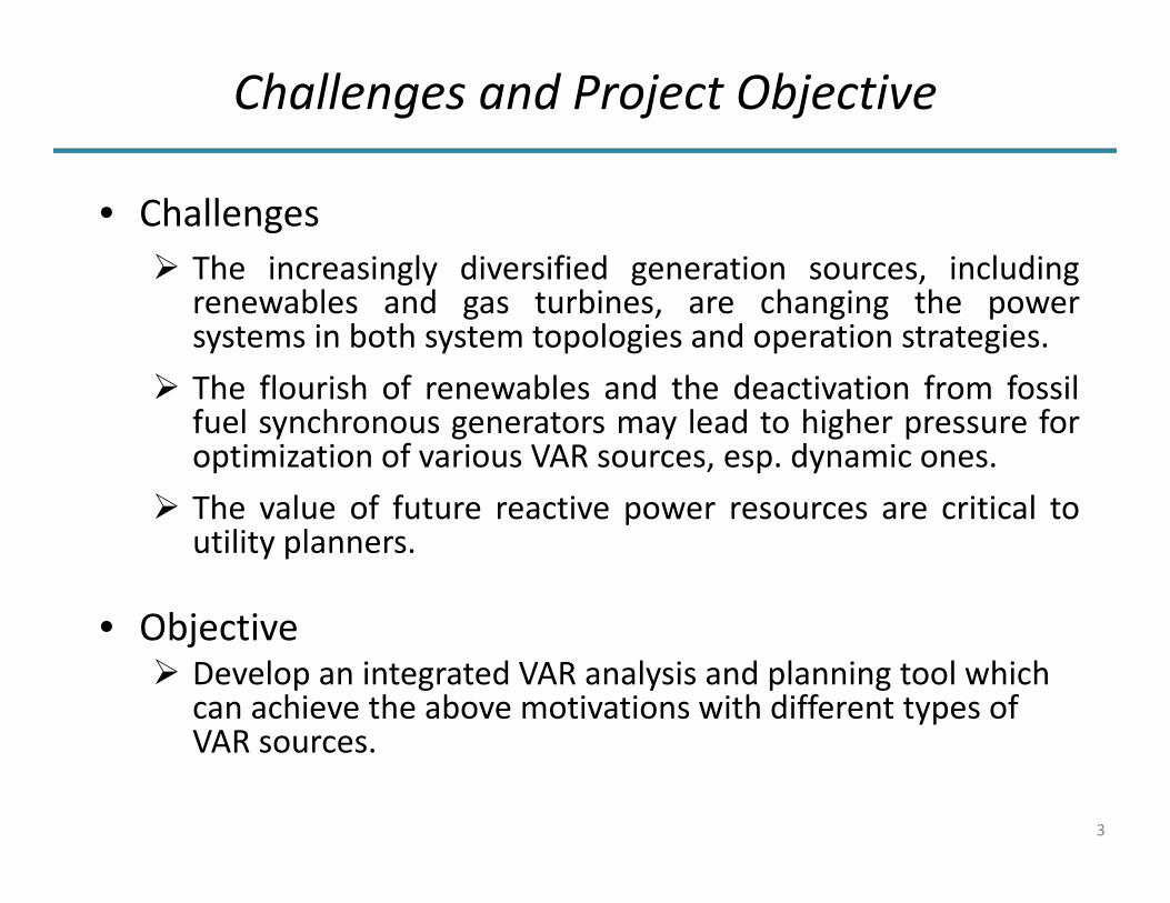
• Challenges The increasingly diversified generation sources, including
renewables and gas turbines, are changing the powersystems in both system topologies and operation strategies.
The flourish of renewables and the deactivation from fossilfuel synchronous generators may lead to higher pressure foroptimization of various VAR sources, esp. dynamic ones.
The value of future reactive power resources are critical toutility planners.
• Objective Develop an integrated VAR analysis and planning tool which
can achieve the above motivations with different types of VAR sources.
Challenges and Project Objective
3

• Generation uncertainty and new characteristics are addressed in the long‐term VAR planning.
• VAR sources are differentiated as static VAR and dynamic VAR sources in the short‐term VAR planning to further optimize the VAR planning and ensure dynamic voltage stability – a utility concern
• The benefit and value of VAR are evaluated and assessed to either determine feasibility of investment or value streams from VAR optimization – a utility benefit
• Framework of the future VAR planning and operation which could lead to the power system VAR planning and operation revolution.
Significance and Impacts
4

5
Presentation Outline
• Project Overview
• Technical Approaches and Accomplishments MOVARTI tool overview
VAR Value Assessment: budget constrained VAR planning
Long‐term VAR planning: considering static voltage constraints
Short‐term VAR planning: considering post‐contingency voltage dynamics
• Conclusions and Future Works

6
MOVARTI Tool Overview ‐ Capability
Static VAR Optimization:Optimal Location and
Capacity for VAR Sources, Optimal Generation and
VAR Costs
Reactive Power Planning Simulation Engine
Detailed System Model
Planning Generation Model:
Gen Types, Location and Plant Parameters Planning
Strategy:VAR Source Type
Preferred Location and Control Strategy
Dynamic VAR Optimization:
Optimal Location and Capacity for VAR Sources, Load Flow and Dynamic Simulation Studies, Dynamic Voltage Profile of the
System
VAR Value Sensitivity Analysis:
VAR value based sensitivity ranking of the system buses

7
MOVARTI Tool Overview ‐ Architecture
GAMSMATLAB GUI
System Data
Python
PSS/E
Static OptimizationPower Flow: MATPOWEROptimization: GAMS
VAR Benefit AnalysisOptimization: GAMS
Dynamic OptimizationPower Flow: PSS/EDynamic Simulation: PSS/EOptimization: MATLAB

8
VAR Value Assessment
P
Q Qloss
PlossP
QlossQ
B2B3
Without VAR compensation
With VAR compensation
B A
SM
P
PoC before Var compensation V
PoC after Var compensation
B1: Benefit from reduced power losses
B2: Benefit from shifting reactive power flow to active power flow
B3: Benefit from increasing line transfer capability
B1
VAR value streams:
Ploss

9
Quantitative Assessment Model
Base Case (z): Base system without VAR compensation (Qc=0). Perturbed Case (z’): Compensation is available at a given bus in the given
amount for evaluation. VAR value (i.e., benefits from the OPF model) = z’ – z, which is essentially a
sensitivity study which can be used for budget‐constrained planning.
0),( VPLiPGiP ( , ) 0Q Q Q Q VGi ci Li
maxminGiPGiPGiP maxmin
GiQGiQGiQ
maxminiViViV maxmin
ciQciQciQ
maxLF LFl l
)( GiPfMin:
Subject to:
(Generation active and reactive limit)
(Voltage limit and VAR capacity limit)
(Line capacity limit)
Based on ACOPF model:
(Nodal power balance)
(Total production cost)
10
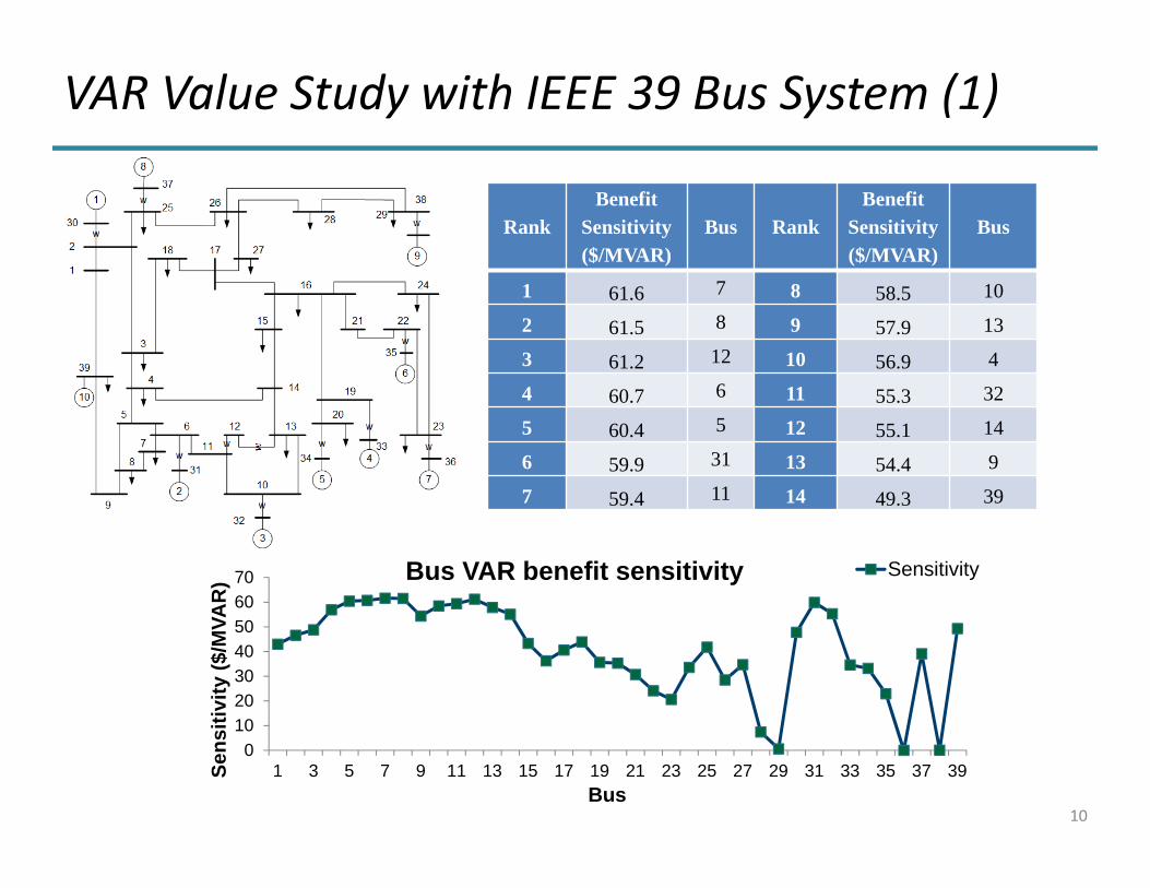
VAR Value Study with IEEE 39 Bus System (1)
RankBenefit
Sensitivity ($/MVAR)
Bus RankBenefit
Sensitivity ($/MVAR)
Bus
1 61.6 7 8 58.5 10
2 61.5 8 9 57.9 13
3 61.2 12 10 56.9 4
4 60.7 6 11 55.3 32
5 60.4 5 12 55.1 14
6 59.9 31 13 54.4 9
7 59.4 11 14 49.3 39
010203040506070
1 3 5 7 9 11 13 15 17 19 21 23 25 27 29 31 33 35 37 39Sens
itivi
ty ($
/MVA
R)
Bus
Bus VAR benefit sensitivity Sensitivity
11
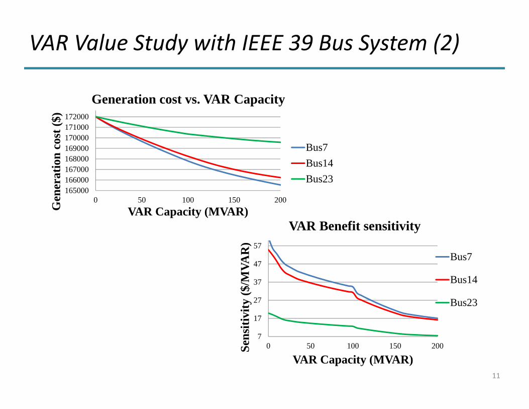
VAR Value Study with IEEE 39 Bus System (2)
165000166000167000168000169000170000171000172000
0 50 100 150 200
Gen
erat
ion
cost
($)
VAR Capacity (MVAR)
Generation cost vs. VAR Capacity
Bus7Bus14Bus23
7
17
27
37
47
57
0 50 100 150 200Sens
itivi
ty ($
/MVA
R)
VAR Capacity (MVAR)
VAR Benefit sensitivity
Bus7
Bus14
Bus23

12
Long‐term VAR Planning: Considering Static Voltage Constraints
Considerations:1. Different generation types including coal, gas, and
renewables2. Wind energy Weibull distribution 3. Correlation between multiple wind farms4. Different VAR capabilities of wind farms5. Static voltage constraints
Results:To determine static VAR source size and location that minimizes the total cost

13
Bi‐level Optimization Model
Wind data
Scenario creation considering wind correlation
System data
Master problem: VAR allocation
Worst scenario
Scenario reduction
Sub-problem: Econ. disp.
All scenarios
Converge?
Output VARallocation result
Yes
No
Objective: minimize VAR cost and expected generation cost.
*1 2 ,min ( )
Q N Gck k t Gi t
k N t W i N
c c Q u p f P
Binary Variable
Probability Weights

14
Case Study with IEEE 39 Bus System (1)
Four wind farms connected at Bus 10, Bus 20, Bus 25 and Bus 29.
193.041.043.093.0158.054.041.058.0181.043.054.081.01
Wind farm data
Correlation Matrix
WF BusWindpower (MW)
1 10 380 8.13 1.992 20 445 8.24 2.33 25 500 7.52 2.114 29 520 9.24 2.41

15
Case Study with IEEE 39 Bus System (2)
Select the worst scenarios in which the system has the least reactive power reserve.
Case a: unity power factor Case b: pf = 0.98 Case c: D curve operation
0 200 400-900
-800
-700
-600
-500
Wind power (MW)(a)
Rea
ctiv
e po
wer
rese
rve
(MV
ar)
0 200 400-800
-600
-400
-200
0
200
Wind power (MW)(c)
Rea
ctiv
e po
wer
rese
rve
(MV
ar)
0 200 400-800
-700
-600
-500
-400
Wind power (MW)(b)
Rea
ctiv
e po
wer
rese
rve
(MV
ar)
WF1WF2WF3WF4
WF1WF2WF3WF4
WF1WF2WF3WF4

16
Content Slides
VAR allocation results under different optimization objectives
When the correlation among wind farms is considered, the worst scenariosfor Case a and Case b are the same. Therefore, VAR allocation results forthese two cases are the same if only VAR cost is the objective.
It is recommended to use total cost as the objective if possible, since thismay lead to different and better results from the overall system perspective.
Objective: VAR Cost Objective: Total CostVAR Size
(Bus)Fuel cost
($/hr)VAR cost
($/hr)Total cost
($/hr)VAR Size
(Bus)Fuel cost
($/hr)VAR cost
($/hr)Total cost
($/hr)
Case a (pf=1)
29.4 (5), 171.5 (7), 200 (8)
143,532 691.3 144,223200 (5),
114.2 (7), 118.2 (18)
143,454 738.6 144,193
Case b (pf=0.98)
29.4 (5), 171.5 (8), 200 (8)
143,524 691.3 144,215152 (7),
186.2 (11), 91.9 (17)
143,435 734.0 144,169
Case c(D curve)
95.3 (7) 143,512 173 143,685 95.6 (7) 143,512 173.4 143,685
Case Study with IEEE 39 Bus System (3)

17
Dynamic VAR Planning: considering post‐contingency voltage dynamics
NERC CriteriaApproaches:1. Use the static VAR optimization results as the
reference.2. Consider NERC criteria on post-fault voltage
recovery performance.3. Solve an nonlinear optimization problem to
minimize the cost while meeting dynamic voltage requirements.
Results:Locations and sizes of dynamic VAR sources

18
Stage 1: Contingency Ranking
• Use a composite load model including motor loads
• Find the most severe N‐1 or N‐2 by a Voltage Recovery Index:
, ,s s
cr cr
t t
dev n m i i j jt ti j
V C A dt D B dt
, ,1 1
1 OC BusN N
k dev n mn mOC
VRI VN
( Voltage deviation for contingency kat bus m under condition n)

19
Stage 2: Placement of Dynamic VAR Sources
1. Evaluate a Voltage Sensitivity Index (VSI) for bus j or the overall system by simulated post‐contingency voltage trajectories with a small qi injected at bus i
2. Select a number (depending on budget) of the buses with the highest VSIs to place SVCs
, ,max , 1 ~ /new t old tij j j iVSI V V t T q
1
1 N
i ijj
VSI VSIN

20
Stage 3: Optimization of the Sizes of Dynamic VAR Sources
A new iterative Linear Programming approach
1
1
nk
i ii
f c Q
1k k k
i i iQ Q Q
,
1
nk L k
ij ij i ji
VSI Q V
, 1 ~i n
, 1 ~j N
, 1 ~j N ,
1
nk U k
ij ij i ji
V S I Q V
Minimize
21
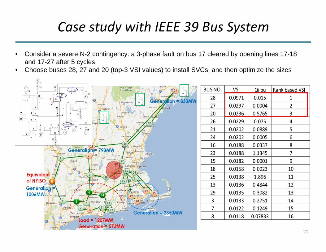
Case study with IEEE 39 Bus System
• Consider a severe N-2 contingency: a 3-phase fault on bus 17 cleared by opening lines 17-18 and 17-27 after 5 cycles
• Choose buses 28, 27 and 20 (top-3 VSI values) to install SVCs, and then optimize the sizes
BUS NO. VSI Qj pu Rank based VSI28 0.0971 0.015 127 0.0297 0.0004 220 0.0236 0.5765 326 0.0229 0.075 421 0.0202 0.0889 524 0.0202 0.0005 616 0.0188 0.0337 823 0.0188 1.1345 715 0.0182 0.0001 918 0.0158 0.0023 1025 0.0138 1.896 1113 0.0136 0.4844 1229 0.0135 0.3082 133 0.0133 0.2751 147 0.0122 0.1249 158 0.0118 0.07833 16
22
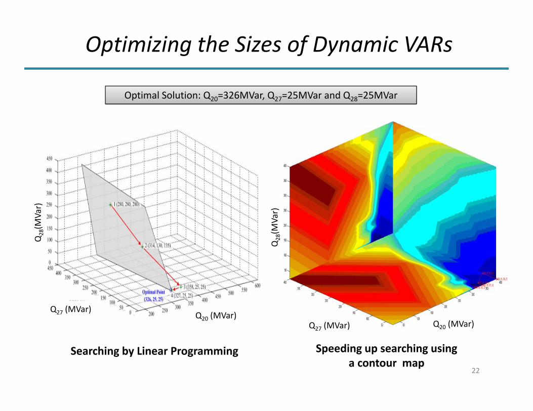
Optimizing the Sizes of Dynamic VARs
Searching by Linear Programming
Q20 (MVar)Q27 (MVar)
Q28(M
Var)
Speeding up searching using a contour map
Q20 (MVar)Q27 (MVar)
Q28(M
Var)
Optimal Solution: Q20=326MVar, Q27=25MVar and Q28=25MVar

23
Comparison of Trajectories
Insecure, without SVCs
Optimal solution (Q20=326Mvar, Q27=25Mvar,
Q28=25Mvar)
Secure but non‐optimal(over‐compensated:
Q20=Q27=Q28=1000Mvar)
The optimized solution gives secure voltage response while minimizing the total cost.

24
Presentation Outline
• Project Overview
• Technical Approaches and Accomplishments
• Conclusions and Future Works

25
Conclusions
• An integrated VAR planning and analysis tool isdeveloped. Concept verification tool for utility users to test and
verify the concepts developed in this project, underthe paradigm of considering uncertainty and post‐contingency voltage dynamics
Functions include VAR value assessment, long‐termVAR planning considering static voltage constraints,and short‐term VAR planning considering post‐contingency voltage dynamics
Easy user interface with PSS/E and GAMS
26
Future Works
• FY 2015: Continue engagement of Dominion Virginia Power (DVP) and other companies to develop the MOVARTI tool to address utility challenges and needs: Operational consideration of VAR sources Uncertainty at the demand side
• FY 2015: Further development of the tool to integrate the static planning and dynamic planning, methodology validation using a real system.
• Out‐year plan: Deployment as an open‐source tool.

Acknowledgements
The authors would like to acknowledge the support of the Oak Ridge National Laboratory and the U.S. Department of Energy’s Office of Electricity Delivery and Energy Reliability under the Advanced Modeling Grid Research Program.
27

28
Contacts
Yan XuOak Ridge National [email protected](865) 574‐7734
Fangxing (Fran) LiThe University of [email protected](865) 974‐8401
Kai SunThe University of [email protected](865) 974‐3982

Thank you!
Q & A?
29