OPTIMIZATION PROBLEMS IN

MASS TRANSPORTATION THEORY

Giuseppe Buttazzo

Dipartimento di Matematica

Universita di Pisa

buttazzo@dm.unipi.it

http://cvgmt.sns.it

School on Calculus of Variations

Roma July 4–8, 2005

Mass transportation theory goes back to

Gaspard Monge (1781) when he presented a

model in a paper on Academie de Sciences

de Paris

déblais

remblais

•x

•T(x)

The elementary work to move a particle x

into T (x) is given by |x−T (x)|, so that the

total work is∫

deblais|x− T (x)| dx .

A map T is called admissible transport map

if it maps “deblais” into “remblais”.

1

The Monge problem is then

min∫

deblais|x− T (x)| dx : T admiss.

.

It is convenient to consider the Monge prob-

lem in the framework of metric spaces:

• (X, d) is a metric space;

• f+, f− are two probabilities on X

(f+ = “deblais”, f− = “remblais”);

• T is an admissible transport map if

T#f+ = f−.

The Monge problem is then

min∫

X

d(x, T (x)

)dx : Tadmiss.

.

In general the problem above does not ad-

mit a solution, when the measures f+ and

f− are singular, since the class of admissible

transport maps can be empty.

2

Example Take the measures

f+ = δA and f− =1

2δB +

1

2δC ;

it is clear that no map T transports f+ into

f− so the Monge formulation above is in

this case meaningless.

Example Take the measures in R2, still sin-

gular but nonatomic

f+ = H1bA and f− =1

2H1bB+

1

2H1bC

where A,B,C are the segments below.

A BC

3

Then the class of admissible transport maps

is nonempty but the minimum in the Monge

problem is not attained. Indeed, if the dis-

tance between the lines is L and the height

is H it can be seen that the infimum of the

Monge cost is HL, while every transport

map T has a cost strictly greater than HL.

Example (book shifting) Consider in R the

measures

f+ = 1[0,a]L1, f− = 1[b,a+b]L1.

Then the two maps

T1(x) = b+ x, T2(x) = a+ b− x

are both optimal; the map T1 corresponds to

a translation, while the map T2 corresponds

to a reflection. Indeed there are infinitely

many optimal transport maps.

4

Example Take

f+ =N∑

i=1

δpi f− =N∑

i=1

δni .

Then the optimal Monge cost is given by the

minimal connection of the pi with the ni.

Relaxed formulation (due to Kantorovich):

consider measures γ on X ×X• γ is an admissible transport plan if

π#1 γ = f+ and π#

2 γ = f−.

• Transport plans γ that are concentrated

on γ-measurable graphs are actually trans-

port maps T : X → X, via the equality

γ = (Id× T )#f+ .

5

Monge-Kantorovich problem:

min∫

X×Xd(x, y) dγ(x, y) : γ admiss.

.

Theorem There exists an optimal trans-

port plan γopt; in the Euclidean case γopt

is actually a transport map Topt whenever

f+ and f− are in L1.

The existence part is easy; indeed in the

case X compact it follows from the weak*

compactness of probabilities and the weak*

continuity of the Monge-Kantorovich cost.

In the general case the same holds by us-

ing the boundedness of the first moments.

Note that, while in the Monge problem the

cost is highly nonlinear with respect to the

unknown T , in the Kantorovich formulation

the cost is linear with respect to the un-

known γ.

6

The Kantorovich formulation can be seen

as the relaxation of the Monge problem; in-

deed, if f+ is nonatomic we have

min(Kantorovich) = inf(Monge).

The existence of an optimal transport map

is a rather delicate question. The first (in-

complete) proof is due to Sudakov (1979);

various different proofs have been given

by Evans-Gangbo (1999), Trudinger-Wang

(2001), Caffarelli-Feldman-McCann (2002),

Ambrosio (2003).

Wasserstein distance of exponent p: replace

the cost by( ∫

X×X dp(x, y) dγ(x, y)

)1/p

.

Most of the results remain valid for more

general cost functions c(x, y).

7

Shape optimization problems

There is a strong link between mass trans-

portation and shape optimization problems.

We present here this relation and we refer to

the papers by Bouchitte-Buttazzo [BB] and

Bouchitte-Buttazzo-Seppecher [BBS] for all

details.

Shape optimization problem in elasticity:

given a force field f in Rn find the elastic

body Ω whose “resistance” to f is maximal

Constraints:

- given volume, |Ω| = m

- possible “design region” D given, Ω ⊂ D- possible support region Σ given,

Dirichlet region

Optimization criterion: elastic compliance

8

More precisely, for every admissible domain

Ω we consider the energy

E(Ω) = inf∫

Ω

j(Du) dx− 〈f, u〉 :

u smooth, u = 0 on Σ

and the elastic compliance

C(Ω) = −E(Ω).

In the linear case, when j is a quadratic

form, an integration by parts gives that the

elastic compliance reduces to the work of

external forces

C(Ω) =1

2〈f, uΩ〉

being uΩ the displacement of minimal en-

ergy in Ω. In linear elasticity, if z∗ = sym(z)

and α, β are the Lame constants,

j(z) = β|z∗|2 +α

2|trz∗|2.

9

Then the shape optimization problem is

minC(Ω) : Ω ⊂ D, |Ω| = m

.

A similar problem can be considered in the

scalar case (optimal conductor), where f is

a scalar function (the heat sources density)

and

j(z) =1

2|z|2.

Note that the minimum problem with re-

spect to u depends on several elements

(Ω,Σ, D, f . . .). Sometimes they are consid-

ered as given data, which for instance oc-

curs in the usual problems of the calculus

of variations, while sometimes they are un-

known to be optimized for some given cri-

terium (here the compliance).

10

The shape optimization problem above has

in general no solution; in fact minimizing se-

quences may develop wild oscillations which

give raise to limit configurations that are not

in a form of a domain.

Therefore, in order to describe the be-

haviour of minimizing sequences a relaxed

formulation is needed.

The literature on this problem is very wide;

starting from the works by Murat and Tar-

tar in the ’70, it has been studied by

many authors (Kohn and Strang, Lurie and

Cherkaev, Allaire, Bendsøe, . . . ). There are

strong links with homogenization theory.

A large parallel literature is present in engi-

neering.

11

The complete relaxed form of the problem

above is not known: several difficulties arise.

For instance:

• Lack of coercivity; in most of the litera-

ture mixtures of two homogeneous iso-

tropic materials are considered. Here

one of the two materials is the empty

space (outside Ω).

• Even for mixtures of two materials in the

elasticity case the set of materials attain-

able by relaxation is not known.

• Possibility of nonlocal problems as limits

of admissible sequences of domains.

• When D is unbounded, it is not clear

that data with compact support provide

minimizing sequences of domains that

are equi-bounded.

12

To overcome some of these difficulties it is

convenient to study a slightly different prob-

lem where we have the freedom to distribute

a given quantity of material without the re-

striction of designing a domain Ω. They are

called Mass Optimization Problems and

consist in finding, given a force field f in Rn

(which may possibly concentrate on sets of

lower dimension), the mass distribution µ

whose “resistance” to f is maximal.

Constraints:

• given mass,∫dµ = m

• possible design region D given,

with sptµ ⊂ D

• possible support region Σ given,

Dirichlet region.

13

Optimization criterium:

elastic compliance

As before for every admissible mass distri-

bution µ we consider the energy

E(µ) = inf∫

j(Du) dµ− 〈f, u〉 :

u smooth, u = 0 on Σ

and the elastic compliance C(µ) = −E(µ).

Then the mass optimization problem is

minC(µ) : sptµ ⊂ D,

∫dµ = m

.

Elasticity: u and f vector-valued,

j(z) = β|z∗|2 +α

2|trz∗|2.

Conductivity: u and f scalar,

j(z) =1

2|z|2.

14

In the mass optimization problem there is

more freedom than in the shape optimiza-

tion problem because we may use measures

different from µ = 1Ω dx, as it occurs in

shape optimization problems.

On the other hand, we are not restricted

only to forces in H−1 or to n or n−1 dimen-

sional Dirichlet regions; for instance we may

consider forces and Dirichlet regions concen-

trated in a single point, or in a finite number

of points.

Of course, for a given f , we may have

E(µ) = −∞ for some measures µ; for in-

stance this occurs when f is a Dirac mass

and µ is the Lebesgue measure on a domain

Ω, but these measures with infinite compli-

ance are ruled out by the optimization cri-

terion which consists in maximizing E(µ).

15

There is a strong link between the mass op-

timization problem and the Monge-Kantoro-

vich mass transfer problem.

This is described below in the scalar case,

the elasticity case being still not completely

understood.

When in the mass optimization problem we

have Σ = ∅ and D = Rn, then the associ-

ated distance in the transportation problem

is the Euclidean one.

On the contrary, if a Dirichlet region Σ and

design region D are present, the Euclidean

distance |x − y| has to be replaced by an-

other distance d(x, y) which measures the

geodesic distance in D between the points x

and y, counting for free the paths along Σ.

16

More precisely, we consider the geodesic dis-

tance on D ×D

dD(x, y) = min∫ 1

0

|γ′(t)| dt :

γ(t) ∈ D, γ(0) = x, γ(1) = y

= sup|ϕ(x)− ϕ(y)| :

|Dϕ| ≤ 1 on D

and its modification by Σ

dD,Σ(x, y) = infdD(x, y) ∧

(dD(x, ξ1)

+ dD(y, ξ2))

: ξ1, ξ2 ∈ Σ

= sup|ϕ(x)− ϕ(y)| :

|Dϕ| ≤ 1 on Ω, ϕ = 0 on Σ.

This semi-distance will play the role of cost

function in the Monge-Kantorovich mass

transport problem.

17

When f = f+ − f− is a smooth function,

D = Rn, Σ = ∅, Evans and Gangbo [Mem.

AMS 1999] have shown that the solution can

be found by solving the PDE− div

(a(x)Du

)= f

u is 1-Lipschitz|Du| = 1 a.e. on a(x) > 0

where the coefficient a is a multiple of the

optimal µ.

However, even simple cases with f ∈ H−1

may produce optimal mass distributions

which are singular measures. For instance

f+

f-

18

produces an optimal µ which has a onedi-

mensional concentration in the vertical seg-

ment.

Then a theory of variational problems with

respect to measures has to be developed.

This has been done by Bouchitte, Buttazzo

and Seppecher [Calc. Var. 1997]. The ap-

plication of transport problems to mass op-

timization has been developed by Bouchitte

and Buttazzo [JEMS 2001]. The key tools

are:

• the tangent space Tµ(x) to a measure µ,

defined for µ a.e. x;

• the tangential gradient Dµ;

• the Sobolev spaces W 1,pµ .

19

Then the transport problem becomes equiv-

alent to the PDE

− div

(µ(x)Dµu

)= f in Rn \ Σ

u is 1-Lipschitz on D, u = 0 on Σ|Dµu| = 1 µ-a.e. on Rn, µ(Σ) = 0.

Theorem. For every measure f there

exists a solution µopt of the mass opti-

mization problem. Moreover, a measure µ

solves the mass optimization problem if and

only if (a multiple of) it solves the Monge-

Kantorovich PDE.

In order to describe the tangential gra-

dients Dµu which appear in the Monge-

Kantorovich equation above we recall the

main steps of the theory of the variational

integrals w.r.t. a measure.

20

Variational integrals w.r.t. a measure

Consider the functional

F (u) =

∫f(x,Du) dµ

defined for smooth functions u (and +∞elsewhere), where µ is a general nonnega-

tive measure. On the integrand f we as-

sume the usual convexity and p-growth con-

ditions. We define the tangent fields

Xp′µ =

φ ∈ Lp′µ (Rn; Rn) :

div(φµ) ∈ Lp′µ (Rn),

the tangent spaces

T pµ(x) = µ-ess⋃

φ(x) : φ ∈ Xp′µ

,

the tangential gradient (for smooth func-

tions)

Dµu(x) = Pµ(x,Du(x)).

21

The operator Dµ is closable, i.e.uh → 0 weakly in LpµDµuh → v weakly in Lpµ

⇒ v = 0 µa.e.

and we still denote by Dµ its closure. The

Sobolev space W 1,pµ is then defined as the

domain of the extension above, with norm

‖u‖1,p,µ = ‖u‖Lpµ + ‖Dµu‖Lpµ .

The relaxation of the integral functional

above is given by

F (u) =

∫fµ(x,Dµu) dµ u ∈W 1,p

µ

where

fµ(x, z) = inff(x, z+ξ) : ξ ∈

(T pµ(x)

)⊥.

In particular,∫|Du|2 dµ relaxes to

∫|Dµu|2 dµ .

22

Here are some cases where the optimal mass

distribution can be computed by using the

Monge-Kantorovich equation (see Bouch-

itte-Buttazzo [JEMS ’01]).

0.6 0.8 1 1.2 1.4 1.6 1.8 2 2.2-0.8

-0.6

-0.4

-0.2

0

0.2

0.4

0.6

0.8

O

S

Optimal distribution of a conductor for heat sources

f = H1bS − LδO .

23

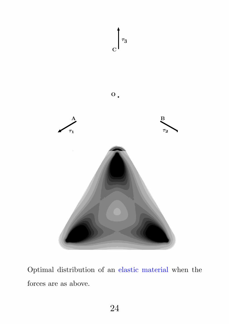
A

C

B

O

τ τ

τ

Optimal distribution of an elastic material when the

forces are as above.

24

-2 -1.5 -1 -0.5 0 0.5 1 1.5 2-1.5

-1

-0.5

0

0.5

1

1.5

A S

Optimal distribution of a conductor, with an obstacle,

for heat sources f = H1bS − 2δA.

0 0.1 0.2 0.3 0.4 0.5 0.6 0.7 0.8 0.9 10

0.1

0.2

0.3

0.4

0.5

0.6

0.7

0.8

0.9

1

A B Σ

x0

2x0

Optimal distribution of a conductor for heat sources

f = 2H1bS0 −H1bS1 and Dirichlet region Σ.

25

We present now some further optimization

problems related to mass transportation

theory.

Given a metric space (X, d) and two prob-

abilities f+ and f− on X, it is conve-

nient to denote by MK(f+, f−, d) the mini-

mum value of the transportation cost in the

Monge-Kantorovich problem, that is

MK(f+, f−, d) = min∫

X×Xd(x, y) dγ(x, y)

: γ has marginals f+, f−.

We will consider some data as fixed and we

will let the remaining ones vary in some suit-

able admissible classes; the goal is to opti-

mize some given total costs which include a

term related to the mass transportation.

26

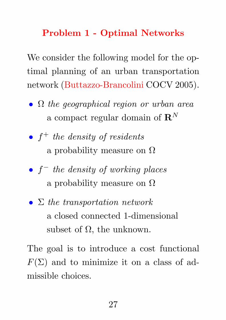
Problem 1 - Optimal Networks

We consider the following model for the op-

timal planning of an urban transportation

network (Buttazzo-Brancolini COCV 2005).

• Ω the geographical region or urban area

a compact regular domain of RN

• f+ the density of residents

a probability measure on Ω

• f− the density of working places

a probability measure on Ω

• Σ the transportation network

a closed connected 1-dimensional

subset of Ω, the unknown.

The goal is to introduce a cost functional

F (Σ) and to minimize it on a class of ad-

missible choices.

27

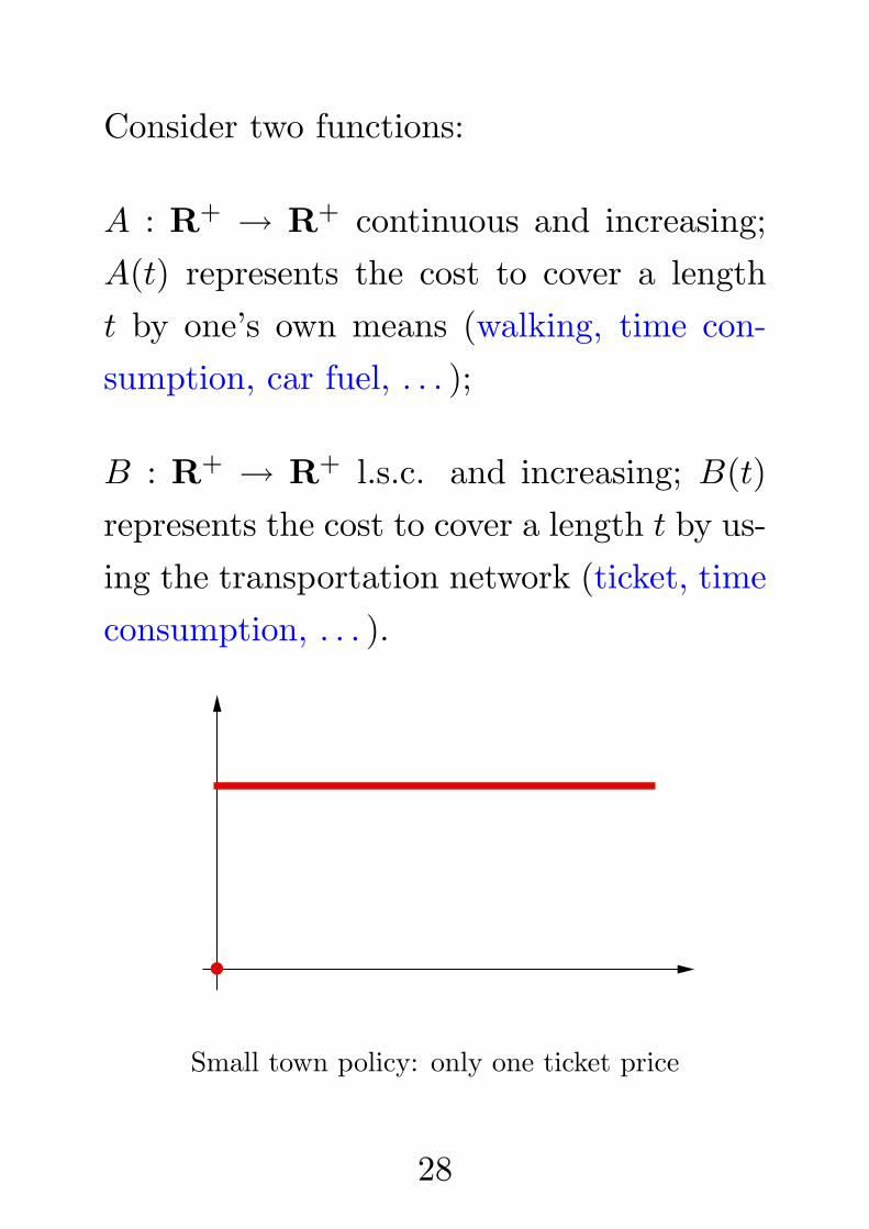
Consider two functions:

A : R+ → R+ continuous and increasing;

A(t) represents the cost to cover a length

t by one’s own means (walking, time con-

sumption, car fuel, . . . );

B : R+ → R+ l.s.c. and increasing; B(t)

represents the cost to cover a length t by us-

ing the transportation network (ticket, time

consumption, . . . ).

•

Small town policy: only one ticket price

28

•

Large town policy: several ticket prices

We define

dΣ(x, y) = infA(H1(Γ \ Σ)

)

+B(H1(Γ ∩ Σ)

): Γ connects x to y

.

The cost of the network Σ is defined via the

Monge-Kantorovich functional:

F (Σ) = MK(f+, f−, dΣ)

and the admissible Σ are simply the closed

connected sets with H1(Σ) ≤ L.

29

Therefore the optimization problem is

minF (Σ) : Σ cl. conn., H1(Σ) ≤ L

.

Theorem There exists an optimal network

Σopt for the optimization problem above.

In the special case A(t) = t and B ≡ 0

(communist model) some necessary condi-

tions of optimality on Σopt have been de-

rived (Buttazzo-Oudet-Stepanov 2002 and

Buttazzo-Stepanov 2003). For instance:

• no closed loops;

• at most triple point junctions;

• 120 at triple junctions;

• no triple junctions for small L;

• asymptotic behavior of Σopt as L→ +∞(Mosconi-Tilli JCA 2005);

• regularity of Σopt is an open problem.

30

It is interesting to study the optimization

problem above if we drop the assumption

that admissible Σ are connected. This could

be for instance of interest in the case of

residents spread over a large area. We

take as admissible Σ all rectifiable sets with

H1(Σ) ≤ L (paper [BPSS] in preparation).

• For general functions A and B an opti-

mal network Σopt may not exist; the op-

timum has to be searched in a relaxed

sense among measures.

• If A and B are concave, then an optimal

network Σopt exists; however there could

also be other optima which are measures.

• If A and B are concave, one of them is

strictly concave, andB′+(0) < A′−(diam Ω),

then all optima (also in a relaxed sense)

are rectifiable networks.

31

Problem 2 - Optimal Pricing Policies

With the notation above, we consider the

measures f+, f− fixed, as well as the trans-

portation network Σ. The unknown is the

pricing policy the manager of the network

has to choose through the l.s.c. monotone

increasing function B. The goal is to maxi-

mize the total income, a functional F (B),

which can be suitably defined (Buttazzo-

Pratelli-Stepanov 2004) by means of the

Monge-Kantorovich transport plans.

Of course, a too low ticket price policy will

not be optimal, but also a too high ticket

price policy will push customers to use their

own transportation means, decreasing the

total income of the company.

32

The function B can be seen as a control vari-

able and the corresponding transport plan

as a state variable, so that the optimization

problem we consider:

minF (B) : B l.s.c. increasing, B(0) = 0

can be seen as an optimal control problem.

Theorem There exists an optimal pric-

ing policy Bopt solving the maximal income

problem above.

Also in this case some necessary conditions

of optimality can be obtained. In particu-

lar, the function Bopt turns out to be con-

tinuous, and its Lipschitz constant can be

bounded by the one of A (the function mea-

suring the own means cost).

33

Here is the case of a service pole at the ori-

gin, with a residence pole at (L,H), with a

network Σ. We take A(t) = t.

Σ

L

H

The optimal pricing policy B(t) is given by

B(t) = (H2 + L2)1/2 − (H2 + (L− t)2)1/2.

0.5 1 1.5 2

0.2

0.4

0.6

0.8

1

1.2

The case L = 2 and H = 1.

34

Here is another case, with a single service

pole at the origin, with two residence poles

at (L,H1) and (L,H2), with a network Σ.

Σ

L H1

H2

The optimal pricing policy B(t) is then

B(t) =

B2(t) in [0, T ]B2(T )−B1(T ) +B1(t) in [T, L]

.

0.5 1 1.5 2

0.2

0.4

0.6

0.8

1

1.2

The case L = 2, H1 = 0.5, H2 = 2.

35

Problem 3 - Optimal City Structures

We consider the following model for the op-

timal planning of an urban area (Buttazzo-

Santambrogio SIAM M.A. 2005).

• Ω the geographical region or urban area

a compact regular domain of RN

• f+ the density of residents

a probability measure on Ω

• f− the density of services

a probability measure on Ω.

Here the distance d in Ω is fixed (for sim-

plicity we take the Euclidean one) while the

unknowns are f+ and f− that have to be

determined in an optimal way taking into

account the following facts:

36

• there is a transportation cost for moving

from the residential areas to the services

poles;

• people desire not to live in areas where

the density of population is too high;

• services need to be concentrated as much

as possible, in order to increase efficiency

and decrease management costs.

The transportation cost will be described

through a Monge-Kantorovich mass trans-

portation model; it is indeed given by a p-

Wasserstein distance (p ≥ 1) Wp(f+, f−),

being p = 1 the classical Monge case.

The total unhappiness of citizens due to

high density of population will be described

by a penalization functional, of the form

H(f+) =

∫Ωh(u) dx if f+ = u dx

+∞ otherwise,

37

where h is assumed convex and superlinear

(i.e. h(t)/t → +∞ as t → +∞). The in-

creasing and diverging function h(t)/t then

represents the unhappiness to live in an area

with population density t.

Finally, there is a third term G(f−) which

penalizes sparse services. We force f− to

be a sum of Dirac masses and we consider

G(f−) a functional defined on measures,

of the form studied by Bouchitte-Buttazzo

(Nonlinear An. 1990, IHP 1992, IHP 1993):

G(f−) =

∑n g(an) if f− =

∑n anδxn

+∞ otherwise,

where g is concave and with infinite slope

at the origin. Every single term g(an) in

the sum represents here the cost for building

and managing a service pole of dimension

an, located at the point xn ∈ Ω.

38

We have then the optimization problem

minWp(f

+, f−) +H(f+) +G(f−) :

f+, f− probabilities on Ω.

Theorem There exists an optimal pair

(f+, f−) solving the problem above.

Also in this case we obtain some necessary

conditions of optimality. In particular, if

Ω is sufficiently large, the optimal structure

of the city consists of a finite number of

disjoint subcities: circular residential areas

with a service pole at the center.

39

Problem 4 - Optimal Riemannian Metrics

Here the domain Ω and the probabilities f+

and f− are given, whereas the distance d

is supposed to be conformally flat, that is

generated by a coefficient a(x) through the

formula

da(x, y) = inf∫ 1

0

a(γ(t)

)|γ′(t)| dt :

γ ∈ Lip(]0, 1[; Ω), γ(0) = x, γ(1) = y.

We can then consider the cost functional

F (a) = MK(f+, f−, da).

The goal is to prevent as much as possible

the transportation of f+ onto f− by maxi-

mizing the cost F (a) among the admissible

coefficients a(x). Of course, increasing a(x)

would increase the values of the distance da

40

and so the value of the cost F (a). The class

of admissible controls is taken as

A =a(x) Borel measurable :

α ≤ a(x) ≤ β,∫

Ω

a(x) dx ≤ m.

In the case when f+ = δx and f− = δy

are Dirac masses concentrated on two fixed

points x, y ∈ Ω, the problem of maximizing

F (a) is nothing else than that of proving

the existence of a conformally flat Euclidean

metric whose geodesics joining x and y are

as long as possible.

This problem has several natural motiva-

tions; indeed, in many concrete examples,

one can be interested in making as diffi-

cult as possible the communication between

some masses f+ and f−. For instance, it

is easy to imagine that this situation may

41

arise in economics, or in medicine, or simply

in traffic planning, each time the connec-

tion between two “enemies” is undesired.

Of course, the problem is made non trivial

by the integral constraint∫

Ωa(x) dx ≤ m,

which has a physical meaning: it prescribes

the quantity of material at one’s disposal to

solve the problem.

The analogous problem of minimizing the

cost functional F (a) over the class A, which

corresponds to favor the transportation of

f+ into f−, is trivial, since

infF (a) : a ∈ A

= F (α).

The existence of a solution for the maxi-

mization problem

maxF (a) : a ∈ A

42

is a delicate matter. Indeed, maximizing

sequences an ⊂ A could develop an os-

cillatory behavior producing only a relaxed

solution. This phenomenon is well known;

basically what happens is that the class A is

not closed with respect to the natural con-

vergence

an → a ⇐⇒ dan → da uniformly

and actually it can be proved thatA is dense

in the class of all geodesic distances (in par-

ticular, in all the Riemannian ones).

Nevertheless, we were able to prove the fol-

lowing existence result.

Theorem The maximization problem above

admits a solution in aopt ∈ A.

43

Several questions remain open:

• Under which conditions is the optimal so-

lution unique?

• Is the optimal solution of bang-bang type?

In other words do we have aopt ∈ α, βor intermediate values (homogenization)

are more performant?

• Can we characterize explicitely the opti-

mal coefficient aopt in the case f+ = δx and

f− = δy?

44

Some Numerical Computations

Here are some numerical computations per-

formed (Buttazzo-Oudet-Stepanov 2002) in

the simpler case of the so-called problem of

optimal irrigation.

This is the optimal network Problem 1 in

the case f− ≡ 0, where customers only want

to minimize the averaged distance from the

network.

In other words, the optimization criterion

becomes simply

F (Σ) =

∫

Ω

dist(x,Σ) df+(x) .

Due to the presence of many local minima

the method is based on a genetic algorithm.

45

Optimal sets of length 0.5 and 1 in a unit disk

Optimal sets of length 1.25 and 1.5 in a unit disk

Optimal sets of length 2 and 3 in a unit disk

46

Optimal sets of length 0.5 and 1 in a unit square

Optimal sets of length 1.5 and 2.5 in a unit square

Optimal sets of length 3 and 4 in a unit square

47

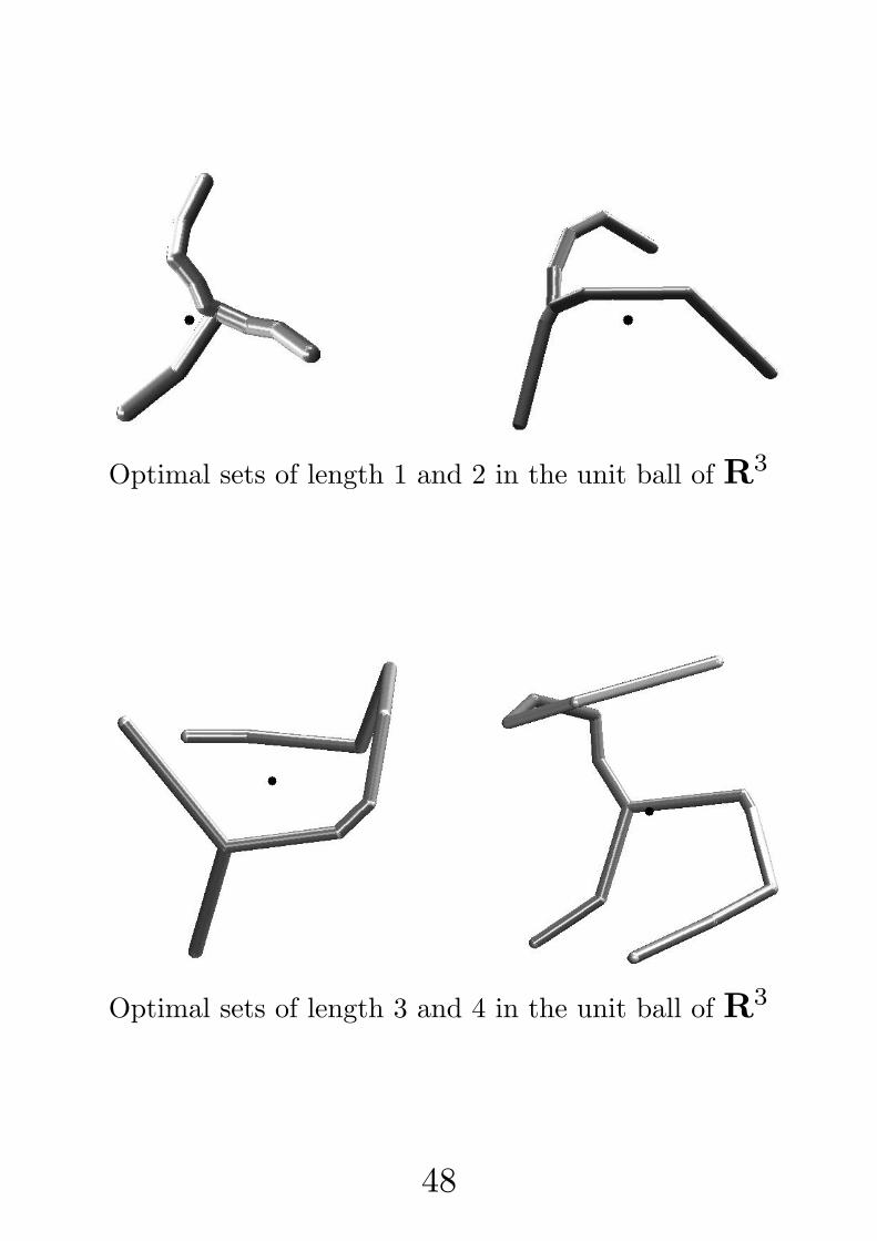
Optimal sets of length 1 and 2 in the unit ball of R3

Optimal sets of length 3 and 4 in the unit ball of R3

48

Now we give a model that takes into account

what occurs in several natural structures

(see figures above). Indeed, they present

some interesting features that should be in-

terpreted in terms of mass transportation.

However the usual Monge-Kantorovich the-

ory does not provide an explaination to the

reasons for which the structures above exist,

and it cannot be taken as a mathematical

model for them. For instance, if the source

is a Dirac mass and the target is a segment,

as in figure below, the Monge-Kantorovich

theory provides a wrong behaviour.

The Monge transport rays.

49

Various approaches have been proposed to

give more appropriated models:

• Q. Xia (Comm. Cont. Math. 2003)

through the minimization of a suitable

functional defined on currents;

• V. Caselles, J. M. Morel, S. Solimini, . . .

(Preprint 2003 http://www.cmla.ens-

cachan.fr/Cmla/, Interfaces and Free

Boundaries 2003, PNLDE 51 2002) through

a kind of analogy of fluid flow in thin

tubes.

• A. Brancolini, G. Buttazzo, E. Oudet, E.

Stepanov, (see http://cvgmt.sns.it)

through a variational model for irrigation

trees.

Here we propose a different approach based

on a definition of path length in a Wasser-

stein space.

50

We also give a model where the opposite

feature occurs: instead of favouring the con-

centration of transport rays, the variational

functional prevents it giving a lower cost to

diffused measures.

The mathematical model will be consid-

ered in an abstract metric space framework

where both behaviours (favouring concen-

tration and diffusion) are included; we do

not know of natural phenomena where the

diffusive behaviour occurs.

The results presented here are contained in

A. Brancolini, G. Buttazzo, F. San-

tambrogio: Path functionals over Wasser-

stein spaces. Preprint 2004, available at

http://cvgmt.sns.it

51

We consider an abstract framework where

a metric space X with distance d is given.

We assume that closed bounded subsets of

X are compact. Fix two points x0 and x1

in X and consider the path functional

J (γ) =

∫ 1

0

J(γ(t))|γ′|(t) dt

where γ : [0, 1] → X ranges among all

Lipschitz curves such that γ(0) = x0 and

γ(1) = x1. Here:

• J : X → [0,+∞] is a given mapping on

X;

• |γ′|(t) is the metric derivative of γ at the

point t, i.e.

|γ′|(t) = lim sups→t

d(γ(s), γ(t)

)

|s− t| .

52

Theorem Assume:

• J is lower semicontinuous in X;

• J ≥ c with c > 0, or more generally∫ +∞0

(infB(r) J

)dr = +∞.

Then, for every x0, x1 ∈ X there exists an

optimal path for the problem

minJ (γ) : γ(0) = x0, γ(1) = x1

provided there exists a curve γ0, connecting

x0 to x1, such that J (γ0) < +∞.

The application of the theorem above con-

sists in taking as X a Wasserstein space

Wp(Ω) where Ω is a compact metric space

equipped with a distance function c and

a positive finite non-atomic Borel measure

m (usually a compact of RN with the Eu-

clidean distance and the Lebesgue measure).

53

We recall that, in the case Ω compact,

Wp(Ω) is the space of all Borel probabil-

ity measures µ on Ω equipped with the p-

Wasserstein distance

wp(µ1, µ2) = inf(∫

Ω×Ω

c(x, y)p λ(dx, dy))1/p

where the infimum is taken on all trans-

port plans λ between µ1 and µ2, that is on

all probability measures λ on Ω × Ω whose

marginals π#1 λ and π#

2 λ coincide with µ1

and µ2 respectively.

In order to define the functional

J (γ) =

∫ 1

0

J(γ(t))|γ′|(t) dt

it remains to fix the “coefficient” J . We

take a l.s.c. functional on the space of mea-

sures, of the kind considered by Bouchitte

and Buttazzo (Nonlinear Anal. 1990, Ann.

IHP 1992, Ann. IHP 1993):

54

J(µ) =

∫

Ω

f(µa)dm+

∫

Ω

f∞(µc)+

∫

Ω

g(µ(x))d#

where

• µ = µa · m + µc + µ# is the Lebesgue-

Nikodym decomposition of µ with re-

spect to m, into absolutely continuous,

Cantor, and atomic parts;

• f : R → [0,+∞] is convex, l.s.c. and

proper;

• f∞ is the recession function of f ;

• g : R→ [0,+∞] is l.s.c. and subadditive,

with g(0) = 0;

• # is the counting measure;

• f and g verify the compatibility condition

limt→+∞

f(ts)

t= limt→0+

g(ts)

t.

55

In this way the functional J is l.s.c. for the

weak* convergence of measures. If we fur-

ther assume that f(s) > 0 for s > 0 and

g(1) > 0, then we have J ≥ c > 0. The ex-

istence theorem then applies and, given two

probabilities µ0 and µ1, we obtain at least

a minimizing path for the problem

minJ (γ) : γ(0) = µ0, γ(1) = µ1

.

provided J is not identically +∞.

We now study two special cases (Ω ⊂ RN

compact and m = dx):

Concentration f ≡ +∞, g(z) = |z|r with

r ∈]0, 1[. We have then

J(µ) =

∫

Ω

|µ(x)|r d# µ atomic

Diffusion f(z) = |z|q with q > 1, g ≡ +∞.

We have then

J(µ) =

∫

Ω

|u(x)|q dx µ = u ·dx, u ∈ Lq.

56

Concentration case. The following facts

in the concentration case hold:

• If µ0 and µ1 are convex combinations

(also countable) of Dirac masses, then

they can be connected by a path γ(t) of

finite minimal cost J .

• If r > 1− 1/N then every pair of proba-

bilities µ0 and µ1 can be connected by a

path γ(t) of finite minimal cost J .

• The bound above is sharp. Indeed, if r ≤1 − 1/N there are measures that cannot

be connected by a finite cost path (for

instance a Dirac mass and the Lebesgue

measure).

57

Example. (Y-shape versus V-shape). We

want to connect (concentration case r < 1

fixed) a Dirac mass to two Dirac masses (of

weight 1/2 each) as in figure below, l and h

are fixed. The value of the functional J is

given by

J (γ) = x+ 21−r√(l − x)2 + h2.

Then the minimum is achieved for

x = l − h√41−r − 1

.

When r = 1/2 we have a Y-shape if l > h

and a V-shape if l ≤ h.

•

•

•

h

l

x

A Y-shaped path for r = 1/2.

58

Diffusion case. The following facts in the

diffusion case hold:

• If µ0 and µ1 are in Lq(Ω), then they can

be connected by a path γ(t) of finite min-

imal cost J . The proof uses the displace-

ment convexity (McCann 1997) which,

for a functional F and every µ0, µ1, is the

convexity of the map t 7→ F (T (t)), being

T (t) = [(1− t)Id + tT ]#µ0 and T an op-

timal transportation between µ0 and µ1.

• If q < 1 + 1/N then every pair of proba-

bilities µ0 and µ1 can be connected by a

path γ(t) of finite minimal cost J .

• The bound above is sharp. Indeed, if q ≥1 + 1/N there are measures that cannot

be connected by a finite cost path (for

instance a Dirac mass and the Lebesgue

measure).

59

The previous existence results were based

on two important assumptions:

• the compactness of Wasserstein spaces

Wp(Ω) for Ω compact and 1 ≤ p < +∞;

• the estimate like Fq ≥ c > 0, that can be

obtained when |Ω| < +∞.

Both the facts do not hold when Ω is un-

bounded (indeed, the corresponding Wasser-

stein spaces are not even locally compact).

The same happens when Ω is compact but

we consider the space W∞(Ω).

Here is a more refined abstract setting which

adapts to the unbounded case.

Notice that in the unbounded case the

Wasserstein spacesWp(Ω) do not contain all

the probabilities on Ω but only those with

finite momentum of order p., that is∫

Ω

|x|p µ < +∞ .

60

Theorem Let (X, d, d′) be a metric space

with two different distances. Assume that:

• d′ ≤ d;

• all d-bounded sets in X are relatively

compact with respect to d′;

• the mapping d : X ×X → R+ is a lower

semicontinuous function with respect to

the distance d′ × d′.Consider a functional J : X → [0,+∞] and

assume that:

• J is d′-l.s.c.;

•∫ +∞

0

(infBd(r) J

)dr = +∞.

Then the functional

J (γ) =

∫ 1

0

J(γ(t))|γ′|d(t) dt

has a minimizer on the set of d−Lipschitz

curves connecting two given points x0 and

x1, provided it is not identically +∞.

61

As an application of the theorem above we

consider the diffusion case when Ω = RN .

The concentration case in the unbounded

setting still presents some extra difficulties

that we did not yet solve. We take:

• d the Wasserstein distance;

• d′ the distance metrizing the weak* topol-

ogy on probabilities:

d′(µ, ν) =∞∑

k=1

2−k

1 + ck

∣∣〈φk, µ− ν〉∣∣

where (φk) is a dense sequence of Lips-

chitz functions in the unit ball of Cb(Ω)

and ck are their Lipschitz constants.

We may prove that the assumptions of the

abstract scheme are fulfilled, and we have

(for the diffusion case):

62

• if q < 1 + 1/N for every µ0 and µ1 there

exists a path giving finite and minimal

value to the cost J ;

• if q ≥ 1 + 1/N there exist measures µ0

(actually a Dirac mass) such that J =

+∞ on every nonconstant path starting

from µ0.

Open Problems

• linking two Lq measures in the diffusion-

unbounded case;

• concentration case in unbounded setting;

• Ω unbounded but not necessarily the

whole space;

• working with the space W∞(Ω);

• comparing this model to the ones by Xia

and by Morel, Solimini, . . . ;

• numerical computations;

• evolution models?

63

References

(all available at http://cvgmt.sns.it)

A. Brancolini, G. Buttazzo: Optimal

networks for mass transportation problems.

Esaim COCV (to appear).

G. Buttazzo, A. Davini, I. Fragala,

F. Macia: Optimal Riemannian distances

preventing mass transfer. J. Reine Angew.

Math., (to appear).

G. Buttazzo, E. Oudet, E. Stepanov:

Optimal transportation problems with free

Dirichlet regions. In PNLDE 51, Birkhauser

Verlag, Basel (2002), 41–65.

G. Buttazzo, A. Pratelli, E. Stepanov:

Optimal pricing policies for public trans-

portation networks. Preprint Dipartimento

di Matematica Universita di Pisa, Pisa (2004).

G. Buttazzo, F. Santambrogio: A Model

for the Optimal Planning of an Urban Area.

Preprint Dipartimento di Matematica Uni-

versita di Pisa, Pisa (2003).

64