optimization problems over unit-distance representations of graphs 1

OPTIMIZATION PROBLEMS OVER

UNIT-DISTANCE REPRESENTATIONS OF GRAPHS

MARCEL K. DE CARLI SILVA AND LEVENT TUNCEL

Abstract. We study the relationship between unit-distance represen-tations and Lovasz theta number of graphs, originally established byLovasz. We derive and prove min-max theorems. This framework allowsus to derive a weighted version of the hypersphere number of a graph anda related min-max theorem. Then, we connect to sandwich theorems viagraph homomorphisms. We present and study a generalization of thehypersphere number of a graph and the related optimization problems.The generalized problem involves finding the smallest ellipsoid of a givenshape which contains a unit-distance representation of the graph. Weprove that arbitrary positive semidefinite forms describing the ellipsoidsyield NP-hard problems.

1. Introduction

Geometric representation of graphs is a beautiful area where combina-torial optimization, graph theory and semidefinite optimization meet andconnect with many other research areas. In this paper, we start by studyinggeometric representations of graphs where each node is mapped to a pointon a hypersphere so that each edge has unit length and the radius of thehypersphere is minimum. Lovasz [15] proved that this graph invariant isrelated to the Lovasz theta number of the complement of the graph via asimple but nonlinear equation. We show that this tight relationship leads tomin-max theorems and to a “dictionary” to translate existing results aboutthe theta function and its variants to the hypersphere representation settingand vice versa.

Based on our approach, we derive a weighted version of the hyperspherenumber of a graph and deduce related min-max theorems. Our viewpointallows us to make new connections, strengthen some facts and correct someinaccuracies in the literature.

Date: September 28, 2012.Marcel K. de Carli Silva: Research of this author was supported in part by a Sinclair

Scholarship, a Tutte Scholarship, Discovery Grants from NSERC, and by ONR researchgrant N00014-12-10049.Levent Tuncel: Research of this author was supported in part by a research grant from Uni-versity of Waterloo, Discovery Grants from NSERC and by ONR research grant N00014-12-10049.

1

2 MARCEL K. DE CARLI SILVA AND LEVENT TUNCEL

After observing that the hypersphere number of a graph is equal to theradius of the smallest Euclidean ball containing a unit-distance representa-tion of the graph, we propose generalizations of the underlying optimizationproblems. Given a graph, the generalized optimization problem seeks thesmallest ellipsoid of given shape which contains a unit-distance representa-tion of the graph. We finally show that at this end of the new spectrumof unit-distance representations, arbitrary positive semidefinite forms de-scribing the shapes of the ellipsoids yield NP-hard geometric representationproblems.

2. Preliminaries

We denote the set of symmetric n×n matrices by Sn, the set of symmetricn× n positive semidefinite matrices by Sn+, and the set of symmetric n× npositive definite matrices by Sn++. For a finite set V , the set of symmetric

V × V matrices is denoted by SV , and the symbols SV+ and SV++ are definedanalogously. For A,B ∈ Sn, we write A ≽ B meaning (A−B) ∈ Sn+. Definean inner product on Sn by ⟨A,B⟩ := Tr(AB), where Tr(X) :=

∑ni=1Xii is

the trace of X ∈ Rn×n. The linear map diag : Sn → Rn extracts the diagonalof a matrix; its adjoint is denoted by Diag.

The vector of all ones is denoted by e. We abbreviate [n] := {1, . . . , n}.The notation ∥·∥ for a norm is the Euclidean norm unless otherwise specified.For a finite set V , the set of orthogonal V × V matrices is denoted by OV .The set of nonnegative reals is denoted by R+. The set of positive reals isdenoted by R++. Define the notations Z+ and Z++ analogously for integernumbers.

For any function f on graphs, we denote by f the function defined byf(G) := f(G) for every graph G, where G denotes the complement of G.For a graph G, we denote the clique number of G by ω(G) and the chromaticnumber of G by χ(G). The complete graph on [n] is denoted by Kn.

Let G be a graph. Its vertex set is V (G) and its edge set is E(G). ForS ⊆ V (G), the subgraph ofG induced by S, denoted byG[S], is the subgraphof G on S whose edges are the edges of G that have both ends in S. Fori ∈ V (G), the neighbourhood of i, denoted by N(i), is the set of nodes of Gadjacent to i. A block of G is an inclusionwise maximal induced subgraphof G with no cut-nodes, where a cut-node of a graph H is a node i ∈ V (H)such that H[V (H) \ {i}] has more connected components than H.

For a graph G = (V,E), the Laplacian of G is the linear extensionLG : RE → SV of the map e{i,j} 7→ (ei − ej)(ei − ej)

T for every {i, j} ∈ E,where ei denotes the ith unit vector. Laplacians arise naturally in spectralgraph theory and spectral geometry; see [3].

3. Hypersphere representations and the Lovasz theta function

Let G = (V,E) be a graph. A unit-distance representation of G is afunction u : V → Rd for some d ≥ 1 such that ∥u(i) − u(j)∥ = 1 whenever

OPTIMIZATION AND UNIT-DISTANCE REPRESENTATIONS OF GRAPHS 3

{i, j} ∈ E. A hypersphere representation of G is a unit-distance represen-tation of G that is contained in a hypersphere centered at the origin, andthe hypersphere number of G, denoted by t(G), is the square of the smallestradius of a hypersphere that contains a unit-distance representation of G.The theta number of G is defined by

ϑ(G) := max{eTXe : Tr(X) = 1, Xij = 0∀{i, j} ∈ E, X ∈ SV+

}. (3.1)

This parameter was introduced by Lovasz in the seminal paper [14]; seealso [8, 12] for further properties and alternative definitions.

Lovasz [15, p. 23] noted the following formula relating t and ϑ:

Theorem 3.1 ([15]). For every graph G, we have

2t(G) + 1/ϑ(G) = 1. (3.2)

We will show how the relation (3.2) can be used to better understandsome of the properties of the theta number and the hypersphere number.This will allow us to obtain simpler proofs of some facts about the thetanumber and new results about hypersphere representations.

3.1. Proof of Theorem 3.1. We include a proof of Theorem 3.1 for thesake of completeness. We may formulate t(G) as the SDP

t(G) = min{t : diag(X) = te, L∗

G(X) = e, X ∈ SV+, t ∈ R}. (3.3)

Here, L∗G is the adjoint of the Laplacian LG of G. The dual of (3.3) is

max{eT z : Diag(y) ≽ LG(z), e

T y = 1, y ∈ RV , z ∈ RE}. (3.4)

Both (3.3) and (3.4) have Slater points, so SDP strong duality holds forthis dual pair of SDPs, i.e., their optimal values coincide and both optima areattained. In particular, t(G) is equal to (3.4). If we write an optimal solutionX∗ of (3.3) as X∗ = UUT , then i 7→ UT ei is a hypersphere representationof G with squared radius t(G).

Proof of Theorem 3.1. We can rewrite the dual (3.4) as

t(G) = max{

12⟨ee

T − I, Y ⟩ : eTY e = 1, Yij = 0 ∀{i, j} ∈ E(G), Y ∈ SV+}

by taking Y := Diag(y)−LG(z). The objective value of a feasible solution Yis 1

2⟨eeT − I, Y ⟩ = 1

2(1− Tr(Y )). Thus, t(G) = 12(1− t(G)), where

t(G) := min{Tr(Y ) : eTY e = 1, Yij = 0 ∀{i, j} ∈ E(G), Y ∈ SV+

}.

It is easy to check that t(G)ϑ(G) = 1. �


3.2. Hypersphere and orthonormal representations of graphs. LetG = (V,E) be a graph. An orthonormal representation of G is a functionfrom V to the unit hypersphere in Rd for some d ≥ 1 that maps non-adjacent nodes to orthogonal vectors. It is well-known that, if u : V → Rd

is a hypersphere representation of G with squared radius t ≤ 1/2, then themap

q : i 7→√2[√

1/2− t⊕ u(i)]∈ R⊕ Rd (3.5)

is an orthonormal representation of G. Define TH(G) as the set of all x ∈ RV+

such that∑

i∈V (cT p(i))2xi ≤ 1 for every orthonormal representation p : V →

Rd of G and unit vector c ∈ Rd. Then ϑ(G) = max{ eTx : x ∈ TH(G)}.The transformation (3.5) allows us to interpret Theorem 3.1 as strong

duality for a nonlinear min-max relation:

Proposition 3.2. Let G be a graph. For every hypersphere representationof G with squared radius t and every nonzero x ∈ TH(G), we have

2t+ 1/(eTx) ≥ 1,

with equality if and only if t = t(G) and eTx = ϑ(G).

Proof. Set V := V (G). Let u : V → Rd be a hypersphere representationof G with squared radius t. We may assume that t < 1/2. Let x ∈ TH(G).Define an orthonormal representation q of G from p as in (3.5). Set c :=1⊕ 0 ∈ R⊕ Rd. Then (1− 2t)eTx =

∑i∈V (c

T q(i))2xi ≤ 1.The equality case now follows from Theorem 3.1. �Proposition 3.2 shows that ϑ(G) and elements from TH(G) are natural

dual objects for t(G) and hypersphere representations of G. In fact, us-ing a well-known description of the elements of TH(G), we recover fromProposition 3.2 the following SDP-free purely geometric min-max relation:

Corollary 3.3. Let G = (V,E) be a graph. For every hypersphere rep-resentation of G with squared radius t, every orthonormal representationp : V → Rd of G, and every unit vector c ∈ Rd such that c ∈ p(V )⊥, we have

2t+[∑

i∈V (cT p(i))2

]−1 ≥ 1,

with equality if and only if t = t(G) and∑

i∈V (cT p(i))2 = ϑ(G).

3.3. A Gallai-type identity. The transformation (3.5) may be reversedas follows. Suppose that q : V → Rd is an orthonormal representation of Gsuch that, for some positive µ ∈ R and some u : V → Rd−1, we have

q(i) =√2[(2µ)−1/2 ⊕ u(i)

]∀i ∈ V. (3.6)

Then u is a hypersphere representation of G with squared radius 12(1−1/µ).

We can use (3.5) and (3.6) to obtain an identity involving these objects.

Proposition 3.4. Let G = (V,E) be a graph. Then

2t(G) + maxp,c

mini∈V

(cT p(i)

)2= 1, (3.7)


where p ranges over all orthonormal representations of G and c over unitvectors of the appropriate dimension.

Proof. We first prove “≤” in (3.7). Let p : V → Rd be an orthonormalrepresentation of G and let c ∈ Rd be a unit vector. We will show that

t(G) ≤ 12

(1−mini∈V

(cT p(i)

)2). (3.8)

It is well-known that there exists an orthonormal representation q of G anda unit vector d such that (dT q(j))2 = β := mini∈V (c

T p(i))2 for all j ∈ V .

If β = 0, then i 7→ 2−1/2ei ∈ RV shows that t(G) ≤ 1/2, so assume thatβ > 0. We may assume that d = e1 and dT q(i) ≥ 0 for every i ∈ V . Nowuse (3.6) with µ = 1/β to get a hypersphere representation u of G from qwith squared radius 1

2(1− β). This proves (3.8).

Next we prove “≥” in (3.7). Let u : V → Rd be a hypersphere representa-tion of G with squared radius t(G). Build an orthonormal representation qof G as in (3.5) and pick c := 1 ⊕ 0 ∈ R ⊕ Rd. Then (cT q(i))2 = 1 − 2t(G)for every i ∈ V . �(The reciprocal of the second term of the sum on the LHS of (3.7) was usedas the original definition of ϑ(G) by Lovasz [14].)

Note that (3.7) does not provide a good characterization of either t(G) orthe maximization problem on the LHS of (3.7). In this sense, Proposition 3.4is akin to Gallai’s identities for graphs [16, Lemmas 1.0.1 and 1.0.2].

3.4. Unit-distance representations in hyperspheres and balls. For agraph G, let tb(G) be the square of the smallest radius of an Euclidean ballthat contains a unit-distance representation of G. This parameter is alsomentioned by Lovasz [15, Proposition 4.1].

To formulate tb(G) as an SDP, replace the constraint diag(X) = te in (3.3)by diag(X) ≤ te. The resulting SDP and its dual have Slater points, so SDPstrong duality holds, i.e., both optima are attained and the optimal valuescoincide.

Evidently, tb(G) ≤ t(G) for every graph G. In fact, equality holds:

Theorem 3.5. For every graph G, we have tb(G) = t(G).

If we mimic the proof of Theorem 3.1 for tb(G), we find that

2tb(G) + 1/ϑb(G) = 1, (3.9)

where ϑb(G) is defined by adding the constraint Xe ≥ 0 to the SDP (3.1).Thus, by (3.2) and (3.9), Theorem 3.5 is equivalent to the fact that ϑb(G) =ϑ(G) for every graph G. This follows from next result [6, Proposition 9] (thiswas pointed out to the first author by Fernando Mario de Oliveira Filho):

Proposition 3.6 ([6]). Let K ⊆ Sn be such that Diag(h)X Diag(h) ∈ Kwhenever X ∈ K and h ∈ Rn

+. If X is an optimal solution for the optimiza-

tion problem max{eTXe : Tr(X) = 1, X ∈ K ∩ Sn+

}, then diag(X) = µXe

for some positive µ ∈ R.


Proof of Theorem 3.5. Since ϑ(G) is a relaxation of ϑb(G), we have ϑb(G) ≤ϑ(G). To prove the reverse inequality, let X be an optimal solution for (3.1).

By Proposition 3.6, we have Xe = µ−1 diag(X) ≥ 0 for some µ > 0. Hence

X is feasible for the SDP that defines ϑb(G), whence ϑb(G) ≥ ϑ(G). �3.5. Hypersphere proofs of ϑ facts. The formula (3.2) relating t(G)and ϑ(G) allows us to infer some basic facts about the theta number froma geometrically simpler viewpoint.

Theorem 3.7 (The Sandwich Theorem [14]). For any graph G, we haveω(G) ≤ ϑ(G) ≤ χ(G).

By Theorem 3.1 and the fact that ϑ(Kn) = n for every n ≥ 1, the Sand-wich Theorem is equivalent to the inequalities t(Kω(G)) ≤ t(G) ≤ t(Kχ(G))for every graph G. The first inequality is obvious: if H is a subgraph of G,then t(H) ≤ t(G). The second one is also obvious: if u : [ℓ] → Rd is a hyper-sphere representation of Kℓ and c : V (G) → [ℓ] is a colouring of G, then u◦cis a hypersphere representation of G. This hints at a strong connection withgraph homomorphisms, which we will look at more closely in Section 4.

Lovasz [15, p. 34] mentions that a graph G is bipartite if and only ifϑ(G) ≤ 2. The less obvious of the implications may be easily proved byshowing that ϑ(Cn) > 2 for every odd cycle Cn. However, we find that thefollowing proof using hypersphere representations gives a more enlighteninggeometric interpretation. By Theorem 3.1, we must show that t(G) ≤ 1/4if and only if G is bipartite. If G is bipartite, then G has a hypersphererepresentation with radius 1/2 even in R1. Suppose G has a hypersphererepresentation with radius ≤ 1/2. The only pairs of points at distance 1 in ahypersphere of radius 1/2 are the pairs of antipodal points, so G is bipartite.

Given graphs G = (V,E) and H = (W,F ) with V ∩ W = ∅, the directsum of G and H is the graph G + H := (V ∪ W,E ∪ F ). It is provedin [12] that ϑ(G+H) = max{ϑ(G), ϑ(H)}. By Theorem 3.1, this is equiv-alent to the geometrically obvious equation t(G + H) = max{t(G), t(H)}.In particular, t(G) = max{ t(C) : C a component of G}. More generally,t(G) = max{ t(B) : B a block of G}. This follows from the next result,where we denoteG1∪G2 := (V1∪V2, E1∪E2) andG1∩G2 := (V1∩V2, E1∩E2)for graphs G1 = (V1, E1) and G2 = (V2, E2).

Proposition 3.8. Let G = (V,E) be a graph, and suppose G = G1 ∪G2 forgraphs G1 and G2, with G1 ∩G2 a complete graph. Then

t(G) = max{t(G1), t(G2)} and ϑ(G) = max{ϑ(G1), ϑ(G2)}.

Proof. By Theorem 3.1, it suffices to prove that t(G) = max{t(G1), t(G2)}.Clearly ‘≥’ holds in the desired equation. Assume t(G1) ≥ t(G2). Since thefeasible region of (3.3) is convex and contains (X, t ) := 1

2(I, 1), there arehypersphere representations u and v of G1 and G2, respectively, both withsquared radius t(G1). We may assume that the images of u and v live inthe same Euclidean space. Since G1 ∩ G2 is a complete graph, there is an


orthogonal matrix Q such that Qv(i) = u(i) for every i ∈ V (G1 ∩ G2). Ifwe glue the hypersphere representation i 7→ Qv(i) of G2 with u, we get ahypersphere representation of G with squared radius t(G1). �

This behavior of t and ϑ with respect to clique sums is shared by manyother graph parameters, e.g., ω, χ, the Hadwiger number (the size of thelargest clique minor), and the graph invariant λ introduced in [9].

Proposition 3.8 and Theorem 3.5 imply the following purely geometricresult:

Corollary 3.9. Let G = (V,E) be a graph, and suppose G = G1 ∪ G2 forgraphs G1 and G2, with G1 ∩ G2 a complete graph. For i ∈ {1, 2}, let uibe a unit-distance representation of Gi contained in an Euclidean ball ofradius ri. Then there is a unit-distance representation of G contained in anEuclidean ball of radius max{r1, r2}.

The proof contains an algorithm to build the desired unit-distance rep-resentation of G. However, whereas one would expect such an algorithm toprovide a geometric construction from u1 and u2, the one presented essen-tially needs to solve an SDP, and it may ignore u1 and u2 altogether.

Using basic properties of Laplacians, we can prove the following behaviourof t and ϑ with respect to edge contraction:

Proposition 3.10. Let G = (V,E) be a graph and let e = {i, j} ∈ E. If(y, z) is an optimal solution for (3.4), then ze ≥ t(G)− t(G/e). If X is anoptimal solution for (3.1) applied to ϑ(G), then ϑ(G) ≤ (2Xij + 1)ϑ(G/e).

Proof. See Appendix A. �

Finally, using basic properties about the intersection of two hyperspheres,we can prove a property of ϑ that is shared by the parameters ω, χ, and thefractional chromatic number χ∗. The proof is based on [11, Lemma 4.3].

Proposition 3.11. Let G be a graph and i ∈ V (G) with N(i) = ∅. Then

t(G[N(i)]) ≤ 1− 1/[4t(G)] and ϑ(G) ≥ ϑ(G[N(i)]) + 1.

Proof. See Appendix A. �

3.6. A weighted version. For w ∈ RV+, define ϑ(G,w) by replacing the

objective function in (3.1) by√w

TX√w, where (

√w)i :=

√wi for every

i ∈ V . It is natural to define a weighted hypersphere number t(G,w) so thatit satisfies a natural generalization of (3.2), namely, 2t(G,w)+1/ϑ(G,w) = 1whenever w = 0. By using the proof of Theorem 3.1 as a guide, we arriveat the definition:

t(G,w) = min tdiag(X) = 1

2 e+ (t− 12)w,

L∗G(X) = e+ (t− 1

2)L∗G(W ),

X ∈ SV+, t ∈ R.

(3.10)


This SDP and its dual have Slater points, so SDP strong duality holds.Even though we cannot offer a nice direct interpretation for this definition

of t(G,w), by construction, we can generalize Proposition 3.2:

Theorem 3.12. Let G be a graph and w ∈ RV (G)+ \ {0}. Then, for every

feasible solution (X, t) of (3.10) and every nonzero x ∈ TH(G), we have

2t+ 1/(wTx) ≥ 1,

with equality if and only if (X, t) is optimal for (3.10) and wTx = ϑ(G,w).

Proof. Set V := V (G). We may assume that t < 1/2. Write X = P TP forsome [d] × V matrix P , and define p : V → Rd by p : i 7→ Pei. The map

q : i 7→√2[√

wi(1/2− t)⊕ p(i)]∈ R⊕Rd is an orthonormal representation

of G. Put c := 1⊕ 0 ∈ R⊕ Rd. Then (1− 2t)wTx =∑

i∈V (cT q(i))2xi ≤ 1.

The equality case now follows by construction. �

If w ∈ ZV+, it can be shown that t(G,w) = t(Gw), where Gw is obtained

from G by replacing each node i by a clique Gi on wi nodes; if {i, j} ∈ E(G),then every node in Gi is adjacent in Gw to every node in Gj .

In fact, every feasible solution (X, t) of (3.10) encodes a hypersphererepresentation of Gw with squared radius t. Indeed, write X = P TP forsome [d]×V matrix P , and define p : i 7→ Pei. For i ∈ V , let qi : V (Gi) → Rdi

be a hypersphere representation of Gi with squared radius t(Gi) = 12(1 −

1/wi). Define u : V (Gw) → Rd ⊕(⊕

i∈V Rdi)as follows. For k ∈ V (Gi),

set u(k) to be the vector whose block in Rd is w−1/2i p(i) and whose block

in Rdi is qi(k); all other blocks of u(k) are zero. Then u is a hypersphererepresentation of Gw with squared radius t.

4. Graph homomorphisms and sandwich theorems

Let G and H be graphs. A homomorphism from G to H is a functionf : V (G) → V (H) such that {f(i), f(j)} ∈ E(H) whenever {i, j} ∈ E(G).If there is a homomorphism from G to H, we write G → H.

Note that t(G) ≤ t(H) whenever G → H. Indeed, if f is a homomorphismfrom G to H and v is a hypersphere representation of H, then v ◦ f is ahypersphere representation of G. This combines with the graph-theoreticobservation that Kω(G) → G → Kχ(G) to yield t(Kω(G)) ≤ t(G) ≤ t(Kχ(G)),which by Theorem 3.1 is equivalent to the Sandwich Theorem 3.7.

Motivated by this, we call a real-valued graph invariant f hom-monotoneif f(G) ≤ f(H) whenever G → H and the following “nondegeneracy”condition holds: there is a non-decreasing function g : Im(f) → R suchthat g(f(Kn)) = n for every integer n ≥ 1. Using these properties foran arbitrary graph G and the fact that Kω(G) → G → Kχ(G), we getf(Kω(G)) ≤ f(G) ≤ f(Kχ(G)), and thus

ω(G) ≤ g(f(G)) ≤ χ(G). (4.1)


(See [2] for a similar use of these ideas.) We point out that hom-monotonicitycannot recover strong Sandwich Theorems which state that ω(G) ≤ ϑ(G) ≤χ∗(G) since this inequality fails to hold for the hom-monotone invariant χ.

The function g(x) := 1/(1− 2x) is non-decreasing on [0, 1/2) ⊇ Im(t), sot is hom-monotone, and we recover from (4.1) the Sandwich Theorem 3.7.

The reason why t satisfies the first condition of hom-monotonicity roughlycomes from the fact that the constraints for the SDP (3.3) of t are “uniform”for the edges, i.e., all edges are treated in the same way. We are thus ledto define other SDPs of the same type. One such example is the parametertb. However, as we have seen in Theorem 3.5, this parameter is equal to t.Now define

t′(G) := min{t : diag(X) = te, L∗

G(X) ≥ e, X ∈ SV+, t ∈ R}. (4.2)

Clearly, t′(G) ≤ t(G) for every graph G, and it is easy to see that equalityholds if G is node-transitive. In particular, t′(Kn) = t(Kn) for every n.Thus, the function g(x) := 1/(1− 2x) proves that t′ is hom-monotone.

Using (4.1) and t′(G) ≤ t(G), we obtain ω(G) ≤ g(t′(G)) ≤ g(t(G)) ≤χ(G) for every graph G. If we mimic the proof of Theorem 3.1 for t′(G),we find that 2t′(G) + 1/ϑ′(G) = 1, where ϑ′(G) is defined by adding theconstraint X ≥ 0 to (3.1), i.e., g(t′(G)) = ϑ′(G) is the graph parameterintroduced in [17] and [20].

Let dim(G) be the minimum d ≥ 0 such that there is a unit-distancerepresentation of G in Rd; consider R0 := {0}. As before, G → H impliesdim(G) ≤ dim(H). Since dim(Kn) = n−1, the function g(x) := x+1 showsthat dim is hom-monotone, so ω(G) ≤ dim(G) + 1 ≤ χ(G). However, wewill see later that computing dim(G) is NP-hard. (A similar parameter wasintroduced in [4].)

Define dimh(G) similarly as dim(G) but for hypersphere representationsofG with squared radius≤ 1/2 and dimo(G) for orthonormal representationsof G. Such parameters are also hom-monotone. Clearly dim(G) ≤ dimh(G)for every graph G, but strict inequality occurs for the Mosers spindle (seeFigure 1 and the proof of Theorem 5.4). Since (3.5) shows that dimo(G) ≤dimh(G) + 1 and [14] shows that ϑ(G) ≤ dimo(G), these parameters arerelated by ω(G) ≤ ϑ′(G) ≤ ϑ(G) ≤ dimo(G) ≤ dimh(G) + 1 ≤ χ(G).In particular, by (3.2), we find that dimh(G) ≥ 2t(G)/(1 − 2t(G)). Alsodimh(G) ≤ χ(G)− 1 ≤ ∆(G), where ∆(G) is the maximum degree of G. Infact, by Brooks’ Theorem, dimh(G) ≤ ∆(G) − 1 when G is connected butnot complete nor an odd cycle.

4.1. Hypersphere representations and vector colourings. The fol-lowing relaxation of graph colouring was introduced in [11]. Let G = (V,E)be a graph. For a real number k ≥ 1, a vector k-colouring of G is a func-tion p from V to the unit hypersphere in Rd for some d ≥ 1 such that⟨p(i), p(j)⟩ ≤ −1/(k − 1) whenever {i, j} ∈ E; we consider the fraction to


be −∞ if k = 1, so the only graphs that have a vector 1-colouring are thegraphs with no edges.

A vector k-colouring p of G is strict if ⟨p(i), p(j)⟩ = −1/(k− 1) for every{i, j} ∈ E, and a strict vector k-colouring p of G is strong if ⟨p(i), p(j)⟩ ≥−1/(k − 1) whenever {i, j} ∈ E(G).

The vector chromatic number of G is the smallest k ≥ 1 for which thereexists a vector k-colouring of G, and the strict vector chromatic number andstrong vector chromatic number are defined analogously.

It is easy to show (see, e.g., [13]) that the vector chromatic number of G isϑ′(G), the strict vector chromatic number of G is ϑ(G), and the strong vector

chromatic number of G is ϑ+(G), known as Szegedy’s number [22], whereϑ+(G) is defined by replacing the constraints Xij = 0 for every {i, j} ∈ Ein (3.1) by Xij ≤ 0 for every {i, j} ∈ E.

Here, we note that a scaling map yields a correspondence between thesevariations of vector colourings and unit-distance representations, providedthat the graph G has at least one edge.

Let p be a strict vector k-colouring of G. Then the map i 7→ tp(i), wheret2 = 1

2(1− 1/k), is a hypersphere representation of G with squared radius t.Conversely, if q is a hypersphere representation of G with squared radiust < 1/2, then the map i 7→ t−1/2q(i), is a strict vector k-colouring ofG, wherek = 1/(1 − 2t). This correspondence shows that t(G) = 1

2(1 − 1/χv(G)),where χv(G) denotes the strict vector chromatic number of G.

The same scaling maps as above yield correspondences between vectork-colourings and the geometric representations arising from the graph in-variant t′, and also between strong vector k-colourings and geometric repre-sentations arising from the graph invariant

t+(G) := min tdiag(X) = te,Xii − 2Xij +Xjj = 1, ∀{i, j} ∈ E(G),Xii − 2Xij +Xjj ≤ 1, ∀{i, j} ∈ E(G),X ∈ SV+, t ∈ R.

(4.3)

Note however, that the parameter t+ does not fit into the framework of hom-monotone graph invariants since the SDP (4.3) has non-edge constraints.

We point out here that, while these equivalences between variants of vec-tor chromatic number and variants of theta number are easy to prove, theyare not as widely known as they should be. For instance, in [1] it is shownthat the vector chromatic number χ′

v(G) of G satisfies

χ′v(G) ≥ max

{1− λmax(B)

λmin(B): B ∈ AG, B ≥ 0

}, (4.4)

where λmax(·) and λmin(·) denote the largest and smallest eigenvalue, re-spectively, and AG denotes the set of all weighted adjacency matrices ofG = (V,E), i.e., all symmetric V × V matrices A such that Aij = 0 =⇒{i, j} ∈ E. However, since χ′

v(G) = ϑ′(G), it is possible to adapt the proof of


the Hoffman bounds for ϑ(G) (see, e.g., [12, Corollary 33]) to show that (4.4)actually holds with equality.

Also, in [18, Remark 3.1] it is reported that a certain graph G has vectorchromatic number strictly smaller than its strict vector chromatic number,and that it was unknown whether some such graph existed. However, thisstatement about the vector chromatic numbers is equivalent to ϑ′(G) <ϑ(G), and the existence of graphs satisfying this strict inequality was alreadyknown as far back as 1979 (see [20]).

We also mention that one of the characterizations of ϑ′(G) in [7] and [5]is inaccurate. Define an obtuse representation of a graph G = (V,E) to bea map p : V → Rd for some d ≥ 1 such that

(i) ∥p(i)∥ = 1 for every i ∈ V , and(ii) ⟨p(i), p(j)⟩ ≤ 0 for every {i, j} ∈ E(G).

In [7, Theorem 1] and [5, p. 133] it is claimed that

ϑ′(G) = minp,c

maxi∈V

1(cT p(i)

)2 , (4.5)

where p ranges over obtuse representations of G and c ranges over unitvectors of appropriate dimension. Let G be a 2n-partite graph with colorclasses C1, . . . , C2n such that ω(G) = 2n. Thus, ϑ′(G) ≥ ω(G) = 2n. Letp(j) := ei ∈ Rn for every j ∈ Ci and i ∈ [n], and p(j) := −ei ∈ Rn for every

j ∈ Cn+i and i ∈ [n]. Set c := n−1/2e ∈ Rn. By (4.5), we get ϑ′(G) ≤ n, acontradiction.

Now we show how to fix the formula (4.5). Given an obtuse representationp : V → Rd of a graph G = (V,E), we say that a vector c ∈ Rd is consistentwith p if cT p(i) ≥ 0 for every i ∈ V . The next result is a Gallai-type identityinvolving t′(G), parallel to Proposition 3.4 for t(G).

Proposition 4.1. Let G = (V,E) be a graph. Then

2t′(G) + maxp,c

mini∈V

(cT p(i)

)2= 1, (4.6)

where p ranges over all obtuse representations of G and c over unit vectorsconsistent with p.

Proof. This proof is analogous to the proof of Proposition 3.4, with the fol-lowing slight adjustments. In the notation of the proof of (3.8), the vector dmay be chosen to be consistent with the obtuse representation q, so we donot need to replace any of the q(i)’s by their opposites. �

Corollary 4.2. Let G = (V,E) be a graph. Then ϑ′(G) is given by (4.5),where p ranges over obtuse representations of G and c ranges over unitvectors consistent with p.

Proof. This follows from Proposition 4.1 together with the formula 2t′(G)+1/ϑ′(G) = 1. �


5. Unit-distance representations in ellipsoids

The graph parameter tb encodes the problem of finding the smallest Eu-clidean ball that contains a unit-distance representation of a given graph. Inthis section, we study graph parameters that encode the problem of findingthe smallest ellipsoid of a given shape that contains a unit-distance repre-sentation of a given graph.

Let G = (V,E) be a graph. In Section 3.4, we defined tb(G) as theminimum infinity-norm of the vector (uTi ui)i∈V over all unit-distance repre-sentations u of G, where we are using the notation ui := u(i). It is natural toreplace the vector (uTi ui)i∈V in the objective function of the previous opti-mization problem with the vector (uTi Aui)i∈V for some fixed A ∈ Sd++. Theresulting optimization problem corresponds to finding the minimum squaredradius t such that the ellipsoid {x ∈ Rd : xTAx ≤ t} contains a unit-distancerepresentation of G.

We are thus led to define, for every graph G = (V,E), every A ∈ Sd+ forsome d ≥ 1, and every p ∈ [1,∞], the number Ep(G;A) as the infimum of

∥(uTi Aui)i∈V ∥p as u ranges over all unit-distance representations of G in Rd,or equivalently,

Ep(G;A) := inf{∥diag(UAUT )∥p : L∗

G(UUT ) = e, U ∈ RV×[d]}. (5.1)

Note that we allow A to be singular.Since the feasible region in (5.1) is invariant under right-multiplication

by matrices in Od, we have Ep(G;A) = Ep(G;QAQT ) for every Q ∈ Od. Inparticular, Ep(G; ·) is a spectral function.

Let us derive some basic properties of the optimal solutions of Ep(G;A).First, we prove that if Ep(G;A) is finite then the corresponding optimalgeometric representation exists. The first observation towards this goal isthat, if G is connected, then the maximum distance between any pair ofpoints in every unit-distance representation is at most (|V (G)| − 1).

Theorem 5.1. Let G = (V,E) be a graph. Let A ∈ Sd+ for some d ≥ 1 and

let p ∈ [1,∞]. If Ep(G;A) < +∞, then there exists U ∈ RV×[d] such thatL∗G(UUT ) = e and ∥ diag(UAUT )∥p = Ep(G;A).

Proof. We may assume that G is connected. (If not, it suffices to focus onthe component H of G with Ep(H;A) = Ep(G;A).) We may further assume

A = Diag(a) where a = λ↓(A) = 0, where λ↓(A) denotes the vector ofeigenvalues of A, with multiplicities, arranged in a nonincreasing order. So,there exists a largest k ∈ [d] so that ak = 0. Let A′ := Diag(a1, . . . , ak).Throughout this proof, let P : Rd → Rk denote the projection onto the firstk components, i.e., P (x1, . . . , xd)

T = (x1, . . . , xk)T , and let Q : Rd → Rd−k

denote the projection onto the last d−k components. Note that A = P TA′Pand A′ ≽ akI.

Let M ∈ R such that Ep(G;A) ≤ M . Fix j ∈ V arbitrarily. We claimthat the following constraints may be added to the RHS of (5.1) without


changing its optimal value:

∥PUT ei∥22 ≤ B := (M + 1)/ak for every i ∈ V, (5.2)

QUT ej = 0. (5.3)

Let us see why this proves the theorem. Let U ∈ RV×[d] be feasible for (5.1)and satisfy (5.2) and (5.3). Let i ∈ V be arbitrary. Since the columns of UT

form a unit-distance representation of G, the distance in G between i and jis an upper bound for ∥UT ei −UT ej∥2. Hence, ∥UT ei∥2 ≤ ∥UT ej∥2 + |V | =∥PUT ej∥2+ |V | ≤ B1/2+ |V |. Thus, the new feasible region is compact andwe will be done.

First, we prove that the constraints (5.2) may be added to (5.1) with-

out changing the optimal value. Suppose U ∈ RV×[d] violates (5.2) forsome i ∈ V . Then ∥diag(UAUT )∥p ≥ eTi UAUT ei = eTi UP TA′PUT ei ≥eTi UP T (akI)PUT ei = ak∥PUT ei∥22 > M + 1 ≥ Ep(G;A) + 1, so U may bediscarded from the feasible set of (5.2).

Next, we add the constraint (5.3). Let U ∈ RV×[d] be feasible for (5.1) and

satisfy (5.2). Define X ∈ RV×[d] by setting PXT ei := PUT ei for every i ∈ Vand QXT ei := QUT ei−QUT ej for every i ∈ V . Hence, X is feasible for (5.1)and satisfies (5.2) and (5.3). Moreover, diag(XAXT ) = diag(UAUT ). Thiscompletes the proof. �

A geometrically pleasing, intuitive conjecture is that a suitably definednotion of a “centre” of an optimal representation of every graph must coin-cide with the centre of the ellipsoid. The next result takes a step along thisdirection by refining the previous theorem.

Theorem 5.2. Let G = (V,E) be a graph. Let A ∈ Sd+ for some d ≥1 and let p ∈ [1,∞]. If Ep(G;A) < +∞, then there is a unit-distance

representation u : V → Rd of G such that ∥(uTi Aui)i∈V ∥p = Ep(G;A) and0 ∈ conv(u(V )).

Proof. We use the same assumptions and notation defined in the first para-graph of the proof of Theorem 5.1. Let u : V → Rd be a feasible solutionfor Ep(G;A). Let U be the set of all unit-distance representations of G of

the form i ∈ V 7→ ui + r for some vector r ∈ Rd such that Pr = 0. Notethat if k = d, then U is a singleton. Clearly, every element of U has thesame objective value as u. We will show that if there does not exist someelement v ∈ U such that 0 ∈ conv(v(V )), then Ep(G;A) < ∥(uTi Aui)i∈V ∥p.Then this theorem will follow from Theorem 5.1.

So, assume that 0 ∈ M :=∪

v∈U conv(v(V )). Since M = conv(u(V )) +

Null(P ) is a polyhedron and 0 ∈ M , there exists h ∈ Rd and α > 0 suchthat hT vi ≥ α for every v ∈ U and i ∈ V . Note that Qh = 0 since foreach j ∈ {k + 1, . . . , d} the linear function hTui + thj = hT (ui + tej) of t isbounded below by α. Thus,

hTui ≥ α > 0, ∀i ∈ V and h ∈ Im(A). (5.4)


Let x ∈ Rd such that Ax = h and let s := εx, where ε > 0 will be chosenlater. Define v : V → Rd by vi := ui− s. Let i ∈ V . Then vTi Avi = uTi Aui−2εhTui + ε2xTAx. Hence vTi Avi < uTi Aui if and only if 2εhTui > ε2xTAx.Thus, we will be done if we can find ε > 0 such that 2hTui > εxTAx. SincehTui ≥ α > 0, such ε exists. This shows that, for some choice of ε > 0, wehave vTi Avi < uTi Aui for every i ∈ V , whence Ep(G;A) ≤ ∥(vTi Avi)i∈V ∥p <∥(uTi Aui)i∈V ∥p. �

The next result shows that it is not very interesting to use arbitrarilylarge prescribed embedding dimension d:

Theorem 5.3. Let G = (V,E) be a graph. Let A ∈ Sd+ for some d ≥ 1and let p ∈ [1,∞]. If k ∈ [d] is such that Ep(G;A) has an optimal solution

u : V → Rd with dim(span(u(V ))) ≤ k, then

Ep(G;A) = Ep(G;Bk) (5.5)

where Bk := Diag(λ↑1(A), . . . , λ

↑k(A)). In particular, Ep(G;A) = Ep(G;Bn−1)

if d ≥ n− 1.

Proof. We may assume that A = Diag(a) where a = λ↑(A) (here, λ↑(A)denotes the vector of eigenvalues of A, with multiplicities, arranged in anondecreasing order). Note that B := Bk = Diag(a1, . . . , ak). The proofof ‘≤’ in (5.5) is immediate by appending extra zero coordinates to an op-timal solution of Ep(G;B).

To prove ‘≥,’ let u : V → Rd be an optimal solution for Ep(G;A) such that

dim(span(u(V ))) = k. Then, there exists Q ∈ Od such that, for each i ∈ V ,the final d−k coordinates of Qui are zero. Let vi ∈ Rk be obtained from Quiby dropping the final d − k (zero) coordinates. If C ∈ Sk+ is the principal

submatrix of QAQT indexed by [k], then (vTi Cvi)i∈V = (uTi Aui)i∈V . Hence,Ep(G;A) = ∥(uTi Aui)i∈V ∥p = ∥(vTi Cvi)i∈V ∥p ≥ Ep(G;C). By interlacing of

eigenvalues, λ↑(C) ≥ λ↑(B). Hence, Ep(G;A) ≥ Ep(G;C) ≥ Ep(G;B).It follows from Theorem 5.2 that Ep(G;A) = Ep(G;Bn−1) if d ≥ n−1. �

It is clear that Ep(G;A) = 0 if and only if dim(G) ≤ dim(Null(A)). Sodeciding whether dim(G) ≤ k for any fixed k reduces to computing Ep(G;A)for any p ∈ [1,∞] where A is a matrix of nullity k. It is easy to see that theformer decision problem is NP-hard (see [10, Theorem 4]). We give below ashorter proof.

Theorem 5.4 ([10]). The problem of deciding whether dim(G) ≤ 2 for agiven input graph G is NP-hard.

Proof. Let k be a fixed positive integer. Saxe [19] showed that the followingproblem is NP-hard: given an input graph G = (V,E) and ℓ : E → R+,decide whether there exists u : V → Rk such that ∥u(i) − u(j)∥ = ℓ{i,j} forevery {i, j} ∈ E. Saxe showed that the problem remains NP-hard even ifwe require ℓ(E) ⊆ {1, 2}.


a

b

cd

e

f

g

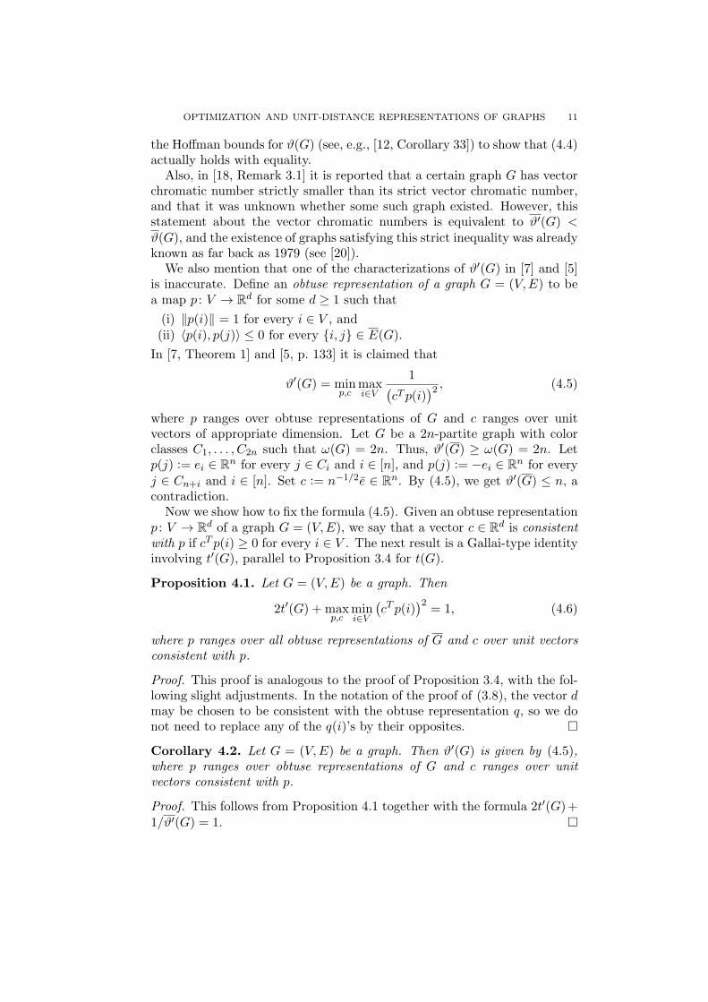
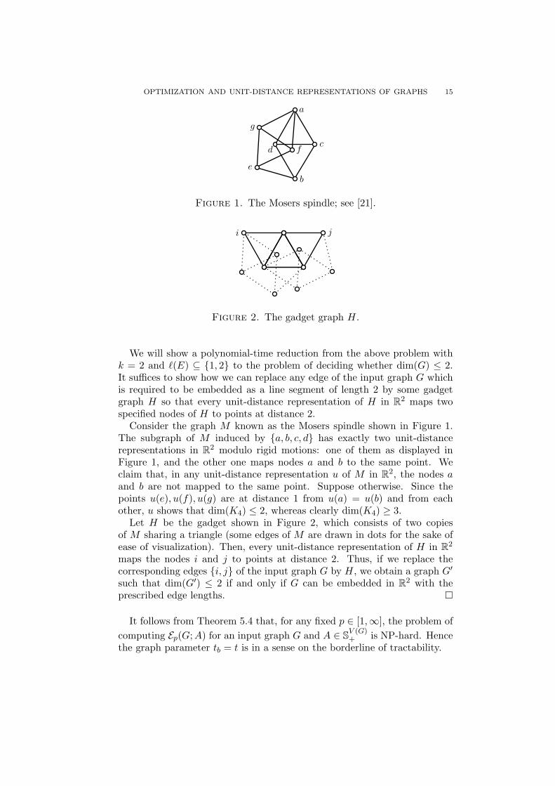
Figure 1. The Mosers spindle; see [21].

i j

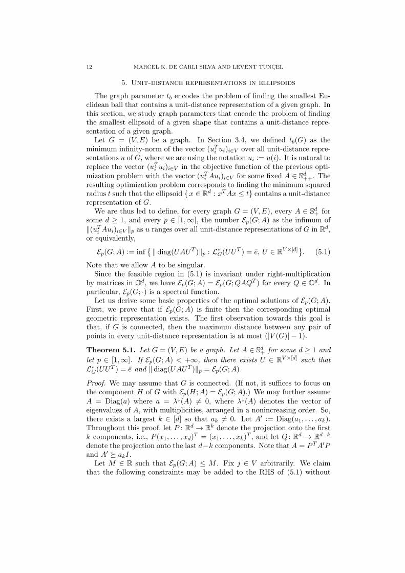
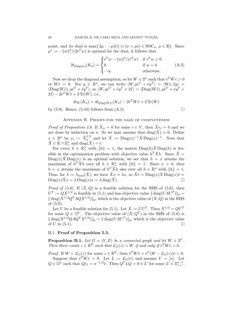
Figure 2. The gadget graph H.

We will show a polynomial-time reduction from the above problem withk = 2 and ℓ(E) ⊆ {1, 2} to the problem of deciding whether dim(G) ≤ 2.It suffices to show how we can replace any edge of the input graph G whichis required to be embedded as a line segment of length 2 by some gadgetgraph H so that every unit-distance representation of H in R2 maps twospecified nodes of H to points at distance 2.

Consider the graph M known as the Mosers spindle shown in Figure 1.The subgraph of M induced by {a, b, c, d} has exactly two unit-distancerepresentations in R2 modulo rigid motions: one of them as displayed inFigure 1, and the other one maps nodes a and b to the same point. Weclaim that, in any unit-distance representation u of M in R2, the nodes aand b are not mapped to the same point. Suppose otherwise. Since thepoints u(e), u(f), u(g) are at distance 1 from u(a) = u(b) and from eachother, u shows that dim(K4) ≤ 2, whereas clearly dim(K4) ≥ 3.

Let H be the gadget shown in Figure 2, which consists of two copiesof M sharing a triangle (some edges of M are drawn in dots for the sake ofease of visualization). Then, every unit-distance representation of H in R2

maps the nodes i and j to points at distance 2. Thus, if we replace thecorresponding edges {i, j} of the input graph G by H, we obtain a graph G′

such that dim(G′) ≤ 2 if and only if G can be embedded in R2 with theprescribed edge lengths. �

It follows from Theorem 5.4 that, for any fixed p ∈ [1,∞], the problem of

computing Ep(G;A) for an input graph G and A ∈ SV (G)+ is NP-hard. Hence

the graph parameter tb = t is in a sense on the borderline of tractability.


5.1. The extreme cases p ∈ {1,∞}. For every matrix U ∈ RV×V , if weset X := UUT , then there exists an orthogonal V × V matrix Q such thatUT = QX1/2. Hence, if A ∈ SV+, then

Ep(G;A) = inf ∥diag(X1/2QTAQX1/2)∥pL∗G(X) = e

X ∈ SV+, Q ∈ OV .(5.6)

When p = 1, the objective function in (5.6) is Tr(QTAQX) = ⟨QTAQ,X⟩so we can write

E1(G;A) = infQ∈OV

tQTAQ(G) (5.7)

where tW (G) is defined for any W ∈ SV as the SDP

tW (G) := inf{⟨W,X⟩ : L∗

G(X) = e, X ∈ SV+}. (5.8)

Proposition 5.5. Let G = (V,E) be a connected graph and let W ∈ SV .Then tW (G) is finite if and only if eTWe > 0 or We = 0. Moreover,whenever tW (G) is finite, both (5.8) and its dual SDP have optimal solutionsand their optimal values coincide.

The parameter tW (G) thus underlies the parameters E1(G;A) as well asthe hypersphere number t(G), since (3.4) shows that

t(G) = min{ tDiag(y)(G) : eT y = 1, y ∈ RV }.

If X is feasible in (5.8) for G = Kn, then X is completely determinedby its diagonal entries. Using this fact, it is easy to prove that the feasibleregion of (5.8) for G = Kn is

{X ∈ Sn+ : L∗Kn

(X) = e}= { (yeT + eyT + 2I)/4 : ∥e∥∥y∥ ≤ eT y + 2, y ∈ Rn}. (5.9)

Using a second-order cone programming formulation, we can show that

2tW (Kn) =

Tr(W )− ∥We∥2

eTWeif eTWe > 0

Tr(W ) if We = 0

−∞ otherwise.

(5.10)

Let us use (5.7) and (5.10) to compute E1(G;A). Let A ∈ Sn+ be nonzero.Since Qe ∈ Null(A) for some Q ∈ On, it follows from (5.7) and (5.10) that

2E1(Kn;A) = Tr(A)− sup{ ∥QTAQe∥2

eTQTAQe: Qe ∈ Null(A), Q ∈ On

}.

The supremum may be replaced by sup{ (hTA2h)/(hTAh) : h ∈ Null(A)⊥},which is easily seen to be λmax(A). This implies with Theorem 5.3 that

E1(Kn;A) =

{12

∑n−1i=1 λ↑

i (A) if A ∈ Sd+ with d ≥ n− 1

+∞ otherwise.(5.11)


For the other extreme p = ∞, the first property of hom-monotonicityholds. More precisely, let (an)n∈Z++ be a nondecreasing sequence of positivereals. Define An := Diag(a1, . . . , an) for every n ∈ Z++. Then,

G → H =⇒ E∞(G;An) ≤ E∞(H;An). (5.12)

We do not know whether the invariant E∞ satisfies the second propertyof hom-monotonicity. In fact, we do not know an analytical formula tocompute E∞(Kn;A) in terms of A. However, we have such a formula foran infinite family of complete graphs, as we now describe. Let H be ann × n Hadamard matrix, i.e., H is {±1}-valued and HTH = nI. We mayassume that H has the form HT =

[e LT

]. Then LTL = nI − eeT , so

12nL

∗Kn

(LTL) = e, i.e., the map i 7→ (2n)−1/2Lei is a unit-distance represen-tation of Kn. This map is called a Hadamard representation of Kn .

Theorem 5.6. Let n ∈ Z++ such that there exists an n × n Hadamardmatrix. Then, for any p ∈ [1,∞] and diagonal A ∈ Sn−1

+ , every Hadamardrepresentation of Kn is an optimal solution for Ep(Kn;A).

Proof. The objective value of the Hadamard representation L of Kn in

the optimization problem Ep(Kn;A) is[Tr(A)

2n

]∥e∥p. Thus, L is optimal

for p = 1 by (5.11). From the inequality ∥x∥1 ≤ n∥x∥∞ we get E∞(Kn;A) ≥1nE1(Kn;A), which shows that L is optimal for p = ∞. Therefore, L is op-timal for every p ∈ [1,∞]. �

It is natural to lift a Hadamard representation h of Kn to obtain a frugalfeasible solution for E(Kn+1;A). The image of h is an (n − 1)-dimensionalsimplex ∆. If v is a vertex of an n-dimensional simplex whose oppositefacet is ∆, then the line segment L joining v to the barycenter of ∆ is theshortest line segment joining v to ∆. It makes sense to align L with the mostexpensive axis, i.e., the one corresponding to λmax(A). Suppose A = Diag(a)and ∥a∥∞ = an. We thus obtain a unit-distance representation u of Kn+1

in Rn of the form

u(i) :=

{h(i)⊕ α, if i ∈ [n]

0⊕[α+

(n+12n

)1/2], if i = n+ 1.

By optimizing the shift parameter α, we obtain the following upper bound:

Proposition 5.7. Let n ∈ Z++ such that there exists an n × n Hadamardmatrix. If A ∈ Sn+, then

E∞(Kn+1;A) ≤Tr(A)

2(n+ 1)+

(Tr(A)− nλmax(A)

)28n(n+ 1)λmax(A)

. (5.13)

Equality holds for n = 2 if A ≻ 0.

The proof of equality for n = 2 involves the obvious parametrization of O2

and basic trigonometry.


References

[1] Y. Bilu. Tales of Hoffman: three extensions of Hoffman’s bound on the graph chro-matic number. J. Combin. Theory Ser. B, 96(4):608–613, 2006.

[2] P. J. Cameron, A. Montanaro, M. W. Newman, S. Severini, and A. Winter. On thequantum chromatic number of a graph. Electron. J. Combin., 14(1):Research Paper81, 15 pp. (electronic), 2007.

[3] F. R. K. Chung. Spectral graph theory, volume 92 of CBMS Regional Conference Seriesin Mathematics. Published for the Conference Board of the Mathematical Sciences,Washington, DC, 1997.

[4] P. Erdos, F. Harary, and W. T. Tutte. On the dimension of a graph. Mathematika,12:118–122, 1965.

[5] A. Galtman. Spectral characterizations of the Lovasz number and the Delsarte num-ber of a graph. J. Algebraic Combin., 12(2):131–143, 2000.

[6] D. Gijswijt. Matrix Algebras and Semidefinite Programming Techniques for Codes.PhD thesis, University of Amsterdam, 2005.

[7] M. X. Goemans. Semidefinite programming in combinatorial optimization.Math. Pro-gramming, 79(1-3, Ser. B):143–161, 1997. Lectures on mathematical programming(ismp97) (Lausanne, 1997).

[8] M. Grotschel, L. Lovasz, and A. Schrijver. Geometric algorithms and combinatorialoptimization, volume 2 of Algorithms and Combinatorics. Springer-Verlag, Berlin,second edition, 1993.

[9] H. van der Holst, M. Laurent, and A. Schrijver. On a minor-monotone graph invariant.J. Combin. Theory Ser. B, 65(2):291–304, 1995.

[10] B. Horvat, J. Kratochvıl, and T. Pisanski. On the computational complexity of degen-erate unit distance representations of graphs. In Combinatorial algorithms, volume6460 of Lecture Notes in Comput. Sci., pages 274–285. Springer, Heidelberg, 2011.

[11] D. Karger, R. Motwani, and M. Sudan. Approximate graph coloring by semidefiniteprogramming. J. ACM, 45(2):246–265, 1998.

[12] D. E. Knuth. The sandwich theorem. Electron. J. Combin., 1:Article 1, approx. 48pp. (electronic), 1994.

[13] M. Laurent and F. Rendl. Semidefinite programming and integer programming. InHandbook on Discrete Optimization, pages 393–514. Elsevier B. V., Amsterdam, 2005.

[14] L. Lovasz. On the Shannon capacity of a graph. IEEE Trans. Inform. Theory, 25(1):1–7, 1979.

[15] L. Lovasz. Semidefinite programs and combinatorial optimization. In Recent advancesin algorithms and combinatorics, pages 137–194. Springer, New York, 2003.

[16] L. Lovasz and M. D. Plummer. Matching theory, volume 121 of North-Holland Math-ematics Studies. North-Holland Publishing Co., Amsterdam, 1986. Annals of DiscreteMathematics, 29.

[17] R. J. McEliece, E. R. Rodemich, and H. C. Rumsey, Jr. The Lovasz bound and somegeneralizations. J. Combin. Inform. System Sci., 3(3):134–152, 1978.

[18] P. Meurdesoif. Strengthening the Lovasz θ(G) bound for graph coloring. Math. Pro-gram., 102(3, Ser. A):577–588, 2005.

[19] J. B. Saxe. Two papers on graph embedding problems. Technical Report CMU-CS-80-102, Department of Computer Science, Carnegie-Mellon University, 1980.

[20] A. Schrijver. A comparison of the Delsarte and Lovasz bounds. IEEE Trans. Inform.Theory, 25(4):425–429, 1979.

[21] A. Soifer. The mathematical coloring book. Springer, New York, 2009. Mathematicsof coloring and the colorful life of its creators, With forewords by Branko Grunbaum,Peter D. Johnson, Jr. and Cecil Rousseau.


[22] M. Szegedy. A note on the theta number of Lovasz and the generalized Delsartebound. In Proceedings of the 35th Annual IEEE Symposium on Foundations of Com-puter Science, 1994.

Appendix A. Proofs of Propositions 3.10 and 3.11 andEquations (5.9) and (5.10)

Proof of Proposition 3.10. Let (y, z) be an optimal solution for (3.4). Wewill construct a feasible solution for (3.4) applied to G/e with objectivevalue t(G) − ze. Assume e = {a, b} and V ′ := V (G/e) = V \ {b}, so weare denoting the contracted node of G/e by a. Let P be the V ′ × V matrixdefined by P := eae

Tb +

∑i∈V ′ eie

Ti . Then PLG(z)P

T = LG/e(z), where

z ∈ RE(G/e) is obtained from z as follows. In taking the contraction G/efrom G, immediately after we identify the ends of e, but before we removeresulting parallel edges, there are at most two edges between each pair ofnodes of G/e, as we assume that G is simple. If there is exactly one edgebetween nodes i and j, we just set z{i,j} := z{i,j}. If there are two edgesjoining nodes i and j, say f and f ′, we put z{i,j} := zf + zf ′ .

Similarly, if we define y : V ′ → R by putting yi := yi for i ∈ V ′ \ {a} and

ya := ya + yb, then P Diag(y)P T = Diag(y). Since P SV+ P T ⊆ SV ′+ , we see

that (y, z) is a feasible solution for (3.4) applied to G/e, and its objectivevalue is z(E(G/e)) = z(E)− ze.

To prove the inequality involving ϑ(G), use (3.2) together with its proof tosee that X corresponds to an optimal solution (y, z) for (3.4) with X/ϑ(G) =Diag(y)− LG(z), so ye = Xij/ϑ(G). �Proof of Proposition 3.11. By Theorem 3.1, it suffices to show t(G[N(i)]) ≤1 − 1/[4t(G)]. Let p : V → Rd be a hypersphere representation of G with

squared radius t := t(G). We may assume that p(i) = t1/2e1. For everyj ∈ N(i), we have 1 = ∥p(i)−p(j)∥2 = ∥p(i)∥2+∥p(j)∥2−2⟨p(i), p(j)⟩ = 2t−2t1/2[p(j)]1. Hence, [p(j)]1 = (2t−1)/(2t1/2) =: β for every j ∈ N(i). Definethe following hypersphere representation of G[N(i)]: for each j ∈ N(i), letq(j) be obtained from p(j) by dropping the first coordinate. The squaredradius of the resulting hypersphere representation is t−β2 = 1−1/(4t). �Proof of (5.9). Let X ∈ SV . Then L∗

Kn(X) = e if and only if 4X = yeT +

eyT + 2I for some y ∈ RV ; for the ‘only if’ part, use y := 2 diag(X)− e.Let y ∈ RV . The smallest eigenvalue of yeT + eyT is eT y−∥e∥∥y∥. Thus,

yeT + eyT + 2I ≽ 0 if and only if ∥e∥∥y∥ ≤ eT y + 2. �Proof of (5.10). Assume first that W = Diag(w) for some w ∈ Rn. ByProposition 5.5, finiteness of tW (Kn) implies eTw > 0 or w = 0. Assumethe former. By (5.9),

2tW (Kn) = eTw +min{wT y : ∥e∥y0 − eT y = 2, y0 ⊕ y ∈ SOCn}, (A.1)

where SOCn := { y0 ⊕ y ∈ R⊕ Rn : ∥y∥ ≤ y0}. The second-order cone pro-gram on the RHS of (A.1) has y0 ⊕ y := (2 + ∥e∥2)/∥e∥ ⊕ e as a Slater


point, and its dual is max{ 2µ : −µ∥e∥ ⊕ (w + µe) ∈ SOCn, µ ∈ R}. Sinceµ∗ := −∥w∥2/(2eTw) is optimal for the dual, it follows that

2tDiag(w)(Kn) =

eTw − ∥w∥2/(eTw) if eTw > 0

0 if w = 0

−∞ otherwise.

(A.2)

Now we drop the diagonal assumption, so let W ∈ Sn such that eTWe > 0or We = 0. For y ∈ Rn, we can write ⟨W,yeT + eyT ⟩ = ⟨We, 2y⟩ =⟨Diag(We), yeT + eyT ⟩, so ⟨W,yeT + eyT + 2I⟩ = ⟨Diag(We), yeT + eyT +2I⟩ − 2eTWe+ 2Tr(W ), i.e.,

4tW (Kn) = 4tDiag(We)(Kn)− 2eTWe+ 2Tr(W )

by (5.9). Hence, (5.10) follows from (A.2). �

Appendix B. Proofs for the sake of completeness

Proof of Proposition 3.6. If Xii = 0 for some i ∈ V , then Xei = 0 and weare done by induction on n. So we may assume that diag(X) > 0. Define

x ∈ Rn by xi := X1/2ii and let X := Diag(x)−1X Diag(x)−1. Note that

X ∈ K ∩ Sn+ and diag(X) = e.For every h ∈ Rn

+ with ∥h∥ = 1, the matrix Diag(h)X Diag(h) is fea-

sible in the optimization problem with objective value hT Xh. Since X =Diag(x)X Diag(x) is an optimal solution, we see that h = x attains themaximum of hT Xh over all h ∈ Rn

+ with ∥h∥ = 1. Since x > 0, then

h = x attains the maximum of hT Xh also over all h ∈ Rn with ∥h∥ = 1.

Thus, for λ := λmax(X), we have Xx = λx, so Xe = Diag(x)X Diag(x)e =

Diag(x)Xx = λDiag(x)x = λdiag(X). �

Proof of (5.6). If (X,Q) is a feasible solution for the RHS of (5.6), then

UT := QX1/2 is feasible in (5.1) and has objective value ∥diag(UAUT )∥p =∥ diag(X1/2QTAQX1/2)∥p, which is the objective value of (X,Q) in the RHSof (5.6).

Let U be a feasible solution for (5.1). Let X := UUT . Then X1/2 = QUT

for some Q ∈ OV . The objective value of (X,QT ) in the RHS of (5.6) is

∥ diag(X1/2QAQTX1/2)∥p = ∥ diag(UAUT )∥p, which is the objective valueof U in (5.1). �

B.1. Proof of Proposition 5.5.

Proposition B.1. Let G = (V,E) be a connected graph and let W ∈ SV .Then there exists z ∈ RE such that LG(z) ≺ W if and only if eTWe > 0.

Proof. If W ≻ LG(z) for some z ∈ RE , then eTWe = eT (W − LG(z))e > 0.Suppose that eTWe > 0. Let L := LG(e) and assume V = [n]. Let

Q ∈ On such that Qe1 = n−1/2e. Then QTLQ = 0⊕L′ for some L′ ∈ Sn−1++ ,


since G. Let A ∈ Sn−1, b ∈ Rn−1 and γ ∈ R such that

QTWQ =

[γ bT

b A

].

Note that γ = eT1 QTWQe1 = n−1eTWe > 0. Thus, for every λ ∈ R, we

have QT (W − λL)Q ≻ 0 if and only if A− λL′ − γ−1bbT ≻ 0. Since L′ ≻ 0,we know that for λ negative and with sufficiently large magnitude, we haveQT (W − λL)Q ≻ 0, and hence W ≻ LG(λe). �

Proposition B.2. Let G be a graph and let W ∈ SV (G) such that eTWe = 0.If tW (G) > −∞, then e ∈ Null(W ).

Proof. Assume tW (G) > −∞. Since (5.8) has 12I as a Slater point, the dual

sup{eT z : W ≽ LG(z), z ∈ RE

}. (B.1)

of (5.8) has an optimal solution z. Assume V = [n] and let Q ∈ On such that

Qe1 = n−1/2e. Then QT (W − LG(z))Q ≽ 0 and eT1 QT (W − LG(z))Qe1 =

n−1eT (W − LG(z))e = 0 imply that

eTkQTWe = eTkQ

T (W − LG(z))e = n1/2eTkQT (W − LG(z))Qe1 = 0

for every k ∈ [n]. Thus, We ∈ {Qe2, . . . , Qen}⊥ = {e}⊥⊥, which togetherwith eTWe = 0 implies We = 0. �Proposition B.3. Let G be a connected graph and let W ∈ SV (G) suchthat We = 0. Then (5.8) and (B.1) have optimal solutions and the optimalvalues coincide.

Proof. Since We = 0, it is easy to check that the constraint eTXe = 0may be added to (5.8) without changing the optimal value. The dual ofthis augmented SDP is sup

{eT z : W − µeeT ≽ LG(z), z ∈ RE , µ ∈ R

}. By

Proposition B.1, this dual has a Slater point (z, µ) with µ = 1, so (5.8) hasan optimal solution. Since (5.8) has a Slater point and is bounded below,its dual (B.1) has an optimal solution and the optimal values coincide. �Proof of Proposition 5.5. If eTWe > 0, then (5.8) and its dual (B.1) haveSlater points by Proposition B.1. If eTWe < 0, then Xt :=

12I + teeT with

t → ∞ shows that tW (G) = −∞. Assume now that eTWe = 0. If We = 0,then tW (G) = −∞. Otherwise, apply Proposition B.3. �

optimization problems over unit-distance representations of graphs 1

Documents