Optimization — Introduction

Optimization — Introduction 1 / 33

Optimization deals with how to do things in the best possible manner:

Design of multi-criteria controllers

Clustering in fuzzy modeling

Trajectory planning of robots

Scheduling in process industry

Estimation of system parameters

Simulation of continuous time systems on digital computers

Design of predictive controllers with input-saturation

Related courses:

SC4060: Predictive and adaptive control

SC4040: Filtering & identification

EE4530 Applied Convex Optimization

WI4207 Continuous Optimization

WI4219 Discrete Optimization

Optimization — Introduction 2 / 33

Overview

Three subproblems:

Formulation:Translation of engineering demands and requirements into amathematically well-defined optimization problem

Initialization:Choice of right algorithmChoice of initial values for parameters

Optimization procedure;Various optimization techniquesVarious computer platforms

Optimization — Introduction 3 / 33

Teaching goals

I. Optimization problem → most efficient and best suited optimizationalgorithm

II. Engineering problem → optimization problem:◮ specifications → mathematical formulation◮ simplifications/approximations?◮ efficiency◮ implementation

Optimization — Introduction 4 / 33

Contents

Part I: Optimization techniques

Part II: Formulating the controller design problem as an optimizationproblem

Optimization — Introduction 5 / 33

Contents of Part I

I. Optimization Techniques1 Introduction2 Linear Programming3 Quadratic Programming4 Nonlinear Optimization5 Constraints in Nonlinear Optimization6 Convex Optimization7 Global Optimization8 Summary9 Matlab Optimization Toolbox10 Multi-Objective Optimization11 Integer Optimization

Optimization — Introduction 6 / 33

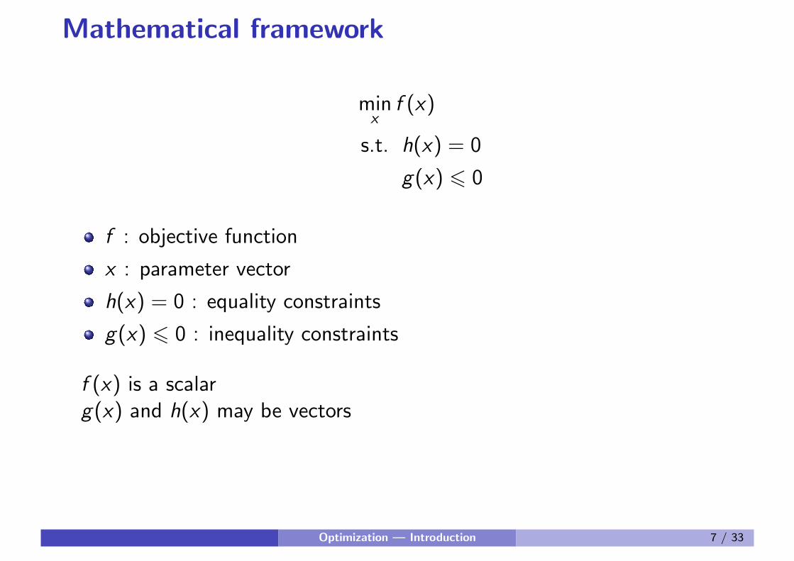
Mathematical framework

minx

f (x)

s.t. h(x) = 0

g(x) 6 0

f : objective function

x : parameter vector

h(x) = 0 : equality constraints

g(x) 6 0 : inequality constraints

f (x) is a scalarg(x) and h(x) may be vectors

Optimization — Introduction 7 / 33

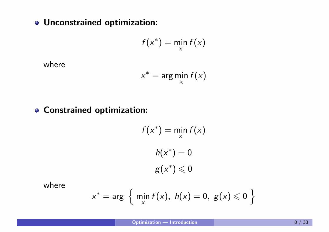
Unconstrained optimization:

f (x∗) = minx

f (x)

wherex∗ = argmin

xf (x)

Constrained optimization:

f (x∗) = minx

f (x)

h(x∗) = 0

g(x∗) 6 0

wherex∗ = arg

{

minx

f (x), h(x) = 0, g(x) 6 0}

Optimization — Introduction 8 / 33

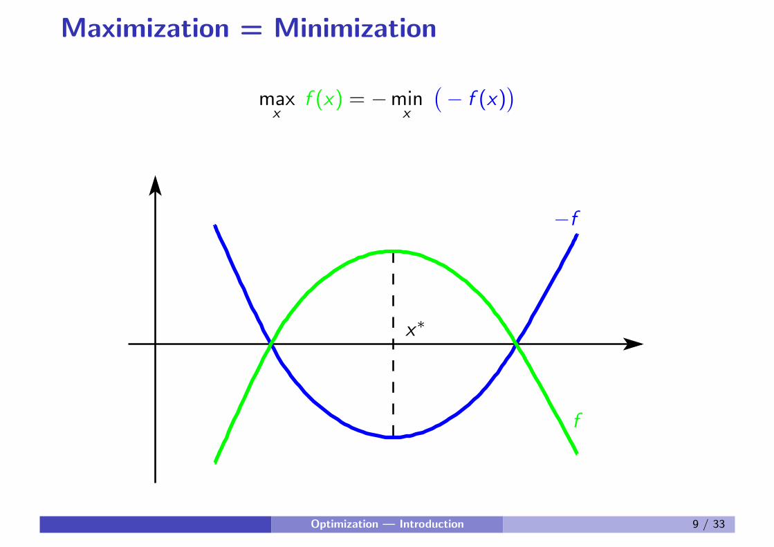
Maximization = Minimization

maxx

f (x) = −minx

(

− f (x))

f

−f

x∗

Optimization — Introduction 9 / 33

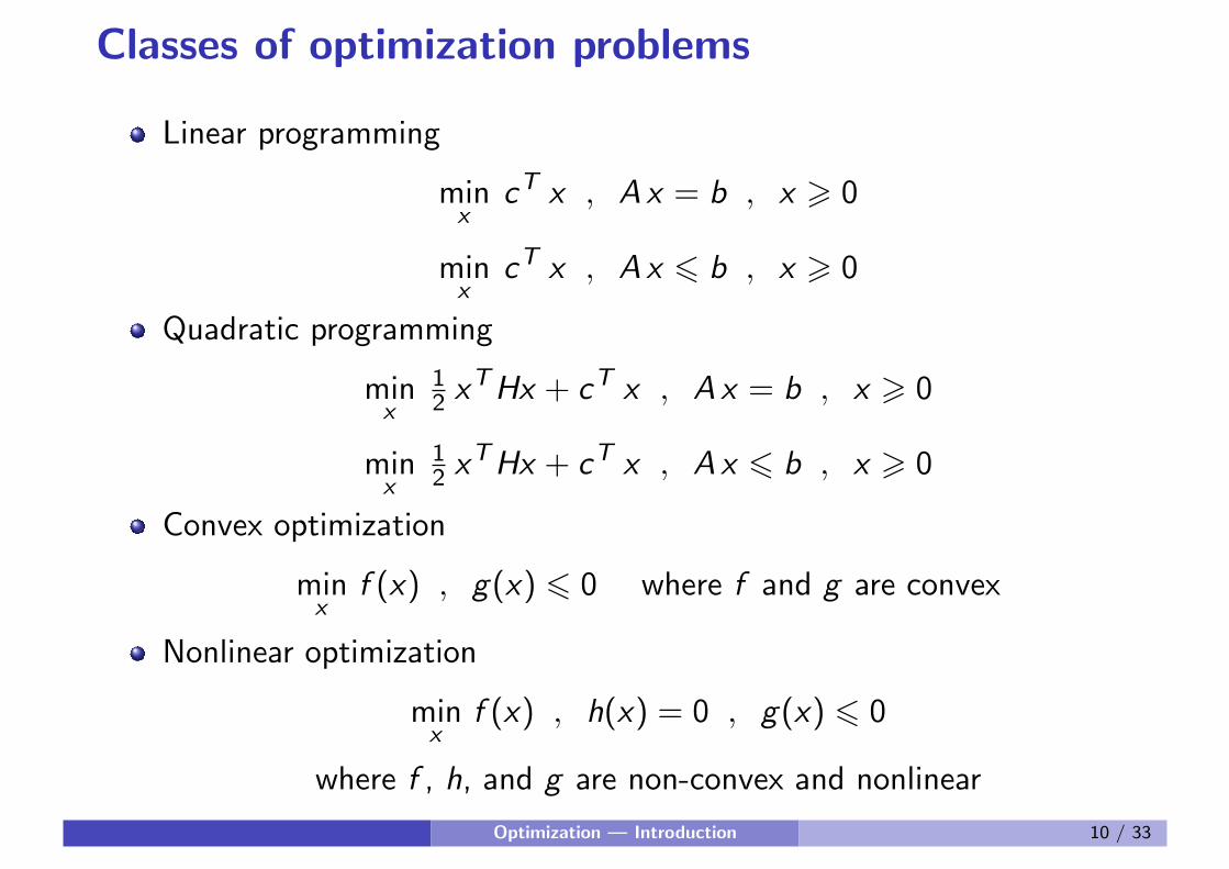
Classes of optimization problems

Linear programming

minx

cT x , Ax = b , x > 0

minx

cT x , Ax 6 b , x > 0

Quadratic programming

minx

12 x

THx + cT x , Ax = b , x > 0

minx

12 x

THx + cT x , Ax 6 b , x > 0

Convex optimization

minx

f (x) , g(x) 6 0 where f and g are convex

Nonlinear optimization

minx

f (x) , h(x) = 0 , g(x) 6 0

where f , h, and g are non-convex and nonlinear

Optimization — Introduction 10 / 33

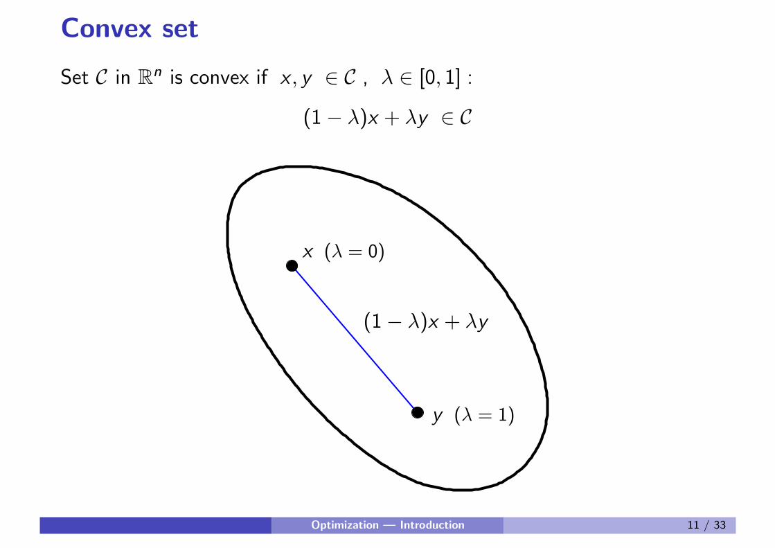
Convex set

Set C in Rn is convex if x , y ∈ C , λ ∈ [0, 1] :

(1− λ)x + λy ∈ C

x (λ = 0)

y (λ = 1)

(1− λ)x + λy

Optimization — Introduction 11 / 33

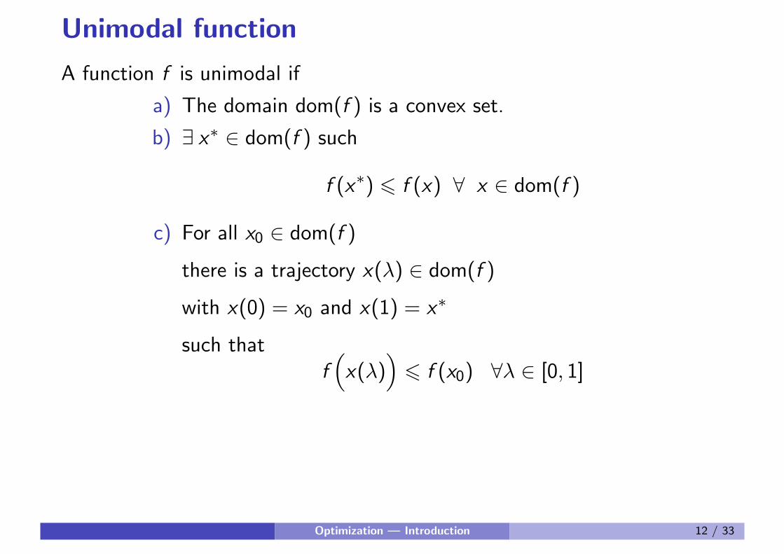
Unimodal function

A function f is unimodal if

a) The domain dom(f ) is a convex set.

b) ∃ x∗ ∈ dom(f ) such

f (x∗) 6 f (x) ∀ x ∈ dom(f )

c) For all x0 ∈ dom(f )

there is a trajectory x(λ) ∈ dom(f )

with x(0) = x0 and x(1) = x∗

such thatf(

x(λ))

6 f (x0) ∀λ ∈ [0, 1]

Optimization — Introduction 12 / 33

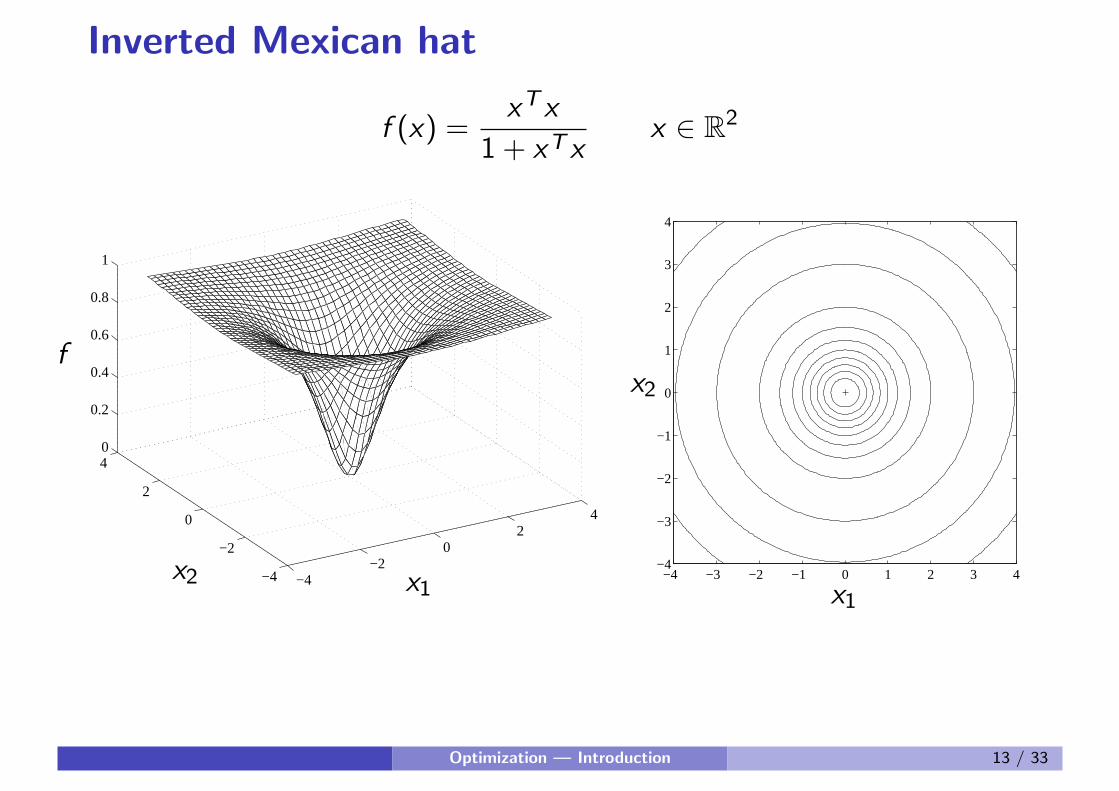
Inverted Mexican hat

f (x) =xT x

1 + xT xx ∈ R

2

−4−2

02

4

−4

−2

0

2

40

0.2

0.4

0.6

0.8

1

x1x2

f

−4 −3 −2 −1 0 1 2 3 4−4

−3

−2

−1

0

1

2

3

4

x1

x2

Optimization — Introduction 13 / 33

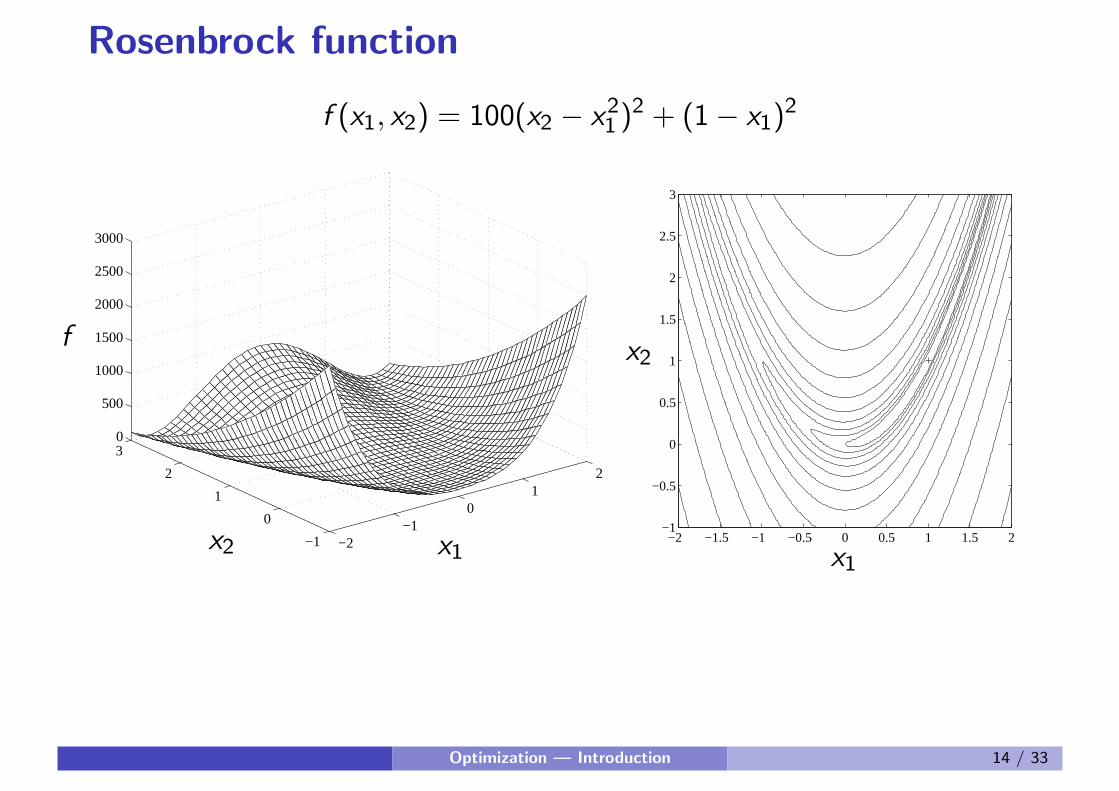
Rosenbrock function

f (x1, x2) = 100(x2 − x21 )2 + (1− x1)

2

−2−1

01

2

−1

0

1

2

30

500

1000

1500

2000

2500

3000

x1x2

f

−2 −1.5 −1 −0.5 0 0.5 1 1.5 2−1

−0.5

0

0.5

1

1.5

2

2.5

3

x1

x2

Optimization — Introduction 14 / 33

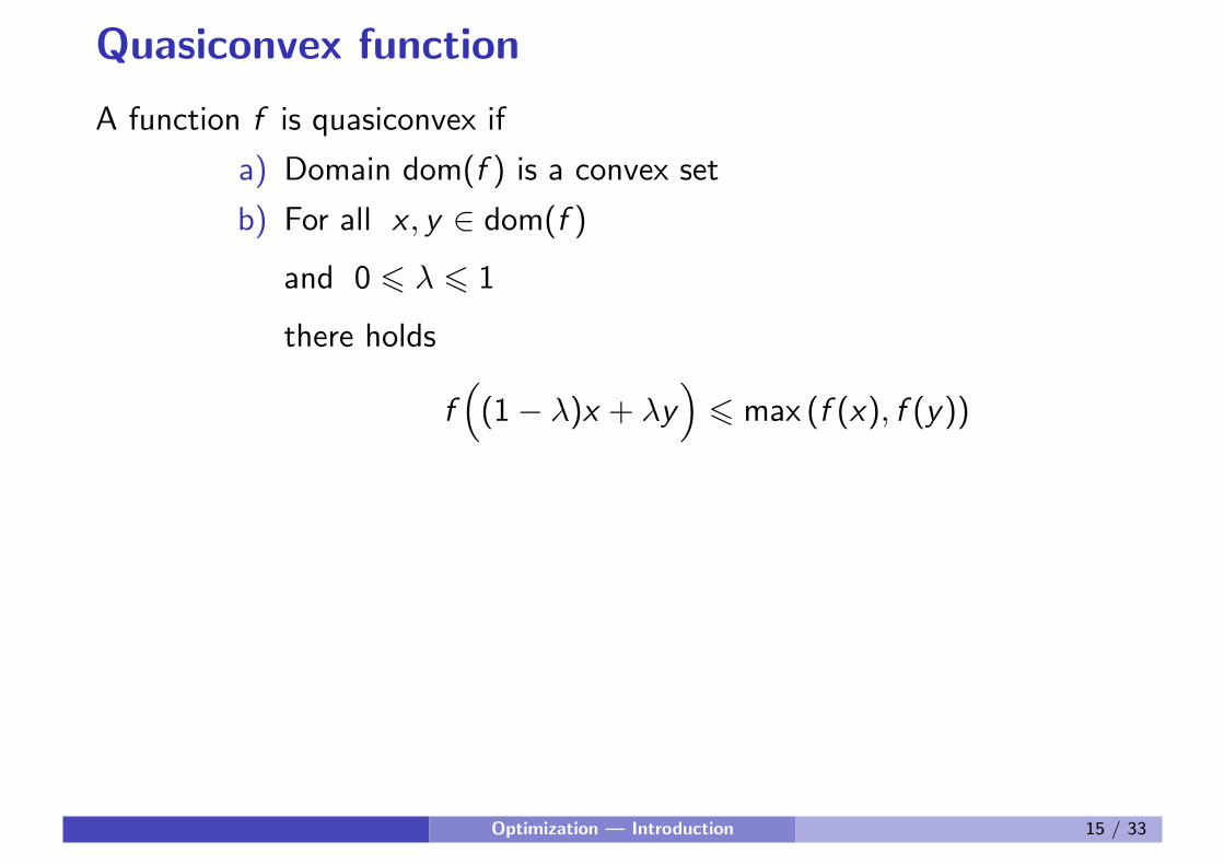
Quasiconvex function

A function f is quasiconvex if

a) Domain dom(f ) is a convex set

b) For all x , y ∈ dom(f )

and 0 6 λ 6 1

there holds

f(

(1− λ)x + λy)

6 max (f (x), f (y))

Optimization — Introduction 15 / 33

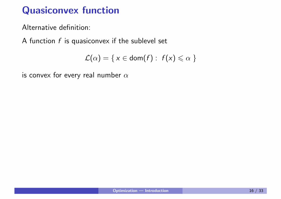
Quasiconvex function

Alternative definition:

A function f is quasiconvex if the sublevel set

L(α) = { x ∈ dom(f ) : f (x) 6 α }

is convex for every real number α

Optimization — Introduction 16 / 33

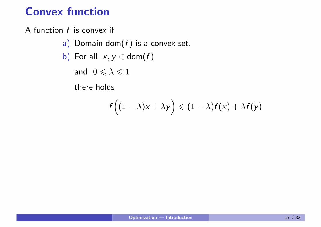
Convex function

A function f is convex if

a) Domain dom(f ) is a convex set.

b) For all x , y ∈ dom(f )

and 0 6 λ 6 1

there holds

f(

(1− λ)x + λy)

6 (1− λ)f (x) + λf (y)

Optimization — Introduction 17 / 33

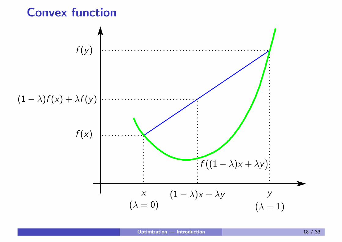
Convex function

x

(λ = 0)

y

(λ = 1)

(1− λ)x + λy

f(

(1− λ)x + λy)

(1− λ)f (x) + λf (y)

f (x)

f (y)

Optimization — Introduction 18 / 33

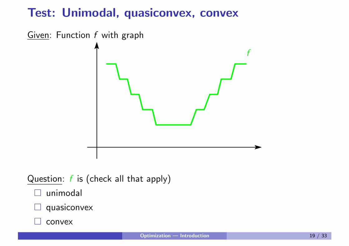
Test: Unimodal, quasiconvex, convex

Given: Function f with graph

f

Question: f is (check all that apply)

� unimodal

� quasiconvex

� convex

Optimization — Introduction 19 / 33

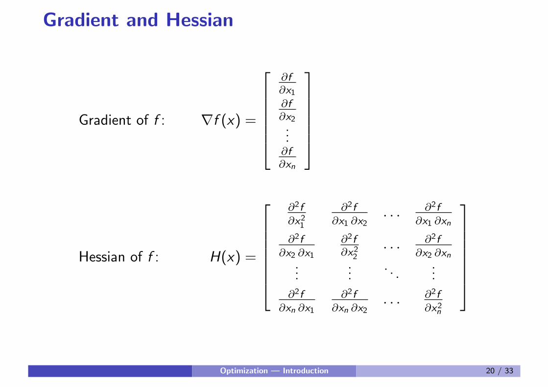
Gradient and Hessian

Gradient of f : ∇f (x) =

∂f

∂x1∂f

∂x2...∂f

∂xn

Hessian of f : H(x) =

∂2f

∂x21

∂2f

∂x1 ∂x2. . . ∂2f

∂x1 ∂xn

∂2f

∂x2 ∂x1

∂2f

∂x22. . . ∂2f

∂x2 ∂xn...

.... . .

...∂2f

∂xn ∂x1

∂2f

∂xn ∂x2. . . ∂2f

∂x2n

Optimization — Introduction 20 / 33

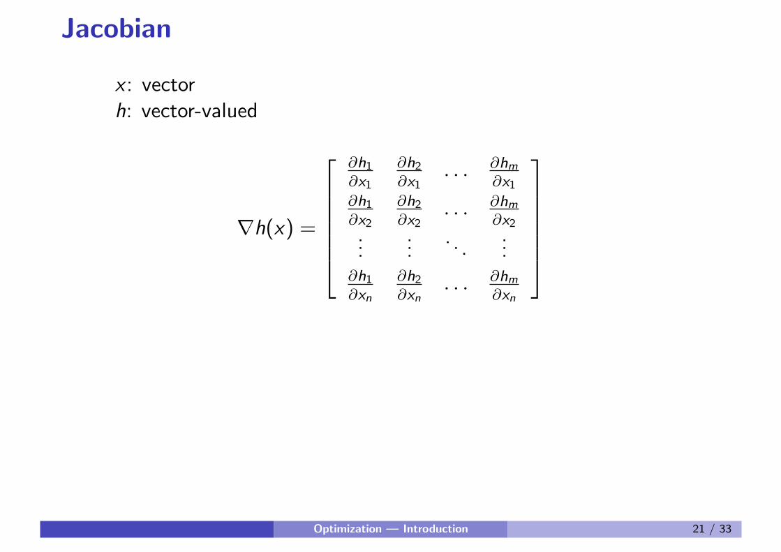
Jacobian

x : vectorh: vector-valued

∇h(x) =

∂h1∂x1

∂h2∂x1

. . . ∂hm∂x1

∂h1∂x2

∂h2∂x2

. . . ∂hm∂x2

......

. . ....

∂h1∂xn

∂h2∂xn

. . . ∂hm∂xn

Optimization — Introduction 21 / 33

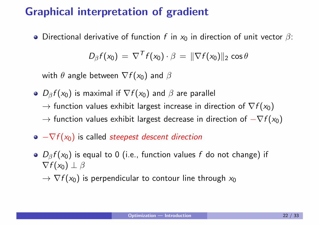
Graphical interpretation of gradient

Directional derivative of function f in x0 in direction of unit vector β:

Dβf (x0) = ∇T f (x0) · β = ‖∇f (x0)‖2 cos θ

with θ angle between ∇f (x0) and β

Dβf (x0) is maximal if ∇f (x0) and β are parallel

→ function values exhibit largest increase in direction of ∇f (x0)

→ function values exhibit largest decrease in direction of −∇f (x0)

−∇f (x0) is called steepest descent direction

Dβf (x0) is equal to 0 (i.e., function values f do not change) if∇f (x0) ⊥ β

→ ∇f (x0) is perpendicular to contour line through x0

Optimization — Introduction 22 / 33

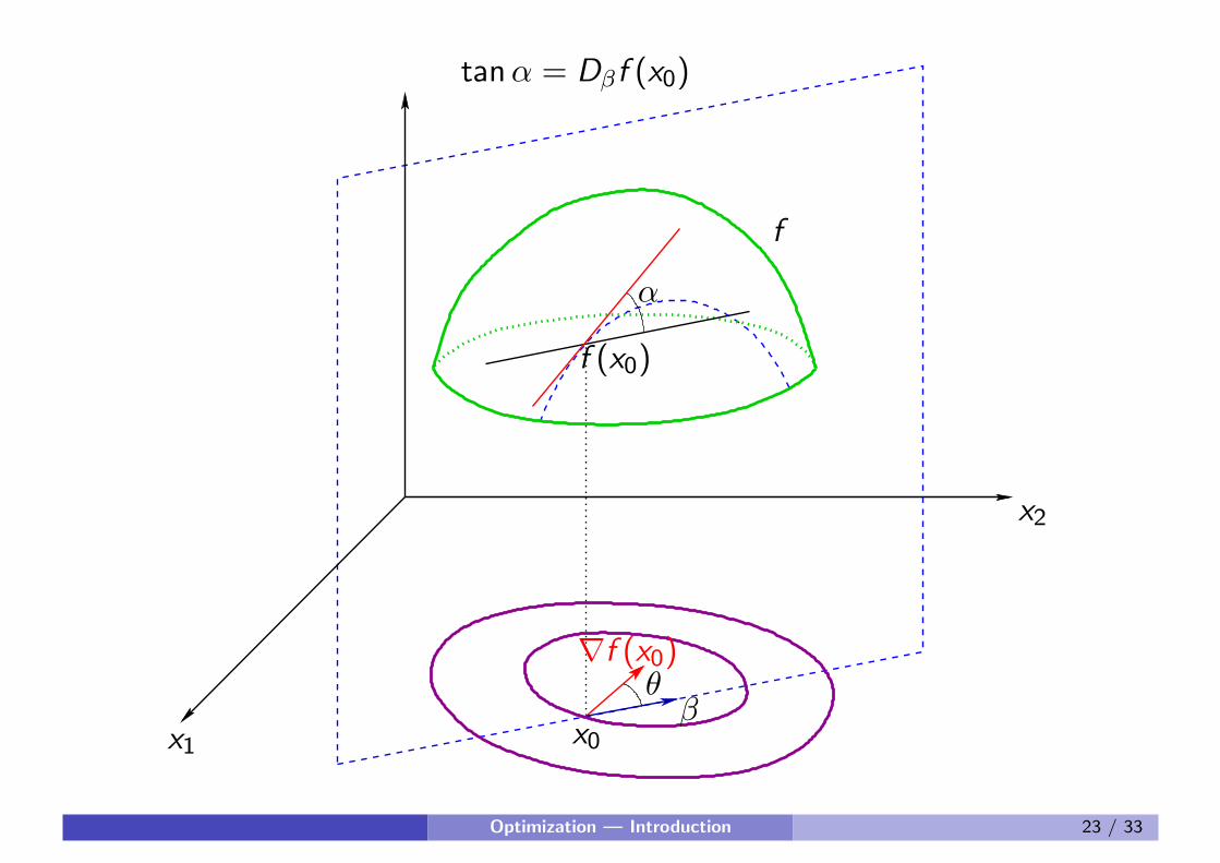
f

α

βθ

x0

f (x0)

x1

x2

∇f (x0)

tanα = Dβf (x0)

Optimization — Introduction 23 / 33

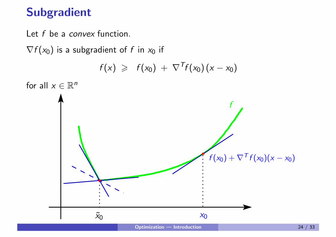
Subgradient

Let f be a convex function.

∇f (x0) is a subgradient of f in x0 if

f (x) > f (x0) + ∇Tf (x0) (x − x0)

for all x ∈ Rn

f

f (x0) +∇T f (x0)(x − x0)

x0x̃0Optimization — Introduction 24 / 33

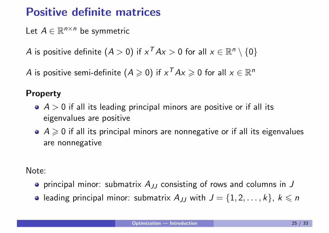
Positive definite matrices

Let A ∈ Rn×n be symmetric

A is positive definite (A > 0) if xTAx > 0 for all x ∈ Rn \ {0}

A is positive semi-definite (A > 0) if xTAx > 0 for all x ∈ Rn

Property

A > 0 if all its leading principal minors are positive or if all itseigenvalues are positive

A > 0 if all its principal minors are nonnegative or if all its eigenvaluesare nonnegative

Note:

principal minor: submatrix AJJ consisting of rows and columns in J

leading principal minor: submatrix AJJ with J = {1, 2, . . . , k}, k 6 n

Optimization — Introduction 25 / 33

Classes of optimization problems

Linear programming

minx

cT x , Ax = b , x > 0

minx

cT x , Ax 6 b , x > 0

Quadratic programming

minx

12x

THx + cT x , Ax = b , x > 0

minx

12x

THx + cT x , Ax 6 b , x > 0

Convex optimization

minx

f (x) , g(x) 6 0 where f and g are convex

Nonlinear optimization

minx

f (x) , h(x) = 0 , g(x) 6 0

where f , h, and g are non-convex and nonlinear

Optimization — Introduction 26 / 33

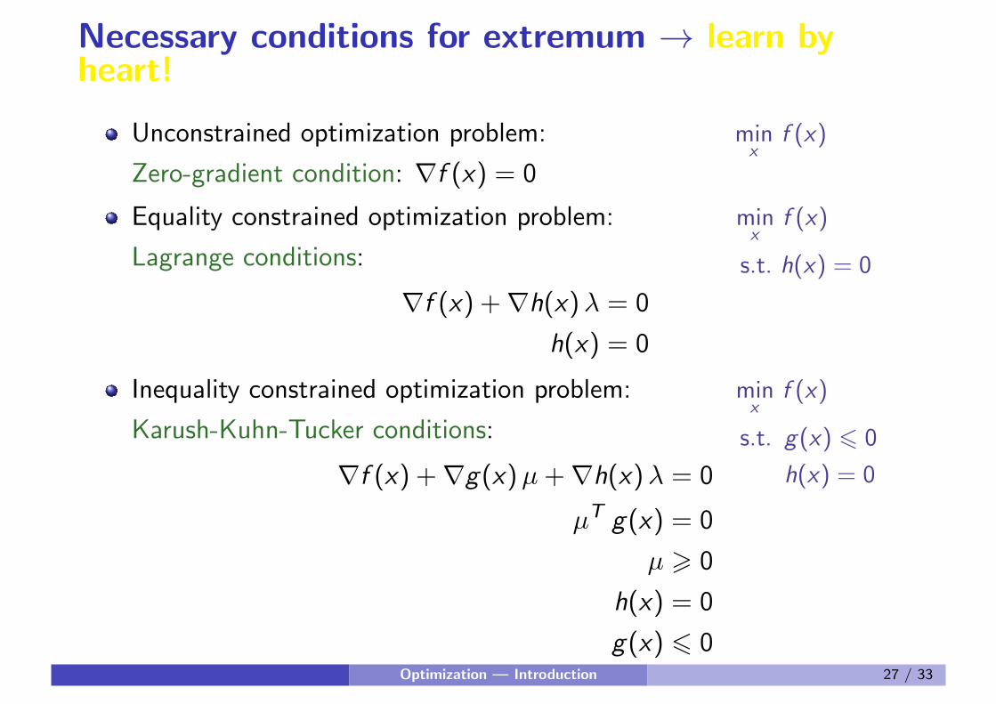
Necessary conditions for extremum → learn byheart!

Unconstrained optimization problem: minx

f (x)

Zero-gradient condition: ∇f (x) = 0

Equality constrained optimization problem: minx

f (x)

s.t. h(x) = 0Lagrange conditions:

∇f (x) +∇h(x)λ = 0

h(x) = 0

Inequality constrained optimization problem: minx

f (x)

s.t. g(x) 6 0

h(x) = 0

Karush-Kuhn-Tucker conditions:

∇f (x) +∇g(x)µ+∇h(x)λ = 0

µT g(x) = 0

µ > 0

h(x) = 0

g(x) 6 0Optimization — Introduction 27 / 33

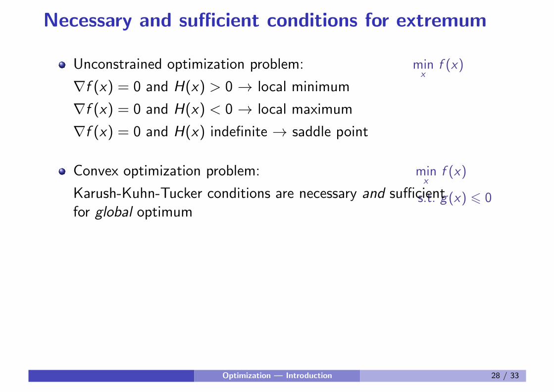
Necessary and sufficient conditions for extremum

Unconstrained optimization problem: minx

f (x)

∇f (x) = 0 and H(x) > 0 → local minimum

∇f (x) = 0 and H(x) < 0 → local maximum

∇f (x) = 0 and H(x) indefinite → saddle point

Convex optimization problem: minx

f (x)

s.t. g(x) 6 0Karush-Kuhn-Tucker conditions are necessary and sufficientfor global optimum

Optimization — Introduction 28 / 33

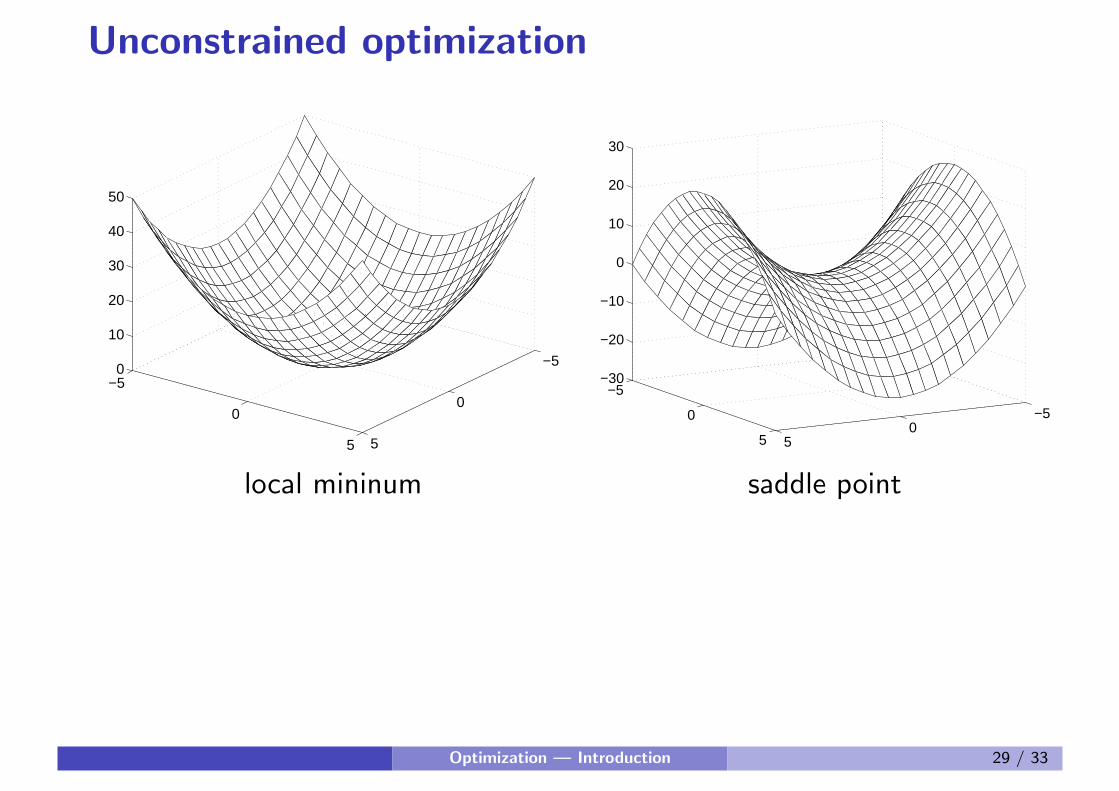
Unconstrained optimization

−5

0

5

−5

0

5

0

10

20

30

40

50

−50

5

−5

0

5

−30

−20

−10

0

10

20

30

local mininum saddle point

Optimization — Introduction 29 / 33

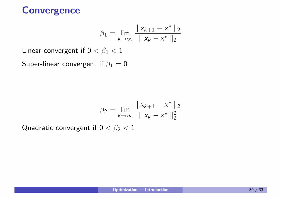
Convergence

β1 = limk→∞

‖ xk+1 − x∗ ‖2‖ xk − x∗ ‖2

Linear convergent if 0 < β1 < 1

Super-linear convergent if β1 = 0

β2 = limk→∞

‖ xk+1 − x∗ ‖2‖ xk − x∗ ‖22

Quadratic convergent if 0 < β2 < 1

Optimization — Introduction 30 / 33

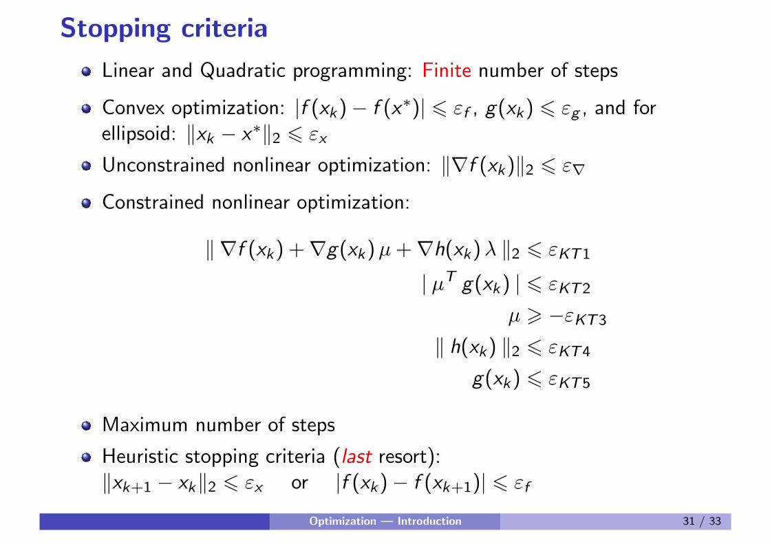
Stopping criteria

Linear and Quadratic programming: Finite number of steps

Convex optimization: |f (xk)− f (x∗)| 6 εf , g(xk) 6 εg , and forellipsoid: ‖xk − x∗‖2 6 εx

Unconstrained nonlinear optimization: ‖∇f (xk)‖2 6 ε∇

Constrained nonlinear optimization:

‖ ∇f (xk) +∇g(xk)µ+∇h(xk)λ ‖2 6 εKT1

| µT g(xk) | 6 εKT2

µ > −εKT3

‖ h(xk) ‖2 6 εKT4

g(xk) 6 εKT5

Maximum number of steps

Heuristic stopping criteria (last resort):‖xk+1 − xk‖2 6 εx or |f (xk)− f (xk+1)| 6 εf

Optimization — Introduction 31 / 33

Summary

Standard form of optimization problem:minx

f (x) s.t. h(x) = 0, g(x) 6 0

Classes of optimization problems: linear, quadratic, convex, nonlinear

Convex sets & functions

Gradient, subgradient, and Hessian

Conditions for extremum

Stopping criteria

Optimization — Introduction 32 / 33

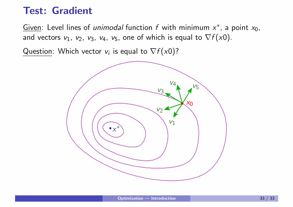
Test: Gradient

Given: Level lines of unimodal function f with minimum x∗, a point x0,and vectors v1, v2, v3, v4, v5, one of which is equal to ∇f (x0).

Question: Which vector vi is equal to ∇f (x0)?

x∗

x0

v1

v2

v3v4 v5

Optimization — Introduction 33 / 33