1

Paper 851-2017

Optimizing Delivery Routes with SAS® Software

Ben Murphy, Zencos; Bruce Bedford, Oberweis Dairy, Inc.

ABSTRACT Optimizing delivery routes and efficiently using delivery drivers are examples of classic problems in operations research, such as the Traveling Salesman Problem. In this paper, Oberweis and Zencos collaborate to describe how to leverage SAS software to solve these problems and optimize delivery routes for a retail delivery service.

Oberweis Dairy specializes in home delivery service that delivers customers premium dairy products directly to their homes. Because freshness is critical to delivering an excellent customer experience, Oberweis is especially motivated to optimize their delivery logistics. As Oberweis works to develop an expanding footprint and a growing business, Zencos is helping to ensure that delivery routes are optimized and delivery drivers are used efficiently.

INTRODUCTION

This paper explores the practical and technical considerations for optimizing delivery routes. When dealing with a complicated network of delivery destinations, the optimization of delivery routes can be broken into two components. The first component problem is to break the full list of delivery destinations into smaller groups that are reasonable to deliver as part of the same delivery route. The second component problem is to optimize the delivery order for all destinations within each group.

This paper explains ways to solve each of these component problems, and explores the ways in which the complexity of these problems may vary in each individual situation. From pragmatic operations and technical analyst perspectives, this paper will help inform ways of thinking about delivery optimization, structuring the problem of delivery optimization, and solving delivery optimization problems with SAS software.

OBERWEIS HOME DELIVERY

DAIRY AND MORE, STRAIGHT TO YOUR DOOR

Oberweis prides itself on delivering high quality dairy products to the doorstep of customers throughout the Midwest and the Virginia Beach area. Oberweis takes great care to ensure that the products are sourced from small family-owned dairy farms with cows that are raised in naturally comfortable environments. Customers can choose from an extensive menu of options that include dairy products, which are the core of the Oberweis brand, and a variety of breakfast, dinner, snack, cheese, beverage and dessert products as well.

As the customers sign up for home delivery service, they build the list of items they would like delivered by selecting from the menu of products available. Oberweis has several regional distribution centers from which these products are delivered. At each distribution center, products are loaded onto delivery trucks and hand delivered to customer door steps once a week.

HOME DELIVERY LOGISTICS

The logistics for the delivery process is traditionally managed manually by experienced analysts at Oberweis. These analysts have some heuristics that they employ to ensure that deliveries are timely and that products remain fresh for customers. The practical motivation for this paper is to seek opportunities to improve and optimize the efficiency of the delivery process to help reduce costs and enable Oberweis to maximize the use of resources for the home delivery service. By ensuring that the deliveries are scheduled in the optimal order, Oberweis can minimize distribution costs, including fuel and delivery vehicle maintenance costs throughout their regional footprint.

2

To understand the details of the home delivery customers, Oberweis tracks the details of their locations and their order specifications. These location details can be represented generally by the longitude and latitude coordinates of each delivery location. In addition to the locations of the delivery destinations, other constraints that might be important for understanding how to optimize the delivery process include the distance from each delivery point to the distribution center (the location of which is tracked using longitude and latitude), capacity of the trucks (by volume and/or weight), and specific considerations for driving directions (such as bodies of water that might cause significant differences between the straight-line distances and actual driving distances).

Of these factors, this paper only considers the location of the distribution center. This paper does not consider the capacity of the vehicles because data about the weight of delivery items and the weight capacity of delivery vehicles is not readily available. Oberweis has experienced significant repair costs that may be related to the heavy weights of deliveries, so delivery vehicles may change to better accommodate delivery needs. To simplify the problem, the complexity of measuring driving distances between thousands of delivery points will be avoided in favor of measuring straight line distances between the delivery points.

CONCEPTUAL SOLUTION FRAMEWORK

CONSIDER A SIMPLE EXAMPLE

Understanding the complexity of optimizing delivery routes is easiest when starting with a sense of the scope and magnitude of the problem. Oberweis has over 10,000 home delivery customers spread across their regional distribution areas, with each distribution center having multiple drivers that each work 5 days a week, and multiple vehicles that can be used for deliveries. What if there were only 50 customers and they were all located near the same distribution center?

For these 50 delivery locations, assume that all 50 are located close enough to each other that 1 delivery person can deliver to all those locations in 1 shift. The first step to optimizing the delivery route for serving those 50 customers is to quantify the distances between all 50 locations and the distribution center. For the 50 locations and the distribution center, that involves 2,550 (512-51) different combinations of distance calculations.

THE TRAVELING SALESMAN PROBLEM

Once the distances are calculated, finding the optimal route through each point is an example of the Traveling Salesman Problem (TSP). The TSP is relevant in many other applications, and studying problems like the TSP is a significant academic pursuit. As a result, a great deal of information is available publicly about the nature and complexity of the TSP, so the full details are not covered in this paper. However, it is important to acknowledge that the TSP is in a class of very difficult problems, called NP-Hard problems, in the fields of combinatorial optimization, operations research and theoretical computer science.

Practically, one of the important implications of the complexity of the TSP is that for 50 delivery destinations, solving it by trying every possible solution would require iterating through about 1.5 * 1064 different possible combinations of routes. Fortunately, the TSP is rarely solved using a brute force approach that iterates through every possible option. Using techniques that eliminate obviously suboptimal solutions requires iterating through far fewer possible solutions to find the optimal route. Even with sophisticated ways of iterating through possible solutions to find the optimal route, identifying the optimal route over 50 destinations is not trivial.

Another attribute of the TSP (and other problems that are similarly difficult) is that the complexity and the time required to find a solution grows exponentially as the size of the problem increases. Solving a TSP routing for 250 destinations (which is 5 times as many as before) could require many more than 25 times the computing resources and time depending on the solution methodology. When the actual problem at hand has many thousands of delivery destinations, and those destinations cannot all be delivered to by the same delivery person, the problem should be broken into smaller pieces.

3

GROUPING DESTINATIONS

There are several compelling practical and technical reasons to take the large list of destinations and group them into smaller lists, including the computational complexity of solving the TSP for a large list of destinations and the practical limitations of one delivery person with one vehicle visiting many destinations in one work shift without returning to the distribution center. By breaking the large list of all destinations into smaller lists, each small list can represent one iteration of the TSP whose optimal route would be traveled by one delivery person with one truck during one work shift. Once these smaller lists are created, there are fewer calculations to perform and solving the TSP to find the optimal route is less computationally demanding.

Of course, these smaller groups cannot be created without consideration for where they fit in the entirety of the full list of delivery destinations. If these smaller lists were created randomly or haphazardly, they may contain destinations that are not located near each other. Optimizing delivery to a set of destinations in each small list would not result in an overall optimal solution unless these smaller groups are created carefully. There are several ways that these smaller groups could be created, and the most successful methodologies will balance the need for certain size restrictions in both the number of groups and the size of each group, minimizing the travel distance to traverse all points in any one of these smaller groups, and minimizing the total travel distance to deliver to every destination.

PUTTING IT ALL TOGETHER

There are several regional distribution centers, and each distribution center has several thousand home delivery customers. Each distribution center also has access to several drivers that can each work 5 days a week and several delivery vehicles that can be shared by the drivers. For each distribution center, the goal is to optimize the delivery logistics to minimize cost for delivery and ensure timeliness for every home delivery customer. The sheer volume of delivery destinations requires that the large list of home delivery customers be broken into smaller lists that can each be delivered by one driver in one shift. By employing the use of multiple drivers and vehicles over the course of the week, every customer can receive a delivery to their doorstep.

For a single distribution center, the first step is to break the list of all delivery destinations into groups that can be on the same delivery route. Using an iterative approach, clusters of delivery destinations are grouped together using attributes that describe their location. This procedure can iterate until several conditions are met: there are few enough clusters that each cluster of delivery destinations can be assigned to one driver and one vehicle for one work shift, and the staff of drivers can cover all of the lists over the course of one week; the geographic borders of the clusters do not overlap much, if at all; and all the clusters are small enough that one driver could get to all the delivery destinations in one work shift, within some reasonable estimate of average speed.

Each cluster is evaluated as a delivery route and the optimal route path can be solved using the TSP solving algorithms. Once each cluster has an optimal route, the total distance required to visit every delivery destination can be used as a measure of the size of the cluster as part of evaluating the clustering methodology. For evaluating multiple methodologies for clustering, these distances can be compared, and metrics like the maximum optimal distance for any one cluster and the total distance across all clusters can help inform which clustering technique works best.

PROGRAMMING THE SOLUTION

Now that the solution framework is established, what SAS programming can help programmatically solve this problem? This paper explores a few ways to use SAS to build the multipart solution to optimizing these delivery routes. As with any other application of SAS programming, there are many ways to approach and solve the problem. These methods are not intended to be taken as the best or only way to write the SAS code that will solve these problems. Instead, these code samples are provided to build a solution and empower the exploration of these and other methods.

For the purposes of these examples, a sample of 2851 actual delivery destinations will be used. This sample of 2851 delivery destinations is assumed to belong to a distribution center that has 5 drivers and 3 vehicles. If each driver can work 5 days a week and each vehicle can only be used by one driver at a

4

time, there are a total of 15 delivery routes that can be serviced each week, with 3 drivers using the 3 vehicles each day but not every driver working every day.

In addition to the location data available for every delivery destination, the calculated metric to measure the distance from each location to the Distribution Center can be found using the GEODIST function:

distance_to_dc = geodist(latitude,longitude,&DC_lat.,&DC_lon.,'M');

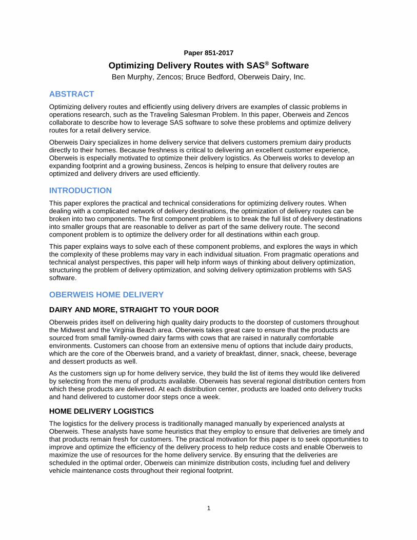
Basic metrics about the 2851 delivery destinations are easily accessible using the MEANS procedure:

proc means data=locations; run;

The results of running PROC MEANS on the sample of 2851 delivery destinations provides a baseline for understanding the data:

Figure 1

Figure 1: PROC MEANS output

BUILDING A BETTER SET OF CLUSTERS

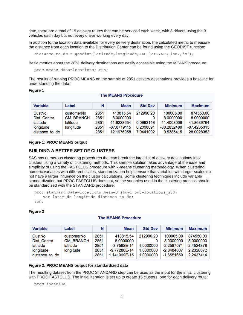
SAS has numerous clustering procedures that can break the large list of delivery destinations into clusters using a variety of clustering methods. This sample solution takes advantage of the ease and simplicity of using the FASTCLUS procedure with k-means clustering methodology. When clustering numeric variables with different scales, standardization helps ensure that variables with larger scales do not have a larger influence on the cluster calculations. Some clustering techniques include variable standardization but PROC FASTCLUS does not, so the variables used in the clustering process should be standardized with the STANDARD procedure:

proc standard data=locations mean=0 std=1 out=locations_std;

var latitude longitude distance_to_dc;

run;

Figure 2

Figure 2: PROC MEANS output for standardized data

The resulting dataset from the PROC STANDARD step can be used as the input for the initial clustering with PROC FASTCLUS. The initial iteration is set up to create 15 clusters, one for each delivery route:

proc fastclus

5

data=locations_std

out=clusters

outseed=clusters_centroids

maxclusters=15;

var latitude longitude distance_to_dc;

run;

After looking at clustering results, often there are clusters that are created that are obviously too small, especially for geographic outliers, or obviously too large, such as very densely populated areas. Taking the initial clustering results and iterating through those results, this example removes delivery destinations that belong to any cluster whose size is below a minimum size threshold level and saves those records to be included later. The iterative process then breaks the largest cluster into two smaller clusters repeatedly until the correct number of clusters remain. Similarly, the process can iterate when one or more clusters are larger than a maximum size threshold, and break the largest cluster into two smaller clusters. The delivery destinations that were withheld and set aside can be carefully integrated into the clusters so that the result is a set of clusters of appropriate size. The size thresholds for minimum and maximum tolerable cluster size are driven in this example by business rules around how many delivery destinations Oberweis requires on each delivery route.

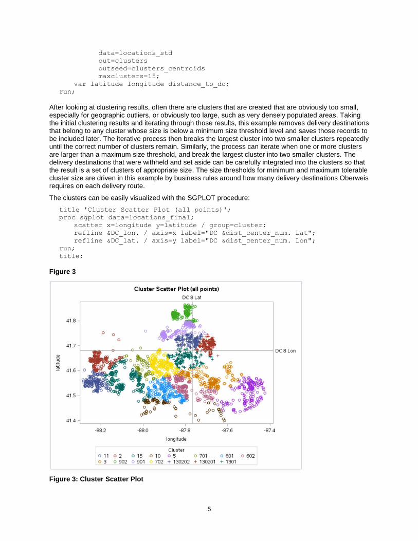
The clusters can be easily visualized with the SGPLOT procedure:

title 'Cluster Scatter Plot (all points)';

proc sgplot data=locations_final;

scatter x=longitude y=latitude / group=cluster;

refline &DC_lon. / axis=x label="DC &dist_center_num. Lat";

refline &DC_lat. / axis=y label="DC &dist_center_num. Lon";

run;

title;

Figure 3

Figure 3: Cluster Scatter Plot

6

TSP SOLUTION 1 – OPTGRAPH

Once a suitable set of clusters has been created, each cluster can be setup as its own Traveling Salesman Problem (TSP). Each cluster needs a row added for the distribution center as the first point in the route, and then all the distances between every combination of 2 points must be calculated. In this example, a SQL procedure step with a self-join to the list of delivery locations used the GEODIST function to calculate all the distances needed:

proc sql noprint;

create table cluster_matrix as

select

a.CustNo as A_CustNo,

a.State as A_State,

a.Dist_Center as A_Dist_Center,

a.latitude as A_latitude,

a.longitude as A_longitude,

b.CustNo as B_CustNo,

b.State as B_State,

b.Dist_Center as B_Dist_Center,

b.latitude as B_latitude,

b.longitude as B_longitude,

geodist(a.latitude,a.longitude,b.latitude,b.longitude,'M') as

distance

from cluster_sample as a

inner join

cluster_sample as b

on a.CustNo < b.CustNo

order by a.CustNo,b.CustNo

;

quit;

Once the distances between every point in the cluster have been calculated, there are two options for solving the TSP. The first option uses the OPTGRAPH procedure, which is available through the Social Network Analysis license. PROC OPTGRAPH has a very straightforward syntax and is easy to use for solving TSPs. The code here comes from examples in the SAS Online Documentation for PROC OPTGRAPH. The input data for PROC OPTGRAPH includes columns FROM, TO, and WEIGHT:

proc sql noprint;

create table optgraph_input_data as

select

A_CustNo as from,

B_CustNo as to,

distance as weight

from cluster_matrix

;

quit;

There are also several helpful options that allow customization for how the solver runs. In this example, the MAXTIME option limits execution to 3 seconds per cluster:

proc optgraph

loglevel = moderate

data_links = optgraph_input_data

out_nodes = optgraph_output_nodes;

tsp

maxtime = 3 /*time in seconds to iterate*/

out = optgraph_output_tsp;

7

run;

TSP SOLUTION 2 – OPTMODEL

There is also a way to solve TSPs with the OPTMODEL procedure, which requires a SAS/OR license, using a subtour formulation and the Mixed Integer Linear Program (MILP) solver. The input data has slightly different structure:

proc sql;

create table tspinput as

select

CustNo as var1,

longitude as var2,

latitude as var3

from cluster_sample

;

quit;

The PROC OPTMODEL setup reads directly from the variables in the input dataset. The code for the PROC OPTMODEL example for solving the TSP comes from an example in the SAS Online Documentation, which is worth reviewing for more detail:

proc optmodel;

set VERTICES;

set EDGES = {i in VERTICES, j in VERTICES: i > j};

num xc {VERTICES};

num yc {VERTICES};

num numsubtour init 0;

set SUBTOUR {1..numsubtour};

/* read in the instance and customer coordinates (xc, yc) */

read data tspinput into VERTICES=[var1] xc=var2 yc=var3;

/*the cost is the geodist*/

num c {<i,j> in EDGES}

init geodist(yc[i],xc[i],yc[j],xc[j],'M');

var x {EDGES} binary;

/* minimize the total cost */

min obj = sum {<i,j> in EDGES} c[i,j] * x[i,j];

/* each vertex has exactly one in-edge and one out-edge */

con two_match {i in VERTICES}:

sum {j in VERTICES: i > j} x[i,j]

+ sum {j in VERTICES: i < j} x[j,i] = 2;

/* no subtours (these constraints are generated dynamically) */

con subtour_elim {s in 1..numsubtour}:

sum {<i,j> in EDGES: (i in SUBTOUR[s] and j not in SUBTOUR[s])

or (i not in SUBTOUR[s] and j in SUBTOUR[s])} x[i,j] >= 2;

/* this starts the algorithm to find violated subtours */

set <num,num> EDGES1;

set INITVERTICES = setof{<i,j> in EDGES1} i;

set VERTICES1;

8

set NEIGHBORS;

set <num,num> CLOSURE;

num component {INITVERTICES};

num numcomp init 2;

num iter init 1;

num numiters init 1;

set ITERS = 1..numiters;

num sol {ITERS, EDGES};

/* initial solve with just matching constraints */

solve;

call symput(compress('obj'||put(iter,best.)),

trim(left(put(round(obj),best.))));

for {<i,j> in EDGES} sol[iter,i,j] = round(x[i,j]);

/* while the solution is disconnected, continue */

do while (numcomp > 1);

iter = iter + 1;

/* find connected components of support graph */

EDGES1 = {<i,j> in EDGES: round(x[i,j].sol) = 1};

EDGES1 = EDGES1 union {setof {<i,j> in EDGES1} <j,i>};

VERTICES1 = INITVERTICES;

CLOSURE = EDGES1;

for {i in INITVERTICES} component[i] = 0;

for {i in VERTICES1} do;

NEIGHBORS = slice(<i,*>,CLOSURE);

CLOSURE = CLOSURE union (NEIGHBORS cross NEIGHBORS);

end;

numcomp = 0;

do while (card(VERTICES1) > 0);

numcomp = numcomp + 1;

for {i in VERTICES1} do;

NEIGHBORS = slice(<i,*>,CLOSURE);

for {j in NEIGHBORS} component[j] = numcomp;

VERTICES1 = VERTICES1 diff NEIGHBORS;

leave;

end;

end;

if numcomp = 1 then leave;

numiters = iter;

numsubtour = numsubtour + numcomp;

for {comp in 1..numcomp} do;

SUBTOUR[numsubtour-numcomp+comp] = {i in VERTICES:

component[i] = comp};

end;

solve;

call symput(compress('obj'||put(iter,best.)),

trim(left(put(round(obj),best.))));

for {<i,j> in EDGES} sol[iter,i,j] = round(x[i,j]);

end;

/* create a data set for use by gplot */

9

create data tsp_solution_data from

[iter i j]={it in ITERS, <i,j> in EDGES: sol[it,i,j] = 1}

xi=xc[i] yi=yc[i] xj=xc[j] yj=yc[j] cost=c[i,j];

call symput('numiters',put(numiters,best.));

quit;

TSP SOLUTION VISUALIZATION

Once the solutions are available, it is helpful to represent them graphically. The PROC OPTGRAPH output is available using the OUT_NODES option and the TSP solution details are available using the OUT= option on the TSP solver. The OUT_NODES dataset contains the information needed to plot the optimal route:

proc sql noprint;

create table optgraph_output_node_detail as

select

a.*,

b.*

from optgraph_output_nodes as a

left join

cluster_sample as b

on a.node = b.CustNo

order by a.tsp_order

;

select max(tsp_order) into :max from optgraph_output_nodes;

quit;

proc sql noprint;

create table optgraph_output_graph as

select

"datavalue" as drawspace,

1 as linethickness,

a.longitude as x1,

b.longitude as x2,

a.latitude as y1,

b.latitude as y2,

'red' as linecolor,

'line' as function,

geodist(a.latitude,a.longitude,b.latitude,b.longitude,'M') as

distance_traveled,

a.CustNo,

a.tsp_order

from optgraph_output_node_detail as a

left join

optgraph_output_node_detail as b

on (a.tsp_order + 1 = b.tsp_order) or (a.tsp_order = &max.

and b.tsp_order = 1)

;

create table node_data as

select

tsp_order as i, /*could also use CustNo*/

longitude as x,

latitude as y

from optgraph_output_node_detail

10

;

quit;

title "Cluster &cluster_num. in Dist Center &dist_center_num.";

proc sgplot data=node_data sganno=optgraph_output_graph;

scatter x=x y=y / datalabel=i;

xaxis display=none;

yaxis display=none;

run;

title;

Figure 4

Figure 4: Sample TSP Routing

As an example of routing solutions, the data also allows calculations of total distance traveled and the order in which delivery destinations are visited on the optimal path. To ensure that the set of TSP routes are practical, assume that deliveries take an average of 1 minute per location and that between deliveries, vehicles can average 35 miles per hour. Summarizing the total number of miles traveled and the number of hours of work per route can provide useful metrics to compare this sample solution to other possible solutions:

11

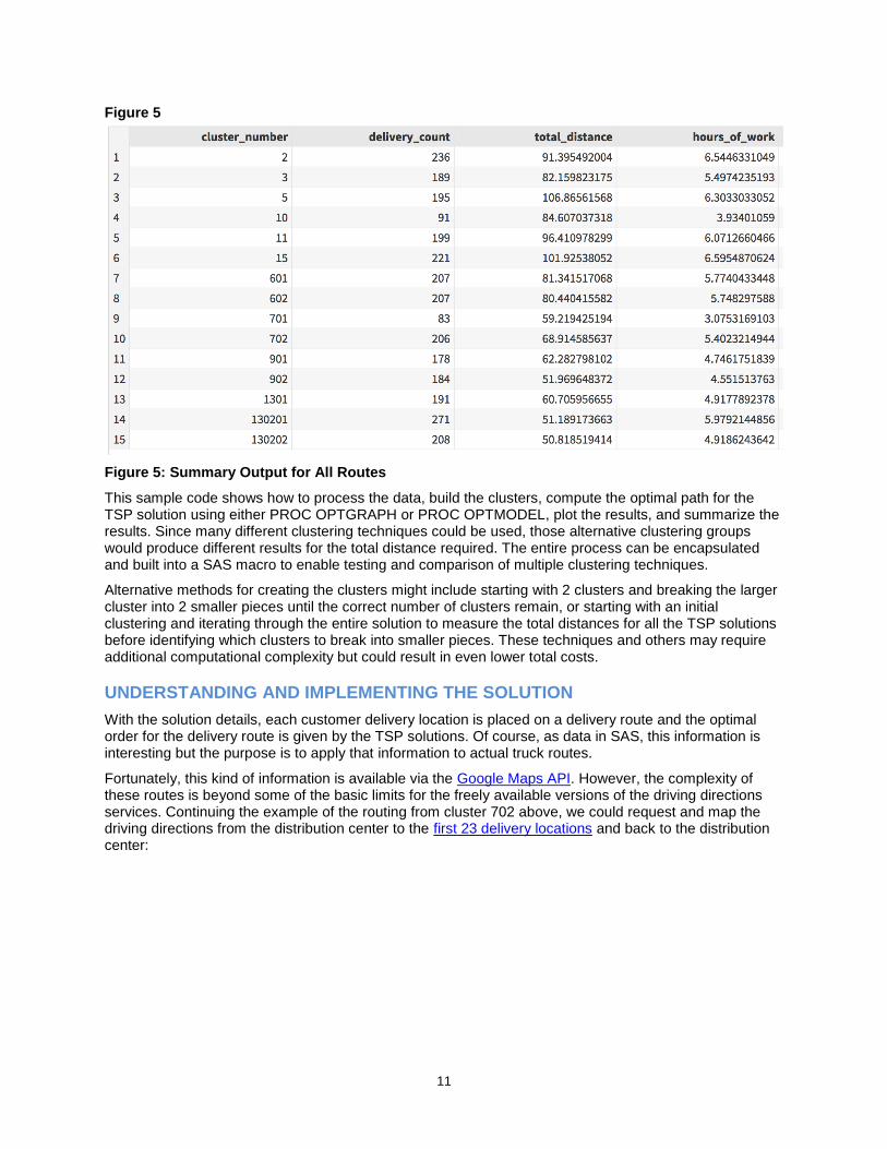
Figure 5

Figure 5: Summary Output for All Routes

This sample code shows how to process the data, build the clusters, compute the optimal path for the TSP solution using either PROC OPTGRAPH or PROC OPTMODEL, plot the results, and summarize the results. Since many different clustering techniques could be used, those alternative clustering groups would produce different results for the total distance required. The entire process can be encapsulated and built into a SAS macro to enable testing and comparison of multiple clustering techniques.

Alternative methods for creating the clusters might include starting with 2 clusters and breaking the larger cluster into 2 smaller pieces until the correct number of clusters remain, or starting with an initial clustering and iterating through the entire solution to measure the total distances for all the TSP solutions before identifying which clusters to break into smaller pieces. These techniques and others may require additional computational complexity but could result in even lower total costs.

UNDERSTANDING AND IMPLEMENTING THE SOLUTION

With the solution details, each customer delivery location is placed on a delivery route and the optimal order for the delivery route is given by the TSP solutions. Of course, as data in SAS, this information is interesting but the purpose is to apply that information to actual truck routes.

Fortunately, this kind of information is available via the Google Maps API. However, the complexity of these routes is beyond some of the basic limits for the freely available versions of the driving directions services. Continuing the example of the routing from cluster 702 above, we could request and map the driving directions from the distribution center to the first 23 delivery locations and back to the distribution center:

12

Figure 6

Figure 6: Sample Routing with Google Maps API

These driving directions help access practical applications for these TSP solutions, and if the Google Maps API supported it, it would be possible to gather turn by turn directions for every single routing option. Unfortunately, the limitations on usage make it impractical to use the Google Maps API to fully detail the driving requirements between every delivery destination. Having that information would solve some of the practicality constraints that could not be accounted for previously.

Regardless of the technical limitations, the usage of Google Maps or a similar service shows that taking interesting details on plausibly optimal delivery routes and turning them into practical driving directions is easier than ever before. Of interest to anybody responsible for the operational logistics of delivery routing, this final step does not involve SAS, but does mean that all the work produced by SAS is now actionable.

CONCLUSIONS & NEXT STEPS

Optimizing delivery routes for a large network of the home delivery service customers for Oberweis Dairy is a complicated problem with many possible solutions. After describing an approach where the large list of delivery destinations is broken into smaller pieces to enable one delivery person to service an entire delivery route in one work shift, the combination of SAS programming and some external resources enabled the building of a practical and actionable solution to vehicle routing. Being able to systematically quantify each potential solution will enable any analyst to develop new ways to route delivery vehicles and hopefully create opportunities to deliver better customer service while minimizing cost.

This example was just one small component of the overall solution, and that overall solution is just one option in an endless list of potential solutions. Follow up work to more completely quantify, itemize, and iterate through potential solutions to find the best possible clustering methodology and individual routing solutions will depend on each specific situation and individual application. The methods that were outlined in this paper provide a starting point, and surely additional possibilities exist that were not covered. Since every situation is different, these techniques are merely the tools to enable a savvy analyst to solve this complicated problem with new techniques and deliver compelling new results.

13

REFERENCES

SAS Online Documentation, SAS Support; “SAS OPTGRAPH Procedure 14.1: Graph Algorithms and Network Analysis – The OPTGRAPH Procedure – Example 1.15 Traveling Salesman Tour through US Capital Cities” Accessed February 2017. http://support.sas.com/documentation/cdl/en/procgralg/68145/HTML/default/viewer.htm#procgralg_optgraph_examples15.htm

SAS Online Documentation, SAS Support; “SAS/OR 13.2 User’s Guide: Mathematical Programming – The OPTMODEL Procedure – Example 5. Traveling Salesman Problem” Accessed February 2017. http://support.sas.com/documentation/cdl/en/ormpug/67517/HTML/default/viewer.htm#ormpug_optmodel_examples06.htm

SAS Online Documentation, SAS Support; “SAS/OR 13.2 User’s Guide: Mathematical Programming – The Mixed Integer Linear Programming Solver – Example 8.4 Traveling Salesman Problem” Accessed February 2017. http://support.sas.com/documentation/cdl/en/ormpug/67517/HTML/default/viewer.htm#ormpug_milpsolver_examples04.htm

ACKNOWLEDGMENTS

Zencos would like to thank Oberweis Dairy for the continued partnership and opportunities for collaboration.

Ben would like to thank Bruce Bedford for his professional support. Ben would also like to thank Tricia Aanderud for writing advice, and to thank Maria Nicholson, Leigh Ann Herhold, and Jared Weiss for writing and editing help.

RECOMMENDED READING

Wikipedia - Traveling Salesman Problem

Paper 161-2012 - The Traveling Salesman Problem: Optimizing Delivery Routes Using Genetic Algorithms

CONTACT INFORMATION

Your comments and questions are valued and encouraged. Contact the authors at:

Ben Murphy Zencos bmurphy@zencos.com Bruce Bedford | Vice President, Marketing Oberweis Dairy, Inc. bruce.bedford@oberweis.com

SAS and all other SAS Institute Inc. product or service names are registered trademarks or trademarks of SAS Institute Inc. in the USA and other countries. ® indicates USA registration.

Other brand and product names are trademarks of their respective companies.