optimizing design of breeding programs 1 introduction

Armidale Animal Breeding Summer Course 2006 Optimizing Breeding Program Design 61

Optimizing design of breeding programs Julius van der Werf

1 Introduction In the previous lectures we discussed criteria for comparing breeding programs. We showed how to predict genetic response for multiple traits and how to evaluate the value of this response economically. It should be noted that the design of those breeding programs was fixed and breeding alternatives can be compared by varying different parameters. However, in practical breeding programs, we often need a more dynamic approach that can help give optimal selection results. Such optimization is needed when optimizing decisions under prevailing circumstances, i.e. for tactical decisions. But also for strategic planning, we can use some dynamic approaches that help to reconsider design parameters when circumstances change. For example, when a trait is measured at an earlier age, it would probably be more optimal to select younger animals, as they will have more accurate EBVs. So selection accuracy and generation interval both change. In the design of a breeding program, many aspects that determine genetic response are interdependent, and changing one variable might result in different optimal values for other variables. Remember the central ‘dogma’ (Rendel and Robertson, 1950) of predicting genetic response: Where i = selection intensity, r = selection accuracy and L is generation interval. The subscripts refer to selection for males and females and σA is genetic variance. In some examples like in dairy programs where breeding males are very important due to the use of AI, four paths are distinguished as the best “elite” parents are especially selected to generate the next generation of AI bulls. . The above formula is central as it allows to put in perspective the importance of the different components in a breeding program. Van Arendonk and Bijma (2002) have succinctly summarized these components as follows: Genetic variance. The genetic variance in selection candidates is equal to :

2 2 2 21 1 14 4 2A As Ad Amσ σ σ σ= + +

Where σ2

Ax is the genetic variance in the selected sires (x=s) and dams (x=d) and σ2Am is the Mendelian

sampling variance. In an unselected and non-inbred population, σ2As = σ2

Ad = σ2A and σ2

Am = ½σ2A

which means that sires and dams contribute each 25 % to the genetic variance in an individual and that 50 % of the genetic variance is due to Mendelian sampling. Selection, however, results in a reduction of the genetic variance in the selected parents, the so-called Bulmer effect. The genetic variance in the selected parents (x) is equal to (Bulmer, 1971):

2 2 2121 (1 )At Atr kσ σ+ = −

m m f fA

m f

i r i rR

L Lσ

+=

+


where k is the variance reduction coefficient calculated as i.(i-x) (I being selection intensity, x is truncation point) and r is the accuracy of selection. The Bulmer effect leads to a reduction in genetic gain because the genetic gain is a direct function of the genetic variance. The variance reduction in the population is often close to 25 %, which leads to a 13 % reduction in the absolute gain. More importantly, however, the Bulmer effect reduces the genetic variance in parents (between family variance) but not the Mendelian sampling variance (within family variance). As a consequence, full and half-sib information becomes less important whereas information that includes the Mendelian sampling component of the selection candidate, such as own performance and progeny information, becomes relatively more important. These effects are important when comparing schemes that use different sources of information (e.g. progeny vs. sib information). Accuracy of selection. The accuracy of selection is the correlation between the selection criteria and the true breeding value for the breeding goal that is to be improved. In most livestock improvement schemes, selection is based on breeding values that are estimated using BLUP. A method use in prediction models for calculating the accuracy of selection on BLUP-EBV was presented by Wray and Hill (1989), based on selection index theory. A multiple-trait extension of this method was presented by Villanueva et al. (1993), and Bijma et al. (2001) presented an extension for overlapping generations. These methods account for the reduction of genetic variance due to selection. Selection intensity. In predicting response to selection, it is generally assumed that the selection criterion is normally distributed and that truncation selection is applied. In that case the selection intensity can be obtained directly from the proportion of animals selected. When the selection criterion is partly based on family information, the EBVs of sibs are correlated. Meuwissen (1991) developed a method to account for finite population and correlated EBV. This correction is particularly important in breeding schemes that rely heavily on information coming from full and half sibs and where the number of selected parents is small Overlapping generations. In most populations, a number of age classes can be distinguished and the amount of information differs between age classes. In general, young age classes have less information than older age classes. Because older age classes have more information, they have higher accuracy. However, the mean level of the EBV of older age classes will be lower than that of younger age classes due to the continuous genetic improvement in the population. Truncation selection across age classes can be performed to obtained the highest selection differential (James, 1987). Mathematical details on truncation across age classes can be found in Ducrocq and Quaas (1988) and Bijma et al. (2001) and an algorithm will also be presented in the next section. Reproductive techniques might increase the amount of sib information and thereby increase the accuracy of EBV of younger age classes. This will change the fraction of parents selected from the younger age classes and thereby also influence the average generation interval. Rate Of Inbreeding The magnitude of inbreeding at the population level is measured by the rate of inbreeding (.F). Only in the absence of selection F is related directly to the number of sires and dams. In selected populations, this equation is no longer valid because parents contribute unequally to the next generation. Wray and Thompson (1990) introduced methods to predict rates of inbreeding in selected populations, based on the concept of long-term genetic contributions. Recently, Woolliams et al. (1999) and Woolliams and Bijma (2000) developed a general theory to predict rates of inbreeding in populations undergoing selection. These methods facilitate a deterministic optimisation of short and long-term response of breeding schemes. Bijma and Woolliams (2000) demonstrated that with BLUP selection, the number of candidates per parent (selection intensity) may be as or more important than the number of parents. Doubling the number of parents failed to halve the rate of inbreeding.


Meuwissen (1997) introduced a dynamic selection tool to maximise the genetic gain while restricting the rate of inbreeding. Given the available selection candidates, the method maximises the genetic level of the selected group of parents while constraining the average coefficient of coancestry. Implementation of this method results in a dynamic breeding program, where the number of parents and number of offspring per parent may vary, depending on the candidates available in a particular generation. In a next section, we’ll discuss in more detail methods to restrict inbreeding. Optimization Of Breeding Schemes Under the infinitesimal model, inbreeding reduces genetic variation, which in turn reduces genetic gain. Furthermore, when inbreeding depression is present, fitness of the population may reduce to an extent where it affects the selection differentials, i.e. indirectly inbreeding may also reduce genetic gain. In the short term, inbreeding and genetic gain have an unfavourable relation, in the sense that maximising short-term response by selecting fewer parents reduces long-term response and involves substantial risk (e.g. Verrier et al., 1993). To balance the short and long-term response a restriction on the rate of inbreeding is required (e.g. Quinton and Smith, 1995). The objective in optimised breeding strategies needs to be maximising genetic gain while restricting inbreeding. Acceptable levels of inbreeding are difficult to determine and are discussed by Bijma (2000), who indicated that inbreeding depression is probably the most important issue. Though detailed knowledge of the relevant parameters to determine the level of the constraint is lacking, different approaches point towards values around 0.5 % and 1 % per generation. Different components of genetic gain interact Alternative options for breeding programs need to be assessed, which can be done based on an analysis of the most important factors that determine rate of genetic gain: selection intensity, selection accuracy and generation interval, as in the Rendel and Robertson formula. It should be pointed point out that the different factors interact. For example, one could try to increase selection intensity, but the result is that breeding animals can be less rapidly replaced when fewer young animals are selected, and the generation interval is increased. The most important interactions are:

• Generation interval versus selection accuracy Selection young animals will not only lead to short generation intervals, but may also imply lower

selection accuracy because young animals have generally less information available (no repeated records, maybe no own performance, no progeny test)

• Generation interval versus selection intensity If more young animals are retained as breeders, and a high replacement rate is applied, the

generation interval may be shorter, but selection intensity will also be lower since more animals of the newborn generation are needed as replacements.

§ Balancing different traits (see course notes summer course 2005)

Strategic vs tactical optimization of breeding programs

Strategic optimization requires a whole population model of the breeding program. The model accommodates parameters that can represent different strategies, e.g. which traits to measure, which animals to measure, how many animals to measure in multiple selection stages, how many to select from each age class, how many from each family. A strategic plan for a breeding program often results in a set of rules, e.g. optimal proportion selected, optimal age structures etc.

By contrast, a tactical optimization tries to address the immediate decisions that need to be made under prevailing circumstances. Maybe optimally we use 30% of the bulls from the 1nd year age class, but a certain crop might be disappointing, and a lower percentage would be optimal for that year. Tools


that can be used for tactical decision making, i.e. selection, are BLUP or mate selection, which is implemented in TGRM (Kinghorn et al., 2002). A tactical approach will make use of knowledge of the full range of actual animals available for breeding at the time of decision making, as well as other factors such as availability of mating paddocks, current costs of specified semen, current quarantine restrictions on animal migration, current or projected market prices, etc. Tactical implementation of breeding programs gives the power to capitalise on prevailing opportunities - opportunities that would often be missed when adhering to a set of rules. The tactical approach to breeding is driven by specifying desired outcomes. Although mate selection analysis is a very powerful computing tool, the results that it gives are closely aligned to the ‘outcome instructions’ that it receives. This means that the breeder can have a high degree of control, not by specifying which animals should be selected, but by specifying desires in terms of direction of genetic change, maintenance of genetic diversity, limits in money spent, constrains to be satisfied etc. In this course we will deal only with strategic optimization and compare breeding program designs. As said, such predictions require a model of the breeding population. Prediction of breeding program outcomes van be based either on a stochastic model, (stochastic simulation) or through a deterministic model (deterministic simulation). Briefly these can be contrasted as § A stochastic simulation generates breeding and phenotypic values for each simulated individual,

select based on such data (e.g. using BLUP) and simply select the best individuals as parents of the next generation.

§ Deterministic simulation uses a whole population model, e.g. characterised by a mean and a

variance, and predicts response to selection based on knowledge of population characteristics, e.g. using selection intensity.

§ Stochastic simulation is relatively simple, but requires repeated running of a simulated breeding

program. For example, there is no need to worry about ‘optimal age structure, as simple selection of the best animals based on BLUP EBV automatically optimizes generation interval (see a later section). Because of the stochastic process, outcomes will vary (like in a real breeding program!), and a mean of outcomes is often required to demonstrate differences between programs. Hence, stochastic simulation has much higher computer requirements. Although computers are fast these days, it I still quite a task to simulate a set of replicated populations, each with many generations for thousands of animals for several traits

§ Deterministic simulation requires formulas to adjust for thing like the Bulmer effect, reduced

selection intensities I small populations, correlations between EBVs, prediction of inbreeding etc. It is therefore more complicated and possibly more approximate.

§ Although computer capacity is not anymore so restrictive these days, it is still useful to have a

simple deterministic method for predicting response in alternative breeding programs. Deterministic prediction models also require more insight and therefore are often more illuminating in detecting the role of different components in genetic change.

In these notes we will look at some specific problems that are relevant in optimizing breeding programs, § Age structure, § Inbreeding rate § Use of gene markers in breeding programs.

For each of these, we will specifically deal with techniques that allow to use the components in deterministic simulation models.


A major component of decision making in breeding programs is to achieve an (economically) balanced progress across multiple traits. For a more in-depth discussion on optimal multiple trait selection we refer to the Armidale summer course notes of 2005.

2 Optimizing selection across age classes (age structure) Van Arendonk and Bijma (2002) state that “ the generation interval should not be regarded as a design parameter for the breeding schemes but needs to be a result selection across the available age classes while constraining”. To understand optimal selection across age classes, there are three points to remember about breeding values in a typical breeding program:

§ The accuracy of breeding values increases with an increased age § The variance of estimated breeding values increases with age.

§ The average estimated breeding value (as well as true breeding value) increases

over time and is therefore higher for younger animals

Each of these will be discussed in a bit more detail, before we discuss selection across age classes. Accuracy of EBV The accuracy is defined as the correlation between true and estimated breeding value. The symbol for accuracy is rIA. Since the EBV is often indicated as an Index (I), - the true breeding value has symbol A and r is a common symbol for correlation. The accuracy is between 0 and 1 (or 0% and 100%). In the extreme case of no information, the accuracy of a breeding value is 0, and with a very large amount of information, the accuracy will approach 1. The following Table shows examples of accuracy. It illustrates that

• Accuracy is higher when more information is used, e.g. on relatives and progeny • The accuracy is higher for traits with a higher heritability, but the effect of heritability becomes

smaller with more information used • The accuracy of parent average depends on the parent EBV accuracy and not on heritability (but

note that with low heritability it will be harder for a parent to achieve a certain accuracy) • The accuracy of information from collateral relatives (i.e. siblings) is limited to 0.5 for HS and 0.71

for FS. A progeny test is required to obtain higher accuracies


Table 2.1. Accuracies of EBV depending on source of information used Information used h2 = 0.10 h2 = 0.30 Sire EBV (rIA=0.5) 0.25 0.25 Sire EBV (rIA=0.9) 0.45 0.45 Sire EBV (rIA=0.5) + Dam EBV (rIA=0.5) 0.35 0.35 Sire EBV (rIA=0.9) + Dam EBV (rIA=0.5) 0.51 0.51 Own Performance only 0.32 0.55 OP+ Sire EBV (rIA=0.9)+ Dam EBV (rIA=0.5) 0.57 0.66 Mean of 5 full sibs 0.32 0.48 Mean of 10 half sibs 0.23 0.33 OP + 5 FS + 10 HS 0.43 0.65 Mean of 1000 half sibs 0.49 0.50 Mean of 1000 full sibs 0.70 0.71 Mean of 20 progeny 0.58 0.79 Mean of 100 progeny 0.85 0.94 Mean of 1000 progeny 0.98 0.99

Accuracies can be derived using selection index theory. Here we only give a simple example for the derivation of accuracy of an EBV based own performance EBV = I = h²P giving rIA = rh2P,A

rh2P,A = Cov h P AV h P VA

h V

h V VA

P A

( ² , )( ² )

²=

4

= h Vh V V

A

A A

²²

= hh²²

= h

If the heritability is higher, EBV’s based on own performance records become more accurate. The accuracy of the progeny test is

i.e. rIA = n

n + a

This simple formula allows you to determine the accuracy, for a given progeny test based on n progeny, for a trait with heritability h2 (where a = (4-h2)/h2). Variance among EBV

The variance among EBVs is of practical value because

• it can give us an indication of the difference in EBV between the highest and lowest animals • It is used to predict selection differential, e.g. the average EBV of the best 10% of animals • An traits will be more impacted by selection on an multiple trait index if that index trait has more

variation.


In general, the variation among EBV can be predicted from accuracy and genetic variance Var(EBV) = rIA²VA and σEBV = rIA σA

where rIA is the accuracy of the EBV. Hence, the variance of the EBV’s is equal to the accuracy-squared multiplied by the variance of the true breeding values (additive genetic variance). It is useful to consider the following If rIA = 0 then var(EBV) = 0 : all EBVs have the same value (=0) If rIA = 1 then var(EBV) = 1 : the variance of EBV is equal to the variance of breeding values. All EBV should be equal to the true BV with this accuracy, and there is no prediction error. Var(EBV) is generally smaller than VA (σ

2A)

Var(EBV) becomes larger when accuracy is higher. i.e. the EBV of older animals will be more apart than those of young animals. The same holds for intensely measured nucleus animals compared to the EBV of base animals that have less information and therefore EBVs closer to each other. Genetic Trend Selection of parents over time leads to genetic improvement, i.e. there is an increase of average breeding value over time. This increase is referred to as ‘genetic trend’, and basically measures the success of breeding programs. The average of each generation is estimated by BLUP as the mean of the parents’ EBV, and since BLUP is also able to work out the difference between all animals and those selected as parents, BLUP can properly estimate the genetic change over time. The genetic trend is estimated from the average EBV’s over time, i.e. the EBV’s are plotted against the birth year of the animals.

Figure 1 Hypothetical example of a genetic trend plotted as average EBV against birth-year. The average of 1990 is set to 100.


The following example illustrates how BLUP distinguishes between genetic trend and environmental trend. Consider 3 sires performing in year 1 and having offspring in year 2. The average performance in years 1 and 2 are 300 and 313. If relationships within years were not considered, an animal’s EBV would be estimated as deviation from the year mean (times h2), and the average EBV per year would be equal to zero. The h2 value used is 0.25. year year estimate sire 1 sire 2 sire 3 1 300.0 350 300 250 phenotype 12.5 0 -12.5 EBV offspr. 1 offspr. 2 offspr. 3 2 313.3 345 305 290 phenotype 7.9 -2.1 -5.8 EBV Now consider the same example, but using the relationships between animals in a BLUP procedure. As the offspring have on average better parents, their average EBV is more than zero. The mean EBV in year 2 is now 4.5. The phenotypic trend from year 1 to year 2 is 13, and we now estimate that 8.9 of this is environmental and 4.5 of it is genetic trend. year year estimate sire 1 sire 2 sire 3 1 300.0 350 300 250 phenotype 14.3 -1.8 -12.5 EBV offspr. 1 offspr. 2 offspr. 3 2 308.9 345 305 290 phenotype 12.9 4.9 -4.5 EBV

Selection of young bulls vs old bulls

When optimising a breeding program, a dilemma often arises on whether young animals should be selected or older animals. Selecting young animals is good for achieving a short generation interval. However, younger animals have usually less accurate EBV. Older animals have generally more accurate EBV but selecting them would lead to longer generation intervals. Another (but essentially similar) argument against selecting older animals is that they are expected to have lower EBV. If there is a genetic gain per year, animals born x years apart are expected to differ x times the annual genetic gain. Figure Truncation points for older proven sires and younger unproven sires.

proven sires

young sires

Truncation Point


It seems not easy to optimise selection over different age classes. However, the solution appears to be remarkably simple in practice, for tactical decision making. Because BLUP accounts for genetic trend, an important practical consequence is that animals can be selected across age classes based on their EBV by truncation selection. For example, all bulls with an index value above 140 will be selected, independent of their age. It has been proven that BLUP selection optimises the use of bulls across age classes (James, 1987). Hence, selection on BLUP EBV, irrespective of age, automatically optimises the generation interval, and the use of old versus young bulls, as demonstrated in the Fig. above. Younger animals have on average better EBV, but also generally less variation in EBV The optimum proportion of younger animals depends on the difference in the variance of the EBV within age classes (i.e. on the accuracy) and on the genetic lag between age classes (i.e. on the genetic gain per year and the number of years). Truncation selection across age classes will automatically optimise the proportion of young bulls used. The proportion that should be optimally selected from each age class is automatically achieved if simply the best animals are selected based on their BLUP EBV. Selecting animals on BLUP EBV irrespective of their age automatically optimises the generation interval. With a larger genetic trend or with increased accuracy of the young bull EBV, the proportion of young bulls will increase (check yourself in the figure). Optimizing ages structure in deterministic simulation In GENUP with the AGES module we can compare age structures for simple breeding programs with phenotypic selection on a single trait. In ZPLAN we can try various age structures and compare the outcomes for more realistic multiple trait examples. Simple exercises such as in AGES show that earlier selection leads to higher replacement rates and therefore affects selection intensity. With BLUP selection, there is an additional argument that early election is usually on EBVs that are less accurate. Moreover, selecting in an early stage of life usually means that BLUP selection is more based on family information, and this would lead to more inbreeding. This will be discussed in the next chapter. Therefore, generation intervals should not be minimized, but rather should they be optimized. In deterministic prediction methods such as AGES and ZPLAN, this can be based on trial and error. However, there is also a method that can optimize selection across age classes, and therefore optimize generation interval. The method is illustrated in the Figure below. It shows overlapping distributions, representing values of animals from different age classes. These values could be phenotypes, EBVs or index values, and assuming selection is for such a single criterion. The distributions most to the left could represent the oldest animals, as they will have the lowest mean if there is a positive genetic trend. The objective is to find a common truncation point x where selection of all animals across all available distributions leads to a total proportion selected P. There will be one truncation point across all distributions. This truncation point has a single value, but relative to the mean of each distribution, the truncation points will differ: x1 > x2 > x3. Therefore, selected proportion will be accordingly smaller: s1 < s2 < s3, and consequently, the selected proportions will be p1 < p2 < p3, and selection intensities will be i1 > i2 > i3. There is no algebraic closed solution to finding the optimal truncation point but the solution can be found iteratively. If the truncation point is too far to the right, the overall selected proportion will be too small, and if too far to the left, too few will be selected. Therefore, an algorithm can work as follows:

1. Choose starting values for to the left and far (e.g. six standard deviations) to the right, xl and xu for lower and upper threshold.


2. Choose a truncation point in the middle, xm = (xL + xU )/2

3. For a given x, determine the total proportion selected.

4. This can be done by working out for each distribution: i. xi = x1 – (µi – µ1). ii. From xi, determine pi iii. Total proportion is Pm = p1s1 + p2s2 + p3s3

5. If Pm – P is very small, stop the iteration

6. If Pm < P then xU = xm

7. If Pm > P then xL = xm

8. Return to step 2

Example:

Proportion Nr Mean of ageclass N in group mean SD Selected Selected selected

1 50 10 1 0.28 14.17 11.18 2 35 9.5 1 0.14 4.96 11.03 3 15 9 1 0.06 0.87 10.74 20.0 11.12 mean of selected

1.33 Age of selected (GenInt)

1

X

x3

x2

x1

P3

p2

p1

P = p1s1 + p2s2 + p3s3

µ1 µ2 µ3 Mean of distribution

σ1 σ2 σ3 SD of distribution s1 s2 s3 Nr. of animals in this distribution as proportion of total nr of animals across all distributions distribution


3 Inbreeding

BLUP and Inbreeding Selection on BLUP EBV maximises response to selection. However, response is only maximised with respect to the next generation. Long term selection response is not necessarily optimised with BLUP selection. The reason is that BLUP selection leads to more inbreeding than for example mass selection (selection based on own phenotype). More inbreeding leads in the longer term to loss of genetic variation, and possibly inbreeding depression, and therefore reduces and offsets genetic gain. Why does BLUP selection lead to more inbreeding? This can be explained by the fact that BLUP uses information on all possible relatives to estimate an animals’ EBV. Using information from family members implies that members of the same (good) family have more chance to be jointly selected. With lower heritability there is relatively more weight on the family information (compared with the own performance), and the lower the heritability, the more BLUP selection resembles family selection and the more it leads to inbreeding. This is illustrated in Table 5.2.3 with a simulation study of a closed swine herd (Belonsky and Kennedy, 1988). Table 5.2.3 shows that: • BLUP selection leads to significantly more selection response than selection on individual

phenotype. The difference is larger for smaller heritability. • BLUP leads to more inbreeding than selection on indivi dual phenotype. With BLUP selection the

rate of inbreeding is considerably higher with lower heritability. With selection on individual phenotype there is (slightly) more inbreeding with higher heritability.

• Even after 10 years of selection, BLUP hadn’t lost its superiority over individual selection. Loss of

variance due to inbreeding was offset by increased used of relatives’ information. However, effects of inbreeding depression were not simulated.

To optimise selection on the longer term, it is useful to combine selection on BLUP EBV with some restriction on the average relatedness of the selected animals. For optimal selection rules see Wray and Goddard (1994) or Meuwissen (1997). Table 2.2. Average genetic merit and average inbreeding of progeny after 5 and 10 years of selection on individual phenotype and on Best Linear Unbiased Prediction of breeding value (BLUP). Source: Belonsky & Kennedy, (1988).

Average Genetic Merit Average Inbreeding

Heritability Year Phenotypic Selection

BLUP Selection

Phenotypic Selection

BLUP Selection

5 0.38 0.63 0.067 0.167 0.10

10 0.78 1.41 0.174 0.383

5 1.10 1.41 0.078 0.141 0.30

10 2.40 3.14 0.193 0.332

5 2.25 2.29 0.087 0.130 0.60

10 5.16 5.31 0.205 0.293


The following notes on Inbreeding are taken from Van Arendonk and Bijma, Armidale Animal Breeding Summer Course 2002.


4 Marker Assisted Selection The following paper is a good illustration of how the benefit from marker assisted selection can be evaluated in a breeding program. The paper is Chapter 5 of the thesis of Ben Wood (UNE, 2005). It also illustrates several other aspects of deterministic modelling of breeding programs.

Incorporating genotype information into two stage selection in beef cattle

– a cost-benefit analysis

Abstract Beef cattle breeders are increasingly being offered gene marker tests for important traits in the breeding objective. They must make an economically rational decision whether to use these tests. Besides a potential immediate effect in seedstock sales, gene marker tests will affect the genetic improvement rate in the population. To examine the returns in a multi-trait breeding objective a pseudo-BLUP selection index was developed to predict selection response using information from both phenotypic and molecular sources. Three objectives were examined each with a significantly different economic value for the meat quality trait marbling score and consequently profitability from investment in a gene marker test for a marble score influenced by the economic value and size of the gene effect. Of the three objectives, targeting long- and short-fed export and a high quality domestic market, only the long-fed export objective had a suitably high economic value to justify investment in genotype information. Increases in selection response above a non-genotyping strategy were 14%, 4% and 0.7%, for the three objectives. An advantage in using a gene marker test is the ability to select sires earlier when not much phenotypic information has been collected. Consequently, the proportion of young bulls used for breeding was important in the model. The improvements in accuracy of selection of young bulls lead to a significant change in the optimal age structure. This led to a decrease in the generation interval and contributed to the increase in annual selection response. Keywords marker-assisted selection, selection index, beef cattle, marbling score Introduction Livestock breeding programmes involve selection of parents based on estimated breeding values using phenotypic information measured on the individual and its relatives. Current genetic evaluation technologies assume that a very large number of genes with very small additive effects contribute to variation in performance among animals. Using this infinitesimal model, Best Linear Unbiased Prediction (BLUP) procedures (Henderson, 1975) have been extensively used for several years in the genetic evaluation of many livestock species. Recently, advances in molecular genetics have lead to the discovery of genomic regions that have a measurable effect on quantitative traits. These are called quantitative trait loci (QTL). Using this marker information the breeder can potentially increase the accuracy of selection beyond that available with phenotypic measurement alone. This is referred to as marker-assisted selection (MAS). A goal of modern breeding is the optimal use of information from QTL and phenotypic data. The challenge to breeders is to maximise the potential gains whilst minimising investment in measurement and testing. The approach to developing optimal selection criteria for profitability was first introduced by Hazel (1943) as the selection index. The foundation involves defining the overall breeding objective based on a linear combination of traits that contribute to the objective weighted by their relative economic importance. Animals are then selected on a criterion that is a linear combination of breeding objective traits or on


traits genetically correlated to the breeding objective. The index weights for each trait optimise the correlation between criteria and objective. The addition of genetic marker information is a natural progression to this procedure. Prediction of response can be complicated by the reduction in variance due to linkage disequilibrium and correlation between selection indexes in two stage selection (Bijma and van Arendonk, 1998) and these should be accounted for in any model used. Some general studies have been published on marker assisted programs in dairy cattle and pigs (Spelman and Garrick, 1997; Hayes and Goddard, 2003). Spelman et al. (1997; 1999) considered the effect of molecular information on response to selection for milk production. Hayes and Goddard (2003) considered a fully integrated pig production enterprise. The impact of molecular information has not been considered in the evaluation of beef cattle breeding programs. A realistic context in beef cattle is to include marker information into a multiple trait breeding objective with the example of a currently available marker for marbling performance (Nicol et al., 2001). The aim of this paper is to consider the returns possible from incorporating genotype information into a multi-trait beef breeding index. The paper compares commercial beef indexes for three different breeding objectives for the Hereford breed in Australia while incorporating the use of a QTL for intramuscular fat. Materials and Methods Selection index theory was used to calculate the return from providing various amounts of information to make a selection decision. A pseudo-BLUP model was used similar to the methods of Villanueva et al. (1993) in which information sources for each trait included phenotype information for the individual, dam, sire, full/half-sibs and progeny. Additionally genotype information was known for one of the traits. Selection Index

Two pathways of selection were used with selection of sires and dams within the breeding nucleus. The two pathways allow different information sources and costs of measurement to be assessed with response calculated from the combination of both indexes. The index was: I = b x′ [0.1]

where the index (I) is based on a vector of both phenotypic and marker information sources (x) and vector with a weight for each source (b). The weighting on each information source was calculated according to selection index theory (e.g. Falconer and Mackay, 1996):

-1b = P G v [0.2]

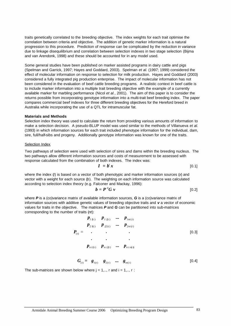
where P is a (co)variance matrix of available information sources, G is a (co)variance matrix of information sources with additive genetic values of breeding objective traits and v a vector of economic values for traits in the objective. The matrices P and G can be partitioned into sub-matrices corresponding to the number of traits (nt):

( ) ( ) ( )

( ) ( ) ( )

( )

( ) ( ) ( )

1 1 t 1 2 t 1nt t

2 1 t 22 t 2nt t

t

n t 1 t n t 2 t n t n t t

=

p p ... pp p ... p

. . .P

. . .p p ... p

[0.3]

( ) ( ) ( ) ( )t 1 t 2 t nt t G = g g ... g [0.4]

The sub-matrices are shown below where j = 1,.., r and i = 1,.., r :


( ) ( ) ( ) ( ) ( ) ( )

( ) ( ) ( )

( ) ( ) ( ) ( )

( ) ( ) ( )

( ) ( )

( )

0 0

symmetrical

1 1 1 1 12 j k t 1 j k t 1 j k t 1 j k t 1 j k t 1 j k t2 2 2 4 2

13 j k t 1 j k t 1 j k t4

1 1 14 j k t 1 j k t 1 j k t 1 j k t2 2 4

1 15 j k t 1 j k t 1 j k t4 4

16 j k t 1 j k t8

7 j k t

P P P P P PP P P

P P P PP P P

P PP

=

jk(t)P [0.5]

( )

( , )( , )

( , )( , )( , )( , )

k j1

k j21

k j2jk t 1

k j21

k j41

k j2

Cov A ACov A A

Cov A ACov A ACov A ACov A A

=

g [0.6]

where Pjk(t) is the phenotypic covariance sub matrix between trait j and trait k at time t and Gjk(t) is a vector of (co)variances between selection criteria of trait j and trait k . Columns 1-6 refer to information sources from individual phenotypes, dam, sire, half sib, full sib and progeny information, respectively. The elements of the sub matrices for the calculation of phenotypic (co)variances between traits j and k (Cov(X j,Xk)(t)) were partitioned into additive genetic (co)variances (Cov(A j,Ak)(t)), common environmental (co)variances (Cov(Cj,Ck)(t)), common environmental (co)variances among full sibs (Cov(CFSj,CFSk)(t)), and individual (co)variances (Cov(E i,Ej)t). Where nj and nk are the number of observations for each trait and nmax is maximum value of nj and nk: ( , )1 k jP Cov A A= [0.7]

max ( )

( ) ( )

( , )( , ) ( , ) j k t

2 j k t k j s j k tj k

n Cov E EP Cov A A Cov C C

n n= + + [0.8]

( )( )( ) ( )

max ( )

( , ) ( , )

( , ) ( , ) ( , ) ( , )

15 j k t j k s FSj FSk t2

1 1 1j k j k t j k FSk FSk2 2 2

j k

P Cov A A Cov C C

n Cov A A Cov X X Cov A A Cov C C

n n

= + +

+ − − [0.9]

( )max ( ) ( ) ( )

( )

( , ) ( , )( , )

31 j k t j k t j k t41

6 j k t k j4j k

n g Cov E E Cov C CP Cov A A

n n

+ += + [0.10]

( )max ( ) ( ) ( )

( )

( , ) ( , )( , )

31 j k t j k t j k t41

7 j k t k j4j k

n g Cov E E Cov C CP Cov A A

n n

+ += + [0.11]

Marker Information

The additive genetic variance was partitioned between unmarked additive polygenic variation and variation due to the QTL in linkage disequilibrium with a marker. Additive variance accounted for by the marker was included in the index equations when marker information was known on those candidates. When the information is added, the genotype and QTL information is assumed known without error. The molecular marker information was assumed to provide no further information to candidate relatives and as noted by Spelman et al. (1999), this has only a minor effect on the selection candidate’s estimated breeding value.


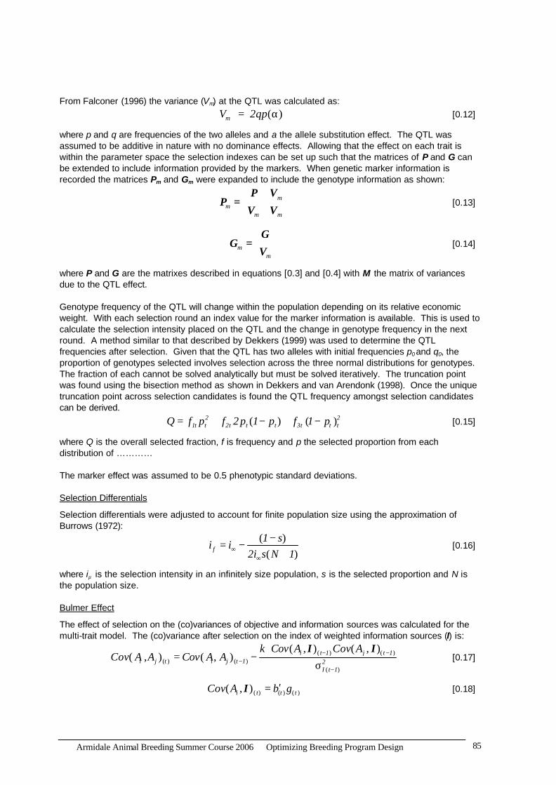
From Falconer (1996) the variance (Vm) at the QTL was calculated as: ( ) mV 2qp= α [0.12]

where p and q are frequencies of the two alleles and a the allele substitution effect. The QTL was assumed to be additive in nature with no dominance effects. Allowing that the effect on each trait is within the parameter space the selection indexes can be set up such that the matrices of P and G can be extended to include information provided by the markers. When genetic marker information is recorded the matrices Pm and Gm were expanded to include the genotype information as shown:

m

mm m

P VP =

V V [0.13]

mm

GG =

V [0.14]

where P and G are the matrixes described in equations [0.3] and [0.4] with M the matrix of variances due to the QTL effect. Genotype frequency of the QTL will change within the population depending on its relative economic weight. With each selection round an index value for the marker information is available. This is used to calculate the selection intensity placed on the QTL and the change in genotype frequency in the next round. A method similar to that described by Dekkers (1999) was used to determine the QTL frequencies after selection. Given that the QTL has two alleles with initial frequencies p0 and q0, the proportion of genotypes selected involves selection across the three normal distributions for genotypes. The fraction of each cannot be solved analytically but must be solved iteratively. The truncation point was found using the bisection method as shown in Dekkers and van Arendonk (1998). Once the unique truncation point across selection candidates is found the QTL frequency amongst selection candidates can be derived.

( ) ( )2 21t t 2t t t 3t t tQ f p f 2 p 1 p f 1 p= + − + − [0.15]

where Q is the overall selected fraction, f is frequency and p the selected proportion from each distribution of ………… The marker effect was assumed to be 0.5 phenotypic standard deviations. Selection Differentials

Selection differentials were adjusted to account for finite population size using the approximation of Burrows (1972):

( )

( )f1 s

i i2i s N 1∞

∞

−= −

+ [0.16]

where i∝ is the selection intensity in an infinitely size population, s is the selected proportion and N is the population size. Bulmer Effect

The effect of selection on the (co)variances of objective and information sources was calculated for the multi-trait model. The (co)variance after selection on the index of weighted information sources (I) is:

( ) ( )

( ) ( )( )

( , ) ( , )( , ) ( , ) i t 1 j t 1

i j t i j t 1 2I t 1

k Cov A Cov ACov A A Cov A A − −

−−

⋅= −

σI I

[0.17]

( ) ( ) ( )( , )i t t tCov A b g′=I [0.18]


( )2I t 1− ′σ = (t) (t) (t)b P b [0.19]

( )( , )i tCov A ′= j(t) i(t)I b g [0.20]

The value ( )2I t 1−σ is equal to the variance of the index in year(t-1) with the variance reduction a function of

the selected proportion where ( )k i i x= − with x the standardised truncation point and i the selection

intensity. Equilibrium values are achieved after a few rounds of selection. The additive genetic variance in selection candidates is equal to the sum of the variance of the sire and dam plus a component for Mendelian sampling (within family variance) shown in equation [0.21].

2 2 2 21 1Ax As Ad Am4 4σ = σ + σ + σ [0.21]

After each generation a new phenotypic (co)variance was calculated as the sum of the additive genetic and common environmental (co)variance. The common environmental and individual (co)variance among individuals in each generation were assumed to be unaffected by selection. The effect of inbreeding is not accounted for in the model and consequently the Mendelian sampling component was assumed to

remain constant over time. The within family variance ( 2Amσ ) was assumed to be equal

to ( )Cov( , )1i j 02 A A .

Calculation of Accuracy of the Index and Response

The accuracy of the index at each stage was calculated as.

IHr′ ′

=′

b GvvCv

[0.22]

where C is a matrix of genetic (co)variance among traits in the aggregate genotype and v a vector of economic values. The response in the objective for single stage selection was calculated as:

HR i′ ′

=′

bGvbPb

[0.23]

where i is the selection intensity of the selection pathway. Multi-stage Selection and Calculation of Response

When candidates are selected in multiple stages, only individuals that are selected in an earlier stage are available at a later stage. The aim is to avoid testing individuals that have low potential and are unlikely to be selected. If the selection indexes are correlated then preselection reduces the cost of measurement of animals at a later stage. Two-stage selection is used for residual feed intake (RFI) to be included as a second stage selection criterion. RFI is expensive to measure, consequently to decrease the cost of measurement only a proportion is measured. There are risks that individuals with high potential are culled prematurely and this is particularly true when there is strong preselection or earlier indexes have low accuracy. The subroutines of Genz (1992) were used to calculate the selection intensities and response to multi-stage selection. Breeding Objectives

The economic weights for the traits in the breeding objective are shown in Table 1. These are typical breeding objectives for the Hereford breed in Australia for three different market endpoints with the main difference being marbling score requirement for each market. The first objective ‘Hereford Prime’, targets the Australian domestic food service segment. The second ‘Short-fed export’ and third ‘Long-fed export’ target export markets with the animal feedlot finished and as a result incur higher feeding costs. The export market objectives differ in the time spent in the feedlot and economic value placed on marbling score. There are a large number of traits of interest to cattle breeders and the effect on response from single genotype testing is of interest with respect to both the total response and response in each trait.


Table 1 Economic values for the three breeding objectives

Breeding Objective Abbreviation. Units. Hereford Prime

Short-fed Export

Long-fed Export

Live sale weight (direct) SWd kg 0.673 0.617 0.542 Calving ease (direct) CEd % 2.007 2.240 2.447 Dressing percentage DP % 7.610 9.210 10.690 Saleable meat percentage SMP % 6.090 7.450 8.750 Fat depth FD mm 1.761 2.815 0.000 Cow weaning rate CWR % 2.770 4.740 5.520 Marbling score MS score 13.470 26.620 59.790 Cow survival rate CSR % 4.691 5.209 5.587 Cow weight CW kg -0.273 -0.273 -0.273 RFI (cow) RFIc kg/d -34.500 -34.500 -34.500 RFI (yearling) RFIy kg/d -22.260 -25.180 -40.680 Live sale weight (maternal) SWm kg 0.673 0.617 0.542 Calving ease (maternal) CEm % 0.821 0.918 1.004

Herd Age Structure and Genetic Mean

Each cohort, defined by age and sex, is described in terms of the genotype frequency, the genetic mean and genetic variance. Across cohort selection was practiced such that the optimal age structure was identified by truncation across the index distribution of each cohort (Ducrocq and Quaas, 1988). To maximise the genetic potential of selected parents the truncation point was determined to provide the total number of animals required across all the distributions. There is no closed algebraic solution and the optimum truncation point was found iteratively by bisection. The selected proportion was used to derive the selection intensity within the cohort. The selection intensity was then used to determine the response within the cohort and this contributed proportionally to the genetic mean of the selected candidates from this cohort. Scenarios Used in the Analysis

There were three different scenarios used for the analysis. The base or Scenario 1 has no marker information. <The phenotypic information available in this scenario is not given for these notes>. It was assumed that a two-stage selection process was used so that RFI information could be included in the selection index. RFI is expensive to measure and as such only a proportion (10%) was measured on the available male candidates. The proportion measured for RFI was pre-determined because it was shown that when insulin-like growth factor-I (IGF-I) information was included a small proportion of the available candidates could be measured without adversely affecting the accuracy and returns while minimising the investment in measurement (Wood et al., 2004). Scenario 2 increases the information available by including genotype at a locus associated with marble score (Nicol et al., 2001). The genotype information was assumed to be available at the first stage of selection (i.e. before selection of RFI measurement) and on all selection candidates both male and female. Scenario 3 limits genotyping to only male candidates. Input Parameters

Previously used parameters for the Australian Hereford breed (Kahi et al., 2003) were used for analysis of the benefits of selection. <Phenotypic standard deviations, heritability and the genetic correlations between traits in the breeding objective, genetic and phenotypic correlations between selection criteria and genetic correlations between selection criteria traits and breeding objective traits not shown in these notes)> The model seedstock enterprise was assumed to consist of a 2000 cow breeding herd of which 300 bulls were sold annually. Artificial insemination technologies were utilized resulting in higher selection intensities than that available with natural selection and it was assumed that 1 sire was used over 250 dams. Molecular information provides information at younger ages and optimal selection will draw more candidates from the younger age classes. Females were assumed to able to produce a calf


in the second year. It was assumed that 30% of all sire selection candidates could produce viable semen and be selected at the end of the first year, increasing to 100% by the second year. Cost-Benefit Analysis

The extra cost from the implementation of marker-assisted selection was assumed to be only the genotyping costs, which includes the cost of sampling (blood or hair samples), transport and associated laboratory genotyping costs. The assumed cost was varied from $10 to $70 per genotyping. It was assumed that marker information was available on all animals of a sex at the first stage of selection. The cumulative profit per bull was calculated as:

,

i i

i 1 t

nrd mxdnt=

−

∑ [0.24]

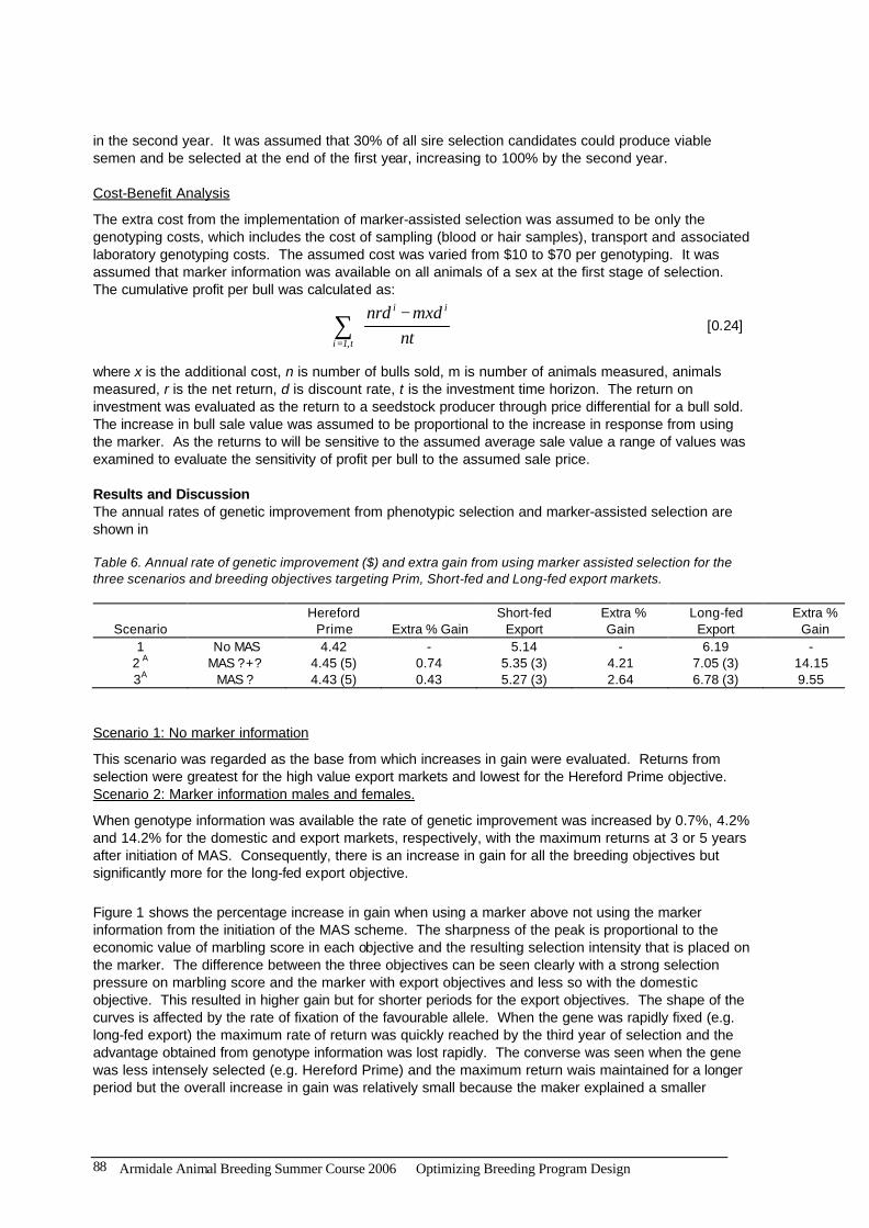
where x is the additional cost, n is number of bulls sold, m is number of animals measured, animals measured, r is the net return, d is discount rate, t is the investment time horizon. The return on investment was evaluated as the return to a seedstock producer through price differential for a bull sold. The increase in bull sale value was assumed to be proportional to the increase in response from using the marker. As the returns to will be sensitive to the assumed average sale value a range of values was examined to evaluate the sensitivity of profit per bull to the assumed sale price. Results and Discussion The annual rates of genetic improvement from phenotypic selection and marker-assisted selection are shown in Table 6. Annual rate of genetic improvement ($) and extra gain from using marker assisted selection for the three scenarios and breeding objectives targeting Prim, Short-fed and Long-fed export markets.

Scenario Hereford

Prime Extra % Gain Short-fed

Export Extra % Gain

Long-fed Export

Extra % Gain

1 No MAS 4.42 - 5.14 - 6.19 - 2 A MAS ?+? 4.45 (5) 0.74 5.35 (3) 4.21 7.05 (3) 14.15 3A MAS ? 4.43 (5) 0.43 5.27 (3) 2.64 6.78 (3) 9.55

Scenario 1: No marker information

This scenario was regarded as the base from which increases in gain were evaluated. Returns from selection were greatest for the high value export markets and lowest for the Hereford Prime objective. Scenario 2: Marker information males and females.

When genotype information was available the rate of genetic improvement was increased by 0.7%, 4.2% and 14.2% for the domestic and export markets, respectively, with the maximum returns at 3 or 5 years after initiation of MAS. Consequently, there is an increase in gain for all the breeding objectives but significantly more for the long-fed export objective. Figure 1 shows the percentage increase in gain when using a marker above not using the marker information from the initiation of the MAS scheme. The sharpness of the peak is proportional to the economic value of marbling score in each objective and the resulting selection intensity that is placed on the marker. The difference between the three objectives can be seen clearly with a strong selection pressure on marbling score and the marker with export objectives and less so with the domestic objective. This resulted in higher gain but for shorter periods for the export objectives. The shape of the curves is affected by the rate of fixation of the favourable allele. When the gene was rapidly fixed (e.g. long-fed export) the maximum rate of return was quickly reached by the third year of selection and the advantage obtained from genotype information was lost rapidly. The converse was seen when the gene was less intensely selected (e.g. Hereford Prime) and the maximum return wais maintained for a longer period but the overall increase in gain was relatively small because the maker explained a smaller


fraction of the breeding objective. Even with a moderate weight on the marker (e.g. short-fed export) the gene is fixed relatively rapidly. shows the change in genotype frequency for each objective in Scenarios 2 and 3. The relationship between economic value and consequently selection intensity placed on the QTL was evident with the most rapid change in allelic frequency for the long-fed export objective. Different selection weights placed on the favourable allele resulted in different rates of fixation for each objective. When selected sires and dams were genotyped for both export objectives the allele frequency was close to 1 by year 10. The largest benefit came from selection when the marker had a genotype frequency around 0.5 and as a result the highest gains calculated for the export objectives returns were earlier in year 3 compared to year 5 for the domestic objective. Between years 1 and 2 there was a plateau in the allele frequency resulting from the delay in genotyped cows producing progeny at 2 years of age compared to males at 1 year.

Fig 2: Frequency o desirable QTL allele in progeny when a) both males and females are genotype. Long fed = triangle, prim = diamond, short fed = square or b) only in males (open marks) Scenario 3: Marker Information available on males only

Scenario 3 demonstrates the gains from selection when genotype information was only available on males. This option utilised genotype information with reduced cost by only measuring one sex. Figure 1 shows that the maximum gains are less than Scenario 2 but that the increase in gain over the base scenario is maintained over a longer period. The total area under the curve reflects the total variance of the QTL under each breeding objective. Consequently, the total area under the curve for Scenarios 2 and 3 were equivalent.

0.2

0.4

0.6

0.8

1

0.2

0.4

0.6

0.8

1

0 3 6 9 12 15

Year

Alle

leic

Fre

quen

cy

(a) Scenario 2

(b) Scenario 3

Table 2: Number of records available for each information source for selection of sire and dam for nucleus Selection Group

Selection Criteria

Information Source A Birth

Weight 200 day weight

400 day weight

400 day weight

Insulin-Like

Growth Factor-I

Ultrasound scan – meat quality traits

Scrotal Size

Days to Calving

Mature Cow

Weight

Residual Feed Intake

Quantitative Trait Loci

Abbreviation BW 200d 400d 600d IGF-ID Scan B SS DC MCW RFIy QTL

Time of Measurement (years)

0 0.55 1.1 1.65 0.7 1.1 0.7 2 3 1.1 0.2

Sires for 1st Stage Measurement Individual 1 1 - - 1 - - - - - 1 PHS - males 12 12 12 12 12 12 12 - - - - PHS - females 12 12 12 12 12 12 - - - - - Sires for 2nd Stage Measurement Individual 1 1 1 1 1 1 1 - - 1 - PHS – males 12 12 12 12 12 12 12 - - - - PHS – females 12 12 12 12 12 12 - - - - - Dams for Breeding Unit Individual 1 1 1 1 1 1 - 1 - - 1 PHS – males 12 12 12 12 12 12 - - - - - PHS - females 15 15 15 15 15 15 - - - - - Extra Information All Groups (All Indexes) Sire 1 1 1 1 1 1 1 - - 1 - Dam 1 1 1 1 1 1 - 1 1 - -

91

Figure 1 Percentage gain in objective using a marker (scenarios 2 and 3) above that of no marker for three objectives (scenario 2 = diamond, scenario3 = square.

-2

0

2

4

6

8

10

12

14

16

3 6 9 12 15Year

0

0.1

0.2

0.3

0.4

0.5

0.6

0.7

0.8

(a) Hereford Prime

-0.5

0

0.5

1

1.5

2

2.5

3

3.5

4

4.5(b) Short-fed Export

Per

cent

age

Incr

ease

in

Gai

n in

Obj

ectiv

e (%

)

(c) Long-fed Export

92

Accuracy of Selection

Table 7 shows the accuracies of the selection index at each selection stage for the three objectives with and without the marker information included in Scenarios 1 and 2. Marker information is assumed to be available at both stages. There are increases in accuracy for all the objectives. The largest increase occurred in the long-fed export objective and corresponds to this objective showing the greatest response when marker information was utilised. The accuracies of the selection indexes are relatively low as none of the individual selection criteria were highly correlated with the breeding objective traits. The accuracies were of a similar magnitude to those calculated by Kahi et al. (2003). Table 7. Accuracy of selection at each stage of selection with and without markers

No Marker (Scheme 1)

Marker

(Scheme 2) Breeding Objective Selection Stage

(yrs) Sire Dam Sire Dam

1 0.12 0.13 0.14 0.13 Hereford prime

2 0.31 0.22 0.33 0.24 1 0.11 0.10 0.13 0.11

Short-fed export 2 0.30 0.18 0.31 0.20 1 0.10 0.09 0.19 0.18

Long-fed export 2 0.30 0.17 0.34 0.25

Selection Response from Individual Traits

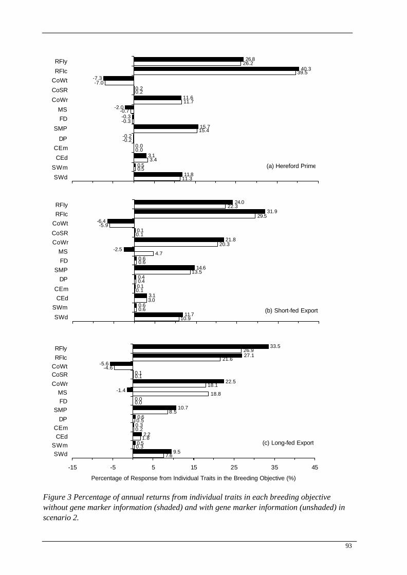
The percentage of annual selection responses contributed from individual traits in the breeding objective is shown in Figure 3. The main driver of all the indexes was RFI in both the mature cow and young animal. This is similar to the findings of other studies (Kahi et al., 2003; Archer et al., 2004). Marbling score has antagonistic correlations with RFI so a small negative response was found in all three objectives for marbling score for Scenario 1. Including genotype information increased the contribution of marbling score from, -2.5%, -2.0%, and -1.4% to 4.7%, -0.7% and 18.8% for Hereford Prime, short-fed and long-fed export objectives, respectively. The change in individual trait response was most evident in the long-fed objective due to the high economic value of marble score. The use of gene markers in this case was able to break antagonistic genetic correlations and increase the response to selection in marbling score while also selecting for the antagonistic trait RFI.

93

Figure 3 Percentage of annual returns from individual traits in each breeding objective without gene marker information (shaded) and with gene marker information (unshaded) in scenario 2.

11.3

0.5

3.4

0.0

-0.2

15.4

-0.3

-0.7

11.7

0.2

-7.0

39.5

26.2

11.8

0.5

3.1

0.0

-0.2

15.7

-0.3

-2.0

11.6

0.2

-7.3

40.3

26.8

SWd

SWm

CEd

CEmDP

SMP

FDMS

CoWr

CoSR

CoWtRFIc

RFIy

(a) Hereford Prime

10.9

0.6

3.0

0.1

0.4

13.5

0.6

4.7

20.3

0.1

-5.9

29.5

22.3

11.7

0.6

3.1

0.1

0.4

14.6

0.6

-2.5

21.8

0.1

-6.4

31.9

24.0

SWd

SWmCEd

CEm

DPSMP

FDMS

CoWrCoSR

CoWtRFIcRFIy

(b) Short-fed Export

7.6

0.3

1.8

0.2

0.5

8.5

0.0

18.8

18.1

0.1

-4.6

21.6

26.9

9.5

0.5

2.2

0.3

0.6

10.7

0.0

-1.4

22.5

0.1

-5.6

27.1

33.5

-15 -5 5 15 25 35 45

SWdSWm

CEdCEm

DPSMP

FDMS

CoWrCoSRCoWtRFIcRFIy

Percentage of Response from Individual Traits in the Breeding Objective (%)

(c) Long-fed Export

94

Sensitivity Analysis of Major Gene Effect

Figure 4 shows the sensitivity of the additional gains due to MAS to the substitution effect of the allele with variation from the base value of 0.5 phenotypic standard deviations down to 0.1 phenotypic standard deviations for the long fed objective.

-5

0

5

10

15

20

25

3 6 9 12 15

Year

Per

cent

age

Gai

n in

Obj

ectiv

e (%

)

Figure 4 Sensitivity of gain in long fed export objective to the size of the major gene effect in phenotypic standard deviations (0.65 = circle, 0.5 = triangle, 0.35 = square, 0.20 = diamond) The size of the QTL as a fraction of the overall breeding objective can be defined as sQTL/sH. Previous studies into the use of QTL have considered only a single trait (Meuwissen and Goddard, 1996; Spelman and Garrick, 1997) and the QTL accounted for a significant proportion of the variance of the trait. For the base scenario (0.5 phenotypic standard deviations of marble score) the QTL explained 6.5% of the breeding objective. Meuwissen and Goddard (1996) considered the use of the marker information before other records were available but did not consider the change in population structure. The increase in response predicted is slightly higher than that predicted by Meuwissen and Goddard (1996) for a similarly size QTL because of the gain was measured as annual genetic response and took into account altered age structure. For the Hereford Prime objective where the age structure does not alter significantly the increase in response is of a similar magnitude to that found by Meuwissen and Goddard (1996). Optimal Age Structure of the Nucleus

The optimal age structure of the males selected in the nucleus is shown in Figure 5. Scenario 1 had an age structure with the majority selected from age classes 2, 3 and 4 for each of the three objectives. The greater variance present in the export objectives resulted in a higher proportion of candidates selected from the younger age classes. When marker information was included the increase in index accuracy in the first year resulted in a substantial increase in the proportion selected from 1 year old age class. The largest increase in accuracy is for the long-fed objective and accordingly the largest change in age structure results in this objective. The Hereford Prime objective has relatively no change in age structure between Scenarios 1 and 2. When the number of sires available for selection under 1 year of age (i.e. those capable of reproduction) was increased to 70% of all the animals in the cohort, the proportion of bulls selected under 1 year old male cohort increased. The annual genetic response to selection was increased. When marker information was included the additional percentage increase in response per annum was similar to when 30% of bulls were available in the first year.

95

Table 8. Annual rate of genetic improvement ($) per cow per year for the Long fed, Short fed and Prime objectives with different percentages of bulls available for selection at 1 year of age.

Cost Benefit Analysis

Figure 6 and Figure 7 show the cumulative profit per bull from the time of initiation of MAS calculated according to the seedstock sale price for the long-fed export objective for Scenarios 2 and 3 respectively. The effect on profit was highly dependent on the economic value of the trait affected by the major gene and the sale price of seedstock animals. The increase in returns from the Hereford Prime and short-fed export objectives was only marginal. When the price of testing was included a negative return on investment occurred as the predicted gain did not exceed the cost of genotyping. The peak of the surface represents the point in time where investment in genotyping is most profitable. Depending on the assumed genotype cost, the expected returns do not exceed investment in the first years of MAS as there is a delay from investment until returns are accrued. Also, the initial years have smaller increases in gain as the favourable allele frequency is increased. The cost benefit is sensitive to the assumed returns and the average sale price was used to calculate the returns. At higher genotype costs the most cost effective strategy was to only measure male candidates (Scenario 3) and when costs were lower measurement of both sexes (Scenario 2) was optimal. When costs are higher the time to accrue returns to account for the investment increases and the maximum profit per bull is lower. The maximal returns in both scenarios are reached by year 5 in both scenarios. The break-even point can be identified on Figure and Figure where cumulative profit per bull sold is equal to zero. As the cost of genotyping increases the minimum average bull price at which the break even point is reached also increases. Any strategy that can reduce the investment required will have a considerable effect on profitability. A number of authors (Kinghorn, 1999; Marshall et al., 2002) have considered strategies to reduce the cost of genotyping whilst maintaining rates of gain such as inferring genotypes using segregation analysis or only genotyping candidates likely to be selected on estimated breeding value. Marshall et al. (2002) showed that genotypes the number of genotypes required could be reduced by 70% with only a 10% decrease in the overall MAS response compared to genotyping all selection candidates. By decreasing the investment in genotyping by only genotyping males, shown in Figure , the initial investment is decreased but the maximum profit per bull is reduced.

% Bulls Available

Hereford Prime

Extra % Gain

Short-fed Export

Extra % Gain

Long-fed Export

Extra % Gain

Annual Rate of Genetic Gain 30 4.36 - 5.09 - 5.87 - 40 4.36 - 5.10 - 5.88 - 50 4.37 - 5.10 - 5.88 - 60 4.37 - 5.10 - 5.88 - 70 4.38 - 5.11 - 5.89 -

Annual Rate of Genetic Gain with Genotype Information 30 4.45 (5) 0.74 5.35 (3) 4.21 7.05 (3) 14.15 40 4.43 (5) 5.30 (3) 6.94 (3) 50 4.42 (5) 5.29 (3) 6.92 (3) 60 4.42 (5) 5.28 (3) 6.90 (3) 70 4.40 (5) 5.26 (3) 6.88 (3)

96

Figure 5. Optimised male nucleus age structure for three breeding objectives when 30% of males are available for selection in the first year. Scenario 1=unshaded, scenario 2 = shaded.

0

20

40

60

80

100

1 2 3 4 5 6 7

Long-fed Export

0

20

40

60

80

100 Short-fed Export

0

20

40

60

80

100Hereford Prime

Per

cent

age

Sel

ecte

d (%

)

Age Class (yrs)

Figure 6. Cumulative profit per bull from time of MAS expressed as a function of the average bull price without MAS when genotyping information is available on both male and female selection candidates. Variation in genotype cost: (a) $10, (b) $30, (c) $50 and (d) $70.

0 5 10 1 5 20 25 $2,000

$3,000 $4,000

$5,000 $6,000

$7,000

-300

-200

-100

0

100

200

300

400

500

Cum

ulat

ive

Pro

fit P

er B

ull (

$)

Year

(b)

0 5 10 15 20 25 $2,000

$3,000 $4,000

$5,000 $6,000

$7,000

-800

-700

-600

-500

-400

-300

-200

-100

0

100

200

300

Cum

ulat

ive

Pro

fit P

er B

ull (

$)

Year

(d)

0 5 10 15 20 25$2,000

$3,000$4,000

$5,000$6,000

$7,000

-100

0

100

200

300

400

500

600

Cum

ulat

ive

Pro

fit P

er B

ull (

$)

Year

(a)

0 5 10 15 20 25 $2,000

$3,000 $4,000

$5,000 $6,000

$7,000

-500

-400

-300

-200

-100

0

100

200

300

400

Cum

ulat

ive

Pro

fit P

er B

ull (

$)

Year

(c)

Figure 7. Cumulative profit per bull from time of MAS expressed as a function of the average bull price without MAS when genotyping information is available on male selection candidates only. Variation in the genotyping cost (a) $10, (b) $30, (c) $50 and (d) $70.

0 5 10 15 20 25$2,000

$3,000$4,000

$5,000$6,000

$7,000

-100

-50

0

50

100

150

200

250

300

350

400

Cum

ulat

ive

Pro

fit P

er B

ull (

$)

Year

(b)

0 5 10 15 20 25 $2,000

$3,000 $4,000

$5,000 $6,000

$7,000

-300

-200

-100

0

100

200

300

Cum

ulat

ive

Pro

fit P

er B

ull (

$)

Year

(d)

0 5 10 15 2 0 25$2,000

$3,000$4,000

$5,000$6,000

$7,000

-50

0

50

100

150

200

250

300

350

400

450

500

Cum

ulat

ive

Pro

fit P

er B

ull (

$)

Year

(a)

0 5 10 15 20 25 $2,000

$3,000 $4,000

$5,000 $6,000

$7,000

-200

-150

-100

-50

0

50

100

150

200

250

300

350

Cum

ulat

ive

Pro

fit P

er B

ull (

$)

Year

(c)


Long-term Response to MAS

Using a selection index to determine the emphasis on the marked trait maximises the response from generation to generation but the response was not optimised over the long-term. The long-term response using the marker was decreased compared to phenotypic selection due to the fixation of the QTL and reduced response for other breeding objective traits. This is similar to the finding of Gibson (1994) who showed that the response in the long-term was less when using genotype information because variation was sacrificed in the unmarked polygenic component. The decrease in long-term selection response is small from MAS and occurs at different times depending on the objective as shown in Figure 1 for the long-fed and short-fed objectives (Scenario 2) the gains fall below BLUP selection at year 11 and 15 respectively. Selection on a marked allele has the potential to decrease the possible level of inbreeding within a population. The use of MAS decreases the reliance on While it is difficult to predict the level of increase it would be related to the within family segregation of the marked gene. Assuming there is no within family difference in gene frequency selection of related individuals will solely due to the polygenic component of the breeding objective. Conclusion The response to MAS in a multi-trait beef objective depends on the size of the QTL and the proportion of the breeding objective that it explains. Of the three objectives examined only the long-fed export objective with a high economic value for marble score resulted in a gain of significant size to warrant the investment in genotype information when the marker effect was 0.5 phenotypic standard deviations. By measuring the genotype of only male selection candidates reduced investment cost and resulted in a lower but more prolonged increase in MAS response as the QTL is not fixed as rapidly. Accounting for discounting returns accrued later, if genotyping costs are reduced it is economically rational to genotype both sexes. Investment is ultimately the decision of the individual but the results presented here suggest that depending on the market, expected seedstock sale price and genotype cost and size of the marker effect investment in MAS can result in significant increases in short term profitability for the seedstock producer. References Case Study Ben Wood Archer, J.A., Barwick, S.A., Graser, H.-U., 2004. Economic evaluation of beef cattle breeding schemes

incorporating performance testing of young bulls for feed intake. Aust. J. Exp. Agric. 44,393-404. Bijma, P., van Arendonk, J.A.M., 1998. Maximizing genetic gain for the sire line of a crossbreeding scheme

utilizing both purebred and crossbred information. Anim. Sci. 66,529-542. Burrows, P.M., 1972. Expected selection differentials for directional selection. Biometrics 28,1091-1100. Dekkers, J.C.M., 1999. Breeding values for identified quantitative trait loci under selection. Gen. Sel. Evol.

31,421-436. Dekkers, J.C.M., 2003. Commercial application of marker- and gene assisted selection in livestock:

strategies and lessons. Proc. 54th Europ. Assoc. Anim. Prod. Dekkers, J.C.M., van Arendonk, J.A.M., 1998. Optimizing selection for quantitative traits with information on

an identified locus in outbred populations. Genet. Res. 71,257-275. Ducrocq, V., Quaas, R.L., 1988. Prediction of genetic response to truncation selection across generations.

J. Dairy. Sci. 71,3543-3553. Falconer, D.S., Mackay, T.F.C. 1996. Introduction to Quantitative Genetics. 4th ed. Pearson Education,

Harlow, England. Genz, A., 1992. Numerical computation of multivariate normal probabilities. J. Comput. Graph. Statist.

1,141-149. Gibson, J.P., 1994. Short term gain at the expense of long term response with selection on identified loci.

5th World Cong. Genet. Appl. Livest. Prod. 21,201-204. Hayes, B., Goddard, M.E., 2003. Evaluation of marker assisted selection in pig enterprises. Livest. Prod.

Sci. 81,197-211. Hazel, L.N., 1943. The genetic basis for constructing selection indexes. Genetics 28,476-490.


Henderson, C.R., 1975. Best linear unbiased prediction under a selection model. Biometrics 31,423-47. Kahi, A.K., Barwick, S.A., Graser, H.-U., 2003. Economic evaluation of Hereford breeding schemes

incorporating direct and indirect measures of feed intake. Aust. J. Agric. Res.,1039-1055. Kinghorn, B.P., 1999. Use of segregation analysis to reduce genotyping costs. J. Anim. Breed. Genet.

116,175-180. Marshall, K., Henshall, J., van der Werf, J.H.J., 2002. Response from marker-assisted selection when

various proportions of animals are marker typed: a multiple trait simulation study relevant to the sheep meat industry. Anim. Sci. 74,223-232.

Meuwissen, T.H.E., Goddard, M.E., 1996. The use of marker haplotypes in animal breeding schemes. Gen. Sel. Evol. 28,161-176.

Nicol, D.C., Armitage, S.M., Hetzel, D.J.S., Davis, G.P., 2001. Genotype frequencies for GENESTAR MARBLING® - A DNA based diagnostic test for beef cattle. Proc. Assoc. Adv. Anim. Breed. Genet. 14,537-540.

Spelman, R.J., Garrick, D.J., 1997. Utilisation of marker assisted selection in a commercial dairy cow population. Livest. Prod. Sci. 47,139-147.

Spelman, R.J., Garrick, D.J., van Arendonk, J.A.M., 1999. Utilization of genetic variation by marker assisted selection in commercial dairy populations. Livest. Prod. Sci. 59,51-60.

Villanueva, B., Wray, N.R., Thompson, R., 1993. Prediction of asymptotic rates of response from selection on multiple traits using univariate and multivariate best linear unbiased prediction. Anim. Prod. 57,1-13.

Wood, B.J., van der Werf, J.H.J., Archer, J.A., 2004. Response to Selection in Beef Cattle Using IGF-1 as a Selection Criterion for Residual Feed Intake Under Different Australian Breeding Objectives. Livest. Prod. Sci. (Accepted).


Further References

.

REFERENCES Belonsky, G.M. and Kennedy, B.W. (1988).. Journal of Animal Science. 66:1124 Betteridge, K.J. (1999). Theriogenology 53 : 3-10. Betteridge, K.J., Smith, C., Stubbings, R.B., Xu, N.P. and King, W.A. (1989) J. Reprod. Fertil. 38

(suppl. 1) : 87-98. Bijma, P., van Arendonk, J.A.M. and Woolliams, J.A. (2001) J. Anim Sci. 79 : 840-853. Bijma, P. (2000) PhD thesis, Wageningen University, 225 pp. Bijma, P. and Woolliams, J.A. (2000) Genetics 156 : 361-373. Brascamp, E.W. (1998) Acta Agric. Scand. 28 (suppl): 61-67. Bulmer, M.G. (1971) Am. Naturalist 105 : 201-211. De Boer, I.J.M. and van Arendonk, J.A.M. (1994) Anim. Prod. 58 : 173-180. De Boer, I.J.M., Meuwissen, T.H.E. and van Arendonk J.A.M. (1994) Anim.Prod. 59 : 345-358. De Boer, I.J.M., Brom, F.W. and Vorstenbosch, J.M.G. (1995) Anim. Sci. 61 : 453-463. Ducrocq, V. and Quaas, R.L. (1988) J. Dairy Sci. 71 : 2543-2553. James, J.W. (1987) J. Anim. Breed. Genet. 104 : 23-27. Kinghorn, B.P. and Dekkers, J.C.M. (1991) J. Dairy Sci. 74 : 611-622. Land, R.B. and Hill, W.G. (1975) Anim. Prod. 21 : 1-12. Meuwissen, T.H.E. (1991) Biometrics 47 : 195-203. Meuwissen, T.H.E. (1997) J. Anim Sci. 75 : 934-940. Meuwissen, T.H.E. (1998) J. Dairy Sci. 81 : 47-54. Meuwissen, T.H.E. and Sonesson, A.K. (1998). J. Anim. Sci. 76 : 2575-2583. Nicholas, F.W. (1996) Anim. Reprod. Sci. 42 : 205-214. Nicholas, F.W. and Smith, C. (1983) Anim. Prod. 36 : 341-353. Quinton, M. and Smith, C. (1995). J. Anim. Sci. 73 : 2208-2212. Rendel, J.M. and Robertson, A. (1950). J. Genet . 50 : 1-8. Seamark, R.F. (1993). Livest. Prod. Sci. 36 : 5-15. Spelman, R.J., Garrick, D.J. and van Arendonk, J.A.M. (1999) Livest. Prod. Sci. 59 : 51-60. Verrier, E., Colleau, J.J. and Foulley, J.L. (1993) Theor. Appl. Genet. 87 : 446-454. Villanueva, B., Wray, N.R. and Thompson, R. (1993) Anim. Prod. 57 : 1-13. Villanueva, B. and Simm, G. (1994) Proc. WCGALP 5. 20 : 200-207. Visscher, P., Pong-Wong, R, Whittemore, C. and Haley, C. (2000). Livest. Prod. Sci. 65 : 57-70. Van der Lende, T., Komen, H. and Brascamp, E.W. (1998) Acta Agric Scand. 29 (sup) : 90-97. Van Arendonk, J.A.M. and P. Bijma. World Congr. Genet. Appl. Livest. Prod. Comm. No.27.02 Willett, E.L., Black, W.G., Casida, L.E., Stone, W.H. and Bucker, P.J. (1951) Science 113 : 247. Woolliams, J.A. (1989) Anim. Prod.. 49 : 1-14. Woolliams, J.W. and Wilmut, I. (1989) Anim. Prod.. 48 : 245-256. Woolliams, J.W., Bijma, P. and Villanueva, B. (1999) Genetics 153 : 1009-1020. Woolliams, J.W. and P. Bijma, P. (2000) Genetics 154 : 1851-1864. Wray, N.R. and Hill, W.G. (1989). Anim. Prod. 49 : 217-227. Wray, N.R., and Thompson, R. (1990) Genet. Res. Camb. 55 : 41-54. Wray, N.R., and M.E. Goddard. (1994).. Genet. Sel. Evol. 26:431.

optimizing design of breeding programs 1 introduction

Documents