optimizing ice thermal storage to reduce energy cost
TRANSCRIPT

North Carolina Agricultural and Technical State University North Carolina Agricultural and Technical State University
Aggie Digital Collections and Scholarship Aggie Digital Collections and Scholarship
Theses Electronic Theses and Dissertations
2014
Optimizing Ice Thermal Storage To Reduce Energy Cost Optimizing Ice Thermal Storage To Reduce Energy Cost
Christopher L. Hall North Carolina Agricultural and Technical State University
Follow this and additional works at: https://digital.library.ncat.edu/theses
Recommended Citation Recommended Citation Hall, Christopher L., "Optimizing Ice Thermal Storage To Reduce Energy Cost" (2014). Theses. 199. https://digital.library.ncat.edu/theses/199
This Thesis is brought to you for free and open access by the Electronic Theses and Dissertations at Aggie Digital Collections and Scholarship. It has been accepted for inclusion in Theses by an authorized administrator of Aggie Digital Collections and Scholarship. For more information, please contact [email protected].

Optimizing Ice Thermal Storage to Reduce Energy Cost
Christopher L. Hall
North Carolina A&T State University
A thesis submitted to the graduate faculty
in partial fulfillment of the requirements for the degree of
MASTER OF SCIENCE
Department: Civil, Architectural, and Environmental Engineering
Major: Civil Engineering
Major Professor: Dr. Nabil Nassif
Greensboro, North Carolina
2014
i
School of Graduate Studies
North Carolina Agricultural and Technical State University
This is to certify that the Master’s Thesis of
Christopher L. Hall
has met the thesis requirements of
North Carolina Agricultural and Technical State University
Greensboro, North Carolina
2014
Approved by:
Dr. Nabil Nassif
Major Professor
Dr. Taher Abu-Lebdeh
Committee Member
Dr. Sanjiv Sarin
Dean of Graduate Studies
Dr. Sameer Hamoush
Department Chair
Dr. Elham Fini
Committee Member

ii
© Copyright by
Christopher L. Hall
2014

iii
Biographical Sketch
Christopher L. Hall was born on March 24, 1990 in Greenville, North Carolina. He is a
second year graduate student from Ahoskie, North Carolina. Presently, he is pursuing a Master
of Science degree in Civil Engineering from The North Carolina Agricultural and Technical
State University. In May of 2012 Christopher earned the Bachelor of Science degree in
Architectural Engineering, also at NC A&T State University.
While studying architectural engineering throughout his undergraduate career, he was
awarded for his academic success and high standard for achievement. During undergrad he was
recognized and inducted into the Tau Beta Pi honor society, exclusively for top tier engineering
students, as well as Phi Alpha Epsilon, an honor society for high level architectural engineering
students. He was a well-rounded architectural engineering student as he found interest in the
design, lighting and electrical disciplines.
It was at the end of his undergraduate tenure that he decided to further his studies in
pursuit of a graduate degree focused on Building Energy. This focus in graduate school allowed
him to work with his major professor and eventually conduct research. After a year of graduate
school Christopher was able to land a summer internship which fell directly in line with his
studies and provided clarity to his thesis research. He spent the summer of 2013 in Champaign,
Illinois and worked as a research intern for the U.S. Army Corps of Engineers.

iv
Dedication
I would like to dedicate this thesis to anyone who finds a way when things may seem
impossible. My greatest characteristic is my persistence. Smart people are a dime a dozen. What
matters is the ability to think different… to think out of the box.

v
Acknowledgements
I would like to acknowledge the U.S. Army Corps of Engineers and their Engineer
Research and Development Center/Construction Engineering Research Laboratory. Spending a
summer working with them and having the privilege and opportunity to work in the same field as
my thesis research proved to be highly beneficial in my research efforts. The mentoring and
guidance provided was superior and greatly appreciated. I would like to give special thanks to
Dr. Nathaniel Putnam, who was my direct mentor with the Environmental Processes Branch. He
helped me to design and develop a project that would allow me to grow as a research student,
attain vital information contributing to my thesis research, all while providing a useful and
valuable reference point for the study to help the branch office where he works.
Most importantly, I have to thank my advisor at NC A&T State University, Dr. Nabil
Nassif. He took me in as one of his Master Thesis students with no hesitation, although he still
advises a number of other MS and PhD students. This research and thesis was a huge success due
to his efforts. His experience and knowledge in HVAC and the field of energy alone is
unbelievable. While working with him I noticed how valuable his guidance and opinion meant to
my research work as well as my advancement towards succeeding and graduating. Time after
time Dr. Nassif never failed in constantly pushing me to do more and aim higher. He aided me in
many ways and made sure I had the tools to become successful and grow as an individual in my
early career. It was truly a pleasure working directly with him for the last couple of years. I thank
you Dr. Nassif for truly caring about me and my work and seeing to it that I graduated a better
student and a promising career individual.

vi
Table of Contents
List of Figures ................................................................................................................................ xi
List of Tables ............................................................................................................................... xiii
Abstract ........................................................................................................................................... 2
CHAPTER 1 Introduction............................................................................................................... 3
1.1 Thesis Format and Flow ........................................................................................................ 3
1.2 Key Terms and Definitions ................................................................................................... 3
1.3 Introduction ........................................................................................................................... 5
1.4 Purpose of Exploratory Research .......................................................................................... 5
1.4.1 Energy use in commercial and industrial buildings. .................................................. 5
1.4.2 Ice thermal storage as a sustainable technology. ....................................................... 6
1.5 Thermal Energy Storage (TES) ............................................................................................. 7
1.6 Ice Thermal Storage (ITS)..................................................................................................... 7
1.6.1 Introduction to ice thermal storage. ........................................................................... 7
1.6.2 The variables behind ice thermal storage................................................................... 7
1.6.3 Ice thermal storage: how it works. ............................................................................. 8
1.6.4 Downside to ice thermal storage. ............................................................................... 9
1.7 Research Constraints ............................................................................................................. 9
1.7.1 Utility rate structure ................................................................................................... 9
1.7.2 Building study .......................................................................................................... 10

vii
1.8 Objectives ............................................................................................................................ 10
CHAPTER 2 Literature Review ................................................................................................... 11
2.1 Overview ............................................................................................................................. 11
2.2 Energetic, Economic, and Environmental Benefits of Utilizing the Ice Thermal Storage
Systems for Office Building Applications ................................................................................ 11
2.3 Optimal Control of Building Storage Systems Using Both Ice Storage and Thermal Mass -
Part I: Simulation Environment................................................................................................. 13
2.4 Optimal Controls of Building Storage Systems Using Both Ice Storage and Thermal Mass -
Part II: Parametric Analysis ...................................................................................................... 15
2.5 Cumulative Energy Analysis of Ice Thermal Storage Air Conditioning System ............... 17
2.6 Performance of Ice Storage System Utilizing a Combined Partial and Full Storage Strategy
................................................................................................................................................... 18
2.7 Optimal Design and Control of Ice Thermal Storage System for a Typical Chilled Water
Plant ........................................................................................................................................... 19
2.8 Genetic Algorithms: An Overview ..................................................................................... 21
CHAPTER 3 Simulations and Exploratory Research ................................................................... 22
3.1 Overview ............................................................................................................................. 22
3.2 Recommended Process ........................................................................................................ 22
3.3 Programs and Models .......................................................................................................... 23
3.3.1 Simulation model ..................................................................................................... 23
3.3.2 MatLab models ........................................................................................................ 23

viii
3.4 EQuest Process .................................................................................................................... 24
3.4.1 Building creation wizard .......................................................................................... 24
3.4.2 Uploading the building via the wizard ..................................................................... 25
3.4.3 EQuest features and functions ................................................................................. 26
3.4.4 Simulating building performance ............................................................................ 28
3.5 Developed MatLab Program Code ...................................................................................... 28
3.5.1 Input variables .......................................................................................................... 29
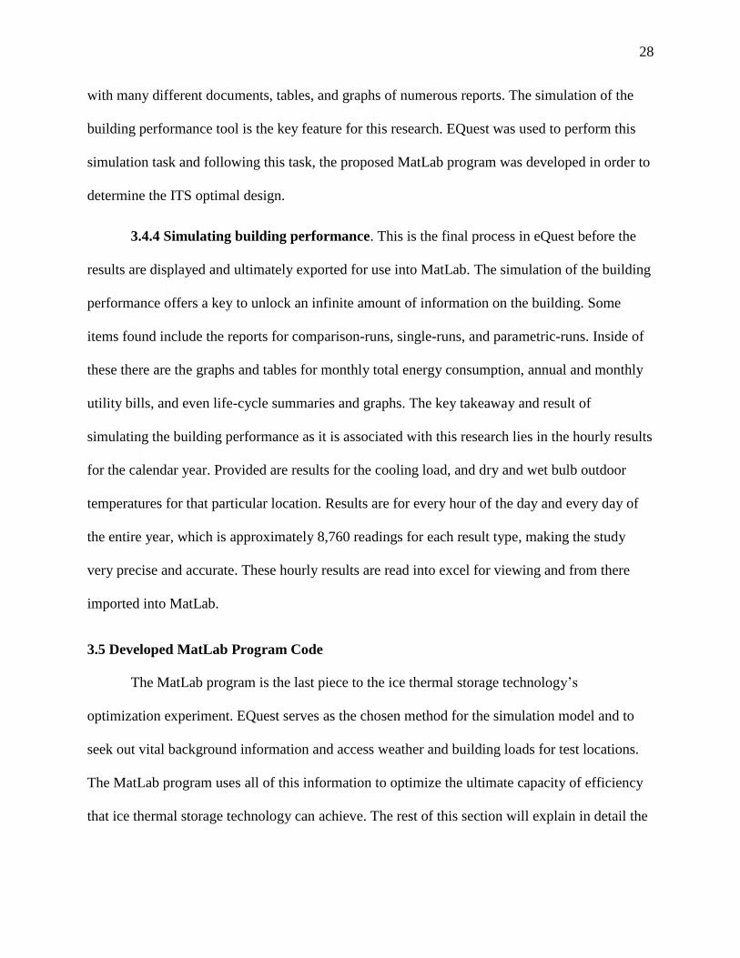
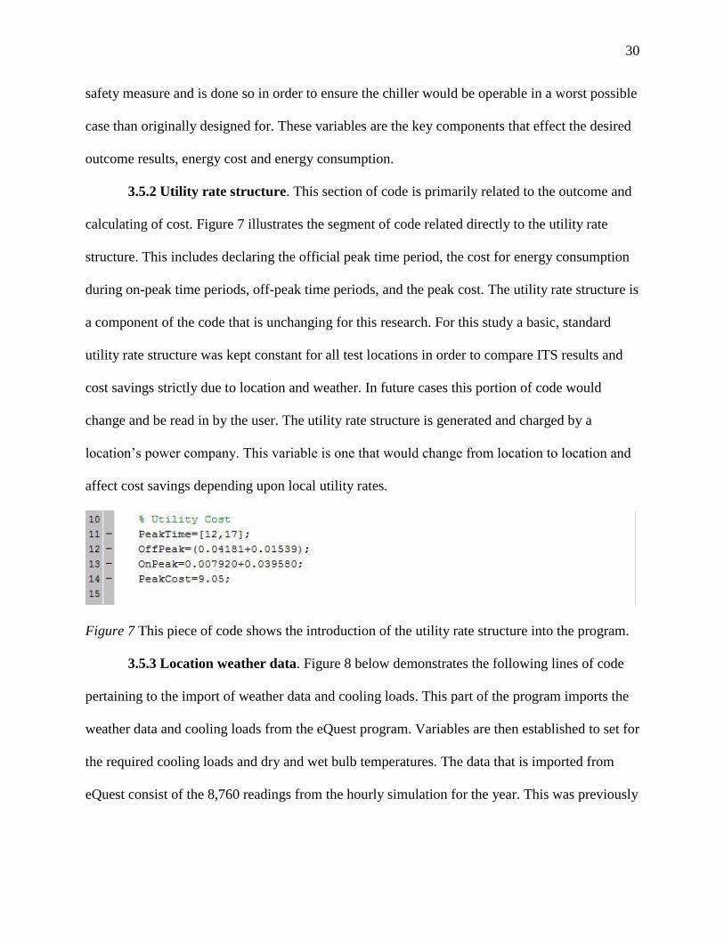
3.5.2 Utility rate structure ................................................................................................. 30
3.5.3 Location weather data .............................................................................................. 30
3.5.4 Chiller and ice thermal storage tank capacities ........................................................ 31
3.5.5 Operation of the chiller and ITS systems ................................................................. 32
3.5.6 Genetic algorithm optimization model .................................................................... 33
3.6 Building Description ........................................................................................................... 34
3.6.1 Brief building history ............................................................................................... 35
3.6.2 IRC design. .............................................................................................................. 35
3.7 Methodology ....................................................................................................................... 36
3.7.1 Preceding research ................................................................................................... 36
3.7.2 ASHRAE climate zones ........................................................................................... 37
3.7.3 Location selection .................................................................................................... 38
ix
CHAPTER 4 Results and Findings ............................................................................................... 40
4.1 Overview ............................................................................................................................. 40
4.2 Research Test Results.......................................................................................................... 40
4.2.1 Climate region subtype A: Moist. ............................................................................ 41
4.2.1.1 Miami, Florida. .............................................................................................. 41
4.2.1.2 Orlando, Florida. ............................................................................................ 43
4.2.1.3 Dallas, Texas. ................................................................................................. 45
4.2.1.4 Greensboro, North Carolina. .......................................................................... 46
4.2.1.5 Philadelphia, Pennsylvania. ........................................................................... 48
4.2.1.6 Green Bay, Wisconsin. .................................................................................. 50
4.2.1.7 Portland, Maine. ............................................................................................. 51
4.2.2 Climate region subtype B: Dry. ............................................................................... 53
4.2.2.1 Phoenix, Arizona............................................................................................ 53
4.2.3 Climate region subtype C: Marine. .......................................................................... 55
4.2.3.1 San Diego, California. .................................................................................... 55
4.2.3.2 Seattle, Washington ....................................................................................... 57
4.3 Test Location Non-Optimal Manual Results ...................................................................... 59
4.3.1 Preliminary testing of locations. .............................................................................. 59
4.4 Test Location Optimal Results ............................................................................................ 59
4.4.1 How it works. ........................................................................................................... 59

x
4.4.2 The ten test locations optimal results. ...................................................................... 60
4.5 Energy consumption ............................................................................................................ 61
4.6 Energy Cost ......................................................................................................................... 63
CHAPTER 5 Conclusion and Future Research ............................................................................ 65
5.1 Overview ............................................................................................................................. 65
5.2 Input Variables .................................................................................................................... 66
5.2.1 Ice capacity factor. ................................................................................................... 66
5.2.2 Ice charge time. ........................................................................................................ 66
5.2.3 Ice discharge time. ................................................................................................... 67
5.2.4 Chiller size factor. .................................................................................................... 67
5.3 Savings ................................................................................................................................ 68
5.4 Moving Forward .................................................................................................................. 72
5.4.1 Cost Analysis. .......................................................................................................... 72
5.4.2 Program and code improvements. ............................................................................ 73
References ..................................................................................................................................... 75
Appendix A ................................................................................................................................... 78
A. Hourly Peak Load Data ........................................................................................................ 78
Appendix B ................................................................................................................................... 82
B. Full Data For Each Climate Zone ......................................................................................... 82
xi
List of Figures
Figure 1 Schematic of (a) conventional AC system & (b) TES system (Rismanchi,2012).......... 13
Figure 2 Flowchart of the simulation environment (Hajiah, 2012 a). .......................................... 15
Figure 3 The developed and recommended optimization tool in the design of the ITS system. .. 23
Figure 4 One screen of building input information for the eQuest schematic design wizard. ..... 26
Figure 5 A two-dimensional digital view of the test building uploaded into eQuest. .................. 27
Figure 6 Code from the MatLab program that references the input variables. ............................. 29
Figure 7 This piece of code shows the introduction of the utility rate structure into the program.
....................................................................................................................................................... 30
Figure 8 The lines of code displaying the import of the weather data & cooling loads from
eQuest into MatLab....................................................................................................................... 31
Figure 9 This code from MatLab is needed for the design of the chiller and ITS tank sizes. ...... 32
Figure 10 The last part of code begins the process of optimizing the system & energy
calculations. .................................................................................................................................. 33
Figure 11 Optimization tool running in MatLab finding the optimal results for Greensboro, NC.
....................................................................................................................................................... 34
Figure 12 A live look at the Interdisciplinary Research Center in Greensboro, NC. ................... 35
Figure 13 An interior view of the IRC and the central atrium leading up to the large skylight. .. 36
Figure 14 A map and graphic of ASHRAE 90.1 Climate Zones. ................................................. 38
Figure 15 The optimal results for energy consumption in the ASHRAE climate zone test
locations. ....................................................................................................................................... 62
Figure 16 The optimal results for energy costs in the ASHRAE climate zone test locations. ..... 64
Figure 17 Graph comparing energy consumption of No ITS system vs. optimized ITS system. 71

xii
Figure 18 Graph comparing energy cost of No ITS system vs. optimized ITS system. ............... 72

xiii
List of Tables
Table 1 Some manual results for ice thermal storage use in Miami, Florida. ............................. 42
Table 2 The output readings for climate zone 2 located in Orlando, Florida. ............................. 44
Table 3 ITS results are shown partly for climate zone 3 in Dallas, Texas. ................................. 45
Table 4 Ice thermal storage results for testing in Greensboro, NC. ............................................. 47
Table 5 The partial results for climate zone 5 in Philadelphia, Pennsylvania. ............................ 49
Table 6 Manual results from ITS testing in Green Bay, Wisconsin. ........................................... 50
Table 7 Ice thermal Storage design output results for Portland, Maine....................................... 52
Table 8 The output readings for climate zone 2 located in Phoenix, Arizona. ............................ 54
Table 9 Some manual results for ice thermal storage use in San Diego, California.................... 56
Table 10 ITS results are shown partly for climate zone 3 in Seattle, Washington. ..................... 58
Table 11 Optimization results for ITS designs from genetic algorithm simulations. .................. 60
Table 12 Outputs for energy cost & consumption for No ITS vs. Optimal ITS & percent savings.
....................................................................................................................................................... 69
2
Abstract
Energy cost for buildings is an issue of concern for owners across the U.S. The bigger the
building, the greater the concern. A part of this is due to the energy required to cool the building
and the way in which charges are set when paying for energy consumed during different times of
the day. This study will prove that designing ice thermal storage properly will minimize energy
cost in buildings. The effectiveness of ice thermal storage as a means to reduce energy costs lies
within transferring the time of most energy consumption from on-peak to off-peak periods.
Multiple variables go into the equation of finding the optimal use of ice thermal storage and they
are all judged with the final objective of minimizing monthly energy costs. This research
discusses the optimal design of ice thermal storage and its impact on energy consumption,
energy demand, and the total energy cost. A tool for optimal design of ice thermal storage is
developed, considering variables such as chiller and ice storage sizes and charging and discharge
times. The simulations take place in a four-story building and investigate the potential of Ice
Thermal Storage as a resource in reducing and minimizing energy cost for cooling. The
simulations test the effectiveness of Ice Thermal Storage implemented into the four-story
building in ten locations across the United States.
3
CHAPTER 1
Introduction
1.1 Thesis Format and Flow
This thesis consists of five chapters, organized to separate the major points in the
progression of the research. The first chapter is a preliminary chapter and serves to introduce the
topic while providing any necessary background information. Following this, chapter two is the
chapter for literature review, where the bulk of the research’s resources reside. Here in the
second chapter a number of references are made to support the research with direct quotations
for the most important information. The third chapter is all about the simulations and research.
Throughout this chapter the models will be explained followed by a detailed building description
and a methodology behind the experiment. In the fourth chapter is where the results will be
located. In this chapter a number of tested results will be revealed and compared to other
findings. The fifth chapter is the last major section and will be the home for the discussion and
conclusion of the entire research, a deeper analysis of results, and at the very end a suggestion
into where the research should go moving forward. After the major chapters is where the
references can be found, listed alphabetically, followed by the appendices of all research work
not directly listed in the body of the thesis.
1.2 Key Terms and Definitions
A. eQuest: a building energy software tool developed by the U.S. Department of Energy. It
is a widely used, time-proven whole building energy performance design tool. It has
wizards, interactive graphics, parametric analysis, and rapid execution. This makes
eQuest able to conduct whole-building performance simulation analysis throughout the
4
entire design process, from the design stage with a schematic design wizard all the way
up to a very detailed design development stage.
B. Dry Bulb Temperature: the temperature of air measured by a thermometer freely exposed
to air, yet shielded from radiation and moisture. Dry bulb temperature is the temperature
that is usually thought of as air temperature, and the true thermodynamic temperature.
This temperature is typically expressed in degrees Celsius, Kelvin, and/or Fahrenheit.
C. Wet Bulb Temperature: the temperature a parcel of air would have if it were cooled to
saturation by the evaporation of water into it, with latent heat supplied by the parcel. Wet
bulb temperature is the temperature felt when the skin is wet and exposed to moving air.
D. MatLab: a numerical computing environment and fourth generation programming
language. It allows for matrix manipulations, plotting of functions and data,
implementation of algorithms, creation of user interfaces, and interfacing with programs
written in other languages like: C, C++, Java, and Fortran.
E. Chiller: A device that removes heat from a liquid by a vapor-compression or absorption
refrigeration cycle. This cooled liquid flows through pipes in a building and passes
through coils in air handlers, fan-coil units, or other systems, cooling and usually
dehumidifying the air in the building.
F. Air Handling Unit: (AHU) A central unit consisting of a blower, heating and cooling
elements, filter racks or chamber, dampers, humidifier, and other central equipment in
direct contact with the airflow.
G. ASHRAE: (American Society of Heating, Refrigerating, and Air-Conditioning
Engineers) is an organization devoted to the improvement of indoor-environment-control
technology in the heating, ventilation, and air conditioning industry.

5
H. ASHRAE Climate Zones: a sorted distribution of regions in the United States based on
climate characteristics split into 7 zones.
1.3 Introduction
There is a cause for concern with the related energy cost that goes hand in hand with big
commercial buildings. Efforts are now widespread in making buildings as energy efficient as
possible. It is not always necessary to gain energy efficiency through expensive investments in
large equipment and technological improvements. Inexpensive efforts to gain energy efficiency
can come from a number of techniques whether it is something as simple as minor maintenance,
how the building is operated, or even the behavior of building tenants. The other more expensive
building enhancements can range from upgrades to energy-efficient lighting, air sealing, and
HVAC equipment, just to name a few. Another form of improving a building’s energy cost can
be provided by storing excess thermal energy for usage at a later time. This technology is known
as Thermal Energy Storage (TES) and has numerous methods in which energy can be stored and
kept for use in the future.
1.4 Purpose of Exploratory Research
1.4.1 Energy use in commercial and industrial buildings. There are over five million
combined commercial and industrial buildings in the United States. The annual energy costs for
these buildings exceed two hundred billion dollars (Energy Efficiency and Renewable Energy,
2010). In addition, it is estimated that about thirty percent of the energy in the commercial and
industrial buildings are deemed to be used inefficiently or unnecessarily. If the energy efficiency
in commercial and industrial buildings in the United States could be enhanced by ten percent at
the very least, the amount of money it would save annually would tip the scales at twenty billion
dollars. These facts show just how important it is to make a change in the operation of
6
commercial and industrial buildings towards a more efficient state. One way to move in that
direction is to add and incorporate some sustainable practices and technology. A possibility that
will be investigated is whether the incorporation of ice thermal storage can provide enough of a
savings in commercial and industrial buildings, no matter if it is in a dominantly hot or cold
climate.
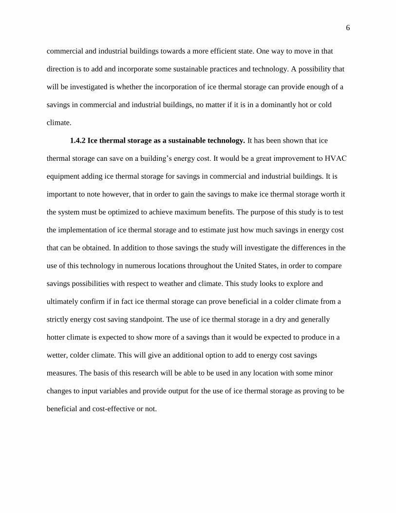
1.4.2 Ice thermal storage as a sustainable technology. It has been shown that ice
thermal storage can save on a building’s energy cost. It would be a great improvement to HVAC
equipment adding ice thermal storage for savings in commercial and industrial buildings. It is
important to note however, that in order to gain the savings to make ice thermal storage worth it
the system must be optimized to achieve maximum benefits. The purpose of this study is to test
the implementation of ice thermal storage and to estimate just how much savings in energy cost
that can be obtained. In addition to those savings the study will investigate the differences in the
use of this technology in numerous locations throughout the United States, in order to compare
savings possibilities with respect to weather and climate. This study looks to explore and
ultimately confirm if in fact ice thermal storage can prove beneficial in a colder climate from a
strictly energy cost saving standpoint. The use of ice thermal storage in a dry and generally
hotter climate is expected to show more of a savings than it would be expected to produce in a
wetter, colder climate. This will give an additional option to add to energy cost savings
measures. The basis of this research will be able to be used in any location with some minor
changes to input variables and provide output for the use of ice thermal storage as proving to be
beneficial and cost-effective or not.

7
1.5 Thermal Energy Storage (TES)
The central idea behind thermal energy storage lies within harnessing energy and saving
it for later use. Thermal energy storage is available in a wide range of fields that span; solar
energy, heat storage (in rocks, tanks, concrete, and electric heaters), cryogenic energy, or even
molten salt technology. Although there are multiple different systems in which thermal energy
can be stored, it is most common that it is used to provide a cooling capacity within commercial
buildings. Thermal energy storage through cooling allows for huge money savings and can
increase the efficiency of a building’s current HVAC equipment. This form of thermal energy
storage is referred to as Ice Thermal Storage.
1.6 Ice Thermal Storage (ITS)
1.6.1 Introduction to ice thermal storage. Ice thermal storage has shown to be a very
capable technology in reducing energy cost, particularly in bigger commercial buildings. The
main objective behind ice thermal storage technology which provides the ability to reduce
energy cost comes from the shifting of energy consumption loads during the highly expensive
on-peak periods of the day to a more affordable off-peak period. The savings behind this
technology is evident but there lies no financial gain from the use of ice thermal storage when
the system is designed and runs poorly in combination with the building’s HVAC equipment.
1.6.2 The variables behind ice thermal storage. With the savings that can result from
the use of ice thermal storage comes a lot of inner conditions that require tuning. These inner
conditions adjusted and set correctly is what provides the biggest savings in ice thermal storage
and a building’s energy costs. Such variables include: location weather data and utility rate
structure, ice capacity factor, ice charge time, ice discharge time, and a chiller size factor. Some
of these variables have wide ranges of possibilities and others are standards that can be decided
8
upon. All in all, the location is a big determination in how many of the other conditions are
resolved. Each condition requires some attention and insight but any and every adjustment can
have some effect on final outcomes of energy cost, as well as energy consumption.
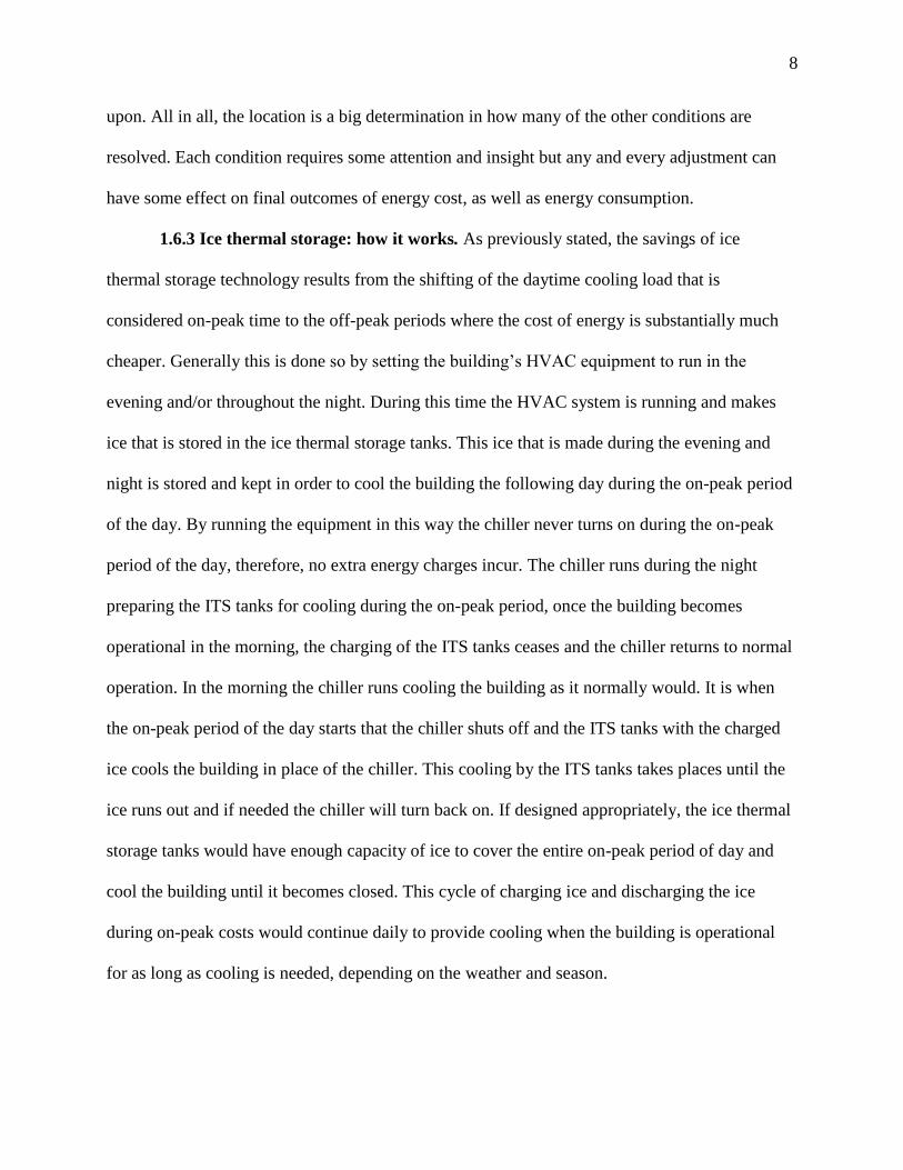
1.6.3 Ice thermal storage: how it works. As previously stated, the savings of ice
thermal storage technology results from the shifting of the daytime cooling load that is
considered on-peak time to the off-peak periods where the cost of energy is substantially much
cheaper. Generally this is done so by setting the building’s HVAC equipment to run in the
evening and/or throughout the night. During this time the HVAC system is running and makes
ice that is stored in the ice thermal storage tanks. This ice that is made during the evening and
night is stored and kept in order to cool the building the following day during the on-peak period
of the day. By running the equipment in this way the chiller never turns on during the on-peak
period of the day, therefore, no extra energy charges incur. The chiller runs during the night
preparing the ITS tanks for cooling during the on-peak period, once the building becomes
operational in the morning, the charging of the ITS tanks ceases and the chiller returns to normal
operation. In the morning the chiller runs cooling the building as it normally would. It is when
the on-peak period of the day starts that the chiller shuts off and the ITS tanks with the charged
ice cools the building in place of the chiller. This cooling by the ITS tanks takes places until the
ice runs out and if needed the chiller will turn back on. If designed appropriately, the ice thermal
storage tanks would have enough capacity of ice to cover the entire on-peak period of day and
cool the building until it becomes closed. This cycle of charging ice and discharging the ice
during on-peak costs would continue daily to provide cooling when the building is operational
for as long as cooling is needed, depending on the weather and season.
9
1.6.4 Downside to ice thermal storage. The benefits that ice thermal storage technology
provides are very much apparent. It is not as evident however of the small hindrance that ice
thermal storage also causes. Although the implementation of ITS results in a savings on energy
cost for buildings, ice thermal storage ultimately increases the amount of energy consumption
that is caused by the building. This increase in energy consumption however is only a minor
concern because of the savings that is due to the decline in energy costs. The increase in the
amount of energy consumed by the building with the addition of ice thermal energy is most
easily explained and accounted for by the operation of the chiller. With the employment of ITS
the chiller runs at night. When the chiller has to run at night to make the ice for the ITS tanks it is
required to run at a higher capacity to be cold enough, making ice. The energy consumption
increase is due to the extent of how much harder the chiller works and runs while making ice.
The positive in this outcome lies in the fact that the savings in energy cost fortunately outweighs
the amount in which the energy consumption increases, and it does so substantially.
1.7 Research Constraints
Some of the major constraints within this research include: the utility rate structure, and
the building study. The constraints in this study are minor and the research has been adapted to
the point where adjustments can be made for future use and alternative research moving forward.
This study makes it so the results shown are adequate for the building used and in the location set
forth.
1.7.1 Utility rate structure. Throughout the study, one constraint lies around the utility
rate structure. For research purposes one utility rate structure was used in all locations. This
means results show how the weather affects usage of ITS in various locations and how it changes
the optimization of the system. It is however possible to manually adjust the utility rate structure
10
for a location in future works, if provided. In order to find the true optimal results for a particular
location, a utility rate structure for an electric company in the local area would be required.
1.7.2 Building study. Another constraint involves the building study. This research was
done with an office building that was the same for each location, where only the location and
weather information was changed. This was done for purposes of comparisons between the test
locations. Future studies would require the specific building being investigated to be entered into
eQuest. This will allow for the building loads to be calculated and sizing of all HVAC equipment
will result from this; including variables that go into sizing the ITS system. Ultimately loading a
floor plan and specific information for the exact building will permit true results for savings of
that building if it were incorporated with ice thermal storage.
1.8 Objectives
The overall objective of this study is very much apparent as it all boils down to the
pursuit of savings on energy costs. There are however, other objectives that contribute to the
success of the overall objective and play an important role in the development of this research.
One specific objective is to develop an optimization design tool for ice thermal storage. This
optimization design tool also includes a simulation model for simulating results and testing input
design variables. The simulation model was developed using MatLab code. The cooling load
used within the simulation model is attained using the simulation software known as eQUEST.
The final part of the optimization design tool is the major piece that solves the optimization for
the design variables. MatLab provides an optimization genetic algorithm tool within its program
as an add-on and this is used for the optimization design process.
11
CHAPTER 2
Literature Review
2.1 Overview
The literature reviewed prior to this research was vital in gaining and understanding
necessary background knowledge before moving forward. Numerous articles were explored from
countless sources. This stage of research was based on targeting and setting a great foundation
and structure of preceding knowledge of works on ice thermal storage technology, as well as
other important categories such as optimization principles, among other subjects and topics of
discussion. Reading some of the writings found about this topic served as an abundant resource
which allowed for strong inferences and conclusions to be made about the programming model.
In total, the review of literature made it possible for the data tested to be understood and
interpreted rather easily than initially imagined.
2.2 Energetic, Economic, and Environmental Benefits of Utilizing the Ice Thermal Storage
Systems for Office Building Applications
This article was written by researchers in Malaysia concerning the effectiveness of ice
thermal storage and the feasibility of employing such practices successfully. The study was
designed and focused to target the active, financial, as well as the ecofriendly profits of
implementing ice thermal storage technologies for office building cooling applications. Air
conditioning (AC) systems account for between 16 and 50% of electricity consumption in many
regions around the world, especially in hot and humid countries near the Equator the electricity
consumption might be more (Rismanchi, 2012). People spend around 90% of their time in
buildings while about 40% of primary energy needs are due to buildings (Rismanchi, 2011).
Here lies more confirmation, from a statistical standpoint, of the weight buildings are guilty of
12
carrying in energy consumption. It is for a fact known that cooling of buildings are a big portion
of this energy consuming problem within buildings. Efforts to reduce or make a positive impact
on the struggles cooling poses in energy needs due to buildings have well been documented. The
ability for ice thermal storage systems to account for such positive results has well been explored
and experimented. The gradual development of cold thermal energy storage (CTES) technology
over the past decade has allowed for wide deployment in many countries, and it is now
considered as one of the best energy saving approaches for AC systems (Rismanchi, 2012).
These thermal energy storage systems have been most commonly used in buildings
commercially such as office buildings, hospitals, schools, and even churches. The
implementation of a thermal storage system simply means adding on to the already current AC
system in place for the cooling of the building. Instead of cooling being done by the chiller
during on-peak hours of the day, a new variable known as the thermal storage system is
introduced and charged during off-peak time. During the on-peak periods of the day when
cooling is needed, the thermal storage system then kicks in and provides cooling for the building,
allowing for the chiller to shut off and not incur on-peak charges. Differences between a typical
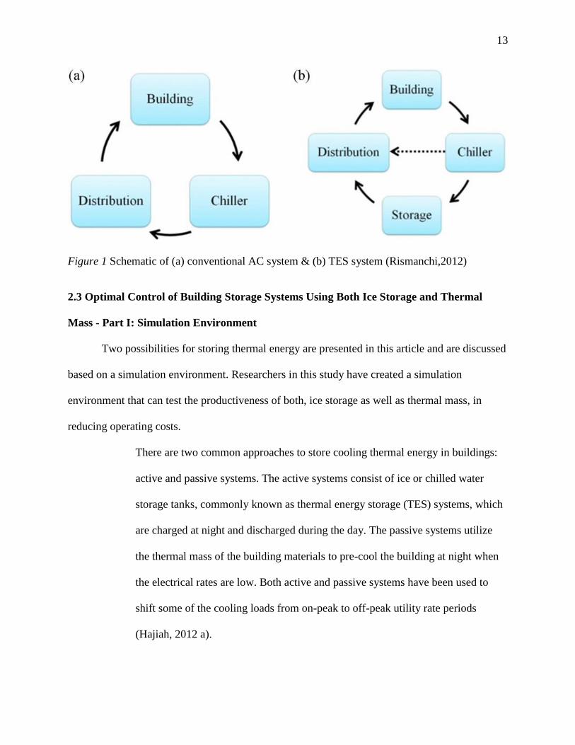
AC system and a system designed with thermal energy storage can been seen below in Figure 1.
This system implemented into building applications can result in big savings of energy costs.
The statistical data show that office buildings consume around 21% of the total electricity
consumption of the country (Rismanchi, 2012). These types of alarming facts combined with the
potential shown to be evident in thermal storage technologies provide a great deal of potential in
advancing the systems discussed and improving upon energy costs concerns. All in all, this
article was presented to examine the economic and environmental benefits of using ice thermal
storage systems in commercial buildings.
13
Figure 1 Schematic of (a) conventional AC system & (b) TES system (Rismanchi,2012)
2.3 Optimal Control of Building Storage Systems Using Both Ice Storage and Thermal
Mass - Part I: Simulation Environment
Two possibilities for storing thermal energy are presented in this article and are discussed
based on a simulation environment. Researchers in this study have created a simulation
environment that can test the productiveness of both, ice storage as well as thermal mass, in
reducing operating costs.
There are two common approaches to store cooling thermal energy in buildings:
active and passive systems. The active systems consist of ice or chilled water
storage tanks, commonly known as thermal energy storage (TES) systems, which
are charged at night and discharged during the day. The passive systems utilize
the thermal mass of the building materials to pre-cool the building at night when
the electrical rates are low. Both active and passive systems have been used to
shift some of the cooling loads from on-peak to off-peak utility rate periods
(Hajiah, 2012 a).
14
The research experiment for this article sets up an environment where both the aggressive and
passive system is tested. In this experiment there is an environment simulation that assesses
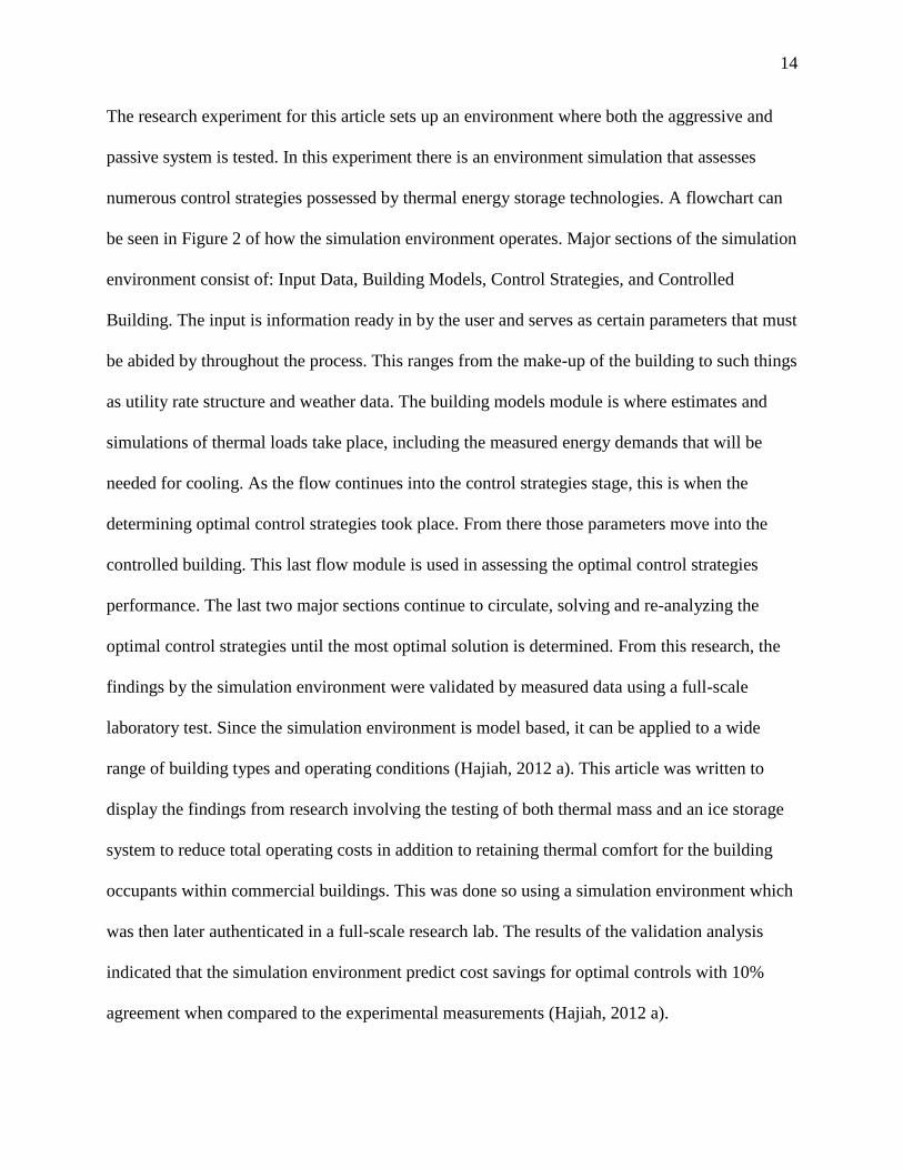
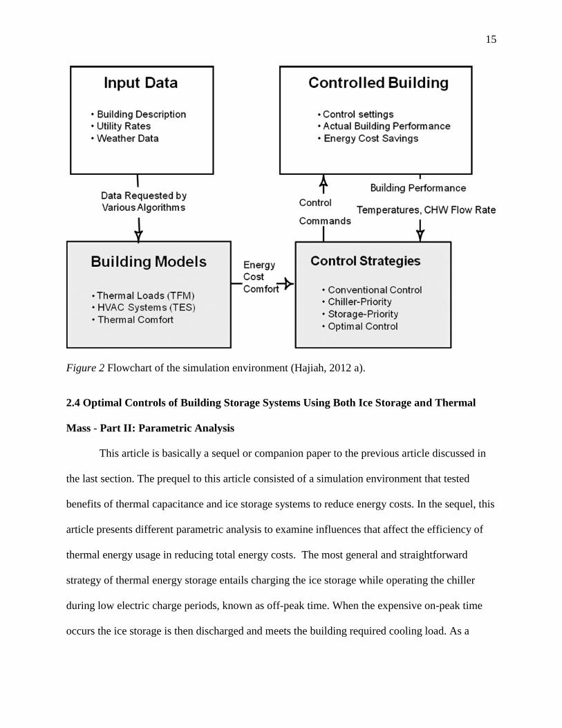
numerous control strategies possessed by thermal energy storage technologies. A flowchart can
be seen in Figure 2 of how the simulation environment operates. Major sections of the simulation
environment consist of: Input Data, Building Models, Control Strategies, and Controlled
Building. The input is information ready in by the user and serves as certain parameters that must
be abided by throughout the process. This ranges from the make-up of the building to such things
as utility rate structure and weather data. The building models module is where estimates and
simulations of thermal loads take place, including the measured energy demands that will be
needed for cooling. As the flow continues into the control strategies stage, this is when the
determining optimal control strategies took place. From there those parameters move into the
controlled building. This last flow module is used in assessing the optimal control strategies
performance. The last two major sections continue to circulate, solving and re-analyzing the
optimal control strategies until the most optimal solution is determined. From this research, the
findings by the simulation environment were validated by measured data using a full-scale
laboratory test. Since the simulation environment is model based, it can be applied to a wide
range of building types and operating conditions (Hajiah, 2012 a). This article was written to
display the findings from research involving the testing of both thermal mass and an ice storage
system to reduce total operating costs in addition to retaining thermal comfort for the building
occupants within commercial buildings. This was done so using a simulation environment which
was then later authenticated in a full-scale research lab. The results of the validation analysis
indicated that the simulation environment predict cost savings for optimal controls with 10%
agreement when compared to the experimental measurements (Hajiah, 2012 a).
15
Figure 2 Flowchart of the simulation environment (Hajiah, 2012 a).
2.4 Optimal Controls of Building Storage Systems Using Both Ice Storage and Thermal
Mass - Part II: Parametric Analysis
This article is basically a sequel or companion paper to the previous article discussed in
the last section. The prequel to this article consisted of a simulation environment that tested
benefits of thermal capacitance and ice storage systems to reduce energy costs. In the sequel, this
article presents different parametric analysis to examine influences that affect the efficiency of
thermal energy usage in reducing total energy costs. The most general and straightforward
strategy of thermal energy storage entails charging the ice storage while operating the chiller
during low electric charge periods, known as off-peak time. When the expensive on-peak time
occurs the ice storage is then discharged and meets the building required cooling load. As a
16
result, it is possible to reduce or even eliminate the chiller operation during on-peak hours
(Hajiah, 2012 b). The parametric study that took place in this article paper was based upon the
simulation environment from the preceding paper. The analysis by this research included
multiple parameters such as; the optimization cost function, base chiller size, and ice storage tank
capacity, as well as weather conditions. The focus here will be on the simulation model analysis;
including parameters like the building model, utility rate structure, and optimization cost
function. The building for the study was a simple rectangular office building consisting of five
zones, nine foot wall heights, operational times from 8:00am to 5:00pm, and typical standard
lighting fixtures, appliances, and miscellaneous equipment. The research’s utility rate structure
had an on-peak time set from 10:00am to 10:00pm, and an on-peak energy charge of
$0.0208/kWh, with a $7.50/kW for demand charges. The off-peak charges were set at zero, and
this consisted of anytime that wasn’t considered to on-peak time. For the optimization cost
function, the simulation environment was used from the prior article in setting up the parametric
analyses. The optimization strategies are evaluated against the following base controls:
1. Conventional control of cooling system using a fixed temperature set point of
76 degrees Fahrenheit from 8:00 am to 5:00 pm. This base case is selected to
investigate the effectiveness of using building thermal mass.
2. Chiller-priority control when an ice storage system is utilized (Hajiah, 2012 b).
There were a number of parametric analyses that were done using the office building model in
determining the efficiency of thermal mass and ice storage under various conditions. The
research from this study took place as if the building was located in Chicago, Illinois, meaning
that the climate and weather data from this city was taken into account during testing. In end, the
second version of this two-part series of articles has examined many of the important factors that

17
affect the performance of the optimal controls using thermal mass and ice storage to reduce the
cooling system’s total operating costs. The optimization results discussed in this paper for a
typical office building model under different weather conditions and various design options
indicate that significant cost savings (up to 40%) can be achieved in the cooling system total
operating cost. Generally, the results indicate that optimal control for both building thermal mass
pre-cooling and ice storage operation outperforms all of other conventional controls and
sequential optimal controls under all climate conditions, utility rate structures, and system
designs (Hajiah, 2012 b).
2.5 Cumulative Energy Analysis of Ice Thermal Storage Air Conditioning System
This article is out of the Applied Energy journal and focuses on the cumulative energy
analysis method. The research analyzes the effects of implementing an ice thermal storage air
conditioning system into a building power supply. The work completed in this article is a product
of researchers out of China. Along with the fast-paced development of modern construction in
China, the energy consumption of air conditioning increases rapidly and is fast approaching the
international level. As the environmental temperature changes, the cooling load and the
electricity consumption change correspondingly (Pu, 2012). This meant that as the outside
temperatures rose, so did the building’s required cooling load, as well as the energy
consumption. In opposition to most studies, the research found in this article examines the effects
of ice thermal storage based upon resource utilization. This is known as using the approach of
cumulative energy analysis. It is defined so that the cumulative energy consumption of a product
is the total energy of all the consumed natural resources (Pu, 2012). Studies have shown that
cumulative energy analysis is a valuable analysis method based on the concept of resource
consumption. However, there is no study that can take claim for investigation of ice thermal

18
storage air conditioning systems from a standpoint of cumulative energy consumption. This
article provides models for the cumulative energy analysis for ice thermal air conditioning
systems with all stages consuming any energy provided by the peak regulating unit considered.
Results are provided and validated by two case studies. It was found to be a linear relationship
between the average cumulative energy variation and both the operating load of the power unit
as well as the load of ice thermal storage. It shows that the cumulative energy variation decreases
as either of the other two increases.
2.6 Performance of Ice Storage System Utilizing a Combined Partial and Full Storage
Strategy
This journal article is research from three individuals out of a University in Iraq that
looks for vital information in expanding the current knowledge of ice thermal storage technology
and its efficiency depending upon the type of storage strategy. This is the first work that is
discussed where more than one charge strategy is addressed or compared and contrasted. In this
research ice storage strategies that are discussed include: a combined system, a partial storage
system, and a full load storage system. Thermal storage is the temporary storage of high or low
temperature energy for later use (Al-Qalamchi, 2007). With the different storage strategies,
experiments were done to decide the potential savings in chiller size in comparison to that of a
more conventional cooling system. The main outcome of this research was to optimize the chiller
size for the combined ice charge strategy, known for utilizing both the partial and full storage
systems. Results turned out that the combined ice strategy system needed a much larger
equipment size in order to meet the cooling load. Combined strategy required chiller size was
found to decrease with decrease in on-peak period, hence the optimum chiller size for this new
strategy was found to occur at zero on-peak hours, and i.e., when the combined system starts to
19
operate as a partial strategy system (Al-Qalamchi, 2007). The key conclusions drawn from the
research of this article are vital in understanding the different ice charge strategies, including
which ones to move forward with in researching deeper. Some other key takeaways included:
1) Combined strategy system requires less chiller size than conventional system
does. A reduction of about 28% may be achieved.
2) Partial chiller strategy requires less chiller size than combined system.
3) Combined strategy chiller size was found to decrease with decrease in on-peak
period (Al-Qalamchi, 2007).
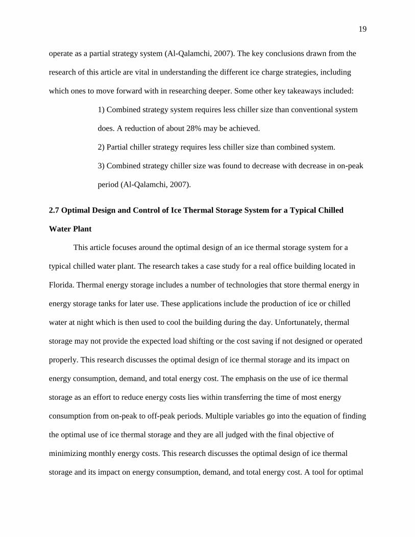
2.7 Optimal Design and Control of Ice Thermal Storage System for a Typical Chilled
Water Plant
This article focuses around the optimal design of an ice thermal storage system for a
typical chilled water plant. The research takes a case study for a real office building located in
Florida. Thermal energy storage includes a number of technologies that store thermal energy in
energy storage tanks for later use. These applications include the production of ice or chilled
water at night which is then used to cool the building during the day. Unfortunately, thermal
storage may not provide the expected load shifting or the cost saving if not designed or operated
properly. This research discusses the optimal design of ice thermal storage and its impact on
energy consumption, demand, and total energy cost. The emphasis on the use of ice thermal
storage as an effort to reduce energy costs lies within transferring the time of most energy
consumption from on-peak to off-peak periods. Multiple variables go into the equation of finding
the optimal use of ice thermal storage and they are all judged with the final objective of
minimizing monthly energy costs. This research discusses the optimal design of ice thermal
storage and its impact on energy consumption, demand, and total energy cost. A tool for optimal
20
design of ice storage is developed, considering variables such as chiller and ice storage sizes
along with ice charge and discharge times. Detailed simulation studies using a real office
building located near Orlando, FL including the utility rate structure are presented. The study
considers the effect of the ice thermal storage on the chiller performance and the associated
energy cost and demonstrates the cost saving achieved from optimal ice storage design. A whole
building energy simulation model is used to generate the hourly cooling load for both the design
day and the entire year. Other collected variables such as condenser entering water temperature,
chilled water leaving temperature, outdoor air dry bulb and wet bulb temperatures are used as
inputs to a chiller model based on DOE-2 chiller model to determine the associated cooling
energy use (Nassif, 2014 b). The results show a significant energy costs savings can be attained
when optimized ice storage design is utilized by the tool proposed in this article.
The results demonstrated that although the energy consumption increases by using
ice thermal storage, the energy cost drops significantly, mainly depending on the
local utility rate structure. It showed a significant cost energy saving can be
obtained by optimal ice storage design through using the tool that proposed in this
paper. The saving could be up to 28% comparing to non-optimal design of ITS.
The results also indicated that that the annual energy consumption increased by
11% and the energy cost dropped by 50% compared to the case when no ITS is
installed (Nassif, 2014 b).
The overall findings in this article displayed and emphasized the potential ice thermal storage
technology holds in efforts of reducing energy costs when properly optimized.

21
2.8 Genetic Algorithms: An Overview
This article is about and was included due to its role on the insight provided on genetic
algorithms. John Holland developed genetic algorithms in order to understand phenomenon of
evolution in nature. From there this phenomenon was applied to computer systems. The central
idea behind the development of genetic algorithms lied within the feature of evolution in
problems that needed deep search in discovering an answer. The general process on how to solve
a problem saw a change once the idea was discovered that different outcomes of a problem could
be solved by the evolution of a solution. The advancement of this theory involved one solution
branching off into numerous solutions in a continuing process and this created a way to solve
many types of complex problems. As computer systems used for genetic algorithms began to
evolve a viable question on exactly how they work did also. Genetic algorithms in a computer
system were described as complex search programs that worked by setting an objective function,
followed by the sorting of parameters needed to achieve and make the objective function work.
From here, many outcomes are formed from the parameters and the system finds solutions
through constant generations and iterations of the program until the most optimal solution is
found. The aggressive and dynamic style of seeking the optimal result to the problem allows
genetic algorithms to be categorized as a very effective as well as efficient optimization tool. All
in all, this article was useful in the understanding of genetic algorithms as it pertains to the use of
the genetic algorithm optimization tool that will be used in the discussions and work of this
thesis.

22
CHAPTER 3
Simulations and Exploratory Research
3.1 Overview
The use of the energy simulation model and MatLab are the key components utilized in
order to test ice thermal storage technology in this research. For the energy simulation model, it
was decided to use the software called eQuest. EQuest is a building energy simulation software
tool and MatLab is a unique programming language with a genetic algorithm feature that allows
the program to solve for optimization. The building that the simulations are run for is an office
research building with four floors. The tests are run for locations all across the United States and
consist of a wide range of ASHRAE climate zones. This includes climate zones from both ends
of the spectrum, zones with hot, dry weather as well as occasionally cold, wet weather regions,
and any possibilities in between. A total of ten different locations are represented in the study.
3.2 Recommended Process
Below in Figure 3 is the developed algorithm for the process in the design of the
variables needed in optimizing the implementation of ice thermal storage technology for
commercial buildings. In this order of processes the program is given inputs and the program
continues to run until the most optimal results have been attained. The procedure begins by
retrieving the hourly cooling loads from the simulation program, for this study eQuest was used.
From there, the utility cost rate structure is set and the outdoor air conditions are simulated and
uploaded into MatLab. As the next steps takes place the program runs and begins its search for
optimal design of the output variables and continues to run again and again to the best results are
produced. During this period cost calculations for both ITS and no ITS cases are found for
various factors including annual energy costs, & annual energy consumption just to name a few.

23
Figure 3 The developed and recommended optimization tool in the design of the ITS system.
3.3 Programs and Models
3.3.1 Simulation model. The simulation model developed in this study used the skillset
offered by the eQuest energy simulation software to simulate the cooling loads throughout the
ten test locations selected. The responsibility of eQuest as it pertains to this research is to gather
and obtain vital information for use in the MatLab programs. This is done via the internet and
simulations. The weather data for the location is downloaded into eQuest and once that is
complete, the software simulates the cooling loads for the entire design year. From the energy
simulations for the building for the year, eQuest provides hourly results for the entire simulated
year. These hourly results for the year include: the required cooling load, the outside wet bulb
temperature, and the outside dry bulb temperature. From this, MatLab is able to upload these
results about the location and the location’s weather effects on the cooling of the building and
display the results for the monthly energy cost as well as the monthly energy consumption for the
building with the implementation of ice thermal storage.
3.3.2 MatLab models. The MatLab program coding developed specifically for this
research consists of three separate programs and ranges depending upon the desired outcome and

24
results. There is a MatLab program written specifically for the chiller. The chiller model is the
code directly related to and used for the chiller design. The program has information for the
chiller, about its rating capacity, chiller power, chiller efficiency, and various temperatures of
water that is in flow throughout the chiller. Information from the chiller model is read into the
other main program models when data about the chiller is requested. The other two MatLab
programs are the two main program models. The biggest differences in the two main program
models is first how the input variables are obtained, and second the process in which the results
are established. One main program model reads the input variables assigned and provides output
results; while the other main program model is given a range for the input variables and the
genetic algorithm allows the program to find the optimum output results in the range of input
variables. The code will be explained in more depth and detail moving forward.
3.4 EQuest Process
EQuest provides a number of tools for building simulations. It allows the ability to test
‘what if’ scenarios and attain useful information before making any hasty decisions without any
type of data to backup theories. To start eQuest, a building creation wizard assists in uploading
the building into the program. From there many unique features in the program provide feedback
on the building performance and how altering any technology or other aspect of the building can
affect the building performance wise and its associated energy needs.
3.4.1 Building creation wizard. The building creation wizard for eQuest can be utilized
in two approaches. When starting a project in eQuest there is the option of starting the building
creation wizard through the schematic design wizard or either the design development wizard.
Both building wizards are useful and helpful but depending on the stage and how much
information on the building one has would determine which wizard would be most suitable. The
25
schematic design wizard is most beneficial in the early design phases and when information on
the building is limited. This is usually a wizard used for small, simple structures for an
assignment pertaining to the building’s internal load and/or HVAC equipment. The more
advanced and detailed wizard would be the design development wizard. This wizard provides a
more detailed design and requires more information on the building. In this setting one would
input larger and very complicated assemblies, resulting in a cutting-edge HVAC system and
more detailed internal loads.
3.4.2 Uploading the building via the wizard. The process of uploading the building into
eQuest through the building creation wizard is an easy and simple yet extensive task. The wizard
requests various, specific information about the building and it is very important as it all can
affect and make a difference on the outcome of the simulation results. In the eQuest schematic
design wizard there consists of forty one different screens of input concerning the building
information. Figure 4 shows one screen and some of the general input information requested
about the building as it is in the process of being uploaded into eQuest by the schematic design
wizard. This figure displays the first prompt screen of the schematic design wizard in eQuest.
The very first input screen in the wizard is where general information is provided regarding the
building. Here information like: building type, location, utility and electric rates, area and floors,
and basic heating and cooling measures is provided. It is here that the location is specified and
later the location’s weather data uploads. The type of data that the wizard request is wide ranging
and works its way through all aspects of the building. Some of the categories about the building
information that the wizard screens require include: general information, building footprint,
building envelope, building interior, doors, windows, room information, lighting loads, building
operational time, electrical and HVAC information, and many others. The biggest and possibly

26
one the most important parts in this process is the HVAC equipment. Multiple screens are
devoted to this as it gets very thorough and many of the simulations are for cooling and
discovering loads for HVAC equipment. A unique aspect about this schematic design wizard is
the ability to skip and leave some things unchanged. Not all fields throughout screens have to be
altered and default choices can be left filled in. Also according to some prior answers some
screens are automatically skipped and passed by.
Figure 4 One screen of building input information for the eQuest schematic design wizard.
3.4.3 EQuest features and functions. After the building and all of its information is
uploaded into eQuest, the system runs through a process where all files are loaded and each
component input throughout the wizard is accounted for and administered into the eQuest file.
From here the building is available in eQuest and there are some features and functions that are
accessible to users. A digital model of the building is now obtainable because of the building
footprint that was input during the wizard process. The building footprint consisted of real
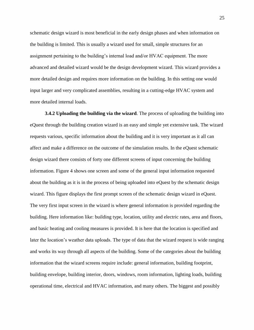
27
working floor plan drawings which, once uploaded, made the digital model of the building
possible in eQuest. The digital model includes a 2-D geometry view as well as a 3-D geometry
that is of a perspective angle. Below Figure 5 provides a look at the test building in this study
uploaded into eQuest and displayed in a two-dimensional view.
Figure 5 A two-dimensional digital view of the test building uploaded into eQuest.
Some other tools in eQuest come from the energy efficiency measure wizard, the ability
to perform compliance analyses, and simulating the building performance. One very interesting
energy savings measure that the eQuest software provides is in the program’s energy efficiency
measures wizard. Here, aspects of the building anywhere from the building envelope, internal
loads, HVAC system, all the way to the site and building can be altered and tested up against the
original baseline design uploaded initially during the wizard phase. This wizard is unique in its
ability to allow for multiple tests run at once. In the end each test can be compared and judged
for possible energy savings. Finally simulating the performance of the building is done to
provide a very detailed report of the building’s operational efficiency from an energy standpoint
28
with many different documents, tables, and graphs of numerous reports. The simulation of the
building performance tool is the key feature for this research. EQuest was used to perform this
simulation task and following this task, the proposed MatLab program was developed in order to
determine the ITS optimal design.
3.4.4 Simulating building performance. This is the final process in eQuest before the
results are displayed and ultimately exported for use into MatLab. The simulation of the building
performance offers a key to unlock an infinite amount of information on the building. Some
items found include the reports for comparison-runs, single-runs, and parametric-runs. Inside of
these there are the graphs and tables for monthly total energy consumption, annual and monthly
utility bills, and even life-cycle summaries and graphs. The key takeaway and result of
simulating the building performance as it is associated with this research lies in the hourly results
for the calendar year. Provided are results for the cooling load, and dry and wet bulb outdoor
temperatures for that particular location. Results are for every hour of the day and every day of
the entire year, which is approximately 8,760 readings for each result type, making the study
very precise and accurate. These hourly results are read into excel for viewing and from there
imported into MatLab.
3.5 Developed MatLab Program Code
The MatLab program is the last piece to the ice thermal storage technology’s
optimization experiment. EQuest serves as the chosen method for the simulation model and to
seek out vital background information and access weather and building loads for test locations.
The MatLab program uses all of this information to optimize the ultimate capacity of efficiency
that ice thermal storage technology can achieve. The rest of this section will explain in detail the

29
design of the MatLab contribution to this experiment. Finally the code in MatLab will be
displayed and dissected by major sections.
3.5.1 Input variables. The code for MatLab is what serves in finding the savings results
for ice thermal storage technology. In starting this process, it is essential that the program is
given some input information. Some of this information is read from the previously explained
eQuest program, while others are still required and read directly in to the program from the user.
Below Figure 6 is a display of the input portion of the code in MatLab.
Figure 6 Code from the MatLab program that references the input variables.
Here the figure shows the first few lines of code of the program that consists of the
program’s input variables. There are four variables that are input by the user: ice capacity factor,
ice charge time, ice discharge time, and chiller size factor. The ice capacity factor serves as a
variable for the input time or amount of hours that the ice thermal storage system will need to
charge for full capacity. The variable for ice charge time is very simple. The declaring and input
of this variable sets the time in which charging of the ice thermal storage system will commence.
Ice discharge time for the system is the variable that tells the system to stop and ultimately shuts
the chiller off altogether. When the discharge time period begins cooling of the building is done
by the ITS system and the chiller remains inactive for as long as the ITS system has an adequate
amount of ice to handle the load of cooling in the building. Finally, the chiller size factor
variable is input to set how much the chiller will be oversized. Oversizing of the chiller is a
30
safety measure and is done so in order to ensure the chiller would be operable in a worst possible
case than originally designed for. These variables are the key components that effect the desired
outcome results, energy cost and energy consumption.
3.5.2 Utility rate structure. This section of code is primarily related to the outcome and
calculating of cost. Figure 7 illustrates the segment of code related directly to the utility rate
structure. This includes declaring the official peak time period, the cost for energy consumption
during on-peak time periods, off-peak time periods, and the peak cost. The utility rate structure is
a component of the code that is unchanging for this research. For this study a basic, standard
utility rate structure was kept constant for all test locations in order to compare ITS results and
cost savings strictly due to location and weather. In future cases this portion of code would
change and be read in by the user. The utility rate structure is generated and charged by a
location’s power company. This variable is one that would change from location to location and
affect cost savings depending upon local utility rates.
Figure 7 This piece of code shows the introduction of the utility rate structure into the program.
3.5.3 Location weather data. Figure 8 below demonstrates the following lines of code
pertaining to the import of weather data and cooling loads. This part of the program imports the
weather data and cooling loads from the eQuest program. Variables are then established to set for
the required cooling loads and dry and wet bulb temperatures. The data that is imported from
eQuest consist of the 8,760 readings from the hourly simulation for the year. This was previously

31
explained throughout the Simulating Building Performance subsection of the EQuest Process in
chapter 3 section 4.
Figure 8 The lines of code displaying the import of the weather data & cooling loads from
eQuest into MatLab.
3.5.4 Chiller and ice thermal storage tank capacities. The design information is a
small section of code in the ITS MatLab program but carries a big title as it is important that both
the chiller and ITS tanks are designed and sized appropriately. Figure 9 displays these two very
important lines of code. In optimizing the ice thermal storage units, under sizing these two
components would cost more in the long run, while oversizing the two would cost a lot of money
initially and be a huge waste. Here in just two lines of code the chiller and size of the ITS tanks
are designed based upon the maximum cooling load reported from eQuest. The highest required
cooling load given from eQuest is multiplied by the user input chiller size factor to give the
chiller size in tons. Once the chiller is sized, it is taken and multiplied by the input ice capacity
factor to determine the maximum capacity of the ice storage tanks sized in ton-hours. If designed
correctly the chiller would be sized perfectly to cover the entire cooling load reported from
eQuest and any possible worst case scenario. The sizing of the ice thermal storage tanks would
be considered to be designed correctly if the cooling during the on-peak time periods are
accounted for entirely and it is never necessary that the chiller be turned on during any on-peak
time period, thereby incurring no peak costs for on-peak time.

32
Figure 9 This code from MatLab is needed for the design of the chiller and ITS tank sizes.
3.5.5 Operation of the chiller and ITS systems. This last part of code from the program
is the biggest and most complex. The most important part of the code is shown in Figure 10. The
rest of the code in MatLab is written for energy use calculations and different periods of the year
and processes of the chiller, as well as ice charging periods, discharging periods, and normal
operation of the cooling system including the chiller. During these different stages the program is
running iterations for the 8,760 hourly cooling loads, and temperatures introduced from eQuest.
For the different time periods, the code is running and telling the variables what to do and what
data to store as it runs through the entire year, day by day. Finally at the end of the code there are
outputs for the results and also figures to display necessary graphs portraying the results. Outputs
for the data show the input ice capacity factor, the ice charge time, the summation of the monthly
cost, and the summation of the monthly energy consumption. The first two outputs are simply
designed to reiterate the input and are compared to how it affected the last two outputs, energy
cost and consumption. Energy cost and consumption are the most important and cost being the
bigger importance of the two.

33
Figure 10 The last part of code begins the process of optimizing the system & energy
calculations.
3.5.6 Genetic algorithm optimization model. The genetic algorithm optimization model
is the other MatLab program main model that is used in finding the optimum results for the ITS
technology. Figure 11 shows an optimization process being run for the office building being
tested in the Greensboro, North Carolina location. This program reads in its input variables in a
different method than previously explained for the main model code. Also the output for this
model is found in a slightly different process because the program is not simply reading the
inputs and presenting the corresponding outputs.
Here in this program the genetic algorithm is given a range of possibilities and from there
the optimization tool finds the most efficient outputs that would fit and work comfortably with
the known constraints. This model is the best of the two models to get a very close and accurate
result of optimization, while the other model displays more data and gives more to work with
and a way to test individual inputs. It is a good idea to use both models in combination and gain
optimal results.
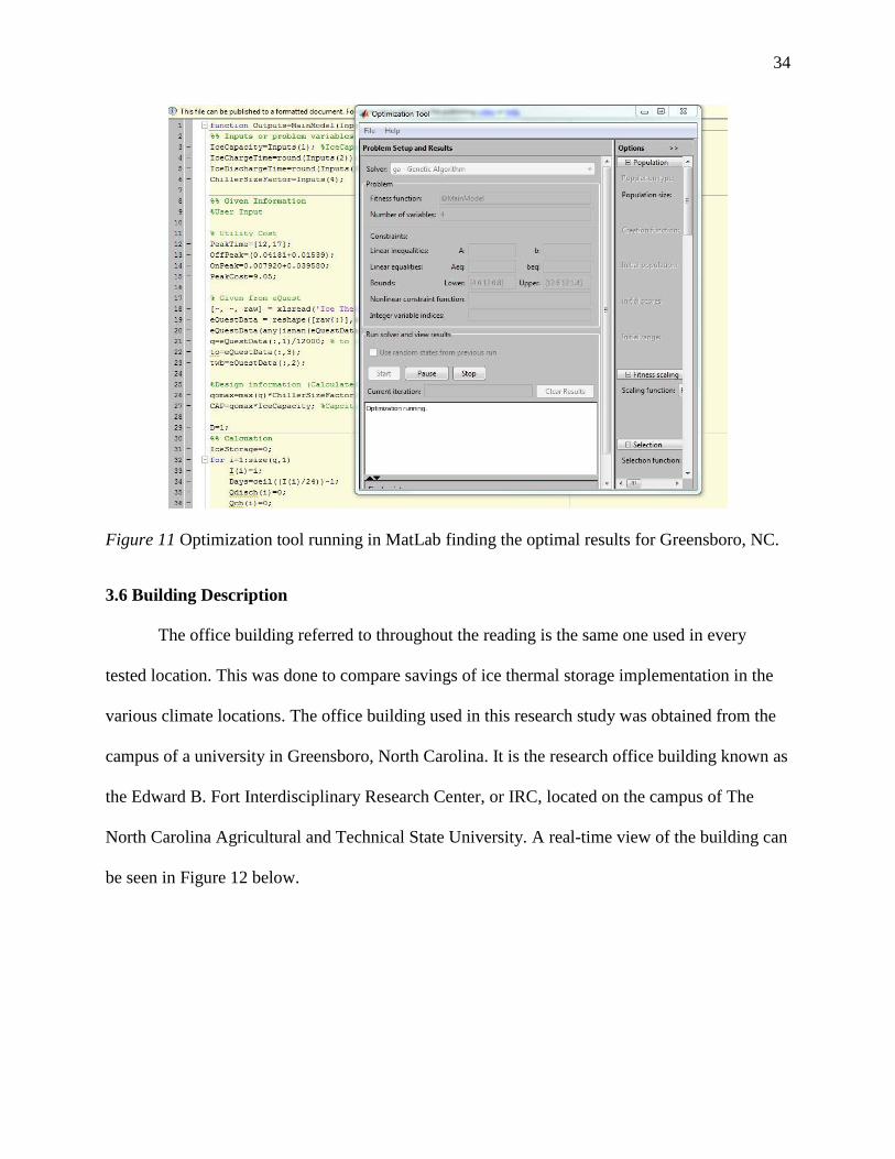
34
Figure 11 Optimization tool running in MatLab finding the optimal results for Greensboro, NC.
3.6 Building Description
The office building referred to throughout the reading is the same one used in every
tested location. This was done to compare savings of ice thermal storage implementation in the
various climate locations. The office building used in this research study was obtained from the
campus of a university in Greensboro, North Carolina. It is the research office building known as
the Edward B. Fort Interdisciplinary Research Center, or IRC, located on the campus of The
North Carolina Agricultural and Technical State University. A real-time view of the building can
be seen in Figure 12 below.
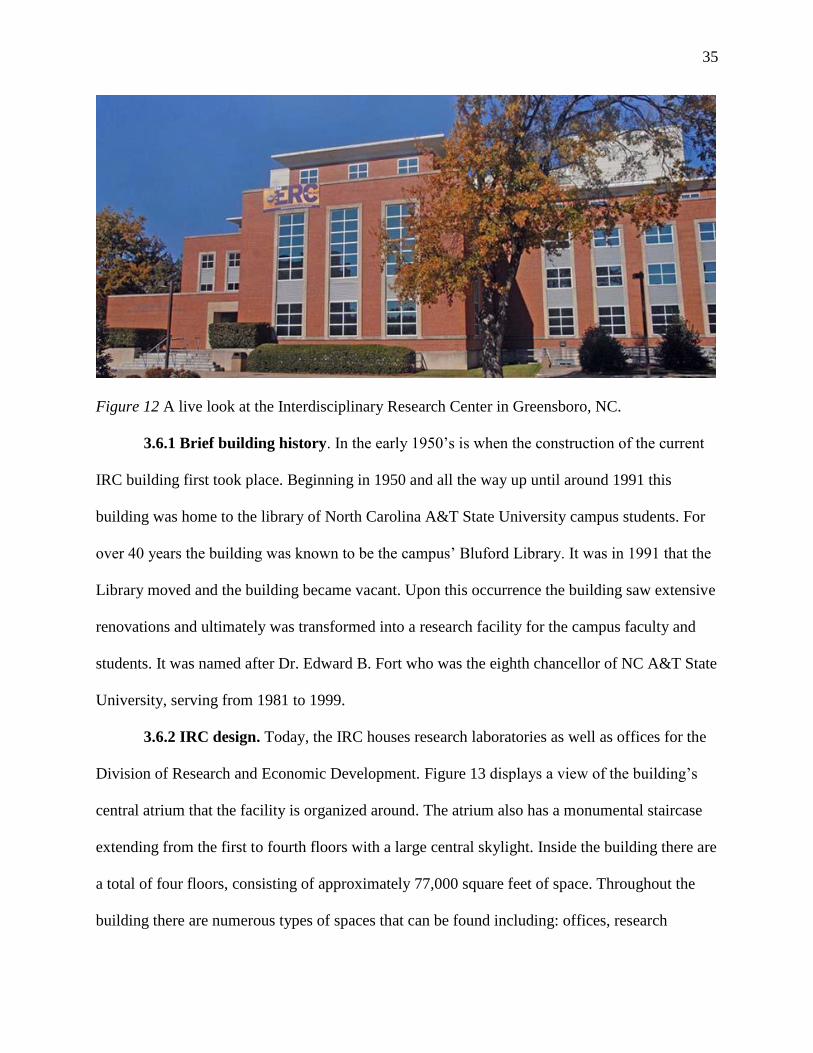
35
Figure 12 A live look at the Interdisciplinary Research Center in Greensboro, NC.
3.6.1 Brief building history. In the early 1950’s is when the construction of the current
IRC building first took place. Beginning in 1950 and all the way up until around 1991 this
building was home to the library of North Carolina A&T State University campus students. For
over 40 years the building was known to be the campus’ Bluford Library. It was in 1991 that the
Library moved and the building became vacant. Upon this occurrence the building saw extensive
renovations and ultimately was transformed into a research facility for the campus faculty and
students. It was named after Dr. Edward B. Fort who was the eighth chancellor of NC A&T State
University, serving from 1981 to 1999.
3.6.2 IRC design. Today, the IRC houses research laboratories as well as offices for the
Division of Research and Economic Development. Figure 13 displays a view of the building’s
central atrium that the facility is organized around. The atrium also has a monumental staircase
extending from the first to fourth floors with a large central skylight. Inside the building there are
a total of four floors, consisting of approximately 77,000 square feet of space. Throughout the
building there are numerous types of spaces that can be found including: offices, research

36
laboratories, storage space, some conference and meeting rooms, and of course bathrooms. The
biggest reason this building is ideal for the simulations lies within the building’s age. Although it
has been renovated, originally built in the 1950’s, its old structure lines up perfectly with typical
commercial buildings that generally need improvements.
Figure 13 An interior view of the IRC and the central atrium leading up to the large skylight.
3.7 Methodology
3.7.1 Preceding research. The idea behind this investigation into ice thermal storage was
to test its efficiency and effectiveness in numerous climates and environments. The original
study was one where the opportunity was present to work on and it took place for an office
building located and tested near Orlando, Florida. That study provided detailed simulations for
the particular office building in Florida. The study considered the effect of the ice thermal
storage technology on the building’s chiller performance and any associated energy cost. The
results of that initial study demonstrated the cost saving achieved from optimal ice thermal
storage design. With the success of that prior research I was able to help gather and the intrigue
to find an answer to just how effective and beneficial ice thermal storage technology can become

37
in the enhancement of current and future buildings in energy cost savings, this study developed
and I was able to take it on as my thesis and carry it out for further discovery. From here, the
research blossomed into a study of the technology in at least one of every ASHRAE climate zone
location.
3.7.2 ASHRAE climate zones. Local weather as well as a region’s climate makes a
substantial difference in the separation and sorting of the map into what are recognized by
ASHRAE as climate zones. A graphic of the United States shaded and separated into ASHRAE’s
recognized climate zones can be seen in Figure 14. Building codes require a structure to meet
certain R-values to achieve a specific level of efficiency. The climate zone plays a big role in
determining what the minimum R-value has to be for a specific region. Additionally, each state
or local code body may be at differing levels of adoption of energy codes.
The climate zones are made up of the typical weather patterns observed over time in the
perspective regions. Based upon ASHRAE 90.1 there are eight recognized climate zones and
three possible subtypes throughout the zones. The ASHRAE map of the climate zones shows the
breakdown of each zone and the subtypes. The three subtypes are labeled at the top of the map
and specify whether that region in the zone is either moist, dry, or marine. Zone 1 is a very hot,
dry, and humid region. This zone can be found the furthest south in Florida and also includes:
Hawaii, Guam, Puerto Rico, and the Virgin Islands. In zone 2 the region is known to be hot,
humid, and on some occasions dry. Zone 3 is typically warm, dry, and depending on the location
either humid or marine. Zone 4 is characterized as mixed and has locations that are humid, dry,
and marine. Moving further north, in zone 5 the climate is cool with differences of being humid,
dry, and marine. Zone 6 is known for being cold and both humid and dry. Zone 7 is the zone that

38
is very cold and visibly furthest north on the map. The last zone is zone 8, which is not visible on
the map. Zone 8 is the subarctic region with locations such as Alaska.
Figure 14 A map and graphic of ASHRAE 90.1 Climate Zones.
3.7.3 Location selection. In determining the test locations for this research it was decided
that every climate zone would be represented. Finally a total of ten test locations were decided
upon. Throughout the climate zones major cities were chosen at random, while in widespread
regions the selection was made to keep the locations spread out and well balanced. Also each
subtype of climate zones was purposely represented in the study. As a result there were some
zones that were represented more than once in the location selection.
The states represented in the experiment came from Florida, North Carolina,
Pennsylvania, Maine, Texas, Wisconsin, Arizona, California, and Washington. The state of
Florida was actually chosen to be represented twice due to it having a small region labeled as a
zone 1 climate, while its primary designation consist of being marked as zone 2. From zone 1,

39
testing was held in Miami, Florida, in zone 2 this region was represented by Orlando, Florida as
well as Phoenix, Arizona. The primary reason zone 2 was represented twice is because the two
city locations lie within two different subtypes of climate zones. In Orlando, Florida zone 2 is
under subtype A, which is moist. Located in Phoenix, Arizona zone 2 is categorized as climate
zone subtype B, known to be dry. In zone 3 the location was Dallas, Texas and also San Diego,
California. This was also due to differing climate zone subtypes. In Dallas, Texas the climate
subtype is type A, moist, and in San Diego, California its climate zone subtype is type C, or
marine. Zone 4 consisted of Greensboro, North Carolina which has a moist subtype A, as well as
Seattle, Washington, having a marine subtype C. Zone 5 is tested in Philadelphia, Pennsylvania,
zone 6 in Green Bay, Wisconsin, and zone 7 in Portland, Maine. The overall selection across the
map allowed for an even spread and well balanced selection of location points, while staying in
major cities for weather data purposes.

40
CHAPTER 4
Results and Findings
4.1 Overview
The energy cost savings that Ice Thermal Storage technology can provide has been well
documented. This study was developed for the research purposes of comparing and analyzing the
savings and benefits of using Ice Thermal Storage technology in different types of weather and
climate regions throughout the United States. In the process of investigating the use of ice
thermal storage technology in these various climate regions, a program was also developed to
optimize the design of ice thermal storage dependent upon the location and that region’s climate,
the building’s make-up, and the amount of cooling needed. Results for the experimented climate
regions show, for the span of a year, the energy consumption in kWh for the building as well as
the energy cost in dollars. With these output results the most optimal design criteria for ice
thermal storage to run effectively and efficiently is determined. This in turn can lead to energy
cost savings.
4.2 Research Test Results
The results obtained in the research of the locations were done so initially by the user
manually entering input data designed for the ITS technology. After doing so, the MatLab
program was able to read the respective inputs and display the requested output results. This
method was done and repeated numerous times for an infinite number of possibilities for the
input variables. This was carried out for each location and evaluated. It is with these manual
results that observations were made and from there parameters were established in assigning
input variable ranges for the proposed optimization model that was developed. These optimal
results for the test locations will be displayed later in the research. The locations in which the ice

41
thermal storage technology was tested and optimized consisted of seven different climate zones
out of eight possible ASHRAE recognized climate zones. In addition to this, there are three
subtypes that the climate regions are divided up into based upon the regions being moist, dry, or
marine. The following results are reported and separated by the region’s subtype.
4.2.1 Climate region subtype A: Moist. The biggest of the climate region subtypes
consist of climate zones that are moist regions. ASHRAE has recognized over half of the United
States’ climate zones as moist. This region is known for being very moist across the map.
Throughout this region there are seven climate zones represented proving there are very differing
and diversifying climates in this region subtype of the United States. For this reason, there are
seven locations tested in this moist subtype region, one being represented by each ASHRAE
recognized climate zone. Stretching across the entire climate region subtype and accounting for
each zone, these cities include: Miami, Orlando, Dallas, Greensboro, Philadelphia, Green Bay,
and Portland.
4.2.1.1 Miami, Florida. Climate zone 1 is a very hot, dry, and humid region and was
evaluated in Miami, Florida. This type of climate zone is primarily found in the farthest southern
tip of Florida and also recognized in Hawaii, Guam, Puerto Rico, and the Virgin Islands. The
following Table 1 shows a portion of some manual results recorded from ice thermal storage
testing for the IRC building if located in Miami, Florida. The results show the differences and
effects multiple ITS design input variables made on the outcomes of the building’s energy
consumption, as well as its energy cost for the year. For the manual results the key factors that
made a difference on the outcomes were the input ice capacity factor and ice charge time. Ice
discharge time was always a given due to the time the ITS system needed to begin cooling
during the on peak period of the day. Finally, the chiller size factor remained constant during the

42
manual testing, providing a twenty percent safety factor. The complete table with all other
manual results for this location can be found in the appendix.
Table 1
Some manual results for ice thermal storage use in Miami, Florida.
The table shows results starting with an ITS system ice capacity factor of four. Testing
was done for an ice capacity factor that ran from a minimum of four all the way up to a
maximum of twelve. For each ice capacity factor size an individual run was tested for ice charge
times of twenty-three, zero, one, and two. These ice charge times are the times of the day in
which the ice charging period is set to begin; twenty three representing eleven at night, zero is
midnight, and so on. The most consistent of the results proved to be the ITS design with an ice
capacity factor of eight. From here the results were taken and used in the genetic algorithm to
Inputs Inputs Inputs Inputs Outputs Outputs
Ice Capacity Factor Ice Charge Time Ice Discharge Time Chiller Size Factor Cost for Year ($) Energy for Year (kWh)
4 23 12 1.2 22927 301,200
4 0 12 1.2 22133 298650
4 1 12 1.2 22133 298650
4 2 12 1.2 21943 298070
5 23 12 1.2 17257 301700
5 0 12 1.2 17096 29888
5 1 12 1.2 17096 29888
5 2 12 1.2 17611 298330
6 23 12 1.2 17268 301890
6 0 12 1.2 17120 299310
6 1 12 1.2 17120 299310
6 2 12 1.2 17085 298690
7 23 12 1.2 17281 302120
7 0 12 1.2 17134 299550
7 1 12 1.2 17134 299550
7 2 12 1.2 17096 298870
8 23 12 1.2 17296 302380
8 0 12 1.2 17147 299780
8 1 12 1.2 17147 299780
8 2 12 1.2 17111 299140
9 23 12 1.2 17310 302610
9 0 12 1.2 17160 300000
9 1 12 1.2 17160 300000
9 2 12 1.2 17123 299350
43
find the most optimum results where even the chiller size factor was open to being adjusted and
changed along with the ice capacity factor and ice charge time. The most optimal results
presented an energy consumption of 296,030 kWh for the year. With that amount of energy
consumed the energy cost for the year in Miami, Florida just from the cooling after simulation
was a mere $16,933. The optimal results that were gathered using the genetic algorithm
optimization tool will be explained in a later section, following the other test location results.
This process continued for the other nine test locations and everything was completed manually
as a course of trial and error. Moving forward the results for other locations will be stated along
with the differences in the outcome results.
4.2.1.2 Orlando, Florida. Moving forward into climate zone 2, this testing also took
place in the state of Florida. Climate zone 2 was held in Orlando, Florida; located square in the
middle of the state as well as the most central part of this climate zone. This climate zone spans
west as far as Texas in climate subtype A, all the way back east and up to southern parts of
Georgia. There is also a portion of Phoenix, Arizona that is considered to be categorized as
climate zone 2, but falls under climate subtype B. This will be discussed in a later section for the
dry subtype B. The outcome of results for testing in Orlando, Florida showed the differences in
the climate zones effect on a building’s energy usage and cost. Both Orlando and Miami, located
in Florida but falling in different climate zones, have uniquely differing weather and climate to
the extent that cooling during the summer resulted in a substantial reduction in energy cost and
consumption for the building while located in Orlando. Below Table 2 shows a portion of the
manual test results simulated in Orlando, Florida. The complete table with all other manual
results for this location can be found in the appendix. The only input differences in these results
in comparison to the previous tests were the location and the location’s weather data information.

44
It is immediately evident that the results became altered and it was due to the difference in
climate data provided for Orlando.
Table 2
The output readings for climate zone 2 located in Orlando, Florida.
The results in this location still proved a most consistent savings when an input capacity
factor of 8 was assigned. The most optimal results presented an energy consumption of 259,340
kWh for the year. With that amount of energy consumed the energy cost for the year in Orlando,
Florida just from the cooling after simulation was a mere $14,834. In obtaining these optimal
results a range of inputs were set and used within the genetic algorithm to optimize the ice
thermal storage design.
Inputs Inputs Inputs Inputs Outputs Outputs
Ice Capacity Factor Ice Charge Time Ice Discharge Time Chiller Size Factor Cost for Year ($) Energy for Year (kWh)
4 23 12 1.2 17395 264,800
4 0 12 1.2 18239 262280
4 1 12 1.2 18239 262280
4 2 12 1.2 17965 261970
5 23 12 1.2 15168 265170
5 0 12 1.2 15007 262360
5 1 12 1.2 15007 262360
5 2 12 1.2 15329 262210
6 23 12 1.2 15177 265330
6 0 12 1.2 15037 262890
6 1 12 1.2 15037 262890
6 2 12 1.2 15006 262340
7 23 12 1.2 15187 265520
7 0 12 1.2 15043 262990
7 1 12 1.2 15043 262990
7 2 12 1.2 15017 262530
8 23 12 1.2 15199 265720
8 0 12 1.2 15054 263180
8 1 12 1.2 15054 263180
8 2 12 1.2 15026 262700
9 23 12 1.2 15211 265920
9 0 12 1.2 15061 263310
9 1 12 1.2 15061 263310
9 2 12 1.2 15041 262950

45
4.2.1.3 Dallas, Texas. The big state of Texas is home to three climate zones throughout
the region. Texas lies within climate zone 2, the biggest portion being climate zone 3, and a
small portion of north Texas that falls in the category of climate zone 4. The simulated tests for
climate zone 3 occurred in Dallas, Texas. Climate zone 3 runs through southern sections of
North Carolina and extends all the way over to Texas and Oklahoma. Another decent size region
of climate zone 3 takes up a huge portion of California. The part of California that is labeled
under climate zone 3 is categorized as climate subtype C and will be discussed in the future. The
results from simulations in Dallas, Texas for climate zone 3 are shown throughout Table 3,
which can be seen below.
Table 3
ITS results are shown partly for climate zone 3 in Dallas, Texas.
Although the table shows the results for ice capacity factors ranging from eight to twelve,
the initial testing was still done for capacity factors of ice starting at a minimum of four. The
Inputs Inputs Inputs Inputs Outputs Outputs
Ice Capacity Factor Ice Charge Time Ice Discharge Time Chiller Size Factor Cost for Year ($) Energy for Year (kWh)
8 23 12 1.2 12031 210330
8 0 12 1.2 11819 206620
8 1 12 1.2 11819 206620
8 2 12 1.2 11780 205940
9 23 12 1.2 12040 210490
9 0 12 1.2 11828 206790
9 1 12 1.2 11828 206790
9 2 12 1.2 11790 206110
10 23 12 1.2 12049 210660
10 0 12 1.2 11840 206990
10 1 12 1.2 11840 206990
10 2 12 1.2 11802 206320
11 23 12 1.2 12059 210820
11 0 12 1.2 11848 207140
11 1 12 1.2 11848 207140
11 2 12 1.2 11810 206470
12 23 12 1.2 12066 210940
12 0 12 1.2 11856 207280
12 1 12 1.2 11856 207280
12 2 12 1.2 11821 206660
46
results displayed for simulations in Dallas, Texas are from higher ice capacity factor inputs. This
is due to the observations drawn in the trial and error runs. The most consistent results were due
to the higher ice capacity factors. It was indicated the best savings were the result of an ice
capacity factor of 12. The most optimal results presented an energy consumption of 202,680
kWh for the year. With that amount of energy consumed the energy cost for the year in Dallas,
Texas just from the cooling after simulation was a mere $11,593. These optimal results were
obtained using the genetic algorithm optimization tool.
4.2.1.4 Greensboro, North Carolina. The breakdown of North Carolina into climate
zones is nearly half and half. The state of North Carolina is composed of climate zones 3 and 4.
A very small division of North Carolina is considered to be climate zone 5. The section of North
Carolina that makeup climate zone 3 is the south and south eastern parts of the state. The north
and northwestern parts of North Carolina is categorized into climate zone 4, with the exception
of the tiny section that is labeled under climate zone 5. For the testing of climate zone 4 in North
Carolina a city location was chosen that was fitting due to the fact that the building resides there
in reality. The testing for the building in climate zone 4 was actually recorded in Greensboro,
North Carolina. This selection in North Carolina was made primarily for the fact that the
building already resides in Greensboro. Another aspect that went into the location of Greensboro
being chosen as the testing spot in North Carolina for climate zone 4 analysis was due to the
city’s well known unpredictable weather patterns and diverse climate. The findings below can be
seen in Table 4 providing the results for ice thermal storage simulations for the Greensboro,
North Carolina location. Climate zone 4 is a mixed climate zone that often sees many different
weather patterns sometimes being humid, dry, and even marine. This is exactly the case when it
is stated that Greensboro weather is typically unpredictable and very rare in that it is unchanging.
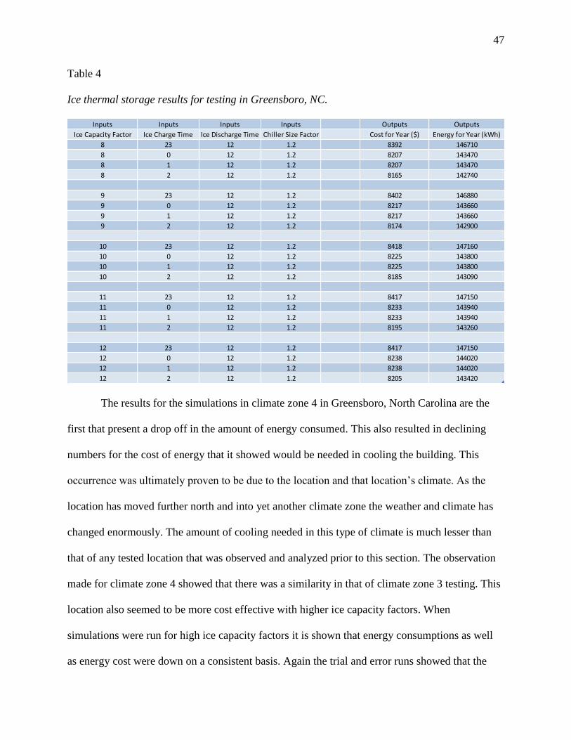
47
Table 4
Ice thermal storage results for testing in Greensboro, NC.
The results for the simulations in climate zone 4 in Greensboro, North Carolina are the
first that present a drop off in the amount of energy consumed. This also resulted in declining
numbers for the cost of energy that it showed would be needed in cooling the building. This
occurrence was ultimately proven to be due to the location and that location’s climate. As the
location has moved further north and into yet another climate zone the weather and climate has
changed enormously. The amount of cooling needed in this type of climate is much lesser than
that of any tested location that was observed and analyzed prior to this section. The observation
made for climate zone 4 showed that there was a similarity in that of climate zone 3 testing. This
location also seemed to be more cost effective with higher ice capacity factors. When
simulations were run for high ice capacity factors it is shown that energy consumptions as well
as energy cost were down on a consistent basis. Again the trial and error runs showed that the
Inputs Inputs Inputs Inputs Outputs Outputs
Ice Capacity Factor Ice Charge Time Ice Discharge Time Chiller Size Factor Cost for Year ($) Energy for Year (kWh)
8 23 12 1.2 8392 146710
8 0 12 1.2 8207 143470
8 1 12 1.2 8207 143470
8 2 12 1.2 8165 142740
9 23 12 1.2 8402 146880
9 0 12 1.2 8217 143660
9 1 12 1.2 8217 143660
9 2 12 1.2 8174 142900
10 23 12 1.2 8418 147160
10 0 12 1.2 8225 143800
10 1 12 1.2 8225 143800
10 2 12 1.2 8185 143090
11 23 12 1.2 8417 147150
11 0 12 1.2 8233 143940
11 1 12 1.2 8233 143940
11 2 12 1.2 8195 143260
12 23 12 1.2 8417 147150
12 0 12 1.2 8238 144020
12 1 12 1.2 8238 144020
12 2 12 1.2 8205 143420

48
optimal results pointed towards an ice capacity factor of 12. The most optimal results presented
an energy consumption of 140,460 kWh for the year. With that amount of energy consumed the
energy cost for the year in Greensboro, North Carolina just from the cooling after simulation was
a mere $8,035. These optimal results were obtained using the genetic algorithm optimization
tool.
4.2.1.5 Philadelphia, Pennsylvania. Climate zone 5 seemingly is the biggest of the eight
climate zones recognized by ASHRAE. Climate zone 5 stretches across the entire width of the
United States, west from California all the way to east in Rhode Island and Massachusetts;
gracing the North, Midwest, and the West Coast. Throughout this stretch across the United States
this climate zone 5 touches approximately twenty-four different states. This climate zone being
characterized primarily as a cool climate will show to need a lot less cooling and therefore
savings will prove to be least likely to be obtained than that of a warmer climate. For the
evaluation of climate zone 5 the testing was done in Philadelphia, Pennsylvania. Philadelphia
was a great choice for testing for its known cold, long winters. It was great to test the
effectiveness of this technology in a city in the climate zone that doesn’t always see a
particularly long stretch of heat in summers. Philadelphia sees stretches of heat in the summer
but also has periods where its summer can see cool days and times that cooling isn’t necessarily
needed. Testing in a city like this gives a look into the type of results that will be expected in
even colder climates that were later tested. Table 5 shown below displays the output results
collected for the trial and error readings taken in climate zone 5 located in Philadelphia,
Pennsylvania. The results here are displayed for the midrange of results produced, due to the
more consistent of results lying near the middle of the data. The complete table with all other
manual results for this location can be found in the appendix. It is now becoming more and more

49
evident that as the test locations move further and further north, energy cost and consumption
will continue to decline. This is the cause of the direct relationship between the climate and the
locations’ need for cooling.
Table 5
The partial results for climate zone 5 in Philadelphia, Pennsylvania.
The range of the results displayed provides outcomes for the testing in Philadelphia,
Pennsylvania where ice capacity factors range from seven up to eleven. In this location of
research the consistency lied within the ice capacity factor most closely provided as 9. The most
optimal results presented an energy consumption of 118,450 kWh for the year. With that amount
of energy consumed the energy cost for the year in Philadelphia, Pennsylvania just from the
cooling after simulation was a mere $6,775. These optimal results were obtained using the
genetic algorithm optimization tool.
Inputs Inputs Inputs Inputs Outputs Outputs
Ice Capacity Factor Ice Charge Time Ice Discharge Time Chiller Size Factor Cost for Year ($) Energy for Year (kWh)
7 23 12 1.2 7012 122580
7 0 12 1.2 6883 120320
7 1 12 1.2 6883 120320
7 2 12 1.2 6853 119810
8 23 12 1.2 7021 122750
8 0 12 1.2 6891 120470
8 1 12 1.2 6891 120470
8 2 12 1.2 6862 119960
9 23 12 1.2 7030 122910
9 0 12 1.2 6901 120650
9 1 12 1.2 6901 120650
9 2 12 1.2 6871 120120
10 23 12 1.2 7040 123070
10 0 12 1.2 6912 120840
10 1 12 1.2 6912 120840
10 2 12 1.2 6880 120280
11 23 12 1.2 7049 123230
11 0 12 1.2 6920 120970
11 1 12 1.2 6920 120970
11 2 12 1.2 6889 120440

50
4.2.1.6 Green Bay, Wisconsin. Typical characteristics of climate zone 6 include being
very cold, and at times even humid and dry. Climate zone 6 is located mostly within the north-
west regions of the United States, while a few areas in the north-east also fall under this climate
zone category. States like Montana, Wyoming, North and South Dakota, Minnesota, Wisconsin,
New York, Vermont, and Maine are states that have climates that makeup climate zone 6. The
test location for this climate zone was taken within the middle of climate zone 6 that stretches
across the United States. Simulations for this zone were taken in the climate for the state of
Wisconsin. Known for its very harsh and cold winters, Green Bay, Wisconsin was a perfect
location to test the ice thermal storage design for a normally colder weather climate. The
following Table 6 shows a portion of some manual results recorded from ice thermal storage
testing for the IRC building if located in Green Bay, Wisconsin.
Table 6
Manual results from ITS testing in Green Bay, Wisconsin.
Inputs Inputs Inputs Inputs Outputs Outputs
Ice Capacity Factor Ice Charge Time Ice Discharge Time Chiller Size Factor Cost for Year ($) Energy for Year (kWh)
8 23 12 1.2 4449 77784
8 0 12 1.2 4329 75677
8 1 12 1.2 4329 75677
8 2 12 1.2 4316 75446
9 23 12 1.2 4456 77899
9 0 12 1.2 4336 75803
9 1 12 1.2 4336 75803
9 2 12 1.2 4307 75299
10 23 12 1.2 4460 77969
10 0 12 1.2 4339 75857
10 1 12 1.2 4339 75857
10 2 12 1.2 4315 75432
11 23 12 1.2 4464 78046
11 0 12 1.2 4348 76006
11 1 12 1.2 4348 76006
11 2 12 1.2 4324 75586
12 23 12 1.2 4455 77889
12 0 12 1.2 4353 76095
12 1 12 1.2 4353 76095
12 2 12 1.2 4332 75740
51
The results here for Green Bay, Wisconsin continues to show the expected drop in cost
and consumption of energy due to the lack of need for cooling. Colder climates require far less
energy for cooling and therefore provide far smaller results. Output results for this climate zone
location show there to be somewhat similar outputs for the different tested ice capacity factors.
The lack of a demand for cooling can be attributed to this unwavering outcome in results even
though inputs are diverse and changing. Still the final outcomes did display a focus where energy
cost and consumption could be optimized. The most consistent and promising of results proved
to be the ice capacity factor designation of 10. The most optimal results presented an energy
consumption of 74,732 kWh for the year. With that amount of energy consumed the energy cost
for the year in Green Bay, Wisconsin just from the cooling after simulation was a mere $4,275.
These optimal results were obtained using the genetic algorithm optimization tool.
4.2.1.7 Portland, Maine. The very tip and most northern part of the United States was
selected for ice thermal storage technology testing to represent ASHRAE’s climate zone 7. The
results for this climate zone were gathered in Portland, Maine. States that are grouped into
climate zone 7 are only partially grouped into this climate zone, including the state of Maine.
Other states that falls under this category include: North Dakota, Minnesota, and Wisconsin. All
4 of these states are represented by climate zone 7, but only a portion of the state, generally the
northern region. Climate zone 7 is the coldest of the represented and tested climate zones, albeit
the most northern tested location. The findings below can be seen in Table 7 which provide the
results for ice thermal storage simulations for the Portland, Maine location. The results here are
displayed for the midrange to the backend of results produced, due to the more consistent of
results lying near the middle of the data. The complete table with all other manual results for this
location can be found in the appendix.

52
Table 7
Ice thermal Storage design output results for Portland, Maine.
These results produced in Portland, Maine are most closely related to the previous
findings presented for Green Bay, Wisconsin. Here the results have remained consistent and
constant for the cold weather climate locations in that cooling lacking has caused limits on
possible energy savings for these colder climate zones. Colder climates see a bigger portion of
their energy consumption in heating costs and ice thermal storage cannot target that to provide
any energy cost savings. In the testing here in Portland, Maine output results still showed a
consistent, even spread throughout the ice capacity factors tested. The most consistent and
promising of results also still proved to be the ice capacity factor designation of 10. The most
optimal results presented an energy consumption of 66,614 kWh for the year. With that amount
of energy consumed the energy cost for the year in Portland, Maine just from the cooling after
Inputs Inputs Inputs Inputs Outputs Outputs
Ice Capacity Factor Ice Charge Time Ice Discharge Time Chiller Size Factor Cost for Year ($) Energy for Year (kWh)
8 23 12 1.2 3960 69233
8 0 12 1.2 3888 67979
8 1 12 1.2 3888 67979
8 2 12 1.2 3860 67476
9 23 12 1.2 3968 69371
9 0 12 1.2 3896 68105
9 1 12 1.2 3896 68105
9 2 12 1.2 3868 67617
10 23 12 1.2 3976 69502
10 0 12 1.2 3901 68204
10 1 12 1.2 3901 68204
10 2 12 1.2 3876 67763
11 23 12 1.2 3983 69632
11 0 12 1.2 3908 68327
11 1 12 1.2 3908 68327
11 2 12 1.2 3884 67898
12 23 12 1.2 3997 69871
12 0 12 1.2 3916 68468
12 1 12 1.2 3916 68468
12 2 12 1.2 3890 68009

53
simulation was a mere $3,810. These optimal results were obtained using the genetic algorithm
optimization tool.
4.2.2 Climate region subtype B: Dry. Climate region subtype B is the next biggest
region subtype. This region subtype is characterized as dry and spans nearly half the amount of
the United States as the moist climate region subtype A. In this climate region subtype there is
four of the climate zones represented. Each climate zone in this subtype region is also
represented throughout the previously discussed subtype A. Due to this reason only one location
in this region subtype was chosen to be tested. For the dry climate region subtype the test
location was selected to be simulated in Phoenix, Arizona for its much known dry desserts and
mainly fierce hot summers.
4.2.2.1 Phoenix, Arizona. The city and state of Phoenix, Arizona fits the exact
characteristics of the climate subtype B, which is generally known for being very dry. Phoenix is
known for big desert areas and an overall ideal choice to result in great energy cost savings due
to optimal design of this ice thermal storage technology. As earlier stated, the testing for the
Phoenix location lies within climate zone 2. This portion of climate zone 2 that falls under the
climate subtype B is very small and is only located within a small region of Arizona. The rest of
and majority of climate zone 2 was inside of climate subtype A and consisted of states as far
west as Texas in climate subtype A, all the way back east and up to southern parts of Georgia.
This climate zone is primarily hot, humid, and dry and was discussed earlier in prior sections.
Below Table 8 shows a portion of the manual test results simulated in Orlando, Florida. The
outcome here again provided results that led to more consistency from midrange to the backend
of the tested input variables. The complete table with all other manual results for this location
can be found in the appendix.

54
Table 8
The output readings for climate zone 2 located in Phoenix, Arizona.
It was most evident at the initial viewing of these results at the re-shifting of the outcome
results. Here testing has changed to a new climate subtype, all while moving back to a far hotter
climate. This has inevitably resulted into the output results shifting into increasing once again.
The switch back to increases in the output results reaffirms the testing that took place earlier for
climate zone 2 in subtype A, for Orlando, Florida. These results confirm that ice thermal storage
can be very beneficial and provide cost savings all throughout locations of climate zone 2. The
testing of ice capacity factors varied and showed most consistency the higher the factor. The
most consistent and promising of results also still proved to be the ice capacity factor designation
of 10. The most optimal results presented an energy consumption of 197,000 kWh for the year.
With that amount of energy consumed the energy cost for the year in Phoenix, Arizona just from
Inputs Inputs Inputs Inputs Outputs Outputs
Ice Capacity Factor Ice Charge Time Ice Discharge Time Chiller Size Factor Cost for Year ($) Energy for Year (kWh)
8 23 12 1.2 11714 204790
8 0 12 1.2 11432 199860
8 1 12 1.2 11432 199860
8 2 12 1.2 11359 198590
9 23 12 1.2 11723 204950
9 0 12 1.2 11439 200000
9 1 12 1.2 11439 200000
9 2 12 1.2 11369 198760
10 23 12 1.2 11731 205090
10 0 12 1.2 11448 200140
10 1 12 1.2 11448 200140
10 2 12 1.2 11378 198920
11 23 12 1.2 11741 205260
11 0 12 1.2 11453 200230
11 1 12 1.2 11453 200230
11 2 12 1.2 11388 199090
12 23 12 1.2 11749 205400
12 0 12 1.2 11462 200390
12 1 12 1.2 11462 200390
12 2 12 1.2 11396 199230

55
the cooling after simulation was a mere $11,269. These optimal results were obtained using the
genetic algorithm optimization tool.
4.2.3 Climate region subtype C: Marine. On the ASHRAE climate zone map the third
and final climate region subtype is the subtype C which is known to be characterized as Marine.
This climate region is very small in size and clips portions of a few states. The marine subtype C
runs through a small piece of Washington, Oregon, and California; which is due to the nature of
marine climate regions. Marine climate regions are essentially on the west coast, near the ocean
coast, and consist of warm but not hot summers, and cool but not cold winters. There are three
climate zones in this marine climate region subtype. The tests for this climate were simulated in
the cities of San Diego, California and Seattle, Washington.
4.2.3.1 San Diego, California. The marine climate subtype C is not hard to miss due to
its brief stint on the ASHRAE climate zone map. This climate subtype is home to just two
climate zones and graces only three of the fifty states in the United States. For climate subtype C
the first of two test locations was decided to be within climate zone 3. This series of manual test
results took place in San Diego, California. In the marine climate subtype C the climate zone 3 is
only located in the state of California. Here in this climate subtype along with the climate being
warm and dry, the marine subtype makes this region’s climate marine due to its relative
closeness to the coast. The partial outcome for ITS testing in this marine climate subtype C can
be viewed in Table 9 below. Full table results for all ice capacity factors that were tested for this
location can be found in the appendix in the back for trial and error manual test results. For the
first tested city in a marine climate subtype we see that the results still cater to a benefit for the
usage of ice thermal storage but with a slight decline. This is due to a move from a dryer climate
to a little more well-balanced climate that is marine and close to the coast. Moving forward it
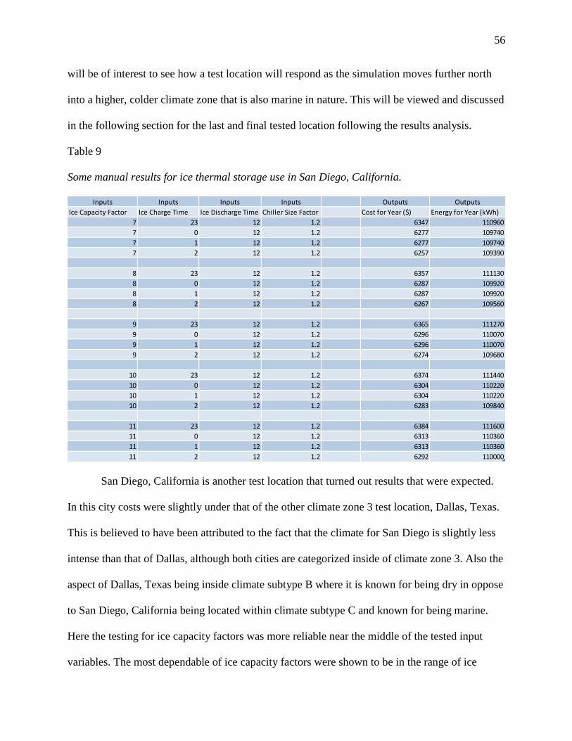
56
will be of interest to see how a test location will respond as the simulation moves further north
into a higher, colder climate zone that is also marine in nature. This will be viewed and discussed
in the following section for the last and final tested location following the results analysis.
Table 9
Some manual results for ice thermal storage use in San Diego, California.
San Diego, California is another test location that turned out results that were expected.
In this city costs were slightly under that of the other climate zone 3 test location, Dallas, Texas.
This is believed to have been attributed to the fact that the climate for San Diego is slightly less
intense than that of Dallas, although both cities are categorized inside of climate zone 3. Also the
aspect of Dallas, Texas being inside climate subtype B where it is known for being dry in oppose
to San Diego, California being located within climate subtype C and known for being marine.
Here the testing for ice capacity factors was more reliable near the middle of the tested input
variables. The most dependable of ice capacity factors were shown to be in the range of ice
Inputs Inputs Inputs Inputs Outputs Outputs
Ice Capacity Factor Ice Charge Time Ice Discharge Time Chiller Size Factor Cost for Year ($) Energy for Year (kWh)
7 23 12 1.2 6347 110960
7 0 12 1.2 6277 109740
7 1 12 1.2 6277 109740
7 2 12 1.2 6257 109390
8 23 12 1.2 6357 111130
8 0 12 1.2 6287 109920
8 1 12 1.2 6287 109920
8 2 12 1.2 6267 109560
9 23 12 1.2 6365 111270
9 0 12 1.2 6296 110070
9 1 12 1.2 6296 110070
9 2 12 1.2 6274 109680
10 23 12 1.2 6374 111440
10 0 12 1.2 6304 110220
10 1 12 1.2 6304 110220
10 2 12 1.2 6283 109840
11 23 12 1.2 6384 111600
11 0 12 1.2 6313 110360
11 1 12 1.2 6313 110360
11 2 12 1.2 6292 110000

57
capacity factors tested at 9. The most optimal results presented an energy consumption of
109,370 kWh for the year. With that amount of energy consumed the energy cost for the year in
San Diego, California just from the cooling after simulation was a mere $6,255. These optimal
results were obtained using the genetic algorithm optimization tool.
4.2.3.2 Seattle, Washington. The tenth and final location for ice thermal storage testing
was done and concluded in climate zone 4 for the marine climate subtype C. This climate zone is
the second of the only two existing climate zones within this climate subtype. The other, climate
zone 3, was recorded in San Diego, California and previously discussed earlier in the text. Here
for climate zone 4 in the marine subtype the city location was selected to be Seattle, Washington.
This location is the most northern tested site on the west coast and in the marine climate subtype.
The partial outcome for ITS testing in this marine climate subtype C can be viewed in Table 10
below. Full table results for all ice capacity factors that were tested for this location can be found
in the appendix in the back for trial and error manual test results. Climate zone 4 is a mixed
climate zone that often sees many different weather patterns sometimes being humid, dry, and
even marine. The results here are displayed for the end-range of results produced, due to the
more consistent of results lying near the higher tested ice capacity factors in the data. It is now
evident as the test locations move further and further north on the west coast that energy cost and
consumption will also continue to decline. This is the cause of the direct relationship between the
climate and the locations’ need for cooling. However, here on the west coast the decline still
exist although the climate zones are not as cold and frigid as the tested locations seen and
observed over on the east coast.
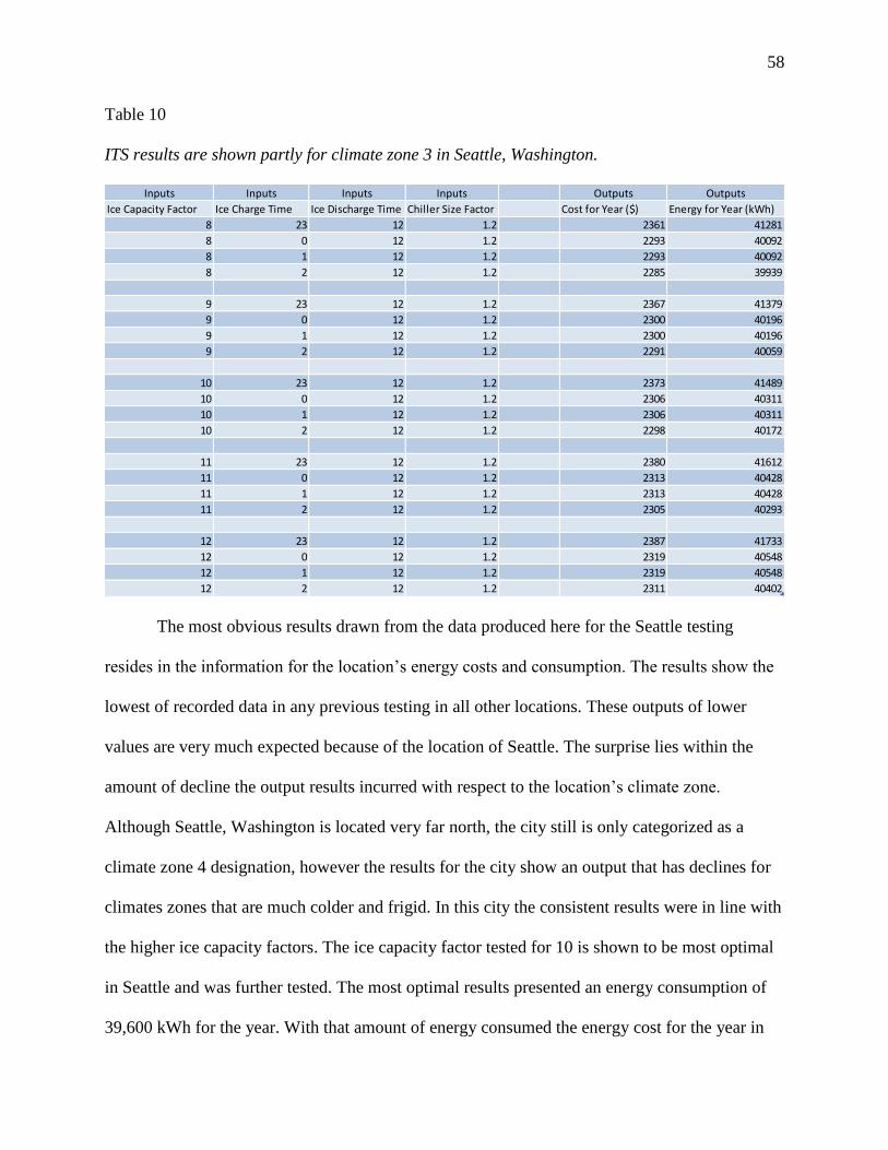
58
Table 10
ITS results are shown partly for climate zone 3 in Seattle, Washington.
The most obvious results drawn from the data produced here for the Seattle testing
resides in the information for the location’s energy costs and consumption. The results show the
lowest of recorded data in any previous testing in all other locations. These outputs of lower
values are very much expected because of the location of Seattle. The surprise lies within the
amount of decline the output results incurred with respect to the location’s climate zone.
Although Seattle, Washington is located very far north, the city still is only categorized as a
climate zone 4 designation, however the results for the city show an output that has declines for
climates zones that are much colder and frigid. In this city the consistent results were in line with
the higher ice capacity factors. The ice capacity factor tested for 10 is shown to be most optimal
in Seattle and was further tested. The most optimal results presented an energy consumption of
39,600 kWh for the year. With that amount of energy consumed the energy cost for the year in
Inputs Inputs Inputs Inputs Outputs Outputs
Ice Capacity Factor Ice Charge Time Ice Discharge Time Chiller Size Factor Cost for Year ($) Energy for Year (kWh)
8 23 12 1.2 2361 41281
8 0 12 1.2 2293 40092
8 1 12 1.2 2293 40092
8 2 12 1.2 2285 39939
9 23 12 1.2 2367 41379
9 0 12 1.2 2300 40196
9 1 12 1.2 2300 40196
9 2 12 1.2 2291 40059
10 23 12 1.2 2373 41489
10 0 12 1.2 2306 40311
10 1 12 1.2 2306 40311
10 2 12 1.2 2298 40172
11 23 12 1.2 2380 41612
11 0 12 1.2 2313 40428
11 1 12 1.2 2313 40428
11 2 12 1.2 2305 40293
12 23 12 1.2 2387 41733
12 0 12 1.2 2319 40548
12 1 12 1.2 2319 40548
12 2 12 1.2 2311 40402

59
Seattle, Washington just from the cooling after simulation was a mere $2,360. These optimal
results were obtained using the genetic algorithm optimization tool.
4.3 Test Location Non-Optimal Manual Results
4.3.1 Preliminary testing of locations. The previously discussed results found in the
tables for the different cities are really broad and simply serve as a basis for the beginning
research. These manual, non-optimal results for the ten tested city locations are for the most part
used as a baseline to measure ice capacity factor effectiveness in the tested climate zone location.
From here, these non-optimal results are judge and analyzed in determining the ranges of input
variables to use for the genetic algorithm that produced the optimal results moving forward. The
non-optimal design generally focused on the trial and error approach in seeking results to be
reviewed in advancing the research onward and reaching an optimal design. The results indicated
the direction in which the optimal results would be reached as well as, which ice capacity factors
were more consistent, based on location and climate zone.
4.4 Test Location Optimal Results
4.4.1 How it works. The final part of the research involved the use of the genetic
algorithm optimization tool. The results gathered during the previous research is used to help
determine the variables that will be input and allow the optimization tool to define the best
results for energy cost savings for the ice thermal storage technology. The manual results found
in the prior work was simply a product of trial and error and was key in finding a primary
direction in which to investigate further to find optimal results. After analyzing those results the
variables pointing to the closest of minimum energy cost and energy consumption was extracted
and set as the range for the input variables when prompted using the genetic algorithm
optimization tool. From here the genetic algorithm optimization tool runs the program seeking a
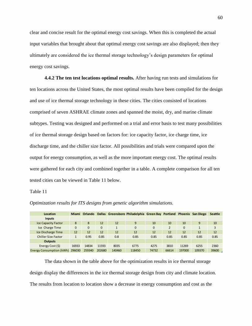
60
clear and concise result for the optimal energy cost savings. When this is completed the actual
input variables that brought about that optimal energy cost savings are also displayed; then they
ultimately are considered the ice thermal storage technology’s design parameters for optimal
energy cost savings.
4.4.2 The ten test locations optimal results. After having run tests and simulations for
ten locations across the United States, the most optimal results have been compiled for the design
and use of ice thermal storage technology in these cities. The cities consisted of locations
comprised of seven ASHRAE climate zones and spanned the moist, dry, and marine climate
subtypes. Testing was designed and performed on a trial and error basis to test many possibilities
of ice thermal storage design based on factors for: ice capacity factor, ice charge time, ice
discharge time, and the chiller size factor. All possibilities and trials were compared upon the
output for energy consumption, as well as the more important energy cost. The optimal results
were gathered for each city and combined together in a table. A complete comparison for all ten
tested cities can be viewed in Table 11 below.
Table 11
Optimization results for ITS designs from genetic algorithm simulations.
The data shown in the table above for the optimization results in ice thermal storage
design display the differences in the ice thermal storage design from city and climate location.
The results from location to location show a decrease in energy consumption and cost as the
Location Miami Orlando Dallas Greensboro Philadelphia Green Bay Portland Phoenix San Diego Seattle
Inputs
Ice Capacity Factor 8 8 12 12 9 10 10 10 9 10
Ice Charge Time 0 0 0 1 0 0 2 0 1 3
Ice Discharge Time 12 12 12 12 12 12 12 12 12 12
Chiller Size Factor 1 0.95 0.85 0.8 0.85 0.85 0.85 0.85 0.85 0.85
Outputs
Energy Cost ($) 16933 14834 11593 8035 6775 4275 3810 11269 6255 2360
Energy Consumption (kWh) 296030 259340 202680 140460 118450 74732 66614 197000 109370 39600
61
locations move further north and the climate zone number rises. It is very apparent that colder
climates will result in lesser savings with the use of ice thermal storage. This is primarily due to
colder climates requiring a substantially less amount of cooling than southern, hotter climates.
The results indicate that the higher ice capacity factors were better for colder climates; as well as
a lower chiller size factor in colder climates. It was also evident that the much colder climates
required later ice charge times, which was primarily due to less required cooling. The optimal
results found differ from the manual, trial and error results, in the aspect that they are a lot more
refined and hone in on the utmost savings in the new ITS technology.
4.5 Energy consumption
The focus of this study and research was designed and concerned primarily for the energy
costs that resulted from the cooling load required of commercial type buildings. As the work
progressed, it also became just as important to make an emphasis to monitor the output results
this new ice thermal storage technology makes on the building’s energy consumption. Although
the implementation of ice thermal storage results in a savings on energy costs for commercial
buildings, ice thermal storage ultimately increases the amount of energy consumption that is
caused by the building. This increase in energy consumption however is only a minor concern
because of the savings, that is in full responsibility due to the decline in energy costs from the
ITS system. Increases in the amount of energy consumed by the building with the addition of ice
thermal energy is most easily explained and accounted for by the operation of the chiller. With
the employment of ITS the chiller runs at night. When the chiller has to run at night to make the
ice for the ITS tanks it is required to run at a higher capacity to be cold enough, making ice. The
energy consumption increase is due to the extent of how much harder the chiller works and runs
while making ice. With the correct design and optimization of ITS input variables, energy

62
consumption became another output result monitored and focused on in minimizing. The results
are shown below in Figure 15 for the optimal results in each city that was tested along with the
corresponding energy consumption output results for that test location.
Figure 15 The optimal results for energy consumption in the ASHRAE climate zone test
locations.
The optimal results shown here in Figure 15 represent the ice thermal storage and total
cooling system’s energy consumption in a year’s time for the test locations. The energy
consumption outputs, in each respective test location, varied; and were later determined to be due
to climate zone needs for cooling. The climate zones of colder regions tended to produce less
energy consumption from cooling, while the warmer climates accounted for a substantial amount
of cooling. The graph in the Figure 15 above shows the relationship between the location and the
energy consumption as the weather becomes colder.
296030
259340
202680
140460 118450
74732 66614
197000
109370
39600
0
50000
100000
150000
200000
250000
300000
350000
kWh
Test Location
Location Energy Consumption
Miami Orlando Dallas Greensboro PhiladelphiaGreen Bay Portland Phoenix San Diego Seattle

63
4.6 Energy Cost
Overall the most important aspect of the results was surrounded by the energy costs
discoveries. Efforts are now widespread in making buildings as energy efficient as possible and
eliminating some of the energy costs that are a product of the cooling loads from commercial
buildings. It was first priority to reduce the energy costs for cooling within the IRC test building
that was simulated in the ten test locations throughout the United States. The results are shown
below in Figure 16 for the optimal results in each city that was tested along with the
corresponding energy costs output results for that test location. The graph in the figure below
shows the relationship between the location and the energy costs as the climates turned colder.
Optimal results shown in the figure below are represented for the total cooling costs for the year
within the air conditioning system, including the ice thermal storage unit. Data is shown for all
test locations spread across climate zones and climate subtypes recognized by ASHRAE.
Analysis of these results was very much similar and fall in line with the theme that was found
present for the energy consumption data results. Hotter climates definitely saw the most potential
savings for energy costs in oppose to the colder climate zone cities tested. This is very much due
to the aforementioned reasons of there being a lack of demand for cooling in primarily cold
weather climates. The interesting aspect that turns out in the energy costs results reside in the
amount of potential savings in relation to the negative increase of potential energy consumption.
The ratio of decreasing energy costs to the increasing energy consumption is highly favorable
towards the energy costs. This is very much desired and respected for a positive feedback in the
value and efficiency of ice thermal storage usage.
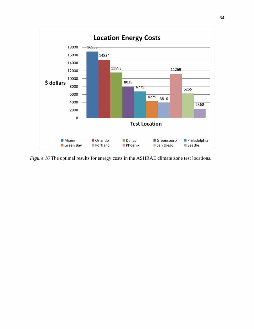
64
Figure 16 The optimal results for energy costs in the ASHRAE climate zone test locations.
16933
14834
11593
8035 6775
4275 3810
11269
6255
2360
0
2000
4000
6000
8000
10000
12000
14000
16000
18000
$ dollars
Test Location
Location Energy Costs
Miami Orlando Dallas Greensboro PhiladelphiaGreen Bay Portland Phoenix San Diego Seattle

65
CHAPTER 5
Conclusion and Future Research
5.1 Overview
The testing of ice thermal storage technology in various ASHRAE climate zones has
presented a great deal of positivity on the idea of the technology being a source of energy cost
savings. The outcome of results illustrates the immense effect the input variables made on energy
cost and energy consumption as it pertains to cooling. The input variables that affect these two
outcomes are both variables that can be controlled, as well as ones that there are not any control
over. The controlled variables included; ice capacity factor, ice charge time, ice discharge time,
chiller size factor, and variable ranges for the genetic algorithm optimization tool. The
uncontrolled variables were; location climate and weather data, as well as the utility cost rate
structure. The effects the input variables had on outcomes for energy cost and consumption was
directly proportional to each other; when one affected cost it even affected consumption as well.
The savings and outcome of this study is a useful tool in conveying the perks and advantages of
ice thermal storage as an energy cost saver, but more research is essential in improving the
advancement of the technology. Some key ways to further improve the research of this
technology include; performing a cost analysis for the implementation of ice thermal storage into
current commercial buildings, and even expanding the optimization genetic algorithm to handle
more instances and different cases throughout the simulations of the year. All in all, the savings
found in these simulated tests provide evidence that the application of ice thermal storage can
provide energy cost savings, although differently depending upon a location’s climate.

66
5.2 Input Variables
5.2.1 Ice capacity factor. This is the most important input variable throughout the
research, as it is key to the cooling of the building during the stretch of the on-peak time period.
The ice capacity factor is the variable that is assigned to determine the amount of time it will take
for the ITS system to charge ice up to full capacity. It is most important that the ice capacity
factor for the ice thermal storage be designed to adequately cover the cooling load during the on-
peak period of the day where charges are much higher than the normal off-peak periods. In
addition to that key factor, it is just as equally important that the ice capacity factor isn’t
oversized, as oversizing the ice capacity factor will take away from potential energy cost savings
that would result from this technology. It was determined that the initial test run manually in the
program would be for ice capacity factors ranging from a four all the way up to twelve. This was
tested in all locations and from here interpretations were made in deciding parameters for the
genetic algorithm optimization tool. Throughout the results it is indicated that ice capacity
factors were most dependable in the mid to high ranges, but varied by climate location.
5.2.2 Ice charge time. The next of the input variables consisted of the settings that start
the charging process for the ice thermal storage system. In addition to making sure there is
enough capacity of cooling to complete the cooling load required during the on-peak period, it is
also necessary to start the charging of the ice in time to ensure that the ice capacity is met before
the building becomes operational at the beginning of the day and the chiller is running to meet
the normal daytime cooling portion for the off-peak time. The ice charge time variable handles
this process and assigns the time in which to start this charging process of ice for the system. For
the manual test here the trials consisted of four separate ice charge time to start the charging
period; they included: 11pm, 12am midnight, 1am, and 2am. The charging period for the ice was
67
designed to occur at night. This was due to multiple reasons which include it be during an off-
peak time period, for obvious reasons of energy cost savings, and also during a time period
where the chiller is not being run by the system for cooling of the building, leaving the only
available time to be when the building is not considered to be operational. The ice charge
strategy times were run for each of the ice capacity factors that ranged from four to twelve and
ultimately considered in the deciding parameters for the genetic algorithm.
5.2.3 Ice discharge time. The ice discharge time was the easiest of the input variables
due to the fact that it remained constant and also because of the fact it is dependent upon another
uncontrolled variable. The ice discharge time is reliant upon the factor known as the utility cost
rate structure. The utility cost rate structure sets the on-peak and off-peak time periods and in
addition to this, the utility cost rate structure states the charges for both of these time periods.
This links the ice discharge time to the utility rate structure by the setting of the on-peak time
period. The cooling for the building during the on-peak time period needs to be controlled by the
ice thermal storage system, therefore, the ice discharge time must be set to begin at the moment
the on-peak time period is set to being each day. For this reason the ice discharge time remains
constant all throughout the manual testing, as well as the genetic algorithm optimization process
also. In future works any changes to the utility cost rate structure where it would alter the on-
peak time period, it would mean the ice discharge time should likewise be reset to match the on-
peak start time.
5.2.4 Chiller size factor. The chiller size factor for the experiment is another input
variable that saw little change initially; but unlike the ice discharge time, the chiller size factor
was later altered and tested for efficiency. The purpose of the chiller size factor is solely to
determine how much to oversize the chiller. For purposes of this research, the chiller size factor
68
being used to oversize the chiller also is the standard which is used to oversize the storage
capacity of the ice, due to the fact that ice capacity is determined based off of chiller size. In the
most common of cases it is necessary to allow for an appropriate safety factor of 20% of the
chiller size, resulting in a chiller size factor of 1.2. This was the case that was run in the manual
testing for the initial baseline trial and error data. For each run tested a chiller size factor of 1.2
was set and this consequently oversized the chiller as well as the capacity of ice storage by 20%.
During the optimizing of the ITS design using the genetic algorithm is when the chiller size
factor variable saw changes to its otherwise constant and consistent setting of 1.2. Here during
this optimizing period the range for this variable was spanned anywhere from possibly being
oversized or even undersized by 20%. The chiller size factor was given the option of outputting a
result anywhere from 0.8 to 1.2. This was determined to be feasible because of the chiller being
designed for the worst possible case of cooling load desired and the use of the ITS system
resulting in downsizing the likelihood of that worst possible case actually happening or coming
true.
5.3 Savings
Studying the optimization of ice thermal storage technology throughout the ASHRAE
climate zones has given rise to a viable source for energy cost savings. Looking over the results
and analyzing the data from all ten test locations, which were spread throughout seven climate
zones and three climate subtypes, many conclusions can be drawn regarding the promising
possibilities that the implementation of ice thermal storage technology presents in incorporating
into the cooling processes of commercial buildings. The outputs for the optimal results of energy
consumption and energy costs can be seen in Table 12 below for both a system with no ice
thermal storage as well as an optimized ice thermal storage system. These results are shown for

69
all ten test locations in a combined table for all of the climate zone test locations. Finally the key
takeaway from this table resides in the row labeled for the percent savings. Here, the percent
savings is calculated to show just how much savings was established in energy costs, comparing
the results between the system run with no ITS technology and with the implementation of an
optimized ITS system. There also is two graphics shown below in Figure 17 and Figure 18 that
display these results of the differences in the IRC building run with and without the application
of an ITS system based on energy consumption and energy costs respectively.
Table 12
Outputs for energy cost & consumption for No ITS vs. Optimal ITS & percent savings.
One key takeaway from the studies lies within the changes observed by the results
produced within the genetic algorithm optimization tool used in seeking the best design results
for input variables. These changes were present throughout the different climate zones as it
pertains to the ice capacity factor and chiller size factor input variables. The ice capacity factor
that worked for optimal cases in the ten locations that were tested changed and seemed to be
based upon the climate of the location. In the warm and hotter climate zones the consistently
optimal return for ice capacity factor exhibited to be in the midrange of the data parameters
tested. However, when it came to the findings for colder climates, the ice capacity factor results
saw a steady increase. Cold weather locations saw optimal design results always at the far end of
Location
System No ITS Optimal No ITS Optimal No ITS Optimal No ITS Optimal No ITS Optimal
Outputs
Energy Cost ($) 27420 16933 24790 14834 21850 11593 17070 8035 15080 6775
Energy Consumption (kWh) 255150 296030 227430 259340 181980 202680 126950 140460 106150 118450
Percent Savings (%)
Location
System No ITS Optimal No ITS Optimal No ITS Optimal No ITS Optimal No ITS Optimal
Outputs
Energy Cost ($) 12205 4275 10337 3810 20610 11269 13169 6255 8395 2360
Energy Consumption (kWh) 69761 74732 61499 66614 179700 197000 94116 109370 34808 39600
Percent Savings (%) 65.0 63.1 45.3 52.5 71.9
Green Bay Portland Phoenix San Diego Seattle
38.2 40.2 46.9 52.9 55.1
Miami Orlando Dallas Greensboro Philadelphia
70
the spectrum near the higher tested ice capacity factors. Moving on, the chiller size factor
displayed some of the same effects. For the higher climate zones, which represent the colder
climates, the chiller size factor was able to be designed for an under-sizing rather than the typical
oversizing, which is done to allow a safety factor load. In the warmer climate regions these
locations provided chiller size factor results that steered closer to the actual size of the design
chiller, allowing for neither an oversizing nor a substantial under-sizing. These changes within
the design input variables were the initial findings that pointed towards the climate zones having
a more than substantial effect on the produced results. The most noticeable of these deductions
include the differences of the produced results in comparison to the tested climate zones. This
major giveaway that ultimately proved truth to the climate’s effect on the results lied within
results themselves. As the research developed it became easily apparent the relationship the
climate location has on the savings potential. Colder climates require far less energy for cooling
and therefore provide far less results in the amount of savings possibilities. As the locations were
tested in northern and cold weather climate, the results dropped off aggressively and the energy
consumption along with the energy costs seemed minimal to none, in comparison to the warmer,
hot weather climates. Colder climates see a bigger portion of their energy consumption in
heating costs and ice thermal storage cannot target that to provide any energy cost savings. It
proved that savings from on energy costs can range depending upon locations, but were as low
an 38% savings in one location, and as high as an 72% savings in another location. Although
these findings prove to show differences in the amount of results in energy savings by climate
zone, still savings with this technology can exist in every type of climate, cold or hot. All in all,
there is a prominent energy savings capability with the correct optimization of ice thermal
storage technology when designed accordingly, regardless of the climate zone. Ice thermal

71
storage technology can play a key role in the reduction of energy cost in the cooling of
commercial buildings.
Figure 17 Graph comparing energy consumption of No ITS system vs. optimized ITS system.
0
50000
100000
150000
200000
250000
300000
350000
Annual Energy
Consumption (kWh)
Test Location
No ITS vs. Optimal ITS Energy Consumption by Location
No ITS
Optimal
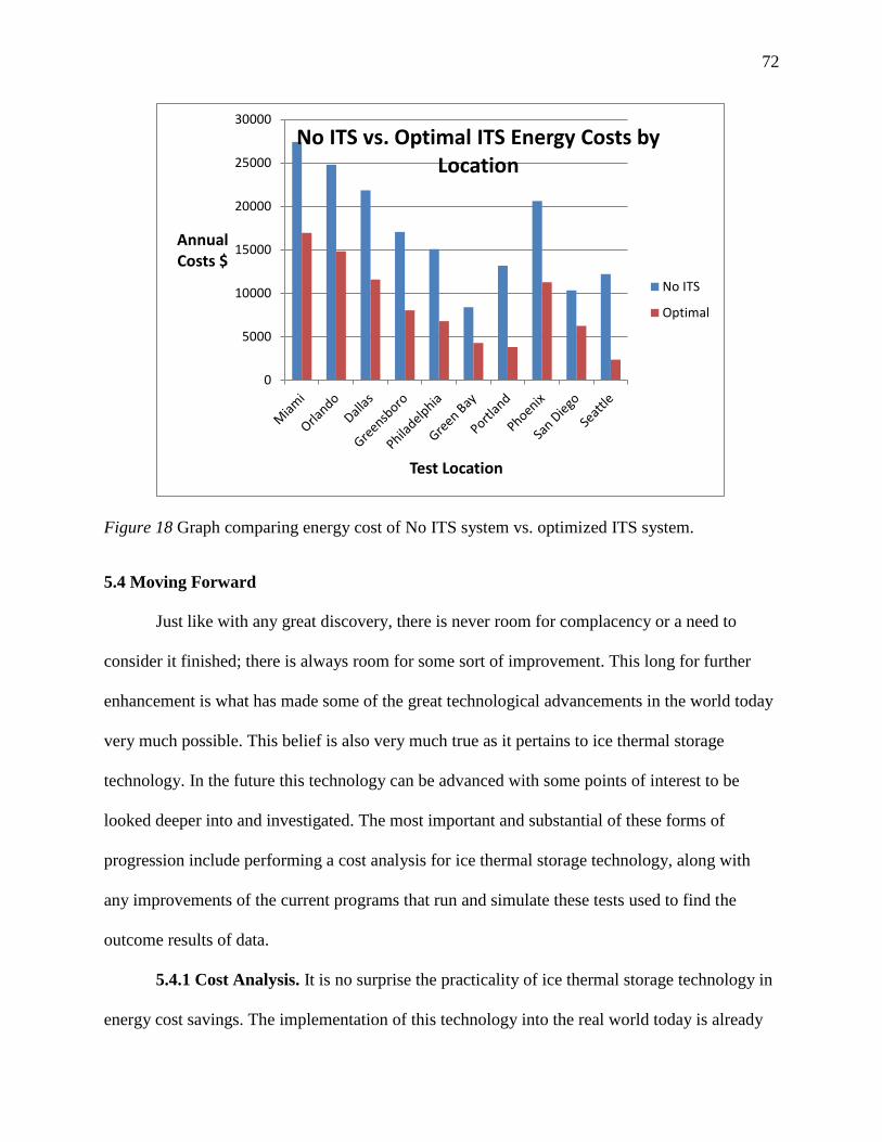
72
Figure 18 Graph comparing energy cost of No ITS system vs. optimized ITS system.
5.4 Moving Forward
Just like with any great discovery, there is never room for complacency or a need to
consider it finished; there is always room for some sort of improvement. This long for further
enhancement is what has made some of the great technological advancements in the world today
very much possible. This belief is also very much true as it pertains to ice thermal storage
technology. In the future this technology can be advanced with some points of interest to be
looked deeper into and investigated. The most important and substantial of these forms of
progression include performing a cost analysis for ice thermal storage technology, along with
any improvements of the current programs that run and simulate these tests used to find the
outcome results of data.
5.4.1 Cost Analysis. It is no surprise the practicality of ice thermal storage technology in
energy cost savings. The implementation of this technology into the real world today is already
0
5000
10000
15000
20000
25000
30000
Annual Costs $
Test Location
No ITS vs. Optimal ITS Energy Costs by Location
No ITS
Optimal
73
present and exists in both primarily cold and hot climates. The need for completing a cost
analysis on the technology would be to further explore the overall benefit in just how cost
effective it is to implement while being sure it remains beneficial and worth-while in the long-
term. This particular study would include and consist of a research of initial costs, and
operational costs. Often it is a cause for concern in dealing with these types of expenses where it
can even outweigh long-term savings down the road. Another portion of the study would
examine a plan for the return of investment. This is generally a performance measure where the
efficiency of an investment is evaluated. Here the investments, including initial costs, operational
costs, and any upkeep or maintenance are used to equate just how profitable the investment was
based on making up expenses and calculating possible future income or savings.
5.4.2 Program and code improvements. The perfecting of the already developed codes
and programs used in this research is another extraordinary way to continue to advance the work
already discovered here for ice thermal storage technology and design. The ice thermal storage
optimization program has room for growth by expanding the optimization genetic algorithm to
handle more instances and different cases throughout the simulations of the year. Such advances
in the optimization algorithm can embrace aspects including using more tested ice charge times,
and many other alterations in code design. Another major way of changing the testing would be
to explore the possibility of using a longer charging time period. It is also worth looking into the
possible savings that could be achieved if the ice thermal storage system replaced and took
control of all cooling while the building is operational, including on-peak periods as well as off-
peak periods. This possibility would mean for a lot more ice charging and therefore need tons
more of ice capacity. This would more than likely result in a constantly charging period for the
ice capacity with the exception of the on-peak time period. These types of future advances and/or

74
upgrades to the ice thermal storage optimization program will advance the technology and make
for a well-balanced and investigated energy cost saving tool for commercial buildings’ cooling.

75
References
Al-Qalamchi, A. A. W., & Adil, A. (2007). Performance of ice storage system utilizing a
combined partial and full storage strategy. Desalination, 209(1–3), 306-311.
ASHRAE. (2011). Energy Standard for Buildings Except Low-Rise Residential Buildings
(189.1). Atlanta, GA: ASHRAE.
Braun JE. A near-optimal control strategy for cool storage systems with dynamic electric rates.
Int J HVAC&R Res 2007;13(4):557–80.
DOE (Department of Energy). (1980). DOE 2 Reference Manual, Part 1, Version 2.1. Lawrence
Berkeley National
Energy Efficiency and Renewable Energy. (2010). 2009 Buildings Energy Data Book. U.S.
Department of Energy. http://buildingsdatabook.eere.energy.gov/
eQUEST. (2011, September 14). Building Energy Software Tools Directory. Retrieved August
16, 2013, from http://apps1.eere.energy.gov/buildings/too.
Freeland, D., (2014). Optimizing the Design of Chilled Water Plants in Large Commercial
Buildings, accepted, ASHRAE Transactions 120(1).
Habeebullah, B., Economic feasibility of thermal energy storage systems, Energy and Buildings
39 (2007) 355–363.
Hajiah, A., & Krarti, M. (2012). Optimal control of building storage systems using both ice
storage and thermal mass – Part I: Simulation environment. Energy Conversion and
Management, 64(0), 499-508. (a)
Hajiah, A., & Krarti, M. (2012). Optimal controls of building storage systems using both ice
storage and thermal mass – Part II: Parametric analysis. Energy Conversion and
Management, 64(0), 509-515. (b)

76
Hall, C., Freeland, D., & Nassif, N. (2013) Optimization of Ice Thermal Storage System Design
and Operation for HVAC Systems. National Conference on Advances in Environmental
Science & Technology, 12-13 September, Greensboro, NC., USA.
Haupt, R. L., & Haupt, S. E. (2004). Practical Genetic Algorithms. Hoboken, NJ: John Wiley &
Sons, Inc.
Liu S, Henze GP. Experimental analysis of simulated reinforcement learning control for active
and passive building thermal storage inventory –Part 1: theoretical foundation. Energy
Build 2006;38(2):142–7.
MacCracken, M., Thermal energy storage in sustainable buildings, ASHRAE Journal 46 (2004)
39–41.
Mitchell, M. (1995). Genetic Algorithms: An Overview, Santa Fe Institute. 1, 1-14.
Morgan, S., Krarti, M., Field Testing of Optimal Controls of Passive and Active
Thermal Storage, accepted, ASHRAE Transactions 116 (2010) 134–146.
Nassif, N. (2013). Modeling and Optimization of HVAC Systems Using Artificial Neural
Network and Genetic Algorithm. International Journal of Building Simulation, in press.
(a)
Nassif, N., Hall, C., & Freeland, D. (2014) Optimal Design and Control of Ice Thermal Storage
System for a Typical Chilled Water Plant, accepted, ASHRAE Transactions 120(1). (b)
Nassif, N., Kajl S., & Sabourin, R. (2005) Optimization of HVAC Control System Strategy
Using Two-objective Genetic Algorithm. ASHRAE, International journal of HVAC&R
Research 11 (3): 459-486. (c)
Nassif, N., Tesiero, R., Singh, H. (2012) Impact of Ice Thermal Storage on Cooling Energy Cost
for Commercial HVAC Systems. accepted, ASHRAE Transactions 120(1). (d)
77
Pu, J., Liu, G., & Feng, X. (2012). Cumulative exergy analysis of ice thermal storage air
conditioning system. Applied Energy, 93(0), 564-569.
Research, Pike. (2012, March 12). Thermal Storage for HVAC in Commercial Buildings,
District Cooling and Heating, Utility and Grid Support Applications, and High
Temperature Storage at CSP Facilities. Navigant Research Energy Storage Category.
Retrieved August 10, 2013, from
http://www.navigantresearch.com/researchenergy/energy-storage.
Rismanchi, B., Saidur, R., Masjuki, H. H., & Mahlia, T. M. I. (2012). Energetic, economic and
environmental benefits of utilizing the ice thermal storage systems for office building
applications. Energy and Buildings, 50(0), 347-354.
Silvetti, B., Application fundamentals of ice-based thermal storage, ASHRAE Journal 44 (2002)
30–35.
Wulfinghoff, D. R. (1999). Energy Efficiency Manual. Wheaton, MD: Energy Institute Press.
Yau, Y., Rismanchi, B., A review on cool thermal storage technologies and operating strategies,
Renewable and Sustainable Energy Reviews 16 (2012) 787–797.

78
Appendix A
A. Hourly Peak Load Data
Table A1
Hourly peak load data for the design day in Miami, Florida.
Peak Load Day: July 29th
Month Day Hour Building cool load (coils+losses&gains) (Btu/hr) Outside wet-bulb temp (F) Outside dry-bulb temp (F)
7 29 1 0 76 79
7 29 2 0 76 78
7 29 3 0 76 78
7 29 4 0 76 79
7 29 5 0 76 78
7 29 6 0 76 79
7 29 7 2.13E+06 77 81
7 29 8 2.85E+06 78 84
7 29 9 2.79E+06 79 84
7 29 10 2.65E+06 77 84
7 29 11 2.74E+06 79 85
7 29 12 2.79E+06 80 85
7 29 13 2.60E+06 78 86
7 29 14 2.70E+06 80 87
7 29 15 2.64E+06 79 87
7 29 16 2.60E+06 78 86
7 29 17 1.47E+06 78 86
7 29 18 0 77 85
7 29 19 0 77 84
7 29 20 0 77 83
7 29 21 0 77 82
7 29 22 0 76 82
7 29 23 0 76 82
7 29 24 0 77 81

79
Table A2
Hourly peak load data for the design day in Orlando, Florida.
Peak Load Day: July 8th
Month Day Hour Building cool load (coils+losses&gains) (Btu/hr) Outside wet-bulb temp (F) Outside dry-bulb temp (F)
7 8 1 0 75 78
7 8 2 0 74 77
7 8 3 0 74 76
7 8 4 0 74 75
7 8 5 0 73 74
7 8 6 0 73 74
7 8 7 2.01E+06 75 77
7 8 8 2.76E+06 76 80
7 8 9 2.66E+06 76 84
7 8 10 2.65E+06 76 87
7 8 11 2.62E+06 76 89
7 8 12 2.56E+06 76 91
7 8 13 2.40E+06 74 92
7 8 14 2.29E+06 72 94
7 8 15 2.30E+06 72 94
7 8 16 2.51E+06 75 96
7 8 17 1.31E+06 75 95
7 8 18 0 76 87
7 8 19 0 75 82
7 8 20 0 74 80
7 8 21 0 75 80
7 8 22 0 75 79
7 8 23 0 75 78
7 8 24 0 75 78

80
Table A3
Hourly peak load data for the design day in Dallas, Texas.
Peak Load Day: July 15th
Month Day Hour Building cool load (coils+losses&gains) (Btu/hr) Outside wet-bulb temp (F) Outside dry-bulb temp (F)
7 15 1 0 71 80
7 15 2 0 72 80
7 15 3 0 72 79
7 15 4 0 71 77
7 15 5 0 71 77
7 15 6 0 71 76
7 15 7 2.34E+06 73 79
7 15 8 2.86E+06 74 82
7 15 9 2.74E+06 74 86
7 15 10 2.82E+06 76 90
7 15 11 2.78E+06 76 92
7 15 12 2.71E+06 76 95
7 15 13 2.61E+06 75 95
7 15 14 2.63E+06 76 97
7 15 15 2.53E+06 74 96
7 15 16 2.42E+06 73 89
7 15 17 1.29E+06 73 87
7 15 18 0 72 89
7 15 19 0 73 89
7 15 20 0 73 86
7 15 21 0 72 83
7 15 22 0 71 81
7 15 23 0 70 80
7 15 24 0 70 79

81
Table A4
Hourly peak load data for the design day in Greensboro, North Carolina.
Peak Load Day: July 8th
Month Day Hour Building cool load (coils+losses&gains) (Btu/hr) Outside wet-bulb temp (F) Outside dry-bulb temp (F)
7 8 1 0 69 70
7 8 2 0 69 70
7 8 3 0 68 69
7 8 4 0 68 68
7 8 5 0 67 68
7 8 6 0 68 69
7 8 7 1.24E+06 70 73
7 8 8 2.53E+06 74 78
7 8 9 2.48E+06 75 82
7 8 10 2.45E+06 75 83
7 8 11 2.45E+06 75 84
7 8 12 2.42E+06 75 85
7 8 13 2.46E+06 76 87
7 8 14 2.36E+06 75 82
7 8 15 2.42E+06 76 86
7 8 16 2.44E+06 76 87
7 8 17 1.36E+06 75 85
7 8 18 0 76 84
7 8 19 0 76 84
7 8 20 0 75 79
7 8 21 0 74 78
7 8 22 0 74 75
7 8 23 0 73 74
7 8 24 0 73 74

82
Appendix B
B. Full Data For Each Climate Zone
Table B1
Full data results for climate zone 1 in Miami, Florida.
Inputs Inputs Inputs Inputs Outputs Outputs
Ice Capacity Factor Ice Charge Time Ice Discharge Time Chiller Size Factor Cost for Year ($) Energy for Year (kWh)
4 23 12 1.2 22927 301,200
4 0 12 1.2 22133 298650
4 1 12 1.2 22133 298650
4 2 12 1.2 21943 298070
5 23 12 1.2 17257 301700
5 0 12 1.2 17096 29888
5 1 12 1.2 17096 29888
5 2 12 1.2 17611 298330
6 23 12 1.2 17268 301890
6 0 12 1.2 17120 299310
6 1 12 1.2 17120 299310
6 2 12 1.2 17085 298690
7 23 12 1.2 17281 302120
7 0 12 1.2 17134 299550
7 1 12 1.2 17134 299550
7 2 12 1.2 17096 298870
8 23 12 1.2 17296 302380
8 0 12 1.2 17147 299780
8 1 12 1.2 17147 299780
8 2 12 1.2 17111 299140
9 23 12 1.2 17310 302610
9 0 12 1.2 17160 300000
9 1 12 1.2 17160 300000
9 2 12 1.2 17123 299350
10 23 12 1.2 17340 303140
10 0 12 1.2 17178 300310
10 1 12 1.2 17178 300310
10 2 12 1.2 17142 299680
11 23 12 1.2 17350 303330
11 0 12 1.2 17188 300490
11 1 12 1.2 17188 300490
11 2 12 1.2 17168 300140
12 23 12 1.2 17364 303560
12 0 12 1.2 17212 300910
12 1 12 1.2 17212 300910
12 2 12 1.2 17178 300320
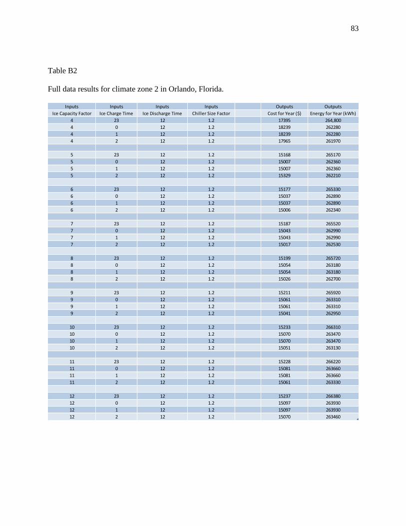
83
Table B2
Full data results for climate zone 2 in Orlando, Florida.
Inputs Inputs Inputs Inputs Outputs Outputs
Ice Capacity Factor Ice Charge Time Ice Discharge Time Chiller Size Factor Cost for Year ($) Energy for Year (kWh)
4 23 12 1.2 17395 264,800
4 0 12 1.2 18239 262280
4 1 12 1.2 18239 262280
4 2 12 1.2 17965 261970
5 23 12 1.2 15168 265170
5 0 12 1.2 15007 262360
5 1 12 1.2 15007 262360
5 2 12 1.2 15329 262210
6 23 12 1.2 15177 265330
6 0 12 1.2 15037 262890
6 1 12 1.2 15037 262890
6 2 12 1.2 15006 262340
7 23 12 1.2 15187 265520
7 0 12 1.2 15043 262990
7 1 12 1.2 15043 262990
7 2 12 1.2 15017 262530
8 23 12 1.2 15199 265720
8 0 12 1.2 15054 263180
8 1 12 1.2 15054 263180
8 2 12 1.2 15026 262700
9 23 12 1.2 15211 265920
9 0 12 1.2 15061 263310
9 1 12 1.2 15061 263310
9 2 12 1.2 15041 262950
10 23 12 1.2 15233 266310
10 0 12 1.2 15070 263470
10 1 12 1.2 15070 263470
10 2 12 1.2 15051 263130
11 23 12 1.2 15228 266220
11 0 12 1.2 15081 263660
11 1 12 1.2 15081 263660
11 2 12 1.2 15061 263330
12 23 12 1.2 15237 266380
12 0 12 1.2 15097 263930
12 1 12 1.2 15097 263930
12 2 12 1.2 15070 263460

84
Table B3
Full data results for climate zone 3 in Dallas, Texas.
Inputs Inputs Inputs Inputs Outputs Outputs
Ice Capacity Factor Ice Charge Time Ice Discharge Time Chiller Size Factor Cost for Year ($) Energy for Year (kWh)
4 23 12 1.2 16250 209,360
4 0 12 1.2 16083 205800
4 1 12 1.2 16083 205800
4 2 12 1.2 15592 205130
5 23 12 1.2 12000 209800
5 0 12 1.2 11790 206120
5 1 12 1.2 11790 206120
5 2 12 1.2 11751 205430
6 23 12 1.2 12012 209990
6 0 12 1.2 11800 206290
6 1 12 1.2 11800 206290
6 2 12 1.2 11761 205610
7 23 12 1.2 12021 210160
7 0 12 1.2 11809 206460
7 1 12 1.2 11809 206460
7 2 12 1.2 11770 205780
8 23 12 1.2 12031 210330
8 0 12 1.2 11819 206620
8 1 12 1.2 11819 206620
8 2 12 1.2 11780 205940
9 23 12 1.2 12040 210490
9 0 12 1.2 11828 206790
9 1 12 1.2 11828 206790
9 2 12 1.2 11790 206110
10 23 12 1.2 12049 210660
10 0 12 1.2 11840 206990
10 1 12 1.2 11840 206990
10 2 12 1.2 11802 206320
11 23 12 1.2 12059 210820
11 0 12 1.2 11848 207140
11 1 12 1.2 11848 207140
11 2 12 1.2 11810 206470
12 23 12 1.2 12066 210940
12 0 12 1.2 11856 207280
12 1 12 1.2 11856 207280
12 2 12 1.2 11821 206660
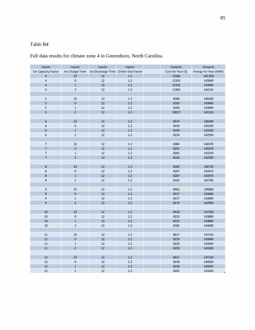
85
Table B4
Full data results for climate zone 4 in Greensboro, North Carolina.
Inputs Inputs Inputs Inputs Outputs Outputs
Ice Capacity Factor Ice Charge Time Ice Discharge Time Chiller Size Factor Cost for Year ($) Energy for Year (kWh)
4 23 12 1.2 12566 145,950
4 0 12 1.2 12310 143040
4 1 12 1.2 12310 143040
4 2 12 1.2 12303 142210
5 23 12 1.2 8366 146260
5 0 12 1.2 8183 143060
5 1 12 1.2 8183 143060
5 2 12 1.2 10017 142310
6 23 12 1.2 8374 146400
6 0 12 1.2 8193 143230
6 1 12 1.2 8193 143230
6 2 12 1.2 8154 142550
7 23 12 1.2 8384 146570
7 0 12 1.2 8201 143370
7 1 12 1.2 8201 143370
7 2 12 1.2 8156 142590
8 23 12 1.2 8392 146710
8 0 12 1.2 8207 143470
8 1 12 1.2 8207 143470
8 2 12 1.2 8165 142740
9 23 12 1.2 8402 146880
9 0 12 1.2 8217 143660
9 1 12 1.2 8217 143660
9 2 12 1.2 8174 142900
10 23 12 1.2 8418 147160
10 0 12 1.2 8225 143800
10 1 12 1.2 8225 143800
10 2 12 1.2 8185 143090
11 23 12 1.2 8417 147150
11 0 12 1.2 8233 143940
11 1 12 1.2 8233 143940
11 2 12 1.2 8195 143260
12 23 12 1.2 8417 147150
12 0 12 1.2 8238 144020
12 1 12 1.2 8238 144020
12 2 12 1.2 8205 143420
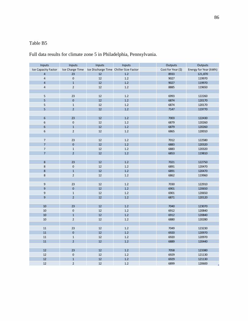
86
Table B5
Full data results for climate zone 5 in Philadelphia, Pennsylvania.
Inputs Inputs Inputs Inputs Outputs Outputs
Ice Capacity Factor Ice Charge Time Ice Discharge Time Chiller Size Factor Cost for Year ($) Energy for Year (kWh)
4 23 12 1.2 8933 121,870
4 0 12 1.2 9027 119970
4 1 12 1.2 9027 119970
4 2 12 1.2 8885 119650
5 23 12 1.2 6993 122260
5 0 12 1.2 6874 120170
5 1 12 1.2 6874 120170
5 2 12 1.2 7147 119770
6 23 12 1.2 7003 122430
6 0 12 1.2 6879 120260
6 1 12 1.2 6879 120260
6 2 12 1.2 6865 120010
7 23 12 1.2 7012 122580
7 0 12 1.2 6883 120320
7 1 12 1.2 6883 120320
7 2 12 1.2 6853 119810
8 23 12 1.2 7021 122750
8 0 12 1.2 6891 120470
8 1 12 1.2 6891 120470
8 2 12 1.2 6862 119960
9 23 12 1.2 7030 122910
9 0 12 1.2 6901 120650
9 1 12 1.2 6901 120650
9 2 12 1.2 6871 120120
10 23 12 1.2 7040 123070
10 0 12 1.2 6912 120840
10 1 12 1.2 6912 120840
10 2 12 1.2 6880 120280
11 23 12 1.2 7049 123230
11 0 12 1.2 6920 120970
11 1 12 1.2 6920 120970
11 2 12 1.2 6889 120440
12 23 12 1.2 7058 123380
12 0 12 1.2 6929 121130
12 1 12 1.2 6929 121130
12 2 12 1.2 6899 120600

87
Table B6
Full data results for climate zone 6 in Green Bay, Wisconsin.
Inputs Inputs Inputs Inputs Outputs Outputs
Ice Capacity Factor Ice Charge Time Ice Discharge Time Chiller Size Factor Cost for Year ($) Energy for Year (kWh)
4 23 12 1.2 6400 77,214
4 0 12 1.2 6029 75424
4 1 12 1.2 6029 75424
4 2 12 1.2 5746 74935
5 23 12 1.2 4428 77415
5 0 12 1.2 4319 75499
5 1 12 1.2 4319 75499
5 2 12 1.2 5020 74996
6 23 12 1.2 4433 77495
6 0 12 1.2 4328 75655
6 1 12 1.2 4328 75655
6 2 12 1.2 4308 75311
7 23 12 1.2 4440 77629
7 0 12 1.2 4336 75806
7 1 12 1.2 4336 75806
7 2 12 1.2 4311 75372
8 23 12 1.2 4449 77784
8 0 12 1.2 4329 75677
8 1 12 1.2 4329 75677
8 2 12 1.2 4316 75446
9 23 12 1.2 4456 77899
9 0 12 1.2 4336 75803
9 1 12 1.2 4336 75803
9 2 12 1.2 4307 75299
10 23 12 1.2 4460 77969
10 0 12 1.2 4339 75857
10 1 12 1.2 4339 75857
10 2 12 1.2 4315 75432
11 23 12 1.2 4464 78046
11 0 12 1.2 4348 76006
11 1 12 1.2 4348 76006
11 2 12 1.2 4324 75586
12 23 12 1.2 4455 77889
12 0 12 1.2 4353 76095
12 1 12 1.2 4353 76095
12 2 12 1.2 4332 75740

88
Table B7
Full data results for climate zone 7 in Portland, Maine.
Inputs Inputs Inputs Inputs Outputs Outputs
Ice Capacity Factor Ice Charge Time Ice Discharge Time Chiller Size Factor Cost for Year ($) Energy for Year (kWh)
4 23 12 1.2 4184 68,713
4 0 12 1.2 4670 67392
4 1 12 1.2 4670 67392
4 2 12 1.2 4854 66904
5 23 12 1.2 3947 68994
5 0 12 1.2 3861 67506
5 1 12 1.2 3861 67506
5 2 12 1.2 3837 67076
6 23 12 1.2 3944 68949
6 0 12 1.2 3873 67702
6 1 12 1.2 3873 67702
6 2 12 1.2 3846 67229
7 23 12 1.2 3952 69090
7 0 12 1.2 3881 67842
7 1 12 1.2 3881 67842
7 2 12 1.2 3853 67365
8 23 12 1.2 3960 69233
8 0 12 1.2 3888 67979
8 1 12 1.2 3888 67979
8 2 12 1.2 3860 67476
9 23 12 1.2 3968 69371
9 0 12 1.2 3896 68105
9 1 12 1.2 3896 68105
9 2 12 1.2 3868 67617
10 23 12 1.2 3976 69502
10 0 12 1.2 3901 68204
10 1 12 1.2 3901 68204
10 2 12 1.2 3876 67763
11 23 12 1.2 3983 69632
11 0 12 1.2 3908 68327
11 1 12 1.2 3908 68327
11 2 12 1.2 3884 67898
12 23 12 1.2 3997 69871
12 0 12 1.2 3916 68468
12 1 12 1.2 3916 68468
12 2 12 1.2 3890 68009
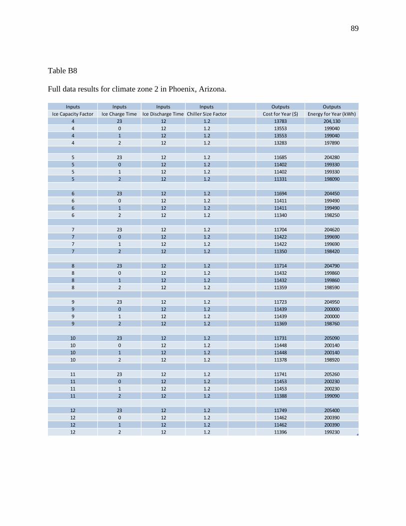
89
Table B8
Full data results for climate zone 2 in Phoenix, Arizona.
Inputs Inputs Inputs Inputs Outputs Outputs
Ice Capacity Factor Ice Charge Time Ice Discharge Time Chiller Size Factor Cost for Year ($) Energy for Year (kWh)
4 23 12 1.2 13783 204,130
4 0 12 1.2 13553 199040
4 1 12 1.2 13553 199040
4 2 12 1.2 13283 197890
5 23 12 1.2 11685 204280
5 0 12 1.2 11402 199330
5 1 12 1.2 11402 199330
5 2 12 1.2 11331 198090
6 23 12 1.2 11694 204450
6 0 12 1.2 11411 199490
6 1 12 1.2 11411 199490
6 2 12 1.2 11340 198250
7 23 12 1.2 11704 204620
7 0 12 1.2 11422 199690
7 1 12 1.2 11422 199690
7 2 12 1.2 11350 198420
8 23 12 1.2 11714 204790
8 0 12 1.2 11432 199860
8 1 12 1.2 11432 199860
8 2 12 1.2 11359 198590
9 23 12 1.2 11723 204950
9 0 12 1.2 11439 200000
9 1 12 1.2 11439 200000
9 2 12 1.2 11369 198760
10 23 12 1.2 11731 205090
10 0 12 1.2 11448 200140
10 1 12 1.2 11448 200140
10 2 12 1.2 11378 198920
11 23 12 1.2 11741 205260
11 0 12 1.2 11453 200230
11 1 12 1.2 11453 200230
11 2 12 1.2 11388 199090
12 23 12 1.2 11749 205400
12 0 12 1.2 11462 200390
12 1 12 1.2 11462 200390
12 2 12 1.2 11396 199230
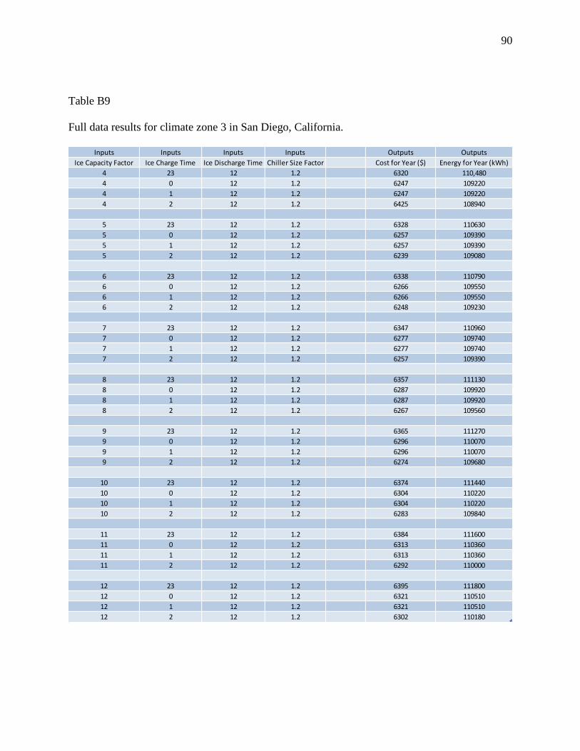
90
Table B9
Full data results for climate zone 3 in San Diego, California.
Inputs Inputs Inputs Inputs Outputs Outputs
Ice Capacity Factor Ice Charge Time Ice Discharge Time Chiller Size Factor Cost for Year ($) Energy for Year (kWh)
4 23 12 1.2 6320 110,480
4 0 12 1.2 6247 109220
4 1 12 1.2 6247 109220
4 2 12 1.2 6425 108940
5 23 12 1.2 6328 110630
5 0 12 1.2 6257 109390
5 1 12 1.2 6257 109390
5 2 12 1.2 6239 109080
6 23 12 1.2 6338 110790
6 0 12 1.2 6266 109550
6 1 12 1.2 6266 109550
6 2 12 1.2 6248 109230
7 23 12 1.2 6347 110960
7 0 12 1.2 6277 109740
7 1 12 1.2 6277 109740
7 2 12 1.2 6257 109390
8 23 12 1.2 6357 111130
8 0 12 1.2 6287 109920
8 1 12 1.2 6287 109920
8 2 12 1.2 6267 109560
9 23 12 1.2 6365 111270
9 0 12 1.2 6296 110070
9 1 12 1.2 6296 110070
9 2 12 1.2 6274 109680
10 23 12 1.2 6374 111440
10 0 12 1.2 6304 110220
10 1 12 1.2 6304 110220
10 2 12 1.2 6283 109840
11 23 12 1.2 6384 111600
11 0 12 1.2 6313 110360
11 1 12 1.2 6313 110360
11 2 12 1.2 6292 110000
12 23 12 1.2 6395 111800
12 0 12 1.2 6321 110510
12 1 12 1.2 6321 110510
12 2 12 1.2 6302 110180

91
Table B10
Full data results for climate zone 4 in Seattle, Washington.
Inputs Inputs Inputs Inputs Outputs Outputs
Ice Capacity Factor Ice Charge Time Ice Discharge Time Chiller Size Factor Cost for Year ($) Energy for Year (kWh)
4 23 12 1.2 2965 40,793
4 0 12 1.2 2317 39653
4 1 12 1.2 2317 39653
4 2 12 1.2 2741 39434
5 23 12 1.2 2341 40925
5 0 12 1.2 2274 39762
5 1 12 1.2 2274 39762
5 2 12 1.2 2267 39630
6 23 12 1.2 2348 41046
6 0 12 1.2 2281 39874
6 1 12 1.2 2281 39874
6 2 12 1.2 2272 39712
7 23 12 1.2 2354 41157
7 0 12 1.2 2287 39984
7 1 12 1.2 2287 39984
7 2 12 1.2 2278 39823
8 23 12 1.2 2361 41281
8 0 12 1.2 2293 40092
8 1 12 1.2 2293 40092
8 2 12 1.2 2285 39939
9 23 12 1.2 2367 41379
9 0 12 1.2 2300 40196
9 1 12 1.2 2300 40196
9 2 12 1.2 2291 40059
10 23 12 1.2 2373 41489
10 0 12 1.2 2306 40311
10 1 12 1.2 2306 40311
10 2 12 1.2 2298 40172
11 23 12 1.2 2380 41612
11 0 12 1.2 2313 40428
11 1 12 1.2 2313 40428
11 2 12 1.2 2305 40293
12 23 12 1.2 2387 41733
12 0 12 1.2 2319 40548
12 1 12 1.2 2319 40548
12 2 12 1.2 2311 40402