optimizing process economics in model predictive control
TRANSCRIPT

Optimizing Process Economics in Model Predictive Control
by
Rishi Amrit
A dissertation submitted in partial fulfillment
of the requirements for the degree of
Doctor of Philosophy
(Chemical Engineering)
at the
UNIVERSITY OF WISCONSIN–MADISON
2011

c© Copyright by Rishi Amrit 2011
All Rights Reserved

To Papa, Mummy, my better self Mannu and the love of my life Sayani.

ii
Optimizing Process Economics in Model Predictive Control
Rishi Amrit
Under the supervision of Professor James B. Rawlings
At the University of Wisconsin–Madison
The overall objective of any process is to convert certain raw material into desired prod-
ucts using available resources. During its operation, the plant must satisfy several re-
quirements imposed by its designers and the general technical, economic and social con-
ditions in the presence of ever-changing external influences. Among such requirements
are product specifications, operational constraints and safety and environmental regula-
tions. But the most significant incentive for using automated feedback control is the fact,
that under the effect of external disturbances, the system must be operated in such a fash-
ion, that it makes the maximum profit. In current practice, this incentive is answered by
means of the setpoint/target terminology, which is essentially the process control objec-
tive translation of the main economic objective. Translation of objectives in this fashion,
results in a loss of economic information and the dynamic regulation layer has no infor-
mation about the original plant economics except for a fixed steady state target.
This thesis aims to address the primary aim of any feedback control strategy, to optimize

iii
plant economics. This thesis presents a plantwide model predictive control strategy that
optimizes plant economics directly in the dynamic regulation problem. A class of systems
is identified for which optimizing economic objective would lead to stable plant opera-
tion, and consequently the asymptotic stability is established for these systems. Not all
of the existing tools of stability analysis for feedback control systems work for generic
nonlinear problems, hence new tools have been developed and used to establish stability
properties.
This thesis also addresses the applications for which nonsteady operation may be desired
and proposes MPC strategies for nonsteady operation. These strategies are demonstrated
by means of suitable examples from the literature. The economic superiority of economic
optimizing controllers is also established.
The benefit of optimizing economics is demonstrated using various chemical engi-
neering process examples from literature. The economic performance is compared to the
standard tracking type controllers and the benefit is calculated as a fraction of the steady
state profit. To demonstrate the feasibility of online solution to economics optimizing
dynamic regulation problem, a software tool is developed using open source nonlinear
solvers and automatic differentiation packages. The utility of this tool is demonstrated by
using it to perform all the simulation studies in this thesis.

iv
Acknowledgments
Among the beliefs that I have grown up believing, I regard knowledge as the greatest
and the most noble gift mankind has. Hence Guru, which means teacher in Sanskrit, is
considered as avatar of God.
In preparing this thesis, I have had the pleasure and deep honor to work with Prof.
James Rawlings. He has been much more than a mentor to me. He always amazes me
with his ability to understand and explain complex problems in micro time scales. All
the intellectual interactions I have had with him, be it about my research or about my
Indian English full of metaphors, are the most enlightening ones and have made me a
better person every time. His most remarkable trait is his approach to any problem, be it
research or any other. His dedication, patience, and his personality have been a yardstick
for me and shaped me into what I am today. I am most thankful to him for choosing to
guide me towards being a better researcher as well as a better person. I also thank Prof.
Christopher DeMarco, Prof. Michael Graham, Prof. Christos Maravelias and Prof. Ross
Swaney for taking time to be on my thesis committee.
I am highly grateful to David Angeli for all his help in developing the core theoret-
ical ideas in my thesis. My discussions with him have always been over email and paper

v
edits, but have been highly insightful. I hope I get a chance to meet him in person some-
day. I also thank Prof. Moritz Diehl for his help in getting the first “breakthrough”. His
short trip to Madison was the seed of Chapter 2 in this thesis. I am also highly grateful
to Prof. Lorenz Biegler and Carl Laird for their help with the numerical solutions and
software tools.
While in Madison, I had the opportunity to work with some wonderful people.
Brett Stewart and Murali Rajamani have been like elder brothers who guided me though
difficult initial years. Brett deserves a special mention who has been my one-man audi-
ence for countless musings, questions, practice talks, my troubleshooter, my office buddy,
a constant source of encouragement and the source of (a lot of pranks and) many fun
conversations. I will miss him a lot. Cliff Amundsen is another person with whom I have
almost always shared a common office and hence was always willing to listen and a sure
company for Jordan’s along with Aaron Lowe and the gang. Fernando Lima has been a
real mentor during his time in the group. He was always ready to share his experiences
and knowledge and always had a smile on his face even if I gave him a bad news. I have
enjoyed my time with Ankur Gupta, who has always greeted my, at times demanding,
requests with a big smile. I also enjoyed working with Ghanzou Wang and thank him
for testing my codes. Antonio Ferramosca and Emil Sokoler have been great colleagues
during their short stay in Madison. I enjoyed my time with Rishi Srivastava and Kaushik
Subramanian. I wish all the best to the younger group members Luo Ji, Megan Zagro-
belny and Cuyler Bates .

vi
I must also thank Mary Diaz, for her willing assistance with administrative details,
and her love and support. I also thank John Eaton, who has saved me from countless
hours of frustration. He always had the answer to my coding and Linux questions.
I thank Kiran Sheth, Tyler Soderstrom, and Bill Morisson at ExxonMobil for giving
me the opportunity to learn about industrial implementation of MPC. My experience
in Baytown helped me a lot in understanding my research problems from the practial
impact aspect. I must also thank Eduardo Dozal, Aswin Venkat and Camille Yousfi at
Shell Global Solutions for giving me the opportunity to work on a different topic of of
control research. I must also thank my old friend Siddharth Singh for making my two
summer stays in Texas, memorable ones. I owe a deep gratitude to the Houston police
department for helping me evacuate during the hurricane Ike and then finding my stolen
car a year later.
I am also thankful to all of the friends I have made during my time in Madison.
Thanks to Sanny Shah for always finding time for snow sledging. Nilesh Patel has been
a real support during the hard times and a wonderful friend during the best of them.
Carlos Haneo and I have shared some really helpful conversations. My roommates Pratik
Pranay, Rajshekhar, Vikram Adhikarla, Rishi Srivastava and Priyananda Shenoy have
been great friends. My cricket team, the Madison Titans, deserves a special mention. I
have cherished some delightful times on the field for two seasons and in the process,
made some great friends. I am also thankful to Ashok, Jayashree, Brahma and Sidharth
for their wonderful company. I will also miss my time working with the IGSA during

vii
Diwali cultural nights and time with the “IGSA gang”.
None of this would be possible without my parents, who taught and encouraged
me early to on to pursue my goals. Their love, support, encouragement and blessings
have made me the person I am today.
I am also highly thankful to my brother Mannu, who always been a constant source
of motivation for me. He has been the constant bundle of joy in my life and has always
understood me even when no one has. His peekings to see if I was able to solve my exam
questions and complaints to mom about my procrastination attempts have always kept
me from deviating in my most vulnerable times.
Finally, I must express my gratitude to my wife, Sayani. She has offered me in-
defatigable support. She has stood by me during the tightest of times and has kept me
sane during the most difficult times. She is a constant source of inspiration and infinite
love. Her patience, especially during the last one year of my graduate studies, has been
priceless. This thesis would not have been possible without her.
RISHI AMRIT
University of Wisconsin–Madison
September 2011

viii
Contents
Abstract ii
Acknowledgments iv
List of Tables xiii
List of Figures xiv
Chapter 1 Introduction 1
1.1 Model Predictive Control . . . . . . . . . . . . . . . . . . . . . . . . . . . . . 2
1.2 Optimizing process economics in MPC . . . . . . . . . . . . . . . . . . . . . . 2
1.3 Academic impact . . . . . . . . . . . . . . . . . . . . . . . . . . . . . . . . . . 4
1.4 Industrial impact . . . . . . . . . . . . . . . . . . . . . . . . . . . . . . . . . . 5
1.5 Overview of the thesis . . . . . . . . . . . . . . . . . . . . . . . . . . . . . . . 7
Chapter 2 Literature Review 9
2.1 Introduction . . . . . . . . . . . . . . . . . . . . . . . . . . . . . . . . . . . . . 9
2.2 Economics literature . . . . . . . . . . . . . . . . . . . . . . . . . . . . . . . . 10
2.3 Real time optimization . . . . . . . . . . . . . . . . . . . . . . . . . . . . . . . 11

ix
2.4 Dynamic optimization of process economics . . . . . . . . . . . . . . . . . . 14
2.4.1 Controller designs . . . . . . . . . . . . . . . . . . . . . . . . . . . . . 15
2.4.2 Implementation and applications . . . . . . . . . . . . . . . . . . . . . 20
Chapter 3 Formulations and nominal stability theory 21
3.1 Introduction . . . . . . . . . . . . . . . . . . . . . . . . . . . . . . . . . . . . . 21
3.2 Preliminaries and Definitions . . . . . . . . . . . . . . . . . . . . . . . . . . . 22
3.2.1 Rotated cost . . . . . . . . . . . . . . . . . . . . . . . . . . . . . . . . . 24
3.3 Terminal constraint formulation . . . . . . . . . . . . . . . . . . . . . . . . . . 25
3.3.1 Objective function . . . . . . . . . . . . . . . . . . . . . . . . . . . . . 26
3.3.2 Constraints . . . . . . . . . . . . . . . . . . . . . . . . . . . . . . . . . 26
3.3.3 Stability . . . . . . . . . . . . . . . . . . . . . . . . . . . . . . . . . . . 27
3.4 Terminal penalty/control formulation . . . . . . . . . . . . . . . . . . . . . . 30
3.4.1 Objective function . . . . . . . . . . . . . . . . . . . . . . . . . . . . . 31
3.4.2 Constraints . . . . . . . . . . . . . . . . . . . . . . . . . . . . . . . . . 31
3.4.3 Stability . . . . . . . . . . . . . . . . . . . . . . . . . . . . . . . . . . . 32
3.4.4 Terminal cost prescription . . . . . . . . . . . . . . . . . . . . . . . . . 39
3.5 Replacing the terminal constraint . . . . . . . . . . . . . . . . . . . . . . . . . 49
3.5.1 Properties of the modified cost function . . . . . . . . . . . . . . . . . 51
3.5.2 Stability . . . . . . . . . . . . . . . . . . . . . . . . . . . . . . . . . . . 52
Chapter 4 Suboptimal control 56

x
4.1 Introduction . . . . . . . . . . . . . . . . . . . . . . . . . . . . . . . . . . . . . 56
4.2 Suboptimal MPC solution . . . . . . . . . . . . . . . . . . . . . . . . . . . . . 57
4.2.1 Properties . . . . . . . . . . . . . . . . . . . . . . . . . . . . . . . . . . 58
4.3 Extended state and difference inclusions . . . . . . . . . . . . . . . . . . . . . 60
4.4 Nominal stability . . . . . . . . . . . . . . . . . . . . . . . . . . . . . . . . . . 62
Chapter 5 Non-steady operation 67
5.1 Introduction . . . . . . . . . . . . . . . . . . . . . . . . . . . . . . . . . . . . . 67
5.2 Average performance . . . . . . . . . . . . . . . . . . . . . . . . . . . . . . . . 68
5.3 Non-steady MPC algorithms . . . . . . . . . . . . . . . . . . . . . . . . . . . 71
5.3.1 Average constraints . . . . . . . . . . . . . . . . . . . . . . . . . . . . 71
5.3.2 Periodic operation . . . . . . . . . . . . . . . . . . . . . . . . . . . . . 74
5.4 Enforcing convergence . . . . . . . . . . . . . . . . . . . . . . . . . . . . . . . 77
5.4.1 Regularization of objective . . . . . . . . . . . . . . . . . . . . . . . . 78
5.4.2 Convergence constraint . . . . . . . . . . . . . . . . . . . . . . . . . . 80
5.5 Illustrative examples . . . . . . . . . . . . . . . . . . . . . . . . . . . . . . . . 81
5.5.1 Batch process: Maximizing production rate in a CSTR . . . . . . . . . 81
5.5.2 CSTR with parallel reactions . . . . . . . . . . . . . . . . . . . . . . . 85
Chapter 6 Computational methods 93
6.1 Introduction . . . . . . . . . . . . . . . . . . . . . . . . . . . . . . . . . . . . . 93
6.2 Problem statement . . . . . . . . . . . . . . . . . . . . . . . . . . . . . . . . . 94

xi
6.3 Methods for dynamic optimization . . . . . . . . . . . . . . . . . . . . . . . . 97
6.3.1 Hamiltonian-Jacobi-Caratheodory-Bellman (HJCB) approach . . . . 97
6.3.2 Variational/Indirect approach . . . . . . . . . . . . . . . . . . . . . . 98
6.3.3 Direct approach . . . . . . . . . . . . . . . . . . . . . . . . . . . . . . . 99
6.4 Sequential methods . . . . . . . . . . . . . . . . . . . . . . . . . . . . . . . . . 100
6.4.1 Sensitivity strategies for gradient calculation . . . . . . . . . . . . . . 102
6.4.2 Adjoint sensitivity calculation . . . . . . . . . . . . . . . . . . . . . . . 105
6.5 Simultaneous approach . . . . . . . . . . . . . . . . . . . . . . . . . . . . . . 108
6.5.1 Formulation . . . . . . . . . . . . . . . . . . . . . . . . . . . . . . . . . 110
6.6 Software tools . . . . . . . . . . . . . . . . . . . . . . . . . . . . . . . . . . . . 113
Chapter 7 Case studies 117
7.1 Introduction . . . . . . . . . . . . . . . . . . . . . . . . . . . . . . . . . . . . . 117
7.2 Evaporation process . . . . . . . . . . . . . . . . . . . . . . . . . . . . . . . . 118
7.3 Williams-Otto reactor . . . . . . . . . . . . . . . . . . . . . . . . . . . . . . . . 125
7.4 Consecutive-competitive reactions . . . . . . . . . . . . . . . . . . . . . . . . 129
Chapter 8 Conclusions and future work 135
8.1 Contributions . . . . . . . . . . . . . . . . . . . . . . . . . . . . . . . . . . . . 135
8.2 Future work . . . . . . . . . . . . . . . . . . . . . . . . . . . . . . . . . . . . . 137
Appendix A Dissipativity 140
A.1 Definitions . . . . . . . . . . . . . . . . . . . . . . . . . . . . . . . . . . . . . . 140

xii
A.1.1 Storage functions . . . . . . . . . . . . . . . . . . . . . . . . . . . . . . 141
A.2 Discrete time systems . . . . . . . . . . . . . . . . . . . . . . . . . . . . . . . . 144
A.2.1 Unconstrained LQR . . . . . . . . . . . . . . . . . . . . . . . . . . . . 144
A.2.2 Inconsistent setpoints (Rawlings, Bonne, Jrgensen, Venkat, and Jr-
gensen, 2008) . . . . . . . . . . . . . . . . . . . . . . . . . . . . . . . . 145
Appendix B NLMPC tool 147
B.1 Installing . . . . . . . . . . . . . . . . . . . . . . . . . . . . . . . . . . . . . . . 147
B.2 Simulation setup . . . . . . . . . . . . . . . . . . . . . . . . . . . . . . . . . . 148
B.2.1 Problem definitions (problemfuncs.h ) . . . . . . . . . . . . . . . . 149
B.2.2 Problem parameters and results using GNU Octave (examplep.m) . 150
B.3 Example . . . . . . . . . . . . . . . . . . . . . . . . . . . . . . . . . . . . . . . 152

xiii
List of Tables
6.1 Discretization schemes for the control variables . . . . . . . . . . . . . . . . . 100
7.1 Disturbance variables in the evaporator system and their nominal values . . 121
7.2 Performance comparison of the evaporator process under economic and
tracking MPC . . . . . . . . . . . . . . . . . . . . . . . . . . . . . . . . . . . . 125
7.3 Performance comparison of the Williams-Otto reactor under economic and
tracking MPC . . . . . . . . . . . . . . . . . . . . . . . . . . . . . . . . . . . . 129
7.4 Performance comparison of the CSTR with consecutive competitive reac-
tions under economic and tracking MPC . . . . . . . . . . . . . . . . . . . . . 134

xiv
List of Figures
1.1 MPC strategy . . . . . . . . . . . . . . . . . . . . . . . . . . . . . . . . . . . . 3
1.2 Economic cost surface and the steady-state plane showing the difference
between the economic steady optimum and the economic global optimum . 4
3.1 (Amrit, Rawlings, and Angeli, 2011); Relationships among the sets levaV f ,
δ2B, levbV , levVf , δ1B, Xu, and X. Lemma 3.27 holds in δ1B; Theorem 3.28
holds in levbV ; Theorem 3.35 holds in δ2B; Theorem 3.38 holds with Xf in
levaV f . Recall that the origin is shifted to the optimal steady state xs. . . . . 47
5.1 Optimal periodic input and state. The achieved production rate is V ∗ =
−0.0835, an 11% improvement over steady operation. . . . . . . . . . . . . . 84
5.2 Closed-loop input (a) and state (b), (c), (d) profiles for economic MPC with
different initial states . . . . . . . . . . . . . . . . . . . . . . . . . . . . . . . . 86
5.3 Periodic solution with period Q = 1.2 for CSTR with parallel reactions . . . 87
5.4 Closed loop input and state profiles of the system under periodic MPC
algorithm . . . . . . . . . . . . . . . . . . . . . . . . . . . . . . . . . . . . . . . 88

xv
5.5 Closed-loop input (a) and state (b), (c), (d) profiles for economic MPC with
a convex term, with different initial states. . . . . . . . . . . . . . . . . . . . . 91
5.6 Closed-loop input (a) and state (b), (c), (d) profiles for economic MPC with
a convex term, with different initial states. . . . . . . . . . . . . . . . . . . . . 91
5.7 Closed-loop input (a) and state (b), (c), (d) profiles for economic MPC with
a convergence constraint, with different initial states. . . . . . . . . . . . . . 92
5.8 Closed-loop input (a) and state (b), (c), (d) profiles for economic MPC with
a convergence constraint. . . . . . . . . . . . . . . . . . . . . . . . . . . . . . . 92
6.1 Classification of dynamic optimization solution methods . . . . . . . . . . . 97
6.2 Sequential dynamic optimization strategy . . . . . . . . . . . . . . . . . . . . 100
6.3 Sequential dynamic optimization strategy . . . . . . . . . . . . . . . . . . . . 112
6.4 Structure of NLMPC tool . . . . . . . . . . . . . . . . . . . . . . . . . . . . . . 114
7.1 Evaporator system . . . . . . . . . . . . . . . . . . . . . . . . . . . . . . . . . 118
7.2 Closed-loop input (c),(d) and state (e),(f) profiles, and the instantaneous
profit (b) of the evaporator process under unmeasured disturbance (a) in
the operating pressure. . . . . . . . . . . . . . . . . . . . . . . . . . . . . . . . 123
7.3 Closed-loop input (c),(d) and state (e),(f) profiles, and the instantaneous
profit (b) of the evaporator process under measured disturbances (a) . . . . 124
7.4 Closed-loop input (c),(d) and state (e),(f) profiles, and the instantaneous
profit (b) of the Williams-Otto reactor under step disturbance in the feed
flow rate of A (a) . . . . . . . . . . . . . . . . . . . . . . . . . . . . . . . . . . 127

xvi
7.5 Closed-loop input (c),(d) and state (e),(f) profiles, and the instantaneous
profit (b) of the Williams-Otto reactor under large random disturbances in
the feed flow rate of A (a) . . . . . . . . . . . . . . . . . . . . . . . . . . . . . 128
7.6 Open-loop input (a), (b) and state (c), (d), (e), (f) profiles for system initial-
ized at the steady state . . . . . . . . . . . . . . . . . . . . . . . . . . . . . . . 132
7.7 Closed-loop input (a), (b) and state (c), (d), (e), (f) profiles for system under
the three controllers, initialized at a random state . . . . . . . . . . . . . . . . 133

1
Chapter 1
Introduction
Process control is an integral part of chemical engineering. Chemical plants convert large
quantities of raw material into value-added products. Each process within a plant must
function efficiently, requiring process units to respond to internal disturbances, e.g., tem-
perature or flow fluctuations, and to external disturbances, e.g., raw material or prod-
uct price. Efficient operation of processes requires efficient control. The drive toward
greater productivity led to the development of PID control. PID controllers reject local
disturbances but require complicated ad-hoc methods to stabilize constrained processes
(Pannocchia, Laachi, and Rawlings, 2005). The need to consider system constraints in a
natural way and the need for better Multi-Input-Multi-Output (MIMO) control led to op-
timization based controllers such as Model Predictive Control (MPC) (Mayne, Rawlings,
Rao, and Scokaert, 2000). MPC satisfies these needs efficiently and, consequently, has had
a significant impact in industry (Qin and Badgwell, 2003; Young, Bartusiak, and Fontaine,
2001; Morari and Lee, 1997).
2
1.1 Model Predictive Control
Model Predictive Control (MPC) is one of the most widely used multi-variable control
techniques in the chemical industry. Among its strengths are the ability to handle con-
straints directly in its framework and satisfaction of some optimal performance criteria
by solving online optimization problems. The most vital component of MPC regulator
is the process model, which is used not only to forecast the effects of future inputs, but
also to estimate the current state of the plant given the history of past measurements and
controls.
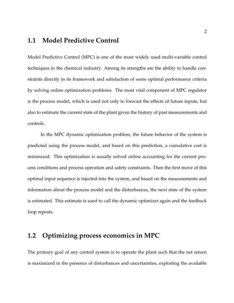
In the MPC dynamic optimization problem, the future behavior of the system is
predicted using the process model, and based on this prediction, a cumulative cost is
minimized. This optimization is usually solved online accounting for the current pro-
cess conditions and process operation and safety constraints. Then the first move of this
optimal input sequence is injected into the system, and based on the measurements and
information about the process model and the disturbances, the next state of the system
is estimated. This estimate is used to call the dynamic optimizer again and the feedback
loop repeats.
1.2 Optimizing process economics in MPC
The primary goal of any control system is to operate the plant such that the net return
is maximized in the presence of disturbances and uncertainties, exploiting the available
3
← Past
Inputs
Setpoint
Future→
u
k = 0
yOutputs
Figure 1.1: MPC strategy
measurements. In current practice, this this done in a two step process, where the pro-
cess economics are solved to obtain the economically best steady operating state called
the setpoint. Hence the economic objective is converted into control objective by means
of a steady-state optimization and the controller is designed such that these control ob-
jectives are tracked. Hence the controller generates a solution that will drive the system
to the economically best steady state. However in the process of converting the process
economic measure into steady-state setpoints, a lot of economic information is lost.
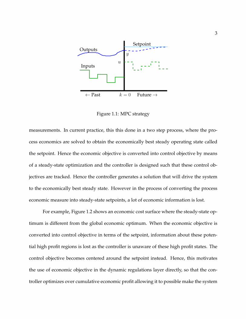
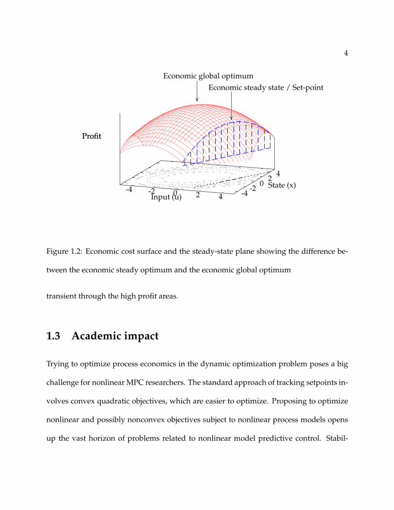
For example, Figure 1.2 shows an economic cost surface where the steady-state op-
timum is different from the global economic optimum. When the economic objective is
converted into control objective in terms of the setpoint, information about these poten-
tial high profit regions is lost as the controller is unaware of these high profit states. The
control objective becomes centered around the setpoint instead. Hence, this motivates
the use of economic objective in the dynamic regulations layer directly, so that the con-
troller optimizes over cumulative economic profit allowing it to possible make the system
4
-4 -2 0 2 4 -4-2
02
4
Profit
Economic steady state / Set-pointEconomic global optimum
Input (u)State (x)
Profit
Figure 1.2: Economic cost surface and the steady-state plane showing the difference be-
tween the economic steady optimum and the economic global optimum
transient through the high profit areas.
1.3 Academic impact
Trying to optimize process economics in the dynamic optimization problem poses a big
challenge for nonlinear MPC researchers. The standard approach of tracking setpoints in-
volves convex quadratic objectives, which are easier to optimize. Proposing to optimize
nonlinear and possibly nonconvex objectives subject to nonlinear process models opens
up the vast horizon of problems related to nonlinear model predictive control. Stabil-

5
ity properties have been well established for linear controllers but there is relatively less
literature on the theory of nonlinear MPC. In this thesis we throw light on some outstand-
ing issues in the stability theory of nonlinear MPC by identifying the class of systems for
which closed loop stability is expected. New tools for constructing a Lyapunov function
are introduced and asymptotic stability is established. A performance comparison is es-
tablished for nonsteady operation establishing the superiority of the economic optimizing
controllers.
1.4 Industrial impact
Process industries today thrive on the performance of advanced control systems. In a
competition based economy, most of the developments in advanced control applications
aim at better economic performance of the control system. In the present day two layer
approach, a lot of focus is on the real time optimization layer, which optimizes the process
economics under steady state assumption. A small gain in profit from a subsystem in a
plant translates into substantial profits for the whole plant. Hence improving economic
performance of the controller is highly attractive for process industries. In this thesis
we demonstrate the benefit of optimizing economics directly over tracking steady-state
setpoints by means of various examples from the literature.
Proposing to optimize process economics instead of tracking setpoints also opens
up the possibility of nonsteady operation, which even though might be unfavorable from
the operator’s perspective, but a possible significant economic advantage may motivate

6
to rethink the operational strategy of that process. In this thesis, we discuss some applica-
tions where nonsteady operation may be desirable and discuss possible ways to control
such operation.

7
1.5 Overview of the thesis
Chapter 2: Literature review
We review the literature used in this thesis and summarize all the previous research on
and related to optimizing process economics in dynamic regulation problems.
Chapter 3: Formulations and nominal stability theory
This chapter formulates present the fundamental nominal stability theory for nonlinear
systems subject to nonlinear costs. A class of systems is identified for which nominal
closed-loop stability is expected for the MPC feedback-control system. The tools for de-
termining Lyapunov functions are extended to this new class of systems and nominal
stability is established.
Chapter 4: Suboptimal control
Global optimality is hard to guarantee for nonlinear optimization problems. The nominal
stability theory is formulated in Chapter 3 based on the assumption that the global opti-
mum is determined for the dynamic regulation problem. This assumption is relaxed in
this chapter to establish the stability properties for suboptimal MPC algorithms.
Chapter 5: Nonsteady operation
This chapter discusses scenarios in which asymptotic stability is not expected and a non-
steady operation is economically better. A performance comparison is established for
such scenarios and two MPC algorithms are discussed for controlling such operations.

8
Chapter 6: Computational methods
Methods to numerically solve dynamic optimization problems are discussed in this chap-
ter. The direct methods for dynamic optimization are discussed in detail and the use of
these methods for the development of a software tool to solve dynamic regulation prob-
lems is presented. A brief manual of the new tool is presented in Appendix B.
Chapter 7: Case studies
Three case studies are presented to demonstrate the economic benefit of optimizing pro-
cess economics in the dynamic regulation layer. The performance is compared with the
tracking type controllers as a fraction of the steady state profit.
Chapter 8: Conclusions
The thesis concludes with a summary of contributions of this thesis and recommend some
research issues for future work.

9
Chapter 2
Literature Review
2.1 Introduction
The controllers proposed in this thesis are model predictive controllers. The theory of
model predictive control (MPC) has evolved a lot over the past three decades. Several
texts on MPC are available (Maciejowski, 2002; Camacho and Bordons, 2004; Rossiter,
2004; Wang, 2009). In particular, this thesis makes use of the monograph by Rawlings
and Mayne (2009) as a standard baseline reference. Rawlings and Mayne (2009, Ch. 2)
investigate the MPC regulation problem in detail. Two types of dynamic regulation for-
mulations are presented and the corresponding stability theory is developed for standard
convex costs. The monograph provides key control principles, such as dynamic regula-
tion stability theory and suboptimal MPC, used in this thesis.

10
2.2 Economics literature
The high level objective for any plant operation is to optimize an economic measure of
the plant, usually the net profit. Optimizing economics in control problems is not a new
concept. Even before extensive research on advanced process control systems, optimal
control problems have been common in economics literature. The earliest work on opti-
mal economic control problems dates back to 1920s (Ramsey, 1928), in which the objective
was to determine optimal savings rates to maximize capital accumulation. An array of
works followed in the 1950s focussing on various economic considerations like scarce re-
sources, expanding populations, multiple products and technologies. All the economic
optimal control problems in these works were infinite time horizon problems since they
tried to optimize based on long term predictions. Among these works was the popu-
lar concept of “turnpikes” (Dorfman, Samuelson, and Solow, 1958), which was used to
characterize the optimal trajectories for these economic control problems. Dorfman et al.
(1958, Ch. 12) were the first ones to introduce this concept, and proposed that in an econ-
omy, if planning a long-run growth, i.e. the planning horizon is sufficiently long, it is
always optimal to reach the optimial steady rate of growth and stay there for most of the
time, even if towards the end of the planning period, the growth needs to drop from the
steady value. This bevaiour, seen in econimics optimal control problems, was called the
“tunrpike” behavior since it was exactly like a turnpike paralleled by a network of minor
roads. Hence the asymptotic properties of efficient paths of capital accumulation were
known as “turnpike theorems.” (McKenzie, 1976). This literature provided the seed for

11
research on optimizing economic performance in the control literature. For infinite hori-
zon optimal control of continuous time systems, Brock and Haurie (1976) established the
existence of overtaking optimal trajectories. Convergence of these trajectories to an opti-
mal steady state is also demonstrated. Leizarowitz (1985) extended the results of (Brock
and Haurie, 1976) to infinite horizon control of discrete time systems. Reduction of the
unbounded cost, infinite horizon optimal control problem to an equivalent optimization
problem with finite costs is established. Carlson, Haurie, and Leizarowitz (1991) provide
a comprehensive overview of these infinite horizon results.
2.3 Real time optimization
In most industrial advanced control systems, the goal of optimizing dynamic plant eco-
nomic performance is addressed by a control structure that splits the problem into a num-
ber of levels (Marlin and Hrymak, 1997). The overall plant hierarchical planning and
operations structure is summarized in numerous books, for example Findeisen, Bailey,
Bryds, Malinowski, Tatjewski, and Wozniak (1980); Marlin (1995); Luyben, Tyreus, and
Luyben (1999). Planning focuses on economic forecasts and provides production goals. It
answers questions like what feed-stocks to purchase, which products to make and how
much of each product to make. Scheduling addresses the timing of actions and events
necessary to execute the chosen plan, with the key consideration being feasibility. The
planning and scheduling unit also provides parameters of the cost functions (e.g. prices
of products, raw materials, energy costs) and constraints (e.g. availability of raw mate-

12
rials). The RTO is concerned with implementing business decisions in real time based
on a fundamental steady-state model of the plant. It is based on a profit function of the
plant and it seeks additional profit based on real-time analysis using a calibrated non-
linear model of the process. The data are first analyzed for stationarity of the process
and, if a stationary situation is confirmed, reconciled using material and energy balances
to compensate for systematic measurement errors. The reconciled plant data are used to
compute a new set of model parameters (including unmeasured external inputs) such that
the plant model represents the plant as accurately as possible at the current (stationary)
operating point. Then new values for critical state variables of the plant are computed
that optimize an economic cost function while meeting the constraints imposed by the
equipment, the product specifications, and safety and environmental regulations as well
as the economic constraints imposed by the plant management system. These values are
filtered by a supervisory system that usually includes the plant operators (e.g. checked
for plausibility, mapped to ramp changes and clipped to avoid large changes (Miletic and
Marlin, 1996)) and forwarded to the process control layer as set points. When viewed
from the dynamic layer, these setpoints are often inconsistent and unreachable because
of the discrepancies between the models used for steady-state optimization and dynamic
regulation. Rao and Rawlings (1999) discuss methods for resolving these inconsistencies
and finding reachable steady-state targets that are as close as possible to the unreachable
setpoints provided by the RTO.
The two main disadvantages of the current two layer approach are:

13
• Models in the optimization layer and in the control layer are not fully consistent (Backx,
Bosgra, and Marquardt, 2000; Sequeira, Graells, and Puigjaner, 2002). It is pointed
out that, in particular, their steady-state gains may be different.
• The two layers have different time scales. The delay in optimization is inevitable
because of the steady-state assumption (Cutler and Perry, 1983).
Because of the disadvantages of long sampling times, several authors have proposed re-
ducing the sampling time in the RTO layer (Sequeira et al., 2002). In an attempt to narrow
the gap between the sampling rates of the nonlinear steady-state optimization performed
in the RTO layer and the linear MPC layer, the so called LP-MPC and QP-MPC two-stage
MPC structures have been suggested (Morshedi, Cutler, and Skrovanek, 1985; Yousfi and
Tournier, 1991; Muske, 1997; Brosilow and Zhao, 1988).
Engell (2007) reviews the developments in the field of feedback control for optimal
plant operations, in which the various disadvantages of the two layer strategy are pointed
out. Jing and Joseph (1999) perform a detailed analysis of this approach and analyze its
properties. The task of the upper MPC layer is to compute the setpoints both for the
controlled variables and for the manipulated inputs for the lower MPC layer by solving
a constrained linear or quadratic optimization problem, using information from the RTO
layer and from the MPC layer. The optimization is performed with the same sampling
period as the lower-level MPC controller.
Forbes and Marlin (1996); Zhang and Forbes (2000) introduce a performance mea-
sure for RTO systems to compare the actual profit with theoretic profit. Three losses were

14
considered as a part of the cost function: the loss in the transient period before the system
reaches a steady state, the loss due to model errors, and the loss due to propagation of
stochastic measurement errors. The issue of model fidelity is discussed by Yip and Marlin
(2004). Yip and Marlin (2003) proposed the inclusion of effect of setpoint changes on the
accuracy of the parameter estimates into the RTO optimization. Duvall and Riggs (2000)
evaluate the performance of RTO for Tennessee Eastman Challenge Problem and point
out “RTO profit should be compared to optimal, knowledgeable operator control of the
process to determine the true benefits of RTO. Plant operators, through daily control of
the process, understand how process setpoint selection affects the production rate and/or
operating costs.”
Kadam, Marquardt, Schlegel, Backx, Bosgra, Brouwer, Dunnebier, van Hessem,
Tiagounov, and de Wolf (2003) point out that the RTO techniques are limited with respect
to the achievable flexibility and economic benefit, especially when considering intention-
ally dynamic processes such as continuous processes with grade transitions and batch
processes. They also describe dynamics as the core of plant operation, motivating eco-
nomically profitable dynamic operation of processes.
2.4 Dynamic optimization of process economics
Morari, Arkun, and Stephanopoulos (1980) state that the objective in the synthesis of a
control structure is to translate the economic objectives into process control objectives. Backx
et al. (2000) describe the need for dynamic operations in the process industries in an in-

15
creasingly market-driven economy where plant operations are embedded in flexible sup-
ply chains striving for just-in-time production in order to maintain competitiveness. They
point out that minimizing operation cost while maintaining the desired product quality
in such an environment is considerably harder than in an environment with infrequent
changes and disturbances, and this minimization cannot be achieved by relying solely on
experienced operators and plant managers using their accumulated knowledge about the
performance of the plant. Profitable agile operations call for a new look at the integration
of process control with process operations.
Huesman, Bosgra, and Van den Hof (2007) point out that doing economic opti-
mization in the dynamic sense leaves some degrees of freedom of the system unused.
With the help of examples, it is shown that economic optimization problems can result in
multiple solutions suggesting unused degrees of freedom. It is proposed to utilize these
additional degrees of freedom for further optimization based on non-economic objectives
to get a unique solution.
2.4.1 Controller designs
Helbig, Abel, and Marquardt (2000) introduce the concept of a dynamic real time opti-
mization (D-RTO) strategy, in which, instead of doing a steady-state economic optimiza-
tion to compute setpoints, a dynamic optimization over a fixed horizon is done to com-
pute a reference trajectory. To avoid dynamic re-optimization, the regulator tracks the
reference trajectory using a simpler linear model (or PID controller) with the standard

16
tracking cost function, hence enabling the regulator to act at a faster sampling rate. When
using a simplified linear model for tracking a dynamic reference trajectory, an inconsis-
tency remains between the model used in the two layers. Often an additional disturbance
model would be required in the linear dynamic model to resolve this inconsistency. These
disturbance states would have to be estimated from the output measurements. Kadam
and Marquardt (2007) review the D-RTO strategy and improvements to it, and discuss
the practical considerations behind splitting the dynamic real-time optimization into two
parts. A trigger strategy is also introduced, in which D-RTO reoptimization is only in-
voked if predicted benefits are significant, otherwise linear updates to the reference tra-
jectory are provided using parametric sensitivity techniques.
Skogestad (2000) describes one approach to implement optimal plant operation by
a conventional feedback control structure, termed “self-optimizing” control. In this ap-
proach, the feedback control structure is chosen so that maintaining some function of
the measured variables constant automatically maintains the process near an economi-
cally optimal steady state in the presence of disturbances. The problem is posed from
the plantwide perspective, since the economics are determined by overall plant behavior.
Aske, Strand, and Skogestad (2008) also point out the lack of capability in steady-state
RTO, in the cases when there are frequent changes in active constraints of large economic
importance. The important special case is addressed in which prices and market condi-
tions are such that economic optimal operation of the plant is the same as maximizing
plant throughput. A coordinator model predictive control strategy is proposed in which

17
a coordinator controller regulates local capacities in all the units.
Sakizlis, Perkins, and Pistikopoulos (2004) describe an approach of integrating op-
timal process design with process control. They discuss integration of process design,
process control and process operability together, and hence deal with the economics of
the process. The incorporation of advanced optimizing controllers in simultaneous pro-
cess and control design is the goal of the optimization strategy. It deals with an offline
control approach where an explicit optimizing control law is derived for the process. The
approach is reported to yield a better economic performance.
Extremum-seeking control is another approach in which the controller drives the
system states to steady values that optimize a chosen performance objective. Krstic and
Wang (2000) address closed-loop stability of the general extremum-seeking approach
when the performance objective is directly measured online. Guay and Zhang (2003)
address the case in which the performance objective is not measurable and available for
feedback. This approach has been evaluated for temperature control in chemical reactors
subject to state constraints (Guay, Dochain, and Perrier, 2003; DeHaan and Guay, 2004).
awrynczuk, Marusak, and Tatjewski (2007) propose two versions of the integrated
MPC and set-point calculation algorithms. In the first one, the nonlinear steady-state
model is used. This leads to a nonlinear optimization problem. In the second version, the
model is linearized on-line. It leads to a quadratic programming problem, which can be
effectively solved using standard routines. In both these problems, the economic objective
used in the steady-state optimization as well as the dynamic optimization is either linear

18
or quadratic in the outputs and inputs.
Heidarinejad, Liu, and Christofides (2011b,a) propose an economic MPC scheme
based on explicit Lyapunov-based nonlinear controller design techniques that allows for
an explicit characterization of the stability region of the closed-loop system. The under-
lying assumption for this design is the existence of a Lyapunov-based controller which
renders the origin of the nominal closed-loop system asymptotically stable. Hence the
methodology assumes that a control law is known such that some corresponding Lya-
punov function has a negative gradient in time. The authors point out that there are
currently no general methods for constructing Lyapunov functions for generic nonlinear
systems, and bases on previous results, use a quadratic controller and a quadratic Lya-
punov function. A two-tier controller approach is proposed in this paper. In the first
mode, the controller drives the system optimizing the economic performance measure
subject to the states of the system remaining inside a defined stability region. The sta-
bility region is defined as a level set of the chosen Lyapunov function such that it is the
largest subset of the neighborhood of the equilibrium point in which a Lyapunov based
controller can be defined. A terminal time is chosen for this first mode and after this time,
an additional constraint is turned on, which is the second mode. In this second mode,
an additional constraint ensures that the chosen Lyapunov function decreases at least at
the rate given by the Lyapunov based controller. The paper is a direct extension on the
authors’ previous work (Mhaskar, El-Farra, and Christofides, 2006). Heidarinejad et al.
(2011b) extended the approach to account for bounded disturbances and asynchronous

19
delayed measurements.
Huang, Harinath, and Biegler (2011b) point out applications like simulated mov-
ing bed (SMB) and pressure swing adsorption (PSA) in which non-steady operation is
desirable due to economic benefit and the design of the process. They provide a nonlin-
ear MPC scheme for cyclic processes for which the period of the process is known. They
present two different formulations. In the first formulation, a finite horizon problem is
formulated with the horizon chosen as a multiple of the process period. A terminal pe-
riodic constraint is implemented which forces the state at the end of the horizon to be
the same as one period before the end of the horizon. The second formulation is an infi-
nite horizon formulation. To deal with the infinite sum of an economically oriented cost,
a discount factor is used to project the future profit. There is no terminal periodic con-
straint since the problem is infinite dimensional. Both the formulations are assumed to
satisfy optimality conditions to assume local uniqueness of the solution, and regulariza-
tion tracking terms are added to the economic stage cost to satisfy these assumptions.
Hence the objective is not purely economic. Asymptotic stability is proved for both the
controllers by proposing the optimal value of the shifted cost as the Lyapunov function
for the system. Huang, Biegler, and Harinath (2011a) extend the concept of concept of
rotated cost, introduced in this thesis and Diehl, Amrit, and Rawlings (2011), and extend
it to the framework of cyclic systems. The authors propose a requirement of convexity
on the rotated cost to ensure closed loop stability. The nominal stability results are then
extended to robust stability using the standard Input-to-State stability framework.

20
2.4.2 Implementation and applications
Zanin, Tvrzska de Gouvea, and Odloak (2000, 2002); Rotava and Zanin (2005) report
the formulation, solution and industrial implementation of a combined MPC/optimizing
control scheme for a fluidized bed catalytic cracker. The economic criterion is the amount
of liquified petroleum gas produced. The optimization problem that is solved in each con-
troller sampling period is formulated in a mixed manner: range control MPC with a fixed
linear plant model (imposing soft constraints on the controlled variables by a quadratic
penalty term that only becomes active when the constraints are violated) plus a quadratic
control move penalty plus an economic objective that depends on the values of the ma-
nipulated inputs at the end of the control horizon.
Ma, Qin, Salsbury, and Xu (2011) demonstrate the effectiveness of model predictive
control (MPC) technique in reducing energy and demand costs, which form the objective
of the controller, for building heating, ventilating, and air conditioning (HVAC) systems.
A simulated multi-zone commercial building equipped with a set of variable air volume
(VAV) cooling system is studied. System identification is performed to obtain zone tem-
perature and power models, which are used in the MPC framework. The economic ob-
jective function in MPC accounts for the daily electricity costs, which include time of use
energy cost and demand cost. In each time step, a min-max optimization is formulated,
converted into a linear programming problem and solved. Cost savings by MPC are esti-
mated by comparing with the baseline and other open-loop control strategies.

21
Chapter 3
Formulations and nominal stability
theory
Note: The text of this chapter appears in Angeli, Amrit, and Rawlings (2011a); Amrit
et al. (2011).
3.1 Introduction
The dynamic optimization problem in model predictive control can be formulated in two
different ways, depending on the choice of objective function and the stabilizing con-
straints, as discussed in detail by Rawlings and Mayne (2009, Ch. 2). In the standard MPC
problem, in which the stage cost is defined as the deviation from the best steady state, the
stability of the closed-loop system is established by observing that the optimal cost along
the closed-loop trajectory is a Lyapunov function. In the economic MPC problem the op-
timal cost is not a Lyapunov function. In this chapter we present the model predictive

22
control formulations using a generic nonlinear economic objective. In Section 3.2, we first
introduce our basic notation and definitions that will be used in developing the theory in
this chapter and the rest of the thesis. We present the terminal constraint and the terminal
penalty MPC formulations in Section 3.3 and Section 3.4 respectively, and state and prove
the respective stability properties of these formulations. In Section 3.5 we propose a third
formulation in which the stabilizing constraint is removed. The performance of the three
formulations is then compared with each other and with the steady state performance.
3.2 Preliminaries and Definitions
We first establish the notation that defines the dynamic nonlinear system and the eco-
nomic cost function. Consider the following nonlinear discrete time system
x+ = f(x, u) (3.1)
with state x ∈ X ⊆ Rn, control u ∈ U ⊂ Rm, and state transition map f : Z → Rn, where
the system is subject to the mixed constraint
(x(k), u(k)) ∈ Z k ∈ I≥0
for some compact set Z ⊆ X × U. We consider a cost function `(x, u) : Z → R, which is
based on the process economics. Consider the following steady-state problem
min(x,u)∈Z
`(x, u) subject to x = f(x, u) (3.2)

23
The solution of the steady-state problem is denoted by (xs, us), and is assumed to be
unique. We now review some important definitions that will be used in the theory devel-
oped in the chapter and rest of the thesis.
Definition 3.1 (Positive definite function). A function ρ(·) is positive definite with respect to
x = a if it is continuous, ρ(a) = 0, and ρ(x) > 0 for all x 6= a.
Definition 3.2 (Class K function). A function γ(·) : R → R≥0 is a class K if it is continuous,
zero at zero and strictly increasing.
Lemma 3.3. Given a positive definite function ρ(x) defined on a compact set C containing the
origin, there exists a class K function γ(·) such that
ρ(x) ≥ γ(|x|), ∀x ∈ C
Definition 3.4 (Positive invariant set). A set A is positive invariant for the nonlinear system
x+ = f(x), if x ∈ A implies x+ ∈ A.
Definition 3.5 (Asymptotic stability). The steady state xs of a nonlinear system x+ = f(x)
is asymptotically stable on X , xs ∈ X , if there exist a class K function γ(·) such that for any
x ∈ X , all solutions φ(k;x) satisfy:
φ(k;x) ∈ X , |φ(k;x)− xs| ≤ γ(|x− xs| , k) for all k ∈ I≥0.
Definition 3.6 (Lyapunov function). A function V : Rn → R≥0 is said to be a Lyapunov
function for the nonlinear system x+ = f(x) in the set X if there exist class K functions γi,

24
i ∈ 1, 2, 3 such that for any x ∈ X
γ1(|x|) ≤ V (x) ≤ γ2(|x|) V (f(x))− V (x) ≤ −γ3(|x|)
Lemma 3.7 (Lyapunov function and asymptotic stability). Consider a set X , that is positive
invariant for the nonlinear system x+ = f(x); f(xs) = xs. The steady state xs is an asymp-
totically stable equilibrium point for the system x+ = f(x) on X , if and only if there exists a
Lyapunov function V on X such that V (x− xs) satisfies the properties in Definition 3.6.
Definition 3.8 (Strictly dissipative system). The system x+ = f(x, u) is strictly dissipative
with respect to the supply rate s : Z → R if there exists a storage function λ : X → R and a
positive definite function ρ : Z→ R≥0, such that for all (x, u) ∈ Z ⊆ X × U
λ(f(x, u))− λ(x) ≤ −ρ(x− xs, u− us) + s(x, u) (3.3)
Next we introduce the concept of rotated cost which forms the backbone of the sta-
bility theory of economic nonlinear MPC.
3.2.1 Rotated cost
Unlike the standard MPC problem, the optimal cost along the closed loop, may not be a
Lyapunov function for the nonlinear system. Hence we introduce a modified stage cost,
which we call the ’rotated cost’. To define the rotated cost, we first make the following
assumptions:

25
Assumption 3.9 (Dissipative system). The nonlinear system x+ = f(x, u) is dissipative with
respect to the supply rate s(x, u) = `(x, u)− `(xs, us).
Assumption 3.10 (Continuity of cost, system and storage). The cost `(·), the system dynam-
ics function f(·), and the storage function λ(·) are continuous on Z.
We define the rotated stage cost L(x, u) : Z→ R≥0 as a function of the economic stage
cost `(·), and the corresponding storage function λ(·):
L(x, u) := `(x, u) + λ(x)− λ(f(x, u))− `(xs, us) (3.4)
Let Assumptions 3.9–3.10 hold. Then the rotated cost has the following properties
1. Steady-state solution: Consider the following steady-state problem
min(x,u)∈Z
L(x, u) subject to x = f(x, u) (3.5)
Problems (3.2) and (3.5) have the same solution (xs,us).
2. Lower bound: The dissipation inequality (3.3) implies that the rotated stage cost
L(x, u) ≥ ρ(x − xs, u − us) for all (x, u) ∈ Z and hence can be underbounded by a
class K function (Lemma 3.3).
L(x, u) ≥ γ(|(x− xs, u− us)|) ≥ γ(|x− xs|) ≥ 0, ∀(x, u) ∈ Z (3.6)
3.3 Terminal constraint formulation
We now formulate the terminal constraint MPC formulation in which the nonlinear sys-
tem is stabilized by means of an equality constraint on the terminal state.
26
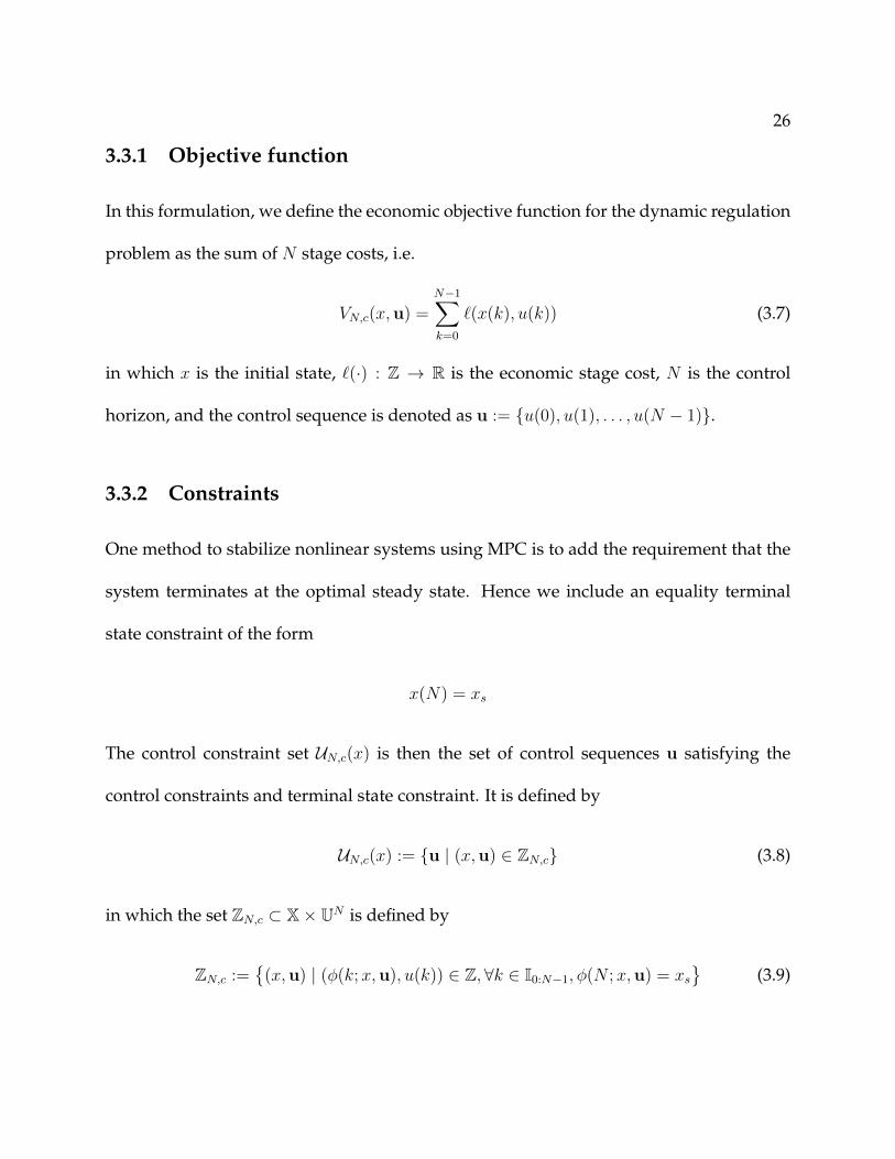
3.3.1 Objective function
In this formulation, we define the economic objective function for the dynamic regulation
problem as the sum of N stage costs, i.e.
VN,c(x,u) =N−1∑k=0
`(x(k), u(k)) (3.7)
in which x is the initial state, `(·) : Z → R is the economic stage cost, N is the control
horizon, and the control sequence is denoted as u := u(0), u(1), . . . , u(N − 1).
3.3.2 Constraints
One method to stabilize nonlinear systems using MPC is to add the requirement that the
system terminates at the optimal steady state. Hence we include an equality terminal
state constraint of the form
x(N) = xs
The control constraint set UN,c(x) is then the set of control sequences u satisfying the
control constraints and terminal state constraint. It is defined by
UN,c(x) := u | (x,u) ∈ ZN,c (3.8)
in which the set ZN,c ⊂ X× UN is defined by
ZN,c :=
(x,u) | (φ(k;x,u), u(k)) ∈ Z,∀k ∈ I0:N−1, φ(N ;x,u) = xs
(3.9)

27
where φ(k;x,u) is the solution to (3.1) at time k ∈ I0:N for initial state x and control
sequence u. The set of admissible states XN,c is defined as the projection of ZN,c onto X.
XN,c = x ∈ X | ∃u such that (x,u) ∈ ZN,c
3.3.3 Stability
We now propose a candidate Lyapunov function and establish asymptotic stability of the
nonlinear system driven by the terminal constraint MPC. We first make the following
assumptions
Assumption 3.11 (Weak controllability). There exists γ of classK∞ such that for each x ∈ XN,c
there exists a feasible u, with
|u− [us, . . . , us]′| ≤ γ(|x− xs|)
Candidate Lyapunov function
With the rotated stage cost as defined in (3.4), we define the rotated regulator cost function
as follows
V N,c(x,u) :=N−1∑k=0
L(x(k), u(k)) (3.10)
The standard and auxiliary nonlinear optimal control problems PN,c(x) and PN,c(x) are
PN,c(x) : V 0N,c(x) := min
uVN,c(x,u) | u ∈ UN,c(x)
PN,c(x) : V0
N,c(x) := minuV N,c(x,u) | u ∈ UN,c(x)

28
Due to Assumptions 3.10, both VN,c(·) and V N,c(·) are defined and continuous on the set
UN,c. Since the set Z is compact, the set UN,c(x) is compact for all x ∈ XN,c. Hence solutions
exist for both problems PN,c(x) and PN,c(x) for x ∈ XN,c. As we shall establish later, the
two problems have identical solution sets. Denote the optimal solution of these problems
as
u0(x) = u0(0;x), u0(1;x), · · · , u0(N − 1, x) (3.11)
In MPC, the control applied to the plant is the first element of the optimal control se-
quence, yielding the implicit MPC control law κN,c(·) defined as
κN,c(x) = u0(0;x)
Then the close loop system evolves according to
x+ = f(x, κN,c(x)) (3.12)
We propose V0
N,c(x) as the candidate Lyapunov function for the system under the control
law κN,c(x).
Proposition 3.12 (Equivalence of solutions). The solution sets for PN,c(x) and PN,c(x) are
identical.
Proof. Expanding the rotated regulator cost function gives
V N,c(x,u) =N−1∑k=0
L(x(k), u(k))
=N−1∑k=0
(`(x(k), u(k))− `(xs, us)) +N−1∑k=0
(λ(x(k))− λ(f(x(k), u(k))))
= VN,c(x,u) + λ(x)− λ(xs)−N`(xs, us)

29
Since λ(x), λ(xs) and N`(xs, us) are independent of the decision variable vector u, the two
objective functions V N,c and VN,c differ by terms which are constant for a given initial state
x, and hence the two optimization problems PN,c(x) and PN,c(x) have the same solution
sets.
Theorem 3.13 (Asymptotic stability). If Assumptions 3.9, 3.10 and 3.11 hold, then the steady-
state solution xs is an asymptotically stable equilibrium point of the nonlinear system (3.12) with
a region of attraction XN,c.
Proof. Consider the rotated cost function (3.10)
V N,c(x,u) =N−1∑k=0
L(x(k), u(k)), x ∈ XN,c
The candidate Lyapunov function for the problem is V0
N,c(x) = V N,c(x,u0(x)), where
u0(x) is the optimal control sequence as defined in (3.22). The resulting optimal state se-
quence is x0(x) = x0(0;x), x0(1;x), . . . , x0(N ;x). We choose a candidate input sequence
and a corresponding state sequence as follows
u(x) = u0(1;x), u0(2;x), . . . , u0(N − 1;x), us)
x(x) =x0(1;x), x0(2;x), . . . , x0(N ;x), xs)
Due to the terminal state constraint, x0(N ;x) = xs, and hence x0(N + 1;x) = xs. For all
x ∈ XN,c, the definition of V N,c(·) gives
V N,c(x+,u) =
N−1∑k=1
L(x0(k;x), u0(k;x)) + L(xs, us)
= V0
N,c(x)− L(x, u0(0;x))

30
Since V0
N,c(x+) ≤ V N,c(x
+,u), it follows that
V0
N,c(x+)− V 0
N,c(x) ≤− L(x, u0(0;x))
≤− γ(|x− xs|) using (3.6)
We also observe that due to (3.6):
V0
N,c(x) ≥ L(x, u(0)) ≥ γ(|x− xs|), x ∈ XN,c
Also using Assumption 3.11, it can be shown that V0
N,c(x) ≤ γ(|x− xs|) for all x ∈ XN,c,
where γ(|x− xs|) is a class K function. Hence V0
N,c is a Lyapunov function and xs is an
asymptotically stable equilibrium point of (3.12) with a region of attraction XN,c.
Hence we have established nominal asymptotic stability for the nonlinear system
under the terminal constraint MPC.
3.4 Terminal penalty/control formulation
Having a terminal equality constraint in the problem can be a demanding constraint,
especially if the control horizon is short. Equality constraints, in general, makes the non-
linear optimization problem, hard to solve for the NLP solver In this section we propose
the terminal control MPC formulation, which attempts to relax the terminal equality con-
straint as used in the previous formulation, and replace it with a terminal state penalty
and a terminal region pair.
31
3.4.1 Objective function
The economic objective function for the dynamic regulation problem in the terminal
penalty formulation is defined as the sum of N stage costs and a penalty cost on the
terminal state
VN,p(x,u) =N−1∑k=0
`(x(k), u(k)) + Vf (x(N)) (3.13)
in which x is the initial state, `(·) : Z → R is the economic stage cost, Vf (·) : Xf → R is
the terminal penalty, where Xf ⊆ X is a compact terminal region containing the steady-
state operating point in its interior, N is the control horizon, and the control sequence is
denoted as u := u(0), u(1), . . . , u(N − 1).
3.4.2 Constraints
For nonlinear models, one often can define Xf in which a control Lyapunov function is
available (Rawlings and Mayne, 2009, Ch. 2). The second method to stabilize nonlinear
systems using MPC is to add the requirement that the terminal state lie in this terminal
region, instead of at the best steady state xs. Hence we include a terminal state constraint
of the form
x(N) ∈ Xf
The standard control constraint set UN,p(x) is then the set of control sequences u
satisfying the control constraints and terminal state constraint. It is defined by
UN,p(x) := u | (x,u) ∈ ZN,p (3.14)

32
in which the set ZN,p ⊂ X× UN is defined by
ZN,p :=
(x,u) | (φ(k;x,u), u(k)) ∈ Z,∀k ∈ I0:N−1, φ(N ;x,u) ∈ Xf
(3.15)
where φ(k;x,u) is the solution to (3.1) at time k ∈ I0:N for initial state x and control
sequence u. The set of admissible states XN,p is defined as the projection of ZN,p onto X.
XN,p = x ∈ X | ∃u such that (x,u) ∈ ZN,p
3.4.3 Stability
Similar to the terminal constraint formulation presented in Section 3.3, we propose a Lya-
punov function for the closed loop system to establish closed-loop stability. We make the
following assumptions.
Assumption 3.14 (Stability assumption). There exists a compact terminal region Xf ⊆ X,
containing the point xs in its interior, and control law κf : Xf → U, such that the following holds
Vf (f(x, κf (x))) ≤ Vf (x)− `(x, κf (x)) + `(xs, us), ∀x ∈ Xf (3.16)
This assumption requires that for each x ∈ Xf , f(x, κf (x)) ∈ Xf , i.e. the set Xf is control
invariant under control law u = κf (x).
Remark 3.15. Since Assumption 3.14 is the only requirement on Vf , we can assume Vf (xs) = 0
without loss of generality. It should be noted that unlike the standard MPC problem, Vf (x) is not
necessarily positive definite with respect to xs.

33
Candidate Lyapunov function
For ease of notation, we first define the shifted stage cost as following
`(x, u) = `(x, u)− `(xs, us) (3.17)
Next we define the rotated terminal cost in the region (x, u) ∈ Z. Correspondingly we
define the rotated regulator cost function.
V f (x) := Vf (x) + λ(x)− Vf (xs)− λ(xs) (3.18)
V N,p(x,u) :=N−1∑k=0
L(x(k), u(k)) + V f (x(N)) (3.19)
The standard and auxiliary nonlinear optimal control problems PN,p(x) and PN,p(x) are
PN,p(x) : V 0N,p(x) := min
uVN,p(x,u) | u ∈ UN,p(x) (3.20)
PN,p(x) : V0
N,p(x) := minuV N,p(x,u) | u ∈ UN,p(x) (3.21)
Due to Assumption 3.10, both VN,p(·) and V N,p(·) are defined and continuous on the set
UN,p. Since the set Z is compact, the set UN,p(x) is compact for all x ∈ XN . Hence solutions
exist for both problems PN,p(x) and PN,p(x) for x ∈ XN . As we shall establish later, the
two problems have identical solution sets. Denote the optimal solution of these problems
as
u0(x) = u0(0;x), u0(1;x), · · · , u0(N − 1, x) (3.22)
In MPC, the control applied to the plant is the first element of the optimal control se-
quence, yielding the implicit MPC control law κN,p(·) defined as
κN,p(x) = u0(0;x)

34
Then the close loop system evolves according to
x+ = f(x, κN,p(x)) (3.23)
We propose V0
N,p(x) as the candidate Lyapunov function for the system under the control
law κN,p(x).
Properties of the rotated costs
We now present some interesting properties of the rotated stage and terminal costs de-
fined above and use them later in the stability analysis of the terminal penalty controller.
Lemma 3.16 (Modified terminal cost). The pair (V f (·), L(·)) satisfies the following property if
and only if (Vf (·), `(·)) satisfies Assumption 3.14.
V f (f(x, κf (x))) ≤ V f (x)− L(x, κf (x)) ∀x ∈ Xf (3.24)
Proof. Adding λ(f(x, κf (x))) + λ(x) to both sides of (3.16) and rearranging gives the de-
sired inequality
V f (f(x, κf (x)))− V f (x) ≤−(`(x, κf (x)) + λ(x)−
λ(f(x, κf (x)))− `(xs, us))
=− L(x, κf (x))

35
Lemma 3.17. If Assumptions 3.9, 3.10 and 3.14 hold, then the rotated terminal cost V f (x) defined
by (3.18) is positive definite on Xf with respect to x = xs.
Proof. From Assumption 3.10, V f (·) is continuous on Xf and from (3.18), V f (xs) = 0.
Next we show V f (x) > 0 for x ∈ Xf , x 6= xs. Let x(x;κf ) and u(x;κf ) denote the state
and control sequences starting from x ∈ Xf and using the control law u = κf (x), defined
in Assumption 3.14, in the closed-loop system x+ = f(x, κf (x)). Consider the sequence
V f (x(k;x, κf )), k ∈ I≥0, which satisfies for all k ∈ I≥0 by (3.24)
V f (x(k + 1;x, κf ))− V f (x(k;x, κf )) ≤ −L(x(k;x, κf ), u(k;x, κf )) (3.25)
From (3.6) we have that the sequence V f (x(k;x, κf )) is nonincreasing with k. It is
bounded below since V f (·) is continuous and Xf is compact. Therefore, the sequence
converges and L(x(k;x, κf ), u(k;x, κf ))→ 0 as k →∞, and, from (3.6), x(k;x, κf )→ xs as
k → ∞. Since V f (·) is continuous and V f (xs) = 0, we also have that Vf (x(k;x, κf )) → 0
as k →∞. Summing (3.25) for k ∈ I0:M−1 gives
V f (x) ≥M−1∑k=0
L(x(k;x, κf ), u(k;x, κf )) + V f (x(M ;x, κf ))
Taking the limit as M →∞ gives
V f (x) ≥∞∑k=0
L(x(k;x, κf ), u(k;x, κf ))
By (3.6), L(x, κf (x) > 0 for x 6= xs, so we have established that V f (x) > 0 for x ∈ Xf , x 6= xs
and the proof is complete.
36
Lemma 3.18 (Rawlings and Mayne (2011)). Let a function V (x) be defined on a set X , which
is a closed susbset of Rn. If V (·) is continuous at the origin and V (0) = 0, then there exists a class
K function α(·) such that
V (x) ≤ α(|x|), ∀x ∈ X
Lemma 3.19 (Bounds on the rotated terminal cost). If Assumptions 3.9, 3.10 and 3.14 hold,
the rotated terminal cost V f (x) satisfies
γ(|x− xs|) ≤ V f (x) ≤ γ(|x− xs|), ∀x ∈ Xf
in which functions γ(·), γ(·) are class K.
Proof. The lower bound follows from (3.24) and (3.6) and Lemma 3.17. For the upper
bound, from Assumption 3.10 and Lemma 3.18 it follows that
V f (x) ≤ γ(|x− xs|), ∀x ∈ Xf
which completes the proof.
Lemma 3.20 (Equivalence of solutions). Let Assumptions 3.10 and 3.14 hold. The solution
sets for PN,p(x) and PN,p(x) are identical.

37
Proof. Expanding the rotated regulator cost function gives
V N,p(x,u) =N−1∑k=0
L(x(k), u(k)) + V f (x(N))
=N−1∑k=0
`(x(k), u(k)) + Vf (x(N))− Vf (xs)− λ(xs)+
N−1∑k=0
(λ(x(k))− λ(f(x(k), u(k)))− `(xs, us)) + λ(x(N))
=VN,p(x,u) + λ(x)− λ(x(N)) + λ(x(N))−
Vf (xs)− λ(xs)−N`(xs, us)
=VN,p(x,u)−N`(xs, us) + λ(x)− λ(xs)− Vf (xs)
Since λ(x), λ(xs), Vf (xs) and N`(xs, us) are independent of the decision variable vector
u, the two objective functions V N,p and VN,p differ by terms that are constant for a given
initial state x, and hence the two optimization problems PN,p(x) and PN,p(x) have the same
solution sets.
Theorem 3.21. Let Assumptions 3.9, 3.10 and 3.14 hold. Then the steady-state solution xs is an
asymptotically stable equilibrium point of the nonlinear system (3.23) with a region of attraction
XN,p.
Proof. Consider the rotated cost function (3.19)
V N,p(x,u) =N−1∑k=0
L(x(k), u(k)) + V f (x(N)), x ∈ XN
The candidate Lyapunov function for the problem is V0
N,p(x) = V N,p(x,u0p(x)), where
u0p(x) is the optimal control sequence as defined in (3.22). The resulting optimal state se-
quence is x0p(x) =
x0p(0;x), x0
p(1;x), . . . , x0p(N ;x)
. We choose a candidate input sequence

38
and a corresponding state sequence as follows
u(x) = u0p(1;x), u0
p(2;x), . . . , u0p(N − 1;x), κf (x
0(N ;x))) (3.26)
x(x) =x0p(1;x), x0
p(2;x), . . . , x0p(N ;x), x0
p(N + 1;x))
(3.27)
where x0p(N+1;x) = f(x0
p(N ;x), κf (x0p(N ;x)). Due to the terminal state constraint, x0
p(N ;x) ∈
Xf , and hence x0p(N + 1; x) ∈ Xf due to the invariance property of Xf (Assumption 3.14).
For all x ∈ XN , the definition of V N,p(·) gives
V N,p(x+,u) =
N−1∑k=1
L(x0p(k;x), u0
p(k;x))+
L(x0p(N, x), κf (x
0p(N ;x))) + V f (x
0p(N + 1;x))
=V0
N(x)− L(x, u0p(0;x)) + L(x0
p(N, x), κf (x0p(N ;x)))−
V f (x0p(N ;x)) + V f (x
0p(N + 1;x))
≤V 0
N(x)− L(x, u0p(0;x)), (from Lemma 3.16)
Since V0
N,p(x+) ≤ V N,p(x
+,u), it follows that
V0
N,p(x+)− V 0
N,p(x) ≤− L(x, u0p(0;x)) (3.28)
≤− γ(|x− xs|) using (3.6)
Due to Lemmas 3.16 and 3.19, γ(|x− xs|) ≤ V0
N,p(x) ≤ γ(|x− xs|) for all x ∈ XN (Rawl-
ings and Mayne, 2009, Propositions 2.17 and 2.18), where γ(|x− xs| is a class K function.
Hence V0
N,p is a Lyapunov function and xs is an asymptotically stable equilibrium point
of (3.23) with a region of attraction XN .

39
Hence we have established nominal asymptotic stability of the nonlinear system
under terminal penalty/control formulation.
3.4.4 Terminal cost prescription
Finding terminal cost function Vf (·) and region Xf that satisfy the stability assumption
(Assumption 3.14) is not obvious for generic costs and nonlinear systems. The most com-
mon case of positive, quadratic cost is addressed in Rawlings and Mayne (2009, Sec. 2.5).
In this section we propose candidate terminal cost functions Vf (·) that satisfy (3.16) inside
well-defined terminal region Xf .
For notational simplicity, in the following discussion we shift the origin to (xs, us),
i.e., the optimal steady state of the system. Similarly, we shift the origin of the sets X, U,
Z, and Xf . We make the following assumption.
Assumption 3.22. The functions f(·) and `(·) are twice continuously differentiable on Rn×Rm,
and the linearized system x+ = Ax+Bu, where A := fx(0, 0) and B := fu(0, 0), is stabilizable.
We choose any controller u = Kx such that the origin is exponentially stable for
the system x+ = AKx,AK := A + BK. Such a K exists since (A,B) is stabilizable. The
following establishes the existence of the invariant set required for Assumption 3.14.
In the standard case, where `(·) is positive definite, one chooses Xf to be a level
set of Vf (·) to inherit control invariance from (3.16). In economic case, `(·) is not positive
definite and hence we use the control invariant set defined in the following way:

40
Lemma 3.23 (Control invariant set for f(·) (Rawlings and Mayne, 2009)). Let Assumption
3.22 hold and consider K such that A + BK is stable. Then there exist matrices P > 0, Q > 0,
and scalar b > 0, such that the following holds for all b′ ≤ b
V (f(x,Kx))− V (x) ≤ −(1/2)x′Qx, ∀x ∈ levb′V
in which V (x) := (1/2)x′Px.
Proof. This result is established in (Rawlings and Mayne, 2009, pp.136–137).
Remark 3.24. From Lemma 3.23 we have the existence of a family of nested ellipsoidal neigh-
borhoods of the origin, levb′V , with b′ ≤ b, and each member of the family (corresponding to a
b′ value) is control invariant for the nonlinear system x+ = f(x, u) under the linear control law
u = Kx.
We next classify the function Vf (·) based on whether or not a storage function λ(·)
is known for the system (Assumption 3.9.)
Prescription 1: Storage function λ(·) unknown
The ideal choice for Vf (x) satisfying (3.16), is the infinite horizon shifted cost to go for the
optimal nonlinear control law κf (x). Since there are no generic ways to know the nature
of this nonlinear control law, we chose the linear control law u = Kx defined above, and
compute the cost to go based on this choice.
Vf (x) =∞∑k=0
`(x,Kx), x+ = AKx, x(0) = 0

41
One can immediately see this choice of Vf satisfies (3.16). In general the summability of
the above infinite sum is not guaranteed. For special cases like quadratic costs, the infinite
sum can be analytically computed. But for most cases, in which the above sum cannot be
explicitly determined, we propose ways to compute a terminal penalty satisfying (3.16)
in the following sections. If the above infinite sum can be determined, one can use the
invariant region Xf = levb′V as the desired terminal region.
Prescription 2: Storage function λ(·) unknown
Note: The results of this section are taken from Amrit et al. (2011).
We now construct a Vf (·) without knowledge of λ(·).
Lemma 3.25. Let Assumption 3.22 hold and let `(x) := `(x,Kx) − `(0, 0). Then there exists
matrix Q? such that for any compact set C ⊂ Rn
x′(Q? − `xx(x)
)x ≥ 0, ∀x ∈ C
Proof. Let λi(`xx(x)), i ∈ I1:n denote the real-valued eigenvalues of symmetric matrix
`xx(x), which depends on x. The eigenvalues are continuous functions of the elements
of the matrix (Horn and Johnson, 1985, p.540), and the elements of the matrix `xx(x) are
continuous functions of x on C by Assumption 3.22, so the following optimization prob-
lem has a solution
λ? = maxx,i
λi(`xx(x)) | x ∈ C, i ∈ I1:n

42
for an arbitrary Hermitian matrixH , x′Hx ≤ λmx′x for all x ∈ Rn, where λm = maxi(λi(H))
(Horn and Johnson, 1985, p.176). Hence we conclude that λ?x′x ≥ x′`xx(x)x for all x ∈ C.
Define Q? as the diagonal matrix Q? := λ?In. We have
x′Q?x = λ?x′x ≥ x′`xx(x)x, ∀x ∈ C
Next we define the quadratic cost function `q(x) := (1/2)x′Qx+ q′x.
Lemma 3.26. Let Assumption 3.22 hold. Choose matrices (Q, q) such that q := `x(0, 0) and
Q := Q? + αI , with Q? defined in Lemma 3.25 and α ∈ R. Then `q(x) ≥ `(x) + (α/2)x′x for all
x ∈ X and α ∈ R.
Proof. Choose compact set C in Lemma 3.25 to be convex and contain X, which is possible
since X is bounded. Then we have that if x ∈ C, sx ∈ C for s ∈ [0, 1]. From Proposition
A.11 (b) (Rawlings and Mayne, 2009), we have that for all x ∈ C
`q(x)− `(x) = (q − `x(0, 0))′x+∫ 1
0
(1− s)x′(Q− `xx(sx)
)xds
=
∫ 1
0
(1− s)x′(Q? − `xx(sx) + αI
)xds
≥ (α/2)x′x
Since X ⊆ C, the inequality holds on X and the result is established.

43
We define the candidate Vf (x) as follows
Vf (x) :=∞∑k=0
`q(x(k)), x+ = AKx, x(0) = x
= (1/2)x′Px+ p′x (3.29)
where Q and q are selected as in Lemma 3.26 with α > −λ? so that Q > 0. Hence P is the
solution to the Lyapunov equation A′KPAK − P = −Q and p = (I −AK)−T q. Note that P
depends on the parameter α. In fact,
P = P ∗ + αPI
in which P ∗ and PI satisfy the Lyapunov equations A′KP∗AK−P ∗ = −Q∗ and A′KP
∗AK−
P ∗ = −I , respectively.
Next we establish that there exists a nonzero neighborhood of the origin in which
(3.16) is satisfied. Define the set Xu ⊆ X as follows
Xu :=x ∈ X | Kx ∈ U
and note that Xu contains the origin in its interior because U contains the origin in its
interior and Kx goes to zero with x. The next lemma characterizes a set on which we can
meet the stability assumption inequality.
Lemma 3.27 (Amrit et al. (2011)). Let Assumption 3.22 hold. There exists δ1 > 0 such that
δ1B ⊆ Xu and the following holds for all x ∈ δ1B
Vf (f(x,Kx))− Vf (x) ≤ −`(x)

44
Proof. The proof of the lemma is provided in Amrit et al. (2011), and is omitted from this
thesis.
Theorem 3.28 (Amrit et al. (2011)). Let Assumption 3.22 hold. There exists a compact set Xf
containing the origin in its interior such that the quadratic function Vf (x) defined in (3.29) and
the linear control law κf (x) = Kx satisfy Assumption 3.14.
Proof. With δ1 > 0 chosen to satisfy Lemma 3.27, choose b′ > 0 with b′ ≤ b of Lemma 3.23
such that levb′V ⊆ δ1B. Since the set δ1B contains the origin in its interior, such a b′ > 0
exists. Then choose Xf = levb′V . We have that the control law κf (·) is feasible on Xf since
Xf ⊆ δ1B ⊆ Xu. The set Xf is forward invariant from Lemma 3.23 since b′ < b, and we
know that
Vf (f(x,Kx))− Vf (x) ≤ −`(x) ∀x ∈ Xf
by Lemma 3.27 because Xf ⊆ δ1B.
Remark 3.29. Unlike the standard MPC tracking problem, `(·) is not necessarily positive, and
hence sublevel sets of Vf (·) are not forward invariant under the terminal control law. See Figure
3.1 for the depiction of sublevel sets of Vf (·) and V . Notice that the center of sublevel sets of Vf (·)
is located at x = −P−1p rather than at x = 0. That is why we choose a sublevel set of V (·) rather
than Vf (·) for the terminal region Xf in economic MPC problems.
Prescription 3: Storage function λ(·) known
Let Assumption 3.9 hold, and it is assumed that the storage function λ(·) is known.

45
Assumption 3.30 (Lipschitz continuity). There exists a r > 0 such that the functions `(·)
and λ(·), and hence the rotated cost L(·), as defined in (3.4), are Lipschitz continuous for all
(x, u) ∈ rB. Denote the corresponding Lipschitz constants as L`, Lλ and LL.
We assume the following error bound.
Assumption 3.31. There exists a δ2 > 0 and cδ > 0, such that
|e(x)| ≤ cδγ(|x|), ∀x ∈ δ2B
where γ(|x|) is the class K function that underbounds the rotated cost satisfying (3.6).
Remark 3.32. Since we assume f(·) to be twice continuously differentiable, for any δ > 0, there
exists a clδ > 0 such that |e(x)| ≤ (1/2)clδ |x|2 for all x ∈ δB (Rawlings and Mayne, 2009, p.
137). Hence it follows that if limx→0
|x|2γ(|x|) is bounded, then there exists a δ > 0 and cδ > 0 such that
|e(x)| ≤ (1/2)clδ |x|2 ≤ cδγ(|x|) for all x ∈ δB ⊆ Xu (Figure 3.1), and hence Assumption 3.31 is
satisfied. For example, if `(·) and λ(·) are at most second order 1 functions, then L(·) is at most a
second order function, and hence γ(|x|) is at most second order, making the above limit bounded.
Now consider the function
V f (x) = α∞∑k=0
L(x(k), u(k)), x+ = Ax+Bu, u = Kx, α > 0 (3.30)
1A function is said to be of finite order if there exists numbers a, r > 0 such that |f(z)| ≤
exp(|z|a), ∀ |z| > r. The infimum of all such numbers a, is called the order of the function f (Krantz,
1999, p. 121)

46
Lemma 3.33. If a continuous function V (x) is Lipschitz continuous in rB, r > 0, with a Lipschitz
constantLV and V (0) = 0, then there exists a c > 0 such that the following holds true in a compact
set C containing the origin.
V (x) ≤ c |x| , ∀x ∈ C
Proof. The proof is analogous to the proof of Proposition 2.18 in Rawlings and Mayne
(2009).
Note that because of Assumption 3.30 and Lemma 3.33, there exists a cL > 0 such
that
L(x, u) ≤ cL |(x, u)| , ∀(x, u) ∈ Xu (3.31)
Since x(k) converges to the origin exponentially as k → ∞ and L(x, u) is defined and
satisfies (3.31) on all trajectories starting from x ∈ Xu, the above infinite sum converges
for all x ∈ Xu. We claim that V f (x) is a local control Lyapunov function for the system
x+ = f(x,Kx) in the region Xf and hence Xf is control invariant for the nonlinear system
x+ = f(x,Kx).
Lemma 3.34. Let Assumptions 3.9, 3.22, 3.30 and 3.31 hold. There exists an α > 0 such that for
all α ≥ α, V f (·) defined in (3.30) is a local control Lyapunov function for the system x+ = f(x, u)
in some neighborhood of the origin.

47
0
levVf
levbV
X
Xu
−P−1p
δ2B
levaV f
δ1B
Figure 3.1: (Amrit et al., 2011); Relationships among the sets levaV f , δ2B, levbV , levVf , δ1B,
Xu, and X. Lemma 3.27 holds in δ1B; Theorem 3.28 holds in levbV ; Theorem 3.35 holds in
δ2B; Theorem 3.38 holds with Xf in levaV f . Recall that the origin is shifted to the optimal
steady state xs.

48
Proof. From the definition of V f (x), we know
V f (AKx)− V f (x) = −αL(x,Kx), ∀x ∈ Xu (3.32)
From (3.30) and (3.31) we have
V f (x) = α∞∑k=0
L(x(k), Kx(k))
≤ cL (|x|+ AK |x|+ · · · )
= cV f|x| , ∀x ∈ X
where cV f= cL(I − AK)−1. Hence using Assumption 3.31 we can write
V f (f(x,Kx))− V f (AKx) ≤ cV f(|f(x,Kx)| − |AKx|)
≤ cV f|f(x,Kx)− Akx|
= cV f|e(x)|
≤ (1/2)cV fcδγ(|x|), ∀x ∈ δ2B (3.33)
From (3.32) and (3.33) we have
V f (f(x,Kx))− V (x) ≤ (1/2)cV fcδγ(|x|)− αL(x,Kx)
≤ cV fcδL(x,Kx)− αL(x,Kx) (using (3.6))
= (cV fcδ − α)L(x,Kx), ∀x ∈ δ2B
Defining α := 1 + cV fcδ and choosing α ≥ α gives V f (f(x,Kx))− V (x) ≤ −L(x,Kx), for
all x ∈ δ2B.

49
Theorem 3.35. Let Assumptions 3.9, 3.22, 3.30 and 3.31 hold. There exists a compact set Xf
containing the origin in its interior such that the function Vf (x) = V f (x)− λ(x) + λ(xs), where
V f (x) is defined in (3.30), and the linear control law κf (x) = Kx satisfy Assumption 3.14.
Proof. With δ2 > 0 chosen to satisfy Lemma 3.34, choose b′ > 0 with b′ ≤ b of Lemma 3.23
such that levb′V ⊆ δ2B. Since the set δ2B contains the origin in its interior, such a b′ > 0
exists. Then choose Xf = levb′V . We have that the control law κf (·) is feasible on Xf since
Xf ⊆ δ2B ⊆ Xu. The set Xf is forward invariant from Lemma 3.23 since b′ < b, and from
Lemma 3.34 we know that V f (f(x,Kx)) − V f (x) ≤ −L(x,Kx) for all x ∈ Xf because
Xf ⊆ δ2B. Hence due to Lemma 3.16 we have
Vf (f(x,Kx))− Vf (x) ≤ −`(x,Kx) ∀x ∈ Xf
where Vf (x) = V f (x)− λ(x) + λ(xs).
3.5 Replacing the terminal constraint
As mentioned in the previous section, the more the number of constraints in the nonlin-
ear optimization problem, the harder it is to solve. We new extend the idea of relaxing
equality constraints by adding penalty to the terminal state, to completely remove any
terminal constraint from the system. We achieve this by modifying our terminal penalty.
To do so, we first assume that the system is dissipative (Assumption 3.9) and the storage
function λ(·) is known. We assume that the terminal region is a sublevel set of V f (x). To
show that we can find an a > 0 such that levaV f ⊆ levbV (Figure 3.1), we observe from

50
(3.6) and Lemma 3.16 that V f (x) ≥ L(x,Kx) ≥ γ(|x− xs|) for all x ∈ Xu. It follows that
x ∈ levaV f implies |x− xs| ≤ γ−1(a). We also know that there exists a c > 0 such that
V (x− xs) ≤ c |x− xs|2 for all x ∈ Rn. Choose a as follows
a = γ(√b/c)
With this choice |x− xs| ≤ γ−1(a) implies V (x − xs) ≤ c |x− xs|2 ≤ b. Hence x ∈ levaV f
implies x ∈ levbV for this choice of a. Hence we use the set levaV f as the terminal re-
gion. Consider the following modified cost function and the corresponding rotated cost
function
V βN (x,u) =
N−1∑k=0
`(x(k), u(k)) + βVf (x(N)) + (β − 1)λ(x(N)
Vβ
N(x,u) =N−1∑k=0
L(x(k), u(k)) + βV f (x(N)), β ≥ 1 (3.34)
For β ≥ 1, define the standard and auxiliary nonlinear optimal control problems as fol-
lowing:
PβN(x) : V 0,βN (x) := min
uV β
N (x,u) | u ∈ UN,p(x)
PβN(x) : V0,β
N (x) := minuV β
N(x,u) | u ∈ UN,p(x) (3.35)
in which the control constraint set UN(x) does not include a terminal state constraint
UN(x) := u ∈ UN | (φ(k;x,u), u(k)) ∈ Z,∀k ∈ I0,N−1
Define the set of admissible states as follows
X βN :=
x | V 0,β
N (x) ≤ V
(3.36)

51
where V > 0 is an arbitrary constant. Denote the optimal solution and the corresponding
implicit MPC control law as
uβ(x) = uβ(0;x), · · · , uβ(N − 1, x) κβN(x) = uβ(0;x)
The corresponding closed-loop system evolves according to
x+ = f(x, κβN(x)) (3.37)
3.5.1 Properties of the modified cost function
We now establish some useful properties of the modified cost function Vβ
N , that we shall
later use to establish stability properties of the new controller.
Lemma 3.36 (Equivalence of solutions). Let Assumptions 3.10 and 3.14 hold. The solution
sets for PβN(x) and PβN(x) are identical.
Proof. Similar to the proof of Lemma 3.20, expanding the rotated regulator cost function
gives
Vβ
N(x,u) = V βN (x,u)−N`(xs, us) + λ(x)− βλ(xs)− βVf (xs)
Since λ(x), λ(xs), Vf (xs) and `(xs, us) are constants for a given initial state, the two objec-
tive functions Vβ
N and V βN differ by a constant, and hence the two optimization problems
PβN(x) and PβN(x) have the same solution sets.
Lemma 3.37. If (V f (·),Xf ) satisfies (3.24) of Lemma 3.16 and L(x, u) satisfies Assumption 3.9,
then (βV f (·),Xf ) also satisfies (3.24) for β ≥ 1 .

52
Proof. Assumption 3.9 implies that −L(x, u) ≤ −ρ(x), where ρ : X → R≥0. Since ρ(x) is
positive definite, −L(x, u) ≤ − 1βL(x, u) for β ≥ 1. Using (3.24)
V f (f(x, κf (x)))− V f (x) ≤ −L(x, κf (x)) ∀x ∈ Xf
≤ − 1
βL(x, κf (x))
Hence β(V f (f(x, κf (x)))− V f (x)
)≤ −L(x, κf (x)), ∀x ∈ Xf , β ≥ 1, which completes
the proof.
3.5.2 Stability
We now show that by removing the terminal state constraint and modifying the terminal
penalty appropriately, nominal stability of the closed-loop system is preserved under the
strict dissipativity assumption.
Theorem 3.38. Let Assumptions 3.10 and 3.14 hold. Suppose uβ(x) is optimal for the terminally
unconstrained problem PβN(x), and xβ(x) is the associated optimal state trajectory. There exists a
β > 1 such that for all β ≥ β and x ∈ X βN , xβ(N ;x) ∈ Xf .
Proof. From (3.36), for any x ∈ X βN , we have
N−1∑k=0
L(xβ(k;x), uβ(k;x)) + βV f (xβ(N ;x)) ≤ V
βV f (xβ(N ;x)) ≤ V (due to (3.6))

53
Choosing β ≥ β = max1, V /a, gives V f (xβ(N ;x)) ≤ a. Hence xβ(N ;x) ∈ Xf , which
completes the proof.
Theorem 3.39. Let Assumptions 3.10 and 3.14 hold. Then the steady-state solution xs is an
asymptotically stable equilibrium point of the nonlinear system (3.37) with a region of attraction
X βN .
Proof. Analogous to the proof of Theorem 3.21, using Lemma 3.37 we have
V0,β
N (x+)− V 0,β
N (x) ≤ −L(x, uβ(0;x))
≤ −γ(|x− xs|), ∀x ∈ X βN
Due to Lemmas 3.16, 3.19 and 3.37, γ(|x− xs|) ≤ V0,β
N (x) ≤ γ(|x− xs|) for all x ∈ XN (Rawl-
ings and Mayne, 2009, Propositions 2.17 and 2.18), where γ(|x− xs| is a class K function.
Hence V0,β
N (x) is a Lyapunov function and xs is an asymptotically stable equilibrium point
of (3.37) with a region of attraction X βN .
Lemma 3.40 (Nesting property of admissible sets). Let Assumptions 3.10 and 3.14 hold.
Define the following two sublevel sets
X1 =x | V 0,β1
N (x) ≤ V1
, X2 =
x | V 0,β2
N (x) ≤ V2
,
where V 0,β
N is defined by (3.35) and V f (x) ≤ a, a > 0.
1. Let β1 = max1, V1/a and β2 = max1, V2/a. If V1 ≤ V2, then X1 ⊆ X2.
2. Let V1 = V2 = V . If max1, V /a ≤ β1 ≤ β2, then X2 ⊆ X1.
54
Proof.1.
(a) In order to prove that X1 ⊆ X2, we show that x ∈ X1 implies x ∈ X2. For all x ∈ X1, we
have
V0,β2N (x) =
N−1∑k=0
L(xβ2(k;x), uβ2(k;x)) + β2V f (xβ2(N ;x))
≤N−1∑k=0
L(xβ1(k;x), uβ1(k;x)) + β2V f (xβ1(N ;x))
=N−1∑k=0
L(xβ1(k;x), uβ1(k;x)) + β2V f (xβ1(N ;x))−
β1V f (xβ1(N ;x)) + β1V f (x
β1(N ;x))
=V0,β1N (x) + (β2 − β1)V f (x
β1(N ;x))
≤V1 + (β2 − β1)a
The inequality follows from the fact that V0,β1N (x) ≤ V1 and V f (x(N)) ≤ a. Now consider
the three possible scenarios for the values of V1 and V2.
• Case 1: a ≤ V1 ≤ V2. Then β1 = V1/a, β2 = V2/a
V1 + (β2 − β1)a = V1 + V2 − V1 = V2
• Case 2: V1 ≤ a ≤ V2. Then β1 = 1, β2 = V2/a
V1 + (β2 − β1)a = V2 + (V1 − a) ≤ V2
• Case 3: V1 ≤ V2 ≤ a. Then β1 = β2 = 1
V1 + (β2 − β1)a = V1 ≤ V2

55
Hence for all x ∈ X1 we have V0,β2N (x) ≤ V2 for the three possible cases. Hence x ∈ X1 and
V1 ≤ V2 imply x ∈ X2 and hence X1 ⊆ X2.
(b) For all x ∈ X2, we have
V0,β1N (x) =
N−1∑k=0
L(xβ1(k;x), uβ1(k;x)) + β1V f (xβ1(N, x))
≤N−1∑k=0
L(xβ2(k;x), uβ2(k;x)) + β1V f (xβ2(N, x))
=N−1∑k=0
L(xβ2(k;x), uβ2(k;x)) + β2V f (xβ2(N, x))+
(β1 − β2)V f (xβ2(N, x))
=V0,β2N (x) + (β1 − β2)V f (x
β2(N, x))
≤V 0,β2N (x)
where the last inequality follows from the fact that β1 ≤ β2 and Lemma 3.17. Hence we
have
V0,β1N (x) ≤ V
0,β2N (x) ≤ V (3.38)
Hence x ∈ X2 and β1 ≤ β2 imply x ∈ X1 and hence X2 ⊆ X1.
Hence we have established that by appropriately modifying the terminal penalty,
we can remove constraints on the terminal state. The modification of the terminal cost
ensures that the terminal state lies in the terminal region, and under appropriate assump-
tions, the closed-loop system is asymptotically stable.

56
Chapter 4
Suboptimal control
4.1 Introduction
All of the stability theory in Chapter 3 assumes that we are able solve our dynamic opti-
mization problem to global optimality. When solving nonconvex optimization problems,
which is usually the case when solving nonlinear problems, it is hard to guarantee global
optimality of the solution, even within a pre-specified tolerance margin. The solution
that the nonlinear solvers converge to are local optimums, where the optimality condi-
tions are satisfied. In this chapter we show that global optimality is not required for the
stability properties stated in Chapter 3 to hold. We develop stability results for subop-
timal economic MPC in parallel to the results for suboptimal MPC with convex costs in
Pannocchia, Rawlings, and Wright (2011).

57
4.2 Suboptimal MPC solution
We consider the terminal penalty formulation (Section 3.4) to develop our results and then
extend them to the terminal constraint formulation. We assume throughout this chapter
that the nonlinear system x+ = f(x, u), is dissipative with respect to the shifted economic
cost (Assumption 3.9). Hence for this class of systems, optimal MPC driven nonlinear
system is asymptotically stable (Theorem 3.21).
Consider the problem PN,p as defined in (3.20).
PN,p(x) : V 0N,p(x) := min
uVN,p(x,u) | u ∈ UN,p(x)
Instead of solving the problem to global optimality, we consider using any suboptimal
algorithm that has the following properties: Let u ∈ UN,p(x) denote the (suboptimal)
control sequence for the initial state x, where UN,p(x) is the input constraint set defined
in (3.14), and let u denote a warm start for the successor initial state x+ = f(x, u(0;x)),
obtained from (x,u) by setting
u = u(1;x), u(2;x), . . . , u(N − 1;x), u+ (4.1)
in which u+ ∈ U is any input that satisfies the invariance conditions of Assumption 3.14
for x = φ(N ;x,u) ∈ Xf . We observe that the warm start is feasible for the successor state,
i.e.
u ∈ UN,p(x+)
The suboptimal solution for the successor state is defined as any input sequence u+ that

58
satisfies the following:
u+ ∈ UN,p(x+) (4.2a)
VN,p(x+,u+) ≤ VN,p(x
+,u) (4.2b)
VN,p(x+,u+) ≤ Vf (x
+) +N`(xs, us) when x+ ∈ rB (4.2c)
in which VN,p is the regulator cost function as defined in (3.13), and r is a positive scalar
sufficiently small that rB ⊆ Xf . Notice that the constraint (4.2c) is required to hold only
if x+ ∈ rB. We now state some properties of the suboptimal MPC solution satisfying the
above properties.
4.2.1 Properties
We first state the rotated cost equivalent of (4.2). We can then use the properties of the
rotated costs stated in Section 3.4.3, to develop our results.
Lemma 4.1. Suboptimal solution conditions (4.2) can be equivalently stated as following
u+ ∈ UN,p(x+) (4.3a)
V N,p(x+,u+) ≤ V N,p(x
+,u) (4.3b)
V N,p(x+,u+) ≤ V f (x
+) when x+ ∈ rB (4.3c)
Proof. From Proposition 3.20, we know that VN,p(x,u) = V N,p(x,u) +N`(xs, us) + λ(xs) +
Vf (xs) − λ(x), and from the definition of V f (x) (3.18), we have Vf (x) = V f (x) + Vf (xs) +
λ(xs)− λ(x). Substituting these in (4.2), we get (4.3).

59
Next we show that the globally optimal solution of the MPC problem satisfies the
suboptimal MPC solution conditions (4.3).
Lemma 4.2. The optimal solution to the problem PN,p(x+), u0(x+), satisfies (4.3a) and (4.3b) for
all x+ ∈ XN,p. Moreover (4.3c) is satisfied by u0(x+) for all x+ ∈ Xf .
Proof. Since the original optimization problem PN,p is equivalent to the auxiliary opti-
mization problem PN,p (Proposition 3.20), and u ∈ UN,p, the optimal solution u0(x+) satis-
fies (4.3a) and (4.3b) due to optimality. Now consider any x+ ∈ Xf , define x(0) = x+ and
choose a u(0) satisfying Assumption 3.14. Due to the invariance property of Xf , x(k) ∈ Xf
for all k ∈ I>0, and we can choose corresponding u(k) satisfying Assumption 3.14. Due to
lemma 3.16, we have
V f (x(k + 1))− V f (x(k)) ≤ −L(x(k), u(k)), ∀k ∈ I≥0 (4.4)
Denote the sequence of u(k) as uf = u(0), u(1), · · · , u(N−1). Adding (4.4) for k ∈ I0:N−1,
we get
V N,p(x+,uf ) =
N−1∑k=0
L(x(k), u(k)) + V f (x(N)) ≤ V f (x+) ∀x+ ∈ Xf
which completes the proof.
We note that u is a set-valued map of the state x, and so too is the associated first
component u(0;x). If we denote the latter map as κN,p(·), we can write the evolution of the
system (3.1) in closed-loop with suboptimal MPC as the following difference inclusion:
x+ ∈ F (x) = f(x, u) | u ∈ κN,p(x) (4.5)

60
A similar difference inclusion approach could be used to describe the evolution of the
closed-loop system under optimal MPC where the optimal solution is nonunique.
Lemma 4.3. We have that κN,p(xs) = us and F (xs) = xs.
Proof. We know that L(x, u) ≥ γ(|x− xs|) (3.6) for all (x, u) ∈ Z. We also know that
Vf (x) ≥ γ(|x− xs|) for all x ∈ Xf (Lemma 3.19). Hence we can write
V N,p(x,u) =N−1∑k=0
L(x(k), u(k)) + Vf (x(N)) ≥ L(x, u(0;x)) ≥ γ(|x− xs|), ∀(x,u) ∈ X× UN
Since Xf contains xs (Assumption 3.14), from (4.3c) we have γ(0) ≤ V N,p(xs,u) ≤ V f (xs) =
0. Hence V N,p(xs,u) = 0. Since L(xs, u(k)) ≥ 0 for all k ∈ I0:N−1, it follows that u(k) = us
and hence κN,p(xs) = us. Consequently, F (xs) = f(xs, us) = xs.
4.3 Extended state and difference inclusions
It is now clear that in suboptimal MPC, we must keep track of the input u as well as
the state x, because the input is not determinable solely by the state as in optimal MPC.
Hence we define an extended state z = (x,u) and observe that it evolves according to the
difference inclusion
z+ ∈ H(z) = (x+,u+) | x+ = f(x, u(0;x)), u+ ∈ G(z) (4.6)
in which (noting that both x+ and u+ depend on z):
G(z) = u+ | u+ ∈ UN,p(x+), V N,p(x+,u+) ≤ V N,p(x
+,u), and V N,p(x+,u+) ≤ V f (x
+) if x+ ∈ rB

61
We also define the following set (notice that rB ⊆ Xf ):
Zr = (x,u) ∈ ZN,p | V N,p(x,u) ≤ V f (x) if x ∈ rB.
Given the difference inclusion (4.6), we denote by ψ(k; z) = z(k) a solution at time k ∈ I≥0
starting from the initial state z(0) = z. We now define Asymptotic stability and Lyapunov
functions for the difference inclusion (4.6).
Definition 4.4 (Asymptotic stability). The steady state zs of the difference inclusion z+ ∈ H(z)
is asymptotically stable (AS) on Z , zs ∈ Z , if there exist a class K function γ(·) such that for
any z ∈ Z , all solutions ψ(k; z) satisfy:
ψ(k; z) ∈ Z, |ψ(k; z)− zs| ≤ γ(|z − zs| , k) for all k ∈ I≥0.
Definition 4.5 (Lyapunov function). V (z) is an Lyapunov function on the set Z for the dif-
ference inclusion z+ ∈ H(z) if there exist class K functions γ1(·), γ2(·), and γ3(·) such that the
following holds for all z ∈ Z :
γ1(|z − zs|) ≤ V (z) ≤ γ2(|z − zs|), maxz+∈H(z)
V (z+) ≤ V (z)− γ3(|z − zs|).
Lemma 4.6. If the set Z is positively invariant for the difference inclusion z+ ∈ H(z), H(0) =
0, and there exists a Lyapunov function V on Z , then zs is asymptotically stable on Z .
Proof. From the definition of V , for all z ∈ Z we have
maxz∈H(z)
V (z+) ≤ V (z)− γ3(|z − zs|) ≤ V (z)

62
Hence we can write V (ψ(k; z)) ≤ V (z) for all k ∈ I≥0. Since ψ(k; z) ∈ Z for all k ∈ I≥0, we
can write
γ1(|ψ(k; z)− zs|) ≤ V (ψ(k; z)) ≤ V (z) ≤ γ2(|z − zs|)
Thus we obtain |ψ(k; z)− zs| ≤ γ−11 (γ2(|z − zs|)). We note that γ(·) = γ−1
1 (γ2(·)) is also a
class K function (Khalil, 2002, Lemma 4.2). Hence we have |ψ(k; z)− zs| ≤ γ(|z − zs|) for
all z ∈ Z , and hence zs is asymptotically stable on Z .
4.4 Nominal stability
We now show that the nonlinear system x+ = f(x, u) driven by a suboptimal algorithm
MPC satisfying (4.3) is asymptotically stable.
Lemma 4.7. There exists a class K function γm(·) such that |u− us| ≤ γm(|x− xs|) for any
(x,u) ∈ Zr.
Proof. We first show that |u − us| ≤ γs|x − xs| holds, for some class K function γs(·), if
x ∈ rB ⊆ Xf . From the definition of V N,p(·) and (3.6) we have
V N,p(x,u) ≥N−1∑k=0
ρ((φ(k;x,u)− xs, u− us)), ∀(x,u) ∈ X× UN
= ρs(x− xs,u− us)
≥ γs(|(x− xs,u− us)|
)= γs(|z − zs|) (Lemma 3.3) (4.7)
where ρ(·) and ρs(·) are positive definite functions and γs(·) is a class K function. From
Lemma 3.19 we know that there exists a classK function γ(·) such that, V f (x) ≤ γ(|x− xs|)

63
for all x ∈ Xf . Hence for all x ∈ rB ⊆ Xf ⊆ X, we can write
γs(|u− us|) ≤ γs(|(x− xs,u− us)|) ≤ V N,p(x,u) ≤ V f (x) ≤ γ(|x− xs|)
Hence we have |u− us| ≤ γs(|x− xs|) for all x ∈ rB, where γs(·) = γ−1s (γ(·)) is also a
class K function (Khalil, 2002, Lemma 4.2). Define µ = maxu∈UN |u|, and note that µ < ∞
because UN is compact. Define a class K function γm(|x|) := maxγs(|x|), µr |x|
. Note
that since both γs(·) and |·| are continuous and strictly increasing, γm(·) is also continuous.
Hence we have |u− us| ≤ γm(|x− xs|) for all (x,u) ∈ Zr.
Lemma 4.8. V N,p(z) is a Lyapunov function for the extended closed-loop system (4.6) in any
compact subset of Zr.
Proof. As established in (4.7) in the proof of Lemma 4.7, V N,p(z) ≥ γs(|z − zs|) for all
z ∈ X× UN . Consider any compact set C ⊆ Zr. From the continuity of `(·), Vf (·) and λ(·)
(Assumption 3.10) and Lemma 3.18, we have
V N,p(x,u) ≤ γ2(|(x− xs,u− us)|), ∀(x,u) ∈ C ⊆ Zr
where γ2(·) = C |·| is a class K function. From the definition of V N,p(z) and (3.6) we
know that V N,p(z+)− V N,p(z) ≤ −L(x, u(0)) ≤ −γ(|(x− xs, u(0)− us)|). From Lemma 4.7
we can write
|z − zs| ≤ |x− xs|+ |u− us| ≤ |x− xs|+ γs(|x− xs|), ∀z ∈ C
= γs(|x− xs|)
≤ γs(|(x− xs, u(0)− us)|)

64
Hence we have
V N,p(z+)− V N,p(z) ≤ −γ
(γ−1s (|z − zs|)
)= −γ3(|z − zs|), ∀z ∈ C
Hence V z(z) is a Lyapunov function for the nonlinear system (4.6) for all z in C ⊆ Zr.
Theorem 4.9. Let Assumptions 3.9, 3.10, and 3.14 hold. Then the steady-state solution xs is
an asymptotically stable equilibrium point of the nonlinear system (4.5), on (arbitrarily large)
compact subsets of XN,p.
Proof. From Lemma 4.8 we have that VN,p(z) is a Lyapunov function for (4.6) in the set Zr.
Let V be an arbitrary positive scalar, and consider the set
S = (x,u) ∈ Zr | VN,p(x,u) ≤ V .
We observe that S ⊆ Zr is compact and is invariant for (4.6). By Lemma 4.6, these facts
prove that zs is asymptotically stable on S for the difference inclusion (4.6), i.e., there
exists a class K function γ(·), such that for any z ∈ S we can write:
ψ(k; z) ∈ S and |ψ(k; z)− zs| ≤ γ(|z − zs| , k) for all k ∈ I≥0
in which ψ(k; z) = z(k) is a solution of (4.6) at time k for a given initial extended state
z(0) = z. We define C = x ∈ XN,p | ∃u ∈ UN,p(x) such that (x,u) ∈ S and note that C ⊆
XN,p and that C is compact because it is the projection onto Rn of the compact set S. Thus
for any x ∈ C and its associated suboptimal input sequence u such that z = (x,u) ∈ S,

65
we denote with φ(k;x) the state component of ψ(k; z) (i.e., a solution of the nonextended
system (4.5)). For all k ∈ I≥0 we can write:
φ(k;x) ∈ C and |φ(k;x)− xs| ≤ |ψ(k; z)− zs| ≤ γ(|z − zs|) ≤ γ(γs|x− xs|)
because from Lemma 4.8 it follows that |z − zs| ≤ |x − xs| + |u − us| ≤ γs|x − xs|. This
inequality establishes that the origin of the closed-loop system is asymptotically stable
on C, and V can be chosen large enough for C to contain any given compact subset of
XN,p.
Corollary 4.10. Let Assumptions 3.9, 3.10, and 3.11 hold. Then the steady-state solution xs is an
asymptotically stable equilibrium point of the nonlinear system driven by the terminal constraint
MPC using a suboptimal algorithm satisfying the following:
u+ ∈ UN,c(x+) (4.8a)
VN,c(x+,u+) ≤ VN,c(x
+,u) (4.8b)
on (arbitrarily large) compact subsets of XN,c.
Proof. The terminal constraint formulation can be viewed as a special case of the terminal
penalty formulation with Xf = xs.
Hence to ensure closed-loop stability in the nominal case, it is sufficient to ensure
that the cost drops when the optimizer is invoked at each iteration with a feasible warm
start (4.3b). The cost drop is easy to check since a feasible warm start is readily generated
and when the NLP solver is initialized with a feasible warm start, it always returns a

66
solution with a lower objective value. For very large problems, this also enables us to stop
the optimizer before it converges to a local optimum, as long as the solution returned has
a lower cost than the warm start. In all the simulation studies in this thesis, a drop in the
cost is ensured since the NLP solver is always initialized with the warm start.

67
Chapter 5
Non-steady operation
Note: The text of this chapter appears in Rawlings and Amrit (2008); Angeli, Amrit, and
Rawlings (2009); Angeli et al. (2011a); Angeli, Amrit, and Rawlings (2011b).
5.1 Introduction
In Chapter 3, we extended the MPC stability theory to generic nonlinear systems and
cost. As established, for general nonlinear systems and/or nonconvex cost functionals,
the optimal steady state xs may not necessarily be an equilibrium point of the closed-loop
system and therefore its stability cannot be expected in general. Chapter 3 establishes
a class of systems - strictly dissipative systems, for which closed loop stability is estab-
lished for different MPC formulations. It is in fact conceivable that the optimal path from
xs, at time 0 to xs at time N , (that is at the end of the control horizon N ), be different
from the constant solution x(k) ≡ xs for all k ∈ I0:N , for systems which are not strictly
dissipative. While this can at first sight appear to be a dangerous drawback of economic

68
MPC, it might be, for specific applications, one of its major strengths. Huang et al. (2011b)
point out applications like simulated moving bed (SMB) and pressure swing adsorption
(PSA) in which non-steady operation is desirable due to the design of the process. As
we saw previously, the economic MPC formulation extracts its benefits compared to stan-
dard tracking formulation from the transient portion of process operation. Hence the
processes, for which non-steady operation outperforms steady operation, have a lot of
potential for extracting economic advantages.
In this chapter, we evaluate the importance of non-steady operation and discuss
the possible benefits, which provide the incentive to extend MPC algorithms to control
processes in non-steady fashion. Unlike Chapter 3 and 4 we do not assume that the non-
linear system x+ = f(x, u) is strictly dissipative with respect to the shifted economic cost.
Hence closed loop stability is not guaranteed.
5.2 Average performance
In this section we show that even though stability is not in general guaranteed, asymptotic
economic performance of the controller is preserved. We first define our performance
measure.
Definition 5.1 (Average performance). The asymptotic average performance of the system
x+ = f(x, u) is defined as
limT→∞
∑Tk=0 `(x(k), u(k))
T + 1, x+ = f(x, u), x(0) = x

69
where u(k) ∈ U for all k ∈ I≥0.
Remark 5.2. It is important to note that the above limit may fail to exist. For example, in cyclic
processes in which a recurring periodic operation is observed, the above limit does not have a finite
value. However, for such cases, the asymptotic average performance can still be quantified as the
following interval rather than a single value.
[limT→∞
inf `av, limT→∞
sup `av
], `av =
∑Tk=0 `(x(k), u(k))
T + 1x+ = f(x, u), x(0) = x
We now show that economics optimizing MPC always outperforms the best steady-
state profit in time average.
Theorem 5.3. Consider the terminal penalty MPC formulation presented in Section 3.4. If As-
sumptions 3.10 and 3.14 hold, the asymptotic average performance of the closed-loop nonlinear
system (3.23) is better, i.e., no worse, than the performance of the optimal admissible steady state.
Proof. Consider the usual optimal input sequence (3.22) corresponding to state x ∈ XN
and the candidate sequences (3.26) and (3.27) at state x+ = f(x, u0p(0;x)):
u0p(x) = u0
p(0;x), u0p(1;x), · · · , u0
p(N − 1, x) (3.22)
u(x) = u0p(1;x), u0
p(2;x), . . . , u0p(N − 1;x), κf (x
0(N ;x))) (3.26)
x(x) =x0p(1;x), x0
p(2;x), . . . , x0p(N ;x), x0
p(N + 1;x))
(3.27)
From the definition of VN,p(·) we can write
VN,p(x+) = V 0(x)− `(x, u0
p(0;x)) + `(x0p(N ;x), Kf (x
0p(N ;x)))− Vf (x0
p(N ;x)) + Vf (x0p(N + 1;x))

70
Using the stability assumption on Vf (·) (Assumption 3.14) gives
V 0N,p(x
+)− V 0N,p(x) ≤ `(xs, us)− `(x, u0
p(0;x)), ∀x ∈ XN (5.1)
The stage cost `(x, u) is bounded on Z since `(·) is continuous on Z and Z is compact.
Hence V 0N,p(x
+) − V 0N,p(x) is also bounded in the set XN , which in turn implies that the
average,∑T
k=0 V0N,p(x(k+1))−V 0
N,p(x(k))
T+1, is also bounded in the set XN . Taking averages on both sides of
(5.1)
lim infT→+∞
∑Tk=0 V
0N,p(x(k + 1))− V 0
N,p(x(k))
T + 1≤ lim inf
T→+∞
∑Tk=0 `(xs, us)− `(x(k), u(k))
T + 1
≤ `(xs, us)− lim supT→+∞
∑Tk=0 `(x(k), u(k))
T + 1
The left hand side of the inequality can be simplified as
lim infT→+∞
∑Tk=0 V
0N,p(x(k + 1))− V 0
N,p(x(k))
T + 1= lim inf
T→+∞
V 0N,p(x(T + 1))− V 0
N,p(x(0)
T + 1= 0
which gives
lim supT→+∞
∑Tk=0 `(x(k), u(k))
T + 1≤ `(xs, us)
which completes the proof.
Corollary 5.4. Consider the system under the terminal constraint MPC presented in Section 3.3.
Let Assumption 3.10 hold. The asymptotic average performance of the closed-loop nonlinear sys-
tem (3.12) is better, i.e., no worse, than the performance of the optimal admissible steady state.
Proof. The terminal constraint formulation can be viewed as a special case of the terminal
penalty formulation with Xf = xs.

71
5.3 Non-steady MPC algorithms
A lot of industrial criticism to nonsteady operation is the possibility of violating process
safety constraints, physical system requirements and raw material constraints, during
its operation, as non-steady operations can be chaotic and unpredictable. As mentioned
earlier, non-steady behavior may be desired in many applications due to its economic
benefit and hence this motivates the formulation of controlled non-steady operations. For
a plant that is not optimally operated at steady state, it is meaningful to aim at an average
asymptotic cost that is strictly less than that of the best feasible equilibrium. In these
cases, to characterize the nature of operation, we introduce the following two concepts:
1. Average constraints
2. Periodic operation
In this section, we define these characterizations and propose MPC formulations to con-
trol the systems in these desired ways.
5.3.1 Average constraints
Note: The results of this section are taken from Angeli et al. (2011a).
For stable systems, the asymptotic averages of variables (typically inputs and states)
are determined by the values of those variables at the equilibrium point. Therefore aver-
age constraints do not deserve special attention as they are taken into account by default
in the single layer economic MPC setup or can be taken into account as static constraints in

72
the RTO layer. But when dealing with nonsteady operation, consideration of constraints
on average values of variables, besides pointwise hard bounds as discussed in the pre-
vious formulations, are necessary. In this section we first define asymptotic average of
any given vector valued bounded variable, and then formulate a MPC scheme to satisfy
constraints on these average quantities.
Definition 5.5 (Average vector quantity). The average of a vector valued bounded variable v is
defined as
Av[v] =v ∈ Rnv | ∃ tn → +∞ : lim
n→+∞
∑tnk=0 v(k)
tn + 1= v
Remark 5.6. Similar to the limit in the definition of average performance, the average vector Av[v]
defined above may be an interval rather than a single value. The interval is always nonempty
(because bounded signals have limit points). The computed value v will depend on the sequence of
time points tn selected.
Formulation
We now present a MPC algorithm that controls the system fulfilling constraints on aver-
age of desired quantities, as described above. Let Y ⊆ Rp be a closed and convex set and y
an auxiliary output variable defined according to:
y = h(x, u) (5.2)
for some continuous map h : Z→ Rp. The following nestedness property is assumed:
h(xs, us) ∈ Y (5.3)

73
Our goal is to design a receding horizon control strategy that ensures the following set of
constraints:
Av[`(x, u)] ⊆ (−∞, `(xs, us)]
(x(k), u(k)) ∈ Z k ∈ I≥0
Av[y] ⊆ Y
(5.4)
Consider the following dynamic regulation problem
PN,av(x) : V 0N,av(x) := min
u
VN,c(x,u) | u ∈ UN,c(x),
N−1∑k=0
h(x(k), u(k)) ∈ Yt
(5.5)
where VN,c(·) and UN,c(x) are the terminal constraint cost function and the corresponding
input constraint set defined in (3.7) and (3.8), respectively. We observe that due to As-
sumption 3.10 and the fact that the set Y is closed and convex, the above problem has a
solution. The time-varying output constraint set is the new feature of this problem. To
enforce the average constraints, we define the constraint sets using the following recur-
sion
Yi+1 = Yi ⊕ Y h(x(i), u(i)) for i ∈ I≥0 (5.6)
Y0 = NY + Y00 (5.7)
in which the set Y00 ⊂ Rp is an arbitrary compact set containing the origin and the sym-
bols ⊕ and denote standard set addition, and subtraction, respectively. By adjusting
the output constraint sets with the closed-loop behavior, we force the average constraints
to be satisfied asymptotically. Denote the optimal solution of PN,av(x) as
u0av(x) = u0
av(0;x), u0av(1;x), · · · , u0
av(N − 1, x) (5.8)

74
Denote the corresponding implicit MPC control law and the closed loop system as
x+ = f(x, κN,av(x)), κN,av(x) = u0av(0;x) (5.9)
Theorem 5.7 (Angeli et al. (2011a)). Let Assumption 3.10 hold. Given a feasible initial con-
dition x for the problem PN,av(x), feasibility is ensured for all subsequent times. Moreover (5.4)
holds for the closed loop system (5.9).
Proof. The detailed proof is provided in Angeli et al. (2011a), and is omitted from this
thesis.
5.3.2 Periodic operation
Note: The results of this section are taken from Angeli et al. (2009).
In many studies, it has been established that the performance of many continuous
chemical processes can be improved by forced periodic operation (Lee and Bailey, 1980;
Sincic and Bailey, 1980; Watanabe, Onogi, and Matsubara, 1981; Watanabe, Matsubara,
Kurimoto, and Onogi, 1982). Bailey (1974) provides a comprehensive review of periodic
operation of chemical reactors. Several applications in the process industry exhibit peri-
odic/cyclic behavior due to their operational nature, such as pressure swing adsorption
(PSA) (Agarwal, Biegler, and Zitney, 2009) and simulated moving bed (SMB) separation
(Kawajiri and Biegler, 2006). This leads us to formulate MPC schemes that enforce pe-
riodic operation, in which the state at the beginning and at the end of the horizon are

75
identical. Note that the steady-state solution is also a periodic solution. In this section
we define periodic solutions that outperform the best steady solution and discuss the MPC
scheme formulated by Angeli et al. (2009), that outperforms the periodic solution in time
average.
Consider a situation in which there is a Q-periodic solution x∗(k), k ∈ I0:Q−1 that
outperforms the best feasible steady state. Q, the period of the process, is assumed to
be either known from process design specifications, or fixed at the time constant of the
system. The periodic solution can be precomputed by solving the following optimization
problem:
minx(0),u
VQ(x(0),u) =
Q−1∑k=0
`(x(k), u(k))
subject to
x+ = f(x, u)
(x(k), u(k)) ∈ Z, k ∈ I0:Q−1
x(Q) = x(0)
(5.10)
with u = u(0), u(1), . . . , u(Q− 1). Denote the optimal state and input sequence for this
problem as (x∗(k), u∗(k)), k ∈ I0:Q−1.
Next we obtain a time-varying state feedback law by solving online the following

76
optimization problem over the set of terminal constraints indexed by integer q ∈ I0:Q−1
minvVN(x,v, q) subject to
z+ = f(z, v)
(z(k), v(k)) ∈ Z, k ∈ I0:N−1
z(N) = x∗(q)
z(0) = x
(5.11)
Let (z0(x, q),v0(x, q)) denote the optimal state and input of (5.11) (assumed unique) for
initial state x using the qth element of the periodic terminal constraint. Next define the
implicit MPC feedback control law κN(·) as the first element of the optimal input sequence
using the qth constraint
κN(x, q) = v0(0;x, q) (5.12)
The corresponding closed loop system evolves according to
x+ = f(x, κN(x, t mod Q)) (5.13)
where t is the current time and x is the state at time t. This control law κN(x, q) is de-
fined on the set of x for which problem (5.11) is feasible. Notice that, due to the periodic
terminal constraint, the resulting closed-loop system is also a Q-periodic nonlinear sys-
tem. As in the case of optimal equilibria, asymptotic convergence to the periodic solution
is not generally to be expected and can only be ensured provided suitable dissipativity
assumptions are in place.
We now show that the asymptotic average cost along the closed loop system (5.13)
is not worse than that of the optimal periodic solution.
77
Theorem 5.8 (Angeli et al. (2009)). The average asymptotic performance of the nonlinear control
system (5.13) fulfills:
lim supT→+∞
∑Tk=0 `(x(k), u(k))
T + 1≤∑Q−1
k=0 `(x∗(k), u∗(k))
Q(5.14)
Proof. As in the proof of Theorem 5.3, we can write
V 0N,p(x
+)− V 0N,p(x) ≤ `(x∗(q), u∗(q))− `(x, u0
p(0;x)), ∀x ∈ XN , q = t mod Q (5.15)
Taking averages on both sides of (5.15)
lim infT→+∞
∑Tk=0 V
0N,p(x(k + 1))− V 0
N,p(x(k))
T + 1≤ lim inf
T→+∞
∑Tk=0 `(x
∗(k mod Q), u∗(k mod Q))− `(x(k), u(k))
T + 1
≤∑Q−1
k=0 `(x∗(k), u∗(k))
Q− lim sup
T→+∞
∑Tk=0 `(x(k), u(k))
T + 1
The left hand side of the inequality can be simplified as
lim infT→+∞
∑Tk=0 V
0N,p(x(k + 1))− V 0
N,p(x(k))
T + 1= lim inf
T→+∞
V 0N,p(x(T + 1))− V 0
N,p(x(0)
T + 1= 0
which gives
lim supT→+∞
∑Tk=0 `(x(k), u(k))
T + 1≤∑Q−1
k=0 `(x∗(k), u∗(k))
Q
which completes the proof.
5.4 Enforcing convergence
As we established in the previous sections, due to potential nonconvexity of costs con-
sidered as well as nonlinearity of the underlying dynamics, convergent behaviors are

78
not always optimal and/or desirable. In many other contexts convergence to an equilib-
rium is a requirement that cannot be sacrificed by trading it off with economics. Hence
in this section we investigate ways to fulfill convergence requirements while still opti-
mizing transient economic performance. In this section, two methods are discussed and
compared to systematically enforce convergence to the best equilibrium provided by the
static optimization layer while still employing an economic MPC scheme.
5.4.1 Regularization of objective
As established in Sections 3.3 and 3.4, satisfaction of strict dissipativity (Definition 3.8)
ensures convergent behavior in the system. Angeli et al. (2011a) use this fact to propose a
method to enforce convergence.
We consider the following modified stage cost in which we shall determine the
function α : X× U→ R≥0
`(x, u) = `(x, u) + α(x, u) (5.16)
in which α(·) is chosen positive definite with respect to (xs, us). Hence, `(·) and `(·) share
the same optimal steady state, (xs, us). To achieve strict dissipativity, it is sufficient to
satisfy the following inequality for some continuous λ(x) : X→ R and all (x, u) ∈ Z
λ(x)− λ(f(x, u)) ≤ −ρ(x) + `(x, u)− `(xs, us) + α(x, u)
Rearranging, we must satisfy for some λ and all (x, u) ∈ Z
α(x, u) ≥ h(x, u, λ) := λ(x)− λ(f(x, u)) + ρ(x)− `(x, u) + `(xs, us)

79
The right hand side in the above inequality is continuous in (x, u) for all λ. To obtain the
weakest modification to the economic stage cost, we first determine the maximum of the
lower bounding function in a ball of radius r around the steady state:
h(r, λ) = max(x,u)∈Z
|(x,u)−(xs,us)|≤r
h(x, u, λ), ∀r ∈ R≥0
in which the maximum exists for all r ∈ R≥0 by the Weierstrass theorem. Define α(·) as:
α(x, u) = h(|(x, u)− (xs, us)| , λ) (5.17)
For any λ(x) : X → R, α(x, u) is positive definite with respect to (xs, us) and suffices for
strict dissipativity. Note that the choice of λ(x) is critical for above analysis. In general,
storage functions can be nonlinear. A special class of strictly dissipative systems are called
strongly dual systems (Diehl et al., 2011), in which the storage function is a linear function
of the state, i.e. λ(x) = λ′x for λ ∈ Rn. Angeli et al. (2011a) present the above analysis for
such a choice of λ(x).
We then have the following stability result.
Theorem 5.9 (Amrit et al. (2011)). Consider a nonlinear control system x+ = f(x, u) and the
MPC control scheme defined in Sections 3.3 and 3.4. If the stage cost is chosen according to
(5.16) with α(x, u) chosen according to (5.17) for any λ ∈ Rn, then xs is an asymptotically stable
equilibrium point of the closed-loop system with region of attraction XN .
Proof. By construction of α(·), strict dissipativity is satisfied and Theorems 3.13 and 3.21
apply, giving asymptotic stability of xs.

80
Theorem 5.9 allows us to add sufficiently convex regularization terms to the eco-
nomic stage cost to enforce convergent behavior, without changing the steady-state opti-
mum. For practical purposes, the most straightforward choice of the regularization term
is the following standard tracking form
α(x, u) = (1/2)(|x− xs|2Q + |u− us|2R)
where the penalties Q and R are chosen as the minimum required to achieve strict dis-
sipativity. Another choice of α(·) is motivated from the fact that non-steady operation
involves the control variables to jump between its bounds (e.g. bang-bang control). To
enforce convergence this observation leads to penalizing the input moves:
α(x, u) = (1/2) |u(k)− u(k − 1)|2S
Note that by adding the regularization terms, the contours of objective function of the
optimization problem change, and the controller is not purely economic anymore. Hence
a decrease in economic performance is expected. This decrease in performance is the
trade off for gain in stability.
5.4.2 Convergence constraint
As pointed in the previous section, changing the objective function changes the cost sur-
face and the controller does not optimize purely economic cost functions. If changing the
objective function is not desired, the next window for modification in the MPC regula-
tion problem are the constraints. In this section we exploit the MPC scheme designed in

81
Section 5.3.1 to enforce constraints on average quantities during closed loop operation.
We introduce convergence constraints which specifically enforce the following zero variance
constraint on the system:
Av[|x− xs|2] ∈ 0
Theorem 5.10 (Angeli et al. (2011b)). Consider the problem PN,av(x) defined in (5.5), with
h(x, u) = |x− xs|2 and Y = 0. The corresponding closed loop system (5.9) asymptotically
converges to the equilibrium point xs.
Proof. The detailed proof is provided in Angeli et al. (2011b), and is omitted from this
thesis.
5.5 Illustrative examples
Having established the benefits of non-steady process operation and developed MPC
schemes to control these processes, we now present two chemical engineering examples
from the literature to demonstrate the application of these concepts.
5.5.1 Batch process: Maximizing production rate in a CSTR
Consider a single second-order, irreversible chemical reaction in an isothermal CSTR (Sin-
cic and Bailey, 1980)
A −→ B r = kcnA

82
in which k is the rate constant and n is the reaction order. The material balance for com-
ponent A is
dcAdt
=1
τ(cAf − cA)− kcnA
dx
dt=
1
τ(u− x)− kxn τ = 10, k = 1.2, n = 2 (5.18)
in which cA = x is the molar A concentration, cAf = u is the feed A concentration, and τ =
10 is the reactor residence time. Consider the simple case in which the process economics
for the reactor are completely determined by the average production rate of B. The reactor
processes a mean feedrate of component A. The available manipulated variable is the
instantaneous feed concentration. The constraints are that the feed rate is nonnegative,
and the mean feed rate must be equal to the amount of A to be processed
u(t) ≥ 01
T
∫ T
0
u(t)dt = 1 (5.19)
in which T is the time interval considered. We wish to maximize the average production
rate or minimize the negative production rate
V (x(0), u(t)) = − 1
T
∫ T
0
kxn(t)dt subject to (5.18) (5.20)
The optimal control problem is then
minu(t)
V (x(0, u(t)) subject to (5.18)–(5.19)
The optimal steady operation is readily determined. In fact, the average flowrate con-
straint admits only a single steady feed rate, u∗ = 1, which determines the optimal steady-
state reactor A concentration and production rate
u∗ = 1 x∗ = 0.25 V ∗ = −0.075

83
For the second-order reaction, we can easily beat this production rate with a nonsteady A
feed policy. Consider the following extreme policy
u(t) = Tδ(t) 0 ≤ t ≤ T
which satisfies the mean feed rate constraint, and let x(0) = 0 be the reactor initial con-
dition at t = 0−. The impulsive feed policy gives a jump in x at t = 0 so x(0+) = T/τ .
Solving the reactor material balance for this initial condition and u = 0 over the remaining
time interval gives
x(t) =T/τ
(1 + 12T/τ)e0.1t − 12T/τ0 ≤ t ≤ T
We see from this solution that by choosing T large, x(T ) is indeed close to zero, and we
are approaching a periodic solution with a large period. Substituting x(t) into (5.20) and
performing the integral in the limit T →∞ gives
V ∗ = limT→∞
− 1
T
∫ T
0
kx2(t)dt = −0.1
The sequence of impulses has increased the average production rate by 33% compared
to steady operation. Of course, we cannot implement this extreme policy, but we can
understand why the production rate is higher. The impulse increases the reactor A con-
centration sharply. For second-order kinetics, that increase pays off in the production of
B, and we obtain a large instantaneous production rate which leads to a large average
production rate.
For an implementable policy we can add upper bounding constraints on u and

84
0
0.5
1
1.5
2
2.5
3
0 10 20 30 40 50 60 70 80 90t
u
0
0.1
0.2
0.3
0.4
0.5
0 10 20 30 40 50 60 70 80 90t
x
Figure 5.1: Optimal periodic input and state. The achieved production rate is V ∗ =
−0.0835, an 11% improvement over steady operation.
constrain the period
0 ≤ u(t) ≤ 31
T
∫ T
0
u(t)dt = 1 0 ≤ T ≤ 100
Solving the optimal control problem subject to this constraint and periodic boundary con-
ditions on x(t) gives the results in Figure 5.1. With the new constraints, switching the
input between the bounds (bang bang control), yields a time average production rate of
0.0835, which is an 11% improvement over the steady-state value of 0.075. The optimal
solution is similar to the extreme policy: increase the reactor A concentration to the high-
est achievable level by maximizing the feed concentration for as long as possible while
meeting the mean constraint.

85
5.5.2 CSTR with parallel reactions
We consider the control of a nonlinear continuous flow stirred-tank reactor with parallel
reactions (Bailey, Horn, and Lin, 1971).
R→ P1
R→ P2
The primary objective of such processes is a desirable distribution of products in the ef-
fluent. The dimensionless heat and mass balances for this problem are
x1 = 1− 104x21e−1/x3 − 400x1e
−0.55/x3 − x1
x2 = 104x21e−1/x3 − x2
x3 = u− x3
where x1 is the concentration of the component R, x2 is the concentration of the desired
product P1 and x3 is the temperature of the mixture in the reactor. P2 is the waste product.
u, which is the heat flux through the reactor wall is the manipulated variable, and is con-
strained to lie between 0.049 and 0.449, while x is considered non-negative. The primary
objective of the process is to maximize the amount of P1 (`(x, u) = −x2). Previous anal-
ysis (Bailey et al., 1971) has clearly highlighted that periodic operation can outperform
steady-state operation. The steady-state problem has a solution xs =
[0.0832 0.0846 0.1491
]′and us = 0.1491. We solve the dynamic regulation problem with the terminal state con-
straint.

86
0.1
0.2
0.3
0.4
0 1 2 3 4 5 6 7 8 9
u
(a)
0.2
0.4
0.6
0 1 2 3 4 5 6 7 8 9
x1
(b)
0
0.04
0.08
0.12
0.16
0.2
0 1 2 3 4 5 6 7 8 9
x2
(c)
0.05
0.1
0.15
0.2
0 1 2 3 4 5 6 7 8 9
x3
(d)
Figure 5.2: Closed-loop input (a) and state (b), (c), (d) profiles for economic MPC with
different initial states
A control horizon of N = 150 is chosen with a sample time Ts = 1/6. The system
is initialized at three different initial states. The closed loop system under the economic
control is seen to jump between the input bounds and hence is unstable (Figure 5.2).
We observe that this system exhibits unsteady behavior and steady state conver-
gence is not optimal. Now we demonstrate the two non-steady MPC schemes.

87
0
0.1
0.2
0.3
0.4
0 0.2 0.4 0.6 0.8 1 1.2
u0.2
0 0.2 0.4 0.6 0.8 1 1.2
x1
0.04
0.08
0.12
0 0.2 0.4 0.6 0.8 1 1.2
x2
0.05
0.1
0.15
0.2
0 0.2 0.4 0.6 0.8 1 1.2
x3
Figure 5.3: Periodic solution with period Q = 1.2 for CSTR with parallel reactions
Periodic operation
We first enforce periodic operation on the process. To do this, as prescribed in Sec-
tion 5.3.2, we first compute the periodic steady state of the system by solving (5.10), with
a fixed period Q = 1.2 and x(0) = xs. Since we saw earlier that this system exhibits non-
steady behavior, the system initialized at the steady state does not stay there. Figure 5.3
shows the periodic state of the system initialized at the best steady state. As mentioned
earlier, the economic objective of the system is to maximize concentration of the desired
product xs. The periodic solution in Figure 5.3 yields a time average value of 0.092 as
compared to the best steady-state value x2s = 0.084, giving an improvement of 9.5%,
which is the incentive for non-steady operation.

88
0
0.1
0.2
0.3
0.4
0.5
0 1 2 3 4 5
u
00.10.20.30.40.50.6
0 1 2 3 4 5
x1
0
0.04
0.08
0.12
0.16
0 1 2 3 4 5
x2
0.04
0.08
0.12
0.16
0.2
0 1 2 3 4 5
x3
Figure 5.4: Closed loop input and state profiles of the system under periodic MPC algo-
rithm
Next the algorithm prescribed in Section 5.3.2 for converging to a recurring peri-
odic operation is implemented. Figure 5.4 shows the closed loop profiles of the system
initialized at a random state under the periodic MPC algorithm. We see that the system
transients from the initial state and settles to a recurring periodic solution.

89
Average constraints: Enforcing convergence
To enforce convergence, we first add a convex term in the stage cost as prescribed in
Section 5.4.1.
VN(x,u) =N∑k=0
−x2(k) + |u(k)− u(k − 1)|2S
For S = 0.17, we observe a stable solution (Figure 5.5), and the closed loop system con-
verges to the optimal steady state.
We can also penalize the distance from the steady state for the convex term in the
objective
VN(x,u) =N∑k=0
−x2(k) + |u(k)− us|2R
For R = 0.15, we again observe that the closed loop system converges to the optimal
steady state (Figure 5.6).
Next we enforce convergence without modifying the objective function, by enforc-
ing the zero variance constraint using the iteration scheme. Figure 5.7 shows closed loop
profiles with the tuning parameter Y00 defined as
Y00 = y | −w ≤ y ≤ w (5.21)
in which w =
[0.5 0.05 0.018
]′. The solution is also seen to converge to the optimal
steady state.
Also note that the rate of convergence depends on the tuning parameter Y00, which
is the initial variance allowance for the system. If the initial allowance is larger, iteration

90
scheme takes a longer time to converge and hence the system is in transient for a longer
time, slowing down the rate of convergence. Figure 5.8 shows closed loop profiles for Y00
defined by and w =
[0.5 0.07 0.07
]′.

91
0.1
0.2
0.3
0.4
0 2 4 6 8 10
u
(a)
00.10.20.30.40.50.60.7
0 2 4 6 8 10
x1
IC 1IC 2IC 3
(b)
0
0.2
0 2 4 6 8 10
x2
(c)
0.05
0.1
0.15
0.2
0 2 4 6 8 10
x3
(d)
Figure 5.5: Closed-loop input (a) and state (b), (c), (d) profiles for economic MPC with a
convex term, with different initial states.
0.1
0.2
0.3
0.4
0 2 4 6 8 10
u
(a)
00.10.20.30.40.50.60.7
0 2 4 6 8 10
x1
IC 1IC 2IC 3
(b)
0
0.2
0 2 4 6 8 10
x2
(c)
0.05
0.1
0.15
0.2
0 2 4 6 8 10
x3
(d)
Figure 5.6: Closed-loop input (a) and state (b), (c), (d) profiles for economic MPC with a
convex term, with different initial states.

92
0.1
0.2
0.3
0.4
0 2 4 6 8 10
u
(a)
00.10.20.30.40.50.60.7
0 2 4 6 8 10
x1
IC 1IC 2IC 3
(b)
0
0.2
0 2 4 6 8 10
x2
(c)
0.05
0.1
0.15
0.2
0 2 4 6 8 10
x3
(d)
Figure 5.7: Closed-loop input (a) and state (b), (c), (d) profiles for economic MPC with a
convergence constraint, with different initial states.
0.1
0.2
0.3
0.4
0 5 10 15 20 25 30 35 40
u
(a)
0.050.1
0.150.2
0.250.3
0.350.4
0 5 10 15 20 25 30 35 40
x1
(b)
0
0.05
0.1
0.15
0 5 10 15 20 25 30 35 40
x2
(c)
0.05
0.1
0.15
0.2
0 5 10 15 20 25 30 35 40
x3
(d)
Figure 5.8: Closed-loop input (a) and state (b), (c), (d) profiles for economic MPC with a
convergence constraint.

93
Chapter 6
Computational methods
6.1 Introduction
In the previous chapters we developed the dynamic optimization formulations for solv-
ing economic MPC problems. The standard class of problems in which the model is linear
and the objective is quadratic, is a well studied class of problems, and the dynamic opti-
mization problem is solved using well established QP algorithms (Nocedal and Wright,
2006). Economic MPC problems are, in general, nonlinear in nature and not necessarily
convex. In this chapter, we discuss solution strategies to efficiently solve these nonlinear
dynamic optimization problems, with focus on direct NLP strategies to solve economic
dynamic MPC problems, one of which is used for all simulation studies in this thesis.
First, we define the problem statement in Section 6.2. In Section 6.3 we briefly discuss
the various strategies for dynamic optimization problems and introduce the direct NLP
solution methods. Section 6.4 and 6.5 discuss the two direct NLP strategies, namely, the

94
sequential and the simultaneous approach.
6.2 Problem statement
We consider the following nonlinear DAE system
dxddt
= f(xd(t), xa(t), u(t))
0 = g(xd(t), xa(t), u(t))
with state x :=
[xd xa
]′∈ X ⊂ Rn, control u ∈ U ⊂ Rm, and state transition maps
f : X × U → Rd and g : X × U → Ra, where d and a are the number of differential and
algebraic variables respectively with d+ a = n. The measurements are related to the state
and input variables by the mapping h : X× U→ Rp.
y(t) = h(xd(t), xa(t), u(t))
We consider the discrete time domain in which time is partitioned into discrete time ele-
ments of size equal to the sample time of the problem. The problem is then parametrized
in terms of the values of the state, input and measurement variables at the boundary
of these finite elements. We discuss the finite horizon problem with a fixed control and
prediction horizon N, which is also the number of finite elements. As mentioned previ-
ously, the constraints are imposed directly at the boundary points. As before, the system
is subject to the mixed constraint
(x(k), u(k), y(k)) ∈ Z k ∈ I≥0

95
for some compact set Z ⊆ X×U×Y. The performance measure is denoted by ` : Z→ R.
The dynamic MPC regulation problem is set up as following:
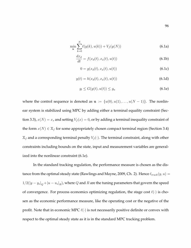
96
minu
N∑k=0
`(y(k), u(k)) + Vf (y(N)) (6.1a)
dxddt
= f(xd(t), xa(t), u(t)) (6.1b)
0 = g(xd(t), xa(t), u(t)) (6.1c)
y(t) = h(xd(t), xa(t), u(t)) (6.1d)
gl ≤ G(y(t), u(t)) ≤ gu (6.1e)
where the control sequence is denoted as u := u(0), u(1), . . . , u(N − 1). The nonlin-
ear system is stabilized using MPC by adding either a terminal equality constraint (Sec-
tion 3.3), x(N) = xs and setting Vf (x) = 0, or by adding a terminal inequality constraint of
the form x(N) ∈ Xf for some appropriately chosen compact terminal region (Section 3.4)
Xf and a corresponding terminal penalty Vf (·). The terminal constraint, along with other
constraints including bounds on the state, input and measurement variables are general-
ized into the nonlinear constraint (6.1e).
In the standard tracking regulation, the performance measure is chosen as the dis-
tance from the optimal steady state (Rawlings and Mayne, 2009, Ch. 2). Hence `track(y, u) =
1/2(|y − ys|Q+ |u− us|R), whereQ andR are the tuning parameters that govern the speed
of convergence. For process economics optimizing regulation, the stage cost `(·) is cho-
sen as the economic performance measure, like the operating cost or the negative of the
profit. Note that in economic MPC `(·) is not necessarily positive definite or convex with
respect to the optimal steady state as it is in the standard MPC tracking problem.
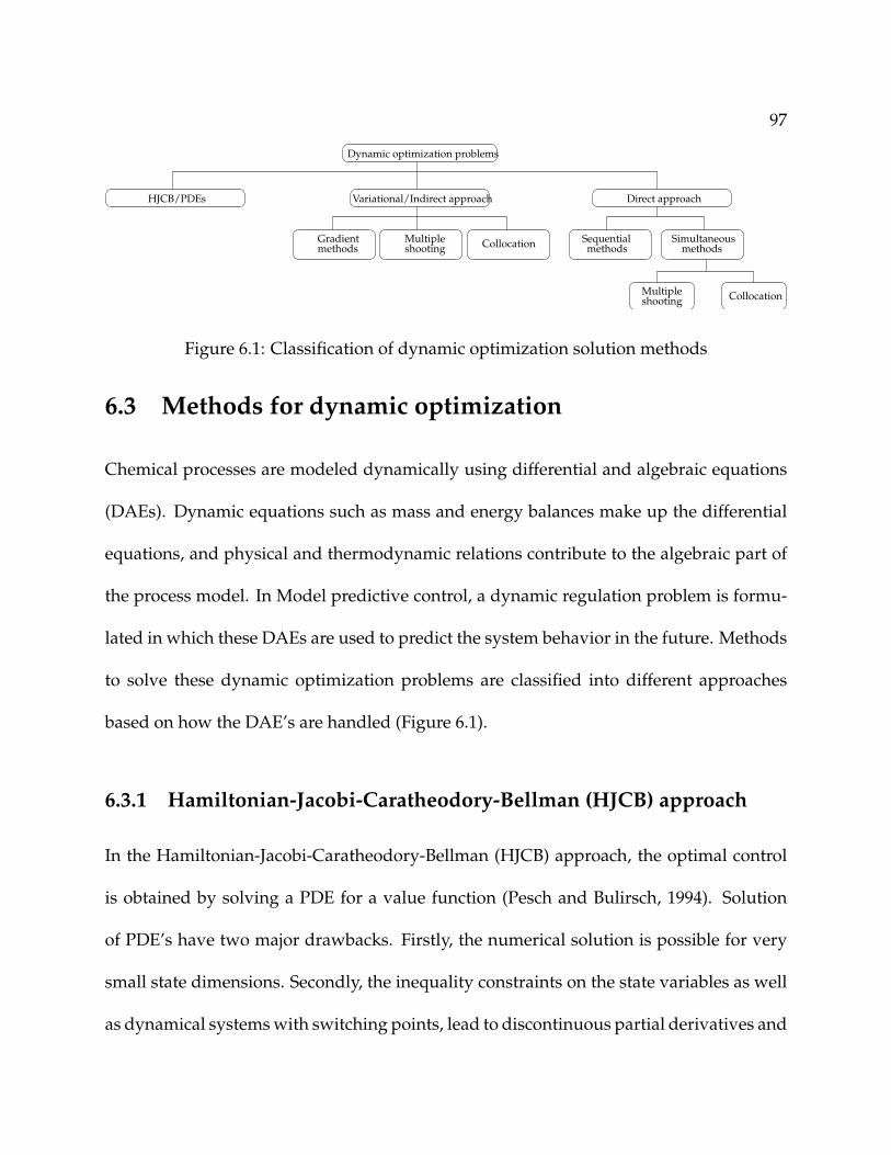
97
CollocationMultipleshooting
Gradient Multipleshooting methods
Variational/Indirect approach
Dynamic optimization problems
HJCB/PDEs Direct approach
Collocation Simultaneousmethods
Sequentialmethods
Figure 6.1: Classification of dynamic optimization solution methods
6.3 Methods for dynamic optimization
Chemical processes are modeled dynamically using differential and algebraic equations
(DAEs). Dynamic equations such as mass and energy balances make up the differential
equations, and physical and thermodynamic relations contribute to the algebraic part of
the process model. In Model predictive control, a dynamic regulation problem is formu-
lated in which these DAEs are used to predict the system behavior in the future. Methods
to solve these dynamic optimization problems are classified into different approaches
based on how the DAE’s are handled (Figure 6.1).
6.3.1 Hamiltonian-Jacobi-Caratheodory-Bellman (HJCB) approach
In the Hamiltonian-Jacobi-Caratheodory-Bellman (HJCB) approach, the optimal control
is obtained by solving a PDE for a value function (Pesch and Bulirsch, 1994). Solution
of PDE’s have two major drawbacks. Firstly, the numerical solution is possible for very
small state dimensions. Secondly, the inequality constraints on the state variables as well
as dynamical systems with switching points, lead to discontinuous partial derivatives and

98
cannot be easily included. Discretization methods to compute numerical approximations
of the value function by solving the first order PDE with dynamic programming has been
discussed in detail by Bardi and Dolcetta (1997); Falcone and Ferretti (1994); Lions (1982).
The application of this methodology is restricted to the case of continuous state systems
with a maximum of three state dimensions(Binder, Blank, Bock, Bulirsch, Dahmen, Diehl,
Kronseder, Marquardt, and Schloder).
6.3.2 Variational/Indirect approach
The indirect or variational approach is a common approach to optimal control problems.
This approach involves defining the Hamiltonian for the problem as a function of the
cost, the constraints and adjoint variables. The necessary conditions for optimality of so-
lution trajectories can then be written as a boundary value problem in the states and
adjoints. Early developments of the Maximum principle have been carried out by Pon-
tryagin, Boltyanskii, Gamkrelidze, and Mishchenko (1962); Isaacs (1965). The approach
has been extended to handle general constraints on the control and state variables (Hartl,
Sethi, and Vickson, 1995). For problems without inequality constraints, the optimality
conditions can be formulated as a set of differential algebraic equations. Often the state
variables have specified initial conditions and the adjoint variables have final conditions.
The resulting two-point boundary value problem (TPBVP) can be addressed with dif-
ferent approaches, including single shooting, invariant embedding, multiple shooting or
some discretization method such as collocation on finite elements or finite differences.

99
A review of these approaches can be found in Cervantes and Biegler (2001).If the prob-
lem requires the handling of active inequality constraints, finding the correct switching
structure as well as suitable initial guesses for state and adjoint variables is often very
difficult.
6.3.3 Direct approach
In this chapter, we discuss the Discretize then Optimize, or the direct NLP approaches. In
these approaches, the system is first discretized to form a nonlinear algebraic problem,
which is then solved using an NLP algorithm. Hence we form finite dimentional prob-
lems that can use the machinery of NLP solvers. As seen in Figure 6.1, the direct NLP ap-
proaches can be separated into two groups: Sequential and Simultaneous strategies, based
on which variables are discretized. Sequential strategy is discussed in Section 6.4. Multi-
ple shooting serves as a hybrid between sequential and simultaneous approaches. Here the
time domain is partitioned into smaller time elements and the DAE models are integrated
separately in each element (Bock and Plitt, 1984; Leineweber, 1999). Control variables are
parametrized in the same way as in sequential approach and gradient information is ob-
tained for both control variables as well as initial conditions of the state variables in each
element. The inequality constraints for state and control variables are imposed directly
at the boundary points. The other simultaneous approach: orthogonal collocation is dis-
cussed in Section 6.5.

100
Discretization scheme in Discretization control
the interval t ∈ [t(k), t(k + 1)) parameters
Piecewise constant u(t) = u(k) u(k), k ∈ I0:N
Piecewise linear u(t) = u(k) +(u(k+1)−u(k)
∆t
)(t− t(k)) u(k), k ∈ I0:N
Polynomial approxima-
tion
u(t) =∑n
q=1 ψq
(t−t(k)
∆t
)uq(k) 1 uq(k), k ∈ I0:N , q ∈
I0:n
Table 6.1: Discretization schemes for the control variables
x(t), y(t)DAE/ODE Solver
GradientsDesicion variablesu(t)
State profiles
CalculationsSensitivity
NLP Solver
Figure 6.2: Sequential dynamic optimization strategy
6.4 Sequential methods
Also known as the control parametrization method, the sequential approach involves dis-
cretization of only the control variables. The time horizon is divided into N time stages,
which is essentially the control horizon in the discrete time formulation. Different dis-
cretization schemes to parametrize the control variables are summarized in Table 6.1.
1uq(k) represents the value of the control variable in stage k the collocation point q. ψq is a Langrange
polynomial of order n satisfying ψq(ρr) = δq,r

101
Figure 6.2 provides a sketch of the sequential dynamic optimization strategy. Con-
sider the formulation (6.1). The input profile u(t), t ≥ 0 is approximated in terms of
the discretization control parameters u = u(k), k ∈ I0:N−1 according to the type of
parametrization chosen (Table 6.1). Hence the optimization problem can be written in
terms of the optimization variable vector u as
minu
N−1∑k=0
`(y(k), u(k)) + Vf (y(N)) (6.2a)
dxddt
= f(xd(t), xa(t),u) (6.2b)
0 = g(xd(t), xa(t),u), t ∈ (t(k − 1)− t(k)], k ∈ I1:N (6.2c)
y(k) = h(xd(k), xa(k), u(k)) (6.2d)
gl ≤ G(y(k), u(k)) ≤ gu (6.2e)
A NLP solver is used to solve this optimization problem. At a given iteration of the opti-
mization cycle, the decision variables are provided by the NLP solver. With these decision
variables, the DAE/ODE system is integrated forward in time until the terminal time to
compute the state profiles that determine the objective and constraint functions. Then the
gradients of the objective and constraints are evaluated through solution of DAE sensi-
tivity equations. The function and gradient information is then passed back to the NLP
solver so that it can update the decision variables. The cycle continues until the NLP
solver converges. Since the optimization problems in question are nonlinear and non-
convex in nature, the performance of the NLP solver depends heavily on the gradient
and Hessian information. Most NLP solvers have inbuilt algorithms to compute first and

102
second order derivatives using finite differences, but as we shall see in the next section,
finite difference method is error prone and does not perform well. Hence sensitivity cal-
culations are usually employed for the purpose, which we shall discuss in the following
section.
It is also well known that sequential approaches cannot handle open loop insta-
bility (Ascher and Petzold, 1998; Flores-Tlacuahuac, Biegler, and Saldvar-Guerra, 2005).
Otherwise, finding a feasible solution for a given set of control parameters may be diffi-
cult. Cervantes and Biegler (2001); Vassiliadis (1993) review these methods in detail.
6.4.1 Sensitivity strategies for gradient calculation
The most important component of the sequential approach, apart from the NLP algo-
rithm, is the gradient calculation for the NLP solver. There are three approaches for gra-
dient calculations
1. Perturbation
2. Forward sensitivity calculation
3. Adjoint sensitivity calculation

103
Gradients by perturbation
Perturbation is the easiest way to compute the gradients. Consider a standard NLP of the
form
minzf(p, z) s.t. c(p, z) = 0 zl ≤ z ≤ zu (6.3)
where p is the parameter, which in our case would be the initial state, and z is the op-
timization variable vector. The derivatives of the objective f(·) and the constraints c(·),
need to be computed implicitly from the DAE model, often in tandem with the DAE so-
lution. To compute the gradients with respect to the decision vector z, we apply forward
difference perturbation to the vector z
zi = z + δei, i ∈ I1:nz
where the ith element of vector ei is 1 and the other elements are zero, and δ is a small
perturbation size. the approximate gradients are
1
δ(f(p, zi)− f(p, z)) = ∇zif(p, z) +O(δ) +O(δ−1)
1
δ(c(p, zi)− c(p, z)) = ∇zic(p, z) +O(δ) +O(δ−1)
It is well known that gradients evaluated by perturbation are often plagued by truncation
errors and roundoff errors. Truncation errors result from neglect of higher order Taylor
series terms that vanish as δ → 0. On the other hand, roundoff errors that result from
internal calculation loops (i.e. convergence noise from the DAE solver) are independent
of δ and lead to large gradient errors as δ → 0. While δ can be selected carefully and

104
roundoff errors can be controlled, the gradient error cannot be eliminated completely.
Biegler (2010, Ch. 7) show that this can lead to inefficient and unreliable performance by
the NLP solver.
Forward sensitivity calculation
Consider the DAE system defined by (6.2a) and (6.2b). Assuming the functions f(·) and
g(·) are sufficiently smooth in all of their arguments, we differentiate the system with
respect to the decision variable u using chain rule as following
d
du
dxddt
= f(xd(t), xa(t), u(t)), xd(0) = x0
g(xd(t), xa(t), u(t)) = 0
Defining sensitivity matrices S(t) = dxddu
Tand R(t) = dxa
du
T , we obtain the following sensi-
tivity equations
dS
dt=
∂f
∂xd
T
S(t) +∂f
∂xa
T
R(t) +∂f
∂u
T
, S(0) =∂x0
∂u
0 =∂g
∂xd
T
S(t) +∂g
∂xa
T
R(t) +∂g
∂u
For n states and N decision variables, we have n × N sensitivity equations. These sensi-
tivity equations are index-1 DAE’s. To avoid the need to store the state profiles, the sen-
sitivity equations are usually solved simultaneously with the state equations. Once the
sensitivities are determined, we compute the gradients for the objective and constraint
functions as following
∇uf = S(tf )∂f
∂x+∂f
∂u

105
Hence we can compute the gradients by solving a larger augmented system of DAE’s and
these estimated gradients are passed to the NLP solver to compute its next iteration.
6.4.2 Adjoint sensitivity calculation
The Adjoint method is rooted in calculus of variations and the Euler-Lagrange approach to
optimal control (Bryson and Ho, 1975; Bryson Jr, 1996; Bryson, 1999). However, the ad-
joint approach to sensitivity analysis has recently had a renaissance as dynamic optimiza-
tion problems of large size and with a large number of parameters appear in engineering
applications. Petzold, Li, Cao, and Serban (2006) provide an overview of sensitivity anal-
ysis in differential algebraic systems by the adjoint approach. Cao, Li, Petzold, and Serban
(2003) analyze the numerical stability properties of the adjoint system. They show that
the stability of the adjoint system is identical to the stability of the original system for
systems of ordinary differential equations as well as for semi- explicit index-1 differen-
tial algebraic equations. For general index-0 and index-1 DAE systems, they define an
augmented adjoint system that is stable if the original DAE system is stable.
As we observed, forward sensitivity setup requires integration of n+(n×N) DAE’s
equation. This number grows if the number of optimization variables and/or the num-
ber of states become large and hence the method becomes inefficient. A complementary
approach can be derived based on variational approach. In this approach to derive the
sensitivities, we consider the sensitivity of the objective and constraint functions sepa-
rately. Denote Ψ as an element of Ψ(u), which represents either the objective or constraint

106
function at the end of the sample time (t = ts).
Consider the DAE system defined by (6.1b) and (6.1c). We define adjoint variables
as follows
Ψ(xd(t), xa(t),u) = Ψ(xd(ts), xa(ts),u)+∫ ts
0
[λd(t)
′(f(xd(t), xa(t),u)− dxd
dt(t)
)+ λa(t)
′g(xd(t), xa(t),u)
]dt (6.4)
where λd(t) and λa(t) are the differential and algebraic adjoint variables respectively. They
can also be seen as the Langrange multipliers of 6.1b and 6.1c, i.e the constraints due the
system dynamics, in the optimization problem (6.1). Integrating (6.4) we get
Ψ(xd(t), xa(t),u) = Ψ(xd(ts), xa(ts),u)− xd(ts)′λd(ts) + xd(0)′λd(0)+∫ ts
0
[λd(t)
′f((xd(t), xa(t),u) + xd(t)′dλddt
(t) + λa(t)′g(xd(t), xa(t),u)
]dt
Applying perturbations to this equation we get
dΨ =
[∂Ψ
∂xd− λd(ts)
]′δxd(ts) + λd(0)′δxd(0) +
∂Ψ
∂u
′du+∫ ts
0
[∂f
∂xdλd −
dλddt
+∂g
∂λa
]′δxd(t) +
[∂f
∂xaλd +
∂g
∂xaλa
]′δxa(t)+[∂f
∂uλd +
∂g
∂uλa
]′dudt
We set all the terms which are not influenced by du to zero so that only du has a direct

107
influence on dΨ. This gives us the following
dλddt
= − ∂f
∂xdλd −
∂g
∂xdλa (6.5a)
0 =∂f
∂xaλd +
∂g
∂xaλa (6.5b)
λd(ts) =∂Ψ
∂xd(6.5c)
δxd(0) = 0 (6.5d)
In the above system, (6.5a) and (6.5b) give us a DAE system in the adjoint variables with
a terminal boundary condition (6.5c). (6.5d) comes from the fact that in our problem, the
initial state is a fixed parameter. Hence we get
dΨ
du=
[∂Ψ
∂u
]′+
∫ ts
0
[∂f
∂uλd +
∂g
∂uλa
]′dt
Hence calculation of adjoint sensitivities requires the solution of a DAE system (6.5) with
a terminal condition instead of an initial condition. Once the state and adjoint variables
are obtained, the integrals allow direct calculation of the gradients ∇uΨ. The adjoint
sensitivity approach is more difficult to implement as compared to the forward sensi-
tivity approach since the solution requires storage of state profiles, which are used later
for backward integration of the adjoint DAE system. To avoid the storage requirement,
especially for large systems, the adjoint approach is usually implemented with a check-
pointing scheme. At the cost of at most one additional forward integration, this approach
offers the best possible estimate of memory requirements for adjoint sensitivity analysis
(Hindmarsh, Brown, Grant, Lee, Serban, Shumaker, and Woodward, 2005). Here the state
variables are stored at only a few checkpoints in time. Starting from the checkpoint closest

108
to ts, the state profile is reconstructed by integrating forward from the checkpoint and
the adjoint variable is calculated by integrating backward up to this checkpoint. Once the
adjoint is calculated at this point, we back up to an earlier checkpoint and the state and
adjoint calculation is repeated until the beginning of the time horizon. The checkpointing
scheme offers a trade-off between repeated adjoint calculation and state variable storage.
Moreover, strategies have been developed for the optimal distribution of checkpoints that
lead to efficient adjoint sensitivity calculations (Griesse and Walther, 2004).
6.5 Simultaneous approach
In this thesis, we will focus on the simultaneous approach, also known as direct tran-
scription approach. In this technique both the state and control variables are discretized,
which leads to a large number of optimization variables. These large scale NLP’s require
special solution strategies (Betts and Huffman, 1990; Betts and Frank, 1994; Cervantes and
Biegler, 1998, 2000; Cervantes, Wachter, Tutuncu, and Biegler, 2000). The simultaneous
approach has a number of advantages over other approaches to dynamic optimization.
1. Control variables are discretized at the same level as the state variables. The Karush
Kuhn Tucker (KKT) conditions of the simultaneous NLP are consistent with the
optimality conditions of the discretized variational problem, and, under mild con-
ditions, convergence rates can be shown (Reddien, 1979; Cuthrell and Biegler, 1989;
Hager, 2000; Kameswaran and Biegler, 2006, 2008).

109
2. As with multiple shooting approaches, simultaneous approaches can deal with in-
stabilities that occur for a range of inputs. Because they can be seen as extensions
of robust boundary value solvers, they are able to “pin down” unstable modes (or
increasing modes in the forward direction). This characteristic has benefits on prob-
lems that include transitions to unstable points, optimization of chaotic systems
(Bock and Plitt, 1984) and systems with limit cycles and bifurcations, as illustrated
in Flores-Tlacuahuac et al. (2005).
3. Simultaneous methods also allow the direct enforcement of state and control vari-
able constraints, at the same level of discretization as the state variables of the DAE
system. As was discussed in Kameswaran and Biegler (2006), these can present
some interesting advantages on large-scale problems.
4. Finally, recent work has shown (Kameswaran and Biegler, 2006, 2005) that simulta-
neous approaches have distinct advantages for singular control problems and prob-
lems with high index path constraints.
Nevertheless, simultaneous strategies require the solution of large non-linear pro-
grams, and specialized methods are required to solve them efficiently. These NLPs are
usually solved using variations of Successive Quadratic Programming (SQP). Both full-
space and reduced-space options exist for these methods. Full-space methods take advan-
tage of the sparsity of the DAE optimization problem. They are best suited for problems
where the number of discretized control variables is large (Betts and Huffman, 1990).
Here, second derivatives of the objective function and constraints are usually required, as

110
are measures to deal with directions of negative curvature in the Hessian matrix (Wachter
and Biegler, 2006). Betts (2000) provides a detailed description of the simultaneous ap-
proach with full-space methods, along with mesh refinement strategies and case studies
in mechanics and aerospace. On the other hand, reduced-space approaches exploit the
structure of the DAE model and decompose the linearized KKT system; second derivative
information is often approximated here with quasi-Newton formulae. This approach has
been very efficient on many problems in process engineering that have few discretized
control variables. The NLP algorithm used for our computation is IPOPT. The details of
the algorithm are sketched and discussed in Wachter and Biegler (2006); Biegler (2007).
6.5.1 Formulation
The DAE optimization problem (6.1), which has the system dynamics in continuous time,
is converted into a discrete time NLP by approximating the state and control profiles by a
family of polynomials on finite elements. These polynomials can be represented as power
series, sums of orthogonal polynomials or in Lagrange form. Here, we use the following
monomial basis representation for the differential profiles, which is popular for Runge-
Kutta discretizations:
x(t) = x(k − 1) + h(k)K∑q=1
Ωq
(t− t(k)
h(k)
)dx
dt k,q(6.6)
Here x(k−1) is the value of the differential variable at the beginning of element k, h(k) the
length of element k, dx/dtk,q the value of its first derivative in element k at the collocation

111
point q, and Ωq is a polynomial of order K, satisfying
Ωq(0) = 0 for q = 1, · · · , K
Ω′q(ρr) = δq,r for q, r = 1, · · · , K
where ρr is the location of the rth collocation point within each element. Continuity of the
differential profiles is enforced by
x(k) = x(k − 1) + h(k)K∑q=1
Ωq(1)dx
dt k,q(6.7)
Based on the recommendation by Biegler (2007), we use Radau collocation points because
they allow constraints to be set at the end of each element and to stabilize the system more
efficiently if high index DAEs are present. In addition, the control and algebraic profiles
are approximated using a Lagrange basis representation which takes the form
y(t) =K∑q=1
Ψq
(t− t(k − 1)
h(k)
)yk,q (6.8)
u(t) =K∑q=1
Ψq
(t− t(k − 1)
h(k)
)uk,q (6.9)
Here yk,q and uk,q represent the values of the algebraic and control variables, respectively,
in element k at collocation point q. Ψq is the Lagrange polynomial of degree K satisfying
Ψq(ρr) = δq,r, for q, r = 1, · · · , K
Note that uk,K = u(k) and yy,K = y(K), i.e. the last collocation point in each finite
element lies on the boundary of that element (see Figure 6.3). Substituting (6.6)-(6.9) into

112
Element boundaryFinite element, i
hi
Collocation points
Figure 6.3: Sequential dynamic optimization strategy
(6.1b)-(6.1e) gives the following NLP
min(dx/dtk,q ,uk,q ,yk,q ,zk,q)
N−1∑k=0
`(y(k), u(k)) + Vf (y(N)) (6.10a)
dx
dt k,q= f(xk,q, uk,q) (6.10b)
xk,q = x(k − 1) + h(k)K∑q=1
Ωq′(ρq)dx
dt k,q(6.10c)
x(k) = x(k − 1) + h(k)K∑q=1
Ωq(1)dx
dt k,q(6.10d)
0 = g(xk,q, uk,q) k = 1, · · · , N q = 1, · · · , K (6.10e)
yk,q = h(xk,q, uk,q) k = 1, · · · , N q = 1, · · · , K (6.10f)
gl ≤ G(yk,q, uk,q) ≤ gu k = 1, · · · , N q = 1, · · · , K (6.10g)
This is a standard NLP of the form
minzf(z) s.t. c(z) = 0 zl ≤ z ≤ zu

113
where z = (dx/dtk,q, uk,q, yk,q, zk,q), and is solved using a nonlinear solver. Hence the dif-
ferential variables are required to be continuous throughout the time horizon, while the
control and algebraic variables are allowed to have discontinuities at the boundaries of
the elements. As seen from Figure 6.3. Bounds are imposed directly on the differential
variables at element boundaries. These can also be enforced at all collocation points by
writing additional point constraints. We use IPOPT as the nonlinear solver for our simu-
lations.
6.6 Software tools
In this section, we describe the structure of the software tool: NLMPC, that was devel-
oped during this thesis. Of the two direct NLP approaches described above, the direct
collocation approach formulated in Section 6.5 has been most efficient in solving our non-
linear nonconvex dynamic regulation problems. The two most important ingredients of
the direct NLP strategy are
1. NLP solver
2. Derivative calculator
As mentioned above we use IPOPT (Wachter and Biegler, 2006) as the NLP solver
for our simulations. IPOPT is a primal-dual interior-point algorithm with a filter line-
search method tailored specifically for large scale problems, and takes advantage of sparse

114
First and secondorder derivatives
Problemparameters
Problem definition:DAE’s, Objective, Constraints
GNU Octave
NLMPC tool
User
IPOPT ADOL-C
ResultsIn
terp
rete
dC
ompi
led
Figure 6.4: Structure of NLMPC tool
matrix memory management capabilities to efficiently implement the NLP solution algo-
rithm. The solver is written in C++.
In the direct collocation approach, the system of DAE’s is converted into a system
of explicit nonlinear algebraic equations. Hence we can use direct differentiation to com-
pute the first and second order derivatives instead of sensitivity calculations, which are
prone to integration and round-off errors as described in Section 6.4.1. We use ADOL-C
(Wagner, Walther, and Schaefer, 2010; Walther, 2008), which is an open-source package
for the automatic differentiation of C and C++ programs, for computing first and second
order derivative information of the NLP resulting from the collocation formulation (6.10).
Both NLP solver and derivative calculator being in C++, enables us to write an
interface between IPOPT and ADOL-C in C++. We call this interface, the NLMPC tool.
This tool has two plugs for interaction with the user (Figure 6.4). The first one reads

115
the problem information i.e., the DAE’s, the objective function and the constraints for
the dynamic regulation problem from a C++ file provided by the user. The second one
is an interface with GNU Octave, that allows the user to pass problem parameters and
read back the results of the optimization problem in a high-level interpreted language for
further analysis.
The interface does the following operations:
1. Formulates the corresponding NLP according to the scheme derived in Section 6.5.1
2. Calls ADOL-C to compute the first and second order derivatives of the objective
and the constraints
3. Passes the NLP and the derivative information to IPOPT to optimize
4. Returns the optimal solution back to the user through the Oct interface with GNU
Octave.
The derivative information is very crucial to the performance of IPOPT’s NLP al-
gorithm and hence providing the problem definition, i.e. the DAE’s, objective and the
constraints, as a C++ code allows us to use automatic differentiation via ADOL-C, which
gives us exact derivatives, and greatly improves the performance of IPOPT. Once the
problem definition has been provided, the NLMPC tool compiles the source along with
the problem definition to transform the toolbox’s algorithm, coupled with IPOPT and
ADOL-C, into compiled code for faster execution. GNU Octave’s OCT interface allows
the toolbox to interact with this compiled code directly. It allows the user to easily pass

116
problem parameters and read the results for further analysis, without having to recom-
pile the code, and hence enables the use of the tool for simulation studies with great ease.
Appendix B provides a brief user manual of the NLMPC tool.

117
Chapter 7
Case studies
7.1 Introduction
The motivation behind extending the MPC framework to handle generic nonlinear non-
convex economic objectives is to gain economic benefit during the transient operation of
the processes controlled using MPC. We developed economic MPC algorithms for both
stable and unstable operation, and the corresponding theory, in the proceeding chap-
ters. In this chapter we present some case studies to demonstrate the application of the
economic dynamic regulation and show the benefits of optimizing process economics di-
rectly in the dynamic regulation problem. To gauge the benefit of using economics based
MPC over the standard tracking MPC, we define the following performance measure
G =PT,eco − PT,track
TPs× 100%
where PT,eco and PT,track are the cumulative profits over T time steps, of the closed loop
systems under the economics and tracking MPC respectively, and Ps is the steady state

118
profit.
7.2 Evaporation process
We first consider an evaporation process that removes a volatile liquid from a nonvolatile
solute, thus concentrating the solution. It consists of a heat exchange vessel with a recir-
culating pump. The overhead vapor is condensed by the use of a process heat exchanger.
The details of the mathematical model can be found in Newell and Lee (1989, Ch. 2). We
use the following modified process model
FeedF1, X1, T1
F5
Condensate
L2
Separator
Evaporator
Condensate
F3
F4, T3
T201
Condenser
waterCooling
T200
F200
P100
LC
LT
ProductX2, T2
F2
T100F100
Steam
Figure 7.1: Evaporator system

119
Differential equations:
MdX2
dt= F1X1 − F2X2
CdP2
dt= F4 − F5
Process liquid energy balance
T2 = 0.5616P2 + 0.3126X2 + 48.43
T3 = 0.507P2 + 55
F4 = (Q100 − F1Cp(T2 − T1))/λ
Heat steam jacket
T100 = 0.1538P100 + 90
Q100 = UA1(T100 − T2)
UA1 = 0.16(F1 + F3)
F100 = Q100/λs
Condenser
Q200 =UA2(T3 − T200)
1 + UA2/(2CpF200)
F5 = Q200/λ

120
Level controller
F2 = F1 − F4
In the above equations, M = 20 kg/m is the liquid holdup in the evaporator, C = 4
kg/kPa is a constant, UA1 and UA2 = 6.84 kW/K are the products of the heat transfer
coefficients and the heat transfer area in the evaporator and condenser respectively, Cp =
0.07 kW/kg·min is the heat capacity of water, λ = 38.5 kW/kg·min is the latent heat of
evaporation of water and λs = 36.6 kW/kg·min is the latent heat of steam at saturated
conditions.
The economic objective of the evaporator process is to minimize the following op-
erating cost (in 10−3 $/h ), which consists of the cost of electricity, steam and cooling water
(Wang and Cameron, 1994; Govatsmark and Skogestad, 2001).
J = 1.009(F2 + F3) + 600F100 + 0.6F200
The product composition X2 and the operating pressure P2 are the state variables as well
as the available measurements, and the steam pressure P100 and the cooling water flow
rate F200 are the manipulated variables. The following variables are the source of distur-
bances in the system. The following bounds are imposed.
X2 ≥ 25% 40 kPa ≤ P2 ≤ 80 kPa
P100 ≤ 400 kPa F200 ≤ 400 kg/min
At the best steady state under nominal conditions, the input and output variables have

121
Variable Description Value
F1 Feed flow rate 10 kg/min
C1 Feed composition 5 %
F3 Circulating flowrate 50 kg/min
T1 Feed temperature 40 C
T200 Cooling water inlet temperature 25 C
Table 7.1: Disturbance variables in the evaporator system and their nominal values
the following values
X2 = 25 P2 = 50.57 P100 = 193.45 F200 = 207.33
We set up the dynamic MPC problems with a sample time of ∆ = 1 min and a control hori-
zon of N = 200. The economic MPC problem is set up with the operating cost as the stage
cost and the tracking problem uses ` = |x− xs|Q+ |u− us|R, whereQ =diag(0.92, 0.3) and
R =diag(1, 1), as the stage cost. Both controllers are implemented with a terminal state
constraint.
We first subject the system to a disturbance in the operating pressure P2. A peri-
odic drop in the pressure was injected into the system and the performance of the two
controllers was compared. Figure 7.2 shows the input and state profiles as well as the
corresponding instantaneous operating costs of the two closed loop systems. A pressure
drop of 8 kPa was injected with a repetition period of 20 mins. A drop in the operating
pressure decreases the instantaneous operating cost and hence the system under eco-

122
nomic MPC tends to stay at a lower pressure as compared to the tracking MPC during its
transient back to the optimal steady state. The corrective control action resulting from this
disturbance also increases the product composition, which in turn, increases the operat-
ing cost. Hence the economic MPC drives the system back to the steady state composition
faster than tracking MPC. The benefit obtained from economic MPC as compared to the
tracking controller is G = 6.15% of the steady state operating cost.
Next we subject the system to a measured disturbance in the feed flow rate (F1), the
feed temperature (T1) and the coolant water inlet temperature (T100). Figure 7.3 shows the
input and state profiles as well as the corresponding instantaneous operating costs of the
two closed loop systems. An increase in the feed flow rate drops the product concentra-
tion. To counter this disturbance both controllers raise the steam pressure and the cooling
water flow rate raising the the product concentration and the operating pressure, increas-
ing the operating cost. The economic controller keeps the system at a lower concentration
and pressure as compared to the tracking controller. In order to drop the instantaneous
operating cost, the economic controller drops the inlet water flow rate when there is a
disturbance in the cooling water inlet temperature causing it to rise. The economic con-
troller drops the water flow more than the tracking controller making higher instanta-
neous profit. In this scenario the benefit obtained from economic MPC as compared to
the tracking controller is G = 2.2% of the steady state operating cost.
Table 7.2 shows the average operating cost of the evaporator process under the two
controllers in the two disturbance scenarios discussed above. The economic MPC’s bene-

123
-8-7-6-5-4-3-2-10
0 20 40 60 80 100
d
time (min)
(a)
2000
4000
6000
8000
10000
12000
14000
0 20 40 60 80 100
cost ($/h)
time (min)
(b)
100
150
200
250
300
350
400
0 20 40 60 80 100
P100 (kPa)
time (min)
(c)
100
120
140
160
180
200
220
0 20 40 60 80 100
F200 (kg/min)
time (min)
(d)
20
30
40
50
60
70
0 20 40 60 80 100
X2(%)
time (min)
(e)
30
35
40
45
50
0 20 40 60 80 100
P2 (kPa)
time (min)
eco-MPCtrack-MPC
(f)
Figure 7.2: Closed-loop input (c),(d) and state (e),(f) profiles, and the instantaneous profit
(b) of the evaporator process under unmeasured disturbance (a) in the operating pressure.

124
101520253035404550
0 10 20 30 40 50 60 70 80 90
d
time (min)
F1
T1
T100
(a)
4000
6000
8000
10000
12000
0 10 20 30 40 50 60 70 80 90
cost ($/h)
time (min)
(b)
100
150
200
250
300
350
400
0 10 20 30 40 50 60 70 80 90
P100 (kPa)
time (min)
(c)
200
240
280
320
360
400
0 10 20 30 40 50 60 70 80 90
F200 (kg/min)
time (min)
(d)
20
24
28
32
36
40
0 10 20 30 40 50 60 70 80 90
X2(%)
time (min)
(e)
48
50
52
54
56
0 10 20 30 40 50 60 70 80 90
P2 (kPa)
time (min)
eco-MPCtrack-MPC
(f)
Figure 7.3: Closed-loop input (c),(d) and state (e),(f) profiles, and the instantaneous profit
(b) of the evaporator process under measured disturbances (a)

125
fit is seen to be 6.15% of the nominal steady state profit under unmeasured disturbances.
Disturbance Avg. operating cost (eco-MPC) Avg. operating cost (track-MPC) G
Measured 5894.3 5965.5 2.2 %
Unmeasured 5804.1 6154.8 6.15 %
Table 7.2: Performance comparison of the evaporator process under economic and track-
ing MPC
7.3 Williams-Otto reactor
The Williams-Otto reactor is one unit of the Williams-Otto plant model (Williams and
Otto, 1960). The reactor is a CSTR with mass holdup 2104.7 kg and temperature TR. The
reactor is fed with two pure component reactant streams FA and FB. The following three
simultaneous reactions involving 6 components occur inside the reactor.
A + B −→ C k1 = 1.6599× 10⁶e−6666.7
TR s−1
B + C −→ P + E k2 = 7.2117× 10⁸e−8333.3
TR s−1
C + P −→ G k3 = 2.6745× 10¹²e−11111
TR s−1

126
the following dynamic mass balances represent the plant behavior
WdXA
dt= FA − (FA + FB)XA − r1
WdXB
dt= FB − (FA + FB)XB − r1 − r2
WdXC
dt= −(FA + FB)XC + 2r1 − 2r2 − r3
WdXE
dt= −(FA + FB)XE + r2
WdXG
dt= −(FA + FB)XG + 1.5r3
WdXP
dt= −(FA + FB)XP + r2 − 0.5r3
where XA, XB, XC , XE , XG and XP are the mass fractions of the respective components
and r1 = k1XAXBW , r2 = k2XBXCW and r1 = k3XCXPW are the three reaction rates.
The economic objective of the process is to maximize the profit, which is the difference
between the sales of the products E and P and the costs of raw materials A and B (Xiong
and Jutan, 2003).
P = 5554.1(FA + FB)XP + 125.91(FA + FB)XE − 370.3FA − 555.42FB
The mass fractions of all the components are the state variables as well as the avail-
able measurements and the input flow rate of component B (FB) and the reactor temper-
ature (TR) are the control variables. The flow rate of component A (FA) is the source of
disturbance with a nominal value 1.8 kg/sec.
We first subject the system to periodic step changes in the feed flow rate of A (FA).
The economic controller tries to extract more profit from the disturbance by raising the
product concentrations (XP and XE) more than the tracking controller. Figure 7.4 shows

127
1
1.2
1.4
1.6
1.8
2
2.2
2.4
0 100 200 300 400 500 600 700 800
d
time (min)
(a)
400
800
1200
1600
0 100 200 300 400 500 600 700 800
cost ($/h)
time (min)
(b)
7678808284868890929496
0 100 200 300 400 500 600 700 800
TR (C)
time (min)
(c)
23456789
10
0 100 200 300 400 500 600 700 800
FB (kg/s)
time (min)
(d)
0.28
0.29
0.3
0 100 200 300 400 500 600 700 800
XE
time (min)
(e)
0.104
0.108
0.112
0 100 200 300 400 500 600 700 800
XP
time (min)
eco-MPCtrack-MPC
(f)
Figure 7.4: Closed-loop input (c),(d) and state (e),(f) profiles, and the instantaneous profit
(b) of the Williams-Otto reactor under step disturbance in the feed flow rate of A (a)

128
00.5
11.5
22.5
33.5
4
0 100 200 300 400 500 600
d
time (min)
(a)
0
400
800
1200
1600
2000
0 100 200 300 400 500 600
cost ($/h)
time (min)
(b)
50
60
70
80
90
100
110
0 100 200 300 400 500 600
TR (C)
time (min)
(c)
23456789
10
0 100 200 300 400 500 600
FB (kg/s)
time (min)
(d)
0.26
0.27
0.28
0.29
0.3
0 100 200 300 400 500 600
XE
time (min)
(e)
0.096
0.1
0.104
0.108
0.112
0.116
0 100 200 300 400 500 600
XP
time (min)
eco-MPCtrack-MPC
(f)
Figure 7.5: Closed-loop input (c),(d) and state (e),(f) profiles, and the instantaneous profit
(b) of the Williams-Otto reactor under large random disturbances in the feed flow rate of
A (a)

129
the control moves and the mass fractions of the product P and E of the two closed loop
systems.
To simulate more transient behavior, FA, which is a measured disturbance vari-
able, is disturbed with large variations. Figure 7.5 shows the control moves and the mass
fractions of the product P and E of the two closed loop systems.
Table 7.3 shows the average operating cost of the Williams-Otto reactor under the
two controllers in the two disturbance scenarios discussed above. The economic MPC’s
benefit is seen to be 5.8% of the nominal steady state profit under large random measured
disturbances.
Disturbance Avg. Profit (eco-MPC) Avg. Profit (track-MPC) G
Step 986.60 966.47 2 %
Random 827.64 622.26 5.8 %
Table 7.3: Performance comparison of the Williams-Otto reactor under economic and
tracking MPC
7.4 Consecutive-competitive reactions
We consider next the control of a nonlinear isothermal chemical reactor with consecutive-
competitive reactions (Lee and Bailey, 1980). Such networks arise in many chemical and
biological applications such as polymerizations, and are characterized by a set of reactions

130
of the following form:
Pi−1 +B → Pi
i ∈ 1, 2, . . . , R. (7.1)
Typically a desirable distribution of products in the effluent is a primary objective in the
reactor design for these processes. For simplicity we consider the case of two reactions:
P0 +B −→ P1
P1 +B −→ P2
The dimensionless mass balances for this problem are:
x1 = u1 − x1 − σ1x1x2
x2 = u2 − x2 + σ1x1x2 − σ2x2x3
x3 = −x3 + σ1x1x2 − σ2x2x3
x4 = −x4 + σ2x2x3
where x1, x2, x3 and x4 are the concentrations of P0, B, P1, and P2 respectively, while u1
and u2 are inflow rates of P0 and B and are the manipulated variables. The parameters σ1
and σ2 have values 1 and 0.4 respectively. The time average value of u1 is constrained to
lie between 0 and 1.
Av[u1] ⊆ [0, 1].
The primary objective for this system is to maximize the average amount of P1 in the
effluent flow (`(x, u) = −x3). Previous analysis has clearly highlighted that periodic op-

131
eration can outperform steady-state operation (Lee and Bailey, 1980). The steady-state
problem has a solution xs =
[0.3874 1.5811 0.3752 0.2373
]′with the optimal input
us =
[1 2.4310
]′.
We solve the dynamic regulation problem using the simultaneous approach (Flores-
Tlacuahuac, Moreno, and Biegler, 2008). The state space is divided into a fixed number
of finite elements. The input is parametrized according to zero order hold with the input
value constant across a finite element. An additional upper bound of 10 is imposed on
u1(t). A terminal state constraint is used in all the simulations.
The system is first initialized at the steady state to check suboptimality of steady-
state operation. A horizon of 100 is chosen with a sample time Ts = 0.1. The steady-state
solution is used as the initial guess for the nonlinear solver. The solution of the dynamic
problem is seen to be unstable (Figure 7.6). The solution returned by the optimizer shows
the inputs jumping between the upper and lower bounds. Different initial guesses gave
different locations of these jumps suggesting that these solutions are local optima, with a
negligible cost difference.
In order to stabilize the system a convex term is added to the objective and the
penalties are varied.
`(x, u) = −x3 + (1/2)(|x− xs|2Q + |u− us|2R
)Next the R penalty is tuned up to 0.04. The optimal solution now converges to
the steady state. The system is initialized at a random initial state, and three different
simulations are carried out under the influence of three different controllers: the purely

132
0
3
6
9
0 2 4 6 8 10
u1
(a)
0
20
40
60
0 2 4 6 8 10
u2
eco-MPCsteady state
(b)
0
0.4
0.8
1.2
1.6
0 2 4 6 8 10
x1
(c)
0
1
2
3
4
0 2 4 6 8 10
x2
(d)
0.4
0.8
1.2
0 2 4 6 8 10
x3
Time (t)
(e)
0.2
0.4
0 2 4 6 8 10
x4
Time (t)
(f)
Figure 7.6: Open-loop input (a), (b) and state (c), (d), (e), (f) profiles for system initialized
at the steady state

133
0
0.5
1
1.5
2
0 1 2 3 4 5 6
u1
(a)
0
2
4
6
8
10
0 1 2 3 4 5 6
u2
(b)
0.5
1
1.5
0 1 2 3 4 5 6
x1
(c)
2
4
0 1 2 3 4 5 6
x2
(d)
0.4
0.8
1.2
0 1 2 3 4 5 6
x3
(e)
0.2
0.4
0.6
0 1 2 3 4 5 6
x3
eco-MPCeco-stable-MPC
track-MPC
(f)
Figure 7.7: Closed-loop input (a), (b) and state (c), (d), (e), (f) profiles for system under
the three controllers, initialized at a random state

134
economic controller, the regularized controller with R = 0.04 and a tracking type con-
troller with Q = 0.36I4 and R = 0.002I2. The closed loop solutions are compared in
Figure 7.7.
Controller Avg. Profit (eco-MPC) Avg. profit (track-MPC) G
Economic 0.44 0.38 15 %
Economic-stable 0.39 0.38 2 %
Table 7.4: Performance comparison of the CSTR with consecutive competitive reactions
under economic and tracking MPC
Table 7.4 lists the performance comparison for the two economic controllers pre-
sented. It is seen that unsteady operation gains significant profit over steady operation
and the purely economic MPC scores 15% of the steady state benefit as compared to the
tracking controller. When convergence is forced, this benefit it reduced to 2% of the steady
state profit.

135
Chapter 8
Conclusions and future work
In this chapter we conclude the thesis by highlighting the contributions and suggest fu-
ture research directions in the topic.
8.1 Contributions
Stability theory for nonlinear MPC: The stability theory for model predictive control
was extended to generic nonlinear systems and costs in Chapter 3. For general nonlinear
problems, the stability of the closed loop system cannot be always expected. Chapter 3
identifies a class of systems: strictly dissipative systems, for which closed-loop stability
is guaranteed. The two standard MPC formulations, namely the terminal constraint and
the terminal control/penalty formulations, are extended to the economic MPC frame-
work. Asymptotic stability is established for both the formulations by proposing Lya-
punov functions based on a modified cost. A third formulation, which does not have any
constraint on the terminal state, is also proposed and asymptotic stability is established.

136
These results were extended to suboptimal MPC algorithm in Chapter 4, which relaxes
the requirement of global optimality of the dynamic optimization problem to maintain
asymptotic closed-loop stability. This fits the simulation studies into the developed theo-
retical framework as numerical NLP solvers do not guarantee global optimality.
Theory and algorithms supporting non-steady operation: It is established that opti-
mizing economic performance may prescribe non-steady operation. In Chapter 5 it is es-
tablished that irrespective of the nature of operation, optimizing economic performance
always performs better in time average as compared to the best steady state solution.
For non-steady operation, a MPC algorithm is presented that ensures satisfaction of con-
straints on average quantities during the closed-loop operation. To characterize non-
steady operation, the concept of periodic/cyclic operation is introduced and an algorithm
to enforce periodic operation in closed-loop is also presented. For cases where conver-
gence to an equilibrium is a requirement that cannot be sacrificed by trading it off with
economics, methods to enforce convergence are presented and demonstrated my means
of a chemical process example from literature.
Solution methods and software tools for implementation: The economic regulation
problems discussed in the thesis are usually nonlinear and nonconvex in nature and
hence numerical solution of these problems poses a challenge. Chapter 6 reviews the
various solution methods for dynamic optimization problems and describes the direct
NLP approaches in detail. Collocation simultaneous strategy described in Chapter 6 is

137
implemented in C and interfaced with GNU Octave to provide a tool for numerically
solving economics optimizing dynamic regulation problems. Open source NLP solvers
and differentiation packages were used and the software allows to solve the optimiza-
tion problem in compiled executable form for efficient memory management and higher
computational speed.
Demonstration of economic benefit: The motivation behind developing theory and nu-
merical solution tools for economic dynamic optimization is the potential economic ben-
efit during the process transients, that is ignored by the standard tracking approach. A
number of case studies are presented in Chapter 7, which demonstrate how optimiz-
ing process economics in the dynamic regulation, exploits this potential to provide eco-
nomic benefits. Performance comparison between the economic MPC and tracking type
MPC is computed with respect to the steady state profit. The examples also demonstrate
non-steady operation and methods to enforce convergence. The drop in performance is
demonstrated for these examples when we move from the economic non-steady regime
to the stable converging regime.
8.2 Future work
Distributed economic MPC: An industrial plant is usually composed of a number of
interacting subsystems. In distributed control, the subsystems are controlled indepen-
dently. Stewart (2010); Stewart, Wright, and Rawlings (2011); Stewart, Venkat, Rawlings,

138
Wright, and Pannocchia (2010) have developed theory and strategies for plantwide dis-
tributed control. The results are based on standard tracking objectives and can be ex-
tended to handle economic objectives. The theory developed in this thesis can be inte-
grated with the theory of distributed control to optimize economics directly in distributed
control systems.
Dial between economic and control performance: Chapter 5 describes ways to enforce
convergence in systems where optimizing economics dictates non-steady behavior. As
discussed in Section 5.4, adding convex terms and enforcing zero variance constraints are
two ways of dialing between economic and control performance in such systems. These
methods open a wide range of operation regimes of processes, ranging from maximal
economic performance to maximal control performance. The possibility of these wide
variety of operations motivates research on ways to dial between the two extremes and
study the characteristics of all these regimes. The results will have the potential to offer
industrial practitioners to to rethink some of their operational strategies.
Storage function for dissipative systems: The new tools developed in this thesis to ad-
dress stability theory involves the strict dissipativity assumption. Section 3.4.4 prescribes
a terminal cost which depends on the storage function. The approach to remove termi-
nal constraints in Section 3.5 also assumes that the storage function is known. Dissipative
systems have been the focus of many research studies in the past (Appendix A). However,
there is no generic way to determine the analytical expression for the storage function of

139
dissipative systems. Appendix A discusses some of the fundamental approaches to for-
mulating these functions. These methods address the case of quadratic supply rates and
linear systems. However, most of the process systems are nonlinear in nature and hence
ways to derive these storage functions for a wider class of systems are required and a
subject for future research.

140
Appendix A
Dissipativity
In this Appendix we review the dissipativity literature and compile some results to get
a better understanding of dissipative systems. The notion of dissipativity in the physical
sciences, dissipativity is closely related to the notion of energy. A dissipative system is
characterized by the property that at any time the amount of energy which the system can
conceivably supply to its environment can not exceed the amount of energy that has been
supplied to it. Theory of dissipative systems have been extensively studied by Lozano,
Brogliato, Egeland, and Maschke (2000) and the references therein. We now briefly review
some of these concepts.
A.1 Definitions
Consider a continuous time dynamical system
x = f(x(t), u(t)), x(0) = x0 (A.1)

141
where x ∈ X ⊆ Rn and u ∈ U ⊆ Rm. We also assume X to be forward invariant.
Definition A.1 (Dissipativity). A nonlinear dynamical system x = f(x(t), u(t)) is said to be
dissipative with respect to a real valued function s(x, u), called as the supply rate, if there exists
a function λ(x) : X→ R, called as the storage, such that the following holds:
λ(x(t))− λ(x(0)) ≤∫ t
0
s(x(t), u(t))dt (A.2)
for all x(0), u(t) and t > 0.
Definition A.2 (Strict Dissipativity). A nonlinear dynamical system x = f(x(t), u(t)) is said
to be strictly dissipative with respect to the supply rate s(x, u), if there exists a storage function
λ(x) and an ε > 0, such that the following holds:
λ(x(t))− λ(x(0)) ≤∫ t
0
s(x(t), u(t))dt− ε2∫ t
0
|x(t)|2 dt (A.3)
for all x(0), u(t) and t > 0.
A.1.1 Storage functions
Consider the system (A.1). Let xs ∈ X be a fixed reference point in the state space. This
is usually the optimum steady state minimizing some performance criterion. Contrary to
the definition in classical papers (Willems, 1972), we do not require the storage function
λ(x) to be non-negative. Next we assume that for all x ∈ X, there exists a u(t), t ≥ 0, such
that x(t) = xs for t sufficiently large, i.e. each state can be reached from and steered to
the equilibrium state. We define two functions, the available storage, λa(x), and the required

142
supply, λr(x), as following (Willems, 1972)
λa(x) := sup
−∫ t
0
s(x(t), u(t))dt | t ≥ 0, x(0) = x, x(t) = xs
λr(x) := inf
∫ 0
−ts(x(t), u(t))dt | t ≥ 0, x(0) = x, x(−t) = xs
λa(x) is the maximum amount of energy which can be extracted from the system and
λr(x) is the minimum required amount of energy to be injected into the system (Lozano
et al., 2000). Without the loss of generality we assume that λ(xs) = 0 i.e. xs is a state of
neutral storage. Next we state the necessary and sufficient conditions for dissipativity as
established by Willems (1972).
Theorem A.3 (Willems (1972)). The following are equivalent
1. There system is dissipative
2. λa(x) <∞, i.e. λa(x) is finite for all x ∈ X
3. −∞ < λr(x), i.e. λr(x) is finite for all x ∈ X
Moreover, if one of these equivalent statements hold, then
1. λa(x) ≤ λ(x) ≤ λr(x), for all x ∈ X
2. λ(x) = αλa(x) + (1− α)λr(x), for all α ∈ [0, 1]
Proof. Let the system (A.1) be dissipative. Assume that for t−1 ≤ 0 ≤ t1, there exists
u(t) ∈ U such that for x(0) = x, x(t−1) = x(t1) = xs, i.e. the state x can be reached from

143
and steered to the equilibrium state. From (A.2) we have
−∫ t1
0
s(x(t), u(t))dt ≤λ(x) <∞ (A.4a)
−∞ <λ(x) ≤∫ 0
t−1
s(x(t), u(t))dt (A.4b)
Taking supremum over all t1 ≥ 0 and u(t) ∈ U such that x(t1) = xs, we get λa(x) <∞ for
all x ∈ X. Similarly taking infimum over all t−1 ≤ 0 and u(t) ∈ U such that x(t−1) = xs,
we get −∞ < λr(x) for all x ∈ X.
To prove the converse, it suffices to show that λa(x) and λr(x) are storage functions
for the system (A.1). Consider 0 ≤ t1 ≤ t2, such that x(t2) = xs. Then
λa(x) = sup
−∫ t2
0
s(x(t), u(t))dt
≥ −
∫ t2
0
s(x(t), u(t))dt, x(t) ∈ X, u(t) ∈ U, t ≥ 0
= −∫ t1
0
s(x(t), u(t))dt−∫ t2
t1
s(x(t), u(t))dt
= −∫ t1
0
s(x(t), u(t))dt+ λa(x(t1))
Hence λa(x) satisfies (A.2). Similarly we can show λr(x) also satisfies (A.2).
We now prove the remaining claims.
1. From (A.4) we conclude
λa(x) = sup
−∫ t1
0
s(x(t), u(t))dt
≤ λ(x) ≤ inf
∫ 0
t−1
s(x(t), u(t))dt
= λr(x)
2. Using the fact that λa(x) and λr(x) are storage functions and satisfy (A.2), we can easily
see that λ(x) = αλa(x) + (1− α)λr(x) also satisfies (A.2).

144
Next we state the dicrete time version of dissipativity equation and then formulate stor-
age functions for the standard class of MPC problems: linear systems with a quadratic
supply rate.
A.2 Discrete time systems
We consider discrete time systems x+ = F (x, u), where F = φ(x;u; ∆) is the solution to the
system (A.1) at time t = ∆ for x(0) = x ∈ X and u(t) = u ∈ U, t ∈ [0,∆). The supply rate
is also considered to be constant over the sample time ∆. s(x(t), u(t)) = (1/∆)s(x, u),∀t ∈
[0,∆)
In this scenario, (A.2) reduces to the following inequality
λ(F (x, u))− λ(x) ≤ s(x, u), ∀x ∈ X, u ∈ U (A.5)
For the remainder of the analysis, we will chose our supply rate to be the shifted stage
cost s(x, u) = `(x, u) − `(xs, us). To understand how dissipativity principles agree with
our existing control theory, we look at the following cases:
A.2.1 Unconstrained LQR
Consider a stable linear system x+ = Ax+Bu and a quadratic cost `(x, u) = 0.5(|x|Q+|u|R).
For this problem xs = us = 0. Consider the following cases

145
• Linear Storage function: Assume λ(x) = K ′x. (A.5) gives
K ′(A− I)x+K ′Bu ≤ (1/2)(x′Qx+ u′Ru)
For Q ≥ 0 and R ≥ 0, the only K that satisfies the above inequality for all x ∈ X and
u ∈ U is K = 0. Hence there is no other linear storage function other than the trivial
zero function.
• Quadratic storage function: Assume λ(x) = (1/2)x′Kx. (A.5) givesA′KA−K −Q A′KB
B′KA B′KB −R
≤ 0 (A.6)
Next we note that
λa(x) = maxu
−∞∑k=0
`(x(k), u(k)), x(0) = x
= −(1/2)x′Πx <∞
where Π is the solution to the Riccati equation.
Π = Q+ A′ΠA− A′ΠB(B′ΠB +R)−1B′ΠA (A.7)
We see that K = −Π satisfies (A.6), and hence λa(x) is a storage function for the
system.
A.2.2 Inconsistent setpoints (Rawlings et al., 2008)
For this problem `(x, u) = 0.5(|x− xsp|Q + |u− usp|R), where xsp and usp are a pair of
inconsistent setpoints i.e. (xsp, usp) is not a steady state of the system. Hence xs and us are
both nonzero.

146
• Linear Storage function: Assume λ(x) = K ′x. (A.5) gives
(K ′(A− I)− (xs − xsp)′Q) (x− xs) + (K ′B − (us − usp)′R) (u− us) ≤
(1/2)(|x− xs|Q + |u− us|R
)(A.8)
Inequality (A.8) is fulfilled if the following is true
K ′(A− I)− (xs − xsp)′Q = 0 (A.9a)
K ′B − (us − usp)′R = 0 (A.9b)
Note that (A.9) are also the KKT conditions for the steady state optimization prob-
lem, with K representing the optimal Langrange multiplier.
• Quadratic storage function: Assume λ(x) = (1/2)x′Kx. (A.5) gives
[x− xs u− us
]′ A′KA−K −Q A′KB
B′KA B′KB −R
x− xsu− us
≤[(xs − xsp)′Q (us − usp)′R
]x− xsu− us
The infinite horizon cost to go for this problem can be computed as following (Rawl-
ings and Amrit, 2008)
min
∞∑k=0
`(x(k), u(k))− `(xs, us)
= (1/2)(x− xs)′Π(x− xs) + π′(x− xs)
in which Π satisfies the usual Lyapunov equation (A.7) and π is given by
π = (I − A′)−1 (Q(xsp − x∗) +K ′R(usp − u∗)) , A = (I −B(B′ΠB +R)−1B′Π)A
Hence for this problem λa(x) = −(1/2)(x− xs)′Π(x− xs)− π′(x− xs).

147
Appendix B
NLMPC tool
In Section 6.6, we introduced a software tool: NLMPC tool, which was developed during
this thesis to solve nonlinear dynamic regulation problems.
We now present some guidelines to use this tool.
B.1 Installing
NLMPC tool used Ipopt as the NLP solver and ADOL-C for derivative calculations. To
be able to use NLMPC, one must first install Ipopt and ADOLC separately. Ipopt is writ-
ten in C++ and is released as open source code under the Eclipse Public License (EPL). It
is available, along with installation instructions, from the COIN-OR initiative website 1.
ADOL-C is an open-source package for the automatic differentiation of C and C++ pro-
grams and is released as open source code under the GNU General Public License (GPL).
It is also available, along with installation instructions, from the COIN-OR initiative web-
1Ipopt: https://projects.coin-or.org/Ipopt

148
site 2.
Once Ipopt and ADOL-C are installed, NLMPC can be checked out from the group
repository 3. After checking out the code, the user must edit the following fields in the
Makefile to specify Ipopt and ADOL-C installation paths:
IPOPT_BASE = /opt/ipopt/310/install ## IPOPT’s installation path
ADOLC_BASE = /opt/ADOLC/copy/trunk ## ADOL-C’s installation path
B.2 Simulation setup
Once the tool has been checked out and its dependencies have been successfully installed
and pointed to, the user can setup the dynamic regulation problem using the tool. As
pointed in Section 6.6, NLMPC tool has two plugs for interaction with the user. The first
one is a C++ file (problemfuncs.h), which is used to define the DAE definitions, the
stage cost and the constraints (other than hard bounds). The second interface is through
GNU Octave, which is used to pass the user parameters to the tool, invoke it and read the
results of the simulation.
We will first describe how to provide the DAE definitions, the stage cost and the
constraints. The NLMPC installation path contains the two sample files: problemfuncs.h
and examplep.m. The user should copy these to a custom location for simulations.
2ADOL-C: https://projects.coin-or.org/ADOL-C
3For the repository location, contact the author of this thesis

149
B.2.1 Problem definitions (problemfuncs.h )
This file contains the problem definitions in the form of C++ subroutines. Each of these
subroutines pass the current state and input vectors in adouble data-type. This is to
enable NLMPC to use ADOL-C for derivative calculations. adouble data-type is identi-
cal to the double data-type in C++ and all operations can be performed identically. All
these subroutines have the following variables common, that pass information for user to
define their functions:
1. params: Contains all the standard problem parameters and the user passed param-
eters. Standard parameters include the control horizon/number of finite elements
(N ), the number of states n, the number of inputs m, the steady state vector xs, the
steady state input vector us and the initial state x0.
2. x: Current state vector, dimension n
3. u: Current input vector, dimension m
The three subroutines of interest in problemfuncs.h are as follows:
1. void oderhs(adouble* x, adouble* u, adouble* xdot, const double*
params)
This is the subroutine in which the DAE/ODE’s are declared. The vector xdot is
assigned the right hand side of the differential equations, which is computed using
the current values of state (x), input (u) and any user passed parameters.

150
2. adouble stagecost(adouble* x, adouble* u, adouble* slacks, const
double* params)
The stage cost of the MPC dynamic regulation problem is defined in this subroutine.
ell is assigned the the value of the stage cost, which is computed using the current
values of state (x), input (u) and any user passed parameters.
3. void constraints(adouble** x, adouble** u, adouble* h, adouble*
slacks,
adouble* residual, const double* params)
All user constraints, excluding the hard bounds are defined in this subroutine. The
constraints should be of the form g(x, u, p) ≤ 0, where p are the user-passed param-
eters, if any. Unlike the previous subroutines, constraints passes x and u as two
dimentional arrays instead of single dimentional vectors. The dimentions of these
arrays are (N + 1)× n and N ×m respectively, and hence allows user to define con-
straints in terms of all the states at each time point in the prediction horizon and all
inputs at all time points in the control horizon. residual is asigned the values of
g(x, u, p).
B.2.2 Problem parameters and results using GNU Octave (examplep.m)
Once the problem definitions have been provided in problemfunc.h, GNU Octave’s
.oct interface allows us to compile the NLMPC tool along with the problem function
provided by the user and Ipopt and ADOL-C libraries, and call it from Octave’s interpret-

151
ter. To call this NLMPC interface, we set up the problem’s parameters using structures in
Octave. The following Octave stuctures are initialized
1. bounds: Bounds for the variables
bounds.ulb, bounds.uub: Input lower and upper bounds
bounds.xlb, bounds.xub: State lower and upper bounds
2. data: Problem parameters:
data.N: Control horizon/Number of finite elements
data.m: Number of inputs
data.n: Number of states
data.T: Final time
data.numslacks: Number of slack variables (for soft constraints)
data.xs: Refference steady state values
data.us: Refference input values
data.params: Parameter vector (which includes the intial state)
Once the problem parameters are defined in the structures above, we are ready to
call the NLMPC tool to solve our optimal control problem. The NLP solver, and hence
NLMPC tool requires an initial guess to start. Once the user defines an initial input se-
quence, NLMPC package provides an Octave routine, gen ic, that generates the intial
values of all the variables in the direct collocation NLP problem. Hence this routine is
called and the return values are stored in the data structure defined above. Then the main
solver is called using the following syntax

152
[outstat, u, x,t,tc,h,xc,xdot,eta] = nlmpc(x0,u0,bounds,data,options);
The following values are returned
1. outstat: Return status of Ipopt
2. u: Optimal input sequence
3. x: Optimal state sequence, values at the end of each finite element
4. t: time vector
5. tc: time values at all the collocation points in each of the finite elements
6. h: Length of each finite element (= sample time)
7. xc: Optimal state values at all the collocation points in each of the finite elements
8. xdot: Optimal values of dx/dt at all the collocation points in each of the finite ele-
ments
9. eta: Optimal value of the slack variables
B.3 Example
To aid the user manual in this appendix, we provide example code for the CSTR example
with consecutive competitve reactions discussed in Section 7.4. As discussed above the
problem definition is declared in the file

153
void oderhs(adouble* x, adouble* u, adouble* xdot, const double* params)
int N = (int)params[0]; // Control horizon = Number of finite elements
int n = (int)params[1]; // Number of states
int m = (int)params[2]; // Number of inputs
int pcount = 6+n+m+n; // This the fixed number of required
// parameters. Counter starts from here for user
// passed parameters
/********** Begin user definintion ***********/
/*******************/
/* ODE definitions */
/*******************/
double sig41 = 1.0;
double sig42 = 0.4;
xdot[0] = (u[0]-x[0] - sig41*x[0]*x[1]);
xdot[1] = (u[1]-x[1]-sig41*x[0]*x[1]-sig42*x[1]*x[2]);
xdot[2] = (-x[2] + sig41*x[0]*x[1]-sig42*x[1]*x[2]);
xdot[3] = -x[3] + sig42*x[1]*x[2];
/********** End user definition ***********/

154

155
adouble stagecost(adouble* x, adouble* u, adouble* slacks,
const double* params)
adouble ell = 0.0;
int i;
int N = (int)params[0]; // Control horizon = Number of finite elements
int n = (int)params[1]; // Number of states
int m = (int)params[2]; // Number of inputs
double xc[n];
double uc[m];
double uprev;
/* Extract reference states */
for(i = 0; i<n; i++) // Extract x_s
xc[i] = params[6+n+m+i];
for(i = 0; i<m; i++) // Extract u_s
uc[i] = params[6+n+i];
int pcount = 6+n+m+n; // This the fixed number of required
// parameters. Counter starts from here for user
// passed parameters

156
/********** Begin user definintion ***********/
ell = -x[2];
/********** End user definition ***********/
return ell;

157
void constraints(adouble** x, adouble** u, adouble* h, adouble* slacks,
adouble* residual, const double* params)
int N = (int)params[0]; // Control horizon = Number of finite elements
int n = (int)params[1]; // Number of states
int m = (int)params[2]; // Number of inputs
int count = 0;
number_of_constraints = 9;
int i, j, k;
adouble sum = 0;
// Extract the refference steady states
double xs[n];
for(i = 0; i<n; i++)
xs[i] = params[6+n+m+i];
double u1s = params[6+n];
// Average constraint
for(i = 0; i<N; i++) /* For all finite elements */
for(j = 0; j<nce; j++) /* For all collocation points */
sum += h[i]*a[j][2]*u[i][0];
residual[count++] = sum - u1s; // Averaging constraint

158
// Terminal Constraint //
residual[count++] = -x[N][0] + xs[0];
residual[count++] = -x[N][1] + xs[1];
residual[count++] = -x[N][2] + xs[2];
residual[count++] = -x[N][3] + xs[3];
residual[count++] = x[N][0] - xs[0];
residual[count++] = x[N][1] - xs[1];
residual[count++] = x[N][2] - xs[2];
residual[count++] = x[N][3] - xs[3];

159
Bibliography
A. Agarwal, L. Biegler, and S. Zitney. Superstructure-based optimal synthesis of pres-
sure swing adsorption cycles for precombustion co2 capture. Industrial and Engineering
Chemistry Research, 49(11):5066–5079, 2009.
R. Amrit, J. B. Rawlings, and D. Angeli. Economic optimization using model predictive
control with a terminal cost. IFAC Workshop: 50 years of Nonlinear Control and Optimiza-
tion. Celebrating David Mayne’s 80th birthday, 2011. Submitted for publication.
D. Angeli, R. Amrit, and J. B. Rawlings. Receding horizon cost optimization for overly
constrained nonlinear plants. In Proceedings of the Conference on Decision and Control,
Shanghai, China, December 2009.
D. Angeli, R. Amrit, and J. B. Rawlings. On average performance and stability of eco-
nomic model predictive control. IEEE Transactions on Automatic Control, 2011a. Ac-
cepted for publication.
D. Angeli, R. Amrit, and J. B. Rawlings. Enforcing convergence in nonlinear economic
mpc. In Proceedings of 50th IEEE Conference on Decision and Control and European Control
Conference, Orlando, FL, December 2011b. Accepted for publication.

160
U. N. Ascher and L. R. Petzold. Computer Methods for Ordinary Differential Equations and
Differential-Algebraic Equations. SIAM, Philadelphia, 1998.
E. M. B. Aske, S. Strand, and S. Skogestad. Coordinator MPC for maximizing plant
throughput. Computers & Chemical Engineering, 32:195–204, 2008.
T. Backx, O. Bosgra, and W. Marquardt. Integration of model predictive control and opti-
mization of processes. In Advanced Control of Chemical Processes, June 2000.
J. Bailey, F. Horn, and R. Lin. Cyclic operation of reaction systems: Effects of heat and
mass transfer resistance. AIChE Journal, 17(4):818–825, 1971.
J. E. Bailey. Periodic Operation of Chemical Reactors: A Review. Chemical Engineering
Communications, 1(3):111–124, 1974.
M. Bardi and I. Dolcetta. Optimal control and viscosity solutions of Hamilton-Jacobi-Bellman
equations. Springer, 1997.
J. Betts. Practical methods for nonlinear control using nonlinear programming. SIAM
series on Advances in Design and Control, SIAM, Philadelphia, 2000.
J. Betts and P. Frank. A sparse nonlinear optimization algorithm. Journal of Optimization
Theory and Applications, 82(3):519–541, 1994.
J. Betts and W. Huffman. The application of sparse nonlinear programming to trajectory
optimization. In AIAA Guidance, Navigation and Control Conference, Portland, OR, pages
1198–1218, 1990.

161
L. Biegler. An overview of simultaneous strategies for dynamic optimization. Chemical
Engineering and Processing: Process Intensification, 46(11):1043–1053, 2007. ISSN 0255-
2701.
L. Biegler. Nonlinear Programming. Concepts, Algorithms, and Applications to Chemical Pro-
cesses. SIAM, 2010.
T. Binder, L. Blank, H. Bock, R. Bulirsch, W. Dahmen, M. Diehl, T. Kronseder, W. Mar-
quardt, and J. Schloder. Introduction to model based optimization of chemical pro-
cesses on moving horizons. Online Optimization of Large Scale Systems: State of the Art,
Springer, pages 295–340.
H. G. Bock and K. J. Plitt. A multiple shooting algorithm for direct solution of optimal on-
trol problems. In Proceedings of the 9th IFAC World Conference, pages 242–247, Budapest,
1984. Pergamon Press.
W. A. Brock and A. Haurie. On existence of overtaking optimal trajectories over an infinite
time horizon. Mathematics of Operations Research, 1:337–346, 1976.
C. Brosilow and G. Q. Zhao. A linear programming approach to constrained multivariable
process control. Contr. Dyn. Syst., 27:141, 1988.
A. Bryson. Dynamic optimization, volume 1. Prentice Hall, 1999.
A. E. Bryson and Y. Ho. Applied Optimal Control. Hemisphere Publishing, New York, 1975.

162
A. Bryson Jr. Optimal control-1950 to 1985. IEEE Control Systems Magazine, 16(3):26–33,
1996.
E. F. Camacho and C. Bordons. Model Predictive Control. Springer-Verlag, London, second
edition, 2004.
Y. Cao, S. Li, L. Petzold, and R. Serban. Adjoint sensitivity analysis for differential-
algebraic equations: The adjoint DAE system and its numerical solution. SIAM Journal
on Scientific Computing, 24(3):1076, 2003.
D. A. Carlson, A. B. Haurie, and A. Leizarowitz. Infinite Horizon Optimal Control. Springer
Verlag, second edition, 1991.
A. Cervantes and L. Biegler. Large-scale dae optimization using a simultaneous nlp for-
mulation. AIChE Journal, 44(5):1038–1050, 1998.
A. Cervantes and L. Biegler. A stable elemental decomposition for dynamic process opti-
mization. Journal of Computational and Applied Mathematics, 120(1-2):41–57, 2000.
A. Cervantes and L. Biegler. Optimization strategies for dynamic systems. Encyclopedia of
Optimization, 5:400–413, 2001.
A. Cervantes, A. Wachter, R. Tutuncu, and L. Biegler. A reduced space interior point
strategy for optimization of differential algebraic systems. Computers & Chemical Engi-
neering, 24(1):39–51, 2000.

163
J. E. Cuthrell and L. T. Biegler. Simultaneous optimization and solution methods for batch
reactor control profiles. Computers & Chemical Engineering, 13(1/2):49–62, 1989.
C. R. Cutler and R. T. Perry. Real time optimization with multivariable control is required
to maximize profits. Computers & Chemical Engineering, 7:663–667, 1983.
D. DeHaan and M. Guay. Extremum seeking control of nonlinear systems with parametric
uncertainties and state constraints. In Proceedings of the 2004 American Control Conference,
pages 596–601, July 2004.
M. Diehl, R. Amrit, and J. B. Rawlings. A Lyapunov function for economic optimizing
model predictive control. IEEE Transactions on Automatic Control, 56(3):703–707, 2011.
R. Dorfman, P. Samuelson, and R. Solow. Linear Programming and Economic Analysis.
McGraw-Hill, New York, 1958.
P. M. Duvall and J. B. Riggs. On-line optimization of the Tennessee Eastman challenge
problem. Journal of Process Control, 10:19–33, 2000.
S. Engell. Feedback control for optimal process operation. Journal of Process Control, 17:
203–219, 2007.
M. Falcone and R. Ferretti. Discrete time high-order schemes for viscosity solutions of
hamilton-jacobi-bellman equations. Numerische Mathematik, 67(3):315–344, 1994.
W. Findeisen, F. N. Bailey, M. Bryds, K. Malinowski, P. Tatjewski, and A. Wozniak. Control
and Coordination in Hierarchical Systems. John Wiley & Sons, New York, N.Y., 1980.

164
A. Flores-Tlacuahuac, L. Biegler, and E. Saldvar-Guerra. Dynamic optimization of hips
open-loop unstable polymerization reactors. Industrial and Engineering Chemistry Re-
search, 44(8):2659–2674, 2005.
A. Flores-Tlacuahuac, S. Moreno, and L. Biegler. Global optimization of highly nonlinear
dynamic systems. Industrial and Engineering Chemistry Research, 47(8):2643–2655, 2008.
J. F. Forbes and T. E. Marlin. Design cost: a systematic approach to technology selection
for model-based real-time optimization systems. Computers & Chemical Engineering, 20:
717–734, 1996.
M. Govatsmark and S. Skogestad. Control structure selection for an evaporation process.
Computer Aided Chemical Engineering, 9:657–662, 2001.
R. Griesse and A. Walther. Evaluating gradients in optimal control: continuous adjoints
versus automatic differentiation. Journal of Optimization Theory and Applications, 122(1):
63–86, 2004.
M. Guay and T. Zhang. Adaptive extremum seeking control of nonlinear dynamic sys-
tems with parametric uncertainty. Automatica, 39:1283–1293, 2003.
M. Guay, D. Dochain, and M. Perrier. Adaptive extremum seeking control of nonisother-
mal continuous stirred tank reactors with temperature constraints. In Proceedings of the
42nd IEEE Conference on Decision and Control, Maui, Hawaii, December 2003.

165
W. W. Hager. Runge-Kutta methods in optimal control and transformed adjoint system.
Numer. Math, 87:247–282, 2000.
R. Hartl, S. Sethi, and R. Vickson. A survey of the maximum principles for optimal control
problems with state constraints. SIAM Review, pages 181–218, 1995.
M. Heidarinejad, J. Liu, and P. Christofides. Lyapunov-based economic model predic-
tive control of nonlinear systems. In Proceedings of the American Control Conference, San
Francisco, CA, USA, June 2011a.
M. Heidarinejad, J. Liu, and P. Christofides. Economic model predictive control of non-
linear process systems using lyapunov techniques. AIChE Journal, 2011b.
A. Helbig, O. Abel, and W. Marquardt. Structural Concepts for Optimization Based Con-
trol of Transient Processes. Nonlinear Model Predictive Control, 2000.
A. C. Hindmarsh, P. N. Brown, K. E. Grant, S. L. Lee, R. Serban, D. E. Shumaker, and C. S.
Woodward. SUNDIALS: Suite of nonlinear and differential/algebraic equation solvers.
ACM Transactions on Mathematical Software, 31(3):363–396, 2005.
R. A. Horn and C. R. Johnson. Matrix Analysis. Cambridge University Press, 1985.
R. Huang, L. Biegler, and E. Harinath. Robust stability of an economically-oriented infi-
nite horizon nmpc for cyclic processes. 2011a. Submitted for publication.
R. Huang, E. Harinath, and L. Biegler. Lyapunov stability of economically oriented nmpc
for cyclic processes. 21:501–509, 2011b.

166
A. E. M. Huesman, O. H. Bosgra, and P. M. J. Van den Hof. Degrees of Freedom Analysis
of Economic Dynamic Optimal Plantwide Operation. In Preprints of 8th IFAC Interna-
tional Symposium on Dynamics and Control of Process Systems (DYCOPS), volume 1, pages
165–170, 2007.
R. Isaacs. Differential games: a mathematical theory with applications to warfare and pursuit,
control and optimization. J. Wiley & Sons, 1965.
C. M. Jing and B. Joseph. Performance and stability analysis of LP-MPC and QP-MPC
cascade control systems. AIChE Journal, 45:1521–1534, 1999.
J. V. Kadam and W. Marquardt. Integration of Economical Optimization and Control
for Intentionally Transient Process Operation. Lecture Notes in Control and Information
Sciences, 358:419–434, 2007.
J. V. Kadam, W. Marquardt, M. Schlegel, T. Backx, O. H. Bosgra, P. J. Brouwer, G. Dun-
nebier, D. van Hessem, A. Tiagounov, and S. de Wolf. Towards integrated dynamic
real-time optimization and control of industrial processes. In Proceedings Foundations of
Computer Aided Process Operations (FOCAPO2003), pages 593–596, 2003.
S. Kameswaran and L. Biegler. Advantages of nonlinear programming based methodolo-
gies for inequality path constrained optimal control problems-an analysis of the betts
and campbell heat conduction problem. Technical report, Technical report, Chemical
Engineering Department Carnegie Mellon University Pittsburgh, 2005.

167
S. Kameswaran and L. Biegler. Convergence rates for direct transcription of optimal con-
trol problems using collocation at radau points. Computational Optimization and Appli-
cations, 41(1):81–126, 2008.
S. Kameswaran and L. T. Biegler. Simultaneous dynamic optimization strategies: Recent
advances and challenges. Computers & Chemical Engineering, 30:1560–1575, September
2006.
Y. Kawajiri and L. Biegler. Optimization strategies for simulated moving bed and power-
feed processes. AIChE Journal, 52(4):1343–1350, 2006.
H. K. Khalil. Nonlinear Systems. Prentice-Hall, Upper Saddle River, NJ, third edition, 2002.
S. Krantz. Handbook of complex variables. Birkhauser, 1999. ISBN 0817640118.
M. Krstic and H.-H. Wang. Stability of extremum seeking feedback for general nonlinear
dynamic systems. Automatica, 36:595–601, 2000.
M. awrynczuk, P. Marusak, and P. Tatjewski. Multilayer and integrated structures for
predictive control and economic optimisation. In Large Scale Complex Systems Theory
and Applications, volume 11, pages 198–205, 2007.
C. K. Lee and J. E. Bailey. Modification of Consecutive-Competitive Reaction Selectivity
by Periodic Operation. Industrial and Engineering Chemistry Process Design and Develop-
ment, 19(1):160–166, 1980.

168
D. Leineweber. Efficient reduced sqp methods for the optimization of chemical processes
described by large sparse dae models. Technical report, 1999.
A. Leizarowitz. Infinite horizon autonomous systems with unbounded cost. Applied Math-
ematics and Optimization, 13:19–43, 1985.
P. Lions. Generalized solutions of Hamilton-Jacobi equations, volume 291. Pitman London,
1982.
R. Lozano, B. Brogliato, O. Egeland, and B. Maschke. Dissipative Systems Analysis and
Control. Theory and Applications. Springer, 2000.
W. L. Luyben, B. Tyreus, and M. L. Luyben. Plantwide Process Control. McGraw-Hill, New
York, 1999.
J. Ma, J. Qin, T. Salsbury, and P. Xu. Demand reduction in building energy systems based
on economic model predictive control. Chemical Engineering Science, 2011. Accepted for
publication.
J. M. Maciejowski. Predictive Control with Contraints. Prentice-Hall, Harlow, UK, 2002.
T. E. Marlin. Process Control. McGraw-Hill, New York, 1995.
T. E. Marlin and A. N. Hrymak. Real-time operations optimization of continuous pro-
cesses. In J. C. Kantor, C. E. Garca, and B. Carnahan, editors, Chemical Process Control–V,
pages 156–164. CACHE, AIChE, 1997.
169
D. Q. Mayne, J. B. Rawlings, C. V. Rao, and P. O. M. Scokaert. Constrained model predic-
tive control: Stability and optimality. Automatica, 36(6):789–814, 2000.
L. W. McKenzie. Turnpike theory. Econometrica, 44(5):841–865, September 1976.
P. Mhaskar, N. El-Farra, and P. Christofides. Stabilization of nonlinear systems with state
and control constraints using lyapunov-based predictive control. Systems & control let-
ters, 55(8):650–659, 2006.
I. Miletic and T. E. Marlin. Results analysis for real-time optimization (RTO): deciding
when to change the plant operation. Computers & Chemical Engineering, 20:1077, 1996.
M. Morari and J. H. Lee. Model predictive control: past, present and future. In Proceedings
of joint 6th international symposium on process systems engineering (PSE ’97) and 30th Eu-
ropean symposium on computer aided process systems engineering (ESCAPE 7), Trondheim,
Norway, 1997.
M. Morari, Y. Arkun, and G. Stephanopoulos. Studies in the synthesis of control struc-
tures for chemical processes. Part I: Formulation of the problem. Process decomposition
and the classification of the control tasks. Analysis of the optimizing control structures.
AIChE Journal, 26(2):220–232, 1980.
A. M. Morshedi, C. R. Cutler, and T. A. Skrovanek. Optimal solution of dynamic ma-
trix control with linear programming techniques (LDMC). In Proceedings of the 1985
American Control Conference, pages 199–208, June 1985.

170
K. R. Muske. Steady-state target optimization in linear model predictive control. In Pro-
ceedings of the American Control Conference, pages 3597–3601, Albuquerque, NM, June
1997.
R. Newell and P. Lee. Applied Process Control – A Case Study. Prentice Hall, Sydney, 1989.
J. Nocedal and S. J. Wright. Numerical Optimization. Springer, New York, second edition,
2006.
G. Pannocchia, N. Laachi, and J. B. Rawlings. A candidate to replace PID con-
trol: SISO constrained LQ control. AIChE Journal, 51(4):1171–1189, April 2005. URL
http://www3.interscience.wiley.com/cgi-bin/fulltext/109933728/PDFSTART.
G. Pannocchia, J. B. Rawlings, and S. J. Wright. Conditions under which suboptimal
nonlinear MPC is inherently robust. Systems & Control Letters, 60:747–755, 2011.
H. Pesch and R. Bulirsch. The maximum principle, bellman’s equation, and
caratheodory’s work. Journal of Optimization Theory and Applications, 80(2):199–225,
1994.
L. Petzold, S. Li, Y. Cao, and R. Serban. Sensitivity analysis of differential-algebraic equa-
tions and partial differential equations. Computers & Chemical Engineering, 30(10-12):
1553–1559, 2006.
L. Pontryagin, V. Boltyanskii, R. Gamkrelidze, and E. Mishchenko. The mathematical
theory of optimal processes. Intersciences, New York, 1962.

171
S. J. Qin and T. A. Badgwell. A survey of industrial model predictive control technology.
Control Engineering Practice, 11(7):733–764, 2003.
F. P. Ramsey. A mathematical theory of saving. Economics Journal, 38(152):543–559, De-
cember 1928.
C. V. Rao and J. B. Rawlings. Steady states and constraints in model predictive control.
AIChE Journal, 45(6):1266–1278, 1999.
J. B. Rawlings and R. Amrit. Optimizing process economic performance using model
predictive control. In Proceedings of the International Workshop on Assessment and Future
Directions of NMPC, Pavia, Italy, September 2008.
J. B. Rawlings and D. Q. Mayne. Model Predictive Control: Theory and Design. Nob Hill
Publishing, Madison, WI, 2009. 576 pages, ISBN 978-0-9759377-0-9.
J. B. Rawlings and D. Q. Mayne. Postface to Model
Predictive Control: Theory and Design, 2011. URL
http://jbrwww.che.wisc.edu/home/jbraw/mpc/postface.pdf.
J. B. Rawlings, D. Bonne, J. B. Jrgensen, A. N. Venkat, and S. B. Jrgensen. Unreachable
setpoints in model predictive control. IEEE Transactions on Automatic Control, 53(9):
2209–2215, October 2008.
G. W. Reddien. Collocation at gauss points as a discretization in optimal control. SIAM
Journal on Control and Optimization, 17(2):298–305, March 1979.

172
J. A. Rossiter. Model-based predictive control: a practical approach. CRC Press LLC, Boca
Raton, FL, 2004.
O. Rotava and A. C. Zanin. Multivariable control and real-time optimization — an indus-
trial practical view. Hydrocarbon Processing, pages 61–71, June 2005.
V. Sakizlis, J. D. Perkins, and E. N. Pistikopoulos. Recent advances in optimization-based
simultaneous process and control design. Computers & Chemical Engineering, 28:2069–
2086, 2004.
E. Sequeira, M. Graells, and L. Puigjaner. Real-time evolution of online optimization of
continuous processes. Industrial and Engineering Chemistry Research, 41:1815–1825, 2002.
D. Sincic and J. Bailey. Analytical optimization and sensitivity analysis of forced periodic
chemical processes. Chemical Engineering Science, 35:1153–1161, 1980.
S. Skogestad. Plantwide control: the search for the self-optimizing control structure. Jour-
nal of Process Control, 10:487–507, 2000.
B. T. Stewart. Plantwide Cooperative Distributed Model Predictive Con-
trol. PhD thesis, University of Wisconsin–Madison, October 2010. URL
http://jbrwww.che.wisc.edu/theses/stewart.pdf.
B. T. Stewart, A. N. Venkat, J. B. Rawlings, S. J. Wright, and G. Pannocchia. Cooperative
distributed model predictive control. Systems & Control Letters, 59:460–469, 2010.

173
B. T. Stewart, S. J. Wright, and J. B. Rawlings. Cooperative distributed model predictive
control for nonlinear systems. Journal of Process Control, 21:698–704, 2011.
V. Vassiliadis. Computational solution of dynamic optimization problems with general
differential-algebraic constraints. PhD thesis, University of London, 1993.
A. Wachter and L. T. Biegler. On the implementation of a primal-dual interior-point filter
line-search algorithm for large-scale nonlinear programming. Mathematical Program-
ming, 106(1):25–57, 2006.
M. Wagner, A. Walther, and B. Schaefer. On the efficient computation of high-order
derivatives for implicitly defined functions. Computer Physics Communications, 181(4):
756–764, 2010.
A. Walther. Computing sparse hessians with automatic differentiation. ACM Transactions
on Mathematical Software, 34(1):1–15, 2008.
F. Wang and I. Cameron. Control studies on a model evaporation process–constrained
state driving with conventional and higher relative degree systems. 4(2):59–75, 1994.
L. Wang. Model Predictive Control System Design and Implementation Using Matlab. Springer,
New York, 2009.
N. Watanabe, K. Onogi, and M. Matsubara. Periodic control of continuous stirred tank
reactors-II: The Pi criterion and its applications to isothermal cases. Chemical Engineer-
ing Science, 36:809–818, 1981.

174
N. Watanabe, M. Matsubara, H. Kurimoto, and K. Onogi. Periodic control of continuous
stirred tank reactors-I: Cases of a nonisothermal single reactor. Chemical Engineering
Science, 37:745–752, 1982.
J. C. Willems. Dissipative dynamic systems part 1: general theory. Archive for Rational
Mechanics and Analysis, 45:321–351, 1972.
T. Williams and R. Otto. A generalized chemical processing model for the investigation
of computer control. AIEE Trans, 79:458, 1960.
Q. Xiong and A. Jutan. Continuous optimization using a dynamic simplex method. Chem-
ical Engineering Science, 58(16):3817–3828, 2003.
W. S. Yip and T. E. Marlin. Designing plant experiments for real-time optimization sys-
tems. Control Engineering Practice, 11:837–845, 2003.
W. S. Yip and T. E. Marlin. The effect of model fidelity on real-time optimization perfor-
mance. Computers & Chemical Engineering, 28:267–280, 2004.
R. E. Young, R. D. Bartusiak, and R. W. Fontaine. Evolution of an industrial nonlinear
model predictive controller. In J. B. Rawlings, B. A. Ogunnaike, and J. W. Eaton, editors,
Chemical Process Control–VI: Sixth International Conference on Chemical Process Control,
pages 342–351, Tucson, Arizona, January 2001. AIChE Symposium Series, Volume 98,
Number 326.

175
C. Yousfi and R. Tournier. Steady-state optimization inside model predictive control. In
Proceedings of American Control Conference, page 1866, 1991.
A. C. Zanin, M. Tvrzska de Gouvea, and D. Odloak. Industrial implementation of a real-
time optimization strategy for maximizing production of LPG in a FCC unit. Computers
& Chemical Engineering, 24:525–531, 2000.
A. C. Zanin, M. Tvrzska de Gouvea, and D. Odloak. Integrating real-time optimization
into the model predictive controller of the FCC system. Control Engineering Practice, 10:
819–831, 2002.
Y. Zhang and J. F. Forbes. Extended design cost: a performance criterion for real-time
optimization. Computers & Chemical Engineering, 24:1829–1841, 2000.