Optimizing Query Processing in Batch Streaming System

Peter Xiang GaoEECS

University of California, Berkeley

Di WangEECS

University of California, Berkeley

ABSTRACTWith the growing need of processing “big data” in real time,modern streaming processing systems should be able to op-erate at the cloud scale. This imposes challenges to build-ing large scale stream processing systems. First, processingtasks should be efficiently distributed to worker nodes withsmall overhead. Second, streaming data processing shouldbe highly available, despite that failures are common in dat-acenters. In Spark Streaming [26], the DStream model isproposed to cope the problems aforementioned. DStreamstands for discretized stream; data in the incoming streamis divided into small batches for processing. Compared withprocessing data at the granularity of a record, batch process-ing has much lower overhead and has a cheaper fault toler-ance model. Lineage information of each batch is kept forrecomputation when failure occurs. Therefore, fault toler-ance can be achieved without duplicating processing nodes.

In this paper, we discuss how to optimize query process-ing in the DStream model. Specifically, we consider thecase of Structured Query Language (SQL). SQL provides adeclarative interface for the users query on the data. Thedeclarative nature of SQL provides opportunity for queryoptimization as the execution is decoupled from the seman-tics of the query. In a streaming system, the same query isexecuted on similar data over and over again. Hence, thestatistics of the data could be obtained for free, as long asthe incoming data pattern is not changing abruptly. Westudy the performance of applying query optimization tech-niques in the DStream model, and show the advantage ofdynamically optimizing stream processing.

1. INTRODUCTIONProcessing big data in real time with bounded latency isbecoming an important task in various application scenar-ios. With the incoming data and historical datasets in thedata warehouse, decisions must be taken based on the an-alytic results. As an example, network intrusion detectionsystems [21] need to aggregate traffic information in the net-work to find out and drop the attacking flows. Twitter needsto quickly find out the topic trend from millions of tweetsgenerated all over the world. Such workload must be pro-cessed by stream processing systems in cloud scale clusters.

In large clusters, a stream processing system must be faulttolerant, scalable and maintains a low processing latency.In Spark Streaming [26], incoming data streaming is dividedinto discretized batches for processing. Such a stream of dis-

cretized batches is called a DStream. The DStream modelhas several advantages. Since the data is processed in batch,the scheduling overhead is easily amortized, which increasesthe throughput of the system. In cloud environment, nodefailure is constant and hence, distributed computing enginesmust be highly fault tolerant. In DStream, lineage informa-tion is kept for fault tolerance. A job on a failed node canbe easily relaunched on other nodes with lineage. Further,failed job usually blocks other jobs from proceeding whenthere is an execution barrier. Spark Streaming allows par-allel recovery by splitting the failed job to smaller jobs andexecuting them on multiple nodes. This speeds up the entireexecution upon failure.

Besides scalability and fault-tolerance, a streaming process-ing system should be robust enough to cope with the varyingworkloads. Since most of the streaming processing systemis operating 24 × 7, the traffic pattern may change over-time. For example, Twitter streams from Britain, India andUnited States may show diurnal patterns with different peakperiod. An efficient execution plan needs to adapt itself tothe change of traffic pattern. If we need to join three streamsto obtain a common set of popular keywords in the abovementioned three countries, we should always first join thetwo streams that are offpeak and then uses the result to joinwith the third stream. However, note that the data rate ofthe streams varies over time, a static execution plan will notbe efficient all the time.

In traditional stream processing systems, operators main-tain states. Hence, to be fault tolerant, operators must bereplicated, which doubles the resource consumption. Fur-ther, once the execution plan is decided at compile time, itis fixed over the lifetime of the stream query. However, atthe compile time, the system usually do not have enoughstatistics on the data stream to decide the optimal queryplan. Worse, the data streams are varying overtime; there isno single query plan that is optimal for the data stream allthe time. Therefore, query plans must be adapted periodi-cally to meet the ever changing data stream characteristics.This is difficult in traditional streaming system due to theinternal states that operators needs to maintain.

Batch streaming system, however, is at an unique positionfor adaptive streaming query. As data is processed in batch,query plan can be rewritten between the execution of twoconsecutive batches. Furthermore, though data character-istics change over time, in a microscopic view, the data is

usually similar in two consecutive batches. Therefore, withthe statistics collected in previous batches, we can optimizethe query plan for future executions. In database systems,collecting statistics for query optimization is at the cost ofsampling. A small fraction of data is sampled to obtain thestatistics such as the size, mean, or histogram of the data. Inbatch streaming system, such data can be obtained almostfor free. We can simply collect the statistics while processingthe previous batch, and use them to optimize the followingbatches’ execution.

In this paper, we consider the case of SQL-like streamingqueries. We adopt SQL because it is declarative; usersonly specify what they want instead of how to obtain them.Query optimizer will figure out the cheapest way to performthe computation. The declarative nature of SQL gives free-dom for re-optimizing the query online. In an imperativequery engine such as Spark Streaming, optimization is dif-ficult, as users already specified a static data flow for thestreams.

We used several types of optimization for streaming queries.

• Predicate Push-down Predicates are operators thatfilter elements in a stream. For example, in the SQLquery“SELECT hash(user name), content FROM tweetsWHERE location = ‘USA”’, the predicate location =‘USA’ should be executed before the hash(user name)to avoid hashing redundant user name outside USA.

• Window Push-up Window operator is unique in stream-ing query. It caches recent several batches and outputto another operator. Note that we can push-up win-dow operator to reduce the amount of redundant work.However, note that we can not push a window opera-tor beyond a “group by” operator or a join operator.We optimize the group by and join operators such thatthey execute data incrementally.

• Join Operators Reordering A set of join opera-tors could be reordered to increase the performancewhile still maintain the semantic correctness. Usually,smaller tables should be joined before large tables.

• Incremental Group By When the input stream ofa group by operator is windowed, we can do this in-crementally to increase the efficiency of the operators.

• Incremental Join Similar to incremental group by,join can be also done incrementally to improve the per-formance.

We implement the streaming SQL query on top of Spark andSpark Streaming. Since we need a dynamic rewritable queryplan, we implement all the operators instead of using SparkStreaming’s operators. We only used Spark Streaming toobtain input data flows.

2. BACKGROUNDThe system is built on top of Spark and Spark Streaming.Spark is a MapReduce-like execution engine that providesan abstract interface called Resilient Distributed Dataset(RDD). Computations are done by transforming RDDs to

new RDDs. DStream is proposed in Spark Streaming, astream processing system. Similar to RDD, DStream can betransformed to another DStream with a predefined trans-form function. Both Spark and Spark streaming providesefficient fault tolerance model for in memory computation.

2.1 SparkSpark is the a cluster compute engine similar to MapReduceframework [9]. While MapReduce only allows a map stagefollowed with a reduce stage, Spark can represent the execu-tion logic as a Directed Acyclic Graph(DAG). Each node inthe DAG is a RDD and edges are functions that transformRDDs to new RDDs. A RDD is divided to multiple par-titions such that computation can be done in parallel. Foreach partition, the lineage information is kept to trace howit is generated. When a partition is lost on node failure, itcan be recomputed using the lineage information.

Hadoop spills intermediate data to disk to provide durabil-ity guarantee. In Spark, RDDs can be cached in memoryfor future use. This is reliable because lost data can be re-covered by lineage information. This significantly improvesperformance as memory has much higher bandwidth thandisk.

Recent research [20] shows that data analytic clusters arerunning shorter and smaller jobs. This is true for streamingtasks, as data is divided into small batches for processing.Spark optimizes the performance of small tasks by launchingtasks efficiently. It is able to launch tasks with millisecondlatency, while Hadoop takes several seconds to launch a task.

2.2 Spark StreamingSpark Streaming introduces a new programming model calleddiscretized streams (DStream). DStream treats streamingcomputation as batches of deterministic tasks on small dis-crete datasets. By batching the computation, the task schedul-ing overhead can be reduced and hence improves the through-put. Specifically, Spark Streaming has the following advan-tages.

The DStream model is highly fault tolerant, as it decouplesoperator from operator state. In traditional stream process-ing systems [5, 10], each operator needs to keep an internalstate. To be fault tolerant, each operator needs to be du-plicated, which doubles the resource consumption. Anotherapproach is to use upstream backup. Each node buffers thedata and resends it if a downstream node fails. Recoverytakes a long time, since all buffered data needs to be re-processed. DStream solves this problem by keeping lineageinformation on each data partition, and recover them byrecomputing the task upon failure.

DStream can easily combine historical data with streamdata. Traditional systems such as Hadoop and Dryad [15]fail to meet this goal as they keep historical data on disk.Loading these data takes significant time and hence delaysthe stream processing data flow. Spark allows data to becached in memory and bounds the processing latency foreach batch.

3. DESIGN

Parser

SQL Query

Operator Graph Generator

Parse Tree

Query Optimizer

Operator Graph

Statistics

Update Operator Tree

RDD

RDD

RDD

RDD

RDD

Figure 1: The architecture for dynamic query optimization.

We discuss the design of our streaming system in this sec-tion. The streaming system is composed of three compo-nents: a SQL parser, a query optimizer, and an operatorgraph. Queries are parsed by the parser to construct aparse tree. The parse tree is then translated into an op-erator tree. The operators in the operator tree collects thestreams statistics while processing the streams. The statis-tics are feed back to the query optimizer after each batch.If necessary, the optimizer will reorganize the operator treefor more efficient execution. Figure 1 shows the architectureof our system.

3.1 Batch ProcessingWe process data in batch granularity instead of record gran-ularity to improve scalability and fault tolerance. The mainidea is to process streams in batches of small time intervals.All incoming data is cached in the cluster until the end of thetime interval. At the end of each time interval, the cacheddata is stored as a RDD and is processed in a deterministicmanner. A stream data query transforms input RDDs tooutput RDDs base on the query the user written, such asselect, where, join, group by.

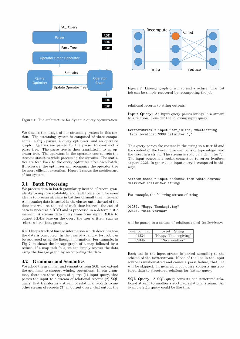
RDD keeps track of lineage information which describes howthe data is computed. In the case of a failure, lost job canbe recovered using the lineage information. For example, inFig 2, it shows the lineage graph of a map followed by areduce. If a map task fails, we can simply recover the datausing the lineage graph by recomputing the data.

3.2 Grammar and SemanticsWe adopt the grammar and semantics from SQL and extendthe grammar to support window operations. In our gram-mar, there are three types of query; (1) input query, thatparses the input to a stream of relational records (2) SQLquery, that transforms a stream of relational records to an-other stream of records (3) an output query, that output the

map reduce

FailedRecompute

Figure 2: Lineage graph of a map and a reduce. The lostjob can be simply recovered by recomputing the job.

relational records to string outputs.

Input Query: An input query parses strings in a streamto a relation. Consider the following input query.

twitterstream = input user_id:int, tweet:string

from localhost:9999 delimiter ","

This query parses the content in the string to a user id andthe content of the tweet. The user id is of type integer andthe tweet is a string. The stream is split by a delimiter “,”.The input source is a socket connection to server localhostat port 9999. In general, an input query is composed in thisway:

<stream name> = input <schema> from <data source>

delimiter <delimiter string>

For example, the following stream of string

01234, "Happy Thanksgiving"

02345, "Nice weather"

will be parsed to a stream of relations called twitterstream

user id : Int tweet : String01234 ”Happy Thanksgiving”02345 ”Nice weather”

Each line in the input stream is parsed according to theschema of the twitterstream. If one of the line in the inputsource is misformatted and causes a parse failure, that linewill be skipped. In general, input query converts unstruc-tured data to structured relations for further query.

SQL Query: A SQL query converts one structured rela-tional stream to another structured relational stream. Anexample SQL query could be like this.

tg_tweets = select * from twitterstream

where tweet like ’%Thanksgiving%’ window 10 seconds

This query selects records from the twitterstream where thetweet content contains keyword “Thanksgiving”. By addingthe window clause, all records in the last 10 seconds willbe retained. The result is assigned to another stream called“tg tweets”, which stands for Thanksgiving tweets. In gen-eral, a SQL query is composed in this way.

<stream name> = <standard SQL query> <window size>

A standard SQL query is applied on previous streams, theresult is windowed with the given window size. The windowclause is optional. If no window clause is specified, a defaultwindow size of 1 batch is applied. The name on the left sideof the = sign is the identifier of the stream.

Output Query: Output query converts structured rela-tion stream into unstructured string stream. Following is anexample of an output statement:

output user_id, tweet from tg_tweets delimiter ","

This converts each relation back to a string. The user idand tweet fields are converted to a string separated by “,”.

The relation tg stream is converted back to strings

user id : Int tweet : String01234 ”Happy Thanksgiving”

01234, "Happy Thanksgiving"

We build our own custom parser to parse the query. Thequery is then converted to an operator tree. Data streamflows through the operators for processing. Note that ourunderlying execution engine is Spark. All data is processedin batch granularity instead of record granularity.

3.3 OperatorsWe introduce the operators we have implemented in our sys-tem here. An operator takes a RDD as the input at the timet and outputs a RDD. A RDD may be totally stateless, suchas a filter operator. The filter operator takes the input RDDon each batch interval, filter the records with a given predi-cate, and output the filtered RDD. Some other operators are“stateful”, where some internal state is kept when process-ing the data stream. Note that the “states” of an operatorare still RDDs, therefore, we do not need to duplicate op-erators for fault tolerance. Instead, when there is a failure,the “state” can be recovered by lineage graph. For exam-ple, a window operator is stateful, where input RDDs in thewindow are cached.

Each operator maintains an output schema that is definedwhen the operator object is initiated. A schema is an array

of (column id, type) pair. The column id is a global uniqueidentifier of that column. We can easily identify a columnwith column id even if they appear in output schema of dif-ferent operators. For example, when two streams are joined,the original column id’s are inherited from their parents.Sometimes we need to create new column id. For example,consider the following query:

select item, price + tax as totalcost from shopping

While item still maintains the old column id, totalcost willbe assigned with a new column id. With this global namingscheme, we can identify a column easily when operators arereordered at runtime. We discuss the details of the operatorswe implemented here.

Select Operator: Select operator filters records in the datastream with some predicate. Everytime a RDD is passed tothe operator, the operator perform calls .filter(predicate) tofilter the records in the RDD according to the predicate. Theoutput schema of select operator is the same as its parent’soutput schema.

Project Operator: Project operator selects the requiredcolumns in the stream specified in the query. We implementthis operator by calling .map(func) on the input RDD. Theoutput schema of project operator is a subset of the outputschema of its parent operator.

Join Operator: Join operator joins the records in twostreams with the same join keys. In a join operator, recordsfrom the two input streams are first converted to key valuepairs and then they are co-partitioned by the key. This shuf-fles all the data in the two input stream, and guarantees therecords with the same keys are located on the same workernodes. Since data has already been partitioned by key in theparent RDDs, the records in the corresponding partition cannow be joined locally.

We collect statistics of the join operation when executingthe join. The size of the two input streams, and the size ofthe output stream is counted. The selectivity of this oper-ator is derived from the input and output cardinality. Thestatistics is collected using accumulator, that collects statis-tics of a RDD efficiently in an incremental manner. Theoutput schema of the joined stream is the concatenation ofthe input stream schemas.

Window Operator: A window operator takes the inputat the current timestamp and outputs the union of all theRDDs within the window. When a new RDD arrives theoperator, we first persist it in memory. This is very impor-tant because it avoids recomputing this RDD at the futuretime. If the RDD is still within the window and need to beused, instead of recomputing it using lineage graph, we cansimply get it from memory. The operator simply union allthe RDDs in the window and output it. The output schemais the same as the input schema.

Aggregation Operator: Aggregation operators aggregatescolumns to a single value by a specific aggregation function(eg. SUM(), AVG()). Similar to join, aggregation operators

first partition the data by the aggregation key. The aggrega-tion functions are then applied to the aggregation values toobtain the results. All columns that belongs to the aggrega-tion key maintains the same column id, while all aggregatedcolumns uses a new column id. The output schema is a com-bination of the aggregation keys and aggregation values.

Input Operator: Input operator parses the unstructuredstrings to construct a relation. The output schema is definedby the user as appeared in the input query.

Output Operator: Output operator converts structureddata to strings separated by a delimiter. There is no outputschema for this operator.

With the parse tree generated, the operator graph generatortakes the parse tree to generate an operator graph. Batchesof RDDs are generated by the stream receiver and the oper-ator graph consumes the RDDs. All the RDDs generated atthe same timestamp is processed by the operators. Finally,the output operators generate the processed data stream.The execution engine evaluates RDD lazily; If the stream isnot output by any output operator, it will not be processedat all.

3.4 Query OptimizationQuery optimization can be done efficiently in batch stream-ing system. Between each batch execution, there is a natu-ral barrier to reoptimize the execution base on the statisticscollected from previous iterations. This is difficult in tradi-tional streaming systems [5, 7, 10, 12]. In traditional streamprocessing system, operators maintain states for incrementalprocessing. To be fault tolerant, operators are replicated andstates must be synchronized between the operators. In batchprocessing system, the cost of replication can be avoided byusing lineage graph. All states are represented as RDDs, sothey are reconstructable by recomputing the lost task. Weconsider applying several query optimization on the operatorgraph.

We implement predicate pushdown on the operator graph.Select operator can be pushed to the data source to reduceunnecessary calculation on filtered records. We implementthis by swapping select operators with its parent until cer-tain conditions:

• The select operator’s parent has multiple children.

• The select operator’s parent is an aggregation operatorand the select predicate is on the aggregation columns.

Predicate pushdown can reduce the amount of computationif it is pushed below expensive operators such as join andaggregation.

Unlike select operators, window operators should be pushedup. Window operator unions all the RDDs in the win-dow and outputs it. Therefore, a window operator canincrease the amount of redundant computation. This isdemonstrated in Figure3. If a stream is first windowed,the following project operation have to recompute certainamount of data every task. Therefore, instead of windowing

RDD

RDD

RDD

RDD

RDD

RDD

Tim

e

RDD

Window(4 batches)

Project

RDD

RDD

RDD

RDD

RDD

Tim

e RDD

RDD

RDD

RDD

RDD

RDD

Window(4 batches)

Project

Figure 3: Window operators should be executed after otheroperators, if possible

the RDDs first, the project operation could be done beforethe window operation. The window operator simply unionsthe RDDs in the window, the operation cost is very low inSpark.

We should avoid pushing up window operators in the follow-ing condition to guarantee the semantic correctness.

• If there are multiple children for the window operator.In this case, we could split the window operator andpush them to all children.

• If the child operator is an aggregation operator, thewindow size affects the aggregation result.

• Similarly, the window operator affects join result, sowe should avoid pushing it below join operator.

Join operators could be reordered online base on the statis-tics we collected. Ideally, join operator with small selectivityshould be applied first (Figure 4). We obtain the selectivityof join operator by estimating the input data size and outputdata size. These statistics are feedback to the query opti-mizer right away. The join optimizer reorders the operatoraccording to the selectivity of the operators. Note that traf-fic pattern is usually static in a short time period. Therefore,it is unnecessary to obtain statistics every batch. Instead,we could estimate the statistics every several batches. Wemodify the query graph only if we are confident that thedata characteristics have been changed.

We implement incremental aggregation to reduce the amountof redundant computation. As we have mentioned, windowoperators could not be pushed beyond aggregation opera-tors. However, we can merge the window and aggregationoperator such that only the new batch is aggregated. Con-sider the following query:

windowed = select topic, tweet from twitter_stream

Select Select Select

Join

Join

Select Select Select

Join

Join

Figure 4: Reorder join operators by selectivity

window 300 seconds

topic_count = select topic, count(*) from windowed

By default, the last 300 seconds data will be windowed andcounted repeatedly. The optimized version would performa two level aggregation; Each batch in the time window isaggregated and cached. The aggregated value is being ag-gregated again as the final result. This method reduces theamount of redundant computation by using the cached ag-gregation value in the window.

The join operator can also be implemented incrementally.Consider joining two streams X and Y to stream W : letX(t) denotes the records at time t. X+(t+ 1) = X(t+ 1)−X(t) and X−(t + 1) = X(t) −X(t + 1) are the records thatadded to and remove from X at time t + 1. Then

W (t + 1) = W (t) + W+(t + 1) −W−(t + 1)

Variable W+(t + 1) can be obtained by

W+(t + 1) = Join(X+(t + 1), Y (t + 1))

+Join(Y +(t + 1), X(t) −X−(t + 1))

Similarly, variable W−(t + 1) can be obtained by

W−(t + 1) = Join(X−(t + 1), Y (t))

+Join(Y −(t + 1), X(t) −X−(t + 1))

Although the equations looks complicated, the semantic isquite simple; Everytime the time advances, we remove therecords that are expired in the join results and add the newjoin results. We are currently studying how to efficientlyimplement incremental join. The current problem is Sparkcan only manipulate data at RDD level, record level modi-fication may not be efficient.

4. EVALUATIONWe evaluate the performance of the query optimization tech-nique in Amazon EC2. We set up a cluster with 6 workernodes using Spark 0.9.0 and deployed our system on top ofit.

4.1 Micro BenchmarkWe first evaluate the benefits of predicate pushdown. Thequery we execute is:

x = input key:int,value:int from localhost:9999

0

200

400

600

800

1000

1200

1400

1 51 101 151 201 251 301 351 401 451

Pro

cess

ing

De

lay

(ms)

Batch

With Predicate Pushdown W/o Predicate Pushdown

Figure 5: Processing delay with and without predicate push-down

delimiter ","

gb = select key, avg(value) as value from x

group by key

pred = select key, value from gb where key > 10

output key, value from pred delimiter ","

The source stream generates 500,000 key value pairs persecond. The key is generated from a random Gaussian dis-tribution with mean equals to 0 and a standard deviationof 5. The predicate key > 10 filters about 97.5% recordsout. Without predicate pushdown, the group by operator isevaluated before the predicate. We evaluate 500 batches ofdata with a batch size of 1 second. Without predicate push-ing, the average processing latency is 712ms. After predicatepushing, the average latency is only 497ms, which reducesthe processing latency by 30%.

We evaluate the performance of window pushup using thesame experimental setting. The cluster processes 500,000records every batch, with batch size 1 second. Following isthe query we executed:

x = input key:int,value:int from localhost:9999

delimiter ","

win = select key, value from x window 10 seconds

pred = select key from win where key = 20

output key from pred delimiter ","

Even with very small window size of 10 seconds, it takes over2 seconds to process 1 second worth of data without opti-mization (Figure 6 (A)). Since the processing rate is lowerthan the incoming data rate, the tasks soon queued up andthe batch delay goes up to infinity. By using window pushup,the processing latency of a batch can be maintained at alow level (Figure 6 (B)). We reduce the data rate to 200,000records per second and reevaluate the performance. By us-ing window pushup, we can reduce the processing latencyby 65%.

To evaluate the performance of dynamic join operator re-ordering, we execute the following query:

x = input key:int,value:int from localhost:9999

0

500

1000

1500

2000

2500

3000

3500

4000

1 51 101 151 201 251 301 351 401 451

Pro

cess

ing

Late

ncy

(m

s)

Batch

(A) 500k rec/s, w/o window pushup

(B) 500k rec/s, with window pushup

(C) 200k rec/s, w/o window pushup

(D) 200k rec/s, with window pushup

Figure 6: Processing delay with and without window pushup

0

200

400

600

800

1000

1200

1400

1600

1800

2000

1 21 41 61 81 101 121 141 161 181 201 221 241

Pro

cess

ing

Late

ncy

Batch

Static Query Plan Dynamic Query Plan

Figure 7: Join with/without operator reordering

delimiter ","

y = input key:int,value:int from localhost:9998

delimiter ","

z = input key:int,value:int from localhost:9997

delimiter ","

joined = select x.key as xk, x.value as xv,

y.key as yk, y.value as yv,

z.key as zk, z.value as zv from x

inner join y on x.key = y.key

inner join z on x.key = z.key

ct = select count(xk) as c from joined

output c from ct delimiter ","

The key of streams y and z are generated from a Gaussiandistribution with mean 0 and 30, respectively. The key ofstream x is generated from a Gaussian Distribution withvarying mean; Every 20 seconds, the mean of x switchesbetween 0 and 30. Therefore, when x’s mean is 0, we shouldjoin x and z first, and the join the result with y. The samerule applies when x’s mean is 30. For all the three streamsx, y and z, the standard deviation is 10 and the data rateis 2000 records per second. The joined stream producesaround 400,000 records per second.

Figure 7 shows the processing latency of the execution withand without join operator reordering. With a static queryplan, the latency follows a bimodal distribution, with an av-erage latency of 921 ms. With dynamic query optimization,the latency distribution is more uniform, and the averagelatency is 748 ms. We observe that every time the meanof stream x switches, there is a spike on the latency even ifthe dynamic query optimization is applied. This is because

0

200

400

600

800

1000

1200

1

12

23

34

45

56

67

78

89

10

0

11

1

12

2

13

3

14

4

15

5

16

6

17

7

18

8

19

9

21

0

22

1

23

2

24

3

25

4

26

5

27

6

28

7

29

8

Pro

cess

ing

Late

ncy

(m

s)

Batch

Naïve Aggregation Incremental Aggregation

Figure 8: Processing delay using naıve aggregation and in-cremental aggregation

there is a one batch delay when obtaining the statistics. Inpractice, the stream characteristics changes less abruptly,hence, the processing latency would be more stable.

Window operators can only be pushed upto an aggregationoperator. Further pushing the window operator above ag-gregation operator changes the semantic. However, by re-placing the aggregation operator with an incremental aggre-gation operator, we can efficiently execute the aggregationwithout doing redundant work. We evaluate the followingquery:

x = input key:int,value:int from localhost:9999

delimiter ","

xx = select key,vallue from x window 10 seconds

ct = select key, count(value) as count from xx

output key,count from ct delimiter ","

The keys in stream x are generated from a Gaussian Distri-bution with mean 0 and standard deviation 5. The data rateof stream x is 100,000 records per second. Figure 8 showsthe processing delay using naıve aggregation and incremen-tal aggregation. By using incremental aggregation, we canreduce the average processing delay from 715 ms to 310 ms.

We evaluate the performance of incremental join with fol-lowing query:

x = input key:int,value:int from localhost:9999

delimiter ","

y = input key:int,value:int from localhost:9998

delimiter ","

xx = select key,value from x window 10 seconds

yy = select key,value from y window 10 seconds

joined = select xx.key as xk, xx.value as xv,

yy.key as yk, yy.value as yv from xx

inner join yy on xx.key = yy.value

ct = select count(xk) as count from joined

output count from ct delimiter ","

Window operators are pushed up to the join operator. Thejoin operator are then replaced with an incremental join op-erator. The incremental join operator caches the join result

in the window. Figure 9 shows the processing latency of anaıve join and an incremental join. The incremental join op-erator checkpoints the data every 10 seconds. Therefore, theprocessing delay spikes every 10 seconds. Figure 10 showsthe performance with varying window size. For window sizevarying from 10 seconds to 40 seconds, incremental join op-erator always performs better.

0

200

400

600

800

1000

1200

1400

1 21 41 61 81 101 121 141 161

Pro

cess

ing

Late

ncy

(m

s)

Batch

Incremental Join Naïve Join

Figure 9: Processing delay using naıve join and incrementaljoin

4.2 Road Traffic BenchmarkLinear Road Benchmark [6] is used in the STREAM [18]project. The benchmark has the locations of the cars ina simulated freeway system. The cars in the freeway sys-tem reports the location of the car to a central repository.Following is the schema of the data:

1. time The timestamp when the record enters the database.

2. vid An unique identification of the vehicle.

3. speed The speed of the vehicle.

4. hwy The highway ID. There are multiple highways inthe system.

5. lane The lane the vehicle is on.

6. dir The direction the vehicle is going.

0

200

400

600

800

1000

1200

1400

10 20 30 40 50

Pro

cess

ing

De

lay

(ms)

Window Size (s)

Naïve Join Incremental Join

Figure 10: Average processing delay using naıve join andincremental join with varying window size

7. seg The segment the vehicle is in. The highway isdivided into 1 mile segments.

8. pos The location the (in feet) the vehicle is from thestarting point of the highway.

The data is three hours long with varying incoming datarates from 5 records per second to 1884 records per second.To increase the workload, we replay the data 5 times faster.The goal of the query is to count the number of cars thatare in the congested segments (average car speed < 40mphin the last minute) in the last 15 seconds. Following is thequery:

records = input time:int, vid:int, speed:int, hwy:int,

lane:int, dir:string, seg:string, pos:string

from localhost:8888 delimiter ","

recWindow60 = select vid, speed, seg, dir, hwy

from records window 60 seconds

segSpeed = select seg, dir, hwy, avg(speed) as avgSpeed

from recWindow60 group by seg, dir, hwy

congestedSeg = select seg, dir, hwy, avgSpeed

from segSpeed where avgSpeed < 40

recWindow15 = select vid, speed, seg, dir, hwy

from records window 15 seconds

congestedCar = select recWindow15.vid as vid

from recWindow15 inner join congestedSeg

on recWindow15.seg = congestedSeg.seg

and recWindow15.dir = congestedSeg.dir

and recWindow15.hwy = congestedSeg.hwy

numCongested = select count(vid) as c

from congestedCar

output c from numCongested delimiter ","

Stream records are the raw input records with the location ofthe vehicle and speed of the car. recWindow10 is a windowedstream with the location and speed of the vehicle in thelast. segSpeed is a stream storing the average speed of thevehicles in a segment. congestedSeg is the segments that arecongested (i.e. avgSpeed < 40). recWindow3 is a windowedstream with the location and speed of the vehicle in thelast 15 seconds. By joining congestedSeg and recWindow15,we obtain congestedCar, the cars that are in the congestedsegments. numCongested counts the number of cars in thecongested segments.

The optimizer automatically applies predicate pushdown,window pushup and incremental aggregation in this query.Figure 11 shows the results of the experiment. At the begin-ning, both approaches have similar performance as the inputdata rate is small. With the increase of input data rate, thequery plan without query optimization has larger latencythan the optimized query plan. The average execution la-tency of the query plan without optimization is 960 ms witha standard deviation of 445 ms. The optimized query planhas an average latency of 679 ms and the standard deviationis 250 ms.

4.3 Twitter DatasetWe use the Twitter API to sample small fraction of Tweetsand dump them to a local file. We replay the Tweets with

0

5000

10000

15000

20000

25000

30000

0

500

1000

1500

2000

1 101 201 301 401 501 601 701 801 901 1001 1101 1201 1301 1401 1501 1601 1701 1801 1901

Dat

a R

ate

(re

c/s)

Late

ncy

(m

s)

Batch

W/o Optimization With Optimization Data Rate

Figure 11: Executing Query with/without optimization on Linear Road Benchmark

0

200

400

600

800

1000

1200

1400

1600

1800

2000

0 10000 20000 30000 40000 50000 60000

Late

ncy

(m

s)

Throughput (Records/s)

Without Optimization With Optimization

Figure 12: Throughput vs Latency. The blue squares arefrom the query plan without optimization. The orange dotsare from optmized query plan.

varying data rate to measure the throughput of the queryplan. We evaluate the following query:

raw = input time:string, tweetId:string,

scrName:string, language:string, userId:string,

userLoc:string, userName:string, text:string

from localhost:7777 delimiter "\t"

win = select lang from raw window 10 seconds

g = select language, count() as c from win

group by language

output language, c from g delimiter ","

Figure 12 shows the evaluation results. Without query opti-mization, latency grows quickly with the increase of through-put. To maintain a latency bound of 1 second, the queryplan without optimization can only process about 7,000 recordsper second. With optimization, the throughput can be ashigh as 40,000 records per second.

5. RELATED WORKStream Processing Systems: Stream processing engines,such as STREAM [18], TelegraphCQ [10], TimeStream [22],Storm [1], Naiad [19], and Borealis [2] are all continuousoperator model. The data flow is expressed as a graph ofoperators. Data is processed by operators and sent to otheroperators for further processing. In fact, in these systems,

batching is a common technique to increase the performanceof stream processing. In these systems, operators maintainstates. When an operator fails, the state of the operator isgone. To reconstruct the state, either the operator needs tobe duplicated or the upstream backup needs to be applied.In DStream, operator is decoupled from operator state bykeeping the lineage information. Therefore, lost state canbe simply recovered by recomputing the lost partition. Allthese stream process system applies a static execution graph.Our system allows the operators to be reordered base on theexecution information from previous batches. Statistics ofthe stream data is collected from executed batches, and thesedata is applied to optimize the execution of new batches.

Adaptive Streaming: Existing papers have extensive dis-cussion on optimizing query execution in traditional record-based stream process engine. [23] discusses how to placethe operators in the query plan. When the processing ca-pacity is not enough to processing the incoming data, somefraction of the data needs to be discarded [8,24]. While thistechnique guarantees the processing time, it is lossy in na-ture and the quality of the query may be sacrificed. Otherpapers have proposed to elastically adjust the amount of re-source according to the incoming workload [4,16,17,25]. Wewould like to study how to adjust the degree of parallelismin the data processing flow in response to the varying incom-ing data rate. Deciding the optimal degree of parallelism isa difficult question. Making the degree of parallelism toosmall increases the processing time of the tasks, while mak-ing it too large increases the task launching overhead. Wewill incorporate this in our future work.

Query Optimization: Optimizing query execution is awell studied topic in database management system [11, 13,14]. To estimate the cost of an operator, sampling is neces-sary to obtain the statistics of the data. However, samplingis costly, especially for “big data”. A recent proposal [3]argues that if a task is executed on the same data again,statistics can be obtained from the first execution. In oursystem, although data between batches is not the same, theyoften show similar statistical properties. Therefore, we couldcollect data statistics from previous executions to optimizefuture execution. In this paper, we implement this idea andshow the benefits of optimizing the execution online.

6. CONCLUSION

We presented several techniques to optimize query executionin batch streaming system. We implemented incrementaloperators and a query optimization framework that dynam-ically reoptimize the data parallel execution on the fly. Weshow the benefits of such optimization with micro bench-mark and real dataset. In the future work, we would liketo investigate elastically adjust the parallelism of the oper-ators to provide performance guarantee in batch streamingsystem.

7. REFERENCES[1] Storm, distributed and fault-tolerant realtime

computation.

[2] D. J. Abadi, Y. Ahmad, M. Balazinska, U. Cetintemel,M. Cherniack, J.-H. Hwang, W. Lindner, A. Maskey,A. Rasin, E. Ryvkina, et al. The design of the borealisstream processing engine. In CIDR, volume 5, pages277–289, 2005.

[3] S. Agarwal, S. Kandula, N. Bruno, M.-C. Wu,I. Stoica, and J. Zhou. Re-optimizing data-parallelcomputing. In Proc. of USENIX NSDI, pages 21–35,2012.

[4] L. Amini, N. Jain, A. Sehgal, J. Silber, andO. Verscheure. Adaptive control of extreme-scalestream processing systems. In Distributed ComputingSystems, 2006. ICDCS 2006. 26th IEEE InternationalConference on, pages 71–71. IEEE, 2006.

[5] A. Arasu, S. Babu, and J. Widom. Cql: A languagefor continuous queries over streams and relations. InDatabase Programming Languages, pages 1–19.Springer, 2004.

[6] A. Arasu, M. Cherniack, E. Galvez, D. Maier, A. S.Maskey, E. Ryvkina, M. Stonebraker, and R. Tibbetts.Linear road: a stream data management benchmark.In Proceedings of the Thirtieth internationalconference on Very large data bases-Volume 30, pages480–491. VLDB Endowment, 2004.

[7] R. Avnur and J. M. Hellerstein. Eddies: Continuouslyadaptive query processing. In ACM sigmod record,volume 29, pages 261–272. ACM, 2000.

[8] B. Babcock, M. Datar, and R. Motwani. Loadshedding for aggregation queries over data streams. InData Engineering, 2004. Proceedings. 20thInternational Conference on, pages 350–361. IEEE,2004.

[9] D. Borthakur. The hadoop distributed file system:Architecture and design, 2007.

[10] S. Chandrasekaran, O. Cooper, A. Deshpande, M. J.Franklin, J. M. Hellerstein, W. Hong,S. Krishnamurthy, S. R. Madden, F. Reiss, and M. A.Shah. Telegraphcq: continuous dataflow processing. InProceedings of the 2003 ACM SIGMOD internationalconference on Management of data, pages 668–668.ACM, 2003.

[11] S. Chaudhuri, R. Krishnamurthy, S. Potamianos, andK. Shim. Optimizing queries with materialized views.In Data Engineering, 1995. Proceedings of theEleventh International Conference on, pages 190–200.IEEE, 1995.

[12] N. Conway, M. J. Franklin, S. Krishnamurthy, A. Li,A. Russakovsky, and N. Thombre. Trusql: Astream-relational extension to sql.

[13] A. Deshpande, Z. Ives, and V. Raman. Adaptive queryprocessing. Foundations and Trends in Databases,1(1):1–140, 2007.

[14] J. C. Freytag. A rule-based view of query optimization,volume 16. ACM, 1987.

[15] M. Isard, M. Budiu, Y. Yu, A. Birrell, and D. Fetterly.Dryad: distributed data-parallel programs fromsequential building blocks. ACM SIGOPS OperatingSystems Review, 41(3):59–72, 2007.

[16] A. Ishii and T. Suzumura. Elastic stream computingwith clouds. In Cloud Computing (CLOUD), 2011IEEE International Conference on, pages 195–202.IEEE, 2011.

[17] A. Jain, E. Y. Chang, and Y.-F. Wang. Adaptivestream resource management using kalman filters. InProceedings of the 2004 ACM SIGMOD internationalconference on Management of data, pages 11–22.ACM, 2004.

[18] R. Motwani, J. Widom, A. Arasu, B. Babcock,S. Babu, M. Datar, G. Manku, C. Olston,J. Rosenstein, and R. Varma. Query processing,resource management, and approximation in a datastream management system. CIDR, 2003.

[19] D. G. Murray, F. McSherry, R. Isaacs, M. Isard,P. Barham, and M. Abadi. Naiad: a timely dataflowsystem. In Proceedings of the Twenty-Fourth ACMSymposium on Operating Systems Principles, pages439–455. ACM, 2013.

[20] K. Ousterhout, P. Wendell, M. Zaharia, and I. Stoica.Sparrow: distributed, low latency scheduling. InProceedings of the Twenty-Fourth ACM Symposium onOperating Systems Principles, pages 69–84. ACM,2013.

[21] V. Paxson. Bro: a system for detecting networkintruders in real-time. Computer networks,31(23):2435–2463, 1999.

[22] Z. Qian, Y. He, C. Su, Z. Wu, H. Zhu, T. Zhang,L. Zhou, Y. Yu, and Z. Zhang. Timestream: Reliablestream computation in the cloud. In Proceedings of the8th ACM European Conference on Computer Systems,pages 1–14. ACM, 2013.

[23] U. Srivastava, K. Munagala, and J. Widom. Operatorplacement for in-network stream query processing. InProceedings of the twenty-fourth ACMSIGMOD-SIGACT-SIGART symposium on Principlesof database systems, pages 250–258. ACM, 2005.

[24] N. Tatbul, U. Cetintemel, S. Zdonik, M. Cherniack,and M. Stonebraker. Load shedding in a data streammanager. In Proceedings of the 29th internationalconference on Very large data bases-Volume 29, pages309–320. VLDB Endowment, 2003.

[25] Y. Xing, S. Zdonik, and J.-H. Hwang. Dynamic loaddistribution in the borealis stream processor. In DataEngineering, 2005. ICDE 2005. Proceedings. 21stInternational Conference on, pages 791–802. IEEE,2005.

[26] M. Zaharia, T. Das, H. Li, S. Shenker, and I. Stoica.Discretized streams: an efficient and fault-tolerantmodel for stream processing on large clusters. InProceedings of the 4th USENIX conference on HotTopics in Cloud Ccomputing, pages 10–10. USENIXAssociation, 2012.