optimizing snake locomotion in the plane - mathematicsalben/optimalsnakepaperpra.pdf · locomotion...

rspa.royalsocietypublishing.org

Research

Article submitted to journal

Subject Areas:

applied mathematics, biomechanics

Keywords:

snake, friction, sliding, locomotion,

optimization

Author for correspondence:

Silas Alben

e-mail: [email protected]

Optimizing snake locomotionin the plane

Silas Alben

Department of Mathematics, University of Michigan,

Ann Arbor, MI, USA

We develop a numerical scheme to determine which

planar snake motions are optimal for locomotory

efficiency, across a wide range of frictional parameter

space. For a large coefficient of transverse friction,

we show that retrograde traveling waves are optimal.

We give an asymptotic analysis showing that the

optimal wave amplitude decays as the -1/4 power

of the coefficient of transverse friction. This result

agrees well with the numerical optima. At the other

extreme, zero coefficient of transverse friction, we

propose a triangular direct wave which is optimal.

Between these two extremes, a variety of complex,

locally optimal motions are found. Some of these

can be classified as standing waves (or ratcheting

motions).

c© The Author(s) Published by the Royal Society. All rights reserved.

http://crossmark.crossref.org/dialog/?doi=10.1098/rspa.&domain=pdf&date_stamp=

mailto:[email protected]

2

rspa.royalsocietypublishing.orgP

rocR

Soc

A0000000

..........................................................

1. IntroductionSnake locomotion has a long history of study by biologists, engineers, and applied

mathematicians [1–6]. A lack of appendages makes snake motions simpler in some respects

than those of other locomoting animals [7]. However, snakes can move through a wide

range of terrestrial [1,8,9], aquatic [10], and aerial [11] environments, with different kinematics

corresponding to the different dynamical laws which apply in each setting. Here we focus on

terrestrial locomotion, with motions restricted to two dimensions, and a Coulomb frictional

force acting on the snake. Even with these simplifying assumptions, there are many possible

snake kinematics to consider. One way to organize our understanding of a diversity of

locomotory kinematics is to propose a measure of locomotory performance (here, efficiency),

and determine which motions are optimal, and how their performance varies with physical

parameters. Well-known examples are optimization studies of organisms moving in low- [12–17]

and high-Reynolds-number fluid flows [18–23].

In this work, we use a recently-proposed model for snake locomotion in the plane which has

shown good agreement with biological snakes [3,6]. The snake is a slender body whose curvature

changes as a prescribed function of arc length distance along the backbone and time. Its net

rotation and translation are then determined by Newton’s laws, with Coulomb friction between

the snake and the ground. This model is perhaps one of the simplest which can represent arbitrary

planar snake motions. Previous studies have used the model to find optimal snake motions

when the motions are restricted to sinusoidal traveling waves [6], or the bodies are composed

of two or three links [24]. These motions are represented by a small number of parameters (2-

10); at the upper end of this range, the optimization problem is difficult to solve using current

methods. In [2], Guo and Mahadevan developed a model which included the internal elasticity

and viscosity of the snake, and studied the effects of these and other physical parameters on

locomotion for a prescribed sinusoidal shape and sinusoidal and square-wave internal bending

moments. In the present work, we neglect the internal mechanics of the snake, and consider only

the work done by the snake on its environment, the ground.However, we consider a more general

class of snake motions. Hu and Shelley assumed a sinusoidal traveling-wave snake shape, and

computed the snake speed and locomotory efficiency across the two-parameter space of traveling-

wave amplitude and wavelength for two values of frictional coefficients [6]. They also considered

the ability of the snake to redistribute its weight during locomotion. Jing and Alben considered

the locomotion of two- and three-link snakes, and found analytical and numerical results for the

scaling of snake speed and efficiency [24]. Among the results were the optimal temporal function

for actuating the internal angles between the links, expressed as Fourier series with one and two

frequencies.

Here we address the optimization problem for planar snakes more generally, by using a much

larger number of parameters (45 in most cases) to represent the snake’s curvature as a function of

arc length and time. Although our snake shape space is limited, it is large enough to represent

a wide range of shapes. To solve the optimization problem in a 45-dimensional shape space,

and simultaneously across a large region of the two-dimensional friction parameter space, we

develop an efficient numerical method based on a quasi-Newton method. The simulations show

clearly that two types of traveling-wave motions, retrograde and direct waves, are optimal when

the coefficient of friction transverse to the snake is large and small, respectively. An asymptotic

analysis shows how the snake’s traveling wave amplitude should scale with the transverse

coefficient of friction when it is large. The analysis gives a −1/4 power law for the amplitude

which agrees well with the numerics. In this limit, the power required to move a snake optimally

is simply that needed to tow a straight snake forward. Another analytical solution gives an

optimally-efficient direct wave motion when the transverse coefficient of friction is zero. Between

these extremes, the numerics show a more complicated set of optima which include standing-

wave (or ratcheting) motions, among a wide variety of other locally-optimal motions. Taken

3


rocR

Soc

A0000000

..........................................................

together, these results show which planar snake motions are optimal within a large space of

possible motions and frictional coefficients.

2. ModelWe use the same frictional snake model as [3,6,24], so we only summarize it here. The snake’s

position is given by X(s, t) = (x(s, t), y(s, t)), a planar curve which is parametrized by arc length

s and varies with time t. A schematic diagram is shown in figure 1.

x

ys = 0

s = 1s

n

θ µbµf

µt

Figure 1. Schematic diagram of snake position, parametrized by arc length s (nondimensionalized by snake

length), at an instant in time. The tangent angle and unit vectors tangent and normal to the curve at a point

are labeled. Vectors representing forward, backward and transverse velocities are shown with the corresponding

friction coefficients µf , µb, and µt.

The unit vectors tangent and normal to the curve are s and n respectively. The tangent angle

and curvature are denoted θ(s, t) and κ(s, t), and satisfy ∂sx= cos θ, ∂sy= sin θ, and κ= ∂sθ.

We consider the problem of prescribing the curvature of the snake in order to obtain efficient

locomotion.When κ(s, t) is prescribed, the tangent angle and position are obtained by integration:

θ(s, t) = θ0(t) +

∫ s

0κ(s′, t)ds′, (2.1)

x(s, t) = x0(t) +

∫ s

0cos θ(s′, t)ds′, (2.2)

y(s, t) = y0(t) +

∫ s

0sin θ(s′, t)ds′. (2.3)

The trailing-edge position (x0, y0) and tangent angle θ0 are determined by the force and torque

balance for the snake, i.e. Newton’s second law:

∫L

0ρ∂ttxds=

∫L

0fxds, (2.4)

∫L

0ρ∂ttyds=

∫L

0fyds, (2.5)

∫L

0ρX⊥ · ∂ttXds=

∫L

0X

⊥ · fds. (2.6)

Here X⊥ = (−y, x), ρ is the snake’s mass per unit length and L is the snake length. The snake is

locally inextensible, ρ is uniform in space and constant in time, and L is constant in time. f is the

force per unit length on the snake due to Coulomb friction with the ground:

f(s, t) =−ρgµt

“

d∂tX · n”

n − ρg“

µfH“

d∂tX · s”

+ µb

“

1 −H“

d∂tX · s”””“

d∂tX · s”

s. (2.7)

Here H is the Heaviside function and the hats denote normalized vectors. When ‖∂tX‖= 0 we

define d∂tX to be 0. According to (2.7) the snake experiences friction with different coefficients

for motions in different directions. The frictional coefficients are µf , µb, and µt for motions in the

4


rocR

Soc

A0000000

..........................................................

forward (s), backward (−s), and transverse (i.e. normal, ±n) directions, respectively. In general

the snake velocity at a given point has both tangential and normal components, and the frictional

force density has components acting in each direction. A similar decomposition of force into

directional components occurs for viscous fluid forces on slender bodies [25].

We assume that the snake curvature κ(s, t) is a prescribed function of s and t that is periodic in

t with period T . Many of the motions commonly observed in real snakes are essentially periodic

in time [3]. We nondimensionalize equations (2.4)–(2.6) by dividing lengths by the snake length

L, time by T , and mass by ρL. Dividing both sides by µfg we obtain:

L

µfgT 2

∫1

0∂ttxds=

∫1

0fxds, (2.8)

L

µfgT 2

∫1

0∂ttyds=

∫1

0fyds, (2.9)

L

µfgT 2

∫1

0X

⊥ · ∂ttXds=

∫1

0X

⊥ · fds. (2.10)

In (2.8)–(2.10) and from now on, all variables are dimensionless. For most of the snake motions

observed in nature, L/µf gT2 ≪ 1 [3], which means that the snake’s inertia is negligible. By

setting this parameter to zero we simplify the problem considerably while maintaining a good

representation of real snakes. (2.8)–(2.10) become:

b = (b1, b2, b3)⊤ = 0 ; b1 ≡

∫1

0fxds, (2.11)

b2 ≡∫1

0fyds, (2.12)

b3 ≡∫1

0X

⊥ · fds. (2.13)

In (2.11)–(2.13), the dimensionless force f is

f(s, t) =− µt

µf

“

d∂tX · n”

n −„

H(d∂tX · s) +µb

µf(1 −H(d∂tX · s))

«

“

d∂tX · s”

s (2.14)

The equations (2.11)–(2.13) thus involve only two parameters, which are ratios of the friction

coefficients. From now on, for simplicity, we refer to µt/µf as µt and µb/µf as µb. Without loss

of generality, we assume µb ≥ 1. This amounts to defining the backward direction as that with

the higher of the tangential frictional coefficients, when they are unequal. µt may assume any

nonnegative value. The same model was used in [3,6,24], and was found to agree well with the

motions of biological snakes in [3].

Given the curvature κ(s, t), we solve the three nonlinear equations (2.11)–(2.13) at each time t

for the three unknowns x0(t), y0(t) and θ0(t). Then we obtain the snake’s position as a function

of time by (2.1)–(2.3). The distance traveled by the snake’s center of mass over one period is

d=

v

u

u

t

∫1

0x(s, 1) − x(s, 0) ds

!2

+

∫1

0y(s, 1) − y(s, 0) ds

!2

. (2.15)

The work done by the snake against friction over one period is

W =

∫1

0

∫1

0f(s, t) · ∂tX(s, t) ds dt. (2.16)

We define the cost of locomotion as

η=W

d(2.17)

and our objective is to find κ(s, t) which minimize η at (µb, µt) values which range widely over

[1,∞) × [0,∞). In our computations, instead of η, we minimize a different function which is more

5


rocR

Soc

A0000000

..........................................................

convenient for physical and numerical reasons:

F =− d

We2 cos(θ(0,1)−θ(0,0)). (2.18)

To obtainF from ηwe have substituted−d/W forW/d, to avoid infinities in the objective function

for a common class of motions with d→ 0 and W of order 1. The exponential term in (2.18)

penalizes rotations over a period, to ensure that the snake moves in a straight path rather than

a circular path over many periods. As will be described in the results section, for µt & 6 and all

µb, we find optima which have an analytical traveling wave form, and in the limit of large µt,

rotations tend to zero for these solutions. These optima are found even with no rotation penalty,

so the rotation penalty plays a negligible role in this region of parameter space. For smaller µt,

however, in the absence of the rotation penalty, many of the optima have significant rotations. In

Appendix A we give a more detailed explanation for the choice of F .

3. Numerical Minimization MethodOur goal is to determine the snake shape, κ(s, t), which minimizes F , for a given (µb, µt). Since

κ(s, t) has t-period one, we represent it via a double series expansion:

κ(s, t) =

m1−1X

j=0

n1−1X

k=0

`

αjk cos(2πjt) + βjk sin(2πjt)´

Tk(s). (3.1)

Here Tk is a Chebyshev polynomial in s:

Tk(s) = cos(k arccos(s)). (3.2)

The expansion (3.1) converges as m1, n1 →∞ for a large class of κ which includes differentiable

functions, and with a convergence rate that increases rapidly with the number of bounded

derivatives of κ [26]. It is reasonable to hope that minimizing F over a class of functions (3.1)

with small m1 and n1 gives a good approximation to the minimizers with infinite m1 and

n1. Since the terms in (3.1) with coefficients β0k are automatically zero, the functions given by

(3.1) are a (2m1 − 1)n1-dimensional space. In most of this work we use m1 = n1 = 5, so we are

minimizing F in a 45-dimensional space. We give a few results at large µt with m1 = n1 = 10

for comparison, and find similar minimizers in this region of parameter space. The minimization

algorithm converges in a smaller portion of (µb, µt) space asm1 and n1 increase, and convergence

is considerably slowed by the increased dimensionality of the search space. We find that m1 =

n1 = 5 is small enough to allow convergence to minima in a large portion of (µb, µt) space, but

large enough to approximate the gross features of a wide range of κ(s, t). Another reason to expect

that good approximations to minimizers can be obtained with small n1 is that the dynamical

equations (2.11)–(2.13) depend only on spatial integrals of body position and velocity.

Using the dynamical equations (2.11)–(2.13), we show in Supplementary Material section A

that d, W , and F are the same for any reparametrization of time. Such a reparametrization can

be used to reduce the high-frequency components of a motion while keeping the efficiency the

same. Therefore, it is reasonable to expect that a good approximation to any minimizer of F can

be obtained with low temporal frequencies, that is, with an expansion in the form of (3.1) with

smallm1.

We use the Broyden-Fletcher-Goldfarb-Shanno (BFGS) algorithm [27] to minimize F

numerically, by computing a sequence of iterates which converge to a local minimizer of F .

The algorithm requires routines for computing the values and gradients of F as well as a line

searchmethod for finding the next iterate at each step, using the search direction providedwithin

the BFGS algorithm. The BFGS algorithm is a quasi-Newton algorithm, and therefore forms an

approximation to the Hessian matrix of second derivatives, without the expense and difficulty of

computing the Hessian matrix explicitly.

We have developed an efficient method for evaluating F and its gradient with respect to the

(2m1 − 1)n1 shape parameters with just a single simulation of the snake trajectory over one

6


rocR

Soc

A0000000

..........................................................

period. Computing the value of F requires computing the trajectory of the snake over one period.

We discretize the period interval uniformly with m time points: {0, 1/m, 2/m, . . . , 1 − 1/m}. At

each time point we write (2.11)–(2.13) as a nonlinear algebraic system of three equations in three

unknowns: {∂tx0, ∂ty0, ∂tθ0}. We also define an artificial frame for each time point in which the

snake’s trailing edge coordinates are {x0, y0, θ0}= {0, 0, 0} at the time in question; each such

frame is fixed in time. We then solve (2.11)–(2.13) for the trailing edge velocities in each of the

artificial frames, {g∂tx0, f∂ty0,f∂tθ0}. Since each artificial frame is obtained from the lab frame by a

fixed translation and rotation, the tangent angle at the snake’s trailing edge changes at the same

rate in the two frames: f∂tθ0 = ∂tθ0. We thus obtain the trailing edge tangent angle in the lab frame

by integrating:

θ0(t) =

∫ t

0

g∂τθ0 dτ. (3.3)

We then obtain the trailing edge position in the lab frame by integrating the trailing edge

translational velocities, rotated to the lab frame:

x0(t)

y0(t)

!

=

∫ t

0

cos θ0(τ ) − sin θ0(τ )

sin θ0(τ ) cos θ0(τ )

!

g∂τx0

g∂τ y0

!

dτ. (3.4)

We then integrate κ(s, t) using {x0(t), y0(t), θ0(t)} to obtain the body trajectory a posteriori.

Using {∂tx0, ∂ty0, ∂tθ0} as the unknowns instead of {x0, y0, θ0} has two advantages: we avoid

cancellation error associated with computing discrete time derivatives of {x0, y0, θ0}, and we

solve m decoupled systems of three equations in three unknowns instead of a larger coupled

system of 3m equations in 3m unknowns ({x0, y0, θ0} at all times points), which is more

expensive to solve.

We solve the system (2.11)–(2.13) using Newton’s method with a finite-difference Jacobian

matrix. We solve it at each time sequentially from t= 0, using a random initial guess for

{∂tx0, ∂ty0, ∂tθ0} at t= 0 and an extrapolation from previous time points as an initial guess at

other t. An important element of our method is the quadrature used to compute the integrals in

(2.11)–(2.13) using (2.14). Here we introduce notation for the tangential and normal components

of the snake velocity:

us = ∂tX · s ; un = ∂tX · n. (3.5)

In (2.14) we can write

d∂tX · s =us

p

u2s + u2

n

; d∂tX · n =un

p

u2s + u2

n

. (3.6)

These terms have unbounded derivatives with respect to us and un when us, un → 0. The

local error when integrating (2.14) using the trapezoidal rule (for example) with uniform mesh

size h is O“

h3 max(us, un)−2”

. To obtain convergence in this case it is necessary to have

h= o(max(us, un)2/3), so the trapezoidal rule (and other classical quadrature rules) need to be

locally adaptive when (us, un) tends to zero.

We use a different approach which allows for a uniform mesh even when (us, un)→ 0. We

perform the quadrature analytically on subintervals using locally linear approximations for us

and un. Using {∂tx0, ∂ty0, ∂tθ0} and κ(s, t), we compute ∂tX, X, and then us and un on a

uniform mesh. On each subinterval, we approximate us and un as linear functions of the form

As+B using their values at the interval endpoints. We approximate X⊥, s, and n as constants

using their values at the midpoints of the intervals. Then the integrals in (2.11)–(2.13), using (2.14),

are of the form

C0

∫ b

a

As+Bp

(As+B)2 + (Cs+D)2ds (3.7)

7


rocR

Soc

A0000000

..........................................................

on each subinterval. We evaluate such integrals analytically using

I1 ≡∫1

0

dsp

s2 + a2s+ a3

=− log“

a2 + 2√a3”

+ log`

2 + a2 + 2√

1 + a2 + a3´

, (3.8)

I2 ≡∫1

0

s dsp

s2 + a2s+ a3

=−√a3 +

√1 + a2 + a3 − a2

2I1. (3.9)

When used to evaluate (3.7), the logarithms in (3.8)–(3.9) have canceling singularities when the

linear approximations to us and un are proportional (including the case in which one is zero), i.e.

when AD −BC→ 0. We use different (and simpler) analytical formulae on these subintervals

because the integrands are constants or sign functions, which are easy to integrate analytically.

This quadrature method is O“

h2”

for mesh size h, due to the use of linear and midpoint

approximations of the functions in the integrands.

With this method for evaluating (2.11)–(2.13), we compute {∂tx0, ∂ty0, ∂tθ0} by Newton’s

method as described above, and obtain the snake trajectory and d, W , and F for the prescribed

curvature function. The BFGS method also requires the gradient of F with respect to the

(2m1 − 1)n1 curvature coefficients {αjk , βjk}. In Appendix B, we describe how the gradient of F

is computed with a cost comparable to that of computing F alone.

4. Results

0 0.5 10

0.2

0.4

0.6

0.8

1

s

t

a)

−5

0

5

0 1000 2000 3000−6

−5

−4

−3

−2

−1

0

1

iteration number

b)Flog10 |∇F |

−1 −0.5 0 0.5 1 1.5 2 2.5−0.2

00.2

x

y

c)

Figure 2. Result of one snake optimization run for µb = 1 and µt = 30. (a) Map of curvature versus arc length

and time. (b) Values of the objective function (dashed line) and log10 of the 2-norm of its gradient (solid line) with

respect to the the iteration count in the optimization routine. (c) Snake trajectory over one period.

8


rocR

Soc

A0000000

..........................................................

In Figure 2 we show the result of one run of the optimization routine with µb = 1 and µt = 30,

starting with a randomly chosen initial vector of curvature coefficients. In panel a we plot a map

of curvature values κ(s, t) over one period, and find that the curvature approximates a sinusoidal

traveling wave with wavelength approximately equal to the snake body length. In this case the

waves appear to travel with nearly constant speed, shown by the straightness of the curvature

bands. The bands deviate from straightness near the ends, where the largest curvatures occur. In

panel b we plot the objective function and log10 of the 2-norm of its gradient over the iteration

count of the optimization routine. We find that the gradient norm decreases by four orders of

magnitude within the first 100 iterations, and the objective function reaches a plateau at the same

time. In panel c we give snapshots of the position of the snake X(s, t) at equal instants in time,

moving from left to right, and see that the snake approximately follows a sinusoidal path.

0 0.5 10

0.2

0.4

0.6

0.8

1

s

t

a)

0 0.5 10

0.2

0.4

0.6

0.8

1

s

t

b)

0 0.5 10

0.2

0.4

0.6

0.8

1

s

t

c)

−5

0

5

−5

0

5

−5

0

5

Figure 3. Results of three additional snake optimization routines for µb = 1 and µt = 30. (a-c) Maps of curvature

versus arc length and time after convergence, starting from three different randomly-chosen initial iterates.

Figure 3 shows three different converged results for the same parameters µb = 1 and µt = 30

but with different randomly-chosen initial iterates. Again we have traveling waves of curvature

shown by bands, but unlike in Figure 2a, the bands are not straight. Also, the bands travel from

right to left instead of left to right. The bands are not straight because the traveling wave speed

changes over time. However, at any given time, the distances in s from the maximum to the

minimum of curvature are nearly the same in Figure 3a–c and Figure 2a, and so are the shapes.

In all four cases, the snake passes through the same sequence of shapes, but at different speeds,

and different (integer) numbers of times in one period. Thus the four motions are essentially the

same after a reparametrization of time. Correspondingly, the values of F for all four are in the

range −5.4418 ± 0.0024. The distances traveled, d, are within 0.2% of integer multiples of 0.597,

with the multiples 4,3,2, and 1 for the motions in Figure 2a and Figures 3a–c, respectively, which

correspond to the number of times they move through the sequence of shapes represented by

Figure 3c. The values of F are the same whether the waves move from left to right or right to left

in s, because µb (or µb/µf ) = 1, so there is a symmetry between forward and backward motions.

Over an ensemble of 20 random initializations, this sinusoidal motion yields the lowest value

of F among the local optima found. We have repeated the search with twice as many spatial

and temporal modes (m1 = 10, n1 = 10) and 48 random initializations. About three-quarters of

the searches converge, and the majority of the converged states are very close to those shown

in Figures 2 and 3. The values of F for these states lie in the range −5.577 ± 0.026. The mean is

systematically lower than the mean form1 = 5, n1 = 5 by about 2.5%. The decrease in the objective

function is slight, and the optimal shape is fairly smooth, which indicates that them1 = 5, n1 = 5

minimizer is representative of the minimizer for much larger m1 and n1, at least for µb = 1 and

µt = 30. Withm1 = 10 and n1 = 10, the curvature bands of Figures 2a and 3 become straighter near

9


rocR

Soc

A0000000

..........................................................

the ends, showing the effect of the truncation in the Chebyshev series. However, it is more difficult

to obtain convergence with four times as many modes, because of the higher dimensionality of

the space. Since a primary goal here is to obtain the optima across as broad a range of (µb, µt)

space as possible, we proceed withm1 = 5 and n1 = 5 except when noted.

0 0.5 1−10

0

10

s

κ

b)

x

y

µt = 5

µt = 300

c)

567 10 20 30 60 100 200 300−7

−6

−5

−4

−3

µt

F

a)

Figure 4. Traveling-wave optima for ten different µt on a logarithmic scale. a) Values of F . b) Curvature versus

arc length at the instant when a curvature maximum crosses the midpoint, for the ten µt values in (a). c) Snake

shapes corresponding to (b).

Performing searches with µb = 1 and a wide range of µt, we find that similar sinusoidal

traveling-wave optima occur for µt & 6. In Figure 4a we plot the values of F corresponding to

the optima over a range of µt on a logarithmic scale, and find that the optima are more efficient at

higher µt. In panel b, the curvatures of the optimal shapes are plotted for the same µt, at the times

when the curvatures have a local maximum at s= 1/2. The corresponding snake body positions

are shown in panel c, and are vertically displaced to make different bodies easier to distinguish.

In all cases the bodies approximate sinusoidal shapes with slightly more than one wavelength of

curvature on the body. The curvature amplitudes decrease monotonically with increasing µt.

Performing searches with a wide range of µt and µb now, we find that similar sinusoidal

traveling-wave optima are found for µt & 6 and all µb used (1≤ µb ≤ 3000). For these motions,

the curvature traveling waves move backward in s, and the tangential motion is purely forward,

so they have the same F at all µb. However, for µb > 1, a separate class of (local, not global) optima

are also found. These have curvature traveling waves which move forward in s, and for which the

tangential motion is purely backward. Since friction is higher in the backward direction, these

local optima have higher F (are less efficient) than the oppositely-moving optima, and the values

of F for these optima decrease with increasing µb, which makes physical sense.

In figure 5a we plot the values of F for these “Reverse” sinusoidal motions at various µb and

µt, with leftward-pointing triangles. The triangles connected by a given solid line are data for

various µt at a particular value of µb, labeled to the right of the line. When µb = 1, the reverse

sinusoidal motions have the same F values as the forward sinusoidal motions shown in figure 4.

These have the lowest F values across all µb for µt & 6, and are thus the most efficient motions

we have found in this region of parameter space.

Three other sets of symbols are used to denote other classes of local optima found by our

method. All are less efficient than the forward sinusoidal motions, but we present examples of

them to show some of the types of local optima that exist for this problem. For these three sets,

shown by circles, downward pointing triangles, and plus signs, we do not join the optima with

10


rocR

Soc

A0000000

..........................................................

5 6 7 10 20 30 60 100 200 300−7

−6

−5

−4

−3

−2

−1

0a)

µt

F

µ

b = 10

µb = 6

µb = 3

µb = 2

µb = 1.5

µb = 1.2

µb = 1

Reverse

Curl

Curl, Reverse

Other

b)

d)c)

Figure 5. Four categories of locally optimal motions: reverse sinusoidal motion, sinusoidal motion with curls,

reverse sinusoidal motion with curls, and other motions, for ten different µt on a logarithmic scale. a) Values

of F . Corresponding values of µb are labeled only for the reverse sinusoidal motions. b) Snapshots of a reverse

sinusoidal motion with curls. Here µb = 1 and µt = 10. c,d) Snapshots of motions in the “Other” category, with

µb = 10 and µt = 60 for (c) and µb = 6 and µt = 20 for (d).

a given µb by lines, to reduce visual clutter. The circles, labeled “Curl,” give F values for shapes

which are like sinusoidal traveling waves, but they have a curl—the snake body winds around

itself once in a closed loop. Snapshots of the snake motion for such a case are shown in figure

5b. Here the snake moves horizontally, but the snapshots are displaced vertically to make them

distinguishable. The arrow shows the direction of increasing time. The tail of the snake is marked

by a circle. The snake body moves rightward while the curvature wave and curl both move

leftward. Because the snake overlaps itself, this motion is not physically valid in 2D. However, a

large number of such optima are found numerically, with various small-integer numbers of curls

(and with both directions of rotation). The efficiency of such motions decreases as the number

of curls increases. The downward-pointing triangles, labeled “Curl, Reverse,” are for traveling

waves with curls which pass backward along the snake. These have a yet smaller efficiency for

the same reason that the reverse sinusoidal motions are less efficient than the forward sinusoidal

motions, in the absence of curls. The plusses, labeled “Other,” are for other local optima, which

have a variety of motions. Panel c shows snapshots of a curling (but not self-intersecting)

motion in which the snake moves horizontally leftward. The horizontal displacement is increased

by 8/9 of a snake length between snapshots to make them distinguishable. Panel d shows a

different curling motion in which the snake moves horizontally rightward, and the snapshots

are displaced vertically to make them distinguishable. These alternative minima increase greatly

in number as µt decreases below 6, and some of them outperform the forward sinusoidal motions

at these transitional µt values. We will discuss this regime further after giving an analytical

traveling-wave solution to the problem in the large-µt regime.

11


rocR

Soc

A0000000

..........................................................

5. Large-µt analysisHu and Shelley [3,6] found that when the curvature of the snake backbone is prescribed as a

sinusoidal travelingwave, high speed and efficiency is obtained when the coefficient of transverse

friction is large compared to the coefficient of forward friction. Jing and Alben [24] found that the

same holds for two- and three-link snakes. In biological snakes, the ratio of transverse to forward

friction is thought to be greater than one [3,6], although how much greater is not clear. In [3,6], a

ratio of only 1.7 was measured for anaesthetized snakes. These works noted that active snakes use

their scales to increase frictional anisotropy, so the ratio in locomoting snakes is potentially much

larger, and indeed, a ratio of 10 was found to give better agreement between the Coulomb friction

model and a biological snake [6]. Wheeled snake robots have been employed very successfully

for locomotion [28,29], and for most wheels the frictional coefficient ratio (with forward friction

defined by the rolling resistance coefficient of the wheel) is much greater than 10 [30].

We now analytically determine the optimal snake motion in the limit of large µt, which helps

us understand the numerical results in this regime. We give the position of the snake in terms of

its components:

X(s, t) = (x(s, t), y(s, t)). (5.1)

If µt is large, the snake moves more easily in the tangential direction than in the transverse

direction for a given shape dynamics. Furthermore, the most efficient shape dynamics will give

motion mainly in the tangential direction, to avoid large work done against friction. We assume

that the mean direction of motion is aligned with the x-axis, and that the deflections from the x-

axis are small—that is, |y|, |∂ty|, |∂sy| and higher derivatives areO (µαt ) for some negative α. This

has been observed in the numerical solutions, and makes intuitive sense. Small deflections allow

the snake to move along a nearly straight path, which is more efficient than a more curved path,

which requires more tangential motion (and work done against tangential friction) for a given

forwardmotion, i.e. d.

We expand each of the terms in the force and torque balance equations in powers of |y| andretain only the terms which are dominant at large µt. We expand the cost of locomotion similarly,

and find the dynamics which minimize it, in terms of y(s, t).

We first expand x(s, t). We decompose x(s, t) into its s-average x and a zero-s-average

remainder:

x(s, t) = x(s, t) + −∫ s

cos θ(s′, t) ds′. (5.2)

where −∫s

means the constant of integration is chosen so that the integrated function has zero

s-average. Hence

∂tx(s, t) = ∂tx(s, t) + −∫ s

−∂tθ(s′, t) sin θ(s′, t) ds′. (5.3)

We denote the s-averaged horizontal velocity (the horizontal velocity of the center of mass) by

U(t)≡ ∂tx(s, t). (5.4)

We expand the integrand in (5.3) in powers of |y| and its derivatives:

− ∂tθ(s, t) sin θ(s, t) =−∂sty(s, t)∂sy(s, t) +O(|∂sy|4). (5.5)

The quartic remainder term in (5.5), O(|∂sy|4), actually includes time derivatives of ∂sy also, but

we assume that |y| and all its derivatives are of the same order of smallness with respect to µt. We

define

h(s, t) =−∫ s

−∂s′ty(s′, t)∂s′y(s′, t)ds′ (5.6)

and with the small-deflection assumption, (5.3) becomes

∂tx(s, t) =U(t) + h(s, t) +O(|∂sy|4), (5.7)

and

∂tX(s, t) = (U(t) + h(s, t), ∂ty(s, t)) +O(|∂sy|4). (5.8)

12


rocR

Soc

A0000000

..........................................................

We will see that for a quite general class of shape dynamics, U(t) is O(1), i.e. of the same order as

one snake length per actuation period, even in the limit of large µt. U is therefore the dominant

term in (5.7) and (5.8). We use this assumption on U to expand the velocity 2-norm:

‖∂tX(s, t)‖=p

∂tx2 + ∂ty2 =U

„

1 +h

U+

1

2

∂ty2

U2

«

+O(|y|4). (5.9)

In writingO(|y|4) we have again assumed |y| has the same order as its derivatives. Dividing (5.8)

by (5.9), we obtain the expansion for the normalized velocity:

d∂tX(s, t) =

0

B

B

B

@

1 − 1

2

∂ty2

U2+O(|y|4)

∂ty

U

„

1 − h

U− 1

2

∂ty2

U2

«

+O(|y|5)

1

C

C

C

A

. (5.10)

We next expand the unit tangent and normal vectors:

s =

∂sx

∂sy

!

=

p

1 − ∂sy2

∂sy

!

=

1 − 12∂sy

2

∂sy

!

+O(|y|4) (5.11)

n =

−∂sy

1 − 12∂sy

2

!

+O(|y|4) (5.12)

Using (5.10) – (5.12),

d∂tX · s = 1 − 1

2

„

∂sy − ∂ty

U

«2

+O(|y|4), (5.13)

d∂tX · n =

„

∂ty

U− ∂sy

«„

1 − 1

2

∂ty2

U2

«

+∂ty

U

„

− h

U− 1

2∂sy

2«

+O(|y|5). (5.14)

Using (5.13) and (5.14) we can write the force and torque balance equations (2.11)–(2.13) and

the cost of locomotion η in terms of U , h, and derivatives of y. We revert to η instead of F here

because it is analytically simpler and the rotation penalty in F does not play a significant role at

large µt, so η and F have the same optima.

We first expand η and use it to argue that the optimal shape dynamics is approximately a

traveling wave. This allows us to neglect certain terms, which simplifies the formulae for the rest

of the analysis. If the power expended at time t is P (t), the cost of locomotion is

η=

∫1

0P (t)dt

, ∫1

0U(t)dt. (5.15)

=

∫1

0U(t)

∫1

0

»

“

d∂tX · s”2

+ µt

“

d∂tX · n”2–

‖∂tX‖U(t)

ds dt

, ∫1

0U(t) dt. (5.16)

In (5.16) we have assumed that the tangential motion of the snake is entirely forward, with no

portion moving backward, so the coefficient in front of the tangential term is unity (i.e. µf , rather

than the Heaviside term that switches between µf and µb). This assumption is not required but

it simplifies the equations from this point onward and will be seen to be correct shortly. The

numerator of (5.16) can be separated into a part involving tangential velocity and a part involving

normal velocity with a factor of µt. Using (5.9), (5.13), and (5.14), we can list the terms with the

lowest powers of y in each part:

“

d∂tX · s”2 ‖∂tX‖

U(t)= 1 +O(|y|2) (5.17)

µt

“

d∂tX · n”2 ‖∂tX‖

U(t)= µt

„

∂sy − ∂ty

U

«2

+O(µt|y|4). (5.18)

13


rocR

Soc

A0000000

..........................................................

The optimal shape dynamics is a y(s, t) that minimizes η subject to the constraints of force and

torque balance. The leading order term in (5.17) is 1, which is independent of the shape dynamics.

At the next (quadratic) order in y, terms appear in both (5.17) and (5.18); only that in (5.18) is given

explicitly. It is multiplied by µt, so it appears to be dominant in the large µt limit. Thus, to a first

approximation, minimizing η is achieved by setting

„

∂sy −∂ty

U

«

= 0, (5.19)

so a first guess for the solution is a traveling wave, i.e. a function of s+ Ut with U constant.

However, such a function does not satisfy the x-component of the force balance equation (2.11),

which is:

∫h“

d∂tX · s”

sx + µt

“

d∂tX · n”

nx

i

ds= 0. (5.20)

Inserting (5.13) and (5.14) and retaining only the lowest powers in y from each expression,

∫1

01 + µt

„

∂sy − ∂ty

U

«

∂sy ds= 0. (5.21)

which cannot be satistied by a function of s+ Ut. Physically, the first term (unity) in (5.21)

represents the leading-order drag force on the body due to forward friction. For a function of

s+ Ut, in which the deflection wave speed equals the forward speed, the snake body moves

purely tangentially (up to this order of expansion in y) along a fixed path on the ground, with

no transverse forces to balance the drag from tangential frictional forces. Also, when a function

of s+ Ut is inserted into (5.21) all factors of U cancel out and U is left undetermined. This is

related to a more fundamental reason why posing the shape dynamics as a function of s+ Ut is

invalid: the problem of solving for the snake dynamics given in section 2 is not then well-posed.

In the well-posed problem we provide the snake curvature and curvature velocity versus time

as inputs, and solve the force and torque balance equations to obtain the average translational

and rotational velocities as outputs. Thus U(t) is one of the three outputs (or unknowns) that is

needed to solve the three equations.

Instead we pose the shape dynamics as

y(s, t) = g(s+ Uwt), (5.22)

which is a traveling wave with a prescribed wave speed Uw , different from U in general. Since

y is periodic in t with period 1, g is periodic with a period of Uw . Inserting (5.22) into (5.21), we

obtain an equation for U in terms of Uw and g:

1 + µt

„

1 − Uw

U

« ∫1

0g′(s+ Uwt)

2ds= 0. (5.23)

In (5.23), as µt →∞, (1 − Uw/U)→ 0−. In the solution given by (5.22) and (5.23), the shape

wave moves backwards along the snake at speed Uw , which propels the snake forward at

a speed U , with U slightly less than Uw . Therefore the snake slips transversely to itself, in

the backward direction, which provides a forward thrust to balance the backward drag due

to forward tangential friction. We refer to (1 − Uw/U) in (5.23), a measure of the amount of

backward slipping of the snake, as the “slip.”

We now solve (5.23) for (1 − Uw/U) and insert the result into (5.16) to find g and Uw which

minimize η. Using the lowest order expansions (5.17) and (5.18) with (5.23) we obtain:

14


rocR

Soc

A0000000

..........................................................η=

∫1

0P (t)dt

, ∫1

0U(t)dt. (5.24)

=

∫1

0U(t)

∫1

01 + µt

„

∂sy −∂ty

U

«2

+O(|y|2, µt|y|4)dsdt

, ∫1

0U(t) dt. (5.25)

= 1

, ∫1

0

1

1 +1

µt〈g′(s+ Uwt)2〉+O(|g|2, µt|g|4)

dt. (5.26)

where

〈g′(s+ Uwt)2〉 ≡

∫1

0g′(s+ Uwt)

2ds. (5.27)

If we minimize (5.26) over possible g for a given µt, using only the terms in the expansion that are

given explicitly, we find that η tends to a minimum of 1 as the amplitude of g diverges. However,

in this limit our small-y power series expansions are no longer valid. We therefore add the next-

order terms in our expansions of η and the Fx equation and search again for an η-minimizer.

We now expand to higher order the components of η, (5.17) and (5.18),

“

d∂tX · s”2 ‖∂tX‖

U(t)= 1 −

„

∂sy −∂ty

U

«2

+h

U+

1

2

∂ty2

U2 +O(|y|4) (5.28)

µt

“

d∂tX · n”2 ‖∂tX‖

U(t)= µt

»„

∂ty

U− ∂sy

«

+∂ty

U

„

− h

U− 1

2∂sy

2«–2

“

1 +O(|y|2)”

, (5.29)

and equation (2.11),∫

1 + µt

„

∂sy − ∂ty

U+∂ty

U

„

h

U+

1

2∂sy

2««

∂sy ds= 0. (5.30)

We again assume the traveling wave form of y (5.22), and use this to evaluate h given by (5.6) in

terms of g:

h(s, t) =−Uw

2g′(s+ Uwt)

2 +Uw

2〈g′(s+ Uwt)

2〉. (5.31)

Inserting the traveling-wave forms of y (5.22) and h (5.31) into (5.30) we obtain

1 + µt

»„

1 − Uw

U

«

〈g′(s+ Uwt)2〉 +

1

2〈g′(s+ Uwt)

2〉2–

= 0. (5.32)

To obtain (5.32) we’ve used the fact that the slip (1 − Uw/U)→ 0 as µt →∞, which will be verified

subsequently. One can also proceedwithout this assumption, at the expense of a lengthier version

of (5.32). We insert the traveling-wave forms of y and h into (5.28) and (5.29) to obtain η, again

with the assumption that (1 − Uw/U)→ 0 as µt →∞ to simplify the result:

η= 1 +

∫1

0

1

2〈g′(s+ Uwt)

2〉 + µt

„

1 − Uw

U+

1

2〈g′(s+ Uwt)

2〉«2

〈g′(s+ Uwt)2〉 dt (5.33)

Solving for the slip (1 − Uw/U) from (5.32) and inserting into (5.33), we obtain an improved

version of (5.26):

η= 1

, ∫1

0

1

1 + 12 〈g′(s+ Uwt)2〉 +

1

µt〈g′(s+ Uwt)2〉+O(|g|4, µt|g|8)

dt. (5.34)

(5.34) is similar to (5.26), but with an additional term in the denominator of the integrand which

penalizes large amplitudes for g. If we approximate 〈g′(s+ Uwt)2〉 as constant in time, we obtain

η= 1 +1

2〈g′2〉 +

1

µt〈g′2〉+O(|g|4, µt|g|8). (5.35)

15


rocR

Soc

A0000000

..........................................................

which is minimized for

〈g′2〉1/2 = 21/4µ−1/4t . (5.36)

Thus the RMS amplitude of the optimal g should scale as µ−1/4t . (5.36) represents a balance

between competing effects. At smaller amplitudes, the forward component of normal friction

is reduced in comparison to the backward component of tangential friction, so the snake slips

more, which reduces its forward motion and does more work in the normal direction. At larger

amplitudes, as already noted, the snake’s path is more curved, which requires more work done

against tangential friction for a given forward distance traveled. (5.36) is only a criterion for the

amplitude of the motion. To obtain information about the shape of the optimal g, we now consider

the balances of the y-component of the force and the torque.

So far we have searched for the optimal shape dynamics in terms of y(s, t), but in fact it is the

curvature κ(s, t), which is prescribed.We obtain y(s, t) from the curvature by integrating twice in

s:

y(s, t) = y(0, t) +

∫s

0sin θ(s′, t)ds′ (5.37)

= y(0, t) +

∫s

0θ(s′, t)ds′ +O(y3) (5.38)

= y(0, t) +

∫s

0

"

θ(0, t) +

∫ s′

0κ(s′′, t)ds′′

#

ds′ +O(y3). (5.39)

= y(0, t) + θ(0, t)s+

∫s

0

∫ s′

0κ(s′′, t)ds′′ds′ +O(y3). (5.40)

≡ Y (t) + sR(t) + k(s, t) +O(y3). (5.41)

where Y and R are defined for notational convenience. Prescribing the curvature is equivalent to

prescribing k(s, t). We set

k(s, t) = g(s+ Uwt) (5.42)

so we have the same form for y as before, with an additional translation Y (t) and rotation R(t).

Y and R are determined by the y-force and torque balance equations:

∫1

0

h“

d∂tX · s”

sy + µt

“

d∂tX · n”

ny

i

ds= 0. (5.43)

∫1

0

h“

d∂tX · s”

(xsy − ysx) + µt

“

d∂tX · n”

(xny − ynx)i

ds= 0. (5.44)

We expand these to leading order in y and obtain

∫1

0∂sy − ∂ty

U+∂ty

U

„

h

U+

1

2∂sy

2«

ds= 0. (5.45)

∫1

0s

„

∂sy − ∂ty

U+∂ty

U

„

h

U+

1

2∂sy

2««

ds= 0. (5.46)

We insert (5.41) with (5.42) into the three equations (5.30), (5.45), and (5.46) to solve for the three

unknowns, U , Y , and R in terms of g and Uw . We obtain:

∫1

01 + µt

»„

Uw

U+ 1 +

1

2〈g′2〉

«

g′2 +

„

−Y′

U− R′s

U+R

«

g′–

ds= 0. (5.47)

∫1

0

„

Uw

U+ 1 +

1

2〈g′2〉

«

g′ − Y ′

U− R′s

U+Rds= 0. (5.48)

∫1

0s

»„

Uw

U+ 1 +

1

2〈g′2〉

«

g′ − Y ′

U− R′s

U+R

–

ds= 0. (5.49)

16


rocR

Soc

A0000000

..........................................................

We solve (5.48) and (5.49) for Y and R in terms of U :

Y ′

U−R= 4B − 6A (5.50)

R′

U= 12A− 6B (5.51)

A≡„

Uw

U+ 1 +

1

2〈g′2〉

«

〈sg′〉 (5.52)

B≡„

Uw

U+ 1 +

1

2〈g′2〉

«

〈g′〉 (5.53)

We then solve (5.47) for U in terms of g:

Uw

U=−1 − 1

2〈g′2〉 +

1

µt

“

−〈g′2〉 + 〈g′〉2 + 3 (〈g′〉 − 2〈sg′〉)2” . (5.54)

We now form η, (5.16) with terms given by (5.28) and (5.29), using the updated from of y ((5.41)

with (5.42)) and (5.54). We obtain a modified version of (5.34):

η= 1

, ∫1

0

1

1 + 12 〈g′2〉 +

1

µt

“

〈g′2〉 − 〈g′〉2 − 3 (〈g′〉 − 2〈sg′〉)2”+O(|g|4, µt|g|8)

dt. (5.55)

We can find η-minimizing g in a few steps. First, let {Lk} be the family of orthonormal

polynomials with unit weight on [0, 1] (essentially the Legendre polynomials):

∫1

0LiLj ds= δij ; L0 ≡ 1 , L1 =

√12(s− 1/2) , . . . . (5.56)

At a fixed time t we expand g′ in the basis of the Lk :

g′(s+ Uwt) =

∞X

k=0

ck(t)Lk(s). (5.57)

Then we have:

〈g′2〉=

∞X

k=0

ck(t)2, (5.58)

〈g′〉2 = c0(t)2, (5.59)

3`

〈g′〉 − 2〈sg′〉´2

= 〈L1g′〉2 = c1(t)

2. (5.60)

Inserting into (5.55), η becomes

η= 1

, ∫1

0

1

1 + 12

`

c0(t)2 + c1(t)2 +P∞

k=2 ck(t)2´

+1

µt`P∞

k=2 ck(t)2´+O(|g|4, µt|g|8)

dt.

(5.61)

The denominator of the integrand in (5.61) is minimized when

c0(t) = 0 ; c1(t) = 0 ;∞X

k=2

ck(t)2 =√

2µ−1/2t . (5.62)

The function g(s+ Uwt) that minimizes η is that for which (5.62) holds for all t. Then the integral

in (5.61) is maximized, so η is minimized. Recall that g is a periodic function with period Uw .

The relations (5.62) hold for any such g in the limit that Uw → 0, as long as g is normalized

17


rocR

Soc

A0000000

..........................................................

appropriately. Define

A≡

1

Uw

∫Uw

0g′(x)2dx

!1/2

. (5.63)

Then∫1

0g′(s+ Uwt)

2ds=A2 +O(Uw) (5.64)

∫1

0g′(s+ Uwt)ds=O(Uw) (5.65)

∫1

0sg′(s+ Uwt)ds=O(Uw). (5.66)

(5.64) – (5.66) are fairly straightforward to show, and we show them in Supplementary Material

section B for completeness. If (5.64) – (5.66) hold, then in the limit that Uw → 0, (5.62) holds with

A= 21/4µ−1/4t , by (5.58) – (5.60). A physical interpretation of the small-wavelength limit is that

the net vertical force and torque on the snake due to the traveling wave alone (g) become zero in

this limit, so no additional heaving motion (Y ) or rotation (R) are needed, and thus the additional

work associated with these motions is avoided. Similar “recoil" conditions were proposed as

kinematic constraints in the context of fish swimming [18]. We also note two other scaling laws.

For a given g∼ µ−1/4t , by (5.54) the slip (1 − Uw/U)∼ µ

−1/2t and by (5.50)–(5.53), Y,R∼ µ

−3/4t .

Now to obtain an η-minimizing function g∗, let g be any periodic function with period Uw .

Define

g∗(s+ Uwt)≡21/4µ

−1/4t

Ag(s+ Uwt) (5.67)

where A is given in (5.63). Then in the limit Uw → 0,

η(g∗)→ 1 +√

2µ−1/2t +O(µ−1

t ), (5.68)

by the estimate in (5.55). Thus the optimal traveling wave motions become more efficient as µt →∞, which agrees with the decrease in F for the numerical solutions in figure 4a.

We consider the relationship of the numerically-found optima to the theoretical results further

in figure 6. Here we take the plots of figure 4 and transform them according to the theory. Figure

6a transforms F from figure 4a into η by the formula η=−e2F−1, since rotations over one

period are negligible. In figure 6a we plot η − 1 versus µt for the numerical solutions (squares)

from figure 4a, along with the leading order terms in the theoretical result (5.68). The numerics

follow the same scaling as the theory, but with a consistent upward shift (as expected from the

finite-mode truncation). In particular, the numerically-determined optima do not have very small

wavelengths, due to the finite number of modes used. This is explained further in Supplementary

Material section C. The uniformity of the shift may be due to the shape consistently assumed by

the numerical optima for various µt. For µt = 300 we have also computed η via the dynamical

simulation for a much shorter-wavelength shape given by κ(s, t) =A1 sin(2πs/Uw + 2πt) with

wavelength Uw = 1/8 and A1 chosen so that −∫sκ≈ g′ satisfies (5.36). The result is given by the

open circle, which outperforms the optimum identified in the truncated-mode space, as expected.

The circle is 0.013 above the solid line. This deviation is due in part to the neglect of the next

term in the asymptotic expansion, proportional to µ−1t or 1/300 here. Numerically, it is difficult

to simulate motions with Uw much smaller than 1/8. Figure 6b shows the curvature, rescaled

by µ1/4t to give a collapse according to (5.36). The data collapse well compared to the unscaled

data in 4b. Figure 6c shows the body shapes from 4c with the vertical coordinate rescaled, and

the shapes plotted with all centers of mass located at the origin. We again find a good collapse,

consistent with the curvature collapse.

18


rocR

Soc

A0000000

..........................................................

0 0.5 1−15

−10

−5

0

5

10

s

µ t1/4 κ

b)

−0.5 0 0.5−0.4

−0.2

0

0.2

x

µ t1/4 y

µt = 5

µt = 300

c)

567 10 20 30 60 100 200 300

−1

−0.8

−0.6

−0.4

−0.2

0

µt

log 10

(η−

1)

a)

√2µ

−1/2t

Figure 6. The µt-scalings of the numerical traveling-wave optima from figure 4. (a) The cost of locomotion η minus

unity, on a log scale, for the numerical optima (squares) of figure 4a together with η − 1 for the analytical optimum

(solid line). (b) The curvature from figure 4b rescaled by µ1/4t . (c) The deflection from figure 4c rescaled by µ

1/4t .

6. Moderate to small µt: from retrograde waves to standingwaves to direct waves

Near µt = 6 there is a qualitative change in the numerically computed optima. At values of

µt & 6, the global minimizers of F are all backward-moving traveling waves. In addition, there

are local minimizers in which the waves move forward along the snake (and the snake moves

backward), and overlapping solutions with integer numbers of curls appearing in the traveling

waves. The values of F at the local minima, shown in figure 5a, are generally well-separated. In

addition, there is a small number of local minima with ratcheting types of motions. For µt ≤ 6 in

figure 5a, there is an increasing number of local minimizers, denoted “Other,” quite close to the

global minimizer. These motions are perturbed traveling waves. Thus the number of local minima

increases greatly as µt decreases below 6, and the spacings between their F values decrease

greatly.

Figure 7 shows the values of F for all computed local optima at four values of µt near the

transition: 2, 3, 6, and 10. For each µt, the F values are plotted against µb. Also, symbols are

used to distinguish whether the local maximum in curvature travels forward or backward on

average, and hence gives the direction of the curvature traveling wave (or perturbed traveling

wave). At µt = 10 we find that the smallest F is nearly constant with respect to µb. The same

is true for µt = 6 except at µb = 2000, where there are several closely spaced values of F which

are slightly below the minimal F at smaller µb. These values mark the first appearance of the

perturbed traveling waves as µt decreases. For µt = 3, the distribution of values is quite different,

with a much stronger decrease in F as µb increases. There are many clusters of closely-spaced but

19


rocR

Soc

A0000000

..........................................................

1 10 100 1000

−5

−4

−3

−2

−1

µt =10

µb

F

Fwd

Rev

a)

1 10 100 1000

−5

−4

−3

−2

−1

µt =6

µb

F

Fwd

Rev

b)

1 10 100 1000

−5

−4

−3

−2

−1

µt =3

µb

F

Fwd

Rev

c)

1 10 100 1000

−5

−4

−3

−2

−1

µt =2

µb

F

Fwd

Rev

d)

Figure 7. Values of F for all computed local optima with various random initial iterates, across µb at four µt (10

(a), 6 (b), 3 (c) and 2 (d)) showing the emergence of non-traveling-wave optima.

distinct values of F , showing a large increase in the number of local equilibria. At each µb the

smallest values of F are spread over a band of about 0.5 in width. At µt = 2, the same qualitative

trend holds, except that the decrease in F with µb is much greater. There is more scatter of values

overall and of those representing forward-moving curvature maxima. There is randomness in the

sample of F values, particularly evident for µt ≤ 3, because they are values for a finite sample of

local minimizers starting from random initial κ coefficients.

Intuitively, the minima for µt = 3 represent perturbations of traveling wave motions towards

“ratcheting”-type motions which involve small amounts of backward motion in a portion of the

snake to “push” the rest of the snake forward. The appearance of backward motion explains

the variation of F with µb. As µt decreases from 2000 to 6, F for the traveling waves increase,

and for µt = 3, other motions outperform the traveling wave motions at sufficiently large µb.

For µt = 2, the motions tend more toward ratcheting-type motions, and we will investigate this

further subsequently.

Another way of viewing the transition is to consider the large-µt solution as µt decreases.

A given traveling wave motion will slip more as µt decreases, unless the amplitude increases.

The component of the transverse force in the forward direction reaches a maximum when the

slope of the snake becomes vertical. Thus there is a limit to how much the slip can be decreased

by increasing the amplitude of the traveling wave. When µt decreases below 6, the slope of the

snake becomes nearly vertical at its maximum.

20


rocR

Soc

A0000000

..........................................................

0.1 1 10 1001

3

10

30

100

300

1000

3000

µt

µb

a)

0

0.2

0.4

0.6

0.8

1

0.1 1 10 1001

3

10

30

100

300

1000

3000

µt

µb

b)

−25

−20

−15

−10

−5

−1

Figure 8. (a) At each (µt, µb), the maximum value of the function ψ over all optima is plotted as a shaded dot. (b)

The values of F corresponding to the optima in (a) are plotted.

In figure 8a we plot a function of the shape dynamics which quantifies the transition away

from traveling wave motions near µt = 6. The quantity is

ψ[κ]≡ mint max0.2≤s≤0.8 |κ(s, t)|maxt max0.2≤s≤0.8 |κ(s, t)|

. (6.1)

For κ(s, t) which is a traveling wave with a wavelength sufficiently small that a maximum

or minimum in curvature occurs in 0.2≤ s≤ 0.8 at all times, and for which the maximum

and minimum are equal in magnitude, ψ equals unity. For µt & 6, the numerical κ(s, t) are

approximately traveling waves with local extrema in 0.2≤ s≤ 0.8; we restrict s away from the

ends to avoid slight intensifications in curvatures near the ends. In figure 8a we plot the maxima

of ψ over all equilibria located at a given (µt, µb) pair.

We find ψ > 0.8 for µt & 6. ψ increases slightly from about 0.8 to 0.9 as µt increases from 6 to

200. For µt = 6, ψ decreases slightly but noticeably, from 0.8 to 0.7, as µb exceeds 200, showing

that at transitional µt, the perturbations away from the traveling wave solutions appear first at

the largest µb. At µt = 3, the values of ψ have decreased to around 0.6 for most µb; ψ is as large

as 0.9 at smaller µb and as small as 0.4 at larger µb. For µt < 3, the values of ψ are generally much

smaller. There is considerable randomness in the values of ψ plotted for µt < 3 because they are

the maxima over samples of 10-20 local equilibria starting from random initial κ coefficients.

In figure 8b we plot the values of F for the optima whose ψ-values are shown in panel a. We

find that F varies smoothly over the region of transitional µt, 2≤ µt ≤ 10, attaining its highest

values (i.e. lowest efficency) there. The retrograde traveling-wave motions and other motions are

equally efficient at a transitional µt, and the other motions become optimal as µt decreases.

A global picture of the optimal states is presented in the “phase diagram” of figure 9. At

large µt, the retrograde traveling waves are optimal. At small µt, all of the optima have the

form of direct traveling waves. Unlike for the large-µt waves, these direct waves all have large

amplitudes, and their specific form varies with µb. Near µt = 1 there is a region where standing

waves with non-zero mean deflection (or ratcheting motions) are seen. Examples will be given

shortly. These optima co-exist with retrograde-wave optima at larger µt. We note that there are

other optima which do not fit easily into one of these categories, throughout the phase plane.

These other optima are generally found less often by the computational search, and are generally

suboptimal to the traveling waves, but there are exceptions. For the sake of brevity we do not

21


rocR

Soc

A0000000

..........................................................

0.1 0.2 0.3 0.5 0.7 1 1.5 2 3 5 6 10

11.4

23

57

10

2030

60

100

200300

600

1000

µt

µb

DirectRetrograde

Standing

Figure 9. Phase diagram of optimal motions in (µt, µb)-space.

discuss such motions here. We also note that with twice the spatial and temporal modes (m1 = 10

and n1 = 10), we again find a transition from retrograde travelling waves to standing waves near

µt = 6, so the transition does not appear to be strongly affected by the mode truncation.

To obtain a clear picture of the snake kinematics across the transitional region shown in figure

9, we give figures showing snapshots of snake kinematics, togetherwith spatiotemporal curvature

plots, at µb = 1 and 3 in this section and at µb = 2, 5, and 20 in Supplementary Material section D.

Each of these figures represents one horizontal “slice” through the phase diagram in figure 9.

In figure 10, we show the optimal snake kinematics for µb = 1 and eight µt spanning the

transition. Each set of snapshots is arranged in a single column, moving downward as time

moves forward over one period, from top to bottom (shown by arrows). Similarly to figure 5b

and d, the snapshots are shown in a frame in which the net motion is purely horizontal, from

left to right. However, the snapshots are displaced vertically to make them visable (i.e. to prevent

overlapping). Below the snapshots, the corresponding curvature plot is shown, in the same format

as in figures 2 and 3, with s increasing from 0 to 1 on the horizontal axis, from left to right, and t

increasing from 0 to 1, from bottom to top. We have omitted the axes, and the specific curvature

values for each plot, instead using a single color bar (shown at bottom) with curvature values

which range from the maximum to the minimum for each plot. By omitting this information we

are able to show several of the optimal motions side-by-side. By comparing a large number of

motions in a single figure, it is easier to see the general trends.

We begin by discussing the rightmost column in figure 10, with µt = 6. A retrograde traveling

wave is clearly seen, so this optimum is a continuation of the large-µt solutions. At this µt,

just above the transition, the wave amplitude is large, and the wave clearly moves backwards

in the lab frame. Thus the snake slips backward considerably even though it moves forward,

22


rocR

Soc

A0000000

..........................................................

µb =1

µt =0.1 µ

t =0.3 µ

t =0.5 µ

t =1.2 µ

t =1.5 µ

t =2 µ

t =3 µ

t =6

Figure 10. Snapshots of optimal snake motions at various µt (one per column, labeled at the top), for µb = 1.

because µt is not very large. Moving one column to the left, the optimum at µt = 3 shows a clear

difference. At certain instants, the curvature becomes locally intensified near the snake midpoint.

This occurs when the local curvature maximum reaches the snake midpoint. The motion is still

that of a retrograde traveling wave, but now the wave shape changes over the period. Hence the

displacement can no longer be written in the form g(s+ Uwt) for a single periodic function g, as

in the previous section. Comparing the curvature plots for µt = 6 and 3, we see that the bands

have nearly constant width across time for µt = 6. At µt = 3, by contrast, the curvature bands

become modulated. The bands show bulges near the curvature intensifications. Moving leftward

again, to µt = 2 and then to 1.5, the curvature intensifications increase further, showing a general

trend. In all cases, however, the curvature peaks move backward along the snake, even as the

peak values change, so these motions are retrograde waves. At µt = 1.2, a novel feature is seen:

the endpoints of the snake curl up (but do not self-intersect), forming “anchor points”. Between

these points, the remainder of the snake moves forward. In the curvature plot, bands can still

be seen corresponding to retrograde waves. The three remaining columns, moving leftward, all

show direct waves. That is, the wave moves in the same direction as the snake. No motion is

shown for µt = 1. The point µb = 1, µt = 1, in which friction is equal in all directions, is in some

sense a singular point for our computations. Near this point, it is difficult to obtain convergence

to optimal motions, and optima are difficult to classify clearly as retrograde or direct waves (or

other simple motions). Nonetheless, we have computed one optimum which can be classifed as a

23


rocR

Soc

A0000000

..........................................................

direct wave, but it has complicated and special features which are not easy to classify. In the three

left columns, the direct waves can be recognized by the bands in the curvature plots. The bands

have the direction of direct waves. However, the bands are not nearly as simple in form as those

for the retrograde waves, at large µt.

µb =3

µt =0.3 µ

t =0.5 µ

t =0.7 µ

t =1 µ

t =1.5 µ

t =2 µ

t =3


Figure 11 shows optima for µb now increased to 3. The same transition is seen, but now in two

middle columns, with µt = 1 and 1.5, standing waves are seen. The curvature plots are nearly

left-right symmetric. In the corresponding motions, the snake bends and unbends itself. Because

µb > 1, there is a preference for motion in the forward direction even though the curvature is

nearly symmetric with respect to s= 1/2. These optima did not occur for µb = 1 (figure 10)

because symmetric motions with equal forward and backward friction would yield zero net

distance traveled. It is somewhat surprising that such motions can be completely ineffective for

µb = 1 and yet represent optima for µb as small as 2, as shown in figure 9.

24


rocR

Soc

A0000000

..........................................................

We have presented only a limited selection of optima for moderate µt, and largely with

pictures, because it is difficult to describe and classify many of the motions we have observed.

Future work may consider this rich region of parameter space further.

We now move on to the limit of zero µt. In this limit, we find a direct-wave motion with zero

cost of locomotion. This explains the preference for direct waves at smaller µt in this section.

7. Zero µt: direct-wave locomotion at zero costWhen µt = 0, it is possible to define a simple shape dynamics with zero cost of locomotion. The

shape moves with a nonzero speed while doing zero work. It is a traveling wave with the shape

of a triangle wave which has zero mean vertical deflection:

y(s, t) =A0 −∫sgn(sin(2π(s− t)))ds. (7.1)

The vertical speed corresponding to (7.1) is a square wave:

∂ty(s, t) =−A0sgn(sin(2π(s− t))). (7.2)

The wave of vertical deflection moves forward with constant speed one, and the horizontal

motion is also forward, with a constant speed U :

∂tx(s, t) =U (7.3)

We determine U by setting the net horizontal force on the snake to zero:∫d∂tX · s sx ds= 0. (7.4)

with

s =

q

1 − A20

A0sgn(sin(2π(s− t)))

!

(7.5)

Solving (7.4) for U we obtain

U =A2

0q

1 − A20

. (7.6)

With this choice of U , d∂tX · s is identically zero on the snake, so the motion is purely in the

normal direction. Therefore, there are no forces and torques on the snake, and no work done

against friction. However, the snake moves forward at a nonzero speed U . This solution has

infinite curvature at the peaks and troughs of the triangle wave, and we may ask if zero cost

of locomotion (η) can be obtained in the limit of a sequence of smooth curvature functions

which tend to this singular curvature function. To answer this question, we have set y to the

Fourier series approximation to (7.1) with n wave numbers, for n ranging from 2 to 1000. At

each time t, we have then calculated a net horizontal speed U(t), net vertical speed V (t) and

a net rotational speed dR(t)/dt such that Fx(t) = 0, Fy(t) = 0 and τ (t) = 0. We find very clear

asymptotic behaviors for U(t), V (t), dR(t)/dt, and η:

U(t) =A2

0q

1 − A20

+O(n−1) , V (t) =O(n−1) ,dR

dt=O(n−1) , η=O(n−1). (7.7)

Therefore zero cost of locomotion does in fact arise in the limit of a sequence of smooth shape

dynamics. This type of traveling wave shape dynamics, which yields locomotion in the direction

of the wave propogation, has been called a “direct” wave in the context of crawling by snails [31]

and worms [32]. A triangular wave motion was previously considered (in less quantitative detail)

by [33].

The triangular traveling wave motion is particularly interesting because it can represent an

optimal motion at both zero and infinite µt, and its motion can be computed analytically for all

25


rocR

Soc

A0000000

..........................................................

µt. We show how this motion embodies many aspects of the general problem in Supplementary

Material section E.

8. ConclusionWe have studied the optimization of planar snake motions for efficiency, using a fairly simple

model for the motion of snakes using friction. Our numerical optimization is performed in a space

of limited dimension (usually 45, increased to 180 at selected (µb, µt) values), but which is large

enough to allow for a wide range of motions. The optimal motions have a clear pattern when the

coefficient of transverse friction is large. Our numerical results and asymptotic analysis indicate

that a traveling-wave motion of small amplitude is optimal.When this coefficient is small, another

traveling-wave motion, of large amplitude, is optimal. When the coefficient of transverse friction

is neither large nor small, the optimal motions are far from simple, and we have only begun to

address this regime.

A natural extension of this work is to include three-dimensional motions of snakes. In other

words, one would give the snake the ability to lift itself off of the plane [2,3,6], as occurs in many

familiar motions such as side-winding [9]. One can consider more general frictional force laws,

perhaps involving a nondiagonal frictional force tensor. Incorporating internal mechanics of the

snake as in [2] would penalize bending with high curvature. Our optima at large and small µt

can be approximatedwell with shapes of small and moderate curvature, respectively. Some of the

more exotic optima at moderate µt which involved curling at the ends would be significantly

modified, however. Another interesting direction is to consider the motions of snakes in the

presence of confining walls or barriers [5,34].

AcknowledgmentWe would like to acknowledge helpful discussions on snake physiology and mechanics with

DavidHu andHamidrezaMarvi, helpful discussionswith Fangxu Jing during our previous study

of two- and three-link snakes, and the support of NSF-DMSMathematical Biology Grant 1022619

and a Sloan Research Fellowship.

A. Appendix: Objective functionTo understand our choice of F , we first describe the class of motions X(s, t) which result from

periodic-in-time κ(s, t). LetX(s, t) and ∂tX(s, t) be given for the moment. Let us rotateX(s, t) by

an angle α and translate X(s, t) by a vector v, uniformly over s, so we have a rigid body motion.

Then s and n are also uniformly rotated by α. Let us also rotate ∂tX(s, t) uniformly by α. Then

by (2.14), f is uniformly rotated by α. Hence, if X(s, t) and ∂tX(s, t) are such that the force and

torque balances (2.11)–(2.13) hold, they will continue to hold if we apply a rigid-body rotation

and translation to X(s, t) and rotate ∂tX(s, t) by the same angle. Now, since κ(s, t+ 1) = κ(s, t),

X(s, t+ 1) is obtained from X(s, t) by a rigid-body rotation by an angle α1 and translation by

a vector v1. In fact, the trajectory of the body during each period is the same as during the

previous period but with a rigid translation by v1 and rotation by α1. Over many periods such

a body follows a circular path when α1 6= 0, and because of the rotation, the distance traveled

over n periods may be much smaller than n times the distance traveled over one period. To

obtain a motion which yields a large distance over many periods, we restrict to body motions

for which X(s, t+ 1) is obtained from X(s, t) by a translation only, with rotation angle α1 = 0.

We implement this constraint approximately in our optimization problem, using a penalization

term. We multiply d in (2.17) by a factor which penalizes rotations over a single period:

d→ de2 cos(θ(0,1)−θ(0,0)) (A 1)

(A 1) involves the change in angle at the snake’s trailing edge over a period, which is the same

as α1. The exponential factor has a maximum of e2 when α1 = 0, and a minimum of e−2 when

26


rocR

Soc

A0000000

..........................................................

α1 = π. Using the factor of 2 in the exponent of (A 1), all of the optima found by our computations

involve very little rotation—less than 0.5 degrees over all of (µb, µt) space. When the factor is

decreased from 2, some of the optima begin to involve nontrivial amounts of rotation. In short,

the factor of 2 represents a choice of how much to weight lack of rotation relative to distance and

work in the objective function.

A secondmodification to η is made to avoid large values of η. There are snakemotions (i.e. with

the κ(s, t) = κ(1 − s, t) symmetry and µb = 1) which have d= 0 and W 6= 0, giving η=∞. The

minimization search commonly encounters motions which are nearly as ineffective throughout

shape space, and η has a large gradient in the vicinity of such motions. It is challenging to

minimize such a function numerically. We therefore substitute −d/W for W/d. The minima are

the same for both because each is an increasing function of the other, but−d/W varies muchmore

smoothly in most of shape parameter space. There are cases where−d/W tends to −∞, but these

only occur in a small region of parameter space which is rarely approached by our computations.

Combining these ideas, the function we minimize in place of η is

F =− d

We2 cos(θ(0,1)−θ(0,0)). (A 2)

B. Appendix: Computing ∇FThe BFGS method requires the gradient of F with respect to the (2m1 − 1)n1 curvature

coefficients {αjk , βjk}. For notation, let a be a (2m1 − 1)n1 × 1 vector whose entries are the

curvature coefficients. We compute a finite-difference gradient using

∇Fj =F (a + 10−8‖a‖ej) − F (a))

10−8‖a‖ , j = 1 . . . (2m1 − 1)n1, (A 1)

where ej is the unit basis vector in the jth coordinate direction. (A 1) requires (2m1 − 1)n1 + 1

evaluations of F , or (2m1 − 1)n1 + 1 computations of the snakemotion over a period.We employ

a very accurate approximationwhich requires only a single computation of the snakemotion over

a period.

Computing F (a + 10−8‖a‖ej) requires solving b = 0 from (2.11)–(2.13) for {∂tx0, ∂ty0, ∂tθ0}at each time tk = k/m ∈ [0, 1/m, . . . 1 − 1/m] using the vector of curvature coefficients a +

10−8‖a‖ej . b is a function of (∂tx0, ∂ty0, ∂tθ0)⊤ and the curvature coefficients, so we write it

as b((∂tx0, ∂ty0, ∂tθ0)⊤,a + 10−8‖a‖ej) and solve b((∂tx0, ∂ty0, ∂tθ0)⊤,a + 10−8‖a‖ej) = 0 at

each time tk . The value of (∂tx0, ∂ty0, ∂tθ0)⊤ which satisifies these equations at each tk may be

written ck(a + 10−8‖a‖ej). Because ck(a) solves a nearby set of equations, it provides a very

good initial guess for a Newton iteration to find ck(a + 10−8‖a‖ej). We define ǫj ≡ 10−8‖a‖ej

for our description.We start with the usual Taylor series expansion fromwhich Newton’s method

is obtained:

0 = b(ck(a + ǫj),a + ǫj) = b(ck(a),a + ǫj) + J(ck(a),a + ǫj)`

ck(a + ǫj) − ck(a)´

+O“

‖ǫj‖2”

.

(A 2)

Here J is the 3-by-3 Jacobian matrix of partial derivatives of b with respect to its leading 3-by-1

vector argument:

J(x,y)ij ≡ ∂xj bi(x,y), i= 1, 2, 3, j = 1, 2, 3. (A 3)

Having previously computed ck(a) via Newton’s method, we have also calculated and stored

J(ck(a),a) at each tk. We therefore modify J in (A 2) while retaining the same order of accuracy

in ǫj:

0 = b(ck(a + ǫj),a + ǫj) = b(ck(a),a + ǫj) + J(ck(a),a)`

ck(a + ǫj) − ck(a)´

+O“

‖ǫj‖2”

.

(A 4)

We solve (A 4) to obtain cjk , our approximation to ck(a + ǫj):

cjk ≡ ck(a) − J(ck(a),a)−1b(ck(a),a + ǫj) = ck(a + ǫj) +O

“

‖ǫj‖2”

. (A 5)

27


rocR

Soc

A0000000

..........................................................

(A 5) requires only a single computation of the snake motion over a period, which gives ck(a)

and J(ck((a),a)−1 at each tk . It also requires (2m1 − 1)n1 evaluations of the function b. These

are much less expensive than even a single computation of the snake motion over a period. The

O“

‖ǫj‖2”

error in cjk is of the same order of magnitude as machine precision. The value of

the cost function Fj ≈ F (a + ǫj) corresponding to cjk has an error which is also comparable

to machine precision, and is therefore subdominant to the ≈ 10−8 error in (A 1). This level of

error leads to essentially no deterioriation in the convergence of BFGS up to machine precision

relative to the version with the exact gradient [35]. Therefore we obtain the gradient of F for

approximately the cost of computing F . Each computation of a search direction in BFGS requires

only one gradient computation. These ingredients give an efficient optimization method, which

is critical to finding optima in the high-dimensional space of curvature coefficients.

References1. J. Gray and H.W. Lissmann. The kinetics of locomotion of the grass-snake. Journal of

Experimental Biology, 26(4):354–367, 1950.2. Z. V. Guo and L. Mahadevan. Limbless undulatory propulsion on land. Proceedings of the

National Academy of Sciences, 105(9):3179, 2008.3. D. L. Hu, J. Nirody, T. Scott, and M. J. Shelley. The mechanics of slithering locomotion.

Proceedings of the National Academy of Sciences, 106(25):10081, 2009.4. R. L. Hatton and H. Choset. Generating gaits for snake robots: annealed chain fitting and

keyframe wave extraction. Autonomous Robots, 28(3):271–281, 2010.5. HamidrezaMarvi and David L Hu. Friction enhancement in concertina locomotion of snakes.

Journal of The Royal Society Interface, 9(76):3067–3080, 2012.6. D L Hu and M Shelley. Slithering Locomotion. Natural Locomotion in Fluids and on Surfaces,

pages 117–135, 2012.7. Michael H Dickinson, Claire T Farley, Robert J Full, MAR Koehl, Rodger Kram, and Steven

Lehman. How animals move: an integrative view. Science, 288(5463):100–106, 2000.8. J Gray. The mechanism of locomotion in snakes. Journal of Experimental Biology, 23(2):101–120,

1946.9. Bruce C Jayne. Kinematics of terrestrial snake locomotion. Copeia, pages 915–927, 1986.10. Richard Shine, Harold G Cogger, Robert R Reed, Sohan Shetty, and Xavier Bonnet. Aquatic

and terrestrial locomotor speeds of amphibious sea-snakes (Serpentes, Laticaudidae). Journalof Zoology, 259(3):261–268, 2003.

11. John J Socha. Kinematics: Gliding flight in the paradise tree snake. Nature, 418(6898):603–604,2002.

12. L E Becker, S A Koehler, and H A Stone. On self-propulsion of micro-machines at lowReynolds number: Purcell’s three-link swimmer. Journal of Fluid Mechanics, 490(1):15–35, 2003.

13. J E Avron, O Gat, and O Kenneth. Optimal swimming at low Reynolds numbers. PhysicalReview Letters, 93(18):186001, 2004.

14. D Tam and A E Hosoi. Optimal stroke patterns for Purcell’s three-link swimmer. PhysicalReview Letters, 98(6):68105, 2007.

15. Henry C Fu, Thomas R Powers, and Charles W Wolgemuth. Theory of swimming filamentsin viscoelastic media. Physical Review Letters, 99(25):258101, 2007.

16. Saverio E Spagnolie and Eric Lauga. The optimal elastic flagellum. Physics of Fluids, 22:031901,2010.

17. Darren Crowdy, Sungyon Lee, Ophir Samson, Eric Lauga, and AE Hosoi. A two-dimensionalmodel of low-Reynolds number swimming beneath a free surface. Journal of Fluid Mechanics,681:24–47, 2011.

18. James Lighthill.Mathematical Biofluiddynamics. SIAM, 1975.19. Stephen Childress.Mechanics of swimming and flying. Cambridge University Press, 1981.20. JA Sparenberg. Hydrodynamic Propulsion and Its Optimization:(Analytic Theory), volume 27.

Kluwer Academic Pub, 1994.21. S. Alben. Passive and active bodies in vortex-street wakes. Journal of Fluid Mechanics, 642:95–

125, 2009.22. Sébastien Michelin and Stefan G Llewellyn Smith. Resonance and propulsion performance of

a heaving flexible wing. Physics of Fluids, 21:071902, 2009.

28


rocR

Soc

A0000000

..........................................................

23. J. Peng and S. Alben. Effects of shape and stroke parameters on the propulsion performanceof an axisymmetric swimmer. Bioinspiration and Biomimetics, 7:016012, 2012.

24. F. Jing and S. Alben. Optimization of two- and three-link snake-like locomotion. PhysicalReview E, 87(2):022711, 2013.

25. RG Cox. The motion of long slender bodies in a viscous fluid. Part 1. General theory. Journalof Fluid Mechanics, 44(04):791–810, 1970.

26. John P Boyd. Chebyshev and Fourier spectral methods. Dover Publications, 2001.27. Jorge Nocedal and Stephen J Wright. Numerical optimization. Springer-Verlag, 1999.28. S Hirose.Biologically Inspired Robots: Snake-Like Locomotors andManipulators. OxfordUniversity

Press, 1993.29. James K Hopkins, Brent W Spranklin, and Satyandra K Gupta. A survey of snake-inspired

robot designs. Bioinspiration & Biomimetics, 4(2):021001, 2009.30. Bo NJ Persson. Sliding Friction: Physical Principles and Applications, volume 1. Springer, 2000.31. Eric Lauga and AE Hosoi. Tuning gastropod locomotion: Modeling the influence of mucus

rheology on the cost of crawling. Physics of Fluids, 18:113102, 2006.32. Michael Sfakiotakis and Dimitris P Tsakiris. Undulatory and pedundulatory robotic

locomotion via direct and retrograde body waves. In Robotics and Automation, 2009. ICRA’09.IEEE International Conference, pages 3457–3463, 2009, IEEE.

33. M.G. Bekker. Theory of land locomotion: the mechanics of vehicle mobility, University of MichiganPress, 1956.

34. Trushant Majmudar, Eric E Keaveny, Jun Zhang, and Michael J Shelley. Experiments andtheory of undulatory locomotion in a simple structured medium. Journal of The Royal SocietyInterface, 9(73):1809–1823, 2012.

35. Carl T Kelley. Iterative methods for optimization, volume 18. Society for Industrial and AppliedMathematics, 1987.

29


rocR

Soc

A0000000

..........................................................

A. Supplementary Material: Invariance under reparametrizationof time

Here we show that d,W , and F are the same for any reparametrization of time—in other words,

for κ(s, γ(t)) with any nondecreasing differentiable mapping γ from [0, 1] to [0, 1] with γ(0) = 0

and γ(1) = 1. Such a reparametrization can be used to reduce the high-frequency components of

a motion while keeping the efficiency the same. Therefore, it is reasonable to expect that a good

approximation to a minimizer of F can be obtained with low temporal frequencies, that is, with

an expansion in the form of (3.1) with small m1. To show that d, W , and F are the same for a

reparametrization of time, let κ(s, t) be given and γ(t) be the aforementioned parametrization

function. Let X(s, t) be the motion obtained by integrating κ(s, t) from s= 0 as in (2.1)–(2.3)

with the integration constants X0(t) = X(0, t) and θ0(t) chosen to satisfy the dynamical equations

(2.11)–(2.13). Now we show that X(s, t) = X(s, γ(t)) also satisfies (2.11)–(2.13) at each time t. By

the chain rule of differentiation,

d∂tX(s, t) =dX(s, γ(t))/dt

‖dX(s, γ(t))/dt‖ =γ′(t)∂γX(s, γ)|γ=γ(t)

‖γ′(t)∂γX(s, γ)|γ=γ(t)‖= ∂γX(s, γ)|γ=γ(t) (A 1)

using γ′(t)≥ 0. Let f(s, t) be the force distribution corresponding to X(s, γ(t)). It is given by (2.14)

with d∂tX in place of d∂tX and (˜s, ˜n) in place of (s, n), where (˜s, ˜n) are the unit vectors tangent and

normal to X(s, t). Using (A 1) we obtain f(s, t) = f(s, γ(t)). Since (2.11)–(2.13) hold for f(s, t) for

all t∈ [0, 1], they also hold for f(s, γ(t)) for all t∈ [0, 1] since γ(t)∈ [0, 1]. Thus they hold for f(s, t)

in place of f(s, t), so X(s, t) satisfies the dynamical equations (2.11)–(2.13). The distance traveled

d for this motion is

d=

v

u

u

t

∫1

0

∫1

0∂tx(s, t)dsdt

!2

+

∫1

0

∫1

0∂ty(s, t)dsdt

!2

. (A 2)

=

v

u

u

t

∫1

0

∫1

0∂γx(s, γ)dsdγ

!2

+

∫1

0

∫1

0∂γy(s, γ)dsdγ

!2

(A 3)

= d (A 4)

using (2.15). The work done is

W =

∫1

0

∫1

0f(s, t) · ∂tX(s, t)dsdt=

∫1

0

∫1

0f(s, γ) · ∂γX(s, γ)dsdγ =W (A 5)

using (2.16). The net rotation over a period is

θ(0, 1) − θ(0, 0) =

∫1

0∂tθ(0, t)dt=

∫1

0∂γθ(0, γ)dγ = θ(0, 1) − θ(0, 0), (A 6)

so F (2.18) is unchanged by the reparametrization of time.

B. Supplementary Material: Small-wavelength integralsSince g is periodic, g′ is periodic with zero average over a period. (5.64) – (5.66) are similar to

results from an analysis course but we show them briefly for completeness. To show (5.64), we

decompose the integral in (5.64) into two intervals:

∫1

0g′(s+ Uwt)

2ds=

∫Uw⌊1/Uw⌋

0g′(s+ Uwt)

2ds+

∫1

Uw⌊1/Uw⌋g′(s+ Uwt)

2ds. (A 1)

The first integral on the right of (A 1) is over an integral number of periods of g′2, and is thus

⌊1/Uw⌋UwA2 =A2 +O(Uw). The second integral is over an interval of length <Uw , and is thus

30


rocR

Soc

A0000000

..........................................................

O(Uw), which shows (5.64). To show (5.65), we use (A 1) again but with g′ in place of g′2:

∫1

0g′(s+ Uwt)ds=

∫Uw⌊1/Uw⌋

0g′(s+ Uwt)ds+

∫1

Uw⌊1/Uw⌋g′(s+ Uwt)ds. (A 2)

The first integral on the right of (A 2) is over an integral number of periods of g′, and is thus zero.

The second integral is over an interval of length <Uw , and is thus O(Uw). To show (5.66), we

decompose the integral into three parts:

∫1

0sg′(s+ Uwt)ds=

∫Uw⌊1/Uw⌋

0Uw⌊s/Uw⌋g′(s+ Uwt)ds

+

∫Uw⌊1/Uw⌋

0(s− Uw⌊s/Uw⌋)g′(s+ Uwt)ds+

∫1

Uw⌊1/Uw⌋sg′(s+ Uwt)ds. (A 3)

The first integral on the right of (A 3) substitutes a constant approximation to s on each subinterval

of period length. It is identically zero since g′ has mean zero. The second integral is the error in

the constant approximation to s,O(Uw) on each subinterval, of which there areO(1/Uw), each of

length Uw . Thus the second integral is O(Uw). The third integral is also O(Uw), as explained for

(A 1) and (A 2), so (5.66) holds.

C. Supplementary Material: Effect of finite mode truncation onlarge-µt optimum

The theory of section 5 predicts that the wavelengths of the optimal shapes should tend to zero,

but the wavelengths for the computed optima shown in figure 4b and c are all in the neighborhood

of one body length, not particularly small. The reason is that it is not possible to represent

traveling waves with very small wavelengths with the value of n1 used here (5), which yields

curvatures which are polynomials in s of up to fourth degree.

A general periodic curvature function can be represented as a Fourier series in x= s+ Uwt.

For any such function, with amplitude scaled appropriately, the theory of section 5 predicts that

the efficiency should tend to the optimum as Uw → 0. For simplicity we focus on a single mode

sin(2πx/Uw) = sin(2πs/Uw + 2πt) and ask: how well can it be approximated by the truncated

Chebyshev series we have used in the numerics? At any time t, sin(2πs/Uw + 2πt) can be

decomposed into a linear combination of sin(2πs/Uw) and cos(2πs/Uw), so we compute the

best approximations to these two functions in L∞ norm by Chebyshev series with n1 terms. In

figure 12 we show the resulting approximation errors (in L2 and L∞) for n1 = 5 and 10, and for

sin(2πs/Uw) (panel a) and cos(2πs/Uw) (panel b). We find the error transitions from small to large

for the wavelength Uw in the neighborhood of 1 for n1 = 5 and 1/2 for n1 = 10. For comparison,

in panels c-e we plot snapshots of the curvatures from the optimal snake motions identified

previously for µt = 30 with m1 = n1 = 5 and m1 = n1 = 10. The panels show the snapshots at

instants when the curvatures have local maxima at s= 0.25 (c), 0.5 (d) and 0.75 (e). These shapes

are approximately sinusoidal, and those withm1 = n1 = 10 have a somewhat smaller wavelength

than those with m1 = n1 = 5. The wavelengths for m1 = n1 = 5 appear to be somewhat smaller

than 1, while those for m1 = n1 = 10 appear to be approximately 2/3. Based on panels a and b,

we would have expected the m1 = n1 = 10 cases in c-e to have still smaller wavelengths, but in

the space spanned by the Chebyshev polynomials of small degree, the smallest Uw is not the only

consideration: certain functional forms for the curvature should be expected to perform better

than others, and the results here may tend towards such forms.

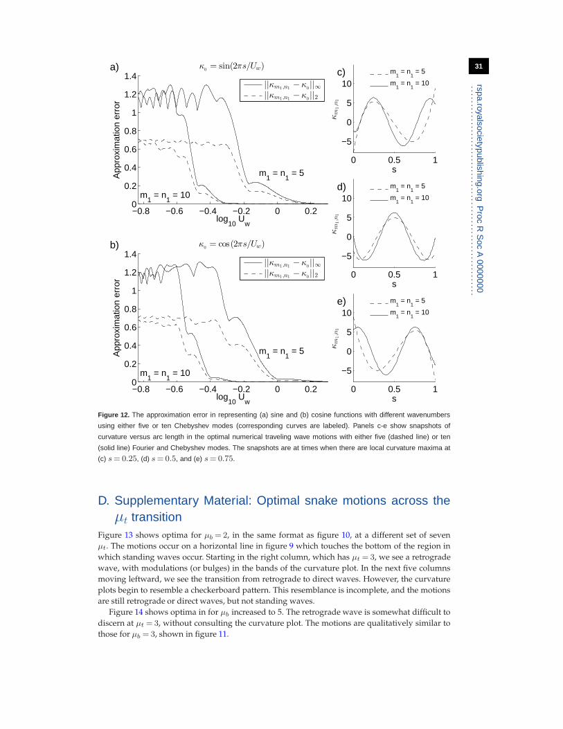
31


rocR

Soc

A0000000

..........................................................

−0.8 −0.6 −0.4 −0.2 0 0.20

0.2

0.4

0.6

0.8

1

1.2

1.4

log10

Uw

App

roxi

mat

ion

erro

r

κ0= sin(2πs/Uw)

m1 = n

1 = 5

m1 = n

1 = 10

a)

||κm1,n1 − κ0||∞

||κm1,n1 − κ0||2

−0.8 −0.6 −0.4 −0.2 0 0.20

0.2

0.4

0.6

0.8

1

1.2

1.4

log10

Uw

App

roxi

mat

ion

erro

r

κ0= cos(2πs/Uw)

m1 = n

1 = 5

m1 = n

1 = 10

b)

||κm1,n1 − κ0||∞

||κm1,n1 − κ0||2

0 0.5 1

−5

0

5

10

s

κm

1,n

1

c)

m

1 = n

1 = 5

m1 = n

1 = 10

0 0.5 1

−5

0

5

10

s

κm

1,n

1

d)

m

1 = n

1 = 5

m1 = n

1 = 10

0 0.5 1

−5

0

5

10

s

κm

1,n

1

e)

m

1 = n

1 = 5

m1 = n

1 = 10

Figure 12. The approximation error in representing (a) sine and (b) cosine functions with different wavenumbers

using either five or ten Chebyshev modes (corresponding curves are labeled). Panels c-e show snapshots of

curvature versus arc length in the optimal numerical traveling wave motions with either five (dashed line) or ten

(solid line) Fourier and Chebyshev modes. The snapshots are at times when there are local curvature maxima at

(c) s= 0.25, (d) s= 0.5, and (e) s= 0.75.

D. Supplementary Material: Optimal snake motions across theµt transition

Figure 13 shows optima for µb = 2, in the same format as figure 10, at a different set of seven

µt. The motions occur on a horizontal line in figure 9 which touches the bottom of the region in

which standing waves occur. Starting in the right column, which has µt = 3, we see a retrograde

wave, with modulations (or bulges) in the bands of the curvature plot. In the next five columns

moving leftward, we see the transition from retrograde to direct waves. However, the curvature

plots begin to resemble a checkerboard pattern. This resemblance is incomplete, and the motions

are still retrograde or direct waves, but not standing waves.

Figure 14 shows optima in for µb increased to 5. The retrograde wave is somewhat difficult to

discern at µt = 3, without consulting the curvature plot. The motions are qualitatively similar to

those for µb = 3, shown in figure 11.

32


rocR

Soc

A0000000

..........................................................

µb =2

µt =0.2 µ

t =0.3 µ

t =0.5 µ

t =0.7 µ

t =1 µ

t =2 µ

t =3


Figure 15 shows optima in for µb increased to 20. For µt = 0.2 we show two local optima. The

second column shows a “swing-and-anchor” motion. The snake forms a loop at one end, the

“anchor,” and then the rest of the body swings forward, rotating about the anchor. The motion

also shows, briefly, a direct wave. This example shows that optima can combine multiple types

of motions within a single period of motion. We have seen many other such “mixed” optima at

moderate µt, but they are not reproduced here for brevity. The other µt = 0.2 optimum, shown

in the first column, is essentially a direct wave. The optima for µt = 0.3, 0.7, and 3 also involve

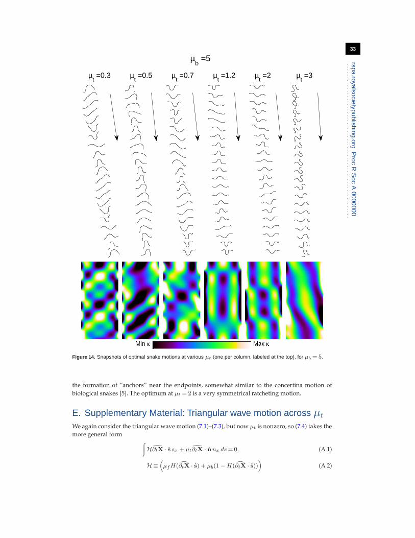
33


rocR

Soc

A0000000

..........................................................µ

b =5

µt =0.3 µ

t =0.5 µ

t =0.7 µ

t =1.2 µ

t =2 µ

t =3


the formation of “anchors” near the endpoints, somewhat similar to the concertina motion of

biological snakes [5]. The optimum at µt = 2 is a very symmetrical ratcheting motion.

E. Supplementary Material: Triangular wave motion across µt

We again consider the triangular wave motion (7.1)–(7.3), but now µt is nonzero, so (7.4) takes the

more general form ∫Hd∂tX · s sx + µtd∂tX · nnx ds= 0, (A 1)

H≡“

µfH(d∂tX · s) + µb(1 −H(d∂tX · s))”

(A 2)

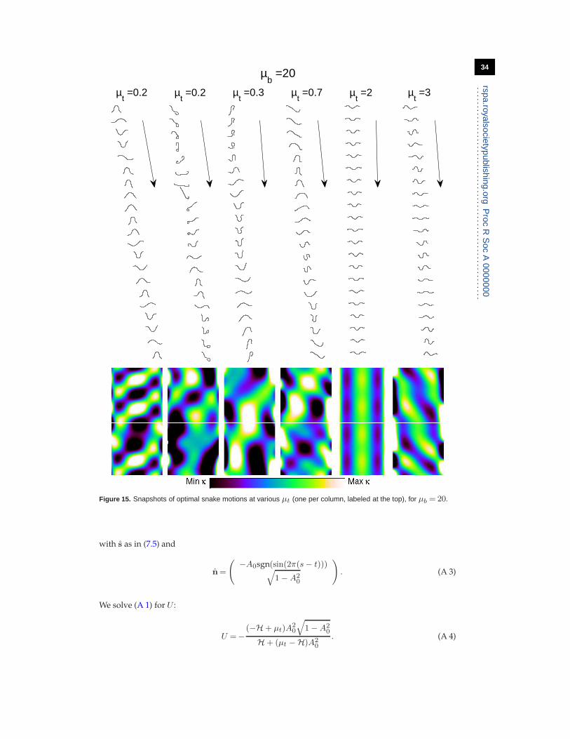
34


rocR

Soc

A0000000

..........................................................

µb =20

µt =0.2 µ

t =0.2 µ

t =0.3 µ

t =0.7 µ

t =2 µ

t =3


with s as in (7.5) and

n =

−A0sgn(sin(2π(s− t)))q

1 − A20

!

. (A 3)

We solve (A 1) for U :

U =−(−H + µt)A

20

q

1 − A20

H + (µt −H)A20

. (A 4)

35


rocR

Soc

A0000000

..........................................................

When µt = 0, (A 4) becomes (7.6). The tangential speed is

us =Usx + ∂tysy =− A20µt

H + (µt −H)A20

≤ 0, (A 5)

so H= µb. The snake speed (A 4), as well as us and un, are functions of A0 and µt/µb only. By

(2.16) and (2.17), so is η/µb. In figure 16 we give a contour plot of log10 η/µb as a function of

q= arcsinA0 and log10 µt/µb. q is the angle that the triangle wave makes with the horizontal

axis.

0 π/8 π/4 3π/8 π/2

−3

−2

−1

0

1

2

3

−3 −3

−2−2

−2

−1

−1 −1

−1

0

00

0

0.05

0.1

0.1

0.2

0.2

0.2

0.5

0.5 0.5

0.5

1

1 1

11

11 1

1

q = 21/4(µt/µ

b)−1/4

q = Acos(21/4(µt/µ

b)1/4)

q

log 10

µt/µ

b

Figure 16. Contour plot of log10 η/µb as a function of the triangular wave angle q= arcsinA0 and the friction

coefficient ratio log10 µt/µb.

The forward speed U is zero, and the cost of locomotion infinite, when µt = µb, represented by

a horizontal line near themiddle of figure 16. This is an example of the “singular point”mentioned

in the previous section, when µt = µb = µf = 1. When µt >µb, above the horizontal line, U < 0,

and the snake moves as a retrograde wave. η/µb decays to 1 as µt/µb →∞. In this regime, for

fixed µt, η itself is the product of µb with a function that decays more slowly than µb as µb → 0.

Thus η is minimized when µb → 1, the minimal value of µb. We plot the optimal amplitude in

the limit of large µt/µb (derived for a wave of any shape in section 5) as a dashed line at the

upper left of the figure, with the formula for the optimal amplitude in this limit. In the lower

portion of figure 16, µt <µb, U > 0, and the snake moves as a direct wave. Here η/µb decays to 0

as µt/µb → 0. In this regime, for fixed µt, η itself is the product of µb with a function that decays

more rapidly than µ−1b as µb →∞. Thus η is minimized by taking µb →∞ and µt → 0. The wave

36


rocR

Soc

A0000000

..........................................................

angle which minimizes η can be found by directly minimizing η with respect to q. We find that in

the limit µt/µb → 0, the optimal wave angle tends to π/2, i.e. the optimal wave becomes steeper.

optimizing snake locomotion in the plane - mathematicsalben/optimalsnakepaperpra.pdf · locomotion...

Documents