optimum design of simplicial uniaxial accelerometersrmsl/index/documents/simondes... · optimum...
TRANSCRIPT

OPTIMUM DESIGN OF SIMPLICIAL
UNIAXIAL ACCELEROMETERS
Simon Desrochers
Department of Mechanical Engineering
McGill University, Montreal
January 2009
A Thesis submitted to the Faculty of Graduate Studies and Research
in partial fulfilment of the requirements for the degree of
Master of Engineering
c© Simon Desrochers, 2008


ABSTRACT
Abstract
This thesis reports on the design, analysis and optimization of an accelerometer. This
accelerometer is designed as a monolithic structure along the concept of compliant
mechanisms. An elastodynamic analysis is performed on the compliant mechanism
to asses the performance of the inertial sensor.
This thesis proposes an innovative compliant hinge intended to stiffen the struc-
ture of compliant mechanisms. In addition, a procedure for the optimum design of
this new hinge is discussed. The structural optimization problem is approached by
coupling a finite element model to an optimization algorithm. A procedure is devel-
oped to generate the mesh at each optimization step according to the values of the
design parameters provided by the optimization algorithm. The objective function to
minimize is the stress concentration in a hinge loaded under bending.
The last chapter focuses on the multi-objective optimization of the compliant-
mechanism accelerometer. The Pareto method is used to optimally design the ac-
celerometer. The purpose is to maximize the sensitivity of the accelerometer in its
sensing direction, while minimizing its sensitivity in all other directions. The a poste-
riori multi-objective optimization is formulated. By using the normalized normal
constrained method (NNCM), an even distribution of the Pareto frontier is found.
The work also provides several optimum solutions of the Pareto plot as well as the
CAD model of the selected solution.
i


RESUME
Resume
Une large gamme d’accelerometres est offerte sur le marche. Cependant, la plupart
des architectures de capteurs inertiels offerts par l’industrie sont constituees d’une
masse suspendue par une poutre encastree. Avec les annees, les chercheurs ont mis
au point des architectures paralleles offrant une bien meilleure rigidite qu’une simple
poutre encastree. Les accelerometres a architecture parallele offrent egalement de
bien meilleures rigidites.
Cette these porte sur la conception, l’analyse et l’optimisation d’un accelerometre
a architecture parallele. Tout d’abord, l’accelerometre est realise comme structure
monolithique dans le cadre des mecanismes flexibles. Par la suite, une analyse elasto-
dynamique est effectuee sur le mecanisme flexible afin de d’evaluer les performances
du capteur inertiel.
Cette these propose egalement une nouvelle articulation flexible visant a ameliorer
la structure des mecanismes flexibles. Une procedure optimisant le profil de cette
nouvelle articulation flexible est egalement proposee. Le probleme d’optimisation
structurelle est aborde en etablissant une boucle entre un modele par elements finis
et un algorithme d’optimisation. Une procedure a ete developpee afin de generer le
maillage a chaque etape d’optimisation en fonction des valeurs des parametres de
conception fournis par l’algorithme d’optimisation. La fonction cible a minimiser
est definie comme la concentration de contrainte generee dans l’articulation flexible
sollicitee en flexion.
iii

RESUME
Le dernier chapitre de la these met l’accent sur l’optimisation multi-objectif
du mecanisme flexible de l’accelerometre. La methode est utilisee afin d’obtenir la
configuration optimale de l’accelerometre. Le but est de maximiser la sensibilite de
l’accelerometre dans la direction de l’axe sensible, tout en reduisant la sensibilite
dans toutes les autres directions. Une formulation de l’optimisation a posteriori des
objectifs est presentee. En utilisant la methode normalisee contrainte (NNCM), une
repartition uniforme de la frontiere de Pareto est produite. Les solutions optimales
de Pareto sont presentees dans un graphique, ainsi que le modele CAO de la solution
selectionnee.
iv

ACKNOWLEDGEMENTS
Acknowledgements
I would like to express my most sincere gratitude to my supervisors, Professors Jorge
Angeles and Damiano Pasini, for their guidance and financial support throughout
the course of this research. I am specially grateful for all their scientific insights
and their careful reviews of the manuscript of this thesis. I would also like to thank
Irene Cartier for her help and support with the administrative side of my studies.
I thank my colleagues from the Centre of Intelligent Machines and the Multi-scale
Design Optimization Group, with whom I had a great time during my studies at
McGill University. Special thanks to Mostafa Yourkhani for teaching me Ansys; and
to Philippe Cardou and Hossein Ghiasi for their availability, scientific insights and
advice. I also want to thank Philippe for all his support during my first moments here
at McGill. Many thanks to my friend Jean-Francois Gauthier, for his support during
the completion of this thesis. I am also grateful to Jean-Francois for the precious
introduction he gave me on LATEX to start writing the manuscript of this thesis. Last
but not least, deep thanks to my family for their love and their encouragement.
v


TABLE OF CONTENTS
TABLE OF CONTENTS
Abstract . . . . . . . . . . . . . . . . . . . . . . . . . . . . . . . . . . . . . . . i
Resume . . . . . . . . . . . . . . . . . . . . . . . . . . . . . . . . . . . . . . . iii
Acknowledgements . . . . . . . . . . . . . . . . . . . . . . . . . . . . . . . . . v
LIST OF FIGURES . . . . . . . . . . . . . . . . . . . . . . . . . . . . . . . . xi
LIST OF TABLES . . . . . . . . . . . . . . . . . . . . . . . . . . . . . . . . . xv
CHAPTER 1. Introduction . . . . . . . . . . . . . . . . . . . . . . . . . . . 1
1.1. General Background . . . . . . . . . . . . . . . . . . . . . . . . . . . . 1
1.1.1. Accelerometer Working Principle . . . . . . . . . . . . . . . . . . 1
1.1.2. Simplicial Architecture for Isotropic Multi-axial Accelerometers . 4
1.1.3. Compliant mechanism . . . . . . . . . . . . . . . . . . . . . . . . 8
1.2. Motivation and Thesis Objectives . . . . . . . . . . . . . . . . . . . . 8
1.3. Structure of the Thesis . . . . . . . . . . . . . . . . . . . . . . . . . . 10
CHAPTER 2. Compliant Mechanism Design . . . . . . . . . . . . . . . . . . 11
2.1. Characteristics of Compliant Mechanisms . . . . . . . . . . . . . . . . 11
2.1.1. Compliant joint . . . . . . . . . . . . . . . . . . . . . . . . . . . . 11
2.1.2. Advantages and disadvantages of compliant mechanisms . . . . . 12
2.1.3. Translation Micro Displacement . . . . . . . . . . . . . . . . . . . 14
2.2. The Compliant Realization of the 2ΠΠ Architecture . . . . . . . . . . 15
2.3. Material Selection for Compliant Accelerometers . . . . . . . . . . . . 18
vii

TABLE OF CONTENTS
CHAPTER 3. Modal Analysis of the Compliant Accelerometer . . . . . . . . 23
3.1. Lumped-parameter Model . . . . . . . . . . . . . . . . . . . . . . . . 24
3.1.1. The System State . . . . . . . . . . . . . . . . . . . . . . . . . . . 24
3.1.2. The System Kinetic Energy . . . . . . . . . . . . . . . . . . . . . 25
3.1.3. The System Potential Energy . . . . . . . . . . . . . . . . . . . . 25
3.1.4. The Mathematical Model of the Compliant Mechanism . . . . . . 30
3.2. Case Study: One-notched Beam System . . . . . . . . . . . . . . . . . 31
3.3. Case Study: The Compliant 2ΠΠ System . . . . . . . . . . . . . . . . 35
3.3.1. Kinetic Energy . . . . . . . . . . . . . . . . . . . . . . . . . . . . 35
3.3.2. Potential Energy . . . . . . . . . . . . . . . . . . . . . . . . . . . 37
3.3.3. Mathematical Model . . . . . . . . . . . . . . . . . . . . . . . . . 38
3.4. Alternative Layout . . . . . . . . . . . . . . . . . . . . . . . . . . . . 39
CHAPTER 4. Shape Optimization of a Corner-filleted Hinge . . . . . . . . . 45
4.1. Lame Curves . . . . . . . . . . . . . . . . . . . . . . . . . . . . . . . . 47
4.1.1. Parameterization of Lame Curves. . . . . . . . . . . . . . . . . . . 49
4.1.2. Curvature of Lame Curves. . . . . . . . . . . . . . . . . . . . . . . 49
4.2. Basic Problem . . . . . . . . . . . . . . . . . . . . . . . . . . . . . . . 51
4.3. Structural Optimization Procedure . . . . . . . . . . . . . . . . . . . . 52
4.3.1. General Scheme . . . . . . . . . . . . . . . . . . . . . . . . . . . . 52
4.3.2. Objective Function and Constraints . . . . . . . . . . . . . . . . . 54
4.4. Optimum Supercircular Fillet . . . . . . . . . . . . . . . . . . . . . . 56
4.5. Optimum Superelliptical Fillet . . . . . . . . . . . . . . . . . . . . . . 59
4.5.1. Optimization Algorithm . . . . . . . . . . . . . . . . . . . . . . . 60
4.5.2. Results . . . . . . . . . . . . . . . . . . . . . . . . . . . . . . . . . 60
4.6. Summary and Discussion . . . . . . . . . . . . . . . . . . . . . . . . . 62
CHAPTER 5. Optimum Design of a Compliant Uniaxial Accelerometer . . . 63
5.1. The Optimization Methodology . . . . . . . . . . . . . . . . . . . . . 64
5.2. Problem Formulation . . . . . . . . . . . . . . . . . . . . . . . . . . . 65
viii

TABLE OF CONTENTS
5.3. Multi-objective Formulation . . . . . . . . . . . . . . . . . . . . . . . 69
5.4. RESULTS . . . . . . . . . . . . . . . . . . . . . . . . . . . . . . . . . 74
5.5. DISCUSSION . . . . . . . . . . . . . . . . . . . . . . . . . . . . . . . 78
CHAPTER 6. Closing Remarks . . . . . . . . . . . . . . . . . . . . . . . . . 81
6.1. Conclusions . . . . . . . . . . . . . . . . . . . . . . . . . . . . . . . . 81
6.2. Recommendations for Future Work . . . . . . . . . . . . . . . . . . . 82
BIBLIOGRAPHY . . . . . . . . . . . . . . . . . . . . . . . . . . . . . . . . . 83
ix


LIST OF FIGURES
LIST OF FIGURES
1.1 Mass-spring system of an accelerometer . . . . . . . . . . . . . . . . . . . . 2
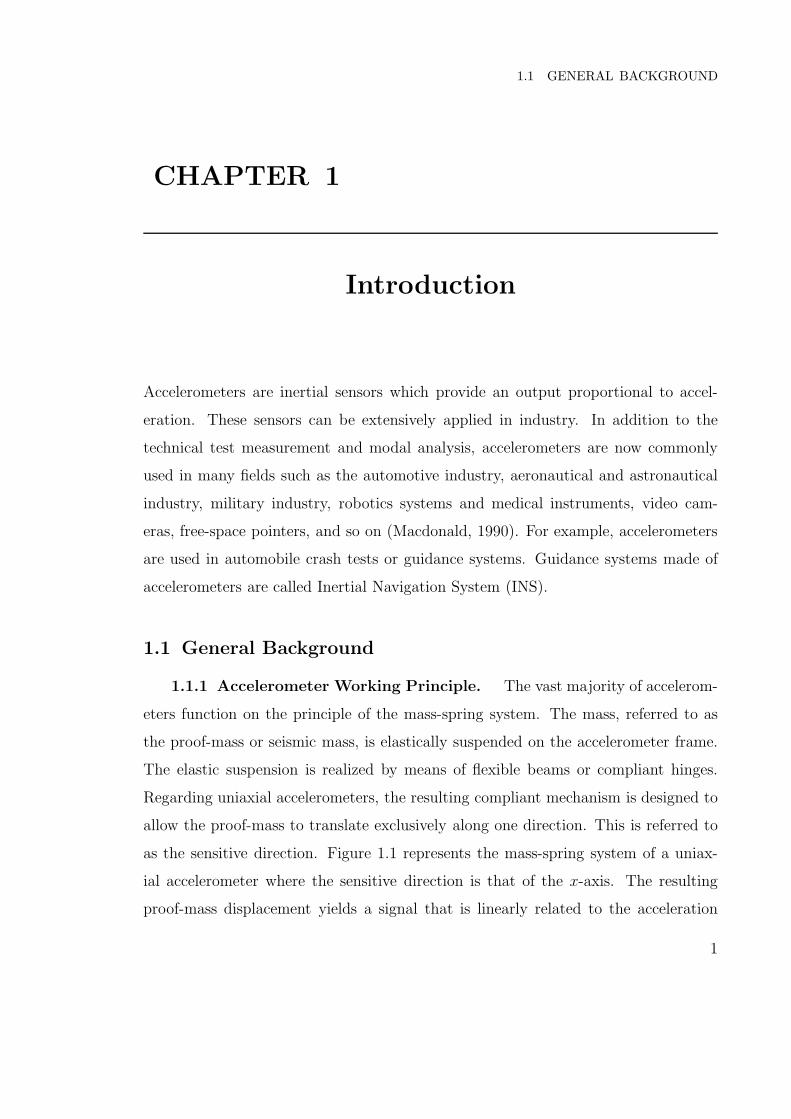
1.2 Example industrial accelerometers: (a) piezoelectric in shear mode, (b)
piezoelectric in flexure mode; and (c) capacitive . . . . . . . . . . . . . . . 3
1.3 Frequency response . . . . . . . . . . . . . . . . . . . . . . . . . . . . . . . 4
1.4 The simplicial 2ΠΠ uniaxial accelerometer: (a)top view (b) front view . . . 5
1.5 The simplicial 3ΠΠ biaxial accelerometer . . . . . . . . . . . . . . . . . . . 6
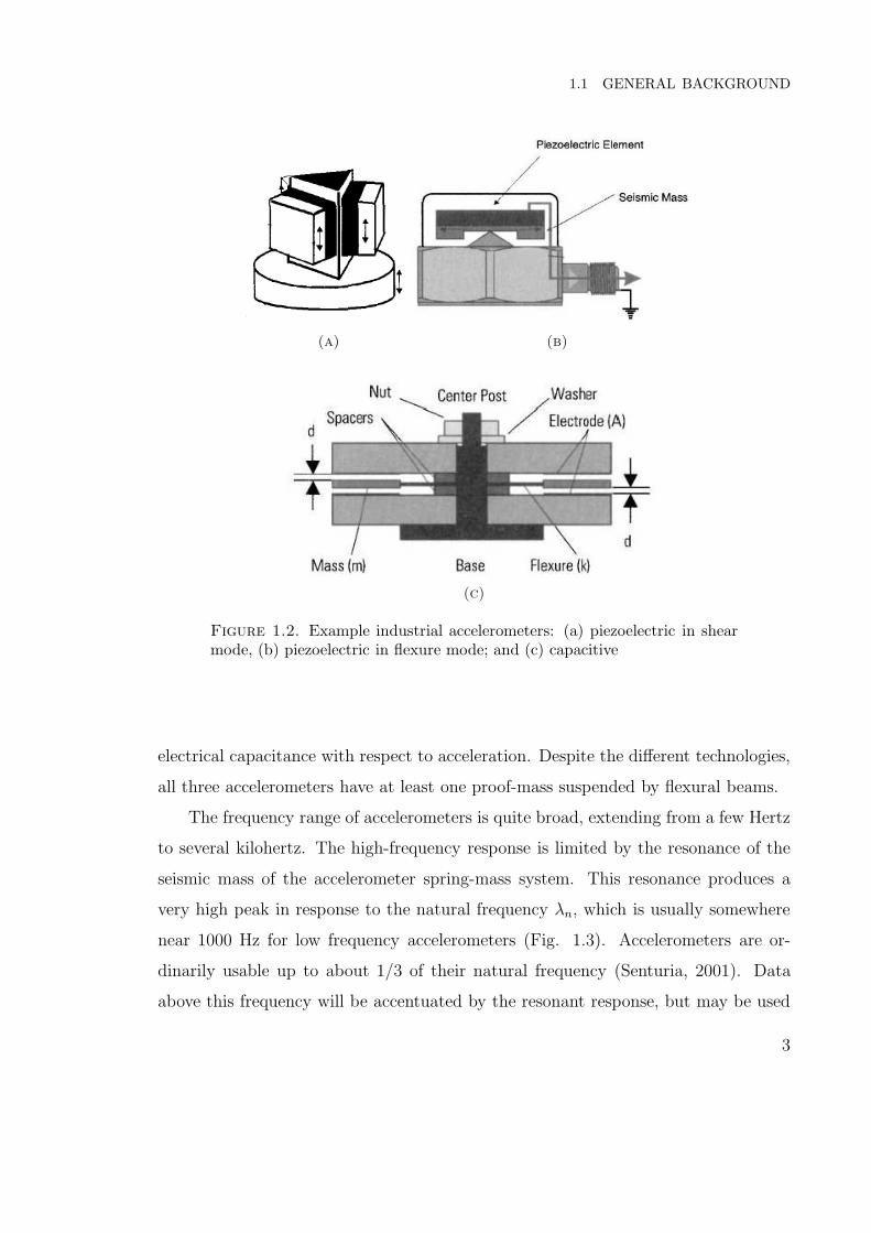
1.6 The simplicial 4RΠΠR triaxial accelerometer . . . . . . . . . . . . . . . . 7
2.1 Revolute joint: (a) notched beam joint; and (b) standard mechanical revolute
joint . . . . . . . . . . . . . . . . . . . . . . . . . . . . . . . . . . . . . . . 12
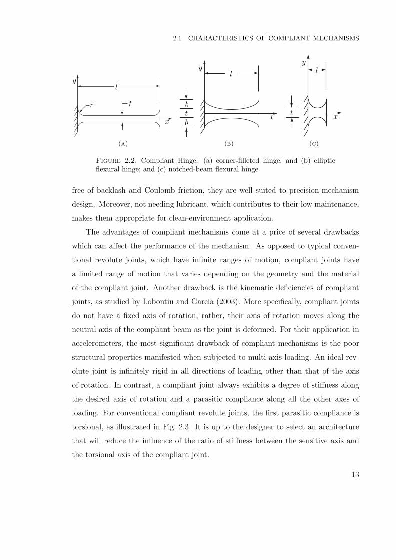
2.2 Compliant Hinge: (a) corner-filleted hinge; and (b) elliptic flexural hinge; and
(c) notched-beam flexural hinge . . . . . . . . . . . . . . . . . . . . . . . . 13
2.3 Revolute compliant hinge subjected to torsional loading . . . . . . . . . . . 14
2.4 Compliant realization of the Π-joint: (a) with a pair of constant cross-section
beams; and (b) with four notched beams . . . . . . . . . . . . . . . . . . . 15
2.5 Compliant realization of the Π-joint in a θ posture . . . . . . . . . . . . . 16
2.6 The complaint realization of the ΠΠ-leg architecture . . . . . . . . . . . . 17
2.7 The Simplicial 2ΠΠ Uniaxial Accelerometer . . . . . . . . . . . . . . . . . 17
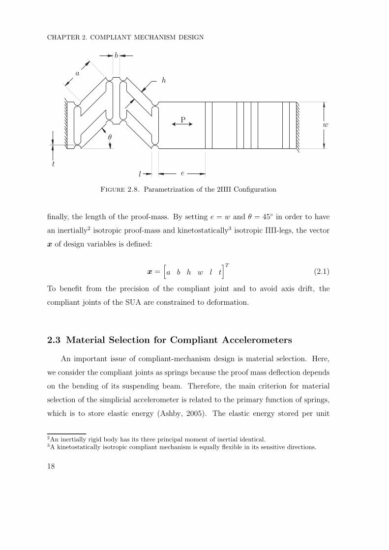
2.8 Parametrization of the 2ΠΠ Configuration . . . . . . . . . . . . . . . . . . 18
2.9 The Sy/ρ-E/ρ chart (Ashby, 2005) . . . . . . . . . . . . . . . . . . . . . . 21
xi

LIST OF FIGURES
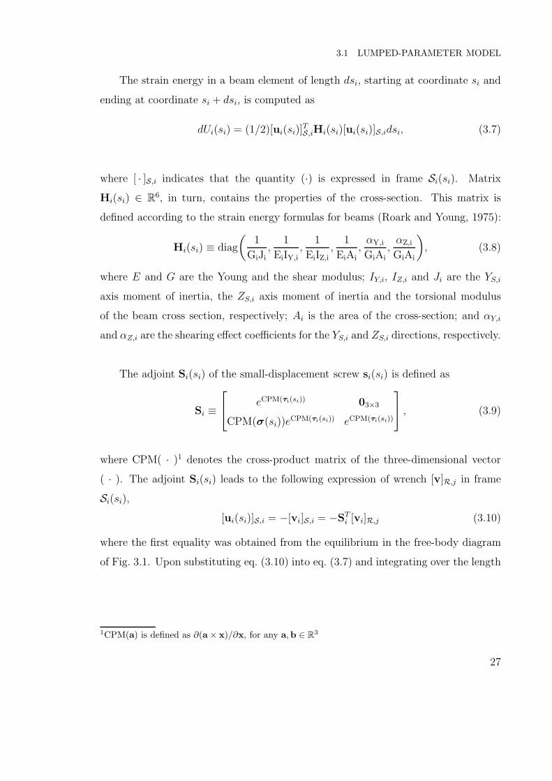
3.1 The ith compliant link attached to the jth rigid link: (a) layout; (b) detail of
the definition of Si(si) . . . . . . . . . . . . . . . . . . . . . . . . . . . . . 26
3.2 Notched beam: (a) Mass-spring representation; (b) compliant joint . . . . 31
3.3 Uniaxial accelerometer: (a) front view; and (b) bottom view . . . . . . . . 36
3.4 New layout: (a) CAD model; and (b) deformation along the sensitive axis 40
3.5 New layout of the uniaxial accelerometer: (a) left view; and (b) top view . 41
4.1 Corner filleted hinge . . . . . . . . . . . . . . . . . . . . . . . . . . . . . . 46
4.2 Lame curves for: (a) η = 2; (b) η = 3; and (c) η = 4 . . . . . . . . . . . . . 47
4.3 Lame curves of eq. (4.2) . . . . . . . . . . . . . . . . . . . . . . . . . . . . 48
4.4 Lame curves polar coordinate for η = 4 . . . . . . . . . . . . . . . . . . . . 49
4.5 Flexible beam profiles and their corresponding curvature distributions: (a)
(b) circular fillets; (c) (d) supercircular fillets; and (e) (f) superelliptical fillets 51
4.6 Geometry of a Lame-filleted hinge: (a) supercircular filleted hinge; (b)
superelliptical filleted hinge; (c) top view of both hinges . . . . . . . . . . 52
4.7 Structural model: (a) front view, (b) top view . . . . . . . . . . . . . . . . 53
4.8 Meshing of the flexible beam: (a) front view; and (b) zoom-in on the fillet 55
4.9 Stress concentration factor as a function of power η of a Lame curve for
supercircular fillet . . . . . . . . . . . . . . . . . . . . . . . . . . . . . . . 57
4.10Von Mises stress distribution with (a) no fillet; (b) circular fillet; and (b)
optimum supercircular fillet with η = 3.2 . . . . . . . . . . . . . . . . . . 58
4.11Link between Matlab and Ansys . . . . . . . . . . . . . . . . . . . . . . . 61
4.12Von Mises stress concentration distribution of the optimum super elliptical
fillet . . . . . . . . . . . . . . . . . . . . . . . . . . . . . . . . . . . . . . . 62
5.1 Methodology flow chart . . . . . . . . . . . . . . . . . . . . . . . . . . . . 66
5.2 Parameterization of the cross-configuration mechanism . . . . . . . . . . . 67
5.3 FE model of the accelerometer . . . . . . . . . . . . . . . . . . . . . . . . 69
xii

LIST OF FIGURES
5.4 Structural model . . . . . . . . . . . . . . . . . . . . . . . . . . . . . . . . 69
5.5 Bi-objective design space . . . . . . . . . . . . . . . . . . . . . . . . . . . 70
5.6 Pareto frontier . . . . . . . . . . . . . . . . . . . . . . . . . . . . . . . . . 71
5.7 Normalized pareto frontier . . . . . . . . . . . . . . . . . . . . . . . . . . . 72
5.8 Pareto frontier . . . . . . . . . . . . . . . . . . . . . . . . . . . . . . . . . 76
5.9 Optimum accelerometer . . . . . . . . . . . . . . . . . . . . . . . . . . . . 77
5.10Von Mises stress distribution . . . . . . . . . . . . . . . . . . . . . . . . . 77
xiii


LIST OF TABLES
LIST OF TABLES
2.1 Material . . . . . . . . . . . . . . . . . . . . . . . . . . . . . . . . . . . . 22
3.1 Dimensions of the one notched-beam system . . . . . . . . . . . . . . . . 32
3.2 Modal analysis of one notched beam system . . . . . . . . . . . . . . . . 34
3.3 Natural frequencies . . . . . . . . . . . . . . . . . . . . . . . . . . . . . . 34
3.4 Dimensions of the 2ΠΠ system . . . . . . . . . . . . . . . . . . . . . . . . 35
3.5 Modal frequencies and modal vectors of the compliant 2ΠΠ mechanism . 43
3.6 Dimensions of the new layout . . . . . . . . . . . . . . . . . . . . . . . . 44
3.7 Modal analysis of the new layout . . . . . . . . . . . . . . . . . . . . . . 44
4.1 Initial values of the parameters for corner-filleted hinge . . . . . . . . . . 56
4.2 Summary of results . . . . . . . . . . . . . . . . . . . . . . . . . . . . . . 62
5.1 Pareto solutions . . . . . . . . . . . . . . . . . . . . . . . . . . . . . . . . 75
5.2 Sensitivity of the accelerometer . . . . . . . . . . . . . . . . . . . . . . . 77
xv

1.1 GENERAL BACKGROUND
CHAPTER 1
Introduction
Accelerometers are inertial sensors which provide an output proportional to accel-
eration. These sensors can be extensively applied in industry. In addition to the
technical test measurement and modal analysis, accelerometers are now commonly
used in many fields such as the automotive industry, aeronautical and astronautical
industry, military industry, robotics systems and medical instruments, video cam-
eras, free-space pointers, and so on (Macdonald, 1990). For example, accelerometers
are used in automobile crash tests or guidance systems. Guidance systems made of
accelerometers are called Inertial Navigation System (INS).
1.1 General Background
1.1.1 Accelerometer Working Principle. The vast majority of accelerom-
eters function on the principle of the mass-spring system. The mass, referred to as
the proof-mass or seismic mass, is elastically suspended on the accelerometer frame.
The elastic suspension is realized by means of flexible beams or compliant hinges.
Regarding uniaxial accelerometers, the resulting compliant mechanism is designed to
allow the proof-mass to translate exclusively along one direction. This is referred to
as the sensitive direction. Figure 1.1 represents the mass-spring system of a uniax-
ial accelerometer where the sensitive direction is that of the x-axis. The resulting
proof-mass displacement yields a signal that is linearly related to the acceleration
1

CHAPTER 1. INTRODUCTION
k
l0x
cv
M
Figure 1.1. Mass-spring system of an accelerometer
component in the sensitive direction. It is common practice to refer to the sensitive
direction as the “sensitive axis”.
The bias errors of inertial measurements come from the off-axis sensitivity of
the mechanisms (Senturia, 2001). From a mechanical viewpoint, off-axis sensitivity
corresponds to the parasitic motion when the accelerometer is subjected to angular
acceleration, or when acceleration is not parallel to the sensitive axis. Therefore, in
order to reduce the bias errors, the off-axis stiffness of the proof-mass suspension must
be increased.
Various types of accelerometers offering a wide range of properties are available
on the market. However, most inertial sensor mechanism found in the industry are
made up of a mass suspended by one cantilever beam acting as spring. For example,
the low-frequency accelerometers shown in Figs. 1.2a, b and c are, respectively, a uni-
axial piezoelectric accelerometer in shear mode, a uniaxial piezoelectric accelerom-
eter in flexural mode, and a capacitive accelerometer (Senturia, 2001; Bao, 2000).
Piezoelectric accelerometers are named after the piezoelectric material of their flex-
ural elements. These materials generate an electric potential in response to applied
mechanical stress. On the other hand, capacitive accelerometers sense a change in
2
1.1 GENERAL BACKGROUND
(a) (b)
(c)
Figure 1.2. Example industrial accelerometers: (a) piezoelectric in shearmode, (b) piezoelectric in flexure mode; and (c) capacitive
electrical capacitance with respect to acceleration. Despite the different technologies,
all three accelerometers have at least one proof-mass suspended by flexural beams.
The frequency range of accelerometers is quite broad, extending from a few Hertz
to several kilohertz. The high-frequency response is limited by the resonance of the
seismic mass of the accelerometer spring-mass system. This resonance produces a
very high peak in response to the natural frequency λn, which is usually somewhere
near 1000 Hz for low frequency accelerometers (Fig. 1.3). Accelerometers are or-
dinarily usable up to about 1/3 of their natural frequency (Senturia, 2001). Data
above this frequency will be accentuated by the resonant response, but may be used
3

CHAPTER 1. INTRODUCTION
Usable
range
1Hz λn/3 λn
Gai
n(d
B)
log(λ)
Figure 1.3. Frequency response
if the effect is taken into consideration. Since the usable frequency range of low-
frequency accelerometers runs from 0 to 600 Hz, the natural frequency should not
exceed 1800 Hz.
Low-frequency accelerometers have the advantage of high sensitivity (Navid et al.,
2003; Suna et al., 2008). Nonetheless, they have very fragile mechanical structures and
high off-axis sensitivity. Consequently, commonly used low frequency accelerometers
have a limited range of acceleration, and an off-axis sensitivity of approximately
5%. To override the low off-axis stiffness of serial architectures, researchers have
developed parallel architectures offering superior properties compared to a simple
cantilever beam.
1.1.2 Simplicial Architecture for Isotropic Multi-axial Accelerometers.
Multi-axis accelerometers currently available on the market are layouts of multiple
uniaxial accelerometers that measure acceleration components in orthogonal direc-
tions of multiple distinct points of a rigid body. Many efforts have been made to meet
the market requirements (Kruglick et al., 1998; Li et al., 2007; Mineta et al., 1996,
Puers and Reyntjens, 1998, Algrain and Quinn, 1993, Navid et al., 2003). However,
the accelerometers found in the literature have anisotropic mechanical architectures,
4

1.1 GENERAL BACKGROUND
M
(a)
M
(b)
Figure 1.4. The simplicial 2ΠΠ uniaxial accelerometer: (a)top view (b)front view
which make them sensitive to parasitic angular acceleration effects. Regarding ac-
celerometers, isotropic mechanical architecture implies that the dynamic properties
of the sensor are the same in all directions.
The simplicial architecture for multi-axial accelerometers, proposed by Cardou
and Angeles (2007) refers to isotropic mechanism architectures proper of parallel-
kinematics machines (PKMs), allowing the measurement of one, two or three accel-
eration components. Here, Cardou and Angeles (2007) characterize the architecture
as simplicial since the proof mass is suspended by n + 1 legs, where n is the number
of acceleration components measured by the accelerometer, with n = 1, 2, 3. The set
of n + 1 legs form the vertices a simplex created by the leg attachment points of the
n-dimensional accelerometer. Recall that in mathematical programming, a simplex is
a polyhedron with the minimum number of vertices embedded in Rn (Kreyszig, 1997).
The polyhedra corresponding to one, two and three dimension are the line, the trian-
gle and the tetrahedron. If the triangle and the tetrahedron are equilateral, then the
5

CHAPTER 1. INTRODUCTION
M
Figure 1.5. The simplicial 3ΠΠ biaxial accelerometer
accelerometer is equally sensitive in all the sensitive directions, therefore making the
accelerometer isotropic. Furthermore, the accelerometers always have one more leg
then dimension, thereby providing redundancy, which considerably adds robustness
against measurement error.
The Simplicial Uniaxial Accelerometer (SUA) at hand is intended to measure
point-acceleration along one direction (Cardou and Angeles, 2007). To constrain the
mass to move along a single axis, we use a ΠΠ-leg architecture, where a Π joint is a
parallelogram linkage as described in detail in Angeles (2004). A planar translation
mechanism can be obtained by coupling two Π-joints together. The intersection of
the two leg-planes forms the new one-dimensional motion line of the mechanism.
Therefore, suspending the proof-mass to each leg on both vertices (Fig. 1.4) allows
the one-dimensional motion of the proof-mass. In order to eliminate the parasitic
displacement due to gravity, each leg-plane is oriented at 45 with respect to the
vertical.
6
1.1 GENERAL BACKGROUND
Figure 1.6. The simplicial 4RΠΠR triaxial accelerometer
By laying out three ΠΠ-legs in a common plane, symmetrically distributed as
show in Fig. 1.5, that is, along the three medians of an equilateral triangle, we obtain
the configuration of the Simplicial Biaxial Accelerometer (SBA). This mechanism
allows translation in the common plane, while providing a high stiffness in a direction
normal to the plane.
The Simplicial Triaxial Accelerometer (STA) is a parallel-robot architecture gen-
erating pure translations of the platform with respect to the base. In order to generate
pure translations we replace the ΠΠ-legs of the previews architecture by that of the
legs of the Japan Mechanical Engineering Laboratory (MEL) Micro Finger (Arai
et al., 1996). The architecture shown in Fig. 1.6 is also made of a regular tetrahedron
which plays the role of the moving platform, used here as a proof-mass.
7

CHAPTER 1. INTRODUCTION
1.1.3 Compliant mechanism. Humankind has always been inspired by na-
ture, which is particularly true in engineering. However, human and nature have dif-
ferent design philosophies. For Ananthasuresh and Kota (1995), the crucial difference
between natural and human designs lies in a different design paradigm. Tradition-
ally, human-made mechanisms are designed to be strong and rigid, as opposed to the
strong and compliant designs of nature. The main point is that rigidity and strength
are independent features, and hence, it is possible to make something both compliant
and strong. Indeed, “stiffness is a measure of how much something deflects under a
load, whereas strength is how much load can be endured before failure” (Howell, 2001).
Thus, compliant mechanisms follow nature’s guidelines by using the compliance prop-
erties of materials to store energy and produce work.
Over the years, engineers have learned that assembly plays a major role in pro-
duction cost. To reduce production cost, compliant mechanisms offer part consol-
idation; the parts experiencing relative motion are joined together with compliant
hinges (Lobontiu, 2003). Before the first publication on the stiffness characteriza-
tion of compliant hinges by Paros and Weisbord (1965), compliant mechanisms were
designed by trial and error. Since than, many studies on compliant hinges have
been published (Moon et al., 2002; Lobontiu et al., 2004; Lobontiu and Garcia, 2003;
Lobontiu and Garcia, 2005; Stuart et al., 1997; De Bona and Munteanu, 2005; Yingfei
and Zhaoying, 2002).
1.2 Motivation and Thesis Objectives
In this thesis, we consider the compliant realization of the Simplicial Uniaxial
Accelerometer (SUA). From a fabrication perspective, compliant mechanisms can be
classified into two categories. The first category, micromachined mechanisms, is lim-
ited to planar mechanisms due to the unidirectional nature of the etching process
used in micromachining (Senturia, 2001). The second category comprises the compli-
ant realization of millimeter-scale three-dimensional mechanisms. The complicated
8
1.2 MOTIVATION AND THESIS OBJECTIVES
geometry of the SUA makes it difficult to manufacture using existing microfabrication
techniques. Thus, the second category is contemplated for fabrication of the SUA.
We can cite two main advantages of a compliant realization for the design of
accelerometers. First, there is a reduction of the cost as a result of element reduction.
Second, the upgraded performance, due to reduced wear, maintenance and weight
(Howell, 2001). However, compliant mechanisms have four main drawbacks that can
affect the performance of the mechanism: limited sensitivity; off-axis sensitivity; axis
drift; and stress concentration (Moon et al., 2002). The sensitivity of the accelerome-
ter is limited by the joint stiffness, which restrains the proof-mass displacement when
subjected to acceleration parallel to the sensitive axis. On the other hand, the off-axis
sensitivity resulting from the parasitic off-axis bending of the compliant joint should
be minimized if the accelerometer is to be insensitive to parasitic off-axis acceler-
ation. The axis drift is governed by the motion precision of the proof-mass. In a
device subject to axis-drift, the proof-mass may undesirably move out of its axis of
motion. Finally, stress concentration affects the life and the range of motion of the
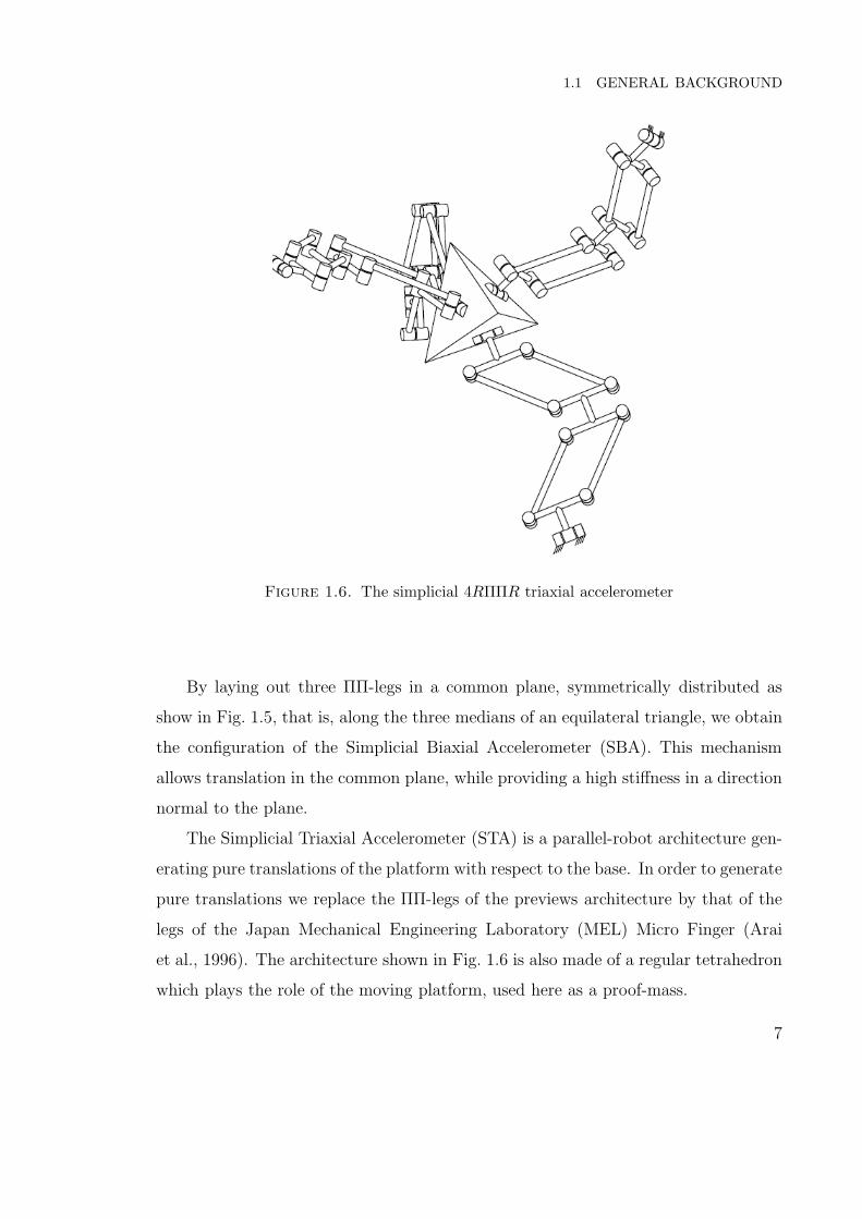
device. The range of motion can be recorded in dimensionless form, according to the
“mechanical advantage”, which is defined by Lobontiu (2003) as
m.a. =|uout||uin|
(1.1)
where uin and uout are the input and output displacement.
Such observations motivate the design of inertial sensors with high resolution and
low bias error. The thesis objectives are, hence,
(i) The optimum design of a compact compliant uniaxial accelerometer;
(ii) the kinematic analysis of lumped compliant accelerometers;
(iii) selection of the best configuration of the Simplicial Uniaxial Architecture;
(iv) stress analysis of flexible beams; and
(v) establishing a design methodology to optimize the stiffness and strength of
accelerometers.
9

CHAPTER 1. INTRODUCTION
1.3 Structure of the Thesis
The remainder of this document is organized as follows. Chapter 2 describes the
compliant mechanism design pursued in this project. Chapter 3 provides a detailed
description of the lumped-parameter model, as well as its application to different
layouts of the SUA. Chapter 4 presents the process used to optimize the compliant
hinge. The design process proposed in this work improves the structural properties of
compliant hinges by using Lame-shaped fillets as opposed to the traditional circular
fillets. Finally, chapter 5 focuses on the multi-objective optimization of the compliant-
mechanism accelerometer. The optimum design of a compact compliant uniaxial
accelerometer proposed in this work is the first attempt to use the Pareto multi-
objective formulation to optimize accelerometers.
10

2.1 CHARACTERISTICS OF COMPLIANT MECHANISMS
CHAPTER 2
Compliant Mechanism Design
A compliant mechanism is defined by Lobontiu (2003) as “a mechanism that is com-
posed of at least one flexible component that is sensibly deformable compared to other
rigid links”. Specifically, a compliant mechanism is a device that generates work by
using compliant hinges instead of conventional rigid joints. Since flexible hinges do
not cause any sliding or rolling, compliant devices are free of backlash and Coulomb
friction; however, they are not friction-free, as they are fabricated out of a viscoelastic
material that generates viscoelastic forces.
2.1 Characteristics of Compliant Mechanisms
Compliant-mechanism components belong to one of two categories (Cardou et al.,
2008). The first category gathers the m compliant links used to transform motion,
force, or energy, where m refers to the number of compliant links of the mechanism.
The second category comprises the n rigid links designed with low compliance in order
to transfer the motion generated by the first category of the components. Here, n
refers to the number of rigid links of the compliant mechanism at hand.
2.1.1 Compliant joint. Almost all typical mechanical joints can be replaced
by compliant joints; however, the conventional revolute joint is the easiest to replace.
A compliant revolute joint, such as those universally described in the works by Paros
and Weisbord (1965), Yingfei and Zhaoying (2002), De Bona and Munteanu (2005),
11

CHAPTER 2. COMPLIANT MECHANISM DESIGN
(a) (b)
Figure 2.1. Revolute joint: (a) notched beam joint; and (b) standard me-chanical revolute joint
and Stuart et al. (1997), is governed by the bending deflection of its cantilever beams.
In contrast, the revolute joint in conventional mechanisms is governed by the rolling
of bearings or pin joints. A compliant and a standard revolute joint are depicted in
Fig. 2.1a and b. Various types of flexural hinges are available to produce compliant
revolute joints, all of them using a different beam profile. Typically, only three compli-
ant hinge profiles are found in the literature: the corner filleted hinges (Fig. 2.2a), the
elliptic flexural hinge (Fig. 2.2b), and the notched-beam flexural hinges (Fig. 2.2c).
Because notched-beam hinges have a good machinability and high off-axis stiffness,
we choose notched-beam flexural hinges for the design of the SUA.
2.1.2 Advantages and disadvantages of compliant mechanisms. In
general, compliant mechanisms offer several significant advantages compared to con-
ventional mechanisms. In addition to reducing the number of parts to assembly and
manufacture, lowering maintenance and miniaturizing the mechanism size, compli-
ant mechanisms are also free of Coulomb friction and backlash, two drawbacks that
compromise performance and precision. Typical mechanisms that use bearings or
pin-joints always exhibit some degree of parasitic motion and high-frequency noise
caused by Coulomb friction. As opposed to compliant mechanisms, bearings and
gears with low backlash and low friction are expensive and need lubricant in order
to reduce wear between moving parts. Since compliant mechanisms are compact and
12
2.1 CHARACTERISTICS OF COMPLIANT MECHANISMS
l
r t
x
y
(a)
l
tb
b
x
y
(b)
l
t x
y
(c)
Figure 2.2. Compliant Hinge: (a) corner-filleted hinge; and (b) ellipticflexural hinge; and (c) notched-beam flexural hinge
free of backlash and Coulomb friction, they are well suited to precision-mechanism
design. Moreover, not needing lubricant, which contributes to their low maintenance,
makes them appropriate for clean-environment application.
The advantages of compliant mechanisms come at a price of several drawbacks
which can affect the performance of the mechanism. As opposed to typical conven-
tional revolute joints, which have infinite ranges of motion, compliant joints have
a limited range of motion that varies depending on the geometry and the material
of the compliant joint. Another drawback is the kinematic deficiencies of compliant
joints, as studied by Lobontiu and Garcia (2003). More specifically, compliant joints
do not have a fixed axis of rotation; rather, their axis of rotation moves along the
neutral axis of the compliant beam as the joint is deformed. For their application in
accelerometers, the most significant drawback of compliant mechanisms is the poor
structural properties manifested when subjected to multi-axis loading. An ideal rev-
olute joint is infinitely rigid in all directions of loading other than that of the axis
of rotation. In contrast, a compliant joint always exhibits a degree of stiffness along
the desired axis of rotation and a parasitic compliance along all the other axes of
loading. For conventional compliant revolute joints, the first parasitic compliance is
torsional, as illustrated in Fig. 2.3. It is up to the designer to select an architecture
that will reduce the influence of the ratio of stiffness between the sensitive axis and
the torsional axis of the compliant joint.
13

CHAPTER 2. COMPLIANT MECHANISM DESIGN
Figure 2.3. Revolute compliant hinge subjected to torsional loading
In the case of the compliant realization of the simplicial accelerometer, three main
drawbacks affect the performance of the SUA: limited sensitivity in the sensitive
direction; off-axis sensitivity; and axis drift. The sensitivity of the accelerometer
is limited by the joint stiffness, which restrains the proof-mass displacement when
subjected to an acceleration parallel to the sensitive axis. On the other hand, the
off-axis sensitivity resulting from the parasitic off-axis bending of the compliant joint
should be minimized if the accelerometer is to be insensitive to parasitic off-axis
acceleration. Finally, the axis drift is related to the motion precision of the proof-
mass. In a device with axis drift problems, the proof-mass may undesirably move out
of the sensitive axis.
2.1.3 Translation Micro Displacement. A compliant prismatic pair can-
not be design by modifying the shape of a flexible beam, as is the case for revolute
joints. In order to realize a prismatic pair, we use Π-joints, whereby two identical
straight flexible beams cast at both ends lie parallel to each other to create a parallel-
guiding mechanism, or parallelogram, as proposed by Derderian et al. (1996) and
depicted in Fig. 2.4a. The resulting mechanism is highly compact but gives only
limited off-axis stiffness. To cope with this problem, Arai et al. (1996) proposed a
different compliant Π-joint (see Fig. 2.4b), which uses notched beams rather than
beams with constant cross-sections. The notched Π-joint brings about higher ratios
between the stiffness in the sensitive direction and the stiffness in the other direc-
tions. The main drawbacks, as pointed out in Moon et al. (2002), are smaller beam
minimum thickness, thereby rendering machining costlier, while giving rise to higher
stress concentration, and leading to limited range of motion.
14

2.2 THE COMPLIANT REALIZATION OF THE 2ΠΠ ARCHITECTURE
(a) (b)
Figure 2.4. Compliant realization of the Π-joint: (a) with a pair of con-stant cross-section beams; and (b) with four notched beams
As the mechanism is intended to undergo only small amplitude motion, compliant
Π-joints are usually referred to as prismatic joints. In fact, the relative displacement
produced is circular translation, which means that all points of one translating line
move on circular trajectories of equal radius and different centres with respect to its
opposite line. The direction of the equivalent P-joint1 is given by a circle tangent,
the small rotational displacement being considered negligible. By adding an angle θ
with respect to the original posture of the Π-joint, we can change the orientation of
the direction of the equivalent P pair, as illustrated in Fig 2.5.
2.2 The Compliant Realization of the 2ΠΠ Architecture
By coupling two notched Π-joints in series on the same plane, we obtain a com-
pliant version of the ΠΠ-leg. The layout of Fig. 2.6 has been adopted to produce a
two-degree-of-freedom translational system with elastodynamic isotropy, i.e., with its
1P denotes a prismatic joint
15

CHAPTER 2. COMPLIANT MECHANISM DESIGN
P
θ
Figure 2.5. Compliant realization of the Π-joint in a θ posture
two natural frequencies identical. The resulting ΠΠ-leg is designed with the Π-joint
axes at an angle θ = 45 in the unloaded configuration of the elastic hinges. To
create the compliant single-axis simplicial accelerometer, we suspend the proof-mass
on two opposite legs, while orienting them so that their respective planes of motion
are mutually orthogonal. The resulting device, shown in Fig. 2.7, is a monolithic
mechanism that is stiff in the plane normal to the sensitive axis, but compliant in the
direction of the latter. This axis is nothing but the intersection of the two leg-planes,
the proof-mass thus moves in the direction depicted in Fig 2.7. However, in Chapter 3
we will see that the resulting asymmetric layout generates axis drift and also provides
only limited off-axis stiffness. Indeed, as pointed out by Moon et al. (2002), a sym-
metric layout of compliant joints greatly improves the ratio of the off-axis stiffness
to the sensitive-axis stiffness; it also eliminates a major part of the axis drift, which
improves the precision in the measurement of the displacement of the proof-mass.
Here, it is important to notice the difference between the symmetric layout of com-
pliant hinges and the symmetric profile of a compliant hinge. The first refers to axis
of symmetry of compliant mechanism and can be use to ease the kinematic analysis
of the system. The second refers to the axis of symmetries of the geometric profile of
a given compliant hinge.
16

2.2 THE COMPLIANT REALIZATION OF THE 2ΠΠ ARCHITECTURE
P P
θ
Figure 2.6. The complaint realization of the ΠΠ-leg architecture
P
Figure 2.7. The Simplicial 2ΠΠ Uniaxial Accelerometer
Eight quantities are needed to parameterize the structure of the SUA, as shown
in Fig 2.8. Among those quantities, only three of them are actually parameters of the
compliant joints. Parameters l, t, and w are, respectively, the radius, the minimum
thickness, and the depth of the joints. Moreover, w represent also the height of the
rigid links, including the proof-mass. The remaining five quantities, θ, a, h, b, and
e are, respectively, the posture angle of the Π-joint, the length and the height of the
rigid links, the thickness of the rigid link coupling the two Π-joints of the legs, and,
17
CHAPTER 2. COMPLIANT MECHANISM DESIGN
a
b
h
w
l
te
P
θ
Figure 2.8. Parametrization of the 2ΠΠ Configuration
finally, the length of the proof-mass. By setting e = w and θ = 45 in order to have
an inertially2 isotropic proof-mass and kinetostatically3 isotropic ΠΠ-legs, the vector
x of design variables is defined:
x =[
a b h w l t]T
(2.1)
To benefit from the precision of the compliant joint and to avoid axis drift, the
compliant joints of the SUA are constrained to deformation.
2.3 Material Selection for Compliant Accelerometers
An important issue of compliant-mechanism design is material selection. Here,
we consider the compliant joints as springs because the proof mass deflection depends
on the bending of its suspending beam. Therefore, the main criterion for material
selection of the simplicial accelerometer is related to the primary function of springs,
which is to store elastic energy (Ashby, 2005). The elastic energy stored per unit
2An inertially rigid body has its three principal moment of inertial identical.3A kinetostatically isotropic compliant mechanism is equally flexible in its sensitive directions.
18

2.3 MATERIAL SELECTION FOR COMPLIANT ACCELEROMETERS
volume of a spring deformed uniformly under an arbitrary stress σ is
V =1
2
(σ2
E
)
(2.2)
where E is the material Young Modulus. The spring will be damaged if the stress σ
exceeds the yield stress (Sy). The standard measurement of the spring capacity is the
modulus of resilience Rm, defined as the energy absorbed by a unit cube of material
when loaded in tension to its elastic limits (Juvinall and Marshek, 2000). Thus, Rm
is equal to the area under the elastic portion of the stress-strain curve. For a linear
spring, we have
Rm =S2
y
2E(2.3)
The material density should be minimized to reduce the inertia forces produced by
the acceleration of the rigid links. As the inertia forces are the only forces acting on
the flexible links, a material with low density improves the range of acceleration of
the accelerometer. Here, the range of acceleration is defined by the maximum acceler-
ation possible before plastic deformation occurs in the flexible beams. Therefore, we
express the first material criterion for the accelerometer as the ratio of the modulus
of resilience Rm and the density ρ. By dropping the constant, we can express the
material selection criterion as
R1 =S2
y
ρE(2.4)
where R1 corresponds to the criterion selection for light spring as expressed in (Ashby,
2005). The choice of material for light springs is based on the Sy/ρ-E/ρ chart of
Fig. 2.9. Candidates of equal performance R1 are identified by family of lines parallel
to the diagonal gray line shown in Fig. 2.9. The materials with highest R1 are the
ones lying at the right of this diagonal gray line. However, since the accelerometer is
a monolithic mechanism, the selected material should also give a high stiffness to the
rigid links. Indeed, the function of a rigid link is to transfer the elastic deflection of
the flexure hinge, without exhibiting any substantial elastic deformation. A material
19
CHAPTER 2. COMPLIANT MECHANISM DESIGN
with high Young modulus reduces the parasitic flexion of the rigid link, and thus, the
off-axis sensitivity of the accelerometer. Since the material should have a low density
to reduce the inertia forces and the stress on the flexible links, we select the specific
modulus as second material index, stated as
R2 =E
ρ(2.5)
where R2 is to be maximized. Candidates of equal R2 values are identified this time
by the horizontal grey line shown in Fig. 2.9. The upper right corner formed by the
two grey lines, shown in Fig. 2.9, isolates the materials with the best suitable prop-
erties. Table 2.1 lists materials typically used in compliant mechanisms. However,
some of these materials are discarded because they do not satisfy all the criteria of
compliant accelerometers. For example, elastomers offer outstanding properties, but,
unfortunately, have the lowest specific modulus of all the materials. Moreover, spring
steel is discarded because of its high density. Therefore, by considering only R1 and
R2 indices, the best choices of materials are carbon fiber reinforced plastic (CFRP),
glass fiber reinforced plastic (GFRP), and titanium alloys. To select one of these
three materials, we consider other material properties which affect the performance
of high-precision instruments. For example, metals have predictable material proper-
ties, low susceptibility to creep, and predictable fatigue life. On the contrary, plastics
and composites have a large variability in their mechanical properties, making their
properties less predictable than those of metals; they are also sensitive to creep and
stress relaxation, which could bring some problems in the presence of a constant ac-
celeration such as gravity. For these reasons, we choose to build the accelerometer
with the best metal alloy of the Sy/ρ-E/ρ chart (Fig. 2.9) that is a titanium alloy
material.
Compliant mechanisms made of titanium alloy may be difficult to manufacture.
To cope with this issue, we recourse to the EOSINT M 270 machine tool for Direct
Metals Laser-Sintering (DMLS). The machine is designed to manufacture complex
20

2.3 MATERIAL SELECTION FOR COMPLIANT ACCELEROMETERS
Figure 2.9. The Sy/ρ-E/ρ chart (Ashby, 2005)
three-dimensional devices in multiple types of metal, such as stainless steel, tool
steel, or, for the case of the accelerometers, TiAl6V4, a titanium alloy. The machine
has also an excellent detail resolution of ǫ = 100µm, which corresponds to the laser
focus diameter. With the precision of the DMLS machine, a monolithic titanium
accelerometer can be manufactured in a small size.
21

CHAPTER 2. COMPLIANT MECHANISM DESIGN
Table 2.1. Material
Material R1 =S2
y
EρComment
Spring Steel 0.4-0.9 Poor, because of high densityTi alloys 0.9-2.6 Metal with the best R1 criterion; expensiveCFRP 3.9-6.5 Anisotropic material; expensiveGFRP 1.0-1.8 Anisotropic material; less expensive than CFRP
Polymers 1.5-2.5 Low properties predictabilityNylon 1.3-2.1 With low specific modulus E/ρRubber 18-45 With low specific modulus E/ρ
22

CHAPTER 3. MODAL ANALYSIS OF THE COMPLIANT ACCELEROMETER
CHAPTER 3
Modal Analysis of the Compliant
Accelerometer
The derivations below apply to three-dimensional motion, with a straightforward
adaptation for one- and two-dimensional motions. Since the mechanism studied here
is intended to measure an inertia force with arbitrary orientation in space, we resort
to the general case of three-dimensional beam deflection. Moreover, even if forces and
moments acting on the off-axis direction of the moving mass should have a negligible
effect on its displacement, we will take it into account, in order to estimate the cross-
effects of angular acceleration on the acceleration measurements.
The lumped-parameter model proposed by Cardou et al. (2008) was originally
introduced to compute the natural frequencies and the dynamic responses of micro-
electromechanical-systems (MEMS). The model is formulated under the assumptions
of long Euler-Bernoulli beams and small displacements. However, notched beams do
not necessarily respect these assumptions because its strain stress is concentrated in
a small region around the centre of rotation. Therefore, before performing the modal
analysis of the SUA, we must validate the above mentioned lumped-parameter model,
adopted here, for millimeter-scale compliant mechanisms using notched beams.
23

CHAPTER 3. MODAL ANALYSIS OF THE COMPLIANT ACCELEROMETER
3.1 Lumped-parameter Model
A compliant mechanism is a chain of components, where each component falls
into one of two categories. The first comprises the m compliant links, which are
assumed to have no inertia and a given compliance in all directions. The second
contains the n rigid links, to which a given inertia and no compliance are assigned.
The compliant links are modeled as Euler-Bernoulli beams, and the deformation
of these links is considered to be small. From this last assumption, the mass and
stiffness properties of the links are assumed to be constant, that is, independent from
the mechanism state.
3.1.1 The System State. Let us first define the fixed frame F , and frames
R′j , j = 1, . . . , n, attached to the jth rigid link. Moreover, we define frame Rj as
the equilibrium pose of the jth rigid body. The origins of frames F , Rj , and R′j are
labelled O, Rj , and R′j, j = 1, ..., n, respectively. Points Rj , and R′
j are located at the
centre of mass of the jth rigid-link. The displacement taking F into Rj is described
by the pose array rj ≡ [θTj ρT
j ], where θj ∈ R3 is the product φjej , with φj and
ej denoting the natural invariants of the associated rotation and ρj ≡ −→ORj ∈ R3.
The natural invariants of a rotation are the unit-vector ej pointing in the axis of
rotation, and φj is the angle of rotation (Angeles, 2007). Notice that, in the presence
of small-amplitude rotations, the rotation is fully described by only three independent
variables, thereby obviating the need of a four-invariable representation.
Let the displacement of the system frame equilibrium at an arbitrary posture be
described by the array x. We define the pose of the jth rigid link with respect to its
equilibrium array as
xj = [νTj ζT
j ]T (3.1)
where νj ∈ R3 is the products of the natural invariants φj and ej of the associated
rotation taking Rj into R′j and ζj ∈ R3 is the vector of the translation displacement.
Under the assumption of small-amplitude rotations, only the vector part of the four
scalar invariants are needed (Angeles, 2007). Since the posture of the mechanism
24

3.1 LUMPED-PARAMETER MODEL
is fully described by the poses of all the rigid links, we will regard the pose arrays
xj, j = 1, . . . , n, as the system states. This results in the 6n-dimensional state vector
x = [xT1 xT
2 . . . xTn ]T (3.2)
3.1.2 The System Kinetic Energy. Let us first store the mass properties
of the jth rigid link into its associated mass matrix
Mj ≡
Ij 03×3
03×3 mj13×3
, (3.3)
where Ij, mj , 03×3, and 13×3 are, respectively, the centroidal inertia matrix computed
with respect to point Rj of the jth, the mass of the jth rigid link, the 3 × 3 zero
matrix, and the 3 × 3 identity matrix. Under the assumption of small deformation,
the kinetic energy of the system is expressed as
T =1
2
n∑
j=1
xTj Mjxj =
1
2xT Mx, (3.4)
where M is the 6n × 6n mass matrix of the system, namely,
M ≡
M1 06×6 · · · 06×6
06×6 M2 · · · 06×6
......
. . ....
06×6 06×6 · · · Mn
, (3.5)
where 06×6 is the 6 × 6 zero matrix.
3.1.3 The System Potential Energy. Consider the ith compliant link that
is clamped, at one end, to the jth rigid link, and, at the other end, to the kth rigid link,
with j < k. From the free-body diagram of the ith compliant link shown in Fig. 3.1, we
see that the wrench vi ∈ R6 applied at the mass centre Rj by the jth rigid link onto the
ith compliant link has to be balanced out by wrench ui(si) ∈ R6 applied at the origin
25

CHAPTER 3. MODAL ANALYSIS OF THE COMPLIANT ACCELEROMETER
si
si
Si
Si(si)
XS,i
YS,i
ZS,i
vi
ui
Rj
Rj
ti(si)
Figure 3.1. The ith compliant link attached to the jth rigid link: (a)layout; (b) detail of the definition of Si(si)
of frame Si(si), Si, where si is a coordinate along the compliant hinge neutral axis.
The positive direction of si is oriented toward the kth rigid link. The wrenches are
defined so that their reciprocal product with the small-displacement screws defined
in eq. (3.1) be dimensionally compatible. Therefore, the first three components of
the wrench represent a moment, whereas the last three represent a force, the latter
applied at the corresponding mass centre, where the wrench is defined. Let us attach
frame Si(si) with axes XS,i, YS,i, and ZS,i, to the beam cross-section at si, as shown
in Fig. 3.1 . Frame Si(si) is defined so as to have its XS,i axis tangent to the beam
neutral axis and pointing in the positive direction of si, its YS,i and ZS,i axes defined
along the principal directions of the cross-section. Let τ (si) be the array of products
of the natural invariants φj and ej of the associated rotation taking frame Rj into
frame Si(si), following the same convention as that used for θ, and σi(si) ∈ R3 be
the vector directed from point Rj to point Si. We group these two arrays in the
cross-section pose array defined as
si(si) ≡ [τ Ti (si) σT
i (si)]T ∈ R6. (3.6)
26
3.1 LUMPED-PARAMETER MODEL
The strain energy in a beam element of length dsi, starting at coordinate si and
ending at coordinate si + dsi, is computed as
dUi(si) = (1/2)[ui(si)]TS,iHi(si)[ui(si)]S,idsi, (3.7)
where [ · ]S,i indicates that the quantity (·) is expressed in frame Si(si). Matrix
Hi(si) ∈ R6, in turn, contains the properties of the cross-section. This matrix is
defined according to the strain energy formulas for beams (Roark and Young, 1975):
Hi(si) ≡ diag
(
1
GiJi,
1
EiIY,i,
1
EiIZ,i,
1
EiAi,
αY,i
GiAi,
αZ,i
GiAi
)
, (3.8)
where E and G are the Young and the shear modulus; IY,i, IZ,i and Ji are the YS,i
axis moment of inertia, the ZS,i axis moment of inertia and the torsional modulus
of the beam cross section, respectively; Ai is the area of the cross-section; and αY,i
and αZ,i are the shearing effect coefficients for the YS,i and ZS,i directions, respectively.
The adjoint Si(si) of the small-displacement screw si(si) is defined as
Si ≡
eCPM(τi(si)) 03×3
CPM(σ(si))eCPM(τi(si)) eCPM(τi(si))
, (3.9)
where CPM( · )1 denotes the cross-product matrix of the three-dimensional vector
( · ). The adjoint Si(si) leads to the following expression of wrench [v]R,j in frame
Si(si),
[ui(si)]S,i = −[vi]S,i = −STi [vi]R,j (3.10)
where the first equality was obtained from the equilibrium in the free-body diagram
of Fig. 3.1. Upon substituting eq. (3.10) into eq. (3.7) and integrating over the length
1CPM(a) is defined as ∂(a × x)/∂x, for any a,b ∈ R3
27
CHAPTER 3. MODAL ANALYSIS OF THE COMPLIANT ACCELEROMETER
of the ith compliant link, we obtain the strain energy as
Vi =1
2[vi]
TR,jBi[vi]R,j , where Bi ≡
∫ li
0
Si(si)Hi(si)Si(si)T dsi, (3.11)
and li is the length of the ith compliant link. To express all the wrenches vi in the
same reference frame F , the adjoint Rj of screw rj is defined as
Ri ≡
eCPM(θi) 03×3
CPM(ρ)eCPM(θi) eCPM(θi)
, (3.12)
which represents the rigid-body motion taking frame F into frame Rj . Hence, we
have the relation
[vi]R,j = RTj [vi]F , (3.13)
and the total strain energy of the system becomes (Cardou, 2007)
V =1
2[v]T
FB[v]F , (3.14)
where [v]F ≡ [[v1]TF
[v2]TF
· · · [vm]TF
]T , and B is a block-diagonal matrix, its
ith block being the 6 × 6 matrix RjBiRTj , with j taking the value of the smallest
index among those of the two rigid links that are connected to the ith compliant link.
According to Cardou et al. (2008), the static equilibrium of the wrenches takes the
form
[w]R = RTA[v]F , (3.15)
where R is a block-diagonal matrix, its jth block being the 6× 6 matrix Rj, while A
is defined as
A ≡
A11 A12 · · · A1m
A21 A22 · · · A2m
......
. . ....
An1 An2 · · · Anm
∈ R6n×6m, (3.16)
with
28

3.1 LUMPED-PARAMETER MODEL
Aji =
06×6 , if compliant link i is not connected to rigid link j;
16×6 , if compliant link i is connected to rigid links j and k, with j < k;
−16×6 , if compliant link i is connected to rigid links j and k, with j > k.
(3.17)
This allows the introduction of the potential energy of the external wrenches as a
function of the internal wrenches, namely,
Π = −[w]TR
[x]R = −[v]TFATR[x]R. (3.18)
For a linearly elastic system, the potential energy V and the complementary potential
energy V take the same value, which is the sum of the strain energy and the potential
energy; i.e.,
V = V = U + Π = (1/2)[v]TFB[v]F − [v]T
FATR[x]R. (3.19)
From eq. (3.19), the problem may now be regarded as that of finding the in-
ternal wrenches v that minimize the complementary potential energy V for a given
displacement x of the rigid links. This follows from the second theorem of Cas-
tigliano (Juvinall and Marshek, 2000). The partial derivative of V with respect to
the internal wrenches yields
∂V
∂[v]F= B[v]F − ATR[x]R (3.20)
whereas the Hessian yields∂2V
∂[v]2F
= B (3.21)
One may readily verify, from eq. (3.21), that B is symmetric, positive-definite and,
therefore, all stationary points v of V are local minima. Matrix B being nonsingular,
eq. (3.20) admits one single root, namely,
[v]F = B−1ATR[x]R. (3.22)
29
CHAPTER 3. MODAL ANALYSIS OF THE COMPLIANT ACCELEROMETER
Upon substituting eq. (3.15) into the foregoing equation, we obtain
[w]R = K[x]R where K = RTAB−1ATR. (3.23)
The potential energy can now be written as a function of the system posture x,
namely,
V =1
2xTKx (3.24)
3.1.4 The Mathematical Model of the Compliant Mechanism. The
Lagrangian of the mechanism is readily computed as
L = T − V =1
2xTMx− 1
2xTKx (3.25)
which leads to the Lagrange equation
d
dt
(
∂L
∂x
)
− ∂L
∂x= 0n (3.26)
whence,
Mx + Kx = 0n (3.27)
As the mass matrix is bound to be symmetric and positive definite, we can express
its Cholesky decomposition as M = LLT . This allows us to rewrite eq. (3.27) through
the change of variable z = LT x, namely,
z + Ω2z = 0 (3.28)
where Ω2 = L−1KL−T and Ω is the system 6n×6n frequency matrix. Let ωi and ωi,
i = 1, . . . , n, be the ith eigenvalue and its corresponding eigenvector of Ω2, and λi and
λi be the ith natural frequency and its corresponding modal vector of the undamped,
non-excited system, i.e.,
λi =√
ωi, and λi = L−T ωi, i = 1, . . . , n. (3.29)
30

3.2 CASE STUDY: ONE-NOTCHED BEAM SYSTEM
t
l a
b
(a) (b)
Y
X
w
R1
OM
R1,F
Figure 3.2. Notched beam: (a) Mass-spring representation; (b) compliant joint
3.2 Case Study: One-notched Beam System
The one-notched beam system is a compliant version of the spring-mass system
depicted in Fig. 3.2. This system is a simple mechanism whose natural frequencies
can be readily computed using either a mass-spring system or finite element analysis.
Thereupon, this is a good starting point to validate the mathematical model.
The single-degree-of-freedom mechanism acts as a mass-spring system made of
one torsional spring and one rigid body in a serial configuration. The first natural
frequency of the compliant mechanism should be along the degree of freedom of the
mass-spring system. To corroborate this, we analyze the mechanical structure of the
compliant mechanism parameterized in Fig. 3.2b. The dept, w, of the mechanism is
measured in the direction normal to the plane of the figure. The dimensions of the
mechanism studied in this work are recorded in Table 3.1.
Frames F and R1 are defined in Fig. 3.2b, with their X axis along the neutral
axis of the flexible beam, and with their Z axis oriented in the sensitive direction,
which is normal to the plane of the figure. The origins O and R1 of these two frames
are located at the proof-mass centre of mass. Therefore, we have
R = R1 = 16×6. (3.30)
The mechanism is made of a Titanium alloy, which has a Young Modulus of
E = 117 GPa, a Poisson ratio of µ = 0.33 and a density of ρ = 4453 Kg/m3. From
31

CHAPTER 3. MODAL ANALYSIS OF THE COMPLIANT ACCELEROMETER
Table 3.1. Dimensions of the one notched beam system
l t w a b3 mm 250 µm 10 mm 10 mm 5 mm
the selected dimension of Table 3.1, the corresponding inertia matrix and mass were
estimated to be
[I1]R1= [I1]F = [I2]R2
=
2.3192 0 0
0 3.7108 0
0 0 2.3193
× 10−8 kg · m2, (3.31)
and m1 = 2.2265 × 10⁻³ kg. The mass matrix M is evaluated directly from these
numerical values and the definition of eq. (3.5).
Calculating the stiffness matrix K of the system requires the definition of the
additional frames S1(s1). This can be done through the definition of its associated
screw s1(s1), which takes frame R1 into frame S1(s1). The screw s1(s1) is evaluated
as
s1 =[
0T3 s1 − l − a
20 0
]T
. (3.32)
The geometric properties of the beams’ cross-sections are computed from beam
theory (Pilkey, 2005; Roark and Young, 1975). We know from (Paros and Weisbord,
1965) that notched beams can be modelled as Euler-Bernoulli beams when loaded in
bending or tension. However, if we observe the elastostatic properties, we realize that
beam theory is not accurate enough for notched beams with a high ratio w/l. The
accuracy depends on the type and direction of loading. To cope with this inaccuracy,
correction factors were computed in Ansys. Since ti(si), the thickness of the profile
of the ith hinge (Fig. 3.1), is a function of si, the coordinate along the beam neutral
32

3.2 CASE STUDY: ONE-NOTCHED BEAM SYSTEM
axis, the properties of the beam cross-section yield
Ji(si) = βJ1
12wt3i (si)
[
16
3− 3.36
ti(si)
w
(
1 − t4i (si)
12w4
)]
with βJ = 37.2, (3.33a)
IZi(si) = βzw3ti(si)
12with βz = 0.8, (3.33b)
IY i(si) =wt3i (si)
12, Ai(si) = wti(si), αY = αZ = 6/5. (3.33c)
where βJ and βz are the correction factors computed with finite element analysis.
Notice that βJ = 37.2 and βz = 0.8 when t = 250 µm, l = 3 mm, and w = 10 mm.
As there is only one flexible link matrix A is a 6 by 6 identity matrix. From eq. (3.26),
we obtain the stiffness matrix of the system,
[K]F =
117.61 0 0 0 0 0
0 3951.7 0 0 0 419470
0 0 674.54 0 −103440 0
0 0 0 210020 0 0
0 0 −103440 0 159140 0
0 419470 0 0 0 645340
. (3.34)
With matrix K and M at hand, the frequency matrix-squared Ω2 can be computed
from its definition, in eq. (3.28). By extracting the eigenvalues and eigenvectors from
matrix Ω2, the natural frequencies and the modal vectors of the system are found and
listed in Table 3.2. Note that the modal vectors show the direction and orientation of
the motion of each rigid link when excited at its natural frequency. From the modal
vectors, it is apparent that the three lower frequencies correspond, respectively, to
an oscillation in the sensitive axis θz, the torsional axis θx, and, finally, the bending
axis θy. The other three frequencies, which are second order effects, are disregarded
in the analysis of the results, since they are much higher than the other frequencies.
Table 3.3 shows the errors in the results of the lumped-parameter model, where the
accurate values of reference were computed with finite element analysis (FEA). With
33

CHAPTER 3. MODAL ANALYSIS OF THE COMPLIANT ACCELEROMETER
errors under 5%, the lumped-parameter model gives a reliable approximation of the
natural frequencies of lumped compliant mechanisms.
Table 3.2. Modal analysis of one notched beam system
i 1 2 3 4 5 6fi (rad/s) 4285.6 71210 86464 190300 30713 357770fi (Hz) 682 11333 13761 30287 48881 56941
λi
0.00 1.00 0.00 0.00 0.00 0.000.00 0.00 −1.00 0.00 0.00 1.00−1.00 0.00 0.00 −1.00 0.00 0.000.00 0.00 0.00 0.00 1.00 0.000.01 0.00 0.00 0.00 0.00 0.000.00 0.00 0.01 0.00 0.00 0.00
Table 3.3. Natural frequencies
Frequency Orientation Lumped-parameter model FEA Errorλ1 θZ 682 Hz 698 Hz 2.3%λ2 θX 11333 Hz 11554 Hz 1.9%λ3 θY 13761 Hz 13238 Hz 3.9%λ4 θZ 30287 Hz 28796 Hz 4.9%
Considering that we want to use the beams as sensors, we designed them so that
they are particularly sensitive to forces parallel to the sensitive axis of the beam.
Hence, for a notched beam to be a robust sensor, its sensitivity along its sensitive
axis needs to be as high as possible with respect to its sensitivity in other directions.
Therefore, we define the ratios below, which are to be maximized, where Z is to be
the sensitive axis. For the parameter values given in Table 3.1, we obtain:
rθX ,θZ≡ λ2
λ1
= 16.6, rθY ,θZ≡ λ3
λ1
= 20.2. (3.35)
These results illustrate that the notched beam hinge has good off-axis stiffness. How-
ever, one flexure hinge cannot produce a translation mechanism. This can be over-
come by using four of them in a parallelogram linkage, as is done in the flexible
realization of the Π-joint introduced in the Chapter 2.
34
3.3 CASE STUDY: THE COMPLIANT 2ΠΠ SYSTEM
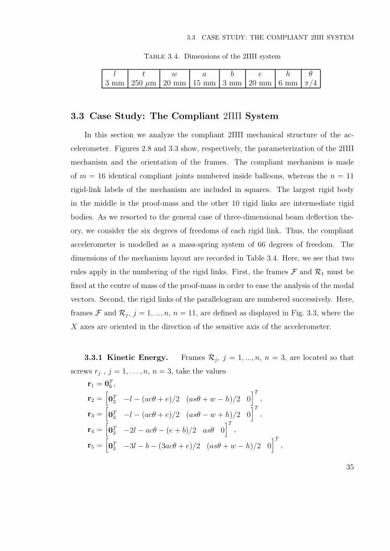
Table 3.4. Dimensions of the 2ΠΠ system
l t w a b e h θ3 mm 250 µm 20 mm 15 mm 3 mm 20 mm 6 mm π/4
3.3 Case Study: The Compliant 2ΠΠ System
In this section we analyze the compliant 2ΠΠ mechanical structure of the ac-
celerometer. Figures 2.8 and 3.3 show, respectively, the parameterization of the 2ΠΠ
mechanism and the orientation of the frames. The compliant mechanism is made
of m = 16 identical compliant joints numbered inside balloons, whereas the n = 11
rigid-link labels of the mechanism are included in squares. The largest rigid body
in the middle is the proof-mass and the other 10 rigid links are intermediate rigid
bodies. As we resorted to the general case of three-dimensional beam deflection the-
ory, we consider the six degrees of freedoms of each rigid link. Thus, the compliant
accelerometer is modelled as a mass-spring system of 66 degrees of freedom. The
dimensions of the mechanism layout are recorded in Table 3.4. Here, we see that two
rules apply in the numbering of the rigid links. First, the frames F and R1 must be
fixed at the centre of mass of the proof-mass in order to ease the analysis of the modal
vectors. Second, the rigid links of the parallelogram are numbered successively. Here,
frames F and Rj , j = 1, ..., n, n = 11, are defined as displayed in Fig. 3.3, where the
X axes are oriented in the direction of the sensitive axis of the accelerometer.
3.3.1 Kinetic Energy. Frames Rj, j = 1, ..., n, n = 3, are located so that
screws rj , j = 1, . . . , n, n = 3, take the values
r1 = 0T6 ,
r2 =[
0T3 −l − (acθ + e)/2 (asθ + w − h)/2 0
]T
,
r3 =[
0T3 −l − (acθ + e)/2 (asθ − w + h)/2 0
]T
,
r4 =[
0T3 −2l − acθ − (e + b)/2 asθ 0
]T
,
r5 =[
0T3 −3l − b − (3acθ + e)/2 (asθ + w − h)/2 0
]T
,
35

CHAPTER 3. MODAL ANALYSIS OF THE COMPLIANT ACCELEROMETER
8
6 4
2
7
5 3
15
4
2
6 3
y
x
y
x
x
y
x
y
1
x
y
replacemen
R2
R3
R4
R5
R6
Y
XF
(a)
y
x
y
x
x
y
x
y
x
y
7
8
9
10
11
9
10
11
12
13
14
15
16
1
R7
R8
R9
R10
R11
Z
XF
(b)
Figure 3.3. Uniaxial accelerometer: (a) front view; and (b) bottom view
r6 =[
0T3 −3l − b − (3acθ + e)/2 (asθ − w + h)/2 0
]T
,
r7 =[
π/2 0 0 l + (acθ + e)/2 0 (asθ + w − h)/2]T
,
r8 =[
π/2 0 0 l + (acθ + e)/2 0 (asθ − w + h)/2]T
,
r9 =[
π/2 0 0 2l + acθ + (e + b)/2 0 asθ]T
,
r10 =[
π/2 0 0 3l + b + (3acθ + e)/2 (asθ + w − h)/2 0]T
,
r11 =[
π/2 0 0 −3l − b − (3acθ + e)/2 (asθ − w + h)/2 0]T
,
where
cθ = cos θ sθ = sin θ (3.36)
36

3.3 CASE STUDY: THE COMPLIANT 2ΠΠ SYSTEM
The mass properties of the rigid links yield
m1 = ρew2, m4 = m9 = ρbw2
mk = ρahwcθ, k = 2, 3, 5, 6, 7, 8, 10, 11
[I1]R1= [I1]F =
2w2 0 0
0 e2 + w2 0
0 0 e2 + w2
ρew2
12
[Ii]Ri=
(asθ)2 + h2 + w2 −a2cθsθ 0
−a2cθsθ (acθ)2 + w2 0
0 0 (acθ)2 + (asθ)2 + a2
ρhw2acθ
12, i = 2, 3, 10, 11
[Ii]Ri=
(asθ)2 + h2 + w2 0 −a2cθsθ
0 (acθ)2 + (asθ)2 + a2 0
−a2cθsθ 0 (acθ)2 + w2
ρhw2acθ
12, i = 5, 6, 7, 8
[I4]R4= [I9]R9
=
2w2 0 0
0 b2 + w2 0
0 0 b2 + w2
ρbw2
12,
The mass matrix is evaluated directly from these numerical values and the defi-
nitions of eq. (3.11).
3.3.2 Potential Energy. Upon defining the lengths L = e+2b+8l+4a cos θ,
screws si, i = 1, . . . , m, m = 16, are evaluated as
[s1]R1=
[
0 π 0 −e/2 − s1 (w − t − l)/2 0]T
,
37
CHAPTER 3. MODAL ANALYSIS OF THE COMPLIANT ACCELEROMETER
[s2]R1=
[
0 π 0 −e/2 − s2 (−w + t + l)/2 0]T
,
[s3]R2=
[
0 π 0 −acθ/2 − s3 (asθ + h − l − t)/2 0]T
,
[s4]R3=
[
0 π 0 −acθ/2 − s4 (asθ − h + l + t)/2 0]T
,
[s5]R4=
[
0 π 0 −b/2 − s5 (w − t − l)/2 0]T
,
[s6]R4=
[
0 π 0 −b/2 − s6 (−w + t + l)/2 0]T
,
[s7]F =[
0T3 −L/2 + s7, (w − t − l)/2 0
]T
,
[s8]F =[
0T3 −L/2 + s8, (−w + t + l)/2 0
]T
,
[s9]R1=
[
π/2 0 0 e/2 + s9 0 (w − t − l)/2]T
,
[s10]R1=
[
π/2 0 0 e/2 + s10 0 (−w + t + l)/2]T
,
[s11]R7=
[
0T3 acθ/2 + s11 (asθ + h − l − t)/2 0
]T
,
[s12]R8=
[
0T3 acθ/2 + s12 (asθ − h + l + t)/2 0
]T
,
[s13]R9=
[
0T3 b/2 + s13 (w − t − l)/2 0
]T
,
[s14]R9=
[
0T3 b/2 + s14 (−w + t + l)/2 0
]T
,
[s15]F =[
0√
2π/2√
2π/2 L/2 − s15 0 (w − t − l)/2]T
,
[s16]F =[
0√
2π/2√
2π/2 L/2 − s16 0 (−w + t + l)/2]T
.
As the notched beams have the same layout as the revolute joint studied in section
3.2, their cross-section have the properties given in eq.(3.33). From the dimensions
listed in Table 3.4, we can compute the stiffness matrix K of the system.
3.3.3 Mathematical Model. We derived the natural frequencies of the
system from the eigenvalues of matrix Ω2. The four lowest frequencies and their
corresponding normalized modal vectors are listed in Table 3.5. As expected, the
first natural frequency, λ1 = 290 Hz, corresponds to an oscillation of the proof-mass
in the X direction. The second and third natural frequencies, λ2 = 1013 Hz and
λ3 = 1066 Hz, are almost equal due to the isotropic stiffness, while the gap between
the two frequencies results in the axis drift. The axis drift also causes the proof-mass
38

3.4 ALTERNATIVE LAYOUT
to move out of the sensitive axis when subjected to accelerations parallel to the sen-
sitive axis. The parasitic motion generated by the axis drift, which is shown by the
modal vector λ1,1, is a combining parasitic rotation around the X, Y and Z axes. To
analyze the off-axis sensitivity, we can once more compute the ratios of sensitivity,
yielding
rθZ ,X ≡ λ2
λ1
= 3.49 , rθY ,X ≡ λ3
λ1
= 3.67 , rθX ,X ≡ λ4
λ1
= 7.33 (3.37)
The loss of off-axis stiffness compared with the notched beam of Section 3.2 comes
from the serial configuration of the accelerometer, and from the asymmetric config-
uration of the ΠΠ-legs. Undoubtedly, as Moon et al. (2002) point out, a symmetric
configuration of compliant joints greatly improves the ratio of off-axis stiffness to
sensitive-axis stiffness; furthermore it eliminates a major part of the axis drift, im-
proving the precision in the measurement of displacement of the proof-mass. As long
as we want to have at least one order of magnitude between λ2 and λ1, a new topology
for the simplicial uniaxial accelerometer is required.
3.4 Alternative Layout
There are two ways to improve the ratio of the off-axis stiffness to sensitive-axis
stiffness and the axis-drift of the compliant realization of the SUA. The first consists
of adding extra ΠΠ-legs to each side of the proof-mass. This solution requires more
space, thereby penalizing the compactness of the accelerometer. The second and best
way, consists in merging the two intermediate rigid links connecting the two Π-joints
of the ΠΠ-legs with the proof-mass and in fixing each Π-joint to the frame of the
accelerometer. The new layout of the mechanism, as shown in Fig. 3.4a, is the most
compact form of the SUA because it is the layout with the lowest number of rigid
and flexible links. Moreover, the Π-joints of the new layout is made of uniform cross-
section beams, which are more compact than the notched beams Π-joints used in the
original layout. The new layout is not only the most compact form of the SUA, but
it also offers an excellent ratio of the off-axis stiffness to sensitive-axis stiffness. By
39

CHAPTER 3. MODAL ANALYSIS OF THE COMPLIANT ACCELEROMETER
(a)
H
L
RY
X
(b)
Figure 3.4. New layout: (a) CAD model; and (b) deformation along thesensitive axis
using straight flexible beams rather than circular hinges to create the approximation
of Π-joints we eliminate all intermediate rigid links likely to bring parasitic inertia
forces by acting as seismic masses. Figure 3.4b illustrates the behaviour of the new
layout mechanism subjected to acceleration along the sensitive-axis direction. The
mechanism works on the principle of large-displacement compliant joint developed
by Moon et al. (2002). The dimensions of the mechanism studied in this work are
recorded in Table 3.6.
Frames F and R1 are defined as displayed in Fig. 3.5, with their X axes along
the direction of the sensitive axis. Moreover, the origins O and R1 of these two frames
are located at the proof-mass centroid. Since frames F and R1 are coincident, we
have
R1 = 16×6. (3.38)
The mass matrix M of the mechanism is the mass matrix of the proof mass as
defined in eq. (3.5). The beam cross-section remains constant in all the compliant
links, and hence,
Ji =1
12wt3
[
16
3− 3.36
t
w
(
1 − t4
12w4
)]
, (3.39a)
IY i =wt3
12, IZi =
w3t
12, Ai = wt, αY = αZ = 6/5. (3.39b)
The screws si, i = 1, ..., m, m = 8, are evaluated as
40
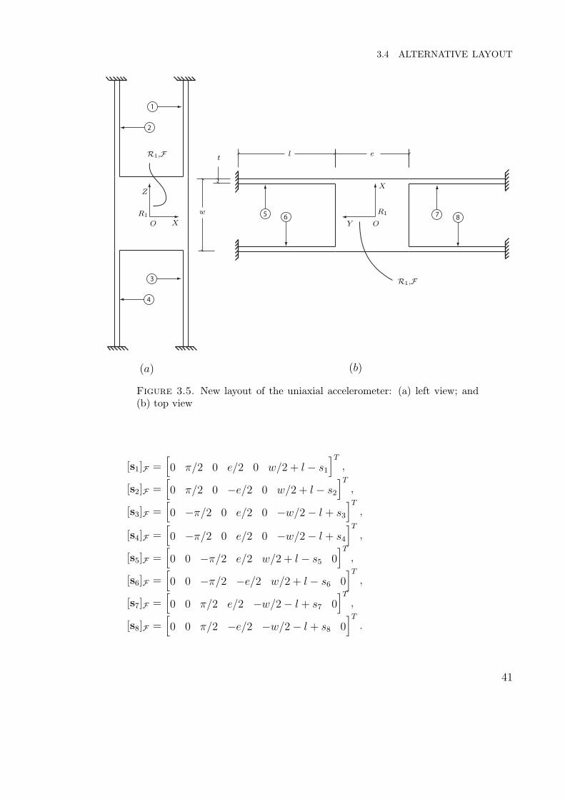
3.4 ALTERNATIVE LAYOUT
1
2
3
4
5 6 7 8
(a) (b)
et
l
w R1R1
R1,F
R1,F
Z
Y
X
X OO
Figure 3.5. New layout of the uniaxial accelerometer: (a) left view; and(b) top view
[s1]F =[
0 π/2 0 e/2 0 w/2 + l − s1
]T
,
[s2]F =[
0 π/2 0 −e/2 0 w/2 + l − s2
]T
,
[s3]F =[
0 −π/2 0 e/2 0 −w/2 − l + s3
]T
,
[s4]F =[
0 −π/2 0 e/2 0 −w/2 − l + s4
]T
,
[s5]F =[
0 0 −π/2 e/2 w/2 + l − s5 0]T
,
[s6]F =[
0 0 −π/2 −e/2 w/2 + l − s6 0]T
,
[s7]F =[
0 0 π/2 e/2 −w/2 − l + s7 0]T
,
[s8]F =[
0 0 π/2 −e/2 −w/2 − l + s8 0]T
.
41
CHAPTER 3. MODAL ANALYSIS OF THE COMPLIANT ACCELEROMETER
Once again, we find the natural frequencies of the system from the eigenvalues
of matrix Ω2 The four lowest frequencies and their corresponding modal vectors are
listed in Table 3.7. The first natural frequency, λ1 = 490.6 Hz, remains in the sensitive
axis, but the mechanism uses the second order deformation of the flexible beam to
allow the translation of the proof-mass. The plane normal to the sensitive axis is
isotropically rigid, in that the second and third frequencies are equal. Moreover, the
mechanism is not subjected to axis drift since the components of vector λ1 are at
zero, with the exception of the component corresponding to translation along the X
direction. The sensitivity ratios of the new layout,
rθZ ,X ≡ λ2
λ1= 7.98, rθY ,X ≡ λ3
λ1= 8.05 (3.40)
We notice here that the sensitivity ratio reveal almost one order of magnitude of
difference between λ2 and λ1. In addition, the sensitive off-axis plane is isotropic,
since rθY ,X ≈ rθZ ,X . The new layout is less sensitive than its original 2ΠΠ counterpart,
because the former uses the second order deformation of the flexible beams to allow
the translation of the proof-mass. However, λ1 does not exceed the maximum natural
frequency, 1800 Hz, of low-frequency accelerometers (see Chapter 1). Moreover, it is
possible to improve the accelerometer properties by optimizing the new layout.
42

3.4 ALTERNATIVE LAYOUT
Table 3.5. Modal frequencies and modal vectors of the compliant 2ΠΠmechanism
i 1 2 3 4 i 1 2 3 4fi (Hz) 290 1013 1066 2128 fi (Hz) 290 1013 1066 2128
λi,1
0.301 −0.032 0.076 0.931
λi,7
0.000 −0.524 −0.423 −0.9820.197 −0.697 0.726 0.244 0.000 0.121 0.175 0.118−0.181 0.716 0.678 0.212 −1.000 −0.843 0.889 0.148−0.915 0.000 0.000 0.000 0.000 0.000 0.000 0.0000.000 0.000 −0.063 0.000 0.000 0.000 0.000 0.0000.000 0.000 −0.068 0.000 0.000 0.000 0.000 0.000
λi,2
0.000 −0.489 0.505 0.980
λi,8
0.000 −0.745 −0.488 −0.9200.000 −0.107 0.201 0.114 0.000 0.115 0.199 0.320−1.000 −0.866 −0.839 −0.160 −1.000 −0.657 0.850 0.2280.000 0.000 0.000 0.000 0.000 0.000 0.000 0.0000.000 0.000 0.000 0.000 0.000 0.000 0.000 0.0000.000 0.000 0.000 0.000 0.000 0.000 0.000 0.000
λi,3
0.000 −0.720 0.601 0.924
λi,9
0.199 −0.898 0.156 −0.9770.000 −0.104 0.224 0.296 −0.143 0.375 0.794 0.131−1.000 −0.686 −0.767 −0.241 −0.105 0.228 −0.581 −0.1670.000 0.000 0.000 0.000 −0.593 0.000 0.000 0.0000.000 0.000 0.000 0.000 −0.760 0.000 −0.060 0.0000.000 0.000 0.000 0.000 0.000 0.000 0.000 0.000
λi,4
0.187 −0.904 0.000 0.978
λi,10
0.000 0.230 0.613 −0.9990.157 −0.344 0.840 0.124 0.000 0.162 0.094 0.000−0.093 0.252 0.535 0.169 1.000 −0.960 0.784 0.051−0.594 0.000 0.000 0.000 0.000 0.000 0.000 0.0000.761 0.000 −0.059 0.000 0.000 0.000 0.000 0.0000.000 0.000 0.000 0.000 0.000 0.000 0.000 0.000
λi,5
0.000 0.133 −0.622 0.999
λi,11
0.000 0.706 0.517 −0.9500.000 −0.135 0.100 0.000 0.000 0.111 0.084 0.0001.000 −0.982 −0.776 0.000 1.000 −0.699 0.852 0.3080.000 0.000 0.000 0.000 0.000 0.000 0.000 0.0000.000 0.000 0.000 0.000 0.000 0.000 0.000 0.0000.000 0.000 0.000 0.000 0.000 0.000 0.000 0.000
λi,6
0.000 0.643 −0.551 0.9510.000 −0.100 0.090 0.0001.000 −0.759 −0.829 −0.3060.000 0.000 0.000 0.0000.000 0.000 0.000 0.0000.000 0.000 0.000 0.000
43

CHAPTER 3. MODAL ANALYSIS OF THE COMPLIANT ACCELEROMETER
Table 3.6. Dimensions of the new layout
l t w e10 mm 250 µm 5 mm 5 mm
Table 3.7. Modal analysis of the new layout
i 1 2 3 4fi (Hz) 1679 13407 13511 13820
λi
0.00 0.14 0.17 0.230.00 0.82 0.11 0.430.00 0.23 0.85 0.341.00 0.01 0.04 0.450.00 0.03 0.01 0.320.00 0.02 0.03 0.45
44

CHAPTER 4. SHAPE OPTIMIZATION OF A CORNER-FILLETED HINGE
CHAPTER 4
Shape Optimization of a Corner-filleted
Hinge
In Chapter 3 the compliant devices were designed based on the stiffness properties
of its flexible elements. However, kinematic synthesis does not consider all the char-
acteristics of compliant mechanisms. As stated by Moon et al. (2002) and De Bona
and Munteanu (2005), one of the main drawbacks of a compliant hinge is the high
stress concentration leading to low fatigue strength. The stress concentration de-
pends on the stress flow which is controlled by the change of curvature in the beam.
Accordingly, designers of a compliant mechanism must take into account not only the
stiffness requirement, but also the strength requirement. For this reason, we choose
to optimize the shape of the flexible-link profile in terms of the stress-concentration
factor.
Straight flexible beams used for compliant mechanisms are integrated within a
monolithic structure by adding a radius at the interface between the beam and the
rigid link. Thus, the resulting flexible beam is said to be a corner-filleted hinge.
However, the circular profile of the fillets, which is the most common shaped found in
the literature (Stuart et al., 1997; Yingfei and Zhaoying, 2002), is not optimal with
respect to stress concentration because circular fillets give rise to G2-discontinuities,
i.e. discontinuities in the curvature of a geometric curve. We know from Williams
45

CHAPTER 4. SHAPE OPTIMIZATION OF A CORNER-FILLETED HINGE
Y
X
l
tr
G2-discontinuities
Figure 4.1. Corner filleted hinge
(1952), Dunn et al. (1997), and Pedersen (2007) that curvature discontinuities in the
structure profile generate stress concentrations. The stress concentration resulting
from the discontinuities of the corner filleted hinge profile depicted in Fig 4.1 can
drastically accelerate fatigue failure and reduce the life of the compliant mechanism.
What is proposed in this work is to optimize the fillet profile of the flexible beam by
designing their shape with Lame curves. By controlling the curvature of the fillet,
the stress flow might be smoothed, to decrease the stress values.
De Bona and Munteanu (2005) proposed an optimum compliant hinge using a
cubic-spline curve to find the best profile which will maximize the flexibility of a
compliant revolute joint (Fig. 2.1a). In this thesis, we choose Lame curves as opposed
to other families of curves, e.g. splines, because of their simplicity. The true optimum
shape can be obtained by resorting to calculus of variations, whereby the dimension
of the design space is infinite. Lame curves are defined, on the contrary, on a two-
dimensional space, as a Lame curve is defined by two independent parameters, as
explained below.
46

4.1 LAME CURVES
x
y
1.0
0.2
−0.6
0.6
0.4
−0.8
−0.2
−0.4
0.5
−1.0
−0.5
0.0
1.00.0−1.0
0.8
(a)
1.6
0.0
−0.8
−1.6
1−1
y
2.0
1.2
0.8
0.4
−0.4
−1.2
x
20
(b)
−0.4
−0.8
y
1.0
0.2
−0.6
0.6
0.4
−0.2x
−1.0
0.5−0.5 1.0
0.0
0.0−1.0
0.8
(c)
Figure 4.2. Lame curves for: (a) η = 2; (b) η = 3; and (c) η = 4
4.1 Lame Curves
Lame curves are η-order curves defined by the equation
(
x
bx
)η
+
(
y
by
)η
= 1 (4.1)
where η can be any rational number, while bx and by correspond to the intersections
of the curve with x and y axes. There are nine different types of Lame curves based
on the form of the exponent η (Loria, 1902). For our study, we resort to η > 2. From
eq. (4.1), it is apparent that Lame curves are analytic everywhere and, as shown in
Fig. 4.2, even-integer-powered curves are closed and doubly symmetric. For η = 2,
the curve results in a circle and, as η tends to infinity, the curve approaches a square.
In the case of odd-integer-powered Lame curves, as depicted in Fig. 4.2b, they are
open and extend infinitely toward an asymptote crossing the second and the four
quadrants and passing through the origin. Fractional-powered Lame curves are also
open and analytic in the first quadrant, but in the other quadrants, eq. (4.1) leads to
complex numbers.
In order to obtain a closed curve for any rational power η, eq. (4.1) is modified
to read∣
∣
∣
∣
x
bx
∣
∣
∣
∣
η
+
∣
∣
∣
∣
y
by
∣
∣
∣
∣
η
= 1 (4.2)
Figure 4.3 shows the curves obtained using eq. (4.2), for η = 2, 3.5, 5, 8, and 30.
Absolute-value bars are essential for all the rational-powered curves, but can be
47

CHAPTER 4. SHAPE OPTIMIZATION OF A CORNER-FILLETED HINGE
0.0
−0.5
−1.0
0.4
−0.8
0.6
0.5
−0.4
0.2
−0.2
−0.6
0.8
−1.0 1.00.0
1.0
η = 2η = 3.5
η = 5η = 8
η = 30
x
y
Figure 4.3. Lame curves of eq. (4.2)
deleted for even-integer-powered curves. Absolute values, however, introduce dis-
continuities in the curvature because the absolute value function is not differentiable
at the origin.
As the curves shown in Fig. 4.3 have double symmetry, it is sufficient to study
only the first quadrant of the curves for the generation of the fillets. Therefore, the
curves that generate the fillets take the form:
f(x, y) =
(
x
bx
)η
+
(
y
by
)η
− 1 = 0; 2 < η ∈ Q, x, y ∈ R+ (4.3)
where Q is the set of rational numbers and bx and by are scaling parameters. Appar-
ently, Lame curves have two independent parameters, the ratio by/bx and η.
48

4.1 LAME CURVES
0.5 1.00.0
0.0
0.5
1.0
s
φ
θ
x
y
O
Figure 4.4. Lame curves polar coordinate for η = 4
4.1.1 Parameterization of Lame Curves. With regard to eq. (4.3), the x
and y coordinates can be defined explicitly in terms of θ as:
x(θ) =1
(1 + tan θη)1
η
, y(θ) =tan θ
(1 + tan θη)1
η
(4.4)
where the angle θ ∈ [0, π/2] is the polar coordinate of one point of the curve, measured
with respect to the x-coordinate axis, and is defined positive counterclockwise. To
generate the shape of the fillets, affine transformations are used to scale the coordinate
x1 and y1 by means of parameters bx and by, namely,
x1(θ) =bx
(1 + tan θη)1/η, y1(θ) =
by tan θ
(1 + tan θη)1/η(4.5)
If bx = by = b, the Lame curve has a super circular layout; otherwise (bx 6= by), the
Lame curve has a super elliptical layout. Thus, Lame curves can create two types of
fillet: the supercircular fillet and the superelliptical fillet.
4.1.2 Curvature of Lame Curves. The advantage of this family of curves
is that for η > 2 their curvature vanishes at the intersections with the coordinate
axes. The curvature κ(s) is defined as
κ(s) ≡ dφ
ds(4.6)
49
CHAPTER 4. SHAPE OPTIMIZATION OF A CORNER-FILLETED HINGE
where φ is the angle made by the tangent with a fixed line and s is the curve length,
as shown in Fig. 4.4. From its definition, curvature has units of inverse length. If
the Lame curve is given by the parametric form of eq. (4.4), then the curvature κ(θ)
takes the form
κ(θ) =x′(θ)y′′(θ) − y′(θ)x′′(θ)
(x′(θ)2 + y′(θ)2)3/2(4.7)
Notice that for η > 2, κ(θ) becomes undefined at θ = 0 and π/2, but the continuity of
the curvature at points (1, 0) and (0, 1) can be shown to be preserved by computing
the limit of κ(θ) as θ approaches 0 or π/2.
limθ→0η>2
κ(θ) = limθ→π/2
η>2
κ(θ) = 0 (4.8)
The curvature can be expressed in a more robust form, namely, implicit (Gray,
1993):
κ(x, y) =2fxyfxfy − fxxf
2y − fyyf
2x
(f 2x + f 2
y )3/2(4.9)
where fx and fxx are the first-and second-order partial derivatives of f(x, y) = 0 with
respect to x, fy and fyy being defined likewise, and fxy is the mixed second-order
partial derivative of f(x, y) = 0. For the curve f(x, y) of eq.(4.3) the curvature takes
the form (Khan, 2007)
κ(x, y) =(η − 1)(xy)η−2(xη + yη)
(x2η−2 + y2η−2)3/2(4.10)
whence, apparently the curvature of rational-powered Lame curves vanishes at the
intersection with the coordinate axes.
The three different profiles of the flexible beam studied in this thesis, are the
profiles made of circular fillets, supercircular fillets, and superelliptical fillets, as rep-
resented, respectively, in Figs. 4.5a, c, and e. Their corresponding curvature distri-
butions in terms of s are illustrated in Figs. 4.5b, d, and f. Each profile has singular
points A and B at the blending points of the curve and the straight line. For the case
of the circular fillet, the curvature attains unbounded values at the singular points A,
50

4.2 BASIC PROBLEM
(a) (b)
(c)(d)
(e)(f )
s
ss
ss
s
O
O
O
A
A
A
B
B
B
C
C
C
κ(s)
κ(s)
κ(s)
sA
sA
sA
sB
sB
sB
sC
sC
sC
η = 2
η = 3.5
η = 5
Figure 4.5. Flexible beam profiles and their corresponding curvature dis-tributions: (a) (b) circular fillets; (c) (d) supercircular fillets; and (e) (f)superelliptical fillets
B and C. The curvature at the singular points is thus indicated with an arrow, to
indicate the presence of a Dirac function. On the other hand, the curvature of the su-
percircular and the superelliptical profiles depicted in Figs. 4.5d and f are continuous
everywhere, which shows that their corresponding flexible beams are G2-continuous
everywhere.
4.2 Basic Problem
In this work, we consider the supercircular and the superelliptical fillets of Figs. 4.6a
and b, the former becoming a circular fillet for η = 2. However, a circular fillet is
not a good profile because it is G2-discontinuous. Here, our goal is to search for the
power (η > 2) of the Lame curve that minimizes the stress concentration without
compromising the compliance of the joint.
51

CHAPTER 4. SHAPE OPTIMIZATION OF A CORNER-FILLETED HINGE
b
b
l
t
FSymmetry axis
x
y
(a)
bx
by
l
t
FSymmetry axis
x
y
(b)
l
w
Symmetry axis
x
z
(c)
Figure 4.6. Geometry of a Lame-filleted hinge: (a) supercircular filletedhinge; (b) superelliptical filleted hinge; (c) top view of both hinges
4.3 Structural Optimization Procedure
4.3.1 General Scheme. Flexibility along the sensitive axis is the main re-
quirement that has to be fulfilled when designing a flexural beam. Therefore, the
reduction of stress concentration must not decrease the flexibility of the beam along
the sensitive axis. It follows that the design problem can be solved by referring to
52

4.3 STRUCTURAL OPTIMIZATION PROCEDURE
F
umax
x
y Symmetry axis
(a)
w/2x
z
Symmetry axis
(b)
Figure 4.7. Structural model: (a) front view, (b) top view
a classical optimization procedure, where the minimum stress concentration is the
objective function with a constraint on the joint flexibility. Objective function and
constraint must be computed by a Finite Element (FE) solver because closed-form
solutions of stresses are not possible for arbitrary shapes. Moreover, only FE analysis
with a fine mesh can determine local stress peaks generated by G2-discontinuities. A
procedure was set-up for the automatic generation of the FE mesh at each optimiza-
tion step according to the values of the design variables provided by the optimization
algorithm.
By exploiting the layout symmetry, we can simplify the structural model of the
hinge to only a quarter of the original structure. Figures 4.6a, b, and c show the
axis of symmetry for the analysis. A symmetry condition applies to problems in
which the geometry, loading, and boundary conditions are symmetric about an axis,
while, an anti-symmetry condition applies when only the geometry is symmetric with
respect to an axis (Moaveni, 2003). In the anti-symmetry case, the loading and the
boundary conditions are not symmetrically spread on each side of the anti-symmetric
axis. Figure 4.7 shows the model used for the structural analysis and the planes
subject to the symmetric and anti-symmetric conditions. The displacements of the
flexible beam left end were set to zero, as is the case for a cantilever beam, while, at
53
CHAPTER 4. SHAPE OPTIMIZATION OF A CORNER-FILLETED HINGE
the other end, a vertical load F is applied. The optimization procedure is introduced
in a dimensionless form similar to the parameterization proposed by De Bona and
Munteanu, (2005). The dimensionless design parameters of the corner-filleted hinge
take the form:
β =r
l, λ =
t
l, and ω =
w
l: geometric parameters
µ =F l
σadmt2w: load parameter
ν =umaxEwt2
l2F: flexibility parameter
where r, l, t, and w are the geometric parameters of the corner-filleted hinge with
circular fillets and where σadm, and umax are, respectively, the maximum yield strength
of the selected material, and the maximum deflection of the hinge. In this case study,
the geometric parameters are set to β = 0.02, λ = 0.02, and ω = 0.02, and the
load parameter is set to µ = 0.0134. Figures 4.8a and b show, respectively, the
mesh of the flexural beam and the refined meshing of one of the fillets where stress
concentration occurs. The meshing was built with eight-node brick elements, which
allow to capture the whole regime of stresses. Finally, the deformed position of the
hinge, umax, resulting from the application of the load F , is depicted in Fig. 4.7a
4.3.2 Objective Function and Constraints. The objective of the opti-
mization procedure is to minimize the stress concentration at the transition between
the fillet and the straight beam. A reference nominal stress is computed for a straight
beam in pure bending. Since the beam has a constant rectangular cross-section of
w × t, the reference stress is not influenced by any change of curvature. When con-
sidering the case of pure bending as defined by Juvinall and Marshek (2000), the
resulting stress is given by the equation:
σ =Mc
I(4.11)
54

4.3 STRUCTURAL OPTIMIZATION PROCEDURE
(a)
(b)
Figure 4.8. Meshing of the flexible beam: (a) front view; and (b) zoom-inon the fillet
where I is the moment of inertia of the cross section with respect to the neutral axis,
and c is the distance from the neutral axis. For consistency with the location of the
stress concentration, the nominal stress, represented by σ, is computed with c = t/2
and M = F l, which yields:
σ =6F l
wt2(4.12)
Thus, at the lower surface we have the reference stress state
σ1 = σ, σvM = σ (4.13)
where σ1 is the reference principal stress and σvM is the reference von Mises stress.
The stress factors c1 and cvM are determined as relative to the nominal values, i.e.,
c1 =σ1
σ1, cvM =
σvM
σvM(4.14)
55

CHAPTER 4. SHAPE OPTIMIZATION OF A CORNER-FILLETED HINGE
Table 4.1. Initial corner-filleted hinge
Profile β τ ω η ν cvM c1
1 0.02 0.02 0.02 2.00 1743 4.42 4.61
where σ1 and σvM are, respectively, the first principal and von Mises stress of the FE
analysis of the flexible beam.
As the goal of a compliant hinge is to allow flexibility in the sensitive axis, the
optimization of the stress concentration is obviously constrained by the stiffness of
the flexible beam. If the flexible parameter ν classifies the characteristics of each
hinge, the compliance constraint is defined by the expression
g(x) = ν − νadm > 0 (4.15)
where νadm is the deflection of the reference corner-filleted hinge. The flexibility
constraint enables the optimization algorithm to discard solutions that are too stiff.
Table 4.1 includes the properties of the initial corner-filleted hinge made of circular
fillets.
4.4 Optimum Supercircular Fillet
The simplest shaped design that fulfils the G2-continuity is a quarter of a super
circular curve. Figure 4.6a shows the parameterization of the supercircular filleted
hinge, where the five parameters, l, t, w, b, η are, respectively, the length, the thickness
and the depth of the hinge, the height and power of the Lame curve defined in eq. (4.5).
It is noteworthy that the circular fillet is a specific case of the super circular fillet
and, therefore, it has the same parameterization, with r = b and η = 2.
The optimization problem consists in finding the power η that minimizes the
stress concentration without decreasing the hinge compliance. Thus, the supercircular
fillet problem is a single-variable optimization, where η is the design variable. The
optimization problem is solved by minimizing the equation:
f(η) = (cvM )max =(σvM )max
σvM→ min
η(4.16)
56

4.4 OPTIMUM SUPERCIRCULAR FILLET
2 2.5 3 3.5 44.1
4.2
4.3
4.4
4.5
4.6
η
(cvM )max
(c1)max
c
Figure 4.9. Stress concentration factor as a function of power η of a Lamecurve for supercircular fillet
subject the design constraint:
g(η) = ν − νadm > 0 (4.17)
and to the boundary constraint:
2 < η (4.18)
The FE analysis of the hinge with a supercircular fillet was conducted for different
values of η. The resulting parametric study reveals the convex shape of the function
describing the maximum stress concentration factor c as a function ofη. Thus, the
minimum stress concentration is located at η = 3.2, as depicted in Fig. 4.9. The
optimum design, for a minimax von Mises stress, is obtained for η = 3.2, which
corresponds to a value of ν = 1797, (cvm)max = 4.227, and (c1)max = 4.357. To
evaluate the influence of η on the stress concentration, we complete the parametric
study with one digit of resolution. The resolution of the design variable η is limited by
57

CHAPTER 4. SHAPE OPTIMIZATION OF A CORNER-FILLETED HINGE
(a)
(b)
(c)
Figure 4.10. Von Mises stress distribution with (a) no fillet; (b) circularfillet; and (b) optimum supercircular fillet with η = 3.2
the accuracy of the FEA which depends on the mesh resolution. Therefore, to obtain
a representative function f(η), the size of the elements needs to be small enough to
capture the small local change in geometry. Here, the element size has been refined
to obtain the convex curves shown in Fig. 4.9.
58
4.5 OPTIMUM SUPERELLIPTICAL FILLET
Figures 4.10a, b, and c illustrate the stress fields of the rectangular, the circular,
and the optimum supercircular hinge. Note that a square corner can be represented by
a Lame curve of infinite exponent (η → ∞). Obviously, square corners are not good
designs; traditionally, compliant hinges have been improved by mean of circular fillets.
By removing material from the circular fillet, the maximum stress condition located
around the fillets decreases with a stress concentration factor of (cvM )max = 4.421
to (cvM )max = 4.227, allowing an improvement of 4.4%. In addition, the flexibility
parameter increases from νadm = 1743 to ν = 1797. This optimization demonstrates
the improvement in the original shape of the corner-filleted hinge. Nevertheless, the
supercircular fillet still has a limited shape domain for maximum stresses. This can
be resolved by extending this domain further.
4.5 Optimum Superelliptical Fillet
A superelliptical fillet shape as an alternative to the supercircular fillet may be
worthwhile because the new design improves even more the stress flow around the
fillet of the compliant joint. However, an extra parameter is necessary to describe
the elliptical shape of the new fillets. Figure 4.6b shows the parameterization of
the superelliptic filleted hinge, bx and by being the two scaling factors of eq. (4.5).
The new optimization problem consists in minimizing the stress concentration of the
superelliptical fillet, where the vector of design variables is expressed:
x = [bx by η]T (4.19)
The optimum superelliptical fillet is found as a solution of the problem:
f(x) = (cvM)max =(σvM )max
σvM→ min
x
(4.20)
subject to the compliance constraint:
g(x) = ν − νadm > 0 (4.21)
59
CHAPTER 4. SHAPE OPTIMIZATION OF A CORNER-FILLETED HINGE
and to the boundary constraints:
0 6 x1 6 l/2, 0 6 x2, 2 < x3, (4.22)
which are set to respect the limitations of the geometry.
4.5.1 Optimization Algorithm. Problem (4.20) is of the constrained non
linear type. Additionally, the objective function at hand is the maximum von Mises
stress throughout the whole structural element, which is a non-analytic function of the
design variables. This feature prevents the use of any gradient algorithm. To handle
the non-analyticity of the objective function, we selected the Nelder-Mead simplex
algorithm (Nelder and Mead, 1965). However, the original simplex algorithm does not
handle constraints; therefore we use the simplex algorithm with a penalty function to
handle the constraint. The modified simplex algorithm, outlined in Rahman (2006),
is implemented in Matlab’s Optimization toolbox. This implementation is used here.
To generate the FE model at each optimization step according to inputs of the
simplex algorithm, a Matlab procedure was implemented, using Ansys as the simula-
tion toolbox. This is feasible, since Matlab can execute any program without inter-
rupting its processing. The procedure linking both softwares is depicted in Fig 4.11.
First, Matlab most prepare the input file written in ANSYS parametric design lan-
guage. Once the input file is created, ANSYS can be launched from Matlab using
the “dos” command. Finally, by loading the FE analysis results to Matlab, Ansys is
completely implemented in the optimization loop. Furthermore, Ansys automatically
generates the mesh of the hinge at each optimization step.
4.5.2 Results. The results are recorded in dimensionless form, according to
the notation:
βx =bx
l, βy =
by
l, η: design parameters
60
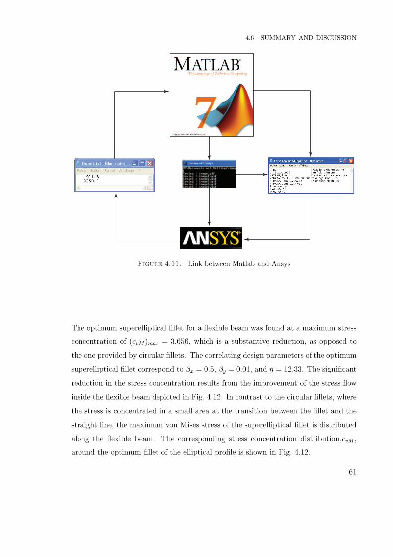
4.6 SUMMARY AND DISCUSSION
Figure 4.11. Link between Matlab and Ansys
The optimum superelliptical fillet for a flexible beam was found at a maximum stress
concentration of (cvM )max = 3.656, which is a substantive reduction, as opposed to
the one provided by circular fillets. The correlating design parameters of the optimum
superelliptical fillet correspond to βx = 0.5, βy = 0.01, and η = 12.33. The significant
reduction in the stress concentration results from the improvement of the stress flow
inside the flexible beam depicted in Fig. 4.12. In contrast to the circular fillets, where
the stress is concentrated in a small area at the transition between the fillet and the
straight line, the maximum von Mises stress of the superelliptical fillet is distributed
along the flexible beam. The corresponding stress concentration distribution,cvM ,
around the optimum fillet of the elliptical profile is shown in Fig. 4.12.
61

CHAPTER 4. SHAPE OPTIMIZATION OF A CORNER-FILLETED HINGE
Figure 4.12. Von Mises stress concentration distribution of the optimumsuper elliptical fillet
Table 4.2. Summary of results
Profile βx βy η cvM ν Improvement0. No fillet n.a. n.a. ∞ 5.217 1806 n.a.1. Circular fillet 0.020 0.020 2.00 4.421 1688 n.a.2. Optimum supercircular fillet 0.020 0.020 3.20 4.227 1762 4.4%3. Optimum superelliptical fillet 0.500 0.010 12.33 3.656 1688 20.9%
4.6 Summary and Discussion
The suggested beam profiles are summarized in Table 4.2. The improvements in
stress concentration of the two new profiles were computed in relation to the stress
concentration of the original corner-filleted hinge profile. It is not surprising that
profile 3 shows the greatest improvement. What is surprising is that profile 3 has an
improvement of 20.9%, which is substantial in comparison with profile 2 improvement
of 4.4%. Throughout the optimization, the design variable bx converges to its upper
boundary condition, causing the fillets of the hinge to merge, the straight portion of
the beam thus vanishing. Therefore, the profile of the hinge is defined with a single
formula. The optimum profile is also analytic everywhere.
The low stress concentration of profile 3 is obtained at the expense of a large
power η that results in high curvature changes and, therefore, higher complexity
(Khan, 2007). On the other hand, profile 2 has a higher stress concentration but
much lower power η. Thus, the designer can make a compromise between stress
concentration and complexity by selecting profile 2.
62

CHAPTER 5. OPTIMUM DESIGN OF A COMPLIANT UNIAXIAL ACCELEROMETER
CHAPTER 5
Optimum Design of a Compliant Uniaxial
Accelerometer
Optimization techniques are used in the design of compliant mechanisms. A popular
technique is topology optimization, which can find the distribution of a given amount
of material that maximizes the stiffness of the structure (Frecker et al., 1997; Bernar-
doni et al., 2004; Mankame and Ananthasuresh, 2004; Werme, 2007 ; Mechkour1
et al., 2007). The technique was originally developed to generate the architecture of
optimum planar mechanisms. The problem with the resulting mechanism is that it
does not consider the sensitivity to out-of-plane forces. Furthermore, this optimiza-
tion technique cannot be used to find the optimum shape of a desired layout, since it
generates its own layout.
The design technique introduced in this thesis does not generate optimum lay-
outs, but optimizes the dimensions of a given layout. Thus, the designer is free to
optimize any preselected three-dimensional compliant mechanism layout. Moreover,
the technique minimizes the parasitic compliance in all off-axis directions. To do so,
the a posteriori multi-objective algorithm is used to find the best trade-off between
conflicting objective criteria of compliant mechanisms. Among the multi-objective op-
timization techniques, we have chosen the Normalized Normal Constraint algorithm
to obtain an evenly distributed Pareto frontier (Messac et al., 2003).
63
CHAPTER 5. OPTIMUM DESIGN OF A COMPLIANT UNIAXIAL ACCELEROMETER
The method is applied to the cross-configuration of the uniaxial simplicial archi-
tecture proposed by Cardou and Angeles (2007). We start with a general formulation
of the optimization methodology; then, the method is applied to the uniaxial ac-
celerometer of the foregoing reference.
5.1 The Optimization Methodology
This section describes the method used to find an optimum accelerometer ar-
chitecture that minimizes the error of the measured acceleration. This error can
be minimized by optimizing the sensitivity and natural frequencies of the compliant
mechanism. The mechanical sensitivity evaluates the input-to-output amplification.
In the field of compliant mechanisms, the input-to-output amplification ratio is called
the “mechanical advantage” and it is defined by Lobontiu (2003) as:
m.a. =|uout||uin|
(5.1)
where uin and uout are the input and output linear or angular displacement. Regarding
accelerometers, the output displacement is not generated by an input displacement
but with an input acceleration (ain). Hence, we define here the mechanical sensitivity
of an accelerometer as
Υ(x) =|uout(x)||ain|
, (5.2)
where |ain| is the amplitude of a step input and |uout(x)| is the steady-state value of
the displacement response. On the other hand, a minimum parasitic compliance in
the plane normal to the sensitive axis, which is inversely proportional to the second
natural frequency λs, can be obtained by minimizing the ratio between the first and
the second natural frequencies. Finally, the axis drift needs to be taken into account
only when the stiffness of the plane orthogonal to the sensitive axis is not isotropic.
In the case of anisotropic stiffness, the resulting inertia forces acting on the system
will not be balanced and will make the proof-mass deflect outside its translation
trajectory. Designers need to ensure elastic isotropy in the normal plane by suitably
specifying the layout of the accelerometer. Thus, the optimization problem can be
64
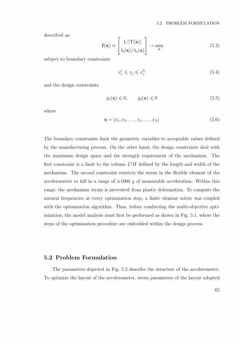
5.2 PROBLEM FORMULATION
described as:
f(x) ≡
1/|Υ(x)|λl(x)/λs(x)
→ minx
(5.3)
subject to boundary constraints
xlj 6 xj 6 xh
j (5.4)
and the design constraints
g1(x) 6 0, g2(x) 6 0 (5.5)
where
x = [x1, x2, . . . , xj, . . . , xN ] (5.6)
The boundary constraints limit the geometric variables to acceptable values defined
by the manufacturing process. On the other hand, the design constraints deal with
the maximum design space and the strength requirement of the mechanism. The
first constraint is a limit to the volume L2H defined by the length and width of the
mechanism. The second constraint restricts the stress in the flexible element of the
accelerometer to fall in a range of ±1000 g of measurable acceleration. Within this
range, the mechanism strain is prevented from plastic deformation. To compute the
natural frequencies at every optimization step, a finite element solver was coupled
with the optimization algorithm. Thus, before conducting the multi-objective opti-
mization, the model analysis must first be performed as shown in Fig. 5.1, where the
steps of the optimization procedure are embedded within the design process.
5.2 Problem Formulation
The parameters depicted in Fig. 5.2 describe the structure of the accelerometer.
To optimize the layout of the accelerometer, seven parameters of the layout adopted
65

CHAPTER 5. OPTIMUM DESIGN OF A COMPLIANT UNIAXIAL ACCELEROMETER
− Architecture− Design Domain− Boundary conditions− Objectives
1. Specification
2. Formulation of the Model Analysis
3. Multi Objective Normalized Normal Constrained Method
Normalization
Utopia line vector
Generate Hyperplane points
Pareto points Generator
Pareto Design Metric Values
b
b
b
bb
4. Choice ofa
Compromise5. Accelerometers Properties
6. Prototype
Figure 5.1. Methodology flow chart
are considered as design variables and arrayed in the design vector x:
x = [w e t l bx by η]T (5.7)
where w, e, t, l, bx, by, and η represent, respectively, the width and length of the
proof-mass, the thickness and length of the compliant joint, and the height, length,
and degree of the Lame curves describing the fillets of the compliant hinges.
66
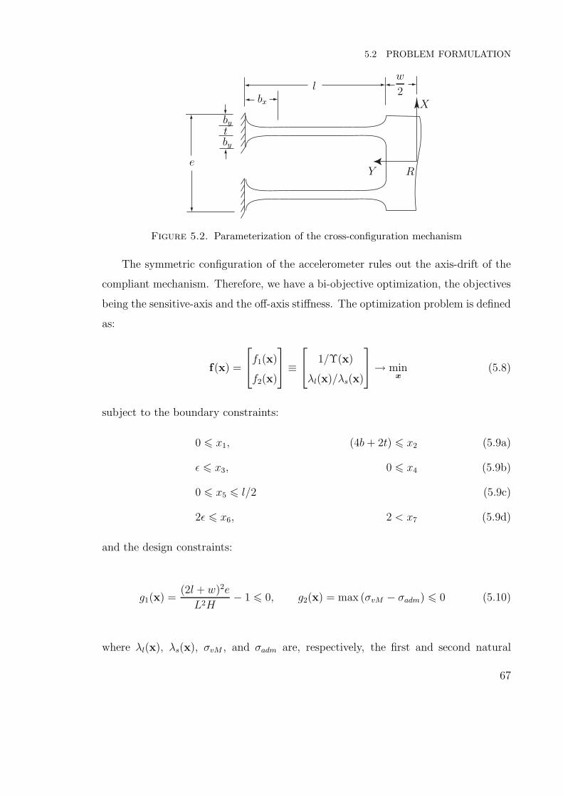
5.2 PROBLEM FORMULATION
t
l
e
w
2bx
by
by
X
Y R
Figure 5.2. Parameterization of the cross-configuration mechanism
The symmetric configuration of the accelerometer rules out the axis-drift of the
compliant mechanism. Therefore, we have a bi-objective optimization, the objectives
being the sensitive-axis and the off-axis stiffness. The optimization problem is defined
as:
f(x) =
f1(x)
f2(x)
≡
1/Υ(x)
λl(x)/λs(x)
→ minx
(5.8)
subject to the boundary constraints:
0 6 x1, (4b + 2t) 6 x2 (5.9a)
ǫ 6 x3, 0 6 x4 (5.9b)
0 6 x5 6 l/2 (5.9c)
2ǫ 6 x6, 2 < x7 (5.9d)
and the design constraints:
g1(x) =(2l + w)2e
L2H− 1 6 0, g2(x) = max (σvM − σadm) 6 0 (5.10)
where λl(x), λs(x), σvM , and σadm are, respectively, the first and second natural
67

CHAPTER 5. OPTIMUM DESIGN OF A COMPLIANT UNIAXIAL ACCELEROMETER
frequency, the von Mises stress and the admissible stress for the maximum acceleration
of 1000 g.
The optimization problem is subjected to the boundary constraints imposed by
the physical dimensioning of the compliance mechanism, except for x3 and x6, which
are limited by the Direct Metals Laser-Sintering (DMLS) machine tool resolution
(Chapter 2). Indeed, the joint thickness t cannot be smaller than the smallest focus
diameter, ǫ = 100 µm. On the other hand, g1(x) describes the compactness, which is
subject to an inequality constraint to limit the design space. This limit is identified
by a box with volume L2H = 103mm3. Finally, to compute the stress constraint
g2(x) and the natural frequencies of the device, a Matlab routine was implemented
to call the FEA solver at each optimization step. Figure 5.3 shows the mesh of the
accelerometer for the modal analysis. In the case of the stress constraint g2(x), we
use a different mesh which considers the symmetries of the accelerometer. Since the
compliant joints are all equally loaded, we computed the stress in only one hinge.
The structural model can be simplified even more with an symmetric analysis of the
compliant joint. Figure 5.4 shows the model used for the structural analysis and
the plane subjected to the anti-symmetric condition. Recall that an anti-symmetry
condition applies when only the geometry is symmetric with respect to an axis. The
displacements of the flexible beam left end were set to zero, while, at the other end,
the rotations and displacement in the neutral axis direction where set to zero in order
to respect the layout of the accelerometer. The load case is also depicted in Fig. 5.4
where the bending load is set to
F = ainmp
n=
1000gw2eρ
8(5.11)
where ain, mp, n, g, and ρ are, respectively, the maximum acceleration input, the
mass of the proof-mass, the number of compliant links, the gravity constant, and the
density of the titanium alloy.
68

5.3 MULTI-OBJECTIVE FORMULATION
Sensitive axis
Figure 5.3. FE model of the accelerometer
F
x
y Symmetry axis
(a)
Figure 5.4. Structural model
5.3 Multi-objective Formulation
The non-analytical nature of the modal analysis prevents us from using gradient-
based methods. To overcome this issue, we use a direct method. In the field of
optimization, the Nelder-Mead simplex algorithm (Nelder and Mead, 1965) is a well-
known effective method for direct-search optimization. Recall that a simplex is a
set of (n + 1) affinely independent points in Rn (Kreyszig, 1997). The Nelder-Mead
simplex algorithm is also the basis of the intelligent moving object optimization al-
gorithm (INTEMOB), proposed by Rahman (2006), due to its capability to handle
non-differentiable, discontinuous, and non-analytical functions. The original simplex
69
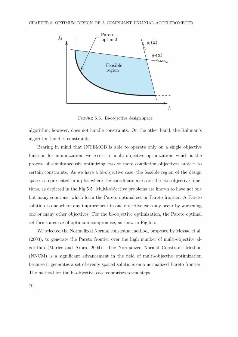
CHAPTER 5. OPTIMUM DESIGN OF A COMPLIANT UNIAXIAL ACCELEROMETER
f1
f2
g1(x)
g2(x)
Paretooptimal
Feasibleregion
Figure 5.5. Bi-objective design space
algorithm, however, does not handle constraints. On the other hand, the Rahman’s
algorithm handles constraints.
Bearing in mind that INTEMOB is able to operate only on a single objective
function for minimization, we resort to multi-objective optimization, which is the
process of simultaneously optimizing two or more conflicting objectives subject to
certain constraints. As we have a bi-objective case, the feasible region of the design
space is represented in a plot where the coordinate axes are the two objective func-
tions, as depicted in the Fig 5.5. Multi-objective problems are known to have not one
but many solutions, which form the Pareto optimal set or Pareto frontier. A Pareto
solution is one where any improvement in one objective can only occur by worsening
one or many other objectives. For the bi-objective optimization, the Pareto optimal
set forms a curve of optimum compromise, as show in Fig 5.5.
We selected the Normalized Normal constraint method, proposed by Messac et al.
(2003), to generate the Pareto frontier over the high number of multi-objective al-
gorithm (Marler and Arora, 2004). The Normalized Normal Constraint Method
(NNCM) is a significant advancement in the field of multi-objective optimization
because it generates a set of evenly spaced solutions on a normalized Pareto frontier.
The method for the bi-objective case comprises seven steps.
70

5.3 MULTI-OBJECTIVE FORMULATION
f1
f2
g1(x)
g2(x)
µuµ2⋆
µ1⋆
l1
l2
00
Paretooptimal
Feasibleregion
Figure 5.6. Pareto frontier
Step 1: ANCHOR POINTS. To normalize the two-dimensional Pareto frontier,
we first need to find the two anchor points, µ1⋆ and µ2⋆, which are the solutions
minimizing both objectives independently. The line joining the two anchor points is
called the Utopia line. The anchor points are obtained by solving problem PU1 and
PU2, defined below, with the INTEMOB algorithm:
Problem PUi (i = 1, 2)
fi(x) → minx
(5.12)
subject to the boundary constraints
xlj 6 xj 6 xuj (j = 1, 2, . . . , N) (5.13a)
71

CHAPTER 5. OPTIMUM DESIGN OF A COMPLIANT UNIAXIAL ACCELEROMETER
1
1
f1
f2
g1(x)
g2(x)
gMO
(x)
Xpk
µ⋆k
µ2⋆
µ1⋆
00
InfeasibleFeasibleregion
region
Utopia line
Figure 5.7. Normalized pareto frontier
and the design constraints
g1(x) 6 0, g2(x) 6 0 (5.14)
with f1(x) and f2(x) defined, respectively, as the first and the second objective func-
tions of eq. (5.3).
Step 2: OBJECTIVE MAPPING. To avoid scaling deficiencies, the optimization
takes place in the normalized design objective space. Utopia point µu of Fig. 5.6 is
defined as
µu = f1(x1⋆) f2(x
2⋆) (5.15)
and the distances l1 and l2 of Fig. 5.6 as
l1 = f1(x2⋆) − f1(x
1⋆) (5.16)
l2 = f2(x1⋆) − f2(x
2⋆) (5.17)
72

5.3 MULTI-OBJECTIVE FORMULATION
If f is the normalized form of f , the normalized design space displayed in Fig. 5.7
can be evaluated as
f(x) =
[
f1(x) − f1(x1⋆)
l1
f2(x) − f2(x2⋆)
l2
]T
(5.18)
Step 3: UTOPIA LINE VECTOR. Define nu as the vector directed from f(x1⋆)
to f(x2⋆), yielding
nu = f(x2⋆) − f(x1⋆) (5.19)
Step 4: NORMALIZED INCREMENTS. Compute a normalized increment δ
along the direction nu for a prescribed number of solutions, m1, as
δ =1
m1 − 1(5.20)
Step 5: GENERATE UTOPIA LINE POINTS. Evaluate a set of vectors xpk
which define Xpk, the set of evenly distributed points on the Utopia line (Fig. 5.7).
xpk = ι1k f(x1⋆) + ι2k f(x
2⋆) (5.21)
where
ι1k + ι2k = 1 0 ≤ ι1k ≤ 1 (5.22)
Note that ιik is incremented by δ between 0 and 1 for k ∈ 1, 2, ..., m1.
Step 6: PARETO POINT GENERATION. Based on the new normalization we
find the other m1 − 2 Pareto solutions using the set of evenly distributed points on
the Utopia line. For each point generated on the Utopia line, we solve
73

CHAPTER 5. OPTIMUM DESIGN OF A COMPLIANT UNIAXIAL ACCELEROMETER
Problem Pk (for k = 2, 3, 4, ..., m1 − 1)
f2(x) → minx
(5.23)
subject to the boundary constraints
xlj 6 xj 6 xuj , j = 1, 2, . . . , N (5.24a)
the design constraints
g1(x) 6 0, g2(x) 6 0, (5.25)
and the new multi-objective constraint
nTu (f(x) − xpk) ≤ 0. (5.26)
Step 7: PARETO DESIGN. Finally, the design solution that corresponds to each
Pareto point can be evaluated in the design space by the relation
f(xk) = [l1f1(xk) + f1(x1⋆) l2f2(xk) + f2(x
2⋆)]T (5.27)
5.4 RESULTS
To define the normalized Pareto optimal set, the two anchor points, µ1⋆ and
µ2⋆, were obtained by solving problems PU1 and PU2 with the INTEMOB algo-
rithm. At the optimum points, x1⋆ = [2.7 2.3 0.1 9.2 0.2 80/9]T and x2⋆ =
[4.5 5.9 0.1 4.5 0.2 43/9]T , we found the two anchor points µ1⋆ = 2.50 ×10⁷ 0.1378 and µ2⋆ = 9.17 × 10⁷ 0.0452. Thus, the Utopia point results to be
µu = 2.50 × 10⁷ 0.0452.
74

5.4 RESULTS
Table 5.1. Pareto solutions
k ι1k ι2k Υ λl(x)λl(x)
λs(x)w e t l bx by η
(nm/g) (Hz) (mm) (mm) (mm) (mm) (mm) (mm)1 1.00 0.00 40.12 834.7 0.1378 2.71 2.31 0.10 9.12 4.12 0.20 80/92 0.83 0.17 35.61 914.3 0.1056 4.57 2.62 0.10 7.45 3.37 0.20 73 0.67 0.33 27.92 1029 0.0840 5.62 2.75 0.10 6.70 3.01 0.20 67/114 0.50 0.50 21.94 1145 0.0713 5.51 3.21 0.10 6.01 2.71 0.20 23/45 0.33 0.67 16.72 1301 0.0623 5.23 4.11 0.10 5.18 2.32 0.20 16/36 0.17 0.83 13.25 1526 0.0540 4.91 4.92 0.10 4.82 2.19 0.20 57 0.00 1.00 10.97 1855 0.0424 4.49 5.87 0.10 4.51 2.02 0.20 43/9
ProblemPU1 : f(x) = 1/|Υ| → minx
(5.28)
subject to eqs. (5.9) and (5.10)
ProblemPU2 : f(x) =λl
λs
→ minx
(5.29)
subject to eqs. (5.9) and (5.10)
In addition to the anchor points, we need to find five additional solutions of
the Pareto frontier to determine a total of seven points. Consequently, the interval
distance on the Utopia line is equal to δ = 0.1666. The Pareto optimum solutions
are listed in Table 5.1; Fig. 5.8 depicts the corresponding Pareto frontier. Note that
each solution satisfies all the optimization constraints.
The Pareto frontier gives freedom to select a design layout to meet specific con-
ditions of the accelerometer. At one extreme, i.e. point 1, of the Pareto frontier, the
75
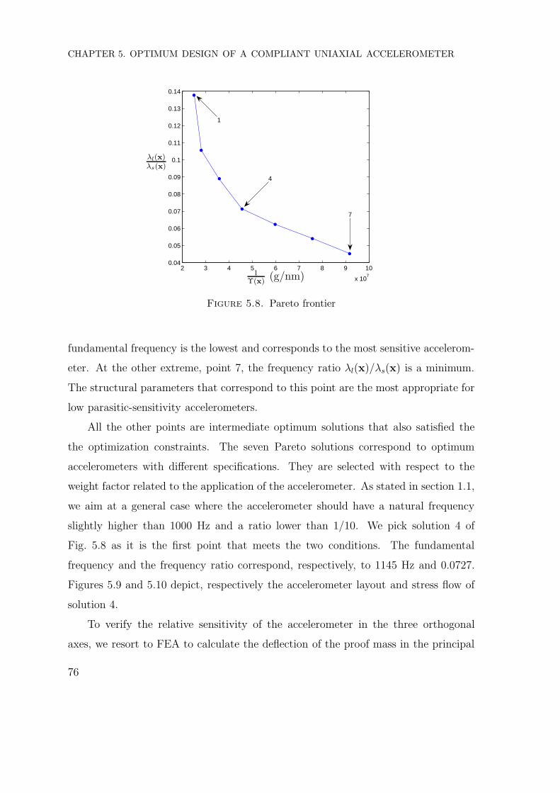
CHAPTER 5. OPTIMUM DESIGN OF A COMPLIANT UNIAXIAL ACCELEROMETER
2 3 4 5 6 7 8 9 10
x 107
0.04
0.05
0.06
0.07
0.08
0.09
0.1
0.11
0.12
0.13
0.14
1
4
7
1Υ(x)
(g/nm)
λl(x)λs(x)
Figure 5.8. Pareto frontier
fundamental frequency is the lowest and corresponds to the most sensitive accelerom-
eter. At the other extreme, point 7, the frequency ratio λl(x)/λs(x) is a minimum.
The structural parameters that correspond to this point are the most appropriate for
low parasitic-sensitivity accelerometers.
All the other points are intermediate optimum solutions that also satisfied the
the optimization constraints. The seven Pareto solutions correspond to optimum
accelerometers with different specifications. They are selected with respect to the
weight factor related to the application of the accelerometer. As stated in section 1.1,
we aim at a general case where the accelerometer should have a natural frequency
slightly higher than 1000 Hz and a ratio lower than 1/10. We pick solution 4 of
Fig. 5.8 as it is the first point that meets the two conditions. The fundamental
frequency and the frequency ratio correspond, respectively, to 1145 Hz and 0.0727.
Figures 5.9 and 5.10 depict, respectively the accelerometer layout and stress flow of
solution 4.
To verify the relative sensitivity of the accelerometer in the three orthogonal
axes, we resort to FEA to calculate the deflection of the proof mass in the principal
76

5.4 RESULTS
Sensitive axis
Figure 5.9. Optimum accelerometer
Table 5.2. Sensitivity of the accelerometer
Proof mass deflection (nm)acceleration
X axis Y axis Z axisax = 1g 22 7.4 × 10⁻⁴ 5.5 × 10⁻⁴
ay = 1g 4.8 × 10⁻⁴ 3.5 × 10⁻² 3.0 × 10⁻⁴
az = 1g 2.6 × 10⁻⁴ 2.7 × 10⁻⁴ 3.9 × 10⁻²
ay = az = 0.707g 5.1 × 10⁻³ 9.7 × 10⁻³ 9.7 × 10⁻³
130075
.232E+08
.463E+08
.694E+08
.925E+08
.116E+09
.139E+09
.162E+09
.185E+09
.208E+09
Figure 5.10. Von Mises stress distribution
direction. The results are listed in Table 5.2 and show that the accelerometer is 103
times more compliant in the sensitive axis than in the other directions.
77

CHAPTER 5. OPTIMUM DESIGN OF A COMPLIANT UNIAXIAL ACCELEROMETER
5.5 DISCUSSION
The NNCM algorithm determines a good approximation of the Pareto frontier
with a small number of optimum solutions; this is a considerable advantage for me-
chanical systems with high computational complexity. In the problem at hand, only
seven solutions were obtained to approximate well the Pareto frontier. The solutions
are equally distributed along the Utopia line, as opposed to a priori multi-objective
optimization methods, which need a larger number of points to represent the Pareto
frontier.
The Pareto frontier helps the designer select the best compromise among a set
of optimum designs. In our case, we choose solution 4 as the resulting accelerom-
eter met the general characteristics of a low-frequency accelerometer with a usable
frequency range that goes from 0 to 600 Hz. Low-frequency accelerometers have the
advantage of a high sensitivity and good compactness; however, they have the dis-
advantages of a very fragile mechanical structure and high off-axis sensitivity. Thus,
commonly used low-frequency accelerometers have a limited range of acceleration be-
tween 1 g and 50 g and high off-axis sensitivity of around 5%. To overcome these
problems, the accelerometer layout was optimized by considering these four charac-
teristics. The first objective of the multi-objective optimization is to maximize the
mechanical sensitivity (Υ) of the accelerometer. However, by minimizing 1/Υ and
the ratio of frequency λf/λs , the optimization also affects the accelerometer usable
frequency range, which cannot exceed 1/3 of its natural frequency. Since the optimum
accelerometer has a natural frequency of 1145 Hz, its usable frequency ranges from 0
to 381 Hz. Moreover, the proposed compliant mechanism exhibits a low mechanical
off-axis sensitivity through the minimization of the second objective. The resulting
compliant mechanism is at least 1000 times more sensitive in its sensitive axis than
in the other directions, which is a significant improvement. Finally, the optimization
constraints allow the mechanism to fit in a box of 17.5×17.5×3.2 mm3, and prevent
failure of the compliant mechanism under ±1000 g.
78

5.5 DISCUSSION
The optimization requires several runs before converging toward a global mini-
mum. In order to converge, the algorithm requires a good compromise between the
mesh resolution and the convergence criterion. A high mesh resolution needs larger
computation time, while a coarse mesh will not represent the objective function cor-
rectly. The convergence criterion is to be set to the required degree of accuracy of
the FEA. The overall CPU cost of the algorithm is very large because the objective
functions are computed with a high resolution meshing. Several hours were necessary
to compute only one Pareto solution.
79

6.1 CONCLUSIONS
CHAPTER 6
Closing Remarks
6.1 Conclusions
The optimum design of a compliant simplicial uniaxial accelerometer (SUA) was
reported in this thesis.
First, in Chapter 2, we described in detail the characteristics of compliant mech-
anisms and the compliant realization of the original layout of the SUA. We selected
the material with properties maximizing the inertial sensor performance.
The advantages and shortcomings of compliant mechanisms were highlighted in
Chapter 3 by conducting the kinematic analysis of three different systems. A lumped-
parameter model was first tested to solve a simple system made of one notched beam
and one mass. Afterwards, the lumped-parameter model was used to highlight the
deficiencies of the original layout of the SUA. To cope with the low off-axis stiffness
and the axis-drift of the SUA, we came up with an new alternative layout.
One of the drawbacks affecting compliant mechanisms is the stress concentration
which limits the range of motion and life cycle of the mechanism. In Chapter 4,
we proposed a new compliant hinge design to decrease the stress concentration. We
called this new hinge Lame-shaped hinge as we used Lame curves to produce the
profile of the hinge. The advantages of Lame curves were demonstrated by studying
the curvature of the profile of compliant hinges and mostly by optimizing the profile
of the Lame-shaped hinge. In this particular optimization problem, the objective
81
CHAPTER 6. CLOSING REMARKS
function was defined as the maximum stress concentration subject to a flexibility
constraint. We found an improvement of up to 20% over the original corner-filleted
hinge of equal compliance.
The Normalized Normal Constraint Method, which is a multi-objective algorithm,
was applied in Chapter 5 to accelerometer design. Although only two objective func-
tions were considered, the method can readily be extended to multiple objective
functions. The method was applied to optimize the new layout of the simplicial uni-
axial accelerometer. The solution found gives an accelerometer with excellent stiffness
and strength properties compared to the initial mechanism (Chapter 2). The stress
flow is improved by using a superelliptical fillet, and the overall volume of the device
is now 1/3 of the initial layout. In addition, the first natural frequency went from
1679 Hz to 1145 Hz, improving the sensitivity of the accelerometer. Therefore, the
usable frequency range of the final accelerometer goes from 0 Hz to 380 Hz. Finally,
the ratio of frequency went from 0.125 to 0.0727; thus, there is now more than one
order of magnitude between the two lowest frequencies. We have thus reached our
design objectives.
6.2 Recommendations for Future Work
As an extension to the work reported here, several issues remain to be further
explored:
(i) The Bode diagrams and the complex frequency responses in the three or-
thogonal axis of the proof mass need to be computed;
(ii) The fabrication process of the accelerometer is to be conducted;
(iii) Compute the mounted frequency of the accelerometer by including the rigid-
ity of the accelerometer frame;
(iv) The compliant realization of the Simplicial Triaxial Accelerometer is to be
designed by adding a notched beam at each end of the compliant ΠΠ-legs
layout proposed in Chapter 2.
82

BIBLIOGRAPHY
BIBLIOGRAPHY
Algrain, M. C. and Quinn, J. (1993), Accelerometer based line-of-sight stabilization
approach for pointing and tracking systems, in ‘In Proceedings of 2nd IEEE Con-
ference on Control Applications’, Vancouver, Canada, pp. 159–163.
Ananthasuresh, G. and Kota, S. (1995), ‘Designing compliant mechanisms’, Mechan-
ical Engineering 68(3), 93–96.
Angeles, J. (2004), ‘The qualitative synthesis of parallele manipulators’, ASME Jour-
nal of Mechanical Design 126(4), 617–624.
Angeles, J. (2007), Fundamentals of Robotic Mechanical Systems. Theory, Methods,
and Algorithms, 3rd edn, Springer, New York.
Arai, T., Herve, J. M. and Tanikawa, T. (1996), Development of 3 dof micro finger,
in ‘Proceedings of IROS Conference’, Vol. 96, Osaka, Japan, pp. 981–987.
Ashby, M. F. (2005), Materials Selection in Mecanical Design, 3nd edn, Elsevier
Butterworth Heinemann: Amsterdam.
Bao, M. (2000), Micro mechanical transducers : pressure sensors, accelerometers, and
gyroscopes, Elsevier Butterworth Heinemann: Amsterdam.
Bernardoni, P., Bibaud, P., Bidard, C. and Gosselin, F. (2004), ‘A new compliant
mechanism design methodology based on flexible building blocks’, Smart Structures
and Materials 2004. Modeling, Signal Processing, and Control 5383(1), 244–254.
Cardou, P. (2007), Design of Multiaxial Accelerometers with Simplicial Architectures
for Rigid-Body Pose and Twist Estimation, PhD thesis, McGill University, Mon-
treal, Canada.
83
BIBLIOGRAPHY
Cardou, P. and Angeles, J. (2007), Simplectic architectures for true multi-axial ac-
celerometers: A novel application of parallel robots, in ‘IEEE International Con-
ference on Robotics and Automation’, Roma, Italy, pp. 181–186.
Cardou, P., Pasini, D. and Jorge, A. (2008), ‘Lumped elastodynamic model for mems:
Formulation and validation’, IEEE Journal of Microelectromechanical Systems .
De Bona, F. and Munteanu, M. G. (2005), ‘Optimized flexural hinges for compliant
micromechanisms’, Springer Science 44, 163–174.
Derderian, A. M., Howell, L., Murphy, M. D., Lyon, S. M. and Pack, S. D. (1996),
Compliant parallel-guiding mechanisms, in ‘Proceding of the 1996 ASME Design
Engineering Technical Conference’, Vol. 96, Irvine, CA, USA.
Dunn, M., Suwito, W. and Cunningham, S. (1997), ‘Stress intensities at notch singu-
larities’, Egineering Fracture Mechanics 57(4), 417–430.
Frecker, M., Ananthasuresh, G., Nishiwaki, S., Kikuchi, N. and Kota, S. (1997),
‘Topological synthesis of compliant mechanisms using multi-criteria optimization.’,
ASME Journal of Mechanical Design 119, 238–245.
Gray, A. (1993), Modern Differential Geometry of Curves and Surfaces, CRC Press:
Boca Raton.
Howell, L. (2001), Compliant Mechanisms, J. Wiley & Sons: New York.
Juvinall, R. and Marshek (2000), Fundamentals of Machine Component Design, 3nd
edn, John Wiley & Sons, Inc.
Khan, W. A. (2007), The Conceptual Design of Robotic Architectures Using Com-
plexity Criteria, PhD thesis, McGill University, Montreal, Canada.
Kreyszig, E. (1997), Advanced Engineering Mathematics, 8nd edn, John Wiley &
Sons: New York.
Kruglick, E., Warneke, B. and Pister, K. (1998), ‘Cmos 3 -axis accelerometers with
integrated amplifier’, IEEE pp. 631–636.
Li, G., Li, Z., Wang, C., Hao, Y., Zhang, D. and Wu, G. (2007), ‘Design and fab-
rication of a highly symmetrical capacitive triaxial accelerometer’, Journal of Mi-
cromechanics and Microengineering 17, 36–41.
84

BIBLIOGRAPHY
Lobontiu, N. (2003), Compliant Mechanisms: Design of Flexure Hinges, CRC Press:
Boca Raton, FL, USA.
Lobontiu, N. and Garcia, E. (2003), ‘Analytical model of displacement amplifica-
tion and stiffness optimization for a class of flexure-based compliant mechanisms’,
Science Direct 81, 981–987.
Lobontiu, N. and Garcia, E. (2005), ‘Circular-hinges line element for finite element
analysis of compliant mechanisms’, Journal of Mechanical Design 127, 766–773.
Lobontiu, N., Garcia, E., Hardau, M. and Bal, N. (2004), ‘Stiffness characterization of
corner-filleted flexure hinges’, Review of scientific instruments 75(11), 4896–4904.
Loria, G. (1902), Spezielle Algebraische und Transscendente Ebene Kurven: Theorie
und Geschichte,, BG Teubner: Leipzig.
Macdonald, G. (1990), ‘Review of low cost accelerometers for vehicle dynamics.’,
Sensors Actuators A(21), 303307.
Mankame, N. and Ananthasuresh, G. (2004), ‘Topology synthesis of electrothermal
compliant mechanisms using line elements.’, Structural Multidisciplinairy Optimiza-
tion 26, 209218.
Marler, R. and Arora, J. (2004), ‘Survey of multi-objective optimizatoin methods for
engineering’, Structural Multidisciplinary Optimization 26, 369–395.
Mechkour1, H., Jouve, F., Rotinat-Libersa, C., Bidard3, C. and Perrot, Y. (2007),
Optimal design of compliant mechanisms by level set and flexible building blocks
methods, in ‘7th World Congress on Structural and Multidisciplinary Optimiza-
tion’, Seaoul, Korea, pp. 1898–1907.
Messac, A., Ismail-Yahaya, A. and Mattson, C. (2003), ‘The normalized normal con-
straint method for generationg the pareto frontier’, Structural Multidisciplinary
Optimization 25(2), 86–98.
Mineta, T., Kobayashi, S., Watanabe, Y., Kanauchi, S., Nakagawa, I., Suganuma,
E. and Esahi, M. (1996), ‘Three-axis capacitive accelerometer with uniform axial
sensitivities’, Journal of Micromechanics and Microengineering 6, 631–635.
85
BIBLIOGRAPHY
Moaveni, S. (2003), Finite Element Analysis: Theory and Application with Ansys,
2nd edn, Pearson Education, Upper Saddle River, New Jersey, USA.
Moon, Y., Trease, P. and Kota, S. (2002), Design of large-displacement compliant
joints, in ‘MECH 27th Biennial Mechanisms and Robotics Conference’, number 3,
Montreal, Canada.
Navid, Y., Najafi, K. and Salian, A. S. (2003), ‘A high-sensitivity silicon accelerome-
ter with a folded-electrode structure.’, Journal of Microelectromechanical Systems
12(4), 479–486.
Nelder, J. and Mead, R. (1965), ‘A simplex method for function minimization’, Com-
put Journal 4, 308–313.
Paros, J. and Weisbord, L. (1965), ‘How to design flexure hinges’, Machine Design
37, 151–156.
Pedersen, P. (2007), Some benchmarks for optimized shapes with stress concentration,
in ‘7th World Congress on Structural and Multidisciplinary Optimization’, Seaoul,
Korea, pp. 1623–1631.
Pilkey, W. D. (2005), Formulas for Stress, Strain, and Structural Matrices, 2nd edn,
John Wiley & Sons, Inc.
Puers, R. and Reyntjens, S. (1998), ‘Design and processing experments of a new
miniaturized capacitive triaxial accelerometer’, Sensors and Actuators A(68), 324–
328.
Rahman, M. (2006), ‘An intelligent moving object optimization algorithm for design
problems with mixed variable, mixed constraints, and multiple objectives’, Struc-
tural Multidisciplinary Optimization 32, 40–58.
Roark, R. J. and Young, W. C. (1975), Formulas for Stress and Strain., 5nd edn,
McGraw-Hill.
Senturia, S. (2001), Microsystem Design, 3nd edn, Kluwer Academic Publishers,
Boston, USA.
Stuart, S., Vivek, B., Jami, D. and Ying, X. (1997), ‘Elliptical flexure hinges’, Review
of Scientific Instruments 68(3), 1474–1483.
86

BIBLIOGRAPHY
Suna, C., Wang, C. and Fang, W. (2008), ‘On the sensitivity improvement of cmos
capacitive accelerometer.’, Sensors and Actuators A(141), 347–352.
Werme, M. (2007), Designing compliant mechanisms with stress constraints using
sequential linear integer programming, in ‘7th World Congress on Structural and
Multidisciplinary Optimization’, Seaoul, Korea, pp. 1862–1871.
Williams, M. (1952), ‘Stress singularities resulting from various boundary conditions
in angular corners of plates in extension.’, Journal of Applied Mechanics 74, 526–
528.
Yingfei, W. and Zhaoying, Z. (2002), ‘Design calculations for flexure hinges’, Review
of Scientific Instruments 73(8).
87

Document Log:
Manuscript Version 0
Typeset by AMS-LATEX— 6 January 2009
Simon Desrochers
Centre for Intelligent Machines, McGill University, 3480 University St., Mon-
treal (Quebec), H3A 2A7, Canada
E-mail address : [email protected]
Typeset by AMS-LATEX