optimum solution to global warming in the control of co2

Non Peer Reviewed Preprint (Submitted): A.Feinberg, Optimum Solution in Global Warming, Vixra 2008.0098, DOI: 10.13140

1

Optimum Solution to Global Warming

In the Control of CO2, Hotspots, & Hydro-Hotspots Forcing Due to the Albedo-GHG Interaction

Alec Feinberg

DfRSoft Research, email: [email protected]

Key Words: Albedo Solution, Reflectivity Solution, Hotspot Forcing, Hydro-Hotspots Forcing, Re-Radiation Model, Albedo-GHG

Interaction

Abstract

The albedo solution can be vital in global warming as results can reverse trends and reduce the probability of

the tipping point. Furthermore, when considering the albedo-GHG interactions, the albedo solution is

certainly an optimum way to mitigate global warming if all known forcing issues are conservatively

considered significant. As well, given the current difficulty in CO2 reverse forcing and the threat of the

tipping point occurring, an additional approach to reducing climate change is now needed. Therefore, it is

important to clarify and model the GHG-albedo interaction strength to aid in solar geoengineering estimates.

This requires a different approach than traditional CO2 doubling theory. Our results are directed toward

influencing climate policy, demonstrating the important immediate need for albedo controls and solutions.

1. Introduction

Although albedo solutions have been recommended in helping to mitigate climate change [1] and likely a

vital supplement to CO2 efforts, little work is being done in this area. There have been a number of proposed

albedo solutions, both surface and atmospheric methods [1-3] to reduce climate change. Such techniques have

not been widely adopted by governments [2] and unfortunately are typically given little funding consideration

by climate groups.

In this paper, we describe the albedo-GHG interactions that applies to three observed forcing issues and using

historical information, model its strength and discuss its unique role for potential albedo solutions in climate

controls [4,5]. That is, if only one solution were available in climate change, the albedo solution would

conservatively be the optimum method as the only control that has strong interaction in mitigating all three

types of forcing. Thus, this interaction strength is important in solar geoengineering for assessing such climate

controls and directing climate policy. The cumulative effect of widespread select [4] albedo-GHG mitigation

areas could potentially have important influence both to the Earth’s solar surface heat absorption and

associated GHG re-radiation power. Therefore, we describe the albedo solution as vital and suggest that its

implementation is needed in the immediate future. Although there remains a lack of knowledge for it in the

public domain, we are hopeful this work may help contribute to climate policy and its funding.

2. Method

It is helpful to describe the albedo-GHG interactions and associated historical information for three types of

observed Goble Warming (GW) forcing issues:

• CO2 (ignoring other GHGs)

• Hotspots (such as Urban Heat Islands and Roads)

• Hydro-hotspots


2

We term a hydro-hotspot [6] as a solar hot impermeable surface common in cities and roads that

creates atmospheric moisture in the presence of precipitation. This moisture increase can act as a local

greenhouse gas. A possible mechanism includes warmer expanded air-surface temperatures due to the

initial hotspot, and then during precipitation, evaporation increases the local atmosphere humidity

GHG (as warm air holds more water vapor). The level of hydro-hotspot significance in climate

change is currently unknown.

However observations of this effect are reasonably well established. For example, Zhao et al. [7]

observed that Urban Heat Islands (UHI) temperatures increase in daytime ΔT by 3.0oC in humid

climates but decrease ΔT by 1.5oC in dry climates. They found a strong correlation between T

increase and daytime precipitation. Their results concluded that albedo management would be a

viable means of reducing T on large scales.

A major benefit of the albedo solution often overlooked is the interaction strength with the greenhouse gas

mechanism which arises from the simple fact that

• Increasing the reflectivity of a hotspot surface reduces its greenhouse gas effect

• Decreasing the reflectivity of a hotspot surface increases its greenhouse gas effect

• The Global Warming (GW) change associated with a reflectivity hotspot modification is given by the

albedo-GHG radiation factor having an approximate inherent value of 1.6 (Sec. 2.2).

This additional benefit means that albedo solutions [1-4] are proficient, and the only climate control having

strong distinct mitigation interactions with all three forcing mechanisms. Such simple knowledge could be

helpful in educating policy makers on realizing the value of the albedo solution.

• In Section 2.2, we detail this 1.6 average albedo-GHG interaction strength for geoengineering and

provide estimates of this additional GHG heat exchange in two different time periods, 1950 and 2019.

• In Section 4, we specifically show how practical the albedo solution is for even mitigating increases

in CO2 levels (see also Eq. 23).

It is important to note that the albedo-GHG heat exchange is often dominated with water vapor and clouds

GHG, 36-72% compared with CO2 GHG 9-26% [8]. This provides a possible breakdown of the GHG power,

but not the forcing strengths [9, 10]. Due to this interaction, albedo solutions would decrease risks of GHG

effects, hydro-hotspot forcing as well as the possible significance of hotspots. Since hydro-hotspots create

higher warming impact in humid climates, these select widespread urban surface areas generally have higher

GW impact and mitigating albedo solutions in these regions would be desirable.

The significance of hotspot forcing has been somewhat controversial in global warming as it relates to UHIs.

Measurements and their assessments have been described by a number of authors [11-21] and more recently

in modeling [4, 23]. One key work often referred to is by McKitrick and Michaels [11, 12] who found that the

net warming bias at the global level may explain as much as half the observed land-based warming. Although

this study was criticized by Schmidt [23] and defended successfully by Mckitrick [12] over many years, the

research still remains apparently difficult to accept. As well, these results [11-21] completed over 10 years

ago, still have not been influential for implementing worldwide albedo controls and solutions. For example,

such solutions were not part of the Paris Climate Accord [24]. In modeling recently, by the author [4, 22],

UHI amplification factors were estimated (for solar area, heat capacity, canyon effect, etc.) with the help of

UHI footprint and dome estimates that extended the UHI effect beyond its own area and applied to albedo

modeling. Results showed reasonable support for these authors’ findings [11-21] that UHIs can significantly


3

contribute to GW with one model showing 4.5%-38% [22] and a second model showing 6%-82% [4] of GW

could be due to UHIs. These large variations are due to uncertainties in UHI amplification factors and

estimates of how much of the Earth is urbanized.

Policy makers should realize that albedo controls can serve two purposes 1) In the event that

hotspots and hydro-hotspots are truly significant and by 2) Offset CO2 GW effects through

enhanced albedo (high reflectivity) solutions (See Sec. 4 for a CO2 albedo mitigation example)

Little is understood about hydro-hotspot GW forcing significance. However, since the industrial revolution,

impermeable surfaces have increased at a high rate (like CO2) correlated to population growth and thus, GW

increases [22]. This is illustrated in Figure 1 that shows correlations to both GW and population growth to

natural aggregates that are used to build cities and roads.

This is coupled with the fact that there has been a lack of hotspot controls in terms of solar

considerations in their construction of UHIs, rooftops, roads, parking lots, car colors, and so forth

by policymakers.

(a) (b)

Figure 1. a) Natural aggregates [25] correlated to U.S. Population Growth (USGS [26]) b) Natural aggregates [25]

correlated to global warming (NASA [27])

In terms of amplification effects, hydro-hotspots would likely have both local water-vapor GHG interactions

and the additional 1.6 warming influence on GW (with UHI heat capacity also playing an important role).

Therefore, albedo solutions should have higher interests for policy makers as they would greatly

reduce risks and significantly add to CO2 reduction efforts when implemented in parallel, since the

interactive albedo-GHG is the only method to help mitigate all three types of forcing.

Furthermore, there are growing concerns regarding the:

slow progress reported in CO2 reduction

yearly increases in reports on large desertification and deforestation occurring [28]

lack of hotspot and hydro-hotspot albedo controls [6] that are continually increasing

threat of the tipping point occurring as we are running out of time

Regarding the interactive strength, it is helpful to determine the geoengineering albedo-GHG re-radiation

inherent 1.6 factor [4] and its change since the pre-industrial revolution. Such values relate to the effective

emissivity constant of the planetary system. Results will also help to demonstrate how albedo solution can

offset CO2 forcing (see Sec. 4). Furthermore, assessment may help strengthen interests in the albedo solution.


4

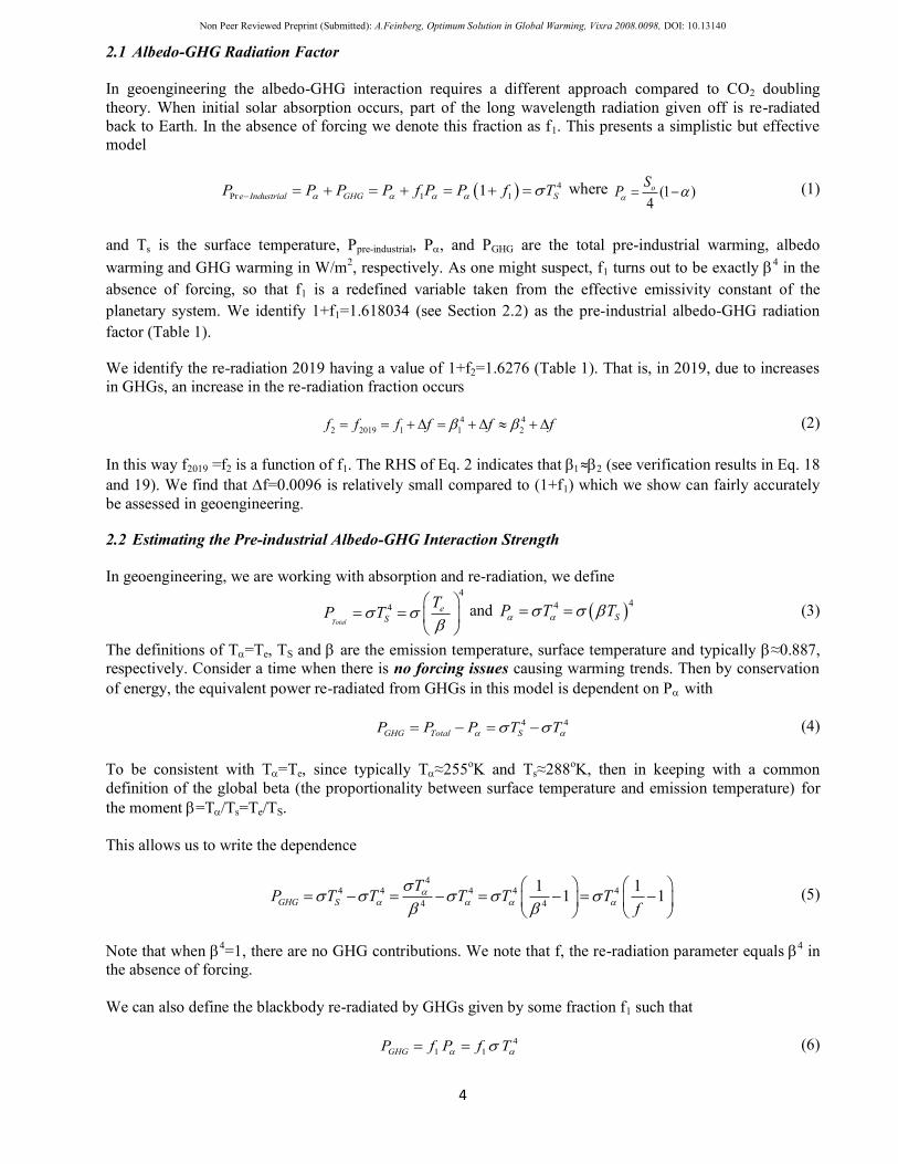
2.1 Albedo-GHG Radiation Factor

In geoengineering the albedo-GHG interaction requires a different approach compared to CO2 doubling

theory. When initial solar absorption occurs, part of the long wavelength radiation given off is re-radiated

back to Earth. In the absence of forcing we denote this fraction as f1. This presents a simplistic but effective

model

4

Pr 1 11e Industrial GHG SP P P P f P P f T where (1 )4

oSP (1)

and Ts is the surface temperature, Ppre-industrial, P, and PGHG are the total pre-industrial warming, albedo

warming and GHG warming in W/m2, respectively. As one might suspect, f1 turns out to be exactly

4 in the

absence of forcing, so that f1 is a redefined variable taken from the effective emissivity constant of the

planetary system. We identify 1+f1=1.618034 (see Section 2.2) as the pre-industrial albedo-GHG radiation

factor (Table 1).

We identify the re-radiation 2019 having a value of 1+f2=1.6276 (Table 1). That is, in 2019, due to increases

in GHGs, an increase in the re-radiation fraction occurs

4 4

2 2019 1 1 2f f f f f f (2)

In this way f2019 =f2 is a function of f1. The RHS of Eq. 2 indicates that ≈ (see verification results in Eq. 18

and 19). We find that f=0.0096 is relatively small compared to (1+f1) which we show can fairly accurately

be assessed in geoengineering.

2.2 Estimating the Pre-industrial Albedo-GHG Interaction Strength

In geoengineering, we are working with absorption and re-radiation, we define 4

4

Total

eS

TP T

and 44

SP T T (3)

The definitions of T=Te, TS and are the emission temperature, surface temperature and typically ≈0.887,

respectively. Consider a time when there is no forcing issues causing warming trends. Then by conservation

of energy, the equivalent power re-radiated from GHGs in this model is dependent on Pwith

4 4

GHG Total SP P P T T (4)

To be consistent with T=Te, since typically T≈255oK and Ts≈288

oK, then in keeping with a common

definition of the global beta (the proportionality between surface temperature and emission temperature) for

the moment =T/Ts=Te/TS.

This allows us to write the dependence

4

4 4 4 4 4

4 4

1 11 1GHG S

TP T T T T T

f

(5)

Note that when 4=1, there are no GHG contributions. We note that f, the re-radiation parameter equals

4 in

the absence of forcing.

We can also define the blackbody re-radiated by GHGs given by some fraction f1 such that

4

1 1GHGP f P f T (6)


5

Consider f=f1, in this case according to Equations 5 and 6, it requires

4 4

1

1

11GHGP T f T

f

(7)

This dependence leads us to the solution of the quadratic expression

2

1 1 1 0f f yielding 4

1 0.618034f , 1/ 4

0.618034 0.886652 (8)

This is very close to the common value estimated for and this has been obtained through energy balance in

the planetary system providing a self-determining assessment. In geoengineering we can view the re-radiation

as part of the albedo effect. Consistency with the Planck parameter is shown in Section 3.1. We note that the

assumption f=f1 only works if planetary energy is in balance without forcing. In the next section, we double

check this model in another way by balancing energy in and out of our global system.

2.3 Balancing Pout and Pin in 1950

In equilibrium the radiation that leaves must balance P, the energy absorbed, so that

1 1 1 1 1

2

1 1

(1 ) (1 ) (1 ) (1 )

2

Out Total

In

Energy f P f P f P f P f P

P f P f P Energy P

(9)

This is consistent, so that in 1950, Eq. 9 requires the same quadratic solution as Eq. 8. It is also apparent that

4

1 _1950 1 _1950Total TotalP f P P (10)

since

1 1 1 1( ) 1 (1 )P f P f P or f f (11)

The RHS of Eq. 11 is Eq. 8. This illustrates f1 from another perspective as the fractional amount of total

radiation in equilibrium. As a final check, the application in the Section 3, in Table 1, illustrates that f1

provides reasonable results.

2.4 Re-radiation Model Applied to 2019

In 2019 due to global warming trends, to apply the model we assume that feedback can be applied as a

separate term and we make use of some IPCC estimates for GHG forcing as a way to calibrate our model. In

the traditional sense of forcing, we assume some small change to the albedo and most of the forcing due to

IPCC estimates for GHGs where

2019 2(1 )Total GHGP P P P f (12)

Then we introduce feedback through an amplification factor AF as follows

4

2019& 1950 1950 2019 1950Total Feedback F F SP P P A P P P A T (13)

Here, we assume a small change in the albedo denoted as P’ and f2 is adjusted to the IPCC GHG forcing

value estimated between 1950 and 2019 of 2.38W/m2 [10]. Although this value does not include hydro-

hotspot forcing assessment described in the introduction, it possibly may be effectively included since forcing

estimates also relate to accurate GW temperature changes. Then the feedback amplification factor, is

calibrated so that TS=T2019 (see Table 1) yielding AF =2.022 [also see ref. 29]. The main difference in our

model is that the forcing is about 6% higher than the IPCC for this period. Here, we take into account a small


6

albedo decline of 0.15% that the author has estimated in another study due to likely issues from UHIs [22]

and their coverage. We note that unlike f1, f2 is not a strict measure of the emissivity due to the increase in

GHGs.

3. Results Applied to 1950 and 2019 with an Estimate for f2

In 1950 we will simplify estimates by assuming the re-radiation parameter is fixed and reasonable close to the

pre-industrial level of f1=0.618034. Then, to obtain the average surface temperature T1950=13.89oC

(287.04oK), the only adjustable parameter left in our basic model is the global albedo (see also Eq. 1). This

requires an albedo value of 0.3008 (see Table 1) to obtain the T1950.=287.04oK. This albedo number is

reasonable and similar to values cited in the literature [30].

In 2019, the average temperature of the Earth is T2019=14.84oC (287.99

oK) given in Eq. 15. We have assumed

a small change in the Earth’s albedo due to UHIs [22]. The f2 parameter is adjusted to 0.6276 to obtain the

GHG forcing shown in Column 7 of 2.38W/m2 [10]. Therefore the next to last row in Table 1 is a summary

without feedback, and the last row incorporates the AF=2.022 feedback amplification factor.

Table 1 Model Results

Year TS(oK) T(

oK) f1, f2 ' Power

Absorbed

W/m2

PGHG’

PGHG

PTotal

W/m2

2019 287.5107 254.55 0.6276 30.03488 238.056 149.4041 387.4605

1950 287.04 254.51 0.6180 30.08 237.9028 147.024 384.9267

2019-1950 0.471 0.041 0.0096 (0.15%) 0.15352 2.38 2.53

Feedback

AF=2.022

0.95 0.083 - - 0.3104 4.81 5.12

From Table 1 we now have identified the reverse forcing at the surface needed since

2 2 2

2019_ 1950 2019 1950 384.927 / (2.5337 / )2.022 390.05 /Total Feedback Amp FP P P P A W m W m W m (14)

and

1/ 4

2019 1950 390.05 / 287.04 287.9899 287.04 0.95ST T T K K K K (15)

as modeled. We also note an estimate has now been obtained in Table 1 for f2=0.6276, AF=2.022, and

PTotal_Feedback_amp=5.12W/m2.

3.1 Model Consistency with the Planck Parameter

As a measure of model consistency, the forcing change with feedback, and resulting temperatures T1950 and

T2019, should be in agreement with expected results using the Planck feedback parameter. From the definition

of the Planck parameter o and results in Table 1, we estimate [31]

2

2

1950

237.9028 /4 4 3.31524 / /

287.041

OLWo

S

R W mW m K

T K

(16)

and 2

2

2019

238.056 /4 4 3.306 / /

287.99

OLWo

S

R W mW m K

T K

(17)

Here ROLW is the outgoing long wave radiation change. We note these are very close in value showing miner

error and consistency with Planck parameter value, often taken as 3.3W/m2/oK.


7

Also note the Betas are very consistent with Eq. 8 for the two different time periods since from Table 1

4

1950 1950

254.510.88667 0.6180785

287.041

e

S S

T Tand

T T

(18)

and

4

2019 2019

254.550.88526 0.6144

287.5107

e

S S

T Tand

T T

(19)

3.2 Hotspot Versus GHG Forcing Equivalency

From Equation 1 and 12 we can estimate the effect in a change in hotspot forcing as

1

1950

1 1.618TotaldPf

dP

and 2

2019

1 1.6276TotaldPf

dP

(20)

However, we note a change in GHGs is only a factor of 1 by comparison

1

GHGTotal

GHG GHG

d P PdP

dP dP

(21)

or from Table 1 data

2.531.063

2.38

Total

GHG

dP

dP (22)

This indicates 1 W/m2 of albedo forcing generally requires 1.6 W/m

2 of GHG forcing to have the same global

warming effect. Alternately, form Eq. 22 and Table 1 data this is about 1.53. This result should be helpful in

albedo forcing estimates.

4. Discussion

From Table 1 we used two key forcing changes that are responsible for climate change since 1950

• f and

We know that can only be controlled by albedo controls. However, in Table 1, the albedo effect used was

fairly minimal contributing only a 0.15 W/m2 (6%) to the warming. However, if we were to implement a

worldwide albedo surface solution of select areas, for example, the following albedo amplification factors can

potentially be realized

Table 2 Albedo Surface Solution Factors

Amplification Type Factor

Albedo enhancement 4

Reduction of heat storage targets 6

Re-radiation reduction 1.6

Total Product 38

Here, selecting surfaces with high heat storage capacity, such as buildings (or possibly mountains) are likely

good strategic targets. These areas are a function of heat capacity, surface albedo, mass, temperature storage,


8

solar irradiance and humid environments, which can yield amplification factors between 3.1-8.4 (averaging 6)

[4, 21]. These estimates are not unreasonable for UHIs. As well there are atmospheric albedo solutions [1].

Consider how this applies to Table 1 GHGs. In Table 1, f is controlled by GHGs assumed to be dominated

by CO2 forcing (recall that part of this may actually intrinsically include hydro-hotspots which are mitigated

only by albedo methods). The reverse forcing albedo reduction to mitigate f when considering albedo

amplification factors in Table 2 on GHG forcing in Table 1

Reverse Forcing Mitigation Requirement =2.38 W/m2/38=0.063 W/m

2 (23)

The amount of Earth that would have to be modify with reflectivity factor between 4-7.5 has been assessed by

the author in Reference [4] for this particular problem, yielding a

Modification area of about 0.2% to 1% of the Earth, depending on the selected target types

Therefore, we note by employing albedo solutions, reverse cooling results would help compensate for CO2

forcing, and conservatively include hotspots and hydro-hotspots mitigation. In the event that hotspots and

hydro-hotspot are truly significant, this would be the optimum approach.

This should help to clarify the benefit and need for including albedo controls and solutions in

climate change policies

5. Summary

In this paper we have focused on the albedo-GHG interaction to show how the albedo solution, could be a

vital method to help mitigate global warming when three types of forcing issues are considered. Such

implementation would greatly supplement CO2 solutions. Results can improve the speed in helping to prevent

a tipping point from occurring (especially with desertification and deforestation occurring). Furthermore,

analysis showed that the albedo solution can effectively compensate for CO2 forcing without having to

modify an unreasonable area of the Earth. Furthermore other albedo solutions are available.

The GHG-albedo interaction strength due to the re-radiation factor has been fully described in application to

two time periods. Results show that the re-radiation factor for 1950 when taken as a pre-industrial value is

1.6181 which is directly given by 4

(the emissivity constant of the planetary system). However in present

day, this factor has increase to 1.6276 due to the increase in GHGs. In order to make the present day

assessment, we assumed a small planetary albedo decrease from 1950 of 0.15% and GHG forcing of about

2.38 W/m2 (in accordance with IPCC estimates). In terms of geoengineering albedo modification estimates,

the interactive value of 1.62 should to be a good approximation.

Below we provide suggestions and corrective actions which include:

Modification of the Paris Climate Agreement to include albedo controls and solutions

Albedo guidelines for both UHIs and roads similar to on-going CO2 efforts

Guidelines for future albedo design considerations of cities

Government money allocation for geoengineering and implement albedo solutions

Recommend an agency like NASA to be tasked with finding applicable albedo solutions and

implementing them

Recommendation for cars to be more reflective. Although world-wide vehicles likely do not embody

much of the Earth’s area, recommending that all new manufactured cars be higher in reflectivity (e.g.,

silver or white) would help raise awareness of this issue similar to electric automobiles that help

improve CO2 emissions.


9

References

1. Dunne D, (2018) Six ideas to limit global warming with solar geoengineering, CarbonBrief,

https://www.carbonbrief.org/explainer-six-ideas-to-limit-global-warming-with-solar-geoengineering

2. Cho A, (2016) To fight global warming, Senate calls for study of making Earth reflect more light, Science,

https://www.sciencemag.org/news/2016/04/fight-global-warming-senate-calls-study-making-earth-reflect-more-

light

3. Levinson, R., Akbari, H. (2010) Potential benefits of cool roofs on commercial buildings: conserving energy,

saving money, and reducing emission of greenhouse gases and air pollutants. Energy Efficiency 3, 53–109.

https://doi.org/10.1007/s12053-008-9038-2

4. Feinberg A., On Geoengineering and Implementing an Albedo Solution with UHI GW and Cooling Estimates

vixra 2006.0198, DOI: 10.13140/RG.2.2.26006.37444/6 (Currently in Peer Review in the J. Mitigation and

Adaptation Strategies for Global Change)

5. Feinberg A., The Reflectivity (Albedo) Solution Urgently Needed to Stop Climate Change, Youtube, August 2020

6. Feinberg A (2020) Review of Global Warming Urban Heat Island Forcing Issues Unaddressed by IPCC

Suggestions Including CO2 Doubling Estimates, viXra:2001.0415

7. Zhao L, Lee X, Smith RB, Oleson K (2014) Strong, contributions of local background climate to urban heat

islands, Nature. 10;511(7508):216-9. doi: 10.1038/nature13462

8. Kiehl, J.T.; Kevin E. Trenberth (1997). Earth's annual global mean energy budget. Bulletin of the American

Meteorological Society. 78 (2): 197–208:1997, doi:10.1175/1520-0477

9. Myhre, G., D. Shindell, F.-M. Bréon, W. Collins, J. Fuglestvedt, J. Huang, D. Koch, J.-F. Lamarque, D. Lee, B.

Mendoza, T. Nakajima, A. Robock, G. Stephens, T. Takemura and H. Zhang, 2013: Anthropogenic and Natural

Radiative Forcing. In: Climate Change 2013: The Physical Science Basis. Contribution of Working Group I to the

Fifth Assessment Report of the Intergovernmental Panel on Climate Change, Cambridge University Press,

10. Butler JH, Montzka SA, (2020) The NOAA Annual Greenhouse Gas Index, Earth System Researh Lab. Global

Monitoring Laboratory, https://www.esrl.noaa.gov/gmd/aggi/aggi.html

11. McKitrick R. and Michaels J. (2004) A Test of Corrections for Extraneous Signals in Gridded Surface

Temperature Data, Climate Research

12. McKitrick R., Michaels P. (2007) Quantifying the influence of anthropogenic surface processes and

inhomogeneities on gridded global climate data, J. of Geophysical Research-Atmospheres. Also see McKitrick

website describing controversy: https://www.rossmckitrick.com/temperature-data-quality.html

13. Zhao ZC (1991) Temperature change in China for the last 39 years and urban effects. Meteorological Monthly (in

Chinese), 17(4), 14-17.

14. Feddema JJ, Oleson KW, Bonan GB, Mearns LO, Buja LE, Meehl GA, and Washington WM (2005) The

importance of land‐cover change in simulating future climates, Science, 310, 1674– 1678,

doi:10.1126/science.1118160

15. Ren G, Chu Z, Chen Z, Ren Y (2007) Implications of temporal change in urban heat island intensity observed at

Beijing and Wuhan stations. Geophys. Res. Lett. , 34, L05711,doi:10.1029/2006GL027927.

16. Ren, GY, Chu ZY, and Zhou JX (2008) Urbanization effects on observed surface air temperature in North China.

J. Climate, 21, 1333-1348

17. Jones PD, Lister DH, and Li QX, (2008) Urbanization effects in large-scale temperature records, with an emphasis

on China. J. Geophys. Res., 113, D16122, doi: 10.1029/2008JD009916.

18. Stone B (2009) Land use as climate change mitigation, Environ. Sci. Technol., 43( 24), 9052– 9056,

doi:10.1021/es902150g

19. Zhao, ZC (2011) Impacts of urbanization on climate change. in: 10,000 Scientific Difficult Problems: Earth

Science, 10,000 scientific difficult problems Earth Science Committee Eds., Science Press, 843-846. 30%

20. Yang X, Hou Y, Chen B (2011) Observed surface warming induced by urbanization in east China. J. Geophys.

Res. Atmos, 116, doi:10.1029/2010JD015452.

21. Huang Q, Lu Y (2015) Effect of Urban Heat Island on Climate Warming in the Yangtze River Delta Urban

Agglomeration in China, Intern. J. of Environmental Research and Public Health 12 (8): 8773 (30%)

22. Feinberg A, (2020) Urban Heat Island Amplification Estimates on Global Warming Using an Albedo Model,

Vixra 2003.0088, DOI: 10.13140/RG.2.2.32758.14402/15 (Currently under peer review in the journal SN Applied

Science)

23. Schmidt GA, (2009) Spurious correlations between recent warming and indices of local economic activity, Int. J.

of Climatology

24. Paris Climate Accord, (2015) https://unfccc.int/process-and-meetings/the-paris-agreement/what-is-the-paris-

agreement

25. USGS 1900-2006, Materials in Use in U.S. Interstate Highways, https://pubs.usgs.gov/fs/2006/3127/2006-

3127.pdf

26. US Population Growth 1900-2006, u-s-history.com/pages/h980.html1

27. NASA 1900-2006 updated, 2020 https://climate.nasa.gov/vital-signs/global-temperature/


10

28. Deforestation, Wikipedia, https://en.wikipedia.org/wiki/Deforestation

29. Dessler AE, Zhang Z, Yang P (2008) Water‐vapor climate feedback inferred from climate fluctuations, 2003–

2008, Geophysical Research Letters, https://doi.org/10.1029/2008GL035333

30. Stephens G, O'Brien D, Webster P, Pilewski P, Kato S, Li J, (2015) The albedo of Earth, Rev. of Geophysics,

https://doi.org/10.1002/2014RG000449

31. Kimoto K (2006) On the Confusion of Planck Feedback Parameters, Energy & Environment (2009)

optimum solution to global warming in the control of co2

Documents