optimum strut-and-tie model for a cantilever curved wall · optimum strut-and-tie model for a ......
TRANSCRIPT

3
University of Southern Queensland
Faculty of Engineering and Surveying
Optimum Strut-and-Tie Model for a Cantilever
Curved Wall
A dissertation submitted by
Nathaniel Caleb Veenstra
in the fulfilment of the requirements of
Courses ENG4111 and 4112 Research Project
towards the degree of
Bachelor of Engineering (Civil)
Submitted: October, 2011

4
ABSTRACT
Topology optimization can be used as a tool for the development of optimized
reinforcement configurations within concrete members. Topology optimization is
the process of optimizing the distribution of material within a design domain, so as
to increase the efficiency with which the material used. This project will focus on
the optimized design of a curved cantilever wall, made of concrete and reinforced
through the traditional method of placing reinforcing steel.
Sigmund (2001) published the paper, A 99 line topology optimization code written in
Matlab, detailing the process of modelling and optimizing a domain to determine the
load transfer path within the member. This code employs a finite element analysis
operation, this being dependant on the use of square elements.
The current code prepared by Andreassen et al only consider domains constructed of
square, uniform finite elements, thus having limited capabilities in modelling
structures. The overall aim of this project is to modify and make additions to the
code to extend its capabilities in modelling domains constructed of non-square
quadrilateral elements with non-uniform geometry and volume.
A curved domain was arbitrarily formed and loaded with a single point load. One
boundary along its least dimension was fixed. A finite element mesh was created for
this domain and was used as the input for the modified optimization code. This code
successfully optimized the topology of the given domain, producing results that
showed the possibility of developing an optimized strut-and-tie model.
Whilst the optimization program functioned, the mesh used to define the domain was
too coarse, proving the results unusable for the development of an objective,
optimized topology. The formation of a closed form truss structure, required for a
strut-and-tie model, was seen to be forming, but a producing a strut-and-tie model
from such would have been highly subjective and inefficient. A refinement of the
finite element mesh, allowing for a lower minimum member size will allow for the
development of an objective topology optimization. In doing so, an efficiently
designed strut-and-tie model can be produced.

5
University of Southern Queensland
Faculty of Engineering and Surveying
ENG4111 Research Project Part 1 &
ENG4112 Research Project Part 2
LIMITATIONS OF USE
The Council of the University of Southern Queensland, its Faculty of Engineering
and Surveying, and the staff of the University of Southern Queensland, do not accept
any responsibility for the truth, accuracy or completeness of material contained
within or associated with this dissertation.
Persons using all or any part of this material do so at their own risk, and not at the
risk of the Council of the University of Southern Queensland, its Faculty of
Engineering and Surveying or the staff of the University of Southern Queensland.
This dissertation reports an educational exercise and has no purpose or validity
beyond this exercise. The sole purpose of the course pair entitled “Research
Project” is to contribute to the overall education within the student's chosen degree
program. This document, the associated hardware, software, drawings, and other
material set out in the associated appendices should not be used for any other
purpose: if they are so used, it is entirely at the risk of the user.
Professor Frank Bullen
Dean
Faculty of Engineering and Surveying

6
CERTIFICATION
I certify that the ideas, designs and experimental work, results, analyses and conclusions
set out in this dissertation are entirely my own effort, except where otherwise indicated
and acknowledged.
I further certify that the work is original and has not been previously submitted for
assessment in any other course or institution, except where specifically stated.
Student Name:
Student Number:
____________________________ Signature
____________________________
Date

7
ACKNOWLEDGEMENTS
I would greatly and most sincerely thank my supervisor, Dr Kazem Ghabraie.
Without his unyielding support, expertise, patience and ever-willingness to help, the
completion of this project would not have been possible. Throughout the entirety of
this project he was an invaluable source of wisdom and support, continuing to
encourage and push for the work to be completed to the highest standard.
Particular thanks goes to my girlfriend Erin for her encouraging me to be continually
pushing forward, ensuring that timelines were met and work was continually being
undertaken.
I would also like to acknowledge the continual, quietly encouraging support that my
family has been throughout the process of completing this work.

8
CONTENTS Abstract ........................................................................................................................ 4
Limitations of Use ........................................................................................................ 5
Certification.................................................................................................................. 6
Acknowledgements ...................................................................................................... 7
List of Figures ............................................................................................................ 10
1 Introduction ........................................................................................................ 11
2 Objectives ........................................................................................................... 13
3 Literature Review ............................................................................................... 15
3.1 Strut-And-Tie Modelling .................................................................................. 16
3.2 Topology Optimization ..................................................................................... 18
3.3 Finite Element Analysis .................................................................................... 20
4 The Element Stiffness Matrix ............................................................................ 25
4.1 Element Mapping .............................................................................................. 27
4.2 Jacobian Matrix................................................................................................. 29
5 Creating The Elements ....................................................................................... 30
5.1 Cantilever Domain ............................................................................................ 31
5.2 Domain Discretization ...................................................................................... 32
5.3 MATLAB Implementation ............................................................................... 34
6 Element Stiffness Matrices ................................................................................ 40
6.1 Mesh Plotting .................................................................................................... 41
6.2 Matrix Organisation .......................................................................................... 42
6.3 Element Stiffness matrix Calculation ............................................................... 43
7 Cantilever Optimization ..................................................................................... 46
7.1 TOPW – Topology Optimization ..................................................................... 47
7.2 FE – Finite Element Analysis ........................................................................... 48
7.3 KE – Element Stiffness Matrices ...................................................................... 48
7.4 Program Output................................................................................................. 49
7.5 Required program Inputs .................................................................................. 51
8 Results and Discussion ....................................................................................... 52
8.1 Results .............................................................................................................. 53
8.2 Discussion ......................................................................................................... 56
8.2.1 Topology Optimization Usability ............................................................. 56

9
8.2.2 Domain Discontinuity ............................................................................... 59
8.2.3 Suggested Modifications ........................................................................... 60
9 Conclusion ......................................................................................................... 63
9.1 Work Completed ............................................................................................... 64
9.2 Future Work ...................................................................................................... 64
10.0 Reference List ................................................................................................ 66
Appendices ................................................................................................................. 69
A.1 99 Line Code .................................................................................................... 70
A.2 coords.m ........................................................................................................... 72
A.3 Element Stiffness Matrices .............................................................................. 74
A.4 Modified Topology Optimization Code........................................................... 77
A.5 Specifications ................................................................................................... 79

10
LIST OF FIGURES Figure 4.1: Element Mapping .................................................................................... 28
Figure 5.1: Curved Cantilever Wall (all dimensions in millimetres) ......................... 31
Figure 5.2: Cosine Rule, as applied to cantilever geometry ...................................... 32
Figure 5.3: Matrix CC structure ................................................................................. 37
Figure 5.4: Nodal coordinate interpolation ................................................................ 37
Figure 6.1: Plotted Finite Element Mesh ................................................................... 41
Figure 7.1 Optimised topology for a curved cantilever: volfrac = 0.3, penal = 1.0. .. 50
Figure 8.1 Optimised topology for a curved cantilever: ............................................ 53
volfrac = 0.3, penal = 1.0. .......................................................................................... 53
Figure 8.2 Optimised topology for a curved cantilever: ............................................ 53
volfrac = 0.3, penal = 2.0. .......................................................................................... 53
Figure 8.4 Optimised topology for a curved cantilever: ............................................ 54
volfrac = 0.5, penal = 2.0. .......................................................................................... 54
Figure 8.3 Optimised topology for a curved cantilever: ............................................ 54
volfrac = 0.5, penal = 1.0. .......................................................................................... 54
Figure 8.6 Optimised topology for a curved cantilever: ............................................ 55
volfrac = 0.7, penal = 2.0. .......................................................................................... 55
Figure 8.5 Optimised topology for a curved cantilever: ............................................ 55
volfrac = 0.7, penal = 1.0. .......................................................................................... 55
Figure 8.7 Compressive regions shown by black elements, tension regions left void
.................................................................................................................................... 56
Figure 8.8 Half-simply supported beam: 120 x 60 elements ..................................... 57
Figure 8.9 The optimized topology showing the connectivity of elements at the
height of the cantilever ............................................................................................... 58
Figure 8.10 Two topologies identical except for rmin; the left has an rmin of 1.0, the
right has an rmin of 0.5 .............................................................................................. 60
Figure 8.11 Optimized Topology with volfrac being 0.2 and rmin 1.5 ..................... 61

11
1 INTRODUCTION

1 INTRODUCTION INTRODUCTION
12
Currently there exists several numerical techniques which can be used as a
preliminary design tool in the distribution or placement of reinforcing steel in
structural concrete members. More specifically, the use of strut-and-tie modelling
identifies the load paths within a concrete member and the actions of the loadings
present, allowing for the optimized placement of reinforcement.
When considering the non-linear behaviour of concrete and the concrete-
reinforcement interaction, followed by employing a Finite Element model that is
optimized, models can become complicated. Adopting a simple linear-elastic model
for the concrete and the concrete-steel interaction allows for the load path through
the member to be determined using Finite Element and optimized in a less
complicated manner.
For this project, it is required that a preliminary reinforcement design for a non-
standard curved cantilever reinforced concrete wall be determined, of which the form
and loading conditions are arbitrarily determined. The optimization of the curved
cantilever will be undertaken through the modification of a current topology
optimization code created by Ole Sigmund (2001). Currently, this code only works
for members of uniform geometry employing the use of square finite elements. This
necessitates the code be modified with additions to be included allowing for the non-
uniform geometry of a curved member to be modelled.
Combining the results gained from the topology optimization code and the methods
given by strut-and-tie modelling, the reinforcement of the curved cantilever will be
designed. The topology optimization will indicate the optimum load transfer paths
through the loaded structure. Nominating service conditions of the curved cantilever
and translating these onto a strut-and-tie model, of which is generated by the results
from the topology optimization, will allow for the reinforcement configuration to be
designed.
Whilst the geometry and loading conditions of the wall will be arbitrarily nominated,
they will be selected such that they represent something close to normally expected
loadings.

13
2 OBJECTIVES

2 OBJECTIVES OBJECTIVES
14
In completion of this research project, it is aimed that the following objectives be
completed;
1. A literature review on finite element analysis, topology optimization and the
use of strut-and-tie modelling in reinforced concrete design.
2. Formulation of a specific, two-dimensional design case of a curved cantilever
wall.
3. Discretise curved cantilever wall for application of finite element analysis,
including determination of element stiffness matrix from element geometry
and material properties.
4. Modify existing 99-line code to perform optimization on curved domain
approximated with quadrilateral elements.
5. Design optimum Strut-and-Tie model based from optimized topology.
Time permitting
6. Change design case from two-dimensional cantilever curved wall to three-
dimensional curved cantilever beam.

15
3 LITERATURE REVIEW

3.1 STRUT-AND-TIE MODELLING LITERATURE REVIEW
16
3.1 STRUT-AND-TIE MODELLING
Strut and tie modelling is used to represent the load transfer mechanisms within a
crack concrete structure at its ultimate load limit state. Strut-and-tie modelling is
formed from a progression of the plastic truss analogy, originally developed by
Ritter (1899). Ritter found that a beam that failed and cracked in such a way that it
could be represented by a parallel chord truss.
More specifically, the inclined shear cracking seen in the failed beam indicated the
direction of the principle stress trajectories. By aligning compressive struts along
these load paths, or the regions bounded by the shear cracking, the principle stresses
are resisted (MacGregor et al.). Providing addition struts and ties between the nodes
of the original struts ensured that transverse equilibrium within the member was
satisfied, thus forming a steel structure that held resemblance to a traditional truss
frame.
Schlaich et al. (1987) extended the standard truss model such that it could be used on
beams where the strain distribution is non-linear. Introducing the concept of D and
B regions, the beam could be segmented into regions where the strain distribution is
linear, in which the region is labelled a B region or that where the strain distribution
is non-linear, named D regions.
A D region is formed by any of the following acting on a concrete structure, that
being a point or distributed load, supports or discontinuity in geometry. Warner et
al. (2007) and Liang (2005) further show that discontinuous regions exist in design
features such as corners of members, corbels, and at the column-footing connection.
The D regions are further broken down into D1 and D2 regions. The region D2 is the
region of discontinuity whilst D1 is the transmission region between D2 and B.
Warner et.al (2007) suggests that the size of these regions is variable, dependant on
the region of discontinuity and of length varying from being equal to the height of
the discontinuous section through to 1.5 times the height of the discontinuous
section. This is shown to apply to both the D1 and D2 regions.
Liang (2005) simply outlines how the load path is determined;
Determine the loading and reactions on each region;
Finding the centroid of the stress distribution; and
Linking the each centroid of the stress distributions, remembering that the
loads transfer through the path of minimum deflection.
The above steps are the same as suggested by Ritter; linking the load paths with
further struts and tie provides transverse equilibrium. It is common practice that in
the design process for several strut and tie models to be generated. This is achieved

3.1 STRUT-AND-TIE MODELLING LITERATURE REVIEW
17
forme mostly because the centroids of the stress distributions can be linked in
different configuration.
Schlaich (1987) proposed that the optimum strut and tie model be selected is based
upon the principle of minimum strain energy. Mathematically, it is expressed as the
following;
∑
where N is the total number of elements, Fi is the force, l is the length and ε is the
mean strain, all of the ith member. This model is applied to the truss formed of
struts and ties, thus the reference to the length, strain and force of each member.
This sum is of all struts and ties in each model, with the model with the minimum
sum being that most suitable.
In literature, what is heavily agreed upon is the subjective nature with which the strut
and tie model is formed. As said, for any geometric structure, several strut-and-tie
models can be formed. As is often the case, a design formed by trial and error,
whilst being able to offer a structurally sound design that meets all loading
conditions, is one such that undue forces are placed upon the structure, simply
because of and over engineered or sub-optimum strut and tie configuration. Whilst
the strut and tie model can be useful in the way that it allows the designer to specify
a load path so as to allow for a certain design requirement, it is also highly possible
and likely that an inefficient design is produced (Liang).
In the present day, the use of Finite Element Analysis identifies the principles and
the directions of for a loaded structure, outputting the results in a visual form. Liang
(2005) mentions that these methods are still reliant on the ability of the designer to
interpret the visualized stresses and ascertain the appropriate location of struts and
ties.
It is this subjective nature in which the strut and tie models are formulated that
increases the need for a more efficient production of a strut-and-tie model.

3.2 TOPOLOGY OPTIMIZATION LITERATURE REVIEW
18
3.2 TOPOLOGY OPTIMIZATION
Considering any structure, the location and distribution of material within that
structure can greatly affect its structural performance. In the optimization of a
structure, Bendsoe et al. (2004) outlines three characteristics can be addressed; the
size, shape and topology. Size optimization refers to finding the optimum thickness
distribution of a linear elastic plate or the optimum member cross sectional area.
This aims to reduce the peak stress and deflection within the structure and its
members whilst external design constraints such as nodal locations and design
domain remain constant through the optimization process. In a similar manner,
shape optimization addresses the shape of existing voids and members whilst
minimizing the peak stress and deflection.
Liang (2002) describes that topology optimization is where by the locations of voids,
their geometric properties and occurrence within the design domain under the given
loading is determined and, how these voids are interconnected to the design domain.
The final form of the structure, known as the layout is defined by the process of
optimizing the size shape and topology of the structure.
In relation to a Finite Element Analysis, topology optimization can be focused on the
design of an isotropic material and the optimum placement of material within the
design domain, in particular finding what elements should be allocated as solid
material or void space. Liang (2005) suggests that this process can be simply
represented as the black and white rendering of an image; where colours of various
scale existed, they are replaced by either black or white. This process of selection
between the colours black and white, or rather elements being found to be solid or
void is the process known as filtering.
Filtering of elements is done by either density analysis (Liang, 2005 & Sigmund,
2001). Briefly considering the process of a FEA, the global stiffness matrix is given
by the multiplication of the global force vector with the inverse of the global
displacement vector (this process is defined in Section 3.3). Modifying the global
stiffness matrix to find each element stiffness matrix allows for the density of each
element to be determined. By employing a density filter, uneconomical elements can
be removed in part of the optimization process.
This whole optimization process can be group into three sections; pre-processing,
optimization and post-processing (Bendsoe). Pre-processing involves;
Selection of the ground structure including nodal coordinates and boundary
conditions;
Definition of design points or those elements within the domain that are to
remain void or solid; and

3.2 TOPOLOGY OPTIMIZATION LITERATURE REVIEW
19
Construction of the FE mesh such that it can define the ground structure and
all design points.
Optimization involves;
Designing an original design including the homogenous distribution of the
material over the design domain;
Starting the iterative loop, perform a FEA on the domain;
Calculate the compliance of the density distribution, comparing to the
compliance of the previous density distribution. In this first iteration, this
step is passed over. If the difference is negligible, the iteration stops with the
current density distribution being selected;
Computing the updated density variable, whilst also ending the iterative
loop; and
Repeat the iteration.
Post processing simply involves analysing a visual output of the optimized structure.

3.3 FINITE ELEMENT ANALYSIS LITERATURE REVIEW
20
3.3 FINITE ELEMENT ANALYSIS
Finite element analysis is used to determine the reactions of a solid state body under
defined conditions, of which affect the physical state of the body. Hutton (2004)
describes that a finite element analysis (FEA) seeks to determine the distribution of
some field variable, like the displacement in a stress analysis, within a defined body
under governing conditions.
FEA was first used to in stress analysis, in which the displacements of a body under
applied conditions where determined. The knowledge of how the body displaced
allows for the determination of the stresses within the body, as dictated by the
materials properties.
Hutton states that the behaviour of a structure is dependent on the geometry or
domain of the system, the property of the material…, and the boundary, initial and
loading conditions. More specifically, the behaviour of a cantilever wall will be
dependent on the geometrical shape of the wall, the properties of the material
(concrete) from which the wall is made, how the wall is fixed to the surrounding
environment (namely how the movement of the wall is or isn‟t restricted), the state
of stresses or actions external or internal to wall before analysis and the path and
magnitude of loadings placed onto the wall.
A FEA generally is undertaken by the following, as given by Hutton;
The geometry of the domain is modelled.
The domain is discretised or meshed.
Material properties of the body are specified.
Boundary, initial and loading conditions specified.
The process of discretization is by which the domain is broken down into a series of
smaller geometric domains, of which are defined by a minimum of three nodes. The
connection of these nodes forms an element. By discretising a large domain into a
larger number of smaller elements, the complexity associated with the solution of a
large domain is reduced; it is easier to determine the solution for a large number of
simply defined, smaller domains, of which form a larger domain, rather than
determine the solution for a single domain, of which is equal to that formed from a
number of elements.
Commonly, elements are defined by either three of four nodes giving triangular or
rectangular elements. Whilst triangular elements can represent a curved or inclined
surface with greater originality, the accuracy of the solution determined is of lesser
accuracy than that obtained with rectangular elements. The shape of rectangular
elements however, restricts their use to domains with perpendicular bounds.

3.3 FINITE ELEMENT ANALYSIS LITERATURE REVIEW
21
The introduction of a quadrilateral element allows for curved or inclined boundaries
to be modelled without losing significant accuracy (Hutton & Liu). Thus, for the
modelling of a cantilever wall, quadrilateral elements are to be used.
For all calculation, the field variables are determined at the nodes. For all nonnodal
points, the determination of the field variables is by interpolation. Generally, Hutton
shows that the field variable at the nonnodal point of (x,y) is equal to;
( ) ( ) ( ) ( ) ( )
where N1, N2, N 3 and N4 are the interpolation functions and Ø1, Ø 2, Ø 3 and Ø 4 at
the nodes.
For a quadrilateral element (Hutton & Liu);
( )
( )( )
( )
( )( )
( )
( )( )
( )
( )( )
where r and s represent the coordinates of natural coordinates, namely the point at
which the field variable is to be determined.
Liu et al. (2003) gives the statics system equations for a structure as;
where K is the global stiffness matrix, U is the nodal displacement vector and F is
the nodal force vector. Liu et al. states that the process of assembly is one of simply
adding up the contributions from all the elements connected at a node. For a given
structure, sections of the nodal force and displacement vector can be known.
Nodes along the domain or structures boundary can either be fixed in their
movement, limited in some actions or free. Numerically, the nodal displacement
vector can be represented by;
[
]

3.3 FINITE ELEMENT ANALYSIS LITERATURE REVIEW
22
where u denotes the horizontal displacement and v denotes the vertical displacement.
For a node where the displacement is known, either by a set displacement or being
fixed (given a value of 0), the displacements can be stated, i.e. u = 0, v = 0 being the
displacement is known to be fixed.
Similarly, for the nodal force vector, it can be defined at which nodes and in which
direction the loadings can be placed. The transposition of point loads onto a finite
element mesh can be simply achieved by locating the point load onto the nearest
node or mesh intersection point. Loadings can only by placed on nodes and cannot
be placed at any point on the mesh between two nodes. Thus, for a distributed
loading, the equivalent loading upon each node on which the distributed load acts
must be determined.
As given by Hutton, the element stiffness matrix for the quadrilateral element e is;
[ ( )] ∫[ ] [ ][ ]| |
The matrix [D] is the elastic property matrix and is defined by Liu as;
[ ]
( )( )[
]
E is the Young‟s modulus and v is the Poisons ratio for the solid body‟s material.
The matrix [D] is dependent on whether a Plain Strain or Plane Stress approach is
used. Hutton identifies the use of the Plane Stress approach for situations in solid
mechanics where the body under analysis adheres to the following conditions;
1. When considering a three-dimensional body, defined by x, y and z axes,
the z axis represents the thickness of the body and is less than one-tenth
of the smallest dimension in the x-y plane.
2. Loading only occurs within the x-y plane.
3. The material of the body is linearly elastic, isotropic and homogeneous.
The Plain Strain approach is used when in comparison; the dimension in the z axis is
larger than in those in the x-y plane. Hutton proposes the following mathematical
relationship defining whether the Plain Strain approach is to be used;
Considering the above further explains the assumptions of the Plain Strain approach.
The normal strain generated within the z axis is due to the effects of Poisons ratio
and is such that its small size proves it negligible. Furthermore, because loading
occurs only within the x-y plane, only small shearing strains are experienced and are
3.3 FINITE ELEMENT ANALYSIS LITERATURE REVIEW
23
again disregarded. For the design of the cantilever wall, the length of the wall is
assumed to be greater than the thickness and height, thus a Plain Strain approach is
used.
For the stiffness matrix relationship, t is the constant element thickness. For the
cantilever, the thickness relates to the length of the wall. Thus, a constant wall
length will result in a constant t and for this case of design can be assumed to be
equal to unity (1).
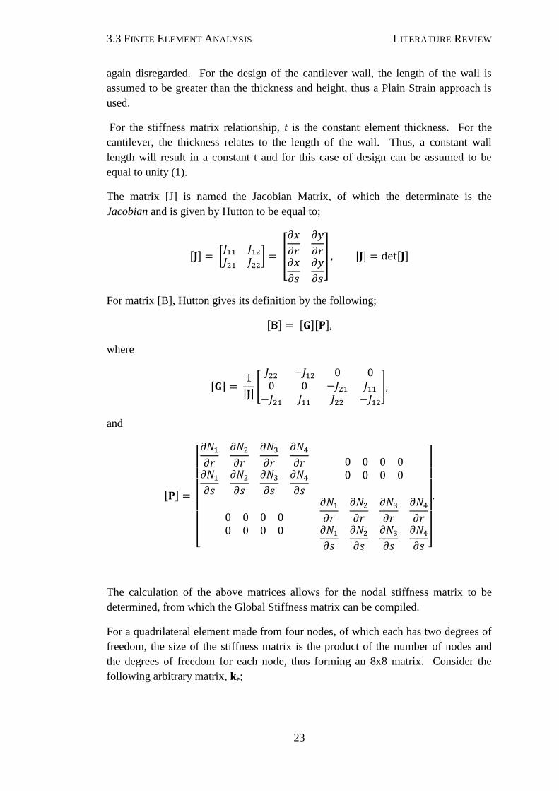
The matrix [J] is named the Jacobian Matrix, of which the determinate is the
Jacobian and is given by Hutton to be equal to;
[ ] [
] [
] | | [ ]
For matrix [B], Hutton gives its definition by the following;
[ ] [ ][ ]
where
[ ]
| |[
]
and
[ ]
[
]
The calculation of the above matrices allows for the nodal stiffness matrix to be
determined, from which the Global Stiffness matrix can be compiled.
For a quadrilateral element made from four nodes, of which each has two degrees of
freedom, the size of the stiffness matrix is the product of the number of nodes and
the degrees of freedom for each node, thus forming an 8x8 matrix. Consider the
following arbitrary matrix, ke;

3.3 FINITE ELEMENT ANALYSIS LITERATURE REVIEW
24
[
]
To assemble the Global Stiffness matrix, element-by-element addition is undertaken.
The Global Stiffness matrix is a square matrix, of magnitude equal to the product of
the number of elements and the degrees of freedom of each element. The matrix is
filled by the respective entry from each of the nodes connecting at that node, i.e;
[ ]
where the series of number m through to n represent all elements intersection at a
common node and k is the element stiffness matrix for node m/n. This completes the
calculation of the unknown constants and allows for the unknown displacements to
be calculated.
Consider the following simple representation of a Finite element solution;
[
] [
] [
]
If it is established that the subscript denotes those fixed degrees of freedom, it shows
that Uq is equal to zero. Thus the above equations reduce to;
Knowing Fp and Kpp, Up can be calculated, thus determining all unknown nodal
displacements. From this, all unknown nodal forces, as denoted by Fq, can also be
calculated.

25
4 THE ELEMENT STIFFNESS MATRIX

4 THE ELEMENT STIFFNESS MATRIX THE ELEMENT STIFFNESS MATRIX
26
The 99-Line MATLAB code, as written by Ole Sigmund uses the finite element
method to determine element stresses so as to optimise the given domain. This
method involves calling a constant element stiffness matrix for use on square finite
elements. The code written by Sigmund uses a constant element size throughout
with every domain being called using a one-by-one finite element. This allows for a
generic element stiffness matrix to be written and called (Lines 91-100).
This code however, as previously discussed is only for the use on square finite
elements; the modification of this code for the use on quadrilateral elements, the
basis for this project, is required. Subsequently, this stiffness matrix must be
adjusted accordingly. As given by Hutton, the element stiffness matrix for any
quadrilateral element is;
[ ( )] ∫[ ] [ ][ ]| |
Where the matrix [D] is the elastic property matrix and is defined by Liu as;
[ ]
( )( )[
]
For matrix [B], Hutton gives its definition by the following;
[ ] [ ][ ]
where
[ ]
| |[
]
and
[ ]
[
]
Also required is the Jacobian Matrix, [J], as given by Hutton to be equal to;

4.1 ELEMENT MAPPING THE ELEMENT STIFFNESS MATRIX
27
[ ] [
] [
] | | [ ]
For any four-sided, four node element, the above relationships hold. The elastic
property matrix ([D]) will remain unchanged, independent of the element geometry
but dependant on the material properties of the domain or element.
The matrix [P], as shown in the above form is that for an element of size unity. This
matrix is that which Sigmunds‟ code uses, remaining constant throughout. For the
solution of a finite element problem using quadrilateral elements, this matrix must be
changed with each element size. This change of element geometry will be
undertaken using a process of element mapping, relating the irregular geometry of
the actual element to an imaginary, „parent‟ element of regular size.
4.1 ELEMENT MAPPING
The mapping of the quadrilateral element will be represented by the shift shown in
Figure 4.1. The irregular element is shown on the left, the geometry as defined by
nodes 1-4. The „mapped‟ element is on the left, its coordinates such that it has a
centroid at the location (0,0) and the area is four square units. The interpolation
functions, as given by Hutton for any quadrilateral element, irregular or regular are
such that at the centroid of the element;
( )
( )( )
( )
( )( )
( )
( )( )
( )
( )( )
These interpolation functions are given for an element of the same geometry as the
parent element (right, Figure 4.1), as per Hutton. Further, Hutton states that the
values of r and s are dependant on the order of the interpolation functions. Since the
interpolatons functions are simple quadratic functions, the values for r and s are;
√

4.1 ELEMENT MAPPING THE ELEMENT STIFFNESS MATRIX
28
Figure 4.1: Element Mapping
Thus, the matrix [P] can be explicity derived, as follows.
The partial derivatives of the element [P] are as follows;
( )( )
( )
( )( )
( )
( )( )
( )
( )( )
( )
( )( )
( )
( )( )
( )
( )( )
( )
( )( )
( )
Hutton shows that, using the given values of r and s as the range for integration (an
approximation of), the previously given solution of the element stiffness matrix is
equal to;
[ ( )] ∑
∑[ ] [ ][ ]| |
The inputs for this sum will thus be;

4.2 JACOBIAN MATRIX THE ELEMENT STIFFNESS MATRIX
29
( ) (√
√
)
( ) (√
√
)
( ) ( √
√
)
( ) ( √
√
)
Taking the sum of the calculation between the four integration points gives the
element stiffness matrix for the particular set of four nodes.
4.2 JACOBIAN MATRIX
In a similar manner to the matrix [P] being dependant on the element geometry, so is
the Jacobian matrix also dependant on the nodal coordinates of each individual
element. As previously stated, Hutton gives the Jacobian matrix to be equal to;
[ ] [
] [
]
Considering the element in its natural coordinates (Figure 4.1), Hutton shows that
the above components of the Jacobian matrix expand to;
∑
[( ) ( ) ( ) ( ) ]
∑
[( ) ( ) ( ) ( ) ]
∑
[( ) ( ) ( ) ( ) ]
∑
[( ) ( ) ( ) ( ) ]
This gives all entries within the Jacobian matrix, completing the matrix [G] and
allowing for the element stiffness matrix to be determined; taking the sum of the
substitutions between (r1,s1) to (r2,s2) gives the required values of the Jacobian.

30
5 CREATING THE ELEMENTS

5.1 CANTILEVER DOMAIN CREATING THE ELEMENTS
31
5.1 CANTILEVER DOMAIN
The cantilever wall to be modelled (approximated by quadrilateral elements) is as
shown in Figure 5.1. The curve of the wall is modelled and represented by the use of
a parabola. The thickness was made to be 500 millimetres, with a total height of
5500 millimetres. To perform the finite element analysis of the wall, the domain
shown must be discretised by a series of elements. The minimum dimension of the
wall is clearly seen to be the base, thus the number of elements will be an
approximated function of this width.
The width of 500 millimetres is chosen to be broken into five elements of an equal
width of 100 millimetres. This allows for the domain to be broken into a series of
smaller domains, 100 millimetres in width and extending along the largest dimension
of the wall.
To allow for easy integration of this new domain into the existing MATLAB code,
the number of element in each of these long, slender domains must be equal.
A line was considered along the centre of the wall, parallel to sides of its longest
dimension. This line was used as a reference point from which to start discretising
the domain of the wall. Whilst not possible for the element dimensions to be exactly
equal, they must be of a similar scale such that the accuracy of the finite element
solution is not compromised; an element with one dimension far greater than the
other will produce discrepancies within the solution and is not desirable.
Figure 5.1: Curved Cantilever Wall
(all dimensions in millimetres)

5.2 DOMAIN DISCRETIZATION CREATING THE ELEMENTS
32
This central line through the domain, one not representing the location of nodes,
serves the purpose of creating an „average‟ element dimension. The width, as given
previously, of each element is equal to 100 millimetres (at the base of the structure).
Thus, an average height for each element of 100 millimetres was also assumed.
5.2 DOMAIN DISCRETIZATION
Figure 5.2 shows a segment of this central line, Line IJ. The point K is an assumed
„centre‟ of the Line IJ, and all successive sections of this line, collectively forming
the central parabolic line through the curved cantilever. Line IJ is a straight line,
approximating a segment of the central parabolic line. The lines KI and KJ are
vectors, representing the distances between point K and I, and K and J, respectively.
The angle formed between the line KI and KJ is set to equal delta theta. James‟ et al
definition of the cosine rule states that;
( )( )
The equation for this central line, being parabolic in nature and represented by a
quadratic equation, can be determined through the use of three known points. If the
point K is assumed to be a central location for the parabola (not in any manner either
of the foci for the parabola), then this point can also be assumed to have the
coordinates of (1500, 0). Therefore, the turning point of parabola representing the
central line will be (1500, 5250), with the points were the line intersects the line of y
= 0 being equal to (250, 0) and (2750, 0), since symmetry of the parabola will hold.
Using a set of simultaneous equations, the following can be formed, being based
upon the general form of a parabolic equation;
For the three points, (1500, 5250), (250, 0) and (2750, 0)
Figure 5.2: Cosine Rule, as applied to cantilever
geometry

5.2 DOMAIN DISCRETIZATION CREATING THE ELEMENTS
33
Entering these into matrix form gives;
[
] [ ] [
]
Solving for the matrix of coefficients;
[
]
[
] [ ] [
]
[
]
[ ] [
]
[
]
Thus giving;
[ ] [
]
Therefore, the equation of this central line is;
With reference to Figure 5.2, the coordinates for point K are known, and remain
constant. The point of I is known, if it assumed that the process of determining the
coordinates for J is an iterative process; since the coordinates for points I and K are
known, similarly the length of IJ (assumed to equal 100 millimetres), the coordinates
of point J can be determined, this allows for the determination of angle delta theta.
This process is based upon the construction of a circle with the centre at point I, and
a radius of 100 millimetres. The point J is the intersection of this point. Whilst there
will also be a second intersection point, the correct, or required point is easily
determined; both components of the coordinates must be greater than the centre of
the circle, or x2 must be greater than x1, and y2 must also be greater than y1.
The equation of a circle, again is given by James as;
( ) ( )
The constants a and b are the centre of the circle, with r being the radius of the
circle. Arranging this function in terms of y gives, making y the subject;
√ ( )
The next step in determining the coordinates of J is to make the functions of the
parabolic and circular functions of the notations given by Figure 5.2. Considering
the equation of a circle;

5.3 MATLAB IMPLEMENTATION CREATING THE ELEMENTS
34
√ ( )
Again, considering the parabola, leaving the coefficients as given by A, B and C;
Having two equations defining y2 as a function of x2, they can be equated, giving the
coordinate x2. This is as follows;
√ ( )
( ) [
( )]
Expanding the squares;
[ ( )][
( )]
( )
( ) ( ) ( ) ( )
[ ] [ ]
[ ( ) ] [ ( )]
[( ) ]
[ ] [ ]
[ ( ) ] [ ( ) ]
[( )
]
This quartic equation is able to be solved, giving the value for x2, dependant on the
coordinates of x1. Similarly, the coordinate y2 can also be determined through use of
the quadratic equation defining the central line. The coefficients A, B and C are as
previously defined.
5.3 MATLAB IMPLEMENTATION
Appendix A.2 contains the MATLA code „coords.m’, the script used to calculate
the coordinates x2 and y2 along the central line in increments where the vector IJ has
a length of 100 millimetres. The first three lines (1-3) exist to clear all previous data
and variables, tables and windows within the MATLAB program. Line (5) defines
the range of x-variables allowable for the given cantilever domain; from x = 0 to x =
1500. Line (6) defines the matrix int1_r, the known x-coordinates for the central
parabolic line, and the matrix int2_r, the known y-coordinates for the same line.
Line (7) contains the calculation for the matrix cr, the coefficients for the central
line as also previously given. Line (8) contains the calculation of all y-coordinates
for the central line within the given range (line (5)). Line (9) lists coefficients again,
equating them to A, B and C, for easy calling further in the script. Line (11) creates
5.3 MATLAB IMPLEMENTATION CREATING THE ELEMENTS
35
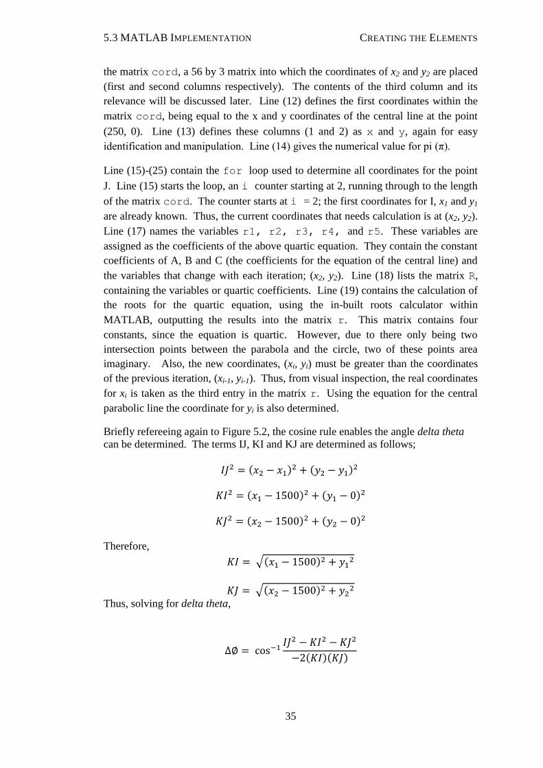
the matrix cord, a 56 by 3 matrix into which the coordinates of x2 and y2 are placed
(first and second columns respectively). The contents of the third column and its
relevance will be discussed later. Line (12) defines the first coordinates within the
matrix cord, being equal to the x and y coordinates of the central line at the point
(250, 0). Line (13) defines these columns (1 and 2) as x and y, again for easy
identification and manipulation. Line (14) gives the numerical value for pi (π).
Line (15)-(25) contain the for loop used to determine all coordinates for the point
J. Line (15) starts the loop, an i counter starting at 2, running through to the length
of the matrix cord. The counter starts at i = 2; the first coordinates for I, x1 and y1
are already known. Thus, the current coordinates that needs calculation is at (x2, y2).
Line (17) names the variables r1, r2, r3, r4, and r5. These variables are
assigned as the coefficients of the above quartic equation. They contain the constant
coefficients of A, B and C (the coefficients for the equation of the central line) and
the variables that change with each iteration; (x2, y2). Line (18) lists the matrix R,
containing the variables or quartic coefficients. Line (19) contains the calculation of
the roots for the quartic equation, using the in-built roots calculator within
MATLAB, outputting the results into the matrix r. This matrix contains four
constants, since the equation is quartic. However, due to there only being two
intersection points between the parabola and the circle, two of these points area
imaginary. Also, the new coordinates, (xi, yi) must be greater than the coordinates
of the previous iteration, (xi-1, yi-1). Thus, from visual inspection, the real coordinates
for xi is taken as the third entry in the matrix r. Using the equation for the central
parabolic line the coordinate for yi is also determined.
Briefly refereeing again to Figure 5.2, the cosine rule enables the angle delta theta
can be determined. The terms IJ, KI and KJ are determined as follows;
( ) ( )
( ) ( )
( ) ( )
Therefore,
√( )
√( )
Thus, solving for delta theta,
( )( )

5.3 MATLAB IMPLEMENTATION CREATING THE ELEMENTS
36
For the incremental value of delta theta that is required, the above relationship is
continued;
( )( )
Referring again to the script coords.m, line (23) contains the calculation of IJ2, KI
2
and KJ2. Line (24) contains the calculation of delta theta, notated by dt. The value
for dt at the iteration i is then stored within the matrix cord. Line (25) terminates
the loop. Line (26) states the coordinates of the turning point for the central line, or
the point at which the domain discontinues. If the iteration loop was continued
beyond 56 iterations, the sum of the angle delta theta would exceed 90 degrees.
From visual inspection, it was limited to 56 iterations, with the 56 value being set to
equal that at the turning point. The turning point will be entered, as with all other
coordinates of the central parabolic line, into the matrix cord.
Lines (28)-(39) are those that define the equations for all other long parabolic lines,
breaking the domain into five, 100 millimetre wide sections (as measured at the base
of the cantilever). For each line, a similar process is followed to that used to
determine the equation of the central line. For each parabolic line (representing a
discretization in the length of the cantilever), a matrix of points is formed, containing
the values of x for the known locations. Similarly, a vector of coordinates (y) is also
formed. These are int1_(i) and int2_ (i), where i is the parabolic line
represented. The following line (29, 31, 33, 35, 37, 39) creates and calculates the
vector containing the coefficients each parabolic line (listed as cr (i), where i is
the parabolic line represented).
Line (41) creates and fills the matrix c; a matrix of zeroes to be filled with the
coefficients of all parabolic lines forming the curved cantilever, a total of six lines
with three coefficients each. The following entries on line (41) then assigned to each
column of c with the respective vector of coefficients, calculated in lines (29, 31, 33,
35, 37, 39). Line (42) similarly creates the matrix of zeroes, CC. This matrix is
contains all coordinates of nodes, eventually forming the finite element mesh. This
mesh is formed from six parabolic lines, each with an x and y coordinates. Thus, CC
has twelve columns. The number of rows is assigned as 56, the same number of
entries within the matrix cord. Lines (43)-(48) then fill the starting points of the
parabolic lines, the intersection points they have with the y axis, or the points at the
base of the cantilever. These points provide the start of the iterations that enable all
other points along the parabola to be determined. A visual representation of the
matrix CC follows (Figure 5.3).

5.3 MATLAB IMPLEMENTATION CREATING THE ELEMENTS
37
Figure 5.4: Nodal coordinate interpolation
Line
1
Line
1
Line
2
Line
2
Line
3
Line
3
Line
4
Line
4
Line
5
Line
5
Line
6
Line
6 x co
ord
inat
es
y coord
inat
es
x coord
inat
es
y coord
inat
es
x coord
inat
es
y coord
inat
es
x coord
inat
es
y coord
inat
es
x coord
inat
es
y coord
inat
es
x coord
inat
es
y coord
inat
es
Lines (49)-(62) contain the calculation of each x and y coordinate for the nodes
along the first defining parabolic line. An identical process is undertaken in lines
(63)-(76), (77)-(90), (91)-(104), (105)-(118) and (119)-(132) for the second, third,
fourth, fifth and sixth parabolic lines, respectively. For each parabolic line (1-6,
Figure 5.4), the nodal coordinates of the finite element mesh along each parabola
must be determined. To form a clear and geometrically neat mesh, the elements are
designed such they are similar in geometry. From the previous steps outlined, the
central line was broken into segments approximating its length, each a total of 100
millimetres long. For each coordinate defining these segments, the angle between
the tangent and the „centre‟ and the previous point (from the immediately previous
iteration) was determined.
Consider the line shown in Figure 5.4 between the centre and (xi, yi). This line is a
straight line, represented by the following;
This equation is easily attainable. The slope m is the slope of the line and is
measured respective to the horizontal. For the current iteration, or point i, the angle
∆θi is equal to the sum of ∆θ1 through to ∆θi. Therefore, knowing the angle between
this line and the horizontal, the slope is equal to;
Figure 5.3: Matrix CC structure

5.3 MATLAB IMPLEMENTATION CREATING THE ELEMENTS
38
(∑
)
Since all lines of i pass through the centre (1500, 0), the constant c will be discrete
and calculable, as follows;
(∑
)
Therefore, rearranging for c gives;
(∑
)
Thus, the equation for any line passing through the centre (1500, 0) will be;
(∑
) (∑
)
In constructing the elements, the assumption was made that each element across the
width of the cantilever will align with its neighbouring elements; all elements‟ nodes
will align/connect to another with no nodes existing at any point along the mesh
aside from the corners of an element. Taking a similar approach as used to
determine the coordinates along the central parabolic line, the intersection point of
the central tangent (the line between the centre (1500, 0) and (xi, yi)) and the
parabola will be determined through letting their equations equal each other.
Taking the equation for the central tangent and making it in terms of xi and yi gives;
(∑
) (∑
)
Taking the equation of any parabolic line as well and performing the same
transformation;
Letting the two equations be equal gives;
(∑
) (∑
)

5.3 MATLAB IMPLEMENTATION CREATING THE ELEMENTS
39
Arranging into the form of a quadratic equation gives;
( ) ( (∑
)) ( (∑
))
Through nature of the tangent of the angle delta theta, the above equation was
modelled in the following manner to give required results;
( ) ( (∑
)) ( (∑
))
Thus, considering any line, the nodes for the finite element mesh and elements
contained can be determined. Referring again to the script coords.m, Line (50)
starts the iterative counter, ranging from 2 through to 56, the total number of nodes
along any one parabola. Line (51) calculates the angle theta, listed as th, for the
current iteration. This was shown to be equal to the sum of all values for theta
previous and including the current iteration. Line (52) names and calls the
coefficients of the parabolic line; here they are called as Aa, Bb and Cc, referring to
A, B and C, respectively. They are all called from the previously defined vector c.
Lines (53)-(55) define the coefficients of the modified quadratic equation, as shown
above containing the equations of the parabolic line and the respective central
tangent; these are named as j1, j2 and j3. Line (56) names and creates the vector
J, containing the coefficients j1, j2 and j3. Line (57) names and creates the
vector j, containing the roots, or intersection points of the parabola and the central
tangent.
Line (58) assigns the correct intersection point (confirmed by visual analysis) as the
second entry of the vector j, then allowing for the corresponding y coordinate to be
determined (line (59)). Line (60) stores the value for xi and yi in the matrix
containing all coordinates (CC). Whilst not required to be part of the loop, line (61)
contains the definition of last nodal point (or turning point of the parabola).
This process was then repeated for the second, third, fourth, fifth and sixth parabolas,
each coordinate being set into the correct placed within the matrix CC. This gave a
complete set of coordinates representing the finite element mesh approximating the
design domain.
Once all lines and their approximating coordinates were calculated and saved within
the matrix CC, the matrix was saved to allow for future use. This operation is shown
in lines (134)-(136).
40
6 ELEMENT STIFFNESS MATRICES

6.1 MESH PLOTTING ELEMENT STIFFNESS MATRICES
41
The script coords.m calculated and stored the coordinates of the finite element
mesh under the filename coords.mat. The new script ke.m takes these nodal
coordinates, organises them and calculates the element stiffness matrix for each
element within the cantilever domain. This chapter explains the process of
calculating the element stiffness matrix for each element, refereeing to the script
ke.m. This script is found in Appendix A.3, complete with line numbering.
6.1 MESH PLOTTING
The script start with clearing and closing all previous data through lines (1)-(3).
Line (5) imports and loads the coordinates calculated in the script coords.m and
returns them as the file coords.mat. Figure 5.3 shows the structure of the matrix
CC. It is such that the coordinates for the first parabola are given in the first and
second columns (x and y respectively), with subsequent lines being found in the
proceeding columns. Lines (7)-(11) plot the finite element mesh; line (7) creates the
figure, Line (8) plots each point along each respective parabola, creating them as
black dots, ('k.'). Line (10) ensures that the axis are scaled equally and print the
correct parabola form, while line (11) defines the limits of the plot.
Figure 6.1: Plotted Finite Element Mesh

6.2 MATRIX ORGANISATION ELEMENT STIFFNESS MATRICES
42
Figure 6.1 is the plotted finite element mesh. The horizontal plane is defined by the
number of elements in the x-direction. The existing code defines the domain by
calling the number of elements in the horizontal and vertical direction, calling them
nelx and nely. Referring to Figure 6.1, the nodes in the horizontal direction are
consequently represented by nelx and the nodes in the vertical direction by nely.
This mesh is what approximately represents the six parabolic line used to define the
curved cantilever wall and lies on the parabolic lines calculated in the script
coords.m; explained in Section 5.1 and 5.2.
6.2 MATRIX ORGANISATION
Lines (13) through to (39) reorganise the nodal coordinates of the mesh, as given by
the matrix CC, into a form more easily used for the calculation of the element
stiffness matrices.
Line (13) defines the number of elements in the horizontal (nelx) and vertical
directions (nely). Whilst already known to the user, they are numerically defined
here as a function of the matrix CC, allowing for future modification or streamlining
of the current codes. Line (14) creates the three-dimensional matrix eCx, used to
store the x-coordinates of each element within the domain. This matrix contains
275, four element matrices; 275 elements each represented by four x-coordinates.
Line (15) contains a similar calculation, creating the matrix eCy, used to store the y-
coordinates of each element within the domain. Considering the element n, the entry
in matrix eCx(:,:,n) contains the x-coordinates for this element, while the entry
in the matrix eCy(:,:,n) contains the y-coordinates for the same element. Line
(16) contains an unused function, creating a matrix used to defined nodal
coordinates. This line has been left for possible future use.
Lines (18)-(39) contain the loop organising the element coordinates, taking them
from the matrix CC and organising them into the matrices eCx and eCy. Line (18)
initiates the loop, creating a counter ranging from 1 to 55; the total number of
element in the vertical direction, nely.
Lines (19)-(20) organise the x-coordinates for the element i. The ordering of the
nodes for each element is as shown in Figure 4.1; the first at the lower left hand
corner (where nelx and nelx are smallest) and proceeding anti-clockwise in
increasingly higher order. Consider the following extract of lines (19) and (20).
19 eCx(1,1,i) = CC(i,1); eCx(2,1,i) = CC(i+1,1);
20 eCx(1,2,i) = CC(i,3); eCx(2,2,i) = CC(i+1,3);
If the counter i is made to equal 2, this refers to the second element in the mesh.
Thus, eCx(1,1,i)refers to the first entry in the first row of the second element.
In the global system this would be element 2. This is made to equal CC(i,1); the
x-coordinate of the node along line 1, the first parabolic line, thus why it called from

6.3 ELEMENT STIFFNESS MATRIX CALCULATION ELEMENT STIFFNESS MATRICES
43
the first column of the matrix CC. Lines (21)-(22) perform the same operation,
except for the y-coordinates of element i.
Lines (23) to (38), while performing the same operation as in (19)-(22), differ
slightly to account for the variance in size of the matrices eCx and eCy and CC.
Where the matrix CC is a 12 -by-56 matrix, the matrices eCx and eCy are both three
dimensional 2 by 2 by 275 matrices. The coordinates are taken from the required
row (given by the ith entry) and column (dependant on the parabolic line used to
defined the coordinate) of the matrix CC. They again are entered into the correct
location in the matrix (eCx or eCy) by defining the „third‟ dimension of the
respective matrix. Particularly note the notation of this third dimension; it is
determined by adding to the counter i, R*(length(CC)-1), where R+1
represents the parabolic line used to defined the coordinates in question. It is
essentially used to locate the coordinates and reorganise them from a matrix with
twelve columns into another with only two columns. This process is that used for
lines (23)-(28), filling the matrices eCx and eCy.
6.3 ELEMENT STIFFNESS MATRIX CALCULATION
The matrices eCx and eCy contain the x and y-coordinates of the cantilever
domain, containing some zero elements. One step undertaken in calculating the
element stiffness matrix for each element involves calculating the determinant of the
Jacobian matrix. Due to the arrangement and ordering of the element nodes, this
cannot be performed while zero elements in the domain exist; the determinant can
only be determined when their exists only non-zero entries within the two-by-two
matrix. Lines (41) to (58) contain two loops in which these zero entries are replaced
by a value approximately equal to zero. Lines (41) to (49) perform the calculation
for the x-coordinates, looping over all entries within the matrix eCx, replacing them
with the value of 1x10⁻⁷
. Below is an extract containing lines (41) to (49), showing
this operation for the matrix eCy.
41 for i = 1:nelx*nely
42 for j = 1:2
43 for k = 1:2
44 if eCy(j,k,i)<=0
45 eCy(j,k,i) = 0.0000001;
46 end
47 end
48 end
49 end
Line (41) starts the loop, passing over each two by two entry in the matrix. Line (42)
and (43) count over each entry within the two-by-two matrix, containing the y-
coordinates of the element i. Lines (44)-(46) then examine the coordinates,
replacing the entry with 1x10⁻⁷
if it is equal to zero. If this statement is false, then

6.3 ELEMENT STIFFNESS MATRIX CALCULATION ELEMENT STIFFNESS MATRICES
44
the loop passes over the entry to the next. The loop is then terminated in lines (47)-
(49). This same operation is performed for the matrix eCx in lines (50)-(58).
The statement of material variables is done in lines (60) and (61), while the element
elastic property matrix ([D]) is calculated in line (62). Line (63) gives the
integration points r and s. Line (64) creates the matrix to contain the final
compilation of the element stiffness matrices, while line (65) creates the 4 matrices
used to store the four integrations done in calculating the element stiffness matrices.
The four integrations are completed between the following points;
( ) (√
√
)
( ) (√
√
)
( ) ( √
√
)
( ) ( √
√
)
The steps used are described in reference to lines (67) to (85), integrating between
the points (r1, s1). Line (67) starts the counter looping over all elements. Lines (86)
to (71) calculate the partial derivatives of the interpolation functions, between the
points r1 and s1. Line (72) and (73) list the entries of the partial derivatives into the
matrix [P]. Lines (74) and (75) call the required x and y-coordinates for the element
i from the matrix eCx and eCy. Lines (76)-(79) calculate the entries for the
Jacobian matrix, calling on the coordinates for element i. The Jacobian matrix is
created from the partial derivatives calculated in lines (76)-(79) in line (80), these
entries then being used to fill the matrix [G] in lines (81) and (82). The matrix [B],
the product of [G] and [P], is calculated in line (83). Line (84) is then used to fill all
entries in the matrix storing the integration between points r1 and s1, taking the
product of; the transpose of [B], the elastic property matrix [D], the matrix [B] and
the determinant of the Jacobian, [J]. The loop is then terminated in line (85). This
same process (as in lines (67)-(85)) is followed in lines (87)-(105), (107)-(125) and
(127)-(145) for the integration between points (r1,s2), (r2,s1) and (r2,s2), respectively.
Lines (147) to (149) collate all entries in the matrices listed in line (65), starting a
loop in line (147), looping over and taking the sum of each entry in line (148) and
terminating in line (149). Lines (151) save the matrix KE, containing all element
stiffness matrices, as a data file called ‘stiff.mat’. Lines (152) and (153) save
the matrices eCx and eCy into the files ‘xcoords.mat’ and ‘ycoords.mat.

6.3 ELEMENT STIFFNESS MATRIX CALCULATION ELEMENT STIFFNESS MATRICES
45
Lines (155)-(161) manipulate and re-save the data in matrices eCx and eCy into a
format usable for use with the MATLAB function, ‘patch’. This function will be
used later to plot the optimised topology of the cantilever. The current format of the
matrices eCx and eCy is such that there are 275, two-by-two matrix entries. The
‘patch’ function requires three entries; two vectors to plot against each other, and
a third containing data specifying the colour to be plotted for each entry in the two
preceding vectors. These two vectors are, for the case of a four-node element, are
sized such that each element represents a row (thus 275 in total), each column having
four rows, each containing either the x or y-coordinates for the element.
Line (155) creates the two vectors, X and Y, used as the entry in the ‘patch’
function. Line (157) and (158) organises the entries in matrices eCx and eCy and
places them into the required place in the matrices X and Y. The loop is ended in
line (159), with the two matrices being each saved into a data file in lines (160) and
(161). This ends the file ke.m.

46
7 CANTILEVER OPTIMIZATION

7.1 TOPW – TOPOLOGY OPTIMIZATION CANTILEVER OPTIMIZATION
47
This chapter outlines the sections of the original topology optimization code top.m
(Appendix A.1) that underwent modification in order to model and optimize the
topology of the curved cantilever (Figure 5.1).
Two sections of this code underwent no modification; the Optimality Criteria Update
and the Mesh-Independency Filter. The code performing the optimality criteria
update is in lines (38) to (49) of the original code, with the mesh-independency filter
being performed in lines (50) to (65).
Lines (3) to (37) of top.m list the main function, it calling on other functions within
the program to complete the optimization process. This section demanded additions,
calling the required data and function files, as well as new variables defining the
varying element stiffness matrices.
Lines (66) to (86) perform the finite element analysis on the domain, including the
definition of loading support conditions. Only slight modification will be required;
no major changes will be made to the way in which function operates. The
definition of the load and support conditions changes, in addition to the calling of the
density distribution (x) and the penalty factor (penal).
Lines (87) to (100) contain the calculation of the element stiffness matrix. Whilst
the element stiffness matrices have been previously calculated in the script ke.m,
they have been recalculated in another, internal function file. The purpose of
calculating them in the file ke.m, was to enable checking of the solution and speed
the computation time. The calculation of the stiffness matrices in the function file
LK, (line 102, Appendix A.4) is also done in a more streamlined manner than in the
script ke.m.
7.1 TOPW – TOPOLOGY OPTIMIZATION
The section details the workings of the function topw. This main function is
contained in lines (4) to (32) of the script topw. It calls on sub-functions throughout
and subsequent sections of this chapter describe them further. While previously the
user had to define the variables nelx, nely, volfrac, penal and rmin, they
have been explicitly stated at the start of the script, so as to improve usability for this
select case.
Line (6) starts with an initial density distribution over the design domain, with
counters started in lines (7) and (8). Lines (10) through to (12) import the required
data files; ‘xcoords.mat’, ‘ycoords.mat’, ‘nodes.mat’,
‘coords.mat’, ‘X.mat’ and ‘Y.mat’, also defining the new variables names
to each; X, Y, nodes, CC, xx and yy, respectively.
The main loop starts in line (13) and continues through to line (46), remaining
virtually unchanged. Small additions are made, starting in line (24), giving a counter
to select the required element stiffness matrix. Line (28) defines which element is

7.2 FE – FINITE ELEMENT ANALYSIS CANTILEVER OPTIMIZATION
48
being selected, with the correct element stiffness matrix variable (KE0) being set in
the calculation of the objective function of the element in line (29). Line (30)
calculates the compliance of the element. Lines (33) to (42) print the same variables
at each iteration, remaining unchanged from the original script.
The lines (43) through to (45) have changed, those being required to plot the curved
cantilever with the optimized topology. Line (44) starts with the calculation of the
element density, rho, being equal as to what is shown. This subtraction is
performed to ensure that the optimized elements are shown as black, with voids as
white. Other entries in line (44) remain unchanged, except for the inclusion of the
patch function.
This function calls the vectors xx and yy, those loaded and made to equal the
vectors X and Y from the script ke.m. The vectors xx and yy are 4-by-275 vectors,
able to be programed into the patch function. The final entry for the patch
function is the transpose of the vectors of element density ratios rho, entered in a
form compatible with the vectors xx and yy.
Following the printing of the optimised topology, the loop is ended in line (46).
7.2 FE – FINITE ELEMENT ANALYSIS
The finite element analysis remains largely unchanged, with only small adjustments
required for the definition of loadings on the cantilever and its support conditions.
Line (77) initiates the function, calling the required inputs previously defined. Line
(78) calls the element stiffness function (KE) , while the number of elements is
defined in line (79). Lines (80) through to (91) again remain almost unchanged, with
only one addition in line (88) being made. This calls the explicit element stiffness
matrix, the counter being defined in line (84). Line (89) is modified to accommodate
the change of the name of element stiffness matrix.
Lines (92) to (99) define the loading and support conditions. Line (93) governs that
the load is placed at the last degree of freedom with an arbitrary load of negative one
being placed. Line (94) defines that all nodes along the horizontal axis, were x is
equal to zero, are fixed in both degrees of freedom. The remaining lines through to
(99) remain unchanged.
7.3 KE – ELEMENT STIFFNESS MATRICES
The function for calculating the element stiffness matrices is started in line (102),
followed by a listing of the required domain constraints in line (103). Again, the
data files ‘xcoords.mat’, ‘ycoords.mat’ are called, line (104), with the
creation of a zeros matrix KE in line (105). The element elastic property matrix [D],
is calculated in line (106) with the integration points r and s being given in line
(107).

7.4 PROGRAM OUTPUT CANTILEVER OPTIMIZATION
49
The three-part nestled loop is started in (108), looping through each element (line
(108)) and taking the required integration points (counters in line (109) and (110)).
The vector x is filled in line (111), calling the required entries from the matrix eCx,
with the same process used in line (112) for filling the vector y. Two vectors
containing the partial derivatives of the interpolation functions are calculated in lines
(113) and (114), filling the matrix [P] in lines (115)-(118). The Jacobian matrix is
then calculated in Line (119), while lines (120) through to (122) fill the matrix [G]
with terms from the Jacobian.
Line (123) calculates the matrix [B], while the element stiffness matrix calculation is
completed in line (124). The loop is terminated in lines (125)-(127). The matrix KE
is that which now contains all elements stiffness matrices, available for calling in
previous functions.
7.4 PROGRAM OUTPUT
The program, completed for the optimization of the curved cantilever shown in
Figure 4.1, gives the following output. The results shown (Figure 7.1) are with an
input of the volume fraction (volfrac) being equal to 0.3 and the penalty factor
(penal) being equal to 1.

7.4 PROGRAM OUTPUT CANTILEVER OPTIMIZATION
50
Figure 7.1 Optimised topology for a curved cantilever: volfrac = 0.3, penal =
1.0.

7.5 REQUIRED PROGRAM INPUTS CANTILEVER OPTIMIZATION
51
7.5 REQUIRED PROGRAM INPUTS
The program (Appendix A.4) has been completed to state that meets the
specification 5, Section 2.0. This required that the code originally written by Ole
Sigmund (Appendix A.1) be modified such that a curved domain, represented by
quadrilateral could be optimized. The code in A.4 can perform this operation
meeting this objective with only minor inputs. Within the code, it is required that the
volume fraction, penalisation factor, minimum member size be defined, in addition
to the number of elements used to model the domain.
The code also requires the input of two data files, containing the coordinates of the
nodes defining the finite element mesh. Each data file contains either the x or y-
coordinates of all nodes within the domain. Whilst the nodes for this cantilever were
defined by another MATLAB script, future users can chose which process is used to
determine the nodes for any domain. The format of the data files called however
must remain in the same format without necessitating changes to the script.

52
8 RESULTS AND DISCUSSION

8.1 RESULTS RESULTS AND DISCUSSION
53
This chapter contains the results obtained from the optimization of the curved
cantilever under various design constraints. The loading and minimum member size
remained constant throughout testing, with variation occurring only to the volume
fraction and penalty factor.
The volume fraction is fraction of the volume that will remain at the end of the
optimization. This remains constant throughout the optimization process, with
variation in the number of elements being accounted for through a variation of their
density, changed in the variation of the element density distribution. The following
figures are those obtained from the optimization. Six images are included, showing
the use of three volume fractions and two penalty factors.
8.1 RESULTS
Figure 8.1 Optimised topology for a curved cantilever:
volfrac = 0.3, penal = 1.0.
Figure 8.2 Optimised topology for a curved cantilever:
volfrac = 0.3, penal = 2.0.

8.1 RESULTS RESULTS AND DISCUSSION
54
Figure 8.3 Optimised topology for a curved cantilever:
volfrac = 0.5, penal = 1.0.
Figure 8.4 Optimised topology for a curved cantilever:
volfrac = 0.5, penal = 2.0.

8.1 RESULTS RESULTS AND DISCUSSION
55
Figures 8.1-8.6 show the six optimized topologies for the curved cantilever under
varying design constraints. Figures 8.1, 8.3 and 8.5 show the topology when the
volume fraction is changed in increments of 0.2 from 0.3 to 0.7, run with a constant
penalisation factor of 1. Figures 8.2, 8.4 and 8.6 represent that same incremental
change in the volume fraction, but with a penalisation factor of 2. The network of
black elements represents the optimized load transfer path through the domain, and
can be seen to vary with varying design inputs.
As expected with any cantilevers member, regions of compression and tension are to
exist. Referring to Figure 8.7, it is by convention that the compressive forces will
exist in the region shaded by the black elements. Different loading conditions will
produce variations of this, but for all cases where the single point load is placed on
the lower, right-hand extremity (last element), it is to be expected that the
compressive forces will exist in the inner regions of the curved cantilever, whilst
tensile forces will act in the outer regions of the same domain, left void.
Figure 8.5 Optimised topology for a curved cantilever:
volfrac = 0.7, penal = 1.0.
Figure 8.6 Optimised topology for a curved cantilever:
volfrac = 0.7, penal = 2.0.

8.2 DISCUSSION RESULTS AND DISCUSSION
56
Since the cantilever is fixed along the bottom boundary, no deflection can occur
along this boundary. Similarly, it is at this location that the greatest bending
moments are expected to occur, being the greatest distance from the point of loading.
8.2 DISCUSSION
8.2.1 TOPOLOGY OPTIMIZATION USABILITY
The filtering of densities during the optimization process is undertaken by means of
calculating the compliance of the domain and making comparison with the
compliance of the domain from the previous iteration. This compliance is relative to
the element stiffness and displacement matrices at each iteration, summed to
calculate the domains compliance. The optimization process is terminated when the
comparison of compliances (current and previous) converges towards a constant,
different for each variation in design variables.
The selection of elements, in the way of those selected for the optimized load path, is
also, in crude terms a comparison of elements, determining which have a greater
deflection or stress and thus distributing to the element a higher density. Figure 8.1
and 8.2 both clearly show that varying densities can experienced, thus also indicating
that stresses within these elements can vary.
Figure 8.7 Compressive regions shown by
black elements, tension regions left void

8.2 DISCUSSION RESULTS AND DISCUSSION
57
Figure 8.8 Half-simply supported beam: 120 x 60 elements
Considering again the expectation of greater bending stresses within the lower
section of the cantilever, this is somewhat proven (in the case of this example) by
considering the density distribution of the elements in Figure 8.1. The outer tensile
region is shown by the colouring of elements; progressing from the fixed boundary
up the cantilever shows a lightening of element colouring, or in physical terms, a
lessening of the density distribution, also indicating less stresses within the structure.
From Section 2.0, the fifth objective was to design an optimum strut-and-tie model,
based upon the results obtained from the topology optimization of the cantilever.
The development of a strut-and-tie model requires that a truss-like structure be
presented in the topology optimization process, as shown by Ritter (1899). Figure
8.8 shows a half-section of a simply supported beam, optimized with the following
input;
top(120,40,0.5,3,1.5)
The topology is such that it does represent a parallel chord truss, and presents a
closed-form structure in which transverse equilibrium is held. The support
conditions allow for the static solution and through the application of a truss
analysis, all forces within the assumed members can be determined, in turn allowing
for a strut-and-tie model to be developed.
Consider the solutions shown in Figure 8.1-8.6; none exhibit a closed form solution
with transverse equilibrium. Whilst all shown connectivity to the boundary
conditions, this is expected and also irrelevant. It is the cantilevered end that
presents a problem in regards to obtaining a truss-like structure. In all plots (Figure
8.1-8.6) the compressive region extends through to the point of loading. This
compressive member is not however, connected to any other. If this structure was
taken, assuming all black elements to indicate the alignment the structures‟
members, this member connected to the point loading would act in compression and
bending.

8.2 DISCUSSION RESULTS AND DISCUSSION
58
Figure 8.9 The optimized topology showing the
connectivity of elements at the height of the cantilever
This solution is not acceptable for two reasons. The first is due to a contradiction in
principles behind the solution of static truss analysis. All members are connected
with pin joints; compression and tensile forces are transferred whilst the pin
connection does not allow for any bending forces to be generated or transferred.
Further, a cantilever cannot be supported by a pin connection. The presence of a
cantilever member would require a fixed connection, meaning the truss would not be
statically determinate.
A finite element analysis could be undertaken, determining all internal stresses, but it
is still not an acceptable solution in regards to producing a strut-and-tie model. Liang
(2005) requires that all nodes are connected so as to provide transverse equilibrium
between struts-and-ties. If a cantilever member exists within the optimized
topology, then this requirement proposed by Liang is not met.
Looking at the variation in plots, an increasing volume fraction shows an increase in
the number of elements allocated as solid material, given a density greater than one.
Similarly, a larger penalisation factor for this case also shows a greater connectivity
between the tensile and compressive regions within the domain. Figure 8.6 (volfrac
= 0.7, penal = 2.0) shows the greatest similarity towards a closed-form structure,
allowing for the generation of a strut-and-tie model.

8.2 DISCUSSION RESULTS AND DISCUSSION
59
The outer tensile and compressive regions are shown, with additional elements
within the domain indicating the location of possible struts or ties. Towards to the
top of the cantilever, elements with a low density can be seen to be forming,
connecting the outer tensile region to the compressive region.
Figure 8.9 shows a plot, used to see what effects exist when a higher volume fraction
is used. This number, from pure visual inspection, can also be seen to be greater
than those shown in Figure 8.6, indicating that a closed truss structure can be
developed. The topology shown in Figure 8.9 cannot however be used for the
derivation of a strut-and-tie model as explained in further detail.
The truss structure formed is only achieved through use of a high volume fraction.
This high fraction, whilst producing a somewhat usable and solvable truss structure,
does not produce an objectively analysable form. The aim of topology optimization
is to remove the subjectivity in which strut-and-tie models are formed, resulting in a
more efficient design not inducing unnecessary stresses within the designed member
and using materials more efficiently. Developing a strut-and-tie model from an
optimized topology such as in Figure 8.9 allows for unnecessary freedom when
assuming the alignment of member.
Remembering that along the fixed boundary, the width of an element is 100
millimetres, also being the mean element dimension. The optimized topology shown
in Figure 8.9 at times extends to the full thickness of the member. Even at the
thinnest point, the optimized topology can be up to 200 millimetres. Whilst
representing a truss, this thickness allows for too much freedom when aligning
tensile or compressive reinforcement. Further considering that the width is only 500
millimetres, this effectively allows for a 40% variation in the placement of the
reinforcement within the domain.
This large variation in possible reinforcement locations introduces high subjectivity
in regards to an „optimized‟ design. The assumption of placing the reinforcement at
the outermost location is valid, but still allows for unnecessary stresses to be
introduced in regions of high discontinuity. The designer is required to assume or
make an educated guess as to at what point the connection between the tensile
regions is made. A wide, pixelated curve, as in Figure 8.9, allows for significant
variation in the definition of the alignment of the reinforcement placed and
consequent inaccuracies and inefficiencies.
8.2.2 DOMAIN DISCONTINUITY
The results given in Figures 8.2, 8.4 and 8.6 lean to suggest that a region of high
shear stress exists within the cantilever, approximately in the middle third of the
member. Figure 8.9, shown with a higher volume fraction but the same penalisation
factor, shows the distribution of a higher density over the elements within this same
region.

8.2 DISCUSSION RESULTS AND DISCUSSION
60
Figure 8.10 Two topologies identical except for rmin; the left has an rmin of 1.0,
the right has an rmin of 0.5
It is within this same, approximate region that the elements have a reasonably
inconsistent geometry. Whilst it could be assumed that this higher density
distribution exists because of errors produce with irregular element geometries, it is
possibly only one factor, another being because of discontinuity within the stress
distributions.
The highest region of geometry discontinuity exists at the end, or top of the
cantilever. At this point however, the tensile and bending stresses induced within the
structure due to bending are minimal, due to their close proximity to the point of
loading. The region showing a higher element density distribution exist within at a
point, balanced between being further from the loading, thus having greater stresses,
and where the discontinuity is greater, there being a greater curvature of the domain.
These two factors; distance producing greater stresses and curvature in domain
producing discontinuity, result in a region where the density distribution is required
to be greater than other regions. It may also be suggested that in this region, higher
shear stresses, in addition to tensile and compressive forces, may be experienced
when contrasted to other regions within the domain.
8.2.3 SUGGESTED MODIFICATIONS
To produce an optimized topology that can be classed as closed-form truss, a
redistribution of material is required. A high volume fraction is undesirable since
high subjectivity is introduced into the interpretation of results. To allow for a
greater distribution of material, whilst maintaining the same process of distributing
the density, a reduction in the minimum member size is required.

8.2 DISCUSSION RESULTS AND DISCUSSION
61
Figure 8.10 shows the optimized topology for two domains, identical except for a
variation in the minimum member size (rmin) used. This shows that any further
reduction in the minimum member size for this domain is to no effect. Further, this
also shows that the discretization of the domain with the given mesh cannot be used
to effectively develop an objectively analysable strut-and-tie model.
Figures 8.1 and 8.2 show an incomplete truss formation. The members existing by
representation through black elements exist as separately acting cantilevers that
cannot be used to construct an optimized strut-and-tie model. Figures 8.3 to 8.6
show a volume fraction too high, resulting in a subjectively placed reinforcement
layout, again resulting in a less-than-optimal strut-and-tie model.
All figures show the requirement for the refinement of the mesh used to discretise
the domain. A refinement in mesh requires a reduction in the size of the elements
used within the domain. To maintain consistency, an increase in the number of
elements in both the horizontal and vertical direction is needed. Combining this with
a small volume fraction will also be of benefit, producing results similar to that
shown in Figure 8.11.
This domain is under loadings and supports identical to those in Figure 8.8. The
input given to produce the topology was;
top(100,40,0.2,2,1.5)
This topology gives clear indication as to the placement of reinforcement within the
domain. It is unknown whether compressive reinforcement is needed, but if
required, little choice or variance is allowed. Similarly, little variation is given in the
placement of the tensile reinforcement. To allow for similar results to be obtained
for the cantilever structure, further work must be undertaken; refining the mesh,
reducing the mean element size and reducing the minimum member size. This
process will have one major benefit; a closed-form truss will be developed allowing
Figure 8.11 Optimized Topology with volfrac being 0.2 and rmin 1.5

8.2 DISCUSSION RESULTS AND DISCUSSION
62
for a strut-and-tie model to be formed. Another subsequent benefit may also include
greater accuracy within the solution. By using a finer finite element mesh, the
approximation made of the domain by using quadrilateral elements will converge on
a more accurate approximation, thus also increasing the accuracy of the finite
element solution. In turn, this could be expected to provide an optimized topology
greater representing the actual conditions of the loaded cantilever.

63
9 CONCLUSION

9.1 WORK COMPLETED CONCLUSION
64
9.1 WORK COMPLETED
It has been demonstrated to certain detail the process in which research and design
work was undertaken to complete the initial objectives (Section 2.0). Through using
topology optimization, the researcher aimed to design an optimized strut-and-tie
model for a curved cantilever wall, loaded by a single point load at its cantilevered
end.
The optimization process was to make use of a previously written optimization code.
The limitations of this code meant that without modification, only rectangular
domains discretised by square elements could be optimized. Use of this code to
approximate and model a curved domain would be both difficult to interpret and
inaccurate with respect to producing a solution that closely represented physical
loadings and resultant internal structural stresses and deformations.
Taking the existing code and remodelling for use with quadrilateral elements
allowed for the curved domain to be closely and accurately modelled. The topology
optimization code (Appendix A.1) performs a finite element analysis, of which was
the main section requiring modification for use on quadrilateral elements. The
derivation of an element stiffness matrix for a quadrilateral element can be found in
Section 6.3, and it was this derivation that was used and programmed into the
modified code (Appendix A.4).
This code (A.4) made slight modifications to the existing one, with additions being
made to the input parameters, additional data files being produced, a new finite
element analysis function being written and case specific design variables being
permanently programmed into it.
The results obtained (Section 8.1) showed that the optimization process was valid
with several different design situations being tested meeting the requirements of
specification 4, Section 2.0. They also showed, however that the mesh used to
discretise the domain was too coarse; accuracy was sufficient but the large elements
used defined member locations and sizes too large to allow for a strut-and-tie model
to be objectively developed. This resulted in the final objective (5) not being met.
Whilst the code and all preluding work met all objectives previous, including the
optimization of a curved cantilever wall, the results obtained resulted in this
objective (6) not being met. This objective can however be met by undertaking and
completing the steps outlined in the following section.
9.2 FUTURE WORK
In order to meet this final objective of developing an objective, optimized strut-and-
tie model, a revision of the finite element mesh must be undertaken. This is
primarily focused on increasing the number of elements within the domain and
reducing the minimum allowable member size. In doing this, a revision of other
internal processes within the script will also be required, mainly small compilation

9.2 FUTURE WORK CONCLUSION
65
functions used to construct matrices used in the computation process. This process
may not be required to be undertaken under the circumstance that futures users may
choose to use a method different to MATLAB programming to produce the finite
element mesh.
In increasing the number of elements used to discretise the domain, it is to be
expected that an increase in computation time and decrease in computation speed
will be experienced. As results of this, the 88-line code produce by Andreassen et al
could be modified in a similar manner to the earlier written 99-line code (A.1). The
99-line code was written to perform the same function, but was streamlined into the
88-line code to produce faster computation speeds. By adapting this code to perform
an optimization on the curved cantilever, a more accurate solution can be achieved in
a faster time than that when using the modified code in Appendix A.4.
By reducing the minimum allowable member size and introducing more elements, an
optimized topology will be produce with similar results as in Figure 8.11, allowing
for a reinforcement design that is designed objectively from the optimized topology.
A low volume fraction with a small minimum member size will allow for a topology
optimization that can be used for a practical application in designing reinforcement
configurations for curved members, approximated by quadrilateral elements. In
doing so, the reinforcement configuration will be one in which the most efficient use
of materials is made whilst not introducing unnecessary stresses through inefficiently
placing reinforcement members.

66
10.0 REFERENCE LIST

10 REFERENCE LIST REFERENCE LIST
67
Andreassen, E, Clausen, A, Schevenels, M, Lazarov, BS & Sigmund, O 2010,
Efficient topology optimization in MATLAB using 88 lines of code, education article,
TopOpt Research Group, viewed 15 March 2011, <
http://www.springerlink.com/content/j321pp130q82g87h/>.
Bendsoe, MP & Sigmund, O 2004, Topology Optimization: Theory, Methods
and Applications, Springer, Germany.
Chessa, A 2002, 'Programming the Finite Element Method with Matlab', educational
article, Northwestern University, Chicago.
Ghabraie, K 2011, 'On the finite elements parts of the 99 and 88-line Matlab codes
for topology optimization', educational article, University of Southern Queensland,
Toowoomba.
Hartmann F. & Katz, C 2007, Structural Analysis with Finite Elements ,
Springer, New York.
Hutton, DV 2004, Fundamentals of Finite Element Analysis , McGraw-Hill, New
York.
James, G, Burley, D, Clements, D, Dyke, P & Searl, J 2007, Modern Engineering
Mathematics,4th
edn, Pearson Prentice Hall, Australia.
Kattan, PI 2003, MATLAB Guide to Finite Elements: An Interactive Approach ,
Springer, Germany.
Liang, QQ 2005, Performance-based Optimization of Structures: Theory,
Methods and Applications, Spon Press, Oxon.
Liang, QQ, Brian, U & Steven, GP 2002, 'Performance-Based Optimization for
Strut-Tie Modelling of Structural Concrete', Journal of Structural Engineering,
June, pp. 815-23.
Liang, QQ, Xie, YM & Steven, GP 2001, Generating Optimal Strut-and-Tie Models
in Prestressed Concrete Beams by Performance-Based Optimization', ACI
Structural Journal, March-April, pp. 226-32.
Liu, GR & Quek, SS 2003, The Finite Element Method, Butterworth-Heinemann,
London.
MacGregor, JG & Wight, JK 2005, Reinforced Concrete: Mechanics and
Design, Pearson Prentice Hall, United States of America.
Sigmund, O 2001, 'A 99 line topology optimization code written in Matlab',
Structural and Multidisciplinary Optimization , vol. 21, pp. 120-27.

10 REFERENCE LIST REFERENCE LIST
68
Warner, RF, Foster, SJ & Kilpatrick, AE 2007, Reinforced Concrete Basics:
Analysis and design of reinforced concrete structures , Pearson Australia,
Sydney.

69
APPENDICES
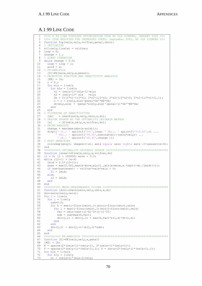
A.1 99 LINE CODE APPENDICES
70
A.1 99 LINE CODE
1 %%%% A 99 LINE TOPOLOGY OPTIMIZATION CODE BY OLE SIGMUND, JANUARY 2000 %%%
2 %%%% CODE MODIFIED FOR INCREASED SPEED, September 2002, BY OLE SIGMUND %%%
3 function top(nelx,nely,volfrac,penal,rmin);
4 % INITIALIZE
5 x(1:nely,1:nelx) = volfrac;
6 loop = 0;
7 change = 1.;
8 % START ITERATION
9 while change > 0.01
10 loop = loop + 1;
11 xold = x;
12 % FE-ANALYSIS
13 [U]=FE(nelx,nely,x,penal);
14 % OBJECTIVE FUNCTION AND SENSITIVITY ANALYSIS
15 [KE] = lk;
16 c = 0.;
17 for ely = 1:nely
18 for elx = 1:nelx
19 n1 = (nely+1)*(elx-1)+ely;
20 n2 = (nely+1)* elx +ely;
21 Ue = U([2*n1-1;2*n1; 2*n2-1;2*n2; 2*n2+1;2*n2+2; 2*n1+1;2*n1+2],1);
22 c = c + x(ely,elx)^penal*Ue'*KE*Ue;
23 dc(ely,elx) = -penal*x(ely,elx)^(penal-1)*Ue'*KE*Ue;
24 end
25 end
26 % FILTERING OF SENSITIVITIES
27 [dc] = check(nelx,nely,rmin,x,dc);
28 % DESIGN UPDATE BY THE OPTIMALITY CRITERIA METHOD
29 [x] = OC(nelx,nely,x,volfrac,dc);
30 % PRINT RESULTS
31 change = max(max(abs(x-xold)));
32 disp([' It.: ' sprintf('%4i',loop) ' Obj.: ' sprintf('%10.4f',c) ...
33 ' Vol.: ' sprintf('%6.3f',sum(sum(x))/(nelx*nely)) ...
34 ' ch.: ' sprintf('%6.3f',change )])
35 % PLOT DENSITIES
36 colormap(gray); imagesc(-x); axis equal; axis tight; axis off;pause(1e-6);
37 end
38 %%%%%%%%%% OPTIMALITY CRITERIA UPDATE %%%%%%%%%%%%%%%%%%%%%%%%%%%%%%%%%%%%%%
39 function [xnew]=OC(nelx,nely,x,volfrac,dc)
40 l1 = 0; l2 = 100000; move = 0.2;
41 while (l2-l1 > 1e-4)
42 lmid = 0.5*(l2+l1);
43 xnew = max(0.001,max(x-move,min(1.,min(x+move,x.*sqrt(-dc./lmid)))));
44 if sum(sum(xnew)) - volfrac*nelx*nely > 0;
45 l1 = lmid;
46 else
47 l2 = lmid;
48 end
49 end
50 %%%%%%%%%% MESH-INDEPENDENCY FILTER %%%%%%%%%%%%%%%%%%%%%%%%%%%%%%%%%%%%%%%%
51 function [dcn]=check(nelx,nely,rmin,x,dc)
52 dcn=zeros(nely,nelx);
53 for i = 1:nelx
54 for j = 1:nely
55 sum=0.0;
56 for k = max(i-floor(rmin),1):min(i+floor(rmin),nelx)
57 for l = max(j-floor(rmin),1):min(j+floor(rmin),nely)
58 fac = rmin-sqrt((i-k)^2+(j-l)^2);
59 sum = sum+max(0,fac);
60 dcn(j,i) = dcn(j,i) + max(0,fac)*x(l,k)*dc(l,k);
61 end
62 end
63 dcn(j,i) = dcn(j,i)/(x(j,i)*sum);
64 end
65 end
66 %%%%%%%%%% FE-ANALYSIS %%%%%%%%%%%%%%%%%%%%%%%%%%%%%%%%%%%%%%%%%%%%%%%%%%%%%
67 function [U]=FE(nelx,nely,x,penal)
68 [KE] = lk;
69 K = sparse(2*(nelx+1)*(nely+1), 2*(nelx+1)*(nely+1));
70 F = sparse(2*(nely+1)*(nelx+1),1); U = zeros(2*(nely+1)*(nelx+1),1);
71 for elx = 1:nelx
72 for ely = 1:nely
73 n1 = (nely+1)*(elx-1)+ely;

A.1 99 LINE CODE APPENDICES
71
74 n2 = (nely+1)* elx +ely;
75 edof = [2*n1-1; 2*n1; 2*n2-1; 2*n2; 2*n2+1; 2*n2+2; 2*n1+1; 2*n1+2];
76 K(edof,edof) = K(edof,edof) + x(ely,elx)^penal*KE;
77 end
78 end
79 % DEFINE LOADS AND SUPPORTS (HALF MBB-BEAM)
80 F(2,1) = -1;
81 fixeddofs = union([1:2:2*(nely+1)],[2*(nelx+1)*(nely+1)]);
82 alldofs = [1:2*(nely+1)*(nelx+1)];
83 freedofs = setdiff(alldofs,fixeddofs);
84 % SOLVING
85 U(freedofs,:) = K(freedofs,freedofs) \ F(freedofs,:);
86 U(fixeddofs,:)= 0;
87 %%%%%%%%%% ELEMENT STIFFNESS MATRIX %%%%%%%%%%%%%%%%%%%%%%%%%%%%%%%%%%%%%%%%
88 function [KE]=lk
89 E = 1.;
90 nu = 0.3;
91 k=[ 1/2-nu/6 1/8+nu/8 -1/4-nu/12 -1/8+3*nu/8 ...
92 -1/4+nu/12 -1/8-nu/8 nu/6 1/8-3*nu/8];
93 KE = E/(1-nu^2)*[ k(1) k(2) k(3) k(4) k(5) k(6) k(7) k(8)
94 k(2) k(1) k(8) k(7) k(6) k(5) k(4) k(3)
95 k(3) k(8) k(1) k(6) k(7) k(4) k(5) k(2)
96 k(4) k(7) k(6) k(1) k(8) k(3) k(2) k(5)
97 k(5) k(6) k(7) k(8) k(1) k(2) k(3) k(4)
98 k(6) k(5) k(4) k(3) k(2) k(1) k(8) k(7)
99 k(7) k(4) k(5) k(2) k(3) k(8) k(1) k(6)
100 k(8) k(3) k(2) k(5) k(4) k(7) k(6) k(1)];
101 %
102 %%%%%%%%%%%%%%%%%%%%%%%%%%%%%%%%%%%%%%%%%%%%%%%%%%%%%%%%%%%%%%%%%%%%%%%%%%%%
103 % This Matlab code was written by Ole Sigmund, Department of Solid %
104 % Mechanics, Technical University of Denmark, DK-2800 Lyngby, Denmark. %
105 % Please sent your comments to the author: [email protected] %
106 % %
107 % The code is intended for educational purposes and theoretical details %
108 % are discussed in the paper %
109 % "A 99 line topology optimization code written in Matlab" %
110 % by Ole Sigmund (2001), Structural and Multidisciplinary Optimization, %
111 % Vol 21, pp. 120--127. %
112 % %
113 % The code as well as a postscript version of the paper can be %
114 % downloaded from the web-site: http://www.topopt.dtu.dk %
115 % %
116 % Disclaimer: %
117 % The author reserves all rights but does not guaranty that the code is %
118 % free from errors. Furthermore, he shall not be liable in any event %
119 % caused by the use of the program. %
120 %%%%%%%%%%%%%%%%%%%%%%%%%%%%%%%%%%%%%%%%%%%%%%%%%%%%%%%%%%%%%%%%%%%%%%%%%%%%
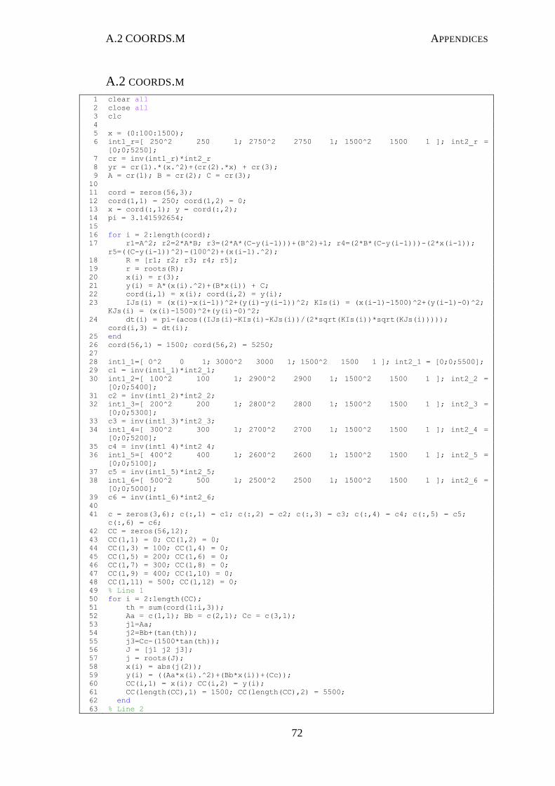
A.2 COORDS.M APPENDICES
72
A.2 COORDS.M
1 clear all
2 close all
3 clc
4
5 x = (0:100:1500);
6 int1_r=[ 250^2 250 1; 2750^2 2750 1; 1500^2 1500 1 ]; int2_r =
[0;0;5250];
7 cr = inv(int1_r)*int2_r
8 yr = cr(1).*(x.^2)+(cr(2).*x) + cr(3);
9 A = cr(1); B = cr(2); C = cr(3);
10
11 cord = zeros(56,3);
12 cord(1,1) = 250; cord(1,2) = 0;
13 x = cord(:,1); y = cord(:,2);
14 pi = 3.141592654;
15
16 for i = 2:length(cord);
17 r1=A^2; r2=2*A*B; r3=(2*A*(C-y(i-1)))+(B^2)+1; r4=(2*B*(C-y(i-1)))-(2*x(i-1));
r5=((C-y(i-1))^2)-(100^2)+(x(i-1).^2);
18 R = [r1; r2; r3; r4; r5];
19 r = roots(R);
20 x(i) = r(3);
21 y(i) = A*(x(i).^2)+(B*x(i)) + C;
22 cord(i,1) = x(i); cord(i,2) = y(i);
23 IJs(i) = (x(i)-x(i-1))^2+(y(i)-y(i-1))^2; KIs(i) = (x(i-1)-1500)^2+(y(i-1)-0)^2;
KJs(i) = (x(i)-1500)^2+(y(i)-0)^2;
24 dt(i) = pi-(acos((IJs(i)-KIs(i)-KJs(i))/(2*sqrt(KIs(i))*sqrt(KJs(i)))));
cord(i,3) = dt(i);
25 end
26 cord(56,1) = 1500; cord(56,2) = 5250;
27
28 int1_1=[ 0^2 0 1; 3000^2 3000 1; 1500^2 1500 1 ]; int2_1 = [0;0;5500];
29 c1 = inv(int1_1)*int2_1;
30 int1_2=[ 100^2 100 1; 2900^2 2900 1; 1500^2 1500 1 ]; int2_2 =
[0;0;5400];
31 c2 = inv(int1_2)*int2_2;
32 int1_3=[ 200^2 200 1; 2800^2 2800 1; 1500^2 1500 1 ]; int2_3 =
[0;0;5300];
33 c3 = inv(int1_3)*int2_3;
34 int1_4=[ 300^2 300 1; 2700^2 2700 1; 1500^2 1500 1 ]; int2_4 =
[0;0;5200];
35 c4 = inv(int1_4)*int2_4;
36 int1_5=[ 400^2 400 1; 2600^2 2600 1; 1500^2 1500 1 ]; int2_5 =
[0;0;5100];
37 c5 = inv(int1_5)*int2_5;
38 int1_6=[ 500^2 500 1; 2500^2 2500 1; 1500^2 1500 1 ]; int2_6 =
[0;0;5000];
39 c6 = inv(int1_6)*int2_6;
40
41 c = zeros(3,6); c(:,1) = c1; c(:,2) = c2; c(:,3) = c3; c(:,4) = c4; c(:,5) = c5;
c(:,6) = c6;
42 CC = zeros(56,12);
43 CC(1,1) = 0; CC(1,2) = 0;
44 CC(1,3) = 100; CC(1,4) = 0;
45 CC(1,5) = 200; CC(1,6) = 0;
46 CC(1,7) = 300; CC(1,8) = 0;
47 CC(1,9) = 400; CC(1,10) = 0;
48 CC(1,11) = 500; CC(1,12) = 0;
49 % Line 1
50 for i = 2:length(CC);
51 th = sum(cord(1:i,3));
52 Aa = c(1,1); Bb = c(2,1); Cc = c(3,1);
53 j1=Aa;
54 j2=Bb+(tan(th));
55 j3=Cc-(1500*tan(th));
56 J = [j1 j2 j3];
57 j = roots(J);
58 x(i) = abs(j(2));
59 y(i) = ((Aa*x(i).^2)+(Bb*x(i))+(Cc));
60 CC(i,1) = x(i); CC(i,2) = y(i);
61 CC(length(CC),1) = 1500; CC(length(CC),2) = 5500;
62 end
63 % Line 2
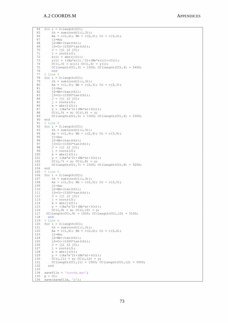
A.2 COORDS.M APPENDICES
73
64 for i = 2:length(CC);
65 th = sum(cord(1:i,3));
66 Aa = c(1,2); Bb = c(2,2); Cc = c(3,2);
67 j1=Aa;
68 j2=Bb+(tan(th));
69 j3=Cc-(1500*tan(th));
70 J = [j1 j2 j3];
71 j = roots(J);
72 x(i) = abs(j(2));
73 y(i) = ((Aa*x(i).^2)+(Bb*x(i))+(Cc));
74 CC(i,3) = x(i); CC(i,4) = y(i);
75 CC(length(CC),3) = 1500; CC(length(CC),4) = 5400;
76 end
77 % Line 3
78 for i = 2:length(CC);
79 th = sum(cord(1:i,3));
80 Aa = c(1,3); Bb = c(2,3); Cc = c(3,3);
81 j1=Aa;
82 j2=Bb+(tan(th));
83 j3=Cc-(1500*tan(th));
84 J = [j1 j2 j3];
85 j = roots(J);
86 x = abs(j(2));
87 y = ((Aa*x^2)+(Bb*x)+(Cc));
88 CC(i,5) = x; CC(i,6) = y;
89 CC(length(CC),5) = 1500; CC(length(CC),6) = 5300;
90 end
91 % Line 4
92 for i = 2:length(CC);
93 th = sum(cord(1:i,3));
94 Aa = c(1,4); Bb = c(2,4); Cc = c(3,4);
95 j1=Aa;
96 j2=Bb+(tan(th));
97 j3=Cc-(1500*tan(th));
98 J = [j1 j2 j3];
99 j = roots(J);
100 x = abs(j(2));
101 y = ((Aa*x^2)+(Bb*x)+(Cc));
102 CC(i,7) = x; CC(i,8) = y;
103 CC(length(CC),7) = 1500; CC(length(CC),8) = 5200;
104 end
105 % Line 5
106 for i = 2:length(CC);
107 th = sum(cord(1:i,3));
108 Aa = c(1,5); Bb = c(2,5); Cc = c(3,5);
109 j1=Aa;
110 j2=Bb+(tan(th));
111 j3=Cc-(1500*tan(th));
112 J = [j1 j2 j3];
113 j = roots(J);
114 x = abs(j(2));
115 y = ((Aa*x^2)+(Bb*x)+(Cc));
116 CC(i,9) = x; CC(i,10) = y;
117 CC(length(CC),9) = 1500; CC(length(CC),10) = 5100;
118 end
119 % Line 6
120 for i = 2:length(CC);
121 th = sum(cord(1:i,3));
122 Aa = c(1,6); Bb = c(2,6); Cc = c(3,6);
123 j1=Aa;
124 j2=Bb+(tan(th));
125 j3=Cc-(1500*tan(th));
126 J = [j1 j2 j3];
127 j = roots(J);
128 x = abs(j(2));
129 y = ((Aa*x^2)+(Bb*x)+(Cc));
130 CC(i,11) = x; CC(i,12) = y;
131 CC(length(CC),11) = 1500; CC(length(CC),12) = 5000;
132 end
133
134 savefile = 'coords.mat';
135 p = CC;
136 save(savefile, 'p');

A.3 ELEMENT STIFFNESS MATRICES APPENDICES
74
A.3 ELEMENT STIFFNESS MATRICES
1 clc
2 clear all
3 close all
4
5 CC = importdata('coords.mat');
6
7 figure
8 plot(CC(:,1),CC(:,2),'k.',CC(:,3),CC(:,4),'k.',CC(:,5),CC(:,6),'k.',...
9 CC(:,7),CC(:,8),'k.',CC(:,9),CC(:,10),'k.',CC(:,11),CC(:,12),'k.')
10 axis equal
11 axis([0 1500 0 5500]);
12
13 nelx = min(size(CC))/2-1; nely = length(CC)-1;
14 eCx = zeros(2,2,nelx*nely);
15 eCy = zeros(2,2,nelx*nely); % element Coordinates
16 % aCC = zeros(nelx*nely,2);
17
18 for i = 1:length(CC)-1
19 eCx(1,1,i) = CC(i,1); eCx(2,1,i) = CC(i+1,1);
20 eCx(1,2,i) = CC(i,3); eCx(2,2,i) = CC(i+1,3);
21 eCy(1,1,i) = CC(i,2); eCy(2,1,i) = CC(i+1,2);
22 eCy(1,2,i) = CC(i,4); eCy(2,2,i) = CC(i+1,4);
23 eCx(1,1,i+length(CC)-1) = CC(i,3); eCx(2,1,i+length(CC)-1) = CC(i+1,3);
24 eCx(1,2,i+length(CC)-1) = CC(i,5); eCx(2,2,i+length(CC)-1) = CC(i+1,5);
25 eCy(1,1,i+length(CC)-1) = CC(i,4); eCy(2,1,i+length(CC)-1) = CC(i+1,4);
26 eCy(1,2,i+length(CC)-1) = CC(i,6); eCy(2,2,i+length(CC)-1) = CC(i+1,6);
27 eCx(1,1,i+2*(length(CC)-1)) = CC(i,5); eCx(2,1,i+2*(length(CC)-1)) = CC(i+1,5);
28 eCx(1,2,i+2*(length(CC)-1)) = CC(i,7); eCx(2,2,i+2*(length(CC)-1)) = CC(i+1,7);
29 eCy(1,1,i+2*(length(CC)-1)) = CC(i,6); eCy(2,1,i+2*(length(CC)-1)) = CC(i+1,6);
30 eCy(1,2,i+2*(length(CC)-1)) = CC(i,8); eCy(2,2,i+2*(length(CC)-1)) = CC(i+1,8);
31 eCx(1,1,i+3*(length(CC)-1)) = CC(i,7); eCx(2,1,i+3*(length(CC)-1)) = CC(i+1,7);
32 eCx(1,2,i+3*(length(CC)-1)) = CC(i,9); eCx(2,2,i+3*(length(CC)-1)) = CC(i+1,9);
33 eCy(1,1,i+3*(length(CC)-1)) = CC(i,8); eCy(2,1,i+3*(length(CC)-1)) = CC(i+1,8);
34 eCy(1,2,i+3*(length(CC)-1)) = CC(i,10);
eCy(2,2,i+3*(length(CC)-1)) = CC(i+1,10);
35 eCx(1,1,i+4*(length(CC)-1)) = CC(i,9); eCx(2,1,i+4*(length(CC)-1)) = CC(i+1,9);
36 eCx(1,2,i+4*(length(CC)-1)) = CC(i,11);
eCx(2,2,i+4*(length(CC)-1)) = CC(i+1,11);
37 eCy(1,1,i+4*(length(CC)-1)) = CC(i,10);
eCy(2,1,i+4*(length(CC)-1)) = CC(i+1,10);
38 eCy(1,2,i+4*(length(CC)-1)) = CC(i,12);
eCy(2,2,i+4*(length(CC)-1)) = CC(i+1,12);
39 end
40
41 for i = 1:nelx*nely
42 for j = 1:2
43 for k = 1:2
44 if eCy(j,k,i)<=0
45 eCy(j,k,i) = 0.0000001;
46 end
47 end
48 end
49 end
50 for i = 1:nelx*nely
51 for j = 1:2
52 for k = 1:2
53 if eCx(j,k,i)<=0
54 eCx(j,k,i) = 0.0000001;
55 end
56 end
57 end
58 end
59
60 v = 0.3;
61 E = 1.;
62 D = (E/((1+v)*(1-2*v)))*[1-v, v, 0; v, 1-v, 0; 0, 0, (1-2*v)/2;];
63 r = [sqrt(3)/3, -sqrt(3)/3]; s = r;
64 KE = zeros(8,8,nelx*nely);
65 Ke1 = zeros(8,8,nelx*nely); Ke2 = zeros(8,8,nelx*nely); Ke3 = zeros(8,8,nelx*nely);
Ke4 = zeros(8,8,nelx*nely);
66
67 for i = 1:nelx*nely
68 n1r = (s(1)-1)/4; n1s = (r(1)-1)/4;

A.3 ELEMENT STIFFNESS MATRICES APPENDICES
75
69 n2r = (1-s(1))/4; n2s = -(1+r(1))/4;
70 n3r = (s(1)+1)/4; n3s = (r(1)+1)/4;
71 n4r = -(1+s(1))/4; n4s = (1-r(1))/4;
72 P = [n1r, n2r, n3r, n4r, 0, 0, 0, 0; n1s, n2s, n3s, n4s, 0, 0, 0, 0;...
73 0, 0, 0, 0, n1r, n2r, n3r, n4r; 0, 0, 0, 0, n1s, n2s, n3s, n4s;];
74 x1 = eCx(1,1,i); x2 = eCx(1,2,i); x3 = eCx(2,2,i); x4 = eCx(2,1,i);
75 y1 = eCy(1,1,i); y2 = eCy(1,2,i); y3 = eCy(2,2,i); y4 = eCy(2,1,i);
76 nxr = ((s(1)-1)*x1+(1-s(1))*x2+(s(1)+1)*x3-(1+s(1))*x4)/4;
77 nyr = ((s(1)-1)*y1+(1-s(1))*y2+(s(1)+1)*y3-(1+s(1))*y4)/4;
78 nxs = ((r(1)-1)*x1-(1+r(1))*x2+(1+r(1))*x3+(1-r(1))*x4)/4;
79 nys = ((r(1)-1)*y1-(1+r(1))*y2+(1+r(1))*y3+(1-r(1))*y4)/4;
80 J = [nxr, nyr; nxs, nys];
81 G = [J(2,2), -J(2,2), 0, 0; 0, 0, -J(2,2), J(2,2);...
82 -J(2,2), J(2,2), J(2,2), -J(2,2)]/det(J);
83 B = G*P;
84 Ke1(:,:,i) = B.'*D*B*det(J);
85 end
86
87 for i = 1:nelx*nely
88 n1r = (s(2)-1)/4; n1s = (r(1)-1)/4;
89 n2r = (1-s(2))/4; n2s = -(1+r(1))/4;
90 n3r = (s(2)+1)/4; n3s = (r(1)+1)/4;
91 n4r = -(1+s(2))/4; n4s = (1-r(1))/4;
92 P = [n1r, n2r, n3r, n4r, 0, 0, 0, 0; n1s, n2s, n3s, n4s, 0, 0, 0, 0;...
93 0, 0, 0, 0, n1r, n2r, n3r, n4r; 0, 0, 0, 0, n1s, n2s, n3s, n4s;];
94 x1 = eCx(1,1,i); x2 = eCx(1,2,i); x3 = eCx(2,2,i); x4 = eCx(2,1,i);
95 y1 = eCy(1,1,i); y2 = eCy(1,2,i); y3 = eCy(2,2,i); y4 = eCy(2,1,i);
96 nxr = ((s(2)-1)*x1+(1-s(2))*x2+(s(2)+1)*x3-(1+s(2))*x4)/4;
97 nyr = ((s(2)-1)*y1+(1-s(2))*y2+(s(2)+1)*y3-(1+s(2))*y4)/4;
98 nxs = ((r(1)-1)*x1-(1+r(1))*x2+(1+r(1))*x3+(1-r(1))*x4)/4;
99 nys = ((r(1)-1)*y1-(1+r(1))*y2+(1+r(1))*y3+(1-r(1))*y4)/4;
100 J = [nxr, nyr; nxs, nys];
101 G = [J(2,2), -J(2,2), 0, 0; 0, 0, -J(2,2), J(2,2);...
102 -J(2,2), J(2,2), J(2,2), -J(2,2)]/det(J);
103 B = G*P;
104 Ke2(:,:,i) = B.'*D*B*det(J);
105 end
106 107 for i = 1:nelx*nely
108 n1r = (s(1)-1)/4; n1s = (r(2)-1)/4;
109 n2r = (1-s(1))/4; n2s = -(1+r(2))/4;
110 n3r = (s(1)+1)/4; n3s = (r(2)+1)/4;
111 n4r = -(1+s(1))/4; n4s = (1-r(2))/4;
112 P = [n1r, n2r, n3r, n4r, 0, 0, 0, 0; n1s, n2s, n3s, n4s, 0, 0, 0, 0;...
113 0, 0, 0, 0, n1r, n2r, n3r, n4r; 0, 0, 0, 0, n1s, n2s, n3s, n4s;];
114 x1 = eCx(1,1,i); x2 = eCx(1,2,i); x3 = eCx(2,2,i); x4 = eCx(2,1,i);
115 y1 = eCy(1,1,i); y2 = eCy(1,2,i); y3 = eCy(2,2,i); y4 = eCy(2,1,i);
116 nxr = ((s(1)-1)*x1+(1-s(1))*x2+(s(1)+1)*x3-(1+s(1))*x4)/4;
117 nyr = ((s(1)-1)*y1+(1-s(1))*y2+(s(1)+1)*y3-(1+s(1))*y4)/4;
118 nxs = ((r(2)-1)*x1-(1+r(2))*x2+(1+r(2))*x3+(1-r(2))*x4)/4;
119 nys = ((r(2)-1)*y1-(1+r(2))*y2+(1+r(2))*y3+(1-r(2))*y4)/4;
120 J = [nxr, nyr; nxs, nys];
121 G = [J(2,2), -J(2,2), 0, 0; 0, 0, -J(2,2), J(2,2);...
122 -J(2,2), J(2,2), J(2,2), -J(2,2)]/det(J);
123 B = G*P;
124 Ke3(:,:,i) = B.'*D*B*det(J);
125 end
126
127 for i = 1:nelx*nely
128 n1r = (s(2)-1)/4; n1s = (r(2)-1)/4;
129 n2r = (1-s(2))/4; n2s = -(1+r(2))/4;
130 n3r = (s(2)+1)/4; n3s = (r(2)+1)/4;
131 n4r = -(1+s(2))/4; n4s = (1-r(2))/4;
132 P = [n1r, n2r, n3r, n4r, 0, 0, 0, 0; n1s, n2s, n3s, n4s, 0, 0, 0, 0;...
133 0, 0, 0, 0, n1r, n2r, n3r, n4r; 0, 0, 0, 0, n1s, n2s, n3s, n4s;];
134 x1 = eCx(1,1,i); x2 = eCx(1,2,i); x3 = eCx(2,2,i); x4 = eCx(2,1,i);
135 y1 = eCy(1,1,i); y2 = eCy(1,2,i); y3 = eCy(2,2,i); y4 = eCy(2,1,i);
136 nxr = ((s(2)-1)*x1+(1-s(2))*x2+(s(2)+1)*x3-(1+s(2))*x4)/4;
137
138
139
140
141
142
143
144
nyr = ((s(2)-1)*y1+(1-s(2))*y2+(s(2)+1)*y3-(1+s(2))*y4)/4;
nxs = ((r(2)-1)*x1-(1+r(2))*x2+(1+r(2))*x3+(1-r(2))*x4)/4;
nys = ((r(2)-1)*y1-(1+r(2))*y2+(1+r(2))*y3+(1-r(2))*y4)/4;
J = [nxr, nyr; nxs, nys];
G = [J(2,2), -J(2,2), 0, 0; 0, 0, -J(2,2), J(2,2);...
-J(2,2), J(2,2), J(2,2), -J(2,2)]/det(J);
B = G*P;
Ke4(:,:,i) = B.'*D*B*det(J);
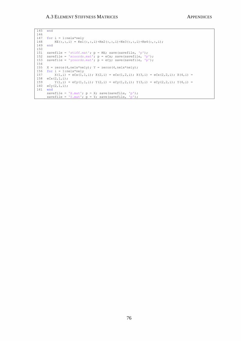
A.3 ELEMENT STIFFNESS MATRICES APPENDICES
76
145
146
147
148
149
150
151
152
153
154
155
156
157
158
159
160
161
end
for i = 1:nelx*nely
KE(:,:,i) = Ke1(:,:,i)+Ke2(:,:,i)+Ke3(:,:,i)+Ke4(:,:,i);
end
savefile = 'stiff.mat'; p = KE; save(savefile, 'p');
savefile = 'xcoords.mat'; p = eCx; save(savefile, 'p');
savefile = 'ycoords.mat'; p = eCy; save(savefile, 'p');
X = zeros(4,nelx*nely); Y = zeros(4,nelx*nely);
for i = 1:nelx*nely
X(1,i) = eCx(1,1,i); X(2,i) = eCx(1,2,i); X(3,i) = eCx(2,2,i); X(4,i) =
eCx(2,1,i);
Y(1,i) = eCy(1,1,i); Y(2,i) = eCy(1,2,i); Y(3,i) = eCy(2,2,i); Y(4,i) =
eCy(2,1,i);
end
savefile = 'X.mat'; p = X; save(savefile, 'p');
savefile = 'Y.mat'; p = Y; save(savefile, 'p');

A.4 MODIFIED TOPOLOGY OPTIMIZATION CODE APPENDICES
77
A.4 MODIFIED TOPOLOGY OPTIMIZATION CODE
1 %%%% A 99 LINE TOPOLOGY OPTIMIZATION CODE BY OLE SIGMUND, JANUARY 2000 %%%
2 %%%% CODE MODIFIED FOR INCREASED SPEED, September 2002, BY OLE SIGMUND %%%
3 %%%% CODE MODIFIED FOR CURVED CANTILEVER, November 2011, BY NATHANIEL VEENSTRA %%%
4 function topw; nelx = 5; nely = 55; volfrac = 0.7; penal = 1; rmin = 1;
5 % INITIALIZE
6 x(1:nely,1:nelx) = volfrac;
7 loop = 0;
8 change = 1.;
9 % LOAD MESH
10 X = importdata('xcoords.mat'); Y = importdata('ycoords.mat');
11 nodes = importdata('nodes.mat'); CC = importdata('coords.mat');
12 xx = importdata('X.mat'); yy = importdata('Y.mat');
13 % START ITERATION
14 while change > 0.01
15 loop = loop + 1;
16 xold = x;
17 % FE-ANALYSIS
18 [U]=FE(x,penal);
19 % OBJECTIVE FUNCTION AND SENSITIVITY ANALYSIS
20 [KE] = LK;
21 c = 0;
22 for ely = 1:nely
23 for elx = 1:nelx
24 i = nely*(elx-1)+ely;
25 n1 = (nely+1)*(elx-1)+ely;
26 n2 = (nely+1)* elx +ely;
27 Ue = U([2*n1-1;2*n1; 2*n2-1;2*n2; 2*n2+1;2*n2+2; 2*n1+1;2*n1+2],1);
28 KE0(1:8,1:8) = KE(:,:,i);
29 c = c + x(ely,elx)^penal*Ue'*KE0*Ue;
30 dc(ely,elx) = -penal*x(ely,elx,1)^(penal-1)*Ue.'*KE0*Ue;
31 end
32 end
33 % FILTERING OF SENSITIVITIES
34 [dc] = check(nelx,nely,rmin,x,dc);
35 % DESIGN UPDATE BY THE OPTIMALITY CRITERIA METHOD
36 [x] = OC(nelx,nely,x,volfrac,dc);
37 % PRINT RESULTS
38 change = max(max(abs(x-xold)));
39 disp([' It.: ' sprintf('%4i',loop) ' Obj.: ' sprintf('%10.4f',c) ...
40 ' Vol.: ' sprintf('%6.3f',sum(sum(x))/(nelx*nely)) ...
41 ' ch.: ' sprintf('%6.3f',change )...
42 ' U: ' sprintf('%6.4f',U(2*(nely+1)*(nelx+1)))])
43 % PLOT DENSITIES
44 rho = 1-x(:); colormap(gray); caxis([0 1]); patch(xx,yy,rho');
45 axis equal; axis tight; axis off;pause(1e-6);
46 end
47
48 %%%%%%%%%% OPTIMALITY CRITERIA UPDATE %%%%%%%%%%%%%%%%%%%%%%%%%%%%%%%%%%%%%%
49 function [xnew]=OC(nelx,nely,x,volfrac,dc)
50 l1 = 0; l2 = 100000; move = 0.2;
51 while (l2-l1 > 1e-4)
52 lmid = 0.5*(l2+l1);
53 xnew = max(0.001,max(x-move,min(1.,min(x+move,x.*sqrt(-dc./lmid)))));
54 if sum(sum(xnew)) - volfrac*nelx*nely > 0;
55 l1 = lmid;
56 else
57 l2 = lmid;
58 end
59 end
60 %%%%%%%%%% MESH-INDEPENDENCY FILTER %%%%%%%%%%%%%%%%%%%%%%%%%%%%%%%%%%%%%%%%
61 function [dcn]=check(nelx,nely,rmin,x,dc)
62 dcn=zeros(nely,nelx);
63 for i = 1:nelx
64 for j = 1:nely
65 sum=0.0;
66 for k = max(i-floor(rmin),1):min(i+floor(rmin),nelx)
67 for l = max(j-floor(rmin),1):min(j+floor(rmin),nely)
68 fac = rmin-sqrt((i-k)^2+(j-l)^2);
69 sum = sum+max(0,fac);
70 dcn(j,i) = dcn(j,i) + max(0,fac)*x(l,k)*dc(l,k);
71 end
72 end
73 dcn(j,i) = dcn(j,i)/(x(j,i)*sum);

A.4 MODIFIED TOPOLOGY OPTIMIZATION CODE APPENDICES
78
74 end
75 end
76 %%%%%%%%%% FE-ANALYSIS %%%%%%%%%%%%%%%%%%%%%%%%%%%%%%%%%%%%%%%%%%%%%%%%%%%%%
77 function [U]=FE(x,penal)
78 [KE] = LK; % Calculates and stores stiffness matrix of sinlge element
79 nelx = 5; nely = 55;
80 K = zeros(2*(nelx+1)*(nely+1), 2*(nelx+1)*(nely+1));
81 F = sparse(2*(nely+1)*(nelx+1),1); U = zeros(2*(nely+1)*(nelx+1),1);
82 for elx = 1:nelx
83 for ely = 1:nely
84 e = nely*(elx-1)+ely;
85 n1 = (nely+1)*(elx-1)+ely;
86 n2 = (nely+1)* elx +ely;
87 edof = [2*n1-1; 2*n1; 2*n2-1; 2*n2; 2*n2+1; 2*n2+2; 2*n1+1; 2*n1+2];
88 KE0(1:8,1:8)=KE(:,:,e);
89 K(edof,edof) = K(edof,edof) + x(ely,elx)^penal*KE0;
90 end
91 end
92 % DEFINE LOADS AND SUPPORTS
93 F(2*(nelx+1)*(nely+1),1) = -1;
94 fixeddofs =
union([1:2*(nely+1):2*(nely+1)*nelx+1],[2:2*(nely+1):2*(nely+1)*nelx+2]);
95 alldofs = [1:2*(nely+1)*(nelx+1)];
96 freedofs = setdiff(alldofs,fixeddofs);
97 % SOLVING
98 U(freedofs,:) = K(freedofs,freedofs) \ F(freedofs,:);
99 U(fixeddofs,:)= 0; % disp(U(2*(nely+1)*(nelx+1)))
100
101 %%%%%%%%%% ELEMENT STIFFNESS MATRIX %%%%%%%%%%%%%%%%%%%%%%%%%%%%%%%%%%%%%%%%
102 function KE=LK
103 nelx = 5; nely = 55; E = 1.; v = 0.3;
104 eCx = importdata('xcoords.mat');eCy = importdata('ycoords.mat');
105 KE = zeros(8,8,nelx*nely);
106 D = (E/(1-v^2))*[1, v, 0; v, 1, 0; 0, 0, (1-v)/2];
107 r = [sqrt(3)/3, -sqrt(3)/3]; s = r;
108 for e = 1:nelx*nely
109 for i = 1:2
110 for j = 1:2
111 x= [eCx(1,1,e);eCx(1,2,e);eCx(2,2,e);eCx(2,1,e)];
112 y= [eCy(1,1,e);eCy(1,2,e);eCy(2,2,e);eCy(2,1,e)];
113 dNdr= [s(j)-1, 1-s(j), 1+s(j), -1-s(j)]/4;
114 dNds= [r(i)-1, -1-r(i), 1+r(i), 1-r(i)]/4;
115 P = [dNdr(1),0,dNdr(2),0,dNdr(3),0,dNdr(4),0;
116 dNds(1),0,dNds(2),0,dNds(3),0,dNds(4),0;
117 0,dNdr(1),0,dNdr(2),0,dNdr(3),0,dNdr(4);
118 0,dNds(1),0,dNds(2),0,dNds(3),0,dNds(4)];
119 J = [dNdr*x, dNdr*y; dNds*x, dNds*y];
120 G = [J(2,2), -J(1,2), 0, 0;
121 0, 0, -J(2,1), J(1,1);
122 -J(2,1), J(1,1), J(2,2), -J(1,2)]/det(J);
123 B = G*P;
124 KE(:,:,e) = KE(:,:,e) + B'*D*B*det(J);
125 end
126 end
127 end
128 %%%%%%%%%%%%%%%%%%%%%%%%%%%%%%%%%%%%%%%%%%%%%%%%%%%%%%%%%%%%%%%%%%%%%%%%%%%%
129 % This Matlab code was written by Ole Sigmund, Department of Solid %
130 % Mechanics, Technical University of Denmark, DK-2800 Lyngby, Denmark. %
131 % Please sent your comments to the author: [email protected] %
132 % %
133 % The code is intended for educational purposes and theoretical details %
134 % are discussed in the paper %
135 % "A 99 line topology optimization code written in Matlab" %
136 % by Ole Sigmund (2001), Structural and Multidisciplinary Optimization, %
137 % Vol 21, pp. 120--127. %
138 % %
139 % The code as well as a postscript version of the paper can be %
140 % downloaded from the web-site: http://www.topopt.dtu.dk %
141 % %
142 % Disclaimer: %
143 % The author reserves all rights but does not guaranty that the code is %
144 % free from errors. Furthermore, he shall not be liable in any event %
145 % caused by the use of the program. %
146 %%%%%%%%%%%%%%%%%%%%%%%%%%%%%%%%%%%%%%%%%%%%%%%%%%%%%%%%%%%%%%%%%%%%%%%%%%%%
147 %%%% A 99 LINE TOPOLOGY OPTIMIZATION CODE BY OLE SIGMUND, JANUARY 2000 %%%

A.5 SPECIFICATIONS SPECIFICATIONS
79
A.5 SPECIFICATIONS
Due to unexpected oversight, the Project Specifications were not included as
Appendix A.1 and are herein included. Apologies are extended for this oversight.
University of Southern Queensland

A.5 SPECIFICATIONS SPECIFICATIONS
80
FACULTY OF ENGINEERING AND SURVEYING
ENG 4111/4112 Research Project
Project Specification
FOR: Nathaniel Veenstra
TOPIC: Optimum Strut-and-Tie model for a Cantilever Curved
Wall.
SUPERVISORS: Kazem Ghabraie
ENROLMENT: ENG4111 – S1, 2011 ENG4112 – S2, 2011
PROJECT AIM: Strut-and-tie modelling in combination with Finite Element analysis
allows for the load paths within concrete members to be determined
and optimized. By adopting a simple linear-elastic model to
represent the concrete behaviour and the concrete-steel interaction,
the strut-and-tie method can be used as a preliminary design tool in
the placement of reinforcing steel. This project aims to investigate
the use of this method in the case-specific example of a cantilever
curved wall verified through comparison of a simply supported
beam, of which an intuitive and modelled design are physically
tested.
PROGRAMME: ISSUE A. 21th
March 2011
1. A literature review on finite element analysis, topology optimization and the
use of strut-and-tie modelling in reinforced concrete design.
2. Formulation of a specific, two-dimensional design case of a curved cantilever
wall.
3. Discretise curved cantilever wall for application of finite element analysis,
including determination of element stiffness matrix from element geometry
and material properties.
4. Modify existing 99-line code to perform optimization on curved domain
approximated with quadrilateral elements.
5. Design optimum Strut-and-Tie model based from optimized topology.
Time permitting
6. Change design case from two-dimensional cantilever curved wall to three-
dimensional curved cantilever beam.

A.5 SPECIFICATIONS SPECIFICATIONS
81
AGREED:
__________________ (Student) __________________ (Supervisor)
___/___/___ ___/___/___