option p&l attribution and pricing

Option P&L Attribution and Pricing

Liuren Wujoint with Peter Carr

Baruch College

September 20, 2019

Carr and Wu (NYU & Baruch) P&L Attribution and Option Pricing September 20, 2019 1 / 25

The classic bottom-up approach of derivative pricing

The approach is analogous to that in classic physics

Identify the smallest common denominator (particle)

Construct everything bottom up with the smallest common particle

The analogy in classic derivative pricing

The common denominatorThe risk-neutral dynamics (or the physical dynamics and pricing) of aset of common driving factor; the pricing of Arrow-Debreu securities

The bottom-up constructionTake expectation of future payoffs of all derivative securities on thesame dynamics; price the payoffs as a basket of Arrow-Debreu securities

The ambition of a classic quant: Build one model that prices everything!

Specify the dynamics of the short-rate (or pricing kernel) →Price bonds of all maturities

Specify the joint factor structure of pricing kernels of all countries →Price bonds of all maturities, all currencies and the exchange rates

Specify the stock price dynamics → Price all options on the stock

Specify the factor structure on stock dynamics → Price all options onall stocks and stock indexes, maybe even bonds...


Why the urge to go to the bottom of everything?

Human nature or animal instinct?

Just like a groundhog who cannot help but keep digging!

For derivative pricing, the approach offers cross-sectional consistency

The common denominator specification provides a single yardstick(pricing menu) for valuing all derivatives built on top of it.

The valuations on different contracts are consistent with one another,in the sense that they are all derived from the same yardstick.

Even if the yardstick is wrong, the valuations remain consistent withone another.

They are just consistently wrong.

A foolish consistency is the hobgoblin of little minds,adored by little statesmen and philosophers and divines.— Ralph Waldo Emerson


Drawbacks of the classic bottom-up approach

It is difficult to get everything under one blanket.

Pricing long-dated contracts requires unrealistically long projections.

Short-term variations of long-dated contracts often look incompatiblewith long-run (stationarity) assumptions.

It is not always desirable to chain everything together

Pooling can be useful for information extraction, but can be limiting forindividual contract pricing/investment, which needs domain expertise.

Jack of all trades, master of none.

Error-contagion: Disturbance on one contract affects everything else.

The net result is the disengagement between Q-quants and P-quants:

Q: Pricing guarantees cross-sectional consistency, but with little regardtoP: Time-series variation, daily P&L attribution, risk management, andinvestment decisions

P-type analysis (data scientists, ML) are in vogue now, can we build pricingon top of statistical P&L analysis?


A new top-down decentralized perspective

What do investors want?

Different types of investors have different domain expertise and focuson different segments of the markets.

They need a model that can lever their domain expertise

Short-term investors do not care much about the terminal payoffs: Allshe worries about is the P&L on her particular investment over theshort investment horizon.

Short-term risk exposures are more of the focus than terminal payoffs

Long-term investors must also worry about their daily P&L fluctuationdue to marking to market and margin trading

We develop a new framework that generates decentralized pricingimplications based on short-term investment risk on a particular contract.

The short-term focus allows the investor to make near-term riskprojections without worrying about long-run dynamics.

The particular contract focus allows the investor to make top-downprojections without generating implications on other contracts.

Do the next right thing. Don’t worry about the unknown future, orconformity with others.


https://www.youtube.com/watch?v=w6g1yQV0dIY

Value representation of an option contract

Imagine we have a position in a single vanilla option contract.

We represent the option via the BMS pricing equation, B(t,St , It ;K ,T )

(K ,T ) capture the contract characteristics.

The value of the contract can vary with calendar time t, the underlyingsecurity price St , and the option’s BMS implied volatility It .

Appropriate representation/transformation is important for highlightinginformation/risk source, stabilizing quotation...

The at-the-money implied volatility term structure reflects the returnvariance expectation.

The implied volatility smile/skew shape across strike reveals thenon-normality of the underlying distribution.

As long as the option price does not allow arbitrage against theunderlying and cash, there existence of a positive It to match the price.(Hodges, 96)

Different transformation can highlight different insights

BMS is a common/nice choice, but one can explore others...Carr and Wu (NYU & Baruch) P&L Attribution and Option Pricing September 20, 2019 6 / 25

P&L attribution of a short-term option investment

With the BMS representation, we can perform a short-term P&L attributionanalysis on the option investment:

dB = [Btdt + BSdSt + BIdIt ]

+[

12BSS (dSt)

2 + 12BII (dIt)

2 + BIS (dStdIt)]

+ HigherOrderTerms,

The expansion can stop at second order for diffusive moves.

Higher order terms can become significant when the security price/impliedvolatility can jump by a random amount.

It is difficult/messy to perform integrated analysis of both small andlarge moves.

Diffusive moves can be handled effectively via dynamic hedging(frequent updating of a few instruments)

Hedging random jumps need careful positioning of many derivativecontracts.

The effects of large jumps are better analyzed separately with scenarioanalysis/stress tests.


Risk-neutral valuation of the investment return

Take risk-neutral expectation on the investment P&L, and assume zero rate,

0 = Et

[dB

dt

]= Bt + BI Itµt +

1

2BSSS

2t σ

2t +

1

2BII I

2t ω

2t + BIS ItStγt (1)

(µt , σ2t , ω

2t , γt) are the conditional mean and variance/covariances:

µt ≡ Et

[dItIt

]/dt, σ2

t ≡ Et

[(dSt

St

)2]/dt,

ω2t ≡ Et

[(dItIt

)2]/dt, γt ≡ Et

[(dSt

St, dItIt

)]/dt.

(1) can be regarded as a pricing equation: The value of the optionmust satisfy this equality to exclude dynamic arbitrage.

At one maturity, vega and theta are co-linear, we expect dollar gamma,vanna, volga to explain the cross-sectional variation of theta decay:

−Bt =1

2BSSS

2t σ

2t +

1

2BII I

2t ω

2t + BIS ItStγt

In absence of vol move, theta decay is compensated by gamma gain.

IV move induces extra expected P&Ls from vanna and volga exposures.


Risk-neutral valuation in BMS implied volatility

Start with the pricing relation

−Bt = BI Itµt +1

2BSSS

2t σ

2t +

1

2BII I

2t ω

2t + BIS ItStγt

Plug in the partial derivatives and rearrange, we obtain a simple valuationequation on the option implied volatility:

I 2t = σ2t + 2τµt I

2t + 2γtz+ + ω2

t z+z−.

z± ≡(lnK/Ft ± 1

2 I2t τ)

— convexity-adjusted moneyness


Top-down mean-variance option pricing

The (risk-neutral) mean-variance risk assumption on the security return andthe implied volatility return for an option contract,[

RSt+1 ≡

∆St+1

St

R It+1 ≡

∆It+1

It

]∼ N

([0µt

],

[σ2t γtγt ω2

t

]).

Determines the fair value of this one option contract in a simple form,

I 2t = σ2

t + 2τµt I2t + 2γtz+ + ω2

t z+z−. (2)

Where the mean-variance estimates come from and how they vary inthe future/past are irrelevant for the current valuation of this contract.

To price any other option contracts, specify/estimate their ownmean-variance risk structure.

To compare the pricing of different contracts, compare theirmean-variance risk structure.

Since Markowitz, mean-variance analysis has a long successful history infinance for both pricing and investing, and now it extends to derivativespricing and investments.


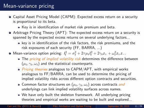
Mean-variance pricing

Capital Asset Pricing Model (CAPM): Expected excess return on a securityis proportional to its beta.

Key is in identification of market risk premium and beta.

Arbitrage Pricing Theory (APT): The expected excess return on a security isspanned by the expected excess returns on several underlying factors...

key is in identification of the risk factors, the risk premiums, and therisk exposures of each security (FF, BARRA, ...)

Mean-variance option pricing: I 2t = σ2

t + 2τµt I2t + 2γtz+ + ω2

t z+z−.

The pricing of implied volatility risk determines the difference between(µt , γt , ωt) and the statistical counterparts.

Pricing theories analogous to CAPM/APT, with empirical worksanalogous to FF/BARRA, can be used to determine the pricing ofimplied volatility risks across different option contracts and securities.

Common factor structures on (µt , γt , ωt) across contracts andunderlyings can link implied volatility surfaces across names.

We have only built the skeleton framework. All underlying pricingtheories and empirical works are waiting to be built and explored...


Common factor structures on an implied volatility surface

I 2t =[2τµt I

2t + σ2

t

]+[2γtz+ + ω2

t z+z−]

Carr&Wu (JFE, 2016): One common-factor governs the short-termmovements of the whole surfacedI (K ,T )/I (K ,T ) = eηt(T−t)(mtdt + wtdZt) for all (K ,T )

That allows them to characterizes the whole implied volatility surfaceat any given time with five states (mt ,wt , ηt , ρt , σt) with no additionalmodel parameters.

PCA often identifies 3 major sources of variation on the surface:

The overall volatility level

Term structure variation (short v. long-dated contracts)

Implied volatility smile/skew variation along moneyness(OTM put v. straddle v. OTM call)

We explore how our framework can be applied to any particular segment ofthe surface.


At-the-money implied variance term structure

We define “at-the-money” as contracts with z+ = 0, or k = − 12 I

2t τ

Such contracts have zero volga and vanna.

The implied volatility level only depends on its expected move (µt), but notits variance/covariance:

A2t = 2τµtA

2t + σ2

t .

Applications:

1 contract: Infer risk-neutral drift from the slope against instantaneous

variance: µt =A2t−σ2

t

2A2t τ

.

2 contracts: Infer locally common drift from the slope of nearbyat-the-money contracts:

µt =A2t (τ2)− A2

t (τ1)

2(A2t (τ2)τ2 − A2

t (τ1)τ1).

Locally constant drift leads to locally linear term structure — Driftestimates can be tied to local linear (nonparametric) regression fittingof the term structure.


The implied volatility smile

To highlight the implied volatility smile at a certain maturity, we can vegahedge the option with the at-the-money contract of the same maturity,assuming they strongly co-move.

Take the ATM implied variance A2t as given and focus on the implied

variance deviation of other contracts from the ATM variance level.

Assume proportional drift at the same maturity: µt I2t = µtA

2t .

Plug in the at-the-money implied variance to highlight the “implied volatilitysmile” effect at the single maturity,

I 2t − A2

t = 2γtz+ + ω2t z+z−, (3)

The smile slope is determined by the covariance rate γt of the contract.

The smile curvature is determined by the variance rate ω2t

Application: Assuming locally common proportional implied volatilitymovements within a particular moneyness range, we can identify thecommon moment conditions (ω2

t , γt) by regressing I 2t − A2

t against(2z+, z+z−).


Application: Extrapolate observed smile to long maturity

Exchange-traded contracts are short-dated, but many OTC deals are long term.How to extrapolate exchange quotes to price long-dated OTC deals?

The classic approach

Calibrate a standard stochastic vol model to observed quotes (say upto 2 years), price long-dated options (say 10 years) with the modelparameter estimates.The atm vol level will flatten out to the long-run mean (roughlymatching the 2-year ATM vol level)The implied volatility smile/skew will flatten due to central limittheorem (and the fact that volatility converges to its long-run mean).

Our pricing approach:

If the atm vol is flat extrapolated from 2 to 10 years, the 2-year and10-year atm variance will vary by the same amount — same (γt , ω

2t ).

Empirically, we do observe long-dated contracts vary much more thansuggested by estimated mean reversion processes.

The smile/skew shape must be extrapolated from 2 to 10 years as well!

Different perspectives often lead to different seemingly innocuousasymptotic assumptions


Empirical analysis

We use exchange-traded SPX options to

Distinguish between changes in floating implied vol series and impliedvolatility changes of a fixed option contract

Traditional models are more related to the dynamics of the former, ourapproach is based on the moments of the latter.

In according with our effort for decentralization, introduce the concept oflocal commonality, and contrast with traditional global factor structures

Compare historical (TS) estimates with cross-sectional option-implied (CS)mean-variance moment conditions

Expected implied volatility change v. the at-the-money term structure

Variance/covariance estimates v. the implied volatility smile

Trade the difference as risk premium (risk-return tradeoff), andcompare with statistical arbitrage trading


Constructing floating series of IV levels and changes

The exchange-listed options have fixed strike and expiry.

The standard approach is to interpolate the implied volatilities of thesecontracts to obtain floating series at fixed time to maturities and moneyness

OptionMetrics provides floating implied vol series at 1,2,3,6,12 monthsand different deltas.

OTC market often provide indicative quotes on floatingtime-to-maturity and relative strike grids.

Analyzing variations of these floating series provides insights fortraditional option pricing modeling

Our model depends on the implied volatility variation of a fixed contract,making it necessary to construct implied volatility changes of fixed contracts

At each date, construct log implied volatility change over the nextbusiness date on each option contract i , R i

t+1 ≡ ln(I it+1/Iit ).

Interpolate (via Gaussian kernel smoothing) the changes to floatingtime to maturity (1,2,3,6,12 months) and moneyness points:x ≡ z+/It

√τ = 0,±0.5,±1,±1.5,±2.


Local commonality v. global factor structure

Our theory links an option’s implied volatility level to its own first andsecond risk-neutral conditional moments (µt , γt , ωt).

To reverse engineer the conditional moments from option observations, wepropose to make local commonality assumptions that implied volatilities ofnearby contracts move closely together and thus share similar moments.

The assumption is not meant to be exact,But it is robust to actual dynamics variations/assumptions.

It is a matter of what you trust: model assumption or contract structure

If you trust a model, you can hedge/combine any contract exactly withany other contract .... contract choice is irrelevant.You can fail miserably if the model turns out wrong (and it is always!)Hedging a $100-strike option with a $101-strike option has a max lossof $1 regardless of what model or what happens.

Empirically identified global factor structures are rarely global

Number of principal components depend on the maturity/strike span

Local commonality in practice (e.g., OCC): divide the implied vol surfaceinto grids and treat contracts with each grid as “common.”


How local is local?

Take 3-month at-the-money at the reference point, measure implied volchange correlations of other contracts with this reference contract

-2 -1.5 -1 -0.5 0 0.5 1 1.5 2

Moneyness, x

55

60

65

70

75

80

85

90

95

100

Corre

lation

, %

1 2 3 612

At the money: Correlations with adjacent maturities (2m & 6m) are > 95%.

Same-month smile: Correlations with |x | < 1 (one std) are > 93%.

Correlations with far-away contracts can be as low as 60%.


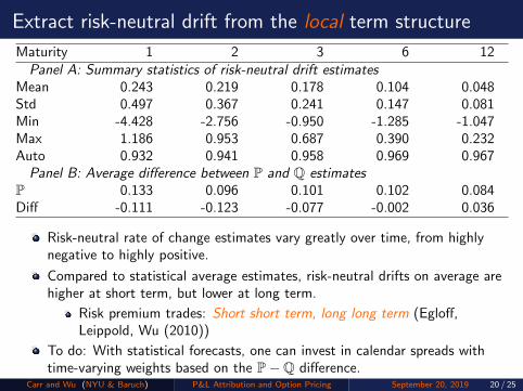
Extract risk-neutral drift from the local term structure

Maturity 1 2 3 6 12Panel A: Summary statistics of risk-neutral drift estimates

Mean 0.243 0.219 0.178 0.104 0.048Std 0.497 0.367 0.241 0.147 0.081Min -4.428 -2.756 -0.950 -1.285 -1.047Max 1.186 0.953 0.687 0.390 0.232Auto 0.932 0.941 0.958 0.969 0.967

Panel B: Average difference between P and Q estimatesP 0.133 0.096 0.101 0.102 0.084Diff -0.111 -0.123 -0.077 -0.002 0.036

Risk-neutral rate of change estimates vary greatly over time, from highlynegative to highly positive.

Compared to statistical average estimates, risk-neutral drifts on average arehigher at short term, but lower at long term.

Risk premium trades: Short short term, long long term (Egloff,Leippold, Wu (2010))

To do: With statistical forecasts, one can invest in calendar spreads withtime-varying weights based on the P−Q difference.


Extract variance and covariance from the local smile

Maturity 1 2 3 6 12

Panel A. Covariance Rate Estimates γtMean -0.142 -0.107 -0.090 -0.068 -0.050Std 0.066 0.046 0.037 0.026 0.018Corr 0.647 0.660 0.641 0.580 0.525

Panel B. Variance Rate Estimates ω2t

Mean 1.002 0.451 0.270 0.102 0.038Std 0.461 0.207 0.128 0.056 0.027Corr -0.142 -0.172 -0.171 -0.130 -0.122

Panel C. Regression R-squared EstimatesMean 0.999 0.999 0.999 1.000 1.000Std 0.001 0.001 0.001 0.001 0.001

Super high R2 — Near perfect fit of a local smile

Skew/covariance are highly correlated, not so for the variance/curvatureestimates


Predicting realized variance/covariance rates

RVt+1 = α + β1CSt + β2TSt + etMaturity α β1 β2 R2, %Panel A. Covariance Rate γt

1 -0.011 ( 1.64 ) 0.120 ( 1.79 ) 0.377 ( 2.97 ) 20.232 -0.011 ( 1.65 ) 0.097 ( 1.20 ) 0.433 ( 3.45 ) 23.113 -0.012 ( 1.70 ) 0.070 ( 0.76 ) 0.463 ( 3.84 ) 24.186 -0.009 ( 1.63 ) 0.056 ( 0.58 ) 0.484 ( 4.21 ) 25.28

12 -0.004 ( 1.11 ) 0.129 ( 1.61 ) 0.466 ( 4.00 ) 25.85

Panel B. Variance Rate ωt

1 0.231 ( 7.02 ) -0.004 ( 0.15 ) 0.19 ( 3.72 ) 3.522 0.148 ( 6.84 ) -0.040 ( 1.07 ) 0.22 ( 3.86 ) 5.403 0.116 ( 6.62 ) -0.091 ( 1.83 ) 0.25 ( 4.08 ) 7.636 0.063 ( 6.47 ) -0.160 ( 2.16 ) 0.29 ( 3.95 ) 10.28

12 0.034 ( 6.58 ) -0.198 ( 2.26 ) 0.34 ( 3.30 ) 13.46

Historical estimators dominate the prediction.


Risk-return tradeoff strategy on the implied volatility smile

Take delta/vega-neutral spread positions (against the ATM contract) ateach maturity

Alpha source: difference between the observed smile and the smileconstructed from the forecasted variance/covariance rates (risk premium).

Annualized information ratio from the investments:

τ\x -1.0 -0.5 0.5 1.0 All

1 0.45 0.23 0.36 0.35 0.522 1.78 1.82 1.75 1.67 1.933 2.52 2.47 2.25 2.11 2.606 3.46 3.39 3.06 2.79 3.46

12 3.53 3.76 3.59 3.21 3.81

The trades are not that profitable at short maturity (one month) — Missingcontribution from jumps can play a large role at short maturity?

The trades are very profitable at long maturity — Variance/covariancedrives the main delta-hedged P&L of long-dated smiles.


Statistical arbitrage strategy on the implied volatility smile

Take delta/vega-neutral spread positions (against the ATM contract)

Alpha source: pricing error of the CS regression (reversion of pricing error)

Annualized information ratio from the investments:

τ\x -1.0 -0.5 0.5 1.0 All

1 0.31 -0.08 0.13 0.03 0.232 -0.04 0.34 0.38 -0.15 0.533 -0.25 0.53 0.58 -0.19 0.666 -0.54 0.55 1.04 -0.28 0.61

12 -0.79 0.28 1.77 -0.24 0.68

Much lower profitability due to concentration of contracts ...

Can be much more profitable (for market making) when applied to alarger universe of contracts

The two strategies focus on different aspects and have different applications


Concluding remarks

Virtually all security classes can be analyzed from two perspectives:

Bottom-up valuation: DCF for stocks, DTSM for bonds, time-changedLevy processes for options

Long-run projections are needed for pricing current securities.Pricing errors can be regarded as stat arb trading opportunities.

Top-down return analysis: CAPM/APT-type research for pricingtheories, FF/BARRA-type empirical research for stock returns...

Focus on current risk-return tradeoff (of different horizons)Identified risk structure can be used to construct robust covariancematrix for mean-variance optimizationIdentified factor risk premiums can be used to constructed“smart-beta” portfolios

A lot has been done on the former (bottom-up valuation) on option pricing.

Much is needed to explore the option pricing implication from the top-downreturn analysis angle.

Ultimately, we hope to tie the pricing analysis to risk management andmean-variance investments for an expanded instruments universe thatinclude both primary securities (stocks, bonds) and their options.


option p&l attribution and pricing

Documents