option pricing by simulation by kemal din§er dinge§ b.s

OPTION PRICING BY SIMULATION

by

Kemal Dincer Dingec

B.S., Industrial Engineering, Istanbul Technical University, 2005

M.S., Industrial Engineering, Bogazici University, 2007

Submitted to the Institute for Graduate Studies in

Science and Engineering in partial fulfillment of

the requirements for the degree of

Doctor of Philosophy

Graduate Program in Industrial Engineering

Bogazici University

2013

ii


APPROVED BY:

Assoc. Prof. Wolfgang Hormann . . . . . . . . . . . . . . . . . . .

(Thesis Supervisor)

Prof. Irini Dimitriyadis . . . . . . . . . . . . . . . . . . .

Prof. Refik Gullu . . . . . . . . . . . . . . . . . . .

Assist. Prof. Aybek Korugan . . . . . . . . . . . . . . . . . . .

Assist. Prof. Halis Sak . . . . . . . . . . . . . . . . . . .

DATE OF APPROVAL: 26.12.2012

iii

ACKNOWLEDGEMENTS

I would like to thank my advisor, Assoc. Prof. Wolfgang Hormann, for his

guidance throughout my thesis study. I also thank to Assist. Prof. Halis Sak for his

help and support in the last year of my thesis. I thank to all of the thesis committee

members for their interest.

I would also like to thank my friend Cagatay Dagıstan for his valuable help on

R and LATEX, and also to my friend Furkan Boru for our stimulating discussions on

mathematical economics.

This work was supported by Bogazici Research Fund (BAP) project 5020 and the

Scientific and Technological Research Council of Turkey (TUBITAK) project 111M108.

iv

ABSTRACT


The valuation of path dependent and multivariate options require efficient numer-

ical methods, as their prices are not available in closed form. Monte Carlo simulation is

one of the widely used techniques. Although simulation is a highly flexible and general

method, its efficiency for specific problems depends on exploiting the special features

of that problem via variance reduction techniques. The aim in variance reduction is

to reduce the variance of the estimator in order to increase the efficiency. This study

proposes new variance reduction methods for path dependent and multivariate options

under the assumption of geometric Brownian motion. These methods are based on

new control variates. Furthermore, a general control variate framework is suggested

for Levy process models. Its application is presented for pricing path dependent op-

tions.The options considered in this thesis are European basket, Asian, lookback and

barrier options. The method suggested for basket and Asian options combines the use

of control variates and conditional Monte Carlo. The new control variate algorithms

for lookback and barrier options use the continuously monitored options as external

control variates for their discrete counterparts. The general control variate framework

for Levy process models contains special and general control variates, which are path

functionals of the original Levy process and a coupled Brownian motion. The method

is based on fast numerical inversion of the cumulative distribution functions.

v

OZET

SIMULASYONLA OPSIYON FIYATLAMA

Patikaya bagımlı ve coklu degiskenli opsiyonların fiyatları icin kapalı formul

bulunmamaktadır. Dolayısıyla bu tur opsiyonlar icin etkin sayısal yontemlere ihtiyac

duyulmaktadır. Monte Carlo simulasyonu opsiyon fiyatlama amacıyla kullanılan en

yaygın yontemlerden biridir. Simulasyon oldukca esnek ve genel bir yontemdir, ancak

belirli bir problem icin etkinligi o probleme ozgu niteliklerin varyans dusurme teknikleri

yoluyla kullanımına baglıdır. Varyans dusurmedeki amac tahminleyicinin varyansını

azaltarak etkinligi arttırabilmektir. Bu calısmada geometrik Brownian hareketi altında

patikaya bagımlı ve coklu degiskenli opsiyonlar icin yeni varyans dusurme teknikleri

one surulmektedir. Bu yontemler yeni kontrol degiskenlerine dayanmaktadır. Ayrıca

Levy sureci modelleri icin genel bir kontrol degiskeni cercevesi onerilmektedir. Yeni

yontemin uygulaması icin patikaya bagımlı opsiyonların fiyatlandırılması ornek olarak

kullanılmıstır. Bu tezde ele alınan opsiyonlar Avrupa tipi sepet, Asya tipi, hatırlatma

ve bariyer opsiyonlarıdır. Sepet ve Asya tipi opsiyonlar icin one surulen yontem kontrol

degiskeni ve kosullu Monte Carlo tekniklerinin bir arada kullanımına dayanmaktadır.

Hatırlatma ve bariyer opsiyonları icin onerilen yeni kontrol degiskeni algoritmalarında

surekli goz lemlenen opsiyonlar kesikli versiyonları icin dıssal kontrol degiskeni olarak

kullanılmaktadır. Levy sureci modelleri icin onerilen genel kontrol degiskeni cercevesi

ozel ve genel kontrol degiskenleri icermektedir. Bu degiskenler asıl Levy sureci ile

bagımlı bir Brownian hareketinin patika fonksiyonlarıdır. Yontem birikimli dagılım

fonksiyonlarının hızlı sayısal ters donusumune dayanmaktadır.

vi

TABLE OF CONTENTS

ACKNOWLEDGEMENTS . . . . . . . . . . . . . . . . . . . . . . . . . . . . . iii

ABSTRACT . . . . . . . . . . . . . . . . . . . . . . . . . . . . . . . . . . . . . iv

OZET . . . . . . . . . . . . . . . . . . . . . . . . . . . . . . . . . . . . . . . . . v

LIST OF FIGURES . . . . . . . . . . . . . . . . . . . . . . . . . . . . . . . . . x

LIST OF TABLES . . . . . . . . . . . . . . . . . . . . . . . . . . . . . . . . . . xiii

LIST OF SYMBOLS . . . . . . . . . . . . . . . . . . . . . . . . . . . . . . . . . xv

LIST OF ACRONYMS/ABBREVIATIONS . . . . . . . . . . . . . . . . . . . . xvii

1. INTRODUCTION . . . . . . . . . . . . . . . . . . . . . . . . . . . . . . . . 1

2. SIMULATION . . . . . . . . . . . . . . . . . . . . . . . . . . . . . . . . . . 3

2.1. Random Variate Generation by Inversion . . . . . . . . . . . . . . . . . 3

2.1.1. Numerical Inversion . . . . . . . . . . . . . . . . . . . . . . . . 4

2.1.1.1. Measuring the Accuracy of Approximate Inversion . . 4

2.1.1.2. Newton’s Interpolation Formula and Gauss-Lobatto Quadra-

ture . . . . . . . . . . . . . . . . . . . . . . . . . . . . . 5

2.1.1.3. Cut-off Points for the Domain . . . . . . . . . . . . . . 6

2.1.1.4. Implementation . . . . . . . . . . . . . . . . . . . . . . 6

2.2. Output Analysis . . . . . . . . . . . . . . . . . . . . . . . . . . . . . . 7

2.3. Variance Reduction Methods . . . . . . . . . . . . . . . . . . . . . . . . 8

2.3.1. Measuring Simulation Efficiency . . . . . . . . . . . . . . . . . . 8

2.3.2. Control Variate Method . . . . . . . . . . . . . . . . . . . . . . 9

2.3.2.1. Multiple Control Variates . . . . . . . . . . . . . . . . 10

2.3.2.2. How to Select Control Variates? . . . . . . . . . . . . . 11

2.3.3. Importance Sampling . . . . . . . . . . . . . . . . . . . . . . . . 12

2.3.4. Conditional Monte Carlo . . . . . . . . . . . . . . . . . . . . . . 13

2.4. Simulation of Options . . . . . . . . . . . . . . . . . . . . . . . . . . . 14

3. BASKET AND ASIAN OPTIONS . . . . . . . . . . . . . . . . . . . . . . . 16

3.1. Introduction . . . . . . . . . . . . . . . . . . . . . . . . . . . . . . . . . 16

3.2. Simulation of Basket and Asian Options . . . . . . . . . . . . . . . . . 18

3.3. Control Variates . . . . . . . . . . . . . . . . . . . . . . . . . . . . . . . 20

vii

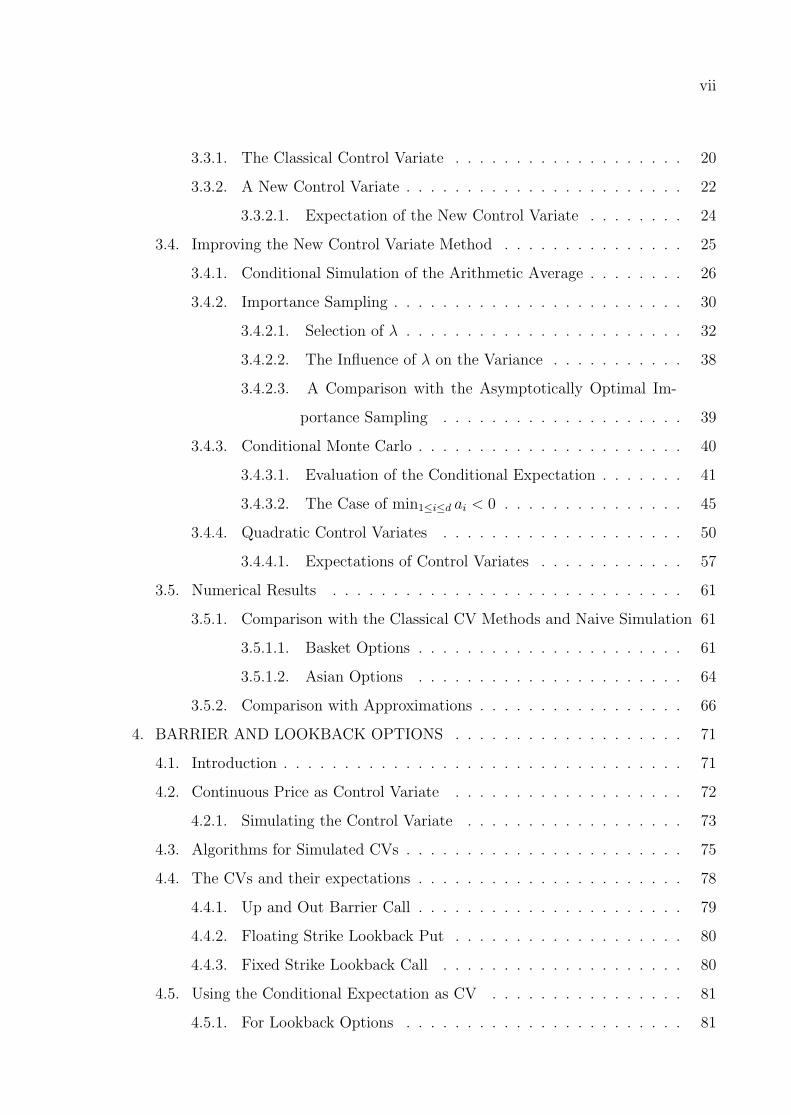
3.3.1. The Classical Control Variate . . . . . . . . . . . . . . . . . . . 20

3.3.2. A New Control Variate . . . . . . . . . . . . . . . . . . . . . . . 22

3.3.2.1. Expectation of the New Control Variate . . . . . . . . 24

3.4. Improving the New Control Variate Method . . . . . . . . . . . . . . . 25

3.4.1. Conditional Simulation of the Arithmetic Average . . . . . . . . 26

3.4.2. Importance Sampling . . . . . . . . . . . . . . . . . . . . . . . . 30

3.4.2.1. Selection of λ . . . . . . . . . . . . . . . . . . . . . . . 32

3.4.2.2. The Influence of λ on the Variance . . . . . . . . . . . 38

3.4.2.3. A Comparison with the Asymptotically Optimal Im-

portance Sampling . . . . . . . . . . . . . . . . . . . . 39

3.4.3. Conditional Monte Carlo . . . . . . . . . . . . . . . . . . . . . . 40

3.4.3.1. Evaluation of the Conditional Expectation . . . . . . . 41

3.4.3.2. The Case of min1≤i≤d ai < 0 . . . . . . . . . . . . . . . 45

3.4.4. Quadratic Control Variates . . . . . . . . . . . . . . . . . . . . 50

3.4.4.1. Expectations of Control Variates . . . . . . . . . . . . 57

3.5. Numerical Results . . . . . . . . . . . . . . . . . . . . . . . . . . . . . 61

3.5.1. Comparison with the Classical CV Methods and Naive Simulation 61

3.5.1.1. Basket Options . . . . . . . . . . . . . . . . . . . . . . 61

3.5.1.2. Asian Options . . . . . . . . . . . . . . . . . . . . . . 64

3.5.2. Comparison with Approximations . . . . . . . . . . . . . . . . . 66

4. BARRIER AND LOOKBACK OPTIONS . . . . . . . . . . . . . . . . . . . 71

4.1. Introduction . . . . . . . . . . . . . . . . . . . . . . . . . . . . . . . . . 71

4.2. Continuous Price as Control Variate . . . . . . . . . . . . . . . . . . . 72

4.2.1. Simulating the Control Variate . . . . . . . . . . . . . . . . . . 73

4.3. Algorithms for Simulated CVs . . . . . . . . . . . . . . . . . . . . . . . 75

4.4. The CVs and their expectations . . . . . . . . . . . . . . . . . . . . . . 78

4.4.1. Up and Out Barrier Call . . . . . . . . . . . . . . . . . . . . . . 79

4.4.2. Floating Strike Lookback Put . . . . . . . . . . . . . . . . . . . 80

4.4.3. Fixed Strike Lookback Call . . . . . . . . . . . . . . . . . . . . 80

4.5. Using the Conditional Expectation as CV . . . . . . . . . . . . . . . . 81

4.5.1. For Lookback Options . . . . . . . . . . . . . . . . . . . . . . . 81

viii

4.5.2. For Barrier Options . . . . . . . . . . . . . . . . . . . . . . . . . 83

4.6. Algorithms for Barrier Options . . . . . . . . . . . . . . . . . . . . . . 84

4.7. Computational Results . . . . . . . . . . . . . . . . . . . . . . . . . . . 88

4.7.1. Computational Results for Lookback Options . . . . . . . . . . 88

4.7.2. Computational Results for Barrier Options . . . . . . . . . . . . 93

4.8. Summary of the Results . . . . . . . . . . . . . . . . . . . . . . . . . . 96

5. LEVY PROCESSES . . . . . . . . . . . . . . . . . . . . . . . . . . . . . . . 97

5.1. Definition . . . . . . . . . . . . . . . . . . . . . . . . . . . . . . . . . . 97

5.2. Examples of Levy Processes . . . . . . . . . . . . . . . . . . . . . . . . 98

5.2.1. Pure Jump Processes . . . . . . . . . . . . . . . . . . . . . . . . 98

5.2.1.1. Variance Gamma Process . . . . . . . . . . . . . . . . 99

5.2.1.2. Normal Inverse Gaussian Process . . . . . . . . . . . . 99

5.2.1.3. Generalized Hyperbolic Process . . . . . . . . . . . . . 100

5.2.1.4. Meixner Process . . . . . . . . . . . . . . . . . . . . . 102

5.2.2. Jump Diffusion Processes . . . . . . . . . . . . . . . . . . . . . 103

5.3. Simulation of Levy Processes . . . . . . . . . . . . . . . . . . . . . . . 104

5.3.1. Pure Jump Processes . . . . . . . . . . . . . . . . . . . . . . . . 104

5.3.1.1. Subordination . . . . . . . . . . . . . . . . . . . . . . . 104

5.3.1.2. Numerical Inversion . . . . . . . . . . . . . . . . . . . 105

5.3.1.3. Comparison of Numerical Inversion and Subordination 106

5.3.2. Jump Diffusion Processes . . . . . . . . . . . . . . . . . . . . . 107

5.3.2.1. The Standard Method . . . . . . . . . . . . . . . . . . 107

5.3.2.2. Numerical Inversion . . . . . . . . . . . . . . . . . . . 108

5.4. Risk Neutral Measures for Option Pricing . . . . . . . . . . . . . . . . 109

5.4.1. Mean Correcting Martingale Measure . . . . . . . . . . . . . . . 110

5.4.2. Esscher Transform . . . . . . . . . . . . . . . . . . . . . . . . . 111

6. NEW CONTROL VARIATES FOR LEVY PROCESS MODELS . . . . . . 113

6.1. Introduction . . . . . . . . . . . . . . . . . . . . . . . . . . . . . . . . . 113

6.2. General CV Framework . . . . . . . . . . . . . . . . . . . . . . . . . . 114

6.3. Possible Control Variates . . . . . . . . . . . . . . . . . . . . . . . . . . 116

6.3.1. Expectation Formulas . . . . . . . . . . . . . . . . . . . . . . . 118

ix

6.3.1.1. Expectations of CVLs . . . . . . . . . . . . . . . . . . 118

6.3.1.2. Expectations of CVWs . . . . . . . . . . . . . . . . . . 119

6.4. A Simple Example . . . . . . . . . . . . . . . . . . . . . . . . . . . . . 121

7. APPLICATION OF NEW CONTROL VARIATE METHOD TO OPTION

PRICING . . . . . . . . . . . . . . . . . . . . . . . . . . . . . . . . . . . . . 123

7.1. Special CVs for Path Dependent Options . . . . . . . . . . . . . . . . . 124

7.1.1. Asian Options . . . . . . . . . . . . . . . . . . . . . . . . . . . . 124

7.1.2. Lookback and Barrier Options . . . . . . . . . . . . . . . . . . . 124

7.2. Numerical Results . . . . . . . . . . . . . . . . . . . . . . . . . . . . . 126

7.2.1. Numerical Results Obtained by Using only the Special CVs . . 128

7.2.1.1. Variance Gamma Process . . . . . . . . . . . . . . . . 128

7.2.1.2. Normal Inverse Gaussian Process . . . . . . . . . . . . 130

7.2.1.3. Generalized Hyperbolic Process . . . . . . . . . . . . . 134

7.2.1.4. Meixner Process . . . . . . . . . . . . . . . . . . . . . 135

7.2.2. Numerical Results Obtained by Using General and Special CVs 135

7.3. Summary . . . . . . . . . . . . . . . . . . . . . . . . . . . . . . . . . . 141

8. CONCLUSIONS . . . . . . . . . . . . . . . . . . . . . . . . . . . . . . . . . 142

REFERENCES . . . . . . . . . . . . . . . . . . . . . . . . . . . . . . . . . . . . 144

x

LIST OF FIGURES

Figure 2.1. Simulation of path dependent options. . . . . . . . . . . . . . . . . 15

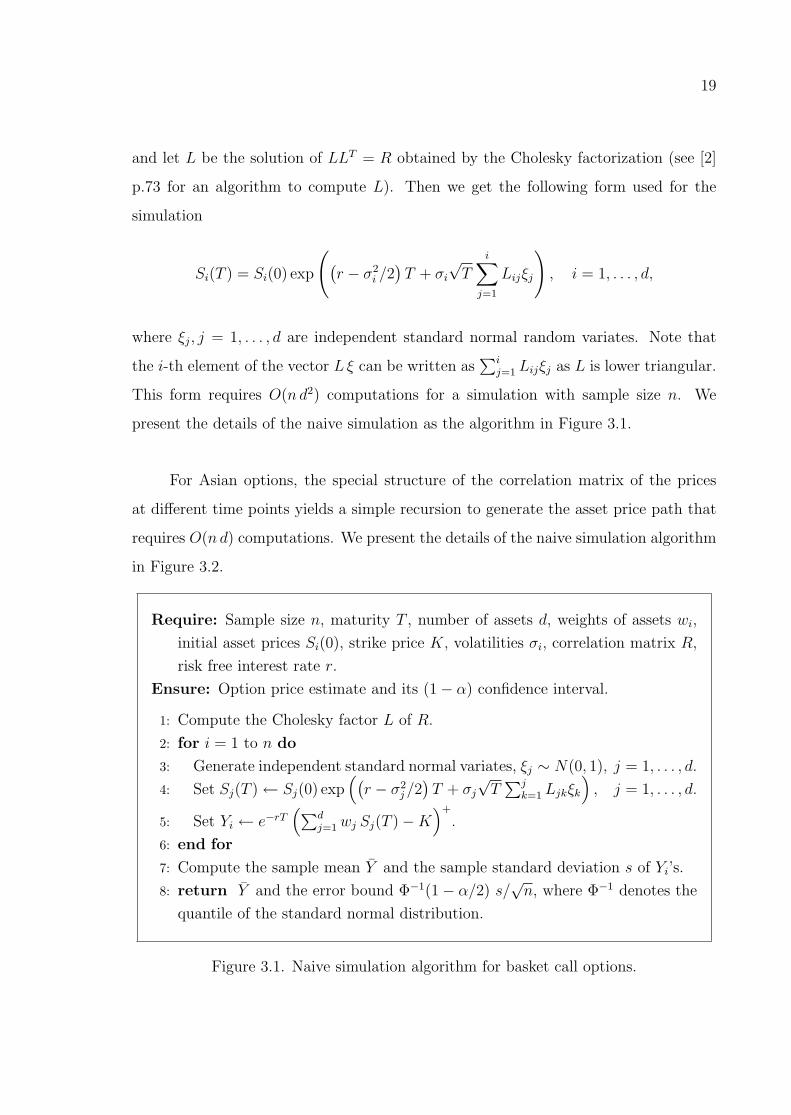
Figure 3.1. Naive simulation algorithm for basket call options. . . . . . . . . . 19

Figure 3.2. Naive simulation algorithm for Asian call options. . . . . . . . . . 20

Figure 3.3. Algorithm for the classical CV method for basket call options. . . 22

Figure 3.4. Algorithm for the classical CV method for Asian call options. . . . 23

Figure 3.5. Conditional simulation of the arithmetic average for basket options. 29

Figure 3.6. Conditional simulation of the arithmetic average for Asian options. 29

Figure 3.7. Optimal IS density g∗(x) ∝ q(x)φ(x) for an Asian option. T =

1, d = 12, σ = 0.1, S(0) = 100. Strike prices K = 90 (left), K = 100

(center) and K = 110 (right). . . . . . . . . . . . . . . . . . . . . 32

Figure 3.8. A new algorithm for basket call options (new CV, conditional sim-

ulation and IS). . . . . . . . . . . . . . . . . . . . . . . . . . . . . 33

Figure 3.9. Pilot simulation for λ. . . . . . . . . . . . . . . . . . . . . . . . . . 38

Figure 3.10. The influence of λ on variance. . . . . . . . . . . . . . . . . . . . . 39

Figure 3.11. Plot of A|X for the G-7 indices basket option example given in

Section 3.5.1.1 (T = 1, K = 100). . . . . . . . . . . . . . . . . . . 47

xi

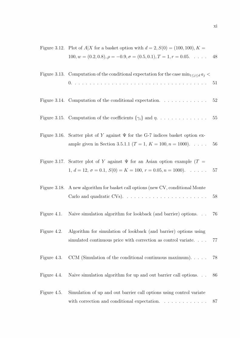
Figure 3.12. Plot of A|X for a basket option with d = 2, S(0) = (100, 100), K =

100, w = (0.2, 0.8), ρ = −0.9, σ = (0.5, 0.1), T = 1, r = 0.05. . . . . 48

Figure 3.13. Computation of the conditional expectation for the case min1≤j≤d aj <

0. . . . . . . . . . . . . . . . . . . . . . . . . . . . . . . . . . . . . 51

Figure 3.14. Computation of the conditional expectation. . . . . . . . . . . . . 52

Figure 3.15. Computation of the coefficients γi and η. . . . . . . . . . . . . . 55

Figure 3.16. Scatter plot of Y against Ψ for the G-7 indices basket option ex-

ample given in Section 3.5.1.1 (T = 1, K = 100, n = 1000). . . . . 56

Figure 3.17. Scatter plot of Y against Ψ for an Asian option example (T =

1, d = 12, σ = 0.1, S(0) = K = 100, r = 0.05, n = 1000). . . . . . 57

Figure 3.18. A new algorithm for basket call options (new CV, conditional Monte

Carlo and quadratic CVs). . . . . . . . . . . . . . . . . . . . . . . 58

Figure 4.1. Naive simulation algorithm for lookback (and barrier) options. . . 76

Figure 4.2. Algorithm for simulation of lookback (and barrier) options using

simulated continuous price with correction as control variate. . . . 77

Figure 4.3. CCM (Simulation of the conditional continuous maximum). . . . . 78

Figure 4.4. Naive simulation algorithm for up and out barrier call options. . . 86

Figure 4.5. Simulation of up and out barrier call options using control variate

with correction and conditional expectation. . . . . . . . . . . . . 87

xii

Figure 4.6. CSP (Calculation of the conditional survival probability of the con-

tinuous option). . . . . . . . . . . . . . . . . . . . . . . . . . . . . 88

Figure 5.1. R codes for generation of GH variates by numerical inversion. . . . 107

Figure 6.1. Algorithm for the general CV method. . . . . . . . . . . . . . . . 115

xiii

LIST OF TABLES

Table 3.1. Parameters of the G-7 indices basket option example of [1]. . . . . 62

Table 3.2. VRFs of different algorithms for basket options. . . . . . . . . . . . 63

Table 3.3. Pricing basket options with the algorithm given in Figure 3.18 (new

CV, conditional Monte Carlo and quadratic CVs); n = 10, 000. . . 65

Table 3.4. VRFs of different algorithms for Asian options. . . . . . . . . . . . 67

Table 3.5. Pricing Asian options with new CV, conditional Monte Carlo and

quadratic CVs; n = 10, 000. . . . . . . . . . . . . . . . . . . . . . . 68

Table 4.1. Numerical results for floating strike lookback put option. . . . . . . 91

Table 4.2. Numerical results for fixed strike lookback call option, σ=0.1. . . . 92

Table 4.3. Numerical results for the up and out barrier call option. . . . . . . 95

Table 4.4. The influence of the barrier level. . . . . . . . . . . . . . . . . . . . 95

Table 6.1. A basket of general CVs (Expectation-M: simpler expectation for-

mulas for the martingale case). . . . . . . . . . . . . . . . . . . . . 117

Table 7.1. Estimated daily parameters for different models. . . . . . . . . . . 126

Table 7.2. Numerical results for VG options with daily monitoring ∆t = 1/250;

n = 10, 000; Error: 95% error bound; VRF: variance reduction factor.130

xiv

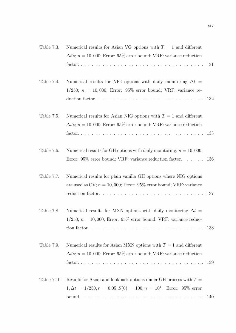
Table 7.3. Numerical results for Asian VG options with T = 1 and different

∆t’s; n = 10, 000; Error: 95% error bound; VRF: variance reduction

factor. . . . . . . . . . . . . . . . . . . . . . . . . . . . . . . . . . . 131

Table 7.4. Numerical results for NIG options with daily monitoring ∆t =

1/250; n = 10, 000; Error: 95% error bound; VRF: variance re-

duction factor. . . . . . . . . . . . . . . . . . . . . . . . . . . . . . 132

Table 7.5. Numerical results for Asian NIG options with T = 1 and different


factor. . . . . . . . . . . . . . . . . . . . . . . . . . . . . . . . . . . 133

Table 7.6. Numerical results for GH options with daily monitoring; n = 10, 000;

Error: 95% error bound; VRF: variance reduction factor. . . . . . 136

Table 7.7. Numerical results for plain vanilla GH options where NIG options

are used as CV; n = 10, 000; Error: 95% error bound; VRF: variance

reduction factor. . . . . . . . . . . . . . . . . . . . . . . . . . . . . 137

Table 7.8. Numerical results for MXN options with daily monitoring ∆t =

1/250; n = 10, 000; Error: 95% error bound; VRF: variance reduc-

tion factor. . . . . . . . . . . . . . . . . . . . . . . . . . . . . . . . 138

Table 7.9. Numerical results for Asian MXN options with T = 1 and different


factor. . . . . . . . . . . . . . . . . . . . . . . . . . . . . . . . . . . 139

Table 7.10. Results for Asian and lookback options under GH process with T =

1,∆t = 1/250, r = 0.05, S(0) = 100, n = 104. Error: 95% error

bound. . . . . . . . . . . . . . . . . . . . . . . . . . . . . . . . . . 140

xv

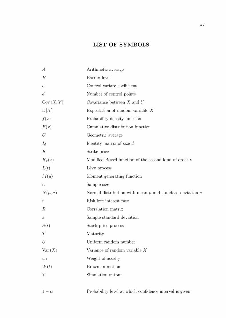
LIST OF SYMBOLS

A Arithmetic average

B Barrier level

c Control variate coefficient

d Number of control points

Cov (X, Y ) Covariance between X and Y

E [X] Expectation of random variable X

f(x) Probability density function

F (x) Cumulative distribution function

G Geometric average

Id Identity matrix of size d

K Strike price

Kν(x) Modified Bessel function of the second kind of order ν

L(t) Levy process

M(u) Moment generating function

n Sample size

N(µ, σ) Normal distribution with mean µ and standard deviation σ

r Risk free interest rate

R Correlation matrix

s Sample standard deviation

S(t) Stock price process

T Maturity

U Uniform random number

Var (X) Variance of random variable X

wj Weight of asset j

W (t) Brownian motion

Y Simulation output

1− α Probability level at which confidence interval is given

xvi

∆t Time interval between control points

εu u-resolution

ρXY Correlation between X and Y

φ(x) Probability density function of standard normal distribution

Φ(x) Cumulative distribution function of standard normal distri-

bution

ψ Payoff function

xvii

LIST OF ACRONYMS/ABBREVIATIONS

BM Brownian Motion

CDF Cumulative Distribution Function

CLT Central Limit Theorem

CMC Conditional Monte Carlo

CV Control Variate

EF Efficiency Factor

FFT Fast Fourier Transform

GBM Geometric Brownian Motion

GH Generalized Hyperbolic

GIG Generalized Inverse Gaussian

HW Half Width

IG Inverse Gaussian

IS Importance Sampling

MXN Meixner

NIG Normal Inverse Gaussian

PDE Partial Differential Equation

PDF Probability Density Function

VG Variance Gamma

VRF Variance Reduction Factor

1

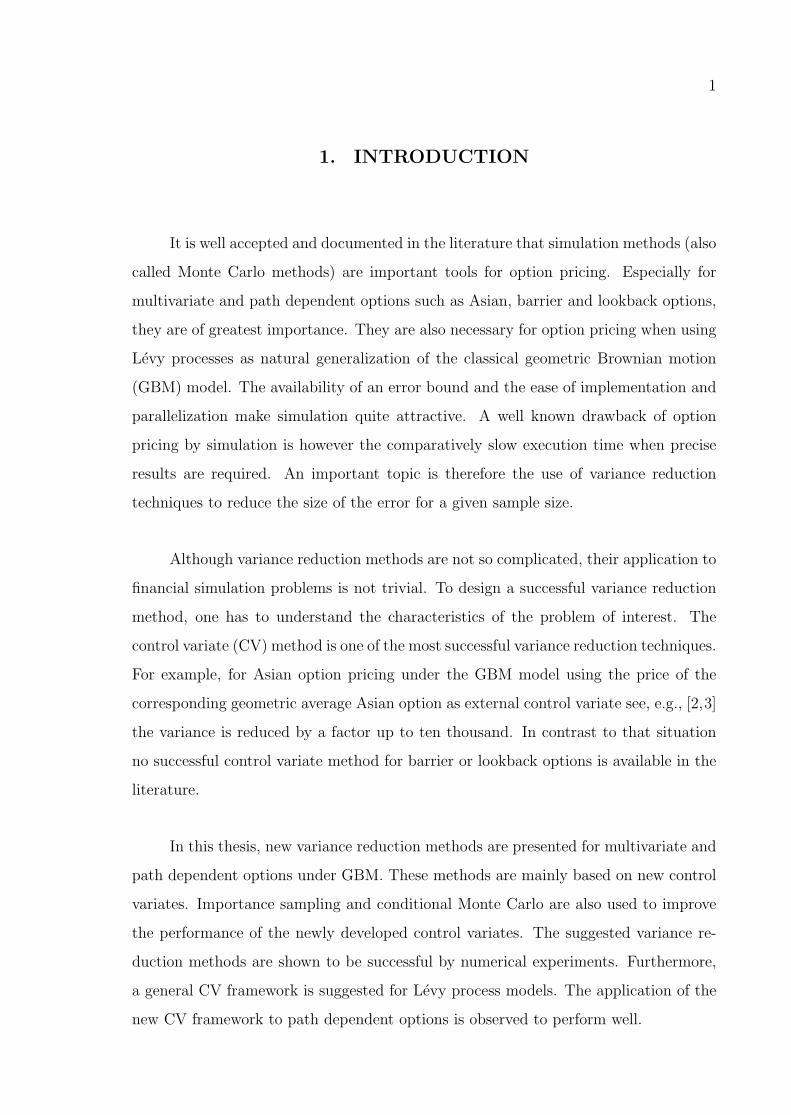
1. INTRODUCTION

It is well accepted and documented in the literature that simulation methods (also

called Monte Carlo methods) are important tools for option pricing. Especially for

multivariate and path dependent options such as Asian, barrier and lookback options,

they are of greatest importance. They are also necessary for option pricing when using

Levy processes as natural generalization of the classical geometric Brownian motion

(GBM) model. The availability of an error bound and the ease of implementation and

parallelization make simulation quite attractive. A well known drawback of option

pricing by simulation is however the comparatively slow execution time when precise

results are required. An important topic is therefore the use of variance reduction

techniques to reduce the size of the error for a given sample size.

Although variance reduction methods are not so complicated, their application to

financial simulation problems is not trivial. To design a successful variance reduction

method, one has to understand the characteristics of the problem of interest. The

control variate (CV) method is one of the most successful variance reduction techniques.

For example, for Asian option pricing under the GBM model using the price of the

corresponding geometric average Asian option as external control variate see, e.g., [2,3]

the variance is reduced by a factor up to ten thousand. In contrast to that situation

no successful control variate method for barrier or lookback options is available in the

literature.

In this thesis, new variance reduction methods are presented for multivariate and

path dependent options under GBM. These methods are mainly based on new control

variates. Importance sampling and conditional Monte Carlo are also used to improve

the performance of the newly developed control variates. The suggested variance re-

duction methods are shown to be successful by numerical experiments. Furthermore,

a general CV framework is suggested for Levy process models. The application of the

new CV framework to path dependent options is observed to perform well.

2

The options considered in this thesis are European basket, Asian, lookback and

barrier options. The basket and Asian options depend on the average of the stock

prices, while lookback and barrier options are contingent on the extremum (maximum

or minimum) stock price. As the characteristics of these options differ, they require

different variance reduction methods. The suggested methods in this thesis are designed

by considering the special properties of these options.

The organization of the thesis is as follows. In Chapter 2, the basics for simu-

lation are explained. Chapter 3 presents new variance reduction methods for basket

and Asian options. In Chapter 4, new control variate methods are introduced for bar-

rier and lookback options. Chapter 5 reviews Levy process models and the simulation

methods for these processes. Option pricing under Levy processes is also discussed

in that chapter. Chapter 6 introduces a general control variate method for Levy pro-

cess models, whereas Chapter 7 contains the application of the new method to path

dependent options. Finally, our conclusions are presented in Chapter 8.

3

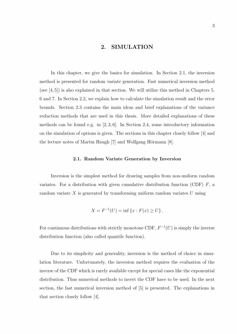
2. SIMULATION

In this chapter, we give the basics for simulation. In Section 2.1, the inversion

method is presented for random variate generation. Fast numerical inversion method

(see [4,5]) is also explained in that section. We will utilize this method in Chapters 5,

6 and 7. In Section 2.2, we explain how to calculate the simulation result and the error

bounds. Section 2.3 contains the main ideas and brief explanations of the variance

reduction methods that are used in this thesis. More detailed explanations of these

methods can be found e.g. in [2, 3, 6]. In Section 2.4, some introductory information

on the simulation of options is given. The sections in this chapter closely follow [4] and

the lecture notes of Martin Haugh [7] and Wolfgang Hormann [8].

2.1. Random Variate Generation by Inversion

Inversion is the simplest method for drawing samples from non-uniform random

variates. For a distribution with given cumulative distribution function (CDF) F , a

random variate X is generated by transforming uniform random variates U using

X = F−1(U) = inf x : F (x) ≥ U .

For continuous distributions with strictly monotone CDF, F−1(U) is simply the inverse

distribution function (also called quantile function).

Due to its simplicity and generality, inversion is the method of choice in simu-

lation literature. Unfortunately, the inversion method requires the evaluation of the

inverse of the CDF which is rarely available except for special cases like the exponential

distribution. Thus numerical methods to invert the CDF have to be used. In the next

section, the fast numerical inversion method of [5] is presented. The explanations in

that section closely follow [4].

4

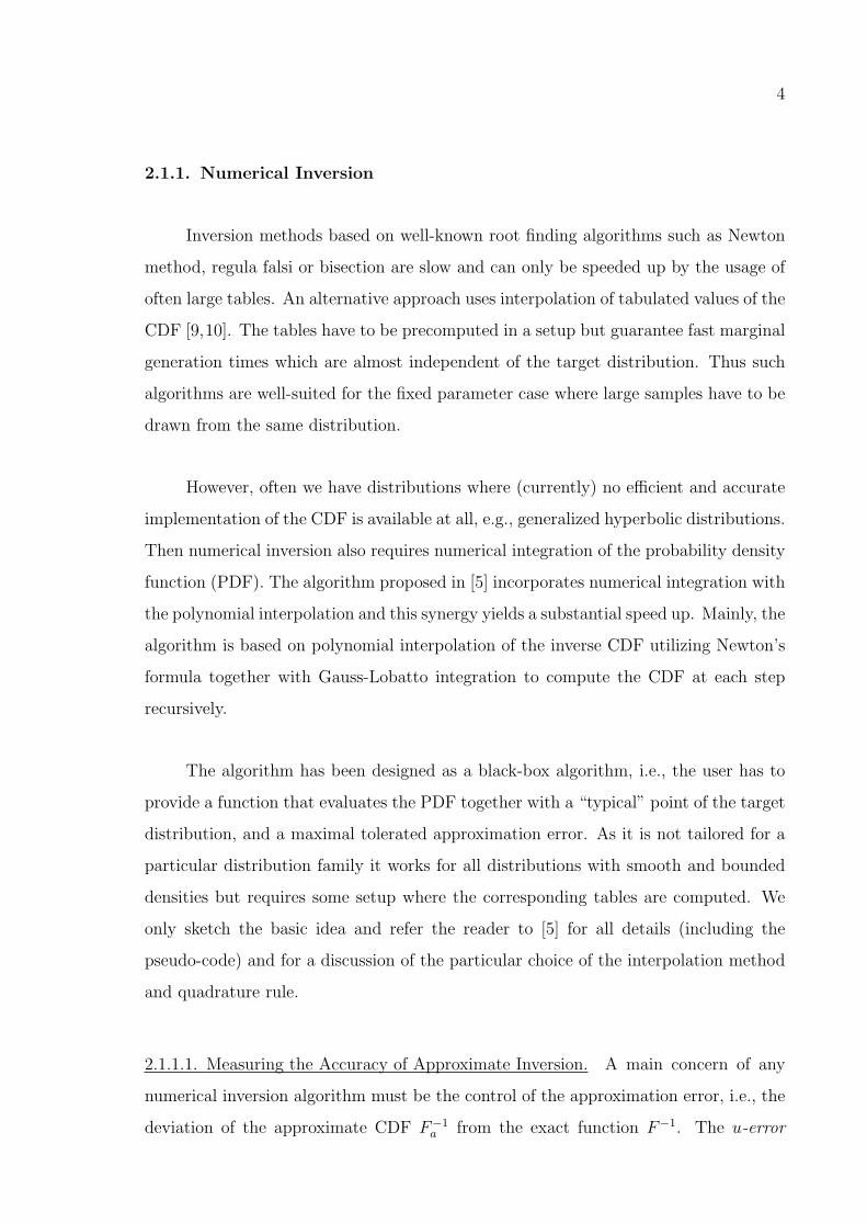
2.1.1. Numerical Inversion

Inversion methods based on well-known root finding algorithms such as Newton

method, regula falsi or bisection are slow and can only be speeded up by the usage of

often large tables. An alternative approach uses interpolation of tabulated values of the

CDF [9,10]. The tables have to be precomputed in a setup but guarantee fast marginal

generation times which are almost independent of the target distribution. Thus such

algorithms are well-suited for the fixed parameter case where large samples have to be

drawn from the same distribution.

However, often we have distributions where (currently) no efficient and accurate

implementation of the CDF is available at all, e.g., generalized hyperbolic distributions.

Then numerical inversion also requires numerical integration of the probability density

function (PDF). The algorithm proposed in [5] incorporates numerical integration with

the polynomial interpolation and this synergy yields a substantial speed up. Mainly, the

algorithm is based on polynomial interpolation of the inverse CDF utilizing Newton’s

formula together with Gauss-Lobatto integration to compute the CDF at each step

recursively.

The algorithm has been designed as a black-box algorithm, i.e., the user has to

provide a function that evaluates the PDF together with a “typical” point of the target

distribution, and a maximal tolerated approximation error. As it is not tailored for a

particular distribution family it works for all distributions with smooth and bounded

densities but requires some setup where the corresponding tables are computed. We

only sketch the basic idea and refer the reader to [5] for all details (including the

pseudo-code) and for a discussion of the particular choice of the interpolation method

and quadrature rule.

2.1.1.1. Measuring the Accuracy of Approximate Inversion. A main concern of any

numerical inversion algorithm must be the control of the approximation error, i.e., the

deviation of the approximate CDF F−1a from the exact function F−1. The u-error

5

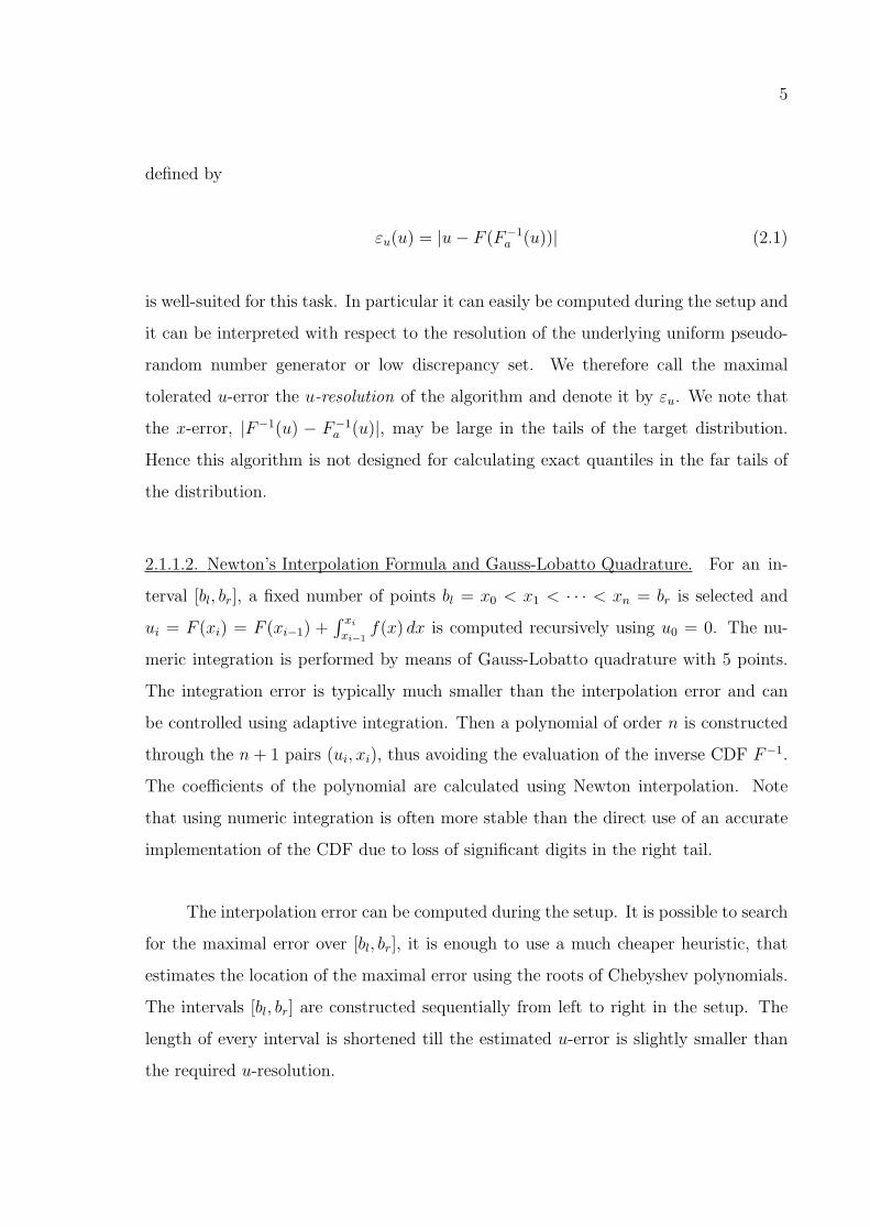
defined by

εu(u) = |u− F (F−1a (u))| (2.1)

is well-suited for this task. In particular it can easily be computed during the setup and

it can be interpreted with respect to the resolution of the underlying uniform pseudo-

random number generator or low discrepancy set. We therefore call the maximal

tolerated u-error the u-resolution of the algorithm and denote it by εu. We note that

the x-error, |F−1(u) − F−1a (u)|, may be large in the tails of the target distribution.

Hence this algorithm is not designed for calculating exact quantiles in the far tails of

the distribution.

2.1.1.2. Newton’s Interpolation Formula and Gauss-Lobatto Quadrature. For an in-

terval [bl, br], a fixed number of points bl = x0 < x1 < · · · < xn = br is selected and

ui = F (xi) = F (xi−1) +∫ xi

xi−1f(x) dx is computed recursively using u0 = 0. The nu-

meric integration is performed by means of Gauss-Lobatto quadrature with 5 points.

The integration error is typically much smaller than the interpolation error and can

be controlled using adaptive integration. Then a polynomial of order n is constructed

through the n+ 1 pairs (ui, xi), thus avoiding the evaluation of the inverse CDF F−1.

The coefficients of the polynomial are calculated using Newton interpolation. Note

that using numeric integration is often more stable than the direct use of an accurate

implementation of the CDF due to loss of significant digits in the right tail.

The interpolation error can be computed during the setup. It is possible to search

for the maximal error over [bl, br], it is enough to use a much cheaper heuristic, that

estimates the location of the maximal error using the roots of Chebyshev polynomials.

The intervals [bl, br] are constructed sequentially from left to right in the setup. The

length of every interval is shortened till the estimated u-error is slightly smaller than

the required u-resolution.

6

2.1.1.3. Cut-off Points for the Domain. The interpolation does not work for densities

where the inverse CDF becomes too steep. In particular this happens in the tails

of distributions with unbounded domains. Thus we have to find the computational

relevant part of the domain, i.e., we have to cut off the tails such that the probability

of either tail is negligible, say about 5% of the given u-resolution εu. Thus it does

not increase the u-error significantly. We approximate the tail of the distribution by a

function of the form x−c fitted to the tail in a starting point x0 and take the cut-off value

of that approximation. The asymptotic tail decay of the distributions that we consider

in this thesis (variance gamma, normal inverse Gaussian, generalized hyperbolic and

Meixner distributions, see Chapter 5) is typically exponential, more precisely of the

form axbe−cx.

2.1.1.4. Implementation.

• Implementation in C

A ready-to-use implementation of the numerical inversion algorithm can be found

in the C library UNU.RAN [11]. Thanks to that library, generating random

variables does not require more than an accurate implementation of the density of

the increments. Moreover, for the distributions considered in this thesis, we do not

have to implement the density as we have ready-to-use density implementations

in the UNU.RAN library.

• Implementation in R

The R package Runuran [12] makes the UNU.RAN library accessible within R [13].

• Implementation in other programming languages

The ready-to-use implementations in UNU.RAN can be used in any appropriate

computing environment that provides an API to use a C library. However, if one

prefers to code the numerical inversion algorithm from scratch, this code can then

be be used for the simulation of many different distributions.

7

2.2. Output Analysis

Monte Carlo is used to calculate the expected value or in other words the mean

of a certain random variate Y . We try to estimate µ = E [Y ] by using a generated

sample (Y1, . . . , Yn) of size n. We use simply the average of all generated variates Yi

for i = 1, . . . , n. For that sample average we write:

Y =1

n

n∑i=1

Yi .

The law of large numbers (LLN) implies that for the case of i.i.d. (independent

and identically distributed) random variates Yi (in other words for a random sample),

Y converges to µ, as n goes to infinity. We write µ = Y to indicate that we use the

sample mean as estimator for µ. We know from statistics that Y is the best unbiased

estimate for µ. We also know that E [Y ] = µ and Var (Y ) = σ2/n, where σ2 = Var (Y ).

All this guarantees that the simulation leads to a correct result. But it is also true that

for finite n, the error of the estimate µ− Y is always non-zero. Therefore, it is essential

to estimate the size of that error. For that purpose, we use the central limit theorem

(CLT). It states that for random samples and for Var (Y ) bounded, the distribution

of the sample mean converges to the normal distribution. Thus we can use the result:

With probability close to 1−α the difference between the sample mean and the correct

result is bounded by Φ−1(1− α/2) s/√n, or in formula notation:

P(|µ− Y | > Φ−1(1− α/2) s/

√n)≈ α ,

where Φ−1(.) denotes the inverse of the CDF of the standard normal distribution and

s is the sample standard deviation. This probabilistic error bound is asymptotically

valid. It thus may not be close to correct for small sample sizes. However, as the

sample size n is always large or very large (at least 10,000 in most applications), we do

not encounter such problems often.

8

2.3. Variance Reduction Methods

The main drawback of simulation is the slow rate of convergence: O(1/√n). In

fact, to get one more digit of accuracy, we need a 100 times larger sample size. Hence

it is of highest importance to reduce the variance. Clearly for a fixed error bound

smaller variance directly implies a smaller sample size and so smaller computational

time. Although variance reduction methods are not so complicated, their application

to financial simulation problems is not trivial. As noted by [2], to design a successful

variance reduction method, one has to understand the characteristics of the problem

of interest.

In this section, we give some basic information about the three main variance

reduction methods, which are mainly used in this thesis. These methods are the con-

trol variate method, importance sampling and conditional Monte Carlo, respectively.

Before giving the details of these methods, we first discuss the efficiency measures of

the variance reduction methods in Section 2.3.1.

2.3.1. Measuring Simulation Efficiency

Suppose there are two random variables, W and Y , such that E [W ] = E [Y ] = µ

and Var (W ) < Var (Y ). As both W and Y are unbiased estimates of µ, we could

choose to either simulate W1, . . .Wn or Y1, . . . , Yn. Let nw and ny be the number of

samples of W and Y , respectively, that are needed to achieve a certain error-bound

(also called half-width (HW) of the confidence interval). Then, from the formula for

the error bound, it is easy to see that

nw =Φ−1(1− α/2)2

HW 2Var (W ) and ny =

Φ−1(1− α/2)2

HW 2Var (Y ) .

From the above formulas for the required sample sizes, it is clear that, assuming

that the execution speed is similar for both methods, the variance reduction factor

V RF = Var (Y )/Var (W ) is the factor ny/nw by which the simulation of W is more

9

efficient than simulation of Y . In our examples, Y will often be the estimator of naive

simulation using no variance reduction, whereas W will denote the estimator of the

(hopefully) better new method using variance reduction.

To decide which method is more efficient we also need information about the speed

of the two different simulation methods. Let tY and tW denote the CPU times of the

simulation of Y and W , respectively. Then the efficiency factor of simulation W with

respect to simulation Y can be written as EF = (Var (Y ) tY )/(Var (W ) tW ). In practice

the speed depends very strongly on code details or on the computing environment used.

We therefore report in our numerical examples mostly the variance reduction factor

V RF = Var (Y )/Var (W ).

2.3.2. Control Variate Method

The control variate (CV) method is the most effective and broadly applicable

technique for variance reduction of simulation estimates. [2] defines the method as a

way of exploiting the information about the errors in estimates of known quantities to

reduce the error in an estimate of an unknown quantity. To describe the method, let’s

suppose that we wish to estimate µ = E [Y ], where Y is the output of a simulation

experiment. Suppose that X is also an output of the simulation or that we can easily

output it if we wish. Finally, we assume that we know E [X]. Then we can construct

many unbiased estimators of µ:

• µ = Y , our usual estimator.

• µc = Y − c (X − E [X]), where c is some real number.

Here X is called a control variate for Y . It is clear that E [µc] = µ. The question is

whether or not µc has a lower variance than µ. To answer this question, we compute

Var (µc) and get:

Var (µc) = Var (Y ) + c2 Var (X)− 2 cCov (X, Y ) .

10

Since we are free to choose c, we should choose it to minimize Var (µc). Simple calculus

then implies that the optimal value of c is given by

c∗ =Cov (X, Y )

Var (X).

Substituting for c∗ into the variance formula above we see that

Var (µc∗) = Var (Y )− Cov (X, Y )2

Var (X)

= Var (Y )− Var (Y ) Var (X) ρ2XY

Var (X)

= Var (Y )(1− ρ2XY ) ,

where ρXY denotes the correlation between X and Y . We therefore get the very simple

formula for the variance reduction factor: V RF = 1/(1 − ρ2XY ) , which is a sharply

increasing function of ρXY . The above formula shows that the CV method is successful

only if the selected CV is highly correlated with the original simulation output.

As we do not know Cov (X, Y ) and Var (X) in closed form, c∗ is usually not

available. But it can be easily estimated by using a pilot simulation run with a smaller

sample size or by using the full sample of the simulation. If we estimate c∗ directly

from the full sample of the simulation, the estimate µc∗ is biased. However, the bias is

of order O(1/n) and vanishes fast for growing n.

2.3.2.1. Multiple Control Variates. It is possible to use multiple CVs. Suppose that

there are m control variates X1, . . . , Xm and that each E [Xi] is known. Unbiased

estimators of µ can then be constructed by setting

µc = Y + c1(X1 − E [X1]) + · · ·+ cm(Xm − E [Xm]) .

It is clear again that E [µc] = µ. The question is whether the ci’s can be chosen such

that µc has a lower variance than µ, the usual estimator. As before, for a single control

11

variate, it is no problem to write down the variance of the estimate µc. It turns out that

the optimal CV coefficients, c∗1, . . . , c∗m, minimizing the variance are the least squares

solutions of the linear regression model with the response variable Y and the covariates

X1, . . . , Xm:

Y = a+ c∗1X1 + · · ·+ c∗mXm .

In R, there are special functions calculating the regression coefficients. These least

square estimates can be obtained by using a pilot run with a smaller sample size or

by using the full sample of the simulation. Like in the case of a single CV, the former

approach leads to an unbiased estimate whereas the latter has a bias of order O(1/n)

which is negligible unless the sample size is small. Note that for multiple control

variates the use of a pilot study is more important as the calculations necessary for

calculating the vector c∗ are slower than for a single control variate.

2.3.2.2. How to Select Control Variates?. Using control variates may lead to substan-

tial variance reduction but in practice the crucial question is: How can we find good

control variates? There are two possible approaches:

• Internal Control Variates: Use a simple function of random variates that are used

in the simulation anyway. In most cases these are simple functions of the “input

random variables” (the random numbers generated for the simulation).

The main advantage of this approach is that it is simple and the necessary extra

computations for such a control variate are fast. The disadvantage is that for

most applications the variance reduction is only moderate.

• External Control Variates: The result of a similar problem for which the exact

solution is known is used as a control variate.

The main disadvantage of this approach is that it is difficult and requires knowl-

edge to find such a control variate; also the additional computations may be quite

slow. The advantage is that for such control variates the variance reduction may

be huge.

12

2.3.3. Importance Sampling

In many simulations the events of main importance only occur with (very) small

probability. Such a situation is called a rare event simulation. Importance sampling

(IS) is the variance reduction technique especially (but not exclusively) useful for rare

event simulations.

The idea of importance sampling is easiest explained when using the integral

representation of simulation. We are interested to estimate the expectation

µ = E [Y ] = E f [q(X)] =

∫q(x) f(x) dx ,

where Y denotes the simulation output, x is the vector of length d of the input variables

of the simulation, the function q describes the operation of a single simulation run (i.e.

the transformation of the input variables x into the single output q(x)) and f(x) is the

joint density function of all input variables. Here the subscript f in E f [q(X)] indicates

that X has density f .

As an example consider the estimation of a very small probability by simulation.

In that case, most of the output values in simulation will be zero and thus the variance

of the result will be large. By generating from a distribution (the so called importance

sampling distribution) that has a higher probability to generate nonzero Y , we can

reduce the variance. Of course we have to do something to correct the error of not

generating from the correct distribution. Writing g(x) for the “importance sampling

density” the correction is done by using:

µ = E [Y ] = E g[q(X) f(X)/g(X)] =

∫q(x)

f(x)

g(x)g(x) dx .

The correction factor w(x) = f(x)/g(x) is called “weight” in the simulation and “likeli-

hood ratio” in the statistical literature. A single repetition of the importance sampling

algorithm consists of the following steps:

13

(i) Generate the input variable X with density g(x).

(ii) Calculate Y = q(X) f(X)/g(X).

If we make many independent repetitions of these two steps we again get an estimate

for µ and can also calculate an error bound. The only problem left is how to select

the IS-density g(x). Of course we must select g(x) such that it is possible to generate

random variates with density g(x) and we want to select g(x) such that the variance

of the estimate is small. It is possible to show that the variance is minimized for

g(x) =|q(x) f(x)|∫|q(x) f(x)| dx

.

In practice we cannot use this result directly as the denominator is of course unknown.

There is also another important theorem saying that the estimate of importance sam-

pling is unbiased and has a bounded variance if the IS-density g(x) has higher tails

than q(x) f(x). So there are two general selection rules:

• The importance sampling density g(x) should mimic the behaviour of |q(x) f(x)|

• The importance sampling density g(x) must have higher tails than |q(x) f(x)|.

2.3.4. Conditional Monte Carlo

Conditional Monte Carlo (CMC) is based on replacing the naive simulation es-

timate by its conditional expectation. Let the simulation output be a function of two

random inputs: Y = q(X,Z). If we apply CMC with conditioning variable Z, then

our new estimator is E [Y |Z]. As E [Y ] = E [E [Y |Z]], the new estimator is unbiased.

To see how the CMC reduces the variance, let’s write the total variance as

Var (Y ) = E [Var (Y |Z)] + Var (E [Y |Z]) .

The first part can be interpreted as the variance coming from X, while the second is the

variance coming from Z. If we use CMC with conditioning variable Z, then our new

14

estimator E [Y |Z] has the variance Var (E [Y |Z]). Thus CMC removes all the variance

coming from X.

When the conditioning variable Z has less influence on the output than the other

input variables (that is Var (E [Y |Z]) is much smaller than E [Var (Y |Z)]), we get a

significant variance reduction as the most important source of variability is smoothed

out. The biggest practical difficulty for the application of the CMC method is the

selection of the input variables for smoothing so that the conditional expectation is

both available in closed form (or at least in a form easy to evaluate) and has a small

variance.

2.4. Simulation of Options

Suppose that we have an option on a stock with the price process S(t), t ≥ 0

which is governed by a continuous time stochastic process. In Chapters 3 and 4, S(t)

follows a geometric Brownian motion (GBM), whereas in Chapters 5 and 7 it follows

a geometric Levy process. The detailed explanations of those stochastic processes can

be found in the respective chapters.

Let ψ denote the payoff function of the option. For discretely monitored path-

dependent options, ψ is a function from <d to < where d denotes the number of control

points in time. With time grid 0 = t0 < t1 < t2 < ... < td = T and maturity T , the

price of the option is given by the discounted risk neutral expectation of the payoff

function

Priceoption = e−r T E [ψ(S(t1), . . . , S(td))] ,

where r is the deterministic risk free interest rate.

To estimate the expectation by Monte Carlo simulation, we simulate n random

payoffs. The sample mean of those payoffs gives us an estimate for the expectation. As

n→∞, the estimator converges in distribution to the normal distribution. Thus we get

15

an asymptotically valid confidence interval for the price estimate by using the quantile

function of the standard normal distribution and the half width of the confidence

interval is a probabilistic error bound for the price estimate. We present the details of

the simulation algorithm in Figure 2.1.

Require: Sample size n, maturity T , number of control points d, initial stock

price S(0), payoff function ψ, risk free interest rate r.

Ensure: Option price estimate and its (1− α) confidence interval.

1: for i = 1 to n do

2: Simulate a stock price path, S(t1), . . . , S(td).

3: Set Yi ← e−r Tψ (S(t1), . . . , S(td)).

4: end for

5: Compute the sample mean Y and the sample standard deviation s of Yi’s.

6: return Y and the error bound Φ−1(1−α/2) s/√n, where Φ−1 denotes the

quantile of the standard normal distribution.

Figure 2.1. Simulation of path dependent options.

16

3. BASKET AND ASIAN OPTIONS

3.1. Introduction

In this chapter, a new variance reduction method is presented for European basket

and Asian options under the geometric Brownian motion assumption. It is based on a

new control variate method that uses the closed form of the expected payoff conditional

on the assumption that the geometric average of all prices is larger than the strike

price. The combination of that new control variate with conditional Monte Carlo and

quadratic control variates leads to the newly proposed algorithm. The contents and

presentation of this chapter closely follows Dingec and Hormann [14,15].

The payoff of basket options depends on the weighted average of the underlying

asset prices and there exists no closed form solution for the price of basket options.

Hence a number of studies emerged that suggest efficient numerical methods for basket

options. Tree methods, PDE based finite difference methods and Fourier transform

methods are among the most widely used techniques for option pricing. For one di-

mensional problems, PDE methods provide a fast solution with quadratic convergence.

However, for multivariate options, the computational complexity increases exponen-

tially with respect to the problem dimension. In fact, for dimensions larger than three,

Duffy [16] p. 270, suggests in his monography on PDE methods to use other techniques

rather than PDE based finite difference methods due to the curse of dimensionality.

Similar problems for increasing dimensions also occur for Fourier transform methods.

Thus for higher dimensional options the most applicable method seems to be Monte

Carlo simulation. Its speed of convergence is not influenced by the dimension of the

problem. In addition, it allows for a simple error bound.

Approximations are fast solution alternatives to the exact methods. There are

a number of studies suggesting new approximations or bounds for the price of basket

options, see, for instance, [1, 17–22]. The disadvantage of the approximations is that

the size of the error is unknown and there is no way to reduce the error.

17

The payoff of Asian options depends on the average of the prices of a single asset

at different time points. Thus the structure of the payoff is similar to that of basket

options. Like for basket options, there exists no closed form solution for the price of

Asian options. However, there are some fast techniques special to Asian options. The

one dimensional PDE method of [23,24] and the FFT based convolution method of [25]

are two important examples. Also, many approximations suggested for basket options

can be used or adapted for Asian options. See [26] for a recent survey of the methods

suggested for Asian options. As mentioned there, Monte Carlo simulation is also well

suited for pricing Asian options.

There are few studies suggesting new variance reduction methods for basket op-

tions (e.g. [27–29]). On the other hand, Asian options are often used as a test case

to exemplify the effectiveness of the general variance reduction methods, see, for ex-

ample, [30–37]. The control variate (CV) method of Kemna and Vorst [38] is widely

recommended in the literature and is regarded as the standard simulation method for

Asian options. We call it classical CV method in the sequel. It can be used for bas-

ket options as well. There are few papers attempting to improve this control variate

(e.g. [39]). However, these improvements are all moderate.

In this chapter, a new variance reduction method is developed for European

basket and Asian options under the geometric Brownian motion (GBM) using formulas

developed for approximation methods. Curran [17] proposes an accurate approximation

exploiting the dependency between the arithmetic and geometric average. We use

this approximation to reduce the variance by suggesting a new control variate and

combining it with conditional Monte Carlo and quadratic control variates. The new

algorithm is fairly simple and reaches very large variance reduction.

In Section 3.2, we formulate and explain the basic principles of the naive sim-

ulation. Section 3.3 presents the classical and the new control variate methods. In

Section 3.4, we introduce the conditional sampling, importance sampling, conditional

Monte Carlo and quadratic control variates to improve the new control variate method.

Section 3.5 reports our numerical results.

18

3.2. Simulation of Basket and Asian Options

The payoff of the basket options depends on the weighted arithmetic average of

the prices of d different assets whereas the payoff of Asian options depends on the

prices of a single asset at d different time points. We consider the GBM model for the

asset price dynamics. The weighted arithmetic average is given by A =∑d

i=1wi Γi,

where Γi’s are the set of prices and wi’s are the weights of these prices. Here each Γi

follows the lognormal distribution due to the GBM assumption. We also assume that

each wi > 0 and∑d

i=1wi = 1.

For basket options, Γi denotes the price of the asset i at maturity T , d the number

of assets, wi the weight of the asset i = 1, . . . , d. Let Si(t) denote the price of the asset

i at time t. Then Γi = Si(T ) and under GBM,

Si(T ) = Si(0) exp((r − σ2

i /2)T + σiWi(T )

), i = 1, . . . , d,

where r is the risk free interest rate, σi is the volatility of the asset i and Wi(T ), i =

1, . . . , d, are correlated standard Brownian motions with correlations ρij.

For Asian options, Γi denotes the asset price at time ti. That is, Γi = S(ti)

for a single asset S(t) following a GBM with risk free interest rate r and volatility σ.

0 = t0 < t1 < t2 < ... < td = T are the control points in time, d is the number of control

points and T is the maturity of the option. Also, each wi equals to 1/d. In this study,

we consider the case of equidistant monitoring intervals, that is ti − ti−1 = ∆t = T/d,

for i = 1, 2, . . . , d. The proposed methods can easily be extended to the case of unequal

intervals.

We restrict our attention to the pricing of call options with payoff function PA =

(A−K)+, where K is the strike price, as the put-call parity automatically yields the

price of the put option when the call option price is available.

For basket options, define R as d × d correlation matrix with entries Rij = ρij

19

and let L be the solution of LLT = R obtained by the Cholesky factorization (see [2]

p.73 for an algorithm to compute L). Then we get the following form used for the

simulation

Si(T ) = Si(0) exp

((r − σ2

i /2)T + σi

√T

i∑j=1

Lijξj

), i = 1, . . . , d,

where ξj, j = 1, . . . , d are independent standard normal random variates. Note that

the i-th element of the vector L ξ can be written as∑i

j=1 Lijξj as L is lower triangular.

This form requires O(n d2) computations for a simulation with sample size n. We

present the details of the naive simulation as the algorithm in Figure 3.1.

For Asian options, the special structure of the correlation matrix of the prices

at different time points yields a simple recursion to generate the asset price path that

requires O(n d) computations. We present the details of the naive simulation algorithm

in Figure 3.2.

Require: Sample size n, maturity T , number of assets d, weights of assets wi,

initial asset prices Si(0), strike price K, volatilities σi, correlation matrix R,

risk free interest rate r.


1: Compute the Cholesky factor L of R.


3: Generate independent standard normal variates, ξj ∼ N(0, 1), j = 1, . . . , d.

4: Set Sj(T )← Sj(0) exp((r − σ2

j/2)T + σj

√T∑j

k=1 Ljkξk

), j = 1, . . . , d.

5: Set Yi ← e−rT(∑d

j=1wj Sj(T )−K)+

.

6: end for


8: return Y and the error bound Φ−1(1− α/2) s/√n, where Φ−1 denotes the


Figure 3.1. Naive simulation algorithm for basket call options.

20

Require: Sample size n, maturity T , number of control points d, initial asset

price S(0), strike price K, volatility σ, risk free interest rate r.

Ensure: Option price estimate and its 1− α confidence interval.

1: Set ∆t← T/d.



4: Set S(tj)← S(tj−1) exp(

(r − σ2/2)∆t+ σ√

∆t ξj

), j = 1, . . . , d.

5: Set Yi ← e−rT(Pd

j=1 S(tj)

d−K

)+

.

6: end for




Figure 3.2. Naive simulation algorithm for Asian call options.

3.3. Control Variates

In this section, we first explain the classical CV method of Kemna and Vorst [38]

and then continue with proposing a similar but much more efficient CV method based

on using the geometric average as a conditioning variable for PA.

3.3.1. The Classical Control Variate

The merits of the classical CV method of [38] for simulating Asian options are

well known in the literature (see, e.g., [2, 3, 26]). Actually it seems to be considered

the state-of-the-art method for Asian option pricing by simulation. Especially for the

cases of low volatility and short maturity, the variance is reduced by factors up to ten

thousand. Due to the similarity between basket and Asian options, the classical CV

method of [38] can be used for basket options as well.

There is no apparent way to find a closed-form solution for the price of an arith-

metic average option as the arithmetic average of the observed prices is the average of

lognormal variates and thus has a non tractable distribution. This situation changes

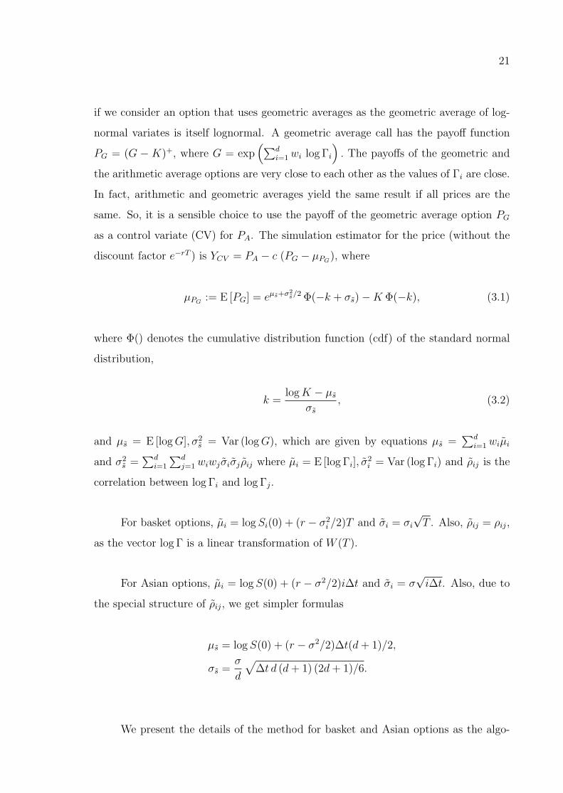
21

if we consider an option that uses geometric averages as the geometric average of log-

normal variates is itself lognormal. A geometric average call has the payoff function

PG = (G −K)+, where G = exp(∑d

i=1wi log Γi

). The payoffs of the geometric and

the arithmetic average options are very close to each other as the values of Γi are close.

In fact, arithmetic and geometric averages yield the same result if all prices are the

same. So, it is a sensible choice to use the payoff of the geometric average option PG

as a control variate (CV) for PA. The simulation estimator for the price (without the

discount factor e−rT ) is YCV = PA − c (PG − µPG), where

µPG:= E [PG] = eµs+σ2

s/2 Φ(−k + σs)−K Φ(−k), (3.1)

where Φ() denotes the cumulative distribution function (cdf) of the standard normal

distribution,

k =logK − µs

σs, (3.2)

and µs = E [logG], σ2s = Var (logG), which are given by equations µs =

∑di=1wiµi

and σ2s =

∑di=1

∑dj=1 wiwjσiσj ρij where µi = E [log Γi], σ

2i = Var (log Γi) and ρij is the

correlation between log Γi and log Γj.

For basket options, µi = logSi(0) + (r − σ2i /2)T and σi = σi

√T . Also, ρij = ρij,

as the vector log Γ is a linear transformation of W (T ).

For Asian options, µi = logS(0) + (r − σ2/2)i∆t and σi = σ√i∆t. Also, due to

the special structure of ρij, we get simpler formulas

µs = logS(0) + (r − σ2/2)∆t(d+ 1)/2,

σs =σ

d

√∆t d (d+ 1) (2d+ 1)/6.

We present the details of the method for basket and Asian options as the algo-

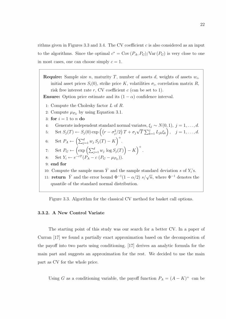
22

rithms given in Figures 3.3 and 3.4. The CV coefficient c is also considered as an input

to the algorithms. Since the optimal c∗ = Cov (PA, PG)/Var (PG) is very close to one

in most cases, one can choose simply c = 1.



risk free interest rate r, CV coefficient c (can be set to 1).



2: Compute µPGby using Equation 3.1.




j/2)T + σj

√T∑j

k=1 Ljkξk

), j = 1, . . . , d.

6: Set PA ←(∑d

j=1wj Sj(T )−K)+

.

7: Set PG ←(

exp(∑d

j=1wj logSj(T ))−K

)+

.

8: Set Yi ← e−rT (PA − c (PG − µPG)).

9: end for




Figure 3.3. Algorithm for the classical CV method for basket call options.

3.3.2. A New Control Variate

The starting point of this study was our search for a better CV. In a paper of

Curran [17] we found a partially exact approximation based on the decomposition of

the payoff into two parts using conditioning. [17] derives an analytic formula for the

main part and suggests an approximation for the rest. We decided to use the main

part as CV for the whole price.

Using G as a conditioning variable, the payoff function PA = (A −K)+ can be

23


price S(0), strike price K, volatility σ, risk free interest rate r, CV coefficient

c (can be set to 1).

Ensure: Option price estimate and its 1− α confidence interval.

1: Set ∆t← T/d.

2: Compute µPGby using Equation 3.1.



5: Set logS(tj)← logS(tj−1) + (r − σ2/2)∆t+ σ√

∆t ξj, j = 1, . . . , d.

6: Set PA ←(Pd

j=1 S(tj)

d−K

)+

and PG ←(

exp

(Pdj=1 logS(tj)

d

)−K

)+

.

7: Set Yi ← e−rT (PA − c (PG − µPG)).

8: end for


10: return Y and Φ−1(1 − α/2) s/√n, where Φ−1 denotes the quantile of the

standard normal distribution.

Figure 3.4. Algorithm for the classical CV method for Asian call options.

split into two parts

(A−K)+ = (A−K)+ 1G≤K + (A−K)+ 1G>K

= (A−K)+ 1G≤K + (A−K) 1G>K , (3.3)

where the second equality follows from the fact that A > G always holds; thus the

condition G > K implies A > K and we can drop the plus in the second term of

Equation 3.3. Our idea is to use exactly that second term of Equation 3.3, W =

(A −K) 1G>K, as CV for PA. We expect that the first term will be zero in most of

the replications due to the strong dependence between A and G. So, the payoff PA

will be equal to our CV in most of the replications. This should imply a strong linear

dependence and a large variance reduction factor (VRF).

Our CV estimator is thus simply YCV = PA−c (W−E [W ]), where PA = (A−K)+

is the naive simulation estimator and W = (A−K) 1G>K is our control variate.

24

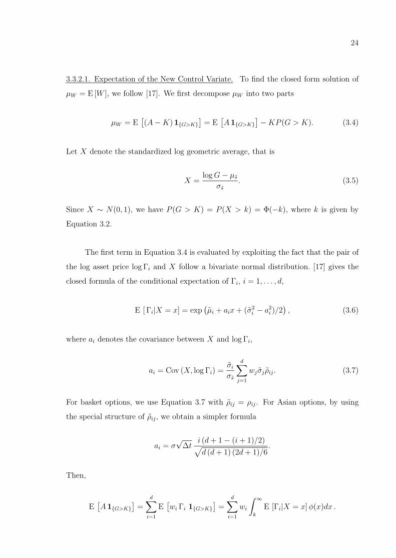
3.3.2.1. Expectation of the New Control Variate. To find the closed form solution of

µW = E [W ], we follow [17]. We first decompose µW into two parts

µW = E[(A−K) 1G>K

]= E

[A1G>K

]−KP (G > K). (3.4)

Let X denote the standardized log geometric average, that is

X =logG− µs

σs. (3.5)

Since X ∼ N(0, 1), we have P (G > K) = P (X > k) = Φ(−k), where k is given by

Equation 3.2.

The first term in Equation 3.4 is evaluated by exploiting the fact that the pair of

the log asset price log Γi and X follow a bivariate normal distribution. [17] gives the

closed formula of the conditional expectation of Γi, i = 1, . . . , d,

E [ Γi|X = x] = exp(µi + aix+ (σ2

i − a2i )/2

), (3.6)

where ai denotes the covariance between X and log Γi,

ai = Cov (X, log Γi) =σiσs

d∑j=1

wjσj ρij. (3.7)

For basket options, we use Equation 3.7 with ρij = ρij. For Asian options, by using

the special structure of ρij, we obtain a simpler formula

ai = σ√

∆ti (d+ 1− (i+ 1)/2)√d (d+ 1) (2d+ 1)/6

.

Then,

E[A1G>K

]=

d∑i=1

E[wi Γi 1G>K

]=

d∑i=1

wi

∫ ∞k

E [Γi|X = x]φ(x)dx .

25

By integration we obtain the following closed formula

µW =

(d∑i=1

wi eµi+σ

2i /2 Φ (−k + ai)

)−KΦ(−k). (3.8)

3.4. Improving the New Control Variate Method

As our numerical experiments show that the optimal c∗ = Cov (Y,W )/Var (W ) is

very close to one in most cases, we decided to fix c = 1 in our method. For the control

variate estimate we can thus write YCV = PA −W + µW . Using Equation 3.3 we get

YCV = V + µW with V = (A−K)+ 1G≤K.

So, we estimate the option price by adding µW to the estimator of E [V ]. With this final

form, our CV method can be interpreted as another variance reduction method called

indirect estimation, see [40] p. 155. Here we indirectly estimate the price by simulating

V = (A−K)+ 1G≤K and adding µW instead of simulating the payoff PA = (A−K)+

itself.

We first tried to use the approximation of [17] for µV = E [V ] as an additional

CV. However, we have seen that the approximation is not well suited as CV since its

correlation with the payoff is not large enough. Then we realized that the key for a

further reduction of the variance is to use c = 1. This choice does not cause a significant

loss of efficiency, but as it allows simulating conditional on the geometric average, it

opens the way to a further substantial variance reduction based on importance sampling

and conditional Monte Carlo.

The simulation of V = (A−K)+ 1G≤K is a rare event simulation problem due

to the strong dependence between A and G. It is a well known fact that, for such

problems, importance sampling (IS) and conditional Monte Carlo (CMC) are the most

suitable variance reduction techniques. We first employ an IS algorithm in Section 3.4.2

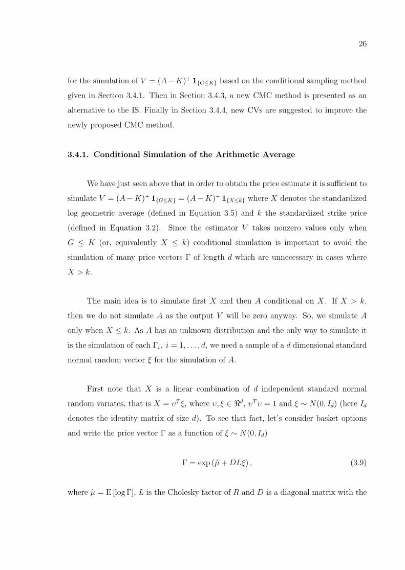
26

for the simulation of V = (A−K)+ 1G≤K based on the conditional sampling method

given in Section 3.4.1. Then in Section 3.4.3, a new CMC method is presented as an

alternative to the IS. Finally in Section 3.4.4, new CVs are suggested to improve the

newly proposed CMC method.

3.4.1. Conditional Simulation of the Arithmetic Average

We have just seen above that in order to obtain the price estimate it is sufficient to

simulate V = (A−K)+ 1G≤K = (A−K)+ 1X≤k where X denotes the standardized

log geometric average (defined in Equation 3.5) and k the standardized strike price

(defined in Equation 3.2). Since the estimator V takes nonzero values only when

G ≤ K (or, equivalently X ≤ k) conditional simulation is important to avoid the

simulation of many price vectors Γ of length d which are unnecessary in cases where

X > k.

The main idea is to simulate first X and then A conditional on X. If X > k,

then we do not simulate A as the output V will be zero anyway. So, we simulate A

only when X ≤ k. As A has an unknown distribution and the only way to simulate it

is the simulation of each Γi, i = 1, . . . , d, we need a sample of a d dimensional standard

normal random vector ξ for the simulation of A.

First note that X is a linear combination of d independent standard normal

random variates, that is X = υT ξ, where υ, ξ ∈ <d, υTυ = 1 and ξ ∼ N(0, Id) (here Id

denotes the identity matrix of size d). To see that fact, let’s consider basket options

and write the price vector Γ as a function of ξ ∼ N(0, Id)

Γ = exp (µ+DLξ) , (3.9)

where µ = E [log Γ], L is the Cholesky factor of R and D is a diagonal matrix with the

27

entries σi, i = 1, . . . , d. By noting that µs = wT µ, we obtain

X =(wT log Γ− µs

)/σs

=(wT (µ+DLξ)− µs

)/σs

=(wT µ+

(wTDLξ

)− µs

)/σs

= υT ξ,

where υT = wTDL/σs. The entries of the vector υ are given by

υi =υi√∑dj=1 υ

2j

, (3.10)

where υj =∑d

i=1wiσiLij, j = 1, . . . , d. For Asian options, by using similar arguments,

we obtain

υi =d− i+ 1√∑dj=1(d− j + 1)2

=d− i+ 1√

d (d+ 1) (2d+ 1)/6, i = 1, . . . , d.

The important fact that conditioning in the multivariate normal again leads to a

multivariate normal (see e.g. [2] p.65) is the starting point for our conditional simulation

method. More precisely, if

Y1

Y2

∼ N

µ1

µ2

,

Σ11 Σ12

Σ21 Σ22

,

then

(Y1|Y2 = x) ∼ N(µ1 + Σ12Σ−1

22 (x− µ2) , Σ11 − Σ12Σ−122 Σ21

). (3.11)

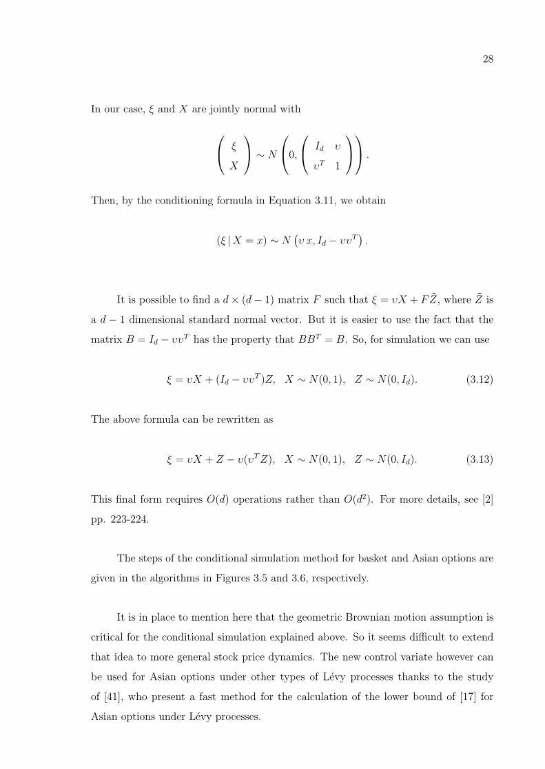
28

In our case, ξ and X are jointly normal with

ξ

X

∼ N

0,

Id υ

υT 1

.

Then, by the conditioning formula in Equation 3.11, we obtain

(ξ |X = x) ∼ N(υ x, Id − υυT

).

It is possible to find a d× (d− 1) matrix F such that ξ = υX + FZ, where Z is

a d − 1 dimensional standard normal vector. But it is easier to use the fact that the

matrix B = Id − υυT has the property that BBT = B. So, for simulation we can use

ξ = υX + (Id − υυT )Z, X ∼ N(0, 1), Z ∼ N(0, Id). (3.12)

The above formula can be rewritten as

ξ = υX + Z − υ(υTZ), X ∼ N(0, 1), Z ∼ N(0, Id). (3.13)

This final form requires O(d) operations rather than O(d2). For more details, see [2]

pp. 223-224.

The steps of the conditional simulation method for basket and Asian options are

given in the algorithms in Figures 3.5 and 3.6, respectively.

It is in place to mention here that the geometric Brownian motion assumption is

critical for the conditional simulation explained above. So it seems difficult to extend

that idea to more general stock price dynamics. The new control variate however can

be used for Asian options under other types of Levy processes thanks to the study

of [41], who present a fast method for the calculation of the lower bound of [17] for

Asian options under Levy processes.

29

Require: Value of the conditioning variable X, maturity T , weights of assets

wi, initial stock prices Si(0), volatilities σi, risk free interest rate r, Cholesky

factor of the correlation matrix L, the coefficients υi (see Equation 3.10).

Ensure: A conditional sample of the arithmetic average.

1: Generate d dimensional standard normal vector, Z ∼ N(0, Id).

2: Set ξ ← υX + Z − υ(υTZ).


j/2)T + σj

√T∑j

k=1 Ljkξk

), j = 1, . . . , d.

4: return∑d

j=1wj Sj(T ).

Figure 3.5. Conditional simulation of the arithmetic average for basket options.

Require: Value of the conditioning variable X, maturity T , number of control

points d, initial stock price S(0), volatility σ, risk free interest rate r.

Ensure: A conditional sample of the arithmetic average.

1: Set ∆t← T/d.

2: Set υj ← (d− j + 1)/√d (d+ 1) (2d+ 1)/6, j = 1, . . . , d.


4: Set ξ ← υX + Z − υ(υTZ).

5: Set S(tj)← S(tj−1) exp((r − σ2/2)∆t+ σ√

∆t ξj), j = 1, . . . , d.

6: returnPd

j=1 S(tj)

d.

Figure 3.6. Conditional simulation of the arithmetic average for Asian options.

30

3.4.2. Importance Sampling

The simulation output V = (A−K)+ 1X≤k takes a nonzero value only if both

G ≤ K (or, equivalently, X ≤ k) and A > K are true. This is a highly rare event

due to the strong dependence between G and A. Our idea is to further reduce the

variance of the estimator by sampling from X values which are more likely to yield

nonzero simulation outputs. In other words, we perform a one dimensional importance

sampling (IS) by changing the distribution of X. Due to the conditional simulation

method presented in Section 3.4.1, one dimensional IS yields a simple and effective

simulation algorithm.

It can be seen that performing IS just for X can result in a significant variance

reduction by considering the two components of the variance,

Var (V ) = E [Var (V |X)] + Var (E [V |X]) . (3.14)

Here E [Var (V |X)] can be called the “unexplained” variance (not explained by X)

whereas Var (E [V |X]) can be called “explained” variance. Due to the strong cor-

relation between G and A, the unexplained variance is expected to be small. (Our

numerical experiments confirmed that it was typically less than two percent of the

total variance.) So, the variance is largely determined by the second term which can

be reduced by using an IS method for X. Here X can be regarded as a “direction”

for importance sampling, as it is in fact a linear combination of the standard normal

variates forming the stock price path. Since this linear combination explains much of

the variability of the estimator V , one dimensional IS in the direction of X can be

quite successful.

Let g denote our IS density for X. Our new estimator under g is V φ(X)/g(X),

where φ is the original density (the standard normal density). The weight φ(X)/g(X) is

the likelihood ratio evaluated atX. The new estimator is unbiased, E g[V φ(X)/g(X)] =

µV . Here the subscript g indicates that X has density g. The variance of this new

31

estimator under g is

Var g

(Vφ(X)

g(X)

)= E g

[(φ(X)

g(X)

)2

Var (V |X)

]+ Var g

(φ(X)

g(X)E [V |X]

). (3.15)

The first term in Equation 3.15, i.e. the “unexplained variance” is very small unless the

likelihood ratio takes extremely large values. So, the main aim is reducing the second

term. Let q(x) denote the conditional expectation of V given that X = x, that is

q(x) = E [V |X = x]. The density, g∗(x) = q(x)φ(x)/µV with domain −∞ < x ≤ k, is

known as optimal IS density and completely removes the second term in Equation 3.15.

(Note that the second term in Equation 3.15 is Var g

(φ(X)g(X)

q(X))

. If we use g∗(x) =

q(x)φ(x)/µV then Var g∗(φ(X)g∗(X)

q(X))

= Var g∗(µV ) = 0). As neither q(x) nor µV

are available in closed form, we select a parametric family of distributions, which is

expected to contain densities that are sufficiently close to the optimal IS density g∗(x).

For practically all parameter values, g∗(x) has a shape similar to the exponential

function. This fact is a consequence of the strong dependence of A on X. In fact,

q(x) takes the largest values in k and decreases sharply when x decreases; this is easily

understood as the probability that the arithmetic average A will be larger than the

strike price K is very small when x is clearly smaller than k. Even for the case k > 0

the shape of g∗(x) is similar to an exponentially increasing function, as the increase

in q(x) is much stronger than the decrease in φ(x). One situation where the shape

of g∗(x) clearly changes, are deep out of the money cases for Asian options with long

maturity and large volatility. There the long maturity and large volatility reduces the

correlation between A and G and g∗(x) looks likes a normal density with chopped

right tail. The other situation is the case of basket options on negatively correlated

assets. In those cases, q(x) may not be a monotically increasing increasing function,

see Section 3.4.3.2.

What we have discussed above is visualised in Figure 3.7 that shows our simula-

tion estimates of g∗(x) ∝ q(x)φ(x) for an in the money, at the money and out of the

money cases of an Asian option.

32

−2.20 −2.18 −2.16 −2.14 −2.12

0.00

00.

001

0.00

20.

003

0.00

40.

005

x

q(x)

φ(x)

−0.45 −0.44 −0.43 −0.42 −0.41 −0.40

0.00

00.

005

0.01

00.

015

0.02

0

xq(

x)φ(

x)

1.06 1.08 1.10 1.12 1.14 1.16

0.00

00.

005

0.01

00.

015

0.02

00.

025

0.03

0

x

q(x)

φ(x)

Figure 3.7. Optimal IS density g∗(x) ∝ q(x)φ(x) for an Asian option.

T = 1, d = 12, σ = 0.1, S(0) = 100. Strike prices K = 90 (left), K = 100 (center) and

K = 110 (right).

We conclude that using the exponential distribution as IS density is a good and

simple choice, as the exponential density has a shape similar to the optimal IS density

g∗(x) in most cases. Even in extreme cases, the use of the exponential distribution

yields a considerable variance reduction. Therefore we use as IS density the shifted

negative exponential distribution with density ge(x) = λ eλ(x−k), −∞ < x ≤ k, where

λ and k are the rate and shift parameters, respectively. The parameter k is given by

Equation 3.2, but the parameter λ is unknown and should be selected such, that the

variance is minimized.

In the algorithm in Figure 3.8, we give details of the new CV method which

is improved by conditional simulation and importance sampling. The algorithm is

presented for basket options. Its modification for Asian options is straightforward. In

the algorithm, the likelihood ratio φ(X)/ge(X) is simply calculated using φ(X)/(λU).

This is correct as ge(X) = λU for the uniform random variate U required for generating

X = k + (1/λ) logU by inversion. The rate parameter λ of the IS density is given as

an argument to the algorithm. For the selection of λ, a pilot simulation method is

proposed in Section 3.4.2.1.

3.4.2.1. Selection of λ. In order to find a nearly optimal λ, we start from the equation

ge(k) = g∗(k) that guarantees that our exponential IS density has a value close to the

33



risk free interest rate r.



2: Compute k by using Equation 3.2.

3: Compute µW by using Equation 3.8.

4: Compute the coefficients υi by using Equation 3.10.

5: Compute the rate parameter λ of the IS density using the algorithm in Fig-

ure 3.9.


7: Generate U ∼ U(0, 1) and set X ← k + (1/λ) logU .

8: Generate A|X by using the algorithm in Figure 3.5.

9: Set Yi ← e−rT[(A−K)+ φ(X)/(λU) + µW

].

10: end for


12: return Y and Φ−1(1− α/2) s/√n.

Figure 3.8. A new algorithm for basket call options (new CV, conditional simulation

and IS).

34

optimal value at x = k. Solving this equation yields

λ =q(k)φ(k)

µV.

q(k) is available in closed form

q(k) = E [V |X = k] = E [A−K|X = k] = E [A|X = k]−K =d∑i=1

wiE [Γi|X = k]−K.

The second equality is due to the fact that X = k implies A > K. (Note that

X = k is by definition equivalent to G = K and G is a lower bound for A.) By using

Equation 3.6, we get

q(k) =d∑i=1

wi exp(µi + aix+ (σ2

i − a2i )/2

)−K. (3.16)

Of course µV is unknown. In fact it is exactly the value we are trying to estimate

by our simulation. To find an initial estimate for µV , we propose an approximate but

very fast simulation procedure to evaluate the integral µV =∫ k−∞ q(x)φ(x)dx where

again q(x) = E [V |X = x]. To obtain a fast approximation of q(x) we approximate

the dependence between A and G by a linear function of G. That is A|G d=G + ε for

some random residual term ε, which is assumed to be independent of G. (Hered=

denotes equality in distribution.) Note that [17] also makes this assumption and con-

tinues approximating ε by a lognormal distribution whose first two moments match the

distribution of A|G = K. We follow a different direction: rather than approximating

the distribution of ε we exactly simulate it at G = K. It is not difficult to show that

the approximate relation A|G d=G+ ε implies that

(A|X = x)d= (A |X = k) + eµs+σsx −K, for x < k . (3.17)

35

To show the above result, we can write

(A |G = K)d=K + ε and (A |G = G0)

d=G0 + ε,

for some G0 < K. Then we obtain the following approximate relation

(A |G = G0)d= (A |G = K) +G0 −K,

by using the fact that εd= (A|G = K)−K. The geometric average G0 can be written

as G0 = eµs+σsx for some x < k. Hence we obtain Equation 3.17.

The simulation estimate for q(x) is then

q(x) =

∑nj=1 [(Aj|X = x)−K]+

n=

∑nj=1 [(Aj |X = k) + eµs+σsx − 2K]+

n, for x < k,

where (Aj|X = x), j = 1, . . . , n, are independent and identically distributed (iid)

samples of (A|X = x). To obtain the required estimate for µV we approximate its

integral using

µV =

∫ k

−∞q(x)φ(x)dx ≈

m∑i=0

q(xi)φ(xi)∆x,

where −∞ < xm < . . . < x0 = k are equidistant evaluations points with xi − xi+1 =

∆x = (x0 − xm)/m, that is xi = k − i∆x, i = 0, . . . ,m. Combining the above two

formulas we get the formula for the estimate:

µV =m∑i=0

(∑nj=1 [(Aj |X = k) + eµs+σs(k−i∆x) − 2K]+

n

)φ(k − i∆x)∆x,

The computation of the above formula is faster if we change the order of summation

36

obtaining:

µV =

∑nj=1 Vj

n, with Vj =

m∑i=0

[(Aj |X = k) + eµs+σs(k−i∆x) − 2K

]+φ(k − i∆x)∆x,

(3.18)

where ∆x = (k − xm)/m. We select xm in the following way

xm =

log(2K−MA)−µs

σs, if 2K > MA

−6, if 2K ≤MA

(3.19)

where MA = max1≤j≤n(Aj|X = k).

Note that for 2K > MA, the value of [(Aj |X = k) + eµs+σsx − 2K]+

is zero for

any x < (log (2K −MA)− µs)/σs and j = 1, . . . , n. Since it is not sensible to consider

x values yielding zero, the domain of x is truncated at xm = (log (2K −MA)−µs)/σs.

On the other hand, for 2K < MA, we do not have such a situation. Hence the domain

of x is truncated at xm = −6 as the normal density and also the integrand are very

close to zero for x values smaller than −6.

Thus we have arrived at the following estimate for a close to optimal λ

λ =q(k)φ(k)

µV, (3.20)

where q(k) and µV are given by Equations 3.16 and 3.18, respectively.

As we use the estimated λ for IS it is important to consider that a higher value of

λ results in an exponential density ge(X) with a lighter tail. A light tail, however, may

cause extremely large values of φ(X)/ge(X) with small probabilities. In that case, the

distribution of the sample mean will be highly skewed and also the total variance is

increased due to the “unexplained variance” term in Equation 3.14 that may become

non-negligible if λ is selected too large. So an estimate for λ, which is larger than the

optimal λ∗ , may result in a large and also in unstable variance estimates yielding a

37

poor coverage level for the final confidence interval, see Sectiom 3.4.2.2. It is therefore

sensible to use a probabilistic lower bound as estimate for λ.

As a result of the delta method in statistics (see [40] p.75), as n→∞, the estimate

λ converges in distribution to a normal random variate with the mean q(k)φ(k)/µV

and variance

(q(k)φ(k))2σ2V

µ4V

,

where µV = E [V ] and σ2V

= Var (V ). Thus the interval (λLB,∞) with

λLB = q(k)φ(k)

(1

µV+ Φ−1(α)

σVµ2V

√n

), (3.21)

where µV and σV are the sample estimates of µV and σV , respectively, is an asymp-

totically valid one sided 1− α percent confidence interval for λ = q(k)φ(k)/µV . Using

the probabilistic lower bound λLB given in Equation 3.21 as estimate for λ helps us to

be on the safe side, as it will give with a probability of 1− α estimates for λ that are

smaller than the optimal λ∗.

In extremely deep out of the money cases with large volatility and long maturity,

as K becomes larger, λ approaches zero, since g∗(k) becomes very small due to the

bell shape of g∗(x). However, such a small λ does not yield a considerable variance

reduction. So, we take the maximum of 1 and λLB to ensure variance reduction even

for extreme cases.

The details of the method are given in Algorithm 3.9. It must be pointed out

that the pilot simulation given by Algorithm 3.9 is very fast. The choices of n = 1000

and m = 5 are sufficient to obtain λ values which are close to the optimal λ∗. The

pilot run with such a small sample size takes negligible amount of time.

38

Require: Sample size n, number of sample points m, confidence level for the

lower bound 1− α.

Ensure: A value of λ, close to the optimal λ∗ but smaller than it.

1: Compute µs, σs, k and q(k).

2: Generate an iid sample of (Aj|X = k), j = 1, . . . , n, by the algorithm in

Figure 3.5 (for basket options) or Figure 3.6 (for Asian options).

3: Compute xm by using Equation 3.19 and set ∆x← (k − xm)/m.

4: Set Vj ←(∑m

i=0

[(Aj |X = k) + eµs+σs(k−i∆x) − 2K

]+φ(k − i∆x)∆x

), j =

1, . . . , n.

5: Compute the sample mean µV and the sample standard deviation σV of

Vj’s.

6: Set λLB ← q(k)φ(k)(

1µV

+ Φ−1(α)σV

µ2V

√n

).

7: return max(λLB, 1).

Figure 3.9. Pilot simulation for λ.

3.4.2.2. The Influence of λ on the Variance. To show the strong influence of λ on the

variance, here we provide plots of the estimates of the variance Var g (V φ(X)/g(X)),

where V = (A−K)+ 1X≤k is our usual estimator, φ(X)/g(X) is the likelihood ratio

and g(x) = λ eλ(x−k), for −∞ < x < k, is the exponential IS density. In Figure 3.10,

for an Asian option example, the variances estimated by simulation with a sample of

size n = 106 are plotted versus the used values of λ (we used common random numbers

to obtain the results). We repeated our variance estimation five times with different

random number seeds. So, we see five different curves in Figure 3.10. The parameters

used for this Asian option example are T = 1, d = 12, r = 0.05, σ = 0.1, S(0) =

100, K = 100. We observe that selecting a λ larger than the optimal one not only

increases the variance but also decreases the stability of the variance estimate. In

fact, for smaller λ values the five variance curves coincide whereas for larger values the

variance estimates are very different. This figure shows the importance of selecting λ

small enough. The marks on the horizontal axes show the results we obtained when

estimating λ 20 times using 20 independent pilot simulation. They show the good

performance of the pilot simulation.

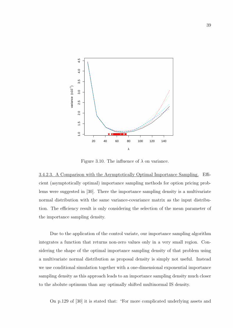
39

20 40 60 80 100 120 140

1.0

1.5

2.0

2.5

3.0

3.5

4.0

4.5

λ

varia

nce

(x1

0−7)

Figure 3.10. The influence of λ on variance.

3.4.2.3. A Comparison with the Asymptotically Optimal Importance Sampling. Effi-

cient (asymptotically optimal) importance sampling methods for option pricing prob-

lems were suggested in [30]. There the importance sampling density is a multivariate

normal distribution with the same variance-covariance matrix as the input distribu-

tion. The efficiency result is only considering the selection of the mean parameter of

the importance sampling density.

Due to the application of the control variate, our importance sampling algorithm

integrates a function that returns non-zero values only in a very small region. Con-

sidering the shape of the optimal importance sampling density of that problem using

a multivariate normal distribution as proposal density is simply not useful. Instead

we use conditional simulation together with a one-dimensional exponential importance

sampling density as this approach leads to an importance sampling density much closer

to the abolute optimum than any optimally shifted multinormal IS density.

On p.129 of [30] it is stated that: “For more complicated underlying assets and

40

option payoffs we find candidate drift vectors through numerical optimization. Veri-

fying global optimality is often difficult, but ultimately what matters is the variance

reduction achieved, and this can be assessed directly.”

We are in that situation. Due to the control variate we have a complicated

function left. We use a numerical procedure to find the parameters of the importance

sampling density. We cannot show any type of optimality but we can observe that the

variance reduction achieved is huge; for our problem (plain basket and Asian options) it

is also much larger than the variance reduction achieved by the asymptotically optimal

method in [30].

3.4.3. Conditional Monte Carlo

We have observed that as V generally takes zero values in most of the replications,

the simulation problem for evaluating E [V ] is a rare event simulation. Our first attempt

was therefore to use IS. In this section, we try conditional Monte Carlo (CMC) where

the estimator is replaced by its conditional expectation.

In Section 3.4.1, it was shown that for conditional sampling of V we need two

random inputs: the standardized log geometric average X and the normal vector of

length of d, Z. According to the law of the total variance, we have

Var (V ) = Var (E [V |Z]) + E [Var (V |Z)].

Due to the strong dependence between G and A, the first term Var (E [V |Z]) is expected

to be small. So, the variance is largely determined by the second term. When the

conditional expectation E [V |Z] is used for the CMC estimator, the variance of the new

estimator is Var (E [V |Z]). Thus the largest variance term E [Var (V |Z)] is removed and

we obtain a significant variance reduction. In Section 3.4.3.1, we present the details of

the evaluation of E [V |Z].

Our experiments show that CMC and IS yield very close variance reductions.

41

However, due to the additional computations required for the evaluation of E [V |Z],

CMC results in a slower algorithm than IS. So, CMC may not appear to be a strong

alternative to the IS method. Nevertheless, as shown in Section 3.4.4, CMC opens the

way to a further substantial variance reduction by using new CVs.

It is important to note that conditional Monte Carlo has the additional advan-

tage of converting the simulation output to a smooth function of the inputs. This is

important for Quasi Monte Carlo applications, where the smoothness of the integrand

has a significant impact on the convergence speed, see [3], and for the sensitivity (or

Greek) estimation by finite difference and pathwise derivative methods, see [2] chap.7.

3.4.3.1. Evaluation of the Conditional Expectation. Let’s write the arithmetic aver-

age as a function of the two random inputs shown in Equation 3.12: A = f(X,Z)

where X ∼ N(0, 1) and Z ∼ N(0, I). Then we have

E [V |Z = z] = E [(f(X,Z)−K)+1X≤k|Z = z] =

∫ k

−∞(f(x, z)−K)+φ(x)dx. (3.22)

Our aim is to find the closed form expression of E [V |Z = z]. Since the above integral

is one dimensional, it is not difficult to derive a simple expression for E [V |Z = z].

However, as the integral is taken with respect to the variable x, we need a representation

showing the explicit dependence on x:

f(x, z) =d∑i=1

wi eaixsi(z). (3.23)

It is obtained by using the conditional simulation formula in Equation 3.12. Here the

coefficients si, i = 1, . . . , d, depend only on z and the ai, i = 1, . . . , d, do not depend on

x or z.

• Basket Options

To see how Equation 3.23 is obtained, let’s first consider basket options and write

the price vector Γ as a function of ξ ∼ N(0, Id) as we have done in Equation 3.9.

42

Then replacing ξ by υX + (Id − υυT )Z, we get

Γ = exp (µ+DLξ)

= exp(µ+DL

(υX + (Id − υυT )Z

))= exp (DLυX) exp

(µ+DL(Id − υυT )Z

)= eaXs(Z).

Here a = DLυ and s(Z) = exp(µ+DL(Id − υυT )Z

). Therefore, as the arith-

metic average is given by A = wT Γ, we obtain Equation 3.23. Note that

a = Cov (X, log Γ). So, the ai’s are given by Equation 3.7 with ρij = ρij. The

explicit form of si(Z) is

si(Z) = Si(0) exp

((r − σ2

i /2)T + σi√T

i∑j=1

Lij ξj

), i = 1, . . . , d, (3.24)

where ξ = Z − υ(υTZ). Note that ξ is the part of ξ that depends only on Z but

not on X. That is ξ = υ X + ξ, see Equation 3.13.

• Asian Options

For Asian options, let’s rewrite Γ as Γ = exp(µ+ σ

√∆t L ξ

), where σ is the

volatility of the single asset, ∆t = T/d and L is a lower triangular matrix of

which the entries on and below the diagonal are all equal to one. Then we obtain

a = σ√

∆t Lυ and s(Z) = exp(µ+ σ

√∆t L(Id − υυT )Z

). More explicitly,

ai = σ√

∆ti∑

j=1

υj = σ√

∆ti (d+ 1− (i+ 1)/2)√d (d+ 1) (2d+ 1)/6

and si(Z) = S(0) exp(

(r − σ2/2)i∆t+ σ√

∆t∑i

j=1 ξj

), where ξ = Z − υ(υTZ).

Note that it is possible to write a simple recursion for si(Z)’s

si(Z) = si−1(Z) exp(

(r − σ2/2)∆t+ σ√

∆t ξi

), for i = 1, . . . , d, (3.25)

with s0(Z) = S(0). So, for Asian options, we need O(n d) computations like for

43

naive simulation.

For Asian options, ai is positive for all i = 1, . . . , d. However, for basket options,

some of the ai’ s can be negative if there exist negative correlations in the correlation

matrix R. Let’s first consider the case that min1≤i≤d ai ≥ 0. The other case will be

analyzed in more detail in Section 3.4.3.2.

The case of min1≤i≤d ai ≥ 0: First note that f(k, z) > K for any z, since A > G and

f(k, z) = A > G = exp(µs + σsk) = K.

Also, since all ai’s are positive, f(x, z) is a strictly increasing function of x. Thus the

equation f(x, z)−K = 0 has a unique root. Moreover, the root is smaller than k, since

f(k, z) > K. Let b(z) denote the root for a given fixed z, i.e. f(b(z), z)−K = 0. Then

we can write the integral in Equation 3.22 as

E [V |Z = z] =

∫ k

b(z)

(f(x, z)−K)φ(x)dx

=

∫ k

b(z)

(d∑i=1

wi eaixsi(z)−K

)φ(x)dx

=d∑i=1

wi si(z)

∫ k

b(z)

eaixφ(x)dx−K∫ k

b(z)

φ(x)dx

=d∑i=1

wi si(z) ea2i /2 [Φ(k − ai)− Φ(b(z)− ai)]−K [Φ(k)− Φ(b(z))] .

(3.26)

In Equation 3.26, the only unknown expression which is not available in closed

form is b(z). To evaluate it, we use Newton’s root finding method (also called Newton-

Raphson method). It requires the first derivative of the function ϕ(x) of which the

44

root is required. In our case, ϕ(x) = f(x, z)−K and so

ϕ(x) =d∑i=1

wi eaixsi(z)−K, (3.27)

ϕ′(x) =d∑i=1

wi ai eaixsi(z). (3.28)

As the starting point for Newton’s method we suggest

x0(z) = k − ϕ(k)

ϕ′(k)= k −

∑di=1wi e

aiksi(z)−K∑di=1 wi ai e

aiksi(z), (3.29)

which is the root of the first order approximation of ϕ(x) at the point k. The reason for

that selection is the close proximity of b(z) to k, which is due to the strong dependence

between A and G.

Conditional Monte Carlo reduces the variance but it increases the execution time.

Actually, the calculation of the coefficients si(z) has the same order of computations

as that of the generation of the prices in naive simulation, as it can be seen from Equa-

tions 3.24 and 3.25. However, there are two main sources of additional computations

that make CMC slower. The first one is Newton’s method; at each iteration of the

method, we have d calls to the exponential function to evaluate ϕ(x) and ϕ′(x). As

the root b(z) has to be recomputed for each replication of Z, these evaluations increase

the computational burden. Fortunately, the number of iterations is quite small as b(z)

lies close to k due to the strong dependence between A and G. In fact, the number

of iterations that we observed in our experiments were always smaller than five for a

tolerance of tol = 10−14.

The second additional computational burden are the d+ 1 calls to the cdf of the

standard normal distribution Φ() in Equation 3.26. The terms reevaluated at each

replication are Φ(b(z)) and Φ(b(z)−ai), i = 1, . . . , d. Due to these computations, con-

ditional Monte Carlo results in a slower algorithm. Therefore, introducing additional

checks to prevent unnecessary computations is of importance for the efficiency of the

45

method. Such checks are especially crucial for the case of min1≤i≤d ai < 0 where we

have to evaluate more than one root as we will show in Section 3.4.3.2.

Using x0(z) instead of k as a starting point can be regarded as one of the efforts

to speed up the method. x0(z) is in fact the number that we will obtain at the first

iteration of the Newton’s method if we use k as the staring point. The advantage of

using it instead of k is the pre-computation of the constants eaik’s before the simulation

starts. So, in fact, we get the same result with one iteration less.

3.4.3.2. The Case of min1≤i≤d ai < 0. In this section, the case of min1≤i≤d ai < 0 is

analyzed and detailed algorithms are provided for the evaluation of E [V |Z]. First

note that max1≤i≤d ai is always positive, since otherwise limx→+∞ f(x, z) = 0 which

contradicts the fact that A > G. That is, at least one of ai’s has to be positive. This

means that limx→−∞ ϕ(x) = limx→+∞ ϕ(x) =∞. Also, note that for a fixed z,

ϕ′′(x) =d∑i=1

wi a2i e

aixsi(z) > 0.

The inequality holds, since all wi and si’s are positive. So, ϕ(x) is a convex function

and has a unique minimum.

Let bl(z) and br(z) denote the roots of ϕ(x) = f(x, z) −K at the left and right

hand sides, respectively. Also, let bmin(z) denote the value minimizing ϕ(x). That is

bmin(z) = arg minx

ϕ(x) = arg minx

f(x, z)−K.

If ϕ(bmin(z)) ≥ 0, then we have no root or a single root and

E [V |Z = z] =

∫ k

−∞(f(x, z)−K)+φ(x)dx =

∫ k

−∞(f(x, z)−K)φ(x)dx

=d∑i=1

wi si(z) ea2i /2Φ(k − ai)−KΦ(k). (3.30)

46

Otherwise, we have two roots bl(z), br(z) and

E [V |Z = z] =

∫ k

−∞(f(x, z)−K)+φ(x)dx

=

∫ bl(z)

−∞(f(x, z)−K)φ(x)dx+

∫ k

br(z)

(f(x, z)−K)φ(x)dx

= IL + IR,

where

IL =d∑i=1

wi si(z) ea2i /2Φ(bl(z)− ai)−KΦ(bl(z)) (3.31)

and IR is given by Equation 3.26 with b(z) = br(z).

The naive algorithm to evaluate E [V |Z] requires bmin(z), br(z) and bl(z). How-

ever, finding bl(z) by Newton-Raphson method is expensive compared to br(z), as we

do not have a starting point very close to bl(z). Furthermore, IL given in Equation 3.31

is usually insignificant. In practice, even if there exist negative correlations in the cor-

relation matrix R, they are often not strong compared to the positive ones. Indeed,

the magnitudes of the negative ai’s are usually small compared to the positive ones. In

those cases, bl(z) takes extremely small values and so IL becomes insignificant. Note

that the cost of evaluating IL is d+ 1 calls to Φ().

In Figure 3.11, we show the plot of a realization of A|X = x (i.e. f(x, z) for a given

z) with respect to x for the G-7 indices basket option example given in Section 3.5.1.1

with parameters T = 1, K = 100. In this example, there are negative correlations in

R, but they are not strong. We can observe that bl(z) is smaller than −500. In this

region, the cdf of the standard normal distribution Φ(x) is almost zero. So, here in

fact only one root br(z) is necessary to evaluate E [V |Z] as IL is clearly insignificant.

In Figure 3.12, we show the plot of a realization of A|X = x (i.e. f(x, z) for a

given z) for a quite unrealistic basket option example with parameters d = 2, S(0) =

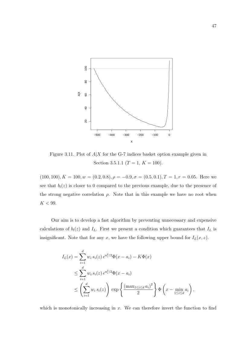
47

−500 −400 −300 −200 −100 0

2040

6080

100

X

A|X

Figure 3.11. Plot of A|X for the G-7 indices basket option example given in

Section 3.5.1.1 (T = 1, K = 100).

(100, 100), K = 100, w = (0.2, 0.8), ρ = −0.9, σ = (0.5, 0.1), T = 1, r = 0.05. Here we

see that bl(z) is closer to 0 compared to the previous example, due to the presence of

the strong negative correlation ρ. Note that in this example we have no root when

K < 99.

Our aim is to develop a fast algorithm by preventing unnecessary and expensive

calculations of bl(z) and IL. First we present a condition which guarantees that IL is

insignificant. Note that for any x, we have the following upper bound for IL(x, z).

IL(x) =d∑i=1

wi si(z) ea2i /2Φ(x− ai)−KΦ(x)

≤d∑i=1

wi si(z) ea2i /2Φ(x− ai)

≤

(d∑i=1

wi si(z)

)exp

(max1≤i≤d ai)

2

2

Φ

(x− min

1≤i≤dai

),

which is monotonically increasing in x. We can therefore invert the function to find

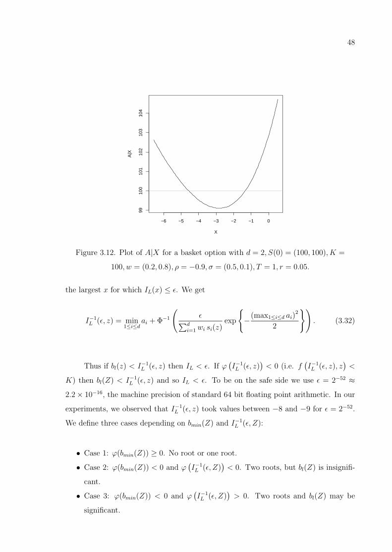
48

−6 −5 −4 −3 −2 −1 0

9910

010

110

210

310

4

X

A|X

Figure 3.12. Plot of A|X for a basket option with d = 2, S(0) = (100, 100), K =

100, w = (0.2, 0.8), ρ = −0.9, σ = (0.5, 0.1), T = 1, r = 0.05.

the largest x for which IL(x) ≤ ε. We get

I−1L (ε, z) = min

1≤i≤dai + Φ−1

(ε∑d

i=1wi si(z)exp

−(max1≤i≤d ai)

2

2

). (3.32)

Thus if bl(z) < I−1L (ε, z) then IL < ε. If ϕ

(I−1L (ε, z)

)< 0 (i.e. f

(I−1L (ε, z), z

)<

K) then bl(Z) < I−1L (ε, z) and so IL < ε. To be on the safe side we use ε = 2−52 ≈

2.2× 10−16, the machine precision of standard 64 bit floating point arithmetic. In our

experiments, we observed that I−1L (ε, z) took values between −8 and −9 for ε = 2−52.

We define three cases depending on bmin(Z) and I−1L (ε, Z):

• Case 1: ϕ(bmin(Z)) ≥ 0. No root or one root.

• Case 2: ϕ(bmin(Z)) < 0 and ϕ(I−1L (ε, Z)

)< 0. Two roots, but bl(Z) is insignifi-

cant.

• Case 3: ϕ(bmin(Z)) < 0 and ϕ(I−1L (ε, Z)

)> 0. Two roots and bl(Z) may be

significant.

49

To detect Case 1, we have to find bmin(Z) numerically. We compute it by solving

the first order condition ϕ′(x) = 0 using Newton-Raphson method with starting point

k. Note that ϕ′′(x) is available in closed form. If we have two roots (i.e. ϕ(bmin(Z)) <

0), we compute br(Z) using Newton-Raphson method with starting point x0(Z). If

ϕ(I−1L (ε, Z)

)> 0, then we compute bl(Z) using Newton-Raphson method with starting

point I−1L (ε, Z). If ϕ

(I−1L (ε, Z)

)< 0, then IL is neglected. In the algorithm given in

Figure 3.13, we present the details.

A faster variant: The algorithm in Figure 3.13 is not the best possible procedure, due

to the unnecessary evaluations of bmin(Z) by Newton-Raphson method. It is possible

to develop the more efficient Algorithm 3.14 by adding three simple pretests before

evaluating ϕ(bmin(Z)) > 0.

First we check the condition x0(Z) > k (line 6) as it directly implies that there is

no root. Note that x0(Z) > k can be true only when ϕ′(k) < 0 as ϕ(k) > 0 is always

true. If ϕ′(k) < 0, then bmin(Z) > k. So,

f(bmin(Z), Z) > exp (µs + σs bmin(Z)) > exp(µs + σsk) = K,

due to the fact that A > G. Thus ϕ(bmin(Z)) > 0 and we have no root.

Next we check if x0(Z) is extremely small, since in this case the probability of

having no root is quite large. Note that x0(Z) takes an extremely small (or large) value

only when ϕ′(k) is close to zero, which is the case when bmin(Z) is close to k. On the

other hand, when bmin(Z) = k, we have ϕ(bmin(Z)) > 0 (i.e. no root), since

f(bmin(Z), Z) = f(k, Z) > exp(µs + σsk) = K,

because of the fact that A > G. Thus for the cases where bmin(Z) is close to k, the

probability of having no root is quite large. Therefore, if x0(Z) < −10, we use the

algorithm in Figure 3.13 to exactly check if ϕ(bmin(Z)) > 0. The last pretest checks

50

the number of iterations of Newton-Raphson method for the evaluation of br(Z). If

the number of iterations equals to a prespecified number N but still the error is not

smaller than the tolerance, tol, then it is likely that there is no root. In this case,

we use the algorithm in Figure 3.13 to exactly check if ϕ(bmin(Z)) > 0. Otherwise we

accept the resulting value as the root br(Z). Here it should be noted that the maximum

number N for the iterations is introduced only for that specific part of the algorithm

(lines 9-10) where we try to evaluate br(Z) but we are not sure about its existence.

For the other root findings, we do not have to restrict the number of iterations, as the

Newton’s method is guaranteed to converge in those cases. The rest of the algorithm,

lines 14-18, where we check the significance of bl(Z) is the same as in the algorithm in

Figure 3.13.

Our numerical experiments show that a reasonable choice for N is between 5

and 10 depending on tol. However, it is also true that selecting a small N is not

creating problems as the algorithm in Figure 3.13 is a complete algorithm covering

all possible cases. For typical examples of the correlation matrix without very strong

negative correlations, the algorithm in Figure 3.14 is about three times faster than the

algorithm in Figure 3.13.

3.4.4. Quadratic Control Variates

In this section, a new control variate method is presented for the simulation of

E [V |Z]. It is related to a lower bound proposed by Curran [17] for µV . First note that

µV can be written as

µV = E [E [V |X]] = E [E [(A−K)+1X≤k|X]] = E [1X≤kE [(A−K)+|X]].

As the function g(x) = x+ is convex, we have E [(Y )+] ≥ (E [Y ])+ by Jensen’s inequal-

ity. Then

E [(A−K)+|X] ≥ (E [A−K|X])+ = (E [A|X]−K)+.

51

Require: Coefficients ai, wi, si(Z), k, strike price K, tolerance for the

Newton’s method tol, critical value I−1L (ε, Z) (see Equation 3.32).

Ensure: Conditional expectation Y = E [V |Z].

1: Compute the root bmin(Z) of ϕ′(x) by Newton’s method with starting point

k.

2: if ϕ(bmin(Z)) > 0 then

3: Case of no root4: Compute Y by Equation 3.30.

5: else

6: Case of two roots7: Compute br(Z) by Newton’s method with starting point x0(Z).

8: Compute IR by Equation 3.26 with b(Z) = br(Z) and set Y ← IR.

9: if ϕ(I−1L (ε, Z)

)> 0 then

10: Compute bl(Z) by Newton’s method with starting point I−1L (ε, Z).

11: Compute IL by Equation 3.31 and set Y ← Y + IL.

12: end if

13: end if

14: return Y .

Figure 3.13. Computation of the conditional expectation for the case min1≤j≤d aj < 0.

52

Require: Coefficients ai, wi, si(Z), k, strike price K, tolerance for the

Newton’s method tol, maximum number of iterations of the Newton’s method

N (required only for lines 9-10), critical value I−1L (ε, Z) (see Equation 3.32).

Ensure: Conditional expectation Y = E [V |Z].

1: Compute x0(Z) by Equation 3.29.

2: if min1≤j≤d aj > 0 then

3: Compute b(Z) by Newton’s method with starting point x0(Z).

4: Compute Y by Equation 3.26.

5: else

6: if x0(Z) > k then

7: Compute Y by Equation 3.30.

8: else if x0(Z) > −10 then

9: Use Newton’s method with starting point x0(Z) to find br(Z).

10: if number of iterations = N and error > tol then

11: Compute Y by the algorithm in Figure 3.13.

12: else

13: Use the resulting value as the root br(Z).

14: Compute IR by Equation 3.26 with b(Z) = br(Z) and set Y ← IR.

15: if ϕ(I−1L (ε, Z)

)> 0 then

16: Compute bl(Z) by Newton’s method with starting point I−1L (ε, Z).

17: Compute IL by Equation 3.31 and set Y ← Y + IL.

18: end if

19: end if

20: else

21: Compute Y by Algorithm 3.13.

22: end if

23: end if

24: return Y .

Figure 3.14. Computation of the conditional expectation.

53

Hence we get the following lower bound µLB

µV = E [1X≤kE [(A−K)+|X]] ≥ E [1X≤k(E [A|X]−K)+] = µLB.

The integral form is µLB =∫ k−∞ (h(x)−K)+φ(x)dx, where

h(x) = E [A|X = x] =

∫z∈<d

f(x, z)φZ(z)dz,

φZ(z) is the multi-variate standard normal density, that is φZ(z) =∏d

i=1 φ(zi), and

f(x, z) is the functional form of A introduced in Equation 3.23. h(x) = E [A|X = x] is

available in closed form (see Section 3.4.4.1).

To explain our CV idea, let’s first consider the case of min1≤i≤d ai > 0 where h(x)

is a monotonically increasing function of x. In this case, the equation h(x) − K = 0

has a unique root b∗ = h−1(K). Thus µLB becomes

µLB =

∫ k

b∗(h(x)−K)φ(x)dx.

The above integral has a closed form solution for the given root b∗ (see Section 3.4.4.1).

When we change the order of integrals in µLB we obtain that

µLB =

∫z∈<d

(∫ k

b∗(f(x, z)−K)φ(x)dx

)φZ(z)dz.

Our idea is to use

Ψ =

∫ k

b∗(f(x, Z)−K)φ(x)dx

as control variate for

Y =

∫ k

b(Z)

(f(x, Z)−K)φ(x)dx.

54

Both integrals have closed form solutions. Y is, in fact, E [V |Z] given in Equation 3.26

and Ψ is obtained from Equation 3.26 by replacing each b(Z) by b∗.

It is possible to use the same CV also for the case of min1≤i≤d ai < 0. In that

case, when we have two roots b∗l and b∗r

Ψ =

∫ b∗l

−∞(f(x, Z)−K)φ(x)dx+

∫ k

b∗r

(f(x, Z)−K)φ(x)dx;

without a root

Ψ =

∫ k

−∞(f(x, Z)−K)φ(x)dx.

(see Section 3.4.4.1 for the formal proof of the existence and uniqueness of the roots.)

However, in any case, Ψ has the following form

Ψ =d∑i=1

γi si(Z)−Kη. (3.33)

The changing parts are the coefficients γi and η and these coefficients do not depend

on Z. If min1≤i≤d ai > 0, then

γi = wi ea2

i /2 [Φ(k − ai)− Φ(b∗ − ai)] and η = Φ(k)− Φ(b∗).

Let b∗min denote the value minimizing the conditional expectation h(x) = E [A|X = x],

i.e.

b∗min = arg minx

h(x).

If min1≤i≤d ai < 0 and h(b∗min) > K, then we have no root and

γi = wi ea2

i /2Φ(k − ai) and η = Φ(k).

55

Otherwise, we have two roots b∗l , b∗r and we get

γi = wi ea2

i /2 [Φ(k − ai) + Φ(b∗l − ai)− Φ(b∗r − ai)] ,

η = Φ(k) + Φ(b∗l )− Φ(b∗r).

In the algorithm given in Figure 3.15, we present the details of the computation

of the coefficients γi and η. It is possible to check the significance of the left hand side

root b∗l by comparing it with a small critical value like we have done in Section 3.4.3.2.

But here such a control is not necessary as the coefficients γi and η are computed only

once.

Require: ai, function h(x), weights wi, k, K.

Ensure: γi and η.

1: if min1≤j≤d aj > 0 then

2: Case of one root3: Compute b∗ = h−1(K) by using Equation 3.36 and Newton-Raphson

method.

4: Set γi ← wi ea2

i /2 [Φ(k − ai)− Φ(b∗ − ai)] , i = 1, . . . , d.

5: Set η ← Φ(k)− Φ(b∗).

6: else

7: Cases of no root and two roots8: Compute b∗min and evaluate h(b∗min).

9: if h(b∗min) > K then


i /2Φ(k − ai), i = 1, . . . , d.

11: Set η ← Φ(k).

12: else

13: Compute b∗l and b∗r.


i /2 [Φ(k − ai) + Φ(b∗l − ai)− Φ(b∗r − ai)] , i = 1, . . . , d.

15: Set η ← Φ(k) + Φ(b∗l )− Φ(b∗r).

16: end if

17: end if

18: return γi and η.

Figure 3.15. Computation of the coefficients γi and η.

56

Ψ and Y have quite similar forms. In fact, both of them are the weighted sums

of si(Z)’s and K. The only difference between them are those weights. Due to that

similarity, it may be expected that Y and Ψ will have a strong linear dependency.

However, although there exists a strong relation between them, it seems to be highly

nonlinear. The scatter plots in Figures 3.16 and 3.17 for basket and Asian options

shows this fact. For these examples, the linear CV yields a small variance reduction

with a factor only around seven. The nonlinear shape that we observed in scatter plots

suggests to use the quadratic term Ψ2 as a second CV in order to exploit the strong

nonlinear relationship for further variance reduction. So, we have decided to use both

Ψ and Ψ2 as CVs for Y . The formulas for the expectations of the CVs are given in

Section 3.4.4.1.

0.00 0.02 0.04 0.06 0.08 0.10 0.12

0.00

0.05

0.10

0.15

0.20

0.25

0.30

0.35

Ψ

Y

Figure 3.16. Scatter plot of Y against Ψ for the G-7 indices basket option example

given in Section 3.5.1.1 (T = 1, K = 100, n = 1000).

In the algorithm in Figure 3.18, we give the details of our new CV method which is

improved by conditional Monte Carlo and quadratic CVs. The coefficients, c1 and c2, of

the two CVs, Ψ and Ψ2, are also considered as inputs to the algorithm. The algorithm

is presented for basket options. Its modification for Asian options is straightforward.

57

0e+00 2e−04 4e−04 6e−04 8e−04

0.00

000.

0005

0.00

100.

0015

0.00

20

ψψ

Y

Figure 3.17. Scatter plot of Y against Ψ for an Asian option example

(T = 1, d = 12, σ = 0.1, S(0) = K = 100, r = 0.05, n = 1000).

3.4.4.1. Expectations of Control Variates. In this section, we derive the formulas for

the expectations of our CVs, E [Ψ] and E [Ψ2]. Note that E [Ψ] = µLB is the lower

bound of [17]. In his article, he mentions this bound and gives its integral form but

does not provide a closed form solution for it.

By using the representation in Equation 3.33, we get

E [Ψ] = E

[d∑i=1

γi si(Z)−Kη

]=

d∑i=1

γi E [si(Z)]−Kη (3.34)

and

E [Ψ2] = E

( d∑i=1

γi si(Z)

)2

− 2Kη

(d∑i=1

γi si(Z)

)+ (Kη)2

=

d∑i=1

d∑j=1

γiγj E [si(Z)sj(Z)]− 2Kηd∑i=1

γi E [si(Z)] + (Kη)2. (3.35)

58

Require: Sample size n, maturity T , weights of assets wi, initial stock prices

Si(0), strike price K, volatilities σi, correlation matrix R, risk free interest

rate r, CV coefficients c1, c2.


1: Compute µW by using Equation 3.8.

2: Evaluate ai by using Equation 3.7.

3: Compute γi and η by the algorithm in Figure 3.15.

4: Compute E [Ψ] and E [Ψ2] by using Equations 3.34 and 3.35.


6: Compute the coefficients υi by Equation 3.10.



9: Set ξ ← Z − υ(υTZ).

10: Evaluate each sj(Z), for j = 1, . . . , d, by using Equation 3.24.

11: Compute Y by the algorithm in Figure 3.14.

12: Set Ψ←∑d

j=1 sj(Z) γj −Kη.

13: Set Yi ← e−rT (Y − c1 (Ψ− E [Ψ])− c2 (Ψ2 − E [Ψ2]) + µW ).

14: end for




Figure 3.18. A new algorithm for basket call options (new CV, conditional Monte

Carlo and quadratic CVs).

59

For evaluation of Equation 3.34 and 3.35, we need to calculate E [si(Z)sj(Z)] and

E [si(Z)]. Notice that each si(Z) is lognormally distributed: si(Z) = exp (µi + σi Υi) ,

where

Υ = L (Id − υυT )Z,

Z ∼ N(0, Id) and L is the solution of LLT = R obtained by the Cholesky factorization.

By the linear transformation property of the multivariate normal distribution, we have

Υ ∼ N(0, C) with the variance matrix C = Var (Υ) = L (Id − υυT )(L (Id − υυT ))T .

The matrix B = Id − υυT has the property that BBT = B. Hence

C = L (Id − υυT )LT = LLT − (Lυ)(Lυ)T = R− ββT ,

where β = Lυ. So, Cij = ρij − βiβj, where

βi =aiσi

=1

σs

d∑j=1

wjσjρij.

Thus

E [si(Z)sj(Z)] = exp(µi + µj + σiσj (Cii + Cjj + 2Cij)/2)

and

E [si(Z)] = exp(µi + σ2i Cii/2).

For Asian options, we can write si(Z) = exp(µi + σ

√∆tΥi

), where

Υ = L (Id − υυT )Z,

and L is a lower triangular matrix of which the entries on and below the diagonal are

60

all equal to one. Here Cij = min i, j − βi βj, where

βi =ai

σ√

∆t=

i (d+ 1− (i+ 1)/2)√d (d+ 1) (2d+ 1)/6

.

Thus

E [si(Z)sj(Z)] = exp(µi + µj + σ2∆t (Cii + Cjj + 2Cij)/2)

and

E [si(Z)] = exp(µi + σ2∆t Cii/2).

Note that eaixE [si(Z)] is the same as the formula of [17], E [Γi|X = x], given in

Equation 3.6.

To evaluate the root b∗ = h−1(K) or roots b∗l , b∗r, we need a numerical method

such as Newton-Raphson method, since the function h(x) can not be inverted in closed

form. The explicit form of h(x) is

h(x) = E [A|X = x] = E [f(X,Z)|X = x] = E

[d∑i=1

wi eaixsi(Z)

]=

d∑i=1

wi eaixE [si(Z)]

=d∑i=1

wi eaix exp

(µi + (σ2

i − a2i )/2

). (3.36)

The first derivative is

h′(x) =d∑i=1

wi ai eaix exp

(µi + (σ2

i − a2i )/2

).

If min1≤i≤d ai > 0, then h(x) is a monotonically increasing function of x. Due to

the fact that A > G, we always have h(k) > K. So, we have a unique root b∗ which is

smaller than k.

61

Let’s consider the case of min1≤i≤d ai < 0. Note that max1≤i≤d ai > 0 has to

be true, because of the fact that A > G. So, limx→−∞ h(x) = limx→+∞ h(x) = ∞.

Moreover, h(x) is convex,

h′′(x) =d∑i=1

wi a2i e

aix exp(µi + (σ2

i − a2i )/2

)> 0.

So, we have a unique minimum b∗min. If h(b∗min) > K, then we have no root. Otherwise,

we have two distinct roots b∗l , b∗r.

3.5. Numerical Results

To compare the performance of the different algorithms we implemented all of

them in R [13]. We mainly compared our new algorithm (given in Figure 3.18) with

naive simulation and the classical CV method of [38]. In the tables, we report as main

result the variance reduction factors. V RFA−B denotes variance reduction factor of

method A with respect to method B. That is V RFA−B = σ2B/σ

2A, where σ2

A are σ2B

are the variances of method A and B, respectively. In the tables, the methods are

abbreviated as

• N: Naive simulation,

• CCV: Classical CV method,

• CMC: New CV combined with conditional Monte Carlo,

• CQ: New CV combined with conditional Monte Carlo and quadratic CVs.

3.5.1. Comparison with the Classical CV Methods and Naive Simulation

3.5.1.1. Basket Options. In our numerical experiments, we used the G-7 indices basket

option example of [1] which was used by several authors who suggests new methods for

basket options. The parameters wi, σi and ρij are given in Table 3.1. Other parameters

are selected as r = 0.05 and Si(0) = 100, i = 1, . . . , 7. Sample size is n = 10, 000. In

the original example, continuous dividend yields were used for different assets. But

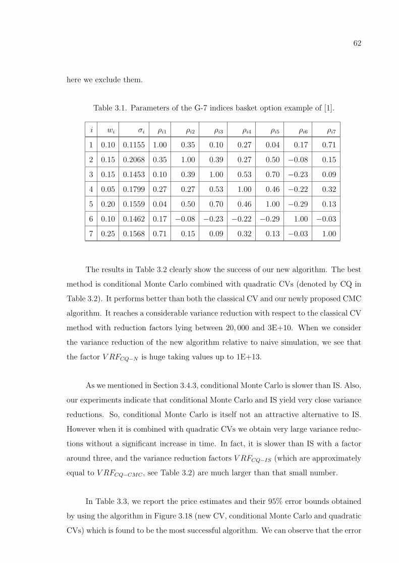
62

here we exclude them.

Table 3.1. Parameters of the G-7 indices basket option example of [1].

i wi σi ρi1 ρi2 ρi3 ρi4 ρi5 ρi6 ρi7

1 0.10 0.1155 1.00 0.35 0.10 0.27 0.04 0.17 0.71

2 0.15 0.2068 0.35 1.00 0.39 0.27 0.50 −0.08 0.15

3 0.15 0.1453 0.10 0.39 1.00 0.53 0.70 −0.23 0.09

4 0.05 0.1799 0.27 0.27 0.53 1.00 0.46 −0.22 0.32

5 0.20 0.1559 0.04 0.50 0.70 0.46 1.00 −0.29 0.13

6 0.10 0.1462 0.17 −0.08 −0.23 −0.22 −0.29 1.00 −0.03

7 0.25 0.1568 0.71 0.15 0.09 0.32 0.13 −0.03 1.00

The results in Table 3.2 clearly show the success of our new algorithm. The best

method is conditional Monte Carlo combined with quadratic CVs (denoted by CQ in

Table 3.2). It performs better than both the classical CV and our newly proposed CMC

algorithm. It reaches a considerable variance reduction with respect to the classical CV

method with reduction factors lying between 20, 000 and 3E+10. When we consider

the variance reduction of the new algorithm relative to naive simulation, we see that

the factor V RFCQ−N is huge taking values up to 1E+13.

As we mentioned in Section 3.4.3, conditional Monte Carlo is slower than IS. Also,

our experiments indicate that conditional Monte Carlo and IS yield very close variance

reductions. So, conditional Monte Carlo is itself not an attractive alternative to IS.

However when it is combined with quadratic CVs we obtain very large variance reduc-

tions without a significant increase in time. In fact, it is slower than IS with a factor

around three, and the variance reduction factors V RFCQ−IS (which are approximately

equal to V RFCQ−CMC , see Table 3.2) are much larger than that small number.

In Table 3.3, we report the price estimates and their 95% error bounds obtained

by using the algorithm in Figure 3.18 (new CV, conditional Monte Carlo and quadratic

CVs) which is found to be the most successful algorithm. We can observe that the error

63

Table 3.2. VRFs of different algorithms for basket options.

T K V RFCCV−N V RFCMC−CCV V RFCQ−CMC V RFCQ−CCV V RFCQ−N

0.5 80 5E+02 1E+08 3E+02 3E+10 1E+13

100 3E+02 6E+02 1E+03 9E+05 3E+08

120 3E+01 2E+03 1E+03 2E+06 7E+07

1 80 2E+02 4E+05 3E+02 1E+08 3E+10

100 2E+02 4E+02 1E+03 4E+05 6E+07

120 4E+01 2E+02 8E+02 2E+05 8E+06

2 80 1E+02 3E+04 3E+02 8E+06 9E+08

100 9E+01 3E+02 4E+02 1E+05 1E+07

120 4E+01 9E+01 4E+02 4E+04 2E+06

3 80 8E+01 1E+04 1E+02 1E+06 9E+07

100 7E+01 2E+02 4E+02 8E+04 5E+06

120 4E+01 9E+01 3E+02 2E+04 8E+05

64

bounds are all small, lying between 0.0002 and 1E−8. The maximum relative error

(4 × 10−5) is observed for T = 3, K = 120, while the minimum (10−9) is observed for

T = 0.5, K = 80. We see that we get smaller errors for in the money cases. So, our

new method seems to be attractive also for pricing far out of the money put options

using put-call parity.

The new method is fast. For n = 10, 000, our R-implementation takes about 0.25

seconds with the computer configuration Intel(R) Core (TM) 2 CPU T7200 2.00GHz,

0.99GB of RAM. It is about eight times slower than the classical CV method. Clearly

this increase in time is negligible when compared to the variance reduction factors

reported in Table 3.2. The time factor seems to be stable and remains approximately

the same for different parameters. Thus it is possible to estimate the efficiency factor of

the new algorithm by dividing the VRFs reported in the last two columns of Table 3.2

(V RFCQ−CCV and V RFCQ−N) by that time factor.

Still we should not overlook that the size of the error and of the variance reduction

strongly depends on the parameters. So we briefly list our main observations: First we

can see that the variance reduction increases with decreasing T . This is due to the fact

that the averages A and G have a stronger correlation when the variance is small. Thus

for decreasing T , the variance reduction of the control variate W = (A−K)+ 1G>K

is increased, and the direction of X explains a larger portion of the variance.

Another observation is the strong influence of the strike price K. We observe

in Table 3.2 that a smaller K leads to larger variance reduction. As K decreases the

probability that G < K and A > K decreases sharply. So, W becomes more frequently

equal to (A−K)+ and we get more variance reduction. However, the decreasing trend

of the variance reduction is curbed when conditional Monte Carlo is combined with

quadratic CVs.

3.5.1.2. Asian Options. In our experiments for Asian options, we selected different

parameter sets by changing the maturity T , the volatility σ and the strike price K.

65

Table 3.3. Pricing basket options with the algorithm given in Figure 3.18 (new CV,

conditional Monte Carlo and quadratic CVs); n = 10, 000.

T K Price Error Bound Error-LB Error-CU Error-DE

0.5 80 21.97532 3E−08 −5E−06 −1E−06 −2E−07

100 4.05674 6E−06 −2E−03 < 6E−07 −1E−05

120 0.02601 1E−06 −3E−04 7E−05 8E−06

1 80 23.90550 1E−06 −2E−04 −4E−05 −8E−06

100 6.62388 3E−05 −6E−03 6E−06 −5E−05

120 0.39593 2E−05 −4E−03 7E−04 5E−05

2 80 27.63800 1E−05 −1E−03 −3E−04 −7E−05

100 11.18449 9E−05 −1E−02 < 9E−06 −2E−04

120 2.35262 1E−04 −2E−02 3E−03 < 1E−05

3 80 31.18809 3E−05 −3E−03 −7E−04 −2E−04

100 15.39381 2E−04 −2E−02 < 2E−05 −5E−04

120 5.19361 2E−04 −4E−02 7E−03 −2E−04

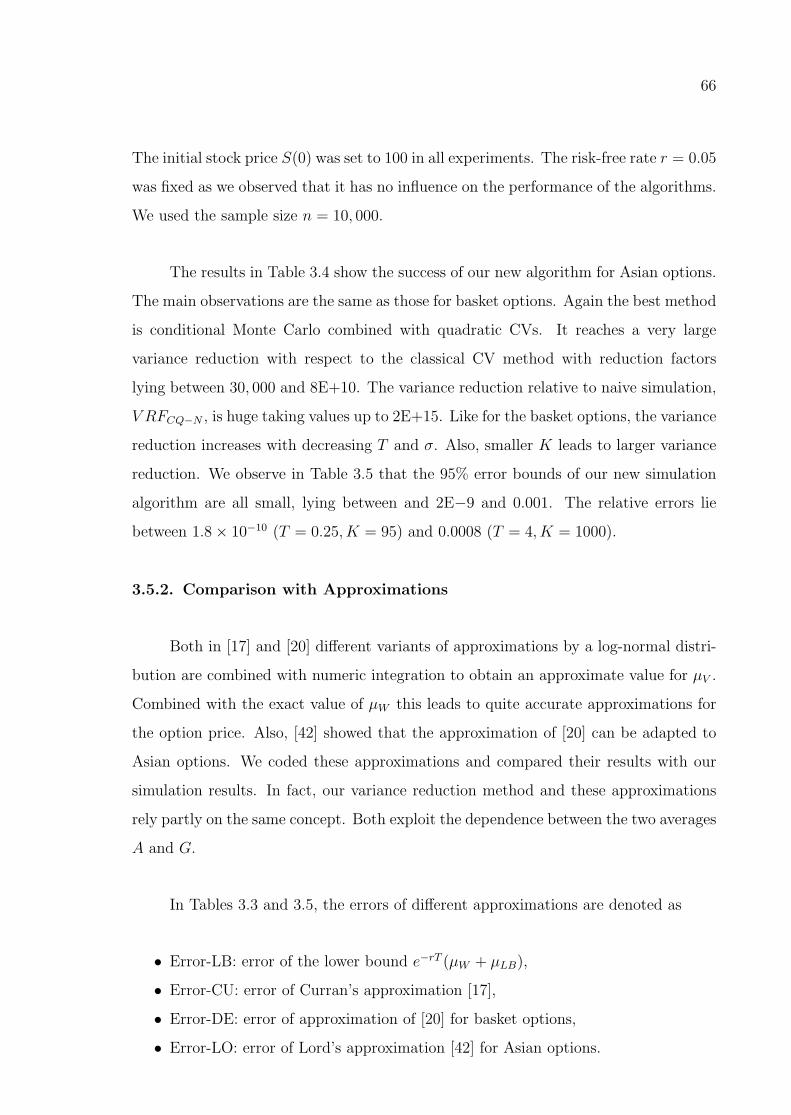
66

The initial stock price S(0) was set to 100 in all experiments. The risk-free rate r = 0.05

was fixed as we observed that it has no influence on the performance of the algorithms.

We used the sample size n = 10, 000.

The results in Table 3.4 show the success of our new algorithm for Asian options.

The main observations are the same as those for basket options. Again the best method

is conditional Monte Carlo combined with quadratic CVs. It reaches a very large

variance reduction with respect to the classical CV method with reduction factors

lying between 30, 000 and 8E+10. The variance reduction relative to naive simulation,

V RFCQ−N , is huge taking values up to 2E+15. Like for the basket options, the variance

reduction increases with decreasing T and σ. Also, smaller K leads to larger variance

reduction. We observe in Table 3.5 that the 95% error bounds of our new simulation

algorithm are all small, lying between and 2E−9 and 0.001. The relative errors lie

between 1.8× 10−10 (T = 0.25, K = 95) and 0.0008 (T = 4, K = 1000).

3.5.2. Comparison with Approximations

Both in [17] and [20] different variants of approximations by a log-normal distri-

bution are combined with numeric integration to obtain an approximate value for µV .

Combined with the exact value of µW this leads to quite accurate approximations for

the option price. Also, [42] showed that the approximation of [20] can be adapted to

Asian options. We coded these approximations and compared their results with our

simulation results. In fact, our variance reduction method and these approximations

rely partly on the same concept. Both exploit the dependence between the two averages

A and G.

In Tables 3.3 and 3.5, the errors of different approximations are denoted as

• Error-LB: error of the lower bound e−rT (µW + µLB),

• Error-CU: error of Curran’s approximation [17],

• Error-DE: error of approximation of [20] for basket options,

• Error-LO: error of Lord’s approximation [42] for Asian options.

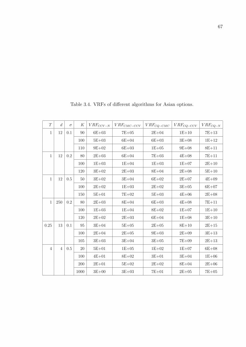
67

Table 3.4. VRFs of different algorithms for Asian options.

T d σ K V RFCCV−N V RFCMC−CCV V RFCQ−CMC V RFCQ−CCV V RFCQ−N

1 12 0.1 90 6E+03 7E+05 2E+04 1E+10 7E+13

100 5E+03 6E+04 6E+03 3E+08 1E+12

110 9E+02 6E+03 1E+05 9E+08 8E+11

1 12 0.2 80 2E+03 6E+04 7E+03 4E+08 7E+11

100 1E+03 1E+04 1E+03 1E+07 2E+10

120 3E+02 2E+03 8E+04 2E+08 5E+10

1 12 0.5 50 3E+02 3E+04 6E+02 2E+07 4E+09

100 2E+02 1E+03 2E+02 3E+05 6E+07

150 5E+01 7E+02 5E+03 4E+06 2E+08

1 250 0.2 80 2E+03 8E+04 6E+03 4E+08 7E+11

100 1E+03 1E+04 8E+02 1E+07 1E+10

120 2E+02 2E+03 6E+04 1E+08 3E+10

0.25 13 0.1 95 3E+04 5E+05 2E+05 8E+10 2E+15

100 2E+04 2E+05 9E+03 2E+09 3E+13

105 3E+03 3E+04 3E+05 7E+09 2E+13

4 4 0.5 20 5E+01 1E+05 1E+02 1E+07 6E+08

100 4E+01 8E+02 3E+01 3E+04 1E+06

200 2E+01 5E+02 2E+02 8E+04 2E+06

1000 3E+00 3E+03 7E+01 2E+05 7E+05

68

Table 3.5. Pricing Asian options with new CV, conditional Monte Carlo and

quadratic CVs; n = 10, 000.

T d σ K Price Error Bound Error-LB Error-CU Error-LO

1 12 0.1 90 12.16339 1E−08 −2E−05 −2E−06 −6E−08

100 3.90496 1E−07 −5E−05 8E−07 < 1E−07

110 0.43087 4E−08 −1E−04 1E−05 −1E−07

1 12 0.2 80 21.71910 3E−07 −2E−04 −4E−05 −2E−06

100 6.15604 1E−06 −4E−04 1E−05 < 1E−06

120 0.67480 3E−07 −8E−04 2E−04 −2E−06

1 12 0.5 50 50.22431 1E−05 −2E−03 −8E−04 −8E−05

100 13.12205 7E−05 −7E−03 4E−04 < 7E−05

150 2.09791 7E−06 −1E−02 6E−03 −1E−04

1 250 0.2 80 21.50221 3E−07 −2E−04 −4E−05 −8E−07

100 5.78197 1E−06 −4E−04 7E−06 < 1E−06

120 0.53362 3E−07 −7E−04 2E−04 < 3E−07

0.25 13 0.1 95 5.63738 2E−09 −5E−06 −3E−07 −7E−08

100 1.57082 7E−09 −7E−06 6E−07 6E−07

105 0.12165 2E−09 −1E−05 4E−07 −2E−07

4 4 0.5 20 76.57007 6E−05 −6E−03 6E−04 −7E−04

100 29.41940 1E−03 −7E−02 2E−02 < 1E−03

200 10.16027 7E−04 −9E−02 1E−01 −3E−03

1000 0.11664 9E−05 −2E−02 4E+00 1E−03

69

First we compare our simulation results with the lower bound e−rT (µW + µLB).

Comparing the simulated price, the simulation error and the errors of the lower bound

in Tables 3.3 and 3.5 we can conclude that the bound is quite tight but still the error

reduction reached by simulation (with n only 104) lies between 70 and 5000.

In Table 3.3, we report the estimates of the errors of the approximations of

[17] and [20] for basket options. To estimate the errors, we used our new simulation

algorithm with sample size n = 106. We observed that for increasing maturity and

out of the money cases the accuracy of Curran’s approximation deteriorates. The

approximation of [20] is considerably more complicated but also more precise for in

and out of the money cases. Nevermore, our simulation remains to be more accurate

than both approximations with the exception of the at the money cases where Curran’s

approximation gives results within the confidence interval of our very small simulation.

In Table 3.5, we see that our simulation for Asian options is more accurate than

the approximations with the exception of the at the money cases where Lord’s approx-

imation gives results within the confidence interval of our very small simulation. Also,

we observed that, as pointed out in [42], Curran’s approximation has problems with

the out of the money case for moderate and large volatilities. There we observed errors

much larger than the error bound of our simulation. For large volatility and far out of

the money cases Curran’s approximation is totally wrong.

Approximations are less accurate, but they are faster than our new simulation

algorithm. For our basket option example, the approximations of [17] and [20] take only

about 0.003 and 0.02 seconds, respectively, while our simulation with n = 104 takes 0.25

seconds (with the computer configuration Intel(R) Core (TM) 2 CPU T7200 2.00GHz,

0.99GB of RAM). Also, for Asian options with T = 1 and d = 12, approximations of [17]

and [42] take about only 0.006 and 0.04 seconds, respectively, while our simulation with

n = 104 takes 0.2 seconds. That is, for d = 12, our new simulation is five times slower

than Lord’s approximation. For d = 50 and 250, this factor reduces to eight and two,

respectively.

70

Of course it is not too useful to compare the speed of approximation and simula-

tion methods, as this comparison strongly depends on the used computing environment

and especially on the method used for numerical integration. The main advantage of

approximation methods is that they are fast and for many parameter settings they

have only a small error. Their disadvantage is that the true size of the error is un-

known and that there is no way to reduce that error. In simulation, however, we have

a probabilistic error bound and it is always possible to reduce the error by selecting a

larger sample size.

71

4. BARRIER AND LOOKBACK OPTIONS

4.1. Introduction

In this chapter, a new and simple variance reduction technique is presented for

pricing discretely monitored lookback and barrier options. It is based on using the

corresponding continuously monitored option as external control variate. The expla-

nations in this chapter closely follow Dingec and Hormann [43].

Barrier and lookback options can be categorized with respect to the monitoring

policy. In most contracts, the stock price is observed at discrete time points and

so in the payoff the maximum or minimum of the finite set of observed stock prices is

required. Such options are called discretely monitored or simply discrete options. In the

second category, the underlying is monitored continuously and so the payoff depends

on the underlying price throughout the life of the option. The basic advantage of

continuous options is that we have closed form solutions for their prices under GBM

(see, e.g., [44]). However, Kou [45] underlines that most of the options traded in the

markets are discretely monitored (typically at daily closings) due to regulatory and

practical issues. Although we have closed form solutions for continuous options, for

their discrete counterparts they are not available, and the price of the continuous option

gives only a rough approximation that can be improved by a correction for the discrete

case. So, to price discrete barrier and lookback options, an effective simulation method

is required.

We therefore develop new control variate methods for discretely monitored barrier

and lookback options under the GBM model for the stock price process S(t), t ≥ 0.

As external control variate we use the payoff of the corresponding continuously mon-

itored option. In order to explain the details of the methodology and to exemplify

the effectiveness of the CV method, we consider here three examples of path depen-

dent options whose payoffs are contingent on the maximum stock price: floating strike

lookback put (LP), fixed strike lookback call (LC) with strike price K and up and out

72

barrier call (UOC) with barrier level B. They have the payoff functions,

PayoffLP (M) = M − S(T ), (4.1)

PayoffLC(M) = (M −K)+, (4.2)

PayoffUOC(M) = (S(T )−K)+ 1M<B, (4.3)

where M denotes the maximum stock price until maturity T .

We have M = max0≤i≤d S(ti) and M = sup0≤t≤T S(t) under discrete and contin-

uous monitoring respectively; d denotes the number of control points ti in time and we

have 0 = t0 < t1 < . . . < td = T . It is important to note here that our CV methods can

be applied directly to all options whose payoff depends on the maximum of a discrete

path; if the minimum instead of the maximum is involved the necessary modifications

of the algorithms are straightforward.

Section 4.2 presents the first version of our control variate method which requires

the simulation of the maximum of a Brownian bridge; Section 4.3 presents the respec-

tive algorithms. Section 4.4 contains the formulas for the expectations of the CVs. In

Section 4.5 the details of the conditional expectation approach for the CV algorithm

are introduced, whereas Section 4.6 contains the corresponding algorithms for Barrier

options. Computational results are reported in Section 4.7 whereas Section 4.8 contains

our conclusions.

4.2. Continuous Price as Control Variate

In continuous monitoring, it is assumed that the stock price S(t) can be observed

at infinitely many points of time between t = 0 and maturity date t = T . In fact, these

types of barrier and lookback options have exact closed form solutions under GBM. So

their payoff can serve as good control variate for their discretely monitored counter-

parts. Especially for daily monitored options the correlation between the discrete and

the continuous maximum should be high enough to get a considerable variance reduc-

73

tion. To simulate a path-dependent option with discrete monitoring, it is sufficient to

simulate stock prices at discrete control points. To use our CV however, it is necessary

to obtain the payoff function of the continuous option conditional on the discrete path.

Here we have two possibilities: We can simulate the payoff of the continuous option

conditional on the discrete path or we can try to calculate its conditional expectation.

For the latter approach, we have to find the conditional expectation of the payoff

function of the continuous option. In other words, we evaluate

E [Payoff |S(0), S(t1), . . . , S(td−1), S(T )].

In this approach, since the variance of the CV is reduced by taking the conditional

expectation, the correlation between the payoff of the discrete option and the CV

is increased. Thus we expect a larger variance reduction. As the calculation of the

conditional expectation is often difficult and differs with respect to the option type,

the details of that approach will be given in Section 4.5 for lookback and barrier options,

respectively. We continue here with explaining the former approach.

4.2.1. Simulating the Control Variate

To simulate the payoff function of the continuous Barrier or lookback option, we

need the maximum of the stock price between control points. So, we have to generate

the maxima of d Brownian bridges for an option controlled at d time points. The

maximum of these d local maxima gives us the maximum stock price in the interval

[0, T ] required for continuous monitoring. In other words, we use the fact that

sup0≤t≤T

S(t) = max1≤i≤d

(sup

ti−1≤u≤tiS(u)

).

To generate these local maxima, we need the cumulative distribution function

of the maximum of a Brownian bridge. Fortunately, it has a simple structure, and

random variate generation from that CDF can be done easily by using the inverse

74

transformation method.

Under GBM assumption and its unique risk neutral measure, the stock price

process can be written as S(t) = S(0) exp(σW (t)) where W (t) = µt + W (t) and

µ = (r−σ2/2)/σ where r is the risk free interest rate and σ is the volatility of the stock

price. The conditional CDF of the supremum of W (t) is well known (see, e.g., [2, 46])

and it is given by

P

(sup

0≤u≤tW (u) ≤ x

∣∣∣∣ W (t) = y

)= 1− exp

(−2x(x− y)

t

), (4.4)

where x ≥ max(y, 0).

From that CDF, the maximum of the Brownian bridge can be generated by the

inversion method as it was e.g. suggested in [47] to decrease the simulation bias under

a general diffusion process:

x = 0.5(y +

√y2 − 2t logU

), (4.5)

where U ∼ U(0, 1) is a uniform random number.

The above formula simulates the maximum of a Brownian bridge in [0, t] given

that W (t) = y. Using Equation 4.5, we can write

logMi = logS(ti−1) + 0.5(

∆ logSi +√

(∆ logSi)2 − 2σ2∆ti logU), (4.6)

where Mi = supti−1≤u≤ti S(u), ∆ logSi = logS(ti)− logS(ti−1) and ∆ti = ti − ti−1.

Therefore, in order to simulate local maxima of log stock prices for each time

interval (ti−1, ti), we first evaluate ∆ logSi and use Equation 4.6 with a uniform random

number U(0, 1). Taking the maximum of the d local maxima and exponentiation yields

sup0≤t≤T S(t). Then the payoff function of the continuous option is obtained from that

maximum.

75

It is clear that the use of Equation 4.6 to simulate the continuous maximum

between all control points is an additional computational burden. In order to speed up

the CV algorithm, we can omit the generation of the local maxima for all intervals for

which the starting and the ending stock prices are small compared to the maximum

of the discrete path. If the probability, that the continuous maximum of an interval

exceeds the discrete maximum of the path, is smaller than a very small number ε we can

omit the simulation of that continuous local maximum without influencing the result

of the simulation. To be on the safe side we use ε = 2−52 , the machine precision for

practical all modern computing environments. Let m denote the discrete maximum of

the path that is m = max0≤i≤d S(ti). Using the conditional CDF given in Equation 4.4,

we can easily calculate the probability P (Mi > m|S(ti−1), S(ti)), that the continuous

maximum Mi over the interval (ti−1, ti) exceeds m. Taking the logarithm we arrive at

the very simple condition

−2(logm− logS(ti−1))(logm− logS(ti))

σ2∆ti> log ε = −36.044 .

It is only necessary to generate the continuous maximum of an interval if this condition

is fulfilled.

4.3. Algorithms for Simulated CVs

We present the details of the naive simulation (Figure 4.1) and the approach with

simulated control variate (Figure 4.2) for lookback and barrier options having equal

monitoring intervals ∆t = T/d. The algorithms presented here can also be used to

price barrier options, although more effective algorithms incorporating the knock out

feature can be developed (see Section 4.6). The payoff functions that are given in

Equations 4.1, 4.2 and 4.3 determine the type of the option.

[48] propose an accurate approximation for discretely monitored barrier options

by using the formula of continuous monitoring with a shifted barrier. [49] extended

that approximation to lookback options. We use the corrected continuous option as

the control variate X for the simulation of the discrete option Y . The simulation output

76


price S(0), volatility σ, risk free interest rate r, payoff function Payoff().

Ensure: Option price estimate and its 1− δ confidence interval.

1: Set ∆t← T/d.


3: Set maxlogSt ← logSt ← logS(0).

4: for j = 1 to d do

5: Generate Z ∼ N(0, 1).

6: Set logSt ← logSt +(r − σ2/2)∆t+ σ√

∆t Z.

7: Set maxlogSt ← max(logSt, maxlogSt).

8: end for

9: Set Yi ← e−rTPayoff(exp(maxlogSt)).

10: end for


12: return Y and the error bound Φ−1(1− δ/2) s/√n, where Φ−1 denotes the

quantile of the normal distribution.

Figure 4.1. Naive simulation algorithm for lookback (and barrier) options.

of the CV algorithm has the form of Y − c (X − E [X]). Here, the optimal coefficient

minimizing the variance is c∗ = Cov (X, Y )/Var (X). In our numerical experiments we

have observed that, as we use the correction that leads to an accurate approximation,

the estimated optimal factor c∗ is very close to 1 and setting c = 1 does not cause a

significant loss of efficiency. So, in the control variate algorithm, we simply drop c.

The expectation of the control variate E [X] is obtained by using the corrected

price formulas ECV() of the continuous versions given in Equations 4.8, 4.10 and 4.13

for the up and out barrier call, floating strike lookback put and fixed strike lookback

call options, respectively. The details of the steps of the CV method are presented as

algorithms in Figures 4.2 and 4.3. In the algorithm given in Figure 4.2, the discrete

path is simulated and stored in an array. Then the algorithm given in Figure 4.3

(function CCM()) is called, that uses that array as an input and returns a simulated

sample of the continuous maximum conditional on the discrete path.

77


price S(0), volatility σ, risk free interest rate r, payoff function Payoff(),

function to evaluate the expectation of the control variate ECV(), procedure

for the simulation of the conditional continuous maximum CCM() (see the

algorithm given in Figure 4.3).


1: Set ∆t← T/d.

2: Compute E [X] using the function ECV() defined in Equations 4.8, 4.10 and

4.13, respectively.


4: Set maxlogSt ← logSt[0] ← logS(0).



7: Set logSt[j] ← logSt[j-1] +(r − σ2/2)∆t+ σ√

∆t Z.

8: Set maxlogSt ← max(logSt[j], maxlogSt).

9: end for

10: Compute maxSt ← exp(maxlogSt).

11: Compute maxStcv← exp(−0.5826σ√

∆t) CCM(maxlogSt, logSt, d, σ,∆t).

12: Set Yi ← e−rTPayoff(maxSt).

13: Set Xi ← e−rTPayoff(maxStcv).

14: Set Yi ← Yi − (Xi − E [X]).

15: end for




Figure 4.2. Algorithm for simulation of lookback (and barrier) options using

simulated continuous price with correction as control variate.

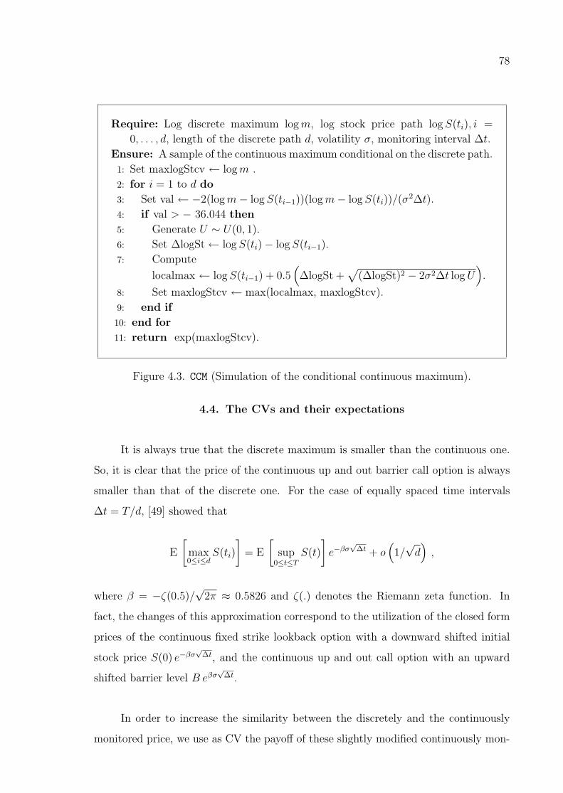
78

Require: Log discrete maximum logm, log stock price path logS(ti), i =

0, . . . , d, length of the discrete path d, volatility σ, monitoring interval ∆t.

Ensure: A sample of the continuous maximum conditional on the discrete path.

1: Set maxlogStcv ← logm .

2: for i = 1 to d do

3: Set val ← −2(logm− logS(ti−1))(logm− logS(ti))/(σ2∆t).

4: if val > − 36.044 then

5: Generate U ∼ U(0, 1).

6: Set ∆logSt← logS(ti)− logS(ti−1).

7: Compute

localmax ← logS(ti−1) + 0.5(

∆logSt +√

(∆logSt)2 − 2σ2∆t logU)

.

8: Set maxlogStcv ← max(localmax, maxlogStcv).

9: end if

10: end for

11: return exp(maxlogStcv).

Figure 4.3. CCM (Simulation of the conditional continuous maximum).

4.4. The CVs and their expectations

It is always true that the discrete maximum is smaller than the continuous one.

So, it is clear that the price of the continuous up and out barrier call option is always

smaller than that of the discrete one. For the case of equally spaced time intervals

∆t = T/d, [49] showed that

E

[max0≤i≤d

S(ti)

]= E

[sup

0≤t≤TS(t)

]e−βσ

√∆t + o

(1/√d),

where β = −ζ(0.5)/√

2π ≈ 0.5826 and ζ(.) denotes the Riemann zeta function. In

fact, the changes of this approximation correspond to the utilization of the closed form

prices of the continuous fixed strike lookback option with a downward shifted initial

stock price S(0) e−βσ√

∆t, and the continuous up and out call option with an upward

shifted barrier level B eβσ√

∆t.

In order to increase the similarity between the discretely and the continuously

monitored price, we use as CV the payoff of these slightly modified continuously mon-

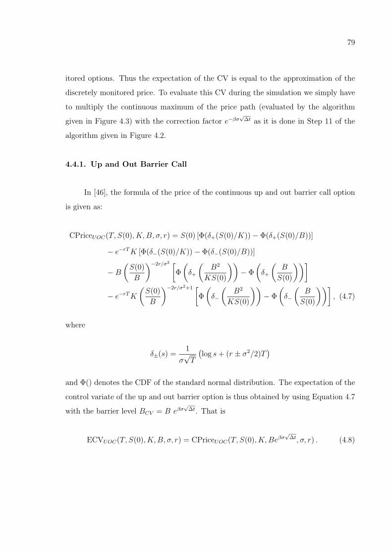
79

itored options. Thus the expectation of the CV is equal to the approximation of the

discretely monitored price. To evaluate this CV during the simulation we simply have

to multiply the continuous maximum of the price path (evaluated by the algorithm

given in Figure 4.3) with the correction factor e−βσ√

∆t as it is done in Step 11 of the

algorithm given in Figure 4.2.

4.4.1. Up and Out Barrier Call

In [46], the formula of the price of the continuous up and out barrier call option

is given as:

CPriceUOC(T, S(0), K,B, σ, r) = S(0) [Φ(δ+(S(0)/K))− Φ(δ+(S(0)/B))]

− e−rTK [Φ(δ−(S(0)/K))− Φ(δ−(S(0)/B))]

−B(S(0)

B

)−2r/σ2 [Φ

(δ+

(B2

KS(0)

))− Φ

(δ+

(B

S(0)

))]− e−rTK

(S(0)

B

)−2r/σ2+1 [Φ

(δ−

(B2

KS(0)

))− Φ

(δ−

(B

S(0)

))], (4.7)

where

δ±(s) =1

σ√T

(log s+ (r ± σ2/2)T

)and Φ() denotes the CDF of the standard normal distribution. The expectation of the

control variate of the up and out barrier option is thus obtained by using Equation 4.7

with the barrier level BCV = B eβσ√

∆t. That is

ECVUOC(T, S(0), K,B, σ, r) = CPriceUOC(T, S(0), K,Beβσ√

∆t, σ, r) . (4.8)

80

4.4.2. Floating Strike Lookback Put

In [44], the formula of the price of the continuous floating strike lookback put

option is given as:

CPriceLP (T, S(0), σ, r) = S(0)e−rTΦ(−b2)− S(0)Φ(−b1)

+ S(0)e−rT(σ2

2r

)[−Φ

(b1 − 2b

√T/σ

)+ erTΦ(b1)

], (4.9)

where b1 = (r+σ2/2)T

σ√T

and b2 = b1 − σ√T . For this option our CV is the payoff of

the continuously monitored option with the corrected maximum but with the same

final stock price S(T ) as for discrete monitoring, because S(T ) is not influenced by the

monitoring policy. To price an option with such a payoff, it is easiest to use the above

formula with modified initial stock price. As the discounted expectation of S(T ) is

equal to S(0) it is not difficult to show that the expectation of our control variate is

equal to

ECVLP (T, S(0), σ, r) = CPriceLP (T, S(0)e−βσ√

∆t, σ, r) + S(0) e−βσ√

∆t − S(0) . (4.10)

4.4.3. Fixed Strike Lookback Call

In [44], the formula of the price of the continuous fixed strike lookback call option

is given for two cases. For K > S(0),

CPriceLC|K>S(0)(T, S(0), K, σ, r) = S(0)Φ(d1)−Ke−rTΦ(d2)

+ S(0)e−rT(σ2

2r

)[−(S(0)/K)−2r/σ2

Φ(d1 − (2r/σ)√T ) + erTΦ(d1)

],

(4.11)

where

d1 =log(S(0)/K) + (r + σ2/2)T

σ√T

, d2 = d1 − σ√T .

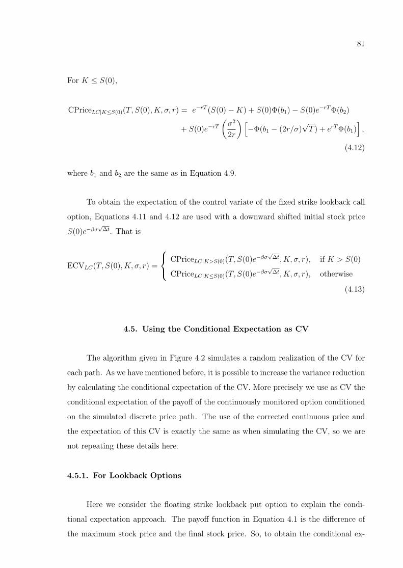
81

For K ≤ S(0),

CPriceLC|K≤S(0)(T, S(0), K, σ, r) = e−rT (S(0)−K) + S(0)Φ(b1)− S(0)e−rTΦ(b2)

+ S(0)e−rT(σ2

2r

)[−Φ(b1 − (2r/σ)

√T ) + erTΦ(b1)

],

(4.12)

where b1 and b2 are the same as in Equation 4.9.

To obtain the expectation of the control variate of the fixed strike lookback call

option, Equations 4.11 and 4.12 are used with a downward shifted initial stock price

S(0)e−βσ√

∆t. That is

ECVLC(T, S(0), K, σ, r) =

CPriceLC|K>S(0)(T, S(0)e−βσ√

∆t, K, σ, r), if K > S(0)

CPriceLC|K≤S(0)(T, S(0)e−βσ√

∆t, K, σ, r), otherwise

(4.13)

4.5. Using the Conditional Expectation as CV

The algorithm given in Figure 4.2 simulates a random realization of the CV for

each path. As we have mentioned before, it is possible to increase the variance reduction

by calculating the conditional expectation of the CV. More precisely we use as CV the

conditional expectation of the payoff of the continuously monitored option conditioned

on the simulated discrete price path. The use of the corrected continuous price and

the expectation of this CV is exactly the same as when simulating the CV, so we are

not repeating these details here.

4.5.1. For Lookback Options

Here we consider the floating strike lookback put option to explain the condi-

tional expectation approach. The payoff function in Equation 4.1 is the difference of

the maximum stock price and the final stock price. So, to obtain the conditional ex-

82

pectation of the payoff we only need to evaluate the conditional expectation of the

continuous maximum M = sup0≤t≤T S(t) as the final stock price S(T ) is already deter-

mined by the discrete path. Therefore, our aim is to find the conditional expectation

of M = sup0≤t≤T S(t) conditional on the discrete stock price path S(ti), i = 0, . . . , d

where d is the number of control points.

Using the Markovian property of the Brownian motion and the conditional inde-

pendence of the local maxima, we can write the conditional CDF of M as

FM |S(x|S(0), . . . , S(T )) = P (M < x | S(0), . . . , S(T ))

= P (logM < log x | logS(0), . . . , logS(T ))

=d∏i=1

P (logMi < log x | logS(ti−1), logS(ti))

=d∏i=1

(1− exp

(−2(log x− logS(ti−1))(log x− logS(ti))

σ2∆t

)),

where x > max0≤i≤d S(ti). The final equality is obtained by using the conditional CDF

given in Equation 4.4.

So, the conditional expectation can be obtained by integrating the tail probability:

E [M |S(0), . . . , S(T )] = m+

∫ ∞m

(1− FM |S(x|S(0), . . . , S(T )))dx,

where m = max0≤i≤d S(ti) is the discrete maximum.

Finding a closed form solution for that integral seems to be impossible. So, the

only viable option is the numerical evaluation of the integral by using a quadrature

rule. However, performing a numerical integration for each simulated discrete path

is slow. We have seen in numerical experiments with lookback options that the vari-

ance reduction factor obtained by the conditional expectation approach is about four

times larger than that obtained by the simulation of the continuous maximum and this

ratio remains approximately the same for different parameters. Since the increase in

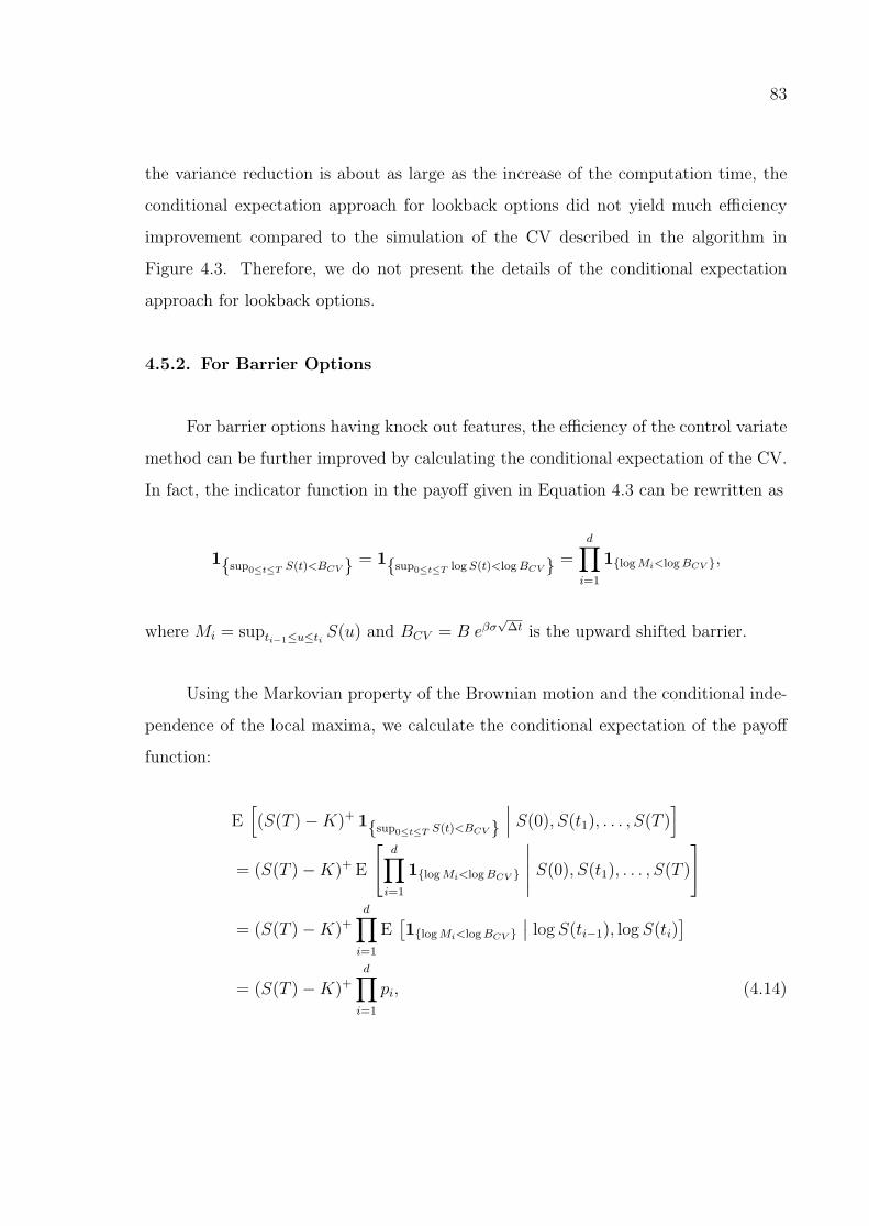
83

the variance reduction is about as large as the increase of the computation time, the

conditional expectation approach for lookback options did not yield much efficiency

improvement compared to the simulation of the CV described in the algorithm in

Figure 4.3. Therefore, we do not present the details of the conditional expectation

approach for lookback options.

4.5.2. For Barrier Options

For barrier options having knock out features, the efficiency of the control variate

method can be further improved by calculating the conditional expectation of the CV.

In fact, the indicator function in the payoff given in Equation 4.3 can be rewritten as

1sup0≤t≤T S(t)<BCV = 1sup0≤t≤T logS(t)<logBCV =d∏i=1

1logMi<logBCV ,

where Mi = supti−1≤u≤ti S(u) and BCV = B eβσ√

∆t is the upward shifted barrier.

Using the Markovian property of the Brownian motion and the conditional inde-

pendence of the local maxima, we calculate the conditional expectation of the payoff

function:

E[(S(T )−K)+ 1sup0≤t≤T S(t)<BCV

∣∣∣ S(0), S(t1), . . . , S(T )]

= (S(T )−K)+ E

[d∏i=1

1logMi<logBCV

∣∣∣∣∣ S(0), S(t1), . . . , S(T )

]

= (S(T )−K)+

d∏i=1

E[1logMi<logBCV

∣∣ logS(ti−1), logS(ti)]

= (S(T )−K)+

d∏i=1

pi, (4.14)

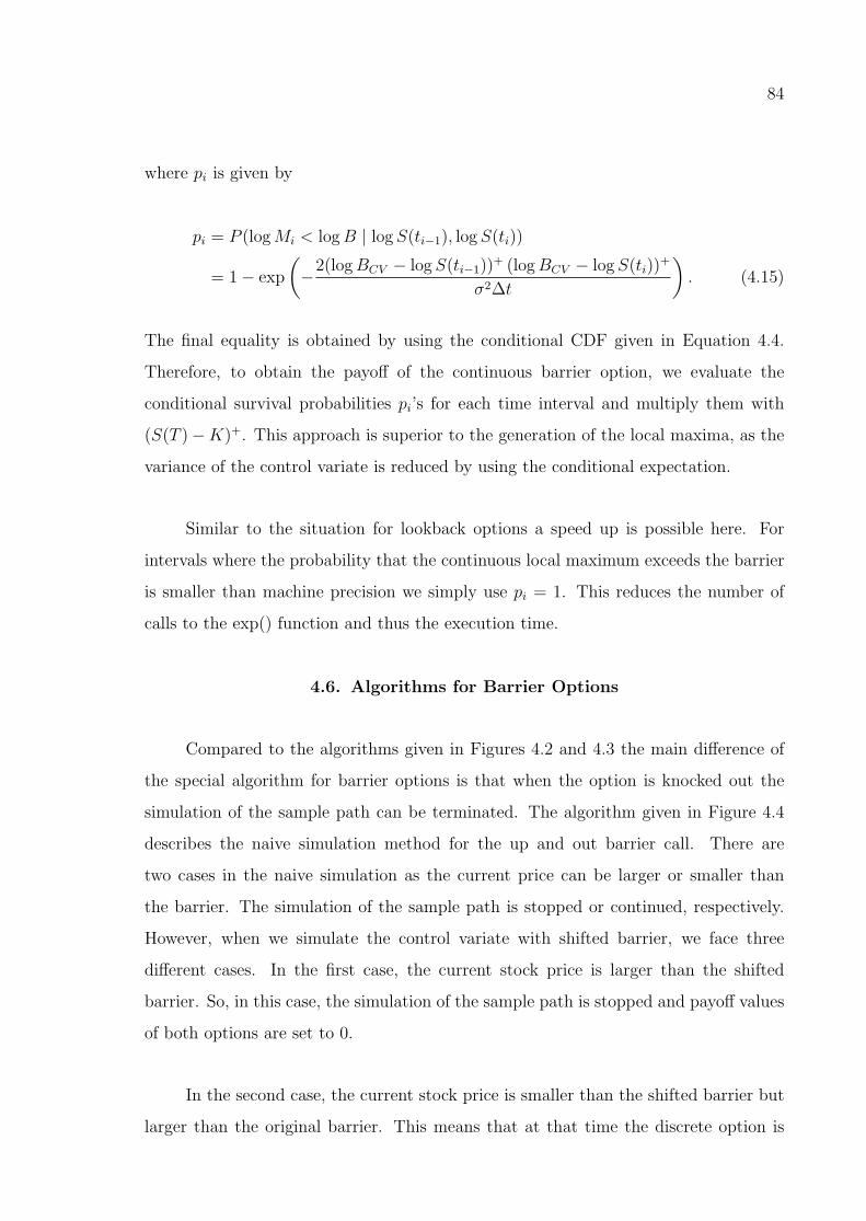
84

where pi is given by

pi = P (logMi < logB | logS(ti−1), logS(ti))

= 1− exp

(−2(logBCV − logS(ti−1))+ (logBCV − logS(ti))

+

σ2∆t

). (4.15)

The final equality is obtained by using the conditional CDF given in Equation 4.4.

Therefore, to obtain the payoff of the continuous barrier option, we evaluate the

conditional survival probabilities pi’s for each time interval and multiply them with

(S(T )−K)+. This approach is superior to the generation of the local maxima, as the

variance of the control variate is reduced by using the conditional expectation.

Similar to the situation for lookback options a speed up is possible here. For

intervals where the probability that the continuous local maximum exceeds the barrier

is smaller than machine precision we simply use pi = 1. This reduces the number of

calls to the exp() function and thus the execution time.

4.6. Algorithms for Barrier Options

Compared to the algorithms given in Figures 4.2 and 4.3 the main difference of

the special algorithm for barrier options is that when the option is knocked out the

simulation of the sample path can be terminated. The algorithm given in Figure 4.4

describes the naive simulation method for the up and out barrier call. There are

two cases in the naive simulation as the current price can be larger or smaller than

the barrier. The simulation of the sample path is stopped or continued, respectively.

However, when we simulate the control variate with shifted barrier, we face three

different cases. In the first case, the current stock price is larger than the shifted

barrier. So, in this case, the simulation of the sample path is stopped and payoff values

of both options are set to 0.

In the second case, the current stock price is smaller than the shifted barrier but

larger than the original barrier. This means that at that time the discrete option is

85

knocked out but the continuous option is not. In that case, the simulation is stopped,

the payoff of the discrete option is set to 0 and the value of the control variate is set

to the expectation of the payoff of the continuously monitored option conditioned on

the values of the discrete price path generated so far. However, the formula given in

Equation 4.14 can not be used directly to calculate the conditional expectation, as the

stopping time can be smaller than maturity. More formally, let’s write

i∗ = min d,min i ≥ 0 : B < S(ti) < BCV .

The conditional expectation of the CV given the information up to the stopping

time ti∗ is

E[(S(T )−K)+ 1sup0≤t≤T S(t)<BCV

∣∣∣ S(0), . . . , S(ti∗)]

= E[(S(T )−K)+ 1sup0≤u≤ti∗

S(u)<BCV 1supti∗≤u≤T S(u)<BCV ∣∣∣ S(0), . . . , S(ti∗)

]=

(i∗∏i=1

pi

)E[(S(T )−K)+ 1supti∗≤u≤T S(u)<BCV

∣∣∣ S(ti∗)], (4.16)

where pi’s are given by Equation 4.15. To obtain the final expression from the previous

one, we have used the Markovian property of the Brownian motion. Note that when

i∗ = d, Equation 4.16 is equivalent to Equation 4.14. On the other hand, when i∗ < d,

the expectation in Equation 4.16 corresponds to the expected payoff of a continuous

barrier option with initial stock price S(ti∗) and maturity T − ti∗ = (d− i∗)∆t. So, it

can be evaluated by using Equation 4.7.

In the third case, the current stock price is smaller than the original barrier and

we continue to simulate the sample path. The details of these steps are given in the

algorithm in Figure 4.5. As for lookback options we use c = 1 as the optimal c∗ is

very close to 1. The algorithm given in Figure 4.6 shows the steps of the calculation of

the survival probability of the continuous option conditional on the discrete path. It

is called by the algorithm given in Figure 4.5 as function CSP().

86

Require: Sample size n, maturity T , number of control points d, barrier level

B, initial stock price S(0), strike price K, volatility σ, risk free interest

rate r.


1: Set ∆t← T/d.


3: Set logSt ← logS(0) and hit ← 0.



6: Set logSt ← logSt +(r − σ2/2)∆t+ σ√

∆t Z.

7: if logSt > logB then

8: Set Yi ← 0, hit ← 1 and exit from the for loop.

9: end if

10: end for

11: if hit=0 then

12: Set Yi ← e−rT (exp(logSt)−K)+.

13: end if

14: end for




Figure 4.4. Naive simulation algorithm for up and out barrier call options.

87

Require: Sample size n, maturity T , number of control points d, initial stockprice S(0), strike price K, barrier level B, volatility σ, risk free interestrate r, formula of the continuous price CPrice() (see Equation 4.7), proce-dure for the evaluation of the conditional survival probability CSP() (see thealgorithm given in Figure 4.6).


1: Set ∆t← T/d.

2: Set BCV ← B exp(

0.5826 σ√

∆t)

.

3: Compute E [X]← CPrice(T, S(0), K,BCV , σ, r).4: for i = 1 to n do5: Set logSt[0]← logS(0), p← 1 and hit ← 0.6: for j = 1 to d do7: Generate Z ∼ N(0, 1).8: Set logSt[j]← logSt[j − 1] + (r − σ2/2)∆t+ σ

√∆t Z.

9: if logSt[j] > logBCV then10: Set Yi ← 0, Xi ← 0, hit ← 1 and exit from the loop.11: else if logSt[j] > logB then12: Set Yi ← 0.13: Compute p← CSP(logBCV , logSt, j, σ,∆t)14: if j = d then15: Set Xi ← p e−rT (exp(logSt[j])−K).16: else17: Set Xi ← p e−r j∆t CPrice((d− j)∆t, exp(logSt[j]), K,BCV , σ, r).18: end if19: Set hit ← 1 and exit from the loop.20: end if21: end for22: if hit = 0 then23: Set Yi ← e−rT (exp(logSt[d])−K)+.24: Compute p← CSP(logBCV , logSt, d, σ,∆t)25: Set Xi ← p Yi.26: end if27: Set Yi ← Yi − (Xi − E [X]).28: end for29: Compute the sample mean Y and the sample standard deviation s of Yi’s.30: return Y and the error bound Φ−1(1− δ/2) s/

√n, where Φ−1 denotes the


Figure 4.5. Simulation of up and out barrier call options using control variate with

correction and conditional expectation.

88

Require: Log barrier level logB, log stock price path logS(ti), i = 0, . . . , d,

length of the discrete path d, volatility σ, monitoring interval ∆t.

Ensure: Conditional survival probability.

1: Set p← 1.

2: for i = 1 to d do

3: Set val ← −2(logB − logS(ti−1))(logB − logS(ti))/(σ2∆t).

4: if val > − 36.044 then

5: Set p← p(1− eval

).

6: end if

7: end for

8: return p.

Figure 4.6. CSP (Calculation of the conditional survival probability of the continuous

option).

4.7. Computational Results

4.7.1. Computational Results for Lookback Options

In this section, we report our numerical results to assess the efficiency of our

control variate method for pricing discrete lookback options. To perform the numerical

experiments, algorithms given in Figures 4.1, 4.2 and 4.3 were implemented in C. The

results for floating strike lookback put and fixed strike lookback call options are given

in Tables 4.1 and 4.2, respectively. We report the option price estimate (Price), 95%

error bound (Error), estimated variance reduction factor (VRF) and the corresponding

continuous price obtained by the formula (Cont. Price). The results of the case where

the correction is not used are given as well, to allow a comparison. In all experiments,

the number of replications is n = 104, the initial stock price is S(0) = 100 and the risk

free interest rate is r = 0.05.

In Table 4.1, the results for three different volatility cases with four different

maturities are reported. We include both weekly and daily monitoring results assuming

250 days and 50 weeks per year. It can be seen that our new control variate is quite

successful. In fact, the VRF is larger than 100 in most cases. Also, the variance

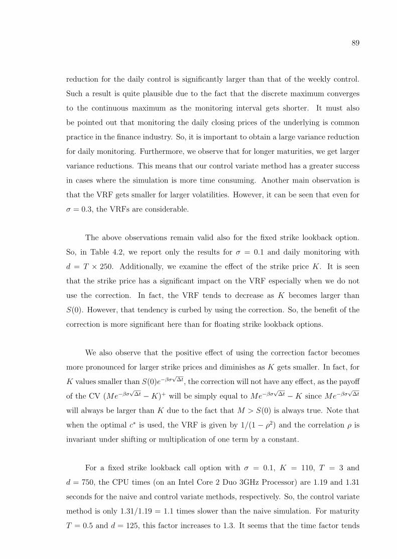
89

reduction for the daily control is significantly larger than that of the weekly control.

Such a result is quite plausible due to the fact that the discrete maximum converges

to the continuous maximum as the monitoring interval gets shorter. It must also

be pointed out that monitoring the daily closing prices of the underlying is common

practice in the finance industry. So, it is important to obtain a large variance reduction

for daily monitoring. Furthermore, we observe that for longer maturities, we get larger

variance reductions. This means that our control variate method has a greater success

in cases where the simulation is more time consuming. Another main observation is

that the VRF gets smaller for larger volatilities. However, it can be seen that even for

σ = 0.3, the VRFs are considerable.

The above observations remain valid also for the fixed strike lookback option.

So, in Table 4.2, we report only the results for σ = 0.1 and daily monitoring with

d = T × 250. Additionally, we examine the effect of the strike price K. It is seen

that the strike price has a significant impact on the VRF especially when we do not

use the correction. In fact, the VRF tends to decrease as K becomes larger than

S(0). However, that tendency is curbed by using the correction. So, the benefit of the

correction is more significant here than for floating strike lookback options.

We also observe that the positive effect of using the correction factor becomes

more pronounced for larger strike prices and diminishes as K gets smaller. In fact, for

K values smaller than S(0)e−βσ√

∆t, the correction will not have any effect, as the payoff

of the CV (Me−βσ√

∆t −K)+ will be simply equal to Me−βσ√

∆t −K since Me−βσ√

∆t

will always be larger than K due to the fact that M > S(0) is always true. Note that

when the optimal c∗ is used, the VRF is given by 1/(1 − ρ2) and the correlation ρ is

invariant under shifting or multiplication of one term by a constant.

For a fixed strike lookback call option with σ = 0.1, K = 110, T = 3 and

d = 750, the CPU times (on an Intel Core 2 Duo 3GHz Processor) are 1.19 and 1.31

seconds for the naive and control variate methods, respectively. So, the control variate

method is only 1.31/1.19 = 1.1 times slower than the naive simulation. For maturity

T = 0.5 and d = 125, this factor increases to 1.3. It seems that the time factor tends

90

to be larger with shorter maturities and less control points. Nevertheless, it remains

approximately the same for the variations of other parameters and also for the floating

strike lookback option. When we divide the VRF over the execution time ratio, we

obtain the estimated efficiency factor of the control variate method.

Finally, we compare our method with other variance reduction techniques. In

the literature, there seems to exist no special technique tailored for lookback options.

To make a comparison, we therefore implemented some of the well known general

techniques, which are antithetic variates (AV), multiple internal CVs and stratification,

and then performed experiments for all parameter settings of Tables 4.1 and 4.2.

The AV method yields a VRF around two in most cases. The largest variance

reduction is obtained for the fixed strike lookback option for T = 3 and K = 100

with a VRF of 4.6. As multiple internal CVs, we used the standard normal variates

which are used to generate the increments of the log stock price path. The optimal

CV coefficients are estimated in a pilot run. The method yields a VRF around four

in most cases. We also tried S(T ) as a single CV. For the floating strike option, the

VRFs are only around two. The largest variance reduction is obtained for the fixed

strike lookback option for T = 3 and K = 100 with a VRF of 7.4. Finally, we tried

stratified sampling by using S(T ) (or equivalently the terminal value of the underlying

Brownian motion W (T )) as single stratification variable. We used Brownian bridge

sampling to generate the stock price path conditional on the value of S(T ). For the

floating strike option, we observed VRFs around four; for the fixed strike option, the

VRFs lie between 6 and 12.

Comparing the results of the above paragraph with those given in the Tables 4.1

and 4.2, which were obtained by our new CV method, we may call it an efficient

variance reduction method for lookback options.

91

Table 4.1. Numerical results for floating strike lookback put option.

CV with correction CV without correction

σ T d Price Error VRF Cont. Price VRF Cont. Price

0.1

0.525 3.77681 0.00877 60.9 3.719402 59.4 4.577498

125 4.20754 0.00383 332.4 4.192872 328.0 4.577498

150 5.08629 0.00869 110.3 5.042871 107.2 5.911916

250 5.53354 0.00387 549.4 5.522382 534.5 5.911916

2100 6.49664 0.00882 165.6 6.459192 158.5 7.339955

500 6.94988 0.00400 823.2 6.945168 785.9 7.339955

3150 7.28629 0.00884 213.9 7.246558 200.4 8.133835

750 7.74288 0.00399 1015.5 7.736129 945.7 8.133835

0.2

0.525 8.77651 0.01848 60.6 8.665125 57.2 10.47059

125 9.68501 0.00805 323.3 9.659483 309.0 10.47059

150 12.49714 0.01908 100.5 12.42267 92.0 14.29057

250 13.46634 0.00848 524.1 13.45141 486.6 14.29057

2100 17.26886 0.01991 164.8 17.19442 143.0 19.14160

500 18.28084 0.00888 813.2 18.26682 708.1 19.14160

3150 20.47765 0.02073 199.1 20.42149 163.0 22.42229

750 21.52947 0.00931 1005.0 21.52343 806.1 22.42229

0.3

0.525 14.00472 0.02909 55.1 13.81435 49.7 16.66263

125 15.41609 0.01310 272.0 15.38013 247.4 16.66263

150 20.43082 0.03053 90.3 20.29039 77.3 23.30073

250 21.98344 0.01372 447.8 21.94526 387.0 23.30073

2100 29.17033 0.03324 137.9 29.05355 106.6 32.28320

500 30.85936 0.01499 665.7 30.82898 525.0 32.28320

3150 35.47464 0.03562 161.2 35.39679 108.6 38.78519

750 37.26362 0.01592 875.6 37.25949 571.5 38.78519

92

Table 4.2. Numerical results for fixed strike lookback call option, σ=0.1.

CV with correction CV without correction

T K Price Error VRF Cont. Price VRF Cont. Price

0.5

100 6.6746 0.0038 682 6.6668 663 7.0465

105 2.9124 0.0030 709 2.9071 390 3.1380

110 0.9923 0.0021 567 0.9897 261 1.0940

1

100 10.4076 0.0039 1506 10.4022 1484 10.7889

105 6.3075 0.0034 1539 6.2974 999 6.5953

110 3.4331 0.0029 1468 3.4265 770 3.6273

2

100 16.4666 0.0039 3195 16.4628 3167 16.8562

105 12.2770 0.0038 3357 12.2695 2587 12.6172

110 8.7566 0.0035 3338 8.7537 2131 9.0442

3

100 21.6735 0.0039 5340 21.6661 5321 22.0630

105 17.5699 0.0038 5672 17.5653 4714 17.9340

110 13.8969 0.0037 5258 13.8914 3794 14.2231

93

4.7.2. Computational Results for Barrier Options

In Table 4.3, numerical results are reported for the algorithms given in Figures 4.4

and 4.5 applied to the up and out barrier call option with parameters n = 104, S(0) =

110, K = 100 and r = 0.05. We consider two different volatility cases σ = 0.1,

σ = 0.3 and maturities of T = 0.5 and T = 2 with daily monitoring, that is d = 125

and d = 500, respectively. To get prices not too close to that of the European call

option, different barrier levels are used for changing volatilities and maturities. We

also include the VRF obtained by using the algorithm given in Figure 4.2. Finally, the

corresponding European call option prices (E. Price) are reported.

In Table 4.3, we see that our control variate method is successful. When we

compare the results of the algorithm given in Figure 4.5 and the algorithm given in

Figure 4.2, we observe that the conditional expectation approach yields a significant

increase in the VRF with a factor around four. For a longer maturity and a lower

volatility, we obtain a larger VRF. But also the barrier level has a great impact on

the VRF. To show the effect of the barrier level more clearly, we report additional

results of the algorithm given in Figure 4.5 in Table 4.4. The parameters of these new

experiments were taken from [48]: T = 0.2, d = 50, S(0) = 110, K = 100, σ = 0.3

and r = 0.1. Sample size is n = 105. The barrier level is changed from B = 155 to

B = 115. The corresponding European price is 13.48422. We observe that when the

barrier level gets closer to the initial stock price, the VRF gets smaller. However, we

also see that it remains significant even when B = 115.

In Table 4.4, CPU times in seconds (on Intel Core 2 Duo 3GHz Processor) for the

CV method, time factors (TF) calculated by dividing the CPU Time of the CV method

with that of the naive simulation, and the efficiency factors (EF) are also reported. We

see that the CV method is slower than the naive simulation method with a factor

between 1.1 and 1.5. It is observed that the TF becomes smaller for higher barrier

levels. This is due to the fact that the CV requires less computations in the algorithm

given in Figure 4.6 for higher barriers, as most of the evaluations of the pi’s can be

skipped. It can also be observed in Table 4.4 that when the barrier level is far from the

94

initial stock price, the simulation becomes slower and the EF gets larger. So, we see

that as for lookback options the control variate method shows a greater success for the

cases where the simulation is more time consuming. Considering the short half widths

and the CPU times we conclude that our new control variate method gives accurate

price estimates with small error bounds within one second.

In the literature we were able to find only one special variance reduction method

proposed for knock out barrier options: The importance sampling (IS) based method

of Glasserman and Staum [50]. In that method, the stock price is simulated conditional

on the survival of the stock price path. However, that method achieves considerable

variance reduction only for small values of d and for barrier levels B very close to S(0).

We implemented that algorithm and tried all parameter settings of Tables 4.3 and 4.4.

Only for the parameters of Table 4.4 with B = 115 we observed a significant variance

reduction (VRF 2.1). For all other cases, the observed VRFs were smaller than two.

We also implemented antithetic variates (AV), multiple internal CVs and strat-

ification for up and out barrier options and tried all parameter settings of Tables 4.3

and 4.4. The AV method yields VRFs around two in most cases. The largest variance

reduction is obtained for the parameters of Table 4.4 with B = 155 (VRF 5.1). As for

lookback options we used the standard normal variates which are required to generate

the stock price path as multiple internal CVs. The observed VRFs are all smaller

than four. When we use the final stock price S(T ) as a single CV, we observed VRFs

smaller than three. When the payoff of the plain option, (S(T )−K)+, is used as CV,

the largest variance reduction is obtained for the parameters of Table 4.4 with B = 155

(VRF 5.4), while the other VRFs we observed were all smaller than three. We also

implemented the terminal stratification that we have tried for lookback options. It is

only successful for large values of the barrier B. The largest VRF (17) is therefore ob-

served for the parameters of Table 4.4 with B = 155. For all other parameter settings

the VRFs are much smaller, often close to one.

Comparing the results of the last two paragraphs with the VRFs given in Ta-

bles 4.3 and 4.4 we may call our new method successful also for barrier options.

95

Table 4.3. Numerical results for the up and out barrier call option.

σ T B Price Error VRF Cont. Price VRF (Alg. 2) E. Price

0.1

0.5115 2.4952 0.0101 62.3 2.4945 12.0 12.6024

130 11.6104 0.0126 121.3 11.6116 38.8

2130 5.7774 0.0128 136.4 5.8001 33.9 20.0546

160 18.0483 0.0097 717.1 18.0615 76.2

0.3

0.5125 1.7883 0.0143 38.9 1.7956 9.3 16.3654

175 14.3888 0.0248 166.0 14.4119 38.4

2150 2.7361 0.0152 93.2 2.7596 28.9 28.3189

250 20.7801 0.0299 354.1 20.7853 48.5

Table 4.4. The influence of the barrier level.

B Price Error VRF Cont. Price CPU Time TF EF

155 12.8995 0.0057 168 12.9053 0.94 1.16 144.8

150 12.4373 0.0064 124 12.4480 0.94 1.18 105.1

145 11.6847 0.0077 78 11.7073 0.94 1.18 66.1

140 10.5495 0.0087 53 10.5812 0.92 1.20 44.2

135 8.9603 0.0089 42 8.9942 0.92 1.23 34.1

130 6.9159 0.0083 36 6.9586 0.91 1.23 29.3

125 4.6175 0.0075 28 4.6491 0.86 1.28 21.9

120 2.4145 0.0059 22 2.4418 0.77 1.32 16.7

115 0.8077 0.0036 17 0.8188 0.58 1.48 11.5

96

4.8. Summary of the Results

New control variate algorithms were presented for discrete lookback and barrier

options under GBM. As control variate the payoff of the continuously monitored version

of the option is used together with a correction factor which is multiplied with the

continuous maximum or with the barrier. Variants of the algorithm utilizing simulation

or conditional expectation to evaluate the control variate were presented and compared.

The new CV methods are applicable to any path dependent option contingent on the

maximum or minimum of the stock price which follows a GBM.

We have seen that for lookback options the most efficient algorithm simulates the

maximum of the Brownian bridge for all intervals of the simulated discrete price path

and thus produces a highly correlated continuously monitored price. For barrier options

the same algorithm is applicable but we increased the variance reduction further using

the conditional probability that the continuous price path does not cross the barrier

in each of the independent intervals. Our numerical results indicate that the newly

proposed control variate methods are successful in reducing the variance. We observed

variance reduction factors between 20 and 5000. Especially in the cases where the

simulation takes more time due to many control points the variance reduction is large.

97

5. LEVY PROCESSES

Levy processes gain an increasing importance in the option pricing literature

due to the well known drawbacks of the classical Black Scholes geometric Brownian

motion (GBM) model. Empirical evidence shows that asset returns follow clearly non

normal distributions having higher kurtosis. A Levy process is a general continuous

time stochastic process with stationary and independent increments that can follow

any type of distribution as long as it is infinitely divisible. In this chapter, we give an

overview of different types of Levy processes and present the methods for the simulation

of those processes. We also discuss their application to option pricing. The explanations

in this chapter follow the presentations of [2, 51,52].

5.1. Definition

A stochastic process L(t), t ≥ 0 is called a Levy process, if

(i) L(0) = 0 almost surely.

(ii) Independent increments: For any 0 ≤ t1 < t2 < . . . < tn < ∞, L(t2) −

L(t1), L(t3)− L(t2), . . . , L(tn)− L(tn−1) are independent.

(iii) Stationary increments: For any s < t, L(t) − L(s) is equal in distribution to

L(t− s).

(iv) Sample paths of L(t) are right continuous with left limits.

Brownian motion and Poisson process are the most basic examples of Levy pro-

cesses. The increments of Brownian motion are normally distributed, while the incre-

ments of the Poisson process follow the Poisson distribution. In fact, in a Levy process,

increments can follow any type of distribution as long as it is infinitely divisible. It is

defined by e.g. [2] as

“A random variable Y (and its distribution) is said to be infinitely divisible,

if for each n = 2, 3, . . ., there exist i.i.d. random variables Z(n)1 , . . . , Z

(n)n such that

98

Z(n)1 + . . .+ Z

(n)n follows the distribution of Y .”

If we use a Levy process for modeling the stock price process i.e. S(t) = S(0)eL(t),

then log returns are not necessarily normal but follow a general infinitely divisible

distribution. Some basic examples for infinitely divisible distributions are normal,

Poisson, negative binomial, exponential, geometric and Gamma distributions. The

uniform distribution and the binomial distribution are two examples which are not

infinitely divisible.

If L(t), t ≥ 0 is a Levy process, then L(t) can be written as a sum of n iid

random variables,

L(t) = L(t/n) + [L(2t/n)− L(t/n)] + . . .+ [L(t)− L((n− 1)t/n)].

So, L(t) has an infinitely divisible distribution. In other words, for every Levy pro-

cess L(t), t ≥ 0, there exist a corresponding infinitely divisible distribution of the

increments of L(t). The converse is also true. That is, for every infinitely divisible

distribution, there exist a Levy process for which L(1) has that distribution. Thus

simulating a Levy process in a fixed time grid is equivalent to sampling from its corre-

sponding infinitely divisible distribution.

5.2. Examples of Levy Processes

5.2.1. Pure Jump Processes

Every Levy process can be represented as the summation of a Brownian motion

and a pure jump process independent of the Brownian motion. If the number of jumps

in every finite time interval is almost surely finite, then the pure jump component is

a compound Poisson process. However, if there exists an infinite number of jumps in

finite time intervals, then the pure jump component is not Poisson anymore. In this

section, we concentrate on the latter type of so called pure jump processes that have

no Brownian component. We consider some new stock price models in the literature

99

that are based on such pure jump processes.

5.2.1.1. Variance Gamma Process. The variance gamma (VG) process was first intro-

duced by Madan and Seneta [53] as an alternative to GBM. Its logreturns follow the

variance gamma distribution, which is the limiting case δ → 0 of the generalized hyper-

bolic distribution (see Section 5.2.1.3). The density of the variance gamma distribution

is given by

fV G(x) =γ2λ|x− µ|λ−1/2Kλ−1/2 (α|x− µ|)√

πΓ(λ)(2α)λ−1/2eβ(x−µ), (5.1)

where α > |β| ≥ 0, λ > 0, µ ∈ <, γ =√α2 − β2, Γ(x) denotes the gamma function

and Kν(x) denotes the modified Bessel function of the second kind of order ν.

Expectation and variance of the distribution are E [X] = µ+2βλ/γ2 and Var (X) =

2λ(1 + 2β2/γ2)/γ2. The moment generating function is

M(u) = eµu(γ/√α2 − (β + u)2

)2λ

.

The VG distribution allows a normal variance-mean mixture representation. Its

mixing variable follows the gamma distribution, which also explains the name of the

distribution. The VG distribution is closed under convolution and independent VG

random variables add up in the following way

V G(α, β, λ1, µ1) ∗ V G(α, β, λ2, µ2) = V G(α, β, λ1 + λ2, µ1 + µ2). (5.2)

5.2.1.2. Normal Inverse Gaussian Process. The normal inverse Gaussian (NIG) pro-

cess was introduced by Barndorff-Nielsen [54] for financial modeling of asset returns.

It is a subclass of the generalized hyperbolic distribution, obtained by fixing the pa-

rameter λ = −1/2 (see Section 5.2.1.3). The density of the NIG distribution is given

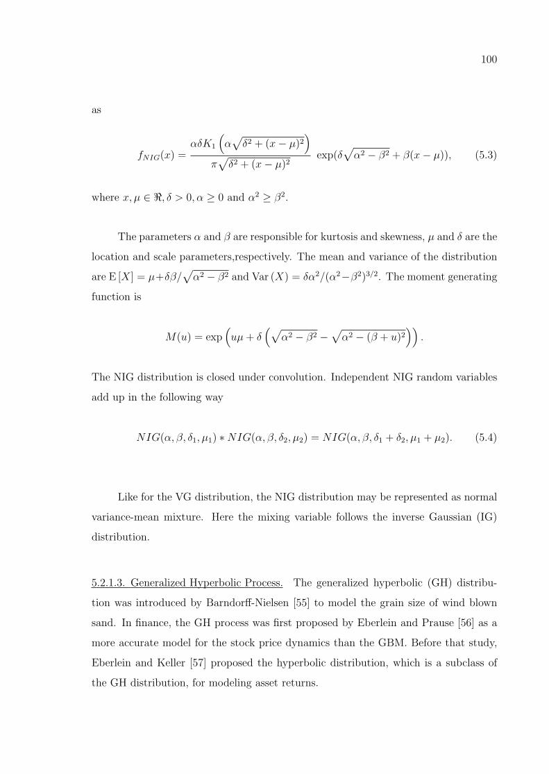
100

as

fNIG(x) =αδK1

(α√δ2 + (x− µ)2

)π√δ2 + (x− µ)2

exp(δ√α2 − β2 + β(x− µ)), (5.3)

where x, µ ∈ <, δ > 0, α ≥ 0 and α2 ≥ β2.

The parameters α and β are responsible for kurtosis and skewness, µ and δ are the

location and scale parameters,respectively. The mean and variance of the distribution

are E [X] = µ+δβ/√α2 − β2 and Var (X) = δα2/(α2−β2)3/2. The moment generating

function is

M(u) = exp(uµ+ δ

(√α2 − β2 −

√α2 − (β + u)2

)).

The NIG distribution is closed under convolution. Independent NIG random variables

add up in the following way

NIG(α, β, δ1, µ1) ∗NIG(α, β, δ2, µ2) = NIG(α, β, δ1 + δ2, µ1 + µ2). (5.4)

Like for the VG distribution, the NIG distribution may be represented as normal

variance-mean mixture. Here the mixing variable follows the inverse Gaussian (IG)

distribution.

5.2.1.3. Generalized Hyperbolic Process. The generalized hyperbolic (GH) distribu-

tion was introduced by Barndorff-Nielsen [55] to model the grain size of wind blown

sand. In finance, the GH process was first proposed by Eberlein and Prause [56] as a

more accurate model for the stock price dynamics than the GBM. Before that study,

Eberlein and Keller [57] proposed the hyperbolic distribution, which is a subclass of

the GH distribution, for modeling asset returns.

101

The GH distribution has five parameters λ, α, β, δ and µ and the density

fGH(x) =(γ/δ)λ√

2πKλ(δγ)eβ(x−µ)

Kλ−1/2

(α√δ2 + (x− µ)2

)(√

δ2 + (x− µ)2/α)1/2−λ , (5.5)

where γ =√α2 − β2. The parameter domain is given by:

α > 0, α2 > β2, δ ≥ 0 if λ > 0

α > 0, α2 > β2, δ > 0 if λ = 0

α ≥ 0, α2 ≥ β2, δ > 0 if λ < 0

In all cases µ ∈ <. α and β determine the shape of the distribution. β is the

skewness, µ location and σ is the scale parameter. For λ = 1, we get the subclass

called hyperbolic distribution.

The GH distribution has the following mean and variance:

E [X] = µ+βδ√α2 − β2

Kλ+1(ζ)

Kλ(ζ), (5.6)

Var (X) = δ2

(Kλ+1(ζ)

ζKλ(ζ)+

β2

α2 − β2

[Kλ+2(ζ)

Kλ(ζ)−(Kλ+1(ζ)

Kλ(ζ)

)2])

, (5.7)

where ζ = δ√α2 − β2. The moment generating function is

M(u) = euµ(

α2 − β2

α2 − (β + u)2

)λ/2Kλ(δ

√α2 − (β + u)2)

Kλ(δ√α2 − β2)

.

The generalized hyperbolic distribution can be represented as normal variance-mean

mixture. Here the mixing variable follows the generalized inverse Gaussian (GIG)

distribution.

The GH distribution is fairly general and capable of representing the leptokurtotic

102

features of returns, but it has the disadvantage that it is not closed under convolution.

In fact, summation of two GH random variates is not generalized hyperbolic in general.

This means that if we model the daily logreturns as GH random variates, then weekly

and monthly logreturns are not GH anymore and their densities are not available in

closed form.

5.2.1.4. Meixner Process. The Meixner (MXN) distribution is an infinitively divisible

distribution introduced by Schoutens and Teugels [58]. It was suggested for the financial

modeling of stock returns and option pricing by Grigelionis [59]. The MXN distribution

has four parameters α, β, δ and µ and the density

fMXN(x) =(2 cos (β/2))2δ

2απ Γ (2δ)exp

(β(x− µ)

α

) ∣∣∣∣Γ(δ + iβ(x− µ)

α

)∣∣∣∣2 ,where α > 0,−π < β < π, δ > 0 and µ ∈ <.

The parameters α and β are responsible for kurtosis and skewness, µ and δ are the

location and scale parameters, respectively. The mean and variance of the distribution

are E [X] = µ + αδ tan(β/2) and Var (X) = α2δ/(cos β + 1). The moment generating

function is

M(u) = euµ

(cos(β/2)

cos(αu+β

2

))2δ

.

The MXN distribution is closed under convolution. Independent MXN random

variables add up in the following way

MXN(α, β, δ1, µ1) ∗MXN(α, β, δ2, µ2) = MXN(α, β, δ1 + δ2, µ1 + µ2).

103

5.2.2. Jump Diffusion Processes

The pure jump processes presented above are infinite activity models i.e. there

exists an infinite number of infinitesimally small jumps in any time interval. As they are

already capable of representing the small movements, adding a diffusion component to

such models does not improve their empirical performance of emulating the dynamics

of the stock price movements in the market. On the other hand, for a Poisson process,

the situation is different. In a Poisson process, there exists a finite number of events in

every finite time interval. So, small movements of the stock price can not be captured

by only using a compound Poisson process. We have to add a diffusion component

so that small movements are represented by the diffusion and large movements in the

stock price are represented by the compound Poisson process.

A jump diffusion model can be specified by the following stochastic differential

equation,

dS(t)

S(t−)= µdt+ σdW (t) + dJ(t), (5.8)

where µ and σ are constants, W is a standard Brownian motion and J is a pure jump

process independent of W . In particular, J is given by J(t) =∑N(t)

j=1 (Yj − 1), where

Yj’s are positive iid random variables and N(t) is a counting process independent of

Yj’s. Here N(t) is assumed to be a Poisson process, and so, J(t) is a compound Poisson

process. In Equation 5.8, S(t−) and S(t) are the left and right hand limits, respectively.

That is S(t−) = limu↑t S(u) and S(t) = limu↓t S(u).

Let τj denotes time of the jth jump. Then the additive jump amount in S at

time τj is

S(τj)− S(τj−) = S(τj−) (J(τj)− J(τj−)) = S(τj−)(Yj − 1).

Hence S(τj) = S(τj−)Yj. Therefore, Yj represents the multiplicative jump amount in

S that is the ratio of stock prices after and before the jump.

104

The solution of Equation 5.8 is

S(t) = S(0) exp((µ− σ2/2)t+ σW (t))

N(t)∏j=1

Yj. (5.9)

This is similar to GBM exept for the multiplicative jump part. Let S(t) = S(0) exp(L(t)).

Then under a jump diffusion model,

L(t) = (µ− σ2/2)t+ σW (t) +

N(t)∑j=1

log Yj. (5.10)

The first jump diffusion model in the literature was introduced by Merton [60].

In that model, jump amplitudes Yj’s are lognormally distributed so it is called as log-

normal jump diffusion model (LNJD). The lognormality assumption makes the model

tractable and yields a closed form solution for plain vanilla options.

Kou [61] proposes the so called double exponential jump diffusion. In this model,

log Yj’s follow the double exponential distribution. Bu using the memoryless property

of the exponential distribution, Kou [61] obtain the density of the increments and

the price of plain vanilla options in closed form. Also, under that model, Kou and

Wang [62] obtain closed from solutions for the Laplace transforms of path dependent

options with continuous monitoring of the price of underlying stock.

5.3. Simulation of Levy Processes

5.3.1. Pure Jump Processes

5.3.1.1. Subordination. For simulation of Levy processes, quants in financial industry

highly likely rely on the “time-changed Brownian motion” structure. All pure jump

Levy processes mentioned in Section 5.2.1 can be represented as a time changed Brow-

105

nian Motion,

L(t) = µ t+ β V (t) +W (V (t)), (5.11)

where V (t), t ≥ 0 is a subordinator (i.e. a Levy process with nondecreasing sam-

ple paths) independent of Brownian motion W (t). This representation is also called

subordination.

Let G denote the distribution of the increment V (ti)−V (ti−1) for the time length

ti − ti−1 = ∆t. To simulate L(t) by using subordination on a fixed time grid t0 < t1 <

... < td with tj = ∆t, the following steps must be carried out for each time interval

(ti−1, ti),

(i) Generate Y ∼ G.

(ii) Generate Z ∼ N(0, 1).

(iii) Set L(ti)← L(ti−1) + µ∆t+ β Y +√Y Z.

The time changed BM representations of Variance Gamma (VG), Normal In-

verse Gaussian (NIG) and Generalized Hyperbolic (GH) processes are evident by their

construction. In fact, the distributions of the increments of those processes allow nor-

mal variance-mean mixture representations, see Section 5.2.1. The subordinators of

VG, NIG and GH processes are gamma, inverse gaussian (IG), and generalized inverse

Gaussian (GIG) processes, respectively. Moreover, Madan and Yor [63] show that

MXN and CGMY processes also allow subordination representations. They give ex-

plicit characterization of their subordinators and provide simulation methods for these

processes.

5.3.1.2. Numerical Inversion. To simulate L(t) by inversion on a fixed time grid t0 <

t1 < ... < td with tj = ∆t, the following steps must be carried out for each time interval

(ti−1, ti),

106

(i) Generate U ∼ U(0, 1).

(ii) Calculate the increment, X ← F−1(U)

(iii) Set L(ti)← L(ti−1) +X.

The inverse CDFs of the increments of the processes mentioned in Section 5.2.1 are not

available in closed form. However, if we can calculate the density of the increments, it

is possible to simulate the Levy processes by using the numerical inversion algorithm

of [5]. That algorithm returns an approximate quantile function F−1a in a reasonable

time, and requires not more than the PDF of the distribution. In Section 5.2.1, the

closed formulas of the PDFs are given. The technical details of the numerical inversion

were also given in Section 2.1.1. In next section, the numerical inversion algorithm is

compared with the classical subordination approach in terms of the simulation speed

and the implementation difficulty.

5.3.1.3. Comparison of Numerical Inversion and Subordination.

• Speed:

The main advantage of numerical inversion is the speed improvement. The

marginal generation times we observed were all smaller than generating an expo-

nential random variate by inversion. Also, the setup times of numerical inversion

were quite small, generally about 0.01 seconds. For large samples, the subordina-

tion approach is at least two times slower than numerical inversion, as it requires

generation of two random variates for each time interval.

• Implementation:

Even if we assume that random variate generation methods for standard distri-

butions are available, the subordination approach is easily implemented without

requiring special algorithms only for the VG process. For the NIG process the

naive (subordination) approach requires generation code for the IG distribution,

for the GH process we require generation code for the GIG distribution. These

are all non-standard distributions and it is not so easy to find trustworthy code

for these generators; to implement the generation algorithms yourself expertise is

107

library(Runuran)

## Create distribution object for GH distribution

distr <- udghyp(lambda=-1, alpha=39, beta=4, delta=0.01, mu=0)

## Generate generator object; use method PINV (inversion)

gen <- pinvd.new(distr)

## Draw a sample of size 100

x <- uq(gen,runif(100))

Figure 5.1. R codes for generation of GH variates by numerical inversion.

required.

On the other hand, numerical inversion requires only a code for evaluating the

density and knowledge about the smoothness of the density. If the density is

smooth, there is no difficulty in using the algorithm directly in C or in R, see Sec-

tion 2.1.1.4. Moreover, for the processes considered in this thesis, we even do not

have to implement the density as we have ready-to-use density implementations

in the UNU.RAN library. Thanks to the R package Runuran, it is quite simple

to implement a path simulation algorithm with numerical inversion. What we

require is not more than three lines of R codes. In Figure 5.1, we present a sim-

ple example where we generate GH variates from uniforms by using the quantile

function uq, the function pinvd.new (Polynomial interpolation of INVerse CDF)

and the density udghyp. For more details, we refer to the manual of the package.

Note that using the R functions in Figure 5.1 does not require any particular

expertise.

5.3.2. Jump Diffusion Processes

5.3.2.1. The Standard Method. The standard method for simulation of jump diffu-

sion processes is based on simulation of compound Poisson processes. Glasserman [2]

summarizes the main steps of the simulation of a jump diffusion Levy process L(t) (see

Equation 5.10) on a fixed time grid t0 < t1 < . . . < td as follows. For each time interval

(ti, ti+1),

108

(i) Generate Z ∼ N(0, 1).

(ii) Generate N ∼ Poisson(λ(ti+1 − ti)).

(iii) Generate log Yj, j = 1, .., N , from their common distribution.

(iv) Set M ←∑N

j=1 log Yj.

(v) Set L(ti+1)← L(ti) + (µ− σ2/2)(ti+1 − ti) + σ√ti+1 − tiZ +M .

The lognormal model of Merton [60] defines Yj ∼ LN(a, b2) and thus log Yj ∼

N(a, b2). Then ∀n ∈ Z+,∑n

j=1 log Yj ∼ N(an, b2n). Therefore, conditional on N(t) =

n, L(t) is normally distributed with mean (µ − σ2/2)t + an, and variance σ2t + b2n.

Hence steps (iii)-(v) of the algorithm of Glasserman [2] can be replaced by

(iii) Set L(ti+1) = L(ti) + (µ−σ2/2)(ti+1− ti) + aN +(√

σ2(ti+1 − ti) + b2N)Z.

5.3.2.2. Numerical Inversion. For the generation of random variates by using numer-

ical inversion, the density of the distribution must be available. However, for jump

diffusion processes, the density is only available as an infinite sum. Let fL(t)(x),

fL(t)|N(t)(x|n) and p(n) be the density of L(t), the density of L(t) conditional on N(t)

and probability mass function of N(t) i.e. p(n) = P (N(t) = n), respectively. Then

fL(t)(x) can be written as fL(t)(x) =∑∞

n=0 fL(t)|N(t)(x|n)p(n). The only possibility to

use numerical inversion is approximation of the infinite sum by truncation. In fact, we

must find a positive integer n such that the remainder term is smaller than a specified

error bound ε. That is∑∞

n=n p(n)fL(t)|N(t)(x|n) ≤ ε.

In the lognormal jump diffusion (LNJD) model, fL(t)|N(t)(x|n) is the normal den-

sity with parameters depending on n. Let σ2n = σ2t + b2n denote the variance of L(t)

conditional on N(t) = n. Also, let f(x|n) = fL(t)|N(t)(x|n) to simplify the notation.

109

Then ∀x ∈ <,

∞∑n=n

p(n)f(x|n) ≤∞∑n=n

p(n) maxx

f(x|n)

=∞∑n=n

p(n)1√

2πσn

<

(1√

2πσn

) ∞∑n=n

p(n)

<

(1√

2πtσ

) ∞∑n=n

p(n).

The equality in the second line comes from the fact that the normal density function

is maximized at the mean. The inequalities in the last two lines are due to the fact

that σ2n is a monotonically increasing function of n. Thus the solution of the following

equality for n will give us the truncation level

∞∑n=n

p(n) = ε√

2πtσ.

The solution can be found easily by using the quantile function of the Poisson distri-

bution qpois in R.

5.4. Risk Neutral Measures for Option Pricing

It is well known that under Levy processes, the risk neutral martingale measure is

not unique and so the market is incomplete (except for the special case of GBM and the

geometric (compensated) Poisson process), see [46, 64, 65]. This means that there are

multiple measures to price the options. So which of the risk neutral measures should be

selected to price the option? In this section, we consider two widely used approaches for

option pricing: The mean correcting martingale measure and the Esscher transform.

110

5.4.1. Mean Correcting Martingale Measure

Under the risk neutral measure, the discounted stock price process must be a

martingale. That goal is achieved by changing the drift parameter m of the process

L(t) (or equivalently by changing the location parameter of the distribution of L(1))

where L(t) is the Levy process in the stock price process S(t) = S(0)eL(t).

Let M(u) be the moment generating function of L(1), that is M(u) = E [euL(1)].

Schoutens [51] explains that we have to use the location parameter

mnew = m+ r − logM(1). (5.12)

Then the stock price process becomes

S(t) = S(0) eLnew(t) = S(0) e(r−logM(1)) t+L(t).

Hence the risk neutral expectation of the discounted stock price is

E [e−rtS(t)] = S(0) E [eL(t)−logM(1) t] =S(0)

M(1)tE [eL(t)] = S(0).

The final equality comes from the fact that the process L(t) has independent and

stationary increments and so E [eL(t)] = E [eL(1)]t = M(1)t.

For GBM case, we have L(t) = (µ− σ2/2)t + σW (t), m = µ− σ2/2, M(1) = eµ

and so from Equation 5.12, mnew = r − σ2/2.

Schoutens [51] note that under the mean correcting martingale measure the stock

price process can be written as the following

S(t) = S(0) exp((r + ω)t+ L(t)) (5.13)

Here L(t) is a Levy process without drift and ω is a compensation parameter given by

111

ω = − log(ML(1)) where ML(u) is the moment generating function of L(1).

5.4.2. Esscher Transform

The Esscher transform, or namely exponential change of measure, was proposed

by Gerber and Shiu [66] for option pricing. For a given probability density function

f(x) and its moment generating function M(u),

fθ(x) = eθx−logM(θ)f(x),

is a probability density for each real θ, and it is called Esscher transform (with param-

eter θ) of the original distribution. In our case f denotes the density of the increments

of the log stock price process. The discounted stock price process is a martingale if θ

satisfies the below equation,

r = logM(θ + 1)

M(θ), (5.14)

assuming there is a solution. We call the Esscher transform with parameter θ that

satisfies the above equation the risk-neutral Esscher transform, and the corresponding

equivalent martingale measure the risk-neutral Esscher measure [66].

Strictly speaking, it is not enough to consider the Esscher transform of the prob-

ability density of one random variable in the present context, as the joint law of

S(t1), . . . , S(td) is required. Here we are using the fact, that the Esscher transform

preserves the independence and the stationarity of the increments. We define the

Esscher transform on the probability space (Ω,FT , P ) by

dQ

dP=

eθL(T )

M(θ)T,

where M(u) = E [euL(1)], assuming the expectation exists. This implies that L re-

mains a Levy process under the new measure Q and we have a similar exponential

112

transformation for the probability densities of the increments.

113

6. NEW CONTROL VARIATES FOR LEVY PROCESS

MODELS

6.1. Introduction

Let L(t), t ≥ 0 be a Levy process and q be a function of the sample path of

L(t) on a discrete time grid 0 = t0 < t1 < t2 < ... < td with equidistant time points

ti = i∆t. The unknown quantity that we are trying to estimate is the expectation

E [q(L(t1), . . . , L(td))]. (6.1)

For high dimensions and complicated functions, it is often not possible to find the exact

value with a closed form solution. Such situations commonly arise e.g. when pricing

options with path dependent payoffs.

In the literature, there exist studies proposing variance reduction methods that

work well for some special Levy processes. However, there seem to exist only a limited

number of studies proposing variance reduction methods, which are generally applicable

to Levy processes and different problem types (see, for example, the variance reduction

methods of Kawai [67–69] and the Quasi Monte Carlo (QMC) method of Imai and

Kawai [70]). In this chapter, a general control variate (CV) method is presented for

the functionals of Levy processes. The method is applicable for all types of Levy

processes for which the probability density function of the increments is available in

closed form. It is based on fast numerical inversion of the cumulative distribution

functions and exploits the strong correlation between the increments of the original

process and a coupled Brownian motion. In the suggested control variate framework,

a similar functional of Brownian motion is used as a main control variate while some

other characteristics of the paths are used as auxiliary control variates.

In Section 6.2, we formulate and explain the basic principles of the general CV

114

framework. Section 6.3 presents our general CV candidates with their expectation

formulas. We consider a simple example in Section 6.4. The presentation in the next

sections closely follows Dingec and Hormann [71].

6.2. General CV Framework

Let W (t), t ≥ 0 be a Brownian motion (BM) with parameters µ and σ > 0,

W (t) = µ t+ σ B(t),

where B(t) is a standard Brownian motion. Assume that increments of W (t), t ≥ 0

are correlated with that of the original Levy process L(t), t ≥ 0 with a comonotonic

copula. Also, assume that there exist a functional ζ of W , which is equal or similar

to q and there exist a solution for E [ζ(W )]. The idea is to use ζ(W ) as main CV

for q(L). The comonotonicity between the increments and the similarity between ζ()

and q() should imply high correlation and thus lead to large variance reduction. One

technical difficulty is the simulation of the comonotonic copula. It requires inversion

of the cumulative distribution functions (CDFs) of the increments of both processes

for a common uniform random number. However, for the Levy processes considered

in the literature, at most the probability density function (PDF) of the increments is

available in closed form while the CDF and the inverse CDF are not tractable. So, to

use inversion we need the fast numerical inversion algorithm (see Sections 2.1.1 and

5.3.1.2) that requires as input only the PDF of the distribution.

When ζ(W ) is used as single CV, the remaining variance is due to the difference

between the two functions, ζ() and q(), and the two processes L and W . In practice,

these functions are contingent on some characteristics of the paths such as average,

maximum and terminal value. By using those characteristics as additional CVs we

can further reduce the variance as they carry some information about the difference

between ζ() and q(). The only requirement is the availability of their expectations.

Moreover, in some cases, it is possible to obtain significant variance reduction by using

only those characteristics as CVs without using ζ(W ). Let γ(W,L) be a function of

115

the paths of W and L that evaluates the set of path characteristics. We call these

additional CVs ’general CVs’ since they are applicable to any q(), whereas ζ(W ) is

called ’special CV’ as it is designed considering the special properties of q().

Algorithm 6.1 presents the general CV method. In the algorithm, the CV coeffi-

cient vector is denoted c = (c1, c2) where c1 denotes the single coefficient of ζ(W ) and

c2 the vector of coefficients necessary for γ(W,L). The increments of W are generated

by inversion of the standard normal CDF Φ():

F−1BM(U) = µ∆t+ σ

√∆t Φ−1(U). (6.2)

Here µ and σ are the unspecified parameters of the BM model. Our choice is to select

them as µ = E [L(1)] and σ =√

Var (L(1)). This selection leads to close to maximal

correlation in our experiments.

Require: Sample size n, simulation output function q, time interval ∆t, num-

ber of time points d, quantile function of the Levy process increments F−1L ,

special CV function ζ, general CV function γ, parameters of BM µ, σ,CV coefficients c.

Ensure: An estimate of E [q(L)] and its 1− α confidence interval.


2: Generate independent uniform variates Uj ∼ U(0, 1), j = 1, . . . , d.

3: Set Xj ← F−1L (Uj) and Zj ← F−1

BM(Uj), j = 1, . . . , d, see Equation 6.2.

4: Set L(tj)← L(tj−1) +Xj and W (tj)← W (tj−1) + Zj, j = 1, . . . , d.

5: Set Yi ← q(L)− c1 (ζ(W )− E [ζ(W )])− cT2 (γ(W,L)− E[γ(W,L)]).

6: end for


8: return Y and the error bound Φ−1(1−α/2) s/√n, where Φ−1 denotes the


Figure 6.1. Algorithm for the general CV method.

116

6.3. Possible Control Variates

In Algorithm 6.1, the user has to provide the CV functions ζ() and γ(). Selection

of ζ() of course depends on the problem type, as it is tailored to q(). However, the

general CVs can be freely chosen from a large pool or basket of CV candidates. For

the selection of the successful CVs from that basket, we can try to use our theoretical

knowledge on the problem and guess which CV will be successful. In this paper, we

propose an alternative approach, which is more automatic and universally applicable

to all problems. We make a stepwise backward regression to detect the useful CVs in

a pilot simulation run. First we start with a full regression model where all possible

CVs in the basket are used. The CV with the smallest absolute t statistic is removed

from the model if its value is smaller than 5. After removal, the t statistics of the other

CVs are recomputed for the new regression model. These two steps are repeated till

all absolute t values are above 5. The CV candidates, which remains in the regression

model, are used for the main simulation. Instead of using only the significant CVs,

one can prefer to use all CVs in the basket. However, simulation or evaluation of

the expectation of some CVs can be computationally expensive compared to that of

the others. The backward regression automatically eliminates the CVs if they are not

useful.

A single regression with k covariates requires O(np k2) operations, where np de-

notes the sample size of the pilot simulation. In the worst case, when all CVs in the

basket are useless, the complexity of the backward regression becomes O(np k3). As

we select np typically much smaller than n the regression round of the algorithm will

not cause a substantial increase in the computational time unless k is larger.

Table 6.1 shows our basket of general CVs that contains the path characteristics

of which the expectation is available in closed form. This list is not exhaustive and

depends on our knowledge of the closed form solutions of the expectations. One can

enlarge this basket by adding new CVs with new expectation formulas. We decided

not to include CVs that require numerical methods to evaluate their expectations. The

details of the expectation formulas of the CVs are given in Section 6.3.1. Some CVs

117

have simpler expectation formulas if the processes exp(−r t+L(t)) and exp(−r t+W (t))

with some r > 0 are martingales. We also give these simpler formulas in Table 6.1, as

they are important for option pricing.

Table 6.1. A basket of general CVs (Expectation-M: simpler expectation formulas for

the martingale case).

Label CV Expectation Expectation-M

CVL1 L(td) dE [X]

CVL2 exp(L(td)) M∆t(1)d er T

CVL3 1d

∑di=1 L(ti) E [X](d+ 1)/2

CVL4 exp(1d

∑di=1 L(ti))

∏di=1 M∆t(i/d)

CVL5 1d

∑di=1 exp(L(ti))

1d

∑di=1 M∆t(1)i 1

d

∑di=1 e

r i∆t

CVW1 W (td) d µ∆t

CVW2 exp(W (td)) e(d(µ∆t+σ2 ∆t/2)) er T

CVW3 1d

∑di=1W (ti) µ∆t(d+ 1)/2

CVW4 exp(1d

∑di=1W (ti)) exp(µ+ σ2/2)

CVW5 1d

∑di=1 exp(W (ti))

1d

∑di=1 e

(i(µ∆t+σ2 ∆t/2)) 1d

∑di=1 e

r i∆t

CVW6 max0≤i≤dW (ti) see Equation 6.3

CVW7 exp(max0≤i≤dW (ti)) xd in Equation 6.4

CVW8 sup0≤u≤td W (u) see Equation 6.6

CVW9 exp(sup0≤u≤td W (u)) see Equation 6.7

In Table 6.1, CVLs are based on the path characteristics of the original Levy

process, while CVWs are based on the auxiliary BM. Indeed CVLs are internal CVs

whereas CVWs are external. The internal CVs do not require any additional effort but

often yield moderate variance reduction. However, when CVLs, CVWs and the special

CV ζ(W ) are used together, they often result in large variance reductions. CVL1-5

and CVW1-5 depend on the terminal value and arithmetic averages of the paths and

their exponentials, while CVW6-9 depend on the maximum of the discrete path and

the supremum of the continuous path of W (t). The counterparts of CVW6-9 for L(t)

are not available in the CV basket as closed form solutions of their expectations only

118

exist for the special case of Brownian motion.

Instead of the averages one could try to use all L(ti)’s and eL(ti)’s as CVs. To

keep the total number of CVs moderate we decided not to include them in our basket.

It is also possible to add some other CVs depending on the averages of the squared

values of L(ti) as their expectations are also available thanks to the variance formulas

of the distribution of increments of the Levy processes. However, their contribution is

expected to be insignificant as the CVs depending on the exponentials already convey

much of the information of the CVs depending on the squared values.

CVL1-5 and CVW1-7 are all easy to simulate as they are simple functions of the

paths. However, CVW8 and CVW9 can not be calculated directly from the gener-

ated paths, as they are random functions of the discrete path. Note that to simulate

sup0≤u≤td W (u) we have to generate the maxima of d Brownian bridges. For simulation

of the maximum of Brownian bridge, see the inversion method given in Section 4.2.

Note that the CVs in the basket are strongly correlated with each other. This

situation, which is called multicollinearity in the statistical literature, can be a problem

for the accuracy of the estimates of the t statistics when the sample size is too small, as

it inflates the standard errors of the estimates of the regression coefficients. So, for the

pilot run, it is important to select a sample size which is not too small. Our numerical

experience shows that the sample size of n = 104 is generally sufficient to get relatively

stable estimates of the t values.

6.3.1. Expectation Formulas

6.3.1.1. Expectations of CVLs. The expectations of L(td) and 1d

∑di=1 L(ti) (CVL1

and CVL3) can be calculated by using the expectation formulas of the increment distri-

bution of the corresponding Levy process (see e.g. the formulas given in Section 5.2.1).

For CVL2, CVL4 and CVL5, we need the moment generating function (MGF) of the

increment distribution (see e.g. Section 5.2.1). Let Xi denote the increment of L

over time interval [ti−1, ti]. As the time lengths are equal to ∆t, Xi’s are iid copies

119

of a random variate X. Expectations of CVL1 and CVL3 are given by dE [X] and

E [X](d+ 1)/2, respectively.

Let M∆t(u) denote the MGF of the increment for the time length ∆t, that is

M∆t(u) = E [euX ]. Then E [exp(L(ti))] = E[exp

(∑ij=1Xj

)]= M∆t(1)i. The expec-

tation of CVL2 is simply M∆t(1)d. Also, the expectation of CVL5 is 1d

∑di=1M∆t(1)i.

The expectation of CVL4 is given by E[exp

(1d

∑di=1 L(ti)

)]=∏d

i=1M∆t(i/d), since

1d

∑di=1 L(ti) = 1

d

∑di=1 (d− i+ 1)Xi.

6.3.1.2. Expectations of CVWs. Let Zi denote the increment of W over time interval

[ti−1, ti]. Then Zi’s are i.i.d. copies of Z ∼ N(µ∆t, σ2 ∆t). The expectations of CVW1

and CVW3 are given by E [W (td)] = d µ∆t and

E

[1

d

d∑i=1

W (ti)

]=µ∆t

d

d∑i=1

i =µ∆t(d+ 1)

2,

respectively. By using the MGF of the normal distribution, we obtain the expectations

of CVW2 and CVW5 as E [exp(W (td))] = exp(d(µ∆t+ σ2 ∆t/2)) and

E

[1

d

d∑i=1

exp(W (ti))

]=

1

d

d∑i=1

exp(i(µ∆t+ σ2 ∆t/2)).

The expectation of CVW4 is obtained by using the fact that any linear combina-

tion of independent normal variates is again normal. Note that 1d

∑di=1W (ti) =

1d

∑di=1 (d− i+ 1)Zi. is equal in distribution to a normal variate with mean µ =

E[

1d

∑di=1 i Zi

]= µ∆t(d+ 1)/2 and variance

σ2 = Var

(1

d

d∑i=1

i Zi

)=σ2 ∆t

d2

d∑i=1

i2 =σ2 ∆t (d+ 1) (2d+ 1)

6d

Hence we get E[exp

(1d

∑di=1W (ti)

)]= exp(µ+ σ2/2).

To find the expectation of CVW6, we use the fact that W (ti), i ≥ 1 is a random

120

walk with iid increments. By Spitzer’s identity [72] we get

E

[max0≤i≤d

W (ti)

]=

d∑j=1

1

jE[W (tj)

+], (6.3)

where

E[W (t)+

]= µ tΦ(µ

√t/σ) + σ

√t φ(−µ

√t/σ),

Φ() and φ() are the CDF and the PDF of the standard normal distribution.

To find the expectation of CVW7, we use the recursion of [73]. Let Xj, j ≥ 1

be iid random variables and X0 = 0. Define Yk =∑k

j=0Xj and Mk = max0≤j≤k Yj.

Also, let xk = E [eMk ] and ak = E [eY+k ]. By using Spitzer’s formula, [73] proves that

xk =1

k

k−1∑j=0

ak−j xj. (6.4)

In our case, Xj ∼ N(µ∆t, σ2 ∆t), Yk ∼ N(kµ∆t, kσ2∆t) and

ak = Φ(−µσ

√k∆t

)+ e(µ+σ2/2)k∆tΦ

(µ+ σ2

σ

√k∆t

). (6.5)

Hence the expectation of CVW7, E [exp(max0≤i≤dW (ti))], is simply equal to xd which

can be calculated using the recursion in Equation 6.4 with the coefficients in Equa-

tion 6.5.

It should be noted that by using the formulas of [72] and [73] it is also possible to

evaluate E [max0≤i≤d L(ti)] and E [exp(max0≤i≤d L(ti))]. However, in that case, we need

numerical integration to evaluate each ak. Furthermore, if the increment distribution

is not closed under convolution, the evaluation of the ak’s requires the inversion of the

characteristic functions.

The expectations of CVW8 and CVW9 are found by using the density of the

121

maximum of Brownian motion with drift on a finite interval see e.g. [46]. By integration

of the density, we obtain

E

[sup

0≤u≤tdW (u)

]=σ2

2µ(2 Φ(b1)− 1) + Φ (b1)µ td + φ (b1)σ

√td, (6.6)

and

E

[exp

(sup

0≤u≤tdW (u)

)]= 1 + ez tdΦ(b1)− Φ(b2)

+

(σ2

2z

)[−Φ(b1 − (2z/σ)

√td) + ez tdΦ(b1)

], (6.7)

where b1 = µ√td/σ, b2 = b1 − σ

√td and z = µ+ σ2/2.

6.4. A Simple Example

The easiest application of our general CV method uses only general CVs of the

basket without a special CV. In this section, we present the use of this general frame-

work for the simple example q(L) = exp (max0≤i≤d L(ti)) , which demonstrates the

effectiveness of the general method. More relevant examples can be found in Chap-

ter 7. To produce the numerical results, the algorithm given in Figure 6.1 was coded in

R [13]. To find the approximate quantile function of the increments (F−1L in Figure 6.1),

we used the numerical inversion algorithm of [5] and the Runuran package of [12]. The

u-resolution of the numerical inversion algorithm was set to εu = 10−10.

We assume that L is a generalized hyperbolic (GH) process. We fix the time step

of the time grid to ∆t = 1/250. The parameters of the distribution of the increments

for the time length ∆t are selected as λ = 1.5 , α = 189.3, β = −5.71, δ = 0.0062,

µ = 0.001 (see Table 7.1). With these parameters, the increment distribution is close

to normal but has a higher kurtosis. We try two cases d = 5 and d = 50. For d = 5, the

backward regression founds all CVs significant except for CVW8 and CVW9. The CV

algorithm with those CVs yields a variance reduction factor (VRF) of 560. For d = 50,

the CVs, which are found to be significant by backward regression, are CVL1,2,4,5,

122

CVW1,2,4,5 and CVW7. The obtained VRF is 395.

123

7. APPLICATION OF NEW CONTROL VARIATE

METHOD TO OPTION PRICING

As in the case of GBM, the valuation of path dependent options under Levy

processes requires efficient numerical methods since the prices are not available in

closed form. Monte Carlo simulation is one of the widely used techniques. Variance

reduction techniques thus play an important role. In this chapter, the application of

the general CV algorithm (see Chapter 6 ) is presented for the simulation of path

dependent options under Levy processes. The formulation and explanations closely

follow [52,71].

Suppose that we have an option on a stock with the price process S(t), t ≥ 0

given by S(t) = S(0)eL(t), where L is a Levy process. Let ψ denote the payoff function

of the option. For discretely monitored path-dependent options, ψ is a function from

<d to < where d denotes the number of control points in time. With time grid 0 = t0 <

t1 < t2 < ... < td = T and maturity T , the price of the option is given by the discounted

risk neutral expectation of the payoff function e−rTE [ψ(S(t1), . . . , S(td))], where r is

the deterministic risk free interest rate. Note that by setting q(L) = ψ(S(0)eL), the

above expectation reduces to Equation 6.1. So, the algorithm in Figure 6.1 can be

applied.

In the application of our general CV approach, the first step is the selection of

a special CV, ζ, which is a functional of W (t). In the option pricing case, that func-

tional corresponds to the payoff function of a similar option with analytically available

price under GBM. Let ψCV denote the payoff function of this new option. Also, letS(t), t ≥ 0

denote the stock price process which follows a GBM with parameters r

and σ: S(t) = S(0)eW (t) = S(0) exp((r − σ2/2)t + σB(t)), where B(t) is a standard

BM. Then our special CV is ζ(W ) = ψCV (S). In this setting, the only unspecified

parameter is the volatility σ of the GBM model, as the drift of BM is automatically

set to µ = r − σ2/2 under the risk neutral measure. We set the volatility equal to

124

the standard deviation of the increments of the original Levy process L(t), that is

σ =√

Var (L(1)). We also use the same initial values for both processes S(0) = S(0).

For option pricing applications, some of the general CVs given in Table 6.1 have

simpler expectation formulas due to the martingale property of the discounted stock

price process under the risk neutral measure, E [e−r tS(t)] = E [e−r tS(t)] = S(0). The

expectations of CVL2 and CVW2 reduce to er T , the expectations of CVL5 and CVW5

are both equal to 1d

∑di=1 e

r i∆t.

7.1. Special CVs for Path Dependent Options

In the sequel, Asian, lookback and barrier options are considered. As special

CVs, those given in Chapters 3 and 4 are used.

7.1.1. Asian Options

We consider the arithmetic average Asian call option with payoff function ψA(S) =(Pdi=1 S(ti)

d−K

)+

where K is the strike price. We use the geometric average Asian call

under GBM as special CV. It has the payoff function ψG(S) =(

exp(Pd

i=1 log S(ti)

d

)−K

)+

.

For its expectation formula, see Equation 3.1 in Chapter 3.

7.1.2. Lookback and Barrier Options

We consider floating strike lookback put, fixed strike lookback call and the up

and out barrier call options. They have the payoff functions

ψLP (S) = max0≤i≤d

S(ti)− S(td), (7.1)

ψLC(S) =

(max0≤i≤d

S(ti)−K)+

, (7.2)

ψB(S) = (S(td)−K)+1max0≤i≤d S(ti)<B, (7.3)

125

where K is the strike price, B is the barrier level and td = T is the maturity. As special

CVs, we use the continuous options under GBM (see Chapter 4) with the respective

payoff functions

ψCLP (S) = sup0≤u≤td

S(u)− S(td), (7.4)

ψCLC(S) =

(sup

0≤u≤tdS(u)−K

)+

, (7.5)

ψCB(S) = (S(td)−K)+1sup0≤u≤tdS(u)<B. (7.6)

As shown in Section 4.2., it is possible to simulate sup0≤u≤td S(u) conditional on the

discrete path S(t1), . . . , S(td). For the expectation formulas, see Section 4.4.

In Chapter 4, it is shown that two additional tricks work well for barrier op-

tions. One is shifting the barrier of the CV by using the correction factor of [48]:

BCV = Beβσ√

∆t where β = −ζ(0.5)/√

2π ≈ 0.5826 and ζ(.) denotes the Riemann zeta

function. The other one is using the conditional expectation of the payoff function, see

Section 4.5.2. For the second trick, we define a new ψCB as conditional expectation of

the previously defined one, that is

ψCB(S(t1), . . . , S(td)) = E[(S(td)−K)+1sup0≤t≤T S(t)<BCV

∣∣∣ S(t1), . . . , S(td)]

Thus ψCB is now only a function of the discrete path. Using the Markovian property

of the Brownian motion and the conditional independence of the local maxima, we

calculate ψCB as: ψCB(S(t1), . . . , S(td)) = (S(td) −K)+∏d

i=1 pi, where pi is given by

Equation 4.15. Therefore, to simulate ψCB, we evaluate the survival probabilities pi for

each time interval and multiply them with (S(td)−K)+. For the complete algorithm

involving all the speed up tricks, see Section 4.6.

126

7.2. Numerical Results

In this section, the effectiveness of the general CV method is demonstrated by

presenting numerical results for the three different path dependent options (Asian, look-

back and barrier) and four different Levy processes (Variance Gamma (VG), Normal

Inverse Gaussian (NIG), Generalized Hyperbolic (GH) and Meixner (MXN) processes).

The parameters of the processes are estimated from the daily log return data of the

Swiss stock “Swiss.Re” given in the R package ghyp of [74]. The sample consists of

500 daily log returns from 2005-01-19 to 2007-01-10. The parameters of the models

were estimated by maximum likelihood estimation. The estimated daily parameters

are shown in Table 7.1.

Table 7.1. Estimated daily parameters for different models.

Model λ α β δ µ

VG 2.25 210.5 −5.14 0.00094

NIG −0.50 131.5 −5.81 0.0134 0.00102

GH 1.50 189.3 −5.71 0.0062 0.00100

MXN 0.018 −0.10 0.6523 0.00100

Note that the parameters given in Table 7.1 are of the real world probability

measure. The option price is however given as the discounted expectation under the

risk neutral probability measure. So, for option pricing, the parameters of the real

world have to be transformed to the risk neutral world. In our study, we have used

the risk neutral Esscher measure explained in Section 5.4.2. To find the risk neutral

Esscher transform, we have solved Equation 5.14 numerically. The moment generating

functions of the VG, NIG, GH and MXN processes are given in Section 5.2.1. The

Esscher density of these processes has a simple representation. In fact the densities of

their Esscher transforms remain in the same family, as their increment distributions

are exponential families. The only parameter that has to be changed is β. It is changed

from β to the new value β+θ for VG, NIG and GH distributions and β+α θ for the MXN

distribution, where θ is the Esscher transform parameter satisfying Equation 5.14. The

127

other parameters of the risk neutral measure remain the same as that of the real world

measure.

To produce the numerical results, the algorithm in Figure 6.1 was coded in R [13].

To find the approximate quantile function of the increments (F−1L in Figure 6.1), we

used the Runuran package of [12]. The u-resolution of the numerical inversion algorithm

was selected as εu = 10−10.

In our numerical results, we report as main result the variance reduction factors

of our new CV method denoted by V RF = σ2N/σ

2CV where σ2

N and σ2CV denote the

variances of naive simulation and our new CV method, respectively. We also report the

time ratio denoted by tN/tCV , where tN and tCV are the CPU times of naive simulation

and the new CV algorithm, respectively. This ratio is important for the efficiency

factor EF = (σ2N tN)/(σ2

CV tCV ) of the new CV algorithm. For tCV , we exclude the

setup time as the quantile function F−1L () obtained in the setup phase can be used for

pricing many options. In our Levy process examples, the setup phase takes about 0.01

seconds, which is negligible compared to the generation times of large samples. In our

naive simulations, we used the standard methods in the literature (e.g. subordination)

for the path generation of the processes. In this way the time ratio tN/tCV reflects not

only the slow down of the new CV but also the speed up of the numerical inversion.

For the experiments, we selected different parameter sets by changing the matu-

rity T , the number of control points d, the strike price K and the barrier level B. The

initial stock price S(0) was set to 100 in all experiments. The risk-free rate r = 0.05

was also fixed. We used the sample size n = 10, 000. The volatility of the CV was

selected as σ = 0.16 as the standard deviations of the yearly increments of the fitted

processes are approximately equal to that value.

The numerical results reported in Section 7.2.1 are obtained by using only the

special CVs (presented in Section 7.1), whereas in Section 7.2.2 the general and special

CVs are used together.

128

7.2.1. Numerical Results Obtained by Using only the Special CVs

7.2.1.1. Variance Gamma Process. In Table 7.2, numerical results for three option

types (Asian call, floating strike lookback put and the up and out barrier call) with daily

monitoring, ∆t = 1/250, are reported, while in Table 7.3 the results of Asian options

are shown for different monitoring intervals. As the common practice for lookback and

barrier options is to monitor daily closing prices, we do not report results for those

options with different ∆t’s. From the reported variance reduction factors in Tables 7.2

and 7.3, we see that our CV method is quite successful. Still we should not overlook

that the size of the variance reduction strongly depends on the parameters and option

types. So we briefly list our main observations.

First we observe the strong influence of the monitoring frequency. As the time

interval ∆t = T/d between the control points gets larger we obtain larger variance

reductions. This is due to the fact that the distribution of the increment over time in-

terval ∆t gets closer to normal for larger ∆t’s. So, as the two quantile functions become

closer to each other, the correlation between the increments gets higher. The increase

in the correlation between logreturns directly implies a higher correlation between two

stock prices, which in turn increases the strength of the linear dependency between the

two payoffs. Hence we obtain larger variance reductions. We also observe the influence

of the strike price K for Asian options. We observe both in Tables 7.2 and 7.3 that a

smaller K leads to larger variance reduction. This observation is consistent with the

behavior observed in the GBM case. In fact, for small K values, the geometric average

and arithmetic average option payoffs become more strongly correlated.

When we look at the results in Table 7.2, we observe that the influence of the

maturity T is small, even negligible in some cases. This can be explained by the fact

that the correlation between∑d

i=1Xi and∑d

i=1 Zi for iid copies of random variates Xi

and Zi is the same as the one between X and Z. Without loss of generality assume

129

E [X] = E [Z] = 0 and note that

Cor

(d∑i=1

Xi,

d∑j=1

Zj

)=

E[(∑d

i=1 Xi

)(∑dj=1 Zj

)]√

Var(∑d

i=1Xi

)Var

(∑dj=1 Zj

) =

∑di=1 E [XiZi]√

d2Var (X)Var (Z)

=E [XZ]√

Var (X)Var (Z)= Cor(X,Z).

In our case, X and Z denote the logreturns of the two stock processes S(t) and S(t),

respectively. The above fact implies that log stock prices log S(t) and log S(t) will

have the same correlation for all values of t. As a result, the effect of the maturity T

is minor compared to that of the other parameters and that minor effect comes from

the nature of the options not from the dependency level of the two processes. As a

final observation, we should note that the success of the CV method seems to be more

pronounced for Asian and lookback options than for barrier options.

For time comparisons, we evaluated the ratio tN/tCV for different option types.

The naive simulation algorithm was implemented using subordination (or, namely, time

changed Brownian motion) representation, as it appears to be the standard simulation

method for the VG processes. It requires generation of a standard normal and a

gamma variate for each time step. We used the built-in R-functions rnorm and rgamma

to generate them. The former performs inversion by using the quantile function of the

standard normal distribution, while the latter uses the rejection methods of Ahrens

and Dieter [75,76] for the gamma distribution.

For Asian options with T = 1 and d = 250, 50, 12 and 4, the ratios tN/tCV

were observed to be equal to 2.6, 2.3, 2.1 and 1.3, respectively. These ratios remain

approximately the same for different parameters. The efficiency factors of the new CV

algorithm can be obtained by multiplying the ratio tN/tCV with the VRFs reported in

Tables 7.2 and 7.3. Usually variance reduction increases the simulation time. However,

in our case, the new CV algorithm is faster than naive simulation. This is thanks to

the speed up obtained by the use of numerical inversion for random variate generation.

For lookback and barrier options, we need more additional calculations to generate the

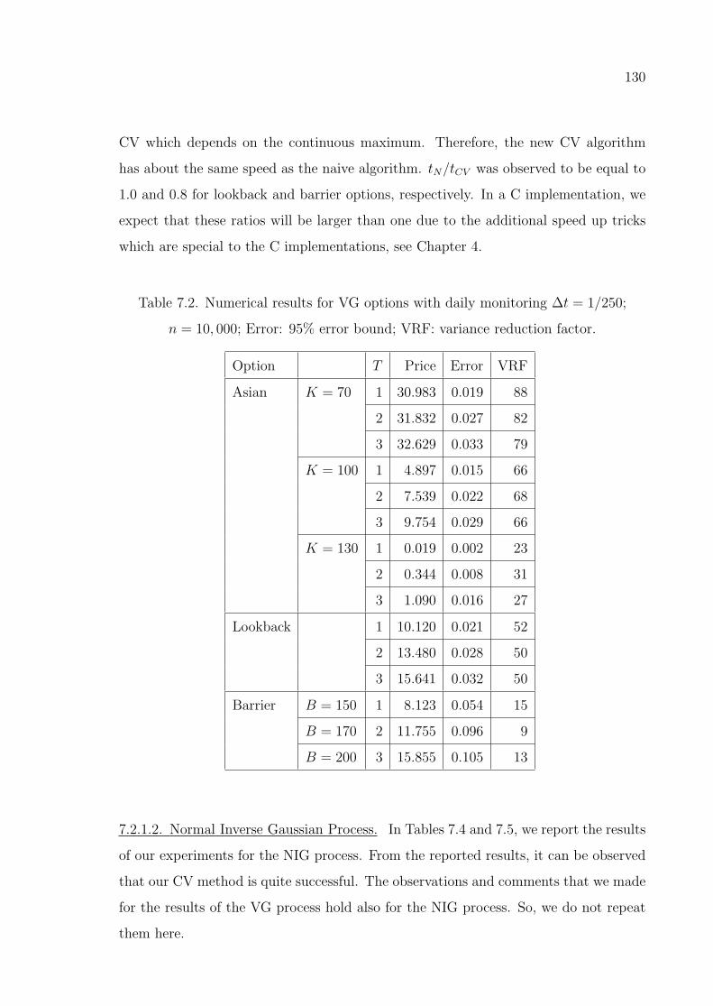
130

CV which depends on the continuous maximum. Therefore, the new CV algorithm

has about the same speed as the naive algorithm. tN/tCV was observed to be equal to

1.0 and 0.8 for lookback and barrier options, respectively. In a C implementation, we

expect that these ratios will be larger than one due to the additional speed up tricks

which are special to the C implementations, see Chapter 4.

Table 7.2. Numerical results for VG options with daily monitoring ∆t = 1/250;

n = 10, 000; Error: 95% error bound; VRF: variance reduction factor.

Option T Price Error VRF

Asian K = 70 1 30.983 0.019 88

2 31.832 0.027 82

3 32.629 0.033 79

K = 100 1 4.897 0.015 66

2 7.539 0.022 68

3 9.754 0.029 66

K = 130 1 0.019 0.002 23

2 0.344 0.008 31

3 1.090 0.016 27

Lookback 1 10.120 0.021 52

2 13.480 0.028 50

3 15.641 0.032 50

Barrier B = 150 1 8.123 0.054 15

B = 170 2 11.755 0.096 9

B = 200 3 15.855 0.105 13

7.2.1.2. Normal Inverse Gaussian Process. In Tables 7.4 and 7.5, we report the results

of our experiments for the NIG process. From the reported results, it can be observed

that our CV method is quite successful. The observations and comments that we made

for the results of the VG process hold also for the NIG process. So, we do not repeat

them here.

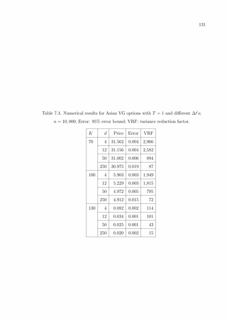
131

Table 7.3. Numerical results for Asian VG options with T = 1 and different ∆t’s;


K d Price Error VRF

70 4 31.562 0.004 2,966

12 31.156 0.004 2,582

50 31.002 0.006 894

250 30.975 0.019 87

100 4 5.903 0.003 1,949

12 5.229 0.003 1,815

50 4.972 0.005 795

250 4.912 0.015 72

130 4 0.082 0.002 114

12 0.034 0.001 101

50 0.025 0.001 43

250 0.020 0.002 15

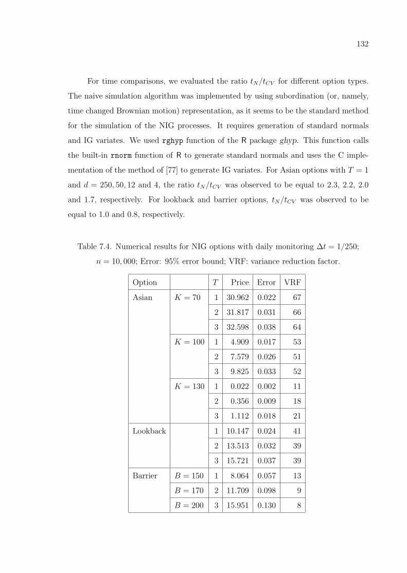
132

For time comparisons, we evaluated the ratio tN/tCV for different option types.

The naive simulation algorithm was implemented by using subordination (or, namely,

time changed Brownian motion) representation, as it seems to be the standard method

for the simulation of the NIG processes. It requires generation of standard normals

and IG variates. We used rghyp function of the R package ghyp. This function calls

the built-in rnorm function of R to generate standard normals and uses the C imple-

mentation of the method of [77] to generate IG variates. For Asian options with T = 1

and d = 250, 50, 12 and 4, the ratio tN/tCV was observed to be equal to 2.3, 2.2, 2.0

and 1.7, respectively. For lookback and barrier options, tN/tCV was observed to be

equal to 1.0 and 0.8, respectively.

Table 7.4. Numerical results for NIG options with daily monitoring ∆t = 1/250;



Asian K = 70 1 30.962 0.022 67

2 31.817 0.031 66

3 32.598 0.038 64

K = 100 1 4.909 0.017 53

2 7.579 0.026 51

3 9.825 0.033 52

K = 130 1 0.022 0.002 11

2 0.356 0.009 18

3 1.112 0.018 21

Lookback 1 10.147 0.024 41

2 13.513 0.032 39

3 15.721 0.037 39

Barrier B = 150 1 8.064 0.057 13

B = 170 2 11.709 0.098 9

B = 200 3 15.951 0.130 8

133

Table 7.5. Numerical results for Asian NIG options with T = 1 and different ∆t’s;


K d Price Error VRF

70 4 31.566 0.004 2,930

12 31.161 0.004 2,262

50 31.004 0.007 695

250 30.959 0.022 68

100 4 5.923 0.003 1,953

12 5.244 0.003 1,783

50 4.982 0.005 580

250 4.924 0.017 56

130 4 0.082 0.001 153

12 0.035 0.001 90

50 0.024 0.001 41

250 0.021 0.002 17

134

7.2.1.3. Generalized Hyperbolic Process. The numerical results reported in Table 7.6

show the success of our CV method for the GH process. The results are quite similar

to the previous ones. The main observations are the same as before. Here contrary to

the previous experiments, we include also the plain vanilla call options in Table 7.6.

As the GH distribution is not closed, the price of the plain vanilla options can not be

represented as one dimensional integrals like for VG and NIG processes. So, the plain

options also need some numerical technique like path dependent options. It can be

observed that variance reductions for the plain call options are very similar to that of

Asian options.

An important consequence of the fact that GH distribution is not closed under

convolution is that we have no chance to directly simulate the weekly or monthly returns

by using the fitted distribution of the daily log returns. That is, to simulate a weekly

return, we must simulate all daily returns in a week. Therefore the number of control

points has little influence on the variance reduction, as the level of the dependency of

the two processes is always the same as that of the daily monitoring case. In fact, for

the plain options, we have just one control point at maturity, but we obtain a very

similar variance reduction to that obtained for the daily monitored Asian options.

As the plain NIG options can be valued by numeric integration of a one dimen-

sional integral, they can be used as CVs for the plain GH options. The only required

modification in Algorithm 6.1 for that is the replacement of the quantile function of

the Brownian motion F−1BM by that of the NIG process F−1

NIG which is also calculated

by using the numerical inversion algorithm. In Table 7.7, we show the results where

the plain NIG call options are used as CVs. For the NIG distribution, we used the

parameters given in Table 7.1. It can be observed that using the NIG option price

yields considerably more variance reduction than using the Black Scholes price of the

GBM model. However, this approach is special to plain options as path dependent

NIG options can not be priced in a simple way.

For time comparisons, the ratio tN/tCV is evaluated for different option types.

For the generation of GH variates in the naive simulation algorithm, the subordination

135

(or, namely, time changed Brownian motion) representation was used, as it is the

standard method in the literature. It requires generation of standard normals and

GIG variates. We used rghyp function of the R package ghyp. This function uses the

C implementation of the ratio of uniforms method of Dagpunar [78] to generate GIG

variates. The time ratios tN/tCV were observed to be equal to 2.7, 1.2 and 0.9, for

Asian, lookback and barrier options, respectively.

7.2.1.4. Meixner Process. The experiments of the previous sections are performed also

for the MXN process with the same option parameters. In Tables 7.8 and 7.9, we report

the results of our experiments. The observed variance reduction factors were almost

the same as the previous ones. The observations and comments that we made for the

results of the VG and NIG processes hold also for the MXN process. So, we do not

repeat them here. The only difference is the time ratio tN/tCV . For naive simulation,

we used the rejection method of Grigoletto and Provasi [79] and Kawai [80], as they

are the only exact generation methods that we were able to find in the literature for

the MXN distribution. For the algorithm of [79], the observed time ratios tN/tCV

were equal to 69, 29 and 23, for Asian, lookback and barrier options, respectively. For

the method of [80], the observed ratios were 103, 44 and 34. These values are quite

large compared to the ratios observed for VG, NIG and GH processes. This is due to

the fact that the rejection methods of Grigoletto and Provasi [79] and Kawai [80] are

comparatively slow due to the expensive evaluations of the complex gamma function

required in every trial of the rejection algorithm.

7.2.2. Numerical Results Obtained by Using General and Special CVs

Numerical results in this section are obtained by using both the general CVs

(CVLs and CVWs in Table 7.10) and the special CVs (given in Section 7.1). Asian

call and fixed strike lookback call options are considered as examples. The results

are given only for the GH process, as it is the most general process among the ones

listed in Section 5.2. Also, when the processes are calibrated by using the same data,

the variance reductions obtained for the other three processes are observed to be very

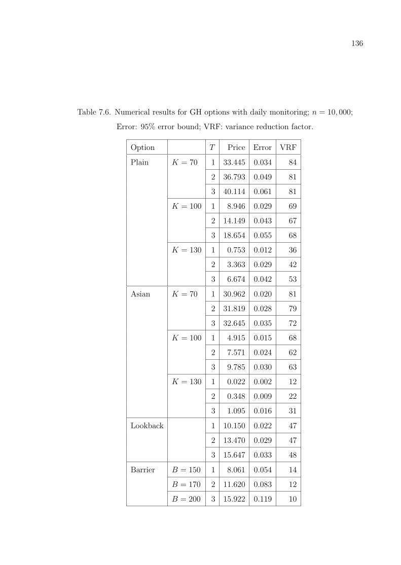
136

Table 7.6. Numerical results for GH options with daily monitoring; n = 10, 000;

Error: 95% error bound; VRF: variance reduction factor.


Plain K = 70 1 33.445 0.034 84

2 36.793 0.049 81

3 40.114 0.061 81

K = 100 1 8.946 0.029 69

2 14.149 0.043 67

3 18.654 0.055 68

K = 130 1 0.753 0.012 36

2 3.363 0.029 42

3 6.674 0.042 53

Asian K = 70 1 30.962 0.020 81

2 31.819 0.028 79

3 32.645 0.035 72

K = 100 1 4.915 0.015 68

2 7.571 0.024 62

3 9.785 0.030 63

K = 130 1 0.022 0.002 12

2 0.348 0.009 22

3 1.095 0.016 31

Lookback 1 10.150 0.022 47

2 13.470 0.029 47

3 15.647 0.033 48

Barrier B = 150 1 8.061 0.054 14

B = 170 2 11.620 0.083 12

B = 200 3 15.922 0.119 10

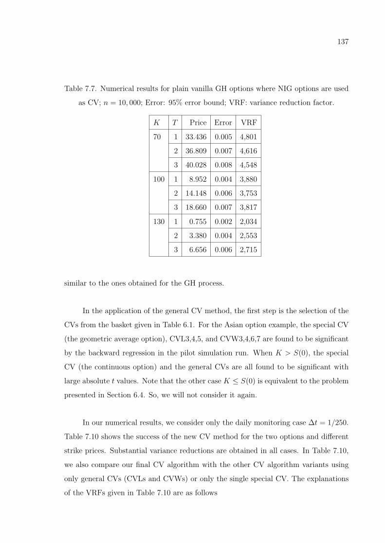
137

Table 7.7. Numerical results for plain vanilla GH options where NIG options are used

as CV; n = 10, 000; Error: 95% error bound; VRF: variance reduction factor.

K T Price Error VRF

70 1 33.436 0.005 4,801

2 36.809 0.007 4,616

3 40.028 0.008 4,548

100 1 8.952 0.004 3,880

2 14.148 0.006 3,753

3 18.660 0.007 3,817

130 1 0.755 0.002 2,034

2 3.380 0.004 2,553

3 6.656 0.006 2,715

similar to the ones obtained for the GH process.

In the application of the general CV method, the first step is the selection of the

CVs from the basket given in Table 6.1. For the Asian option example, the special CV

(the geometric average option), CVL3,4,5, and CVW3,4,6,7 are found to be significant

by the backward regression in the pilot simulation run. When K > S(0), the special

CV (the continuous option) and the general CVs are all found to be significant with

large absolute t values. Note that the other case K ≤ S(0) is equivalent to the problem

presented in Section 6.4. So, we will not consider it again.

In our numerical results, we consider only the daily monitoring case ∆t = 1/250.

Table 7.10 shows the success of the new CV method for the two options and different

strike prices. Substantial variance reductions are obtained in all cases. In Table 7.10,

we also compare our final CV algorithm with the other CV algorithm variants using

only general CVs (CVLs and CVWs) or only the single special CV. The explanations

of the VRFs given in Table 7.10 are as follows

138

Table 7.8. Numerical results for MXN options with daily monitoring ∆t = 1/250;



Asian K = 70 1 30.962 0.020 74

2 31.836 0.029 71

3 32.628 0.036 67

K = 100 1 4.908 0.016 61

2 7.568 0.025 59

3 9.816 0.031 56

K = 130 1 0.023 0.002 14

2 0.350 0.009 22

3 1.097 0.017 27

Lookback 1 10.143 0.023 44

2 13.476 0.030 45

3 15.654 0.035 42

Barrier B = 150 1 8.051 0.052 15

B = 170 2 11.690 0.087 10

B = 200 3 16.036 0.115 11

139

Table 7.9. Numerical results for Asian MXN options with T = 1 and different ∆t’s;


K d Price Error VRF

70 4 31.568 0.004 3,028

12 31.157 0.004 2394

50 31.001 0.006 807

250 30.985 0.021 75

100 4 5.916 0.003 1,892

12 5.239 0.003 1,784

50 4.977 0.005 627

250 4.902 0.017 57

130 4 0.083 0.002 125

12 0.034 0.001 116

50 0.025 0.001 15

250 0.021 0.002 11

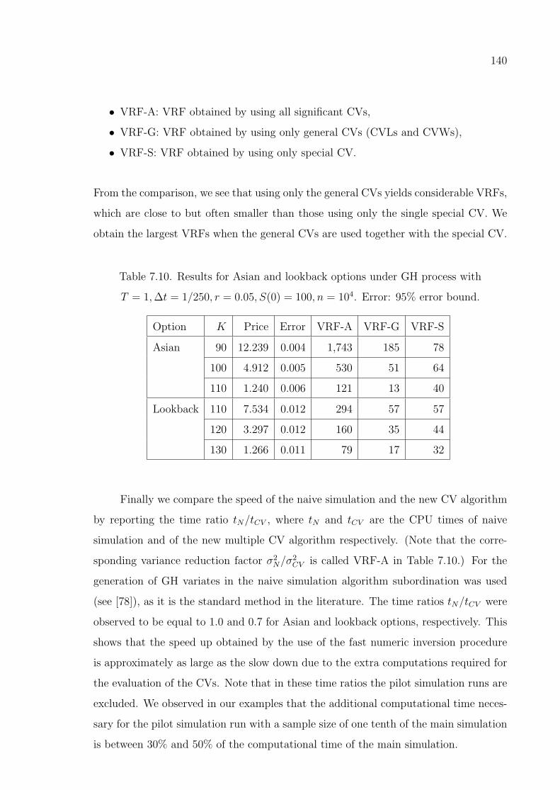
140

• VRF-A: VRF obtained by using all significant CVs,

• VRF-G: VRF obtained by using only general CVs (CVLs and CVWs),

• VRF-S: VRF obtained by using only special CV.

From the comparison, we see that using only the general CVs yields considerable VRFs,

which are close to but often smaller than those using only the single special CV. We

obtain the largest VRFs when the general CVs are used together with the special CV.

Table 7.10. Results for Asian and lookback options under GH process with

T = 1,∆t = 1/250, r = 0.05, S(0) = 100, n = 104. Error: 95% error bound.

Option K Price Error VRF-A VRF-G VRF-S

Asian 90 12.239 0.004 1,743 185 78

100 4.912 0.005 530 51 64

110 1.240 0.006 121 13 40

Lookback 110 7.534 0.012 294 57 57

120 3.297 0.012 160 35 44

130 1.266 0.011 79 17 32

Finally we compare the speed of the naive simulation and the new CV algorithm

by reporting the time ratio tN/tCV , where tN and tCV are the CPU times of naive

simulation and of the new multiple CV algorithm respectively. (Note that the corre-

sponding variance reduction factor σ2N/σ

2CV is called VRF-A in Table 7.10.) For the

generation of GH variates in the naive simulation algorithm subordination was used

(see [78]), as it is the standard method in the literature. The time ratios tN/tCV were

observed to be equal to 1.0 and 0.7 for Asian and lookback options, respectively. This

shows that the speed up obtained by the use of the fast numeric inversion procedure

is approximately as large as the slow down due to the extra computations required for

the evaluation of the CVs. Note that in these time ratios the pilot simulation runs are

excluded. We observed in our examples that the additional computational time neces-

sary for the pilot simulation run with a sample size of one tenth of the main simulation

is between 30% and 50% of the computational time of the main simulation.

141

7.3. Summary

The application of our new control variate method to four families of Levy pro-

cesses and three different path dependent options shows that our control variate method

works well. The size of the variance reduction mainly depends on the option type and

the shape of the increment distribution. In our examples, we observed, depending on

the problem parameters, mainly variance reduction factors between 10 and 100. In

some cases values up to 4800 occurred. Compared to the naive simulation methods

using standard random variate generation procedures, the efficiency factors are up to

2.5 times larger than the variance reduction factors.

142

8. CONCLUSIONS

Monte Carlo simulation is a widely used tool for option pricing. However, its

effectiveness strongly depends on employing a successful variance reduction method.

The aim of the studies presented in this thesis was to develop new variance reduction

methods for European multivariate and path dependent options. Numerical experi-

ments confirmed the significant success of those newly suggested methods in variance

reduction.

Firstly a very successful variance reduction method was proposed for basket and

Asian options. It is based on exploiting the strong dependence between the arithmetic

and geometric averages of the stock prices. It utilizes a new control variate combined

with conditional Monte Carlo and quadratic control variates. The variance reduction

factors that we observed in our experiments were very large.

Secondly, new control variate algorithms were developed for discrete lookback and

barrier options. The main idea was to use the continuously monitored versions of the

options as external control variates. In fact, the method exploits the strong dependence

between the discrete and the continuous maxima. The suggested control variates were

used together with a correction factor which is multiplied with the continuous maximum

or with the barrier. Two different approaches were proposed for evaluating the control

variates depending on its simulation conditional on the discrete path or its evaluation

as conditional expectation. In numerical experiments, large variance reductions were

observed especially for options with many control points.

The two methods mentioned above were specially designed for the options un-

der the classical geometric Brownian motion model. Levy processes are widely used

stock price models suggested as more realistic alternatives to the geometric Brownian

motion model. In this thesis, firstly, some background information was given for Levy

processes and the existing simulation methods were discussed. Then a general con-

trol variate method was presented for Levy process models. The new method exploits

143

the dependence between the sample paths of the original Levy process and a cou-

pled Brownian motion. A fast numerical inversion method was utilized to introduce a

strong correlation between the increments of the two processes. The new control vari-

ate method is based on a general framework consisting of general and special control

variates. In the application to path dependent options, substantial variance reductions

were observed. Up to our knowledge this is the first general framework for efficiently

simulating functionals of the paths of Levy processes in the literature.

144

REFERENCES

1. Milevsky, M. A. and S. Posner, “A Closed-Form Approximation for Valuing Basket

Options”, Journal of Derivatives , Vol. 5, No. 4, pp. 54–61, 1998.

2. Glasserman, P., Monte Carlo Methods in Financial Engineering , Springer-Verlag,

New York, 2004.

3. Lemieux, C., Monte Carlo and Quasi-Monte Carlo Sampling , Springer-Verlag, New

York, 2009.

4. Derflinger, G., W. Hormann, J. Leydold and H. Sak, “Efficient Numerical Inversion

for Financial Simulations”, P. L’Ecuyer and A. B. Owen (Editors), Monte Carlo

and Quasi-Monte Carlo Methods 2008 , Springer-Verlag, 2009.

5. Derflinger, G., W. Hormann and J. Leydold, “Random Variate Generation by

Numerical Inversion When Only the Density is Known”, ACM Transactions on

Modeling and Computer Simulation, Vol. 20, No. 18, pp. 1–25, November 2010.

6. Asmussen, S. and P. W. Glynn, Stochastic Simulation: Algorithms and Analysis ,

Springer, New York, 2007.

7. Haugh, M., “Simulation Efficiency and Variance Reduction Techniques”, Lecture

Notes for Monte Carlo Simulation Course, Department of Industrial Engineering

and Operations Research, Columbia University, 2010.

8. Hormann, W., “Quantitative Methods in Finance”, Lecture Notes for Quantita-

tive Methods in Finance Course, Department of Industrial Engineering, Bogazici

University, Istanbul, Turkey, 2012.

9. Ahrens, J. and K. Kohrt, “Computer Methods for Efficient Sampling from Largely

Arbitrary Statistical Distributions”, Computing , Vol. 26, pp. 19–31, 1981.

145

10. Hormann, W. and J. Leydold, “Continuous Random Variate Generation by Fast

Numerical Inversion”, ACM Transactions on Modeling and Computer Simulation,

Vol. 13, No. 4, pp. 347–362, 2003.

11. Leydold, J. and W. Hormann, UNU.RAN – A Library for Non-Uniform Universal

Random Variate Generation, 2011, http://statmath.wu-wien.ac.at/unuran/,

version 1.8.0, accessed at June 2012.

12. Leydold, J. and W. Hormann, Runuran: R Interface to the UNU.RAN Ran-

dom Variate Generators , 2012, http://CRAN.R-project.org/package=Runuran,

R package version 0.20.0.

13. R Development Core Team, R: A Language and Environment for Statistical

Computing , R Foundation for Statistical Computing, Vienna, Austria, 2011,

http://www.R-project.org/, ISBN 3-900051-07-0.

14. Dingec, K. D. and W. Hormann, Variance Reduction for Asian Options , Tech.

rep., Department of Industrial Engineering, Bogazici University, 2010.

15. Dingec, K. D. and W. Hormann, Control Variates and Conditional Monte Carlo

for Basket and Asian Options , Tech. rep., Department of Industrial Engineering,

Bogazici University, 2011.

16. Duffy, D. J., Finite Difference Methods in Financial Engineering: A Partial Dif-

ferential Equation Approach, Wiley finance series, John Wiley, Hoboken, 2006.

17. Curran, M., “Valuing Asian and Portfolio Options by Conditioning on the Geo-

metric Mean Price”, Management Science, Vol. 40, No. 12, pp. 1705–1711, 1994.

18. Ju, N., “Pricing Asian and Basket Options Via Taylor Expansion”, Journal of

Computational Finance, Vol. 5, No. 3, pp. 79–103, 2002.

19. Brigo, D., F. Mercurio, F. Rapisarda and R. Scotti, “Approximated Moment-

146

Matching Dynamics for Basket-Options Pricing”, Quantitative Finance, Vol. 4,

No. 1, pp. 1–16, 2004.

20. Deelstra, G., J. Liinev and M. Vanmaele, “Pricing of Arithmetic Basket Options by

Conditioning”, Insurance: Mathematics and Economics , Vol. 34, No. 1, pp. 55–77,

2004.

21. Deelstra, G., I. Diallo and M. Vanmaele, “Moment Matching Approximation of

Asian Basket Option Prices”, Journal of Computational and Applied Mathematics ,

Vol. 234, No. 4, pp. 1006–1016, 2010.

22. Zhou, J. and X. Wang, “Accurate Closed-Form Approximation for Pricing Asian

and Basket Options”, Applied Stochastic Models in Business and Industry , Vol. 24,

No. 4, pp. 343–358, 2008.

23. Vecer, J., “A New PDE Approach for Pricing Arithmetic Average Asian Options”,

The Journal of Computational Finance, Vol. 4, No. 4, pp. 105– 113, 2001.

24. Vecer, J., “Unified Pricing of Asian Options”, Risk , Vol. 15, No. 6, pp. 1–9, 2002.

25. Cerny, A. and I. Kyriakou, “An Improved Convolution Algorithm for Discretely

Sampled Asian Options”, Quantitative Finance, Vol. 11, No. 3, pp. 381–389, 2011.

26. Boyle, P. and A. Potapchik, “Prices and Sensitivities of Asian Options: A Survey”,

Insurance: Mathematics and Economics , Vol. 42, pp. 189–211, 2008.

27. Dahl, L. O. and F. E. Benth, Valuation of Asian Basket Options with Quasi-

Monte Carlo Techniques and Singular Value Decomposition, Tech. rep., Norwegian

University of Science and Technology, Department of Mathematical Sciences, 2001.

28. Dahl, L. O. and F. E. Benth, “Fast Evaluation of the Asian Basket Option by Singu-

lar Value Decomposition”, K. Fang, H. Niederreiter and F. J. Hickernell (Editors),

Monte Carlo and Quasi-Monte Carlo Methods 2000 , pp. 201–214, Springer-Verlag,

147

2002.

29. Pellizzari, P., “Efficient Monte Carlo Pricing of European Options Using Mean

Value Control Variates”, Decisions in Economics and Finance, Vol. 24, No. 2, pp.

107–126, 2001.

30. Glasserman, P., P. Heidelberger and P. Shahabuddin, “Asymptotically Optimal Im-

portance Sampling and Stratification for Pricing Path-Dependent Options”, Math-

ematical Finance, Vol. 9, No. 2, pp. 117–152, 1999.

31. L’Ecuyer, P. and C. Lemieux, “Variance Reduction via Lattice Rules”, Manage-

ment Science, Vol. 46, No. 9, pp. 1214–1235, 2000.

32. Guasoni, P. and S. Robertson, “Optimal Importance Sampling with Explicit For-

mulas in Continuous Time”, Finance and Stochastics , Vol. 12, No. 1, pp. 1–19,

2008.

33. Kawai, R., “Asymptotically Optimal Allocation of Stratified Sampling with Adap-

tive Variance Reduction by Strata”, ACM Transactions on Modeling and Computer

Simulation, Vol. 20, No. 2, pp. 9:1–9:17, May 2010.

34. Etore, P. and B. Jourdain, “Adaptive Optimal Allocation in Stratified Sampling

Methods”, Methodology and Computing in Applied Probability , Vol. 12, No. 3, pp.

335–360, 2010.

35. Etore, P., G. Fort, B. Jourdain and E. Moulines, “On adaptive stratification”,

Annals of Operations Research, Vol. 189, No. 1, pp. 127–154, 2011.

36. Jasra, A. and P. Del Moral, “Sequential Monte Carlo Methods for Option Pricing”,

Stochastic Analysis and Applications , Vol. 29, No. 2, pp. 292–316, 2011.

37. Wang, X. and I. H. Sloan, “Quasi-Monte Carlo Methods in Financial Engineer-

ing: An Equivalence Principle and Dimension Reduction”, Operations Research,

148

Vol. 59, No. 1, pp. 80–95, 2011.

38. Kemna, A. G. Z. and T. Vorst, “A Pricing Method for Options Based on Average

Asset Values”, Journal of Banking and Finance, Vol. 14, No. 1, pp. 113–129, 1990.

39. Vazquez-Abad, F. J. and D. Dufresne, “Accelerated Simulation for Pricing Asian

Options”, D. J. Medeiros, E. F. Watson, J. S. Carson and M. S. Manivannan

(Editors), Proceedings of the 1998 Winter Simulation Conference, pp. 1493–1500,

Piscalaway, New Jersey, 1998.

40. Asmussen, S. and P. W. Glynn, Stochastic Simulation: Algorithms and Analysis ,

Springer, New York, 2007.

41. Lemmens, D., L. Liang, J. Tempere and A. D. Schepper, “Pricing bounds for

discrete arithmetic Asian options under Levy models”, Physica A, Vol. 389, No. 22,

pp. 5193–5207, 2010.

42. Lord, R., “Partially Exact and Bounded Approximations for Arithmetic Asian

Options”, Journal of Computational Finance, Vol. 10, No. 2, pp. 1–52, 2006.

43. Dingec, K. D. and W. Hormann, “Using the Continuous Price as Control Variate

for Discretely Monitored Options”, Mathematics and Computers in Simulation,

Vol. 82, No. 4, pp. 691–704, 2011.

44. Haug, E. G., The Complete Guide to Option Pricing Formulas , McGraw-Hill, New

York, 2007.

45. Kou, S., “Discrete Barrier and Lookback Options”, J. R. Birge and V. Linetsky

(Editors), Financial Engineering , Vol. 15 of Handbooks in Operations Research and

Management Science, pp. 343 – 373, Elsevier, 2007.

46. Shreve, S., Stochastic Calculus for Finance II: Continuous Time Models , Springer-

Verlag, New York, 2004.

149

47. Beaglehole, D. R., P. H. Dybvig and G. Zhou, “Going to Extremes: Correcting

Simulation Bias in Exotic Option Valuation”, Financial Analysts Journal , Vol. 53,

No. 1, pp. 62–68, 1997.

48. Broadie, M., P. Glasserman and S. G. Kou, “A Continuity Correction for Discrete

Barrier Options”, Mathematical Finance, Vol. 7, pp. 325–349, 1997.

49. Broadie, M., P. Glasserman and S. Kou, “Connecting Discrete and Continuous

Path-Dependent Options”, Finance and Stochastics , Vol. 3, No. 1, pp. 55–82, 1999.

50. Glasserman, P. and J. Staum, “Conditioning on One-Step Survival for Barrier

Option Simulations”, Operations Research, Vol. 49, No. 6, pp. 923–937, 2001.

51. Schoutens, W., Levy Processes in Finance: Pricing Financial Derivatives , John

Wiley & Sons, New York, 2003.

52. Dingec, K. D. and W. Hormann, “A General Control Variate Method for Option

Pricing Under Levy Processes”, European Journal of Operational Research, Vol.

221, No. 2, pp. 368–377, 2012.

53. Madan, D. B. and E. Seneta, “The Variance Gamma (V.G.) Model for Share

Market Returns”, The Journal of Business , Vol. 63, No. 4, pp. 511–524, 1990.

54. Barndorff-Nielsen, O. E., “Processes of Normal Inverse Gaussian Type”, Finance

and Stochastics , Vol. 2, No. 1, pp. 41–68, 1998.

55. Barndorff-Nielsen, O. E., “Exponentially Decreasing Distributions for the Loga-

rithm of Particle Size”, Proceedings of the Royal Society London, Vol. 353, pp.

401–419, London, 1977.

56. Eberlein, E. and K. Prause, “The Generalized Hyperbolic Model: Financial Deriva-

tives and Risk Measures”, Mathematical Finance Bachelier Congress 2000, Geman,

pp. 245–267, Springer, 1998.

150

57. Eberlein, E. and U. Keller, “Hyperbolic Distributions in Finance”, Bernoulli ,

Vol. 1, pp. 281–299, 1995.

58. Schoutens, W. and J. L. Teugels, “Levy Processes, Polynomials and Martingales”,

Communications in Statistics. Stochastic Models , Vol. 14, No. 1-2, pp. 335–349,

1998.

59. Grigelionis, B., “Processes of Meixner Type”, Lithuanian Mathematical Journal ,

Vol. 39, pp. 33–41, 1999.

60. Merton, R. C., “Option Pricing when Underlying Stock Returns are Discontinu-

ous”, Journal of Financial Economics , Vol. 3, pp. 125–144, 1976.

61. Kou, S. G., “A Jump Diffusion Model for Option Pricing”, Management Science,

Vol. 48, No. 8, pp. 1086–1101, 2002.

62. Kou, S. G. and H. Wang, “Option Pricing Under a Double Exponential Jump

Diffusion Model”, Management Science, Vol. 50, No. 9, pp. 1178–1192, 2004.

63. Madan, D. B. and M. Yor, “Representing the CGMY and Meixner Levy Processes

as Time Changed Brownian Motions”, The Journal of Computational Finance,

Vol. 12, No. 1, pp. 27–47, 2008.

64. Cherny, A., No-arbitrage and Completeness for the Linear and Exponential Models

based on Levy Processes , Tech. Rep. 33, MaPhySto, Department of Mathematical

Sciences, University of Aarhus, 2001.

65. Dzhaparidze, K. O., “Introduction To Option Pricing In A Securities Market

II. Poisson Approximation. Mathematics Of Finance, Part II”, CWI Quarterly ,

Vol. 10, No. 1, pp. 65–100, 1997.

66. Gerber, H. U. and E. S. W. Shiu, “Option Pricing by Esscher Transforms”, Trans-

actions of the Society of Actuaries , Vol. 46, pp. 99–191, 1994.

151

67. Kawai, R., “An Importance Sampling Method Based on the Density Transforma-

tion of Levy Processes”, Monte Carlo Methods and Applications , Vol. 12, No. 2,

pp. 171–186, 2006.

68. Kawai, R., “Adaptive Monte Carlo Variance Reduction for Levy Processes with

Two-Time-Scale Stochastic Approximation”, Methodology and Computing in Ap-

plied Probability , Vol. 10, pp. 199–223, 2008.

69. Kawai, R., “Optimal Importance Sampling Parameter Search for Levy Processes

via Stochastic Approximation”, SIAM Journal on Numerical Analysis , Vol. 47,

No. 1, pp. 293–307, 2008.

70. Imai, J. and R. Kawai, “Quasi-Monte Carlo Method for Infinitely Divisible Ran-

dom Vectors via Series Representations”, SIAM Journal on Scientific Computing ,

Vol. 32, No. 4, pp. 1879–1897, 2010.

71. Dingec, K. D. and W. Hormann, “New Control Variates for Levy Process Models”,

C. Laroque, J. Himmelspach, R. Pasupathy, O. Rose and A. M. Uhrmacher (Ed-

itors), Proceedings of the 2012 Winter Simulation Conference, WSC ’12, Winter

Simulation Conference, Berlin, Germany, December 2012.

72. Spitzer, F., “A Combinatorial Lemma and Its Application to Probability Theory”,

Transactions of the American Mathematical Society , Vol. 82, No. 2, pp. 323–339,

1956.

73. Ohgren, A., “A Remark on the Pricing of Discrete Lookback Options”, Journal of

Computational Finance, Vol. 4, No. 3, pp. 141–147, 2001.

74. Luethi, D. and W. Breymann, Ghyp: A Package on the Gen-

eralized Hyperbolic Distribution and Its Special Cases , 2011,

http://CRAN.R-project.org/package=ghyp, R package version 1.5.5.

75. Ahrens, J. and U. Dieter, “Computer Methods for Sampling from Gamma, Beta,

152

Poisson and Binomial Distributions”, Computing , Vol. 12, pp. 223–246, 1974.

76. Ahrens, J. H. and U. Dieter, “Generating Gamma Variates by a Modified Rejection

Technique”, Communications of the ACM , Vol. 25, No. 1, pp. 47–54, January 1982.

77. Michael, J. R., W. R. Schucany and R. W. Haas, “Generating Random Variates

Using Transformations with Multiple Roots”, The American Statistician, Vol. 30,

No. 2, pp. 88–90, 1976.

78. Dagpunar, J., “An Easily Implemented Generalised Inverse Gaussian Generator”,

Communications in Statistics - Simulation and Computation, Vol. 18, No. 2, pp.

703–710, 1989.

79. Grigoletto, M. and C. Provasi, “Simulation and Estimation of the Meixner Dis-

tribution”, Communications in Statistics: Simulation and Computation, Vol. 38,

No. 1, pp. 58–77, 2008.

80. Kawai, R., “Likelihood Ratio Gradient Estimation for Meixner Distribution and

Levy Processes”, Computational Statistics , Vol. 27, No. 4, pp. 739–755, 2012.

option pricing by simulation by kemal din§er dinge§ b.s

Documents