1413

Options as an Asset Class

Jean-Frangois Boulier, Remi Bourrette and Etienne Trussant’

Abstract This paper treats options from an investor’s point of view. We first recall the basics of arbitrage theory. We then define the value of an option as its discounted future payoff and we analyze the spread between value and premium. For common stocks, the call value is theoretically greater than the call price. Our statistics on the french stock index and on its composing securities confirm this analysis, but display scattered payoffs. We also show that buying derivative products for investment purposes is always profitable, for all the criteria considered except classical mean- Variance.

R & U d Cet article considtre les options du point de vue de I’investisseur. Nous commenpns par rappeler quelques ClCments de la thbrie de I’arbitrage. Nous dtfinissons alors la valeur d’une option comme son gain futur actualid. Nous analysons ensuite l’&art entre valeur et prime. En thbrie, pour des actions, la valeur d’un call est suphieure son prix. Nos rtsultats statistiques sur le CAC 40 et les titres qui le composent, s’ils confortent cette analyse, ttmoignent n h m o i n s d’une grande dispersion des gains. Lorsque l’on s’inttresse au choix des options en investissement, nous montrons, pour plusieurs types de crittres, que l’acquisition de produits dtrives est toujours profitable, si I’on excepte la traditionnelle approche en moyenne et variance.

Keywords

Derivatives, optimal investment, options, portfolio selection.

Mots clefs Choix de portefeuille, dtrivCs, investissement optimal, options.

Direction Recherche et Innovation, Credit Commercial de France, 103, Avenue des Champs-Elysees, F-75008 Pans (France); Tel: + 33-1-40 70 34 83, Fax: + 33-1-40 70 30 31, E-mail: dri@cdvacom.fr

’ We wish to thank Jod Gasquez for his help on Part 111.

1414

Introduction

The use of derivative securities has been increasing steadily, even though 1995 was a less buoyant year. Although the principal contracts traded on organised or over-the- counter markets involve hture and forward instruments, corporate treasurers and portfolio managers have adopted option-based hedging and investment techniques. Two such techniques, which have rapidly become commonplace, are portfolio insurance and the purchase of exchange rate collars to limit exposure to import-export flows. Spurred by the success of these techniques, the process of financial innovation gathered momentum at the end of the 1980s, spawning a range of exotic options suitable for a wide variety of specific requirements. However, the reputation of derivatives has been tainted by a number of widely publicised bankruptcies and by the fact that the products themselves remain something of an enigma. Like all hi-tech products, options are often sold inappropriately to clients who are unfamiliar with them. If things go wrong, those clients quickly become disillusioned.

By comparison, producers of derivatives are in an enviable position. Financial theory offers a comprehensive set of techniques for "fabricating" a highly varied range of options contracts and to evaluate the associated fabrication costs, known as arbitrage value. These methods are based on mathematical computation methods, including the solution of partial differential equations, stochastic calculus, numerical analysis, tree techniques and Monte Carlo methods. Indeed, the scope of useable methods increases every year with the development of new techniques (cf. the recent example of Wiener's chaos). All these methods shed light on the fabrication process, which is based on dynamic management, from an unusual angle. This allows the producer to analyse the residual risks of his positions, the impact of transaction costs, the variability of volatility - in short virtually every departure from the restrictive set of mathematical hypotheses that describe the underlying asset and the trading conditions in the particular market. In this way, practitioners can appreciate the robustness of the fabrication process. It is surprising to observe that, in financial theory, the mathematical computation of the price of a call option on a share is much more precise than the price of the share itself

All these methods concur on the fact that the price of an option does not depend on the hture values of the underlying asset but on its hture variability, which is measured by volatility.

1415

However, financial theory has come in for criticism recently, as witnessed at the AFIR conference in Brussels in 1995. Reflecting the opinion of one section of the profession, a number of papers challenged the current method of pricing financial assets. Why does the price of an option, which can be considered as an insurance policy, not depend on the expected future movements of the underlying stock? In the case of a non-life insurance policy, the premium is assessed on the basis of the historical cost as the expected value of the losses arising from the risks insured. Under this approach, it is natural that the premium should be assessed at the value, discounted on the day of purchase, of the future returns generated by exercising the option. From this perspective, an option's value depends explicitly on the future trend in the underlying asset (see, inter alia, Jousseaume, 1995).

The aim of this paper is to untangle the controversy by looking at an option's value in use. If the value afforded by the economic agent is not the same as the market price, it may be in his interest to buy or sell options or to rely on dynamic management. In the first section, we compare the banker and the insurer viewpoints. In the second section, we compute the difference between the discounted return at maturity and the price of an option, focusing first on theoretical aspects then on a practical exercise involving the Paris Bourse's CAC 40 index and the component stocks since it was created in 1988. We conclude by presenting an approach to the decision to purchase these products based on several criteria.

I. Bankers an insurers

Consider the case of a banker and an insurer whose clients wish to offload certain risks. For simplicity's sake, let us assume that neither professional charges for his services. The question now is to establish the price that each will require for assuming their clients' risks.

Basically, a banker assumes risks and sells them on. If he sells them directly, without repackaging them, he is essentially a broker, i.e. a simple intermediary. If he repackages the risks, he is doing the banker's conventional job of transformation. In both cases, he executes two equivalent and antithetical transactions. In effect, he is cancelling out his own position. Note that if a transformation occurs, it must take one of two forms: either once for all - the banker resells his risk by breaking it down into discrete parts and selling each one - or on a continual basis until each of the products utilised has expired been extinguished; this is the case with dynamic management of options with the

1416

underlying asset. The price of the product the banker sells to his client is simply the price of the components of that product sold onto other counterparties.

The role of the insurer is radically different: he must assume risks that cannot be sold on (except in the case of reinsurance). He must therefore determine the value of those risks himself. Since he cannot cancel the risk systematically, he attempts to cancel it on an average basis.

Consider a risk where the value, for a given maturity, is C, . For the banker, the typical risk is the payoff from a financial product sold to the client. For the insurer, it consists of the compensation that must be paid to an insured who claims on his policy.

As regards the banker, the current price of this risk is quite simply the cost of fabrication, hence the notion of arbitrage. The cost is the expected value of the final risk under the risk-neutral probability Q, adjusted for the cost of carry. The insurer, on the other hand, seeks to cancel out the average risk. He does so by pooling the risk, i.e. aggregating a large number of risks, which are usually independent. In our example, the insurer makes no charge for his services nor for the risk he assumes. Thus the premium is equivalent to the same quantity, but valued under the real probability P:

E Q I C T l C, (Banker) = ~

I+r

EP[CT] C, (Insurer) = - I+r

In reality, both the banker and the insurer are paid for their services via a margin, which may take the form of a fixed commission, received at the beginning of the operation. For the client, the margin must be factored into the prices computed above. Fundamentally, however, this changes nothing.

At maturity, the banker's hedging portfolio coincides exactly with the payoff that he must hand over to the client. His final flow F, is zero:

1417

As for the insurer, he is usually unable to invest the premiums in financial products with the same risk profile inasmuch as the risks he covers are, by nature, nonfinancial. Thus, it is assumed that the premium is invested in a riskless product. The insurer's final flow F, is therefore:

In this form, we note that the expected value of the final flow is indeed zero, but that the flow itself is not systematically zero. The insurer is therefore still at risk. By diversifying, he increases the number of clients and thus reduces the risk. For N independent risks, each involving a nominal 1 /N, the total risk decreases as n, in other words slowly.

In fact, the banker is not in a situation where he would have sold an option and managed it in such a way as to replicate it exactly. He is doubly at risk. First, management techniques cannot always be applied down to the last detail. In practice, the hypotheses underpinning the models are verified more or less exactly in the markets. Thus, the banker is sometimesforced to take a position since he is unable to produce the ideal replication. Like the insurer, his solution lies in pooling risk. But the banker generally takes risks advisedly. Banks, like corporate treasurers, take positions according to their expectations. This activity, which is far removed from the banker's traditional business of transformation, has become increasingly important. For the insurer, one possible avenue of research consists in finding financial assets which, if not identical, are at least correlated with the risks he insures.

We are now going to look at the historical behaviour of certain types of option. In particular, we will compare their prices and expected payoffs.

11. Value and price of options

By analogy with the value of an insurance policy, discussed in Part I, we will now analyse the difference between the value of an option and its price. Like insurers, we consider that the value of the option is the expectation of the discounted hture payoff to the holder. In contrast, the purchase price of an option is always equal to its cost. This section is divided into three parts: in Part 11.1, which show the theoretical distribution of hture payoffs to a call option in a Black-Scholes world. From this, we deduce the differences between the value and the price. In Part 11.2, we look at the empirical

1418

distribution of these payoffs in the setting of the French equity market. Finally, in Part 11.3, we examine options markets in general, and the French options exchange, Monep, in particular, in order to take account of the differences between an option's market price and the theoretical price provided by the Black-Scholes model.

11.1. Theoretical distribution of option payoffs

a) Distribution of payoffs

The underlying asset, which we assume pays no interest or dividend, follows a classical geometrical Brownian motion as in Black and Scholes (1976). The asset's return is hence lognormally distributed. In the case of a European call option with maturity T and strike price K , the payoff G = ma,(& - K , 0), always positive, follows a positive truncated log-normal distribution.

Having examined the expected payoff, we will now look at the uncertainty that surrounds it. The expression of the density of payoffs allows us to compute the statistical moments of this payoffs using Lee's method (1993). From this we deduce the coefficients of skewness and kurtosis, which characterise the shape of the distribution. Both are null in a normal distribution and very close to zero for the lognormal distribution followed by the underlying asset.

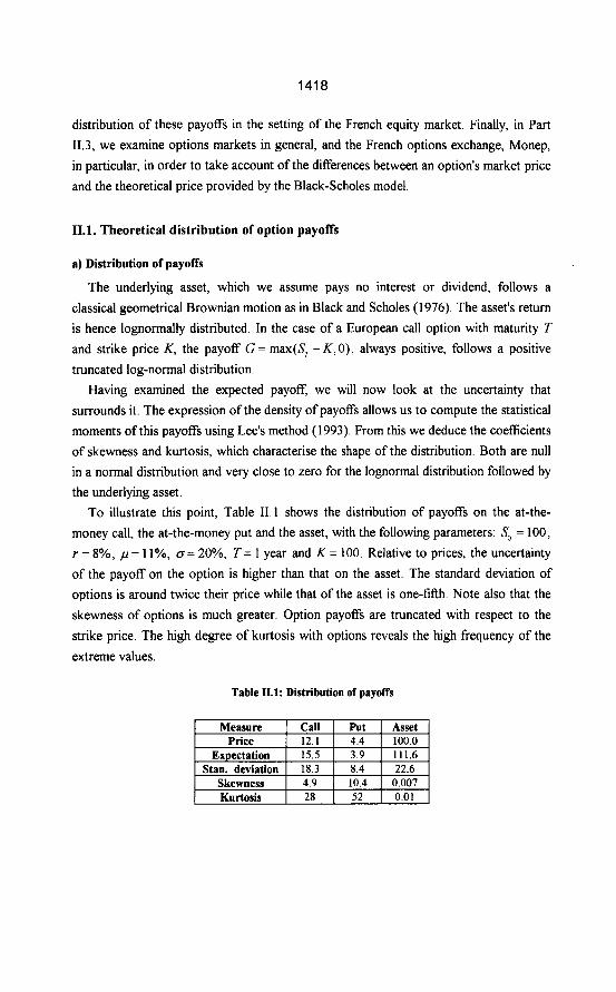
To illustrate this point, Table 11.1 shows the distribution of payoffs on the at-the- money call, the at-the-money put and the asset, with the following parameters: So = 100, r = 8%, p = 1 I%, o= 20%, T = 1 year and K = 100. Relative to prices, the uncertainty of the payoff on the option is higher than that on the asset. The standard deviation of options is around twice their price while that of the asset is one-fifth. Note also that the skewness of options is much greater. Option payoffs are truncated with respect to the strike price. The high degree of kurtosis with options reveals the high frequency of the extreme values.

Table 11.1: Distribution of payoffs

1419

Given the asymmetry of the distribution of payoffs, variance alone may not be sufficiently representative. For this reason, we will concentrate in Part I11 on the relevance of asset selection criteria as applied to options.

b) Value and price

We now return to the comparison between the expected payoff and the price. In the remainder of this section, we define the value V of an option as the expected fiture payoff discounted to present value under real probability P.

We obtain:

(11.1)

(11.2)

where we note as BS(p) the Black and Scholes price of the call for an interest rate p. As Jousseaume (1995) noted, this value generalises Black and Scholes and takes

specific account of the growth term p of the risky asset. To find the price of the call, the trend must be put equal to the interest rate. Hence when p = r , we have:

In the general case where p f r , the value and the price do not coincide. It is even possible to specify the manner in which the value behaves depending on the trend. The sensitivity of this value to the trend is:

where p is the sensitivity to the interest rate of the Black-Scholes price, taken on the basis of p= r . Since a call's rho is always positive, this sensitivity is also positive. Therefore, the call's value always increases with the trend. Since it is logical that p > r , since risk demands a return, we deduce that the value of a call is always greater than its price.

At this stage, it can naturally be objected that the rate used to discount the call's payoff is too low and that it takes no account of the huge degree of uncertainty of this

1420

payoff G, as we saw in paragraph 11.1 .b. If we note as z the discount rate that makes the value equal to the price, defined implicitly by:

(11.5)

then it can easily be expressed using equation (11.2):

(11.6) 1

T T = ,u +-In( BS(,u)/BS(r)) .

The calculation can be further simplified by writing that trend ,u is equal to interest rate r plus a risk premiump:

,u=r+p , (11.7)

and by assuming that premium p is much smaller than interest rate r . A first-order development produces:

P P z=,u+-

T. BS(r)

[ T.E&r))’ = I + 1+-

(11.8)

(11.9)

The discount rate z is therefore always higher than the trend. This is mainly due to the fact that, because of its distribution, the call carries a higher risk than the underlying asset. Note that the term p/BS(r) can be considered as the sensitivity ofthe option - the relative variation of the option price for a rise or fall in the interest rate. The leverage p / T . B S ( r ) is expressed as the relation between this sensitivity and the maturity of the option.

In the case of a put, the situation is different insofar as the expected payoff declines as ,u increases The relation between the put’s value and its theoretical price is still given by equations (11.8) and (11.9), but here the rho is negative. Thus the value of the put is not monotonous in the trend. We will not discuss this phenomenon any further.

1421

11.2 Empirical distribution of payoffs on the call

Following on from the theoretical discussion, we will now analyse the empirical distribution of the payoffs obtained by buying three-month calls on an equity index or on the component stocks. We first present the experimental scheme, then the results obtained therefrom.

a) Empirical scheme

Consider the purchase of a European call option with a three-month maturity on the CAC 40 index of the Paris Bourse and on the component stocks of that index. Created in January 1988, the CAC 40 has been regularly revised, in particular to integrate privatised companies such as Renault and BNP. We assume that the investor buys the call option on the first day of each month and holds it to maturity. The acquisition price is assumed to be the theoretical price given by Black-Scholes.

The prices under consideration are closing prices. We have envisaged three strike prices: at the money, 5% out of the money and 5% in the money. The chosen rate of interest is the 3-month PIBOR on the day the option is purchased. Lastly, we have made two assumptions for volatility: historical volatility, i.e. for the three months prior to the period, and fonvard volatility, i.e. for the three months corresponding to the period. The dividend rate is the last known dividend expressed in terms of the share price on the day of purchase. For the index, a market dividend is computed by aggregating dividend payouts received in proportion to the market capitalisations of the component stocks.

On the day of purchase, we compare the payoffs received, discounted at PIBOR, with the price of the calls.

b) Results

Table 11.2 below summarises the main features of the underlying stocks, beginning with the number of months each stock has been included in the CAC 40. Darty and Spie, which remained only seven and three months respectively, have been removed from the following tables but are included in the overall statistics. Despite a sharp rebound in 1988 after the crash of November 1987, the period under review has been unfavourable for equities, as Figure 11.2 shows. During the period, the return on the CAC 40 index is just 9.0%, or a risk premium of 0.6%, and the Sharpe ratio is 0.04. The premium is small when compared with the premiums computed over longer periods. Nevertheless, the Sharpe ratios of most stocks are positive: only 16 out of 54 are negative.

1422

I 2 4 0 0 ,

nw MOO

1800

16W

ow 12w

Figure 11.2: CAC 40 index since April 1988

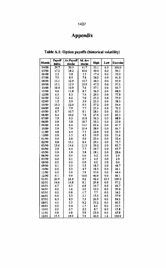
In Table A. 1 in the Appendix, we analyse on a monthly basis the payoffs obtained by exercising calls that are assumed to have been purchased at the money. The first column shows the date the call was purchased; the second column shows the payoff obtained by exercising the call on the index as a percentage of the index's initial price; the third column gives the average, equally weighted payoff resulting from the exercise of 54 calls on individual stocks; the fourth column gives the standard deviation of the sample of 54

payoffs, the largest and smallest elements of which are shown in columns five and six; and the seventh column specifies the percentage of calls exercised. This exercise rate is shown in Figure 11.3.

1oow

80%

MU

40%

20%

ow

Figure IL3: Rate of exercise of at-the-money options on CAC 40 stocks

1423

Table II.2: Characteristics of underlying stocks

1424

We note that certain periods - Spring 1988, Winter 1991 and Winter 1992 - are particularly good, with exercise rates of 100%. In contrast, the invasion of Kuwait triggered a sharp fall in all major stocks, which drove the exercise rate down to zero. Similarly, the slide in the bond market in Spring 1994 had a knock-on effect on the Paris Bourse. It is hardly surprising to note that the payoff on the index was less than the average payoff on the stocks (see Figure 11.4), which the theory would show if the average payoff had been computed on the basis of capitalisation weightings - by convexity, an option on an average is less than the average of the associated options. However, the payoffs of the different stocks vary considerably, notably when the exercise rate is high

15

10

5

Figure IL4: Historical payoffs

Table A.2 in the Appendix analyses the deviation between the payoffs discounted at PIBOR and the price of the calls computed on the basis of historical volatility. When the acquisition price of the calls is taken into account, the conclusions are less favourable. The average deviation between the stocks is negative more than one in two times, with a standard deviation of the same magnitude as that of the payoff In fact, the dispersion of the call prices, which is related to the differences in historical volatility, is moderate. We note that, approximately two times out of three, the deviation of the index is greater than that of the stocks. This demonstrates that the price deviation in favour of the index call, which has lower volatility, partially offsets the differences in payoffs shown in Table A. 1.

1425

Table IL3: Option payoffs (historical volatility)

THOMSON CSF 9.5 I 38.6 I 1.6 I 1.8 TOTAL I 4.4 I 5.3 I 18.8 I 1.2 I 0.8

UAP I 5.2 8.4 I 33.2 I 1.7 I 2.1

1426

Table 114: Option spreads (historical volatility)

After that historical analysis, we shall use Table 11.3 to analyse the payoffs and Table 11.4 to analyse the spreads corresponding to the different stocks. Thus the first line of Table 11.3 shows that the average payoff on Accor was 6.9% with a historical standard deviation, over 94 months, of 8.6% and a high of 35.4%, it also allows us to appreciate

1427

the statistical distribution, viz. skewness and kurtosis. These data show that the variability of payoffs between the stocks is greater than that between the periods; that the distributions are noticeably skewed, which means that a small number of significant payoffs make up for a large number of small or nonexistent payoffs; and that the spreads are less frequently positive - 20 cases - than negative. The latter point is attributable to the period, as we already mentioned.

10

0

Figure IL5: Historical spreads

Table 11.5 summarises and supplements the above data. In it, we have included the average spreads for the index and its component stocks, with strike prices of 95, 100 and 105 as well as historical and foward volatility. Note that forward volatility corresponds to the three-month period covered by the option and that it is unknown on the day the call is purchased. The third line of Table 11.5 reviews the results of Tables 11.3 and 11.4 in terms of at-the-money calls computed with historical volatility.

Strategies involving the purchase of index calls produced a net return over the period. The payoffs are all the greater because the option was in the money and it was possible to anticipate the volatility. Under these circumstances, the additional payoff is 0.03%, which is nevertheless small. It should also be noted that the historical volatilities we have used are generally lower than the implied volatilities traded in markets (see Table 11.6).

In contrast with index options, equity option strategies all resulted in a net loss over the period. This is due to the underperformance of certain small stocks, such as Eurotunnel and Euro Disney. The weight of these stocks in the index is small whereas their weights in our averages are the same as those of all the other stocks. Loss is relatively insensitive to volatility and the strike price; note that the standard deviation is higher for options bought when they are in the money, an effect that is probably due to

1428

the exercise rate. It is not surprising that we obtain significantly positive coefficients of skewness. Figure 11.6 plots the empirical distribution of spreads.

K

95

Table 11.5: Spreads according to strike price and volatility

Vol. Spread Spread S. dev Skew.

hist. -0.73 0.26 9.86 1.03

I Parameters I Stocks I Index

fonv. -0.76 0.19 105 hist. -0.66 0.00 6.82 1.74

Ifonv.) -0.70 1 0.03 I 6.84 I 1.69

Kurt.

0.85 0.68 1.89 1.75 3.78 3.65

- -

-

Figure IL6: Distribution of spreads for stocks Q = 100, historical volatility)

II.3 Spreads between theoretical prices and market prices

This subject has been comprehensively addressed in literature, starting with the observations of Black and Scholes on the prices of options on stocks quoted on US exchanges. Nevertheless, it is interesting to examine the spread between quoted and theoretical prices. Quoted prices are generally expressed through implied volatility, obtained by inverting the Black-Scholes formula (which, it should be noted, requires a homogenous set of values for the other parameters of the calculation). First, we usually observe that implied volatility is higher than historical volatility. By way of example, we show the recent spreads in volatility on the most liquid options markets in Table 11.6. For

1429

the CAC 40, DAX, S&PSOO, Nikkei and FT-SE 100 indexes, we give the historical volatility for October 1995, the implied volatility quoted at month’s end, and the maximum and minimum implied volatilities over the month.

Table IL6: Index volatility (October 1995)

Source: Goldman Sachs.

Also, we note a so-called smile effect, which denotes the deviation of implied volatility according to maturities and strike prices. However, the traditional curved form of the smile seems to have disappeared since the 1987 crash. The volatility of options with strike prices out of the money is much stronger than that of in-the-money options. Further, short-term volatility tends to be higher than the volatility on longer maturities. This effect is partially due to the variation of volatility itself over time.

In theory, if the assumptions of the Black-Scholes model are satisfied, investors should buy calls as soon as the trend rate of the underlying asset exceeds the riskless rate; similarly, they should sell puts. However, theory can give no firm indication of the future movements of the underlying asset. In practice, while equities turn out to be less profitable - even though they are supposed to yield more than cash - the price of the option will not be offset by the payoff obtained by exercising that option. Clearly, the main factor at work - far more than the choice of volatility and strike price - is the ex

post performance of the underlying asset. This remains true even though in certain cases implied volatility is much higher than expost volatility.

However, we cannot over-emphasise the extreme variability of payoffs, their non- normality and pronounced skewness. Thus the comparison we have just made of expected values is inadequate. Such is the pattern of distribution that it requires a pertinent analysis of the benefits that investors can really derive from options. This is the purpose of the following section.

111. Options and portfolio selection

1430

Having analysed the conceptual and statistical features of options, we will now examine their use. Should investors buy options and, if so, in what quantity? To answer that questions, we must first identi@ and then accurately model the needs of the investor. We then have to address the question of .selection: when a number of different investment possibilities respond to an investor's need, it is not always easy to choose between them. For this reason, it is necessary to define criteria that provide a method of assessing and comparing all the various possibilities. However, such criteria are always an approximation of investor preferences, which has then to be fine-tuned. Accordingly, we will first demonstrate why the classic Markowitz criterion is unsuitable and then propose an alternative: the loss function criterion.

According to the Black-Scholes method, the standard asset used in this part, and noted S, is assumed to be lognormal, with trend ,u = 10% and volatility Q = 15%. The continuously compounded riskless rate is r = 5% and the investment horizon 3 months.

III.1 The Markowitz criterion

Proposed by Markowitz in 1952, this criterion has since been widely adopted by portfolio managers. The principle of the criterion is summed up in its name: mean- variance. The value that the investor seeks to maximise is the expected return on his investment. The counterpart to his search for higher returns is the risk he must assume. Markowitz sets out to model that risk by variance, or, in the same way, by the volatility of portfolio returns. The resulting allocation, known as optimal allocation, results from a trade-off between these two values, which the investor determines on the basis of his own preferences.

Two of the hypotheses underpinning the Markowitz criterion are particularly important when considering an investment in option-based assets.

The first of these hypotheses concerns management policy: the investor puts his money into different assets at the beginning of the period and does not rebalance his portfolio until the end of the period. This strategy is known as buy and hold. No thought is given to dynamic trading.

The second hypothesis concerns the choice of the criterion itself The risk measure used in a mean-variance approach must be viewed with caution. The drawback of choosing variance is that the skewness of the asset return distribution is unknown. An asset that could take only two values, one stable, which is unlikely, and the other trending upwards, which is more likely, may have the same mean-variance characteristics as an asset with significant downside probability. The Markowitz criterion is incapable of

1431

distinguishing between the two. Neither does it take into account the differences, which this time are symmetrical, between the probabilities of the extreme values that could be taken by two assets with the same mean and variance. In statistical terms, we say that Markowitz criterion does not make the difference between a thick-tail distribution (with a high coefficient of kurtosis) and standard distribution. These two points are important when the assets in question are options, as seen in Part 11.

Figure IIL1: Distribution of returns, standard asset and equivalent normally-distributed asset

Figure III.2: Distribution of returns, call option and equivalent normally-distributed asset

Figures 111.1 and 111.2 show, for a given asset, the actual distribution of the asset and an equivalent normally-distributed asset, as defined by Markowitz. The normal distribution has the same expectation and variance as the asset's return. Figure 111.1 deals with the standard asset and Figure 111.2 shows an at-the-money call option on that asset. As regards the normally distributed asset associated with the standard asset, which is lognormal, the pattern is very similar except that it more often exhibits a strong

1432

downward movement and less often a strong upward movement. The distribution of the call is, as we discussed in Part 11, truncated lognormal, with a peak corresponding to the numerous instances in which the option is not exercised (return -100 %). The call appears to be a high-yielding but also very risky asset. Naturally, the highly asymmetrical distribution is not found with the corresponding normally-distributed asset. Moreover, that asset carries a high probability for returns below -100 % and, conversely, a much lower probability than that of the option for high returns.

The close correlation between the option and its underlying asset, when taken in conjunction with the above observations, explains why this mean-variance criterion is of little use to investors wanting to include options in a portfolio of standard assets. In particular, the criterion does not select protected portfolios, see znter a k Bellity and Bertrand (1993). A protected portfolio would be composed solely of cash and a call option, or similarly of the asset and a put. In view of these shortcomings, other methods have to be used to assess the relevance of an asset allocation strategy that includes options.

III.2 Loss functions

Loss fimctions provide an initial response to the shortcomings of the Markowitz formula. Bawa and Lindenberg (1977) have even developed an equilibrium model based on their use. The principle of loss fbnctions stems directly from the questions raised in the previous part: the aim is to achieve a better description of risk by stressing events that are considered to be unfavourable. The loss function associated with a random variable X, also called a lower partial moment, in X, of order a is formally written:

(111.1)

This moment is limited to the values of X below the threshold X,. It is linked to the broader notion of stochastic dominance, which is a principle used for comparing random variables. However, this notion is of little practical use because the induced order is partial: in many cases, it is not possible to say whether one variable stochastically dominates another. By providing a measure of risk, loss hnctions permit comparisons at all fixed orders and thresholds.

In practice, two orders of partial moments are selected: a = 0 and a = 2 . Once again, the aim is to maximise the return on the investment. For a same level of return, one

1433

allocation is preferable to another if its associated risk, measured by a loss function rather than variance, is smaller. Thus the aim is to minimise that loss function.

a ) a = O

Here, the loss function is the probability that Xwill be below the threshold X , . For an investor, this quantity could be a probability of ruin, i.e. a level of return below which he would no longer be able to remain in business. Asset-liability management techniques are based on this type of approach, which Leibowitz and Langetied (1991) have formalised and extended to the strategic and tactical stages of portfolio selection.

By way of illustration, we have compared two portfolios for a three-month investment horizon. One portfolio comprises the standard asset S and cash. The other is composed of the at-the-money call written on this asset as well as cash. The expected returns to the standard asset and the option are derived from Part 11. For a range of expected returns, we have shown in Figure 111.3 the corresponding cash portion of each portfolio. The portion of standard assets or calls to be bought makes up the full complement. Note that it is sufficient to buy a small number of options to reach the target return, 6% at most, for an expected return equal to that on the standard asset.

m

0% 5Gm 80% 7 0 % 80% 90% 100%

stmama as-1 p o h l i o - - - Omon pwthlio

Figure IIL3: Allocation according to expected return, cash portion

We set a threshold for the loss function of a 0% return. This corresponds to an investor with money to invest over a three-month period who wishes to protect his capital. This guarantee is his main consideration; it may, for example, correspond to an obligation to pay out the same amount at the end of the period. In this case, his risk is clearly identified and can be correctly valued by the loss function of order 0 and threshold 0%, which represents the probability of not meeting future commitments.

1434

Naturally, the target return is higher than the money market rate because, by accepting the possibility of null returns, the investor is in a position to buy a risky asset. In Figure 111.4, the target varies between the riskless rate, assumed to be 5%, and the expected return to the asset, i.e. around 10%. The Y-axis represents the loss function, in other words the probability of negative returns, that the investor is seeking to minimise.

Figure 111.4: Loss function of order 0, threshold at O%, according to the target return

We note that only the call affords full protection against negative returns, on condition however that the expected return i s not too ambitious. For an objective of less than 6%, the recommended investment vehicle is the call option plus a cash component. For anything above 6%, the capital cannot be guaranteed, and the investment in the standard asset becomes preferrable to the former investment policy.

b ) a = 2

The loss fbnction is a generalisation of the notion of variance. When the expected value of X is equal to the threshold, it is called semi-variance. It weights the probability of being below the threshold by the deviation at that threshold. It is therefore less brutal than its zero-degree counterpart when breaching the floor; in contrast, it factors in highly unfavourable events - even improbable ones - with a weight proportional to the square of the difference.

Let us return to the previous example. If, instead of choosing the 0 order loss fhction, we use order 2 to measure the risk, we obtain Figure 111.5. The investor choosing this criterion is less intransigent than the investor in the previous example: he is prepared to accept a negative return but wants to avoid excessively unfavourable events. In this case, the portfolio composed of the call and cash is the best choice because its

1435

end-of-period value is always higher than the value of its cash component capitalised at the money market rate

Figure III.5: Order 2 loss function, threshold at O%, according to the target return

III.3 Selecting criteria

When the assets to be selected are normally distributed, the mean-loss hnction criterion becomes equal to the mean-variance criterion. Consequently, it should not be seen as an udhoc criterion but as a refinement of an unsuitable methodology.

Although the order a adopted can be limited to the two values discussed above, the question of choosing the order and the threshold X , is nevertheless an awkward one. In cases such as those covered above, the investor's objective coincides with a loss hnction model, and this criterion is highly relevant. While the partial-moment risk measure should not be applied systematically to every case, it often gives a good approximation. Consequently, an investor who decides to avoid derivatives would be depriving himself of an investment opportunity that could considerably reduce his risk. Furthermore, the loss hnction approach, which justifies the investment in options, also quantifies the terms of that investment. In particular, it shows that the quantity of options that needs to be purchased is generally small. The sum spent on acquiring the options is not so important as the leverage that the purchase provides. This is achieved through exposure to the underlying asset, i.e. the delta, induced by holding a derivative which is already a portfolio.

For the sake of clarity, the examples we have chosen involve portfolios with a simple structure. Nevertheless, the loss hnctions apply in the same way to more complex

1436

allocations. For the investor, these functions provide a robust asset-selection methodology that gives due consideration to derivatives.

Conclusion

Options should be seen as portfolios that are constantly reallocated. A comparison between option prices and insurance premiums highlights two types of risk: those that can be hedged and those that can only be disposed of if they are pooled. That comparison was extended in Part 11, where we compare price and value. Statistics for the French market prove that the two notions are very different. In the same way as with basic assets, investors must consider the value of options and not just their price. However, this view entails a precise analysis of the highly asymmetrical distribution of options. The investor's selection choice criteria must be suited to the inherent characteristics of options. This is addressed in Part 111, where we observe that, with the exception of the classic Markowitz approach, which is not suited to options, loss hnctions point to the choice of options, even if their weight in the portfolio is small in view of the significant leverage they provide.

Certainly, options are investment vehicles with highly singular properties. For this reason, they have an advantage over all basic assets and the future contracts associated with them: option-based products have a highly promising future.

1437

Appendix

Table kl: Option payoffs (historical volatility) - Month

04/88 05/88 06/88 07/88 08/88 09/88 10188 11/88 12/88 01/89 02/89 03/89 04/89 05/89 06/89 07/89 08/89 09/89 10189 11/89 12/89 01/90 02/90 03/90 04/90 05/90 06/90 07/90 08/90 09/90 10/90 11/90 12/90 01/91 0219 1 03/91 0419 1 05/91 0619 1 0719 1 0819 1 0919 1 10191 11/91 12/91

-

-

Payoff index 29.7 17.2 2.2 7.0 13.1 15.1 10.4 9.6 6.5 5.2 1.5

10.3 4.8 8.7 8.4 7.9 0.0 1.8 5.9 4.0 0.0 0.0 8.8 13.6 2.9 0.0 0.0 0.0 0.0 0.1 0.0 0.0 6.1 20.9 14.6 6.7 0.0 0.0 0.0 6.3 4.1 0.0 0.0 0.8 15.5

Lv.Payofl stock8 30.3 18.2 3.8 8.5 12.9 15.9 10.9 11.8 8.3 6.0 3.9 12.0 7.9 10.7 10.0 9.3 5.8 6.4 7.9 6.4 1.5 2.0 10.1 14.6 6.4 1.8 0.0 0.1 0.0 3.3 2.3 3.9 9.9 22.4 14.8 6.5 1.6 0.8 2.3 8.3 5.5 0.4 0.7 4.8 19.0

- Sd. dev stock8 11.7 10.6 5.5 7.8 10.7 10.9 7.6 8.7 7.4 7.0 5.9 9.5 7.7 8.1 7.6 10.8 18.7 13.1 10.4 7.5 4.3 5.0 8.4 11.5 7.7 3.8 0.0 0.7 0.0 5.3 4.7 7.9 10.0 8.2 8.1 6.8 3.0 1.7 3.1 7.3 8.2 1.5 2.2 5.8 7.9 -

- Weh - 55.1 49.0 17.4 28.0 48.3 47.2 27.1 36.5 29.1 25.2 23.3 37.2 25.1 28.1 27.6 56.3 33.3 62.6 38.0 22.0 19.9 23.4 29.1 50.2 24.7 18.1 0.2 4.3 0.0 18.5 18.5 37.0 40.0 42.4 29.8 19.7 10.3 7.7 15.5 26.9 33.2 6.6 8.7

23.0 40.0 -

- LOW

6.0 0.0 0.0 0.0 0.0 0.0 0.0 0.0 0.0 0.0 0.0 0.0 0.0 0.0 0.0 0.0 0.0 0.0 0.0 0.0 0.0 0.0 0.0 0.0 0.0 0.0 0.0 0.0 0.0 0.0 0.0 0.0 0.0 10.5 0.0 0.0 0.0 0.0 0.0 0.0 0.0 0.0 0.0 0.0 1.6

-

-

- Ire&

100.0 94.1 52.9 81.8 93.9 97.1 85.7 88.9 77.8 75.0 58.3 94.4 72.2 83.3 83.3 88.9 25.0 41.7 66.7 59.5 21.6 32.4 75.7 85.7 65.7 28.6 2.9 2.9 0.0 48.7 36.1 44.4 86.1 100.0 97.2 66.7 29.0 34.2 57.9 84.2 60.5 10.5 15.8 65.8 100.0

-

-

1438

Table A1 (cont.): Option payoffs (historical volatility)

Low 0.0 0.0 0.0 0.0 0.0 0.0 0.0 0.0 0.0 0.0 0.0 0.0 0.0 0.0 0.0 0.0 0.0 0.0 0.0 0.0 0.0 0.0 0.0 0.0 0.0 0.0 0.0 0.0 0.0 0.0 0.0 0.0 0.0 0.0 0.0 0.0 0.0 0.0 0.0 0.0 0.0 0.0 0.0 0.0 0.0

Month

02/92 03/92 04/92 05/92 06/92 07/92 08/92 09/92 10192 11/92 12/92 01/93 02/93 03/93 04/93 05/93 06/93 07/93 08/93 09/93 10193 11/93 12/93 01/94 02/94 03/94 04/94 05/94 06/94 07/94 08/94 09/94 10194 11/94 12/94 01/95 02/95 03/95 04/95 05/95 06/95 07/95 08/95

01/92

09/95

Exerch 91.9 81.1 66.7 30.8 10.3 5.1 17.5 42.5 72.5 75.0 65.0 89.7 79.5 74.4 10.3 33.3 89.7 97.5 85.0 61.5 36.1 83.3 83.3 66.7 21.6 30.6 5.1 0.0 12.8 61.5 48.7 15.0 32.5 60.0 27.5 18.4 42.1 84.2 86.8 63.2 37.5 27.5 20.0 32.5 41.0

Payoff index 9.9 9.7 1.9 0.0 0.0 0.0 0.0 0.0 6.9 6.7 2.4 11.2 8.6 8.2 0.0 0.0 9.7 16.7 7.9 1.9 0.0 8.1 7.3 1.3 0.0 0.0 0.0 0.0 0.0 2.8 0.0 0.0 0.0 1.8 0.0 0.0 0.0 5.9 8.3 0.8 0.0 0.0 0.0 0.0 0.0

iv.Pay0f stocks

13.9 10.7 4.4 2.2 0.6 0.1 0.6 2.7 8.8 7.6 7.5 15.7 12.2 9.0 0.4 1.8 10.6 16.8 8.8 3.6 3.0 10.4 12.1 7.1 2.3 1.3 0.4 0.0 0.3 4.2 3.4 0.6 1.9 3.9 2.7 0.4 3.6 8.6 9.6 4.2 2.7 1.8 1.8 1.8 1.8

- Sd. dev stocks

8.8 8.2 5.8 4.5 2.1 0.7 1.6 4.3 9.7 7.1 9.2 12.7 12.2 7.5 1.3 3.6 8.1 8.2 5.8 4.8 6.0 8.3 10.7 8.4 4.9 3.5 1.6 0.0 0.8 4.7 5.6 1.9 3.4 8.2 10.3 0.9 4.9 7.0 6.3 5.6 4.3 3.7 5.1 4.9 3.1

High - 33.9 35.0 26.6 21.1 11.4 3.9 6.5 16.8 31.6 28.3 29.9 62.5 50.1 27.7 6.7 14.9 27.8 36.5 19.3 17.6 27.5 25.0 44.3 32.5 19.3 18.0 9.3 0.0 3.7 18.3 19.2 8.8 11.3 49.0 65.1 3.2 16.8 26.1 23.7 23.4 15.9 14.3 23.6 28.4 12.6 -

1439

Table A.2: Value-price spread (historical volatility)

Month 04/88 05/88 06/88 07/88 08/88 09/88 10188 11/88 12/88 01/89 02/89 03/89 04/89 05/89 06/89 07/89 08/89 09/89 10189 11/89 12/89 01/90 02/90 03/90 04/90 05/90 06/90 07/90 08/90 09/90 10190 11/90 12/90 01/91 02/91 03/91 0419 1 05/91 0619 1 0719 1 0819 1 0919 1 10191 11/91 12/91

- Spread index 24.0 12.2 -2.5 2.1 8.4 10.7 6.7 6.0 3.0 1.9 -2.1 5.8 0.4 4.7 5.2 4.8 -3.0 -1.2 3.1 -1.0 -5.1 -5.4 5.1 9.5 -1.5 -4.4 -4.1 -3.8 -3.4 -6.3 -6.8 -7.3 0.8 15.9 8.6 0.6 -5.9 -4.2 -4.2 2.4 0.4 -5.3 -5.0 -4.0 12.1 -

4v. spread stocks 22.0 10.2 -3.2 1.4 3.3 7.1 2.3 5.8 2.2 0.4 -2.0 5.5 1.5 4.7 4.7 4.0 0.8 1.2 2.6 -0.7 -5.6 -5.3 4.4 8.6 0.3 -4.5 -6.1 -5.8 -5.6 -5.1 -6.7 -5.8 2.1 15.1 6.8 -1.6 -6.4 -5.5 -3.8 2.5 -0.2 -6.4 -5.8 -1.4 13.9

Std. dev. StOClB 12.0 11.7 6.1 7.7 18.8 18.0 17.3 9.0 7.8 7.2 6.1 9.6 7.9 8.0 7.3 10.8 18.7 12.4 10.0 7.6 4.8 5.4 8.8 12.0 8.3 4.1 0.9 1.2 1.4 5.2 4.7 7.8 9.3 7.5 8.5 7.5 3.5 2.1 2.9 7.1 8.2 2.1 2.9 6.2 7.9

md! 48.2 43.8 10.8 18.9 37.5 40.2 21.0 27.6 24.1 19.9 18.0 31.2 19.4 22.9 22.2 50.9 27.2 51.2 32.3 14.3 15.3 18.2 23.9 44.6 18.7 12.0 -4.1 -2.8 -3.4 10.5 8.3 28.8 29.3 31.1 23.1 13.1 2.9 2.9 7.8 19.0 26.8 0.1 2.8 17.9 33.2

L O W

-3.6 -13.0 -11.4 -9.2 -85.0 -77.5 -86.0 -9.8 -10.1 -10.2 -9.5 -6.3 -8.3 -7.4 -6.4 -5.4 -7.0 -6.9 -6.1 -10.9 -9.9 -10.4 -8.3 -8.5 -9.0 -8.3 -8.1 -9.1

-10.2 -11.6 -12.5 -13.4 -8.3

-10.5 -1 1.5 -11.5 -10.0 -7.6 -7.2 -8.3

-10.1 -9.2 -9.5 -3.3

2.7

1440

Table A2 (cont.): Value-price spread (historical volatility)

Month 01/92 02/92 03/92 04/92 05/92 06/92 07/92 08/92 09/92 10192 11/92 12/92 01/93 02/93 03/93 04/93 05/93 06/93 07/93 08/93 09193 10193 11/93 12/93 01/94 02/94 03/94 04/94 05/94 06/94 07/94 08/94 09/94 10194 11/94 12/94 01/95 02/95 03/95 04/95 05/95 06/95 07/95 08/95 09/95

- Spread index

5.5 4.9 -2.7 -3.9 -4.1 -4.2 -4.2 -4.1 2.6 0.7

4.8 2.9 3.1 -4.7 -4.2 5.9 13.1 4.3 -1.9 -3.6 4.2 3.7 -2.6 -3.8 -4.0 -3.8 -4.1 -4.1 -1.2 -4.0 -4.1 -4.2 -2.2 -4.2 -4.3 -4.0 2.4 4.9 -3.6 -4.5 -4.6 -4.1 -4.0 -3.8

-3.6

-

LV. spread stoeka

7.7 3.7 -2.4 -3.8 -5.1 -5.5 -5.1 -3.3 2.3 -0.8 -1.2 6.6 4.2 1.8

-6.5 -4.6 4.6 11.2 3.3 -2.1 -2.5 4.7 6.7 1.3

-3.6 -4.8 -5.4 -5.9 -5.4 -1.4 -2.6 -5.7 -4.5 -2.1 -3.4 -5.7 -1.9 3.6 4.7 -1.8 -3.7 -4.8 -4.2 -4.0 -3.6

Std. dev. stofkr

9.0 8.3 5.8 4.5 2.2 1.2 1.8 4.2 9.6 7.1 9.0 11.2 11.0 7.2 2.1 3.4 8.0 8.3 5.8 5.2 6.3 8.4 10.6 8.7 5.4 4.1 2.2 1.2 1.5 5.0 5.8 2.7 4.0 7.4 9.5 1.2 5.0 7.0 6.2 5.5 4.7 3.9 5.4 5.1 3.2

High 26.8 26.7 18.3 13.2 4.9 -2.5 0.8 10.6 23.6 17.6 18.3 44.5 34.2 20.6 -0.2 7.1 20.3 28.4 13.9 11.6 23.2 20.0 37.2 25.2 12.2 12.3 4.3 -4.1 -0.6 13.7 11.9 3.1 5.7 37.0 53.5 -3.2 10.2 21.9 17.7 16.8 9.6 7.1 16.5 22.2 6.2

-

-

LOW

-8.6 -11.0 -12.1 -10.4 -10.0 -8.0 -8.1 -9.4 -11.0 -12.8 -17.9 -8.6 -8.9 -8.8 -1 1.8 -10.7 -8.0 -8.5 -8.1 -9.4 -9.4 -9.7 -8.5 -14.8 -15.6 -17.3 -13.2 -11.0 -10.4 -11.0 -15.0 -16.2 -16.0 -8.9 -7.6 -8.2 -7.3 -6.5 -5.2 -7.7 -11.9 -13.0 -12.1 -9.3 -1 1.6

1441

References

Bawa, V., and E. Lindenberg, 1977 Capital market equilibrium in a mean-lower partial moment framework Journal of Financial Economics, 5

Bellity, L., and J.-C. Bertrand, 1993 Optimisation de Portefeuille contenant des options Conference de I'AFFI, Paris

Black, F., and M. Scholes, 1973 7he pricing of options and corporate liabilities Journal of Political Economy 81,637-59

Cox, J., and M. Rubinstein, 1985 Options Markets

Prentice Hall

Jousseaume, J.-P.,1995 Paradoxes mr le calcul des options: et si ce nVtait qu'une illusion ... AFIR Conference, Brussels

Lee, P., 1993 Portfolio selection in the presence of options and the distribution of return of portfolios containing options AFIR Conference, Rome

Leibowitz, M., and T. Langetied, 1991 Shortfall risk and the asset allocation decision The Journal of Portfolio Management, winter 199 1

Markowitz, H., 1952 Portfolio selection The Journal of Finance, 7