options for updating wyoming’s regional cost...
TRANSCRIPT
Options for Updating Wyoming’s RCA
Options for Updating Wyoming’s Regional Cost Adjustment
Submitted to: The Select Committee on School Finance Recalibration Submitted by:
Lori L. Taylor, Ph.D.
October 2015
Options for Updating Wyoming’s RCA
Page 1
Options for Updating Wyoming’s Regional Cost Adjustment Executive Summary
Like 11 other states, Wyoming adjusts its school funding formula to reflect regional differences in the cost of hiring a school district’s most important (and most expensive) resource—teachers. The Wyoming Regional Cost Adjustment (RCA) which only applies to the salary components of the school funding model, is an amalgam of two alternative labor cost indices—the Wyoming Cost-of-Living Index (WCLI) and the Wyoming Hedonic Wage Index (HWI). Both labor cost indices are constructed so that the state average has an index value of 100. Locations where labor costs are 10% above the state average have an index value of 110 while locations where labor costs are 10% below the state average have an index value of 90. The WCLI is updated bi-annually, but the Wyoming HWI has not been updated since 2005.
Each district’s RCA is the larger of the WCLI, the 2005 Wyoming HWI or 100. In other words, districts where labor costs are below the state average are treated as if their costs were equal to the state average. This Lake Woebegone approach, wherein no districts are below average, narrows the range of the geographic cost adjustment and greatly diminishes the ability of the RCA to equalize district purchasing power.
During both the 2005 and 2010 recalibrations of the funding model, state consultants recommended that the RCA be based solely on the HWI. This report contributes to the 2015 recalibration effort by:
1. Refining the WCLI to better reflect regional differences in labor cost in Wyoming. The current WCLI is based on budget weights that reflect the consumption patterns of the typical urban consumer in the rest of the country. Reweighting the WCLI using the weights generated by the U.S. Bureau of Labor Statistics (BLS) for Class D cities (those with populations below 50,000) would raise the WCLI for counties with relatively low housing costs, lower the WCLI for counties with relatively high housing costs, and make this indicator a more accurate measure of the cost of living in Wyoming.
2. Updating and improving the 2005 Wyoming HWI. The 2015 Wyoming HWI, which was estimated using data from the 2010-11 through 2014-15 school years, improves on the 2005 Wyoming HWI is a number of ways. The underlying hedonic wage analysis covers a much longer time frame (five years instead of two) and includes a much richer set of discretionary and nondiscretionary cost factors. For example, the 2015 Wyoming HWI replaces the problematic distance to Yellowstone National Park factor (which is used to calculate the 2005 Wyoming HWI) with an indicator for whether the nearest hospital is more than 25 miles away, a measure of geographic isolation that is more relevant to the everyday lives of teachers.
3. Developing a comparable wage index (CWI) for Wyoming. A CWI measures regional differences in the cost of hiring teachers by observing regional differences in the cost of hiring comparable non-teachers. Using data from the Wyoming Department of Workforce
Options for Updating Wyoming’s RCA
Page 2
Services and the BLS’ Occupational Employment Survey (OES) I have estimated a CWI for each county in Wyoming. This OES CWI reflects labor cost estimates that control for the mix of occupations in a location, but cannot control for differences in the age or educational attainment of those workers.
4. Exploring the implications of replacing the three-way RCA with one of these three alternatives.
Analysis suggests that the any of the three options outlined above would improve the accuracy of the Wyoming RCA. However, basing the RCA solely on the OES CWI would, in many ways, be the most attractive strategy for updating Wyoming’s RCA.
The OES CWI has a number of attractive features. It is clearly outside of school district influence, eliminating the risk that the regional cost index would misidentify high spending districts as high cost ones. It reflects not only regional differences in cost of living, but also differences in local amenities. The CWI methodology is also the most common approach to regional cost adjustment in other states.
If the OES CWI were rebased so that 100 equaled the state minimum, then most Wyoming school districts would benefit from the change to the OES CWI. Only a handful of districts—most notably Teton County #1—would experience a decline in their RCA. Furthermore, by properly calibrating the salary used in the funding model calculations, this change in the RCA could be accomplished with only a limited budgetary impact.
Whichever option the Legislature chooses, a mechanism for regular updates to the RCA should be put in place. The Wyoming economy is dynamic and labor market conditions in Wyoming are constantly changing. For the RCA to work as intended, it must accurately reflect current differences in labor cost, and not be allowed to drift out of date.
Options for Updating Wyoming’s RCA
Page 3
Introduction
The price school districts must pay for their most important resource—teachers—varies from place to place. As a result, some school districts must pay higher wages to attract the same high quality teachers available to other districts at lower cost. Cost adjustments to a school funding formula equalize the purchasing power of school districts so they can recruit and retain equivalent school personnel.
The challenge in constructing a regional cost adjustment (RCA) is ensuring that the adjustment accurately reflects costs, and only reflects costs. A RCA that misidentifies high spending districts as high cost districts would exacerbate existing inequities instead of reducing them.
Wyoming is one of the dozen states that use a RCA in their school finance formulas. The Wyoming RCA is designed to provide additional resources to school districts with higher labor costs. As such, it only applies to the salary components of the school funding model.
The Wyoming RCA is an amalgam of two alternative labor cost indices—the Wyoming Cost-of-Living Index (WCLI) and the Wyoming Hedonic Wage Index (HWI).1 Both indices are constructed so that the state average has an index value of 100. Locations where labor costs are 10% above the state average have an index value of 110 while locations where labor costs are 10% below the state average have an index value of 90.
Each district’s RCA is the larger of the WCLI, the Wyoming HWI or 100. In other words, districts where labor costs are below the state average are treated as if their costs were equal to the state average. This Lake Woebegone approach, wherein no districts are below average, narrows the range of the geographic cost adjustment and greatly diminishes the ability of the RCA to equalize district purchasing power.
During both the 2005 and 2010 recalibrations of the funding model, state consultants recommended that the RCA be based solely on the HWI. This report contributes to the 2015 recalibration effort by:
1. Refining the WCLI to better reflect regional differences in labor cost in Wyoming, 2. Updating and improving the 2005 Wyoming HWI, 3. Developing a comparable wage index (CWI) for Wyoming , and 4. Exploring the implications of replacing the three-way RCA with one of these three
alternatives.
Analysis suggests that the any of the three options outlined above would improve the accuracy of the Wyoming RCA. However, basing the RCA solely on a county-level CWI would in many ways be the most attractive strategy for updating Wyoming’s RCA.
1 For more on the Wyoming Cost of Living Index, visit http://eadiv.state.wy.us/WCLI/Cost.html
Options for Updating Wyoming’s RCA
Page 4
Regional Cost Adjustments in Theory and Practice
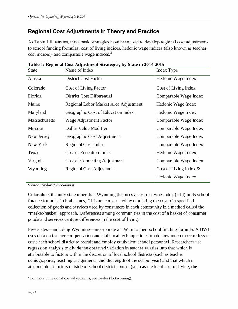
As Table 1 illustrates, three basic strategies have been used to develop regional cost adjustments to school funding formulas: cost of living indices, hedonic wage indices (also known as teacher cost indices), and comparable wage indices.2
Table 1: Regional Cost Adjustment Strategies, by State in 2014-2015 State Name of Index Index Type
Alaska District Cost Factor Hedonic Wage Index
Colorado Cost of Living Factor Cost of Living Index
Florida District Cost Differential Comparable Wage Index
Maine Regional Labor Market Area Adjustment Hedonic Wage Index
Maryland Geographic Cost of Education Index Hedonic Wage Index
Massachusetts Wage Adjustment Factor Comparable Wage Index
Missouri Dollar Value Modifier Comparable Wage Index
New Jersey Geographic Cost Adjustment Comparable Wage Index
New York Regional Cost Index Comparable Wage Index
Texas Cost of Education Index Hedonic Wage Index
Virginia Cost of Competing Adjustment Comparable Wage Index
Wyoming Regional Cost Adjustment Cost of Living Index &
Hedonic Wage Index
Source: Taylor (forthcoming).
Colorado is the only state other than Wyoming that uses a cost of living index (CLI) in its school finance formula. In both states, CLIs are constructed by tabulating the cost of a specified collection of goods and services used by consumers in each community in a method called the “market-basket” approach. Differences among communities in the cost of a basket of consumer goods and services capture differences in the cost of living.
Five states—including Wyoming—incorporate a HWI into their school funding formula. A HWI uses data on teacher compensation and statistical technique to estimate how much more or less it costs each school district to recruit and employ equivalent school personnel. Researchers use regression analysis to divide the observed variation in teacher salaries into that which is attributable to factors within the discretion of local school districts (such as teacher demographics, teaching assignments, and the length of the school year) and that which is attributable to factors outside of school district control (such as the local cost of living, the
2 For more on regional cost adjustments, see Taylor (forthcoming).
Options for Updating Wyoming’s RCA
Page 5
degree of geographic isolation and student demographics).3 Only factors outside of school district control represent cost differences that should be accounted for in funding formulas, so researchers construct a HWI by predicting the full-time-equivalent salary in each school district, assuming that all districts had the same values for the discretionary cost factors.
Six states use a comparable wage index (CWI) to make regional cost adjustments. A CWI measures regional variations in the price that school districts must pay to attract high quality teachers by observing regional variations in the salaries of comparable professionals who are not teachers.4 It is based on the premise that all types of workers—not just teachers—demand a higher salary where the price of a home is high, the climate is inhospitable, or the closest hospital is many miles away.
Advantages and Disadvantages of the Three Approaches Each method has its advantages and disadvantages. Either a CLI or a CWI will provide cost adjustments that are clearly outside of school district influence, but they are both market-level measures. They cannot detect cost differences at the school or district levels.
In contrast, HWIs are able to pick up systematic differences in cost from one district to another within the same labor market, but must rely on statistical technique and researcher judgment to control for the influence of school district choices and thereby avoid mislabeling high spending districts as high cost districts. Statistical models and researcher judgment are inherently subject to criticism. HWIs have also been criticized as subject to school district manipulation (McMahon 1994), vulnerable to omitted variables bias (Goldhaber 1999) and distorted by the noncompetitive nature of the teacher labor markets (Hanushek 1999).
A CLI tends to overstate the cost of hiring in locations with a lot of amenities that make it a desirable place to live and work (Rothstein and Smith 1997, Stoddard 2005). CLIs can also be biased if the market basket used to construct them does not reflect teacher spending patterns, or teachers do not live and work in the same labor market area.
A CWI reflects not only differences in the cost of purchased goods and services (like housing) but also differences in amenities (like the climate or access to health care). As such, a CWI offers a more comprehensive measure of local conditions than does a CLI. However, comparability is always a concern. If the non-educator population differs substantially from the educator population in terms of age, educational background, or tastes for local amenities, then the CWI may overstate (or understate) the wage differentials that teachers will require.
3 For more on the use of hedonic wage models in education, see Chambers (1995, 1997, 1998), Goldhaber (1999), or Taylor (2010, 2008a and 2008b). 4 For more on comparable wage indices, see Taylor (2014), Taylor and Fowler (2006), Rothstein and Smith (1997), Goldhaber (1999), or Guthrie and Rothstein (1999).
Options for Updating Wyoming’s RCA
Page 6
Refining the WCLI
The WCLI is modeled after the U.S. Bureau of Labor Statistics’ (BLS’s) Consumer Price Index for urban consumers (CPI-U). It is produced bi-annually by the Wyoming Department of Administration & Information’s Economic Analysis Division. Twice a year, the Economic Analysis Division collects data on prices for food, housing, apparel, transportation, medical services, and recreation and personal care. The WCLI is a weighted average of the prices for each of these components, where the weights reflect the share of the typical consumer’s budget devoted to each component. Because they are designed to measure consumption costs, the CPI-U and WCLI exclude any consumer expenditures that the BLS does not consider to be consumption. Thus, these indices are constructed using a zero weight for taxes not directly associated with the purchase of consumer goods and services (such as income and Social Security taxes) and investment items (such as stocks, bonds, real estate, and life insurance).
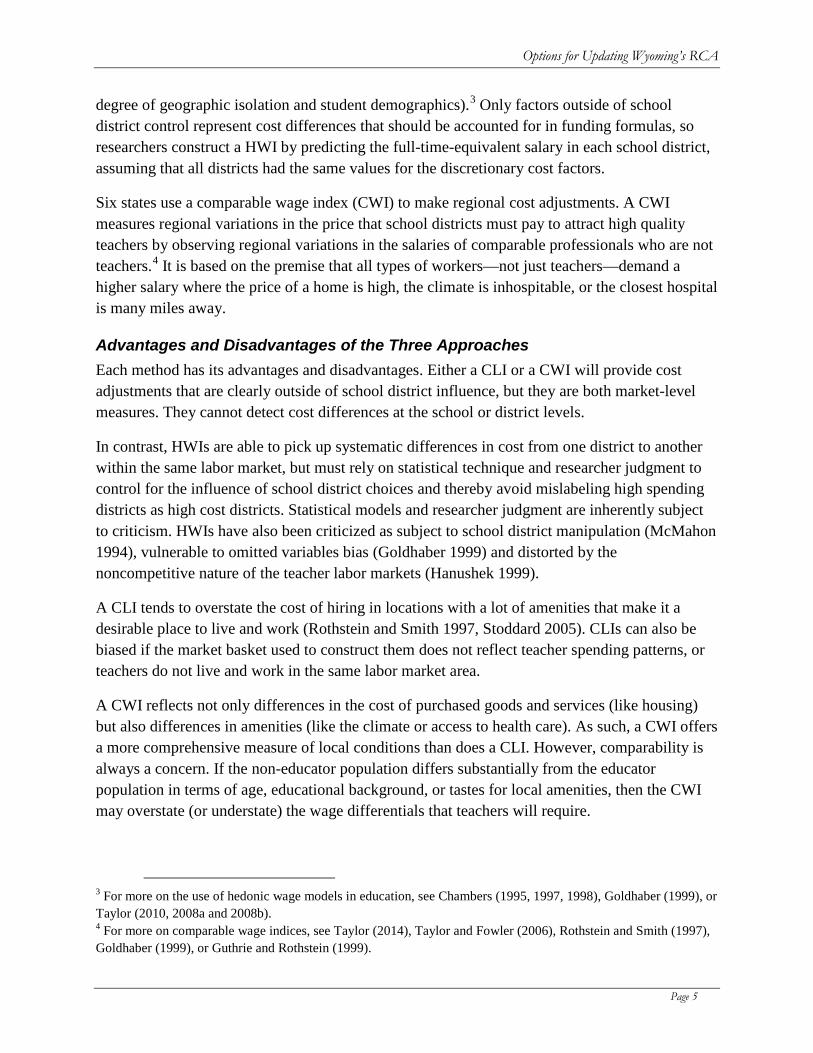
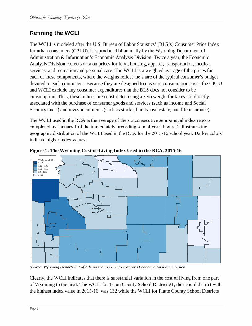
The WCLI used in the RCA is the average of the six consecutive semi-annual index reports completed by January 1 of the immediately preceding school year. Figure 1 illustrates the geographic distribution of the WCLI used in the RCA for the 2015-16 school year. Darker colors indicate higher index values.
Figure 1: The Wyoming Cost-of-Living Index Used in the RCA, 2015-16
Source: Wyoming Department of Administration & Information’s Economic Analysis Division.
Clearly, the WCLI indicates that there is substantial variation in the cost of living from one part of Wyoming to the next. The WCLI for Teton County School District #1, the school district with the highest index value in 2015-16, was 132 while the WCLI for Platte County School Districts
WCLI 2015-16> 120110 - 120100 - 11090 - 100< 90
Options for Updating Wyoming’s RCA
Page 7
#1 and #2, the school districts with the lowest index values in 2015-16, was 87. Thus, the WCLI indicates that costs differ by as much as 52 percent (132/87=1.52) from one part of Wyoming to the next.
The wide range of index values across the state and the particularly high index values in Teton County are almost exclusively attributable to the housing component of the WCLI. Regional differences in housing cost explain 96 percent of the regional variation in the WCLI.
The WCLI is based on the same market basket as the CPI-U.5 In other words, the WCLI is constructed assuming that the purchasing patterns of Wyoming consumers mirror those of city-dwellers in the rest of the United States. They don’t. As a general rule, the residents of Wyoming spend a smaller share of their budgets on housing than the residents of any other state except Iowa and North Dakota.6
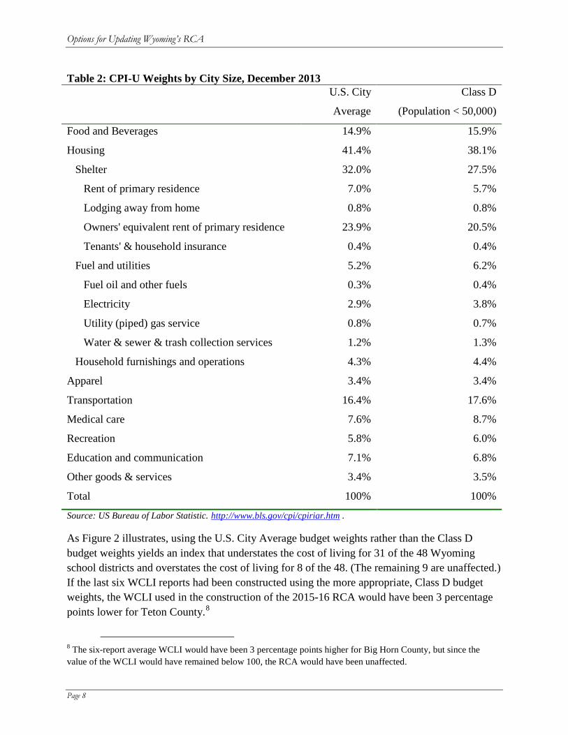
The BLS recognizes that the typical budget shares for consumers in large cities like San Francisco, New York City and Boston are not the same as the typical budget shares for consumers in smaller cities. Therefore, the BLS publishes not only budget shares for the average U.S. city (i.e. the CPI-U weights used in the construction of the WCLI) but also budget shares that differ according to city size.7 As Table 2 illustrates, the BLS estimates that consumers in cities with a population less than 50,000—which the BLS labels Class D locations—typically spend a much smaller share of their budgets on housing than the average urban consumer.
Based on the Census Bureau’s 2014 population estimates, Casper and Cheyenne are the only Wyoming cities that are larger than the Class D threshold, and neither city has a population greater than 65,000. Therefore, the Class D budget weights are a much better fit for Wyoming than the U.S. City Average budget weights.
5 Wyoming Department of Administration and Information, Division of Economic Analysis (1999). 6 The share of households spending more than 30 percent of their incomes on housing was calculated by taking a weighted average of the share of owner-occupants spending 30 percent or more of their incomes on housing and the share of renters spending 30 percent or more of their incomes on housing. The weights were the shares of housing units in each type. The data come from the 2011 Statistical Abstract of the United States. For the data tables, visit http://www.census.gov/compendia/statab/cats/construction_housing/homeownership_and_housing_costs.html 7 Tables downloaded September 24, 2015 from http://www.bls.gov/cpi/cpiriar.htm.
Options for Updating Wyoming’s RCA
Page 8
Table 2: CPI-U Weights by City Size, December 2013
U.S. City
Average
Class D
(Population < 50,000)
Food and Beverages 14.9% 15.9%
Housing 41.4% 38.1%
Shelter 32.0% 27.5%
Rent of primary residence 7.0% 5.7%
Lodging away from home 0.8% 0.8%
Owners' equivalent rent of primary residence 23.9% 20.5%
Tenants' & household insurance 0.4% 0.4%
Fuel and utilities 5.2% 6.2%
Fuel oil and other fuels 0.3% 0.4%
Electricity 2.9% 3.8%
Utility (piped) gas service 0.8% 0.7%
Water & sewer & trash collection services 1.2% 1.3%
Household furnishings and operations 4.3% 4.4%
Apparel 3.4% 3.4%
Transportation 16.4% 17.6%
Medical care 7.6% 8.7%
Recreation 5.8% 6.0%
Education and communication 7.1% 6.8%
Other goods & services 3.4% 3.5%
Total 100% 100%
Source: US Bureau of Labor Statistic. http://www.bls.gov/cpi/cpiriar.htm .
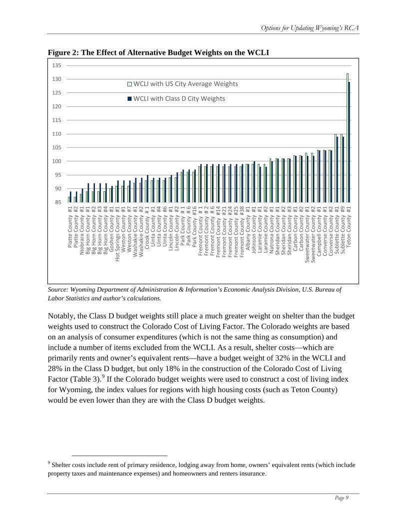
As Figure 2 illustrates, using the U.S. City Average budget weights rather than the Class D budget weights yields an index that understates the cost of living for 31 of the 48 Wyoming school districts and overstates the cost of living for 8 of the 48. (The remaining 9 are unaffected.) If the last six WCLI reports had been constructed using the more appropriate, Class D budget weights, the WCLI used in the construction of the 2015-16 RCA would have been 3 percentage points lower for Teton County.8
8 The six-report average WCLI would have been 3 percentage points higher for Big Horn County, but since the value of the WCLI would have remained below 100, the RCA would have been unaffected.
Options for Updating Wyoming’s RCA
Page 9
Figure 2: The Effect of Alternative Budget Weights on the WCLI
Source: Wyoming Department of Administration & Information’s Economic Analysis Division, U.S. Bureau of Labor Statistics and author’s calculations.
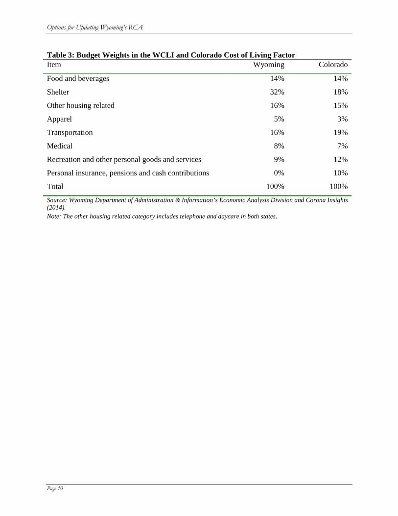
Notably, the Class D budget weights still place a much greater weight on shelter than the budget weights used to construct the Colorado Cost of Living Factor. The Colorado weights are based on an analysis of consumer expenditures (which is not the same thing as consumption) and include a number of items excluded from the WCLI. As a result, shelter costs—which are primarily rents and owner’s equivalent rents—have a budget weight of 32% in the WCLI and 28% in the Class D budget, but only 18% in the construction of the Colorado Cost of Living Factor (Table 3).9 If the Colorado budget weights were used to construct a cost of living index for Wyoming, the index values for regions with high housing costs (such as Teton County) would be even lower than they are with the Class D budget weights.
9 Shelter costs include rent of primary residence, lodging away from home, owners’ equivalent rents (which include property taxes and maintenance expenses) and homeowners and renters insurance.
85
90
95
100
105
110
115
120
125
130
135Pl
atte
Cou
nty
#1
Plat
te C
ount
y #
2N
iobr
ara
Coun
ty #
1Bi
g Ho
rn C
ount
y #
1Bi
g Ho
rn C
ount
y #
2Bi
g Ho
rn C
ount
y #
3Bi
g Ho
rn C
ount
y #
4Go
shen
Cou
nty
#1
Hot S
prin
gs C
ount
y #
1W
esto
n Co
unty
#1
Wes
ton
Coun
ty #
7W
asha
kie
Coun
ty #
1W
asha
kie
Coun
ty #
2Cr
ook
Coun
ty #
1U
inta
Cou
nty
#1
Uin
ta C
ount
y #
4U
inta
Cou
nty
#6
Linc
oln
Coun
ty #
1Li
ncol
n Co
unty
#2
Park
Cou
nty
# 1
Park
Cou
nty
# 6
Park
Cou
nty
#16
Frem
ont C
ount
y #
1Fr
emon
t Cou
nty
# 2
Frem
ont C
ount
y #
6Fr
emon
t Cou
nty
#14
Frem
ont C
ount
y #
21Fr
emon
t Cou
nty
#24
Frem
ont C
ount
y #
25Fr
emon
t Cou
nty
#38
Alba
ny C
ount
y #
1Jo
hnso
n Co
unty
#1
Lara
mie
Cou
nty
#1
Lara
mie
Cou
nty
#2
Nat
rona
Cou
nty
#1
Sher
idan
Cou
nty
#1
Sher
idan
Cou
nty
#2
Sher
idan
Cou
nty
#3
Carb
on C
ount
y #
1Ca
rbon
Cou
nty
#2
Swee
twat
er C
ount
y #
1Sw
eetw
ater
Cou
nty
#2
Cam
pbel
l Cou
nty
#1
Conv
erse
Cou
nty
#1
Conv
erse
Cou
nty
#2
Subl
ette
Cou
nty
#1
Subl
ette
Cou
nty
#9
Teto
n Co
unty
#1
WCLI with US City Average Weights
WCLI with Class D City Weights
Options for Updating Wyoming’s RCA
Page 10
Table 3: Budget Weights in the WCLI and Colorado Cost of Living Factor Item Wyoming Colorado
Food and beverages 14% 14%
Shelter 32% 18%
Other housing related 16% 15%
Apparel 5% 3%
Transportation 16% 19%
Medical 8% 7%
Recreation and other personal goods and services 9% 12%
Personal insurance, pensions and cash contributions 0% 10%
Total 100% 100%
Source: Wyoming Department of Administration & Information’s Economic Analysis Division and Corona Insights (2014). Note: The other housing related category includes telephone and daycare in both states.
Options for Updating Wyoming’s RCA
Page 11
Updating and Improving the Wyoming Hedonic Wage Index
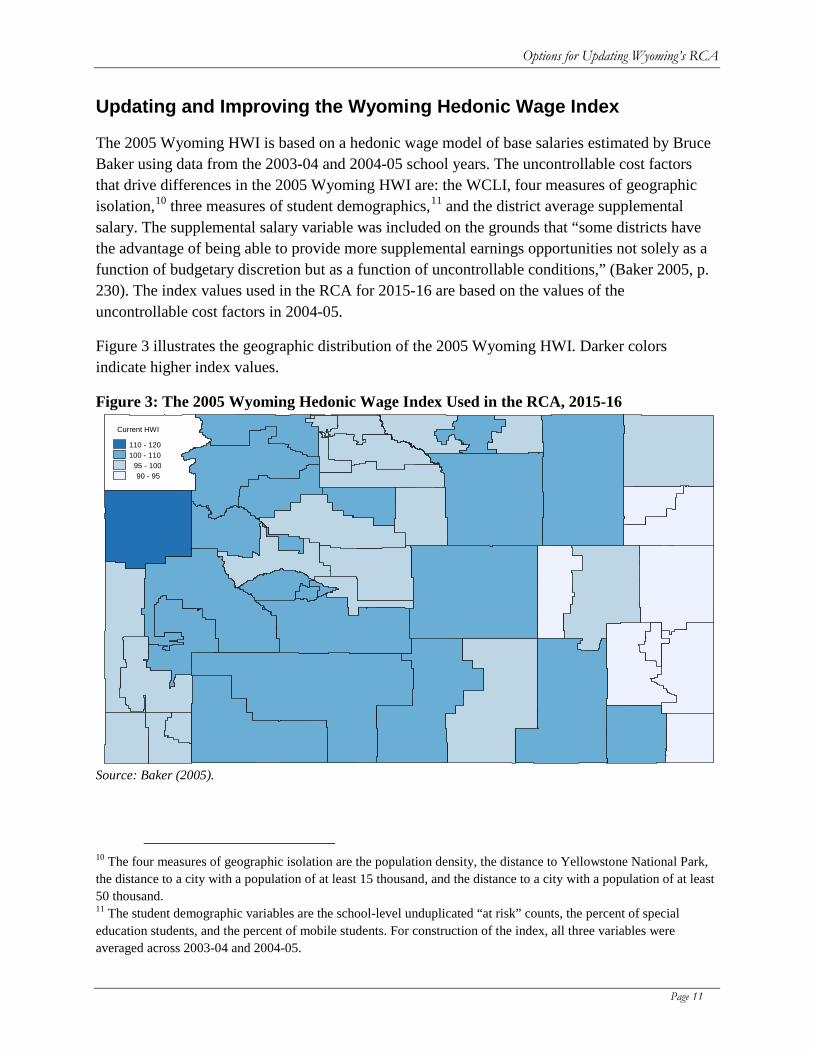
The 2005 Wyoming HWI is based on a hedonic wage model of base salaries estimated by Bruce Baker using data from the 2003-04 and 2004-05 school years. The uncontrollable cost factors that drive differences in the 2005 Wyoming HWI are: the WCLI, four measures of geographic isolation,10 three measures of student demographics,11 and the district average supplemental salary. The supplemental salary variable was included on the grounds that “some districts have the advantage of being able to provide more supplemental earnings opportunities not solely as a function of budgetary discretion but as a function of uncontrollable conditions,” (Baker 2005, p. 230). The index values used in the RCA for 2015-16 are based on the values of the uncontrollable cost factors in 2004-05.
Figure 3 illustrates the geographic distribution of the 2005 Wyoming HWI. Darker colors indicate higher index values.
Figure 3: The 2005 Wyoming Hedonic Wage Index Used in the RCA, 2015-16
Source: Baker (2005).
10 The four measures of geographic isolation are the population density, the distance to Yellowstone National Park, the distance to a city with a population of at least 15 thousand, and the distance to a city with a population of at least 50 thousand. 11 The student demographic variables are the school-level unduplicated “at risk” counts, the percent of special education students, and the percent of mobile students. For construction of the index, all three variables were averaged across 2003-04 and 2004-05.
Current HWI
110 - 120100 - 110
95 - 10090 - 95
Options for Updating Wyoming’s RCA
Page 12
As the figure illustrates, according to the 2005 Wyoming HWI there is substantial variation in the teacher salary cost from one part of Wyoming to the next. The lowest index values are found in the rural and eastern parts of the state, while the highest index values are in Teton County. The 2005 Wyoming HWI for Teton County School District #1, the school district with the highest index value, is 118, while the 2005 Wyoming HWI for Platte County School District #2, the school district with the lowest index value, is 93. Thus, the 2005 Wyoming HWI indicates that labor costs differ by as much as 27 percent (118/93) from one part of Wyoming to the next.
The inclusion of the district’s average supplemental salary in the construction of the 2005 Wyoming HWI makes the index particularly vulnerable to criticism. As Baker acknowledges, the extent to which a school district provides supplemental earnings opportunities is at least partially discretionary. Basing a HWI on a variable that is subject to school district discretion undermines the argument that the index reflects only cost variations that are outside of school district control. The 2005 Wyoming HWI has also been criticized for including the distance to Yellowstone National Park as one of the measures of geographic isolation.
In addition to the technical criticisms of the 2005 Wyoming HWI, there is a more fundamental concern: the 2005 Wyoming HWI is badly out of date. While geography does not change over time, student demographics and the WCLI clearly do. It is hard to defend the position that the HWI should remain unchanged when the WCLI—one of the uncontrollable cost factors used to construct the HWI—is updated annually.
To help inform the 2015 recalibration effort, this analysis presents a 2015 Wyoming HWI. The 2015 Wyoming HWI improves on the 2005 Wyoming HWI in four important ways:
1. The analysis underpinning the 2015 Wyoming HWI uses more recent data and a much longer time series. The 2005 Wyoming HWI was estimated using two years of data covering the 2003-04 and 2004-05 school years. This analysis covers the five school years from 2010-11 through 2014-15.12 All 9,678 individuals with complete data who taught full time in a Wyoming public school for at least one year during that period are included in the analysis.13
Using a longer time series allows for a richer specification of controllable and uncontrollable cost factors and should lead to more precisely measured regional cost adjustments.
2. Where the analysis underlying the 2005 Wyoming HWI treated the district average level of supplemental pay as an uncontrollable cost factor that could influence the base salary a teacher was willing to accept from a district, this analysis takes a different tack. Teachers are likely to consider their total salary not just their base salary when deciding whether or not to
12 Data on earnings, teacher characteristics and job assignments were drawn from the Wyoming Department of Education (WDE) 602 fall data collection files for each school year. 13 Due to data quality concerns, teacher records with full-time-equivalent (FTE) total salaries greater than $120,000 or less than 80 percent of the first step on the district’s salary schedule were excluded from the analysis, as were individuals with a reported FTE less than 0.9 or greater than 1.1, or an FTE in teaching greater than 110 percent of the individual’s total FTE. Individuals with contracts for fewer than 150 days or more than 200 days were also excluded.
Options for Updating Wyoming’s RCA
Page 13
accept a new position or stay in their existing one, and school districts have great discretion over the size of the supplements they offer for coaching, tutoring after school or advising the debate team. Therefore, this analysis treats most forms of supplemental salary as just another part of an individual’s compensation package, and estimates a hedonic model of total salary, not just base salary.14
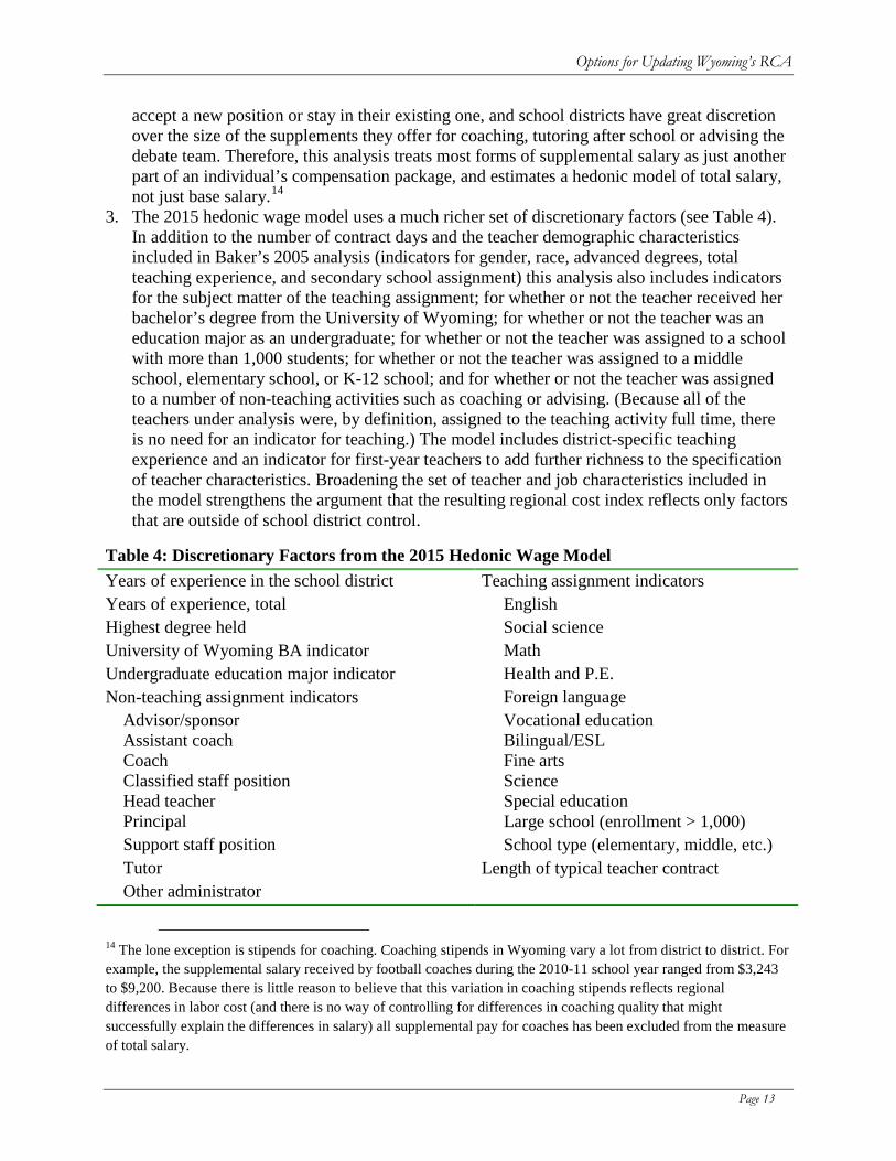
3. The 2015 hedonic wage model uses a much richer set of discretionary factors (see Table 4). In addition to the number of contract days and the teacher demographic characteristics included in Baker’s 2005 analysis (indicators for gender, race, advanced degrees, total teaching experience, and secondary school assignment) this analysis also includes indicators for the subject matter of the teaching assignment; for whether or not the teacher received her bachelor’s degree from the University of Wyoming; for whether or not the teacher was an education major as an undergraduate; for whether or not the teacher was assigned to a school with more than 1,000 students; for whether or not the teacher was assigned to a middle school, elementary school, or K-12 school; and for whether or not the teacher was assigned to a number of non-teaching activities such as coaching or advising. (Because all of the teachers under analysis were, by definition, assigned to the teaching activity full time, there is no need for an indicator for teaching.) The model includes district-specific teaching experience and an indicator for first-year teachers to add further richness to the specification of teacher characteristics. Broadening the set of teacher and job characteristics included in the model strengthens the argument that the resulting regional cost index reflects only factors that are outside of school district control.
Table 4: Discretionary Factors from the 2015 Hedonic Wage Model Years of experience in the school district Teaching assignment indicators Years of experience, total English Highest degree held Social science University of Wyoming BA indicator Math Undergraduate education major indicator Health and P.E. Non-teaching assignment indicators Foreign language Advisor/sponsor Vocational education Assistant coach Bilingual/ESL Coach Fine arts Classified staff position Science Head teacher Special education Principal Large school (enrollment > 1,000) Support staff position School type (elementary, middle, etc.) Tutor Length of typical teacher contract Other administrator
14 The lone exception is stipends for coaching. Coaching stipends in Wyoming vary a lot from district to district. For example, the supplemental salary received by football coaches during the 2010-11 school year ranged from $3,243 to $9,200. Because there is little reason to believe that this variation in coaching stipends reflects regional differences in labor cost (and there is no way of controlling for differences in coaching quality that might successfully explain the differences in salary) all supplemental pay for coaches has been excluded from the measure of total salary.

Options for Updating Wyoming’s RCA
Page 14
4. The 2015 hedonic wage model relies on an improved set of uncontrollable cost factors (Table 5). As with the construction of the 2005 Wyoming HWI, the uncontrollable cost factors include the WCLI, multiple measures of geographic isolation and multiple measures of student need. However, the 2015 hedonic wage model replaces the distance to Yellowstone National Park with an indicator for whether or not the nearest hospital is more than 25 miles away, a measure of geographic isolation that is more relevant to the everyday lives of teachers.15 Due to data availability, population density is measured at the county level. In addition, the 2015 analysis replaces the unduplicated-at-risk percent and the percent mobile students with two alternative measures of student need—the percent of students who are English language learners and the percentage of students who qualify to receive free school lunches. Taylor (2011) found that these two variables better explain salaries than do the student demographic indicators used in Baker’s 2005 analysis. In addition, the set of uncontrollable cost factors also includes a newly developed CWI for Wyoming counties. Including the CWI strengthens the model by providing a direct measure of the labor market alternatives available to Wyoming school teachers.
Table 5: Uncontrollable Cost Factors from the 2015 Hedonic Wage Model, with Comparison to the Factors Used in Construction of the 2005 Wyoming HWI
Uncontrollable Cost Factors Used in the 2015 HWI?
Used in the 2005 HWI?
Impact of the Cost Factor on the 2005 HWI
WCLI Yes Yes Positive OES CWI Yes No Geographic isolation Nearest hospital > 25 miles Yes No Miles to nearest city of 50,00016 Yes Yes Positive Miles to nearest city of 15,000 Yes Yes Negative Miles to Yellowstone National Park No Yes Negative Population density (county) Yes No Population density (10-mile radius) No Yes Positive Student demographics Percent Free Lunch Yes No Percent Special Ed. Yes Yes Positive Percent English language learners Yes No Percent unduplicated at risk No Yes Negative Percent mobile No Yes Negative District average supplemental salary No Yes Negative
15 Distance to the nearest hospital was determined as the crow flies using data from the National Center for Education Statistics on the latitude and longitude of each Wyoming campus, and data from the Wyoming Hospital Association on the street address of each Wyoming Hospital. 16 For the 2015 HWI analysis, the distance to the nearest city with a population of 50,000 and the nearest city with a population of 15,000 were calculated as-the-crow-flies using the U.S. Census Bureau’s 2009 population estimates and latitude and longitude files for places. For both measures, the nearest city need not be within the state of Wyoming. Indeed, half of the school districts in Wyoming are closer to a city of 50,000 in another state than they are to a city of that size within Wyoming.
Options for Updating Wyoming’s RCA
Page 15
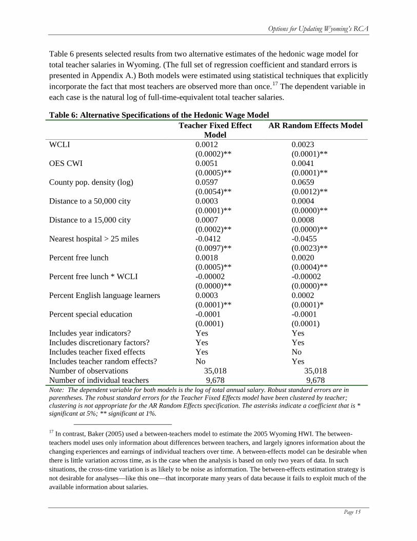
Table 6 presents selected results from two alternative estimates of the hedonic wage model for total teacher salaries in Wyoming. (The full set of regression coefficient and standard errors is presented in Appendix A.) Both models were estimated using statistical techniques that explicitly incorporate the fact that most teachers are observed more than once.17 The dependent variable in each case is the natural log of full-time-equivalent total teacher salaries.
Table 6: Alternative Specifications of the Hedonic Wage Model Teacher Fixed Effect
Model AR Random Effects Model
WCLI 0.0012 0.0023 (0.0002)** (0.0001)**
OES CWI 0.0051 0.0041 (0.0005)** (0.0001)** County pop. density (log) 0.0597 0.0659
(0.0054)** (0.0012)** Distance to a 50,000 city 0.0003 0.0004
(0.0001)** (0.0000)** Distance to a 15,000 city 0.0007 0.0008
(0.0002)** (0.0000)** Nearest hospital > 25 miles -0.0412 -0.0455
(0.0097)** (0.0023)** Percent free lunch 0.0018 0.0020
(0.0005)** (0.0004)** Percent free lunch * WCLI -0.00002 -0.00002
(0.0000)** (0.0000)** Percent English language learners 0.0003 0.0002
(0.0001)** (0.0001)* Percent special education -0.0001 -0.0001
(0.0001) (0.0001) Includes year indicators? Yes Yes Includes discretionary factors? Yes Yes Includes teacher fixed effects Yes No Includes teacher random effects? No Yes Number of observations 35,018 35,018 Number of individual teachers 9,678 9,678 Note: The dependent variable for both models is the log of total annual salary. Robust standard errors are in parentheses. The robust standard errors for the Teacher Fixed Effects model have been clustered by teacher; clustering is not appropriate for the AR Random Effects specification. The asterisks indicate a coefficient that is * significant at 5%; ** significant at 1%.
17 In contrast, Baker (2005) used a between-teachers model to estimate the 2005 Wyoming HWI. The between-teachers model uses only information about differences between teachers, and largely ignores information about the changing experiences and earnings of individual teachers over time. A between-effects model can be desirable when there is little variation across time, as is the case when the analysis is based on only two years of data. In such situations, the cross-time variation is as likely to be noise as information. The between-effects estimation strategy is not desirable for analyses—like this one—that incorporate many years of data because it fails to exploit much of the available information about salaries.
Options for Updating Wyoming’s RCA
Page 16
The first model is a teacher fixed effects model. The fixed effects methodology adjusts for any variation in salaries that might arise from persistent, but unmeasured teacher characteristics such as intelligence or verbal ability. As such, it does the best possible job of controlling for differences in salary that can be attributed to discretionary factors. Unfortunately, in doing so, it also removes much of the variation in cost that is driven by stable characteristics of school districts. Stable district characteristics—such as geographic remoteness or a persistently high cost of living—will only register for teachers who change districts. If teachers who change districts are not representative of the teaching population as a whole, the fixed-effects model can be misleading. During the period under analysis, less than 7 percent of the teachers in Wyoming changed school districts. Movers were disproportionately inexperienced teachers who did not have an advanced degree, suggesting that mobile teachers may be systematically different from teacher who do not move between school districts.
The second model is an autoregressive (AR) random effects model. Like the fixed effects model, the AR random effects model incorporates all of the information in the data and (partially) adjusts for persistent but unmeasured differences in teacher quality. Unlike the fixed effects model, the AR random effects model captures the influence of cost factors that are relatively stable over time using data from all teachers, not just the teachers who move between districts. Here, the random effects model has been estimated allowing the residuals to follow the autoregressive pattern found in the data.18 (An autoregressive pattern to teacher salaries means that if a teacher earns more than the model predicts in one year, he or she will probably earn more than the model predicts the next year too.)
Both models do a good job of capturing variations in teacher salaries. As expected, salaries increase with teaching experience and educational attainment. Salaries are systematically higher in school districts where the school year is longer. Teachers who take on nonteaching duties earn more than other teachers, but there is no evidence of a salary premium for science and math teachers. Teachers who majored in something other than education earned systematically more than other teachers, all other things being equal. On the other hand, teachers with a bachelor’s degree from the University of Wyoming earned systematically less than teachers with a bachelor’s degree from another institution (at least according to the AR random effects model.)
On purely statistical grounds, the fixed effects model fits the data better than the AR random effects model. Statistical tests easily reject the AR random effects model in favor of the fixed effects model.19 Furthermore, relying on the fixed effects model to construct the 2015 HWI would largely address concerns about the potential for bias arising from an incomplete specification of teacher characteristics. On the other hand, the fixed effects modeling strategy
18 A Wald test for the absence of autocorrelation was rejected at the 1 percent level. See Drukker (2003) and Wooldridge (2002). 19 A Hausman test of model specification reject the random effects model in favor of the fixed effects model at the 1 percent level.
Options for Updating Wyoming’s RCA
Page 17
may also strip from the index much of the information about important, quasi-fixed district characteristics like a relatively low cost of living.
Because the fixed effect model may be failing to pick up important cost factors and the relatively small number of teachers who move between districts appear to be systematically different from other teachers, the AR random effects model is the best option for updating the Wyoming HWI. The AR random effects model incorporates all of the available information about the distribution of teacher salaries and some of the information about unmeasured teacher characteristics without losing the ability to capture the impact of the stable cost factors. Furthermore, the list of discretionary characteristics is quite extensive. The additional detail incorporated into this update greatly reduces the risk that there are important teacher characteristics that have been omitted from the model.
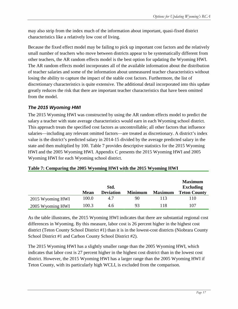
The 2015 Wyoming HWI The 2015 Wyoming HWI was constructed by using the AR random effects model to predict the salary a teacher with state average characteristics would earn in each Wyoming school district. This approach treats the specified cost factors as uncontrollable; all other factors that influence salaries—including any relevant omitted factors—are treated as discretionary. A district’s index value is the district’s predicted salary in 2014-15 divided by the average predicted salary in the state and then multiplied by 100. Table 7 provides descriptive statistics for the 2015 Wyoming HWI and the 2005 Wyoming HWI. Appendix C presents the 2015 Wyoming HWI and 2005 Wyoming HWI for each Wyoming school district.
Table 7: Comparing the 2005 Wyoming HWI with the 2015 Wyoming HWI
Mean Std.
Deviation Minimum Maximum
Maximum Excluding
Teton County 2015 Wyoming HWI 100.0 4.7 90 113 110
2005 Wyoming HWI 100.3 4.6 93 118 107 As the table illustrates, the 2015 Wyoming HWI indicates that there are substantial regional cost differences in Wyoming. By this measure, labor cost is 26 percent higher in the highest cost district (Teton County School District #1) than it is in the lowest-cost districts (Niobrara County School District #1 and Carbon County School District #2).
The 2015 Wyoming HWI has a slightly smaller range than the 2005 Wyoming HWI, which indicates that labor cost is 27 percent higher in the highest cost district than in the lowest cost district. However, the 2015 Wyoming HWI has a larger range than the 2005 Wyoming HWI if Teton County, with its particularly high WCLI, is excluded from the comparison.
Options for Updating Wyoming’s RCA
Page 18
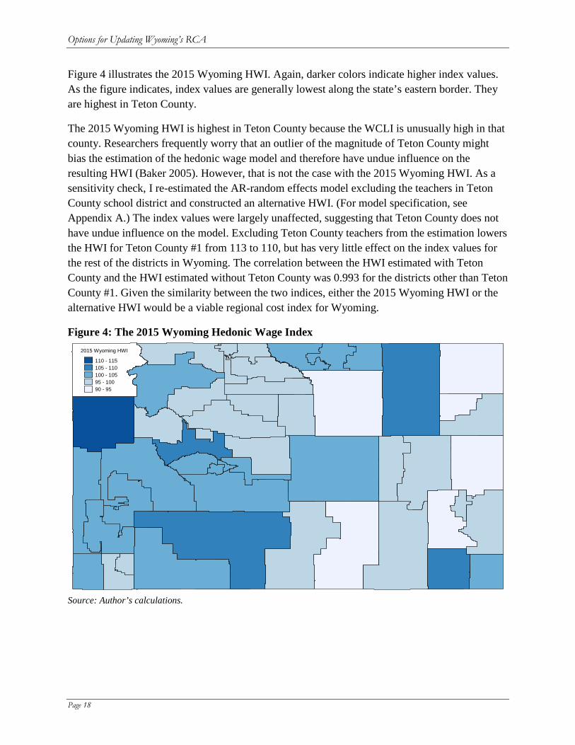
Figure 4 illustrates the 2015 Wyoming HWI. Again, darker colors indicate higher index values. As the figure indicates, index values are generally lowest along the state’s eastern border. They are highest in Teton County.
The 2015 Wyoming HWI is highest in Teton County because the WCLI is unusually high in that county. Researchers frequently worry that an outlier of the magnitude of Teton County might bias the estimation of the hedonic wage model and therefore have undue influence on the resulting HWI (Baker 2005). However, that is not the case with the 2015 Wyoming HWI. As a sensitivity check, I re-estimated the AR-random effects model excluding the teachers in Teton County school district and constructed an alternative HWI. (For model specification, see Appendix A.) The index values were largely unaffected, suggesting that Teton County does not have undue influence on the model. Excluding Teton County teachers from the estimation lowers the HWI for Teton County #1 from 113 to 110, but has very little effect on the index values for the rest of the districts in Wyoming. The correlation between the HWI estimated with Teton County and the HWI estimated without Teton County was 0.993 for the districts other than Teton County #1. Given the similarity between the two indices, either the 2015 Wyoming HWI or the alternative HWI would be a viable regional cost index for Wyoming.
Figure 4: The 2015 Wyoming Hedonic Wage Index
Source: Author’s calculations.
2015 Wyoming HWI
110 - 115105 - 110100 - 10595 - 10090 - 95
Options for Updating Wyoming’s RCA
Page 19
Developing a Comparable Wage Index for Wyoming
The comparable wage approach to geographic cost adjustment recognizes that teachers are not the only workers who are sensitive to the cost of living and the general attractiveness of the community. All types of workers demand a higher salary in locations with a high cost of living and a lack of offsetting amenities. Therefore, regional variations in the price that school districts must pay to attract high quality teachers will be reflected in the cost of hiring comparable individuals who are not teachers. Conceptually, if nurses in Laramie earn 10 percent more than the national average for nurses, accountants in Laramie earn 10 percent more than the national average for accountants, computer programmers in Laramie earn 10 percent more than the national average for programmers, and so on, then a reasonable estimate is that teachers in Laramie will also expect to earn 10 percent more than the national average for teachers.
The National Center for Education Statistics’ (NCES) Comparable Wage Index (CWI) was designed specifically to capture regional wage differences for college graduates who are not educators.20 The baseline estimates come from a regression analysis of the individual earnings data from the 2000 U.S. Census. Subsequent updates to that baseline came from regression analyses of earnings data from the BLS’ Occupational Employment Survey (OES).
The two components of the NCES CWI suggest two complementary strategies for estimating a CWI for Wyoming. First, one could estimate a CWI using data from the American Community Survey (ACS). Second, one could estimate a CWI using the earnings data in the OES.
The ACS, which is conducted annually by the U.S. Census Bureau, has replaced the decennial census as the primary source of demographic information about the U.S. population. The advantage to using the ACS to estimate a CWI is that the ACS provides information not only on the annual earnings of workers, but also on their other demographic characteristics, including their hours worked, ages and levels of educational attainment. The rich demographic detail in the ACS make it possible to control for regional demographic differences in the construction of a CWI, ensuring that the index does not indicate that labor cost are low in a location simply because the typical worker in that location is younger or less well educated than the typical worker in other locations.
The disadvantage to using the ACS to estimate a CWI is that the level of geographic detail is low. To protect the privacy of the survey respondents, the Census Bureau only provides geographic information about “place-of-work areas.” Place-of-work areas are geographic regions designed to contain at least 100,000 persons. There are only five ACS place of work areas in Wyoming.
20 For more on the estimation of the NCES CWI, see Taylor and Fowler (2006).
Options for Updating Wyoming’s RCA
Page 20
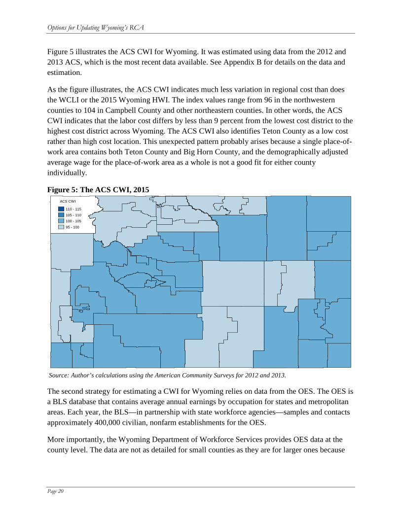
Figure 5 illustrates the ACS CWI for Wyoming. It was estimated using data from the 2012 and 2013 ACS, which is the most recent data available. See Appendix B for details on the data and estimation.
As the figure illustrates, the ACS CWI indicates much less variation in regional cost than does the WCLI or the 2015 Wyoming HWI. The index values range from 96 in the northwestern counties to 104 in Campbell County and other northeastern counties. In other words, the ACS CWI indicates that the labor cost differs by less than 9 percent from the lowest cost district to the highest cost district across Wyoming. The ACS CWI also identifies Teton County as a low cost rather than high cost location. This unexpected pattern probably arises because a single place-of-work area contains both Teton County and Big Horn County, and the demographically adjusted average wage for the place-of-work area as a whole is not a good fit for either county individually.
Figure 5: The ACS CWI, 2015
Source: Author’s calculations using the American Community Surveys for 2012 and 2013.
The second strategy for estimating a CWI for Wyoming relies on data from the OES. The OES is a BLS database that contains average annual earnings by occupation for states and metropolitan areas. Each year, the BLS—in partnership with state workforce agencies—samples and contacts approximately 400,000 civilian, nonfarm establishments for the OES.
More importantly, the Wyoming Department of Workforce Services provides OES data at the county level. The data are not as detailed for small counties as they are for larger ones because
ACS CWI
110 - 115105 - 110100 - 105
95 - 100
Options for Updating Wyoming’s RCA
Page 21
privacy concerns lead to the suppression of occupational detail. Nevertheless, the level of geographic detail is unmatched.
The disadvantage to using the OES to construct a CWI is that the OES does not have any data on the demographic characteristics of workers. It is not possible to adjust for regional differences in educational attainment or to limit the sample to college graduates. It is possible to limit the analysis to occupations that are commonly held by college graduates, but only in locations with fine-grained details on specific occupations. Such data are not available for most Wyoming counties. Therefore, in order to produce estimates for all Wyoming counties, it is necessary to include all available occupations. As such, there is a somewhat higher risk that systematic differences between the teacher population and the non-educator population (in terms of educational background or tastes for local amenities) could lead the OES CWI to overstate (or understate) the wage differentials that teachers would require in specific locations.
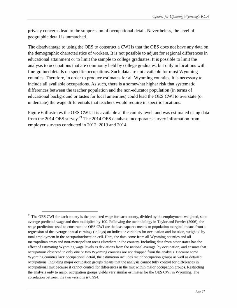
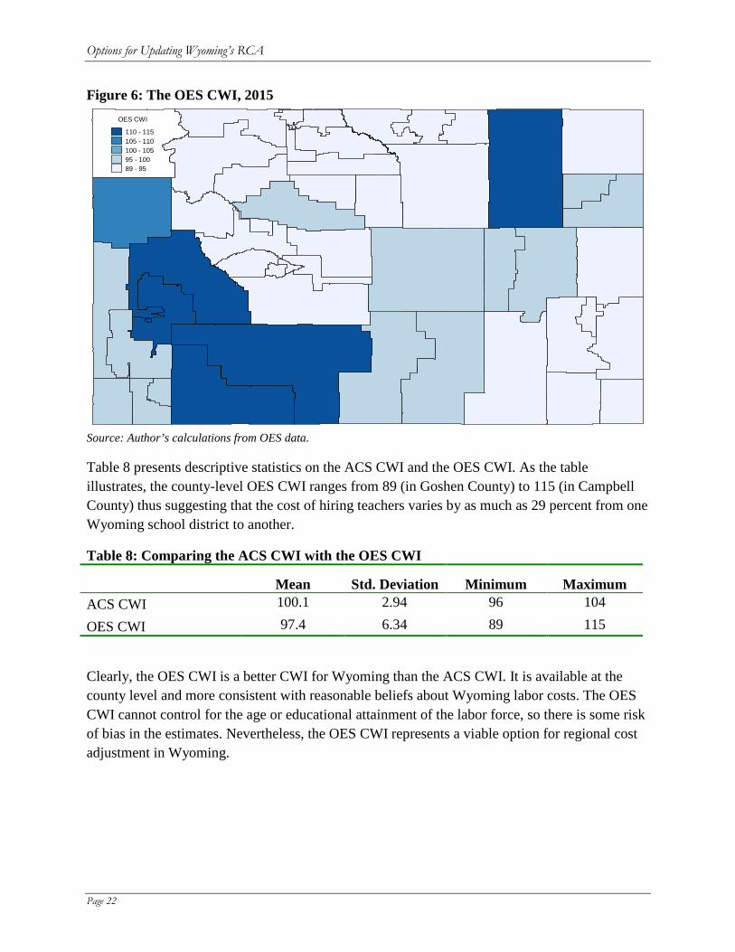
Figure 6 illustrates the OES CWI. It is available at the county level, and was estimated using data from the 2014 OES survey.21 The 2014 OES database incorporates survey information from employer surveys conducted in 2012, 2013 and 2014.
21 The OES CWI for each county is the predicted wage for each county, divided by the employment-weighted, state average predicted wage and then multiplied by 100. Following the methodology in Taylor and Fowler (2006), the wage predictions used to construct the OES CWI are the least squares means or population marginal means from a regression of the average annual earnings (in logs) on indicator variables for occupation and location, weighted by total employment in the occupation/location cell. Here, the data come from all Wyoming counties and all metropolitan areas and non-metropolitan areas elsewhere in the country. Including data from other states has the effect of estimating Wyoming wage levels as deviations from the national average, by occupation, and ensures that occupations observed in only one or two Wyoming counties are not dropped from the analysis. Because some Wyoming counties lack occupational detail, the estimation includes major occupation groups as well as detailed occupations. Including major occupation groups means that the analysis cannot fully control for differences in occupational mix because it cannot control for differences in the mix within major occupation groups. Restricting the analysis only to major occupation groups yields very similar estimates for the OES CWI in Wyoming. The correlation between the two versions is 0.994.
Options for Updating Wyoming’s RCA
Page 22
Figure 6: The OES CWI, 2015
Source: Author’s calculations from OES data.
Table 8 presents descriptive statistics on the ACS CWI and the OES CWI. As the table illustrates, the county-level OES CWI ranges from 89 (in Goshen County) to 115 (in Campbell County) thus suggesting that the cost of hiring teachers varies by as much as 29 percent from one Wyoming school district to another.
Table 8: Comparing the ACS CWI with the OES CWI
Mean Std. Deviation Minimum Maximum ACS CWI 100.1 2.94 96 104
OES CWI 97.4 6.34 89 115
Clearly, the OES CWI is a better CWI for Wyoming than the ACS CWI. It is available at the county level and more consistent with reasonable beliefs about Wyoming labor costs. The OES CWI cannot control for the age or educational attainment of the labor force, so there is some risk of bias in the estimates. Nevertheless, the OES CWI represents a viable option for regional cost adjustment in Wyoming.
OES CWI
110 - 115105 - 110100 - 10595 - 10089 - 95
Options for Updating Wyoming’s RCA
Page 23
Exploring the Implications Updating the RCA could substantially alter the distribution of state aid to Wyoming school districts. Arguably, any of three indices—the reweighted WCLI, the 2015 Wyoming HWI or the OES CWI could be used to make regional cost adjustments. However, the three most likely scenarios are that either:
1. The reweighted WCLI and the 2015 Wyoming HWI would simply replace the existing WCLI and HWI in the calculation of the RCA. Thus, the updated RCA would be the larger of the WCLI with Class D weights, the 2015 Wyoming HWI or 100. Or,
2. The 2015 Wyoming HWI would replace the RCA. Or, 3. The OES CWI would replace the RCA.
Appendix C lists the current and updated RCA under each scenario for each Wyoming district.
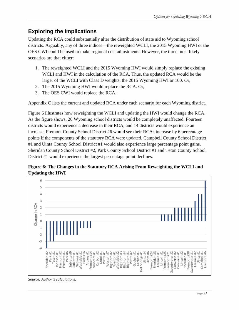
Figure 6 illustrates how reweighting the WCLI and updating the HWI would change the RCA. As the figure shows, 20 Wyoming school districts would be completely unaffected. Fourteen districts would experience a decrease in their RCA, and 14 districts would experience an increase. Fremont County School District #6 would see their RCAs increase by 6 percentage points if the components of the statutory RCA were updated. Campbell County School District #1 and Uinta County School District #1 would also experience large percentage point gains. Sheridan County School District #2, Park County School District #1 and Teton County School District #1 would experience the largest percentage point declines.
Figure 6: The Changes in the Statutory RCA Arising From Reweighting the WCLI and Updating the HWI
Source: Author’s calculations.
-4
-3
-2
-1
0
1
2
3
4
5
6
Sher
idan
#2
Park
#1
Teto
n #1
John
son
#1Fr
emon
t #2
Frem
ont #
1Pa
rk #
6Su
blet
te #
9Su
blet
te #
1N
atro
na #
1W
asha
kie
#1Pa
rk #
16Al
bany
#1
Frem
ont #
14N
iobr
ara
#1Ca
rbon
#2
Croo
k #1
Plat
te #
1W
esto
n #7
Big
Horn
#2
Wes
ton
#1W
asha
kie
#2Bi
g Ho
rn #
3Bi
g Ho
rn #
4Bi
g Ho
rn #
1Pl
atte
#2
Gosh
en #
1Ca
rbon
#1
Hot S
prin
gs #
1U
inta
#4
Uin
ta #
6Fr
emon
t #24
Sher
idan
#3
Lara
mie
#1
Linc
oln
#1Fr
emon
t #25
Frem
ont #
21Sw
eetw
ater
#2
Conv
erse
#2
Conv
erse
#1
Linc
oln
#2Sh
erid
an #
1Fr
emon
t #38
Swee
twat
er #
1La
ram
ie #
2U
inta
#1
Cam
pbel
l #1
Frem
ont #
6
Chan
ge in
RCA
Options for Updating Wyoming’s RCA
Page 24
After reweighting and updating, 23 of the 48 school districts in Wyoming would have their RCA based on the 2015 Wyoming HWI. Seventeen districts would have their RCA set to 100 despite below average labor costs. The RCA for eight school districts (including Teton County School District #1) would be based on the reweighted WCLI.
Unfortunately, defining the RCA as the greater of three alternatives—the WCLI, the HWI or 100—has unintended consequences for school funding equity in Wyoming that will not be resolved simply by reweighting the WCLI and updating the HWI. From a strict equity perspective, continuing to apply the regional cost index only to districts with above-average costs will overfund more than one third of the school districts in Wyoming. Continuing to offer the WCLI option will also overfund some districts, because any cost of living index—even the reweighted WCLI—overstates the cost of hiring in locations that have attractive amenities.
One solution is to use the 2015 Wyoming HWI as the sole source of regional cost adjustment. The 2015 Wyoming HWI is a direct measure of regional variations in the cost of educator labor. It represents a significant improvement on the 2005 Wyoming HWI, which has become badly outdated.
If the Legislature were to adopt the 2015 Wyoming HWI as the RCA, it would not be desirable to apply the regional cost adjustment only to districts with above average costs. Regional cost adjustments exist to equalize the purchasing power of school districts. If one district has labor costs that are 5 percent higher than another, then it should receive more funding than the other, even if both have below average costs. Rounding all the districts up to the state average defeats the purpose of regional cost adjustments and can exacerbate inequalities in the system.
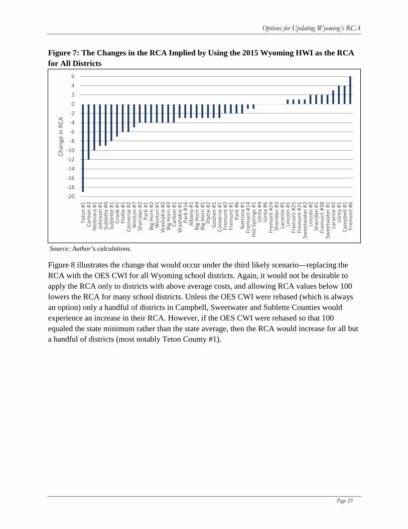
Figure 7 illustrates the changes that would occur if the 2015 Wyoming HWI were adopted as the RCA for all Wyoming school districts. Not surprisingly, allowing RCA values below 100 would lower the RCA for many school districts. However, the biggest declines in the RCA would be for districts where the WCLI is particularly high. The biggest beneficiaries of replacing the statutory RCA with the 2015 Wyoming HWI would be districts in Campbell, Fremont and Uinta counties.
Options for Updating Wyoming’s RCA
Page 25
Figure 7: The Changes in the RCA Implied by Using the 2015 Wyoming HWI as the RCA for All Districts
Source: Author’s calculations.
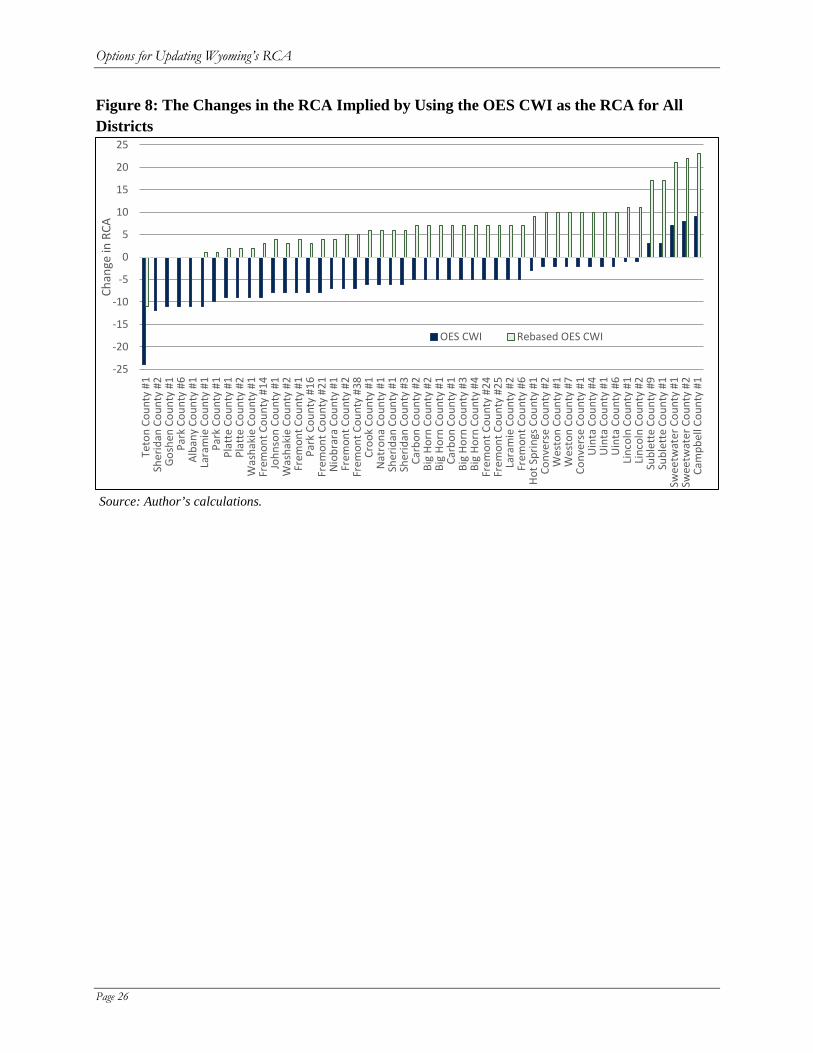
Figure 8 illustrates the change that would occur under the third likely scenario—replacing the RCA with the OES CWI for all Wyoming school districts. Again, it would not be desirable to apply the RCA only to districts with above average costs, and allowing RCA values below 100 lowers the RCA for many school districts. Unless the OES CWI were rebased (which is always an option) only a handful of districts in Campbell, Sweetwater and Sublette Counties would experience an increase in their RCA. However, if the OES CWI were rebased so that 100 equaled the state minimum rather than the state average, then the RCA would increase for all but a handful of districts (most notably Teton County #1).
-20-18-16-14-12-10
-8-6-4-20246
Teto
n #1
Carb
on #
2N
iobr
ara
#1Jo
hnso
n #1
Subl
ette
#9
Subl
ette
#1
Croo
k #1
Plat
te #
1Co
nver
se #
2W
esto
n #7
Sher
idan
#2
Park
#1
Big
Horn
#2
Wes
ton
#1W
asha
kie
#2Bi
g Ho
rn #
3Ca
rbon
#1
Was
haki
e #1
Park
#16
Alba
ny #
1Bi
g Ho
rn #
4Bi
g Ho
rn #
1Pl
atte
#2
Gosh
en #
1Co
nver
se #
1Fr
emon
t #2
Frem
ont #
1Pa
rk #
6N
atro
na #
1Fr
emon
t #14
Hot S
prin
gs #
1U
inta
#4
Uin
ta #
6Fr
emon
t #24
Sher
idan
#3
Lara
mie
#1
Linc
oln
#1Fr
emon
t #25
Frem
ont #
21Sw
eetw
ater
#2
Linc
oln
#2Sh
erid
an #
1Fr
emon
t #38
Swee
twat
er #
1La
ram
ie #
2U
inta
#1
Cam
pbel
l #1
Frem
ont #
6
Chan
ge in
RCA
Options for Updating Wyoming’s RCA
Page 26
Figure 8: The Changes in the RCA Implied by Using the OES CWI as the RCA for All Districts
Source: Author’s calculations.
-25
-20
-15
-10
-5
0
5
10
15
20
25Te
ton
Coun
ty #
1Sh
erid
an C
ount
y #2
Gosh
en C
ount
y #1
Park
Cou
nty
#6Al
bany
Cou
nty
#1La
ram
ie C
ount
y #1
Park
Cou
nty
#1Pl
atte
Cou
nty
#1Pl
atte
Cou
nty
#2W
asha
kie
Coun
ty #
1Fr
emon
t Cou
nty
#14
John
son
Coun
ty #
1W
asha
kie
Coun
ty #
2Fr
emon
t Cou
nty
#1Pa
rk C
ount
y #1
6Fr
emon
t Cou
nty
#21
Nio
brar
a Co
unty
#1
Frem
ont C
ount
y #2
Frem
ont C
ount
y #3
8Cr
ook
Coun
ty #
1N
atro
na C
ount
y #1
Sher
idan
Cou
nty
#1Sh
erid
an C
ount
y #3
Carb
on C
ount
y #2
Big
Horn
Cou
nty
#2Bi
g Ho
rn C
ount
y #1
Carb
on C
ount
y #1
Big
Horn
Cou
nty
#3Bi
g Ho
rn C
ount
y #4
Frem
ont C
ount
y #2
4Fr
emon
t Cou
nty
#25
Lara
mie
Cou
nty
#2Fr
emon
t Cou
nty
#6Ho
t Spr
ings
Cou
nty
#1Co
nver
se C
ount
y #2
Wes
ton
Coun
ty #
1W
esto
n Co
unty
#7
Conv
erse
Cou
nty
#1U
inta
Cou
nty
#4U
inta
Cou
nty
#1U
inta
Cou
nty
#6Li
ncol
n Co
unty
#1
Linc
oln
Coun
ty #
2Su
blet
te C
ount
y #9
Subl
ette
Cou
nty
#1Sw
eetw
ater
Cou
nty
#1Sw
eetw
ater
Cou
nty
#2Ca
mpb
ell C
ount
y #1
Chan
ge in
RCA
OES CWI Rebased OES CWI
Options for Updating Wyoming’s RCA
Page 27
Conclusions Wyoming is one of the few states in the nation to adjust its school finance formula to reflect regional variations in the cost of education. This analysis suggests that the cost of education varies widely within the state, offering strong support for continuing such adjustments.
Although any of the three options discussed above would represent an improvement over the status quo, I recommend that the Wyoming Legislature consider replacing the current, three-way design of the RCA with the OES CWI. The OES CWI has a number of attractive features. It is clearly outside of school district influence, eliminating the risk that the regional cost index would misidentify high spending districts as high cost ones. It reflects not only regional differences in cost of living, but also differences in local amenities. The CWI methodology is also the most common approach to regional cost adjustment in other states.
If the OES CWI were rebased so that 100 equaled the state minimum, then most Wyoming school districts would benefit from the change to the OES CWI. Only a handful of districts—most notably Teton County #1—would experience a decline in their RCA. Furthermore, by properly calibrating the salary used in the funding model calculations, this change in the RCA could be accomplished with only a limited budgetary impact.
Whichever option the Legislature chooses, I also recommend that it put in place a mechanism for regular updates to the RCA. The Wyoming economy is dynamic and labor market conditions in Wyoming are constantly changing. For the RCA to work as intended, it must accurately reflect current differences in labor cost, and not be allowed to drift out of date.
Options for Updating Wyoming’s RCA
Page 28
Bibliography Baker, Bruce D. 2005. Development of an Hedonic Wage Index for the Wyoming School
Funding Model, in An Evidence-Based Approach To Recalibrating Wyoming’s Block Grant School Funding Formula, a report prepared for the Wyoming Legislative Select Committee on Recalibration by Lawrence O. Picus and Associates. Retrieved July 19, 2011 from http://legisweb.state.wy.us/2009/interim/schoolfinance/WYRecalibration.pdf.
Chambers, J.G. (1998). Geographic Variations in Public Schools’ Costs (NCES 98-04). U.S. Department of Education. Wyoming, DC: National Center for Education Statistics Working Paper.
Chambers, Jay G. 1997. Geographic Variations in Public School Costs. Washington, D.C.: U.S. Department of Education, National Center for Education Statistics.
Chambers, Jay G. 1995. “Public School Teacher Cost Differences Across the United States: Introduction to a Teacher Cost Index (TCI)” [online] Retrieved November 22, 1999, from http://nces.ed.gov/pubs/96344cha.htm.
Corona Insights (2014). 2013 Colorado school district cost of living study. Retrieved March 31, 2015 from http://www.colorado.gov/cs/Satellite?blobcol=urldata&blobheader=application%2Fpdf&blobkey=id&blobtable=MungoBlobs&blobwhere=1251990492659&ssbinary=true.
Drukker, D. M. 2003. Testing for serial correlation in linear panel-data models. Stata Journal (3)2: 168-177.
Goldhaber, D.D. (1999). An Alternative Measure of Inflation in Teacher Salaries. In W.J. Fowler, Jr. (Ed.), Selected Papers in School Finance, 1997–99 (NCES 1999-334) (pp. 29–54). U.S. Department of Education. Wyoming, DC: National Center for Education Statistics.
Guthrie, James, and Richard Rothstein. 1999. Enabling ‘adequacy’ to achieve reality: Translating adequacy into state school finance distribution arrangements. In Equity and adequacy in education finance, edited by H.F. Ladd, R. Chalk, and J.S. Hansen. Washington, D.C.: National Academy Press, pp. 209–59.
Hanushek, Eric A. 1999. Adjusting for differences in the costs of educational inputs. In Selected papers in school finance, 1997–99, edited by W.J. Fowler, Jr.. Washington, D.C.: National Center for Education Statistics, pp. 13–28.
McMahon, Walter W. 1994. Intrastate cost adjustments. In Selected papers in school finance, 1994, edited by W.J. Fowler, Jr.. Washington, D.C.: National Center for Education Statistics, pp. 93–114.
Rothstein, Richard and James R. Smith. 1997. Adjusting Oregon Education Expenditures for Regional Cost Differences: A Feasibility Study. Sacramento, CA: Management Analysis & Planning Associates, L.L.C.
Ruggles, Steven, Katie Genadek, Ronald Goeken, Josiah Grover, and Matthew Sobek. 2015. Integrated Public Use Microdata Series: Version 6.0 [Machine-readable database]. Minneapolis: University of Minnesota.
Options for Updating Wyoming’s RCA
Page 29
Stoddard, Christiana. 2005. Adjusting Teacher Salaries for the Cost Of Living: The Effect on Salary Comparisons and Policy Conclusions. Economics of Education Review 24 (2005) 323–339.
Taylor, L.L. forthcoming. “Equality is Not Equity: Regional Cost Differences and the Real Allocation of Educational Resources,” in Legal Frontiers in Education: Complex Law Issues for Leaders, Policymakers and Policy Implementers, Anthony H. Normore, Patricia Ehrensal, Patricia First, and Mario Torres, editors.
Taylor, L.L. 2014. “Comparable Wage Index,” in Encyclopedia of Education Economics and Finance, Dominic J. Brewer and Lawrence O. Picus, editors (SAGE).
Taylor, L.L. 2011. “Updating the Wyoming Hedonic Wage Index,” A report prepared for the Wyoming Joint Appropriations and Joint Education Committees.
Taylor, L.L. 2010. Putting Teachers in Context: A Comparable Wage Analysis of Wyoming Teacher Salaries. A report prepared for the Select Committee on School Finance Recalibration.
Taylor L.L. 2008. Washington Wages: An Analysis of Educator and Comparable Non-educator Wages in the State of Washington, A report to the Joint Task Force on Basic Education Finance. Retrieved December 1, 2010 from http://www.leg.wa.gov/JointCommittees/BEF/Documents/Mtg11-10_11-08/WAWagesDraftRpt.pdf.
Taylor, L.L. 2008. Comparing Teacher Salaries: Insights from the U.S. Census. Economics of Education Review, 27(1): 48-57.
Taylor, L.L. 2006. Comparable Wages, Inflation and School Finance Equity. Education Finance and Policy. 1(3): 349-71.
Taylor, L.L., and W.J. Fowler, Jr.. 2006. A comparable wage approach to geographic cost adjustment NCES 2006–321. Wyoming, D.C.: National Center for Education Statistics.
Willmarth, Matthew, Michael Goetz, Lawrence O. Picus and Allan Odden. 2008. The Wyoming Funding Model: Guidebook and Technical Specifications. Cheyenne, WY: The Wyoming Department of Education.
Wooldridge, J. M. 2002. Econometric Analysis of Cross Section and Panel Data. Cambridge, MA: MIT Press.
The Wyoming Department of Administration & Information, Division of Economic Analysis. 1999. The Wyoming Cost of Living Index Policies & Procedures. Cheyenne, WY: Wyoming. Department of Administration & Information. Retrieved July 19, 2011 from http://eadiv.state.wy.us/wcli/policies.pdf.
Options for Updating Wyoming’s RCA
Page 30
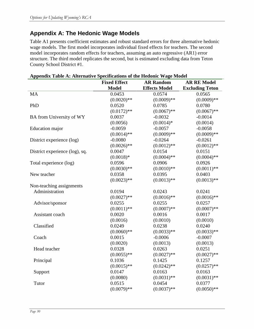
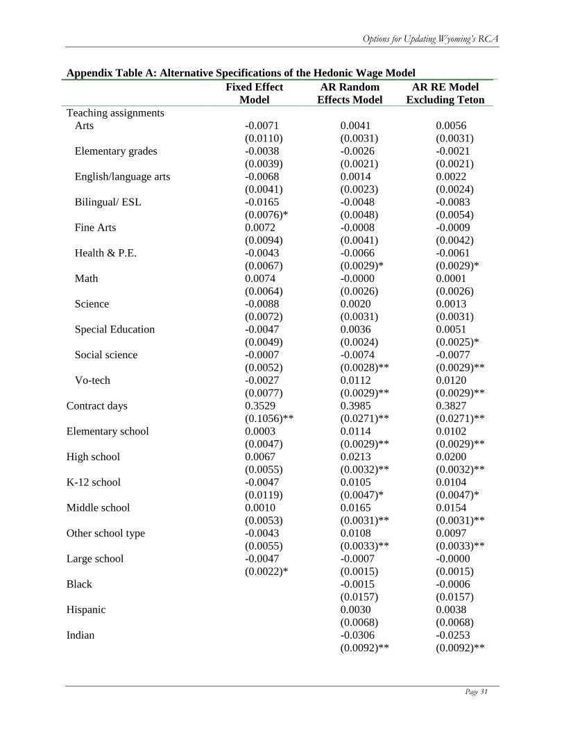
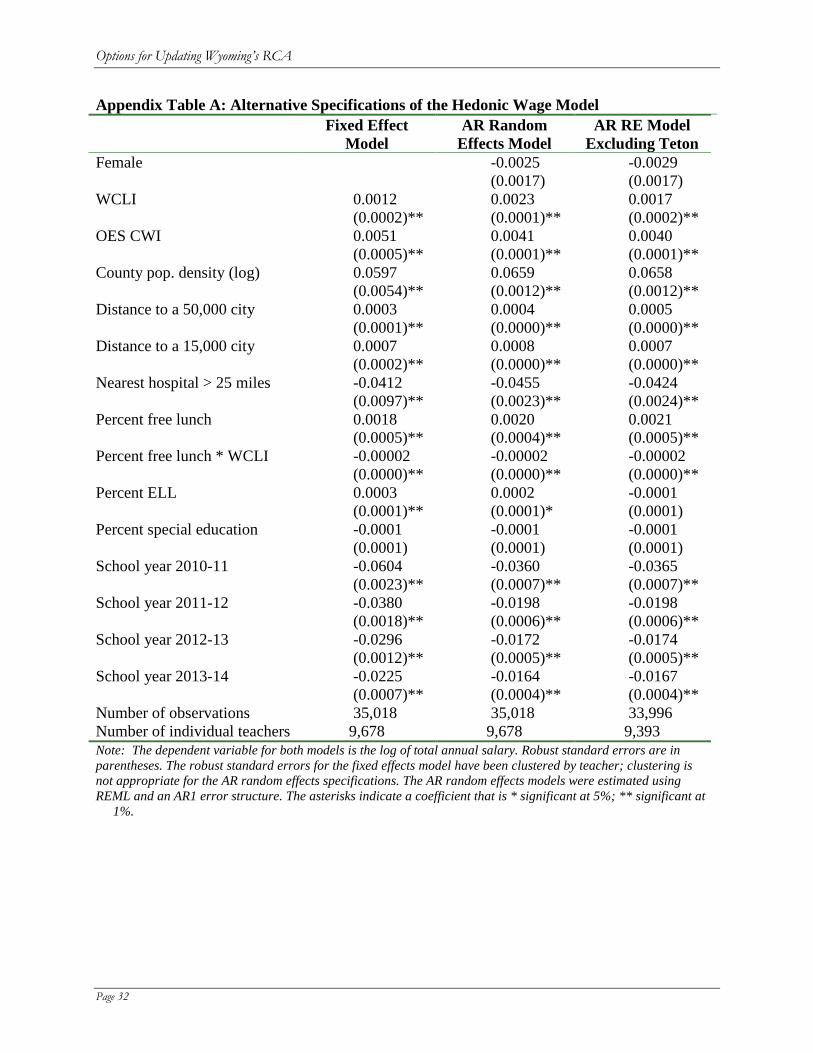
Appendix A: The Hedonic Wage Models Table A1 presents coefficient estimates and robust standard errors for three alternative hedonic wage models. The first model incorporates individual fixed effects for teachers. The second model incorporates random effects for teachers, assuming an auto regressive (AR1) error structure. The third model replicates the second, but is estimated excluding data from Teton County School District #1. Appendix Table A: Alternative Specifications of the Hedonic Wage Model
Fixed Effect Model
AR Random Effects Model
AR RE Model Excluding Teton
MA 0.0453 0.0574 0.0565 (0.0020)** (0.0009)** (0.0009)**
PhD 0.0520 0.0785 0.0780 (0.0172)** (0.0067)** (0.0067)**
BA from University of WY 0.0037 -0.0032 -0.0014 (0.0056) (0.0014)* (0.0014)
Education major -0.0059 -0.0057 -0.0058 (0.0014)** (0.0009)** (0.0009)**
District experience (log) -0.0080 -0.0264 -0.0261 (0.0026)** (0.0012)** (0.0012)**
District experience (log), sq. 0.0047 0.0154 0.0151 (0.0018)* (0.0004)** (0.0004)**
Total experience (log) 0.0596 0.0906 0.0926 (0.0030)** (0.0010)** (0.0011)**
New teacher 0.0358 0.0395 0.0403 (0.0023)** (0.0013)** (0.0013)**
Non-teaching assignments Administration 0.0194 0.0243 0.0241
(0.0027)** (0.0016)** (0.0016)** Advisor/sponsor 0.0255 0.0255 0.0257
(0.0011)** (0.0007)** (0.0007)** Assistant coach 0.0020 0.0016 0.0017
(0.0016) (0.0010) (0.0010) Classified 0.0249 0.0238 0.0240
(0.0060)** (0.0033)** (0.0033)** Coach 0.0015 -0.0006 -0.0007
(0.0020) (0.0013) (0.0013) Head teacher 0.0328 0.0263 0.0251
(0.0055)** (0.0027)** (0.0027)** Principal 0.1036 0.1425 0.1257
(0.0015)** (0.0242)** (0.0257)** Support 0.0147 0.0163 0.0163
(0.0080) (0.0031)** (0.0031)** Tutor 0.0515 0.0454 0.0377
(0.0079)** (0.0037)** (0.0050)**
Options for Updating Wyoming’s RCA
Page 31
Appendix Table A: Alternative Specifications of the Hedonic Wage Model Fixed Effect
Model AR Random
Effects Model AR RE Model
Excluding Teton Teaching assignments Arts -0.0071 0.0041 0.0056
(0.0110) (0.0031) (0.0031) Elementary grades -0.0038 -0.0026 -0.0021
(0.0039) (0.0021) (0.0021) English/language arts -0.0068 0.0014 0.0022
(0.0041) (0.0023) (0.0024) Bilingual/ ESL -0.0165 -0.0048 -0.0083
(0.0076)* (0.0048) (0.0054) Fine Arts 0.0072 -0.0008 -0.0009
(0.0094) (0.0041) (0.0042) Health & P.E. -0.0043 -0.0066 -0.0061
(0.0067) (0.0029)* (0.0029)* Math 0.0074 -0.0000 0.0001
(0.0064) (0.0026) (0.0026) Science -0.0088 0.0020 0.0013
(0.0072) (0.0031) (0.0031) Special Education -0.0047 0.0036 0.0051
(0.0049) (0.0024) (0.0025)* Social science -0.0007 -0.0074 -0.0077
(0.0052) (0.0028)** (0.0029)** Vo-tech -0.0027 0.0112 0.0120
(0.0077) (0.0029)** (0.0029)** Contract days 0.3529 0.3985 0.3827
(0.1056)** (0.0271)** (0.0271)** Elementary school 0.0003 0.0114 0.0102
(0.0047) (0.0029)** (0.0029)** High school 0.0067 0.0213 0.0200
(0.0055) (0.0032)** (0.0032)** K-12 school -0.0047 0.0105 0.0104
(0.0119) (0.0047)* (0.0047)* Middle school 0.0010 0.0165 0.0154
(0.0053) (0.0031)** (0.0031)** Other school type -0.0043 0.0108 0.0097
(0.0055) (0.0033)** (0.0033)** Large school -0.0047 -0.0007 -0.0000
(0.0022)* (0.0015) (0.0015) Black -0.0015 -0.0006
(0.0157) (0.0157) Hispanic 0.0030 0.0038
(0.0068) (0.0068) Indian -0.0306 -0.0253
(0.0092)** (0.0092)**
Options for Updating Wyoming’s RCA
Page 32
Appendix Table A: Alternative Specifications of the Hedonic Wage Model Fixed Effect
Model AR Random
Effects Model AR RE Model
Excluding Teton Female -0.0025 -0.0029
(0.0017) (0.0017) WCLI 0.0012 0.0023 0.0017
(0.0002)** (0.0001)** (0.0002)** OES CWI 0.0051 0.0041 0.0040 (0.0005)** (0.0001)** (0.0001)** County pop. density (log) 0.0597 0.0659 0.0658
(0.0054)** (0.0012)** (0.0012)** Distance to a 50,000 city 0.0003 0.0004 0.0005
(0.0001)** (0.0000)** (0.0000)** Distance to a 15,000 city 0.0007 0.0008 0.0007
(0.0002)** (0.0000)** (0.0000)** Nearest hospital > 25 miles -0.0412 -0.0455 -0.0424
(0.0097)** (0.0023)** (0.0024)** Percent free lunch 0.0018 0.0020 0.0021
(0.0005)** (0.0004)** (0.0005)** Percent free lunch * WCLI -0.00002 -0.00002 -0.00002
(0.0000)** (0.0000)** (0.0000)** Percent ELL 0.0003 0.0002 -0.0001
(0.0001)** (0.0001)* (0.0001) Percent special education -0.0001 -0.0001 -0.0001
(0.0001) (0.0001) (0.0001) School year 2010-11 -0.0604 -0.0360 -0.0365
(0.0023)** (0.0007)** (0.0007)** School year 2011-12 -0.0380 -0.0198 -0.0198
(0.0018)** (0.0006)** (0.0006)** School year 2012-13 -0.0296 -0.0172 -0.0174
(0.0012)** (0.0005)** (0.0005)** School year 2013-14 -0.0225 -0.0164 -0.0167
(0.0007)** (0.0004)** (0.0004)** Number of observations 35,018 35,018 33,996 Number of individual teachers 9,678 9,678 9,393 Note: The dependent variable for both models is the log of total annual salary. Robust standard errors are in parentheses. The robust standard errors for the fixed effects model have been clustered by teacher; clustering is not appropriate for the AR random effects specifications. The AR random effects models were estimated using REML and an AR1 error structure. The asterisks indicate a coefficient that is * significant at 5%; ** significant at
1%.
Options for Updating Wyoming’s RCA
Page 33
Appendix B: An ACS-CWI for Regional Cost Adjustment in Wyoming The basic premise of a CWI is that all types of workers demand higher wages in areas with a higher cost of living or a lack of amenities. One should be able to measure the effect on teacher wages of differences in amenities and the cost of living by observing systematic variations in the earnings of comparable workers who are not educators. Intuitively, if Laramie construction workers are paid 5 percent less than the national average construction wage, Laramie engineers are paid 5 percent less than the national average engineering wage, Laramie nurses are paid 5 percent less than the national average nursing wage, and so on, then the best estimate of the cost of hiring teachers in Laramie is also 5 percent less than the national average.
The NCES CWI measures the prevailing wage for college graduates in 800 U.S. labor markets. The baseline estimates (for 1999) come from a regression analysis of the individual earnings data from the 2000 U.S. Census. Annual updates to that baseline come from regression analyses of occupational earnings data provided by the U.S. Bureau of Labor Statistics (BLS).
This analysis updates the NCES CWI using the American Community Survey (ACS). The ACS, which is conducted annually by the U.S. Census Bureau, has replaced the decennial census as the primary source of demographic information about the U.S. population. It provides information about the earnings, age, occupation, industry, and other demographic characteristics for millions of U.S. workers. The ACS-CWI measures earnings differences for college graduates.
Like the NCES CWI, the ACS-CWI is derived from a regression analysis of individual earnings data. Workers with incomplete data and workers without a college degree were excluded from the ACS regression analysis, as was anyone who had a teaching or educational administration occupation or who was employed in the elementary and secondary education industry. Self-employed workers were excluded because their reported earnings may not represent the market value of their time. Individuals who reported working less than half time or for more than 90 hours a week were also excluded, as were workers under the age of 18 and over the age of 80. Finally, individuals employed outside the United States were excluded because their earnings may represent compensation for foreign travel or other working conditions not faced by domestic workers.
The ACS-CWI is estimated from nationwide data because the national sample is much larger and yields much more precise estimates of wages by industry and occupation than could be generated using only the ACS data for the state of Wyoming. For similar reasons, the analysis combines data from the two most recent ACS reports (2012 and 2013). Data from before 2012 could not be incorporated into the analysis because the Census Bureau has changed the way it defines geographic areas, making the publically available data for 2012 a poor match for the publically available data from earlier years.
As with the NCES CWI, the labor markets in the ACS CWI are based on “place-of-work areas” as defined by the Census Bureau for the 2012 ACS. Place-of-work areas are geographic regions
Options for Updating Wyoming’s RCA
Page 34
designed to contain at least 100,000 persons. The place-of-work areas do not cross state boundaries and generally follow the boundaries of county groups, single counties, or census-defined places (Ruggles et al. 2015). Counties in sparsely-populated parts of a state are clustered together into a single place-of-work area. Each labor market in the ACS CWI is either a single place of work, or a cluster of the places-of-work that comprise a metropolitan area. There are five ACS place of work areas in Wyoming.
Table B.1 presents the results from the regression analysis underpinning the ACS-CWI. The dependent variable in each case is the log of annual wage and salary earnings. Key independent variables include the age, gender, race, educational attainment, language ability and amount of time worked for each individual in the nationwide sample. The model includes the interaction between gender and age, to allow for the possibility that men and women have different career paths, and therefore different age-earnings profiles. In addition, the estimation includes indicator variables for occupation and industry for each year. This specification allows wages to rise (or fall) more slowly in some occupations or industries than it does in others. Finally, the regression model includes indicator variables for each labor market area and random effects for states.22
As the table illustrates, the estimated model is consistent with reasonable expectations about labor markets. Wage and salary earnings increase with the amount of time worked per week and the number of weeks worked per year. Earnings also rise as workers get older, but the increase is more rapid for men than for women (perhaps because age is not as good an indicator of experience for women as it is for men). Workers with advanced degrees earn systematically more than workers with a bachelor’s degree. Whites earn systematically more than apparently comparable individuals from other racial groups. College-educated workers who do not speak English well earn substantially less than other workers, all other things being equal.
The predicted wage level in each labor market area captures systematic variations in labor earnings while controlling for demographics, industrial and occupational mix, and amount of time worked.23 Dividing each local wage prediction by the state average prediction for Wyoming yields the ACS-CWI for each of the five Wyoming place of work areas, and therefore for the corresponding Wyoming school districts. Appendix C presents the ACS-CWI for each Wyoming school district.
22 Treating state effects as random rather than fixed ensures that the predicted wage is the same in Kansas City, Kansas as it is in Kansas City, Missouri, while allowing for a correlation in the errors among labor markets within any given state. 23 Formally, the predicted wage level in each market is the least-squares mean for the market fixed effect. The least-squares mean (or population marginal mean) is defined as the expected value of the mean for each effect (in this context, each market) that you would expect from a balanced design holding all covariates at their mean values and all classification variables (such as occupation or gender) at their population frequencies.
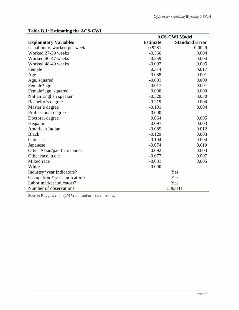
Options for Updating Wyoming’s RCA
Page 35
Table B.1: Estimating the ACS-CWI
Explanatory Variables ACS-CWI Model
Estimate Standard Error Usual hours worked per week 0.9281 0.0029 Worked 27-39 weeks -0.566 0.004 Worked 40-47 weeks -0.259 0.004 Worked 48-49 weeks -0.097 0.005 Female 0.314 0.017 Age 0.088 0.001 Age, squared -0.001 0.000 Female*age -0.017 0.001 Female*age, squared 0.000 0.000 Not an English speaker -0.520 0.030 Bachelor’s degree -0.219 0.004 Master’s degree -0.101 0.004 Professional degree 0.000 Doctoral degree 0.064 0.005 Hispanic -0.097 0.003 American Indian -0.085 0.012 Black -0.129 0.003 Chinese -0.104 0.004 Japanese -0.074 0.010 Other Asian/pacific islander -0.092 0.003 Other race, n.e.c. -0.077 0.007 Mixed race -0.081 0.005 White 0.000 Industry*year indicators? Yes Occupation * year indicators? Yes Labor market indicators? Yes Number of observations 536,841 Source: Ruggles et al. (2015) and author’s calculations.
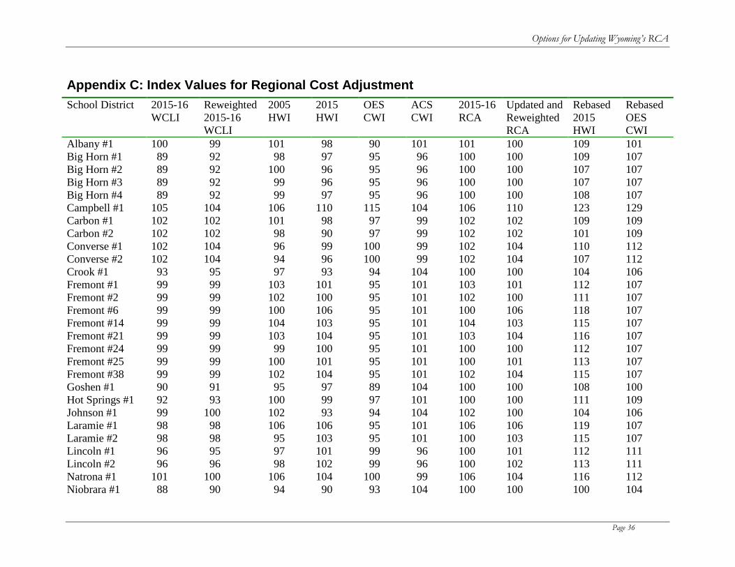
Options for Updating Wyoming’s RCA
Page 36
Appendix C: Index Values for Regional Cost Adjustment School District 2015-16
WCLI Reweighted 2015-16 WCLI
2005 HWI
2015 HWI
OES CWI
ACS CWI
2015-16 RCA
Updated and Reweighted RCA
Rebased 2015 HWI
Rebased OES CWI
Albany #1 100 99 101 98 90 101 101 100 109 101 Big Horn #1 89 92 98 97 95 96 100 100 109 107 Big Horn #2 89 92 100 96 95 96 100 100 107 107 Big Horn #3 89 92 99 96 95 96 100 100 107 107 Big Horn #4 89 92 99 97 95 96 100 100 108 107 Campbell #1 105 104 106 110 115 104 106 110 123 129 Carbon #1 102 102 101 98 97 99 102 102 109 109 Carbon #2 102 102 98 90 97 99 102 102 101 109 Converse #1 102 104 96 99 100 99 102 104 110 112 Converse #2 102 104 94 96 100 99 102 104 107 112 Crook #1 93 95 97 93 94 104 100 100 104 106 Fremont #1 99 99 103 101 95 101 103 101 112 107 Fremont #2 99 99 102 100 95 101 102 100 111 107 Fremont #6 99 99 100 106 95 101 100 106 118 107 Fremont #14 99 99 104 103 95 101 104 103 115 107 Fremont #21 99 99 103 104 95 101 103 104 116 107 Fremont #24 99 99 99 100 95 101 100 100 112 107 Fremont #25 99 99 100 101 95 101 100 101 113 107 Fremont #38 99 99 102 104 95 101 102 104 115 107 Goshen #1 90 91 95 97 89 104 100 100 108 100 Hot Springs #1 92 93 100 99 97 101 100 100 111 109 Johnson #1 99 100 102 93 94 104 102 100 104 106 Laramie #1 98 98 106 106 95 101 106 106 119 107 Laramie #2 98 98 95 103 95 101 100 103 115 107 Lincoln #1 96 95 97 101 99 96 100 101 112 111 Lincoln #2 96 96 98 102 99 96 100 102 113 111 Natrona #1 101 100 106 104 100 99 106 104 116 112 Niobrara #1 88 90 94 90 93 104 100 100 100 104
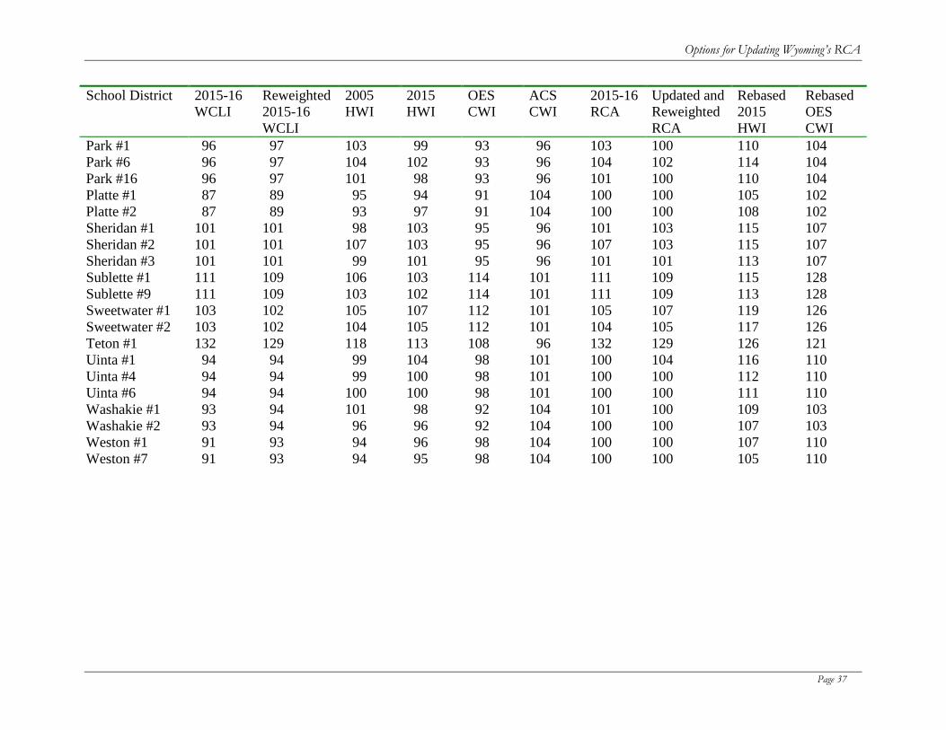
Options for Updating Wyoming’s RCA
Page 37
School District 2015-16 WCLI
Reweighted 2015-16 WCLI
2005 HWI
2015 HWI
OES CWI
ACS CWI
2015-16 RCA
Updated and Reweighted RCA
Rebased 2015 HWI
Rebased OES CWI
Park #1 96 97 103 99 93 96 103 100 110 104 Park #6 96 97 104 102 93 96 104 102 114 104 Park #16 96 97 101 98 93 96 101 100 110 104 Platte #1 87 89 95 94 91 104 100 100 105 102 Platte #2 87 89 93 97 91 104 100 100 108 102 Sheridan #1 101 101 98 103 95 96 101 103 115 107 Sheridan #2 101 101 107 103 95 96 107 103 115 107 Sheridan #3 101 101 99 101 95 96 101 101 113 107 Sublette #1 111 109 106 103 114 101 111 109 115 128 Sublette #9 111 109 103 102 114 101 111 109 113 128 Sweetwater #1 103 102 105 107 112 101 105 107 119 126 Sweetwater #2 103 102 104 105 112 101 104 105 117 126 Teton #1 132 129 118 113 108 96 132 129 126 121 Uinta #1 94 94 99 104 98 101 100 104 116 110 Uinta #4 94 94 99 100 98 101 100 100 112 110 Uinta #6 94 94 100 100 98 101 100 100 111 110 Washakie #1 93 94 101 98 92 104 101 100 109 103 Washakie #2 93 94 96 96 92 104 100 100 107 103 Weston #1 91 93 94 96 98 104 100 100 107 110 Weston #7 91 93 94 95 98 104 100 100 105 110