optistruct 13.0 user guide
DESCRIPTION
User Guide to the optimization code OptistructTRANSCRIPT

HyperWorks is a division of Altair altairhyperworks.com

Altair Engineering Support Contact Information Web site www.altairhyperworks.com
Location Telephone e-mail
Australia 64.9.413.7981 [email protected]
Brazil 55.11.3884.0414 [email protected]
Canada 416.447.6463 [email protected]
China 86.400.619.6186 [email protected]
France 33.1.4133.0992 [email protected]
Germany 49.7031.6208.22 [email protected]
India 91.80. 6629.4500 1.800.425.0234 (toll free)
Italy 39.800.905.595 [email protected]
Japan 81.3.5396.2881 [email protected]
Korea 82.70.4050.9200 [email protected]
Mexico 55.56.58.68.08 [email protected]
New Zealand 64.9.413.7981 [email protected]
North America 248.614.2425 [email protected]
Scandinavia 46.46.460.2828 [email protected]
United Kingdom 01926.468.600 [email protected]
In addition, the following countries have resellers for Altair Engineering: Colombia, Czech Republic, Ecuador, Israel, Russia, Netherlands, Turkey, Poland, Singapore, Vietnam, Indonesia
Official offices with resellers: Canada, China, France, Germany, India, Malaysia, Italy, Japan, Korea, Spain, Taiwan, United Kingdom, USA
Copyright© Altair Engineering Inc. All Rights Reserved for: HyperMesh® 1990-2014; HyperCrash® 2001-2014; OptiStruct® 1996-2014; RADIOSS®1986-2014; HyperView®1999-2014; HyperView Player® 2001-2014; HyperStudy® 1999-2014; HyperGraph®1995-2014; MotionView® 1993-2014; MotionSolve® 2002-2014; HyperForm® 1998-2014; HyperXtrude® 1999-2014; Process Manager™ 2003-2014; Templex™ 1990-2014; TextView™ 1996-2014; MediaView™ 1999-2014; TableView™ 2013-2014; BatchMesher™ 2003-2014; HyperMath® 2007-2014; Manufacturing Solutions™ 2005-2014; HyperWeld® 2009-2014; HyperMold® 2009-2014; solidThinking® 1993-2014; solidThinking Inspire® 2009-2014; solidThinking Evolve®™ 1993-2014; Durability Director™ 2009-2014; Suspension Director™ 2009-2014; AcuSolve® 1997-2014; AcuConsole® 2006-2014; SimLab®™2004-2014 and Virtual Wind Tunnel™ 2012-2014.
In addition to HyperWorks® trademarks noted above, Display Manager™, Simulation Manager™, Compute Manager™, PBS™, PBSWorks™, PBS GridWorks®, PBS Professional®, PBS Analytics™, PBS Desktop™, PBS Portal™, PBS Application Services™, e-BioChem™, e-Compute™ and e-Render™ are trademarks of ALTAIR ENGINEERING INC.
Altair trademarks are protected under U.S. and international laws and treaties. Copyright© 1994-2014. Additionally, Altair software is protected under patent #6,859,792 and other patents pending. All other marks are the property of their respective owners. ALTAIR ENGINEERING INC. Proprietary and Confidential. Contains Trade Secret Information. Not for use or disclosure outside of ALTAIR and its licensed clients. Information contained inHyperWorks® shall not be decompiled, disassembled, or “unlocked”, reverse translated, reverse engineered, or publicly displayed or publicly performed in any manner. Usage of the software is only as explicitly permitted in the end user software license agreement. Copyright notice does not imply publication
OptiStruct 13.0 User's Guidei Altair Engineering
Proprietary Information of Altair Engineering
OptiStruct 13.0 User's Guide
........................................................................................................................................... 1User's Guide
............................................................................................................................................... 2Overview
................................................................................................................................... 5Features
................................................................................................................................... 12Capabilities
................................................................................................................................... 13Formats
................................................................................................................................... 14Enhancing the Design Process
................................................................................................................................... 17Pre-processing and Post-processing in HyperWorks
............................................................................................................................................... 21Running OptiStruct
................................................................................................................................... 25Run Options for OptiStruct
................................................................................................................................... 39OptiStruct GPU
................................................................................................................................... 41OptiStruct SPMD
................................................................................................................................... 60Platforms and Hardware Recommendations
................................................................................................................................... 62OptiStruct Configuration File
................................................................................................................................... 67Expanded Error Message File
................................................................................................................................... 69Memory Limitations
................................................................................................................................... 71Restarting OptiStruct
................................................................................................................................... 72OptiStruct Compression Run
............................................................................................................................................... 74Structural Analysis
................................................................................................................................... 75Linear Static Analysis
................................................................................................................................... 76Linear Buckling Analysis
................................................................................................................................... 78Nonlinear Analysis
................................................................................................................................... 103Normal Modes Analysis
................................................................................................................................... 107Frequency Response Analysis
................................................................................................................................... 113Complex Eigenvalue Analysis
................................................................................................................................... 115Random Response Analysis
................................................................................................................................... 119Response Spectrum Analysis
................................................................................................................................... 123Transient Response Analysis
............................................................................................................................................... 129Thermal Analysis
................................................................................................................................... 130Linear Steady-State Heat Transfer Analysis
................................................................................................................................... 133Linear Transient Heat Transfer Analysis
................................................................................................................................... 135Nonlinear Steady-State Heat Transfer Analysis
................................................................................................................................... 137Contact-based Thermal Analysis
............................................................................................................................................... 140Acoustic Analysis
................................................................................................................................... 141Coupled Frequency Response Analysis of Fluid-Structure Models
................................................................................................................................... 258Radiated Sound Analysis
............................................................................................................................................... 266Fatigue Analysis
............................................................................................................................................... 282Multi-body Dynamics Simulation
OptiStruct 13.0 User's Guide iiAltair Engineering
Proprietary Information of Altair Engineering
................................................................................................................................... 284Transient Analysis for MBD
................................................................................................................................... 286Static Analysis for MBD
................................................................................................................................... 287Quasi-static Analysis for MBD
................................................................................................................................... 288Linear Analysis for MBD
................................................................................................................................... 289Bodies
................................................................................................................................... 290Markers
................................................................................................................................... 291Constraints
................................................................................................................................... 293Contact
................................................................................................................................... 295Compliant Elements
................................................................................................................................... 296Applied Forces and Motions
................................................................................................................................... 297Initial Velocity
................................................................................................................................... 298Function Expressions
................................................................................................................................... 299Results of a Multi-body Dynamics Analysis
............................................................................................................................................... 300Rotor Dynamics
............................................................................................................................................... 309NVH Applications and Techniques
................................................................................................................................... 310Transfer Path Analysis on an Automobile
................................................................................................................................... 316Residual Runs using Super Elements
................................................................................................................................... 319Basic OptiStruct NVH Output Files
................................................................................................................................... 322Global Search Option
................................................................................................................................... 325Create Door and Deck Lid Seals
................................................................................................................................... 328Create a HyperGraph Template for Reading in Multiple Files
................................................................................................................................... 329Using AMSES (Automatic Multi-Level Sub-Structuring Eigensolver Solution)
............................................................................................................................................... 331Modeling Techniques
................................................................................................................................... 332Parts and Instances
................................................................................................................................... 341Subcase Specific Modeling
................................................................................................................................... 345Direct Matrix Input (Superelements)
................................................................................................................................... 364Flexible Body Generation
................................................................................................................................... 369Poroelastic Materials (Biot theory)
................................................................................................................................... 371Elements and Materials
................................................................................................................................... 385Loads and Boundary Conditions
................................................................................................................................... 404Modeling Errors
............................................................................................................................................... 407Results
............................................................................................................................................... 417Coupling OptiStruct with Third Party Software
............................................................................................................................................... 425Design Optimization
................................................................................................................................... 426Optimization Problem
................................................................................................................................... 429Responses
................................................................................................................................... 446Topology Optimization
................................................................................................................................... 460Free-size Optimization
................................................................................................................................... 467Topography Optimization
................................................................................................................................... 471Size Optimization
................................................................................................................................... 473Shape Optimization
OptiStruct 13.0 User's Guideiii Altair Engineering
Proprietary Information of Altair Engineering
................................................................................................................................... 475Free-shape Optimization
................................................................................................................................... 493Manufacturing Constraints
................................................................................................................................... 558Reliability-based Design Optimization (Beta)
................................................................................................................................... 564Optimization of Arbitrary Beam Sections
................................................................................................................................... 565Optimization of Composite Structures
................................................................................................................................... 573Equivalent Static Load Method (ESLM)
................................................................................................................................... 587Gradient-based Optimization Method
................................................................................................................................... 596Global Search Option
............................................................................................................................................... 598Design Interpretation - OSSmooth
................................................................................................................................... 601OSSmooth Parameter File
................................................................................................................................... 606Running OSSmooth
................................................................................................................................... 607Interpretation of Topology Optimization Results
................................................................................................................................... 608Laplacian Smoothing
................................................................................................................................... 610Interpretation of Topography Optimization Results
................................................................................................................................... 613FEA Topology for Reanalysis
................................................................................................................................... 615FEA Topography for Reanalysis
............................................................................................................................................... 617OptiStruct References

Altair Engineering OptiStruct 13.0 User's Guide 1
Proprietary Information of Altair Engineering
User's Guide
Overview
Running OptiStruct
Structural Analysis
Thermal Analysis
Acoustic Analysis
Fatigue Analysis
Multi-body Dynamics Simulation
Rotor Dynamics
NVH Applications and Techniques
Modeling Techniques
Results
Coupling OptiStruct with Third Party Software
Design Optimization
Design Interpretation - OSSmooth
OptiStruct References
OptiStruct 13.0 User's Guide2 Altair Engineering
Proprietary Information of Altair Engineering
Overview
Altair® OptiStruct® is an industry proven, modern structural analysis solver for linear andnon-linear structural problems under static and dynamic loadings. It is the market-leadingsolution for structural design and optimization. Based on finite element and multi-bodydynamics technology, and through advanced analysis and optimization algorithms, OptiStructhelps designers and engineers rapidly develop innovative, lightweight and structurallyefficient designs. OptiStruct is used by thousands of companies worldwide to analyze andOptimize structures for their strength, durability and NVH (noise, vibration and harshness)characteristics. Refer to the Features page for a list of solutions available in OptiStruct.
Finite element solutions via OptiStruct include:
Linear static analysis
Nonlinear implicit quasi-static analysis
Linear buckling analysis
Normal modes analysis
Complex eigenvalue analysis
Frequency response analysis
Random response analysis
Linear transient response analysis
Geometric non-linear explicit and implicit analysis
Linear fluid-structure coupled (acoustic) analysis
Linear steady-state heat transfer analysis
Coupled thermal-structural analysis
Nonlinear steady-state heat transfer analysis
Linear transient heat transfer analysis
Contact-based thermal analysis
Inertia relief analysis with static, non-linear contact, modal frequency response, andmodal transient response analyses
Component Mode Synthesis (CMS) for the generation of flexible bodies for multi-bodydynamics analysis
Reduced matrix generation
One-step (inverse) sheet metal stamping analysis
Fatigue analysis
A typical set of finite elements including shell, solid, bar, scalar, and rigid elements as well asloads and materials are available for modeling complex events.
Multi-body dynamics solutions integrated via OptiStruct for rigid and flexible bodies include:
Kinematics analysis
Dynamics analysis
Altair Engineering OptiStruct 13.0 User's Guide 3
Proprietary Information of Altair Engineering
Static and quasi-static analysis
Linearization
All typical types of constraints like joints, gears, couplers, user-defined constraints, and high-pair joints can be defined. High pair joints include point-to-curve, point-to-surface, curve-to-curve, curve-to-surface, and surface-to-surface constraints. They can connect rigid bodies,flexible bodies, or rigid and flexible bodies. For this multi-body dynamics solution, the powerof Altair MotionSolve has been integrated with OptiStruct.
Structural Design and Optimization
Structural design tools include topology, topography, and free-size optimization. Sizing,shape and free-shape optimization are available for structural optimization.
In the formulation of design and optimization problems, the following responses can beapplied as the objective or as constraints: compliance, frequency, volume, mass, moment ofinertia, center of gravity, displacement, velocity, acceleration, buckling factor, stress, strain,composite failure, force, synthetic response, and external (user-defined) functions. Static,inertia relief, nonlinear quasi-static (contact), normal modes, buckling, and frequencyresponse solutions can be included in a multi-disciplinary optimization setup.
Topology, topography, size, and shape optimization can be combined in a general problemformulation.
Topology Optimization
Topology optimization generates an optimized material distribution for a set of loads andconstraints within a given design space. The design space can be defined using shell or solidelements, or both. The classical topology optimization set up solving the minimumcompliance problem, as well as the dual formulation with multiple constraints are available. Constraints on von Mises stress and buckling factor are available with limitations. Manufacturing constraints can be imposed using a minimum member size constraint, drawdirection constraints, extrusion constraints, symmetry planes, pattern grouping, and patternrepetition. A conceptual design can be imported in a CAD system using an iso-surfacegenerated with OSSmooth, which is part of the OptiStruct package.
Free-size optimization is available for shell design spaces. The shell thickness or compositeply-thickness of each element is the design variable.
Topography Optimization
Topography optimization generates an optimized distribution of shape based reinforcementssuch as stamped beads in shell structures. The problem set up is simply done by definingthe design region, the maximum bead depth and the draw angle. OptiStruct automaticallyprovides the design variable creation and optimization control. Manufacturing constraintscan be imposed using symmetry planes, pattern grouping, and pattern repetition.
Size and Shape Optimization
General size and shape optimization problems can be solved. Variables can be assigned toperturbation vectors, which control the shape of the model. Variables can also be assigned to
OptiStruct 13.0 User's Guide4 Altair Engineering
Proprietary Information of Altair Engineering
properties, which control the thickness, area, moments of inertia, stiffness, and non-structural mass of elements in the model. All of the variables supported by OptiStruct can beassigned using HyperMesh. Shape perturbation vectors can be created using HyperMorph.
The reduction of local stress can be accomplished easily using free-shape optimization. Shape perturbations are automatically determined by OptiStruct (based on the stress levelsin the design) when using this technique.
The layout of laminated shells can be improved by modifying the ply thickness and ply angleof these materials.
Multi-body Dynamics Analysis
Different solution sequences for the analysis of mechanical systems are available; theseinclude Kinematics, Dynamics, Static, and Quasi-static solutions.
Flexible bodies can be derived from any finite element model defined in OptiStruct.
Altair Engineering OptiStruct 13.0 User's Guide 5
Proprietary Information of Altair Engineering
Features
Finite Element Analysis using OptiStruct
Structural Analysis
- Linear Static Analysis
- Linear Buckling Analysis
- Nonlinear Quasi-Static Analysis
- Large Displacement Nonlinear Static Analysis
- Geometric Nonlinear Analysis (RADIOSS Integration)
- Normal Modes Analysis
- Frequency Response Analysis
- Complex Eigenvalue Analysis
- Random Response Analysis
- Response Spectrum Analysis
- Transient Response Analysis
Thermal Analysis
- Linear Steady-State Heat Transfer Analysis
- Linear Transient Heat Transfer Analysis
- Nonlinear Steady-State Heat Transfer Analysis
- Contact-based Thermal Analysis
Acoustic Analysis
- Coupled Frequency Response Analysis of Fluid-Structure Models
- Radiated Sound Analysis
Fatigue Analysis
- Stress-Life method
- Strain-Life method
Rotor Dynamics
Fast equation solver
- Sparse matrix solver
- Iterative PCG solver
- Lanczos eigensolver
- SMP parallelization
- SPMD parallelization
- DMIG input
- AMLS Interface
- FastFRS Interface
OptiStruct 13.0 User's Guide6 Altair Engineering
Proprietary Information of Altair Engineering
Advanced element formulations
- Triangular, quadrilateral, first and second order shells
- Laminated shells
- Hexahedron, pyramid, tetrahedron first and second order solids
- Bar, beam, bushing, and rod elements
- Spring, mass, and damping scalar elements
- Mesh independent gap and weld elements
- Rigid elements
- Concentrated and non-structural mass
- Direct matrix input
Geometric element quality check
Local coordinate systems
Multi-point constraints
Contact, tie interfaces
Prestressed analysis
Linear-elastic materials
- Isotropic
- Anisotropic
- Orthotropic
Nonlinear materials
- Elastoplastic
- Hyperelastic
- Viscoelastic
Material consistency checks
Ground check for unintentionally constrained rigid body modes.
Modeling Techniques
Parts and Instances
Subcase Specific Modeling
Direct Matrix Input (Superelements)
- Direct Matrix Input
- Creating Superelements
- Component Dynamic Analysis
Flexible Body Generation
Poroelastic Materials
Altair Engineering OptiStruct 13.0 User's Guide 7
Proprietary Information of Altair Engineering
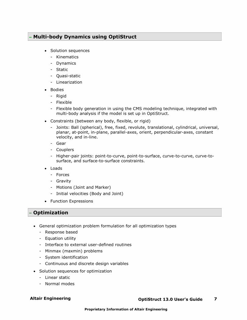
Multi-body Dynamics using OptiStruct
Solution sequences
- Kinematics
- Dynamics
- Static
- Quasi-static
- Linearization
Bodies
- Rigid
- Flexible
- Flexible body generation in using the CMS modeling technique, integrated withmulti-body analysis if the model is set up in OptiStruct.
Constraints (between any body, flexible, or rigid)
- Joints: Ball (spherical), free, fixed, revolute, translational, cylindrical, universal,planar, at-point, in-plane, parallel-axes, orient, perpendicular-axes, constantvelocity, and in-line.
- Gear
- Couplers
- Higher-pair joints: point-to-curve, point-to-surface, curve-to-curve, curve-to-surface, and surface-to-surface constraints.
Loads
- Forces
- Gravity
- Motions (Joint and Marker)
- Initial velocities (Body and Joint)
Function Expressions
Optimization
General optimization problem formulation for all optimization types
- Response based
- Equation utility
- Interface to external user-defined routines
- Minmax (maxmin) problems
- System identification
- Continuous and discrete design variables
Solution sequences for optimization
- Linear static
- Normal modes
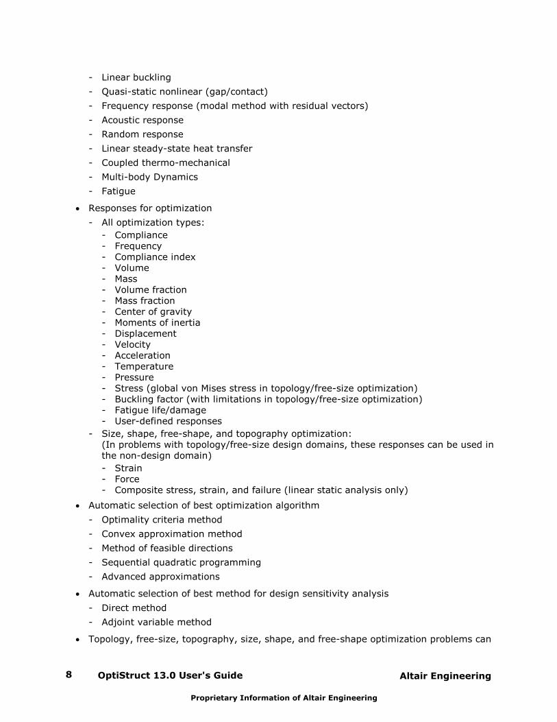
OptiStruct 13.0 User's Guide8 Altair Engineering
Proprietary Information of Altair Engineering
- Linear buckling
- Quasi-static nonlinear (gap/contact)
- Frequency response (modal method with residual vectors)
- Acoustic response
- Random response
- Linear steady-state heat transfer
- Coupled thermo-mechanical
- Multi-body Dynamics
- Fatigue
Responses for optimization
- All optimization types:
- Compliance- Frequency- Compliance index- Volume- Mass- Volume fraction- Mass fraction- Center of gravity- Moments of inertia- Displacement- Velocity- Acceleration- Temperature- Pressure - Stress (global von Mises stress in topology/free-size optimization)- Buckling factor (with limitations in topology/free-size optimization)- Fatigue life/damage- User-defined responses
- Size, shape, free-shape, and topography optimization: (In problems with topology/free-size design domains, these responses can be used inthe non-design domain)
- Strain- Force- Composite stress, strain, and failure (linear static analysis only)
Automatic selection of best optimization algorithm
- Optimality criteria method
- Convex approximation method
- Method of feasible directions
- Sequential quadratic programming
- Advanced approximations
Automatic selection of best method for design sensitivity analysis
- Direct method
- Adjoint variable method
Topology, free-size, topography, size, shape, and free-shape optimization problems can
Altair Engineering OptiStruct 13.0 User's Guide 9
Proprietary Information of Altair Engineering
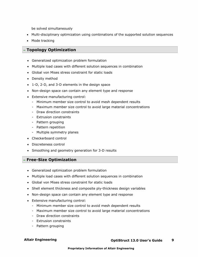
be solved simultaneously
Multi-disciplinary optimization using combinations of the supported solution sequences
Mode tracking
Topology Optimization
Generalized optimization problem formulation
Multiple load cases with different solution sequences in combination
Global von Mises stress constraint for static loads
Density method
1-D, 2-D, and 3-D elements in the design space
Non-design space can contain any element type and response
Extensive manufacturing control:
- Minimum member size control to avoid mesh dependent results
- Maximum member size control to avoid large material concentrations
- Draw direction constraints
- Extrusion constraints
- Pattern grouping
- Pattern repetition
- Multiple symmetry planes
Checkerboard control
Discreteness control
Smoothing and geometry generation for 3-D results
Free-Size Optimization
Generalized optimization problem formulation
Multiple load cases with different solution sequences in combination
Global von Mises stress constraint for static loads
Shell element thickness and composite ply-thickness design variables
Non-design space can contain any element type and response
Extensive manufacturing control:
- Minimum member size control to avoid mesh dependent results
- Maximum member size control to avoid large material concentrations
- Draw direction constraints
- Extrusion constraints
- Pattern grouping
OptiStruct 13.0 User's Guide10 Altair Engineering
Proprietary Information of Altair Engineering
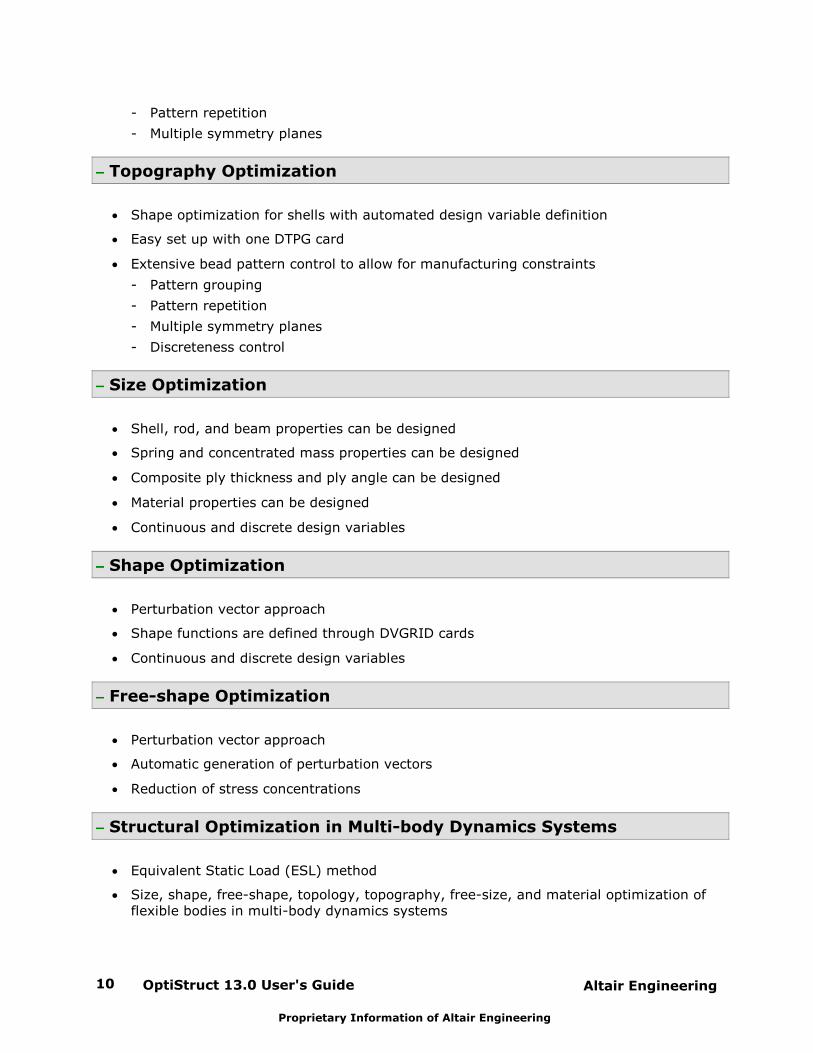
- Pattern repetition
- Multiple symmetry planes
Topography Optimization
Shape optimization for shells with automated design variable definition
Easy set up with one DTPG card
Extensive bead pattern control to allow for manufacturing constraints
- Pattern grouping
- Pattern repetition
- Multiple symmetry planes
- Discreteness control
Size Optimization
Shell, rod, and beam properties can be designed
Spring and concentrated mass properties can be designed
Composite ply thickness and ply angle can be designed
Material properties can be designed
Continuous and discrete design variables
Shape Optimization
Perturbation vector approach
Shape functions are defined through DVGRID cards
Continuous and discrete design variables
Free-shape Optimization
Perturbation vector approach
Automatic generation of perturbation vectors
Reduction of stress concentrations
Structural Optimization in Multi-body Dynamics Systems
Equivalent Static Load (ESL) method
Size, shape, free-shape, topology, topography, free-size, and material optimization offlexible bodies in multi-body dynamics systems

Altair Engineering OptiStruct 13.0 User's Guide 11
Proprietary Information of Altair Engineering
Generalized optimization problem definition
Large number of design variables and constraints
Pre-processing
Fully supported in HyperMesh and MotionView
Nastran type input format
Post-processing
HyperView
- Direct output of H3D format for model and results
- Direct output for iteration history
- Export of iso-density surface in STL format
HyperGraph
- Iteration history graphs
- Sensitivity bar charts
- Complex frequency response displacement, velocity, and acceleration plots for up to500 nodes
- Random response PSD and auto/cross correlation of displacement, velocity, andacceleration
- Transient response displacement, velocity, and acceleration time history plots for upto 500 nodes
- Bar chart for effective mass
HTML report
- Model summary
- Model and result displayed using HyperView Player
HyperMesh
- Direct binary result file output
Microsoft Excel
- Design sensitivities for size and shape variable approximations
Support of Nastran Punch and OP2 output formats
OptiStruct 13.0 User's Guide12 Altair Engineering
Proprietary Information of Altair Engineering
Capabilities
OptiStruct can be used to solve and optimize a wide variety of design problems in which thestructural and system behavior can be simulated using finite element and multi-bodydynamics analysis.
The design and optimization capabilities of OptiStruct allow for the development ofpreliminary design concepts and for the improvement of existing designs based on finiteelement analyses. Some types of optimization problems are listed below:
Two-dimensional truss structure optimization
Ribbed reinforcement patterns for 3-D shell structures
Ribbed reinforcements for solid structures
Spotweld reduction
Lightening holes for existing 2-D planar and 3-D bending shell problems
Discrete optimized structures for problems modeled using 3 dimensional solid elementproblems
Bead (Swages) reinforcements in 3-D shell structures
Shape modifications for volume parts
Gage optimization of 3-D shell structures
Beam cross-section optimization of structures modeled with beam elements
Layout of laminated shell by modifying ply thickness and ply angle
Reduction of stress concentrations
Optimization of mechanisms and mechanical systems to minimize weight and reducestress
Altair Engineering OptiStruct 13.0 User's Guide 13
Proprietary Information of Altair Engineering
Formats
OptiStruct supports the following input/output formats:
Formats
Input Nastran Bulk Data Format
Output HyperMesh Result File (Results)
H3D Binary File (Results)
Patran ASCII (Results)
Nastran Output2 (Results)
Nastran Punch File (Results)
OptiStruct 2.0 (Results)
HyperView Format (Iteration history, sensitivities,effective mass)
Microsoft Excel (Sensitivities)
From Bulk Data Format input:
HyperMesh Result File
Nastran Output2 File
Nastran Punch File
OptiStruct 2.0 File
Patran ASCII File

OptiStruct 13.0 User's Guide14 Altair Engineering
Proprietary Information of Altair Engineering
Enhancing the Design Process
OptiStruct enhances the design process by:
Accelerating the design process
Shortening the number of design cycles
Increasing the design performance
Providing fast and accurate finite element analysis
Generating optimal design concepts using topology and topography optimization
Providing traditional size and shape optimization to maximize the design performance
The design process can be viewed as an optimization process to find structures, mechanicalsystems, and structural parts that fulfill certain expectations towards their economy,functionality, and appearance. Generally, the design process is an iterative procedureconsisting of the following components:
Conceptual design
Design
Testing
Optimization
Today’s testing ground is usually the computer. Finite element analysis (FEA) and Multi-bodydynamics analysis (MBD) are the most used tools for computational design testing. Theresults of computational analyses are used to determine design improvements.
Changes to the design are introduced in all phases of the process. At a certain stage of thisprocess, changes to the concept become prohibitive. The concept phase plays a fundamentalrole concerning overall efficiency of the design and the cost of the overall developmentprocess.
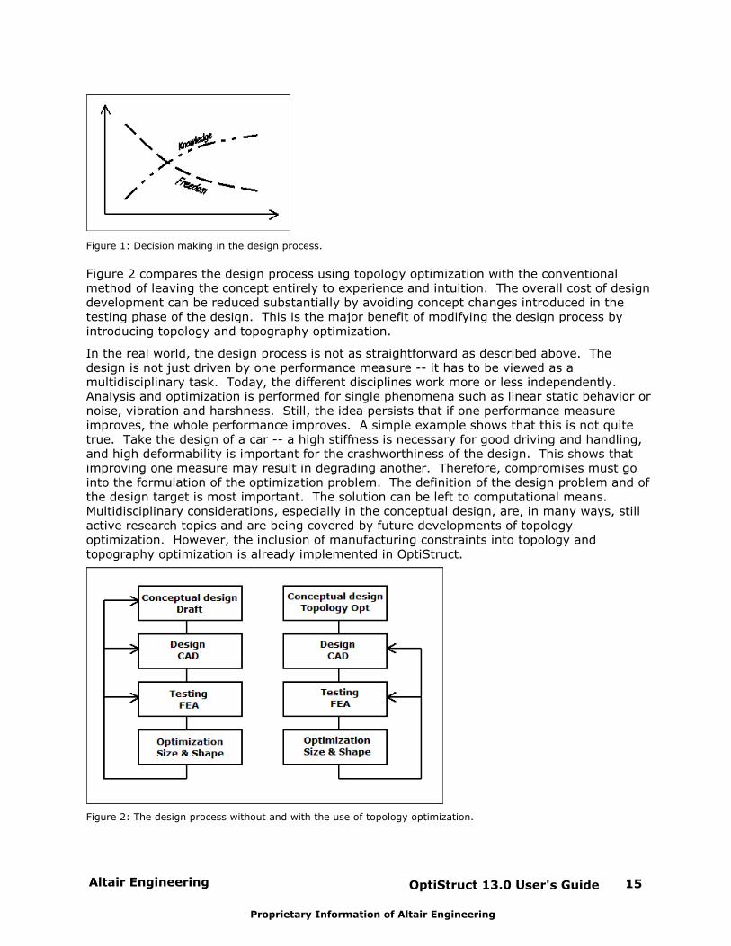
In the concept phase of a design process, the freedom of the designer is limited only by thespecifications of the design (Figure 1). Today, the decision on how a new design should lookis based largely upon a benchmark design or on previous designs. The decision making isbased on the experience of those involved in the design process. Conceptual design toolssuch as topology and topography optimization can be introduced to enhance the process. The concept can be based on results of a computational optimization rather than onestimations. Using topology and topography optimization, the initial design step is alreadybased on input generated using computational analysis. Topology and topographyoptimization redefine the role of computational analysis and simulation in the design process. Finite element analysis has matured from a testing tool to a design tool.
Altair Engineering OptiStruct 13.0 User's Guide 15
Proprietary Information of Altair Engineering
Figure 1: Decision making in the design process.
Figure 2 compares the design process using topology optimization with the conventionalmethod of leaving the concept entirely to experience and intuition. The overall cost of designdevelopment can be reduced substantially by avoiding concept changes introduced in thetesting phase of the design. This is the major benefit of modifying the design process byintroducing topology and topography optimization.
In the real world, the design process is not as straightforward as described above. Thedesign is not just driven by one performance measure -- it has to be viewed as amultidisciplinary task. Today, the different disciplines work more or less independently. Analysis and optimization is performed for single phenomena such as linear static behavior ornoise, vibration and harshness. Still, the idea persists that if one performance measureimproves, the whole performance improves. A simple example shows that this is not quitetrue. Take the design of a car -- a high stiffness is necessary for good driving and handling,and high deformability is important for the crashworthiness of the design. This shows thatimproving one measure may result in degrading another. Therefore, compromises must gointo the formulation of the optimization problem. The definition of the design problem and ofthe design target is most important. The solution can be left to computational means. Multidisciplinary considerations, especially in the conceptual design, are, in many ways, stillactive research topics and are being covered by future developments of topologyoptimization. However, the inclusion of manufacturing constraints into topology andtopography optimization is already implemented in OptiStruct.
Figure 2: The design process without and with the use of topology optimization.

OptiStruct 13.0 User's Guide16 Altair Engineering
Proprietary Information of Altair Engineering
OptiStruct also provides size and shape optimization to completely support the designprocess with finite element based structural optimization. Using the advanced interfacingwith HyperMesh, the generation of input data for structural optimization becomes an easytask. This allows structural optimization to be integrated into the design process seamlessly.
Altair Engineering OptiStruct 13.0 User's Guide 17
Proprietary Information of Altair Engineering
Pre-processing and Post-processing in HyperWorks
Pre-processing
Pre-processing tools must be used to prepare models for OptiStruct, RADIOSS, andMotionSolve. HyperWorks provides specialized pre-processors interfacing with the solvers.
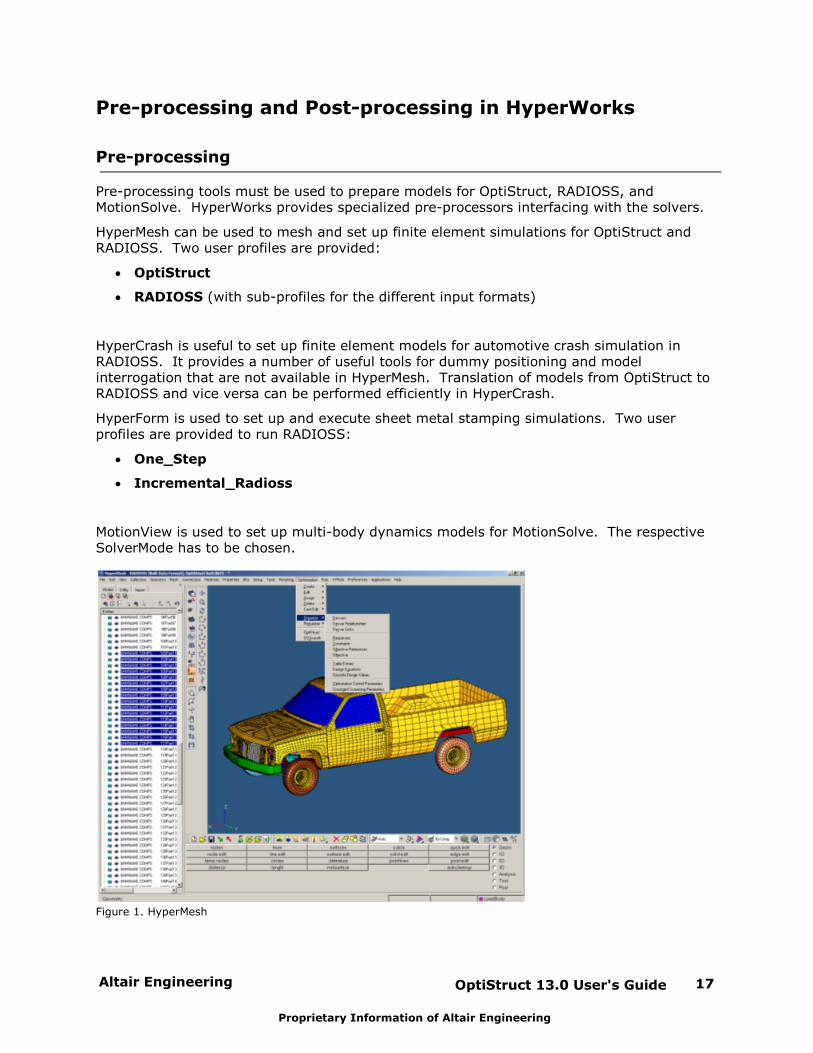
HyperMesh can be used to mesh and set up finite element simulations for OptiStruct andRADIOSS. Two user profiles are provided:
OptiStruct
RADIOSS (with sub-profiles for the different input formats)
HyperCrash is useful to set up finite element models for automotive crash simulation inRADIOSS. It provides a number of useful tools for dummy positioning and modelinterrogation that are not available in HyperMesh. Translation of models from OptiStruct toRADIOSS and vice versa can be performed efficiently in HyperCrash.
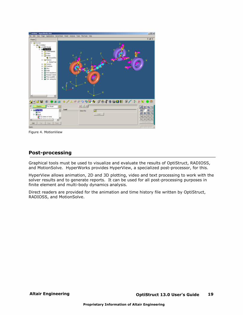
HyperForm is used to set up and execute sheet metal stamping simulations. Two userprofiles are provided to run RADIOSS:
One_Step
Incremental_Radioss
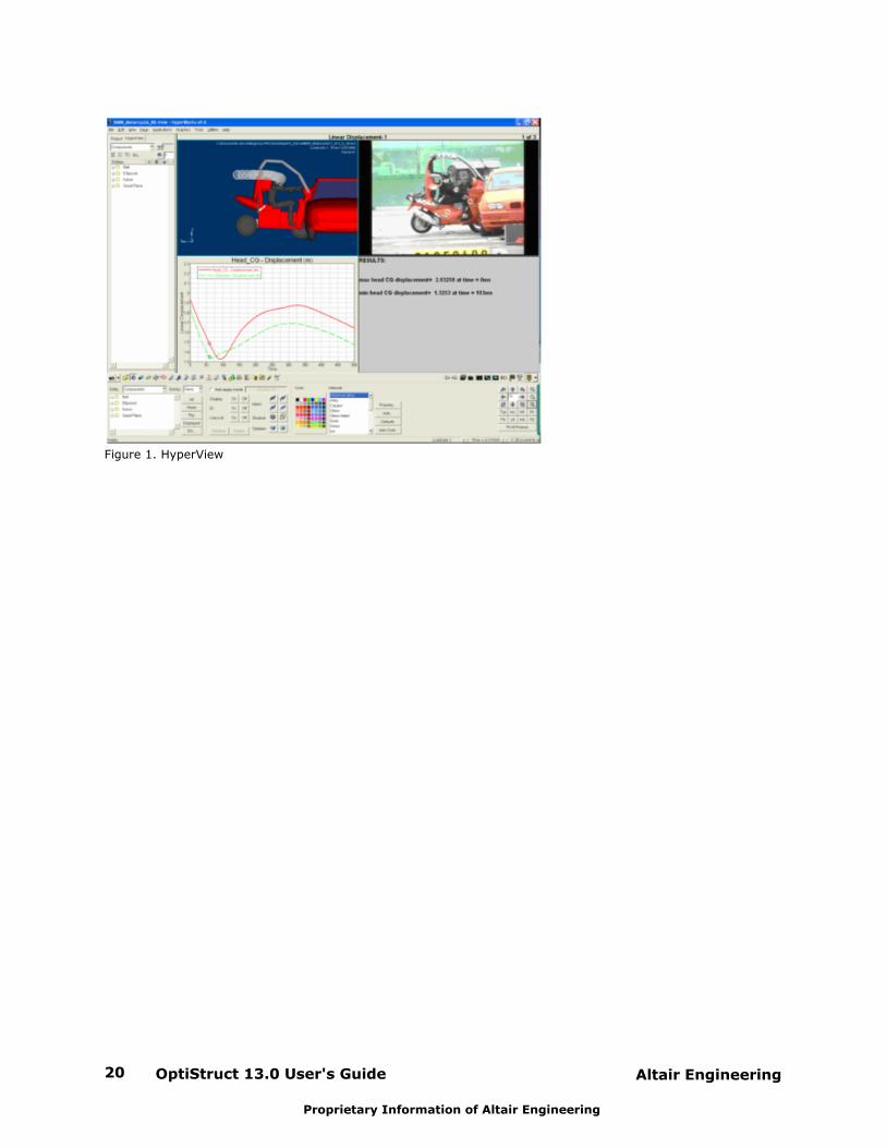
MotionView is used to set up multi-body dynamics models for MotionSolve. The respectiveSolverMode has to be chosen.
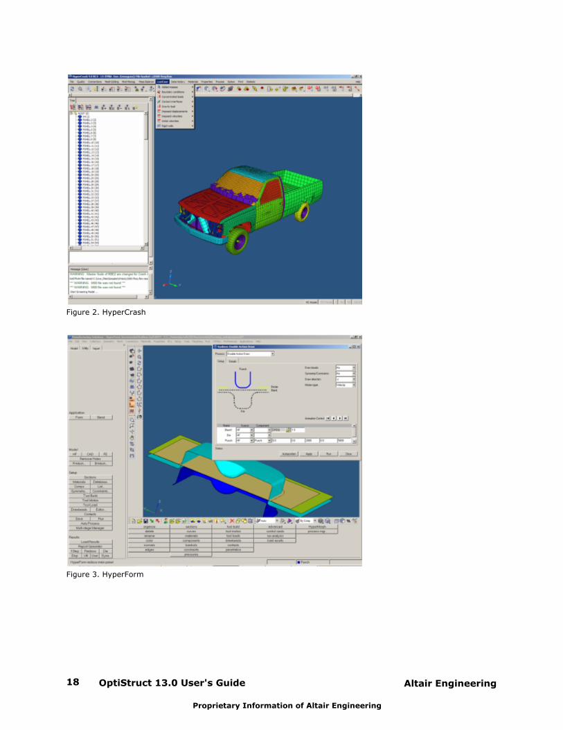
Figure 1. HyperMesh
OptiStruct 13.0 User's Guide18 Altair Engineering
Proprietary Information of Altair Engineering
Figure 2. HyperCrash
Figure 3. HyperForm
Altair Engineering OptiStruct 13.0 User's Guide 19
Proprietary Information of Altair Engineering
Figure 4. MotionView
Post-processing
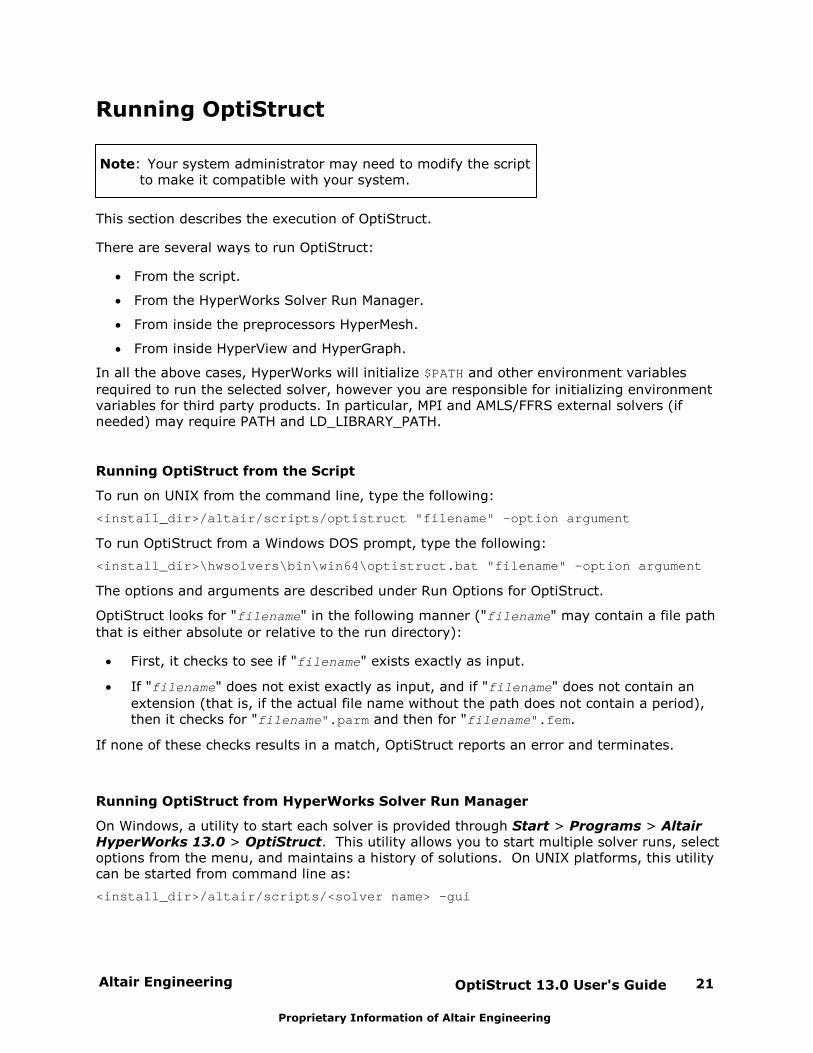
Graphical tools must be used to visualize and evaluate the results of OptiStruct, RADIOSS,and MotionSolve. HyperWorks provides HyperView, a specialized post-processor, for this.
HyperView allows animation, 2D and 3D plotting, video and text processing to work with thesolver results and to generate reports. It can be used for all post-processing purposes infinite element and multi-body dynamics analysis.
Direct readers are provided for the animation and time history file written by OptiStruct,RADIOSS, and MotionSolve.
OptiStruct 13.0 User's Guide20 Altair Engineering
Proprietary Information of Altair Engineering
Figure 1. HyperView
Altair Engineering OptiStruct 13.0 User's Guide 21
Proprietary Information of Altair Engineering
Running OptiStruct
Note: Your system administrator may need to modify the scriptto make it compatible with your system.
This section describes the execution of OptiStruct.
There are several ways to run OptiStruct:
From the script.
From the HyperWorks Solver Run Manager.
From inside the preprocessors HyperMesh.
From inside HyperView and HyperGraph.
In all the above cases, HyperWorks will initialize $PATH and other environment variables
required to run the selected solver, however you are responsible for initializing environmentvariables for third party products. In particular, MPI and AMLS/FFRS external solvers (ifneeded) may require PATH and LD_LIBRARY_PATH.
Running OptiStruct from the Script
To run on UNIX from the command line, type the following:
<install_dir>/altair/scripts/optistruct "filename" –option argument
To run OptiStruct from a Windows DOS prompt, type the following:
<install_dir>\hwsolvers\bin\win64\optistruct.bat "filename" –option argument
The options and arguments are described under Run Options for OptiStruct.
OptiStruct looks for "filename" in the following manner ("filename" may contain a file path
that is either absolute or relative to the run directory):
First, it checks to see if "filename" exists exactly as input.
If "filename" does not exist exactly as input, and if "filename" does not contain an
extension (that is, if the actual file name without the path does not contain a period),then it checks for "filename".parm and then for "filename".fem.
If none of these checks results in a match, OptiStruct reports an error and terminates.
Running OptiStruct from HyperWorks Solver Run Manager
On Windows, a utility to start each solver is provided through Start > Programs > AltairHyperWorks 13.0 > OptiStruct. This utility allows you to start multiple solver runs, selectoptions from the menu, and maintains a history of solutions. On UNIX platforms, this utilitycan be started from command line as:
<install_dir>/altair/scripts/<solver name> -gui
OptiStruct 13.0 User's Guide22 Altair Engineering
Proprietary Information of Altair Engineering
Running OptiStruct from HyperMesh
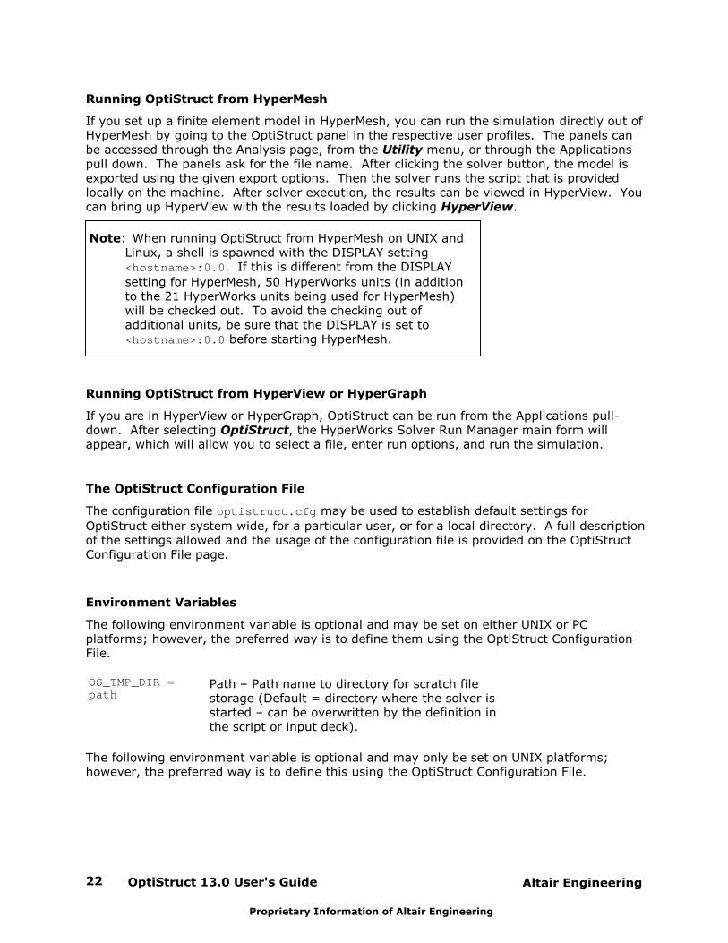
If you set up a finite element model in HyperMesh, you can run the simulation directly out ofHyperMesh by going to the OptiStruct panel in the respective user profiles. The panels canbe accessed through the Analysis page, from the Utility menu, or through the Applicationspull down. The panels ask for the file name. After clicking the solver button, the model isexported using the given export options. Then the solver runs the script that is providedlocally on the machine. After solver execution, the results can be viewed in HyperView. Youcan bring up HyperView with the results loaded by clicking HyperView.
Note: When running OptiStruct from HyperMesh on UNIX andLinux, a shell is spawned with the DISPLAY setting <hostname>:0.0. If this is different from the DISPLAY
setting for HyperMesh, 50 HyperWorks units (in additionto the 21 HyperWorks units being used for HyperMesh)will be checked out. To avoid the checking out ofadditional units, be sure that the DISPLAY is set to <hostname>:0.0 before starting HyperMesh.
Running OptiStruct from HyperView or HyperGraph
If you are in HyperView or HyperGraph, OptiStruct can be run from the Applications pull-down. After selecting OptiStruct, the HyperWorks Solver Run Manager main form willappear, which will allow you to select a file, enter run options, and run the simulation.
The OptiStruct Configuration File
The configuration file optistruct.cfg may be used to establish default settings for
OptiStruct either system wide, for a particular user, or for a local directory. A full descriptionof the settings allowed and the usage of the configuration file is provided on the OptiStructConfiguration File page.
Environment Variables
The following environment variable is optional and may be set on either UNIX or PCplatforms; however, the preferred way is to define them using the OptiStruct ConfigurationFile.
OS_TMP_DIR =path
Path – Path name to directory for scratch filestorage (Default = directory where the solver isstarted – can be overwritten by the definition inthe script or input deck).
The following environment variable is optional and may only be set on UNIX platforms;however, the preferred way is to define this using the OptiStruct Configuration File.
Altair Engineering OptiStruct 13.0 User's Guide 23
Proprietary Information of Altair Engineering
DOS_DRIVE_$ =path
This environment variable allows drive letters tobe assigned to UNIX paths. This facilitatescopying files which contain INCLUDE, TMPDIR,INFILE or OUTFILE definitions containing driveletters from PC to UNIX on hybrid networks.
$ - Drive letter to be defined (case sensitive).
Path - UNIX path with which you want to replacethe drive letter.
Note that after such expansion, the paths arealways interpreted as if there were a ‘\’immediately after the drive letter in the originalPC path.
Memory Allocation
Memory is dynamically allocated for a run. The allocation starts with the initial memory.
The default setting for the memory limit is 1GB for 64-bit solver version (PC and Linux). Thissetting can be changed by using the SYSSETTING option OS_RAM, or by defining the –len
option in the run script. The script overwrites the environment variable.
OptiStruct will always attempt to assign enough memory for a minimum core solution.
The initial memory is 10% of the memory limit by default. This setting can be changed byusing the SYSSETTING option OS_RAM_INIT.
A check run can be very helpful in estimating the memory and disk space usage. In a checkrun, the memory necessary is automatically allocated.
The solver automatically chooses an in-core, out-of-core, or minimum core solution based onthe memory allocated. A solution type can be forced by defining the –core option in the run
script; the memory necessary for the specified solution type is then assigned.
Refer to the Memory Limitations section for detailed information on the following topics: 32-bit versus 64-bit computations, virtual versus physical memory, and automatic memoryallocation versus fixed memory runs.
Summary Information
OptiStruct always creates an .out file which contains summary information for the job. Thisinformation can be echoed to the screen through the inclusion of the SCREEN I/O option inthe input data or through the use of the -out command line option (see Run Options for
OptiStruct).
This file also contains memory and disk space estimates. The disk space estimates foreigenvalue analyses (normal modes, linear buckling, modal methods of frequency, transientresponse, and fluid-structure coupling (acoustics)) are sometimes very conservative and canbe three times as much as is truly used. This is because it is not fully predictable how muchdata needs to be saved to scratch files.
The true usage of memory and disk space is reported at the bottom of the file after the solverhas finished.

OptiStruct 13.0 User's Guide24 Altair Engineering
Proprietary Information of Altair Engineering
Should the job be re-run in the same location, the .out file is not overwritten, but is instead
moved to _#.out, where # is the lowest available three digit number that creates a unique
file name.
For example, if filename.fem were run in a directory already containing filename.out, the
existing filename.out would be moved to filename_001.out, and the summary information
for the new job would be written to filename.out. Should the job be repeated again, the
existing filename.out would be moved to filename_002.out, and the summary information
for the latest job would be written to filename.out.
filename.out is the only file that is saved in this manner. All other results files will be
overwritten.
Recommendations
1. Try running OptiStruct with the default setting first (without specification of the –len or –
core options).
2. Do a check run before submitting large jobs (>500,000 dof) to NQS to make suresufficient NQS memory is being provided. The –lM option can be used to change the NQS
memory. Be sure to include at least 12Mb for the executable in addition to the memorynecessary to solve the problem. A check run can also assist in debugging input datawithout having to wait in a queue.
Altair Engineering OptiStruct 13.0 User's Guide 25
Proprietary Information of Altair Engineering
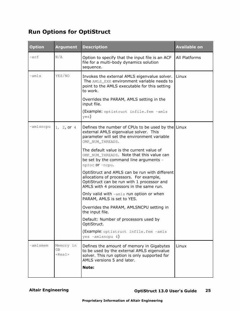
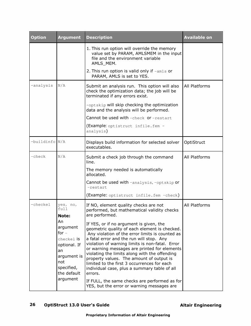
Run Options for OptiStruct
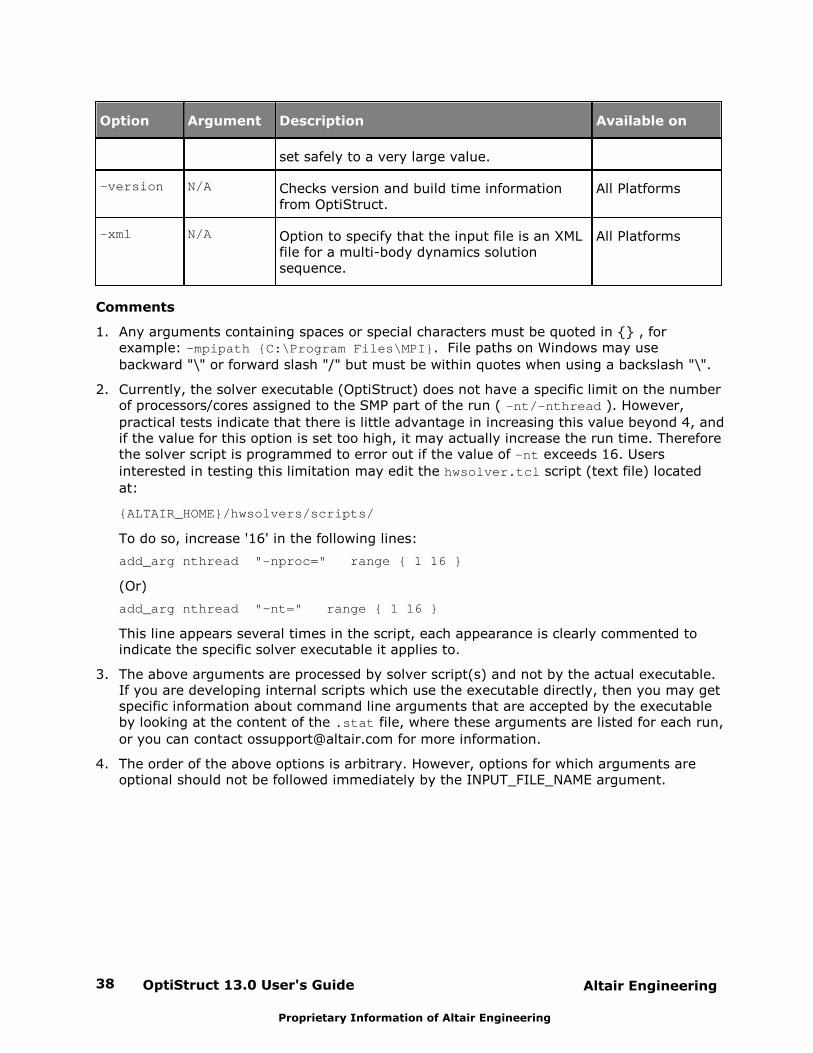
Option Argument Description Available on
-acf N/A Option to specify that the input file is an ACFfile for a multi-body dynamics solutionsequence.
All Platforms
-amls YES/NO Invokes the external AMLS eigenvalue solver. The AMLS_EXE environment variable needs to
point to the AMLS executable for this settingto work.
Overrides the PARAM, AMLS setting in theinput file.
(Example: optistruct infile.fem –amls
yes)
Linux
-amlsncpu 1, 2, or 4 Defines the number of CPUs to be used by theexternal AMLS eigenvalue solver. Thisparameter will set the environment variable OMP_NUM_THREADS.
The default value is the current value of OMP_NUM_THREADS. Note that this value can
be set by the command line arguments –
nproc or –ncpu.
OptiStruct and AMLS can be run with differentallocations of processors. For example,OptiStruct can be run with 1 processor andAMLS with 4 processors in the same run.
Only valid with –amls run option or when
PARAM, AMLS is set to YES.
Overrides the PARAM, AMLSNCPU setting inthe input file.
Default: Number of processors used byOptiStruct.
(Example: optistruct infile.fem –amls
yes –amlsncpu 4)
Linux
-amlsmem Memory inGB<Real>
Defines the amount of memory in Gigabytesto be used by the external AMLS eigenvaluesolver. This run option is only supported forAMLS versions 5 and later.
Note:
Linux
OptiStruct 13.0 User's Guide26 Altair Engineering
Proprietary Information of Altair Engineering
Option Argument Description Available on
1. This run option will override the memoryvalue set by PARAM, AMLSMEM in the inputfile and the environment variableAMLS_MEM.
2. This run option is valid only if –amls or
PARAM, AMLS is set to YES.
-analysis N/A Submit an analysis run. This option will alsocheck the optimization data; the job will beterminated if any errors exist.
-optskip will skip checking the optimization
data and the analysis will be performed.
Cannot be used with -check or -restart
(Example: optistruct infile.fem –
analysis)
All Platforms
-buildinfo N/A Displays build information for selected solverexecutables.
OptiStruct
-check N/A Submit a check job through the commandline.
The memory needed is automaticallyallocated.
Cannot be used with –analysis, -optskip or -restart
(Example: optistruct infile.fem –check)
All Platforms
-checkel yes, no,full
Note:
An
argument
for –
checkel is
optional. If
an
argument is
not
specified,
the default
argument
If NO, element quality checks are notperformed, but mathematical validity checksare performed.
If YES, or if no argument is given, thegeometric quality of each element is checked. Any violation of the error limits is counted asa fatal error and the run will stop. Anyviolation of warning limits is non-fatal. Erroror warning messages are printed for elementsviolating the limits along with the offendingproperty values. The amount of output islimited to the first 3 occurrences for eachindividual case, plus a summary table of allerrors.
If FULL, the same checks are performed as forYES, but the error or warning messages are
All Platforms
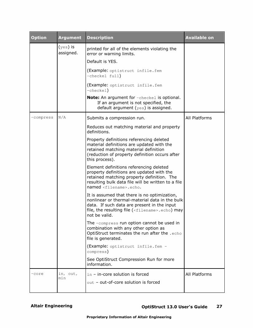
Altair Engineering OptiStruct 13.0 User's Guide 27
Proprietary Information of Altair Engineering
Option Argument Description Available on
(yes) is
assigned.printed for all of the elements violating theerror or warning limits.
Default is YES.
(Example: optistruct infile.fem
–checkel full)
(Example: optistruct infile.fem
–checkel)
Note: An argument for –checkel is optional.
If an argument is not specified, thedefault argument (yes) is assigned.
-compress N/A Submits a compression run.
Reduces out matching material and propertydefinitions.
Property definitions referencing deletedmaterial definitions are updated with theretained matching material definition(reduction of property definition occurs afterthis process).
Element definitions referencing deletedproperty definitions are updated with theretained matching property definition. Theresulting bulk data file will be written to a filenamed <filename>.echo.
It is assumed that there is no optimization,nonlinear or thermal-material data in the bulkdata. If such data are present in the inputfile, the resulting file (<filename>.echo) may
not be valid.
The –compress run option cannot be used in
combination with any other option asOptiStruct terminates the run after the .echo
file is generated.
(Example: optistruct infile.fem –
compress)
See OptiStruct Compression Run for moreinformation.
All Platforms
-core in, out,min
in – in-core solution is forced
out – out-of-core solution is forced
All Platforms

OptiStruct 13.0 User's Guide28 Altair Engineering
Proprietary Information of Altair Engineering
Option Argument Description Available on
min – minimum core solution is forced
The solver assigns the appropriate memoryrequired. If there is not enough memoryavailable, OptiStruct will error out. Overwrites the –len option.
(Example: optistruct infile.fem –core
in)
-cpu
or -proc
or -nproc
or -ncpu
or-nt
Number ofcores
Number of cores to be used for SMP solution. (See comment 2).
(Example: optistruct infile.fem -ncpu
2)
All Platforms
-ddm N/A Runs MPI based OptiStruct SPMD in DomainDecomposition Mode.
Not all platformsare supported.Refer to the OptiStruct SPMDUser's Guide forthe list ofsupportedplatforms.
-delay Number ofseconds
Delays the start of an OptiStruct run for thespecified number of seconds. Thisfunctionality does not use licenses, computermemory or CPU before the start of the run(the delay expires).
Note:
The –delay option can only be used for
a single job. Delays cannot bescheduled for multiple jobs in a queue.
If the run is started using the HWSolverRun Manager (GUI), the Scheduledelay option should be used.
All Platforms
-dir N/A Change directory to the location of input filebefore starting the solver.
All Platforms
-ffrs YES/NO Invokes the external FastFRS (Fast FrequencyResponse Solver) solver. The FASTFRS_EXE
Linux

Altair Engineering OptiStruct 13.0 User's Guide 29
Proprietary Information of Altair Engineering
Option Argument Description Available on
environment variable should point to theFastFRS executable for this setting to work.
Overrides the PARAM, FFRS setting in theinput file.
(Example: optistruct infile.fem –ffrs
yes)
-ffrsncpu 1, 2, or 4 Defines the number of CPUs to be used by theexternal FastFRS eigenvalue solver. Thisparameter will set the environment variable OMP_NUM_THREADS.
The default value is the current value of OMP_NUM_THREADS. Note that this value can
be set by the command line arguments –
nproc or –ncpu.
OptiStruct and FastFRS can be run withdifferent allocations of processors. Forexample, OptiStruct can be run with 1processor and FastFRS with 4 processors inthe same run.
Valid only when the –ffrs run option or
PARAM, FFRS is set to YES.
Overrides the PARAM, FFRSNCPU setting inthe input file.
Default: Number of processors used byOptiStruct.
(Example: optistruct infile.fem –ffrs
yes –ffrsncpu 4)
Linux
-ffrsmem Memory inGB<Real>
Defines the amount of memory in Gigabytesto be used by the external FastFRSeigenvalue solver. This run option is onlysupported for FastFRS versions 2 and later.
Note:
1. This run option will override the memoryvalue set by PARAM, FFRSMEM in the inputfile and the environment variableFFRS_MEM.
2. This run option is valid only when the –
ffrs run option or PARAM, FFRS is set to
YES.
Linux

OptiStruct 13.0 User's Guide30 Altair Engineering
Proprietary Information of Altair Engineering
Option Argument Description Available on
-fixlen RAM inMBytes
Disables dynamic memory allocation.
OptiStruct will allocate the given amount ofmemory and use it throughout the run. Ifthis memory is not available, or if theallocated amount is not sufficient for thesolution process, OptiStruct will terminatewith an error.
To avoid over specifying the memory whenusing this option, it is suggested first to runOptiStruct with the -check option and use the
results of that run to properly define thememory size for the -fixlen option.
This option allows, on certain platforms, toavoid memory fragmentation and allocatemore memory than is possible with dynamicmemory allocation.
Overwritten by -len and -core options.
(Example: optistruct infile.fem -
fixlen 500)
All Platforms
-gpu N/A Activates GPU Computing All Platforms
-gpuid N/A N: Integer, Optional, Selects the GPU Card.Default = 1.
All Platforms
-h N/A Displays script usage. All Platforms
-len RAM inMBytes
Preferred upper bound on dynamic memoryallocation.
When different algorithms can be chosen, thesolver will try to use the fastest algorithmwhich can run within the specified amount ofmemory. If no such algorithm is available,then the algorithm with minimum memoryrequirement will be used. For example, thesparse linear solver, which can run in-core,out-of-core or min-core will be selected. The –
core option will override the –len option. The
default for –len is 1000MB, this means that
all except for very small models, OptiStructwill use only the minimum memory needed torun the job. If –len value is larger than the
amount of available physical RAM, it maycause excessive swapping during
All Platforms
Altair Engineering OptiStruct 13.0 User's Guide 31
Proprietary Information of Altair Engineering
Option Argument Description Available on
computations, and significantly slow down thesolution process.
Default = 1000 MB.
(Example: optistruct infile.fem –len
32)
Best practices for –len specification:For proper memory allocation while using –
len in an OptiStruct run, avoid using the
exact reported memory estimate value (foreg. Using Check). The –len value should be
provided based on the actual memory of thesystem. This would be the recommendedmemory limit to run the job, it may notnecessarily represent the memory utilized bythe job or the actual memory limit. This way,the job is more likely to run with the bestpossible performance. If the same system isshared by multiple jobs, then the memoryallocation should follow the same procedureas above; except, that the individualmaximum memory should be used in place ofthe total system memory. (If a job runs out-of-core instead of in-core (it exceeded thememory allocation) it will still run veryefficiently. However, make sure that the jobdoes not exceed the actual memory of thesystem itself as this will slow the run down bya large factor. The recommended method todeal with this is to specify –maxlen as the
actual memory of the system to limit themaximum memory that can be used on thesystem.
-lic FEA, OPT FEA - FE analysis only(OptiStructFEA).
All Platforms
OPT - Optimization (OptiStruct orOptiStructMulti).
The solver checks out a license of thespecified type before reading the input data. Once the input data is read, the solververifies that the requested license is of thecorrect type. If this is not the case,OptiStruct will terminate with an error.
OptiStruct 13.0 User's Guide32 Altair Engineering
Proprietary Information of Altair Engineering
Option Argument Description Available on
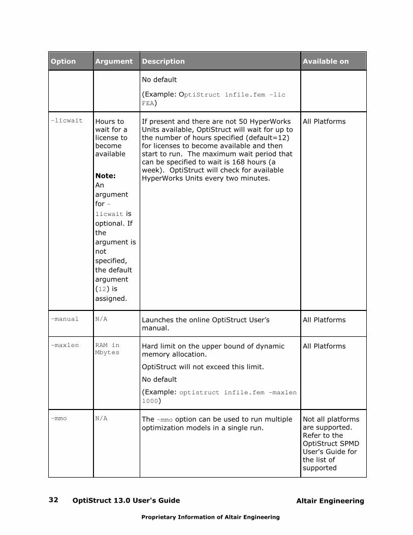
No default
(Example: OptiStruct infile.fem -lic
FEA)
-licwait Hours towait for alicense tobecomeavailable
Note:
An
argument
for –
licwait is
optional. If
the
argument is
not
specified,
the default
argument
(12) is
assigned.
If present and there are not 50 HyperWorksUnits available, OptiStruct will wait for up tothe number of hours specified (default=12)for licenses to become available and thenstart to run. The maximum wait period thatcan be specified to wait is 168 hours (aweek). OptiStruct will check for availableHyperWorks Units every two minutes.
All Platforms
-manual N/A Launches the online OptiStruct User’smanual.
All Platforms
-maxlen RAM inMbytes
Hard limit on the upper bound of dynamicmemory allocation.
OptiStruct will not exceed this limit.
No default
(Example: optistruct infile.fem –maxlen
1000)
All Platforms
-mmo N/A The –mmo option can be used to run multiple
optimization models in a single run.
Not all platformsare supported.Refer to the OptiStruct SPMDUser's Guide forthe list ofsupported
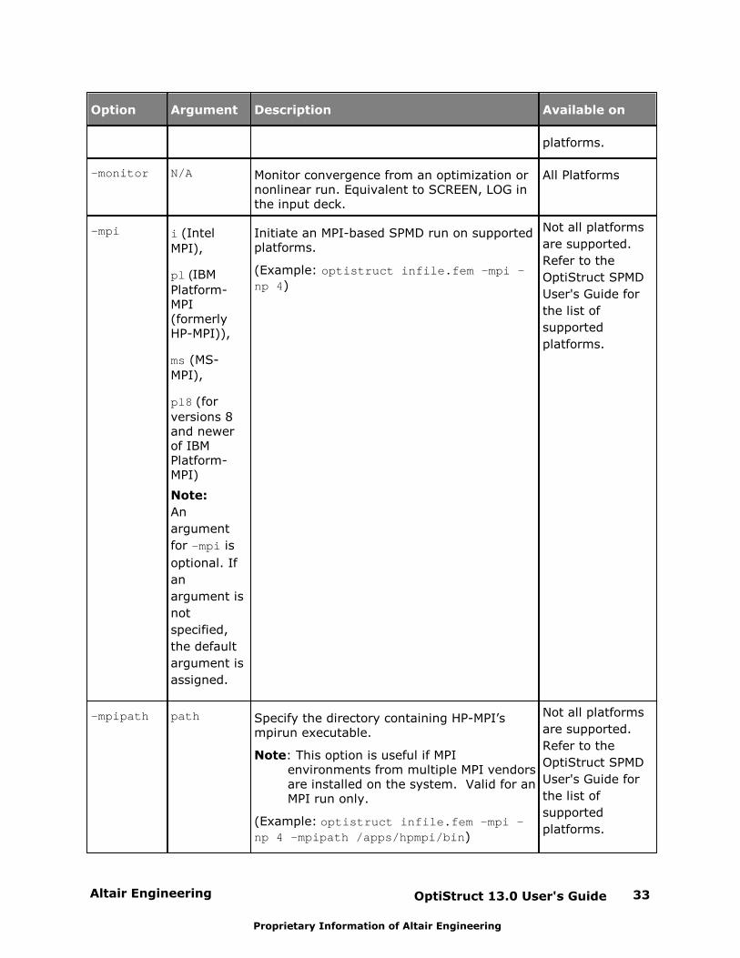
Altair Engineering OptiStruct 13.0 User's Guide 33
Proprietary Information of Altair Engineering
Option Argument Description Available on
platforms.
-monitor N/A Monitor convergence from an optimization ornonlinear run. Equivalent to SCREEN, LOG inthe input deck.
All Platforms
-mpi i (Intel
MPI),
pl (IBM
Platform-MPI(formerlyHP-MPI)),
ms (MS-
MPI),
pl8 (for
versions 8and newerof IBMPlatform-MPI)
Note:
An
argument
for –mpi is
optional. If
an
argument is
not
specified,
the default
argument is
assigned.
Initiate an MPI-based SPMD run on supportedplatforms.
(Example: optistruct infile.fem –mpi –
np 4)
Not all platforms
are supported.
Refer to the
OptiStruct SPMD
User's Guide for
the list of
supported
platforms.
-mpipath path Specify the directory containing HP-MPI’smpirun executable.
Note: This option is useful if MPIenvironments from multiple MPI vendorsare installed on the system. Valid for anMPI run only.
(Example: optistruct infile.fem –mpi –
np 4 –mpipath /apps/hpmpi/bin)
Not all platforms
are supported.
Refer to the
OptiStruct SPMD
User's Guide for
the list of
supported
platforms.
OptiStruct 13.0 User's Guide34 Altair Engineering
Proprietary Information of Altair Engineering
Option Argument Description Available on
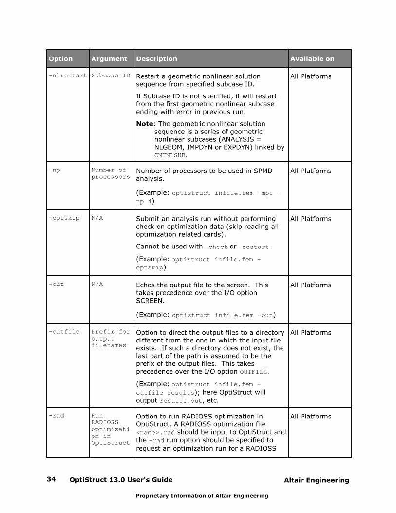
-nlrestart Subcase ID Restart a geometric nonlinear solutionsequence from specified subcase ID.
If Subcase ID is not specified, it will restartfrom the first geometric nonlinear subcaseending with error in previous run.
Note: The geometric nonlinear solutionsequence is a series of geometricnonlinear subcases (ANALYSIS =NLGEOM, IMPDYN or EXPDYN) linked by CNTNLSUB.
All Platforms
-np Number ofprocessors
Number of processors to be used in SPMDanalysis.
(Example: optistruct infile.fem –mpi –
np 4)
All Platforms
-optskip N/A Submit an analysis run without performingcheck on optimization data (skip reading alloptimization related cards).
Cannot be used with –check or –restart.
(Example: optistruct infile.fem -
optskip)
All Platforms
-out N/A Echos the output file to the screen. Thistakes precedence over the I/O optionSCREEN.
(Example: optistruct infile.fem -out)
All Platforms
-outfile Prefix foroutputfilenames
Option to direct the output files to a directorydifferent from the one in which the input fileexists. If such a directory does not exist, thelast part of the path is assumed to be theprefix of the output files. This takesprecedence over the I/O option OUTFILE.
(Example: optistruct infile.fem -
outfile results); here OptiStruct will
output results.out, etc.
All Platforms
-rad RunRADIOSSoptimization inOptiStruct
Option to run RADIOSS optimization inOptiStruct. A RADIOSS optimization file <name>.rad should be input to OptiStruct and
the –rad run option should be specified to
request an optimization run for a RADIOSS
All Platforms
Altair Engineering OptiStruct 13.0 User's Guide 35
Proprietary Information of Altair Engineering
Option Argument Description Available on
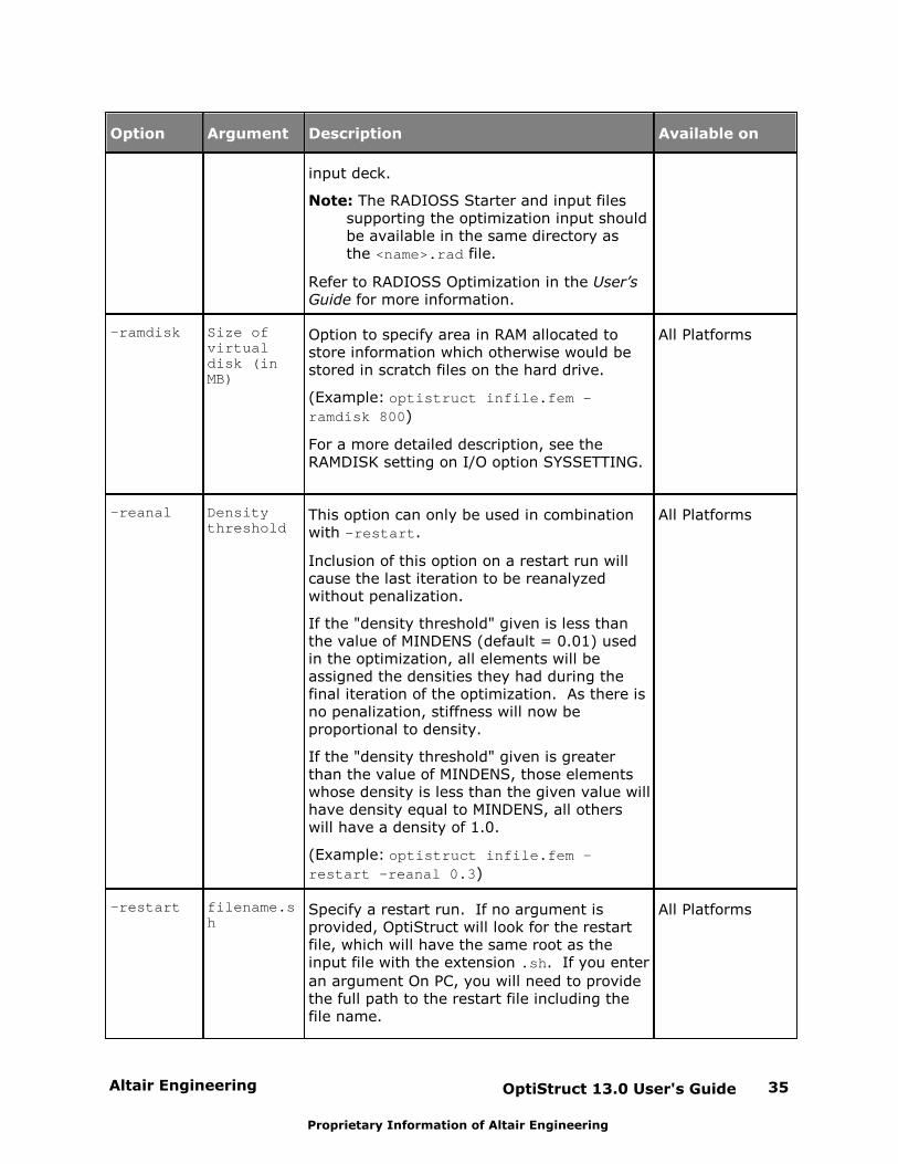
input deck.
Note: The RADIOSS Starter and input filessupporting the optimization input shouldbe available in the same directory asthe <name>.rad file.
Refer to RADIOSS Optimization in the User’sGuide for more information.
-ramdisk Size ofvirtualdisk (inMB)
Option to specify area in RAM allocated tostore information which otherwise would bestored in scratch files on the hard drive.
(Example: optistruct infile.fem –
ramdisk 800)
For a more detailed description, see theRAMDISK setting on I/O option SYSSETTING.
All Platforms
-reanal Densitythreshold
This option can only be used in combinationwith -restart.
Inclusion of this option on a restart run willcause the last iteration to be reanalyzedwithout penalization.
If the "density threshold" given is less thanthe value of MINDENS (default = 0.01) usedin the optimization, all elements will beassigned the densities they had during thefinal iteration of the optimization. As there isno penalization, stiffness will now beproportional to density.
If the "density threshold" given is greaterthan the value of MINDENS, those elementswhose density is less than the given value willhave density equal to MINDENS, all otherswill have a density of 1.0.
(Example: optistruct infile.fem -
restart -reanal 0.3)
All Platforms
-restart filename.sh
Specify a restart run. If no argument isprovided, OptiStruct will look for the restartfile, which will have the same root as theinput file with the extension .sh. If you enter
an argument On PC, you will need to providethe full path to the restart file including thefile name.
All Platforms
OptiStruct 13.0 User's Guide36 Altair Engineering
Proprietary Information of Altair Engineering
Option Argument Description Available on
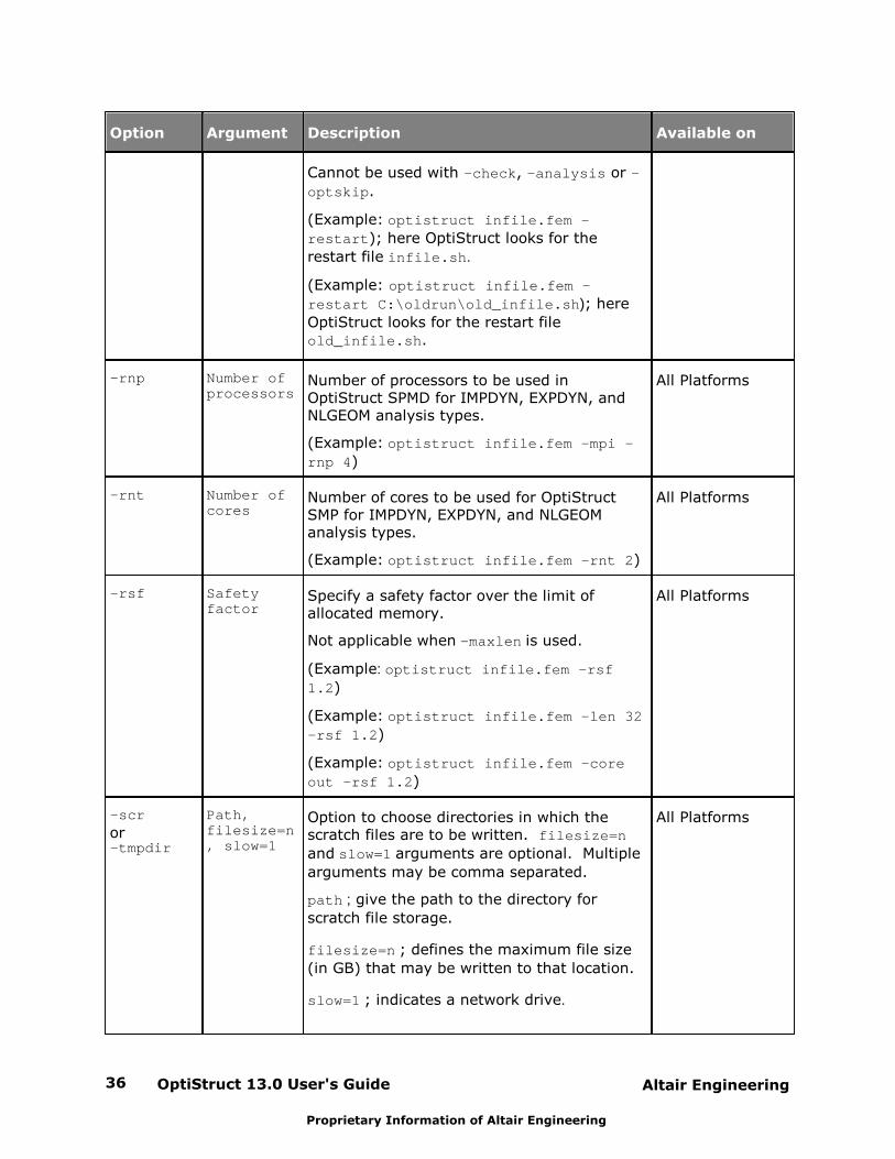
Cannot be used with –check, -analysis or –
optskip.
(Example: optistruct infile.fem -
restart); here OptiStruct looks for the
restart file infile.sh.
(Example: optistruct infile.fem –
restart C:\oldrun\old_infile.sh); here
OptiStruct looks for the restart fileold_infile.sh.
-rnp Number ofprocessors
Number of processors to be used inOptiStruct SPMD for IMPDYN, EXPDYN, andNLGEOM analysis types.
(Example: optistruct infile.fem –mpi –
rnp 4)
All Platforms
-rnt Number ofcores
Number of cores to be used for OptiStructSMP for IMPDYN, EXPDYN, and NLGEOManalysis types.
(Example: optistruct infile.fem -rnt 2)
All Platforms
-rsf Safetyfactor
Specify a safety factor over the limit ofallocated memory.
Not applicable when -maxlen is used.
(Example: optistruct infile.fem –rsf
1.2)
(Example: optistruct infile.fem –len 32
–rsf 1.2)
(Example: optistruct infile.fem –core
out –rsf 1.2)
All Platforms
-scr
or-tmpdir
Path,filesize=n, slow=1
Option to choose directories in which thescratch files are to be written. filesize=n
and slow=1 arguments are optional. Multiple
arguments may be comma separated.
path ; give the path to the directory for
scratch file storage.
filesize=n ; defines the maximum file size
(in GB) that may be written to that location.
slow=1 ; indicates a network drive.
All Platforms
Altair Engineering OptiStruct 13.0 User's Guide 37
Proprietary Information of Altair Engineering
Option Argument Description Available on
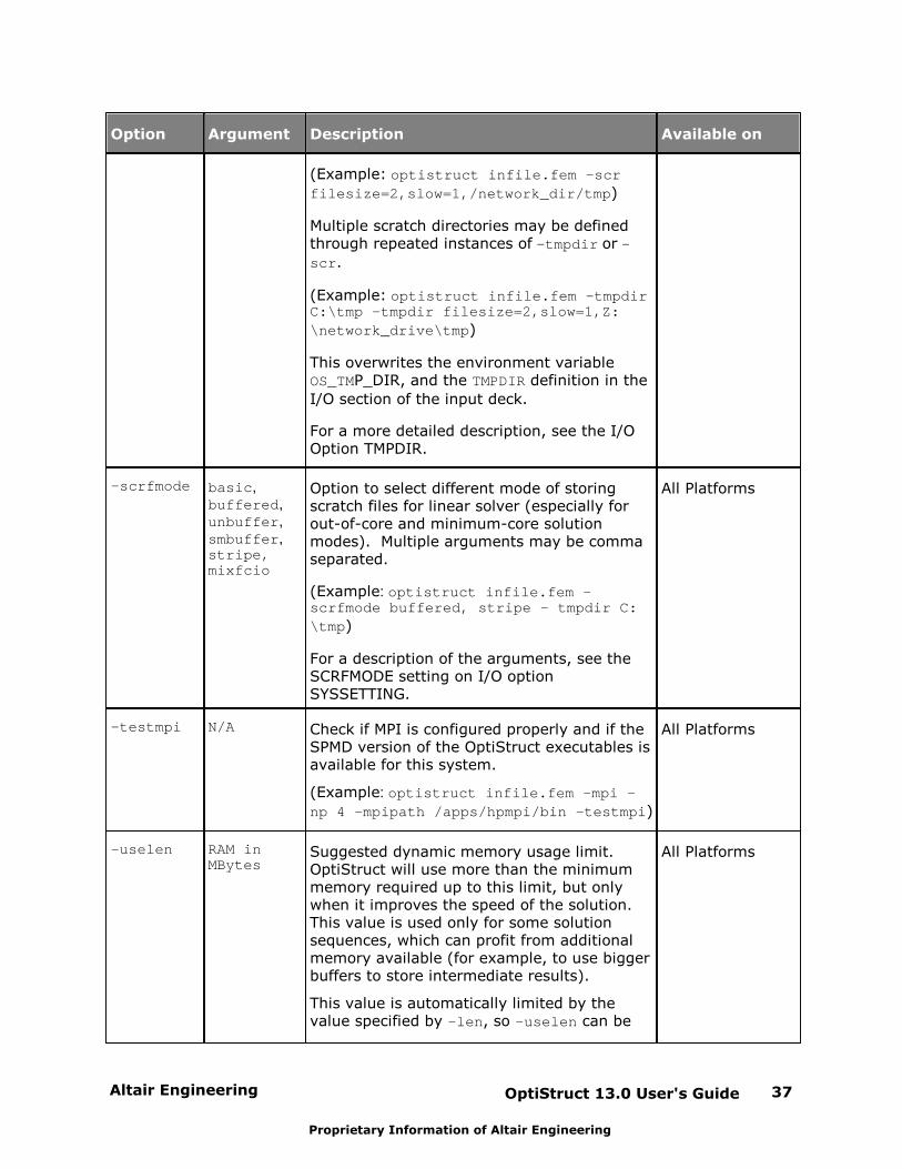
(Example: optistruct infile.fem –scr
filesize=2,slow=1,/network_dir/tmp)
Multiple scratch directories may be definedthrough repeated instances of –tmpdir or –
scr.
(Example: optistruct infile.fem –tmpdirC:\tmp –tmpdir filesize=2,slow=1,Z:
\network_drive\tmp)
This overwrites the environment variable OS_TMP_DIR, and the TMPDIR definition in the
I/O section of the input deck.
For a more detailed description, see the I/OOption TMPDIR.
-scrfmode basic,buffered,unbuffer,smbuffer,stripe,mixfcio
Option to select different mode of storingscratch files for linear solver (especially forout-of-core and minimum-core solutionmodes). Multiple arguments may be commaseparated.
(Example: optistruct infile.fem –scrfmode buffered, stripe – tmpdir C:
\tmp)
For a description of the arguments, see theSCRFMODE setting on I/O option SYSSETTING.
All Platforms
-testmpi N/A Check if MPI is configured properly and if theSPMD version of the OptiStruct executables isavailable for this system.
(Example: optistruct infile.fem –mpi –
np 4 –mpipath /apps/hpmpi/bin -testmpi)
All Platforms
-uselen RAM inMBytes
Suggested dynamic memory usage limit.OptiStruct will use more than the minimummemory required up to this limit, but onlywhen it improves the speed of the solution.This value is used only for some solutionsequences, which can profit from additionalmemory available (for example, to use biggerbuffers to store intermediate results).
This value is automatically limited by thevalue specified by –len, so –uselen can be
All Platforms
OptiStruct 13.0 User's Guide38 Altair Engineering
Proprietary Information of Altair Engineering
Option Argument Description Available on
set safely to a very large value.
-version N/A Checks version and build time informationfrom OptiStruct.
All Platforms
-xml N/A Option to specify that the input file is an XMLfile for a multi-body dynamics solutionsequence.
All Platforms
Comments
1. Any arguments containing spaces or special characters must be quoted in {} , forexample: -mpipath {C:\Program Files\MPI}. File paths on Windows may use
backward "\" or forward slash "/" but must be within quotes when using a backslash "\".
2. Currently, the solver executable (OptiStruct) does not have a specific limit on the numberof processors/cores assigned to the SMP part of the run ( -nt/-nthread ). However,
practical tests indicate that there is little advantage in increasing this value beyond 4, andif the value for this option is set too high, it may actually increase the run time. Thereforethe solver script is programmed to error out if the value of -nt exceeds 16. Users
interested in testing this limitation may edit the hwsolver.tcl script (text file) located
at:
{ALTAIR_HOME}/hwsolvers/scripts/
To do so, increase '16' in the following lines:
add_arg nthread "-nproc=" range { 1 16 }
(Or)
add_arg nthread "-nt=" range { 1 16 }
This line appears several times in the script, each appearance is clearly commented toindicate the specific solver executable it applies to.
3. The above arguments are processed by solver script(s) and not by the actual executable.If you are developing internal scripts which use the executable directly, then you may getspecific information about command line arguments that are accepted by the executableby looking at the content of the .stat file, where these arguments are listed for each run,
or you can contact [email protected] for more information.
4. The order of the above options is arbitrary. However, options for which arguments areoptional should not be followed immediately by the INPUT_FILE_NAME argument.
Altair Engineering OptiStruct 13.0 User's Guide 39
Proprietary Information of Altair Engineering
OptiStruct GPU
Introduction
A Graphics Processing Unit (GPU) is a system which can be used to improve the performanceof computationally intensive engineering applications. GPU Computing is a process whichuses the GPU to execute the time consuming sections of the application and the rest of thecode runs on the CPU.
Implementation
Starting from OptiStruct version 12.0, the GPU can be used to accelerate the sparse directequation solver through the NVIDIA CUDA programming model. GPU computing isimplemented by off-loading most of the computation intensive work to the GPU andconcurrently overlapping the communication and data transfer between the CPU cores andthe GPU.
Speedup
A speedup in the equation solver of up to 4 times, and up to 3 times overall when comparedto a Quad-core Intel Nehalem Xeon run, can be achieved. This heterogeneous computingmodel is particularly suitable for jobs dominated by the equation solver. For example:nonlinear static analysis on power train structures, topology optimization on blocky structuresand so on.
Compatibility
1. GPU computing is available for static analysis/optimization.
2. GPU computing is available in 64-bit Linux platform only.
3. GPU computing is NOT supported in the SPMD module.
4. NVIDIA Fermi and Kepler architecture based Tesla and Quadro graphic cards aresupported. Tesla C2050/C2070/M2090/K10/K20, Quadro 6000/K5000/K6000 cards arerecommended for computing by NVIDIA.
Activating OptiStruct GPU
Command option “-gpu” is used to activate OptiStruct GPU. Currently, only one graphics card
is supported, and “–gpuid” can be used to pick the desired graphic card for computation
when multiple cards are present. Compatible drivers for the graphics card needs to beinstalled by the user prior to launching OptiStruct GPU using the option “-gpu”.
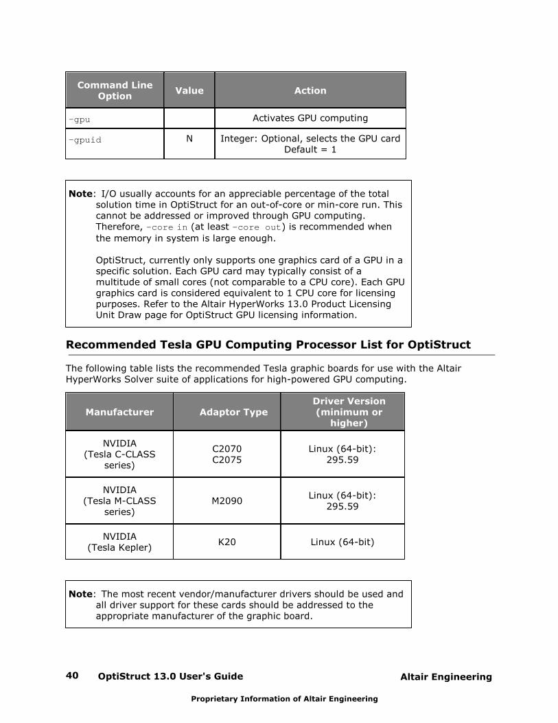
OptiStruct 13.0 User's Guide40 Altair Engineering
Proprietary Information of Altair Engineering
Command LineOption
Value Action
-gpu Activates GPU computing
-gpuid N Integer: Optional, selects the GPU cardDefault = 1
Note: I/O usually accounts for an appreciable percentage of the totalsolution time in OptiStruct for an out-of-core or min-core run. Thiscannot be addressed or improved through GPU computing.Therefore, -core in (at least –core out) is recommended when
the memory in system is large enough.
OptiStruct, currently only supports one graphics card of a GPU in aspecific solution. Each GPU card may typically consist of amultitude of small cores (not comparable to a CPU core). Each GPUgraphics card is considered equivalent to 1 CPU core for licensingpurposes. Refer to the Altair HyperWorks 13.0 Product LicensingUnit Draw page for OptiStruct GPU licensing information.
Recommended Tesla GPU Computing Processor List for OptiStruct
The following table lists the recommended Tesla graphic boards for use with the AltairHyperWorks Solver suite of applications for high-powered GPU computing.
Manufacturer Adaptor TypeDriver Version(minimum or
higher)
NVIDIA(Tesla C-CLASS
series)
C2070C2075
Linux (64-bit):295.59
NVIDIA(Tesla M-CLASS
series)M2090
Linux (64-bit):295.59
NVIDIA(Tesla Kepler)
K20 Linux (64-bit)
Note: The most recent vendor/manufacturer drivers should be used andall driver support for these cards should be addressed to theappropriate manufacturer of the graphic board.
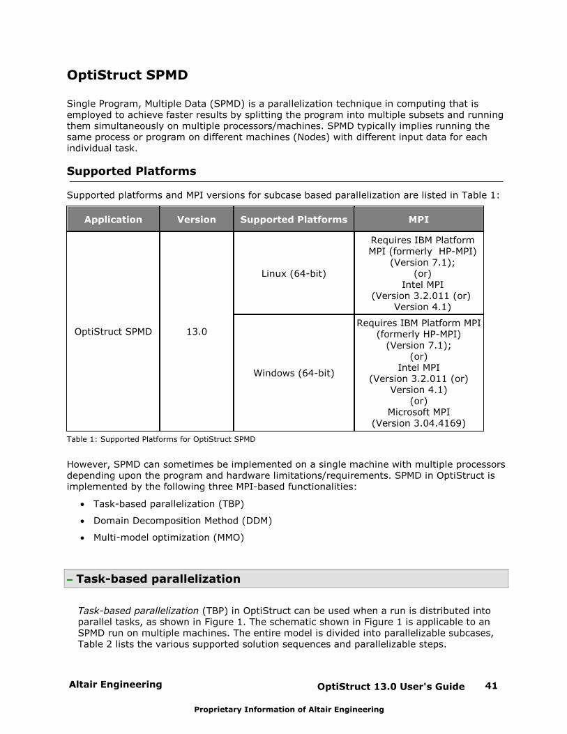
Altair Engineering OptiStruct 13.0 User's Guide 41
Proprietary Information of Altair Engineering
OptiStruct SPMD
Single Program, Multiple Data (SPMD) is a parallelization technique in computing that isemployed to achieve faster results by splitting the program into multiple subsets and runningthem simultaneously on multiple processors/machines. SPMD typically implies running thesame process or program on different machines (Nodes) with different input data for eachindividual task.
Supported Platforms
Supported platforms and MPI versions for subcase based parallelization are listed in Table 1:
Application Version Supported Platforms MPI
OptiStruct SPMD 13.0
Linux (64-bit)
Requires IBM PlatformMPI (formerly HP-MPI)
(Version 7.1);(or)
Intel MPI(Version 3.2.011 (or)
Version 4.1)
Windows (64-bit)
Requires IBM Platform MPI(formerly HP-MPI)
(Version 7.1);(or)
Intel MPI(Version 3.2.011 (or)
Version 4.1)(or)
Microsoft MPI(Version 3.04.4169)
Table 1: Supported Platforms for OptiStruct SPMD
However, SPMD can sometimes be implemented on a single machine with multiple processorsdepending upon the program and hardware limitations/requirements. SPMD in OptiStruct isimplemented by the following three MPI-based functionalities:
Task-based parallelization (TBP)
Domain Decomposition Method (DDM)
Multi-model optimization (MMO)
Task-based parallelization
Task-based parallelization (TBP) in OptiStruct can be used when a run is distributed intoparallel tasks, as shown in Figure 1. The schematic shown in Figure 1 is applicable to anSPMD run on multiple machines. The entire model is divided into parallelizable subcases,Table 2 lists the various supported solution sequences and parallelizable steps.
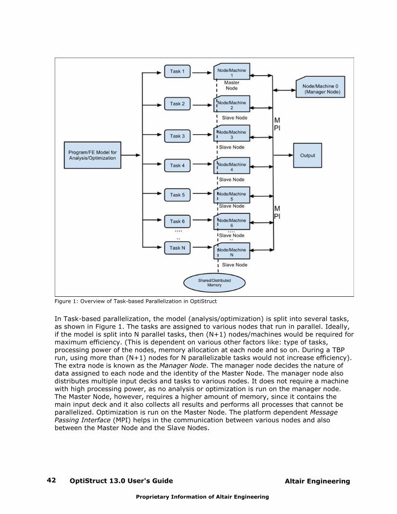
OptiStruct 13.0 User's Guide42 Altair Engineering
Proprietary Information of Altair Engineering
Figure 1: Overview of Task-based Parallelization in OptiStruct
In Task-based parallelization, the model (analysis/optimization) is split into several tasks,as shown in Figure 1. The tasks are assigned to various nodes that run in parallel. Ideally,if the model is split into N parallel tasks, then (N+1) nodes/machines would be required formaximum efficiency. (This is dependent on various other factors like: type of tasks,processing power of the nodes, memory allocation at each node and so on. During a TBPrun, using more than (N+1) nodes for N parallelizable tasks would not increase efficiency).The extra node is known as the Manager Node. The manager node decides the nature ofdata assigned to each node and the identity of the Master Node. The manager node alsodistributes multiple input decks and tasks to various nodes. It does not require a machinewith high processing power, as no analysis or optimization is run on the manager node.The Master Node, however, requires a higher amount of memory, since it contains themain input deck and it also collects all results and performs all processes that cannot beparallelized. Optimization is run on the Master Node. The platform dependent MessagePassing Interface (MPI) helps in the communication between various nodes and alsobetween the Master Node and the Slave Nodes.
Altair Engineering OptiStruct 13.0 User's Guide 43
Proprietary Information of Altair Engineering
Note:
1. A Task is a minimum distribution unit used in parallelization.Each buckling analysis subcase is one task. Each Left-HandSide (LHS) of the static analysis subcases is one task. Typically,the static analysis subcases sharing the same SPC (Single PointConstraint) belong to one task. Not all tasks can be run inparallel at the same time (For example: A buckling subcase cannot start before the execution of its STATSUB subcase).
2. The manager can also be included within the master node byspecifying np = N+1 for N nodes and repeating the first node inthe appfile/hostfile in a cluster setup (-np option, appfile/
hostfile are explained in the following sections).
Supported Solution Sequences
OptiStruct can handle a variety of solution sequences as listed in the overview. However,all solution sequences do not lend themselves to parallelization. In general, many steps ina program execution are not parallelized. Steps like Pre-processing and Matrix Assemblyare repeated on all nodes, while response recovery, screening, approximation, optimizationand output of results are all executed on the Master Node.
SolutionSequences that
SupportParallelization
Parallelizable Steps Non-Parallelizable Steps
Static Analysis Two or more staticBoundary Conditions areparallelized (MatrixFactorization is the stepthat is parallelized sinceit is computationallyintensive.)
Sensitivities areparallelized (Even for asingle BoundaryCondition as analysis isrepeated on all slavenodes).
Iterative Solution is notparallelized. (Only DirectSolution is parallelized).
Buckling Analysis Two or more BucklingSubcases areparallelized.
Sensitivities areparallelized.
OptiStruct 13.0 User's Guide44 Altair Engineering
Proprietary Information of Altair Engineering
SolutionSequences that
SupportParallelization
Parallelizable Steps Non-Parallelizable Steps
Direct FrequencyResponse Analysis
Loading Frequencies areparallelized.
No Optimization.
Modal FrequencyResponse Analysis
Loading Frequencies areparallelized.
Modal FRF pre-processing is notparallelized.
Sensitivities are notparallelized.
Table 2: Task-based parallelization - Parallelizable Steps for various solution sequences
As of HyperWorks 11.0, the presence of non-parallelizable subcases WILL NOT make theentire program non-parallelizable. The program execution will continue in parallel and thenon-parallelizable subcase will be executed as a serial run.
Number and Type of Nodes available for Parallelization
The types and functions of the nodes that are used in Task-based Parallelization areindicated in Table 3. The first node is automatically selected as the manager, the secondnode is the master node and the rest are slave nodes.
Node Type Functions
Master Node
(1 Node)
Runs all non-parallelizable tasks
Optimization is run here
Slave Node
(N-2 Nodes)
Runs all parallelizable tasks
Input deck copies are provided
Manager Node
(1 Node)
No tasks are run on this node, it manages theway nodes are assigned tasks.
Manager makes multiple copies of the inputdeck and sends them to the slave nodes.
Table 3: Types and functions of the Nodes
This assignment is based on the sequence of nodes that you specify in the appfile. The
appfile is a text file which contains process counts and the list of programs. Nodes can be
repeated in the appfile, multiple cores of the repeated nodes will be assigned parallel
jobs in the same sequence discussed here.

Altair Engineering OptiStruct 13.0 User's Guide 45
Proprietary Information of Altair Engineering
Frequently Asked Questions
How many nodes should I use?
Parallelization is based on task distribution. If the maximum number of tasks which can berun at the same time is N, then using (N+1) nodes is ideal (the extra one node for themanager distributing tasks). Using more than (N+1) nodes will not improve theperformance.
The .out file suggests the number of nodes you can use, based on your model.
When there are only M physical nodes available (M < N), then the correct way to start thejob is to use M+1 nodes in the hostfile/appfile. The manager node requires only a smallamount of resources and can be safely shared with the master: The way to assign such adistribution is repeating the first physical host in the hostfile/appfile. For example: Hostfilefor Intel MPI can be:
Node1Node1Node2Node3…….
Note: For Frequency Response Analysis any number of nodes may be used.(up to the number of loading frequencies in the model.)
How to run OptiStruct SPMD on a dual/quad CPU’s/Cores machine?
Follow the instructions to run OptiStruct SPMD on a single machine. The ideal number ofnodes is min(N+1, M), where N is the maximum number of tasks that can be run at thesame time, and M is the number of CPU’s/Cores.
Note: For dual/quad code machines it may be more efficient to run OptiStructin serial + SMP mode. (that is, use –nt argument in the solver script).
How to run OptiStruct SPMD over LAN?
It is possible to run OptiStruct SPMD over LAN. Follow the HP-MPI manual to setupdifferent working directories of each node the OptiStruct SPMD is launched.
Is it better to run on cluster of separate machines or on shared memorymachine(s) with multiple CPU’s?
There is no easy answer to this question. If the computer has enough memory to run alltasks in-core, then we can expect faster solution times as MPI communication is not sloweddown by the network speed. But if the tasks have to run out-of-core, then computationsare slowed down by disk read/write delay. Multiple tasks on the same machine maycompete for disk access, and (in extreme situations) even result in wall clock time slowerthan that for serial (non-MPI) runs.
OptiStruct 13.0 User's Guide46 Altair Engineering
Proprietary Information of Altair Engineering
Will OptiStruct SPMD use less memory on each node than in the serial run?
No, Memory estimates for serial runs and parallel runs on each node are the same. Theyare based on the solution of a single (most demanding) subcase.
Will OptiStruct SPMD use less disk space on each node than in the serial run?
Yes. Disk space usage on each node will be smaller, because only temporary files related totask(s) solved on this node will be stored. But the total amount of disk space will be largerthan that in the serial run and this can be noticed, especially in parallel runs on a shared-memory machine.
I have a cluster with N nodes each with M cores. What is the most efficient way Ican use the resources that I possess?
1. When each host has sufficient RAM to execute only a single serial OptiStruct run, thenuse multiple cores to activate SMP on each node. (using more than four cores is usuallynot effective). For example: on a 4 host cluster, each with 8 cores, you can run:
optistruct <inputfile> -mpi <mode> -np 5 –nt 4 –hostfile…
2. When each host has sufficient RAM to efficiently execute more than one serial run, thenyou can assign multiple MPI nodes to each host. For example:
optistruct <inputfile> -mpi <mode> -np 9 –nt 4 –hostfile…
Domain Decomposition Method
In addition to Task-based parallelization (TBP), OptiStruct SPMD includes another approachfor parallelization called Domain Decomposition Method (DDM) for static analysis andoptimization. DDM allows you to run a single subcase of static analysis and/or optimizationwith multiple processors in either Shared Memory Processing (SMP) or Distributed MemoryProcessing (DMP) cluster computers. The solution time will be significantly reduced in DDMmode and the scalability is much higher compared to the legacy shared memoryprocessing parallelization approach, especially on machines with a high number ofprocessors (for example, greater than 8).
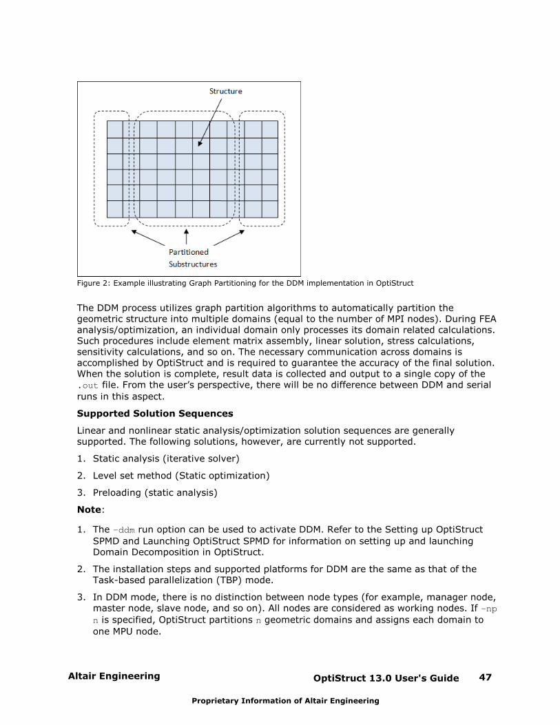
Altair Engineering OptiStruct 13.0 User's Guide 47
Proprietary Information of Altair Engineering
Figure 2: Example illustrating Graph Partitioning for the DDM implementation in OptiStruct
The DDM process utilizes graph partition algorithms to automatically partition thegeometric structure into multiple domains (equal to the number of MPI nodes). During FEAanalysis/optimization, an individual domain only processes its domain related calculations.Such procedures include element matrix assembly, linear solution, stress calculations,sensitivity calculations, and so on. The necessary communication across domains isaccomplished by OptiStruct and is required to guarantee the accuracy of the final solution.When the solution is complete, result data is collected and output to a single copy of the .out file. From the user’s perspective, there will be no difference between DDM and serial
runs in this aspect.
Supported Solution Sequences
Linear and nonlinear static analysis/optimization solution sequences are generallysupported. The following solutions, however, are currently not supported.
1. Static analysis (iterative solver)
2. Level set method (Static optimization)
3. Preloading (static analysis)
Note:
1. The –ddm run option can be used to activate DDM. Refer to the Setting up OptiStruct
SPMD and Launching OptiStruct SPMD for information on setting up and launchingDomain Decomposition in OptiStruct.
2. The installation steps and supported platforms for DDM are the same as that of the Task-based parallelization (TBP) mode.
3. In DDM mode, there is no distinction between node types (for example, manager node,master node, slave node, and so on). All nodes are considered as working nodes. If –np
n is specified, OptiStruct partitions n geometric domains and assigns each domain to
one MPU node.
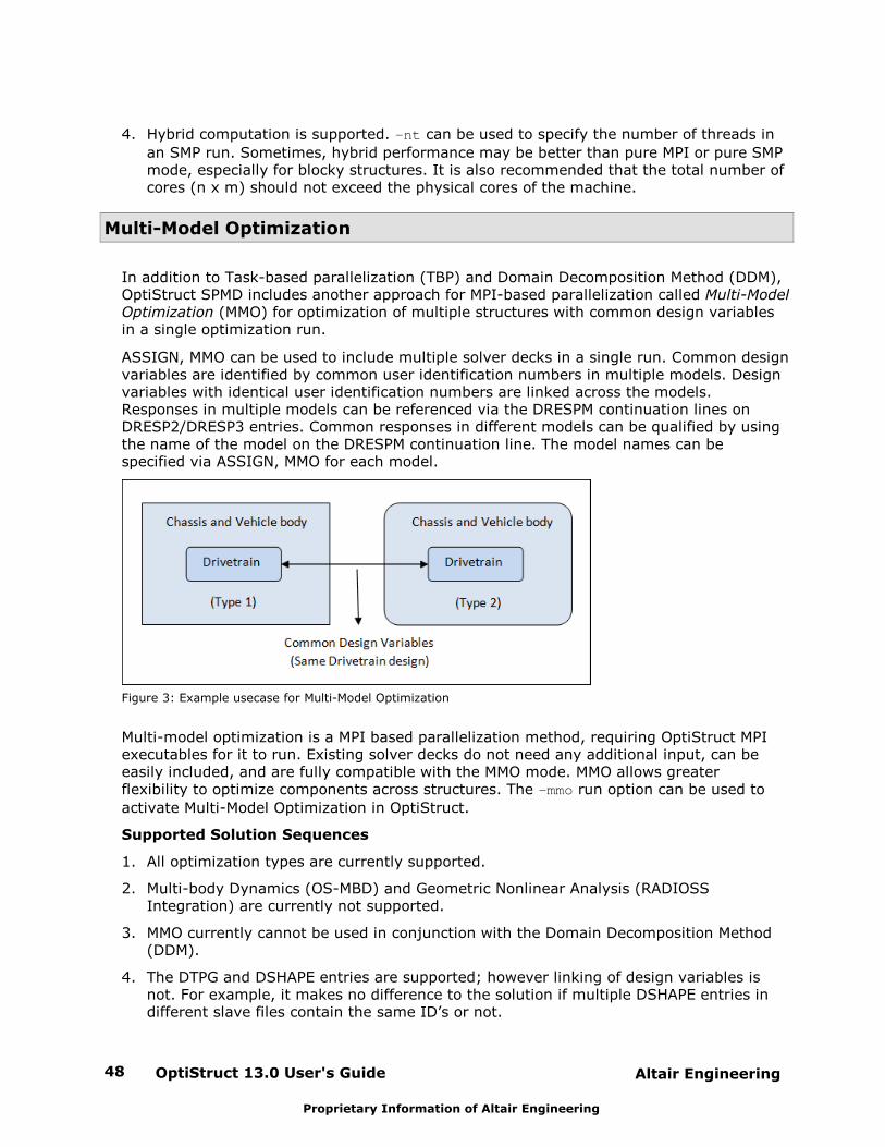
OptiStruct 13.0 User's Guide48 Altair Engineering
Proprietary Information of Altair Engineering
4. Hybrid computation is supported. –nt can be used to specify the number of threads in
an SMP run. Sometimes, hybrid performance may be better than pure MPI or pure SMPmode, especially for blocky structures. It is also recommended that the total number ofcores (n x m) should not exceed the physical cores of the machine.
Multi-Model Optimization
In addition to Task-based parallelization (TBP) and Domain Decomposition Method (DDM),OptiStruct SPMD includes another approach for MPI-based parallelization called Multi-ModelOptimization (MMO) for optimization of multiple structures with common design variablesin a single optimization run.
ASSIGN, MMO can be used to include multiple solver decks in a single run. Common designvariables are identified by common user identification numbers in multiple models. Designvariables with identical user identification numbers are linked across the models.Responses in multiple models can be referenced via the DRESPM continuation lines on DRESP2/DRESP3 entries. Common responses in different models can be qualified by usingthe name of the model on the DRESPM continuation line. The model names can bespecified via ASSIGN, MMO for each model.
Figure 3: Example usecase for Multi-Model Optimization
Multi-model optimization is a MPI based parallelization method, requiring OptiStruct MPIexecutables for it to run. Existing solver decks do not need any additional input, can beeasily included, and are fully compatible with the MMO mode. MMO allows greaterflexibility to optimize components across structures. The –mmo run option can be used to
activate Multi-Model Optimization in OptiStruct.
Supported Solution Sequences
1. All optimization types are currently supported.
2. Multi-body Dynamics (OS-MBD) and Geometric Nonlinear Analysis (RADIOSSIntegration) are currently not supported.
3. MMO currently cannot be used in conjunction with the Domain Decomposition Method(DDM).
4. The DTPG and DSHAPE entries are supported; however linking of design variables isnot. For example, it makes no difference to the solution if multiple DSHAPE entries indifferent slave files contain the same ID’s or not.
Altair Engineering OptiStruct 13.0 User's Guide 49
Proprietary Information of Altair Engineering
Note:
1. The number of processes should be equal to one more than the number of models.
2. Refer to the Setting up OptiStruct SPMD and Launching OptiStruct SPMD sections forinformation on setting up and launching Multi-Model Optimization in OptiStruct.
3. The installation steps and supported platforms for MMO are the same as that of the Task-based parallelization (TBP) and Domain Decomposition (DDM) modes.
4. If multiple objective functions are defined across different models in the master/slaves,then OptiStruct always uses minmax [Objective(i)] (where, i is the number ofobjective functions) to define the overall objective for the solution.
5. The following entries are allowed in the Master deck:
Control cards: SCREEN, DIAG/OSDIAG, DEBUG/OSDEBUG, TITLE, ASSIGN, RESPRINT, DESOBJ, DESGLB, REPGLB, MINMAX, MAXMIN, ANALYSIS, LOADLIB
Bulk data cards:DSCREEN, DOPTPRM (see section below), DRESP3, DRESP3, DOBJREF, DCONSTR,DCONADD, DREPORT, DREPADD, DEQATN, DTABLE, PARAM
DOPTPRM parameters (these work from within the master deck – all other DOPTPRM’sshould be specified in the slave):CHECKER, DDVOPT, DELSHP, DELSIZ, DELTOP, DESMAX, DISCRETE, OBJTOL,OPTMETH, SHAPEOPT
Setting up OptiStruct SPMD
Linux Machines
Below are detailed instructions on installing and launching OptiStruct SPM on Linuxmachines.
Installing OptiStruct SPMD
System Requirements
Operating system: Linux64
The MPI library: IBM Platform-MPI (Formerly HP-MPI) or Intel MPI must be installedand accessible from every machine in the cluster.
Installing Software and activating the License
1. OptiStruct SPMD is included with the OptiStruct solver package and the SPMDexecutables are included in the installation.
2. Test if OptiStruct SPMD is able to run in serial mode.

OptiStruct 13.0 User's Guide50 Altair Engineering
Proprietary Information of Altair Engineering
Configuring the machines
1. The account used to run OptiStruct SPMD must exist on every node in the cluster.
2. OptiStruct SPMD executables must be accessible to all cluster nodes.
3. The local scratch directories must be the same (same path).
4. It is highly recommended to have all the computation (working) directories at the samelocation on all cluster nodes.
SSH installation
1. IBM Platform MPI (formerly HP-MPI) default installation uses ssh to launch OptiStruct
SPMD on different nodes.
2. ssh should be configured to permit the connection on all hosts of the cluster without theneed to type passwords.
3. Refer to ssh man pages to generate and install rsa keys (ssh-keygen tool).
To check the functionality of ssh, the following test can be performed on the different
nodes:
[optistruct@host1] ssh host1 ls
[optistruct@host1] ssh host2 ls
...
[optistruct@host1] ssh host[n] ls
RSH (An alternative to SSH)
1. It is also possible to use rsh instead of ssh to launch OptiStruct SPMD.
2. Computation nodes need to be accessible to all the other nodes without need for apassword.
3. Refer to the rsh manpages for installation instructions. Check with IBM Platform MPI
(formerly HP-MPI) manual for instructions on how to use RSH instead of SSH.
4. To check the functionality of rsh, the following test can be performed on the different
nodes:
[optistruct@host1] rsh host1 ls
[optistruct@host1] rsh host2 ls
...
[optistruct@host1] rsh host[n] ls
IBM Platform MPI (formerly HP-MPI) installation
1. IBM Platform MPI (formerly HP-MPI) should be accessible to all computation nodes onwhich OptiStruct SPMD will be launched.
2. Download the IBM Platform MPI images for the platform you desire to use from thevendor (Contact IBM for help with procuring IBM Platform MPI).
3. Install the IBM Platform MPI package on each node.
Altair Engineering OptiStruct 13.0 User's Guide 51
Proprietary Information of Altair Engineering
4. No license is required for Platform-MPI to run OptiStruct SPMD.
5. Add $MPI_ROOT/platform_mpi/lib/[platform] into LD_LIBRARY_PATH, if needed.
Intel-MPI installation
1. Intel-MPI must be accessible from all computation nodes on which OptiStruct SPMD willbe launched.
2. Users can download (purchase/trial) the Intel-MPI images for their respective platformsfrom the following Intel MPI download site:http://software.intel.com/en-us/intel-mpi-library
3. Install the Intel-MPI package on each node.
[root@host[i]] ./install.sh
A license is required to install Intel-MPI libraries. (However, OptiStruct SPMD does notrequire a separate license).
4. Add $MPI_ROOT/intel/impi/3.2.2.006/lib into LD_LIBRARY_PATH, if needed.
Launching OptiStruct SPMD
There are several ways to launch parallel programs with OptiStruct SPMD. Remember topropagate environment variables when launching OptiStruct SPMD, if needed. Refer to therespective MPI vendor’s manual for more details.
Note:
1. A minimum of three processes are required to launchOptiStruct SPMD.
2. OptiStruct SPMD must match the MPI implementation youuse.
Using Solver Scripts
On a single host (for IBM Platform MPI (Formerly HP-MPI) using solver script
Task-based Parallelization (TBP)
[optistruct@host1~]$ $ALTAIR_HOME/scripts/optistruct –mpi [MPI_TYPE] –np[n] [INPUTDECK] [OS_ARGS]
Domain Decomposition Method (DDM)
[optistruct@host1~]$ $ALTAIR_HOME/scripts/optistruct –ddm [MPI_TYPE] –np[n] [INPUTDECK] [OS_ARGS]
Multi Model Optimization (MMO)
[optistruct@host1~]$ $ALTAIR_HOME/scripts/optistruct –mmo [MPI_TYPE] –np[n] [INPUTDECK] [OS_ARGS]
Where,
[MPI_TYPE]: is the MPI implementation used:
pl for IBM Platform-MPI (Formerly HP-MPI)
i for Intel MPI

OptiStruct 13.0 User's Guide52 Altair Engineering
Proprietary Information of Altair Engineering
-- ( [MPI_TYPE] is optional, default MPI implementation on Linux machines is pl
Refer to the Run Options page for further information).
[n]: is the number of processors
[INPUTDECK]: is the input deck file name
[OS_ARGS]: lists the arguments to OptiStruct
-- ( [OS_ARGS] is optional. Refer to the Run Options page for further information).
Note:
1. Adding the command line option “-testmpi”, runs a small
program which verifies whether your MPI installation,setup, library paths and so on are accurate.
2. OptiStruct SPMD can also be launched using the RunManager GUI. (Refer to HyperWorks Solver Run Manager)
3. It is also possible to launch OptiStruct SPMD without theGUI/ Solver Scripts. (Refer to the Appendix)
4. Adding the optional command line option “–mpipath PATH”
helps you find the MPI installation if it is not included in thecurrent search path or when multiple MPI’s are installed.
Windows Machines
Below are detailed instructions on installing and launching OptiStruct SPM on Windowsmachines.
Installing OptiStruct SPMD
System Requirements
Operating system: Windows XP/Vista/7: 64-bit only
The MPI library: IBM Platform-MPI (Formerly HP-MPI), Intel MPI or MS-MPI must beinstalled and accessible to each machine in the cluster.
Software Installation and License Activation
1. OptiStruct SPMD is included with the OptiStruct solver package and the SPMDexecutables are included in the installation.
2. Test if the OptiStruct SPMD be able to run in serial mode.
Machine Configuration
1. The account used to run OptiStruct SPMD must exist on every node in a cluster.
2. OptiStruct SPMD executables must be accessible to all cluster nodes. The local scratchdirectories must be the same (same path). It is highly recommended that the
computation (working) directories also remain the same on all nodes in a cluster.
Altair Engineering OptiStruct 13.0 User's Guide 53
Proprietary Information of Altair Engineering
IBM Platform-MPI, MS-MPI installation
On windows it is quite straightforward to install the MPI implementation. Refer to theirrespective Installation Guides for further assistance.
Below are the instructions for MPI download:
1. Download the IBM Platform MPI images for the platform you desire to use from thevendor (Contact IBM for help with procuring IBM Platform MPI).
2. Users can download (purchase/trial) the Intel-MPI images for their respective platformsfrom the following Intel MPI download site:
http://software.intel.com/en-us/intel-mpi-library
3. Users can download (purchase/trial) the Microsoft-MPI images for their respectiveplatforms from the following Microsoft MPI (MS-MPI) download site:
http://www.microsoft.com/en-us/download/details.aspx?id=14737
Launching OptiStruct SPMD
There are several ways to launch parallel programs with each MPI. Below are some typicalways to launch OptiStruct SPMD. Remember to propagate environment variables whenlaunching OptiStruct SPMD, if needed. Refer to corresponding MPI’s manual for moredetails.
Note:
1. A minimum of three processes are required to launchOptiStruct SPMD.
2. OptiStruct SPMD must match the MPI implementation youuse.
Using Solver Scripts
On a single host using solver script (for HP-MPI, Platform-MPI, Intel-MPI and MS-MPI)
Task-based Parallelization (TBP)
[optistruct@host1~]$ $ALTAIR_HOME/hwsolvers/scripts/optistruct.bat –mpi[MPI_TYPE] –np [n] [INPUTDECK] [OS_ARGS]
Domain Decomposition Method (DDM)
[optistruct@host1~]$ $ALTAIR_HOME/hwsolvers/scripts/optistruct.bat –ddm[MPI_TYPE] –np [n] [INPUTDECK] [OS_ARGS]
Multi Model Optimization (MMO)
[optistruct@host1~]$ $ALTAIR_HOME/hwsolvers/scripts/optistruct.bat –mmo[MPI_TYPE] –np [n] [INPUTDECK] [OS_ARGS]
Where,
[MPI_TYPE]: is the MPI implementation used:
pl for versions 7 and older of IBM Platform-MPI (Formerly HP-MPI).
OptiStruct 13.0 User's Guide54 Altair Engineering
Proprietary Information of Altair Engineering
pl8 for versions 8 and newer of IBM Platform-MPI
i for Intel MPI
ms for MS-MPI
-- ( [MPI_TYPE] is optional, default MPI implementation on Windows machines is pl
Refer to the Run Options page for further information)
[n]: is the number of processors
[INPUTDECK]: is the input deck file name
[OS_ARGS]: lists the arguments to OptiStruct
-- ( [OS_ARGS] is optional. Refer to the Run Options page for further information)
Notes:
1. Adding the command line option “-testmpi”, runs a small
program which verifies whether your MPI installation,setup, library paths and so on are accurate.
2. OptiStruct SPMD can also be launched using the RunManager GUI. (Refer to HyperWorks Solver Run Manager)
3. It is also possible to launch OptiStruct SPMD without theGUI/ Solver Scripts. (Refer to the Appendix)
4. Adding the optional command line option “–mpipath PATH”
helps you find the MPI installation if it is not included in thecurrent search path or when multiple MPI’s are installed.
Appendix
Launching OptiStruct SPMD on Linux Machines using Direct calls toExecutable
On a Single Host (for IBM Platform-MPI and Intel MPI)
Task-based Parallelization (TBP)
[optistruct@host1~]$ mpirun -np [n] $ALTAIR_HOME/hwsolvers/optistruct/bin/linux64/optistruct_spmd [INPUTDECK] [OS_ARGS] -mpimode
Domain Decomposition Method (DDM)
[optistruct@host1~]$ mpirun -np [n] $ALTAIR_HOME/hwsolvers/optistruct/bin/linux64/optistruct_spmd [INPUTDECK] [OS_ARGS] -ddmmode
Multi-Model Optimization (MMO)
[optistruct@host1~]$ mpirun -np [n] $ALTAIR_HOME/hwsolvers/optistruct/bin/linux64/optistruct_spmd [INPUTDECK] [OS_ARGS] -mmomode
Where,
Altair Engineering OptiStruct 13.0 User's Guide 55
Proprietary Information of Altair Engineering
optistruct_spmd is the OptiStruct SPMD binary
[n]: is the number of processors
[INPUTDECK]: is the input deck file name
[OS_ARGS]: lists the arguments to OptiStruct other than –mpimode/-ddmmode/-mmomode
-- ( [OS_ARGS] is optional. Refer to the Run Options page for further information).
Note: Running OptiStruct SPMD, using direct calls to theexecutable, requires an additional command-line option –
mpimode/-ddmmode/-mmomode (as shown above). If one of
these run options is not used, there will be no parallelizationand the entire program will be run on each node.
On a Linux cluster (for IBM Platform-MPI)
Task-based Parallelization (TBP)
[optistruct@host1~]$ mpirun –f [appfile]
-h [host i] -np [n] $ALTAIR_HOME/hwsolvers/optistruct/bin/linux64/optistruct_spmd [INPUTDECK] -mpimode
Domain Decomposition Method (DDM)
[optistruct@host1~]$ mpirun –f [appfile]
-h [host i] -np [n] $ALTAIR_HOME/hwsolvers/optistruct/bin/linux64/optistruct_spmd [INPUTDECK] -ddmmode
Multi-Model Optimization (MMO)
[optistruct@host1~]$ mpirun –f [appfile]
-h [host i] -np [n] $ALTAIR_HOME/hwsolvers/optistruct/bin/linux64/optistruct_spmd [INPUTDECK] -mmomode
Where,
[appfile]: is a text file which contains process counts and a list of programs.
Note: Running OptiStruct SPMD, using direct calls to theexecutable, requires an additional command-line option –
mpimode/-ddmmode/-mmomode (as shown above). If one of
these options is not used, there will be no parallelization andthe entire program will be run on each node.
Example: 4 CPU job on 2 dual-CPU hosts (the two machines are named: c1 and c2)
[optistruct@host1~]$ cat appfile
-h c1 –np 2 $ALTAIR_HOME/hwsolvers/optistruct/bin/linux64/optistruct_spmd [INPUTDECK] -mpimode
-h c2 –np 2 $ALTAIR_HOME/hwsolvers/optistruct/bin/linux64/optistruct_spmd [INPUTDECK] –mpimode
OptiStruct 13.0 User's Guide56 Altair Engineering
Proprietary Information of Altair Engineering
On a Linux cluster (for Intel-MPI)
Task-based Parallelization (TBP)
[optistruct@host1~]$ mpirun –f [hostfile] -np [n] $ALTAIR_HOME/hwsolvers/optistruct/bin/linux64/optistruct_spmd [INPUTDECK] [OS_ARGS] -mpimode
Domain Decomposition Method (DDM)
[optistruct@host1~]$ mpirun –f [hostfile] -np [n] $ALTAIR_HOME/hwsolvers/optistruct/bin/linux64/optistruct_spmd [INPUTDECK] [OS_ARGS] -ddmmode
Multi-Model Optimization (MMO)
[optistruct@host1~]$ mpirun –f [hostfile] -np [n] $ALTAIR_HOME/hwsolvers/optistruct/bin/linux64/optistruct_spmd [INPUTDECK] [OS_ARGS] -mmomode
Where,
[hostfile]: is a text file which contains the host names.
Line format is as follows:
[host i]
Note:
1. One host requires only one line.
2. Running OptiStruct SPMD, using direct calls to the executable,requires an additional command-line option –mpimode/-
ddmmode/-mmomode (as shown above). If one of these options is
not used, there will be no parallelization and the entireprogram will be run on each node.
Example: 4 CPU job on 2 dual-CPU hosts (the two machines are named: c1 and c2)
[optistruct@host1~]$ cat hostfile
c1
c2
Launching OptiStruct SPMD on Windows Machines using Direct callsto Executable
On a Single Host (for IBM Platform-MPI)
Task-based Parallelization (TBP)
[optistruct@host1~]$ mpirun -np [n]
$ALTAIR_HOME/hwsolvers/optistruct/bin/win64/optistruct_spmd [INPUTDECK][OS_ARGS] -mpimode
Domain Decomposition Method (DDM)
[optistruct@host1~]$ mpirun -np [n]
$ALTAIR_HOME/hwsolvers/optistruct/bin/win64/optistruct_spmd [INPUTDECK][OS_ARGS] -ddmmode

Altair Engineering OptiStruct 13.0 User's Guide 57
Proprietary Information of Altair Engineering
Multi-Model Optimization (MMO)
[optistruct@host1~]$ mpirun -np [n]
$ALTAIR_HOME/hwsolvers/optistruct/bin/win64/optistruct_spmd [INPUTDECK][OS_ARGS] -mmomode
Where,
optistruct_spmd is the OptiStruct SPMD binary
[n]: is the number of processors
[INPUTDECK]: is the input deck file name
[OS_ARGS]: lists the arguments to OptiStruct other than –mpimode/-ddmmode/-mmomode
-- ( [OS_ARGS] is optional. Refer to the Run Options page for further information)
Note: Running OptiStruct SPMD, using direct calls to theexecutable, requires an additional command-line option -mpimode/-ddmmode/-mmomode (as shown above). If one
of these options is not used, there will be noparallelization and the entire program will be run oneach node.
On a Single Host (for Intel-MPI and MS-MPI)
Task-based Parallelization (TBP)
[optistruct@host1~]$ mpiexec -np [n]
$ALTAIR_HOME/hwsolvers/optistruct/bin/win64/optistruct_spmd [INPUTDECK][OS_ARGS] -mpimode
Domain Decomposition Method (DDM)
[optistruct@host1~]$ mpiexec -np [n]
$ALTAIR_HOME/hwsolvers/optistruct/bin/win64/optistruct_spmd [INPUTDECK][OS_ARGS] -ddmmode
Multi-Model Optimization (MMO)
[optistruct@host1~]$ mpiexec -np [n]
$ALTAIR_HOME/hwsolvers/optistruct/bin/win64/optistruct_spmd [INPUTDECK][OS_ARGS] -mmomode
Where,
optistruct_spmd is the OS SPMD binary
[n]: is the number of processors
[INPUTDECK]: is the input deck file name
[OS_ARGS]: lists the arguments to OptiStruct SPMD other than –mpimode
-- ( [OS_ARGS] is optional. Refer to the Run Options page for further information)
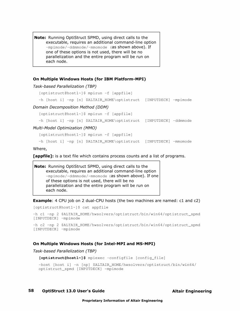
OptiStruct 13.0 User's Guide58 Altair Engineering
Proprietary Information of Altair Engineering
Note: Running OptiStruct SPMD, using direct calls to theexecutable, requires an additional command-line option –mpimode/-ddmmode/-mmomode (as shown above). If
one of these options is not used, there will be noparallelization and the entire program will be run oneach node.
On Multiple Windows Hosts (for IBM Platform-MPI)
Task-based Parallelization (TBP)
[optistruct@host1~]$ mpirun –f [appfile]
-h [host i] -np [n] $ALTAIR_HOME\optistruct [INPUTDECK] -mpimode
Domain Decomposition Method (DDM)
[optistruct@host1~]$ mpirun –f [appfile]
-h [host i] -np [n] $ALTAIR_HOME\optistruct [INPUTDECK] -ddmmode
Multi-Model Optimization (MMO)
[optistruct@host1~]$ mpirun –f [appfile]
-h [host i] -np [n] $ALTAIR_HOME\optistruct [INPUTDECK] -mmomode
Where,
[appfile]: is a text file which contains process counts and a list of programs.
Note: Running OptiStruct SPMD, using direct calls to theexecutable, requires an additional command-line option –mpimode/-ddmmode/-mmomode (as shown above). If one
of these options is not used, there will be noparallelization and the entire program will be run oneach node.
Example: 4 CPU job on 2 dual-CPU hosts (the two machines are named: c1 and c2)
[optistruct@host1~]$ cat appfile
-h c1 –np 2 $ALTAIR_HOME/hwsolvers/optistruct/bin/win64/optistruct_spmd [INPUTDECK] -mpimode
-h c2 –np 2 $ALTAIR_HOME/hwsolvers/optistruct/bin/win64/optistruct_spmd [INPUTDECK] –mpimode
On Multiple Windows Hosts (for Intel-MPI and MS-MPI)
Task-based Parallelization (TBP)
[optistruct@host1~]$ mpiexec –configfile [config_file]
-host [host i] –n [np] $ALTAIR_HOME/hwsolvers/optistruct/bin/win64/optistruct_spmd [INPUTDECK] -mpimode
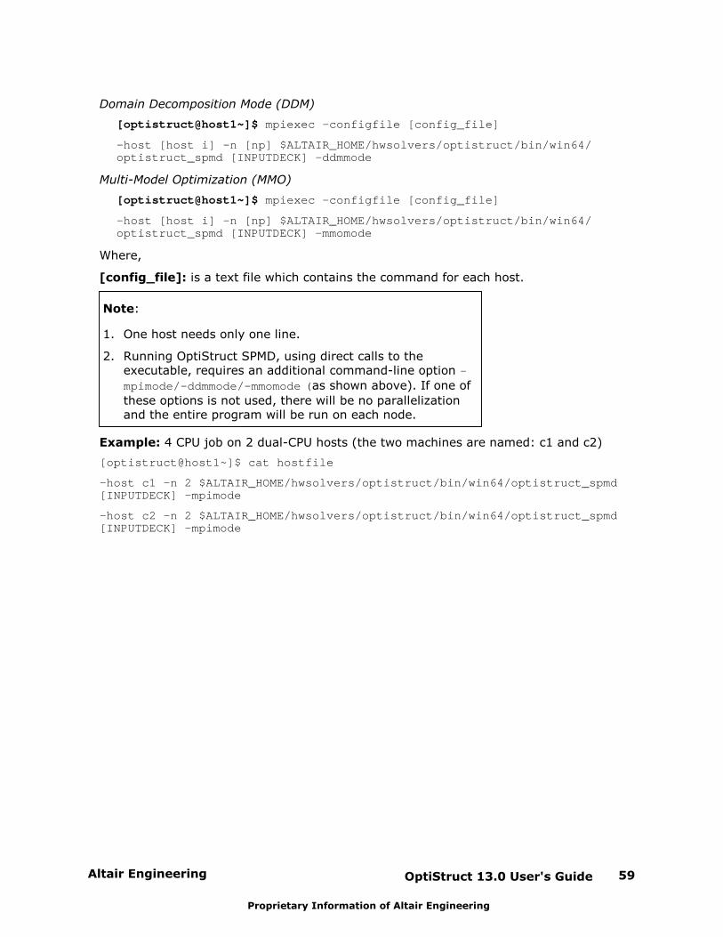
Altair Engineering OptiStruct 13.0 User's Guide 59
Proprietary Information of Altair Engineering
Domain Decomposition Mode (DDM)
[optistruct@host1~]$ mpiexec –configfile [config_file]
-host [host i] –n [np] $ALTAIR_HOME/hwsolvers/optistruct/bin/win64/optistruct_spmd [INPUTDECK] –ddmmode
Multi-Model Optimization (MMO)
[optistruct@host1~]$ mpiexec –configfile [config_file]
-host [host i] –n [np] $ALTAIR_HOME/hwsolvers/optistruct/bin/win64/optistruct_spmd [INPUTDECK] -mmomode
Where,
[config_file]: is a text file which contains the command for each host.
Note:
1. One host needs only one line.
2. Running OptiStruct SPMD, using direct calls to theexecutable, requires an additional command-line option –
mpimode/-ddmmode/-mmomode (as shown above). If one of
these options is not used, there will be no parallelizationand the entire program will be run on each node.
Example: 4 CPU job on 2 dual-CPU hosts (the two machines are named: c1 and c2)
[optistruct@host1~]$ cat hostfile
-host c1 –n 2 $ALTAIR_HOME/hwsolvers/optistruct/bin/win64/optistruct_spmd [INPUTDECK] -mpimode
-host c2 –n 2 $ALTAIR_HOME/hwsolvers/optistruct/bin/win64/optistruct_spmd [INPUTDECK] –mpimode
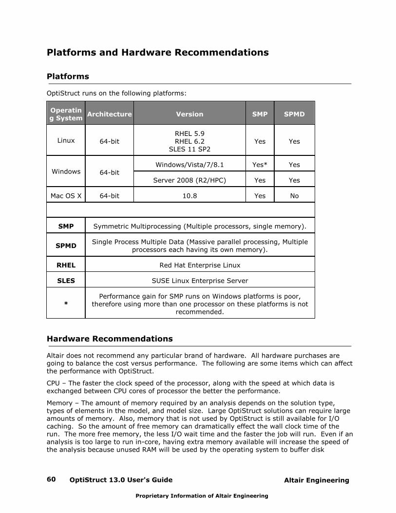
OptiStruct 13.0 User's Guide60 Altair Engineering
Proprietary Information of Altair Engineering
Platforms and Hardware Recommendations
Platforms
OptiStruct runs on the following platforms:
Operating System
Architecture Version SMP SPMD
Linux 64-bitRHEL 5.9RHEL 6.2
SLES 11 SP2Yes Yes
Windows 64-bitWindows/Vista/7/8.1 Yes* Yes
Server 2008 (R2/HPC) Yes Yes
Mac OS X 64-bit 10.8 Yes No
SMP Symmetric Multiprocessing (Multiple processors, single memory).
SPMDSingle Process Multiple Data (Massive parallel processing, Multiple
processors each having its own memory).
RHEL Red Hat Enterprise Linux
SLES SUSE Linux Enterprise Server
*Performance gain for SMP runs on Windows platforms is poor,
therefore using more than one processor on these platforms is notrecommended.
Hardware Recommendations
Altair does not recommend any particular brand of hardware. All hardware purchases aregoing to balance the cost versus performance. The following are some items which can affectthe performance with OptiStruct.
CPU – The faster the clock speed of the processor, along with the speed at which data isexchanged between CPU cores of processor the better the performance.
Memory – The amount of memory required by an analysis depends on the solution type,types of elements in the model, and model size. Large OptiStruct solutions can require largeamounts of memory. Also, memory that is not used by OptiStruct is still available for I/Ocaching. So the amount of free memory can dramatically effect the wall clock time of therun. The more free memory, the less I/O wait time and the faster the job will run. Even if ananalysis is too large to run in-core, having extra memory available will increase the speed ofthe analysis because unused RAM will be used by the operating system to buffer disk

Altair Engineering OptiStruct 13.0 User's Guide 61
Proprietary Information of Altair Engineering
requests.
Disk drives – OptiStruct solutions often require the writing of large temporary scratch files tothe hard drive. Therefore, it is important to have fast hard drives. The best solution is touse two or more fast hard drives in RAID 0 (striped) as a dedicated place for scratch filesduring the solution. A typical configuration is to have one drive for the operating system andsoftware, and then 2-15 drives striped together as the scratch space for the runs.
Interconnect – The parallel SPMD versions of OptiStruct can run on multiple processors and/or on multiple nodes in the cluster. To run parallel jobs on a cluster, each should haveenough RAM to run a full job in non-parallel mode. And, each node in a cluster should haveits own disk space that is sufficient to store all the scratch files on that node. Clusterarchitecture with separate disks for each node will achieve better performance than singleshared RAID array of disks. A fast interconnect is important, but anything over GigabitEthernet will not speed the solution visibly. When nodes use a shared scratch disk area, theinterconnect speed is a critical factor for all out-of-core jobs.
For a large NVH analysis, it is recommended to have at least 8 GB per CPU with at least 4disks in RAID 0 for temporary scratch files.
OptiStruct 13.0 User's Guide62 Altair Engineering
Proprietary Information of Altair Engineering
OptiStruct Configuration File
OptiStruct configuration files may be used to establish default settings for the OptiStruct. Configuration files must be named optistruct.cfg. Any errors or warnings caused by the
content of these files will be echoed to the screen only.
Any default setting will be ignored if it is defined by an environment variable (see RunningOptiStruct), bulk data input deck entry (see The Input File), or command line argument (seeRun Options for OptiStruct).
File Location
The configuration file allows default settings to be established on five different levels:
1. System level
If a configuration file is located in the ${ALTAIR_HOME}/hwsolvers directory, the
default settings defined in this file apply to all solver runs.
A configuration file is included in the installation at this location. This configurationfile contains all of the configuration file options in a comment format. Uncommentingan option will activate it. This file may be used as a template for all configurationfiles.
If the ${ALTAIR_HOME} environment variable is not set, then the configuration file at
this location will not be used. This variable is automatically set when therecommended HyperWorks installation and execution procedures are followed.
2. Corporate level
If a configuration file is located in the ${HW_CORPORATE_CUSTOMIZATION_DIR}
directory, the default settings defined in this file are added to the system defaults.
If a default setting, which was defined at the system level, is redefined at this level,the redefined setting is used.
If the ${HW_CORPORATE_CUSTOMIZATION_DIR} environment variable is not set, then
the configuration file at this location will not be used.
3. Group level
If a configuration file is located in the ${HW_GROUP_CUSTOMIZATION_DIR} directory,
the default settings defined in this file are added to the system and corporatedefaults.
If a default setting, which was defined at the system or corporate level, is redefinedat this level, the redefined setting is used.
If the ${HW_GROUP_CUSTOMIZATION_DIR} environment variable is not set, then the
configuration file at this location will not be used.
4. User level
If a configuration file is located in the ${HOME} directory, the default settings defined
in this file are added to the system, corporate and group defaults.
If a default setting, which was defined at the system, corporate or group level, isredefined at this level, the redefined setting is used.
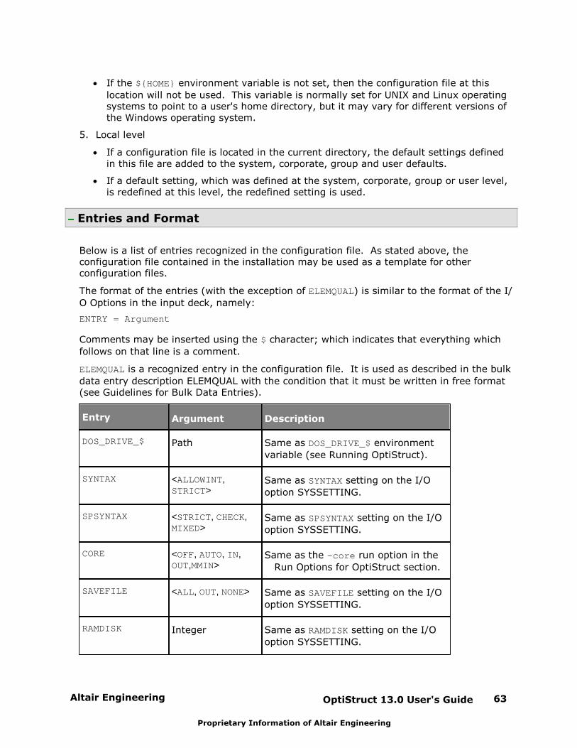
Altair Engineering OptiStruct 13.0 User's Guide 63
Proprietary Information of Altair Engineering
If the ${HOME} environment variable is not set, then the configuration file at this
location will not be used. This variable is normally set for UNIX and Linux operatingsystems to point to a user's home directory, but it may vary for different versions ofthe Windows operating system.
5. Local level
If a configuration file is located in the current directory, the default settings definedin this file are added to the system, corporate, group and user defaults.
If a default setting, which was defined at the system, corporate, group or user level,is redefined at this level, the redefined setting is used.
Entries and Format
Below is a list of entries recognized in the configuration file. As stated above, theconfiguration file contained in the installation may be used as a template for otherconfiguration files.
The format of the entries (with the exception of ELEMQUAL) is similar to the format of the I/
O Options in the input deck, namely:
ENTRY = Argument
Comments may be inserted using the $ character; which indicates that everything which
follows on that line is a comment.
ELEMQUAL is a recognized entry in the configuration file. It is used as described in the bulk
data entry description ELEMQUAL with the condition that it must be written in free format(see Guidelines for Bulk Data Entries).
Entry Argument Description
DOS_DRIVE_$ Path Same as DOS_DRIVE_$ environment
variable (see Running OptiStruct).
SYNTAX <ALLOWINT,STRICT>
Same as SYNTAX setting on the I/O
option SYSSETTING.
SPSYNTAX <STRICT, CHECK, MIXED>
Same as SPSYNTAX setting on the I/O
option SYSSETTING.
CORE <OFF, AUTO, IN,OUT,MMIN>
Same as the –core run option in the
Run Options for OptiStruct section.
SAVEFILE <ALL, OUT, NONE> Same as SAVEFILE setting on the I/O
option SYSSETTING.
RAMDISK Integer Same as RAMDISK setting on the I/O
option SYSSETTING.
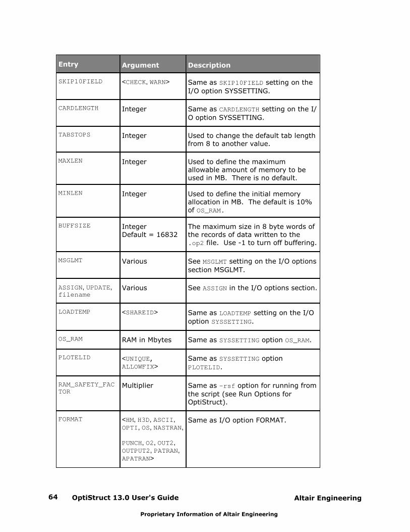
OptiStruct 13.0 User's Guide64 Altair Engineering
Proprietary Information of Altair Engineering
Entry Argument Description
SKIP10FIELD <CHECK, WARN> Same as SKIP10FIELD setting on the
I/O option SYSSETTING.
CARDLENGTH Integer Same as CARDLENGTH setting on the I/
O option SYSSETTING.
TABSTOPS Integer Used to change the default tab lengthfrom 8 to another value.
MAXLEN Integer Used to define the maximumallowable amount of memory to beused in MB. There is no default.
MINLEN Integer Used to define the initial memoryallocation in MB. The default is 10%of OS_RAM.
BUFFSIZE IntegerDefault = 16832
The maximum size in 8 byte words ofthe records of data written to the .op2 file. Use -1 to turn off buffering.
MSGLMT Various See MSGLMT setting on the I/O options
section MSGLMT.
ASSIGN, UPDATE,filename
Various See ASSIGN in the I/O options section.
LOADTEMP <SHAREID> Same as LOADTEMP setting on the I/O
option SYSSETTING.
OS_RAM RAM in Mbytes Same as SYSSETTING option OS_RAM.
PLOTELID <UNIQUE,ALLOWFIX>
Same as SYSSETTING option
PLOTELID.
RAM_SAFETY_FACTOR
Multiplier Same as -rsf option for running from
the script (see Run Options forOptiStruct).
FORMAT <HM, H3D, ASCII, OPTI, OS, NASTRAN, PUNCH, O2, OUT2, OUTPUT2, PATRAN, APATRAN>
Same as I/O option FORMAT.
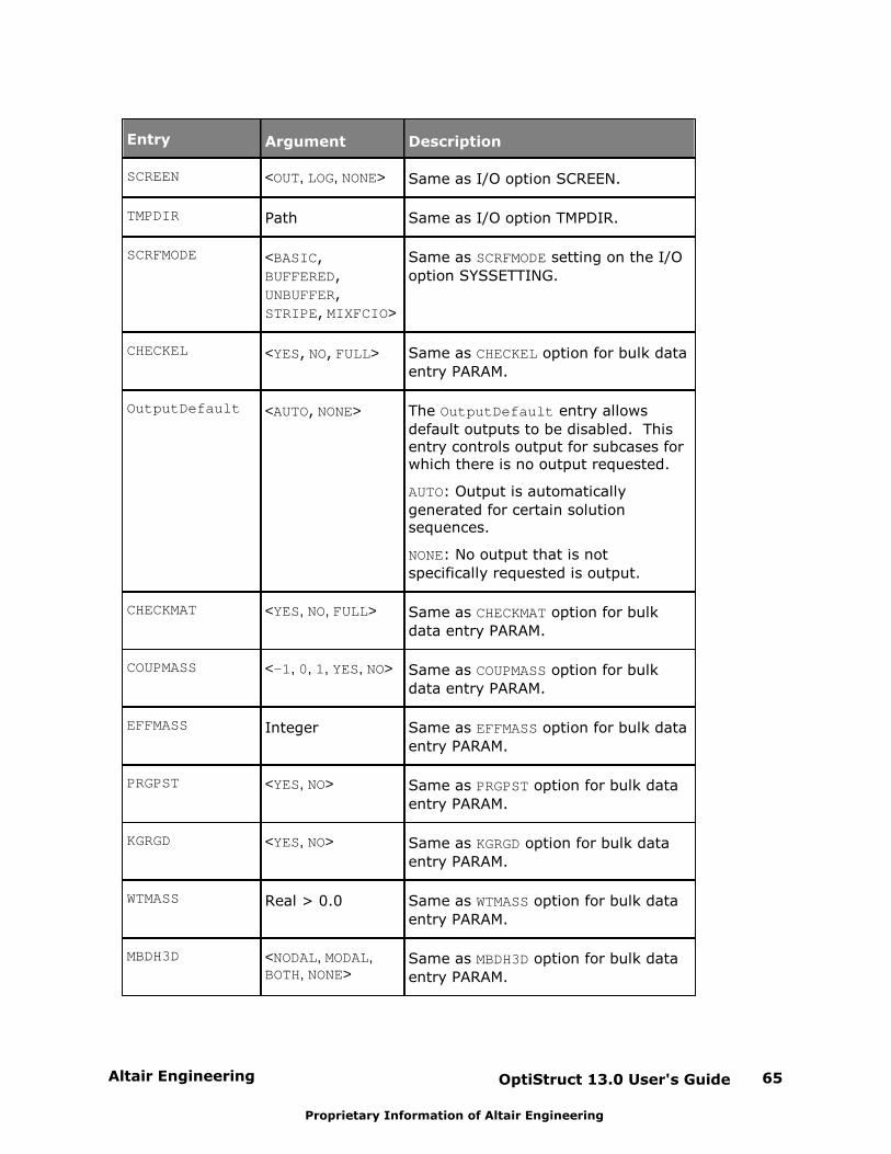
Altair Engineering OptiStruct 13.0 User's Guide 65
Proprietary Information of Altair Engineering
Entry Argument Description
SCREEN <OUT, LOG, NONE> Same as I/O option SCREEN.
TMPDIR Path Same as I/O option TMPDIR.
SCRFMODE <BASIC,
BUFFERED,
UNBUFFER,
STRIPE, MIXFCIO>
Same as SCRFMODE setting on the I/O
option SYSSETTING.
CHECKEL <YES, NO, FULL> Same as CHECKEL option for bulk data
entry PARAM.
OutputDefault <AUTO, NONE> The OutputDefault entry allows
default outputs to be disabled. Thisentry controls output for subcases forwhich there is no output requested.
AUTO: Output is automatically
generated for certain solutionsequences.
NONE: No output that is not
specifically requested is output.
CHECKMAT <YES, NO, FULL> Same as CHECKMAT option for bulk
data entry PARAM.
COUPMASS <-1, 0, 1, YES, NO> Same as COUPMASS option for bulk
data entry PARAM.
EFFMASS Integer Same as EFFMASS option for bulk data
entry PARAM.
PRGPST <YES, NO> Same as PRGPST option for bulk data
entry PARAM.
KGRGD <YES, NO> Same as KGRGD option for bulk data
entry PARAM.
WTMASS Real > 0.0 Same as WTMASS option for bulk data
entry PARAM.
MBDH3D <NODAL, MODAL, BOTH, NONE>
Same as MBDH3D option for bulk data
entry PARAM.

OptiStruct 13.0 User's Guide66 Altair Engineering
Proprietary Information of Altair Engineering
Entry Argument Description
FLEXH3D <AUTO, YES, NO> Same as FLEXH3D option for bulk data
entry PARAM.
USERAM RAM in Mbytes Same as SYSSETTING option USERAM.
Altair Engineering OptiStruct 13.0 User's Guide 67
Proprietary Information of Altair Engineering
Expanded Error Message File
OptiStruct Expanded Error Message files may be used to expand the error and warningmessages for the OptiStruct. In this way, you can customize the error and warningmessages so that they are more meaningful and informative for you and others in yourorganization. The Expanded Error Message file must be named optistruct_err.msg.
The file contains an expanded message for each message you wish to expand. If the samemessage is expanded in multiple files, then all expansions will be printed. The expandederror message is printed only for the first instance of the error.
The format of the file is to have four asterisks left justified on a line followed by the errornumber to be expanded. The next lines contain the expanded error message. An examplefor error 9009 and 9008 are below. Note that the order of the error message numbers doesnot matter.
**** 9009This error usually happens when there isnot enough room on the disk, but it canhappen also when one of the output filesdoes not have write permissions for thecurrent user, or when the directoryassigned for output or temporary filesdoes not exist, does not have writepermission or is located on a read-onlyfilesystem (e.g. on a CD). Please checkfollowing cards: OUTFILE, TMPDIR,EIGVSAVE, ASSIGN, or the command linearguments. Note that TMPDIR may belocated in any of config files, and (onUnix) the filenames may be affected byDos_drive conversion (e.g. DOS_DRIVE_nenvironment variable).
**** 9008This error usually happens when theinput file name is mistyped, either on acommand line or on any of followingcards: INFILE, INCLUDE, EIGVNAE,RESTART, LOADLIB, ASSIGN. It can alsohappen if the user does not have readpermission to an input file, or to anydirectory on a path leading to the inputfile.
File Location
The expanded error message file allows default settings to be established on four differentlevels:
1. System level
If an expanded error message file is located in the ${ALTAIR_HOME}/hwsolvers

OptiStruct 13.0 User's Guide68 Altair Engineering
Proprietary Information of Altair Engineering
directory, the expanded error messages defined in this file are added to all solverruns.
An expanded error message file is included in the installation at this location. Thisfile contains samples of expanded messages. This file may be used as a template forall expanded error message files.
If the ${ALTAIR_HOME} environment variable is not set, then the expanded error
message file at this location will not be used.
2. Corporate level
If an expanded error message file is located in the ${HW_CORPORATE_CUSTOMIZATION_DIR} directory, the expanded messages defined in
this file are added to the system expanded messages.
If the ${HW_CORPORATE_CUSTOMIZATION_DIR} environment variable is not set, then
the expanded error message file at this location will not be used.
3. Group level
If an expanded error message file is located in the ${HW_GROUP_CUSTOMIZATION_DIR}
directory, the expanded error message defined in this file are added to the systemand corporate messages.
If the ${HW_GROUP_CUSTOMIZATION_DIR} environment variable is not set, then the
expanded error message file at this location will not be used.
4. User level
If an expanded error message file is located in the ${HOME} directory, the expanded
error messages defined in this file are added to the system, corporate and groupexpanded error messages.
If the ${HOME} environment variable is not set, then the expanded error message file
at this location will not be used. This variable is normally set for UNIX and Linuxoperating systems to point to a user's home directory, but it may vary for differentversions of the Windows operating system.
Altair Engineering OptiStruct 13.0 User's Guide 69
Proprietary Information of Altair Engineering
Memory Limitations
32-bit Versus 64-bit Computations
On 64-bit machines, when using a 64-bit compiled version of OptiStruct and a 64-bitoperating system, OptiStruct can use all memory available in the system (real RAM andvirtual memory). There are still some size limitations as a result of the size of standardinteger variables, but they should only occur in very rare cases. Currently, OptiStruct is builtwith two versions of linear solvers: one using 32-bit integers, and the other one using 64-bitintegers. By default, the 32-bit solver is used (as it requires less memory/disk and runsvisibly faster), but the 64-bit solver is automatically selected when the size of a problemrequires it.
Virtual Versus Physical Memory
OptiStruct can use more memory than is actually installed on a given system (i.e. more thanthe installed RAM). This is what the virtual memory (swap space) is for. OptiStruct is moreefficient, however, if it uses only actual RAM (remember to allow some RAM to be used by theoperating system and other codes running at the same time). When more memory isrequested than actual available RAM, OptiStruct will run much slower due to swapping. Youwill hear disks working constantly with little CPU being used, and there will be a significantdifference between the elapsed time and the CPU time.
Memory specification for OptiStruct (using –len command line option) is actually only giving
OptiStruct a hint about the amount of physical RAM available for the run (i.e. it shouldspecify the amount of physical memory not used by the operating system and other runningprograms, and as explained above, always less than the total amount of RAM in thecomputer). Based on this information, OptiStruct will try to use the fastest algorithm whichcan run within the specified amount of memory. If no such algorithm is available, then thealgorithm with minimum memory requirement will be used. Specifying a larger value for –
len than the amount of physical RAM may cause excessive swapping during computations,
and will significantly slow down the solution process.
On most machines OptiStruct asks operating systems for information about availablememory. This information is printed in the header of the .out file, and can be used to issue
a warning, when it is possible that the run may fail because of lack of this resource. Thisinformation is dynamic (changes with other programs running at the machine) and thereforeis never used inside OptiStruct – user supplied information (example: with –len argument or
from the config file) is used instead.
Automatic Memory Allocation Versus Fixed Memory Runs
In standard modes of operation, OptiStruct automatically estimates the amount of memoryrequired, and this memory is requested in successive steps from the operating system. Sometimes the memory could be used more efficiently if requested at once and not inincrements. This can be done using the "-fixlen" command line option (see Run Options).
When using the "-fixlen" option, OptiStruct may start to run, but fail after some time with a
memory allocation error. This can happen when almost all available memory is requested by
OptiStruct 13.0 User's Guide70 Altair Engineering
Proprietary Information of Altair Engineering
the "-fixlen" argument, because in addition to the memory required by the OptiStruct
solver, OptiStruct launches a bandwidth minimizer, which uses an additional small amount ofmemory. Requesting slightly less memory with the "-fixlen" option is a possible solution.
Again, you see that it is incorrect to assign too much memory to OptiStruct.
Additional Control of Used Memory
OptiStruct has new command line argument "-maxlen" which can be used in automatic
mode. This switch can be useful in some batch scheduling installations, as it will not allowOptiStruct to use more than a given amount of memory. Note that for models which requiremore memory than allowed by this argument, OptiStruct will abort during the solution,potentially after spending some time in computations.
OptiStruct has a new command line argument “-uselen” which can be used in automatic
mode. –uselen is used to specify an increased dynamic memory usage limit. If –uselen is
not defined, then the algorithms which may use variable amount of memory try to use asminimal an amount as possible. When this option is used, OptiStruct will use more than theminimum memory required, up to this limit, but only when it improves the speed of thesolution. This value is used only for some solution sequences, which can profit fromadditional memory available (for example, to use bigger buffers to store intermediateresults).
This value is automatically limited by the value specified by –len, so –uselen can be set
safely to a very large value.
(Example: optistruct infile.fem –uselen 32)
Best practices for –uselen specification:
The speed gain is usually modest, and is limited to certain solution sequences, therefore, thisrun option should not be used unless solution speed is critical and excess memory isavailable. For single-user hosts, it is useful to set this value to the same as –len (or higher).
This maximizes the use of available memory to achieve possible better performance.
Different values of this run option may be used on systems shared by multiple jobs (forexample HyperMesh or other solvers). In such scenarios, using a lower value of this runoption (or not using it at all), will result in a lower use of memory and may improve overallspeed an response time.
OptiStruct Configuration File
All options for memory control can be specified in the OptiStruct Configuration File, however,this is not advisable if the configuration file is shared on the common file server. Theconfiguration files should be tuned for specific hardware independently, and should be placedin the configuration file local to each machine.

Altair Engineering OptiStruct 13.0 User's Guide 71
Proprietary Information of Altair Engineering
Restarting OptiStruct
It is possible to restart an OptiStruct optimization by using the command line option -
restart (see Run Options), by adding the I/O option RESTART to the input file, or from the
OptiStruct panel in HyperMesh.
To restart an optimization, you will need information about the final iteration of the previousoptimization run. This information is stored in the .sh file.
The DESMAX entry on the DOPTPRM card, in the .fem file, specifies the maximum number of
additional iterations. To perform an analysis on the optimized structure, restart with DESMAX
set to 0. If DESMAX is not defined, then the default value of DESMAX is assumed (30 iterations
is the default value for DESMAX unless topology manufacturing constraints are used, in which
case the default is 80 iterations).
There are a number of conditions that must be observed when restarting an optimization:
The number of design variables or design elements cannot be changed.
It is invalid to restart with minimum member size control removed if it was present inthe original run.
It is invalid to restart with checkerboard control turned on if it was not activated in theoriginal run. It is, however, acceptable to deactivate checkerboard control in the restartif it was activated in the original run.
It is invalid to restart with manufacturing constraints that differ from those of theoriginal run.
The purpose of the restart functionality is for restarting with unconverged optimization runsor optimization runs that were terminated before completion (due to a power outage, etc.).
Output files from a restart run are appended with the extension _rst#, where # is a 3 digit
number indicating the starting iteration for the restart run. For example, filename_rst030.out is the .out file created when restarting filename.fem from iteration
30.
Iterations for the restart are numbered starting with the iteration number in the .sh file (the
last iteration from the previous run).
You may manually append new .dens, .disp, and .strs files to old ones and post-process
the combined files.
OptiStruct 13.0 User's Guide72 Altair Engineering
Proprietary Information of Altair Engineering
OptiStruct Compression Run
The OptiStruct solver can be used as a simple input deck preprocessor, intended to reduceout matching material and property definitions. It is useful for models (produced on somesimpleminded mesh generator tools) which sometimes have unique property IDs and uniquematerial IDs assigned to each element, even in cases where actual data is identical. Suchmodels (although technically correct) will be expensive to solve, or slow to process inHyperMesh or HyperView. In this special run mode, OptiStruct will simply read the model,compare all material and property data, and remove redundant data.
Example of Run
optistruct infile.fem -compress
will produce a new bulk data file named:
infile.echo
which will contain a new model with all duplicate materials and properties deleted. Allreferences to removed data will be replaced with the remaining ones, so for all practicalpurposes the model should yield identical results.
The additional argument to -compress represents the tolerance value in percent. All floating
point values in material and property data are compared using that tolerance. Usingtolerance may increase significantly run time.
Restrictions
1. Comparison is performed exactly (meaning all data are compared without allowing for anytolerance or round-off). If optional tolerance value is specified, then the run is performedin two passes: exact matches are removed first, then all remaining materials andproperties are compared with each other using following formula:
(2 * abs(value1-value2)) / (abs(value1)+abs(value2)) < tolerance *0.01.
2. Optimization data, nonlinear data, and thermal materials are not processed. If such dataare present they may reference removed entities, but a compress run will not adjustreferences. The resulting file (<filename>.echo) may not be valid.
3. Cards which extend or modify Materials or Properties (such as MATT1, MATX02, MATS1,or PSHELLX) are not used in comparison, and can also be left orphaned as a result of acompress run.
4. SETs referencing Materials or Properties are not processed. This will not result in a baddeck because SETs are allowed to reference non-existent IDs, however SETs in the outputfile may be different from the input file.
5. After the .echo file is produced, OptiStruct terminates the run, therefore -compress
cannot be combined with any other option.

Altair Engineering OptiStruct 13.0 User's Guide 73
Proprietary Information of Altair Engineering
The following cards are processed:
1. Properties:
PBEAM, PBAR, PBEAML, PBARL, PSOLID (also fluid), PCOMP, PSHELL, PROD, PWELD, andPSHEAR
as well as properties not referring to materials:
PELAS, PBUSH, PVISC, PDAMP, PGAP, PCONT, PAABSF, and PACABS.
2. Materials:
MAT1, MAT2, MAT4, MAT5, MAT8, MAT9, and MAT10.
3. All elements referencing properties or materials, including PRBODY and PFBODY.
Any other cards present in the deck are allowed only if they do not reference materials orproperties; however OptiStruct does not verify this assumption. If such a card is present inthe deck (for example, DTPG referring to a list of properties), it may be printed with negativeIDs for removed entities.
The resulting file (<filename>.echo) is produced using the same routines which produce
ECHO; all restrictions present for ECHO will affect a -compress run; in particular:
Some optimization cards are currently known to produce incorrect ECHO, meaning anECHO of these cards cannot be read back into OptiStruct.
Results are formatted in fixed format, irrespective of the format used in the input file. This limits the accuracy of most coefficients because of 8 character fields. Currentformatting preserves as many decimal places as possible within 8 characters, but forvalues which require an exponential form, it is sometimes possible to retain accuracy toonly 3-4 decimal places. Exceptions: GRID and DMIG cards are printed in free formatwith accuracy to at least 10 decimal places.
Only bulk data is printed to .echo file (no i/o or control sections).
Some cards are not printed: in particular, PARAM and DOPTRM do not appear in ECHOfiles.

OptiStruct 13.0 User's Guide74 Altair Engineering
Proprietary Information of Altair Engineering
Structural Analysis
The Structural Analysis section provides an overview of the following analyses:
Linear Static Analysis
Linear Buckling Analysis
Nonlinear Analysis
Normal Modes Analysis
Frequency Response Analysis
Complex Eigenvalue Analysis
Random Response Analysis
Response Spectrum Analysis
Transient Response Analysis

Altair Engineering OptiStruct 13.0 User's Guide 75
Proprietary Information of Altair Engineering
Linear Static Analysis
The basic finite element equation to be solved for structures experiencing static loads can beexpressed as:
Ku P
Where, K is the stiffness matrix of the structure (an assemblage of individual element
stiffness matrices). The vector u is the displacement vector, and P is the vector of loads
applied to the structure. The above equation is the equilibrium of external and internalforces.
The stiffness matrix is singular, unless displacement boundary conditions are applied to fixthe rigid body degrees of freedom of the model.
The equilibrium equation is solved either by a direct or an iterative solver. By default, thedirect solver is invoked, whereby the unknown displacements are simultaneously solvedusing a Gauss elimination method that exploits the sparseness and symmetry of the stiffnessmatrix, K, for computational efficiency. Alternatively, an iterative solver using the
preconditioning conjugate gradient method may be used. While the direct solver is veryrobust, accurate and efficient, the iterative solver is sometimes superior, in terms of speed,for thick-walled solid structures. The iterative solver is selected through the SOLVTYPsubcase information entry, which in turn references a SOLVTYP bulk data entry.
Once the unknown displacements at the nodal points of the elements are calculated, thestresses can be calculated by using the constitutive relations for the material. For linear
static analysis where the deformations are in the elastic range, ta=hat is the stresses, , are
assumed to be linear functions of the strains, , Hooke’s law can be used to calculate thestresses. Hooke’s law can be stated as:
C
with the elasticity matrix C of the material. The strains are a function of the
displacements.
The static loads and boundary conditions are defined in the bulk data section of the inputdeck. They need to be referenced in the subcase information section using an SPC and LOADstatement in a SUBCASE. Each SUBCASE defines a load vector. Thermal loading is definedby referencing bulk data entries with the TEMPERATURE statement in a SUBCASE.
Unconstrained models can be solved using inertia relief. SUPORT1 subcase statements canthen reference the boundary conditions that restrain the rigid body motions. Up to sixdegrees of freedom can be restrained. These restraints can also be defined without subcasereference using the SUPORT bulk data entry or automated using PARAM, INREL, -2.
OptiStruct 13.0 User's Guide76 Altair Engineering
Proprietary Information of Altair Engineering
Linear Buckling Analysis
The problem of linear buckling in finite element analysis is solved by first applying areference level of loading, PRef , to the structure. A standard linear static analysis is then
carried out to obtain stresses which are needed to form the geometric stiffness matrix KG.
The buckling loads are then calculated by solving an eigenvalue problem:
0GK K x
Where, K is the stiffness matrix of the structure and is the multiplier to the reference load.
The solution of the eigenvalue problem generally yields n eigenvalues , where n is thenumber of degrees of freedom (in practice, only a subset of eigenvalues is usuallycalculated). The vector x is the eigenvector corresponding to the eigenvalue.
The eigenvalue problem is solved using a matrix method called the Lanczos method. Not alleigenvalues are required. Only a small number of the lowest eigenvalues are normallycalculated for buckling analysis.
The lowest eigenvalue Cr is associated with buckling. The critical or buckling load is:
ReCr Cr fP P
In order to run a linear buckling analysis, an EIGRL bulk data entry needs to be givenbecause it defines the number of modes to be extracted. The EIGRL card needs to bereferenced by a METHOD statement in a SUBCASE in the subcase information section. Inaddition, it is necessary to use a STATSUB card to reference the appropriate referential staticloading, fre , SUBCASE. STATSUB cannot refer to a subcase that uses inertia relief.
The buckling analysis will ignore zero-dimensional elements, MPC, RBE3, and CBUSHelements. These elements can be used in buckling analysis, but they do not contribute to thegeometric stiffness matrix, KG. By default, the contribution from the rigid elements to the
geometric stiffness matrix is not included. You have to add PARAM,KGRGD,YES to the bulkdata section to include the contribution of rigid elements to the geometric stiffness matrix.
In addition, through the EXCLUDE subcase information entry, you may decide to omit thecontribution of other elements to the geometric stiffness matrix, effectively allowing you tocontrol which parts of the structure are analyzed for buckling. The excluded properties areonly removed from the geometric stiffness matrix, resulting in a buckling analysis with elasticboundary conditions. This means that the excluded properties may still be showingmovement in the buckling mode.
Buckling analysis cannot be performed if the referential static loading subcase uses inertiarelief. In such cases, the stiffness matrix is positive semi-definite and the bucklingeigenvalue solution ends in singularity.
Linear Buckling and Offset Elements
Some one-dimensional and shell elements can use offset to “shift” the element stiffnessrelative to the location determined by element’s nodes. For example, shell elements can beoffset from the plane defined by element nodes by means of ZOFFS. In this case all other
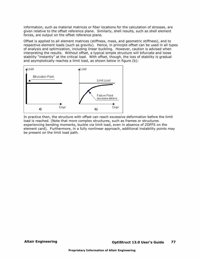
Altair Engineering OptiStruct 13.0 User's Guide 77
Proprietary Information of Altair Engineering
information, such as material matrices or fiber locations for the calculation of stresses, aregiven relative to the offset reference plane. Similarly, shell results, such as shell elementforces, are output on the offset reference plane.
Offset is applied to all element matrices (stiffness, mass, and geometric stiffness), and torespective element loads (such as gravity). Hence, in principle offset can be used in all typesof analysis and optimization, including linear buckling. However, caution is advised wheninterpreting the results. Without offset, a typical simple structure will bifurcate and loosestability “instantly” at the critical load. With offset, though, the loss of stability is gradualand asymptotically reaches a limit load, as shown below in figure (b):
In practice then, the structure with offset can reach excessive deformation before the limitload is reached. (Note that more complex structures, such as frames or structuresexperiencing bending moments, buckle via limit load, even in absence of ZOFFS on theelement card). Furthermore, in a fully nonlinear approach, additional instability points maybe present on the limit load path.

OptiStruct 13.0 User's Guide78 Altair Engineering
Proprietary Information of Altair Engineering
Nonlinear Analysis
Nonlinear Quasi-Static Analysis
Large Displacement Nonlinear Static Analysis
Geometric Nonlinear Analysis
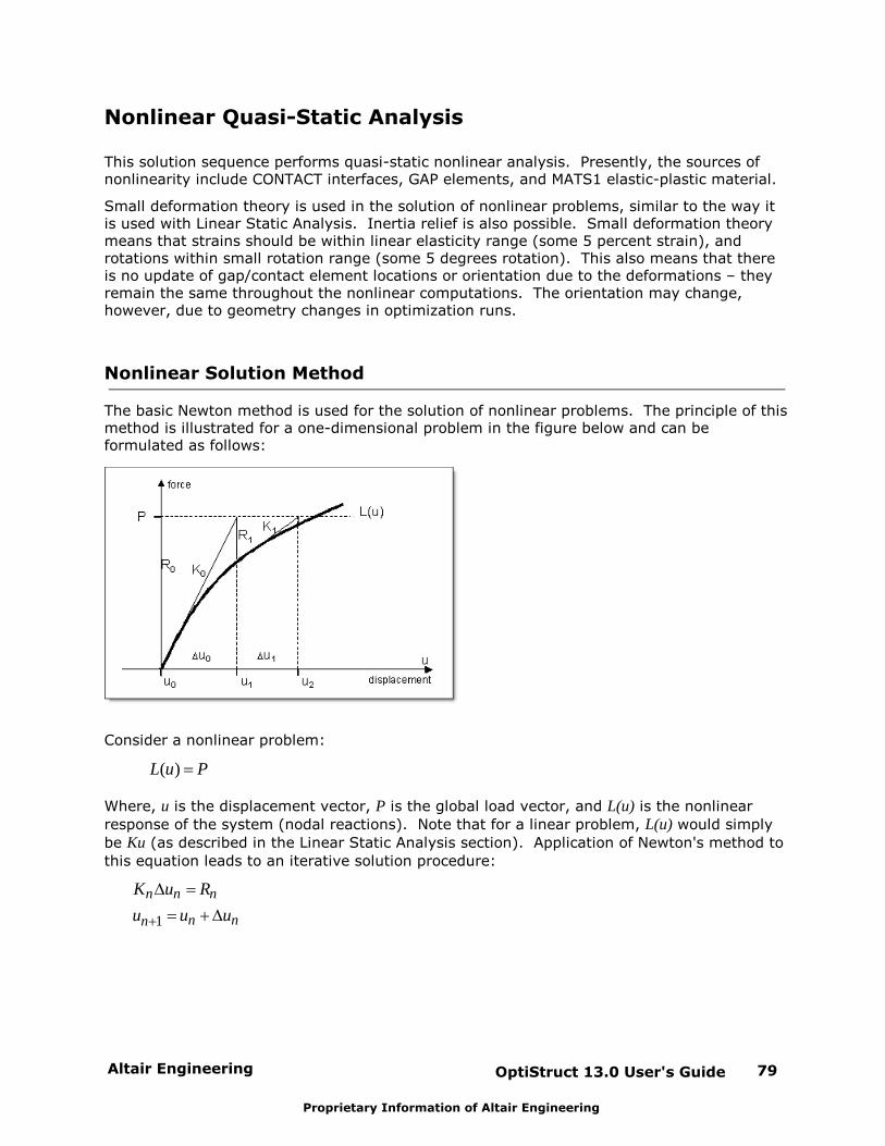
Altair Engineering OptiStruct 13.0 User's Guide 79
Proprietary Information of Altair Engineering
Nonlinear Quasi-Static Analysis
This solution sequence performs quasi-static nonlinear analysis. Presently, the sources ofnonlinearity include CONTACT interfaces, GAP elements, and MATS1 elastic-plastic material.
Small deformation theory is used in the solution of nonlinear problems, similar to the way itis used with Linear Static Analysis. Inertia relief is also possible. Small deformation theorymeans that strains should be within linear elasticity range (some 5 percent strain), androtations within small rotation range (some 5 degrees rotation). This also means that thereis no update of gap/contact element locations or orientation due to the deformations – theyremain the same throughout the nonlinear computations. The orientation may change,however, due to geometry changes in optimization runs.
Nonlinear Solution Method
The basic Newton method is used for the solution of nonlinear problems. The principle of thismethod is illustrated for a one-dimensional problem in the figure below and can beformulated as follows:
Consider a nonlinear problem:
( )L u P
Where, u is the displacement vector, P is the global load vector, and L(u) is the nonlinear
response of the system (nodal reactions). Note that for a linear problem, L(u) would simply
be Ku (as described in the Linear Static Analysis section). Application of Newton's method to
this equation leads to an iterative solution procedure:
1
n n n
n nn
K u R
u u u
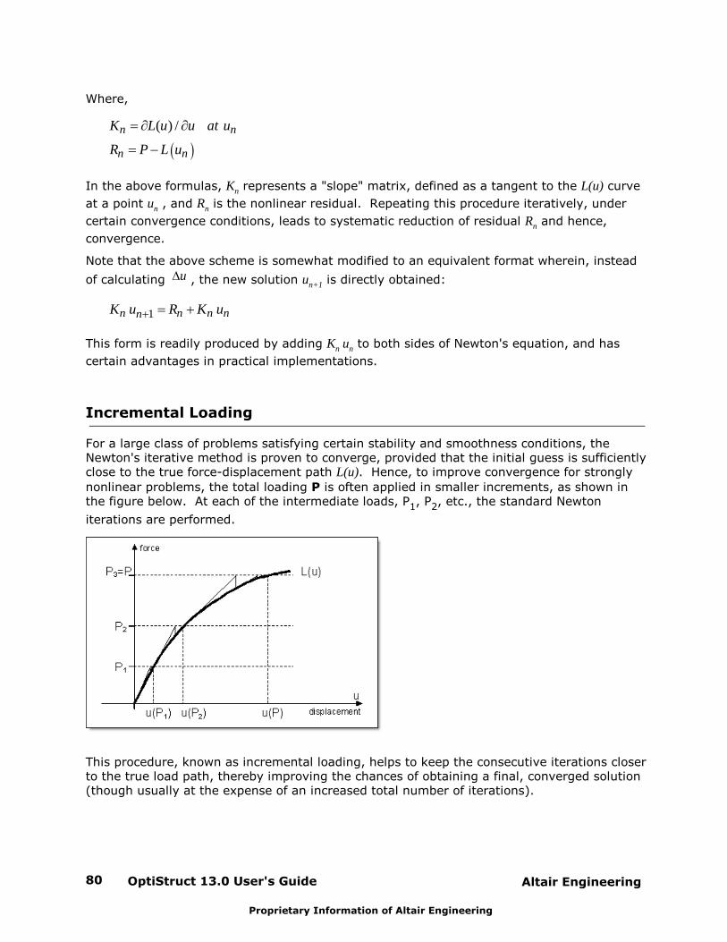
OptiStruct 13.0 User's Guide80 Altair Engineering
Proprietary Information of Altair Engineering
Where,
( ) /n n
n n
K L u u at u
R P L u
In the above formulas, Kn represents a "slope" matrix, defined as a tangent to the L(u) curve
at a point un , and Rn is the nonlinear residual. Repeating this procedure iteratively, under
certain convergence conditions, leads to systematic reduction of residual Rn and hence,
convergence.
Note that the above scheme is somewhat modified to an equivalent format wherein, instead
of calculating u , the new solution un+1 is directly obtained:
1n n n nnK u R K u
This form is readily produced by adding Kn un to both sides of Newton's equation, and has
certain advantages in practical implementations.
Incremental Loading
For a large class of problems satisfying certain stability and smoothness conditions, theNewton's iterative method is proven to converge, provided that the initial guess is sufficientlyclose to the true force-displacement path L(u). Hence, to improve convergence for strongly
nonlinear problems, the total loading P is often applied in smaller increments, as shown inthe figure below. At each of the intermediate loads, P1, P2, etc., the standard Newton
iterations are performed.
This procedure, known as incremental loading, helps to keep the consecutive iterations closerto the true load path, thereby improving the chances of obtaining a final, converged solution(though usually at the expense of an increased total number of iterations).
Altair Engineering OptiStruct 13.0 User's Guide 81
Proprietary Information of Altair Engineering
Nonlinear Convergence Criteria
In order to assess whether the nonlinear process has converged, a number of convergencecriteria are available. These criteria and respective tolerances can be selected on the NLPARM bulk data card. The basic principle in assessing nonlinear convergence is tocompare an error measure of the solution with a pre-determined tolerance level. When theerror falls below the prescribed tolerance, the problem is considered converged. In a case ofmultiple, simultaneous convergence criteria, all criteria need to be satisfied for the solutionto be converged.
The relative error in displacements (printed in the convergence summary as EUI) iscalculated as:
1UA uq
Eq A u
Here, A is a normalizing vector consisting of square roots of diagonal elements of stiffness
matrix 1 iiK A K
and the vector norm II. II is calculated as:
i ii
A u A u
Furthermore, q is a contraction factor that corrects the increment of solution nu to better
represent the actual error in the nonlinear solution. It is expressed as:
1
n
n
uq
u
In order to stabilize the behavior of q in practical computations, it is updated iteratively
according to the formula:
11
2 13 3
nn n
n
uq q
u
starting from initial value q1 = 0.99. Note that the contraction factor is meaningful when the
solution is close to having converged – it then reasonably well estimates the actual errorremaining in the nonlinear solution.
The relative error in terms of loads (printed in convergence summary as EPI) measures therelative strength of the residual R, and is calculated as:
P
R uE
P u
The load vector P in this formula includes nodal reactions due to prescribed displacements.
OptiStruct 13.0 User's Guide82 Altair Engineering
Proprietary Information of Altair Engineering
The relative error in terms of work (printed in convergence summary as EWI) measuresthe relative change in solution energy, and is calculated as:
W
R uE
P u
Note that the above norms only measure the error of the nonlinear iterative process. Theirvalues do not represent the accuracy of the finite element solution, only the fact that thenonlinear process has converged properly.
Nonlinear Problem Setup
The setup for the nonlinear solution is very straightforward. The static loads and boundaryconditions are defined in the bulk data section of the input deck. They need to be referencedin the subcase information section using an SPC and LOAD statement in a SUBCASE. EachSUBCASE defines a load vector. Loads or enforced displacements are not mandatory fornonlinear quasi-static solutions, if GAP or CONTACT elements are present in the model.
Unconstrained models can be solved using inertia relief. SUPORT1 subcase statements canthen reference the boundary conditions that restrain the rigid body motions. Up to sixdegrees of freedom can be restrained. These restraints can also be defined without subcasereference using the SUPORT bulk data entry or automated using PARAM, INREL, -2.
To indicate that a nonlinear solution is required for any subcase, a subcase informationcommand NLPARM needs to be present for the subcase. This command, in turn, points to thebulk data NLPARM card that contains the convergence tolerances and other nonlinearparameters.
Example:
SUBCASE 10 SPC = 1 LOAD = 2 NLPARM = 99..BEGIN BULKNLPARM 99 12 UPW+1.1e-5
.
Note that nonlinear gap and contact analysis are also supported in optimization.
Nonlinear Convergence Considerations
The Newton's method is a reliable tool for the solution of nonlinear problems and can providea fast quadratic convergence rate. However, convergence is not guaranteed under allcircumstances. Contact problems, especially those with friction, often cause convergencedifficulties.
In order to improve the chances of a successfully converged solution, methods have beenbuilt in to help problems converge that would otherwise oscillate back-and-forth and never
Altair Engineering OptiStruct 13.0 User's Guide 83
Proprietary Information of Altair Engineering
converge. One method involves a "sticky gap," wherein a residual stickiness is introduced toprevent the "undecided" nodes from bouncing in and out of contact. Another method is gap/contact status freezing where, after a number of oscillating iterations, gap/contact elementsare not allowed to change their open/closed status. Note that these methods are activatedonly for near-converging yet stagnated problems, and do not interfere with converging (orradically diverging) cases.
User's Considerations for Nonlinear Convergence
There are a number of precautions you can take to increase the chances of a successfulconvergence.
Realistic Problem Setup
Make sure that the nonlinear problem represents a realistic physical situation for which afeasible solution exists. In particular, special care needs to be taken in selecting the properorientation of gap elements. This is especially important when using a prescribed gapcoordinate system. See the description of the CGAP and CGAPG elements for more details.
Sufficient Support
Since gap/contact elements only provide one-way support, it is possible to formulate theproblem in such a way that the individual components will have rigid body freedom undercertain loading conditions. This will manifest as zero pivot in the solution process. To avoidsuch situations, it is advisable to provide sufficient support to all components so that, evenwithout gap/contact elements, there are no rigid body modes. If "solid" supports are notfeasible for all parts (the part needs to move), a very weak set of springs can be used toprevent the part from "flying away" when gap/contact elements are not engaged. Thestiffness of such auxiliary springs can be selected so as to allow for large motion of the part,compatible with the overall size of the model. If the gap elements and contact interfaces areproperly set up, such weak springs will exert virtually no effect when the solution hasconverged.
Reasonable Gap Stiffness
The gap stiffness values KA and KT essentially represent penalty springs that are hard enoughto prevent perceptible penetration of contacting nodes. While, theoretically, higher stiffnessvalues enforce the contact conditions more precisely, excessively high values may causedifficulties in convergence or poor conditioning of the stiffness matrix (this is especially truefor KT). If any such symptoms are observed, it may be beneficial to reduce the value of gapstiffness. As a baseline recommendation, a reasonable range of gap stiffness is of the orderof:
3 610 10 * *to E h
Where, E is the typical value of elastic modulus and h is the typical element size in the area
surrounding the gap elements. Such range will generally keep the gap penetration below onethousandth / one millionth of the element size, respectively. A good value for KT is of theorder of 0.1*KA.
To facilitate reasonable values of KA and KT, OptiStruct supports the automatic calculation ofthese parameters, specifically:
OptiStruct 13.0 User's Guide84 Altair Engineering
Proprietary Information of Altair Engineering
Option KA=AUTO determines the value of KA for each gap element using the stiffnessof surrounding elements. Additional options SOFT and HARD create respectively softeror harder penalties. SOFT can be used in cases of convergence difficulties and HARDcan be used if undesirable penetration is detected in the solution.
Option KT=AUTO automatically calculates the value of KT. If MU1>0, the result here isthe same as with blank KT -- its value is calculated as MU1*KA. However, if MU1=0 orblank, KT=AUTO produces a non-zero value of KT, calculated as KT=0.1*KA. Therefore, KT=AUTO can be used to prescribe enforced stick conditions.
Friction
The presence of friction, due to its strongly nonlinear, non-conservative nature, may causedifficulties in nonlinear convergence, especially when sliding is present. Therefore, solvingthe problem without friction can often provide convergence in otherwise failing problems. Or,in cases when presence of frictional resistance is necessary and minimal sliding is expected,enforcing a stick condition may be a viable solution, and will often lead to a betterconvergence than Coulomb friction (see the PGAP and PCONT bulk data card for details). Note that in cases of larger sliding motions, the stick condition may lead to divergencethrough a "tumbling" mode.
Gap Offset
In order to provide theoretical correctness, friction produces bending moments in gap/contactelements of non-zero length (this results from the transfer of frictional force from the contactsurface to the end nodes). This offset operation can, however, cause convergence problemsand counter-intuitive results. In problems with friction, it may be advisable to turn off theoffset operation via a parameter:
GAPPRM,GAPOFFS,NO
This will produce more intuitive results in the presence of friction. However, it may violatethe rigid body balance of the body, and should therefore be used with caution, especially forproblems without full SPC support. See the PGAP and PCONT bulk data card for details.
Incremental Loading
If the nonlinear procedure diverges in spite of taking the measures described above, theincremental loading procedure (applying the total load in a number of increments) can beused to achieve convergence. See the description of the NLPARM bulk data card for details. Note, however, that if the problem is incorrectly formulated (the solution exhibits excessivedeformations, free rigid body motions, an ill-conditioned stiffness matrix, extremely highnonlinear error, etc.), then incremental loading cannot be counted on to provide a convergedsolution.
Nonlinear Expert System
In some difficult to converge cases an expert system can be used to achieve convergence:
PARAM,EXPERTNL,YES
The expert system will try to adjust the load increment and other nonlinear parameters toachieve convergence. Note, however, that if the problem is incorrectly formulated (thesolution exhibits excessive deformations, free rigid body motions, an ill-conditioned stiffnessmatrix, extremely high nonlinear error, etc.), then expert system cannot be counted on toprovide a converged solution.
Moreover, in some cases it can lead to long computational times without success. This may

Altair Engineering OptiStruct 13.0 User's Guide 85
Proprietary Information of Altair Engineering
be due to using very small load increments or re-running the solution with modified nonlinearparameters.
OptiStruct 13.0 User's Guide86 Altair Engineering
Proprietary Information of Altair Engineering
Large Displacement Nonlinear Static Analysis
Large displacement nonlinear static analysis is used for the solution of problems wherein theload-response relationship is nonlinear and structural large displacements are involved. Thesource of this nonlinearity can be attributed to multiple system properties, for example,materials, geometry, nonlinear loading and constraint. Currently, in OptiStruct the followinglarge displacement nonlinear capabilities are available, including large strain elasto-plasticity,hyperelasticity of polynomial form, contact with small tangential motion, and rigid bodyconstraints.
Geometric Nonlinearity
In analyses involving geometric nonlinearity, changes in geometry as the structure deformsare considered in formulating the constitutive and equilibrium equations. Many engineeringapplications require the use of large deformation analysis based on geometric nonlinearity.Applications such as metal forming, tire analysis, and medical device analysis. Smalldeformation analysis based on geometric nonlinearity is required for some applications, likeanalysis involving cables, arches and shells. Such applications involve small deformation,except finite displacement or rotation.
Material Nonlinearity
Material nonlinearity involves the nonlinear behavior of a material based on currentdeformation, deformation history, rate of deformation, temperature, pressure, and so on.
Constraint and Contact Nonlinearity
Constraint nonlinearity in a system can occur if kinematic constraints are present in themodel. The kinematic degrees of freedom of a model can be constrained by imposingrestrictions on its movement. In OptiStruct, constraints are enforced with Lagrangemultipliers.
In the case of contact, the constraint condition is based on inequalities and such a constraintgenerally does not allow penetration between any two bodies in contact.
Nonlinear Solution Method
Nonlinear problems are generally history dependent. In order to achieve a certain level ofaccuracy, the solution must be obtained in a series of small increments. For this purpose weneed to solve the equilibrium equation at each increment and a corresponding increment sizeis selected.
Newton’s method is used to solve the nonlinear equilibrium equation in OptiStruct. If thesolution is smooth, quadratic of rate of convergence may be achieved when compared withother methods. This method is also very robust in highly nonlinear situations.
Choosing a suitable time increment is very important. In OptiStruct, an automatic timeincrement control is available. It should be suitable for a wide range of nonlinear problemsand, in general, is a very reliable approach.
The automatic time increment control functionality measures the difficulty of convergence atthe current increment. If the calculated number of iterations is equal to optimal number ofiterations for convergence, OptiStruct will proceed with the same increment size. If a lessernumber of iterations is required to achiever convergence, the increment size will be increasedfor next increment. Similarly if it is determined that too many iterations are required, thecurrent increment will be attempted again with a smaller increment size.
Altair Engineering OptiStruct 13.0 User's Guide 87
Proprietary Information of Altair Engineering
Nonlinear Large Displacement Analysis Problem Setup
The setup for the large displacement nonlinear static solution is straightforward.
1. PARAM, LGDISP,1 is used to activate large displacement analysis.
2. To indicate that a nonlinear solution is required for any subcase, the NLPARM subcaseinformation entry should be included in the corresponding subcase.
3. This subcase entry, in turn, references a NLPARM bulk data entry that contains theconvergence tolerances and other nonlinear parameters.
4. If constraints or contacts are defined in the model, the matrix profile may be updatedover time, so it is recommended that hash assembly is used for nonlinear analysis. This isactivated using PARAM, HASHASSM,1.
5. The material MATS1 (TYPE=PLASTIC) is required in conjunction with PARAM, LGDISP,1 toactivate large strain elasto-plasticity analysis.
6. The material MATHE can be used in conjunction with PARAM, LGDISP, 1 to activate largedisplacement analysis with hyperelastic materials.
ExamplePARAM,LGDISP,1PARAM,HASHASSM,YESSUBCASE 10 SPC = 1 LOAD = 2 NLPARM = 99..BEGIN BULKNLPARM 99 12 UPW+1.1e-5
Note:
1. Large displacement nonlinear analysis is supported only for solid elements, RROD, RBAR,and RBE2 entries. (see Note 8 for further details).
2. 1D/3D Bolt Pretensioning and RBE3 rigid elements are not currently supported in largedisplacement nonlinear analysis.
3. Direct Matrix Input (using the DMIG entry) is currently not supported in largedisplacement nonlinear analysis.
4. Linear Buckling Analysis and Preloaded Analysis are not supported with largedisplacement nonlinear analysis. However, you can use PARAM,PRESUBNL,YES to forceOptiStruct to run in such models. Linear Buckling Analysis or Preloaded Analysis is notrecommended in models with nonlinear materials or in large displacement nonlinearanalysis. It is the user’s responsibility to interpret the results with caution.
5. Currently, MATS1 (TYPE=PLASTIC) should be specified to conduct a large displacementnonlinear analysis. However, if linear material properties are required, then a very largevalue can be specified for the LIMIT1 field on the MATS1 entry.
6. The expert system (PARAM, EXPERTNL) is currently not supported with large displacementnonlinear analysis.

OptiStruct 13.0 User's Guide88 Altair Engineering
Proprietary Information of Altair Engineering
7. Nonlinear Heat Transfer Analysis is currently not supported with Large DisplacementNonlinear Analysis.
8. Large Displacement Nonlinear Analysis is not supported in conjunction with the followingelements:
(a) The following elements can exist in the model, but they will be resolved using smalldisplacement theory:
SHELL, GASKET, BUSHING, RROD, RBAR, RBE2, CROD, CELAS, CONM
(b) The following elements are not allowed and OptiStruct will error out if they arepresent:
CBAR, CBEAM, CGAP, CGAPG, CWELD, CSEAM, CFAST, RBE1, RBE3
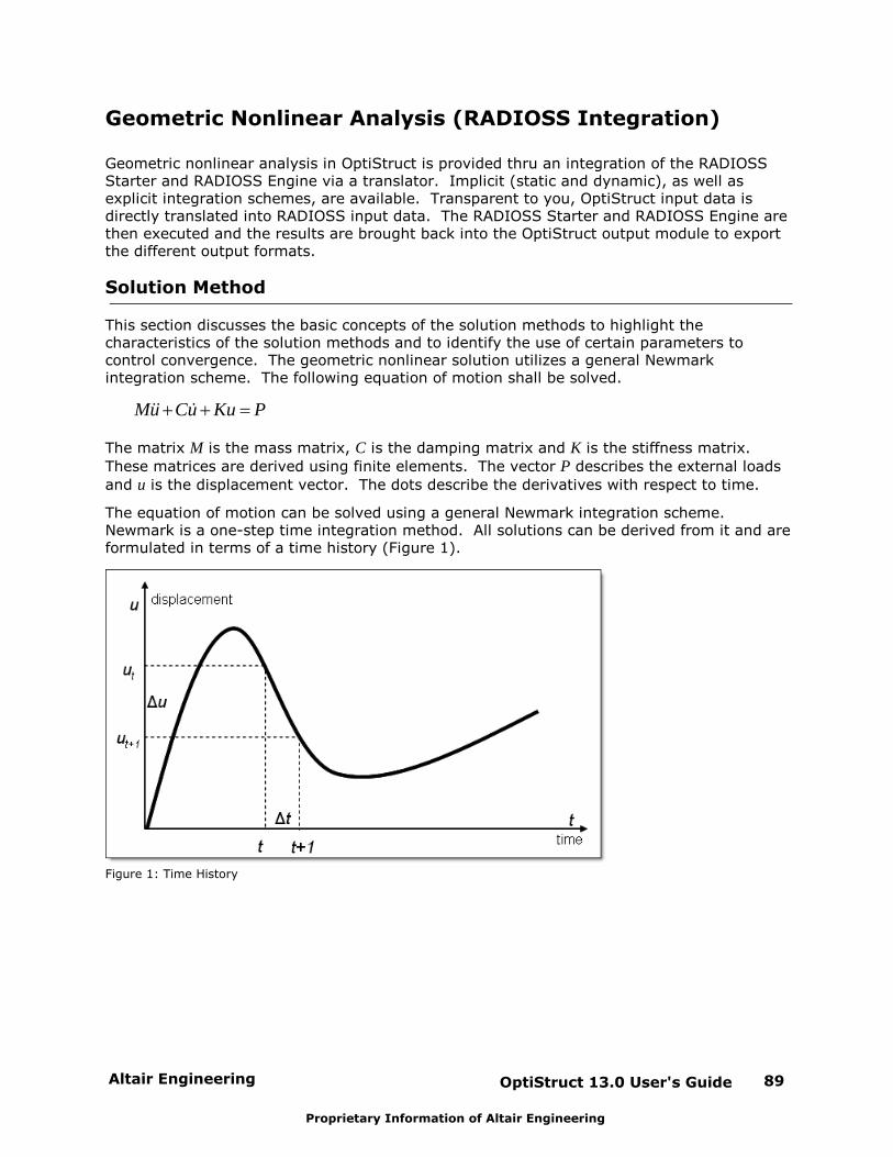
Altair Engineering OptiStruct 13.0 User's Guide 89
Proprietary Information of Altair Engineering
Geometric Nonlinear Analysis (RADIOSS Integration)
Geometric nonlinear analysis in OptiStruct is provided thru an integration of the RADIOSSStarter and RADIOSS Engine via a translator. Implicit (static and dynamic), as well asexplicit integration schemes, are available. Transparent to you, OptiStruct input data isdirectly translated into RADIOSS input data. The RADIOSS Starter and RADIOSS Engine arethen executed and the results are brought back into the OptiStruct output module to exportthe different output formats.
Solution Method
This section discusses the basic concepts of the solution methods to highlight thecharacteristics of the solution methods and to identify the use of certain parameters tocontrol convergence. The geometric nonlinear solution utilizes a general Newmarkintegration scheme. The following equation of motion shall be solved.
Mu Cu Ku P&& &
The matrix M is the mass matrix, C is the damping matrix and K is the stiffness matrix.
These matrices are derived using finite elements. The vector P describes the external loads
and u is the displacement vector. The dots describe the derivatives with respect to time.
The equation of motion can be solved using a general Newmark integration scheme. Newmark is a one-step time integration method. All solutions can be derived from it and areformulated in terms of a time history (Figure 1).
Figure 1: Time History
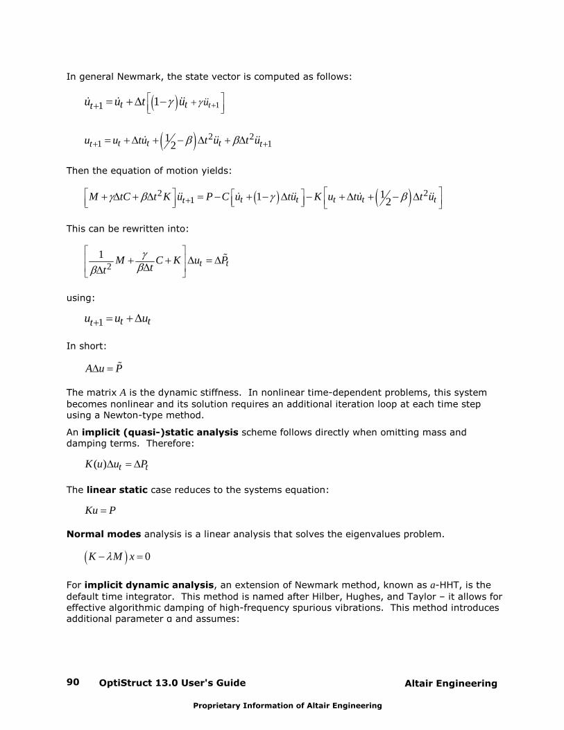
OptiStruct 13.0 User's Guide90 Altair Engineering
Proprietary Information of Altair Engineering
In general Newmark, the state vector is computed as follows:
11 1 tut ttu u t u &&& & &&
2 21 1
12t t tt tu u tu t u t u& && &&
Then the equation of motion yields:
2 21
11 2t t t t ttM tC t K u P C u tu K u tu t u&& & && & &&
This can be rewritten into:
2
1t tM C K u P
tt%
using:
1 t ttu u u
In short:
A u P%
The matrix A is the dynamic stiffness. In nonlinear time-dependent problems, this system
becomes nonlinear and its solution requires an additional iteration loop at each time stepusing a Newton-type method.
An implicit (quasi-)static analysis scheme follows directly when omitting mass anddamping terms. Therefore:
( ) t tK u u P
The linear static case reduces to the systems equation:
Ku P
Normal modes analysis is a linear analysis that solves the eigenvalues problem.
0K M x
For implicit dynamic analysis, an extension of Newmark method, known as a-HHT, is the
default time integrator. This method is named after Hilber, Hughes, and Taylor – it allows foreffective algorithmic damping of high-frequency spurious vibrations. This method introducesadditional parameter α and assumes:
Altair Engineering OptiStruct 13.0 User's Guide 91
Proprietary Information of Altair Engineering
211 2 1, 032 4
with
2
1 11 t tM C K u P
tt%
The smaller the value of a, the more algorithmic damping is included in the numerical
solution. With a = 0.0 there is no numerical damping and the method is the trapezoidal
method.
The second method available is the general Newmark with user-defined and . Thedefaults are typically:
1 1,2 4
which is equivalent to HHT method with a = 0.0. This is an unconditionally stable implicit
integration scheme with:
1 11
2t tt tu u t u u& & && &&
21 1
14t t tt tu u tu t u u& && &&
And from the equation of motion:
2
4 2t tM C K u P
tt%
By default a Modified Newton method is employed to solve the implicit problems stated above(Figure 2).
( )t i iK u u R
1 i iiu u u
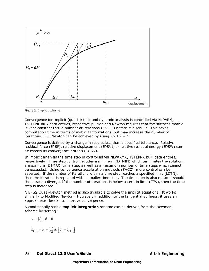
OptiStruct 13.0 User's Guide92 Altair Engineering
Proprietary Information of Altair Engineering
Figure 2: Implicit scheme
Convergence for implicit (quasi-)static and dynamic analysis is controlled via NLPARM,TSTEPNL bulk data entries, respectively. Modified Newton requires that the stiffness matrixis kept constant thru a number of iterations (KSTEP) before it is rebuilt. This savescomputation time in terms of matrix factorizations, but may increase the number ofiterations. Full Newton can be achieved by using KSTEP = 1.
Convergence is defined by a change in results less than a specified tolerance. Relativeresidual force (EPSP), relative displacement (EPSU), or relative residual energy (EPSW) canbe chosen as convergence criteria (CONV).
In implicit analysis the time step is controlled via NLPARMX, TSTEPNX bulk data entries,respectively. Time step control includes a minimum (DTMIN) which terminates the solution,a maximum (DTMAX) time step, as well as a maximum number of time steps which cannotbe exceeded. Using convergence acceleration methods (SACC), more control can beasserted. If the number of iterations within a time step reaches a specified limit (LDTN),then the iteration is repeated with a smaller time step. The time step is also reduced shouldthe iteration diverge. If the number of iterations is below a certain limit (ITW), then the timestep is increased.
A BFGS Quasi-Newton method is also available to solve the implicit equations. It workssimilarly to Modified Newton. However, in addition to the tangential stiffness, it uses anapproximate Hessian to improve convergence.
A conditionally stable explicit integration scheme can be derived from the Newmarkscheme by setting:
12 , 0
1 11
2t tt tu u t u u& & && &&
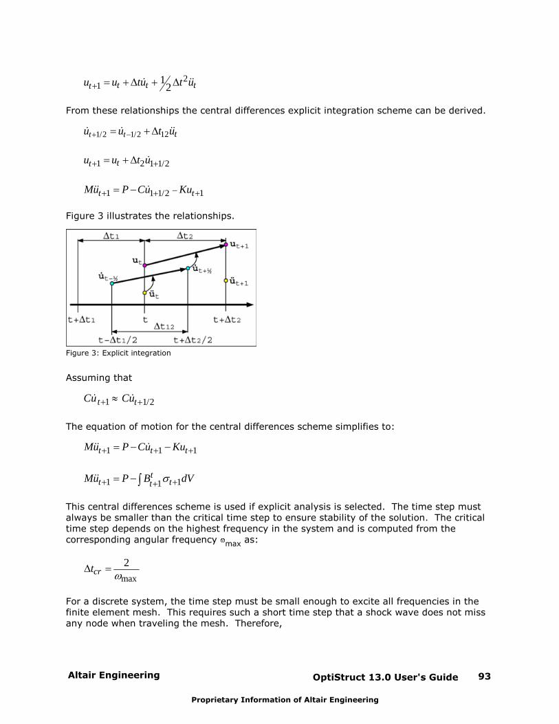
Altair Engineering OptiStruct 13.0 User's Guide 93
Proprietary Information of Altair Engineering
21
12t t ttu u tu t u& &&
From these relationships the central differences explicit integration scheme can be derived.
121/2 1/2t t tu u t u& & &&
1 2 1 1/2ttu u t u&
1 11 1/2t tMu P Cu Ku&& &
Figure 3 illustrates the relationships.
Figure 3: Explicit integration
Assuming that
1 1/2t tCu Cu& &
The equation of motion for the central differences scheme simplifies to:
1 1 1t t tMu P Cu Ku&& &
1 11t
t ttMu P B dV&&
This central differences scheme is used if explicit analysis is selected. The time step mustalways be smaller than the critical time step to ensure stability of the solution. The criticaltime step depends on the highest frequency in the system and is computed from thecorresponding angular frequency max as:
max
2crt
For a discrete system, the time step must be small enough to excite all frequencies in thefinite element mesh. This requires such a short time step that a shock wave does not missany node when traveling the mesh. Therefore,
OptiStruct 13.0 User's Guide94 Altair Engineering
Proprietary Information of Altair Engineering
cltc
with lc being the critical length of an element and c is the speed of sound in the given
material.
Different ways of time step control are available. The default method is the nodal time stepwhich is computed from the nodal mass m and the equivalent nodal stiffness k such that:
2mincrn
n
mt
k
The element time step based on the critical length of each element is also available. Thechoice can be made on the XSTEP bulk data entry.
Problem Setup
Geometric nonlinear analysis is defined thru a SUBCASE.
For implicit (quasi-)static analysis an NLPARM statement as well as ANALYSIS = NLGEOMmust be present in the subcase. To define the termination time a TTERM subcase entry canbe used. TTERM is mandatory if a nonlinear load NLOAD is used. NLPARM references an NLPARM bulk data entry. Additional parameters to control the geometric nonlinear solutioncan be defined on the optional NLPARMX bulk data entry. These include convergenceacceleration methods. In the case of post-buckling analysis Riks method can be selected.
Linear static analysis is provided as a debugging option. It is defined thru NLPARMX, ILIN. Such analysis can help investigate the model for modeling errors. In linear static analysisthe load vector is determined at the termination time. Normal modes analysis requires aMETHOD subcase statement in addition.
For implicit dynamic analysis a TSTEPNL statement as well as ANALYSIS = IMPDYN must bepresent in the subcase. To define the termination time a TTERM subcase entry is mandatory. TSTEPNL references a TSTEPNL bulk data entry. Additional parameters to control thegeometric nonlinear solution can be defined on the optional TSTEPNX bulk data entry.
For explicit dynamic analysis an XSTEP statement as well as ANALYSIS = EXPDYN must bepresent in the subcase. To define the termination time a TTERM subcase entry is mandatory. XSTEP references an XSTEP bulk data entry. Time step control can be defined on the XSTEPbulk data entry.
The implicit schemes require the solution of linear systems equations. By default, the directsolver is invoked, whereby the unknowns are simultaneously solved using a Gausselimination method that exploits the sparseness and symmetry of the stiffness matrix, K, for
computational efficiency. Alternatively, an iterative solver using the preconditioningconjugate gradient method may be used. While the direct solver is very robust, accurate andefficient, the iterative solver is sometimes superior in terms of speed, for example for bulkysolid structures. The iterative solver is selected through the SOLVTYP subcase informationentry, which in turn references a SOLVTYP bulk data entry.
The definition of a unit system thru the DTI, UNITS or UNITS bulk data statement is required.
The geometric nonlinear analysis loads and boundary conditions are defined in the bulk data
Altair Engineering OptiStruct 13.0 User's Guide 95
Proprietary Information of Altair Engineering
section of the input deck. They need to be referenced under the SUBCASE using an SPC,NLOAD, LOAD, IC and RWALL statements in a SUBCASE. Each SUBCASE defines one loadingcondition that is executed separately.
Subcase continuation is available thru the use of CNTNLSUB. Any number of explicit andimplicit analyses can be linked. However, geometric nonlinear (ANALYSIS = NLGEOM,EXPDYN, or IMPDYN) analysis subcases cannot yet be linked with small displacement quasi-static nonlinear (ANALYSIS = NLSTAT) analysis subcases and vice versa.
Example for implicit (quasi-)static analysis
SUBCASE 1 ANALYSIS = NLGEOM SPC = 1 NLOAD = 2 NLPARM = 3 TTERM = 1.0 DISP = ALL STRESS = ALLBEGIN BULKNLPARM,3NLOAD1,2,2,,L,88TABLED1,88,+,0.0,0.0,1.0,1.0,ENDTDTI,UNITS,1,kg,N,m,s
Alternative example for implicit (quasi-)static analysis
SUBCASE 1 ANALYSIS = NLGEOM SPC = 1 LOAD = 4 NLPARM = 3 DISP = ALL STRESS = ALLBEGIN BULKNLPARM,3 FORCE,4,233,,1.0,0.0,0.0,1.0DTI,UNITS,1,kg,N,m,s
Example for implicit dynamic analysis
SUBCASE 2 ANALYSIS = IMPDYN SPC = 1 IC = 5 TSTEPNL = 3 TTERM = 0.2 DISP = ALL STRESS = ALLBEGIN BULKTSTEPNL,3TIC,5,123,1,,13.88DTI,UNITS,1,kg,N,m,s
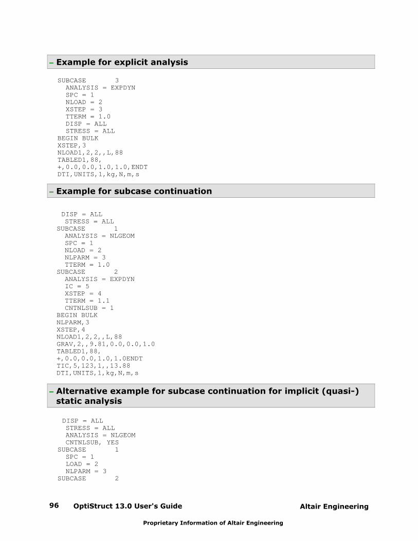
OptiStruct 13.0 User's Guide96 Altair Engineering
Proprietary Information of Altair Engineering
Example for explicit analysis
SUBCASE 3 ANALYSIS = EXPDYN SPC = 1 NLOAD = 2 XSTEP = 3 TTERM = 1.0 DISP = ALL STRESS = ALLBEGIN BULKXSTEP,3NLOAD1,2,2,,L,88TABLED1,88,+,0.0,0.0,1.0,1.0,ENDTDTI,UNITS,1,kg,N,m,s
Example for subcase continuation
DISP = ALL STRESS = ALLSUBCASE 1 ANALYSIS = NLGEOM SPC = 1 NLOAD = 2 NLPARM = 3 TTERM = 1.0SUBCASE 2 ANALYSIS = EXPDYN IC = 5 XSTEP = 4 TTERM = 1.1 CNTNLSUB = 1BEGIN BULKNLPARM,3XSTEP,4NLOAD1,2,2,,L,88GRAV,2,,9.81,0.0,0.0,1.0TABLED1,88,+,0.0,0.0,1.0,1.0ENDT TIC,5,123,1,,13.88DTI,UNITS,1,kg,N,m,s
Alternative example for subcase continuation for implicit (quasi-)static analysis
DISP = ALL STRESS = ALL ANALYSIS = NLGEOM CNTNLSUB, YESSUBCASE 1 SPC = 1 LOAD = 2 NLPARM = 3SUBCASE 2
Altair Engineering OptiStruct 13.0 User's Guide 97
Proprietary Information of Altair Engineering
SPC = 1 LOAD = 4 NLPARM = 3BEGIN BULKNLPARM,3GRAV,2,,9.81,0.0,0.0,1.0FORCE,4,233,,1.0,0.0,0.0,1.0UNITS = SI
User's Considerations
Geometric Nonlinear Analysis Properties and Materials
Special element types and nonlinear materials are available for geometric nonlinear analysis. As a general rule property and material definitions that are only applicable in geometricnonlinear analysis are defined on extensions to the original property and to a MAT1 material,respectively. The extensions are grouped with the base entry by sharing the same PID orMID. In the case of a subcase that is not a geometric nonlinear analysis, these extensionsare ignored. Property defaults can be set for shells (XSHLPRM) and solids (XSOLPRM) thatmay replace the use of property extensions.
Property example:
PSHELL, 3, 7, 1.0, 7, , 7PSHELLX, 3, 24, , , 5
Material example:
MAT1, 102, 60.4, , 0.33, 2.70e-6MATX02, 102, 0.09026, 0.22313, 0.3746, 100.0, 0.175
Coordinate Systems
In geometric nonlinear analysis there are moving and fixed coordinate systems. Rectangularcoordinate systems that are defined thru grid points (CORD1R, CORD3R) are moving with thedeformations of the model. Systems defined in terms of point coordinates (CORD2R,CORD4R) are fixed.
The behavior of loads depends on the coordinate system referenced. If the loads FORCE,MOMENT are desired to be follower forces, a CID that references a moving coordinate system(CORD1R, CORD3R) must be defined. Otherwise these loads are not following thedeformation. PLOAD always follows the deformations.
Difference Between Geometric Linear and Geometric Nonlinear Analysis
In geometric linear analysis all deformations and rotations are small (infinitesimal). As ageneral rule, displacements of say 5% of the model dimension and rotations up to 5 degreescan be treated as small. Rotations are trickier. A rotating body seems to get bigger linearlyunder deformation even if defined as rigid. Nonlinearities can only come from contact ormaterials. This type of analysis is supported in Nonlinear Quasi-Static Analysis withANALYSIS = NLSTAT. Loads stay in the undeformed coordinates and simply move along the
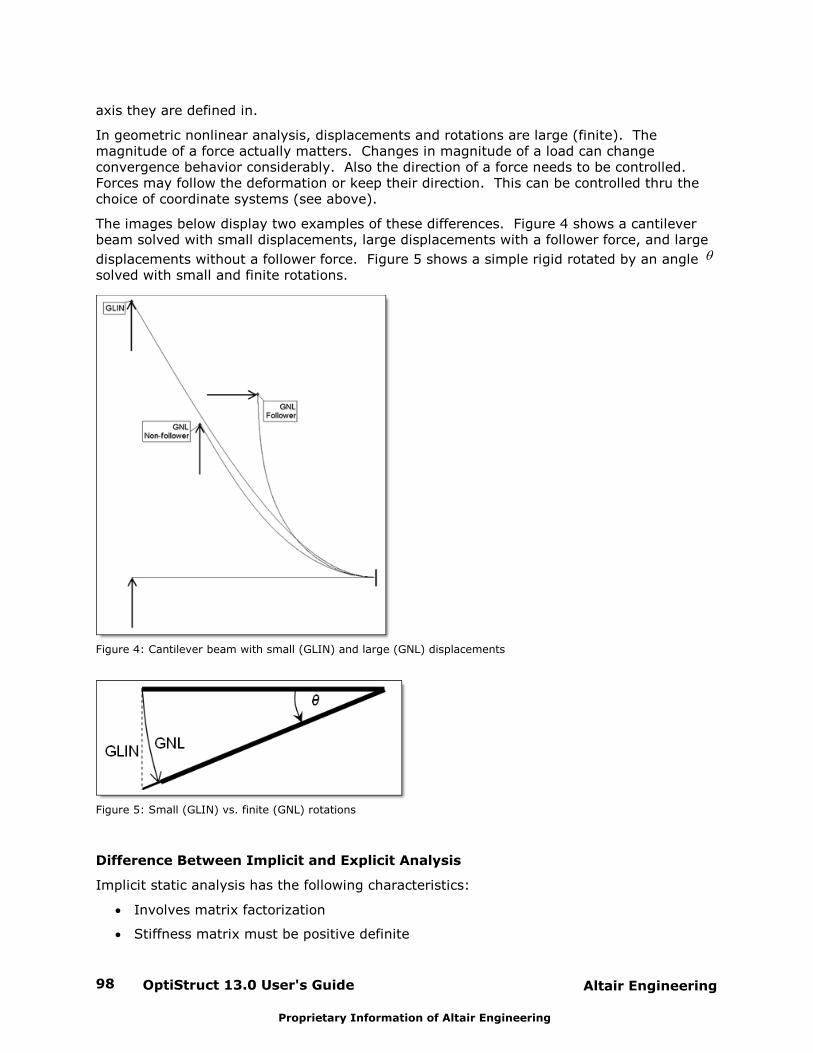
OptiStruct 13.0 User's Guide98 Altair Engineering
Proprietary Information of Altair Engineering
axis they are defined in.
In geometric nonlinear analysis, displacements and rotations are large (finite). Themagnitude of a force actually matters. Changes in magnitude of a load can changeconvergence behavior considerably. Also the direction of a force needs to be controlled. Forces may follow the deformation or keep their direction. This can be controlled thru thechoice of coordinate systems (see above).
The images below display two examples of these differences. Figure 4 shows a cantileverbeam solved with small displacements, large displacements with a follower force, and large
displacements without a follower force. Figure 5 shows a simple rigid rotated by an angle solved with small and finite rotations.
Figure 4: Cantilever beam with small (GLIN) and large (GNL) displacements
Figure 5: Small (GLIN) vs. finite (GNL) rotations
Difference Between Implicit and Explicit Analysis
Implicit static analysis has the following characteristics:
Involves matrix factorization
Stiffness matrix must be positive definite
Altair Engineering OptiStruct 13.0 User's Guide 99
Proprietary Information of Altair Engineering
- Model must be sufficiently constraint
- No unattached parts
Iteration is needed to reach equilibrium
Equilibrium is achieved within iteration tolerances
Larger time steps
Long-term, (quasi-)static events
Implicit dynamic analysis has the following characteristics:
Involves matrix factorization
Dynamic stiffness matrix must be positive definite
Iteration is needed to reach equilibrium
Equilibrium is achieved within iteration tolerances
Larger time steps
Long-term events
Explicit (dynamic) analysis has the following characteristics:
In general a diagonal mass matrix is used
No matrix factorization necessary
Equilibrium is always guaranteed
Maximum stable time step needs to be respected
Small time steps
Short-term events
Implicit Contact
In an implicit contact analysis, you need to take care of the following two concerns:
First, there should be no initial penetrations in the mesh. Sometimes, initial penetration isnecessary to begin the simulation then only a small (< 0.01*GAP) value is recommended tonot change reality too much. With high initial penetrations, the solution will progress butmay lead to incorrect results. You will be warned about initial penetration during the checkrun.
Secondly, in quasi-static analysis the model needs to be sufficiently constrained. Forexample, having two blocks on top of each other (Figure 6) the top part is not constrained. It is recommended to have the meshes completely depenetrated and to define a very smallGAP. This would create small springs constraining the upper body in vertical direction. Ofcourse, the other rigid body motions of the part have to be constrained too.
More information can be found in CONTACT, CONTPRM, and PCONTX bulk data definitions.
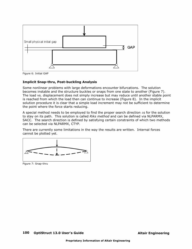
OptiStruct 13.0 User's Guide100 Altair Engineering
Proprietary Information of Altair Engineering
Figure 6: Initial GAP
Implicit Snap-thru, Post-buckling Analysis
Some nonlinear problems with large deformations encounter bifurcations. The solutionbecomes instable and the structure buckles or snaps from one state to another (Figure 7). The load vs. displacement does not simply increase but may reduce until another stable pointis reached from which the load then can continue to increase (Figure 8). In the implicitsolution procedure it is clear that a simple load increment may not be sufficient to determinethe point where the force starts reducing.
A special method needs to be employed to find the proper search direction s for the solutionto stay on its path. This solution is called Riks method and can be defined via NLPARMX,SACC. The search direction is defined by satisfying certain constraints of which two methodscan be selected via NLPARMX, CTYP.
There are currently some limitations in the way the results are written. Internal forcescannot be plotted yet.
Figure 7: Snap-thru
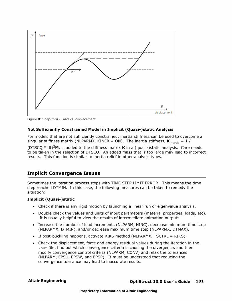
Altair Engineering OptiStruct 13.0 User's Guide 101
Proprietary Information of Altair Engineering
Figure 8: Snap-thru - Load vs. displacement
Not Sufficiently Constrained Model in Implicit (Quasi-)static Analysis
For models that are not sufficiently constrained, inertia stiffness can be used to overcome asingular stiffness matrix (NLPARMX, KINER = ON). The inertia stiffness, Kinertia = 1 /
(DTSCQ * dt)2M, is added to the stiffness matrix K in a (quasi-)static analysis. Care needsto be taken in the selection of DTSCQ. An added mass that is too large may lead to incorrectresults. This function is similar to inertia relief in other analysis types.
Implicit Convergence Issues
Sometimes the iteration process stops with TIME STEP LIMIT ERROR. This means the timestep reached DTMIN. In this case, the following measures can be taken to remedy thesituation:
Implicit (Quasi-)static
Check if there is any rigid motion by launching a linear run or eigenvalue analysis.
Double check the values and units of input parameters (material properties, loads, etc). It is usually helpful to view the results of intermediate animation outputs.
Increase the number of load increments (NLPARM, NINC), decrease minimum time step(NLPARMX, DTMIN), and/or decrease maximum time step (NLPARMX, DTMAX).
If post-buckling happens, activate RIKS method (NLPARMX, TSCTRL = RIKS).
Check the displacement, force and energy residual values during the iteration in the .out file, find out which convergence criteria is causing the divergence, and then
modify convergence control criteria (NLPARM, CONV) and relax the tolerances(NLPARM, EPSU, EPSW, and EPSP). It must be understood that reducing theconvergence tolerance may lead to inaccurate results.

OptiStruct 13.0 User's Guide102 Altair Engineering
Proprietary Information of Altair Engineering
Use small displacement formulation (PARAM, SMDISP, 1) if the displacements androtations are small.
Implicit Dynamic
Double check the values and units of input parameters (material properties, loads, etc). It is usually helpful to view the results of intermediate animation outputs.
Decrease the initial time step (TSTEPNL, NX), decrease minimum time step (TSTEPNX,DTMIN), and/or decrease maximum time step (TSTEPNX, DTMAX).
Check the displacement, force and energy residual values during the iteration in the .out file, find out which convergence criteria is causing the divergence, and then
modify convergence control criteria (NLPARM, CONV) and relax the tolerances(NLPARM, EPSU, EPSW, and EPSP). It must be understood that reducing theconvergence tolerance may lead to inaccurate results.
Use small displacement formulation (PARAM, SMDISP, 1) if the displacements androtations are small.
Limitations
The solution will be terminated if unsupported Bulk Data entries are encountered.
The following Bulk Data properties and elements are currently not translated:
- PBUSHT (partially, KN is translated)
- PDAMP, CDAMPi
- PGAP, CGAP, CGAPG (partially, friction is not allowed)
- PMASS, CMASSi
- PSHEAR, CSHEAR
- PVISC, CVISC
Additional relevant Bulk Data entries (except loads) that are currently not translated:
- CORD1C, CORD1S, CORD2S
- DMIG
- MAT2, MAT4, MAT5, MAT8, MAT9, MAT10
- MATTi, TABLEST
- MPC, MPCADD
- RBE1, RROD
Relevant loads that are currently not translated:
- PLOAD1, PLOAD2
- PLOAD4 (partially, N1, N2, N3 cannot be used)
- RFORCE (partially, RACC is not supported)
- TLOAD1, TLOAD2
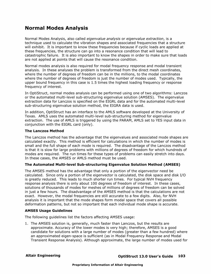
Altair Engineering OptiStruct 13.0 User's Guide 103
Proprietary Information of Altair Engineering
Normal Modes Analysis
Normal Modes Analysis, also called eigenvalue analysis or eigenvalue extraction, is atechnique used to calculate the vibration shapes and associated frequencies that a structurewill exhibit. It is important to know these frequencies because if cyclic loads are applied atthese frequencies, the structure can go into a resonance condition that will lead tocatastrophic failure. It is also important to know the shapes in order to make sure that loadsare not applied at points that will cause the resonance condition.
Normal modes analysis is also required for modal frequency response and modal transientanalysis. In these analyses the problem is transformed from the direct mesh coordinates,where the number of degrees of freedom can be in the millions, to the modal coordinateswhere the number of degrees of freedom is just the number of modes used. Typically, theupper bound frequency in this case is 1.5 times the highest loading frequency or responsefrequency of interest.
In OptiStruct, normal modes analysis can be performed using one of two algorithms: Lanczosor the automated multi-level sub-structuring eigenvalue solution (AMSES). The eigenvalueextraction data for Lanczos is specified on the EIGRL data and for the automated multi-levelsub-structuring eigenvalue solution method, the EIGRA data is used.
In addition, OptiStruct has an interface to the AMLS software developed at the University ofTexas. AMLS uses the automated multi-level sub-structuring method for eigenvalueextraction. The use of AMLS is triggered by using the PARAM, AMLS set to YES input data inconjunction with the EIGRL card (only).
The Lanczos Method
The Lanczos method has the advantage that the eigenvalues and associated mode shapes arecalculated exactly. This method is efficient for calculations in which the number of modes issmall and the full shape of each mode is required. The disadvantage of the Lanczos methodis that it is slow for large problems with millions of degrees of freedom for which hundreds ofmodes are required. The run times for these types of problems can easily stretch into days. In these cases, the AMSES or AMLS method must be used.
The Automated Multi-level Sub-structuring Eigenvalue Solution Method (AMSES)
The AMSES method has the advantage that only a portion of the eigenvector need becalculated. Since only a portion of the eigenvector is calculated, the disk space and disk I/Ois greatly reduced. This leads to much shorter run times. For typical NVH frequencyresponse analysis there is only about 100 degrees of freedom of interest. In these cases,solutions of thousands of modes for meshes of millions of degrees of freedom can be solvedin just a few hours. The disadvantage of the AMSES method is that the calculations are notexact. However, the modal frequencies are still accurate to a few digits. Also, for NVHanalysis it is important that the mode shapes form modal space that covers all possibledeformation patterns, but not so important that each individual mode shape is accurate.
AMSES Usage Guidelines
The following guidelines list the factors affecting AMSES usage:
1. The AMSES solution is, generally, much faster than Lanczos, but the results areapproximate. Accuracy of the lower modes is very high; therefore, AMSES is a goodcandidate for solutions with a large number of modes (greater than a few hundred) wherean approximated eigen-space is sufficient (as in Modal Frequency Response and ModalTransient Response Analysis). Although approximate, the large number of modes used for
OptiStruct 13.0 User's Guide104 Altair Engineering
Proprietary Information of Altair Engineering
modal analysis will encompass the modal space and the resulting motion will match veryclosely with the Lanczos results. Lanczos is recommended in solutions where accuratemode shapes of a small number of modes are required.
2. AMSES is also recommended in cases where: 1) A low number of eigenvalues arerequested but the model consists of more than a million degrees of freedom, and/or; 2)The upper bound (V2) is specified or the number of modes (ND) is greater than 50 on theEIGRL entry. In such cases, it is likely that Lanczos runs are slower than AMSES runs.
3. For optimization runs, if accuracy of the eigenvector is important, normal modes analysiswith AMSES can be run first and then Lanczos can be run with precise lower and upperbounds to check the AMSES run for accuracy. The AMSES upper bound can then beadjusted to achieve acceptable accuracy of the desired eigenvectors. Now, AMSES can beused for all optimization runs in this analysis.
4. The AMSES solution is much faster for flexible body generation and modal solutions withmany residual vectors.
5. AMSES should be used cautiously in situations with very large RBE3’s (if the RBE3 isconnected to 1/4th of the structure). It may be better to eliminate such RBE3’s.
6. AMSES solution speeds depend on the number of eigenvector degrees of freedom (DOF)to be calculated. DISP=ALL will cause the entire eigenvector to be calculated and thespeedup will not be large. However, if results for only a few DOF are required (typical forNVH analysis), AMSES can be up to 100 times faster than Lanczos. To improve AMSESrun times, it is recommended to request results only for the required DOF.
7. For an AMSES run with V1, V2 and ND specified on the EIGRA entry, AMSES calculates allthe modes up to the specified V2 (upper bound) regardless of the value of ND. Then “ND”number of requested modes is output. Therefore, reducing ND by keeping the upperbound (V2) the same will not significantly improve the AMSES run times, the upper boundmust also be correspondingly reduced to prevent the extraction of extra modes.
8. AMSES is also useful in checking for model irregularities. AMSES can be used to print thelist of grids associated with a massless mechanism or a singularity.
The Governing Equations
Normal Modes Analysis
The equilibrium equation for a structure performing free vibration appears as the eigenvalueproblem:
0K M x
Where, K is the stiffness matrix of the structure and M is the mass matrix. Damping is
neglected.
The solution of the eigenvalue problem yields n eigenvalues , where n is the number of
degrees of freedom. The vector { i } is the eigenvector corresponding to the eigenvalue.
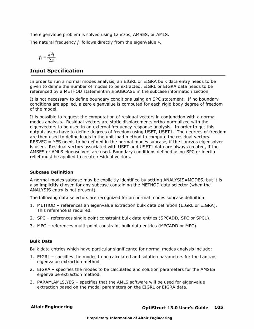
Altair Engineering OptiStruct 13.0 User's Guide 105
Proprietary Information of Altair Engineering
The eigenvalue problem is solved using Lanczos, AMSES, or AMLS.
The natural frequency fi follows directly from the eigenvalue .
2i
if
Input Specification
In order to run a normal modes analysis, an EIGRL or EIGRA bulk data entry needs to begiven to define the number of modes to be extracted. EIGRL or EIGRA data needs to bereferenced by a METHOD statement in a SUBCASE in the subcase information section.
It is not necessary to define boundary conditions using an SPC statement. If no boundaryconditions are applied, a zero eigenvalue is computed for each rigid body degree of freedomof the model.
It is possible to request the computation of residual vectors in conjunction with a normalmodes analysis. Residual vectors are static displacements ortho-normalized with theeigenvectors to be used in an external frequency response analysis. In order to get thisoutput, users have to define degrees of freedom using USET, USET1. The degrees of freedomare then used to define loads in the unit load method to compute the residual vectors. RESVEC = YES needs to be defined in the normal modes subcase, if the Lanczos eigensolveris used. Residual vectors associated with USET and USET1 data are always created, if theAMSES or AMLS eigensolvers are used. Boundary conditions defined using SPC or inertiarelief must be applied to create residual vectors.
Subcase Definition
A normal modes subcase may be explicitly identified by setting ANALYSIS=MODES, but it isalso implicitly chosen for any subcase containing the METHOD data selector (when theANALYSIS entry is not present).
The following data selectors are recognized for an normal modes subcase definition.
1. METHOD – references an eigenvalue extraction bulk data definition (EIGRL or EIGRA).This reference is required.
2. SPC – references single point constraint bulk data entries (SPCADD, SPC or SPC1).
3. MPC – references multi-point constraint bulk data entries (MPCADD or MPC).
Bulk Data
Bulk data entries which have particular significance for normal modes analysis include:
1. EIGRL – specifies the modes to be calculated and solution parameters for the Lanczoseigenvalue extraction method.
2. EIGRA – specifies the modes to be calculated and solution parameters for the AMSESeigenvalue extraction method.
3. PARAM,AMLS,YES – specifies that the AMLS software will be used for eigenvalueextraction based on the modal parameters on the EIGRL or EIGRA data.
OptiStruct 13.0 User's Guide106 Altair Engineering
Proprietary Information of Altair Engineering
4. SPC, SPC1, and SPCADD - specify the base where excitation is applied and otherconstraints.
5. MPC and MPCADD - specify multi-point constraints.
Sample Input
SUBCASE 100SPC = 5METHOD = 24
$BEGIN BULK$EIGRL, 24, 0.0, 1000.ENDDATA$
Output
Results of interest from eigenvalue extraction include maximum displacement, modalstresses, energies and multi-point constraint forces. These are requested via the I/O Options DISPLACEMENT, EKE, ESE, STRESS, GPSTRESS and MPCFORCE respectively.
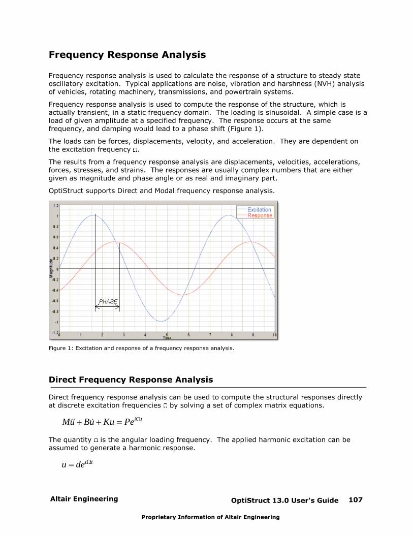
Altair Engineering OptiStruct 13.0 User's Guide 107
Proprietary Information of Altair Engineering
Frequency Response Analysis
Frequency response analysis is used to calculate the response of a structure to steady stateoscillatory excitation. Typical applications are noise, vibration and harshness (NVH) analysisof vehicles, rotating machinery, transmissions, and powertrain systems.
Frequency response analysis is used to compute the response of the structure, which isactually transient, in a static frequency domain. The loading is sinusoidal. A simple case is aload of given amplitude at a specified frequency. The response occurs at the samefrequency, and damping would lead to a phase shift (Figure 1).
The loads can be forces, displacements, velocity, and acceleration. They are dependent onthe excitation frequency .
The results from a frequency response analysis are displacements, velocities, accelerations,forces, stresses, and strains. The responses are usually complex numbers that are eithergiven as magnitude and phase angle or as real and imaginary part.
OptiStruct supports Direct and Modal frequency response analysis.
Figure 1: Excitation and response of a frequency response analysis.
Direct Frequency Response Analysis
Direct frequency response analysis can be used to compute the structural responses directlyat discrete excitation frequencies by solving a set of complex matrix equations.
i tMu Bu Ku Pe&& &
The quantity is the angular loading frequency. The applied harmonic excitation can beassumed to generate a harmonic response.
i tu de
OptiStruct 13.0 User's Guide108 Altair Engineering
Proprietary Information of Altair Engineering
The vector u is the displacement vector. Substituting the assumed harmonic displacementresponse into the equation of motion and rewriting the damping matrix (B), you get:
21
i t i tEK M iGK iK i B de Pe
The matrix K is the stiffness matrix and the matrix M is the mass matrix.
There are three ways to define damping in the system.
1. Using a uniform structural damping coefficient G.
2. Structural element damping using the damping coefficients GE on the materials as well
as GE on bushing and spring element property definitions. These form the matrix KE.
3. Viscous damping generated by damper elements. These form the matrix B1.
The equation of motion is solved directly using complex algebra.
Running Direct Frequency Response Analysis using OptiStruct
The frequency response loads and boundary conditions are defined in the bulk data section ofthe input deck. They need to be referenced in the subcase information section using an SPCand DLOAD statement in a SUBCASE.
OptiStruct does not support inertia relief for direct frequency response analysis. The solverwill error out if it is attempted.
A frequency set must be referenced using a FREQUENCY statement.
In addition to the various damping elements and material damping, uniform structuraldamping G can be applied using PARAM, G.
Modal Frequency Response Analysis
The modal method first performs a normal modes analysis to obtain the eigenvalues 2
i i
and the corresponding eigenvectors iX X
of the system. The response can be expressedas a scalar product of the eigenvectors X and the modal responses d.
i tu Xde
The equation of motion without damping is then transformed into modal coordinates usingthe eigenvectors.
T T i t T i tX MX X KX de X Pe
The modal mass matrix TX MX and the modal stiffness matrix
TX KX are diagonal. If theeigenvectors are normalized with respect to the mass matrix, the modal mass matrix is the
Altair Engineering OptiStruct 13.0 User's Guide 109
Proprietary Information of Altair Engineering
unity matrix and the modal stiffness matrix is a diagonal matrix holding the eigenvalues ofthe system. This way, the system equation is reduced to a set of uncoupled equations for thecomponents of d that can be solved easily.
The inclusion of damping, as discussed in the direct method, yields:
21
T T T T T i t T i tEX KX X MX iGX KX iX K X i X B X de X Pe
Here, the matrices T
EX K Xand 1
TX B Xare generally non-diagonal. Then the coupled
problem is similar to the system solved in the direct method, but of much lesser degree offreedom. It is solved using the direct method.
The evaluation of the equation of motion is much faster if the equations can be keptdecoupled. This can be achieved if the damping is applied to each mode separately. This isdone through a damping table TABDMP1 that lists damping values gi versus natural
frequency fi . If this approach is used, no structural element or viscous damping should be
defined.
The decoupled equation is:
2 i t i ti i i i im i b k d e p e
Where, / (2 )i i i ib m
is the modal damping ratio, and 2i is the modal eigenvalue.
Three types of modal damping values ( )i ig f
can be defined: G – Structural damping, CRIT– Critical damping, and Q – Quality factor. They are related through the following three
equations at resonance:
:2
i ii
cr
b gG
b
: 2cr i iCRIT b m
1 1:
2i
i i
Q Qg
Modal damping is entered in to the complex stiffness matrix as structural damping if PARAM,KDAMP, -1 is used. Then the uncoupled equation becomes:
2 (1 ( ))* i t i ti i i im ig k d e p e
A METHOD statement is required for the modal method to control the normal modes analysis. The METHOD statement can refer to either EIGRL or EIGRA data.
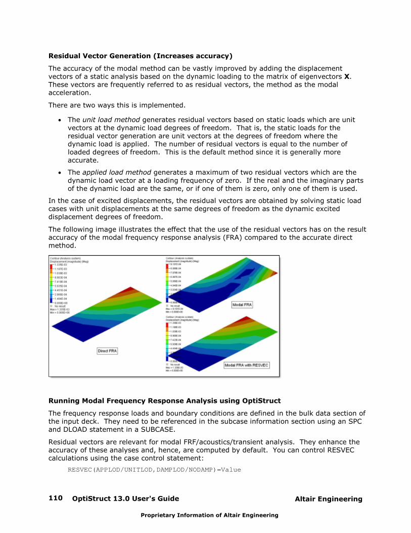
OptiStruct 13.0 User's Guide110 Altair Engineering
Proprietary Information of Altair Engineering
Residual Vector Generation (Increases accuracy)
The accuracy of the modal method can be vastly improved by adding the displacementvectors of a static analysis based on the dynamic loading to the matrix of eigenvectors X. These vectors are frequently referred to as residual vectors, the method as the modalacceleration.
There are two ways this is implemented.
The unit load method generates residual vectors based on static loads which are unitvectors at the dynamic load degrees of freedom. That is, the static loads for theresidual vector generation are unit vectors at the degrees of freedom where thedynamic load is applied. The number of residual vectors is equal to the number ofloaded degrees of freedom. This is the default method since it is generally moreaccurate.
The applied load method generates a maximum of two residual vectors which are thedynamic load vector at a loading frequency of zero. If the real and the imaginary partsof the dynamic load are the same, or if one of them is zero, only one of them is used.
In the case of excited displacements, the residual vectors are obtained by solving static loadcases with unit displacements at the same degrees of freedom as the dynamic exciteddisplacement degrees of freedom.
The following image illustrates the effect that the use of the residual vectors has on the resultaccuracy of the modal frequency response analysis (FRA) compared to the accurate directmethod.
Running Modal Frequency Response Analysis using OptiStruct
The frequency response loads and boundary conditions are defined in the bulk data section ofthe input deck. They need to be referenced in the subcase information section using an SPCand DLOAD statement in a SUBCASE.
Residual vectors are relevant for modal FRF/acoustics/transient analysis. They enhance theaccuracy of these analyses and, hence, are computed by default. You can control RESVECcalculations using the case control statement:
RESVEC(APPLOD/UNITLOD,DAMPLOD/NODAMP)=Value

Altair Engineering OptiStruct 13.0 User's Guide 111
Proprietary Information of Altair Engineering
Where, Value can be Yes or No. The keyword(s) within parentheses are ignored if the Valuespecified is No – in this case all RESVEC calculations are turned off. The keyword APPLODgenerates RESVECs based on the dynamic loading of the modal FRF/acoustics/transientanalysis. The keyword UNITLOAD generates RESVECs based on unit loads at the dynamicloading’s degrees of freedom. The keyword DAMPLOD generates viscous damping RESVECsbased on unit loads at the viscous damping degrees of freedom. The keyword NODAMP turnsoff the generation of the viscous damping RESVECs that are otherwise generated by default. Even though DAMPLOD and NODAMP are options in the case control, they are global switchesthat will be applied to all the modal FRF/acoustics/transient subcases in the model.
When the underlying eigenvalue analysis is done using the Lanczos method, the defaultRESVECs are generated based on the applied loading and viscous damping degrees offreedom. If the underlying eigenvalue analysis is done using AMSES or AMLS, the defaultRESVECs are generated based on unit loading at the load degrees of freedom and viscousdamping degrees of freedom. Residual vectors are always generated if enforceddisplacements, velocities or accelerations are defined. In addition, if there is USET U6 data,residual vectors will be calculated if the AMSES or AMLS eigensolver is used. USET U6residual vectors will not be calculated if the Lanczos eigensolver is used.
When residual vectors are included, inertia relief will be applied by default to unconstrainedmodels. If inertia relief is not desired for RESVECs, it has to be turned off using PARAM,INREL, 0.
When residual vectors are included, the eigenmodes from the underlying eigenvalue analysisof the FRF/transient subcase are used in inertia relief. All modes with eigenvalues below alimit value (FZERO) are used as rigid body modes in the inertia relief analysis. If there areno eigenmodes below FZERO, up to 6 global rigid body modes are internally generated basedon the geometry of the model and used in the inertia relief. You can set FZERO using PARAM, FZERO, Value. The default value for FZERO is 0.1
A frequency set must be referenced using a FREQUENCY statement. A METHOD statement isrequired for the modal method to control the normal modes analysis. In order to savecomputational effort, previously saved eigenvectors can be retrieved using the EIGVRETRIEVEsubcase statement.
In addition to the various damping elements and material damping, uniform structuraldamping G can be applied using PARAM, G.
Modal damping is being applied using the SDAMPING reference of a damping table TABDMP1. The parameter PARAM, KDAMP is to define the method of applying the damping table.
Frequency-dependent materials (MATFi bulk data entries) can be used in Direct and ModalFrequency Response Analysis, via TABLEDi entries for corresponding fields on the MATientries. MATF1, MATF2, MATF3, MATF8, MATF9 and MATF10 bulk data entries can be used todefine the currently available frequency-dependent materials.
Frequency-dependent properties (PBUSHT bulk data entry) can also be used in FrequencyResponse Analysis, via TABLEDi entries for the corresponding fields on the PBUSHT entry.

OptiStruct 13.0 User's Guide112 Altair Engineering
Proprietary Information of Altair Engineering
Output
The results of a frequency response analysis are displacements, velocities, accelerations,forces, stresses, and strains. The usual output entries like STRESS, STRAIN, DISPLACEMENT,etc. can be used to request corresponding output values.
PARAM, ENFMOTN, REL can be used to generate displacement, velocity and accelerationoutput relative to the specified enforced motion. In such cases, subsequently calculatedoutputs like stresses and forces are also generated relative to the specified enforced motion.PARAM, ENFMOTN, TOTAL/ABS can be used to generate the total output values including thespecified enforced motion (TOTAL/ABS is the default).
Altair Engineering OptiStruct 13.0 User's Guide 113
Proprietary Information of Altair Engineering
Complex Eigenvalue Analysis
Real eigenvalue analysis is used to compute the normal modes of a structure. Complexeigenvalue analysis computes the complex modes of the structure. The complex modescontain the imaginary part, which represents the cyclic frequency, and the real part whichrepresents the damping of the mode. If the real part is negative, then the mode is said to bestable. If the real part is positive, then the mode is unstable. Complex eigenvalue analysisis usually used to determine the stability of a structure when unsymmetric matrices arepresented due to special physical behavior. It is also used to determine the modes of adamped structure.
The complex eigenvalue analysis is formulated in the following manner:
2 0E f fp M pB K igK i G K
Where,
K is the stiffness matrix of the structure
M is the mass matrix
GE is the element structural damping matrix
B is viscous damping matrix
g is global structural damping coefficient
Kf is the extra stiffness matrix by direct matrix input
f is the coefficient of extra stiffness matrix
The solution of the complex eigenvalue problem yields complex eigenvalue, ip, and
complex mode shape, . Complex modes with positive real parts are considered unstablemodes. Unstable modes are often in pairs.
The circular frequency f is then calculated through the relationship:
2f
The damping coefficient is also computed from the equation:
2g
This corresponds to the real part of a complex eigenvalue; modes with negative dampingcoefficients have positive real parts and are unstable modes.
The extraction of complex modes directly from the above formulation is usually quitecomputationally expensive, especially if the problem size is not small. Instead, a modalmethod is used to solve the complex eigenvalue problem. First, the real modes arecalculated via a normal modes analysis. Then, a complex eigenvalue problem is formed on

OptiStruct 13.0 User's Guide114 Altair Engineering
Proprietary Information of Altair Engineering
the projected subspace spanned by the real modes and thus much smaller than the realspace. Finally, the complex modes extraction of the reduced problem follows the well knownHessenberg reduction method.
In order to run a complex eigenvalue analysis, both the EIGRL bulk data and the EIGC bulkdata entry need to be given. They define the number of the real modes and the number ofcomplex modes to be extracted, respectively. The EIGRL card has to be referenced by aMETHOD statement in a SUBCASE definition. The EIGC card is referenced by a CMETHODstatement in the same SUBCASE definition.
The complex eigen value analysis usually involves an unsymmetric matrix which representsthe source of the physical instability. The external matrix should be provided as a DMIG bulkdata entry, and then referenced by a K2PP statement in the SUBCASE definition. You candefine a specific coefficient for the external matrix by PARAM, FRIC. Otherwise, the defaultvalue of the coefficient is 1.0.
Altair Engineering OptiStruct 13.0 User's Guide 115
Proprietary Information of Altair Engineering
Random Response Analysis
Random response analysis is used when a structure is subjected to a nondeterministic,continuous excitation. Cases likely to involve nondeterministic loads are those linked toconditions such as turbulence on an airplane structure, road surface imperfections on a carstructure, noise loads on a given structure, etc.
The complex frequency response can be achieved by direct and modal frequency response. If Hxa( f ) and Hxb( f ) are the complex frequency responses (displacement, velocity or
acceleration) of x th degree of freedom, due to load cases a and b respectively, the power
spectral density of the response of x th degree of freedom Rx( f ) is as follows:
( ) H ( ) ( ) ( )x xa ab xbR f f S f H f
Sab( f ) is the power spectral density of the two sources, where the individual source a is the
excited load case and b is the applied load case. If Sa( f ) is the spectral density of the
individual source (a th load case), the power spectral density of the response of x th degree of
freedom due to a th load case will be:
2( ) ( ) ( )x xa aR f H f S f
The cross spectral density Sab( f ) with two different sources b
could possibly be a
complex number. The power spectral density of the response of x th degree of freedom due
to a th and b th load cases will be:
( ) ( ) ( ) ( )x xa ab xbR f H f S f H f
The total power spectral density of the response will be the summation of the power spectraldensity of all individual load cases as well as all cross load cases.
The autocorrelation of a variable x(t) can be defined by the following equation:
/2
/2
( ) ( ) ( )limT
xT T
A x t x t dt
The variance of the x(t) will be equal to Ax(0). The variance can be expressed as a
function of power spectral density Sx( f ) as follows:
2(0) (x) ( )x xA S f df
The root mean square value of the response x(t) can also be written in the following equation:
( )xS f dfRMSx
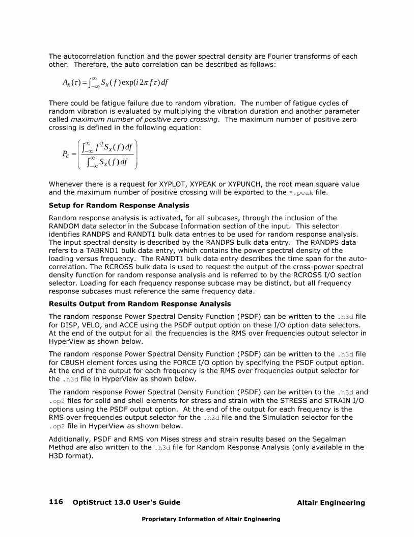
OptiStruct 13.0 User's Guide116 Altair Engineering
Proprietary Information of Altair Engineering
The autocorrelation function and the power spectral density are Fourier transforms of eachother. Therefore, the auto correlation can be described as follows:
( ) ( ) exp( 2 )x xA S f i f df
There could be fatigue failure due to random vibration. The number of fatigue cycles ofrandom vibration is evaluated by multiplying the vibration duration and another parametercalled maximum number of positive zero crossing. The maximum number of positive zerocrossing is defined in the following equation:
2 ( )
( )
xc
x
f S f dfP
S f df
Whenever there is a request for XYPLOT, XYPEAK or XYPUNCH, the root mean square valueand the maximum number of positive crossing will be exported to the *.peak file.
Setup for Random Response Analysis
Random response analysis is activated, for all subcases, through the inclusion of the RANDOM data selector in the Subcase Information section of the input. This selectoridentifies RANDPS and RANDT1 bulk data entries to be used for random response analysis. The input spectral density is described by the RANDPS bulk data entry. The RANDPS datarefers to a TABRND1 bulk data entry, which contains the power spectral density of theloading versus frequency. The RANDT1 bulk data entry describes the time span for the auto-correlation. The RCROSS bulk data is used to request the output of the cross-power spectraldensity function for random response analysis and is referred to by the RCROSS I/O sectionselector. Loading for each frequency response subcase may be distinct, but all frequencyresponse subcases must reference the same frequency data.
Results Output from Random Response Analysis
The random response Power Spectral Density Function (PSDF) can be written to the .h3d file
for DISP, VELO, and ACCE using the PSDF output option on these I/O option data selectors. At the end of the output for all the frequencies is the RMS over frequencies output selector inHyperView as shown below.
The random response Power Spectral Density Function (PSDF) can be written to the .h3d file
for CBUSH element forces using the FORCE I/O option by specifying the PSDF output option. At the end of the output for each frequency is the RMS over frequencies output selector forthe .h3d file in HyperView as shown below.
The random response Power Spectral Density Function (PSDF) can be written to the .h3d and
.op2 files for solid and shell elements for stress and strain with the STRESS and STRAIN I/O
options using the PSDF output option. At the end of the output for each frequency is theRMS over frequencies output selector for the .h3d file and the Simulation selector for the
.op2 file in HyperView as shown below.
Additionally, PSDF and RMS von Mises stress and strain results based on the SegalmanMethod are also written to the .h3d file for Random Response Analysis (only available in the
H3D format).
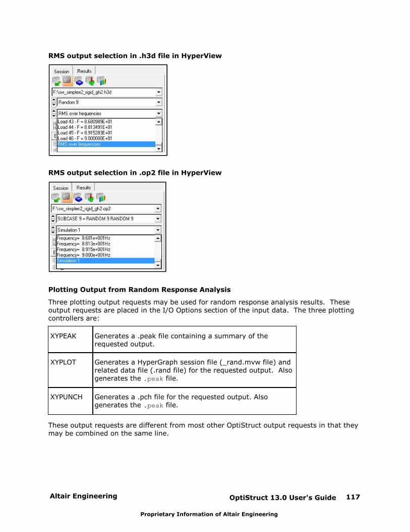
Altair Engineering OptiStruct 13.0 User's Guide 117
Proprietary Information of Altair Engineering
RMS output selection in .h3d file in HyperView
RMS output selection in .op2 file in HyperView
Plotting Output from Random Response Analysis
Three plotting output requests may be used for random response analysis results. Theseoutput requests are placed in the I/O Options section of the input data. The three plottingcontrollers are:
XYPEAK Generates a .peak file containing a summary of therequested output.
XYPLOT Generates a HyperGraph session file (_rand.mvw file) andrelated data file (.rand file) for the requested output. Alsogenerates the .peak file.
XYPUNCH Generates a .pch file for the requested output. Alsogenerates the .peak file.
These output requests are different from most other OptiStruct output requests in that theymay be combined on the same line.
OptiStruct 13.0 User's Guide118 Altair Engineering
Proprietary Information of Altair Engineering
The requests are formatted as follows:
Operation, Curve-type, Plot-type or / Grid (Component) list.
"Operation" can be any combination of XYPLOT, XYPUNCH, and XYPEAK.
"Curve-type" can be FORCE, STRESS, STRAIN, DISP, VELO, or ACCE to request force,stress, strain, displacement, velocity or acceleration, respectively.
"Plot-type" can be either PSDF or AUTO to request power spectral density function orautocorrelation, respectively.
"Grid (Component) list" must come after a slash "/". Each entry in the list is commaseparated. Each entry consists of a GRID or SPOINT ID followed by a component ofmotion (T1, T2, T3, R1, R2, or R3) in parentheses. For SPOINTs the component must beT1.
In addition, plot titles and axis labels may be controlled using TCURVE (plot title), XTITLE (x-axis label), and YTITLE (y-axis label). Default titles and labels are generated when thesecontrols are not used.
Example 1
Requesting random response results in a HyperGraph session file for the velocity PSDF forGRIDs 3 and 6 for component T2:
XYPLOT, VELO, PSDF / 3(T2), 6(T2)
Example 2
Requesting random response summary results to be written to the .peak file for the
autocorrelation of displacement for GRID 223 for component R3:
XYPEAK, DISP, AUTO / 223(T3)
Example 3
Requesting random response results output, in all formats, for the acceleration PSDF forGRIDS 8 and 9 for components T1 and T2:
XYPEAK, XYPLOT, XYPUNCH, ACCE, PSDF / 8(T1), 9(T1), 8(T2), 9(T2)
Here the XYPEAK request is valid, but redundant as it is always created when XYPLOT orXYPUNCH is present.
Altair Engineering OptiStruct 13.0 User's Guide 119
Proprietary Information of Altair Engineering
Response Spectrum Analysis
Response Spectrum Analysis (RSA) is a technique used to estimate the maximum response ofa structure for a transient event. Maximum displacement, stresses, and/or forces may bedetermined in this manner. The technique combines response spectra for a prescribeddynamic loading with results of a normal modes analysis. The time-history of the responsesare not available.
Response spectra describes the maximum response versus natural frequency of a 1-DOFsystem for a prescribed dynamic loading. They are employed to calculate the maximummodal response for each structural mode. These modal maxima may then be combined usingvarious methods, such as the Absolute Sum (ABS) method or the Complete QuadraticCombination (CQC) method, to obtain an estimate of the peak structural response.
RSA is a simple and computationally inexpensive method to provide an approximation ofpeak response, compared to conventional transient analysis. The major computational effortis to obtain a sufficient number of normal modes in order to represent the entire frequencyrange of input excitation and resulting response. Response spectra are usually provided bydesign specifications; given these, peak responses under various dynamic excitations can bequickly calculated. Therefore, it is widely used as a design tool in areas such as seismicanalysis of buildings.
The Governing Equations
Normal Modes Analysis
The equilibrium equation for a structure performing free vibration appears as the eigenvalueproblem:
[ ] 0K M
Where, K is the stiffness matrix of the structure and M is the mass matrix. Damping is
neglected.
The solution of the eigenvalue problem yields n eigenvalues i , where n is the number of
degrees of freedom. The vector { }i is the eigenvector corresponding to the eigenvalue.
The eigenvalue problem is solved using the Lanczos or the AMLS method. Not all eigenvaluesare required and only a small number of the lowest eigenvalues are normally calculated. Theresults of eigenvalue analysis are the fundamentals of response spectrum analysis.
Response spectrum analysis can be performed together with normal modes analysis in asingle run, or eigenvalue analysis with Lanczos solver can be performed first to saveeigenvalues and eigenvectors by using EIGVSAVE, which can be retrieved later by usingEIGVRETRIEVE for response spectrum analysis.
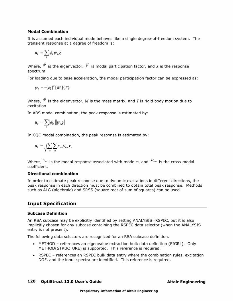
OptiStruct 13.0 User's Guide120 Altair Engineering
Proprietary Information of Altair Engineering
Modal Combination
It is assumed each individual mode behaves like a single degree-of-freedom system. Thetransient response at a degree of freedom is:
k ik ii
u
Where, is the eigenvector, is modal participation factor, and X is the response
spectrum
For loading due to base acceleration, the modal participation factor can be expressed as:
[ ] [ ]{ }Ti i M T
Where, is the eigenvector, M is the mass matrix, and T is rigid body motion due to
excitation
In ABS modal combination, the peak response is estimated by:
k ik ii
u
In CQC modal combination, the peak response is estimated by:
k m mn nm n
u v
Where, mv is the modal response associated with mode m, and mn is the cross-modal
coefficient.
Directional combination
In order to estimate peak response due to dynamic excitations in different directions, thepeak response in each direction must be combined to obtain total peak response. Methodssuch as ALG (algebraic) and SRSS (square root of sum of squares) can be used.
Input Specification
Subcase Definition
An RSA subcase may be explicitly identified by setting ANALYSIS=RSPEC, but it is alsoimplicitly chosen for any subcase containing the RSPEC data selector (when the ANALYSISentry is not present).
The following data selectors are recognized for an RSA subcase definition.
METHOD – references an eigenvalue extraction bulk data definition (EIGRL). OnlyMETHOD(STRUCTURE) is supported. This reference is required.
RSPEC – references an RSPEC bulk data entry where the combination rules, excitationDOF, and the input spectra are identified. This reference is required.
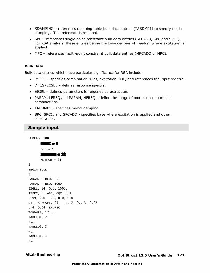
Altair Engineering OptiStruct 13.0 User's Guide 121
Proprietary Information of Altair Engineering
SDAMPING – references damping table bulk data entries (TABDMP1) to specify modaldamping. This reference is required.
SPC – references single point constraint bulk data entries (SPCADD, SPC and SPC1). For RSA analysis, these entries define the base degrees of freedom where excitation isapplied.
MPC – references multi-point constraint bulk data entries (MPCADD or MPC).
Bulk Data
Bulk data entries which have particular significance for RSA include:
RSPEC – specifies combination rules, excitation DOF, and references the input spectra.
DTI,SPECSEL – defines response spectra.
EIGRL – defines parameters for eigenvalue extraction.
PARAM, LFREQ and PARAM, HFREQ – define the range of modes used in modalcombinations.
TABDMP1 – specifies modal damping
SPC, SPC1, and SPCADD - specifies base where excitation is applied and otherconstraints.
Sample input
SUBCASE 100
RSPEC = 2
SPC = 5
SDAMPING = 12
METHOD = 24
$
BEGIN BULK
$
PARAM, LFREQ, 0.1
PARAM, HFREQ, 1000.
EIGRL, 24, 0.0, 1000.
RSPEC, 2, ABS, CQC, 0.1
, 99, 2.0, 1.0, 0.0, 0.0
DTI, SPECSEL, 99, , A, 2, 0., 3, 0.02,
, 4, 0.04, ENDREC
TABDMP1, 12, …
TABLED1, 2
+,…
TABLED1, 3
+,…
TABLED1, 4
+,…

OptiStruct 13.0 User's Guide122 Altair Engineering
Proprietary Information of Altair Engineering
ENDDATA
$
Output
Results of interest from RSA include maximum displacement, stress and force. These arerequested via the I/O Options DISPLACEMENT, STRESS and FORCE respectively.
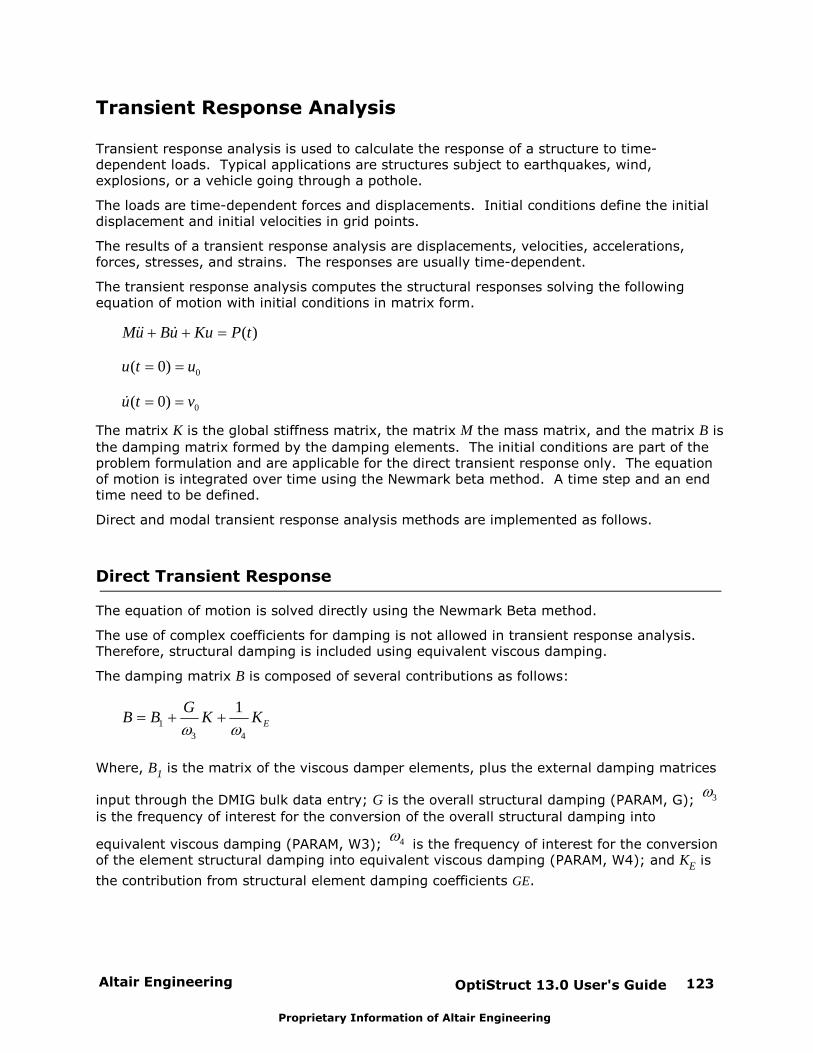
Altair Engineering OptiStruct 13.0 User's Guide 123
Proprietary Information of Altair Engineering
Transient Response Analysis
Transient response analysis is used to calculate the response of a structure to time-dependent loads. Typical applications are structures subject to earthquakes, wind,explosions, or a vehicle going through a pothole.
The loads are time-dependent forces and displacements. Initial conditions define the initialdisplacement and initial velocities in grid points.
The results of a transient response analysis are displacements, velocities, accelerations,forces, stresses, and strains. The responses are usually time-dependent.
The transient response analysis computes the structural responses solving the followingequation of motion with initial conditions in matrix form.
( )Mu Bu Ku P t&& &
0( 0)u t u
0( 0)u t v&
The matrix K is the global stiffness matrix, the matrix M the mass matrix, and the matrix B is
the damping matrix formed by the damping elements. The initial conditions are part of theproblem formulation and are applicable for the direct transient response only. The equationof motion is integrated over time using the Newmark beta method. A time step and an endtime need to be defined.
Direct and modal transient response analysis methods are implemented as follows.
Direct Transient Response
The equation of motion is solved directly using the Newmark Beta method.
The use of complex coefficients for damping is not allowed in transient response analysis. Therefore, structural damping is included using equivalent viscous damping.
The damping matrix B is composed of several contributions as follows:
1
3 4
1E
GB B K K
Where, B1 is the matrix of the viscous damper elements, plus the external damping matrices
input through the DMIG bulk data entry; G is the overall structural damping (PARAM, G); 3
is the frequency of interest for the conversion of the overall structural damping into
equivalent viscous damping (PARAM, W3); 4 is the frequency of interest for the conversionof the element structural damping into equivalent viscous damping (PARAM, W4); and KE is
the contribution from structural element damping coefficients GE.
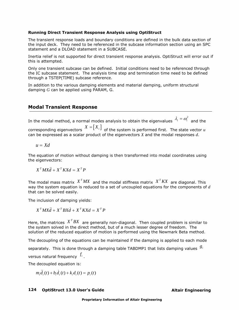
OptiStruct 13.0 User's Guide124 Altair Engineering
Proprietary Information of Altair Engineering
Running Direct Transient Response Analysis using OptiStruct
The transient response loads and boundary conditions are defined in the bulk data section ofthe input deck. They need to be referenced in the subcase information section using an SPCstatement and a DLOAD statement in a SUBCASE.
Inertia relief is not supported for direct transient response analysis. OptiStruct will error out ifthis is attempted.
Only one transient subcase can be defined. Initial conditions need to be referenced throughthe IC subcase statement. The analysis time step and termination time need to be definedthrough a TSTEP(TIME) subcase reference.
In addition to the various damping elements and material damping, uniform structuraldamping G can be applied using PARAM, G.
Modal Transient Response
In the modal method, a normal modes analysis to obtain the eigenvalues 2
i i and the
corresponding eigenvectors iX X of the system is performed first. The state vector u
can be expressed as a scalar product of the eigenvectors X and the modal responses d.
u Xd
The equation of motion without damping is then transformed into modal coordinates usingthe eigenvectors:
T T TX MXd X KXd X P&&
The modal mass matrix TX MX and the modal stiffness matrix
TX KX are diagonal. Thisway the system equation is reduced to a set of uncoupled equations for the components of dthat can be solved easily.
The inclusion of damping yields:
T T T TX MXd X BXd X KXd X P&& &
Here, the matrices TX BX are generally non-diagonal. Then coupled problem is similar to
the system solved in the direct method, but of a much lesser degree of freedom. Thesolution of the reduced equation of motion is performed using the Newmark Beta method.
The decoupling of the equations can be maintained if the damping is applied to each mode
separately. This is done through a damping table TABDMP1 that lists damping values ig
versus natural frequency if .
The decoupled equation is:
( ) ( ) ( ) ( )i i i i i i im d t b d t k d t p t&& &
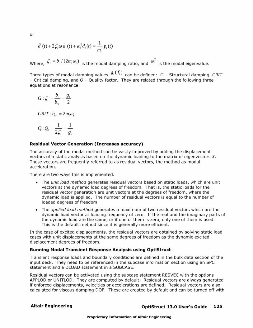
Altair Engineering OptiStruct 13.0 User's Guide 125
Proprietary Information of Altair Engineering
or
2 1( ) 2 ( ) ( ) ( )i i i i i i i
i
d t d t d t p tm
&& &
Where, / (2 )i i i ib m
is the modal damping ratio, and 2i is the modal eigenvalue.
Three types of modal damping values ( )i ig f
can be defined: G – Structural damping, CRIT– Critical damping, and Q – Quality factor. They are related through the following three
equations at resonance:
:2
i ii
cr
b gG
b
: 2cr i iCRIT b m
1 1:
2i
i i
Q Qg
Residual Vector Generation (Increases accuracy)
The accuracy of the modal method can be vastly improved by adding the displacementvectors of a static analysis based on the dynamic loading to the matrix of eigenvectors X.
These vectors are frequently referred to as residual vectors, the method as modalacceleration.
There are two ways this is implemented.
The unit load method generates residual vectors based on static loads, which are unitvectors at the dynamic load degrees of freedom. That is, the static loads for theresidual vector generation are unit vectors at the degrees of freedom, where thedynamic load is applied. The number of residual vectors is equal to the number ofloaded degrees of freedom.
The applied load method generates a maximum of two residual vectors which are thedynamic load vector at loading frequency of zero. If the real and the imaginary parts ofthe dynamic load are the same, or if one of them is zero, only one of them is used. This is the default method since it is generally more efficient.
In the case of excited displacements, the residual vectors are obtained by solving static loadcases with unit displacements at the same degrees of freedom as the dynamic exciteddisplacement degrees of freedom.
Running Modal Transient Response Analysis using OptiStruct
Transient response loads and boundary conditions are defined in the bulk data section of theinput deck. They need to be referenced in the subcase information section using an SPCstatement and a DLOAD statement in a SUBCASE.
Residual vectors can be activated using the subcase statement RESVEC with the optionsAPPLOD or UNITLOD. They are computed by default. Residual vectors are always generatedif enforced displacements, velocities or accelerations are defined. Residual vectors are alsocalculated for viscous damping DOF. These are created by default and can be turned off with
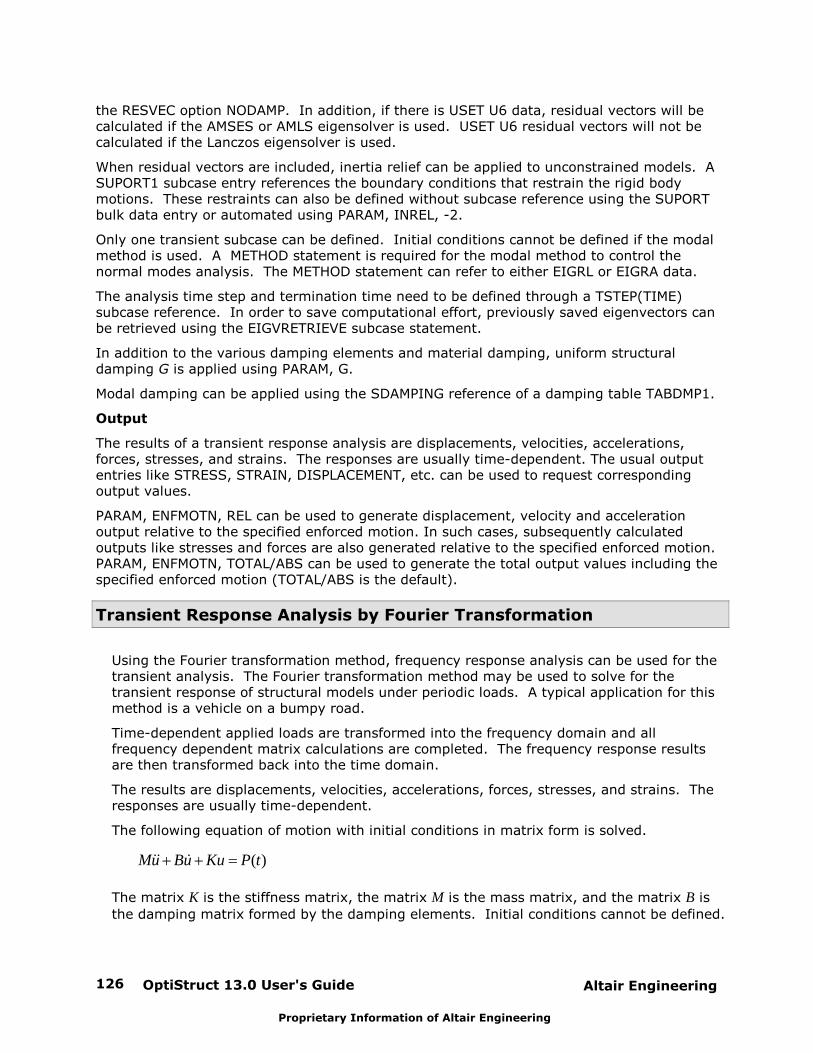
OptiStruct 13.0 User's Guide126 Altair Engineering
Proprietary Information of Altair Engineering
the RESVEC option NODAMP. In addition, if there is USET U6 data, residual vectors will becalculated if the AMSES or AMLS eigensolver is used. USET U6 residual vectors will not becalculated if the Lanczos eigensolver is used.
When residual vectors are included, inertia relief can be applied to unconstrained models. ASUPORT1 subcase entry references the boundary conditions that restrain the rigid bodymotions. These restraints can also be defined without subcase reference using the SUPORTbulk data entry or automated using PARAM, INREL, -2.
Only one transient subcase can be defined. Initial conditions cannot be defined if the modalmethod is used. A METHOD statement is required for the modal method to control thenormal modes analysis. The METHOD statement can refer to either EIGRL or EIGRA data.
The analysis time step and termination time need to be defined through a TSTEP(TIME)subcase reference. In order to save computational effort, previously saved eigenvectors canbe retrieved using the EIGVRETRIEVE subcase statement.
In addition to the various damping elements and material damping, uniform structuraldamping G is applied using PARAM, G.
Modal damping can be applied using the SDAMPING reference of a damping table TABDMP1.
Output
The results of a transient response analysis are displacements, velocities, accelerations,forces, stresses, and strains. The responses are usually time-dependent. The usual outputentries like STRESS, STRAIN, DISPLACEMENT, etc. can be used to request correspondingoutput values.
PARAM, ENFMOTN, REL can be used to generate displacement, velocity and accelerationoutput relative to the specified enforced motion. In such cases, subsequently calculatedoutputs like stresses and forces are also generated relative to the specified enforced motion.PARAM, ENFMOTN, TOTAL/ABS can be used to generate the total output values including thespecified enforced motion (TOTAL/ABS is the default).
Transient Response Analysis by Fourier Transformation
Using the Fourier transformation method, frequency response analysis can be used for thetransient analysis. The Fourier transformation method may be used to solve for thetransient response of structural models under periodic loads. A typical application for thismethod is a vehicle on a bumpy road.
Time-dependent applied loads are transformed into the frequency domain and allfrequency dependent matrix calculations are completed. The frequency response resultsare then transformed back into the time domain.
The results are displacements, velocities, accelerations, forces, stresses, and strains. Theresponses are usually time-dependent.
The following equation of motion with initial conditions in matrix form is solved.
( )Mu Bu Ku P t&& &
The matrix K is the stiffness matrix, the matrix M is the mass matrix, and the matrix B is
the damping matrix formed by the damping elements. Initial conditions cannot be defined.
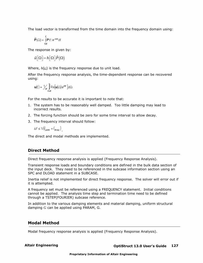
Altair Engineering OptiStruct 13.0 User's Guide 127
Proprietary Information of Altair Engineering
The load vector is transformed from the time domain into the frequency domain using:
The response in given by:
u h P%%
Where, h( ) is the frequency response due to unit load.
After the frequency response analysis, the time-dependent response can be recoveredusing:
For the results to be accurate it is important to note that:
1. The system has to be reasonably well damped. Too little damping may lead toincorrect results.
2. The forcing function should be zero for some time interval to allow decay.
3. The frequency interval should follow:
.
The direct and modal methods are implemented.
Direct Method
Direct frequency response analysis is applied (Frequency Response Analysis).
Transient response loads and boundary conditions are defined in the bulk data section ofthe input deck. They need to be referenced in the subcase information section using an SPC and DLOAD statement in a SUBCASE.
Inertia relief is not implemented for direct frequency response. The solver will error out ifit is attempted.
A frequency set must be referenced using a FREQUENCY statement. Initial conditionscannot be applied. The analysis time step and termination time need to be definedthrough a TSTEP(FOURIER) subcase reference.
In addition to the various damping elements and material damping, uniform structuraldamping G can be applied using PARAM, G.
Modal Method
Modal frequency response analysis is applied (Frequency Response Analysis).

OptiStruct 13.0 User's Guide128 Altair Engineering
Proprietary Information of Altair Engineering
Transient response loads and boundary conditions are defined in the bulk data section ofthe input deck. They need to be referenced in the subcase information section using anSPC statement and a DLOAD statement in a SUBCASE.
Residual vectors can be activated using the subcase statement RESVEC with the optionsAPPLOD or UNITLOD. They are computed by default. Residual vectors are alwaysgenerated if enforced displacements, velocities or accelerations are defined.
When residual vectors are included, inertia relief can be applied to unconstrained models. A SUPORT1 subcase entry references the boundary conditions that restrain the rigid bodymotions. These restraints can also be defined without subcase reference using the SUPORT bulk data entry or automated using PARAM, INREL, -2.
A frequency set must be referenced using a FREQUENCY statement. Initial conditionscannot be defined. A METHOD statement is required for the modal method to control thenormal modes analysis. The analysis time step and termination time need to be definedthrough a TSTEP(FOURIER) subcase reference. In order to save computational effort,previously saved eigenvectors can be retrieved using the EIGVRETRIEVE subcasestatement.
In addition to the various damping elements and material damping, uniform structuraldamping G can be applied using PARAM, G.
Modal damping can be applied using the SDAMPING reference of a damping tableTABDMP1. The parameter PARAM, KDAMP is to define the method of applying thedamping table.

Altair Engineering OptiStruct 13.0 User's Guide 129
Proprietary Information of Altair Engineering
Thermal Analysis
The Thermal Analysis section provides an overview of the following analyses:
Linear Steady-State Heat Transfer Analysis
Linear Transient Heat Transfer Analysis
Nonlinear Steady-State Heat Transfer Analysis
Contact-based Thermal Analysis
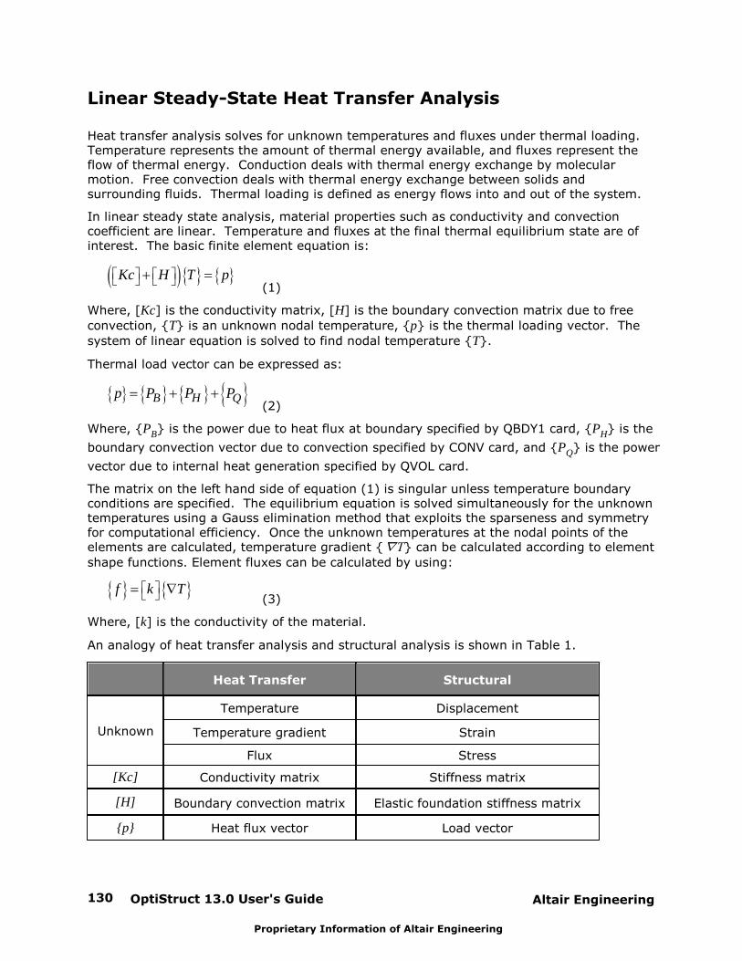
OptiStruct 13.0 User's Guide130 Altair Engineering
Proprietary Information of Altair Engineering
Linear Steady-State Heat Transfer Analysis
Heat transfer analysis solves for unknown temperatures and fluxes under thermal loading. Temperature represents the amount of thermal energy available, and fluxes represent theflow of thermal energy. Conduction deals with thermal energy exchange by molecularmotion. Free convection deals with thermal energy exchange between solids andsurrounding fluids. Thermal loading is defined as energy flows into and out of the system.
In linear steady state analysis, material properties such as conductivity and convectioncoefficient are linear. Temperature and fluxes at the final thermal equilibrium state are ofinterest. The basic finite element equation is:
Kc H T p(1)
Where, [Kc] is the conductivity matrix, [H] is the boundary convection matrix due to free
convection, {T} is an unknown nodal temperature, {p} is the thermal loading vector. The
system of linear equation is solved to find nodal temperature {T}.
Thermal load vector can be expressed as:
B H Qp P P P(2)
Where, {PB} is the power due to heat flux at boundary specified by QBDY1 card, {PH} is the
boundary convection vector due to convection specified by CONV card, and {PQ} is the power
vector due to internal heat generation specified by QVOL card.
The matrix on the left hand side of equation (1) is singular unless temperature boundaryconditions are specified. The equilibrium equation is solved simultaneously for the unknowntemperatures using a Gauss elimination method that exploits the sparseness and symmetryfor computational efficiency. Once the unknown temperatures at the nodal points of theelements are calculated, temperature gradient { } can be calculated according to element
shape functions. Element fluxes can be calculated by using:
f k T(3)
Where, [k] is the conductivity of the material.
An analogy of heat transfer analysis and structural analysis is shown in Table 1.
Heat Transfer Structural
Unknown
Temperature Displacement
Temperature gradient Strain
Flux Stress
[Kc] Conductivity matrix Stiffness matrix
[H] Boundary convection matrix Elastic foundation stiffness matrix
{p} Heat flux vector Load vector
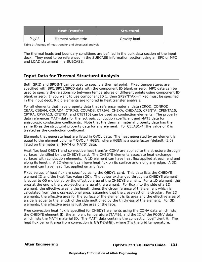
Altair Engineering OptiStruct 13.0 User's Guide 131
Proprietary Information of Altair Engineering
Heat Transfer Structural
{PQp} Element volumetric Gravity load
Table 1. Analogy of heat transfer and structural analysis
The thermal loads and boundary conditions are defined in the bulk data section of the inputdeck. They need to be referenced in the SUBCASE information section using an SPC or MPCand LOAD statement in a SUBCASE.
Input Data for Thermal Structural Analysis
Both GRID and SPOINT can be used to specify a thermal point. Fixed temperatures arespecified with SPC/SPC1/SPCD data with the component ID blank or zero. MPC data can beused to specify the relationship between temperatures of different points using component IDblank or zero. If you want to use component ID 1, then SPSYNTAX=mixed must be specifiedin the input deck. Rigid elements are ignored in heat transfer analysis.
For all elements that have property data that reference material data (CROD, CONROD,CBAR, CBEAM, CQUAD4, CTRIA3, CQUAD8, CTRIA6, CHEXA, CHEXA20, CPENTA, CPENTA15,CPYRA, CPYRA13, CTETRA, and CTET10) can be used as conduction elements. The propertydata references MAT4 data for the isotropic conduction coefficient and MAT5 data foranisotropic conduction coefficients. Note that the thermal material property data has thesame ID as the structural property data for any element. For CELAS1-4, the value of K istreated as the conduction coefficient.
Elements that generate heat are listed in QVOL data. The heat generated by an element isequal to the element volume * QVOL * HGEN, where HGEN is a scale factor (default=1.0)listed on the material (MAT4 or MAT5) data.
Heat flux load QBDY1 and convective heat transfer CONV are applied to the structure throughsurfaces identified by the CHBDYE card. The CHBDYE elements associate heat exchangesurfaces with conduction elements. A 1D element can have heat flux applied at each end andalong its length. A 2D element can have heat flux on its surface and along any edge. A 3Delement can have head flux applied on any face.
Fixed values of heat flux are specified using the QBDY1 card. This data lists the CHBDYEelement ID and the heat flux value (Q0). The power exchanged through a CHBDYE elementis equal to Q0 multiplied by the effective area of the CHBDYE element. For a 1D element, thearea at the end is the cross-sectional area of the element. For flux into the side of a 1Delement, the effective area is the length times the circumference of the element which iscalculated from the cross-sectional area, assuming that the cross-section is circular. For 2Delements, the effective area for the surface of the element is its area and the effective area ofa side is equal to the length of the side multiplied by the thickness of the element. For 3Delements, the effective area is just the area of the face.
Free convection heat flux is specified for CHBDYE elements using the CONV data which liststhe CHBDYE element ID, the ambient temperature (TAMB), and the ID of the PCONV datawhich lists the MAT4 material ID. The MAT4 data contains the convection coefficient H. Theheat flux per unit area from convection is H*(T-TAMB), where T is the grid temperature.
OptiStruct 13.0 User's Guide132 Altair Engineering
Proprietary Information of Altair Engineering
Coupled Thermal Structural Analysis and Optimization
Each heat transfer SUBCASE defines a temperature set, which can be referred by a structuralSUBCASE by TEMP(LOAD) to perform thermal-structural analysis. The temperature setidentification is the same as heat transfer SUBCASE identification by default. It can bechanged by using TSTRU card. If the temperature set identification is the same as a bulkdata temperature set identification, the temperatures from heat transfer analysis overridebulk data temperatures.
Coupled thermal structural analysis is done in the following fashion. Heat transfer analysis isperformed first to determine the temperature field of the structure. The temperature field isused as part of the loading for structural analysis. A single finite element mesh is usuallyused for both thermal and structural analysis. The finite element governing equation forstatic structural analysis is:
TK D f f(4)
Where, [K] is the global stiffness matrix, {D} is the unknown displacement vector, {fT} is the
temperature loading, and {f} is the structural loading such as forces, pressures, etc. Displacement vector {D} is solved by the linear equation solver.
In coupled thermal structural optimization, {fT} sensitivities due to design changes are
calculated. Besides the usual responses such as displacement, stress, mass, etc.,temperature can also be a response in optimization.
The coupling in thermal structural analysis is sequential, i.e. the thermal analysis affects thesubsequent structural analysis. On the other hand, in coupled thermal structuraloptimization, the coupling works both ways, that is the thermal influence on structural andthe structural influence on thermal. In other words, the optimizer modifies the structuraldesign to satisfy constraints, which in turn affects the thermal analysis.
Temperature responses are supported in Sizing, Shape, Topography, and TopologyOptimization, but the CHBDYE element cannot be used in the Design Domain of TopologyOptimization.
Altair Engineering OptiStruct 13.0 User's Guide 133
Proprietary Information of Altair Engineering
Linear Transient Heat Transfer Analysis
Linear transient heat transfer analysis can be used to calculate the temperature distributionin a system with respect to time. The applied thermal loads can either be time-dependent ortime-invariant; transient thermal analysis is used to capture the thermal behavior of asystem over a specific period in time.
The basic finite element equation for transient heat transfer analysis is given by:
C T K H T p&(1)
Where,
[C] is the heat capacity matrix
[K] is the conductivity matrix
[H] is the boundary convection matrix due to free convection
is the temperature derivative with respect to time
{T} is the unknown nodal temperature
{p} is the thermal loading vector.
The differential equation (1) is solved to find nodal temperature {T} at the specified time
steps. When equation (1) is compared to the steady-state heat transfer equation, you see
that there is an additional term that captures the transient nature of the analysis.
Guide to Request a Linear Transient Heat Transfer Analysis
The following steps can be considered as a guide to define the linear transient heat transfersubcase.
1. Use the solution sequence identifier (ANALYSIS) in the subcase information section to
select the linear transient heat transfer analysis using: ANALYSIS=HEAT.
2. Define the time step intervals at which the solutions will be calculated for transientanalysis using the TSTEP bulk data entry. This is referenced in the subcase information
section by the TSTEP subcase information entry which is used to select the integration
type (TSTEP=SID) for transient analysis.
3. The initial conditions for transient heat transfer analysis are selected by the use of the IC
subcase information entry. This entry can be used in the subcase information section tospecify the set identification number of the temperature field defined by TEMP or TEMPD
bulk data entries.
4. Use the single point constraint (SPC) data entry to specify the fixed boundary conditions
for this analysis.
5. Use the DLOAD subcase information entry to reference the set ID’s of DLOAD, TLOAD1 and
TLOAD2 bulk data entries Use the TLOAD1 and TLOAD2 bulk data entries to specify:
(a) Time dependent thermal loading The EXCITEID field of the TLOAD1 and TLOAD2 bulk data entries should point to the ID’s
of QVOL, QBDY1 bulk data entries or a combination of them using LOADADD.

OptiStruct 13.0 User's Guide134 Altair Engineering
Proprietary Information of Altair Engineering
(b) Temperature boundary condition The EXCITEID field of the TLOAD1 and TLOAD2 bulk data entries should point to the ID of
the SPCD bulk data entry. Also, the TYPE field in the TLOAD1 and TLOAD2 entries should be
set to 1.
6. The MAT4 and MAT5 bulk data entries can be used to define thermal material properties
such as thermal conductivity [K], heat capacity [C], density [RHO], convection heat
transfer coefficient [H] and heat generation capability [HGEN] used in the QVOL data
entry.
7. The THERMAL I/O option can be used to request nodal temperature output {T} for
transient heat transfer analysis subcases. The FLUX I/O options entry can be used to
request temperature gradient and flux output for transient heat transfer analysissubcases.
Applying Heat Flux Loads
In Step 5(a) of the guide above, the ability to use QBDY1 data to apply heat flux loading is
illustrated. This is accomplished as explained in the following steps:
1. The value of the heat flux load is input in the Q0 field of a QBDY1 data entry.
2. The EID# field in the QBDY1 data entry requires the identification number of CHBDYE
surface elements. These surface elements should be created on the surfaces of the modelto which heat flux loads are to be applied.
3. This is done in HyperMesh by creating an interface of type CONDUCTION, selecting all the
relevant surfaces and then adding CHBDYE surface elements to those surfaces.
4. These newly created surface elements via the interface group can then be referenced inthe EID# field of the QBDY1 data entry.
Refer to the OS-1090 tutorial for detailed information on setting up heat flux loads and freeconvection for transient heat transfer analysis.
Coupled Thermal-structural Analysis
The temperature results from the final time step of a linear transient heat transfer analysiscan be applied to a structural subcase. Both TEMPERATURE(LOAD) and
TEMPERATURE(MATERIAL) are allowed to reference the subcase ID or temperature result sets
from the linear transient heat transfer analysis for use in either material property calculationsor thermal loading.
Note: Non-zero SPC will be considered as zero SPC fortransient thermal analysis, except when non-zero SPC areused to specify ambient points for convection. When anambient point is controlled by TLOAD1/TLOAD2 via SPCD,the corresponding SPC should be zero.

Altair Engineering OptiStruct 13.0 User's Guide 135
Proprietary Information of Altair Engineering
Nonlinear Steady-State Heat Transfer Analysis
Nonlinear steady-state heat transfer analysis can be used to calculate the temperaturedistribution in a system, in which material properties are a function of temperature.
The basic finite element equation for nonlinear heat transfer can be written as:
L(T) = P (1)
Where, {T} is unknown temperature, P is the global power vector, and L(T) is the global
response (nodal power).
The system of equations (1) is solved using the Newton’s method. Solution control isprovided by defining parameters on the NLPARM bulk data entry. TEMPERATURE (INITIAL)can be used to provide a likely initial temperature distribution. The temperature results fromthe nonlinear heat transfer analysis can be used in subsequent structural analysis.
Nonlinear Steady-State Heat Transfer Analysis Setup
The following steps can be considered as a guide to setup a nonlinear steady-state heattransfer analysis:
1. Use the solution sequence identifier (ANALYSIS) in the subcase information section toselect the nonlinear steady-state heat transfer analysis using: ANALYSIS=NLHEAT.
2. The likely initial temperature distribution can be defined using the TEMPERATURE subcaseinformation entry (type=INITIAL). A good initial temperature estimate improves theconvergence of the solver.
3. The MATT4 bulk data entry can be used to define temperature dependent thermalmaterial properties.
4. To indicate that a nonlinear solution is required for any subcase, a NLPARM subcaseinformation entry is required. This subcase entry points to a NLPARM bulk data entry thatspecifies convergence tolerances and other nonlinear parameters.
5. Loads and boundary conditions are defined in the bulk data section of the input deck.These should be referenced in the subcase information section using SPC and LOADentries in a subcase. Each subcase defines a load vector.
Example
An example solver deck section showing the usage of ANALYSIS and NLPARM is shownbelow:
SUBCASE 5ANALYSIS=NLHEATSPC=10LOAD=20NLPARM=30…BEGIN BULK…NLPARM, 30…

OptiStruct 13.0 User's Guide136 Altair Engineering
Proprietary Information of Altair Engineering
ENDDATA
Note: Optimization based on nonlinear heat transfer analysis iscurrently not supported.
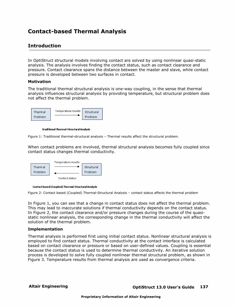
Altair Engineering OptiStruct 13.0 User's Guide 137
Proprietary Information of Altair Engineering
Contact-based Thermal Analysis
Introduction
In OptiStruct structural models involving contact are solved by using nonlinear quasi-staticanalysis. The analysis involves finding the contact status, such as contact clearance andpressure. Contact clearance spans the distance between the master and slave, while contactpressure is developed between two surfaces in contact.
Motivation
The traditional thermal structural analysis is one-way coupling, in the sense that thermalanalysis influences structural analysis by providing temperature, but structural problem doesnot affect the thermal problem.
Figure 1: Traditional thermal-structural analysis – Thermal results affect the structural problem.
When contact problems are involved, thermal structural analysis becomes fully coupled sincecontact status changes thermal conductivity.
Figure 2: Contact based (Coupled) Thermal-Structural Analysis – contact status affects the thermal problem
In Figure 1, you can see that a change in contact status does not affect the thermal problem.This may lead to inaccurate solutions if thermal conductivity depends on the contact status.In Figure 2, the contact clearance and/or pressure changes during the course of the quasi-static nonlinear analysis, the corresponding change in the thermal conductivity will affect thesolution of the thermal problem.
Implementation
Thermal analysis is performed first using initial contact status. Nonlinear structural analysis isemployed to find contact status. Thermal conductivity at the contact interface is calculatedbased on contact clearance or pressure or based on user-defined values. Coupling is essentialbecause the contact status is used to determine thermal conductivity. An iterative solutionprocess is developed to solve fully coupled nonlinear thermal structural problem, as shown inFigure 3. Temperature results from thermal analysis are used as convergence criteria.
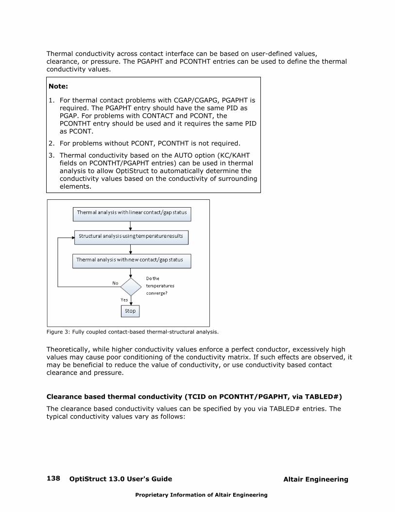
OptiStruct 13.0 User's Guide138 Altair Engineering
Proprietary Information of Altair Engineering
Thermal conductivity across contact interface can be based on user-defined values,clearance, or pressure. The PGAPHT and PCONTHT entries can be used to define the thermalconductivity values.
Note:
1. For thermal contact problems with CGAP/CGAPG, PGAPHT isrequired. The PGAPHT entry should have the same PID asPGAP. For problems with CONTACT and PCONT, thePCONTHT entry should be used and it requires the same PIDas PCONT.
2. For problems without PCONT, PCONTHT is not required.
3. Thermal conductivity based on the AUTO option (KC/KAHTfields on PCONTHT/PGAPHT entries) can be used in thermalanalysis to allow OptiStruct to automatically determine theconductivity values based on the conductivity of surroundingelements.
Figure 3: Fully coupled contact-based thermal-structural analysis.
Theoretically, while higher conductivity values enforce a perfect conductor, excessively highvalues may cause poor conditioning of the conductivity matrix. If such effects are observed, itmay be beneficial to reduce the value of conductivity, or use conductivity based contactclearance and pressure.
Clearance based thermal conductivity (TCID on PCONTHT/PGAPHT, via TABLED#)
The clearance based conductivity values can be specified by you via TABLED# entries. Thetypical conductivity values vary as follows:
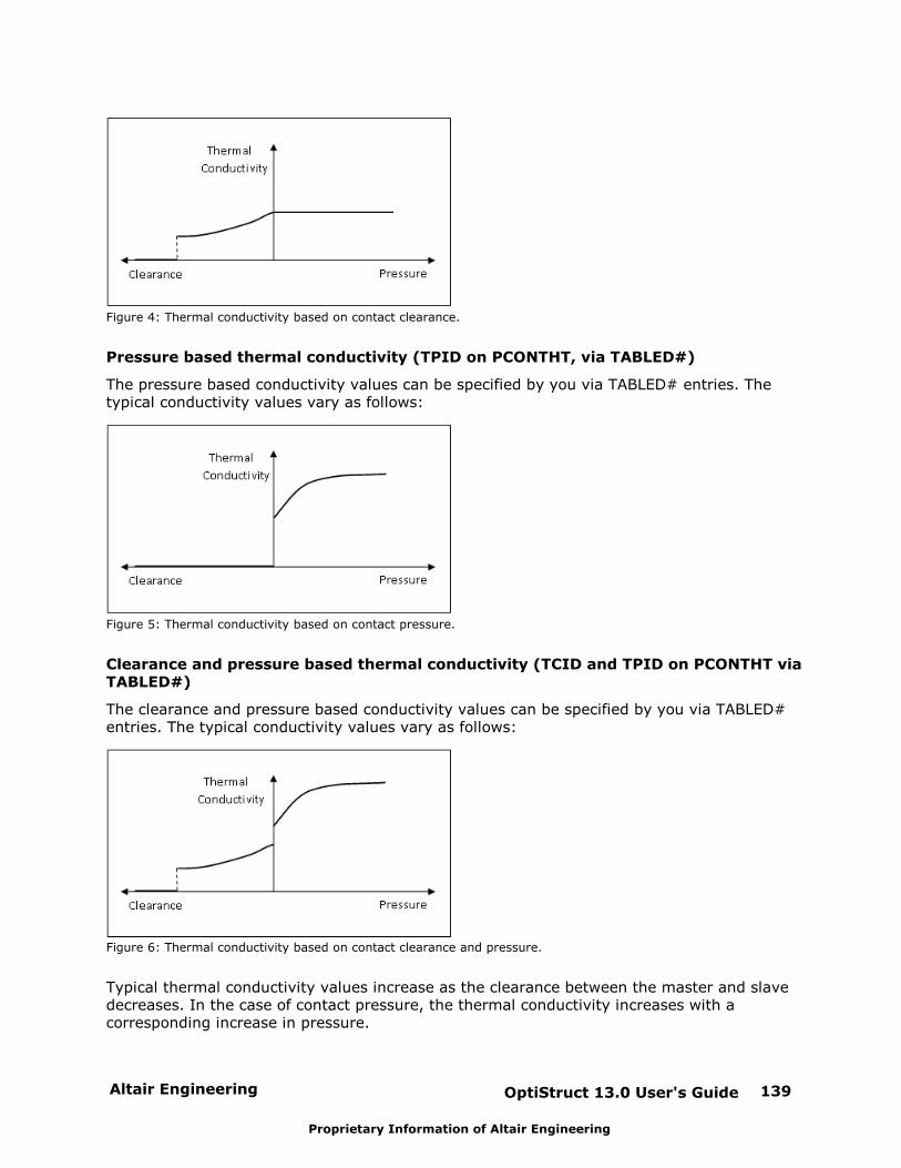
Altair Engineering OptiStruct 13.0 User's Guide 139
Proprietary Information of Altair Engineering
Figure 4: Thermal conductivity based on contact clearance.
Pressure based thermal conductivity (TPID on PCONTHT, via TABLED#)
The pressure based conductivity values can be specified by you via TABLED# entries. Thetypical conductivity values vary as follows:
Figure 5: Thermal conductivity based on contact pressure.
Clearance and pressure based thermal conductivity (TCID and TPID on PCONTHT viaTABLED#)
The clearance and pressure based conductivity values can be specified by you via TABLED#entries. The typical conductivity values vary as follows:
Figure 6: Thermal conductivity based on contact clearance and pressure.
Typical thermal conductivity values increase as the clearance between the master and slavedecreases. In the case of contact pressure, the thermal conductivity increases with acorresponding increase in pressure.

OptiStruct 13.0 User's Guide140 Altair Engineering
Proprietary Information of Altair Engineering
Acoustic Analysis
The Acoustic Analysis section provides an overview of the following analyses:
Coupled Frequency Response Analysis of Fluid-Structure Models
Radiated Sound Analysis
Altair Engineering OptiStruct 13.0 User's Guide 141
Proprietary Information of Altair Engineering
Coupled Frequency Response Analysis of Fluid-StructureModels
Coupled frequency response analysis of fluid-structure models, commonly termed acousticanalysis, is generally performed to model sound propagation within a structural cavity, suchas the interior of a vehicle or a musical instrument.
OptiStruct allows both direct and modal frequency response analysis for fluid-structuremodels. The responses of both the structural and fluid domains are computed; for thestructural domain, these responses are the displacements and rotations of the structuralgrids, and for the fluid domain, these responses are the pressures at the fluid grid points.
The accelerations of structural grids at the fluid-structure interface excite the fluid domainand conversely, the pressures on the fluid grids at the fluid-structure interface excite thestructural domain. Hence the problem is coupled and the motions of structural and fluiddegrees-of-freedom are solved simultaneously.
Loading is sinusoidal with excitation frequency , and can be in the form of forces, acousticsources enforced displacements, enforced velocities, and/or enforced accelerations. Frequency response loads and boundary conditions are defined in the bulk data section of theinput deck. These are then referenced in a subcase definition through an SPC or DLOAD dataselector.
Damping may be defined for both the structural and fluid domains. For the structural domaindamping may be defined through structural damping elements, material damping, structuraldamping (PARAM,G), or modal damping (SDAMPING referenced by a SDAMPING(STRUCT)subcase data selector). For the fluid domain damping may be defined through materialdamping, fluid damping (PARAM,GFL), or modal damping (SDAMPING referenced by aSDAMPING(FLUID) subcase data selector). In addition, the normalized admittance coefficientfor porous materials can be specified by ALPHA on the MAT10 data.
Frequency dependent fluid acoustic absorber elements can be specified on the fluid faces ofthe fluid-structure boundary using the CAABSF elements. The absorber elements can bepoint, line, triangular, or quadrilateral in shape. The CAABSF data references the PAABSFdata which is used to specify the frequency dependent resistance (real part of theimpendence) and reactance (imaginary part of the impendence) as well as the area factorsfor point and line elements.
Frequency dependent structural acoustic absorber elements can be specified on the fluid-structure boundary using the CHACAB elements. These absorbers are solid elementsbetween the fluid and structural meshes. The CHACAB data references the PACABS datawhich is used to specify the frequency dependent resistance (real part of the impendence)and reactance (imaginary part of the impendence). Another option is to calculate thesevalues mass, stiffness, and damping values per unit area specified in this data.
PARAM, LFREQFL and PARAM, HFREQFL can be used to exclude modes from a coupled modalfrequency response analysis (Acoustic analysis).
The acoustic analysis is based on inviscid flow with linear pressure-density relation as:
10P u&&
OptiStruct 13.0 User's Guide142 Altair Engineering
Proprietary Information of Altair Engineering
and the continuity equation is:
. 0P u
Where,
P and u are the pressure of the fluid domain and displacement of the structural domain
respectively,
and are the compressibility of the fluid domain and density of the structural domainrespectively.
Combining the above equations, the governing equation of the fluid domain is:
210
PP
&&
Effect of the structure on the fluid domain at the interface
After finite element discretization, the assembly of equations for the fluid domain is:
p p p pM P B P K P Au S&& & &&
Where, Mp, Bp, Kp and Sp are the mass matrix, damping matrix, stiffness matrix and source
vector respectively, of the fluid domain.
The matrix A represents the interface matrix and is the acceleration of the structural grids
at the fluid-structure interface. (The pressure gradient at the interface will be influenced bythe acceleration of the structural grids).
Effect of fluid on the structural domain at the interface
The structural equation assembly can be written as:
TS S S SM u B u K u A P S&& &&
Where, MS, BS, KS and SS are the mass matrix, damping matrix, stiffness matrix and source
vector respectively, of the structural domain.
The matrix A represents the transpose of the interface matrix and is the pressure at the
interface fluid grids at the fluid-structure interface (The displacement, velocity andacceleration of the structural grids at the interface will be influenced by the pressure at theinterface fluid grids).
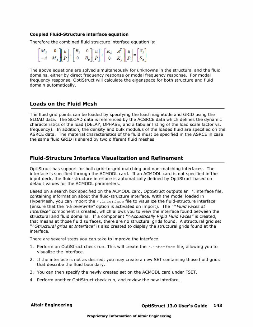
Altair Engineering OptiStruct 13.0 User's Guide 143
Proprietary Information of Altair Engineering
Coupled Fluid-Structure interface equation
Therefore the combined fluid structure interface equation is:
The above equations are solved simultaneously for unknowns in the structural and the fluiddomains, either by direct frequency response or modal frequency response. For modalfrequency response, OptiStruct will calculate the eigenspace for both structure and fluiddomain automatically.
Loads on the Fluid Mesh
The fluid grid points can be loaded by specifying the load magnitude and GRID using theSLOAD data. The SLOAD data is referenced by the ACSRCE data which defines the dynamiccharacteristics of the load (DELAY, DPHASE, and a tabular listing of the load scale factor vs.frequency). In addition, the density and bulk modulus of the loaded fluid are specified on theASRCE data. The material characteristics of the fluid must be specified in the ASRCE in casethe same fluid GRID is shared by two different fluid meshes.
Fluid-Structure Interface Visualization and Refinement
OptiStruct has support for both grid-to-grid matching and non-matching interfaces. Theinterface is specified through the ACMODL card. If an ACMODL card is not specified in theinput deck, the fluid-structure interface is automatically defined by OptiStruct based ondefault values for the ACMODL parameters.
Based on a search box specified on the ACMODL card, OptiStruct outputs an *.interface file,containing information about the fluid-structure interface. With the model loaded inHyperMesh, you can import the *.interface file to visualize the fluid-structure interface
(ensure that the “FE overwrite” option is activated on import). The “^Fluid Faces atInterface” component is created, which allows you to view the interface found between thestructural and fluid domains. If a component “^Acoustically Rigid Fluid Faces” is created,that means at those fluid surfaces, there are no structural grids found. A structural grid set “^Structural grids at Interface” is also created to display the structural grids found at theinterface.
There are several steps you can take to improve the interface:
1. Perform an OptiStruct check run. This will create the *.interface file, allowing you to
visualize the interface.
2. If the interface is not as desired, you may create a new SET containing those fluid gridsthat describe the fluid boundary.
3. You can then specify the newly created set on the ACMODL card under FSET.
4. Perform another OptiStruct check run, and review the new interface.
OptiStruct 13.0 User's Guide144 Altair Engineering
Proprietary Information of Altair Engineering
Using an External Fluid Structure Coupling Definition File
OptiStruct can use the binary ftn.70 coupling file generated by AKUSMOD instead of
internally calculating the coupling. To use this option, add PARAM,AKUSMOD,YES to theinput deck.
Modal and Panel Participation
Modal participation is a measure of how much each mode participates at a given frequency ina modal frequency response calculation. Output of modal participation may be requested forstructural degrees of freedom as well as for fluid degrees of freedom. Calculation and outputof modal participation can be requested, for any number of degrees of freedom, using the PFMODE I/O Option.
Panel participation is a measure of the influence of sets of specified structural grids, definedby PANEL bulk data entries. The response of a fluid grid is influenced through each panel oreach grid at the acoustic interface. Calculation and output of the contribution from each panelat specific loading frequencies can be requested through the PFPANEL I/O Option, for modalfrequency response. Also, the calculation and output of the contribution from each grid atthe interface can be requested through the PFGRID I/O Option.
A file *.pfmode.pch is generated based on the definition of the I/O Options PFMODE and
PFPANEL. The output for PFGRID would be in a H3D file. The results for PFMODE andPFPANEL are best plotted in HyperGraph, whereas the contour results for PFGRID are bestvisualized in HyperView.
Non-Reflecting Boundary
To create a non-reflecting boundary, set the values of the TABLEDi entry referenced by theTZREID field (Resistance-real part of Impedance) in the PAABSF data entry to be equal to
*fluid fluidCfor all frequencies. This will allow the acoustic wave to propagate normally
through the boundary, without reflection. This condition is called the Sommerfeld boundarycondition.
Where, is the density of the fluid, and is the speed of sound in the fluid.
Input File - chacab.fem
$$------------------------------------------------------------------------------$$$ $$$ NASTRAN Input Deck Generated by HyperMesh Version : 8.0SR1 $$$ Generated using HyperMesh-Nastran Template Version : 8.0sr1$$ $$$ Template: general $$$ $$$------------------------------------------------------------------------------$$$------------------------------------------------------------------------------$$$ Executive Control Cards $$$------------------------------------------------------------------------------$SOL 111
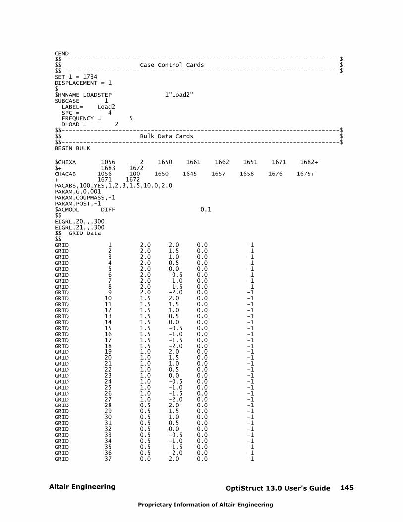
Altair Engineering OptiStruct 13.0 User's Guide 145
Proprietary Information of Altair Engineering
CEND$$------------------------------------------------------------------------------$$$ Case Control Cards $$$------------------------------------------------------------------------------$SET 1 = 1734DISPLACEMENT = 1$$HMNAME LOADSTEP 1"Load2"SUBCASE 1 LABEL= Load2 SPC = 4 FREQUENCY = 5 DLOAD = 2$$------------------------------------------------------------------------------$$$ Bulk Data Cards $$$------------------------------------------------------------------------------$BEGIN BULK
$CHEXA 1056 2 1650 1661 1662 1651 1671 1682+ $+ 1683 1672CHACAB 1056 100 1650 1645 1657 1658 1676 1675+ + 1671 1672PACABS,100,YES,1,2,3,1.5,10.0,2.0PARAM,G,0.001PARAM,COUPMASS,-1 PARAM,POST,-1 $ACMODL DIFF 0.1 $$EIGRL,20,,,300EIGRL,21,,,300$$ GRID Data$$GRID 1 2.0 2.0 0.0 -1 GRID 2 2.0 1.5 0.0 -1 GRID 3 2.0 1.0 0.0 -1 GRID 4 2.0 0.5 0.0 -1 GRID 5 2.0 0.0 0.0 -1 GRID 6 2.0 -0.5 0.0 -1 GRID 7 2.0 -1.0 0.0 -1 GRID 8 2.0 -1.5 0.0 -1 GRID 9 2.0 -2.0 0.0 -1 GRID 10 1.5 2.0 0.0 -1 GRID 11 1.5 1.5 0.0 -1 GRID 12 1.5 1.0 0.0 -1 GRID 13 1.5 0.5 0.0 -1 GRID 14 1.5 0.0 0.0 -1 GRID 15 1.5 -0.5 0.0 -1 GRID 16 1.5 -1.0 0.0 -1 GRID 17 1.5 -1.5 0.0 -1 GRID 18 1.5 -2.0 0.0 -1 GRID 19 1.0 2.0 0.0 -1 GRID 20 1.0 1.5 0.0 -1 GRID 21 1.0 1.0 0.0 -1 GRID 22 1.0 0.5 0.0 -1 GRID 23 1.0 0.0 0.0 -1 GRID 24 1.0 -0.5 0.0 -1 GRID 25 1.0 -1.0 0.0 -1 GRID 26 1.0 -1.5 0.0 -1 GRID 27 1.0 -2.0 0.0 -1 GRID 28 0.5 2.0 0.0 -1 GRID 29 0.5 1.5 0.0 -1 GRID 30 0.5 1.0 0.0 -1 GRID 31 0.5 0.5 0.0 -1 GRID 32 0.5 0.0 0.0 -1 GRID 33 0.5 -0.5 0.0 -1 GRID 34 0.5 -1.0 0.0 -1 GRID 35 0.5 -1.5 0.0 -1 GRID 36 0.5 -2.0 0.0 -1 GRID 37 0.0 2.0 0.0 -1
OptiStruct 13.0 User's Guide146 Altair Engineering
Proprietary Information of Altair Engineering
GRID 38 0.0 1.5 0.0 -1 GRID 39 0.0 1.0 0.0 -1 GRID 40 0.0 0.5 0.0 -1 GRID 41 0.0 0.0 0.0 -1 GRID 42 0.0 -0.5 0.0 -1 GRID 43 0.0 -1.0 0.0 -1 GRID 44 0.0 -1.5 0.0 -1 GRID 45 0.0 -2.0 0.0 -1 GRID 46 -0.5 2.0 0.0 -1 GRID 47 -0.5 1.5 0.0 -1 GRID 48 -0.5 1.0 0.0 -1 GRID 49 -0.5 0.5 0.0 -1 GRID 50 -0.5 0.0 0.0 -1 GRID 51 -0.5 -0.5 0.0 -1 GRID 52 -0.5 -1.0 0.0 -1 GRID 53 -0.5 -1.5 0.0 -1 GRID 54 -0.5 -2.0 0.0 -1 GRID 55 -1.0 2.0 0.0 -1 GRID 56 -1.0 1.5 0.0 -1 GRID 57 -1.0 1.0 0.0 -1 GRID 58 -1.0 0.5 0.0 -1 GRID 59 -1.0 0.0 0.0 -1 GRID 60 -1.0 -0.5 0.0 -1 GRID 61 -1.0 -1.0 0.0 -1 GRID 62 -1.0 -1.5 0.0 -1 GRID 63 -1.0 -2.0 0.0 -1 GRID 64 -1.5 2.0 0.0 -1 GRID 65 -1.5 1.5 0.0 -1 GRID 66 -1.5 1.0 0.0 -1 GRID 67 -1.5 0.5 0.0 -1 GRID 68 -1.5 0.0 0.0 -1 GRID 69 -1.5 -0.5 0.0 -1 GRID 70 -1.5 -1.0 0.0 -1 GRID 71 -1.5 -1.5 0.0 -1 GRID 72 -1.5 -2.0 0.0 -1 GRID 73 -2.0 2.0 0.0 -1 GRID 74 -2.0 1.5 0.0 -1 GRID 75 -2.0 1.0 0.0 -1 GRID 76 -2.0 0.5 0.0 -1 GRID 77 -2.0 0.0 0.0 -1 GRID 78 -2.0 -0.5 0.0 -1 GRID 79 -2.0 -1.0 0.0 -1 GRID 80 -2.0 -1.5 0.0 -1 GRID 81 -2.0 -2.0 0.0 -1 GRID 82 2.5 2.0 0.0 -1 GRID 83 2.5 1.5 0.0 -1 GRID 84 2.5 1.0 0.0 -1 GRID 85 2.5 0.5 0.0 -1 GRID 86 2.5 0.0 0.0 -1 GRID 87 2.5 -0.5 0.0 -1 GRID 88 2.5 -1.0 0.0 -1 GRID 89 2.5 -1.5 0.0 -1 GRID 90 2.5 -2.0 0.0 -1 GRID 91 -2.5 2.0 0.0 -1 GRID 92 -2.5 1.5 0.0 -1 GRID 93 -2.5 1.0 0.0 -1 GRID 94 -2.5 0.5 0.0 -1 GRID 95 -2.5 0.0 0.0 -1 GRID 96 -2.5 -0.5 0.0 -1 GRID 97 -2.5 -1.0 0.0 -1 GRID 98 -2.5 -1.5 0.0 -1 GRID 99 -2.5 -2.0 0.0 -1 GRID 100 2.5 2.5 0.0 -1 GRID 101 2.5 -2.5 0.0 -1 GRID 102 2.0 2.5 0.0 -1 GRID 103 2.0 -2.5 0.0 -1 GRID 104 1.5 2.5 0.0 -1 GRID 105 1.5 -2.5 0.0 -1 GRID 106 1.0 2.5 0.0 -1 GRID 107 1.0 -2.5 0.0 -1
Altair Engineering OptiStruct 13.0 User's Guide 147
Proprietary Information of Altair Engineering
GRID 108 0.5 2.5 0.0 -1 GRID 109 0.5 -2.5 0.0 -1 GRID 110 0.0 2.5 0.0 -1 GRID 111 0.0 -2.5 0.0 -1 GRID 112 -0.5 2.5 0.0 -1 GRID 113 -0.5 -2.5 0.0 -1 GRID 114 -1.0 2.5 0.0 -1 GRID 115 -1.0 -2.5 0.0 -1 GRID 116 -1.5 2.5 0.0 -1 GRID 117 -1.5 -2.5 0.0 -1 GRID 118 -2.0 2.5 0.0 -1 GRID 119 -2.0 -2.5 0.0 -1 GRID 120 -2.5 2.5 0.0 -1 GRID 121 -2.5 -2.5 0.0 -1 GRID 727 2.5 2.5 1.0 -1 GRID 728 2.5 2.0 1.0 -1 GRID 729 2.0 2.0 1.0 -1 GRID 730 2.0 2.5 1.0 -1 GRID 731 2.5 1.5 1.0 -1 GRID 732 2.0 1.5 1.0 -1 GRID 733 2.5 1.0 1.0 -1 GRID 734 2.0 1.0 1.0 -1 GRID 735 2.5 0.5 1.0 -1 GRID 736 2.0 0.5 1.0 -1 GRID 737 2.5 -4.2E-191.0 -1 GRID 738 2.0 -6.5E-201.0 -1 GRID 739 2.5 -0.5 1.0 -1 GRID 740 2.0 -0.5 1.0 -1 GRID 741 2.5 -1.0 1.0 -1 GRID 742 2.0 -1.0 1.0 -1 GRID 743 2.5 -1.5 1.0 -1 GRID 744 2.0 -1.5 1.0 -1 GRID 745 2.5 -2.0 1.0 -1 GRID 746 2.0 -2.0 1.0 -1 GRID 747 2.5 -2.5 1.0 -1 GRID 748 2.0 -2.5 1.0 -1 GRID 749 1.5 2.0 1.0 -1 GRID 750 1.5 2.5 1.0 -1 GRID 751 1.5 1.5 1.0 -1 GRID 752 1.5 1.0 1.0 -1 GRID 753 1.5 0.5 1.0 -1 GRID 754 1.5 -9.8E-211.0 -1 GRID 755 1.5 -0.5 1.0 -1 GRID 756 1.5 -1.0 1.0 -1 GRID 757 1.5 -1.5 1.0 -1 GRID 758 1.5 -2.0 1.0 -1 GRID 759 1.5 -2.5 1.0 -1 GRID 760 1.0 2.0 1.0 -1 GRID 761 1.0 2.5 1.0 -1 GRID 762 1.0 1.5 1.0 -1 GRID 763 1.0 1.0 1.0 -1 GRID 764 1.0 0.5 1.0 -1 GRID 765 1.0 -1.5E-211.0 -1 GRID 766 1.0 -0.5 1.0 -1 GRID 767 1.0 -1.0 1.0 -1 GRID 768 1.0 -1.5 1.0 -1 GRID 769 1.0 -2.0 1.0 -1 GRID 770 1.0 -2.5 1.0 -1 GRID 771 0.5 2.0 1.0 -1 GRID 772 0.5 2.5 1.0 -1 GRID 773 0.5 1.5 1.0 -1 GRID 774 0.5 1.0 1.0 -1 GRID 775 0.5 0.5 1.0 -1 GRID 776 0.5 -2.3E-221.0 -1 GRID 777 0.5 -0.5 1.0 -1 GRID 778 0.5 -1.0 1.0 -1 GRID 779 0.5 -1.5 1.0 -1 GRID 780 0.5 -2.0 1.0 -1 GRID 781 0.5 -2.5 1.0 -1 GRID 782 0.0 2.0 1.0 -1
OptiStruct 13.0 User's Guide148 Altair Engineering
Proprietary Information of Altair Engineering
GRID 783 0.0 2.5 1.0 -1 GRID 784 0.0 1.5 1.0 -1 GRID 785 0.0 1.0 1.0 -1 GRID 786 0.0 0.5 1.0 -1 GRID 787 0.0 -3.5E-231.0 -1 GRID 788 0.0 -0.5 1.0 -1 GRID 789 0.0 -1.0 1.0 -1 GRID 790 0.0 -1.5 1.0 -1 GRID 791 0.0 -2.0 1.0 -1 GRID 792 0.0 -2.5 1.0 -1 GRID 793 -0.5 2.0 1.0 -1 GRID 794 -0.5 2.5 1.0 -1 GRID 795 -0.5 1.5 1.0 -1 GRID 796 -0.5 1.0 1.0 -1 GRID 797 -0.5 0.5 1.0 -1 GRID 798 -0.5 -5.3E-241.0 -1 GRID 799 -0.5 -0.5 1.0 -1 GRID 800 -0.5 -1.0 1.0 -1 GRID 801 -0.5 -1.5 1.0 -1 GRID 802 -0.5 -2.0 1.0 -1 GRID 803 -0.5 -2.5 1.0 -1 GRID 804 -1.0 2.0 1.0 -1 GRID 805 -1.0 2.5 1.0 -1 GRID 806 -1.0 1.5 1.0 -1 GRID 807 -1.0 1.0 1.0 -1 GRID 808 -1.0 0.5 1.0 -1 GRID 809 -1.0 -8.1E-251.0 -1 GRID 810 -1.0 -0.5 1.0 -1 GRID 811 -1.0 -1.0 1.0 -1 GRID 812 -1.0 -1.5 1.0 -1 GRID 813 -1.0 -2.0 1.0 -1 GRID 814 -1.0 -2.5 1.0 -1 GRID 815 -1.5 2.0 1.0 -1 GRID 816 -1.5 2.5 1.0 -1 GRID 817 -1.5 1.5 1.0 -1 GRID 818 -1.5 1.0 1.0 -1 GRID 819 -1.5 0.5 1.0 -1 GRID 820 -1.5 -9.3E-181.0 -1 GRID 821 -1.5 -0.5 1.0 -1 GRID 822 -1.5 -1.0 1.0 -1 GRID 823 -1.5 -1.5 1.0 -1 GRID 824 -1.5 -2.0 1.0 -1 GRID 825 -1.5 -2.5 1.0 -1 GRID 826 -2.0 2.0 1.0 -1 GRID 827 -2.0 2.5 1.0 -1 GRID 828 -2.0 1.5 1.0 -1 GRID 829 -2.0 1.0 1.0 -1 GRID 830 -2.0 0.5 1.0 -1 GRID 831 -2.0 -2.0E-181.0 -1 GRID 832 -2.0 -0.5 1.0 -1 GRID 833 -2.0 -1.0 1.0 -1 GRID 834 -2.0 -1.5 1.0 -1 GRID 835 -2.0 -2.0 1.0 -1 GRID 836 -2.0 -2.5 1.0 -1 GRID 837 -2.5 2.0 1.0 -1 GRID 838 -2.5 2.5 1.0 -1 GRID 839 -2.5 1.5 1.0 -1 GRID 840 -2.5 1.0 1.0 -1 GRID 841 -2.5 0.5 1.0 -1 GRID 842 -2.5 -1.0E-181.0 -1 GRID 843 -2.5 -0.5 1.0 -1 GRID 844 -2.5 -1.0 1.0 -1 GRID 845 -2.5 -1.5 1.0 -1 GRID 846 -2.5 -2.0 1.0 -1 GRID 847 -2.5 -2.5 1.0 -1 GRID 848 2.5 2.5 2.0 -1 GRID 849 2.5 2.0 2.0 -1 GRID 850 2.0 2.0 2.0 -1 GRID 851 2.0 2.5 2.0 -1 GRID 852 2.5 1.5 2.0 -1
Altair Engineering OptiStruct 13.0 User's Guide 149
Proprietary Information of Altair Engineering
GRID 853 2.0 1.5 2.0 -1 GRID 854 2.5 1.0 2.0 -1 GRID 855 2.0 1.0 2.0 -1 GRID 856 2.5 0.5 2.0 -1 GRID 857 2.0 0.5 2.0 -1 GRID 858 2.5 -6.0E-192.0 -1 GRID 859 2.0 -1.2E-192.0 -1 GRID 860 2.5 -0.5 2.0 -1 GRID 861 2.0 -0.5 2.0 -1 GRID 862 2.5 -1.0 2.0 -1 GRID 863 2.0 -1.0 2.0 -1 GRID 864 2.5 -1.5 2.0 -1 GRID 865 2.0 -1.5 2.0 -1 GRID 866 2.5 -2.0 2.0 -1 GRID 867 2.0 -2.0 2.0 -1 GRID 868 2.5 -2.5 2.0 -1 GRID 869 2.0 -2.5 2.0 -1 GRID 870 1.5 2.0 2.0 -1 GRID 871 1.5 2.5 2.0 -1 GRID 872 1.5 1.5 2.0 -1 GRID 873 1.5 1.0 2.0 -1 GRID 874 1.5 0.5 2.0 -1 GRID 875 1.5 -2.1E-202.0 -1 GRID 876 1.5 -0.5 2.0 -1 GRID 877 1.5 -1.0 2.0 -1 GRID 878 1.5 -1.5 2.0 -1 GRID 879 1.5 -2.0 2.0 -1 GRID 880 1.5 -2.5 2.0 -1 GRID 881 1.0 2.0 2.0 -1 GRID 882 1.0 2.5 2.0 -1 GRID 883 1.0 1.5 2.0 -1 GRID 884 1.0 1.0 2.0 -1 GRID 885 1.0 0.5 2.0 -1 GRID 886 1.0 -3.8E-212.0 -1 GRID 887 1.0 -0.5 2.0 -1 GRID 888 1.0 -1.0 2.0 -1 GRID 889 1.0 -1.5 2.0 -1 GRID 890 1.0 -2.0 2.0 -1 GRID 891 1.0 -2.5 2.0 -1 GRID 892 0.5 2.0 2.0 -1 GRID 893 0.5 2.5 2.0 -1 GRID 894 0.5 1.5 2.0 -1 GRID 895 0.5 1.0 2.0 -1 GRID 896 0.5 0.5 2.0 -1 GRID 897 0.5 -6.7E-222.0 -1 GRID 898 0.5 -0.5 2.0 -1 GRID 899 0.5 -1.0 2.0 -1 GRID 900 0.5 -1.5 2.0 -1 GRID 901 0.5 -2.0 2.0 -1 GRID 902 0.5 -2.5 2.0 -1 GRID 903 0.0 2.0 2.0 -1 GRID 904 0.0 2.5 2.0 -1 GRID 905 0.0 1.5 2.0 -1 GRID 906 0.0 1.0 2.0 -1 GRID 907 0.0 0.5 2.0 -1 GRID 908 0.0 -1.2E-222.0 -1 GRID 909 0.0 -0.5 2.0 -1 GRID 910 0.0 -1.0 2.0 -1 GRID 911 0.0 -1.5 2.0 -1 GRID 912 0.0 -2.0 2.0 -1 GRID 913 0.0 -2.5 2.0 -1 GRID 914 -0.5 2.0 2.0 -1 GRID 915 -0.5 2.5 2.0 -1 GRID 916 -0.5 1.5 2.0 -1 GRID 917 -0.5 1.0 2.0 -1 GRID 918 -0.5 0.5 2.0 -1 GRID 919 -0.5 -2.0E-232.0 -1 GRID 920 -0.5 -0.5 2.0 -1 GRID 921 -0.5 -1.0 2.0 -1 GRID 922 -0.5 -1.5 2.0 -1
OptiStruct 13.0 User's Guide150 Altair Engineering
Proprietary Information of Altair Engineering
GRID 923 -0.5 -2.0 2.0 -1 GRID 924 -0.5 -2.5 2.0 -1 GRID 925 -1.0 2.0 2.0 -1 GRID 926 -1.0 2.5 2.0 -1 GRID 927 -1.0 1.5 2.0 -1 GRID 928 -1.0 1.0 2.0 -1 GRID 929 -1.0 0.5 2.0 -1 GRID 930 -1.0 -1.4E-182.0 -1 GRID 931 -1.0 -0.5 2.0 -1 GRID 932 -1.0 -1.0 2.0 -1 GRID 933 -1.0 -1.5 2.0 -1 GRID 934 -1.0 -2.0 2.0 -1 GRID 935 -1.0 -2.5 2.0 -1 GRID 936 -1.5 2.0 2.0 -1 GRID 937 -1.5 2.5 2.0 -1 GRID 938 -1.5 1.5 2.0 -1 GRID 939 -1.5 1.0 2.0 -1 GRID 940 -1.5 0.5 2.0 -1 GRID 941 -1.5 -1.3E-172.0 -1 GRID 942 -1.5 -0.5 2.0 -1 GRID 943 -1.5 -1.0 2.0 -1 GRID 944 -1.5 -1.5 2.0 -1 GRID 945 -1.5 -2.0 2.0 -1 GRID 946 -1.5 -2.5 2.0 -1 GRID 947 -2.0 2.0 2.0 -1 GRID 948 -2.0 2.5 2.0 -1 GRID 949 -2.0 1.5 2.0 -1 GRID 950 -2.0 1.0 2.0 -1 GRID 951 -2.0 0.5 2.0 -1 GRID 952 -2.0 -4.1E-182.0 -1 GRID 953 -2.0 -0.5 2.0 -1 GRID 954 -2.0 -1.0 2.0 -1 GRID 955 -2.0 -1.5 2.0 -1 GRID 956 -2.0 -2.0 2.0 -1 GRID 957 -2.0 -2.5 2.0 -1 GRID 958 -2.5 2.0 2.0 -1 GRID 959 -2.5 2.5 2.0 -1 GRID 960 -2.5 1.5 2.0 -1 GRID 961 -2.5 1.0 2.0 -1 GRID 962 -2.5 0.5 2.0 -1 GRID 963 -2.5 -2.5E-182.0 -1 GRID 964 -2.5 -0.5 2.0 -1 GRID 965 -2.5 -1.0 2.0 -1 GRID 966 -2.5 -1.5 2.0 -1 GRID 967 -2.5 -2.0 2.0 -1 GRID 968 -2.5 -2.5 2.0 -1 GRID 969 2.5 2.5 3.0 -1 GRID 970 2.5 2.0 3.0 -1 GRID 971 2.0 2.0 3.0 -1 GRID 972 2.0 2.5 3.0 -1 GRID 973 2.5 1.5 3.0 -1 GRID 974 2.0 1.5 3.0 -1 GRID 975 2.5 1.0 3.0 -1 GRID 976 2.0 1.0 3.0 -1 GRID 977 2.5 0.5 3.0 -1 GRID 978 2.0 0.5 3.0 -1 GRID 979 2.5 -6.7E-193.0 -1 GRID 980 2.0 -1.5E-193.0 -1 GRID 981 2.5 -0.5 3.0 -1 GRID 982 2.0 -0.5 3.0 -1 GRID 983 2.5 -1.0 3.0 -1 GRID 984 2.0 -1.0 3.0 -1 GRID 985 2.5 -1.5 3.0 -1 GRID 986 2.0 -1.5 3.0 -1 GRID 987 2.5 -2.0 3.0 -1 GRID 988 2.0 -2.0 3.0 -1 GRID 989 2.5 -2.5 3.0 -1 GRID 990 2.0 -2.5 3.0 -1 GRID 991 1.5 2.0 3.0 -1 GRID 992 1.5 2.5 3.0 -1
Altair Engineering OptiStruct 13.0 User's Guide 151
Proprietary Information of Altair Engineering
GRID 993 1.5 1.5 3.0 -1 GRID 994 1.5 1.0 3.0 -1 GRID 995 1.5 0.5 3.0 -1 GRID 996 1.5 -3.1E-203.0 -1 GRID 997 1.5 -0.5 3.0 -1 GRID 998 1.5 -1.0 3.0 -1 GRID 999 1.5 -1.5 3.0 -1 GRID 1000 1.5 -2.0 3.0 -1 GRID 1001 1.5 -2.5 3.0 -1 GRID 1002 1.0 2.0 3.0 -1 GRID 1003 1.0 2.5 3.0 -1 GRID 1004 1.0 1.5 3.0 -1 GRID 1005 1.0 1.0 3.0 -1 GRID 1006 1.0 0.5 3.0 -1 GRID 1007 1.0 -6.2E-213.0 -1 GRID 1008 1.0 -0.5 3.0 -1 GRID 1009 1.0 -1.0 3.0 -1 GRID 1010 1.0 -1.5 3.0 -1 GRID 1011 1.0 -2.0 3.0 -1 GRID 1012 1.0 -2.5 3.0 -1 GRID 1013 0.5 2.0 3.0 -1 GRID 1014 0.5 2.5 3.0 -1 GRID 1015 0.5 1.5 3.0 -1 GRID 1016 0.5 1.0 3.0 -1 GRID 1017 0.5 0.5 3.0 -1 GRID 1018 0.5 -1.2E-213.0 -1 GRID 1019 0.5 -0.5 3.0 -1 GRID 1020 0.5 -1.0 3.0 -1 GRID 1021 0.5 -1.5 3.0 -1 GRID 1022 0.5 -2.0 3.0 -1 GRID 1023 0.5 -2.5 3.0 -1 GRID 1024 1.50E-322.0 3.0 -1 GRID 1025 3.80E-332.5 3.0 -1 GRID 1026 2.67E-331.5 3.0 -1 GRID 1027 4.07E-341.0 3.0 -1 GRID 1028 6.20E-350.5 3.0 -1 GRID 1029 6.35E-32-2.3E-223.0 -1 GRID 1030 1.29E-31-0.5 3.0 -1 GRID 1031 -4.0E-32-1.0 3.0 -1 GRID 1032 -5.5E-32-1.5 3.0 -1 GRID 1033 -3.2E-32-2.0 3.0 -1 GRID 1034 -4.8E-33-2.5 3.0 -1 GRID 1035 -0.5 2.0 3.0 -1 GRID 1036 -0.5 2.5 3.0 -1 GRID 1037 -0.5 1.5 3.0 -1 GRID 1038 -0.5 1.0 3.0 -1 GRID 1039 -0.5 0.5 3.0 -1 GRID 1040 -0.5 -2.2E-193.0 -1 GRID 1041 -0.5 -0.5 3.0 -1 GRID 1042 -0.5 -1.0 3.0 -1 GRID 1043 -0.5 -1.5 3.0 -1 GRID 1044 -0.5 -2.0 3.0 -1 GRID 1045 -0.5 -2.5 3.0 -1 GRID 1046 -1.0 2.0 3.0 -1 GRID 1047 -1.0 2.5 3.0 -1 GRID 1048 -1.0 1.5 3.0 -1 GRID 1049 -1.0 1.0 3.0 -1 GRID 1050 -1.0 0.5 3.0 -1 GRID 1051 -1.0 -2.6E-183.0 -1 GRID 1052 -1.0 -0.5 3.0 -1 GRID 1053 -1.0 -1.0 3.0 -1 GRID 1054 -1.0 -1.5 3.0 -1 GRID 1055 -1.0 -2.0 3.0 -1 GRID 1056 -1.0 -2.5 3.0 -1 GRID 1057 -1.5 2.0 3.0 -1 GRID 1058 -1.5 2.5 3.0 -1 GRID 1059 -1.5 1.5 3.0 -1 GRID 1060 -1.5 1.0 3.0 -1 GRID 1061 -1.5 0.5 3.0 -1 GRID 1062 -1.5 -1.5E-173.0 -1
OptiStruct 13.0 User's Guide152 Altair Engineering
Proprietary Information of Altair Engineering
GRID 1063 -1.5 -0.5 3.0 -1 GRID 1064 -1.5 -1.0 3.0 -1 GRID 1065 -1.5 -1.5 3.0 -1 GRID 1066 -1.5 -2.0 3.0 -1 GRID 1067 -1.5 -2.5 3.0 -1 GRID 1068 -2.0 2.0 3.0 -1 GRID 1069 -2.0 2.5 3.0 -1 GRID 1070 -2.0 1.5 3.0 -1 GRID 1071 -2.0 1.0 3.0 -1 GRID 1072 -2.0 0.5 3.0 -1 GRID 1073 -2.0 -5.3E-183.0 -1 GRID 1074 -2.0 -0.5 3.0 -1 GRID 1075 -2.0 -1.0 3.0 -1 GRID 1076 -2.0 -1.5 3.0 -1 GRID 1077 -2.0 -2.0 3.0 -1 GRID 1078 -2.0 -2.5 3.0 -1 GRID 1079 -2.5 2.0 3.0 -1 GRID 1080 -2.5 2.5 3.0 -1 GRID 1081 -2.5 1.5 3.0 -1 GRID 1082 -2.5 1.0 3.0 -1 GRID 1083 -2.5 0.5 3.0 -1 GRID 1084 -2.5 -3.3E-183.0 -1 GRID 1085 -2.5 -0.5 3.0 -1 GRID 1086 -2.5 -1.0 3.0 -1 GRID 1087 -2.5 -1.5 3.0 -1 GRID 1088 -2.5 -2.0 3.0 -1 GRID 1089 -2.5 -2.5 3.0 -1 GRID 1090 2.5 2.5 4.0 -1 GRID 1091 2.5 2.0 4.0 -1 GRID 1092 2.0 2.0 4.0 -1 GRID 1093 2.0 2.5 4.0 -1 GRID 1094 2.5 1.5 4.0 -1 GRID 1095 2.0 1.5 4.0 -1 GRID 1096 2.5 1.0 4.0 -1 GRID 1097 2.0 1.0 4.0 -1 GRID 1098 2.5 0.5 4.0 -1 GRID 1099 2.0 0.5 4.0 -1 GRID 1100 2.5 -1.0E-164.0 -1 GRID 1101 2.0 -1.8E-164.0 -1 GRID 1102 2.5 -0.5 4.0 -1 GRID 1103 2.0 -0.5 4.0 -1 GRID 1104 2.5 -1.0 4.0 -1 GRID 1105 2.0 -1.0 4.0 -1 GRID 1106 2.5 -1.5 4.0 -1 GRID 1107 2.0 -1.5 4.0 -1 GRID 1108 2.5 -2.0 4.0 -1 GRID 1109 2.0 -2.0 4.0 -1 GRID 1110 2.5 -2.5 4.0 -1 GRID 1111 2.0 -2.5 4.0 -1 GRID 1112 1.5 2.0 4.0 -1 GRID 1113 1.5 2.5 4.0 -1 GRID 1114 1.5 1.5 4.0 -1 GRID 1115 1.5 1.0 4.0 -1 GRID 1116 1.5 0.5 4.0 -1 GRID 1117 1.5 -3.1E-164.0 -1 GRID 1118 1.5 -0.5 4.0 -1 GRID 1119 1.5 -1.0 4.0 -1 GRID 1120 1.5 -1.5 4.0 -1 GRID 1121 1.5 -2.0 4.0 -1 GRID 1122 1.5 -2.5 4.0 -1 GRID 1123 1.0 2.0 4.0 -1 GRID 1124 1.0 2.5 4.0 -1 GRID 1125 1.0 1.5 4.0 -1 GRID 1126 1.0 1.0 4.0 -1 GRID 1127 1.0 0.5 4.0 -1 GRID 1128 1.0 -3.6E-164.0 -1 GRID 1129 1.0 -0.5 4.0 -1 GRID 1130 1.0 -1.0 4.0 -1 GRID 1131 1.0 -1.5 4.0 -1 GRID 1132 1.0 -2.0 4.0 -1
Altair Engineering OptiStruct 13.0 User's Guide 153
Proprietary Information of Altair Engineering
GRID 1133 1.0 -2.5 4.0 -1 GRID 1134 0.5 2.0 4.0 -1 GRID 1135 0.5 2.5 4.0 -1 GRID 1136 0.5 1.5 4.0 -1 GRID 1137 0.5 1.0 4.0 -1 GRID 1138 0.5 0.5 4.0 -1 GRID 1139 0.5 -2.8E-164.0 -1 GRID 1140 0.5 -0.5 4.0 -1 GRID 1141 0.5 -1.0 4.0 -1 GRID 1142 0.5 -1.5 4.0 -1 GRID 1143 0.5 -2.0 4.0 -1 GRID 1144 0.5 -2.5 4.0 -1 GRID 1145 -1.7E-162.0 4.0 -1 GRID 1146 -2.3E-162.5 4.0 -1 GRID 1147 -2.7E-171.5 4.0 -1 GRID 1148 -3.0E-171.0 4.0 -1 GRID 1149 -7.0E-170.5 4.0 -1 GRID 1150 2.16E-17-1.4E-164.0 -1 GRID 1151 1.65E-16-0.5 4.0 -1 GRID 1152 3.53E-16-1.0 4.0 -1 GRID 1153 2.86E-16-1.5 4.0 -1 GRID 1154 -5.5E-17-2.0 4.0 -1 GRID 1155 -2.5E-16-2.5 4.0 -1 GRID 1156 -0.5 2.0 4.0 -1 GRID 1157 -0.5 2.5 4.0 -1 GRID 1158 -0.5 1.5 4.0 -1 GRID 1159 -0.5 1.0 4.0 -1 GRID 1160 -0.5 0.5 4.0 -1 GRID 1161 -0.5 -2.5E-174.0 -1 GRID 1162 -0.5 -0.5 4.0 -1 GRID 1163 -0.5 -1.0 4.0 -1 GRID 1164 -0.5 -1.5 4.0 -1 GRID 1165 -0.5 -2.0 4.0 -1 GRID 1166 -0.5 -2.5 4.0 -1 GRID 1167 -1.0 2.0 4.0 -1 GRID 1168 -1.0 2.5 4.0 -1 GRID 1169 -1.0 1.5 4.0 -1 GRID 1170 -1.0 1.0 4.0 -1 GRID 1171 -1.0 0.5 4.0 -1 GRID 1172 -1.0 9.63E-174.0 -1 GRID 1173 -1.0 -0.5 4.0 -1 GRID 1174 -1.0 -1.0 4.0 -1 GRID 1175 -1.0 -1.5 4.0 -1 GRID 1176 -1.0 -2.0 4.0 -1 GRID 1177 -1.0 -2.5 4.0 -1 GRID 1178 -1.5 2.0 4.0 -1 GRID 1179 -1.5 2.5 4.0 -1 GRID 1180 -1.5 1.5 4.0 -1 GRID 1181 -1.5 1.0 4.0 -1 GRID 1182 -1.5 0.5 4.0 -1 GRID 1183 -1.5 2.14E-164.0 -1 GRID 1184 -1.5 -0.5 4.0 -1 GRID 1185 -1.5 -1.0 4.0 -1 GRID 1186 -1.5 -1.5 4.0 -1 GRID 1187 -1.5 -2.0 4.0 -1 GRID 1188 -1.5 -2.5 4.0 -1 GRID 1189 -2.0 2.0 4.0 -1 GRID 1190 -2.0 2.5 4.0 -1 GRID 1191 -2.0 1.5 4.0 -1 GRID 1192 -2.0 1.0 4.0 -1 GRID 1193 -2.0 0.5 4.0 -1 GRID 1194 -2.0 1.84E-164.0 -1 GRID 1195 -2.0 -0.5 4.0 -1 GRID 1196 -2.0 -1.0 4.0 -1 GRID 1197 -2.0 -1.5 4.0 -1 GRID 1198 -2.0 -2.0 4.0 -1 GRID 1199 -2.0 -2.5 4.0 -1 GRID 1200 -2.5 2.0 4.0 -1 GRID 1201 -2.5 2.5 4.0 -1 GRID 1202 -2.5 1.5 4.0 -1
OptiStruct 13.0 User's Guide154 Altair Engineering
Proprietary Information of Altair Engineering
GRID 1203 -2.5 1.0 4.0 -1 GRID 1204 -2.5 0.5 4.0 -1 GRID 1205 -2.5 1.10E-164.0 -1 GRID 1206 -2.5 -0.5 4.0 -1 GRID 1207 -2.5 -1.0 4.0 -1 GRID 1208 -2.5 -1.5 4.0 -1 GRID 1209 -2.5 -2.0 4.0 -1 GRID 1210 -2.5 -2.5 4.0 -1 GRID 1211 2.5 2.5 5.0 -1 GRID 1212 2.5 2.0 5.0 -1 GRID 1213 2.0 2.0 5.0 -1 GRID 1214 2.0 2.5 5.0 -1 GRID 1215 2.5 1.5 5.0 -1 GRID 1216 2.0 1.5 5.0 -1 GRID 1217 2.5 1.0 5.0 -1 GRID 1218 2.0 1.0 5.0 -1 GRID 1219 2.5 0.5 5.0 -1 GRID 1220 2.0 0.5 5.0 -1 GRID 1221 2.5 -1.8E-165.0 -1 GRID 1222 2.0 -2.4E-165.0 -1 GRID 1223 2.5 -0.5 5.0 -1 GRID 1224 2.0 -0.5 5.0 -1 GRID 1225 2.5 -1.0 5.0 -1 GRID 1226 2.0 -1.0 5.0 -1 GRID 1227 2.5 -1.5 5.0 -1 GRID 1228 2.0 -1.5 5.0 -1 GRID 1229 2.5 -2.0 5.0 -1 GRID 1230 2.0 -2.0 5.0 -1 GRID 1231 2.5 -2.5 5.0 -1 GRID 1232 2.0 -2.5 5.0 -1 GRID 1233 1.5 2.0 5.0 -1 GRID 1234 1.5 2.5 5.0 -1 GRID 1235 1.5 1.5 5.0 -1 GRID 1236 1.5 1.0 5.0 -1 GRID 1237 1.5 0.5 5.0 -1 GRID 1238 1.5 -2.8E-165.0 -1 GRID 1239 1.5 -0.5 5.0 -1 GRID 1240 1.5 -1.0 5.0 -1 GRID 1241 1.5 -1.5 5.0 -1 GRID 1242 1.5 -2.0 5.0 -1 GRID 1243 1.5 -2.5 5.0 -1 GRID 1244 1.0 2.0 5.0 -1 GRID 1245 1.0 2.5 5.0 -1 GRID 1246 1.0 1.5 5.0 -1 GRID 1247 1.0 1.0 5.0 -1 GRID 1248 1.0 0.5 5.0 -1 GRID 1249 1.0 -3.0E-165.0 -1 GRID 1250 1.0 -0.5 5.0 -1 GRID 1251 1.0 -1.0 5.0 -1 GRID 1252 1.0 -1.5 5.0 -1 GRID 1253 1.0 -2.0 5.0 -1 GRID 1254 1.0 -2.5 5.0 -1 GRID 1255 0.5 2.0 5.0 -1 GRID 1256 0.5 2.5 5.0 -1 GRID 1257 0.5 1.5 5.0 -1 GRID 1258 0.5 1.0 5.0 -1 GRID 1259 0.5 0.5 5.0 -1 GRID 1260 0.5 -2.4E-165.0 -1 GRID 1261 0.5 -0.5 5.0 -1 GRID 1262 0.5 -1.0 5.0 -1 GRID 1263 0.5 -1.5 5.0 -1 GRID 1264 0.5 -2.0 5.0 -1 GRID 1265 0.5 -2.5 5.0 -1 GRID 1266 -2.4E-162.0 5.0 -1 GRID 1267 -2.4E-162.5 5.0 -1 GRID 1268 -1.4E-161.5 5.0 -1 GRID 1269 -1.1E-161.0 5.0 -1 GRID 1270 -6.8E-170.5 5.0 -1 GRID 1271 -2.1E-17-1.4E-165.0 -1 GRID 1272 1.13E-16-0.5 5.0 -1
Altair Engineering OptiStruct 13.0 User's Guide 155
Proprietary Information of Altair Engineering
GRID 1273 2.64E-16-1.0 5.0 -1 GRID 1274 2.07E-16-1.5 5.0 -1 GRID 1275 -8.9E-18-2.0 5.0 -1 GRID 1276 -1.0E-16-2.5 5.0 -1 GRID 1277 -0.5 2.0 5.0 -1 GRID 1278 -0.5 2.5 5.0 -1 GRID 1279 -0.5 1.5 5.0 -1 GRID 1280 -0.5 1.0 5.0 -1 GRID 1281 -0.5 0.5 5.0 -1 GRID 1282 -0.5 -2.9E-175.0 -1 GRID 1283 -0.5 -0.5 5.0 -1 GRID 1284 -0.5 -1.0 5.0 -1 GRID 1285 -0.5 -1.5 5.0 -1 GRID 1286 -0.5 -2.0 5.0 -1 GRID 1287 -0.5 -2.5 5.0 -1 GRID 1288 -1.0 2.0 5.0 -1 GRID 1289 -1.0 2.5 5.0 -1 GRID 1290 -1.0 1.5 5.0 -1 GRID 1291 -1.0 1.0 5.0 -1 GRID 1292 -1.0 0.5 5.0 -1 GRID 1293 -1.0 8.84E-175.0 -1 GRID 1294 -1.0 -0.5 5.0 -1 GRID 1295 -1.0 -1.0 5.0 -1 GRID 1296 -1.0 -1.5 5.0 -1 GRID 1297 -1.0 -2.0 5.0 -1 GRID 1298 -1.0 -2.5 5.0 -1 GRID 1299 -1.5 2.0 5.0 -1 GRID 1300 -1.5 2.5 5.0 -1 GRID 1301 -1.5 1.5 5.0 -1 GRID 1302 -1.5 1.0 5.0 -1 GRID 1303 -1.5 0.5 5.0 -1 GRID 1304 -1.5 1.34E-165.0 -1 GRID 1305 -1.5 -0.5 5.0 -1 GRID 1306 -1.5 -1.0 5.0 -1 GRID 1307 -1.5 -1.5 5.0 -1 GRID 1308 -1.5 -2.0 5.0 -1 GRID 1309 -1.5 -2.5 5.0 -1 GRID 1310 -2.0 2.0 5.0 -1 GRID 1311 -2.0 2.5 5.0 -1 GRID 1312 -2.0 1.5 5.0 -1 GRID 1313 -2.0 1.0 5.0 -1 GRID 1314 -2.0 0.5 5.0 -1 GRID 1315 -2.0 1.09E-165.0 -1 GRID 1316 -2.0 -0.5 5.0 -1 GRID 1317 -2.0 -1.0 5.0 -1 GRID 1318 -2.0 -1.5 5.0 -1 GRID 1319 -2.0 -2.0 5.0 -1 GRID 1320 -2.0 -2.5 5.0 -1 GRID 1321 -2.5 2.0 5.0 -1 GRID 1322 -2.5 2.5 5.0 -1 GRID 1323 -2.5 1.5 5.0 -1 GRID 1324 -2.5 1.0 5.0 -1 GRID 1325 -2.5 0.5 5.0 -1 GRID 1326 -2.5 5.75E-175.0 -1 GRID 1327 -2.5 -0.5 5.0 -1 GRID 1328 -2.5 -1.0 5.0 -1 GRID 1329 -2.5 -1.5 5.0 -1 GRID 1330 -2.5 -2.0 5.0 -1 GRID 1331 -2.5 -2.5 5.0 -1 GRID 1332 2.0 2.0 0.0 GRID 1333 2.0 1.5 0.0 GRID 1334 2.0 1.0 0.0 GRID 1335 2.0 0.5 0.0 GRID 1336 2.0 -2.2E-180.0 GRID 1337 2.0 -0.5 0.0 GRID 1338 2.0 -1.0 0.0 GRID 1339 2.0 -1.5 0.0 GRID 1340 2.0 -2.0 0.0 GRID 1341 1.5 2.0 0.0 GRID 1342 1.5 1.5 0.0
OptiStruct 13.0 User's Guide156 Altair Engineering
Proprietary Information of Altair Engineering
GRID 1343 1.5 1.0 0.0 GRID 1344 1.5 0.5 0.0 GRID 1345 1.5 -1.9E-180.0 GRID 1346 1.5 -0.5 0.0 GRID 1347 1.5 -1.0 0.0 GRID 1348 1.5 -1.5 0.0 GRID 1349 1.5 -2.0 0.0 GRID 1350 1.0 2.0 0.0 GRID 1351 1.0 1.5 0.0 GRID 1352 1.0 1.0 0.0 GRID 1353 1.0 0.5 0.0 GRID 1354 1.0 -1.9E-180.0 GRID 1355 1.0 -0.5 0.0 GRID 1356 1.0 -1.0 0.0 GRID 1357 1.0 -1.5 0.0 GRID 1358 1.0 -2.0 0.0 GRID 1359 0.5 2.0 0.0 GRID 1360 0.5 1.5 0.0 GRID 1361 0.5 1.0 0.0 GRID 1362 0.5 0.5 0.0 GRID 1363 0.5 -1.9E-180.0 GRID 1364 0.5 -0.5 0.0 GRID 1365 0.5 -1.0 0.0 GRID 1366 0.5 -1.5 0.0 GRID 1367 0.5 -2.0 0.0 GRID 1368 -2.8E-182.0 0.0 GRID 1369 -2.8E-181.5 0.0 GRID 1370 -2.5E-181.0 0.0 GRID 1371 -2.8E-180.5 0.0 GRID 1372 -3.1E-18-1.7E-180.0 GRID 1373 -2.8E-18-0.5 0.0 GRID 1374 -3.1E-18-1.0 0.0 GRID 1375 -1.9E-18-1.5 0.0 GRID 1376 -2.8E-18-2.0 0.0 GRID 1377 -0.5 2.0 0.0 GRID 1378 -0.5 1.5 0.0 GRID 1379 -0.5 1.0 0.0 GRID 1380 -0.5 0.5 0.0 GRID 1381 -0.5 -1.7E-180.0 GRID 1382 -0.5 -0.5 0.0 GRID 1383 -0.5 -1.0 0.0 GRID 1384 -0.5 -1.5 0.0 GRID 1385 -0.5 -2.0 0.0 GRID 1386 -1.0 2.0 0.0 GRID 1387 -1.0 1.5 0.0 GRID 1388 -1.0 1.0 0.0 GRID 1389 -1.0 0.5 0.0 GRID 1390 -1.0 -1.9E-180.0 GRID 1391 -1.0 -0.5 0.0 GRID 1392 -1.0 -1.0 0.0 GRID 1393 -1.0 -1.5 0.0 GRID 1394 -1.0 -2.0 0.0 GRID 1395 -1.5 2.0 0.0 GRID 1396 -1.5 1.5 0.0 GRID 1397 -1.5 1.0 0.0 GRID 1398 -1.5 0.5 0.0 GRID 1399 -1.5 -1.7E-180.0 GRID 1400 -1.5 -0.5 0.0 GRID 1401 -1.5 -1.0 0.0 GRID 1402 -1.5 -1.5 0.0 GRID 1403 -1.5 -2.0 0.0 GRID 1404 -2.0 2.0 0.0 GRID 1405 -2.0 1.5 0.0 GRID 1406 -2.0 1.0 0.0 GRID 1407 -2.0 0.5 0.0 GRID 1408 -2.0 -2.2E-180.0 GRID 1409 -2.0 -0.5 0.0 GRID 1410 -2.0 -1.0 0.0 GRID 1411 -2.0 -1.5 0.0 GRID 1412 -2.0 -2.0 0.0
Altair Engineering OptiStruct 13.0 User's Guide 157
Proprietary Information of Altair Engineering
GRID 1413 2.4964642.0 0.004472 GRID 1414 2.4964641.5 0.004472 GRID 1415 2.4964641.0 0.004472 GRID 1416 2.4964640.5 0.004472 GRID 1417 2.496464-2.6E-180.004472 GRID 1418 2.496464-0.5 0.004472 GRID 1419 2.496464-1.0 0.004472 GRID 1420 2.496464-1.5 0.004472 GRID 1421 2.496464-2.0 0.004472 GRID 1422 -2.496462.0 0.004472 GRID 1423 -2.496461.5 0.004472 GRID 1424 -2.496461.0 0.004472 GRID 1425 -2.496460.5 0.004472 GRID 1426 -2.49646-2.6E-180.004472 GRID 1427 -2.49646-0.5 0.004472 GRID 1428 -2.49646-1.0 0.004472 GRID 1429 -2.49646-1.5 0.004472 GRID 1430 -2.49646-2.0 0.004472 GRID 1431 2.4961522.4961520.005963 GRID 1432 2.496152-2.496150.005963 GRID 1433 2.0 2.4964640.004472 GRID 1434 2.0 -2.496460.004472 GRID 1435 1.5 2.4964640.004472 GRID 1436 1.5 -2.496460.004472 GRID 1437 1.0 2.4964640.004472 GRID 1438 1.0 -2.496460.004472 GRID 1439 0.5 2.4964640.004472 GRID 1440 0.5 -2.496460.004472 GRID 1441 -2.6E-182.4964640.004472 GRID 1442 -2.6E-18-2.496460.004472 GRID 1443 -0.5 2.4964640.004472 GRID 1444 -0.5 -2.496460.004472 GRID 1445 -1.0 2.4964640.004472 GRID 1446 -1.0 -2.496460.004472 GRID 1447 -1.5 2.4964640.004472 GRID 1448 -1.5 -2.496460.004472 GRID 1449 -2.0 2.4964640.004472 GRID 1450 -2.0 -2.496460.004472 GRID 1451 -2.496152.4961520.005963 GRID 1452 -2.49615-2.496150.005963 GRID 1453 -2.49615-2.496154.994037 GRID 1454 -2.49646-2.0 4.995528 GRID 1455 -2.49646-1.5 4.995528 GRID 1456 -2.49646-1.0 4.995528 GRID 1457 -2.49646-0.5 4.995528 GRID 1458 -2.496465.58E-174.995528 GRID 1459 -2.496460.5 4.995528 GRID 1460 -2.496461.0 4.995528 GRID 1461 -2.496461.5 4.995528 GRID 1462 -2.496152.4961524.994037 GRID 1463 -2.496462.0 4.995528 GRID 1464 -2.0 -2.496464.995528 GRID 1465 -2.0 -2.0 5.0 GRID 1466 -2.0 -1.5 5.0 GRID 1467 -2.0 -1.0 5.0 GRID 1468 -2.0 -0.5 5.0 GRID 1469 -2.0 1.05E-165.0 GRID 1470 -2.0 0.5 5.0 GRID 1471 -2.0 1.0 5.0 GRID 1472 -2.0 1.5 5.0 GRID 1473 -2.0 2.4964644.995528 GRID 1474 -2.0 2.0 5.0 GRID 1475 -1.5 -2.496464.995528 GRID 1476 -1.5 -2.0 5.0 GRID 1477 -1.5 -1.5 5.0 GRID 1478 -1.5 -1.0 5.0 GRID 1479 -1.5 -0.5 5.0 GRID 1480 -1.5 1.32E-165.0 GRID 1481 -1.5 0.5 5.0 GRID 1482 -1.5 1.0 5.0
OptiStruct 13.0 User's Guide158 Altair Engineering
Proprietary Information of Altair Engineering
GRID 1483 -1.5 1.5 5.0 GRID 1484 -1.5 2.4964644.995528 GRID 1485 -1.5 2.0 5.0 GRID 1486 -1.0 -2.496464.995528 GRID 1487 -1.0 -2.0 5.0 GRID 1488 -1.0 -1.5 5.0 GRID 1489 -1.0 -1.0 5.0 GRID 1493 -1.0 1.0 5.0 GRID 1494 -1.0 1.5 5.0 GRID 1495 -1.0 2.4964644.995528 GRID 1496 -1.0 2.0 5.0 GRID 1497 -0.5 -2.496464.995528 GRID 1498 -0.5 -2.0 5.0 GRID 1499 -0.5 -1.5 5.0 GRID 1500 -0.5 -1.0 5.0 GRID 1504 -0.5 1.0 5.0 GRID 1505 -0.5 1.5 5.0 GRID 1506 -0.5 2.4964644.995528 GRID 1507 -0.5 2.0 5.0 GRID 1508 -1.0E-16-2.496464.995528 GRID 1509 -1.1E-17-2.0 5.0 GRID 1510 2.04E-16-1.5 5.0 GRID 1511 2.61E-16-1.0 5.0 GRID 1515 -1.2E-161.0 5.0 GRID 1516 -1.4E-161.5 5.0 GRID 1517 -2.4E-162.4964644.995528 GRID 1518 -2.4E-162.0 5.0 GRID 1519 0.5 -2.496464.995528 GRID 1520 0.5 -2.0 5.0 GRID 1521 0.5 -1.5 5.0 GRID 1522 0.5 -1.0 5.0 GRID 1526 0.5 1.0 5.0 GRID 1527 0.5 1.5 5.0 GRID 1528 0.5 2.4964644.995528 GRID 1529 0.5 2.0 5.0 GRID 1530 1.0 -2.496464.995528 GRID 1531 1.0 -2.0 5.0 GRID 1532 1.0 -1.5 5.0 GRID 1533 1.0 -1.0 5.0 GRID 1534 1.0 -0.5 5.0 GRID 1535 1.0 -3.0E-165.0 GRID 1536 1.0 0.5 5.0 GRID 1537 1.0 1.0 5.0 GRID 1538 1.0 1.5 5.0 GRID 1539 1.0 2.4964644.995528 GRID 1540 1.0 2.0 5.0 GRID 1541 1.5 -2.496464.995528 GRID 1542 1.5 -2.0 5.0 GRID 1543 1.5 -1.5 5.0 GRID 1544 1.5 -1.0 5.0 GRID 1545 1.5 -0.5 5.0 GRID 1546 1.5 -2.8E-165.0 GRID 1547 1.5 0.5 5.0 GRID 1548 1.5 1.0 5.0 GRID 1549 1.5 1.5 5.0 GRID 1550 1.5 2.4964644.995528 GRID 1551 1.5 2.0 5.0 GRID 1552 2.0 -2.496464.995528 GRID 1553 2.496152-2.496154.994037 GRID 1554 2.0 -2.0 5.0 GRID 1555 2.496464-2.0 4.995528 GRID 1556 2.0 -1.5 5.0 GRID 1557 2.496464-1.5 4.995528 GRID 1558 2.0 -1.0 5.0 GRID 1559 2.496464-1.0 4.995528 GRID 1560 2.0 -0.5 5.0 GRID 1561 2.496464-0.5 4.995528 GRID 1562 2.0 -2.4E-165.0 GRID 1563 2.496464-1.8E-164.995528 GRID 1564 2.0 0.5 5.0
Altair Engineering OptiStruct 13.0 User's Guide 159
Proprietary Information of Altair Engineering
GRID 1565 2.4964640.5 4.995528 GRID 1566 2.0 1.0 5.0 GRID 1567 2.4964641.0 4.995528 GRID 1568 2.0 1.5 5.0 GRID 1569 2.4964641.5 4.995528 GRID 1570 2.0 2.4964644.995528 GRID 1571 2.0 2.0 5.0 GRID 1572 2.4964642.0 4.995528 GRID 1573 2.4961522.4961524.994037 GRID 1574 -2.49776-2.497764.0 GRID 1575 -2.5 -2.0 4.0 GRID 1576 -2.5 -1.5 4.0 GRID 1577 -2.5 -1.0 4.0 GRID 1578 -2.5 -0.5 4.0 GRID 1579 -2.5 1.07E-164.0 GRID 1580 -2.5 0.5 4.0 GRID 1581 -2.5 1.0 4.0 GRID 1582 -2.5 1.5 4.0 GRID 1583 -2.497762.4977644.0 GRID 1584 -2.5 2.0 4.0 GRID 1585 -2.0 -2.5 4.0 GRID 1586 -2.0 2.5 4.0 GRID 1587 -1.5 -2.5 4.0 GRID 1588 -1.5 2.5 4.0 GRID 1589 -1.0 -2.5 4.0 GRID 1590 -1.0 2.5 4.0 GRID 1591 -0.5 -2.5 4.0 GRID 1592 -0.5 2.5 4.0 GRID 1593 -2.5E-16-2.5 4.0 GRID 1594 -2.3E-162.5 4.0 GRID 1595 0.5 -2.5 4.0 GRID 1596 0.5 2.5 4.0 GRID 1597 1.0 -2.5 4.0 GRID 1598 1.0 2.5 4.0 GRID 1599 1.5 -2.5 4.0 GRID 1600 1.5 2.5 4.0 GRID 1601 2.0 -2.5 4.0 GRID 1602 2.497764-2.497764.0 GRID 1603 2.5 -2.0 4.0 GRID 1604 2.5 -1.5 4.0 GRID 1605 2.5 -1.0 4.0 GRID 1606 2.5 -0.5 4.0 GRID 1607 2.5 -1.0E-164.0 GRID 1608 2.5 0.5 4.0 GRID 1609 2.5 1.0 4.0 GRID 1610 2.5 1.5 4.0 GRID 1611 2.0 2.5 4.0 GRID 1612 2.5 2.0 4.0 GRID 1613 2.4977642.4977644.0 GRID 1614 -2.49776-2.497763.0 GRID 1615 -2.5 -2.0 3.0 GRID 1616 -2.5 -1.5 3.0 GRID 1617 -2.5 -1.0 3.0 GRID 1618 -2.5 -0.5 3.0 GRID 1619 -2.5 -5.4E-183.0 GRID 1620 -2.5 0.5 3.0 GRID 1621 -2.5 1.0 3.0 GRID 1622 -2.5 1.5 3.0 GRID 1623 -2.497762.4977643.0 GRID 1624 -2.5 2.0 3.0 GRID 1625 -2.0 -2.5 3.0 GRID 1626 -2.0 2.5 3.0 GRID 1627 -1.5 -2.5 3.0 GRID 1628 -1.5 2.5 3.0 GRID 1629 -1.0 -2.5 3.0 GRID 1630 -1.0 2.5 3.0 GRID 1631 -0.5 -2.5 3.0 GRID 1632 -0.5 2.5 3.0 GRID 1633 -2.9E-18-2.5 3.0 GRID 1634 -3.1E-182.5 3.0
OptiStruct 13.0 User's Guide160 Altair Engineering
Proprietary Information of Altair Engineering
GRID 1635 0.5 -2.5 3.0 GRID 1636 0.5 2.5 3.0 GRID 1637 1.0 -2.5 3.0 GRID 1638 1.0 2.5 3.0 GRID 1639 1.5 -2.5 3.0 GRID 1640 1.5 2.5 3.0 GRID 1641 2.0 -2.5 3.0 GRID 1642 2.497764-2.497763.0 GRID 1643 2.5 -2.0 3.0 GRID 1644 2.5 -1.5 3.0 GRID 1645 2.5 -1.0 3.0 GRID 1646 2.5 -0.5 3.0 GRID 1647 2.5 -3.4E-183.0 GRID 1648 2.5 0.5 3.0 GRID 1649 2.5 1.0 3.0 GRID 1650 2.5 1.5 3.0 GRID 1651 2.0 2.5 3.0 GRID 1652 2.5 2.0 3.0 GRID 1653 2.4977642.4977643.0 GRID 1654 -2.49776-2.497762.0 GRID 1655 -2.5 -2.0 2.0 GRID 1656 -2.5 -1.5 2.0 GRID 1657 -2.5 -1.0 2.0 GRID 1658 -2.5 -0.5 2.0 GRID 1659 -2.5 -5.0E-182.0 GRID 1660 -2.5 0.5 2.0 GRID 1661 -2.5 1.0 2.0 GRID 1662 -2.5 1.5 2.0 GRID 1663 -2.497762.4977642.0 GRID 1664 -2.5 2.0 2.0 GRID 1665 -2.0 -2.5 2.0 GRID 1666 -2.0 2.5 2.0 GRID 1667 -1.5 -2.5 2.0 GRID 1668 -1.5 2.5 2.0 GRID 1669 -1.0 -2.5 2.0 GRID 1670 -1.0 2.5 2.0 GRID 1671 -0.5 -2.5 2.0 GRID 1672 -0.5 2.5 2.0 GRID 1673 -2.5E-18-2.5 2.0 GRID 1674 -2.5E-182.5 2.0 GRID 1675 0.5 -2.5 2.0 GRID 1676 0.5 2.5 2.0 GRID 1677 1.0 -2.5 2.0 GRID 1678 1.0 2.5 2.0 GRID 1679 1.5 -2.5 2.0 GRID 1680 1.5 2.5 2.0 GRID 1681 2.0 -2.5 2.0 GRID 1682 2.497764-2.497762.0 GRID 1683 2.5 -2.0 2.0 GRID 1684 2.5 -1.5 2.0 GRID 1685 2.5 -1.0 2.0 GRID 1686 2.5 -0.5 2.0 GRID 1687 2.5 -3.1E-182.0 GRID 1688 2.5 0.5 2.0 GRID 1689 2.5 1.0 2.0 GRID 1690 2.5 1.5 2.0 GRID 1691 2.0 2.5 2.0 GRID 1692 2.5 2.0 2.0 GRID 1693 2.4977642.4977642.0 GRID 1694 -2.49776-2.497761.0 GRID 1695 -2.5 -2.0 1.0 GRID 1696 -2.5 -1.5 1.0 GRID 1697 -2.5 -1.0 1.0 GRID 1698 -2.5 -0.5 1.0 GRID 1699 -2.5 -3.5E-181.0 GRID 1700 -2.5 0.5 1.0 GRID 1701 -2.5 1.0 1.0 GRID 1702 -2.5 1.5 1.0 GRID 1703 -2.497762.4977641.0 GRID 1704 -2.5 2.0 1.0
Altair Engineering OptiStruct 13.0 User's Guide 161
Proprietary Information of Altair Engineering
GRID 1705 -2.0 -2.5 1.0 GRID 1706 -2.0 2.5 1.0 GRID 1707 -1.5 -2.5 1.0 GRID 1708 -1.5 2.5 1.0 GRID 1709 -1.0 -2.5 1.0 GRID 1710 -1.0 2.5 1.0 GRID 1711 -0.5 -2.5 1.0 GRID 1712 -0.5 2.5 1.0 GRID 1713 -2.5E-18-2.5 1.0 GRID 1714 -2.5E-182.5 1.0 GRID 1715 0.5 -2.5 1.0 GRID 1716 0.5 2.5 1.0 GRID 1717 1.0 -2.5 1.0 GRID 1718 1.0 2.5 1.0 GRID 1719 1.5 -2.5 1.0 GRID 1720 1.5 2.5 1.0 GRID 1721 2.0 -2.5 1.0 GRID 1722 2.497764-2.497761.0 GRID 1723 2.5 -2.0 1.0 GRID 1724 2.5 -1.5 1.0 GRID 1725 2.5 -1.0 1.0 GRID 1726 2.5 -0.5 1.0 GRID 1727 2.5 -2.9E-181.0 GRID 1728 2.5 0.5 1.0 GRID 1729 2.5 1.0 1.0 GRID 1730 2.5 1.5 1.0 GRID 1731 2.0 2.5 1.0 GRID 1732 2.5 2.0 1.0 GRID 1733 2.4977642.4977641.0 GRID 1734 -0.25 3.33E-165.0 $$$$ SPOINT Data$$$$$$------------------------------------------------------------------------------$$$ Group Definitions $$$------------------------------------------------------------------------------$$$$$ RBE2 Elements - Multiple dependent nodes$$RBE2 1553 1734 123456 1478 1479 1480 1481 1482+ + 1489 1493 1500 1504 1511 1515 1522 1526+ + 1533 1534 1535 1536 1537 $$HMMOVE 6$ 1553$$ CQUAD4 Elements$CQUAD4 1101 4 1332 1341 1342 1333 CQUAD4 1102 4 1333 1342 1343 1334 CQUAD4 1103 4 1334 1343 1344 1335 CQUAD4 1104 4 1335 1344 1345 1336 CQUAD4 1105 4 1336 1345 1346 1337 CQUAD4 1106 4 1337 1346 1347 1338 CQUAD4 1107 4 1338 1347 1348 1339 CQUAD4 1108 4 1339 1348 1349 1340 CQUAD4 1109 4 1341 1350 1351 1342 CQUAD4 1110 4 1342 1351 1352 1343 CQUAD4 1111 4 1343 1352 1353 1344 CQUAD4 1112 4 1344 1353 1354 1345 CQUAD4 1113 4 1345 1354 1355 1346 CQUAD4 1114 4 1346 1355 1356 1347 CQUAD4 1115 4 1347 1356 1357 1348 CQUAD4 1116 4 1348 1357 1358 1349 CQUAD4 1117 4 1350 1359 1360 1351 CQUAD4 1118 4 1351 1360 1361 1352 CQUAD4 1119 4 1352 1361 1362 1353 CQUAD4 1120 4 1353 1362 1363 1354 CQUAD4 1121 4 1354 1363 1364 1355
OptiStruct 13.0 User's Guide162 Altair Engineering
Proprietary Information of Altair Engineering
CQUAD4 1122 4 1355 1364 1365 1356 CQUAD4 1123 4 1356 1365 1366 1357 CQUAD4 1124 4 1357 1366 1367 1358 CQUAD4 1125 4 1359 1368 1369 1360 CQUAD4 1126 4 1360 1369 1370 1361 CQUAD4 1127 4 1361 1370 1371 1362 CQUAD4 1128 4 1362 1371 1372 1363 CQUAD4 1129 4 1363 1372 1373 1364 CQUAD4 1130 4 1364 1373 1374 1365 CQUAD4 1131 4 1365 1374 1375 1366 CQUAD4 1132 4 1366 1375 1376 1367 CQUAD4 1133 4 1368 1377 1378 1369 CQUAD4 1134 4 1369 1378 1379 1370 CQUAD4 1135 4 1370 1379 1380 1371 CQUAD4 1136 4 1371 1380 1381 1372 CQUAD4 1137 4 1372 1381 1382 1373 CQUAD4 1138 4 1373 1382 1383 1374 CQUAD4 1139 4 1374 1383 1384 1375 CQUAD4 1140 4 1375 1384 1385 1376 CQUAD4 1141 4 1377 1386 1387 1378 CQUAD4 1142 4 1378 1387 1388 1379 CQUAD4 1143 4 1379 1388 1389 1380 CQUAD4 1144 4 1380 1389 1390 1381 CQUAD4 1145 4 1381 1390 1391 1382 CQUAD4 1146 4 1382 1391 1392 1383 CQUAD4 1147 4 1383 1392 1393 1384 CQUAD4 1148 4 1384 1393 1394 1385 CQUAD4 1149 4 1386 1395 1396 1387 CQUAD4 1150 4 1387 1396 1397 1388 CQUAD4 1151 4 1388 1397 1398 1389 CQUAD4 1152 4 1389 1398 1399 1390 CQUAD4 1153 4 1390 1399 1400 1391 CQUAD4 1154 4 1391 1400 1401 1392 CQUAD4 1155 4 1392 1401 1402 1393 CQUAD4 1156 4 1393 1402 1403 1394 CQUAD4 1157 4 1395 1404 1405 1396 CQUAD4 1158 4 1396 1405 1406 1397 CQUAD4 1159 4 1397 1406 1407 1398 CQUAD4 1160 4 1398 1407 1408 1399 CQUAD4 1161 4 1399 1408 1409 1400 CQUAD4 1162 4 1400 1409 1410 1401 CQUAD4 1163 4 1401 1410 1411 1402 CQUAD4 1164 4 1402 1411 1412 1403 CQUAD4 1165 4 1413 1332 1333 1414 CQUAD4 1166 4 1414 1333 1334 1415 CQUAD4 1167 4 1415 1334 1335 1416 CQUAD4 1168 4 1416 1335 1336 1417 CQUAD4 1169 4 1417 1336 1337 1418 CQUAD4 1170 4 1418 1337 1338 1419 CQUAD4 1171 4 1419 1338 1339 1420 CQUAD4 1172 4 1420 1339 1340 1421 CQUAD4 1173 4 1404 1422 1423 1405 CQUAD4 1174 4 1405 1423 1424 1406 CQUAD4 1175 4 1406 1424 1425 1407 CQUAD4 1176 4 1407 1425 1426 1408 CQUAD4 1177 4 1408 1426 1427 1409 CQUAD4 1178 4 1409 1427 1428 1410 CQUAD4 1179 4 1410 1428 1429 1411 CQUAD4 1180 4 1411 1429 1430 1412 CQUAD4 1181 4 1431 1433 1332 1413 CQUAD4 1182 4 1433 1435 1341 1332 CQUAD4 1183 4 1421 1340 1434 1432 CQUAD4 1184 4 1340 1349 1436 1434 CQUAD4 1185 4 1435 1437 1350 1341 CQUAD4 1186 4 1349 1358 1438 1436 CQUAD4 1187 4 1437 1439 1359 1350 CQUAD4 1188 4 1358 1367 1440 1438 CQUAD4 1189 4 1439 1441 1368 1359 CQUAD4 1190 4 1367 1376 1442 1440 CQUAD4 1191 4 1441 1443 1377 1368
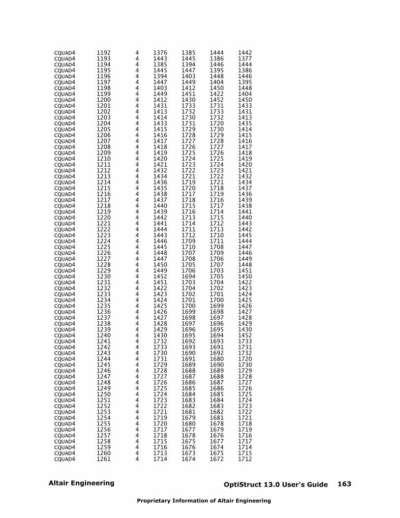
Altair Engineering OptiStruct 13.0 User's Guide 163
Proprietary Information of Altair Engineering
CQUAD4 1192 4 1376 1385 1444 1442 CQUAD4 1193 4 1443 1445 1386 1377 CQUAD4 1194 4 1385 1394 1446 1444 CQUAD4 1195 4 1445 1447 1395 1386 CQUAD4 1196 4 1394 1403 1448 1446 CQUAD4 1197 4 1447 1449 1404 1395 CQUAD4 1198 4 1403 1412 1450 1448 CQUAD4 1199 4 1449 1451 1422 1404 CQUAD4 1200 4 1412 1430 1452 1450 CQUAD4 1201 4 1431 1733 1731 1433 CQUAD4 1202 4 1413 1732 1733 1431 CQUAD4 1203 4 1414 1730 1732 1413 CQUAD4 1204 4 1433 1731 1720 1435 CQUAD4 1205 4 1415 1729 1730 1414 CQUAD4 1206 4 1416 1728 1729 1415 CQUAD4 1207 4 1417 1727 1728 1416 CQUAD4 1208 4 1418 1726 1727 1417 CQUAD4 1209 4 1419 1725 1726 1418 CQUAD4 1210 4 1420 1724 1725 1419 CQUAD4 1211 4 1421 1723 1724 1420 CQUAD4 1212 4 1432 1722 1723 1421 CQUAD4 1213 4 1434 1721 1722 1432 CQUAD4 1214 4 1436 1719 1721 1434 CQUAD4 1215 4 1435 1720 1718 1437 CQUAD4 1216 4 1438 1717 1719 1436 CQUAD4 1217 4 1437 1718 1716 1439 CQUAD4 1218 4 1440 1715 1717 1438 CQUAD4 1219 4 1439 1716 1714 1441 CQUAD4 1220 4 1442 1713 1715 1440 CQUAD4 1221 4 1441 1714 1712 1443 CQUAD4 1222 4 1444 1711 1713 1442 CQUAD4 1223 4 1443 1712 1710 1445 CQUAD4 1224 4 1446 1709 1711 1444 CQUAD4 1225 4 1445 1710 1708 1447 CQUAD4 1226 4 1448 1707 1709 1446 CQUAD4 1227 4 1447 1708 1706 1449 CQUAD4 1228 4 1450 1705 1707 1448 CQUAD4 1229 4 1449 1706 1703 1451 CQUAD4 1230 4 1452 1694 1705 1450 CQUAD4 1231 4 1451 1703 1704 1422 CQUAD4 1232 4 1422 1704 1702 1423 CQUAD4 1233 4 1423 1702 1701 1424 CQUAD4 1234 4 1424 1701 1700 1425 CQUAD4 1235 4 1425 1700 1699 1426 CQUAD4 1236 4 1426 1699 1698 1427 CQUAD4 1237 4 1427 1698 1697 1428 CQUAD4 1238 4 1428 1697 1696 1429 CQUAD4 1239 4 1429 1696 1695 1430 CQUAD4 1240 4 1430 1695 1694 1452 CQUAD4 1241 4 1732 1692 1693 1733 CQUAD4 1242 4 1733 1693 1691 1731 CQUAD4 1243 4 1730 1690 1692 1732 CQUAD4 1244 4 1731 1691 1680 1720 CQUAD4 1245 4 1729 1689 1690 1730 CQUAD4 1246 4 1728 1688 1689 1729 CQUAD4 1247 4 1727 1687 1688 1728 CQUAD4 1248 4 1726 1686 1687 1727 CQUAD4 1249 4 1725 1685 1686 1726 CQUAD4 1250 4 1724 1684 1685 1725 CQUAD4 1251 4 1723 1683 1684 1724 CQUAD4 1252 4 1722 1682 1683 1723 CQUAD4 1253 4 1721 1681 1682 1722 CQUAD4 1254 4 1719 1679 1681 1721 CQUAD4 1255 4 1720 1680 1678 1718 CQUAD4 1256 4 1717 1677 1679 1719 CQUAD4 1257 4 1718 1678 1676 1716 CQUAD4 1258 4 1715 1675 1677 1717 CQUAD4 1259 4 1716 1676 1674 1714 CQUAD4 1260 4 1713 1673 1675 1715 CQUAD4 1261 4 1714 1674 1672 1712
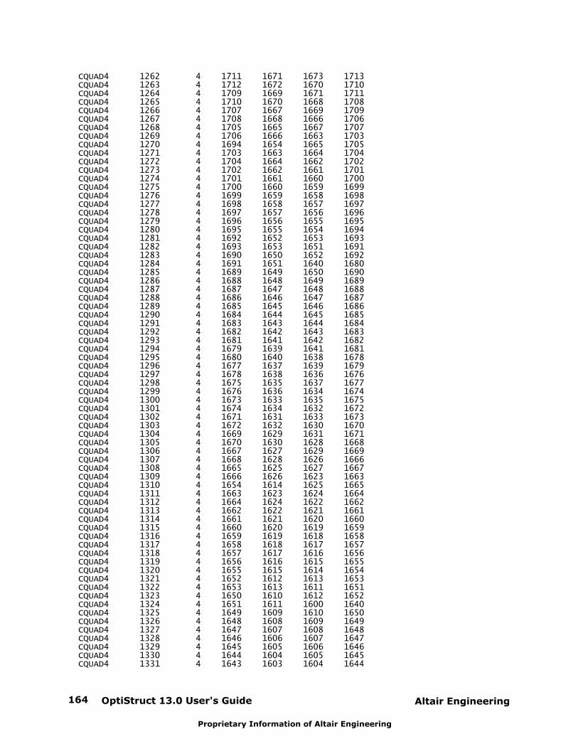
OptiStruct 13.0 User's Guide164 Altair Engineering
Proprietary Information of Altair Engineering
CQUAD4 1262 4 1711 1671 1673 1713 CQUAD4 1263 4 1712 1672 1670 1710 CQUAD4 1264 4 1709 1669 1671 1711 CQUAD4 1265 4 1710 1670 1668 1708 CQUAD4 1266 4 1707 1667 1669 1709 CQUAD4 1267 4 1708 1668 1666 1706 CQUAD4 1268 4 1705 1665 1667 1707 CQUAD4 1269 4 1706 1666 1663 1703 CQUAD4 1270 4 1694 1654 1665 1705 CQUAD4 1271 4 1703 1663 1664 1704 CQUAD4 1272 4 1704 1664 1662 1702 CQUAD4 1273 4 1702 1662 1661 1701 CQUAD4 1274 4 1701 1661 1660 1700 CQUAD4 1275 4 1700 1660 1659 1699 CQUAD4 1276 4 1699 1659 1658 1698 CQUAD4 1277 4 1698 1658 1657 1697 CQUAD4 1278 4 1697 1657 1656 1696 CQUAD4 1279 4 1696 1656 1655 1695 CQUAD4 1280 4 1695 1655 1654 1694 CQUAD4 1281 4 1692 1652 1653 1693 CQUAD4 1282 4 1693 1653 1651 1691 CQUAD4 1283 4 1690 1650 1652 1692 CQUAD4 1284 4 1691 1651 1640 1680 CQUAD4 1285 4 1689 1649 1650 1690 CQUAD4 1286 4 1688 1648 1649 1689 CQUAD4 1287 4 1687 1647 1648 1688 CQUAD4 1288 4 1686 1646 1647 1687 CQUAD4 1289 4 1685 1645 1646 1686 CQUAD4 1290 4 1684 1644 1645 1685 CQUAD4 1291 4 1683 1643 1644 1684 CQUAD4 1292 4 1682 1642 1643 1683 CQUAD4 1293 4 1681 1641 1642 1682 CQUAD4 1294 4 1679 1639 1641 1681 CQUAD4 1295 4 1680 1640 1638 1678 CQUAD4 1296 4 1677 1637 1639 1679 CQUAD4 1297 4 1678 1638 1636 1676 CQUAD4 1298 4 1675 1635 1637 1677 CQUAD4 1299 4 1676 1636 1634 1674 CQUAD4 1300 4 1673 1633 1635 1675 CQUAD4 1301 4 1674 1634 1632 1672 CQUAD4 1302 4 1671 1631 1633 1673 CQUAD4 1303 4 1672 1632 1630 1670 CQUAD4 1304 4 1669 1629 1631 1671 CQUAD4 1305 4 1670 1630 1628 1668 CQUAD4 1306 4 1667 1627 1629 1669 CQUAD4 1307 4 1668 1628 1626 1666 CQUAD4 1308 4 1665 1625 1627 1667 CQUAD4 1309 4 1666 1626 1623 1663 CQUAD4 1310 4 1654 1614 1625 1665 CQUAD4 1311 4 1663 1623 1624 1664 CQUAD4 1312 4 1664 1624 1622 1662 CQUAD4 1313 4 1662 1622 1621 1661 CQUAD4 1314 4 1661 1621 1620 1660 CQUAD4 1315 4 1660 1620 1619 1659 CQUAD4 1316 4 1659 1619 1618 1658 CQUAD4 1317 4 1658 1618 1617 1657 CQUAD4 1318 4 1657 1617 1616 1656 CQUAD4 1319 4 1656 1616 1615 1655 CQUAD4 1320 4 1655 1615 1614 1654 CQUAD4 1321 4 1652 1612 1613 1653 CQUAD4 1322 4 1653 1613 1611 1651 CQUAD4 1323 4 1650 1610 1612 1652 CQUAD4 1324 4 1651 1611 1600 1640 CQUAD4 1325 4 1649 1609 1610 1650 CQUAD4 1326 4 1648 1608 1609 1649 CQUAD4 1327 4 1647 1607 1608 1648 CQUAD4 1328 4 1646 1606 1607 1647 CQUAD4 1329 4 1645 1605 1606 1646 CQUAD4 1330 4 1644 1604 1605 1645 CQUAD4 1331 4 1643 1603 1604 1644
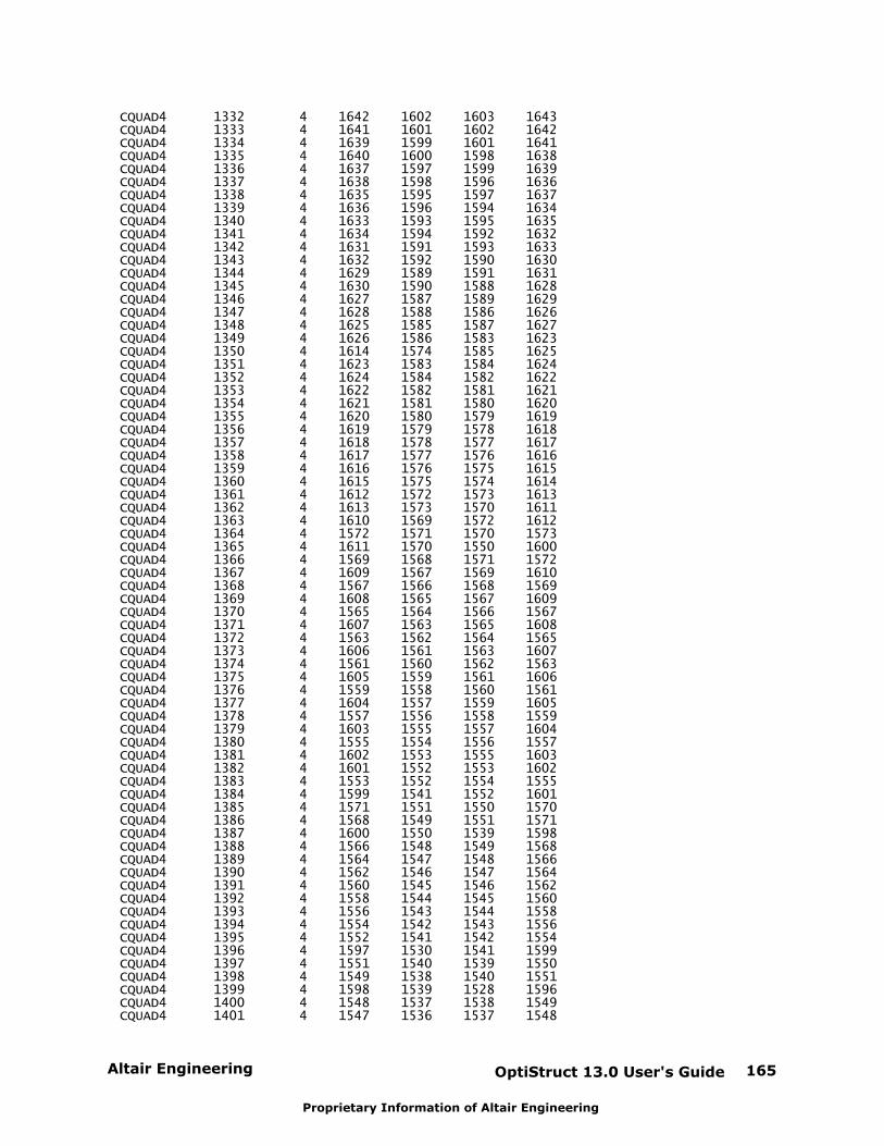
Altair Engineering OptiStruct 13.0 User's Guide 165
Proprietary Information of Altair Engineering
CQUAD4 1332 4 1642 1602 1603 1643 CQUAD4 1333 4 1641 1601 1602 1642 CQUAD4 1334 4 1639 1599 1601 1641 CQUAD4 1335 4 1640 1600 1598 1638 CQUAD4 1336 4 1637 1597 1599 1639 CQUAD4 1337 4 1638 1598 1596 1636 CQUAD4 1338 4 1635 1595 1597 1637 CQUAD4 1339 4 1636 1596 1594 1634 CQUAD4 1340 4 1633 1593 1595 1635 CQUAD4 1341 4 1634 1594 1592 1632 CQUAD4 1342 4 1631 1591 1593 1633 CQUAD4 1343 4 1632 1592 1590 1630 CQUAD4 1344 4 1629 1589 1591 1631 CQUAD4 1345 4 1630 1590 1588 1628 CQUAD4 1346 4 1627 1587 1589 1629 CQUAD4 1347 4 1628 1588 1586 1626 CQUAD4 1348 4 1625 1585 1587 1627 CQUAD4 1349 4 1626 1586 1583 1623 CQUAD4 1350 4 1614 1574 1585 1625 CQUAD4 1351 4 1623 1583 1584 1624 CQUAD4 1352 4 1624 1584 1582 1622 CQUAD4 1353 4 1622 1582 1581 1621 CQUAD4 1354 4 1621 1581 1580 1620 CQUAD4 1355 4 1620 1580 1579 1619 CQUAD4 1356 4 1619 1579 1578 1618 CQUAD4 1357 4 1618 1578 1577 1617 CQUAD4 1358 4 1617 1577 1576 1616 CQUAD4 1359 4 1616 1576 1575 1615 CQUAD4 1360 4 1615 1575 1574 1614 CQUAD4 1361 4 1612 1572 1573 1613 CQUAD4 1362 4 1613 1573 1570 1611 CQUAD4 1363 4 1610 1569 1572 1612 CQUAD4 1364 4 1572 1571 1570 1573 CQUAD4 1365 4 1611 1570 1550 1600 CQUAD4 1366 4 1569 1568 1571 1572 CQUAD4 1367 4 1609 1567 1569 1610 CQUAD4 1368 4 1567 1566 1568 1569 CQUAD4 1369 4 1608 1565 1567 1609 CQUAD4 1370 4 1565 1564 1566 1567 CQUAD4 1371 4 1607 1563 1565 1608 CQUAD4 1372 4 1563 1562 1564 1565 CQUAD4 1373 4 1606 1561 1563 1607 CQUAD4 1374 4 1561 1560 1562 1563 CQUAD4 1375 4 1605 1559 1561 1606 CQUAD4 1376 4 1559 1558 1560 1561 CQUAD4 1377 4 1604 1557 1559 1605 CQUAD4 1378 4 1557 1556 1558 1559 CQUAD4 1379 4 1603 1555 1557 1604 CQUAD4 1380 4 1555 1554 1556 1557 CQUAD4 1381 4 1602 1553 1555 1603 CQUAD4 1382 4 1601 1552 1553 1602 CQUAD4 1383 4 1553 1552 1554 1555 CQUAD4 1384 4 1599 1541 1552 1601 CQUAD4 1385 4 1571 1551 1550 1570 CQUAD4 1386 4 1568 1549 1551 1571 CQUAD4 1387 4 1600 1550 1539 1598 CQUAD4 1388 4 1566 1548 1549 1568 CQUAD4 1389 4 1564 1547 1548 1566 CQUAD4 1390 4 1562 1546 1547 1564 CQUAD4 1391 4 1560 1545 1546 1562 CQUAD4 1392 4 1558 1544 1545 1560 CQUAD4 1393 4 1556 1543 1544 1558 CQUAD4 1394 4 1554 1542 1543 1556 CQUAD4 1395 4 1552 1541 1542 1554 CQUAD4 1396 4 1597 1530 1541 1599 CQUAD4 1397 4 1551 1540 1539 1550 CQUAD4 1398 4 1549 1538 1540 1551 CQUAD4 1399 4 1598 1539 1528 1596 CQUAD4 1400 4 1548 1537 1538 1549 CQUAD4 1401 4 1547 1536 1537 1548
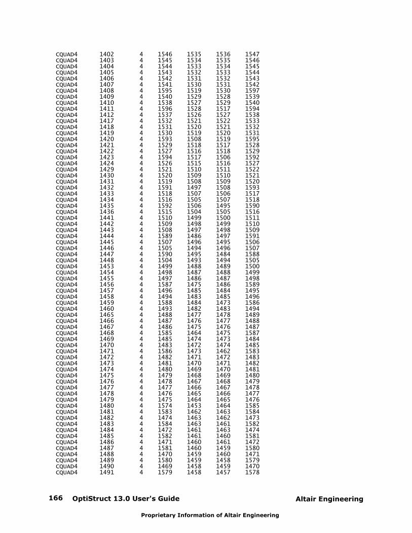
OptiStruct 13.0 User's Guide166 Altair Engineering
Proprietary Information of Altair Engineering
CQUAD4 1402 4 1546 1535 1536 1547 CQUAD4 1403 4 1545 1534 1535 1546 CQUAD4 1404 4 1544 1533 1534 1545 CQUAD4 1405 4 1543 1532 1533 1544 CQUAD4 1406 4 1542 1531 1532 1543 CQUAD4 1407 4 1541 1530 1531 1542 CQUAD4 1408 4 1595 1519 1530 1597 CQUAD4 1409 4 1540 1529 1528 1539 CQUAD4 1410 4 1538 1527 1529 1540 CQUAD4 1411 4 1596 1528 1517 1594 CQUAD4 1412 4 1537 1526 1527 1538 CQUAD4 1417 4 1532 1521 1522 1533 CQUAD4 1418 4 1531 1520 1521 1532 CQUAD4 1419 4 1530 1519 1520 1531 CQUAD4 1420 4 1593 1508 1519 1595 CQUAD4 1421 4 1529 1518 1517 1528 CQUAD4 1422 4 1527 1516 1518 1529 CQUAD4 1423 4 1594 1517 1506 1592 CQUAD4 1424 4 1526 1515 1516 1527 CQUAD4 1429 4 1521 1510 1511 1522 CQUAD4 1430 4 1520 1509 1510 1521 CQUAD4 1431 4 1519 1508 1509 1520 CQUAD4 1432 4 1591 1497 1508 1593 CQUAD4 1433 4 1518 1507 1506 1517 CQUAD4 1434 4 1516 1505 1507 1518 CQUAD4 1435 4 1592 1506 1495 1590 CQUAD4 1436 4 1515 1504 1505 1516 CQUAD4 1441 4 1510 1499 1500 1511 CQUAD4 1442 4 1509 1498 1499 1510 CQUAD4 1443 4 1508 1497 1498 1509 CQUAD4 1444 4 1589 1486 1497 1591 CQUAD4 1445 4 1507 1496 1495 1506 CQUAD4 1446 4 1505 1494 1496 1507 CQUAD4 1447 4 1590 1495 1484 1588 CQUAD4 1448 4 1504 1493 1494 1505 CQUAD4 1453 4 1499 1488 1489 1500 CQUAD4 1454 4 1498 1487 1488 1499 CQUAD4 1455 4 1497 1486 1487 1498 CQUAD4 1456 4 1587 1475 1486 1589 CQUAD4 1457 4 1496 1485 1484 1495 CQUAD4 1458 4 1494 1483 1485 1496 CQUAD4 1459 4 1588 1484 1473 1586 CQUAD4 1460 4 1493 1482 1483 1494 CQUAD4 1465 4 1488 1477 1478 1489 CQUAD4 1466 4 1487 1476 1477 1488 CQUAD4 1467 4 1486 1475 1476 1487 CQUAD4 1468 4 1585 1464 1475 1587 CQUAD4 1469 4 1485 1474 1473 1484 CQUAD4 1470 4 1483 1472 1474 1485 CQUAD4 1471 4 1586 1473 1462 1583 CQUAD4 1472 4 1482 1471 1472 1483 CQUAD4 1473 4 1481 1470 1471 1482 CQUAD4 1474 4 1480 1469 1470 1481 CQUAD4 1475 4 1479 1468 1469 1480 CQUAD4 1476 4 1478 1467 1468 1479 CQUAD4 1477 4 1477 1466 1467 1478 CQUAD4 1478 4 1476 1465 1466 1477 CQUAD4 1479 4 1475 1464 1465 1476 CQUAD4 1480 4 1574 1453 1464 1585 CQUAD4 1481 4 1583 1462 1463 1584 CQUAD4 1482 4 1474 1463 1462 1473 CQUAD4 1483 4 1584 1463 1461 1582 CQUAD4 1484 4 1472 1461 1463 1474 CQUAD4 1485 4 1582 1461 1460 1581 CQUAD4 1486 4 1471 1460 1461 1472 CQUAD4 1487 4 1581 1460 1459 1580 CQUAD4 1488 4 1470 1459 1460 1471 CQUAD4 1489 4 1580 1459 1458 1579 CQUAD4 1490 4 1469 1458 1459 1470 CQUAD4 1491 4 1579 1458 1457 1578
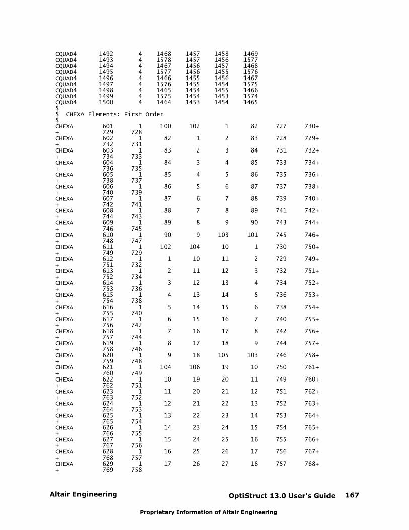
Altair Engineering OptiStruct 13.0 User's Guide 167
Proprietary Information of Altair Engineering
CQUAD4 1492 4 1468 1457 1458 1469 CQUAD4 1493 4 1578 1457 1456 1577 CQUAD4 1494 4 1467 1456 1457 1468 CQUAD4 1495 4 1577 1456 1455 1576 CQUAD4 1496 4 1466 1455 1456 1467 CQUAD4 1497 4 1576 1455 1454 1575 CQUAD4 1498 4 1465 1454 1455 1466 CQUAD4 1499 4 1575 1454 1453 1574 CQUAD4 1500 4 1464 1453 1454 1465 $$ CHEXA Elements: First Order$CHEXA 601 1 100 102 1 82 727 730+ + 729 728CHEXA 602 1 82 1 2 83 728 729+ + 732 731CHEXA 603 1 83 2 3 84 731 732+ + 734 733CHEXA 604 1 84 3 4 85 733 734+ + 736 735CHEXA 605 1 85 4 5 86 735 736+ + 738 737CHEXA 606 1 86 5 6 87 737 738+ + 740 739CHEXA 607 1 87 6 7 88 739 740+ + 742 741CHEXA 608 1 88 7 8 89 741 742+ + 744 743CHEXA 609 1 89 8 9 90 743 744+ + 746 745CHEXA 610 1 90 9 103 101 745 746+ + 748 747CHEXA 611 1 102 104 10 1 730 750+ + 749 729CHEXA 612 1 1 10 11 2 729 749+ + 751 732CHEXA 613 1 2 11 12 3 732 751+ + 752 734CHEXA 614 1 3 12 13 4 734 752+ + 753 736CHEXA 615 1 4 13 14 5 736 753+ + 754 738CHEXA 616 1 5 14 15 6 738 754+ + 755 740CHEXA 617 1 6 15 16 7 740 755+ + 756 742CHEXA 618 1 7 16 17 8 742 756+ + 757 744CHEXA 619 1 8 17 18 9 744 757+ + 758 746CHEXA 620 1 9 18 105 103 746 758+ + 759 748CHEXA 621 1 104 106 19 10 750 761+ + 760 749CHEXA 622 1 10 19 20 11 749 760+ + 762 751CHEXA 623 1 11 20 21 12 751 762+ + 763 752CHEXA 624 1 12 21 22 13 752 763+ + 764 753CHEXA 625 1 13 22 23 14 753 764+ + 765 754CHEXA 626 1 14 23 24 15 754 765+ + 766 755CHEXA 627 1 15 24 25 16 755 766+ + 767 756CHEXA 628 1 16 25 26 17 756 767+ + 768 757CHEXA 629 1 17 26 27 18 757 768+ + 769 758
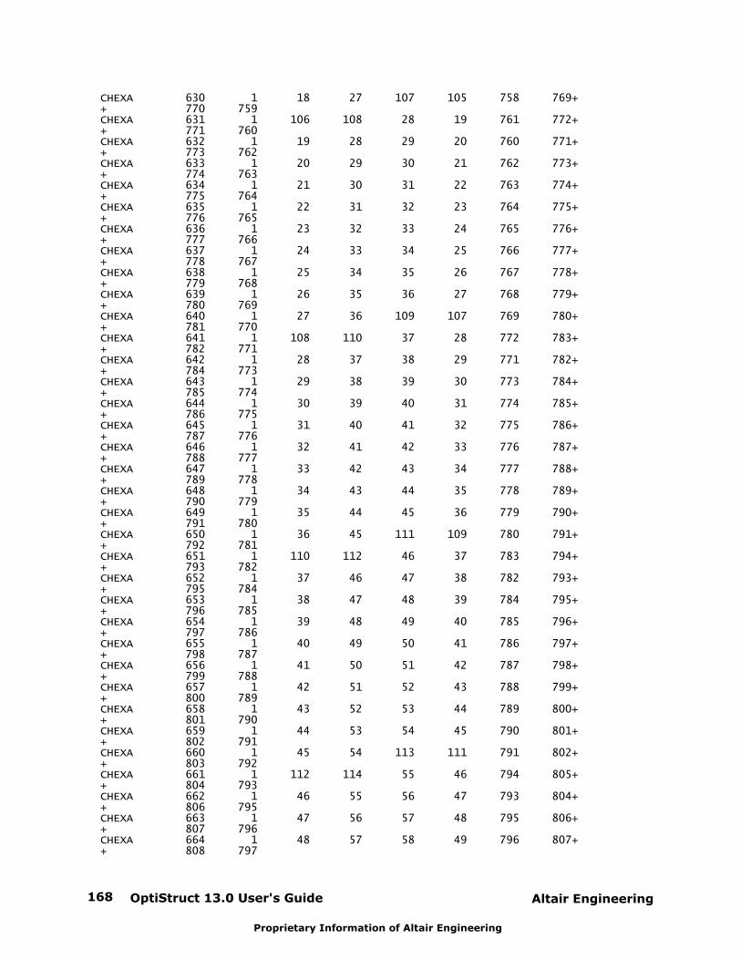
OptiStruct 13.0 User's Guide168 Altair Engineering
Proprietary Information of Altair Engineering
CHEXA 630 1 18 27 107 105 758 769+ + 770 759CHEXA 631 1 106 108 28 19 761 772+ + 771 760CHEXA 632 1 19 28 29 20 760 771+ + 773 762CHEXA 633 1 20 29 30 21 762 773+ + 774 763CHEXA 634 1 21 30 31 22 763 774+ + 775 764CHEXA 635 1 22 31 32 23 764 775+ + 776 765CHEXA 636 1 23 32 33 24 765 776+ + 777 766CHEXA 637 1 24 33 34 25 766 777+ + 778 767CHEXA 638 1 25 34 35 26 767 778+ + 779 768CHEXA 639 1 26 35 36 27 768 779+ + 780 769CHEXA 640 1 27 36 109 107 769 780+ + 781 770CHEXA 641 1 108 110 37 28 772 783+ + 782 771CHEXA 642 1 28 37 38 29 771 782+ + 784 773CHEXA 643 1 29 38 39 30 773 784+ + 785 774CHEXA 644 1 30 39 40 31 774 785+ + 786 775CHEXA 645 1 31 40 41 32 775 786+ + 787 776CHEXA 646 1 32 41 42 33 776 787+ + 788 777CHEXA 647 1 33 42 43 34 777 788+ + 789 778CHEXA 648 1 34 43 44 35 778 789+ + 790 779CHEXA 649 1 35 44 45 36 779 790+ + 791 780CHEXA 650 1 36 45 111 109 780 791+ + 792 781CHEXA 651 1 110 112 46 37 783 794+ + 793 782CHEXA 652 1 37 46 47 38 782 793+ + 795 784CHEXA 653 1 38 47 48 39 784 795+ + 796 785CHEXA 654 1 39 48 49 40 785 796+ + 797 786CHEXA 655 1 40 49 50 41 786 797+ + 798 787CHEXA 656 1 41 50 51 42 787 798+ + 799 788CHEXA 657 1 42 51 52 43 788 799+ + 800 789CHEXA 658 1 43 52 53 44 789 800+ + 801 790CHEXA 659 1 44 53 54 45 790 801+ + 802 791CHEXA 660 1 45 54 113 111 791 802+ + 803 792CHEXA 661 1 112 114 55 46 794 805+ + 804 793CHEXA 662 1 46 55 56 47 793 804+ + 806 795CHEXA 663 1 47 56 57 48 795 806+ + 807 796CHEXA 664 1 48 57 58 49 796 807+ + 808 797
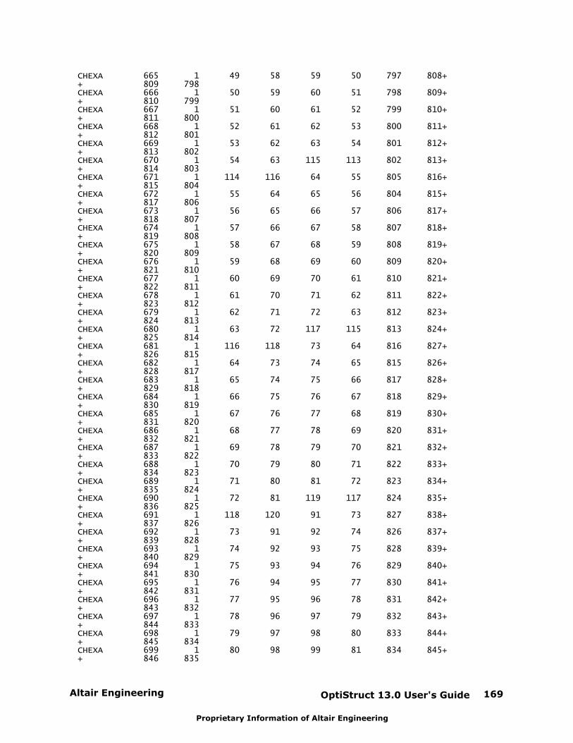
Altair Engineering OptiStruct 13.0 User's Guide 169
Proprietary Information of Altair Engineering
CHEXA 665 1 49 58 59 50 797 808+ + 809 798CHEXA 666 1 50 59 60 51 798 809+ + 810 799CHEXA 667 1 51 60 61 52 799 810+ + 811 800CHEXA 668 1 52 61 62 53 800 811+ + 812 801CHEXA 669 1 53 62 63 54 801 812+ + 813 802CHEXA 670 1 54 63 115 113 802 813+ + 814 803CHEXA 671 1 114 116 64 55 805 816+ + 815 804CHEXA 672 1 55 64 65 56 804 815+ + 817 806CHEXA 673 1 56 65 66 57 806 817+ + 818 807CHEXA 674 1 57 66 67 58 807 818+ + 819 808CHEXA 675 1 58 67 68 59 808 819+ + 820 809CHEXA 676 1 59 68 69 60 809 820+ + 821 810CHEXA 677 1 60 69 70 61 810 821+ + 822 811CHEXA 678 1 61 70 71 62 811 822+ + 823 812CHEXA 679 1 62 71 72 63 812 823+ + 824 813CHEXA 680 1 63 72 117 115 813 824+ + 825 814CHEXA 681 1 116 118 73 64 816 827+ + 826 815CHEXA 682 1 64 73 74 65 815 826+ + 828 817CHEXA 683 1 65 74 75 66 817 828+ + 829 818CHEXA 684 1 66 75 76 67 818 829+ + 830 819CHEXA 685 1 67 76 77 68 819 830+ + 831 820CHEXA 686 1 68 77 78 69 820 831+ + 832 821CHEXA 687 1 69 78 79 70 821 832+ + 833 822CHEXA 688 1 70 79 80 71 822 833+ + 834 823CHEXA 689 1 71 80 81 72 823 834+ + 835 824CHEXA 690 1 72 81 119 117 824 835+ + 836 825CHEXA 691 1 118 120 91 73 827 838+ + 837 826CHEXA 692 1 73 91 92 74 826 837+ + 839 828CHEXA 693 1 74 92 93 75 828 839+ + 840 829CHEXA 694 1 75 93 94 76 829 840+ + 841 830CHEXA 695 1 76 94 95 77 830 841+ + 842 831CHEXA 696 1 77 95 96 78 831 842+ + 843 832CHEXA 697 1 78 96 97 79 832 843+ + 844 833CHEXA 698 1 79 97 98 80 833 844+ + 845 834CHEXA 699 1 80 98 99 81 834 845+ + 846 835
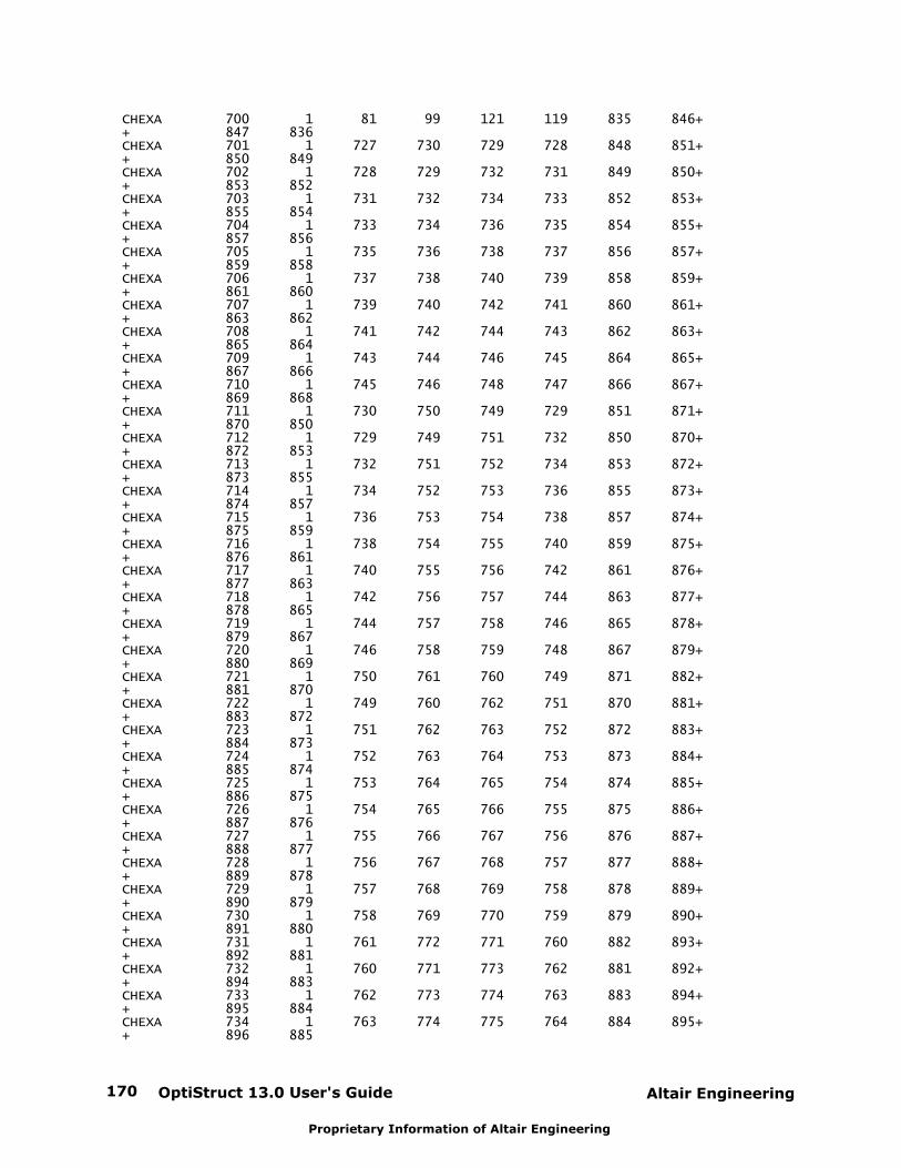
OptiStruct 13.0 User's Guide170 Altair Engineering
Proprietary Information of Altair Engineering
CHEXA 700 1 81 99 121 119 835 846+ + 847 836CHEXA 701 1 727 730 729 728 848 851+ + 850 849CHEXA 702 1 728 729 732 731 849 850+ + 853 852CHEXA 703 1 731 732 734 733 852 853+ + 855 854CHEXA 704 1 733 734 736 735 854 855+ + 857 856CHEXA 705 1 735 736 738 737 856 857+ + 859 858CHEXA 706 1 737 738 740 739 858 859+ + 861 860CHEXA 707 1 739 740 742 741 860 861+ + 863 862CHEXA 708 1 741 742 744 743 862 863+ + 865 864CHEXA 709 1 743 744 746 745 864 865+ + 867 866CHEXA 710 1 745 746 748 747 866 867+ + 869 868CHEXA 711 1 730 750 749 729 851 871+ + 870 850CHEXA 712 1 729 749 751 732 850 870+ + 872 853CHEXA 713 1 732 751 752 734 853 872+ + 873 855CHEXA 714 1 734 752 753 736 855 873+ + 874 857CHEXA 715 1 736 753 754 738 857 874+ + 875 859CHEXA 716 1 738 754 755 740 859 875+ + 876 861CHEXA 717 1 740 755 756 742 861 876+ + 877 863CHEXA 718 1 742 756 757 744 863 877+ + 878 865CHEXA 719 1 744 757 758 746 865 878+ + 879 867CHEXA 720 1 746 758 759 748 867 879+ + 880 869CHEXA 721 1 750 761 760 749 871 882+ + 881 870CHEXA 722 1 749 760 762 751 870 881+ + 883 872CHEXA 723 1 751 762 763 752 872 883+ + 884 873CHEXA 724 1 752 763 764 753 873 884+ + 885 874CHEXA 725 1 753 764 765 754 874 885+ + 886 875CHEXA 726 1 754 765 766 755 875 886+ + 887 876CHEXA 727 1 755 766 767 756 876 887+ + 888 877CHEXA 728 1 756 767 768 757 877 888+ + 889 878CHEXA 729 1 757 768 769 758 878 889+ + 890 879CHEXA 730 1 758 769 770 759 879 890+ + 891 880CHEXA 731 1 761 772 771 760 882 893+ + 892 881CHEXA 732 1 760 771 773 762 881 892+ + 894 883CHEXA 733 1 762 773 774 763 883 894+ + 895 884CHEXA 734 1 763 774 775 764 884 895+ + 896 885
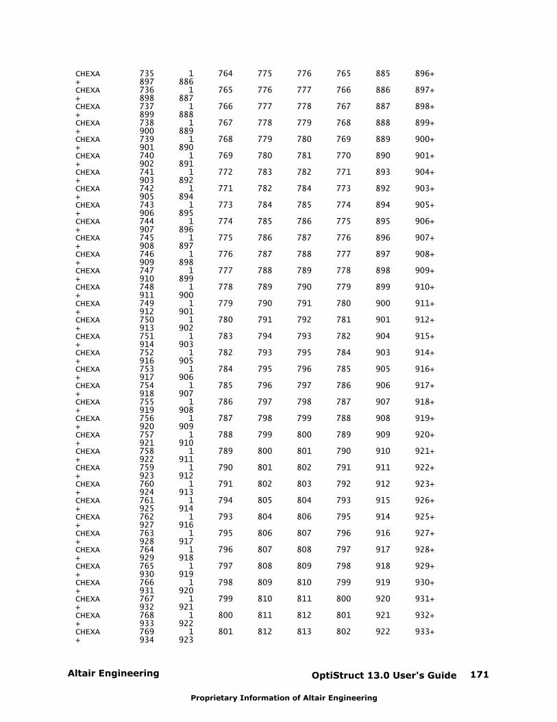
Altair Engineering OptiStruct 13.0 User's Guide 171
Proprietary Information of Altair Engineering
CHEXA 735 1 764 775 776 765 885 896+ + 897 886CHEXA 736 1 765 776 777 766 886 897+ + 898 887CHEXA 737 1 766 777 778 767 887 898+ + 899 888CHEXA 738 1 767 778 779 768 888 899+ + 900 889CHEXA 739 1 768 779 780 769 889 900+ + 901 890CHEXA 740 1 769 780 781 770 890 901+ + 902 891CHEXA 741 1 772 783 782 771 893 904+ + 903 892CHEXA 742 1 771 782 784 773 892 903+ + 905 894CHEXA 743 1 773 784 785 774 894 905+ + 906 895CHEXA 744 1 774 785 786 775 895 906+ + 907 896CHEXA 745 1 775 786 787 776 896 907+ + 908 897CHEXA 746 1 776 787 788 777 897 908+ + 909 898CHEXA 747 1 777 788 789 778 898 909+ + 910 899CHEXA 748 1 778 789 790 779 899 910+ + 911 900CHEXA 749 1 779 790 791 780 900 911+ + 912 901CHEXA 750 1 780 791 792 781 901 912+ + 913 902CHEXA 751 1 783 794 793 782 904 915+ + 914 903CHEXA 752 1 782 793 795 784 903 914+ + 916 905CHEXA 753 1 784 795 796 785 905 916+ + 917 906CHEXA 754 1 785 796 797 786 906 917+ + 918 907CHEXA 755 1 786 797 798 787 907 918+ + 919 908CHEXA 756 1 787 798 799 788 908 919+ + 920 909CHEXA 757 1 788 799 800 789 909 920+ + 921 910CHEXA 758 1 789 800 801 790 910 921+ + 922 911CHEXA 759 1 790 801 802 791 911 922+ + 923 912CHEXA 760 1 791 802 803 792 912 923+ + 924 913CHEXA 761 1 794 805 804 793 915 926+ + 925 914CHEXA 762 1 793 804 806 795 914 925+ + 927 916CHEXA 763 1 795 806 807 796 916 927+ + 928 917CHEXA 764 1 796 807 808 797 917 928+ + 929 918CHEXA 765 1 797 808 809 798 918 929+ + 930 919CHEXA 766 1 798 809 810 799 919 930+ + 931 920CHEXA 767 1 799 810 811 800 920 931+ + 932 921CHEXA 768 1 800 811 812 801 921 932+ + 933 922CHEXA 769 1 801 812 813 802 922 933+ + 934 923
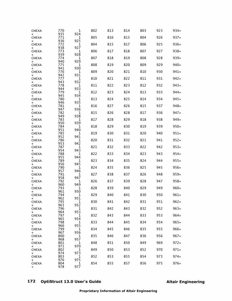
OptiStruct 13.0 User's Guide172 Altair Engineering
Proprietary Information of Altair Engineering
CHEXA 770 1 802 813 814 803 923 934+ + 935 924CHEXA 771 1 805 816 815 804 926 937+ + 936 925CHEXA 772 1 804 815 817 806 925 936+ + 938 927CHEXA 773 1 806 817 818 807 927 938+ + 939 928CHEXA 774 1 807 818 819 808 928 939+ + 940 929CHEXA 775 1 808 819 820 809 929 940+ + 941 930CHEXA 776 1 809 820 821 810 930 941+ + 942 931CHEXA 777 1 810 821 822 811 931 942+ + 943 932CHEXA 778 1 811 822 823 812 932 943+ + 944 933CHEXA 779 1 812 823 824 813 933 944+ + 945 934CHEXA 780 1 813 824 825 814 934 945+ + 946 935CHEXA 781 1 816 827 826 815 937 948+ + 947 936CHEXA 782 1 815 826 828 817 936 947+ + 949 938CHEXA 783 1 817 828 829 818 938 949+ + 950 939CHEXA 784 1 818 829 830 819 939 950+ + 951 940CHEXA 785 1 819 830 831 820 940 951+ + 952 941CHEXA 786 1 820 831 832 821 941 952+ + 953 942CHEXA 787 1 821 832 833 822 942 953+ + 954 943CHEXA 788 1 822 833 834 823 943 954+ + 955 944CHEXA 789 1 823 834 835 824 944 955+ + 956 945CHEXA 790 1 824 835 836 825 945 956+ + 957 946CHEXA 791 1 827 838 837 826 948 959+ + 958 947CHEXA 792 1 826 837 839 828 947 958+ + 960 949CHEXA 793 1 828 839 840 829 949 960+ + 961 950CHEXA 794 1 829 840 841 830 950 961+ + 962 951CHEXA 795 1 830 841 842 831 951 962+ + 963 952CHEXA 796 1 831 842 843 832 952 963+ + 964 953CHEXA 797 1 832 843 844 833 953 964+ + 965 954CHEXA 798 1 833 844 845 834 954 965+ + 966 955CHEXA 799 1 834 845 846 835 955 966+ + 967 956CHEXA 800 1 835 846 847 836 956 967+ + 968 957CHEXA 801 1 848 851 850 849 969 972+ + 971 970CHEXA 802 1 849 850 853 852 970 971+ + 974 973CHEXA 803 1 852 853 855 854 973 974+ + 976 975CHEXA 804 1 854 855 857 856 975 976+ + 978 977
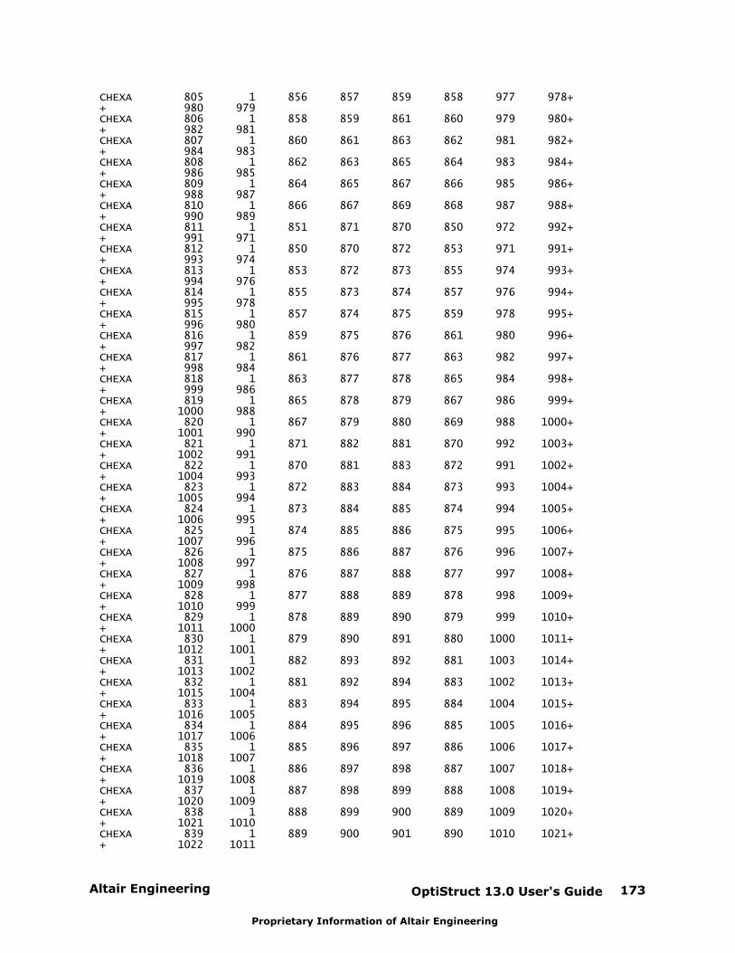
Altair Engineering OptiStruct 13.0 User's Guide 173
Proprietary Information of Altair Engineering
CHEXA 805 1 856 857 859 858 977 978+ + 980 979CHEXA 806 1 858 859 861 860 979 980+ + 982 981CHEXA 807 1 860 861 863 862 981 982+ + 984 983CHEXA 808 1 862 863 865 864 983 984+ + 986 985CHEXA 809 1 864 865 867 866 985 986+ + 988 987CHEXA 810 1 866 867 869 868 987 988+ + 990 989CHEXA 811 1 851 871 870 850 972 992+ + 991 971CHEXA 812 1 850 870 872 853 971 991+ + 993 974CHEXA 813 1 853 872 873 855 974 993+ + 994 976CHEXA 814 1 855 873 874 857 976 994+ + 995 978CHEXA 815 1 857 874 875 859 978 995+ + 996 980CHEXA 816 1 859 875 876 861 980 996+ + 997 982CHEXA 817 1 861 876 877 863 982 997+ + 998 984CHEXA 818 1 863 877 878 865 984 998+ + 999 986CHEXA 819 1 865 878 879 867 986 999+ + 1000 988CHEXA 820 1 867 879 880 869 988 1000+ + 1001 990CHEXA 821 1 871 882 881 870 992 1003+ + 1002 991CHEXA 822 1 870 881 883 872 991 1002+ + 1004 993CHEXA 823 1 872 883 884 873 993 1004+ + 1005 994CHEXA 824 1 873 884 885 874 994 1005+ + 1006 995CHEXA 825 1 874 885 886 875 995 1006+ + 1007 996CHEXA 826 1 875 886 887 876 996 1007+ + 1008 997CHEXA 827 1 876 887 888 877 997 1008+ + 1009 998CHEXA 828 1 877 888 889 878 998 1009+ + 1010 999CHEXA 829 1 878 889 890 879 999 1010+ + 1011 1000CHEXA 830 1 879 890 891 880 1000 1011+ + 1012 1001CHEXA 831 1 882 893 892 881 1003 1014+ + 1013 1002CHEXA 832 1 881 892 894 883 1002 1013+ + 1015 1004CHEXA 833 1 883 894 895 884 1004 1015+ + 1016 1005CHEXA 834 1 884 895 896 885 1005 1016+ + 1017 1006CHEXA 835 1 885 896 897 886 1006 1017+ + 1018 1007CHEXA 836 1 886 897 898 887 1007 1018+ + 1019 1008CHEXA 837 1 887 898 899 888 1008 1019+ + 1020 1009CHEXA 838 1 888 899 900 889 1009 1020+ + 1021 1010CHEXA 839 1 889 900 901 890 1010 1021+ + 1022 1011
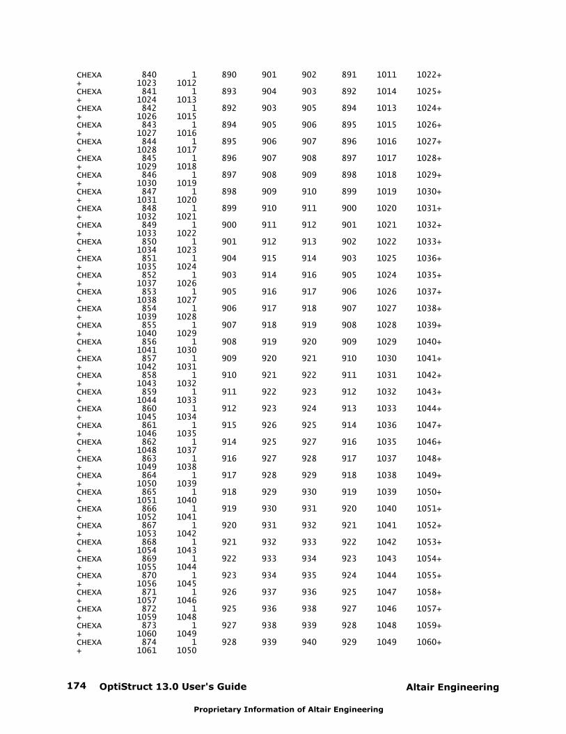
OptiStruct 13.0 User's Guide174 Altair Engineering
Proprietary Information of Altair Engineering
CHEXA 840 1 890 901 902 891 1011 1022+ + 1023 1012CHEXA 841 1 893 904 903 892 1014 1025+ + 1024 1013CHEXA 842 1 892 903 905 894 1013 1024+ + 1026 1015CHEXA 843 1 894 905 906 895 1015 1026+ + 1027 1016CHEXA 844 1 895 906 907 896 1016 1027+ + 1028 1017CHEXA 845 1 896 907 908 897 1017 1028+ + 1029 1018CHEXA 846 1 897 908 909 898 1018 1029+ + 1030 1019CHEXA 847 1 898 909 910 899 1019 1030+ + 1031 1020CHEXA 848 1 899 910 911 900 1020 1031+ + 1032 1021CHEXA 849 1 900 911 912 901 1021 1032+ + 1033 1022CHEXA 850 1 901 912 913 902 1022 1033+ + 1034 1023CHEXA 851 1 904 915 914 903 1025 1036+ + 1035 1024CHEXA 852 1 903 914 916 905 1024 1035+ + 1037 1026CHEXA 853 1 905 916 917 906 1026 1037+ + 1038 1027CHEXA 854 1 906 917 918 907 1027 1038+ + 1039 1028CHEXA 855 1 907 918 919 908 1028 1039+ + 1040 1029CHEXA 856 1 908 919 920 909 1029 1040+ + 1041 1030CHEXA 857 1 909 920 921 910 1030 1041+ + 1042 1031CHEXA 858 1 910 921 922 911 1031 1042+ + 1043 1032CHEXA 859 1 911 922 923 912 1032 1043+ + 1044 1033CHEXA 860 1 912 923 924 913 1033 1044+ + 1045 1034CHEXA 861 1 915 926 925 914 1036 1047+ + 1046 1035CHEXA 862 1 914 925 927 916 1035 1046+ + 1048 1037CHEXA 863 1 916 927 928 917 1037 1048+ + 1049 1038CHEXA 864 1 917 928 929 918 1038 1049+ + 1050 1039CHEXA 865 1 918 929 930 919 1039 1050+ + 1051 1040CHEXA 866 1 919 930 931 920 1040 1051+ + 1052 1041CHEXA 867 1 920 931 932 921 1041 1052+ + 1053 1042CHEXA 868 1 921 932 933 922 1042 1053+ + 1054 1043CHEXA 869 1 922 933 934 923 1043 1054+ + 1055 1044CHEXA 870 1 923 934 935 924 1044 1055+ + 1056 1045CHEXA 871 1 926 937 936 925 1047 1058+ + 1057 1046CHEXA 872 1 925 936 938 927 1046 1057+ + 1059 1048CHEXA 873 1 927 938 939 928 1048 1059+ + 1060 1049CHEXA 874 1 928 939 940 929 1049 1060+ + 1061 1050
Altair Engineering OptiStruct 13.0 User's Guide 175
Proprietary Information of Altair Engineering
CHEXA 875 1 929 940 941 930 1050 1061+ + 1062 1051CHEXA 876 1 930 941 942 931 1051 1062+ + 1063 1052CHEXA 877 1 931 942 943 932 1052 1063+ + 1064 1053CHEXA 878 1 932 943 944 933 1053 1064+ + 1065 1054CHEXA 879 1 933 944 945 934 1054 1065+ + 1066 1055CHEXA 880 1 934 945 946 935 1055 1066+ + 1067 1056CHEXA 881 1 937 948 947 936 1058 1069+ + 1068 1057CHEXA 882 1 936 947 949 938 1057 1068+ + 1070 1059CHEXA 883 1 938 949 950 939 1059 1070+ + 1071 1060CHEXA 884 1 939 950 951 940 1060 1071+ + 1072 1061CHEXA 885 1 940 951 952 941 1061 1072+ + 1073 1062CHEXA 886 1 941 952 953 942 1062 1073+ + 1074 1063CHEXA 887 1 942 953 954 943 1063 1074+ + 1075 1064CHEXA 888 1 943 954 955 944 1064 1075+ + 1076 1065CHEXA 889 1 944 955 956 945 1065 1076+ + 1077 1066CHEXA 890 1 945 956 957 946 1066 1077+ + 1078 1067CHEXA 891 1 948 959 958 947 1069 1080+ + 1079 1068CHEXA 892 1 947 958 960 949 1068 1079+ + 1081 1070CHEXA 893 1 949 960 961 950 1070 1081+ + 1082 1071CHEXA 894 1 950 961 962 951 1071 1082+ + 1083 1072CHEXA 895 1 951 962 963 952 1072 1083+ + 1084 1073CHEXA 896 1 952 963 964 953 1073 1084+ + 1085 1074CHEXA 897 1 953 964 965 954 1074 1085+ + 1086 1075CHEXA 898 1 954 965 966 955 1075 1086+ + 1087 1076CHEXA 899 1 955 966 967 956 1076 1087+ + 1088 1077CHEXA 900 1 956 967 968 957 1077 1088+ + 1089 1078CHEXA 901 1 969 972 971 970 1090 1093+ + 1092 1091CHEXA 902 1 970 971 974 973 1091 1092+ + 1095 1094CHEXA 903 1 973 974 976 975 1094 1095+ + 1097 1096CHEXA 904 1 975 976 978 977 1096 1097+ + 1099 1098CHEXA 905 1 977 978 980 979 1098 1099+ + 1101 1100CHEXA 906 1 979 980 982 981 1100 1101+ + 1103 1102CHEXA 907 1 981 982 984 983 1102 1103+ + 1105 1104CHEXA 908 1 983 984 986 985 1104 1105+ + 1107 1106CHEXA 909 1 985 986 988 987 1106 1107+ + 1109 1108
OptiStruct 13.0 User's Guide176 Altair Engineering
Proprietary Information of Altair Engineering
CHEXA 910 1 987 988 990 989 1108 1109+ + 1111 1110CHEXA 911 1 972 992 991 971 1093 1113+ + 1112 1092CHEXA 912 1 971 991 993 974 1092 1112+ + 1114 1095CHEXA 913 1 974 993 994 976 1095 1114+ + 1115 1097CHEXA 914 1 976 994 995 978 1097 1115+ + 1116 1099CHEXA 915 1 978 995 996 980 1099 1116+ + 1117 1101CHEXA 916 1 980 996 997 982 1101 1117+ + 1118 1103CHEXA 917 1 982 997 998 984 1103 1118+ + 1119 1105CHEXA 918 1 984 998 999 986 1105 1119+ + 1120 1107CHEXA 919 1 986 999 1000 988 1107 1120+ + 1121 1109CHEXA 920 1 988 1000 1001 990 1109 1121+ + 1122 1111CHEXA 921 1 992 1003 1002 991 1113 1124+ + 1123 1112CHEXA 922 1 991 1002 1004 993 1112 1123+ + 1125 1114CHEXA 923 1 993 1004 1005 994 1114 1125+ + 1126 1115CHEXA 924 1 994 1005 1006 995 1115 1126+ + 1127 1116CHEXA 925 1 995 1006 1007 996 1116 1127+ + 1128 1117CHEXA 926 1 996 1007 1008 997 1117 1128+ + 1129 1118CHEXA 927 1 997 1008 1009 998 1118 1129+ + 1130 1119CHEXA 928 1 998 1009 1010 999 1119 1130+ + 1131 1120CHEXA 929 1 999 1010 1011 1000 1120 1131+ + 1132 1121CHEXA 930 1 1000 1011 1012 1001 1121 1132+ + 1133 1122CHEXA 931 1 1003 1014 1013 1002 1124 1135+ + 1134 1123CHEXA 932 1 1002 1013 1015 1004 1123 1134+ + 1136 1125CHEXA 933 1 1004 1015 1016 1005 1125 1136+ + 1137 1126CHEXA 934 1 1005 1016 1017 1006 1126 1137+ + 1138 1127CHEXA 935 1 1006 1017 1018 1007 1127 1138+ + 1139 1128CHEXA 936 1 1007 1018 1019 1008 1128 1139+ + 1140 1129CHEXA 937 1 1008 1019 1020 1009 1129 1140+ + 1141 1130CHEXA 938 1 1009 1020 1021 1010 1130 1141+ + 1142 1131CHEXA 939 1 1010 1021 1022 1011 1131 1142+ + 1143 1132CHEXA 940 1 1011 1022 1023 1012 1132 1143+ + 1144 1133CHEXA 941 1 1014 1025 1024 1013 1135 1146+ + 1145 1134CHEXA 942 1 1013 1024 1026 1015 1134 1145+ + 1147 1136CHEXA 943 1 1015 1026 1027 1016 1136 1147+ + 1148 1137CHEXA 944 1 1016 1027 1028 1017 1137 1148+ + 1149 1138
Altair Engineering OptiStruct 13.0 User's Guide 177
Proprietary Information of Altair Engineering
CHEXA 945 1 1017 1028 1029 1018 1138 1149+ + 1150 1139CHEXA 946 1 1018 1029 1030 1019 1139 1150+ + 1151 1140CHEXA 947 1 1019 1030 1031 1020 1140 1151+ + 1152 1141CHEXA 948 1 1020 1031 1032 1021 1141 1152+ + 1153 1142CHEXA 949 1 1021 1032 1033 1022 1142 1153+ + 1154 1143CHEXA 950 1 1022 1033 1034 1023 1143 1154+ + 1155 1144CHEXA 951 1 1025 1036 1035 1024 1146 1157+ + 1156 1145CHEXA 952 1 1024 1035 1037 1026 1145 1156+ + 1158 1147CHEXA 953 1 1026 1037 1038 1027 1147 1158+ + 1159 1148CHEXA 954 1 1027 1038 1039 1028 1148 1159+ + 1160 1149CHEXA 955 1 1028 1039 1040 1029 1149 1160+ + 1161 1150CHEXA 956 1 1029 1040 1041 1030 1150 1161+ + 1162 1151CHEXA 957 1 1030 1041 1042 1031 1151 1162+ + 1163 1152CHEXA 958 1 1031 1042 1043 1032 1152 1163+ + 1164 1153CHEXA 959 1 1032 1043 1044 1033 1153 1164+ + 1165 1154CHEXA 960 1 1033 1044 1045 1034 1154 1165+ + 1166 1155CHEXA 961 1 1036 1047 1046 1035 1157 1168+ + 1167 1156CHEXA 962 1 1035 1046 1048 1037 1156 1167+ + 1169 1158CHEXA 963 1 1037 1048 1049 1038 1158 1169+ + 1170 1159CHEXA 964 1 1038 1049 1050 1039 1159 1170+ + 1171 1160CHEXA 965 1 1039 1050 1051 1040 1160 1171+ + 1172 1161CHEXA 966 1 1040 1051 1052 1041 1161 1172+ + 1173 1162CHEXA 967 1 1041 1052 1053 1042 1162 1173+ + 1174 1163CHEXA 968 1 1042 1053 1054 1043 1163 1174+ + 1175 1164CHEXA 969 1 1043 1054 1055 1044 1164 1175+ + 1176 1165CHEXA 970 1 1044 1055 1056 1045 1165 1176+ + 1177 1166CHEXA 971 1 1047 1058 1057 1046 1168 1179+ + 1178 1167CHEXA 972 1 1046 1057 1059 1048 1167 1178+ + 1180 1169CHEXA 973 1 1048 1059 1060 1049 1169 1180+ + 1181 1170CHEXA 974 1 1049 1060 1061 1050 1170 1181+ + 1182 1171CHEXA 975 1 1050 1061 1062 1051 1171 1182+ + 1183 1172CHEXA 976 1 1051 1062 1063 1052 1172 1183+ + 1184 1173CHEXA 977 1 1052 1063 1064 1053 1173 1184+ + 1185 1174CHEXA 978 1 1053 1064 1065 1054 1174 1185+ + 1186 1175CHEXA 979 1 1054 1065 1066 1055 1175 1186+ + 1187 1176
OptiStruct 13.0 User's Guide178 Altair Engineering
Proprietary Information of Altair Engineering
CHEXA 980 1 1055 1066 1067 1056 1176 1187+ + 1188 1177CHEXA 981 1 1058 1069 1068 1057 1179 1190+ + 1189 1178CHEXA 982 1 1057 1068 1070 1059 1178 1189+ + 1191 1180CHEXA 983 1 1059 1070 1071 1060 1180 1191+ + 1192 1181CHEXA 984 1 1060 1071 1072 1061 1181 1192+ + 1193 1182CHEXA 985 1 1061 1072 1073 1062 1182 1193+ + 1194 1183CHEXA 986 1 1062 1073 1074 1063 1183 1194+ + 1195 1184CHEXA 987 1 1063 1074 1075 1064 1184 1195+ + 1196 1185CHEXA 988 1 1064 1075 1076 1065 1185 1196+ + 1197 1186CHEXA 989 1 1065 1076 1077 1066 1186 1197+ + 1198 1187CHEXA 990 1 1066 1077 1078 1067 1187 1198+ + 1199 1188CHEXA 991 1 1069 1080 1079 1068 1190 1201+ + 1200 1189CHEXA 992 1 1068 1079 1081 1070 1189 1200+ + 1202 1191CHEXA 993 1 1070 1081 1082 1071 1191 1202+ + 1203 1192CHEXA 994 1 1071 1082 1083 1072 1192 1203+ + 1204 1193CHEXA 995 1 1072 1083 1084 1073 1193 1204+ + 1205 1194CHEXA 996 1 1073 1084 1085 1074 1194 1205+ + 1206 1195CHEXA 997 1 1074 1085 1086 1075 1195 1206+ + 1207 1196CHEXA 998 1 1075 1086 1087 1076 1196 1207+ + 1208 1197CHEXA 999 1 1076 1087 1088 1077 1197 1208+ + 1209 1198CHEXA 1000 1 1077 1088 1089 1078 1198 1209+ + 1210 1199CHEXA 1001 1 1090 1093 1092 1091 1211 1214+ + 1213 1212CHEXA 1002 1 1091 1092 1095 1094 1212 1213+ + 1216 1215CHEXA 1003 1 1094 1095 1097 1096 1215 1216+ + 1218 1217CHEXA 1004 1 1096 1097 1099 1098 1217 1218+ + 1220 1219CHEXA 1005 1 1098 1099 1101 1100 1219 1220+ + 1222 1221CHEXA 1006 1 1100 1101 1103 1102 1221 1222+ + 1224 1223CHEXA 1007 1 1102 1103 1105 1104 1223 1224+ + 1226 1225CHEXA 1008 1 1104 1105 1107 1106 1225 1226+ + 1228 1227CHEXA 1009 1 1106 1107 1109 1108 1227 1228+ + 1230 1229CHEXA 1010 1 1108 1109 1111 1110 1229 1230+ + 1232 1231CHEXA 1011 1 1093 1113 1112 1092 1214 1234+ + 1233 1213CHEXA 1012 1 1092 1112 1114 1095 1213 1233+ + 1235 1216CHEXA 1013 1 1095 1114 1115 1097 1216 1235+ + 1236 1218CHEXA 1014 1 1097 1115 1116 1099 1218 1236+ + 1237 1220
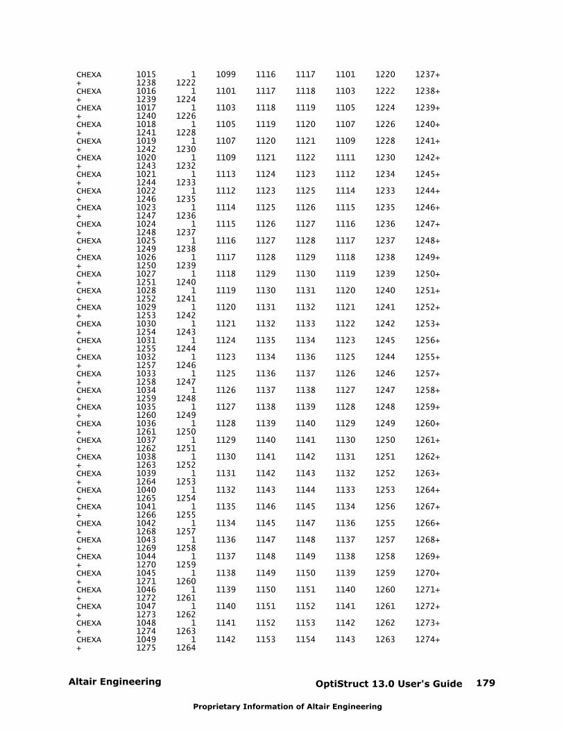
Altair Engineering OptiStruct 13.0 User's Guide 179
Proprietary Information of Altair Engineering
CHEXA 1015 1 1099 1116 1117 1101 1220 1237+ + 1238 1222CHEXA 1016 1 1101 1117 1118 1103 1222 1238+ + 1239 1224CHEXA 1017 1 1103 1118 1119 1105 1224 1239+ + 1240 1226CHEXA 1018 1 1105 1119 1120 1107 1226 1240+ + 1241 1228CHEXA 1019 1 1107 1120 1121 1109 1228 1241+ + 1242 1230CHEXA 1020 1 1109 1121 1122 1111 1230 1242+ + 1243 1232CHEXA 1021 1 1113 1124 1123 1112 1234 1245+ + 1244 1233CHEXA 1022 1 1112 1123 1125 1114 1233 1244+ + 1246 1235CHEXA 1023 1 1114 1125 1126 1115 1235 1246+ + 1247 1236CHEXA 1024 1 1115 1126 1127 1116 1236 1247+ + 1248 1237CHEXA 1025 1 1116 1127 1128 1117 1237 1248+ + 1249 1238CHEXA 1026 1 1117 1128 1129 1118 1238 1249+ + 1250 1239CHEXA 1027 1 1118 1129 1130 1119 1239 1250+ + 1251 1240CHEXA 1028 1 1119 1130 1131 1120 1240 1251+ + 1252 1241CHEXA 1029 1 1120 1131 1132 1121 1241 1252+ + 1253 1242CHEXA 1030 1 1121 1132 1133 1122 1242 1253+ + 1254 1243CHEXA 1031 1 1124 1135 1134 1123 1245 1256+ + 1255 1244CHEXA 1032 1 1123 1134 1136 1125 1244 1255+ + 1257 1246CHEXA 1033 1 1125 1136 1137 1126 1246 1257+ + 1258 1247CHEXA 1034 1 1126 1137 1138 1127 1247 1258+ + 1259 1248CHEXA 1035 1 1127 1138 1139 1128 1248 1259+ + 1260 1249CHEXA 1036 1 1128 1139 1140 1129 1249 1260+ + 1261 1250CHEXA 1037 1 1129 1140 1141 1130 1250 1261+ + 1262 1251CHEXA 1038 1 1130 1141 1142 1131 1251 1262+ + 1263 1252CHEXA 1039 1 1131 1142 1143 1132 1252 1263+ + 1264 1253CHEXA 1040 1 1132 1143 1144 1133 1253 1264+ + 1265 1254CHEXA 1041 1 1135 1146 1145 1134 1256 1267+ + 1266 1255CHEXA 1042 1 1134 1145 1147 1136 1255 1266+ + 1268 1257CHEXA 1043 1 1136 1147 1148 1137 1257 1268+ + 1269 1258CHEXA 1044 1 1137 1148 1149 1138 1258 1269+ + 1270 1259CHEXA 1045 1 1138 1149 1150 1139 1259 1270+ + 1271 1260CHEXA 1046 1 1139 1150 1151 1140 1260 1271+ + 1272 1261CHEXA 1047 1 1140 1151 1152 1141 1261 1272+ + 1273 1262CHEXA 1048 1 1141 1152 1153 1142 1262 1273+ + 1274 1263CHEXA 1049 1 1142 1153 1154 1143 1263 1274+ + 1275 1264
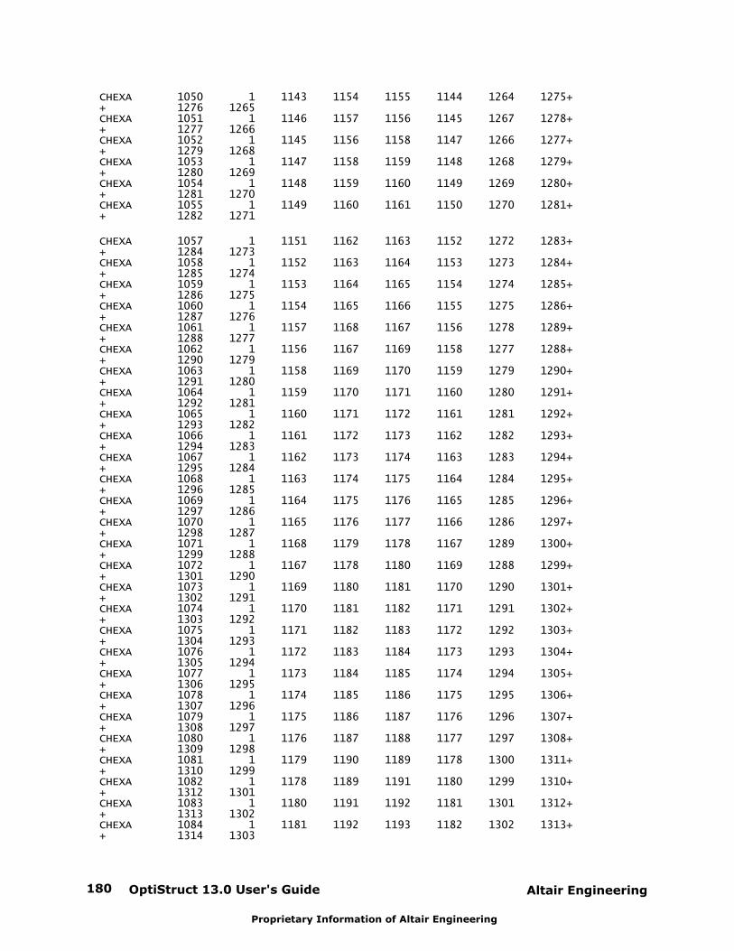
OptiStruct 13.0 User's Guide180 Altair Engineering
Proprietary Information of Altair Engineering
CHEXA 1050 1 1143 1154 1155 1144 1264 1275+ + 1276 1265CHEXA 1051 1 1146 1157 1156 1145 1267 1278+ + 1277 1266CHEXA 1052 1 1145 1156 1158 1147 1266 1277+ + 1279 1268CHEXA 1053 1 1147 1158 1159 1148 1268 1279+ + 1280 1269CHEXA 1054 1 1148 1159 1160 1149 1269 1280+ + 1281 1270CHEXA 1055 1 1149 1160 1161 1150 1270 1281+ + 1282 1271
CHEXA 1057 1 1151 1162 1163 1152 1272 1283+ + 1284 1273CHEXA 1058 1 1152 1163 1164 1153 1273 1284+ + 1285 1274CHEXA 1059 1 1153 1164 1165 1154 1274 1285+ + 1286 1275CHEXA 1060 1 1154 1165 1166 1155 1275 1286+ + 1287 1276CHEXA 1061 1 1157 1168 1167 1156 1278 1289+ + 1288 1277CHEXA 1062 1 1156 1167 1169 1158 1277 1288+ + 1290 1279CHEXA 1063 1 1158 1169 1170 1159 1279 1290+ + 1291 1280CHEXA 1064 1 1159 1170 1171 1160 1280 1291+ + 1292 1281CHEXA 1065 1 1160 1171 1172 1161 1281 1292+ + 1293 1282CHEXA 1066 1 1161 1172 1173 1162 1282 1293+ + 1294 1283CHEXA 1067 1 1162 1173 1174 1163 1283 1294+ + 1295 1284CHEXA 1068 1 1163 1174 1175 1164 1284 1295+ + 1296 1285CHEXA 1069 1 1164 1175 1176 1165 1285 1296+ + 1297 1286CHEXA 1070 1 1165 1176 1177 1166 1286 1297+ + 1298 1287CHEXA 1071 1 1168 1179 1178 1167 1289 1300+ + 1299 1288CHEXA 1072 1 1167 1178 1180 1169 1288 1299+ + 1301 1290CHEXA 1073 1 1169 1180 1181 1170 1290 1301+ + 1302 1291CHEXA 1074 1 1170 1181 1182 1171 1291 1302+ + 1303 1292CHEXA 1075 1 1171 1182 1183 1172 1292 1303+ + 1304 1293CHEXA 1076 1 1172 1183 1184 1173 1293 1304+ + 1305 1294CHEXA 1077 1 1173 1184 1185 1174 1294 1305+ + 1306 1295CHEXA 1078 1 1174 1185 1186 1175 1295 1306+ + 1307 1296CHEXA 1079 1 1175 1186 1187 1176 1296 1307+ + 1308 1297CHEXA 1080 1 1176 1187 1188 1177 1297 1308+ + 1309 1298CHEXA 1081 1 1179 1190 1189 1178 1300 1311+ + 1310 1299CHEXA 1082 1 1178 1189 1191 1180 1299 1310+ + 1312 1301CHEXA 1083 1 1180 1191 1192 1181 1301 1312+ + 1313 1302CHEXA 1084 1 1181 1192 1193 1182 1302 1313+ + 1314 1303
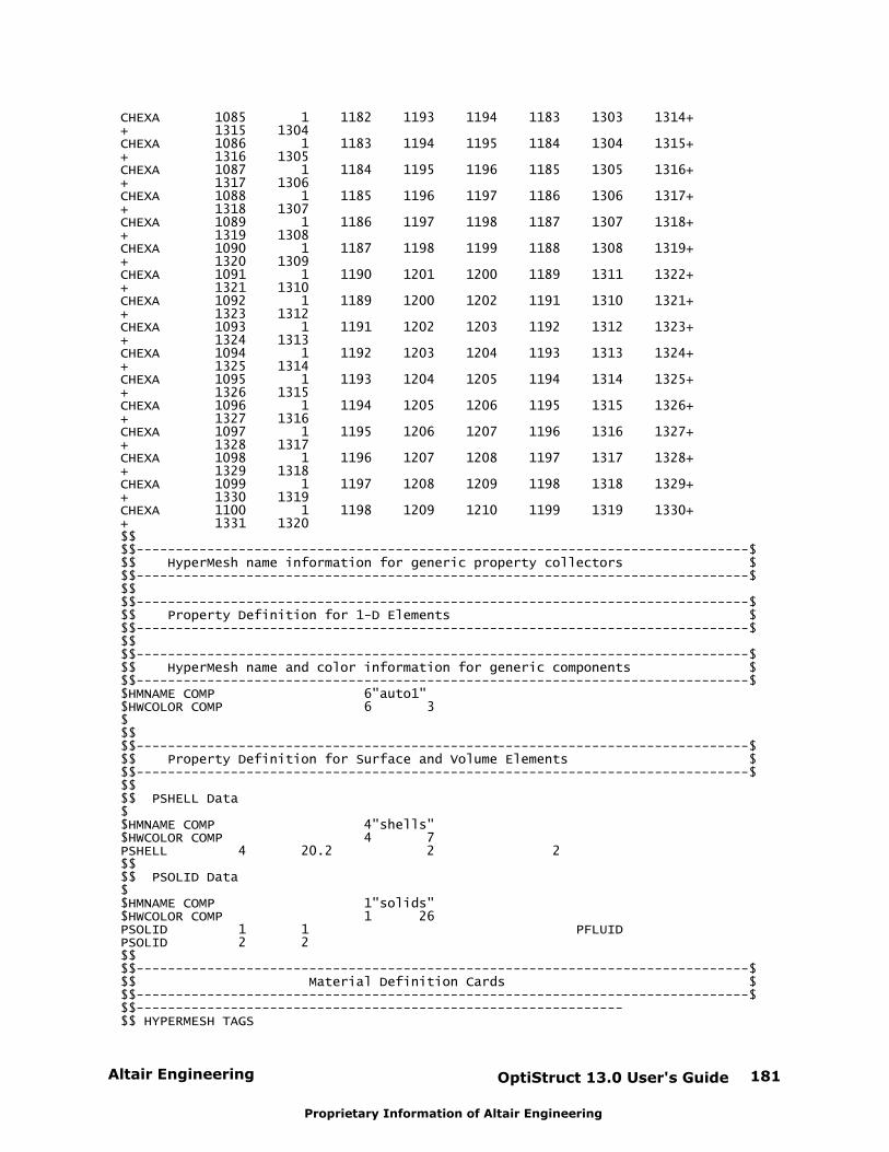
Altair Engineering OptiStruct 13.0 User's Guide 181
Proprietary Information of Altair Engineering
CHEXA 1085 1 1182 1193 1194 1183 1303 1314+ + 1315 1304CHEXA 1086 1 1183 1194 1195 1184 1304 1315+ + 1316 1305CHEXA 1087 1 1184 1195 1196 1185 1305 1316+ + 1317 1306CHEXA 1088 1 1185 1196 1197 1186 1306 1317+ + 1318 1307CHEXA 1089 1 1186 1197 1198 1187 1307 1318+ + 1319 1308CHEXA 1090 1 1187 1198 1199 1188 1308 1319+ + 1320 1309CHEXA 1091 1 1190 1201 1200 1189 1311 1322+ + 1321 1310CHEXA 1092 1 1189 1200 1202 1191 1310 1321+ + 1323 1312CHEXA 1093 1 1191 1202 1203 1192 1312 1323+ + 1324 1313CHEXA 1094 1 1192 1203 1204 1193 1313 1324+ + 1325 1314CHEXA 1095 1 1193 1204 1205 1194 1314 1325+ + 1326 1315CHEXA 1096 1 1194 1205 1206 1195 1315 1326+ + 1327 1316CHEXA 1097 1 1195 1206 1207 1196 1316 1327+ + 1328 1317CHEXA 1098 1 1196 1207 1208 1197 1317 1328+ + 1329 1318CHEXA 1099 1 1197 1208 1209 1198 1318 1329+ + 1330 1319CHEXA 1100 1 1198 1209 1210 1199 1319 1330+ + 1331 1320$$$$------------------------------------------------------------------------------$$$ HyperMesh name information for generic property collectors $$$------------------------------------------------------------------------------$$$$$------------------------------------------------------------------------------$$$ Property Definition for 1-D Elements $$$------------------------------------------------------------------------------$$$$$------------------------------------------------------------------------------$$$ HyperMesh name and color information for generic components $$$------------------------------------------------------------------------------$$HMNAME COMP 6"auto1"$HWCOLOR COMP 6 3$$$$$------------------------------------------------------------------------------$$$ Property Definition for Surface and Volume Elements $$$------------------------------------------------------------------------------$$$$$ PSHELL Data$$HMNAME COMP 4"shells"$HWCOLOR COMP 4 7PSHELL 4 20.2 2 2 $$$$ PSOLID Data$$HMNAME COMP 1"solids"$HWCOLOR COMP 1 26PSOLID 1 1 PFLUIDPSOLID 2 2$$$$------------------------------------------------------------------------------$$$ Material Definition Cards $$$------------------------------------------------------------------------------$$$--------------------------------------------------------------$$ HYPERMESH TAGS
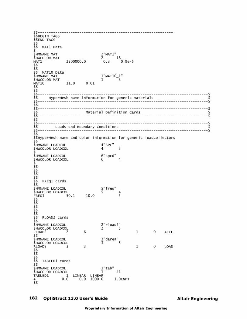
OptiStruct 13.0 User's Guide182 Altair Engineering
Proprietary Information of Altair Engineering
$$--------------------------------------------------------------$$BEGIN TAGS$$END TAGS$$$$ MAT1 Data$$HMNAME MAT 2"MAT1"$HWCOLOR MAT 2 18MAT1 2200000.0 0.3 0.9e-5 $$$$$$ MAT10 Data$HMNAME MAT 1"MAT10_1"$HWCOLOR MAT 1 3MAT10 11.0 0.01 $$$$$$------------------------------------------------------------------------------$$$ HyperMesh name information for generic materials $$$------------------------------------------------------------------------------$$$$$------------------------------------------------------------------------------$$$ Material Definition Cards $$$------------------------------------------------------------------------------$$$$$------------------------------------------------------------------------------$$$ Loads and Boundary Conditions $$$------------------------------------------------------------------------------$$$$$HyperMesh name and color information for generic loadcollectors$$$HMNAME LOADCOL 4"SPC"$HWCOLOR LOADCOL 4 3$$HMNAME LOADCOL 6"spcd"$HWCOLOR LOADCOL 6 4$$$$$$$$$$$ FREQ1 cards$$$HMNAME LOADCOL 5"freq"$HWCOLOR LOADCOL 5 4FREQ1 50.1 10.0 5$$$$$$$$$$$$ RLOAD2 cards$$$HMNAME LOADCOL 2"rload2"$HWCOLOR LOADCOL 2 5RLOAD2 2 6 1 0 ACCE$$$HMNAME LOADCOL 3"darea"$HWCOLOR LOADCOL 3 5RLOAD2 3 3 1 0 LOAD$$$$$$$$ TABLED1 cards$$$HMNAME LOADCOL 1"tab"$HWCOLOR LOADCOL 1 41TABLED1 1 LINEAR LINEAR+ 0.0 0.0 1000.0 1.0ENDT $$
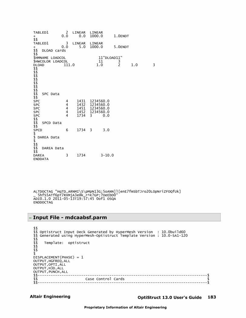
Altair Engineering OptiStruct 13.0 User's Guide 183
Proprietary Information of Altair Engineering
TABLED1 2 LINEAR LINEAR+ 0.0 0.0 1000.0 1.0ENDT$$TABLED1 3 LINEAR LINEAR+ 0.0 5.0 1000.0 5.0ENDT$$ DLOAD cards$$$HMNAME LOADCOL 11"DLOAD11"$HWCOLOR LOADCOL 11 3DLOAD 111.0 1.0 2 1.0 3$$$$$$$$$$$$$$$$ SPC Data$$SPC 4 1431 1234560.0 SPC 4 1432 1234560.0 SPC 4 1451 1234560.0 SPC 4 1452 1234560.0 SPC 4 1734 3 0.0 $$$$ SPCD Data$$SPCD 6 1734 3 3.0 $$ DAREA Data$$$$$ DAREA Data$$DAREA 3 1734 3-10.0 ENDDATA
ALTDOCTAG "HqTD_ARNMI\S\pMpN13G;5oANN]l[enE7fmSbTJro20LOpNriZFOQfUk]_`5hfS5ATf6pT7RXMjA3e@k_r^K?GP;?OeEbD0"ADI0.1.0 2011-05-13T19:57:45 0of1 OSQAENDDOCTAG
Input File - mdcaabsf.parm
$$$$ Optistruct Input Deck Generated by HyperMesh Version : 10.0build60$$ Generated using HyperMesh-Optistruct Template Version : 10.0-SA1-120$$$$ Template: optistruct$$$$$DISPLACEMENT(PHASE) = 1OUTPUT,HGFREQ,ALLOUTPUT,OPTI,ALLOUTPUT,H3D,ALLOUTPUT,PUNCH,ALL$$------------------------------------------------------------------------------$$$ Case Control Cards $$$------------------------------------------------------------------------------$
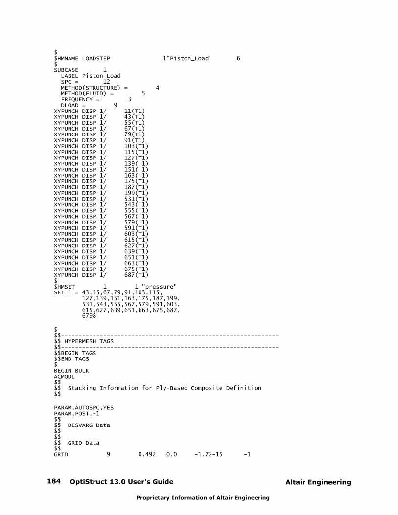
OptiStruct 13.0 User's Guide184 Altair Engineering
Proprietary Information of Altair Engineering
$$HMNAME LOADSTEP 1"Piston_Load" 6$SUBCASE 1 LABEL Piston_Load SPC = 12 METHOD(STRUCTURE) = 4 METHOD(FLUID) = 5 FREQUENCY = 3 DLOAD = 9XYPUNCH DISP 1/ 11(T1) XYPUNCH DISP 1/ 43(T1) XYPUNCH DISP 1/ 55(T1) XYPUNCH DISP 1/ 67(T1) XYPUNCH DISP 1/ 79(T1) XYPUNCH DISP 1/ 91(T1) XYPUNCH DISP 1/ 103(T1) XYPUNCH DISP 1/ 115(T1) XYPUNCH DISP 1/ 127(T1) XYPUNCH DISP 1/ 139(T1) XYPUNCH DISP 1/ 151(T1) XYPUNCH DISP 1/ 163(T1) XYPUNCH DISP 1/ 175(T1) XYPUNCH DISP 1/ 187(T1) XYPUNCH DISP 1/ 199(T1) XYPUNCH DISP 1/ 531(T1) XYPUNCH DISP 1/ 543(T1) XYPUNCH DISP 1/ 555(T1) XYPUNCH DISP 1/ 567(T1) XYPUNCH DISP 1/ 579(T1) XYPUNCH DISP 1/ 591(T1) XYPUNCH DISP 1/ 603(T1) XYPUNCH DISP 1/ 615(T1) XYPUNCH DISP 1/ 627(T1) XYPUNCH DISP 1/ 639(T1) XYPUNCH DISP 1/ 651(T1) XYPUNCH DISP 1/ 663(T1) XYPUNCH DISP 1/ 675(T1) XYPUNCH DISP 1/ 687(T1) $$HMSET 1 1 "pressure"SET 1 = 43,55,67,79,91,103,115, 127,139,151,163,175,187,199, 531,543,555,567,579,591,603, 615,627,639,651,663,675,687, 6798
$$$--------------------------------------------------------------$$ HYPERMESH TAGS $$--------------------------------------------------------------$$BEGIN TAGS$$END TAGS$BEGIN BULKACMODL $$$$ Stacking Information for Ply-Based Composite Definition$$
PARAM,AUTOSPC,YES PARAM,POST,-1 $$$$ DESVARG Data$$$$$$ GRID Data$$GRID 9 0.492 0.0 -1.72-15 -1
Altair Engineering OptiStruct 13.0 User's Guide 185
Proprietary Information of Altair Engineering
GRID 10 0.246 0.0 -8.59-16 -1 GRID 11 0.0 0.0 0.0 -1 GRID 12 -0.246 0.0 8.589-16 -1 GRID 13 -0.492 0.0 1.718-15 -1 GRID 14 -0.492 0.246 1.718-15 -1 GRID 15 -0.492 0.492 1.718-15 -1 GRID 16 -0.246 0.492 8.589-16 -1 GRID 17 0.0 0.492 0.0 -1 GRID 18 0.246 0.492 -8.59-16 -1 GRID 19 0.492 0.492 -1.72-15 -1 GRID 20 0.492 0.246 -1.72-15 -1 GRID 21 0.0 0.246 0.0 -1 GRID 22 -0.246 0.246 8.589-16 -1 GRID 23 0.246 0.246 -8.59-16 -1 GRID 24 0.492 -0.246 -1.72-15 -1 GRID 25 0.492 -0.492 -1.72-15 -1 GRID 26 0.246 -0.492 -8.59-16 -1 GRID 27 0.0 -0.492 0.0 -1 GRID 28 -0.246 -0.492 8.589-16 -1 GRID 29 -0.492 -0.492 1.718-15 -1 GRID 30 -0.492 -0.246 1.718-15 -1 GRID 31 0.0 -0.246 0.0 -1 GRID 32 0.246 -0.246 -8.59-16 -1 GRID 33 -0.246 -0.246 8.589-16 -1 GRID 34 0.246 5.049-29-.300073 -1 GRID 35 -5.99-130.0 -.300073 -1 GRID 36 -5.62-130.246 -.300073 -1 GRID 37 0.246 0.246 -.300073 -1 GRID 38 0.246 2.524-29-.600146 -1 GRID 39 -1.2-12 0.0 -.600146 -1 GRID 40 -1.12-120.246 -.600146 -1 GRID 41 0.246 0.246 -.600146 -1 GRID 42 0.246 2.919-29-0.90022 -1 GRID 43 -1.79-120.0 -.900219 -1 GRID 44 -1.68-120.246 -.900219 -1 GRID 45 0.246 0.246 -0.90022 -1 GRID 46 0.246 3.787-29-1.20029 -1 GRID 47 -2.39-120.0 -1.20029 -1 GRID 48 -2.24-120.246 -1.20029 -1 GRID 49 0.246 0.246 -1.20029 -1 GRID 50 0.246 4.733-29-1.50037 -1 GRID 51 -3.0-12 0.0 -1.50037 -1 GRID 52 -2.81-120.246 -1.50037 -1 GRID 53 0.246 0.246 -1.50037 -1 GRID 54 0.246 5.364-29-1.80044 -1 GRID 55 -3.6-12 0.0 -1.80044 -1 GRID 56 -3.37-120.246 -1.80044 -1 GRID 57 0.246 0.246 -1.80044 -1 GRID 58 0.246 6.311-29-2.10051 -1 GRID 59 -4.2-12 0.0 -2.10051 -1 GRID 60 -3.93-120.246 -2.10051 -1 GRID 61 0.246 0.246 -2.10051 -1 GRID 62 0.246 7.258-29-2.40059 -1 GRID 63 -4.79-120.0 -2.40059 -1 GRID 64 -4.49-120.246 -2.40059 -1 GRID 65 0.246 0.246 -2.40059 -1 GRID 66 0.246 8.204-29-2.70066 -1 GRID 67 -5.39-120.0 -2.70066 -1 GRID 68 -5.06-120.246 -2.70066 -1 GRID 69 0.246 0.246 -2.70066 -1 GRID 70 0.246 8.835-29-3.00073 -1 GRID 71 -5.99-120.0 -3.00073 -1 GRID 72 -5.62-120.246 -3.00073 -1 GRID 73 0.246 0.246 -3.00073 -1 GRID 74 0.246 9.782-29-3.30081 -1 GRID 75 -6.59-120.0 -3.30081 -1 GRID 76 -6.18-120.246 -3.30081 -1 GRID 77 0.246 0.246 -3.30081 -1 GRID 78 0.246 1.073-28-3.60088 -1 GRID 79 -7.19-120.0 -3.60088 -1

OptiStruct 13.0 User's Guide186 Altair Engineering
Proprietary Information of Altair Engineering
GRID 80 -6.74-120.246 -3.60088 -1 GRID 81 0.246 0.246 -3.60088 -1 GRID 82 0.246 1.136-28-3.90095 -1 GRID 83 -7.78-120.0 -3.90095 -1 GRID 84 -7.3-12 0.246 -3.90095 -1 GRID 85 0.246 0.246 -3.90095 -1 GRID 86 0.246 1.231-28-4.20102 -1 GRID 87 -8.38-120.0 -4.20102 -1 GRID 88 -7.86-120.246 -4.20102 -1 GRID 89 0.246 0.246 -4.20102 -1 GRID 90 0.246 1.294-28-4.5011 -1 GRID 91 -8.99-120.0 -4.5011 -1 GRID 92 -8.43-120.246 -4.5011 -1 GRID 93 0.246 0.246 -4.5011 -1 GRID 94 0.246 1.388-28-4.80117 -1 GRID 95 -9.59-120.0 -4.80117 -1 GRID 96 -8.99-120.246 -4.80117 -1 GRID 97 0.246 0.246 -4.80117 -1 GRID 98 0.246 1.452-28-5.10124 -1 GRID 99 -1.02-110.0 -5.10124 -1 GRID 100 -9.55-120.246 -5.10124 -1 GRID 101 0.246 0.246 -5.10124 -1 GRID 102 0.246 1.515-28-5.40132 -1 GRID 103 -1.08-110.0 -5.40132 -1 GRID 104 -1.01-110.246 -5.40132 -1 GRID 105 0.246 0.246 -5.40132 -1 GRID 106 0.246 1.609-28-5.70139 -1 GRID 107 -1.14-110.0 -5.70139 -1 GRID 108 -1.07-110.246 -5.70139 -1 GRID 109 0.246 0.246 -5.70139 -1 GRID 110 0.246 1.672-28-6.00146 -1 GRID 111 -1.2-11 0.0 -6.00146 -1 GRID 112 -1.12-110.246 -6.00146 -1 GRID 113 0.246 0.246 -6.00146 -1 GRID 114 0.246 1.735-28-6.30154 -1 GRID 115 -1.26-110.0 -6.30154 -1 GRID 116 -1.18-110.246 -6.30154 -1 GRID 117 0.246 0.246 -6.30154 -1 GRID 118 0.246 1.83-28 -6.60161 -1 GRID 119 -1.32-110.0 -6.60161 -1 GRID 120 -1.23-110.246 -6.60161 -1 GRID 121 0.246 0.246 -6.60161 -1 GRID 122 0.246 1.893-28-6.90168 -1 GRID 123 -1.38-110.0 -6.90168 -1 GRID 124 -1.29-110.246 -6.90168 -1 GRID 125 0.246 0.246 -6.90168 -1 GRID 126 0.246 1.956-28-7.20176 -1 GRID 127 -1.44-110.0 -7.20176 -1 GRID 128 -1.35-110.246 -7.20176 -1 GRID 129 0.246 0.246 -7.20176 -1 GRID 130 0.246 2.019-28-7.50183 -1 GRID 131 -1.5-11 0.0 -7.50183 -1 GRID 132 -1.4-11 0.246 -7.50183 -1 GRID 133 0.246 0.246 -7.50183 -1 GRID 134 0.246 2.083-28-7.8019 -1 GRID 135 -1.55-110.0 -7.8019 -1 GRID 136 -1.46-110.246 -7.8019 -1 GRID 137 0.246 0.246 -7.8019 -1 GRID 138 0.246 2.146-28-8.10198 -1 GRID 139 -1.61-110.0 -8.10198 -1 GRID 140 -1.51-110.246 -8.10198 -1 GRID 141 0.246 0.246 -8.10198 -1 GRID 142 0.246 2.209-28-8.40205 -1 GRID 143 -1.67-110.0 -8.40205 -1 GRID 144 -1.57-110.246 -8.40205 -1 GRID 145 0.246 0.246 -8.40205 -1 GRID 146 0.246 2.272-28-8.70212 -1 GRID 147 -1.73-110.0 -8.70212 -1 GRID 148 -1.63-110.246 -8.70212 -1 GRID 149 0.246 0.246 -8.70212 -1
Altair Engineering OptiStruct 13.0 User's Guide 187
Proprietary Information of Altair Engineering
GRID 150 0.246 2.335-28-9.0022 -1 GRID 151 -1.79-110.0 -9.0022 -1 GRID 152 -1.68-110.246 -9.0022 -1 GRID 153 0.246 0.246 -9.0022 -1 GRID 154 0.246 2.398-28-9.30227 -1 GRID 155 -1.85-110.0 -9.30227 -1 GRID 156 -1.74-110.246 -9.30227 -1 GRID 157 0.246 0.246 -9.30227 -1 GRID 158 0.246 2.461-28-9.60234 -1 GRID 159 -1.91-110.0 -9.60234 -1 GRID 160 -1.79-110.246 -9.60234 -1 GRID 161 0.246 0.246 -9.60234 -1 GRID 162 0.246 2.524-28-9.90241 -1 GRID 163 -1.97-110.0 -9.90241 -1 GRID 164 -1.85-110.246 -9.90241 -1 GRID 165 0.246 0.246 -9.90241 -1 GRID 166 0.246 2.556-28-10.2025 -1 GRID 167 -2.03-110.0 -10.2025 -1 GRID 168 -1.91-110.246 -10.2025 -1 GRID 169 0.246 0.246 -10.2025 -1 GRID 170 0.246 2.619-28-10.5026 -1 GRID 171 -2.09-110.0 -10.5026 -1 GRID 172 -1.96-110.246 -10.5026 -1 GRID 173 0.246 0.246 -10.5026 -1 GRID 174 0.246 2.682-28-10.8026 -1 GRID 175 -2.15-110.0 -10.8026 -1 GRID 176 -2.02-110.246 -10.8026 -1 GRID 177 0.246 0.246 -10.8026 -1 GRID 178 0.246 2.745-28-11.1027 -1 GRID 179 -2.21-110.0 -11.1027 -1 GRID 180 -2.07-110.246 -11.1027 -1 GRID 181 0.246 0.246 -11.1027 -1 GRID 182 0.246 2.777-28-11.4028 -1 GRID 183 -2.27-110.0 -11.4028 -1 GRID 184 -2.13-110.246 -11.4028 -1 GRID 185 0.246 0.246 -11.4028 -1 GRID 186 0.246 2.84-28 -11.7029 -1 GRID 187 -2.33-110.0 -11.7029 -1 GRID 188 -2.19-110.246 -11.7029 -1 GRID 189 0.246 0.246 -11.7029 -1 GRID 190 0.246 2.871-28-12.0029 -1 GRID 191 -2.39-110.0 -12.0029 -1 GRID 192 -2.24-110.246 -12.0029 -1 GRID 193 0.246 0.246 -12.0029 -1 GRID 194 0.246 2.935-28-12.303 -1 GRID 195 -2.45-110.0 -12.303 -1 GRID 196 -2.3-11 0.246 -12.303 -1 GRID 197 0.246 0.246 -12.303 -1 GRID 198 0.246 2.966-28-12.6031 -1 GRID 199 -2.51-110.0 -12.6031 -1 GRID 200 -2.35-110.246 -12.6031 -1 GRID 201 0.246 0.246 -12.6031 -1 GRID 522 0.246 2.935-28-12.903 -1 GRID 523 -7.36-110.0 -12.903 -1 GRID 524 -6.9-11 0.246 -12.903 -1 GRID 525 0.246 0.246 -12.903 -1 GRID 526 0.246 2.903-28-13.2031 -1 GRID 527 -7.42-110.0 -13.2031 -1 GRID 528 -6.95-110.246 -13.2031 -1 GRID 529 0.246 0.246 -13.2031 -1 GRID 530 0.246 2.84-28 -13.5032 -1 GRID 531 -7.48-110.0 -13.5032 -1 GRID 532 -7.01-110.246 -13.5032 -1 GRID 533 0.246 0.246 -13.5032 -1 GRID 534 0.246 2.777-28-13.8032 -1 GRID 535 -7.54-110.0 -13.8032 -1 GRID 536 -7.06-110.246 -13.8032 -1 GRID 537 0.246 0.246 -13.8032 -1 GRID 538 0.246 2.745-28-14.1033 -1 GRID 539 -7.6-11 0.0 -14.1033 -1
OptiStruct 13.0 User's Guide188 Altair Engineering
Proprietary Information of Altair Engineering
GRID 540 -7.12-110.246 -14.1033 -1 GRID 541 0.246 0.246 -14.1033 -1 GRID 542 0.246 2.682-28-14.4034 -1 GRID 543 -7.67-110.0 -14.4034 -1 GRID 544 -7.19-110.246 -14.4034 -1 GRID 545 0.246 0.246 -14.4034 -1 GRID 546 0.246 2.619-28-14.7034 -1 GRID 547 -7.73-110.0 -14.7034 -1 GRID 548 -7.24-110.246 -14.7034 -1 GRID 549 0.246 0.246 -14.7034 -1 GRID 550 0.246 2.587-28-15.0035 -1 GRID 551 -7.78-110.0 -15.0035 -1 GRID 552 -7.3-11 0.246 -15.0035 -1 GRID 553 0.246 0.246 -15.0035 -1 GRID 554 0.246 2.524-28-15.3036 -1 GRID 555 -7.84-110.0 -15.3036 -1 GRID 556 -7.35-110.246 -15.3036 -1 GRID 557 0.246 0.246 -15.3036 -1 GRID 558 0.246 2.461-28-15.6037 -1 GRID 559 -7.9-11 0.0 -15.6037 -1 GRID 560 -7.41-110.246 -15.6037 -1 GRID 561 0.246 0.246 -15.6037 -1 GRID 562 0.246 2.398-28-15.9037 -1 GRID 563 -7.96-110.0 -15.9037 -1 GRID 564 -7.47-110.246 -15.9037 -1 GRID 565 0.246 0.246 -15.9037 -1 GRID 566 0.246 2.335-28-16.2038 -1 GRID 567 -8.02-110.0 -16.2038 -1 GRID 568 -7.52-110.246 -16.2038 -1 GRID 569 0.246 0.246 -16.2038 -1 GRID 570 0.246 2.272-28-16.5039 -1 GRID 571 -8.08-110.0 -16.5039 -1 GRID 572 -7.58-110.246 -16.5039 -1 GRID 573 0.246 0.246 -16.5039 -1 GRID 574 0.246 2.209-28-16.804 -1 GRID 575 -8.14-110.0 -16.804 -1 GRID 576 -7.63-110.246 -16.804 -1 GRID 577 0.246 0.246 -16.804 -1 GRID 578 0.246 2.146-28-17.104 -1 GRID 579 -8.2-11 0.0 -17.104 -1 GRID 580 -7.69-110.246 -17.104 -1 GRID 581 0.246 0.246 -17.104 -1 GRID 582 0.246 2.083-28-17.4041 -1 GRID 583 -8.26-110.0 -17.4041 -1 GRID 584 -7.75-110.246 -17.4041 -1 GRID 585 0.246 0.246 -17.4041 -1 GRID 586 0.246 2.019-28-17.7042 -1 GRID 587 -8.32-110.0 -17.7042 -1 GRID 588 -7.8-11 0.246 -17.7042 -1 GRID 589 0.246 0.246 -17.7042 -1 GRID 590 0.246 1.956-28-18.0042 -1 GRID 591 -8.38-110.0 -18.0042 -1 GRID 592 -7.86-110.246 -18.0042 -1 GRID 593 0.246 0.246 -18.0042 -1 GRID 594 0.246 1.893-28-18.3043 -1 GRID 595 -8.44-110.0 -18.3043 -1 GRID 596 -7.91-110.246 -18.3043 -1 GRID 597 0.246 0.246 -18.3043 -1 GRID 598 0.246 1.83-28 -18.6044 -1 GRID 599 -8.5-11 0.0 -18.6044 -1 GRID 600 -7.97-110.246 -18.6044 -1 GRID 601 0.246 0.246 -18.6044 -1 GRID 602 0.246 1.735-28-18.9045 -1 GRID 603 -8.56-110.0 -18.9045 -1 GRID 604 -8.03-110.246 -18.9045 -1 GRID 605 0.246 0.246 -18.9045 -1 GRID 606 0.246 1.672-28-19.2045 -1 GRID 607 -8.62-110.0 -19.2045 -1 GRID 608 -8.08-110.246 -19.2045 -1 GRID 609 0.246 0.246 -19.2045 -1
Altair Engineering OptiStruct 13.0 User's Guide 189
Proprietary Information of Altair Engineering
GRID 610 0.246 1.609-28-19.5046 -1 GRID 611 -8.68-110.0 -19.5046 -1 GRID 612 -8.14-110.246 -19.5046 -1 GRID 613 0.246 0.246 -19.5046 -1 GRID 614 0.246 1.515-28-19.8047 -1 GRID 615 -8.74-110.0 -19.8047 -1 GRID 616 -8.19-110.246 -19.8047 -1 GRID 617 0.246 0.246 -19.8047 -1 GRID 618 0.246 1.452-28-20.1048 -1 GRID 619 -8.8-11 0.0 -20.1048 -1 GRID 620 -8.25-110.246 -20.1048 -1 GRID 621 0.246 0.246 -20.1048 -1 GRID 622 0.246 1.388-28-20.4048 -1 GRID 623 -8.86-110.0 -20.4048 -1 GRID 624 -8.31-110.246 -20.4048 -1 GRID 625 0.246 0.246 -20.4048 -1 GRID 626 0.246 1.294-28-20.7049 -1 GRID 627 -8.92-110.0 -20.7049 -1 GRID 628 -8.36-110.246 -20.7049 -1 GRID 629 0.246 0.246 -20.7049 -1 GRID 630 0.246 1.231-28-21.005 -1 GRID 631 -8.98-110.0 -21.005 -1 GRID 632 -8.42-110.246 -21.005 -1 GRID 633 0.246 0.246 -21.005 -1 GRID 634 0.246 1.136-28-21.3051 -1 GRID 635 -9.04-110.0 -21.3051 -1 GRID 636 -8.47-110.246 -21.3051 -1 GRID 637 0.246 0.246 -21.3051 -1 GRID 638 0.246 1.073-28-21.6051 -1 GRID 639 -9.1-11 0.0 -21.6051 -1 GRID 640 -8.53-110.246 -21.6051 -1 GRID 641 0.246 0.246 -21.6051 -1 GRID 642 0.246 9.782-29-21.9052 -1 GRID 643 -9.16-110.0 -21.9052 -1 GRID 644 -8.59-110.246 -21.9052 -1 GRID 645 0.246 0.246 -21.9052 -1 GRID 646 0.246 8.835-29-22.2053 -1 GRID 647 -9.22-110.0 -22.2053 -1 GRID 648 -8.64-110.246 -22.2053 -1 GRID 649 0.246 0.246 -22.2053 -1 GRID 650 0.246 8.204-29-22.5053 -1 GRID 651 -9.28-110.0 -22.5053 -1 GRID 652 -8.7-11 0.246 -22.5053 -1 GRID 653 0.246 0.246 -22.5053 -1 GRID 654 0.246 7.258-29-22.8054 -1 GRID 655 -9.34-110.0 -22.8054 -1 GRID 656 -8.75-110.246 -22.8054 -1 GRID 657 0.246 0.246 -22.8054 -1 GRID 658 0.246 6.311-29-23.1055 -1 GRID 659 -9.4-11 0.0 -23.1055 -1 GRID 660 -8.81-110.246 -23.1055 -1 GRID 661 0.246 0.246 -23.1055 -1 GRID 662 0.246 5.364-29-23.4056 -1 GRID 663 -9.46-110.0 -23.4056 -1 GRID 664 -8.87-110.246 -23.4056 -1 GRID 665 0.246 0.246 -23.4056 -1 GRID 666 0.246 4.733-29-23.7056 -1 GRID 667 -9.52-110.0 -23.7056 -1 GRID 668 -8.92-110.246 -23.7056 -1 GRID 669 0.246 0.246 -23.7056 -1 GRID 670 0.246 3.787-29-24.0057 -1 GRID 671 -9.58-110.0 -24.0057 -1 GRID 672 -8.98-110.246 -24.0057 -1 GRID 673 0.246 0.246 -24.0057 -1 GRID 674 0.246 2.84-29 -24.3058 -1 GRID 675 -9.64-110.0 -24.3058 -1 GRID 676 -9.04-110.246 -24.3058 -1 GRID 677 0.246 0.246 -24.3058 -1 GRID 678 0.246 1.893-29-24.6059 -1 GRID 679 -9.7-11 0.0 -24.6059 -1
OptiStruct 13.0 User's Guide190 Altair Engineering
Proprietary Information of Altair Engineering
GRID 680 -9.09-110.246 -24.6059 -1 GRID 681 0.246 0.246 -24.6059 -1 GRID 682 0.246 9.466-30-24.9059 -1 GRID 683 -9.76-110.0 -24.9059 -1 GRID 684 -9.15-110.246 -24.9059 -1 GRID 685 0.246 0.246 -24.9059 -1 GRID 686 0.246 4.151-12-25.206 -1 GRID 687 -9.82-112.767-12-25.206 -1 GRID 688 -9.16-110.246 -25.206 -1 GRID 689 0.246 0.246 -25.206 -1 GRID 690 0.492 4.323-13-.300073 -1 GRID 691 0.492 0.246 -.300073 -1 GRID 692 0.492 1.621-13-.600146 -1 GRID 693 0.492 0.246 -.600146 -1 GRID 694 0.492 1.592-13-0.90022 -1 GRID 695 0.492 0.246 -0.90022 -1 GRID 696 0.492 2.009-13-1.20029 -1 GRID 697 0.492 0.246 -1.20029 -1 GRID 698 0.492 2.5-13 -1.50037 -1 GRID 699 0.492 0.246 -1.50037 -1 GRID 700 0.492 3.004-13-1.80044 -1 GRID 701 0.492 0.246 -1.80044 -1 GRID 702 0.492 3.51-13 -2.10051 -1 GRID 703 0.492 0.246 -2.10051 -1 GRID 704 0.492 4.016-13-2.40059 -1 GRID 705 0.492 0.246 -2.40059 -1 GRID 706 0.492 4.522-13-2.70066 -1 GRID 707 0.492 0.246 -2.70066 -1 GRID 708 0.492 5.028-13-3.00073 -1 GRID 709 0.492 0.246 -3.00073 -1 GRID 710 0.492 5.534-13-3.30081 -1 GRID 711 0.492 0.246 -3.30081 -1 GRID 712 0.492 6.041-13-3.60088 -1 GRID 713 0.492 0.246 -3.60088 -1 GRID 714 0.492 6.547-13-3.90095 -1 GRID 715 0.492 0.246 -3.90095 -1 GRID 716 0.492 7.053-13-4.20102 -1 GRID 717 0.492 0.246 -4.20102 -1 GRID 718 0.492 7.559-13-4.5011 -1 GRID 719 0.492 0.246 -4.5011 -1 GRID 720 0.492 8.066-13-4.80117 -1 GRID 721 0.492 0.246 -4.80117 -1 GRID 722 0.492 8.572-13-5.10124 -1 GRID 723 0.492 0.246 -5.10124 -1 GRID 724 0.492 9.078-13-5.40132 -1 GRID 725 0.492 0.246 -5.40132 -1 GRID 726 0.492 9.584-13-5.70139 -1 GRID 727 0.492 0.246 -5.70139 -1 GRID 728 0.492 1.009-12-6.00146 -1 GRID 729 0.492 0.246 -6.00146 -1 GRID 730 0.492 1.06-12 -6.30154 -1 GRID 731 0.492 0.246 -6.30154 -1 GRID 732 0.492 1.11-12 -6.60161 -1 GRID 733 0.492 0.246 -6.60161 -1 GRID 734 0.492 1.161-12-6.90168 -1 GRID 735 0.492 0.246 -6.90168 -1 GRID 736 0.492 1.212-12-7.20176 -1 GRID 737 0.492 0.246 -7.20176 -1 GRID 738 0.492 1.262-12-7.50183 -1 GRID 739 0.492 0.246 -7.50183 -1 GRID 740 0.492 1.313-12-7.8019 -1 GRID 741 0.492 0.246 -7.8019 -1 GRID 742 0.492 1.363-12-8.10198 -1 GRID 743 0.492 0.246 -8.10198 -1 GRID 744 0.492 1.414-12-8.40205 -1 GRID 745 0.492 0.246 -8.40205 -1 GRID 746 0.492 1.465-12-8.70212 -1 GRID 747 0.492 0.246 -8.70212 -1 GRID 748 0.492 1.515-12-9.0022 -1 GRID 749 0.492 0.246 -9.0022 -1
Altair Engineering OptiStruct 13.0 User's Guide 191
Proprietary Information of Altair Engineering
GRID 750 0.492 1.566-12-9.30227 -1 GRID 751 0.492 0.246 -9.30227 -1 GRID 752 0.492 1.616-12-9.60234 -1 GRID 753 0.492 0.246 -9.60234 -1 GRID 754 0.492 1.667-12-9.90242 -1 GRID 755 0.492 0.246 -9.90242 -1 GRID 756 0.492 1.718-12-10.2025 -1 GRID 757 0.492 0.246 -10.2025 -1 GRID 758 0.492 1.768-12-10.5026 -1 GRID 759 0.492 0.246 -10.5026 -1 GRID 760 0.492 1.819-12-10.8026 -1 GRID 761 0.492 0.246 -10.8026 -1 GRID 762 0.492 1.87-12 -11.1027 -1 GRID 763 0.492 0.246 -11.1027 -1 GRID 764 0.492 1.92-12 -11.4028 -1 GRID 765 0.492 0.246 -11.4028 -1 GRID 766 0.492 1.971-12-11.7029 -1 GRID 767 0.492 0.246 -11.7029 -1 GRID 768 0.492 2.021-12-12.0029 -1 GRID 769 0.492 0.246 -12.0029 -1 GRID 770 0.492 2.072-12-12.303 -1 GRID 771 0.492 0.246 -12.303 -1 GRID 772 0.492 2.123-12-12.6031 -1 GRID 773 0.492 0.246 -12.6031 -1 GRID 934 0.492 6.223-12-12.903 -1 GRID 935 0.492 0.246 -12.903 -1 GRID 936 0.492 6.274-12-13.2031 -1 GRID 937 0.492 0.246 -13.2031 -1 GRID 938 0.492 6.324-12-13.5032 -1 GRID 939 0.492 0.246 -13.5032 -1 GRID 940 0.492 6.375-12-13.8032 -1 GRID 941 0.492 0.246 -13.8032 -1 GRID 942 0.492 6.425-12-14.1033 -1 GRID 943 0.492 0.246 -14.1033 -1 GRID 944 0.492 6.476-12-14.4034 -1 GRID 945 0.492 0.246 -14.4034 -1 GRID 946 0.492 6.527-12-14.7034 -1 GRID 947 0.492 0.246 -14.7034 -1 GRID 948 0.492 6.577-12-15.0035 -1 GRID 949 0.492 0.246 -15.0035 -1 GRID 950 0.492 6.628-12-15.3036 -1 GRID 951 0.492 0.246 -15.3036 -1 GRID 952 0.492 6.679-12-15.6037 -1 GRID 953 0.492 0.246 -15.6037 -1 GRID 954 0.492 6.729-12-15.9037 -1 GRID 955 0.492 0.246 -15.9037 -1 GRID 956 0.492 6.78-12 -16.2038 -1 GRID 957 0.492 0.246 -16.2038 -1 GRID 958 0.492 6.83-12 -16.5039 -1 GRID 959 0.492 0.246 -16.5039 -1 GRID 960 0.492 6.881-12-16.804 -1 GRID 961 0.492 0.246 -16.804 -1 GRID 962 0.492 6.932-12-17.104 -1 GRID 963 0.492 0.246 -17.104 -1 GRID 964 0.492 6.982-12-17.4041 -1 GRID 965 0.492 0.246 -17.4041 -1 GRID 966 0.492 7.033-12-17.7042 -1 GRID 967 0.492 0.246 -17.7042 -1 GRID 968 0.492 7.083-12-18.0042 -1 GRID 969 0.492 0.246 -18.0042 -1 GRID 970 0.492 7.134-12-18.3043 -1 GRID 971 0.492 0.246 -18.3043 -1 GRID 972 0.492 7.185-12-18.6044 -1 GRID 973 0.492 0.246 -18.6044 -1 GRID 974 0.492 7.235-12-18.9045 -1 GRID 975 0.492 0.246 -18.9045 -1 GRID 976 0.492 7.286-12-19.2045 -1 GRID 977 0.492 0.246 -19.2045 -1 GRID 978 0.492 7.337-12-19.5046 -1 GRID 979 0.492 0.246 -19.5046 -1
OptiStruct 13.0 User's Guide192 Altair Engineering
Proprietary Information of Altair Engineering
GRID 980 0.492 7.387-12-19.8047 -1 GRID 981 0.492 0.246 -19.8047 -1 GRID 982 0.492 7.438-12-20.1048 -1 GRID 983 0.492 0.246 -20.1048 -1 GRID 984 0.492 7.488-12-20.4048 -1 GRID 985 0.492 0.246 -20.4048 -1 GRID 986 0.492 7.539-12-20.7049 -1 GRID 987 0.492 0.246 -20.7049 -1 GRID 988 0.492 7.59-12 -21.005 -1 GRID 989 0.492 0.246 -21.005 -1 GRID 990 0.492 7.64-12 -21.3051 -1 GRID 991 0.492 0.246 -21.3051 -1 GRID 992 0.492 7.691-12-21.6051 -1 GRID 993 0.492 0.246 -21.6051 -1 GRID 994 0.492 7.742-12-21.9052 -1 GRID 995 0.492 0.246 -21.9052 -1 GRID 996 0.492 7.792-12-22.2053 -1 GRID 997 0.492 0.246 -22.2053 -1 GRID 998 0.492 7.843-12-22.5053 -1 GRID 999 0.492 0.246 -22.5053 -1 GRID 1000 0.492 7.893-12-22.8054 -1 GRID 1001 0.492 0.246 -22.8054 -1 GRID 1002 0.492 7.944-12-23.1055 -1 GRID 1003 0.492 0.246 -23.1055 -1 GRID 1004 0.492 7.995-12-23.4056 -1 GRID 1005 0.492 0.246 -23.4056 -1 GRID 1006 0.492 8.045-12-23.7056 -1 GRID 1007 0.492 0.246 -23.7056 -1 GRID 1008 0.492 8.096-12-24.0057 -1 GRID 1009 0.492 0.246 -24.0057 -1 GRID 1010 0.492 8.146-12-24.3058 -1 GRID 1011 0.492 0.246 -24.3058 -1 GRID 1012 0.492 8.197-12-24.6059 -1 GRID 1013 0.492 0.246 -24.6059 -1 GRID 1014 0.492 8.248-12-24.9059 -1 GRID 1015 0.492 0.246 -24.9059 -1 GRID 1016 0.492 5.534-12-25.206 -1 GRID 1017 0.492 0.246 -25.206 -1 GRID 1018 -5.24-130.492 -.300073 -1 GRID 1019 0.246 0.492 -.300073 -1 GRID 1020 -1.05-120.492 -.600146 -1 GRID 1021 0.246 0.492 -.600146 -1 GRID 1022 -1.57-120.492 -.900219 -1 GRID 1023 0.246 0.492 -0.90022 -1 GRID 1024 -2.09-120.492 -1.20029 -1 GRID 1025 0.246 0.492 -1.20029 -1 GRID 1026 -2.63-120.492 -1.50037 -1 GRID 1027 0.246 0.492 -1.50037 -1 GRID 1028 -3.15-120.492 -1.80044 -1 GRID 1029 0.246 0.492 -1.80044 -1 GRID 1030 -3.67-120.492 -2.10051 -1 GRID 1031 0.246 0.492 -2.10051 -1 GRID 1032 -4.19-120.492 -2.40059 -1 GRID 1033 0.246 0.492 -2.40059 -1 GRID 1034 -4.72-120.492 -2.70066 -1 GRID 1035 0.246 0.492 -2.70066 -1 GRID 1036 -5.24-120.492 -3.00073 -1 GRID 1037 0.246 0.492 -3.00073 -1 GRID 1038 -5.76-120.492 -3.30081 -1 GRID 1039 0.246 0.492 -3.30081 -1 GRID 1040 -6.29-120.492 -3.60088 -1 GRID 1041 0.246 0.492 -3.60088 -1 GRID 1042 -6.81-120.492 -3.90095 -1 GRID 1043 0.246 0.492 -3.90095 -1 GRID 1044 -7.33-120.492 -4.20102 -1 GRID 1045 0.246 0.492 -4.20102 -1 GRID 1046 -7.87-120.492 -4.5011 -1 GRID 1047 0.246 0.492 -4.5011 -1 GRID 1048 -8.39-120.492 -4.80117 -1 GRID 1049 0.246 0.492 -4.80117 -1
Altair Engineering OptiStruct 13.0 User's Guide 193
Proprietary Information of Altair Engineering
GRID 1050 -8.91-120.492 -5.10124 -1 GRID 1051 0.246 0.492 -5.10124 -1 GRID 1052 -9.44-120.492 -5.40132 -1 GRID 1053 0.246 0.492 -5.40132 -1 GRID 1054 -9.96-120.492 -5.70139 -1 GRID 1055 0.246 0.492 -5.70139 -1 GRID 1056 -1.05-110.492 -6.00146 -1 GRID 1057 0.246 0.492 -6.00146 -1 GRID 1058 -1.1-11 0.492 -6.30154 -1 GRID 1059 0.246 0.492 -6.30154 -1 GRID 1060 -1.15-110.492 -6.60161 -1 GRID 1061 0.246 0.492 -6.60161 -1 GRID 1062 -1.2-11 0.492 -6.90168 -1 GRID 1063 0.246 0.492 -6.90168 -1 GRID 1064 -1.26-110.492 -7.20176 -1 GRID 1065 0.246 0.492 -7.20176 -1 GRID 1066 -1.31-110.492 -7.50183 -1 GRID 1067 0.246 0.492 -7.50183 -1 GRID 1068 -1.36-110.492 -7.8019 -1 GRID 1069 0.246 0.492 -7.8019 -1 GRID 1070 -1.41-110.492 -8.10198 -1 GRID 1071 0.246 0.492 -8.10198 -1 GRID 1072 -1.46-110.492 -8.40205 -1 GRID 1073 0.246 0.492 -8.40205 -1 GRID 1074 -1.52-110.492 -8.70212 -1 GRID 1075 0.246 0.492 -8.70212 -1 GRID 1076 -1.57-110.492 -9.0022 -1 GRID 1077 0.246 0.492 -9.0022 -1 GRID 1078 -1.62-110.492 -9.30227 -1 GRID 1079 0.246 0.492 -9.30227 -1 GRID 1080 -1.67-110.492 -9.60234 -1 GRID 1081 0.246 0.492 -9.60234 -1 GRID 1082 -1.73-110.492 -9.90241 -1 GRID 1083 0.246 0.492 -9.90241 -1 GRID 1084 -1.78-110.492 -10.2025 -1 GRID 1085 0.246 0.492 -10.2025 -1 GRID 1086 -1.83-110.492 -10.5026 -1 GRID 1087 0.246 0.492 -10.5026 -1 GRID 1088 -1.88-110.492 -10.8026 -1 GRID 1089 0.246 0.492 -10.8026 -1 GRID 1090 -1.94-110.492 -11.1027 -1 GRID 1091 0.246 0.492 -11.1027 -1 GRID 1092 -1.99-110.492 -11.4028 -1 GRID 1093 0.246 0.492 -11.4028 -1 GRID 1094 -2.04-110.492 -11.7029 -1 GRID 1095 0.246 0.492 -11.7029 -1 GRID 1096 -2.09-110.492 -12.0029 -1 GRID 1097 0.246 0.492 -12.0029 -1 GRID 1098 -2.14-110.492 -12.303 -1 GRID 1099 0.246 0.492 -12.303 -1 GRID 1100 -2.2-11 0.492 -12.6031 -1 GRID 1101 0.246 0.492 -12.6031 -1 GRID 1262 -6.43-110.492 -12.903 -1 GRID 1263 0.246 0.492 -12.903 -1 GRID 1264 -6.49-110.492 -13.2031 -1 GRID 1265 0.246 0.492 -13.2031 -1 GRID 1266 -6.54-110.492 -13.5032 -1 GRID 1267 0.246 0.492 -13.5032 -1 GRID 1268 -6.59-110.492 -13.8032 -1 GRID 1269 0.246 0.492 -13.8032 -1 GRID 1270 -6.64-110.492 -14.1033 -1 GRID 1271 0.246 0.492 -14.1033 -1 GRID 1272 -6.71-110.492 -14.4034 -1 GRID 1273 0.246 0.492 -14.4034 -1 GRID 1274 -6.76-110.492 -14.7034 -1 GRID 1275 0.246 0.492 -14.7034 -1 GRID 1276 -6.81-110.492 -15.0035 -1 GRID 1277 0.246 0.492 -15.0035 -1 GRID 1278 -6.86-110.492 -15.3036 -1 GRID 1279 0.246 0.492 -15.3036 -1
OptiStruct 13.0 User's Guide194 Altair Engineering
Proprietary Information of Altair Engineering
GRID 1280 -6.91-110.492 -15.6037 -1 GRID 1281 0.246 0.492 -15.6037 -1 GRID 1282 -6.97-110.492 -15.9037 -1 GRID 1283 0.246 0.492 -15.9037 -1 GRID 1284 -7.02-110.492 -16.2038 -1 GRID 1285 0.246 0.492 -16.2038 -1 GRID 1286 -7.07-110.492 -16.5039 -1 GRID 1287 0.246 0.492 -16.5039 -1 GRID 1288 -7.12-110.492 -16.804 -1 GRID 1289 0.246 0.492 -16.804 -1 GRID 1290 -7.18-110.492 -17.104 -1 GRID 1291 0.246 0.492 -17.104 -1 GRID 1292 -7.23-110.492 -17.4041 -1 GRID 1293 0.246 0.492 -17.4041 -1 GRID 1294 -7.28-110.492 -17.7042 -1 GRID 1295 0.246 0.492 -17.7042 -1 GRID 1296 -7.33-110.492 -18.0042 -1 GRID 1297 0.246 0.492 -18.0042 -1 GRID 1298 -7.39-110.492 -18.3043 -1 GRID 1299 0.246 0.492 -18.3043 -1 GRID 1300 -7.44-110.492 -18.6044 -1 GRID 1301 0.246 0.492 -18.6044 -1 GRID 1302 -7.49-110.492 -18.9045 -1 GRID 1303 0.246 0.492 -18.9045 -1 GRID 1304 -7.54-110.492 -19.2045 -1 GRID 1305 0.246 0.492 -19.2045 -1 GRID 1306 -7.59-110.492 -19.5046 -1 GRID 1307 0.246 0.492 -19.5046 -1 GRID 1308 -7.65-110.492 -19.8047 -1 GRID 1309 0.246 0.492 -19.8047 -1 GRID 1310 -7.7-11 0.492 -20.1048 -1 GRID 1311 0.246 0.492 -20.1048 -1 GRID 1312 -7.75-110.492 -20.4048 -1 GRID 1313 0.246 0.492 -20.4048 -1 GRID 1314 -7.8-11 0.492 -20.7049 -1 GRID 1315 0.246 0.492 -20.7049 -1 GRID 1316 -7.86-110.492 -21.005 -1 GRID 1317 0.246 0.492 -21.005 -1 GRID 1318 -7.91-110.492 -21.3051 -1 GRID 1319 0.246 0.492 -21.3051 -1 GRID 1320 -7.96-110.492 -21.6051 -1 GRID 1321 0.246 0.492 -21.6051 -1 GRID 1322 -8.01-110.492 -21.9052 -1 GRID 1323 0.246 0.492 -21.9052 -1 GRID 1324 -8.07-110.492 -22.2053 -1 GRID 1325 0.246 0.492 -22.2053 -1 GRID 1326 -8.12-110.492 -22.5053 -1 GRID 1327 0.246 0.492 -22.5053 -1 GRID 1328 -8.17-110.492 -22.8054 -1 GRID 1329 0.246 0.492 -22.8054 -1 GRID 1330 -8.22-110.492 -23.1055 -1 GRID 1331 0.246 0.492 -23.1055 -1 GRID 1332 -8.27-110.492 -23.4056 -1 GRID 1333 0.246 0.492 -23.4056 -1 GRID 1334 -8.33-110.492 -23.7056 -1 GRID 1335 0.246 0.492 -23.7056 -1 GRID 1336 -8.38-110.492 -24.0057 -1 GRID 1337 0.246 0.492 -24.0057 -1 GRID 1338 -8.43-110.492 -24.3058 -1 GRID 1339 0.246 0.492 -24.3058 -1 GRID 1340 -8.48-110.492 -24.6059 -1 GRID 1341 0.246 0.492 -24.6059 -1 GRID 1342 -8.54-110.492 -24.9059 -1 GRID 1343 0.246 0.492 -24.9059 -1 GRID 1344 -8.59-110.492 -25.206 -1 GRID 1345 0.246 0.492 -25.206 -1 GRID 1346 0.492 0.492 -.300073 -1 GRID 1347 0.492 0.492 -.600146 -1 GRID 1348 0.492 0.492 -0.90022 -1 GRID 1349 0.492 0.492 -1.20029 -1
Altair Engineering OptiStruct 13.0 User's Guide 195
Proprietary Information of Altair Engineering
GRID 1350 0.492 0.492 -1.50037 -1 GRID 1351 0.492 0.492 -1.80044 -1 GRID 1352 0.492 0.492 -2.10051 -1 GRID 1353 0.492 0.492 -2.40059 -1 GRID 1354 0.492 0.492 -2.70066 -1 GRID 1355 0.492 0.492 -3.00073 -1 GRID 1356 0.492 0.492 -3.30081 -1 GRID 1357 0.492 0.492 -3.60088 -1 GRID 1358 0.492 0.492 -3.90095 -1 GRID 1359 0.492 0.492 -4.20102 -1 GRID 1360 0.492 0.492 -4.5011 -1 GRID 1361 0.492 0.492 -4.80117 -1 GRID 1362 0.492 0.492 -5.10124 -1 GRID 1363 0.492 0.492 -5.40132 -1 GRID 1364 0.492 0.492 -5.70139 -1 GRID 1365 0.492 0.492 -6.00146 -1 GRID 1366 0.492 0.492 -6.30154 -1 GRID 1367 0.492 0.492 -6.60161 -1 GRID 1368 0.492 0.492 -6.90168 -1 GRID 1369 0.492 0.492 -7.20176 -1 GRID 1370 0.492 0.492 -7.50183 -1 GRID 1371 0.492 0.492 -7.8019 -1 GRID 1372 0.492 0.492 -8.10198 -1 GRID 1373 0.492 0.492 -8.40205 -1 GRID 1374 0.492 0.492 -8.70212 -1 GRID 1375 0.492 0.492 -9.0022 -1 GRID 1376 0.492 0.492 -9.30227 -1 GRID 1377 0.492 0.492 -9.60234 -1 GRID 1378 0.492 0.492 -9.90242 -1 GRID 1379 0.492 0.492 -10.2025 -1 GRID 1380 0.492 0.492 -10.5026 -1 GRID 1381 0.492 0.492 -10.8026 -1 GRID 1382 0.492 0.492 -11.1027 -1 GRID 1383 0.492 0.492 -11.4028 -1 GRID 1384 0.492 0.492 -11.7029 -1 GRID 1385 0.492 0.492 -12.0029 -1 GRID 1386 0.492 0.492 -12.303 -1 GRID 1387 0.492 0.492 -12.6031 -1 GRID 1468 0.492 0.492 -12.903 -1 GRID 1469 0.492 0.492 -13.2031 -1 GRID 1470 0.492 0.492 -13.5032 -1 GRID 1471 0.492 0.492 -13.8032 -1 GRID 1472 0.492 0.492 -14.1033 -1 GRID 1473 0.492 0.492 -14.4034 -1 GRID 1474 0.492 0.492 -14.7034 -1 GRID 1475 0.492 0.492 -15.0035 -1 GRID 1476 0.492 0.492 -15.3036 -1 GRID 1477 0.492 0.492 -15.6037 -1 GRID 1478 0.492 0.492 -15.9037 -1 GRID 1479 0.492 0.492 -16.2038 -1 GRID 1480 0.492 0.492 -16.5039 -1 GRID 1481 0.492 0.492 -16.804 -1 GRID 1482 0.492 0.492 -17.104 -1 GRID 1483 0.492 0.492 -17.4041 -1 GRID 1484 0.492 0.492 -17.7042 -1 GRID 1485 0.492 0.492 -18.0042 -1 GRID 1486 0.492 0.492 -18.3043 -1 GRID 1487 0.492 0.492 -18.6044 -1 GRID 1488 0.492 0.492 -18.9045 -1 GRID 1489 0.492 0.492 -19.2045 -1 GRID 1490 0.492 0.492 -19.5046 -1 GRID 1491 0.492 0.492 -19.8047 -1 GRID 1492 0.492 0.492 -20.1048 -1 GRID 1493 0.492 0.492 -20.4048 -1 GRID 1494 0.492 0.492 -20.7049 -1 GRID 1495 0.492 0.492 -21.005 -1 GRID 1496 0.492 0.492 -21.3051 -1 GRID 1497 0.492 0.492 -21.6051 -1 GRID 1498 0.492 0.492 -21.9052 -1 GRID 1499 0.492 0.492 -22.2053 -1
OptiStruct 13.0 User's Guide196 Altair Engineering
Proprietary Information of Altair Engineering
GRID 1500 0.492 0.492 -22.5053 -1 GRID 1501 0.492 0.492 -22.8054 -1 GRID 1502 0.492 0.492 -23.1055 -1 GRID 1503 0.492 0.492 -23.4056 -1 GRID 1504 0.492 0.492 -23.7056 -1 GRID 1505 0.492 0.492 -24.0057 -1 GRID 1506 0.492 0.492 -24.3058 -1 GRID 1507 0.492 0.492 -24.6059 -1 GRID 1508 0.492 0.492 -24.9059 -1 GRID 1509 0.492 0.492 -25.206 -1 GRID 1510 -0.246 0.0 -.300073 -1 GRID 1511 -0.492 8.522-26-.300073 -1 GRID 1512 -0.492 0.246 -.300073 -1 GRID 1513 -0.246 0.246 -.300073 -1 GRID 1514 -0.246 0.0 -.600146 -1 GRID 1515 -0.492 1.441-26-.600146 -1 GRID 1516 -0.492 0.246 -.600146 -1 GRID 1517 -0.246 0.246 -.600146 -1 GRID 1518 -0.246 0.0 -.900219 -1 GRID 1519 -0.492 2.685-27-.900219 -1 GRID 1520 -0.492 0.246 -.900219 -1 GRID 1521 -0.246 0.246 -.900219 -1 GRID 1522 -0.246 0.0 -1.20029 -1 GRID 1523 -0.492 8.709-28-1.20029 -1 GRID 1524 -0.492 0.246 -1.20029 -1 GRID 1525 -0.246 0.246 -1.20029 -1 GRID 1526 -0.246 0.0 -1.50037 -1 GRID 1527 -0.492 6.595-28-1.50037 -1 GRID 1528 -0.492 0.246 -1.50037 -1 GRID 1529 -0.246 0.246 -1.50037 -1 GRID 1530 -0.246 0.0 -1.80044 -1 GRID 1531 -0.492 7.258-28-1.80044 -1 GRID 1532 -0.492 0.246 -1.80044 -1 GRID 1533 -0.246 0.246 -1.80044 -1 GRID 1534 -0.246 0.0 -2.10051 -1 GRID 1535 -0.492 7.936-28-2.10051 -1 GRID 1536 -0.492 0.246 -2.10051 -1 GRID 1537 -0.246 0.246 -2.10051 -1 GRID 1538 -0.246 0.0 -2.40058 -1 GRID 1539 -0.492 8.993-28-2.40058 -1 GRID 1540 -0.492 0.246 -2.40058 -1 GRID 1541 -0.246 0.246 -2.40058 -1 GRID 1542 -0.246 0.0 -2.70066 -1 GRID 1543 -0.492 1.01-27 -2.70066 -1 GRID 1544 -0.492 0.246 -2.70066 -1 GRID 1545 -0.246 0.246 -2.70066 -1 GRID 1546 -0.246 0.0 -3.00073 -1 GRID 1547 -0.492 1.185-27-3.00073 -1 GRID 1548 -0.492 0.246 -3.00073 -1 GRID 1549 -0.246 0.246 -3.00073 -1 GRID 1550 -0.246 0.0 -3.3008 -1 GRID 1551 -0.492 1.313-27-3.3008 -1 GRID 1552 -0.492 0.246 -3.3008 -1 GRID 1553 -0.246 0.246 -3.3008 -1 GRID 1554 -0.246 0.0 -3.60088 -1 GRID 1555 -0.492 1.341-27-3.60088 -1 GRID 1556 -0.492 0.246 -3.60088 -1 GRID 1557 -0.246 0.246 -3.60088 -1 GRID 1558 -0.246 0.0 -3.90095 -1 GRID 1559 -0.492 1.36-27 -3.90095 -1 GRID 1560 -0.492 0.246 -3.90095 -1 GRID 1561 -0.246 0.246 -3.90095 -1 GRID 1562 -0.246 0.0 -4.20102 -1 GRID 1563 -0.492 1.447-27-4.20102 -1 GRID 1564 -0.492 0.246 -4.20102 -1 GRID 1565 -0.246 0.246 -4.20102 -1 GRID 1566 -0.246 0.0 -4.5011 -1 GRID 1567 -0.492 1.549-27-4.5011 -1 GRID 1568 -0.492 0.246 -4.5011 -1 GRID 1569 -0.246 0.246 -4.5011 -1
Altair Engineering OptiStruct 13.0 User's Guide 197
Proprietary Information of Altair Engineering
GRID 1570 -0.246 0.0 -4.80117 -1 GRID 1571 -0.492 1.775-27-4.80117 -1 GRID 1572 -0.492 0.246 -4.80117 -1 GRID 1573 -0.246 0.246 -4.80117 -1 GRID 1574 -0.246 0.0 -5.10124 -1 GRID 1575 -0.492 1.907-27-5.10124 -1 GRID 1576 -0.492 0.246 -5.10124 -1 GRID 1577 -0.246 0.246 -5.10124 -1 GRID 1578 -0.246 0.0 -5.40132 -1 GRID 1579 -0.492 2.023-27-5.40132 -1 GRID 1580 -0.492 0.246 -5.40132 -1 GRID 1581 -0.246 0.246 -5.40132 -1 GRID 1582 -0.246 0.0 -5.70139 -1 GRID 1583 -0.492 2.136-27-5.70139 -1 GRID 1584 -0.492 0.246 -5.70139 -1 GRID 1585 -0.246 0.246 -5.70139 -1 GRID 1586 -0.246 0.0 -6.00146 -1 GRID 1587 -0.492 2.248-27-6.00146 -1 GRID 1588 -0.492 0.246 -6.00146 -1 GRID 1589 -0.246 0.246 -6.00146 -1 GRID 1590 -0.246 0.0 -6.30154 -1 GRID 1591 -0.492 2.36-27 -6.30154 -1 GRID 1592 -0.492 0.246 -6.30154 -1 GRID 1593 -0.246 0.246 -6.30154 -1 GRID 1594 -0.246 0.0 -6.60161 -1 GRID 1595 -0.492 2.474-27-6.60161 -1 GRID 1596 -0.492 0.246 -6.60161 -1 GRID 1597 -0.246 0.246 -6.60161 -1 GRID 1598 -0.246 0.0 -6.90168 -1 GRID 1599 -0.492 2.551-27-6.90168 -1 GRID 1600 -0.492 0.246 -6.90168 -1 GRID 1601 -0.246 0.246 -6.90168 -1 GRID 1602 -0.246 0.0 -7.20176 -1 GRID 1603 -0.492 2.693-27-7.20176 -1 GRID 1604 -0.492 0.246 -7.20176 -1 GRID 1605 -0.246 0.246 -7.20176 -1 GRID 1606 -0.246 0.0 -7.50183 -1 GRID 1607 -0.492 2.965-27-7.50183 -1 GRID 1608 -0.492 0.246 -7.50183 -1 GRID 1609 -0.246 0.246 -7.50183 -1 GRID 1610 -0.246 0.0 -7.8019 -1 GRID 1611 -0.492 3.113-27-7.8019 -1 GRID 1612 -0.492 0.246 -7.8019 -1 GRID 1613 -0.246 0.246 -7.8019 -1 GRID 1614 -0.246 0.0 -8.10198 -1 GRID 1615 -0.492 3.067-27-8.10198 -1 GRID 1616 -0.492 0.246 -8.10198 -1 GRID 1617 -0.246 0.246 -8.10198 -1 GRID 1618 -0.246 0.0 -8.40205 -1 GRID 1619 -0.492 2.979-27-8.40205 -1 GRID 1620 -0.492 0.246 -8.40205 -1 GRID 1621 -0.246 0.246 -8.40205 -1 GRID 1622 -0.246 0.0 -8.70212 -1 GRID 1623 -0.492 3.233-27-8.70212 -1 GRID 1624 -0.492 0.246 -8.70212 -1 GRID 1625 -0.246 0.246 -8.70212 -1 GRID 1626 -0.246 0.0 -9.0022 -1 GRID 1627 -0.492 3.323-27-9.00219 -1 GRID 1628 -0.492 0.246 -9.00219 -1 GRID 1629 -0.246 0.246 -9.0022 -1 GRID 1630 -0.246 0.0 -9.30227 -1 GRID 1631 -0.492 3.67-27 -9.30227 -1 GRID 1632 -0.492 0.246 -9.30227 -1 GRID 1633 -0.246 0.246 -9.30227 -1 GRID 1634 -0.246 0.0 -9.60234 -1 GRID 1635 -0.492 3.58-27 -9.60234 -1 GRID 1636 -0.492 0.246 -9.60234 -1 GRID 1637 -0.246 0.246 -9.60234 -1 GRID 1638 -0.246 0.0 -9.90241 -1 GRID 1639 -0.492 3.454-27-9.90241 -1
OptiStruct 13.0 User's Guide198 Altair Engineering
Proprietary Information of Altair Engineering
GRID 1640 -0.492 0.246 -9.90241 -1 GRID 1641 -0.246 0.246 -9.90241 -1 GRID 1642 -0.246 0.0 -10.2025 -1 GRID 1643 -0.492 3.782-27-10.2025 -1 GRID 1644 -0.492 0.246 -10.2025 -1 GRID 1645 -0.246 0.246 -10.2025 -1 GRID 1646 -0.246 0.0 -10.5026 -1 GRID 1647 -0.492 3.659-27-10.5026 -1 GRID 1648 -0.492 0.246 -10.5026 -1 GRID 1649 -0.246 0.246 -10.5026 -1 GRID 1650 -0.246 0.0 -10.8026 -1 GRID 1651 -0.492 4.003-27-10.8026 -1 GRID 1652 -0.492 0.246 -10.8026 -1 GRID 1653 -0.246 0.246 -10.8026 -1 GRID 1654 -0.246 0.0 -11.1027 -1 GRID 1655 -0.492 4.154-27-11.1027 -1 GRID 1656 -0.492 0.246 -11.1027 -1 GRID 1657 -0.246 0.246 -11.1027 -1 GRID 1658 -0.246 0.0 -11.4028 -1 GRID 1659 -0.492 4.274-27-11.4028 -1 GRID 1660 -0.492 0.246 -11.4028 -1 GRID 1661 -0.246 0.246 -11.4028 -1 GRID 1662 -0.246 0.0 -11.7029 -1 GRID 1663 -0.492 4.388-27-11.7028 -1 GRID 1664 -0.492 0.246 -11.7028 -1 GRID 1665 -0.246 0.246 -11.7029 -1 GRID 1666 -0.246 0.0 -12.0029 -1 GRID 1667 -0.492 4.5-27 -12.0029 -1 GRID 1668 -0.492 0.246 -12.0029 -1 GRID 1669 -0.246 0.246 -12.0029 -1 GRID 1670 -0.246 0.0 -12.303 -1 GRID 1671 -0.492 4.358-27-12.303 -1 GRID 1672 -0.492 0.246 -12.303 -1 GRID 1673 -0.246 0.246 -12.303 -1 GRID 1674 -0.246 0.0 -12.6031 -1 GRID 1675 -0.492 4.424-27-12.6031 -1 GRID 1676 -0.492 0.246 -12.6031 -1 GRID 1677 -0.246 0.246 -12.6031 -1 GRID 1998 -0.246 0.0 -12.903 -1 GRID 1999 -0.492 1.381-26-12.903 -1 GRID 2000 -0.492 0.246 -12.903 -1 GRID 2001 -0.246 0.246 -12.903 -1 GRID 2002 -0.246 0.0 -13.2031 -1 GRID 2003 -0.492 1.395-26-13.2031 -1 GRID 2004 -0.492 0.246 -13.2031 -1 GRID 2005 -0.246 0.246 -13.2031 -1 GRID 2006 -0.246 0.0 -13.5032 -1 GRID 2007 -0.492 1.407-26-13.5031 -1 GRID 2008 -0.492 0.246 -13.5031 -1 GRID 2009 -0.246 0.246 -13.5032 -1 GRID 2010 -0.246 0.0 -13.8032 -1 GRID 2011 -0.492 1.418-26-13.8032 -1 GRID 2012 -0.492 0.246 -13.8032 -1 GRID 2013 -0.246 0.246 -13.8032 -1 GRID 2014 -0.246 0.0 -14.1033 -1 GRID 2015 -0.492 1.429-26-14.1033 -1 GRID 2016 -0.492 0.246 -14.1033 -1 GRID 2017 -0.246 0.246 -14.1033 -1 GRID 2018 -0.246 0.0 -14.4034 -1 GRID 2019 -0.492 1.441-26-14.4034 -1 GRID 2020 -0.492 0.246 -14.4034 -1 GRID 2021 -0.246 0.246 -14.4034 -1 GRID 2022 -0.246 0.0 -14.7034 -1 GRID 2023 -0.492 1.452-26-14.7034 -1 GRID 2024 -0.492 0.246 -14.7034 -1 GRID 2025 -0.246 0.246 -14.7034 -1 GRID 2026 -0.246 0.0 -15.0035 -1 GRID 2027 -0.492 1.463-26-15.0035 -1 GRID 2028 -0.492 0.246 -15.0035 -1 GRID 2029 -0.246 0.246 -15.0035 -1
Altair Engineering OptiStruct 13.0 User's Guide 199
Proprietary Information of Altair Engineering
GRID 2030 -0.246 0.0 -15.3036 -1 GRID 2031 -0.492 1.454-26-15.3036 -1 GRID 2032 -0.492 0.246 -15.3036 -1 GRID 2033 -0.246 0.246 -15.3036 -1 GRID 2034 -0.246 0.0 -15.6037 -1 GRID 2035 -0.492 1.38-26 -15.6037 -1 GRID 2036 -0.492 0.246 -15.6037 -1 GRID 2037 -0.246 0.246 -15.6037 -1 GRID 2038 -0.246 0.0 -15.9037 -1 GRID 2039 -0.492 1.479-26-15.9037 -1 GRID 2040 -0.492 0.246 -15.9037 -1 GRID 2041 -0.246 0.246 -15.9037 -1 GRID 2042 -0.246 0.0 -16.2038 -1 GRID 2043 -0.492 1.505-26-16.2038 -1 GRID 2044 -0.492 0.246 -16.2038 -1 GRID 2045 -0.246 0.246 -16.2038 -1 GRID 2046 -0.246 0.0 -16.5039 -1 GRID 2047 -0.492 1.519-26-16.5039 -1 GRID 2048 -0.492 0.246 -16.5039 -1 GRID 2049 -0.246 0.246 -16.5039 -1 GRID 2050 -0.246 0.0 -16.804 -1 GRID 2051 -0.492 1.531-26-16.804 -1 GRID 2052 -0.492 0.246 -16.804 -1 GRID 2053 -0.246 0.246 -16.804 -1 GRID 2054 -0.246 0.0 -17.104 -1 GRID 2055 -0.492 1.542-26-17.104 -1 GRID 2056 -0.492 0.246 -17.104 -1 GRID 2057 -0.246 0.246 -17.104 -1 GRID 2058 -0.246 0.0 -17.4041 -1 GRID 2059 -0.492 1.553-26-17.4041 -1 GRID 2060 -0.492 0.246 -17.4041 -1 GRID 2061 -0.246 0.246 -17.4041 -1 GRID 2062 -0.246 0.0 -17.7042 -1 GRID 2063 -0.492 1.564-26-17.7042 -1 GRID 2064 -0.492 0.246 -17.7042 -1 GRID 2065 -0.246 0.246 -17.7042 -1 GRID 2066 -0.246 0.0 -18.0042 -1 GRID 2067 -0.492 1.576-26-18.0042 -1 GRID 2068 -0.492 0.246 -18.0042 -1 GRID 2069 -0.246 0.246 -18.0042 -1 GRID 2070 -0.246 0.0 -18.3043 -1 GRID 2071 -0.492 1.477-26-18.3043 -1 GRID 2072 -0.492 0.246 -18.3043 -1 GRID 2073 -0.246 0.246 -18.3043 -1 GRID 2074 -0.246 0.0 -18.6044 -1 GRID 2075 -0.492 1.58-26 -18.6044 -1 GRID 2076 -0.492 0.246 -18.6044 -1 GRID 2077 -0.246 0.246 -18.6044 -1 GRID 2078 -0.246 0.0 -18.9045 -1 GRID 2079 -0.492 1.606-26-18.9045 -1 GRID 2080 -0.492 0.246 -18.9045 -1 GRID 2081 -0.246 0.246 -18.9045 -1 GRID 2082 -0.246 0.0 -19.2045 -1 GRID 2083 -0.492 1.62-26 -19.2045 -1 GRID 2084 -0.492 0.246 -19.2045 -1 GRID 2085 -0.246 0.246 -19.2045 -1 GRID 2086 -0.246 0.0 -19.5046 -1 GRID 2087 -0.492 1.632-26-19.5046 -1 GRID 2088 -0.492 0.246 -19.5046 -1 GRID 2089 -0.246 0.246 -19.5046 -1 GRID 2090 -0.246 0.0 -19.8047 -1 GRID 2091 -0.492 1.643-26-19.8047 -1 GRID 2092 -0.492 0.246 -19.8047 -1 GRID 2093 -0.246 0.246 -19.8047 -1 GRID 2094 -0.246 0.0 -20.1048 -1 GRID 2095 -0.492 1.655-26-20.1048 -1 GRID 2096 -0.492 0.246 -20.1048 -1 GRID 2097 -0.246 0.246 -20.1048 -1 GRID 2098 -0.246 0.0 -20.4048 -1 GRID 2099 -0.492 1.666-26-20.4048 -1

OptiStruct 13.0 User's Guide200 Altair Engineering
Proprietary Information of Altair Engineering
GRID 2100 -0.492 0.246 -20.4048 -1 GRID 2101 -0.246 0.246 -20.4048 -1 GRID 2102 -0.246 0.0 -20.7049 -1 GRID 2103 -0.492 1.677-26-20.7049 -1 GRID 2104 -0.492 0.246 -20.7049 -1 GRID 2105 -0.246 0.246 -20.7049 -1 GRID 2106 -0.246 0.0 -21.005 -1 GRID 2107 -0.492 1.572-26-21.005 -1 GRID 2108 -0.492 0.246 -21.005 -1 GRID 2109 -0.246 0.246 -21.005 -1 GRID 2110 -0.246 0.0 -21.3051 -1 GRID 2111 -0.492 1.68-26 -21.3051 -1 GRID 2112 -0.492 0.246 -21.3051 -1 GRID 2113 -0.246 0.246 -21.3051 -1 GRID 2114 -0.246 0.0 -21.6051 -1 GRID 2115 -0.492 1.708-26-21.6051 -1 GRID 2116 -0.492 0.246 -21.6051 -1 GRID 2117 -0.246 0.246 -21.6051 -1 GRID 2118 -0.246 0.0 -21.9052 -1 GRID 2119 -0.492 1.722-26-21.9052 -1 GRID 2120 -0.492 0.246 -21.9052 -1 GRID 2121 -0.246 0.246 -21.9052 -1 GRID 2122 -0.246 0.0 -22.2053 -1 GRID 2123 -0.492 1.733-26-22.2053 -1 GRID 2124 -0.492 0.246 -22.2053 -1 GRID 2125 -0.246 0.246 -22.2053 -1 GRID 2126 -0.246 0.0 -22.5053 -1 GRID 2127 -0.492 1.745-26-22.5053 -1 GRID 2128 -0.492 0.246 -22.5053 -1 GRID 2129 -0.246 0.246 -22.5053 -1 GRID 2130 -0.246 0.0 -22.8054 -1 GRID 2131 -0.492 1.756-26-22.8054 -1 GRID 2132 -0.492 0.246 -22.8054 -1 GRID 2133 -0.246 0.246 -22.8054 -1 GRID 2134 -0.246 0.0 -23.1055 -1 GRID 2135 -0.492 1.767-26-23.1055 -1 GRID 2136 -0.492 0.246 -23.1055 -1 GRID 2137 -0.246 0.246 -23.1055 -1 GRID 2138 -0.246 0.0 -23.4056 -1 GRID 2139 -0.492 1.778-26-23.4056 -1 GRID 2140 -0.492 0.246 -23.4056 -1 GRID 2141 -0.246 0.246 -23.4056 -1 GRID 2142 -0.246 0.0 -23.7056 -1 GRID 2143 -0.492 1.666-26-23.7056 -1 GRID 2144 -0.492 0.246 -23.7056 -1 GRID 2145 -0.246 0.246 -23.7056 -1 GRID 2146 -0.246 0.0 -24.0057 -1 GRID 2147 -0.492 1.78-26 -24.0057 -1 GRID 2148 -0.492 0.246 -24.0057 -1 GRID 2149 -0.246 0.246 -24.0057 -1 GRID 2150 -0.246 0.0 -24.3058 -1 GRID 2151 -0.492 1.809-26-24.3058 -1 GRID 2152 -0.492 0.246 -24.3058 -1 GRID 2153 -0.246 0.246 -24.3058 -1 GRID 2154 -0.246 0.0 -24.6059 -1 GRID 2155 -0.492 1.823-26-24.6059 -1 GRID 2156 -0.492 0.246 -24.6059 -1 GRID 2157 -0.246 0.246 -24.6059 -1 GRID 2158 -0.246 0.0 -24.9059 -1 GRID 2159 -0.492 1.835-26-24.9059 -1 GRID 2160 -0.492 0.246 -24.9059 -1 GRID 2161 -0.246 0.246 -24.9059 -1 GRID 2162 -0.246 1.384-12-25.206 -1 GRID 2163 -0.492 1.272-26-25.206 -1 GRID 2164 -0.492 0.246 -25.206 -1 GRID 2165 -0.246 0.246 -25.206 -1 GRID 2166 -0.492 0.492 -.300073 -1 GRID 2167 -0.246 0.492 -.300073 -1 GRID 2168 -0.492 0.492 -.600146 -1 GRID 2169 -0.246 0.492 -.600146 -1
Altair Engineering OptiStruct 13.0 User's Guide 201
Proprietary Information of Altair Engineering
GRID 2170 -0.492 0.492 -.900219 -1 GRID 2171 -0.246 0.492 -.900219 -1 GRID 2172 -0.492 0.492 -1.20029 -1 GRID 2173 -0.246 0.492 -1.20029 -1 GRID 2174 -0.492 0.492 -1.50037 -1 GRID 2175 -0.246 0.492 -1.50037 -1 GRID 2176 -0.492 0.492 -1.80044 -1 GRID 2177 -0.246 0.492 -1.80044 -1 GRID 2178 -0.492 0.492 -2.10051 -1 GRID 2179 -0.246 0.492 -2.10051 -1 GRID 2180 -0.492 0.492 -2.40058 -1 GRID 2181 -0.246 0.492 -2.40058 -1 GRID 2182 -0.492 0.492 -2.70066 -1 GRID 2183 -0.246 0.492 -2.70066 -1 GRID 2184 -0.492 0.492 -3.00073 -1 GRID 2185 -0.246 0.492 -3.00073 -1 GRID 2186 -0.492 0.492 -3.3008 -1 GRID 2187 -0.246 0.492 -3.3008 -1 GRID 2188 -0.492 0.492 -3.60088 -1 GRID 2189 -0.246 0.492 -3.60088 -1 GRID 2190 -0.492 0.492 -3.90095 -1 GRID 2191 -0.246 0.492 -3.90095 -1 GRID 2192 -0.492 0.492 -4.20102 -1 GRID 2193 -0.246 0.492 -4.20102 -1 GRID 2194 -0.492 0.492 -4.5011 -1 GRID 2195 -0.246 0.492 -4.5011 -1 GRID 2196 -0.492 0.492 -4.80117 -1 GRID 2197 -0.246 0.492 -4.80117 -1 GRID 2198 -0.492 0.492 -5.10124 -1 GRID 2199 -0.246 0.492 -5.10124 -1 GRID 2200 -0.492 0.492 -5.40132 -1 GRID 2201 -0.246 0.492 -5.40132 -1 GRID 2202 -0.492 0.492 -5.70139 -1 GRID 2203 -0.246 0.492 -5.70139 -1 GRID 2204 -0.492 0.492 -6.00146 -1 GRID 2205 -0.246 0.492 -6.00146 -1 GRID 2206 -0.492 0.492 -6.30154 -1 GRID 2207 -0.246 0.492 -6.30154 -1 GRID 2208 -0.492 0.492 -6.60161 -1 GRID 2209 -0.246 0.492 -6.60161 -1 GRID 2210 -0.492 0.492 -6.90168 -1 GRID 2211 -0.246 0.492 -6.90168 -1 GRID 2212 -0.492 0.492 -7.20176 -1 GRID 2213 -0.246 0.492 -7.20176 -1 GRID 2214 -0.492 0.492 -7.50183 -1 GRID 2215 -0.246 0.492 -7.50183 -1 GRID 2216 -0.492 0.492 -7.8019 -1 GRID 2217 -0.246 0.492 -7.8019 -1 GRID 2218 -0.492 0.492 -8.10198 -1 GRID 2219 -0.246 0.492 -8.10198 -1 GRID 2220 -0.492 0.492 -8.40205 -1 GRID 2221 -0.246 0.492 -8.40205 -1 GRID 2222 -0.492 0.492 -8.70212 -1 GRID 2223 -0.246 0.492 -8.70212 -1 GRID 2224 -0.492 0.492 -9.00219 -1 GRID 2225 -0.246 0.492 -9.0022 -1 GRID 2226 -0.492 0.492 -9.30227 -1 GRID 2227 -0.246 0.492 -9.30227 -1 GRID 2228 -0.492 0.492 -9.60234 -1 GRID 2229 -0.246 0.492 -9.60234 -1 GRID 2230 -0.492 0.492 -9.90241 -1 GRID 2231 -0.246 0.492 -9.90241 -1 GRID 2232 -0.492 0.492 -10.2025 -1 GRID 2233 -0.246 0.492 -10.2025 -1 GRID 2234 -0.492 0.492 -10.5026 -1 GRID 2235 -0.246 0.492 -10.5026 -1 GRID 2236 -0.492 0.492 -10.8026 -1 GRID 2237 -0.246 0.492 -10.8026 -1 GRID 2238 -0.492 0.492 -11.1027 -1 GRID 2239 -0.246 0.492 -11.1027 -1
OptiStruct 13.0 User's Guide202 Altair Engineering
Proprietary Information of Altair Engineering
GRID 2240 -0.492 0.492 -11.4028 -1 GRID 2241 -0.246 0.492 -11.4028 -1 GRID 2242 -0.492 0.492 -11.7028 -1 GRID 2243 -0.246 0.492 -11.7029 -1 GRID 2244 -0.492 0.492 -12.0029 -1 GRID 2245 -0.246 0.492 -12.0029 -1 GRID 2246 -0.492 0.492 -12.303 -1 GRID 2247 -0.246 0.492 -12.303 -1 GRID 2248 -0.492 0.492 -12.6031 -1 GRID 2249 -0.246 0.492 -12.6031 -1 GRID 2410 -0.492 0.492 -12.903 -1 GRID 2411 -0.246 0.492 -12.903 -1 GRID 2412 -0.492 0.492 -13.2031 -1 GRID 2413 -0.246 0.492 -13.2031 -1 GRID 2414 -0.492 0.492 -13.5031 -1 GRID 2415 -0.246 0.492 -13.5032 -1 GRID 2416 -0.492 0.492 -13.8032 -1 GRID 2417 -0.246 0.492 -13.8032 -1 GRID 2418 -0.492 0.492 -14.1033 -1 GRID 2419 -0.246 0.492 -14.1033 -1 GRID 2420 -0.492 0.492 -14.4034 -1 GRID 2421 -0.246 0.492 -14.4034 -1 GRID 2422 -0.492 0.492 -14.7034 -1 GRID 2423 -0.246 0.492 -14.7034 -1 GRID 2424 -0.492 0.492 -15.0035 -1 GRID 2425 -0.246 0.492 -15.0035 -1 GRID 2426 -0.492 0.492 -15.3036 -1 GRID 2427 -0.246 0.492 -15.3036 -1 GRID 2428 -0.492 0.492 -15.6037 -1 GRID 2429 -0.246 0.492 -15.6037 -1 GRID 2430 -0.492 0.492 -15.9037 -1 GRID 2431 -0.246 0.492 -15.9037 -1 GRID 2432 -0.492 0.492 -16.2038 -1 GRID 2433 -0.246 0.492 -16.2038 -1 GRID 2434 -0.492 0.492 -16.5039 -1 GRID 2435 -0.246 0.492 -16.5039 -1 GRID 2436 -0.492 0.492 -16.804 -1 GRID 2437 -0.246 0.492 -16.804 -1 GRID 2438 -0.492 0.492 -17.104 -1 GRID 2439 -0.246 0.492 -17.104 -1 GRID 2440 -0.492 0.492 -17.4041 -1 GRID 2441 -0.246 0.492 -17.4041 -1 GRID 2442 -0.492 0.492 -17.7042 -1 GRID 2443 -0.246 0.492 -17.7042 -1 GRID 2444 -0.492 0.492 -18.0042 -1 GRID 2445 -0.246 0.492 -18.0042 -1 GRID 2446 -0.492 0.492 -18.3043 -1 GRID 2447 -0.246 0.492 -18.3043 -1 GRID 2448 -0.492 0.492 -18.6044 -1 GRID 2449 -0.246 0.492 -18.6044 -1 GRID 2450 -0.492 0.492 -18.9045 -1 GRID 2451 -0.246 0.492 -18.9045 -1 GRID 2452 -0.492 0.492 -19.2045 -1 GRID 2453 -0.246 0.492 -19.2045 -1 GRID 2454 -0.492 0.492 -19.5046 -1 GRID 2455 -0.246 0.492 -19.5046 -1 GRID 2456 -0.492 0.492 -19.8047 -1 GRID 2457 -0.246 0.492 -19.8047 -1 GRID 2458 -0.492 0.492 -20.1048 -1 GRID 2459 -0.246 0.492 -20.1048 -1 GRID 2460 -0.492 0.492 -20.4048 -1 GRID 2461 -0.246 0.492 -20.4048 -1 GRID 2462 -0.492 0.492 -20.7049 -1 GRID 2463 -0.246 0.492 -20.7049 -1 GRID 2464 -0.492 0.492 -21.005 -1 GRID 2465 -0.246 0.492 -21.005 -1 GRID 2466 -0.492 0.492 -21.3051 -1 GRID 2467 -0.246 0.492 -21.3051 -1 GRID 2468 -0.492 0.492 -21.6051 -1 GRID 2469 -0.246 0.492 -21.6051 -1
Altair Engineering OptiStruct 13.0 User's Guide 203
Proprietary Information of Altair Engineering
GRID 2470 -0.492 0.492 -21.9052 -1 GRID 2471 -0.246 0.492 -21.9052 -1 GRID 2472 -0.492 0.492 -22.2053 -1 GRID 2473 -0.246 0.492 -22.2053 -1 GRID 2474 -0.492 0.492 -22.5053 -1 GRID 2475 -0.246 0.492 -22.5053 -1 GRID 2476 -0.492 0.492 -22.8054 -1 GRID 2477 -0.246 0.492 -22.8054 -1 GRID 2478 -0.492 0.492 -23.1055 -1 GRID 2479 -0.246 0.492 -23.1055 -1 GRID 2480 -0.492 0.492 -23.4056 -1 GRID 2481 -0.246 0.492 -23.4056 -1 GRID 2482 -0.492 0.492 -23.7056 -1 GRID 2483 -0.246 0.492 -23.7056 -1 GRID 2484 -0.492 0.492 -24.0057 -1 GRID 2485 -0.246 0.492 -24.0057 -1 GRID 2486 -0.492 0.492 -24.3058 -1 GRID 2487 -0.246 0.492 -24.3058 -1 GRID 2488 -0.492 0.492 -24.6059 -1 GRID 2489 -0.246 0.492 -24.6059 -1 GRID 2490 -0.492 0.492 -24.9059 -1 GRID 2491 -0.246 0.492 -24.9059 -1 GRID 2492 -0.492 0.492 -25.206 -1 GRID 2493 -0.246 0.492 -25.206 -1 GRID 2494 -0.246 -0.246 -.300073 -1 GRID 2495 -5.62-13-0.246 -.300073 -1 GRID 2496 -0.246 -0.246 -.600146 -1 GRID 2497 -1.12-12-0.246 -.600146 -1 GRID 2498 -0.246 -0.246 -.900219 -1 GRID 2499 -1.68-12-0.246 -.900219 -1 GRID 2500 -0.246 -0.246 -1.20029 -1 GRID 2501 -2.24-12-0.246 -1.20029 -1 GRID 2502 -0.246 -0.246 -1.50037 -1 GRID 2503 -2.81-12-0.246 -1.50037 -1 GRID 2504 -0.246 -0.246 -1.80044 -1 GRID 2505 -3.37-12-0.246 -1.80044 -1 GRID 2506 -0.246 -0.246 -2.10051 -1 GRID 2507 -3.93-12-0.246 -2.10051 -1 GRID 2508 -0.246 -0.246 -2.40058 -1 GRID 2509 -4.49-12-0.246 -2.40059 -1 GRID 2510 -0.246 -0.246 -2.70066 -1 GRID 2511 -5.06-12-0.246 -2.70066 -1 GRID 2512 -0.246 -0.246 -3.00073 -1 GRID 2513 -5.62-12-0.246 -3.00073 -1 GRID 2514 -0.246 -0.246 -3.3008 -1 GRID 2515 -6.18-12-0.246 -3.30081 -1 GRID 2516 -0.246 -0.246 -3.60088 -1 GRID 2517 -6.74-12-0.246 -3.60088 -1 GRID 2518 -0.246 -0.246 -3.90095 -1 GRID 2519 -7.3-12 -0.246 -3.90095 -1 GRID 2520 -0.246 -0.246 -4.20102 -1 GRID 2521 -7.86-12-0.246 -4.20102 -1 GRID 2522 -0.246 -0.246 -4.5011 -1 GRID 2523 -8.43-12-0.246 -4.5011 -1 GRID 2524 -0.246 -0.246 -4.80117 -1 GRID 2525 -8.99-12-0.246 -4.80117 -1 GRID 2526 -0.246 -0.246 -5.10124 -1 GRID 2527 -9.55-12-0.246 -5.10124 -1 GRID 2528 -0.246 -0.246 -5.40132 -1 GRID 2529 -1.01-11-0.246 -5.40132 -1 GRID 2530 -0.246 -0.246 -5.70139 -1 GRID 2531 -1.07-11-0.246 -5.70139 -1 GRID 2532 -0.246 -0.246 -6.00146 -1 GRID 2533 -1.12-11-0.246 -6.00146 -1 GRID 2534 -0.246 -0.246 -6.30154 -1 GRID 2535 -1.18-11-0.246 -6.30154 -1 GRID 2536 -0.246 -0.246 -6.60161 -1 GRID 2537 -1.23-11-0.246 -6.60161 -1 GRID 2538 -0.246 -0.246 -6.90168 -1 GRID 2539 -1.29-11-0.246 -6.90168 -1
OptiStruct 13.0 User's Guide204 Altair Engineering
Proprietary Information of Altair Engineering
GRID 2540 -0.246 -0.246 -7.20176 -1 GRID 2541 -1.35-11-0.246 -7.20176 -1 GRID 2542 -0.246 -0.246 -7.50183 -1 GRID 2543 -1.4-11 -0.246 -7.50183 -1 GRID 2544 -0.246 -0.246 -7.8019 -1 GRID 2545 -1.46-11-0.246 -7.8019 -1 GRID 2546 -0.246 -0.246 -8.10198 -1 GRID 2547 -1.51-11-0.246 -8.10198 -1 GRID 2548 -0.246 -0.246 -8.40205 -1 GRID 2549 -1.57-11-0.246 -8.40205 -1 GRID 2550 -0.246 -0.246 -8.70212 -1 GRID 2551 -1.63-11-0.246 -8.70212 -1 GRID 2552 -0.246 -0.246 -9.0022 -1 GRID 2553 -1.68-11-0.246 -9.0022 -1 GRID 2554 -0.246 -0.246 -9.30227 -1 GRID 2555 -1.74-11-0.246 -9.30227 -1 GRID 2556 -0.246 -0.246 -9.60234 -1 GRID 2557 -1.79-11-0.246 -9.60234 -1 GRID 2558 -0.246 -0.246 -9.90241 -1 GRID 2559 -1.85-11-0.246 -9.90241 -1 GRID 2560 -0.246 -0.246 -10.2025 -1 GRID 2561 -1.91-11-0.246 -10.2025 -1 GRID 2562 -0.246 -0.246 -10.5026 -1 GRID 2563 -1.96-11-0.246 -10.5026 -1 GRID 2564 -0.246 -0.246 -10.8026 -1 GRID 2565 -2.02-11-0.246 -10.8026 -1 GRID 2566 -0.246 -0.246 -11.1027 -1 GRID 2567 -2.07-11-0.246 -11.1027 -1 GRID 2568 -0.246 -0.246 -11.4028 -1 GRID 2569 -2.13-11-0.246 -11.4028 -1 GRID 2570 -0.246 -0.246 -11.7029 -1 GRID 2571 -2.19-11-0.246 -11.7029 -1 GRID 2572 -0.246 -0.246 -12.0029 -1 GRID 2573 -2.24-11-0.246 -12.0029 -1 GRID 2574 -0.246 -0.246 -12.303 -1 GRID 2575 -2.3-11 -0.246 -12.303 -1 GRID 2576 -0.246 -0.246 -12.6031 -1 GRID 2577 -2.35-11-0.246 -12.6031 -1 GRID 2738 -0.246 -0.246 -12.903 -1 GRID 2739 -6.9-11 -0.246 -12.903 -1 GRID 2740 -0.246 -0.246 -13.2031 -1 GRID 2741 -6.95-11-0.246 -13.2031 -1 GRID 2742 -0.246 -0.246 -13.5032 -1 GRID 2743 -7.01-11-0.246 -13.5032 -1 GRID 2744 -0.246 -0.246 -13.8032 -1 GRID 2745 -7.06-11-0.246 -13.8032 -1 GRID 2746 -0.246 -0.246 -14.1033 -1 GRID 2747 -7.12-11-0.246 -14.1033 -1 GRID 2748 -0.246 -0.246 -14.4034 -1 GRID 2749 -7.19-11-0.246 -14.4034 -1 GRID 2750 -0.246 -0.246 -14.7034 -1 GRID 2751 -7.24-11-0.246 -14.7034 -1 GRID 2752 -0.246 -0.246 -15.0035 -1 GRID 2753 -7.3-11 -0.246 -15.0035 -1 GRID 2754 -0.246 -0.246 -15.3036 -1 GRID 2755 -7.35-11-0.246 -15.3036 -1 GRID 2756 -0.246 -0.246 -15.6037 -1 GRID 2757 -7.41-11-0.246 -15.6037 -1 GRID 2758 -0.246 -0.246 -15.9037 -1 GRID 2759 -7.47-11-0.246 -15.9037 -1 GRID 2760 -0.246 -0.246 -16.2038 -1 GRID 2761 -7.52-11-0.246 -16.2038 -1 GRID 2762 -0.246 -0.246 -16.5039 -1 GRID 2763 -7.58-11-0.246 -16.5039 -1 GRID 2764 -0.246 -0.246 -16.804 -1 GRID 2765 -7.63-11-0.246 -16.804 -1 GRID 2766 -0.246 -0.246 -17.104 -1 GRID 2767 -7.69-11-0.246 -17.104 -1 GRID 2768 -0.246 -0.246 -17.4041 -1 GRID 2769 -7.75-11-0.246 -17.4041 -1
Altair Engineering OptiStruct 13.0 User's Guide 205
Proprietary Information of Altair Engineering
GRID 2770 -0.246 -0.246 -17.7042 -1 GRID 2771 -7.8-11 -0.246 -17.7042 -1 GRID 2772 -0.246 -0.246 -18.0042 -1 GRID 2773 -7.86-11-0.246 -18.0042 -1 GRID 2774 -0.246 -0.246 -18.3043 -1 GRID 2775 -7.91-11-0.246 -18.3043 -1 GRID 2776 -0.246 -0.246 -18.6044 -1 GRID 2777 -7.97-11-0.246 -18.6044 -1 GRID 2778 -0.246 -0.246 -18.9045 -1 GRID 2779 -8.03-11-0.246 -18.9045 -1 GRID 2780 -0.246 -0.246 -19.2045 -1 GRID 2781 -8.08-11-0.246 -19.2045 -1 GRID 2782 -0.246 -0.246 -19.5046 -1 GRID 2783 -8.14-11-0.246 -19.5046 -1 GRID 2784 -0.246 -0.246 -19.8047 -1 GRID 2785 -8.19-11-0.246 -19.8047 -1 GRID 2786 -0.246 -0.246 -20.1048 -1 GRID 2787 -8.25-11-0.246 -20.1048 -1 GRID 2788 -0.246 -0.246 -20.4048 -1 GRID 2789 -8.31-11-0.246 -20.4048 -1 GRID 2790 -0.246 -0.246 -20.7049 -1 GRID 2791 -8.36-11-0.246 -20.7049 -1 GRID 2792 -0.246 -0.246 -21.005 -1 GRID 2793 -8.42-11-0.246 -21.005 -1 GRID 2794 -0.246 -0.246 -21.3051 -1 GRID 2795 -8.47-11-0.246 -21.3051 -1 GRID 2796 -0.246 -0.246 -21.6051 -1 GRID 2797 -8.53-11-0.246 -21.6051 -1 GRID 2798 -0.246 -0.246 -21.9052 -1 GRID 2799 -8.59-11-0.246 -21.9052 -1 GRID 2800 -0.246 -0.246 -22.2053 -1 GRID 2801 -8.64-11-0.246 -22.2053 -1 GRID 2802 -0.246 -0.246 -22.5053 -1 GRID 2803 -8.7-11 -0.246 -22.5053 -1 GRID 2804 -0.246 -0.246 -22.8054 -1 GRID 2805 -8.75-11-0.246 -22.8054 -1 GRID 2806 -0.246 -0.246 -23.1055 -1 GRID 2807 -8.81-11-0.246 -23.1055 -1 GRID 2808 -0.246 -0.246 -23.4056 -1 GRID 2809 -8.87-11-0.246 -23.4056 -1 GRID 2810 -0.246 -0.246 -23.7056 -1 GRID 2811 -8.92-11-0.246 -23.7056 -1 GRID 2812 -0.246 -0.246 -24.0057 -1 GRID 2813 -8.98-11-0.246 -24.0057 -1 GRID 2814 -0.246 -0.246 -24.3058 -1 GRID 2815 -9.04-11-0.246 -24.3058 -1 GRID 2816 -0.246 -0.246 -24.6059 -1 GRID 2817 -9.09-11-0.246 -24.6059 -1 GRID 2818 -0.246 -0.246 -24.9059 -1 GRID 2819 -9.15-11-0.246 -24.9059 -1 GRID 2820 -0.246 -0.246 -25.206 -1 GRID 2821 -9.16-11-0.246 -25.206 -1 GRID 2822 -0.492 -0.246 -.300074 -1 GRID 2823 -0.492 -0.246 -.600146 -1 GRID 2824 -0.492 -0.246 -.900219 -1 GRID 2825 -0.492 -0.246 -1.20029 -1 GRID 2826 -0.492 -0.246 -1.50037 -1 GRID 2827 -0.492 -0.246 -1.80044 -1 GRID 2828 -0.492 -0.246 -2.10051 -1 GRID 2829 -0.492 -0.246 -2.40058 -1 GRID 2830 -0.492 -0.246 -2.70066 -1 GRID 2831 -0.492 -0.246 -3.00073 -1 GRID 2832 -0.492 -0.246 -3.3008 -1 GRID 2833 -0.492 -0.246 -3.60088 -1 GRID 2834 -0.492 -0.246 -3.90095 -1 GRID 2835 -0.492 -0.246 -4.20102 -1 GRID 2836 -0.492 -0.246 -4.5011 -1 GRID 2837 -0.492 -0.246 -4.80117 -1 GRID 2838 -0.492 -0.246 -5.10124 -1 GRID 2839 -0.492 -0.246 -5.40132 -1
OptiStruct 13.0 User's Guide206 Altair Engineering
Proprietary Information of Altair Engineering
GRID 2840 -0.492 -0.246 -5.70139 -1 GRID 2841 -0.492 -0.246 -6.00146 -1 GRID 2842 -0.492 -0.246 -6.30154 -1 GRID 2843 -0.492 -0.246 -6.60161 -1 GRID 2844 -0.492 -0.246 -6.90168 -1 GRID 2845 -0.492 -0.246 -7.20176 -1 GRID 2846 -0.492 -0.246 -7.50183 -1 GRID 2847 -0.492 -0.246 -7.8019 -1 GRID 2848 -0.492 -0.246 -8.10198 -1 GRID 2849 -0.492 -0.246 -8.40205 -1 GRID 2850 -0.492 -0.246 -8.70212 -1 GRID 2851 -0.492 -0.246 -9.00219 -1 GRID 2852 -0.492 -0.246 -9.30227 -1 GRID 2853 -0.492 -0.246 -9.60234 -1 GRID 2854 -0.492 -0.246 -9.90241 -1 GRID 2855 -0.492 -0.246 -10.2025 -1 GRID 2856 -0.492 -0.246 -10.5026 -1 GRID 2857 -0.492 -0.246 -10.8026 -1 GRID 2858 -0.492 -0.246 -11.1027 -1 GRID 2859 -0.492 -0.246 -11.4028 -1 GRID 2860 -0.492 -0.246 -11.7028 -1 GRID 2861 -0.492 -0.246 -12.0029 -1 GRID 2862 -0.492 -0.246 -12.303 -1 GRID 2863 -0.492 -0.246 -12.6031 -1 GRID 2944 -0.492 -0.246 -12.903 -1 GRID 2945 -0.492 -0.246 -13.2031 -1 GRID 2946 -0.492 -0.246 -13.5031 -1 GRID 2947 -0.492 -0.246 -13.8032 -1 GRID 2948 -0.492 -0.246 -14.1033 -1 GRID 2949 -0.492 -0.246 -14.4034 -1 GRID 2950 -0.492 -0.246 -14.7034 -1 GRID 2951 -0.492 -0.246 -15.0035 -1 GRID 2952 -0.492 -0.246 -15.3036 -1 GRID 2953 -0.492 -0.246 -15.6037 -1 GRID 2954 -0.492 -0.246 -15.9037 -1 GRID 2955 -0.492 -0.246 -16.2038 -1 GRID 2956 -0.492 -0.246 -16.5039 -1 GRID 2957 -0.492 -0.246 -16.804 -1 GRID 2958 -0.492 -0.246 -17.104 -1 GRID 2959 -0.492 -0.246 -17.4041 -1 GRID 2960 -0.492 -0.246 -17.7042 -1 GRID 2961 -0.492 -0.246 -18.0042 -1 GRID 2962 -0.492 -0.246 -18.3043 -1 GRID 2963 -0.492 -0.246 -18.6044 -1 GRID 2964 -0.492 -0.246 -18.9045 -1 GRID 2965 -0.492 -0.246 -19.2045 -1 GRID 2966 -0.492 -0.246 -19.5046 -1 GRID 2967 -0.492 -0.246 -19.8047 -1 GRID 2968 -0.492 -0.246 -20.1048 -1 GRID 2969 -0.492 -0.246 -20.4048 -1 GRID 2970 -0.492 -0.246 -20.7049 -1 GRID 2971 -0.492 -0.246 -21.005 -1 GRID 2972 -0.492 -0.246 -21.3051 -1 GRID 2973 -0.492 -0.246 -21.6051 -1 GRID 2974 -0.492 -0.246 -21.9052 -1 GRID 2975 -0.492 -0.246 -22.2053 -1 GRID 2976 -0.492 -0.246 -22.5053 -1 GRID 2977 -0.492 -0.246 -22.8054 -1 GRID 2978 -0.492 -0.246 -23.1055 -1 GRID 2979 -0.492 -0.246 -23.4056 -1 GRID 2980 -0.492 -0.246 -23.7056 -1 GRID 2981 -0.492 -0.246 -24.0057 -1 GRID 2982 -0.492 -0.246 -24.3058 -1 GRID 2983 -0.492 -0.246 -24.6059 -1 GRID 2984 -0.492 -0.246 -24.9059 -1 GRID 2985 -0.492 -0.246 -25.206 -1 GRID 2986 -0.246 -0.492 -.300073 -1 GRID 2987 -5.24-13-0.492 -.300073 -1 GRID 2988 -0.246 -0.492 -.600146 -1 GRID 2989 -1.05-12-0.492 -.600146 -1
Altair Engineering OptiStruct 13.0 User's Guide 207
Proprietary Information of Altair Engineering
GRID 2990 -0.246 -0.492 -.900219 -1 GRID 2991 -1.57-12-0.492 -.900219 -1 GRID 2992 -0.246 -0.492 -1.20029 -1 GRID 2993 -2.09-12-0.492 -1.20029 -1 GRID 2994 -0.246 -0.492 -1.50037 -1 GRID 2995 -2.63-12-0.492 -1.50037 -1 GRID 2996 -0.246 -0.492 -1.80044 -1 GRID 2997 -3.15-12-0.492 -1.80044 -1 GRID 2998 -0.246 -0.492 -2.10051 -1 GRID 2999 -3.67-12-0.492 -2.10051 -1 GRID 3000 -0.246 -0.492 -2.40058 -1 GRID 3001 -4.19-12-0.492 -2.40059 -1 GRID 3002 -0.246 -0.492 -2.70066 -1 GRID 3003 -4.72-12-0.492 -2.70066 -1 GRID 3004 -0.246 -0.492 -3.00073 -1 GRID 3005 -5.24-12-0.492 -3.00073 -1 GRID 3006 -0.246 -0.492 -3.3008 -1 GRID 3007 -5.76-12-0.492 -3.30081 -1 GRID 3008 -0.246 -0.492 -3.60088 -1 GRID 3009 -6.29-12-0.492 -3.60088 -1 GRID 3010 -0.246 -0.492 -3.90095 -1 GRID 3011 -6.81-12-0.492 -3.90095 -1 GRID 3012 -0.246 -0.492 -4.20102 -1 GRID 3013 -7.33-12-0.492 -4.20102 -1 GRID 3014 -0.246 -0.492 -4.5011 -1 GRID 3015 -7.87-12-0.492 -4.5011 -1 GRID 3016 -0.246 -0.492 -4.80117 -1 GRID 3017 -8.39-12-0.492 -4.80117 -1 GRID 3018 -0.246 -0.492 -5.10124 -1 GRID 3019 -8.91-12-0.492 -5.10124 -1 GRID 3020 -0.246 -0.492 -5.40132 -1 GRID 3021 -9.44-12-0.492 -5.40132 -1 GRID 3022 -0.246 -0.492 -5.70139 -1 GRID 3023 -9.96-12-0.492 -5.70139 -1 GRID 3024 -0.246 -0.492 -6.00146 -1 GRID 3025 -1.05-11-0.492 -6.00146 -1 GRID 3026 -0.246 -0.492 -6.30154 -1 GRID 3027 -1.1-11 -0.492 -6.30154 -1 GRID 3028 -0.246 -0.492 -6.60161 -1 GRID 3029 -1.15-11-0.492 -6.60161 -1 GRID 3030 -0.246 -0.492 -6.90168 -1 GRID 3031 -1.2-11 -0.492 -6.90168 -1 GRID 3032 -0.246 -0.492 -7.20176 -1 GRID 3033 -1.26-11-0.492 -7.20176 -1 GRID 3034 -0.246 -0.492 -7.50183 -1 GRID 3035 -1.31-11-0.492 -7.50183 -1 GRID 3036 -0.246 -0.492 -7.8019 -1 GRID 3037 -1.36-11-0.492 -7.8019 -1 GRID 3038 -0.246 -0.492 -8.10198 -1 GRID 3039 -1.41-11-0.492 -8.10198 -1 GRID 3040 -0.246 -0.492 -8.40205 -1 GRID 3041 -1.46-11-0.492 -8.40205 -1 GRID 3042 -0.246 -0.492 -8.70212 -1 GRID 3043 -1.52-11-0.492 -8.70212 -1 GRID 3044 -0.246 -0.492 -9.0022 -1 GRID 3045 -1.57-11-0.492 -9.0022 -1 GRID 3046 -0.246 -0.492 -9.30227 -1 GRID 3047 -1.62-11-0.492 -9.30227 -1 GRID 3048 -0.246 -0.492 -9.60234 -1 GRID 3049 -1.67-11-0.492 -9.60234 -1 GRID 3050 -0.246 -0.492 -9.90241 -1 GRID 3051 -1.73-11-0.492 -9.90241 -1 GRID 3052 -0.246 -0.492 -10.2025 -1 GRID 3053 -1.78-11-0.492 -10.2025 -1 GRID 3054 -0.246 -0.492 -10.5026 -1 GRID 3055 -1.83-11-0.492 -10.5026 -1 GRID 3056 -0.246 -0.492 -10.8026 -1 GRID 3057 -1.88-11-0.492 -10.8026 -1 GRID 3058 -0.246 -0.492 -11.1027 -1 GRID 3059 -1.94-11-0.492 -11.1027 -1
OptiStruct 13.0 User's Guide208 Altair Engineering
Proprietary Information of Altair Engineering
GRID 3060 -0.246 -0.492 -11.4028 -1 GRID 3061 -1.99-11-0.492 -11.4028 -1 GRID 3062 -0.246 -0.492 -11.7029 -1 GRID 3063 -2.04-11-0.492 -11.7029 -1 GRID 3064 -0.246 -0.492 -12.0029 -1 GRID 3065 -2.09-11-0.492 -12.0029 -1 GRID 3066 -0.246 -0.492 -12.303 -1 GRID 3067 -2.14-11-0.492 -12.303 -1 GRID 3068 -0.246 -0.492 -12.6031 -1 GRID 3069 -2.2-11 -0.492 -12.6031 -1 GRID 3230 -0.246 -0.492 -12.903 -1 GRID 3231 -6.43-11-0.492 -12.903 -1 GRID 3232 -0.246 -0.492 -13.2031 -1 GRID 3233 -6.49-11-0.492 -13.2031 -1 GRID 3234 -0.246 -0.492 -13.5032 -1 GRID 3235 -6.54-11-0.492 -13.5032 -1 GRID 3236 -0.246 -0.492 -13.8032 -1 GRID 3237 -6.59-11-0.492 -13.8032 -1 GRID 3238 -0.246 -0.492 -14.1033 -1 GRID 3239 -6.64-11-0.492 -14.1033 -1 GRID 3240 -0.246 -0.492 -14.4034 -1 GRID 3241 -6.71-11-0.492 -14.4034 -1 GRID 3242 -0.246 -0.492 -14.7034 -1 GRID 3243 -6.76-11-0.492 -14.7034 -1 GRID 3244 -0.246 -0.492 -15.0035 -1 GRID 3245 -6.81-11-0.492 -15.0035 -1 GRID 3246 -0.246 -0.492 -15.3036 -1 GRID 3247 -6.86-11-0.492 -15.3036 -1 GRID 3248 -0.246 -0.492 -15.6037 -1 GRID 3249 -6.91-11-0.492 -15.6037 -1 GRID 3250 -0.246 -0.492 -15.9037 -1 GRID 3251 -6.97-11-0.492 -15.9037 -1 GRID 3252 -0.246 -0.492 -16.2038 -1 GRID 3253 -7.02-11-0.492 -16.2038 -1 GRID 3254 -0.246 -0.492 -16.5039 -1 GRID 3255 -7.07-11-0.492 -16.5039 -1 GRID 3256 -0.246 -0.492 -16.804 -1 GRID 3257 -7.12-11-0.492 -16.804 -1 GRID 3258 -0.246 -0.492 -17.104 -1 GRID 3259 -7.18-11-0.492 -17.104 -1 GRID 3260 -0.246 -0.492 -17.4041 -1 GRID 3261 -7.23-11-0.492 -17.4041 -1 GRID 3262 -0.246 -0.492 -17.7042 -1 GRID 3263 -7.28-11-0.492 -17.7042 -1 GRID 3264 -0.246 -0.492 -18.0042 -1 GRID 3265 -7.33-11-0.492 -18.0042 -1 GRID 3266 -0.246 -0.492 -18.3043 -1 GRID 3267 -7.39-11-0.492 -18.3043 -1 GRID 3268 -0.246 -0.492 -18.6044 -1 GRID 3269 -7.44-11-0.492 -18.6044 -1 GRID 3270 -0.246 -0.492 -18.9045 -1 GRID 3271 -7.49-11-0.492 -18.9045 -1 GRID 3272 -0.246 -0.492 -19.2045 -1 GRID 3273 -7.54-11-0.492 -19.2045 -1 GRID 3274 -0.246 -0.492 -19.5046 -1 GRID 3275 -7.59-11-0.492 -19.5046 -1 GRID 3276 -0.246 -0.492 -19.8047 -1 GRID 3277 -7.65-11-0.492 -19.8047 -1 GRID 3278 -0.246 -0.492 -20.1048 -1 GRID 3279 -7.7-11 -0.492 -20.1048 -1 GRID 3280 -0.246 -0.492 -20.4048 -1 GRID 3281 -7.75-11-0.492 -20.4048 -1 GRID 3282 -0.246 -0.492 -20.7049 -1 GRID 3283 -7.8-11 -0.492 -20.7049 -1 GRID 3284 -0.246 -0.492 -21.005 -1 GRID 3285 -7.86-11-0.492 -21.005 -1 GRID 3286 -0.246 -0.492 -21.3051 -1 GRID 3287 -7.91-11-0.492 -21.3051 -1 GRID 3288 -0.246 -0.492 -21.6051 -1 GRID 3289 -7.96-11-0.492 -21.6051 -1
Altair Engineering OptiStruct 13.0 User's Guide 209
Proprietary Information of Altair Engineering
GRID 3290 -0.246 -0.492 -21.9052 -1 GRID 3291 -8.01-11-0.492 -21.9052 -1 GRID 3292 -0.246 -0.492 -22.2053 -1 GRID 3293 -8.07-11-0.492 -22.2053 -1 GRID 3294 -0.246 -0.492 -22.5053 -1 GRID 3295 -8.12-11-0.492 -22.5053 -1 GRID 3296 -0.246 -0.492 -22.8054 -1 GRID 3297 -8.17-11-0.492 -22.8054 -1 GRID 3298 -0.246 -0.492 -23.1055 -1 GRID 3299 -8.22-11-0.492 -23.1055 -1 GRID 3300 -0.246 -0.492 -23.4056 -1 GRID 3301 -8.27-11-0.492 -23.4056 -1 GRID 3302 -0.246 -0.492 -23.7056 -1 GRID 3303 -8.33-11-0.492 -23.7056 -1 GRID 3304 -0.246 -0.492 -24.0057 -1 GRID 3305 -8.38-11-0.492 -24.0057 -1 GRID 3306 -0.246 -0.492 -24.3058 -1 GRID 3307 -8.43-11-0.492 -24.3058 -1 GRID 3308 -0.246 -0.492 -24.6059 -1 GRID 3309 -8.48-11-0.492 -24.6059 -1 GRID 3310 -0.246 -0.492 -24.9059 -1 GRID 3311 -8.54-11-0.492 -24.9059 -1 GRID 3312 -0.246 -0.492 -25.206 -1 GRID 3313 -8.59-11-0.492 -25.206 -1 GRID 3314 -0.492 -0.492 -.300073 -1 GRID 3315 -0.492 -0.492 -.600146 -1 GRID 3316 -0.492 -0.492 -.900219 -1 GRID 3317 -0.492 -0.492 -1.20029 -1 GRID 3318 -0.492 -0.492 -1.50037 -1 GRID 3319 -0.492 -0.492 -1.80044 -1 GRID 3320 -0.492 -0.492 -2.10051 -1 GRID 3321 -0.492 -0.492 -2.40058 -1 GRID 3322 -0.492 -0.492 -2.70066 -1 GRID 3323 -0.492 -0.492 -3.00073 -1 GRID 3324 -0.492 -0.492 -3.3008 -1 GRID 3325 -0.492 -0.492 -3.60088 -1 GRID 3326 -0.492 -0.492 -3.90095 -1 GRID 3327 -0.492 -0.492 -4.20102 -1 GRID 3328 -0.492 -0.492 -4.5011 -1 GRID 3329 -0.492 -0.492 -4.80117 -1 GRID 3330 -0.492 -0.492 -5.10124 -1 GRID 3331 -0.492 -0.492 -5.40132 -1 GRID 3332 -0.492 -0.492 -5.70139 -1 GRID 3333 -0.492 -0.492 -6.00146 -1 GRID 3334 -0.492 -0.492 -6.30154 -1 GRID 3335 -0.492 -0.492 -6.60161 -1 GRID 3336 -0.492 -0.492 -6.90168 -1 GRID 3337 -0.492 -0.492 -7.20176 -1 GRID 3338 -0.492 -0.492 -7.50183 -1 GRID 3339 -0.492 -0.492 -7.8019 -1 GRID 3340 -0.492 -0.492 -8.10198 -1 GRID 3341 -0.492 -0.492 -8.40205 -1 GRID 3342 -0.492 -0.492 -8.70212 -1 GRID 3343 -0.492 -0.492 -9.00219 -1 GRID 3344 -0.492 -0.492 -9.30227 -1 GRID 3345 -0.492 -0.492 -9.60234 -1 GRID 3346 -0.492 -0.492 -9.90241 -1 GRID 3347 -0.492 -0.492 -10.2025 -1 GRID 3348 -0.492 -0.492 -10.5026 -1 GRID 3349 -0.492 -0.492 -10.8026 -1 GRID 3350 -0.492 -0.492 -11.1027 -1 GRID 3351 -0.492 -0.492 -11.4028 -1 GRID 3352 -0.492 -0.492 -11.7028 -1 GRID 3353 -0.492 -0.492 -12.0029 -1 GRID 3354 -0.492 -0.492 -12.303 -1 GRID 3355 -0.492 -0.492 -12.6031 -1 GRID 3436 -0.492 -0.492 -12.903 -1 GRID 3437 -0.492 -0.492 -13.2031 -1 GRID 3438 -0.492 -0.492 -13.5031 -1 GRID 3439 -0.492 -0.492 -13.8032 -1
OptiStruct 13.0 User's Guide210 Altair Engineering
Proprietary Information of Altair Engineering
GRID 3440 -0.492 -0.492 -14.1033 -1 GRID 3441 -0.492 -0.492 -14.4034 -1 GRID 3442 -0.492 -0.492 -14.7034 -1 GRID 3443 -0.492 -0.492 -15.0035 -1 GRID 3444 -0.492 -0.492 -15.3036 -1 GRID 3445 -0.492 -0.492 -15.6037 -1 GRID 3446 -0.492 -0.492 -15.9037 -1 GRID 3447 -0.492 -0.492 -16.2038 -1 GRID 3448 -0.492 -0.492 -16.5039 -1 GRID 3449 -0.492 -0.492 -16.804 -1 GRID 3450 -0.492 -0.492 -17.104 -1 GRID 3451 -0.492 -0.492 -17.4041 -1 GRID 3452 -0.492 -0.492 -17.7042 -1 GRID 3453 -0.492 -0.492 -18.0042 -1 GRID 3454 -0.492 -0.492 -18.3043 -1 GRID 3455 -0.492 -0.492 -18.6044 -1 GRID 3456 -0.492 -0.492 -18.9045 -1 GRID 3457 -0.492 -0.492 -19.2045 -1 GRID 3458 -0.492 -0.492 -19.5046 -1 GRID 3459 -0.492 -0.492 -19.8047 -1 GRID 3460 -0.492 -0.492 -20.1048 -1 GRID 3461 -0.492 -0.492 -20.4048 -1 GRID 3462 -0.492 -0.492 -20.7049 -1 GRID 3463 -0.492 -0.492 -21.005 -1 GRID 3464 -0.492 -0.492 -21.3051 -1 GRID 3465 -0.492 -0.492 -21.6051 -1 GRID 3466 -0.492 -0.492 -21.9052 -1 GRID 3467 -0.492 -0.492 -22.2053 -1 GRID 3468 -0.492 -0.492 -22.5053 -1 GRID 3469 -0.492 -0.492 -22.8054 -1 GRID 3470 -0.492 -0.492 -23.1055 -1 GRID 3471 -0.492 -0.492 -23.4056 -1 GRID 3472 -0.492 -0.492 -23.7056 -1 GRID 3473 -0.492 -0.492 -24.0057 -1 GRID 3474 -0.492 -0.492 -24.3058 -1 GRID 3475 -0.492 -0.492 -24.6059 -1 GRID 3476 -0.492 -0.492 -24.9059 -1 GRID 3477 -0.492 -0.492 -25.206 -1 GRID 3478 0.246 -0.246 -.300073 -1 GRID 3479 0.492 -0.246 -.300074 -1 GRID 3480 0.246 -0.246 -.600146 -1 GRID 3481 0.492 -0.246 -.600146 -1 GRID 3482 0.246 -0.246 -0.90022 -1 GRID 3483 0.492 -0.246 -0.90022 -1 GRID 3484 0.246 -0.246 -1.20029 -1 GRID 3485 0.492 -0.246 -1.20029 -1 GRID 3486 0.246 -0.246 -1.50037 -1 GRID 3487 0.492 -0.246 -1.50037 -1 GRID 3488 0.246 -0.246 -1.80044 -1 GRID 3489 0.492 -0.246 -1.80044 -1 GRID 3490 0.246 -0.246 -2.10051 -1 GRID 3491 0.492 -0.246 -2.10051 -1 GRID 3492 0.246 -0.246 -2.40059 -1 GRID 3493 0.492 -0.246 -2.40059 -1 GRID 3494 0.246 -0.246 -2.70066 -1 GRID 3495 0.492 -0.246 -2.70066 -1 GRID 3496 0.246 -0.246 -3.00073 -1 GRID 3497 0.492 -0.246 -3.00073 -1 GRID 3498 0.246 -0.246 -3.30081 -1 GRID 3499 0.492 -0.246 -3.30081 -1 GRID 3500 0.246 -0.246 -3.60088 -1 GRID 3501 0.492 -0.246 -3.60088 -1 GRID 3502 0.246 -0.246 -3.90095 -1 GRID 3503 0.492 -0.246 -3.90095 -1 GRID 3504 0.246 -0.246 -4.20102 -1 GRID 3505 0.492 -0.246 -4.20102 -1 GRID 3506 0.246 -0.246 -4.5011 -1 GRID 3507 0.492 -0.246 -4.5011 -1 GRID 3508 0.246 -0.246 -4.80117 -1 GRID 3509 0.492 -0.246 -4.80117 -1
Altair Engineering OptiStruct 13.0 User's Guide 211
Proprietary Information of Altair Engineering
GRID 3510 0.246 -0.246 -5.10124 -1 GRID 3511 0.492 -0.246 -5.10124 -1 GRID 3512 0.246 -0.246 -5.40132 -1 GRID 3513 0.492 -0.246 -5.40132 -1 GRID 3514 0.246 -0.246 -5.70139 -1 GRID 3515 0.492 -0.246 -5.70139 -1 GRID 3516 0.246 -0.246 -6.00146 -1 GRID 3517 0.492 -0.246 -6.00146 -1 GRID 3518 0.246 -0.246 -6.30154 -1 GRID 3519 0.492 -0.246 -6.30154 -1 GRID 3520 0.246 -0.246 -6.60161 -1 GRID 3521 0.492 -0.246 -6.60161 -1 GRID 3522 0.246 -0.246 -6.90168 -1 GRID 3523 0.492 -0.246 -6.90168 -1 GRID 3524 0.246 -0.246 -7.20176 -1 GRID 3525 0.492 -0.246 -7.20176 -1 GRID 3526 0.246 -0.246 -7.50183 -1 GRID 3527 0.492 -0.246 -7.50183 -1 GRID 3528 0.246 -0.246 -7.8019 -1 GRID 3529 0.492 -0.246 -7.8019 -1 GRID 3530 0.246 -0.246 -8.10198 -1 GRID 3531 0.492 -0.246 -8.10198 -1 GRID 3532 0.246 -0.246 -8.40205 -1 GRID 3533 0.492 -0.246 -8.40205 -1 GRID 3534 0.246 -0.246 -8.70212 -1 GRID 3535 0.492 -0.246 -8.70212 -1 GRID 3536 0.246 -0.246 -9.0022 -1 GRID 3537 0.492 -0.246 -9.0022 -1 GRID 3538 0.246 -0.246 -9.30227 -1 GRID 3539 0.492 -0.246 -9.30227 -1 GRID 3540 0.246 -0.246 -9.60234 -1 GRID 3541 0.492 -0.246 -9.60234 -1 GRID 3542 0.246 -0.246 -9.90241 -1 GRID 3543 0.492 -0.246 -9.90242 -1 GRID 3544 0.246 -0.246 -10.2025 -1 GRID 3545 0.492 -0.246 -10.2025 -1 GRID 3546 0.246 -0.246 -10.5026 -1 GRID 3547 0.492 -0.246 -10.5026 -1 GRID 3548 0.246 -0.246 -10.8026 -1 GRID 3549 0.492 -0.246 -10.8026 -1 GRID 3550 0.246 -0.246 -11.1027 -1 GRID 3551 0.492 -0.246 -11.1027 -1 GRID 3552 0.246 -0.246 -11.4028 -1 GRID 3553 0.492 -0.246 -11.4028 -1 GRID 3554 0.246 -0.246 -11.7029 -1 GRID 3555 0.492 -0.246 -11.7029 -1 GRID 3556 0.246 -0.246 -12.0029 -1 GRID 3557 0.492 -0.246 -12.0029 -1 GRID 3558 0.246 -0.246 -12.303 -1 GRID 3559 0.492 -0.246 -12.303 -1 GRID 3560 0.246 -0.246 -12.6031 -1 GRID 3561 0.492 -0.246 -12.6031 -1 GRID 3722 0.246 -0.246 -12.903 -1 GRID 3723 0.492 -0.246 -12.903 -1 GRID 3724 0.246 -0.246 -13.2031 -1 GRID 3725 0.492 -0.246 -13.2031 -1 GRID 3726 0.246 -0.246 -13.5032 -1 GRID 3727 0.492 -0.246 -13.5032 -1 GRID 3728 0.246 -0.246 -13.8032 -1 GRID 3729 0.492 -0.246 -13.8032 -1 GRID 3730 0.246 -0.246 -14.1033 -1 GRID 3731 0.492 -0.246 -14.1033 -1 GRID 3732 0.246 -0.246 -14.4034 -1 GRID 3733 0.492 -0.246 -14.4034 -1 GRID 3734 0.246 -0.246 -14.7034 -1 GRID 3735 0.492 -0.246 -14.7034 -1 GRID 3736 0.246 -0.246 -15.0035 -1 GRID 3737 0.492 -0.246 -15.0035 -1 GRID 3738 0.246 -0.246 -15.3036 -1 GRID 3739 0.492 -0.246 -15.3036 -1

OptiStruct 13.0 User's Guide212 Altair Engineering
Proprietary Information of Altair Engineering
GRID 3740 0.246 -0.246 -15.6037 -1 GRID 3741 0.492 -0.246 -15.6037 -1 GRID 3742 0.246 -0.246 -15.9037 -1 GRID 3743 0.492 -0.246 -15.9037 -1 GRID 3744 0.246 -0.246 -16.2038 -1 GRID 3745 0.492 -0.246 -16.2038 -1 GRID 3746 0.246 -0.246 -16.5039 -1 GRID 3747 0.492 -0.246 -16.5039 -1 GRID 3748 0.246 -0.246 -16.804 -1 GRID 3749 0.492 -0.246 -16.804 -1 GRID 3750 0.246 -0.246 -17.104 -1 GRID 3751 0.492 -0.246 -17.104 -1 GRID 3752 0.246 -0.246 -17.4041 -1 GRID 3753 0.492 -0.246 -17.4041 -1 GRID 3754 0.246 -0.246 -17.7042 -1 GRID 3755 0.492 -0.246 -17.7042 -1 GRID 3756 0.246 -0.246 -18.0042 -1 GRID 3757 0.492 -0.246 -18.0042 -1 GRID 3758 0.246 -0.246 -18.3043 -1 GRID 3759 0.492 -0.246 -18.3043 -1 GRID 3760 0.246 -0.246 -18.6044 -1 GRID 3761 0.492 -0.246 -18.6044 -1 GRID 3762 0.246 -0.246 -18.9045 -1 GRID 3763 0.492 -0.246 -18.9045 -1 GRID 3764 0.246 -0.246 -19.2045 -1 GRID 3765 0.492 -0.246 -19.2045 -1 GRID 3766 0.246 -0.246 -19.5046 -1 GRID 3767 0.492 -0.246 -19.5046 -1 GRID 3768 0.246 -0.246 -19.8047 -1 GRID 3769 0.492 -0.246 -19.8047 -1 GRID 3770 0.246 -0.246 -20.1048 -1 GRID 3771 0.492 -0.246 -20.1048 -1 GRID 3772 0.246 -0.246 -20.4048 -1 GRID 3773 0.492 -0.246 -20.4048 -1 GRID 3774 0.246 -0.246 -20.7049 -1 GRID 3775 0.492 -0.246 -20.7049 -1 GRID 3776 0.246 -0.246 -21.005 -1 GRID 3777 0.492 -0.246 -21.005 -1 GRID 3778 0.246 -0.246 -21.3051 -1 GRID 3779 0.492 -0.246 -21.3051 -1 GRID 3780 0.246 -0.246 -21.6051 -1 GRID 3781 0.492 -0.246 -21.6051 -1 GRID 3782 0.246 -0.246 -21.9052 -1 GRID 3783 0.492 -0.246 -21.9052 -1 GRID 3784 0.246 -0.246 -22.2053 -1 GRID 3785 0.492 -0.246 -22.2053 -1 GRID 3786 0.246 -0.246 -22.5053 -1 GRID 3787 0.492 -0.246 -22.5053 -1 GRID 3788 0.246 -0.246 -22.8054 -1 GRID 3789 0.492 -0.246 -22.8054 -1 GRID 3790 0.246 -0.246 -23.1055 -1 GRID 3791 0.492 -0.246 -23.1055 -1 GRID 3792 0.246 -0.246 -23.4056 -1 GRID 3793 0.492 -0.246 -23.4056 -1 GRID 3794 0.246 -0.246 -23.7056 -1 GRID 3795 0.492 -0.246 -23.7056 -1 GRID 3796 0.246 -0.246 -24.0057 -1 GRID 3797 0.492 -0.246 -24.0057 -1 GRID 3798 0.246 -0.246 -24.3058 -1 GRID 3799 0.492 -0.246 -24.3058 -1 GRID 3800 0.246 -0.246 -24.6059 -1 GRID 3801 0.492 -0.246 -24.6059 -1 GRID 3802 0.246 -0.246 -24.9059 -1 GRID 3803 0.492 -0.246 -24.9059 -1 GRID 3804 0.246 -0.246 -25.206 -1 GRID 3805 0.492 -0.246 -25.206 -1 GRID 3806 0.246 -0.492 -.300073 -1 GRID 3807 0.492 -0.492 -.300074 -1 GRID 3808 0.246 -0.492 -.600146 -1 GRID 3809 0.492 -0.492 -.600146 -1
Altair Engineering OptiStruct 13.0 User's Guide 213
Proprietary Information of Altair Engineering
GRID 3810 0.246 -0.492 -0.90022 -1 GRID 3811 0.492 -0.492 -0.90022 -1 GRID 3812 0.246 -0.492 -1.20029 -1 GRID 3813 0.492 -0.492 -1.20029 -1 GRID 3814 0.246 -0.492 -1.50037 -1 GRID 3815 0.492 -0.492 -1.50037 -1 GRID 3816 0.246 -0.492 -1.80044 -1 GRID 3817 0.492 -0.492 -1.80044 -1 GRID 3818 0.246 -0.492 -2.10051 -1 GRID 3819 0.492 -0.492 -2.10051 -1 GRID 3820 0.246 -0.492 -2.40059 -1 GRID 3821 0.492 -0.492 -2.40059 -1 GRID 3822 0.246 -0.492 -2.70066 -1 GRID 3823 0.492 -0.492 -2.70066 -1 GRID 3824 0.246 -0.492 -3.00073 -1 GRID 3825 0.492 -0.492 -3.00073 -1 GRID 3826 0.246 -0.492 -3.30081 -1 GRID 3827 0.492 -0.492 -3.30081 -1 GRID 3828 0.246 -0.492 -3.60088 -1 GRID 3829 0.492 -0.492 -3.60088 -1 GRID 3830 0.246 -0.492 -3.90095 -1 GRID 3831 0.492 -0.492 -3.90095 -1 GRID 3832 0.246 -0.492 -4.20102 -1 GRID 3833 0.492 -0.492 -4.20102 -1 GRID 3834 0.246 -0.492 -4.5011 -1 GRID 3835 0.492 -0.492 -4.5011 -1 GRID 3836 0.246 -0.492 -4.80117 -1 GRID 3837 0.492 -0.492 -4.80117 -1 GRID 3838 0.246 -0.492 -5.10124 -1 GRID 3839 0.492 -0.492 -5.10124 -1 GRID 3840 0.246 -0.492 -5.40132 -1 GRID 3841 0.492 -0.492 -5.40132 -1 GRID 3842 0.246 -0.492 -5.70139 -1 GRID 3843 0.492 -0.492 -5.70139 -1 GRID 3844 0.246 -0.492 -6.00146 -1 GRID 3845 0.492 -0.492 -6.00146 -1 GRID 3846 0.246 -0.492 -6.30154 -1 GRID 3847 0.492 -0.492 -6.30154 -1 GRID 3848 0.246 -0.492 -6.60161 -1 GRID 3849 0.492 -0.492 -6.60161 -1 GRID 3850 0.246 -0.492 -6.90168 -1 GRID 3851 0.492 -0.492 -6.90168 -1 GRID 3852 0.246 -0.492 -7.20176 -1 GRID 3853 0.492 -0.492 -7.20176 -1 GRID 3854 0.246 -0.492 -7.50183 -1 GRID 3855 0.492 -0.492 -7.50183 -1 GRID 3856 0.246 -0.492 -7.8019 -1 GRID 3857 0.492 -0.492 -7.8019 -1 GRID 3858 0.246 -0.492 -8.10198 -1 GRID 3859 0.492 -0.492 -8.10198 -1 GRID 3860 0.246 -0.492 -8.40205 -1 GRID 3861 0.492 -0.492 -8.40205 -1 GRID 3862 0.246 -0.492 -8.70212 -1 GRID 3863 0.492 -0.492 -8.70212 -1 GRID 3864 0.246 -0.492 -9.0022 -1 GRID 3865 0.492 -0.492 -9.0022 -1 GRID 3866 0.246 -0.492 -9.30227 -1 GRID 3867 0.492 -0.492 -9.30227 -1 GRID 3868 0.246 -0.492 -9.60234 -1 GRID 3869 0.492 -0.492 -9.60234 -1 GRID 3870 0.246 -0.492 -9.90241 -1 GRID 3871 0.492 -0.492 -9.90242 -1 GRID 3872 0.246 -0.492 -10.2025 -1 GRID 3873 0.492 -0.492 -10.2025 -1 GRID 3874 0.246 -0.492 -10.5026 -1 GRID 3875 0.492 -0.492 -10.5026 -1 GRID 3876 0.246 -0.492 -10.8026 -1 GRID 3877 0.492 -0.492 -10.8026 -1 GRID 3878 0.246 -0.492 -11.1027 -1 GRID 3879 0.492 -0.492 -11.1027 -1
OptiStruct 13.0 User's Guide214 Altair Engineering
Proprietary Information of Altair Engineering
GRID 3880 0.246 -0.492 -11.4028 -1 GRID 3881 0.492 -0.492 -11.4028 -1 GRID 3882 0.246 -0.492 -11.7029 -1 GRID 3883 0.492 -0.492 -11.7029 -1 GRID 3884 0.246 -0.492 -12.0029 -1 GRID 3885 0.492 -0.492 -12.0029 -1 GRID 3886 0.246 -0.492 -12.303 -1 GRID 3887 0.492 -0.492 -12.303 -1 GRID 3888 0.246 -0.492 -12.6031 -1 GRID 3889 0.492 -0.492 -12.6031 -1 GRID 4050 0.246 -0.492 -12.903 -1 GRID 4051 0.492 -0.492 -12.903 -1 GRID 4052 0.246 -0.492 -13.2031 -1 GRID 4053 0.492 -0.492 -13.2031 -1 GRID 4054 0.246 -0.492 -13.5032 -1 GRID 4055 0.492 -0.492 -13.5032 -1 GRID 4056 0.246 -0.492 -13.8032 -1 GRID 4057 0.492 -0.492 -13.8032 -1 GRID 4058 0.246 -0.492 -14.1033 -1 GRID 4059 0.492 -0.492 -14.1033 -1 GRID 4060 0.246 -0.492 -14.4034 -1 GRID 4061 0.492 -0.492 -14.4034 -1 GRID 4062 0.246 -0.492 -14.7034 -1 GRID 4063 0.492 -0.492 -14.7034 -1 GRID 4064 0.246 -0.492 -15.0035 -1 GRID 4065 0.492 -0.492 -15.0035 -1 GRID 4066 0.246 -0.492 -15.3036 -1 GRID 4067 0.492 -0.492 -15.3036 -1 GRID 4068 0.246 -0.492 -15.6037 -1 GRID 4069 0.492 -0.492 -15.6037 -1 GRID 4070 0.246 -0.492 -15.9037 -1 GRID 4071 0.492 -0.492 -15.9037 -1 GRID 4072 0.246 -0.492 -16.2038 -1 GRID 4073 0.492 -0.492 -16.2038 -1 GRID 4074 0.246 -0.492 -16.5039 -1 GRID 4075 0.492 -0.492 -16.5039 -1 GRID 4076 0.246 -0.492 -16.804 -1 GRID 4077 0.492 -0.492 -16.804 -1 GRID 4078 0.246 -0.492 -17.104 -1 GRID 4079 0.492 -0.492 -17.104 -1 GRID 4080 0.246 -0.492 -17.4041 -1 GRID 4081 0.492 -0.492 -17.4041 -1 GRID 4082 0.246 -0.492 -17.7042 -1 GRID 4083 0.492 -0.492 -17.7042 -1 GRID 4084 0.246 -0.492 -18.0042 -1 GRID 4085 0.492 -0.492 -18.0042 -1 GRID 4086 0.246 -0.492 -18.3043 -1 GRID 4087 0.492 -0.492 -18.3043 -1 GRID 4088 0.246 -0.492 -18.6044 -1 GRID 4089 0.492 -0.492 -18.6044 -1 GRID 4090 0.246 -0.492 -18.9045 -1 GRID 4091 0.492 -0.492 -18.9045 -1 GRID 4092 0.246 -0.492 -19.2045 -1 GRID 4093 0.492 -0.492 -19.2045 -1 GRID 4094 0.246 -0.492 -19.5046 -1 GRID 4095 0.492 -0.492 -19.5046 -1 GRID 4096 0.246 -0.492 -19.8047 -1 GRID 4097 0.492 -0.492 -19.8047 -1 GRID 4098 0.246 -0.492 -20.1048 -1 GRID 4099 0.492 -0.492 -20.1048 -1 GRID 4100 0.246 -0.492 -20.4048 -1 GRID 4101 0.492 -0.492 -20.4048 -1 GRID 4102 0.246 -0.492 -20.7049 -1 GRID 4103 0.492 -0.492 -20.7049 -1 GRID 4104 0.246 -0.492 -21.005 -1 GRID 4105 0.492 -0.492 -21.005 -1 GRID 4106 0.246 -0.492 -21.3051 -1 GRID 4107 0.492 -0.492 -21.3051 -1 GRID 4108 0.246 -0.492 -21.6051 -1 GRID 4109 0.492 -0.492 -21.6051 -1
Altair Engineering OptiStruct 13.0 User's Guide 215
Proprietary Information of Altair Engineering
GRID 4110 0.246 -0.492 -21.9052 -1 GRID 4111 0.492 -0.492 -21.9052 -1 GRID 4112 0.246 -0.492 -22.2053 -1 GRID 4113 0.492 -0.492 -22.2053 -1 GRID 4114 0.246 -0.492 -22.5053 -1 GRID 4115 0.492 -0.492 -22.5053 -1 GRID 4116 0.246 -0.492 -22.8054 -1 GRID 4117 0.492 -0.492 -22.8054 -1 GRID 4118 0.246 -0.492 -23.1055 -1 GRID 4119 0.492 -0.492 -23.1055 -1 GRID 4120 0.246 -0.492 -23.4056 -1 GRID 4121 0.492 -0.492 -23.4056 -1 GRID 4122 0.246 -0.492 -23.7056 -1 GRID 4123 0.492 -0.492 -23.7056 -1 GRID 4124 0.246 -0.492 -24.0057 -1 GRID 4125 0.492 -0.492 -24.0057 -1 GRID 4126 0.246 -0.492 -24.3058 -1 GRID 4127 0.492 -0.492 -24.3058 -1 GRID 4128 0.246 -0.492 -24.6059 -1 GRID 4129 0.492 -0.492 -24.6059 -1 GRID 4130 0.246 -0.492 -24.9059 -1 GRID 4131 0.492 -0.492 -24.9059 -1 GRID 4132 0.246 -0.492 -25.206 -1 GRID 4133 0.492 -0.492 -25.206 -1 GRID 6776 -0.246 -0.246 8.589-16 GRID 6777 0.246 -0.246 -8.59-16 GRID 6778 0.0 -0.246 0.0 GRID 6779 -0.492 -0.246 1.718-15 GRID 6780 -0.492 -0.492 1.718-15 GRID 6781 -0.246 -0.492 8.589-16 GRID 6782 0.0 -0.492 0.0 GRID 6783 0.246 -0.492 -8.59-16 GRID 6784 0.492 -0.492 -1.72-15 GRID 6785 0.492 -0.246 -1.72-15 GRID 6786 0.246 0.246 -8.59-16 GRID 6787 -0.246 0.246 8.589-16 GRID 6788 0.0 0.246 0.0 GRID 6789 0.492 0.246 -1.72-15 GRID 6790 0.492 0.492 -1.72-15 GRID 6791 0.246 0.492 -8.59-16 GRID 6792 0.0 0.492 0.0 GRID 6793 -0.246 0.492 8.589-16 GRID 6794 -0.492 0.492 1.718-15 GRID 6795 -0.492 0.246 1.718-15 GRID 6796 -0.492 0.0 1.718-15 GRID 6797 -0.246 0.0 8.589-16 GRID 6798 0.0 0.0 0.0 GRID 6799 0.246 0.0 -8.59-16 GRID 6800 0.492 0.0 -1.72-15 $$$$ SPOINT Data$$$$ CQUAD4 Elements$CQUAD4 5627 1 6778 6798 6799 6777 CQUAD4 5629 1 6782 6778 6777 6783 CQUAD4 6116 1 6777 6799 6800 6785 CQUAD4 6122 1 6783 6777 6785 6784 CQUAD4 6125 1 6799 6798 6788 6786 CQUAD4 6520 1 6779 6796 6797 6776 CQUAD4 6521 1 6776 6797 6798 6778 CQUAD4 6523 1 6780 6779 6776 6781 CQUAD4 6528 1 6781 6776 6778 6782 CQUAD4 6954 1 6797 6796 6795 6787 CQUAD4 7220 1 6788 6787 6793 6792 CQUAD4 7647 1 6787 6795 6794 6793 CQUAD4 7652 1 6798 6797 6787 6788 CQUAD4 7945 1 6786 6788 6792 6791 CQUAD4 7948 1 6789 6786 6791 6790
OptiStruct 13.0 User's Guide216 Altair Engineering
Proprietary Information of Altair Engineering
CQUAD4 7955 1 6800 6799 6786 6789 $$HMMOVE 5$ 5627 5629 6116 6122 6125 6520THRU 6521 6523$ 6528 6954 7220 7647 7652 7945 7948 7955$ $$ CHEXA Elements: First Order$ CHEXA 17 2 10 11 21 23 34 35+ 36 37CHEXA 18 2 34 35 36 37 38 39+ 40 41CHEXA 19 2 38 39 40 41 42 43+ 44 45CHEXA 20 2 42 43 44 45 46 47+ 48 49CHEXA 21 2 46 47 48 49 50 51+ 52 53CHEXA 22 2 50 51 52 53 54 55+ 56 57CHEXA 23 2 54 55 56 57 58 59+ 60 61CHEXA 24 2 58 59 60 61 62 63+ 64 65CHEXA 25 2 62 63 64 65 66 67+ 68 69CHEXA 26 2 66 67 68 69 70 71+ 72 73CHEXA 27 2 70 71 72 73 74 75+ 76 77CHEXA 28 2 74 75 76 77 78 79+ 80 81CHEXA 29 2 78 79 80 81 82 83+ 84 85CHEXA 30 2 82 83 84 85 86 87+ 88 89CHEXA 31 2 86 87 88 89 90 91+ 92 93CHEXA 32 2 90 91 92 93 94 95+ 96 97CHEXA 33 2 94 95 96 97 98 99+ 100 101CHEXA 34 2 98 99 100 101 102 103+ 104 105CHEXA 35 2 102 103 104 105 106 107+ 108 109CHEXA 36 2 106 107 108 109 110 111+ 112 113CHEXA 37 2 110 111 112 113 114 115+ 116 117CHEXA 38 2 114 115 116 117 118 119+ 120 121CHEXA 39 2 118 119 120 121 122 123+ 124 125CHEXA 40 2 122 123 124 125 126 127+ 128 129CHEXA 41 2 126 127 128 129 130 131+ 132 133CHEXA 42 2 130 131 132 133 134 135+ 136 137CHEXA 43 2 134 135 136 137 138 139+ 140 141CHEXA 44 2 138 139 140 141 142 143+ 144 145CHEXA 45 2 142 143 144 145 146 147+ 148 149CHEXA 46 2 146 147 148 149 150 151+ 152 153CHEXA 47 2 150 151 152 153 154 155
Altair Engineering OptiStruct 13.0 User's Guide 217
Proprietary Information of Altair Engineering
+ 156 157CHEXA 48 2 154 155 156 157 158 159+ 160 161CHEXA 49 2 158 159 160 161 162 163+ 164 165CHEXA 50 2 162 163 164 165 166 167+ 168 169CHEXA 51 2 166 167 168 169 170 171+ 172 173CHEXA 52 2 170 171 172 173 174 175+ 176 177CHEXA 53 2 174 175 176 177 178 179+ 180 181CHEXA 54 2 178 179 180 181 182 183+ 184 185CHEXA 55 2 182 183 184 185 186 187+ 188 189CHEXA 56 2 186 187 188 189 190 191+ 192 193CHEXA 57 2 190 191 192 193 194 195+ 196 197CHEXA 58 2 194 195 196 197 198 199+ 200 201CHEXA 139 2 198 199 200 201 522 523+ 524 525CHEXA 140 2 522 523 524 525 526 527+ 528 529CHEXA 141 2 526 527 528 529 530 531+ 532 533CHEXA 142 2 530 531 532 533 534 535+ 536 537CHEXA 143 2 534 535 536 537 538 539+ 540 541CHEXA 144 2 538 539 540 541 542 543+ 544 545CHEXA 145 2 542 543 544 545 546 547+ 548 549CHEXA 146 2 546 547 548 549 550 551+ 552 553CHEXA 147 2 550 551 552 553 554 555+ 556 557CHEXA 148 2 554 555 556 557 558 559+ 560 561CHEXA 149 2 558 559 560 561 562 563+ 564 565CHEXA 150 2 562 563 564 565 566 567+ 568 569CHEXA 151 2 566 567 568 569 570 571+ 572 573CHEXA 152 2 570 571 572 573 574 575+ 576 577CHEXA 153 2 574 575 576 577 578 579+ 580 581CHEXA 154 2 578 579 580 581 582 583+ 584 585CHEXA 155 2 582 583 584 585 586 587+ 588 589CHEXA 156 2 586 587 588 589 590 591+ 592 593CHEXA 157 2 590 591 592 593 594 595+ 596 597CHEXA 158 2 594 595 596 597 598 599+ 600 601CHEXA 159 2 598 599 600 601 602 603+ 604 605CHEXA 160 2 602 603 604 605 606 607+ 608 609CHEXA 161 2 606 607 608 609 610 611+ 612 613CHEXA 162 2 610 611 612 613 614 615
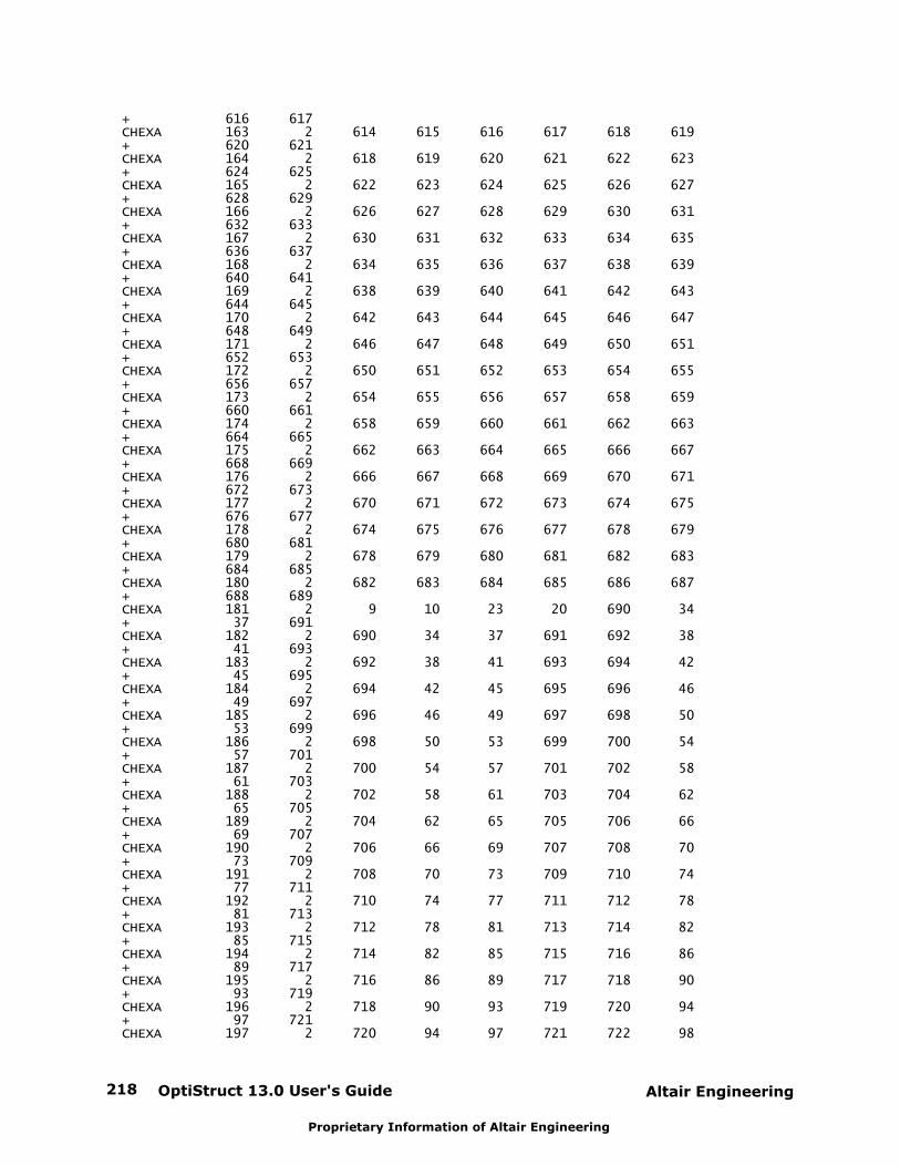
OptiStruct 13.0 User's Guide218 Altair Engineering
Proprietary Information of Altair Engineering
+ 616 617CHEXA 163 2 614 615 616 617 618 619+ 620 621CHEXA 164 2 618 619 620 621 622 623+ 624 625CHEXA 165 2 622 623 624 625 626 627+ 628 629CHEXA 166 2 626 627 628 629 630 631+ 632 633CHEXA 167 2 630 631 632 633 634 635+ 636 637CHEXA 168 2 634 635 636 637 638 639+ 640 641CHEXA 169 2 638 639 640 641 642 643+ 644 645CHEXA 170 2 642 643 644 645 646 647+ 648 649CHEXA 171 2 646 647 648 649 650 651+ 652 653CHEXA 172 2 650 651 652 653 654 655+ 656 657CHEXA 173 2 654 655 656 657 658 659+ 660 661CHEXA 174 2 658 659 660 661 662 663+ 664 665CHEXA 175 2 662 663 664 665 666 667+ 668 669CHEXA 176 2 666 667 668 669 670 671+ 672 673CHEXA 177 2 670 671 672 673 674 675+ 676 677CHEXA 178 2 674 675 676 677 678 679+ 680 681CHEXA 179 2 678 679 680 681 682 683+ 684 685CHEXA 180 2 682 683 684 685 686 687+ 688 689CHEXA 181 2 9 10 23 20 690 34+ 37 691CHEXA 182 2 690 34 37 691 692 38+ 41 693CHEXA 183 2 692 38 41 693 694 42+ 45 695CHEXA 184 2 694 42 45 695 696 46+ 49 697CHEXA 185 2 696 46 49 697 698 50+ 53 699CHEXA 186 2 698 50 53 699 700 54+ 57 701CHEXA 187 2 700 54 57 701 702 58+ 61 703CHEXA 188 2 702 58 61 703 704 62+ 65 705CHEXA 189 2 704 62 65 705 706 66+ 69 707CHEXA 190 2 706 66 69 707 708 70+ 73 709CHEXA 191 2 708 70 73 709 710 74+ 77 711CHEXA 192 2 710 74 77 711 712 78+ 81 713CHEXA 193 2 712 78 81 713 714 82+ 85 715CHEXA 194 2 714 82 85 715 716 86+ 89 717CHEXA 195 2 716 86 89 717 718 90+ 93 719CHEXA 196 2 718 90 93 719 720 94+ 97 721CHEXA 197 2 720 94 97 721 722 98
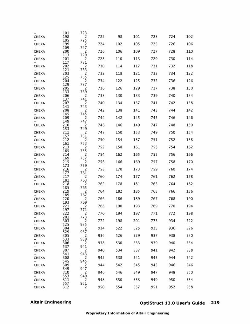
Altair Engineering OptiStruct 13.0 User's Guide 219
Proprietary Information of Altair Engineering
+ 101 723CHEXA 198 2 722 98 101 723 724 102+ 105 725CHEXA 199 2 724 102 105 725 726 106+ 109 727CHEXA 200 2 726 106 109 727 728 110+ 113 729CHEXA 201 2 728 110 113 729 730 114+ 117 731CHEXA 202 2 730 114 117 731 732 118+ 121 733CHEXA 203 2 732 118 121 733 734 122+ 125 735CHEXA 204 2 734 122 125 735 736 126+ 129 737CHEXA 205 2 736 126 129 737 738 130+ 133 739CHEXA 206 2 738 130 133 739 740 134+ 137 741CHEXA 207 2 740 134 137 741 742 138+ 141 743CHEXA 208 2 742 138 141 743 744 142+ 145 745CHEXA 209 2 744 142 145 745 746 146+ 149 747CHEXA 210 2 746 146 149 747 748 150+ 153 749CHEXA 211 2 748 150 153 749 750 154+ 157 751CHEXA 212 2 750 154 157 751 752 158+ 161 753CHEXA 213 2 752 158 161 753 754 162+ 165 755CHEXA 214 2 754 162 165 755 756 166+ 169 757CHEXA 215 2 756 166 169 757 758 170+ 173 759CHEXA 216 2 758 170 173 759 760 174+ 177 761CHEXA 217 2 760 174 177 761 762 178+ 181 763CHEXA 218 2 762 178 181 763 764 182+ 185 765CHEXA 219 2 764 182 185 765 766 186+ 189 767CHEXA 220 2 766 186 189 767 768 190+ 193 769CHEXA 221 2 768 190 193 769 770 194+ 197 771CHEXA 222 2 770 194 197 771 772 198+ 201 773CHEXA 303 2 772 198 201 773 934 522+ 525 935CHEXA 304 2 934 522 525 935 936 526+ 529 937CHEXA 305 2 936 526 529 937 938 530+ 533 939CHEXA 306 2 938 530 533 939 940 534+ 537 941CHEXA 307 2 940 534 537 941 942 538+ 541 943CHEXA 308 2 942 538 541 943 944 542+ 545 945CHEXA 309 2 944 542 545 945 946 546+ 549 947CHEXA 310 2 946 546 549 947 948 550+ 553 949CHEXA 311 2 948 550 553 949 950 554+ 557 951CHEXA 312 2 950 554 557 951 952 558
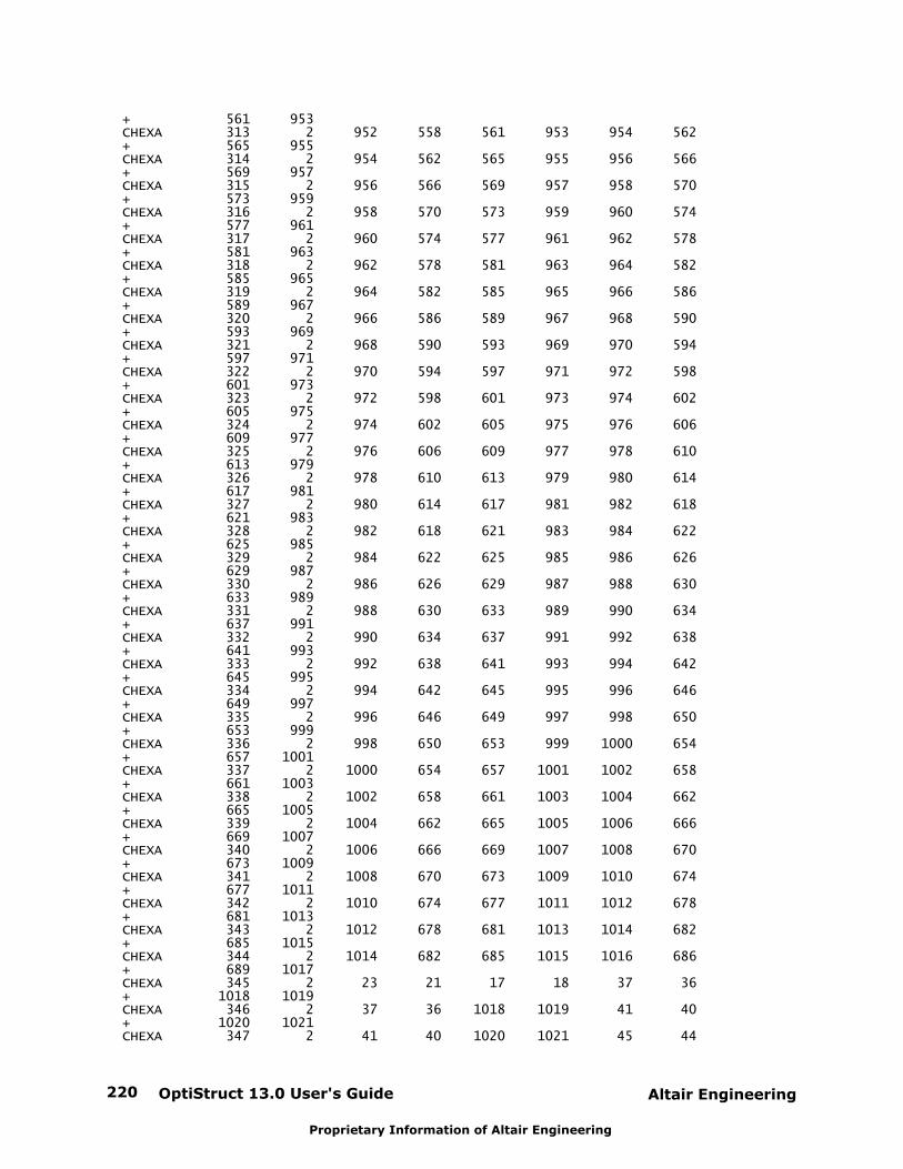
OptiStruct 13.0 User's Guide220 Altair Engineering
Proprietary Information of Altair Engineering
+ 561 953CHEXA 313 2 952 558 561 953 954 562+ 565 955CHEXA 314 2 954 562 565 955 956 566+ 569 957CHEXA 315 2 956 566 569 957 958 570+ 573 959CHEXA 316 2 958 570 573 959 960 574+ 577 961CHEXA 317 2 960 574 577 961 962 578+ 581 963CHEXA 318 2 962 578 581 963 964 582+ 585 965CHEXA 319 2 964 582 585 965 966 586+ 589 967CHEXA 320 2 966 586 589 967 968 590+ 593 969CHEXA 321 2 968 590 593 969 970 594+ 597 971CHEXA 322 2 970 594 597 971 972 598+ 601 973CHEXA 323 2 972 598 601 973 974 602+ 605 975CHEXA 324 2 974 602 605 975 976 606+ 609 977CHEXA 325 2 976 606 609 977 978 610+ 613 979CHEXA 326 2 978 610 613 979 980 614+ 617 981CHEXA 327 2 980 614 617 981 982 618+ 621 983CHEXA 328 2 982 618 621 983 984 622+ 625 985CHEXA 329 2 984 622 625 985 986 626+ 629 987CHEXA 330 2 986 626 629 987 988 630+ 633 989CHEXA 331 2 988 630 633 989 990 634+ 637 991CHEXA 332 2 990 634 637 991 992 638+ 641 993CHEXA 333 2 992 638 641 993 994 642+ 645 995CHEXA 334 2 994 642 645 995 996 646+ 649 997CHEXA 335 2 996 646 649 997 998 650+ 653 999CHEXA 336 2 998 650 653 999 1000 654+ 657 1001CHEXA 337 2 1000 654 657 1001 1002 658+ 661 1003CHEXA 338 2 1002 658 661 1003 1004 662+ 665 1005CHEXA 339 2 1004 662 665 1005 1006 666+ 669 1007CHEXA 340 2 1006 666 669 1007 1008 670+ 673 1009CHEXA 341 2 1008 670 673 1009 1010 674+ 677 1011CHEXA 342 2 1010 674 677 1011 1012 678+ 681 1013CHEXA 343 2 1012 678 681 1013 1014 682+ 685 1015CHEXA 344 2 1014 682 685 1015 1016 686+ 689 1017CHEXA 345 2 23 21 17 18 37 36+ 1018 1019CHEXA 346 2 37 36 1018 1019 41 40+ 1020 1021CHEXA 347 2 41 40 1020 1021 45 44
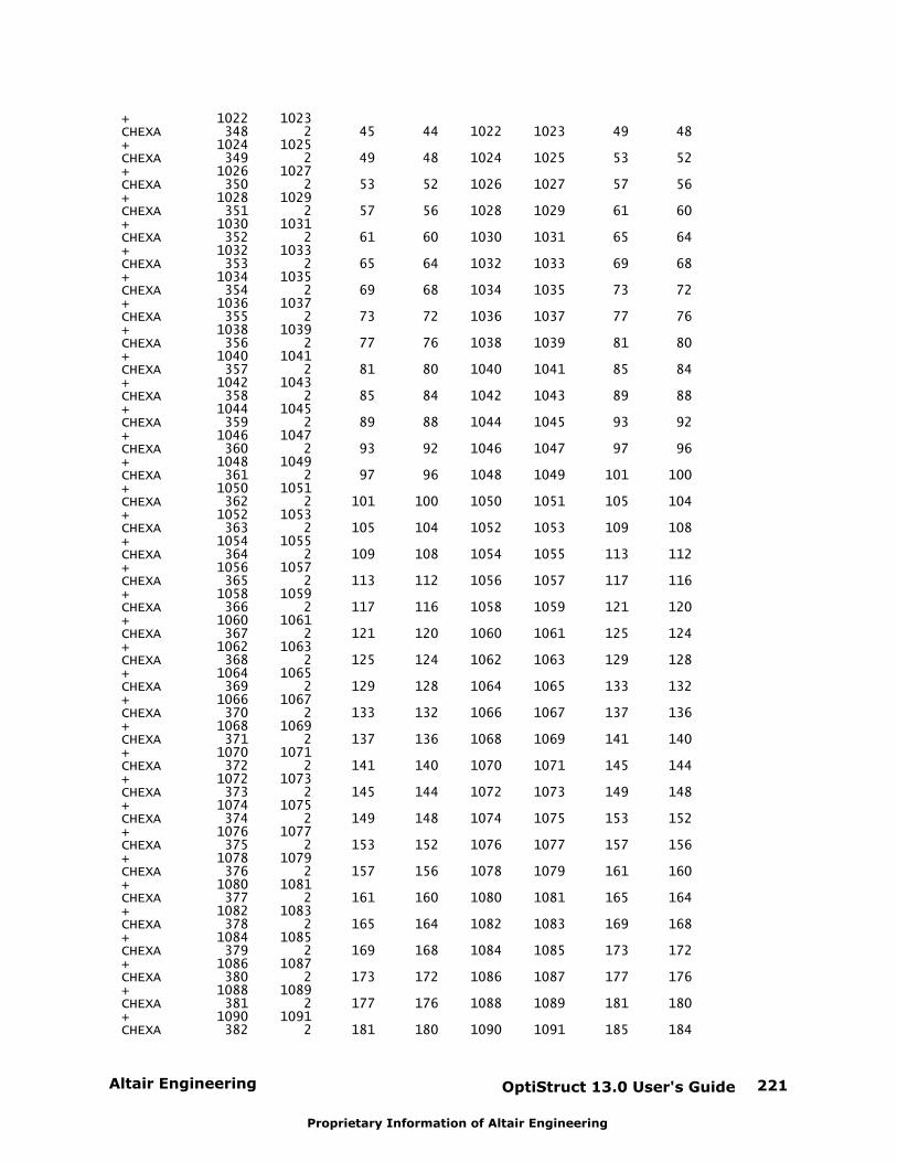
Altair Engineering OptiStruct 13.0 User's Guide 221
Proprietary Information of Altair Engineering
+ 1022 1023CHEXA 348 2 45 44 1022 1023 49 48+ 1024 1025CHEXA 349 2 49 48 1024 1025 53 52+ 1026 1027CHEXA 350 2 53 52 1026 1027 57 56+ 1028 1029CHEXA 351 2 57 56 1028 1029 61 60+ 1030 1031CHEXA 352 2 61 60 1030 1031 65 64+ 1032 1033CHEXA 353 2 65 64 1032 1033 69 68+ 1034 1035CHEXA 354 2 69 68 1034 1035 73 72+ 1036 1037CHEXA 355 2 73 72 1036 1037 77 76+ 1038 1039CHEXA 356 2 77 76 1038 1039 81 80+ 1040 1041CHEXA 357 2 81 80 1040 1041 85 84+ 1042 1043CHEXA 358 2 85 84 1042 1043 89 88+ 1044 1045CHEXA 359 2 89 88 1044 1045 93 92+ 1046 1047CHEXA 360 2 93 92 1046 1047 97 96+ 1048 1049CHEXA 361 2 97 96 1048 1049 101 100+ 1050 1051CHEXA 362 2 101 100 1050 1051 105 104+ 1052 1053CHEXA 363 2 105 104 1052 1053 109 108+ 1054 1055CHEXA 364 2 109 108 1054 1055 113 112+ 1056 1057CHEXA 365 2 113 112 1056 1057 117 116+ 1058 1059CHEXA 366 2 117 116 1058 1059 121 120+ 1060 1061CHEXA 367 2 121 120 1060 1061 125 124+ 1062 1063CHEXA 368 2 125 124 1062 1063 129 128+ 1064 1065CHEXA 369 2 129 128 1064 1065 133 132+ 1066 1067CHEXA 370 2 133 132 1066 1067 137 136+ 1068 1069CHEXA 371 2 137 136 1068 1069 141 140+ 1070 1071CHEXA 372 2 141 140 1070 1071 145 144+ 1072 1073CHEXA 373 2 145 144 1072 1073 149 148+ 1074 1075CHEXA 374 2 149 148 1074 1075 153 152+ 1076 1077CHEXA 375 2 153 152 1076 1077 157 156+ 1078 1079CHEXA 376 2 157 156 1078 1079 161 160+ 1080 1081CHEXA 377 2 161 160 1080 1081 165 164+ 1082 1083CHEXA 378 2 165 164 1082 1083 169 168+ 1084 1085CHEXA 379 2 169 168 1084 1085 173 172+ 1086 1087CHEXA 380 2 173 172 1086 1087 177 176+ 1088 1089CHEXA 381 2 177 176 1088 1089 181 180+ 1090 1091CHEXA 382 2 181 180 1090 1091 185 184
OptiStruct 13.0 User's Guide222 Altair Engineering
Proprietary Information of Altair Engineering
+ 1092 1093CHEXA 383 2 185 184 1092 1093 189 188+ 1094 1095CHEXA 384 2 189 188 1094 1095 193 192+ 1096 1097CHEXA 385 2 193 192 1096 1097 197 196+ 1098 1099CHEXA 386 2 197 196 1098 1099 201 200+ 1100 1101CHEXA 467 2 201 200 1100 1101 525 524+ 1262 1263CHEXA 468 2 525 524 1262 1263 529 528+ 1264 1265CHEXA 469 2 529 528 1264 1265 533 532+ 1266 1267CHEXA 470 2 533 532 1266 1267 537 536+ 1268 1269CHEXA 471 2 537 536 1268 1269 541 540+ 1270 1271CHEXA 472 2 541 540 1270 1271 545 544+ 1272 1273CHEXA 473 2 545 544 1272 1273 549 548+ 1274 1275CHEXA 474 2 549 548 1274 1275 553 552+ 1276 1277CHEXA 475 2 553 552 1276 1277 557 556+ 1278 1279CHEXA 476 2 557 556 1278 1279 561 560+ 1280 1281CHEXA 477 2 561 560 1280 1281 565 564+ 1282 1283CHEXA 478 2 565 564 1282 1283 569 568+ 1284 1285CHEXA 479 2 569 568 1284 1285 573 572+ 1286 1287CHEXA 480 2 573 572 1286 1287 577 576+ 1288 1289CHEXA 481 2 577 576 1288 1289 581 580+ 1290 1291CHEXA 482 2 581 580 1290 1291 585 584+ 1292 1293CHEXA 483 2 585 584 1292 1293 589 588+ 1294 1295CHEXA 484 2 589 588 1294 1295 593 592+ 1296 1297CHEXA 485 2 593 592 1296 1297 597 596+ 1298 1299CHEXA 486 2 597 596 1298 1299 601 600+ 1300 1301CHEXA 487 2 601 600 1300 1301 605 604+ 1302 1303CHEXA 488 2 605 604 1302 1303 609 608+ 1304 1305CHEXA 489 2 609 608 1304 1305 613 612+ 1306 1307CHEXA 490 2 613 612 1306 1307 617 616+ 1308 1309CHEXA 491 2 617 616 1308 1309 621 620+ 1310 1311CHEXA 492 2 621 620 1310 1311 625 624+ 1312 1313CHEXA 493 2 625 624 1312 1313 629 628+ 1314 1315CHEXA 494 2 629 628 1314 1315 633 632+ 1316 1317CHEXA 495 2 633 632 1316 1317 637 636+ 1318 1319CHEXA 496 2 637 636 1318 1319 641 640+ 1320 1321CHEXA 497 2 641 640 1320 1321 645 644
Altair Engineering OptiStruct 13.0 User's Guide 223
Proprietary Information of Altair Engineering
+ 1322 1323CHEXA 498 2 645 644 1322 1323 649 648+ 1324 1325CHEXA 499 2 649 648 1324 1325 653 652+ 1326 1327CHEXA 500 2 653 652 1326 1327 657 656+ 1328 1329CHEXA 501 2 657 656 1328 1329 661 660+ 1330 1331CHEXA 502 2 661 660 1330 1331 665 664+ 1332 1333CHEXA 503 2 665 664 1332 1333 669 668+ 1334 1335CHEXA 504 2 669 668 1334 1335 673 672+ 1336 1337CHEXA 505 2 673 672 1336 1337 677 676+ 1338 1339CHEXA 506 2 677 676 1338 1339 681 680+ 1340 1341CHEXA 507 2 681 680 1340 1341 685 684+ 1342 1343CHEXA 508 2 685 684 1342 1343 689 688+ 1344 1345CHEXA 509 2 20 23 18 19 691 37+ 1019 1346CHEXA 510 2 691 37 1019 1346 693 41+ 1021 1347CHEXA 511 2 693 41 1021 1347 695 45+ 1023 1348CHEXA 512 2 695 45 1023 1348 697 49+ 1025 1349CHEXA 513 2 697 49 1025 1349 699 53+ 1027 1350CHEXA 514 2 699 53 1027 1350 701 57+ 1029 1351CHEXA 515 2 701 57 1029 1351 703 61+ 1031 1352CHEXA 516 2 703 61 1031 1352 705 65+ 1033 1353CHEXA 517 2 705 65 1033 1353 707 69+ 1035 1354CHEXA 518 2 707 69 1035 1354 709 73+ 1037 1355CHEXA 519 2 709 73 1037 1355 711 77+ 1039 1356CHEXA 520 2 711 77 1039 1356 713 81+ 1041 1357CHEXA 521 2 713 81 1041 1357 715 85+ 1043 1358CHEXA 522 2 715 85 1043 1358 717 89+ 1045 1359CHEXA 523 2 717 89 1045 1359 719 93+ 1047 1360CHEXA 524 2 719 93 1047 1360 721 97+ 1049 1361CHEXA 525 2 721 97 1049 1361 723 101+ 1051 1362CHEXA 526 2 723 101 1051 1362 725 105+ 1053 1363CHEXA 527 2 725 105 1053 1363 727 109+ 1055 1364CHEXA 528 2 727 109 1055 1364 729 113+ 1057 1365CHEXA 529 2 729 113 1057 1365 731 117+ 1059 1366CHEXA 530 2 731 117 1059 1366 733 121+ 1061 1367CHEXA 531 2 733 121 1061 1367 735 125+ 1063 1368CHEXA 532 2 735 125 1063 1368 737 129
OptiStruct 13.0 User's Guide224 Altair Engineering
Proprietary Information of Altair Engineering
+ 1065 1369CHEXA 533 2 737 129 1065 1369 739 133+ 1067 1370CHEXA 534 2 739 133 1067 1370 741 137+ 1069 1371CHEXA 535 2 741 137 1069 1371 743 141+ 1071 1372CHEXA 536 2 743 141 1071 1372 745 145+ 1073 1373CHEXA 537 2 745 145 1073 1373 747 149+ 1075 1374CHEXA 538 2 747 149 1075 1374 749 153+ 1077 1375CHEXA 539 2 749 153 1077 1375 751 157+ 1079 1376CHEXA 540 2 751 157 1079 1376 753 161+ 1081 1377CHEXA 541 2 753 161 1081 1377 755 165+ 1083 1378CHEXA 542 2 755 165 1083 1378 757 169+ 1085 1379CHEXA 543 2 757 169 1085 1379 759 173+ 1087 1380CHEXA 544 2 759 173 1087 1380 761 177+ 1089 1381CHEXA 545 2 761 177 1089 1381 763 181+ 1091 1382CHEXA 546 2 763 181 1091 1382 765 185+ 1093 1383CHEXA 547 2 765 185 1093 1383 767 189+ 1095 1384CHEXA 548 2 767 189 1095 1384 769 193+ 1097 1385CHEXA 549 2 769 193 1097 1385 771 197+ 1099 1386CHEXA 550 2 771 197 1099 1386 773 201+ 1101 1387CHEXA 631 2 773 201 1101 1387 935 525+ 1263 1468CHEXA 632 2 935 525 1263 1468 937 529+ 1265 1469CHEXA 633 2 937 529 1265 1469 939 533+ 1267 1470CHEXA 634 2 939 533 1267 1470 941 537+ 1269 1471CHEXA 635 2 941 537 1269 1471 943 541+ 1271 1472CHEXA 636 2 943 541 1271 1472 945 545+ 1273 1473CHEXA 637 2 945 545 1273 1473 947 549+ 1275 1474CHEXA 638 2 947 549 1275 1474 949 553+ 1277 1475CHEXA 639 2 949 553 1277 1475 951 557+ 1279 1476CHEXA 640 2 951 557 1279 1476 953 561+ 1281 1477CHEXA 641 2 953 561 1281 1477 955 565+ 1283 1478CHEXA 642 2 955 565 1283 1478 957 569+ 1285 1479CHEXA 643 2 957 569 1285 1479 959 573+ 1287 1480CHEXA 644 2 959 573 1287 1480 961 577+ 1289 1481CHEXA 645 2 961 577 1289 1481 963 581+ 1291 1482CHEXA 646 2 963 581 1291 1482 965 585+ 1293 1483CHEXA 647 2 965 585 1293 1483 967 589
Altair Engineering OptiStruct 13.0 User's Guide 225
Proprietary Information of Altair Engineering
+ 1295 1484CHEXA 648 2 967 589 1295 1484 969 593+ 1297 1485CHEXA 649 2 969 593 1297 1485 971 597+ 1299 1486CHEXA 650 2 971 597 1299 1486 973 601+ 1301 1487CHEXA 651 2 973 601 1301 1487 975 605+ 1303 1488CHEXA 652 2 975 605 1303 1488 977 609+ 1305 1489CHEXA 653 2 977 609 1305 1489 979 613+ 1307 1490CHEXA 654 2 979 613 1307 1490 981 617+ 1309 1491CHEXA 655 2 981 617 1309 1491 983 621+ 1311 1492CHEXA 656 2 983 621 1311 1492 985 625+ 1313 1493CHEXA 657 2 985 625 1313 1493 987 629+ 1315 1494CHEXA 658 2 987 629 1315 1494 989 633+ 1317 1495CHEXA 659 2 989 633 1317 1495 991 637+ 1319 1496CHEXA 660 2 991 637 1319 1496 993 641+ 1321 1497CHEXA 661 2 993 641 1321 1497 995 645+ 1323 1498CHEXA 662 2 995 645 1323 1498 997 649+ 1325 1499CHEXA 663 2 997 649 1325 1499 999 653+ 1327 1500CHEXA 664 2 999 653 1327 1500 1001 657+ 1329 1501CHEXA 665 2 1001 657 1329 1501 1003 661+ 1331 1502CHEXA 666 2 1003 661 1331 1502 1005 665+ 1333 1503CHEXA 667 2 1005 665 1333 1503 1007 669+ 1335 1504CHEXA 668 2 1007 669 1335 1504 1009 673+ 1337 1505CHEXA 669 2 1009 673 1337 1505 1011 677+ 1339 1506CHEXA 670 2 1011 677 1339 1506 1013 681+ 1341 1507CHEXA 671 2 1013 681 1341 1507 1015 685+ 1343 1508CHEXA 672 2 1015 685 1343 1508 1017 689+ 1345 1509CHEXA 673 2 12 13 14 22 1510 1511+ 1512 1513CHEXA 674 2 1510 1511 1512 1513 1514 1515+ 1516 1517CHEXA 675 2 1514 1515 1516 1517 1518 1519+ 1520 1521CHEXA 676 2 1518 1519 1520 1521 1522 1523+ 1524 1525CHEXA 677 2 1522 1523 1524 1525 1526 1527+ 1528 1529CHEXA 678 2 1526 1527 1528 1529 1530 1531+ 1532 1533CHEXA 679 2 1530 1531 1532 1533 1534 1535+ 1536 1537CHEXA 680 2 1534 1535 1536 1537 1538 1539+ 1540 1541CHEXA 681 2 1538 1539 1540 1541 1542 1543+ 1544 1545CHEXA 682 2 1542 1543 1544 1545 1546 1547
OptiStruct 13.0 User's Guide226 Altair Engineering
Proprietary Information of Altair Engineering
+ 1548 1549CHEXA 683 2 1546 1547 1548 1549 1550 1551+ 1552 1553CHEXA 684 2 1550 1551 1552 1553 1554 1555+ 1556 1557CHEXA 685 2 1554 1555 1556 1557 1558 1559+ 1560 1561CHEXA 686 2 1558 1559 1560 1561 1562 1563+ 1564 1565CHEXA 687 2 1562 1563 1564 1565 1566 1567+ 1568 1569CHEXA 688 2 1566 1567 1568 1569 1570 1571+ 1572 1573CHEXA 689 2 1570 1571 1572 1573 1574 1575+ 1576 1577CHEXA 690 2 1574 1575 1576 1577 1578 1579+ 1580 1581CHEXA 691 2 1578 1579 1580 1581 1582 1583+ 1584 1585CHEXA 692 2 1582 1583 1584 1585 1586 1587+ 1588 1589CHEXA 693 2 1586 1587 1588 1589 1590 1591+ 1592 1593CHEXA 694 2 1590 1591 1592 1593 1594 1595+ 1596 1597CHEXA 695 2 1594 1595 1596 1597 1598 1599+ 1600 1601CHEXA 696 2 1598 1599 1600 1601 1602 1603+ 1604 1605CHEXA 697 2 1602 1603 1604 1605 1606 1607+ 1608 1609CHEXA 698 2 1606 1607 1608 1609 1610 1611+ 1612 1613CHEXA 699 2 1610 1611 1612 1613 1614 1615+ 1616 1617CHEXA 700 2 1614 1615 1616 1617 1618 1619+ 1620 1621CHEXA 701 2 1618 1619 1620 1621 1622 1623+ 1624 1625CHEXA 702 2 1622 1623 1624 1625 1626 1627+ 1628 1629CHEXA 703 2 1626 1627 1628 1629 1630 1631+ 1632 1633CHEXA 704 2 1630 1631 1632 1633 1634 1635+ 1636 1637CHEXA 705 2 1634 1635 1636 1637 1638 1639+ 1640 1641CHEXA 706 2 1638 1639 1640 1641 1642 1643+ 1644 1645CHEXA 707 2 1642 1643 1644 1645 1646 1647+ 1648 1649CHEXA 708 2 1646 1647 1648 1649 1650 1651+ 1652 1653CHEXA 709 2 1650 1651 1652 1653 1654 1655+ 1656 1657CHEXA 710 2 1654 1655 1656 1657 1658 1659+ 1660 1661CHEXA 711 2 1658 1659 1660 1661 1662 1663+ 1664 1665CHEXA 712 2 1662 1663 1664 1665 1666 1667+ 1668 1669CHEXA 713 2 1666 1667 1668 1669 1670 1671+ 1672 1673CHEXA 714 2 1670 1671 1672 1673 1674 1675+ 1676 1677CHEXA 795 2 1674 1675 1676 1677 1998 1999+ 2000 2001CHEXA 796 2 1998 1999 2000 2001 2002 2003+ 2004 2005CHEXA 797 2 2002 2003 2004 2005 2006 2007

Altair Engineering OptiStruct 13.0 User's Guide 227
Proprietary Information of Altair Engineering
+ 2008 2009CHEXA 798 2 2006 2007 2008 2009 2010 2011+ 2012 2013CHEXA 799 2 2010 2011 2012 2013 2014 2015+ 2016 2017CHEXA 800 2 2014 2015 2016 2017 2018 2019+ 2020 2021CHEXA 801 2 2018 2019 2020 2021 2022 2023+ 2024 2025CHEXA 802 2 2022 2023 2024 2025 2026 2027+ 2028 2029CHEXA 803 2 2026 2027 2028 2029 2030 2031+ 2032 2033CHEXA 804 2 2030 2031 2032 2033 2034 2035+ 2036 2037CHEXA 805 2 2034 2035 2036 2037 2038 2039+ 2040 2041CHEXA 806 2 2038 2039 2040 2041 2042 2043+ 2044 2045CHEXA 807 2 2042 2043 2044 2045 2046 2047+ 2048 2049CHEXA 808 2 2046 2047 2048 2049 2050 2051+ 2052 2053CHEXA 809 2 2050 2051 2052 2053 2054 2055+ 2056 2057CHEXA 810 2 2054 2055 2056 2057 2058 2059+ 2060 2061CHEXA 811 2 2058 2059 2060 2061 2062 2063+ 2064 2065CHEXA 812 2 2062 2063 2064 2065 2066 2067+ 2068 2069CHEXA 813 2 2066 2067 2068 2069 2070 2071+ 2072 2073CHEXA 814 2 2070 2071 2072 2073 2074 2075+ 2076 2077CHEXA 815 2 2074 2075 2076 2077 2078 2079+ 2080 2081CHEXA 816 2 2078 2079 2080 2081 2082 2083+ 2084 2085CHEXA 817 2 2082 2083 2084 2085 2086 2087+ 2088 2089CHEXA 818 2 2086 2087 2088 2089 2090 2091+ 2092 2093CHEXA 819 2 2090 2091 2092 2093 2094 2095+ 2096 2097CHEXA 820 2 2094 2095 2096 2097 2098 2099+ 2100 2101CHEXA 821 2 2098 2099 2100 2101 2102 2103+ 2104 2105CHEXA 822 2 2102 2103 2104 2105 2106 2107+ 2108 2109CHEXA 823 2 2106 2107 2108 2109 2110 2111+ 2112 2113CHEXA 824 2 2110 2111 2112 2113 2114 2115+ 2116 2117CHEXA 825 2 2114 2115 2116 2117 2118 2119+ 2120 2121CHEXA 826 2 2118 2119 2120 2121 2122 2123+ 2124 2125CHEXA 827 2 2122 2123 2124 2125 2126 2127+ 2128 2129CHEXA 828 2 2126 2127 2128 2129 2130 2131+ 2132 2133CHEXA 829 2 2130 2131 2132 2133 2134 2135+ 2136 2137CHEXA 830 2 2134 2135 2136 2137 2138 2139+ 2140 2141CHEXA 831 2 2138 2139 2140 2141 2142 2143+ 2144 2145CHEXA 832 2 2142 2143 2144 2145 2146 2147
OptiStruct 13.0 User's Guide228 Altair Engineering
Proprietary Information of Altair Engineering
+ 2148 2149CHEXA 833 2 2146 2147 2148 2149 2150 2151+ 2152 2153CHEXA 834 2 2150 2151 2152 2153 2154 2155+ 2156 2157CHEXA 835 2 2154 2155 2156 2157 2158 2159+ 2160 2161CHEXA 836 2 2158 2159 2160 2161 2162 2163+ 2164 2165CHEXA 837 2 11 12 22 21 35 1510+ 1513 36CHEXA 838 2 35 1510 1513 36 39 1514+ 1517 40CHEXA 839 2 39 1514 1517 40 43 1518+ 1521 44CHEXA 840 2 43 1518 1521 44 47 1522+ 1525 48CHEXA 841 2 47 1522 1525 48 51 1526+ 1529 52CHEXA 842 2 51 1526 1529 52 55 1530+ 1533 56CHEXA 843 2 55 1530 1533 56 59 1534+ 1537 60CHEXA 844 2 59 1534 1537 60 63 1538+ 1541 64CHEXA 845 2 63 1538 1541 64 67 1542+ 1545 68CHEXA 846 2 67 1542 1545 68 71 1546+ 1549 72CHEXA 847 2 71 1546 1549 72 75 1550+ 1553 76CHEXA 848 2 75 1550 1553 76 79 1554+ 1557 80CHEXA 849 2 79 1554 1557 80 83 1558+ 1561 84CHEXA 850 2 83 1558 1561 84 87 1562+ 1565 88CHEXA 851 2 87 1562 1565 88 91 1566+ 1569 92CHEXA 852 2 91 1566 1569 92 95 1570+ 1573 96CHEXA 853 2 95 1570 1573 96 99 1574+ 1577 100CHEXA 854 2 99 1574 1577 100 103 1578+ 1581 104CHEXA 855 2 103 1578 1581 104 107 1582+ 1585 108CHEXA 856 2 107 1582 1585 108 111 1586+ 1589 112CHEXA 857 2 111 1586 1589 112 115 1590+ 1593 116CHEXA 858 2 115 1590 1593 116 119 1594+ 1597 120CHEXA 859 2 119 1594 1597 120 123 1598+ 1601 124CHEXA 860 2 123 1598 1601 124 127 1602+ 1605 128CHEXA 861 2 127 1602 1605 128 131 1606+ 1609 132CHEXA 862 2 131 1606 1609 132 135 1610+ 1613 136CHEXA 863 2 135 1610 1613 136 139 1614+ 1617 140CHEXA 864 2 139 1614 1617 140 143 1618+ 1621 144CHEXA 865 2 143 1618 1621 144 147 1622+ 1625 148CHEXA 866 2 147 1622 1625 148 151 1626+ 1629 152CHEXA 867 2 151 1626 1629 152 155 1630
Altair Engineering OptiStruct 13.0 User's Guide 229
Proprietary Information of Altair Engineering
+ 1633 156CHEXA 868 2 155 1630 1633 156 159 1634+ 1637 160CHEXA 869 2 159 1634 1637 160 163 1638+ 1641 164CHEXA 870 2 163 1638 1641 164 167 1642+ 1645 168CHEXA 871 2 167 1642 1645 168 171 1646+ 1649 172CHEXA 872 2 171 1646 1649 172 175 1650+ 1653 176CHEXA 873 2 175 1650 1653 176 179 1654+ 1657 180CHEXA 874 2 179 1654 1657 180 183 1658+ 1661 184CHEXA 875 2 183 1658 1661 184 187 1662+ 1665 188CHEXA 876 2 187 1662 1665 188 191 1666+ 1669 192CHEXA 877 2 191 1666 1669 192 195 1670+ 1673 196CHEXA 878 2 195 1670 1673 196 199 1674+ 1677 200CHEXA 959 2 199 1674 1677 200 523 1998+ 2001 524CHEXA 960 2 523 1998 2001 524 527 2002+ 2005 528CHEXA 961 2 527 2002 2005 528 531 2006+ 2009 532CHEXA 962 2 531 2006 2009 532 535 2010+ 2013 536CHEXA 963 2 535 2010 2013 536 539 2014+ 2017 540CHEXA 964 2 539 2014 2017 540 543 2018+ 2021 544CHEXA 965 2 543 2018 2021 544 547 2022+ 2025 548CHEXA 966 2 547 2022 2025 548 551 2026+ 2029 552CHEXA 967 2 551 2026 2029 552 555 2030+ 2033 556CHEXA 968 2 555 2030 2033 556 559 2034+ 2037 560CHEXA 969 2 559 2034 2037 560 563 2038+ 2041 564CHEXA 970 2 563 2038 2041 564 567 2042+ 2045 568CHEXA 971 2 567 2042 2045 568 571 2046+ 2049 572CHEXA 972 2 571 2046 2049 572 575 2050+ 2053 576CHEXA 973 2 575 2050 2053 576 579 2054+ 2057 580CHEXA 974 2 579 2054 2057 580 583 2058+ 2061 584CHEXA 975 2 583 2058 2061 584 587 2062+ 2065 588CHEXA 976 2 587 2062 2065 588 591 2066+ 2069 592CHEXA 977 2 591 2066 2069 592 595 2070+ 2073 596CHEXA 978 2 595 2070 2073 596 599 2074+ 2077 600CHEXA 979 2 599 2074 2077 600 603 2078+ 2081 604CHEXA 980 2 603 2078 2081 604 607 2082+ 2085 608CHEXA 981 2 607 2082 2085 608 611 2086+ 2089 612CHEXA 982 2 611 2086 2089 612 615 2090
OptiStruct 13.0 User's Guide230 Altair Engineering
Proprietary Information of Altair Engineering
+ 2093 616CHEXA 983 2 615 2090 2093 616 619 2094+ 2097 620CHEXA 984 2 619 2094 2097 620 623 2098+ 2101 624CHEXA 985 2 623 2098 2101 624 627 2102+ 2105 628CHEXA 986 2 627 2102 2105 628 631 2106+ 2109 632CHEXA 987 2 631 2106 2109 632 635 2110+ 2113 636CHEXA 988 2 635 2110 2113 636 639 2114+ 2117 640CHEXA 989 2 639 2114 2117 640 643 2118+ 2121 644CHEXA 990 2 643 2118 2121 644 647 2122+ 2125 648CHEXA 991 2 647 2122 2125 648 651 2126+ 2129 652CHEXA 992 2 651 2126 2129 652 655 2130+ 2133 656CHEXA 993 2 655 2130 2133 656 659 2134+ 2137 660CHEXA 994 2 659 2134 2137 660 663 2138+ 2141 664CHEXA 995 2 663 2138 2141 664 667 2142+ 2145 668CHEXA 996 2 667 2142 2145 668 671 2146+ 2149 672CHEXA 997 2 671 2146 2149 672 675 2150+ 2153 676CHEXA 998 2 675 2150 2153 676 679 2154+ 2157 680CHEXA 999 2 679 2154 2157 680 683 2158+ 2161 684CHEXA 1000 2 683 2158 2161 684 687 2162+ 2165 688CHEXA 1001 2 22 14 15 16 1513 1512+ 2166 2167CHEXA 1002 2 1513 1512 2166 2167 1517 1516+ 2168 2169CHEXA 1003 2 1517 1516 2168 2169 1521 1520+ 2170 2171CHEXA 1004 2 1521 1520 2170 2171 1525 1524+ 2172 2173CHEXA 1005 2 1525 1524 2172 2173 1529 1528+ 2174 2175CHEXA 1006 2 1529 1528 2174 2175 1533 1532+ 2176 2177CHEXA 1007 2 1533 1532 2176 2177 1537 1536+ 2178 2179CHEXA 1008 2 1537 1536 2178 2179 1541 1540+ 2180 2181CHEXA 1009 2 1541 1540 2180 2181 1545 1544+ 2182 2183CHEXA 1010 2 1545 1544 2182 2183 1549 1548+ 2184 2185CHEXA 1011 2 1549 1548 2184 2185 1553 1552+ 2186 2187CHEXA 1012 2 1553 1552 2186 2187 1557 1556+ 2188 2189CHEXA 1013 2 1557 1556 2188 2189 1561 1560+ 2190 2191CHEXA 1014 2 1561 1560 2190 2191 1565 1564+ 2192 2193CHEXA 1015 2 1565 1564 2192 2193 1569 1568+ 2194 2195CHEXA 1016 2 1569 1568 2194 2195 1573 1572+ 2196 2197CHEXA 1017 2 1573 1572 2196 2197 1577 1576

Altair Engineering OptiStruct 13.0 User's Guide 231
Proprietary Information of Altair Engineering
+ 2198 2199CHEXA 1018 2 1577 1576 2198 2199 1581 1580+ 2200 2201CHEXA 1019 2 1581 1580 2200 2201 1585 1584+ 2202 2203CHEXA 1020 2 1585 1584 2202 2203 1589 1588+ 2204 2205CHEXA 1021 2 1589 1588 2204 2205 1593 1592+ 2206 2207CHEXA 1022 2 1593 1592 2206 2207 1597 1596+ 2208 2209CHEXA 1023 2 1597 1596 2208 2209 1601 1600+ 2210 2211CHEXA 1024 2 1601 1600 2210 2211 1605 1604+ 2212 2213CHEXA 1025 2 1605 1604 2212 2213 1609 1608+ 2214 2215CHEXA 1026 2 1609 1608 2214 2215 1613 1612+ 2216 2217CHEXA 1027 2 1613 1612 2216 2217 1617 1616+ 2218 2219CHEXA 1028 2 1617 1616 2218 2219 1621 1620+ 2220 2221CHEXA 1029 2 1621 1620 2220 2221 1625 1624+ 2222 2223CHEXA 1030 2 1625 1624 2222 2223 1629 1628+ 2224 2225CHEXA 1031 2 1629 1628 2224 2225 1633 1632+ 2226 2227CHEXA 1032 2 1633 1632 2226 2227 1637 1636+ 2228 2229CHEXA 1033 2 1637 1636 2228 2229 1641 1640+ 2230 2231CHEXA 1034 2 1641 1640 2230 2231 1645 1644+ 2232 2233CHEXA 1035 2 1645 1644 2232 2233 1649 1648+ 2234 2235CHEXA 1036 2 1649 1648 2234 2235 1653 1652+ 2236 2237CHEXA 1037 2 1653 1652 2236 2237 1657 1656+ 2238 2239CHEXA 1038 2 1657 1656 2238 2239 1661 1660+ 2240 2241CHEXA 1039 2 1661 1660 2240 2241 1665 1664+ 2242 2243CHEXA 1040 2 1665 1664 2242 2243 1669 1668+ 2244 2245CHEXA 1041 2 1669 1668 2244 2245 1673 1672+ 2246 2247CHEXA 1042 2 1673 1672 2246 2247 1677 1676+ 2248 2249CHEXA 1123 2 1677 1676 2248 2249 2001 2000+ 2410 2411CHEXA 1124 2 2001 2000 2410 2411 2005 2004+ 2412 2413CHEXA 1125 2 2005 2004 2412 2413 2009 2008+ 2414 2415CHEXA 1126 2 2009 2008 2414 2415 2013 2012+ 2416 2417CHEXA 1127 2 2013 2012 2416 2417 2017 2016+ 2418 2419CHEXA 1128 2 2017 2016 2418 2419 2021 2020+ 2420 2421CHEXA 1129 2 2021 2020 2420 2421 2025 2024+ 2422 2423CHEXA 1130 2 2025 2024 2422 2423 2029 2028+ 2424 2425CHEXA 1131 2 2029 2028 2424 2425 2033 2032+ 2426 2427CHEXA 1132 2 2033 2032 2426 2427 2037 2036
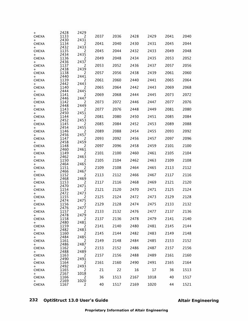
OptiStruct 13.0 User's Guide232 Altair Engineering
Proprietary Information of Altair Engineering
+ 2428 2429CHEXA 1133 2 2037 2036 2428 2429 2041 2040+ 2430 2431CHEXA 1134 2 2041 2040 2430 2431 2045 2044+ 2432 2433CHEXA 1135 2 2045 2044 2432 2433 2049 2048+ 2434 2435CHEXA 1136 2 2049 2048 2434 2435 2053 2052+ 2436 2437CHEXA 1137 2 2053 2052 2436 2437 2057 2056+ 2438 2439CHEXA 1138 2 2057 2056 2438 2439 2061 2060+ 2440 2441CHEXA 1139 2 2061 2060 2440 2441 2065 2064+ 2442 2443CHEXA 1140 2 2065 2064 2442 2443 2069 2068+ 2444 2445CHEXA 1141 2 2069 2068 2444 2445 2073 2072+ 2446 2447CHEXA 1142 2 2073 2072 2446 2447 2077 2076+ 2448 2449CHEXA 1143 2 2077 2076 2448 2449 2081 2080+ 2450 2451CHEXA 1144 2 2081 2080 2450 2451 2085 2084+ 2452 2453CHEXA 1145 2 2085 2084 2452 2453 2089 2088+ 2454 2455CHEXA 1146 2 2089 2088 2454 2455 2093 2092+ 2456 2457CHEXA 1147 2 2093 2092 2456 2457 2097 2096+ 2458 2459CHEXA 1148 2 2097 2096 2458 2459 2101 2100+ 2460 2461CHEXA 1149 2 2101 2100 2460 2461 2105 2104+ 2462 2463CHEXA 1150 2 2105 2104 2462 2463 2109 2108+ 2464 2465CHEXA 1151 2 2109 2108 2464 2465 2113 2112+ 2466 2467CHEXA 1152 2 2113 2112 2466 2467 2117 2116+ 2468 2469CHEXA 1153 2 2117 2116 2468 2469 2121 2120+ 2470 2471CHEXA 1154 2 2121 2120 2470 2471 2125 2124+ 2472 2473CHEXA 1155 2 2125 2124 2472 2473 2129 2128+ 2474 2475CHEXA 1156 2 2129 2128 2474 2475 2133 2132+ 2476 2477CHEXA 1157 2 2133 2132 2476 2477 2137 2136+ 2478 2479CHEXA 1158 2 2137 2136 2478 2479 2141 2140+ 2480 2481CHEXA 1159 2 2141 2140 2480 2481 2145 2144+ 2482 2483CHEXA 1160 2 2145 2144 2482 2483 2149 2148+ 2484 2485CHEXA 1161 2 2149 2148 2484 2485 2153 2152+ 2486 2487CHEXA 1162 2 2153 2152 2486 2487 2157 2156+ 2488 2489CHEXA 1163 2 2157 2156 2488 2489 2161 2160+ 2490 2491CHEXA 1164 2 2161 2160 2490 2491 2165 2164+ 2492 2493CHEXA 1165 2 21 22 16 17 36 1513+ 2167 1018CHEXA 1166 2 36 1513 2167 1018 40 1517+ 2169 1020CHEXA 1167 2 40 1517 2169 1020 44 1521
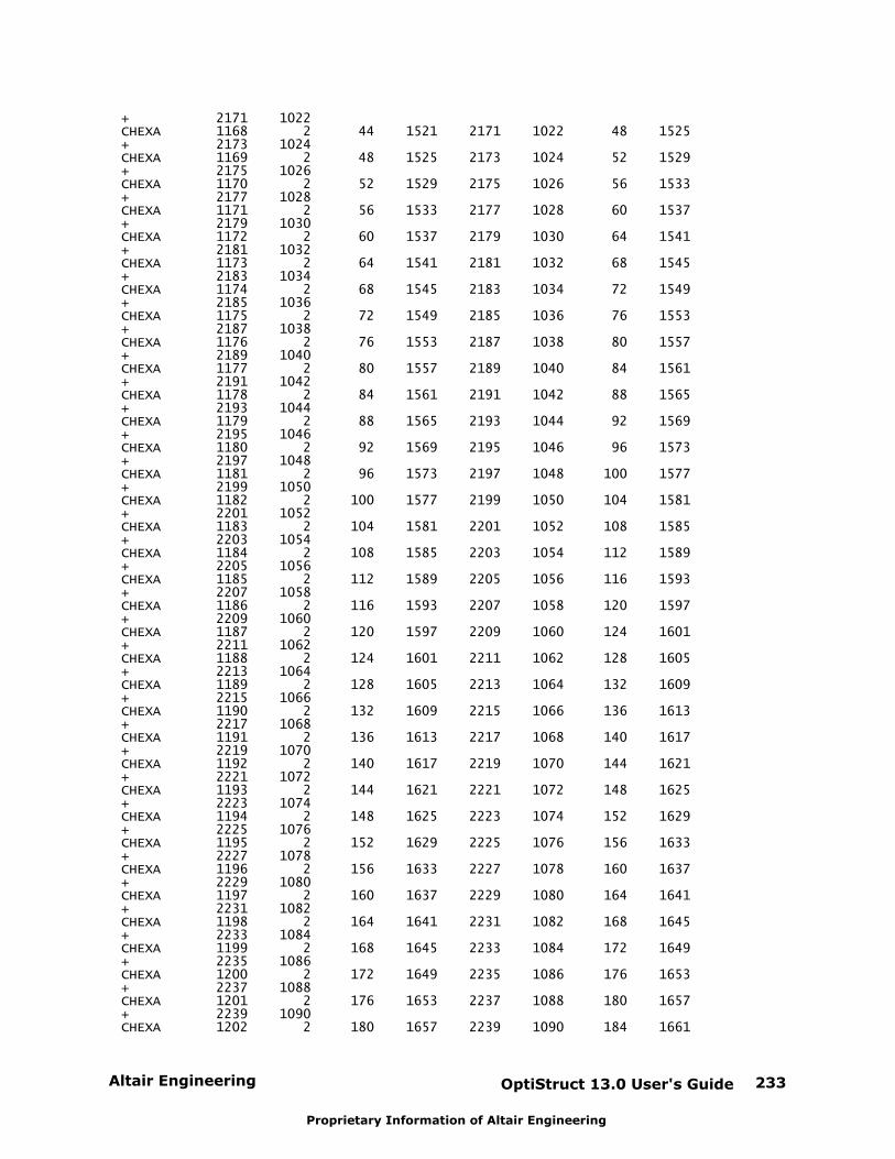
Altair Engineering OptiStruct 13.0 User's Guide 233
Proprietary Information of Altair Engineering
+ 2171 1022CHEXA 1168 2 44 1521 2171 1022 48 1525+ 2173 1024CHEXA 1169 2 48 1525 2173 1024 52 1529+ 2175 1026CHEXA 1170 2 52 1529 2175 1026 56 1533+ 2177 1028CHEXA 1171 2 56 1533 2177 1028 60 1537+ 2179 1030CHEXA 1172 2 60 1537 2179 1030 64 1541+ 2181 1032CHEXA 1173 2 64 1541 2181 1032 68 1545+ 2183 1034CHEXA 1174 2 68 1545 2183 1034 72 1549+ 2185 1036CHEXA 1175 2 72 1549 2185 1036 76 1553+ 2187 1038CHEXA 1176 2 76 1553 2187 1038 80 1557+ 2189 1040CHEXA 1177 2 80 1557 2189 1040 84 1561+ 2191 1042CHEXA 1178 2 84 1561 2191 1042 88 1565+ 2193 1044CHEXA 1179 2 88 1565 2193 1044 92 1569+ 2195 1046CHEXA 1180 2 92 1569 2195 1046 96 1573+ 2197 1048CHEXA 1181 2 96 1573 2197 1048 100 1577+ 2199 1050CHEXA 1182 2 100 1577 2199 1050 104 1581+ 2201 1052CHEXA 1183 2 104 1581 2201 1052 108 1585+ 2203 1054CHEXA 1184 2 108 1585 2203 1054 112 1589+ 2205 1056CHEXA 1185 2 112 1589 2205 1056 116 1593+ 2207 1058CHEXA 1186 2 116 1593 2207 1058 120 1597+ 2209 1060CHEXA 1187 2 120 1597 2209 1060 124 1601+ 2211 1062CHEXA 1188 2 124 1601 2211 1062 128 1605+ 2213 1064CHEXA 1189 2 128 1605 2213 1064 132 1609+ 2215 1066CHEXA 1190 2 132 1609 2215 1066 136 1613+ 2217 1068CHEXA 1191 2 136 1613 2217 1068 140 1617+ 2219 1070CHEXA 1192 2 140 1617 2219 1070 144 1621+ 2221 1072CHEXA 1193 2 144 1621 2221 1072 148 1625+ 2223 1074CHEXA 1194 2 148 1625 2223 1074 152 1629+ 2225 1076CHEXA 1195 2 152 1629 2225 1076 156 1633+ 2227 1078CHEXA 1196 2 156 1633 2227 1078 160 1637+ 2229 1080CHEXA 1197 2 160 1637 2229 1080 164 1641+ 2231 1082CHEXA 1198 2 164 1641 2231 1082 168 1645+ 2233 1084CHEXA 1199 2 168 1645 2233 1084 172 1649+ 2235 1086CHEXA 1200 2 172 1649 2235 1086 176 1653+ 2237 1088CHEXA 1201 2 176 1653 2237 1088 180 1657+ 2239 1090CHEXA 1202 2 180 1657 2239 1090 184 1661
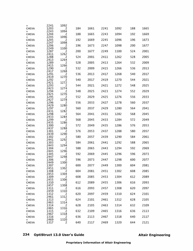
OptiStruct 13.0 User's Guide234 Altair Engineering
Proprietary Information of Altair Engineering
+ 2241 1092CHEXA 1203 2 184 1661 2241 1092 188 1665+ 2243 1094CHEXA 1204 2 188 1665 2243 1094 192 1669+ 2245 1096CHEXA 1205 2 192 1669 2245 1096 196 1673+ 2247 1098CHEXA 1206 2 196 1673 2247 1098 200 1677+ 2249 1100CHEXA 1287 2 200 1677 2249 1100 524 2001+ 2411 1262CHEXA 1288 2 524 2001 2411 1262 528 2005+ 2413 1264CHEXA 1289 2 528 2005 2413 1264 532 2009+ 2415 1266CHEXA 1290 2 532 2009 2415 1266 536 2013+ 2417 1268CHEXA 1291 2 536 2013 2417 1268 540 2017+ 2419 1270CHEXA 1292 2 540 2017 2419 1270 544 2021+ 2421 1272CHEXA 1293 2 544 2021 2421 1272 548 2025+ 2423 1274CHEXA 1294 2 548 2025 2423 1274 552 2029+ 2425 1276CHEXA 1295 2 552 2029 2425 1276 556 2033+ 2427 1278CHEXA 1296 2 556 2033 2427 1278 560 2037+ 2429 1280CHEXA 1297 2 560 2037 2429 1280 564 2041+ 2431 1282CHEXA 1298 2 564 2041 2431 1282 568 2045+ 2433 1284CHEXA 1299 2 568 2045 2433 1284 572 2049+ 2435 1286CHEXA 1300 2 572 2049 2435 1286 576 2053+ 2437 1288CHEXA 1301 2 576 2053 2437 1288 580 2057+ 2439 1290CHEXA 1302 2 580 2057 2439 1290 584 2061+ 2441 1292CHEXA 1303 2 584 2061 2441 1292 588 2065+ 2443 1294CHEXA 1304 2 588 2065 2443 1294 592 2069+ 2445 1296CHEXA 1305 2 592 2069 2445 1296 596 2073+ 2447 1298CHEXA 1306 2 596 2073 2447 1298 600 2077+ 2449 1300CHEXA 1307 2 600 2077 2449 1300 604 2081+ 2451 1302CHEXA 1308 2 604 2081 2451 1302 608 2085+ 2453 1304CHEXA 1309 2 608 2085 2453 1304 612 2089+ 2455 1306CHEXA 1310 2 612 2089 2455 1306 616 2093+ 2457 1308CHEXA 1311 2 616 2093 2457 1308 620 2097+ 2459 1310CHEXA 1312 2 620 2097 2459 1310 624 2101+ 2461 1312CHEXA 1313 2 624 2101 2461 1312 628 2105+ 2463 1314CHEXA 1314 2 628 2105 2463 1314 632 2109+ 2465 1316CHEXA 1315 2 632 2109 2465 1316 636 2113+ 2467 1318CHEXA 1316 2 636 2113 2467 1318 640 2117+ 2469 1320CHEXA 1317 2 640 2117 2469 1320 644 2121
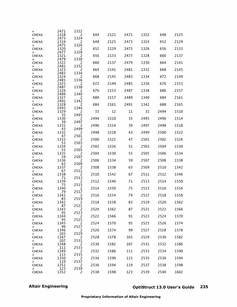
Altair Engineering OptiStruct 13.0 User's Guide 235
Proprietary Information of Altair Engineering
+ 2471 1322CHEXA 1318 2 644 2121 2471 1322 648 2125+ 2473 1324CHEXA 1319 2 648 2125 2473 1324 652 2129+ 2475 1326CHEXA 1320 2 652 2129 2475 1326 656 2133+ 2477 1328CHEXA 1321 2 656 2133 2477 1328 660 2137+ 2479 1330CHEXA 1322 2 660 2137 2479 1330 664 2141+ 2481 1332CHEXA 1323 2 664 2141 2481 1332 668 2145+ 2483 1334CHEXA 1324 2 668 2145 2483 1334 672 2149+ 2485 1336CHEXA 1325 2 672 2149 2485 1336 676 2153+ 2487 1338CHEXA 1326 2 676 2153 2487 1338 680 2157+ 2489 1340CHEXA 1327 2 680 2157 2489 1340 684 2161+ 2491 1342CHEXA 1328 2 684 2161 2491 1342 688 2165+ 2493 1344CHEXA 1329 2 33 12 11 31 2494 1510+ 35 2495CHEXA 1330 2 2494 1510 35 2495 2496 1514+ 39 2497CHEXA 1331 2 2496 1514 39 2497 2498 1518+ 43 2499CHEXA 1332 2 2498 1518 43 2499 2500 1522+ 47 2501CHEXA 1333 2 2500 1522 47 2501 2502 1526+ 51 2503CHEXA 1334 2 2502 1526 51 2503 2504 1530+ 55 2505CHEXA 1335 2 2504 1530 55 2505 2506 1534+ 59 2507CHEXA 1336 2 2506 1534 59 2507 2508 1538+ 63 2509CHEXA 1337 2 2508 1538 63 2509 2510 1542+ 67 2511CHEXA 1338 2 2510 1542 67 2511 2512 1546+ 71 2513CHEXA 1339 2 2512 1546 71 2513 2514 1550+ 75 2515CHEXA 1340 2 2514 1550 75 2515 2516 1554+ 79 2517CHEXA 1341 2 2516 1554 79 2517 2518 1558+ 83 2519CHEXA 1342 2 2518 1558 83 2519 2520 1562+ 87 2521CHEXA 1343 2 2520 1562 87 2521 2522 1566+ 91 2523CHEXA 1344 2 2522 1566 91 2523 2524 1570+ 95 2525CHEXA 1345 2 2524 1570 95 2525 2526 1574+ 99 2527CHEXA 1346 2 2526 1574 99 2527 2528 1578+ 103 2529CHEXA 1347 2 2528 1578 103 2529 2530 1582+ 107 2531CHEXA 1348 2 2530 1582 107 2531 2532 1586+ 111 2533CHEXA 1349 2 2532 1586 111 2533 2534 1590+ 115 2535CHEXA 1350 2 2534 1590 115 2535 2536 1594+ 119 2537CHEXA 1351 2 2536 1594 119 2537 2538 1598+ 123 2539CHEXA 1352 2 2538 1598 123 2539 2540 1602
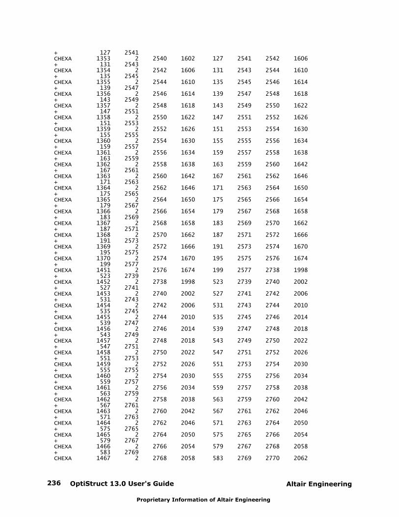
OptiStruct 13.0 User's Guide236 Altair Engineering
Proprietary Information of Altair Engineering
+ 127 2541CHEXA 1353 2 2540 1602 127 2541 2542 1606+ 131 2543CHEXA 1354 2 2542 1606 131 2543 2544 1610+ 135 2545CHEXA 1355 2 2544 1610 135 2545 2546 1614+ 139 2547CHEXA 1356 2 2546 1614 139 2547 2548 1618+ 143 2549CHEXA 1357 2 2548 1618 143 2549 2550 1622+ 147 2551CHEXA 1358 2 2550 1622 147 2551 2552 1626+ 151 2553CHEXA 1359 2 2552 1626 151 2553 2554 1630+ 155 2555CHEXA 1360 2 2554 1630 155 2555 2556 1634+ 159 2557CHEXA 1361 2 2556 1634 159 2557 2558 1638+ 163 2559CHEXA 1362 2 2558 1638 163 2559 2560 1642+ 167 2561CHEXA 1363 2 2560 1642 167 2561 2562 1646+ 171 2563CHEXA 1364 2 2562 1646 171 2563 2564 1650+ 175 2565CHEXA 1365 2 2564 1650 175 2565 2566 1654+ 179 2567CHEXA 1366 2 2566 1654 179 2567 2568 1658+ 183 2569CHEXA 1367 2 2568 1658 183 2569 2570 1662+ 187 2571CHEXA 1368 2 2570 1662 187 2571 2572 1666+ 191 2573CHEXA 1369 2 2572 1666 191 2573 2574 1670+ 195 2575CHEXA 1370 2 2574 1670 195 2575 2576 1674+ 199 2577CHEXA 1451 2 2576 1674 199 2577 2738 1998+ 523 2739CHEXA 1452 2 2738 1998 523 2739 2740 2002+ 527 2741CHEXA 1453 2 2740 2002 527 2741 2742 2006+ 531 2743CHEXA 1454 2 2742 2006 531 2743 2744 2010+ 535 2745CHEXA 1455 2 2744 2010 535 2745 2746 2014+ 539 2747CHEXA 1456 2 2746 2014 539 2747 2748 2018+ 543 2749CHEXA 1457 2 2748 2018 543 2749 2750 2022+ 547 2751CHEXA 1458 2 2750 2022 547 2751 2752 2026+ 551 2753CHEXA 1459 2 2752 2026 551 2753 2754 2030+ 555 2755CHEXA 1460 2 2754 2030 555 2755 2756 2034+ 559 2757CHEXA 1461 2 2756 2034 559 2757 2758 2038+ 563 2759CHEXA 1462 2 2758 2038 563 2759 2760 2042+ 567 2761CHEXA 1463 2 2760 2042 567 2761 2762 2046+ 571 2763CHEXA 1464 2 2762 2046 571 2763 2764 2050+ 575 2765CHEXA 1465 2 2764 2050 575 2765 2766 2054+ 579 2767CHEXA 1466 2 2766 2054 579 2767 2768 2058+ 583 2769CHEXA 1467 2 2768 2058 583 2769 2770 2062
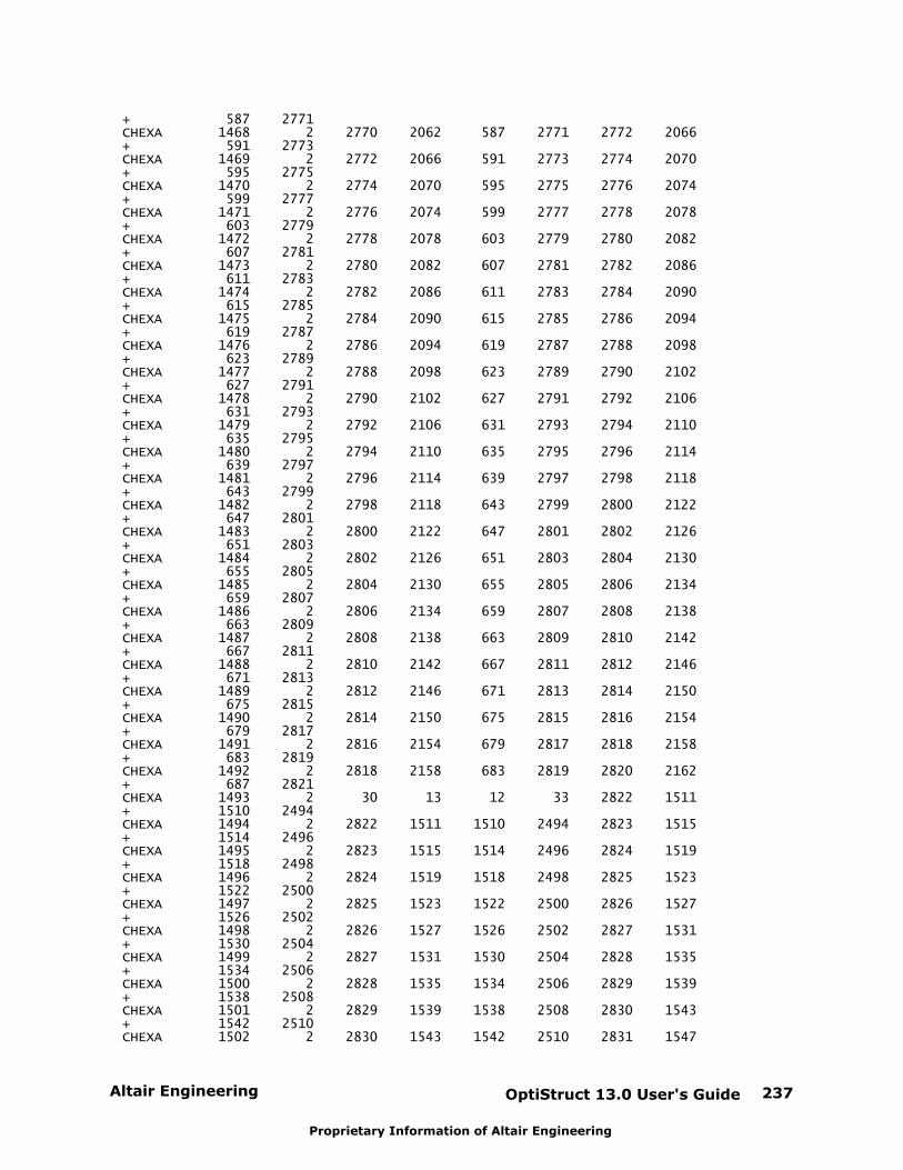
Altair Engineering OptiStruct 13.0 User's Guide 237
Proprietary Information of Altair Engineering
+ 587 2771CHEXA 1468 2 2770 2062 587 2771 2772 2066+ 591 2773CHEXA 1469 2 2772 2066 591 2773 2774 2070+ 595 2775CHEXA 1470 2 2774 2070 595 2775 2776 2074+ 599 2777CHEXA 1471 2 2776 2074 599 2777 2778 2078+ 603 2779CHEXA 1472 2 2778 2078 603 2779 2780 2082+ 607 2781CHEXA 1473 2 2780 2082 607 2781 2782 2086+ 611 2783CHEXA 1474 2 2782 2086 611 2783 2784 2090+ 615 2785CHEXA 1475 2 2784 2090 615 2785 2786 2094+ 619 2787CHEXA 1476 2 2786 2094 619 2787 2788 2098+ 623 2789CHEXA 1477 2 2788 2098 623 2789 2790 2102+ 627 2791CHEXA 1478 2 2790 2102 627 2791 2792 2106+ 631 2793CHEXA 1479 2 2792 2106 631 2793 2794 2110+ 635 2795CHEXA 1480 2 2794 2110 635 2795 2796 2114+ 639 2797CHEXA 1481 2 2796 2114 639 2797 2798 2118+ 643 2799CHEXA 1482 2 2798 2118 643 2799 2800 2122+ 647 2801CHEXA 1483 2 2800 2122 647 2801 2802 2126+ 651 2803CHEXA 1484 2 2802 2126 651 2803 2804 2130+ 655 2805CHEXA 1485 2 2804 2130 655 2805 2806 2134+ 659 2807CHEXA 1486 2 2806 2134 659 2807 2808 2138+ 663 2809CHEXA 1487 2 2808 2138 663 2809 2810 2142+ 667 2811CHEXA 1488 2 2810 2142 667 2811 2812 2146+ 671 2813CHEXA 1489 2 2812 2146 671 2813 2814 2150+ 675 2815CHEXA 1490 2 2814 2150 675 2815 2816 2154+ 679 2817CHEXA 1491 2 2816 2154 679 2817 2818 2158+ 683 2819CHEXA 1492 2 2818 2158 683 2819 2820 2162+ 687 2821CHEXA 1493 2 30 13 12 33 2822 1511+ 1510 2494CHEXA 1494 2 2822 1511 1510 2494 2823 1515+ 1514 2496CHEXA 1495 2 2823 1515 1514 2496 2824 1519+ 1518 2498CHEXA 1496 2 2824 1519 1518 2498 2825 1523+ 1522 2500CHEXA 1497 2 2825 1523 1522 2500 2826 1527+ 1526 2502CHEXA 1498 2 2826 1527 1526 2502 2827 1531+ 1530 2504CHEXA 1499 2 2827 1531 1530 2504 2828 1535+ 1534 2506CHEXA 1500 2 2828 1535 1534 2506 2829 1539+ 1538 2508CHEXA 1501 2 2829 1539 1538 2508 2830 1543+ 1542 2510CHEXA 1502 2 2830 1543 1542 2510 2831 1547
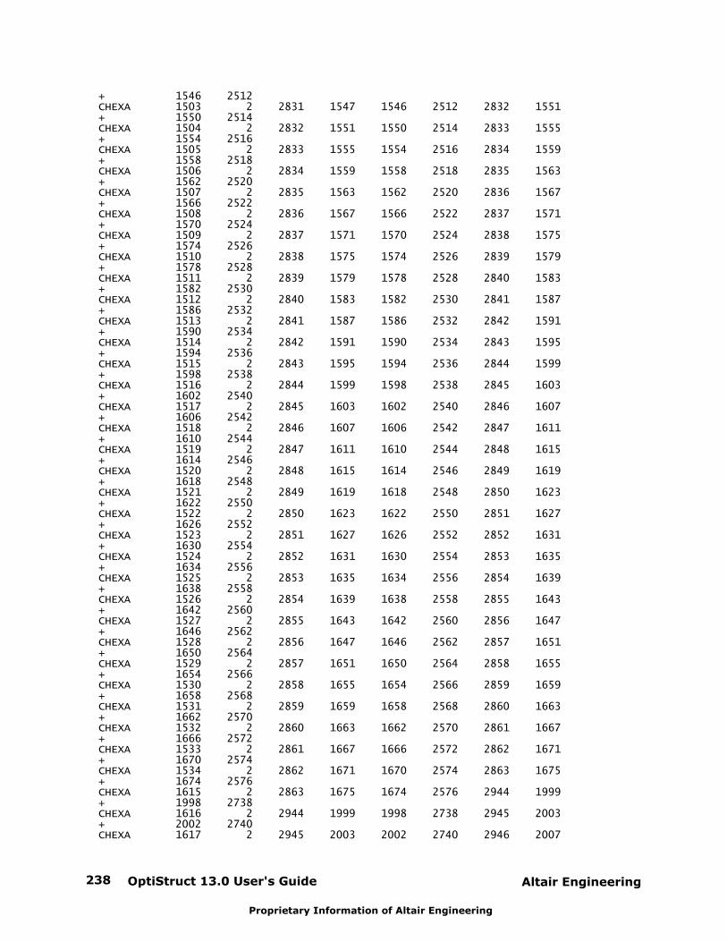
OptiStruct 13.0 User's Guide238 Altair Engineering
Proprietary Information of Altair Engineering
+ 1546 2512CHEXA 1503 2 2831 1547 1546 2512 2832 1551+ 1550 2514CHEXA 1504 2 2832 1551 1550 2514 2833 1555+ 1554 2516CHEXA 1505 2 2833 1555 1554 2516 2834 1559+ 1558 2518CHEXA 1506 2 2834 1559 1558 2518 2835 1563+ 1562 2520CHEXA 1507 2 2835 1563 1562 2520 2836 1567+ 1566 2522CHEXA 1508 2 2836 1567 1566 2522 2837 1571+ 1570 2524CHEXA 1509 2 2837 1571 1570 2524 2838 1575+ 1574 2526CHEXA 1510 2 2838 1575 1574 2526 2839 1579+ 1578 2528CHEXA 1511 2 2839 1579 1578 2528 2840 1583+ 1582 2530CHEXA 1512 2 2840 1583 1582 2530 2841 1587+ 1586 2532CHEXA 1513 2 2841 1587 1586 2532 2842 1591+ 1590 2534CHEXA 1514 2 2842 1591 1590 2534 2843 1595+ 1594 2536CHEXA 1515 2 2843 1595 1594 2536 2844 1599+ 1598 2538CHEXA 1516 2 2844 1599 1598 2538 2845 1603+ 1602 2540CHEXA 1517 2 2845 1603 1602 2540 2846 1607+ 1606 2542CHEXA 1518 2 2846 1607 1606 2542 2847 1611+ 1610 2544CHEXA 1519 2 2847 1611 1610 2544 2848 1615+ 1614 2546CHEXA 1520 2 2848 1615 1614 2546 2849 1619+ 1618 2548CHEXA 1521 2 2849 1619 1618 2548 2850 1623+ 1622 2550CHEXA 1522 2 2850 1623 1622 2550 2851 1627+ 1626 2552CHEXA 1523 2 2851 1627 1626 2552 2852 1631+ 1630 2554CHEXA 1524 2 2852 1631 1630 2554 2853 1635+ 1634 2556CHEXA 1525 2 2853 1635 1634 2556 2854 1639+ 1638 2558CHEXA 1526 2 2854 1639 1638 2558 2855 1643+ 1642 2560CHEXA 1527 2 2855 1643 1642 2560 2856 1647+ 1646 2562CHEXA 1528 2 2856 1647 1646 2562 2857 1651+ 1650 2564CHEXA 1529 2 2857 1651 1650 2564 2858 1655+ 1654 2566CHEXA 1530 2 2858 1655 1654 2566 2859 1659+ 1658 2568CHEXA 1531 2 2859 1659 1658 2568 2860 1663+ 1662 2570CHEXA 1532 2 2860 1663 1662 2570 2861 1667+ 1666 2572CHEXA 1533 2 2861 1667 1666 2572 2862 1671+ 1670 2574CHEXA 1534 2 2862 1671 1670 2574 2863 1675+ 1674 2576CHEXA 1615 2 2863 1675 1674 2576 2944 1999+ 1998 2738CHEXA 1616 2 2944 1999 1998 2738 2945 2003+ 2002 2740CHEXA 1617 2 2945 2003 2002 2740 2946 2007
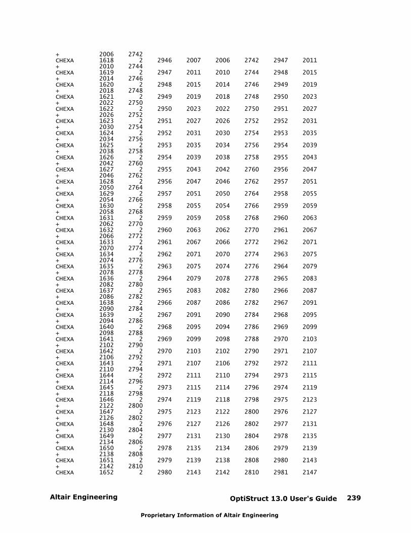
Altair Engineering OptiStruct 13.0 User's Guide 239
Proprietary Information of Altair Engineering
+ 2006 2742CHEXA 1618 2 2946 2007 2006 2742 2947 2011+ 2010 2744CHEXA 1619 2 2947 2011 2010 2744 2948 2015+ 2014 2746CHEXA 1620 2 2948 2015 2014 2746 2949 2019+ 2018 2748CHEXA 1621 2 2949 2019 2018 2748 2950 2023+ 2022 2750CHEXA 1622 2 2950 2023 2022 2750 2951 2027+ 2026 2752CHEXA 1623 2 2951 2027 2026 2752 2952 2031+ 2030 2754CHEXA 1624 2 2952 2031 2030 2754 2953 2035+ 2034 2756CHEXA 1625 2 2953 2035 2034 2756 2954 2039+ 2038 2758CHEXA 1626 2 2954 2039 2038 2758 2955 2043+ 2042 2760CHEXA 1627 2 2955 2043 2042 2760 2956 2047+ 2046 2762CHEXA 1628 2 2956 2047 2046 2762 2957 2051+ 2050 2764CHEXA 1629 2 2957 2051 2050 2764 2958 2055+ 2054 2766CHEXA 1630 2 2958 2055 2054 2766 2959 2059+ 2058 2768CHEXA 1631 2 2959 2059 2058 2768 2960 2063+ 2062 2770CHEXA 1632 2 2960 2063 2062 2770 2961 2067+ 2066 2772CHEXA 1633 2 2961 2067 2066 2772 2962 2071+ 2070 2774CHEXA 1634 2 2962 2071 2070 2774 2963 2075+ 2074 2776CHEXA 1635 2 2963 2075 2074 2776 2964 2079+ 2078 2778CHEXA 1636 2 2964 2079 2078 2778 2965 2083+ 2082 2780CHEXA 1637 2 2965 2083 2082 2780 2966 2087+ 2086 2782CHEXA 1638 2 2966 2087 2086 2782 2967 2091+ 2090 2784CHEXA 1639 2 2967 2091 2090 2784 2968 2095+ 2094 2786CHEXA 1640 2 2968 2095 2094 2786 2969 2099+ 2098 2788CHEXA 1641 2 2969 2099 2098 2788 2970 2103+ 2102 2790CHEXA 1642 2 2970 2103 2102 2790 2971 2107+ 2106 2792CHEXA 1643 2 2971 2107 2106 2792 2972 2111+ 2110 2794CHEXA 1644 2 2972 2111 2110 2794 2973 2115+ 2114 2796CHEXA 1645 2 2973 2115 2114 2796 2974 2119+ 2118 2798CHEXA 1646 2 2974 2119 2118 2798 2975 2123+ 2122 2800CHEXA 1647 2 2975 2123 2122 2800 2976 2127+ 2126 2802CHEXA 1648 2 2976 2127 2126 2802 2977 2131+ 2130 2804CHEXA 1649 2 2977 2131 2130 2804 2978 2135+ 2134 2806CHEXA 1650 2 2978 2135 2134 2806 2979 2139+ 2138 2808CHEXA 1651 2 2979 2139 2138 2808 2980 2143+ 2142 2810CHEXA 1652 2 2980 2143 2142 2810 2981 2147

OptiStruct 13.0 User's Guide240 Altair Engineering
Proprietary Information of Altair Engineering
+ 2146 2812CHEXA 1653 2 2981 2147 2146 2812 2982 2151+ 2150 2814CHEXA 1654 2 2982 2151 2150 2814 2983 2155+ 2154 2816CHEXA 1655 2 2983 2155 2154 2816 2984 2159+ 2158 2818CHEXA 1656 2 2984 2159 2158 2818 2985 2163+ 2162 2820CHEXA 1657 2 28 33 31 27 2986 2494+ 2495 2987CHEXA 1658 2 2986 2494 2495 2987 2988 2496+ 2497 2989CHEXA 1659 2 2988 2496 2497 2989 2990 2498+ 2499 2991CHEXA 1660 2 2990 2498 2499 2991 2992 2500+ 2501 2993CHEXA 1661 2 2992 2500 2501 2993 2994 2502+ 2503 2995CHEXA 1662 2 2994 2502 2503 2995 2996 2504+ 2505 2997CHEXA 1663 2 2996 2504 2505 2997 2998 2506+ 2507 2999CHEXA 1664 2 2998 2506 2507 2999 3000 2508+ 2509 3001CHEXA 1665 2 3000 2508 2509 3001 3002 2510+ 2511 3003CHEXA 1666 2 3002 2510 2511 3003 3004 2512+ 2513 3005CHEXA 1667 2 3004 2512 2513 3005 3006 2514+ 2515 3007CHEXA 1668 2 3006 2514 2515 3007 3008 2516+ 2517 3009CHEXA 1669 2 3008 2516 2517 3009 3010 2518+ 2519 3011CHEXA 1670 2 3010 2518 2519 3011 3012 2520+ 2521 3013CHEXA 1671 2 3012 2520 2521 3013 3014 2522+ 2523 3015CHEXA 1672 2 3014 2522 2523 3015 3016 2524+ 2525 3017CHEXA 1673 2 3016 2524 2525 3017 3018 2526+ 2527 3019CHEXA 1674 2 3018 2526 2527 3019 3020 2528+ 2529 3021CHEXA 1675 2 3020 2528 2529 3021 3022 2530+ 2531 3023CHEXA 1676 2 3022 2530 2531 3023 3024 2532+ 2533 3025CHEXA 1677 2 3024 2532 2533 3025 3026 2534+ 2535 3027CHEXA 1678 2 3026 2534 2535 3027 3028 2536+ 2537 3029CHEXA 1679 2 3028 2536 2537 3029 3030 2538+ 2539 3031CHEXA 1680 2 3030 2538 2539 3031 3032 2540+ 2541 3033CHEXA 1681 2 3032 2540 2541 3033 3034 2542+ 2543 3035CHEXA 1682 2 3034 2542 2543 3035 3036 2544+ 2545 3037CHEXA 1683 2 3036 2544 2545 3037 3038 2546+ 2547 3039CHEXA 1684 2 3038 2546 2547 3039 3040 2548+ 2549 3041CHEXA 1685 2 3040 2548 2549 3041 3042 2550+ 2551 3043CHEXA 1686 2 3042 2550 2551 3043 3044 2552+ 2553 3045CHEXA 1687 2 3044 2552 2553 3045 3046 2554
Altair Engineering OptiStruct 13.0 User's Guide 241
Proprietary Information of Altair Engineering
+ 2555 3047CHEXA 1688 2 3046 2554 2555 3047 3048 2556+ 2557 3049CHEXA 1689 2 3048 2556 2557 3049 3050 2558+ 2559 3051CHEXA 1690 2 3050 2558 2559 3051 3052 2560+ 2561 3053CHEXA 1691 2 3052 2560 2561 3053 3054 2562+ 2563 3055CHEXA 1692 2 3054 2562 2563 3055 3056 2564+ 2565 3057CHEXA 1693 2 3056 2564 2565 3057 3058 2566+ 2567 3059CHEXA 1694 2 3058 2566 2567 3059 3060 2568+ 2569 3061CHEXA 1695 2 3060 2568 2569 3061 3062 2570+ 2571 3063CHEXA 1696 2 3062 2570 2571 3063 3064 2572+ 2573 3065CHEXA 1697 2 3064 2572 2573 3065 3066 2574+ 2575 3067CHEXA 1698 2 3066 2574 2575 3067 3068 2576+ 2577 3069CHEXA 1779 2 3068 2576 2577 3069 3230 2738+ 2739 3231CHEXA 1780 2 3230 2738 2739 3231 3232 2740+ 2741 3233CHEXA 1781 2 3232 2740 2741 3233 3234 2742+ 2743 3235CHEXA 1782 2 3234 2742 2743 3235 3236 2744+ 2745 3237CHEXA 1783 2 3236 2744 2745 3237 3238 2746+ 2747 3239CHEXA 1784 2 3238 2746 2747 3239 3240 2748+ 2749 3241CHEXA 1785 2 3240 2748 2749 3241 3242 2750+ 2751 3243CHEXA 1786 2 3242 2750 2751 3243 3244 2752+ 2753 3245CHEXA 1787 2 3244 2752 2753 3245 3246 2754+ 2755 3247CHEXA 1788 2 3246 2754 2755 3247 3248 2756+ 2757 3249CHEXA 1789 2 3248 2756 2757 3249 3250 2758+ 2759 3251CHEXA 1790 2 3250 2758 2759 3251 3252 2760+ 2761 3253CHEXA 1791 2 3252 2760 2761 3253 3254 2762+ 2763 3255CHEXA 1792 2 3254 2762 2763 3255 3256 2764+ 2765 3257CHEXA 1793 2 3256 2764 2765 3257 3258 2766+ 2767 3259CHEXA 1794 2 3258 2766 2767 3259 3260 2768+ 2769 3261CHEXA 1795 2 3260 2768 2769 3261 3262 2770+ 2771 3263CHEXA 1796 2 3262 2770 2771 3263 3264 2772+ 2773 3265CHEXA 1797 2 3264 2772 2773 3265 3266 2774+ 2775 3267CHEXA 1798 2 3266 2774 2775 3267 3268 2776+ 2777 3269CHEXA 1799 2 3268 2776 2777 3269 3270 2778+ 2779 3271CHEXA 1800 2 3270 2778 2779 3271 3272 2780+ 2781 3273CHEXA 1801 2 3272 2780 2781 3273 3274 2782+ 2783 3275CHEXA 1802 2 3274 2782 2783 3275 3276 2784
OptiStruct 13.0 User's Guide242 Altair Engineering
Proprietary Information of Altair Engineering
+ 2785 3277CHEXA 1803 2 3276 2784 2785 3277 3278 2786+ 2787 3279CHEXA 1804 2 3278 2786 2787 3279 3280 2788+ 2789 3281CHEXA 1805 2 3280 2788 2789 3281 3282 2790+ 2791 3283CHEXA 1806 2 3282 2790 2791 3283 3284 2792+ 2793 3285CHEXA 1807 2 3284 2792 2793 3285 3286 2794+ 2795 3287CHEXA 1808 2 3286 2794 2795 3287 3288 2796+ 2797 3289CHEXA 1809 2 3288 2796 2797 3289 3290 2798+ 2799 3291CHEXA 1810 2 3290 2798 2799 3291 3292 2800+ 2801 3293CHEXA 1811 2 3292 2800 2801 3293 3294 2802+ 2803 3295CHEXA 1812 2 3294 2802 2803 3295 3296 2804+ 2805 3297CHEXA 1813 2 3296 2804 2805 3297 3298 2806+ 2807 3299CHEXA 1814 2 3298 2806 2807 3299 3300 2808+ 2809 3301CHEXA 1815 2 3300 2808 2809 3301 3302 2810+ 2811 3303CHEXA 1816 2 3302 2810 2811 3303 3304 2812+ 2813 3305CHEXA 1817 2 3304 2812 2813 3305 3306 2814+ 2815 3307CHEXA 1818 2 3306 2814 2815 3307 3308 2816+ 2817 3309CHEXA 1819 2 3308 2816 2817 3309 3310 2818+ 2819 3311CHEXA 1820 2 3310 2818 2819 3311 3312 2820+ 2821 3313CHEXA 1821 2 29 30 33 28 3314 2822+ 2494 2986CHEXA 1822 2 3314 2822 2494 2986 3315 2823+ 2496 2988CHEXA 1823 2 3315 2823 2496 2988 3316 2824+ 2498 2990CHEXA 1824 2 3316 2824 2498 2990 3317 2825+ 2500 2992CHEXA 1825 2 3317 2825 2500 2992 3318 2826+ 2502 2994CHEXA 1826 2 3318 2826 2502 2994 3319 2827+ 2504 2996CHEXA 1827 2 3319 2827 2504 2996 3320 2828+ 2506 2998CHEXA 1828 2 3320 2828 2506 2998 3321 2829+ 2508 3000CHEXA 1829 2 3321 2829 2508 3000 3322 2830+ 2510 3002CHEXA 1830 2 3322 2830 2510 3002 3323 2831+ 2512 3004CHEXA 1831 2 3323 2831 2512 3004 3324 2832+ 2514 3006CHEXA 1832 2 3324 2832 2514 3006 3325 2833+ 2516 3008CHEXA 1833 2 3325 2833 2516 3008 3326 2834+ 2518 3010CHEXA 1834 2 3326 2834 2518 3010 3327 2835+ 2520 3012CHEXA 1835 2 3327 2835 2520 3012 3328 2836+ 2522 3014CHEXA 1836 2 3328 2836 2522 3014 3329 2837+ 2524 3016CHEXA 1837 2 3329 2837 2524 3016 3330 2838

Altair Engineering OptiStruct 13.0 User's Guide 243
Proprietary Information of Altair Engineering
+ 2526 3018CHEXA 1838 2 3330 2838 2526 3018 3331 2839+ 2528 3020CHEXA 1839 2 3331 2839 2528 3020 3332 2840+ 2530 3022CHEXA 1840 2 3332 2840 2530 3022 3333 2841+ 2532 3024CHEXA 1841 2 3333 2841 2532 3024 3334 2842+ 2534 3026CHEXA 1842 2 3334 2842 2534 3026 3335 2843+ 2536 3028CHEXA 1843 2 3335 2843 2536 3028 3336 2844+ 2538 3030CHEXA 1844 2 3336 2844 2538 3030 3337 2845+ 2540 3032CHEXA 1845 2 3337 2845 2540 3032 3338 2846+ 2542 3034CHEXA 1846 2 3338 2846 2542 3034 3339 2847+ 2544 3036CHEXA 1847 2 3339 2847 2544 3036 3340 2848+ 2546 3038CHEXA 1848 2 3340 2848 2546 3038 3341 2849+ 2548 3040CHEXA 1849 2 3341 2849 2548 3040 3342 2850+ 2550 3042CHEXA 1850 2 3342 2850 2550 3042 3343 2851+ 2552 3044CHEXA 1851 2 3343 2851 2552 3044 3344 2852+ 2554 3046CHEXA 1852 2 3344 2852 2554 3046 3345 2853+ 2556 3048CHEXA 1853 2 3345 2853 2556 3048 3346 2854+ 2558 3050CHEXA 1854 2 3346 2854 2558 3050 3347 2855+ 2560 3052CHEXA 1855 2 3347 2855 2560 3052 3348 2856+ 2562 3054CHEXA 1856 2 3348 2856 2562 3054 3349 2857+ 2564 3056CHEXA 1857 2 3349 2857 2564 3056 3350 2858+ 2566 3058CHEXA 1858 2 3350 2858 2566 3058 3351 2859+ 2568 3060CHEXA 1859 2 3351 2859 2568 3060 3352 2860+ 2570 3062CHEXA 1860 2 3352 2860 2570 3062 3353 2861+ 2572 3064CHEXA 1861 2 3353 2861 2572 3064 3354 2862+ 2574 3066CHEXA 1862 2 3354 2862 2574 3066 3355 2863+ 2576 3068CHEXA 1943 2 3355 2863 2576 3068 3436 2944+ 2738 3230CHEXA 1944 2 3436 2944 2738 3230 3437 2945+ 2740 3232CHEXA 1945 2 3437 2945 2740 3232 3438 2946+ 2742 3234CHEXA 1946 2 3438 2946 2742 3234 3439 2947+ 2744 3236CHEXA 1947 2 3439 2947 2744 3236 3440 2948+ 2746 3238CHEXA 1948 2 3440 2948 2746 3238 3441 2949+ 2748 3240CHEXA 1949 2 3441 2949 2748 3240 3442 2950+ 2750 3242CHEXA 1950 2 3442 2950 2750 3242 3443 2951+ 2752 3244CHEXA 1951 2 3443 2951 2752 3244 3444 2952+ 2754 3246CHEXA 1952 2 3444 2952 2754 3246 3445 2953
OptiStruct 13.0 User's Guide244 Altair Engineering
Proprietary Information of Altair Engineering
+ 2756 3248CHEXA 1953 2 3445 2953 2756 3248 3446 2954+ 2758 3250CHEXA 1954 2 3446 2954 2758 3250 3447 2955+ 2760 3252CHEXA 1955 2 3447 2955 2760 3252 3448 2956+ 2762 3254CHEXA 1956 2 3448 2956 2762 3254 3449 2957+ 2764 3256CHEXA 1957 2 3449 2957 2764 3256 3450 2958+ 2766 3258CHEXA 1958 2 3450 2958 2766 3258 3451 2959+ 2768 3260CHEXA 1959 2 3451 2959 2768 3260 3452 2960+ 2770 3262CHEXA 1960 2 3452 2960 2770 3262 3453 2961+ 2772 3264CHEXA 1961 2 3453 2961 2772 3264 3454 2962+ 2774 3266CHEXA 1962 2 3454 2962 2774 3266 3455 2963+ 2776 3268CHEXA 1963 2 3455 2963 2776 3268 3456 2964+ 2778 3270CHEXA 1964 2 3456 2964 2778 3270 3457 2965+ 2780 3272CHEXA 1965 2 3457 2965 2780 3272 3458 2966+ 2782 3274CHEXA 1966 2 3458 2966 2782 3274 3459 2967+ 2784 3276CHEXA 1967 2 3459 2967 2784 3276 3460 2968+ 2786 3278CHEXA 1968 2 3460 2968 2786 3278 3461 2969+ 2788 3280CHEXA 1969 2 3461 2969 2788 3280 3462 2970+ 2790 3282CHEXA 1970 2 3462 2970 2790 3282 3463 2971+ 2792 3284CHEXA 1971 2 3463 2971 2792 3284 3464 2972+ 2794 3286CHEXA 1972 2 3464 2972 2794 3286 3465 2973+ 2796 3288CHEXA 1973 2 3465 2973 2796 3288 3466 2974+ 2798 3290CHEXA 1974 2 3466 2974 2798 3290 3467 2975+ 2800 3292CHEXA 1975 2 3467 2975 2800 3292 3468 2976+ 2802 3294CHEXA 1976 2 3468 2976 2802 3294 3469 2977+ 2804 3296CHEXA 1977 2 3469 2977 2804 3296 3470 2978+ 2806 3298CHEXA 1978 2 3470 2978 2806 3298 3471 2979+ 2808 3300CHEXA 1979 2 3471 2979 2808 3300 3472 2980+ 2810 3302CHEXA 1980 2 3472 2980 2810 3302 3473 2981+ 2812 3304CHEXA 1981 2 3473 2981 2812 3304 3474 2982+ 2814 3306CHEXA 1982 2 3474 2982 2814 3306 3475 2983+ 2816 3308CHEXA 1983 2 3475 2983 2816 3308 3476 2984+ 2818 3310CHEXA 1984 2 3476 2984 2818 3310 3477 2985+ 2820 3312CHEXA 1985 2 32 10 9 24 3478 34+ 690 3479CHEXA 1986 2 3478 34 690 3479 3480 38+ 692 3481CHEXA 1987 2 3480 38 692 3481 3482 42

Altair Engineering OptiStruct 13.0 User's Guide 245
Proprietary Information of Altair Engineering
+ 694 3483CHEXA 1988 2 3482 42 694 3483 3484 46+ 696 3485CHEXA 1989 2 3484 46 696 3485 3486 50+ 698 3487CHEXA 1990 2 3486 50 698 3487 3488 54+ 700 3489CHEXA 1991 2 3488 54 700 3489 3490 58+ 702 3491CHEXA 1992 2 3490 58 702 3491 3492 62+ 704 3493CHEXA 1993 2 3492 62 704 3493 3494 66+ 706 3495CHEXA 1994 2 3494 66 706 3495 3496 70+ 708 3497CHEXA 1995 2 3496 70 708 3497 3498 74+ 710 3499CHEXA 1996 2 3498 74 710 3499 3500 78+ 712 3501CHEXA 1997 2 3500 78 712 3501 3502 82+ 714 3503CHEXA 1998 2 3502 82 714 3503 3504 86+ 716 3505CHEXA 1999 2 3504 86 716 3505 3506 90+ 718 3507CHEXA 2000 2 3506 90 718 3507 3508 94+ 720 3509CHEXA 2001 2 3508 94 720 3509 3510 98+ 722 3511CHEXA 2002 2 3510 98 722 3511 3512 102+ 724 3513CHEXA 2003 2 3512 102 724 3513 3514 106+ 726 3515CHEXA 2004 2 3514 106 726 3515 3516 110+ 728 3517CHEXA 2005 2 3516 110 728 3517 3518 114+ 730 3519CHEXA 2006 2 3518 114 730 3519 3520 118+ 732 3521CHEXA 2007 2 3520 118 732 3521 3522 122+ 734 3523CHEXA 2008 2 3522 122 734 3523 3524 126+ 736 3525CHEXA 2009 2 3524 126 736 3525 3526 130+ 738 3527CHEXA 2010 2 3526 130 738 3527 3528 134+ 740 3529CHEXA 2011 2 3528 134 740 3529 3530 138+ 742 3531CHEXA 2012 2 3530 138 742 3531 3532 142+ 744 3533CHEXA 2013 2 3532 142 744 3533 3534 146+ 746 3535CHEXA 2014 2 3534 146 746 3535 3536 150+ 748 3537CHEXA 2015 2 3536 150 748 3537 3538 154+ 750 3539CHEXA 2016 2 3538 154 750 3539 3540 158+ 752 3541CHEXA 2017 2 3540 158 752 3541 3542 162+ 754 3543CHEXA 2018 2 3542 162 754 3543 3544 166+ 756 3545CHEXA 2019 2 3544 166 756 3545 3546 170+ 758 3547CHEXA 2020 2 3546 170 758 3547 3548 174+ 760 3549CHEXA 2021 2 3548 174 760 3549 3550 178+ 762 3551CHEXA 2022 2 3550 178 762 3551 3552 182

OptiStruct 13.0 User's Guide246 Altair Engineering
Proprietary Information of Altair Engineering
+ 764 3553CHEXA 2023 2 3552 182 764 3553 3554 186+ 766 3555CHEXA 2024 2 3554 186 766 3555 3556 190+ 768 3557CHEXA 2025 2 3556 190 768 3557 3558 194+ 770 3559CHEXA 2026 2 3558 194 770 3559 3560 198+ 772 3561CHEXA 2107 2 3560 198 772 3561 3722 522+ 934 3723CHEXA 2108 2 3722 522 934 3723 3724 526+ 936 3725CHEXA 2109 2 3724 526 936 3725 3726 530+ 938 3727CHEXA 2110 2 3726 530 938 3727 3728 534+ 940 3729CHEXA 2111 2 3728 534 940 3729 3730 538+ 942 3731CHEXA 2112 2 3730 538 942 3731 3732 542+ 944 3733CHEXA 2113 2 3732 542 944 3733 3734 546+ 946 3735CHEXA 2114 2 3734 546 946 3735 3736 550+ 948 3737CHEXA 2115 2 3736 550 948 3737 3738 554+ 950 3739CHEXA 2116 2 3738 554 950 3739 3740 558+ 952 3741CHEXA 2117 2 3740 558 952 3741 3742 562+ 954 3743CHEXA 2118 2 3742 562 954 3743 3744 566+ 956 3745CHEXA 2119 2 3744 566 956 3745 3746 570+ 958 3747CHEXA 2120 2 3746 570 958 3747 3748 574+ 960 3749CHEXA 2121 2 3748 574 960 3749 3750 578+ 962 3751CHEXA 2122 2 3750 578 962 3751 3752 582+ 964 3753CHEXA 2123 2 3752 582 964 3753 3754 586+ 966 3755CHEXA 2124 2 3754 586 966 3755 3756 590+ 968 3757CHEXA 2125 2 3756 590 968 3757 3758 594+ 970 3759CHEXA 2126 2 3758 594 970 3759 3760 598+ 972 3761CHEXA 2127 2 3760 598 972 3761 3762 602+ 974 3763CHEXA 2128 2 3762 602 974 3763 3764 606+ 976 3765CHEXA 2129 2 3764 606 976 3765 3766 610+ 978 3767CHEXA 2130 2 3766 610 978 3767 3768 614+ 980 3769CHEXA 2131 2 3768 614 980 3769 3770 618+ 982 3771CHEXA 2132 2 3770 618 982 3771 3772 622+ 984 3773CHEXA 2133 2 3772 622 984 3773 3774 626+ 986 3775CHEXA 2134 2 3774 626 986 3775 3776 630+ 988 3777CHEXA 2135 2 3776 630 988 3777 3778 634+ 990 3779CHEXA 2136 2 3778 634 990 3779 3780 638+ 992 3781CHEXA 2137 2 3780 638 992 3781 3782 642
Altair Engineering OptiStruct 13.0 User's Guide 247
Proprietary Information of Altair Engineering
+ 994 3783CHEXA 2138 2 3782 642 994 3783 3784 646+ 996 3785CHEXA 2139 2 3784 646 996 3785 3786 650+ 998 3787CHEXA 2140 2 3786 650 998 3787 3788 654+ 1000 3789CHEXA 2141 2 3788 654 1000 3789 3790 658+ 1002 3791CHEXA 2142 2 3790 658 1002 3791 3792 662+ 1004 3793CHEXA 2143 2 3792 662 1004 3793 3794 666+ 1006 3795CHEXA 2144 2 3794 666 1006 3795 3796 670+ 1008 3797CHEXA 2145 2 3796 670 1008 3797 3798 674+ 1010 3799CHEXA 2146 2 3798 674 1010 3799 3800 678+ 1012 3801CHEXA 2147 2 3800 678 1012 3801 3802 682+ 1014 3803CHEXA 2148 2 3802 682 1014 3803 3804 686+ 1016 3805CHEXA 2149 2 31 11 10 32 2495 35+ 34 3478CHEXA 2150 2 2495 35 34 3478 2497 39+ 38 3480CHEXA 2151 2 2497 39 38 3480 2499 43+ 42 3482CHEXA 2152 2 2499 43 42 3482 2501 47+ 46 3484CHEXA 2153 2 2501 47 46 3484 2503 51+ 50 3486CHEXA 2154 2 2503 51 50 3486 2505 55+ 54 3488CHEXA 2155 2 2505 55 54 3488 2507 59+ 58 3490CHEXA 2156 2 2507 59 58 3490 2509 63+ 62 3492CHEXA 2157 2 2509 63 62 3492 2511 67+ 66 3494CHEXA 2158 2 2511 67 66 3494 2513 71+ 70 3496CHEXA 2159 2 2513 71 70 3496 2515 75+ 74 3498CHEXA 2160 2 2515 75 74 3498 2517 79+ 78 3500CHEXA 2161 2 2517 79 78 3500 2519 83+ 82 3502CHEXA 2162 2 2519 83 82 3502 2521 87+ 86 3504CHEXA 2163 2 2521 87 86 3504 2523 91+ 90 3506CHEXA 2164 2 2523 91 90 3506 2525 95+ 94 3508CHEXA 2165 2 2525 95 94 3508 2527 99+ 98 3510CHEXA 2166 2 2527 99 98 3510 2529 103+ 102 3512CHEXA 2167 2 2529 103 102 3512 2531 107+ 106 3514CHEXA 2168 2 2531 107 106 3514 2533 111+ 110 3516CHEXA 2169 2 2533 111 110 3516 2535 115+ 114 3518CHEXA 2170 2 2535 115 114 3518 2537 119+ 118 3520CHEXA 2171 2 2537 119 118 3520 2539 123+ 122 3522CHEXA 2172 2 2539 123 122 3522 2541 127
OptiStruct 13.0 User's Guide248 Altair Engineering
Proprietary Information of Altair Engineering
+ 126 3524CHEXA 2173 2 2541 127 126 3524 2543 131+ 130 3526CHEXA 2174 2 2543 131 130 3526 2545 135+ 134 3528CHEXA 2175 2 2545 135 134 3528 2547 139+ 138 3530CHEXA 2176 2 2547 139 138 3530 2549 143+ 142 3532CHEXA 2177 2 2549 143 142 3532 2551 147+ 146 3534CHEXA 2178 2 2551 147 146 3534 2553 151+ 150 3536CHEXA 2179 2 2553 151 150 3536 2555 155+ 154 3538CHEXA 2180 2 2555 155 154 3538 2557 159+ 158 3540CHEXA 2181 2 2557 159 158 3540 2559 163+ 162 3542CHEXA 2182 2 2559 163 162 3542 2561 167+ 166 3544CHEXA 2183 2 2561 167 166 3544 2563 171+ 170 3546CHEXA 2184 2 2563 171 170 3546 2565 175+ 174 3548CHEXA 2185 2 2565 175 174 3548 2567 179+ 178 3550CHEXA 2186 2 2567 179 178 3550 2569 183+ 182 3552CHEXA 2187 2 2569 183 182 3552 2571 187+ 186 3554CHEXA 2188 2 2571 187 186 3554 2573 191+ 190 3556CHEXA 2189 2 2573 191 190 3556 2575 195+ 194 3558CHEXA 2190 2 2575 195 194 3558 2577 199+ 198 3560CHEXA 2271 2 2577 199 198 3560 2739 523+ 522 3722CHEXA 2272 2 2739 523 522 3722 2741 527+ 526 3724CHEXA 2273 2 2741 527 526 3724 2743 531+ 530 3726CHEXA 2274 2 2743 531 530 3726 2745 535+ 534 3728CHEXA 2275 2 2745 535 534 3728 2747 539+ 538 3730CHEXA 2276 2 2747 539 538 3730 2749 543+ 542 3732CHEXA 2277 2 2749 543 542 3732 2751 547+ 546 3734CHEXA 2278 2 2751 547 546 3734 2753 551+ 550 3736CHEXA 2279 2 2753 551 550 3736 2755 555+ 554 3738CHEXA 2280 2 2755 555 554 3738 2757 559+ 558 3740CHEXA 2281 2 2757 559 558 3740 2759 563+ 562 3742CHEXA 2282 2 2759 563 562 3742 2761 567+ 566 3744CHEXA 2283 2 2761 567 566 3744 2763 571+ 570 3746CHEXA 2284 2 2763 571 570 3746 2765 575+ 574 3748CHEXA 2285 2 2765 575 574 3748 2767 579+ 578 3750CHEXA 2286 2 2767 579 578 3750 2769 583+ 582 3752CHEXA 2287 2 2769 583 582 3752 2771 587

Altair Engineering OptiStruct 13.0 User's Guide 249
Proprietary Information of Altair Engineering
+ 586 3754CHEXA 2288 2 2771 587 586 3754 2773 591+ 590 3756CHEXA 2289 2 2773 591 590 3756 2775 595+ 594 3758CHEXA 2290 2 2775 595 594 3758 2777 599+ 598 3760CHEXA 2291 2 2777 599 598 3760 2779 603+ 602 3762CHEXA 2292 2 2779 603 602 3762 2781 607+ 606 3764CHEXA 2293 2 2781 607 606 3764 2783 611+ 610 3766CHEXA 2294 2 2783 611 610 3766 2785 615+ 614 3768CHEXA 2295 2 2785 615 614 3768 2787 619+ 618 3770CHEXA 2296 2 2787 619 618 3770 2789 623+ 622 3772CHEXA 2297 2 2789 623 622 3772 2791 627+ 626 3774CHEXA 2298 2 2791 627 626 3774 2793 631+ 630 3776CHEXA 2299 2 2793 631 630 3776 2795 635+ 634 3778CHEXA 2300 2 2795 635 634 3778 2797 639+ 638 3780CHEXA 2301 2 2797 639 638 3780 2799 643+ 642 3782CHEXA 2302 2 2799 643 642 3782 2801 647+ 646 3784CHEXA 2303 2 2801 647 646 3784 2803 651+ 650 3786CHEXA 2304 2 2803 651 650 3786 2805 655+ 654 3788CHEXA 2305 2 2805 655 654 3788 2807 659+ 658 3790CHEXA 2306 2 2807 659 658 3790 2809 663+ 662 3792CHEXA 2307 2 2809 663 662 3792 2811 667+ 666 3794CHEXA 2308 2 2811 667 666 3794 2813 671+ 670 3796CHEXA 2309 2 2813 671 670 3796 2815 675+ 674 3798CHEXA 2310 2 2815 675 674 3798 2817 679+ 678 3800CHEXA 2311 2 2817 679 678 3800 2819 683+ 682 3802CHEXA 2312 2 2819 683 682 3802 2821 687+ 686 3804CHEXA 2313 2 26 32 24 25 3806 3478+ 3479 3807CHEXA 2314 2 3806 3478 3479 3807 3808 3480+ 3481 3809CHEXA 2315 2 3808 3480 3481 3809 3810 3482+ 3483 3811CHEXA 2316 2 3810 3482 3483 3811 3812 3484+ 3485 3813CHEXA 2317 2 3812 3484 3485 3813 3814 3486+ 3487 3815CHEXA 2318 2 3814 3486 3487 3815 3816 3488+ 3489 3817CHEXA 2319 2 3816 3488 3489 3817 3818 3490+ 3491 3819CHEXA 2320 2 3818 3490 3491 3819 3820 3492+ 3493 3821CHEXA 2321 2 3820 3492 3493 3821 3822 3494+ 3495 3823CHEXA 2322 2 3822 3494 3495 3823 3824 3496
OptiStruct 13.0 User's Guide250 Altair Engineering
Proprietary Information of Altair Engineering
+ 3497 3825CHEXA 2323 2 3824 3496 3497 3825 3826 3498+ 3499 3827CHEXA 2324 2 3826 3498 3499 3827 3828 3500+ 3501 3829CHEXA 2325 2 3828 3500 3501 3829 3830 3502+ 3503 3831CHEXA 2326 2 3830 3502 3503 3831 3832 3504+ 3505 3833CHEXA 2327 2 3832 3504 3505 3833 3834 3506+ 3507 3835CHEXA 2328 2 3834 3506 3507 3835 3836 3508+ 3509 3837CHEXA 2329 2 3836 3508 3509 3837 3838 3510+ 3511 3839CHEXA 2330 2 3838 3510 3511 3839 3840 3512+ 3513 3841CHEXA 2331 2 3840 3512 3513 3841 3842 3514+ 3515 3843CHEXA 2332 2 3842 3514 3515 3843 3844 3516+ 3517 3845CHEXA 2333 2 3844 3516 3517 3845 3846 3518+ 3519 3847CHEXA 2334 2 3846 3518 3519 3847 3848 3520+ 3521 3849CHEXA 2335 2 3848 3520 3521 3849 3850 3522+ 3523 3851CHEXA 2336 2 3850 3522 3523 3851 3852 3524+ 3525 3853CHEXA 2337 2 3852 3524 3525 3853 3854 3526+ 3527 3855CHEXA 2338 2 3854 3526 3527 3855 3856 3528+ 3529 3857CHEXA 2339 2 3856 3528 3529 3857 3858 3530+ 3531 3859CHEXA 2340 2 3858 3530 3531 3859 3860 3532+ 3533 3861CHEXA 2341 2 3860 3532 3533 3861 3862 3534+ 3535 3863CHEXA 2342 2 3862 3534 3535 3863 3864 3536+ 3537 3865CHEXA 2343 2 3864 3536 3537 3865 3866 3538+ 3539 3867CHEXA 2344 2 3866 3538 3539 3867 3868 3540+ 3541 3869CHEXA 2345 2 3868 3540 3541 3869 3870 3542+ 3543 3871CHEXA 2346 2 3870 3542 3543 3871 3872 3544+ 3545 3873CHEXA 2347 2 3872 3544 3545 3873 3874 3546+ 3547 3875CHEXA 2348 2 3874 3546 3547 3875 3876 3548+ 3549 3877CHEXA 2349 2 3876 3548 3549 3877 3878 3550+ 3551 3879CHEXA 2350 2 3878 3550 3551 3879 3880 3552+ 3553 3881CHEXA 2351 2 3880 3552 3553 3881 3882 3554+ 3555 3883CHEXA 2352 2 3882 3554 3555 3883 3884 3556+ 3557 3885CHEXA 2353 2 3884 3556 3557 3885 3886 3558+ 3559 3887CHEXA 2354 2 3886 3558 3559 3887 3888 3560+ 3561 3889CHEXA 2435 2 3888 3560 3561 3889 4050 3722+ 3723 4051CHEXA 2436 2 4050 3722 3723 4051 4052 3724+ 3725 4053CHEXA 2437 2 4052 3724 3725 4053 4054 3726
Altair Engineering OptiStruct 13.0 User's Guide 251
Proprietary Information of Altair Engineering
+ 3727 4055CHEXA 2438 2 4054 3726 3727 4055 4056 3728+ 3729 4057CHEXA 2439 2 4056 3728 3729 4057 4058 3730+ 3731 4059CHEXA 2440 2 4058 3730 3731 4059 4060 3732+ 3733 4061CHEXA 2441 2 4060 3732 3733 4061 4062 3734+ 3735 4063CHEXA 2442 2 4062 3734 3735 4063 4064 3736+ 3737 4065CHEXA 2443 2 4064 3736 3737 4065 4066 3738+ 3739 4067CHEXA 2444 2 4066 3738 3739 4067 4068 3740+ 3741 4069CHEXA 2445 2 4068 3740 3741 4069 4070 3742+ 3743 4071CHEXA 2446 2 4070 3742 3743 4071 4072 3744+ 3745 4073CHEXA 2447 2 4072 3744 3745 4073 4074 3746+ 3747 4075CHEXA 2448 2 4074 3746 3747 4075 4076 3748+ 3749 4077CHEXA 2449 2 4076 3748 3749 4077 4078 3750+ 3751 4079CHEXA 2450 2 4078 3750 3751 4079 4080 3752+ 3753 4081CHEXA 2451 2 4080 3752 3753 4081 4082 3754+ 3755 4083CHEXA 2452 2 4082 3754 3755 4083 4084 3756+ 3757 4085CHEXA 2453 2 4084 3756 3757 4085 4086 3758+ 3759 4087CHEXA 2454 2 4086 3758 3759 4087 4088 3760+ 3761 4089CHEXA 2455 2 4088 3760 3761 4089 4090 3762+ 3763 4091CHEXA 2456 2 4090 3762 3763 4091 4092 3764+ 3765 4093CHEXA 2457 2 4092 3764 3765 4093 4094 3766+ 3767 4095CHEXA 2458 2 4094 3766 3767 4095 4096 3768+ 3769 4097CHEXA 2459 2 4096 3768 3769 4097 4098 3770+ 3771 4099CHEXA 2460 2 4098 3770 3771 4099 4100 3772+ 3773 4101CHEXA 2461 2 4100 3772 3773 4101 4102 3774+ 3775 4103CHEXA 2462 2 4102 3774 3775 4103 4104 3776+ 3777 4105CHEXA 2463 2 4104 3776 3777 4105 4106 3778+ 3779 4107CHEXA 2464 2 4106 3778 3779 4107 4108 3780+ 3781 4109CHEXA 2465 2 4108 3780 3781 4109 4110 3782+ 3783 4111CHEXA 2466 2 4110 3782 3783 4111 4112 3784+ 3785 4113CHEXA 2467 2 4112 3784 3785 4113 4114 3786+ 3787 4115CHEXA 2468 2 4114 3786 3787 4115 4116 3788+ 3789 4117CHEXA 2469 2 4116 3788 3789 4117 4118 3790+ 3791 4119CHEXA 2470 2 4118 3790 3791 4119 4120 3792+ 3793 4121CHEXA 2471 2 4120 3792 3793 4121 4122 3794+ 3795 4123CHEXA 2472 2 4122 3794 3795 4123 4124 3796

OptiStruct 13.0 User's Guide252 Altair Engineering
Proprietary Information of Altair Engineering
+ 3797 4125CHEXA 2473 2 4124 3796 3797 4125 4126 3798+ 3799 4127CHEXA 2474 2 4126 3798 3799 4127 4128 3800+ 3801 4129CHEXA 2475 2 4128 3800 3801 4129 4130 3802+ 3803 4131CHEXA 2476 2 4130 3802 3803 4131 4132 3804+ 3805 4133CHEXA 2477 2 27 31 32 26 2987 2495+ 3478 3806CHEXA 2478 2 2987 2495 3478 3806 2989 2497+ 3480 3808CHEXA 2479 2 2989 2497 3480 3808 2991 2499+ 3482 3810CHEXA 2480 2 2991 2499 3482 3810 2993 2501+ 3484 3812CHEXA 2481 2 2993 2501 3484 3812 2995 2503+ 3486 3814CHEXA 2482 2 2995 2503 3486 3814 2997 2505+ 3488 3816CHEXA 2483 2 2997 2505 3488 3816 2999 2507+ 3490 3818CHEXA 2484 2 2999 2507 3490 3818 3001 2509+ 3492 3820CHEXA 2485 2 3001 2509 3492 3820 3003 2511+ 3494 3822CHEXA 2486 2 3003 2511 3494 3822 3005 2513+ 3496 3824CHEXA 2487 2 3005 2513 3496 3824 3007 2515+ 3498 3826CHEXA 2488 2 3007 2515 3498 3826 3009 2517+ 3500 3828CHEXA 2489 2 3009 2517 3500 3828 3011 2519+ 3502 3830CHEXA 2490 2 3011 2519 3502 3830 3013 2521+ 3504 3832CHEXA 2491 2 3013 2521 3504 3832 3015 2523+ 3506 3834CHEXA 2492 2 3015 2523 3506 3834 3017 2525+ 3508 3836CHEXA 2493 2 3017 2525 3508 3836 3019 2527+ 3510 3838CHEXA 2494 2 3019 2527 3510 3838 3021 2529+ 3512 3840CHEXA 2495 2 3021 2529 3512 3840 3023 2531+ 3514 3842CHEXA 2496 2 3023 2531 3514 3842 3025 2533+ 3516 3844CHEXA 2497 2 3025 2533 3516 3844 3027 2535+ 3518 3846CHEXA 2498 2 3027 2535 3518 3846 3029 2537+ 3520 3848CHEXA 2499 2 3029 2537 3520 3848 3031 2539+ 3522 3850CHEXA 2500 2 3031 2539 3522 3850 3033 2541+ 3524 3852CHEXA 2501 2 3033 2541 3524 3852 3035 2543+ 3526 3854CHEXA 2502 2 3035 2543 3526 3854 3037 2545+ 3528 3856CHEXA 2503 2 3037 2545 3528 3856 3039 2547+ 3530 3858CHEXA 2504 2 3039 2547 3530 3858 3041 2549+ 3532 3860CHEXA 2505 2 3041 2549 3532 3860 3043 2551+ 3534 3862CHEXA 2506 2 3043 2551 3534 3862 3045 2553+ 3536 3864CHEXA 2507 2 3045 2553 3536 3864 3047 2555

Altair Engineering OptiStruct 13.0 User's Guide 253
Proprietary Information of Altair Engineering
+ 3538 3866CHEXA 2508 2 3047 2555 3538 3866 3049 2557+ 3540 3868CHEXA 2509 2 3049 2557 3540 3868 3051 2559+ 3542 3870CHEXA 2510 2 3051 2559 3542 3870 3053 2561+ 3544 3872CHEXA 2511 2 3053 2561 3544 3872 3055 2563+ 3546 3874CHEXA 2512 2 3055 2563 3546 3874 3057 2565+ 3548 3876CHEXA 2513 2 3057 2565 3548 3876 3059 2567+ 3550 3878CHEXA 2514 2 3059 2567 3550 3878 3061 2569+ 3552 3880CHEXA 2515 2 3061 2569 3552 3880 3063 2571+ 3554 3882CHEXA 2516 2 3063 2571 3554 3882 3065 2573+ 3556 3884CHEXA 2517 2 3065 2573 3556 3884 3067 2575+ 3558 3886CHEXA 2518 2 3067 2575 3558 3886 3069 2577+ 3560 3888CHEXA 2599 2 3069 2577 3560 3888 3231 2739+ 3722 4050CHEXA 2600 2 3231 2739 3722 4050 3233 2741+ 3724 4052CHEXA 2601 2 3233 2741 3724 4052 3235 2743+ 3726 4054CHEXA 2602 2 3235 2743 3726 4054 3237 2745+ 3728 4056CHEXA 2603 2 3237 2745 3728 4056 3239 2747+ 3730 4058CHEXA 2604 2 3239 2747 3730 4058 3241 2749+ 3732 4060CHEXA 2605 2 3241 2749 3732 4060 3243 2751+ 3734 4062CHEXA 2606 2 3243 2751 3734 4062 3245 2753+ 3736 4064CHEXA 2607 2 3245 2753 3736 4064 3247 2755+ 3738 4066CHEXA 2608 2 3247 2755 3738 4066 3249 2757+ 3740 4068CHEXA 2609 2 3249 2757 3740 4068 3251 2759+ 3742 4070CHEXA 2610 2 3251 2759 3742 4070 3253 2761+ 3744 4072CHEXA 2611 2 3253 2761 3744 4072 3255 2763+ 3746 4074CHEXA 2612 2 3255 2763 3746 4074 3257 2765+ 3748 4076CHEXA 2613 2 3257 2765 3748 4076 3259 2767+ 3750 4078CHEXA 2614 2 3259 2767 3750 4078 3261 2769+ 3752 4080CHEXA 2615 2 3261 2769 3752 4080 3263 2771+ 3754 4082CHEXA 2616 2 3263 2771 3754 4082 3265 2773+ 3756 4084CHEXA 2617 2 3265 2773 3756 4084 3267 2775+ 3758 4086CHEXA 2618 2 3267 2775 3758 4086 3269 2777+ 3760 4088CHEXA 2619 2 3269 2777 3760 4088 3271 2779+ 3762 4090CHEXA 2620 2 3271 2779 3762 4090 3273 2781+ 3764 4092CHEXA 2621 2 3273 2781 3764 4092 3275 2783+ 3766 4094CHEXA 2622 2 3275 2783 3766 4094 3277 2785
OptiStruct 13.0 User's Guide254 Altair Engineering
Proprietary Information of Altair Engineering
+ 3768 4096CHEXA 2623 2 3277 2785 3768 4096 3279 2787+ 3770 4098CHEXA 2624 2 3279 2787 3770 4098 3281 2789+ 3772 4100CHEXA 2625 2 3281 2789 3772 4100 3283 2791+ 3774 4102CHEXA 2626 2 3283 2791 3774 4102 3285 2793+ 3776 4104CHEXA 2627 2 3285 2793 3776 4104 3287 2795+ 3778 4106CHEXA 2628 2 3287 2795 3778 4106 3289 2797+ 3780 4108CHEXA 2629 2 3289 2797 3780 4108 3291 2799+ 3782 4110CHEXA 2630 2 3291 2799 3782 4110 3293 2801+ 3784 4112CHEXA 2631 2 3293 2801 3784 4112 3295 2803+ 3786 4114CHEXA 2632 2 3295 2803 3786 4114 3297 2805+ 3788 4116CHEXA 2633 2 3297 2805 3788 4116 3299 2807+ 3790 4118CHEXA 2634 2 3299 2807 3790 4118 3301 2809+ 3792 4120CHEXA 2635 2 3301 2809 3792 4120 3303 2811+ 3794 4122CHEXA 2636 2 3303 2811 3794 4122 3305 2813+ 3796 4124CHEXA 2637 2 3305 2813 3796 4124 3307 2815+ 3798 4126CHEXA 2638 2 3307 2815 3798 4126 3309 2817+ 3800 4128CHEXA 2639 2 3309 2817 3800 4128 3311 2819+ 3802 4130CHEXA 2640 2 3311 2819 3802 4130 3313 2821+ 3804 4132$$HMMOVE 2$ 17THRU 58 139THRU 222 303THRU 386$ 467THRU 550 631THRU 714 795THRU 878$ 959THRU 1042 1123THRU 1206 1287THRU 1370$ 1451THRU 1534 1615THRU 1698 1779THRU 1862$ 1943THRU 2026 2107THRU 2190 2271THRU 2354$ 2435THRU 2518 2599THRU 2640$ $$$$------------------------------------------------------------------------------$$$ HyperMesh name and color information for generic components $$$------------------------------------------------------------------------------$$HMNAME COMP 2"Air" 2 "Air" 5 $HWCOLOR COMP 2 5$$HMNAME COMP 5"Piston" $HWCOLOR COMP 5 8$$HMNAME COMP 6"absorber" $HWCOLOR COMP 6 3$$$HMDPRP $ 17THRU 58 139THRU 222 303THRU 386$ 467THRU 550 631THRU 714 795THRU 878$ 959THRU 1042 1123THRU 1206 1287THRU 1370$ 1451THRU 1534 1615THRU 1698 1779THRU 1862$ 1943THRU 2026 2107THRU 2190 2271THRU 2354$ 2435THRU 2518 2599THRU 2640 5627 5629 6116$ 6122 6125 6520THRU 6521 6523 6528 6954 7220$ 7647 7652 7945 7948 7955$
Altair Engineering OptiStruct 13.0 User's Guide 255
Proprietary Information of Altair Engineering
$$$$$ PSHELL Data$$$ $ $ $ $ $ $ $HMNAME PROP 1"tube" 4$HWCOLOR PROP 1 52PSHELL 1 20.1 2 2 0.0 $$$$ PSOLID Data$$$HMNAME PROP 2"Air" 5$HWCOLOR PROP 2 4PSOLID 2 1 PFLUID$$$$ MAT1 Data$$$HMNAME MAT 2"alum" "MAT1"$HWCOLOR MAT 2 3MAT1 21.0+7 0.3 0.000254 $$$$ MAT10 Data$HMNAME MAT 1"Air" "MAT10"$HWCOLOR MAT 1 3MAT10 1 1.21-7 13000.0 $$$$------------------------------------------------------------------------------$$$ HyperMesh Commands for loadcollectors name and color information $$$------------------------------------------------------------------------------$$HMNAME LOADCOL 2"spc"$HWCOLOR LOADCOL 2 6$$$HMNAME LOADCOL 8"Force"$HWCOLOR LOADCOL 8 7$$$HMNAME LOADCOL 12"SPC"$HWCOLOR LOADCOL 12 5$$$$$$ FREQi cards$$$HMNAME LOADCOL 3"Freq"$HWCOLOR LOADCOL 3 6$FREQ1 3 0.0 5.0 600FREQ 3480.$$$$$ RLOAD1 cards$$$HMNAME LOADCOL 6"Rload"$HWCOLOR LOADCOL 6 6RLOAD1 6 8 7 0 VELO$$$$$$ TABLED1 cards$$$HMNAME LOADCOL 7"Table"$HWCOLOR LOADCOL 7 6TABLED1 7 LINEAR LINEAR+ 0.0 1.0 3000.0 1.0ENDT $$$HMNAME LOADCOL 10"reactance"
OptiStruct 13.0 User's Guide256 Altair Engineering
Proprietary Information of Altair Engineering
$HWCOLOR LOADCOL 10 5TABLED1 10 LINEAR LINEAR+ 0.0 0.00154 3000.0 0.00154ENDT $$$HMNAME LOADCOL 11"Impedance"$HWCOLOR LOADCOL 11 5TABLED1 11 LINEAR LINEAR+ 0.0 0.0 3000.0 0.0ENDT $$$$$$ DLOAD cards$$$HMNAME LOADCOL 9"Dload"$HWCOLOR LOADCOL 9 6DLOAD 91.0 1.0 6$$$$ EIGRL cards$$$HMNAME LOADCOL 4"EigrlTube"$HWCOLOR LOADCOL 4 6EIGRL 4 5 MASS$HMNAME LOADCOL 5"EigrlAir"$HWCOLOR LOADCOL 5 6EIGRL 5 30 MASS$$$$ SPC Data$$SPC1 12123456 6776 thru 6800spcd 86776 3 1.0spcd 86777 3 1.0spcd 86778 3 1.0spcd 86779 3 1.0spcd 86780 3 1.0spcd 86781 3 1.0spcd 86782 3 1.0spcd 86783 3 1.0spcd 86784 3 1.0spcd 86785 3 1.0spcd 86786 3 1.0spcd 86788 3 1.0spcd 86789 3 1.0spcd 86790 3 1.0spcd 86791 3 1.0spcd 86792 3 1.0spcd 86793 3 1.0spcd 86794 3 1.0spcd 86795 3 1.0spcd 86796 3 1.0spcd 86797 3 1.0spcd 86798 3 1.0spcd 86799 3 1.0spcd 86800 3 1.0$$ DAREA Data$$$$$ DAREA Data$$DAREA 8 6798 3-15.0 $$$$CAABSF 7957 5 689 688 687 686 CAABSF 7960 5 1017 689 686 1016 CAABSF 7964 5 1345 1344 688 689 CAABSF 7969 5 1509 1345 689 1017 CAABSF 7972 5 2165 2164 2163 2162 CAABSF 7977 5 688 2165 2162 687 CAABSF 7978 5 4133 3805 3804 4132 CAABSF 7980 5 2493 2492 2164 2165 CAABSF 7984 5 1344 2493 2165 688
Altair Engineering OptiStruct 13.0 User's Guide 257
Proprietary Information of Altair Engineering
CAABSF 7985 5 2821 687 2162 2820 CAABSF 7988 5 2820 2162 2163 2985 CAABSF 7990 5 3313 2821 2820 3312 CAABSF 7994 5 3312 2820 2985 3477 CAABSF 7996 5 3805 1016 686 3804 CAABSF 7998 5 3804 686 687 2821 CAABSF 8003 5 4132 3804 2821 3313 PAABSF 5 11 10 ENDDATA$$$$------------------------------------------------------------------------------$$$$ Data Definition for AutoDV $$$$------------------------------------------------------------------------------$$$$$$-----------------------------------------------------------------------------$$$$ Design Variables Card for Control Perturbations $$$$-----------------------------------------------------------------------------$$$$------------------------------------------------------------------------------$$ Domain Element Definitions $$------------------------------------------------------------------------------$$$$$------------------------------------------------------------------------------$$$$ Nodeset Definitions $$$$------------------------------------------------------------------------------$$$$ Design domain node sets$$$$------------------------------------------------------------------------------$$$$ Control Perturbation $$$$------------------------------------------------------------------------------$$$$$$$$ CONTROL PERTURBATION Data$$
ALTDOCTAG "0mjpRI@DXd^3_0ASnbi`;l;q6A23R@9_67hgW8R?OiZ]Eq:PeN``A;WXh3ITgJeq5NZRd5jSHQK3X@:`a12;n4qD_I^RYMo"ADI0.1.0 2011-02-11T20:16:20 0of1 OSQAENDDOCTAG

OptiStruct 13.0 User's Guide258 Altair Engineering
Proprietary Information of Altair Engineering
Radiated Sound Analysis
Radiated Sound Output
Radiated Sound Output can be requested for grid points on the structural surface and in theexterior acoustic field. Grid points are used to represent microphones to record the radiatedsound, sound power, and sound intensity.
Guide for Requesting Radiated Sound Output
The following procedure can be considered as a guide for requesting radiated soundoutput:
1. Microphones that record sound levels in the acoustic field can be defined as grid pointsets using the RADSND (MSET field) bulk data entry.
2. PANELG (TYPE=SOUND/Blank) can be used to define the sound generating panel(s)which are to be considered for radiated sound output calculations.
3. The PANEL continuation line in the RADSND bulk data entry can be used to list thepanel ID’s of the panels defined using PANELG (TYPE=SOUND/Blank). This allows thedefinition of the sound generating panels that contribute to the calculation of radiatedsound output at the microphones (Grid points) listed in the MSET field of the RADSNDbulk data entry.
4. The value of the speed of sound “c” required to define the wave number and the
complex particle velocity vector is input using PARAM, SPLC. The density of the acousticmedium “e” used in the calculation of the complex acoustic sound pressure and thecomplex particle velocity vector is defined using PARAM, SPLRHO. An additional scalefactor “q” can be specified using PARAM, SPLFAC in the Sound Pressure Levelcalculation.
5. Various outputs can be requested for this analysis. SPOWER output request can beused to request sound power, SINTENS can be used to request sound intensity and SPLcan be used to request sound pressure.
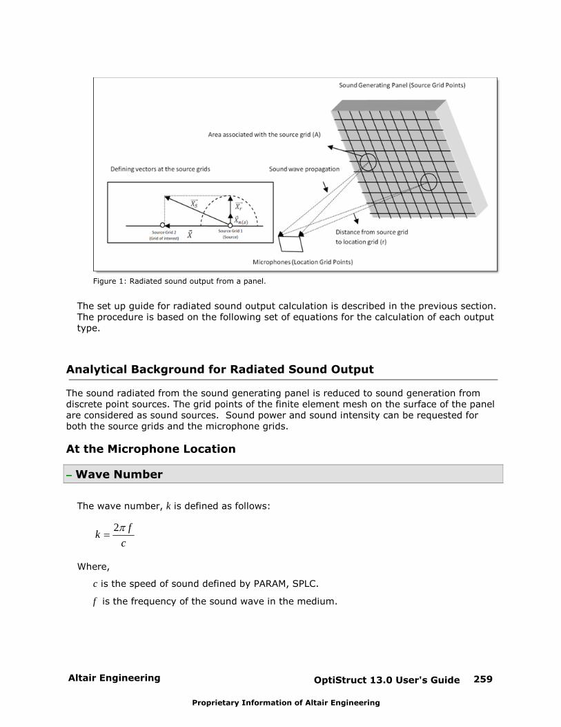
Altair Engineering OptiStruct 13.0 User's Guide 259
Proprietary Information of Altair Engineering
Figure 1: Radiated sound output from a panel.
The set up guide for radiated sound output calculation is described in the previous section.The procedure is based on the following set of equations for the calculation of each outputtype.
Analytical Background for Radiated Sound Output
The sound radiated from the sound generating panel is reduced to sound generation fromdiscrete point sources. The grid points of the finite element mesh on the surface of the panelare considered as sound sources. Sound power and sound intensity can be requested forboth the source grids and the microphone grids.
At the Microphone Location
Wave Number
The wave number, k is defined as follows:
2 fk
c
Where,
c is the speed of sound defined by PARAM, SPLC.
f is the frequency of the sound wave in the medium.
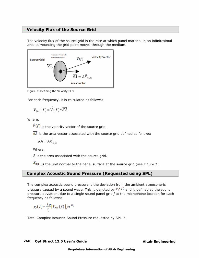
OptiStruct 13.0 User's Guide260 Altair Engineering
Proprietary Information of Altair Engineering
Velocity Flux of the Source Grid
The velocity flux of the source grid is the rate at which panel material in an infinitesimalarea surrounding the grid point moves through the medium.
Figure 2: Defining the Velocity Flux
For each frequency, it is calculated as follows:
uuurflux f V f AV
Where,
is the velocity vector of the source grid.
is the area vector associated with the source grid defined as follows:
uuur rn s
A XA
Where,
A is the area associated with the source grid.
is the unit normal to the panel surface at the source grid (see Figure 2).
Complex Acoustic Sound Pressure (Requested using SPL)
The complex acoustic sound pressure is the deviation from the ambient atmospheric
pressure caused by a sound wave. This is denoted by and is defined as the sound
pressure deviation, due to a single sound panel grid j at the microphone location for each
frequency as follows:
Total Complex Acoustic Sound Pressure requested by SPL is:
Altair Engineering OptiStruct 13.0 User's Guide 261
Proprietary Information of Altair Engineering
Where,
is the frequency of the sound wave in the medium.
is the density of the acoustic medium defined by PARAM, SPLRHO.
rj is the distance from the acoustic source grid j on the panel to the microphone
location grid (see Figure 1).
is the velocity flux of the source grid.
k is the wave number as defined in Wave Number.
i is the square root of -1
np is the number of source grids (see Figure 1).
q is the value of the scale factor specified using the parameter PARAM, SPLFAC.
The Sound Pressure Level in decibels (SPLdB - Also requested using SPL) can be calculated
using the following equation:
1020.0* log ( )dB
SPLSPL
SPLREFDB
Where,
SPLdB is the Sound Pressure Level in decibels.
SPL is the magnitude of the acoustic sound pressure.
SPLREFDB is the reference sound pressure value specified using the parameter PARAM,
SPLREFDB
Complex Particle Velocity Vector
The complex particle velocity vector is the velocity of a particle in a medium measured as awave passes through it. The particle velocity is not the velocity of the wave itself; rather itis the velocity of a particle as it oscillates about a mean position, due to the passage of the
wave. It is denoted by at the location of the microphone, due to the source grid j(see Figure 1) and is defined for each frequency as follows:
ˆ( ) X) ( )( 1
uuurj j
j
j
pvp f i
fc kr
OptiStruct 13.0 User's Guide262 Altair Engineering
Proprietary Information of Altair Engineering
Where,
is the complex acoustic pressure, due to source grid, j at the microphone location.
is the unit vector from the source grid j to the microphone grid (see Figure 1).
X XX̂
X
r r
rj j
j
jjr
is the density of the acoustic medium defined by PARAM, SPLRHO.
c is the speed of sound defined by PARAM, SPLC.
k is the wave number as defined in Wave Number.
rj is the distance from the acoustic source grid j on the panel to the microphone grid
(see Figure 1).
i is the square root of -1
Total Sound Power (Requested using SPOWER)
The total sound power is the rate of change of sound energy with time in the domain of
reference. The total sound power , due to all the source grids can be calculated at amicrophone location for each frequency as follows:
1
( ) ( ). ( )np
j jj
sp f real p f p f
Where,
is the acoustic pressure at a microphone location, due to the source grid "j".
is the complex conjugate of .
np is the number of source grids (see Figure 1).
Total Complex Intensity Vector (Requested using SINTENS)
The total complex intensity vector is the sound power per unit area. The sound intensitycan be defined as a product of sound pressure and the particle velocity vector. For multiplesource grids, the total sound intensity at a microphone location for each frequency is givenas follows:
1
1( ) ( ).( ) ( )
2
uuuuruur np
j jj
iv pf real p f fv

Altair Engineering OptiStruct 13.0 User's Guide 263
Proprietary Information of Altair Engineering
Where,
is the acoustic pressure at the microphone location due to the sound generated at
the source grid "j".
is the complex conjugate of , which is the complex particle velocity
vector at the microphone location, due to the sound generated at the source grid "j".
At the Source Grid Location
Wave Number
The wave number is independent of the location of the grid points. Now define a set ofdisplacement vectors that relate source grids to one another. To do this, each source grid
is considered to be associated with an area (A) on the panel.
Figure 3: Displacement vectors at the source grids.
The vector addition operation for displacement vectors from Figure 3 is as follows:
uuur uur uuurrsX X X
Where,
is the vector from a source grid (1) to the source grid (2) of interest.
is defined as:
12
uuur rr n s
AX X
Where,
A is the area associated with a source grid.
is the unit normal to the area, A associated with a source grid.
Complex Acoustic Sound Pressure [at the source grid]
The complex acoustic sound pressure is the deviation from the ambient atmospheric
OptiStruct 13.0 User's Guide264 Altair Engineering
Proprietary Information of Altair Engineering
pressure caused by a sound wave. This is denoted using and is defined at thesource grid for each frequency as follows:
i ( )( ) ie
( )s jk r
s j flux js j
fp f V f
r
Total Complex Acoustic Sound Pressure at a source grid requested by SPL is:
( 1)i ( )
1
( ) ie( )
s j
npk r
s flux js
totalj j
fp f V f
r
Where,
is the frequency of the sound wave in the medium.
is the density of the acoustic medium defined by PARAM, SPLRHO.
is equal to , for each grid, j (j=1 to np), the magnitude (length) of as defined
in At the Source Grid Location (see Figure 1).
is the velocity flux of the source grid, j (see Velocity Flux of the Source Grid)
k is the wave number as defined in Wave Number.
i is the square root of -1
np is the number of source grids (see Figure 1).
q is the value of the scale factor specified using the parameter PARAM, SPLFAC.
Total Sound Power (Requested using SPOWER) [at the source grid]
The total sound power is the rate of change of sound energy with time in the domain of
reference. The total sound power , due to all the source grids can be calculated at asource grid of interest for each frequency as follows:
*( 1)
1
( ) (( ) ( . )) s j s j
np
sj
p f p fsp f real
Where,
is the acoustic pressure at a source grid, due to the source grid "j".
is the complex conjugate of .
np is the number of source grids (see Figure 1).
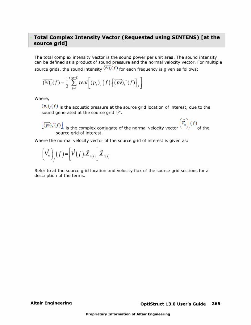
Altair Engineering OptiStruct 13.0 User's Guide 265
Proprietary Information of Altair Engineering
Total Complex Intensity Vector (Requested using SINTENS) [at thesource grid]
The total complex intensity vector is the sound power per unit area. The sound intensitycan be defined as a product of sound pressure and the normal velocity vector. For multiple
source grids, the sound intensity for each frequency is given as follows:
( 1)
1
1( ) . ) ( )( ) ( ) (
2
uuuuur uuuurnp
sj
sj
s jiv p ff real pv f
Where,
is the acoustic pressure at the source grid location of interest, due to the
sound generated at the source grid "j".
is the complex conjugate of the normal velocity vector of thesource grid of interest.
Where the normal velocity vector of the source grid of interest is given as:
.r r
n n s n sj
V f V f X X
Refer to at the source grid location and velocity flux of the source grid sections for adescription of the terms.
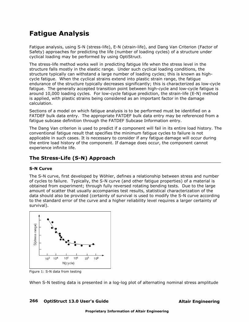
OptiStruct 13.0 User's Guide266 Altair Engineering
Proprietary Information of Altair Engineering
Fatigue Analysis
Fatigue analysis, using S-N (stress-life), E-N (strain-life), and Dang Van Criterion (Factor ofSafety) approaches for predicting the life (number of loading cycles) of a structure undercyclical loading may be performed by using OptiStruct.
The stress-life method works well in predicting fatigue life when the stress level in thestructure falls mostly in the elastic range. Under such cyclical loading conditions, thestructure typically can withstand a large number of loading cycles; this is known as high-cycle fatigue. When the cyclical strains extend into plastic strain range, the fatigueendurance of the structure typically decreases significantly; this is characterized as low-cyclefatigue. The generally accepted transition point between high-cycle and low-cycle fatigue isaround 10,000 loading cycles. For low-cycle fatigue prediction, the strain-life (E-N) methodis applied, with plastic strains being considered as an important factor in the damagecalculation.
Sections of a model on which fatigue analysis is to be performed must be identified on a FATDEF bulk data entry. The appropriate FATDEF bulk data entry may be referenced from afatigue subcase definition through the FATDEF Subcase Information entry.
The Dang Van criterion is used to predict if a component will fail in its entire load history. Theconventional fatigue result that specifies the minimum fatigue cycles to failure is notapplicable in such cases. It is necessary to consider if any fatigue damage will occur duringthe entire load history of the component. If damage does occur, the component cannotexperience infinite life.
The Stress-Life (S-N) Approach
S-N Curve
The S-N curve, first developed by Wöhler, defines a relationship between stress and numberof cycles to failure. Typically, the S-N curve (and other fatigue properties) of a material isobtained from experiment; through fully reversed rotating bending tests. Due to the largeamount of scatter that usually accompanies test results, statistical characterization of thedata should also be provided (certainty of survival is used to modify the S-N curve accordingto the standard error of the curve and a higher reliability level requires a larger certainty ofsurvival).
Figure 1: S-N data from testing
When S-N testing data is presented in a log-log plot of alternating nominal stress amplitude
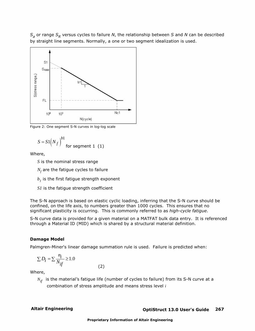
Altair Engineering OptiStruct 13.0 User's Guide 267
Proprietary Information of Altair Engineering
Sa or range SR versus cycles to failure N, the relationship between S and N can be described
by straight line segments. Normally, a one or two segment idealization is used.
Figure 2: One segment S-N curves in log-log scale
11
b
fS S Nfor segment 1 (1)
Where,
S is the nominal stress range
Nf are the fatigue cycles to failure
b1 is the first fatigue strength exponent
S1 is the fatigue strength coefficient
The S-N approach is based on elastic cyclic loading, inferring that the S-N curve should beconfined, on the life axis, to numbers greater than 1000 cycles. This ensures that nosignificant plasticity is occurring. This is commonly referred to as high-cycle fatigue.
S-N curve data is provided for a given material on a MATFAT bulk data entry. It is referencedthrough a Material ID (MID) which is shared by a structural material definition.
Damage Model
Palmgren-Miner's linear damage summation rule is used. Failure is predicted when:
1.0niDi Nif
(2)
Where,
Nif is the material’s fatigue life (number of cycles to failure) from its S-N curve at a
combination of stress amplitude and means stress level i
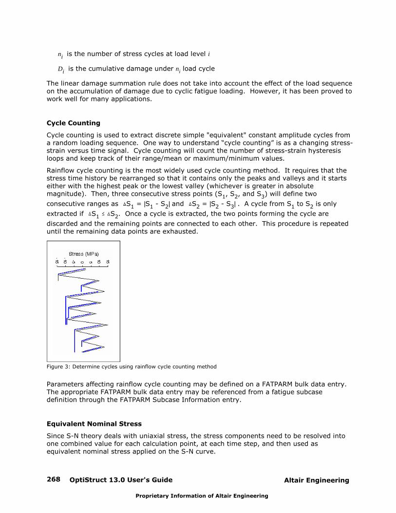
OptiStruct 13.0 User's Guide268 Altair Engineering
Proprietary Information of Altair Engineering
ni is the number of stress cycles at load level i
Di is the cumulative damage under ni load cycle
The linear damage summation rule does not take into account the effect of the load sequenceon the accumulation of damage due to cyclic fatigue loading. However, it has been proved towork well for many applications.
Cycle Counting
Cycle counting is used to extract discrete simple "equivalent" constant amplitude cycles froma random loading sequence. One way to understand “cycle counting” is as a changing stress-strain versus time signal. Cycle counting will count the number of stress-strain hysteresisloops and keep track of their range/mean or maximum/minimum values.
Rainflow cycle counting is the most widely used cycle counting method. It requires that thestress time history be rearranged so that it contains only the peaks and valleys and it startseither with the highest peak or the lowest valley (whichever is greater in absolutemagnitude). Then, three consecutive stress points (S1, S2, and S3) will define two
consecutive ranges as S1 = |S1 - S2| and S2 = |S2 - S3| . A cycle from S1 to S2 is only
extracted if S1 S2. Once a cycle is extracted, the two points forming the cycle are
discarded and the remaining points are connected to each other. This procedure is repeateduntil the remaining data points are exhausted.
Figure 3: Determine cycles using rainflow cycle counting method
Parameters affecting rainflow cycle counting may be defined on a FATPARM bulk data entry. The appropriate FATPARM bulk data entry may be referenced from a fatigue subcasedefinition through the FATPARM Subcase Information entry.
Equivalent Nominal Stress
Since S-N theory deals with uniaxial stress, the stress components need to be resolved intoone combined value for each calculation point, at each time step, and then used asequivalent nominal stress applied on the S-N curve.
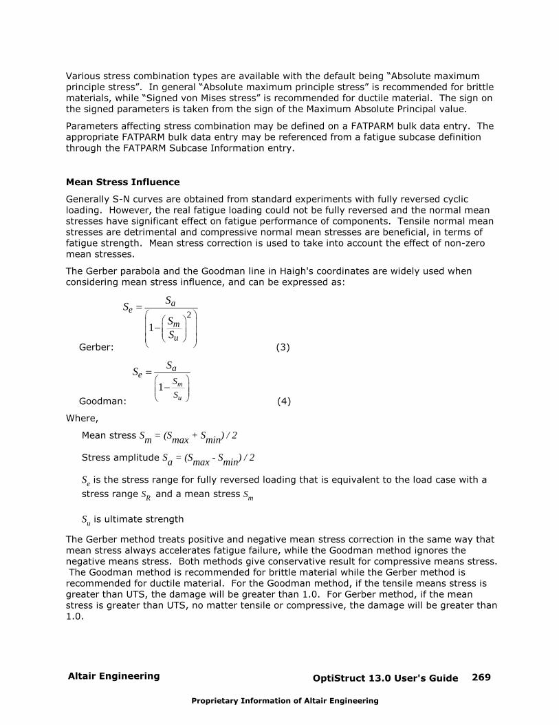
Altair Engineering OptiStruct 13.0 User's Guide 269
Proprietary Information of Altair Engineering
Various stress combination types are available with the default being “Absolute maximumprinciple stress”. In general “Absolute maximum principle stress” is recommended for brittlematerials, while “Signed von Mises stress” is recommended for ductile material. The sign onthe signed parameters is taken from the sign of the Maximum Absolute Principal value.
Parameters affecting stress combination may be defined on a FATPARM bulk data entry. Theappropriate FATPARM bulk data entry may be referenced from a fatigue subcase definitionthrough the FATPARM Subcase Information entry.
Mean Stress Influence
Generally S-N curves are obtained from standard experiments with fully reversed cyclicloading. However, the real fatigue loading could not be fully reversed and the normal meanstresses have significant effect on fatigue performance of components. Tensile normal meanstresses are detrimental and compressive normal mean stresses are beneficial, in terms offatigue strength. Mean stress correction is used to take into account the effect of non-zeromean stresses.
The Gerber parabola and the Goodman line in Haigh's coordinates are widely used whenconsidering mean stress influence, and can be expressed as:
Gerber:
2
1
ae
m
u
SS
S
S(3)
Goodman:
1 m
u
ae
S
S
SS
(4)
Where,
Mean stress Sm = (Smax + Smin) / 2
Stress amplitude Sa = (Smax - Smin) / 2
Se is the stress range for fully reversed loading that is equivalent to the load case with a
stress range SR and a mean stress Sm
Su is ultimate strength
The Gerber method treats positive and negative mean stress correction in the same way thatmean stress always accelerates fatigue failure, while the Goodman method ignores thenegative means stress. Both methods give conservative result for compressive means stress. The Goodman method is recommended for brittle material while the Gerber method isrecommended for ductile material. For the Goodman method, if the tensile means stress isgreater than UTS, the damage will be greater than 1.0. For Gerber method, if the meanstress is greater than UTS, no matter tensile or compressive, the damage will be greater than1.0.
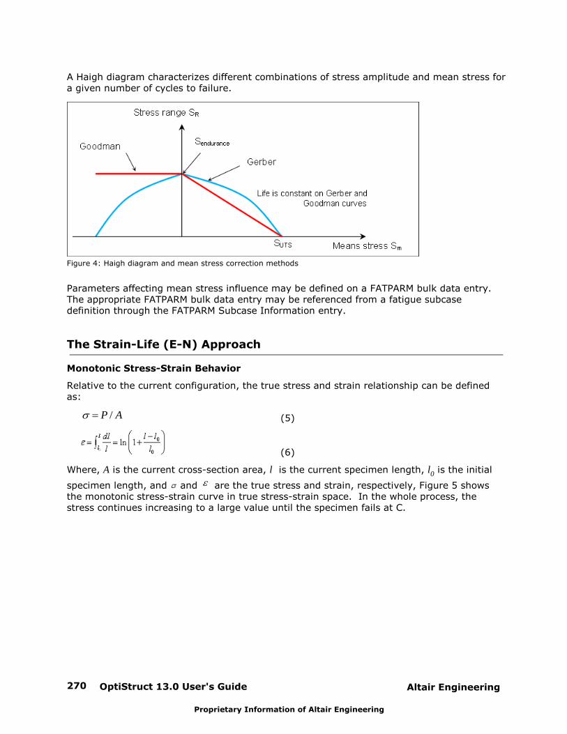
OptiStruct 13.0 User's Guide270 Altair Engineering
Proprietary Information of Altair Engineering
A Haigh diagram characterizes different combinations of stress amplitude and mean stress fora given number of cycles to failure.
Figure 4: Haigh diagram and mean stress correction methods
Parameters affecting mean stress influence may be defined on a FATPARM bulk data entry. The appropriate FATPARM bulk data entry may be referenced from a fatigue subcasedefinition through the FATPARM Subcase Information entry.
The Strain-Life (E-N) Approach
Monotonic Stress-Strain Behavior
Relative to the current configuration, the true stress and strain relationship can be definedas:
/P A (5)
(6)
Where, A is the current cross-section area, l is the current specimen length, l0 is the initial
specimen length, and and are the true stress and strain, respectively, Figure 5 showsthe monotonic stress-strain curve in true stress-strain space. In the whole process, thestress continues increasing to a large value until the specimen fails at C.
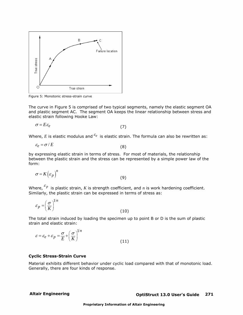
Altair Engineering OptiStruct 13.0 User's Guide 271
Proprietary Information of Altair Engineering
Figure 5: Monotonic stress-strain curve
The curve in Figure 5 is comprised of two typical segments, namely the elastic segment OAand plastic segment AC. The segment OA keeps the linear relationship between stress andelastic strain following Hooke Law:
eE(7)
Where, E is elastic modulus and e is elastic strain. The formula can also be rewritten as:
/e E(8)
by expressing elastic strain in terms of stress. For most of materials, the relationshipbetween the plastic strain and the stress can be represented by a simple power law of theform:
npK
(9)
Where, p is plastic strain, K is strength coefficient, and n is work hardening coefficient.
Similarly, the plastic strain can be expressed in terms of stress as:
1 n
p K(10)
The total strain induced by loading the specimen up to point B or D is the sum of plasticstrain and elastic strain:
1 n
e p E K(11)
Cyclic Stress-Strain Curve
Material exhibits different behavior under cyclic load compared with that of monotonic load. Generally, there are four kinds of response.
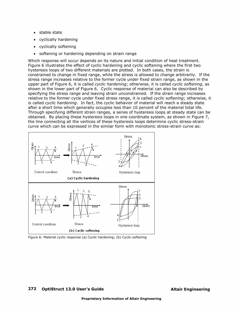
OptiStruct 13.0 User's Guide272 Altair Engineering
Proprietary Information of Altair Engineering
stable state
cyclically hardening
cyclically softening
softening or hardening depending on strain range
Which response will occur depends on its nature and initial condition of heat treatment. Figure 6 illustrates the effect of cyclic hardening and cyclic softening where the first twohysteresis loops of two different materials are plotted. In both cases, the strain isconstrained to change in fixed range, while the stress is allowed to change arbitrarily. If thestress range increases relative to the former cycle under fixed strain range, as shown in theupper part of Figure 6, it is called cyclic hardening; otherwise, it is called cyclic softening, asshown in the lower part of Figure 6. Cyclic response of material can also be described byspecifying the stress range and leaving strain unconstrained. If the strain range increasesrelative to the former cycle under fixed stress range, it is called cyclic softening; otherwise, itis called cyclic hardening. In fact, the cyclic behavior of material will reach a steady stateafter a short time which generally occupies less than 10 percent of the material total life. Through specifying different strain ranges, a series of hysteresis loops at steady state can beobtained. By placing these hysteresis loops in one coordinate system, as shown in Figure 7,the line connecting all the vertices of these hysteresis loops determine cyclic stress-straincurve which can be expressed in the similar form with monotonic stress-strain curve as:
Figure 6: Material cyclic response (a) Cyclic hardening; (b) Cyclic softening
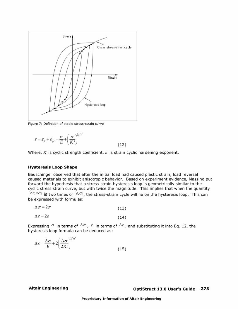
Altair Engineering OptiStruct 13.0 User's Guide 273
Proprietary Information of Altair Engineering
Figure 7: Definition of stable stress-strain curve
1 '
'
n
e p E K(12)
Where, K' is cyclic strength coefficient, n' is strain cyclic hardening exponent.
Hysteresis Loop Shape
Bauschinger observed that after the initial load had caused plastic strain, load reversalcaused materials to exhibit anisotropic behavior. Based on experiment evidence, Massing putforward the hypothesis that a stress-strain hysteresis loop is geometrically similar to thecyclic stress strain curve, but with twice the magnitude. This implies that when the quantity
is two times of , the stress-strain cycle will lie on the hysteresis loop. This canbe expressed with formulas:
2 (13)
2 (14)
Expressing in terms of , in terms of , and substituting it into Eq. 12, thehysteresis loop formula can be deduced as:
1 '
22 '
n
E K(15)
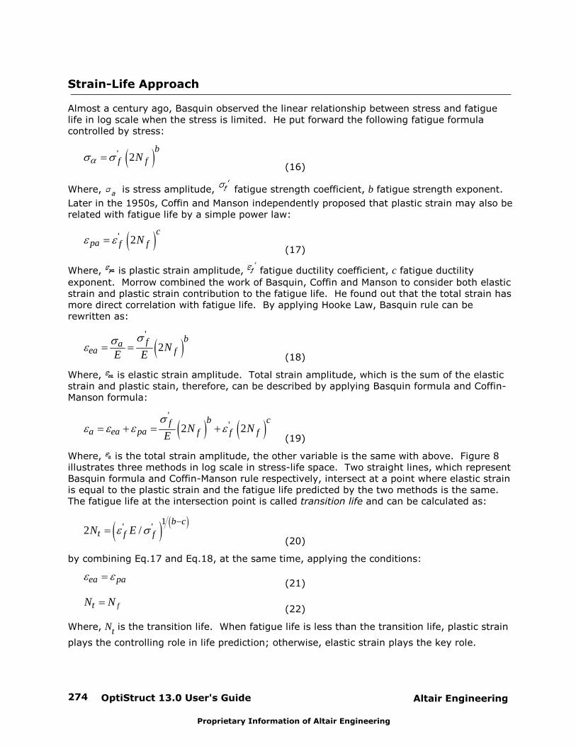
OptiStruct 13.0 User's Guide274 Altair Engineering
Proprietary Information of Altair Engineering
Strain-Life Approach
Almost a century ago, Basquin observed the linear relationship between stress and fatiguelife in log scale when the stress is limited. He put forward the following fatigue formulacontrolled by stress:
' 2b
f fN(16)
Where, a is stress amplitude, fatigue strength coefficient, b fatigue strength exponent.
Later in the 1950s, Coffin and Manson independently proposed that plastic strain may also berelated with fatigue life by a simple power law:
' 2c
pa f fN(17)
Where, is plastic strain amplitude, fatigue ductility coefficient, c fatigue ductility
exponent. Morrow combined the work of Basquin, Coffin and Manson to consider both elasticstrain and plastic strain contribution to the fatigue life. He found out that the total strain hasmore direct correlation with fatigue life. By applying Hooke Law, Basquin rule can berewritten as:
'
2bfa
ea fNE E (18)
Where, is elastic strain amplitude. Total strain amplitude, which is the sum of the elasticstrain and plastic stain, therefore, can be described by applying Basquin formula and Coffin-Manson formula:
''2 2
b cfa ea pa f f fN N
E (19)
Where, is the total strain amplitude, the other variable is the same with above. Figure 8illustrates three methods in log scale in stress-life space. Two straight lines, which representBasquin formula and Coffin-Manson rule respectively, intersect at a point where elastic strainis equal to the plastic strain and the fatigue life predicted by the two methods is the same. The fatigue life at the intersection point is called transition life and can be calculated as:
1' '2 /
b c
t f fN E(20)
by combining Eq.17 and Eq.18, at the same time, applying the conditions:
ea pa (21)
ftN N(22)
Where, Nt is the transition life. When fatigue life is less than the transition life, plastic strain
plays the controlling role in life prediction; otherwise, elastic strain plays the key role.
Altair Engineering OptiStruct 13.0 User's Guide 275
Proprietary Information of Altair Engineering
Figure 8: Strain-life curve in log scale
Damage Accumulation Model
In the E-N approach, use the same damage accumulation model as the S-N approach, whichis Palmgren-Miner's linear damage summation rule.
Mean Stress Influence
The fatigue experiments carried out in the laboratory are always fully reversed, whereas inpractice, the mean stress is inevitable, thus the fatigue law established by the fully reversedexperiments must be corrected before applied to engineering problems. Morrow is the first toconsider the effect of mean stress through introducing the mean stress 0 in fatigue strength
coefficient by:
'0
2bf
ea fNE (23)
Thus the entire fatigue life formula becomes:
'0 '2 2
b cfa f f fN N
E (24)
Morrow's equation is consistent with the observation that mean stress effects are significantat low value of plastic strain and of little effect at high plastic strain.
Smith, Watson and Topper proposed a different method to account for the effect of meanstress by considering the maximum stress during one cycle (for convenience, this method iscalled SWT in the following). In this case, the damage parameter is modified as the productof the maximum stress and strain range in one cycle. For a fully reversed cycle, themaximum stress is given by:
'max 2
b
f fN(25)
OptiStruct 13.0 User's Guide276 Altair Engineering
Proprietary Information of Altair Engineering
By multiplying Eq.19 with Eq.25, it can be rewritten as:
' 2' '
max 2 2b b cf
a f f f fN NE (26)
The SWT method will predict that no damage will occur when the maximum stress is zero ornegative, which is not consistent with the reality.
When comparing the two methods, the SWT method predicted conservative life for loadspredominantly tensile, whereas, the Morrow approach provides more realistic results whenthe load is predominantly compressive.
Neuber Correction
Strain-life analysis is based on the fact that many critical locations such as notch roots havestress concentration, which will have obvious plastic deformation during the cyclic loadingbefore fatigue failure. Thus, the elastic-plastic strain results are essential for performingstrain-life analysis. Neuber correction is the most popular practice to correct elastic analysisresults into elastic-plastic results.
In order to derive the local stress from the nominal stress that is easier to obtain, the
concentration factors are introduced such as the local stress concentration factor K
, and
the local strain concentration factor K
.
/K S(27)
/K e(28)
Where, is the local stress, is the local strain, S is the nominal stress, and e is the nominal
strain. If nominal stress and local stress are both elastic, the local stress concentration factoris equal to the local strain concentration factor. However, if the plastic strain is present, the
relationship between K
and K
no long holds. Thereafter, focusing on this situation,Neuber introduced a theoretically elastic stress concentration factor Kt defined as:
2tK K K
(29)
Substitute Eq.27 and Eq.28 into Eq.29, the theoretical stress concentration factor Kt can be
rewritten as:
2tK
S e(30)
Through linear static FEA, the local stress instead of nominal stress is provided, which impliesthe effect of the geometry in Eq.30 is removed, thus you can set Kt as 1 and rewrite Eq.30
as:
e e (31)
Where, e , is locally elastic stress and locally elastic strain obtained from elastic analysis,
, the stress and strain at the presence of plastic strain. Both and can be calculated
Altair Engineering OptiStruct 13.0 User's Guide 277
Proprietary Information of Altair Engineering
from Eq.31 together with the equations for the cyclic stress-strain curve and hysteresis loop.
Dang Van Criterion (Factor of Safety)
The Dang Van criterion is used to predict if a component will fail in its entire load history. Incertain physical systems, components may be required to last infinitely long. For example,automobile components which undergo multiaxial cyclic loading at high rotational velocities(like propeller shafts) reach their high cycle fatigue limit within a short operating life. Theconventional fatigue result that specifies the minimum fatigue cycles to failure is notapplicable in such cases. It is not necessary to quantify the amount of fatigue damage, butjust to consider if any fatigue damage will occur during the entire load history of thecomponent. If damage does occur, the component cannot experience infinite life. Fatigueanalysis based on the Dang Van criterion is designed for this purpose.
Fatigue crack initiation usually occurs at zones of stress concentration such as geometricdiscontinuities, fillets, notches and so on. This phenomenon takes place in the microscopiclevel and is localized to certain regions like grains which have undergone local plasticdeformation in characteristic intra-crystalline bands. The Dang Van approach postulates afatigue criterion using microscopic variables in the apparent stabilization state; this is a stateof elastic shakedown if no damage occurs. The main principle of the criterion is that the usualcharacterization of the fatigue cycle is replaced by the local loading path and so damagingloads can be distinguished.
The general procedure of Dang Van fatigue analysis is:
1. Evaluate the macroscopic stresses ( )ij t
, for each location at a different point in time.
2. Split the macroscopic stress ( )ij t
into a hydrostatic part( )p t
and a deviatoric part( )ijS t
.
3. Calculate the stabilized microscopic residual stress *dev based on the following
equation:
*
2( ( ( ( ) )))ijdev Min Max J S t dev
The expression is minimized with respect to and maximized with respect to t.
4. Calculate the deviatoric part of microscopic stress.
*( ) ( )ij ijs t S t dev
5. Calculate factor of safety (FOS):
( ) ( )
bFOS Min
t ap t
( ) 0.5 ( ( ))ijt Tresca s t
Where, b and a are material constants.
If FOS is less than 1, the component cannot experience infinite life.
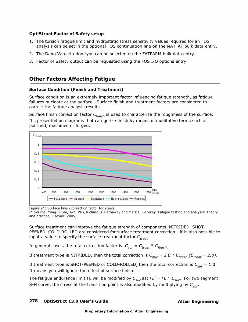
OptiStruct 13.0 User's Guide278 Altair Engineering
Proprietary Information of Altair Engineering
OptiStruct Factor of Safety setup
1. The torsion fatigue limit and hydrostatic stress sensitivity values required for an FOSanalysis can be set in the optional FOS continuation line on the MATFAT bulk data entry.
2. The Dang Van criterion type can be selected on the FATPARM bulk data entry.
3. Factor of Safety output can be requested using the FOS I/O options entry.
Other Factors Affecting Fatigue
Surface Condition (Finish and Treatment)
Surface condition is an extremely important factor influencing fatigue strength, as fatiguefailures nucleate at the surface. Surface finish and treatment factors are considered tocorrect the fatigue analysis results.
Surface finish correction factor Cfinish is used to characterize the roughness of the surface.
It's presented on diagrams that categorize finish by means of qualitative terms such aspolished, machined or forged.
Figure 9*: Surface finish correction factor for steels(* Source: Yung-Li Lee, Jwo. Pan, Richard B. Hathaway and Mark E. Barekey. Fatigue testing and analysis: Theoryand practice, Elsevier, 2005)
Surface treatment can improve the fatigue strength of components. NITRIDED, SHOT-PEENED, COLD-ROLLED are considered for surface treatment correction. It is also possible toinput a value to specify the surface treatment factor Ctreat.
In general cases, the total correction factor is Csur = Ctreat * Cfinish.
If treatment type is NITRIDED, then the total correction is Csur = 2.0 * Cfinish (Ctreat = 2.0).
If treatment type is SHOT-PEENED or COLD-ROLLED, then the total correction is Csur = 1.0.
It means you will ignore the effect of surface finish.
The fatigue endurance limit FL will be modified by Csur as: FL' = FL * Csur. For two segment
S-N curve, the stress at the transition point is also modified by multiplying by Csur.
Altair Engineering OptiStruct 13.0 User's Guide 279
Proprietary Information of Altair Engineering
Surface conditions may be defined on a PFAT bulk data entry. Surface conditions are thenassociated with sections of the model through the FATDEF bulk data entry.
Fatigue Strength Reduction Factor
In addition to the factors mentioned above, there are various others factors that could affectthe fatigue strength of a structure, e.g., notch effect, size effect, loading type. Fatiguestrength reduction factor Kf is introduced to account for the combined effect of all such
corrections. The fatigue endurance limit FL will be modified by Kf as: FL' = FL / Kf
The fatigue strength reduction factor may be defined on a PFAT bulk data entry. It may thenbe associated with sections of the model through the FATDEF bulk data entry.
If both Csur and Kf are specified, the fatigue endurance limit FL will be modified as: FL' = FL
* Csur / Kf.
Csur and Kf have similar influences on the E-N formula through its elastic part as on the S-N
formula. In the elastic part of the E-N formula, a nominal fatigue endurance limit FL iscalculated internally from the reversal limit of endurance Nc. FL will be corrected if Csur and
Kf are presented. The elastic part will be modified as well with the updated nominal fatigue
limit.
Setting Up a Fatigue Analysis
Linear Superposition of Multiple FEA/Load Time History Load Cases
When there are several load cases at the same time, all of which vary independently of oneanother, the principle of linear superposition will be used to combine all load cases togetherto determine the stress variation at each calculation point due to the combination of all loads. The formula is:
,
1 ,( ) ( )
nij k
ij kk FEA k
t P tP
(32)
Where,
n is the total number of load cases
Pk(t) and are, respectively, the time variation of the k-th load time history and the
total stress tensor
PFEA,k and are, respectively, the k-th load magnitude and stress tensor from FE
analysis
Load Time History Compression
This option is used to save calculation time. It will remove small cycles (defined by a gatevalue) and intermediate points.
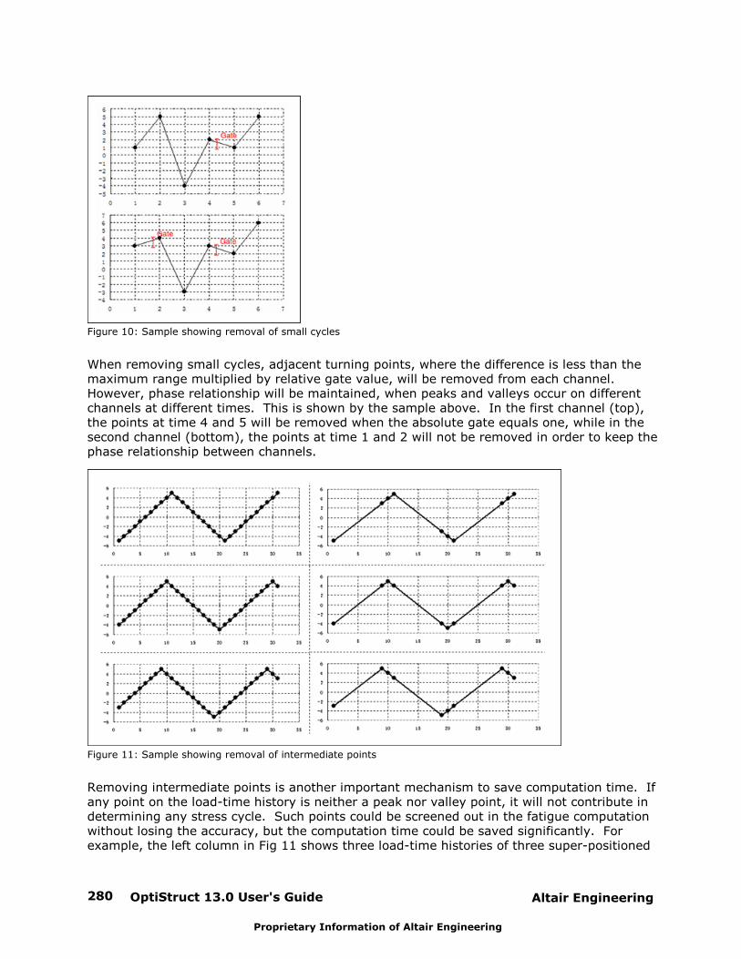
OptiStruct 13.0 User's Guide280 Altair Engineering
Proprietary Information of Altair Engineering
Figure 10: Sample showing removal of small cycles
When removing small cycles, adjacent turning points, where the difference is less than themaximum range multiplied by relative gate value, will be removed from each channel. However, phase relationship will be maintained, when peaks and valleys occur on differentchannels at different times. This is shown by the sample above. In the first channel (top),the points at time 4 and 5 will be removed when the absolute gate equals one, while in thesecond channel (bottom), the points at time 1 and 2 will not be removed in order to keep thephase relationship between channels.
Figure 11: Sample showing removal of intermediate points
Removing intermediate points is another important mechanism to save computation time. Ifany point on the load-time history is neither a peak nor valley point, it will not contribute indetermining any stress cycle. Such points could be screened out in the fatigue computationwithout losing the accuracy, but the computation time could be saved significantly. Forexample, the left column in Fig 11 shows three load-time histories of three super-positioned
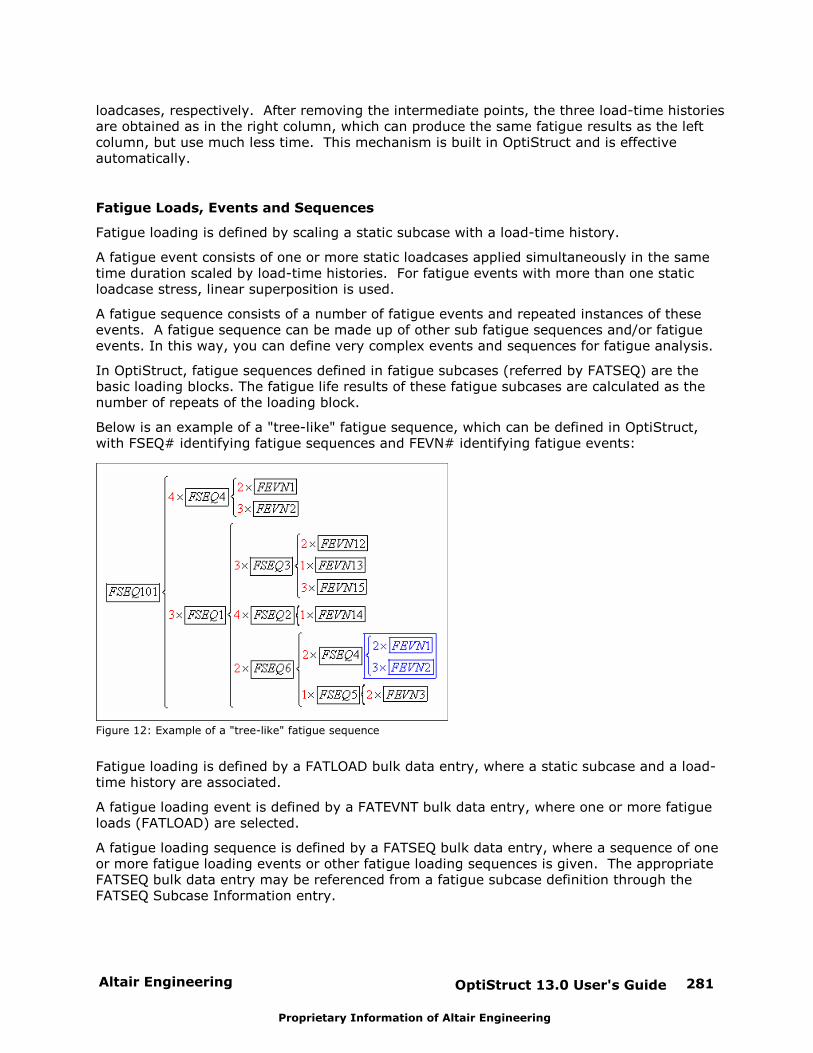
Altair Engineering OptiStruct 13.0 User's Guide 281
Proprietary Information of Altair Engineering
loadcases, respectively. After removing the intermediate points, the three load-time historiesare obtained as in the right column, which can produce the same fatigue results as the leftcolumn, but use much less time. This mechanism is built in OptiStruct and is effectiveautomatically.
Fatigue Loads, Events and Sequences
Fatigue loading is defined by scaling a static subcase with a load-time history.
A fatigue event consists of one or more static loadcases applied simultaneously in the sametime duration scaled by load-time histories. For fatigue events with more than one staticloadcase stress, linear superposition is used.
A fatigue sequence consists of a number of fatigue events and repeated instances of theseevents. A fatigue sequence can be made up of other sub fatigue sequences and/or fatigueevents. In this way, you can define very complex events and sequences for fatigue analysis.
In OptiStruct, fatigue sequences defined in fatigue subcases (referred by FATSEQ) are thebasic loading blocks. The fatigue life results of these fatigue subcases are calculated as thenumber of repeats of the loading block.
Below is an example of a "tree-like" fatigue sequence, which can be defined in OptiStruct,with FSEQ# identifying fatigue sequences and FEVN# identifying fatigue events:
Figure 12: Example of a "tree-like" fatigue sequence
Fatigue loading is defined by a FATLOAD bulk data entry, where a static subcase and a load-time history are associated.
A fatigue loading event is defined by a FATEVNT bulk data entry, where one or more fatigueloads (FATLOAD) are selected.
A fatigue loading sequence is defined by a FATSEQ bulk data entry, where a sequence of oneor more fatigue loading events or other fatigue loading sequences is given. The appropriateFATSEQ bulk data entry may be referenced from a fatigue subcase definition through the FATSEQ Subcase Information entry.
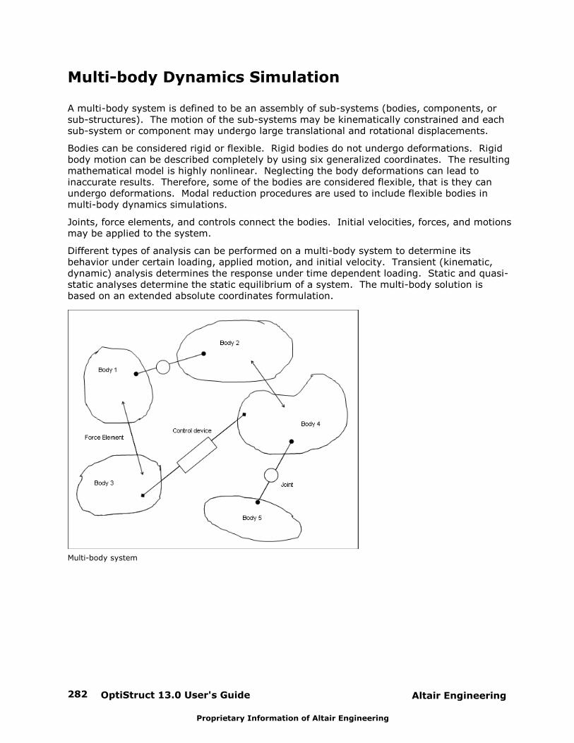
OptiStruct 13.0 User's Guide282 Altair Engineering
Proprietary Information of Altair Engineering
Multi-body Dynamics Simulation
A multi-body system is defined to be an assembly of sub-systems (bodies, components, orsub-structures). The motion of the sub-systems may be kinematically constrained and eachsub-system or component may undergo large translational and rotational displacements.
Bodies can be considered rigid or flexible. Rigid bodies do not undergo deformations. Rigidbody motion can be described completely by using six generalized coordinates. The resultingmathematical model is highly nonlinear. Neglecting the body deformations can lead toinaccurate results. Therefore, some of the bodies are considered flexible, that is they canundergo deformations. Modal reduction procedures are used to include flexible bodies inmulti-body dynamics simulations.
Joints, force elements, and controls connect the bodies. Initial velocities, forces, and motionsmay be applied to the system.
Different types of analysis can be performed on a multi-body system to determine itsbehavior under certain loading, applied motion, and initial velocity. Transient (kinematic,dynamic) analysis determines the response under time dependent loading. Static and quasi-static analyses determine the static equilibrium of a system. The multi-body solution isbased on an extended absolute coordinates formulation.
Multi-body system

Altair Engineering OptiStruct 13.0 User's Guide 283
Proprietary Information of Altair Engineering
This implementation is targeted at the typical finite-element user who wants to solve multi-body dynamics problems in the context of a finite element model, and is still somewhatlimited. HyperMesh is used for modeling. All geometry entities are defined in terms of afinite element mesh. Flexible body modeling is fully integrated.
HyperStudy can be used for optimization. Shape optimization of rigid and flexible bodies isavailable through the use of HyperMorph.
OptiStruct 13.0 User's Guide284 Altair Engineering
Proprietary Information of Altair Engineering
Transient Analysis for MBD
Transient analysis is used to calculate the response of a multi-body system to time-dependent loads and motions.
Forces and motions are time-dependent. Body initial conditions define the initial bodyvelocities, while joint initial conditions define the initial displacement of a particular joint.
The results of a transient analysis are displacements, velocities, accelerations, forces, as wellas modal contributions to stresses and strains in flexible bodies. The responses are usuallytime-dependent.
The equation of motion is given in the following form:
0
( )
( 0)
M q P t
q t v
&&
&
The matrix M is the mass matrix, the vector P is the vector of external forces, and the vector
q represents the generalized coordinates. Stiffness, damping, constraint forces, external
loads, and gravity are all included in the external force vector P. An initial and maximum
integration time step, an end time, and integrator tolerance need to be defined.
Two analyses, kinematic and dynamic, are defined depending on the degree of freedom ofthe system analysis.
A kinematic simulation is performed if all degrees of freedom are constrained throughappropriate joints and/or motions, making it a zero degree of freedom model. A kinematicssimulation finds a system configuration that satisfies all kinematic constraints and motionequations at any given time. The configuration is obtained by solving a system of nonlinearalgebraic equations representing constraints.
During a kinematic simulation, there is no need to integrate the differential equations ofmotion because the system configuration is fully determined by solving the constraint andmotion equations alone. Even though forces are not used to compute the kinematicssolution, joint reaction forces can be computed at any given time. The mass and inertiaproperties of bodies involved, and external forces acting on them, do not affect the resultantsystem configuration, but they do affect the joint reaction forces requested as outputs.
A dynamic simulation is employed whenever the model has one or more degrees of freedom. A dynamic simulation involves integrating the differential equations of motion subject tononlinear algebraic equations representing kinematics constraints. In other words, thesolution is obtained by solving a mixed system of differential-algebraic equations.
The resultant solution takes into account various dynamic effects and is dependent uponmass and inertia properties of bodies, damping within the system, and applied forces andmotions. Additional simulation parameters, such as the integration scheme, integration timestep, convergence tolerance, etc. could also affect the solution and; therefore, need to bespecified appropriately.
If a simulation type of transient is requested, the solver automatically determines whether torun a kinematic or dynamic solution from the degree of freedom.
The equation of motion is solved using one of the three different integrators that areavailable. The choice is based on the stiffness of the problem. A problem is stiff if thenumerical solution has its step size limited more severely by the stability of the numericaltechnique than by the accuracy of the technique. These are systems with high damping and

Altair Engineering OptiStruct 13.0 User's Guide 285
Proprietary Information of Altair Engineering
low transience.
VSTIFF (Default) – Implicit integrator that utilizes the Variable CoefficientDifferential Equation Solver (VODE). It is suited for stiff and non-stiffproblems.
MSTIFF – Implicit integrator that utilizes the Modified Extended BackwardDifferentiation Formula (MEBDF) to solve the nonlinear equations of motion. It is suited for stiff problems.
ABAM (Adams-Bashforth-Adams-Moulton) – Explicit integrator that uses afinite differences scheme to solve the nonlinear equations of motion. Thisintegrator is suitable for systems that are non-stiff.
A multi-body subcase needs to be defined in the input deck. Only one such subcase can beused in a model. The simulation type "transient" is defined on an MBSIM bulk data entrywhich must be referenced through a subcase statement MBSIM. The MBSIM bulk data entityalso defines the integrator, end time, and time step. A sequence of several simulations ofdifferent types can be defined by referring to an MBSEQ bulk data statement instead. Loadsand motions are referenced on MLOAD and MOTION subcase entries, respectively. Initialvelocity is referenced through INVEL. SPC type constraints in Multi-body Dynamics analysisare allowed only for MBD-ESL optimization of a flexible body if displacements are used asconstraints. Further information on loads and boundary conditions can be obtained from thesections Applied Forces and Motions and Initial Velocity.
The unit system for the simulation can be defined using a DTI, UNITS bulk data entry.

OptiStruct 13.0 User's Guide286 Altair Engineering
Proprietary Information of Altair Engineering
Static Analysis for MBD
A static simulation is also called an equilibrium simulation. The system must have at leastone degree of freedom to undergo a static simulation and an initial configuration must bespecified. A zero degree of freedom system is always considered to be in static equilibriumonce all of the kinematic constraints are satisfied.
Starting with the user-specified initial configuration, a final configuration is arrived atiteration-by-iteration, such that there are no unbalanced forces or torques on any of thebodies in the system and all of the kinematics constraints are satisfied. All of the velocitiesand accelerations are set to zero.
A multi-body subcase needs to be defined in the input deck. Only one such subcase can beused in a model. The simulation type "static" is defined on an MBSIM bulk data entry whichmust be referenced through a subcase statement MBSIM. The MBSIM bulk data entity alsodefines the integrator, end time, and time step. A sequence of several simulations ofdifferent types can be defined by referring to an MBSEQ bulk data statement instead. Loadsand motions are referenced on MLOAD and MOTION subcase entries, respectively. Initialvelocities do not apply here. SPC type constraints in Multi-body Dynamics analysis areallowed only for MBD-ESL optimization of a flexible body if displacements are used asconstraints. Further information on loads and boundary conditions can be obtained from thesections Applied Forces and Motions and Initial Velocity.
The unit system for the simulation can be defined using a DTI, UNITS bulk data entry.

Altair Engineering OptiStruct 13.0 User's Guide 287
Proprietary Information of Altair Engineering
Quasi-static Analysis for MBD
A quasi-static simulation is a sequence of static simulation steps applied to a model over agiven duration at specified intervals. A quasi-static simulation is employed when you havetime-dependent forces or motions in the model and you want a static equilibriumconfiguration at every time step. The system must have at least one degree of freedom toundergo a quasi-static simulation and you must specify the initial configuration.
For the first time step, the user-specified initial configuration is used as a starting point,whereas for all other time-steps, a configuration from the previous time step is used as thestarting point for equilibrium simulation at that time step. A final configuration is arrived atiteration-by-iteration, such that there are no unbalanced forces or torques on any of thebodies in the system and all of the kinematic constraints are satisfied at that time step. Forevery step, all velocities and accelerations are set to zero.
A multi-body subcase needs to be defined in the input deck. Only one such subcase can beused in a model. The simulation type "quasi-static" is defined on an MBSIM bulk data entrywhich must be referenced through a subcase statement MBSIM. The MBSIM bulk data entityalso defines the integrator, end time, and time step. A sequence of several simulations ofdifferent types can be defined by referring to a MBSEQ bulk data statement instead. Loadsand motions are referenced on MLOAD and MOTION subcase entries, respectively. Initialvelocities do not apply here. SPC type constraints in Multi-body Dynamics analysis areallowed only for MBD-ESL optimization of a flexible body if displacements are used asconstraints. Further information on loads and boundary conditions can be obtained from thesections Applied Forces and Motions and Initial Velocity.
The unit system for the simulation can be defined using a DTI, UNITS bulk data entry.

OptiStruct 13.0 User's Guide288 Altair Engineering
Proprietary Information of Altair Engineering
Linear Analysis for MBD
In linearization analysis, the nonlinear representations of force, motion, stiffness, or dampingare linearized. A linearization can be performed on these models to prepare a model for usewith Matlab or to obtain eigenmodes characteristics of the model. In the case of performinga linear analysis on the mechanical system, optional files of type eig_info, Simulink MDL,
and Matlab ABCD matrices are available to be exported.
A multi-body subcase needs to be defined in the input deck. Only one such subcase can beused in a model. A linear simulation is defined by referring an MBSIM subcase entry to aMBLIN bulk data statement. The MBLIN bulk data entity also selects linear analysis types,EIGEN or STMAT. A sequence of several simulations of different types can be defined byreferring to an MBSEQ bulk data statement instead. Loads and motions are referenced onMLOAD and MOTION subcase entries, respectively. SPC type constraints in Multi-bodyDynamics analysis are allowed only for MBD-ESL optimization of a flexible body ifdisplacements are used as constraints. Initial velocities do not apply here. Furtherinformation on loads and boundary conditions can be obtained from the sections AppliedForces and Motions and Initial Velocity.
The unit system for the simulation can be defined using a DTI, UNITS bulk data entry.

Altair Engineering OptiStruct 13.0 User's Guide 289
Proprietary Information of Altair Engineering
Bodies
Bodies are the model elements that have mass and inertia. Bodies can be rigid or flexible.
A rigid body has only mass and inertia, and does not deform during the simulation. An initialvelocity can be assigned. Mass and inertia information can be omitted for kinematic, static,and quasi-static simulations. It does not affect displacement, velocity, and accelerationresults of kinematic simulation or displacement results of a static or a quasi-static simulation. Mass and inertia information must be correctly specified if joint-reaction forces are ofinterest in kinematic, static, or quasi-static simulations.
A flexible body deforms during the simulation. Mass and inertia are determined by thegeometry and material of the structure defining the body. An initial velocity and dampingcan be assigned. Flexible bodies are formulated using an orthogonal set of modes that
represent the displacements u of the flexible body such that
q
where, q are the modal coordinates which are to be determined by the multi-body dynamics
analysis. The set of orthogonal modes is determined in a Component Mode Synthesis (CMS). Depending on the model, CMS can be performed as a pre-processing step using a specialsimulation (see Direct Matrix Approach). Besides displacements, velocities, andaccelerations, stresses and strains can also be computed for flexible bodies.
One special rigid body is the ground body. It describes the reference environment, and doesnot add any degrees of freedom to the system. It is at absolute rest. Any grounded body ismerged into one.
Bodies are defined in terms of a finite element model. A body is formed by a group ofproperties, elastic, rigid, and mass elements as well as grid points.
Rigid bodies are defined on a PRBODY entry. Mass and inertia are either determined fromthe geometric entities or can be entered on PRBODY.
The ground body is defined using the GROUND bulk data entry.
Flexible bodies are defined using the PFBODY bulk data entry. The interface grid points areautomatically determined or are defined on PFBODY using the FLXNODE flag. The procedure,as described in Direct Matrix Approach, is applied to each PFBODY definition. The procedureis fully integrated in the multi-body dynamics solution sequence, where flexh3d files are
generated for multiple flexible bodies in the same model. The parameter PARAM, FLEXH3Dmay be used to control the regeneration of flexh3d files for subsequent runs.

OptiStruct 13.0 User's Guide290 Altair Engineering
Proprietary Information of Altair Engineering
Markers
A marker is a coordinate system attached to a body at a geometric point. Markers are usedas a reference for joints, compliant elements, applied loads, and output requests.
Markers are defined using a grid point and a coordinate system. The MARKER bulk dataentry is used.
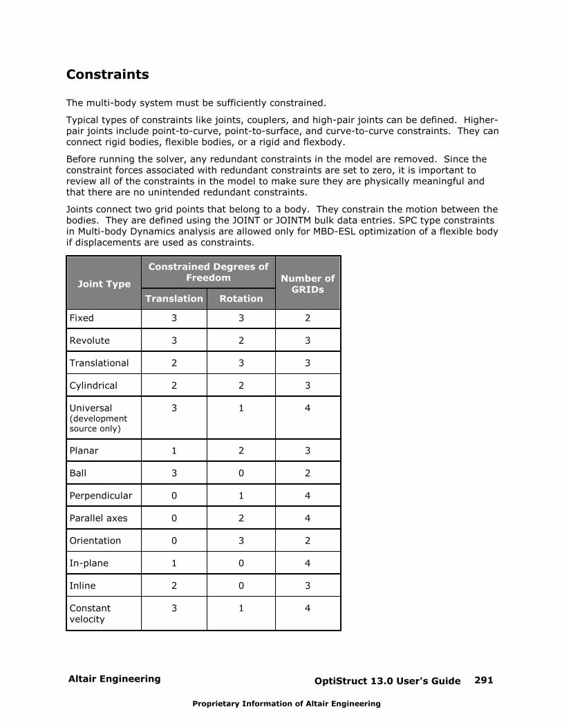
Altair Engineering OptiStruct 13.0 User's Guide 291
Proprietary Information of Altair Engineering
Constraints
The multi-body system must be sufficiently constrained.
Typical types of constraints like joints, couplers, and high-pair joints can be defined. Higher-pair joints include point-to-curve, point-to-surface, and curve-to-curve constraints. They canconnect rigid bodies, flexible bodies, or a rigid and flexbody.
Before running the solver, any redundant constraints in the model are removed. Since theconstraint forces associated with redundant constraints are set to zero, it is important toreview all of the constraints in the model to make sure they are physically meaningful andthat there are no unintended redundant constraints.
Joints connect two grid points that belong to a body. They constrain the motion between thebodies. They are defined using the JOINT or JOINTM bulk data entries. SPC type constraintsin Multi-body Dynamics analysis are allowed only for MBD-ESL optimization of a flexible bodyif displacements are used as constraints.
Joint Type
Constrained Degrees ofFreedom Number of
GRIDsTranslation Rotation
Fixed 3 3 2
Revolute 3 2 3
Translational 2 3 3
Cylindrical 2 2 3
Universal(developmentsource only)
3 1 4
Planar 1 2 3
Ball 3 0 2
Perpendicular 0 1 4
Parallel axes 0 2 4
Orientation 0 3 2
In-plane 1 0 4
Inline 2 0 3
Constantvelocity
3 1 4

OptiStruct 13.0 User's Guide292 Altair Engineering
Proprietary Information of Altair Engineering
Couplers are constraints between the translational and/or the rotational motion of two orthree joints. They are defined using the COUPLER bulk data entries.
Higher-pair joints are connecting points, curves and surfaces. They can be rigid ordeformable.
Higher-pair JointType
Bulk DataEntry
Point-to-curve MBPTCV
Point-to-deformablecurve
MBPTDCV
Point-to-deformablesurface
MBPTDSF
Curve-to-curve MBCVCV
These entries refer to the parametric curve definition (MBPCRV), deformable curve definition(MBPTDCV), and deformable surface definition (MBDSRF).
Altair Engineering OptiStruct 13.0 User's Guide 293
Proprietary Information of Altair Engineering
Contact
The contact modeling capability for multi-body dynamics can handle complex contactscenarios between rigid bodies and rigid and flexible bodies. For the definition you have toidentify geometries on one body that can contact a different set of geometries on a secondbody. You also specify the contact material properties such as coefficient of restitution andfriction. The solver monitors the proximity of the specified geometries to each other. Whencontact between the two sets of geometry occurs, a force based on the defined physicalproperties is generated. This represents the contact force. Both normal and frictional forcesare modeled. When the bodies separate, the force becomes zero.
There are four key features to the contact capability:
Modeling the geometry of the bodies that are in contact
Detecting the onset of contact
Applying the contact force
Detecting the end of a contact "incident" and removing the contact force
Two contact types are available: Rigid body to rigid body (MBCNTR) which is defined as thecontact of two element sets (SET) and rigid to flexible body (MBCNTDS) which is defined asthe contact between a node set (SET) and a deformable surface. The deformable surfacemust be defined by the MBDSRF bulk data entry.
When the onset of a collision is detected, the collision detection algorithm returns a set ofinterfering polygons. From those the solver computes the following:
The point of contact and surface normal vector
The magnitude and direction of the normal and friction forces
Once the point of contact and surface normal vector are known, the normal and friction forcemagnitudes are computed using a penalty-based Poisson contact normal force model. Thetwo primary inputs to this model are the penalty and the coefficient of restitution (COR). COR is defined as the ratio of relative speed of separation to the relative speed of approach ofthe colliding bodies. A COR of 1.0 implies a perfectly elastic collision and a COR of 0.0represents a perfectly plastic collision. One may think of the COR as damping and penalty asstiffness. Too high of a penalty value may cause numerical difficulties, while too small of avalue may lead to excessive penetration. Some fine-tuning of these two parameters isusually required to reach stable and accurate results.
The frictional force is modeled as a viscous force according to the following law:
In the above equations:
is the current slip speed at the point of contact.
is the coefficient of static friction.
is the coefficient of dynamic friction.
is the stiction transition slip speed at which the full value of is used for thecoefficient of friction.

OptiStruct 13.0 User's Guide294 Altair Engineering
Proprietary Information of Altair Engineering
is the dynamic friction slip speed at which the full value of is used for thecoefficient of friction.
is the friction force that is to be applied. The friction force opposes the direction ofthe slip velocity.

Altair Engineering OptiStruct 13.0 User's Guide 295
Proprietary Information of Altair Engineering
Compliant Elements
Compliant elements are bushings, spring-dampers, and beams. For each, the relevantinformation such as stiffness, damping, preload, attachment markers, etc. needs to bedefined. Stiffness and damping value numbers should correctly represent the actual systemand must be physically meaningful. Otherwise, the system may inadvertently turn out to benumerically stiff, even though the physical system may not be.
Compliant elements can be defined with respect to grid points or with respect to markers.
CMBEAM and CMBEAMM bulk data entries define beam elements.
CMBUSH and CMBUSHM bulk data entries define bushing elements. A bushing element haslinear stiffness and damping properties.
CMSPDP and CMSPDPM bulk data entries define spring-damper elements.
OptiStruct 13.0 User's Guide296 Altair Engineering
Proprietary Information of Altair Engineering
Applied Forces and Motions
Forces and moments can be present in the system. There are action-only forces which areapplied to one point, and action-reaction forces which are applied to two points. Forcecomponents can be a constant value, a curve, an expression, or a user-written subroutine.
A special force is gravity. Acceleration is applied to a body and from mass and acceleration,the gravitational force is computed.
Motion is a scalar constraint to the system. Displacement, velocity, and acceleration-typemotions are possible. The motion must depend only on time and not on any other measuresin the model that could change during the simulation. In other words, at every time stepwith only time as the independent parameter, the solver should be able to evaluate theexpression completely without using any other information about the model. For example,the motion cannot depend upon displacement or velocity or acceleration between two pointsin the model.
Motion can be specified as a constant value, a curve, an expression, or user-writtensubroutine. Motion is either defined as motion between two points or joint motion. When amotion is applied on a joint, one joint degree of freedom is controlled as a function of time. When a motion is applied between two points, movement along a user-specified direction iscontrolled as a function of time.
Forces are always defined at grid points, and can be applied to one grid point (action-only) ortwo (action-reaction). The bulk data entry MBFRC defines constant force; the entry MBFRCCdefines force by a curve; and the entry MBFRCE defines a force by equation.
Moments are always defined at grid points, and can be applied to one grid point (action-only)or two (action-reaction). The bulk data entry MBMNT defines constant moment; the entryMBMNTC defines moment by a curve; and the entry MBMNTE defines a moment by equation.
GRAV defines the gravity acceleration.
The entry MLOAD can be used to derive force and moment set combinations.
Motion can be defined as grid point motion or as joint motion. Grid point motion can beapplied to one grid point or two (relative motion). The bulk data entry MOTNG definesconstant motion; the entry MOTNGC defines motion by a curve, and MOTNGE defines motionby an equation. Joint motion can be applied to translational or revolute joints only. The bulkdata entry MOTNJ defines constant motion; the entry MOTNJC defines motion by a curve, and MOTNJE defines motion by an equation. The entry MOTION can be used to derive motion setcombinations.

Altair Engineering OptiStruct 13.0 User's Guide 297
Proprietary Information of Altair Engineering
Initial Velocity
Initial velocity is part of the problem formulation of the equation of motion. It can be appliedto bodies or to cylindrical, translational, and rotational joints.
The INVELB bulk data entry defines body initial velocity. The entry INVEL can be used toderive initial velocity set combinations.

OptiStruct 13.0 User's Guide298 Altair Engineering
Proprietary Information of Altair Engineering
Function Expressions
Expressions can be used in many places. They formulate relationships as functions of time,displacements, velocities, acceleration, forces, etc. If geometric points are used in anequation, they are always related to markers.
The bulk data entry MBVAR is used to define equations.
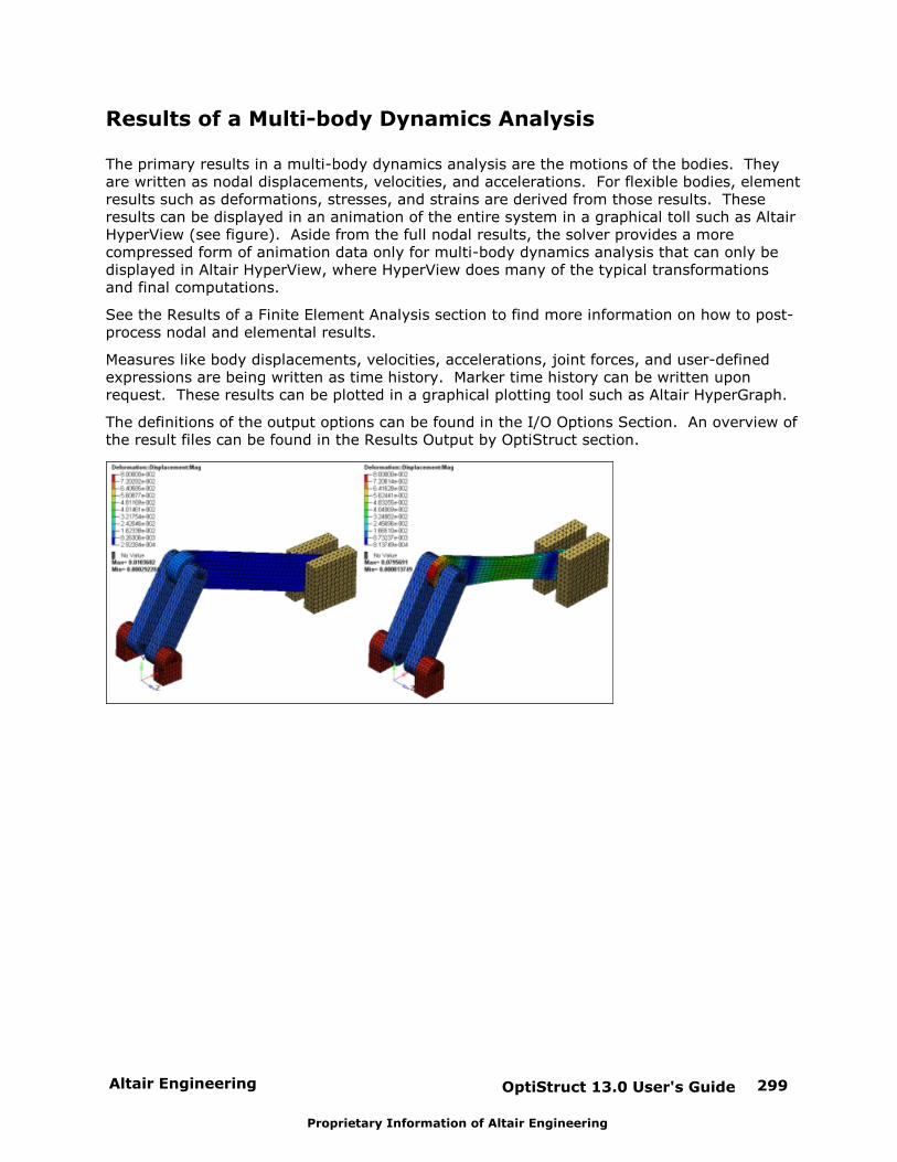
Altair Engineering OptiStruct 13.0 User's Guide 299
Proprietary Information of Altair Engineering
Results of a Multi-body Dynamics Analysis
The primary results in a multi-body dynamics analysis are the motions of the bodies. Theyare written as nodal displacements, velocities, and accelerations. For flexible bodies, elementresults such as deformations, stresses, and strains are derived from those results. Theseresults can be displayed in an animation of the entire system in a graphical toll such as AltairHyperView (see figure). Aside from the full nodal results, the solver provides a morecompressed form of animation data only for multi-body dynamics analysis that can only bedisplayed in Altair HyperView, where HyperView does many of the typical transformationsand final computations.
See the Results of a Finite Element Analysis section to find more information on how to post-process nodal and elemental results.
Measures like body displacements, velocities, accelerations, joint forces, and user-definedexpressions are being written as time history. Marker time history can be written uponrequest. These results can be plotted in a graphical plotting tool such as Altair HyperGraph.
The definitions of the output options can be found in the I/O Options Section. An overview ofthe result files can be found in the Results Output by OptiStruct section.
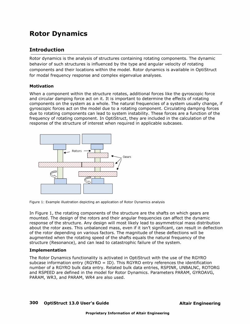
OptiStruct 13.0 User's Guide300 Altair Engineering
Proprietary Information of Altair Engineering
Rotor Dynamics
Introduction
Rotor dynamics is the analysis of structures containing rotating components. The dynamic
behavior of such structures is influenced by the type and angular velocity of rotating
components and their locations within the model. Rotor dynamics is available in OptiStruct
for modal frequency response and complex eigenvalue analyses.
Motivation
When a component within the structure rotates, additional forces like the gyroscopic forceand circular damping force act on it. It is important to determine the effects of rotatingcomponents on the system as a whole. The natural frequencies of a system usually change, ifgyroscopic forces act on the model due to a rotating component. Circulating damping forcesdue to rotating components can lead to system instability. These forces are a function of thefrequency of rotating component. In OptiStruct, they are included in the calculation of theresponse of the structure of interest when required in applicable subcases.
Figure 1: Example illustration depicting an application of Rotor Dynamics analysis
In Figure 1, the rotating components of the structure are the shafts on which gears aremounted. The design of the rotors and their angular frequencies can affect the dynamicresponse of the structure. Any design will most likely lead to asymmetrical mass distributionabout the rotor axes. This unbalanced mass, even if it isn’t significant, can result in deflectionof the rotor depending on various factors. The magnitude of these deflections will beaugmented when the rotating speed of the shafts equals the natural frequency of thestructure (Resonance), and can lead to catastrophic failure of the system.
Implementation
The Rotor Dynamics functionality is activated in OptiStruct with the use of the RGYROsubcase information entry (RGYRO = ID). This RGYRO entry references the identificationnumber of a RGYRO bulk data entry. Related bulk data entries, RSPINR, UNBALNC, ROTORGand RSPEED are defined in the model for Rotor Dynamics. Parameters PARAM, GYROAVG,PARAM, WR3, and PARAM, WR4 are also used.
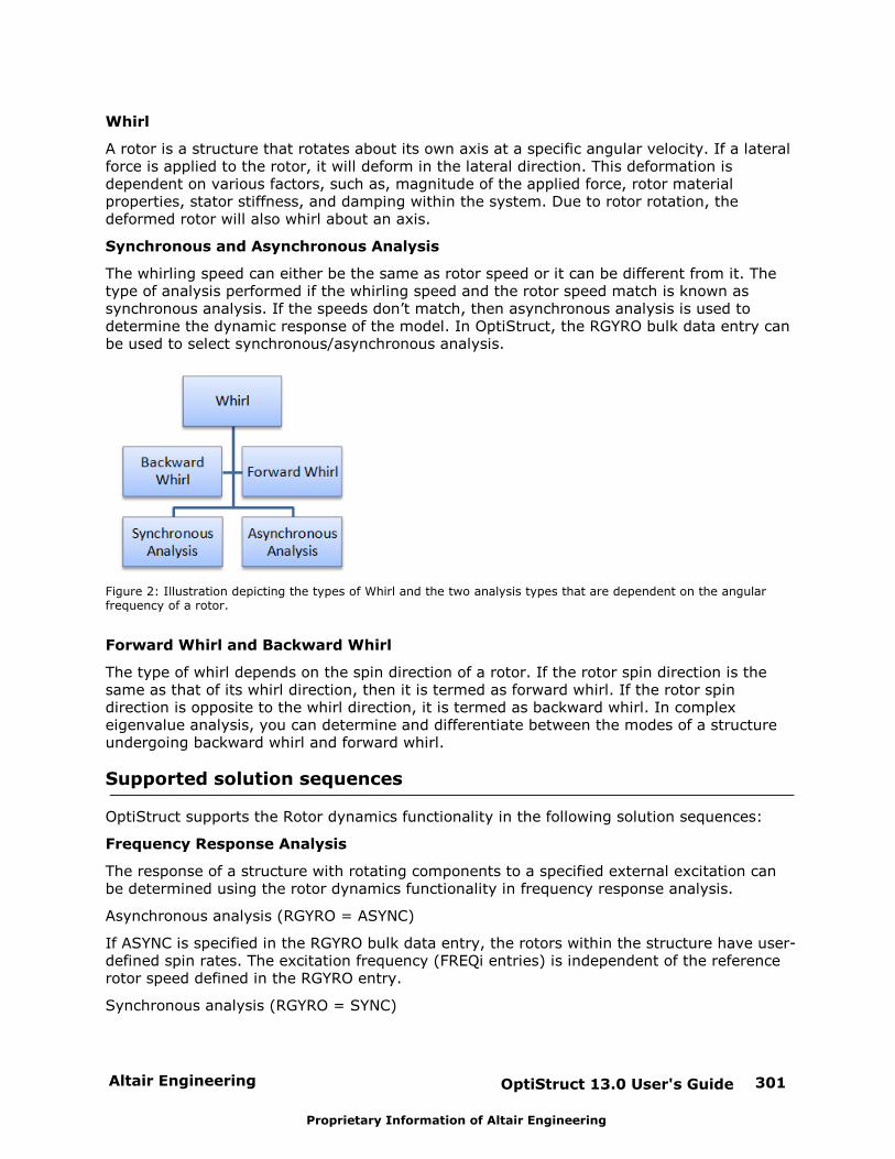
Altair Engineering OptiStruct 13.0 User's Guide 301
Proprietary Information of Altair Engineering
Whirl
A rotor is a structure that rotates about its own axis at a specific angular velocity. If a lateralforce is applied to the rotor, it will deform in the lateral direction. This deformation isdependent on various factors, such as, magnitude of the applied force, rotor materialproperties, stator stiffness, and damping within the system. Due to rotor rotation, thedeformed rotor will also whirl about an axis.
Synchronous and Asynchronous Analysis
The whirling speed can either be the same as rotor speed or it can be different from it. Thetype of analysis performed if the whirling speed and the rotor speed match is known assynchronous analysis. If the speeds don’t match, then asynchronous analysis is used todetermine the dynamic response of the model. In OptiStruct, the RGYRO bulk data entry canbe used to select synchronous/asynchronous analysis.
Figure 2: Illustration depicting the types of Whirl and the two analysis types that are dependent on the angularfrequency of a rotor.
Forward Whirl and Backward Whirl
The type of whirl depends on the spin direction of a rotor. If the rotor spin direction is thesame as that of its whirl direction, then it is termed as forward whirl. If the rotor spindirection is opposite to the whirl direction, it is termed as backward whirl. In complexeigenvalue analysis, you can determine and differentiate between the modes of a structureundergoing backward whirl and forward whirl.
Supported solution sequences
OptiStruct supports the Rotor dynamics functionality in the following solution sequences:
Frequency Response Analysis
The response of a structure with rotating components to a specified external excitation canbe determined using the rotor dynamics functionality in frequency response analysis.
Asynchronous analysis (RGYRO = ASYNC)
If ASYNC is specified in the RGYRO bulk data entry, the rotors within the structure have user-defined spin rates. The excitation frequency (FREQi entries) is independent of the referencerotor speed defined in the RGYRO entry.
Synchronous analysis (RGYRO = SYNC)
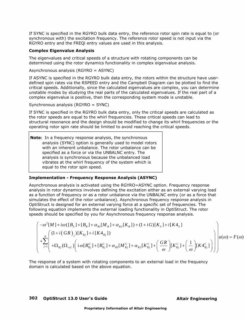
OptiStruct 13.0 User's Guide302 Altair Engineering
Proprietary Information of Altair Engineering
If SYNC is specified in the RGYRO bulk data entry, the reference rotor spin rate is equal to (orsynchronous with) the excitation frequency. The reference rotor speed is not input via theRGYRO entry and the FREQi entry values are used in this analysis.
Complex Eigenvalue Analysis
The eigenvalues and critical speeds of a structure with rotating components can bedetermined using the rotor dynamics functionality in complex eigenvalue analysis.
Asynchronous analysis (RGYRO = ASYNC)
If ASYNC is specified in the RGYRO bulk data entry, the rotors within the structure have user-defined spin rates via the RSPEED entry and the Campbell Diagram can be plotted to find thecritical speeds. Additionally, since the calculated eigenvalues are complex, you can determineunstable modes by studying the real parts of the calculated eigenvalues. If the real part of acomplex eigenvalue is positive, then the corresponding system mode is unstable.
Synchronous analysis (RGYRO = SYNC)
If SYNC is specified in the RGYRO bulk data entry, only the critical speeds are calculated asthe rotor speeds are equal to the whirl frequencies. These critical speeds can lead tostructural resonance and the design should be modified to change its whirl frequencies or theoperating rotor spin rate should be limited to avoid reaching the critical speeds.
Note: In a frequency response analysis, the synchronous
analysis (SYNC) option is generally used to model rotorswith an inherent unbalance. The rotor unbalance can bespecified as a force or via the UNBALNC entry. Theanalysis is synchronous because the unbalanced loadvibrates at the whirl frequency of the system which isequal to the rotor spin speed.
Implementation - Frequency Response Analysis (ASYNC)
Asynchronous analysis is activated using the RGYRO=ASYNC option. Frequency responseanalysis in rotor dynamics involves defining the excitation either as an external varying loadas a function of frequency or as a rotor unbalance via the UNBALNC entry (or as a force thatsimulates the effect of the rotor unbalance). Asynchronous frequency response analysis inOptiStruct is designed for an external varying force at a specific set of frequencies. Thefollowing equation implements the external loading functionality in OptiStruct. The rotorspeeds should be specified by you for Asynchronous frequency response analysis.
21 2
1 1 2
[ ] ([ ] [ ] [ ] [ ]) (1 )[ ] [ 4 ]
(1 )[ ] [ 4 ])( ) ( )
1( ) i [ ] [ ] [ ] [ ] [ ] [ 4 ]
S R R R R R S S
Rj RjjN
G C C C C Cj Rj ref Rj Rj R Rj R Rj Rj Rj
M i B B M K iG K i K
i GR K i Ku F
GRB B M K K K
The response of a system with rotating components to an external load in the frequencydomain is calculated based on the above equation.
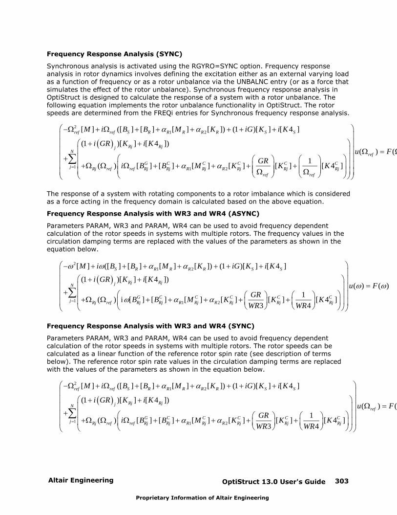
Altair Engineering OptiStruct 13.0 User's Guide 303
Proprietary Information of Altair Engineering
Frequency Response Analysis (SYNC)
Synchronous analysis is activated using the RGYRO=SYNC option. Frequency responseanalysis in rotor dynamics involves defining the excitation either as an external varying loadas a function of frequency or as a rotor unbalance via the UNBALNC entry (or as a force thatsimulates the effect of the rotor unbalance). Synchronous frequency response analysis inOptiStruct is designed to calculate the response of a system with a rotor unbalance. Thefollowing equation implements the rotor unbalance functionality in OptiStruct. The rotorspeeds are determined from the FREQi entries for Synchronous frequency response analysis.
21 2
1 1 2
[ ] ([ ] [ ] [ ] [ ]) (1 )[ ] [ 4 ]
(1 )[ ] [ 4 ])
1( ) [ ] [ ] [ ] [ ] [ ] [ 4 ]
ref ref S R R R R R S S
Rj RjjN
G C C C C Cj Rj ref ref Rj Rj R Rj R Rj Rj Rj
ref ref
M i B B M K iG K i K
i GR K i K
GRi B B M K K K
( ) ( )ref refu F
The response of a system with rotating components to a rotor imbalance which is consideredas a force acting in the frequency domain is calculated based on the above equation.
Frequency Response Analysis with WR3 and WR4 (ASYNC)
Parameters PARAM, WR3 and PARAM, WR4 can be used to avoid frequency dependentcalculation of the rotor speeds in systems with multiple rotors. The frequency values in thecirculation damping terms are replaced with the values of the parameters as shown in theequation below.
21 2
1 1 2
[ ] ([ ] [ ] [ ] [ ]) (1 )[ ] [ 4 ]
(1 )[ ] [ 4 ])( ) (
1( ) i [ ] [ ] [ ] [ ] [ ] [ 4 ]
3 4
S R R R R R S S
Rj RjjN
G C C C C Cj Rj ref Rj Rj R Rj R Rj Rj Rj
M i B B M K iG K i K
i GR K i Ku F
GRB B M K K K
WR WR
)
Frequency Response Analysis with WR3 and WR4 (SYNC)
Parameters PARAM, WR3 and PARAM, WR4 can be used to avoid frequency dependentcalculation of the rotor speeds in systems with multiple rotors. The rotor speeds can becalculated as a linear function of the reference rotor spin rate (see description of termsbelow). The reference rotor spin rate values in the circulation damping terms are replacedwith the values of the parameters as shown in the equation below.
21 2
1 1 2
[ ] ([ ] [ ] [ ] [ ]) (1 )[ ] [ 4 ]
(1 )[ ] [ 4 ])
1( ) [ ] [ ] [ ] [ ] [ ] [ 4 ]
3 4
ref ref S R R R R R S S
Rj RjjN
G C C C C Cj Rj ref ref Rj Rj R Rj R Rj Rj Rj
M i B B M K iG K i K
i GR K i K
GRi B B M K K K
WR WR
( ) ( )ref refu F
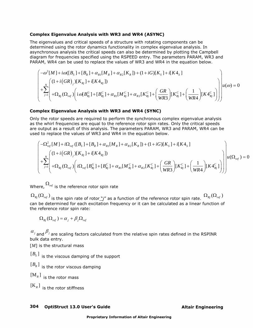
OptiStruct 13.0 User's Guide304 Altair Engineering
Proprietary Information of Altair Engineering
Complex Eigenvalue Analysis with WR3 and WR4 (ASYNC)
The eigenvalues and critical speeds of a structure with rotating components can bedetermined using the rotor dynamics functionality in complex eigenvalue analysis. Inasynchronous analysis the critical speeds can also be determined by plotting the Campbelldiagram for frequencies specified using the RSPEED entry. The parameters PARAM, WR3 andPARAM, WR4 can be used to replace the values of WR3 and WR4 in the equation below.
21 2
1 1 2
[ ] ([ ] [ ] [ ] [ ]) (1 )[ ] [ 4 ]
(1 )[ ] [ 4 ])( ) 0
1( ) i [ ] [ ] [ ] [ ] [ ] [ 4 ]
3 4
S R R R R R S S
Rj RjjN
G C C C C Cj Rj ref Rj Rj R Rj R Rj Rj Rj
M i B B M K iG K i K
i GR K i Ku
GRB B M K K K
WR WR
Complex Eigenvalue Analysis with WR3 and WR4 (SYNC)
Only the rotor speeds are required to perform the synchronous complex eigenvalue analysisas the whirl frequencies are equal to the reference rotor spin rates. Only the critical speedsare output as a result of this analysis. The parameters PARAM, WR3 and PARAM, WR4 can beused to replace the values of WR3 and WR4 in the equation below.
21 2
1 1 2
[ ] ([ ] [ ] [ ] [ ]) (1 )[ ] [ 4 ]
(1 )[ ] [ 4 ])
1( ) [ ] [ ] [ ] [ ] [ ] [ 4 ]
3 4
ref ref S R R R R R S S
Rj RjjN
G C C C C Cj Rj ref ref Rj Rj R Rj R Rj Rj Rj
M i B B M K iG K i K
i GR K i K
GRi B B M K K K
WR WR
( ) 0refu
Where, ref is the reference rotor spin rate
( )Rj ref is the spin rate of rotor “j” as a function of the reference rotor spin rate. ( )Rj ref
can be determined for each excitation frequency or it can be calculated as a linear function ofthe reference rotor spin rate:
( )Rj ref j j ref
j and j are scaling factors calculated from the relative spin rates defined in the RSPINRbulk data entry.
[M] is the structural mass
[ ]SB is the viscous damping of the support
[ ]RB is the rotor viscous damping
[M ]R is the rotor mass
[K ]R is the rotor stiffness
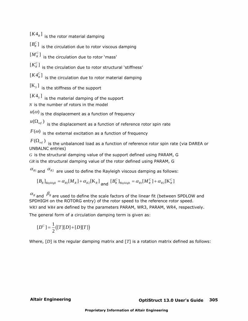
Altair Engineering OptiStruct 13.0 User's Guide 305
Proprietary Information of Altair Engineering
[ 4 ]RK is the rotor material damping
[ ]CRB
is the circulation due to rotor viscous damping
[ ]CRM
is the circulation due to rotor ‘mass’
[ ]CRK
is the circulation due to rotor structural ‘stiffness’
[ 4 ]CRK
is the circulation due to rotor material damping
[K ]S is the stiffness of the support
[ 4 ]SK is the material damping of the support
N is the number of rotors in the model
( )uis the displacement as a function of frequency
( )refu is the displacement as a function of reference rotor spin rate
( )F is the external excitation as a function of frequency
( )refF is the unbalanced load as a function of reference rotor spin rate (via DAREA or
UNBALNC entries)
G is the structural damping value of the support defined using PARAM, G
GR is the structural damping value of the rotor defined using PARAM, G
1R and 2R are used to define the Rayleigh viscous damping as follows:
1 2[ ] [ ] [K ]R Rayleigh R R R RB Mand 1 2[ ] [ ] [K ]C C C
R Rayleigh R R R RB M
R and R are used to define the scale factors of the linear fit (between SPDLOW andSPDHIGH on the ROTORG entry) of the rotor speed to the reference rotor speed.
WR3 and WR4 are defined by the parameters PARAM, WR3, PARAM, WR4, respectively.
The general form of a circulation damping term is given as:
1[ ] [ ][ ] [ ][ ]
2CD T D D T
Where, [D] is the regular damping matrix and [T] is a rotation matrix defined as follows:
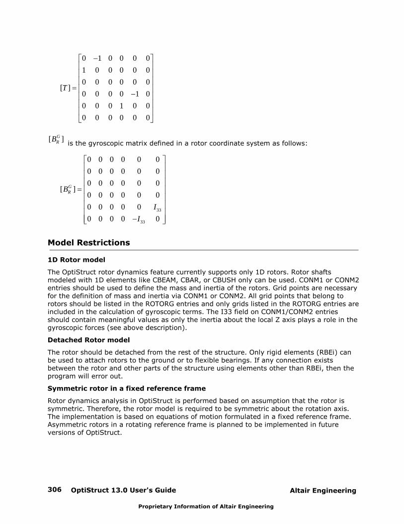
OptiStruct 13.0 User's Guide306 Altair Engineering
Proprietary Information of Altair Engineering
0 1 0 0 0 0
1 0 0 0 0 0
0 0 0 0 0 0[ ]
0 0 0 0 1 0
0 0 0 1 0 0
0 0 0 0 0 0
T
[ ]GRB
is the gyroscopic matrix defined in a rotor coordinate system as follows:
33
33
0 0 0 0 0 0
0 0 0 0 0 0
0 0 0 0 0 0[ ]
0 0 0 0 0 0
0 0 0 0 0
0 0 0 0 0
GRB
I
I
Model Restrictions
1D Rotor model
The OptiStruct rotor dynamics feature currently supports only 1D rotors. Rotor shaftsmodeled with 1D elements like CBEAM, CBAR, or CBUSH only can be used. CONM1 or CONM2entries should be used to define the mass and inertia of the rotors. Grid points are necessaryfor the definition of mass and inertia via CONM1 or CONM2. All grid points that belong torotors should be listed in the ROTORG entries and only grids listed in the ROTORG entries areincluded in the calculation of gyroscopic terms. The I33 field on CONM1/CONM2 entriesshould contain meaningful values as only the inertia about the local Z axis plays a role in thegyroscopic forces (see above description).
Detached Rotor model
The rotor should be detached from the rest of the structure. Only rigid elements (RBEi) canbe used to attach rotors to the ground or to flexible bearings. If any connection existsbetween the rotor and other parts of the structure using elements other than RBEi, then theprogram will error out.
Symmetric rotor in a fixed reference frame
Rotor dynamics analysis in OptiStruct is performed based on assumption that the rotor issymmetric. Therefore, the rotor model is required to be symmetric about the rotation axis.The implementation is based on equations of motion formulated in a fixed reference frame.Asymmetric rotors in a rotating reference frame is planned to be implemented in futureversions of OptiStruct.
Altair Engineering OptiStruct 13.0 User's Guide 307
Proprietary Information of Altair Engineering
Multiple Rotors
During synchronous analysis, the calculations are performed with respect to the referencerotor. In synchronous frequency response analysis, the reference rotor is rotating at thefrequency of the unbalanced load and in synchronous complex eigenvalue analysis, thereference rotor is rotating at the whirl frequency of the system. The interpretation of resultsin a multiple rotor system should always be done with respect to the reference rotor. Anydeduction of results from the behavior of rotors other than the reference rotor will beinaccurate and can lead to incorrect results. If the behavior of a rotor other than thereference rotor is to be studied, a different analysis should be run with the rotor of interest asthe reference rotor.
Campbell Diagram
The critical speeds of a rotating structure should be calculated and the design parameters canthen be altered if necessary to restrict the operating speeds of the structure from attainingthose resonant speeds. The structure may undergo excessive amplitude and phase changes ifits operating speeds reach critical speeds. The calculation of critical speeds in OptiStruct canbe undertaken in two ways:
1. Synchronous Complex Eigenvalue Analysis
The RGYRO=SYNC option in Complex Eigenvalue Analysis can be used to determine theexact critical speeds of the rotating structure. During a synchronous analysis, the rotorspeed is equal to the whirl frequency of the structure, which by definition, are the criticalspeeds of the structure that should be avoided during its operation.
Figure 3: An example Campbell Diagram to calculate the critical speeds.
2. Asynchronous Complex Eigenvalue Analysis
The RGYRO=ASYNC option and the RSPEED bulk data entry in Complex EigenvalueAnalysis can be used to determine the whirl frequencies (backward whirl and forwardwhirl) of the structure. These Whirl frequencies can be calculated for a sequence of rotorspin rates. Forward Whirl and Backward Whirl frequencies can then be plotted against therange of rotor spin rates (Figure 3). The critical speeds can be calculated bysuperimposing the “Rotor Spin Rate = Whirl Frequencies” line on the plot. The points ofintersection are the critical speeds.

OptiStruct 13.0 User's Guide308 Altair Engineering
Proprietary Information of Altair Engineering
Note: The rotor speeds specified on the RSPEED entry shouldbe input with sufficiently fine resolution to be able tocapture the critical speeds. If the specified rotor speedsare too far apart, the critical speeds may be missed.
Altair Engineering OptiStruct 13.0 User's Guide 309
Proprietary Information of Altair Engineering
NVH Applications and Techniques
The NVH Applications and Techniques section provides an overview of the following:
Transfer Path Analysis on an Automobile
Residual Runs using Super Elements
Basic OptiStruct NVH Output Files
Global Search Option
Create Door and Deck Lid Seals
Create a HyperGraph Template for Reading in Multiple Files
Using AMSES (Automatic Multi-Level Sub-Structuring Eigensolver Solution)
Poroelastic Materials (Biot theory)
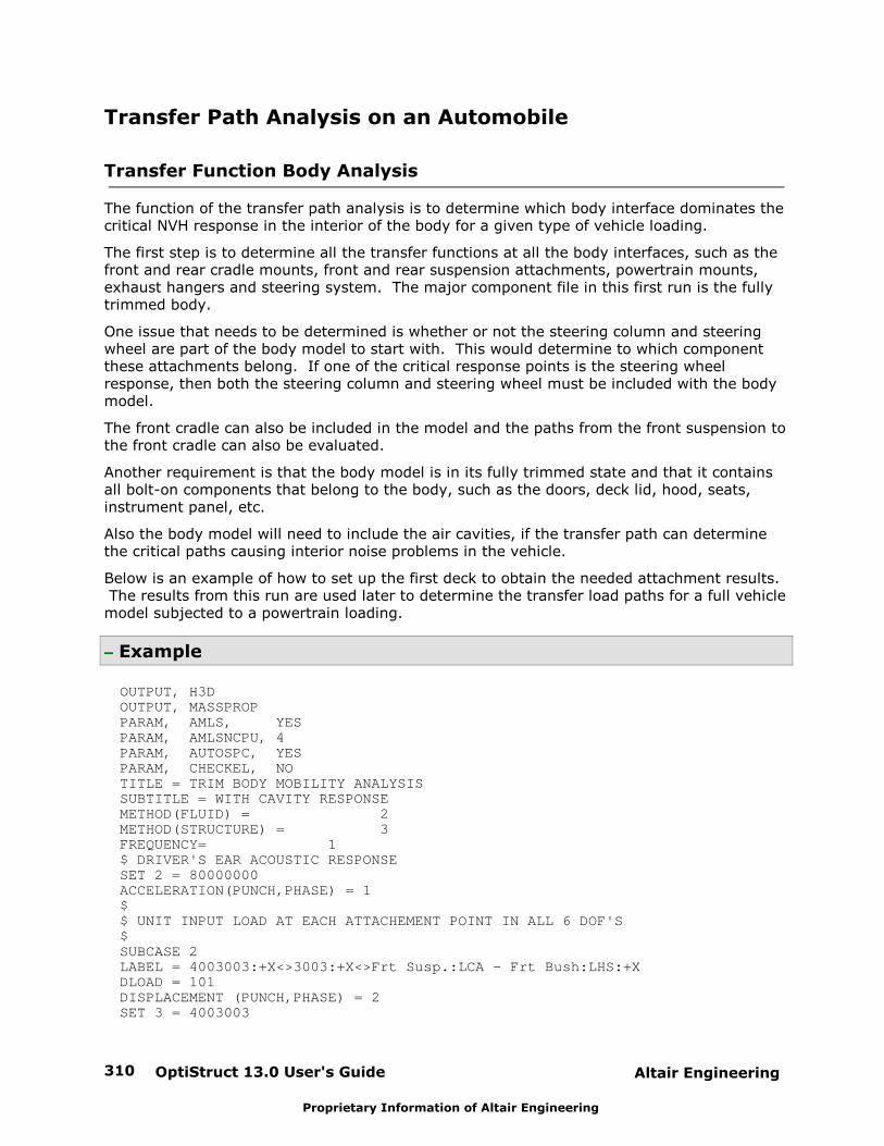
OptiStruct 13.0 User's Guide310 Altair Engineering
Proprietary Information of Altair Engineering
Transfer Path Analysis on an Automobile
Transfer Function Body Analysis
The function of the transfer path analysis is to determine which body interface dominates thecritical NVH response in the interior of the body for a given type of vehicle loading.
The first step is to determine all the transfer functions at all the body interfaces, such as thefront and rear cradle mounts, front and rear suspension attachments, powertrain mounts,exhaust hangers and steering system. The major component file in this first run is the fullytrimmed body.
One issue that needs to be determined is whether or not the steering column and steeringwheel are part of the body model to start with. This would determine to which componentthese attachments belong. If one of the critical response points is the steering wheelresponse, then both the steering column and steering wheel must be included with the bodymodel.
The front cradle can also be included in the model and the paths from the front suspension tothe front cradle can also be evaluated.
Another requirement is that the body model is in its fully trimmed state and that it containsall bolt-on components that belong to the body, such as the doors, deck lid, hood, seats,instrument panel, etc.
Also the body model will need to include the air cavities, if the transfer path can determinethe critical paths causing interior noise problems in the vehicle.
Below is an example of how to set up the first deck to obtain the needed attachment results. The results from this run are used later to determine the transfer load paths for a full vehiclemodel subjected to a powertrain loading.
Example
OUTPUT, H3DOUTPUT, MASSPROPPARAM, AMLS, YESPARAM, AMLSNCPU, 4PARAM, AUTOSPC, YESPARAM, CHECKEL, NOTITLE = TRIM BODY MOBILITY ANALYSIS SUBTITLE = WITH CAVITY RESPONSE METHOD(FLUID) = 2METHOD(STRUCTURE) = 3FREQUENCY= 1$ DRIVER'S EAR ACOUSTIC RESPONSESET 2 = 80000000ACCELERATION(PUNCH,PHASE) = 1$$ UNIT INPUT LOAD AT EACH ATTACHEMENT POINT IN ALL 6 DOF'S$SUBCASE 2LABEL = 4003003:+X<>3003:+X<>Frt Susp.:LCA - Frt Bush:LHS:+XDLOAD = 101DISPLACEMENT (PUNCH,PHASE) = 2SET 3 = 4003003
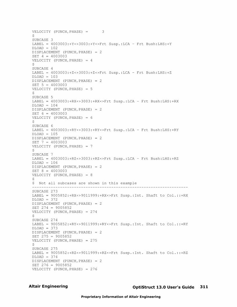
Altair Engineering OptiStruct 13.0 User's Guide 311
Proprietary Information of Altair Engineering
VELOCITY (PUNCH,PHASE) = 3$SUBCASE 3LABEL = 4003003:+Y<>3003:+Y<>Frt Susp.:LCA - Frt Bush:LHS:+YDLOAD = 102DISPLACEMENT (PUNCH,PHASE) = 2SET 4 = 4003003VELOCITY (PUNCH,PHASE) = 4$SUBCASE 4LABEL = 4003003:+Z<>3003:+Z<>Frt Susp.:LCA - Frt Bush:LHS:+ZDLOAD = 103DISPLACEMENT (PUNCH,PHASE) = 2SET 5 = 4003003VELOCITY (PUNCH,PHASE) = 5$SUBCASE 5LABEL = 4003003:+RX<>3003:+RX<>Frt Susp.:LCA - Frt Bush:LHS:+RXDLOAD = 104DISPLACEMENT (PUNCH,PHASE) = 2SET 6 = 4003003VELOCITY (PUNCH,PHASE) = 6$SUBCASE 6LABEL = 4003003:+RY<>3003:+RY<>Frt Susp.:LCA - Frt Bush:LHS:+RYDLOAD = 105DISPLACEMENT (PUNCH,PHASE) = 2SET 7 = 4003003VELOCITY (PUNCH,PHASE) = 7$SUBCASE 7LABEL = 4003003:+RZ<>3003:+RZ<>Frt Susp.:LCA - Frt Bush:LHS:+RZDLOAD = 106DISPLACEMENT (PUNCH,PHASE) = 2SET 8 = 4003003VELOCITY (PUNCH,PHASE) = 8$ $ Not all subcases are shown in this example-------------------------------------------------------------------SUBCASE 273LABEL = 9005852:+RX<>9011999:+RX<>Frt Susp.:Int. Shaft to Col.::+RXDLOAD = 372DISPLACEMENT (PUNCH,PHASE) = 2SET 274 = 9005852VELOCITY (PUNCH,PHASE) = 274$SUBCASE 274LABEL = 9005852:+RY<>9011999:+RY<>Frt Susp.:Int. Shaft to Col.::+RYDLOAD = 373DISPLACEMENT (PUNCH,PHASE) = 2SET 275 = 9005852VELOCITY (PUNCH,PHASE) = 275$SUBCASE 275LABEL = 9005852:+RZ<>9011999:+RZ<>Frt Susp.:Int. Shaft to Col.::+RZDLOAD = 374DISPLACEMENT (PUNCH,PHASE) = 2SET 276 = 9005852VELOCITY (PUNCH,PHASE) = 276
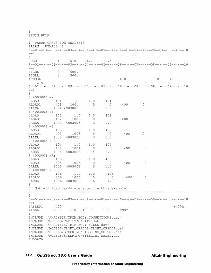
OptiStruct 13.0 User's Guide312 Altair Engineering
Proprietary Information of Altair Engineering
$$BEGIN BULK$$ PARAM CARDS FOR ANALYSISPARAM WTMASS 1.$==01==><==02==><==03==><==04==><==05==><==06==><==07==><==08==><==09==><==10==>$FREQ1 1 5.0 1.0 195 $==01==><==02==><==03==><==04==><==05==><==06==><==07==><==08==><==09==><==10==>EIGRL 2 600. EIGRL 3 300. ACMODL 4.0 1.0 1.0 1.0$==01==><==02==><==03==><==04==><==05==><==06==><==07==><==08==><==09==><==10==>$$ 4003003 +XDLOAD 101 1.0 1.0 401RLOAD1 401 1001 0 0 400 0DAREA 1001 4003003 1 1.0$ 4003003 +YDLOAD 102 1.0 1.0 402RLOAD1 402 1002 0 0 400 0DAREA 1002 4003003 2 1.0 $ 4003003 +ZDLOAD 103 1.0 1.0 403RLOAD1 403 1003 0 0 400 0DAREA 1003 4003003 3 1.0$ 4003003 +RXDLOAD 104 1.0 1.0 404RLOAD1 404 1004 0 0 400 0DAREA 1004 4003003 4 1.0$ 4003003 +RYDLOAD 105 1.0 1.0 405RLOAD1 405 1005 0 0 400 0DAREA 1005 4003003 5 1.0$ 4003003 +RZDLOAD 106 1.0 1.0 406RLOAD1 406 1006 0 0 400 0DAREA 1006 4003003 6 1.0$$ Not all load cards are shown in this example ----------------------------------------------------------------------------$$==01==><==02==><==03==><==04==><==05==><==06==><==07==><==08==><==09==><==10==>TABLED1 400 +400A+400A 20.0 1.0 400.0 1.0 ENDT$INCLUDE '/ANALYSIS/TRIM_BODY_CONNECTIONS.dat'INCLUDE '/MODELS/CAVITY/CAVITY.dat'INCLUDE '/ANALYSIS/TRIM_BODY_FILES.dat'INCLUDE '/MODELS/FRONT_CRADLE/FRONT_CRADLE.dat'INCLUDE '/MODELS/STEERING/STEERING_COLUMN.dat'INCLUDE '/MODELS/STEERING/STEERING_WHEEL.dat'ENDDATA
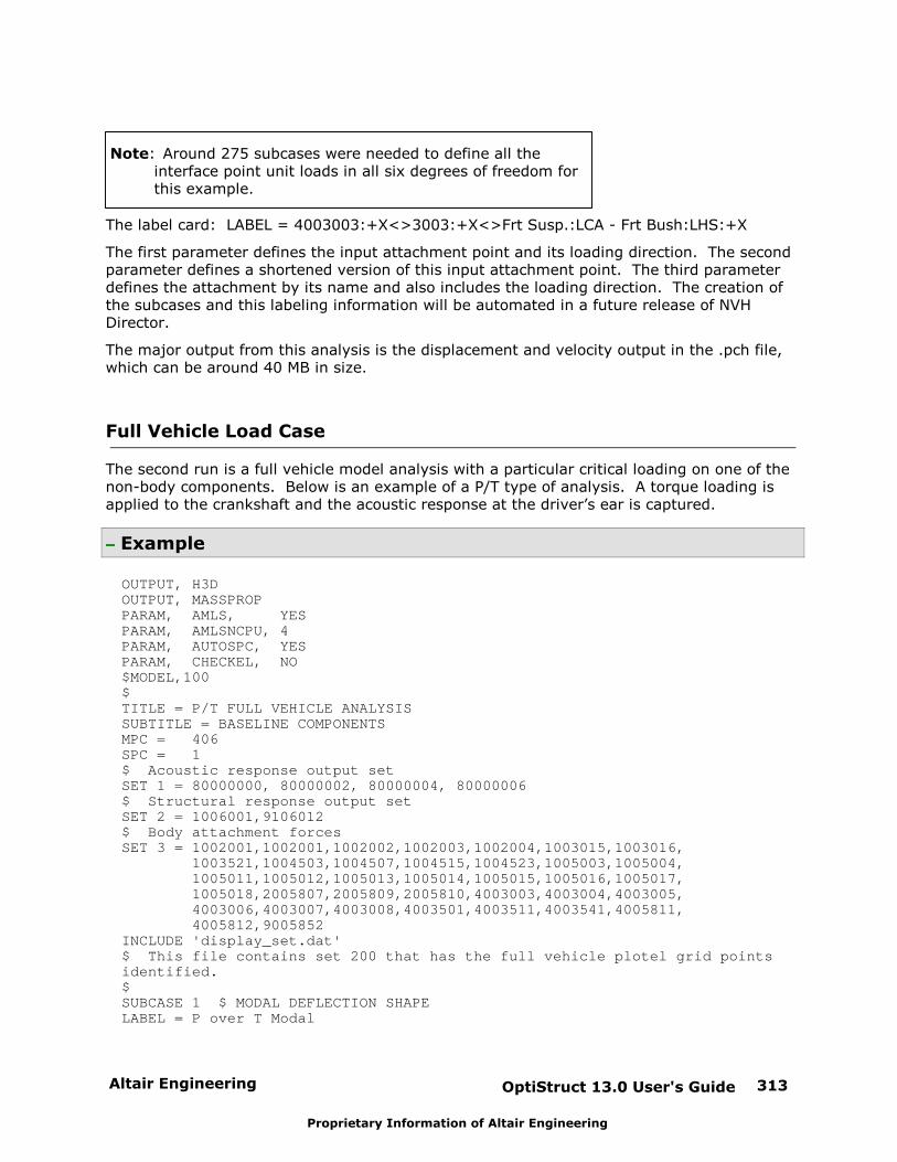
Altair Engineering OptiStruct 13.0 User's Guide 313
Proprietary Information of Altair Engineering
Note: Around 275 subcases were needed to define all theinterface point unit loads in all six degrees of freedom forthis example.
The label card: LABEL = 4003003:+X<>3003:+X<>Frt Susp.:LCA - Frt Bush:LHS:+X
The first parameter defines the input attachment point and its loading direction. The secondparameter defines a shortened version of this input attachment point. The third parameterdefines the attachment by its name and also includes the loading direction. The creation ofthe subcases and this labeling information will be automated in a future release of NVHDirector.
The major output from this analysis is the displacement and velocity output in the .pch file,which can be around 40 MB in size.
Full Vehicle Load Case
The second run is a full vehicle model analysis with a particular critical loading on one of thenon-body components. Below is an example of a P/T type of analysis. A torque loading isapplied to the crankshaft and the acoustic response at the driver’s ear is captured.
Example
OUTPUT, H3DOUTPUT, MASSPROPPARAM, AMLS, YESPARAM, AMLSNCPU, 4PARAM, AUTOSPC, YESPARAM, CHECKEL, NO$MODEL,100$TITLE = P/T FULL VEHICLE ANALYSISSUBTITLE = BASELINE COMPONENTSMPC = 406SPC = 1$ Acoustic response output setSET 1 = 80000000, 80000002, 80000004, 80000006$ Structural response output setSET 2 = 1006001,9106012$ Body attachment forcesSET 3 = 1002001,1002001,1002002,1002003,1002004,1003015,1003016, 1003521,1004503,1004507,1004515,1004523,1005003,1005004, 1005011,1005012,1005013,1005014,1005015,1005016,1005017, 1005018,2005807,2005809,2005810,4003003,4003004,4003005, 4003006,4003007,4003008,4003501,4003511,4003541,4005811, 4005812,9005852INCLUDE 'display_set.dat'$ This file contains set 200 that has the full vehicle plotel grid pointsidentified.$SUBCASE 1 $ MODAL DEFLECTION SHAPELABEL = P over T Modal
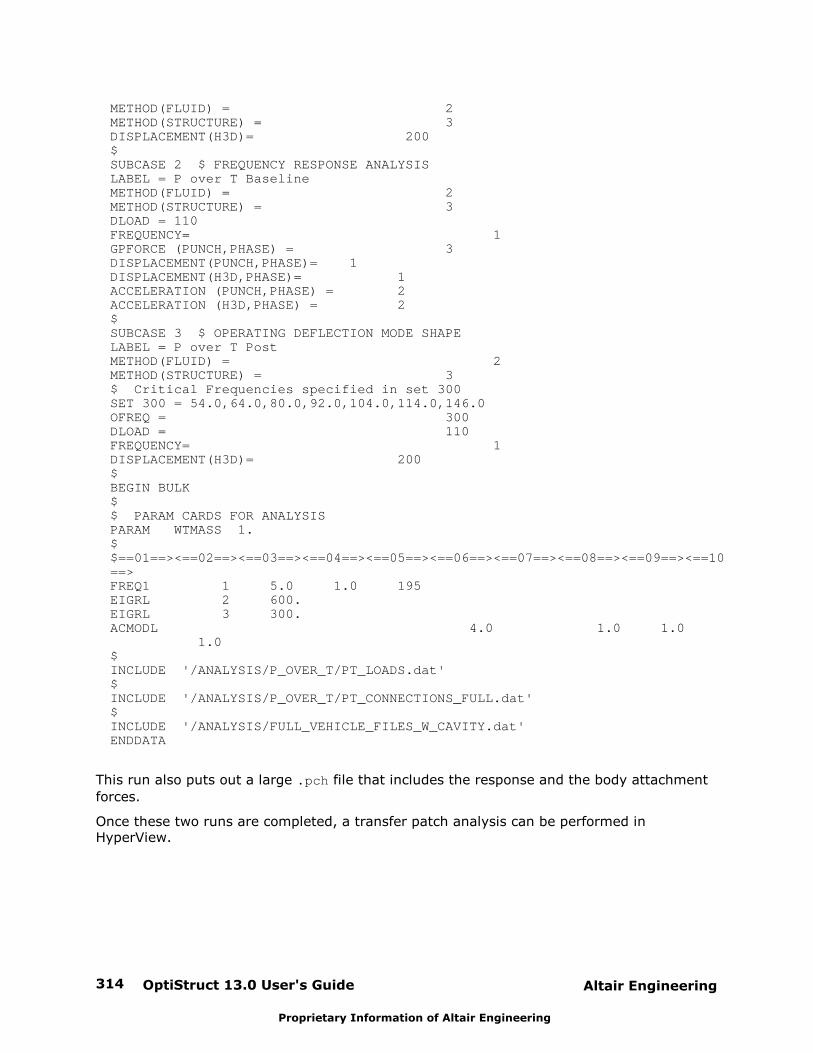
OptiStruct 13.0 User's Guide314 Altair Engineering
Proprietary Information of Altair Engineering
METHOD(FLUID) = 2METHOD(STRUCTURE) = 3DISPLACEMENT(H3D)= 200$SUBCASE 2 $ FREQUENCY RESPONSE ANALYSISLABEL = P over T BaselineMETHOD(FLUID) = 2METHOD(STRUCTURE) = 3DLOAD = 110FREQUENCY= 1GPFORCE (PUNCH,PHASE) = 3DISPLACEMENT(PUNCH,PHASE)= 1DISPLACEMENT(H3D,PHASE)= 1ACCELERATION (PUNCH,PHASE) = 2ACCELERATION (H3D,PHASE) = 2$SUBCASE 3 $ OPERATING DEFLECTION MODE SHAPELABEL = P over T PostMETHOD(FLUID) = 2METHOD(STRUCTURE) = 3$ Critical Frequencies specified in set 300SET 300 = 54.0,64.0,80.0,92.0,104.0,114.0,146.0OFREQ = 300DLOAD = 110FREQUENCY= 1DISPLACEMENT(H3D)= 200$BEGIN BULK$$ PARAM CARDS FOR ANALYSISPARAM WTMASS 1.$$==01==><==02==><==03==><==04==><==05==><==06==><==07==><==08==><==09==><==10==>FREQ1 1 5.0 1.0 195 EIGRL 2 600.EIGRL 3 300. ACMODL 4.0 1.0 1.0 1.0$ INCLUDE '/ANALYSIS/P_OVER_T/PT_LOADS.dat'$INCLUDE '/ANALYSIS/P_OVER_T/PT_CONNECTIONS_FULL.dat'$ INCLUDE '/ANALYSIS/FULL_VEHICLE_FILES_W_CAVITY.dat'ENDDATA
This run also puts out a large .pch file that includes the response and the body attachment
forces.
Once these two runs are completed, a transfer patch analysis can be performed inHyperView.
Altair Engineering OptiStruct 13.0 User's Guide 315
Proprietary Information of Altair Engineering
Transfer Path Analysis
To perform a transfer path analysis on this model, open up HyperView.
1. From the File menu, select Load > Preference File.
2. From the Preference dialog, select NVH Utilities and click Load.
3. From the NVH menu, select Transfer Path Analysis.
4. Click on the file browser icon to select a Transfer Function file.
This is the PCH from the first run.
5. Click on the file browser icon to select a Force file.
6. Select Load.
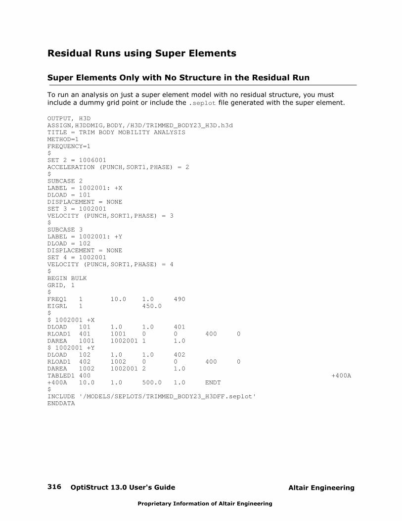
OptiStruct 13.0 User's Guide316 Altair Engineering
Proprietary Information of Altair Engineering
Residual Runs using Super Elements
Super Elements Only with No Structure in the Residual Run
To run an analysis on just a super element model with no residual structure, you mustinclude a dummy grid point or include the .seplot file generated with the super element.
OUTPUT, H3DASSIGN,H3DDMIG,BODY,/H3D/TRIMMED_BODY23_H3D.h3dTITLE = TRIM BODY MOBILITY ANALYSIS METHOD=1FREQUENCY=1$SET 2 = 1006001ACCELERATION (PUNCH,SORT1,PHASE) = 2$SUBCASE 2LABEL = 1002001: +XDLOAD = 101DISPLACEMENT = NONESET 3 = 1002001VELOCITY (PUNCH,SORT1,PHASE) = 3$SUBCASE 3LABEL = 1002001: +YDLOAD = 102DISPLACEMENT = NONESET 4 = 1002001VELOCITY (PUNCH,SORT1,PHASE) = 4$BEGIN BULKGRID, 1$FREQ1 1 10.0 1.0 490EIGRL 1 450.0$$ 1002001 +XDLOAD 101 1.0 1.0 401 RLOAD1 401 1001 0 0 400 0 DAREA 1001 1002001 1 1.0 $ 1002001 +YDLOAD 102 1.0 1.0 402 RLOAD1 402 1002 0 0 400 0 DAREA 1002 1002001 2 1.0 TABLED1 400 +400A +400A 10.0 1.0 500.0 1.0 ENDT $ INCLUDE '/MODELS/SEPLOTS/TRIMMED_BODY23_H3DFF.seplot'ENDDATA
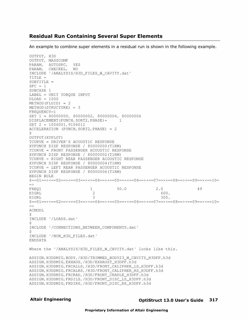
Altair Engineering OptiStruct 13.0 User's Guide 317
Proprietary Information of Altair Engineering
Residual Run Containing Several Super Elements
An example to combine super elements in a residual run is shown in the following example.
OUTPUT, H3DOUTPUT, MASSCOMPPARAM, AUTOSPC, YESPARAM, CHECKEL, NOINCLUDE '/ANALYSIS/H3D_FILES_W_CAVITY.dat'TITLE = SUBTITLE = SPC = 1 SUBCASE 1LABEL = UNIT TORQUE INPUT DLOAD = 1000METHOD(FLUID) = 2METHOD(STRUCTURE) = 3FREQUENCY=1SET 1 = 80000000, 80000002, 80000004, 80000006DISPLACEMENT(PUNCH,SORT2,PHASE)= 1SET 2 = 1006001,9106012ACCELERATION (PUNCH,SORT2,PHASE) = 2$OUTPUT(XYPLOT)TCURVE = DRIVER'S ACOUSTIC RESPONSEXYPUNCH DISP RESPONSE / 80000000(T1RM)TCURVE = FRONT PASSENGER ACOUSTIC RESPONSEXYPUNCH DISP RESPONSE / 80000002(T1RM)TCURVE = RIGHT REAR PASSENGER ACOUSTIC RESPONSEXYPUNCH DISP RESPONSE / 80000004(T1RM)TCURVE = LEFT REAR PASSENGER ACOUSTIC RESPONSEXYPUNCH DISP RESPONSE / 80000006(T1RM)BEGIN BULK$==01==><==02==><==03==><==04==><==05==><==06==><==07==><==08==><==09==><==10==>FREQ1 1 50.0 2.0 49 EIGRL 2 600. EIGRL 3 300. $==01==><==02==><==03==><==04==><==05==><==06==><==07==><==08==><==09==><==10==>ACMODL $ INCLUDE '/LOADS.dat'$INCLUDE '/CONNECTIONS_BETWEEN_COMPONENTS.dat'$ INCLUDE '/NON_H3D_FILES.dat'ENDDATA
Where the '/ANALYSIS/H3D_FILES_W_CAVITY.dat' looks like this.
ASSIGN,H3DDMIG,BODY,/H3D/TRIMMED_BODY23_W_CAVITY_H3DFF.h3dASSIGN,H3DDMIG,EXHAUS,/H3D/EXHAUST_H3DFF.h3dASSIGN,H3DDMIG,FRCALLS,/H3D/FRONT_CALIPHER_LS_H3DFF.h3dASSIGN,H3DDMIG,FRCALRS,/H3D/FRONT_CALIPHER_RS_H3DFF.h3dASSIGN,H3DDMIG,FRCRAD,/H3D/FRONT_CRADLE_H3DFF.h3dASSIGN,H3DDMIG,FRDILS,/H3D/FRONT_DISC_LS_H3DFF.h3dASSIGN,H3DDMIG,FRDIRS,/H3D/FRONT_DISC_RS_H3DFF.h3d

OptiStruct 13.0 User's Guide318 Altair Engineering
Proprietary Information of Altair Engineering
--------------------------------------------------ASSIGN,H3DDMIG,RRKNRS,/H3D/REAR_KNUCKLE_RS_H3DFF.h3dASSIGN,H3DDMIG,RRRLLS,/H3D/REAR_LAT_LINK_LS_H3DFF.h3dASSIGN,H3DDMIG,RRRLRS,/H3D/REAR_LAT_LINK_RS_H3DFF.h3dASSIGN,H3DDMIG,RRSTAB,/H3D/REAR_STAB_BAR_H3DFF.h3dASSIGN,H3DDMIG,RRSTLS,/H3D/REAR_STRUT_LS_H3DFF.h3dASSIGN,H3DDMIG,RRSTRS,/H3D/REAR_STRUT_RS_H3DFF.h3d
A unique name, six or less characters long, must be entered in the third field for eachcomponent.
Note: A residual run with a large Craig-Chang super elementshould be run in either Lanczos or the Direct method. Itwill be extremely slow with AMLS. AMLS is not neededsince the residual run is small in size.
Note that to get results for interior points in the super element response points that were notincluded in the list with the interface points, output using the PUNCH command; you mustalso include the DEBUG,SETDMIG,1 line in the file. It is the only output command thatrequires this extra line.
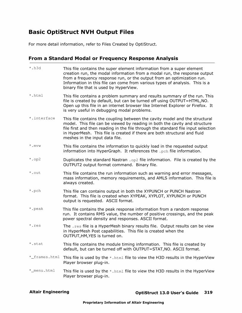
Altair Engineering OptiStruct 13.0 User's Guide 319
Proprietary Information of Altair Engineering
Basic OptiStruct NVH Output Files
For more detail information, refer to Files Created by OptiStruct.
From a Standard Modal or Frequency Response Analysis
*.h3d This file contains the super element information from a super elementcreation run, the modal information from a modal run, the response outputfrom a frequency response run, or the output from an optimization run. Information in this file can come from various types of analysis. This is abinary file that is used by HyperView.
*.html This file contains a problem summary and results summary of the run. Thisfile is created by default, but can be turned off using OUTPUT=HTML,NO. Open up this file in an internet browser like Internet Explorer or Firefox. Itis very useful in debugging modal problems.
*.interface This file contains the coupling between the cavity model and the structuralmodel. This file can be viewed by reading in both the cavity and structurefile first and then reading in the file through the standard file input selectionin HyperMesh. This file is created if there are both structural and fluidmeshes in the input data file.
*.mvw This file contains the information to quickly load in the requested outputinformation into HyperGraph. It references the .pch file information.
*.op2 Duplicates the standard Nastran .op2 file information. File is created by the
OUTPUT2 output format command. Binary file.
*.out This file contains the run information such as warning and error messages,mass information, memory requirements, and AMLS information. This file isalways created.
*.pch This file can contains output in both the XYPUNCH or PUNCH Nastranformat. This file is created when XYPEAK, XYPLOT, XYPUNCH or PUNCHoutput is requested. ASCII format.
*.peak This file contains the peak response information from a random responserun. It contains RMS value, the number of positive crossings, and the peakpower spectral density and responses. ASCII format.
*.res The .res file is a HyperMesh binary results file. Output results can be view
in HyperMesh Post capabilities. This file is created when the OUTPUT,HM,YES is turned on.
*.stat This file contains the module timing information. This file is created bydefault, but can be turned off with OUTPUT=STAT,NO. ASCII format.
*_frames.html This file is used by the *.html file to view the H3D results in the HyperView
Player browser plug-in.
*_menu.html This file is used by the *.html file to view the H3D results in the HyperView
Player browser plug-in.
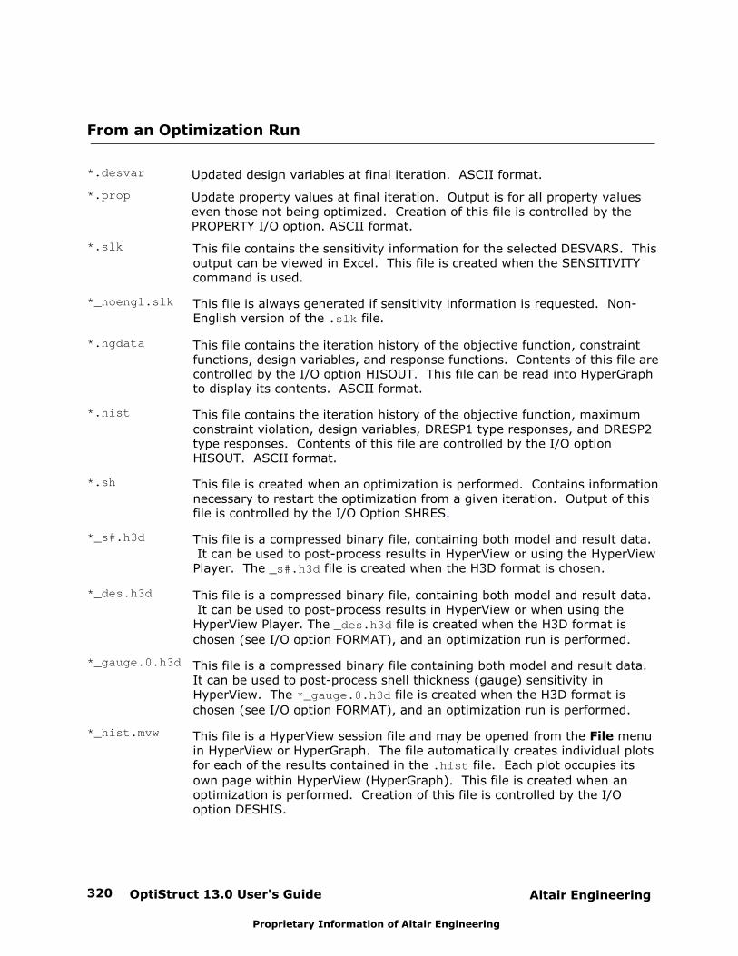
OptiStruct 13.0 User's Guide320 Altair Engineering
Proprietary Information of Altair Engineering
From an Optimization Run
*.desvar Updated design variables at final iteration. ASCII format.
*.prop Update property values at final iteration. Output is for all property valueseven those not being optimized. Creation of this file is controlled by the PROPERTY I/O option. ASCII format.
*.slk This file contains the sensitivity information for the selected DESVARS. Thisoutput can be viewed in Excel. This file is created when the SENSITIVITYcommand is used.
*_noengl.slk This file is always generated if sensitivity information is requested. Non-English version of the .slk file.
*.hgdata This file contains the iteration history of the objective function, constraintfunctions, design variables, and response functions. Contents of this file arecontrolled by the I/O option HISOUT. This file can be read into HyperGraphto display its contents. ASCII format.
*.hist This file contains the iteration history of the objective function, maximumconstraint violation, design variables, DRESP1 type responses, and DRESP2type responses. Contents of this file are controlled by the I/O option HISOUT. ASCII format.
*.sh This file is created when an optimization is performed. Contains informationnecessary to restart the optimization from a given iteration. Output of thisfile is controlled by the I/O Option SHRES.
*_s#.h3d This file is a compressed binary file, containing both model and result data. It can be used to post-process results in HyperView or using the HyperViewPlayer. The _s#.h3d file is created when the H3D format is chosen.
*_des.h3d This file is a compressed binary file, containing both model and result data. It can be used to post-process results in HyperView or when using theHyperView Player. The _des.h3d file is created when the H3D format is
chosen (see I/O option FORMAT), and an optimization run is performed.
*_gauge.0.h3d This file is a compressed binary file containing both model and result data. It can be used to post-process shell thickness (gauge) sensitivity inHyperView. The *_gauge.0.h3d file is created when the H3D format is
chosen (see I/O option FORMAT), and an optimization run is performed.
*_hist.mvw This file is a HyperView session file and may be opened from the File menuin HyperView or HyperGraph. The file automatically creates individual plotsfor each of the results contained in the .hist file. Each plot occupies its
own page within HyperView (HyperGraph). This file is created when anoptimization is performed. Creation of this file is controlled by the I/Ooption DESHIS.

Altair Engineering OptiStruct 13.0 User's Guide 321
Proprietary Information of Altair Engineering
From PFMODE, PFGRID Analysis
*.pfmode.pch This file contains the output from PFMODE and PFPANEL requests. Thisinformation can be viewed in the HyperView NVH PFMODE-PFGRID module.In version 12.0, this file is only available when output=punch is requested
in PFMODE and PFPANEL. It is recommended to export the modal and panelparticipation data into a H3D file, due to the large volume of data.
*.h3d This file contains the output from PFMODE, PFPANEL, and PFGRID requests.Results of PFGRID is only available in H3D file.
From a Super Element Creation Analysis
*.seplot This file contains the exterior and interior grids, plotels and plate plotels,retained in the super element creation run. This file is created when the PARAM, SEPLOT,YES command is included in the run. ASCII format.
*.h3d This file contains the super element binary information to be included in afuture residual run. Always created for a super element run. This file iscreated by default, but can be turned off with OUTPUT,H3D, NO.
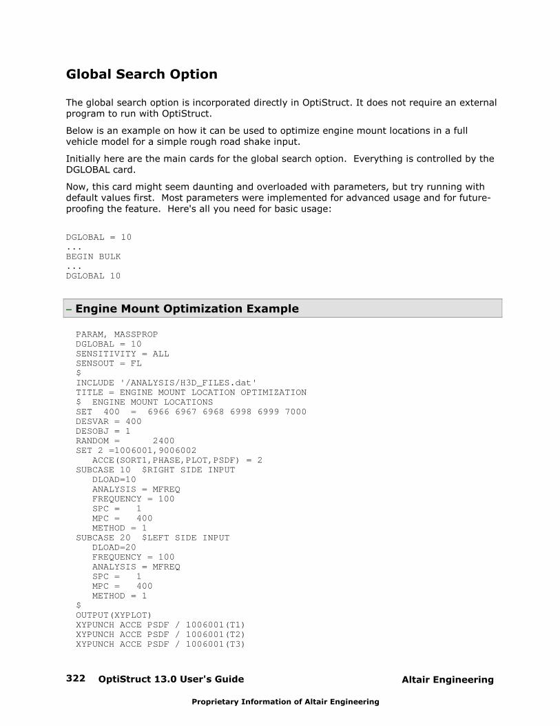
OptiStruct 13.0 User's Guide322 Altair Engineering
Proprietary Information of Altair Engineering
Global Search Option
The global search option is incorporated directly in OptiStruct. It does not require an externalprogram to run with OptiStruct.
Below is an example on how it can be used to optimize engine mount locations in a fullvehicle model for a simple rough road shake input.
Initially here are the main cards for the global search option. Everything is controlled by the DGLOBAL card.
Now, this card might seem daunting and overloaded with parameters, but try running withdefault values first. Most parameters were implemented for advanced usage and for future-proofing the feature. Here's all you need for basic usage:
DGLOBAL = 10...BEGIN BULK...DGLOBAL 10
Engine Mount Optimization Example
PARAM, MASSPROPDGLOBAL = 10SENSITIVITY = ALLSENSOUT = FL $INCLUDE '/ANALYSIS/H3D_FILES.dat'TITLE = ENGINE MOUNT LOCATION OPTIMIZATION$ ENGINE MOUNT LOCATIONSSET 400 = 6966 6967 6968 6998 6999 7000DESVAR = 400DESOBJ = 1RANDOM = 2400SET 2 =1006001,9006002 ACCE(SORT1,PHASE,PLOT,PSDF) = 2SUBCASE 10 $RIGHT SIDE INPUT DLOAD=10 ANALYSIS = MFREQ FREQUENCY = 100 SPC = 1 MPC = 400 METHOD = 1SUBCASE 20 $LEFT SIDE INPUT DLOAD=20 FREQUENCY = 100 ANALYSIS = MFREQ SPC = 1 MPC = 400 METHOD = 1$OUTPUT(XYPLOT)XYPUNCH ACCE PSDF / 1006001(T1)XYPUNCH ACCE PSDF / 1006001(T2)XYPUNCH ACCE PSDF / 1006001(T3)
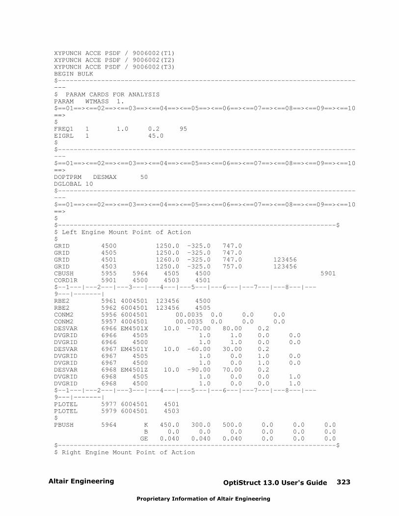
Altair Engineering OptiStruct 13.0 User's Guide 323
Proprietary Information of Altair Engineering
XYPUNCH ACCE PSDF / 9006002(T1)XYPUNCH ACCE PSDF / 9006002(T2)XYPUNCH ACCE PSDF / 9006002(T3)BEGIN BULK$-------------------------------------------------------------------------------$ PARAM CARDS FOR ANALYSISPARAM WTMASS 1.$==01==><==02==><==03==><==04==><==05==><==06==><==07==><==08==><==09==><==10==>$FREQ1 1 1.0 0.2 95EIGRL 1 45.0 $$-------------------------------------------------------------------------------$==01==><==02==><==03==><==04==><==05==><==06==><==07==><==08==><==09==><==10==>DOPTPRM DESMAX 50DGLOBAL 10$-------------------------------------------------------------------------------$==01==><==02==><==03==><==04==><==05==><==06==><==07==><==08==><==09==><==10==>$$-----------------------------------------------------------------------$$ Left Engine Mount Point of Action$GRID 4500 1250.0 -325.0 747.0 GRID 4505 1250.0 -325.0 747.0 GRID 4501 1260.0 -325.0 747.0 123456GRID 4503 1250.0 -325.0 757.0 123456CBUSH 5955 5964 4505 4500 5901CORD1R 5901 4500 4503 4501$--1---|---2---|---3---|---4---|---5---|---6---|---7---|---8---|---9---|-------|RBE2 5961 4004501 123456 4500RBE2 5962 6004501 123456 4505CONM2 5956 6004501 00.0035 0.0 0.0 0.0 CONM2 5957 4004501 00.0035 0.0 0.0 0.0 DESVAR 6966 EM4501X 10.0 -70.00 80.00 0.2DVGRID 6966 4505 1.0 1.0 0.0 0.0DVGRID 6966 4500 1.0 1.0 0.0 0.0DESVAR 6967 EM4501Y 10.0 -60.00 30.00 0.2DVGRID 6967 4505 1.0 0.0 1.0 0.0DVGRID 6967 4500 1.0 0.0 1.0 0.0DESVAR 6968 EM4501Z 10.0 -90.00 70.00 0.2DVGRID 6968 4505 1.0 0.0 0.0 1.0 DVGRID 6968 4500 1.0 0.0 0.0 1.0 $--1---|---2---|---3---|---4---|---5---|---6---|---7---|---8---|---9---|-------|PLOTEL 5977 6004501 4501 PLOTEL 5979 6004501 4503 $ PBUSH 5964 K 450.0 300.0 500.0 0.0 0.0 0.0 B 0.0 0.0 0.0 0.0 0.0 0.0 GE 0.040 0.040 0.040 0.0 0.0 0.0$-----------------------------------------------------------------------$$ Right Engine Mount Point of Action
OptiStruct 13.0 User's Guide324 Altair Engineering
Proprietary Information of Altair Engineering
$$GRID 4510 1250.0 325.0 747.0 GRID 4515 1250.0 325.0 747.0 GRID 4511 1260.0 325.0 747.0 123456GRID 4517 1250.0 325.0 757.0 123456CBUSH 5964 5964 4515 4510 6001CORD1R 6001 4510 4517 4511 $--1---|---2---|---3---|---4---|---5---|---6---|---7---|---8---|---9---|-------|RBE2 5994 4004511 123456 4510RBE2 5995 6004511 123456 4515CONM2 5996 6004511 00.0035 0.0 0.0 0.0CONM2 5997 4004511 00.0035 0.0 0.0 0.0DESVAR 6998 EM4511X 10.0 -75.00 80.00 0.2DVGRID 5998 4515 1.0 1.0 0.0 0.0DVGRID 5998 4510 1.0 1.0 0.0 0.0DESVAR 6999 EM4511Y 10.0 -20.00 80.00 0.2DVGRID 6999 4515 1.0 0.0 1.0 0.0DVGRID 6999 4510 1.0 0.0 1.0 0.0DESVAR 7000 EM4511Z 10.0 -65.00 60.00 0.2DVGRID 7000 4515 1.0 0.0 0.0 1.0DVGRID 7000 4510 1.0 0.0 0.0 1.0$--1---|---2---|---3---|---4---|---5---|---6---|---7---|---8---|---9---|-------|PLOTEL 6011 6004511 4511 PLOTEL 6013 6004511 4517 PLOTEL 24511 6004511 4004511INCLUDE '/ANALYSIS/OPTIMIZATION_CARDS.dat' INCLUDE '/ANALYSIS/SIMPLE_ROAD_INPUT.dat'INCLUDE '/ANALYSIS/CONNECTIONS_WO_ENGING_MOUNTS.dat' INCLUDE '/ANALYSIS/NON_H3D_FILES.dat'ENDDATA
In this model, the left and right mount locations are being optimized for improving thedriver’s seat track for a simple rough road shake input. Most of the component files are inthe CMS super element format. The simple component files are in OptiStruct. The superelements are required in order to make each optimization run faster.
This run will make several optimization runs from different starting points. Each optimizationoutput will be put into a separate directory. The .pch files from each directory can be viewed
in HyperGraph and the best results can be chosen.
The resulting .grid file for the best results can be included in the basic model file by the
ASSIGN UPDATE card. This will automatically update the engine mount locations for you.

Altair Engineering OptiStruct 13.0 User's Guide 325
Proprietary Information of Altair Engineering
Create Door and Deck Lid Seals
1. The first thing that needs to be done is to save this HyperMesh macro in one of yourdirectories. The best directory to use is the Work_dir_hw11. This is the default directory
for the HyperMesh command window. It orients the seal CBUSH elements properly.
2. The easiest way to create the door seals is to isolate both side of the structure that theseal is attached to. To do this, open up the body model in HyperMesh and save the outerdoor frame in a separate file. Do the same thing with the door inner panel to which thedoor seal contacts.
3. Open up both the body side frame and the door inner panel in HyperMesh.
4. Display only the body side frame.
5. Go to the Geom panel and select lines.
6. In the Lines panel, select node list and smooth as the two options displayed.
7. Start at one point on the door side frame where the seal is attached to the body. Donot select the edge point if the door seal is perpendicular to the door edge. For the decklid seal the deck lid edge is parallel to the seal and the edge points can be picked. Do notpick nodes that are shared by two components.
8. Continue around the perimeter selecting points. The points can be spaced far apart ifthey are in a straight line. Around the curve areas, select enough points to adequatelyfollow the curve surface. Select almost each point around a curve. If you select a wrongpoint, right-click on the last point to remove it. The right-click option can be performedseveral times to remove the last few points. Do not close the line. Select the last pointclose to the first point.
9. Click create. A line will be created along the path chosen.
10.Click return.
11.In the Geom panel, select Nodes.
12.Select on line.
Number of nodes =: around 200
bias style: linear
bias intensity: 0.0
13.Click the lines button and select the line just created.
14.Click create. The temporary nodes will be created equidistant from each other.
15.Display just these new nodes using the Model panel on the left side. Turn off the bodyside frame. Note the distance between nodes using the distance option in the Geompanel and selecting two sequential points.
Record this distance for future use.
16.Select the 1D panel at the bottom. Then click connectors > spot.
17.Select the spot selection.
Location: nodes

OptiStruct 13.0 User's Guide326 Altair Engineering
Proprietary Information of Altair Engineering
connect with: comps
type = sealing
fe file; <<econfig.cfg
prop file: <<sealing.tcl
diameter: 0.0
mesh: independent
no systems
Tolerance: 100
18.Click the nodes button and select displayed.
19.Bring up the body side frame and the door inner panel. Click comps and then select boththe body side frame and the door inner panel to which the door seal will attach to.
20.Click create.
The spot welds representing the door seals will be created. A message at the bottom lefthand corner appears reporting how many good spot welds have been created. Thereshould not be any bad spot welds.
21.Go to the Geom panel and select temp nodes.
22.Click nodes, then select all:
23.Click add and then clear all. This will remove the initial temporary nodes create with theline command.
24.Go to Mask by Config in the left hand panel. Select Springs/Gaps. To isolate just thespot welds, select 1. Just the CBUSH elements of the spot welds will appear.
25.Go to the Tool panel and select renumber. Select nodes.
26.Click nodes and select displayed.
27.Select a start with value that will move these nodes above all other nodes in the fullvehicle model.
Increment by 1 Offset 0.
28.Click renumber > return.
29.Go to the Properties selection on the top menu line. Select Edit > Prop and select thePBUSH0 property that represent the property for the spot weld CBUSH elements.
Note that there may be multiple PBUSH properties for the door seals. The Spot commandcreates a new property card when one of the components that the door seal attaches tochanges. The following needs to be performed for each door seal property card.
30.Click Select > update/edit.
This will bring up the PBUSH card. Enter your values for the door seal properties. Theseal stiffness properties will normally be given in stiffness per unit length for each of thethree translation directions. Multiply these numbers by the length distance recordedabove and enter the values into the K1, K2 and K3 locations. K1 will be the compressivedirection; K2 the direction along the seal length; and K3 the direction perpendicular tothe seal length.

Altair Engineering OptiStruct 13.0 User's Guide 327
Proprietary Information of Altair Engineering
31.For K4, K5 and K6, enter 0.0.
32.Click Return twice.
33.Go to the Model panel on the left hand side and turn on the spot welds auto1.
34.Select the Tool > renumber panel.
35.Select elems. Click the elems button and select displayed.
36.Enter a start with value that moves the element IDs above all the rest of the elements inthe full vehicle model.
37.Click the renumber button.
38.Go to Mask by Config in the left hand panel. Select the Springs/Gaps to isolate justthe spot welds. Just the CBUSH elements of the spot welds will appear.
39.Now select lines and click the “+” symbol. This will bring up the line created initially.
40.Now use the macro to align the CBUSH elements properly. Go to the top line in theHyperMesh window and select View; select command window, if it is not alreadypresent.
41.Enter the macro name source orient…tbc. in the white command window.
42.Click enter.
43.In the bottom window there is a button named nodes list, which is highlighted. Expandthe CBUSH elements. Select the node closest to the line on each CBUSH element. This isthe GA point for the CBUSH element. Click proceed at any time and the macro will alignjust those CBUSH’s that were selected. Vectors that are created pointing along the linedirection are shown. This defines the “XY” plane for the CBUSH elements. You canrestart the macro by moving the curser into the command window and hitting the uparrow button.
44.Click enter. Now proceed to do all the seal CBUSH elements.
45.Go to the Model panel on the left hand side and turn on the spot welds auto1.
46.Either keep the welds with the body or the door, or the seals can be put into a separatefile by going to the file output panel entering a new name for the file and set export to Displayed.
47.Click Export.
48.Presently in HyperMesh 10.0, the PBUSH ID cannot be renumbered initially. If the sealmodel is put in a separate file, close HyperMesh and reopen it and read this seal modelback in.
49.The PBUSH property can now be renumbered by clicking Tool > Renumber. Select propand click the prop button. Now select the PBUSH associated with the door seal CBUSHs.
50.Enter a start with value that moves the property ID above all the rest of the propertiesin the full vehicle model.
51.Click the renumber button. You will now need to resave the door seal file.
52.If you save the door seals in a separate file for use with your trim body model, the bodyand door seal grid points from the deck will need to be removed. You will also need toremove the control cards at the top of the deck and the enddata card at the end of thedeck, so that when it is included with the body and doors there will be no duplicate ID’s.

OptiStruct 13.0 User's Guide328 Altair Engineering
Proprietary Information of Altair Engineering
Create a HyperGraph Template for Reading in Multiple Files
All the .pch files should be in the same directory and the $label values should be the same.
1. Open HyperGraph.
2. Read in file number 1.
3. To read in multiple curves at one time, select one Y Type. Select multiple Y Request. Select multiple Y Components.
4. From the Layout menu, select One curve per plot.
5. Click Apply. Multiple plots will be created.
6. From the File menu, select Save as > Report Template. Save file as a .tpl in the
same directory as where the .pch files are located.
7. From the File menu, select New > Session. This will restart HyperGraph.
8. From the Tools toolbar, select Open Reports Panel.
9. In the Report definition list, the .tpl file will be listed.
10.Click Apply. The original curves will be shown.
11.Click Add to open another file to compare the results.
12.Select Overlay.
13.Once you have finished adding the files, Save the .tpl.
14.You can now open the .tpl file in HyperGraph and enter new file names for different
comparisons.

Altair Engineering OptiStruct 13.0 User's Guide 329
Proprietary Information of Altair Engineering
Using AMSES (Automatic Multi-Level Sub-StructuringEigensolver Solution)
For the solution of large eigenvalue problems, the AMSES solution can be used instead of theLanczos eigensolver. The resulting eigenvalues and eigenvectors are used in eigenvalueanalysis, CMS Super Element creation, Modal Frequency Response, and Modal TransientAnalysis. In addition, the AMSES solver can be used during topology, topography, shape,and sizing optimizations. The AMSES solver can be 2-100 times faster than Lanczos.
AMSES is a multi-threaded application and can use any number of processors. AMSES willuse the same number of processors that OptiStruct is using.
Activating AMSES
To use AMSES, one of the following must be defined:
1. Use of the EIGRA data, instead of EIGRL data.
2. Use of AMSES solver keyword on the CMSMETH data
AMSES Usage Guidelines
The following guidelines list the factors affecting AMSES usage:
1. The AMSES solution is, generally, much faster than Lanczos, but the results areapproximate. Accuracy of the lower modes is very high; therefore, AMSES is a goodcandidate for solutions with a large number of modes (greater than a few hundred) wherean approximated eigen-space is sufficient (as in Modal Frequency Response and ModalTransient Response Analysis). Although approximate, the large number of modes used formodal analysis will encompass the modal space and the resulting motion will match veryclosely with the Lanczos results. Lanczos is recommended in solutions where accuratemode shapes of a small number of modes are required.
2. AMSES is also recommended in cases where: 1) A low number of eigenvalues arerequested but the model consists of more than a million degrees of freedom, and/or; 2)The upper bound (V2) is specified or the number of modes (ND) is greater than 50 on theEIGRL entry. In such cases, it is likely that Lanczos runs are slower than AMSES runs.
3. For optimization runs, if accuracy of the eigenvector is important, normal modes analysiswith AMSES can be run first and then Lanczos can be run with precise lower and upperbounds to check the AMSES run for accuracy. The AMSES upper bound can then beadjusted to achieve acceptable accuracy of the desired eigenvectors. Now, AMSES can beused for all optimization runs in this analysis.
4. The AMSES solution is much faster for flexible body generation and modal solutions withmany residual vectors.
5. AMSES should be used cautiously in situations with very large RBE3’s (i.e., if the RBE3 isconnected to 1/4th of the structure). It may be better to eliminate such RBE3’s.
6. AMSES solution speeds depend on the number of eigenvector degrees of freedom (DOF)to be calculated. DISP=ALL will cause the entire eigenvector to be calculated and thespeedup will not be large. However, if results for only a few DOF are required (typical forNVH analysis), AMSES can be up to 100 times faster than Lanczos. To improve AMSES runtimes, it is recommended to request results only for the required DOF.

OptiStruct 13.0 User's Guide330 Altair Engineering
Proprietary Information of Altair Engineering
7. For an AMSES run with V1, V2 and ND specified on the EIGRA entry, AMSES calculates allthe modes up to the specified V2 (upper bound) regardless of the value of ND. Then “ND”number of requested modes is output. Therefore, reducing ND by keeping the upperbound (V2) the same will not significantly improve the AMSES run times, the upper boundmust also be correspondingly reduced to prevent the extraction of extra modes.
8. AMSES is also useful in checking for model irregularities. AMSES can be used to print thelist of grids associated with a massless mechanism or a singularity.
Parameters Affecting AMSES
AMSES controls the accuracy and the cost of a solution with the parameter AMPFFACT. The
“optimal” value of AMPFFACT for typical NVH analysis, 5.0, has been established through
extensive testing. AMPFFACT is set on the EIGRA and CMSMETH data.
In case of predominately solid models, such as engine blocks, AMPFACT should be set to 10.0.
PARAM,RBMEIG can be used to adjust the upper limit on eigenvalues associated with rigid
body modes. The default upper limit is 1.0 (equivalent to a natural frequency of 0.16 Hz) if PARAM,RBMEIG is not included in the deck.
Residual Vector Calculations
When the AMSES eigensolver is used, residual vectors for each of the following arecalculated:
USET U6 data
Frequency Response Dynamic Loads
Transient Response Dynamic Loads
Damping DOF from CBUSH, CDAMPi or CVISC data
One Residual Vector is calculated for each USET U6 degree of freedom, each DAREA degree offreedom, and each damping degree of freedom associated with the CBUSH, CDAMPi andCVISC data.
The Residual Vector calculations are controlled by the Solution Control data RESVEC. Tocontrol Residual Vector calculations with AMSES, the following commands can be used:
Use RESVEC=NO to turn off Residual Vector calculations with AMSES
Use RESVEC(NODAMP)=YES to turn off Residual Vectors associated with Damping DOF.
If the center of a large RBE3 is loaded, a residual vector will be created that includesterms for each of the independent DOF. If this number is large, say over 500, theAMSES run time will increase dramatically. For large loaded RBE3 it is recommended touse the RBE3 UM data to make the center GRID independent.

Altair Engineering OptiStruct 13.0 User's Guide 331
Proprietary Information of Altair Engineering
Modeling Techniques
The Modeling Techniques section provides an overview of the following:
Parts and Instances
Subcase Specific Modeling
Direct Matrix Input
Flexible Body Generation
Poroelastic Materials
Elements and Materials
Loads and Boundary Conditions
Virtual Fluid Mass
Modeling Errors
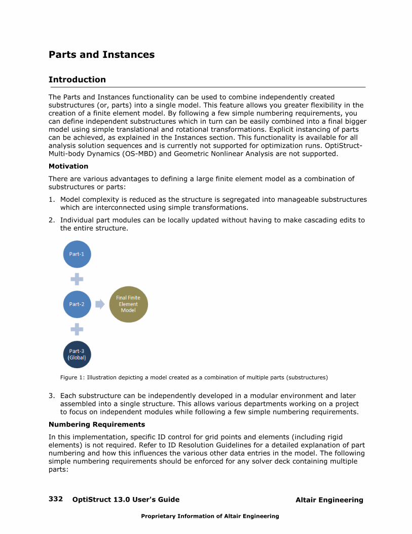
OptiStruct 13.0 User's Guide332 Altair Engineering
Proprietary Information of Altair Engineering
Parts and Instances
Introduction
The Parts and Instances functionality can be used to combine independently createdsubstructures (or, parts) into a single model. This feature allows you greater flexibility in thecreation of a finite element model. By following a few simple numbering requirements, youcan define independent substructures which in turn can be easily combined into a final biggermodel using simple translational and rotational transformations. Explicit instancing of partscan be achieved, as explained in the Instances section. This functionality is available for allanalysis solution sequences and is currently not supported for optimization runs. OptiStruct-Multi-body Dynamics (OS-MBD) and Geometric Nonlinear Analysis are not supported.
Motivation
There are various advantages to defining a large finite element model as a combination ofsubstructures or parts:
1. Model complexity is reduced as the structure is segregated into manageable substructureswhich are interconnected using simple transformations.
2. Individual part modules can be locally updated without having to make cascading edits tothe entire structure.
Figure 1: Illustration depicting a model created as a combination of multiple parts (substructures)
3. Each substructure can be independently developed in a modular environment and laterassembled into a single structure. This allows various departments working on a projectto focus on independent modules while following a few simple numbering requirements.
Numbering Requirements
In this implementation, specific ID control for grid points and elements (including rigidelements) is not required. Refer to ID Resolution Guidelines for a detailed explanation of partnumbering and how this influences the various other data entries in the model. The followingsimple numbering requirements should be enforced for any solver deck containing multipleparts:
Altair Engineering OptiStruct 13.0 User's Guide 333
Proprietary Information of Altair Engineering
1. Entities which are part specific, like grid points and elements, are numbered by part
based local numbering.
2. Global entities such as properties, materials, loads and boundary conditions are defined inthe global numbering system.
3. The individual parts forming the total structure can be combined without any changes informat if the numbering requirements (1) and (2) are met.
Parts
A part can be visualized as an independent entity which is connected to a global structureduring assembly (The global structure is also considered to be a part). Each part can bedefined as a section of the entire finite element model that is used for a specific purpose. Forexample, a door of an automobile can be defined as a part and multiple instances of this partcan be instantiated (refer to Instances for a detailed explanation of part instancing) to savetime during modeling.
Definition
A part is included in the global structure between BEGIN and END bulk data entriespotentially using the INCLUDE entry. The INCLUDE entry accepts a string that references thefile name (filename.fem) of a specific part. Parts are defined as separate solver decks and
could be included within the same working directory. Multiple INCLUDE entries can be usedwithin a single set of BEGIN and END entries to add multiple sections of a single part (referto Instances for a detailed explanation of part instancing). A part can also be split betweenseparate BEGIN and END entries with the same part name.
Format
BEGIN and END bulk data entries mark the start and end of the definition of a part in theglobal structure. A part is defined as a separate file which is included in the global structureusing the INCLUDE bulk data entry (The entire solver deck of the part can also be insertedbetween the BEGIN and END entries, instead of using the INCLUDE entry).
The format used to include a part in a global structure is as follows:
BEGIN, FEMODEL, name
INCLUDE “filename.fem”
END, FEMODEL, name
The second field of the BEGIN entry should be set to FEMODEL and the third field shouldcontain the name of the part. This part name will be used to define fully qualified referencesto local entries within the part from anywhere in the model. All part names in the modelshould be unique. Part names are not case sensitive and should start with a letter. They cancontain letters, digits, and underscores, only. filename.fem follows standard requirements
for INCLUDE, that is, it can refer to a local file or contain the full path. No other BEGIN orEND entries are allowed between BEGIN and END. All bulk data entries should be locatedbetween BEGIN, FEMODEL and END, FEMODEL. A full model consists of several parts. Onepart is designated as global. The other parts can be moved to arbitrary locations using the INSTNCE bulk data entry and connected to each other using connector elements or CONNECTbulk data entries.

OptiStruct 13.0 User's Guide334 Altair Engineering
Proprietary Information of Altair Engineering
Local and Global Entries
Local entries, as their name suggests, are data entries that can be defined locally within aspecific part. Local entries are currently limited to the following (refer to the Appendix for alist of all local entries).
Grid Point Definition
GRID Bulk Data Entry
Rigid Elements
RROD Bulk Data EntryRBAR Bulk Data EntryRBE1 Bulk Data EntryRBE2 Bulk Data Entry
Elements
CHEXA Bulk Data EntryCQUAD Bulk Data Entry CBUSH Bulk Data Entry and so on
All other data entries are considered global and should be defined in the global structure.Even if they are located within BEGIN – END entries in a different part, they are stillinterpreted as if they are in the global part. Some global data entries can reference local dataentries (see above list) using fully qualified references.
Fully Qualified References
The same ID number can be used for non-unique local data entries defined in multiple parts.Such ID’s cannot be referenced by entries in the global structure without the use of fullyqualified references. Fully qualified references contain information about both the local dataentry and its corresponding part.
Numeric Reference Fully Qualified Reference
A numeric reference on a local entryreferences another local entity withinthe same part, or a global entity. Anumeric reference can be used toreference a global entry only ifanother entry of the same type andwith the same ID does not existwithin the current part.
References a local entry definedwithin any part.
A numeric reference on a global entryreferences an entity within the globalpart only.
A fully qualified reference can beused to reference an entry whenanother entry of the same type andwith the same ID exists within themodel.
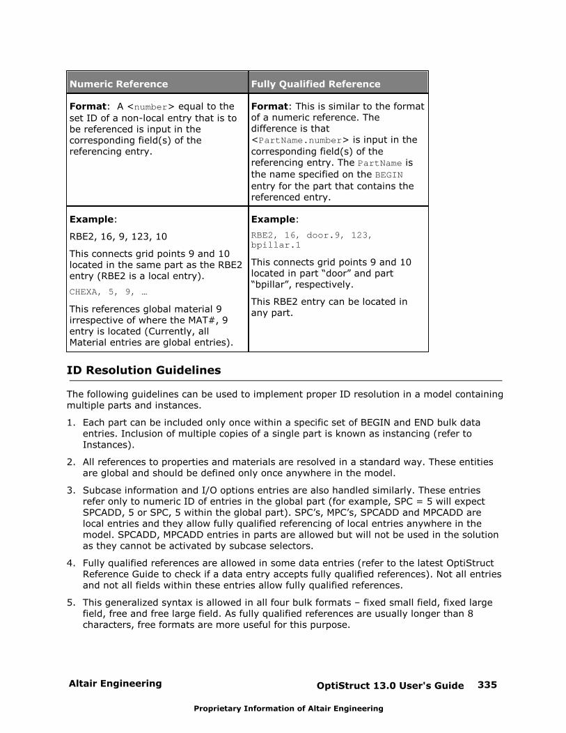
Altair Engineering OptiStruct 13.0 User's Guide 335
Proprietary Information of Altair Engineering
Numeric Reference Fully Qualified Reference
Format: A <number> equal to the
set ID of a non-local entry that is tobe referenced is input in thecorresponding field(s) of thereferencing entry.
Format: This is similar to the formatof a numeric reference. Thedifference is that<PartName.number> is input in the
corresponding field(s) of thereferencing entry. The PartName is
the name specified on the BEGIN
entry for the part that contains thereferenced entry.
Example:
RBE2, 16, 9, 123, 10
This connects grid points 9 and 10located in the same part as the RBE2entry (RBE2 is a local entry).
CHEXA, 5, 9, …
This references global material 9irrespective of where the MAT#, 9entry is located (Currently, allMaterial entries are global entries).
Example:
RBE2, 16, door.9, 123,bpillar.1
This connects grid points 9 and 10located in part “door” and part“bpillar”, respectively.
This RBE2 entry can be located inany part.
ID Resolution Guidelines
The following guidelines can be used to implement proper ID resolution in a model containingmultiple parts and instances.
1. Each part can be included only once within a specific set of BEGIN and END bulk dataentries. Inclusion of multiple copies of a single part is known as instancing (refer to Instances).
2. All references to properties and materials are resolved in a standard way. These entitiesare global and should be defined only once anywhere in the model.
3. Subcase information and I/O options entries are also handled similarly. These entriesrefer only to numeric ID of entries in the global part (for example, SPC = 5 will expectSPCADD, 5 or SPC, 5 within the global part). SPC’s, MPC’s, SPCADD and MPCADD arelocal entries and they allow fully qualified referencing of local entries anywhere in themodel. SPCADD, MPCADD entries in parts are allowed but will not be used in the solutionas they cannot be activated by subcase selectors.
4. Fully qualified references are allowed in some data entries (refer to the latest OptiStructReference Guide to check if a data entry accepts fully qualified references). Not all entriesand not all fields within these entries allow fully qualified references.
5. This generalized syntax is allowed in all four bulk formats – fixed small field, fixed largefield, free and free large field. As fully qualified references are usually longer than 8characters, free formats are more useful for this purpose.
OptiStruct 13.0 User's Guide336 Altair Engineering
Proprietary Information of Altair Engineering
6. As a general practice, all data entries using fully qualified references are placed inside theglobal part. This is not mandatory.
7. The own ID of each data entry (usually the second field after the card name) cannot be afully qualified reference.
8. As explained previously, for local entries, their own ID’s within a particular part cannot beequal. Whereas, similar data entries can be the same own ID if they are defined indifferent parts. In such cases they are completely independent entities and their ID’s areresolved by using fully qualified references. The same rules apply to set ID’s, for example,in SPC’s or MPC’s – the same SID in different parts represent completely independententities.
9. Any reference to a global entry must be a numeric reference regardless of whether it isbeing referred to from a global or a local part.
10.A fully qualified reference (if allowed) is resolved to a specific instance defined by partname and ID within that part.
11.If a local entry contains a numeric reference (instead of a fully qualified reference),OptiStruct resolves the reference to a local entry within the same part. If the part doesnot contain an entry (of the required type) with the ID equal to the numeric reference,OptiStruct looks in the global part for a possible match. If the entry is not available in theglobal part also, then the program errors out, regardless of whether the required entry(with same ID) is available locally in a different part. For example:
This entry is located in local part “grip”:
RBE2, 15, 5, 123, 7, 8
Grid points 1,3,5 are included in part “grip”
Grid points 1,3,5,7,8 are included in local part “frame”
Grid points 3,5,7 are included in global part “racquet”
In the above example, on the RBE2 element, grid point 5 refers to grid grip.5, grid point
7 refers to racquet.8 and grid point results in an error.
12.OptiStruct allows repetition of some global data entries, even if only unique ID’s areallowed, only if the content of such cards is identical (for example, material and propertyentries).
Logical Sets
The SET bulk data entry can be used in the global part to reference SET’s defined withindifferent parts. These SET entries in the global part can contain fully qualified references topart-specific SET data only if logical operators (OPERATOR field on the SET entry) are used.For example:
The following SET entry exists in part “A”:
BEGIN, FEMODEL, ASET, 29, ELEM, LIST 15 THRU 30…END, FEMODEL, A
Altair Engineering OptiStruct 13.0 User's Guide 337
Proprietary Information of Altair Engineering
Referencing SET, 29 in the global part “G”:
BEGIN, FEMODEL, GSET, 78, ELEM, OR A.29…END, FEMODEL, G
This process can be used to reference local sets in the global part on entries which do notsupport fully-qualified referencing of local sets (like, output entries). For example:
The following SET entry exists in part “A”:
BEGIN, FEMODEL, ASET, 3, GRID, LIST 15 THRU 30…END, FEMODEL, A
In the global part “G”:
Incorrect
BEGIN, FEMODEL, G
DISPLACEMENT(H3D)=part.3orDISPLACEMENT(H3D)=3 …END, FEMODEL, G
Correct
BEGIN, FEMODEL, G
DISPLACEMENT(H3D)=3
SET, 3, GRID, OR A.3…END, FEMODEL, G
Relocation
A full model in an OptiStruct Parts and Instances consists of a collection of parts. These partsare inserted into the global structure automatically (without relocation) or by using entrieswhich allow relocation (RELOC and INSTNCE). Relocation involves the positioning of partswithin the model relative to each other or the global structure. Currently relocation of partsincluded in the full structure can be accomplished using the INSTNCE and RELOC bulk dataentries. Relocation involves translational and rotational movement of parts relative to theirinitial position.
INSTNCE Bulk Data Entry
The full model consists of several parts. One part is designated as global and the rest of theincluded parts are relatively positioned with respect to the global part with the help of theINSTNCE entry. The INSTNCE entry references the RELOC bulk data entry that defines therelocation or mapping of grid points from one position to another.
OptiStruct 13.0 User's Guide338 Altair Engineering
Proprietary Information of Altair Engineering
Format
A INSTNCE bulk data entry can be specified only within the global part. No INSTNCE entrycan reference the global part. Each INSTNCE entry should reference a unique part name,however, it is not required that every part is positioned using an INSTNCE entry. Parts whichare not specified on the INSTNCE entry are included in the full model without any relocation.
INSTNCE, SID, name, NN
The third field “name” specifies the name of the part defined via the BEGIN, FEMODEL, name
entry and NN references the ID of the RELOC bulk data entry. The RELOC bulk data entry
defines the actual location of the part in the final model. Refer to the OptiStruct ReferenceGuide for detailed information.
RELOC Bulk Data Entry
The RELOC bulk data entry defines relocation or mapping of grid points from one position toanother. It can be used in conjunction with the INSTNCE entry to relocate parts relative toeach other or to the global structure.
Format
RELOC entries are used to relocate grid points within the full model. RELOC definesindependent transformation of each part, not the transformation of one part with respect toanother. In particular, it does define that two parts should be connected together and thenrelocated as an assembly. It can be specified in the global part and is referred to by partspecific entries like INSTNCE.
RELOC, ID, type, GID# …
The third field “type” specifies the type of relocation: MOVE, MATCH, ROTATE, or MIRROR. There
are multiple formats of the RELOC entry depending on the specified type. Refer to the OptiStruct Reference Guide for detailed information.
Connectivity
The final step in the part assembly process is connection. Connectivity between parts can beachieved in two different ways, the first involves using the CONNECT bulk data entry and theother is using connectors like rigid or bush elements that can explicitly reference grids in anypart.
Connectors can contain a mix of regular and fully qualified ID’s. Regular ID’s reference:
In a Local entry:
An entry with that ID in the same part, or to an entry with the same ID in the global part.
In a Global entry:
An entry with that ID in the global part.
Refer to comment 11 in the ID Resolution Guidelines section for information on how regularID references in localized entries are resolved. The Appendix contains a list of supportedLocal entries which can be defined within a part.
CONNECT Bulk Data Entry
The CONNECT bulk data entry defines equivalence for degrees of freedom between two parts.
Using two forms of the entry, you can equivalence all degrees of freedom for grids of both
parts within the specified tolerance distance from each other.
Altair Engineering OptiStruct 13.0 User's Guide 339
Proprietary Information of Altair Engineering
CONNECT always equivalences grid points located within two parts at the same location (X,Y, and Z) after all parts are moved to their final location using INSTNCE entries. If multiplegrid points exist in both parts at the same location (within the specified tolerance), then theywill be equivalenced together.
Format
The CONNECT entry can be used to define equivalence between two parts (name_a and
name_b) by searching for all grid points within a specified tolerance (tol). The alternate form
involves specifying a set of grid points at which to search for neighboring grids of either part“name_a” or part “name_b” within a specific tolerance (tol).
CONNECT, name_a, name_b, tol
The tolerance (tol) is a numeric value defining the maximum distance between two grid
points to allow equivalence. All grids in “part_a” are considered, if the search in “part_b”
finds a grid point matching the location (within the specified tolerance), then these two gridsare equivalenced. Refer to the OptiStruct Reference Guide for detailed information.
Instances
Instances are multiple copies of a part that are exactly the same as the part itself in allrespects. Currently, part instancing in OptiStruct is available as a logical extension to the partinclusion process. A direct approach to part instancing will be available in a future release.
Creating instances of a part
To create an additional instance of an existing part, the part inclusion process can berepeated.
For example, to create an additional instance of the part “CrankShaft”, the BEGIN FEMODEL
and END FEMODEL statements are repeated. The same set of include files (using the INCLUDE
entry) are repeated inside multiple part definitions.
BEGIN, FEMODEL, CrankShaft_1
include “CrankS_a.fem”
include “CrankS_b.fem”
END, FEMODEL, CrankShaft
BEGIN, FEMODEL, CrankShaft_2
include “CrankS_a.fem”
include “CrankS_b.fem”
END, FEMODEL, CrankShaft
Appendix
Local Data Entries
A list of data entries which can currently be defined as local entries in OptiStruct are listedbelow:
Miscellaneous
GRID, SPC, MPC, SET

OptiStruct 13.0 User's Guide340 Altair Engineering
Proprietary Information of Altair Engineering
Elements
CAABSF, CBAR, CBUSH1D, CBUSH, CDUM1, CELAS1, CELAS2, CELAS3, CELAS4, CFAST,CGAP, CGAPG, CGASK12, CGASK16, CGASK6, CGASK8, CHACAB, CHEXA, CONM1, CONM2,CONROD, CONV, CPENTA, CPYRA, CQUAD4, CQUAD8, CROD, CSEAM, CSHEAR, CTETRA,CTRIA3, CTRIA6, CTRIAX6, CTUBE, CVISC, CWELD, and PLOTEL
Rigid Elements
RBAR, RROD, RBE1, and RBE2
Entries which allow fully qualified references
TO GRID POINTS:
A list of data entries which currently allow fully qualified references to grid points inOptiStruct are listed below:
Local entries
CBUSH1D, CBUSH, RBAR, RROD, RBE1, RBE2, and RBE3
Global entries
SPC, MPC, FORCE, MOMENT, SPCD, and RELOC
TO OTHER ENTITIES:
A list of data entries which currently allow fully qualified references to other entities inOptiStruct are listed below:
SPCADD and MPCADD (allow fully qualified references to SPC and MPC, respectively)
SET (allow fully qualified references to other local SET entries only if logical operators areused)
Refer to the Release Notes for the latest list of all global/local entries and for entries whichallow fully qualified references to other entries. Analysis entries are available for Parts andInstances entries specific to optimization (for example, DVGRID, DESVAR) are not allowed.
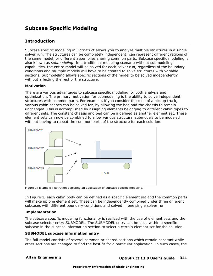
Altair Engineering OptiStruct 13.0 User's Guide 341
Proprietary Information of Altair Engineering
Subcase Specific Modeling
Introduction
Subcase specific modeling in OptiStruct allows you to analyze multiple structures in a singlesolver run. The structures can be completely independent; can represent different regions ofthe same model, or different assemblies sharing common parts. Subcase specific modeling isalso known as submodeling. In a traditional modeling scenario without submodelingcapabilities, the entire model will be solved for each solver run, regardless of the boundaryconditions and multiple models will have to be created to solve structures with variablesections. Submodeling allows specific sections of the model to be solved independentlywithout affecting the rest of the structure.
Motivation
There are various advantages to subcase specific modeling for both analysis andoptimization. The primary motivation for submodeling is the ability to solve independentstructures with common parts. For example, if you consider the case of a pickup truck,various cabin shapes can be solved for, by allowing the bed and the chassis to remainunchanged. This is accomplished by assigning elements belonging to different cabin types todifferent sets. The constant chassis and bed can be a defined as another element set. Theseelement sets can now be combined to allow various structural submodels to be modeledwithout having to repeat the common parts of the structure for each solution.
Figure 1: Example illustration depicting an application of subcase specific modeling.
In Figure 1, each cabin body can be defined as a specific element set and the common partswill make up one element set. These can be independently combined under three differentsubcases with different boundary conditions and solved in one single solver run.
Implementation
The subcase specific modeling functionality is realized with the use of element sets and thesubcase selector entry SUBMODEL. The SUBMODEL entry can be used within a specificsubcase in the subcase information section to select a certain element set for the solution.
SUBMODEL subcase information entry
The full model consists of several common or shared sections which remain constant whileother sections are changed to find the best fit for a particular application. In such cases, the
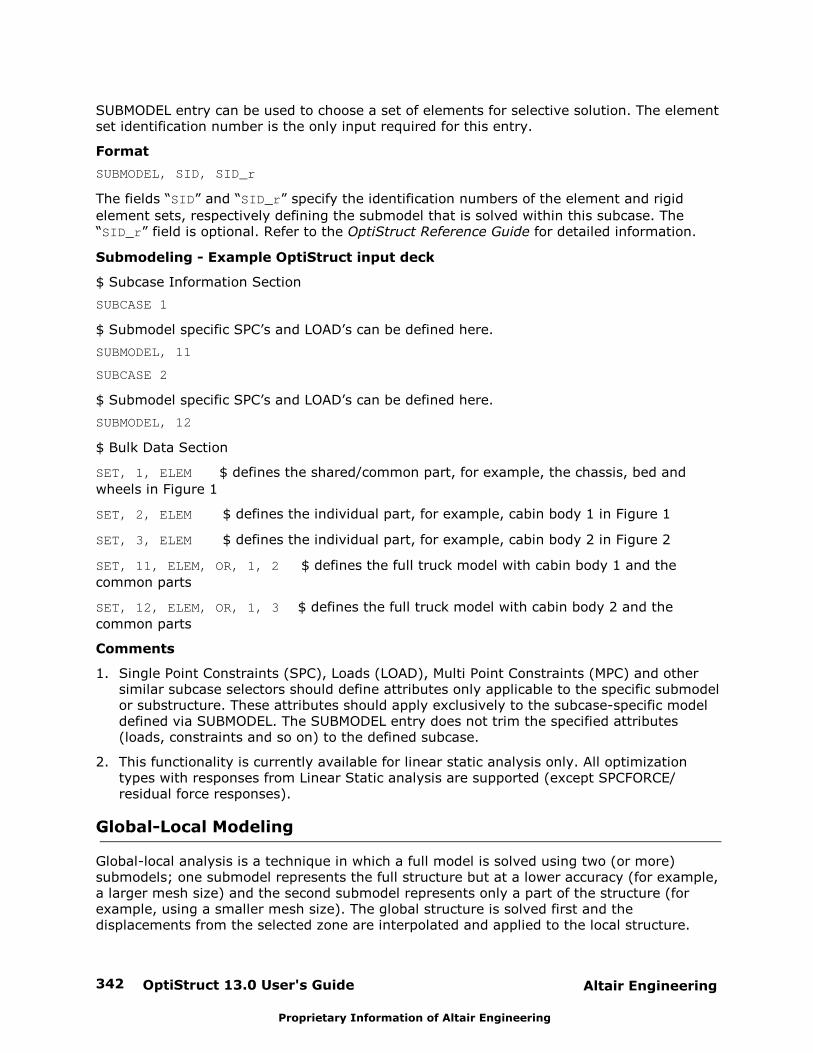
OptiStruct 13.0 User's Guide342 Altair Engineering
Proprietary Information of Altair Engineering
SUBMODEL entry can be used to choose a set of elements for selective solution. The elementset identification number is the only input required for this entry.
Format
SUBMODEL, SID, SID_r
The fields “SID” and “SID_r” specify the identification numbers of the element and rigid
element sets, respectively defining the submodel that is solved within this subcase. The“SID_r” field is optional. Refer to the OptiStruct Reference Guide for detailed information.
Submodeling - Example OptiStruct input deck
$ Subcase Information Section
SUBCASE 1
$ Submodel specific SPC’s and LOAD’s can be defined here.
SUBMODEL, 11
SUBCASE 2
$ Submodel specific SPC’s and LOAD’s can be defined here.
SUBMODEL, 12
$ Bulk Data Section
SET, 1, ELEM $ defines the shared/common part, for example, the chassis, bed and
wheels in Figure 1
SET, 2, ELEM $ defines the individual part, for example, cabin body 1 in Figure 1
SET, 3, ELEM $ defines the individual part, for example, cabin body 2 in Figure 2
SET, 11, ELEM, OR, 1, 2 $ defines the full truck model with cabin body 1 and the
common parts
SET, 12, ELEM, OR, 1, 3 $ defines the full truck model with cabin body 2 and the
common parts
Comments
1. Single Point Constraints (SPC), Loads (LOAD), Multi Point Constraints (MPC) and othersimilar subcase selectors should define attributes only applicable to the specific submodelor substructure. These attributes should apply exclusively to the subcase-specific modeldefined via SUBMODEL. The SUBMODEL entry does not trim the specified attributes(loads, constraints and so on) to the defined subcase.
2. This functionality is currently available for linear static analysis only. All optimizationtypes with responses from Linear Static analysis are supported (except SPCFORCE/residual force responses).
Global-Local Modeling
Global-local analysis is a technique in which a full model is solved using two (or more)submodels; one submodel represents the full structure but at a lower accuracy (for example,a larger mesh size) and the second submodel represents only a part of the structure (forexample, using a smaller mesh size). The global structure is solved first and thedisplacements from the selected zone are interpolated and applied to the local structure.
Altair Engineering OptiStruct 13.0 User's Guide 343
Proprietary Information of Altair Engineering
Global-local analysis is implemented with the use of the subcase specific modeling techniquedefined above.
Note that Global-local modeling is only an approximation, and its use depends on theassumption that a more accurate local model will not significantly affect the displacements ofthe global structure. This process should not be used whenever small stiffness changes in thelocal submodel may have a large impact on the solution outside of it.
Motivation
Global-local analysis may help improve results in models with local stress concentrations.Parts of the structure with small details which require relatively higher accuracy can bemodeled as local submodels with a fine mesh and the full structure can be modeled using acoarse mesh. This will allow for faster solution times as only a part of the structure is beingsolved with a fine mesh.
Figure 2: Example illustration depicting an application of global-local analysis.
In Figure 2, an example building is illustrated wherein sections containing the pillar-roof joint
are modeled as separate submodels with a refined mesh. The finer mesh allows for better
accuracy at regions with high stress concentrations. Using the global-local analysis capability,
the results from the coarser global model are interpolated and applied to the finer mesh of
the local model at the transfer region. This allows for the local model to be driven by the
results of the global model.
Implementation
The global-local modeling functionality is realized with the help of the subcase specificmodeling feature and the subcase selector entry GLOBSUB. This entry is defined in thesubcase which contains the local model definition. The GLOBSUB entry identifies the globalmodel which is used to drive the specific local model.
GLOBSUB subcase information entry
The full model consists of several sections with areas of high stress concentration or regionsof interest which require a higher accuracy. In such cases, the entire model can be solvedwith a coarser mesh and in each local subcase defining the submodel of interest, the globalstructure can be referenced using the GLOBSUB entry. The set of grids within the localstructure at the transfer zone is also specified.

OptiStruct 13.0 User's Guide344 Altair Engineering
Proprietary Information of Altair Engineering
Format
GLOBSUB, SUBID, SID
The field “SUBID” specifies the identification number of the subcase that contains the global
structure definition (via SUBMODEL) and the field “SID” specifies the set of grid points in the
local structure that defines the transfer zone. The displacements from the global structure areapplied to this set of grid points. Refer to the OptiStruct Reference Guide for detailedinformation.
Global-Local Analysis - Example OptiStruct input deck
$ Subcase Information Section
SUBCASE 1
$ Submodel specific SPC’s and LOAD’s can be defined here.
SUBMODEL, 11
SUBCASE 2
$ Submodel specific SPC’s and LOAD’s can be defined here.
SUBMODEL, 12
GLOBSUB, 1, 15
$ Bulk Data Section
SET, 11, ELEM $ defines the global structure, for example, the full building in Figure 2
SET, 12, ELEM $ defines the local structure, for example, the pillar-roof joint in Figure 2
SET, 15, GRID $ defines the transfer zone, for example, the interface grids of the pillar-
roof joint in Figure 2 at which the displacements are interpolated.
Comments
1. The transfer zone should contain only 3-dimensional elements in both the local and globalstructures. Second order elements (for example, CHEXA20) are allowed. There is nofurther restriction on element types elsewhere in the structure.
2. The transfer zone may represent single or multiple cuts (sections) through the structure.Multiple cuts should be separated from each other, that is, they should not exist closerthan the element size of the global model.
3. The GLOBSUB entry should always reference the subcase ID of a global subcase that isdefined above its corresponding local subcase.
4. This functionality is currently available for linear static analysis only. All optimizationtypes with responses from Linear Static analysis are supported.
Exceptions:
SPCFORCE/residual force responses are not supported.
Topology must lie outside the local part(s) and, any design variables affecting the localsubmodel should also be mapped to the global model.

Altair Engineering OptiStruct 13.0 User's Guide 345
Proprietary Information of Altair Engineering
Direct Matrix Input (Superelements)
Direct Matrix Input
Creating Superelements
Component Dynamic Analysis Super Element Generation
OptiStruct 13.0 User's Guide346 Altair Engineering
Proprietary Information of Altair Engineering
Direct Matrix Input
In the course of a finite element solution, matrix representations of a structure's stiffness,mass, damping, and loading are generated. The matrices are based on the informationprovided in the Bulk Data section of the input file. Depending on the analysis type, systemequations using these matrices are solved to simulate the structure’s behavior.
In a linear static analysis, for example, a system of linear equations Ku=f is solved. Here, Kis the stiffness matrix, f is the loading vector, and u is the vector of the unknown
displacements.
The time taken for these matrix solutions is about proportional to the square of the numberof degrees-of-freedom of the structure. The solution speed can be improved by representingsections of the structure (super element assemblies) with a smaller subset of degrees offreedom of those sections (boundary degrees of freedom of the super element assemblies)and a representative set of reduced matrices. In an optimization, for example, the solutionspeed can be improved dramatically by removing the non-design portion of the structure andkeeping only the design portion of the model.
For the purpose of deriving the matrices, the displacement vector may be partitioned intodisplacements of inner (OSET) and outer (ASET, interface) degrees of freedom.
(1)
Here, the subscript ‘o’ denotes the inner degrees of freedom, and ‘a’ the interface degrees of
freedom.
The static equilibrium is given as:
(2)
The eigenvalue problem for a normal modes analysis of the body using a diagonal massmatrix represents itself as:
(3)
Note: PARAM, WTMASS cannot be applied to superelements (.h3d or .pch) that are read
into the model. If the unit of mass is incorrect on the MAT# entries and PARAM,WTMASS is required to update the structural mass matrix; then this should be done inthe creation run.
There are two ways of obtaining the reduced matrices:
1. Static Condensation (or Guyan Reduction) reduces the linear matrix equation to theinterface degrees of freedom of the substructure through algebraic substitution. Theresult can be used as external matrices, representing a super element assembly, in afinite element analysis. This method is accurate for the stiffness matrix and approximatefor the mass matrix.
Altair Engineering OptiStruct 13.0 User's Guide 347
Proprietary Information of Altair Engineering
In addition, the load vectors are reduced to the ASET DOF. This includes the load vectorsfrom point and pressure loads as well as distributed loads due to acceleration (GRAV andRLOAD).
2. Component Mode Synthesis (CMS) reduces a finite element model of an elastic body tothe interface degrees of freedom and a set of normal modes. The result can either beused for inclusion as a flexible body in a multi-body dynamics analysis (see Flexible BodyGeneration) or as external matrices, representing a super element assembly, in a finiteelement analysis. It is always an approximation; however, it is the preferred method fordynamic analysis as it captures the mass matrix correctly.
Load vectors are not reduced during CMS Super Element creation.
Static Condensation
The first line of equation (2) reads as:
oo o oa a oK u K u P
The displacements of the inner degrees of freedom, therefore are:
1o oo o oa au K P K u (4)
Also from equation (2):
ao o aa a aK u K u P
Substituting equation (4) into this:
1ao oo o oa a aa a aK K P K u K u P
or
1 1oaKaa ao oo a a ao oo oK K K u P K K P
This is interpreted as:
areduced reducedK u P
So the reduced stiffness is:
1aa ao oo oareducedK K K K K
And the reduced loading is:
1a ao oo oreducedP P K K P
OptiStruct 13.0 User's Guide348 Altair Engineering
Proprietary Information of Altair Engineering
The reduced matrix can also be written as:
1Taa ao oo oareducedK S KS K K K K
Then, using the same transformation, you can obtain the reduced mass matrix:
1 1 1 1aa ao oo oa oo oa ao oo oa ao oo oareducedM M K K M K K K K M M K K
The solution of the reduced linear static problem provides an exact solution, whereas the
solution of the reduced eigen problem, a areduced reducedK u M u, only provides
approximations to the solution of the full eigenvalue problem as only vectors that satisfy the
constraint 1
o oo oa au K K u will be included in the solution.
Component Mode Synthesis (CMS)
The interface or boundary degrees of freedom (ASET) that are used in the construction ofmode shapes should be representative of the set of force-bearing degrees of freedom in thesubsequent analysis. For a finite element analysis, this refers to those nodes that connect toeither the residual structure or other super element assemblies.
The purpose of specifying the interface or boundary degrees of freedom for CMS is mainly toaccount for the static deformation due to constraint or applied forces acting on the interfacedegrees of freedom. A large number of eigenmodes is required if these static modes areomitted. The flexible deformations due to constraint forces, compared to the deformationdue to the body inertia forces, are often dominant in most constrained models. The inclusionof all force-bearing degrees of freedom as interface degrees of freedom is therefore anessential step to get accurate results from subsequent analyses.
The task of the component mode synthesis is to find a set of orthogonal modes thatrepresent the displacements u of the reduced structure such that:
q
Where, q is the matrix of modal participation factors or modal coordinates which are to be
determined by the analysis.
For creating external matrix representations of super element assemblies for use insubsequent finite element analyses, only the Craig-Bamption method of component modesynthesis is currently available.
Craig-Bampton Method
This method uses a system constrained in the interface degrees of freedom. Normal modes
analysis of the system yields the diagonal matrix of eigenvalue and the matrix of
eigenmodes . In this normal analysis, you can select the cut-off frequency or the number
of modes to be solved. This determines the column dimension of .
In addition, a static analysis is performed with a unit displacement in each interface degree
Altair Engineering OptiStruct 13.0 User's Guide 349
Proprietary Information of Altair Engineering
of freedom while all other interface degrees of freedom are fixed. The number of subcases inthis static analysis is six times the number of interface nodes. Note that it is important toconstrain each interface node with its neighboring nodes, if necessary, to ensure that it hasnon-zero stiffness along the direction of all six degree of freedom. This yields the
displacement matrix and the interface forces .
Reduced modal stiffness and mass matrices are now generated using,
which yields:
.
It follows an othogonalization step that transforms the original shapes X into a set of
orthogonal modes .
Eigenvector Normalization
First, a new eigenvalue problem using the reduced matrices above is solved.
The resulting diagonal matrix of eigenvalues D and the normal modes N are used to
transform the set of original shapes into the set of orthogonal modes .
It can be shown that the resulting modes are orthogonal with respect to the system stiffnessmatrix K and mass matrix M.
If the orthogonal modes are normalized with respect to the mass matrix M, the reduced
matrices for the subsequent analysis appear as:
Generating the Matrices
Through the inclusion of certain bulk data and I/O options entries described here, staticcondensation and component mode synthesis may be performed on a structure and thereduced matrices written to a file for use in subsequent analyses.
For static condensation, only stiffness, mass, and load matrices can be generated. If theSUBCASE is for static analysis, by default the reduced mass matrix will not be created. However, PARAM,DMIGMASS,YES can be used to create the reduces mass matrix for staticanalysis. For eigenvalue analysis, the mass and stiffness matrix will be reduced, but there is

OptiStruct 13.0 User's Guide350 Altair Engineering
Proprietary Information of Altair Engineering
no reduced load vector.
For component mode synthesis, stiffness, mass, structural and viscous damping, and fluid-structure coupling matrices can all be generated. No reduced load vector is created.
Matrix reduction is activated by the presence of ASET or ASET1 bulk data entries. These bulkdata entries indicate the interface or boundary degrees of freedom of a super elementassembly, i.e. the set of degrees-of-freedom where the component, being replaced by directmatrix input, connects to the modeled structure.
If ASET or ASET1 bulk data entries are present, and there is no CMSMETH I/O Option, thenthe static condensation method is used to generate the reduced matrices.
Component mode synthesis is activated by the presence of the I/O Option CMSMETH. The I/O Option references a CMSMETH bulk data entry, which defines the method of matrixreduction to be used (CBN or GUYAN methods apply to external super element generation). When CBN is the selected method, the frequency range or number of modes to be calculatedand the starting SPOINT ID for storing the modal data are also defined on CMSMETH. ForGUYAN, this additional information is ignored.
With component mode synthesis, no loads or SPC boundary conditions can be applied directlyto the portion of the structure that is being removed. For the definition of loads or SPCs,however, an ASET can be defined at the grid point of a load or SPC. Then, loads or SPCs canbe applied to that grid point in the assembled model.
Reduced matrices are automatically written to the .h3d output format, unless
OUTPUT,H3D,NONE is defined. The matrices can also be saved in the Nastran punch format(.pch file) or in a binary format (.dmg file) by using the PARAM, EXTOUT bulk data entry.
The matrices are written to the .pch file in the DMIG bulk data entry format. They are
defined by a single header entry and one or more column entries. The I/O option entry DMIGNAME provides you with control of the name of the matrices written to the .pch and
.dmg files. This is an optional entry and if not used matrices are given the suffix “AX.”
With static condensation, the stiffness matrix is always output when PARAM, EXTOUT ispresent in the input file; however, the load matrix is only output if a linear static subcase ispresent, and the mass matrix is only output if an eigenvalue subcase is present. All subcasesmust use the same boundary conditions (SPC set) and multi-point constraints (MPC set) oran error termination will occur.
With component mode synthesis, the orthogonal modes and the correspondingeigenvalues D are exported to the .h3d file by default. The export of the model to this file
can be controlled using the MODEL output statement. This allows for only a small portion ofthe model or a “display model” (a coarse representation of the structure consisting ofPLOTELs) to be exported.
For component modal synthesis super elements written to the .h3d file, there is no interior
grid or element data stored by default. However, the MODEL data can be used to specifyinterior grids for displacement, velocity, or acceleration results, and interior elements forstress and strain results in the residual run. The SEINTPNT data can be used to convert theinterior points to exterior points in the residual run, so that they can be used as connectionpoints, loading points, or response points in optimization.

Altair Engineering OptiStruct 13.0 User's Guide 351
Proprietary Information of Altair Engineering
Using the Matrices in a Finite Element Analysis
To use the reduced matrices that were written to an .h3d file, the ASSIGN I/O option must
be used to assign names to such matrices. Unlike matrices stored in .pch or .dmg formats,
those stored in the .h3d file are named on retrieval, rather than on creation. The ASSIGN,
H3DDMIG command provides a suffix “matrixname” for the matrices retrieved from that file. Once matrices in an .h3d file have been assigned a name they may be referenced using one
of the subcase information entries listed below. All of the matrices in the .h3d file are used in
the analysis by default. If only some of the matrices are to be used, then use the K2GG,M2GG, K42GG, and B2GG data to specify which matrices are to be used. The unreferencedmatrices will not be used in this case. The SEINTPNT can be used to convert the interiorpoints specified by the MODEL data in the creation run to exterior points in the residual run,so that they can be used as connection points, loading points, or response points inoptimization.
Reduced matrices that are written to .pch files are stored as DMIG bulk data input. As these
reduced matrices are already in a recognized input format, the files simply need to beincluded in the bulk data section by an INCLUDE statement.
Reduced matrices that are written to a .dmg file are stored in a binary format. Similar to the
.pch file, these reduced matrices simply need to be included in the bulk data section by an
INCLUDE statement.
As matrices are referred to by name, it is important to ensure that when multiple reducedmatrices are used that they have unique names. Matrices may be chosen through one of thefollowing subcase information entries as either stiffness, mass, damping, or load matrices.
The K2GG subcase information entry references a matrix by name, indicating that it is astiffness matrix. The stiffness matrix must be symmetric and it applies to all subcases.
The M2GG subcase information entry references a matrix by name, indicating that it is amass matrix. The mass matrix must be symmetric and it applies to all subcases. Gravityand centrifugal loads are not considered on the external mass matrix (M2GG). Gravity andcentrifugal loads must be included in generating the reduced loads (P2G). The P2G can thenbe used in DMIG input to get the exact static results.
The B2GG subcase information entry references a matrix by name, indicating that it is aviscous damping matrix. The viscous damping matrix must be symmetric and terms areadded to it before any constraints are applied.
The K42GG subcase information entry references a matrix by name, indicating that it is astructural element damping matrix. The structural element damping matrix must besymmetric and terms are added to it before any constraints are applied.
The P2G and P2GSUB subcase information entries reference a matrix by name, indicating thatit is a load matrix. The load matrix must be columnar and terms are added to it before anyconstraints are applied. Gravity and centrifugal loads are not considered on the externalmass matrix (M2GG). Gravity and centrifugal loads must be included in generating thereduced loads. The P2G and P2GSUB can then be used in DMIG input to get the exact staticresults. P2G must be used above the first SUBCASE. If there are multiple load vectors in theDMIG, then they will be applied in successive static SUBCASE until they are all used or untilevery static SUBCASE has a load vector. P2GSUB is used within a specific SUBCASE. If thereis more than one load vector in the DMIG, then P2GSUB can be used to specify which loadvector is to be used in that SUBCASE.
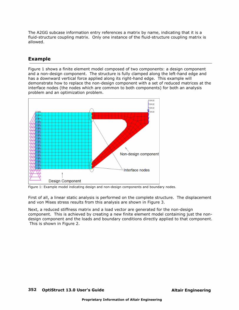
OptiStruct 13.0 User's Guide352 Altair Engineering
Proprietary Information of Altair Engineering
The A2GG subcase information entry references a matrix by name, indicating that it is afluid-structure coupling matrix. Only one instance of the fluid-structure coupling matrix isallowed.
Example
Figure 1 shows a finite element model composed of two components: a design componentand a non-design component. The structure is fully clamped along the left-hand edge andhas a downward vertical force applied along its right-hand edge. This example willdemonstrate how to replace the non-design component with a set of reduced matrices at theinterface nodes (the nodes which are common to both components) for both an analysisproblem and an optimization problem.
Figure 1: Example model indicating design and non-design components and boundary nodes.
First of all, a linear static analysis is performed on the complete structure. The displacementand von Mises stress results from this analysis are shown in Figure 3.
Next, a reduced stiffness matrix and a load vector are generated for the non-designcomponent. This is achieved by creating a new finite element model containing just the non-design component and the loads and boundary conditions directly applied to that component. This is shown in Figure 2.

Altair Engineering OptiStruct 13.0 User's Guide 353
Proprietary Information of Altair Engineering
Figure 2: Reducing out the non-design component.
All of the degrees of freedom at the interface nodes (see Figure 1) are selected as boundarydegrees of freedom. ASET or ASET1 bulk data entries are used to indicate this. The reducedmatrices output is requested through the inclusion of the PARAM, EXTOUT, DMIGPCH bulkdata entry. The model is submitted to OptiStruct, resulting in the creation of the file filename_AX.pch which contains the reduced matrices in ASCII format. (Had
PARAM,EXTOUT,DMIGBIN been used, the reduced matrices would be written in binary form tothe file filename_AX.dmg).
The non-design component can now be replaced in the original model by its reduced matrixrepresentation. This is done by manipulating the original model as follows:
1. Delete the bulk data entries for the nodes and elements of the non-design component.
2. Delete all loads and boundary conditions that were only applied to the non-designcomponent.
3. Include the file containing the reduced matrices in the bulk data section.
4. Select the reduced stiffness matrix with the subcase information entry K2GG. (In thisexample, the reduced stiffness matrix will have the default name KAAX).
5. Select the reduced load vector with the subcase information entry P2G. (In this example,the reduced load vector will have the default name PAX).
Figure 4 shows the displacement and von Mises Stress for the design component when thenon-design component was replaced by a reduced matrix representation. It can clearly beseen, they match perfectly with the original model's results.
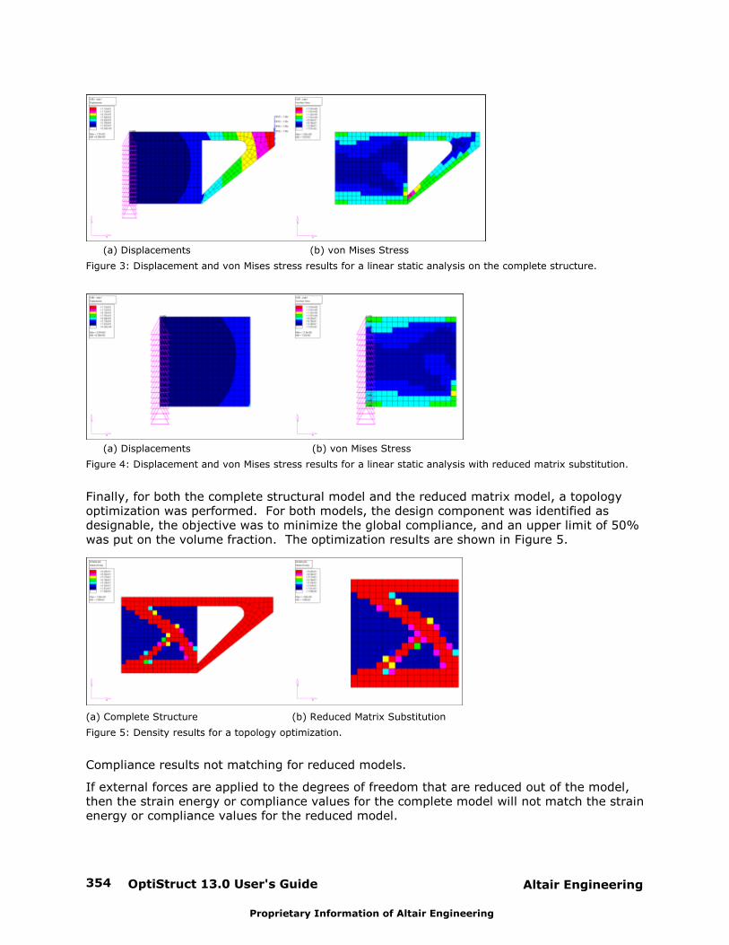
OptiStruct 13.0 User's Guide354 Altair Engineering
Proprietary Information of Altair Engineering
(a) Displacements (b) von Mises Stress
Figure 3: Displacement and von Mises stress results for a linear static analysis on the complete structure.
(a) Displacements (b) von Mises Stress
Figure 4: Displacement and von Mises stress results for a linear static analysis with reduced matrix substitution.
Finally, for both the complete structural model and the reduced matrix model, a topologyoptimization was performed. For both models, the design component was identified asdesignable, the objective was to minimize the global compliance, and an upper limit of 50%was put on the volume fraction. The optimization results are shown in Figure 5.
(a) Complete Structure (b) Reduced Matrix Substitution
Figure 5: Density results for a topology optimization.
Compliance results not matching for reduced models.
If external forces are applied to the degrees of freedom that are reduced out of the model,then the strain energy or compliance values for the complete model will not match the strainenergy or compliance values for the reduced model.
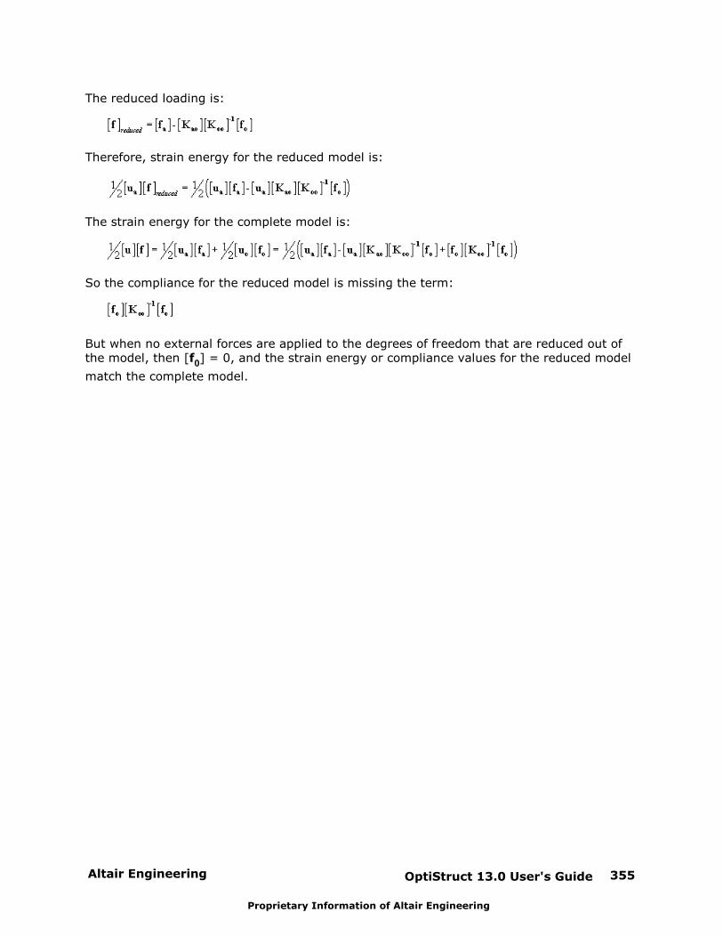
Altair Engineering OptiStruct 13.0 User's Guide 355
Proprietary Information of Altair Engineering
The reduced loading is:
Therefore, strain energy for the reduced model is:
The strain energy for the complete model is:
So the compliance for the reduced model is missing the term:
But when no external forces are applied to the degrees of freedom that are reduced out ofthe model, then [f0] = 0, and the strain energy or compliance values for the reduced model
match the complete model.
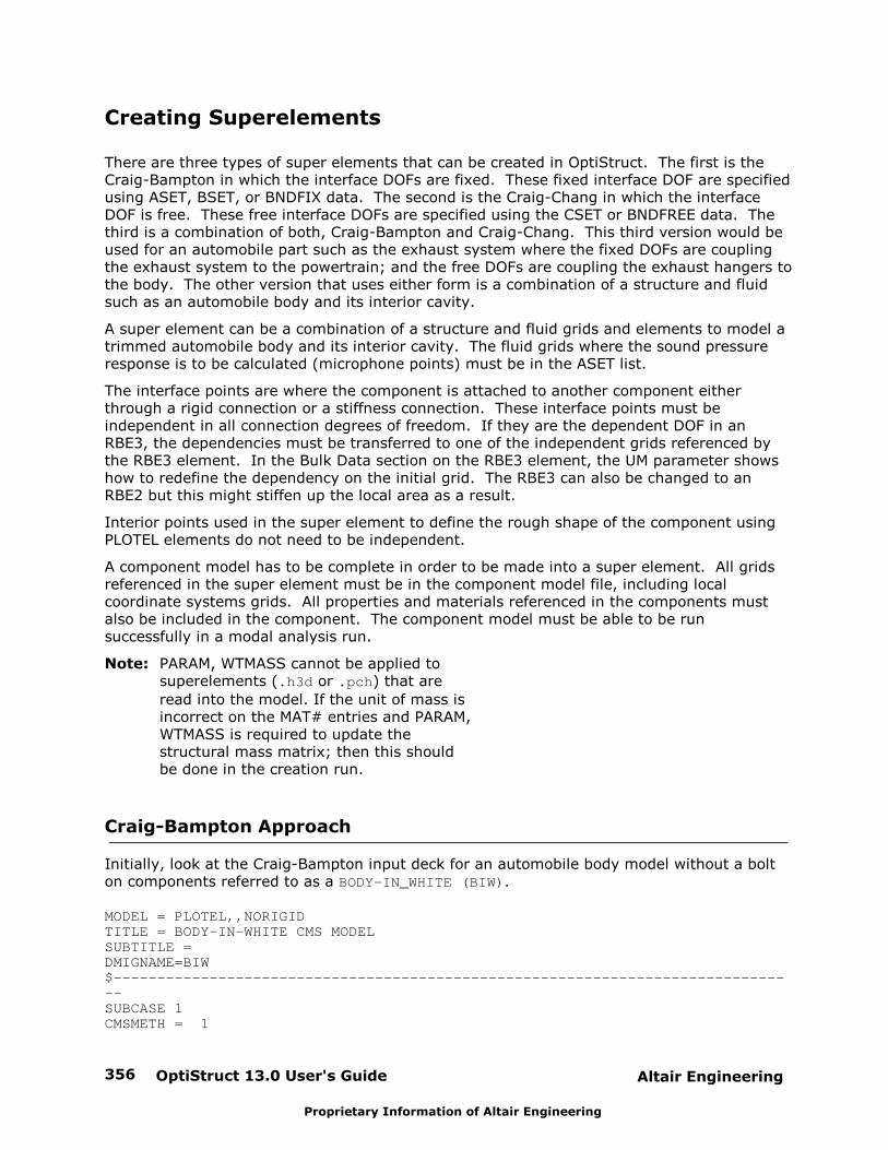
OptiStruct 13.0 User's Guide356 Altair Engineering
Proprietary Information of Altair Engineering
Creating Superelements
There are three types of super elements that can be created in OptiStruct. The first is theCraig-Bampton in which the interface DOFs are fixed. These fixed interface DOF are specifiedusing ASET, BSET, or BNDFIX data. The second is the Craig-Chang in which the interfaceDOF is free. These free interface DOFs are specified using the CSET or BNDFREE data. Thethird is a combination of both, Craig-Bampton and Craig-Chang. This third version would beused for an automobile part such as the exhaust system where the fixed DOFs are couplingthe exhaust system to the powertrain; and the free DOFs are coupling the exhaust hangers tothe body. The other version that uses either form is a combination of a structure and fluidsuch as an automobile body and its interior cavity.
A super element can be a combination of a structure and fluid grids and elements to model atrimmed automobile body and its interior cavity. The fluid grids where the sound pressureresponse is to be calculated (microphone points) must be in the ASET list.
The interface points are where the component is attached to another component eitherthrough a rigid connection or a stiffness connection. These interface points must beindependent in all connection degrees of freedom. If they are the dependent DOF in an RBE3, the dependencies must be transferred to one of the independent grids referenced bythe RBE3 element. In the Bulk Data section on the RBE3 element, the UM parameter showshow to redefine the dependency on the initial grid. The RBE3 can also be changed to anRBE2 but this might stiffen up the local area as a result.
Interior points used in the super element to define the rough shape of the component usingPLOTEL elements do not need to be independent.
A component model has to be complete in order to be made into a super element. All gridsreferenced in the super element must be in the component model file, including localcoordinate systems grids. All properties and materials referenced in the components mustalso be included in the component. The component model must be able to be runsuccessfully in a modal analysis run.
Note: PARAM, WTMASS cannot be applied tosuperelements (.h3d or .pch) that are
read into the model. If the unit of mass isincorrect on the MAT# entries and PARAM,WTMASS is required to update thestructural mass matrix; then this shouldbe done in the creation run.
Craig-Bampton Approach
Initially, look at the Craig-Bampton input deck for an automobile body model without a bolton components referred to as a BODY-IN_WHITE (BIW).
MODEL = PLOTEL,,NORIGIDTITLE = BODY-IN-WHITE CMS MODEL SUBTITLE = DMIGNAME=BIW$-------------------------------------------------------------------------------SUBCASE 1CMSMETH = 1

Altair Engineering OptiStruct 13.0 User's Guide 357
Proprietary Information of Altair Engineering
BEGIN BULK$==01==><==02==><==03==><==04==><==05==><==06==><==07==><==08==><==09==><==10==>CMSMETH 1 CBN 300.0 1008000 AMSESASET1 123456 1000000 THRU 1006004INCLUDE '/MODELS/BODY/BODY.dat'ENDDATA
First, the Craig-Bampton approach can be run in either AMSES or in Lanczos. The resultsshould be the same. Use AMSES for large component models and Lanczos for smallcomponent models.
Second, the MODEL card will include all PLOTEL and the associated interior grids in the superelement. An alternate method to include extra grids can be accomplished by listing the gridsin a set and referencing the set in the MODEL card between the ,, in the MODEL card. ThePLOTEL generally are used to define a rough outline of the component for viewing its modeshapes.
The PLOTEL value will also now include the new plate PLOTEL that are available in OptiStruct.
Third, the PARAM, SEPLOT, YES will create a file including all the grids referenced in theMODEL card, plus the interface grids and the PLOTEL referenced in the MODEL card. This filecan be used later in residual runs, if desired, along with the super element H3D file, althoughit is not required. If a residual run on just this single component is to be made, such as amodal or mobility run, then the .seplot file should be created and used in the residual run.
Otherwise the runs will fail without having any other input besides the H3D file because noGRID data is in the input data.
The DMIGNAME is optional and can be specified later in the residual run. It creates a uniquename to the stiffness, mass and damping matrix and can only be a maximum of sixcharacters.
The CMSMETH case control card calls the new OptiStruct super element eigenvalue cardCMSMETH.
The CMSMETH bulk data card referenced in this case the CBN (Craig-Bampton Method). Thenext field is the upper frequency bound for the modes. The sixth field references the startingnumber for where the SPOINTS for the modes will be stored. This range of numbers must beunique for the full vehicle model and each super element will need its own numbering range. The seventh field is used to specify the eigensolver (Lanczos or AMSES).
The ASET1 lists the interface points of the super element model in the example above.
Only the connection and specific response points should be included in the ASET list. Theother points in the super element are called interior points. The interior points should not bein this ASET list, since the model size and run time will increase with the number of pointsincluded in the ASET list. If you have special response points in the component, they shouldbe included in the ASET list. Generally there are only a few critical response points. Thecritical response points must be independent points. The calculated responses will show upin the output files. If any type of random analysis is being performed, it is essential that theresponse points be included in the ASET list with the exterior points.
This file will generate an H3D binary file that includes all the information that is needed forthis super element. It can also create the optional .seplot ASCII file, if requested. The
H3D file will include matrices for the mass and stiffness and it will also include the matricesfor structural damping and viscous damping if these elements exist in the model. Look at thebottom of the .out file to see what matrices are created.
OptiStruct 13.0 User's Guide358 Altair Engineering
Proprietary Information of Altair Engineering
Below is an example. There were 274 modes found for this model. There were 166connection grids with six DOF each for a total of 996 connections DOF. The total number ofmodes (connection plus normal modes) is 1270.
OUTPUT DMIG MATRIX IN H3D FORMAT OUTPUT DMIG MATRIX: KA NCOL = 1270 OUTPUT DMIG MATRIX: MA NCOL = 1270 OUTPUT DMIG MATRIX: K4 NCOL = 1270
The .out file will show the modes for the fixed boundary condition. In general, it is desirable
to have at least 30 modes for each component model. For small items like a control arm, anupper limit of around 5,000 Hz may be needed.
Craig-Chang Approach
The following cards show the Craig-Chang approach.
PARAM, SEPLOT, YESPARAM, AUTOSPC, YESMODEL = PLOTEL,,NORIGIDTITLE = BODY-IN-WHITE CMS MODEL SUBTITLE = DMIGNAME=BIW$-------------------------------------------------------------------------------SUBCASE 1CMSMETH = 1BEGIN BULK$==01==><==02==><==03==><==04==><==05==><==06==><==07==><==08==><==09==><==10==>CMSMETH 1 GM 300.0 1008000 AMSESBNDFREE1 123456 1000000 THRU 1006016INCLUDE '/MODELS/BODY/BODY.dat'ENDDATA
For the Craig-Chang Approach, use AMSES to generate the super element. With AMSES youwill get the appropriate static modes. Static modes are additional modes created byperturbing each connection DOF. The number of static modes is the number of BNDFREEDOF. Since Lanczos does not generate the static modes for the Craig-Chang approach, theAMSES eigensolver must be used.
The only difference in the input data for creating Craig-Chang super elements from Craig-Bampton super elements is in the CMSMETH and the BNDFREE1 cards. The CMSMETH cardnow references the GM (General Method). This method is used for the Craig-Chang or thecombination of both methods. The BNDFIX or ASET data should be changed to BNDFREE orCSET data.
The BNDFREE1 card replaces the ASET1 card and has the same meaning for the inclusions ofthe interface points.
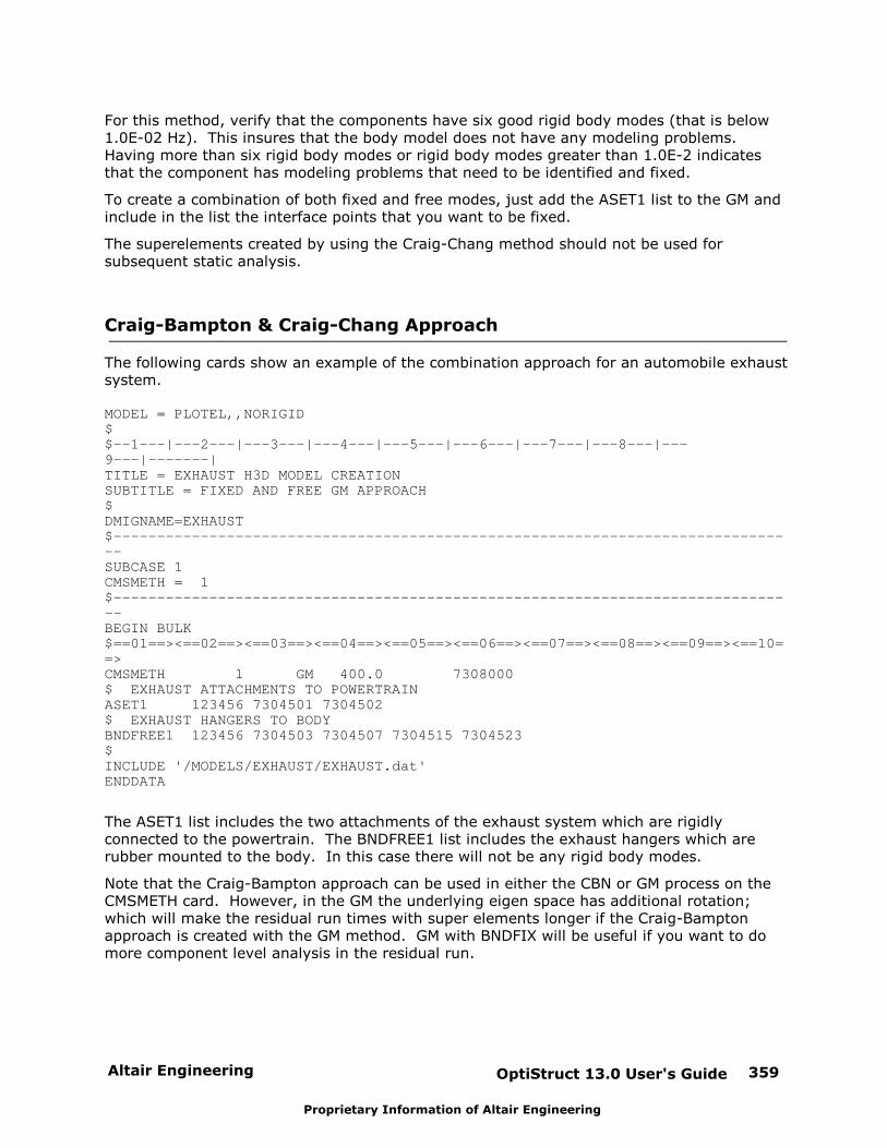
Altair Engineering OptiStruct 13.0 User's Guide 359
Proprietary Information of Altair Engineering
For this method, verify that the components have six good rigid body modes (that is below1.0E-02 Hz). This insures that the body model does not have any modeling problems. Having more than six rigid body modes or rigid body modes greater than 1.0E-2 indicatesthat the component has modeling problems that need to be identified and fixed.
To create a combination of both fixed and free modes, just add the ASET1 list to the GM andinclude in the list the interface points that you want to be fixed.
The superelements created by using the Craig-Chang method should not be used forsubsequent static analysis.
Craig-Bampton & Craig-Chang Approach
The following cards show an example of the combination approach for an automobile exhaustsystem.
MODEL = PLOTEL,,NORIGID$$--1---|---2---|---3---|---4---|---5---|---6---|---7---|---8---|---9---|-------|TITLE = EXHAUST H3D MODEL CREATIONSUBTITLE = FIXED AND FREE GM APPROACH $DMIGNAME=EXHAUST$-------------------------------------------------------------------------------SUBCASE 1CMSMETH = 1 $-------------------------------------------------------------------------------BEGIN BULK$==01==><==02==><==03==><==04==><==05==><==06==><==07==><==08==><==09==><==10==>CMSMETH 1 GM 400.0 7308000 $ EXHAUST ATTACHMENTS TO POWERTRAINASET1 123456 7304501 7304502$ EXHAUST HANGERS TO BODY BNDFREE1 123456 7304503 7304507 7304515 7304523$INCLUDE '/MODELS/EXHAUST/EXHAUST.dat'ENDDATA
The ASET1 list includes the two attachments of the exhaust system which are rigidlyconnected to the powertrain. The BNDFREE1 list includes the exhaust hangers which arerubber mounted to the body. In this case there will not be any rigid body modes.
Note that the Craig-Bampton approach can be used in either the CBN or GM process on theCMSMETH card. However, in the GM the underlying eigen space has additional rotation;which will make the residual run times with super elements longer if the Craig-Bamptonapproach is created with the GM method. GM with BNDFIX will be useful if you want to domore component level analysis in the residual run.
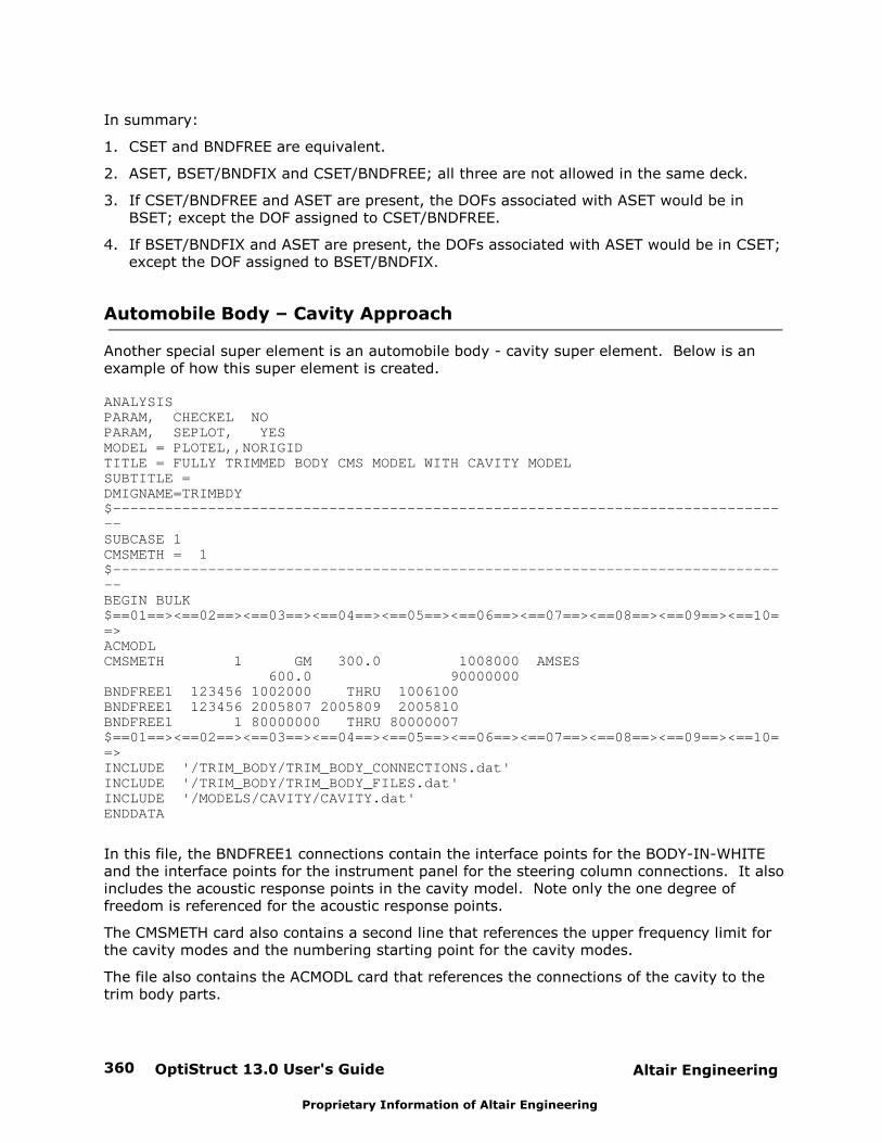
OptiStruct 13.0 User's Guide360 Altair Engineering
Proprietary Information of Altair Engineering
In summary:
1. CSET and BNDFREE are equivalent.
2. ASET, BSET/BNDFIX and CSET/BNDFREE; all three are not allowed in the same deck.
3. If CSET/BNDFREE and ASET are present, the DOFs associated with ASET would be inBSET; except the DOF assigned to CSET/BNDFREE.
4. If BSET/BNDFIX and ASET are present, the DOFs associated with ASET would be in CSET;except the DOF assigned to BSET/BNDFIX.
Automobile Body – Cavity Approach
Another special super element is an automobile body - cavity super element. Below is anexample of how this super element is created.
ANALYSISPARAM, CHECKEL NO PARAM, SEPLOT, YESMODEL = PLOTEL,,NORIGIDTITLE = FULLY TRIMMED BODY CMS MODEL WITH CAVITY MODEL SUBTITLE = DMIGNAME=TRIMBDY $-------------------------------------------------------------------------------SUBCASE 1CMSMETH = 1$------------------------------------------------------------------------------- BEGIN BULK$==01==><==02==><==03==><==04==><==05==><==06==><==07==><==08==><==09==><==10==>ACMODL CMSMETH 1 GM 300.0 1008000 AMSES 600.0 90000000BNDFREE1 123456 1002000 THRU 1006100BNDFREE1 123456 2005807 2005809 2005810 BNDFREE1 1 80000000 THRU 80000007$==01==><==02==><==03==><==04==><==05==><==06==><==07==><==08==><==09==><==10==>INCLUDE '/TRIM_BODY/TRIM_BODY_CONNECTIONS.dat'INCLUDE '/TRIM_BODY/TRIM_BODY_FILES.dat'INCLUDE '/MODELS/CAVITY/CAVITY.dat'ENDDATA
In this file, the BNDFREE1 connections contain the interface points for the BODY-IN-WHITEand the interface points for the instrument panel for the steering column connections. It alsoincludes the acoustic response points in the cavity model. Note only the one degree offreedom is referenced for the acoustic response points.
The CMSMETH card also contains a second line that references the upper frequency limit forthe cavity modes and the numbering starting point for the cavity modes.
The file also contains the ACMODL card that references the connections of the cavity to thetrim body parts.

Altair Engineering OptiStruct 13.0 User's Guide 361
Proprietary Information of Altair Engineering
The .out file shows the inclusion of the acoustic modes in the A matrix.
OUTPUT DMIG MATRIX IN H3D FORMAT OUTPUT DMIG MATRIX: KA NCOL = 1687 OUTPUT DMIG MATRIX: MA NCOL = 1687 OUTPUT DMIG MATRIX: K4 NCOL = 1402 OUTPUT DMIG MATRIX: A NCOL = 285
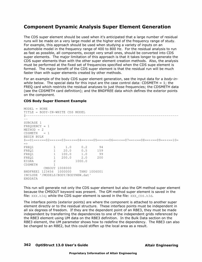
OptiStruct 13.0 User's Guide362 Altair Engineering
Proprietary Information of Altair Engineering
Component Dynamic Analysis Super Element Generation
The CDS super element should be used when it's anticipated that a large number of residualruns will be made on a very large model at the higher end of the frequency range of study. For example, this approach should be used when studying a variety of inputs on anautomobile model in the frequency range of 400 to 800 Hz. For the residual analysis to runas fast as possible, all components, except very small ones, should be converted into CDSsuper elements. The major limitation of this approach is that it takes longer to generate theCDS super elements than with the other super element creation methods. Also, the analysismust be performed at the fixed set of frequencies specified when the CDS supe element isformed. The major benefit of the CDS super element is that the residual run will be muchfaster than with super elements created by other methods.
For an example of the body CDS super element generation, see the input data for a body-in-white below. The special data for this input are the case control data: CDSMETH = 1; theFREQ card which restricts the residual analyses to just those frequencies; the CDSMETH data(see the CDSMETH card definition); and the BNDFREE data which defines the exterior pointson the component.
CDS Body Super Element Example
MODEL = NONETITLE = BODY-IN-WHITE CDS MODEL$-------------------------------------------------------------------------------SUBCASE 1FREQUENCY = 1METHOD = 2CDSMETH = 1BEGIN BULK$==01==><==02==><==03==><==04==><==05==><==06==><==07==><==08==><==09==><==10==>FREQ1 1 1.0 0.2 94FREQ1 1 20.0 0.5 159FREQ1 1 100.0 1.0 99FREQ1 1 200.0 2.0 200EIGRA 2 1000.0CDSMETH 1 CMSOUT 1008000BNDFREE1 123456 1000000 THRU 1006001INCLUDE '/MODELS/BODY/BODYNEW.dat'ENDDATA
This run will generate not only the CDS super element but also the GM method super elementbecause the CMSOUT keyword was present. The GM method super element is saved in thefile: XXX.h3d; while the CDS super element is saved in the file: XXX_CDS.h3d.
The interface points (exterior points) are where the component is attached to another superelement directly or to the residual structure. These interface points must be independent inall six degrees of freedom. If they are the dependent point of an RBE3, they must be madeindependent by transferring the dependencies to one of the independent grids referenced bythe RBE3 element using UM data on the RBE3 definition. In the Bulk Data section on theRBE3 element, the UM parameter shows how to redefine the dependency. The RBE3 can alsobe changed to an RBE2, but this could stiffen up the local area as a result.
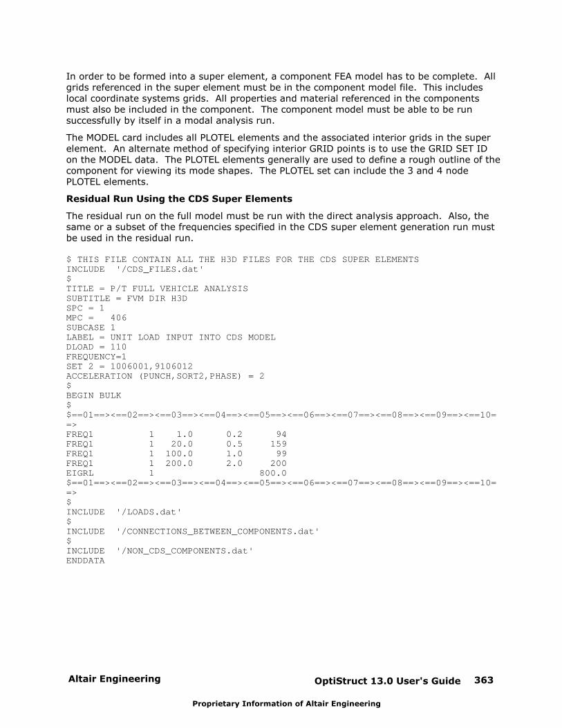
Altair Engineering OptiStruct 13.0 User's Guide 363
Proprietary Information of Altair Engineering
In order to be formed into a super element, a component FEA model has to be complete. Allgrids referenced in the super element must be in the component model file. This includeslocal coordinate systems grids. All properties and material referenced in the componentsmust also be included in the component. The component model must be able to be runsuccessfully by itself in a modal analysis run.
The MODEL card includes all PLOTEL elements and the associated interior grids in the superelement. An alternate method of specifying interior GRID points is to use the GRID SET IDon the MODEL data. The PLOTEL elements generally are used to define a rough outline of thecomponent for viewing its mode shapes. The PLOTEL set can include the 3 and 4 nodePLOTEL elements.
Residual Run Using the CDS Super Elements
The residual run on the full model must be run with the direct analysis approach. Also, thesame or a subset of the frequencies specified in the CDS super element generation run mustbe used in the residual run.
$ THIS FILE CONTAIN ALL THE H3D FILES FOR THE CDS SUPER ELEMENTSINCLUDE '/CDS_FILES.dat'$TITLE = P/T FULL VEHICLE ANALYSISSUBTITLE = FVM DIR H3DSPC = 1MPC = 406SUBCASE 1LABEL = UNIT LOAD INPUT INTO CDS MODELDLOAD = 110FREQUENCY=1SET 2 = 1006001,9106012ACCELERATION (PUNCH,SORT2,PHASE) = 2$BEGIN BULK$$==01==><==02==><==03==><==04==><==05==><==06==><==07==><==08==><==09==><==10==>FREQ1 1 1.0 0.2 94FREQ1 1 20.0 0.5 159FREQ1 1 100.0 1.0 99FREQ1 1 200.0 2.0 200EIGRL 1 800.0 $==01==><==02==><==03==><==04==><==05==><==06==><==07==><==08==><==09==><==10==>$ INCLUDE '/LOADS.dat'$INCLUDE '/CONNECTIONS_BETWEEN_COMPONENTS.dat'$ INCLUDE '/NON_CDS_COMPONENTS.dat'ENDDATA
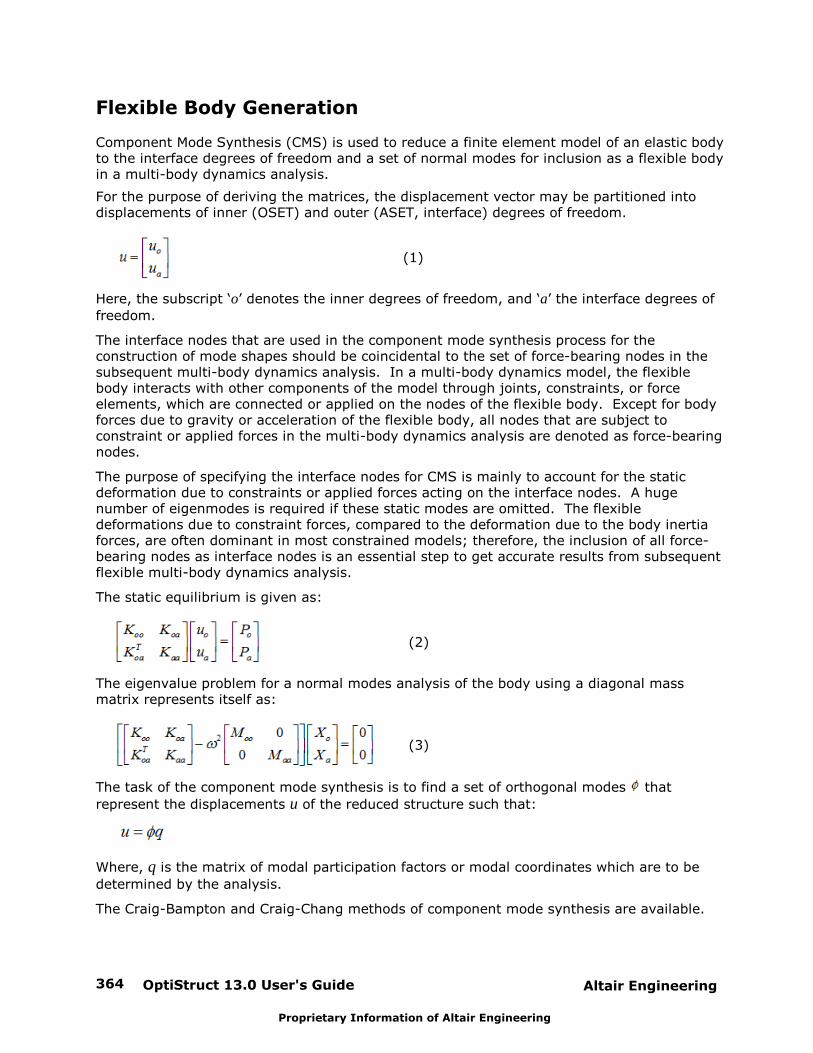
OptiStruct 13.0 User's Guide364 Altair Engineering
Proprietary Information of Altair Engineering
Flexible Body Generation
Component Mode Synthesis (CMS) is used to reduce a finite element model of an elastic bodyto the interface degrees of freedom and a set of normal modes for inclusion as a flexible bodyin a multi-body dynamics analysis.
For the purpose of deriving the matrices, the displacement vector may be partitioned intodisplacements of inner (OSET) and outer (ASET, interface) degrees of freedom.
(1)
Here, the subscript ‘o’ denotes the inner degrees of freedom, and ‘a’ the interface degrees of
freedom.
The interface nodes that are used in the component mode synthesis process for theconstruction of mode shapes should be coincidental to the set of force-bearing nodes in thesubsequent multi-body dynamics analysis. In a multi-body dynamics model, the flexiblebody interacts with other components of the model through joints, constraints, or forceelements, which are connected or applied on the nodes of the flexible body. Except for bodyforces due to gravity or acceleration of the flexible body, all nodes that are subject toconstraint or applied forces in the multi-body dynamics analysis are denoted as force-bearingnodes.
The purpose of specifying the interface nodes for CMS is mainly to account for the staticdeformation due to constraints or applied forces acting on the interface nodes. A hugenumber of eigenmodes is required if these static modes are omitted. The flexibledeformations due to constraint forces, compared to the deformation due to the body inertiaforces, are often dominant in most constrained models; therefore, the inclusion of all force-bearing nodes as interface nodes is an essential step to get accurate results from subsequentflexible multi-body dynamics analysis.
The static equilibrium is given as:
(2)
The eigenvalue problem for a normal modes analysis of the body using a diagonal massmatrix represents itself as:
(3)
The task of the component mode synthesis is to find a set of orthogonal modes that
represent the displacements u of the reduced structure such that:
Where, q is the matrix of modal participation factors or modal coordinates which are to be
determined by the analysis.
The Craig-Bampton and Craig-Chang methods of component mode synthesis are available.
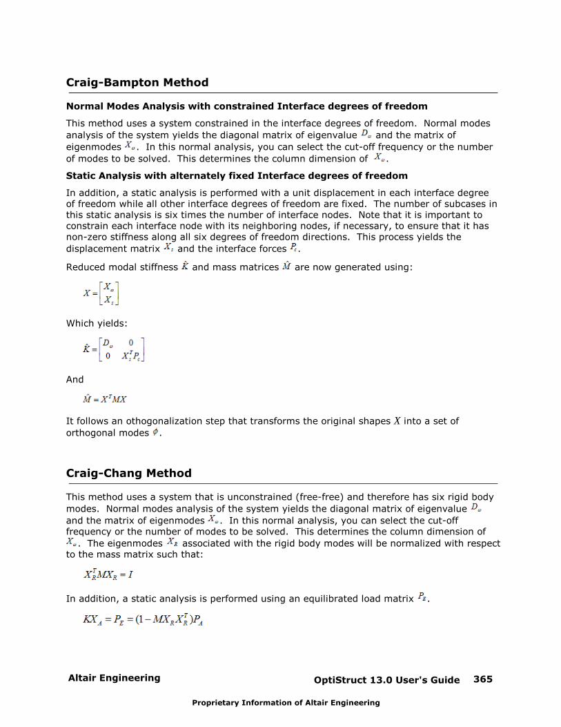
Altair Engineering OptiStruct 13.0 User's Guide 365
Proprietary Information of Altair Engineering
Craig-Bampton Method
Normal Modes Analysis with constrained Interface degrees of freedom
This method uses a system constrained in the interface degrees of freedom. Normal modes
analysis of the system yields the diagonal matrix of eigenvalue and the matrix of
eigenmodes . In this normal analysis, you can select the cut-off frequency or the number
of modes to be solved. This determines the column dimension of .
Static Analysis with alternately fixed Interface degrees of freedom
In addition, a static analysis is performed with a unit displacement in each interface degreeof freedom while all other interface degrees of freedom are fixed. The number of subcases inthis static analysis is six times the number of interface nodes. Note that it is important toconstrain each interface node with its neighboring nodes, if necessary, to ensure that it hasnon-zero stiffness along all six degrees of freedom directions. This process yields the
displacement matrix and the interface forces .
Reduced modal stiffness and mass matrices are now generated using:
Which yields:
And
It follows an othogonalization step that transforms the original shapes X into a set of
orthogonal modes .
Craig-Chang Method
This method uses a system that is unconstrained (free-free) and therefore has six rigid body
modes. Normal modes analysis of the system yields the diagonal matrix of eigenvalue
and the matrix of eigenmodes . In this normal analysis, you can select the cut-offfrequency or the number of modes to be solved. This determines the column dimension of
. The eigenmodes associated with the rigid body modes will be normalized with respectto the mass matrix such that:
In addition, a static analysis is performed using an equilibrated load matrix .
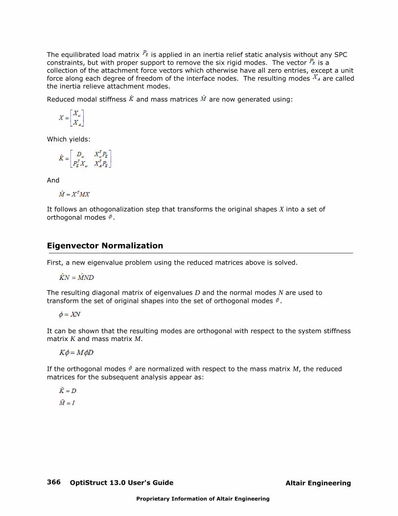
OptiStruct 13.0 User's Guide366 Altair Engineering
Proprietary Information of Altair Engineering
The equilibrated load matrix is applied in an inertia relief static analysis without any SPCconstraints, but with proper support to remove the six rigid modes. The vector is acollection of the attachment force vectors which otherwise have all zero entries, except a unitforce along each degree of freedom of the interface nodes. The resulting modes are calledthe inertia relieve attachment modes.
Reduced modal stiffness and mass matrices are now generated using:
Which yields:
And
It follows an othogonalization step that transforms the original shapes X into a set of
orthogonal modes .
Eigenvector Normalization
First, a new eigenvalue problem using the reduced matrices above is solved.
The resulting diagonal matrix of eigenvalues D and the normal modes N are used to
transform the set of original shapes into the set of orthogonal modes .
It can be shown that the resulting modes are orthogonal with respect to the system stiffnessmatrix K and mass matrix M.
If the orthogonal modes are normalized with respect to the mass matrix M, the reduced
matrices for the subsequent analysis appear as:
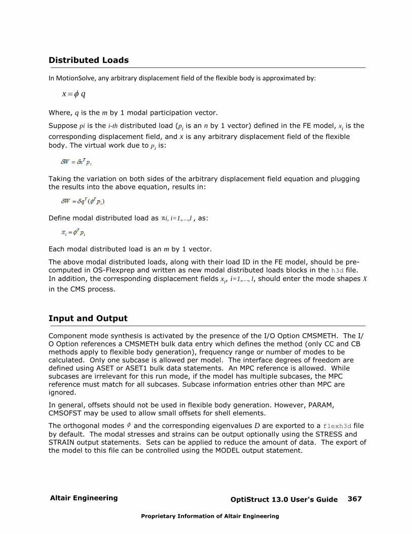
Altair Engineering OptiStruct 13.0 User's Guide 367
Proprietary Information of Altair Engineering
Distributed Loads
In MotionSolve, any arbitrary displacement field of the flexible body is approximated by:
x q
Where, q is the m by 1 modal participation vector.
Suppose pi is the i-th distributed load (pi is an n by 1 vector) defined in the FE model, xi is the
corresponding displacement field, and x is any arbitrary displacement field of the flexible
body. The virtual work due to pi is:
Taking the variation on both sides of the arbitrary displacement field equation and pluggingthe results into the above equation, results in:
Define modal distributed load as i, i=1,…,l , as:
Each modal distributed load is an m by 1 vector.
The above modal distributed loads, along with their load ID in the FE model, should be pre-computed in OS-Flexprep and written as new modal distributed loads blocks in the h3d file.
In addition, the corresponding displacement fields xi, i=1,…, l, should enter the mode shapes X
in the CMS process.
Input and Output
Component mode synthesis is activated by the presence of the I/O Option CMSMETH. The I/O Option references a CMSMETH bulk data entry which defines the method (only CC and CBmethods apply to flexible body generation), frequency range or number of modes to becalculated. Only one subcase is allowed per model. The interface degrees of freedom aredefined using ASET or ASET1 bulk data statements. An MPC reference is allowed. Whilesubcases are irrelevant for this run mode, if the model has multiple subcases, the MPCreference must match for all subcases. Subcase information entries other than MPC areignored.
In general, offsets should not be used in flexible body generation. However, PARAM,CMSOFST may be used to allow small offsets for shell elements.
The orthogonal modes and the corresponding eigenvalues D are exported to a flexh3d file
by default. The modal stresses and strains can be output optionally using the STRESS andSTRAIN output statements. Sets can be applied to reduce the amount of data. The export ofthe model to this file can be controlled using the MODEL output statement.
OptiStruct 13.0 User's Guide368 Altair Engineering
Proprietary Information of Altair Engineering
Recovering MBD Analysis results in OptiStruct
After MotionSolve is run, it is possible to recover displacements, velocities, accelerations,stresses, and strains for the flexbody in OptiStruct in order to create .op2 and .h3d results
files for fatigue analysis. The procedure is explained below.
After running MotionSolve, a residual run can be made to recover displacement, velocity,acceleration, stress, and strain results for interior grids and elements in the Flex Body basedon the modal participation results from MotionSolve. After running MotionSolve, a resulting <filename>.mrf file is created that contains MotionSolve results including the modal
participation factors at each time step for the Flex Body for transient analysis. In the residualrun, the Flex Body <filename>_recov.h3d file and the .mrf results file are specified using
the ASSIGN data:
ASSIGN,H3DMBD,30101,’pfbody_1_recov.h3d'
ASSIGN,H3DMBD,30102,’pfbody_2_recov.h3d'
ASSIGN,MBDINP,10,’pfbody.mrf'
Where the 10 in the ASSIGN,MBDINP data references the SUBCASE for which the MotionSolve
results will be used. In SUBCASE 10, instead of performing a transient analysis, OptiStruct
will just use the results from MotionSolve.
The 30101 and 30102 in the ASSIGN,H3DMBD data refer to the Flex Body ID’s in the .mrf file.
For transient analysis, the number of time steps in the transient analysis run must match thenumber of time steps used in the MotionSolve analysis. While the transient analysis data isignored, there must still be some dummy loading data (TLOAD, DAREA, and TABLED data). A sample of input data for a transient analysis run is shown below:
OUTPUT OP2OUTPUT H3DASSIGN,H3DMBD,30103,MBD_pfbody_BODY_2_PROP_6_recov.h3dASSIGN,H3DMBD,30102,MBD_pfbody_BODY_1_PROP_9_recov.h3dASSIGN,H3DMBD,30104,MBD_pfbody_BODY_3_PROP_10_recov.h3dASSIGN,MBDINP,1,MBD_pfbody_mbd.mrfSUBCASE 1 TSTEP(TIME) = 4 DLOAD = 3 DISPLACEMENT = ALL STRESS = ALL SPC = 1$BEGIN BULKGRID 9999999 $ Dummy GRID since at least one GRID is required$------+-------+-------+-------+-------+-------+-------+-------+-------TSTEP 4 300 .0003333 1 TLOAD1 3 3 DISP 2TABLED1 2 LINEAR LINEAR+ 0.0 1.0 10.0 1.0ENDT $$ Dummy load on the dummy gridSPC 1 9999999 1SPCD 3 9999999 1 -200.0 ENDDATA
A dummy grid and a dummy load have been added for the OptiStruct analysis run.
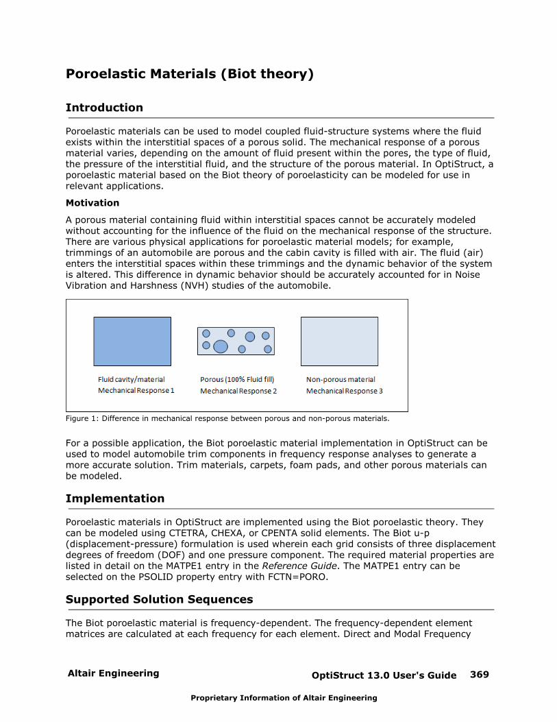
Altair Engineering OptiStruct 13.0 User's Guide 369
Proprietary Information of Altair Engineering
Poroelastic Materials (Biot theory)
Introduction
Poroelastic materials can be used to model coupled fluid-structure systems where the fluidexists within the interstitial spaces of a porous solid. The mechanical response of a porousmaterial varies, depending on the amount of fluid present within the pores, the type of fluid,the pressure of the interstitial fluid, and the structure of the porous material. In OptiStruct, aporoelastic material based on the Biot theory of poroelasticity can be modeled for use inrelevant applications.
Motivation
A porous material containing fluid within interstitial spaces cannot be accurately modeledwithout accounting for the influence of the fluid on the mechanical response of the structure.There are various physical applications for poroelastic material models; for example,trimmings of an automobile are porous and the cabin cavity is filled with air. The fluid (air)enters the interstitial spaces within these trimmings and the dynamic behavior of the systemis altered. This difference in dynamic behavior should be accurately accounted for in NoiseVibration and Harshness (NVH) studies of the automobile.
Figure 1: Difference in mechanical response between porous and non-porous materials.
For a possible application, the Biot poroelastic material implementation in OptiStruct can beused to model automobile trim components in frequency response analyses to generate amore accurate solution. Trim materials, carpets, foam pads, and other porous materials canbe modeled.
Implementation
Poroelastic materials in OptiStruct are implemented using the Biot poroelastic theory. Theycan be modeled using CTETRA, CHEXA, or CPENTA solid elements. The Biot u-p(displacement-pressure) formulation is used wherein each grid consists of three displacementdegrees of freedom (DOF) and one pressure component. The required material properties arelisted in detail on the MATPE1 entry in the Reference Guide. The MATPE1 entry can beselected on the PSOLID property entry with FCTN=PORO.
Supported Solution Sequences
The Biot poroelastic material is frequency-dependent. The frequency-dependent elementmatrices are calculated at each frequency for each element. Direct and Modal Frequency

OptiStruct 13.0 User's Guide370 Altair Engineering
Proprietary Information of Altair Engineering
Response Analyses are supported. The frequency-dependent matrices are reduced to modalspaces for modal frequency response analysis. Panel participation calculation for the Biotmaterial is available similar to that of other panels. The fluid-structural grid participation isalso available for detailed interpretation of panel contributions.
Note
1. Coupling between the acoustic cavity (FLUID) and trim component (BIOT):
(a)A GRID to GRID match or Multi-point constraints (MPCs) are required to connect theacoustic cavity to fluid dof of the BIOT material.
(b)The ACMODL entry will be used to couple the fluid dof and the structural dof of theBIOT material.
(c) If a GRID to GRID match is used to couple the acoustic cavity to the BIOT material, thegrids on the fluid that are shared with the BIOT material should not have their CDfields set to -1. However, if Multi-point constraints (MPCs) are used, then the CD fieldsshould be set equal to -1.
2. Coupling between the trim component (BIOT) and the body structure:
(a) Coincident nodes (GRID to GRID match) can be used to achieve displacementcontinuity. However, if the nodes between the trim component and the body structureare not shared, TIE/CONTACT entries with the FREEZE option, rigids, MPC’s, or otherstructural elements can be used to ensure continuity.
Limitations
The pressure output for the trim component (poroelastic Biot material) is not currentlysupported. However, the pressure of the closest acoustic domain is available.
Altair Engineering OptiStruct 13.0 User's Guide 371
Proprietary Information of Altair Engineering
Elements and Materials
The following features can be found in this section
Elastic, Damper, and Mass Elements
Zero-dimensional Elements
Elements in this group only connect to grid points having a single degree of freedom ateach end. Elements also included in this group are those that connect to scalar points atone end and ground at the other, like the following:
CELAS1, CELAS2, CELAS3, and CELAS4 that are used to model elastic springs. Theproperties for CELAS1 and CELAS3 are defined on PELAS. CELAS2 and CELAS4define spring properties.
CDAMP1, CDAMP2, CDAMP3, and CDAMP4 that are used to model scalar dampers. The properties for CDAMP1 and CDAMP3 are defined on PDAMP. CDAMP2 andCDAMP4 define scalar damper properties.
CMASS1, CMASS2, CMASS3, and CMASS4 that are used to model point masses. Theproperties for CMASS1 and CMASS3 are defined on PMASS. CMASS2 and CMASS4define the mass.
CONM1 and CONM2, which are concentrated mass elements. CONM1 defines a 6x6mass matrix at a grid point. CONM2 defines mass and inertia properties at a gridpoint.
CVISC is used to model viscous dampers. The properties for CVISC are defined onPVISC.
One-dimensional Elements
Elements in this group are represented by a line connecting grid points at each end. Thefollowing actions involving forces (and displacements) at each end are possible:
Forces and displacements along the axis of the element.
Transverse shear forces (and displacements) in the two lateral directions.
Bending moments (and rotations) in two perpendicular, bending planes.
Torsional moments (and resulting rotations).
Twisting of the cross-section (or cross-sectional warping).
The elements in this category are:
CBEAM - a general beam element that supports all types of action listed above.
CBAR - a simple, prismatic beam element that supports all of the above types ofactions except cross-sectional warping.
CBUSH - a general spring-damper element that supports forces, moments, anddisplacements along the axis of the element.
OptiStruct 13.0 User's Guide372 Altair Engineering
Proprietary Information of Altair Engineering
CBUSH1D - a rod-type spring-damper element.
CGAP - a gap element that supports axial and friction forces.
CGAPG - a gap element that supports axial and friction forces. It does not have to beplaced between grid points. It can also connect surface patches.
CROD - a simple, axial bar element that supports only axial forces and torsionalmoments.
CWELD - a simple, axial bar element that supports forces, moments, and torsionalmoments. It does not have to be placed between grid points. It can also connectsurface patches.
The properties for these elements are defined on PBEAM, PBAR, PBUSH, PBUSH1D, PGAP,PROD, and PWELD, respectively.
CONROD - a simple, axial bar element that supports only axial forces and torsionalmoments. This element does not reference a property definition; the propertyinformation is provided with the element definition.
Two-dimensional Elements
Two-dimensional elements are used to model thin-shell behavior, which incorporates in-plane or membrane actions, plane strain, and bending action (including transverse shearcharacteristics and membrane-bending coupling actions). Reissner-Mindlin shell theory isused to model bending. A plane strain option is available for pure 2D applications. Theelement shapes may be triangular (CTRIA3) or quadrilateral (CQUAD4). Second ordertriangular (CTRIA6) and quadrilateral (CQUAD8) shell elements are also available. Theshell properties, including the behavior, are defined on the PSHELL entry.
The first order shell element formulation for CQUAD4 and CTRIA3 has the specialcharacteristic of using six degrees of freedom per grid. Hence, there is stiffness associatedto each degree of freedom. In some finite element codes, shell elements do not have adrilling stiffness normal to the mid-plane, which may cause singular stiffness matrix. Then, a user-defined artificial stiffness value is assigned to this degree of freedom to avoidthe singularity.
The second order shell elements (CTRIA6 and CQUAD8) have five degrees of freedom pergrid. Rotational degrees of freedom without stiffness are removed through SPC.
Another form of two-dimensional elements may also be used to model thin buckled plates. These elements support shear stress in their interior and extensional forces between theiradjacent grid points. These elements are used in situations where the bending stiffnessand axial membrane stiffness of a plate is negligible. The elements are quadrilateral andare defined as CSHEAR. Their properties are defined on the PSHEAR entry.
Three-dimensional Elements
The three-dimensional solid elements are used to model thick plates, solid structures. Ingeneral, structures in which the lateral dimensions are of the same order of magnitude asthe longitudinal dimensions can support the use of three-dimensional solid elements inmodeling. The elements in this category are the CHEXA, CPENTA, CPYRA, and CTETRAelements. The property definition associated with these elements is called PSOLID.
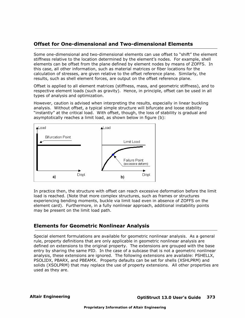
Altair Engineering OptiStruct 13.0 User's Guide 373
Proprietary Information of Altair Engineering
Offset for One-dimensional and Two-dimensional Elements
Some one-dimensional and two-dimensional elements can use offset to “shift” the elementstiffness relative to the location determined by the element’s nodes. For example, shellelements can be offset from the plane defined by element nodes by means of ZOFFS. Inthis case, all other information, such as material matrices or fiber locations for thecalculation of stresses, are given relative to the offset reference plane. Similarly, theresults, such as shell element forces, are output on the offset reference plane.
Offset is applied to all element matrices (stiffness, mass, and geometric stiffness), and torespective element loads (such as gravity). Hence, in principle, offset can be used in alltypes of analysis and optimization.
However, caution is advised when interpreting the results, especially in linear bucklinganalysis. Without offset, a typical simple structure will bifurcate and loose stability“instantly” at the critical load. With offset, though, the loss of stability is gradual andasymptotically reaches a limit load, as shown below in figure (b):
In practice then, the structure with offset can reach excessive deformation before the limitload is reached. (Note that more complex structures, such as frames or structuresexperiencing bending moments, buckle via limit load even in absence of ZOFFS on theelement card). Furthermore, in a fully nonlinear approach, additional instability pointsmay be present on the limit load path.
Elements for Geometric Nonlinear Analysis
Special element formulations are available for geometric nonlinear analysis. As a generalrule, property definitions that are only applicable in geometric nonlinear analysis aredefined on extensions to the original property. The extensions are grouped with the baseentry by sharing the same PID. In the case of a subcase that is not a geometric nonlinearanalysis, these extensions are ignored. The following extensions are available: PSHELLX,PSOLIDX, PBARX, and PBEAMX. Property defaults can be set for shells (XSHLPRM) andsolids (XSOLPRM) that may replace the use of property extensions. All other properties areused as they are.
OptiStruct 13.0 User's Guide374 Altair Engineering
Proprietary Information of Altair Engineering
Example:
PSHELL, 3, 7, 1.0, 7, , 7PSHELLX, 3, 24, , , 5
Non-structural Mass
Non-structural mass may be specified in two different ways.
1. Many property definitions (PSHELL, PCOMP, PBAR, PBARL, PBEAM, PBEAML, PROD,CONROD, PSHEAR, and PTUBE), have an NSM data field that allows a value of non-structural mass per unit area or non-structural mass per unit length to be defined.
When non-structural mass is defined in this way, it is considered in all analyses.
2. Non-structural mass may be defined via a number of non-structural mass bulk dataentries (NSM, NSM1, NSML, NSML1, and NSMADD) for a list of elements or properties. In the case of a list of properties, non-structural mass is applied to the elementsreferencing the properties in the list.
These non-structural mass definitions must be selected for use in an analysis throughthe NSM subcase information entry. Only one NSM subcase information entry can existin a model and it must occur before the first SUBCASE statement.
The bulk data entry NSM and its alternate form NSM1 allow you to define a value ofnon-structural mass per unit area or non-structural mass per unit length to be appliedto a selected list of elements.
The bulk data entry NSML and its alternate form NSML1 allow you to allocate andsmear a lumped non-structural mass value to be evenly distributed over a list ofelements. The non-structural mass value per unit area or per unit length to be appliedto the elements is computed as:
1
n
i
VALUENSM per unit area
area of element i
1
n
i
VALUENSM per unit length
length of element i
Where, n is the number of elements in the set and VALUE is the value of the lumpedmass. The NSML and NSML1 entries cannot mix "area" and "line" elements on thesame entry. The "area" elements are: CQUAD4, CQUAD8, CTRIA3, CTRIA6, andCSHEAR; "line" elements are: CBAR, CBEAM, CTUBE, CROD, and CONROD.
The bulk data entry NSMADD allows you to form combinations of NSM, NSM1, NSML,and NSML1.
An element can have more than one non-structural mass value specified for it. The actualnon-structural mass value will be the sum of all of the individual non-structural massvalues.
Altair Engineering OptiStruct 13.0 User's Guide 375
Proprietary Information of Altair Engineering
Virtual Fluid Mass
Virtual Fluid Mass mimics the mass effect of an incompressible inviscid fluid in contact witha structure. It does not represent the actual mass of the fluid. There is no mesh needed forthe fluid domain. The Virtual Fluid Mass represents the full coupling between accelerationand pressure at the fluid-structure interface. A dense mass matrix is generated amongdamp grids at the fluid-structure interface. This simulation is applicable to automobilecontainers, such as a fuel tank, which hold non-pressurized fluids.
Assumptions
1. The fluid is inviscid and incompressible. The fluid flow is a potential flow.
2. Because the fluid is nearly incompressible, the structural modes are below thecompressible fluid modes.
3. There is no gravity effect or sloshing effect.
4. There is no acoustic effect involved. The modes from the structural side do not couplewith the modes of the nearly incompressible fluid modes.
MFLUID Interface
If a fish can swim to every point inside fluid domain without leaving the fluid, the fluiddomain can be represented by a single MFLUID card in the bulk data section. Each MFLUIDcard in the bulk section can only be referred to by a single MFLUID card in the controlsection. Multiple bulk data MFLUID cards can be referred by a single MFLUID card in thecontrol section. Symmetry and anti-symmetry options can be applied to a MFLUID card.
If PARAM,VMOPT,1 is used (default), the virtual mass is included in the regular massmatrix and it can be applied to both direct and modal dynamic subcases. Because thevirtual mass matrix is dense for the damp grids, the computational time increasessignificantly. However, you have the option to use PARAM,VMOPT,2. Although,PARAM,VMOPT,2 can only be applied to modal dynamic subcases. In this case the virtualmass is added after the eigen solution, and the computational time is not increasedsignificantly. When PARAM,VMOPT,2 is used, the dry modes are computed without addingvirtual mass in the computation. Then the modes are modified based on the virtual massmatrix.
Theory
The elemental pressure and acceleration are calculated with respect to the source potentialof the element. The pressure is calculated based on displacement potential as:
If the source potential of element j is , then the pressure can be represented as:
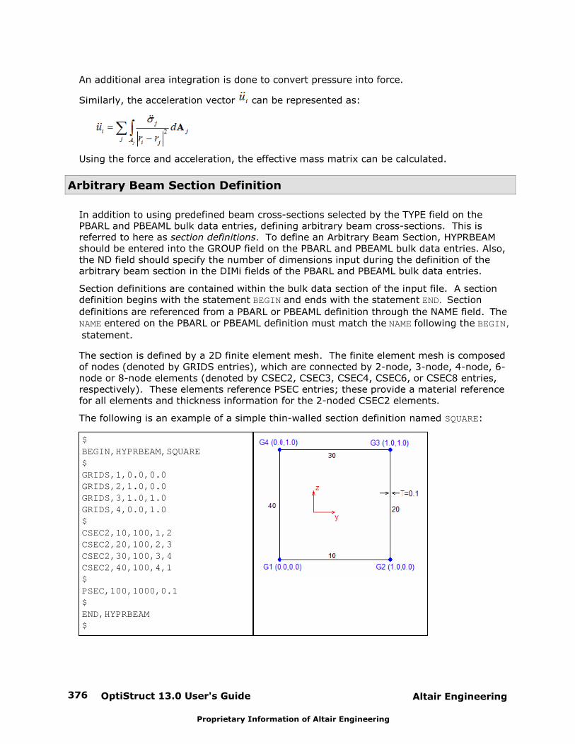
OptiStruct 13.0 User's Guide376 Altair Engineering
Proprietary Information of Altair Engineering
An additional area integration is done to convert pressure into force.
Similarly, the acceleration vector can be represented as:
Using the force and acceleration, the effective mass matrix can be calculated.
Arbitrary Beam Section Definition
In addition to using predefined beam cross-sections selected by the TYPE field on the PBARL and PBEAML bulk data entries, defining arbitrary beam cross-sections. This isreferred to here as section definitions. To define an Arbitrary Beam Section, HYPRBEAMshould be entered into the GROUP field on the PBARL and PBEAML bulk data entries. Also,the ND field should specify the number of dimensions input during the definition of thearbitrary beam section in the DIMi fields of the PBARL and PBEAML bulk data entries.
Section definitions are contained within the bulk data section of the input file. A sectiondefinition begins with the statement BEGIN and ends with the statement END. Section
definitions are referenced from a PBARL or PBEAML definition through the NAME field. TheNAME entered on the PBARL or PBEAML definition must match the NAME following the BEGIN,
statement.
The section is defined by a 2D finite element mesh. The finite element mesh is composedof nodes (denoted by GRIDS entries), which are connected by 2-node, 3-node, 4-node, 6-node or 8-node elements (denoted by CSEC2, CSEC3, CSEC4, CSEC6, or CSEC8 entries,respectively). These elements reference PSEC entries; these provide a material referencefor all elements and thickness information for the 2-noded CSEC2 elements.
The following is an example of a simple thin-walled section definition named SQUARE:
$BEGIN,HYPRBEAM,SQUARE$GRIDS,1,0.0,0.0GRIDS,2,1.0,0.0GRIDS,3,1.0,1.0GRIDS,4,0.0,1.0$CSEC2,10,100,1,2CSEC2,20,100,2,3CSEC2,30,100,3,4CSEC2,40,100,4,1$PSEC,100,1000,0.1$END,HYPRBEAM$
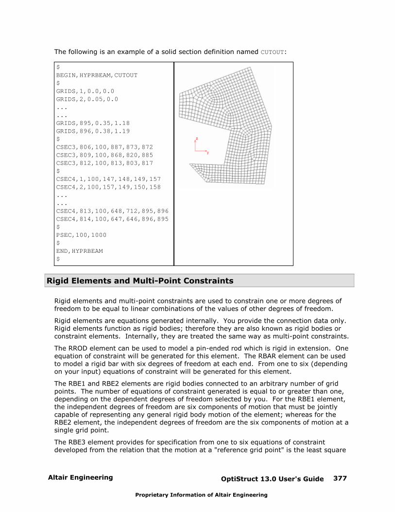
Altair Engineering OptiStruct 13.0 User's Guide 377
Proprietary Information of Altair Engineering
The following is an example of a solid section definition named CUTOUT:
$BEGIN,HYPRBEAM,CUTOUT$GRIDS,1,0.0,0.0GRIDS,2,0.05,0.0......GRIDS,895,0.35,1.18GRIDS,896,0.38,1.19$CSEC3,806,100,887,873,872CSEC3,809,100,868,820,885CSEC3,812,100,813,803,817$CSEC4,1,100,147,148,149,157CSEC4,2,100,157,149,150,158......CSEC4,813,100,648,712,895,896CSEC4,814,100,647,646,896,895$PSEC,100,1000$END,HYPRBEAM$
Rigid Elements and Multi-Point Constraints
Rigid elements and multi-point constraints are used to constrain one or more degrees offreedom to be equal to linear combinations of the values of other degrees of freedom.
Rigid elements are equations generated internally. You provide the connection data only. Rigid elements function as rigid bodies; therefore they are also known as rigid bodies orconstraint elements. Internally, they are treated the same way as multi-point constraints.
The RROD element can be used to model a pin-ended rod which is rigid in extension. Oneequation of constraint will be generated for this element. The RBAR element can be usedto model a rigid bar with six degrees of freedom at each end. From one to six (dependingon your input) equations of constraint will be generated for this element.
The RBE1 and RBE2 elements are rigid bodies connected to an arbitrary number of gridpoints. The number of equations of constraint generated is equal to or greater than one,depending on the dependent degrees of freedom selected by you. For the RBE1 element,the independent degrees of freedom are six components of motion that must be jointlycapable of representing any general rigid body motion of the element; whereas for theRBE2 element, the independent degrees of freedom are the six components of motion at asingle grid point.
The RBE3 element provides for specification from one to six equations of constraintdeveloped from the relation that the motion at a "reference grid point" is the least square
OptiStruct 13.0 User's Guide378 Altair Engineering
Proprietary Information of Altair Engineering
weighted average of the motion at other grid points. This element is generally used to"beam" loads and masses from a reference point to a set of grid points. Multi-pointconstraints are equations in which you explicitly provide the coefficients of the equations. Each multi-point constraint is described by a single equation that specifies a linearrelationship for two or more degrees of freedom. Multiple sets of multi-point constraintscan be provided in the bulk data section. In the subcase information section, the multi-point constraints are assigned to the specific load case using the MPC statement.
The bulk data entry MPC is the statement for defining multi-point constraints. The firstcoordinate mentioned on the card is taken as the dependent degree of freedom (that is,the degree of freedom that is removed from the equations of motion). Dependent degreesof freedom may appear as independent terms in other equations of the set; however, theymay appear as dependent terms in only a single equation.
Some uses of multi-point constraints are:
To enforce zero motion in directions other than those corresponding to componentsof the global coordinate system. In this case, the multi-point constraint will involveonly the degrees of freedom at a single grid point. The constraint equation relatesthe displacement in the direction of zero motion to the displacement components inthe global system at the grid point.
To describe rigid elements and mechanisms such as levers, pulleys, and gear trains. In this application, the degrees of freedom associated with the rigid element that arein excess of those needed to describe rigid body motion are eliminated with multi-point constraint equations. Treatment of very stiff members as being rigid elementseliminates the ill-conditioning associated with their treatment as ordinary elasticelements.
To be used with scalar elements to generate non-standard structural elements andother special effects.
When using rigid elements or multi-point constraints, you must make sure that thefollowing requirements are satisfied:
A dependent degree of freedom cannot be in the SPC.
A dependent degree of freedom in any rigid element or multi-point constraint cannotbe defined as a dependent degree of freedom in any other rigid element or multi-point constraint.
Materials
The different elastic material types provided by OptiStruct are: isotropic, orthotropic, andan-isotropic materials. The material property definition cards are used to define theproperties for each of the materials used in a structural model.
The MAT1 bulk data entry is used to define the properties for isotropic elastic materials. Itcan be referenced by any of the structural elements, and can also be referenced by anyproperty card.
The MAT2 entry is used to define the properties for an-isotropic materials. It applies onlyto triangular or quadrilateral membrane and bending elements, and can only be referencedby PSHELL, PCOMP, and PCOMPG property cards. This material type specifies therelationship between the in-plane stresses and strains. The angle between the materialcoordinate system and the element coordinate system is specified on the connection cards.

Altair Engineering OptiStruct 13.0 User's Guide 379
Proprietary Information of Altair Engineering
The MAT4 entry is used to define the properties for isotropic elastic materials. It can bereferenced by any of the structural elements, and can also be referenced by any propertycard.
The MAT5 entry is used to define the properties for an-isotropic elastic materials. It can bereferenced by any of the structural elements, and can also be referenced by any propertycard.
The MAT8 card is used to define the properties for planar orthotropic elastic materials intwo dimensions. Individual plys of a layered composite lay-up typically possess suchorthotropic properties. Since layered composite laminates are modeled using shellelements, MAT8 property data can only be referenced by PSHELL, PCOMP, and PCOMPGproperty cards.
The MAT9 bulk data entry can be used to define the properties for an-isotropic elasticmaterials for three dimensional solid elements. The general an-isotropic stress-strainrelationship linking the six independent stress components of the stress tensor at a pointand the six independent strain components of the tensor at the point contain 21independent constants in the elasticity matrix. These values are supplied using the MAT9bulk data card. The MAT9 bulk data card is used with the CHEXA, CPENTA, CPYRA, andCTETRA solid elements, and can only be referenced on the PSOLID property card. Theoptional coordinate system in which MAT9 data are specified is supplied via the PSOLIDbulk data entry.
The MAT10 bulk data entry is used to define material properties for fluid elements incoupled fluid-structural (acoustic) analysis. It may only be referenced on PSOLID entrieswith FCTN=’PFLUID’.
Temperature dependent material properties are defined using MATT1, MATT2, MATT8, andMATT9. All four have the same characteristics as described above. The temperaturedependency of each property is defined through TABLEM1, TABLEM2, TABLEM3, orTABLEM4 table entries.
Composite laminates are defined using the PCOMP and PCOMPG properties. They are notmaterial types; each ply in the laminate lay-up can reference a different material.
Nonlinear material properties are defined using MATS1. The nonlinear materialcharacteristics may need the table input TABLES1. MATS1 is defined as an extension to aMAT1 with the same MID. MATS1 is applicable to all nonlinear solutions.
For geometric nonlinear subcases, more nonlinear material laws are available. As ageneral rule, material definitions that are only applicable in geometric nonlinear analysisare defined on extensions to a MAT1 material that defines the basic elastic properties. Theextensions are grouped with the base entry by sharing the same MID. The table belowlists the MATXyz extensions available. If a law requires material curves, TABLES1 entriesare used.
Example
MAT1, 102, 60.4, , 0.33, 2.70e-6MATX02, 102, 0.09026, 0.22313, 0.3746, 100.0, 0.175
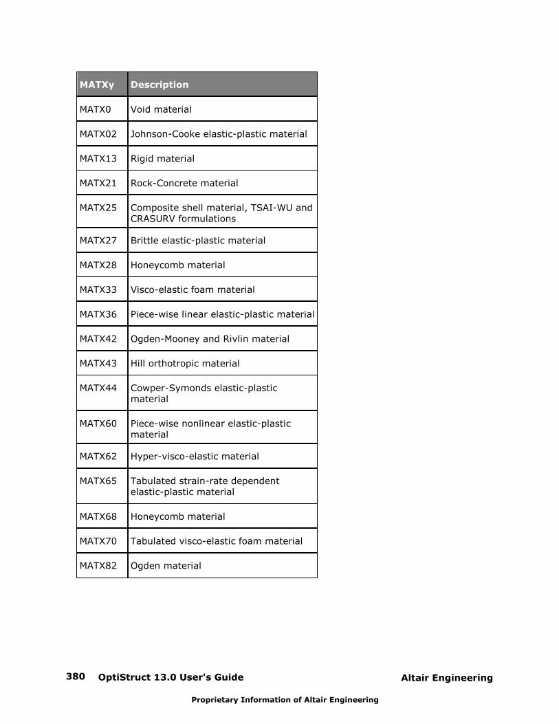
OptiStruct 13.0 User's Guide380 Altair Engineering
Proprietary Information of Altair Engineering
MATXy Description
MATX0 Void material
MATX02 Johnson-Cooke elastic-plastic material
MATX13 Rigid material
MATX21 Rock-Concrete material
MATX25 Composite shell material, TSAI-WU andCRASURV formulations
MATX27 Brittle elastic-plastic material
MATX28 Honeycomb material
MATX33 Visco-elastic foam material
MATX36 Piece-wise linear elastic-plastic material
MATX42 Ogden-Mooney and Rivlin material
MATX43 Hill orthotropic material
MATX44 Cowper-Symonds elastic-plasticmaterial
MATX60 Piece-wise nonlinear elastic-plasticmaterial
MATX62 Hyper-visco-elastic material
MATX65 Tabulated strain-rate dependentelastic-plastic material
MATX68 Honeycomb material
MATX70 Tabulated visco-elastic foam material
MATX82 Ogden material
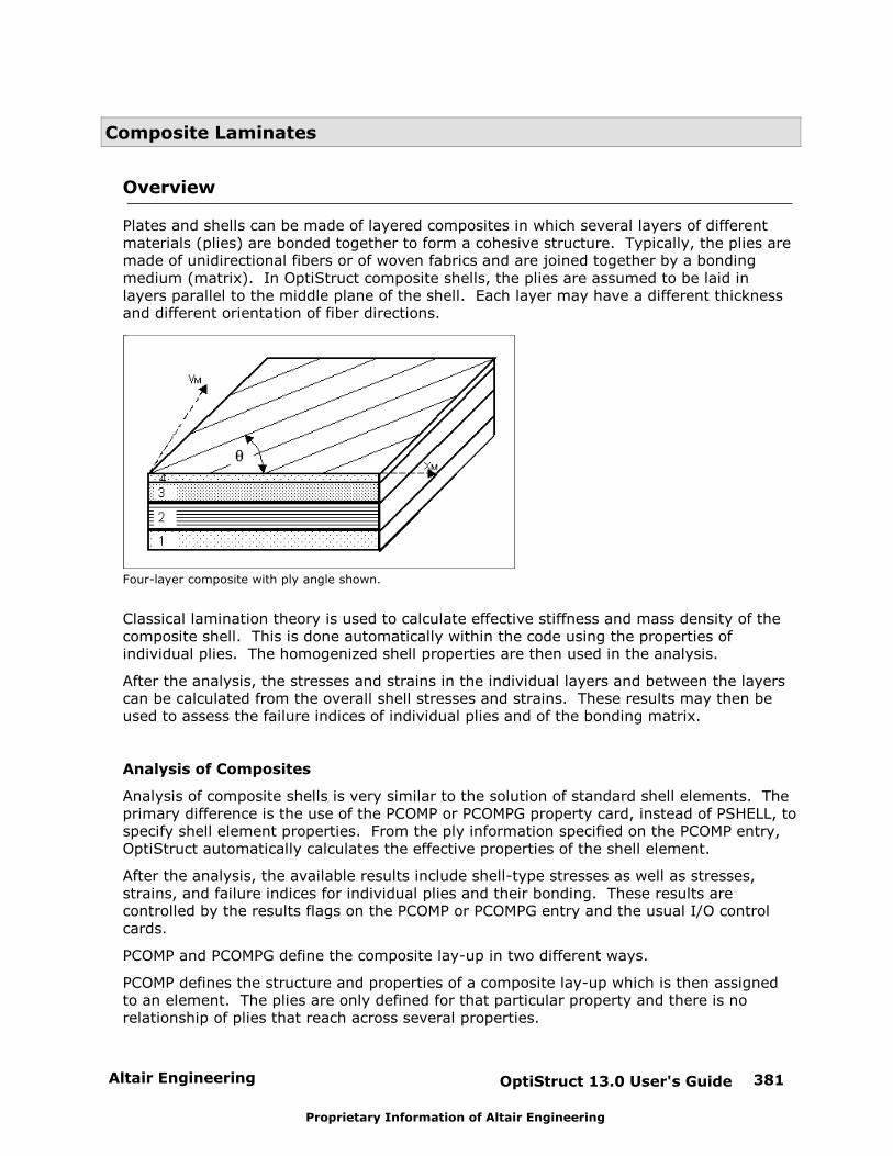
Altair Engineering OptiStruct 13.0 User's Guide 381
Proprietary Information of Altair Engineering
Composite Laminates
Overview
Plates and shells can be made of layered composites in which several layers of differentmaterials (plies) are bonded together to form a cohesive structure. Typically, the plies aremade of unidirectional fibers or of woven fabrics and are joined together by a bondingmedium (matrix). In OptiStruct composite shells, the plies are assumed to be laid inlayers parallel to the middle plane of the shell. Each layer may have a different thicknessand different orientation of fiber directions.
Four-layer composite with ply angle shown.
Classical lamination theory is used to calculate effective stiffness and mass density of thecomposite shell. This is done automatically within the code using the properties ofindividual plies. The homogenized shell properties are then used in the analysis.
After the analysis, the stresses and strains in the individual layers and between the layerscan be calculated from the overall shell stresses and strains. These results may then beused to assess the failure indices of individual plies and of the bonding matrix.
Analysis of Composites
Analysis of composite shells is very similar to the solution of standard shell elements. Theprimary difference is the use of the PCOMP or PCOMPG property card, instead of PSHELL, tospecify shell element properties. From the ply information specified on the PCOMP entry,OptiStruct automatically calculates the effective properties of the shell element.
After the analysis, the available results include shell-type stresses as well as stresses,strains, and failure indices for individual plies and their bonding. These results arecontrolled by the results flags on the PCOMP or PCOMPG entry and the usual I/O controlcards.
PCOMP and PCOMPG define the composite lay-up in two different ways.
PCOMP defines the structure and properties of a composite lay-up which is then assignedto an element. The plies are only defined for that particular property and there is norelationship of plies that reach across several properties.
OptiStruct 13.0 User's Guide382 Altair Engineering
Proprietary Information of Altair Engineering
PCOMPG defines the structure and properties of a composite lay-up allowing for global plyidentification which is then assigned to an element. The plies of different PCOMPGdefinitions can have a relationship because of the use of global ply IDs.
Some remarks are in place regarding the specifics of composite analysis:
1. The most typical material type used for composite plies is MAT8, which is planarorthotropic material. The use of isotropic MAT1 or general anisotropic MAT2 for plyproperties is also supported.
2. While it is possible to specify ply angles relative to the element coordinate system, theresults become strongly dependent upon the node numbering in individual elements. Thus, it is advisable to prescribe a material coordinate system for composite elementsand specify ply angles relative to this system.
3. Depending on the specific lay-up structure, the composite may be offset from thereference plane of the shell element, i.e. have more material below than above thereference plane (or vice versa).
4. Stress results for composites include both shell-type stresses and individual plystresses. Importantly, shell-type stresses are calculated using homogenized propertiesand thus only represent the overall stress-state in the shell. To assess the actualstress-state in the composite, individual ply results need to be examined.
Interpretation of Results for Composites
A number of composite-specific results are calculated for composite shell elements. Due tothe specialized nature of these results, some explanation is required regarding theirmeaning.
Ply Stresses and Strains
Classical lamination theory assumes two-dimensional stress-state in individual plies(so-called membrane state). The values of stresses and strains are calculated at themid-plane of each ply, i.e. halfway between its upper and lower surface. Forsufficiently thin plies, these values can be interpreted as representing uniform stressin the ply.
Ply stresses and strains are calculated in coordinate systems aligned with plymaterial angles as specified on the PCOMP card. In particular, correspond to theprimary ply direction, is orthogonal to it, and represents in-plane shear stress.
Inter-laminar Stress
Inter-laminar bonding matrix usually has different material properties and stress-state than the individual plies. The primary stress that is of importance here is inter-laminar shear with two components:
Failure Indices
To facilitate prediction of potential failure of the laminate, failure indices arecalculated for plies and bonding material. While there are several theories availablefor such calculations, their common feature is that failure indices are scaled relativeto allowable stresses or strains, so that:
- the value of a failure index lower than 1.0 indicates that the stress/strain is withinthe allowable limits (as specified on the material data card), and
- a failure index above 1.0 indicates that the allowable stress/strain has been
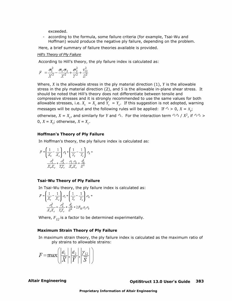
Altair Engineering OptiStruct 13.0 User's Guide 383
Proprietary Information of Altair Engineering
exceeded.
- according to the formula, some failure criteria (for example, Tsai-Wu andHoffman) would produce the negative ply failure, depending on the problem.
Here, a brief summary of failure theories available is provided.
Hill's Theory of Ply Failure
According to Hill's theory, the ply failure index is calculated as:
Where, X is the allowable stress in the ply material direction (1), Y is the allowable
stress in the ply material direction (2), and S is the allowable in-plane shear stress. It
should be noted that Hill’s theory does not differentiate between tensile andcompressive stresses and it is strongly recommended to use the same values for bothallowable stresses, i.e. Xt = Xc and Yt = Yc. If this suggestion is not adopted, warning
messages will be output and the following rules will be applied: If > 0, X = Xt;
otherwise, X = Xc, and similarly for Y and . For the interaction term / X2, if >
0, X = Xt; otherwise, X = Xc.
Hoffman's Theory of Ply Failure
In Hoffman's theory, the ply failure index is calculated as:
Tsai-Wu Theory of Ply Failure
In Tsai-Wu theory, the ply failure index is calculated as:
Where, F12 is a factor to be determined experimentally.
Maximum Strain Theory of Ply Failure
In maximum strain theory, the ply failure index is calculated as the maximum ratio ofply strains to allowable strains:
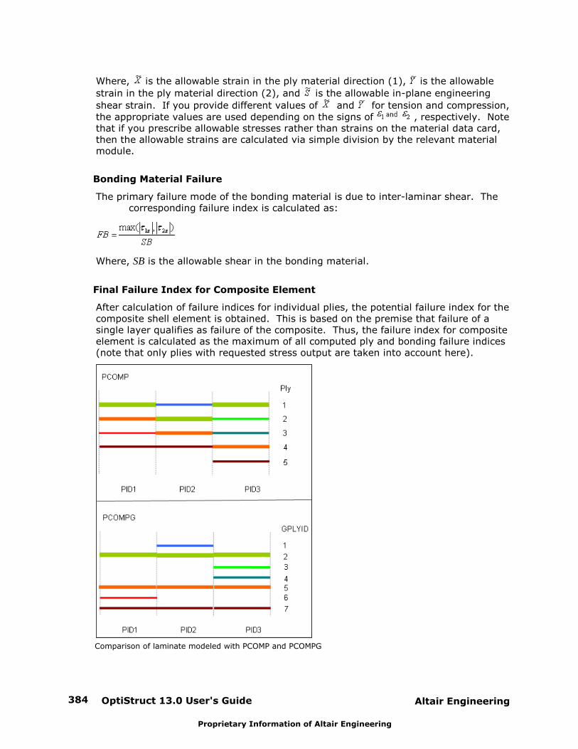
OptiStruct 13.0 User's Guide384 Altair Engineering
Proprietary Information of Altair Engineering
Where, is the allowable strain in the ply material direction (1), is the allowable
strain in the ply material direction (2), and is the allowable in-plane engineering
shear strain. If you provide different values of and for tension and compression,the appropriate values are used depending on the signs of , respectively. Notethat if you prescribe allowable stresses rather than strains on the material data card,then the allowable strains are calculated via simple division by the relevant materialmodule.
Bonding Material Failure
The primary failure mode of the bonding material is due to inter-laminar shear. Thecorresponding failure index is calculated as:
Where, SB is the allowable shear in the bonding material.
Final Failure Index for Composite Element
After calculation of failure indices for individual plies, the potential failure index for thecomposite shell element is obtained. This is based on the premise that failure of asingle layer qualifies as failure of the composite. Thus, the failure index for compositeelement is calculated as the maximum of all computed ply and bonding failure indices(note that only plies with requested stress output are taken into account here).
Comparison of laminate modeled with PCOMP and PCOMPG
Altair Engineering OptiStruct 13.0 User's Guide 385
Proprietary Information of Altair Engineering
Loads and Boundary Conditions
The following boundary conditions are outlined here.
Static Loads and Boundary Conditions
Static loads are applied at grid points in a variety of ways, including:
Loads applied directly to grid points
Pressure on surfaces
Gravity loads
Centrifugal forces due to steady rotation
Equivalent loads resulting from:
thermal expansion
- enforced deformations of structural elements
- enforced displacements of grid points
Any number of load sets can be defined in the bulk data section of the input file. However,only those sets selected in the subcase information section (as described in the LinearStatic Analysis, Inertia Relief, and Nonlinear Quasi-Static Analysis sections) will be used inthe problem solution. The manner in which each type of load is selected is specified on theassociated bulk data statement description.
The FORCE statement is used to define a static load applied to a grid point in terms ofcomponents defined by a local coordinate system. The orientation of the load componentsdepends on the type of local coordinate system used to define the load.
The FORCE1 statement is used if the direction is determined by a vector connecting twogrid points.
The MOMENT and MOMENT1 statements are used to define the application of aconcentrated moment at a grid point.
Pressure loads on triangular and quadrilateral elements are defined with a PLOAD2 card. The positive direction of the loading is determined by the order of the grid points on theelement connection card (using the right-hand rule). The magnitude and direction of theload is automatically computed from the value of the pressure and the coordinates of theconnected grid points. The load is applied to the connected grid points.
PLOAD pressure loads are used in a similar fashion to define the loading of any three orfour grid points, regardless of whether or not they are connected with two-dimensionalelements.
Pressure loads on the HEXA, PENTA and TETRA solid elements are defined with the PLOAD4card. The pressure is defined positively outward from the element. The magnitude anddirection of the equivalent grid point forces are automatically computed using the iso-parametric shape functions of the element to which the load has been applied. Pressureloads on the QUAD4 and TRIA3 elements can also be applied using the PLOAD4 card.
OptiStruct 13.0 User's Guide386 Altair Engineering
Proprietary Information of Altair Engineering
The PLOAD1 card is used to describe concentrated, uniformly distributed or linearlydistributed loads on the CBAR or CBEAM elements.
The GRAV bulk data entry is used to specify a gravity load by providing the components ofthe gravity vector in any defined coordinate system. The gravity load is obtained from thegravity vector and the mass matrix of the structural model. Because the gravitationalacceleration is not calculated at scalar points, you are required to introduce gravity loadsat scalar points directly.
The RFORCE statement is used to define a static loading condition due to a centrifugalforce field. A centrifugal force load is specified by the designation of a grid point that lieson the axis of rotation and by the components of rotational velocity and acceleration in anydefined coordinate system. In the calculation of the centrifugal force, the mass matrixpertains to a set of distinct rigid bodies connected to grid points. Deviations from thisviewpoint, such as the use of scalar points or the use of mass coupling between gridpoints, can result in errors.
Temperature loads can only be defined at grid points. The temperatures of the connectedgrid points are given on the TEMP and TEMPD bulk data entries. The thermal expansioncoefficients are defined on the material definition cards. The mere presence of a thermalfield does not imply the application of a thermal load. A thermal load will not be appliedunless you make a specific request in the subcase information section.
The LOAD card in the bulk data section defines a static loading condition that is a linearcombination of load sets consisting of loads applied directly to grid points, pressure loads,gravity loads, and centrifugal forces. This card must be used if gravity loads are to beused in combination with loads applied directly to grid points, pressure loads, or centrifugalforces. The application of the combined loading condition is requested in the subcaseinformation section by selecting the set number of the LOAD combination.
It should be noted that the equivalent loads (thermal and enforced displacement) musthave unique set identification numbers and be selected separately in the subcaseinformation section. For any particular solution, the total load will be the sum of theapplied loads (grid point loading, pressure loading, gravity loading, and centrifugal forces)and the equivalent loads.
Zero enforced displacements may be specified on SPC or SPC1 cards. Zero displacementsresult in non-zero forces on the grid point constrained (SPC forces).
The SPCADD statement allows the combination of different SPC sets.
For inertia relief, the reaction degrees of freedom for the computation of the accelerationload are defined through SUPORT or SUPORT1 statements. Up to six degrees of freedomcan be defined per subcase.
Non-zero enforced displacements may be specified on SPC or SPCD cards. The SPC cardspecifies both the component to be constrained and the magnitude of the enforceddisplacement. The SPCD card only specifies the magnitude of the enforced displacement. When an SPCD card is used, the component to be constrained must be specified on eitheran SPC or an SPC1 card. The use of the SPCD card avoids the decomposition of thestiffness matrix when changes are only made in the magnitudes of the enforceddisplacements.
The equivalent loads resulting from enforced displacements of grid points are calculated bythe program and added to the other applied loads.
If the magnitudes of the enforced displacements are specified on SPC cards, the application
Altair Engineering OptiStruct 13.0 User's Guide 387
Proprietary Information of Altair Engineering
of the load is automatic when you select the associated SPC set in the subcase informationsection.
If the magnitude of the displacement is defined on an SPCD card, the load is applied if youselect the associated LOAD set in the subcase information section.
Prestressed Analysis
Preloaded or prestressed analysis is any type of structural analysis performed on astructure under prior loading (also termed preloading or prestressing). The response of astructure is affected by its initial state and this is in turn affected by the variouspreloading/prestressing applied to the structure, prior to the analysis of interest. Examples of prestressed analysis include analysis of rotorcraft blades under centrifugalpreloading, analysis of pillar-like structures under compressive preloading, etc. OptiStructcan be used to take into account such preloading or prestressing effects. The prestressing/preloading loadcase is a linear or nonlinear static loadcase. Prestressed/preloaded analysisis currently only supported for linear statics, eigenvalue analysis and direct frequencyresponse analysis. Specifying prestress in any other unsupported analysis will generate anappropriate user error. Prestressing is specified through the STATSUB(PRELOAD) CaseControl card, which refers to the preloading static loadcase ID. Nested preloading is notsupported and will generate an appropriate user error (that is: User error will be reported ifSubcase C has preloading from Subcase B, which in turn has preloading from Subcase A).
The preloading is captured or defined by a geometric stiffness matrix [KG] which is based
on the stresses of the preloading static subcase. In prestressed analysis, this geometricstiffness matrix is subtracted from the original stiffness matrix [K] of the (unloaded)structure. Depending on preloading conditions, the resulting effect could be a weakened orstiffened structure. If the preloading is compressive, it typically has a weakening effect onthe structure (example: column or pillar under compressive preloading). If the preloadingis tensile, it typically has a stiffening effect (for example: rotorcraft blade under centrifugalpreloading).
Prestressed Static Analysis
Prestressed static analysis is governed by the following equation (where, F is the loading
and U is the displacement).
GK K U F
While linear static subcases can have prestressing, nonlinear static subcases underprestressing are not supported.
Prestressed Eigenvalue Analysis
Prestressed eigenvalue analysis is governed by the following equation (where, M is the
mass matrix, F is the eigenvector and l is the eigenvalue).
0GK K lM F
OptiStruct 13.0 User's Guide388 Altair Engineering
Proprietary Information of Altair Engineering
Prestressed eigenvalue analysis is currently supported by AMSES, AMLS and the LanczosMethod. However, if the specified preload is greater than the first critical buckling load, anappropriate error will be reported for AMSES/AMLS runs.
Prestressed Direct Frequency Response Analysis
Prestressed direct FRF analysis is governed by the following equation.
2G G GEK K ig K K iK iwC w M U F
Where, M is the mass matrix, U is the complex displacement vector, KGE is the material
damping matrix, C is the viscous damping matrix that includes the Area Matrix for fluid-
structure coupling, w is the loading frequency and g is the structural damping coefficient.
Results
All results that are supported for regular structural analyses are also available in thecorresponding prestressed analyses. It is important to note that, while the prestressedanalysis includes the effects of preloading as a weakening or a stiffening of the structure,the results from the prestressed analysis do not include the preloading results. Forexample, the displacements from prestressed static analysis do not include the preloadingdisplacements. In order to get the overall deflection/stresses of the structure, thedisplacements/stresses from the prestressed analyses have to be carefully superposed withthe preloading displacements/stresses while post-processing. Particularly, while post-processing complex results from prestressed direct FRF, the correct approach would be tofirst obtain the complex results for a certain phase and then superpose the appropriatepreloading result. Any other superposing approach would lead to incorrect results.
Pretensioned Bolt Analysis
Overview
Many engineering assemblies are put together using bolts, which are usually pretensionedbefore application of working loads. A typical sequence is described below.
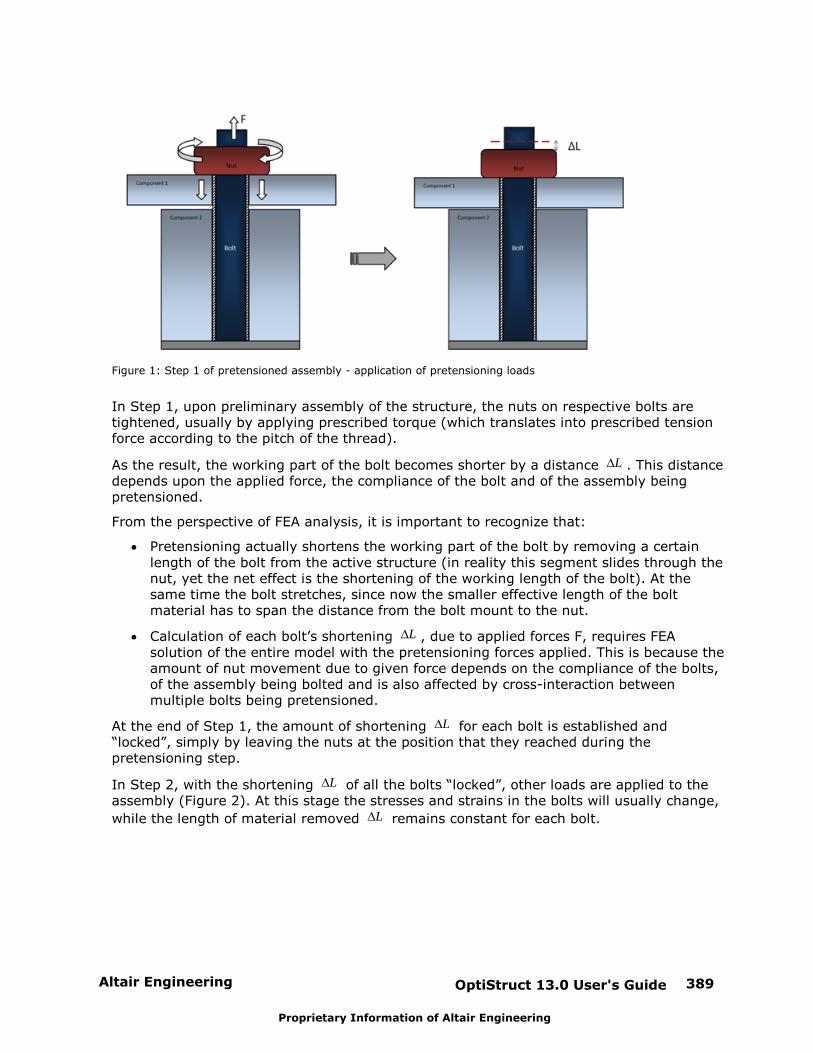
Altair Engineering OptiStruct 13.0 User's Guide 389
Proprietary Information of Altair Engineering
Figure 1: Step 1 of pretensioned assembly - application of pretensioning loads
In Step 1, upon preliminary assembly of the structure, the nuts on respective bolts aretightened, usually by applying prescribed torque (which translates into prescribed tensionforce according to the pitch of the thread).
As the result, the working part of the bolt becomes shorter by a distance L . This distancedepends upon the applied force, the compliance of the bolt and of the assembly beingpretensioned.
From the perspective of FEA analysis, it is important to recognize that:
Pretensioning actually shortens the working part of the bolt by removing a certainlength of the bolt from the active structure (in reality this segment slides through thenut, yet the net effect is the shortening of the working length of the bolt). At thesame time the bolt stretches, since now the smaller effective length of the boltmaterial has to span the distance from the bolt mount to the nut.
Calculation of each bolt’s shortening L , due to applied forces F, requires FEAsolution of the entire model with the pretensioning forces applied. This is because theamount of nut movement due to given force depends on the compliance of the bolts,of the assembly being bolted and is also affected by cross-interaction betweenmultiple bolts being pretensioned.
At the end of Step 1, the amount of shortening L for each bolt is established and“locked”, simply by leaving the nuts at the position that they reached during thepretensioning step.
In Step 2, with the shortening L of all the bolts “locked”, other loads are applied to theassembly (Figure 2). At this stage the stresses and strains in the bolts will usually change,
while the length of material removed L remains constant for each bolt.
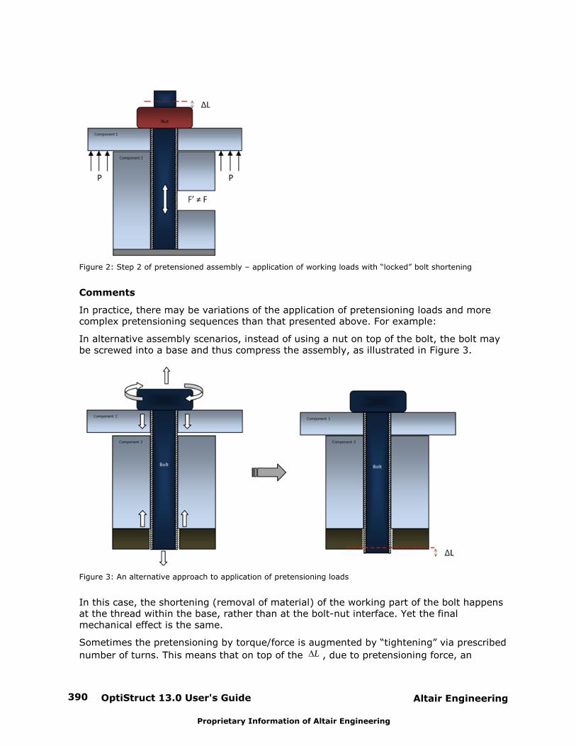
OptiStruct 13.0 User's Guide390 Altair Engineering
Proprietary Information of Altair Engineering
Figure 2: Step 2 of pretensioned assembly – application of working loads with “locked” bolt shortening
Comments
In practice, there may be variations of the application of pretensioning loads and morecomplex pretensioning sequences than that presented above. For example:
In alternative assembly scenarios, instead of using a nut on top of the bolt, the bolt maybe screwed into a base and thus compress the assembly, as illustrated in Figure 3.
Figure 3: An alternative approach to application of pretensioning loads
In this case, the shortening (removal of material) of the working part of the bolt happensat the thread within the base, rather than at the bolt-nut interface. Yet the finalmechanical effect is the same.
Sometimes the pretensioning by torque/force is augmented by “tightening” via prescribed
number of turns. This means that on top of the L , due to pretensioning force, an

Altair Engineering OptiStruct 13.0 User's Guide 391
Proprietary Information of Altair Engineering
additional L ’ is added according to the number of turns and the pitch of the thread.
In an automated assembly process, usually all bolts are pretensioned simultaneously.Sometimes, however, the tensioning may happen in sequence or in groups. In such cases,
while L is “locked” for bolts that have already been pretensioned, consecutivepretensioning force is applied to the next batch of bolts, which then become “locked” forthe following step.
FEA Solution with Pretensioning
In analysis of structures, the FEA model is usually defined in material reference frame andthe amount of material is assumed to remain fixed, while the structure undergoesstretching and deformation. However, in the case of pretensioning, the actual working partof the model has some material removed by being driven through the nut (usually theprotruding part of the bolt is not included in the working FEA model, since it does notparticipate in the balance of forces on the structure).
The simulation of this phenomenon in Optistruct follows the approach described below:
First, it is recognized that for straight bolts, from the viewpoint of balance of forces it doesnot matter at what location the removal of the material happens in the bolt. Therefore,instead of simulating the precise interaction between the nut and the bolt, thepretensioning is handled within the length of the bolt. Pretensioning in OptiStruct isimplemented with the help of Multiple Point Constraints (MPC’s) via two differentprocesses:
1D Bolt Pretensioning
3D Bolt Pretensioning
Multiple point constraints (MPC’s) are used in both 1D and 3D pretensioning, the differencebetween the two implementations is the number of duplicate grid points created andcontrolled via MPC’s.
1D Bolt Pretensioning
In this process, the bolt or its selected section is represented by single or multiple 1Delement(s) (beam or rod).
Note: If a bolt is meshed with 3D (solid) elements, 1Dpretensioning can be applied by replacing a transversesection of the bolt with 1D beam/rod elements. In suchcases; however, 3D pretensioning is recommended sinceit is easier to implement and accuracy is improved. If abolt is constructed using 1D elements, 1D pretensioningcan be used effectively.
Step 1
The conceptual FEA handling of 1D bolt pretensioning is illustrated in Figure 4. A bolt ismodeled using 3D elements and a beam or rod element represents the selected section ofthe bolt where pretensioning will be applied.
1. First, an imaginary cut is introduced into the beam (This is automatically doneinternally for a subcase that includes a PRETENSION command) and two duplicate gridpoints are created at the location of the cut.
OptiStruct 13.0 User's Guide392 Altair Engineering
Proprietary Information of Altair Engineering
Figure 4: FEA implementation of Bolt Pretensioning applied to a 1D Bolt using a 1D element
Additionally, a scalar point (SPOINT) is automatically created to act as an independent gridpoint. A pair of self-balanced pretensioning forces is applied to both ends of the cut withthe help of the newly created SPOINT. The specified pretensioning force is internallyapplied on the SPOINT and this is transferred to the duplicated grid points via an MPC. TheMPC controls the movement of the newly created duplicate grid points and the scalar pointbased on the following equation:
int igspo dgu u u
Where,
spointu is the displacement of the independent scalar point (SPOINT)
dgu is the displacement of the dependent grid point
igu is the displacement of the independent grid point
The reaction force on the scalar point due to an enforced displacement of spointu on it can
be shown to be equal to the forces acting on the dependent or independent grid point.
int igspo dgF F F or spoint dg igF F F
depending on the direction of the forces.
Altair Engineering OptiStruct 13.0 User's Guide 393
Proprietary Information of Altair Engineering
Where,
spointF is the total reaction force on the independent scalar point (SPOINT) due to an
enforced displacement of spointu
dgF is the force acting on the dependent grid point
igF is the force acting on the independent grid point
2. With these forces (plus other loads referenced in this subcase) applied, static analysis isperformed to calculate deformation of the structure. Among the results of such analysis
is the “overlap” L across the cut portion of the beam, which is equivalent to thedistance that the bolt would move relative to the nut in Figure 1.
Figure 5: FEA implementation of Bolt Pretensioning applied to a 3D Bolt using a 1D element (Step 1)
Step 2
As shown in Figure 5, the amount of overlap L calculated in Step 1 is removed from thebolt length, and the bolt is reconnected at the cut location. This represents the shorterworking length of a pretensioned bolt on which the nut has been tightened (Mechanically,this is similar to the effect of the DEFORM command).
With bolt pretensioning “locked” in this way, additional working loads are applied and aFEA solution is performed.
OptiStruct 13.0 User's Guide394 Altair Engineering
Proprietary Information of Altair Engineering
Figure 6: FEA implementation of Bolt Pretensioning applied to a 3D Bolt using a 1D element (Step 2)
As mentioned already, it is possible to construct more complex sequences of pretensioning,wherein some bolts have already been pretensioned (Step 2) while the next batch of boltsis being pretensioned (Step 1). (Note that a specific tensioning sequence has an effect onthe final result only in path-dependent problems, such as contact with friction or elasto-plastic materials.)
3D Bolt Pretensioning
In 3D Bolt Pretensioning, the bolt is represented (meshed) using 3D solid elements. Atransverse surface in the beam is identified (cross-section) along which it is cut and theduplicate grids are then controlled by Multiple Point Constraints (MPC’s) and a SPOINT tosimulate the pretensioning effect.
Step 1
The first step in 3D pretensioning is to identify the transverse cross-sectional surface of thebolt. OptiStruct automatically cuts the bolt at the selected surface and duplicate grid pointsare created mirroring the existing grid points at the cut surface. This is automatically doneinternally for a subcase that includes a PRETENSION command.
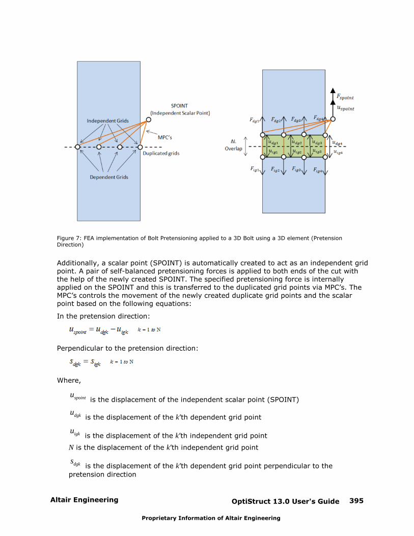
Altair Engineering OptiStruct 13.0 User's Guide 395
Proprietary Information of Altair Engineering
Figure 7: FEA implementation of Bolt Pretensioning applied to a 3D Bolt using a 3D element (PretensionDirection)
Additionally, a scalar point (SPOINT) is automatically created to act as an independent gridpoint. A pair of self-balanced pretensioning forces is applied to both ends of the cut withthe help of the newly created SPOINT. The specified pretensioning force is internallyapplied on the SPOINT and this is transferred to the duplicated grid points via MPC’s. TheMPC’s controls the movement of the newly created duplicate grid points and the scalarpoint based on the following equations:
In the pretension direction:
Perpendicular to the pretension direction:
Where,
spointu is the displacement of the independent scalar point (SPOINT)
dgku is the displacement of the k’th dependent grid point
igku is the displacement of the k’th independent grid point
N is the displacement of the k’th independent grid point
dgks is the displacement of the k’th dependent grid point perpendicular to the
pretension direction
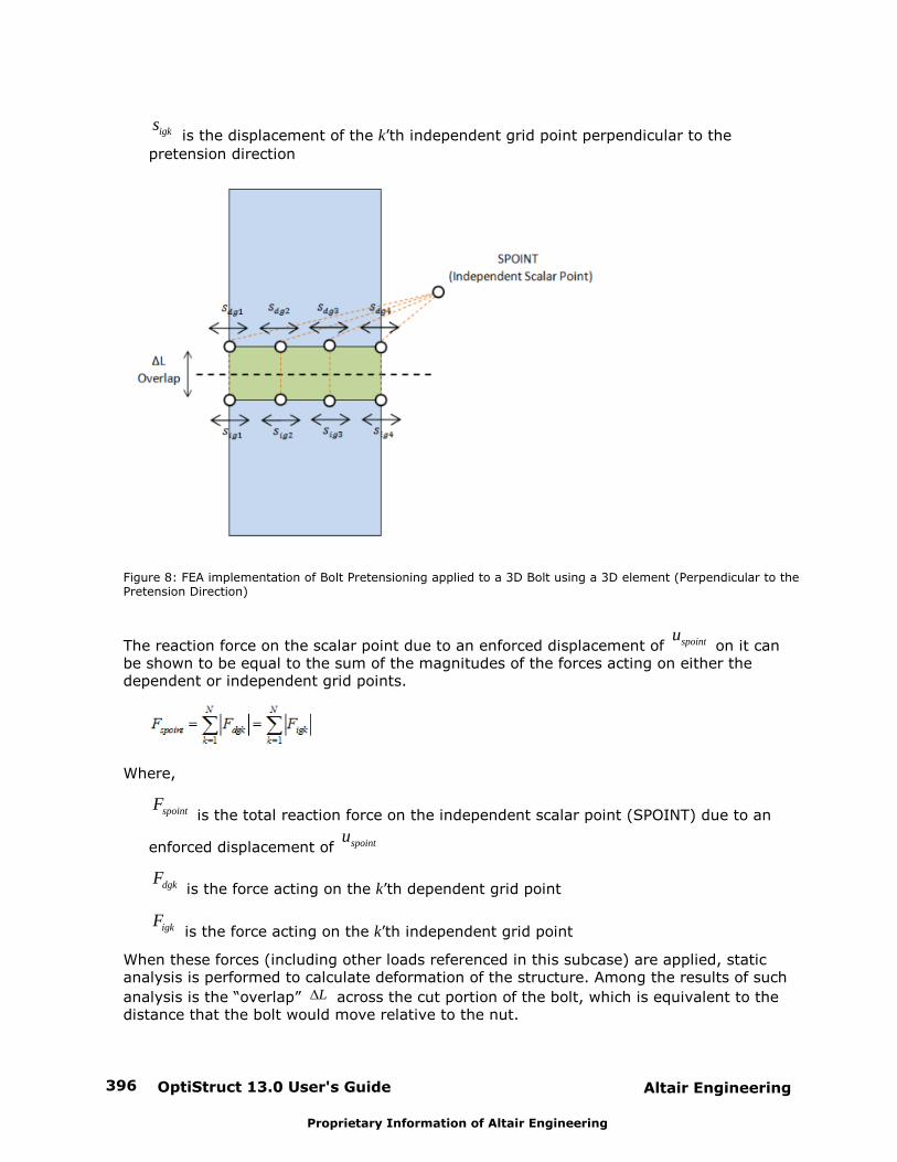
OptiStruct 13.0 User's Guide396 Altair Engineering
Proprietary Information of Altair Engineering
igks is the displacement of the k’th independent grid point perpendicular to the
pretension direction
Figure 8: FEA implementation of Bolt Pretensioning applied to a 3D Bolt using a 3D element (Perpendicular to thePretension Direction)
The reaction force on the scalar point due to an enforced displacement of spointu on it can
be shown to be equal to the sum of the magnitudes of the forces acting on either thedependent or independent grid points.
Where,
spointF is the total reaction force on the independent scalar point (SPOINT) due to an
enforced displacement of spointu
dgkF is the force acting on the k’th dependent grid point
igkF is the force acting on the k’th independent grid point
When these forces (including other loads referenced in this subcase) are applied, staticanalysis is performed to calculate deformation of the structure. Among the results of such
analysis is the “overlap” L across the cut portion of the bolt, which is equivalent to thedistance that the bolt would move relative to the nut.
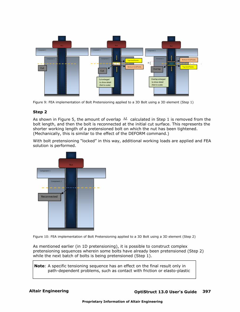
Altair Engineering OptiStruct 13.0 User's Guide 397
Proprietary Information of Altair Engineering
Figure 9: FEA implementation of Bolt Pretensioning applied to a 3D Bolt using a 3D element (Step 1)
Step 2
As shown in Figure 5, the amount of overlap L calculated in Step 1 is removed from thebolt length, and then the bolt is reconnected at the initial cut surface. This represents theshorter working length of a pretensioned bolt on which the nut has been tightened.(Mechanically, this is similar to the effect of the DEFORM command.)
With bolt pretensioning “locked” in this way, additional working loads are applied and FEAsolution is performed.
Figure 10: FEA implementation of Bolt Pretensioning applied to a 3D Bolt using a 3D element (Step 2)
As mentioned earlier (in 1D pretensioning), it is possible to construct complexpretensioning sequences wherein some bolts have already been pretensioned (Step 2)while the next batch of bolts is being pretensioned (Step 1).
Note: A specific tensioning sequence has an effect on the final result only inpath-dependent problems, such as contact with friction or elasto-plastic
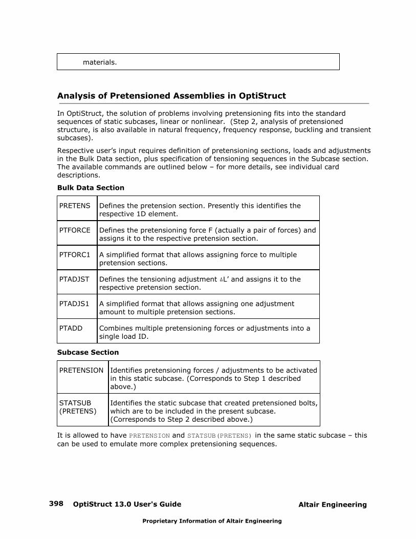
OptiStruct 13.0 User's Guide398 Altair Engineering
Proprietary Information of Altair Engineering
materials.
Analysis of Pretensioned Assemblies in OptiStruct
In OptiStruct, the solution of problems involving pretensioning fits into the standardsequences of static subcases, linear or nonlinear. (Step 2, analysis of pretensionedstructure, is also available in natural frequency, frequency response, buckling and transientsubcases).
Respective user’s input requires definition of pretensioning sections, loads and adjustmentsin the Bulk Data section, plus specification of tensioning sequences in the Subcase section.The available commands are outlined below – for more details, see individual carddescriptions.
Bulk Data Section
PRETENS Defines the pretension section. Presently this identifies therespective 1D element.
PTFORCE Defines the pretensioning force F (actually a pair of forces) andassigns it to the respective pretension section.
PTFORC1 A simplified format that allows assigning force to multiplepretension sections.
PTADJST Defines the tensioning adjustment L’ and assigns it to therespective pretension section.
PTADJS1 A simplified format that allows assigning one adjustmentamount to multiple pretension sections.
PTADD Combines multiple pretensioning forces or adjustments into asingle load ID.
Subcase Section
PRETENSION Identifies pretensioning forces / adjustments to be activatedin this static subcase. (Corresponds to Step 1 describedabove.)
STATSUB(PRETENS)
Identifies the static subcase that created pretensioned bolts,which are to be included in the present subcase.(Corresponds to Step 2 described above.)
It is allowed to have PRETENSION and STATSUB(PRETENS) in the same static subcase – this
can be used to emulate more complex pretensioning sequences.
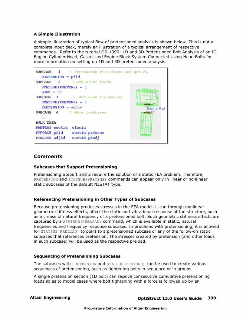
Altair Engineering OptiStruct 13.0 User's Guide 399
Proprietary Information of Altair Engineering
A Simple Illustration
A simple illustration of typical flow of pretensioned analysis is shown below. This is not a
complete input deck, merely an illustration of a typical arrangement of respectivecommands. Refer to the tutorial OS-1390: 1D and 3D Pretensioned Bolt Analysis of an ICEngine Cylinder Head, Gasket and Engine Block System Connected Using Head Bolts formore information on setting up 1D and 3D pretensioned analysis.
Comments
Subcases that Support Pretensioning
Pretensioning Steps 1 and 2 require the solution of a static FEA problem. Therefore, PRETENSION and STATSUB(PRETENS) commands can appear only in linear or nonlinear
static subcases of the default NLSTAT type.
Referencing Pretensioning in Other Types of Subcases
Because pretensioning produces stresses in the FEA model, it can through nonlineargeometric stiffness effects, affect the static and vibrational response of the structure, suchas increase of natural frequency of a pretensioned bolt. Such geometric stiffness effects arecaptured by a STATSUB(PRELOAD) command, which is available in static, natural
frequencies and frequency response subcases. In problems with pretensioning, it is allowedfor STATSUB(PRELOAD) to point to a pretensioned subcase or any of the follow-on static
subcases that references pretension. The stresses created by pretension (and other loadsin such subcase) will be used as the respective preload.
Sequencing of Pretensioning Subcases
The subcases with PRETENSION and STATSUB(PRETENS) can be used to create various
sequences of pretensioning, such as tightening bolts in sequence or in groups.
A single pretension section (1D bolt) can receive consecutive cumulative pretensioningloads so as to model cases where bolt tightening with a force is followed up by an
OptiStruct 13.0 User's Guide400 Altair Engineering
Proprietary Information of Altair Engineering
additional adjustment by a prescribed distance (number of turns of the nut). Such astacked sequence is presented in the simple illustration above.
The specific rules for sequencing pretensioning subcases on the same section are asfollows:
1. Pretensioning force (PTFORCE) can only be activated in the new or “fresh”pretensioning subcase for a given section. In other words, subcase with PRETENSIONpointing to PTFORCE cannot also include STATSUB(PRETENS) referencing a subcasethat had already pretensioned this section.
2. Pretensioning adjustment (PTADJST) may be activated in any of the pretensioningsubcases for a given section. The effect of adjustment is cumulative relative to thepretensioning status reached in the respective previous subcase, as referenced by STATSUB(PRETENS).
In nonlinear path-dependent problems, this sequencing of pretensioning can be combinedwith continuation of nonlinear subcases, as controlled by subcase command CNTNLSUB, inquite arbitrary combination. STATSUB(PRETENS) controls the sequencing of pretensioning
steps and CNTNLSUB controls the sequencing of nonlinear aspects (plasticity, contact withfriction, and so on) for quite arbitrary loading scenarios.
Inertia Relief
Inertia relief allows the simulation of unconstrained structures. Typical applications are anairplane in flight, suspension parts of a car, or a satellite in space.
With inertia relief, the applied loads are balanced by a set of translational and rotationalaccelerations. These accelerations provide body forces, distributed over the structure insuch a way that the sum total of the applied forces on the structure is zero. This providesthe steady-state stress and deformed shape in the structure as if it were freely acceleratingdue to the applied loads. Boundary conditions are applied only to restrain rigid bodymotion. Because the external loads are balanced by the accelerations, the reaction forcescorresponding to these boundary conditions are zero.
This calculation is automated.
Inertia relief boundary conditions may be defined in the bulk data section of the input deckor they may be determined automatically by the solver.
The SUPORT and SUPORT1 bulk data entries are used to define up to six reactiondegrees of freedom of the free body.
SUPORT entries will be used in all relevant subcases and therefore do not need to bereferenced in the Subcase Information section.
SUPORT1 entries need to be referenced by a SUPORT1 data selector statement foruse within a subcase.
Inertia relief boundary conditions may be generated automatically by using PARAM,INREL, -2.
In OptiStruct, inertia relief can be applied to linear static, nonlinear gap, modal frequencyresponse (with residual vectors), and transient response (with residual vectors) analyses. A static case with inertia relief cannot be referenced in a linear buckling analysis. Inertiarelief is meaningless in normal modes analysis.
Altair Engineering OptiStruct 13.0 User's Guide 401
Proprietary Information of Altair Engineering
Geometric Nonlinear Analysis Loads and Boundary Conditions
Any number of load sets can be defined in the bulk data section of the input file. However,only those sets selected in the subcase information section (as described in the GeometricNonlinear Analysis section) will be used in the problem solution. The manner in whicheach type of load is selected is specified on the associated bulk data statement description.
Geometric nonlinear analysis, whether implicit or explicit, (quasi-)static or dynamic, isperformed as a time-dependent event with time-dependent loads. A termination time TTERM needs to be defined. Subcases can be combined to a successive load history usingthe CNYNLSUB subcase statement. Each continued subcases starts from the end time andfinal load of the previous (reference) subcase. TTERM is defined in terms of total time.
The NLOAD1 bulk data statement defines a time-dependent load of the form:
( ) * *t
f t A C FB
The load history function F is defined using TABLED1.
For both definitions, a DAREA or SPCD statement defines the force, displacement, velocity,or acceleration amplitude A, respectively. Aside from DAREA, FORCE, MOMENT, PLOAD,
and PLOAD4 entries can be used to define the load amplitude. The quantities B and C are
scale factors.
The NLOAD card in the bulk data section defines a loading condition that is a linearcombination of load sets consisting of loads applied directly to grid points. The applicationof the combined loading condition is requested in the subcase information section byselecting the set number of the NLOAD combination.
Rigid walls may be defined using RWALL. Multiple rigid wall sets can be combined into asingle set using RWALADD. The subcase selection is made by RWALL.
Zero enforced displacements may be specified on SPC or SPC1 cards. The SPCADDstatement allows the combination of different SPC sets.
In dynamic analysis (explicit and implicit), initial velocities can be defined using TIC andTICA bulk data entries. TIC defines an initial velocity on a grid point, while TICA definesthe initial velocities of a grid set along and/or about an axis. A subcase selection must bemade with IC.
In (quasi-)static analysis, static loads can also be defined by using FORCE, MOMENT,PLOAD, and PLOAD4 directly thru a LOAD reference in the subcase. These loads are thentreated as linear ramp-up. In this case, TTERM is not mandatory, but if defined the loadramps up from the end time of the previous subcase to TTERM. If TTERM is absent it willbe determined from the subcase identification number SID such that TTERM = SID.
Frequency Response Loads and Boundary Conditions
Frequency dependent dynamic loads are applied at grid points. There are two differentdefinitions available.
Any number of load sets can be defined in the bulk data section of the input file. However,
OptiStruct 13.0 User's Guide402 Altair Engineering
Proprietary Information of Altair Engineering
only those sets selected in the subcase information section (as described in the FrequencyResponse Analysis section) will be used in the problem solution. The manner in whicheach type of load is selected is specified on the associated bulk data statement description.
The RLOAD1 bulk data statement defines a frequency dependent excitation of the form:
The RLOAD2 bulk data statement defines a frequency dependent excitation of the form:
For both definitions, a combination of DAREA, FORCE, FORCE1, FORCE2, MOMENT,MOMENT1, MOMENT2, PLOAD, PLOAD1, PLOAD2, PLOAD4, and RLOAD, or SPCD define theamplitude A of an excitation force or motion, respectively. A DPHASE reference defines the
phase angle , and a DELAY reference defines the delay . The quantities B, C, D, and ,
are frequency dependent. They are defined using TABLED1, TABLED2, TABLED3, orTABLED4.
It is recommended that SPCD be used for enforced motion. If the old inferior Large MassMethod is used for modal frequency response analysis with EIGRA, use PARAM,AMSESLMfor better accuracy.
The range for the loading frequency is defined using the FREQ, FREQ1, FREQ2, FREQ3,FREQ4, or FREQ5 bulk data statements.
The DLOAD card in the bulk data section defines a static loading condition that is a linearcombination of load sets consisting of loads applied directly to grid points. The applicationof the combined loading condition is requested in the subcase information section byselecting the set number of the DLOAD combination.
Zero enforced displacements may be specified on SPC or SPC1 cards.
The SPCADD statement allows the combination of different SPC sets.
Combinations of dynamic loads (DAREA) with static loads (FORCE, FORCE1, FORCE2,MOMENT, MOMENT1, MOMENT2, PLOAD, PLOAD1, PLOAD2, PLOAD4, and RLOAD), issupported.
Transient Response Loads and Boundary Conditions
Transient dynamic loads are applied at grid points. Two different definitions are available.
Any number of load sets can be defined in the bulk data section of the input file. However,only those sets selected in the subcase information section (as described in the TransientResponse Analysis section) will be used in the problem solution. The manner in whicheach type of load is selected is specified on the associated bulk data statement description.
The TLOAD1 bulk data statement defines a time dependent load of the form:
( ) ( )f t AF t
where, F is defined using TABLED1, TABLED2, TABLED3, or TABLED4.

Altair Engineering OptiStruct 13.0 User's Guide 403
Proprietary Information of Altair Engineering
The TLOAD2 bulk data statement defines a time dependent load of the form:
The quantities T1, T2 are time constants, a frequency and a phase angle, C is an
exponential coefficient, and B is a growth coefficient.
For both definitions, a DAREA or SPCD statement defines the force or displacementamplitude A, respectively. A DELAY statement defines the delay .
The DLOAD card in the bulk data section defines a static loading condition that is a linearcombination of load sets consisting of loads applied directly to grid points. The applicationof the combined loading condition is requested in the subcase information section byselecting the set number of the DLOAD combination.
Transient initial conditions are defined using a TIC bulk data entry. Initial displacementsand initial velocities can be defined.
Zero enforced displacements may be specified on SPC or SPC1 cards.
The SPCADD statement allows the combination of different SPC sets.
Combinations of dynamic loads with static loads are not currently supported.
It is recommended that SPCD be used for enforced motion. If the old inferior Large MassMethod is used for modal transient analysis with EIGRA, use PARAM,AMSESLM for betteraccuracy.
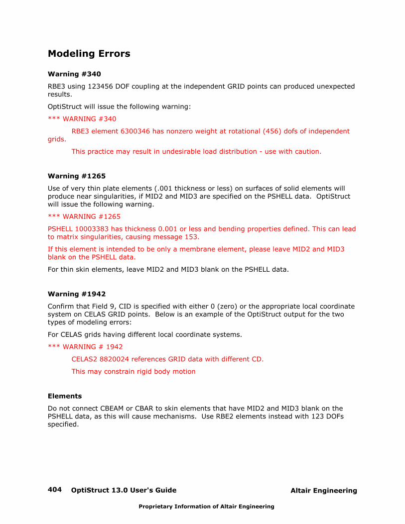
OptiStruct 13.0 User's Guide404 Altair Engineering
Proprietary Information of Altair Engineering
Modeling Errors
Warning #340
RBE3 using 123456 DOF coupling at the independent GRID points can produced unexpectedresults.
OptiStruct will issue the following warning:
*** WARNING #340
RBE3 element 6300346 has nonzero weight at rotational (456) dofs of independentgrids.
This practice may result in undesirable load distribution - use with caution.
Warning #1265
Use of very thin plate elements (.001 thickness or less) on surfaces of solid elements willproduce near singularities, if MID2 and MID3 are specified on the PSHELL data. OptiStructwill issue the following warning.
*** WARNING #1265
PSHELL 10003383 has thickness 0.001 or less and bending properties defined. This can leadto matrix singularities, causing message 153.
If this element is intended to be only a membrane element, please leave MID2 and MID3blank on the PSHELL data.
For thin skin elements, leave MID2 and MID3 blank on the PSHELL data.
Warning #1942
Confirm that Field 9, CID is specified with either 0 (zero) or the appropriate local coordinatesystem on CELAS GRID points. Below is an example of the OptiStruct output for the twotypes of modeling errors:
For CELAS grids having different local coordinate systems.
*** WARNING # 1942
CELAS2 8820024 references GRID data with different CD.
This may constrain rigid body motion
Elements
Do not connect CBEAM or CBAR to skin elements that have MID2 and MID3 blank on thePSHELL data, as this will cause mechanisms. Use RBE2 elements instead with 123 DOFsspecified.
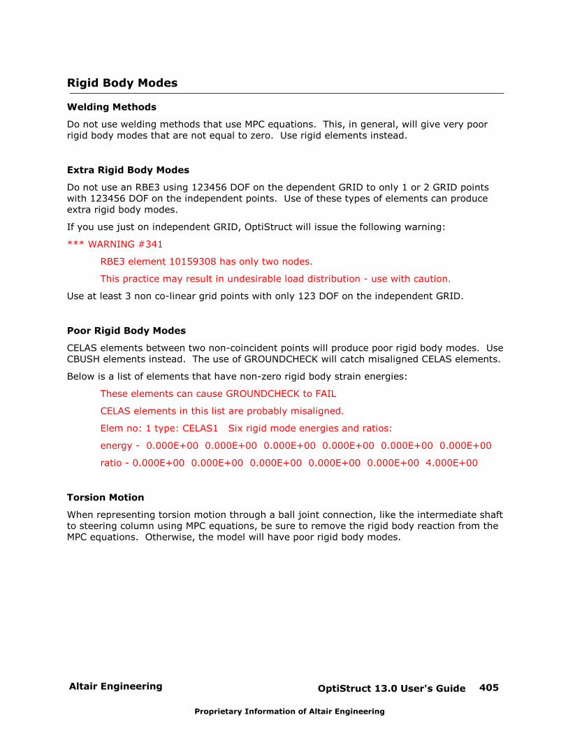
Altair Engineering OptiStruct 13.0 User's Guide 405
Proprietary Information of Altair Engineering
Rigid Body Modes
Welding Methods
Do not use welding methods that use MPC equations. This, in general, will give very poorrigid body modes that are not equal to zero. Use rigid elements instead.
Extra Rigid Body Modes
Do not use an RBE3 using 123456 DOF on the dependent GRID to only 1 or 2 GRID pointswith 123456 DOF on the independent points. Use of these types of elements can produceextra rigid body modes.
If you use just on independent GRID, OptiStruct will issue the following warning:
*** WARNING #341
RBE3 element 10159308 has only two nodes.
This practice may result in undesirable load distribution - use with caution.
Use at least 3 non co-linear grid points with only 123 DOF on the independent GRID.
Poor Rigid Body Modes
CELAS elements between two non-coincident points will produce poor rigid body modes. UseCBUSH elements instead. The use of GROUNDCHECK will catch misaligned CELAS elements.
Below is a list of elements that have non-zero rigid body strain energies:
These elements can cause GROUNDCHECK to FAIL
CELAS elements in this list are probably misaligned.
Elem no: 1 type: CELAS1 Six rigid mode energies and ratios:
energy - 0.000E+00 0.000E+00 0.000E+00 0.000E+00 0.000E+00 0.000E+00
ratio - 0.000E+00 0.000E+00 0.000E+00 0.000E+00 0.000E+00 4.000E+00
Torsion Motion
When representing torsion motion through a ball joint connection, like the intermediate shaftto steering column using MPC equations, be sure to remove the rigid body reaction from theMPC equations. Otherwise, the model will have poor rigid body modes.
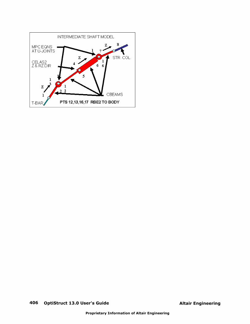
OptiStruct 13.0 User's Guide406 Altair Engineering
Proprietary Information of Altair Engineering
Altair Engineering OptiStruct 13.0 User's Guide 407
Proprietary Information of Altair Engineering
Results
The following features are outlined here.
Results of a Finite Element Analysis
The primary results in a finite element analysis are grid point displacements and rotations. Element results such as stresses, strains, and strain energy density are derived from thoseresults. Other results include element forces, MPC forces, SPC forces, and grid pointforces.
Results of a finite element analysis are post-processed using a graphical tool.
The definitions of the output options can be found in the I/O Options Section. An overviewof the result files can be found in the Results Output by OptiStruct section.
Information on stress, strain and force definitions regarding their coordinate systemdefinition can be found in the section Element Results Representation in OptiStruct and onthe respective element definitions.
Displacements
Displacements and rotations are computed in linear static, and frequency responseanalyses. In addition, in frequency response velocities and acceleration are computed.
Eigenvectors are the primary result in a normal modes and buckling analyses. In a normalmodes analysis, they are normalized with respect to the mass matrix or with respect to themaximum vector component. In a buckling analysis, the latter always applies.
Displacements, velocities, accelerations, and eigenvectors are grid point results. They areplotted as a deformed structure, or as a contour on the undeformed structure. Some post-processors, such as Altair HyperMesh and Altair HyperView, also allow the animation of thedisplacements.
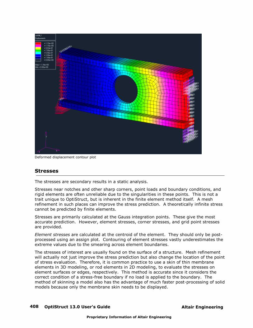
OptiStruct 13.0 User's Guide408 Altair Engineering
Proprietary Information of Altair Engineering
Deformed displacement contour plot
Stresses
The stresses are secondary results in a static analysis.
Stresses near notches and other sharp corners, point loads and boundary conditions, andrigid elements are often unreliable due to the singularities in these points. This is not atrait unique to OptiStruct, but is inherent in the finite element method itself. A meshrefinement in such places can improve the stress prediction. A theoretically infinite stresscannot be predicted by finite elements.
Stresses are primarily calculated at the Gauss integration points. These give the mostaccurate prediction. However, element stresses, corner stresses, and grid point stressesare provided.
Element stresses are calculated at the centroid of the element. They should only be post-processed using an assign plot. Contouring of element stresses vastly underestimates theextreme values due to the smearing across element boundaries.
The stresses of interest are usually found on the surface of a structure. Mesh refinementwill actually not just improve the stress prediction but also change the location of the pointof stress evaluation. Therefore, it is common practice to use a skin of thin membraneelements in 3D modeling, or rod elements in 2D modeling, to evaluate the stresses onelement surfaces or edges, respectively. This method is accurate since it considers thecorrect condition of a stress-free boundary if no load is applied to the boundary. Themethod of skinning a model also has the advantage of much faster post-processing of solidmodels because only the membrane skin needs to be displayed.
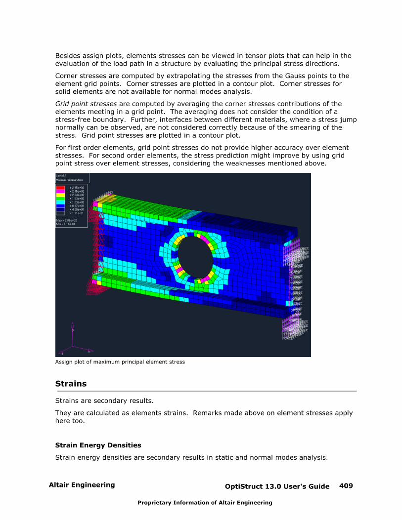
Altair Engineering OptiStruct 13.0 User's Guide 409
Proprietary Information of Altair Engineering
Besides assign plots, elements stresses can be viewed in tensor plots that can help in theevaluation of the load path in a structure by evaluating the principal stress directions.
Corner stresses are computed by extrapolating the stresses from the Gauss points to theelement grid points. Corner stresses are plotted in a contour plot. Corner stresses forsolid elements are not available for normal modes analysis.
Grid point stresses are computed by averaging the corner stresses contributions of theelements meeting in a grid point. The averaging does not consider the condition of astress-free boundary. Further, interfaces between different materials, where a stress jumpnormally can be observed, are not considered correctly because of the smearing of thestress. Grid point stresses are plotted in a contour plot.
For first order elements, grid point stresses do not provide higher accuracy over elementstresses. For second order elements, the stress prediction might improve by using gridpoint stress over element stresses, considering the weaknesses mentioned above.
Assign plot of maximum principal element stress
Strains
Strains are secondary results.
They are calculated as elements strains. Remarks made above on element stresses applyhere too.
Strain Energy Densities
Strain energy densities are secondary results in static and normal modes analysis.
OptiStruct 13.0 User's Guide410 Altair Engineering
Proprietary Information of Altair Engineering
They are calculated as element strain energy densities. Remarks made above on elementstresses apply here too.
Forces
Element forces, MPC forces, SPC forces, and grid point forces are printed as tabulatedoutput.
Grid Point Stresses
The default method of calculating stresses in OptiStruct produces values of stresscomponents at the centroids of elements. (Typically a post-processor, such as HyperView,will then average these values to produce smooth contour plots). This method, whileuseful for viewing stress distribution, may underestimate stress maxima, especially on thesurface of the body.
To provide higher accuracy stresses, OptiStruct supports grid point stress calculation. Gridpoint stresses are computed using the following steps:
1. Calculate stress components at integration points of elements (these are generally themost accurate stress locations).
2. Extrapolate stress values to element nodes (grid points).
3. Calculate average at each grid point using values from surrounding elements.
4. Calculate derived quantities, such as von Mises stress or principal stresses, at each gridpoint (this assures that these values are consistent and make physical sense).
The above approach produces continuous stress field, typically in the entire domain. Since, however, stresses can be discontinuous between different materials, OptiStructsupports calculation of separate grid point stress field per each material sub domain. Thepresence of more than one material is detected automatically and then grid point stressesare calculated for the entire domain and as a separate field for each material region.
Grid point stress calculation is activated through the I/O subcase command GPSTRESS. When activated, grid point stresses are produced in addition to default stress results – theycan be found in a separate results subcase.
The present support for grid point stress capability has the following scope:
It is supported for nodes connected to three-dimensional solid elements
It is available for static load cases and non-design elements
Grid point stresses are always calculated in the basic coordinate system
Element Results Representation for Models in OptiStruct
Elemental results (namely stresses, strains and element forces) may be provided withreference to either the material system or the elemental system. For the HM, PUNCH, andOPTI output formats, results are provided with reference to the material system; for firstorder shell element results, PARAM, OMID may be used to output with eitherrepresentation. The H3D and OUTPUT2 output formats, to which these elemental results
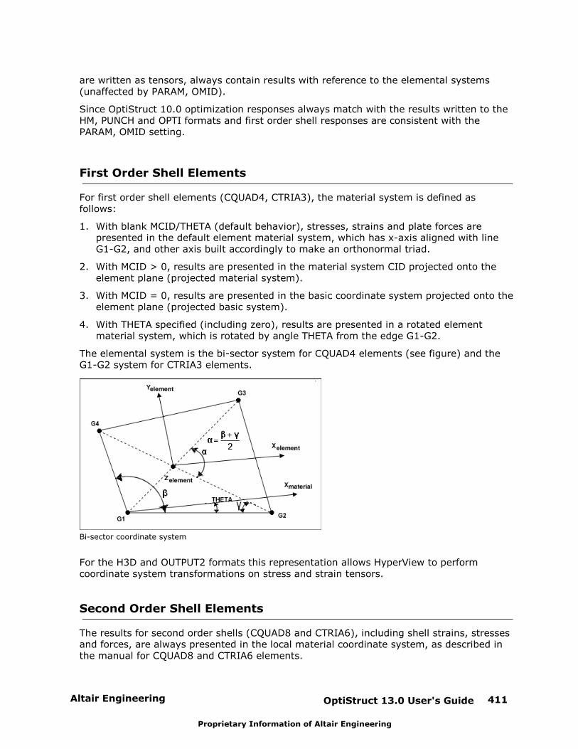
Altair Engineering OptiStruct 13.0 User's Guide 411
Proprietary Information of Altair Engineering
are written as tensors, always contain results with reference to the elemental systems(unaffected by PARAM, OMID).
Since OptiStruct 10.0 optimization responses always match with the results written to theHM, PUNCH and OPTI formats and first order shell responses are consistent with thePARAM, OMID setting.
First Order Shell Elements
For first order shell elements (CQUAD4, CTRIA3), the material system is defined asfollows:
1. With blank MCID/THETA (default behavior), stresses, strains and plate forces arepresented in the default element material system, which has x-axis aligned with lineG1-G2, and other axis built accordingly to make an orthonormal triad.
2. With MCID > 0, results are presented in the material system CID projected onto theelement plane (projected material system).
3. With MCID = 0, results are presented in the basic coordinate system projected onto theelement plane (projected basic system).
4. With THETA specified (including zero), results are presented in a rotated elementmaterial system, which is rotated by angle THETA from the edge G1-G2.
The elemental system is the bi-sector system for CQUAD4 elements (see figure) and theG1-G2 system for CTRIA3 elements.
Bi-sector coordinate system
For the H3D and OUTPUT2 formats this representation allows HyperView to performcoordinate system transformations on stress and strain tensors.
Second Order Shell Elements
The results for second order shells (CQUAD8 and CTRIA6), including shell strains, stressesand forces, are always presented in the local material coordinate system, as described inthe manual for CQUAD8 and CTRIA6 elements.

OptiStruct 13.0 User's Guide412 Altair Engineering
Proprietary Information of Altair Engineering
Composite Shells
Shell-type strains and stresses for composite shells use the same representation ashomogeneous shells. By shell-type results, we mean strains and stresses calculated at Z1,Z2 using homogenized shell properties. Strains and stresses for individual plies are alwayspresented in the respective ply coordinate system.
Solid Elements
For solid elements (CHEXA, CTETRA, CPENTA and CPYRA), the results are always providedin the material coordinate system.
1. With blank CORDM on the PSOLID card (default behavior), strains and stresses arepresented in the basic coordinate system.
2. With CORDM > 0, strains and stresses are presented in the material system CID.
3. With CORDM = -1, stresses are presented in the local element coordinate system(described in detail on respective solid element manual pages).
Gap Elements
For gap elements, gap forces are represented in the gap coordinate system, as describedon respective gap element manual pages (CGAP and CGAPG). Compression is positive.
Saving and Retrieving Normal Modes Analysis Results
OptiStruct allows Normal Modes Analysis results to be retrieved for use in FrequencyResponse Analysis or Transient Response Analysis using the modal method. Thus, multipledynamic loading analyses can be performed using the eigenvalue results of a single normalmodes analysis.
The following input I/O options and subcase information section entries may be used forthis purpose:
EIGVSAVE
EIGVRETRIEVE
EIGVNAME
Saving Eigenvalues and Eigenvectors from a Normal Modes Analysis
EIGVSAVE is a subcase information entry that, if used within a normal modes analysissubcase, causes the eigenvalues and eigenvectors of that subcase to be written to anexternal data file. The external data file will use the default output file prefix unless theEIGVNAME I/O option is present, followed by an underscore, then followed by theEIGVSAVE integer argument and the .eigv extension.
Altair Engineering OptiStruct 13.0 User's Guide 413
Proprietary Information of Altair Engineering
For example, the input:
EIGVNAME = test_file$Subcase 10
spc = 1method = 20EIGVSAVE= 50
will save the eigenvector and eigenvalue results from a normal modes analysis to the file"test_file_50.eigv."
Retrieving Eigenvalues and Eigenvectors for a Modal Frequency Response Analysisor for a Modal Transient Analysis
EIGVRETRIEVE is a subcase information entry that, if used within a modal frequencyresponse analysis or a modal transient response analysis subcase, retrieves eigenvaluesand eigenvectors from external data files. EIGVRETRIEVE may have multiple integerarguments, each referring to a different external data file. The external data files musthave the default output file prefix unless EIGVNAME I/O option is present, followed by anunderscore, followed then by the EIGVRETRIEVE integer argument and the extension .eigv.
For example, the following input can be used in a frequency response analysis subcaseusing the modal method to retrieve the eigenvalues and eigenvectors that were saved inthe example above:
EIGVNAME = test_file$Subcase 40
Spc = 1Dload = 30Method = 20EIGVRETRIEVE = 50
Combining Eigenvalues and Eigenvectors from Two or More Normal ModesAnalyses for a Single Modal Frequency Response or Modal Transient ResponseAnalysis
The results of two or more normal modes analyses can be retrieved in combination for amodal frequency response analysis.
For example, a normal modes analysis is performed with the real eigenvalue extraction(EIGRL) data:
(1) (2) (3) (4) (5) (6) (7) (8) (9) (10)
EIGRL 20 50.0
The results are written to an external data file as follows:
EIGVNAME = test_file$Subcase 10
spc = 1
OptiStruct 13.0 User's Guide414 Altair Engineering
Proprietary Information of Altair Engineering
method = 20EIGVSAVE= 50
In this case, all of the eigenmodes up to 50 Hz have been calculated and written to the file"test_file_50.eigv."
In order to perform a modal frequency response analysis with all of the modes up to 70 Hz,another normal modes analysis can be performed with the real eigenvalue extraction data:
(1) (2) (3) (4) (5) (6) (7) (8) (9) (10)
EIGRL 20 50.0 70.0
This time, the results are written to an external data file as follows:
EIGVNAME = test_file$subcase 10
spc = 1method = 20EIGVSAVE= 70
All eigenmodes between 50 Hz and 70 Hz are written to the file "test_file_70.eigv."
You can now run a modal transient response analysis with:
EIGVNAME = test_file$subcase 40
spc = 1dload = 30method 20tstep(time) = 100EIGVRETRIEVE = 50, 70
The real eigenvalue extraction data referenced in the modal transient response analysissubcase must not request eigenvalue and eigenvector results outside of the range ofretrieved values. If it does, OptiStruct will terminate with an error. In this example, thefollowing EIGRL cards are valid:
(1) (2) (3) (4) (5) (6) (7) (8) (9) (10)
EIGRL 20 0.0 70.0
(1) (2) (3) (4) (5) (6) (7) (8) (9) (10)
EIGRL 20 0.0 50.0
(1) (2) (3) (4) (5) (6) (7) (8) (9) (10)
EIGRL 20 30.0 40.0
Altair Engineering OptiStruct 13.0 User's Guide 415
Proprietary Information of Altair Engineering
The following EIGRL cards would cause error terminations for this example:
(1) (2) (3) (4) (5) (6) (7) (8) (9) (10)
EIGRL 20 0 100.0
(1) (2) (3) (4) (5) (6) (7) (8) (9) (10)
EIGRL 20 50.0 70.01
It is recommended to use a frequency range without the maximum number of modes onthe EIGRL bulk data entries referenced in normal modes analyses from which eigenvalueresults are saved. If the maximum number of modes is specified and these eigenvalueresults are retrieved by a modal frequency response analysis, and it cannot be determinedwhether all of the modes are obtained for the requested range, OptiStruct will terminatewith an error.
For example, assume there are exactly 300 modes in the frequency range 0.0 to 5.0.0 Hz. Now assume that a normal modes analysis is performed referencing the EIGRL bulk dataentry.
(1) (2) (3) (4) (5) (6) (7) (8) (9) (10)
EIGRL 20 0.0 50.0 300
The eigenvectors and eigenvalues are saved as follows:
EIGVNAME = test_file$Subcase 10
spc = 1method = 20EIGVSAVE = 50
All 300 modes in the range of 0 to 50.0 Hz are extracted and saved to the file"test_file_50.eigv."
Now try to retrieve these results to use in a modal frequency response analysis, as follows:
EIGVNAME = test_file$subcase 40
spc = 1dload = 30method 20EIGVRETRIEVE = 50
where the referenced EIGRL definition is:
(1) (2) (3) (4) (5) (6) (7) (8) (9) (10)
EIGRL 20 0.0 50.0

OptiStruct 13.0 User's Guide416 Altair Engineering
Proprietary Information of Altair Engineering
This will cause an error termination because it is known (through the external data file)that there are 300 modes within the 0.0 to 50.0 Hz range, but do not know if this is all ofthe modes.
If the EIGRL definition referenced in the normal modes analysis were specified as:
(1) (2) (3) (4) (5) (6) (7) (8) (9) (10)
EIGRL 20 0.0 50.0 301
and only 300 modes were found, you would know that these are all of the modes withinthe 0.0 to 50.0 Hz range, and would retrieve the saved eigenvalue results in this case. OptiStruct would not terminate with an error.
Altair Engineering OptiStruct 13.0 User's Guide 417
Proprietary Information of Altair Engineering
Coupling OptiStruct with Third Party Software
The following features can be found in this section:
Using the AMLS (Automatic Multi-Level Sub-structuring) Eigensolvers
For the solution of large eigenvalue problems, the AMLS (Automatic Multi-Level Sub-structuring) eigensolver developed by the University of Texas can be used instead of theinternal OptiStruct Lanczos eigensolver. The AMLS eigensolver is a separate program fromOptiStruct and must be installed and licensed separately. OptiStruct interfaces with AMLSby writing AMLS input files, launching AMLS, and then reading the AMLS results back intoOptiStruct once the AMLS execution is complete. The resulting eigenvalues andeigenvectors can then be used by OptiStruct for eigenvalue analysis, modal frequencyresponse, and modal transient analysis. In addition, the AMLS solver can be used duringtopology and sizing optimizations.
OptiStruct only supports AMLS version 3.2.0128 or later. To use AMLS version 5 or later,OptiStruct version 13.0 or later must be used. To use AMLS, the following should bedefined:
1. The environment variable AMLS_EXE must be set by you to point to the AMLS
executable.
On UNIX and Linux platforms the script that is used to invoke OptiStruct (~altair/
scripts/invoke/optistruct) contains a "placeholder" where AMLS_EXE may be defined
(search for AMLS_EXE). The definition contained in the invoke script will only be used if
there is no pre-existing AMLS_EXE environment variable at invoke.
Example: setenv AMLS_EXE /share/ams/cdhopt/2005/AIX-5.3/3.2.r159_exe/amls.main_AIX.5
2. PARAM, AMLS must be set to YES in the OptiStruct input file. The run option –amls can
also be used to activate AMLS.
AMLS is a multithreaded application and can use 1, 2, or 4 processors. PARAM,AMLSNCPU may be defined in the OptiStruct input file to define the number ofprocessors that are to be used by AMLS. If PARAM, AMLSNCPU is not set, then theAMLS eignersolver will use only 1 CPU. Note that when PARAM, AMLSNCPU is defined,it is possible for OptiStruct and AMLS to use different numbers of processors.
Parameters Affecting AMLS
AMLS controls the accuracy and the cost of a solution primarily with three parameters. The “optimal” values of these parameters for typical NVH analysis have been establishedthrough extensive testing. The parameters and their values are:
PARAM,SS2GCR,5.0
PARAM,GMAR,1.1
PARAM,GMAR1,1.7
In case of predominately solid models, such as engine blocks, SS2GCR should be set to10.0 and GMAR1 should be set to 2.1. In case of typical shell models, such as car bodies,
OptiStruct 13.0 User's Guide418 Altair Engineering
Proprietary Information of Altair Engineering
a slight improvement in FRF accuracy can be obtained without large increases in elapsedtime by setting two of the parameters as follows:
PARAM,SS2GCR,7.5
PARAM,GMAR1,2.1
However, you are discouraged from adjusting these values unless the accuracyimprovement is known to be worth the increase in resource requirements.
The default upper limit on eigenvalues that are taken to be associated with rigid bodymodes is 1.0 (equivalent to a natural frequency of about 0.16 Hz). This parameter can beadjusted by parameter RBMEIG, which can be set by the command:
PARAM,RBMEIG,0.2
AMLS distinguishes between rigid body modes and flexible modes to improve the numericalconditioning, and hence accuracy, with which the flexible eigenvalues are computed.
Control of the singularity processing is performed using PARAM, AMLSMAXR. If AMLSMAXRis exceeded in the process of factoring a stiffness matrix, this indicates a singularity in K. If the mass of this DOF is also zero, there is a "massless mechanism", and an SPC isapplied and a message is written to the .out file. If there is mass, then this is a
mechanism, which is treated as a rigid body mode, and a message is written to the .out
file.
By default AMLS does not handle disconnected structures. There are two solutions forhandling disconnected structures:
PARAM,AMLSUCON,YES
PARAM,DISJOINT,n
If PARAM,AMLSUCON is set to YES then OptiStruct will SPC out the disconnected components
if there is a total of less than 4000 disconnected grids. This works with all versions ofAMLS.
When PARAM,DISJOINT is set to a value that is at least one larger than the number of
disconnected parts then AMLS will be able to solve the eigenvalue calculation problem. This feature is only available in AMLS versions 4.2r22 or newer.
For AMLS Versions 5 and later, the run option –amlsmem, the environment variable
AMLS_MEM or the parameter PARAM, AMLSMEM can be used to set the amount of memoryin Gigabytes used by AMLS. By default, AMLS will use the same amount of memory usedby OptiStruct. The run option –amlsmem, the environment variable AMLS_MEM or the
parameter PARAM, AMLSMEM can be used to override this default value. The run optionoverrides the value set by the environment variable and the parameter. If both AMLS_MEM and PARAM, AMLSMEM are set, then the value specified by the environmentvariable is used.
Residual Vector Calculations
When the AMLS eigensolver is used, OptiStruct’s Residual Vector calculations are ignored. The AMLS eigensolver calculates its own residual vectors for each of the following:
USET U6 data
Frequency Response Dynamic Loads
Altair Engineering OptiStruct 13.0 User's Guide 419
Proprietary Information of Altair Engineering
Transient Response Dynamic Loads
Damping DOF from CBUSH, CDAMPi or CVISC data
One Residual Vector is calculated for each USET U6 degree of freedom, each DAREA degreeof freedom, and each damping degree of freedom associated with the CBUSH, CDAMPi andCVISC data.
The Residual Vector calculations are controlled by the Solution Control data RESVEC. Tocontrol Residual Vector calculations with AMLS, use the following commands:
Use RESVEC=NO to turn off Residual Vector calculations with AMLS
Use RESVEC(NODAMP)=YES to turn off Residual Vectors associated with DampingDOF
Singularities
If AMLS detects a large number of singularities in the model this is most likely due to thinCQUAD4/CTRIA3 elements used to “skin” solid models. These singularities causenumerical ill-conditioning and increase run time. The singularities are caused by the verylow bending stiffness of these thin shell elements. To remove the singularities, convert thethin bending elements to membrane only elements by removing the MID2 and MID3 MID’sfrom the associated PSHELL data. The thin membrane elements will still calculate thecorrect surface stresses, but the singularities will not be present as the elements will haveno bending stiffness.
PARAM, AMLSMAXR is used to determine singularities in the stiffness matrix.
If the value of AMLSMAXR is exceeded in the process of factoring a stiffness matrix, thisindicates a singularity in K. If the mass of this degree-of-freedom is zero, there is a"massless mechanism"; an SPC is applied and a message is written to the .out file. If
there is mass, then this is a mechanism which is treated as a rigid body mode and amessage is written to the .out file.
The list of GRID identification numbers of singular grids during an AMLS run is output tothe .amls_singularity.cmf file.
Remote File Systems
If the execution directory is on a remote file system, long run times will result as the AMLSscratch files will have to be accessed over the NFS mounted file system. Use theenvironment variable TMPDIR to redefine the scratch directory to be on the local machine. Note that the environment variable TMPDIR is different from the scratch file directoryspecified by the command line argument –tmpdir.
The input and output files from AMLS (generic_real_file, generic_integer_file, and
generic_amls_output) are stored in the directory specified by the environment variable
AMLSDIR. In general, the environment variable AMLSDIR should be set to be the samedirectory as the environment variable TMPDIR.
Limitations
1. AMLS is designed for large problems. Problems less than a few hundred degrees offreedom cannot be solved by AMLS.
OptiStruct 13.0 User's Guide420 Altair Engineering
Proprietary Information of Altair Engineering
2. The model must consist of only one structure. Models of unconnected parts cannot besolved by AMLS. When the CBN method of creating CSM Super Elements is used onthe CMSMETH data, unconnected models can be generated if the center GRID of anRBE2 is an ASET GRID. If unconnected are found, a file named filename.unconnected.cmf is generated. This file can be used in HyperMesh to show
the unconnected parts. If the parts are small, PARAM, AMLSUCON,1 can be used toSPC out the unconnected structure and AMLS will run correctly. If the unconnectedpart is large, you can:
Remove one spider GRID of the RBE2 to make the structure connected
Use a small CBAR, CBEAM, or CROD to connect the two structures
FastFRS Usage (Fast Frequency Response Solver)
FastFRS is a solver developed by the University of Texas at Austin. It is very efficient for acertain class of large modal frequency response problems, such as NVH problems. OptiStruct has an interface to FastFRS. OptiStruct writes the file FastFRS_Gen.in as input
for FastFRS, and reads results from FastFRS_gen.out. FastFRS will run in the directory
specified by the environment variable AMLSDIR, or the current directory if AMSLDIR is notspecified.
The following parameters can be used within the OptiStruct to control the FastFRS solver.
1. Set the environment variable FASTFRS_EXE to point to the location of the FastFRS
executable.
2. The run option –ffrs yes or the parameter PARAM,FFRs,YES can be used to activate
FastFRS:
3. Add the following optional parameters to adjust the settings for FastFRS runs:
PARAM,FFRSLFRQ
PARAM,LOWRANK
PARAM,K4CUTOFF
PARAM,CSTOL
PARAM,FFRSNCPU (or the run option –ffrsncpu)
PARAM,FFRSMEM (or the run option –ffrsmem or the environment variable FFRS_MEM)
Note:
1. OptiStruct version 13.0 or above is required to run FastFRS version 2 or above.
2. If FFRSNCPU is not set (using either the parameter or the run option), and AMLSNCPU
is set, then FastFRS will use the number of CPU’s specified by AMLSNCPU.
3. For FastFRS versions 2 and later, the run option –ffrsmem, the environment variable
FFRS_MEM, or the parameter PARAM,FFRSMEM can be used to set the amount of memory
in Gigabytes used by FastFRS. By default, FastFRS will use the same amount ofmemory used by OptiStruct. The run option –ffrsmem, the environment variable,
FFRS_MEM, or the parameter PARAM, FFRSMEM can be used to override this defaultvalue. The run option overrides the environment variable and the parameter. If bothFFRS_MEM and PARAM, FFRSMEM are set, then the value specified by the environment
Altair Engineering OptiStruct 13.0 User's Guide 421
Proprietary Information of Altair Engineering
variable is used.
Creating Output for Third Party Software
The section describes how to create output from OptiStruct for third party programs forFatigue Analysis (FEMFAT, Design Life, and FE-SAFE), Multi-Body Dynamic Analysis (AVL/EXCITE, SIMPACK, ROMAX, ADAMS, RecurDyn and Virtual Lab), and Fluid StructureInteraction (AcuSolve).
Fatigue Analysis
The .op2 file from OptiStruct can be used directly by Third Party Fatigue Analysis software
programs FEMFAT, Design Life, FE-Fatigue, and FE-SAFE. Just request stress output tothe .op2 file:
STRESS(OP2) = SET or ALL
Multi-Body Dynamic Analysis
AVL/EXCITE
To create the condensed CMS Super Element information for AVL/EXCITE, use the CMSMETH CBN Method with ASET data for the connection DOF.
The MODEL data can used specify interior grid data to be included in the Super Element forviewing in AVL/EXCITE. The MODEL data format is:
MODEL=Element Set, Grid Set, RIGID/NORIGID.
All grids associated with elements in the element set and rigid elements, if RIGID isspecified, are combined with the grids in the Grid Set and output to AVL/EXCITE. Inaddition, the keyword PLOTEL can be used instead of an Element Set ID to specify all thegrids associated with all of the PLOTEL data in the model.
GPSTRESS is used to specify set of grids for which Grid Point Stresses are calculated forAVL/EXCITE.
The PARAM,EXCEXB data controls the output of the AVL/EXCITE .exb file directly from
OptiStruct.
The PARAM,EXCOUT data is used to specify what data is written out for AVL/EXCITE. TheEXCOUT values produce the information for AVL/EXCITE specified below:
$ EXCOUT - -1: no output$ 0: all output (default)$ 1: DOF, geometry, and elements tables$ (GEOM1,GEOM2,EQEXIN,USET),$ reduced mass and stiffness matrices (MAA and KMAA)$ 3: 1 + GOA transpose$ 4: 3 + unreduced mass matrix (MFF) (CON6) $ 5: 1 + eigenvectors of condensed system (PHA) and$ grid point stress table, SORT 1 (OGS1)$ 6: 4 + eigenvectors of condensed system (PHA) and$ grid point stress table, SORT 1 (OGS1)$ 7: 3 + eigenvectors of condensed system (PHA) and
OptiStruct 13.0 User's Guide422 Altair Engineering
Proprietary Information of Altair Engineering
$ grid point stress table, SORT 1 (OGS1)
After running AVL/EXCITE, a residual run can be made to recover displacement, velocity,acceleration, stress, and strain results for interior grids and elements in the CMS SuperElement based on the modal participation results from AVL/EXCITE. Note that the resultsare only calculated for GRID and elements specified by the MODEL data in the CMS SuperElement creation run. The residual run can be any combination of frequency response andtransient analysis SUBCASE’s. After running AVL/EXCITE, a resulting filename.INP4 file is
created that contains the modal participation factors for the modes of the CMS SuperElement for each loading frequency or transient analysis time step. In the residual run,the CMS Super Element .h3d file and the AVL/EXCITE modal results file are specified using
the ASSIGN data:
ASSIGN,H3DDMIG,AX,'Crank_split2h_all.h3d'ASSIGN,EXCINP,10,'Crankshaft_SOL109_time.INP4'
Where the 10 in the ASSIGN,EXCINP data corresponds to the SUBCASE for which the modal
participation results will be used. In SUBCASE 10, instead of performing a frequency
response or transient response analysis, OptiStruct will just use the modal participationresults from AVL/EXCITE. Note that since the analysis is skipped, it does not matter if theresidual run is modal or direct frequency response/transient analysis.
For transient analysis, the number of time steps in the transient analysis residual run mustmatch the number of time steps used in the AVL/EXCITE analysis. For frequency responseanalysis, the number of loading frequencies in the frequency response analysis residual runmust match number of loading frequencies used in the AVL/EXCITE analysis. While thefrequency response/transient analysis data is ignored, there must still be some dummyloading data (TLOAD/RLOAD, DAREA, and TABLED data). A sample of input data for atransient analysis residual run is shown below:
ASSIGN,H3DDMIG,AX,'Crank_split2h_all.h3d'ASSIGN,EXCINP,10,'Crankshaft_SOL109_time.INP4'$DISPLACEMENT = ALLSTRESS = ALL$SUBCASE 10 DLOAD = 10201 TSTEP = 10133$BEGIN BULK$GRID,80001,,0.,-62.,0.$ TLOAD1,10201,10202,,,10301DAREA,10202,80001,1,1.0TABLED1,10301,,0.0,1.0,0.1,1.0,0.2,1.0,0.3,1.0,ENDTTSTEP,10133,143,2.7778-4ENDDATA
SIMPACK
To create the condensed CMS Super Element information for SIMPACK, you must use the CMSMETH CBN Method with ASET or CSET data for the connection DOF. If CSET connectionDOF is used, then the AMSES solver must be specified on the CMSMETH data.
Altair Engineering OptiStruct 13.0 User's Guide 423
Proprietary Information of Altair Engineering
The PARAM,SIMPACK data is used to specify what data is written out for SIMPACK. TheSIMPACK values produce the information for SIMPACK.
Recover SIMPACK results in OptiStruct
ASSIGN, SIMPIMP identifies an external .unv file generated after running a multibody
dynamic analysis in SIMPACK. The resulting CMS flexbody modal participation factors inthe .unv file can be used by OptiStruct to recover the dynamic displacements, velocities,
accelerations, stresses and strains. The format is as follows:
ASSIGN, SIMPINP, Subcase ID, Filename
Subcase ID is used to specify which SUBCASE the modal participation factors should beused for.
RecurDyn
To create the modal CMS Super Element information for RecurDyn, you must use the CMSMETH CBN Method with ASET data for the connection DOF.
The PARAM,RFIOUT,YES data is used to turn on the generation of the .rfi file, which
contains the modal super element that is used by RecurDyn.
Note: This .rfi file can be created only by OptiStruct
executables running on 64-bit Windows machines. Thisfile cannot be created while using OptiStruct on Linux orMac OS X machines.
ROMAX
To create the condensed CMS Super Element information for ROMAX, use the CMSMETHCBN Method with ASET data for the connection DOF.
Use PARAM,EXTOUT,DMIGPCH to create a PUNCH file containing the Super Element data. This data can be read by any version of ROMAX after release R12.6.2.
ADAMS
To create the condensed Flex Body information for ADAMS, use the CMSMETH CC or CBMethod.
The MODEL data used can specify interior grid and element data to be included in the FlexBody for viewing in ADAMS. The MODEL data format is:
MODEL=Element Set, Grid Set, RIGID/NORIGID.
All grids associated with elements in the element set and rigid elements if RIGID isspecified are combined with the grids in the Grid Set and output to ADAMS. In addition,the keyword PLOTEL can be used instead of an Element Set ID to specify all the gridsassociated with all of the PLOTEL data in the model.
GPSTRESS is used to specify set of grids for which Grid Point Stresses are calculated forADAMS.
OptiStruct 13.0 User's Guide424 Altair Engineering
Proprietary Information of Altair Engineering
The OUTPUT command is used to generate the .mnf file for ADAMS. The command is:
OUTPUT=ADAMSMNF
Virtual Lab
To create the condensed Flex Body Modes and Full Diagonal Mass Matrix to the .op2 file for
Virtual Lab, use the CMSMETH CB or CC Methods.
The PARAM,LMSOUT data is to trigger the output of the condensed Flex Body Modes andfull Diagonal Mass Matrix to the .op2 file. PARAM,POST is not required. OUTPUT=OP2 is
not required.
Fluid Structure Interaction Analysis
The .op2 file from OptiStruct can be used directly by the AcuSolve CFD code.
Just request the eigenvector output to the .op2 file:
DISP(OP2) = ALL
Then run the Python script from ACUSIM called acuNASTRAN2pev.py:
python acuNastran2Pev.py problem.op2
This will create the nodes.dat, elems.dat, and modeXX.dat files. Be sure to use the latest
version of acuNASTRAN2pev.py from ACUSIM.

Altair Engineering OptiStruct 13.0 User's Guide 425
Proprietary Information of Altair Engineering
Design Optimization
The following features can be found in this section:
Optimization Problem
Responses
Topology Optimization
Free-size Optimization
Topography Optimization
Size Optimization
Shape Optimization
Free-shape Optimization
Manufacturing Constraints
Reliability-based Design Optimization (Beta)
Optimization of Arbitrary Beam Sections
Optimization of Composite Structures
Equivalent Static Load Method (ESLM)
Gradient-based Optimization Method
Global Search Option
Multi-Model Optimization
OptiStruct 13.0 User's Guide426 Altair Engineering
Proprietary Information of Altair Engineering
Optimization Problem
The following features can be found in this section:
Minimize Objective Function
OptiStruct solves the following structural optimization problem:
1 2, , , )min ( ) ( nx xf x f x K
Subject to:
( ) 0 1, ,
1, ,
j
L Uii i
g x j m
x x x i n
K
K
The objective function f(x) and the functions g(x) in the constraint function are structural
responses obtained from a finite element analysis. A constraint is considered active if it issatisfied exactly (g = 0); it is considered inactive if g < 0; it is considered violated if g > 0.
The selection of the vector of design variables x depends on the type of optimization beingperformed. In topology optimization, the design variables are element densities (see Design Variables for Topology Optimization). In size optimization (including free-size), thedesign variables are properties of structural elements (see Design Variables for SizeOptimization). In topography and shape (including free-shape) optimization, the designvariables are the factors in a linear combination of shape perturbations (see DesignVariables for Topography Optimization and Design Variables for Shape Optimization).
The objective function is defined using a DESOBJ entry in the subcase information section. DESOBJ references a response defined by either the DRESP1, DRESP2, or DRESP3 bulkdata entry. Depending on the type of response, DESOBJ is located inside or outside of aSUBCASE. The constraints are defined using a DESSUB or DESGLB entry in the subcaseinformation section, depending on if the type of response is subcase related or global,respectively. DESSUB and DESGLB refer to DCONSTR or DCONADD bulk data entries. DCONSTR relates the constraint value or bound to a response defined by DRESP1, DRESP2,or DRESP3.
Minmax Objective Function
The minmax optimization problem is given as:
1 1 2 2min max / , (x) / f , , ( ) / fK Kf x f f f xK
Subject to:
( ) 0 1, ,
1, ,
j
L Uii i
g x j m
x x x i n
K
K
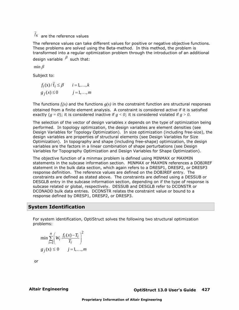
Altair Engineering OptiStruct 13.0 User's Guide 427
Proprietary Information of Altair Engineering
Kf are the reference values
The reference values can take different values for positive or negative objective functions. These problems are solved using the Beta-method. In this method, the problem istransformed into a regular optimization problem through the introduction of an additional
design variable such that:
min
Subject to:
(x) / f 1, ,
( ) 0 1, ,
i i
j
f i k
g x j m
K
K
The functions fi(x) and the functions g(x) in the constraint function are structural responses
obtained from a finite element analysis. A constraint is considered active if it is satisfiedexactly (g = 0); it is considered inactive if g < 0; it is considered violated if g > 0.
The selection of the vector of design variables x depends on the type of optimization being
performed. In topology optimization, the design variables are element densities (see Design Variables for Topology Optimization). In size optimization (including free-size), thedesign variables are properties of structural elements (see Design Variables for SizeOptimization). In topography and shape (including free-shape) optimization, the designvariables are the factors in a linear combination of shape perturbations (see DesignVariables for Topography Optimization and Design Variables for Shape Optimization).
The objective function of a minmax problem is defined using MINMAX or MAXMINstatements in the subcase information section. MINMAX or MAXMIN references a DOBJREFstatement in the bulk data section, which again refers to a DRESP1, DRESP2, or DRESP3response definition. The reference values are defined on the DOBJREF entry. Theconstraints are defined as stated above. The constraints are defined using a DESSUB orDESGLB entry in the subcase information section, depending on if the type of response issubcase related or global, respectively. DESSUB and DESGLB refer to DCONSTR orDCONADD bulk data entries. DCONSTR relates the constraint value or bound to aresponse defined by DRESP1, DRESP2, or DRESP3.
System Identification
For system identification, OptiStruct solves the following two structural optimizationproblems:
2
1
( )min
(x) 0 1, ,
ni i
iii
j
f x TW
T
g j mK
or
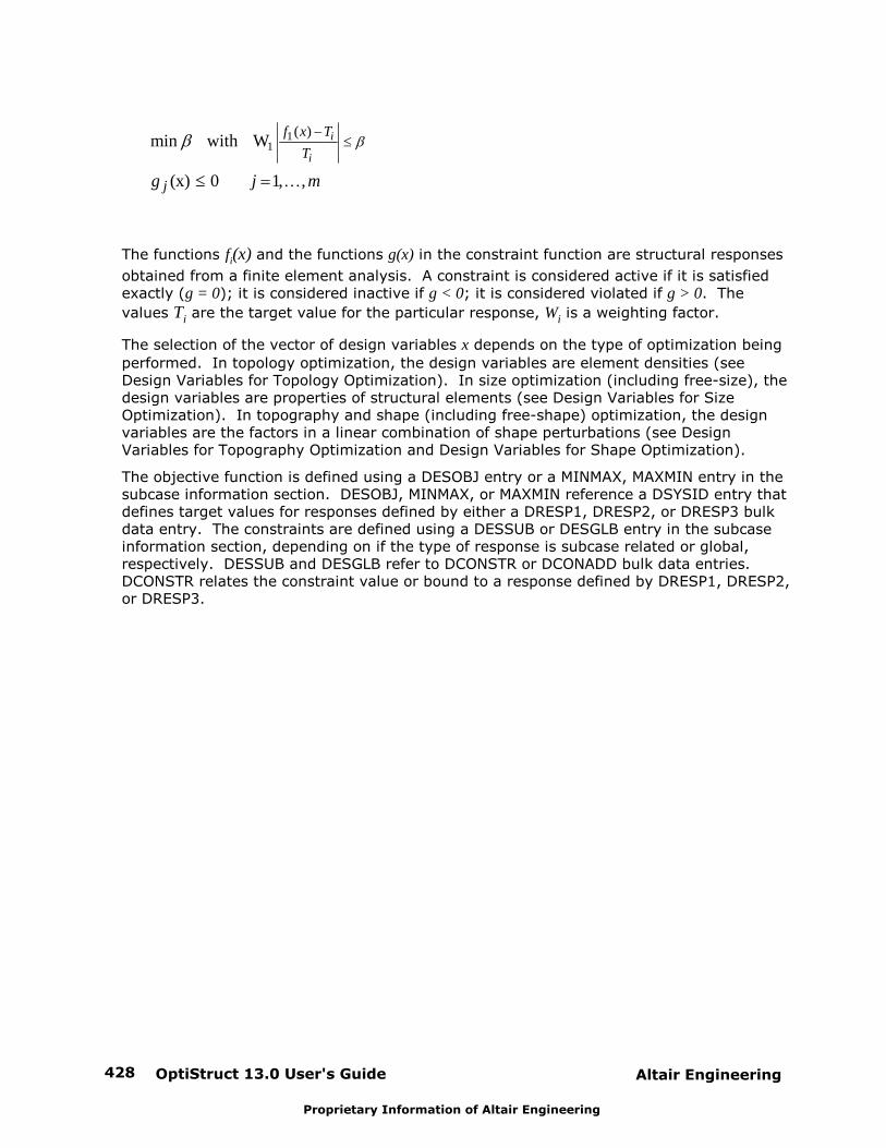
OptiStruct 13.0 User's Guide428 Altair Engineering
Proprietary Information of Altair Engineering
11
( )min with W
(x) 0 1, ,
i
i
f x T
T
jg j mK
The functions fi(x) and the functions g(x) in the constraint function are structural responses
obtained from a finite element analysis. A constraint is considered active if it is satisfiedexactly (g = 0); it is considered inactive if g < 0; it is considered violated if g > 0. The
values Ti are the target value for the particular response, Wi is a weighting factor.
The selection of the vector of design variables x depends on the type of optimization being
performed. In topology optimization, the design variables are element densities (see Design Variables for Topology Optimization). In size optimization (including free-size), thedesign variables are properties of structural elements (see Design Variables for SizeOptimization). In topography and shape (including free-shape) optimization, the designvariables are the factors in a linear combination of shape perturbations (see DesignVariables for Topography Optimization and Design Variables for Shape Optimization).
The objective function is defined using a DESOBJ entry or a MINMAX, MAXMIN entry in thesubcase information section. DESOBJ, MINMAX, or MAXMIN reference a DSYSID entry thatdefines target values for responses defined by either a DRESP1, DRESP2, or DRESP3 bulkdata entry. The constraints are defined using a DESSUB or DESGLB entry in the subcaseinformation section, depending on if the type of response is subcase related or global,respectively. DESSUB and DESGLB refer to DCONSTR or DCONADD bulk data entries. DCONSTR relates the constraint value or bound to a response defined by DRESP1, DRESP2,or DRESP3.
Altair Engineering OptiStruct 13.0 User's Guide 429
Proprietary Information of Altair Engineering
Responses
The following responses can be found in this section:
Internal Responses
OptiStruct allows the use of numerous structural responses, calculated in a finite elementanalysis, or combinations of these responses to be used as objective and constraintfunctions in a structural optimization.
Responses are defined using DRESP1 bulk data entries. Combinations of responses aredefined using either DRESP2 entries, which reference an equation defined by a DEQATNbulk data entry, or DRESP3 entries, which make use of user-defined external routinesidentified by the LOADLIB I/O option. Responses are either global or subcase (loadstep,load case) related. The character of a response determines whether or not a constraint orobjective referencing that particular response needs to be referenced within a subcase.
Subcase Independent
Mass and Volume
Both are global responses that can be defined for the whole structure, for individualproperties (components) and materials, or for groups of properties (components) andmaterials.
It is not recommended to use mass and volume as constraints or objectives in atopography optimization. Neither is very sensitive towards design modifications made in atopography optimization.
In order to constrain the mass or volume for a region containing a number of properties(components), the SUM function can be used to sum the mass or volume of the selectedproperties (components), otherwise, the constraint is assumed to apply to each individualproperty (component) within the region. Alternatively, a DRESP2 equation needs to bedefined to sum the mass or volume of these properties (components). This can be avoidedby having all properties (components) use the same material and applying the mass orvolume constraint to that material.
Fraction of Mass and Fraction of Design Volume
Both are global responses with values between 0.0 and 1.0. They describe a fraction ofthe initial design space in a topology optimization. They can be defined for the wholestructure, for individual properties (components) and materials, or for groups of properties(components) and materials.
The difference between the mass fraction and the volume fraction is that the mass fractionincludes the non-design mass in the fraction calculation, whereas the volume fraction onlyconsiders the design volume.
Formulation for volume fraction:Volume fraction = (total volume at current iteration – initial non-design volume)/initialdesign volume
Formulation for mass fraction:
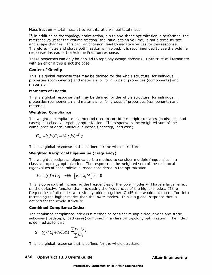
OptiStruct 13.0 User's Guide430 Altair Engineering
Proprietary Information of Altair Engineering
Mass fraction = total mass at current iteration/initial total mass
If, in addition to the topology optimization, a size and shape optimization is performed, thereference value for the volume fraction (the initial design volume) is not altered by sizeand shape changes. This can, on occasion, lead to negative values for this response. Therefore, if size and shape optimization is involved, it is recommended to use the Volumeresponses instead of the Volume Fraction response.
These responses can only be applied to topology design domains. OptiStruct will terminatewith an error if this is not the case.
Center of Gravity
This is a global response that may be defined for the whole structure, for individualproperties (components) and materials, or for groups of properties (components) andmaterials.
Moments of Inertia
This is a global response that may be defined for the whole structure, for individualproperties (components) and materials, or for groups of properties (components) andmaterials.
Weighted Compliance
The weighted compliance is a method used to consider multiple subcases (loadsteps, loadcases) in a classical topology optimization. The response is the weighted sum of thecompliance of each individual subcase (loadstep, load case).
12
Ti i i iW iC W C W u f
This is a global response that is defined for the whole structure.
Weighted Reciprocal Eigenvalue (Frequency)
The weighted reciprocal eigenvalue is a method to consider multiple frequencies in aclassical topology optimization. The response is the weighted sum of the reciprocaleigenvalues of each individual mode considered in the optimization.
0i i i iW withf W l K M u
This is done so that increasing the frequencies of the lower modes will have a larger effecton the objective function than increasing the frequencies of the higher modes. If thefrequencies of all modes were simply added together, OptiStruct would put more effort intoincreasing the higher modes than the lower modes. This is a global response that isdefined for the whole structure.
Combined Compliance Index
The combined compliance index is a method to consider multiple frequencies and staticsubcases (loadsteps, load cases) combined in a classical topology optimization. The indexis defined as follows:
j ji i
j
W lS W C NORM
W
This is a global response that is defined for the whole structure.
Altair Engineering OptiStruct 13.0 User's Guide 431
Proprietary Information of Altair Engineering
The normalization factor, NORM, is used for normalizing the contributions of compliancesand eigenvalues. A typical structural compliance value is of the order of 1.0e4 to 1.0e6. However, a typical inverse eigenvalue is on the order of 1.0e-5. If NORM is not used, thelinear static compliance requirements dominate the solution.
The quantity NORM is typically computed using the formula:
max minNF C
where, Cmax is the highest compliance value in all subcases (loadsteps, load cases) and
min is the lowest eigenvalue included in the index.
In a new design problem, you may not have a close estimate for NORM. If this happens,OptiStruct automatically computes the NORM value based on compliances and eigenvaluescomputed in the first iteration step.
von Mises Stress in a Topology or Free-Size Optimization
The von Mises stress constraints may be defined for topology and free-size optimizationthrough the STRESS optional continuation line on the DTPL or the DSIZE card. There are anumber of restrictions with this constraint:
The definition of stress constraints is limited to a single von Mises permissible stress. The phenomenon of singular topology is pronounced when different materials withdifferent permissible stresses exist in a structure. Singular topology refers to theproblem associated with the conditional nature of stress constraints, i.e. the stressconstraint of an element disappears when the element vanishes. This createsanother problem in that a huge number of reduced problems exist with solutions thatcannot usually be found by a gradient-based optimizer in the full design space.
Stress constraints for a partial domain of the structure are not allowed because theyoften create an ill-posed optimization problem since elimination of the partial domainwould remove all stress constraints. Consequently, the stress constraint applies tothe entire model when active, including both design and non-design regions, andstress constraint settings must be identical for all DSIZE and DTPL cards.
The capability has built-in intelligence to filter out artificial stress concentrationsaround point loads and point boundary conditions. Stress concentrations due toboundary geometry are also filtered to some extent as they can be improved moreeffectively with local shape optimization.
Due to the large number of elements with active stress constraints, no element stressreport is given in the table of retained constraints in the .out file. The iterative
history of the stress state of the model can be viewed in HyperView or HyperMesh.
Stress constraints do not apply to 1-D elements.
Stress constraints may not be used when enforced displacements are present in themodel.
Bead Discreteness Fraction
This is a global response for topography design domains. This response indicates theamount of shape variation for one or more topography design domains. The responsevaries in the range 0.0 to 1.0 (0.0 < BEADFRAC < 1.0), where 0.0 indicates that no shapevariation has occurred, and 1.0 indicates that the entire topography design domain hasassumed the maximum allowed shape variation.
OptiStruct 13.0 User's Guide432 Altair Engineering
Proprietary Information of Altair Engineering
Subcase Dependent
Linear Static Analysis
Static Compliance
The compliance C is calculated using the following relationship:
12
T withC u f Ku f
or
1 12 2
T TC u Ku dv
The compliance is the strain energy of the structure and can be considered a reciprocalmeasure for the stiffness of the structure. It can be defined for the whole structure, forindividual properties (components) and materials, or for groups of properties (components)and materials. The compliance must be assigned to a linear static subcase (loadstep, loadcase).
In order to constrain the compliance for a region containing a number of properties(components), the SUM function can be used to sum the compliance of the selectedproperties (components), otherwise, the constraint is assumed to apply to each individualproperty (component) within the region. Alternatively, a DRESP2 equation needs to bedefined to sum the compliance of these properties (components). This can be avoided byhaving all properties (components) use the same material and applying the complianceconstraint to that material.
Static Displacement
Displacements are the result of a linear static analysis. Nodal displacements can beselected as a response. They can be selected as vector components or as absolutemeasures. They must be assigned to a linear static subcase.
Static Stress of Homogeneous Material
Different stress types can be defined as responses. They are defined for components,properties, or elements. Element stresses are used, and constraint screening is applied. Itis also not possible to define static stress constraints in a topology design space (seeabove). This is a linear static subcase (loadstep, load case) related response.
Static Strain of Homogeneous Material
Different strain types can be defined as responses. They are defined for components,properties, or elements. Element strains are used, and constraint screening is applied. Itis also not possible to define strain constraints in a topology design space. This is a linearstatic subcase (loadstep, load case) related response.
Static Stress of Composite Lay-up
Different composite stress types can be defined as responses. They are defined forPCOMP(G) components or elements, or PLY type properties. Ply level results are used, andconstraint screening is applied. It is also not possible to define composite stressconstraints in a topology design space. This is a linear static subcase (loadstep, load case)related response.
Altair Engineering OptiStruct 13.0 User's Guide 433
Proprietary Information of Altair Engineering
Static Strain of Composite Lay-up
Different composite strain types can be defined as responses. They are defined forPCOMP(G) components or elements, or PLY type properties. Ply level results are used, andconstraint screening is applied. It is also not possible to define composite strainconstraints in a topology design space. This is a linear static subcase (loadstep, load case)related response.
Static Failure in a Composite Lay-up
Different composite failure criterion can be defined as responses. They are defined forPCOMP(G) components or elements, or PLY type properties. Ply level results are used, andconstraint screening is applied. It is also not possible to define composite failure criterionconstraints in a topology design space. This is a linear static subcase (loadstep, load case)related response.
Static Force
Different force types can be defined as responses. They are defined for components,properties, or elements. Constraint screening is applied. It is also not possible to defineforce constraints in a topology design space. This is a linear static subcase (loadstep, loadcase) related response.
Single Point Force at a constrained grid point
This response can be defined using the DRESP1 bulk data entry (with RTYPE=SPCFORCE). This response is defined for constrained grid points. Constraint screening is applied to thisresponse. This is a linear static subcase (loadstep, load case) related response.
Grid Point Force
This response can be defined using the DRESP1 bulk data entry (with RTYPE=GPFORCE). This response defines the contribution to a specific grid point force component from a non-rigid element (which is connected to that grid). Constraint screening is applied to thisresponse. If ATTi specify multiple elements, then multiple responses will be generated,where, each response calculates a specified element’s contribution to the grid point forcecomponent at the specified grid. This is a linear static subcase (loadstep, load case)related response.
Linear Heat Transfer Analysis
Temperature
Temperatures are the result of a heat transfer analysis, and must be assigned to a heattransfer subcase (loadstep, load case). Temperature response cannot be used in composite topology or free-size optimization.
Normal Modes Analysis
Frequency
Natural frequencies are the result of a normal modes analysis, and must be assigned to thenormal modes subcase (loadstep, load case). It is recommended to constrain thefrequency for several of the lower modes, not just of the first mode.
OptiStruct 13.0 User's Guide434 Altair Engineering
Proprietary Information of Altair Engineering
Mode Shape
Mode shapes are the result of a normal modes analysis. Mode shapes can be selected as aresponse. They can be selected as vector components or as absolute measures. Theymust be assigned to a normal modes subcase.
Linear Buckling Analysis
Buckling Factor
The buckling factor is the result of a buckling analysis, and must be assigned to a bucklingsubcase (loadstep, load case). A typical buckling constraint is a lower bound of 1.0,indicating that the structure is not to buckle with the given static load. It is recommendedto constrain the buckling factor for several of the lower modes, not just of the first mode.
Frequency Response Function (FRF Analysis)
Frequency Response Displacement
Displacements are the result of a frequency response analysis. Nodal displacements, i.e.translational, rotational and normal*, can be selected as a response. They can be selectedas vector components in real/imaginary or magnitude/phase form. They must be assignedto a frequency response subcase (loadstep, load case).
*The normal at a grid point is calculated based on the normals of the surroundingelements. The normal frequency response displacement at a grid point can be selected as aresponse and it is the displacement in the normal’s direction. The normals are also updatedwhen shape changes occur during shape optimization.
Frequency Response Velocity
Velocities are the result of a frequency response analysis. Nodal velocities, i.e.translational, rotational and normal, can be selected as a response. They can be selectedas vector components in real/imaginary or magnitude/phase form. They must be assignedto a frequency response subcase (loadstep, load case).
*The normal at a grid point is calculated based on the normals of the surroundingelements. The normal frequency response velocity at a grid point can be selected as aresponse and it is the velocity in the normal’s direction. The normals are also updatedwhen shape changes occur during shape optimization.
Frequency Response Acceleration
Accelerations are the result of a frequency response analysis. Nodal accelerations, i.e.translational, rotational and normal, can be selected as a response. They can be selectedas vector components in real/imaginary or magnitude/phase form. They must be assignedto a frequency response subcase (loadstep, load case).
*The normal at a grid point is calculated based on the normals of the surroundingelements. The normal frequency response acceleration at a grid point can be selected as aresponse and it is the acceleration in the normal’s direction. The normals are also updatedwhen shape changes occur during shape optimization.
Altair Engineering OptiStruct 13.0 User's Guide 435
Proprietary Information of Altair Engineering
Frequency Response Stress
Different stress types can be defined as responses. They are defined for components,properties, or elements. Element stresses are not used in real/imaginary or magnitude/phase form, and constraint screening is applied. The von Mises stress for solids and shellscan also be defined as direct responses. It is not possible to define stress constraints in atopology design space. This is a frequency response subcase (loadstep, load case) relatedresponse.
Frequency Response Strain
Different strain types can be defined as responses. They are defined for components,properties, or elements. Element strains are used in real/imaginary or magnitude/phaseform, and constraint screening is applied. The von Mises strain for solids and shells canalso be defined as direct responses. It is not possible to define strain constraints in atopology design space. This is a frequency response subcase (loadstep, load case) relatedresponse.
Frequency Response Force
Different force types can be defined as responses. They are defined for components,properties, or elements in real/imaginary or magnitude/phase form. Constraint screeningis applied. It is also not possible to define force constraints in a topology design space. This is a frequency response subcase (loadstep, load case) related response.
Random Response Analysis
PSD and RMS Responses
PSD displacement, PSD velocity, PSD acceleration, PSD acoustic pressure, PSD stress, PSDstrain, RMS displacement, RMS velocity, RMS acceleration, RMS acoustic pressure, RMSstress and RMS strain responses are available.
Coupled FRF Analysis on a Fluid-structure Model (Acoustic Analysis)
Acoustic Pressure
Acoustic pressures are the result of a coupled frequency response analysis on a fluid-structure model. This response is available for fluid grids. It must be assigned to acoupled frequency response subcase (loadstep, load case) on a fluid-structure model.
Multi-body Dynamics Analysis
Flexible Body Responses
For Multi-body Dynamics problems, the Mass, Center of gravity, and Moment of Inertia ofone or more flexible bodies are available as responses. This is in addition to other usualstructural responses.

OptiStruct 13.0 User's Guide436 Altair Engineering
Proprietary Information of Altair Engineering
MBD Displacement
MBD displacements are the result of a multi-body dynamics analysis. They must beassigned to a multi-body dynamics subcase (loadstep, load case).
MBD Velocity
MBD velocities are the result of a multi-body dynamics analysis. They must be assigned toa multi-body dynamics subcase (loadstep, load case).
MBD Acceleration
MBD acceleration are the result of a multi-body dynamics analysis. They must be assignedto a multi-body dynamics subcase (loadstep, load case).
MBD Force
MBD forces are the result of a multi-body dynamics analysis. They must be assigned to amulti-body dynamics subcase (loadstep, load case).
MBD Expression
MBD expression responses are the result of a multi-body dynamics analysis. They are theresult of the evaluation of an expression. They must be assigned to a multi-body dynamicssubcase (loadstep, load case).
Fatigue
Life/Damage
Life and Damage are results of a fatigue analysis. They must be assigned to a Fatiguesubcase.
Dynamic/Nonlinear Analysis
Equivalent Plastic Strain
Equivalent plastic strain can be used as an internal response when a nonlinear responseoptimization is run using the equivalent static load method. This is made possible throughthe use of an approximated correlation between linear strain and plastic strain, which arecalculated in the inner and outer loops respectively, of the ESL method.
User Responses
Function
A function response is one that uses a mathematical expression to combine designvariables, grid point locations, responses, and/or table entries. Whether the function issubcase (loadstep, load case) related or global, is dependent on the response types used inthe equation.
Altair Engineering OptiStruct 13.0 User's Guide 437
Proprietary Information of Altair Engineering
External
An external response is one that uses an external user-defined routine to combine designvariables, grid point locations, eigenvectors, responses, and/or table entries. Whether thefunction is subcase (loadstep, load case) related or global is dependent on the responsetypes used in the routine. Refer to External Responses below for more information.
External Responses
The DRESP3 bulk data entry, in combination with the LOADLIB I/O option entry, allows forthe definition of responses through user-defined external functions. The external functionsmay be written in HyperMath Language (HML), FORTRAN, C or a Microsoft Excel workbook. The resulting libraries and files should be accessible by OptiStruct regardless of the codinglanguage, providing that consistent function prototyping is respected, and adequatecompiling and linking options are used.
Writing External Functions
The OptiStruct installation provides "barebone" functions for FORTRAN(dresp3_barebone.F) and for C (dresp3_barebone.c) with proper function definition,
arguments, and compilation directives. These files can be used as starting points to writeyour own functions. Refer to Referencing External Files for information on responsedefinition through a user-defined Microsoft Excel workbook.
HyperMath Language (HML) functions are defined as follows:
integer function myfunct(iparam, rparam, iresp, rresp, userdata)
If sensitivities need to be requested, then the following external function can be used.
integer function myfunct(iparam, rparam, iresp, rresp, dresp, isens userdata)
FORTRAN functions are defined as follows:
integer function myfunct(iparam, rparam, nparam, iresp, rresp, nresp, userdata)
If sensitivities need to be requested, then the following external function can be used.
integer function myfunct(iparam, rparam, nparam, iresp, rresp, dresp, nresp, isens userdata)
character*32000 userdatainteger nparam, nrespinteger iparam(nparam), iresp(nresp)double precision param(nparam), rresp(nresp), dresp(nparam,nresp)
OptiStruct 13.0 User's Guide438 Altair Engineering
Proprietary Information of Altair Engineering
C functions are defined as follows:
int myfunct(int* iparam, double* rparam, int* nparam, int* iresp, double* rresp, int* nresp, char* userdata)
If sensitivities need to be requested, then the following external function can be used.
int myfunct(int* iparam, double* rparam, int* nparam,int* iresp, double* rresp, double* dresp, int* nresp, int* isens, char* userdata)
Note that the functions' arguments are identical in both languages so as to preservecompatibility. However, since FORTRAN always passes arguments by address, it isimportant to understand that external C functions receive pointers instead of variables.
In order to ensure portability, the following must be adhered to:
Function names should be written using either all lower-case or all upper-casecharacters.
Only alphanumeric characters should be used.
Underscore characters are prohibited.
Names cannot be longer than eight characters.
Regarding implementing of external, user-defined routines using HyperMath, refer to theonline documentation for writing scripts in HyperMath. HyperMath is supported on theWindows and Linux operating systems only.
Function Return Values
External functions should return 0 or 1 for successful completion, where 1 indicates that auser-defined information message should be output by OptiStruct. External functionsshould return -1 in case of fatal error, in which case OptiStruct will terminate afteroutputting a user-defined error message. See below for more information about error andinformation messages.
Function Arguments
The following table briefly describes the arguments which are passed from OptiStruct tothe external functions.
Argument TypeInput /Output
Description
iparam integer(table)
Input Input parameters types (optional use)
rparam double(table)
Input Input parameters values
nparam integer Input Number of parameters
iresp integer(table)
Input Output responses requests (optional use)
Altair Engineering OptiStruct 13.0 User's Guide 439
Proprietary Information of Altair Engineering
Argument TypeInput /Output
Description
rresp double(table)
Output Output responses values
dresp double(table)
Output Output sensitivity values
nresp integer Input Number of responses
isens integer Input Sensitivity output flag
userdata string Input / Output User data / Error or informationmessage
Parameters:
nparam is the number of input parameters that were defined on the DRESP3 card.
rparam(nparam) contains the values of the input parameters as evaluated byOptiStruct.
iparam(nparam) indicates the types of the input parameters as described below.
Parameter values are passed in the exact order in which they were defined on theDRESP3 card, regardless of their type. Using the parameter types table is optional,for instance to perform verifications or code-branching.
The following types are currently supported:
Parameter type iparam value
DESVAR 1
DTABLE 2
DGRID/DGRIDB 3
DRESP1 4
DRESP2 5
DRESP1L 6
DRESP2L 7
DVPREL1 8
DVPREL2 9
DVMREL1 10
DVMREL2 11
DVCREL1 12
DVCREL2 13
DVMBRL1 14
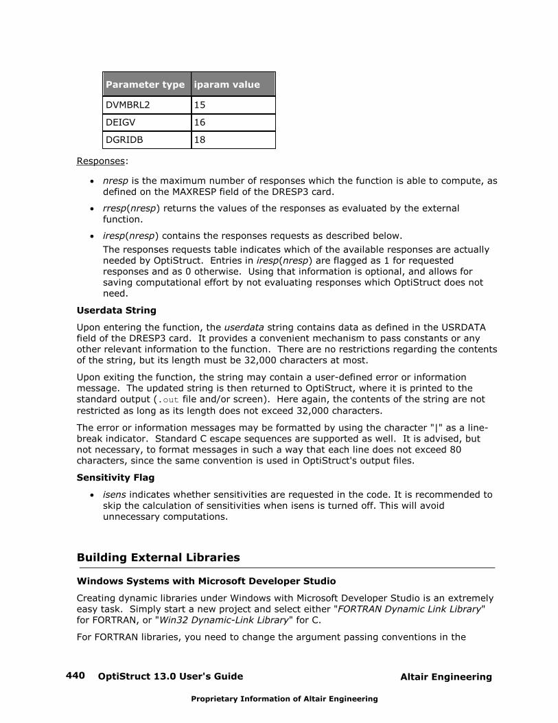
OptiStruct 13.0 User's Guide440 Altair Engineering
Proprietary Information of Altair Engineering
Parameter type iparam value
DVMBRL2 15
DEIGV 16
DGRIDB 18
Responses:
nresp is the maximum number of responses which the function is able to compute, asdefined on the MAXRESP field of the DRESP3 card.
rresp(nresp) returns the values of the responses as evaluated by the externalfunction.
iresp(nresp) contains the responses requests as described below.
The responses requests table indicates which of the available responses are actuallyneeded by OptiStruct. Entries in iresp(nresp) are flagged as 1 for requestedresponses and as 0 otherwise. Using that information is optional, and allows forsaving computational effort by not evaluating responses which OptiStruct does notneed.
Userdata String
Upon entering the function, the userdata string contains data as defined in the USRDATAfield of the DRESP3 card. It provides a convenient mechanism to pass constants or anyother relevant information to the function. There are no restrictions regarding the contentsof the string, but its length must be 32,000 characters at most.
Upon exiting the function, the string may contain a user-defined error or informationmessage. The updated string is then returned to OptiStruct, where it is printed to thestandard output (.out file and/or screen). Here again, the contents of the string are not
restricted as long as its length does not exceed 32,000 characters.
The error or information messages may be formatted by using the character "|" as a line-break indicator. Standard C escape sequences are supported as well. It is advised, butnot necessary, to format messages in such a way that each line does not exceed 80characters, since the same convention is used in OptiStruct's output files.
Sensitivity Flag
isens indicates whether sensitivities are requested in the code. It is recommended toskip the calculation of sensitivities when isens is turned off. This will avoidunnecessary computations.
Building External Libraries
Windows Systems with Microsoft Developer Studio
Creating dynamic libraries under Windows with Microsoft Developer Studio is an extremelyeasy task. Simply start a new project and select either "FORTRAN Dynamic Link Library"for FORTRAN, or "Win32 Dynamic-Link Library" for C.
For FORTRAN libraries, you need to change the argument passing conventions in the
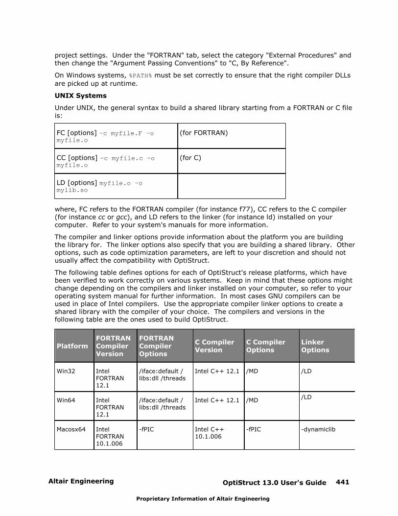
Altair Engineering OptiStruct 13.0 User's Guide 441
Proprietary Information of Altair Engineering
project settings. Under the "FORTRAN" tab, select the category "External Procedures" andthen change the "Argument Passing Conventions" to "C, By Reference".
On Windows systems, %PATH% must be set correctly to ensure that the right compiler DLLs
are picked up at runtime.
UNIX Systems
Under UNIX, the general syntax to build a shared library starting from a FORTRAN or C fileis:
FC [options] -c myfile.F -omyfile.o
(for FORTRAN)
CC [options] -c myfile.c -omyfile.o
(for C)
LD [options] myfile.o -omylib.so
where, FC refers to the FORTRAN compiler (for instance f77), CC refers to the C compiler(for instance cc or gcc), and LD refers to the linker (for instance ld) installed on yourcomputer. Refer to your system's manuals for more information.
The compiler and linker options provide information about the platform you are buildingthe library for. The linker options also specify that you are building a shared library. Otheroptions, such as code optimization parameters, are left to your discretion and should notusually affect the compatibility with OptiStruct.
The following table defines options for each of OptiStruct's release platforms, which havebeen verified to work correctly on various systems. Keep in mind that these options mightchange depending on the compilers and linker installed on your computer, so refer to youroperating system manual for further information. In most cases GNU compilers can beused in place of Intel compilers. Use the appropriate compiler linker options to create ashared library with the compiler of your choice. The compilers and versions in thefollowing table are the ones used to build OptiStruct.
PlatformFORTRANCompiler Version
FORTRANCompiler Options
C Compiler Version
C Compiler Options
LinkerOptions
Win32 IntelFORTRAN12.1
/iface:default /libs:dll /threads
Intel C++ 12.1 /MD /LD
Win64 IntelFORTRAN12.1
/iface:default /libs:dll /threads
Intel C++ 12.1 /MD/LD
Macosx64 IntelFORTRAN10.1.006
-fPIC Intel C++10.1.006
-fPIC -dynamiclib
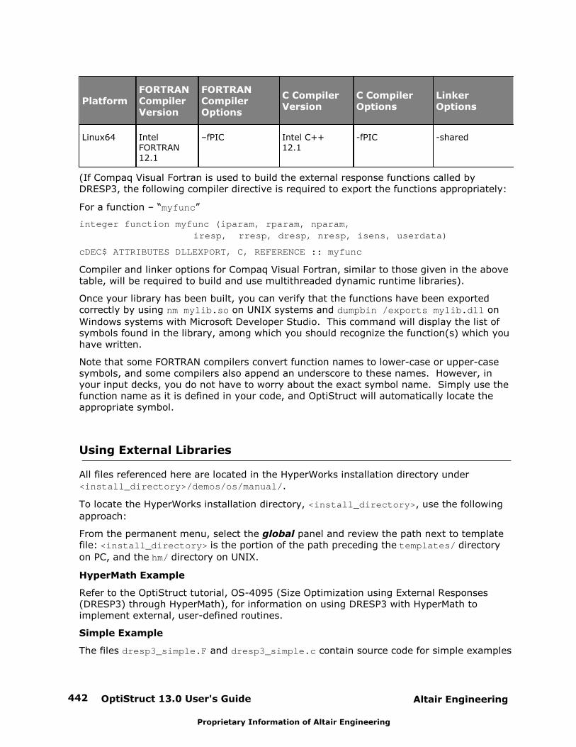
OptiStruct 13.0 User's Guide442 Altair Engineering
Proprietary Information of Altair Engineering
PlatformFORTRANCompiler Version
FORTRANCompiler Options
C Compiler Version
C Compiler Options
LinkerOptions
Linux64 IntelFORTRAN 12.1
–fPIC Intel C++ 12.1
-fPIC -shared
(If Compaq Visual Fortran is used to build the external response functions called byDRESP3, the following compiler directive is required to export the functions appropriately:
For a function – “myfunc”
integer function myfunc (iparam, rparam, nparam, iresp, rresp, dresp, nresp, isens, userdata)
cDEC$ ATTRIBUTES DLLEXPORT, C, REFERENCE :: myfunc
Compiler and linker options for Compaq Visual Fortran, similar to those given in the abovetable, will be required to build and use multithreaded dynamic runtime libraries).
Once your library has been built, you can verify that the functions have been exportedcorrectly by using nm mylib.so on UNIX systems and dumpbin /exports mylib.dll on
Windows systems with Microsoft Developer Studio. This command will display the list ofsymbols found in the library, among which you should recognize the function(s) which youhave written.
Note that some FORTRAN compilers convert function names to lower-case or upper-casesymbols, and some compilers also append an underscore to these names. However, inyour input decks, you do not have to worry about the exact symbol name. Simply use thefunction name as it is defined in your code, and OptiStruct will automatically locate theappropriate symbol.
Using External Libraries
All files referenced here are located in the HyperWorks installation directory under<install_directory>/demos/os/manual/.
To locate the HyperWorks installation directory, <install_directory>, use the following
approach:
From the permanent menu, select the global panel and review the path next to templatefile: <install_directory> is the portion of the path preceding the templates/ directory
on PC, and the hm/ directory on UNIX.
HyperMath Example
Refer to the OptiStruct tutorial, OS-4095 (Size Optimization using External Responses(DRESP3) through HyperMath), for information on using DRESP3 with HyperMath toimplement external, user-defined routines.
Simple Example
The files dresp3_simple.F and dresp3_simple.c contain source code for simple examples
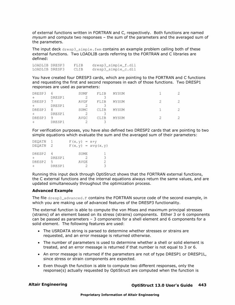
Altair Engineering OptiStruct 13.0 User's Guide 443
Proprietary Information of Altair Engineering
of external functions written in FORTRAN and C, respectively. Both functions are named mysum and compute two responses – the sum of the parameters and the averaged sum ofthe parameters.
The input deck dresp3_simple.fem contains an example problem calling both of these
external functions. Two LOADLIB cards referring to the FORTRAN and C libraries aredefined:
LOADLIB DRESP3 FLIB dresp3_simple_f.dllLOADLIB DRESP3 CLIB dresp3_simple_c.dll
You have created four DRESP3 cards, which are pointing to the FORTRAN and C functionsand requesting the first and second responses in each of those functions. Two DRESP1responses are used as parameters:
DRESP3 6 SUMF FLIB MYSUM 1 2+ DRESP1 2 3DRESP3 7 AVGF FLIB MYSUM 2 2+ DRESP1 2 3DRESP3 8 SUMC CLIB MYSUM 1 2+ DRESP1 2 3DRESP3 9 AVGC CLIB MYSUM 2 2+ DRESP1 2 3
For verification purposes, you have also defined two DRESP2 cards that are pointing to twosimple equations which evaluate the sum and the averaged sum of their parameters:
DEQATN 1 F(x,y) = x+yDEQATN 2 F(x,y) = avg(x,y)
DRESP2 4 SUME 1+ DRESP1 2 3DRESP2 5 AVGE 2+ DRESP1 2 3
Running this input deck through OptiStruct shows that the FORTRAN external functions,the C external functions and the internal equations always return the same values, and areupdated simultaneously throughout the optimization process.
Advanced Example
The file dresp3_advanced.F contains the FORTRAN source code of the second example, in
which you are making use of advanced features of the DRESP3 functionality.
The external function is able to compute the von Mises and maximum principal stresses(strains) of an element based on its stress (strains) components. Either 3 or 6 componentscan be passed as parameters – 3 components for a shell element and 6 components for asolid element. The following features are used:
The USRDATA string is parsed to determine whether stresses or strains arerequested, and an error message is returned otherwise.
The number of parameters is used to determine whether a shell or solid element istreated, and an error message is returned if that number is not equal to 3 or 6.
An error message is returned if the parameters are not of type DRESP1 or DRESP1L,since stress or strain components are expected.
Even though the function is able to compute two different responses, only theresponse(s) actually requested by OptiStruct are computed when the function is
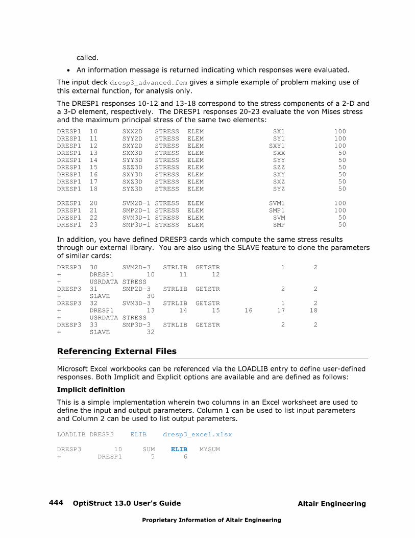
OptiStruct 13.0 User's Guide444 Altair Engineering
Proprietary Information of Altair Engineering
called.
An information message is returned indicating which responses were evaluated.
The input deck dresp3_advanced.fem gives a simple example of problem making use of
this external function, for analysis only.
The DRESP1 responses 10-12 and 13-18 correspond to the stress components of a 2-D anda 3-D element, respectively. The DRESP1 responses 20-23 evaluate the von Mises stressand the maximum principal stress of the same two elements:
DRESP1 10 SXX2D STRESS ELEM SX1 100DRESP1 11 SYY2D STRESS ELEM SY1 100DRESP1 12 SXY2D STRESS ELEM SXY1 100DRESP1 13 SXX3D STRESS ELEM SXX 50DRESP1 14 SYY3D STRESS ELEM SYY 50DRESP1 15 SZZ3D STRESS ELEM SZZ 50DRESP1 16 SXY3D STRESS ELEM SXY 50DRESP1 17 SXZ3D STRESS ELEM SXZ 50DRESP1 18 SYZ3D STRESS ELEM SYZ 50
DRESP1 20 SVM2D-1 STRESS ELEM SVM1 100DRESP1 21 SMP2D-1 STRESS ELEM SMP1 100DRESP1 22 SVM3D-1 STRESS ELEM SVM 50DRESP1 23 SMP3D-1 STRESS ELEM SMP 50
In addition, you have defined DRESP3 cards which compute the same stress resultsthrough our external library. You are also using the SLAVE feature to clone the parametersof similar cards:
DRESP3 30 SVM2D-3 STRLIB GETSTR 1 2+ DRESP1 10 11 12 + USRDATA STRESSDRESP3 31 SMP2D-3 STRLIB GETSTR 2 2+ SLAVE 30DRESP3 32 SVM3D-3 STRLIB GETSTR 1 2+ DRESP1 13 14 15 16 17 18+ USRDATA STRESSDRESP3 33 SMP3D-3 STRLIB GETSTR 2 2+ SLAVE 32
Referencing External Files
Microsoft Excel workbooks can be referenced via the LOADLIB entry to define user-definedresponses. Both Implicit and Explicit options are available and are defined as follows:
Implicit definition
This is a simple implementation wherein two columns in an Excel worksheet are used todefine the input and output parameters. Column 1 can be used to list input parametersand Column 2 can be used to list output parameters.
LOADLIB DRESP3 ELIB dresp3_excel.xlsx
DRESP3 10 SUM ELIB MYSUM+ DRESP1 5 6
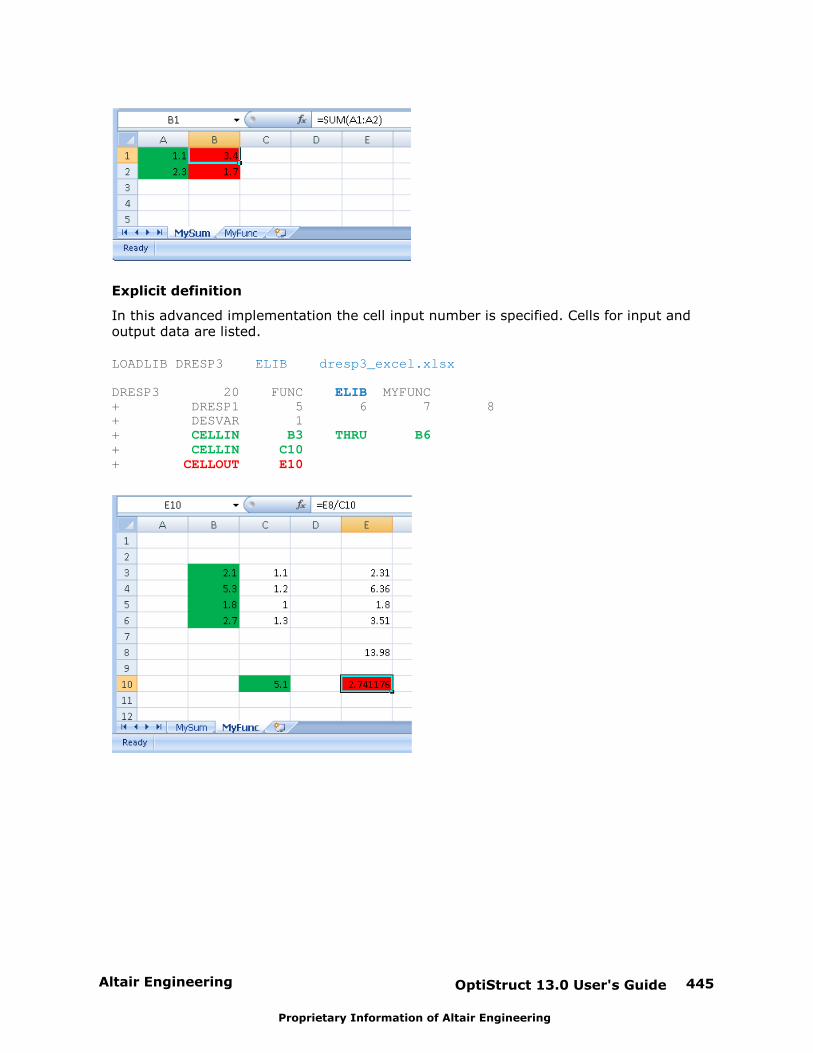
Altair Engineering OptiStruct 13.0 User's Guide 445
Proprietary Information of Altair Engineering
Explicit definition
In this advanced implementation the cell input number is specified. Cells for input andoutput data are listed.
LOADLIB DRESP3 ELIB dresp3_excel.xlsx
DRESP3 20 FUNC ELIB MYFUNC+ DRESP1 5 6 7 8+ DESVAR 1+ CELLIN B3 THRU B6 + CELLIN C10+ CELLOUT E10
OptiStruct 13.0 User's Guide446 Altair Engineering
Proprietary Information of Altair Engineering
Topology Optimization
Topology Optimization is a mathematical technique that produces an optimized shape andmaterial distribution for a structure within a given package space. By discretizing the domaininto a finite element mesh, OptiStruct calculates material properties for each element. TheOptiStruct algorithm alters the material distribution to optimize the user-defined objectiveunder given constraints. Convergence occurs in line with the description provided on the Iterative Solution page.
The following responses (see Responses for a description) are currently available as theobjective or as constraint functions:
Mass Volume Volume or MassFraction
Center of Gravity Moment of Inertia Static Compliance
Static Displacement Natural Frequency von Mises Stress onEntire Model (only asconstraint)
Buckling Factor (specialcase)
FrequencyResponseDisplacement,Velocity,Acceleration
Temperature
Weighted Compliance WeightedFrequency
Combined ComplianceIndex
Function
The von Mises stress constraints may be defined for topology and free-size optimizationthrough the STRESS optional continuation line on the DTPL or the DSIZE card. There are anumber of restrictions with this constraint:
The definition of stress constraints is limited to a single von Mises permissible stress. The phenomenon of singular topology is pronounced when different materials withdifferent permissible stresses exist in a structure. Singular topology refers to theproblem associated with the conditional nature of stress constraints, i.e. the stressconstraint of an element disappears when the element vanishes. This creates anotherproblem in that a huge number of reduced problems exist with solutions that cannotusually be found by a gradient-based optimizer in the full design space.
Stress constraints for a partial domain of the structure are not allowed because theyoften create an ill-posed optimization problem since elimination of the partial domainwould remove all stress constraints. Consequently, the stress constraint applies to theentire model when active, including both design and non-design regions, and stressconstraint settings must be identical for all DSIZE and DTPL cards.
Altair Engineering OptiStruct 13.0 User's Guide 447
Proprietary Information of Altair Engineering
The capability has built-in intelligence to filter out artificial stress concentrations aroundpoint loads and point boundary conditions. Stress concentrations due to boundarygeometry are also filtered to some extent as they can be improved more effectivelywith local shape optimization.
Due to the large number of elements with active stress constraints, no element stressreport is given in the table of retained constraints in the .out file. The iterative history
of the stress state of the model can be viewed in HyperView or HyperMesh.
Stress constraints do not apply to 1-D elements.
Stress constraints may not be used when enforced displacements are present in themodel.
The buckling factor can be constrained for shell topology optimization problems with a basethickness not equal to zero. Constraints on the buckling factor are not allowed in any othercases of topology optimization.
The following responses are currently available as the objective or as constraint functions forelements that do not form part of the design space:
Static Stress Static Strain Static Force
Composite Stress Composite Strain Composite Failure Criterion
Frequency ResponseStress
Frequency ResponseStrain
Frequency Response Force
If an element is in the topology design region, its individual stress/strain or force criterionvalue cannot be constrained.
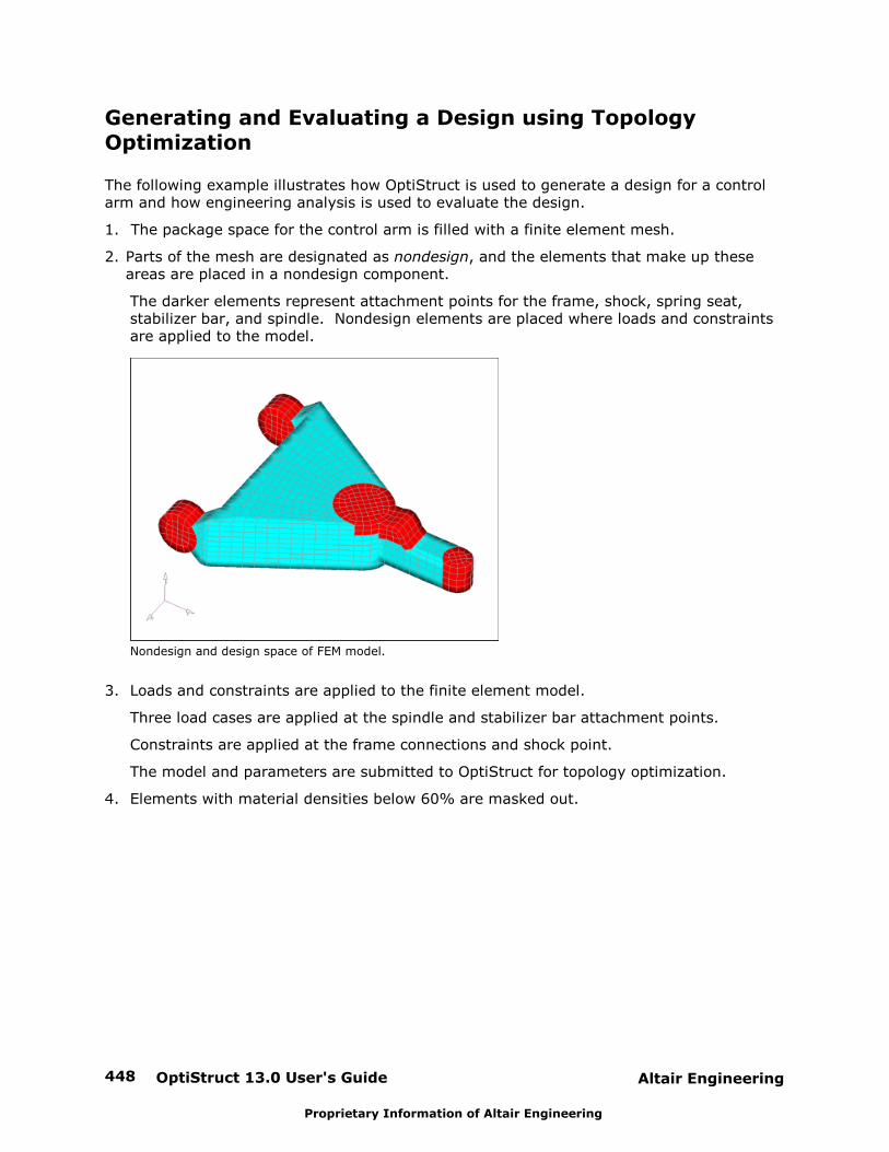
OptiStruct 13.0 User's Guide448 Altair Engineering
Proprietary Information of Altair Engineering
Generating and Evaluating a Design using TopologyOptimization
The following example illustrates how OptiStruct is used to generate a design for a controlarm and how engineering analysis is used to evaluate the design.
1. The package space for the control arm is filled with a finite element mesh.
2. Parts of the mesh are designated as nondesign, and the elements that make up theseareas are placed in a nondesign component.
The darker elements represent attachment points for the frame, shock, spring seat,stabilizer bar, and spindle. Nondesign elements are placed where loads and constraintsare applied to the model.
Nondesign and design space of FEM model.
3. Loads and constraints are applied to the finite element model.
Three load cases are applied at the spindle and stabilizer bar attachment points.
Constraints are applied at the frame connections and shock point.
The model and parameters are submitted to OptiStruct for topology optimization.
4. Elements with material densities below 60% are masked out.
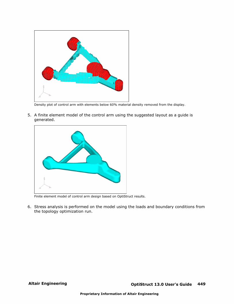
Altair Engineering OptiStruct 13.0 User's Guide 449
Proprietary Information of Altair Engineering
Density plot of control arm with elements below 60% material density removed from the display.
5. A finite element model of the control arm using the suggested layout as a guide isgenerated.
Finite element model of control arm design based on OptiStruct results.
6. Stress analysis is performed on the model using the loads and boundary conditions fromthe topology optimization run.
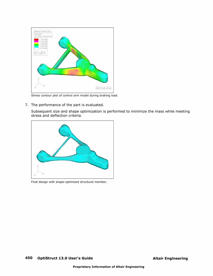
OptiStruct 13.0 User's Guide450 Altair Engineering
Proprietary Information of Altair Engineering
Stress contour plot of control arm model during braking load.
7. The performance of the part is evaluated.
Subsequent size and shape optimization is performed to minimize the mass while meetingstress and deflection criteria.
Final design with shape-optimized structural member.
Altair Engineering OptiStruct 13.0 User's Guide 451
Proprietary Information of Altair Engineering
Design Variables for Topology Optimization
OptiStruct solves topological optimization problems using the density method, also known asthe SIMP method in the research community.
Under topology optimization, the material density of each element should take a value ofeither 0 or 1, defining the element as being either void or solid, respectively. Unfortunately,optimization of a large number of discrete variables is computationally prohibitive. Therefore, representation of the material distribution problem in terms of continuousvariables has to be used.
With the density method, the material density of each element is directly used as the designvariable, and varies continuously between 0 and 1; these represent the state of void andsolid, respectively. Intermediate values of density represent fictitious material. The stiffnessof the material is assumed to be linearly dependent on the density. This material formulationis consistent with our understanding of common materials. For example, steel, which isdenser than aluminum, is stronger than aluminum. Following this logic, the representation offictitious material at intermediate densities does reflect engineering intuitions.
In general, the optimal solution of problems involves large gray areas of intermediatedensities in the structural domain. Such solutions are not meaningful when you are lookingfor the topology of a given material, and not meaningful when considering the use ofdifferent materials within the design space. Therefore, techniques need to be introduced topenalize intermediate densities and to force the final design to be represented by densities of0 or 1 for each element. The penalization technique used is the "power law representation ofelasticity properties," which can be expressed for any solid 3-D or 2-D element as follows:
pK K
Where, K and K represent the penalized and the real stiffness matrix of an element,
respectively, is the density and p is the penalization factor which is always greater than 1.
In OptiStruct, the DISCRETE parameter corresponds to (p - 1). DISCRETE can be defined on
the DOPTPRM bulk data entry. p usually takes a value between 2.0 and 4.0. For example,
compared to the non-penalized formulation (which is equivalent to p=1) at =0.3, p=2reduces the stiffness of the element from 0.3 to 0.09 times the stiffness of the fully denseelement. The default DISCRETE is 1.0 for shell dominant structures, and 2.0 for solids
dominant structures (the dominance is defined by the proportion of number of elements). Anadditional parameter, DISCRT1D, can also be defined on the DOPTPRM bulk data entry.
DISCRT1D allows 1-D elements to use a different penalization to 2-D or 3-D elements.
When minimum member size control is used, the penalty starts at 2 and is increased to 3 forthe second and third iterative phases. This is done in order to achieve a more discretesolution. For other manufacturing constraints such as draw direction, extrustion, patternrepetition, and pattern grouping, the penalty starts at 2 and increases to 3 and 4 for thesecond and third iterative phases, respectively. Obviously, due to the existence of semi-dense elements, the analysis results may change dramatically when the design processenters a new phase using a different penalization factor.
Three types of finite elements can be defined as topology design elements in OptiStruct:Solid elements, shell elements, and 1-D elements (including ROD, BAR/BEAM, BUSH, andWELD elements).
OptiStruct 13.0 User's Guide452 Altair Engineering
Proprietary Information of Altair Engineering
Design Elements
Solid Elements
The SIMP method (Solid Isotropic Material with Penalty) is used in OptiStruct. In the SIMPmethod, a pseudo material density is the design variable, and hence it is often called density method as well. The material density varies continuously between 0 and 1, with 0representing void state and 1 solid state. The SIMP method applies a power-lawpenalization for stiffness-density relationship in order to push density toward 0/1 (void/solid) distribution:
pK K
Where,
K is the penalized stiffness matrix of an element.
K is the real stiffness matrix of an element.
is the density.
p is the penalization factor (Always greater than 1, with default penalty at 3.0 if no
manufacturing constraints are applied).
Shell Elements
The SIMP method (Solid Isotropic Material with Penalty) is used in OptiStruct. In the SIMPmethod, a pseudo material density is the design variable, and hence it is often called density method as well. The material density varies continuously between 0 and 1., with 0representing void state and 1 solid state. The SIMP method applies a power-lawpenalization for stiffness-density relationship in order to push density toward 0/1 (void/solid) distribution.
pK K
Where,
K is the penalized stiffness matrix of an element.
K is the real stiffness matrix of an element.
is the density.
p is the penalization factor (Always greater than 1)
For isotropic material a non-zero base plate thickness can be defined. For a compositeplate or a plate with anisotropic material, the base plate thickness must be zero (thelimitation of the current development).
Topology optimization of composites has certain unique characteristics and is discussed in Composite Topology and Free-size Optimization.
Altair Engineering OptiStruct 13.0 User's Guide 453
Proprietary Information of Altair Engineering
1-D Elements
Only the density method is implemented for topology optimization of 1-D elements. Currently available elements include ROD, BAR/BEAM, BUSH, and WELD elements. Each
element is controlled by a single design variable that is the material density of thiselement that varies between 0 (numerically a small value is used) and 1.0. In essence, 0represents nonexistence and 1.0 represents full existence of the corresponding element. The following power law representation of elastic properties is used to penalizeintermediate density:
pK K
Where, K and K represent the penalized and the real stiffness matrix of an element,
respectively, p is the penalization factor which is always bigger than 1. The penalty is
controlled by the DISCRETE or DISCRT1D parameters, the value of these parameters
correspond to (p - 1).
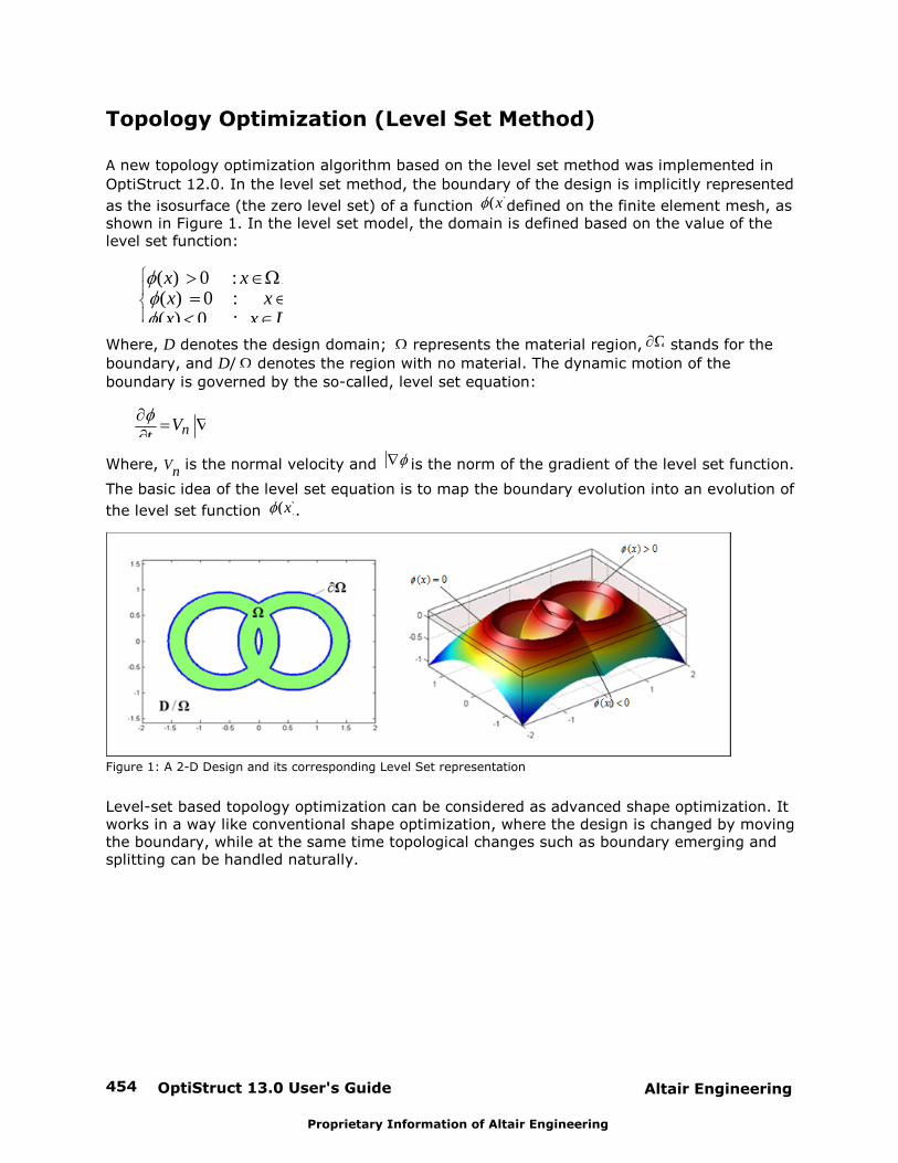
OptiStruct 13.0 User's Guide454 Altair Engineering
Proprietary Information of Altair Engineering
Topology Optimization (Level Set Method)
A new topology optimization algorithm based on the level set method was implemented in
OptiStruct 12.0. In the level set method, the boundary of the design is implicitly represented
as the isosurface (the zero level set) of a function ( )x defined on the finite element mesh, asshown in Figure 1. In the level set model, the domain is defined based on the value of thelevel set function:
( ) 0 : /( ) 0 :( ) 0 : /
x xx xx x D
Where, D denotes the design domain; represents the material region, stands for the
boundary, and D/ denotes the region with no material. The dynamic motion of the
boundary is governed by the so-called, level set equation:
nVt
Where, Vn is the normal velocity and is the norm of the gradient of the level set function.
The basic idea of the level set equation is to map the boundary evolution into an evolution of
the level set function ( )x .
Figure 1: A 2-D Design and its corresponding Level Set representation
Level-set based topology optimization can be considered as advanced shape optimization. Itworks in a way like conventional shape optimization, where the design is changed by movingthe boundary, while at the same time topological changes such as boundary emerging andsplitting can be handled naturally.
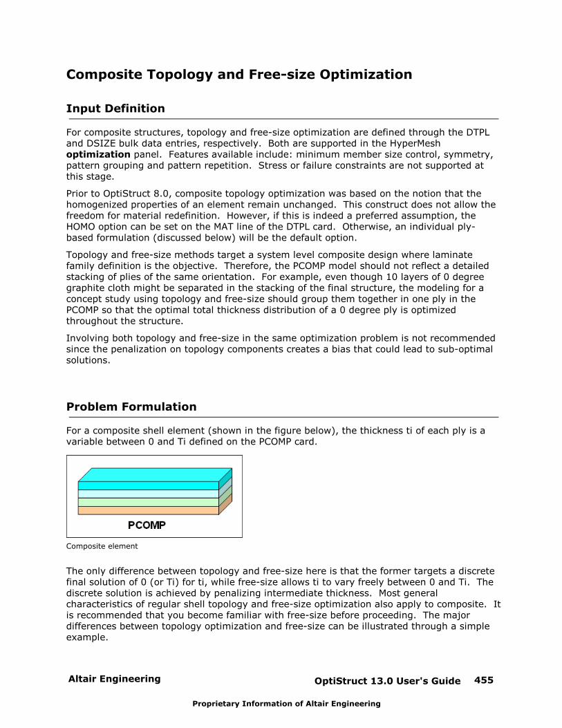
Altair Engineering OptiStruct 13.0 User's Guide 455
Proprietary Information of Altair Engineering
Composite Topology and Free-size Optimization
Input Definition
For composite structures, topology and free-size optimization are defined through the DTPLand DSIZE bulk data entries, respectively. Both are supported in the HyperMeshoptimization panel. Features available include: minimum member size control, symmetry,pattern grouping and pattern repetition. Stress or failure constraints are not supported atthis stage.
Prior to OptiStruct 8.0, composite topology optimization was based on the notion that thehomogenized properties of an element remain unchanged. This construct does not allow thefreedom for material redefinition. However, if this is indeed a preferred assumption, theHOMO option can be set on the MAT line of the DTPL card. Otherwise, an individual ply-based formulation (discussed below) will be the default option.
Topology and free-size methods target a system level composite design where laminatefamily definition is the objective. Therefore, the PCOMP model should not reflect a detailedstacking of plies of the same orientation. For example, even though 10 layers of 0 degreegraphite cloth might be separated in the stacking of the final structure, the modeling for aconcept study using topology and free-size should group them together in one ply in thePCOMP so that the optimal total thickness distribution of a 0 degree ply is optimizedthroughout the structure.
Involving both topology and free-size in the same optimization problem is not recommendedsince the penalization on topology components creates a bias that could lead to sub-optimalsolutions.
Problem Formulation
For a composite shell element (shown in the figure below), the thickness ti of each ply is avariable between 0 and Ti defined on the PCOMP card.
Composite element
The only difference between topology and free-size here is that the former targets a discretefinal solution of 0 (or Ti) for ti, while free-size allows ti to vary freely between 0 and Ti. Thediscrete solution is achieved by penalizing intermediate thickness. Most generalcharacteristics of regular shell topology and free-size optimization also apply to composite. Itis recommended that you become familiar with free-size before proceeding. The majordifferences between topology optimization and free-size can be illustrated through a simpleexample.
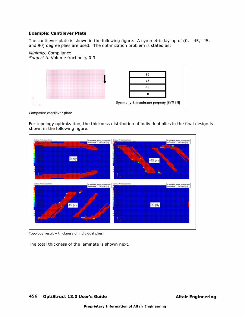
OptiStruct 13.0 User's Guide456 Altair Engineering
Proprietary Information of Altair Engineering
Example: Cantilever Plate
The cantilever plate is shown in the following figure. A symmetric lay-up of (0, +45, -45,and 90) degree plies are used. The optimization problem is stated as:
Minimize ComplianceSubject to Volume fraction < 0.3
Composite cantilever plate
For topology optimization, the thickness distribution of individual plies in the final design isshown in the following figure.
Topology result – thickness of individual plies
The total thickness of the laminate is shown next.
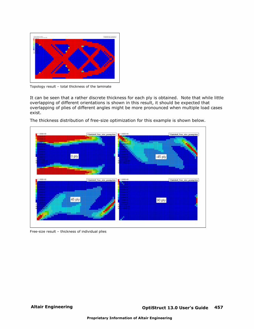
Altair Engineering OptiStruct 13.0 User's Guide 457
Proprietary Information of Altair Engineering
Topology result – total thickness of the laminate
It can be seen that a rather discrete thickness for each ply is obtained. Note that while littleoverlapping of different orientations is shown in this result, it should be expected thatoverlapping of plies of different angles might be more pronounced when multiple load casesexist.
The thickness distribution of free-size optimization for this example is shown below.
Free-size result – thickness of individual plies
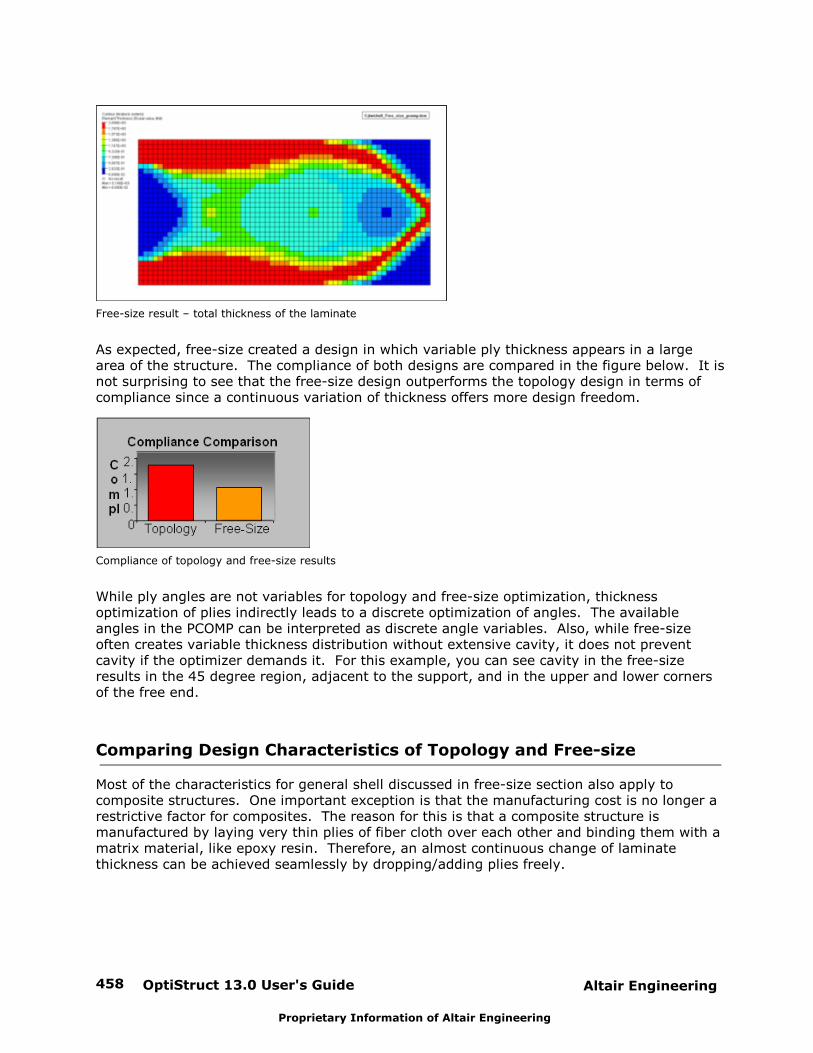
OptiStruct 13.0 User's Guide458 Altair Engineering
Proprietary Information of Altair Engineering
Free-size result – total thickness of the laminate
As expected, free-size created a design in which variable ply thickness appears in a largearea of the structure. The compliance of both designs are compared in the figure below. It isnot surprising to see that the free-size design outperforms the topology design in terms ofcompliance since a continuous variation of thickness offers more design freedom.
Compliance of topology and free-size results
While ply angles are not variables for topology and free-size optimization, thicknessoptimization of plies indirectly leads to a discrete optimization of angles. The availableangles in the PCOMP can be interpreted as discrete angle variables. Also, while free-sizeoften creates variable thickness distribution without extensive cavity, it does not preventcavity if the optimizer demands it. For this example, you can see cavity in the free-sizeresults in the 45 degree region, adjacent to the support, and in the upper and lower cornersof the free end.
Comparing Design Characteristics of Topology and Free-size
Most of the characteristics for general shell discussed in free-size section also apply tocomposite structures. One important exception is that the manufacturing cost is no longer arestrictive factor for composites. The reason for this is that a composite structure ismanufactured by laying very thin plies of fiber cloth over each other and binding them with amatrix material, like epoxy resin. Therefore, an almost continuous change of laminatethickness can be achieved seamlessly by dropping/adding plies freely.
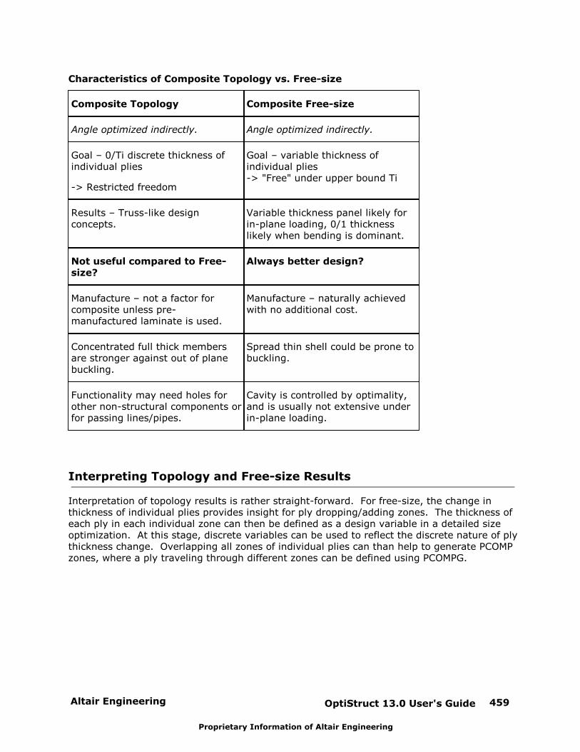
Altair Engineering OptiStruct 13.0 User's Guide 459
Proprietary Information of Altair Engineering
Characteristics of Composite Topology vs. Free-size
Composite Topology Composite Free-size
Angle optimized indirectly. Angle optimized indirectly.
Goal – 0/Ti discrete thickness ofindividual plies
-> Restricted freedom
Goal – variable thickness ofindividual plies-> "Free" under upper bound Ti
Results – Truss-like designconcepts.
Variable thickness panel likely forin-plane loading, 0/1 thicknesslikely when bending is dominant.
Not useful compared to Free-size?
Always better design?
Manufacture – not a factor forcomposite unless pre-manufactured laminate is used.
Manufacture – naturally achievedwith no additional cost.
Concentrated full thick membersare stronger against out of planebuckling.
Spread thin shell could be prone tobuckling.
Functionality may need holes forother non-structural components orfor passing lines/pipes.
Cavity is controlled by optimality,and is usually not extensive underin-plane loading.
Interpreting Topology and Free-size Results
Interpretation of topology results is rather straight-forward. For free-size, the change inthickness of individual plies provides insight for ply dropping/adding zones. The thickness ofeach ply in each individual zone can then be defined as a design variable in a detailed sizeoptimization. At this stage, discrete variables can be used to reflect the discrete nature of plythickness change. Overlapping all zones of individual plies can than help to generate PCOMPzones, where a ply traveling through different zones can be defined using PCOMPG.
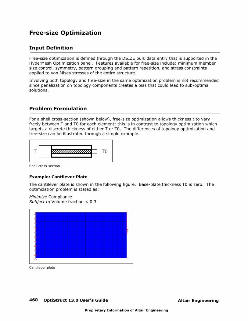
OptiStruct 13.0 User's Guide460 Altair Engineering
Proprietary Information of Altair Engineering
Free-size Optimization
Input Definition
Free-size optimization is defined through the DSIZE bulk data entry that is supported in theHyperMesh Optimization panel. Features available for free-size include: minimum membersize control, symmetry, pattern grouping and pattern repetition, and stress constraintsapplied to von Mises stresses of the entire structure.
Involving both topology and free-size in the same optimization problem is not recommendedsince penalization on topology components creates a bias that could lead to sub-optimalsolutions.
Problem Formulation
For a shell cross-section (shown below), free-size optimization allows thickness t to varyfreely between T and T0 for each element; this is in contrast to topology optimization whichtargets a discrete thickness of either T or T0. The differences of topology optimization andfree-size can be illustrated through a simple example.
Shell cross-section
Example: Cantilever Plate
The cantilever plate is shown in the following figure. Base-plate thickness T0 is zero. Theoptimization problem is stated as:
Minimize ComplianceSubject to Volume fraction < 0.3
Cantilever plate
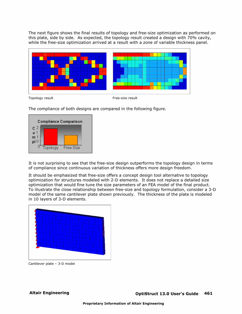
Altair Engineering OptiStruct 13.0 User's Guide 461
Proprietary Information of Altair Engineering
The next figure shows the final results of topology and free-size optimization as performed onthis plate, side by side. As expected, the topology result created a design with 70% cavity,while the free-size optimization arrived at a result with a zone of variable thickness panel.
Topology result Free-size result
The compliance of both designs are compared in the following figure.
It is not surprising to see that the free-size design outperforms the topology design in termsof compliance since continuous variation of thickness offers more design freedom.
It should be emphasized that free-size offers a concept design tool alternative to topologyoptimization for structures modeled with 2-D elements. It does not replace a detailed sizeoptimization that would fine tune the size parameters of an FEA model of the final product. To illustrate the close relationship between free-size and topology formulation, consider a 3-Dmodel of the same cantilever plate shown previously. The thickness of the plate is modeledin 10 layers of 3-D elements.
Cantilever plate – 3-D model
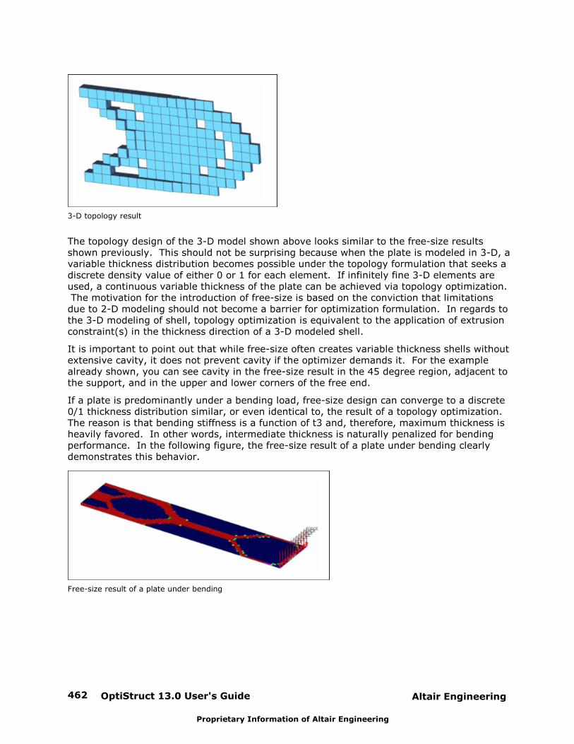
OptiStruct 13.0 User's Guide462 Altair Engineering
Proprietary Information of Altair Engineering
3-D topology result
The topology design of the 3-D model shown above looks similar to the free-size resultsshown previously. This should not be surprising because when the plate is modeled in 3-D, avariable thickness distribution becomes possible under the topology formulation that seeks adiscrete density value of either 0 or 1 for each element. If infinitely fine 3-D elements areused, a continuous variable thickness of the plate can be achieved via topology optimization. The motivation for the introduction of free-size is based on the conviction that limitationsdue to 2-D modeling should not become a barrier for optimization formulation. In regards tothe 3-D modeling of shell, topology optimization is equivalent to the application of extrusionconstraint(s) in the thickness direction of a 3-D modeled shell.
It is important to point out that while free-size often creates variable thickness shells withoutextensive cavity, it does not prevent cavity if the optimizer demands it. For the examplealready shown, you can see cavity in the free-size result in the 45 degree region, adjacent tothe support, and in the upper and lower corners of the free end.
If a plate is predominantly under a bending load, free-size design can converge to a discrete0/1 thickness distribution similar, or even identical to, the result of a topology optimization. The reason is that bending stiffness is a function of t3 and, therefore, maximum thickness isheavily favored. In other words, intermediate thickness is naturally penalized for bendingperformance. In the following figure, the free-size result of a plate under bending clearlydemonstrates this behavior.
Free-size result of a plate under bending
Altair Engineering OptiStruct 13.0 User's Guide 463
Proprietary Information of Altair Engineering
Stress Constraints for Free-size Optimization
The von Mises stress constraints may be defined for topology and free-size optimizationthrough the STRESS optional continuation line on the DTPL or the DSIZE card. There are anumber of restrictions with this constraint:
The definition of stress constraints is limited to a single von Mises permissible stress. The phenomenon of singular topology is pronounced when different materials withdifferent permissible stresses exist in a structure. Singular topology refers to theproblem associated with the conditional nature of stress constraints, i.e. the stressconstraint of an element disappears when the element vanishes. This creates anotherproblem in that a huge number of reduced problems exist with solutions that cannotusually be found by a gradient-based optimizer in the full design space.
Stress constraints for a partial domain of the structure are not allowed because theyoften create an ill-posed optimization problem since elimination of the partial domainwould remove all stress constraints. Consequently, the stress constraint applies to theentire model when active, including both design and non-design regions, and stressconstraint settings must be identical for all DSIZE and DTPL cards.
The capability has built-in intelligence to filter out artificial stress concentrations aroundpoint loads and point boundary conditions. Stress concentrations due to boundarygeometry are also filtered to some extent as they can be improved more effectivelywith local shape optimization.
Due to the large number of elements with active stress constraints, no element stressreport is given in the table of retained constraints in the .out file. The iterative history
of the stress state of the model can be viewed in HyperView or HyperMesh.
Stress constraints do not apply to 1-D elements.
Stress constraints may not be used when enforced displacements are present in themodel.
Comparing Design Characteristics of Topology and Free-size
The differences in the characteristics of topology and free-size are summarized in thefollowing table. It is important to note that while the free-size design concept generallyachieves better performance when buckling constraints are ignored, the topology conceptcould outperform free-size if buckling constraints become the driving criteria during the sizeand/or shape optimization stage. The reason for this is that topology optimization eliminatesintermediate thicknesses, which leads to a more concentrated material distribution and ashell that is stronger against out-of-plane buckling. The performance of topology and free-size is compared in the next practical example. Since it is usually not possible to know whatcriteria are most critical for a given structure, it is recommended to follow both designconcepts until detailed size and shape optimization is complete and can be evaluated. If it isnot possible to derive two designs for every structural component, a benchmark of therelative performance of both concepts for every type of commonly evaluated structure shouldbe established so that general guidelines can be used for reference.
Manufacturing and functional considerations may favor topology optimization. Two cases inwhich free-size may not be the best choice from the start include those in which:
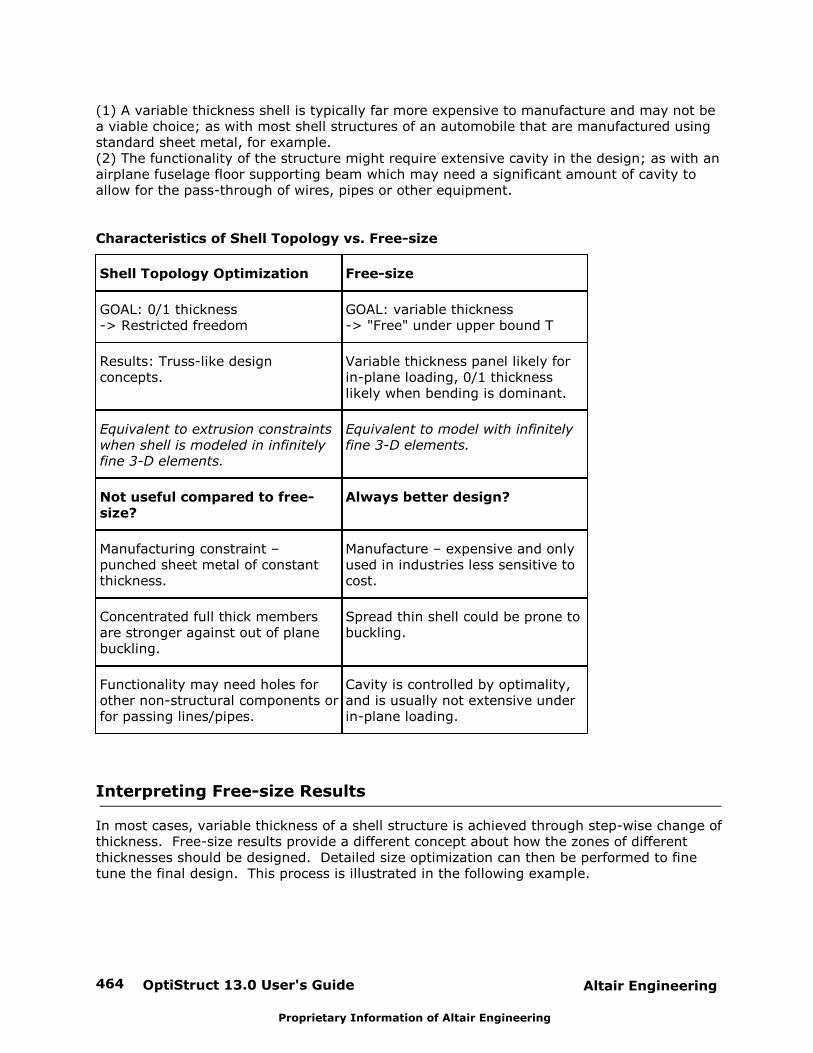
OptiStruct 13.0 User's Guide464 Altair Engineering
Proprietary Information of Altair Engineering
(1) A variable thickness shell is typically far more expensive to manufacture and may not bea viable choice; as with most shell structures of an automobile that are manufactured usingstandard sheet metal, for example. (2) The functionality of the structure might require extensive cavity in the design; as with anairplane fuselage floor supporting beam which may need a significant amount of cavity toallow for the pass-through of wires, pipes or other equipment.
Characteristics of Shell Topology vs. Free-size
Shell Topology Optimization Free-size
GOAL: 0/1 thickness-> Restricted freedom
GOAL: variable thickness-> "Free" under upper bound T
Results: Truss-like designconcepts.
Variable thickness panel likely forin-plane loading, 0/1 thicknesslikely when bending is dominant.
Equivalent to extrusion constraintswhen shell is modeled in infinitelyfine 3-D elements.
Equivalent to model with infinitelyfine 3-D elements.
Not useful compared to free-size?
Always better design?
Manufacturing constraint –punched sheet metal of constantthickness.
Manufacture – expensive and onlyused in industries less sensitive tocost.
Concentrated full thick membersare stronger against out of planebuckling.
Spread thin shell could be prone tobuckling.
Functionality may need holes forother non-structural components orfor passing lines/pipes.
Cavity is controlled by optimality,and is usually not extensive underin-plane loading.
Interpreting Free-size Results
In most cases, variable thickness of a shell structure is achieved through step-wise change ofthickness. Free-size results provide a different concept about how the zones of differentthicknesses should be designed. Detailed size optimization can then be performed to finetune the final design. This process is illustrated in the following example.
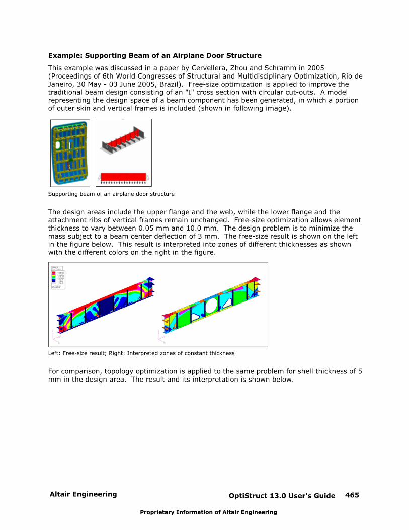
Altair Engineering OptiStruct 13.0 User's Guide 465
Proprietary Information of Altair Engineering
Example: Supporting Beam of an Airplane Door Structure
This example was discussed in a paper by Cervellera, Zhou and Schramm in 2005(Proceedings of 6th World Congresses of Structural and Multidisciplinary Optimization, Rio deJaneiro, 30 May - 03 June 2005, Brazil). Free-size optimization is applied to improve thetraditional beam design consisting of an "I" cross section with circular cut-outs. A modelrepresenting the design space of a beam component has been generated, in which a portionof outer skin and vertical frames is included (shown in following image).
Supporting beam of an airplane door structure
The design areas include the upper flange and the web, while the lower flange and theattachment ribs of vertical frames remain unchanged. Free-size optimization allows elementthickness to vary between 0.05 mm and 10.0 mm. The design problem is to minimize themass subject to a beam center deflection of 3 mm. The free-size result is shown on the leftin the figure below. This result is interpreted into zones of different thicknesses as shownwith the different colors on the right in the figure.
Left: Free-size result; Right: Interpreted zones of constant thickness
For comparison, topology optimization is applied to the same problem for shell thickness of 5mm in the design area. The result and its interpretation is shown below.
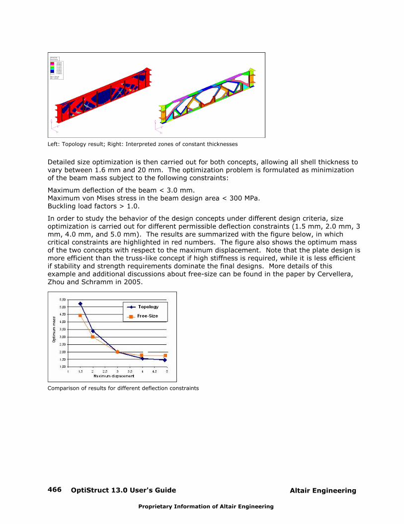
OptiStruct 13.0 User's Guide466 Altair Engineering
Proprietary Information of Altair Engineering
Left: Topology result; Right: Interpreted zones of constant thicknesses
Detailed size optimization is then carried out for both concepts, allowing all shell thickness tovary between 1.6 mm and 20 mm. The optimization problem is formulated as minimizationof the beam mass subject to the following constraints:
Maximum deflection of the beam < 3.0 mm.Maximum von Mises stress in the beam design area < 300 MPa.Buckling load factors > 1.0.
In order to study the behavior of the design concepts under different design criteria, sizeoptimization is carried out for different permissible deflection constraints (1.5 mm, 2.0 mm, 3mm, 4.0 mm, and 5.0 mm). The results are summarized with the figure below, in whichcritical constraints are highlighted in red numbers. The figure also shows the optimum massof the two concepts with respect to the maximum displacement. Note that the plate design ismore efficient than the truss-like concept if high stiffness is required, while it is less efficientif stability and strength requirements dominate the final designs. More details of thisexample and additional discussions about free-size can be found in the paper by Cervellera,Zhou and Schramm in 2005.
Comparison of results for different deflection constraints
Altair Engineering OptiStruct 13.0 User's Guide 467
Proprietary Information of Altair Engineering
Topography Optimization
Topography optimization is an advanced form of shape optimization in which a design regionfor a given part is defined and a pattern of shape variable-based reinforcements within thatregion is generated using OptiStruct. The approach in topography optimization is similar tothe approach used in topology optimization, except that shape variables are used rather thandensity variables. The design region is subdivided into a large number of separate variableswhose influence on the structure is calculated and optimized over a series of iterations. Thelarge number of shape variables allows you to create any reinforcement pattern within thedesign domain instead of being restricted to a few.
The following responses (see Responses for a description) are currently available as theobjective or as constraint functions:
Mass* Volume* Center of Gravity
Moment of Inertia Static Compliance StaticDisplacement
Natural Frequency Buckling Factor Static Stress,Strain, Forces
Static CompositeStress, Strain, Failure Index
Frequency ResponseDisplacement, Velocity,Acceleration
FrequencyResponse Stress,Strain, Forces
Weighted Compliance Weighted Frequency CombinedCompliance Index
Function Bead discretenessfraction
Temperature
* Mass and Volume are not recommended for use as objectives or constraints since
mass and volume are not very sensitive to design changes in topography
optimization.
Design Variables for Topography Optimization
OptiStruct solves topography optimization problems using shape optimization withinternally generated shape variables. One or more design domains are defined using the DTPG card. These cards must, in turn, reference PSHELL, PCOMP or DESVAR definitions. If a DESVAR definition is referenced, it must be a shape design variable, meaning that itmust, in turn, be referenced by one or more DVGRID cards. If a PSHELL or PCOMPdefinition is referenced, OptiStruct generates shape variables using the parameters definedon the DTPG card, creating internal DVGRID data for the nodes associated with the PSHELLor PCOMP definitions. In both cases, the end result is that each DTPG card references asingle shape variable. This shape variable then gets converted into topography shapevariables.
OptiStruct 13.0 User's Guide468 Altair Engineering
Proprietary Information of Altair Engineering
Basic topography shape variables follow the user-defined parameters on the DTPG card(minimum bead width, and draw angle), they are circular in shape, and they are laid outacross the design domain in a roughly hexagonal distribution. Each topography shapevariable has a circular central region of diameter equal to the minimum bead width. Gridswithin this region are perturbed as a group, which prevents the formation of anyreinforcement bead of less than the minimum bead width. Grids outside of the centralcircular region of the topographical variables are perturbed as the average of the variablesto which they are nearest. This results in smooth transitions between neighboringvariables. If two adjacent variables are fully perturbed, all of the nodes between them willbe fully perturbed. If one variable is fully perturbed and its neighbor is unperturbed, thenodes in between will form a smooth slope connecting them at an angle equal to the drawangle. The spacing of the variables is determined by the minimum bead width and thedraw angle in such a way that no part of the bead reinforcement pattern forms an anglegreater than the draw angle.
Pattern grouping options link topographical variables together in such a way that thedesired reinforcement patterns are formed. Linear, planar, circular, radial, etc. shapedreinforcements are controlled by single variables, ensuring that the reinforcements followthe desired pattern. One-plane, two-plane, three-plane and cyclical symmetry patterngrouping options also use a similar approach to ensure that symmetry is created in thesolution.
Although topography optimization is primarily a tool for creating bead type reinforcementsin shell elements, it can accommodate solid models as well. Many pattern groupingoptions (such as planar and cylindrical) are intended to be used with solid models sincethey effectively reduce 3-D problems into 2-D ones.
Variable Generation
There are three methods of automatically generating shape variables for topographyoptimization using the DTPG card. The first two, element normal and draw vector, areperformed entirely in OptiStruct. The third (user-defined) requires that the input datacontain one or more shape design variables that are used as the design domain.
Method Description
Elementnormal
This method is the easiest one to use. When norm isentered for the draw direction, the normal vectors ofthe elements are used to define the draw vector forthe shape variables. This method is especiallyeffective for curved surfaces and enclosed volumeswhere the beads are intended to be drawn normal tothe surface.
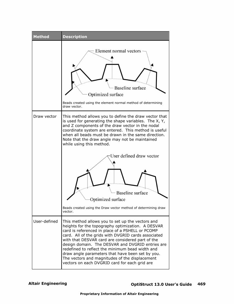
Altair Engineering OptiStruct 13.0 User's Guide 469
Proprietary Information of Altair Engineering
Method Description
Beads created using the element normal method of determiningdraw vector.
Draw vector This method allows you to define the draw vector thatis used for generating the shape variables. The X, Y,and Z components of the draw vector in the nodalcoordinate system are entered. This method is usefulwhen all beads must be drawn in the same direction. Note that the draw angle may not be maintainedwhile using this method.
Beads created using the Draw vector method of determining drawvector.
User-defined This method allows you to set up the vectors andheights for the topography optimization. A DESVARcard is referenced in place of a PSHELL or PCOMPcard. All of the grids with DVGRID cards associatedwith that DESVAR card are considered part of thedesign domain. The DESVAR and DVGRID entries areredefined to reflect the minimum bead width anddraw angle parameters that have been set by you. The vectors and magnitudes of the displacementvectors on each DVGRID card for each grid are
OptiStruct 13.0 User's Guide470 Altair Engineering
Proprietary Information of Altair Engineering
Method Description
retained, so these entries must be left blank on theDTPG card. This allows you to create a design domainin which each node can have its own draw vector anddraw height.
Multiple Topography Design Regions
OptiStruct generates topography shape variables for each design domain defined by a DTPG card. It allows for overlapping of design domains. A grid that is in more than onedesign domain will be a part of shape variables for each design domain. For automaticallygenerated bead variables, the draw height is divided by the number of bead variablesacting on that grid. Thus, if a grid is a part of two DTPG cards that have draw heights of3.0mm and 5.0mm, the draw heights become 1.5mm and 2.5mm. If this is not desired,simply make sure that no grid is in more than one design domain. In cases where twodesign components touch each other and the design domains are not user-defined (i.e.PSHELL or PCOMP definitions are referenced), a row of non-design elements needs to beinserted between them to prevent averaging. If the bead variables are user-defined (i.e.DESVAR definition is referenced), no averaging will be performed. It is assumed that youintend to have the shape variables overlap, which will result in the grid deflection beingcumulative between multiple influencing bead cards.
Bead Discreteness Fraction
The bead discreteness fraction is a response that can be used to control the amount ofshape variation for topography design domains. This response indicates the amount ofshape variation for one or more topography design domains. The response varies in therange 0.0 to 1.0 (0.0 < BEADFRAC < 1.0), where 0.0 indicates that no shape variation hasoccurred, and 1.0 indicates that the entire topography design domain has assumed themaximum allowed shape variation.
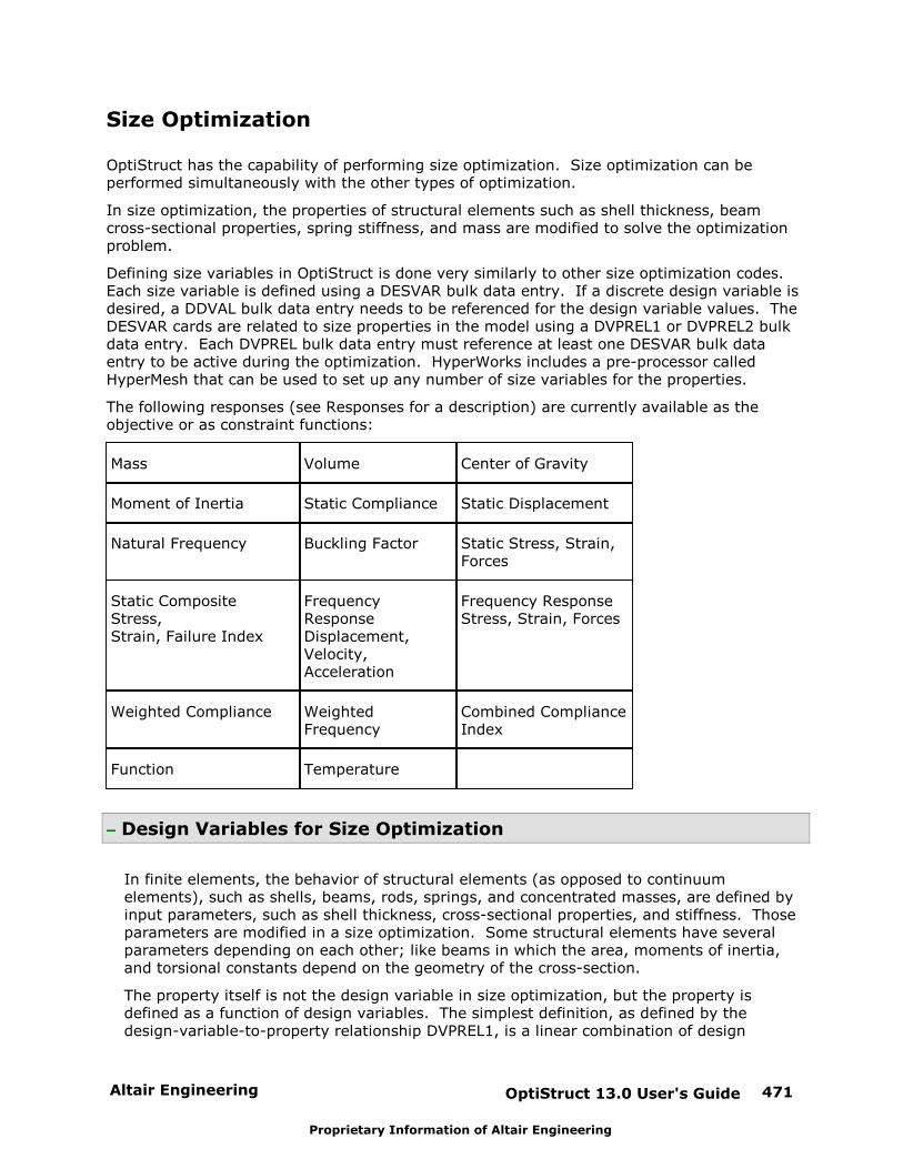
Altair Engineering OptiStruct 13.0 User's Guide 471
Proprietary Information of Altair Engineering
Size Optimization
OptiStruct has the capability of performing size optimization. Size optimization can beperformed simultaneously with the other types of optimization.
In size optimization, the properties of structural elements such as shell thickness, beamcross-sectional properties, spring stiffness, and mass are modified to solve the optimizationproblem.
Defining size variables in OptiStruct is done very similarly to other size optimization codes. Each size variable is defined using a DESVAR bulk data entry. If a discrete design variable isdesired, a DDVAL bulk data entry needs to be referenced for the design variable values. TheDESVAR cards are related to size properties in the model using a DVPREL1 or DVPREL2 bulkdata entry. Each DVPREL bulk data entry must reference at least one DESVAR bulk dataentry to be active during the optimization. HyperWorks includes a pre-processor calledHyperMesh that can be used to set up any number of size variables for the properties.
The following responses (see Responses for a description) are currently available as theobjective or as constraint functions:
Mass Volume Center of Gravity
Moment of Inertia Static Compliance Static Displacement
Natural Frequency Buckling Factor Static Stress, Strain,Forces
Static CompositeStress, Strain, Failure Index
FrequencyResponseDisplacement,Velocity,Acceleration
Frequency ResponseStress, Strain, Forces
Weighted Compliance WeightedFrequency
Combined ComplianceIndex
Function Temperature
Design Variables for Size Optimization
In finite elements, the behavior of structural elements (as opposed to continuumelements), such as shells, beams, rods, springs, and concentrated masses, are defined byinput parameters, such as shell thickness, cross-sectional properties, and stiffness. Thoseparameters are modified in a size optimization. Some structural elements have severalparameters depending on each other; like beams in which the area, moments of inertia,and torsional constants depend on the geometry of the cross-section.
The property itself is not the design variable in size optimization, but the property isdefined as a function of design variables. The simplest definition, as defined by thedesign-variable-to-property relationship DVPREL1, is a linear combination of design

OptiStruct 13.0 User's Guide472 Altair Engineering
Proprietary Information of Altair Engineering
variables defined on a DESVAR statement such that
0 i ip C DV C
Where, p is the property to be optimized, and Ci are linear factors associated to the design
variable DVi.
Using the equation utility DEQATN, more complicated functional dependencies using eventrigonometric functions can be established. Such design-variable-to-property relations arethen defined using the DVPREL2 statement.
For a simple gage optimization of a shell structure, the design-variable-to-propertyrelationship turns into:
iT DV
Where, the gage thickness, T is identical to the design variable.
If a discrete design variable is desired, a DDVAL bulk data entry needs to be referenced onthe DESVAR bulk data entry for the design variable values.
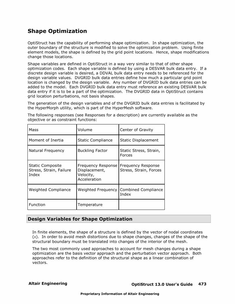
Altair Engineering OptiStruct 13.0 User's Guide 473
Proprietary Information of Altair Engineering
Shape Optimization
OptiStruct has the capability of performing shape optimization. In shape optimization, theouter boundary of the structure is modified to solve the optimization problem. Using finiteelement models, the shape is defined by the grid point locations. Hence, shape modificationschange those locations.
Shape variables are defined in OptiStruct in a way very similar to that of other shapeoptimization codes. Each shape variable is defined by using a DESVAR bulk data entry. If adiscrete design variable is desired, a DDVAL bulk data entry needs to be referenced for thedesign variable values. DVGRID bulk data entries define how much a particular grid pointlocation is changed by the design variable. Any number of DVGRID bulk data entries can beadded to the model. Each DVGRID bulk data entry must reference an existing DESVAR bulkdata entry if it is to be a part of the optimization. The DVGRID data in OptiStruct containsgrid location perturbations, not basis shapes.
The generation of the design variables and of the DVGRID bulk data entries is facilitated bythe HyperMorph utility, which is part of the HyperMesh software.
The following responses (see Responses for a description) are currently available as theobjective or as constraint functions:
Mass Volume Center of Gravity
Moment of Inertia Static Compliance Static Displacement
Natural Frequency Buckling Factor Static Stress, Strain,Forces
Static CompositeStress, Strain, FailureIndex
Frequency ResponseDisplacement,Velocity,Acceleration
Frequency ResponseStress, Strain, Forces
Weighted Compliance Weighted Frequency Combined ComplianceIndex
Function Temperature
Design Variables for Shape Optimization
In finite elements, the shape of a structure is defined by the vector of nodal coordinates(x). In order to avoid mesh distortions due to shape changes, changes of the shape of the
structural boundary must be translated into changes of the interior of the mesh.
The two most commonly used approaches to account for mesh changes during a shapeoptimization are the basis vector approach and the perturbation vector approach. Bothapproaches refer to the definition of the structural shape as a linear combination ofvectors.
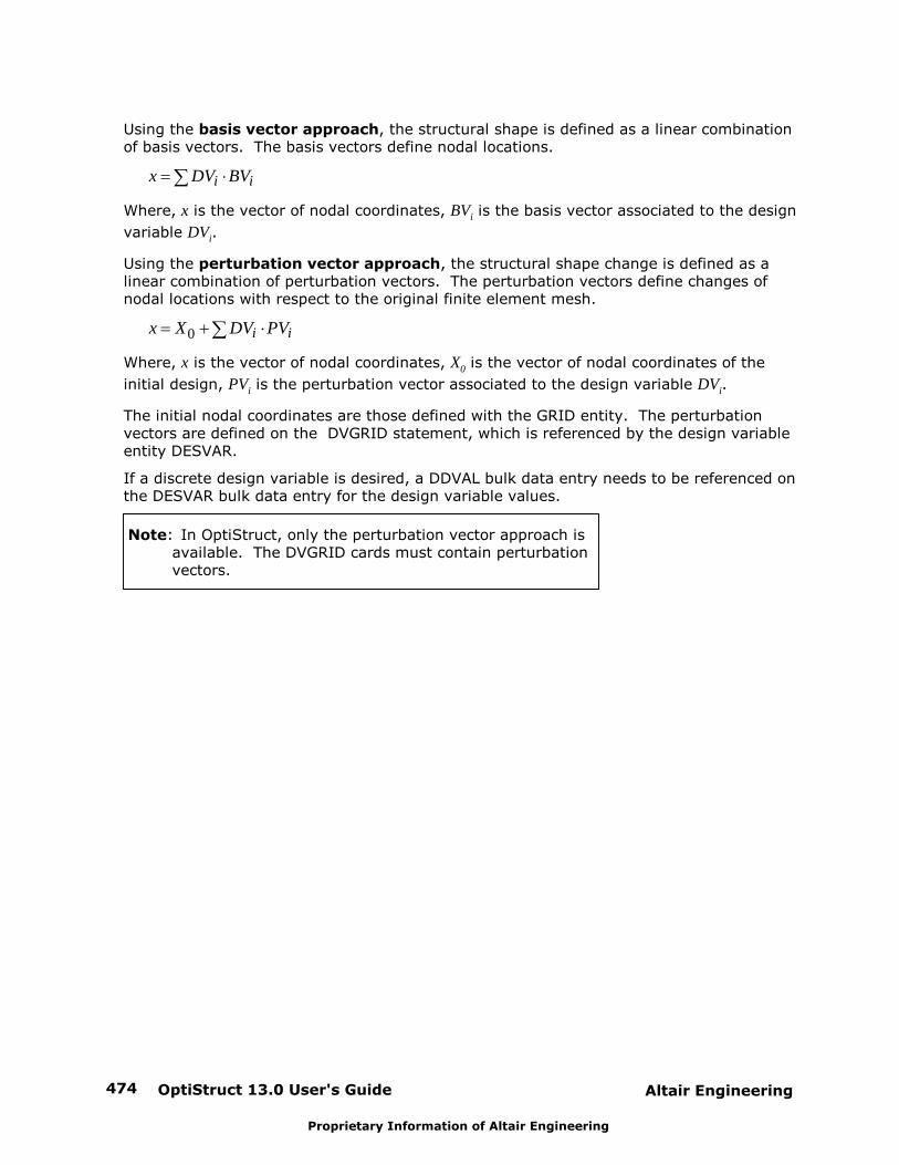
OptiStruct 13.0 User's Guide474 Altair Engineering
Proprietary Information of Altair Engineering
Using the basis vector approach, the structural shape is defined as a linear combinationof basis vectors. The basis vectors define nodal locations.
i ix DV BV
Where, x is the vector of nodal coordinates, BVi is the basis vector associated to the design
variable DVi.
Using the perturbation vector approach, the structural shape change is defined as alinear combination of perturbation vectors. The perturbation vectors define changes ofnodal locations with respect to the original finite element mesh.
0 i ix X DV PV
Where, x is the vector of nodal coordinates, X0 is the vector of nodal coordinates of the
initial design, PVi is the perturbation vector associated to the design variable DVi.
The initial nodal coordinates are those defined with the GRID entity. The perturbationvectors are defined on the DVGRID statement, which is referenced by the design variableentity DESVAR.
If a discrete design variable is desired, a DDVAL bulk data entry needs to be referenced onthe DESVAR bulk data entry for the design variable values.
Note: In OptiStruct, only the perturbation vector approach isavailable. The DVGRID cards must contain perturbationvectors.

Altair Engineering OptiStruct 13.0 User's Guide 475
Proprietary Information of Altair Engineering
Free-shape Optimization
Free-shape optimization uses a proprietary optimization technique developed by AltairEngineering Inc., wherein the outer boundary of a structure is altered to meet with pre-defined objectives and constraints. The essential idea of free-shape optimization, and whereit differs from other shape optimization techniques, is that the allowable movement of theouter boundary is automatically determined, thus relieving you of the burden of definingshape perturbations.
Free-shape design regions are defined through the DSHAPE bulk data entry. Design regionsare identified by the grids on the outer boundary of the structure (the edge of a shellstructure or the surface of a solid structure). These grids are listed on the DSHAPE entry.
Free-shape optimization allows these design grids to move in one of two ways:
1. For shell structures; grids move normal to the surface edge in the tangential plane.
2. For solid structures; grids move normal to the surface.
During free-shape optimization, the normal directions change with the change in shape of thestructure, thus, for each iteration, the design grids move along the updated normals.
Defining Free-shape Design Regions
Ideally, free-shape design regions should be selected where it can be assumed that theshape of the structure is most sensitive to the concerned responses. For example, it wouldbe appropriate to select grids in a high stress region when the objective is to reducestress.
Free-shape design regions should be defined at different locations on the structure where itis desired for the shape to change independently. For solid structures, feature lines oftendefine natural boundaries for free-shape design regions. Containing any feature linesinside a free-shape design region should be avoided unless the intention is to smooth thefeature lines during an optimization. Likewise for a shell structure, sharp corners shouldnot be contained inside a free-shape design region unless the intention is to smooth outsuch corners.
The DSHAPE card identifies the design region through the GRID continuation card, shownhere:
(1) (2) (3) (4) (5) (6) (7) (8) (9) (10)
GRID GID1 GID2 GID3 GID4 GID5 GID6 GID7
GID8 GID9 … …
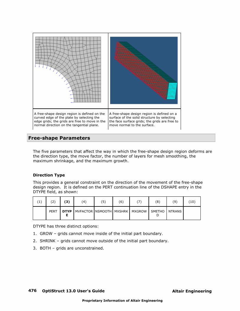
OptiStruct 13.0 User's Guide476 Altair Engineering
Proprietary Information of Altair Engineering
A free-shape design region is defined on thecurved edge of the plate by selecting theedge grids; the grids are free to move in thenormal direction on the tangential plane.
A free-shape design region is defined on asurface of the solid structure by selectingthe face surface grids; the grids are free tomove normal to the surface.
Free-shape Parameters
The five parameters that affect the way in which the free-shape design region deforms arethe direction type, the move factor, the number of layers for mesh smoothing, themaximum shrinkage, and the maximum growth.
Direction Type
This provides a general constraint on the direction of the movement of the free-shapedesign region. It is defined on the PERT continuation line of the DSHAPE entry in theDTYPE field, as shown:
(1) (2) (3) (4) (5) (6) (7) (8) (9) (10)
PERT DTYPE
MVFACTOR NSMOOTH MXSHRK MXGROW SMETHOD
NTRANS
DTYPE has three distinct options:
1. GROW – grids cannot move inside of the initial part boundary.
2. SHRINK – grids cannot move outside of the initial part boundary.
3. BOTH – grids are unconstrained.
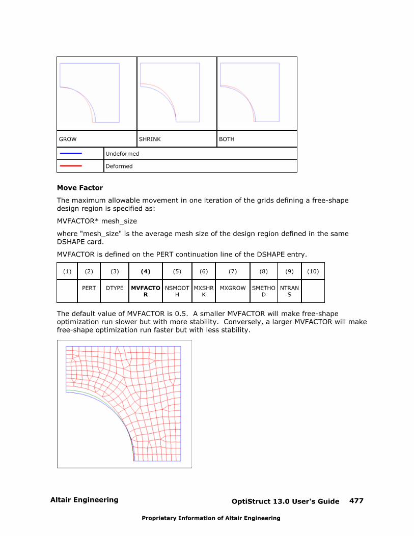
Altair Engineering OptiStruct 13.0 User's Guide 477
Proprietary Information of Altair Engineering
GROW SHRINK BOTH
Undeformed
Deformed
Move Factor
The maximum allowable movement in one iteration of the grids defining a free-shapedesign region is specified as:
MVFACTOR* mesh_size
where "mesh_size" is the average mesh size of the design region defined in the sameDSHAPE card.
MVFACTOR is defined on the PERT continuation line of the DSHAPE entry.
(1) (2) (3) (4) (5) (6) (7) (8) (9) (10)
PERT DTYPE MVFACTOR
NSMOOTH
MXSHRK
MXGROW SMETHOD
NTRANS
The default value of MVFACTOR is 0.5. A smaller MVFACTOR will make free-shapeoptimization run slower but with more stability. Conversely, a larger MVFACTOR will makefree-shape optimization run faster but with less stability.
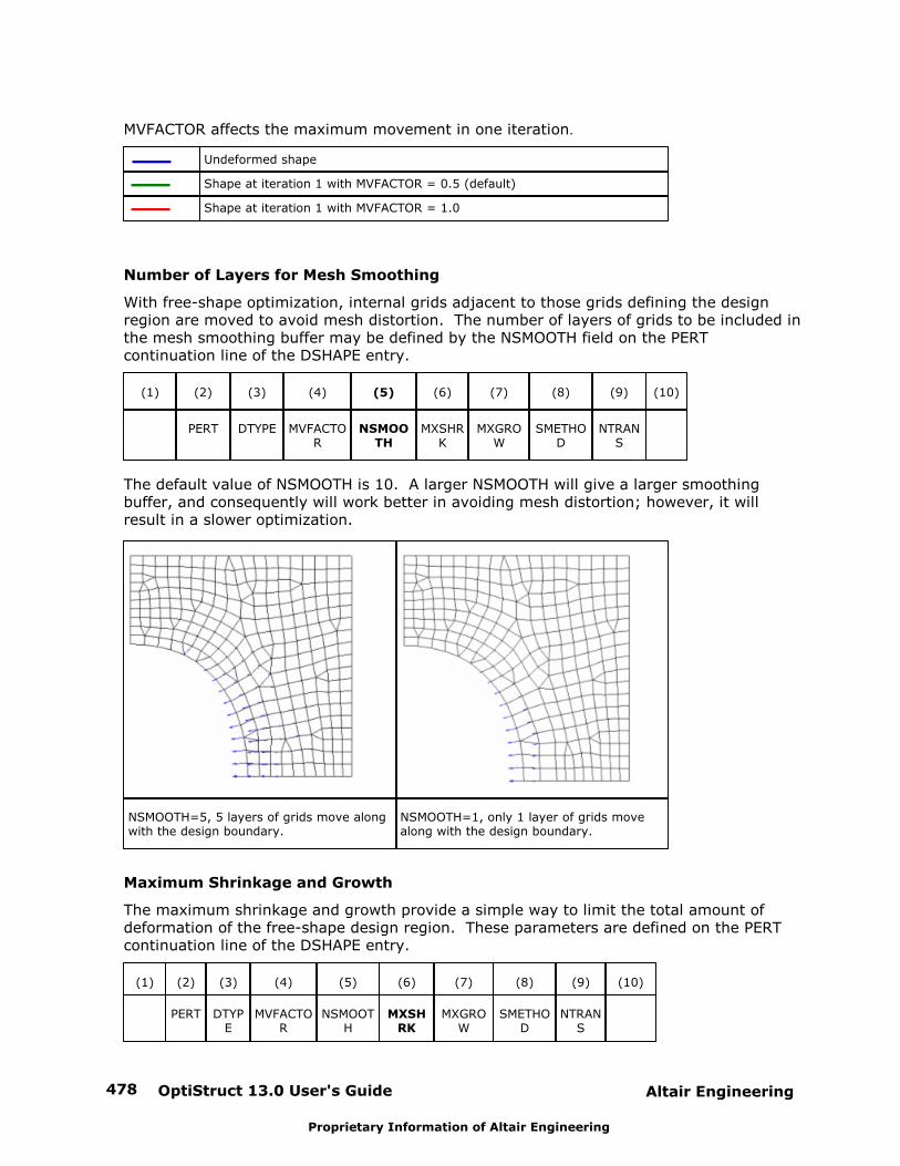
OptiStruct 13.0 User's Guide478 Altair Engineering
Proprietary Information of Altair Engineering
MVFACTOR affects the maximum movement in one iteration.
Undeformed shape
Shape at iteration 1 with MVFACTOR = 0.5 (default)
Shape at iteration 1 with MVFACTOR = 1.0
Number of Layers for Mesh Smoothing
With free-shape optimization, internal grids adjacent to those grids defining the designregion are moved to avoid mesh distortion. The number of layers of grids to be included inthe mesh smoothing buffer may be defined by the NSMOOTH field on the PERTcontinuation line of the DSHAPE entry.
(1) (2) (3) (4) (5) (6) (7) (8) (9) (10)
PERT DTYPE MVFACTOR
NSMOOTH
MXSHRK
MXGROW
SMETHOD
NTRANS
The default value of NSMOOTH is 10. A larger NSMOOTH will give a larger smoothingbuffer, and consequently will work better in avoiding mesh distortion; however, it willresult in a slower optimization.
NSMOOTH=5, 5 layers of grids move alongwith the design boundary.
NSMOOTH=1, only 1 layer of grids movealong with the design boundary.
Maximum Shrinkage and Growth
The maximum shrinkage and growth provide a simple way to limit the total amount ofdeformation of the free-shape design region. These parameters are defined on the PERTcontinuation line of the DSHAPE entry.
(1) (2) (3) (4) (5) (6) (7) (8) (9) (10)
PERT DTYPE
MVFACTOR
NSMOOTH
MXSHRK
MXGROW
SMETHOD
NTRANS
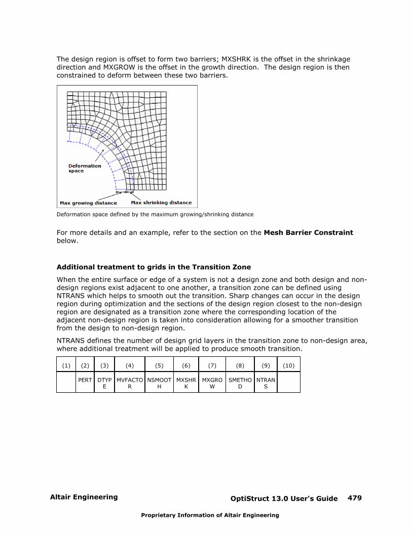
Altair Engineering OptiStruct 13.0 User's Guide 479
Proprietary Information of Altair Engineering
The design region is offset to form two barriers; MXSHRK is the offset in the shrinkagedirection and MXGROW is the offset in the growth direction. The design region is thenconstrained to deform between these two barriers.
Deformation space defined by the maximum growing/shrinking distance
For more details and an example, refer to the section on the Mesh Barrier Constraintbelow.
Additional treatment to grids in the Transition Zone
When the entire surface or edge of a system is not a design zone and both design and non-design regions exist adjacent to one another, a transition zone can be defined usingNTRANS which helps to smooth out the transition. Sharp changes can occur in the designregion during optimization and the sections of the design region closest to the non-designregion are designated as a transition zone where the corresponding location of theadjacent non-design region is taken into consideration allowing for a smoother transitionfrom the design to non-design region.
NTRANS defines the number of design grid layers in the transition zone to non-design area,where additional treatment will be applied to produce smooth transition.
(1) (2) (3) (4) (5) (6) (7) (8) (9) (10)
PERT DTYPE
MVFACTOR
NSMOOTH
MXSHRK
MXGROW
SMETHOD
NTRANS
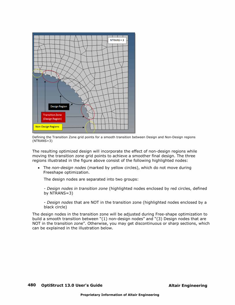
OptiStruct 13.0 User's Guide480 Altair Engineering
Proprietary Information of Altair Engineering
Defining the Transition Zone grid points for a smooth transition between Design and Non-Design regions(NTRANS=3)
The resulting optimized design will incorporate the effect of non-design regions whilemoving the transition zone grid points to achieve a smoother final design. The threeregions illustrated in the figure above consist of the following highlighted nodes:
The non-design nodes (marked by yellow circles), which do not move duringFreeshape optimization.
The design nodes are separated into two groups:
- Design nodes in transition zone (highlighted nodes enclosed by red circles, definedby NTRANS=3)
- Design nodes that are NOT in the transition zone (highlighted nodes enclosed by ablack circle)
The design nodes in the transition zone will be adjusted during Free-shape optimization tobuild a smooth transition between “(1) non-design nodes” and “(3) Design nodes that areNOT in the transition zone”. Otherwise, you may get discontinuous or sharp sections, whichcan be explained in the illustration below.
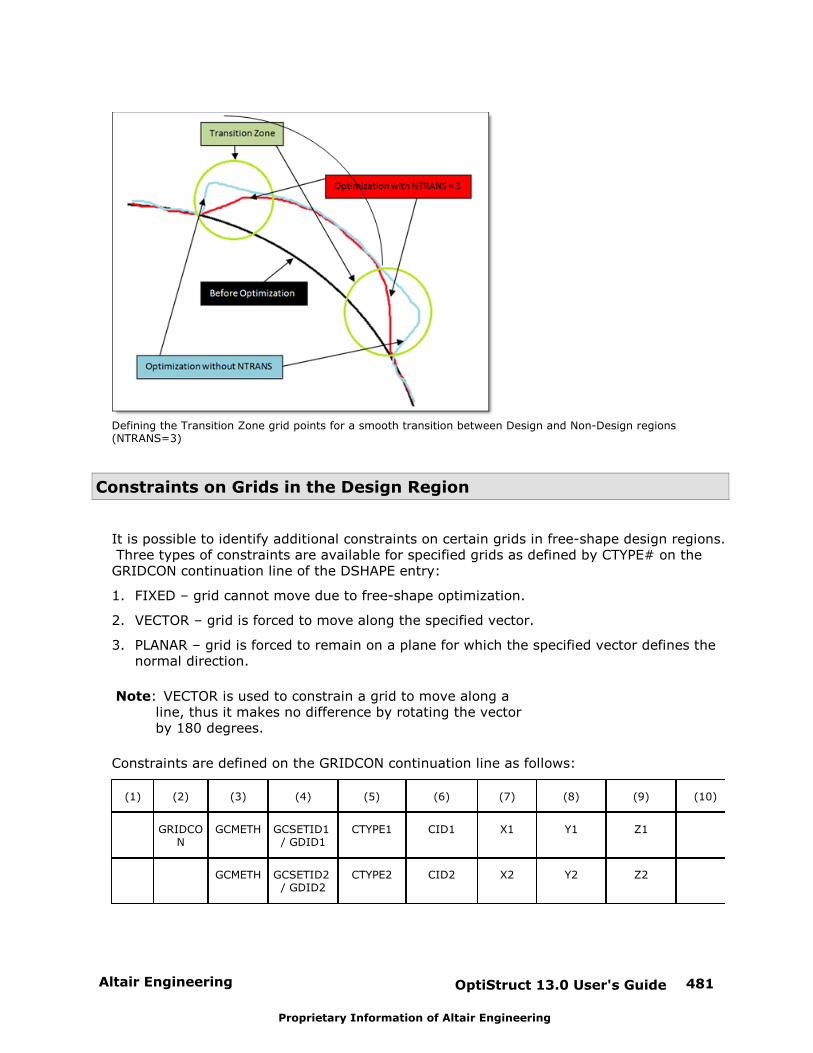
Altair Engineering OptiStruct 13.0 User's Guide 481
Proprietary Information of Altair Engineering
Defining the Transition Zone grid points for a smooth transition between Design and Non-Design regions(NTRANS=3)
Constraints on Grids in the Design Region
It is possible to identify additional constraints on certain grids in free-shape design regions. Three types of constraints are available for specified grids as defined by CTYPE# on theGRIDCON continuation line of the DSHAPE entry:
1. FIXED – grid cannot move due to free-shape optimization.
2. VECTOR – grid is forced to move along the specified vector.
3. PLANAR – grid is forced to remain on a plane for which the specified vector defines thenormal direction.
Note: VECTOR is used to constrain a grid to move along aline, thus it makes no difference by rotating the vectorby 180 degrees.
Constraints are defined on the GRIDCON continuation line as follows:
(1) (2) (3) (4) (5) (6) (7) (8) (9) (10)
GRIDCON
GCMETH GCSETID1 / GDID1
CTYPE1 CID1 X1 Y1 Z1
GCMETH GCSETID2 / GDID2
CTYPE2 CID2 X2 Y2 Z2
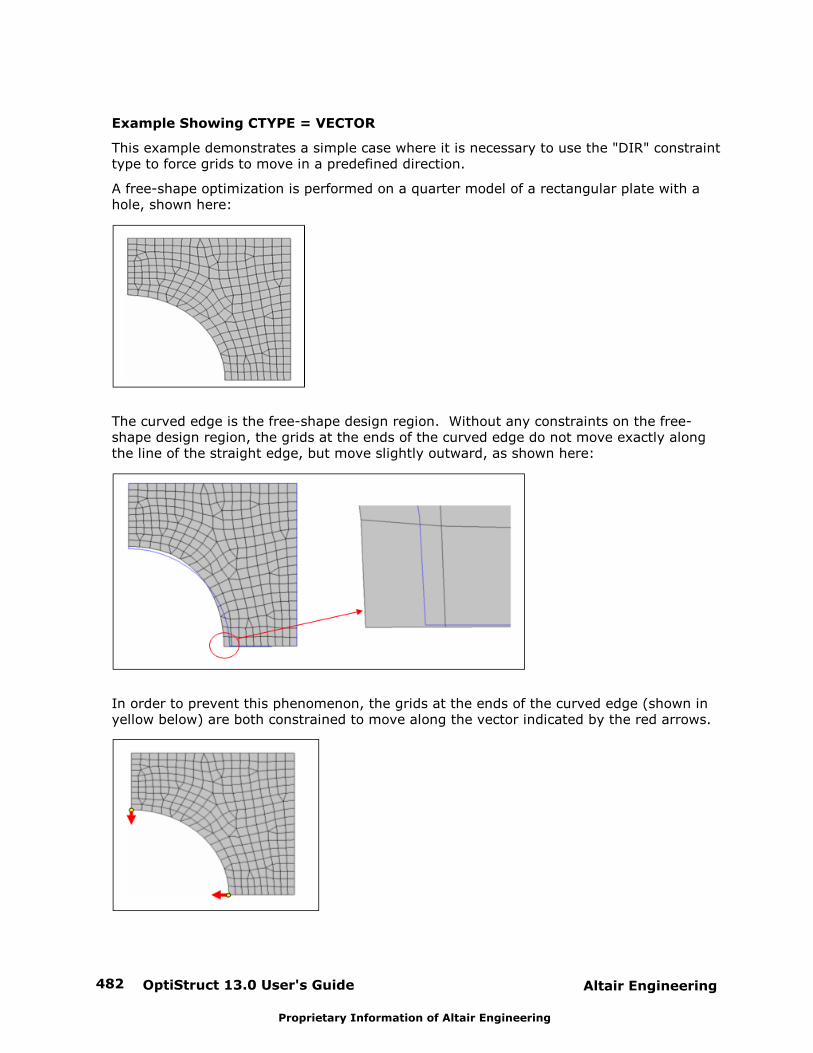
OptiStruct 13.0 User's Guide482 Altair Engineering
Proprietary Information of Altair Engineering
Example Showing CTYPE = VECTOR
This example demonstrates a simple case where it is necessary to use the "DIR" constrainttype to force grids to move in a predefined direction.
A free-shape optimization is performed on a quarter model of a rectangular plate with ahole, shown here:
The curved edge is the free-shape design region. Without any constraints on the free-shape design region, the grids at the ends of the curved edge do not move exactly alongthe line of the straight edge, but move slightly outward, as shown here:
In order to prevent this phenomenon, the grids at the ends of the curved edge (shown inyellow below) are both constrained to move along the vector indicated by the red arrows.
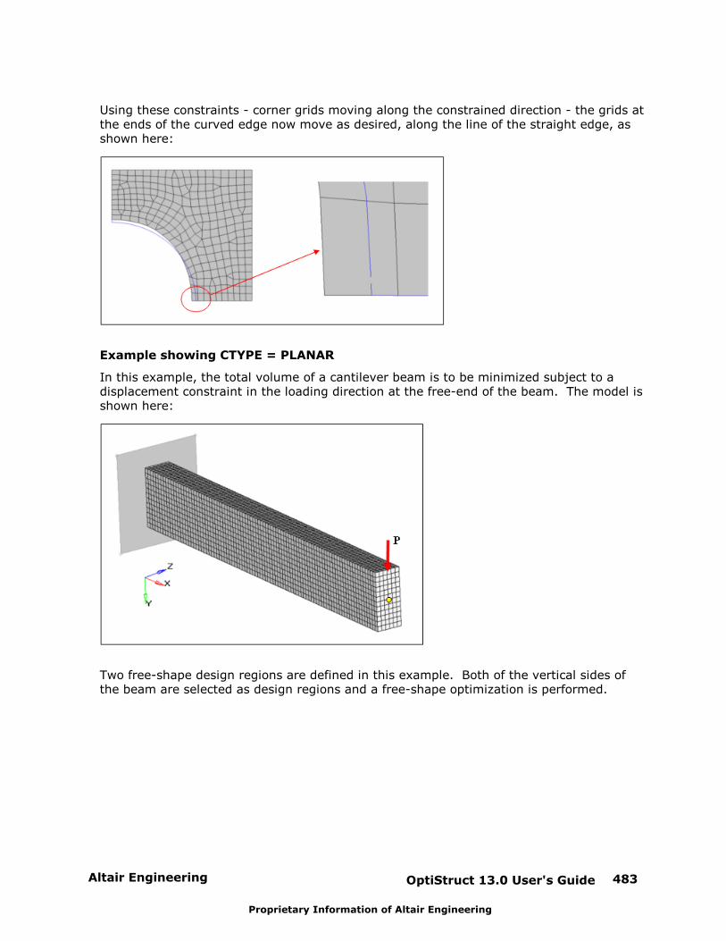
Altair Engineering OptiStruct 13.0 User's Guide 483
Proprietary Information of Altair Engineering
Using these constraints - corner grids moving along the constrained direction - the grids atthe ends of the curved edge now move as desired, along the line of the straight edge, asshown here:
Example showing CTYPE = PLANAR
In this example, the total volume of a cantilever beam is to be minimized subject to adisplacement constraint in the loading direction at the free-end of the beam. The model isshown here:
Two free-shape design regions are defined in this example. Both of the vertical sides ofthe beam are selected as design regions and a free-shape optimization is performed.
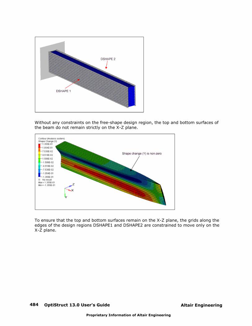
OptiStruct 13.0 User's Guide484 Altair Engineering
Proprietary Information of Altair Engineering
Without any constraints on the free-shape design region, the top and bottom surfaces ofthe beam do not remain strictly on the X-Z plane.
To ensure that the top and bottom surfaces remain on the X-Z plane, the grids along theedges of the design regions DSHAPE1 and DSHAPE2 are constrained to move only on theX-Z plane.
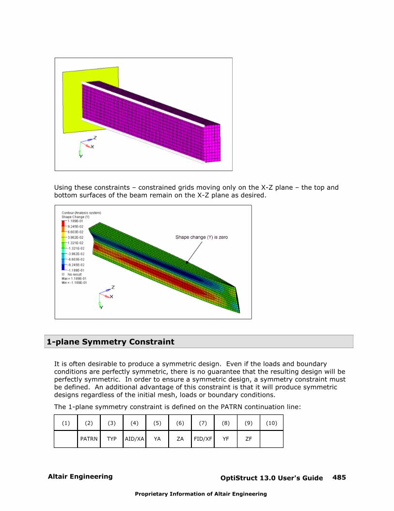
Altair Engineering OptiStruct 13.0 User's Guide 485
Proprietary Information of Altair Engineering
Using these constraints – constrained grids moving only on the X-Z plane – the top andbottom surfaces of the beam remain on the X-Z plane as desired.
1-plane Symmetry Constraint
It is often desirable to produce a symmetric design. Even if the loads and boundaryconditions are perfectly symmetric, there is no guarantee that the resulting design will beperfectly symmetric. In order to ensure a symmetric design, a symmetry constraint mustbe defined. An additional advantage of this constraint is that it will produce symmetricdesigns regardless of the initial mesh, loads or boundary conditions.
The 1-plane symmetry constraint is defined on the PATRN continuation line:
(1) (2) (3) (4) (5) (6) (7) (8) (9) (10)
PATRN TYP AID/XA YA ZA FID/XF YF ZF
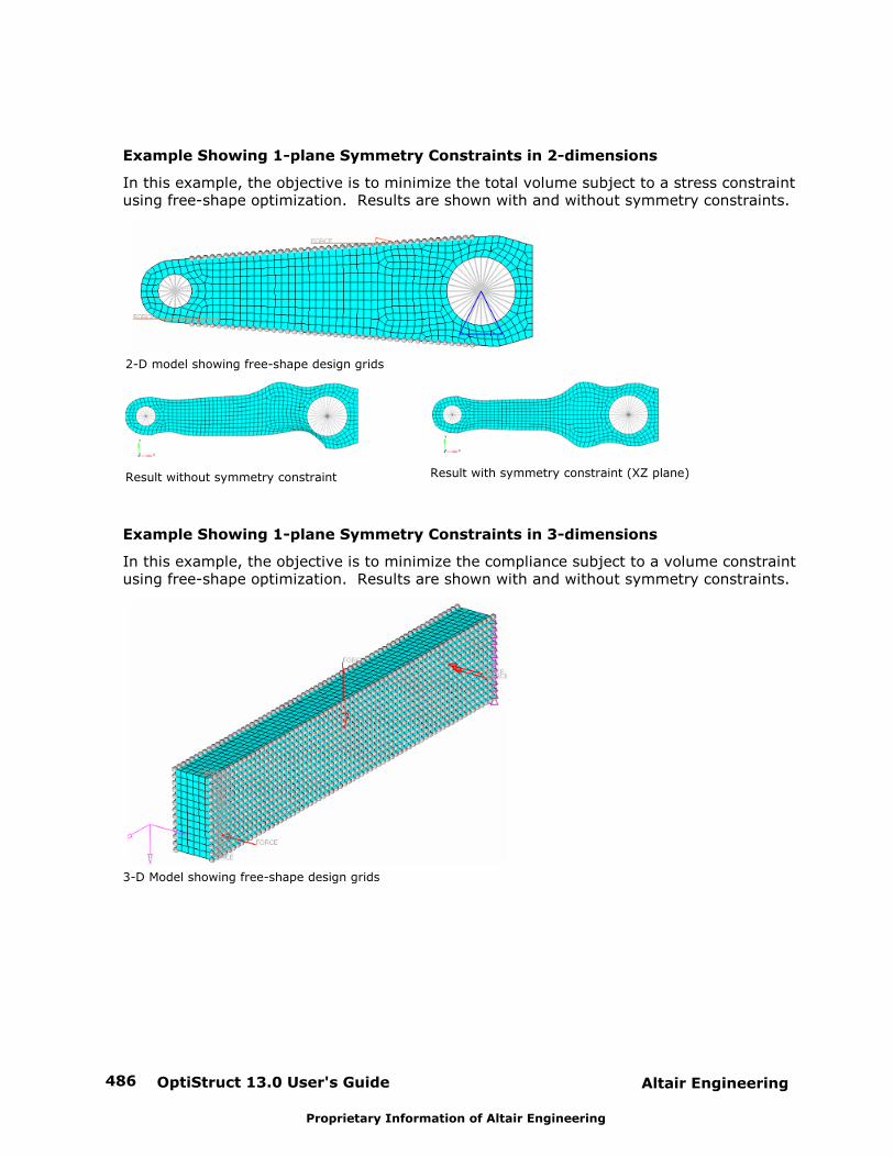
OptiStruct 13.0 User's Guide486 Altair Engineering
Proprietary Information of Altair Engineering
Example Showing 1-plane Symmetry Constraints in 2-dimensions
In this example, the objective is to minimize the total volume subject to a stress constraintusing free-shape optimization. Results are shown with and without symmetry constraints.
2-D model showing free-shape design grids
Result without symmetry constraint Result with symmetry constraint (XZ plane)
Example Showing 1-plane Symmetry Constraints in 3-dimensions
In this example, the objective is to minimize the compliance subject to a volume constraintusing free-shape optimization. Results are shown with and without symmetry constraints.
3-D Model showing free-shape design grids
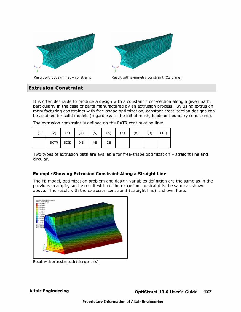
Altair Engineering OptiStruct 13.0 User's Guide 487
Proprietary Information of Altair Engineering
Result without symmetry constraint Result with symmetry constraint (XZ plane)
Extrusion Constraint
It is often desirable to produce a design with a constant cross-section along a given path,particularly in the case of parts manufactured by an extrusion process. By using extrusionmanufacturing constraints with free-shape optimization, constant cross-section designs canbe attained for solid models (regardless of the initial mesh, loads or boundary conditions).
The extrusion constraint is defined on the EXTR continuation line:
(1) (2) (3) (4) (5) (6) (7) (8) (9) (10)
EXTR ECID XE YE ZE
Two types of extrusion path are available for free-shape optimization – straight line andcircular.
Example Showing Extrusion Constraint Along a Straight Line
The FE model, optimization problem and design variables definition are the same as in theprevious example, so the result without the extrusion constraint is the same as shownabove. The result with the extrusion constraint (straight line) is shown here.
Result with extrusion path (along x-axis)
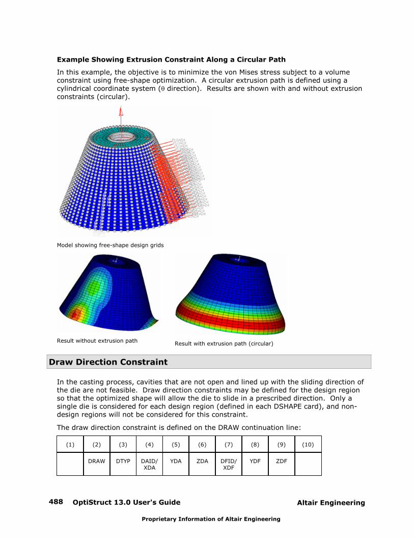
OptiStruct 13.0 User's Guide488 Altair Engineering
Proprietary Information of Altair Engineering
Example Showing Extrusion Constraint Along a Circular Path
In this example, the objective is to minimize the von Mises stress subject to a volumeconstraint using free-shape optimization. A circular extrusion path is defined using acylindrical coordinate system ( direction). Results are shown with and without extrusionconstraints (circular).
Model showing free-shape design grids
Result without extrusion pathResult with extrusion path (circular)
Draw Direction Constraint
In the casting process, cavities that are not open and lined up with the sliding direction ofthe die are not feasible. Draw direction constraints may be defined for the design regionso that the optimized shape will allow the die to slide in a prescribed direction. Only asingle die is considered for each design region (defined in each DSHAPE card), and non-design regions will not be considered for this constraint.
The draw direction constraint is defined on the DRAW continuation line:
(1) (2) (3) (4) (5) (6) (7) (8) (9) (10)
DRAW DTYP DAID/XDA
YDA ZDA DFID/XDF
YDF ZDF
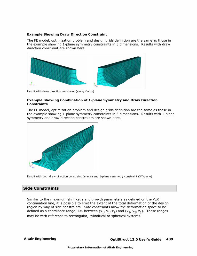
Altair Engineering OptiStruct 13.0 User's Guide 489
Proprietary Information of Altair Engineering
Example Showing Draw Direction Constraint
The FE model, optimization problem and design grids definition are the same as those inthe example showing 1-plane symmetry constraints in 3 dimensions. Results with drawdirection constraint are shown here.
Result with draw direction constraint (along Y-axis)
Example Showing Combination of 1-plane Symmetry and Draw DirectionConstraints
The FE model, optimization problem and design grids definition are the same as those inthe example showing 1-plane symmetry constraints in 3 dimensions. Results with 1-planesymmetry and draw direction constraints are shown here.
Result with both draw direction constraint (Y-axis) and 1-plane symmetry constraint (XY-plane)
Side Constraints
Similar to the maximum shrinkage and growth parameters as defined on the PERTcontinuation line, it is possible to limit the extent of the total deformation of the designregion by way of side constraints. Side constraints allow the deformation space to bedefined as a coordinate range; i.e. between (x1, y1, z1) and (x2, y2, z2). These ranges
may be with reference to rectangular, cylindrical or spherical systems.
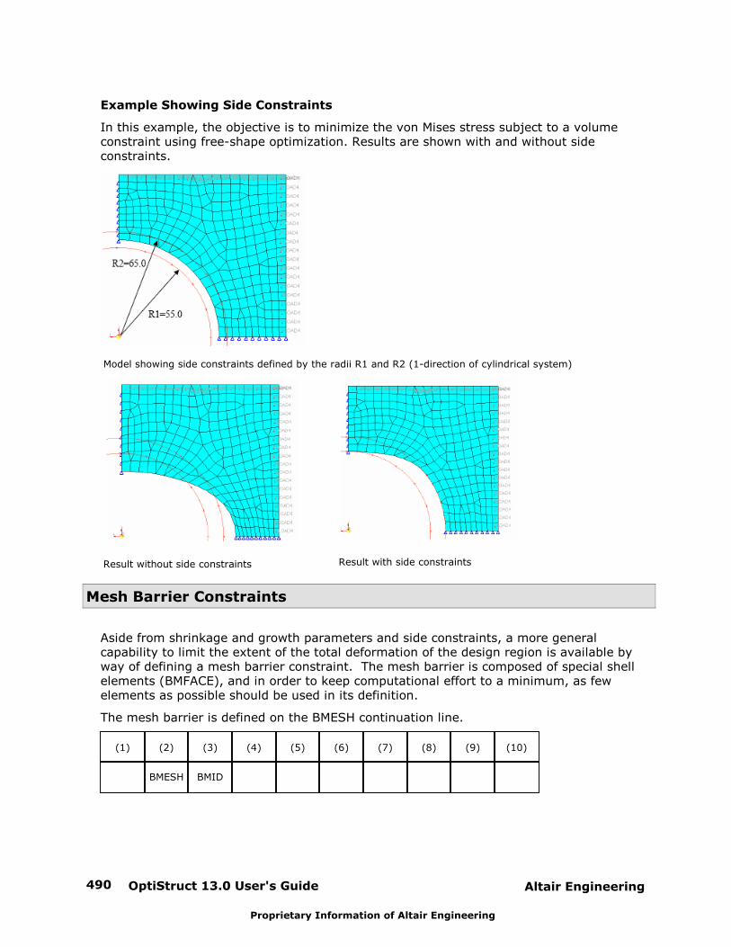
OptiStruct 13.0 User's Guide490 Altair Engineering
Proprietary Information of Altair Engineering
Example Showing Side Constraints
In this example, the objective is to minimize the von Mises stress subject to a volumeconstraint using free-shape optimization. Results are shown with and without sideconstraints.
Model showing side constraints defined by the radii R1 and R2 (1-direction of cylindrical system)
Result without side constraints Result with side constraints
Mesh Barrier Constraints
Aside from shrinkage and growth parameters and side constraints, a more generalcapability to limit the extent of the total deformation of the design region is available byway of defining a mesh barrier constraint. The mesh barrier is composed of special shellelements (BMFACE), and in order to keep computational effort to a minimum, as fewelements as possible should be used in its definition.
The mesh barrier is defined on the BMESH continuation line.
(1) (2) (3) (4) (5) (6) (7) (8) (9) (10)
BMESH BMID
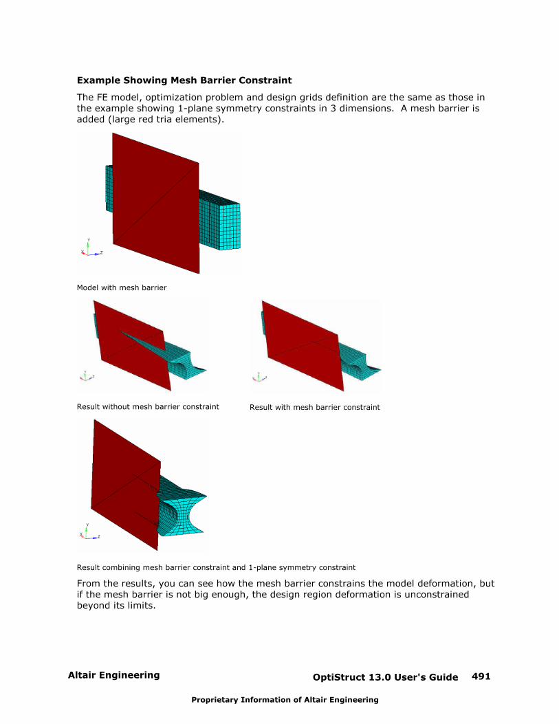
Altair Engineering OptiStruct 13.0 User's Guide 491
Proprietary Information of Altair Engineering
Example Showing Mesh Barrier Constraint
The FE model, optimization problem and design grids definition are the same as those inthe example showing 1-plane symmetry constraints in 3 dimensions. A mesh barrier isadded (large red tria elements).
Model with mesh barrier
Result without mesh barrier constraint Result with mesh barrier constraint
Result combining mesh barrier constraint and 1-plane symmetry constraint
From the results, you can see how the mesh barrier constrains the model deformation, butif the mesh barrier is not big enough, the design region deformation is unconstrainedbeyond its limits.
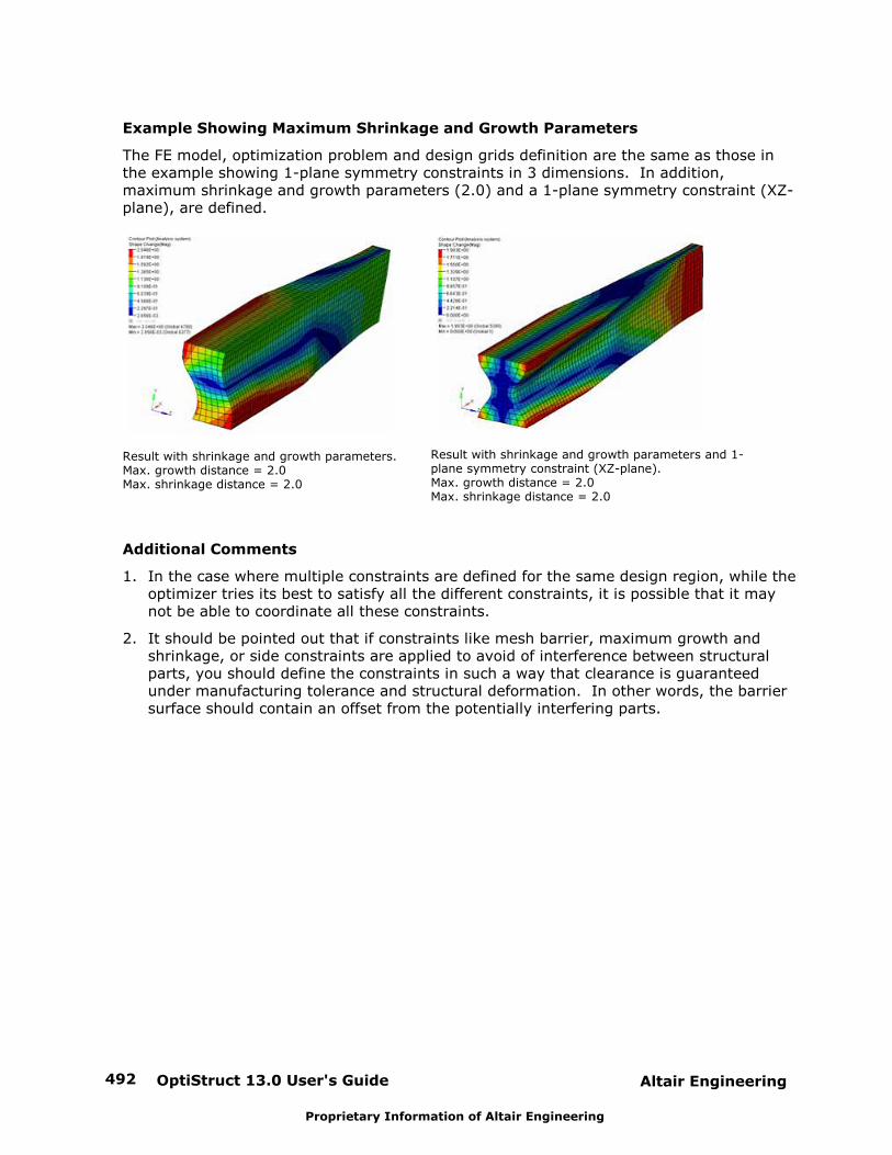
OptiStruct 13.0 User's Guide492 Altair Engineering
Proprietary Information of Altair Engineering
Example Showing Maximum Shrinkage and Growth Parameters
The FE model, optimization problem and design grids definition are the same as those inthe example showing 1-plane symmetry constraints in 3 dimensions. In addition,maximum shrinkage and growth parameters (2.0) and a 1-plane symmetry constraint (XZ-plane), are defined.
Result with shrinkage and growth parameters.Max. growth distance = 2.0Max. shrinkage distance = 2.0
Result with shrinkage and growth parameters and 1-plane symmetry constraint (XZ-plane).Max. growth distance = 2.0Max. shrinkage distance = 2.0
Additional Comments
1. In the case where multiple constraints are defined for the same design region, while theoptimizer tries its best to satisfy all the different constraints, it is possible that it maynot be able to coordinate all these constraints.
2. It should be pointed out that if constraints like mesh barrier, maximum growth andshrinkage, or side constraints are applied to avoid of interference between structuralparts, you should define the constraints in such a way that clearance is guaranteedunder manufacturing tolerance and structural deformation. In other words, the barriersurface should contain an offset from the potentially interfering parts.

Altair Engineering OptiStruct 13.0 User's Guide 493
Proprietary Information of Altair Engineering
Manufacturing Constraints
The following optimization features can be found in this section:
Manufacturability for Topology Optimization
Manufacturability for Topography Optimization
Manufacturability for Free-size Optimization
Multi-Model Optimization

OptiStruct 13.0 User's Guide494 Altair Engineering
Proprietary Information of Altair Engineering
Manufacturability for Topology Optimization
A concern in topology optimization is that the design concepts developed are very often notmanufacturable. Another problem is that the solution of a topology optimization problem canbe mesh dependent, if no appropriate measure is taken.
OptiStruct offers a number of different methods to account for manufacturability whenperforming topology optimization:
Member Size Control
Draw Direction Constraints
Extrusion Constraints
Pattern Repetition
Pattern Grouping
Altair Engineering OptiStruct 13.0 User's Guide 495
Proprietary Information of Altair Engineering
Member Size Control for Topology Optimization
Member size control allows you some control over the member size in the final topology andthe resulting degree of simplicity of the final design. This feature may be added one of thetwo ways described below.
1. The DOPTPRM card:
(1) (2) (3) (4) (5) (6) (7) (8) (9) (10)
DOPTPRM MINDIM VALUE
Here, only the preferred minimum diameter (width in 2-D) of members may be defined asthe VALUE field, following the MINDIM keyword. A global minimum member size isdefined in this way.
2. The DTPL card:
(1) (2) (3) (4) (5) (6) (7) (8) (9) (10)
DTPL ID PTYPE PID1 PID2 PID3 PID4 PID5 PID6
PID7 … … …
MEMBSIZ MINDIM MAXDIM
MINGAP
Here, both the preferred minimum, MINDIM, and the maximum, MAXDIM, diameter ofmembers may be defined on the MEMBSIZ continuation line. Member size dimensions canbe defined differently for each DTPL in this way.
Minimum Member Size Control
Although minimum member size control penalizes the formation of small members, resultsthat contain members significantly under the prescribed minimum member size can still beobtained. This is because a small member in the structure can be very important to the loadtransmission and may not be removed by penalization. Minimum member size controlfunctions more as a quality control than a quantity control.
A discrete solution is achieved in two iterative steps. The first step converges to a solutionwith a large number of semi-dense elements. The second step tries to refine this solution toa solution with fully dense members. Each step consists of a number of iterations. The firststep consists of two entire convergence phases - the first run with the initial discretenessvalues (defined by DISCRETE and DISCRT1D parameters on the DOPTPRM bulk data entry),followed by a run with the discreteness values increased by 1.0. This procedure isimplemented in order to achieve a solution with clearly defined members. If this step couldnot create a solution with clearly defined members, the preferred minimum member size willnot be preserved in the second step. In which case, you need to increase the discretenessparameters and/or reduce the convergence tolerance (defined by the OBJTOL parameter onthe DOPTPRM bulk data entry) to improve the solution of the first phase. The defaultdiscreteness is set to 1.0 for 1-D elements, plates and shells, and 2.0 for 3-D solids.
OptiStruct 13.0 User's Guide496 Altair Engineering
Proprietary Information of Altair Engineering
In general, once MINDIM is activated, checkerboarding is controlled by the methods appliedfor this feature, eliminating the need for the CHECKER parameter. In rare circumstances,checkerboards may still be introduced in the second phase described above for 3-D solids. Ifthis happens, an additional checkerboard control algorithm can be activated with theMMCHECK parameter. (The CHECKER and MMCHECK parameters are defined using theDOPTPRM bulk data entry).
The use of this card will assure a checkerboard-free solution, although with the undesiredside effect of achieving a solution that involves a large number of semi-dense elements,similar to the result of setting CHECKER equal to 1. Therefore, use this card only when it isnecessary.
It is recommended that MINDIM be at least 3 times, and no greater than 12 times, theaverage element size for all elements referenced by that DTPL (or all designable elementswhen defined on DOPTPRM). The average element size for 2-D elements is calculated as theaverage of the square root of the area of the elements, and for 3-D elements, as the averageof the cubic root of the volume of the elements.
This recommendation is enforced when combined with other manufacturing constraints, andif the defined MINDIM is less than this value, it will be reset to a default value equal to 3times the average element size. Similarly, if the defined MINDIM is larger than 12 times theaverage element size, it will be reset to a value equal to 12 times the average element size. This limit has been set to trim memory requirements that can become too large as a result ofhaving to keep track of a much larger number of elements needed to satisfy the MINDIMconstraint. In structures where the mesh is aligned with the draw or extrusion direction,setting MTYP as ALIGN on the MESH continuation line of the DTPL card may circumvent thisconstraint.
The following examples demonstrate significant improvement in the manufacturability ofresults through the use of minimum member size control:
Michell-truss Example
MBB-Beam Example
Arch Example
3-D Bridge Model Example
Maximum Member Size Control
Maximum member size control penalizes the formation of large members. The control is notdirectional, meaning that if the thickness of a member is less than MAXDIM in any direction,this constraint is satisfied. This reflects the need to control the rib thickness of castingparts.
MAXDIM must be at least twice MINDIM, and hence the minimum mesh requirement is thatMAXDIM has to be at least 6 times the average element size for all elements referenced bythat DTPL. This constraint is strongly enforced and an error termination will occur when thiscriteria is not met. In addition, MAXDIM should be less than half the width of the thinnestpart of the design region.
Based on the constraints mentioned above, a fine mesh is required to achieve good resultswith this manufacturing constraint.
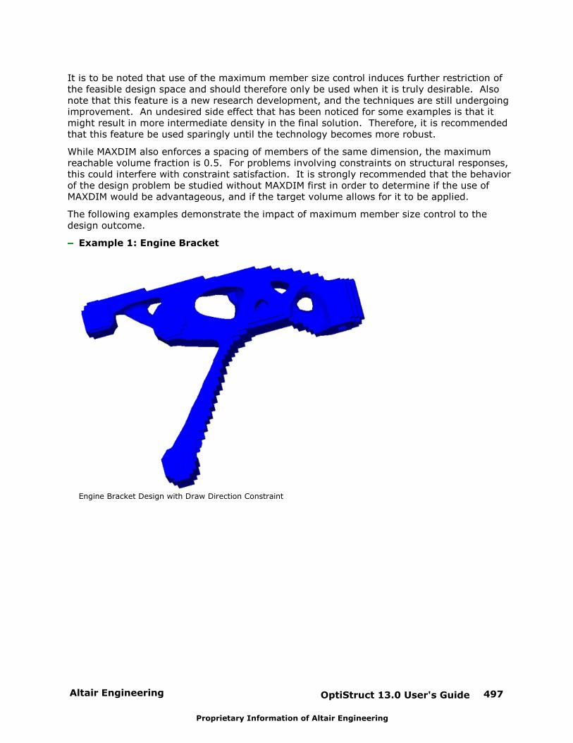
Altair Engineering OptiStruct 13.0 User's Guide 497
Proprietary Information of Altair Engineering
It is to be noted that use of the maximum member size control induces further restriction ofthe feasible design space and should therefore only be used when it is truly desirable. Alsonote that this feature is a new research development, and the techniques are still undergoingimprovement. An undesired side effect that has been noticed for some examples is that itmight result in more intermediate density in the final solution. Therefore, it is recommendedthat this feature be used sparingly until the technology becomes more robust.
While MAXDIM also enforces a spacing of members of the same dimension, the maximumreachable volume fraction is 0.5. For problems involving constraints on structural responses,this could interfere with constraint satisfaction. It is strongly recommended that the behaviorof the design problem be studied without MAXDIM first in order to determine if the use ofMAXDIM would be advantageous, and if the target volume allows for it to be applied.
The following examples demonstrate the impact of maximum member size control to thedesign outcome.
Example 1: Engine Bracket
Engine Bracket Design with Draw Direction Constraint
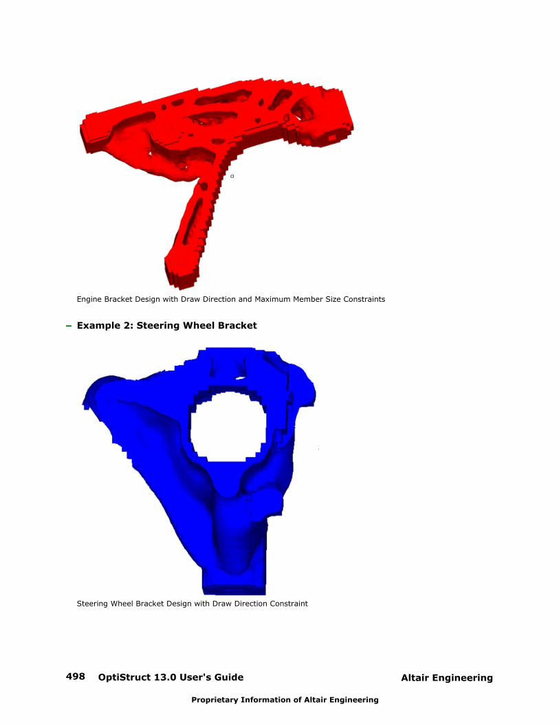
OptiStruct 13.0 User's Guide498 Altair Engineering
Proprietary Information of Altair Engineering
Engine Bracket Design with Draw Direction and Maximum Member Size Constraints
Example 2: Steering Wheel Bracket
Steering Wheel Bracket Design with Draw Direction Constraint
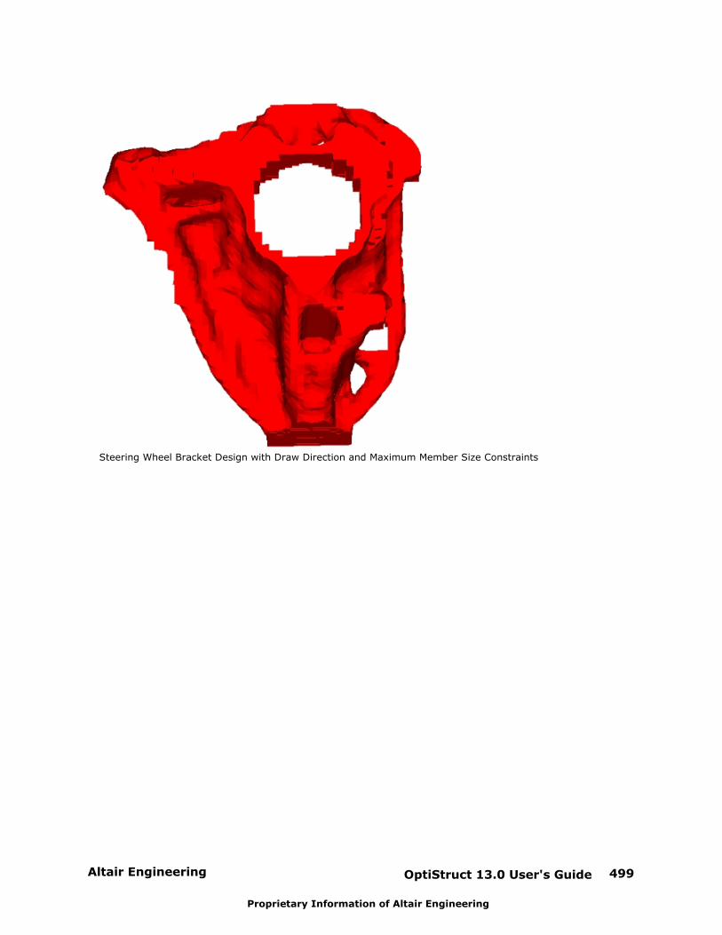
Altair Engineering OptiStruct 13.0 User's Guide 499
Proprietary Information of Altair Engineering
Steering Wheel Bracket Design with Draw Direction and Maximum Member Size Constraints
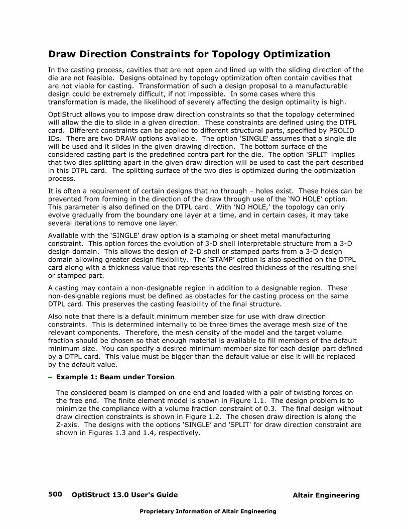
OptiStruct 13.0 User's Guide500 Altair Engineering
Proprietary Information of Altair Engineering
Draw Direction Constraints for Topology Optimization
In the casting process, cavities that are not open and lined up with the sliding direction of thedie are not feasible. Designs obtained by topology optimization often contain cavities thatare not viable for casting. Transformation of such a design proposal to a manufacturabledesign could be extremely difficult, if not impossible. In some cases where thistransformation is made, the likelihood of severely affecting the design optimality is high.
OptiStruct allows you to impose draw direction constraints so that the topology determinedwill allow the die to slide in a given direction. These constraints are defined using the DTPLcard. Different constraints can be applied to different structural parts, specified by PSOLIDIDs. There are two DRAW options available. The option 'SINGLE' assumes that a single diewill be used and it slides in the given drawing direction. The bottom surface of theconsidered casting part is the predefined contra part for the die. The option 'SPLIT' impliesthat two dies splitting apart in the given draw direction will be used to cast the part describedin this DTPL card. The splitting surface of the two dies is optimized during the optimizationprocess.
It is often a requirement of certain designs that no through – holes exist. These holes can beprevented from forming in the direction of the draw through use of the ‘NO HOLE’ option. This parameter is also defined on the DTPL card. With ‘NO HOLE,’ the topology can onlyevolve gradually from the boundary one layer at a time, and in certain cases, it may takeseveral iterations to remove one layer.
Available with the ‘SINGLE’ draw option is a stamping or sheet metal manufacturingconstraint. This option forces the evolution of 3-D shell interpretable structure from a 3-Ddesign domain. This allows the design of 2-D shell or stamped parts from a 3-D designdomain allowing greater design flexibility. The ‘STAMP’ option is also specified on the DTPLcard along with a thickness value that represents the desired thickness of the resulting shellor stamped part.
A casting may contain a non-designable region in addition to a designable region. Thesenon-designable regions must be defined as obstacles for the casting process on the sameDTPL card. This preserves the casting feasibility of the final structure.
Also note that there is a default minimum member size for use with draw directionconstraints. This is determined internally to be three times the average mesh size of therelevant components. Therefore, the mesh density of the model and the target volumefraction should be chosen so that enough material is available to fill members of the defaultminimum size. You can specify a desired minimum member size for each design part definedby a DTPL card. This value must be bigger than the default value or else it will be replacedby the default value.
Example 1: Beam under Torsion
The considered beam is clamped on one end and loaded with a pair of twisting forces onthe free end. The finite element model is shown in Figure 1.1. The design problem is tominimize the compliance with a volume fraction constraint of 0.3. The final design withoutdraw direction constraints is shown in Figure 1.2. The chosen draw direction is along theZ-axis. The designs with the options 'SINGLE’ and 'SPLIT' for draw direction constraint areshown in Figures 1.3 and 1.4, respectively.
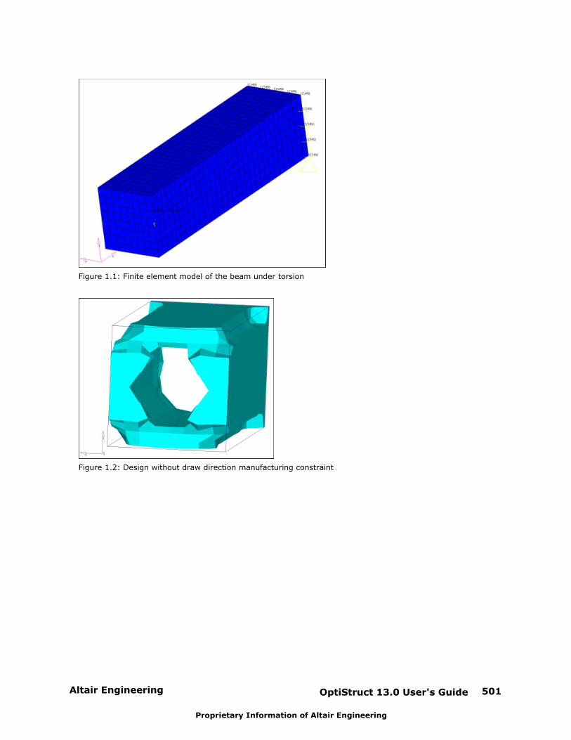
Altair Engineering OptiStruct 13.0 User's Guide 501
Proprietary Information of Altair Engineering
Figure 1.1: Finite element model of the beam under torsion
Figure 1.2: Design without draw direction manufacturing constraint
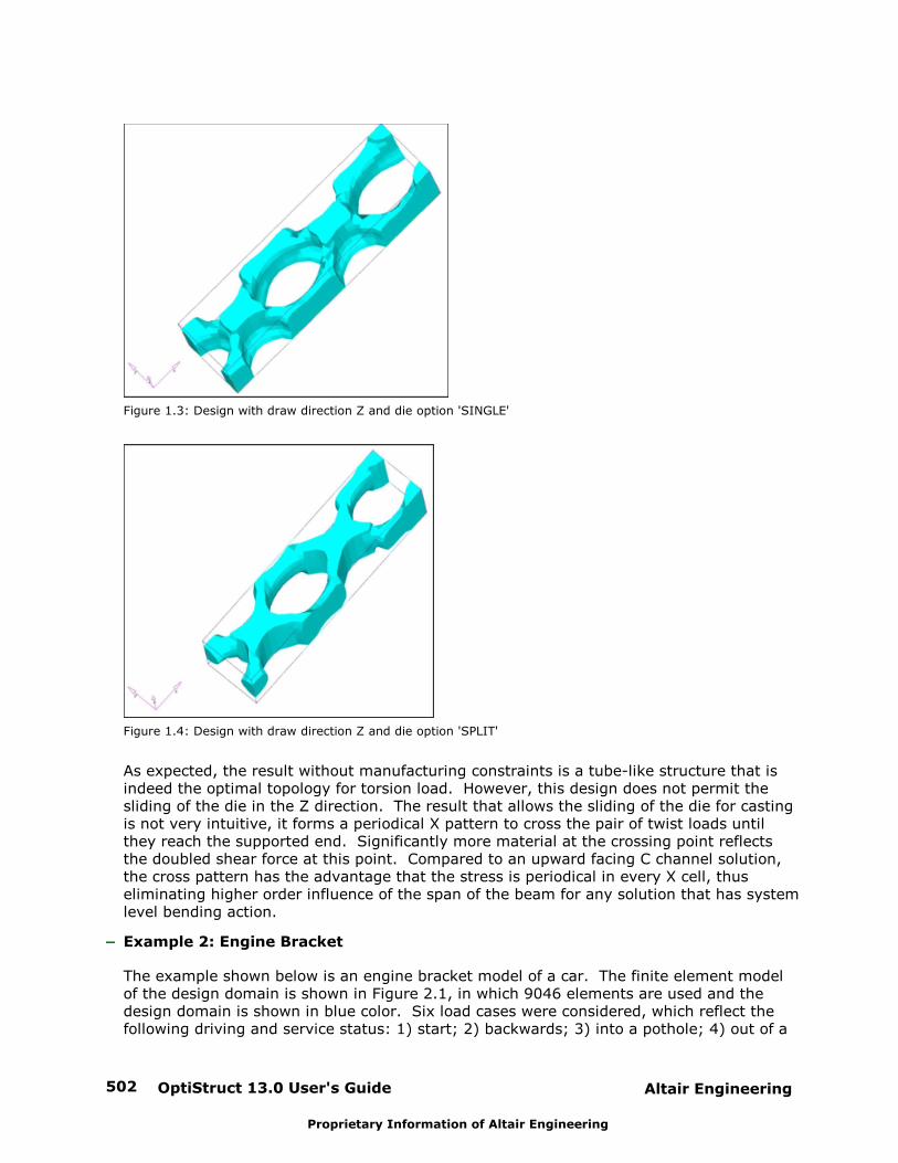
OptiStruct 13.0 User's Guide502 Altair Engineering
Proprietary Information of Altair Engineering
Figure 1.3: Design with draw direction Z and die option 'SINGLE'
Figure 1.4: Design with draw direction Z and die option 'SPLIT'
As expected, the result without manufacturing constraints is a tube-like structure that isindeed the optimal topology for torsion load. However, this design does not permit thesliding of the die in the Z direction. The result that allows the sliding of the die for castingis not very intuitive, it forms a periodical X pattern to cross the pair of twist loads untilthey reach the supported end. Significantly more material at the crossing point reflectsthe doubled shear force at this point. Compared to an upward facing C channel solution,the cross pattern has the advantage that the stress is periodical in every X cell, thuseliminating higher order influence of the span of the beam for any solution that has systemlevel bending action.
Example 2: Engine Bracket
The example shown below is an engine bracket model of a car. The finite element modelof the design domain is shown in Figure 2.1, in which 9046 elements are used and thedesign domain is shown in blue color. Six load cases were considered, which reflect thefollowing driving and service status: 1) start; 2) backwards; 3) into a pothole; 4) out of a
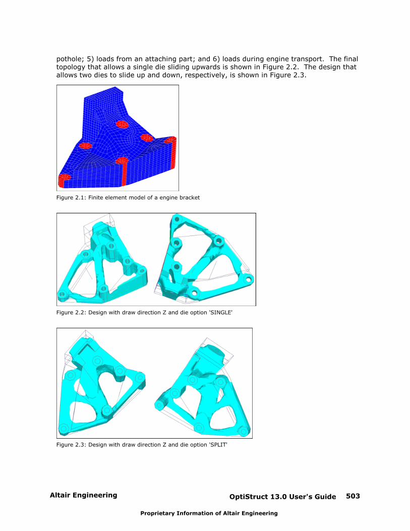
Altair Engineering OptiStruct 13.0 User's Guide 503
Proprietary Information of Altair Engineering
pothole; 5) loads from an attaching part; and 6) loads during engine transport. The finaltopology that allows a single die sliding upwards is shown in Figure 2.2. The design thatallows two dies to slide up and down, respectively, is shown in Figure 2.3.
Figure 2.1: Finite element model of a engine bracket
Figure 2.2: Design with draw direction Z and die option 'SINGLE'
Figure 2.3: Design with draw direction Z and die option 'SPLIT'
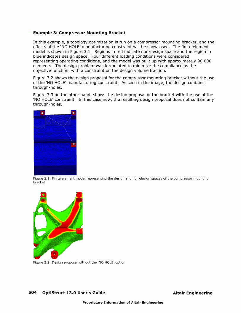
OptiStruct 13.0 User's Guide504 Altair Engineering
Proprietary Information of Altair Engineering
Example 3: Compressor Mounting Bracket
In this example, a topology optimization is run on a compressor mounting bracket, and theeffects of the ‘NO HOLE’ manufacturing constraint will be showcased. The finite elementmodel is shown in Figure 3.1. Regions in red indicate non-design space and the region inblue indicates design space. Four different loading conditions were consideredrepresenting operating conditions, and the model was built up with approximately 90,000elements. The design problem was formulated to minimize the compliance as theobjective function, with a constraint on the design volume fraction.
Figure 3.2 shows the design proposal for the compressor mounting bracket without the useof the ‘NO HOLE’ manufacturing constraint. As seen in the image, the design containsthrough-holes.
Figure 3.3 on the other hand, shows the design proposal of the bracket with the use of the‘NO HOLE’ constraint. In this case now, the resulting design proposal does not contain anythrough-holes.
Figure 3.1: Finite element model representing the design and non-design spaces of the compressor mountingbracket
Figure 3.2: Design proposal without the ‘NO HOLE’ option
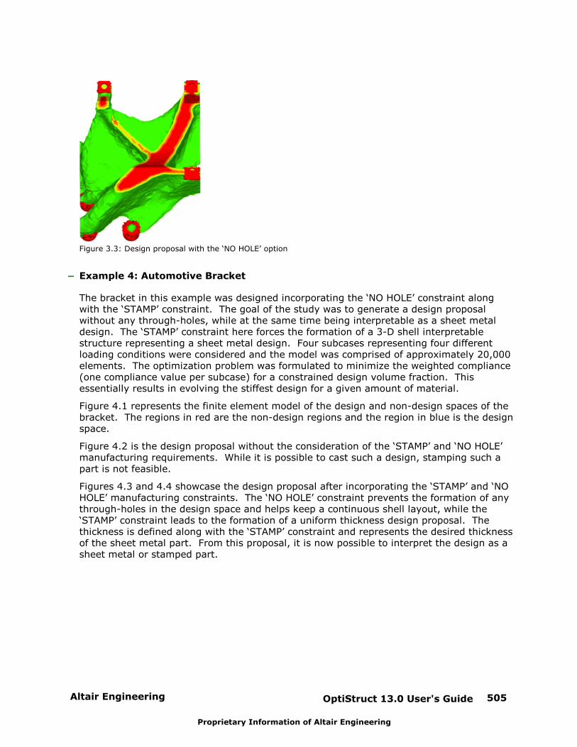
Altair Engineering OptiStruct 13.0 User's Guide 505
Proprietary Information of Altair Engineering
Figure 3.3: Design proposal with the ‘NO HOLE’ option
Example 4: Automotive Bracket
The bracket in this example was designed incorporating the ‘NO HOLE’ constraint alongwith the ‘STAMP’ constraint. The goal of the study was to generate a design proposalwithout any through-holes, while at the same time being interpretable as a sheet metaldesign. The ‘STAMP’ constraint here forces the formation of a 3-D shell interpretablestructure representing a sheet metal design. Four subcases representing four differentloading conditions were considered and the model was comprised of approximately 20,000elements. The optimization problem was formulated to minimize the weighted compliance(one compliance value per subcase) for a constrained design volume fraction. Thisessentially results in evolving the stiffest design for a given amount of material.
Figure 4.1 represents the finite element model of the design and non-design spaces of thebracket. The regions in red are the non-design regions and the region in blue is the designspace.
Figure 4.2 is the design proposal without the consideration of the ‘STAMP’ and ‘NO HOLE’manufacturing requirements. While it is possible to cast such a design, stamping such apart is not feasible.
Figures 4.3 and 4.4 showcase the design proposal after incorporating the ‘STAMP’ and ‘NOHOLE’ manufacturing constraints. The ‘NO HOLE’ constraint prevents the formation of anythrough-holes in the design space and helps keep a continuous shell layout, while the‘STAMP’ constraint leads to the formation of a uniform thickness design proposal. Thethickness is defined along with the ‘STAMP’ constraint and represents the desired thicknessof the sheet metal part. From this proposal, it is now possible to interpret the design as asheet metal or stamped part.
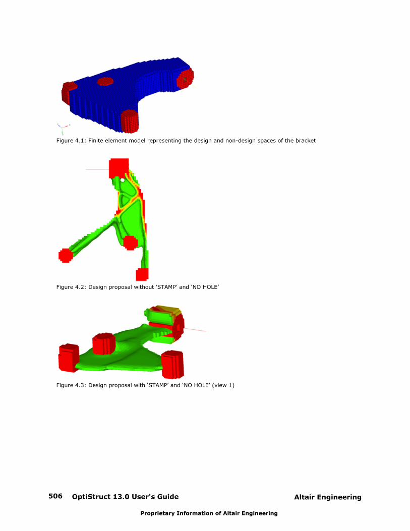
OptiStruct 13.0 User's Guide506 Altair Engineering
Proprietary Information of Altair Engineering
Figure 4.1: Finite element model representing the design and non-design spaces of the bracket
Figure 4.2: Design proposal without ‘STAMP’ and ‘NO HOLE’
Figure 4.3: Design proposal with ‘STAMP’ and ‘NO HOLE’ (view 1)

Altair Engineering OptiStruct 13.0 User's Guide 507
Proprietary Information of Altair Engineering
Figure 4.4: Design proposal with ‘STAMP’ and ‘NO HOLE’ (view 2)
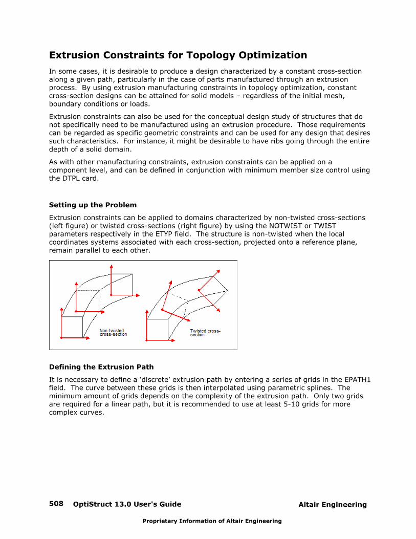
OptiStruct 13.0 User's Guide508 Altair Engineering
Proprietary Information of Altair Engineering
Extrusion Constraints for Topology Optimization
In some cases, it is desirable to produce a design characterized by a constant cross-sectionalong a given path, particularly in the case of parts manufactured through an extrusionprocess. By using extrusion manufacturing constraints in topology optimization, constantcross-section designs can be attained for solid models – regardless of the initial mesh,boundary conditions or loads.
Extrusion constraints can also be used for the conceptual design study of structures that donot specifically need to be manufactured using an extrusion procedure. Those requirementscan be regarded as specific geometric constraints and can be used for any design that desiressuch characteristics. For instance, it might be desirable to have ribs going through the entiredepth of a solid domain.
As with other manufacturing constraints, extrusion constraints can be applied on acomponent level, and can be defined in conjunction with minimum member size control usingthe DTPL card.
Setting up the Problem
Extrusion constraints can be applied to domains characterized by non-twisted cross-sections(left figure) or twisted cross-sections (right figure) by using the NOTWIST or TWISTparameters respectively in the ETYP field. The structure is non-twisted when the localcoordinates systems associated with each cross-section, projected onto a reference plane,remain parallel to each other.
Defining the Extrusion Path
It is necessary to define a ‘discrete’ extrusion path by entering a series of grids in the EPATH1field. The curve between these grids is then interpolated using parametric splines. Theminimum amount of grids depends on the complexity of the extrusion path. Only two gridsare required for a linear path, but it is recommended to use at least 5-10 grids for morecomplex curves.
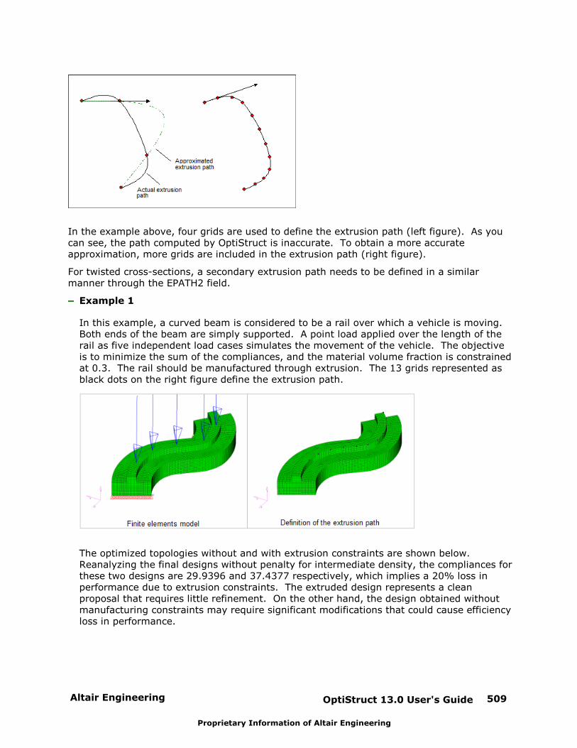
Altair Engineering OptiStruct 13.0 User's Guide 509
Proprietary Information of Altair Engineering
In the example above, four grids are used to define the extrusion path (left figure). As youcan see, the path computed by OptiStruct is inaccurate. To obtain a more accurateapproximation, more grids are included in the extrusion path (right figure).
For twisted cross-sections, a secondary extrusion path needs to be defined in a similarmanner through the EPATH2 field.
Example 1
In this example, a curved beam is considered to be a rail over which a vehicle is moving. Both ends of the beam are simply supported. A point load applied over the length of therail as five independent load cases simulates the movement of the vehicle. The objectiveis to minimize the sum of the compliances, and the material volume fraction is constrainedat 0.3. The rail should be manufactured through extrusion. The 13 grids represented asblack dots on the right figure define the extrusion path.
The optimized topologies without and with extrusion constraints are shown below. Reanalyzing the final designs without penalty for intermediate density, the compliances forthese two designs are 29.9396 and 37.4377 respectively, which implies a 20% loss inperformance due to extrusion constraints. The extruded design represents a cleanproposal that requires little refinement. On the other hand, the design obtained withoutmanufacturing constraints may require significant modifications that could cause efficiencyloss in performance.
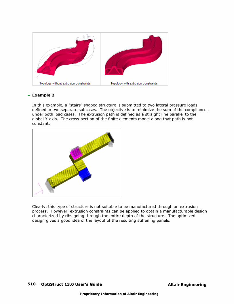
OptiStruct 13.0 User's Guide510 Altair Engineering
Proprietary Information of Altair Engineering
Example 2
In this example, a "stairs" shaped structure is submitted to two lateral pressure loadsdefined in two separate subcases. The objective is to minimize the sum of the compliancesunder both load cases. The extrusion path is defined as a straight line parallel to theglobal Y-axis. The cross-section of the finite elements model along that path is notconstant.
Clearly, this type of structure is not suitable to be manufactured through an extrusionprocess. However, extrusion constraints can be applied to obtain a manufacturable designcharacterized by ribs going through the entire depth of the structure. The optimizeddesign gives a good idea of the layout of the resulting stiffening panels.
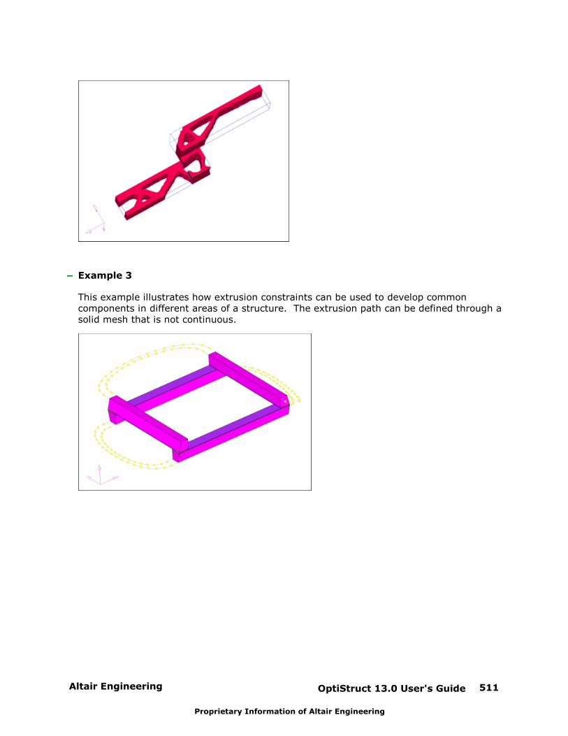
Altair Engineering OptiStruct 13.0 User's Guide 511
Proprietary Information of Altair Engineering
Example 3
This example illustrates how extrusion constraints can be used to develop commoncomponents in different areas of a structure. The extrusion path can be defined through asolid mesh that is not continuous.
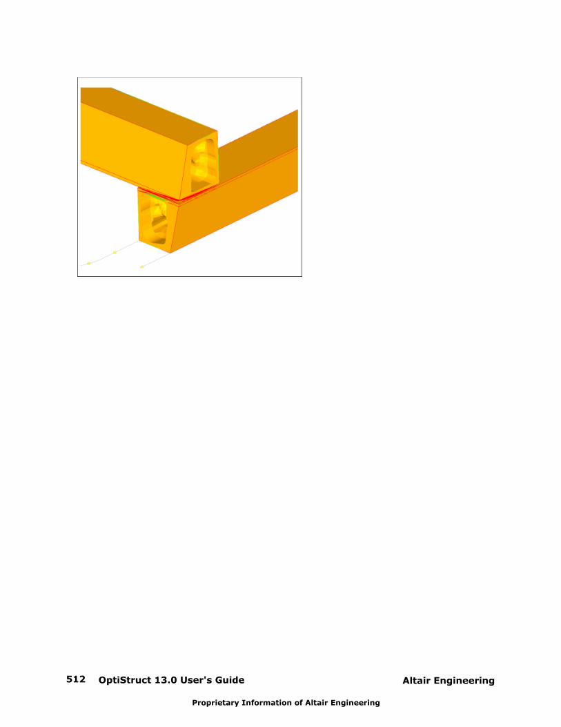
OptiStruct 13.0 User's Guide512 Altair Engineering
Proprietary Information of Altair Engineering
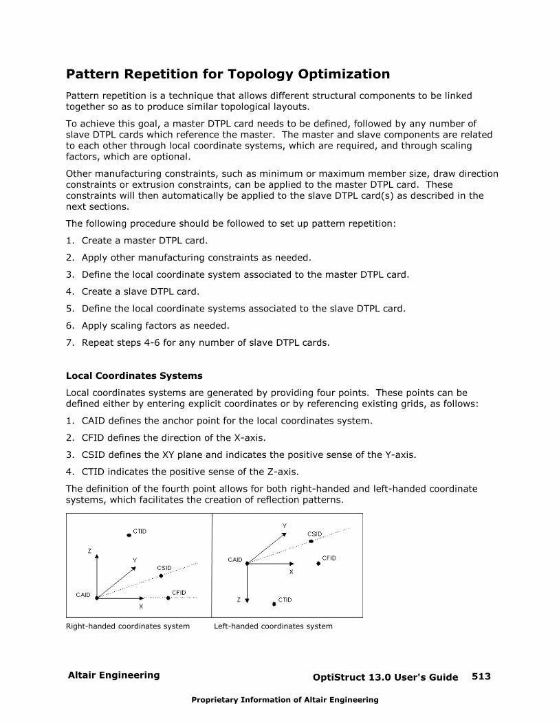
Altair Engineering OptiStruct 13.0 User's Guide 513
Proprietary Information of Altair Engineering
Pattern Repetition for Topology Optimization
Pattern repetition is a technique that allows different structural components to be linkedtogether so as to produce similar topological layouts.
To achieve this goal, a master DTPL card needs to be defined, followed by any number ofslave DTPL cards which reference the master. The master and slave components are relatedto each other through local coordinate systems, which are required, and through scalingfactors, which are optional.
Other manufacturing constraints, such as minimum or maximum member size, draw directionconstraints or extrusion constraints, can be applied to the master DTPL card. Theseconstraints will then automatically be applied to the slave DTPL card(s) as described in thenext sections.
The following procedure should be followed to set up pattern repetition:
1. Create a master DTPL card.
2. Apply other manufacturing constraints as needed.
3. Define the local coordinate system associated to the master DTPL card.
4. Create a slave DTPL card.
5. Define the local coordinate systems associated to the slave DTPL card.
6. Apply scaling factors as needed.
7. Repeat steps 4-6 for any number of slave DTPL cards.
Local Coordinates Systems
Local coordinates systems are generated by providing four points. These points can bedefined either by entering explicit coordinates or by referencing existing grids, as follows:
1. CAID defines the anchor point for the local coordinates system.
2. CFID defines the direction of the X-axis.
3. CSID defines the XY plane and indicates the positive sense of the Y-axis.
4. CTID indicates the positive sense of the Z-axis.
The definition of the fourth point allows for both right-handed and left-handed coordinatesystems, which facilitates the creation of reflection patterns.
Right-handed coordinates system Left-handed coordinates system
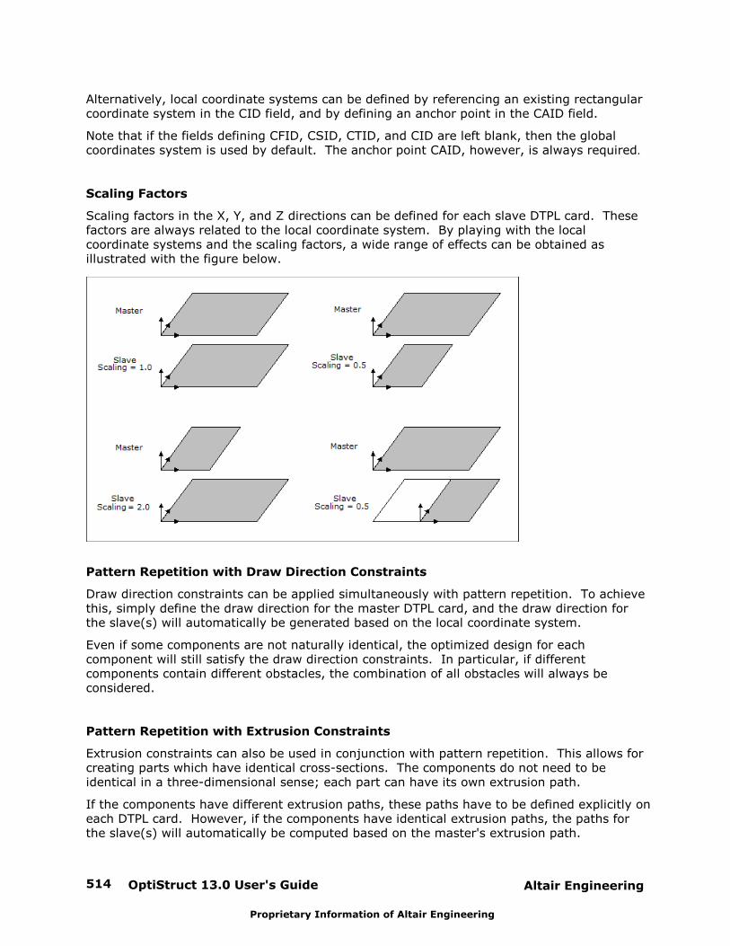
OptiStruct 13.0 User's Guide514 Altair Engineering
Proprietary Information of Altair Engineering
Alternatively, local coordinate systems can be defined by referencing an existing rectangularcoordinate system in the CID field, and by defining an anchor point in the CAID field.
Note that if the fields defining CFID, CSID, CTID, and CID are left blank, then the globalcoordinates system is used by default. The anchor point CAID, however, is always required.
Scaling Factors
Scaling factors in the X, Y, and Z directions can be defined for each slave DTPL card. Thesefactors are always related to the local coordinate system. By playing with the localcoordinate systems and the scaling factors, a wide range of effects can be obtained asillustrated with the figure below.
Pattern Repetition with Draw Direction Constraints
Draw direction constraints can be applied simultaneously with pattern repetition. To achievethis, simply define the draw direction for the master DTPL card, and the draw direction forthe slave(s) will automatically be generated based on the local coordinate system.
Even if some components are not naturally identical, the optimized design for eachcomponent will still satisfy the draw direction constraints. In particular, if differentcomponents contain different obstacles, the combination of all obstacles will always beconsidered.
Pattern Repetition with Extrusion Constraints
Extrusion constraints can also be used in conjunction with pattern repetition. This allows forcreating parts which have identical cross-sections. The components do not need to beidentical in a three-dimensional sense; each part can have its own extrusion path.
If the components have different extrusion paths, these paths have to be defined explicitly oneach DTPL card. However, if the components have identical extrusion paths, the paths forthe slave(s) will automatically be computed based on the master's extrusion path.
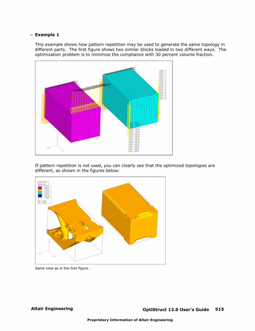
Altair Engineering OptiStruct 13.0 User's Guide 515
Proprietary Information of Altair Engineering
Example 1
This example shows how pattern repetition may be used to generate the same topology indifferent parts. The first figure shows two similar blocks loaded in two different ways. Theoptimization problem is to minimize the compliance with 30 percent volume fraction.
If pattern repetition is not used, you can clearly see that the optimized topologies aredifferent, as shown in the figures below:
Same view as in the first figure.
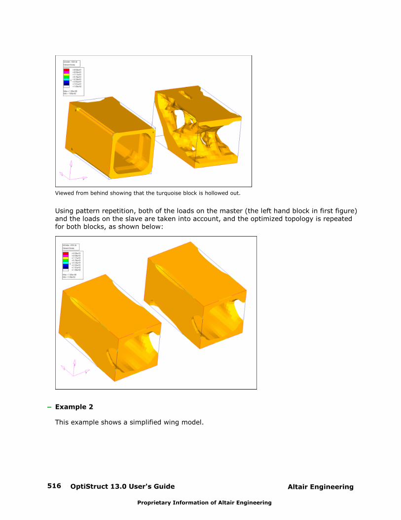
OptiStruct 13.0 User's Guide516 Altair Engineering
Proprietary Information of Altair Engineering
Viewed from behind showing that the turquoise block is hollowed out.
Using pattern repetition, both of the loads on the master (the left hand block in first figure)and the loads on the slave are taken into account, and the optimized topology is repeatedfor both blocks, as shown below:
Example 2
This example shows a simplified wing model.
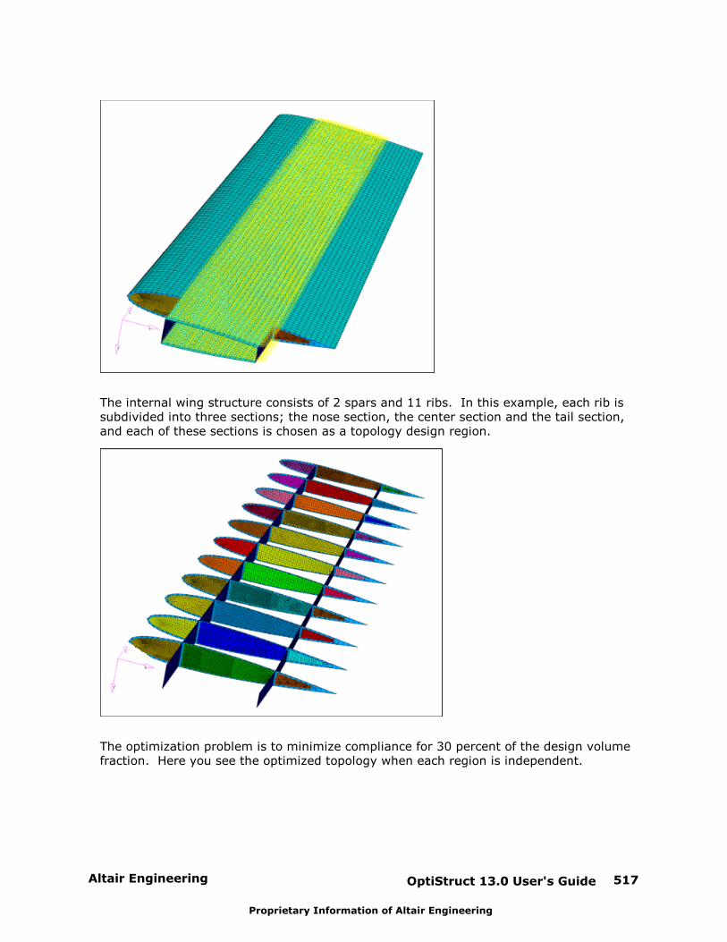
Altair Engineering OptiStruct 13.0 User's Guide 517
Proprietary Information of Altair Engineering
The internal wing structure consists of 2 spars and 11 ribs. In this example, each rib issubdivided into three sections; the nose section, the center section and the tail section,and each of these sections is chosen as a topology design region.
The optimization problem is to minimize compliance for 30 percent of the design volumefraction. Here you see the optimized topology when each region is independent.
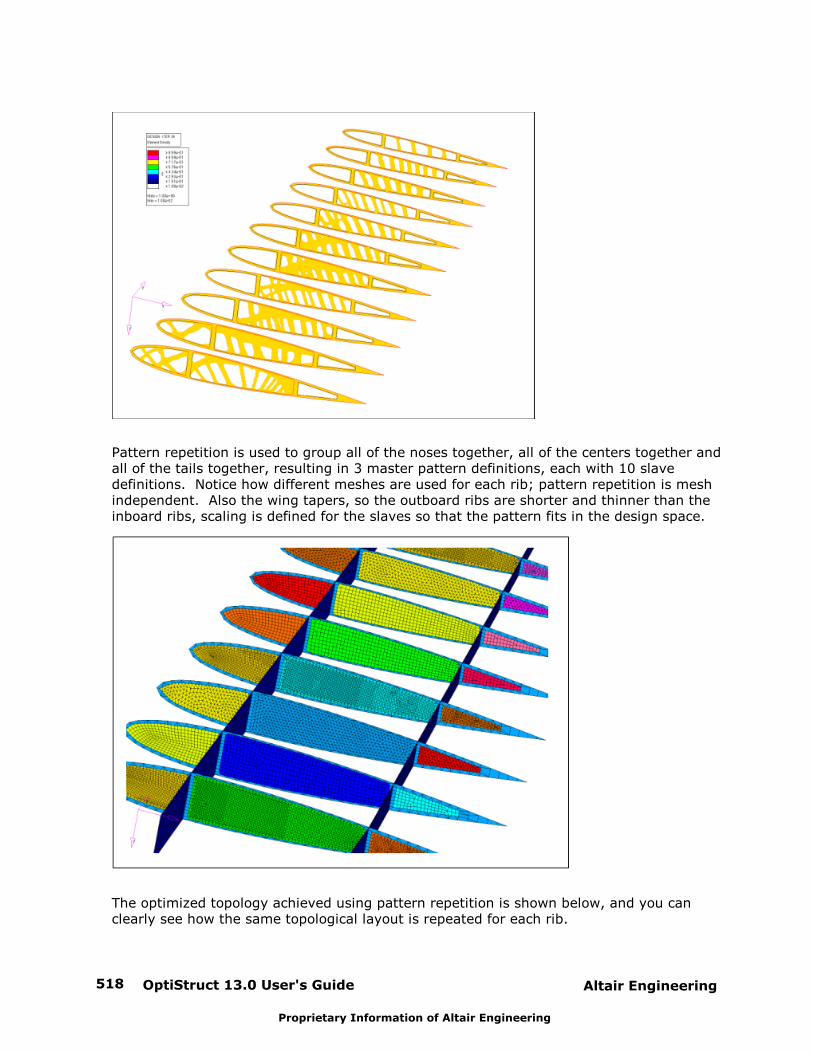
OptiStruct 13.0 User's Guide518 Altair Engineering
Proprietary Information of Altair Engineering
Pattern repetition is used to group all of the noses together, all of the centers together andall of the tails together, resulting in 3 master pattern definitions, each with 10 slavedefinitions. Notice how different meshes are used for each rib; pattern repetition is meshindependent. Also the wing tapers, so the outboard ribs are shorter and thinner than theinboard ribs, scaling is defined for the slaves so that the pattern fits in the design space.
The optimized topology achieved using pattern repetition is shown below, and you canclearly see how the same topological layout is repeated for each rib.
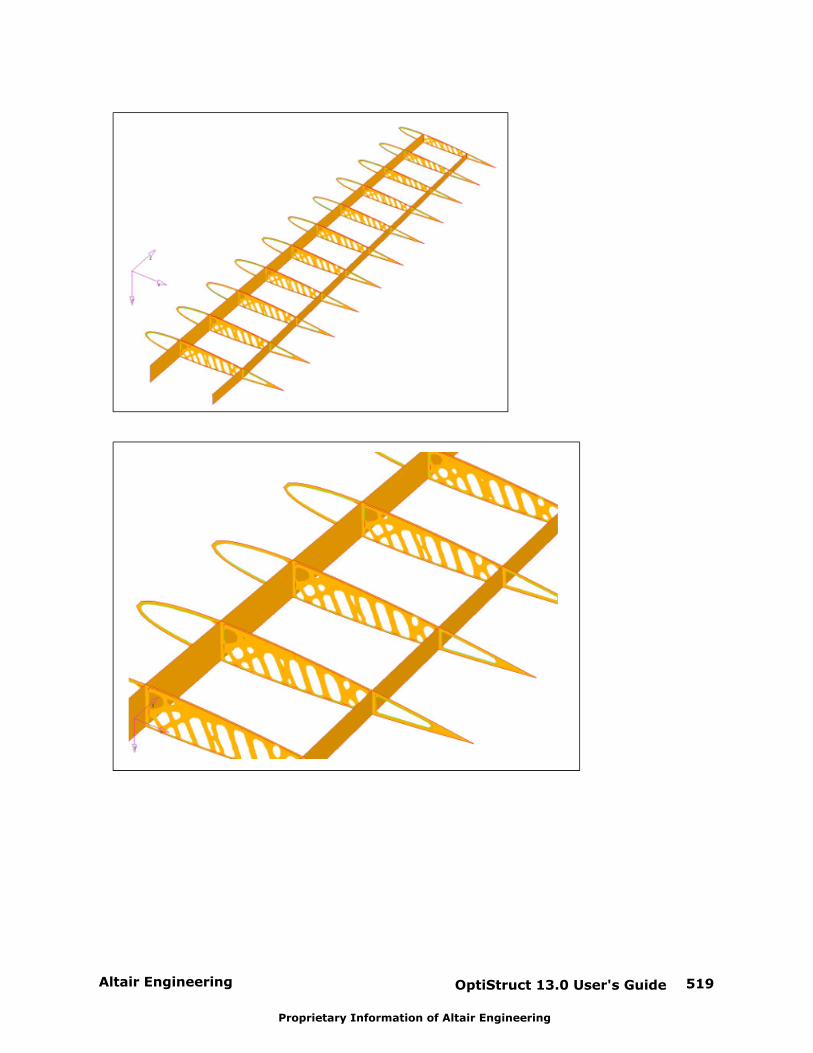
Altair Engineering OptiStruct 13.0 User's Guide 519
Proprietary Information of Altair Engineering
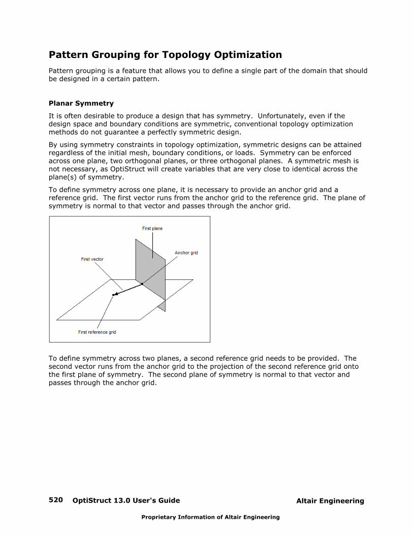
OptiStruct 13.0 User's Guide520 Altair Engineering
Proprietary Information of Altair Engineering
Pattern Grouping for Topology Optimization
Pattern grouping is a feature that allows you to define a single part of the domain that shouldbe designed in a certain pattern.
Planar Symmetry
It is often desirable to produce a design that has symmetry. Unfortunately, even if thedesign space and boundary conditions are symmetric, conventional topology optimizationmethods do not guarantee a perfectly symmetric design.
By using symmetry constraints in topology optimization, symmetric designs can be attainedregardless of the initial mesh, boundary conditions, or loads. Symmetry can be enforcedacross one plane, two orthogonal planes, or three orthogonal planes. A symmetric mesh isnot necessary, as OptiStruct will create variables that are very close to identical across theplane(s) of symmetry.
To define symmetry across one plane, it is necessary to provide an anchor grid and areference grid. The first vector runs from the anchor grid to the reference grid. The plane ofsymmetry is normal to that vector and passes through the anchor grid.
To define symmetry across two planes, a second reference grid needs to be provided. Thesecond vector runs from the anchor grid to the projection of the second reference grid ontothe first plane of symmetry. The second plane of symmetry is normal to that vector andpasses through the anchor grid.
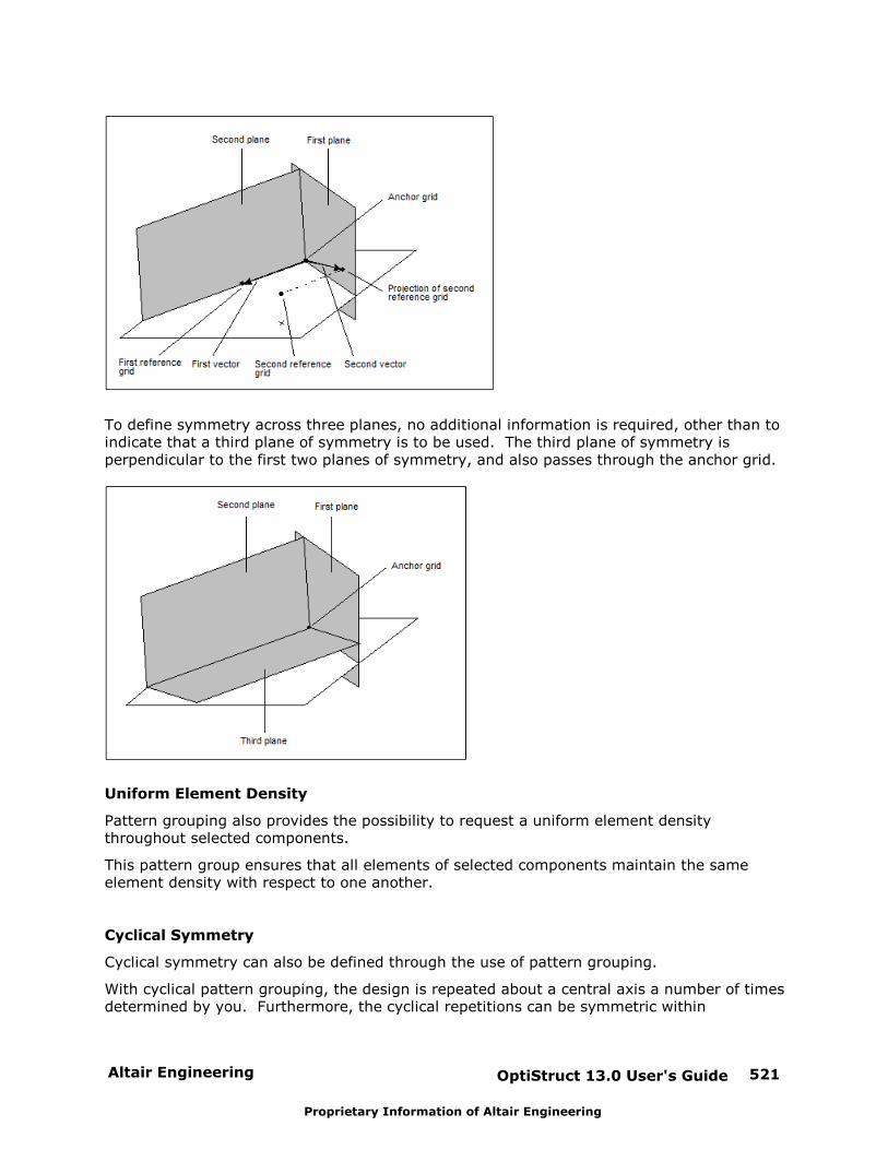
Altair Engineering OptiStruct 13.0 User's Guide 521
Proprietary Information of Altair Engineering
To define symmetry across three planes, no additional information is required, other than toindicate that a third plane of symmetry is to be used. The third plane of symmetry isperpendicular to the first two planes of symmetry, and also passes through the anchor grid.
Uniform Element Density
Pattern grouping also provides the possibility to request a uniform element densitythroughout selected components.
This pattern group ensures that all elements of selected components maintain the sameelement density with respect to one another.
Cyclical Symmetry
Cyclical symmetry can also be defined through the use of pattern grouping.
With cyclical pattern grouping, the design is repeated about a central axis a number of timesdetermined by you. Furthermore, the cyclical repetitions can be symmetric within
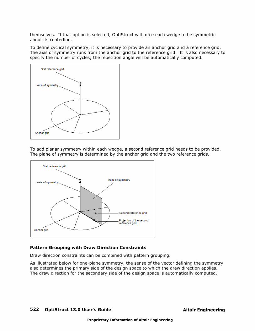
OptiStruct 13.0 User's Guide522 Altair Engineering
Proprietary Information of Altair Engineering
themselves. If that option is selected, OptiStruct will force each wedge to be symmetricabout its centerline.
To define cyclical symmetry, it is necessary to provide an anchor grid and a reference grid. The axis of symmetry runs from the anchor grid to the reference grid. It is also necessary tospecify the number of cycles; the repetition angle will be automatically computed.
To add planar symmetry within each wedge, a second reference grid needs to be provided. The plane of symmetry is determined by the anchor grid and the two reference grids.
Pattern Grouping with Draw Direction Constraints
Draw direction constraints can be combined with pattern grouping.
As illustrated below for one-plane symmetry, the sense of the vector defining the symmetryalso determines the primary side of the design space to which the draw direction applies. The draw direction for the secondary side of the design space is automatically computed.
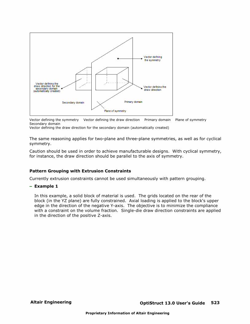
Altair Engineering OptiStruct 13.0 User's Guide 523
Proprietary Information of Altair Engineering
Vector defining the symmetry Vector defining the draw direction Primary domain Plane of symmetry Secondary domain Vector defining the draw direction for the secondary domain (automatically created)
The same reasoning applies for two-plane and three-plane symmetries, as well as for cyclicalsymmetry.
Caution should be used in order to achieve manufacturable designs. With cyclical symmetry,for instance, the draw direction should be parallel to the axis of symmetry.
Pattern Grouping with Extrusion Constraints
Currently extrusion constraints cannot be used simultaneously with pattern grouping.
Example 1
In this example, a solid block of material is used. The grids located on the rear of theblock (in the YZ plane) are fully constrained. Axial loading is applied to the block's upperedge in the direction of the negative Y-axis. The objective is to minimize the compliancewith a constraint on the volume fraction. Single-die draw direction constraints are appliedin the direction of the positive Z-axis.
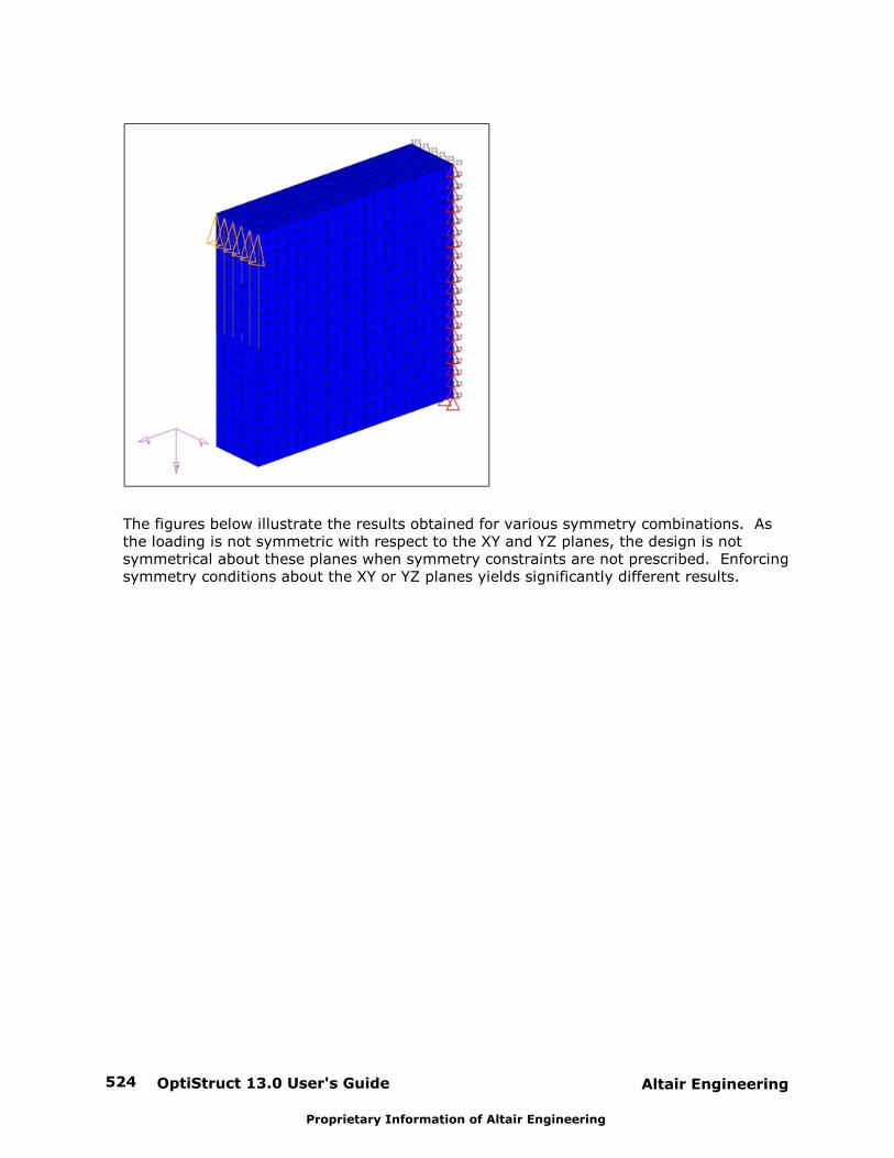
OptiStruct 13.0 User's Guide524 Altair Engineering
Proprietary Information of Altair Engineering
The figures below illustrate the results obtained for various symmetry combinations. Asthe loading is not symmetric with respect to the XY and YZ planes, the design is notsymmetrical about these planes when symmetry constraints are not prescribed. Enforcingsymmetry conditions about the XY or YZ planes yields significantly different results.
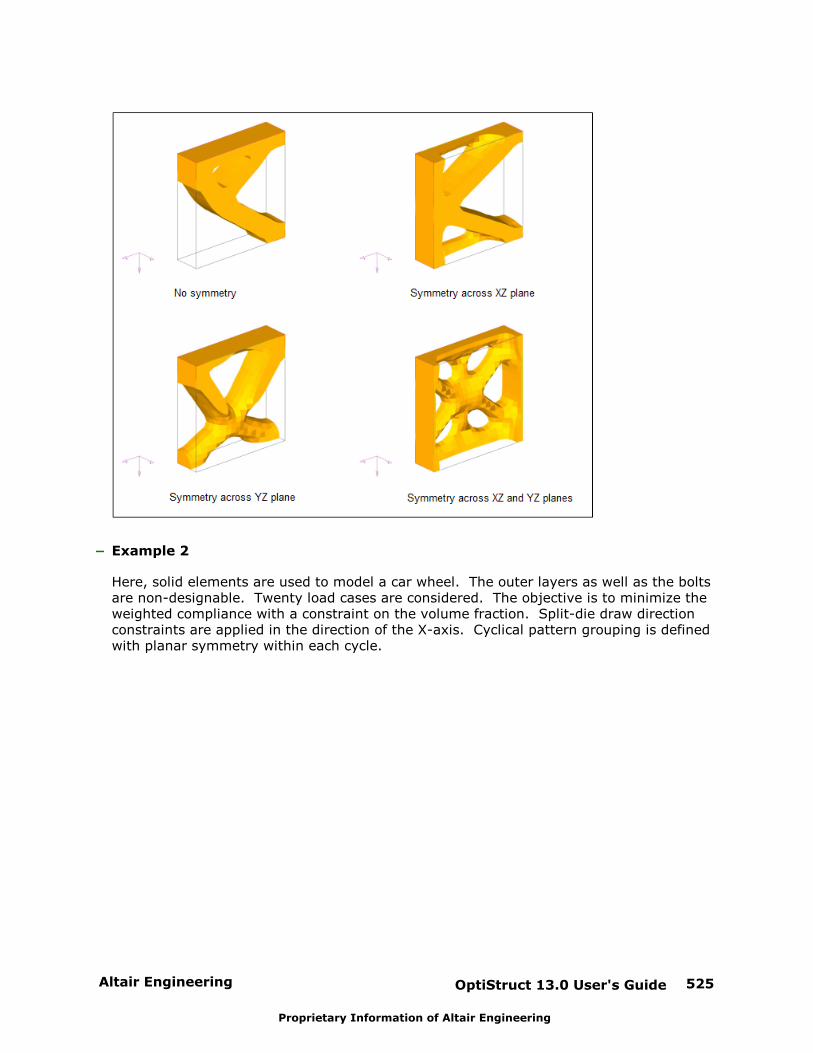
Altair Engineering OptiStruct 13.0 User's Guide 525
Proprietary Information of Altair Engineering
Example 2
Here, solid elements are used to model a car wheel. The outer layers as well as the boltsare non-designable. Twenty load cases are considered. The objective is to minimize theweighted compliance with a constraint on the volume fraction. Split-die draw directionconstraints are applied in the direction of the X-axis. Cyclical pattern grouping is definedwith planar symmetry within each cycle.
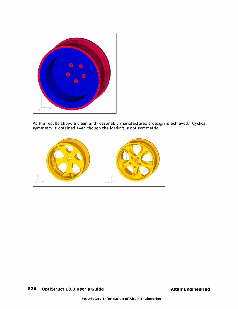
OptiStruct 13.0 User's Guide526 Altair Engineering
Proprietary Information of Altair Engineering
As the results show, a clean and reasonably manufacturable design is achieved. Cyclicalsymmetry is obtained even though the loading is not symmetric.
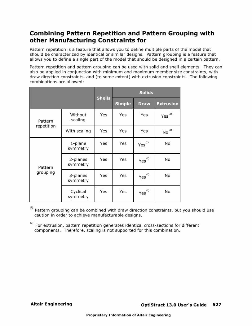
Altair Engineering OptiStruct 13.0 User's Guide 527
Proprietary Information of Altair Engineering
Combining Pattern Repetition and Pattern Grouping withother Manufacturing Constraints for
Pattern repetition is a feature that allows you to define multiple parts of the model thatshould be characterized by identical or similar designs. Pattern grouping is a feature thatallows you to define a single part of the model that should be designed in a certain pattern.
Pattern repetition and pattern grouping can be used with solid and shell elements. They canalso be applied in conjunction with minimum and maximum member size constraints, withdraw direction constraints, and (to some extent) with extrusion constraints. The followingcombinations are allowed:
Shells
Solids
Simple Draw Extrusion
Patternrepetition
Withoutscaling
Yes Yes Yes Yes
With scaling Yes Yes Yes No
Patterngrouping
1-planesymmetry
Yes Yes Yes No
2-planessymmetry
Yes Yes Yes No
3-planessymmetry
Yes Yes Yes No
Cyclicalsymmetry
Yes Yes Yes No
Pattern grouping can be combined with draw direction constraints, but you should usecaution in order to achieve manufacturable designs.
For extrusion, pattern repetition generates identical cross-sections for differentcomponents. Therefore, scaling is not supported for this combination.

OptiStruct 13.0 User's Guide528 Altair Engineering
Proprietary Information of Altair Engineering
Manufacturability for Topography Optimization
Manufacturing methods can place constraints on the types of reinforcement patternsavailable for a given part. Some examples of this are: channels, which must have acontinuous cross-section; discs, which must be turned on a lathe; and stampings, whichcannot have the die lock conditions.
These constraints can be accounted for in topography optimization by using Pattern GroupingOptions, and a design with a manufacturable reinforcement pattern can be generated.
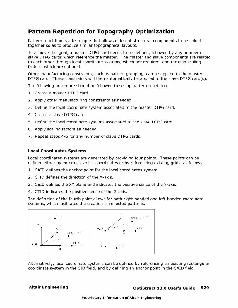
Altair Engineering OptiStruct 13.0 User's Guide 529
Proprietary Information of Altair Engineering
Pattern Repetition for Topography Optimization
Pattern repetition is a technique that allows different structural components to be linkedtogether so as to produce similar topographical layouts.
To achieve this goal, a master DTPG card needs to be defined, followed by any number ofslave DTPG cards which reference the master. The master and slave components are relatedto each other through local coordinate systems, which are required, and through scalingfactors, which are optional.
Other manufacturing constraints, such as pattern grouping, can be applied to the masterDTPG card. These constraints will then automatically be applied to the slave DTPG card(s).
The following procedure should be followed to set up pattern repetition:
1. Create a master DTPG card.
2. Apply other manufacturing constraints as needed.
3. Define the local coordinate system associated to the master DTPG card.
4. Create a slave DTPG card.
5. Define the local coordinate systems associated to the slave DTPG card.
6. Apply scaling factors as needed.
7. Repeat steps 4-6 for any number of slave DTPG cards.
Local Coordinates Systems
Local coordinates systems are generated by providing four points. These points can bedefined either by entering explicit coordinates or by referencing existing grids, as follows:
1. CAID defines the anchor point for the local coordinates system.
2. CFID defines the direction of the X-axis.
3. CSID defines the XY plane and indicates the positive sense of the Y-axis.
4. CTID indicates the positive sense of the Z-axis.
The definition of the fourth point allows for both right-handed and left-handed coordinatesystems, which facilitates the creation of reflected patterns.
Alternatively, local coordinate systems can be defined by referencing an existing rectangularcoordinate system in the CID field, and by defining an anchor point in the CAID field.
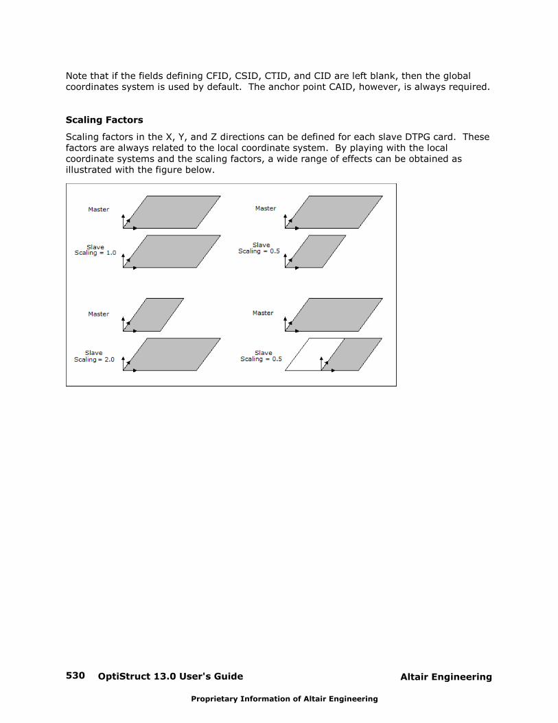
OptiStruct 13.0 User's Guide530 Altair Engineering
Proprietary Information of Altair Engineering
Note that if the fields defining CFID, CSID, CTID, and CID are left blank, then the globalcoordinates system is used by default. The anchor point CAID, however, is always required.
Scaling Factors
Scaling factors in the X, Y, and Z directions can be defined for each slave DTPG card. Thesefactors are always related to the local coordinate system. By playing with the localcoordinate systems and the scaling factors, a wide range of effects can be obtained asillustrated with the figure below.
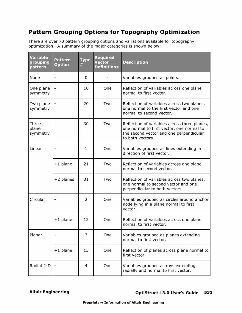
Altair Engineering OptiStruct 13.0 User's Guide 531
Proprietary Information of Altair Engineering
Pattern Grouping Options for Topography Optimization
There are over 70 pattern grouping options and variations available for topographyoptimization. A summary of the major categories is shown below:
Variablegroupingpattern
PatternOption
Type#
RequiredVectorDefinitions
Description
None - 0 - Variables grouped as points.
One planesymmetry
- 10 One Reflection of variables across one planenormal to first vector.
Two planesymmetry
- 20 Two Reflection of variables across two planes,one normal to the first vector and onenormal to second vector.
Threeplanesymmetry
- 30 Two Reflection of variables across three planes,one normal to first vector, one normal tothe second vector and one perpendicularto both vectors.
Linear - 1 One Variables grouped as lines extending indirection of first vector.
+1 plane 21 Two Reflection of variables across one planenormal to second vector.
+2 planes 31 Two Reflection of variables across two planes,one normal to second vector and oneperpendicular to both vectors.
Circular - 2 One Variables grouped as circles around anchornode lying in a plane normal to firstvector.
+1 plane 12 One Reflection of variables across one planenormal to first vector.
Planar - 3 One Variables grouped as planes extendingnormal to first vector.
+1 plane 13 One Reflection of planes across plane normal tofirst vector.
Radial 2-D - 4 One Variables grouped as rays extendingradially and normal to first vector.
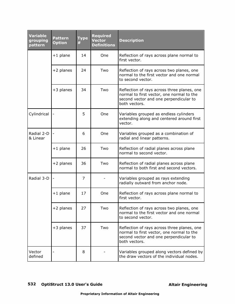
OptiStruct 13.0 User's Guide532 Altair Engineering
Proprietary Information of Altair Engineering
Variablegroupingpattern
PatternOption
Type#
RequiredVectorDefinitions
Description
+1 plane 14 One Reflection of rays across plane normal tofirst vector.
+2 planes 24 Two Reflection of rays across two planes, onenormal to the first vector and one normalto second vector.
+3 planes 34 Two Reflection of rays across three planes, onenormal to first vector, one normal to thesecond vector and one perpendicular toboth vectors.
Cylindrical - 5 One Variables grouped as endless cylindersextending along and centered around firstvector.
Radial 2-D& Linear
- 6 One Variables grouped as a combination ofradial and linear patterns.
+1 plane 26 Two Reflection of radial planes across planenormal to second vector.
+2 planes 36 Two Reflection of radial planes across planenormal to both first and second vectors.
Radial 3-D - 7 - Variables grouped as rays extendingradially outward from anchor node.
+1 plane 17 One Reflection of rays across plane normal tofirst vector.
+2 planes 27 Two Reflection of rays across two planes, onenormal to the first vector and one normalto second vector.
+3 planes 37 Two Reflection of rays across three planes, onenormal to first vector, one normal to thesecond vector and one perpendicular toboth vectors.
Vectordefined
- 8 - Variables grouped along vectors defined bythe draw vectors of the individual nodes.
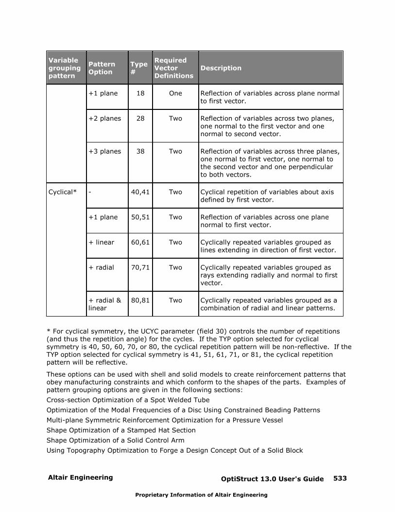
Altair Engineering OptiStruct 13.0 User's Guide 533
Proprietary Information of Altair Engineering
Variablegroupingpattern
PatternOption
Type#
RequiredVectorDefinitions
Description
+1 plane 18 One Reflection of variables across plane normalto first vector.
+2 planes 28 Two Reflection of variables across two planes,one normal to the first vector and onenormal to second vector.
+3 planes 38 Two Reflection of variables across three planes,one normal to first vector, one normal tothe second vector and one perpendicularto both vectors.
Cyclical* - 40,41 Two Cyclical repetition of variables about axisdefined by first vector.
+1 plane 50,51 Two Reflection of variables across one planenormal to first vector.
+ linear 60,61 Two Cyclically repeated variables grouped aslines extending in direction of first vector.
+ radial 70,71 Two Cyclically repeated variables grouped asrays extending radially and normal to firstvector.
+ radial &linear
80,81 Two Cyclically repeated variables grouped as acombination of radial and linear patterns.
* For cyclical symmetry, the UCYC parameter (field 30) controls the number of repetitions(and thus the repetition angle) for the cycles. If the TYP option selected for cyclicalsymmetry is 40, 50, 60, 70, or 80, the cyclical repetition pattern will be non-reflective. If theTYP option selected for cyclical symmetry is 41, 51, 61, 71, or 81, the cyclical repetitionpattern will be reflective.
These options can be used with shell and solid models to create reinforcement patterns thatobey manufacturing constraints and which conform to the shapes of the parts. Examples ofpattern grouping options are given in the following sections:
Cross-section Optimization of a Spot Welded Tube
Optimization of the Modal Frequencies of a Disc Using Constrained Beading Patterns
Multi-plane Symmetric Reinforcement Optimization for a Pressure Vessel
Shape Optimization of a Stamped Hat Section
Shape Optimization of a Solid Control Arm
Using Topography Optimization to Forge a Design Concept Out of a Solid Block

OptiStruct 13.0 User's Guide534 Altair Engineering
Proprietary Information of Altair Engineering
None
If no variable grouping pattern is selected, OptiStruct will automatically generate circularbead variable definitions throughout the design variable domain as shown below:
TYP = 0: No symmetry
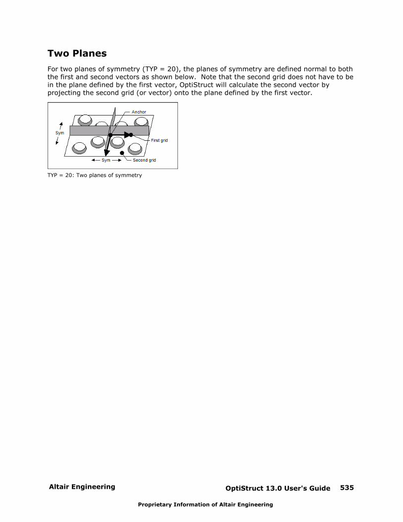
Altair Engineering OptiStruct 13.0 User's Guide 535
Proprietary Information of Altair Engineering
Two Planes
For two planes of symmetry (TYP = 20), the planes of symmetry are defined normal to boththe first and second vectors as shown below. Note that the second grid does not have to bein the plane defined by the first vector, OptiStruct will calculate the second vector byprojecting the second grid (or vector) onto the plane defined by the first vector.
TYP = 20: Two planes of symmetry
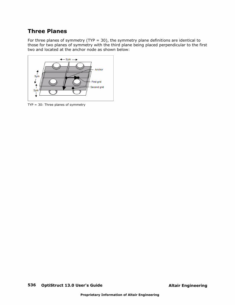
OptiStruct 13.0 User's Guide536 Altair Engineering
Proprietary Information of Altair Engineering
Three Planes
For three planes of symmetry (TYP = 30), the symmetry plane definitions are identical tothose for two planes of symmetry with the third plane being placed perpendicular to the firsttwo and located at the anchor node as shown below:
TYP = 30: Three planes of symmetry

Altair Engineering OptiStruct 13.0 User's Guide 537
Proprietary Information of Altair Engineering
One Plane - Simple Symmetry Options
For a single plane of symmetry (TYP = 10), the plane is defined normal to the first vector andis located at the anchor node as shown below:
TYP = 10: One plane of symmetry
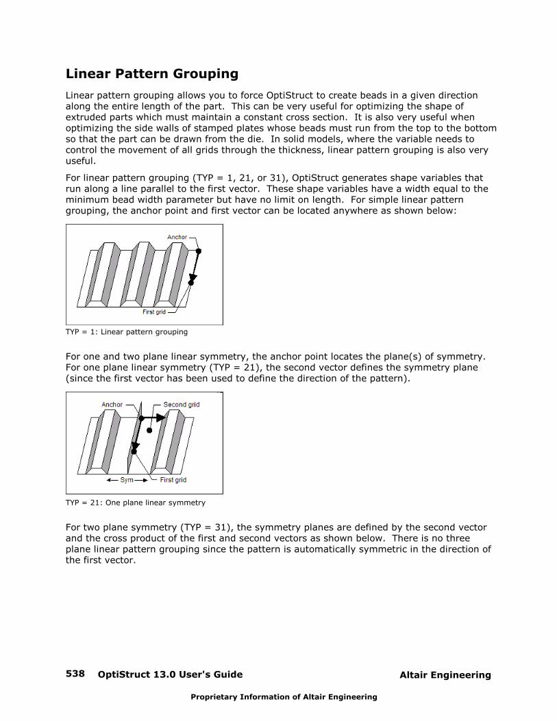
OptiStruct 13.0 User's Guide538 Altair Engineering
Proprietary Information of Altair Engineering
Linear Pattern Grouping
Linear pattern grouping allows you to force OptiStruct to create beads in a given directionalong the entire length of the part. This can be very useful for optimizing the shape ofextruded parts which must maintain a constant cross section. It is also very useful whenoptimizing the side walls of stamped plates whose beads must run from the top to the bottomso that the part can be drawn from the die. In solid models, where the variable needs tocontrol the movement of all grids through the thickness, linear pattern grouping is also veryuseful.
For linear pattern grouping (TYP = 1, 21, or 31), OptiStruct generates shape variables thatrun along a line parallel to the first vector. These shape variables have a width equal to theminimum bead width parameter but have no limit on length. For simple linear patterngrouping, the anchor point and first vector can be located anywhere as shown below:
TYP = 1: Linear pattern grouping
For one and two plane linear symmetry, the anchor point locates the plane(s) of symmetry. For one plane linear symmetry (TYP = 21), the second vector defines the symmetry plane(since the first vector has been used to define the direction of the pattern).
TYP = 21: One plane linear symmetry
For two plane symmetry (TYP = 31), the symmetry planes are defined by the second vectorand the cross product of the first and second vectors as shown below. There is no threeplane linear pattern grouping since the pattern is automatically symmetric in the direction ofthe first vector.
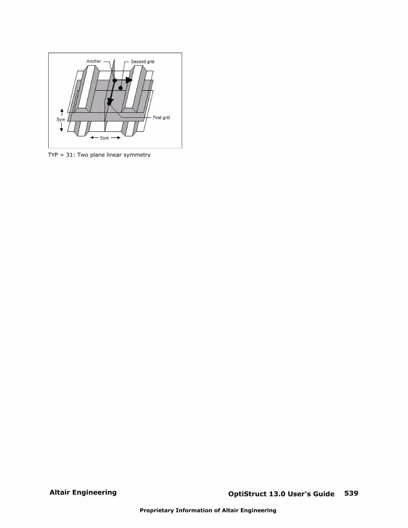
Altair Engineering OptiStruct 13.0 User's Guide 539
Proprietary Information of Altair Engineering
TYP = 31: Two plane linear symmetry
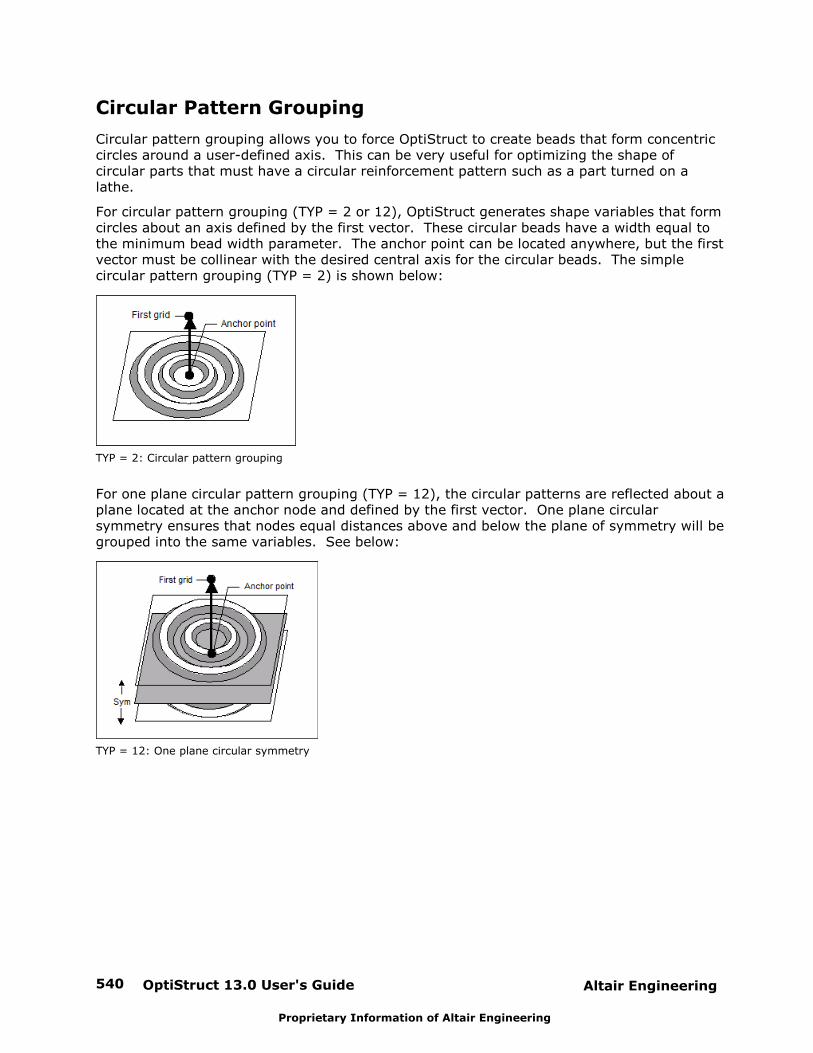
OptiStruct 13.0 User's Guide540 Altair Engineering
Proprietary Information of Altair Engineering
Circular Pattern Grouping
Circular pattern grouping allows you to force OptiStruct to create beads that form concentriccircles around a user-defined axis. This can be very useful for optimizing the shape ofcircular parts that must have a circular reinforcement pattern such as a part turned on alathe.
For circular pattern grouping (TYP = 2 or 12), OptiStruct generates shape variables that formcircles about an axis defined by the first vector. These circular beads have a width equal tothe minimum bead width parameter. The anchor point can be located anywhere, but the firstvector must be collinear with the desired central axis for the circular beads. The simplecircular pattern grouping (TYP = 2) is shown below:
TYP = 2: Circular pattern grouping
For one plane circular pattern grouping (TYP = 12), the circular patterns are reflected about aplane located at the anchor node and defined by the first vector. One plane circularsymmetry ensures that nodes equal distances above and below the plane of symmetry will begrouped into the same variables. See below:
TYP = 12: One plane circular symmetry
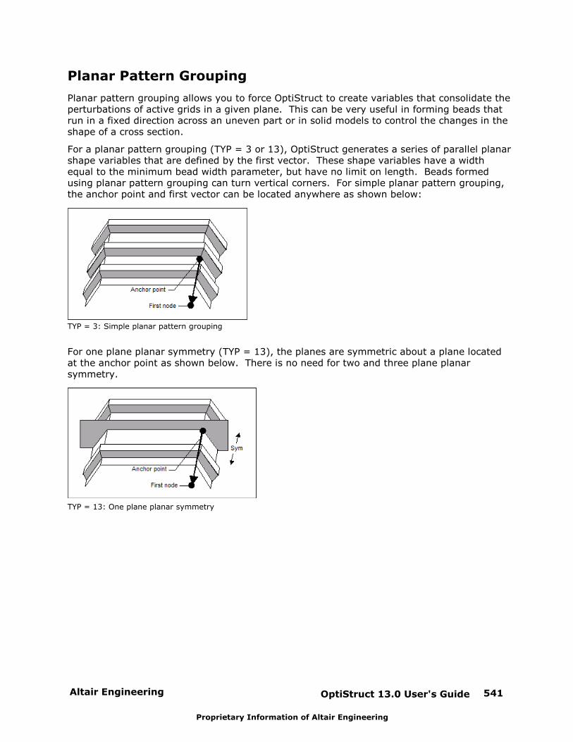
Altair Engineering OptiStruct 13.0 User's Guide 541
Proprietary Information of Altair Engineering
Planar Pattern Grouping
Planar pattern grouping allows you to force OptiStruct to create variables that consolidate theperturbations of active grids in a given plane. This can be very useful in forming beads thatrun in a fixed direction across an uneven part or in solid models to control the changes in theshape of a cross section.
For a planar pattern grouping (TYP = 3 or 13), OptiStruct generates a series of parallel planarshape variables that are defined by the first vector. These shape variables have a widthequal to the minimum bead width parameter, but have no limit on length. Beads formedusing planar pattern grouping can turn vertical corners. For simple planar pattern grouping,the anchor point and first vector can be located anywhere as shown below:
TYP = 3: Simple planar pattern grouping
For one plane planar symmetry (TYP = 13), the planes are symmetric about a plane locatedat the anchor point as shown below. There is no need for two and three plane planarsymmetry.
TYP = 13: One plane planar symmetry
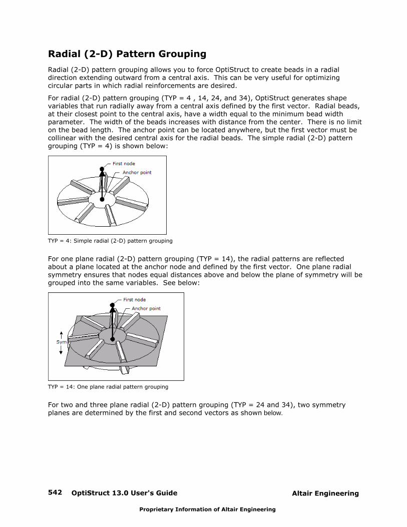
OptiStruct 13.0 User's Guide542 Altair Engineering
Proprietary Information of Altair Engineering
Radial (2-D) Pattern Grouping
Radial (2-D) pattern grouping allows you to force OptiStruct to create beads in a radialdirection extending outward from a central axis. This can be very useful for optimizingcircular parts in which radial reinforcements are desired.
For radial (2-D) pattern grouping (TYP = 4 , 14, 24, and 34), OptiStruct generates shapevariables that run radially away from a central axis defined by the first vector. Radial beads,at their closest point to the central axis, have a width equal to the minimum bead widthparameter. The width of the beads increases with distance from the center. There is no limiton the bead length. The anchor point can be located anywhere, but the first vector must becollinear with the desired central axis for the radial beads. The simple radial (2-D) patterngrouping (TYP = 4) is shown below:
TYP = 4: Simple radial (2-D) pattern grouping
For one plane radial (2-D) pattern grouping (TYP = 14), the radial patterns are reflectedabout a plane located at the anchor node and defined by the first vector. One plane radialsymmetry ensures that nodes equal distances above and below the plane of symmetry will begrouped into the same variables. See below:
TYP = 14: One plane radial pattern grouping
For two and three plane radial (2-D) pattern grouping (TYP = 24 and 34), two symmetryplanes are determined by the first and second vectors as shown below.
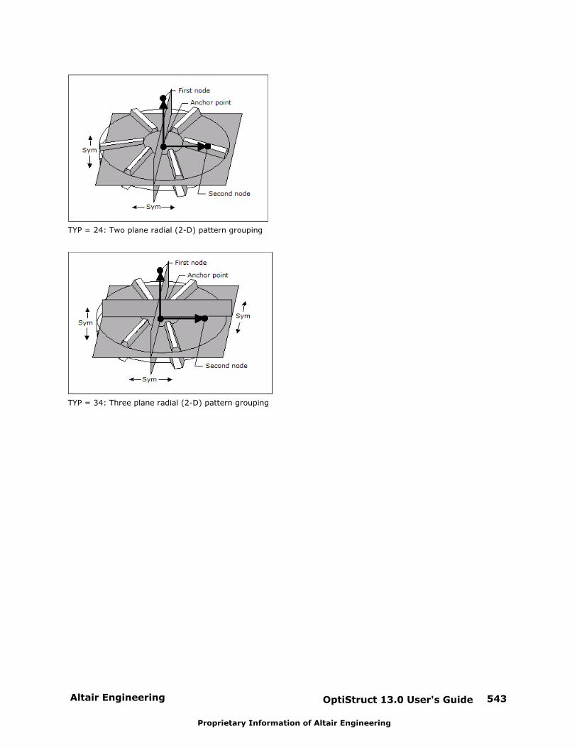
Altair Engineering OptiStruct 13.0 User's Guide 543
Proprietary Information of Altair Engineering
TYP = 24: Two plane radial (2-D) pattern grouping
TYP = 34: Three plane radial (2-D) pattern grouping

OptiStruct 13.0 User's Guide544 Altair Engineering
Proprietary Information of Altair Engineering
Cylindrical Pattern Grouping
Cylindrical pattern grouping allows you to force OptiStruct to create variables thatconsolidate the perturbations of active grids along the surface of a cylinder. This can beuseful in assigning a circular pattern grouping through the thickness of a solid model.
For a cylindrical pattern grouping (TYP = 5), OptiStruct generates a series of concentriccylinders that run parallel to and are positioned about the first vector. The cylindrical patterngrouping is essentially the linear pattern grouping combined with the circular patterngrouping. The anchor point can be located anywhere, but the first vector must be collinearwith the desired central axis for the cylinders.

Altair Engineering OptiStruct 13.0 User's Guide 545
Proprietary Information of Altair Engineering
Radial 2-D and Linear Pattern Grouping
Radial linear pattern grouping allows you to force OptiStruct to create variables thatconsolidate the perturbations of active grids along planes running radially from a central axis. This can be useful for assigning radial pattern groupings through the thickness of a solidmodel.
For a radial linear pattern grouping (TYP = 6), OptiStruct generates a series of planes thatrun radially away from, and in the same plane as, the first vector. The radial linear patterngrouping is essentially the linear pattern grouping combined with the radial pattern grouping. The anchor point can be located anywhere, but the first vector must be collinear with thedesired central axis for the radial planes.
One and two planes of radial linear pattern grouping (TYP = 26 and 36) can be created byusing the second vector to define the planes of symmetry. The symmetry planes areassigned in a manner similar to that for two and three plane radial symmetry.
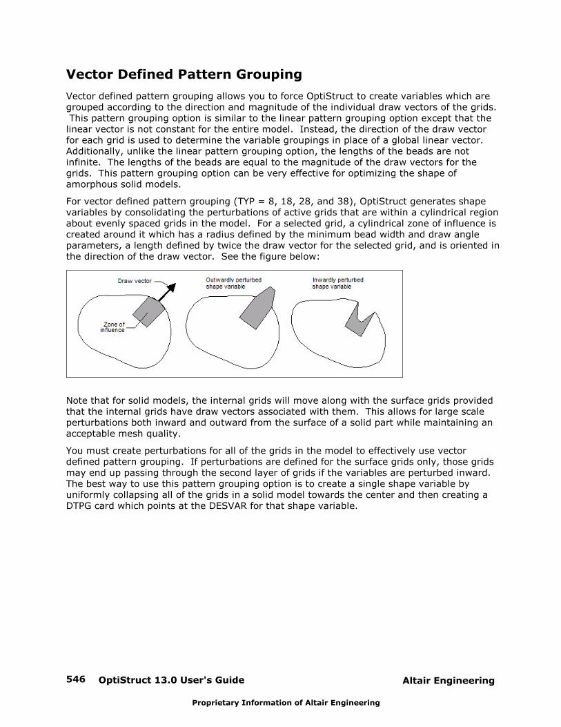
OptiStruct 13.0 User's Guide546 Altair Engineering
Proprietary Information of Altair Engineering
Vector Defined Pattern Grouping
Vector defined pattern grouping allows you to force OptiStruct to create variables which aregrouped according to the direction and magnitude of the individual draw vectors of the grids. This pattern grouping option is similar to the linear pattern grouping option except that thelinear vector is not constant for the entire model. Instead, the direction of the draw vectorfor each grid is used to determine the variable groupings in place of a global linear vector. Additionally, unlike the linear pattern grouping option, the lengths of the beads are notinfinite. The lengths of the beads are equal to the magnitude of the draw vectors for thegrids. This pattern grouping option can be very effective for optimizing the shape ofamorphous solid models.
For vector defined pattern grouping (TYP = 8, 18, 28, and 38), OptiStruct generates shapevariables by consolidating the perturbations of active grids that are within a cylindrical regionabout evenly spaced grids in the model. For a selected grid, a cylindrical zone of influence iscreated around it which has a radius defined by the minimum bead width and draw angleparameters, a length defined by twice the draw vector for the selected grid, and is oriented inthe direction of the draw vector. See the figure below:
Note that for solid models, the internal grids will move along with the surface grids providedthat the internal grids have draw vectors associated with them. This allows for large scaleperturbations both inward and outward from the surface of a solid part while maintaining anacceptable mesh quality.
You must create perturbations for all of the grids in the model to effectively use vectordefined pattern grouping. If perturbations are defined for the surface grids only, those gridsmay end up passing through the second layer of grids if the variables are perturbed inward. The best way to use this pattern grouping option is to create a single shape variable byuniformly collapsing all of the grids in a solid model towards the center and then creating aDTPG card which points at the DESVAR for that shape variable.

Altair Engineering OptiStruct 13.0 User's Guide 547
Proprietary Information of Altair Engineering
Radial (3-D) Pattern Grouping
Radial (3-D) pattern grouping allows you to force OptiStruct to create variables thatconsolidate the perturbations of active grids in a radial direction away from a central point. This can be very useful for optimizing spherical models with solid elements.
For radial (3-D) pattern grouping (TYP = 7, 17, 27, and 37), OptiStruct generates shapevariables that run radially away from a central point defined by the anchor node. Radialbeads, at their closest point to the central axis, have a width equal to the minimum beadwidth parameter. The width of the beads increases with distance from the center. There isno limit on the bead length. The anchor point can be located anywhere, but is ideally locatedat the center of a sphere.
The planes for one, two, and three plane radial (3-D) symmetry are established in a manneridentically to one, two and three plane symmetry without radial (3-D) pattern grouping (TYP= 10, 20, and 30).
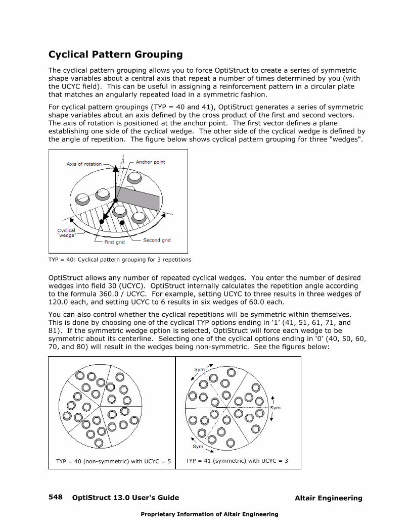
OptiStruct 13.0 User's Guide548 Altair Engineering
Proprietary Information of Altair Engineering
Cyclical Pattern Grouping
The cyclical pattern grouping allows you to force OptiStruct to create a series of symmetricshape variables about a central axis that repeat a number of times determined by you (withthe UCYC field). This can be useful in assigning a reinforcement pattern in a circular platethat matches an angularly repeated load in a symmetric fashion.
For cyclical pattern groupings (TYP = 40 and 41), OptiStruct generates a series of symmetricshape variables about an axis defined by the cross product of the first and second vectors. The axis of rotation is positioned at the anchor point. The first vector defines a planeestablishing one side of the cyclical wedge. The other side of the cyclical wedge is defined bythe angle of repetition. The figure below shows cyclical pattern grouping for three "wedges".
TYP = 40: Cyclical pattern grouping for 3 repetitions
OptiStruct allows any number of repeated cyclical wedges. You enter the number of desiredwedges into field 30 (UCYC). OptiStruct internally calculates the repetition angle accordingto the formula 360.0 / UCYC. For example, setting UCYC to three results in three wedges of120.0 each, and setting UCYC to 6 results in six wedges of 60.0 each.
You can also control whether the cyclical repetitions will be symmetric within themselves. This is done by choosing one of the cyclical TYP options ending in ‘1’ (41, 51, 61, 71, and81). If the symmetric wedge option is selected, OptiStruct will force each wedge to besymmetric about its centerline. Selecting one of the cyclical options ending in ‘0’ (40, 50, 60,70, and 80) will result in the wedges being non-symmetric. See the figures below:
TYP = 40 (non-symmetric) with UCYC = 5
TYP = 41 (symmetric) with UCYC = 3
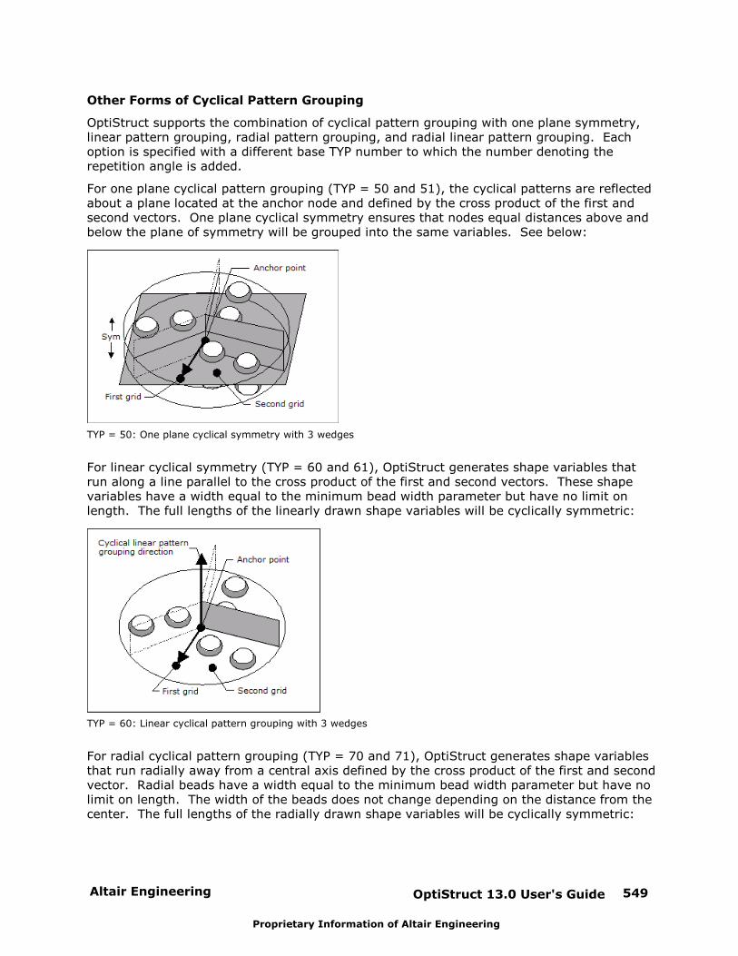
Altair Engineering OptiStruct 13.0 User's Guide 549
Proprietary Information of Altair Engineering
Other Forms of Cyclical Pattern Grouping
OptiStruct supports the combination of cyclical pattern grouping with one plane symmetry,linear pattern grouping, radial pattern grouping, and radial linear pattern grouping. Eachoption is specified with a different base TYP number to which the number denoting therepetition angle is added.
For one plane cyclical pattern grouping (TYP = 50 and 51), the cyclical patterns are reflectedabout a plane located at the anchor node and defined by the cross product of the first andsecond vectors. One plane cyclical symmetry ensures that nodes equal distances above andbelow the plane of symmetry will be grouped into the same variables. See below:
TYP = 50: One plane cyclical symmetry with 3 wedges
For linear cyclical symmetry (TYP = 60 and 61), OptiStruct generates shape variables thatrun along a line parallel to the cross product of the first and second vectors. These shapevariables have a width equal to the minimum bead width parameter but have no limit onlength. The full lengths of the linearly drawn shape variables will be cyclically symmetric:
TYP = 60: Linear cyclical pattern grouping with 3 wedges
For radial cyclical pattern grouping (TYP = 70 and 71), OptiStruct generates shape variablesthat run radially away from a central axis defined by the cross product of the first and secondvector. Radial beads have a width equal to the minimum bead width parameter but have nolimit on length. The width of the beads does not change depending on the distance from thecenter. The full lengths of the radially drawn shape variables will be cyclically symmetric:
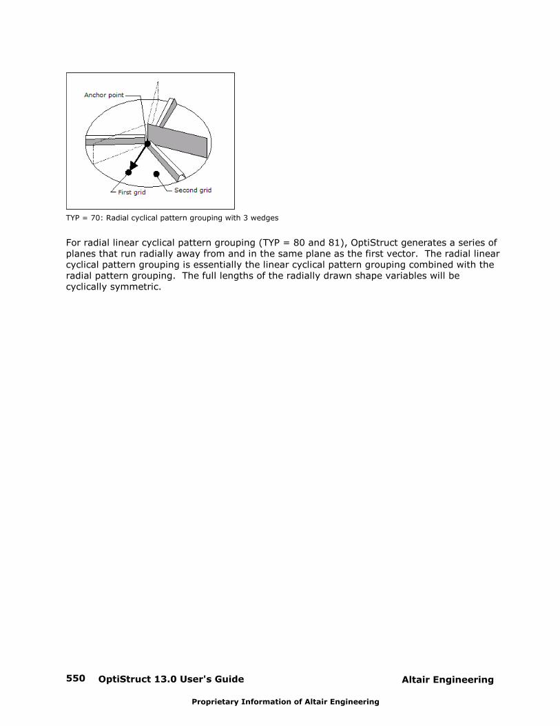
OptiStruct 13.0 User's Guide550 Altair Engineering
Proprietary Information of Altair Engineering
TYP = 70: Radial cyclical pattern grouping with 3 wedges
For radial linear cyclical pattern grouping (TYP = 80 and 81), OptiStruct generates a series ofplanes that run radially away from and in the same plane as the first vector. The radial linearcyclical pattern grouping is essentially the linear cyclical pattern grouping combined with theradial pattern grouping. The full lengths of the radially drawn shape variables will becyclically symmetric.

Altair Engineering OptiStruct 13.0 User's Guide 551
Proprietary Information of Altair Engineering
Manufacturability for Free-size Optimization
A concern in free-size optimization is that the design concepts developed are very often notmanufacturable. Another problem is that the solution of a free-size optimization problem canbe mesh dependent, if no appropriate measure is taken.
OptiStruct offers a number of different methods to account for manufacturability whenperforming free-size optimization:
Member Size Control
Member size control allows you some control over the member size in the final free-sizedesign and the resulting degree of simplicity therein. This feature may be added one ofthe two ways described below.
1. The DOPTPRM card:
(1) (2) (3) (4) (5) (6) (7) (8) (9) (10)
DOPTPRM MINDIM VALUE
Here, only the preferred minimum diameter (width in 2-D) of members may be definedas the VALUE field, following the MINDIM keyword. A global minimum member size isdefined in this way.
2. The DSIZE card:
(1) (2) (3) (4) (5) (6) (7) (8) (9) (10)
MEMBSIZ
MINDIM
Here, the preferred minimum, MINDIM member may be defined on the MEMBSIZcontinuation line. Member size dimensions can be defined differently for each DSIZEentry in this way.
Minimum Member Size Control
Although minimum member size control penalizes the formation of small members, resultsthat contain members significantly under the prescribed minimum member size can still beobtained. This is because a small member in the structure can be very important to theload transmission and may not be removed by penalization. Minimum member size controlfunctions more as a quality control than a quantity control.
A discrete solution is achieved in two iterative steps. The first step converges to a solutionwith a large number of semi-dense elements. The second step tries to refine this solutionto a solution with fully dense members. Each step consists of a number of iterations. Thefirst step consists of two entire convergence phases - the first run with the initialdiscreteness values (defined by DISCRETE and DISCRT1D parameters on the DOPTPRMbulk data entry), followed by a run with the discreteness values increased by 1.0. This
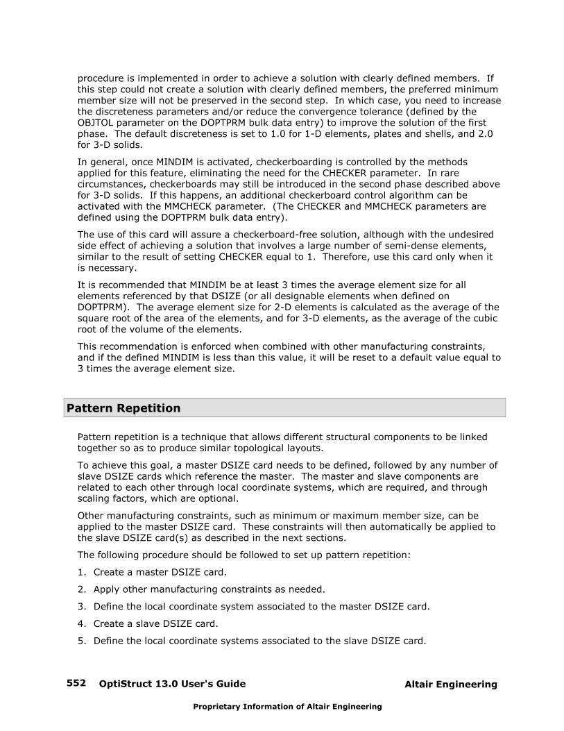
OptiStruct 13.0 User's Guide552 Altair Engineering
Proprietary Information of Altair Engineering
procedure is implemented in order to achieve a solution with clearly defined members. Ifthis step could not create a solution with clearly defined members, the preferred minimummember size will not be preserved in the second step. In which case, you need to increasethe discreteness parameters and/or reduce the convergence tolerance (defined by theOBJTOL parameter on the DOPTPRM bulk data entry) to improve the solution of the firstphase. The default discreteness is set to 1.0 for 1-D elements, plates and shells, and 2.0for 3-D solids.
In general, once MINDIM is activated, checkerboarding is controlled by the methodsapplied for this feature, eliminating the need for the CHECKER parameter. In rarecircumstances, checkerboards may still be introduced in the second phase described abovefor 3-D solids. If this happens, an additional checkerboard control algorithm can beactivated with the MMCHECK parameter. (The CHECKER and MMCHECK parameters aredefined using the DOPTPRM bulk data entry).
The use of this card will assure a checkerboard-free solution, although with the undesiredside effect of achieving a solution that involves a large number of semi-dense elements,similar to the result of setting CHECKER equal to 1. Therefore, use this card only when itis necessary.
It is recommended that MINDIM be at least 3 times the average element size for allelements referenced by that DSIZE (or all designable elements when defined onDOPTPRM). The average element size for 2-D elements is calculated as the average of thesquare root of the area of the elements, and for 3-D elements, as the average of the cubicroot of the volume of the elements.
This recommendation is enforced when combined with other manufacturing constraints,and if the defined MINDIM is less than this value, it will be reset to a default value equal to3 times the average element size.
Pattern Repetition
Pattern repetition is a technique that allows different structural components to be linkedtogether so as to produce similar topological layouts.
To achieve this goal, a master DSIZE card needs to be defined, followed by any number ofslave DSIZE cards which reference the master. The master and slave components arerelated to each other through local coordinate systems, which are required, and throughscaling factors, which are optional.
Other manufacturing constraints, such as minimum or maximum member size, can beapplied to the master DSIZE card. These constraints will then automatically be applied tothe slave DSIZE card(s) as described in the next sections.
The following procedure should be followed to set up pattern repetition:
1. Create a master DSIZE card.
2. Apply other manufacturing constraints as needed.
3. Define the local coordinate system associated to the master DSIZE card.
4. Create a slave DSIZE card.
5. Define the local coordinate systems associated to the slave DSIZE card.
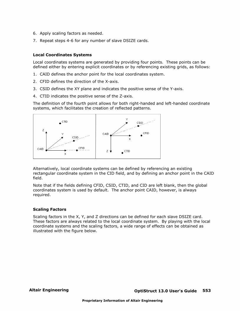
Altair Engineering OptiStruct 13.0 User's Guide 553
Proprietary Information of Altair Engineering
6. Apply scaling factors as needed.
7. Repeat steps 4-6 for any number of slave DSIZE cards.
Local Coordinates Systems
Local coordinates systems are generated by providing four points. These points can bedefined either by entering explicit coordinates or by referencing existing grids, as follows:
1. CAID defines the anchor point for the local coordinates system.
2. CFID defines the direction of the X-axis.
3. CSID defines the XY plane and indicates the positive sense of the Y-axis.
4. CTID indicates the positive sense of the Z-axis.
The definition of the fourth point allows for both right-handed and left-handed coordinatesystems, which facilitates the creation of reflected patterns.
Alternatively, local coordinate systems can be defined by referencing an existingrectangular coordinate system in the CID field, and by defining an anchor point in the CAIDfield.
Note that if the fields defining CFID, CSID, CTID, and CID are left blank, then the globalcoordinates system is used by default. The anchor point CAID, however, is alwaysrequired.
Scaling Factors
Scaling factors in the X, Y, and Z directions can be defined for each slave DSIZE card. These factors are always related to the local coordinate system. By playing with the localcoordinate systems and the scaling factors, a wide range of effects can be obtained asillustrated with the figure below.
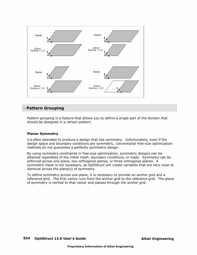
OptiStruct 13.0 User's Guide554 Altair Engineering
Proprietary Information of Altair Engineering
Pattern Grouping
Pattern grouping is a feature that allows you to define a single part of the domain thatshould be designed in a certain pattern.
Planar Symmetry
It is often desirable to produce a design that has symmetry. Unfortunately, even if thedesign space and boundary conditions are symmetric, conventional free-size optimizationmethods do not guarantee a perfectly symmetric design.
By using symmetry constraints in free-size optimization, symmetric designs can beattained regardless of the initial mesh, boundary conditions, or loads. Symmetry can beenforced across one plane, two orthogonal planes, or three orthogonal planes. Asymmetric mesh is not necessary, as OptiStruct will create variables that are very close toidentical across the plane(s) of symmetry.
To define symmetry across one plane, it is necessary to provide an anchor grid and areference grid. The first vector runs from the anchor grid to the reference grid. The planeof symmetry is normal to that vector and passes through the anchor grid.
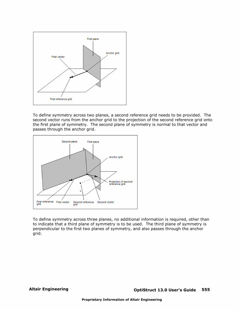
Altair Engineering OptiStruct 13.0 User's Guide 555
Proprietary Information of Altair Engineering
To define symmetry across two planes, a second reference grid needs to be provided. Thesecond vector runs from the anchor grid to the projection of the second reference grid ontothe first plane of symmetry. The second plane of symmetry is normal to that vector andpasses through the anchor grid.
To define symmetry across three planes, no additional information is required, other thanto indicate that a third plane of symmetry is to be used. The third plane of symmetry isperpendicular to the first two planes of symmetry, and also passes through the anchorgrid.
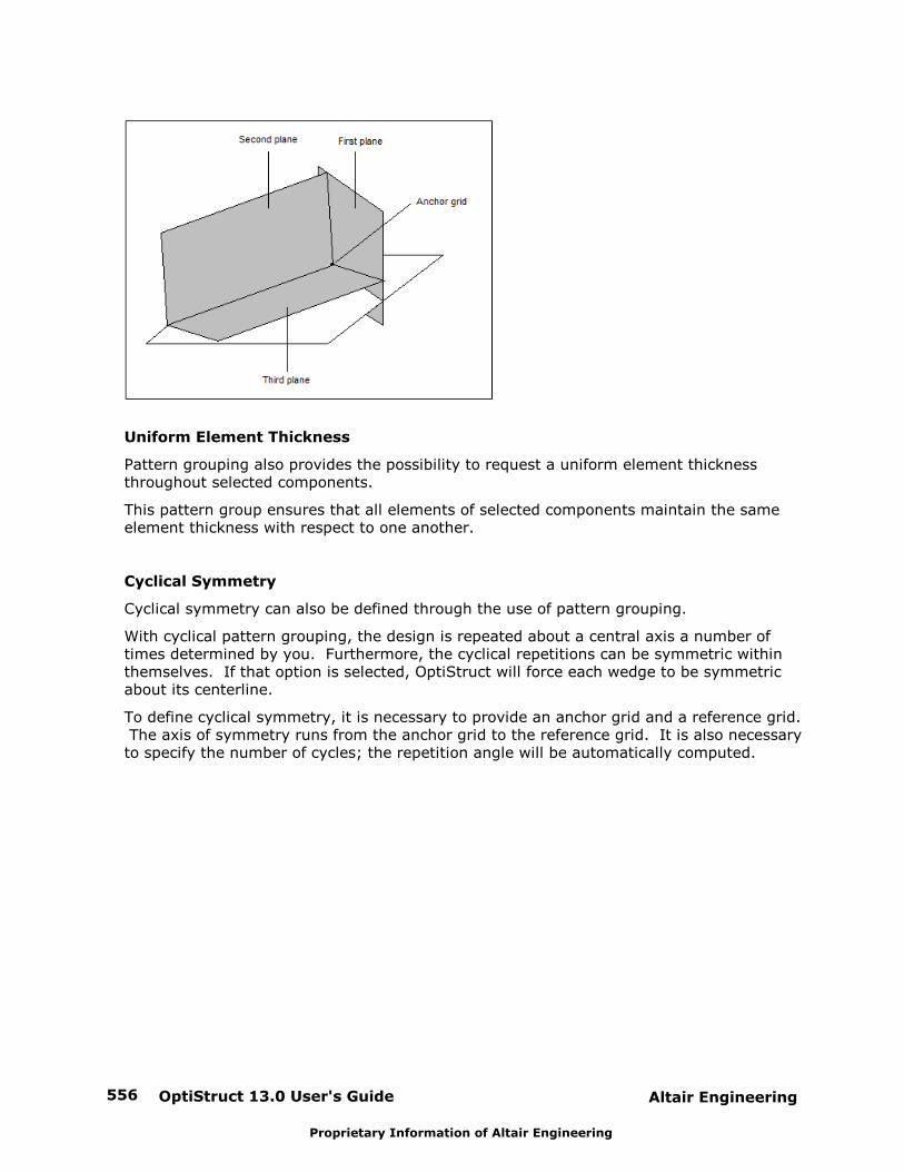
OptiStruct 13.0 User's Guide556 Altair Engineering
Proprietary Information of Altair Engineering
Uniform Element Thickness
Pattern grouping also provides the possibility to request a uniform element thicknessthroughout selected components.
This pattern group ensures that all elements of selected components maintain the sameelement thickness with respect to one another.
Cyclical Symmetry
Cyclical symmetry can also be defined through the use of pattern grouping.
With cyclical pattern grouping, the design is repeated about a central axis a number oftimes determined by you. Furthermore, the cyclical repetitions can be symmetric withinthemselves. If that option is selected, OptiStruct will force each wedge to be symmetricabout its centerline.
To define cyclical symmetry, it is necessary to provide an anchor grid and a reference grid. The axis of symmetry runs from the anchor grid to the reference grid. It is also necessaryto specify the number of cycles; the repetition angle will be automatically computed.
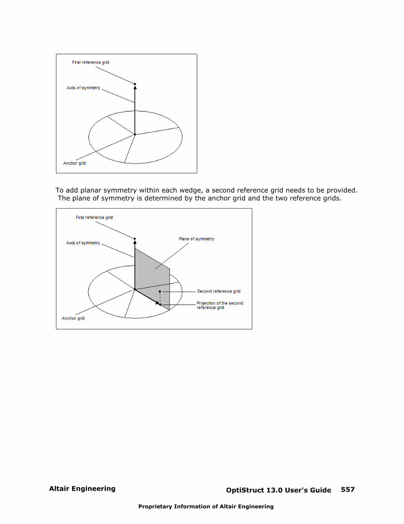
Altair Engineering OptiStruct 13.0 User's Guide 557
Proprietary Information of Altair Engineering
To add planar symmetry within each wedge, a second reference grid needs to be provided. The plane of symmetry is determined by the anchor grid and the two reference grids.

OptiStruct 13.0 User's Guide558 Altair Engineering
Proprietary Information of Altair Engineering
Reliability-based Design Optimization (Beta)
Introduction
Reliability-based Design Optimization (RBDO) is an optimization method that can be used toprovide optimum designs in the presence of uncertainty. A gradient-based localapproximation of responses is used to perform reliability analysis. The design variables,constraints, and objective are tested for reliability based on user-defined reliabilityrequirements.
Deterministic and Random design variables can be selected for a design optimization run,while a Random parameter is also available to check for Robustness of a particular designwithin specified bounds. Similarly, Design Constraints and Objectives can also be specified asDeterministic (mean) or Percentile values.
Implementation
The Single Loop Approach (SLA) is used to optimize structures using Reliability-based DesignOptimization in OptiStruct. Reliability-based optimization methods test the reliability ofdesigns for each optimization iteration. The traditional, double-loop RBDO algorithm requiresnested optimization loops, where the design optimization (outer) loop repeatedly calls aseries of reliability (inner) loops.
The computational time can be prohibitive for practical problems due to the nestedoptimization-reliability loops. The SLA converts the nested loops into a single loop usingKarush-Kuhn-Tucker (KKT) conditions of the inner reliability loops in the outer optimizationloop. The probabilistic optimization problem is converted into a deterministic optimizationproblem. SLA is highly efficient compared to the traditional double-loop RBDO process.
The Single Loop Approach (SLA) is terminated if one of the following conditions is met:
1. The Sequential Quadratic Programming (SQP) convergence criterion is achieved.
2. Design variable convergence criterion is achieved.
3. Maximum number of allowable iterations is attained.
Variables
The following design variables and parameters can be used to define the structural designspace in OptiStruct:
Random Design Variables
Random design variables are defined via the RAND continuation lines on the DESVAR bulkdata entry. Various random distribution types can be selected and their parameters aredefined accordingly. In an RBDO process, during reliability and/or robustness analysis, thedesign should satisfy optimality based on the specified distributions.
Random parameters
The definition of Random parameters is similar to that of Random Design Variables, usingRANP definition. However, the important difference is that, while the mean values of randomvariables are changed to improve the design, the mean values of random parameters remainconstant. For example, typically sheet metal thickness can be a random variable, due to
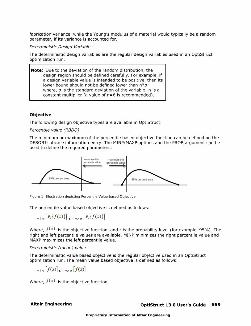
Altair Engineering OptiStruct 13.0 User's Guide 559
Proprietary Information of Altair Engineering
fabrication variance, while the Young’s modulus of a material would typically be a randomparameter, if its variance is accounted for.
Deterministic Design Variables
The deterministic design variables are the regular design variables used in an OptiStructoptimization run.
Note: Due to the deviation of the random distribution, thedesign region should be defined carefully. For example, ifa design variable value is intended to be positive, then itslower bound should not be defined lower than n*σ;where, σ is the standard deviation of the variable; n is aconstant multiplier (a value of n=6 is recommended).
Objective
The following design objective types are available in OptiStruct:
Percentile value (RBDO)
The minimum or maximum of the percentile based objective function can be defined on the DESOBJ subcase information entry. The MINP/MAXP options and the PROB argument can beused to define the required parameters.
Figure 1: Illustration depicting Percentile Value based Objective
The percentile value based objective is defined as follows:
min or max
Where, is the objective function, and r is the probability level (for example, 95%). The
right and left percentile values are available. MINP minimizes the right percentile value andMAXP maximizes the left percentile value.
Deterministic (mean) value
The deterministic value based objective is the regular objective used in an OptiStructoptimization run. The mean value based objective is defined as follows:
min or max
Where, is the objective function.

OptiStruct 13.0 User's Guide560 Altair Engineering
Proprietary Information of Altair Engineering
Constraints
The following design constraint types are available in OptiStruct:
Percentile value (RBDO)
The probability of one constraint satisfying its bounds should not be less than the predefinedreliability value. The reliability value is defined via the PROB field on the DCONSTR bulk dataentry.
The reliability-based constraints are defined as follows:
Where,
c(x) is the constraint value
ub is the upper bound of the constraint
lb is the lower bound of the constraint
r is the probability level (for example, 95%)
For the “ ” constraint, the right percentile value of c(x) is forced to be
less than or equal to the upper bound “ub”. For the “ ” constraint, the
left percentile value of c(x) is forced to be greater than or equal to the lower bound “lb”.
Deterministic (mean) value
The deterministic value based constraint is the regular constraint definition used in anOptiStruct optimization run. The mean value based constraint is defined as follows:
c(x) < ub
c(x) > lb
Where, c(x) is the constraint value, ub is the upper bound of the constraint, and lb is the
lower bound of the constraint.
OptiStruct RBDO
The RBDO process is illustrated in Figure 2.
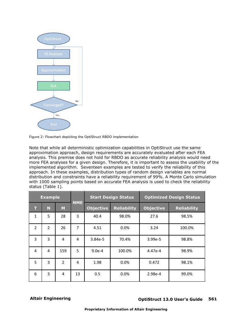
Altair Engineering OptiStruct 13.0 User's Guide 561
Proprietary Information of Altair Engineering
Figure 2: Flowchart depicting the OptiStruct RBDO implementation
Note that while all deterministic optimization capabilities in OptiStruct use the sameapproximation approach, design requirements are accurately evaluated after each FEAanalysis. This premise does not hold for RBDO as accurate reliability analysis would needmore FEA analyses for a given design. Therefore, it is important to assess the usability of theimplemented algorithm. Seventeen examples are tested to verify the reliability of thisapproach. In these examples, distribution types of random design variables are normaldistribution and constraints have a reliability requirement of 99%. A Monte Carlo simulationwith 1000 sampling points based on accurate FEA analysis is used to check the reliabilitystatus (Table 1).
Example
NME
Start Design Status Optimized Design Status
T N M Objective Reliability Objective Reliability
1 5 28 3 40.4 98.0% 27.6 98.5%
2 2 26 7 4.51 0.0% 3.24 100.0%
3 3 4 4 3.84e-5 70.4% 3.99e-5 98.8%
4 4 159 5 9.0e-4 100.0% 4.47e-4 98.9%
5 3 2 4 1.98 0.0% 0.472 98.1%
6 3 4 13 0.5 0.0% 2.98e-4 99.0%
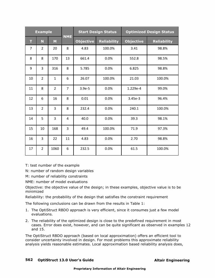
OptiStruct 13.0 User's Guide562 Altair Engineering
Proprietary Information of Altair Engineering
Example
NME
Start Design Status Optimized Design Status
T N M Objective Reliability Objective Reliability
7 2 20 8 4.83 100.0% 3.41 98.8%
8 8 170 13 661.4 0.0% 552.8 98.5%
9 3 316 8 5.785 0.0% 6.825 98.8%
10 2 1 6 26.07 100.0% 21.03 100.0%
11 8 2 7 3.9e-5 0.0% 1.229e-4 99.0%
12 6 16 8 0.01 0.0% 3.45e-3 96.4%
13 2 3 8 232.4 0.0% 240.1 100.0%
14 5 3 4 40.0 0.0% 39.3 98.1%
15 10 168 3 49.4 100.0% 71.9 97.3%
16 3 22 11 4.83 0.0% 2.70 98.8%
17 2 1060 6 232.5 0.0% 61.5 100.0%
T: test number of the example
N: number of random design variables
M: number of reliability constraints
NME: number of model evaluations
Objective: the objective value of the design; in these examples, objective value is to beminimized
Reliability: the probability of the design that satisfies the constraint requirement
The following conclusions can be drawn from the results in Table 1:
1. The OptiStruct RBDO approach is very efficient, since it consumes just a few modelevaluations.
2. The reliability of the optimized design is close to the predefined requirement in mostcases. Error does exist, however, and can be quite significant as observed in examples 12and 15.
The OptiStruct RBDO approach (based on local approximation) offers an efficient tool toconsider uncertainty involved in design. For most problems this approximate reliabilityanalysis yields reasonable estimates. Local approximation based reliability analysis does,

Altair Engineering OptiStruct 13.0 User's Guide 563
Proprietary Information of Altair Engineering
however, contain some error of varying degree. Accurate reliability analysis should be carriedout if accurate satisfaction of reliability requirements is critical. Also note that for theapproximation-based OptiStruct RBDO approach, reliability analysis is performed only forretained constraints for which sensitivity is available. You can adjust the screening criteriausing the DSCREEN bulk data entry, if required.
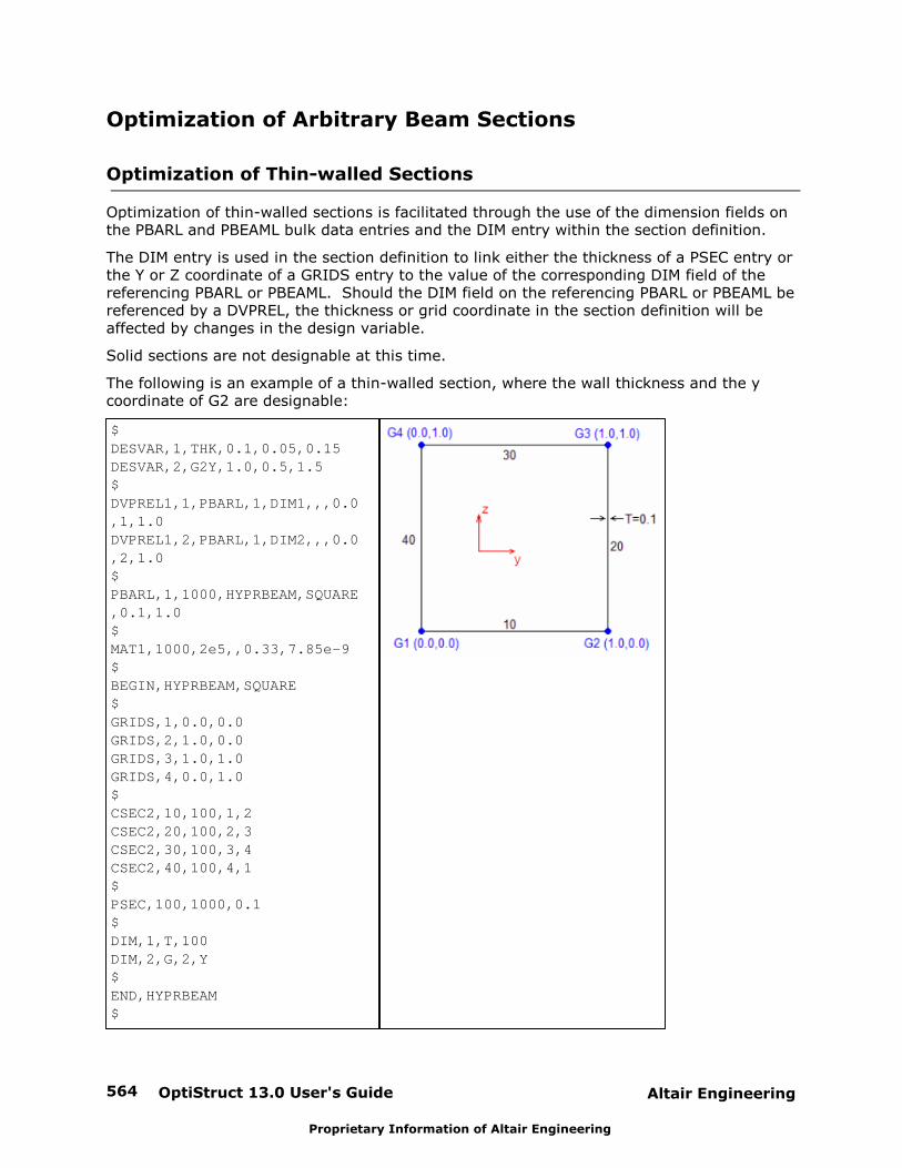
OptiStruct 13.0 User's Guide564 Altair Engineering
Proprietary Information of Altair Engineering
Optimization of Arbitrary Beam Sections
Optimization of Thin-walled Sections
Optimization of thin-walled sections is facilitated through the use of the dimension fields onthe PBARL and PBEAML bulk data entries and the DIM entry within the section definition.
The DIM entry is used in the section definition to link either the thickness of a PSEC entry orthe Y or Z coordinate of a GRIDS entry to the value of the corresponding DIM field of thereferencing PBARL or PBEAML. Should the DIM field on the referencing PBARL or PBEAML bereferenced by a DVPREL, the thickness or grid coordinate in the section definition will beaffected by changes in the design variable.
Solid sections are not designable at this time.
The following is an example of a thin-walled section, where the wall thickness and the ycoordinate of G2 are designable:
$DESVAR,1,THK,0.1,0.05,0.15DESVAR,2,G2Y,1.0,0.5,1.5$DVPREL1,1,PBARL,1,DIM1,,,0.0,1,1.0DVPREL1,2,PBARL,1,DIM2,,,0.0,2,1.0$PBARL,1,1000,HYPRBEAM,SQUARE,0.1,1.0$MAT1,1000,2e5,,0.33,7.85e-9$BEGIN,HYPRBEAM,SQUARE$GRIDS,1,0.0,0.0GRIDS,2,1.0,0.0GRIDS,3,1.0,1.0GRIDS,4,0.0,1.0$CSEC2,10,100,1,2CSEC2,20,100,2,3CSEC2,30,100,3,4CSEC2,40,100,4,1$PSEC,100,1000,0.1$DIM,1,T,100DIM,2,G,2,Y$END,HYPRBEAM$
Altair Engineering OptiStruct 13.0 User's Guide 565
Proprietary Information of Altair Engineering
Optimization of Composite Structures
OptiStruct offers a comprehensive optimization solution aimed at guiding and simplifying thedesign of laminate composite structures. The solution includes the following optimizationphases and associated techniques:
Phase I – Concept. Free-sizing optimization is used to generate design concepts, while considering globalresponses and optional manufacturing constraints.
Phase II – System. Sizing optimization – with ply-based modeling – is performed to control the thickness ofeach ply bundle, while considering all design responses and optional manufacturingconstraints.
Phase III – Detail. Ply-stacking optimization is applied to determine the detailed stacking sequence, againwhile considering all behavioral responses, manufacturing constraints and various plybook rules.
While these techniques can be applied independently, it is recommended to use themtogether as a three-phase integrated process guiding the design from concept to completion. This is particularly important when manufacturing constraints are involved. In order tosatisfy such constraints at the finishing stage, they should be incorporated at the beginningso that the design concept can be carried forward. Automated tools are provided to facilitatethe transition between the design optimization phases.
Composite Structures - Free-sizing Optimization
The purpose of composite free-sizing optimization is to create design concepts that utilizeall the potential of a composite structure where both structure and material can bedesigned simultaneously. By varying the thickness of each ply with a particular fiberorientation for every element, the total laminate thickness can change ‘continuously’throughout the structure, and at the same time, the optimal composition of the compositelaminate at every point (element) is achieved simultaneously. At this stage, a super-plyconcept should be adopted, in which each available fiber orientation is assigned a super-ply whose thickness is free-sized. In other words, a super-ply is the total designablethickness of a particular fiber orientation. In addition, in order to neutralize the effect ofply stacking sequence, the SMEAR option is usually a good choice for this design phaseunless it is intended to follow through with the stacking preference of the super-plylaminate model.
In OptiStruct, additional manufacturing constraints can be defined for free-sizingoptimization. As a composite laminate is typically manufactured through a stacking andcuring process, certain manufacturing requirements are necessary in order to limitundesired side effects emerging during this curing process. For example, one such typicalconstraint for carbon fiber reinforced composites is that plies of a given orientation cannotbe stacked successively for more than 3 or 4 plies. This implies that a design concept thatcontains areas of predominantly a single fiber orientation would never satisfy thisrequirement. Therefore, to achieve a manufacturable design concept, manufacturingrequirements for the final product need to be reflected during the concept design stage. For the particular constraint mentioned above, for instance, the design concept would offerenough alternative ply orientations to break the succession of plies of the same orientation
OptiStruct 13.0 User's Guide566 Altair Engineering
Proprietary Information of Altair Engineering
if the percentage of each fiber orientation is controlled (for example, no ply orientationshould drop below 15%). In addition, balancing of a pair of ply orientations could beuseful for practical reasons. For example, balancing 45° and -45° plies would eliminatetwisting of a plate under bending along the 0 axis. In order to address these needs, thefollowing manufacturing constraints are made available for composite free-sizing:
Lower and upper bounds on the total thickness of the laminate.
Lower and upper bounds on the thickness of individual orientations.
Lower and upper bounds on the thickness percentage of individual orientations.
Constant thickness of individual orientations.
Thickness balancing between two given orientations.
As for the constraints on laminate thickness, ply thickness and thickness percentage, thesecan be applied locally through the definition of element sets. Therefore, multiple instancesof these constraints are supported. Advantages include being able to allow differentconstraints in different regions while preserving the continuity of plies. For example,different thickness requirements in critical regions, such as bolted areas, can be factoredinto the design process. Additionally, zone based free-sizing optimization can beperformed. Zones are defined through groups of elements and there can be elements thatdo not belong to any zone. Zones are typically defined to simplify the designinterpretation process and improve manufacturability. Instead of having to interpretmanufacturable zones from the solution of a free-sizing optimization, the optimization isrun based on pre-defined zones. While the interpretation process is simplified, there is aloss in design freedom as now the optimization is restricted to some extent due to thedefined zones.
Refer to the DSIZE card for detailed information regarding composite free-sizingoptimization and its associated manufacturing constraints. Note also that other genericmanufacturing constraints, such as pattern grouping or member size control, can beactivated for composite free-sizing as well.
The standard result from a free-sizing optimization is the thickness contribution of eachorientation defined on the PCOMP(G) or STACK card referenced by the DSIZE card in theoptimal laminate design. But, using free-sizing as part of the three-phase compositedesign and optimization process, and the mechanism to automatically generate an inputfile for phase two of this process, an additional level of detail/results can be drilled down toin terms of the thickness contributions per orientation. The automatically generated inputfile for phase two contains ply bundle data that can be reviewed in HyperMesh.
A ply bundle is a continuous stack of plies of the same shape (or coverage area). Eachsuper-ply results in the formation of 4 ply bundles. This is the default behavior and can bechanged, that is a different number of ply bundles can be requested from the super-plies. However, in most cases, it is recommended to use the default approach.
As described above, multiple ply shapes per orientation (through ply bundles) can bedetermined and generated from a free-sizing optimization.
Note: Automatic offset control is available in composite free-size and sizingoptimization wherein the specified offset values are automaticallyupdated based on thickness changes. The offset values can bespecified on the PCOMP(P/G) property entries or the CTRIA3/6,CQUAD4/8 element entries using the Z0 or ZOFFS fields.
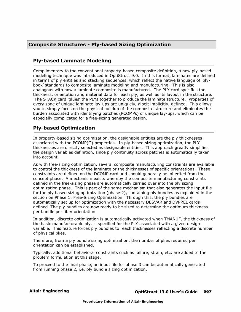
Altair Engineering OptiStruct 13.0 User's Guide 567
Proprietary Information of Altair Engineering
Composite Structures - Ply-based Sizing Optimization
Ply-based Laminate Modeling
Complimentary to the conventional property-based composite definition, a new ply-basedmodeling technique was introduced in OptiStruct 9.0. In this format, laminates are definedin terms of ply entities and stacking sequences, which reflect the native language of ‘ply-book’ standards to composite laminate modeling and manufacturing. This is alsoanalogous with how a laminate composite is manufactured. The PLY card specifies thethickness, orientation and material data for each ply, as well as its layout in the structure. The STACK card ‘glues’ the PLYs together to produce the laminate structure. Properties ofevery zone of unique laminate lay-ups are uniquely, albeit implicitly, defined. This allowsyou to simply focus on the physical buildup of the composite structure and eliminates theburden associated with identifying patches (PCOMPs) of unique lay-ups, which can beespecially complicated for a free-sizing generated design.
Ply-based Optimization
In property-based sizing optimization, the designable entities are the ply thicknessesassociated with the PCOMP(G) properties. In ply-based sizing optimization, the PLYthicknesses are directly selected as designable entities. This approach greatly simplifiesthe design variables definition, since ply continuity across patches is automatically takeninto account.
As with free-sizing optimization, several composite manufacturing constraints are availableto control the thickness of the laminate or the thicknesses of specific orientations. Theseconstraints are defined on the DCOMP card and should generally be inherited from theconcept phase. A mechanism exists whereby the composite manufacturing constraintsdefined in the free-sizing phase are automatically carried over into the ply sizingoptimization phase. This is part of the same mechanism that also generates the input filefor the ply based sizing optimization (phase 2), containing ply bundles as explained in thesection on Phase 1: Free-Sizing Optimization. Through this, the ply bundles areautomatically set up for optimization with the necessary DESVAR and DVPREL cardsdefined. The ply bundles are now ready to be sized to determine the optimum thicknessper bundle per fiber orientation.
In addition, discrete optimization is automatically activated when TMANUF, the thickness ofthe basic manufacturable ply, is specified for the PLY associated with a given designvariable. This feature forces ply bundles to reach thicknesses reflecting a discrete numberof physical plies.
Therefore, from a ply bundle sizing optimization, the number of plies required perorientation can be established.
Typically, additional behavioral constraints such as failure, strain, etc. are added to theproblem formulation at this stage.
To proceed to the final phase, an input file for phase 3 can be automatically generatedfrom running phase 2, i.e. ply bundle sizing optimization.
OptiStruct 13.0 User's Guide568 Altair Engineering
Proprietary Information of Altair Engineering
Note: Automatic offset control is available in composite free-size and sizingoptimization wherein the specified offset values are automaticallyupdated based on thickness changes. The offset values can bespecified on the PCOMP(P/G) property entries or the CTRIA3/6,CQUAD4/8 element entries using the Z0 or ZOFFS fields.
Composite Structures - Stacking Sequence Optimization
Composite plies are shuffled to determine the optimal stacking sequence for the givendesign optimization problem while also satisfying additional manufacturing constraints,defined on the DSHUFFLE card, such as:
The stacking sequence should not contain any section with more than a givennumber of successive plies of same orientation.
The 45° and -45° orientations should be paired together.
The cover and/or core sections should follow a predefined stacking sequence.
Using the three-phase process, composite plies are generated from running a discrete plybundle sizing optimization (through TMANUF) in phase 2. Additionally, an input file forphase 3, i.e. stacking sequence optimization, is automatically generated from phase 2.
An efficient proprietary technique is developed to allow the process to evaluate a hugenumber of stacking combinations from both performance and manufacturabilityperspectives.
Phase Transitions in the Optimization of Composite Structures
In order to simplify the transition between the three design phases, OptiStruct is able toautomatically generate input decks after the free-sizing optimization or the sizingoptimization stages have converged.
OUTPUT,FSTOSZ (free-sizing to sizing) is an output request that can be used during thefree-sizing optimization phase to write a ply-based sizing optimization input deck. Foreach orientation, the composite interpreter identifies regions of similar thickness andcreates PLYs for these regions. The resulting deck contains PCOMPP, STACK, PLY, and SETcards describing the ply-based composite model, as well as DCOMP, DESVAR, and DVPRELcards defining the optimization data. Manufacturing constraints are transferred from theDSIZE card to the DCOMP card. Typically, additional design responses such as stress/failure constraints would be introduced at this optimization stage.
OUTPUT,SZTOSH (sizing to shuffling) is an output request that can be used during the ply-based sizing optimization stage to write a ply stacking optimization input deck. Each PLYbundle is divided into multiple PLYs whose thickness is equal to the manufacturablethickness TMANUF, and the STACK card is updated accordingly. The DESVAR and DVPRELcards from the previous stage are removed, and a bare DSHUFFLE card is introduced. Asrequired by the design, additional ply-book rules or manufacturing constraints can bedefined on the DSHUFFLE card.
Altair Engineering OptiStruct 13.0 User's Guide 569
Proprietary Information of Altair Engineering
Example of Composite Structure Optimization - RectangularComposite Panel
In this example, a rectangular composite panel is clamped on one side and subjected to atip load on the other side. This simple model can be used to demonstrate how the threephases of the composite optimization package interact with each other to ultimatelygenerate a manufacturable design.
Free-sizing Optimization
During the concept phase, the composite panel is modeled with four orientations (0°, 90°,45° and -45°) of uniform thickness, and the SMEAR option is applied to eliminate stackbiasing. At this stage, you are minimizing the compliance of the structure whilemaintaining its volume fraction below 30%. Manufacturing constraints are introduced tolimit the total thickness of the panel and to ensure that each orientation accounts for atleast 10% of the total thickness. In addition, the thicknesses of the 45° and -45°orientations should be balanced. The resulting DSIZE card is:
DSIZE 1 PCOMP 1
+ COMP LAMTHK 3.2
+ COMP PLYPCT ALL 0.10
+ COMP BALANCE 45.0 -45.0
The optimization converges in seven iterations, after which the ply-based interpreteridentifies thickness zones and generates a ply-based input deck. As illustrated by thefollowing image (Figure 1), four ply bundles are created for each orientation. Figure 2shows the thickness of each orientation after free-sizing optimization, while Figure 3 showsthe equivalent thicknesses after going through the ply-based interpreter. As expected, thethickness zones are considerably more discrete in the interpreted design.
Figure 1: Ply bundles after ply-based interpretation
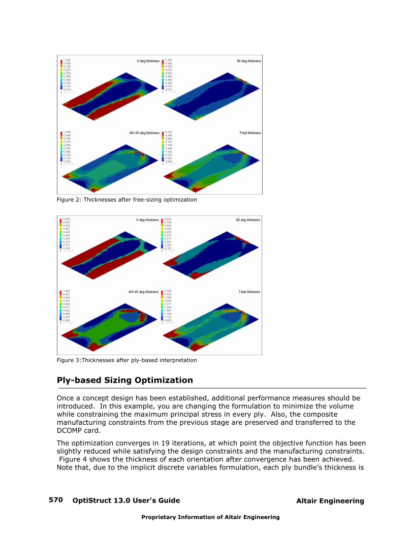
OptiStruct 13.0 User's Guide570 Altair Engineering
Proprietary Information of Altair Engineering
Figure 2: Thicknesses after free-sizing optimization
Figure 3:Thicknesses after ply-based interpretation
Ply-based Sizing Optimization
Once a concept design has been established, additional performance measures should beintroduced. In this example, you are changing the formulation to minimize the volumewhile constraining the maximum principal stress in every ply. Also, the compositemanufacturing constraints from the previous stage are preserved and transferred to theDCOMP card.
The optimization converges in 19 iterations, at which point the objective function has beenslightly reduced while satisfying the design constraints and the manufacturing constraints. Figure 4 shows the thickness of each orientation after convergence has been achieved. Note that, due to the implicit discrete variables formulation, each ply bundle’s thickness is
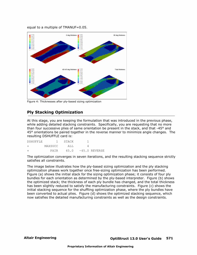
Altair Engineering OptiStruct 13.0 User's Guide 571
Proprietary Information of Altair Engineering
equal to a multiple of TMANUF=0.05.
Figure 4: Thicknesses after ply-based sizing optimization
Ply Stacking Optimization
At this stage, you are keeping the formulation that was introduced in the previous phase,while adding detailed stacking constraints. Specifically, you are requesting that no morethan four successive plies of same orientation be present in the stack, and that -45° and45° orientations be paired together in the reverse manner to minimize angle changes. Theresulting DSHUFFLE card is:
DSHUFFLE 1 STACK 1
+ MAXSUCC ALL 4
+ PAIR 45.0 -45.0 REVERSE
The optimization converges in seven iterations, and the resulting stacking sequence strictlysatisfies all constraints.
The image below illustrates how the ply-based sizing optimization and the ply stackingoptimization phases work together once free-sizing optimization has been performed. Figure (a) shows the initial stack for the sizing optimization phase; it consists of four plybundles for each orientation as determined by the ply-based interpreter. Figure (b) showsthe optimized stack; the thickness of each ply bundle has changed, and the total thicknesshas been slightly reduced to satisfy the manufacturing constraints. Figure (c) shows theinitial stacking sequence for the shuffling optimization phase, where the ply bundles havebeen converted to actual plies. Figure (d) shows the optimized stacking sequence, whichnow satisfies the detailed manufacturing constraints as well as the design constraints.
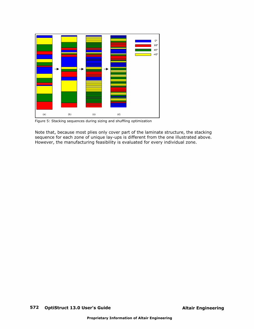
OptiStruct 13.0 User's Guide572 Altair Engineering
Proprietary Information of Altair Engineering
Figure 5: Stacking sequences during sizing and shuffling optimization
Note that, because most plies only cover part of the laminate structure, the stackingsequence for each zone of unique lay-ups is different from the one illustrated above. However, the manufacturing feasibility is evaluated for every individual zone.

Altair Engineering OptiStruct 13.0 User's Guide 573
Proprietary Information of Altair Engineering
Equivalent Static Load Method (ESLM)
The equivalent static load method, originally published by Dr. Park, Hanyang University, is atechnique suitable for optimization of designs undergoing dynamic loads. The method hasbeen implemented for the optimization of the following solutions:
Multi-body dynamics problems including flexible bodies.
Nonlinear responses from implicit static analysis, implicit dynamic analysis and explicitdynamic analysis.
The equivalent static load method takes advantage of the well established static responseoptimization capabilities of OptiStruct.
Equivalent Static Load
Figure 1.1: Displacement – time history response
The equivalent static load is that load which creates the same response field as that of thedynamic/nonlinear analysis at a given time step. From Figure 1.1, an equivalent static load iscalculated corresponding to each time step in the time history of the solution, therebyreplicating the dynamic/nonlinear behavior of the system in a static environment.
The calculated equivalent static loads from the analysis (as explained above) are consideredas separate load cases, and these multiple load cases are used in the linear responseoptimization loop. An updated design from the optimization loop is then passed back to theanalysis for validation and overall convergence. The design is validated against the originaldynamic/nonlinear analysis. Based on the outcome of this validation, the solution convergesor an updated set of equivalent static loads is calculated for the updated geometry, and theentire process is repeated till convergence. Figure 1.2 is a graphic description of theequivalent static load method for optimization.
Figure 1.2: Equivalent static load method
The equivalent static load method is completely automated in OptiStruct and is an efficientapproach for the optimization of responses from transient, dynamic and nonlinear solutions.
Apart from others, the equivalent static load method offers the following benefits:

OptiStruct 13.0 User's Guide574 Altair Engineering
Proprietary Information of Altair Engineering
It can be applied at the concept design phase as well as design fine tuning phase, i.e. itcan be used with topology, free-sizing, topography, size, shape and free-shapeoptimization.
A design is optimized for updated loads due to an updated design during theoptimization process.
Altair Engineering OptiStruct 13.0 User's Guide 575
Proprietary Information of Altair Engineering
ESLM for MBD
The equivalent static load method has been implemented for the solution of multi-bodydynamics problems that include flexible bodies. Size, shape, free-shape, topology,topography, free-size, and material optimization can be applied to flexible bodies. Responsesare mass, volume, center of gravity, moment of inertia, stress, strain, compliance (strainenergy), and displacement of the flexible bodies. Displacement responses are taken intoaccount with respect to local boundary conditions defined on the flexible body (see definitionbelow). The optimization problem setup follows the setup typical for size, shape, free-shape,topology, topography, free-size, and material optimizations in OptiStruct. Responses aredefined using DRESP1, DRESP2, and DRESP3 bulk data entries. Responses can only bedefined on flexible bodies (PFBODY) using the properties, elements and grid points includedin such bodies as reference. Design variables are defined using DESVAR, DVPREL1,DVPREL2, DVMREL1, DVMREL2, DSHAPE, DTPL, DTPG, DSIZE, and DVGRID bulk data entries. Free-size optimization is currently only available when PTYPE=PSHELL on the DSIZE card. Design variables can only be defined on flexible bodies (PFBODY) using the propertiesincluded in such bodies as reference. Constraints are defined using DCONSTR, DCONADDand DOBJREF bulk data entries. Constraints and objectives are referenced in the multi-bodydynamics subcase or globally through DESOBJ, DESSUB, DESGLB, and MINMAX, respectively.
ESLM specific parameters can be set through the DOPTPRM bulk data entry (see Parametersfor the ESLM).
The Method
An optimum solution can be found through a series of static response optimizations with theequivalent static load set, that is:
eqf Ku f Ma Cv
Where, feq, u, a, v, and f are the equivalent static load, deformation, acceleration, velocity, and
external load, respectively. The steps involved in the ESLM can be summarized as:
Step 1 Initial design.
Step 2 Dynamic analysis.
Step 3 Static response optimization with the multiple subcasesthat consist of multiple equivalent static load sets.
Step 4 If design converged, Stop. Otherwise go to Step 2.
The iteration at the third step is referred to as an inner iteration; Steps 2 through 4 form theouter loop. The converged solution at Step 3 is the starting point of the next outer loop (ifthe design does not converge at the current outer loop). Note that if there are time steps inthe multi-body dynamics analysis at Step 2, subcases in static response optimization aregenerated at Step 3 (provided that the time step screening option is deactivated). See Parameters for the ESLM.
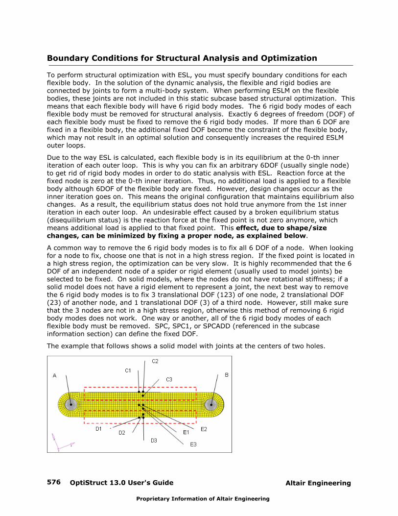
OptiStruct 13.0 User's Guide576 Altair Engineering
Proprietary Information of Altair Engineering
Boundary Conditions for Structural Analysis and Optimization
To perform structural optimization with ESL, you must specify boundary conditions for eachflexible body. In the solution of the dynamic analysis, the flexible and rigid bodies areconnected by joints to form a multi-body system. When performing ESLM on the flexiblebodies, these joints are not included in this static subcase based structural optimization. Thismeans that each flexible body will have 6 rigid body modes. The 6 rigid body modes of eachflexible body must be removed for structural analysis. Exactly 6 degrees of freedom (DOF) ofeach flexible body must be fixed to remove the 6 rigid body modes. If more than 6 DOF arefixed in a flexible body, the additional fixed DOF become the constraint of the flexible body,which may not result in an optimal solution and consequently increases the required ESLMouter loops.
Due to the way ESL is calculated, each flexible body is in its equilibrium at the 0-th inneriteration of each outer loop. This is why you can fix an arbitrary 6DOF (usually single node)to get rid of rigid body modes in order to do static analysis with ESL. Reaction force at thefixed node is zero at the 0-th inner iteration. Thus, no additional load is applied to a flexiblebody although 6DOF of the flexible body are fixed. However, design changes occur as theinner iteration goes on. This means the original configuration that maintains equilibrium alsochanges. As a result, the equilibrium status does not hold true anymore from the 1st inneriteration in each outer loop. An undesirable effect caused by a broken equilibrium status(disequilibrium status) is the reaction force at the fixed point is not zero anymore, whichmeans additional load is applied to that fixed point. This effect, due to shape/sizechanges, can be minimized by fixing a proper node, as explained below.
A common way to remove the 6 rigid body modes is to fix all 6 DOF of a node. When lookingfor a node to fix, choose one that is not in a high stress region. If the fixed point is located ina high stress region, the optimization can be very slow. It is highly recommended that the 6DOF of an independent node of a spider or rigid element (usually used to model joints) beselected to be fixed. On solid models, where the nodes do not have rotational stiffness; if asolid model does not have a rigid element to represent a joint, the next best way to removethe 6 rigid body modes is to fix 3 translational DOF (123) of one node, 2 translational DOF(23) of another node, and 1 translational DOF (3) of a third node. However, still make surethat the 3 nodes are not in a high stress region, otherwise this method of removing 6 rigidbody modes does not work. One way or another, all of the 6 rigid body modes of eachflexible body must be removed. SPC, SPC1, or SPCADD (referenced in the subcaseinformation section) can define the fixed DOF.
The example that follows shows a solid model with joints at the centers of two holes.
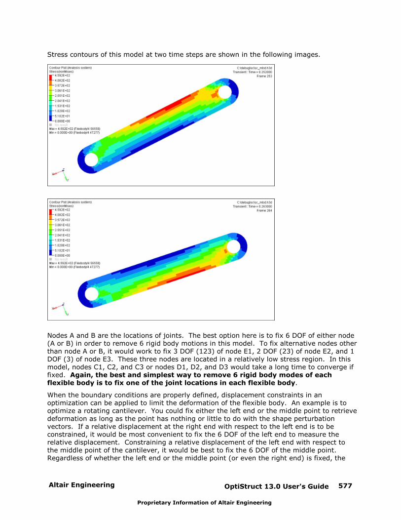
Altair Engineering OptiStruct 13.0 User's Guide 577
Proprietary Information of Altair Engineering
Stress contours of this model at two time steps are shown in the following images.
Nodes A and B are the locations of joints. The best option here is to fix 6 DOF of either node(A or B) in order to remove 6 rigid body motions in this model. To fix alternative nodes otherthan node A or B, it would work to fix 3 DOF (123) of node E1, 2 DOF (23) of node E2, and 1DOF (3) of node E3. These three nodes are located in a relatively low stress region. In thismodel, nodes C1, C2, and C3 or nodes D1, D2, and D3 would take a long time to converge iffixed. Again, the best and simplest way to remove 6 rigid body modes of eachflexible body is to fix one of the joint locations in each flexible body.
When the boundary conditions are properly defined, displacement constraints in anoptimization can be applied to limit the deformation of the flexible body. An example is tooptimize a rotating cantilever. You could fix either the left end or the middle point to retrievedeformation as long as the point has nothing or little to do with the shape perturbationvectors. If a relative displacement at the right end with respect to the left end is to beconstrained, it would be most convenient to fix the 6 DOF of the left end to measure therelative displacement. Constraining a relative displacement of the left end with respect tothe middle point of the cantilever, it would be best to fix the 6 DOF of the middle point. Regardless of whether the left end or the middle point (or even the right end) is fixed, the
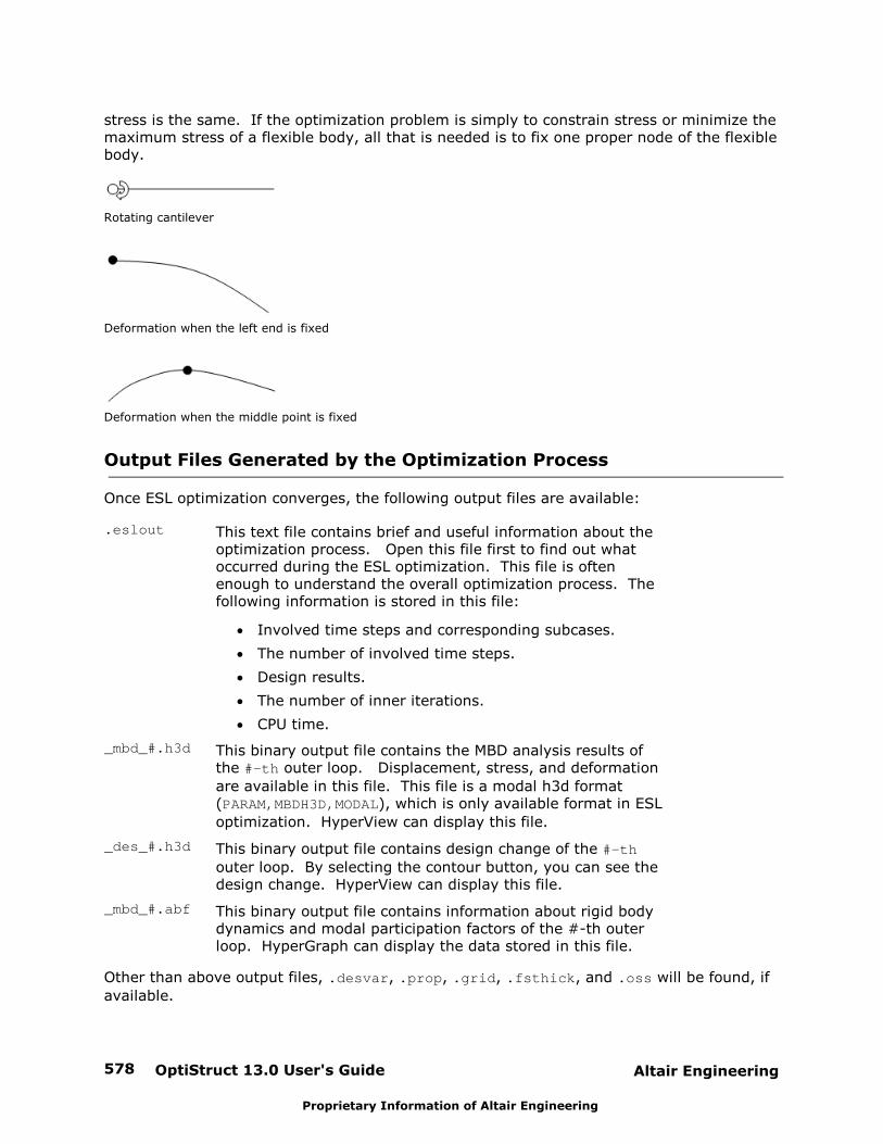
OptiStruct 13.0 User's Guide578 Altair Engineering
Proprietary Information of Altair Engineering
stress is the same. If the optimization problem is simply to constrain stress or minimize themaximum stress of a flexible body, all that is needed is to fix one proper node of the flexiblebody.
Rotating cantilever
Deformation when the left end is fixed
Deformation when the middle point is fixed
Output Files Generated by the Optimization Process
Once ESL optimization converges, the following output files are available:
.eslout This text file contains brief and useful information about theoptimization process. Open this file first to find out whatoccurred during the ESL optimization. This file is oftenenough to understand the overall optimization process. Thefollowing information is stored in this file:
Involved time steps and corresponding subcases.
The number of involved time steps.
Design results.
The number of inner iterations.
CPU time.
_mbd_#.h3d This binary output file contains the MBD analysis results ofthe #-th outer loop. Displacement, stress, and deformation
are available in this file. This file is a modal h3d format(PARAM,MBDH3D,MODAL), which is only available format in ESL
optimization. HyperView can display this file.
_des_#.h3d This binary output file contains design change of the #-th
outer loop. By selecting the contour button, you can see thedesign change. HyperView can display this file.
_mbd_#.abf This binary output file contains information about rigid bodydynamics and modal participation factors of the #-th outerloop. HyperGraph can display the data stored in this file.
Other than above output files, .desvar, .prop, .grid, .fsthick, and .oss will be found, if
available.
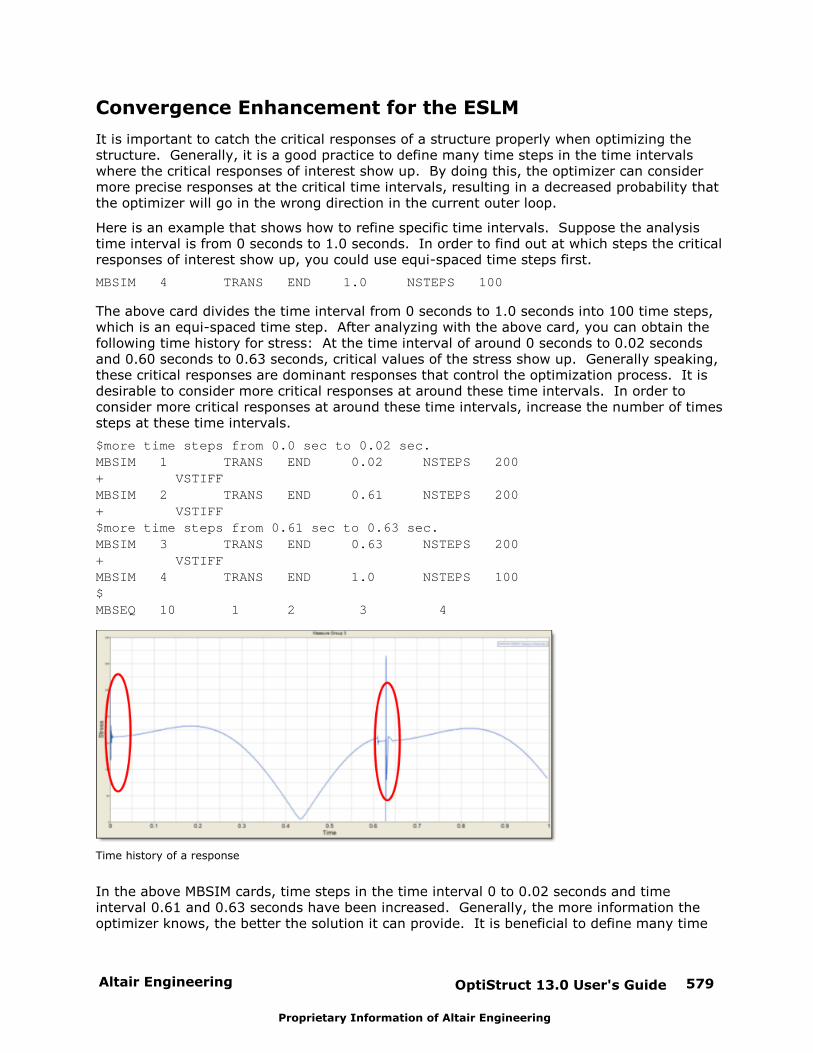
Altair Engineering OptiStruct 13.0 User's Guide 579
Proprietary Information of Altair Engineering
Convergence Enhancement for the ESLM
It is important to catch the critical responses of a structure properly when optimizing thestructure. Generally, it is a good practice to define many time steps in the time intervalswhere the critical responses of interest show up. By doing this, the optimizer can considermore precise responses at the critical time intervals, resulting in a decreased probability thatthe optimizer will go in the wrong direction in the current outer loop.
Here is an example that shows how to refine specific time intervals. Suppose the analysistime interval is from 0 seconds to 1.0 seconds. In order to find out at which steps the criticalresponses of interest show up, you could use equi-spaced time steps first.
MBSIM 4 TRANS END 1.0 NSTEPS 100
The above card divides the time interval from 0 seconds to 1.0 seconds into 100 time steps,which is an equi-spaced time step. After analyzing with the above card, you can obtain thefollowing time history for stress: At the time interval of around 0 seconds to 0.02 secondsand 0.60 seconds to 0.63 seconds, critical values of the stress show up. Generally speaking,these critical responses are dominant responses that control the optimization process. It isdesirable to consider more critical responses at around these time intervals. In order toconsider more critical responses at around these time intervals, increase the number of timessteps at these time intervals.
$more time steps from 0.0 sec to 0.02 sec.MBSIM 1 TRANS END 0.02 NSTEPS 200 + VSTIFF MBSIM 2 TRANS END 0.61 NSTEPS 200 + VSTIFF $more time steps from 0.61 sec to 0.63 sec.MBSIM 3 TRANS END 0.63 NSTEPS 200 + VSTIFF MBSIM 4 TRANS END 1.0 NSTEPS 100 $MBSEQ 10 1 2 3 4
Time history of a response
In the above MBSIM cards, time steps in the time interval 0 to 0.02 seconds and timeinterval 0.61 and 0.63 seconds have been increased. Generally, the more information theoptimizer knows, the better the solution it can provide. It is beneficial to define many time

OptiStruct 13.0 User's Guide580 Altair Engineering
Proprietary Information of Altair Engineering
steps; enough to catch precisely the critical responses in the time intervals where criticalresponse of interest show up. This will enhance convergence of the optimization process.
Altair Engineering OptiStruct 13.0 User's Guide 581
Proprietary Information of Altair Engineering
Parameters for the ESLM
Control the maximum number of outer loops executed in the ESLM by using the followingparameter:
DOPTPRM, ESLMAX
In this case, the ESLMAX is an integer value, greater than or equal to 0. If the ESLMAX is
equal to 0, then optimization process is not activated. The default value for the ESLMAX is 30.
The ESLM has a feature that screens out the time steps that are not dominant during theoptimization. In the most cases, this feature is very helpful to improve the efficiency of theESL optimization process in terms of CPU time. This feature can be activated or deactivatedby using:
DOPTPRM, ESLSOPT
The ESLSOPT can be either 0 or 1. If ESLSOPT is 0, then the screening is deactivated. If
ESLSOPT is 1, then this screening is activated. The default value is 1. Unless deactivated by
DOPTPRM, ESLSOPT, 0, this feature is always activated.
The time step screening feature is different from the constraint screening of the staticresponse optimization in Step 3, although the concepts of both screening capabilities aresimilar. The time step screening is performed at time Step 2, which is right before enteringthe static response optimization phase. By performing the time step screening beforeentering the static response optimization phase, the huge amounts of CPU time required forstructural analysis and subsequent constraint screening strategy can be saved at the 0-thiteration in the static response optimization phase.
Once ESLSOPT is activated, the number of time steps that should be screened out can be
controlled by using:
DOPTPRM, ESLSTOL
ESLSTOL is a real number between 0.0 and 1.0. The smaller the value of ESLSTOL, the fewer
the number of time steps involved in the optimization process. If ESLSTOL is 1.0, all of the
time steps in multi-body dynamic analysis will be involved in the optimization process. Obviously, the smaller the ESLSTOL value, the less total CPU time will be used. Note,
however, that assigning too small a value to the ESLSTOL could cause the optimization
process to diverge. Therefore, if the number of time steps retained by ESLSTOL is less than
10, the 10 most dominant time steps will be involved in the optimization process. Thedefault value for the ESLSTOL is 0.3.

OptiStruct 13.0 User's Guide582 Altair Engineering
Proprietary Information of Altair Engineering
Output Requests and ESLM
Users are not allowed to control analysis output in ESL optimization. All information from theMBD analysis is already available in _mbd_#.h3d, including displacement, stress, and
deformation. All analysis output requests are invalidated during ESL optimization except thatOutput Request = option is allowed above the first subcase. For example, STRESS = ALL or
DISPLACEMENT = SID is allowed above the first subcase.
Optimization output is not controllable in ESL optimization. See Equivalent Static LoadMethod (ESLM) for more details.
Output and format in output format controls are not controllable in ESL optimization. Allrequests on output and format are invalidated during ESL optimization, except for FSTHICKand OSS.
Altair Engineering OptiStruct 13.0 User's Guide 583
Proprietary Information of Altair Engineering
MBD System Level Response Optimization
The original ESLM implemented in OptiStruct is for the optimization of flexible bodies in MBDsystems through the control of structural responses, such as stress or deformation. Theoriginal ESLM is not capable of handling system level responses, such as joint force of a jointor velocity of a node of a body. System-level responses referred to in this section can bedisplacement, velocities, acceleration, joint force, and functions of those 4 quantities definedby MBVAR. In addition to the original ESLM, MBD system level response optimization is alsoavailable in OptiStruct. ESLM and MBD system level optimization can be combined togetherto optimize MBD systems. One of typical optimization formulations that can be solved byOptiStruct could be:
Minimize joint force of a joint
subject to stress < allowable value
deformation < allowable value
velocities of a node < allowable value
MBD system level responses can be controlled by the properties of PRBODY, CMBUSH(M),CMBEAM(M), and CMSPDP(M) as well as usual design variables in structural optimizationsuch as thickness of bodies, shape of bodies, etc. DVMBRL1 and DVMBRL2 are available todefine relationships between design variables and properties of PRBODY, CMBUSH(M),CMBEAM(M), and CMSPDP(M).
Large Number of Design Variables
MBD system level responses are approximated by adaptive response surfaces. The basicsolution strategy for MBD system level optimization is the same as that implemented inHyperStudy. In general, response surface based optimization cannot handle large number ofdesign variables. This issue has been resolved in OptiStruct through the introduction ofintermediate design variables for bodies. All the design variables defined on rigid/flexiblebodies are converted to some predefined intermediate design variables. Adaptive responsesurfaces are built based on those intermediate design variables. As a result, even if there arehundreds of design variables defined on bodies, adaptive response surfaces for MBD systemlevel responses can be built with only several intermediate design variables. This way,OptiStruct can handle MBD system level responses with large number of design variables.
Change of Length of Bodies as Shape Optimization
When you try to achieve a specific velocity value less than an allowed value, changing thelength of bodies is an efficient way to achieve it. You can set up shape optimization problemto change the length of bodies. The designable bodies can be either rigid bodies or flexiblebodies. When defining shape perturbation vectors with DVGRID, you have to make sure thateach perturbation vector does not break down the original joint configuration as the designchanges. For example, a revolute joint must have two coincident nodes attached to twodifferent bodies. Be aware while defining shape perturbation vectors, that the perturbationvector could cause a location change for only one of the two coincident nodes so that therevolute joint definition would not be valid after one design iteration.

OptiStruct 13.0 User's Guide584 Altair Engineering
Proprietary Information of Altair Engineering
Limitations of MBD System Level Response Optimization
Design variables associated with PRBODY, CMBUSH(M), CMBEAM(M), and CMSPDP(M) cannotcontrol structural responses, such as deformation or stress. They can only control MBDsystem level responses such as MBDIS, MBVEL, MBACC, MBFRC, and MBEXPR. Designvariables associated with structures such as length, shape, and thickness can control MBDsystem level responses. Thus, if interaction between structural responses and MBD systemlevel responses are mutually strong, this feature is not applicable.
Rigid bodies cannot have structural design variables (shape, properties, thickness, etc.) andthe design variables associated with DVMBRL1/2 with TYPE=PRBODY at the same time.
Currently, system level responses must be scalar values. OptiStruct provides an option topick up the maximum, minimum, maximum absolute, or minimum absolute value ofdisplacement/velocity/acceleration/ joint force when defining MBD system level responsesusing the DRESP1 card. If a system level response is an objective function, and the timewhen the objective function is picked up jumps around during the optimization process,convergence could be slow or even diverge in some cases.
Altair Engineering OptiStruct 13.0 User's Guide 585
Proprietary Information of Altair Engineering
ESLM for Nonlinear Response Optimization
The equivalent static load method has been extended to support nonlinear responseoptimization. The following geometric nonlinear analyses are supported for optimization inOptiStruct:
Implicit (quasi-) static analysis (NLGEOM)
Implicit dynamic analysis (IMPDYN)
Explicit dynamic analysis (EXPDYN)
Refer to the Geometric Nonlinear Analysis section for more details on the supported analysistypes.
This method is implemented to support various types of responses that are available in ausual static response optimization problem, i.e. displacement, strain, stress, etc., forexample. Only responses defined by DRESP1 are currently supported.
Concept level design techniques such as topology, free-sizing and topography optimization,and design fine tuning techniques such as size, shape and free-shape optimization aresupported for nonlinear response optimization using ESLM. In the current implementation,for topology optimization, PSHELL and PSOLID are supported and PSHELL is supported forfree-size optimization.
The optimization setup using ESLM for nonlinear response optimization in terms of designvariables, responses, constraints and objective function is the same as the setup for a typicalstatic response optimization problem for topology, topography, free-size, size, shape andfree-shape optimization.
Output Files Generated by the Optimization Process
In addition to the standard optimization outputs, the following files are output:
[model]_#.h3d: Analysis results for each #th outer loop.
[model].eslout: Outer loop iteration history summary.
Parameters of ESLM
Several parameters are available to control the optimization process:
DOPTPRM, ESLMAX
This parameter controls the maximum number of outer loops.
DOPTPRM, DESMAX
This parameter controls the maximum number of inner loop iterations.
DOPTPRM, NESLNLGM
This parameter controls the number of ESLs generated for each NLGEOM subcase.
DOPTPRM, NESLIMPD
This parameter controls the number of ESLs generated for each IMPDYN subcase.

OptiStruct 13.0 User's Guide586 Altair Engineering
Proprietary Information of Altair Engineering
DOPTPRM, NESLEXPD
This parameter controls the number of ESLs generated for each EXPDYN subcase.
For more details, refer to DOPTPRM parameters.
Altair Engineering OptiStruct 13.0 User's Guide 587
Proprietary Information of Altair Engineering
Gradient-based Optimization Method
The following features can be found in this section:
Iterative Solution
OptiStruct uses an iterative procedure known as the local approximation method to solvethe optimization problem. This method determines the solution of the optimizationproblem using the following steps:
1. Analysis of the physical problem using finite elements.
2. Convergence test; whether or not the convergence is achieved.
3. Response screening to retain potentially active responses for the current iteration.
4. Design sensitivity analysis for retained responses.
5. Optimization of an explicit approximate problem formulated using the sensitivityinformation. Back to 1.
To achieve a stable convergence, design variable changes during each iteration are limitedto a narrow range within their bounds, called move limits. The biggest design variablechanges occur within the first few iterations and, due to an advanced formulation andother stabilizing measures, convergence for practical applications is typically reached withonly a small number of FE analyses.
The design sensitivity analysis calculates derivatives of structural responses with respect tothe design variables. This is one of the most important ingredients for taking FEA from asimple design validation tool to an automated design optimization framework.
The design update is generated by solving the explicit approximate optimization problem,based on sensitivity information. OptiStruct has two classes of optimization methodsimplemented: dual method and primal method. The dual method solves the optimizationproblem in the dual space of Largrange multipliers associated with active constraints. It ishighly efficient for design problems involving a very large number of design variables butmuch fewer constraints (common to topology and topography optimization). The primalmethod searches the optimum in the original design variable space. It is used forproblems that involve equally as many design constraints as design variables, which iscommon for size and shape optimizations. The choice of optimizer is made automaticallyby OptiStruct, based on the characteristics of the optimization problem.
Regular or Soft Convergence
Two convergence tests are used in OptiStruct and satisfaction of only one of these tests isrequired.
Regular convergence (design is feasible) is achieved when the convergence criteria aresatisfied for two consecutive iterations. This means that for two consecutive iterations, thechange in the objective function is less than the objective tolerance and constraintviolations are less than 1%. At least three analyses are required for regular convergence,as the convergence is based on the comparison of true objective values (values obtainedfrom an analysis at the latest design point). An exception (design is infeasible) is whenthe constraints remain violated by more than 1%, and for three consecutive iterations thechange in the objective function is less than the objective tolerance and the change in the
OptiStruct 13.0 User's Guide588 Altair Engineering
Proprietary Information of Altair Engineering
constraint violations is less than 0.2%. In this case, the iterative process will beterminated with a conclusion ‘No feasible design can be obtained.’
Soft convergence is achieved when there is little or no change in the design variables fortwo consecutive iterations. It is not necessary to evaluate the objective (or constraints) forthe final design point, as the model is unchanged from the previous iteration. Therefore,soft convergence requires one less iteration than regular convergence.
OptiStruct Optimization Algorithms
OptiStruct utilizes gradient-based optimization algorithms to solve the optimizationproblem. The default optimization algorithm is known as the Method of Feasible Directions(MFD). You can select a different algorithm using the DOPTPRM, OPTMETH parameter. Thefollowing algorithms are available in OptiStruct:
Method of feasible directions (MFD)
Sequential quadratic programming (SQP)
Dual Optimizer based on separate convex approximation (DUAL)
Large scale optimization algorithm (BIGOPT)
MFD, SQP, and DUAL are standard optimization algorithms. For further information, referto relevant books and papers in the OptiStruct References section.
Large Scale Optimization Algorithm (BIGOPT)
The Large scale optimization algorithm (BIGOPT) is a gradient-based method. It consumesless memory and is relatively more computationally efficient, compared to MFD and SQP.
Implementation
Consider an optimization problem that involves minimizing f(X) based on a set of
constraints. It is described as follows:
Where,
f(X) is the objective function,
gi(X) is the i’th constraint function,
me is the number of equality constraints,
m is the total number of constraints,
X is the design variable vector,
X L and XU are the lower and upper bound vectors of design variables, respectively.
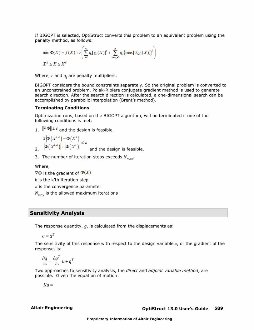
Altair Engineering OptiStruct 13.0 User's Guide 589
Proprietary Information of Altair Engineering
If BIGOPT is selected, OptiStruct converts this problem to an equivalent problem using thepenalty method, as follows:
Where, r and qi are penalty multipliers.
BIGOPT considers the bound constraints separately. So the original problem is converted toan unconstrained problem. Polak-Ribiere conjugate gradient method is used to generatesearch direction. After the search direction is calculated, a one-dimensional search can beaccomplished by parabolic interpolation (Brent’s method).
Terminating Conditions
Optimization runs, based on the BIGOPT algorithm, will be terminated if one of thefollowing conditions is met:
1. and the design is feasible.
2. and the design is feasible.
3. The number of iteration steps exceeds Nmax.
Where,
is the gradient of
k is the k’th iteration step
is the convergence parameter
Nmax is the allowed maximum iterations
Sensitivity Analysis
The response quantity, g, is calculated from the displacements as:
Tg q u
The sensitivity of this response with respect to the design variable x, or the gradient of the
response, is:
TTg q u
u qx x x
Two approaches to sensitivity analysis, the direct and adjoint variable method, arepossible. Given the equation of motion:
Ku f
OptiStruct 13.0 User's Guide590 Altair Engineering
Proprietary Information of Altair Engineering
and its derivative with respect to design variable x,
fK uu K
x x x
one can calculate the sensitivity of the displacement vector u as:
fu KK u
x x x
Using this equation, the largest cost in the calculation of the response gradient is theforward-backward substitution required for the calculation of the derivative of thedisplacement vector with respect to the design variable. This is called the direct method. One forward-backward substitution is required for each design variable.
If constraints are active in more than one load case, and the load is a function of thedesign variable (say body force or pressure loads for shape optimization), then the set offorward-backward substitutions must be performed for each active load case. If the loadsare not a function of the design variables, but there are active load cases with multipleboundary conditions, then the set of forward-backward substitutions must be performed foreach active boundary condition.
For the adjoint variable method of sensitivity analysis, the vector (adjoint variable) a is
introduced, which is calculated as:
Ka q
Then the derivative of the constraint can be calculated as:
TTg q f K
u a ux x x x
When the adjoint variable method for sensitivity analysis is used, a single forward-backward substitution is needed for each retained constraint. This forward-backwardsubstitution is needed to calculate the vector a.
There are typically a small number of design variables in shape and size optimization (say5 to 50) and a large number of constraints. The large number of constraints comes fromstress constraints. If there are 20,000 elements, each with a single stress constraint, and10 load cases, there are a total of 200,000 possible stress constraints.
There are typically a large number of design variables in topology optimization (between 1and 3 per element) and a small number of constraints. Because stress constraints are notusually considered in topology optimization, it makes sense that the adjoint variablemethod of sensitivity analysis be used for topology optimization (in order to reducecomputational costs).
For shape and sizing optimization, it is often beneficial to use the direct method forsensitivity analysis. However, in some cases, when there are a large number of designvariables and a small number of constraints, the adjoint variable method should be used. For example, in a topography optimization, the number of constraints that gradients needto be calculated for can be reduced using constraint screening. With constraint screening,constraints that are not close to being violated are ignored. Only constraints that areviolated, or nearly violated, are retained. Also, if there are many stress constraints thatare retained in a small region of the structure, say at a stress concentration, only a few ofthe most critical need to be retained.
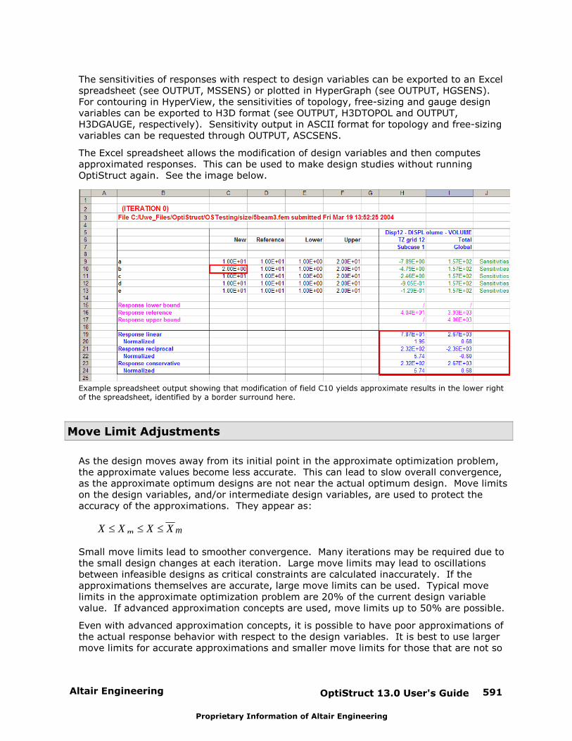
Altair Engineering OptiStruct 13.0 User's Guide 591
Proprietary Information of Altair Engineering
The sensitivities of responses with respect to design variables can be exported to an Excelspreadsheet (see OUTPUT, MSSENS) or plotted in HyperGraph (see OUTPUT, HGSENS). For contouring in HyperView, the sensitivities of topology, free-sizing and gauge designvariables can be exported to H3D format (see OUTPUT, H3DTOPOL and OUTPUT,H3DGAUGE, respectively). Sensitivity output in ASCII format for topology and free-sizingvariables can be requested through OUTPUT, ASCSENS.
The Excel spreadsheet allows the modification of design variables and then computesapproximated responses. This can be used to make design studies without runningOptiStruct again. See the image below.
Example spreadsheet output showing that modification of field C10 yields approximate results in the lower rightof the spreadsheet, identified by a border surround here.
Move Limit Adjustments
As the design moves away from its initial point in the approximate optimization problem,the approximate values become less accurate. This can lead to slow overall convergence,as the approximate optimum designs are not near the actual optimum design. Move limitson the design variables, and/or intermediate design variables, are used to protect theaccuracy of the approximations. They appear as:
mmX X X X X
Small move limits lead to smoother convergence. Many iterations may be required due tothe small design changes at each iteration. Large move limits may lead to oscillationsbetween infeasible designs as critical constraints are calculated inaccurately. If theapproximations themselves are accurate, large move limits can be used. Typical movelimits in the approximate optimization problem are 20% of the current design variablevalue. If advanced approximation concepts are used, move limits up to 50% are possible.
Even with advanced approximation concepts, it is possible to have poor approximations ofthe actual response behavior with respect to the design variables. It is best to use largermove limits for accurate approximations and smaller move limits for those that are not so
OptiStruct 13.0 User's Guide592 Altair Engineering
Proprietary Information of Altair Engineering
accurate.
Note that the same set of design variable move limits must be used for all of the responseapproximations. It is important to look at the approximations of the responses that aredriving the design. These are the objective function and most critical constraints. If theobjective function moves in the wrong direction, or critical constraints become even moreviolated, it is a sign that the approximations are not accurate. In this case, all of thedesign variable move limits are reduced. However, if the move limits become too small,convergence may be slowed, as design variables that are a long way from the optimumdesign are forced to change slowly. Therefore, the move limits on the individual designvariables that keep hitting the same upper or lower move limit bound are increased. Movelimits are automatically adjusted by OptiStruct.
Constraint Screening
At each iteration of the optimization process, the objective function(s) and all constraintsof the design problem are evaluated. Retaining all of these responses in the optimizationproblem has two potential disadvantages:
1. This can result in a big optimization problem with a large number of responses anddesign variables. Most optimization algorithms are designed to handle either a largenumber of responses or a large number of design variables, but not both.
2. For gradient-based optimization, the design sensitivities of these responses need to becalculated. The design sensitivity calculation can be very computationally expensivewhen there are a large number of responses and a large number of design variables.
Constraint screening is the process by which the number of responses in the optimizationproblem is trimmed to a representative set. This set of retained responses captures theessence of the original design problem while keeping the size of the optimization problemat an acceptable level. Constraint screening utilizes the fact that constrained responsesthat are a long way from their bounding values (on the satisfactory side) or which are lesscritical (i.e. for an upper bound more negative and for a lower bound more positive) than agiven number of constrained responses of the same type, within the same designatedregion and for the same subcase, will not affect the direction of the optimization problemand therefore can be removed from the problem for the current design iteration.
Consider the optimization problem where the objective is to minimize the mass of a finiteelement model composed of 100,000 elements, while keeping the elemental stresses belowtheir associated material's yield stress. In this problem, you have 100,000 constraints (thestress for every element must be below its associated material's yield stress) for eachsubcase. For every design variable, 100,000 sensitivity calculations must be performed foreach subcase, at every iteration. Because design variable changes are restricted by movelimits, stresses are not expected to change drastically from one iteration to the next. Therefore, it is wasteful to calculate the sensitivities for those elements whose stresses areconsiderably lower than their associated material's yield stress. Also the direction of theoptimization will be driven primarily by the highest elemental stresses. Therefore, thenumber of required calculations can be further reduced by only considering an arbitrarynumber of the highest elemental stresses.
Of course there is trade-off involved in using constraint screening. By not considering allof the constrained responses, it may take more iterations to reach a converged solution. Iftoo many constrained responses are screened, it may take considerably longer to reach aconverged solution or, in the worst case, it may not be able to converge on a solution if the

Altair Engineering OptiStruct 13.0 User's Guide 593
Proprietary Information of Altair Engineering
number of retained responses is less than the number of active constraints for the givenproblem.
Through extensive testing it has been found that, for the majority of problems, usingconstraint screening saves a lot of time and computational effort. Therefore, constraintscreening is active in OptiStruct by default. The default settings consider only the 20 mostcritical (i.e. for an upper bound most positive and for a lower bound most negative)constraints that come within 50 percent of their bound value (on the satisfactory side) foreach response type, for each region, for each subcase.
The DSCREEN bulk data entry controls both the screening threshold and number ofretained constraints. Different DSCREEN settings are allowed for all of the response typessupported by the DRESP1 bulk data entry. Responses defined by the DRESP2 bulk dataentry are controlled by a single DSCREEN entry with RTYPE = EQUA. Likewise, responsesdefined by the DRESP3 bulk data entry are controlled by a single DSCREEN entry withRTYPE = EXTERNAL. It is important to ensure that DRESP2 and DRESP3 definitions thatuse the same region identifier use similar equations. (In order for constraint screening towork effectively, responses within the same region should be of similar magnitudes anddemonstrate similar sensitivities, the easiest way to ensure that is through the use ofsimilar variable combinations).
In order to reduce the burden on the user, it is possible to allow the screening criteria to beautomatically and adaptively adjusted in an effort to retain the least number of responsesnecessary for stable convergence. Setting RTYPE=AUTO on the DSCREEN bulk data entrywill enable this feature. Region definition is also automated with this setting. This settingis useful for less experienced users and can be particularly useful when there are manylocal constraints. However, there are some drawbacks; experienced users may be able toachieve better performance through manual definition of screening criteria, more memorymay be required to run with RTYPE=AUTO, and manual under-retention of constraints willrequire less memory and may, therefore, be desirable for very large problems (even withcompromised convergence stability and optimality).
Regions and Their Purpose
In OptiStruct, a region is a group of responses of the same type.
Regions are defined by the region identifier field on the DRESP1, DRESP2, and DRESP3bulk data entries used to define the responses. If the region identifier field is left blank,then each property associated with the response forms its own region. The same regionidentifier may be used for responses of different types, but remember that because theyare not of the same type they cannot form the same region.
Example 1
(1) (2) (3) (4) (5) (6) (7) (8) (9) (10)
DRESP1 1 label STRESS PSHELL SMP1 1
2 3
DRESP1 with ID 1 defines stress responses for all the elements that reference thePSHELL definitions with PID 1, 2, or 3. As no region identifier is defined, the stress
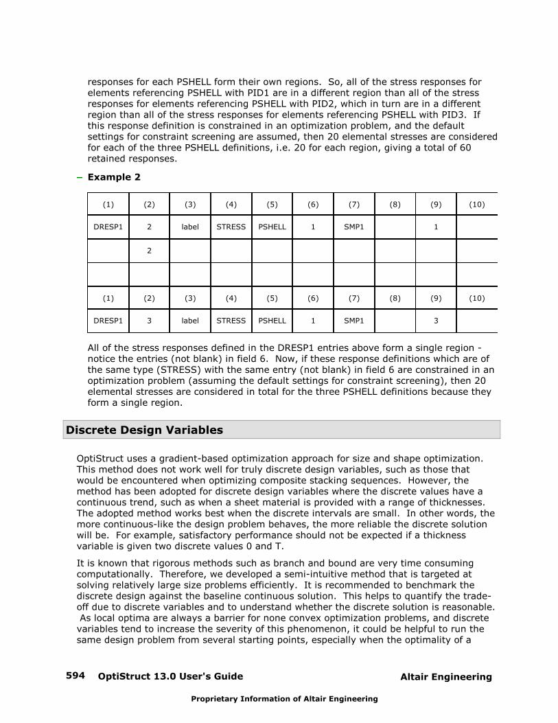
OptiStruct 13.0 User's Guide594 Altair Engineering
Proprietary Information of Altair Engineering
responses for each PSHELL form their own regions. So, all of the stress responses forelements referencing PSHELL with PID1 are in a different region than all of the stressresponses for elements referencing PSHELL with PID2, which in turn are in a differentregion than all of the stress responses for elements referencing PSHELL with PID3. Ifthis response definition is constrained in an optimization problem, and the defaultsettings for constraint screening are assumed, then 20 elemental stresses are consideredfor each of the three PSHELL definitions, i.e. 20 for each region, giving a total of 60retained responses.
Example 2
(1) (2) (3) (4) (5) (6) (7) (8) (9) (10)
DRESP1 2 label STRESS PSHELL 1 SMP1 1
2
(1) (2) (3) (4) (5) (6) (7) (8) (9) (10)
DRESP1 3 label STRESS PSHELL 1 SMP1 3
All of the stress responses defined in the DRESP1 entries above form a single region -notice the entries (not blank) in field 6. Now, if these response definitions which are ofthe same type (STRESS) with the same entry (not blank) in field 6 are constrained in anoptimization problem (assuming the default settings for constraint screening), then 20elemental stresses are considered in total for the three PSHELL definitions because theyform a single region.
Discrete Design Variables
OptiStruct uses a gradient-based optimization approach for size and shape optimization. This method does not work well for truly discrete design variables, such as those thatwould be encountered when optimizing composite stacking sequences. However, themethod has been adopted for discrete design variables where the discrete values have acontinuous trend, such as when a sheet material is provided with a range of thicknesses. The adopted method works best when the discrete intervals are small. In other words, themore continuous-like the design problem behaves, the more reliable the discrete solutionwill be. For example, satisfactory performance should not be expected if a thicknessvariable is given two discrete values 0 and T.
It is known that rigorous methods such as branch and bound are very time consumingcomputationally. Therefore, we developed a semi-intuitive method that is targeted atsolving relatively large size problems efficiently. It is recommended to benchmark thediscrete design against the baseline continuous solution. This helps to quantify the trade-off due to discrete variables and to understand whether the discrete solution is reasonable. As local optima are always a barrier for none convex optimization problems, and discretevariables tend to increase the severity of this phenomenon, it could be helpful to run thesame design problem from several starting points, especially when the optimality of a

Altair Engineering OptiStruct 13.0 User's Guide 595
Proprietary Information of Altair Engineering
solution is in doubt.
It is also possible to mix these discrete variables with continuous variables in anoptimization problem.
Discrete design variables are activated by referencing a DDVAL entry on a DESVAR card.
The DDVOPT parameter on the DOPTPRM card allows you to choose between a fullydiscrete optimization or a two phased approach where a continuous optimization isperformed first, and a discrete optimization is started from the continuous optimum.
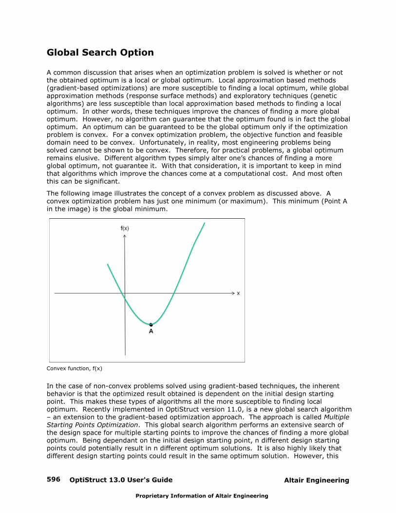
OptiStruct 13.0 User's Guide596 Altair Engineering
Proprietary Information of Altair Engineering
Global Search Option
A common discussion that arises when an optimization problem is solved is whether or notthe obtained optimum is a local or global optimum. Local approximation based methods(gradient-based optimizations) are more susceptible to finding a local optimum, while globalapproximation methods (response surface methods) and exploratory techniques (geneticalgorithms) are less susceptible than local approximation based methods to finding a localoptimum. In other words, these techniques improve the chances of finding a more globaloptimum. However, no algorithm can guarantee that the optimum found is in fact the globaloptimum. An optimum can be guaranteed to be the global optimum only if the optimizationproblem is convex. For a convex optimization problem, the objective function and feasibledomain need to be convex. Unfortunately, in reality, most engineering problems beingsolved cannot be shown to be convex. Therefore, for practical problems, a global optimumremains elusive. Different algorithm types simply alter one’s chances of finding a moreglobal optimum, not guarantee it. With that consideration, it is important to keep in mindthat algorithms which improve the chances come at a computational cost. And most oftenthis can be significant.
The following image illustrates the concept of a convex problem as discussed above. Aconvex optimization problem has just one minimum (or maximum). This minimum (Point Ain the image) is the global minimum.
Convex function, f(x)
In the case of non-convex problems solved using gradient-based techniques, the inherentbehavior is that the optimized result obtained is dependent on the initial design startingpoint. This makes these types of algorithms all the more susceptible to finding localoptimum. Recently implemented in OptiStruct version 11.0, is a new global search algorithm– an extension to the gradient-based optimization approach. The approach is called MultipleStarting Points Optimization. This global search algorithm performs an extensive search ofthe design space for multiple starting points to improve the chances of finding a more globaloptimum. Being dependant on the initial design starting point, n different design startingpoints could potentially result in n different optimum solutions. It is also highly likely thatdifferent design starting points could result in the same optimum solution. However, this
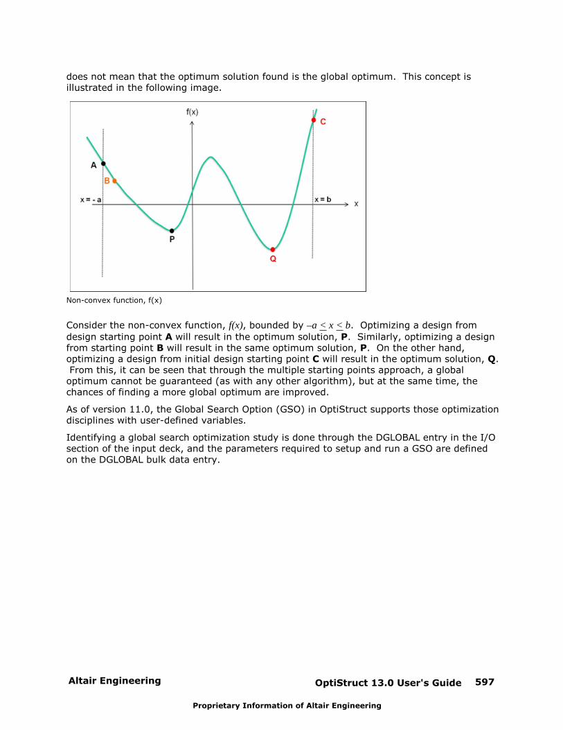
Altair Engineering OptiStruct 13.0 User's Guide 597
Proprietary Information of Altair Engineering
does not mean that the optimum solution found is the global optimum. This concept isillustrated in the following image.
Non-convex function, f(x)
Consider the non-convex function, f(x), bounded by –a < x < b. Optimizing a design from
design starting point A will result in the optimum solution, P. Similarly, optimizing a designfrom starting point B will result in the same optimum solution, P. On the other hand,optimizing a design from initial design starting point C will result in the optimum solution, Q. From this, it can be seen that through the multiple starting points approach, a globaloptimum cannot be guaranteed (as with any other algorithm), but at the same time, thechances of finding a more global optimum are improved.
As of version 11.0, the Global Search Option (GSO) in OptiStruct supports those optimizationdisciplines with user-defined variables.
Identifying a global search optimization study is done through the DGLOBAL entry in the I/Osection of the input deck, and the parameters required to setup and run a GSO are definedon the DGLOBAL bulk data entry.
OptiStruct 13.0 User's Guide598 Altair Engineering
Proprietary Information of Altair Engineering
Design Interpretation - OSSmooth
OSSmooth is a semi-automated design interpretation software, facilitating the recovery of amodified geometry resulting from a structural optimization, for further use in the designprocess and FEA reanalysis. The tool has two incarnations: a standalone version that comeswith the OptiStruct installation, and a dependent version that is embedded in HyperMesh.
OSSmooth can be used in three different ways: OSSmooth for geometry, FEA topologyreanalysis, and FEA topography reanalysis.
Note: FEA topology reanalysis and FEA topography reanalysisare features which are available only in the version ofOSSmooth that is embedded within HyperMesh, they arenot supported by the standalone OSSmooth software.
OSSmooth (for geometry) has several uses and can be used to:
Interpret topology optimization results, creating an iso-density boundary surface (Iso-surface).
Interpret topography optimization results, creating beads or swages on the designsurface.
Recover and smooth geometry resulting from a shape optimization.
Reduce the amount of surface data from a given set of triangular patches by combiningsmaller patches.
Smooth surface data given as triangular patches.
For FEA topology reanalysis and FEA topography reanalysis, OSSmooth can be used to:
Preserve component boundaries for multiple design components.
Recover geometry with or without an artificial layer of elements around a non-designspace optionally.
Tetramesh Iso-surfaces ‘by property’.
Preserve boundary conditions upon geometry recovery to enable quick reanalysis.
The following flowchart provides an overview of how OSSmooth works to interpretoptimization results from OptiStruct:
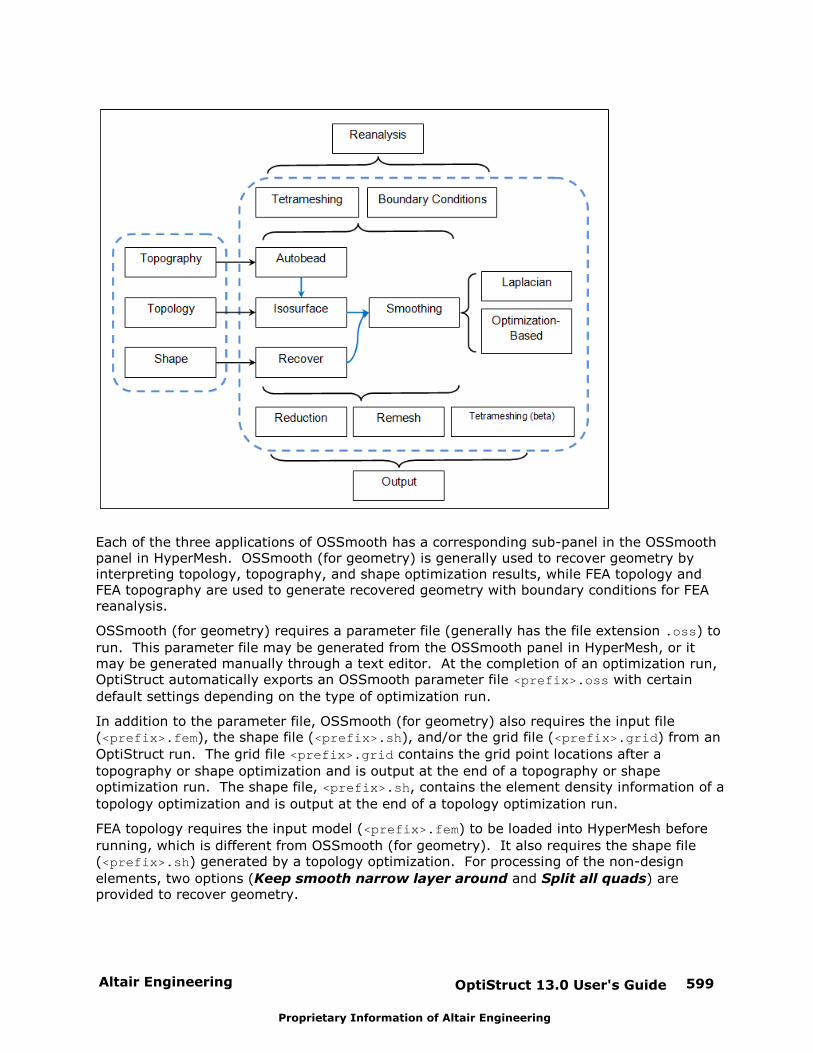
Altair Engineering OptiStruct 13.0 User's Guide 599
Proprietary Information of Altair Engineering
Each of the three applications of OSSmooth has a corresponding sub-panel in the OSSmoothpanel in HyperMesh. OSSmooth (for geometry) is generally used to recover geometry byinterpreting topology, topography, and shape optimization results, while FEA topology andFEA topography are used to generate recovered geometry with boundary conditions for FEAreanalysis.
OSSmooth (for geometry) requires a parameter file (generally has the file extension .oss) to
run. This parameter file may be generated from the OSSmooth panel in HyperMesh, or itmay be generated manually through a text editor. At the completion of an optimization run,OptiStruct automatically exports an OSSmooth parameter file <prefix>.oss with certain
default settings depending on the type of optimization run.
In addition to the parameter file, OSSmooth (for geometry) also requires the input file(<prefix>.fem), the shape file (<prefix>.sh), and/or the grid file (<prefix>.grid) from an
OptiStruct run. The grid file <prefix>.grid contains the grid point locations after a
topography or shape optimization and is output at the end of a topography or shapeoptimization run. The shape file, <prefix>.sh, contains the element density information of a
topology optimization and is output at the end of a topology optimization run.
FEA topology requires the input model (<prefix>.fem) to be loaded into HyperMesh before
running, which is different from OSSmooth (for geometry). It also requires the shape file(<prefix>.sh) generated by a topology optimization. For processing of the non-design
elements, two options (Keep smooth narrow layer around and Split all quads) areprovided to recover geometry.

OptiStruct 13.0 User's Guide600 Altair Engineering
Proprietary Information of Altair Engineering
FEA topography requires a grid file (<prefix>.grid) to run. Similar to FEA topology, it also
requires that the input model (<prefix>.fem) be loaded into HyperMesh first, with the option
for iso-surface that performs the same functionality as FEA topology.
Note: OSSmooth currently does not recognize OptiStruct long-format input data. A possible work-around for thisproblem is to import the long-format input file intoHyperMesh and export it using the regular OptiStructtemplate before running OSSmooth.
The interpreted design from OSSmooth can be exportedas a finite element mesh in the bulk data format, as IGESsurfaces, as a stereolithography file, or as a Hyper3D file.
Altair Engineering OptiStruct 13.0 User's Guide 601
Proprietary Information of Altair Engineering
OSSmooth Parameter File
The OSSmooth parameter file is composed of a number of parameter statements, each ofwhich has the following format:
parameter_name arg1,arg2,...,argn
The parameter_name and arguments can be separated either by spaces or commas. The file
is not case sensitive.
Comment lines in the OSSmooth parameter file should start with either ‘#’ or ‘$’.
The following is a list of allowable parameters and their respective arguments:
Parameter Description
input_file Identifies the files to be interpreted by OSSmooth.
arg1 The file name (without extension) of the OptiStruct .fem, .sh, and/or .grid files to be interpreted by
OSSmooth.
output_file Name of the file to be output by OSSmooth.
arg1 Full name of the file output by OSSmooth.
output_code Identifies the type of output.
Argument Description
arg1 Output format for iso-surface:
1 – Bulk data trias2 – IGES patches3 – STL trias [default]4 – H3D trias
arg2 Output control for tet-meshing of volume enclosed by theiso-surface.
[Default: no tet-meshing]
1 – Tetra4 + Tria3 elements2 – Tetra10 + Tria6 elements3 – Tetra4 elements4 – Tetra10 elements
The tet-mesh is written in OptiStruct input format to a file <input_file>_mesh.fem. In this file, the design space of
the file <input_file>.fem is replaced with a tet-mesh for
immediate reanalysis. Loads, boundary conditions, andnon-design elements are carried over from the input file.
OptiStruct 13.0 User's Guide602 Altair Engineering
Proprietary Information of Altair Engineering
Parameter Description
units Defines output units for IGES format. This information gets written tothe header of the IGES file and may be recognized by your CAD system.
1 – inch [default]2 – mm4 – foot6 – m10 – cm
autobead Improves the recovered geometry from a topography optimization byapplying automatic geometry creation.
Argument Description
arg1 Operation flag [integer]:
0 – autobead off1 – autobead on [default]
arg2 Threshold value for creating autobead.
[real, between 0.0 and 1.0, default = 0.3]
arg3 Bead layer [integer]:
1 – create 1 layer bead [default]2 – create 2 layers bead
isosurface Generate threshold surface from a topology optimization by applyingautomatic geometry creation.
Argument Description
arg1 Operation flag [integer]:
0 – isosurface off1 – isosurface on [default]
arg2 Type of surface created [integer]:
0 – isosurface only1 – isosurface with Optimization-based smoothing2 – Element threshold surface3 – isosurface with Laplacian smoothing [default]
For topology results, smoothing maintains the topology assuggested by OptiStruct, but it can deviate from the givendensity distribution. If option 1 or 3 is used, check themaximum and average smoothing error output byOSSmooth.
arg3 Density threshold for creating isosurface.
[real, between 0.0 and 1.0, default = 0.3]
Altair Engineering OptiStruct 13.0 User's Guide 603
Proprietary Information of Altair Engineering
Parameter Description
opti_smoothing Optimization-based smoothing [Only used if isosurface C2=1].
Argument Description
arg1 Unit-less surface distance coefficient
[real, default = 0.0]
Defines closeness of the smooth surface from the thresholdsurface. The effect of this coefficient varies for differentinput meshes. Higher magnitudes (both positive andnegative) give smoother results, but the surface deviatesmore from the original density distribution. Therecommended range is from -50 to 50. When thecoefficient is set between 0 and 50, the surface usuallytends to smooth and shrink. When the coefficient is setbetween 0 and -50, the surface usually tends to smooth andexpand.
arg2 Smooth isosurface boundary flag [integer]:
0 – boundary not included in smoothing [default]1 – boundary included in smoothing
laplacian_smoothing
Laplacian smoothing [Only used if isosurface C2=3].
Argument Description
arg1 Number of iteration for Laplacian smoothing
[integer > 0, default = 10]
arg2 Feature angle threshold in degrees
[real, default = 30.0]
The feature angle is defined as the angle of normal betweentwo intersected element planes. All corners with a featureangle larger than the threshold will be preserved in thesmoothing process.
arg3 Smooth isosurface boundary flag [integer]:
0 – boundary not included in smoothing1 – boundary included in smoothing [default]
remesh Remesh autobead surface and/or isosurface flag [integer]:
0 – remesh off [default]1 – remesh on
Remesh detects 2-layer elements around bead shape and/or boundaryof isosurface. Use mixed type remesh if input mesh contains any QUADelements, otherwise remesh with TRIA elements.
OptiStruct 13.0 User's Guide604 Altair Engineering
Proprietary Information of Altair Engineering
Parameter Description
surface_reduction
Reduces the number of surfaces representing the geometry. Can reducethe number of surfaces by up to 80%.
Argument Description
arg1 Surface reduction flag [integer]:
0 – no surface reduction [default]1 – do surface reduction
arg2 Feature angle threshold in degrees
[real, default = 10.0]
The feature angle is defined as the angle formed by thesurface normal of two adjacent elements. The surfacereduction will be performed on any two adjacent elementsin which the feature angle between the two elements issmaller than the threshold. The greater the threshold, themore surface reduction will be conducted. The valid rangeof the threshold is [1.0, 80.0].
pure_surf_smoothing
Surface smoothing only.
Argument Description
arg1 Pure surface smoothing flag [integer]:
0 – no surface smoothing [default]1 – Optimization-based smoothing2 – Laplacian smoothing
arg2 Number of iteration [Only used if G1=2]
[integer > 0, default = 10]
arg3 Feature angle threshold in degrees [Only used if G1=2]
[real, default = 30.0]
The feature angle is defined as the angle of normal betweentwo intersected element planes. All corners with a featureangle larger than the threshold will be preserved in thesmoothing process.
pure_surf_reduction
Surface reduction only.
Argument Description
arg1 Pure surface reduction flag [integer]:
0 – no surface reduction [default]1 – do surface reduction
arg2 Feature angle threshold in degrees
Altair Engineering OptiStruct 13.0 User's Guide 605
Proprietary Information of Altair Engineering
Parameter Description
[real, default = 10.0]
The feature angle is defined as the angle formed by thesurface normal of two adjacent elements. The surfacereduction will be performed on any two adjacent elementsin which the feature angle between the two elements issmaller than the threshold. The greater the threshold, themore surface reduction will be conducted. The valid rangeof the threshold is [1.0, 80.0].
OSS Example Input File
Parameter Description
input_file example Identifies the root of the input files as example, soOSSmooth will look for the files example.fem,
example.grid, and example.sh.
output_file example.stl The resulting output will be example.stl.
output_code 3 The output will be in stereolithography format.
Autobead 1 0.3 1 Topography results will be interpreted using theautobead feature with a threshold value of 30%creating single depth beads.
Isosurface 1 3 0.3 Topology results will be interpreted by creating aniso-density boundary surface with at a density valueof 30% and smooth using laplacian smoothing.
laplacian_smoothing 10 30 1 The Laplacian smoothing will run for 10 iterations,consider a feature angle of 30-degrees andincluding the boundary in the smoothing.
Remesh 1 The two rows of elements around the recoveredgeometry will be remeshed in an attempt to smooththe mesh transition.

OptiStruct 13.0 User's Guide606 Altair Engineering
Proprietary Information of Altair Engineering
Running OSSmooth
To run OSSmooth from the command line, type:
ossmooth <prefix>.oss
To run OSSmooth from the HyperMesh solver panel:
1. Select Solver from the Tools menu.
2. Click the switch and select OSSmooth.
3. After input file=, enter <prefix>.oss.
4. Click solve.
Note: OSSmooth standalone, which can also be invokedfrom the solver panel in HyperMesh, checks out 50HyperWorks Units.
To run OSSmooth from the HyperMesh ossmooth panel:
1. Select the ossmooth panel on the post page.
2. Choose either OSSmooth (for geometry), FEA topology or FEA topography.
3. Select the OptiStruct input file (<prefix.fem> and/or <prefix.sh> and/or <prefix.
grid>) using the file= browser.
4. Edit the OSSmooth input data by making selections on the screen.
5. Click ossmooth.
6. OSSmooth (for geometry) will write a new <prefix.oss> file with the screen settings
and load the geometry recovered into HyperMesh if the data format is IGES, STL, orNastran. FEA topology and FEA topography will update the model in HyperMesh withoutoutputting the result; if required, data can be exported from HyperMesh.
Note: OSSmooth invoked from the ossmooth panel inHyperMesh checks out 42 HyperWorks Units (21 leveledand 21 stacked).
To run OSSmooth from the HyperWorks Run Manager:
1. Select the .oss file using the Input file(s) browser.
2. The Options field must be empty.
3. Click Run.
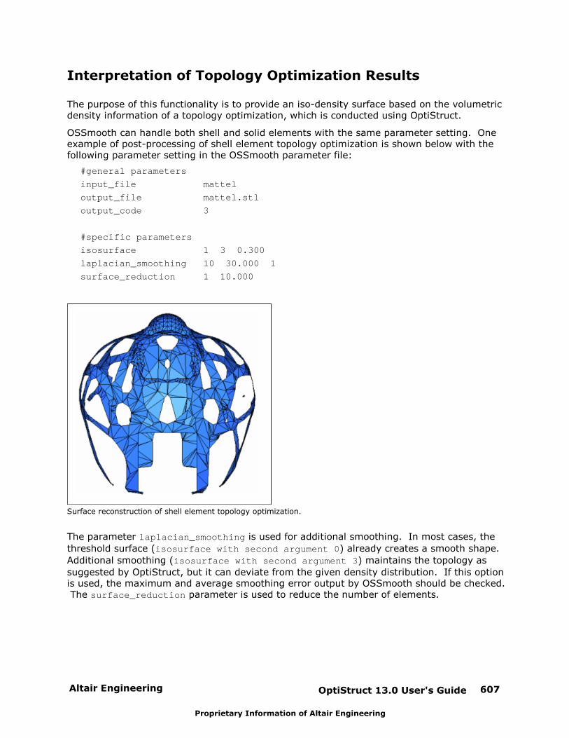
Altair Engineering OptiStruct 13.0 User's Guide 607
Proprietary Information of Altair Engineering
Interpretation of Topology Optimization Results
The purpose of this functionality is to provide an iso-density surface based on the volumetricdensity information of a topology optimization, which is conducted using OptiStruct.
OSSmooth can handle both shell and solid elements with the same parameter setting. Oneexample of post-processing of shell element topology optimization is shown below with thefollowing parameter setting in the OSSmooth parameter file:
#general parameters
input_file mattel
output_file mattel.stl
output_code 3
#specific parameters
isosurface 1 3 0.300
laplacian_smoothing 10 30.000 1
surface_reduction 1 10.000
Surface reconstruction of shell element topology optimization.
The parameter laplacian_smoothing is used for additional smoothing. In most cases, the
threshold surface (isosurface with second argument 0) already creates a smooth shape.
Additional smoothing (isosurface with second argument 3) maintains the topology as
suggested by OptiStruct, but it can deviate from the given density distribution. If this optionis used, the maximum and average smoothing error output by OSSmooth should be checked. The surface_reduction parameter is used to reduce the number of elements.
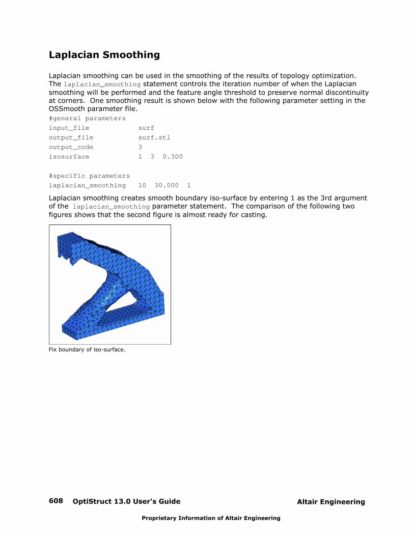
OptiStruct 13.0 User's Guide608 Altair Engineering
Proprietary Information of Altair Engineering
Laplacian Smoothing
Laplacian smoothing can be used in the smoothing of the results of topology optimization. The laplacian_smoothing statement controls the iteration number of when the Laplacian
smoothing will be performed and the feature angle threshold to preserve normal discontinuityat corners. One smoothing result is shown below with the following parameter setting in theOSSmooth parameter file.
#general parameters
input_file surf
output_file surf.stl
output_code 3
isosurface 1 3 0.300
#specific parameters
laplacian_smoothing 10 30.000 1
Laplacian smoothing creates smooth boundary iso-surface by entering 1 as the 3rd argumentof the laplacian_smoothing parameter statement. The comparison of the following two
figures shows that the second figure is almost ready for casting.
Fix boundary of iso-surface.
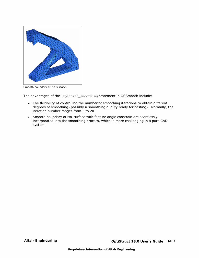
Altair Engineering OptiStruct 13.0 User's Guide 609
Proprietary Information of Altair Engineering
Smooth boundary of iso-surface.
The advantages of the laplacian_smoothing statement in OSSmooth include:
The flexibility of controlling the number of smoothing iterations to obtain differentdegrees of smoothing (possibly a smoothing quality ready for casting). Normally, theiteration number ranges from 5 to 20.
Smooth boundary of iso-surface with feature angle constrain are seamlesslyincorporated into the smoothing process, which is more challenging in a pure CADsystem.
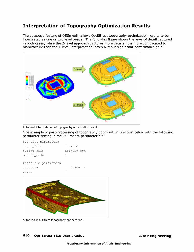
OptiStruct 13.0 User's Guide610 Altair Engineering
Proprietary Information of Altair Engineering
Interpretation of Topography Optimization Results
The autobead feature of OSSmooth allows OptiStruct topography optimization results to beinterpreted as one or two level beads. The following figure shows the level of detail capturedin both cases; while the 2-level approach captures more details, it is more complicated tomanufacture than the 1-level interpretation, often without significant performance gain.
Autobead interpretation of topography optimization result.
One example of post-processing of topography optimization is shown below with the followingparameter setting in the OSSmooth parameter file:
#general parameters
input_file decklid
output_file decklid.fem
output_code 1
#specific parameters
autobead 1 0.300 1
remesh 1
Autobead result from topography optimization.
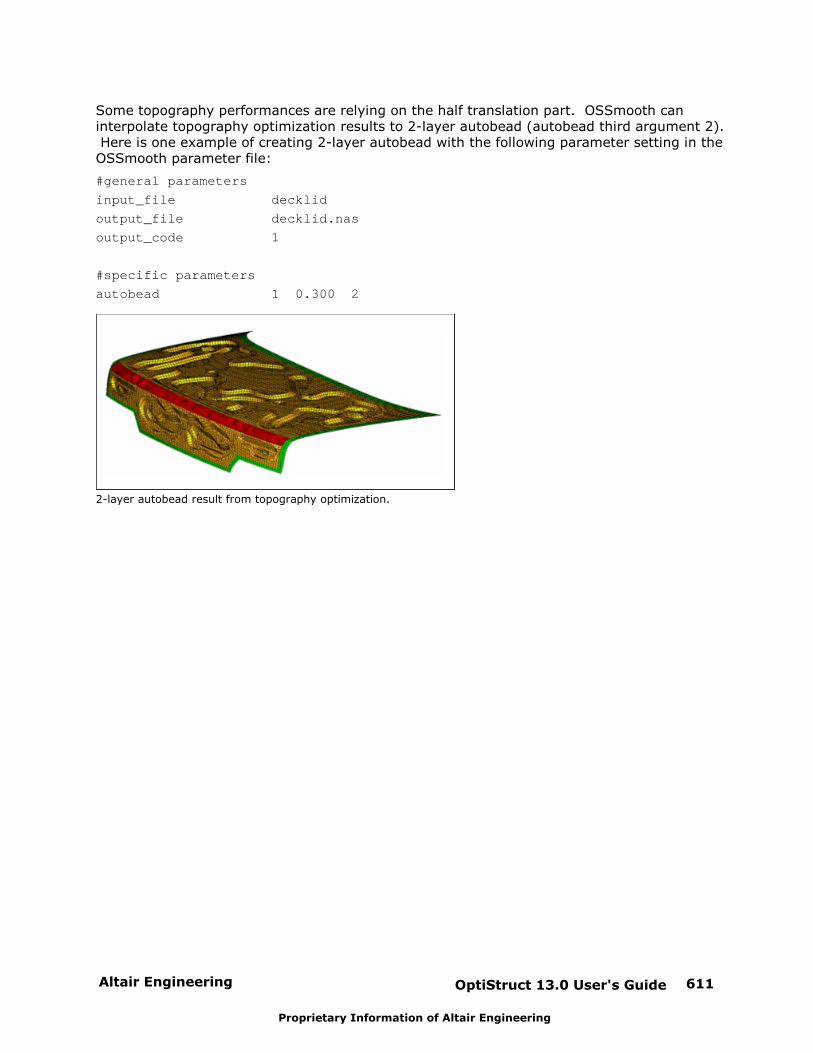
Altair Engineering OptiStruct 13.0 User's Guide 611
Proprietary Information of Altair Engineering
Some topography performances are relying on the half translation part. OSSmooth caninterpolate topography optimization results to 2-layer autobead (autobead third argument 2). Here is one example of creating 2-layer autobead with the following parameter setting in theOSSmooth parameter file:
#general parameters
input_file decklid
output_file decklid.nas
output_code 1
#specific parameters
autobead 1 0.300 2
2-layer autobead result from topography optimization.
OptiStruct 13.0 User's Guide612 Altair Engineering
Proprietary Information of Altair Engineering
Shape Optimization Results, Surface Reduction and SurfaceSmoothing
OSSmooth may also be used to reduce and smooth surfaces or the surfaces of a domain. Theparameter statements pure_surf_reduction and pure_surf_smoothing may be used for
this purpose.
The file defined by input_file must be in OptiStruct, and OSSmooth can smooth the surface
or the surfaces of a domain of the model.
The usage of in the OSSmooth parameter file is as follows:
#general parameters
input_file surf
output_file surf.stl
output_code 3
#specific parameters
pure_surf_smoothing 2 10 30.000
pure_surf_reduction 1 10.000
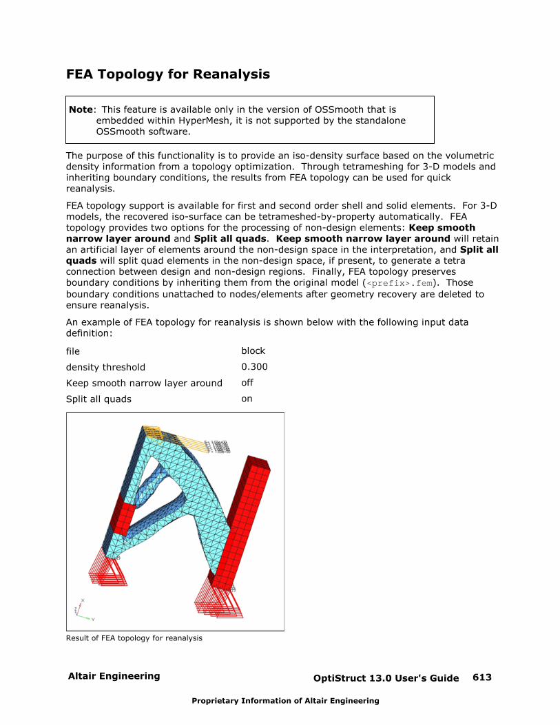
Altair Engineering OptiStruct 13.0 User's Guide 613
Proprietary Information of Altair Engineering
FEA Topology for Reanalysis
Note: This feature is available only in the version of OSSmooth that isembedded within HyperMesh, it is not supported by the standaloneOSSmooth software.
The purpose of this functionality is to provide an iso-density surface based on the volumetricdensity information from a topology optimization. Through tetrameshing for 3-D models andinheriting boundary conditions, the results from FEA topology can be used for quickreanalysis.
FEA topology support is available for first and second order shell and solid elements. For 3-Dmodels, the recovered iso-surface can be tetrameshed-by-property automatically. FEAtopology provides two options for the processing of non-design elements: Keep smoothnarrow layer around and Split all quads. Keep smooth narrow layer around will retainan artificial layer of elements around the non-design space in the interpretation, and Split allquads will split quad elements in the non-design space, if present, to generate a tetraconnection between design and non-design regions. Finally, FEA topology preservesboundary conditions by inheriting them from the original model (<prefix>.fem). Those
boundary conditions unattached to nodes/elements after geometry recovery are deleted toensure reanalysis.
An example of FEA topology for reanalysis is shown below with the following input datadefinition:
file block
density threshold 0.300
Keep smooth narrow layer around off
Split all quads on
Result of FEA topology for reanalysis
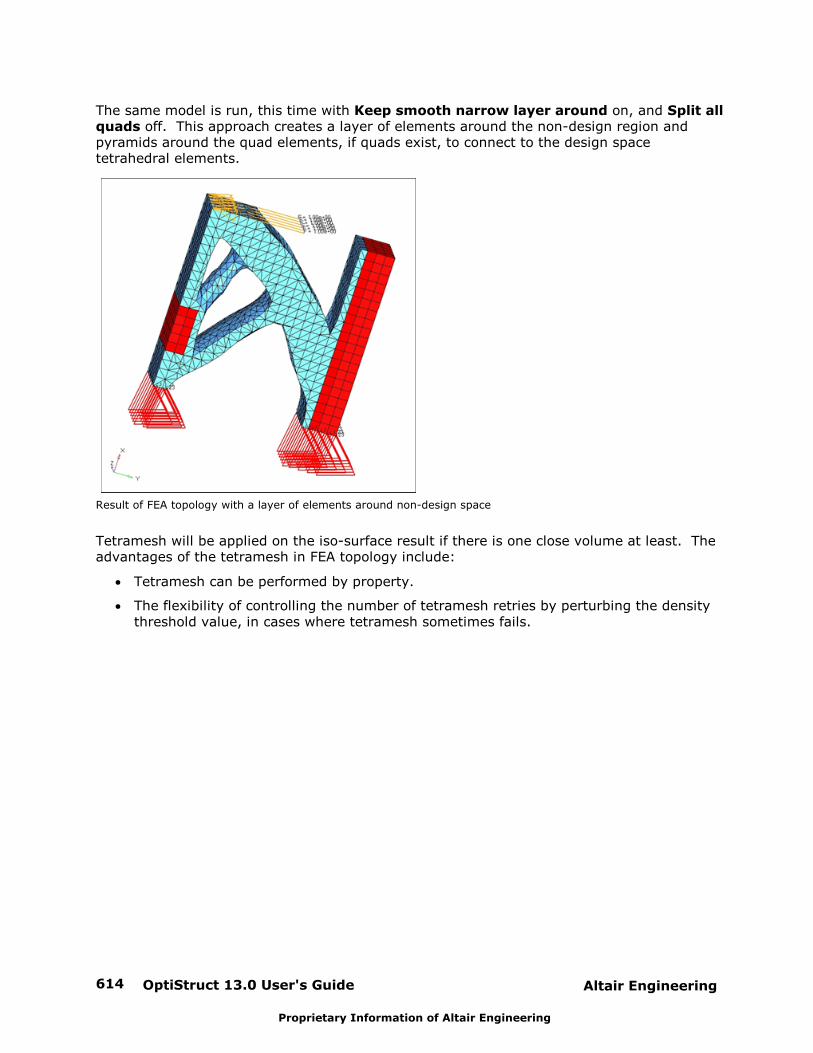
OptiStruct 13.0 User's Guide614 Altair Engineering
Proprietary Information of Altair Engineering
The same model is run, this time with Keep smooth narrow layer around on, and Split allquads off. This approach creates a layer of elements around the non-design region andpyramids around the quad elements, if quads exist, to connect to the design spacetetrahedral elements.
Result of FEA topology with a layer of elements around non-design space
Tetramesh will be applied on the iso-surface result if there is one close volume at least. Theadvantages of the tetramesh in FEA topology include:
Tetramesh can be performed by property.
The flexibility of controlling the number of tetramesh retries by perturbing the densitythreshold value, in cases where tetramesh sometimes fails.
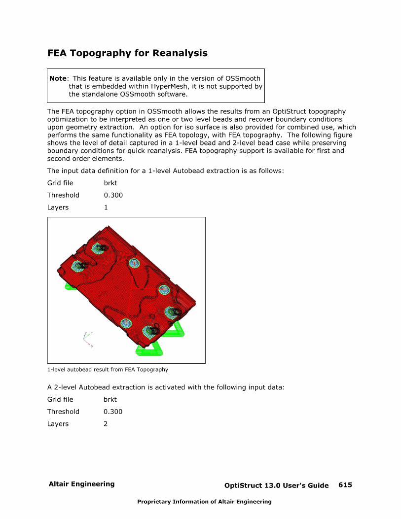
Altair Engineering OptiStruct 13.0 User's Guide 615
Proprietary Information of Altair Engineering
FEA Topography for Reanalysis
Note: This feature is available only in the version of OSSmooththat is embedded within HyperMesh, it is not supported bythe standalone OSSmooth software.
The FEA topography option in OSSmooth allows the results from an OptiStruct topographyoptimization to be interpreted as one or two level beads and recover boundary conditionsupon geometry extraction. An option for iso surface is also provided for combined use, whichperforms the same functionality as FEA topology, with FEA topography. The following figureshows the level of detail captured in a 1-level bead and 2-level bead case while preservingboundary conditions for quick reanalysis. FEA topography support is available for first andsecond order elements.
The input data definition for a 1-level Autobead extraction is as follows:
Grid file brkt
Threshold 0.300
Layers 1
1-level autobead result from FEA Topography
A 2-level Autobead extraction is activated with the following input data:
Grid file brkt
Threshold 0.300
Layers 2
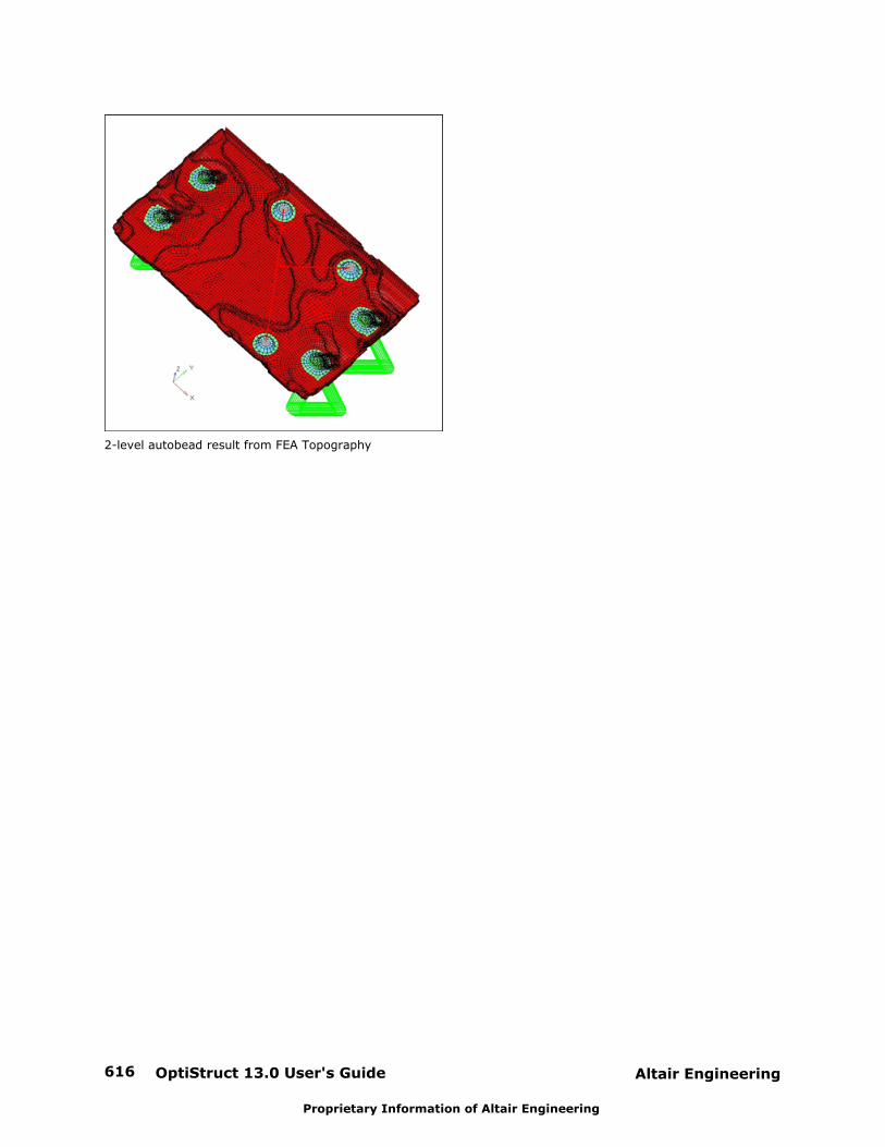
OptiStruct 13.0 User's Guide616 Altair Engineering
Proprietary Information of Altair Engineering
2-level autobead result from FEA Topography
Altair Engineering OptiStruct 13.0 User's Guide 617
Proprietary Information of Altair Engineering
OptiStruct References
Finite Element Analysis – Books
Bathe, K-J., Finite Element Procedures (Prentice Hall, 1996).
Davies, G.A.O., Fenner, R.T., and Lewis, R.W., eds., NAFEMS - Background to Benchmarks(NAFEMS, 1992).
Hitchings, D., ed., A Finite Element Dynamics Primer (NAFEMS, 1992).
N.N., NAFEMS - A Finite Element Primer (NAFEMS, 1992).
N.N., The Standard NAFEMS Benchmarks (NAFEMS, 1990).
Zienkiewicz, O.C., and Taylor, R.L., The Finite Element Method 4th Edition (McGraw-Hill,1989).
Golub, G. H., and Van Loan, C. F., Matrix Computations (The Johns Hopkins University Press).
Finite Element Analysis – Papers
MacNeal, R.H., and Harder, R.L., A Proposed Standard Set of Problems to Test Finite Element
Accuracy, Finite Elements in Analysis and Design, 1 (1985) 3-20.
Multi-body Dynamics – Books
Haug, E., Computer Aided Kinematics and Dynamics of Mechanical Systems: Basic Methods(Prentice Hall, 1989).
Shabana, A.A., Dynamics of Multibody Systems (Cambridge University Press, 1998).
Powerflow – Papers
Hambric, S.A., Power Flow and Mechanical Intensity Calculations in Structural Finite ElementAnalysis, Journal of Vibration and Acoustics, 112 (October 1990) 542-549.
Hambric, S.A. and Szwerc, R.P., Predictions of Structural Intensity Fields Using Solid FiniteElements, Noise Control Engineering Journal, 47(6) (Nov-Dec 1999) 209-217.
Kuhn, M.S.; Lee, H.P. and Lim, S.P., Structural Intensity in Plates with Multiple Discrete andDistributed Spring-Dashpot Systems, Journal of Sound and Vibration, 276 (2004) 627-648.
Design Optimization – Books
Arora, J., Introduction to Optimum Design (McGraw-Hill, 1989).
Bendsoe, M.P., and Sigmund, O., Topology Optimization - Theory, Methods and Applications(Springer, 2003).
Haftka, R.T., and Guerdal, Z., Elements of Structural Optimization (Kluwer AcademicPublishers, 1996).
Rozvany, G.I.N., Topology Optimization in Structural Mechanics (Springer, 1997).
OptiStruct 13.0 User's Guide618 Altair Engineering
Proprietary Information of Altair Engineering
Design Optimization – Papers
Bendsoe, M., and Kikuchi, N., Generating Optimal Topologies in Optimal Design using aHomogenization Method. Computer Methods in Applied Mechanics and Engineering, 71(1988), 197-224.
Canfield, R.A., Design of Frames Against Buckling using a Rayleigh Quotient Approximation. AIAA Journal, 31 (1993) 1143-1149.
Canfield, R.A., High-quality Approximation of Eigenvalues in Structural Optimization. AIAAJournal, 28 (1990) 1116-1122.
Choi, W.S., and Park, G.J. Structural Optimization Using Equivalent Static Loads at All theTime Intervals. Computer Methods in Applied Mechanics and Engineering, 191 (2002) 2105-2122.
Duysinx, P., and Bendsøe, M., Topology Optimization of Continuum Structures with LocalStress Constraints. DCAMM Report, Technical University of Denmark, 1996.
Duysinx, P., and Sigmund, O., New Developments in Handling Stress Constraints in OptimalMaterial Distribution. Proceedings of the 7th AIAA/USAF/NASA/ISSMO Symposium onMultidisciplinary Analysis and Optimization, St. Louis, Missouri, 1997, 1501-1509.
Fleury, C., Structural Weight Optimization by Dual Methods of Convex Programming. International Journal for Numerical Methods in Engineering, 14 (1979) 1761-1783.
Fleury, C., and Braibant, V., Structural Optimization: A New Dual Method using MixedVariables. International Journal for Numerical Methods in Engineering, 23 (1986) 409-428.
Kang, B.S., Park, G.J., and Arora, J.S. Optimization of Flexible Multibody Dynamic SystemsUsing the Equivalent Static Load Method. AIAA Journal, 43 (4) (2005) 846-852.
Kidd, B.J.G., Kemp, M.D., and Jones, R.D., Application of Topology Optimization Technologyto an Automotive Bracket Component. Engineering Design Optimization: Product and ProcessImprovements, 1st ASMO UK Conference, West Yorkshire, 1999.
Kirsch, U., On Singular Topologies in Optimum Structural Design. Structural Optimization, 2(1990) 133-142.
Meyer-Prüßner, R., Prozeßkette Topologieoptimierung. Beiträge zum NAFEMS Seminar zurTopologieoptimie rung, Aalen, GY, 1997, 12.1 - 12.5.
Park, G.J., and Kang, B.S. Validation of a Structural Optimization Algorithm TransformingDynamic Loads into Equivalent Static Loads. Journal of Optimization Theory and Applications,119 (1) (2003) 191-200.
Rozvany, G.I.N., A Critical Investigation of Industrially used Structural Topology OptimizationMethods, 7th World Congress on Structural and Multi-disciplinary Optimization, Seoul, Korea,2007.
Schmit, L.A., Structural Design by Systematic Synthesis, Proc. of the 2nd Conference onElectronic Computation, ASCE, (1960), New York, 105-132.
Schmit, L.A., and Farshi, B., Some Approximation Concepts for Structural Synthesis, AIAAJournal, 12 (1974), 692-699.
Schmit, L.A., and Fleury, C., Structural Synthesis by Combining Approximation Concepts andDual Methods, AIAA Journal, 18 (1980) 1252-1260.
Schramm, U., Structural Optimization – An Efficient Tool in Automotive Design. ATZ –Automobiltechnische Zeitschrift, 100 (1998) Part 1: 456-462, Part 2: 566-572. (In German,English in ATZ Worldwide).
Schramm, U., Thomas, H.L., Zhou, M., and Voth, B., Topology Optimization with AltairOptiStruct, Proceedings of the Optimization in Industry II Conference, Banff, CAN, 1999.
Altair Engineering OptiStruct 13.0 User's Guide 619
Proprietary Information of Altair Engineering
Sigmund, O., and Petersson, J., Numerical Instabilities in Topology Optimization: A Surveyon Procedures Dealing with Checkerboards, Mesh-dependencies and Local Minima. StructuralOptimization, 16 (1998), 68-75.
Svanberg, K., Method of Moving Asymptotes – A New Method for Structural Optimization. International Journal for Numerical Methods in Engineering, 24 (1987) 359-373.
Thomas, H. L., Vanderplaats, G. N., and Shyy, Y.-K., A study of move limit adjustmentstrategies in the approximation concepts approach to structural synthesis, Proceedings of the4th AIAA/USAF/NASA/OAI Symposium on Multidisciplinary Design Optimization, Cleveland,OH, 1992, 507-512.
Vanderplaats, G.N., and Salajehgeh, E., A New Approximation Method for Stress Constraintsin Structural Synthesis. AIAA Journal, 27 (1989) 352-358.
Vanderplaats, G.N., and Thomas, H.L., An Improved Approximation for Stress Constraints inPlate Structures. Structural Optimization, 6 (1993) 1-6.
Zhou, M., Difficulties in Truss Topology Optimization with Stress and Local BucklingConstraints. Structural Optimization, 11 (1996) 134-136.
Zhou, M., Geometrical Optimization of Trusses by a Two-Level Approximation Concept. Structural Optimization, 1 (1989) 47-72.
Zhou, M., and Haftka, R.T., A Comparison Study of Optimality Criteria Methods for Stress andDisplacement Constraints. Computer Methods in Applied Mechanics and Engineering, 124(1995), 253-271.
Zhou, M., and Rozvany, G.I.N., DCOC: An Optimality Criteria Method for Large Systems, PartI: Theory; Part II: Algorithm. Structural Optimization, 5 (1992) 12-25, 6 (1993) 250-262.
Zhou, M., Shyy, Y.K., and Thomas, H.L., Checkerboard and Minimum Member Size Control inTopology Optimization. Proceedings of the 3rd WCSMO, Buffalo, NY, 1999.
Zhou, M., and Thomas, H.L., Alternative Approximation for Stresses in Plate Structures. AIAAJournal, 31 (1993) 2169-2174.
Zhou, M., and Xia, R.W., Two Level Approximation Concept in Structural Synthesis. International Journal for Numerical Methods in Engineering, 29 (1990) 1681-1699.