oracle financial services retail portfolio risk … financial... · user guide: oracle financial...
TRANSCRIPT

Oracle Financial Services Retail Portfolio Risk Models
and Pooling
User Guide Release 34100
April 2014
User Guide Oracle Financial Services Retail Portfolio Risk Models and Pooling Release 34100
Oracle Financial Software Services Confidential-Restricted ii
Contents
LIST OF FIGURES III
1 INTRODUCTION 1
11 OVERVIEW OF ORACLE FINANCIAL SERVICES RETAIL PORTFOLIO RISK MODELS AND POOLING 1 12 SUMMARY 1 13 APPROACH FOLLOWED IN THE PRODUCT 2
2 IMPLEMENTING THE PRODUCT USING THE OFSAAI INFRASTRUCTURE 5
21 INTRODUCTION TO RULES 6 211 Types of Rules 6 212 Rule Definition 6
22 INTRODUCTION TO PROCESSES 7 221 Type of Process Trees 8
23 INTRODUCTION TO RUN 9 231 Run Definition 9 232 Types of Runs 9
24 BUILDING BUSINESS PROCESSORS FOR CALCULATION BLOCKS 9 241 What is a Business Processor 10 242 Why Define a Business Processor 10
25 MODELING FRAMEWORK TOOLS OR TECHNIQUES USED IN RP 10
3 UNDERSTANDING DATA EXTRACTION 12
31 INTRODUCTION 12 32 STRUCTURE 12
ANNEXURE A ndash DEFINITIONS 13
ANNEXURE B ndash FREQUENTLY ASKED QUESTIONS 15
ANNEXURE Cndash K MEANS CLUSTERING BASED ON BUSINESS LOGIC 16
ANNEXURE D GENERATING DOWNLOAD SPECIFICATIONS 19
User Guide Oracle Financial Services Retail Portfolio Risk Models and Pooling Release 34100
Oracle Financial Software Services Confidential-Restricted iii
List of Figures
Figure 1 Data Warehouse Schemas 5
Figure 2 Process Tree 8
User Guide Oracle Financial Services Retail Portfolio Risk Models and Pooling Release 34100
Oracle Financial Software Services Confidential-Restricted 1
1 Introduction
Oracle Financial Services Analytical Applications Infrastructure (OFSAAI) provides the core
foundation for delivering the Oracle Financial Services Analytical Applications an integrated
suite of solutions that sit on top of a common account level relational data model and
infrastructure components Oracle Financial Services Analytical Applications enable financial
institutions to measure and meet risk-adjusted performance objectives cultivate a risk
management culture through transparency manage their customers better improve organizationrsquos
profitability and lower the costs of compliance and regulation
All OFSAAI processes including those related to business are metadata-driven thereby
providing a high degree of operational and usage flexibility and a single consistent view of
information to all users
Business Solution Packs (BSP) are pre-packaged and ready to install analytical solutions and are
available for specific analytical segments to aid management in their strategic tactical and
operational decision-making
11 Overview of Oracle Financial Services Retail Portfolio Risk Models
and Pooling
Under the Capital Adequacy framework of Basel II banks will for the first time be permitted to
group their loans to private individuals and small corporate clients into a Retail Portfolio As a
result they will be able to calculate the capital requirements for the credit risk of these retail
portfolios rather than for the individual accounts Basel accord has given a high degree of
flexibility in the design and implementation of the pool formation process However creation of
pools can be voluminous and time-consuming Oracle Financial Services Retail Portfolio Risk
Models and Pooling Release 34100 referred to as Retail Pooling in this document classifies
the retail exposures into segments (pools) using OFSAAI Modeling framework
Abbreviation Comments
RP Retail Pooling (Oracle Financial Services Retail Portfolio Risk Models
and Pooling)
DL Spec Download Specification
DI Data Integrator
PR2 Process Run Rule
DQ Data Quality
DT Data Transformation
Table 1 Abbreviations
12 Summary
Oracle Financial Services Retail Portfolio Risk Models and Pooling Release 34100 product
uses modeling techniques available in OFSAAI Modeling framework The product restricts itself
to the following operation
Sandbox (Dataset) Creation
RP Variable Management
Variable Reduction
Correlation
Factor Analysis
Clustering Model for Pool Creation
User Guide Oracle Financial Services Retail Portfolio Risk Models and Pooling Release 34100
Oracle Financial Software Services Confidential-Restricted 2
Hierarchical Clustering
K Means Clustering
Report Generation
Pool Stability Report
OFSAAI Modeling framework provides Model Fitting (Sandbox Infodom) and Model
Deployment (Production Infodom) Model Fitting Logic will be deployed in Production Infodom
and the Pool Stability report is generated from Production Infodom
13 Approach Followed in the Product
Following are the approaches followed in the product
Sandbox (Dataset) Creation
Within the modeling environment (Sandbox environment) data would be extracted or imported
from the Production infodom based on the dataset defined there For clustering we should have
one dataset In this step we get the data for all the raw attributes for a particular time period table
Dataset can be created by joining FCT_RETAIL_EXPOSURE with DIM_PRODUCT table
Ideally one dataset should be created per product product family or product class
RP Variable Management
For modeling purposes you need to select the variables required for modeling You can select and
treat these variables in the Variable Management screen You can select variables in the form of
Measures Hierarchy or Business Processors Also as pooling cannot be done using character
attributes therefore all attributes have to be converted to numeric values
A measure refers to the underlying column value in data and you may consider this as the direct
value available for modeling You may select hierarchy for modeling purposes For modeling
purposes qualitative variables need to be converted to dummy variables and such dummy
variables need to be used in Model definition Dummy variables can be created on a hierarchy
Business Processors are used to derive any variable value You can include such derived variables
in model creation Pooling is very sensitive to extreme values and hence extreme values could be
excluded or treated This is done by capping the extreme values by using outlier detection
technique Missing raw attributes gets imputed by statistically determined value or manually given
value It is recommended to use imputed values only when the missing rate is not exceeding 10-
15
Binning is a method of variable discretization or grouping records into lsquonrsquo groups Continuous
variables contain more information than discrete variables However discretization could help
obtain the set of clusters faster and hence it is easier to implement a cluster solution obtained from
discrete variables For example Month on Books Age of the customer Income Utilization
Balance Credit Line Fees Payments Delinquency and so on are some examples of variables
which are generally treated as discrete and discontinuous
Factor Analysis Model for Variable Reduction
Correlation
We cannot build the pooling product if there is any co-linearity between the variables used This
can be overcome by computing the co-relation matrix and if there exists a perfect or almost
perfect co-relation between any two variables one among them needs to be dropped for factor
analysis
Factor Analysis
Factor analysis is a widely used technique of reducing data Factor analysis is a statistical
technique used to explain variability among observed random variables in terms of fewer
User Guide Oracle Financial Services Retail Portfolio Risk Models and Pooling Release 34100
Oracle Financial Software Services Confidential-Restricted 3
unobserved random variables called factors The observed variables are modeled as linear
combinations of the factors plus error terms Factor analysis using principal components method
helps in selecting variables having higher explanatory relationships
Based on Factor Analysis output the business user may eliminate variables from the dataset which
has communalities far from 1 The choice of which variables will be dropped is subjective and is
left to you In addition to this OFSAAI Modeling Framework also allows you to define and
execute Linear or Logistic Regression technique
Clustering Model for Pool Creation
There could be various approaches to pool creation Some could approach the problem by using
supervised learning techniques such as Decision Tree methods to split grow and understand
homogeneity in terms of known objectives
However Basel mentions that pools of exposures should be homogenous in terms of their risk
characteristics (determinants of underlying loss behavior or predicting loss behavior) and therefore
instead of an objective method it would be better to use a non objective approach which is the
method of natural grouping of data using risk characteristics alone
For natural grouping of data clustering is done using two of the prominent techniques Final
clusters are typically arrived at after testing several models and examining their results The
variations could be based on number of clusters variables and so on
There are two methods of clustering Hierarchical and K means Each one of these methods has its
pros and cons given the enormity of the problem For larger number of variables and bigger
sample sizes or presence of continuous variables K means is a superior method over Hierarchical
Further Hierarchical method can run into days without generating any dendrogram and hence may
become unsolvable Since hierarchical method gives a better exploratory view of the clusters
formed it is used only to determine the initial number of clusters that you would start with to
build the K means clustering solution Nevertheless if hierarchical does not generate any
dendrogram at all then you are left to grow K means method only
In hierarchical cluster analysis dendrogram graphs are used to visualize how clusters are formed
Since each observation is displayed dendrograms are impractical when the data set is large Also
dendrograms are too time-consuming for larger data sets For non-hierarchical cluster algorithms a
graph like the dendrogram does not exist
Hierarchical Clustering
Choose a distance criterion Based on that you are shown a dendrogram based on which the
number of clusters are decided A manual iterative process is then used to arrive at the final
clusters with the distance criterion being modified in each step Since hierarchical clustering is a
computationally intensive exercise presence of continuous variables and high sample size can
make the problem explode in terms of computational complexity Therefore you are free to do
either of following
Drop continuous variables for faster calculation This method would be preferred only if the sole
purpose of hierarchical clustering is to arrive at the dendrogram
Use a random sample drawn from the data Again this method would be preferred only if the
sole purpose of hierarchical clustering is to arrive at the dendrogram
Use a binning method to convert continuous variables into discrete variables
K Means Cluster Analysis
Number of clusters is a random or manual input or based on the results of hierarchical clustering
This kind of clustering method is also called a k-means model since the cluster centers are the
means of the observations assigned to each cluster when the algorithm is run to complete
convergence Again we will use the Euclidean distance criterion The cluster centers are based on
least-squares estimation Iteration reduces the least-squares criterion until convergence is
User Guide Oracle Financial Services Retail Portfolio Risk Models and Pooling Release 34100
Oracle Financial Software Services Confidential-Restricted 4
achieved
Pool Stability Report
Pool Stability report will contain pool level information across all MIS dates since the pool
building It indicates number of exposures exposure amount and default rate for the pool
Frequency Distribution Report
Frequency distribution table for a categorical variable contain frequency count for a given value
User Guide Oracle Financial Services Retail Portfolio Risk Models and Pooling Release 34100
Oracle Financial Software Services Confidential-Restricted 5
2 Implementing the Product using the OFSAAI Infrastructure
The following terminologies are constantly referred to in this manual
Data Model - A logical map that represents the inherent properties of the data independent of
software hardware or machine performance considerations The data model consists of entities
(tables) and attributes (columns) and shows data elements grouped into records as well as the
association around those records
Dataset - It is the simplest of data warehouse schemas This schema resembles a star diagram
While the center contains one or more fact tables the points (rays) contain the dimension tables
(see Figure 1)
Figure 1 Data Warehouse Schemas
Fact Table In a star schema only one join is required to establish the relationship between the
FACT table and any one of the dimension tables which optimizes queries as all the information
about each level is stored in a row The set of records resulting from this star join is known as a
dataset
Metadata is a term used to denote data about data Business metadata objects are available to
in the form of Measures Business Processors Hierarchies Dimensions Datasets and Cubes and
so on The commonly used metadata definitions in this manual are Hierarchies Measures and
Business Processors
Hierarchy ndash A tree structure across which data is reported is known as a hierarchy The
members that form the hierarchy are attributes of an entity Thus a hierarchy is necessarily
based upon one or many columns of a table Hierarchies may be based on either the FACT table
or dimensional tables
Measure - A simple measure represents a quantum of data and is based on a specific attribute
(column) of an entity (table) The measure by itself is an aggregation performed on the specific
column such as summation count or a distinct count
Dimension Table Dimension Table
Time
Fact Table
Sales
Customer Channel
Products Geography
User Guide Oracle Financial Services Retail Portfolio Risk Models and Pooling Release 34100
Oracle Financial Software Services Confidential-Restricted 6
Business Processor ndash This is a metric resulting from a computation performed on a simple
measure The computation that is performed on the measure often involves the use of statistical
mathematical or database functions
Modelling Framework ndash The OFSAAI Modeling Environment performs estimations for a
given input variable using historical data It relies on pre-built statistical applications to build
models The framework stores these applications so that models can be built easily by business
users The metadata abstraction layer is actively used in the definition of models Underlying
metadata objects such as Measures Hierarchies and Datasets are used along with statistical
techniques in the definition of models
21 Introduction to Rules
Institutions in the financial sector may require constant monitoring and measurement of risk in
order to conform to prevalent regulatory and supervisory standards Such measurement often
entails significant computations and validations with historical data Data must be transformed to
support such measurements and calculations The data transformation is achieved through a set of
defined rules
The Rules option in the Rules Framework Designer provides a framework that facilitates the
definition and maintenance of a transformation The metadata abstraction layer is actively used in
the definition of rules where you are permitted to re-classify the attributes in the data warehouse
model thus transforming the data Underlying metadata objects such as Hierarchies that are non-
large or non-list Datasets and Business Processors drive the Rule functionality
211 Types of Rules
From a business perspective Rules can be of 3 types
Type 1 This type of Rule involves the creation of a subset of records from a given set of
records in the data model based on certain filters This process may or may not involve
transformations or aggregation or both Such type 1 rule definitions are achieved through Table-
to-Table (T2T) Extract (Refer to the section Defining Extracts in the Data Integrator User
Manual for more details on T2T Extraction)
Type 2 This type of Rule involves re-classification of records in a table in the data model based
on criteria that include complex Group By clauses and Sub Queries within the tables
Type 3 This type of Rule involves computation of a new value or metric based on a simple
measure and updating an identified set of records within the data model with the computed
value
212 Rule Definition
A rule is defined using existing metadata objects The various components of a rule definition are
Dataset ndash This is a set of tables that are joined together by keys A dataset must have at least
one FACT table Type 3 rule definitions may be based on datasets that contain more than 1
FACT tables Type 2 rule definitions must be based on datasets that contain a single FACT
table The values in one or more columns of the FACT tables within a dataset are transformed
with a new value
Source ndash This component determines the basis on which a record set within the dataset is
classified The classification is driven by a combination of members of one or more hierarchies
A hierarchy is based on a specific column of an underlying table in the data warehouse model
The table on which the hierarchy is defined must be a part of the dataset selected One or more
hierarchies can participate as a source so long as the underlying tables on which they are defined
belong to the dataset selected
User Guide Oracle Financial Services Retail Portfolio Risk Models and Pooling Release 34100
Oracle Financial Software Services Confidential-Restricted 7
Target ndash This component determines the column in the data warehouse model that will be
impacted with an update It also encapsulates the business logic for the update The
identification of the business logic can vary depending on the type of rule that is being defined
For type 3 rules the business processors determine the target column that is required to be
updated Only those business processors must be selected that are based on the same measure of
a FACT table present in the selected dataset Further all the business processors used as a target
must have the same aggregation mode For type 2 rules the hierarchy determines the target
column that is required to be updated The target column is in the FACT table and has a
relationship with the table on which the hierarchy is based The target hierarchy must not be
based on the FACT table
Mapping ndash This is an operation that classifies the final record set of the target that is to be
updated into multiple sections It also encapsulates the update logic for each section The logic
for the update can vary depending on the hierarchy member or business processor used The
logic is defined through the selection of members from an intersection of a combination of
source members with target members
Node Identifier ndash This is a property of a hierarchy member In a Rule definition the members
of a hierarchy that cannot participate in a mapping operation are target members whose node
identifiers identify them to be an lsquoOthersrsquo node lsquoNon-Leafrsquo node or those defined with a range
expression (Refer to the section Defining Business Hierarchies in the Unified Metadata
Manager Manual for more details on hierarchy properties) Source members whose node
identifiers identify them to be lsquoNon-Leafrsquo nodes can also not participate in the mapping
22 Introduction to Processes
A set of rules collectively forms a Process A process definition is represented as a Process Tree
The Process option in the Rules Framework Designer provides a framework that facilitates the
definition and maintenance of a process A hierarchical structure is adopted to facilitate the
construction of a process tree A process tree can have many levels and one or many nodes within
each level Sub-processes are defined at level members and rules form the leaf members of the
tree Through the definition of Process you are permitted to logically group a collection of rules
that pertain to a functional process
Further the business may require simulating conditions under different business scenarios and
evaluate the resultant calculations with respect to the baseline calculation Such simulations are
done through the construction of Simulation Processes and Simulation Process trees
Underlying metadata objects such as Rules T2T Definitions Non End-to-End Processes and
Database Stored Procedures drive the Process functionality
From a business perspective processes can be of 2 types
End-to-End Process ndash As the name suggests this process denotes functional completeness
This process is ready for execution
Non End-to-End Process ndash This is a sub-process that is a logical collection of rules It cannot
be executed by itself It must be defined as a sub-process in an end-to-end process to achieve a
state ready for execution A process is defined using existing rule metadata objects
Process Tree - This is a hierarchical collection of rules that are processed in the natural
sequence of the tree The process tree can have levels and members Each level constitutes a
sub-process Each member can either be a Type 2 rule or Type 3 rule an existing non end-to-
end process a Type 1 rule (T2T) or an existing transformation that is defined through Data
Integrator If no predecessor is defined the process tree is executed in its natural hierarchical
sequence as explained in the stated example
User Guide Oracle Financial Services Retail Portfolio Risk Models and Pooling Release 34100
Oracle Financial Software Services Confidential-Restricted 8
Root
Rule 4
SP 1 SP 1a
Rule 1
Rule 2
SP 2 Rule 3
Rule 5
Figure 2 Process Tree
For example In the above figure first the sub process SP1 will be executed The sub process SP1
will be executed in following manner - Rule 1 gt SP1a gt Rule 2gt SP1 The execution sequence
will be start with Rule 1 followed by sub-process SP1a followed by Rule 2 and will end with
sub-process SP1
The Sub Process SP2 will be executed after execution of SP1 SP2 will be executed in following
manner - Rule 3 gt SP2 The execution sequence will start with Rule 3 followed by sub-process
SP2 After execution of sub-process SP2 Rule 4 will be executed and then finally the Rule 5 will
be executed The Process tree can be built by adding one or more members called Process Nodes
If there are Predecessor Tasks associated with any member the tasks defined as predecessors will
precede the execution of that member
221 Type of Process Trees
Two types of process trees can be defined
Base Process Tree - is a hierarchical collection of rules that are processed in the natural
sequence of the tree The rules are sequenced in a manner required by the business condition
The base process tree does not include sub-processes that are created at run time during
execution
Simulation Process Tree - as the name suggests is a tree constructed using a base process tree
It is also a hierarchical collection of rules that are processed in the natural sequence of the tree
It is however different from the base process tree in that it reflects a different business scenario
User Guide Oracle Financial Services Retail Portfolio Risk Models and Pooling Release 34100
Oracle Financial Software Services Confidential-Restricted 9
The scenarios are built by either substituting an existing process with another or inserting a new
process or rules
23 Introduction to Run
In this chapter we will describe how the processes are combined together and defined as lsquoRunrsquo
From a business perspective different lsquoRunsrsquo of the same set of processes may be required to
satisfy different approaches to the underlying data
The Run Framework enables the various Rules defined in the Rules Framework to be combined
together (as processes) and executed as different lsquoBaseline Runsrsquo for different underlying
approaches Different approaches are achieved through process definitions Further run level
conditions or process level conditions can be specified while defining a lsquoRunrsquo
In addition to the baseline runs simulation runs can be executed through the usage of the different
Simulation Processes Such simulation runs are used to compare the resultant performance
calculations with respect to the baseline runs This comparison will provide useful insights on the
effect of anticipated changes to the business
231 Run Definition
A Run is a collection of processes that are required to be executed on the database The various
components of a run definition are
Process- you may select one or many End-to-End processes that need to be executed as part of
the Run
Run Condition- When multiple processes are selected there is likelihood that the processes
may contain rules T2Ts whose target entities are across multiple datasets When the selected
processes contain Rules the target entities (hierarchies) which are common across the datasets
are made available for defining Run Conditions When the selected processes contain T2Ts the
hierarchies that are based on the underlying destination tables which are common across the
datasets are made available for defining the Run Condition A Run Condition is defined as a
filter on the available hierarchies
Process Condition - A further level of filter can be applied at the process level This is
achieved through a mapping process
232 Types of Runs
Two types of runs can be defined namely Baseline Runs and Simulation Runs
Baseline Runs - are those base End-to-End processes that are executed
Simulation Runs - are those scenario End-to-End processes that are executed Simulation Runs
are compared with the Baseline Runs and therefore the Simulation Processes used during the
execution of a simulation run are associated with the base process
24 Building Business Processors for Calculation Blocks
This chapter describes what a Business Processor is and explains the process involved in its
creation and modification
The Business Processor function allows you to generate values that are functions of base measure
values Using the metadata abstraction of a business processor power users have the ability to
design rule-based transformation to the underlying data within the data warehouse store (Refer
to the section defining a Rule in the Rules Process and Run Framework Manual for more details
on the use of business processors)
User Guide Oracle Financial Services Retail Portfolio Risk Models and Pooling Release 34100
Oracle Financial Software Services Confidential-Restricted 10
241 What is a Business Processor
A Business Processor encapsulates business logic for assigning a value to a measure as a function
of observed values for other measures
Let us take an example of risk management in the financial sector that requires calculating the risk
weight of an exposure while using the Internal Ratings Based Foundation approach Risk weight is
a function of measures such as Probability of Default (PD) Loss Given Default and Effective
Maturity of the exposure in question The function (risk weight) can vary depending on the
various dimensions of the exposure like its customer type product type and so on Risk weight is
an example of a business processor
242 Why Define a Business Processor
Measurements that require complex transformations that entail transforming data based on a
function of available base measures require business processors A supervisory requirement
necessitates the definition of such complex transformations with available metadata constructs
Business Processors are metadata constructs that are used in the definition of such complex rules
(Refer to the section Accessing Rule in the Rules Process and Run Framework Manual for more
details on the use of business processors)
Business Processors are designed to update a measure with another computed value When a rule
that is defined with a business processor is processed the newly computed value is updated on the
defined target Let us take the example cited in the above section where risk weight is the
business processor A business processor is used in a rule definition (Refer to the section defining
a Rule in the Rules Process and Run Framework Manual for more details) In this example a rule
is used to assign a risk weight to an exposure with a certain combination of dimensions
25 Modeling Framework Tools or Techniques used in RP
Oracle Financial Services Retail Portfolio Risk Models and Pooling Release 34100 uses
modeling features available in the OFSAAI Modeling Framework Major tools or techniques that
are required for Retail Pooling are briefly described in this section Please refer OFSAAI Modeling
Framework User Manual for usage in detail
Outlier Detection - Pooling is very sensitive to Extreme Values and hence extreme values could
be excluded or treated Records having extreme values can be excluded by applying a dataset
filter Extreme values can be treated by capping the extreme values which are beyond a certain
bound This kind of bounds can be determined statistically (using inter-quartile range) or given
manually
Missing Value ndash Missing value in a variable needs to be impute with suitable values depending
on other data values in the variable Imputation can be done by manually specifying the value
with which it needs to be imputed or by using the mean for the variables created from numeric
attributes or Mode for variables created from qualitative attributes If it gets replaced by mean or
mode it is recommended to use outlier treatment before applying missing value Also it is
recommended that Imputation should only be done when the missing rate does not exceed 10-
15
Binning - Binning is the method of variable discretization whereby continuous variable can be
discredited and each group contains a set of values falling under specified bracket Binning
could be Equi-width Equi-frequency or manual binning The number of bins required for each
variable can be decided by the business user For each group created above you could consider
the mean value for that group and call them as bins or the bin values
Correlation - Correlation technique helps identify the correlated variable Perfect or almost
perfect correlated variables can be identified and the business user can remove either of such
variables for factor analysis to effectively run on remaining set of variables
User Guide Oracle Financial Services Retail Portfolio Risk Models and Pooling Release 34100
Oracle Financial Software Services Confidential-Restricted 11
Factor Analysis ndash Factor analysis is a statistical technique used to explain variability among
observed random variables in terms of fewer unobserved random variables called factors The
observed variables are modeled as linear combinations of the factors plus error terms From the
output of factor analysis business user can determine the variables that may yield the same
result and need not be retained for further techniques
Hierarchical Clustering - In hierarchical cluster analysis dendrogram graphs are used to
visualize how clusters are formed You can choose a distance criterion Based on that a
dendrogram is shown and based on which the number of clusters are decided upon Manual
iterative process is then used to arrive at the final clusters with the distance criterion being
modified with iteration Since hierarchical method may give a better exploratory view of the
clusters formed it is used only to determine the initial number of clusters that you would start
with to build the K means clustering solution
Dendrograms are impractical when the data set is large because each observation must be
displayed as a leaf they can only be used for a small number of observations For large numbers of
observations hierarchical cluster algorithms can be time consuming Also hierarchical clustering
is computationally intensive exercise and hence presence of continuous variables and high sample
size can make the problem explode in terms of computational complexity Therefore you have to
ensure that continuous variables are binned prior to its usage in Hierarchical clustering
K Means Cluster Analysis - Number of clusters is a random or manual input based on the
results of hierarchical clustering In K-Means model the cluster centers are the means of the
observations assigned to each cluster when the algorithm is run to complete convergence The
cluster centers are based on least-squares estimation and the Euclidean distance criterion is used
Iteration reduces the least-squares criterion until convergence is achieved
K Means Cluster and Boundary based Analysis This process of clustering uses K-Means
Clustering to arrive at an initial cluster and then based on business logic assigns each record to a
particular cluster based on the bounds of the variables For more information on K means
clustering refer Annexure C
CART (GINI TREE) - Classification tree analysis is a term used when the predicted outcome
is the class to which the data belongs to Regression tree analysis is a term used when the
predicted outcome can be considered a real number CART analysis is a term used to refer to
both of the above procedures GINI is used to grow the decision trees for where dependent
variable is binary in nature
CART (Entropy) - Entropy is used to grow the decision trees where dependent variable can
take any value between 0 and 1 Decision tree is a predictive model that is a mapping of
observations about an item to arrive at conclusions about the items target value
User Guide Oracle Financial Services Retail Portfolio Risk Models and Pooling Release 34100
Oracle Financial Software Services Confidential-Restricted 12
3 Understanding Data Extraction
31 Introduction
In order to receive input data in a systematic way we provide the bank with a detailed
specification called a Data Download Specification or a DL Spec These DL Specs help the bank
understand the input requirements of the product and prepare and provide these inputs in proper
standards and formats
32 Structure
A DL Spec is an excel file having the following structure
Index sheet This sheet lists out the various entities whose download specifications or DL Specs
are included in the file It also gives the description and purpose of the entities and the
corresponding physical table names in which the data gets loaded
Glossary sheet This sheet explains the various headings and terms used for explaining the data
requirements in the table structure sheets
Table structure sheet Every DL spec contains one or more table structure sheets These sheets
are named after the corresponding staging tables This contains the actual table and data
elements required as input for the Oracle Financial Services Basel Product This also includes
the name of the expected download file staging table name and name description data type
and length and so on of every data element
Setup data sheet This sheet contains a list of master dimension and system tables that are
required for the system to function properly
The DL spec has been divided into various files based on risk types as follows
Retail Pooling
DLSpecs_Retail_Poolingxls details the data requirements for retail pools
Dimension Tables
DLSpec_DimTablesxls lists out the data requirements for dimension tables like Customer
Lines of Business Product and so on
User Guide Oracle Financial Services Retail Portfolio Risk Models and Pooling Release 34100
Oracle Financial Software Services Confidential-Restricted 13
Annexure A ndash Definitions
This section defines various terms which are relevant or is used in the user guide These terms are
necessarily generic in nature and are used across various sections of this user guide Specific
definitions which are used only for handling a particular exposure are covered in the respective
section of this document
Retail Exposure
Exposures to individuals such as revolving credits and lines of credit (credit cards overdrafts
and retail facilities secured by financial instruments) as well as personal term loans and leases
(installment loans auto loans and leases student and educational loans personal finance and
other exposures with similar characteristics) are generally eligible for retail treatment regardless
of exposure size
Residential mortgage loans (including first and subsequent liens term loans and revolving home
equity lines of credit) are eligible for retail treatment regardless of exposure size so long as the
credit is extended to an individual that is an owner occupier of the property Loans secured by a
single or small number of condominium or co-operative residential housing units in a single
building or complex also fall within the scope of the residential mortgage category
Loans extended to small businesses and managed as retail exposures are eligible for retail
treatment provided the total exposure of the banking group to a small business borrower (on a
consolidated basis where applicable) is less than 1 million Small business loans extended
through or guaranteed by an individual are subject to the same exposure threshold The fact that
an exposure is rated individually does not by itself deny the eligibility as a retail exposure
Borrower risk characteristics
Socio-Demographic Attributes related to the customer like income age gender educational
status type of job time at current job zip code External Credit Bureau attributes (if available)
such as credit history of the exposure like Payment History Relationship External Utilization
Performance on those Accounts and so on
Transaction risk characteristics
Exposure characteristics Basic Attributes of the exposure like Account number Product name
Product type Mitigant type Location Outstanding amount Sanctioned Limit Utilization
payment spending behavior age of the account opening balance closing balance delinquency
etc
Delinquency of exposure characteristics
Total Delinquency Amount Pct Delinquency Amount to Total Max Delinquency Amount
Number of More equal than 30 Days Delinquency in last 3 Months and so on
Factor Analysis
Factor analysis is a widely used technique of reducing data Factor analysis is a statistical
technique used to explain variability among observed random variables in terms of fewer
unobserved random variables called factors
Classes of Variables
We need to specify two classes of variables
Target variable (Dependent Variable) Default Indictor Recovery Ratio
Driver variable(Independent Variable) Input Data forming the cluster product
Hierarchical Clustering
Hierarchical Clustering gives initial number of clusters based on data values In hierarchical
cluster analysis dendrogram graphs are used to visualize how clusters are formed As each
User Guide Oracle Financial Services Retail Portfolio Risk Models and Pooling Release 34100
Oracle Financial Software Services Confidential-Restricted 14
observation is displayed dendrograms are impractical when the data set is large
K Means Clustering
Number of clusters is a random or manual input or based on the results of hierarchical clustering
This kind of clustering method is also called a k-means model since the cluster centers are the
means of the observations assigned to each cluster when the algorithm is run to complete
convergence
Binning
Binning is the method of variable discretization or grouping into 10 groups where each group
contains equal number of records as far as possible For each group created above we could take
the mean or the median value for that group and call them as bins or the bin values
Where p is the probability of the jth incidence in the ith split
New Accounts
New Accounts are accounts which are new to the portfolio and they do not have a performance
history of 1 year on our books
User Guide Oracle Financial Services Retail Portfolio Risk Models and Pooling Release 34100
Oracle Financial Software Services Confidential-Restricted 15
Annexure B ndash Frequently Asked Questions
Please refer to the attached Oracle Financial Services Retail Portfolio Risk Models and Pooling
Release 34100 FAQ
FAQpdf

User Guide Oracle Financial Services Retail Portfolio Risk Models and Pooling Release 34100
Oracle Financial Software Services Confidential-Restricted 6
Business Processor ndash This is a metric resulting from a computation performed on a simple
measure The computation that is performed on the measure often involves the use of statistical
mathematical or database functions
Modelling Framework ndash The OFSAAI Modeling Environment performs estimations for a
given input variable using historical data It relies on pre-built statistical applications to build
models The framework stores these applications so that models can be built easily by business
users The metadata abstraction layer is actively used in the definition of models Underlying
metadata objects such as Measures Hierarchies and Datasets are used along with statistical
techniques in the definition of models
21 Introduction to Rules
Institutions in the financial sector may require constant monitoring and measurement of risk in
order to conform to prevalent regulatory and supervisory standards Such measurement often
entails significant computations and validations with historical data Data must be transformed to
support such measurements and calculations The data transformation is achieved through a set of
defined rules
The Rules option in the Rules Framework Designer provides a framework that facilitates the
definition and maintenance of a transformation The metadata abstraction layer is actively used in
the definition of rules where you are permitted to re-classify the attributes in the data warehouse
model thus transforming the data Underlying metadata objects such as Hierarchies that are non-
large or non-list Datasets and Business Processors drive the Rule functionality
211 Types of Rules
From a business perspective Rules can be of 3 types
Type 1 This type of Rule involves the creation of a subset of records from a given set of
records in the data model based on certain filters This process may or may not involve
transformations or aggregation or both Such type 1 rule definitions are achieved through Table-
to-Table (T2T) Extract (Refer to the section Defining Extracts in the Data Integrator User
Manual for more details on T2T Extraction)
Type 2 This type of Rule involves re-classification of records in a table in the data model based
on criteria that include complex Group By clauses and Sub Queries within the tables
Type 3 This type of Rule involves computation of a new value or metric based on a simple
measure and updating an identified set of records within the data model with the computed
value
212 Rule Definition
A rule is defined using existing metadata objects The various components of a rule definition are
Dataset ndash This is a set of tables that are joined together by keys A dataset must have at least
one FACT table Type 3 rule definitions may be based on datasets that contain more than 1
FACT tables Type 2 rule definitions must be based on datasets that contain a single FACT
table The values in one or more columns of the FACT tables within a dataset are transformed
with a new value
Source ndash This component determines the basis on which a record set within the dataset is
classified The classification is driven by a combination of members of one or more hierarchies
A hierarchy is based on a specific column of an underlying table in the data warehouse model
The table on which the hierarchy is defined must be a part of the dataset selected One or more
hierarchies can participate as a source so long as the underlying tables on which they are defined
belong to the dataset selected
User Guide Oracle Financial Services Retail Portfolio Risk Models and Pooling Release 34100
Oracle Financial Software Services Confidential-Restricted 7
Target ndash This component determines the column in the data warehouse model that will be
impacted with an update It also encapsulates the business logic for the update The
identification of the business logic can vary depending on the type of rule that is being defined
For type 3 rules the business processors determine the target column that is required to be
updated Only those business processors must be selected that are based on the same measure of
a FACT table present in the selected dataset Further all the business processors used as a target
must have the same aggregation mode For type 2 rules the hierarchy determines the target
column that is required to be updated The target column is in the FACT table and has a
relationship with the table on which the hierarchy is based The target hierarchy must not be
based on the FACT table
Mapping ndash This is an operation that classifies the final record set of the target that is to be
updated into multiple sections It also encapsulates the update logic for each section The logic
for the update can vary depending on the hierarchy member or business processor used The
logic is defined through the selection of members from an intersection of a combination of
source members with target members
Node Identifier ndash This is a property of a hierarchy member In a Rule definition the members
of a hierarchy that cannot participate in a mapping operation are target members whose node
identifiers identify them to be an lsquoOthersrsquo node lsquoNon-Leafrsquo node or those defined with a range
expression (Refer to the section Defining Business Hierarchies in the Unified Metadata
Manager Manual for more details on hierarchy properties) Source members whose node
identifiers identify them to be lsquoNon-Leafrsquo nodes can also not participate in the mapping
22 Introduction to Processes
A set of rules collectively forms a Process A process definition is represented as a Process Tree
The Process option in the Rules Framework Designer provides a framework that facilitates the
definition and maintenance of a process A hierarchical structure is adopted to facilitate the
construction of a process tree A process tree can have many levels and one or many nodes within
each level Sub-processes are defined at level members and rules form the leaf members of the
tree Through the definition of Process you are permitted to logically group a collection of rules
that pertain to a functional process
Further the business may require simulating conditions under different business scenarios and
evaluate the resultant calculations with respect to the baseline calculation Such simulations are
done through the construction of Simulation Processes and Simulation Process trees
Underlying metadata objects such as Rules T2T Definitions Non End-to-End Processes and
Database Stored Procedures drive the Process functionality
From a business perspective processes can be of 2 types
End-to-End Process ndash As the name suggests this process denotes functional completeness
This process is ready for execution
Non End-to-End Process ndash This is a sub-process that is a logical collection of rules It cannot
be executed by itself It must be defined as a sub-process in an end-to-end process to achieve a
state ready for execution A process is defined using existing rule metadata objects
Process Tree - This is a hierarchical collection of rules that are processed in the natural
sequence of the tree The process tree can have levels and members Each level constitutes a
sub-process Each member can either be a Type 2 rule or Type 3 rule an existing non end-to-
end process a Type 1 rule (T2T) or an existing transformation that is defined through Data
Integrator If no predecessor is defined the process tree is executed in its natural hierarchical
sequence as explained in the stated example
User Guide Oracle Financial Services Retail Portfolio Risk Models and Pooling Release 34100
Oracle Financial Software Services Confidential-Restricted 8
Root
Rule 4
SP 1 SP 1a
Rule 1
Rule 2
SP 2 Rule 3
Rule 5
Figure 2 Process Tree
For example In the above figure first the sub process SP1 will be executed The sub process SP1
will be executed in following manner - Rule 1 gt SP1a gt Rule 2gt SP1 The execution sequence
will be start with Rule 1 followed by sub-process SP1a followed by Rule 2 and will end with
sub-process SP1
The Sub Process SP2 will be executed after execution of SP1 SP2 will be executed in following
manner - Rule 3 gt SP2 The execution sequence will start with Rule 3 followed by sub-process
SP2 After execution of sub-process SP2 Rule 4 will be executed and then finally the Rule 5 will
be executed The Process tree can be built by adding one or more members called Process Nodes
If there are Predecessor Tasks associated with any member the tasks defined as predecessors will
precede the execution of that member
221 Type of Process Trees
Two types of process trees can be defined
Base Process Tree - is a hierarchical collection of rules that are processed in the natural
sequence of the tree The rules are sequenced in a manner required by the business condition
The base process tree does not include sub-processes that are created at run time during
execution
Simulation Process Tree - as the name suggests is a tree constructed using a base process tree
It is also a hierarchical collection of rules that are processed in the natural sequence of the tree
It is however different from the base process tree in that it reflects a different business scenario
User Guide Oracle Financial Services Retail Portfolio Risk Models and Pooling Release 34100
Oracle Financial Software Services Confidential-Restricted 9
The scenarios are built by either substituting an existing process with another or inserting a new
process or rules
23 Introduction to Run
In this chapter we will describe how the processes are combined together and defined as lsquoRunrsquo
From a business perspective different lsquoRunsrsquo of the same set of processes may be required to
satisfy different approaches to the underlying data
The Run Framework enables the various Rules defined in the Rules Framework to be combined
together (as processes) and executed as different lsquoBaseline Runsrsquo for different underlying
approaches Different approaches are achieved through process definitions Further run level
conditions or process level conditions can be specified while defining a lsquoRunrsquo
In addition to the baseline runs simulation runs can be executed through the usage of the different
Simulation Processes Such simulation runs are used to compare the resultant performance
calculations with respect to the baseline runs This comparison will provide useful insights on the
effect of anticipated changes to the business
231 Run Definition
A Run is a collection of processes that are required to be executed on the database The various
components of a run definition are
Process- you may select one or many End-to-End processes that need to be executed as part of
the Run
Run Condition- When multiple processes are selected there is likelihood that the processes
may contain rules T2Ts whose target entities are across multiple datasets When the selected
processes contain Rules the target entities (hierarchies) which are common across the datasets
are made available for defining Run Conditions When the selected processes contain T2Ts the
hierarchies that are based on the underlying destination tables which are common across the
datasets are made available for defining the Run Condition A Run Condition is defined as a
filter on the available hierarchies
Process Condition - A further level of filter can be applied at the process level This is
achieved through a mapping process
232 Types of Runs
Two types of runs can be defined namely Baseline Runs and Simulation Runs
Baseline Runs - are those base End-to-End processes that are executed
Simulation Runs - are those scenario End-to-End processes that are executed Simulation Runs
are compared with the Baseline Runs and therefore the Simulation Processes used during the
execution of a simulation run are associated with the base process
24 Building Business Processors for Calculation Blocks
This chapter describes what a Business Processor is and explains the process involved in its
creation and modification
The Business Processor function allows you to generate values that are functions of base measure
values Using the metadata abstraction of a business processor power users have the ability to
design rule-based transformation to the underlying data within the data warehouse store (Refer
to the section defining a Rule in the Rules Process and Run Framework Manual for more details
on the use of business processors)
User Guide Oracle Financial Services Retail Portfolio Risk Models and Pooling Release 34100
Oracle Financial Software Services Confidential-Restricted 10
241 What is a Business Processor
A Business Processor encapsulates business logic for assigning a value to a measure as a function
of observed values for other measures
Let us take an example of risk management in the financial sector that requires calculating the risk
weight of an exposure while using the Internal Ratings Based Foundation approach Risk weight is
a function of measures such as Probability of Default (PD) Loss Given Default and Effective
Maturity of the exposure in question The function (risk weight) can vary depending on the
various dimensions of the exposure like its customer type product type and so on Risk weight is
an example of a business processor
242 Why Define a Business Processor
Measurements that require complex transformations that entail transforming data based on a
function of available base measures require business processors A supervisory requirement
necessitates the definition of such complex transformations with available metadata constructs
Business Processors are metadata constructs that are used in the definition of such complex rules
(Refer to the section Accessing Rule in the Rules Process and Run Framework Manual for more
details on the use of business processors)
Business Processors are designed to update a measure with another computed value When a rule
that is defined with a business processor is processed the newly computed value is updated on the
defined target Let us take the example cited in the above section where risk weight is the
business processor A business processor is used in a rule definition (Refer to the section defining
a Rule in the Rules Process and Run Framework Manual for more details) In this example a rule
is used to assign a risk weight to an exposure with a certain combination of dimensions
25 Modeling Framework Tools or Techniques used in RP
Oracle Financial Services Retail Portfolio Risk Models and Pooling Release 34100 uses
modeling features available in the OFSAAI Modeling Framework Major tools or techniques that
are required for Retail Pooling are briefly described in this section Please refer OFSAAI Modeling
Framework User Manual for usage in detail
Outlier Detection - Pooling is very sensitive to Extreme Values and hence extreme values could
be excluded or treated Records having extreme values can be excluded by applying a dataset
filter Extreme values can be treated by capping the extreme values which are beyond a certain
bound This kind of bounds can be determined statistically (using inter-quartile range) or given
manually
Missing Value ndash Missing value in a variable needs to be impute with suitable values depending
on other data values in the variable Imputation can be done by manually specifying the value
with which it needs to be imputed or by using the mean for the variables created from numeric
attributes or Mode for variables created from qualitative attributes If it gets replaced by mean or
mode it is recommended to use outlier treatment before applying missing value Also it is
recommended that Imputation should only be done when the missing rate does not exceed 10-
15
Binning - Binning is the method of variable discretization whereby continuous variable can be
discredited and each group contains a set of values falling under specified bracket Binning
could be Equi-width Equi-frequency or manual binning The number of bins required for each
variable can be decided by the business user For each group created above you could consider
the mean value for that group and call them as bins or the bin values
Correlation - Correlation technique helps identify the correlated variable Perfect or almost
perfect correlated variables can be identified and the business user can remove either of such
variables for factor analysis to effectively run on remaining set of variables
User Guide Oracle Financial Services Retail Portfolio Risk Models and Pooling Release 34100
Oracle Financial Software Services Confidential-Restricted 11
Factor Analysis ndash Factor analysis is a statistical technique used to explain variability among
observed random variables in terms of fewer unobserved random variables called factors The
observed variables are modeled as linear combinations of the factors plus error terms From the
output of factor analysis business user can determine the variables that may yield the same
result and need not be retained for further techniques
Hierarchical Clustering - In hierarchical cluster analysis dendrogram graphs are used to
visualize how clusters are formed You can choose a distance criterion Based on that a
dendrogram is shown and based on which the number of clusters are decided upon Manual
iterative process is then used to arrive at the final clusters with the distance criterion being
modified with iteration Since hierarchical method may give a better exploratory view of the
clusters formed it is used only to determine the initial number of clusters that you would start
with to build the K means clustering solution
Dendrograms are impractical when the data set is large because each observation must be
displayed as a leaf they can only be used for a small number of observations For large numbers of
observations hierarchical cluster algorithms can be time consuming Also hierarchical clustering
is computationally intensive exercise and hence presence of continuous variables and high sample
size can make the problem explode in terms of computational complexity Therefore you have to
ensure that continuous variables are binned prior to its usage in Hierarchical clustering
K Means Cluster Analysis - Number of clusters is a random or manual input based on the
results of hierarchical clustering In K-Means model the cluster centers are the means of the
observations assigned to each cluster when the algorithm is run to complete convergence The
cluster centers are based on least-squares estimation and the Euclidean distance criterion is used
Iteration reduces the least-squares criterion until convergence is achieved
K Means Cluster and Boundary based Analysis This process of clustering uses K-Means
Clustering to arrive at an initial cluster and then based on business logic assigns each record to a
particular cluster based on the bounds of the variables For more information on K means
clustering refer Annexure C
CART (GINI TREE) - Classification tree analysis is a term used when the predicted outcome
is the class to which the data belongs to Regression tree analysis is a term used when the
predicted outcome can be considered a real number CART analysis is a term used to refer to
both of the above procedures GINI is used to grow the decision trees for where dependent
variable is binary in nature
CART (Entropy) - Entropy is used to grow the decision trees where dependent variable can
take any value between 0 and 1 Decision tree is a predictive model that is a mapping of
observations about an item to arrive at conclusions about the items target value
User Guide Oracle Financial Services Retail Portfolio Risk Models and Pooling Release 34100
Oracle Financial Software Services Confidential-Restricted 12
3 Understanding Data Extraction
31 Introduction
In order to receive input data in a systematic way we provide the bank with a detailed
specification called a Data Download Specification or a DL Spec These DL Specs help the bank
understand the input requirements of the product and prepare and provide these inputs in proper
standards and formats
32 Structure
A DL Spec is an excel file having the following structure
Index sheet This sheet lists out the various entities whose download specifications or DL Specs
are included in the file It also gives the description and purpose of the entities and the
corresponding physical table names in which the data gets loaded
Glossary sheet This sheet explains the various headings and terms used for explaining the data
requirements in the table structure sheets
Table structure sheet Every DL spec contains one or more table structure sheets These sheets
are named after the corresponding staging tables This contains the actual table and data
elements required as input for the Oracle Financial Services Basel Product This also includes
the name of the expected download file staging table name and name description data type
and length and so on of every data element
Setup data sheet This sheet contains a list of master dimension and system tables that are
required for the system to function properly
The DL spec has been divided into various files based on risk types as follows
Retail Pooling
DLSpecs_Retail_Poolingxls details the data requirements for retail pools
Dimension Tables
DLSpec_DimTablesxls lists out the data requirements for dimension tables like Customer
Lines of Business Product and so on
User Guide Oracle Financial Services Retail Portfolio Risk Models and Pooling Release 34100
Oracle Financial Software Services Confidential-Restricted 13
Annexure A ndash Definitions
This section defines various terms which are relevant or is used in the user guide These terms are
necessarily generic in nature and are used across various sections of this user guide Specific
definitions which are used only for handling a particular exposure are covered in the respective
section of this document
Retail Exposure
Exposures to individuals such as revolving credits and lines of credit (credit cards overdrafts
and retail facilities secured by financial instruments) as well as personal term loans and leases
(installment loans auto loans and leases student and educational loans personal finance and
other exposures with similar characteristics) are generally eligible for retail treatment regardless
of exposure size
Residential mortgage loans (including first and subsequent liens term loans and revolving home
equity lines of credit) are eligible for retail treatment regardless of exposure size so long as the
credit is extended to an individual that is an owner occupier of the property Loans secured by a
single or small number of condominium or co-operative residential housing units in a single
building or complex also fall within the scope of the residential mortgage category
Loans extended to small businesses and managed as retail exposures are eligible for retail
treatment provided the total exposure of the banking group to a small business borrower (on a
consolidated basis where applicable) is less than 1 million Small business loans extended
through or guaranteed by an individual are subject to the same exposure threshold The fact that
an exposure is rated individually does not by itself deny the eligibility as a retail exposure
Borrower risk characteristics
Socio-Demographic Attributes related to the customer like income age gender educational
status type of job time at current job zip code External Credit Bureau attributes (if available)
such as credit history of the exposure like Payment History Relationship External Utilization
Performance on those Accounts and so on
Transaction risk characteristics
Exposure characteristics Basic Attributes of the exposure like Account number Product name
Product type Mitigant type Location Outstanding amount Sanctioned Limit Utilization
payment spending behavior age of the account opening balance closing balance delinquency
etc
Delinquency of exposure characteristics
Total Delinquency Amount Pct Delinquency Amount to Total Max Delinquency Amount
Number of More equal than 30 Days Delinquency in last 3 Months and so on
Factor Analysis
Factor analysis is a widely used technique of reducing data Factor analysis is a statistical
technique used to explain variability among observed random variables in terms of fewer
unobserved random variables called factors
Classes of Variables
We need to specify two classes of variables
Target variable (Dependent Variable) Default Indictor Recovery Ratio
Driver variable(Independent Variable) Input Data forming the cluster product
Hierarchical Clustering
Hierarchical Clustering gives initial number of clusters based on data values In hierarchical
cluster analysis dendrogram graphs are used to visualize how clusters are formed As each
User Guide Oracle Financial Services Retail Portfolio Risk Models and Pooling Release 34100
Oracle Financial Software Services Confidential-Restricted 14
observation is displayed dendrograms are impractical when the data set is large
K Means Clustering
Number of clusters is a random or manual input or based on the results of hierarchical clustering
This kind of clustering method is also called a k-means model since the cluster centers are the
means of the observations assigned to each cluster when the algorithm is run to complete
convergence
Binning
Binning is the method of variable discretization or grouping into 10 groups where each group
contains equal number of records as far as possible For each group created above we could take
the mean or the median value for that group and call them as bins or the bin values
Where p is the probability of the jth incidence in the ith split
New Accounts
New Accounts are accounts which are new to the portfolio and they do not have a performance
history of 1 year on our books
User Guide Oracle Financial Services Retail Portfolio Risk Models and Pooling Release 34100
Oracle Financial Software Services Confidential-Restricted 15
Annexure B ndash Frequently Asked Questions
Please refer to the attached Oracle Financial Services Retail Portfolio Risk Models and Pooling
Release 34100 FAQ
FAQpdf
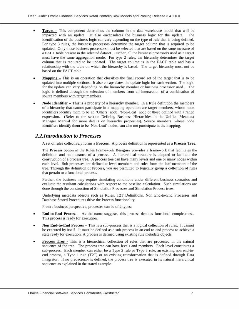
User Guide Oracle Financial Services Retail Portfolio Risk Models and Pooling Release 34100
Oracle Financial Software Services Confidential-Restricted 15
Annexure B ndash Frequently Asked Questions
Please refer to the attached Oracle Financial Services Retail Portfolio Risk Models and Pooling
Release 34100 FAQ
FAQpdf

Oracle Financial Services Retail Portfolio Risk
Models and Pooling
Frequently Asked Questions
Release 34100
February 2014
FAQ Oracle Financial Services Retail Portfolio Risk Models and Pooling Release 34100
Oracle Financial Services Software Confidential-Restricted ii
Contents
1 DEFINITIONS 1
2 QUESTIONS ON RETAIL POOLING 3
3 QUESTIONS IN APPLIED STATISTICS 8
FAQ Oracle Financial Services Retail Portfolio Risk Models and Pooling Release 34100
Oracle Financial Services Software Confidential-Restricted 1
1 Definitions
This section defines various terms which are used either in RFD or in this document Thus these
terms are necessarily generic in nature and are used across various RFDs or various sections of
this document Specific definitions which are used only for handling a particular exposure are
covered in the respective section of this document
D1 Retail Exposure
Exposures to individuals such as revolving credits and lines of credit (For
Example credit cards overdrafts and retail facilities secured by financial
instruments) as well as personal term loans and leases (For Example
installment loans auto loans and leases student and educational loans
personal finance and other exposures with similar characteristics) are
generally eligible for retail treatment regardless of exposure size
Residential mortgage loans (including first and subsequent liens term
loans and revolving home equity lines of credit) are eligible for retail
treatment regardless of exposure size so long as the credit is extended to an
individual that is an owner occupier of the property Loans secured by a
single or small number of condominium or co-operative residential
housing units in a single building or complex also fall within the scope of
the residential mortgage category
Loans extended to small businesses and managed as retail exposures are
eligible for retail treatment provided the total exposure of the banking
group to a small business borrower (on a consolidated basis where
applicable) is less than 1 million Small business loans extended through or
guaranteed by an individual are subject to the same exposure threshold
The fact that an exposure is rated individually does not by itself deny the
eligibility as a retail exposure
D2 Borrower risk characteristics
Socio-Demographic Attributes related to the customer like income age gender
educational status type of job time at current job zip code External Credit Bureau
attributes (if available) such as credit history of the exposure like Payment History
Relationship External Utilization Performance on those Accounts and so on
D3 Transaction risk characteristics
Exposure characteristics Basic Attributes of the exposure like Account number Product
name Product type Mitigant type Location Outstanding amount Sanctioned Limit
Utilization payment spending behavior age of the account opening balance closing
balance delinquency etc
D4 Delinquency of exposure characteristics
Total Delinquency Amount Pct Delq Amount to Total Max Delq Amount or Number
of More equal than 30 Days Delinquency in last 3 Months and so on
D5 Factor Analysis
Factor analysis is the widely used technique of reducing data Factor analysis is a
statistical technique used to explain variability among observed random variables in terms
of fewer unobserved random variables called factors
D6 Classes of Variables
We need to specify variables Driver variable These would be all the raw attributes
described above like income band month on books and so on
FAQ Oracle Financial Services Retail Portfolio Risk Models and Pooling Release 34100
Oracle Financial Services Software Confidential-Restricted 2
D7 Hierarchical Clustering
In hierarchical cluster analysis dendrogram graphs are used to visualize how clusters are
formed Because each observation is displayed dendrogram are impractical when the data
set is large
D8 K Means Clustering
Number of clusters is a random or manual input or based on the results of hierarchical
clustering This kind of clustering method is also called a k-means model since the cluster
centers are the means of the observations assigned to each cluster when the algorithm is
run to complete convergence
D9 Homogeneous Pools
There exists no standard definition of homogeneity and that needs to be defined based on
risk characteristics
D10 Binning
Binning is the method of variable discretization or grouping into 10 groups where each
group contains equal number of records as far as possible For each group created above
we could take the mean or the median value for that group and call them as bins or the bin
values
FAQ Oracle Financial Services Retail Portfolio Risk Models and Pooling Release 34100
Oracle Financial Services Software Confidential-Restricted 3
2 Questions on Retail Pooling
1 How to extract data
Within a workflow environment (modeling environment) data would be extracted or
imported from source tables and one or more output datasets would be created that has few or
all of the raw attributes at record level (say an exposure level) For clustering ultimately we
need to have one dataset
2 How to create Variables
Date and Time Related attributes could help create Time Variables such as
Month on books
Months since delinquency gt 2
Summary and averages
3month total balance 3 month total payment 6 month total late fees and
so on
3 month 6 month 12 month averages of many attributes
Average 3 month delinquency utilization and so on
Derived variables and indicators
Payment Rate (Payment amount closing balance for credit cards)
Fees Charge Rate
Interest Charges rate and so on
Qualitative attributes
For example Dummy variables for attributes such as regions products asset codes and so
on
3 How to prepare variables
Imputation of missing attributes can be done only when the missing rate is not exceeding
10-15
Extreme Values are treated Lower extremes and Upper extremes are treated based on a
Quintile Plot or Normal Probability Plot and the extreme values which are identified are
not deleted but capped in the dataset
Some of the attributes would be the outcomes of risk such as default indicator pay off
indicator Losses Write Off Amount etc and hence will not be used as input variables in
the cluster analysis However these variables could be used for understanding the
distribution of the pools and also for loss modeling subsequently
4 How to reduce the of variables
In case of model fitting variable reduction is done through collineraity diagnostics or bivariate
correlation measures etc However clustering variables could be reduced by factor analysis
5 How to run hierarchical clustering
You can choose a distance criterion Based on that you are shown a dendrogram based on
which he decides the number of clusters A manual iterative process is then used to arrive at
the final clusters with the distance criterion being modified in each step
FAQ Oracle Financial Services Retail Portfolio Risk Models and Pooling Release 34100
Oracle Financial Services Software Confidential-Restricted 4
6 What are the outputs to be seen in hierarchical clustering
Cluster Summary giving the following for each cluster
Number of Clusters
7 How to run K Means Clustering
On the Dataset give Seeds= Value with full replacement method and K= Value For multiple
runs as you reduce K also change the seed for validity of formation
8 What outputs to see K Means Clustering
Cluster number for all the K clusters
Frequency the number of observations in the cluster
RMS Std Deviation the root mean square across variables of the cluster standard
deviations which is equal to the root mean square distance between observations in the
cluster
Maximum Distance from Seed to Observation the maximum distance from the cluster
seed to any observation in the cluster
Nearest Cluster the number of the cluster with mean closest to the mean of the current
cluster
Centroid Distance the distance between the centroids (means) of the current cluster and
the nearest other cluster
A table of statistics for each variable is displayed
Total STD the total standard deviation
Within STD the pooled within-cluster standard deviation
R-Squared the R2 for predicting the variable from the cluster
RSQ(1 - RSQ) the ratio of between-cluster variance to within-cluster variance (R2(1 -
R2))
Distances Between Cluster Means
Cluster Summary Report containing the list of clusters drivers (variables) behind
clustering details about the relevant variables in each cluster like Mean Median
Minimum Maximum and similar details about target variables like Number of defaults
Recovery rate and so on
RSQ(1 - RSQ) the ratio of between-cluster variance to within-cluster variance (R2(1 -
R2))
OVER-ALL all of the previous quantities pooled across variables
Pseudo F Statistic = [( [(R2)(c - 1)] )( [(1 - R2)(n - c)] )]
Approximate Expected Overall R-Squared the approximate expected value of the overall
R2 under the uniform null hypothesis assuming that the variables are uncorrelated
Distances Between Cluster Means
Cluster Means for each variable
9 How to define clusters
Validation of the cluster solution is an art in itself and therefore never done by re-growing the
cluster solution on the test sample instead the score formula of the training sample is used to
create the new group of clusters in the test sample
FAQ Oracle Financial Services Retail Portfolio Risk Models and Pooling Release 34100
Oracle Financial Services Software Confidential-Restricted 5
of clusters formed size of each cluster new cluster means and cluster distances
cluster standard deviations
For example say in the Training sample the following results were obtained after developing the
clusters
Variable X1 Variable X2 Variable X3 Variable X4
Mean1 STD1 Mean2 STD2 Mean3 STD3 Mean4 STD4
Clus1 200 100 220 100 180 100 170 100
Clus2 160 90 180 90 140 90 130 90
Clus3 110 60 130 60 90 60 80 60
Clus4 90 45 110 45 70 45 60 45
Clus5 35 10 55 10 15 10 5 10
Table 1 Defining Clusters Example
When we apply the above cluster solution on the test data set as below
For each Variable calculate the distances from every cluster This is followed by associating with
each row a distance from every cluster using the below formulae
Square Distance for Clus1= (X1-Mean11)STD11- (X2-Mean21)STD212+(X1-
Mean11)STD11-(X3-Mean31)STD312+(X1-Mean11)STD11-(X4-Mean41)STD412
Square Distance for Clus2= (X1-Mean11)STD11- (X2-Mean21)STD212+(X1-
Mean11)STD11-(X3-Mean31)STD312+(X1-Mean11)STD11-(X4-Mean41)STD412
Square Distance for Clus3= (X1-Mean11)STD11- (X2-Mean21)STD212+(X1-
Mean11)STD11-(X3-Mean31)STD312+(X1-Mean11)STD11-(X4-Mean41)STD412
Square Distance for Clus4= (X1-Mean11)STD11- (X2-Mean21)STD212+(X1-
Mean11)STD11-(X3-Mean31)STD312+(X1-Mean11)STD11-(X4-Mean41)STD412
Square Distance for Clus5= (X1-Mean11)STD11- (X2-Mean21)STD212+(X1-
Mean11)STD11-(X3-Mean31)STD312+(X1-Mean11)STD11-(X4-Mean41)STD412
We do not need to standardize each variable in the Test Dataset since we need to calculate the new
distances by using the means and STD from the Training dataset
New Clus1= Minimum(Distance1 Distance2 Distance3 Distance4 Distance5)
New Clus2= Minimum(Distance1 Distance2 Distance3 Distance4 Distance5)
New Clus3= Minimum(Distance1 Distance2 Distance3 Distance4 Distance5)
New Clus4= Minimum(Distance1 Distance2 Distance3 Distance4 Distance5)
New Clus5= Minimum(Distance1 Distance2 Distance3 Distance4 Distance5)
After applying the solution on the test dataset the new distances are compared for each of the
clusters and cluster summary report containing the list of clusters is prepared their drivers
(variables) details about the relevant variables in each cluster like Mean Median Minimum
Maximum and similar details about target variables like Number of defaults Recovery rate and so
on
10 What is homogeneity
There exists no standard definition of homogeneity and that needs to be defined based on risk
characteristics
11 What is Pool Summary Report
FAQ Oracle Financial Services Retail Portfolio Risk Models and Pooling Release 34100
Oracle Financial Services Software Confidential-Restricted 6
Pool definitions are created out of the Pool report that summarizes
Pool Variables Profiles
Pool Size and Proportion
Pool Default Rates across time
12 What is Probability of Default
Default Probability is the likelihood of default that can be assigned to each account or
exposure It is a number that varies between 00 and 10
13 What is Loss Given Default
It is also known as recovery ratio It can vary between 0 and 100 and could be available
for each exposure or a group of exposures The recovery ratio can also be calculated by the
business user if the related attributes are downloaded from the Recovery Data Mart using
variables such as Write off Amount Outstanding Balance Collected Amount Discount
Offered Market Value of Collateral and so on
14 What is CCF or Credit Conversion Factor
For off-balance sheet items exposure is calculated as the committed but undrawn amount
multiplied by a CCF (that is the Credit Conversion Factor) as given in Basel
15 What is Exposure at Default
EAD is the risk measure that denotes the amount of exposure that is at risk and hence the
amount on which we need to apply the Risk Weight Function to calculate the amount of loss
or capital In general EAD is the sum of drawn amount and CCF multiplied undrawn amount
16 What is the difference between Principal Component Analysis and Common Factor
Analysis
The purpose of principal component analysis (Rao 1964) is to derive a small number of linear
combinations (principal components) of a set of variables that retain as much of the
information in the original variables as possible Often a small number of principal
components can be used in place of the original variables for plotting regression clustering
and so on Principal component analysis can also be viewed as an attempt to uncover
approximate linear dependencies among variables
Principal factors vs principal components The defining characteristic that distinguishes
between the two factor analytic models is that in principal components analysis we assume
that all variability in an item should be used in the analysis while in principal factors analysis
we only use the variability in an item that it has in common with the other items In most
cases these two methods usually yield very similar results However principal components
analysis is often preferred as a method for data reduction while principal factors analysis is
often preferred when the goal of the analysis is to detect structure (see Factor Analysis as a
Classification Method)
17 What is the segment information that should be stored in the database (example
segment name) Will they be used to define any report
For the purpose of reporting out and validation and tracking we need to have the following ids
created
Cluster Id
Decision Tree Node Id
Final Segment Id
Sometimes you would need to regroup the combinations of clusters and nodes and create
final segments of your own
FAQ Oracle Financial Services Retail Portfolio Risk Models and Pooling Release 34100
Oracle Financial Services Software Confidential-Restricted 7
18 Discretize the variables ndash what is the method to be used
Binning Methods are more popular which are Equal Groups Binning or Equal Interval
Binning or Ranking The value for a bin could be the mean or median
19 Qualitative attributes ndash will be treated at a data model level
Such as City Name Product Name or Credit Line and so on can be handled using Binary Indicators or
Nominal Indicators
20 Substitute for Missing values ndash what is the method
Categorical data Mode or Group Modes and Continuous Data Mean or Median could be used
21 Pool stability report ndash what is this
Movements can happen between subsequent pool over months and such movements are
summarized with the help of a transition report
FAQ Oracle Financial Services Retail Portfolio Risk Models and Pooling Release 34100
Oracle Financial Services Software Confidential-Restricted 8
3 Questions in Applied Statistics
1 Eigenvalues How to Choose of Factors
The Kaiser criterion First we can retain only factors with eigen values greater than 1 In
essence this is like saying that unless a factor extract at least as much as the equivalent of one
original variable we drop it This criterion was proposed by Kaiser (1960) and is probably
the one most widely used In our example above using this criterion we would retain 2
factors The other method called (screen test) sometimes retains too few factors
Choose of Variables (Input of factors Eigen Value gt=10 as in 33 )
The variable selection would be based on both communality estimates between 09 to 11 and
also based on individual factor loadings of variables for a given factor The closer the
communality is to 1 the better the variable is explained by the factors and hence retain all
variable within these set of communality between 09 to 11
Beyond communality measure we could also use Factor loading as a variable selection
criterion which helps you to select other variables which contribute to the uncommon (unlike
common as in communality)
Factor Loading A rule of thumb frequently used is that factor loadings greater than 4 or 05
in absolute value are considered to be significant This criterion is just a guideline and may
need to be adjusted As the sample size and the number of variables increase the criterion
may need to be adjusted slightly downward it may need to be adjusted upward as the number
of factors increases A good measure of selecting variables could be also by selecting the top
2 or top 3 variables influencing each factor It is assumed that top 2 or top 3 variables
contribute to the maximum explanation of that factor
However if you have satisfied the eigen value and communality criterion selection of
variables based on factor loadings could be left to you In the second column (Eigen value)
above we find the variance on the new factors that were successively extracted In the third
column these values are expressed as a percent of the total variance (in this example 10) As
we can see factor 1 accounts for 61 percent of the variance factor 2 for 18 percent and so on
As expected the sum of the eigen values is equal to the number of variables The third
column contains the cumulative variance extracted The variances extracted by the factors are
called the eigen values This name derives from the computational issues involved
FAQ Oracle Financial Services Retail Portfolio Risk Models and Pooling Release 34100
Oracle Financial Services Software Confidential-Restricted 9
2 How do you determine the Number of Clusters
An important question that needs to be answered before applying the k-means or EM
clustering algorithms is how many clusters are there in the data This is not known a priori
and in fact there might be no definite or unique answer as to what value k should take In
other words k is a nuisance parameter of the clustering model Luckily an estimate of k can
be obtained from the data using the method of cross-validation Remember that the k-means
methods will determine cluster solutions for a particular user-defined number of clusters The
k-means techniques (described above) can be optimized and enhanced for typical applications
in data mining The general metaphor of data mining implies the situation in which an analyst
searches for useful structures and nuggets in the data usually without any strong a priori
expectations of what the analyst might find (in contrast to the hypothesis-testing approach of
scientific research) In practice the analyst usually does not know ahead of time how many
clusters there might be in the sample For that reason some programs include an
implementation of a v-fold cross-validation algorithm for automatically determining the
number of clusters in the data
Cluster analysis is an unsupervised learning technique and we cannot observe the (real)
number of clusters in the data However it is reasonable to replace the usual notion
(applicable to supervised learning) of accuracy with that of distance In general we can
apply the v-fold cross-validation method to a range of numbers of clusters in k-means
To complete convergence the final cluster seeds will equal the cluster means or cluster
centers
3 What is the displayed output
Initial Seeds cluster seeds selected after one pass through the data
Change in Cluster Seeds for each iteration if you specify MAXITER=ngt1
Cluster number
Frequency the number of observations in the cluster
Weight the sum of the weights of the observations in the cluster if you specify the
WEIGHT statement
RMS Std Deviation the root mean square across variables of the cluster standard
deviations which is equal to the root mean square distance between observations in the
cluster
Maximum Distance from Seed to Observation the maximum distance from the cluster
seed to any observation in the cluster
Nearest Cluster the number of the cluster with mean closest to the mean of the current
cluster
Centroid Distance the distance between the centroids (means) of the current cluster and
the nearest other cluster
A table of statistics for each variable is displayed unless you specify the SUMMARY option
The table contains
Total STD the total standard deviation
Within STD the pooled within-cluster standard deviation
R-Squared the R2 for predicting the variable from the cluster
RSQ(1 - RSQ) the ratio of between-cluster variance to within-cluster variance (R2(1 -
R2))
OVER-ALL all of the previous quantities pooled across variables
FAQ Oracle Financial Services Retail Portfolio Risk Models and Pooling Release 34100
Oracle Financial Services Software Confidential-Restricted 10
Pseudo F Statistic
[( [(R2)(c - 1)] )( [(1 - R2)(n - c)] )]
where R2 is the observed overall R2 c is the number of clusters and n is the number of
observations The pseudo F statistic was suggested by Calinski and Harabasz (1974) Refer
to Milligan and Cooper (1985) and Cooper and Milligan (1988) regarding the use of the
pseudo F statistic in estimating the number of clusters
Observed Overall R-Squared
Approximate Expected Overall R-Squared the approximate expected value of the overall
R2 under the uniform null hypothesis assuming that the variables are uncorrelated
Cubic Clustering Criterion computed under the assumption that the variables are
uncorrelated
Distances Between Cluster Means
Cluster Means for each variable
4 What are the Classes of Variables
You need to specify three classes of variables when performing a decision tree analysis
Target variable -- The ldquotarget variablerdquo is the variable whose values are to be modeled and
predicted by other variables It is analogous to the dependent variable (ithe variable on the left
of the equal sign) in linear regression
Predictor variable -- A ldquopredictor variablerdquo is a variable whose values will be used to predict
the value of the target variable It is analogous to the independent variables (variables on the
right side of the equal sign) in linear regression There must be at least one predictor variable
specified for decision tree analysis there may be many predictor variables
5 What are the types of Variables
Variables may have two types continuous and categorical
Continuous variables -- A continuous variable has numeric values such as 1 2 314 -5 etc
The relative magnitude of the values is significant (For example a value of 2 indicates twice
the magnitude of 1) Continuous variables are also called ldquoorderedrdquo or ldquomonotonicrdquo variables
Categorical variables -- A categorical variable has values that function as labels rather than as
numbers Some programs call categorical variables ldquonominalrdquo variables For example a
categorical variable for gender might use the value 1 for male and 2 for female The actual
magnitude of the value is not significant coding male as 7 and female as 3 would work just as
well As another example marital status might be coded as 1 for single 2 for married 3 for
divorced and 4 for widowed So your dataset could have the strings ldquoMalerdquo and ldquoFemalerdquo or
ldquoMrdquo and ldquoFrdquo for a categorical gender variable Since categorical values are stored and
compared as string values a categorical value of 001 is different than a value of 1 In contrast
values of 001 and 1 would be equal for continuous variables
6 What are Misclassification costs
Sometimes more accurate classification of the response is desired for some classes than others
for reasons not related to the relative class sizes If the criterion for predictive accuracy is
Misclassification costs then minimizing costs would amount to minimizing the proportion of
misclassified cases when priors are considered proportional to the class sizes and
misclassification costs are taken to be equal for every class
7 What are Estimates of the accuracy
In classification problems (categorical dependent variable) three estimates of the accuracy are
used resubstitution estimate test sample estimate and v-fold cross-validation These
estimates are defined here
FAQ Oracle Financial Services Retail Portfolio Risk Models and Pooling Release 34100
Oracle Financial Services Software Confidential-Restricted 11
Re-substitution estimate Re-substitution estimate is the proportion of cases that are
misclassified by the classifier constructed from the entire sample This estimate is computed
in the following manner
where X is the indicator function
X = 1 if the statement is true
X = 0 if the statement is false
and d (x) is the classifier
The resubstitution estimate is computed using the same data as used in constructing the
classifier d
Test sample estimate The total number of cases is divided into two subsamples Z1 and Z2
The test sample estimate is the proportion of cases in the subsample Z2 which are
misclassified by the classifier constructed from the subsample Z1 This estimate is computed
in the following way
Let the learning sample Z of size N be partitioned into subsamples Z1 and Z2 of sizes N and
N2 respectively
where Z2 is the sub sample that is not used for constructing the classifier
v-fold cross validation The total number of cases are divided into v sub samples Z1 Z2
Zv of almost equal sizes v-fold cross validation estimate is the proportion of cases in the
subsample Z that are misclassified by the classifier constructed from the subsample Z - Zv
This estimate is computed in the following way
Let the learning sample Z of size N be partitioned into v sub samples Z1 Z2 Zv of almost
sizes N1 N2 Nv respectively
where is computed from the sub sample Z - Zv
Estimation of Accuracy in Regression
In the regression problem (continuous dependent variable) three estimates of the accuracy are
used re-substitution estimate test sample estimate and v-fold cross-validation These
estimates are defined here
Re-substitution estimate The re-substitution estimate is the estimate of the expected squared
error using the predictor of the continuous dependent variable This estimate is computed in
the following way
where the learning sample Z consists of (xiyi)i = 12N The re-substitution estimate is
computed using the same data as used in constructing the predictor d
FAQ Oracle Financial Services Retail Portfolio Risk Models and Pooling Release 34100
Oracle Financial Services Software Confidential-Restricted 12
Test sample estimate The total number of cases is divided into two subsamples Z1 and Z2
The test sample estimate of the mean squared error is computed in the following way
Let the learning sample Z of size N be partitioned into subsamples Z1 and Z2 of sizes N and
N2 respectively
where Z2 is the sub-sample that is not used for constructing the predictor
v-fold cross-validation The total number of cases is divided into v sub samples Z1 Z2 Zv of
almost equal sizes The subsample Z - Zv is used to construct the predictor d Then v-fold
cross validation estimate is computed from the subsample Zv in the following way
Let the learning sample Z of size N be partitioned into v sub samples Z1 Z2 Zv of almost
sizes N1 N2 Nv respectively
where is computed from the sub sample Z - Zv
8 How to Estimate of Node Impurity Gini Measure
The Gini measure is the measure of impurity of a node and is commonly used when the
dependent variable is a categorical variable defined as
if costs of misclassification are not specified
if costs of misclassification are specified
where the sum extends over all k categories p( j t) is the probability of category j at the node
t and C(i j ) is the probability of misclassifying a category j case as category i
The Gini Criterion Function Q(st) for split s at node t is defined as
Q(st)=g(t)-Plg(tl)-prg(tr)
Where pl is the proportion of cases in t sent to the left child node and pr is the proportion sent
to the right child node The proportion pl and pr are defined as
Pl=p(tl)p(t)
and
Pr=p(tr)p(t)
The split s is chosen to maximize the value of Q(st) This value is reported as the
improvement in the tree
9 What is Towing
The towing index is based on splitting the target categories into two superclasses and then
finding the best split on the predictor variable based on those two superclasses The towing
critetioprn function for split s at node t is defined as
FAQ Oracle Financial Services Retail Portfolio Risk Models and Pooling Release 34100
Oracle Financial Services Software Confidential-Restricted 13
Q(st)=plpr[sum(j|p(jtl)-p(jtr))2
Where tl and tr are the nodes created by the split s The split s is chosen as the split that
maximizes this criterion This value weighted by the proportion of all cases in node t is the
value reported as improvement in the tree
10 Estimation of Node Impurity Other Measure
In addition to measuring accuracy the following measures of node impurity are used for
classification problems The Gini measure generalized Chi-square measure and generalized
G-square measure The Chi-square measure is similar to the standard Chi-square value
computed for the expected and observed classifications (with priors adjusted for
misclassification cost) and the G-square measure is similar to the maximum-likelihood Chi-
square (as for example computed in the Log-Linear technique) The Gini measure is the one
most often used for measuring purity in the context of classification problems and it is
described below
For continuous dependent variables (regression-type problems) the least squared deviation
(LSD) measure of impurity is automatically applied
Estimation of Node Impurity Least-Squared Deviation
Least-squared deviation (LSD) is used as the measure of impurity of a node when the
response variable is continuous and is computed as
where Nw(t) is the weighted number of cases in node t wi is the value of the weighting
variable for case i fi is the value of the frequency variable yi is the value of the response
variable and y(t) is the weighted mean for node
11 How to select splits
The process of computing classification and regression trees can be characterized as involving
four basic steps Specifying the criteria for predictive accuracy
Selecting splits
Determining when to stop splitting
Selecting the right-sized tree
These steps are very similar to those discussed in the context of Classification Trees Analysis
(see also Breiman et al 1984 for more details) See also Computational Formulas
12 Specifying the Criteria for Predictive Accuracy
The classification and regression trees (CART) algorithms are generally aimed at achieving
the best possible predictive accuracy Operationally the most accurate prediction is defined as
the prediction with the minimum costs The notion of costs was developed as a way to
generalize to a broader range of prediction situations the idea that the best prediction has the
lowest misclassification rate In most applications the cost is measured in terms of proportion
of misclassified cases or variance
13 Priors
In the case of a categorical response (classification problem) minimizing costs amounts to
minimizing the proportion of misclassified cases when priors are taken to be proportional to
the class sizes and when misclassification costs are taken to be equal for every class
The a priori probabilities used in minimizing costs can greatly affect the classification of
cases or objects Therefore care has to be taken while using the priors If differential base
rates are not of interest for the study or if one knows that there are about an equal number of
FAQ Oracle Financial Services Retail Portfolio Risk Models and Pooling Release 34100
Oracle Financial Services Software Confidential-Restricted 14
cases in each class then one would use equal priors If the differential base rates are reflected
in the class sizes (as they would be if the sample is a probability sample) then one would use
priors estimated by the class proportions of the sample Finally if you have specific
knowledge about the base rates (for example based on previous research) then one would
specify priors in accordance with that knowledge The general point is that the relative size of
the priors assigned to each class can be used to adjust the importance of misclassifications
for each class However no priors are required when one is building a regression tree
The second basic step in classification and regression trees is to select the splits on the
predictor variables that are used to predict membership in classes of the categorical dependent
variables or to predict values of the continuous dependent (response) variable In general
terms the split at each node will be found that will generate the greatest improvement in
predictive accuracy This is usually measured with some type of node impurity measure
which provides an indication of the relative homogeneity (the inverse of impurity) of cases in
the terminal nodes If all cases in each terminal node show identical values then node
impurity is minimal homogeneity is maximal and prediction is perfect (at least for the cases
used in the computations predictive validity for new cases is of course a different matter)
14 Impurity Measures
For classification problems CART gives you the choice of several impurity measures The
Gini index Chi-square or G-square The Gini index of node impurity is the measure most
commonly chosen for classification-type problems As an impurity measure it reaches a value
of zero when only one class is present at a node With priors estimated from class sizes and
equal misclassification costs the Gini measure is computed as the sum of products of all pairs
of class proportions for classes present at the node it reaches its maximum value when class
sizes at the node are equal the Gini index is equal to zero if all cases in a node belong to the
same class The Chi-square measure is similar to the standard Chi-square value computed for
the expected and observed classifications (with priors adjusted for misclassification cost) and
the G-square measure is similar to the maximum-likelihood Chi-square (as for example
computed in the Log-Linear technique) For regression-type problems a least-squares
deviation criterion (similar to what is computed in least squares regression) is automatically
used Computational Formulas provides further computational details
15 When to Stop Splitting
As discussed in Basic Ideas in principal splitting could continue until all cases are perfectly
classified or predicted However this wouldnt make much sense since one would likely end
up with a tree structure that is as complex and tedious as the original data file (with many
nodes possibly containing single observations) and that would most likely not be very useful
or accurate for predicting new observations What is required is some reasonable stopping
rule
Minimum n One way to control splitting is to allow splitting to continue until all terminal
nodes are pure or contain no more than a specified minimum number of cases or objects
Fraction of objects Another way to control splitting is to allow splitting to continue until all
terminal nodes are pure or contain no more cases than a specified minimum fraction of the
sizes of one or more classes (in the case of classification problems or all cases in regression
problems)
Alternatively if the priors used in the analysis are not equal splitting will stop when all
terminal nodes containing more than one class have no more cases than the specified fraction
for one or more classes See Loh and Vanichestakul 1988 for details
Pruning and Selecting the Right-Sized Tree
The size of a tree in the classification and regression trees analysis is an important issue since
an unreasonably big tree can only make the interpretation of results more difficult Some
generalizations can be offered about what constitutes the right-sized tree It should be
sufficiently complex to account for the known facts but at the same time it should be as
FAQ Oracle Financial Services Retail Portfolio Risk Models and Pooling Release 34100
Oracle Financial Services Software Confidential-Restricted 15
simple as possible It should exploit information that increases predictive accuracy and ignore
information that does not It should if possible lead to greater understanding of the
phenomena it describes These procedures are not foolproof as Breiman et al (1984) readily
acknowledges but at least they take subjective judgment out of the process of selecting the
right-sized tree
Sub samples from the computations and using that subsample as a test sample for cross-
validation so that each subsample is used (v - 1) times in the learning sample and just once as
the test sample The CV costs (cross-validation cost) computed for each of the v test samples
are then averaged to give the v-fold estimate of the CV costs
Minimal cost-complexity cross-validation pruning In CART minimal cost-complexity cross-
validation pruning is performed if Prune on misclassification error has been selected as the
Stopping rule On the other hand if Prune on deviance has been selected as the Stopping rule
then minimal deviance-complexity cross-validation pruning is performed The only difference
in the two options is the measure of prediction error that is used Prune on misclassification
error uses the costs that equals the misclassification rate when priors are estimated and
misclassification costs are equal while Prune on deviance uses a measure based on
maximum-likelihood principles called the deviance (see Ripley 1996)
The sequence of trees obtained by this algorithm have a number of interesting properties
They are nested because the successively pruned trees contain all the nodes of the next
smaller tree in the sequence Initially many nodes are often pruned going from one tree to the
next smaller tree in the sequence but fewer nodes tend to be pruned as the root node is
approached The sequence of largest trees is also optimally pruned because for every size of
tree in the sequence there is no other tree of the same size with lower costs Proofs andor
explanations of these properties can be found in Breiman et al (1984)
Tree selection after pruning The pruning as discussed above often results in a sequence of
optimally pruned trees So the next task is to use an appropriate criterion to select the right-
sized tree from this set of optimal trees A natural criterion would be the CV costs (cross-
validation costs) While there is nothing wrong with choosing the tree with the minimum CV
costs as the right-sized tree often times there will be several trees with CV costs close to
the minimum Following Breiman et al (1984) one could use the automatic tree selection
procedure and choose as the right-sized tree the smallest-sized (least complex) tree whose
CV costs do not differ appreciably from the minimum CV costs In particular they proposed a
1 SE rule for making this selection that is choose as the right-sized tree the smallest-
sized tree whose CV costs do not exceed the minimum CV costs plus 1 times the standard
error of the CV costs for the minimum CV costs tree
As can be been seen minimal cost-complexity cross-validation pruning and subsequent
right-sized tree selection is a automatic process The algorithms make all the decisions
leading to the selection of the right-sized tree except for specification of a value for the SE
rule V-fold cross-validation allows you to evaluate how well each tree performs when
repeatedly cross-validated in different samples randomly drawn from the data
16 Computational Formulas
In Classification and Regression Trees estimates of accuracy are computed by different
formulas for categorical and continuous dependent variables (classification and regression-
type problems) For classification-type problems (categorical dependent variable) accuracy is
measured in terms of the true classification rate of the classifier while in the case of
regression (continuous dependent variable) accuracy is measured in terms of mean squared
error of the predictor
FAQ Oracle Financial Services Retail Portfolio Risk Models and Pooling Release 34100
Oracle Financial Services Software Confidential-Restricted 16
Oracle Financial Services Retail Portfolio Risk Models and Pooling - FAQ
February 2014
Version number 10
Oracle Corporation
World Headquarters
500 Oracle Parkway
Redwood Shores CA 94065
USA
Worldwide Inquiries
Phone +16505067000
Fax +16505067200
wwworaclecom financial_services
Copyright copy 2014 Oracle andor its affiliates All rights reserved
No part of this work may be reproduced stored in a retrieval system adopted or transmitted in any form or by any means electronic mechanical photographic graphic optic recording or otherwise translated in any language or computer language without the prior written permission of Oracle Financial Services Software Limited
Due care has been taken to make this Oracle Financial Services Retail Portfolio Risk Models and Pooling FAQ and accompanying software package as accurate as possible However Oracle Financial Services Software Limited makes no representation or warranties with respect to the contents hereof and shall not be responsible for any loss or damage caused to the user by the direct or indirect use of this User Manual and the accompanying Software System Furthermore Oracle Financial Services Software Limited reserves the right to alter modify or otherwise change in any manner the content hereof without obligation of Oracle Financial Services Software Limited to notify any person of such revision or changes
All company and product names are trademarks of the respective companies with which they are associated
- 1 Definitions
- 2 Questions on Retail Pooling
- 3 Questions in Applied Statistics
-
- 1 Introduction
-
- 11 Overview of Oracle Financial Services Retail Portfolio Risk Models and Pooling
- 12 Summary
- 13 Approach Followed in the Product
-
- 2 Implementing the Product using the OFSAAI Infrastructure
-
- 21 Introduction to Rules
-
- 211 Types of Rules
- 212 Rule Definition
-
- 22 Introduction to Processes
-
- 221 Type of Process Trees
-
- 23 Introduction to Run
-
- 231 Run Definition
- 232 Types of Runs
-
- 24 Building Business Processors for Calculation Blocks
-
- 241 What is a Business Processor
- 242 Why Define a Business Processor
-
- 25 Modeling Framework Tools or Techniques used in RP
-
- 3 Understanding Data Extraction
-
- 31 Introduction
- 32 Structure
-
- Annexure A ndash Definitions
- Annexure B ndash Frequently Asked Questions
- Annexure Cndash K Means Clustering Based On Business Logic
- ANNEXURE D Generating Download Specifications
-
FAQpdfUser Guide Oracle Financial Services Retail Portfolio Risk Models and Pooling Release 34100
Oracle Financial Software Services Confidential-Restricted 16
Annexure Cndash K Means Clustering Based On Business Logic
The process of clustering based on business logic assigns each record to a particular cluster based
on the bounds of the variables Steps 1 and 2 are followed to find out the bounds of each variable
for each of the given cluster Step 3 helps in deciding the cluster id for a given record
Steps 1 to 3 are together known as a RULE BASED FORMULA
In certain cases the rule based formula does not return us a unique cluster id so we then need to
use the MINIMUM DISTANCE FORMULA which is given in Step 4
1 The first step is to obtain the mean matrix by running a K Means process The following
is an example of such mean matrix which represents clusters in rows and variables in
columns
V1 V2 V3 V4
C1 15 10 9 57
C2 5 80 17 40
C3 45 20 37 55
C4 40 62 45 70
C5 12 7 30 20
2 The next step is to calculate bounds for the variable values Before this is done each set
of variables across all clusters have to be arranged in ascending order Bounds are then
calculated by taking the mean of consecutive values The process is as follows
V1
C2 5
C5 12
C1 15
C3 45
C4 40
The bounds have been calculated as follows for Variable 1
Less than 85
[(5+12)2] C2
Between 85 and
135 C5
Between 135 and
30 C1
Between 30 and
425 C3
Greater than 425 C4
The above mentioned process has to be repeated for all the variables
Variable 2
Less than 85 C5
Between 85 and
15 C1
User Guide Oracle Financial Services Retail Portfolio Risk Models and Pooling Release 34100
Oracle Financial Software Services Confidential-Restricted 17
Between 15 and
41 C3
Between 41 and
71 C4
Greater than 71 C2
Variable 3
Less than 13 C1
Between 13 and
235 C2
Between 235 and
335 C5
Between 335 and
41 C3
Greater than 41 C4
Variable 4
Less than 30 C5
Between 30 and
475 C2
Between 475 and
56 C3
Between 56 and
635 C1
Greater than 635 C4
3 The variables of the new record are put in their respective clusters according to the
bounds mentioned above Let us assume the new record to have the following variable
values
V1 V2 V3 V4
46 21 3 40
They are put in the respective clusters as follows (based on the bounds for each variable
and cluster combination)
V1 V2 V3 V4
46 21 3 40
C4 C3 C1 C1
As C1 is the cluster that occurs for the most number of times the new record is mapped to
C1
4 This is an additional step which is required if it is difficult to decide which cluster to map
to This may happen if more than one cluster gets repeated equal number of times or if
all of the clusters are unique
User Guide Oracle Financial Services Retail Portfolio Risk Models and Pooling Release 34100
Oracle Financial Software Services Confidential-Restricted 18
Let us assume that the new record was mapped as under
V1 V2 V3 V4
40 21 3 40
C3 C2 C1 C4
To avoid this and decide upon one cluster we use the minimum distance formula The
minimum distance formula is as follows-
(x2 ndash x1) ^2 + (y2 ndash y1) ^2 + helliphellip
Where x1 y1 and so on represent the variables of the new record and x2 y2 and so on
represent the variables of an existing record The distances between the new record and
each of the clusters have been calculated as follows-
C1 1407
C2 5358
C3 1383
C4 4381
C5 2481
C3 is the cluster which has the minimum distance Therefore the new record is to be
mapped to Cluster 3
User Guide Oracle Financial Services Retail Portfolio Risk Models and Pooling Release 34100
Oracle Financial Software Services Confidential-Restricted 19
ANNEXURE D Generating Download Specifications
Data Model for OFS Retail Portfolio Risk Models and Pooling is available on customer request as
an ERwin file
Download Specifications can be extracted from this model Refer the whitepaper present in OTN
for more details
User Guide Oracle Financial Services Retail Portfolio Risk Models and Pooling Release 34100
Oracle Financial Software Services Confidential-Restricted 19
Oracle Financial Services Retail Portfolio Risk Models and Pooling Release 34100
April 2014
Version number 10
Oracle Corporation
World Headquarters
500 Oracle Parkway
Redwood Shores CA 94065
USA
Worldwide Inquiries
Phone +16505067000
Fax +16505067200
wwworaclecom financial_services
Copyright copy 2014 Oracle andor its affiliates All rights reserved
No part of this work may be reproduced stored in a retrieval system adopted or transmitted in any form or by any means electronic mechanical photographic graphic optic recording or otherwise translated in any language or computer language without the prior written permission of Oracle Financial Services Software Limited
Due care has been taken to make this Oracle Financial Services Retail Portfolio Risk Models and Pooling User Guide and accompanying software package as accurate as possible However Oracle Financial Services Software Limited makes no representation or warranties with respect to the contents hereof and shall not be responsible for any loss or damage caused to the user by the direct or indirect use of this User Manual and the accompanying Software System Furthermore Oracle Financial Services Software Limited reserves the right to alter modify or otherwise change in any manner the content hereof without obligation of Oracle Financial Services Software Limited to notify any person of such revision or changes
All company and product names are trademarks of the respective companies with which they are associated

FAQ Oracle Financial Services Retail Portfolio Risk Models and Pooling Release 34100
Oracle Financial Services Software Confidential-Restricted ii
Contents
1 DEFINITIONS 1
2 QUESTIONS ON RETAIL POOLING 3
3 QUESTIONS IN APPLIED STATISTICS 8
FAQ Oracle Financial Services Retail Portfolio Risk Models and Pooling Release 34100
Oracle Financial Services Software Confidential-Restricted 1
1 Definitions
This section defines various terms which are used either in RFD or in this document Thus these
terms are necessarily generic in nature and are used across various RFDs or various sections of
this document Specific definitions which are used only for handling a particular exposure are
covered in the respective section of this document
D1 Retail Exposure
Exposures to individuals such as revolving credits and lines of credit (For
Example credit cards overdrafts and retail facilities secured by financial
instruments) as well as personal term loans and leases (For Example
installment loans auto loans and leases student and educational loans
personal finance and other exposures with similar characteristics) are
generally eligible for retail treatment regardless of exposure size
Residential mortgage loans (including first and subsequent liens term
loans and revolving home equity lines of credit) are eligible for retail
treatment regardless of exposure size so long as the credit is extended to an
individual that is an owner occupier of the property Loans secured by a
single or small number of condominium or co-operative residential
housing units in a single building or complex also fall within the scope of
the residential mortgage category
Loans extended to small businesses and managed as retail exposures are
eligible for retail treatment provided the total exposure of the banking
group to a small business borrower (on a consolidated basis where
applicable) is less than 1 million Small business loans extended through or
guaranteed by an individual are subject to the same exposure threshold
The fact that an exposure is rated individually does not by itself deny the
eligibility as a retail exposure
D2 Borrower risk characteristics
Socio-Demographic Attributes related to the customer like income age gender
educational status type of job time at current job zip code External Credit Bureau
attributes (if available) such as credit history of the exposure like Payment History
Relationship External Utilization Performance on those Accounts and so on
D3 Transaction risk characteristics
Exposure characteristics Basic Attributes of the exposure like Account number Product
name Product type Mitigant type Location Outstanding amount Sanctioned Limit
Utilization payment spending behavior age of the account opening balance closing
balance delinquency etc
D4 Delinquency of exposure characteristics
Total Delinquency Amount Pct Delq Amount to Total Max Delq Amount or Number
of More equal than 30 Days Delinquency in last 3 Months and so on
D5 Factor Analysis
Factor analysis is the widely used technique of reducing data Factor analysis is a
statistical technique used to explain variability among observed random variables in terms
of fewer unobserved random variables called factors
D6 Classes of Variables
We need to specify variables Driver variable These would be all the raw attributes
described above like income band month on books and so on
FAQ Oracle Financial Services Retail Portfolio Risk Models and Pooling Release 34100
Oracle Financial Services Software Confidential-Restricted 2
D7 Hierarchical Clustering
In hierarchical cluster analysis dendrogram graphs are used to visualize how clusters are
formed Because each observation is displayed dendrogram are impractical when the data
set is large
D8 K Means Clustering
Number of clusters is a random or manual input or based on the results of hierarchical
clustering This kind of clustering method is also called a k-means model since the cluster
centers are the means of the observations assigned to each cluster when the algorithm is
run to complete convergence
D9 Homogeneous Pools
There exists no standard definition of homogeneity and that needs to be defined based on
risk characteristics
D10 Binning
Binning is the method of variable discretization or grouping into 10 groups where each
group contains equal number of records as far as possible For each group created above
we could take the mean or the median value for that group and call them as bins or the bin
values
FAQ Oracle Financial Services Retail Portfolio Risk Models and Pooling Release 34100
Oracle Financial Services Software Confidential-Restricted 3
2 Questions on Retail Pooling
1 How to extract data
Within a workflow environment (modeling environment) data would be extracted or
imported from source tables and one or more output datasets would be created that has few or
all of the raw attributes at record level (say an exposure level) For clustering ultimately we
need to have one dataset
2 How to create Variables
Date and Time Related attributes could help create Time Variables such as
Month on books
Months since delinquency gt 2
Summary and averages
3month total balance 3 month total payment 6 month total late fees and
so on
3 month 6 month 12 month averages of many attributes
Average 3 month delinquency utilization and so on
Derived variables and indicators
Payment Rate (Payment amount closing balance for credit cards)
Fees Charge Rate
Interest Charges rate and so on
Qualitative attributes
For example Dummy variables for attributes such as regions products asset codes and so
on
3 How to prepare variables
Imputation of missing attributes can be done only when the missing rate is not exceeding
10-15
Extreme Values are treated Lower extremes and Upper extremes are treated based on a
Quintile Plot or Normal Probability Plot and the extreme values which are identified are
not deleted but capped in the dataset
Some of the attributes would be the outcomes of risk such as default indicator pay off
indicator Losses Write Off Amount etc and hence will not be used as input variables in
the cluster analysis However these variables could be used for understanding the
distribution of the pools and also for loss modeling subsequently
4 How to reduce the of variables
In case of model fitting variable reduction is done through collineraity diagnostics or bivariate
correlation measures etc However clustering variables could be reduced by factor analysis
5 How to run hierarchical clustering
You can choose a distance criterion Based on that you are shown a dendrogram based on
which he decides the number of clusters A manual iterative process is then used to arrive at
the final clusters with the distance criterion being modified in each step
FAQ Oracle Financial Services Retail Portfolio Risk Models and Pooling Release 34100
Oracle Financial Services Software Confidential-Restricted 4
6 What are the outputs to be seen in hierarchical clustering
Cluster Summary giving the following for each cluster
Number of Clusters
7 How to run K Means Clustering
On the Dataset give Seeds= Value with full replacement method and K= Value For multiple
runs as you reduce K also change the seed for validity of formation
8 What outputs to see K Means Clustering
Cluster number for all the K clusters
Frequency the number of observations in the cluster
RMS Std Deviation the root mean square across variables of the cluster standard
deviations which is equal to the root mean square distance between observations in the
cluster
Maximum Distance from Seed to Observation the maximum distance from the cluster
seed to any observation in the cluster
Nearest Cluster the number of the cluster with mean closest to the mean of the current
cluster
Centroid Distance the distance between the centroids (means) of the current cluster and
the nearest other cluster
A table of statistics for each variable is displayed
Total STD the total standard deviation
Within STD the pooled within-cluster standard deviation
R-Squared the R2 for predicting the variable from the cluster
RSQ(1 - RSQ) the ratio of between-cluster variance to within-cluster variance (R2(1 -
R2))
Distances Between Cluster Means
Cluster Summary Report containing the list of clusters drivers (variables) behind
clustering details about the relevant variables in each cluster like Mean Median
Minimum Maximum and similar details about target variables like Number of defaults
Recovery rate and so on
RSQ(1 - RSQ) the ratio of between-cluster variance to within-cluster variance (R2(1 -
R2))
OVER-ALL all of the previous quantities pooled across variables
Pseudo F Statistic = [( [(R2)(c - 1)] )( [(1 - R2)(n - c)] )]
Approximate Expected Overall R-Squared the approximate expected value of the overall
R2 under the uniform null hypothesis assuming that the variables are uncorrelated
Distances Between Cluster Means
Cluster Means for each variable
9 How to define clusters
Validation of the cluster solution is an art in itself and therefore never done by re-growing the
cluster solution on the test sample instead the score formula of the training sample is used to
create the new group of clusters in the test sample
FAQ Oracle Financial Services Retail Portfolio Risk Models and Pooling Release 34100
Oracle Financial Services Software Confidential-Restricted 5
of clusters formed size of each cluster new cluster means and cluster distances
cluster standard deviations
For example say in the Training sample the following results were obtained after developing the
clusters
Variable X1 Variable X2 Variable X3 Variable X4
Mean1 STD1 Mean2 STD2 Mean3 STD3 Mean4 STD4
Clus1 200 100 220 100 180 100 170 100
Clus2 160 90 180 90 140 90 130 90
Clus3 110 60 130 60 90 60 80 60
Clus4 90 45 110 45 70 45 60 45
Clus5 35 10 55 10 15 10 5 10
Table 1 Defining Clusters Example
When we apply the above cluster solution on the test data set as below
For each Variable calculate the distances from every cluster This is followed by associating with
each row a distance from every cluster using the below formulae
Square Distance for Clus1= (X1-Mean11)STD11- (X2-Mean21)STD212+(X1-
Mean11)STD11-(X3-Mean31)STD312+(X1-Mean11)STD11-(X4-Mean41)STD412
Square Distance for Clus2= (X1-Mean11)STD11- (X2-Mean21)STD212+(X1-
Mean11)STD11-(X3-Mean31)STD312+(X1-Mean11)STD11-(X4-Mean41)STD412
Square Distance for Clus3= (X1-Mean11)STD11- (X2-Mean21)STD212+(X1-
Mean11)STD11-(X3-Mean31)STD312+(X1-Mean11)STD11-(X4-Mean41)STD412
Square Distance for Clus4= (X1-Mean11)STD11- (X2-Mean21)STD212+(X1-
Mean11)STD11-(X3-Mean31)STD312+(X1-Mean11)STD11-(X4-Mean41)STD412
Square Distance for Clus5= (X1-Mean11)STD11- (X2-Mean21)STD212+(X1-
Mean11)STD11-(X3-Mean31)STD312+(X1-Mean11)STD11-(X4-Mean41)STD412
We do not need to standardize each variable in the Test Dataset since we need to calculate the new
distances by using the means and STD from the Training dataset
New Clus1= Minimum(Distance1 Distance2 Distance3 Distance4 Distance5)
New Clus2= Minimum(Distance1 Distance2 Distance3 Distance4 Distance5)
New Clus3= Minimum(Distance1 Distance2 Distance3 Distance4 Distance5)
New Clus4= Minimum(Distance1 Distance2 Distance3 Distance4 Distance5)
New Clus5= Minimum(Distance1 Distance2 Distance3 Distance4 Distance5)
After applying the solution on the test dataset the new distances are compared for each of the
clusters and cluster summary report containing the list of clusters is prepared their drivers
(variables) details about the relevant variables in each cluster like Mean Median Minimum
Maximum and similar details about target variables like Number of defaults Recovery rate and so
on
10 What is homogeneity
There exists no standard definition of homogeneity and that needs to be defined based on risk
characteristics
11 What is Pool Summary Report
FAQ Oracle Financial Services Retail Portfolio Risk Models and Pooling Release 34100
Oracle Financial Services Software Confidential-Restricted 6
Pool definitions are created out of the Pool report that summarizes
Pool Variables Profiles
Pool Size and Proportion
Pool Default Rates across time
12 What is Probability of Default
Default Probability is the likelihood of default that can be assigned to each account or
exposure It is a number that varies between 00 and 10
13 What is Loss Given Default
It is also known as recovery ratio It can vary between 0 and 100 and could be available
for each exposure or a group of exposures The recovery ratio can also be calculated by the
business user if the related attributes are downloaded from the Recovery Data Mart using
variables such as Write off Amount Outstanding Balance Collected Amount Discount
Offered Market Value of Collateral and so on
14 What is CCF or Credit Conversion Factor
For off-balance sheet items exposure is calculated as the committed but undrawn amount
multiplied by a CCF (that is the Credit Conversion Factor) as given in Basel
15 What is Exposure at Default
EAD is the risk measure that denotes the amount of exposure that is at risk and hence the
amount on which we need to apply the Risk Weight Function to calculate the amount of loss
or capital In general EAD is the sum of drawn amount and CCF multiplied undrawn amount
16 What is the difference between Principal Component Analysis and Common Factor
Analysis
The purpose of principal component analysis (Rao 1964) is to derive a small number of linear
combinations (principal components) of a set of variables that retain as much of the
information in the original variables as possible Often a small number of principal
components can be used in place of the original variables for plotting regression clustering
and so on Principal component analysis can also be viewed as an attempt to uncover
approximate linear dependencies among variables
Principal factors vs principal components The defining characteristic that distinguishes
between the two factor analytic models is that in principal components analysis we assume
that all variability in an item should be used in the analysis while in principal factors analysis
we only use the variability in an item that it has in common with the other items In most
cases these two methods usually yield very similar results However principal components
analysis is often preferred as a method for data reduction while principal factors analysis is
often preferred when the goal of the analysis is to detect structure (see Factor Analysis as a
Classification Method)
17 What is the segment information that should be stored in the database (example
segment name) Will they be used to define any report
For the purpose of reporting out and validation and tracking we need to have the following ids
created
Cluster Id
Decision Tree Node Id
Final Segment Id
Sometimes you would need to regroup the combinations of clusters and nodes and create
final segments of your own
FAQ Oracle Financial Services Retail Portfolio Risk Models and Pooling Release 34100
Oracle Financial Services Software Confidential-Restricted 7
18 Discretize the variables ndash what is the method to be used
Binning Methods are more popular which are Equal Groups Binning or Equal Interval
Binning or Ranking The value for a bin could be the mean or median
19 Qualitative attributes ndash will be treated at a data model level
Such as City Name Product Name or Credit Line and so on can be handled using Binary Indicators or
Nominal Indicators
20 Substitute for Missing values ndash what is the method
Categorical data Mode or Group Modes and Continuous Data Mean or Median could be used
21 Pool stability report ndash what is this
Movements can happen between subsequent pool over months and such movements are
summarized with the help of a transition report
FAQ Oracle Financial Services Retail Portfolio Risk Models and Pooling Release 34100
Oracle Financial Services Software Confidential-Restricted 8
3 Questions in Applied Statistics
1 Eigenvalues How to Choose of Factors
The Kaiser criterion First we can retain only factors with eigen values greater than 1 In
essence this is like saying that unless a factor extract at least as much as the equivalent of one
original variable we drop it This criterion was proposed by Kaiser (1960) and is probably
the one most widely used In our example above using this criterion we would retain 2
factors The other method called (screen test) sometimes retains too few factors
Choose of Variables (Input of factors Eigen Value gt=10 as in 33 )
The variable selection would be based on both communality estimates between 09 to 11 and
also based on individual factor loadings of variables for a given factor The closer the
communality is to 1 the better the variable is explained by the factors and hence retain all
variable within these set of communality between 09 to 11
Beyond communality measure we could also use Factor loading as a variable selection
criterion which helps you to select other variables which contribute to the uncommon (unlike
common as in communality)
Factor Loading A rule of thumb frequently used is that factor loadings greater than 4 or 05
in absolute value are considered to be significant This criterion is just a guideline and may
need to be adjusted As the sample size and the number of variables increase the criterion
may need to be adjusted slightly downward it may need to be adjusted upward as the number
of factors increases A good measure of selecting variables could be also by selecting the top
2 or top 3 variables influencing each factor It is assumed that top 2 or top 3 variables
contribute to the maximum explanation of that factor
However if you have satisfied the eigen value and communality criterion selection of
variables based on factor loadings could be left to you In the second column (Eigen value)
above we find the variance on the new factors that were successively extracted In the third
column these values are expressed as a percent of the total variance (in this example 10) As
we can see factor 1 accounts for 61 percent of the variance factor 2 for 18 percent and so on
As expected the sum of the eigen values is equal to the number of variables The third
column contains the cumulative variance extracted The variances extracted by the factors are
called the eigen values This name derives from the computational issues involved
FAQ Oracle Financial Services Retail Portfolio Risk Models and Pooling Release 34100
Oracle Financial Services Software Confidential-Restricted 9
2 How do you determine the Number of Clusters
An important question that needs to be answered before applying the k-means or EM
clustering algorithms is how many clusters are there in the data This is not known a priori
and in fact there might be no definite or unique answer as to what value k should take In
other words k is a nuisance parameter of the clustering model Luckily an estimate of k can
be obtained from the data using the method of cross-validation Remember that the k-means
methods will determine cluster solutions for a particular user-defined number of clusters The
k-means techniques (described above) can be optimized and enhanced for typical applications
in data mining The general metaphor of data mining implies the situation in which an analyst
searches for useful structures and nuggets in the data usually without any strong a priori
expectations of what the analyst might find (in contrast to the hypothesis-testing approach of
scientific research) In practice the analyst usually does not know ahead of time how many
clusters there might be in the sample For that reason some programs include an
implementation of a v-fold cross-validation algorithm for automatically determining the
number of clusters in the data
Cluster analysis is an unsupervised learning technique and we cannot observe the (real)
number of clusters in the data However it is reasonable to replace the usual notion
(applicable to supervised learning) of accuracy with that of distance In general we can
apply the v-fold cross-validation method to a range of numbers of clusters in k-means
To complete convergence the final cluster seeds will equal the cluster means or cluster
centers
3 What is the displayed output
Initial Seeds cluster seeds selected after one pass through the data
Change in Cluster Seeds for each iteration if you specify MAXITER=ngt1
Cluster number
Frequency the number of observations in the cluster
Weight the sum of the weights of the observations in the cluster if you specify the
WEIGHT statement
RMS Std Deviation the root mean square across variables of the cluster standard
deviations which is equal to the root mean square distance between observations in the
cluster
Maximum Distance from Seed to Observation the maximum distance from the cluster
seed to any observation in the cluster
Nearest Cluster the number of the cluster with mean closest to the mean of the current
cluster
Centroid Distance the distance between the centroids (means) of the current cluster and
the nearest other cluster
A table of statistics for each variable is displayed unless you specify the SUMMARY option
The table contains
Total STD the total standard deviation
Within STD the pooled within-cluster standard deviation
R-Squared the R2 for predicting the variable from the cluster
RSQ(1 - RSQ) the ratio of between-cluster variance to within-cluster variance (R2(1 -
R2))
OVER-ALL all of the previous quantities pooled across variables
FAQ Oracle Financial Services Retail Portfolio Risk Models and Pooling Release 34100
Oracle Financial Services Software Confidential-Restricted 10
Pseudo F Statistic
[( [(R2)(c - 1)] )( [(1 - R2)(n - c)] )]
where R2 is the observed overall R2 c is the number of clusters and n is the number of
observations The pseudo F statistic was suggested by Calinski and Harabasz (1974) Refer
to Milligan and Cooper (1985) and Cooper and Milligan (1988) regarding the use of the
pseudo F statistic in estimating the number of clusters
Observed Overall R-Squared
Approximate Expected Overall R-Squared the approximate expected value of the overall
R2 under the uniform null hypothesis assuming that the variables are uncorrelated
Cubic Clustering Criterion computed under the assumption that the variables are
uncorrelated
Distances Between Cluster Means
Cluster Means for each variable
4 What are the Classes of Variables
You need to specify three classes of variables when performing a decision tree analysis
Target variable -- The ldquotarget variablerdquo is the variable whose values are to be modeled and
predicted by other variables It is analogous to the dependent variable (ithe variable on the left
of the equal sign) in linear regression
Predictor variable -- A ldquopredictor variablerdquo is a variable whose values will be used to predict
the value of the target variable It is analogous to the independent variables (variables on the
right side of the equal sign) in linear regression There must be at least one predictor variable
specified for decision tree analysis there may be many predictor variables
5 What are the types of Variables
Variables may have two types continuous and categorical
Continuous variables -- A continuous variable has numeric values such as 1 2 314 -5 etc
The relative magnitude of the values is significant (For example a value of 2 indicates twice
the magnitude of 1) Continuous variables are also called ldquoorderedrdquo or ldquomonotonicrdquo variables
Categorical variables -- A categorical variable has values that function as labels rather than as
numbers Some programs call categorical variables ldquonominalrdquo variables For example a
categorical variable for gender might use the value 1 for male and 2 for female The actual
magnitude of the value is not significant coding male as 7 and female as 3 would work just as
well As another example marital status might be coded as 1 for single 2 for married 3 for
divorced and 4 for widowed So your dataset could have the strings ldquoMalerdquo and ldquoFemalerdquo or
ldquoMrdquo and ldquoFrdquo for a categorical gender variable Since categorical values are stored and
compared as string values a categorical value of 001 is different than a value of 1 In contrast
values of 001 and 1 would be equal for continuous variables
6 What are Misclassification costs
Sometimes more accurate classification of the response is desired for some classes than others
for reasons not related to the relative class sizes If the criterion for predictive accuracy is
Misclassification costs then minimizing costs would amount to minimizing the proportion of
misclassified cases when priors are considered proportional to the class sizes and
misclassification costs are taken to be equal for every class
7 What are Estimates of the accuracy
In classification problems (categorical dependent variable) three estimates of the accuracy are
used resubstitution estimate test sample estimate and v-fold cross-validation These
estimates are defined here
FAQ Oracle Financial Services Retail Portfolio Risk Models and Pooling Release 34100
Oracle Financial Services Software Confidential-Restricted 11
Re-substitution estimate Re-substitution estimate is the proportion of cases that are
misclassified by the classifier constructed from the entire sample This estimate is computed
in the following manner
where X is the indicator function
X = 1 if the statement is true
X = 0 if the statement is false
and d (x) is the classifier
The resubstitution estimate is computed using the same data as used in constructing the
classifier d
Test sample estimate The total number of cases is divided into two subsamples Z1 and Z2
The test sample estimate is the proportion of cases in the subsample Z2 which are
misclassified by the classifier constructed from the subsample Z1 This estimate is computed
in the following way
Let the learning sample Z of size N be partitioned into subsamples Z1 and Z2 of sizes N and
N2 respectively
where Z2 is the sub sample that is not used for constructing the classifier
v-fold cross validation The total number of cases are divided into v sub samples Z1 Z2
Zv of almost equal sizes v-fold cross validation estimate is the proportion of cases in the
subsample Z that are misclassified by the classifier constructed from the subsample Z - Zv
This estimate is computed in the following way
Let the learning sample Z of size N be partitioned into v sub samples Z1 Z2 Zv of almost
sizes N1 N2 Nv respectively
where is computed from the sub sample Z - Zv
Estimation of Accuracy in Regression
In the regression problem (continuous dependent variable) three estimates of the accuracy are
used re-substitution estimate test sample estimate and v-fold cross-validation These
estimates are defined here
Re-substitution estimate The re-substitution estimate is the estimate of the expected squared
error using the predictor of the continuous dependent variable This estimate is computed in
the following way
where the learning sample Z consists of (xiyi)i = 12N The re-substitution estimate is
computed using the same data as used in constructing the predictor d
FAQ Oracle Financial Services Retail Portfolio Risk Models and Pooling Release 34100
Oracle Financial Services Software Confidential-Restricted 12
Test sample estimate The total number of cases is divided into two subsamples Z1 and Z2
The test sample estimate of the mean squared error is computed in the following way
Let the learning sample Z of size N be partitioned into subsamples Z1 and Z2 of sizes N and
N2 respectively
where Z2 is the sub-sample that is not used for constructing the predictor
v-fold cross-validation The total number of cases is divided into v sub samples Z1 Z2 Zv of
almost equal sizes The subsample Z - Zv is used to construct the predictor d Then v-fold
cross validation estimate is computed from the subsample Zv in the following way
Let the learning sample Z of size N be partitioned into v sub samples Z1 Z2 Zv of almost
sizes N1 N2 Nv respectively
where is computed from the sub sample Z - Zv
8 How to Estimate of Node Impurity Gini Measure
The Gini measure is the measure of impurity of a node and is commonly used when the
dependent variable is a categorical variable defined as
if costs of misclassification are not specified
if costs of misclassification are specified
where the sum extends over all k categories p( j t) is the probability of category j at the node
t and C(i j ) is the probability of misclassifying a category j case as category i
The Gini Criterion Function Q(st) for split s at node t is defined as
Q(st)=g(t)-Plg(tl)-prg(tr)
Where pl is the proportion of cases in t sent to the left child node and pr is the proportion sent
to the right child node The proportion pl and pr are defined as
Pl=p(tl)p(t)
and
Pr=p(tr)p(t)
The split s is chosen to maximize the value of Q(st) This value is reported as the
improvement in the tree
9 What is Towing
The towing index is based on splitting the target categories into two superclasses and then
finding the best split on the predictor variable based on those two superclasses The towing
critetioprn function for split s at node t is defined as
FAQ Oracle Financial Services Retail Portfolio Risk Models and Pooling Release 34100
Oracle Financial Services Software Confidential-Restricted 13
Q(st)=plpr[sum(j|p(jtl)-p(jtr))2
Where tl and tr are the nodes created by the split s The split s is chosen as the split that
maximizes this criterion This value weighted by the proportion of all cases in node t is the
value reported as improvement in the tree
10 Estimation of Node Impurity Other Measure
In addition to measuring accuracy the following measures of node impurity are used for
classification problems The Gini measure generalized Chi-square measure and generalized
G-square measure The Chi-square measure is similar to the standard Chi-square value
computed for the expected and observed classifications (with priors adjusted for
misclassification cost) and the G-square measure is similar to the maximum-likelihood Chi-
square (as for example computed in the Log-Linear technique) The Gini measure is the one
most often used for measuring purity in the context of classification problems and it is
described below
For continuous dependent variables (regression-type problems) the least squared deviation
(LSD) measure of impurity is automatically applied
Estimation of Node Impurity Least-Squared Deviation
Least-squared deviation (LSD) is used as the measure of impurity of a node when the
response variable is continuous and is computed as
where Nw(t) is the weighted number of cases in node t wi is the value of the weighting
variable for case i fi is the value of the frequency variable yi is the value of the response
variable and y(t) is the weighted mean for node
11 How to select splits
The process of computing classification and regression trees can be characterized as involving
four basic steps Specifying the criteria for predictive accuracy
Selecting splits
Determining when to stop splitting
Selecting the right-sized tree
These steps are very similar to those discussed in the context of Classification Trees Analysis
(see also Breiman et al 1984 for more details) See also Computational Formulas
12 Specifying the Criteria for Predictive Accuracy
The classification and regression trees (CART) algorithms are generally aimed at achieving
the best possible predictive accuracy Operationally the most accurate prediction is defined as
the prediction with the minimum costs The notion of costs was developed as a way to
generalize to a broader range of prediction situations the idea that the best prediction has the
lowest misclassification rate In most applications the cost is measured in terms of proportion
of misclassified cases or variance
13 Priors
In the case of a categorical response (classification problem) minimizing costs amounts to
minimizing the proportion of misclassified cases when priors are taken to be proportional to
the class sizes and when misclassification costs are taken to be equal for every class
The a priori probabilities used in minimizing costs can greatly affect the classification of
cases or objects Therefore care has to be taken while using the priors If differential base
rates are not of interest for the study or if one knows that there are about an equal number of
FAQ Oracle Financial Services Retail Portfolio Risk Models and Pooling Release 34100
Oracle Financial Services Software Confidential-Restricted 14
cases in each class then one would use equal priors If the differential base rates are reflected
in the class sizes (as they would be if the sample is a probability sample) then one would use
priors estimated by the class proportions of the sample Finally if you have specific
knowledge about the base rates (for example based on previous research) then one would
specify priors in accordance with that knowledge The general point is that the relative size of
the priors assigned to each class can be used to adjust the importance of misclassifications
for each class However no priors are required when one is building a regression tree
The second basic step in classification and regression trees is to select the splits on the
predictor variables that are used to predict membership in classes of the categorical dependent
variables or to predict values of the continuous dependent (response) variable In general
terms the split at each node will be found that will generate the greatest improvement in
predictive accuracy This is usually measured with some type of node impurity measure
which provides an indication of the relative homogeneity (the inverse of impurity) of cases in
the terminal nodes If all cases in each terminal node show identical values then node
impurity is minimal homogeneity is maximal and prediction is perfect (at least for the cases
used in the computations predictive validity for new cases is of course a different matter)
14 Impurity Measures
For classification problems CART gives you the choice of several impurity measures The
Gini index Chi-square or G-square The Gini index of node impurity is the measure most
commonly chosen for classification-type problems As an impurity measure it reaches a value
of zero when only one class is present at a node With priors estimated from class sizes and
equal misclassification costs the Gini measure is computed as the sum of products of all pairs
of class proportions for classes present at the node it reaches its maximum value when class
sizes at the node are equal the Gini index is equal to zero if all cases in a node belong to the
same class The Chi-square measure is similar to the standard Chi-square value computed for
the expected and observed classifications (with priors adjusted for misclassification cost) and
the G-square measure is similar to the maximum-likelihood Chi-square (as for example
computed in the Log-Linear technique) For regression-type problems a least-squares
deviation criterion (similar to what is computed in least squares regression) is automatically
used Computational Formulas provides further computational details
15 When to Stop Splitting
As discussed in Basic Ideas in principal splitting could continue until all cases are perfectly
classified or predicted However this wouldnt make much sense since one would likely end
up with a tree structure that is as complex and tedious as the original data file (with many
nodes possibly containing single observations) and that would most likely not be very useful
or accurate for predicting new observations What is required is some reasonable stopping
rule
Minimum n One way to control splitting is to allow splitting to continue until all terminal
nodes are pure or contain no more than a specified minimum number of cases or objects
Fraction of objects Another way to control splitting is to allow splitting to continue until all
terminal nodes are pure or contain no more cases than a specified minimum fraction of the
sizes of one or more classes (in the case of classification problems or all cases in regression
problems)
Alternatively if the priors used in the analysis are not equal splitting will stop when all
terminal nodes containing more than one class have no more cases than the specified fraction
for one or more classes See Loh and Vanichestakul 1988 for details
Pruning and Selecting the Right-Sized Tree
The size of a tree in the classification and regression trees analysis is an important issue since
an unreasonably big tree can only make the interpretation of results more difficult Some
generalizations can be offered about what constitutes the right-sized tree It should be
sufficiently complex to account for the known facts but at the same time it should be as
FAQ Oracle Financial Services Retail Portfolio Risk Models and Pooling Release 34100
Oracle Financial Services Software Confidential-Restricted 15
simple as possible It should exploit information that increases predictive accuracy and ignore
information that does not It should if possible lead to greater understanding of the
phenomena it describes These procedures are not foolproof as Breiman et al (1984) readily
acknowledges but at least they take subjective judgment out of the process of selecting the
right-sized tree
Sub samples from the computations and using that subsample as a test sample for cross-
validation so that each subsample is used (v - 1) times in the learning sample and just once as
the test sample The CV costs (cross-validation cost) computed for each of the v test samples
are then averaged to give the v-fold estimate of the CV costs
Minimal cost-complexity cross-validation pruning In CART minimal cost-complexity cross-
validation pruning is performed if Prune on misclassification error has been selected as the
Stopping rule On the other hand if Prune on deviance has been selected as the Stopping rule
then minimal deviance-complexity cross-validation pruning is performed The only difference
in the two options is the measure of prediction error that is used Prune on misclassification
error uses the costs that equals the misclassification rate when priors are estimated and
misclassification costs are equal while Prune on deviance uses a measure based on
maximum-likelihood principles called the deviance (see Ripley 1996)
The sequence of trees obtained by this algorithm have a number of interesting properties
They are nested because the successively pruned trees contain all the nodes of the next
smaller tree in the sequence Initially many nodes are often pruned going from one tree to the
next smaller tree in the sequence but fewer nodes tend to be pruned as the root node is
approached The sequence of largest trees is also optimally pruned because for every size of
tree in the sequence there is no other tree of the same size with lower costs Proofs andor
explanations of these properties can be found in Breiman et al (1984)
Tree selection after pruning The pruning as discussed above often results in a sequence of
optimally pruned trees So the next task is to use an appropriate criterion to select the right-
sized tree from this set of optimal trees A natural criterion would be the CV costs (cross-
validation costs) While there is nothing wrong with choosing the tree with the minimum CV
costs as the right-sized tree often times there will be several trees with CV costs close to
the minimum Following Breiman et al (1984) one could use the automatic tree selection
procedure and choose as the right-sized tree the smallest-sized (least complex) tree whose
CV costs do not differ appreciably from the minimum CV costs In particular they proposed a
1 SE rule for making this selection that is choose as the right-sized tree the smallest-
sized tree whose CV costs do not exceed the minimum CV costs plus 1 times the standard
error of the CV costs for the minimum CV costs tree
As can be been seen minimal cost-complexity cross-validation pruning and subsequent
right-sized tree selection is a automatic process The algorithms make all the decisions
leading to the selection of the right-sized tree except for specification of a value for the SE
rule V-fold cross-validation allows you to evaluate how well each tree performs when
repeatedly cross-validated in different samples randomly drawn from the data
16 Computational Formulas
In Classification and Regression Trees estimates of accuracy are computed by different
formulas for categorical and continuous dependent variables (classification and regression-
type problems) For classification-type problems (categorical dependent variable) accuracy is
measured in terms of the true classification rate of the classifier while in the case of
regression (continuous dependent variable) accuracy is measured in terms of mean squared
error of the predictor
FAQ Oracle Financial Services Retail Portfolio Risk Models and Pooling Release 34100
Oracle Financial Services Software Confidential-Restricted 16
Oracle Financial Services Retail Portfolio Risk Models and Pooling - FAQ
February 2014
Version number 10
Oracle Corporation
World Headquarters
500 Oracle Parkway
Redwood Shores CA 94065
USA
Worldwide Inquiries
Phone +16505067000
Fax +16505067200
wwworaclecom financial_services
Copyright copy 2014 Oracle andor its affiliates All rights reserved
No part of this work may be reproduced stored in a retrieval system adopted or transmitted in any form or by any means electronic mechanical photographic graphic optic recording or otherwise translated in any language or computer language without the prior written permission of Oracle Financial Services Software Limited
Due care has been taken to make this Oracle Financial Services Retail Portfolio Risk Models and Pooling FAQ and accompanying software package as accurate as possible However Oracle Financial Services Software Limited makes no representation or warranties with respect to the contents hereof and shall not be responsible for any loss or damage caused to the user by the direct or indirect use of this User Manual and the accompanying Software System Furthermore Oracle Financial Services Software Limited reserves the right to alter modify or otherwise change in any manner the content hereof without obligation of Oracle Financial Services Software Limited to notify any person of such revision or changes
All company and product names are trademarks of the respective companies with which they are associated
- 1 Definitions
- 2 Questions on Retail Pooling
- 3 Questions in Applied Statistics
-
- 1 Introduction
-
- 11 Overview of Oracle Financial Services Retail Portfolio Risk Models and Pooling
- 12 Summary
- 13 Approach Followed in the Product
-
- 2 Implementing the Product using the OFSAAI Infrastructure
-
- 21 Introduction to Rules
-
- 211 Types of Rules
- 212 Rule Definition
-
- 22 Introduction to Processes
-
- 221 Type of Process Trees
-
- 23 Introduction to Run
-
- 231 Run Definition
- 232 Types of Runs
-
- 24 Building Business Processors for Calculation Blocks
-
- 241 What is a Business Processor
- 242 Why Define a Business Processor
-
- 25 Modeling Framework Tools or Techniques used in RP
-
- 3 Understanding Data Extraction
-
- 31 Introduction
- 32 Structure
-
- Annexure A ndash Definitions
- Annexure B ndash Frequently Asked Questions
- Annexure Cndash K Means Clustering Based On Business Logic
- ANNEXURE D Generating Download Specifications
-
FAQpdfUser Guide Oracle Financial Services Retail Portfolio Risk Models and Pooling Release 34100
Oracle Financial Software Services Confidential-Restricted 16
Annexure Cndash K Means Clustering Based On Business Logic
The process of clustering based on business logic assigns each record to a particular cluster based
on the bounds of the variables Steps 1 and 2 are followed to find out the bounds of each variable
for each of the given cluster Step 3 helps in deciding the cluster id for a given record
Steps 1 to 3 are together known as a RULE BASED FORMULA
In certain cases the rule based formula does not return us a unique cluster id so we then need to
use the MINIMUM DISTANCE FORMULA which is given in Step 4
1 The first step is to obtain the mean matrix by running a K Means process The following
is an example of such mean matrix which represents clusters in rows and variables in
columns
V1 V2 V3 V4
C1 15 10 9 57
C2 5 80 17 40
C3 45 20 37 55
C4 40 62 45 70
C5 12 7 30 20
2 The next step is to calculate bounds for the variable values Before this is done each set
of variables across all clusters have to be arranged in ascending order Bounds are then
calculated by taking the mean of consecutive values The process is as follows
V1
C2 5
C5 12
C1 15
C3 45
C4 40
The bounds have been calculated as follows for Variable 1
Less than 85
[(5+12)2] C2
Between 85 and
135 C5
Between 135 and
30 C1
Between 30 and
425 C3
Greater than 425 C4
The above mentioned process has to be repeated for all the variables
Variable 2
Less than 85 C5
Between 85 and
15 C1
User Guide Oracle Financial Services Retail Portfolio Risk Models and Pooling Release 34100
Oracle Financial Software Services Confidential-Restricted 17
Between 15 and
41 C3
Between 41 and
71 C4
Greater than 71 C2
Variable 3
Less than 13 C1
Between 13 and
235 C2
Between 235 and
335 C5
Between 335 and
41 C3
Greater than 41 C4
Variable 4
Less than 30 C5
Between 30 and
475 C2
Between 475 and
56 C3
Between 56 and
635 C1
Greater than 635 C4
3 The variables of the new record are put in their respective clusters according to the
bounds mentioned above Let us assume the new record to have the following variable
values
V1 V2 V3 V4
46 21 3 40
They are put in the respective clusters as follows (based on the bounds for each variable
and cluster combination)
V1 V2 V3 V4
46 21 3 40
C4 C3 C1 C1
As C1 is the cluster that occurs for the most number of times the new record is mapped to
C1
4 This is an additional step which is required if it is difficult to decide which cluster to map
to This may happen if more than one cluster gets repeated equal number of times or if
all of the clusters are unique
User Guide Oracle Financial Services Retail Portfolio Risk Models and Pooling Release 34100
Oracle Financial Software Services Confidential-Restricted 18
Let us assume that the new record was mapped as under
V1 V2 V3 V4
40 21 3 40
C3 C2 C1 C4
To avoid this and decide upon one cluster we use the minimum distance formula The
minimum distance formula is as follows-
(x2 ndash x1) ^2 + (y2 ndash y1) ^2 + helliphellip
Where x1 y1 and so on represent the variables of the new record and x2 y2 and so on
represent the variables of an existing record The distances between the new record and
each of the clusters have been calculated as follows-
C1 1407
C2 5358
C3 1383
C4 4381
C5 2481
C3 is the cluster which has the minimum distance Therefore the new record is to be
mapped to Cluster 3
User Guide Oracle Financial Services Retail Portfolio Risk Models and Pooling Release 34100
Oracle Financial Software Services Confidential-Restricted 19
ANNEXURE D Generating Download Specifications
Data Model for OFS Retail Portfolio Risk Models and Pooling is available on customer request as
an ERwin file
Download Specifications can be extracted from this model Refer the whitepaper present in OTN
for more details
User Guide Oracle Financial Services Retail Portfolio Risk Models and Pooling Release 34100
Oracle Financial Software Services Confidential-Restricted 19
Oracle Financial Services Retail Portfolio Risk Models and Pooling Release 34100
April 2014
Version number 10
Oracle Corporation
World Headquarters
500 Oracle Parkway
Redwood Shores CA 94065
USA
Worldwide Inquiries
Phone +16505067000
Fax +16505067200
wwworaclecom financial_services
Copyright copy 2014 Oracle andor its affiliates All rights reserved
No part of this work may be reproduced stored in a retrieval system adopted or transmitted in any form or by any means electronic mechanical photographic graphic optic recording or otherwise translated in any language or computer language without the prior written permission of Oracle Financial Services Software Limited
Due care has been taken to make this Oracle Financial Services Retail Portfolio Risk Models and Pooling User Guide and accompanying software package as accurate as possible However Oracle Financial Services Software Limited makes no representation or warranties with respect to the contents hereof and shall not be responsible for any loss or damage caused to the user by the direct or indirect use of this User Manual and the accompanying Software System Furthermore Oracle Financial Services Software Limited reserves the right to alter modify or otherwise change in any manner the content hereof without obligation of Oracle Financial Services Software Limited to notify any person of such revision or changes
All company and product names are trademarks of the respective companies with which they are associated
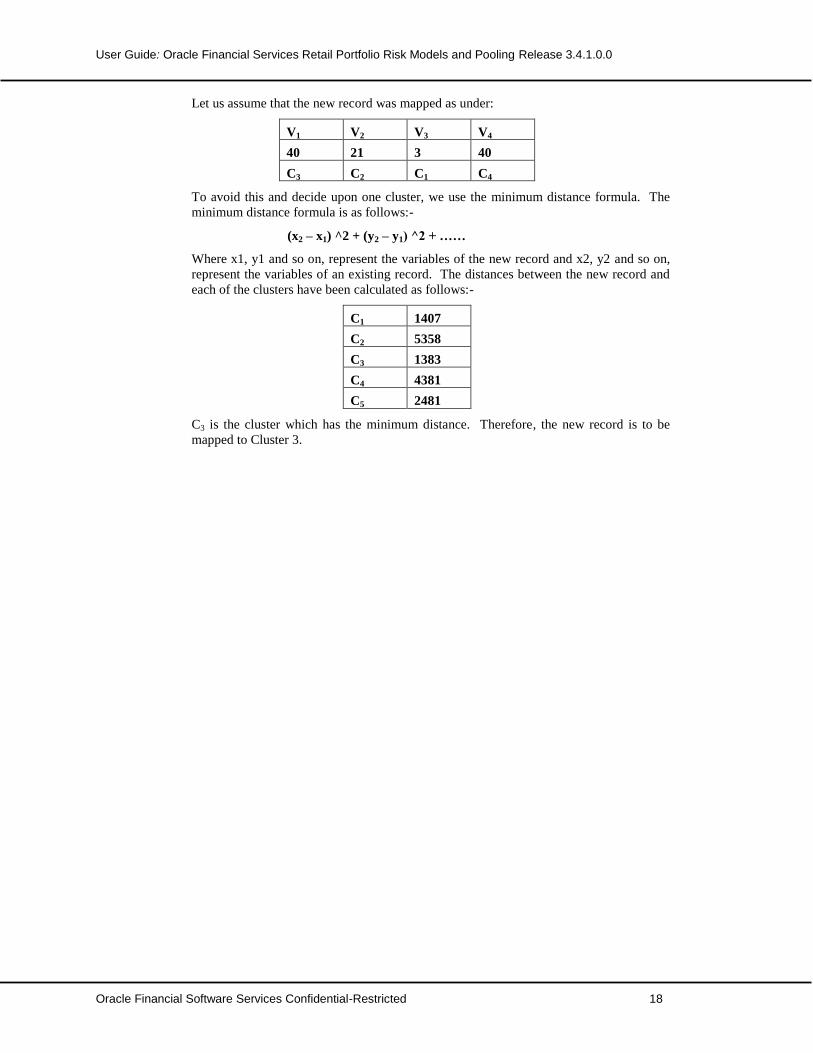
FAQ Oracle Financial Services Retail Portfolio Risk Models and Pooling Release 34100
Oracle Financial Services Software Confidential-Restricted 2
D7 Hierarchical Clustering
In hierarchical cluster analysis dendrogram graphs are used to visualize how clusters are
formed Because each observation is displayed dendrogram are impractical when the data
set is large
D8 K Means Clustering
Number of clusters is a random or manual input or based on the results of hierarchical
clustering This kind of clustering method is also called a k-means model since the cluster
centers are the means of the observations assigned to each cluster when the algorithm is
run to complete convergence
D9 Homogeneous Pools
There exists no standard definition of homogeneity and that needs to be defined based on
risk characteristics
D10 Binning
Binning is the method of variable discretization or grouping into 10 groups where each
group contains equal number of records as far as possible For each group created above
we could take the mean or the median value for that group and call them as bins or the bin
values
FAQ Oracle Financial Services Retail Portfolio Risk Models and Pooling Release 34100
Oracle Financial Services Software Confidential-Restricted 3
2 Questions on Retail Pooling
1 How to extract data
Within a workflow environment (modeling environment) data would be extracted or
imported from source tables and one or more output datasets would be created that has few or
all of the raw attributes at record level (say an exposure level) For clustering ultimately we
need to have one dataset
2 How to create Variables
Date and Time Related attributes could help create Time Variables such as
Month on books
Months since delinquency gt 2
Summary and averages
3month total balance 3 month total payment 6 month total late fees and
so on
3 month 6 month 12 month averages of many attributes
Average 3 month delinquency utilization and so on
Derived variables and indicators
Payment Rate (Payment amount closing balance for credit cards)
Fees Charge Rate
Interest Charges rate and so on
Qualitative attributes
For example Dummy variables for attributes such as regions products asset codes and so
on
3 How to prepare variables
Imputation of missing attributes can be done only when the missing rate is not exceeding
10-15
Extreme Values are treated Lower extremes and Upper extremes are treated based on a
Quintile Plot or Normal Probability Plot and the extreme values which are identified are
not deleted but capped in the dataset
Some of the attributes would be the outcomes of risk such as default indicator pay off
indicator Losses Write Off Amount etc and hence will not be used as input variables in
the cluster analysis However these variables could be used for understanding the
distribution of the pools and also for loss modeling subsequently
4 How to reduce the of variables
In case of model fitting variable reduction is done through collineraity diagnostics or bivariate
correlation measures etc However clustering variables could be reduced by factor analysis
5 How to run hierarchical clustering
You can choose a distance criterion Based on that you are shown a dendrogram based on
which he decides the number of clusters A manual iterative process is then used to arrive at
the final clusters with the distance criterion being modified in each step
FAQ Oracle Financial Services Retail Portfolio Risk Models and Pooling Release 34100
Oracle Financial Services Software Confidential-Restricted 4
6 What are the outputs to be seen in hierarchical clustering
Cluster Summary giving the following for each cluster
Number of Clusters
7 How to run K Means Clustering
On the Dataset give Seeds= Value with full replacement method and K= Value For multiple
runs as you reduce K also change the seed for validity of formation
8 What outputs to see K Means Clustering
Cluster number for all the K clusters
Frequency the number of observations in the cluster
RMS Std Deviation the root mean square across variables of the cluster standard
deviations which is equal to the root mean square distance between observations in the
cluster
Maximum Distance from Seed to Observation the maximum distance from the cluster
seed to any observation in the cluster
Nearest Cluster the number of the cluster with mean closest to the mean of the current
cluster
Centroid Distance the distance between the centroids (means) of the current cluster and
the nearest other cluster
A table of statistics for each variable is displayed
Total STD the total standard deviation
Within STD the pooled within-cluster standard deviation
R-Squared the R2 for predicting the variable from the cluster
RSQ(1 - RSQ) the ratio of between-cluster variance to within-cluster variance (R2(1 -
R2))
Distances Between Cluster Means
Cluster Summary Report containing the list of clusters drivers (variables) behind
clustering details about the relevant variables in each cluster like Mean Median
Minimum Maximum and similar details about target variables like Number of defaults
Recovery rate and so on
RSQ(1 - RSQ) the ratio of between-cluster variance to within-cluster variance (R2(1 -
R2))
OVER-ALL all of the previous quantities pooled across variables
Pseudo F Statistic = [( [(R2)(c - 1)] )( [(1 - R2)(n - c)] )]
Approximate Expected Overall R-Squared the approximate expected value of the overall
R2 under the uniform null hypothesis assuming that the variables are uncorrelated
Distances Between Cluster Means
Cluster Means for each variable
9 How to define clusters
Validation of the cluster solution is an art in itself and therefore never done by re-growing the
cluster solution on the test sample instead the score formula of the training sample is used to
create the new group of clusters in the test sample
FAQ Oracle Financial Services Retail Portfolio Risk Models and Pooling Release 34100
Oracle Financial Services Software Confidential-Restricted 5
of clusters formed size of each cluster new cluster means and cluster distances
cluster standard deviations
For example say in the Training sample the following results were obtained after developing the
clusters
Variable X1 Variable X2 Variable X3 Variable X4
Mean1 STD1 Mean2 STD2 Mean3 STD3 Mean4 STD4
Clus1 200 100 220 100 180 100 170 100
Clus2 160 90 180 90 140 90 130 90
Clus3 110 60 130 60 90 60 80 60
Clus4 90 45 110 45 70 45 60 45
Clus5 35 10 55 10 15 10 5 10
Table 1 Defining Clusters Example
When we apply the above cluster solution on the test data set as below
For each Variable calculate the distances from every cluster This is followed by associating with
each row a distance from every cluster using the below formulae
Square Distance for Clus1= (X1-Mean11)STD11- (X2-Mean21)STD212+(X1-
Mean11)STD11-(X3-Mean31)STD312+(X1-Mean11)STD11-(X4-Mean41)STD412
Square Distance for Clus2= (X1-Mean11)STD11- (X2-Mean21)STD212+(X1-
Mean11)STD11-(X3-Mean31)STD312+(X1-Mean11)STD11-(X4-Mean41)STD412
Square Distance for Clus3= (X1-Mean11)STD11- (X2-Mean21)STD212+(X1-
Mean11)STD11-(X3-Mean31)STD312+(X1-Mean11)STD11-(X4-Mean41)STD412
Square Distance for Clus4= (X1-Mean11)STD11- (X2-Mean21)STD212+(X1-
Mean11)STD11-(X3-Mean31)STD312+(X1-Mean11)STD11-(X4-Mean41)STD412
Square Distance for Clus5= (X1-Mean11)STD11- (X2-Mean21)STD212+(X1-
Mean11)STD11-(X3-Mean31)STD312+(X1-Mean11)STD11-(X4-Mean41)STD412
We do not need to standardize each variable in the Test Dataset since we need to calculate the new
distances by using the means and STD from the Training dataset
New Clus1= Minimum(Distance1 Distance2 Distance3 Distance4 Distance5)
New Clus2= Minimum(Distance1 Distance2 Distance3 Distance4 Distance5)
New Clus3= Minimum(Distance1 Distance2 Distance3 Distance4 Distance5)
New Clus4= Minimum(Distance1 Distance2 Distance3 Distance4 Distance5)
New Clus5= Minimum(Distance1 Distance2 Distance3 Distance4 Distance5)
After applying the solution on the test dataset the new distances are compared for each of the
clusters and cluster summary report containing the list of clusters is prepared their drivers
(variables) details about the relevant variables in each cluster like Mean Median Minimum
Maximum and similar details about target variables like Number of defaults Recovery rate and so
on
10 What is homogeneity
There exists no standard definition of homogeneity and that needs to be defined based on risk
characteristics
11 What is Pool Summary Report
FAQ Oracle Financial Services Retail Portfolio Risk Models and Pooling Release 34100
Oracle Financial Services Software Confidential-Restricted 6
Pool definitions are created out of the Pool report that summarizes
Pool Variables Profiles
Pool Size and Proportion
Pool Default Rates across time
12 What is Probability of Default
Default Probability is the likelihood of default that can be assigned to each account or
exposure It is a number that varies between 00 and 10
13 What is Loss Given Default
It is also known as recovery ratio It can vary between 0 and 100 and could be available
for each exposure or a group of exposures The recovery ratio can also be calculated by the
business user if the related attributes are downloaded from the Recovery Data Mart using
variables such as Write off Amount Outstanding Balance Collected Amount Discount
Offered Market Value of Collateral and so on
14 What is CCF or Credit Conversion Factor
For off-balance sheet items exposure is calculated as the committed but undrawn amount
multiplied by a CCF (that is the Credit Conversion Factor) as given in Basel
15 What is Exposure at Default
EAD is the risk measure that denotes the amount of exposure that is at risk and hence the
amount on which we need to apply the Risk Weight Function to calculate the amount of loss
or capital In general EAD is the sum of drawn amount and CCF multiplied undrawn amount
16 What is the difference between Principal Component Analysis and Common Factor
Analysis
The purpose of principal component analysis (Rao 1964) is to derive a small number of linear
combinations (principal components) of a set of variables that retain as much of the
information in the original variables as possible Often a small number of principal
components can be used in place of the original variables for plotting regression clustering
and so on Principal component analysis can also be viewed as an attempt to uncover
approximate linear dependencies among variables
Principal factors vs principal components The defining characteristic that distinguishes
between the two factor analytic models is that in principal components analysis we assume
that all variability in an item should be used in the analysis while in principal factors analysis
we only use the variability in an item that it has in common with the other items In most
cases these two methods usually yield very similar results However principal components
analysis is often preferred as a method for data reduction while principal factors analysis is
often preferred when the goal of the analysis is to detect structure (see Factor Analysis as a
Classification Method)
17 What is the segment information that should be stored in the database (example
segment name) Will they be used to define any report
For the purpose of reporting out and validation and tracking we need to have the following ids
created
Cluster Id
Decision Tree Node Id
Final Segment Id
Sometimes you would need to regroup the combinations of clusters and nodes and create
final segments of your own
FAQ Oracle Financial Services Retail Portfolio Risk Models and Pooling Release 34100
Oracle Financial Services Software Confidential-Restricted 7
18 Discretize the variables ndash what is the method to be used
Binning Methods are more popular which are Equal Groups Binning or Equal Interval
Binning or Ranking The value for a bin could be the mean or median
19 Qualitative attributes ndash will be treated at a data model level
Such as City Name Product Name or Credit Line and so on can be handled using Binary Indicators or
Nominal Indicators
20 Substitute for Missing values ndash what is the method
Categorical data Mode or Group Modes and Continuous Data Mean or Median could be used
21 Pool stability report ndash what is this
Movements can happen between subsequent pool over months and such movements are
summarized with the help of a transition report
FAQ Oracle Financial Services Retail Portfolio Risk Models and Pooling Release 34100
Oracle Financial Services Software Confidential-Restricted 8
3 Questions in Applied Statistics
1 Eigenvalues How to Choose of Factors
The Kaiser criterion First we can retain only factors with eigen values greater than 1 In
essence this is like saying that unless a factor extract at least as much as the equivalent of one
original variable we drop it This criterion was proposed by Kaiser (1960) and is probably
the one most widely used In our example above using this criterion we would retain 2
factors The other method called (screen test) sometimes retains too few factors
Choose of Variables (Input of factors Eigen Value gt=10 as in 33 )
The variable selection would be based on both communality estimates between 09 to 11 and
also based on individual factor loadings of variables for a given factor The closer the
communality is to 1 the better the variable is explained by the factors and hence retain all
variable within these set of communality between 09 to 11
Beyond communality measure we could also use Factor loading as a variable selection
criterion which helps you to select other variables which contribute to the uncommon (unlike
common as in communality)
Factor Loading A rule of thumb frequently used is that factor loadings greater than 4 or 05
in absolute value are considered to be significant This criterion is just a guideline and may
need to be adjusted As the sample size and the number of variables increase the criterion
may need to be adjusted slightly downward it may need to be adjusted upward as the number
of factors increases A good measure of selecting variables could be also by selecting the top
2 or top 3 variables influencing each factor It is assumed that top 2 or top 3 variables
contribute to the maximum explanation of that factor
However if you have satisfied the eigen value and communality criterion selection of
variables based on factor loadings could be left to you In the second column (Eigen value)
above we find the variance on the new factors that were successively extracted In the third
column these values are expressed as a percent of the total variance (in this example 10) As
we can see factor 1 accounts for 61 percent of the variance factor 2 for 18 percent and so on
As expected the sum of the eigen values is equal to the number of variables The third
column contains the cumulative variance extracted The variances extracted by the factors are
called the eigen values This name derives from the computational issues involved
FAQ Oracle Financial Services Retail Portfolio Risk Models and Pooling Release 34100
Oracle Financial Services Software Confidential-Restricted 9
2 How do you determine the Number of Clusters
An important question that needs to be answered before applying the k-means or EM
clustering algorithms is how many clusters are there in the data This is not known a priori
and in fact there might be no definite or unique answer as to what value k should take In
other words k is a nuisance parameter of the clustering model Luckily an estimate of k can
be obtained from the data using the method of cross-validation Remember that the k-means
methods will determine cluster solutions for a particular user-defined number of clusters The
k-means techniques (described above) can be optimized and enhanced for typical applications
in data mining The general metaphor of data mining implies the situation in which an analyst
searches for useful structures and nuggets in the data usually without any strong a priori
expectations of what the analyst might find (in contrast to the hypothesis-testing approach of
scientific research) In practice the analyst usually does not know ahead of time how many
clusters there might be in the sample For that reason some programs include an
implementation of a v-fold cross-validation algorithm for automatically determining the
number of clusters in the data
Cluster analysis is an unsupervised learning technique and we cannot observe the (real)
number of clusters in the data However it is reasonable to replace the usual notion
(applicable to supervised learning) of accuracy with that of distance In general we can
apply the v-fold cross-validation method to a range of numbers of clusters in k-means
To complete convergence the final cluster seeds will equal the cluster means or cluster
centers
3 What is the displayed output
Initial Seeds cluster seeds selected after one pass through the data
Change in Cluster Seeds for each iteration if you specify MAXITER=ngt1
Cluster number
Frequency the number of observations in the cluster
Weight the sum of the weights of the observations in the cluster if you specify the
WEIGHT statement
RMS Std Deviation the root mean square across variables of the cluster standard
deviations which is equal to the root mean square distance between observations in the
cluster
Maximum Distance from Seed to Observation the maximum distance from the cluster
seed to any observation in the cluster
Nearest Cluster the number of the cluster with mean closest to the mean of the current
cluster
Centroid Distance the distance between the centroids (means) of the current cluster and
the nearest other cluster
A table of statistics for each variable is displayed unless you specify the SUMMARY option
The table contains
Total STD the total standard deviation
Within STD the pooled within-cluster standard deviation
R-Squared the R2 for predicting the variable from the cluster
RSQ(1 - RSQ) the ratio of between-cluster variance to within-cluster variance (R2(1 -
R2))
OVER-ALL all of the previous quantities pooled across variables
FAQ Oracle Financial Services Retail Portfolio Risk Models and Pooling Release 34100
Oracle Financial Services Software Confidential-Restricted 10
Pseudo F Statistic
[( [(R2)(c - 1)] )( [(1 - R2)(n - c)] )]
where R2 is the observed overall R2 c is the number of clusters and n is the number of
observations The pseudo F statistic was suggested by Calinski and Harabasz (1974) Refer
to Milligan and Cooper (1985) and Cooper and Milligan (1988) regarding the use of the
pseudo F statistic in estimating the number of clusters
Observed Overall R-Squared
Approximate Expected Overall R-Squared the approximate expected value of the overall
R2 under the uniform null hypothesis assuming that the variables are uncorrelated
Cubic Clustering Criterion computed under the assumption that the variables are
uncorrelated
Distances Between Cluster Means
Cluster Means for each variable
4 What are the Classes of Variables
You need to specify three classes of variables when performing a decision tree analysis
Target variable -- The ldquotarget variablerdquo is the variable whose values are to be modeled and
predicted by other variables It is analogous to the dependent variable (ithe variable on the left
of the equal sign) in linear regression
Predictor variable -- A ldquopredictor variablerdquo is a variable whose values will be used to predict
the value of the target variable It is analogous to the independent variables (variables on the
right side of the equal sign) in linear regression There must be at least one predictor variable
specified for decision tree analysis there may be many predictor variables
5 What are the types of Variables
Variables may have two types continuous and categorical
Continuous variables -- A continuous variable has numeric values such as 1 2 314 -5 etc
The relative magnitude of the values is significant (For example a value of 2 indicates twice
the magnitude of 1) Continuous variables are also called ldquoorderedrdquo or ldquomonotonicrdquo variables
Categorical variables -- A categorical variable has values that function as labels rather than as
numbers Some programs call categorical variables ldquonominalrdquo variables For example a
categorical variable for gender might use the value 1 for male and 2 for female The actual
magnitude of the value is not significant coding male as 7 and female as 3 would work just as
well As another example marital status might be coded as 1 for single 2 for married 3 for
divorced and 4 for widowed So your dataset could have the strings ldquoMalerdquo and ldquoFemalerdquo or
ldquoMrdquo and ldquoFrdquo for a categorical gender variable Since categorical values are stored and
compared as string values a categorical value of 001 is different than a value of 1 In contrast
values of 001 and 1 would be equal for continuous variables
6 What are Misclassification costs
Sometimes more accurate classification of the response is desired for some classes than others
for reasons not related to the relative class sizes If the criterion for predictive accuracy is
Misclassification costs then minimizing costs would amount to minimizing the proportion of
misclassified cases when priors are considered proportional to the class sizes and
misclassification costs are taken to be equal for every class
7 What are Estimates of the accuracy
In classification problems (categorical dependent variable) three estimates of the accuracy are
used resubstitution estimate test sample estimate and v-fold cross-validation These
estimates are defined here
FAQ Oracle Financial Services Retail Portfolio Risk Models and Pooling Release 34100
Oracle Financial Services Software Confidential-Restricted 11
Re-substitution estimate Re-substitution estimate is the proportion of cases that are
misclassified by the classifier constructed from the entire sample This estimate is computed
in the following manner
where X is the indicator function
X = 1 if the statement is true
X = 0 if the statement is false
and d (x) is the classifier
The resubstitution estimate is computed using the same data as used in constructing the
classifier d
Test sample estimate The total number of cases is divided into two subsamples Z1 and Z2
The test sample estimate is the proportion of cases in the subsample Z2 which are
misclassified by the classifier constructed from the subsample Z1 This estimate is computed
in the following way
Let the learning sample Z of size N be partitioned into subsamples Z1 and Z2 of sizes N and
N2 respectively
where Z2 is the sub sample that is not used for constructing the classifier
v-fold cross validation The total number of cases are divided into v sub samples Z1 Z2
Zv of almost equal sizes v-fold cross validation estimate is the proportion of cases in the
subsample Z that are misclassified by the classifier constructed from the subsample Z - Zv
This estimate is computed in the following way
Let the learning sample Z of size N be partitioned into v sub samples Z1 Z2 Zv of almost
sizes N1 N2 Nv respectively
where is computed from the sub sample Z - Zv
Estimation of Accuracy in Regression
In the regression problem (continuous dependent variable) three estimates of the accuracy are
used re-substitution estimate test sample estimate and v-fold cross-validation These
estimates are defined here
Re-substitution estimate The re-substitution estimate is the estimate of the expected squared
error using the predictor of the continuous dependent variable This estimate is computed in
the following way
where the learning sample Z consists of (xiyi)i = 12N The re-substitution estimate is
computed using the same data as used in constructing the predictor d
FAQ Oracle Financial Services Retail Portfolio Risk Models and Pooling Release 34100
Oracle Financial Services Software Confidential-Restricted 12
Test sample estimate The total number of cases is divided into two subsamples Z1 and Z2
The test sample estimate of the mean squared error is computed in the following way
Let the learning sample Z of size N be partitioned into subsamples Z1 and Z2 of sizes N and
N2 respectively
where Z2 is the sub-sample that is not used for constructing the predictor
v-fold cross-validation The total number of cases is divided into v sub samples Z1 Z2 Zv of
almost equal sizes The subsample Z - Zv is used to construct the predictor d Then v-fold
cross validation estimate is computed from the subsample Zv in the following way
Let the learning sample Z of size N be partitioned into v sub samples Z1 Z2 Zv of almost
sizes N1 N2 Nv respectively
where is computed from the sub sample Z - Zv
8 How to Estimate of Node Impurity Gini Measure
The Gini measure is the measure of impurity of a node and is commonly used when the
dependent variable is a categorical variable defined as
if costs of misclassification are not specified
if costs of misclassification are specified
where the sum extends over all k categories p( j t) is the probability of category j at the node
t and C(i j ) is the probability of misclassifying a category j case as category i
The Gini Criterion Function Q(st) for split s at node t is defined as
Q(st)=g(t)-Plg(tl)-prg(tr)
Where pl is the proportion of cases in t sent to the left child node and pr is the proportion sent
to the right child node The proportion pl and pr are defined as
Pl=p(tl)p(t)
and
Pr=p(tr)p(t)
The split s is chosen to maximize the value of Q(st) This value is reported as the
improvement in the tree
9 What is Towing
The towing index is based on splitting the target categories into two superclasses and then
finding the best split on the predictor variable based on those two superclasses The towing
critetioprn function for split s at node t is defined as
FAQ Oracle Financial Services Retail Portfolio Risk Models and Pooling Release 34100
Oracle Financial Services Software Confidential-Restricted 13
Q(st)=plpr[sum(j|p(jtl)-p(jtr))2
Where tl and tr are the nodes created by the split s The split s is chosen as the split that
maximizes this criterion This value weighted by the proportion of all cases in node t is the
value reported as improvement in the tree
10 Estimation of Node Impurity Other Measure
In addition to measuring accuracy the following measures of node impurity are used for
classification problems The Gini measure generalized Chi-square measure and generalized
G-square measure The Chi-square measure is similar to the standard Chi-square value
computed for the expected and observed classifications (with priors adjusted for
misclassification cost) and the G-square measure is similar to the maximum-likelihood Chi-
square (as for example computed in the Log-Linear technique) The Gini measure is the one
most often used for measuring purity in the context of classification problems and it is
described below
For continuous dependent variables (regression-type problems) the least squared deviation
(LSD) measure of impurity is automatically applied
Estimation of Node Impurity Least-Squared Deviation
Least-squared deviation (LSD) is used as the measure of impurity of a node when the
response variable is continuous and is computed as
where Nw(t) is the weighted number of cases in node t wi is the value of the weighting
variable for case i fi is the value of the frequency variable yi is the value of the response
variable and y(t) is the weighted mean for node
11 How to select splits
The process of computing classification and regression trees can be characterized as involving
four basic steps Specifying the criteria for predictive accuracy
Selecting splits
Determining when to stop splitting
Selecting the right-sized tree
These steps are very similar to those discussed in the context of Classification Trees Analysis
(see also Breiman et al 1984 for more details) See also Computational Formulas
12 Specifying the Criteria for Predictive Accuracy
The classification and regression trees (CART) algorithms are generally aimed at achieving
the best possible predictive accuracy Operationally the most accurate prediction is defined as
the prediction with the minimum costs The notion of costs was developed as a way to
generalize to a broader range of prediction situations the idea that the best prediction has the
lowest misclassification rate In most applications the cost is measured in terms of proportion
of misclassified cases or variance
13 Priors
In the case of a categorical response (classification problem) minimizing costs amounts to
minimizing the proportion of misclassified cases when priors are taken to be proportional to
the class sizes and when misclassification costs are taken to be equal for every class
The a priori probabilities used in minimizing costs can greatly affect the classification of
cases or objects Therefore care has to be taken while using the priors If differential base
rates are not of interest for the study or if one knows that there are about an equal number of
FAQ Oracle Financial Services Retail Portfolio Risk Models and Pooling Release 34100
Oracle Financial Services Software Confidential-Restricted 14
cases in each class then one would use equal priors If the differential base rates are reflected
in the class sizes (as they would be if the sample is a probability sample) then one would use
priors estimated by the class proportions of the sample Finally if you have specific
knowledge about the base rates (for example based on previous research) then one would
specify priors in accordance with that knowledge The general point is that the relative size of
the priors assigned to each class can be used to adjust the importance of misclassifications
for each class However no priors are required when one is building a regression tree
The second basic step in classification and regression trees is to select the splits on the
predictor variables that are used to predict membership in classes of the categorical dependent
variables or to predict values of the continuous dependent (response) variable In general
terms the split at each node will be found that will generate the greatest improvement in
predictive accuracy This is usually measured with some type of node impurity measure
which provides an indication of the relative homogeneity (the inverse of impurity) of cases in
the terminal nodes If all cases in each terminal node show identical values then node
impurity is minimal homogeneity is maximal and prediction is perfect (at least for the cases
used in the computations predictive validity for new cases is of course a different matter)
14 Impurity Measures
For classification problems CART gives you the choice of several impurity measures The
Gini index Chi-square or G-square The Gini index of node impurity is the measure most
commonly chosen for classification-type problems As an impurity measure it reaches a value
of zero when only one class is present at a node With priors estimated from class sizes and
equal misclassification costs the Gini measure is computed as the sum of products of all pairs
of class proportions for classes present at the node it reaches its maximum value when class
sizes at the node are equal the Gini index is equal to zero if all cases in a node belong to the
same class The Chi-square measure is similar to the standard Chi-square value computed for
the expected and observed classifications (with priors adjusted for misclassification cost) and
the G-square measure is similar to the maximum-likelihood Chi-square (as for example
computed in the Log-Linear technique) For regression-type problems a least-squares
deviation criterion (similar to what is computed in least squares regression) is automatically
used Computational Formulas provides further computational details
15 When to Stop Splitting
As discussed in Basic Ideas in principal splitting could continue until all cases are perfectly
classified or predicted However this wouldnt make much sense since one would likely end
up with a tree structure that is as complex and tedious as the original data file (with many
nodes possibly containing single observations) and that would most likely not be very useful
or accurate for predicting new observations What is required is some reasonable stopping
rule
Minimum n One way to control splitting is to allow splitting to continue until all terminal
nodes are pure or contain no more than a specified minimum number of cases or objects
Fraction of objects Another way to control splitting is to allow splitting to continue until all
terminal nodes are pure or contain no more cases than a specified minimum fraction of the
sizes of one or more classes (in the case of classification problems or all cases in regression
problems)
Alternatively if the priors used in the analysis are not equal splitting will stop when all
terminal nodes containing more than one class have no more cases than the specified fraction
for one or more classes See Loh and Vanichestakul 1988 for details
Pruning and Selecting the Right-Sized Tree
The size of a tree in the classification and regression trees analysis is an important issue since
an unreasonably big tree can only make the interpretation of results more difficult Some
generalizations can be offered about what constitutes the right-sized tree It should be
sufficiently complex to account for the known facts but at the same time it should be as
FAQ Oracle Financial Services Retail Portfolio Risk Models and Pooling Release 34100
Oracle Financial Services Software Confidential-Restricted 15
simple as possible It should exploit information that increases predictive accuracy and ignore
information that does not It should if possible lead to greater understanding of the
phenomena it describes These procedures are not foolproof as Breiman et al (1984) readily
acknowledges but at least they take subjective judgment out of the process of selecting the
right-sized tree
Sub samples from the computations and using that subsample as a test sample for cross-
validation so that each subsample is used (v - 1) times in the learning sample and just once as
the test sample The CV costs (cross-validation cost) computed for each of the v test samples
are then averaged to give the v-fold estimate of the CV costs
Minimal cost-complexity cross-validation pruning In CART minimal cost-complexity cross-
validation pruning is performed if Prune on misclassification error has been selected as the
Stopping rule On the other hand if Prune on deviance has been selected as the Stopping rule
then minimal deviance-complexity cross-validation pruning is performed The only difference
in the two options is the measure of prediction error that is used Prune on misclassification
error uses the costs that equals the misclassification rate when priors are estimated and
misclassification costs are equal while Prune on deviance uses a measure based on
maximum-likelihood principles called the deviance (see Ripley 1996)
The sequence of trees obtained by this algorithm have a number of interesting properties
They are nested because the successively pruned trees contain all the nodes of the next
smaller tree in the sequence Initially many nodes are often pruned going from one tree to the
next smaller tree in the sequence but fewer nodes tend to be pruned as the root node is
approached The sequence of largest trees is also optimally pruned because for every size of
tree in the sequence there is no other tree of the same size with lower costs Proofs andor
explanations of these properties can be found in Breiman et al (1984)
Tree selection after pruning The pruning as discussed above often results in a sequence of
optimally pruned trees So the next task is to use an appropriate criterion to select the right-
sized tree from this set of optimal trees A natural criterion would be the CV costs (cross-
validation costs) While there is nothing wrong with choosing the tree with the minimum CV
costs as the right-sized tree often times there will be several trees with CV costs close to
the minimum Following Breiman et al (1984) one could use the automatic tree selection
procedure and choose as the right-sized tree the smallest-sized (least complex) tree whose
CV costs do not differ appreciably from the minimum CV costs In particular they proposed a
1 SE rule for making this selection that is choose as the right-sized tree the smallest-
sized tree whose CV costs do not exceed the minimum CV costs plus 1 times the standard
error of the CV costs for the minimum CV costs tree
As can be been seen minimal cost-complexity cross-validation pruning and subsequent
right-sized tree selection is a automatic process The algorithms make all the decisions
leading to the selection of the right-sized tree except for specification of a value for the SE
rule V-fold cross-validation allows you to evaluate how well each tree performs when
repeatedly cross-validated in different samples randomly drawn from the data
16 Computational Formulas
In Classification and Regression Trees estimates of accuracy are computed by different
formulas for categorical and continuous dependent variables (classification and regression-
type problems) For classification-type problems (categorical dependent variable) accuracy is
measured in terms of the true classification rate of the classifier while in the case of
regression (continuous dependent variable) accuracy is measured in terms of mean squared
error of the predictor
FAQ Oracle Financial Services Retail Portfolio Risk Models and Pooling Release 34100
Oracle Financial Services Software Confidential-Restricted 16
Oracle Financial Services Retail Portfolio Risk Models and Pooling - FAQ
February 2014
Version number 10
Oracle Corporation
World Headquarters
500 Oracle Parkway
Redwood Shores CA 94065
USA
Worldwide Inquiries
Phone +16505067000
Fax +16505067200
wwworaclecom financial_services
Copyright copy 2014 Oracle andor its affiliates All rights reserved
No part of this work may be reproduced stored in a retrieval system adopted or transmitted in any form or by any means electronic mechanical photographic graphic optic recording or otherwise translated in any language or computer language without the prior written permission of Oracle Financial Services Software Limited
Due care has been taken to make this Oracle Financial Services Retail Portfolio Risk Models and Pooling FAQ and accompanying software package as accurate as possible However Oracle Financial Services Software Limited makes no representation or warranties with respect to the contents hereof and shall not be responsible for any loss or damage caused to the user by the direct or indirect use of this User Manual and the accompanying Software System Furthermore Oracle Financial Services Software Limited reserves the right to alter modify or otherwise change in any manner the content hereof without obligation of Oracle Financial Services Software Limited to notify any person of such revision or changes
All company and product names are trademarks of the respective companies with which they are associated
- 1 Definitions
- 2 Questions on Retail Pooling
- 3 Questions in Applied Statistics
-
- 1 Introduction
-
- 11 Overview of Oracle Financial Services Retail Portfolio Risk Models and Pooling
- 12 Summary
- 13 Approach Followed in the Product
-
- 2 Implementing the Product using the OFSAAI Infrastructure
-
- 21 Introduction to Rules
-
- 211 Types of Rules
- 212 Rule Definition
-
- 22 Introduction to Processes
-
- 221 Type of Process Trees
-
- 23 Introduction to Run
-
- 231 Run Definition
- 232 Types of Runs
-
- 24 Building Business Processors for Calculation Blocks
-
- 241 What is a Business Processor
- 242 Why Define a Business Processor
-
- 25 Modeling Framework Tools or Techniques used in RP
-
- 3 Understanding Data Extraction
-
- 31 Introduction
- 32 Structure
-
- Annexure A ndash Definitions
- Annexure B ndash Frequently Asked Questions
- Annexure Cndash K Means Clustering Based On Business Logic
- ANNEXURE D Generating Download Specifications
-
FAQpdfUser Guide Oracle Financial Services Retail Portfolio Risk Models and Pooling Release 34100
Oracle Financial Software Services Confidential-Restricted 16
Annexure Cndash K Means Clustering Based On Business Logic
The process of clustering based on business logic assigns each record to a particular cluster based
on the bounds of the variables Steps 1 and 2 are followed to find out the bounds of each variable
for each of the given cluster Step 3 helps in deciding the cluster id for a given record
Steps 1 to 3 are together known as a RULE BASED FORMULA
In certain cases the rule based formula does not return us a unique cluster id so we then need to
use the MINIMUM DISTANCE FORMULA which is given in Step 4
1 The first step is to obtain the mean matrix by running a K Means process The following
is an example of such mean matrix which represents clusters in rows and variables in
columns
V1 V2 V3 V4
C1 15 10 9 57
C2 5 80 17 40
C3 45 20 37 55
C4 40 62 45 70
C5 12 7 30 20
2 The next step is to calculate bounds for the variable values Before this is done each set
of variables across all clusters have to be arranged in ascending order Bounds are then
calculated by taking the mean of consecutive values The process is as follows
V1
C2 5
C5 12
C1 15
C3 45
C4 40
The bounds have been calculated as follows for Variable 1
Less than 85
[(5+12)2] C2
Between 85 and
135 C5
Between 135 and
30 C1
Between 30 and
425 C3
Greater than 425 C4
The above mentioned process has to be repeated for all the variables
Variable 2
Less than 85 C5
Between 85 and
15 C1
User Guide Oracle Financial Services Retail Portfolio Risk Models and Pooling Release 34100
Oracle Financial Software Services Confidential-Restricted 17
Between 15 and
41 C3
Between 41 and
71 C4
Greater than 71 C2
Variable 3
Less than 13 C1
Between 13 and
235 C2
Between 235 and
335 C5
Between 335 and
41 C3
Greater than 41 C4
Variable 4
Less than 30 C5
Between 30 and
475 C2
Between 475 and
56 C3
Between 56 and
635 C1
Greater than 635 C4
3 The variables of the new record are put in their respective clusters according to the
bounds mentioned above Let us assume the new record to have the following variable
values
V1 V2 V3 V4
46 21 3 40
They are put in the respective clusters as follows (based on the bounds for each variable
and cluster combination)
V1 V2 V3 V4
46 21 3 40
C4 C3 C1 C1
As C1 is the cluster that occurs for the most number of times the new record is mapped to
C1
4 This is an additional step which is required if it is difficult to decide which cluster to map
to This may happen if more than one cluster gets repeated equal number of times or if
all of the clusters are unique
User Guide Oracle Financial Services Retail Portfolio Risk Models and Pooling Release 34100
Oracle Financial Software Services Confidential-Restricted 18
Let us assume that the new record was mapped as under
V1 V2 V3 V4
40 21 3 40
C3 C2 C1 C4
To avoid this and decide upon one cluster we use the minimum distance formula The
minimum distance formula is as follows-
(x2 ndash x1) ^2 + (y2 ndash y1) ^2 + helliphellip
Where x1 y1 and so on represent the variables of the new record and x2 y2 and so on
represent the variables of an existing record The distances between the new record and
each of the clusters have been calculated as follows-
C1 1407
C2 5358
C3 1383
C4 4381
C5 2481
C3 is the cluster which has the minimum distance Therefore the new record is to be
mapped to Cluster 3
User Guide Oracle Financial Services Retail Portfolio Risk Models and Pooling Release 34100
Oracle Financial Software Services Confidential-Restricted 19
ANNEXURE D Generating Download Specifications
Data Model for OFS Retail Portfolio Risk Models and Pooling is available on customer request as
an ERwin file
Download Specifications can be extracted from this model Refer the whitepaper present in OTN
for more details
User Guide Oracle Financial Services Retail Portfolio Risk Models and Pooling Release 34100
Oracle Financial Software Services Confidential-Restricted 19
Oracle Financial Services Retail Portfolio Risk Models and Pooling Release 34100
April 2014
Version number 10
Oracle Corporation
World Headquarters
500 Oracle Parkway
Redwood Shores CA 94065
USA
Worldwide Inquiries
Phone +16505067000
Fax +16505067200
wwworaclecom financial_services
Copyright copy 2014 Oracle andor its affiliates All rights reserved
No part of this work may be reproduced stored in a retrieval system adopted or transmitted in any form or by any means electronic mechanical photographic graphic optic recording or otherwise translated in any language or computer language without the prior written permission of Oracle Financial Services Software Limited
Due care has been taken to make this Oracle Financial Services Retail Portfolio Risk Models and Pooling User Guide and accompanying software package as accurate as possible However Oracle Financial Services Software Limited makes no representation or warranties with respect to the contents hereof and shall not be responsible for any loss or damage caused to the user by the direct or indirect use of this User Manual and the accompanying Software System Furthermore Oracle Financial Services Software Limited reserves the right to alter modify or otherwise change in any manner the content hereof without obligation of Oracle Financial Services Software Limited to notify any person of such revision or changes
All company and product names are trademarks of the respective companies with which they are associated
FAQ Oracle Financial Services Retail Portfolio Risk Models and Pooling Release 34100
Oracle Financial Services Software Confidential-Restricted 3
2 Questions on Retail Pooling
1 How to extract data
Within a workflow environment (modeling environment) data would be extracted or
imported from source tables and one or more output datasets would be created that has few or
all of the raw attributes at record level (say an exposure level) For clustering ultimately we
need to have one dataset
2 How to create Variables
Date and Time Related attributes could help create Time Variables such as
Month on books
Months since delinquency gt 2
Summary and averages
3month total balance 3 month total payment 6 month total late fees and
so on
3 month 6 month 12 month averages of many attributes
Average 3 month delinquency utilization and so on
Derived variables and indicators
Payment Rate (Payment amount closing balance for credit cards)
Fees Charge Rate
Interest Charges rate and so on
Qualitative attributes
For example Dummy variables for attributes such as regions products asset codes and so
on
3 How to prepare variables
Imputation of missing attributes can be done only when the missing rate is not exceeding
10-15
Extreme Values are treated Lower extremes and Upper extremes are treated based on a
Quintile Plot or Normal Probability Plot and the extreme values which are identified are
not deleted but capped in the dataset
Some of the attributes would be the outcomes of risk such as default indicator pay off
indicator Losses Write Off Amount etc and hence will not be used as input variables in
the cluster analysis However these variables could be used for understanding the
distribution of the pools and also for loss modeling subsequently
4 How to reduce the of variables
In case of model fitting variable reduction is done through collineraity diagnostics or bivariate
correlation measures etc However clustering variables could be reduced by factor analysis
5 How to run hierarchical clustering
You can choose a distance criterion Based on that you are shown a dendrogram based on
which he decides the number of clusters A manual iterative process is then used to arrive at
the final clusters with the distance criterion being modified in each step
FAQ Oracle Financial Services Retail Portfolio Risk Models and Pooling Release 34100
Oracle Financial Services Software Confidential-Restricted 4
6 What are the outputs to be seen in hierarchical clustering
Cluster Summary giving the following for each cluster
Number of Clusters
7 How to run K Means Clustering
On the Dataset give Seeds= Value with full replacement method and K= Value For multiple
runs as you reduce K also change the seed for validity of formation
8 What outputs to see K Means Clustering
Cluster number for all the K clusters
Frequency the number of observations in the cluster
RMS Std Deviation the root mean square across variables of the cluster standard
deviations which is equal to the root mean square distance between observations in the
cluster
Maximum Distance from Seed to Observation the maximum distance from the cluster
seed to any observation in the cluster
Nearest Cluster the number of the cluster with mean closest to the mean of the current
cluster
Centroid Distance the distance between the centroids (means) of the current cluster and
the nearest other cluster
A table of statistics for each variable is displayed
Total STD the total standard deviation
Within STD the pooled within-cluster standard deviation
R-Squared the R2 for predicting the variable from the cluster
RSQ(1 - RSQ) the ratio of between-cluster variance to within-cluster variance (R2(1 -
R2))
Distances Between Cluster Means
Cluster Summary Report containing the list of clusters drivers (variables) behind
clustering details about the relevant variables in each cluster like Mean Median
Minimum Maximum and similar details about target variables like Number of defaults
Recovery rate and so on
RSQ(1 - RSQ) the ratio of between-cluster variance to within-cluster variance (R2(1 -
R2))
OVER-ALL all of the previous quantities pooled across variables
Pseudo F Statistic = [( [(R2)(c - 1)] )( [(1 - R2)(n - c)] )]
Approximate Expected Overall R-Squared the approximate expected value of the overall
R2 under the uniform null hypothesis assuming that the variables are uncorrelated
Distances Between Cluster Means
Cluster Means for each variable
9 How to define clusters
Validation of the cluster solution is an art in itself and therefore never done by re-growing the
cluster solution on the test sample instead the score formula of the training sample is used to
create the new group of clusters in the test sample
FAQ Oracle Financial Services Retail Portfolio Risk Models and Pooling Release 34100
Oracle Financial Services Software Confidential-Restricted 5
of clusters formed size of each cluster new cluster means and cluster distances
cluster standard deviations
For example say in the Training sample the following results were obtained after developing the
clusters
Variable X1 Variable X2 Variable X3 Variable X4
Mean1 STD1 Mean2 STD2 Mean3 STD3 Mean4 STD4
Clus1 200 100 220 100 180 100 170 100
Clus2 160 90 180 90 140 90 130 90
Clus3 110 60 130 60 90 60 80 60
Clus4 90 45 110 45 70 45 60 45
Clus5 35 10 55 10 15 10 5 10
Table 1 Defining Clusters Example
When we apply the above cluster solution on the test data set as below
For each Variable calculate the distances from every cluster This is followed by associating with
each row a distance from every cluster using the below formulae
Square Distance for Clus1= (X1-Mean11)STD11- (X2-Mean21)STD212+(X1-
Mean11)STD11-(X3-Mean31)STD312+(X1-Mean11)STD11-(X4-Mean41)STD412
Square Distance for Clus2= (X1-Mean11)STD11- (X2-Mean21)STD212+(X1-
Mean11)STD11-(X3-Mean31)STD312+(X1-Mean11)STD11-(X4-Mean41)STD412
Square Distance for Clus3= (X1-Mean11)STD11- (X2-Mean21)STD212+(X1-
Mean11)STD11-(X3-Mean31)STD312+(X1-Mean11)STD11-(X4-Mean41)STD412
Square Distance for Clus4= (X1-Mean11)STD11- (X2-Mean21)STD212+(X1-
Mean11)STD11-(X3-Mean31)STD312+(X1-Mean11)STD11-(X4-Mean41)STD412
Square Distance for Clus5= (X1-Mean11)STD11- (X2-Mean21)STD212+(X1-
Mean11)STD11-(X3-Mean31)STD312+(X1-Mean11)STD11-(X4-Mean41)STD412
We do not need to standardize each variable in the Test Dataset since we need to calculate the new
distances by using the means and STD from the Training dataset
New Clus1= Minimum(Distance1 Distance2 Distance3 Distance4 Distance5)
New Clus2= Minimum(Distance1 Distance2 Distance3 Distance4 Distance5)
New Clus3= Minimum(Distance1 Distance2 Distance3 Distance4 Distance5)
New Clus4= Minimum(Distance1 Distance2 Distance3 Distance4 Distance5)
New Clus5= Minimum(Distance1 Distance2 Distance3 Distance4 Distance5)
After applying the solution on the test dataset the new distances are compared for each of the
clusters and cluster summary report containing the list of clusters is prepared their drivers
(variables) details about the relevant variables in each cluster like Mean Median Minimum
Maximum and similar details about target variables like Number of defaults Recovery rate and so
on
10 What is homogeneity
There exists no standard definition of homogeneity and that needs to be defined based on risk
characteristics
11 What is Pool Summary Report
FAQ Oracle Financial Services Retail Portfolio Risk Models and Pooling Release 34100
Oracle Financial Services Software Confidential-Restricted 6
Pool definitions are created out of the Pool report that summarizes
Pool Variables Profiles
Pool Size and Proportion
Pool Default Rates across time
12 What is Probability of Default
Default Probability is the likelihood of default that can be assigned to each account or
exposure It is a number that varies between 00 and 10
13 What is Loss Given Default
It is also known as recovery ratio It can vary between 0 and 100 and could be available
for each exposure or a group of exposures The recovery ratio can also be calculated by the
business user if the related attributes are downloaded from the Recovery Data Mart using
variables such as Write off Amount Outstanding Balance Collected Amount Discount
Offered Market Value of Collateral and so on
14 What is CCF or Credit Conversion Factor
For off-balance sheet items exposure is calculated as the committed but undrawn amount
multiplied by a CCF (that is the Credit Conversion Factor) as given in Basel
15 What is Exposure at Default
EAD is the risk measure that denotes the amount of exposure that is at risk and hence the
amount on which we need to apply the Risk Weight Function to calculate the amount of loss
or capital In general EAD is the sum of drawn amount and CCF multiplied undrawn amount
16 What is the difference between Principal Component Analysis and Common Factor
Analysis
The purpose of principal component analysis (Rao 1964) is to derive a small number of linear
combinations (principal components) of a set of variables that retain as much of the
information in the original variables as possible Often a small number of principal
components can be used in place of the original variables for plotting regression clustering
and so on Principal component analysis can also be viewed as an attempt to uncover
approximate linear dependencies among variables
Principal factors vs principal components The defining characteristic that distinguishes
between the two factor analytic models is that in principal components analysis we assume
that all variability in an item should be used in the analysis while in principal factors analysis
we only use the variability in an item that it has in common with the other items In most
cases these two methods usually yield very similar results However principal components
analysis is often preferred as a method for data reduction while principal factors analysis is
often preferred when the goal of the analysis is to detect structure (see Factor Analysis as a
Classification Method)
17 What is the segment information that should be stored in the database (example
segment name) Will they be used to define any report
For the purpose of reporting out and validation and tracking we need to have the following ids
created
Cluster Id
Decision Tree Node Id
Final Segment Id
Sometimes you would need to regroup the combinations of clusters and nodes and create
final segments of your own
FAQ Oracle Financial Services Retail Portfolio Risk Models and Pooling Release 34100
Oracle Financial Services Software Confidential-Restricted 7
18 Discretize the variables ndash what is the method to be used
Binning Methods are more popular which are Equal Groups Binning or Equal Interval
Binning or Ranking The value for a bin could be the mean or median
19 Qualitative attributes ndash will be treated at a data model level
Such as City Name Product Name or Credit Line and so on can be handled using Binary Indicators or
Nominal Indicators
20 Substitute for Missing values ndash what is the method
Categorical data Mode or Group Modes and Continuous Data Mean or Median could be used
21 Pool stability report ndash what is this
Movements can happen between subsequent pool over months and such movements are
summarized with the help of a transition report
FAQ Oracle Financial Services Retail Portfolio Risk Models and Pooling Release 34100
Oracle Financial Services Software Confidential-Restricted 8
3 Questions in Applied Statistics
1 Eigenvalues How to Choose of Factors
The Kaiser criterion First we can retain only factors with eigen values greater than 1 In
essence this is like saying that unless a factor extract at least as much as the equivalent of one
original variable we drop it This criterion was proposed by Kaiser (1960) and is probably
the one most widely used In our example above using this criterion we would retain 2
factors The other method called (screen test) sometimes retains too few factors
Choose of Variables (Input of factors Eigen Value gt=10 as in 33 )
The variable selection would be based on both communality estimates between 09 to 11 and
also based on individual factor loadings of variables for a given factor The closer the
communality is to 1 the better the variable is explained by the factors and hence retain all
variable within these set of communality between 09 to 11
Beyond communality measure we could also use Factor loading as a variable selection
criterion which helps you to select other variables which contribute to the uncommon (unlike
common as in communality)
Factor Loading A rule of thumb frequently used is that factor loadings greater than 4 or 05
in absolute value are considered to be significant This criterion is just a guideline and may
need to be adjusted As the sample size and the number of variables increase the criterion
may need to be adjusted slightly downward it may need to be adjusted upward as the number
of factors increases A good measure of selecting variables could be also by selecting the top
2 or top 3 variables influencing each factor It is assumed that top 2 or top 3 variables
contribute to the maximum explanation of that factor
However if you have satisfied the eigen value and communality criterion selection of
variables based on factor loadings could be left to you In the second column (Eigen value)
above we find the variance on the new factors that were successively extracted In the third
column these values are expressed as a percent of the total variance (in this example 10) As
we can see factor 1 accounts for 61 percent of the variance factor 2 for 18 percent and so on
As expected the sum of the eigen values is equal to the number of variables The third
column contains the cumulative variance extracted The variances extracted by the factors are
called the eigen values This name derives from the computational issues involved
FAQ Oracle Financial Services Retail Portfolio Risk Models and Pooling Release 34100
Oracle Financial Services Software Confidential-Restricted 9
2 How do you determine the Number of Clusters
An important question that needs to be answered before applying the k-means or EM
clustering algorithms is how many clusters are there in the data This is not known a priori
and in fact there might be no definite or unique answer as to what value k should take In
other words k is a nuisance parameter of the clustering model Luckily an estimate of k can
be obtained from the data using the method of cross-validation Remember that the k-means
methods will determine cluster solutions for a particular user-defined number of clusters The
k-means techniques (described above) can be optimized and enhanced for typical applications
in data mining The general metaphor of data mining implies the situation in which an analyst
searches for useful structures and nuggets in the data usually without any strong a priori
expectations of what the analyst might find (in contrast to the hypothesis-testing approach of
scientific research) In practice the analyst usually does not know ahead of time how many
clusters there might be in the sample For that reason some programs include an
implementation of a v-fold cross-validation algorithm for automatically determining the
number of clusters in the data
Cluster analysis is an unsupervised learning technique and we cannot observe the (real)
number of clusters in the data However it is reasonable to replace the usual notion
(applicable to supervised learning) of accuracy with that of distance In general we can
apply the v-fold cross-validation method to a range of numbers of clusters in k-means
To complete convergence the final cluster seeds will equal the cluster means or cluster
centers
3 What is the displayed output
Initial Seeds cluster seeds selected after one pass through the data
Change in Cluster Seeds for each iteration if you specify MAXITER=ngt1
Cluster number
Frequency the number of observations in the cluster
Weight the sum of the weights of the observations in the cluster if you specify the
WEIGHT statement
RMS Std Deviation the root mean square across variables of the cluster standard
deviations which is equal to the root mean square distance between observations in the
cluster
Maximum Distance from Seed to Observation the maximum distance from the cluster
seed to any observation in the cluster
Nearest Cluster the number of the cluster with mean closest to the mean of the current
cluster
Centroid Distance the distance between the centroids (means) of the current cluster and
the nearest other cluster
A table of statistics for each variable is displayed unless you specify the SUMMARY option
The table contains
Total STD the total standard deviation
Within STD the pooled within-cluster standard deviation
R-Squared the R2 for predicting the variable from the cluster
RSQ(1 - RSQ) the ratio of between-cluster variance to within-cluster variance (R2(1 -
R2))
OVER-ALL all of the previous quantities pooled across variables
FAQ Oracle Financial Services Retail Portfolio Risk Models and Pooling Release 34100
Oracle Financial Services Software Confidential-Restricted 10
Pseudo F Statistic
[( [(R2)(c - 1)] )( [(1 - R2)(n - c)] )]
where R2 is the observed overall R2 c is the number of clusters and n is the number of
observations The pseudo F statistic was suggested by Calinski and Harabasz (1974) Refer
to Milligan and Cooper (1985) and Cooper and Milligan (1988) regarding the use of the
pseudo F statistic in estimating the number of clusters
Observed Overall R-Squared
Approximate Expected Overall R-Squared the approximate expected value of the overall
R2 under the uniform null hypothesis assuming that the variables are uncorrelated
Cubic Clustering Criterion computed under the assumption that the variables are
uncorrelated
Distances Between Cluster Means
Cluster Means for each variable
4 What are the Classes of Variables
You need to specify three classes of variables when performing a decision tree analysis
Target variable -- The ldquotarget variablerdquo is the variable whose values are to be modeled and
predicted by other variables It is analogous to the dependent variable (ithe variable on the left
of the equal sign) in linear regression
Predictor variable -- A ldquopredictor variablerdquo is a variable whose values will be used to predict
the value of the target variable It is analogous to the independent variables (variables on the
right side of the equal sign) in linear regression There must be at least one predictor variable
specified for decision tree analysis there may be many predictor variables
5 What are the types of Variables
Variables may have two types continuous and categorical
Continuous variables -- A continuous variable has numeric values such as 1 2 314 -5 etc
The relative magnitude of the values is significant (For example a value of 2 indicates twice
the magnitude of 1) Continuous variables are also called ldquoorderedrdquo or ldquomonotonicrdquo variables
Categorical variables -- A categorical variable has values that function as labels rather than as
numbers Some programs call categorical variables ldquonominalrdquo variables For example a
categorical variable for gender might use the value 1 for male and 2 for female The actual
magnitude of the value is not significant coding male as 7 and female as 3 would work just as
well As another example marital status might be coded as 1 for single 2 for married 3 for
divorced and 4 for widowed So your dataset could have the strings ldquoMalerdquo and ldquoFemalerdquo or
ldquoMrdquo and ldquoFrdquo for a categorical gender variable Since categorical values are stored and
compared as string values a categorical value of 001 is different than a value of 1 In contrast
values of 001 and 1 would be equal for continuous variables
6 What are Misclassification costs
Sometimes more accurate classification of the response is desired for some classes than others
for reasons not related to the relative class sizes If the criterion for predictive accuracy is
Misclassification costs then minimizing costs would amount to minimizing the proportion of
misclassified cases when priors are considered proportional to the class sizes and
misclassification costs are taken to be equal for every class
7 What are Estimates of the accuracy
In classification problems (categorical dependent variable) three estimates of the accuracy are
used resubstitution estimate test sample estimate and v-fold cross-validation These
estimates are defined here
FAQ Oracle Financial Services Retail Portfolio Risk Models and Pooling Release 34100
Oracle Financial Services Software Confidential-Restricted 11
Re-substitution estimate Re-substitution estimate is the proportion of cases that are
misclassified by the classifier constructed from the entire sample This estimate is computed
in the following manner
where X is the indicator function
X = 1 if the statement is true
X = 0 if the statement is false
and d (x) is the classifier
The resubstitution estimate is computed using the same data as used in constructing the
classifier d
Test sample estimate The total number of cases is divided into two subsamples Z1 and Z2
The test sample estimate is the proportion of cases in the subsample Z2 which are
misclassified by the classifier constructed from the subsample Z1 This estimate is computed
in the following way
Let the learning sample Z of size N be partitioned into subsamples Z1 and Z2 of sizes N and
N2 respectively
where Z2 is the sub sample that is not used for constructing the classifier
v-fold cross validation The total number of cases are divided into v sub samples Z1 Z2
Zv of almost equal sizes v-fold cross validation estimate is the proportion of cases in the
subsample Z that are misclassified by the classifier constructed from the subsample Z - Zv
This estimate is computed in the following way
Let the learning sample Z of size N be partitioned into v sub samples Z1 Z2 Zv of almost
sizes N1 N2 Nv respectively
where is computed from the sub sample Z - Zv
Estimation of Accuracy in Regression
In the regression problem (continuous dependent variable) three estimates of the accuracy are
used re-substitution estimate test sample estimate and v-fold cross-validation These
estimates are defined here
Re-substitution estimate The re-substitution estimate is the estimate of the expected squared
error using the predictor of the continuous dependent variable This estimate is computed in
the following way
where the learning sample Z consists of (xiyi)i = 12N The re-substitution estimate is
computed using the same data as used in constructing the predictor d
FAQ Oracle Financial Services Retail Portfolio Risk Models and Pooling Release 34100
Oracle Financial Services Software Confidential-Restricted 12
Test sample estimate The total number of cases is divided into two subsamples Z1 and Z2
The test sample estimate of the mean squared error is computed in the following way
Let the learning sample Z of size N be partitioned into subsamples Z1 and Z2 of sizes N and
N2 respectively
where Z2 is the sub-sample that is not used for constructing the predictor
v-fold cross-validation The total number of cases is divided into v sub samples Z1 Z2 Zv of
almost equal sizes The subsample Z - Zv is used to construct the predictor d Then v-fold
cross validation estimate is computed from the subsample Zv in the following way
Let the learning sample Z of size N be partitioned into v sub samples Z1 Z2 Zv of almost
sizes N1 N2 Nv respectively
where is computed from the sub sample Z - Zv
8 How to Estimate of Node Impurity Gini Measure
The Gini measure is the measure of impurity of a node and is commonly used when the
dependent variable is a categorical variable defined as
if costs of misclassification are not specified
if costs of misclassification are specified
where the sum extends over all k categories p( j t) is the probability of category j at the node
t and C(i j ) is the probability of misclassifying a category j case as category i
The Gini Criterion Function Q(st) for split s at node t is defined as
Q(st)=g(t)-Plg(tl)-prg(tr)
Where pl is the proportion of cases in t sent to the left child node and pr is the proportion sent
to the right child node The proportion pl and pr are defined as
Pl=p(tl)p(t)
and
Pr=p(tr)p(t)
The split s is chosen to maximize the value of Q(st) This value is reported as the
improvement in the tree
9 What is Towing
The towing index is based on splitting the target categories into two superclasses and then
finding the best split on the predictor variable based on those two superclasses The towing
critetioprn function for split s at node t is defined as
FAQ Oracle Financial Services Retail Portfolio Risk Models and Pooling Release 34100
Oracle Financial Services Software Confidential-Restricted 13
Q(st)=plpr[sum(j|p(jtl)-p(jtr))2
Where tl and tr are the nodes created by the split s The split s is chosen as the split that
maximizes this criterion This value weighted by the proportion of all cases in node t is the
value reported as improvement in the tree
10 Estimation of Node Impurity Other Measure
In addition to measuring accuracy the following measures of node impurity are used for
classification problems The Gini measure generalized Chi-square measure and generalized
G-square measure The Chi-square measure is similar to the standard Chi-square value
computed for the expected and observed classifications (with priors adjusted for
misclassification cost) and the G-square measure is similar to the maximum-likelihood Chi-
square (as for example computed in the Log-Linear technique) The Gini measure is the one
most often used for measuring purity in the context of classification problems and it is
described below
For continuous dependent variables (regression-type problems) the least squared deviation
(LSD) measure of impurity is automatically applied
Estimation of Node Impurity Least-Squared Deviation
Least-squared deviation (LSD) is used as the measure of impurity of a node when the
response variable is continuous and is computed as
where Nw(t) is the weighted number of cases in node t wi is the value of the weighting
variable for case i fi is the value of the frequency variable yi is the value of the response
variable and y(t) is the weighted mean for node
11 How to select splits
The process of computing classification and regression trees can be characterized as involving
four basic steps Specifying the criteria for predictive accuracy
Selecting splits
Determining when to stop splitting
Selecting the right-sized tree
These steps are very similar to those discussed in the context of Classification Trees Analysis
(see also Breiman et al 1984 for more details) See also Computational Formulas
12 Specifying the Criteria for Predictive Accuracy
The classification and regression trees (CART) algorithms are generally aimed at achieving
the best possible predictive accuracy Operationally the most accurate prediction is defined as
the prediction with the minimum costs The notion of costs was developed as a way to
generalize to a broader range of prediction situations the idea that the best prediction has the
lowest misclassification rate In most applications the cost is measured in terms of proportion
of misclassified cases or variance
13 Priors
In the case of a categorical response (classification problem) minimizing costs amounts to
minimizing the proportion of misclassified cases when priors are taken to be proportional to
the class sizes and when misclassification costs are taken to be equal for every class
The a priori probabilities used in minimizing costs can greatly affect the classification of
cases or objects Therefore care has to be taken while using the priors If differential base
rates are not of interest for the study or if one knows that there are about an equal number of
FAQ Oracle Financial Services Retail Portfolio Risk Models and Pooling Release 34100
Oracle Financial Services Software Confidential-Restricted 14
cases in each class then one would use equal priors If the differential base rates are reflected
in the class sizes (as they would be if the sample is a probability sample) then one would use
priors estimated by the class proportions of the sample Finally if you have specific
knowledge about the base rates (for example based on previous research) then one would
specify priors in accordance with that knowledge The general point is that the relative size of
the priors assigned to each class can be used to adjust the importance of misclassifications
for each class However no priors are required when one is building a regression tree
The second basic step in classification and regression trees is to select the splits on the
predictor variables that are used to predict membership in classes of the categorical dependent
variables or to predict values of the continuous dependent (response) variable In general
terms the split at each node will be found that will generate the greatest improvement in
predictive accuracy This is usually measured with some type of node impurity measure
which provides an indication of the relative homogeneity (the inverse of impurity) of cases in
the terminal nodes If all cases in each terminal node show identical values then node
impurity is minimal homogeneity is maximal and prediction is perfect (at least for the cases
used in the computations predictive validity for new cases is of course a different matter)
14 Impurity Measures
For classification problems CART gives you the choice of several impurity measures The
Gini index Chi-square or G-square The Gini index of node impurity is the measure most
commonly chosen for classification-type problems As an impurity measure it reaches a value
of zero when only one class is present at a node With priors estimated from class sizes and
equal misclassification costs the Gini measure is computed as the sum of products of all pairs
of class proportions for classes present at the node it reaches its maximum value when class
sizes at the node are equal the Gini index is equal to zero if all cases in a node belong to the
same class The Chi-square measure is similar to the standard Chi-square value computed for
the expected and observed classifications (with priors adjusted for misclassification cost) and
the G-square measure is similar to the maximum-likelihood Chi-square (as for example
computed in the Log-Linear technique) For regression-type problems a least-squares
deviation criterion (similar to what is computed in least squares regression) is automatically
used Computational Formulas provides further computational details
15 When to Stop Splitting
As discussed in Basic Ideas in principal splitting could continue until all cases are perfectly
classified or predicted However this wouldnt make much sense since one would likely end
up with a tree structure that is as complex and tedious as the original data file (with many
nodes possibly containing single observations) and that would most likely not be very useful
or accurate for predicting new observations What is required is some reasonable stopping
rule
Minimum n One way to control splitting is to allow splitting to continue until all terminal
nodes are pure or contain no more than a specified minimum number of cases or objects
Fraction of objects Another way to control splitting is to allow splitting to continue until all
terminal nodes are pure or contain no more cases than a specified minimum fraction of the
sizes of one or more classes (in the case of classification problems or all cases in regression
problems)
Alternatively if the priors used in the analysis are not equal splitting will stop when all
terminal nodes containing more than one class have no more cases than the specified fraction
for one or more classes See Loh and Vanichestakul 1988 for details
Pruning and Selecting the Right-Sized Tree
The size of a tree in the classification and regression trees analysis is an important issue since
an unreasonably big tree can only make the interpretation of results more difficult Some
generalizations can be offered about what constitutes the right-sized tree It should be
sufficiently complex to account for the known facts but at the same time it should be as
FAQ Oracle Financial Services Retail Portfolio Risk Models and Pooling Release 34100
Oracle Financial Services Software Confidential-Restricted 15
simple as possible It should exploit information that increases predictive accuracy and ignore
information that does not It should if possible lead to greater understanding of the
phenomena it describes These procedures are not foolproof as Breiman et al (1984) readily
acknowledges but at least they take subjective judgment out of the process of selecting the
right-sized tree
Sub samples from the computations and using that subsample as a test sample for cross-
validation so that each subsample is used (v - 1) times in the learning sample and just once as
the test sample The CV costs (cross-validation cost) computed for each of the v test samples
are then averaged to give the v-fold estimate of the CV costs
Minimal cost-complexity cross-validation pruning In CART minimal cost-complexity cross-
validation pruning is performed if Prune on misclassification error has been selected as the
Stopping rule On the other hand if Prune on deviance has been selected as the Stopping rule
then minimal deviance-complexity cross-validation pruning is performed The only difference
in the two options is the measure of prediction error that is used Prune on misclassification
error uses the costs that equals the misclassification rate when priors are estimated and
misclassification costs are equal while Prune on deviance uses a measure based on
maximum-likelihood principles called the deviance (see Ripley 1996)
The sequence of trees obtained by this algorithm have a number of interesting properties
They are nested because the successively pruned trees contain all the nodes of the next
smaller tree in the sequence Initially many nodes are often pruned going from one tree to the
next smaller tree in the sequence but fewer nodes tend to be pruned as the root node is
approached The sequence of largest trees is also optimally pruned because for every size of
tree in the sequence there is no other tree of the same size with lower costs Proofs andor
explanations of these properties can be found in Breiman et al (1984)
Tree selection after pruning The pruning as discussed above often results in a sequence of
optimally pruned trees So the next task is to use an appropriate criterion to select the right-
sized tree from this set of optimal trees A natural criterion would be the CV costs (cross-
validation costs) While there is nothing wrong with choosing the tree with the minimum CV
costs as the right-sized tree often times there will be several trees with CV costs close to
the minimum Following Breiman et al (1984) one could use the automatic tree selection
procedure and choose as the right-sized tree the smallest-sized (least complex) tree whose
CV costs do not differ appreciably from the minimum CV costs In particular they proposed a
1 SE rule for making this selection that is choose as the right-sized tree the smallest-
sized tree whose CV costs do not exceed the minimum CV costs plus 1 times the standard
error of the CV costs for the minimum CV costs tree
As can be been seen minimal cost-complexity cross-validation pruning and subsequent
right-sized tree selection is a automatic process The algorithms make all the decisions
leading to the selection of the right-sized tree except for specification of a value for the SE
rule V-fold cross-validation allows you to evaluate how well each tree performs when
repeatedly cross-validated in different samples randomly drawn from the data
16 Computational Formulas
In Classification and Regression Trees estimates of accuracy are computed by different
formulas for categorical and continuous dependent variables (classification and regression-
type problems) For classification-type problems (categorical dependent variable) accuracy is
measured in terms of the true classification rate of the classifier while in the case of
regression (continuous dependent variable) accuracy is measured in terms of mean squared
error of the predictor
FAQ Oracle Financial Services Retail Portfolio Risk Models and Pooling Release 34100
Oracle Financial Services Software Confidential-Restricted 16
Oracle Financial Services Retail Portfolio Risk Models and Pooling - FAQ
February 2014
Version number 10
Oracle Corporation
World Headquarters
500 Oracle Parkway
Redwood Shores CA 94065
USA
Worldwide Inquiries
Phone +16505067000
Fax +16505067200
wwworaclecom financial_services
Copyright copy 2014 Oracle andor its affiliates All rights reserved
No part of this work may be reproduced stored in a retrieval system adopted or transmitted in any form or by any means electronic mechanical photographic graphic optic recording or otherwise translated in any language or computer language without the prior written permission of Oracle Financial Services Software Limited
Due care has been taken to make this Oracle Financial Services Retail Portfolio Risk Models and Pooling FAQ and accompanying software package as accurate as possible However Oracle Financial Services Software Limited makes no representation or warranties with respect to the contents hereof and shall not be responsible for any loss or damage caused to the user by the direct or indirect use of this User Manual and the accompanying Software System Furthermore Oracle Financial Services Software Limited reserves the right to alter modify or otherwise change in any manner the content hereof without obligation of Oracle Financial Services Software Limited to notify any person of such revision or changes
All company and product names are trademarks of the respective companies with which they are associated
- 1 Definitions
- 2 Questions on Retail Pooling
- 3 Questions in Applied Statistics
-
- 1 Introduction
-
- 11 Overview of Oracle Financial Services Retail Portfolio Risk Models and Pooling
- 12 Summary
- 13 Approach Followed in the Product
-
- 2 Implementing the Product using the OFSAAI Infrastructure
-
- 21 Introduction to Rules
-
- 211 Types of Rules
- 212 Rule Definition
-
- 22 Introduction to Processes
-
- 221 Type of Process Trees
-
- 23 Introduction to Run
-
- 231 Run Definition
- 232 Types of Runs
-
- 24 Building Business Processors for Calculation Blocks
-
- 241 What is a Business Processor
- 242 Why Define a Business Processor
-
- 25 Modeling Framework Tools or Techniques used in RP
-
- 3 Understanding Data Extraction
-
- 31 Introduction
- 32 Structure
-
- Annexure A ndash Definitions
- Annexure B ndash Frequently Asked Questions
- Annexure Cndash K Means Clustering Based On Business Logic
- ANNEXURE D Generating Download Specifications
-
FAQpdfUser Guide Oracle Financial Services Retail Portfolio Risk Models and Pooling Release 34100
Oracle Financial Software Services Confidential-Restricted 16
Annexure Cndash K Means Clustering Based On Business Logic
The process of clustering based on business logic assigns each record to a particular cluster based
on the bounds of the variables Steps 1 and 2 are followed to find out the bounds of each variable
for each of the given cluster Step 3 helps in deciding the cluster id for a given record
Steps 1 to 3 are together known as a RULE BASED FORMULA
In certain cases the rule based formula does not return us a unique cluster id so we then need to
use the MINIMUM DISTANCE FORMULA which is given in Step 4
1 The first step is to obtain the mean matrix by running a K Means process The following
is an example of such mean matrix which represents clusters in rows and variables in
columns
V1 V2 V3 V4
C1 15 10 9 57
C2 5 80 17 40
C3 45 20 37 55
C4 40 62 45 70
C5 12 7 30 20
2 The next step is to calculate bounds for the variable values Before this is done each set
of variables across all clusters have to be arranged in ascending order Bounds are then
calculated by taking the mean of consecutive values The process is as follows
V1
C2 5
C5 12
C1 15
C3 45
C4 40
The bounds have been calculated as follows for Variable 1
Less than 85
[(5+12)2] C2
Between 85 and
135 C5
Between 135 and
30 C1
Between 30 and
425 C3
Greater than 425 C4
The above mentioned process has to be repeated for all the variables
Variable 2
Less than 85 C5
Between 85 and
15 C1
User Guide Oracle Financial Services Retail Portfolio Risk Models and Pooling Release 34100
Oracle Financial Software Services Confidential-Restricted 17
Between 15 and
41 C3
Between 41 and
71 C4
Greater than 71 C2
Variable 3
Less than 13 C1
Between 13 and
235 C2
Between 235 and
335 C5
Between 335 and
41 C3
Greater than 41 C4
Variable 4
Less than 30 C5
Between 30 and
475 C2
Between 475 and
56 C3
Between 56 and
635 C1
Greater than 635 C4
3 The variables of the new record are put in their respective clusters according to the
bounds mentioned above Let us assume the new record to have the following variable
values
V1 V2 V3 V4
46 21 3 40
They are put in the respective clusters as follows (based on the bounds for each variable
and cluster combination)
V1 V2 V3 V4
46 21 3 40
C4 C3 C1 C1
As C1 is the cluster that occurs for the most number of times the new record is mapped to
C1
4 This is an additional step which is required if it is difficult to decide which cluster to map
to This may happen if more than one cluster gets repeated equal number of times or if
all of the clusters are unique
User Guide Oracle Financial Services Retail Portfolio Risk Models and Pooling Release 34100
Oracle Financial Software Services Confidential-Restricted 18
Let us assume that the new record was mapped as under
V1 V2 V3 V4
40 21 3 40
C3 C2 C1 C4
To avoid this and decide upon one cluster we use the minimum distance formula The
minimum distance formula is as follows-
(x2 ndash x1) ^2 + (y2 ndash y1) ^2 + helliphellip
Where x1 y1 and so on represent the variables of the new record and x2 y2 and so on
represent the variables of an existing record The distances between the new record and
each of the clusters have been calculated as follows-
C1 1407
C2 5358
C3 1383
C4 4381
C5 2481
C3 is the cluster which has the minimum distance Therefore the new record is to be
mapped to Cluster 3
User Guide Oracle Financial Services Retail Portfolio Risk Models and Pooling Release 34100
Oracle Financial Software Services Confidential-Restricted 19
ANNEXURE D Generating Download Specifications
Data Model for OFS Retail Portfolio Risk Models and Pooling is available on customer request as
an ERwin file
Download Specifications can be extracted from this model Refer the whitepaper present in OTN
for more details
User Guide Oracle Financial Services Retail Portfolio Risk Models and Pooling Release 34100
Oracle Financial Software Services Confidential-Restricted 19
Oracle Financial Services Retail Portfolio Risk Models and Pooling Release 34100
April 2014
Version number 10
Oracle Corporation
World Headquarters
500 Oracle Parkway
Redwood Shores CA 94065
USA
Worldwide Inquiries
Phone +16505067000
Fax +16505067200
wwworaclecom financial_services
Copyright copy 2014 Oracle andor its affiliates All rights reserved
No part of this work may be reproduced stored in a retrieval system adopted or transmitted in any form or by any means electronic mechanical photographic graphic optic recording or otherwise translated in any language or computer language without the prior written permission of Oracle Financial Services Software Limited
Due care has been taken to make this Oracle Financial Services Retail Portfolio Risk Models and Pooling User Guide and accompanying software package as accurate as possible However Oracle Financial Services Software Limited makes no representation or warranties with respect to the contents hereof and shall not be responsible for any loss or damage caused to the user by the direct or indirect use of this User Manual and the accompanying Software System Furthermore Oracle Financial Services Software Limited reserves the right to alter modify or otherwise change in any manner the content hereof without obligation of Oracle Financial Services Software Limited to notify any person of such revision or changes
All company and product names are trademarks of the respective companies with which they are associated

FAQ Oracle Financial Services Retail Portfolio Risk Models and Pooling Release 34100
Oracle Financial Services Software Confidential-Restricted 16
Oracle Financial Services Retail Portfolio Risk Models and Pooling - FAQ
February 2014
Version number 10
Oracle Corporation
World Headquarters
500 Oracle Parkway
Redwood Shores CA 94065
USA
Worldwide Inquiries
Phone +16505067000
Fax +16505067200
wwworaclecom financial_services
Copyright copy 2014 Oracle andor its affiliates All rights reserved
No part of this work may be reproduced stored in a retrieval system adopted or transmitted in any form or by any means electronic mechanical photographic graphic optic recording or otherwise translated in any language or computer language without the prior written permission of Oracle Financial Services Software Limited
Due care has been taken to make this Oracle Financial Services Retail Portfolio Risk Models and Pooling FAQ and accompanying software package as accurate as possible However Oracle Financial Services Software Limited makes no representation or warranties with respect to the contents hereof and shall not be responsible for any loss or damage caused to the user by the direct or indirect use of this User Manual and the accompanying Software System Furthermore Oracle Financial Services Software Limited reserves the right to alter modify or otherwise change in any manner the content hereof without obligation of Oracle Financial Services Software Limited to notify any person of such revision or changes
All company and product names are trademarks of the respective companies with which they are associated
- 1 Definitions
- 2 Questions on Retail Pooling
- 3 Questions in Applied Statistics
-
- 1 Introduction
-
- 11 Overview of Oracle Financial Services Retail Portfolio Risk Models and Pooling
- 12 Summary
- 13 Approach Followed in the Product
-
- 2 Implementing the Product using the OFSAAI Infrastructure
-
- 21 Introduction to Rules
-
- 211 Types of Rules
- 212 Rule Definition
-
- 22 Introduction to Processes
-
- 221 Type of Process Trees
-
- 23 Introduction to Run
-
- 231 Run Definition
- 232 Types of Runs
-
- 24 Building Business Processors for Calculation Blocks
-
- 241 What is a Business Processor
- 242 Why Define a Business Processor
-
- 25 Modeling Framework Tools or Techniques used in RP
-
- 3 Understanding Data Extraction
-
- 31 Introduction
- 32 Structure
-
- Annexure A ndash Definitions
- Annexure B ndash Frequently Asked Questions
- Annexure Cndash K Means Clustering Based On Business Logic
- ANNEXURE D Generating Download Specifications
-
FAQpdfUser Guide Oracle Financial Services Retail Portfolio Risk Models and Pooling Release 34100
Oracle Financial Software Services Confidential-Restricted 16
Annexure Cndash K Means Clustering Based On Business Logic
The process of clustering based on business logic assigns each record to a particular cluster based
on the bounds of the variables Steps 1 and 2 are followed to find out the bounds of each variable
for each of the given cluster Step 3 helps in deciding the cluster id for a given record
Steps 1 to 3 are together known as a RULE BASED FORMULA
In certain cases the rule based formula does not return us a unique cluster id so we then need to
use the MINIMUM DISTANCE FORMULA which is given in Step 4
1 The first step is to obtain the mean matrix by running a K Means process The following
is an example of such mean matrix which represents clusters in rows and variables in
columns
V1 V2 V3 V4
C1 15 10 9 57
C2 5 80 17 40
C3 45 20 37 55
C4 40 62 45 70
C5 12 7 30 20
2 The next step is to calculate bounds for the variable values Before this is done each set
of variables across all clusters have to be arranged in ascending order Bounds are then
calculated by taking the mean of consecutive values The process is as follows
V1
C2 5
C5 12
C1 15
C3 45
C4 40
The bounds have been calculated as follows for Variable 1
Less than 85
[(5+12)2] C2
Between 85 and
135 C5
Between 135 and
30 C1
Between 30 and
425 C3
Greater than 425 C4
The above mentioned process has to be repeated for all the variables
Variable 2
Less than 85 C5
Between 85 and
15 C1
User Guide Oracle Financial Services Retail Portfolio Risk Models and Pooling Release 34100
Oracle Financial Software Services Confidential-Restricted 17
Between 15 and
41 C3
Between 41 and
71 C4
Greater than 71 C2
Variable 3
Less than 13 C1
Between 13 and
235 C2
Between 235 and
335 C5
Between 335 and
41 C3
Greater than 41 C4
Variable 4
Less than 30 C5
Between 30 and
475 C2
Between 475 and
56 C3
Between 56 and
635 C1
Greater than 635 C4
3 The variables of the new record are put in their respective clusters according to the
bounds mentioned above Let us assume the new record to have the following variable
values
V1 V2 V3 V4
46 21 3 40
They are put in the respective clusters as follows (based on the bounds for each variable
and cluster combination)
V1 V2 V3 V4
46 21 3 40
C4 C3 C1 C1
As C1 is the cluster that occurs for the most number of times the new record is mapped to
C1
4 This is an additional step which is required if it is difficult to decide which cluster to map
to This may happen if more than one cluster gets repeated equal number of times or if
all of the clusters are unique
User Guide Oracle Financial Services Retail Portfolio Risk Models and Pooling Release 34100
Oracle Financial Software Services Confidential-Restricted 18
Let us assume that the new record was mapped as under
V1 V2 V3 V4
40 21 3 40
C3 C2 C1 C4
To avoid this and decide upon one cluster we use the minimum distance formula The
minimum distance formula is as follows-
(x2 ndash x1) ^2 + (y2 ndash y1) ^2 + helliphellip
Where x1 y1 and so on represent the variables of the new record and x2 y2 and so on
represent the variables of an existing record The distances between the new record and
each of the clusters have been calculated as follows-
C1 1407
C2 5358
C3 1383
C4 4381
C5 2481
C3 is the cluster which has the minimum distance Therefore the new record is to be
mapped to Cluster 3
User Guide Oracle Financial Services Retail Portfolio Risk Models and Pooling Release 34100
Oracle Financial Software Services Confidential-Restricted 19
ANNEXURE D Generating Download Specifications
Data Model for OFS Retail Portfolio Risk Models and Pooling is available on customer request as
an ERwin file
Download Specifications can be extracted from this model Refer the whitepaper present in OTN
for more details
User Guide Oracle Financial Services Retail Portfolio Risk Models and Pooling Release 34100
Oracle Financial Software Services Confidential-Restricted 19
Oracle Financial Services Retail Portfolio Risk Models and Pooling Release 34100
April 2014
Version number 10
Oracle Corporation
World Headquarters
500 Oracle Parkway
Redwood Shores CA 94065
USA
Worldwide Inquiries
Phone +16505067000
Fax +16505067200
wwworaclecom financial_services
Copyright copy 2014 Oracle andor its affiliates All rights reserved
No part of this work may be reproduced stored in a retrieval system adopted or transmitted in any form or by any means electronic mechanical photographic graphic optic recording or otherwise translated in any language or computer language without the prior written permission of Oracle Financial Services Software Limited
Due care has been taken to make this Oracle Financial Services Retail Portfolio Risk Models and Pooling User Guide and accompanying software package as accurate as possible However Oracle Financial Services Software Limited makes no representation or warranties with respect to the contents hereof and shall not be responsible for any loss or damage caused to the user by the direct or indirect use of this User Manual and the accompanying Software System Furthermore Oracle Financial Services Software Limited reserves the right to alter modify or otherwise change in any manner the content hereof without obligation of Oracle Financial Services Software Limited to notify any person of such revision or changes
All company and product names are trademarks of the respective companies with which they are associated

User Guide Oracle Financial Services Retail Portfolio Risk Models and Pooling Release 34100
Oracle Financial Software Services Confidential-Restricted 16
Annexure Cndash K Means Clustering Based On Business Logic
The process of clustering based on business logic assigns each record to a particular cluster based
on the bounds of the variables Steps 1 and 2 are followed to find out the bounds of each variable
for each of the given cluster Step 3 helps in deciding the cluster id for a given record
Steps 1 to 3 are together known as a RULE BASED FORMULA
In certain cases the rule based formula does not return us a unique cluster id so we then need to
use the MINIMUM DISTANCE FORMULA which is given in Step 4
1 The first step is to obtain the mean matrix by running a K Means process The following
is an example of such mean matrix which represents clusters in rows and variables in
columns
V1 V2 V3 V4
C1 15 10 9 57
C2 5 80 17 40
C3 45 20 37 55
C4 40 62 45 70
C5 12 7 30 20
2 The next step is to calculate bounds for the variable values Before this is done each set
of variables across all clusters have to be arranged in ascending order Bounds are then
calculated by taking the mean of consecutive values The process is as follows
V1
C2 5
C5 12
C1 15
C3 45
C4 40
The bounds have been calculated as follows for Variable 1
Less than 85
[(5+12)2] C2
Between 85 and
135 C5
Between 135 and
30 C1
Between 30 and
425 C3
Greater than 425 C4
The above mentioned process has to be repeated for all the variables
Variable 2
Less than 85 C5
Between 85 and
15 C1
User Guide Oracle Financial Services Retail Portfolio Risk Models and Pooling Release 34100
Oracle Financial Software Services Confidential-Restricted 17
Between 15 and
41 C3
Between 41 and
71 C4
Greater than 71 C2
Variable 3
Less than 13 C1
Between 13 and
235 C2
Between 235 and
335 C5
Between 335 and
41 C3
Greater than 41 C4
Variable 4
Less than 30 C5
Between 30 and
475 C2
Between 475 and
56 C3
Between 56 and
635 C1
Greater than 635 C4
3 The variables of the new record are put in their respective clusters according to the
bounds mentioned above Let us assume the new record to have the following variable
values
V1 V2 V3 V4
46 21 3 40
They are put in the respective clusters as follows (based on the bounds for each variable
and cluster combination)
V1 V2 V3 V4
46 21 3 40
C4 C3 C1 C1
As C1 is the cluster that occurs for the most number of times the new record is mapped to
C1
4 This is an additional step which is required if it is difficult to decide which cluster to map
to This may happen if more than one cluster gets repeated equal number of times or if
all of the clusters are unique
User Guide Oracle Financial Services Retail Portfolio Risk Models and Pooling Release 34100
Oracle Financial Software Services Confidential-Restricted 18
Let us assume that the new record was mapped as under
V1 V2 V3 V4
40 21 3 40
C3 C2 C1 C4
To avoid this and decide upon one cluster we use the minimum distance formula The
minimum distance formula is as follows-
(x2 ndash x1) ^2 + (y2 ndash y1) ^2 + helliphellip
Where x1 y1 and so on represent the variables of the new record and x2 y2 and so on
represent the variables of an existing record The distances between the new record and
each of the clusters have been calculated as follows-
C1 1407
C2 5358
C3 1383
C4 4381
C5 2481
C3 is the cluster which has the minimum distance Therefore the new record is to be
mapped to Cluster 3
User Guide Oracle Financial Services Retail Portfolio Risk Models and Pooling Release 34100
Oracle Financial Software Services Confidential-Restricted 19
ANNEXURE D Generating Download Specifications
Data Model for OFS Retail Portfolio Risk Models and Pooling is available on customer request as
an ERwin file
Download Specifications can be extracted from this model Refer the whitepaper present in OTN
for more details
User Guide Oracle Financial Services Retail Portfolio Risk Models and Pooling Release 34100
Oracle Financial Software Services Confidential-Restricted 19
Oracle Financial Services Retail Portfolio Risk Models and Pooling Release 34100
April 2014
Version number 10
Oracle Corporation
World Headquarters
500 Oracle Parkway
Redwood Shores CA 94065
USA
Worldwide Inquiries
Phone +16505067000
Fax +16505067200
wwworaclecom financial_services
Copyright copy 2014 Oracle andor its affiliates All rights reserved
No part of this work may be reproduced stored in a retrieval system adopted or transmitted in any form or by any means electronic mechanical photographic graphic optic recording or otherwise translated in any language or computer language without the prior written permission of Oracle Financial Services Software Limited
Due care has been taken to make this Oracle Financial Services Retail Portfolio Risk Models and Pooling User Guide and accompanying software package as accurate as possible However Oracle Financial Services Software Limited makes no representation or warranties with respect to the contents hereof and shall not be responsible for any loss or damage caused to the user by the direct or indirect use of this User Manual and the accompanying Software System Furthermore Oracle Financial Services Software Limited reserves the right to alter modify or otherwise change in any manner the content hereof without obligation of Oracle Financial Services Software Limited to notify any person of such revision or changes
All company and product names are trademarks of the respective companies with which they are associated
- 1 Introduction
-
- 11 Overview of Oracle Financial Services Retail Portfolio Risk Models and Pooling
- 12 Summary
- 13 Approach Followed in the Product
-
- 2 Implementing the Product using the OFSAAI Infrastructure
-
- 21 Introduction to Rules
-
- 211 Types of Rules
- 212 Rule Definition
-
- 22 Introduction to Processes
-
- 221 Type of Process Trees
-
- 23 Introduction to Run
-
- 231 Run Definition
- 232 Types of Runs
-
- 24 Building Business Processors for Calculation Blocks
-
- 241 What is a Business Processor
- 242 Why Define a Business Processor
-
- 25 Modeling Framework Tools or Techniques used in RP
-
- 3 Understanding Data Extraction
-
- 31 Introduction
- 32 Structure
-
- Annexure A ndash Definitions
- Annexure B ndash Frequently Asked Questions
- Annexure Cndash K Means Clustering Based On Business Logic
- ANNEXURE D Generating Download Specifications
-

User Guide Oracle Financial Services Retail Portfolio Risk Models and Pooling Release 34100
Oracle Financial Software Services Confidential-Restricted 19
Oracle Financial Services Retail Portfolio Risk Models and Pooling Release 34100
April 2014
Version number 10
Oracle Corporation
World Headquarters
500 Oracle Parkway
Redwood Shores CA 94065
USA
Worldwide Inquiries
Phone +16505067000
Fax +16505067200
wwworaclecom financial_services
Copyright copy 2014 Oracle andor its affiliates All rights reserved
No part of this work may be reproduced stored in a retrieval system adopted or transmitted in any form or by any means electronic mechanical photographic graphic optic recording or otherwise translated in any language or computer language without the prior written permission of Oracle Financial Services Software Limited
Due care has been taken to make this Oracle Financial Services Retail Portfolio Risk Models and Pooling User Guide and accompanying software package as accurate as possible However Oracle Financial Services Software Limited makes no representation or warranties with respect to the contents hereof and shall not be responsible for any loss or damage caused to the user by the direct or indirect use of this User Manual and the accompanying Software System Furthermore Oracle Financial Services Software Limited reserves the right to alter modify or otherwise change in any manner the content hereof without obligation of Oracle Financial Services Software Limited to notify any person of such revision or changes
All company and product names are trademarks of the respective companies with which they are associated
- 1 Introduction
-
- 11 Overview of Oracle Financial Services Retail Portfolio Risk Models and Pooling
- 12 Summary
- 13 Approach Followed in the Product
-
- 2 Implementing the Product using the OFSAAI Infrastructure
-
- 21 Introduction to Rules
-
- 211 Types of Rules
- 212 Rule Definition
-
- 22 Introduction to Processes
-
- 221 Type of Process Trees
-
- 23 Introduction to Run
-
- 231 Run Definition
- 232 Types of Runs
-
- 24 Building Business Processors for Calculation Blocks
-
- 241 What is a Business Processor
- 242 Why Define a Business Processor
-
- 25 Modeling Framework Tools or Techniques used in RP
-
- 3 Understanding Data Extraction
-
- 31 Introduction
- 32 Structure
-
- Annexure A ndash Definitions
- Annexure B ndash Frequently Asked Questions
- Annexure Cndash K Means Clustering Based On Business Logic
- ANNEXURE D Generating Download Specifications
-