MEDIUM AND LONG RUN EFFECTS OF

NUTRITION AND CHILD CARE:EVALUATION OF A COMMUNITY NURSERY PROGRAMME IN RURAL COLOMBIA

Orazio AttanasioMarcos Vera-Hernandez

EDePoCentre for the Evaluationof Development Policies

THE INSTITUTE FOR FISCAL STUDIES

EWP04/06

Medium and Long Run Effects of Nutrition and Child Care:

Evaluation of a Community Nursery Programme in Rural Colombia∗

Orazio P. Attanasio♣ and Marcos Vera-Hernández♦

November 2004 Abstract

In this paper we evaluate the effect of a large nutrition programme in rural Colombia on

children nutritional status, school achievement and female labour supply. We find that the

programme has very large and positive impacts. Dealing with the endogeneity of treatment is

crucial, as the poorest children tend to select into the programme. Methods like Propensity

Score Matching would even yield negative estimates of the impact of the program. Our

results are robust to the use of instruments that do not depend on individual household

choices. We also validate our evaluation strategy by considering the effect of the program on

pre-intervention variables. Further, we explore the heterogeneity of the impact of the

programme. Children from the poorest backgrounds are the ones that benefit the most.

JEL: C21, I12, I38

∗ We are very grateful to Erich Battistin, Jere Behrman, Samuel Berlinski, Pedro Carneiro, Emla Fitzsimons, Luis Carlos Gomez, Alejandro Gaviria, Beatriz Londoño, Costas Meghir, Jairo Nuñez, Jim Smith and seminar audiences at LSE and UCL, Stanford, Universidad de Los Andes, INRA (Paris), the University of Toulouse, the World Bank, the London School of Hygiene and Tropical Medicine for many useful comments and suggestions. We are particularly grateful to the staff of Instituto Colombiano de Bienestar Familiar (ICBF), including Maria Francisca Concha, Ana Maria Peñuela and Yaneth Romero, for answering many questions about the details of the programme Hogares Comunitario and to the Departamento Nacional de Planeación for allowing us the use of the data for the evaluation of the Familias en Acción programme. ♣ UCL, IFS and NBER ♦ IFS

1. Introduction

The purpose of this study is the evaluation of a large nutrition programme in rural

Colombia, called Hogares Comunitarios de Bienestar Familiar. This is a large intervention based

on community nursery where poor children receive food (purchased by the government) and

child care from one of the mothers in the community. Our purpose is to measure the effects

of this programme on the nutritional status of young children, its long run effects on school

achievement, as well as in female labour supply

Malnutrition is a very serious problem in developing countries. According to Onis et al.

(2000) about one third of less than five years old children are stunted in growth. There is

evidence that inadequate nutrition in childhood affects long term physical development

(Martorell and Habicht, 1986, Barker, 1990), as well as the development of cognitive skills

(Brown and Pollitt, 1996 and Balazs et al. 1986) and educational attainment (Behrman, 1996,

Strauss and Thomas 1995). This in turn affects productivity later in life (Dasgupta 1993,

Strauss and Thomas 1998, and Schultz 1999).

Because of the importance that obviously malnutrition plays in development and because of

the accumulating evidence that early year interventions might be the most important, several

different types of nutritional programs have been proposed in the developing world and

have received considerable attention in recent years. Given the scarcity of resources and the

abundance of different interventions, it is crucial to assess what are, in different situations,

the most cost effective.

Nutrition interventions come in many different types. There are interventions that provide

food or nutritional supplements to poor households or children, others (such as the

programme we are studying) that combine these in-kind transfers with child care,

interventions that subsidize prices of some commodities in some areas, interventions that

provide cash to poor households with children either unconditionally or, as in some recent

programs inspired by the Mexican PROGRESA, in exchange of some forms of behaviour,

including the registration of children in growth and development check-ups and vaccinations

in health centres.

Some of these interventions have been evaluated. In one of the cleanest evaluations

available, the Mexican PROGRESA was shown to have some impact on the height of

children aged 12 to 36 months (see Behrman and Hoddinott, 2004). More recently, Familias

en acción, which is widely perceived as an alternative to the Hogares Comunitarios program,

1

has been evaluated by Attanasio et al. (2004a). That evaluation shows that this conditional

cash transfer program, similar to PROGRESA, increases the height of children aged 0 to 2,

but had limited effects on older children.

Behrman, Cheng and Todd (2003) study a programme in Bolivia called PIDI. This study is

particularly relevant for us because PIDI is remarkably similar to Hogares Comunitarios. The

authors evaluate it using a matching strategy. They show that, given the assumption of

selection on observables, the programme has no positive effect on children height.

Conditional on participation, however, they find some moderate positive effect of length of

exposure. Ruel et al. (2000) study a programme very similar, even in name, to Hogares

Comunitarios, implemented in Guatemala City. Using a ‘selection on observables’ strategy they

find very limited effects of the program.

In this paper we exploit a large and high quality data base recently collected to evaluate a

different a new intervention in rural Colombia. In particular, we use information on the

children living in the towns where the new programme (which is an alternative to HC) did

not operate to evaluate the effect of HC. The survey on which our study is based contains

rich information both on young children, who might be attending a HC and on older

children. As, for the latter we can reconstruct past attendance to HC, we are able to study

long run effects of the program. As we do not have a ‘control’ group, we use an instrumental

variable technique. In particular, we will be assuming that, conditional on some observables,

the distance of each household from the nearest HC is exogenous to the outcome of

interest. As always, this type of assumption is debatable: in what follows we discuss it at

length and present several arguments and pieces of evidence to justify it in our context.

The results we get are remarkable. We find that the programme has important effects both

on the nutritional status of young children and on the academic performance of older

children. We also find important effects on female labour supply. Allowing for the

endogeneity of treatment is crucial: simple comparison of participants and non-participants

find (conditional or non-conditional) find no significant effects of the program. This result is

consistent with the evidence from the participation equations that point to the fact that the

participating children are the poorest. The programme seems to be able to compensate the

difference between these children and those that are slightly better off. In terms of

2

nutritional status these outcomes are large: they amount to two centimetres in height for

young children.

We also study the effect of HC on later school attendance and school achievement. There is

already some literature that convincingly argues that malnutrition in childhood influence later

schooling decisions (Glewwe et al. 2001, Alderman et al. 2001a). The studies in this literature

found that controlling for unobserved variables is very important. Our paper is related to

them as we study the effect of HC directly on schooling related outcomes. Clearly, part of

this effect could come from improving child malnutrition; but other channels as women

empowerment cannot be ruled out. Behrman et al. (2003) study the effect of receiving a

nutritious supplement when children are between 6 and 24 months on education related

outcomes. They find significant and substantial effects of the nutritional supplement on all

the outcomes they consider. Their great advantage is that the intervention was randomized at

the village level. However, they study a specific intervention that is very different from the

one we consider. In particular, the programme they study does not include child care and

consequently it is unlikely to have effects on female labour supply.

The rest of the paper is organized as follows. In Section 2, we describe the operation of the

programme. In Section 3, we discuss our identification strategy. In section 4, we present the

data we use and some descriptive statistics. Section 5 presents our main results. Section 6

discusses heterogonous impacts of the programme.. Section 7 concludes. The definitions of

control variables and the full set of results are relegated to the Appendix.

2. The Hogares Comunitarios programme

In the late 1970s, the Colombian government legislated a new nutrition intervention targeted

towards poor families. The programme, that took the name of Hogares Comunitarios de

Bienestar Familiar, was legislated in 1979 as the development of previous initiatives where

nutrition interventions tried to stimulate community participation and initiatives.

The programme is run by the Instituto Colombiano de Bienestar Familiar (ICBF). At the beginning

of the programme, which started between 1984 and 1986, the ICBF regional office targeted

3

poor neighbourhoods and localities and encouraged eligible parents with children aged 0 to 6

to form ‘parents associations’. Households belonging to the so called SISBEN levels 1 to 3

can participate.1 After a few meetings with programme officials, the parents association was

registered with the programme and elected a madre comunitaria (or community mother). This

mother had to satisfy some criteria, such as having basic education and a large enough house

and would be certified by the regional office of the ICBF. The madre comunitaria would then

receive in her house the children aged 0 to 6 of the parents belonging to the associations.

Each family would pay a small monthly fee (roughly the equivalent of four US dollars),

which would be used to pay a small salary to the madre comunitaria. Each madre would receive

up to 15 children. The average number of children is around 12. The parents association

would then receive funds from the government to purchase food. The food would be

delivered weekly at the house of the madre comunitaria who would keep it in her fridge. The

menu varies regionally and is established by a nutritionist in the regional office of ICBF. In

addition to the food included in the regional menu, the children would also be given a

nutritional beverage called bienestarina. Children are fed three times: lunch and two snacks.

According to ICBF, the food received by the children (including the beverage) would

provide them with 70% of the advisable daily amount of calories.

Therefore, in exchange for the small monthly fee, the parents would get child care and some

food. The programme objectives included the improvement of the nutritional status of poor

children as well as the provision of child care that could stimulate labour force participation

of women and the generation of additional income.

The program, whose cost is financed with a 3% tax on the wage bill, expanded very rapidly

in Colombia. It is now the largest welfare programme in the country: there are roughly

80,000 HC across the country and more than a million children that attend one. The cost of

the programme is approximately 250 million US$, or almost 0.2% of GDP.

As we discuss below, the location of the HC plays an important role in our identification

strategy. After the start of the programme and its rapid growth, the turnover among the

madre comunitarias seems to be substantial. According to officials of the ICBF, between 10

1 In Colombia all welfare programs are targeted through the so-called SISBEN indicator. This indicator is computed using a number of different indicators of economic well-being. SISBEN is constructed on the basis of an index that is the first principal component of a number of variables related to poverty. Depending on the value of the index, each household is assigned to one of six levels. Information on the variables used in the construction of SISBEN is collected periodically. For most welfare programs, only households belonging to level 1 and 2 are deemed eligible. FA households are in SISBEN 1.

4

and 15% of the existing HC are relocated in each year, in that a madre comunitaria ceases to be

such and a new madre starts to operate it. Moreover, if a household moves to a certain

neighbourhood, it can normally register its children in an existing HC. It seems that over

time, the HC have evolved into relatively mobile and informal nurseries and have lost some

of the tight connection with the original parents association. In rural and very disperse areas,

an apparently common problem is the difficulty to set up a new HC because the ICBF does

not register new HC’s unless there is a sufficient number of children attending it.

3. Evaluation strategy The HC programme, even though is the largest welfare programme in Colombia, has barely

been studied. One of the reasons for the paucity of systematic evidence on the programme,

is the lack of a control group, in turn explained by the speed with which the programme was

developed when it first started. The HC programme now covers all of Colombia, both in

rural and urban areas. Besides some early internal studies which considered mainly the

operation of the program, the only attempt at measuring the effect of the programme was a

study in 1996 (published in 1998) that used a relatively large survey designed for the explicit

purpose of evaluating the HC programme (Profamilia, 1998). However, that study only

measured children observed in HC’s. No measurements were taken of children not attending

the programme. While the study provides a wealth of useful statistics and observations about

the children and the madres comunitarias, the basic (and implicit) evaluation strategy is to

compare the anthropometric measures of HC children with those of children of similar socio-

economic background (observed in other surveys). The most striking observation was the fact

that most nutritional indicators, such as height per age, did not systematically differ. The

implicit conclusion reached in that study was that the programme fails to improve the

nutritional status of poor children substantially. Such a conclusion, obviously, ignores

selection problems.

Like in the evaluation of most social interventions, the fact that a programme is not assigned

randomly, can create substantial problems. A comparison of children attending a HC to

children not attending one, even if we control for observed characteristics, can yield very

misleading results as it ignores the endogeneity of the participation decisions: the children

whose parents decide to send to a HC, are in all likelihood very different from the children

that are not sent to a HC.

5

In this section, we first discuss our definition of outcomes and treatment. We then discuss

our identification strategy for the effects of the programme. Finally, we propose a simple

model which constitutes an attempt to go beyond the simple measurement of the

programme and understand the channel through which the programme operates.

3.1 Outcomes and treatment In our analysis of the impact of HC we define several outcomes of interest. First, we look at

several anthropometric measures that are available in our data base. In particular, for

children aged 0 to 6, we consider height, weight and leg length. Height and weight,

standardized by age and gender, are extremely common indicators of nutritional status in the

literature. Leg length has recently received some attention because of evidence that reflects

well the stock of past nutrition flows and is a good predictor for illnesses in adulthood.

Following the literature, we do not use height and weight directly, but we construct the so-

called z-scores for these variables standardizing them by age and sex according to the World

Health Organization/Centre for Disease and Control (WHO/CDC) reference population.2

In particular, the z-score for height per age is obtained from the height of a child, subtracting

the median height of WHO/CDC reference population of the same age and gender and

dividing by the standard deviation of height of the WHO/CDC reference population of the

same age and gender. An analogous procedure is followed for weight per age. As the growth

patterns of the WHO/CDC reference population might be different from the ones of our

population, we always introduce additional controls for age and age interacted by sex in our

regressions.

Probably the most interesting of the three measures is height for age, which is considered to

be a good index of the stock of malnutrition. A child is considered as chronically

malnourished if his or her z-score is below -2, that is, if his or her height is 2 standard

deviations below the median of the reference population for the same age and gender.

A slightly less usual measure we use is leg length, which is obtained, in children aged 2 to 6

as the difference between standing height and sitting height. There is some evidence in the

literature that leg length is a good marker of the stock of malnutrition and a very good

2 This reference population are mostly conformed by the 1975 US children population. At the moment this is the reference population most widely used. The World Health Organization is working in a project to build a true international reference population.

6

predictor of illnesses in adulthood (see, for instance, Buschang et al. (1986), Gunnell et al.

(1998, 2003) and Davey-Smith et al. (2001)). To the best of our knowledge, there are no z-

scores for leg-length, so that for this variable we perform the analysis simply controlling for

a polynomial in age and sex.

The long run effects of nutritional programs have recently received considerable attention.

There is increasing evidence that nutrition at young ages can have long lasting impacts on

school achievement and even future earnings. To assess the possibility that the programme

has long term effects, we consider some outcomes for children that are no longer attending a

HC because they are past the age limit, but that might have attended in the past. For these

children we consider two measures of academic achievements: whether they are currently

attending school and whether they progressed a grade between the baseline and the follow

up survey.

In addition to variables directly related to the welfare of children, we also look at the

potential effect that the programme has on other outcomes, such as female employment

rates and hours of work.

As for treatment, we use several alternative definitions. For children younger than 6, we

define treatment on the basis of current attendance to a HC. Moreover, for each child we

can reconstruct, for each age between 0 and 6, the number of months in which the child has

attended a HC. Therefore, both for children aged 0 to 6 and those aged between 8 and 17,

we use the number of months as a continuous definition of treatment. For children aged 0

to 6 we also normalize the number of months during which he or she attended a HC by the

child’s age in months, therefore defining treatment as the fraction of his or her life spent in a

HC. For children older than 7, in addition to the number of months we also construct a

discrete treatment definition and consider a child as treated if he or she has ever attended a

Hogar Comunitario between ages 0 and 6. In the case of female labour supply, we define a

mother as ‘treated’ if she has at least one of her children attending a HC.

3.2 Identification

Given that the HC programme has a very extensive geographic coverage it is difficult to

identify a ‘control’ group that could be used to estimate the impact of the program. Of

7

course, as we will see, it is not difficult to find children that do not attend a HC. But the

choice to attend is likely to be related to the outcomes of interest. To solve this problem, we

decide to adopt an Instrumental Variable approach, that is, to identify at least one variable

that is likely to affect the decision to send a child to a HC but is unlikely to affect directly the

outcomes of interest. We discuss below the choice of the instrumental variable.

Given outcome for child i, we will be estimating the following equation: iy

(1) iiii upxy ++= γβ '

where x represents some control variables that we assume to be exogenous (such as mother

height or village variables), and p the treatment, defined above to be either current

attendance or fraction of the child’s life spent into the program. The assumption we make is

that the treatment is defined by the equation:

(2) ,' iiii vzxp ++= πθ

where the variables represent the instrumental variables. The possibility that and are

correlated makes the OLS estimation of (1) yield biased estimates of the parameter of

interest

iz iv iu

γ . In order to obtain consistent estimates we assume that both 0≠π and that is

uncorrelated with . Given the evolution of the HC programme and in particular the high

turnover of mothers in the last few years we believe that both the distance from the

household to the nearest HC, and this distance averaged at the town level will be good

instruments. We will present evidence of the extent to which both the household distance to

the nearest HC and its town average affects participation choices, that is, that

iz

iu

0≠π . We

also believe that these two distances are unrelated to nutritional outcomes, conditional on

the other variables xi we control for. However, we acknowledge that this assumption is not

uncontroversial and should be justified. We do this below.

Two obvious problems can arise if the location of the HCs is endogenous or if the location

of individual households relative to the HC is endogenous. The first problem could be

relevant if the government, through the process of formation of parents associations,

implicitly targets the programme towards the parents that care the most or have most to gain

from the program. The second problem might arise if the parents that care the most or have

most to gain actively located themselves closed to a HC.

8

The exogeneity of an instrument cannot be tested. However, we provide several pieces of

evidence that can justify our approach. First, conversations with programme officials

indicated that, especially in isolated rural areas, which make a substantial proportion of our

sample, there might be severe supply restrictions induced by the need of a minimum number

of children for ICBF to register a new HC. Moreover, after the first few years of the

program, the turn over of madre comunitarias, induced by a variety of factors, contributed to

substantially weaken the link between the original parent association and the location of the

HC. It seems that many of the current clients of HC are households that move to a given

neighbourhood and access an existing HC. Second, we can provide evidence that

households do not move to be closer to a HC. Between the first and second survey,

approximately 1,900 households (more than 16% of the sample) changes address of

residence. Of these we were able to re-interview 1423.3 To these households, we asked the

reason for changing address. None of them said that they moved to be closer to a HC, even

though moving closer to a HC was explicitly listed as a possible reason to move.4 Third, we

include a rich set of household level controls, including the distance from the household to

the nearest school, and to the nearest health care centre. We believe that these are valuable

controls because HC could be located close to clinics or school and access to health care

services and nutritional information could be potentially important in determining child

nutritional status. Moreover, they would capture the fact that households living in somewhat

‘central’ locations could be both closer to a Hogar Comunitario and systematically different in

terms of nutritional status. Fourth, we also use as an instrument the average distance from

the households to the nearest HC in the town, that is, the density of HC in a town. This is a

valuable instrument because it is independent of the location decisions of individual

households. Of course, the variability we are exploiting in this case is only across

municipalities. For this reason, we also include a rich set of municipality level controls in

equation (1). The results we obtain when we use the individual household distance from to

the nearest HC or when we use its town level average are very similar, therefore supporting

our identification strategy.

3 It seems that most of the movers we lost were households that moved to large cities. 4 301 households moved to find a better equipped house, 284 moved due to labour related motives, 124 moved to be closer to a relative, 54 moved to be closer to a school, 41 moved due to violence, 13 moved to be closer to the village centre, 0 moved to be closer to a HC, and 606 moved due to other reasons.

9

The final piece of evidence we present in support of our identification strategy appeals to the

idea that if any effect we find is driven by a correlation between the error term of the

outcome equation and the instrument we use, we would be likely to find effects on variables

related to the outcomes we study but on which the programme should not have any effect.

For this reason we look at children’s birth weights and mother’s height: the programme

should not affect such variables as they are realized before the exposure to it.

4. The data The data we use in this paper was collected with the specific purpose of evaluating a

different and new welfare program. For this reason, the sample we use is concentrated in a

certain type of communities. In this section we first describe the nature of the data set and

then present some descriptive evidence on the children who compose our sample.

4.1 The Familias en Acción programme and the evaluation database. Between 2001 and 2002, the Colombian government started a new intervention in towns

with less than 100,000 inhabitants, modelled after the PROGRESA programme in Mexico

and financed with a loan from the World Bank and the Inter American Development Bank.

This program, called Familias en Acción (FA from now on) has an education, a health and a

nutrition component and is directed to the poorest families living in the municipalities

targeted by the program. As in the case of PROGRESA, the targeting of the programme is

first done at the community level and then, within the chosen communities, at the individual

level. The targeted communities were chosen on the basis of several criteria. First, they had

to be relatively small towns (less than 100,000 inhabitants and no departmental capitals).

Moreover, given that FA is a conditional cash transfer program, a town could be included

only if it had enough education and health infrastructure. Finally, for security reasons in

delivering the payments, the presence of a bank in the municipality was also a condition for

qualifying.5 At the individual level, the programme was targeted to households with children

aged 0 to 17 belonging to the lowest level of the so called SISBEN index (see footnote 1).

5 An additional condition (that turned out to be binding in some situations) was that the mayoral office had to process some documents and have a list of potential beneficiaries ready.

10

The nutrition component of FA consists of a cash subsidy that is given to the mother of

children aged 0 to 5 living in beneficiary households. The subsidy is about 15 US dollars per

month and is conditional on certain behaviours. In particular, the children have to be

registered and taken to growth and development check ups and the mother is supposed to

attend some courses on hygiene and vaccination. Clearly such a programme is very different

from Hogares Comunitarios and, indeed, is widely perceived as a substitute for it. While HC

provides childcare, in-kind transfers and up to certain extent nutritional insurance, FA relies

on monetary transfers under a conditionality of visits to health care professionals. Moreover,

in the targeted municipalities, households entitled to the nutrition component of FA have to

choose between that programme and HC, in that they cannot send their children to an HC if

they register for FA.

When the FA programme was started, a large scale evaluation of its impact was also started.

In particular, a large data collection project was undertaken in 122 municipalities, 57 of

which were targeted by the programme. The remaining 65 were chosen as ‘controls’. While

the assignment of the programme to municipalities was not random, the control towns were

chosen so be as similar as possible to the random sample of 57 ‘treatment’ municipality. In

practice, most of the control towns satisfy most of the conditions imposed by the

programme with the exception of the bank presence.6

The FA evaluation survey is a longitudinal dataset whose collection started with the baseline

survey in the summer of 2002. A total of 11,502 households in the 122 survey towns were

administered a detailed questionnaires including detailed information on a large number of

individual and household level variables.

The households included had to satisfy the eligibility rules of Familias en Acción, that is they

had to be registered as SISBEN 1 as of December 1999 and have children aged 0 to 17.

This implies that our sample is representative of the poorest households in small towns. In

addition to a very large number of questions covering consumption, income, school

attendance, labour supply and a variety of other variables, every child aged 0 to 6 was 6 The municipalities were classified in 25 strata according to geographical region, population size living in the urban part of the municipality, the value of synthetic index for quality of life (QLI) as well as education and health infrastructure. Two treatment municipalities were randomly selected within each stratum among the municipalities participating in Familias en Acción. For each treatment municipality, a control municipality was chosen as the most similar to the treatment municipality in terms of population size, population living in the urban part of the municipality, and QLI among the set of municipalities not participating in Familias en Acción but belonging to the same stratum than the treatment municipality.

11

weighted and measured. In particular, his or her standing and sitting height was measured

with a precision instrument. The questionnaire included a number of questions about

current and past attendance of each child to a HC. In particular, for each child, we know

whether he or she is currently attending a HC, and, for each year of the child’s life, how

many months he or she had attended a HC. Finally and important for our identification

strategy, for each household, regardless of whether it has children attending a HC, we know

the distance to the nearest HC.

In the summer of 2003, when FA was operating in all treatment towns, the same households

in the baseline survey were re-contacted in a follow-up survey, during which a questionnaire

very similar to the baseline was administered. Two noticeable additions to the questionnaire

were a question for children aged 7 to 10 about past attendance to a HC and additional

questions about the distance of the household residence from a variety of public structures,

such as the main hospital and health centre, the city hall and so on.

As we are interested in evaluating the impact of the HC programme and we want to avoid

contaminations by the new programme (FA), in what follows we focus on the towns where

Familias en Acción was not implemented. That is data from the 65 ‘control’ municipalities. In

the baseline, in these municipalities 4,689 households were interviewed, including 4,147

children aged 0 to 6. As these households are all SISBEN 1 then these children are eligible to

participate in HC. In the first follow up, we re-interviewed 4,426 of these households. As in

what follows we use some municipality level averages, we drop from our sample

municipalities where we observe less than 30 households. This leaves us with 54 of the 65

control municipalities.

As some of the impacts we will be measuring are likely to take some time to build up, we

focus on cross sectional ‘stock’ outcomes (such as height) rather than longitudinal (growth)

outcomes. We obtain most of the results below by pooling the baseline and follow up data.

As all standard errors are computed taking into account cluster effects at the municipality

level, we also allow for correlation among children interviewed twice. Most of our results do

not change if we use only follow-up or only baseline data.

4.2 Descriptive statistics Our sample is made of very poor households, mostly living in very difficult conditions. Most

towns have been widely affected by the civil war in Colombia. A striking indication of the

12

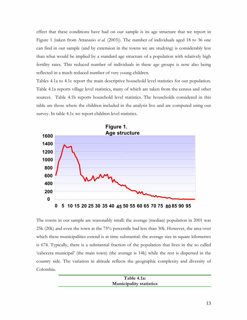
effect that these conditions have had on our sample is its age structure that we report in

Figure 1 (taken from Attanasio et al. (2003)). The number of individuals aged 18 to 36 one

can find in our sample (and by extension in the towns we are studying) is considerably less

than what would be implied by a standard age structure of a population with relatively high

fertility rates. This reduced number of individuals in these age groups is now also being

reflected in a much reduced number of very young children.

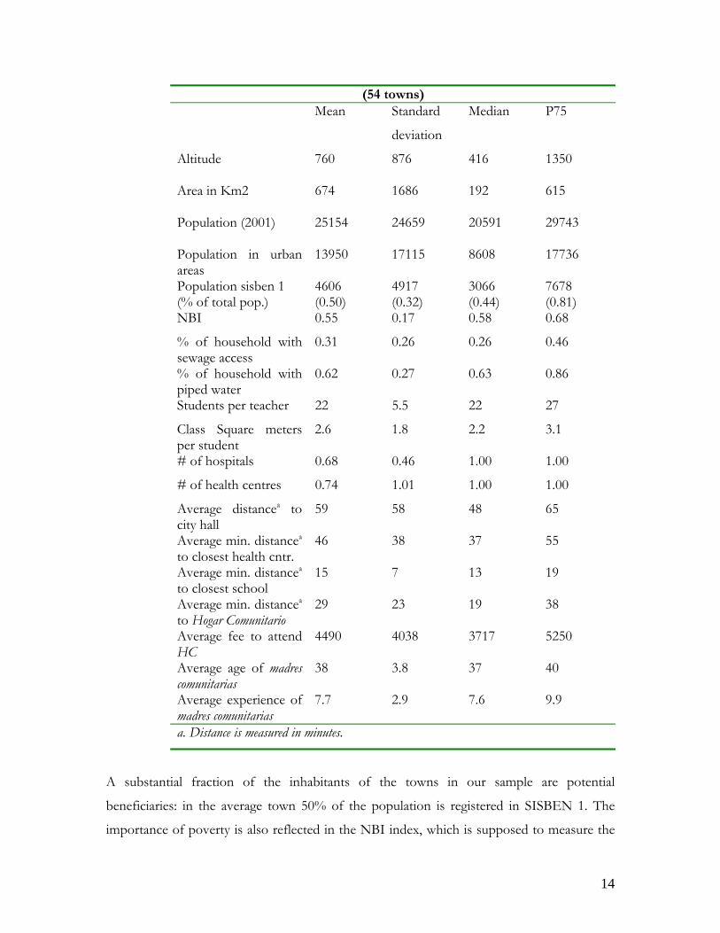
Tables 4.1a to 4.1c report the main descriptive household level statistics for our population.

Table 4.1a reports village level statistics, many of which are taken from the census and other

sources. Table 4.1b reports household level statistics. The households considered in this

table are those where the children included in the analysis live and are computed using our

survey. In table 4.1c we report children level statistics.

The towns in our sample are reasonably small: the average (median) population in 2001 was

25k (20k) and even the town at the 75% percentile had less than 30k. However, the area over

which these municipalities extend is at time substantial: the average size in square kilometres

is 674. Typically, there is a substantial fraction of the population that lives in the so called

‘cabecera municipal’ (the main town) (the average is 14k) while the rest is dispersed in the

country side. The variation in altitude reflects the geographic complexity and diversity of

Colombia.

Table 4.1a: Municipality statistics

Figure 1. Age structure

0020040060

008001000120014

1600

0 5 10 15 20 25 30 35 40 50 55 60 65 70 75 85 90 958045

13

(54 towns) Mean Standard

deviation

Median P75

Altitude

760 876 416 1350

Area in Km2

674 1686 192 615

Population (2001)

25154 24659 20591 29743

Population in urban areas

13950 17115 8608 17736

Population sisben 1 (% of total pop.)

4606 (0.50)

4917 (0.32)

3066 (0.44)

7678 (0.81)

NBI 0.55 0.17 0.58 0.68

% of household with sewage access

0.31 0.26 0.26 0.46

% of household with piped water

0.62 0.27 0.63 0.86

Students per teacher 22 5.5 22 27

Class Square meters per student

2.6 1.8 2.2 3.1

# of hospitals 0.68 0.46 1.00 1.00

# of health centres 0.74 1.01 1.00 1.00

Average distancea to city hall

59 58 48 65

Average min. distancea to closest health cntr.

46 38 37 55

Average min. distancea to closest school

15 7 13 19

Average min. distancea to Hogar Comunitario

29 23 19 38

Average fee to attend HC

4490 4038 3717 5250

Average age of madres comunitarias

38 3.8 37 40

Average experience of madres comunitarias

7.7 2.9 7.6 9.9

a. Distance is measured in minutes.

A substantial fraction of the inhabitants of the towns in our sample are potential

beneficiaries: in the average town 50% of the population is registered in SISBEN 1. The

importance of poverty is also reflected in the NBI index, which is supposed to measure the

14

percentage of households with ‘unsatisfied basic needs’: this index averages 0.55 in our

towns. On average, only 31% of households in our towns have access to sewage and 62% of

households have access to piped water. These percentages are substantially lower for our

sample.

The next group of variables in the Table provides information on the infrastructure present

in the municipalities. Schools do not seem to be particularly crowded and class sizes are not

very large. Likewise, there is on average 1 health centre and one hospital per town (although

not necessarily both). The average distance to the health centre is 46 minutes.

Another indication of the reasonably supply of schools in this towns is the fact that, even

though the population appears to be quite disperse (the average travel time to the city hall is,

in the average town, an hour) the average distance to schools is only 15 minutes and even for

the town on the 75th percentile, it is less than twenty minutes.

The last group of variables in Table 4.1a gives information, at the municipality level, on the

HC. The average distance to a HC is just short of half hour. The average age of a madre

comunitaria is 38, and she has an average experience of 7 years. Interestingly, the average

monthly fee is, in our data, only 4500 pesos (less than 2 US$). According to the ICBF, the

monthly fees should be between 7,000 and 14,000 pesos: however, as also confirmed by our

field workers, in our towns there are many HC where the madre comunitaria charges very little,

if at all.

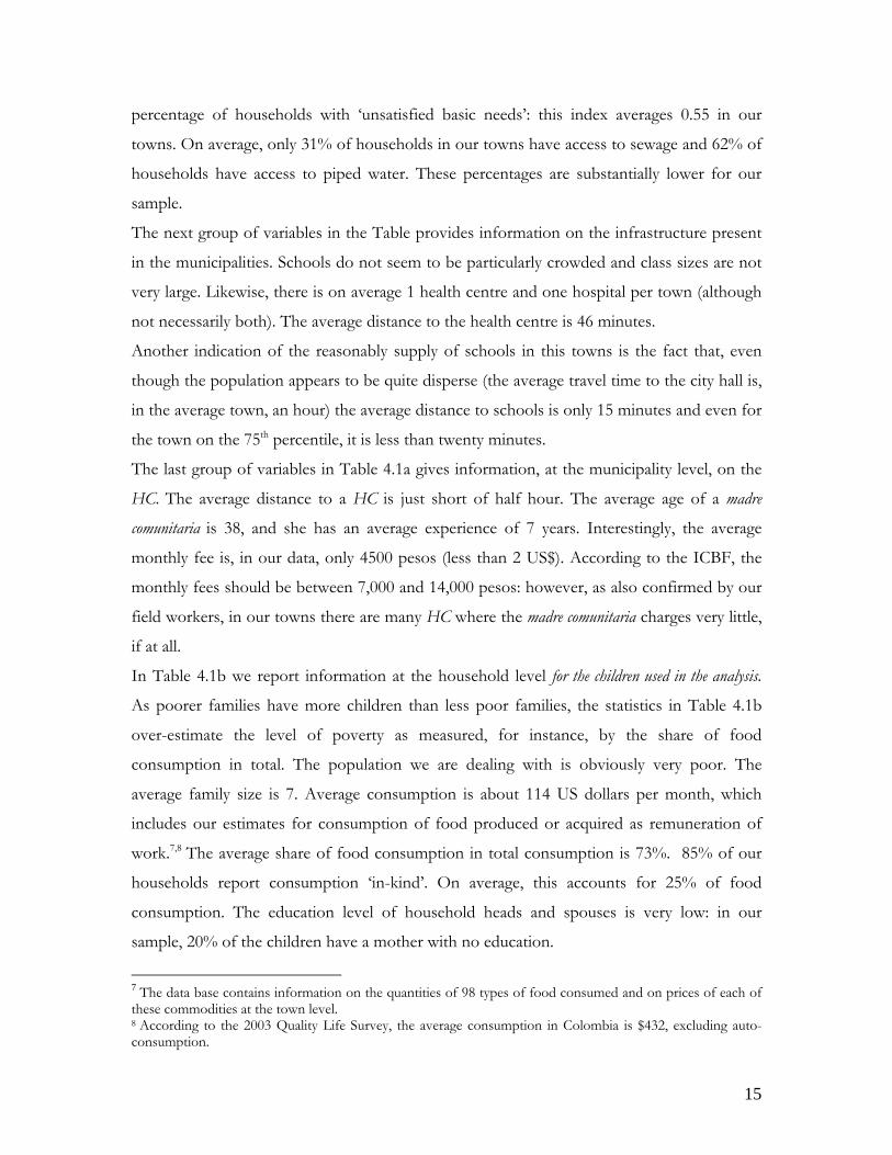
In Table 4.1b we report information at the household level for the children used in the analysis.

As poorer families have more children than less poor families, the statistics in Table 4.1b

over-estimate the level of poverty as measured, for instance, by the share of food

consumption in total. The population we are dealing with is obviously very poor. The

average family size is 7. Average consumption is about 114 US dollars per month, which

includes our estimates for consumption of food produced or acquired as remuneration of

work.7,8 The average share of food consumption in total consumption is 73%. 85% of our

households report consumption ‘in-kind’. On average, this accounts for 25% of food

consumption. The education level of household heads and spouses is very low: in our

sample, 20% of the children have a mother with no education.

7 The data base contains information on the quantities of 98 types of food consumed and on prices of each of these commodities at the town level. 8 According to the 2003 Quality Life Survey, the average consumption in Colombia is $432, excluding auto-consumption.

15

Table 4.1b Household level statistics

Mean Standard

deviation

Median P75

Monthly Consumption

114 67.2 100.5 142.1

Food share 0.727 0.146 0.753 0.835

Family size 6.7 2.5 6 8

% of mother with no education.

20.1 0.40 - -

The numbers in this table refer to averages of household variables for the children in our samples. Consumption is reported in US$ using an exchange rate of 2,600 to the peso.

In table 4.1c, we report mean, median and standard deviation of the z-score for height per

age, weight per age, weight per height and leg length. Z-scores are computed as the variable

of interest (say height) minus the median value for the same variable for children of the

WHO/CDC reference population of the same age (or height in the case of weight per

height) and gender, divided by the standard deviation of the same group of children of the

WHO/CDC reference population. This is the normalization most commonly used in the

literature

If we take at face value the figures in Table 4.1c, we observe that our population presents

substantial deficits in height per age, which are much reduced for weight per age and almost

non-existent in weight per height.

In the case of leg length, which will be one of our outcomes, we do not have a normalization

or standard Z-scores. In Table 4.1c we report the mean, median and standard deviation of

this variable in our sample. This variable has been shown to be an important marker of the

stock of malnutrition as well as a very good predictor of illnesses in adult age.

16

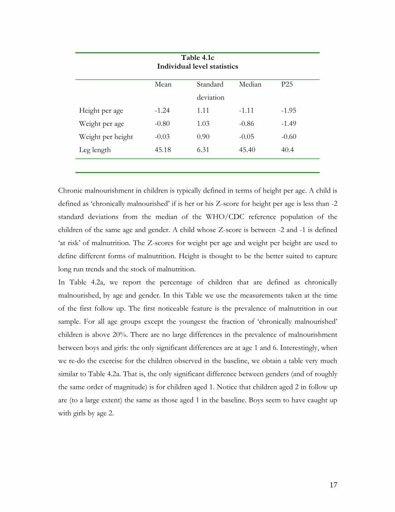
Table 4.1c Individual level statistics

Mean Standard

deviation

Median P25

Height per age -1.24 1.11 -1.11 -1.95

Weight per age -0.80 1.03 -0.86 -1.49

Weight per height -0.03 0.90 -0.05 -0.60

Leg length 45.18 6.31 45.40 40.4

Chronic malnourishment in children is typically defined in terms of height per age. A child is

defined as ‘chronically malnourished’ if is her or his Z-score for height per age is less than -2

standard deviations from the median of the WHO/CDC reference population of the

children of the same age and gender. A child whose Z-score is between -2 and -1 is defined

‘at risk’ of malnutrition. The Z-scores for weight per age and weight per height are used to

define different forms of malnutrition. Height is thought to be the better suited to capture

long run trends and the stock of malnutrition.

In Table 4.2a, we report the percentage of children that are defined as chronically

malnourished, by age and gender. In this Table we use the measurements taken at the time

of the first follow up. The first noticeable feature is the prevalence of malnutrition in our

sample. For all age groups except the youngest the fraction of ‘chronically malnourished’

children is above 20%. There are no large differences in the prevalence of malnourishment

between boys and girls: the only significant differences are at age 1 and 6. Interestingly, when

we re-do the exercise for the children observed in the baseline, we obtain a table very much

similar to Table 4.2a. That is, the only significant difference between genders (and of roughly

the same order of magnitude) is for children aged 1. Notice that children aged 2 in follow up

are (to a large extent) the same as those aged 1 in the baseline. Boys seem to have caught up

with girls by age 2.

17

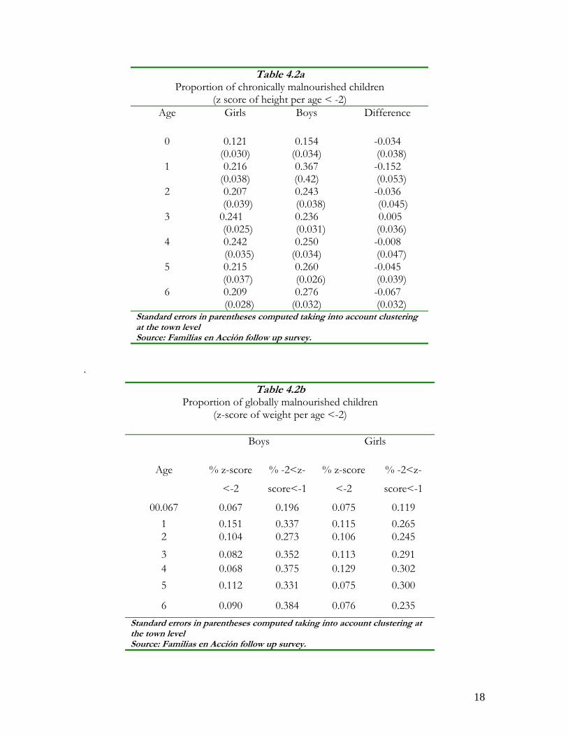
Table 4.2a Proportion of chronically malnourished children

(z score of height per age < -2) Age Girls Boys Difference

0 0.121 (0.030)

0.154 (0.034)

-0.034 (0.038)

1 0.216 (0.038)

0.367 (0.42)

-0.152 (0.053)

2 0.207 (0.039)

0.243 (0.038)

-0.036 (0.045)

3 0.241 (0.025)

0.236 (0.031)

0.005 (0.036)

4 0.242 (0.035)

0.250 (0.034)

-0.008 (0.047)

5 0.215 (0.037)

0.260 (0.026)

-0.045 (0.039)

6 0.209 (0.028)

0.276 (0.032)

-0.067 (0.032)

Standard errors in parentheses computed taking into account clustering at the town level Source: Familias en Acción follow up survey.

.

Table 4.2b Proportion of globally malnourished children

(z-score of weight per age <-2)

Boys Girls

Age % z-score

<-2

% -2<z-

score<-1

% z-score

<-2

% -2<z-

score<-1

00.067 0.067 0.196 0.075 0.119 1 0.151 0.337 0.115 0.265 2 0.104 0.273 0.106 0.245 3 0.082 0.352 0.113 0.291 4 0.068 0.375 0.129 0.302 5 0.112 0.331 0.075 0.300

6 0.090 0.384 0.076 0.235 Standard errors in parentheses computed taking into account clustering at the town level Source: Familias en Acción follow up survey.

18

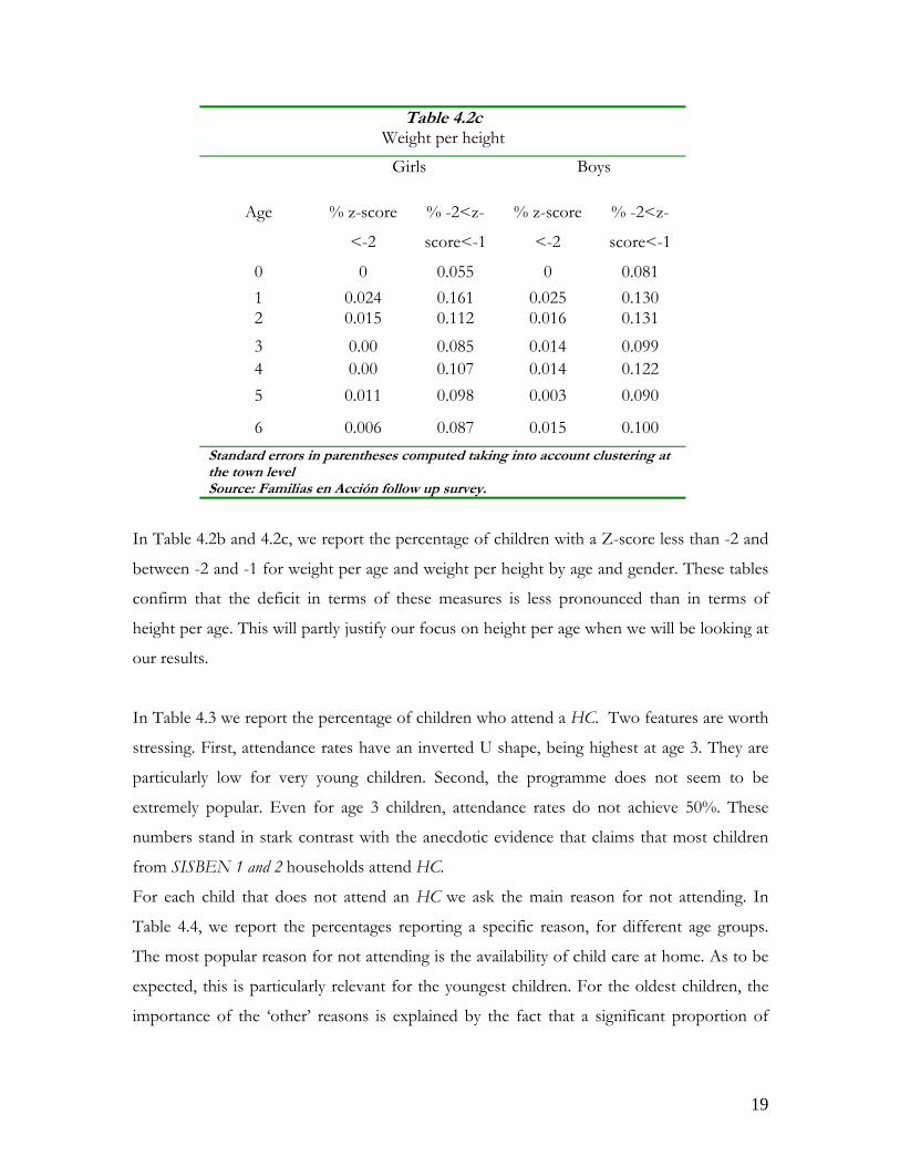
Table 4.2c Weight per height

Girls Boys

Age % z-score

<-2

% -2<z-

score<-1

% z-score

<-2

% -2<z-

score<-1

0 0 0.055 0 0.081 1 0.024 0.161 0.025 0.130 2 0.015 0.112 0.016 0.131 3 0.00 0.085 0.014 0.099 4 0.00 0.107 0.014 0.122 5 0.011 0.098 0.003 0.090

6 0.006 0.087 0.015 0.100 Standard errors in parentheses computed taking into account clustering at the town level Source: Familias en Acción follow up survey.

In Table 4.2b and 4.2c, we report the percentage of children with a Z-score less than -2 and

between -2 and -1 for weight per age and weight per height by age and gender. These tables

confirm that the deficit in terms of these measures is less pronounced than in terms of

height per age. This will partly justify our focus on height per age when we will be looking at

our results.

In Table 4.3 we report the percentage of children who attend a HC. Two features are worth

stressing. First, attendance rates have an inverted U shape, being highest at age 3. They are

particularly low for very young children. Second, the programme does not seem to be

extremely popular. Even for age 3 children, attendance rates do not achieve 50%. These

numbers stand in stark contrast with the anecdotic evidence that claims that most children

from SISBEN 1 and 2 households attend HC.

For each child that does not attend an HC we ask the main reason for not attending. In

Table 4.4, we report the percentages reporting a specific reason, for different age groups.

The most popular reason for not attending is the availability of child care at home. As to be

expected, this is particularly relevant for the youngest children. For the oldest children, the

importance of the ‘other’ reasons is explained by the fact that a significant proportion of

19

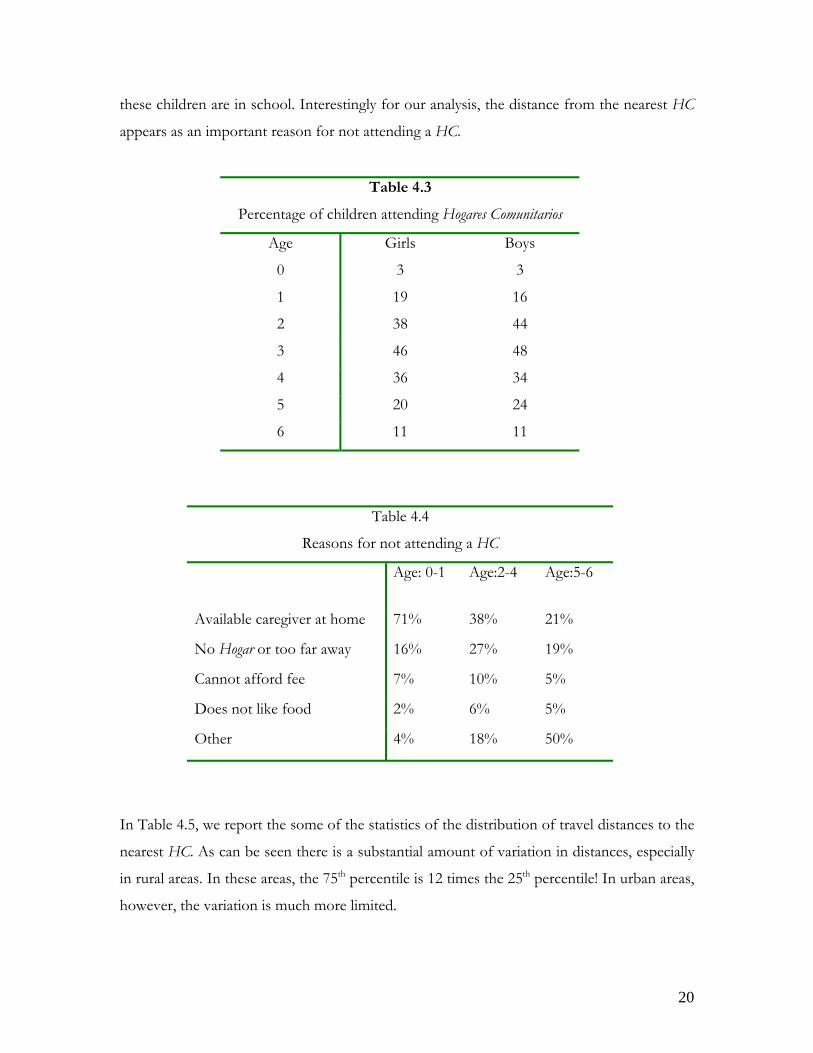
these children are in school. Interestingly for our analysis, the distance from the nearest HC

appears as an important reason for not attending a HC.

Table 4.3

Percentage of children attending Hogares Comunitarios

Age Girls Boys

0 3 3

1 19 16

2 38 44

3 46 48

4 36 34

5 20 24

6 11 11

Table 4.4

Reasons for not attending a HC

Age: 0-1 Age:2-4 Age:5-6

Available caregiver at home 71% 38% 21%

No Hogar or too far away 16% 27% 19%

Cannot afford fee 7% 10% 5%

Does not like food 2% 6% 5%

Other 4% 18% 50%

In Table 4.5, we report the some of the statistics of the distribution of travel distances to the

nearest HC. As can be seen there is a substantial amount of variation in distances, especially

in rural areas. In these areas, the 75th percentile is 12 times the 25th percentile! In urban areas,

however, the variation is much more limited.

20

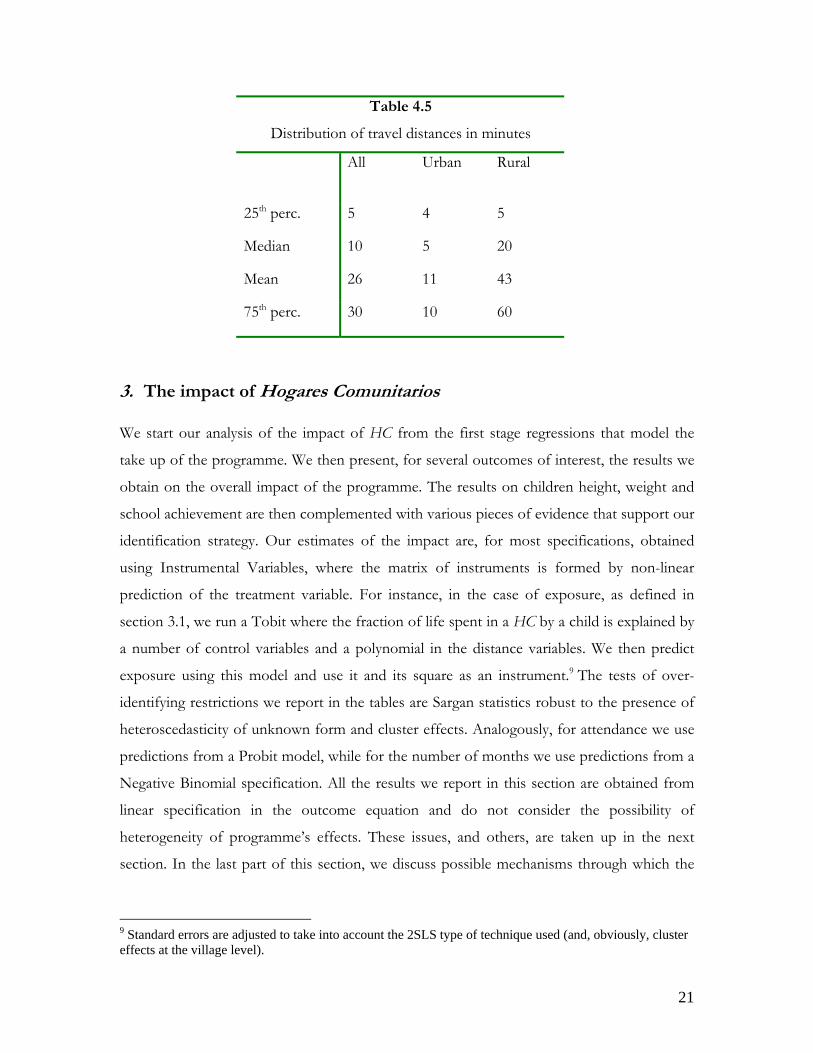
Table 4.5

Distribution of travel distances in minutes

All Urban Rural

25th perc. 5 4 5

Median 10 5 20

Mean 26 11 43

75th perc. 30 10 60

3. The impact of Hogares Comunitarios We start our analysis of the impact of HC from the first stage regressions that model the

take up of the programme. We then present, for several outcomes of interest, the results we

obtain on the overall impact of the programme. The results on children height, weight and

school achievement are then complemented with various pieces of evidence that support our

identification strategy. Our estimates of the impact are, for most specifications, obtained

using Instrumental Variables, where the matrix of instruments is formed by non-linear

prediction of the treatment variable. For instance, in the case of exposure, as defined in

section 3.1, we run a Tobit where the fraction of life spent in a HC by a child is explained by

a number of control variables and a polynomial in the distance variables. We then predict

exposure using this model and use it and its square as an instrument.9 The tests of over-

identifying restrictions we report in the tables are Sargan statistics robust to the presence of

heteroscedasticity of unknown form and cluster effects. Analogously, for attendance we use

predictions from a Probit model, while for the number of months we use predictions from a

Negative Binomial specification. All the results we report in this section are obtained from

linear specification in the outcome equation and do not consider the possibility of

heterogeneity of programme’s effects. These issues, and others, are taken up in the next

section. In the last part of this section, we discuss possible mechanisms through which the

9 Standard errors are adjusted to take into account the 2SLS type of technique used (and, obviously, cluster effects at the village level).

21

programme might be operating, such as female labour supply, and discuss the robustness of

our identification strategy.

5.1 First stage regressions As we mentioned above, we use three different definitions of ‘treatment’. First we look at

whether a child is currently attending a HC. We then consider exposure, that is, the number

of months a child has spent in a HC divided by the child’s age in months. Finally, we also

consider the number of months spent in a HC. When considering long run outcomes, such

as the school outcomes of children aged 8 to 17, we consider the number of months and a

binary indicator that tells us if the child has ever attended.

The results on the first stage are reported in Tables 5.1 and 5.2. While for instrumenting

purposes we use predictions of the non-linear models in this tables, here we report also the

results obtained with linear models. In the case of attendance we use a Probit, in the case of

exposure we use a Tobit model and for months of attendance, we use a Negative Binomial

regression.

As mentioned above we use two sets of instruments. First, for each single child, regardless

of whether he or she attends a HC, we consider the distance to the nearest HC from the

child’s household residence in minutes and its square. Second, in each town, we compute the

average distance for all the households in the town to the nearest HC. Again we consider

both the level and the square of this variable. The first stage regressions, both in their linear

and non linear incarnations, included, in additional to these identifying instruments all the

controls used in the outcome equations. The fact that the distance from the household to

the nearest HC affects participation in the programme is not surprising. This is evident even

from the self-reported reasons not to participate in HC that can be found in Table 4.4. The

average distance from the households to the HC in the municipality measures the density of

the programme in the town. This can also influence participation because if the closest HC is

full, the density of the programme on the town becomes relevant for the participation.

22

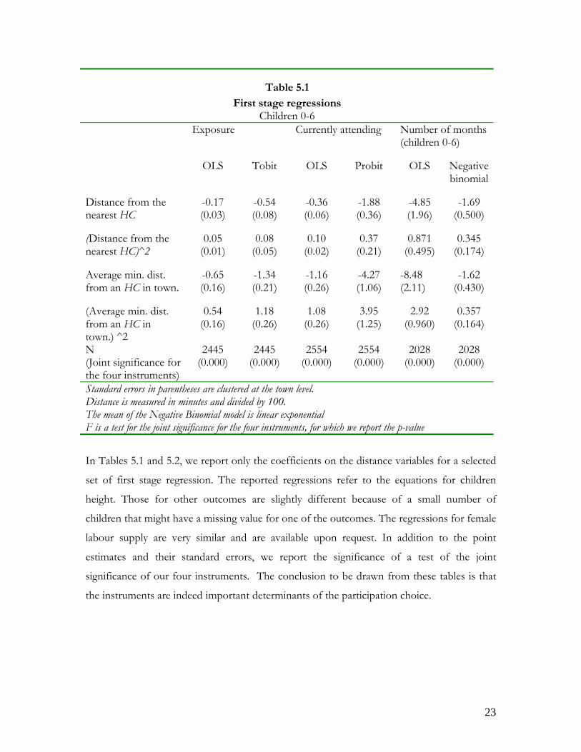
Table 5.1

First stage regressions Children 0-6

Exposure Currently attending Number of months (children 0-6)

OLS Tobit OLS Probit OLS Negative binomial

Distance from the nearest HC

-0.17 (0.03)

-0.54 (0.08)

-0.36 (0.06)

-1.88 (0.36)

-4.85 (1.96)

-1.69 (0.500)

(Distance from the nearest HC)^2

0.05 (0.01)

0.08 (0.05)

0.10 (0.02)

0.37 (0.21)

0.871 (0.495)

0.345 (0.174)

Average min. dist. from an HC in town.

-0.65 (0.16)

-1.34 (0.21)

-1.16 (0.26)

-4.27 (1.06)

-8.48 (2.11)

-1.62 (0.430)

(Average min. dist. from an HC in town.) ^2

0.54 (0.16)

1.18 (0.26)

1.08 (0.26)

3.95 (1.25)

2.92 (0.960)

0.357 (0.164)

N (Joint significance for the four instruments)

2445 (0.000)

2445 (0.000)

2554 (0.000)

2554 (0.000)

2028 (0.000)

2028 (0.000)

Standard errors in parentheses are clustered at the town level. Distance is measured in minutes and divided by 100. The mean of the Negative Binomial model is linear exponential F is a test for the joint significance for the four instruments, for which we report the p-value

In Tables 5.1 and 5.2, we report only the coefficients on the distance variables for a selected

set of first stage regression. The reported regressions refer to the equations for children

height. Those for other outcomes are slightly different because of a small number of

children that might have a missing value for one of the outcomes. The regressions for female

labour supply are very similar and are available upon request. In addition to the point

estimates and their standard errors, we report the significance of a test of the joint

significance of our four instruments. The conclusion to be drawn from these tables is that

the instruments are indeed important determinants of the participation choice.

23

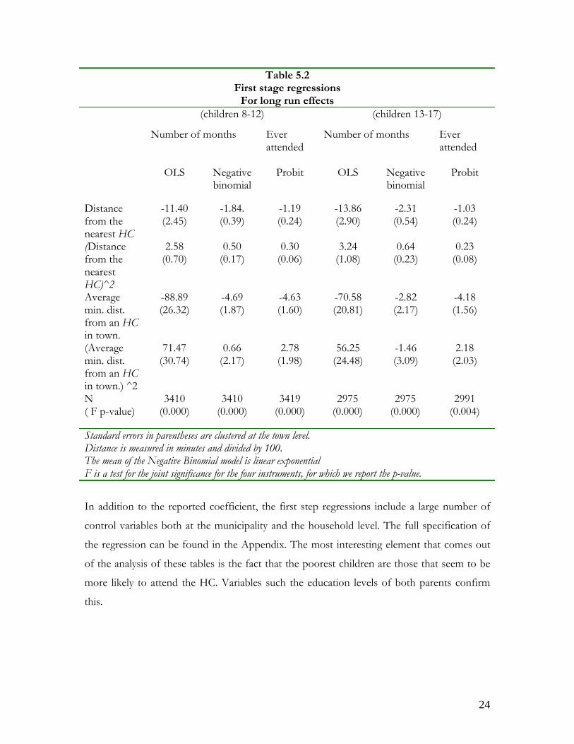
Table 5.2 First stage regressions

For long run effects (children 8-12) (children 13-17)

Number of months

Ever attended

Number of months

Ever attended

OLS Negative binomial

Probit OLS Negative binomial

Probit

Distance from the nearest HC

-11.40 (2.45)

-1.84. (0.39)

-1.19 (0.24)

-13.86 (2.90)

-2.31 (0.54)

-1.03 (0.24)

(Distance from the nearest HC)^2

2.58 (0.70)

0.50 (0.17)

0.30 (0.06)

3.24 (1.08)

0.64 (0.23)

0.23 (0.08)

Average min. dist. from an HC in town.

-88.89 (26.32)

-4.69 (1.87)

-4.63 (1.60)

-70.58 (20.81)

-2.82 (2.17)

-4.18 (1.56)

(Average min. dist. from an HC in town.) ^2

71.47 (30.74)

0.66 (2.17)

2.78 (1.98)

56.25 (24.48)

-1.46 (3.09)

2.18 (2.03)

N ( F p-value)

3410 (0.000)

3410 (0.000)

3419 (0.000)

2975 (0.000)

2975 (0.000)

2991 (0.004)

Standard errors in parentheses are clustered at the town level. Distance is measured in minutes and divided by 100. The mean of the Negative Binomial model is linear exponential F is a test for the joint significance for the four instruments, for which we report the p-value.

In addition to the reported coefficient, the first step regressions include a large number of

control variables both at the municipality and the household level. The full specification of

the regression can be found in the Appendix. The most interesting element that comes out

of the analysis of these tables is the fact that the poorest children are those that seem to be

more likely to attend the HC. Variables such the education levels of both parents confirm

this.

24

5.2 Programme Impacts In this section we present our estimates of the programme impacts. We will start with the

impacts on anthropometric measures: height, weight and leg length. We then move to the

impacts on long run effects on the school achievements of older children.

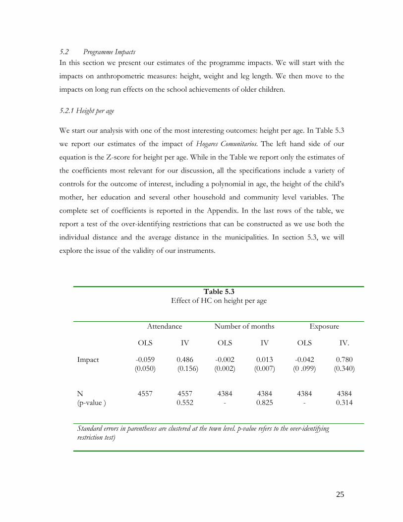
5.2.1 Height per age We start our analysis with one of the most interesting outcomes: height per age. In Table 5.3

we report our estimates of the impact of Hogares Comunitarios. The left hand side of our

equation is the Z-score for height per age. While in the Table we report only the estimates of

the coefficients most relevant for our discussion, all the specifications include a variety of

controls for the outcome of interest, including a polynomial in age, the height of the child’s

mother, her education and several other household and community level variables. The

complete set of coefficients is reported in the Appendix. In the last rows of the table, we

report a test of the over-identifying restrictions that can be constructed as we use both the

individual distance and the average distance in the municipalities. In section 5.3, we will

explore the issue of the validity of our instruments.

Table 5.3 Effect of HC on height per age

Attendance Number of months Exposure

OLS IV OLS IV OLS IV.

Impact -0.059 (0.050)

0.486 (0.156)

-0.002 (0.002)

0.013 (0.007)

-0.042 (0 .099)

0.780 (0.340)

N (p-value )

4557 4557 0.552

4384 -

4384 0.825

4384 -

4384 0.314

Standard errors in parentheses are clustered at the town level. p-value refers to the over-identifying restriction test)

25

In the first two columns, we report the coefficient we get on current attendance, that is, a

dummy that is zero for children who are not currently attending a HC and one for those

who are. In columns 3 and 4, we report the coefficient on the number of months. Finally,

the last two columns contain the coefficients on exposure, that is, the number of months a

child attended HC over her age in months. In Columns 1, 3 and 5, we report the estimates

we obtain by OLS, that is, without controlling for the endogeneity of participation into a

HC, while in columns 2, 4 and 6 we report the IV estimates.

The OLS estimates are small and negative numbers. However, when we instrument

participation, months or exposure using distance from a HC and average distance in a town

the estimated coefficient is positive and significantly different from zero. We never reject the

over-identifying restrictions.

The effects we report are large. Current attendance is estimated to have an effect of 0.4486

standard deviations on the Z-score. This effect corresponds to 2.36 centimetres for a boy

(2.39 for a girl) aged 72 months. Even more interestingly, if we look at exposure we obtain

that the effect of having attended a HC during the first six years of life is 3.78 centimetres

for a boy (3.83 for a girl) aged 72 months. The fact that the OLS estimates are negatively

biased is an interesting result in its own right. This piece of evidence is consistent with the

evidence from the 1998 study we mentioned in the introduction, which did not find

significant differences between children attending HC and children of ‘similar socio-

economic background’. It is also consistent with the fact that the participation equations

seem to indicate that the poorest households are those that are sending children to HC. This

indicates that the programme is remarkably well targeted, in that the households most in

need seem to self-select as HC customers. It seems that the programme allows the poorest

children to keep up with their better off peers.

As we mentioned above, all specifications include a large set of controls. The complete set of

estimates is reported in the Appendix. It is worth noting that the specifications we have

estimated included a large number of town and areas specific variables. The reason for our

un-parsimonious specification in this respect is our worry that our instruments could capture

some unobserved feature of the environment where the households live and have a direct

effect on the outcome of interest. While such an identification assumption is clearly un-

testable, we will provide indirect evidence of the validity of our approach in section 5.3. The

26

remaining coefficients have, reassuringly, the expected sign: tall mothers have tall children, as

do better educated mothers and so on. Notice that the polynomial in the age of the child

(interacted with gender) is strongly significant, indicating that difference between our

population and the reference population is not invariant to age. 10 Several of the

environmental variables, including those referring to the availability of health infrastructure,

seem to be important determinants of children height (and other outcomes).

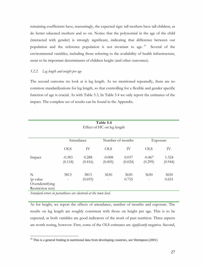
5.2.2. Leg length and weight per age The second outcome we look at is leg length. As we mentioned repeatedly, there are no

common standardizations for leg length, so that controlling for a flexible and gender specific

function of age is crucial. As with Table 5.3, In Table 5.4 we only report the estimates of the

impact. The complete set of results can be found in the Appendix.

Table 5.4 Effect of HC on leg length

Attendance Number of months Exposure

OLS IV OLS IV OLS IV.

Impact -0.383 (0.118)

0.288 (0.416)

-0.008 (0.005)

0.037 (0.024)

-0.467 (0.299)

1.324 (0.944)

N (p-value Overidentifying Restriction test)

3813 -

3813 (0.693)

3650 -

3650 0.755

3650 -

3650 0.651

Standard errors in parentheses are clustered at the town level.

As for height, we report the effects of attendance, number of months and exposure. The

results on leg length are roughly consistent with those on height per age. This is to be

expected, as both variables are good indicators of the stock of past nutrition. Three aspects

are worth noting, however. First, some of the OLS estimates are significantly negative. Second,

10 This is a general finding in nutritional data from developing countries, see Shrimpton (2001)

27

the positive effects obtained by IV are not as precisely estimated as in the case of height per

age. This might be a consequence of the smaller number of observations for which the leg

measurement is available. Finally, notice that the effect of current attendance is remarkably

smaller than that of the number of months or what we define as ‘exposure’. This is

consistent with the fact that the variable is more reactive to long run than short run

nutrition.

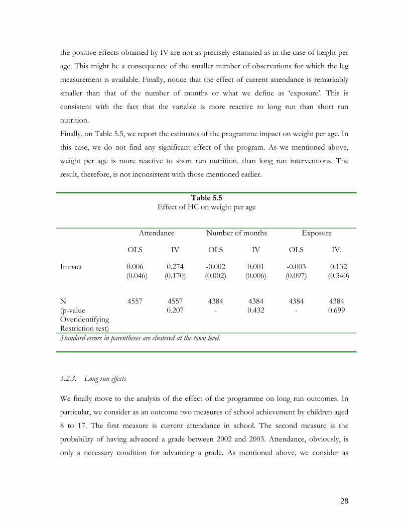
Finally, on Table 5.5, we report the estimates of the programme impact on weight per age. In

this case, we do not find any significant effect of the program. As we mentioned above,

weight per age is more reactive to short run nutrition, than long run interventions. The

result, therefore, is not inconsistent with those mentioned earlier.

Table 5.5

Effect of HC on weight per age

Attendance Number of months Exposure

OLS IV OLS IV OLS IV.

Impact 0.006 (0.046)

0.274 (0.170)

-0.002 (0.002)

0.001 (0.006)

-0.003 (0.097)

0.132 (0.340)

N (p-value Overidentifying Restriction test)

4557 4557 0.207

4384 -

4384 0.432

4384 -

4384 0.699

Standard errors in parentheses are clustered at the town level.

5.2.3. Long run effects We finally move to the analysis of the effect of the programme on long run outcomes. In

particular, we consider as an outcome two measures of school achievement by children aged

8 to 17. The first measure is current attendance in school. The second measure is the

probability of having advanced a grade between 2002 and 2003. Attendance, obviously, is

only a necessary condition for advancing a grade. As mentioned above, we consider as

28

treatment whether the child has ever attended in his/her life a HC and the number of

months spent in a HC.

We instrument the ‘treatment’ variable, as we did for the other Tables, following the IV

procedure discussed in Section 3. In particular, to model the ‘ever attended’ variable we use a

Probit, while for the number of months we used a negative binomial regression. The first

step results were reported in Table 5.2. As with the other specifications, in addition to the

treatment variable, we also consider a variety of controls that include parental education

variables, age, and many village infrastructure variables, such as the number of children per

teacher in the village. Finally, rather than considering all children together, we split the

sample and consider separately children aged 8 to 12 and those aged 13 to 17. Attendance

rates among the first group are very high in our sample, while they start dropping quite

dramatically at age 13. Once again, in table 5.6, we only report the estimates of the long run

effects of the programme. The coefficients of the complete specification are relegated to the

Appendix.

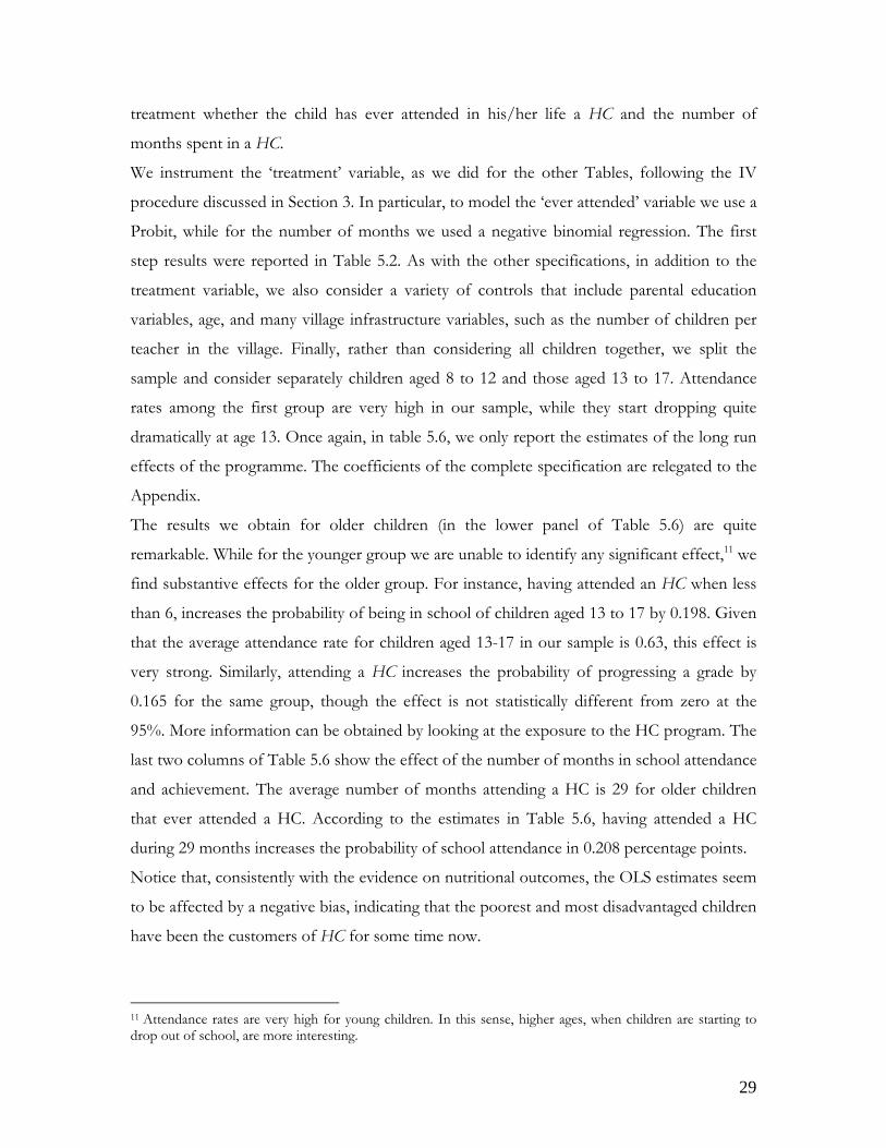
The results we obtain for older children (in the lower panel of Table 5.6) are quite

remarkable. While for the younger group we are unable to identify any significant effect,11 we

find substantive effects for the older group. For instance, having attended an HC when less

than 6, increases the probability of being in school of children aged 13 to 17 by 0.198. Given

that the average attendance rate for children aged 13-17 in our sample is 0.63, this effect is

very strong. Similarly, attending a HC increases the probability of progressing a grade by

0.165 for the same group, though the effect is not statistically different from zero at the

95%. More information can be obtained by looking at the exposure to the HC program. The

last two columns of Table 5.6 show the effect of the number of months in school attendance

and achievement. The average number of months attending a HC is 29 for older children

that ever attended a HC. According to the estimates in Table 5.6, having attended a HC

during 29 months increases the probability of school attendance in 0.208 percentage points.

Notice that, consistently with the evidence on nutritional outcomes, the OLS estimates seem

to be affected by a negative bias, indicating that the poorest and most disadvantaged children

have been the customers of HC for some time now.

11 Attendance rates are very high for young children. In this sense, higher ages, when children are starting to drop out of school, are more interesting.

29

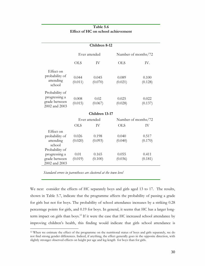
Table 5.6 Effect of HC on school achievement

Children 8-12

Ever attended Number of months/72

OLS IV OLS IV.

0.044 0.045 0.089 0.100 Effect on

probability of attending

school (0.011) (0.070) (0.021) (0.128)

0.008 0.02 0.025 0.022 Probability of progressing a grade between 2002 and 2003

(0.015) (0.067) (0.028) (0.137)

Children 13-17

Ever attended Number of months/72 OLS IV OLS IV

0.026 0.198 0.040 0.517 Effect on

probability of attending

school (0.020) (0.093) (0.040) (0.170)

0.01 0.165 0.055 0.411 Probability of progressing a grade between 2002 and 2003

(0.019) (0.100) (0.036) (0.181)

Standard errors in parentheses are clustered at the town level

We next consider the effects of HC separately boys and girls aged 13 to 17. The results,

shown in Table 5.7, indicate that the programme affects the probability of passing a grade

for girls but not for boys. The probability of school attendance increases by a striking 0.28

percentage points for girls, and 0.19 for boys. In general, it seems that HC has a larger long-

term impact on girls than boys.12 If it were the case that HC increased school attendance by

improving children’s health, this finding would indicate that girls school attendance is 12 When we estimate the effect of the programme on the nutritional status of boys and girls separately, we do not find strong gender differences. Indeed, if anything, the effect generally goes in the opposite direction, with slightly stronger observed effects on height per age and leg-length for boys than for girls.

30

relatively more sensitive to their health. This interpretation is consistent with evidence from

Pakistan reported by Alderman et al. (2001a), who find that an improvement in nutritional

status increases the school attendance of girls but not of boys.13

Table 5.7 Effect of HC on school achievement

Boys 13-17

Ever attended HC Number of months/72

OLS IV OLS IV.

0.015 0.193 0.0043 0.506 Effect on probability of attending school

(0.026) (0.105) (0.050) (0.188)

-0.014 0.045 0.008 0.148 Probability of progressing a grade between 2002 and 2003

(0.025) (0.098) (0.048) (0.182)

Girls 13-17

Ever attended HC Number of months/72 OLS IV OLS IV

0.035 0.284 0.026 0.393 Effect on probability of attending school

(0.024) (0.115) (0.043) (0.206)

0.036 0.35 0.104 0.667 Probability of progressing a grade between 2002 and 2003

(0.029) (0.13) (0.046) (0.227)

Standard errors in parentheses are clustered at the town level

13 There is also evidence of other characteristics having differential effects across boys and girls. For instance, we find that distance to school has a relatively large effect on girls’ rather than boys’ school attendance. This is also found in data from Pakistan (Alderman et al. 2001b). Of course, many other explanations are also possible. It could be that HC did not improve school attendance through improving children nutritional status, but the benefit comes indirectly through other siblings. It could be that older girls living closer to a HC benefit from the programme because they do not have to take care of their small siblings who attend the HC instead. However, we detect an important impact of HC even on older girls that live in households without small siblings.

31

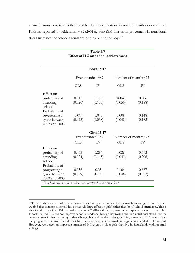
5.2.3 Female labour supply

In this section, we look at the effect of the programme on female labour supply, both in

terms of employment rates and number of hours worked. This might be important, as the

childcare aspect of the program could allow mothers to work and earn additional resources

that might benefit the child indirectly.

Table 5.8 Effect of HC on female labour supply

Employment rates Hours

Simple probit

Bi-variate probit

OLS IV

Programme effect

0.121 (0.027)

0.377 (0.061)

16.639 (3.914)

75.302 (13.504)

N

2936 2936 2920 2920

Standard errors are corrected for clusters at the municipality level. The coefficient on the probits are marginal effects

We report our estimates of the effects of HC on female labour supply in Table 5.8. As

outcomes, we consider both employment rates and number of hours; as treatment we define

a binary variable that is one if the mother has at least one child currently attending HC. In

the case of employment rate, we estimate a bi-variate Probit for employment and

programme participation. Consistently with our IV strategy, the distance variables enter the

participation decision, but not the employment rate decision. The assistance variable enters

the index for the employment decision.

The effects of the programme on female employment rates and participation are remarkable.

Once again, taking into account the endogeneity of programme participation increases

substantially the estimated effect of the program. In the case of employment rates, the

probability of employment increases from 0.12 to a staggering 0.37. We see similar evidence

about the effect on hours worked. The programme increases the number of hours worked

32

by 75 hours per month. In our sample, 37% of the mothers are working. They work, on

average, 39 hours per month.

5.3 Is the identification strategy credible? In this section we present some evidence that justifies our identifying strategy. First, we

supplement the evidence provided by the tests of over-identifying restrictions and identify

the parameters of interest with different sets of instruments. Second, as we mentioned

above, we consider whether, using our identification strategy, the programme would be

shown to have an effect on variables on which it should not.

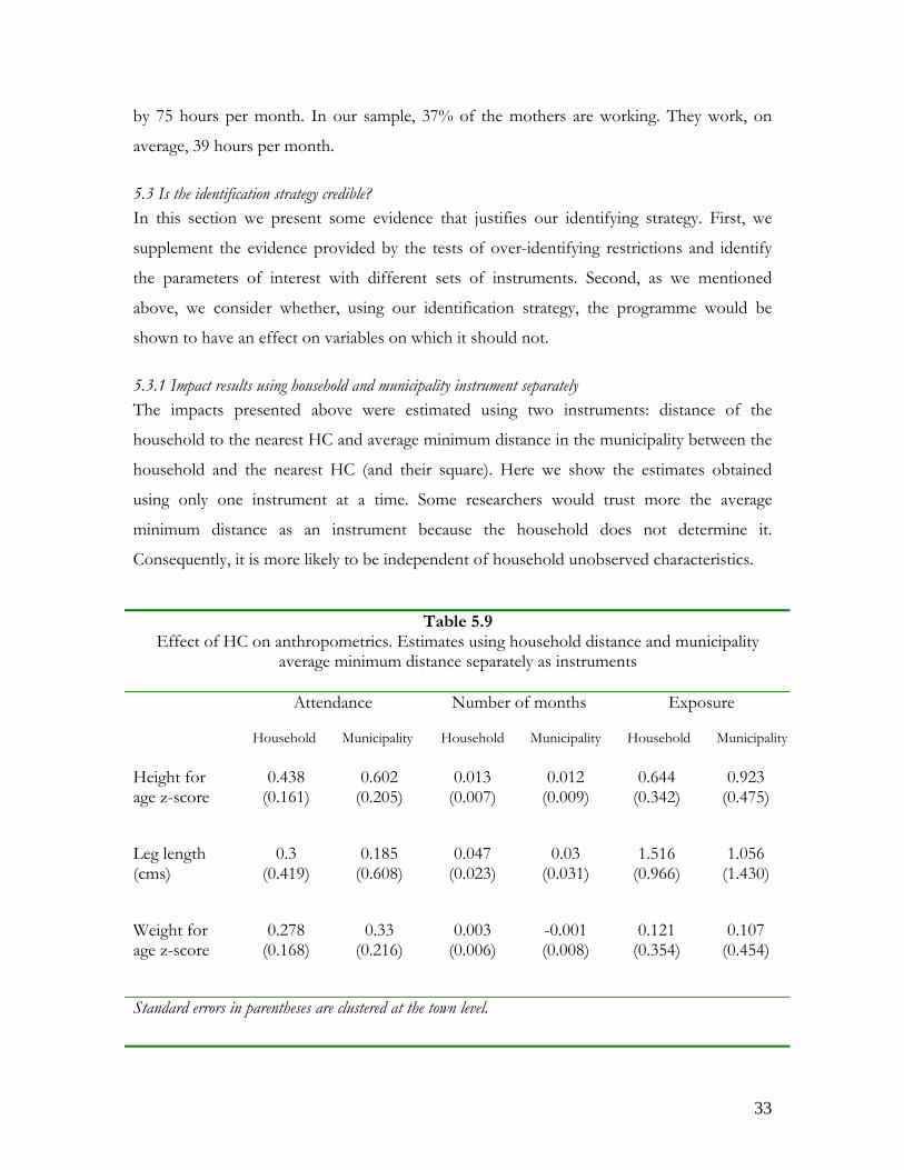
5.3.1 Impact results using household and municipality instrument separately The impacts presented above were estimated using two instruments: distance of the

household to the nearest HC and average minimum distance in the municipality between the

household and the nearest HC (and their square). Here we show the estimates obtained

using only one instrument at a time. Some researchers would trust more the average

minimum distance as an instrument because the household does not determine it.

Consequently, it is more likely to be independent of household unobserved characteristics.

Table 5.9 Effect of HC on anthropometrics. Estimates using household distance and municipality

average minimum distance separately as instruments

Attendance Number of months Exposure

Household Municipality Household Municipality Household Municipality

Height for age z-score

0.438 (0.161)

0.602 (0.205)

0.013 (0.007)

0.012 (0.009)

0.644 (0.342)

0.923 (0.475)

Leg length (cms)

0.3 (0.419)

0.185 (0.608)

0.047 (0.023)

0.03 (0.031)

1.516 (0.966)

1.056 (1.430)

Weight for age z-score

0.278 (0.168)

0.33 (0.216)

0.003 (0.006)

-0.001 (0.008)

0.121 (0.354)

0.107 (0.454)

Standard errors in parentheses are clustered at the town level.

33

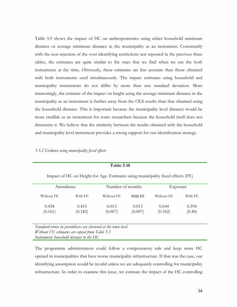
Table 5.9 shows the impact of HC on anthropometrics using either household minimum

distance or average minimum distance in the municipality as an instrument. Consistently

with the non-rejection of the over-identifying restrictions test reported in the previous three

tables, the estimates are quite similar to the ones that we find when we use the both

instruments at the time. Obviously, these estimates are less accurate than those obtained

with both instruments used simultaneously. The impact estimates using household and

municipality instruments do not differ by more than one standard deviation. More

interestingly, the estimate of the impact on height using the average minimum distance in the

municipality as an instrument is further away from the OLS results than that obtained using

the household distance. This is important because the municipality level distance would be

more credible as an instrument for some researchers because the household itself does not

determine it. We believe that the similarity between the results obtained with the household

and municipality level instrument provides a strong support for our identification strategy.

5.3.2 Evidence using municipality fixed effects

Table 5.10

Impact of HC on Height for Age. Estimates using municipality fixed effects (FE)

Attendance Number of months Exposure

Without FE With FE Without FE With FE Without FE With FE

0.438 (0.161)

0.415 (0.182)

0.013 (0.007)

0.013 (0.007)

0.644 (0.342)

0.594 (0.40)

Standard errors in parentheses are clustered at the town level. Without FE estimates are copied from Table 5.3 Instrument: household distance to the HC The programme administrators could follow a compensatory rule and keep more HC

opened in municipalities that have worse municipality infrastructure. If that was the case, our

identifying assumption would be invalid unless we are adequately controlling for municipality

infrastructure. In order to examine this issue, we estimate the impact of the HC controlling

34

for municipality fixed effects, and using only distance from the household to the HC as

instrument. The results, shown in Table 5.10, show that the introduction of fixed effects

only increases the estimated standard errors but hardly changes the parameter estimates.

Consequently, our results are robust to the correlation between household distance and

unobserved municipality variables.

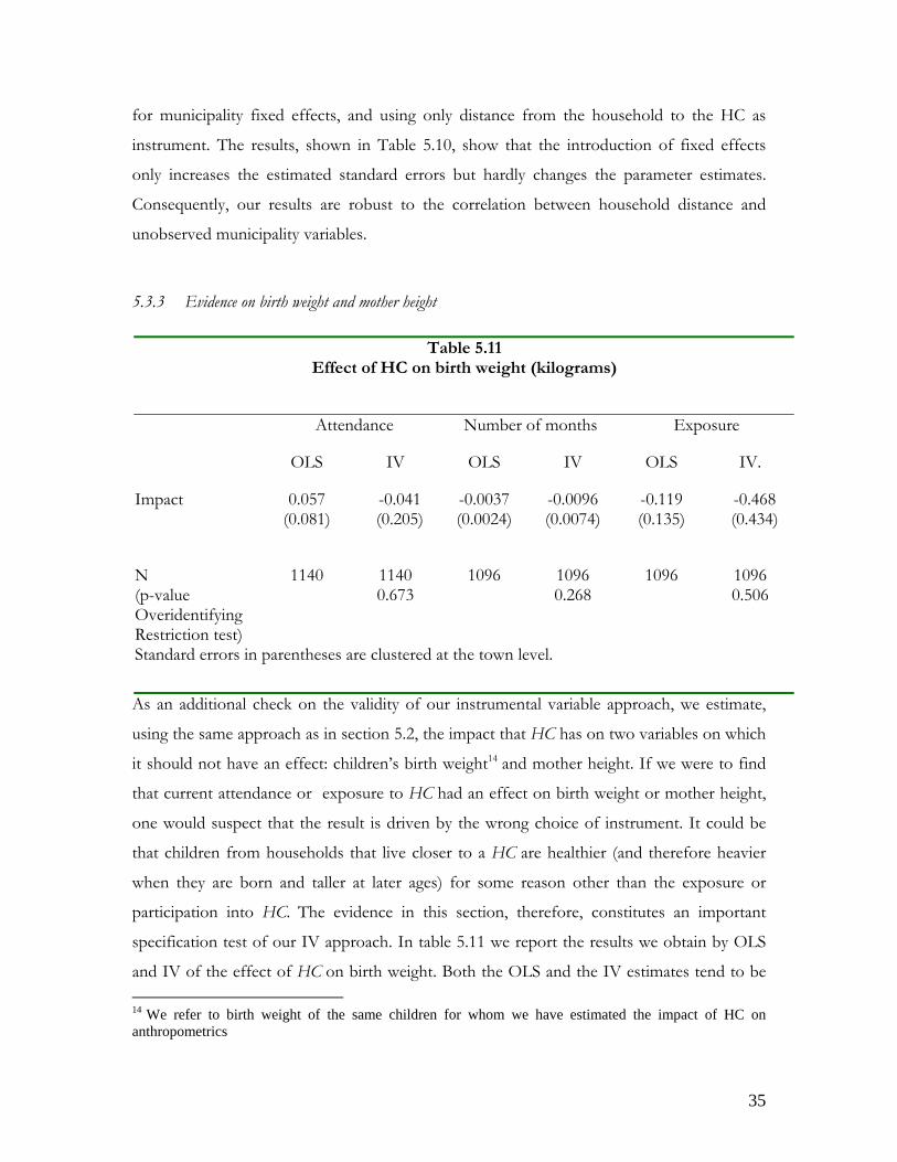
5.3.3 Evidence on birth weight and mother height

Table 5.11 Effect of HC on birth weight (kilograms)

Attendance Number of months Exposure

OLS IV OLS IV OLS IV.

Impact 0.057 (0.081)

-0.041 (0.205)

-0.0037 (0.0024)

-0.0096 (0.0074)

-0.119 (0.135)

-0.468 (0.434)

N (p-value Overidentifying Restriction test)

1140 1140 0.673

1096 1096 0.268

1096 1096 0.506

Standard errors in parentheses are clustered at the town level.

As an additional check on the validity of our instrumental variable approach, we estimate,

using the same approach as in section 5.2, the impact that HC has on two variables on which

it should not have an effect: children’s birth weight14 and mother height. If we were to find

that current attendance or exposure to HC had an effect on birth weight or mother height,

one would suspect that the result is driven by the wrong choice of instrument. It could be

that children from households that live closer to a HC are healthier (and therefore heavier

when they are born and taller at later ages) for some reason other than the exposure or

participation into HC. The evidence in this section, therefore, constitutes an important

specification test of our IV approach. In table 5.11 we report the results we obtain by OLS

and IV of the effect of HC on birth weight. Both the OLS and the IV estimates tend to be 14 We refer to birth weight of the same children for whom we have estimated the impact of HC on anthropometrics

35

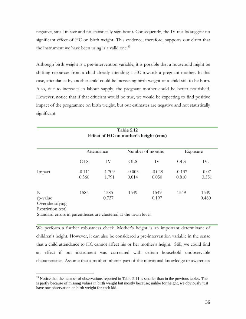
negative, small in size and no statistically significant. Consequently, the IV results suggest no

significant effect of HC on birth weight. This evidence, therefore, supports our claim that

the instrument we have been using is a valid one.15

Although birth weight is a pre-intervention variable, it is possible that a household might be

shifting resources from a child already attending a HC towards a pregnant mother. In this

case, attendance by another child could be increasing birth weight of a child still to be born.

Also, due to increases in labour supply, the pregnant mother could be better nourished.

However, notice that if that criticism would be true, we would be expecting to find positive

impact of the programme on birth weight, but our estimates are negative and not statistically

significant.

Table 5.12 Effect of HC on mother’s height (cms)

Attendance Number of months Exposure

OLS IV OLS IV OLS IV.

Impact -0.111 0.360

1.709 1.791

-0.003 0.014

-0.028 0.050

-0.137 0.810

0.07 3.551

N (p-value Overidentifying Restriction test)

1585 1585 0.727

1549 1549 0.197

1549 1549 0.480

Standard errors in parentheses are clustered at the town level.

We perform a further robustness check. Mother’s height is an important determinant of

children’s height. However, it can also be considered a pre-intervention variable in the sense

that a child attendance to HC cannot affect his or her mother’s height. Still, we could find

an effect if our instrument was correlated with certain household unobservable

characteristics. Assume that a mother inherits part of the nutritional knowledge or awareness

15 Notice that the number of observations reported in Table 5.11 is smaller than in the previous tables. This is partly because of missing values in birth weight but mostly because; unlike for height, we obviously just have one observation on birth weight for each kid.

36

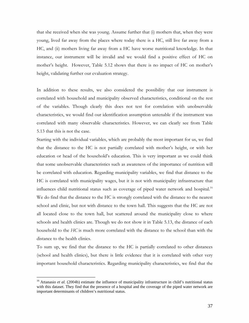
that she received when she was young. Assume further that (i) mothers that, when they were

young, lived far away from the places where today there is a HC, still live far away from a

HC, and (ii) mothers living far away from a HC have worse nutritional knowledge. In that

instance, our instrument will be invalid and we would find a positive effect of HC on

mother’s height. However, Table 5.12 shows that there is no impact of HC on mother’s

height, validating further our evaluation strategy.

In addition to these results, we also considered the possibility that our instrument is

correlated with household and municipality observed characteristics, conditional on the rest

of the variables. Though clearly this does not test for correlation with unobservable

characteristics, we would find our identification assumption untenable if the instrument was

correlated with many observable characteristics. However, we can clearly see from Table

5.13 that this is not the case.

Starting with the individual variables, which are probably the most important for us, we find

that the distance to the HC is not partially correlated with mother’s height, or with her

education or head of the household’s education. This is very important as we could think

that some unobservable characteristics such as awareness of the importance of nutrition will

be correlated with education. Regarding municipality variables, we find that distance to the

HC is correlated with municipality wages, but it is not with municipality infrastructure that

influences child nutritional status such as coverage of piped water network and hospital.16

We do find that the distance to the HC is strongly correlated with the distance to the nearest

school and clinic, but not with distance to the town hall. This suggests that the HC are not

all located close to the town hall, but scattered around the municipality close to where

schools and health clinics are. Though we do not show it in Table 5.13, the distance of each

household to the HC is much more correlated with the distance to the school than with the

distance to the health clinics.

To sum up, we find that the distance to the HC is partially correlated to other distances

(school and health clinics), but there is little evidence that it is correlated with other very

important household characteristics. Regarding municipality characteristics, we find that the

16 Attanasio et al. (2004b) estimate the influence of municipality infrastructure in child’s nutritional status with this dataset. They find that the presence of a hospital and the coverage of the piped water network are important determinants of children’s nutritional status.

37

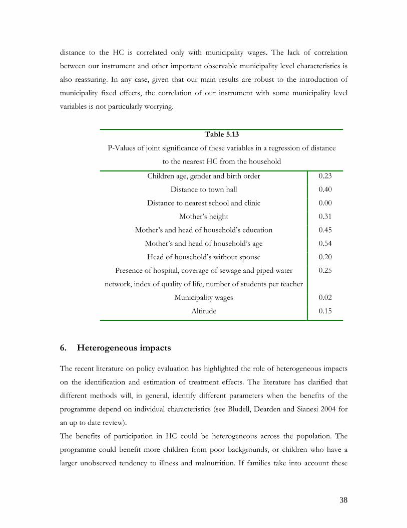
distance to the HC is correlated only with municipality wages. The lack of correlation

between our instrument and other important observable municipality level characteristics is

also reassuring. In any case, given that our main results are robust to the introduction of

municipality fixed effects, the correlation of our instrument with some municipality level

variables is not particularly worrying.

Table 5.13

P-Values of joint significance of these variables in a regression of distance

to the nearest HC from the household

Children age, gender and birth order 0.23

Distance to town hall 0.40

Distance to nearest school and clinic 0.00

Mother’s height 0.31

Mother’s and head of household’s education 0.45

Mother’s and head of household’s age 0.54

Head of household’s without spouse 0.20

Presence of hospital, coverage of sewage and piped water

network, index of quality of life, number of students per teacher

0.25

Municipality wages 0.02

Altitude 0.15

6. Heterogeneous impacts The recent literature on policy evaluation has highlighted the role of heterogeneous impacts

on the identification and estimation of treatment effects. The literature has clarified that

different methods will, in general, identify different parameters when the benefits of the

programme depend on individual characteristics (see Bludell, Dearden and Sianesi 2004 for

an up to date review).

The benefits of participation in HC could be heterogeneous across the population. The

programme could benefit more children from poor backgrounds, or children who have a

larger unobserved tendency to illness and malnutrition. If families take into account these

38

idiosyncratic benefits when taking decisions about children participation into the program,

the IV estimates presented before would not identify the average treatment effect, but a

Local Average Treatment Effect (Imbens and Angrist, 1994). Control function methods

have been advocated as a method to estimate the average treatment effect under

heterogeneous impacts but requiring stronger assumptions than IV.

From a policy perspective, when impacts are heterogeneous, it is not only important to

estimate the Average Treatment Effect, but also to estimate what types of people benefit

differently from the program. There are now several papers that try to estimate differential

impacts by individual characteristics (Aakvid et al. 2002; Carneiro et al. 2003; Blundell,

Dearden and Sianesi 2004, Moffitt 2004). In what follows, we explore this issue in two

different ways: through interactions between observable characteristics and treatment, and

through the use of quantiles methods. To take into account the endogenous selection into

the programme we use methods based on control functions.

Before presenting our results obtained with control functions, however, we report the results

that can be obtained by propensity score matching. There are several reasons to look at these

results. First, propensity score matching has become an extremely popular method to use in

the evaluation of public policies when a randomised control group does not exist. Second,

PSM does allow for heterogeneous programme effects in a simple and flexible way.

However, the assumptions needed for PSM to work are very stringent. We will be arguing

that they are not satisfied in our application.

For the sake of brevity, we will focus on the most significant results of Section 5, those on

height per age.

6.1 Propensity score matching As is well known, matching methods assume that conditional on observable variables, the

assignment of a programme is random. Given this assumption, Propensity Score Matching

(Rosenbaum and Rubin, 1983) uses the propensity score to re-weight the untreated sample.

Propensity Score Matching (PSM) improves over OLS with a dummy variable for treatment

because (i) PSM is a semi-parametric method, (ii) it does not require homogenous effects to

identify the parameter of interest, and (iii) it does not extrapolate outside the common

support. However, as OLS, it requires that selection take place on observables only.

39

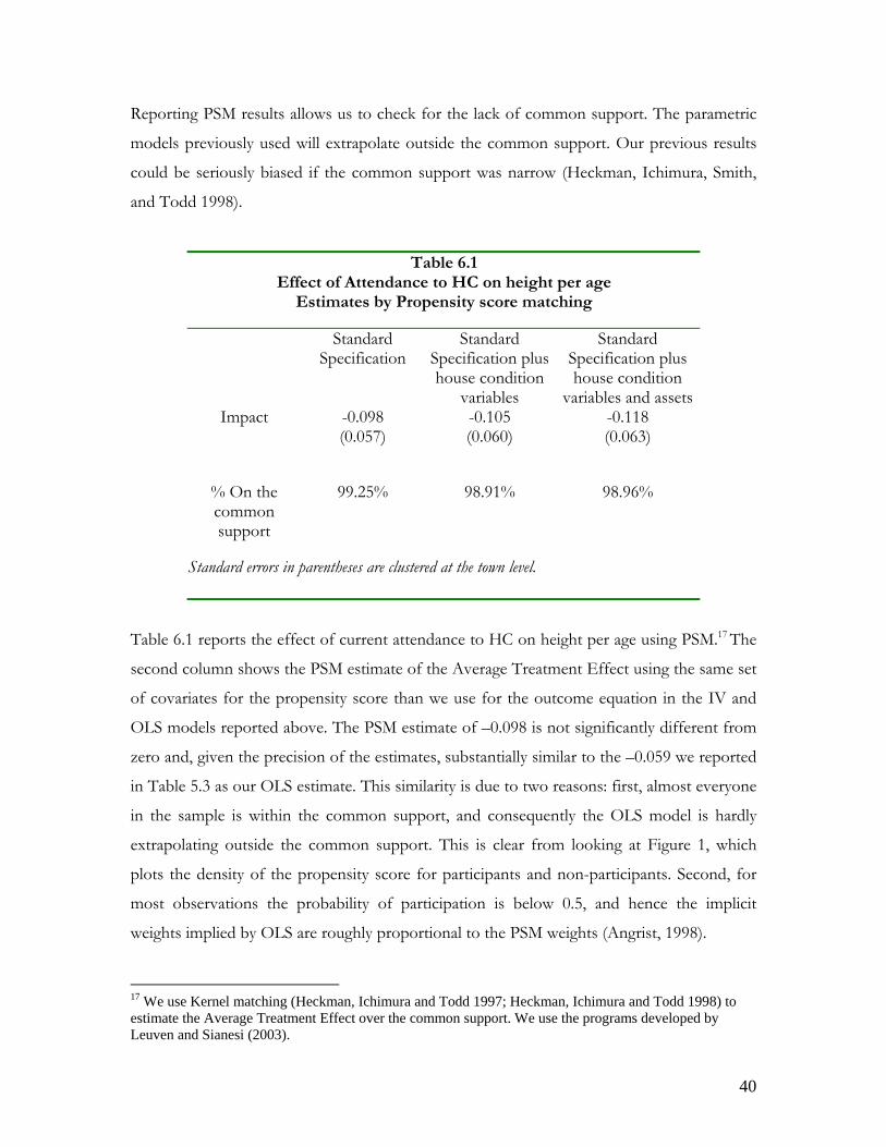
Reporting PSM results allows us to check for the lack of common support. The parametric

models previously used will extrapolate outside the common support. Our previous results

could be seriously biased if the common support was narrow (Heckman, Ichimura, Smith,

and Todd 1998).

Table 6.1 Effect of Attendance to HC on height per age

Estimates by Propensity score matching

Standard Specification

Standard Specification plus house condition

variables

Standard Specification plus house condition

variables and assets Impact -0.098

(0.057) -0.105 (0.060)

-0.118 (0.063)

% On the common support

99.25% 98.91% 98.96%

Standard errors in parentheses are clustered at the town level.

Table 6.1 reports the effect of current attendance to HC on height per age using PSM.17 The

second column shows the PSM estimate of the Average Treatment Effect using the same set

of covariates for the propensity score than we use for the outcome equation in the IV and

OLS models reported above. The PSM estimate of –0.098 is not significantly different from

zero and, given the precision of the estimates, substantially similar to the –0.059 we reported

in Table 5.3 as our OLS estimate. This similarity is due to two reasons: first, almost everyone

in the sample is within the common support, and consequently the OLS model is hardly

extrapolating outside the common support. This is clear from looking at Figure 1, which

plots the density of the propensity score for participants and non-participants. Second, for

most observations the probability of participation is below 0.5, and hence the implicit

weights implied by OLS are roughly proportional to the PSM weights (Angrist, 1998).

17 We use Kernel matching (Heckman, Ichimura and Todd 1997; Heckman, Ichimura and Todd 1998) to estimate the Average Treatment Effect over the common support. We use the programs developed by Leuven and Sianesi (2003).

40

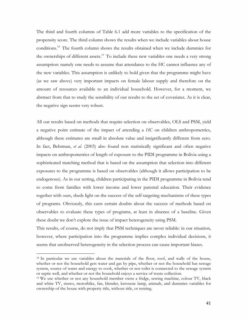
The third and fourth columns of Table 6.1 add more variables to the specification of the

propensity score. The third column shows the results when we include variables about house

conditions.18 The fourth column shows the results obtained when we include dummies for

the ownerships of different assets.19 To include these new variables one needs a very strong

assumption: namely one needs to assume that attendance to the HC cannot influence any of

the new variables. This assumption is unlikely to hold given that the programme might have

(as we saw above) very important impacts on female labour supply and therefore on the

amount of resources available to an individual household. However, for a moment, we

abstract from that to study the sensibility of our results to the set of covariates. As it is clear,

the negative sign seems very robust.

All our results based on methods that require selection on observables, OLS and PSM, yield

a negative point estimate of the impact of attending a HC on children anthropometrics,

although these estimates are small in absolute value and insignificantly different from zero.

In fact, Behrman, et al. (2003) also found non statistically significant and often negative

impacts on anthropometrics of length of exposure to the PIDI programme in Bolivia using a

sophisticated matching method that is based on the assumption that selection into different

exposures to the programme is based on observables (although it allows participation to be

endogenous). As in our setting, children participating in the PIDI programme in Bolivia tend

to come from families with lower income and lower parental education. Their evidence

together with ours, sheds light on the success of the self-targeting mechanisms of these types

of programs. Obviously, this casts certain doubts about the success of methods based on

observables to evaluate these types of programs, at least in absence of a baseline. Given

these doubt we don’t explore the issue of impact heterogeneity using PSM.

This results, of course, do not imply that PSM techniques are never reliable: in our situation,

however, where participation into the programme implies complex individual decisions, it

seems that unobserved heterogeneity in the selection process can cause important biases.

18 In particular we use variables about the materials of the floor, roof, and walls of the house, whether or not the household gets water and gas by pipe, whether or not the household has sewage system, source of water and energy to cook, whether or not toilet is connected to the sewage system or septic well, and whether or not the household enjoys a service of waste collection. 19 We use whether or not any household member owns a fridge, sewing machine, colour TV, black and white TV, stereo, motorbike, fan, blender, kerosene lamp, animals, and dummies variables for ownership of the house with property title, without title, or renting.

41

0

Untreated: Off support Treated: On support Untreated: On support Treated: Off support

.025.075

.125.175

.225.275

.325.375

.425.475

.525.575

.625.675

.725.775

.825.875

.925.975

Figure 1. Distribution of the estimated propensity score

6.2 Control functions The basis of the control function approach is to recover the average treatment effect by

controlling directly for the correlation between the error term in the outcome equation with

the treatment variable. To do that, one requires an explicit model of treatment choice. The

control function approach treats the selection problem as an omitted variable problem and

augments the outcome equation by a term to control for this variable omission. The

traditional example is the Heckman (1979) sample selection model that augments the

outcome equation by an estimate of the Mills Ratio. Using a control function approach we

will estimate the impact of HC on both the mean and different quantiles of the conditional

distribution of the error term. And when looking at the mean we will allow the effect to be

heterogeneous in observable dimensions.

6.2.1 Impact of the programme over the mean outcome In columns (1) and (2) of Table 6.2, we report the estimates of ATE using the control

function approach. In order to compute these estimates, the outcome equation was

42

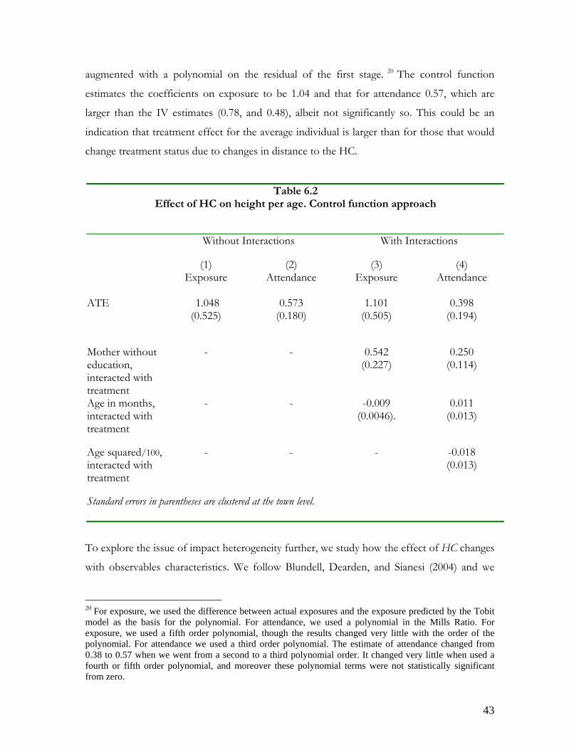
augmented with a polynomial on the residual of the first stage. 20 The control function

estimates the coefficients on exposure to be 1.04 and that for attendance 0.57, which are

larger than the IV estimates (0.78, and 0.48), albeit not significantly so. This could be an

indication that treatment effect for the average individual is larger than for those that would

change treatment status due to changes in distance to the HC.

Table 6.2 Effect of HC on height per age. Control function approach

Without Interactions With Interactions

(1) Exposure

(2) Attendance

(3) Exposure

(4) Attendance

ATE 1.048 (0.525)

0.573 (0.180)

1.101 (0.505)

0.398 (0.194)

Mother without education, interacted with treatment

- - 0.542 (0.227)

0.250 (0.114)

Age in months, interacted with treatment

- - -0.009 (0.0046).

0.011 (0.013)

Age squared/100, interacted with treatment

- - - -0.018 (0.013)

Standard errors in parentheses are clustered at the town level.

To explore the issue of impact heterogeneity further, we study how the effect of HC changes

with observables characteristics. We follow Blundell, Dearden, and Sianesi (2004) and we

20 For exposure, we used the difference between actual exposures and the exposure predicted by the Tobit model as the basis for the polynomial. For attendance, we used a polynomial in the Mills Ratio. For exposure, we used a fifth order polynomial, though the results changed very little with the order of the polynomial. For attendance we used a third order polynomial. The estimate of attendance changed from 0.38 to 0.57 when we went from a second to a third polynomial order. It changed very little when used a fourth or fifth order polynomial, and moreover these polynomial terms were not statistically significant from zero.

43

interact the treatment variable with the observable characteristic while the first stage residual

is entering only additively in the augmented outcome equation. This fiercely exploits the

additive structure of the error term. Moffitt (2004) proposes an alternative method that

allows the interactions to enter in a more flexible way, but also needs to exploit both the

additive structure of the error term and the participation model.21 As Blundel, Dearden and

Sianesi (2004) emphasize, the IV assumptions would require instrumenting the main

treatment variable as well as each of the interactions. However, this is unlikely to give good

results in practice as the interaction of the observable characteristics and the instrument will

normally have little explicative power in the first stage regression.

Columns (3) and (4) of Table 6.2 report the results we obtain when we interact the

programme with children age and mother education. We also tried interactions in gender,

and a dummy for female head of household but they were not individually or jointly

significant. For education, we also tried several dummies, for different levels of education. It

turned out that the group with mothers without any formal education (about 20% of our

sample) is the only systematically different in this dimension. There is clear evidence that

children whose mother does not have any education will tend to benefit more from the

treatment. There is also some evidence of differences in impact by children age. In the case

of attendance the effect is quadratic in age, with a maximum at two years and a half. The P-

Value of the joint hypothesis that the age interactions are both zero is 0.005. As for

exposure, we only observe a significant linear term. The quadratic coefficient had a t-statistic

of 0.63. The effectiveness of the programme (as measured by the coefficient on exposure)

seems to be decreasing in age. In interpreting these coefficients, it should be remembered

that there are very few children aged less than 2 who attend the program. In general, these

estimates support the view that heterogeneity is present in the benefits of this programme.

6.2.2 Quantiles

To further explore impact heterogeneity , we also study the possibility of differentials effects

of HC according to where in the conditional distribution of the error term an individual

child is. That is, we ask the question whether HC is especially beneficial for those children

that would be otherwise in the bottom part of the conditional distribution of height. Here 21 Moffitt (2004) uses splines to obtain more flexibility in how the treatment status and observable characteristics interact. However, it turns hard to estimate the parameter of the splines in his empirical application.

44

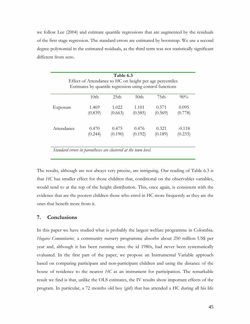
we follow Lee (2004) and estimate quantile regressions that are augmented by the residuals

of the first stage regression. The standard errors are estimated by bootstrap. We use a second

degree polynomial in the estimated residuals, as the third term was not statistically significant

different from zero.

Table 6.3 Effect of Attendance to HC on height per age percentiles Estimates by quantile regression using control functions

10th 25th 50th 75th 90%

Exposure 1.469 (0.839)

1.022 (0.663)

1.101 (0.585)

0.571 (0.569)

0.095 (0.778)

Attendance 0.470 (0.244)

0.475 (0.190)

0.476 (0.192)

0.321 (0.189)

-0.118 (0.233)

Standard errors in parentheses are clustered at the town level.

The results, although are not always very precise, are intriguing. Our reading of Table 6.3 is

that HC has smaller effect for those children that, conditional on the observables variables,

would tend to at the top of the height distribution. This, once again, is consistent with the

evidence that are the poorest children those who enrol in HC more frequently as they are the

ones that benefit more from it.

7. Conclusions In this paper we have studied what is probably the largest welfare programme in Colombia.

Hogares Comunitarios¸ a community nursery programme absorbs about 250 million US$ per

year and, although it has been running since the id 1980s, had never been systematically

evaluated. In the first part of the paper, we propose an Instrumental Variable approach

based on comparing participant and non-participant children and using the distance of the

house of residence to the nearest HC as an instrument for participation. The remarkable

result we find is that, unlike the OLS estimates, the IV results show important effects of the

program. In particular, a 72 months old boy (girl) that has attended a HC during all his life

45

will be 3.78 (3.83) centimetres taller than if he had not attended a HC at all. The negative

bias that characterizes OLS (and PSM) estimates is a consequence of the fact that the

poorest children are those that select into the program. The program, therefore, seems to be

well targeted and to help maintaining the nutritional status of the poorest children.

We show what believe to be credible evidence on the reliability of our instrument: when we

perform the same exercise on birth weight and mother height we do not obtain any effect of

the program. We find similar results when we instrument using only the average distance to a

HC in the municipality. This is important because this instrument is independent of

individual household location decisions.

The programme also has a long run effect: we identify some positive effects on children aged

13-17 who in the past have attended a HC: these children are more likely to be in school and

to have advanced a grade. We estimate positive effects of the programme on mothers

employment rates and hours of work. Finally, in the last section, we explore the issue of

impact heterogeneity and find, once more that the most disadvantaged children seem to be

those that most benefit from the programme.

This evidence is important as the Colombian government is currently considering the

possibility of scrapping the HC programme in favour of conditional cash subsidies. What we

have shown should give an element of caution in implementing these plans.

There is much work that still needs to be done. First, it should be stressed that our results

cannot be extrapolated to different contexts. The large majority of HC in Colombia operates

in large cities and urban areas: our results are from a sample of small towns with an

important rural component. Second, as we have evidence on the effectiveness of the

alternative programme being considered, it would be interesting to compare them explicitly

and model impact heterogeneity, especially in terms of children ages. It might be that the

two programs, rather than being substitutes, are complements. It might be that the youngest

children are best targeted by the conditional cash subsidies, while children aged 2 to 4 might

benefit more from the HC programme.

46

References

Angrist, J. (1998) “Estimating the labour market impact of voluntary military service using social security data on military applicatnts”, Econometrica, 66, 249-88.

Angrist, J. and Imbens, G. (1995) “Two-stage least squares estimation of average causal effects in models with variable treatment instensity”, Journal of the American Statistical Association, 90, 431-42. Attanasio, O., Meghir, C. and M. Vera-Hernández (2004a) “Do Conditonal Cash Transfers Improve Child Health and Nutrition. Evidence from Colombia” Mimeo Attanasio, O., Gómez, L., Gómez, A., and M. Vera-Hernández (2004b) “Child Health in Rural Colombia: Determinants and Policy Interventions” Economics and Human Biology, forthcoming. Attanasio et al. (2003): “Baseline Report on the Evaluation of Familias en Acción”. EDePo-IFS. Available at: http://www.ifs.org.uk/edepo/wps/familias_accion.pdf . Aakvik, A, Heckman, J. and Vytlacil, E. (2002) “Estimating Treatment Effects for Discrete Outcomes when Responses to Treatment Vary: An Application to Norwegian Vocational Rehabilitation Programs”. Mimeo Alderman, H., Behrman, J., Lavy, V., and R. Menon (2001a) “Child Health and School Enrollment. A Longitudinal Analysis”, The Journal of Human Resources, Vol. 36(1), pp. 185-205. Alderman, J., Orazem, P., and E. Paterno (2001b) “School Quality, School Cost, ad the Public/Private School Choices of Low Income Households in Pakistan”, The Journal of Human Resources, Vol. 36(2), pp. 304-326. Behrman, J.R., Cheng, Y. and P.E. Todd (2004): “Evaluating Preschool Programs when Length of Exposure to the Programme Varies: A Nonparametric Approach”, The Review of Economics and Statistics, February, 86(1): 108-132. Behrman, J.R. and J. Hoddinott (2004): “An Evaluation of the Impact of PROGRESA on Pre-School Child Height” , IFPRI, mimeo. Behrman, J., Hoddinott, J., Maluccio, J., Quisumbing, A., Martorell, R., and Stein, A. (2003) “The Impact of Experimental Nutritional Interventions on Education into Adulthood in Rural Guatemala: Preliminary Longitudinal Analysis” Mimeo. Blundell, R., Dearden, L. and Sianesi, B. (2004): “Evaluating the Impact of Education on Earnings in the UK: Models, Methods and Results from the NCDS” forthcoming on The Journal of the Royal Statistical Society: Series A. Buschang PH, Malina RM, Little BB (1986) Linear growth of Zapotec schoolchildren: growth status and yearly velocity for leg length and sitting height. Ann Hum Biol 13:225-233.

47

Carneiro, P, Heckman, J., and Vytlacil, E. (2003) “Understanding What Instrumental Variables Estimate: Estimating Marginal and Average Returns to Education” Mimeo Davey Smith G, Greenwood R, Gunnell D, Sweetnam P, Yarnell Jelwwod P (2001) “Leg length, insulin resistance, and coronary heart disease risk: The caerphilly Study.” Journal of Epidemiology and Community Health, 55:1-6. Gertler, P., Rivera, J., Levy, S. and Sepulveda J. (2004): “Mexico’s PROGRESA: Using a Poverty Alleviation Program as an Incentive for Poor Families to Invest in Child Health”, Mimeo. Glewwe, P., Jacoby, H., King, E. (2001) “Early Childhood nutrition and academic achievement: a longitudinal analysis” Journal of Public Economics 81, pp. 345-368. Gunnell, D., Smith, G.D., Frankel, S., Nanchahal, K. (1998)Childhood leg length and adult mortality: follow up of the Carnegie (Boyd Orr) Survey of Diet and Health in Pre-war Britain Journal of Epidemology and Community Health 52: 142-152. Gunnell, D., Whitlye, E., Upton, M., McConnachie, A., Smith, G.D., Watt, G. (2003) “Associations of height, leg length, and lung function with cardiovascular risk factors in the Midspan Family Study”, Journal of Epidemology and Community Health 57: 141-146. Heckman, J.J. (1979), “Sample selection bias as a specification error”, Econometrica, 47, 153-61. Heckman, J.J., Ichimura, H. and Todd, P. (1997), “Matching as an econometric evaluation estimator: evidence from evaluating a job training programme”, Review of Economic Studies, 64, 605-54. Heckman, J.J., Ichimura, H. and Todd, P. (1998), “Matching as an econometric evaluation estimator”, Review of Economic Studies, 65, 261-94. Heckman, J.J., Ichimura, H., Smith, J. and Todd, P. (1998), “Characterizing selection bias using experimental data”, Econometrica, 66: 1017-98. Imbens, G., and Angrist, J. (1994) “Identification and Estimation of Local Average Treatment Effects”, Econometrica, 62: 467-475. Lee, S. (2004), “Endogeneity in Quantile Regression Models: A Control Function Approach”, Cemmap working paper 08/04. http://cemmap.ifs.org.uk/docs/cwp0804.pdf Leuven, E. and Sianesi, B (2003), “PSMATCH2: Stata module to perform full Mahalanobis and propensity score matching, common support graphing, and covariate imbalance testing”, htpp://ideas.repec.org/c/boc/bocode/s432001.html. Moffitt, R. (2004) “The Effect of Transfer Programs on Labor Supply in the Presence of Prefence Heterogeneity and Variable Takeup” Mimeo.

48

Ruel, M.T.; Brière (de la), B.; Hallman, K.; Quisumbing, A.; Coj, N. (2002): “Does subsidized childcare help poor working women in urban areas?: evaluation of a government-sponsored programme in Guatemala City”, IFPRI, Mimeo. Rosenbaum, P.R. and Rubin, D.B. (1983), "The Central Role of the Propensity Score in Observational Studies for Causal Effects", Biometrika 70, 1, 41-55. Shrimpton, R., Victora, C., de Onis, M., Costa Lima, R., Blössner, M., and Graeme Clugston. (2001), Worldwide Timing of Growth Faltering: Implications for Nutritional Interventions. Pediatrics, May; 107: 75. Wadsworth MEJ, Hardy RJ, Paul AA, Marshall SF & Cole TJ. “Leg and trunk length at 43 years in relation to childhood health, diet and family circumstances; evidence from the 1946 national birth cohort”. International Journal of Epidemiology

49

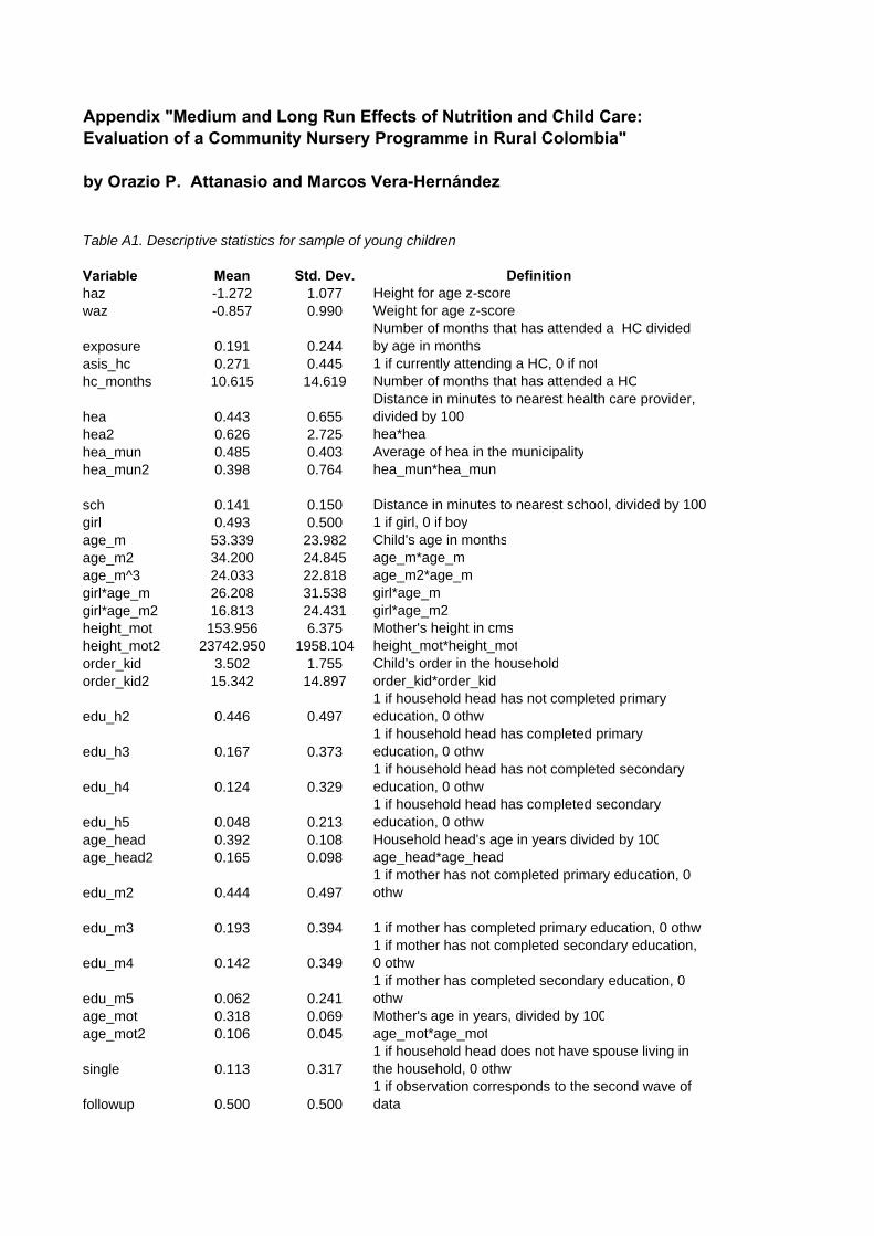
Appendix "Medium and Long Run Effects of Nutrition and Child Care:Evaluation of a Community Nursery Programme in Rural Colombia"

by Orazio P. Attanasio and Marcos Vera-Hernández

Table A1. Descriptive statistics for sample of young children

Variable Mean Std. Dev. Definitionhaz -1.272 1.077 Height for age z-scorewaz -0.857 0.990 Weight for age z-score

exposure 0.191 0.244Number of months that has attended a HC divided by age in months

asis_hc 0.271 0.445 1 if currently attending a HC, 0 if nothc_months 10.615 14.619 Number of months that has attended a HC

hea 0.443 0.655Distance in minutes to nearest health care provider, divided by 100

hea2 0.626 2.725 hea*heahea_mun 0.485 0.403 Average of hea in the municipalityhea_mun2 0.398 0.764 hea_mun*hea_mun

sch 0.141 0.150 Distance in minutes to nearest school, divided by 100girl 0.493 0.500 1 if girl, 0 if boyage_m 53.339 23.982 Child's age in monthsage_m2 34.200 24.845 age_m*age_mage_m^3 24.033 22.818 age_m2*age_mgirl*age_m 26.208 31.538 girl*age_mgirl*age_m2 16.813 24.431 girl*age_m2height_mot 153.956 6.375 Mother's height in cmsheight_mot2 23742.950 1958.104 height_mot*height_motorder_kid 3.502 1.755 Child's order in the householdorder_kid2 15.342 14.897 order_kid*order_kid

edu_h2 0.446 0.4971 if household head has not completed primary education, 0 othw

edu_h3 0.167 0.3731 if household head has completed primary education, 0 othw

edu_h4 0.124 0.3291 if household head has not completed secondary education, 0 othw

edu_h5 0.048 0.2131 if household head has completed secondary education, 0 othw

age_head 0.392 0.108 Household head's age in years divided by 100age_head2 0.165 0.098 age_head*age_head

edu_m2 0.444 0.4971 if mother has not completed primary education, 0 othw

edu_m3 0.193 0.394 1 if mother has completed primary education, 0 othw

edu_m4 0.142 0.3491 if mother has not completed secondary education, 0 othw

edu_m5 0.062 0.2411 if mother has completed secondary education, 0 othw

age_mot 0.318 0.069 Mother's age in years, divided by 100age_mot2 0.106 0.045 age_mot*age_mot

single 0.113 0.3171 if household head does not have spouse living in the household, 0 othw

followup 0.500 0.5001 if observation corresponds to the second wave of data

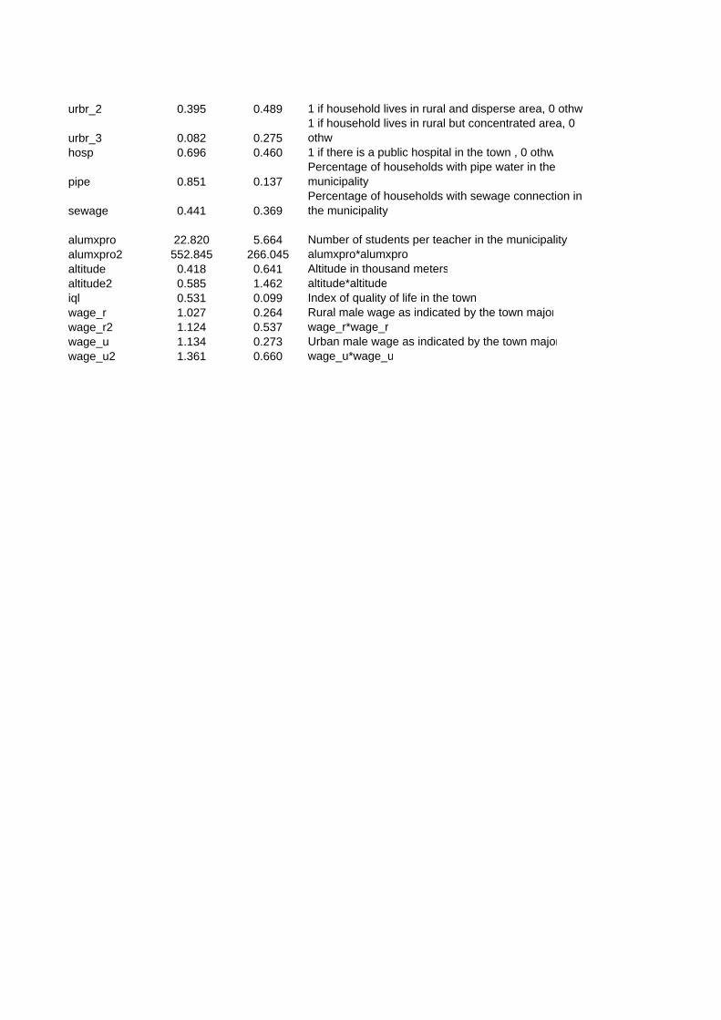
urbr_2 0.395 0.489 1 if household lives in rural and disperse area, 0 othw

urbr_3 0.082 0.2751 if household lives in rural but concentrated area, 0 othw

hosp 0.696 0.460 1 if there is a public hospital in the town , 0 othw

pipe 0.851 0.137Percentage of households with pipe water in the municipality

sewage 0.441 0.369Percentage of households with sewage connection in the municipality

alumxpro 22.820 5.664 Number of students per teacher in the municipalityalumxpro2 552.845 266.045 alumxpro*alumxproaltitude 0.418 0.641 Altitude in thousand metersaltitude2 0.585 1.462 altitude*altitudeiql 0.531 0.099 Index of quality of life in the townwage_r 1.027 0.264 Rural male wage as indicated by the town majorwage_r2 1.124 0.537 wage_r*wage_rwage_u 1.134 0.273 Urban male wage as indicated by the town majorwage_u2 1.361 0.660 wage_u*wage_u

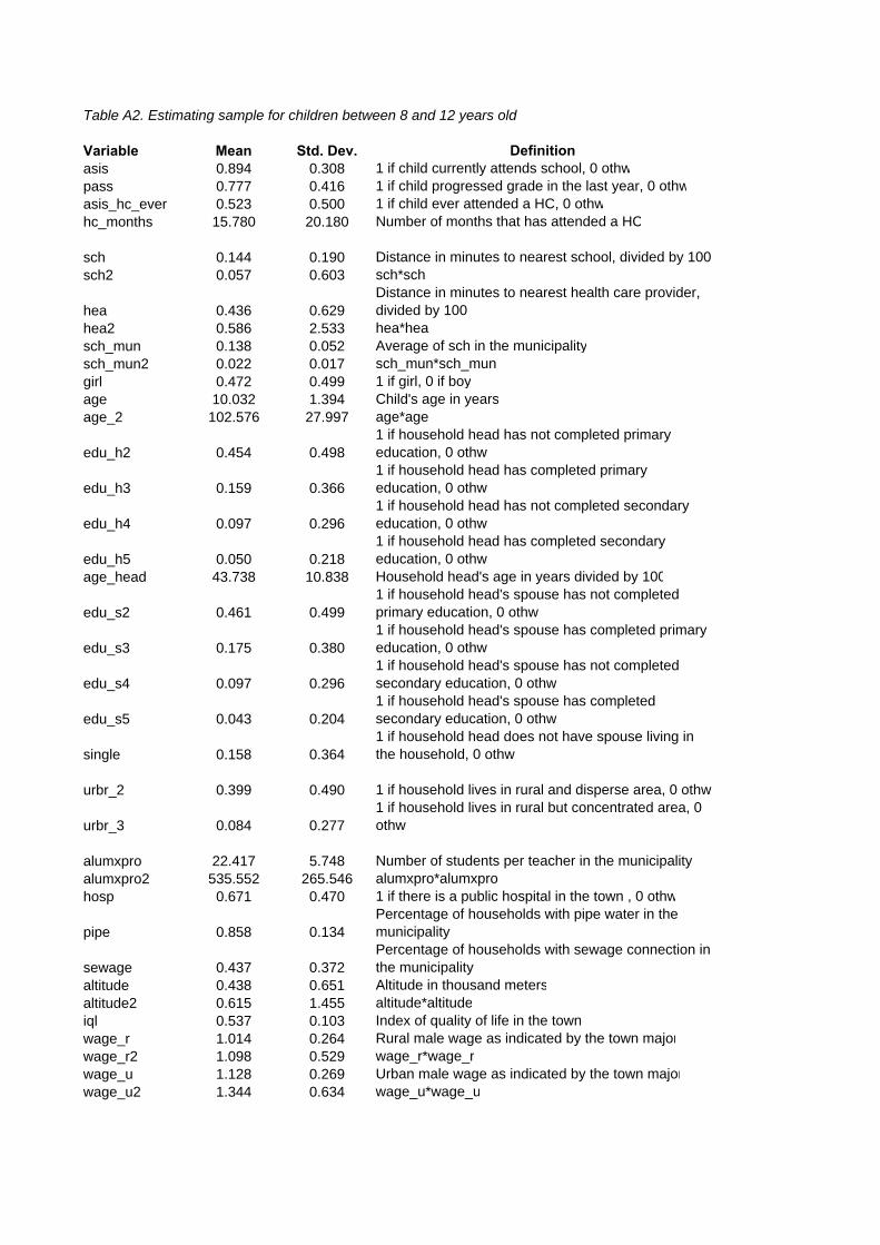
Table A2. Estimating sample for children between 8 and 12 years old

Variable Mean Std. Dev. Definitionasis 0.894 0.308 1 if child currently attends school, 0 othwpass 0.777 0.416 1 if child progressed grade in the last year, 0 othwasis_hc_ever 0.523 0.500 1 if child ever attended a HC, 0 othwhc_months 15.780 20.180 Number of months that has attended a HC

sch 0.144 0.190 Distance in minutes to nearest school, divided by 100sch2 0.057 0.603 sch*sch

hea 0.436 0.629Distance in minutes to nearest health care provider, divided by 100

hea2 0.586 2.533 hea*heasch_mun 0.138 0.052 Average of sch in the municipalitysch_mun2 0.022 0.017 sch_mun*sch_mungirl 0.472 0.499 1 if girl, 0 if boyage 10.032 1.394 Child's age in yearsage_2 102.576 27.997 age*age

edu_h2 0.454 0.4981 if household head has not completed primary education, 0 othw

edu_h3 0.159 0.3661 if household head has completed primary education, 0 othw

edu_h4 0.097 0.2961 if household head has not completed secondary education, 0 othw

edu_h5 0.050 0.2181 if household head has completed secondary education, 0 othw

age_head 43.738 10.838 Household head's age in years divided by 100

edu_s2 0.461 0.4991 if household head's spouse has not completed primary education, 0 othw

edu_s3 0.175 0.3801 if household head's spouse has completed primary education, 0 othw

edu_s4 0.097 0.2961 if household head's spouse has not completed secondary education, 0 othw

edu_s5 0.043 0.2041 if household head's spouse has completed secondary education, 0 othw

single 0.158 0.3641 if household head does not have spouse living in the household, 0 othw

urbr_2 0.399 0.490 1 if household lives in rural and disperse area, 0 othw

urbr_3 0.084 0.2771 if household lives in rural but concentrated area, 0 othw

alumxpro 22.417 5.748 Number of students per teacher in the municipalityalumxpro2 535.552 265.546 alumxpro*alumxprohosp 0.671 0.470 1 if there is a public hospital in the town , 0 othw

pipe 0.858 0.134Percentage of households with pipe water in the municipality

sewage 0.437 0.372Percentage of households with sewage connection in the municipality

altitude 0.438 0.651 Altitude in thousand metersaltitude2 0.615 1.455 altitude*altitudeiql 0.537 0.103 Index of quality of life in the townwage_r 1.014 0.264 Rural male wage as indicated by the town majorwage_r2 1.098 0.529 wage_r*wage_rwage_u 1.128 0.269 Urban male wage as indicated by the town majorwage_u2 1.344 0.634 wage_u*wage_u

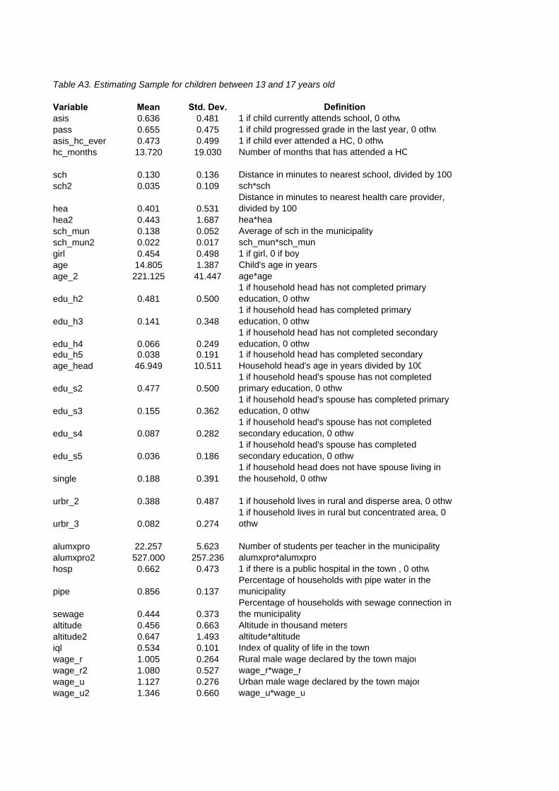
Table A3. Estimating Sample for children between 13 and 17 years old

Variable Mean Std. Dev. Definitionasis 0.636 0.481 1 if child currently attends school, 0 othwpass 0.655 0.475 1 if child progressed grade in the last year, 0 othwasis_hc_ever 0.473 0.499 1 if child ever attended a HC, 0 othwhc_months 13.720 19.030 Number of months that has attended a HC

sch 0.130 0.136 Distance in minutes to nearest school, divided by 100sch2 0.035 0.109 sch*sch

hea 0.401 0.531Distance in minutes to nearest health care provider, divided by 100

hea2 0.443 1.687 hea*heasch_mun 0.138 0.052 Average of sch in the municipalitysch_mun2 0.022 0.017 sch_mun*sch_mungirl 0.454 0.498 1 if girl, 0 if boyage 14.805 1.387 Child's age in yearsage_2 221.125 41.447 age*age

edu_h2 0.481 0.5001 if household head has not completed primary education, 0 othw

edu_h3 0.141 0.3481 if household head has completed primary education, 0 othw

edu_h4 0.066 0.2491 if household head has not completed secondary education, 0 othw

edu_h5 0.038 0.191 1 if household head has completed secondary age_head 46.949 10.511 Household head's age in years divided by 100

edu_s2 0.477 0.5001 if household head's spouse has not completed primary education, 0 othw

edu_s3 0.155 0.3621 if household head's spouse has completed primary education, 0 othw

edu_s4 0.087 0.2821 if household head's spouse has not completed secondary education, 0 othw

edu_s5 0.036 0.1861 if household head's spouse has completed secondary education, 0 othw

single 0.188 0.3911 if household head does not have spouse living in the household, 0 othw

urbr_2 0.388 0.487 1 if household lives in rural and disperse area, 0 othw

urbr_3 0.082 0.2741 if household lives in rural but concentrated area, 0 othw

alumxpro 22.257 5.623 Number of students per teacher in the municipalityalumxpro2 527.000 257.236 alumxpro*alumxprohosp 0.662 0.473 1 if there is a public hospital in the town , 0 othw

pipe 0.856 0.137Percentage of households with pipe water in the municipality

sewage 0.444 0.373Percentage of households with sewage connection in the municipality

altitude 0.456 0.663 Altitude in thousand metersaltitude2 0.647 1.493 altitude*altitudeiql 0.534 0.101 Index of quality of life in the townwage_r 1.005 0.264 Rural male wage declared by the town majorwage_r2 1.080 0.527 wage_r*wage_rwage_u 1.127 0.276 Urban male wage declared by the town majorwage_u2 1.346 0.660 wage_u*wage_u

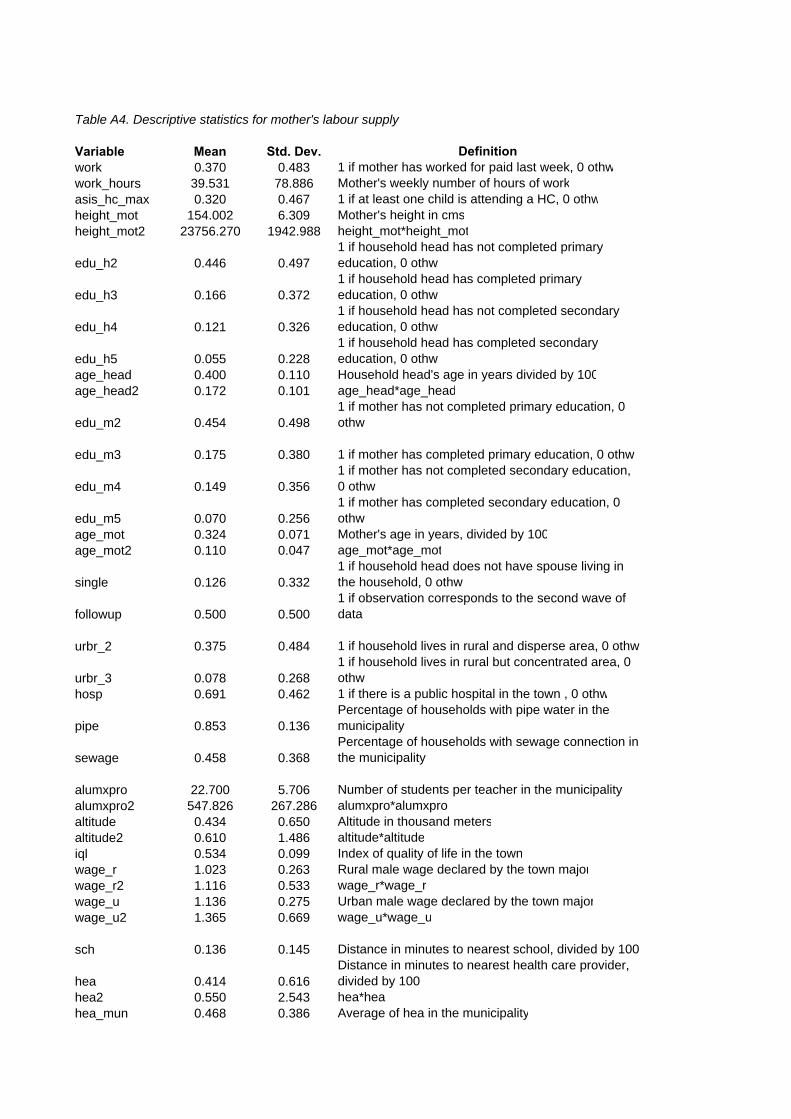
Table A4. Descriptive statistics for mother's labour supply

Variable Mean Std. Dev. Definitionwork 0.370 0.483 1 if mother has worked for paid last week, 0 othwwork_hours 39.531 78.886 Mother's weekly number of hours of workasis_hc_max 0.320 0.467 1 if at least one child is attending a HC, 0 othwheight_mot 154.002 6.309 Mother's height in cmsheight_mot2 23756.270 1942.988 height_mot*height_mot

edu_h2 0.446 0.4971 if household head has not completed primary education, 0 othw

edu_h3 0.166 0.3721 if household head has completed primary education, 0 othw

edu_h4 0.121 0.3261 if household head has not completed secondary education, 0 othw

edu_h5 0.055 0.2281 if household head has completed secondary education, 0 othw

age_head 0.400 0.110 Household head's age in years divided by 100age_head2 0.172 0.101 age_head*age_head

edu_m2 0.454 0.4981 if mother has not completed primary education, 0 othw

edu_m3 0.175 0.380 1 if mother has completed primary education, 0 othw

edu_m4 0.149 0.3561 if mother has not completed secondary education, 0 othw

edu_m5 0.070 0.2561 if mother has completed secondary education, 0 othw

age_mot 0.324 0.071 Mother's age in years, divided by 100age_mot2 0.110 0.047 age_mot*age_mot

single 0.126 0.3321 if household head does not have spouse living in the household, 0 othw

followup 0.500 0.5001 if observation corresponds to the second wave of data

urbr_2 0.375 0.484 1 if household lives in rural and disperse area, 0 othw

urbr_3 0.078 0.2681 if household lives in rural but concentrated area, 0 othw

hosp 0.691 0.462 1 if there is a public hospital in the town , 0 othw

pipe 0.853 0.136Percentage of households with pipe water in the municipality

sewage 0.458 0.368Percentage of households with sewage connection in the municipality

alumxpro 22.700 5.706 Number of students per teacher in the municipalityalumxpro2 547.826 267.286 alumxpro*alumxproaltitude 0.434 0.650 Altitude in thousand metersaltitude2 0.610 1.486 altitude*altitudeiql 0.534 0.099 Index of quality of life in the townwage_r 1.023 0.263 Rural male wage declared by the town majorwage_r2 1.116 0.533 wage_r*wage_rwage_u 1.136 0.275 Urban male wage declared by the town majorwage_u2 1.365 0.669 wage_u*wage_u

sch 0.136 0.145 Distance in minutes to nearest school, divided by 100

hea 0.414 0.616Distance in minutes to nearest health care provider, divided by 100

hea2 0.550 2.543 hea*heahea_mun 0.468 0.386 Average of hea in the municipality

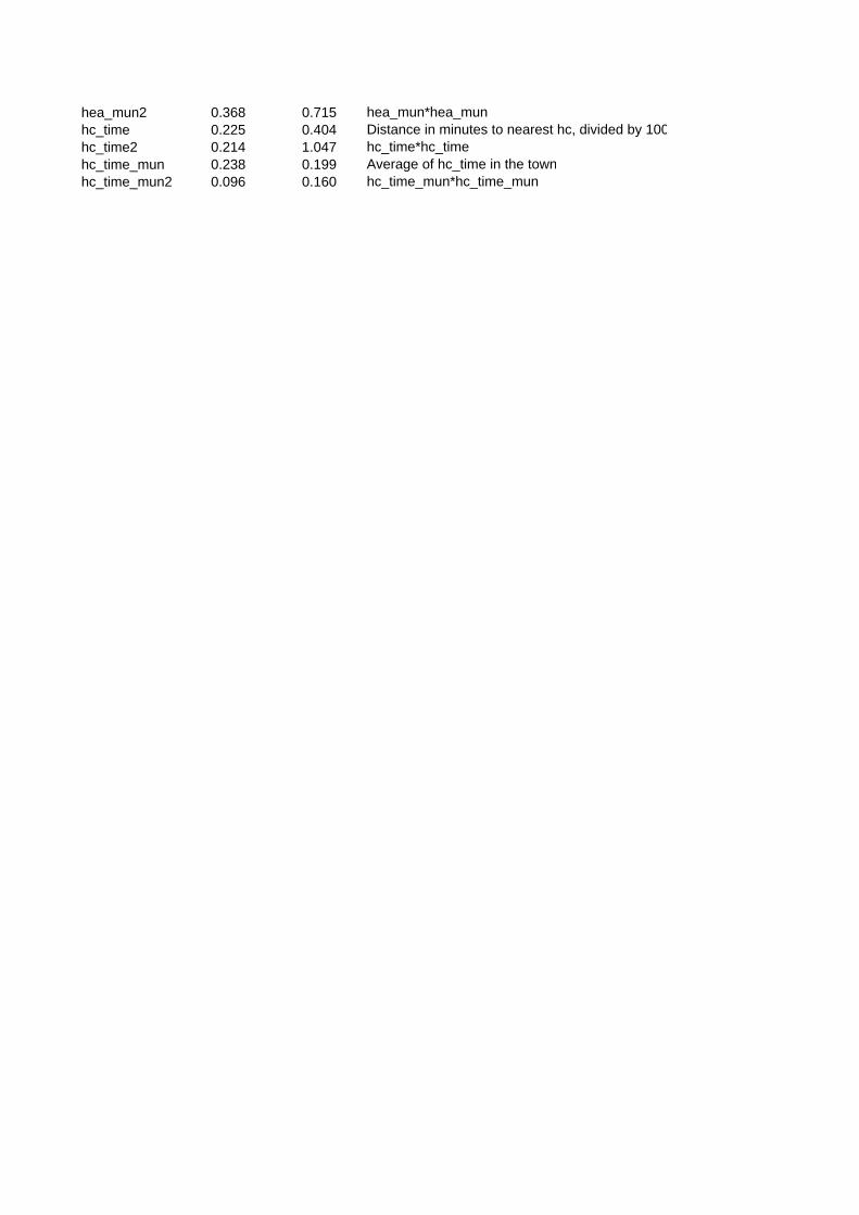
hea_mun2 0.368 0.715 hea_mun*hea_munhc_time 0.225 0.404 Distance in minutes to nearest hc, divided by 100hc_time2 0.214 1.047 hc_time*hc_timehc_time_mun 0.238 0.199 Average of hc_time in the townhc_time_mun2 0.096 0.160 hc_time_mun*hc_time_mun

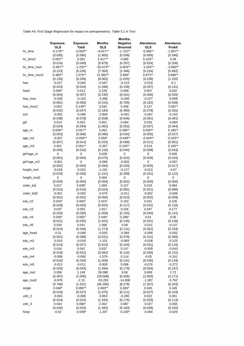
Table A4. First Stage Regression for impact on antropometrics. Table 5.1 in Text

Exposure. OLS

Exposure. Tobit

Months. OLS

Months. Negative Binomial

Atendance. OLS

Atendance. Probit

hc_time -0.178** -0.553** -9.917** -1.722** -0.366** -1.907**[0.035] [0.080] [1.900] [0.508] [0.059] [0.346]

hc_time2 0.052** 0.091 2.917** 0.085 0.104** 0.39[0.016] [0.049] [0.879] [0.297] [0.024] [0.206]

hc_time_mun -0.587** -1.232** -26.474** -4.403** -1.042** -3.960**[0.123] [0.226] [7.354] [1.346] [0.216] [0.982]

hc_time_mun2 0.483** 1.075** 21.682** 3.599* 0.973** 3.668**[0.130] [0.269] [8.063] [1.625] [0.238] [1.255]

hea -0.027 -0.045 -0.567 -0.219 -0.019 -0.1[0.023] [0.034] [1.268] [0.159] [0.037] [0.131]

hea2 0.008* 0.013 0.228 0.058 0.007 0.032[0.004] [0.007] [0.230] [0.041] [0.006] [0.026]

hea_mun -0.036 -0.154 -3.396 -0.348 -0.227 -0.858[0.081] [0.093] [4.315] [0.765] [0.162] [0.558]

hea_mun2 0.053 0.149** 3.042 0.458 0.147 0.587*[0.042] [0.047] [2.184] [0.480] [0.078] [0.281]

sch -0.055 -0.096 -2.859 -0.091 -0.067 -0.102[0.038] [0.078] [2.058] [0.646] [0.081] [0.481]

girl 0.014 0.023 0.451 0.064 0.025 -0.064[0.024] [0.094] [1.062] [0.552] [0.037] [0.344]

age_m 0.009** 0.057** 0.062 0.288** 0.030** 0.185**[0.003] [0.006] [0.096] [0.034] [0.005] [0.027]

age_m2 -0.007 -0.093** 0.559* -0.448** -0.044** -0.325**[0.007] [0.014] [0.253] [0.068] [0.011] [0.061]

age_m3 0.001 0.051** -0.367 0.245** 0.014 0.156**[0.005] [0.010] [0.216] [0.044] [0.008] [0.043]

girl*age_m 0 0 0.028 0 0 0.006[0.001] [0.004] [0.075] [0.022] [0.003] [0.016]

girl*age_m2 -0.001 0 -0.068 -0.003 0 -0.007[0.002] [0.004] [0.094] [0.020] [0.003] [0.017]

height_mot -0.018 -0.023 -1.191 -0.127 -0.013 -0.07[0.019] [0.035] [1.151] [0.289] [0.031] [0.122]

height_mot2 0 0 0.004 0 0 0[0.000] [0.000] [0.004] [0.001] [0.000] [0.000]

order_kid 0.017 0.038* 1.059 0.127 0.019 0.084[0.010] [0.019] [0.624] [0.081] [0.021] [0.080]

order_kid2 -0.001 -0.003 -0.076 -0.011 -0.002 -0.008[0.001] [0.002] [0.060] [0.010] [0.002] [0.009]

edu_h2 0.043* 0.060* 2.415* 0.163 0.031 0.105[0.018] [0.025] [0.924] [0.117] [0.031] [0.116]

edu_h3 0.037 0.053 1.917 0.226 0.047 0.177[0.020] [0.030] [1.059] [0.154] [0.040] [0.141]

edu_h4 0.048* 0.082* 2.446* 0.286* 0.01 0.05[0.021] [0.032] [1.022] [0.145] [0.041] [0.146]

edu_h5 0.034 0.041 1.568 0.09 -0.021 -0.127[0.024] [0.046] [1.273] [0.131] [0.062] [0.234]

age_head -0.01 -0.048 -0.555 -0.084 -0.006 -0.002[0.051] [0.089] [3.031] [0.378] [0.101] [0.365]

edu_m2 -0.016 -0.018 -1.101 -0.083 -0.028 -0.125[0.014] [0.027] [0.810] [0.104] [0.031] [0.116]

edu_m3 0.016 0.041 0.637 0.147 -0.009 -0.043[0.018] [0.031] [0.992] [0.142] [0.036] [0.131]

edu_m4 -0.008 -0.006 -1.079 0.114 -0.05 -0.161[0.016] [0.034] [1.006] [0.141] [0.035] [0.134]

edu_m5 -0.013 -0.011 -0.928 0.096 -0.076 -0.272[0.029] [0.043] [1.494] [0.179] [0.054] [0.197]

age_mot 0.556 1.149 28.088 8.58 0.659 2.72[0.497] [1.065] [29.568] [5.406] [1.063] [4.171]

age_mot2 -0.978 -2.15 -53.293 -14.008 -1.387 -5.762[0.768] [1.631] [46.285] [8.278] [1.557] [6.203]

single 0.048* 0.095** 2.993** 0.283* 0.045 0.165[0.019] [0.027] [1.075] [0.111] [0.027] [0.104]

urbr_2 -0.004 -0.008 -0.853 -0.206 0.022 0.091[0.024] [0.024] [1.334] [0.176] [0.029] [0.113]

urbr_3 0.044 0.066* 2.352 0.087 -0.027 -0.094[0.030] [0.033] [1.465] [0.160] [0.038] [0.150]

hosp -0.02 -0.048* -1.297 -0.230* -0.004 -0.029

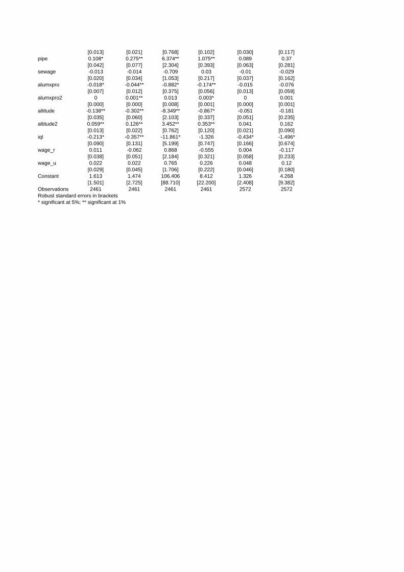
[0.013] [0.021] [0.768] [0.102] [0.030] [0.117]pipe 0.108* 0.275** 6.374** 1.075** 0.089 0.37

[0.042] [0.077] [2.304] [0.393] [0.063] [0.281]sewage -0.013 -0.014 -0.709 0.03 -0.01 -0.029

[0.020] [0.034] [1.053] [0.217] [0.037] [0.162]alumxpro -0.018* -0.044** -0.882* -0.174** -0.015 -0.076

[0.007] [0.012] [0.375] [0.056] [0.013] [0.059]alumxpro2 0 0.001** 0.013 0.003* 0 0.001

[0.000] [0.000] [0.008] [0.001] [0.000] [0.001]altitude -0.138** -0.302** -8.349** -0.867* -0.051 -0.181

[0.035] [0.060] [2.103] [0.337] [0.051] [0.235]altitude2 0.059** 0.126** 3.452** 0.353** 0.041 0.162

[0.013] [0.022] [0.762] [0.120] [0.021] [0.090]iql -0.213* -0.357** -11.861* -1.326 -0.434* -1.496*

[0.090] [0.131] [5.199] [0.747] [0.166] [0.674]wage_r 0.011 -0.062 0.868 -0.555 0.004 -0.117

[0.038] [0.051] [2.184] [0.321] [0.058] [0.233]wage_u 0.022 0.022 0.765 0.226 0.048 0.12

[0.029] [0.045] [1.706] [0.222] [0.046] [0.180]Constant 1.613 1.474 106.406 8.412 1.326 4.268

[1.501] [2.725] [88.710] [22.200] [2.408] [9.382]Observations 2461 2461 2461 2461 2572 2572Robust standard errors in brackets* significant at 5%; ** significant at 1%

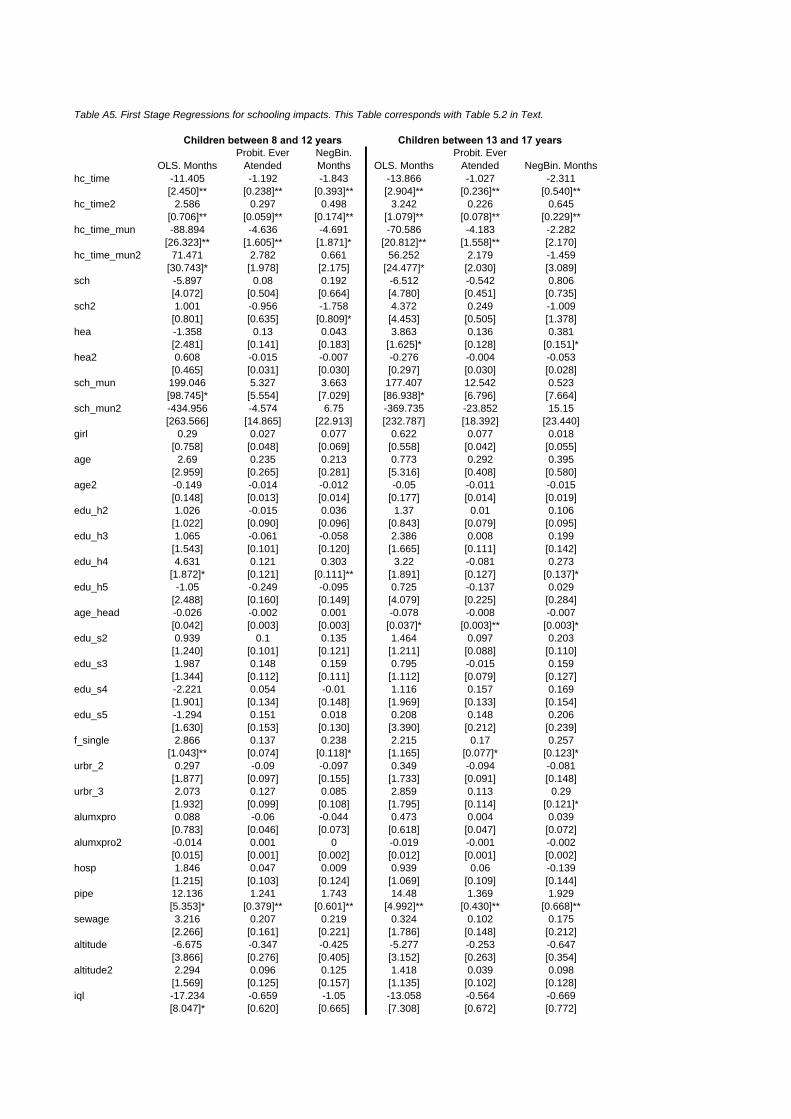
Table A5. First Stage Regressions for schooling impacts. This Table corresponds with Table 5.2 in Text.

Children between 8 and 12 years Children between 13 and 17 years

OLS. MonthsProbit. Ever

AtendedNegBin. Months OLS. Months

Probit. Ever Atended NegBin. Months

hc_time -11.405 -1.192 -1.843 -13.866 -1.027 -2.311[2.450]** [0.238]** [0.393]** [2.904]** [0.236]** [0.540]**

hc_time2 2.586 0.297 0.498 3.242 0.226 0.645[0.706]** [0.059]** [0.174]** [1.079]** [0.078]** [0.229]**

hc_time_mun -88.894 -4.636 -4.691 -70.586 -4.183 -2.282[26.323]** [1.605]** [1.871]* [20.812]** [1.558]** [2.170]

hc_time_mun2 71.471 2.782 0.661 56.252 2.179 -1.459[30.743]* [1.978] [2.175] [24.477]* [2.030] [3.089]

sch -5.897 0.08 0.192 -6.512 -0.542 0.806[4.072] [0.504] [0.664] [4.780] [0.451] [0.735]

sch2 1.001 -0.956 -1.758 4.372 0.249 -1.009[0.801] [0.635] [0.809]* [4.453] [0.505] [1.378]

hea -1.358 0.13 0.043 3.863 0.136 0.381[2.481] [0.141] [0.183] [1.625]* [0.128] [0.151]*

hea2 0.608 -0.015 -0.007 -0.276 -0.004 -0.053[0.465] [0.031] [0.030] [0.297] [0.030] [0.028]

sch_mun 199.046 5.327 3.663 177.407 12.542 0.523[98.745]* [5.554] [7.029] [86.938]* [6.796] [7.664]

sch_mun2 -434.956 -4.574 6.75 -369.735 -23.852 15.15[263.566] [14.865] [22.913] [232.787] [18.392] [23.440]

girl 0.29 0.027 0.077 0.622 0.077 0.018[0.758] [0.048] [0.069] [0.558] [0.042] [0.055]

age 2.69 0.235 0.213 0.773 0.292 0.395[2.959] [0.265] [0.281] [5.316] [0.408] [0.580]

age2 -0.149 -0.014 -0.012 -0.05 -0.011 -0.015[0.148] [0.013] [0.014] [0.177] [0.014] [0.019]

edu_h2 1.026 -0.015 0.036 1.37 0.01 0.106[1.022] [0.090] [0.096] [0.843] [0.079] [0.095]

edu_h3 1.065 -0.061 -0.058 2.386 0.008 0.199[1.543] [0.101] [0.120] [1.665] [0.111] [0.142]

edu_h4 4.631 0.121 0.303 3.22 -0.081 0.273[1.872]* [0.121] [0.111]** [1.891] [0.127] [0.137]*

edu_h5 -1.05 -0.249 -0.095 0.725 -0.137 0.029[2.488] [0.160] [0.149] [4.079] [0.225] [0.284]

age_head -0.026 -0.002 0.001 -0.078 -0.008 -0.007[0.042] [0.003] [0.003] [0.037]* [0.003]** [0.003]*

edu_s2 0.939 0.1 0.135 1.464 0.097 0.203[1.240] [0.101] [0.121] [1.211] [0.088] [0.110]

edu_s3 1.987 0.148 0.159 0.795 -0.015 0.159[1.344] [0.112] [0.111] [1.112] [0.079] [0.127]

edu_s4 -2.221 0.054 -0.01 1.116 0.157 0.169[1.901] [0.134] [0.148] [1.969] [0.133] [0.154]

edu_s5 -1.294 0.151 0.018 0.208 0.148 0.206[1.630] [0.153] [0.130] [3.390] [0.212] [0.239]

f_single 2.866 0.137 0.238 2.215 0.17 0.257[1.043]** [0.074] [0.118]* [1.165] [0.077]* [0.123]*

urbr_2 0.297 -0.09 -0.097 0.349 -0.094 -0.081[1.877] [0.097] [0.155] [1.733] [0.091] [0.148]

urbr_3 2.073 0.127 0.085 2.859 0.113 0.29[1.932] [0.099] [0.108] [1.795] [0.114] [0.121]*

alumxpro 0.088 -0.06 -0.044 0.473 0.004 0.039[0.783] [0.046] [0.073] [0.618] [0.047] [0.072]

alumxpro2 -0.014 0.001 0 -0.019 -0.001 -0.002[0.015] [0.001] [0.002] [0.012] [0.001] [0.002]

hosp 1.846 0.047 0.009 0.939 0.06 -0.139[1.215] [0.103] [0.124] [1.069] [0.109] [0.144]

pipe 12.136 1.241 1.743 14.48 1.369 1.929[5.353]* [0.379]** [0.601]** [4.992]** [0.430]** [0.668]**

sewage 3.216 0.207 0.219 0.324 0.102 0.175[2.266] [0.161] [0.221] [1.786] [0.148] [0.212]

altitude -6.675 -0.347 -0.425 -5.277 -0.253 -0.647[3.866] [0.276] [0.405] [3.152] [0.263] [0.354]

altitude2 2.294 0.096 0.125 1.418 0.039 0.098[1.569] [0.125] [0.157] [1.135] [0.102] [0.128]

iql -17.234 -0.659 -1.05 -13.058 -0.564 -0.669[8.047]* [0.620] [0.665] [7.308] [0.672] [0.772]

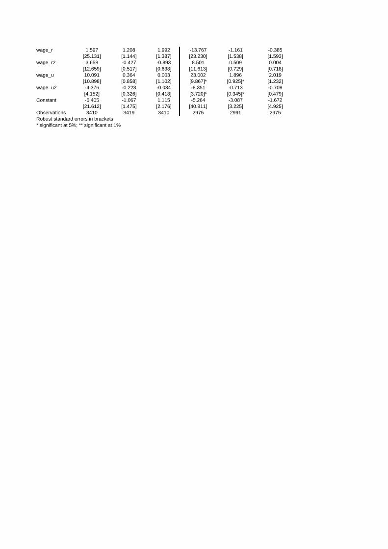
wage_r 1.597 1.208 1.992 -13.767 -1.161 -0.385[25.131] [1.144] [1.387] [23.230] [1.538] [1.593]

wage_r2 3.658 -0.427 -0.893 8.501 0.509 0.004[12.659] [0.517] [0.638] [11.613] [0.729] [0.718]

wage_u 10.091 0.364 0.003 23.002 1.896 2.019[10.898] [0.858] [1.102] [9.867]* [0.925]* [1.232]

wage_u2 -4.376 -0.228 -0.034 -8.351 -0.713 -0.708[4.152] [0.326] [0.418] [3.720]* [0.345]* [0.479]

Constant -6.405 -1.067 1.115 -5.264 -3.087 -1.672[21.612] [1.475] [2.176] [40.811] [3.225] [4.925]

Observations 3410 3419 3410 2975 2991 2975Robust standard errors in brackets* significant at 5%; ** significant at 1%

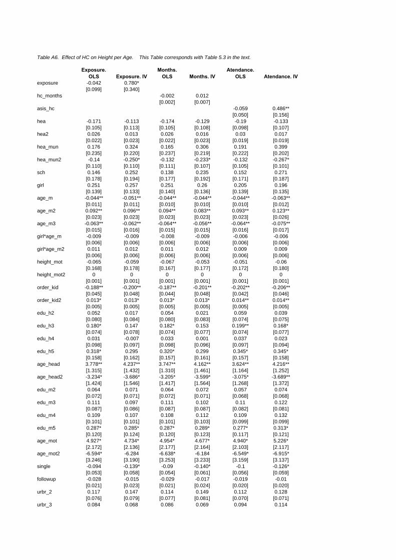
Table A6. Effect of HC on Height per Age. This Table corresponds with Table 5.3 in the text.

Exposure. OLS Exposure. IV

Months. OLS Months. IV

Atendance. OLS Atendance. IV

exposure -0.042 0.780*[0.099] [0.340]

hc_months -0.002 0.012[0.002] [0.007]

asis_hc -0.059 0.486**[0.050] [0.156]

hea -0.171 -0.113 -0.174 -0.129 -0.19 -0.133[0.105] [0.113] [0.105] [0.108] [0.098] [0.107]

hea2 0.026 0.013 0.026 0.016 0.03 0.017[0.022] [0.023] [0.022] [0.023] [0.019] [0.019]

hea_mun 0.176 0.324 0.165 0.306 0.191 0.399[0.235] [0.220] [0.237] [0.219] [0.222] [0.202]

hea_mun2 -0.14 -0.250* -0.132 -0.233* -0.132 -0.267*[0.110] [0.110] [0.111] [0.107] [0.105] [0.101]

sch 0.146 0.252 0.138 0.235 0.152 0.271[0.178] [0.194] [0.177] [0.192] [0.171] [0.187]

girl 0.251 0.257 0.251 0.26 0.205 0.196[0.139] [0.133] [0.140] [0.136] [0.139] [0.135]

age_m -0.044** -0.051** -0.044** -0.044** -0.044** -0.063**[0.011] [0.011] [0.010] [0.010] [0.010] [0.012]

age_m2 0.092** 0.096** 0.094** 0.083** 0.093** 0.123**[0.023] [0.023] [0.023] [0.023] [0.023] [0.026]

age_m3 -0.063** -0.062** -0.064** -0.056** -0.064** -0.075**[0.015] [0.016] [0.015] [0.015] [0.016] [0.017]

girl*age_m -0.009 -0.009 -0.008 -0.009 -0.006 -0.006[0.006] [0.006] [0.006] [0.006] [0.006] [0.006]

girl*age_m2 0.011 0.012 0.011 0.012 0.009 0.009[0.006] [0.006] [0.006] [0.006] [0.006] [0.006]

height_mot -0.065 -0.059 -0.067 -0.053 -0.051 -0.06[0.168] [0.178] [0.167] [0.177] [0.172] [0.180]

height_mot2 0 0 0 0 0 0[0.001] [0.001] [0.001] [0.001] [0.001] [0.001]

order_kid -0.188** -0.200** -0.187** -0.201** -0.202** -0.206**[0.045] [0.048] [0.044] [0.048] [0.042] [0.046]

order_kid2 0.013* 0.013* 0.013* 0.013* 0.014** 0.014**[0.005] [0.005] [0.005] [0.005] [0.005] [0.005]

edu_h2 0.052 0.017 0.054 0.021 0.059 0.039[0.080] [0.084] [0.080] [0.083] [0.074] [0.075]

edu_h3 0.180* 0.147 0.182* 0.153 0.199** 0.168*[0.074] [0.078] [0.074] [0.077] [0.074] [0.077]

edu_h4 0.031 -0.007 0.033 0.001 0.037 0.023[0.098] [0.097] [0.098] [0.096] [0.097] [0.094]

edu_h5 0.318* 0.295 0.320* 0.299 0.345* 0.345*[0.158] [0.162] [0.157] [0.161] [0.157] [0.158]

age_head 3.778** 4.237** 3.747** 4.162** 3.624** 4.216**[1.315] [1.432] [1.310] [1.461] [1.164] [1.252]

age_head2 -3.234* -3.686* -3.205* -3.599* -3.075* -3.689**[1.424] [1.546] [1.417] [1.564] [1.268] [1.372]

edu_m2 0.064 0.071 0.064 0.072 0.057 0.074[0.072] [0.071] [0.072] [0.071] [0.068] [0.068]

edu_m3 0.111 0.097 0.111 0.102 0.11 0.122[0.087] [0.086] [0.087] [0.087] [0.082] [0.081]

edu_m4 0.109 0.107 0.108 0.112 0.109 0.132[0.101] [0.101] [0.101] [0.103] [0.099] [0.099]

edu_m5 0.287* 0.285* 0.287* 0.289* 0.277* 0.313*[0.120] [0.124] [0.120] [0.123] [0.117] [0.121]

age_mot 4.927* 4.734* 4.954* 4.677* 4.940* 5.226*[2.172] [2.136] [2.177] [2.164] [2.103] [2.117]

age_mot2 -6.594* -6.284 -6.638* -6.184 -6.549* -6.915*[3.246] [3.190] [3.253] [3.233] [3.159] [3.137]

single -0.094 -0.139* -0.09 -0.140* -0.1 -0.126*[0.053] [0.058] [0.054] [0.061] [0.056] [0.059]

followup -0.028 -0.015 -0.029 -0.017 -0.019 -0.01[0.021] [0.023] [0.021] [0.024] [0.020] [0.020]

urbr_2 0.117 0.147 0.114 0.149 0.112 0.128[0.076] [0.079] [0.077] [0.081] [0.070] [0.071]

urbr_3 0.084 0.068 0.086 0.069 0.094 0.114

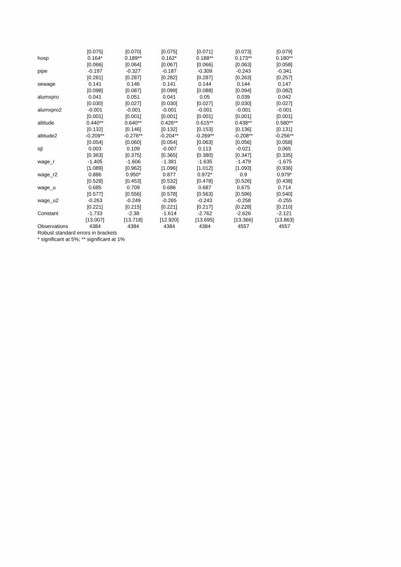
[0.075] [0.070] [0.075] [0.071] [0.073] [0.079]hosp 0.164* 0.189** 0.162* 0.188** 0.173** 0.180**

[0.066] [0.064] [0.067] [0.066] [0.063] [0.058]pipe -0.197 -0.327 -0.187 -0.309 -0.243 -0.341

[0.281] [0.287] [0.282] [0.287] [0.263] [0.257]sewage 0.141 0.146 0.141 0.144 0.144 0.147

[0.098] [0.087] [0.099] [0.088] [0.094] [0.082]alumxpro 0.041 0.051 0.041 0.05 0.039 0.042

[0.030] [0.027] [0.030] [0.027] [0.030] [0.027]alumxpro2 -0.001 -0.001 -0.001 -0.001 -0.001 -0.001

[0.001] [0.001] [0.001] [0.001] [0.001] [0.001]altitude 0.440** 0.640** 0.426** 0.615** 0.438** 0.580**

[0.132] [0.146] [0.132] [0.153] [0.136] [0.131]altitude2 -0.209** -0.276** -0.204** -0.269** -0.208** -0.256**

[0.054] [0.060] [0.054] [0.063] [0.056] [0.058]iql 0.003 0.109 -0.007 0.113 -0.021 0.065

[0.363] [0.375] [0.365] [0.380] [0.347] [0.335]wage_r -1.405 -1.606 -1.381 -1.635 -1.479 -1.675

[1.089] [0.962] [1.096] [1.012] [1.093] [0.936]wage_r2 0.886 0.950* 0.877 0.972* 0.9 0.979*

[0.528] [0.453] [0.532] [0.478] [0.526] [0.438]wage_u 0.685 0.709 0.686 0.687 0.675 0.714

[0.577] [0.556] [0.578] [0.563] [0.596] [0.540]wage_u2 -0.263 -0.249 -0.265 -0.243 -0.258 -0.255

[0.221] [0.215] [0.221] [0.217] [0.228] [0.210]Constant -1.733 -2.38 -1.614 -2.762 -2.626 -2.121

[13.007] [13.718] [12.920] [13.695] [13.366] [13.863]Observations 4384 4384 4384 4384 4557 4557Robust standard errors in brackets* significant at 5%; ** significant at 1%

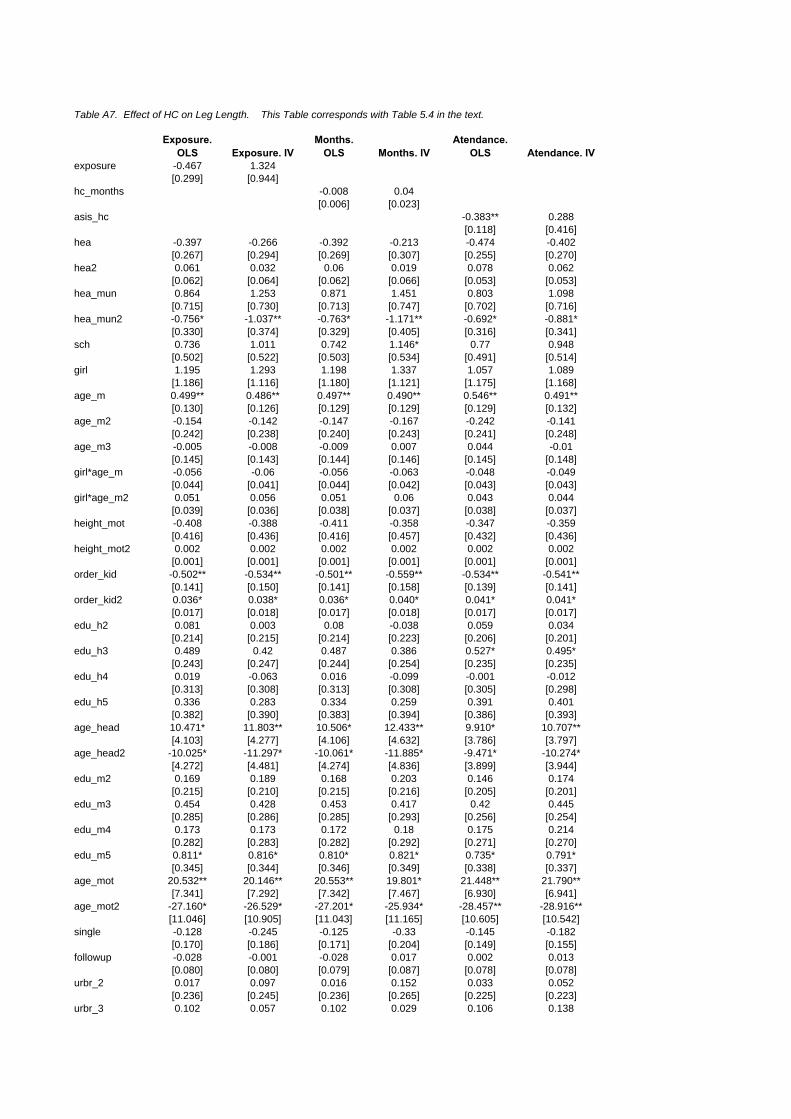
Table A7. Effect of HC on Leg Length. This Table corresponds with Table 5.4 in the text.

Exposure. OLS Exposure. IV

Months. OLS Months. IV

Atendance. OLS Atendance. IV

exposure -0.467 1.324[0.299] [0.944]

hc_months -0.008 0.04[0.006] [0.023]

asis_hc -0.383** 0.288[0.118] [0.416]

hea -0.397 -0.266 -0.392 -0.213 -0.474 -0.402[0.267] [0.294] [0.269] [0.307] [0.255] [0.270]

hea2 0.061 0.032 0.06 0.019 0.078 0.062[0.062] [0.064] [0.062] [0.066] [0.053] [0.053]

hea_mun 0.864 1.253 0.871 1.451 0.803 1.098[0.715] [0.730] [0.713] [0.747] [0.702] [0.716]

hea_mun2 -0.756* -1.037** -0.763* -1.171** -0.692* -0.881*[0.330] [0.374] [0.329] [0.405] [0.316] [0.341]

sch 0.736 1.011 0.742 1.146* 0.77 0.948[0.502] [0.522] [0.503] [0.534] [0.491] [0.514]

girl 1.195 1.293 1.198 1.337 1.057 1.089[1.186] [1.116] [1.180] [1.121] [1.175] [1.168]

age_m 0.499** 0.486** 0.497** 0.490** 0.546** 0.491**[0.130] [0.126] [0.129] [0.129] [0.129] [0.132]

age_m2 -0.154 -0.142 -0.147 -0.167 -0.242 -0.141[0.242] [0.238] [0.240] [0.243] [0.241] [0.248]

age_m3 -0.005 -0.008 -0.009 0.007 0.044 -0.01[0.145] [0.143] [0.144] [0.146] [0.145] [0.148]

girl*age_m -0.056 -0.06 -0.056 -0.063 -0.048 -0.049[0.044] [0.041] [0.044] [0.042] [0.043] [0.043]

girl*age_m2 0.051 0.056 0.051 0.06 0.043 0.044[0.039] [0.036] [0.038] [0.037] [0.038] [0.037]

height_mot -0.408 -0.388 -0.411 -0.358 -0.347 -0.359[0.416] [0.436] [0.416] [0.457] [0.432] [0.436]

height_mot2 0.002 0.002 0.002 0.002 0.002 0.002[0.001] [0.001] [0.001] [0.001] [0.001] [0.001]

order_kid -0.502** -0.534** -0.501** -0.559** -0.534** -0.541**[0.141] [0.150] [0.141] [0.158] [0.139] [0.141]

order_kid2 0.036* 0.038* 0.036* 0.040* 0.041* 0.041*[0.017] [0.018] [0.017] [0.018] [0.017] [0.017]

edu_h2 0.081 0.003 0.08 -0.038 0.059 0.034[0.214] [0.215] [0.214] [0.223] [0.206] [0.201]

edu_h3 0.489 0.42 0.487 0.386 0.527* 0.495*[0.243] [0.247] [0.244] [0.254] [0.235] [0.235]

edu_h4 0.019 -0.063 0.016 -0.099 -0.001 -0.012[0.313] [0.308] [0.313] [0.308] [0.305] [0.298]

edu_h5 0.336 0.283 0.334 0.259 0.391 0.401[0.382] [0.390] [0.383] [0.394] [0.386] [0.393]

age_head 10.471* 11.803** 10.506* 12.433** 9.910* 10.707**[4.103] [4.277] [4.106] [4.632] [3.786] [3.797]

age_head2 -10.025* -11.297* -10.061* -11.885* -9.471* -10.274*[4.272] [4.481] [4.274] [4.836] [3.899] [3.944]

edu_m2 0.169 0.189 0.168 0.203 0.146 0.174[0.215] [0.210] [0.215] [0.216] [0.205] [0.201]

edu_m3 0.454 0.428 0.453 0.417 0.42 0.445[0.285] [0.286] [0.285] [0.293] [0.256] [0.254]

edu_m4 0.173 0.173 0.172 0.18 0.175 0.214[0.282] [0.283] [0.282] [0.292] [0.271] [0.270]

edu_m5 0.811* 0.816* 0.810* 0.821* 0.735* 0.791*[0.345] [0.344] [0.346] [0.349] [0.338] [0.337]

age_mot 20.532** 20.146** 20.553** 19.801* 21.448** 21.790**[7.341] [7.292] [7.342] [7.467] [6.930] [6.941]

age_mot2 -27.160* -26.529* -27.201* -25.934* -28.457** -28.916**[11.046] [10.905] [11.043] [11.165] [10.605] [10.542]

single -0.128 -0.245 -0.125 -0.33 -0.145 -0.182[0.170] [0.186] [0.171] [0.204] [0.149] [0.155]

followup -0.028 -0.001 -0.028 0.017 0.002 0.013[0.080] [0.080] [0.079] [0.087] [0.078] [0.078]

urbr_2 0.017 0.097 0.016 0.152 0.033 0.052[0.236] [0.245] [0.236] [0.265] [0.225] [0.223]

urbr_3 0.102 0.057 0.102 0.029 0.106 0.138

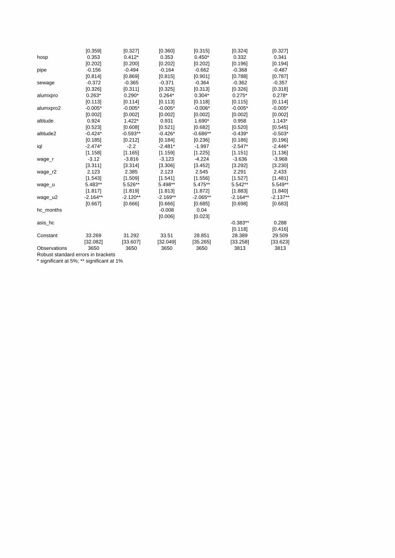
[0.359] [0.327] [0.360] [0.315] [0.324] [0.327]hosp 0.353 0.412* 0.353 0.450* 0.332 0.341

[0.202] [0.200] [0.202] [0.202] [0.196] [0.194]pipe -0.156 -0.494 -0.164 -0.662 -0.368 -0.487

[0.814] [0.869] [0.815] [0.901] [0.788] [0.787]sewage -0.372 -0.365 -0.371 -0.364 -0.362 -0.357

[0.326] [0.311] [0.325] [0.313] [0.326] [0.318]alumxpro 0.263* 0.290* 0.264* 0.304* 0.275* 0.278*

[0.113] [0.114] [0.113] [0.118] [0.115] [0.114]alumxpro2 -0.005* -0.005* -0.005* -0.006* -0.005* -0.005*

[0.002] [0.002] [0.002] [0.002] [0.002] [0.002]altitude 0.924 1.422* 0.931 1.690* 0.958 1.143*

[0.523] [0.608] [0.521] [0.682] [0.520] [0.545]altitude2 -0.424* -0.593** -0.426* -0.686** -0.439* -0.503*

[0.185] [0.212] [0.184] [0.236] [0.186] [0.196]iql -2.474* -2.2 -2.481* -1.997 -2.547* -2.446*

[1.158] [1.165] [1.159] [1.225] [1.151] [1.136]wage_r -3.12 -3.816 -3.123 -4.224 -3.636 -3.968

[3.311] [3.314] [3.306] [3.452] [3.292] [3.230]wage_r2 2.123 2.385 2.123 2.545 2.291 2.433

[1.543] [1.509] [1.541] [1.556] [1.527] [1.481]wage_u 5.483** 5.526** 5.498** 5.475** 5.542** 5.549**

[1.817] [1.819] [1.813] [1.872] [1.883] [1.840]wage_u2 -2.164** -2.120** -2.169** -2.065** -2.164** -2.137**

[0.667] [0.666] [0.666] [0.685] [0.698] [0.683]hc_months -0.008 0.04

[0.006] [0.023]asis_hc -0.383** 0.288

[0.118] [0.416]Constant 33.269 31.292 33.51 28.851 28.389 29.509

[32.082] [33.607] [32.049] [35.265] [33.258] [33.623]Observations 3650 3650 3650 3650 3813 3813Robust standard errors in brackets* significant at 5%; ** significant at 1%

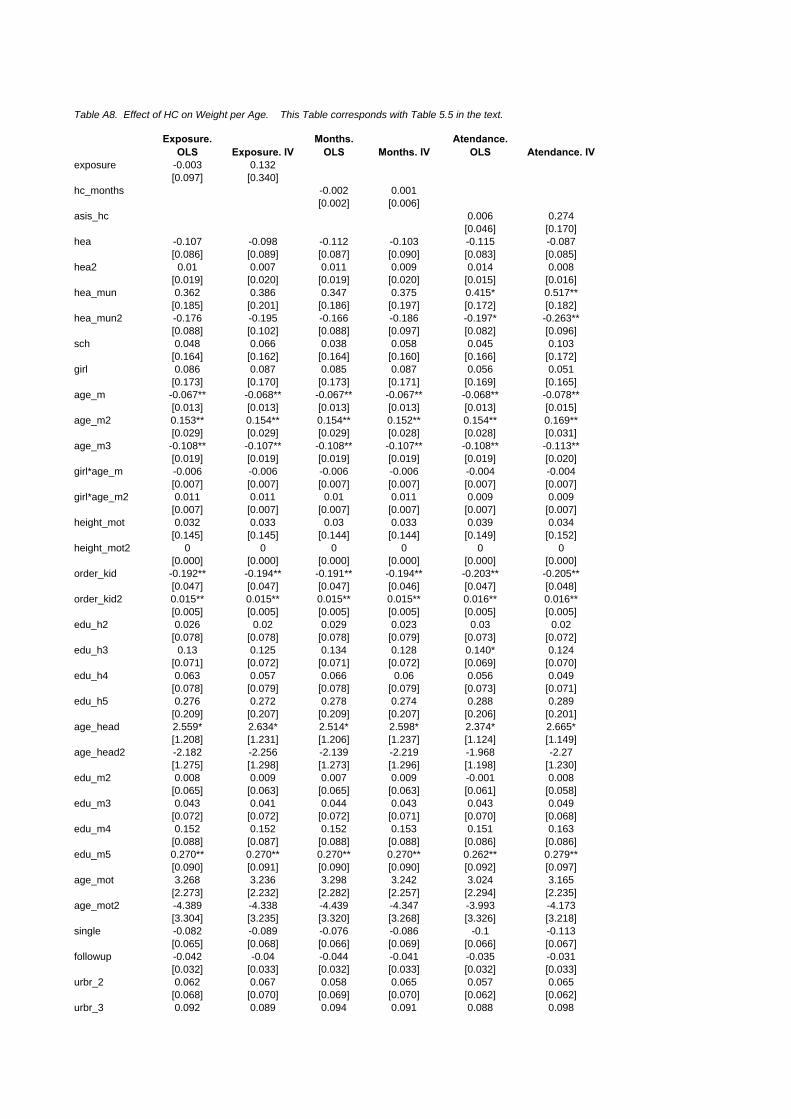
Table A8. Effect of HC on Weight per Age. This Table corresponds with Table 5.5 in the text.

Exposure. OLS Exposure. IV

Months. OLS Months. IV

Atendance. OLS Atendance. IV

exposure -0.003 0.132[0.097] [0.340]

hc_months -0.002 0.001[0.002] [0.006]

asis_hc 0.006 0.274[0.046] [0.170]

hea -0.107 -0.098 -0.112 -0.103 -0.115 -0.087[0.086] [0.089] [0.087] [0.090] [0.083] [0.085]

hea2 0.01 0.007 0.011 0.009 0.014 0.008[0.019] [0.020] [0.019] [0.020] [0.015] [0.016]

hea_mun 0.362 0.386 0.347 0.375 0.415* 0.517**[0.185] [0.201] [0.186] [0.197] [0.172] [0.182]

hea_mun2 -0.176 -0.195 -0.166 -0.186 -0.197* -0.263**[0.088] [0.102] [0.088] [0.097] [0.082] [0.096]

sch 0.048 0.066 0.038 0.058 0.045 0.103[0.164] [0.162] [0.164] [0.160] [0.166] [0.172]

girl 0.086 0.087 0.085 0.087 0.056 0.051[0.173] [0.170] [0.173] [0.171] [0.169] [0.165]

age_m -0.067** -0.068** -0.067** -0.067** -0.068** -0.078**[0.013] [0.013] [0.013] [0.013] [0.013] [0.015]

age_m2 0.153** 0.154** 0.154** 0.152** 0.154** 0.169**[0.029] [0.029] [0.029] [0.028] [0.028] [0.031]

age_m3 -0.108** -0.107** -0.108** -0.107** -0.108** -0.113**[0.019] [0.019] [0.019] [0.019] [0.019] [0.020]

girl*age_m -0.006 -0.006 -0.006 -0.006 -0.004 -0.004[0.007] [0.007] [0.007] [0.007] [0.007] [0.007]

girl*age_m2 0.011 0.011 0.01 0.011 0.009 0.009[0.007] [0.007] [0.007] [0.007] [0.007] [0.007]

height_mot 0.032 0.033 0.03 0.033 0.039 0.034[0.145] [0.145] [0.144] [0.144] [0.149] [0.152]

height_mot2 0 0 0 0 0 0[0.000] [0.000] [0.000] [0.000] [0.000] [0.000]

order_kid -0.192** -0.194** -0.191** -0.194** -0.203** -0.205**[0.047] [0.047] [0.047] [0.046] [0.047] [0.048]

order_kid2 0.015** 0.015** 0.015** 0.015** 0.016** 0.016**[0.005] [0.005] [0.005] [0.005] [0.005] [0.005]

edu_h2 0.026 0.02 0.029 0.023 0.03 0.02[0.078] [0.078] [0.078] [0.079] [0.073] [0.072]

edu_h3 0.13 0.125 0.134 0.128 0.140* 0.124[0.071] [0.072] [0.071] [0.072] [0.069] [0.070]

edu_h4 0.063 0.057 0.066 0.06 0.056 0.049[0.078] [0.079] [0.078] [0.079] [0.073] [0.071]

edu_h5 0.276 0.272 0.278 0.274 0.288 0.289[0.209] [0.207] [0.209] [0.207] [0.206] [0.201]

age_head 2.559* 2.634* 2.514* 2.598* 2.374* 2.665*[1.208] [1.231] [1.206] [1.237] [1.124] [1.149]

age_head2 -2.182 -2.256 -2.139 -2.219 -1.968 -2.27[1.275] [1.298] [1.273] [1.296] [1.198] [1.230]

edu_m2 0.008 0.009 0.007 0.009 -0.001 0.008[0.065] [0.063] [0.065] [0.063] [0.061] [0.058]

edu_m3 0.043 0.041 0.044 0.043 0.043 0.049[0.072] [0.072] [0.072] [0.071] [0.070] [0.068]

edu_m4 0.152 0.152 0.152 0.153 0.151 0.163[0.088] [0.087] [0.088] [0.088] [0.086] [0.086]

edu_m5 0.270** 0.270** 0.270** 0.270** 0.262** 0.279**[0.090] [0.091] [0.090] [0.090] [0.092] [0.097]

age_mot 3.268 3.236 3.298 3.242 3.024 3.165[2.273] [2.232] [2.282] [2.257] [2.294] [2.235]

age_mot2 -4.389 -4.338 -4.439 -4.347 -3.993 -4.173[3.304] [3.235] [3.320] [3.268] [3.326] [3.218]

single -0.082 -0.089 -0.076 -0.086 -0.1 -0.113[0.065] [0.068] [0.066] [0.069] [0.066] [0.067]

followup -0.042 -0.04 -0.044 -0.041 -0.035 -0.031[0.032] [0.033] [0.032] [0.033] [0.032] [0.033]

urbr_2 0.062 0.067 0.058 0.065 0.057 0.065[0.068] [0.070] [0.069] [0.070] [0.062] [0.062]

urbr_3 0.092 0.089 0.094 0.091 0.088 0.098

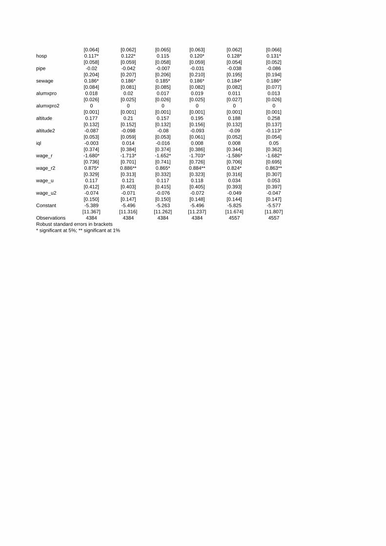
[0.064] [0.062] [0.065] [0.063] [0.062] [0.066]hosp 0.117* 0.122* 0.115 0.120* 0.128* 0.131*

[0.058] [0.059] [0.058] [0.059] [0.054] [0.052]pipe -0.02 -0.042 -0.007 -0.031 -0.038 -0.086

[0.204] [0.207] [0.206] [0.210] [0.195] [0.194]sewage 0.186* 0.186* 0.185* 0.186* 0.184* 0.186*

[0.084] [0.081] [0.085] [0.082] [0.082] [0.077]alumxpro 0.018 0.02 0.017 0.019 0.011 0.013

[0.026] [0.025] [0.026] [0.025] [0.027] [0.026]alumxpro2 0 0 0 0 0 0

[0.001] [0.001] [0.001] [0.001] [0.001] [0.001]altitude 0.177 0.21 0.157 0.195 0.188 0.258

[0.132] [0.152] [0.132] [0.156] [0.132] [0.137]altitude2 -0.087 -0.098 -0.08 -0.093 -0.09 -0.113*

[0.053] [0.059] [0.053] [0.061] [0.052] [0.054]iql -0.003 0.014 -0.016 0.008 0.008 0.05

[0.374] [0.384] [0.374] [0.386] [0.344] [0.362]wage_r -1.680* -1.713* -1.652* -1.703* -1.586* -1.682*

[0.736] [0.701] [0.741] [0.726] [0.706] [0.695]wage_r2 0.875* 0.886** 0.865* 0.884** 0.824* 0.863**

[0.329] [0.313] [0.332] [0.323] [0.316] [0.307]wage_u 0.117 0.121 0.117 0.118 0.034 0.053

[0.412] [0.403] [0.415] [0.405] [0.393] [0.397]wage_u2 -0.074 -0.071 -0.076 -0.072 -0.049 -0.047

[0.150] [0.147] [0.150] [0.148] [0.144] [0.147]Constant -5.389 -5.496 -5.263 -5.496 -5.825 -5.577

[11.367] [11.316] [11.262] [11.237] [11.674] [11.807]Observations 4384 4384 4384 4384 4557 4557Robust standard errors in brackets* significant at 5%; ** significant at 1%

Table A9. Effect of HC on Schooling outcomes. Kids 8 to 12. This Table corresponds with Table 5.6 in the text.Atendance to School Passing Grade

OLS. Ever Attended

IV. Ever Attended OLS. Months IV. Months

OLS. Ever Attended IV. Ever Attended

OLS. Months IV. Months

asis_hc_ever 0.044 0.045 0.008 0.02[0.011]** [0.070] [0.015] [0.067]

hc_months 0.001 0.001 0 0[0.000]** [0.002] [0.000] [0.002]

sch -0.109 -0.108 -0.109 -0.108 -0.14 -0.137 -0.137 -0.137[0.062] [0.067] [0.061] [0.062] [0.066]* [0.068] [0.066]* [0.067]*

sch2 0.024 0.024 0.024 0.024 0.017 0.016 0.016 0.016[0.011]* [0.012]* [0.011]* [0.011]* [0.013] [0.013] [0.013] [0.013]

hea -0.04 -0.04 -0.039 -0.038 -0.018 -0.017 -0.017 -0.017[0.027] [0.027] [0.026] [0.028] [0.037] [0.036] [0.037] [0.035]

hea2 0.006 0.006 0.007 0.006 -0.005 -0.005 -0.006 -0.006[0.005] [0.005] [0.005] [0.006] [0.006] [0.006] [0.007] [0.006]

sch_mun -0.699 -0.695 -0.732 -0.725 -0.26 -0.223 -0.233 -0.235[0.546] [0.525] [0.548] [0.545] [1.091] [1.112] [1.093] [1.097]

sch_mun2 2.041 2.034 2.17 2.168 0.793 0.715 0.734 0.735[1.561] [1.495] [1.591] [1.595] [3.190] [3.235] [3.206] [3.204]

girl 0.035 0.035 0.034 0.034 0.063 0.062 0.063 0.063[0.011]** [0.011]** [0.011]** [0.011]** [0.014]** [0.014]** [0.014]** [0.014]**

age 0.139 0.139 0.129 0.128 0.399 0.398 0.399 0.399[0.067]* [0.069]* [0.069] [0.069] [0.088]** [0.089]** [0.089]** [0.089]**

age2 -0.008 -0.008 -0.007 -0.007 -0.018 -0.018 -0.018 -0.018[0.003]* [0.004]* [0.004]* [0.004]* [0.004]** [0.004]** [0.004]** [0.004]**

edu_h2 0.015 0.015 0.012 0.011 0.034 0.034 0.034 0.034[0.017] [0.017] [0.017] [0.018] [0.022] [0.022] [0.022] [0.023]

edu_h3 0.027 0.027 0.023 0.023 0.06 0.06 0.06 0.06[0.016] [0.016] [0.015] [0.016] [0.025]* [0.025]* [0.025]* [0.026]*

edu_h4 0.038 0.038 0.033 0.032 0.067 0.066 0.066 0.066[0.020] [0.022] [0.020] [0.026] [0.029]* [0.029]* [0.029]* [0.033]

edu_h5 0.06 0.06 0.055 0.055 0.083 0.084 0.081 0.081[0.020]** [0.020]** [0.020]** [0.020]** [0.041]* [0.040]* [0.040]* [0.040]*

age_head 0 0 0 0 0.001 0.001 0.001 0.001[0.001] [0.001] [0.001] [0.001] [0.001] [0.001] [0.001] [0.001]

edu_s2 0.053 0.053 0.055 0.055 0.079 0.078 0.078 0.078[0.020]* [0.020]* [0.020]* [0.020]* [0.026]** [0.026]** [0.026]** [0.026]**

edu_s3 0.109 0.109 0.108 0.108 0.161 0.16 0.16 0.16[0.020]** [0.020]** [0.020]** [0.021]** [0.031]** [0.031]** [0.031]** [0.030]**

edu_s4 0.11 0.11 0.114 0.114 0.19 0.19 0.19 0.19[0.024]** [0.024]** [0.025]** [0.025]** [0.032]** [0.032]** [0.032]** [0.033]**

edu_s5 0.112 0.112 0.115 0.115 0.203 0.202 0.202 0.202[0.021]** [0.021]** [0.021]** [0.021]** [0.036]** [0.036]** [0.035]** [0.036]**

f_single -0.048 -0.048 -0.047 -0.048 -0.025 -0.026 -0.025 -0.025[0.019]* [0.021]* [0.020]* [0.021]* [0.023] [0.023] [0.024] [0.023]

urbr_2 0.001 0.001 -0.002 -0.002 -0.056 -0.055 -0.057 -0.057[0.020] [0.019] [0.019] [0.019] [0.020]** [0.020]** [0.020]** [0.020]**

urbr_3 -0.055 -0.055 -0.059 -0.059 -0.096 -0.097 -0.099 -0.099[0.037] [0.037] [0.037] [0.038] [0.047]* [0.047]* [0.048]* [0.047]*

alumxpro -0.003 -0.003 -0.005 -0.005 -0.018 -0.018 -0.018 -0.018[0.007] [0.007] [0.007] [0.008] [0.012] [0.012] [0.012] [0.011]

alumxpro2 0 0 0 0 0 0 0 0[0.000] [0.000] [0.000] [0.000] [0.000] [0.000] [0.000] [0.000]

hosp -0.015 -0.015 -0.016 -0.016 -0.031 -0.031 -0.03 -0.03[0.015] [0.015] [0.015] [0.015] [0.025] [0.025] [0.025] [0.025]

pipe -0.039 -0.039 -0.032 -0.036 -0.133 -0.14 -0.131 -0.13[0.066] [0.061] [0.067] [0.060] [0.065]* [0.071] [0.065] [0.070]

sewage -0.042 -0.042 -0.043 -0.044 -0.043 -0.044 -0.045 -0.045[0.026] [0.026] [0.026] [0.026] [0.037] [0.037] [0.038] [0.037]

altitude -0.108 -0.108 -0.104 -0.103 -0.093 -0.09 -0.093 -0.093[0.050]* [0.050]* [0.050]* [0.050]* [0.058] [0.058] [0.059] [0.058]

altitude2 0.046 0.046 0.044 0.044 0.048 0.048 0.049 0.049[0.016]** [0.016]** [0.016]** [0.016]** [0.021]* [0.020]* [0.021]* [0.020]*

iql -0.021 -0.021 -0.018 -0.016 0.11 0.11 0.111 0.111[0.106] [0.107] [0.104] [0.105] [0.173] [0.173] [0.173] [0.173]

wage_r 0.613 0.613 0.657 0.663 0.64 0.647 0.649 0.648[0.176]** [0.175]** [0.196]** [0.216]** [0.384] [0.382] [0.390] [0.385]

wage_r2 -0.321 -0.321 -0.343 -0.347 -0.391 -0.394 -0.395 -0.394[0.085]** [0.084]** [0.097]** [0.106]** [0.193]* [0.192]* [0.196]* [0.194]*

wage_u -0.097 -0.097 -0.117 -0.121 -0.198 -0.204 -0.201 -0.2

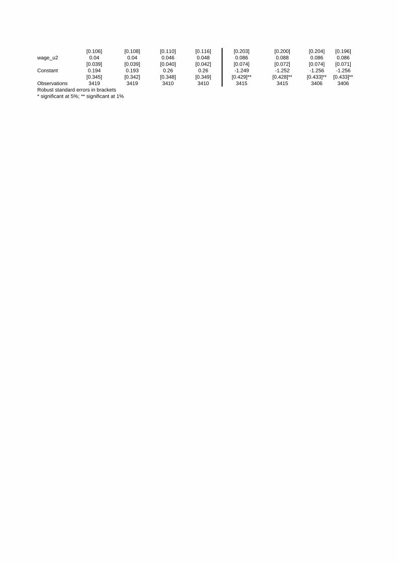
[0.106] [0.108] [0.110] [0.116] [0.203] [0.200] [0.204] [0.196]wage_u2 0.04 0.04 0.046 0.048 0.086 0.088 0.086 0.086

[0.039] [0.039] [0.040] [0.042] [0.074] [0.072] [0.074] [0.071]Constant 0.194 0.193 0.26 0.26 -1.249 -1.252 -1.256 -1.256

[0.345] [0.342] [0.348] [0.349] [0.429]** [0.428]** [0.433]** [0.433]**Observations 3419 3419 3410 3410 3415 3415 3406 3406Robust standard errors in brackets* significant at 5%; ** significant at 1%

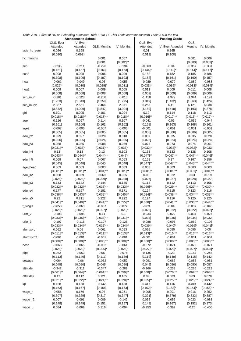
Table A10. Effect of HC on Schooling outcomes. Kids 13 to 17. This Table corresponds with Table 5.6 in the text.Atendance to School Passing Grade

OLS. Ever Attended

IV. Ever Attended OLS. Months IV. Months

OLS. Ever Attended IV. Ever Attended

OLS. Months IV. Months

asis_hc_ever 0.026 0.198 0.01 0.165[0.020] [0.093]* [0.019] [0.100]

hc_months 0.001 0.007 0.001 0.006[0.001] [0.002]** [0.000] [0.003]*

sch -0.235 -0.211 -0.226 -0.194 -0.363 -0.34 -0.357 -0.331[0.161] [0.157] [0.163] [0.163] [0.144]* [0.142]* [0.144]* [0.147]*

sch2 0.098 0.098 0.096 0.099 0.182 0.182 0.185 0.186[0.198] [0.196] [0.197] [0.193] [0.162] [0.161] [0.160] [0.157]

hea -0.061 -0.049 -0.06 -0.053 -0.089 -0.079 -0.089 -0.083[0.029]* [0.030] [0.029]* [0.031] [0.033]* [0.035]* [0.033]* [0.034]*

hea2 0.009 0.007 0.009 0.005 0.011 0.009 0.011 0.008[0.008] [0.008] [0.008] [0.008] [0.009] [0.009] [0.009] [0.009]

sch_mun -0.181 -0.128 -0.208 -0.013 -1.418 -1.372 -1.344 -1.191[1.253] [1.343] [1.250] [1.275] [1.349] [1.432] [1.363] [1.424]

sch_mun2 2.387 2.551 2.464 2.371 6.255 6.41 6.121 6.038[3.872] [4.099] [3.847] [3.904] [4.169] [4.418] [4.193] [4.378]

girl 0.101 0.095 0.101 0.094 0.12 0.114 0.118 0.113[0.018]** [0.018]** [0.018]** [0.018]** [0.016]** [0.017]** [0.016]** [0.017]**

age 0.116 0.097 0.114 0.107 -0.041 -0.06 -0.039 -0.044[0.161] [0.160] [0.161] [0.162] [0.168] [0.163] [0.168] [0.161]

age2 -0.007 -0.006 -0.007 -0.006 -0.001 -0.001 -0.001 -0.001[0.005] [0.005] [0.005] [0.005] [0.006] [0.006] [0.006] [0.005]

edu_h2 0.029 0.027 0.028 0.018 0.037 0.035 0.035 0.028[0.026] [0.025] [0.026] [0.025] [0.025] [0.024] [0.024] [0.024]

edu_h3 0.088 0.085 0.088 0.069 0.075 0.073 0.074 0.061[0.031]** [0.033]* [0.031]** [0.033]* [0.032]* [0.034]* [0.032]* [0.033]

edu_h4 0.13 0.13 0.13 0.103 0.133 0.133 0.128 0.108[0.043]** [0.044]** [0.044]** [0.047]* [0.047]** [0.047]** [0.047]** [0.046]*

edu_h5 0.068 0.07 0.067 0.053 0.168 0.17 0.167 0.156[0.045] [0.048] [0.045] [0.048] [0.047]** [0.047]** [0.046]** [0.044]**

age_head 0.003 0.003 0.003 0.003 0.003 0.003 0.003 0.003[0.001]** [0.001]** [0.001]** [0.001]** [0.001]* [0.001]** [0.001]* [0.001]**

edu_s2 0.068 0.059 0.069 0.055 0.03 0.022 0.03 0.019[0.028]* [0.028]* [0.029]* [0.028] [0.027] [0.027] [0.028] [0.027]

edu_s3 0.143 0.142 0.144 0.135 0.113 0.112 0.113 0.106[0.032]** [0.032]** [0.033]** [0.033]** [0.029]** [0.029]** [0.029]** [0.030]**

edu_s4 0.177 0.167 0.181 0.171 0.124 0.115 0.123 0.116[0.038]** [0.043]** [0.038]** [0.045]** [0.034]** [0.038]** [0.034]** [0.038]**

edu_s5 0.22 0.211 0.222 0.222 0.124 0.116 0.125 0.125[0.041]** [0.049]** [0.041]** [0.055]** [0.038]** [0.041]** [0.038]** [0.044]**

f_single -0.053 -0.063 -0.057 -0.072 -0.03 -0.04 -0.037 -0.048[0.026]* [0.026]* [0.027]* [0.028]* [0.022] [0.022] [0.022] [0.022]*

urbr_2 -0.108 -0.095 -0.11 -0.1 -0.034 -0.022 -0.034 -0.027[0.033]** [0.035]** [0.033]** [0.031]** [0.035] [0.036] [0.034] [0.032]

urbr_3 -0.107 -0.115 -0.107 -0.128 -0.088 -0.095 -0.089 -0.105[0.033]** [0.034]** [0.033]** [0.034]** [0.039]* [0.040]* [0.039]* [0.041]*

alumxpro 0.062 0.06 0.061 0.053 0.056 0.055 0.055 0.05[0.011]** [0.013]** [0.011]** [0.013]** [0.013]** [0.015]** [0.013]** [0.016]**

alumxpro2 -0.001 -0.001 -0.001 -0.001 -0.001 -0.001 -0.001 -0.001[0.000]** [0.000]** [0.000]** [0.000]** [0.000]** [0.000]** [0.000]** [0.000]**

hosp -0.063 -0.065 -0.062 -0.061 -0.072 -0.074 -0.072 -0.071[0.025]* [0.028]* [0.025]* [0.026]* [0.027]* [0.029]* [0.027]* [0.028]*

pipe 0.052 -0.053 0.06 -0.074 -0.135 -0.23 -0.144 -0.245[0.113] [0.146] [0.111] [0.139] [0.119] [0.148] [0.118] [0.142]

sewage -0.064 -0.06 -0.062 -0.052 -0.091 -0.087 -0.088 -0.081[0.045] [0.050] [0.045] [0.050] [0.049] [0.056] [0.050] [0.057]

altitude -0.342 -0.311 -0.347 -0.288 -0.266 -0.238 -0.266 -0.223[0.061]** [0.064]** [0.061]** [0.059]** [0.068]** [0.070]** [0.069]** [0.068]**

altitude2 0.12 0.112 0.121 0.105 0.09 0.083 0.09 0.078[0.021]** [0.022]** [0.021]** [0.020]** [0.025]** [0.025]** [0.025]** [0.024]**

iql 0.158 0.158 0.142 0.188 0.417 0.416 0.409 0.442[0.163] [0.167] [0.168] [0.163] [0.162]* [0.158]* [0.164]* [0.155]**

wage_r -0.056 0.176 -0.07 0.251 -0.005 0.201 0.016 0.252[0.307] [0.329] [0.317] [0.347] [0.321] [0.379] [0.332] [0.387]

wage_r2 0.007 -0.091 0.009 -0.142 0.035 -0.052 0.023 -0.088[0.148] [0.149] [0.151] [0.157] [0.149] [0.167] [0.152] [0.173]

wage_u 0.084 -0.069 0.116 -0.094 -0.253 -0.392 -0.25 -0.406

[0.210] [0.255] [0.214] [0.254] [0.235] [0.289] [0.244] [0.289]wage_u2 -0.014 0.045 -0.026 0.053 0.122 0.175 0.121 0.18

[0.080] [0.097] [0.081] [0.095] [0.090] [0.109] [0.092] [0.108]Constant -0.535 -0.474 -0.515 -0.525 0.914 0.984 0.896 0.889

[1.177] [1.181] [1.181] [1.200] [1.181] [1.144] [1.183] [1.136]Observations 2991 2991 2975 2975 2984 2984 2968 2968Robust standard errors in brackets* significant at 5%; ** significant at 1%

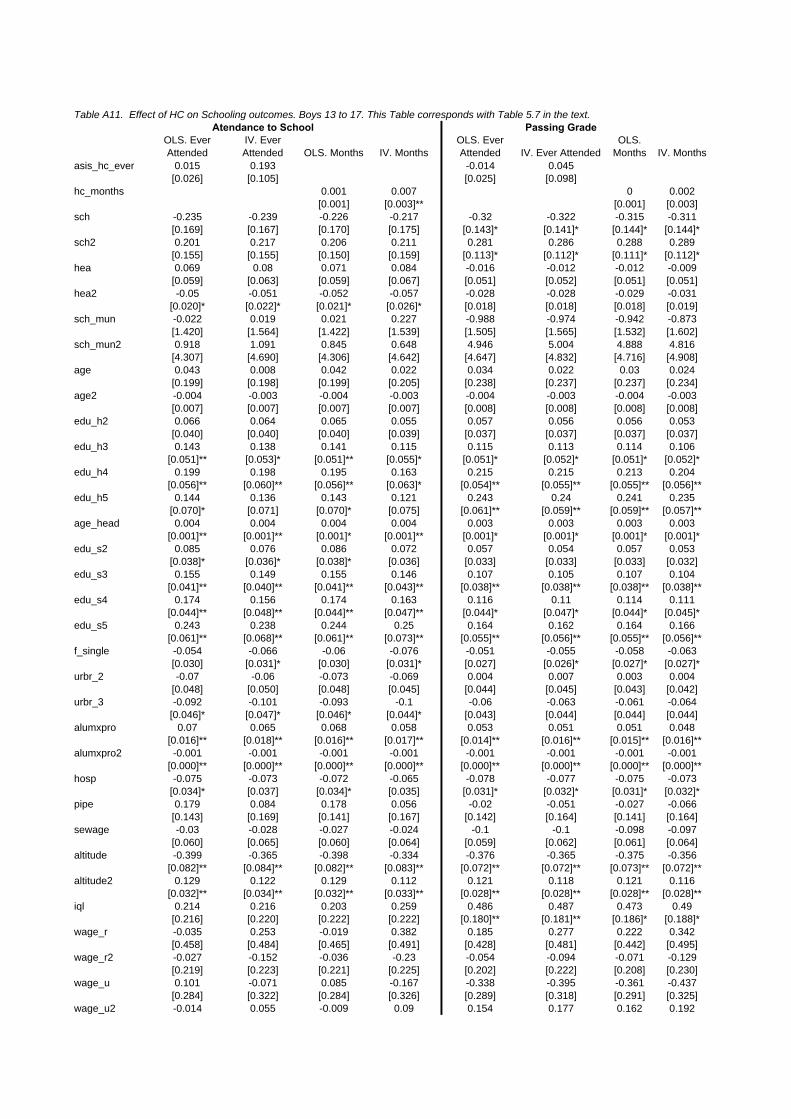
Table A11. Effect of HC on Schooling outcomes. Boys 13 to 17. This Table corresponds with Table 5.7 in the text.Atendance to School Passing Grade

OLS. Ever Attended

IV. Ever Attended OLS. Months IV. Months

OLS. Ever Attended IV. Ever Attended

OLS. Months IV. Months

asis_hc_ever 0.015 0.193 -0.014 0.045[0.026] [0.105] [0.025] [0.098]

hc_months 0.001 0.007 0 0.002[0.001] [0.003]** [0.001] [0.003]

sch -0.235 -0.239 -0.226 -0.217 -0.32 -0.322 -0.315 -0.311[0.169] [0.167] [0.170] [0.175] [0.143]* [0.141]* [0.144]* [0.144]*

sch2 0.201 0.217 0.206 0.211 0.281 0.286 0.288 0.289[0.155] [0.155] [0.150] [0.159] [0.113]* [0.112]* [0.111]* [0.112]*

hea 0.069 0.08 0.071 0.084 -0.016 -0.012 -0.012 -0.009[0.059] [0.063] [0.059] [0.067] [0.051] [0.052] [0.051] [0.051]

hea2 -0.05 -0.051 -0.052 -0.057 -0.028 -0.028 -0.029 -0.031[0.020]* [0.022]* [0.021]* [0.026]* [0.018] [0.018] [0.018] [0.019]

sch_mun -0.022 0.019 0.021 0.227 -0.988 -0.974 -0.942 -0.873[1.420] [1.564] [1.422] [1.539] [1.505] [1.565] [1.532] [1.602]

sch_mun2 0.918 1.091 0.845 0.648 4.946 5.004 4.888 4.816[4.307] [4.690] [4.306] [4.642] [4.647] [4.832] [4.716] [4.908]

age 0.043 0.008 0.042 0.022 0.034 0.022 0.03 0.024[0.199] [0.198] [0.199] [0.205] [0.238] [0.237] [0.237] [0.234]

age2 -0.004 -0.003 -0.004 -0.003 -0.004 -0.003 -0.004 -0.003[0.007] [0.007] [0.007] [0.007] [0.008] [0.008] [0.008] [0.008]

edu_h2 0.066 0.064 0.065 0.055 0.057 0.056 0.056 0.053[0.040] [0.040] [0.040] [0.039] [0.037] [0.037] [0.037] [0.037]

edu_h3 0.143 0.138 0.141 0.115 0.115 0.113 0.114 0.106[0.051]** [0.053]* [0.051]** [0.055]* [0.051]* [0.052]* [0.051]* [0.052]*

edu_h4 0.199 0.198 0.195 0.163 0.215 0.215 0.213 0.204[0.056]** [0.060]** [0.056]** [0.063]* [0.054]** [0.055]** [0.055]** [0.056]**

edu_h5 0.144 0.136 0.143 0.121 0.243 0.24 0.241 0.235[0.070]* [0.071] [0.070]* [0.075] [0.061]** [0.059]** [0.059]** [0.057]**

age_head 0.004 0.004 0.004 0.004 0.003 0.003 0.003 0.003[0.001]** [0.001]** [0.001]* [0.001]** [0.001]* [0.001]* [0.001]* [0.001]*

edu_s2 0.085 0.076 0.086 0.072 0.057 0.054 0.057 0.053[0.038]* [0.036]* [0.038]* [0.036] [0.033] [0.033] [0.033] [0.032]

edu_s3 0.155 0.149 0.155 0.146 0.107 0.105 0.107 0.104[0.041]** [0.040]** [0.041]** [0.043]** [0.038]** [0.038]** [0.038]** [0.038]**

edu_s4 0.174 0.156 0.174 0.163 0.116 0.11 0.114 0.111[0.044]** [0.048]** [0.044]** [0.047]** [0.044]* [0.047]* [0.044]* [0.045]*

edu_s5 0.243 0.238 0.244 0.25 0.164 0.162 0.164 0.166[0.061]** [0.068]** [0.061]** [0.073]** [0.055]** [0.056]** [0.055]** [0.056]**

f_single -0.054 -0.066 -0.06 -0.076 -0.051 -0.055 -0.058 -0.063[0.030] [0.031]* [0.030] [0.031]* [0.027] [0.026]* [0.027]* [0.027]*

urbr_2 -0.07 -0.06 -0.073 -0.069 0.004 0.007 0.003 0.004[0.048] [0.050] [0.048] [0.045] [0.044] [0.045] [0.043] [0.042]

urbr_3 -0.092 -0.101 -0.093 -0.1 -0.06 -0.063 -0.061 -0.064[0.046]* [0.047]* [0.046]* [0.044]* [0.043] [0.044] [0.044] [0.044]

alumxpro 0.07 0.065 0.068 0.058 0.053 0.051 0.051 0.048[0.016]** [0.018]** [0.016]** [0.017]** [0.014]** [0.016]** [0.015]** [0.016]**

alumxpro2 -0.001 -0.001 -0.001 -0.001 -0.001 -0.001 -0.001 -0.001[0.000]** [0.000]** [0.000]** [0.000]** [0.000]** [0.000]** [0.000]** [0.000]**

hosp -0.075 -0.073 -0.072 -0.065 -0.078 -0.077 -0.075 -0.073[0.034]* [0.037] [0.034]* [0.035] [0.031]* [0.032]* [0.031]* [0.032]*

pipe 0.179 0.084 0.178 0.056 -0.02 -0.051 -0.027 -0.066[0.143] [0.169] [0.141] [0.167] [0.142] [0.164] [0.141] [0.164]

sewage -0.03 -0.028 -0.027 -0.024 -0.1 -0.1 -0.098 -0.097[0.060] [0.065] [0.060] [0.064] [0.059] [0.062] [0.061] [0.064]

altitude -0.399 -0.365 -0.398 -0.334 -0.376 -0.365 -0.375 -0.356[0.082]** [0.084]** [0.082]** [0.083]** [0.072]** [0.072]** [0.073]** [0.072]**

altitude2 0.129 0.122 0.129 0.112 0.121 0.118 0.121 0.116[0.032]** [0.034]** [0.032]** [0.033]** [0.028]** [0.028]** [0.028]** [0.028]**

iql 0.214 0.216 0.203 0.259 0.486 0.487 0.473 0.49[0.216] [0.220] [0.222] [0.222] [0.180]** [0.181]** [0.186]* [0.188]*

wage_r -0.035 0.253 -0.019 0.382 0.185 0.277 0.222 0.342[0.458] [0.484] [0.465] [0.491] [0.428] [0.481] [0.442] [0.495]

wage_r2 -0.027 -0.152 -0.036 -0.23 -0.054 -0.094 -0.071 -0.129[0.219] [0.223] [0.221] [0.225] [0.202] [0.222] [0.208] [0.230]

wage_u 0.101 -0.071 0.085 -0.167 -0.338 -0.395 -0.361 -0.437[0.284] [0.322] [0.284] [0.326] [0.289] [0.318] [0.291] [0.325]

wage_u2 -0.014 0.055 -0.009 0.09 0.154 0.177 0.162 0.192

[0.109] [0.123] [0.109] [0.124] [0.109] [0.120] [0.110] [0.123]Constant -0.342 -0.172 -0.323 -0.224 0.183 0.245 0.218 0.246

[1.446] [1.440] [1.444] [1.498] [1.695] [1.687] [1.688] [1.669]Observations 1631 1631 1623 1623 1626 1626 1618 1618Robust standard errors in brackets* significant at 5%; ** significant at 1%

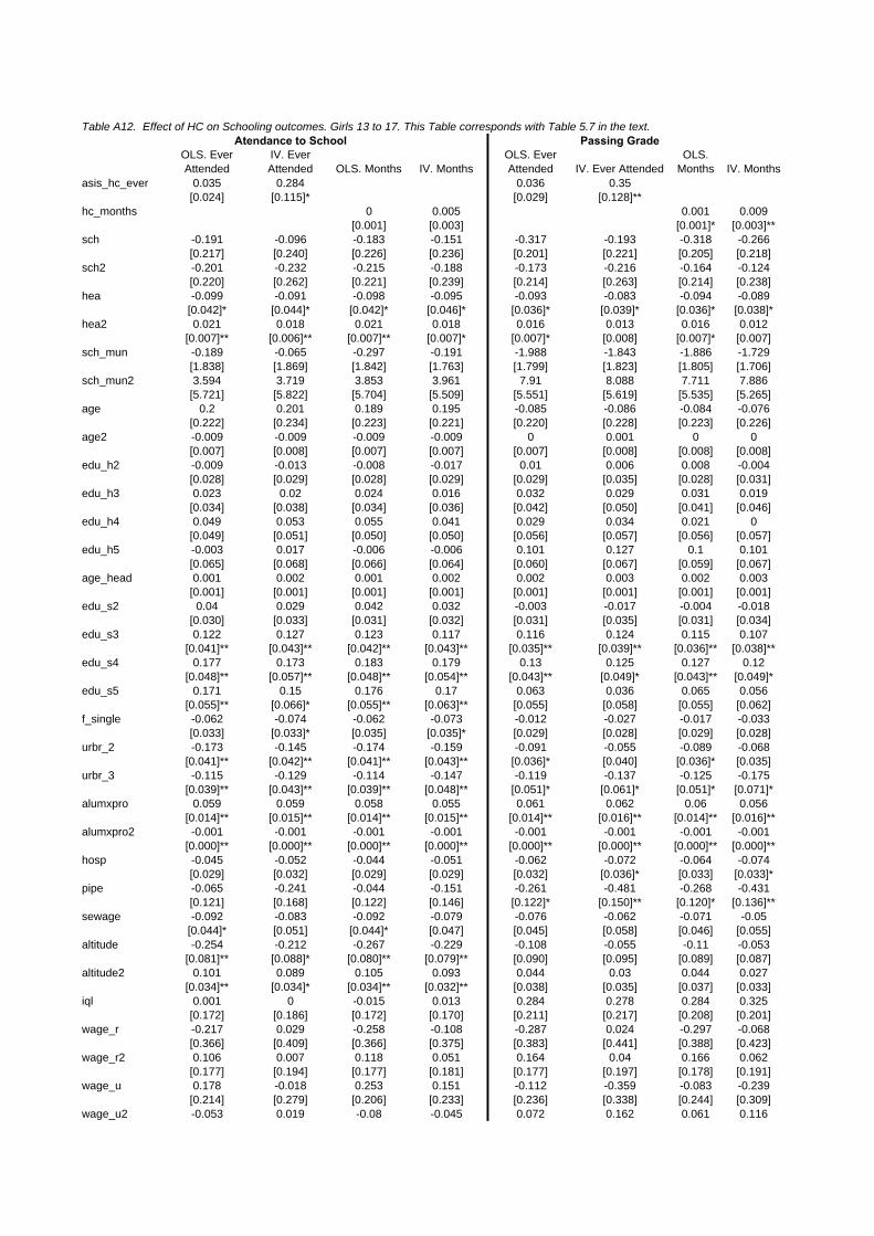
Table A12. Effect of HC on Schooling outcomes. Girls 13 to 17. This Table corresponds with Table 5.7 in the text.Atendance to School Passing Grade

OLS. Ever Attended

IV. Ever Attended OLS. Months IV. Months

OLS. Ever Attended IV. Ever Attended

OLS. Months IV. Months

asis_hc_ever 0.035 0.284 0.036 0.35[0.024] [0.115]* [0.029] [0.128]**

hc_months 0 0.005 0.001 0.009[0.001] [0.003] [0.001]* [0.003]**

sch -0.191 -0.096 -0.183 -0.151 -0.317 -0.193 -0.318 -0.266[0.217] [0.240] [0.226] [0.236] [0.201] [0.221] [0.205] [0.218]

sch2 -0.201 -0.232 -0.215 -0.188 -0.173 -0.216 -0.164 -0.124[0.220] [0.262] [0.221] [0.239] [0.214] [0.263] [0.214] [0.238]

hea -0.099 -0.091 -0.098 -0.095 -0.093 -0.083 -0.094 -0.089[0.042]* [0.044]* [0.042]* [0.046]* [0.036]* [0.039]* [0.036]* [0.038]*

hea2 0.021 0.018 0.021 0.018 0.016 0.013 0.016 0.012[0.007]** [0.006]** [0.007]** [0.007]* [0.007]* [0.008] [0.007]* [0.007]

sch_mun -0.189 -0.065 -0.297 -0.191 -1.988 -1.843 -1.886 -1.729[1.838] [1.869] [1.842] [1.763] [1.799] [1.823] [1.805] [1.706]

sch_mun2 3.594 3.719 3.853 3.961 7.91 8.088 7.711 7.886[5.721] [5.822] [5.704] [5.509] [5.551] [5.619] [5.535] [5.265]

age 0.2 0.201 0.189 0.195 -0.085 -0.086 -0.084 -0.076[0.222] [0.234] [0.223] [0.221] [0.220] [0.228] [0.223] [0.226]

age2 -0.009 -0.009 -0.009 -0.009 0 0.001 0 0[0.007] [0.008] [0.007] [0.007] [0.007] [0.008] [0.008] [0.008]

edu_h2 -0.009 -0.013 -0.008 -0.017 0.01 0.006 0.008 -0.004[0.028] [0.029] [0.028] [0.029] [0.029] [0.035] [0.028] [0.031]

edu_h3 0.023 0.02 0.024 0.016 0.032 0.029 0.031 0.019[0.034] [0.038] [0.034] [0.036] [0.042] [0.050] [0.041] [0.046]

edu_h4 0.049 0.053 0.055 0.041 0.029 0.034 0.021 0[0.049] [0.051] [0.050] [0.050] [0.056] [0.057] [0.056] [0.057]

edu_h5 -0.003 0.017 -0.006 -0.006 0.101 0.127 0.1 0.101[0.065] [0.068] [0.066] [0.064] [0.060] [0.067] [0.059] [0.067]

age_head 0.001 0.002 0.001 0.002 0.002 0.003 0.002 0.003[0.001] [0.001] [0.001] [0.001] [0.001] [0.001] [0.001] [0.001]

edu_s2 0.04 0.029 0.042 0.032 -0.003 -0.017 -0.004 -0.018[0.030] [0.033] [0.031] [0.032] [0.031] [0.035] [0.031] [0.034]

edu_s3 0.122 0.127 0.123 0.117 0.116 0.124 0.115 0.107[0.041]** [0.043]** [0.042]** [0.043]** [0.035]** [0.039]** [0.036]** [0.038]**

edu_s4 0.177 0.173 0.183 0.179 0.13 0.125 0.127 0.12[0.048]** [0.057]** [0.048]** [0.054]** [0.043]** [0.049]* [0.043]** [0.049]*

edu_s5 0.171 0.15 0.176 0.17 0.063 0.036 0.065 0.056[0.055]** [0.066]* [0.055]** [0.063]** [0.055] [0.058] [0.055] [0.062]

f_single -0.062 -0.074 -0.062 -0.073 -0.012 -0.027 -0.017 -0.033[0.033] [0.033]* [0.035] [0.035]* [0.029] [0.028] [0.029] [0.028]

urbr_2 -0.173 -0.145 -0.174 -0.159 -0.091 -0.055 -0.089 -0.068[0.041]** [0.042]** [0.041]** [0.043]** [0.036]* [0.040] [0.036]* [0.035]

urbr_3 -0.115 -0.129 -0.114 -0.147 -0.119 -0.137 -0.125 -0.175[0.039]** [0.043]** [0.039]** [0.048]** [0.051]* [0.061]* [0.051]* [0.071]*

alumxpro 0.059 0.059 0.058 0.055 0.061 0.062 0.06 0.056[0.014]** [0.015]** [0.014]** [0.015]** [0.014]** [0.016]** [0.014]** [0.016]**

alumxpro2 -0.001 -0.001 -0.001 -0.001 -0.001 -0.001 -0.001 -0.001[0.000]** [0.000]** [0.000]** [0.000]** [0.000]** [0.000]** [0.000]** [0.000]**

hosp -0.045 -0.052 -0.044 -0.051 -0.062 -0.072 -0.064 -0.074[0.029] [0.032] [0.029] [0.029] [0.032] [0.036]* [0.033] [0.033]*

pipe -0.065 -0.241 -0.044 -0.151 -0.261 -0.481 -0.268 -0.431[0.121] [0.168] [0.122] [0.146] [0.122]* [0.150]** [0.120]* [0.136]**

sewage -0.092 -0.083 -0.092 -0.079 -0.076 -0.062 -0.071 -0.05[0.044]* [0.051] [0.044]* [0.047] [0.045] [0.058] [0.046] [0.055]

altitude -0.254 -0.212 -0.267 -0.229 -0.108 -0.055 -0.11 -0.053[0.081]** [0.088]* [0.080]** [0.079]** [0.090] [0.095] [0.089] [0.087]

altitude2 0.101 0.089 0.105 0.093 0.044 0.03 0.044 0.027[0.034]** [0.034]* [0.034]** [0.032]** [0.038] [0.035] [0.037] [0.033]

iql 0.001 0 -0.015 0.013 0.284 0.278 0.284 0.325[0.172] [0.186] [0.172] [0.170] [0.211] [0.217] [0.208] [0.201]

wage_r -0.217 0.029 -0.258 -0.108 -0.287 0.024 -0.297 -0.068[0.366] [0.409] [0.366] [0.375] [0.383] [0.441] [0.388] [0.423]

wage_r2 0.106 0.007 0.118 0.051 0.164 0.04 0.166 0.062[0.177] [0.194] [0.177] [0.181] [0.177] [0.197] [0.178] [0.191]

wage_u 0.178 -0.018 0.253 0.151 -0.112 -0.359 -0.083 -0.239[0.214] [0.279] [0.206] [0.233] [0.236] [0.338] [0.244] [0.309]

wage_u2 -0.053 0.019 -0.08 -0.045 0.072 0.162 0.061 0.116

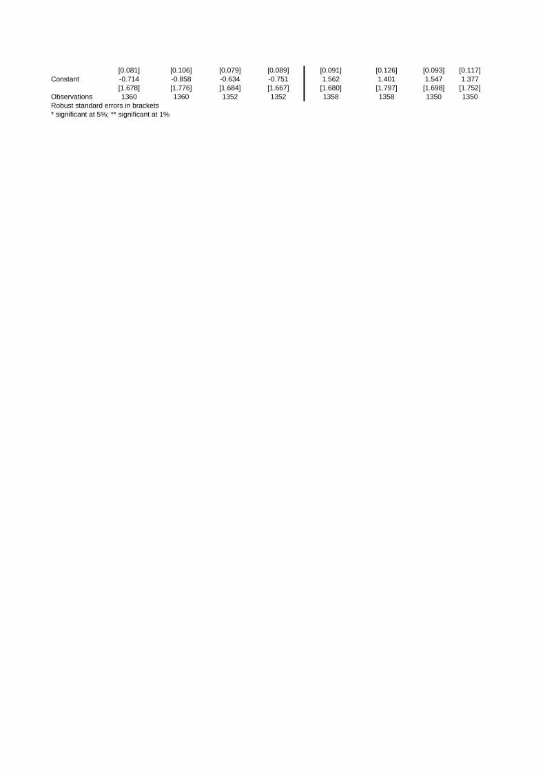
[0.081] [0.106] [0.079] [0.089] [0.091] [0.126] [0.093] [0.117]Constant -0.714 -0.858 -0.634 -0.751 1.562 1.401 1.547 1.377

[1.678] [1.776] [1.684] [1.667] [1.680] [1.797] [1.698] [1.752]Observations 1360 1360 1352 1352 1358 1358 1350 1350Robust standard errors in brackets* significant at 5%; ** significant at 1%

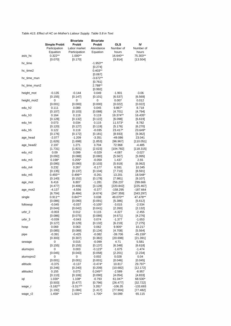
Table A13. Effect of HC on Mother's Labour Supply. Table 5.8 in Text

Simple ProbitBivariate

ProbitBivariate

Probit OLS IVParticipation

EquationLabor market Participation

Atendance Equation

Number of hours

Number of hours

asis_hc 0.322** 1.000** 16.640** 75.303**[0.070] [0.170] [3.914] [13.504]

hc_time -1.953**[0.274]

hc_time2 0.403**[0.067]

hc_time_mun -3.672**[0.761]

hc_time_mun2 2.788**[0.992]

height_mot -0.135 -0.144 0.049 -1.901 -3.06[0.155] [0.147] [0.101] [6.537] [6.569]

height_mot2 0 0 0 0.007 0.012[0.001] [0.000] [0.000] [0.022] [0.022]

edu_h2 0.111 0.089 0.045 9.867* 8.718[0.107] [0.103] [0.088] [4.701] [4.794]

edu_h3 0.164 0.119 0.119 19.374** 16.435*[0.128] [0.132] [0.122] [6.098] [6.619]

edu_h4 0.073 0.034 0.115 11.573* 8.782[0.120] [0.127] [0.119] [5.176] [6.270]

edu_h5 0.122 0.119 -0.035 23.417* 23.649*[0.176] [0.172] [0.181] [8.933] [9.362]

age_head -2.077 -1.209 -3.351 -49.086 23.041[1.626] [1.698] [1.853] [96.967] [110.051]

age_head2 2.197 1.271 3.704 72.968 -4.485[1.731] [1.821] [2.023] [104.782] [118.315]

edu_m2 0.09 0.099 -0.029 -4.087 -3.027[0.092] [0.088] [0.080] [5.567] [5.995]

edu_m3 0.198* 0.205* -0.059 1.437 2.55[0.095] [0.090] [0.103] [5.919] [6.062]

edu_m4 0.232 0.267 -0.177 6.591 10.345[0.135] [0.137] [0.104] [7.710] [8.591]

edu_m5 0.455** 0.496** -0.261 13.201 18.548*[0.140] [0.152] [0.178] [7.981] [9.107]

age_mot 6.416 6.807 -1.281 256.237 299.666[4.477] [4.406] [3.128] [220.842] [225.467]

age_mot2 -4.137 -4.556 -0.377 -158.295 -187.664[6.704] [6.484] [4.674] [347.359] [343.297]

single 0.911** 0.847** 0.038 49.070** 47.478**[0.086] [0.090] [0.091] [5.386] [5.612]

followup -0.045 -0.037 -0.105* -3.015 -2.534[0.044] [0.042] [0.041] [2.260] [2.132]

urbr_2 -0.003 0.012 0.115 -4.327 -2.455[0.086] [0.075] [0.086] [4.671] [4.276]

urbr_3 -0.039 -0.043 0.074 -1.377 -1.653[0.127] [0.129] [0.132] [6.219] [7.275]

hosp 0.069 0.063 0.062 9.905* 10.217[0.085] [0.089] [0.134] [4.708] [5.564]

pipe -0.391 -0.425 -0.082 -39.706 -45.159*[0.303] [0.307] [0.382] [20.698] [21.391]

sewage 0 0.015 -0.099 4.71 5.581[0.155] [0.155] [0.137] [6.348] [6.618]

alumxpro 0 0.003 -0.123* -1.675 -1.474[0.045] [0.043] [0.058] [2.201] [2.234]

alumxpro2 0 0 0.002 0.028 0.04[0.001] [0.001] [0.001] [0.046] [0.045]

altitude -0.375 -0.137 -0.474* 10.817 29.797*[0.246] [0.240] [0.209] [10.682] [12.172]

altitude2 0.155 0.073 0.245** -2.589 -8.957[0.110] [0.106] [0.090] [4.054] [4.833]

iql 1.030* 1.108* -0.793 61.047* 68.530*[0.503] [0.477] [0.796] [26.477] [32.722]

wage_r -3.182** -3.317** 3.281* -106.35 -133.693[1.192] [1.084] [1.417] [77.904] [77.482]

wage_r2 1.458* 1.501** -1.700* 54.099 65.115

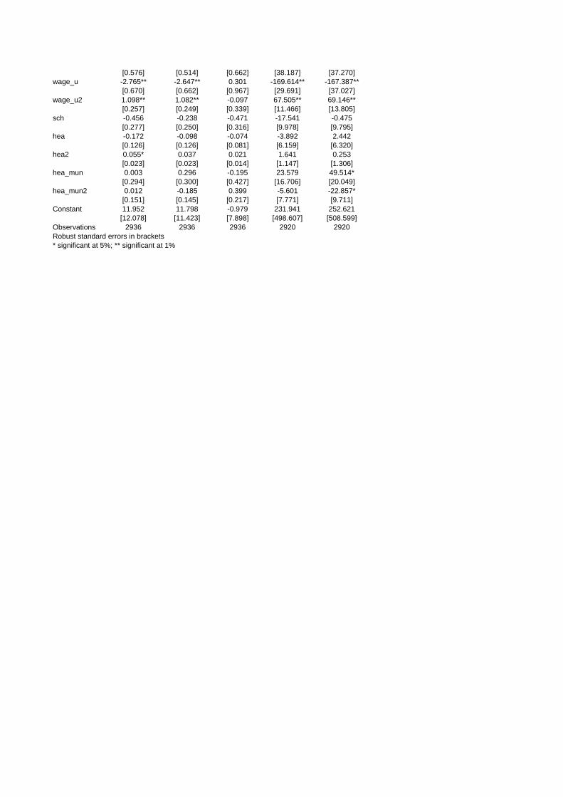
[0.576] [0.514] [0.662] [38.187] [37.270]wage_u -2.765** -2.647** 0.301 -169.614** -167.387**

[0.670] [0.662] [0.967] [29.691] [37.027]wage_u2 1.098** 1.082** -0.097 67.505** 69.146**

[0.257] [0.249] [0.339] [11.466] [13.805]sch -0.456 -0.238 -0.471 -17.541 -0.475

[0.277] [0.250] [0.316] [9.978] [9.795]hea -0.172 -0.098 -0.074 -3.892 2.442

[0.126] [0.126] [0.081] [6.159] [6.320]hea2 0.055* 0.037 0.021 1.641 0.253

[0.023] [0.023] [0.014] [1.147] [1.306]hea_mun 0.003 0.296 -0.195 23.579 49.514*

[0.294] [0.300] [0.427] [16.706] [20.049]hea_mun2 0.012 -0.185 0.399 -5.601 -22.857*

[0.151] [0.145] [0.217] [7.771] [9.711]Constant 11.952 11.798 -0.979 231.941 252.621

[12.078] [11.423] [7.898] [498.607] [508.599]Observations 2936 2936 2936 2920 2920Robust standard errors in brackets* significant at 5%; ** significant at 1%

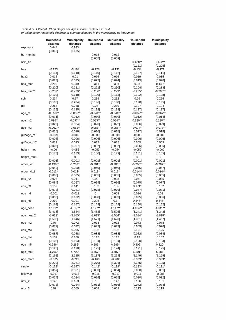
Table A14. Effect of HC on Height per Age z-score. Table 5.9 in TextIV using either household distance or average distance in the municipality as instrument

Household distance

Municipality distance

Household distance

Municipality distance

Household distance

Municipality distance

exposure 0.644 0.923[0.342] [0.475]

hc_months 0.013 0.012[0.007] [0.009]

asis_hc 0.438** 0.602**[0.161] [0.205]

hea -0.123 -0.103 -0.128 -0.131 -0.138 -0.121[0.114] [0.118] [0.110] [0.112] [0.107] [0.111]

hea2 0.015 0.01 0.016 0.016 0.019 0.015[0.023] [0.025] [0.023] [0.024] [0.019] [0.020]

hea_mun 0.299 0.349 0.311 0.301 0.38 0.443*[0.220] [0.231] [0.221] [0.230] [0.204] [0.213]

hea_mun2 -0.232* -0.270* -0.236* -0.229* -0.255* -0.295**[0.109] [0.118] [0.109] [0.113] [0.102] [0.108]

sch 0.234 0.27 0.239 0.232 0.26 0.296[0.196] [0.204] [0.196] [0.198] [0.190] [0.195]

girl 0.256 0.258 0.26 0.259 0.197 0.194[0.136] [0.135] [0.138] [0.138] [0.137] [0.137]

age_m -0.050** -0.052** -0.044** -0.044** -0.062** -0.067**[0.011] [0.012] [0.010] [0.010] [0.012] [0.014]

age_m2 0.096** 0.097** 0.083** 0.084** 0.120** 0.130**[0.023] [0.024] [0.023] [0.022] [0.026] [0.029]

age_m3 -0.062** -0.062** -0.056** -0.056** -0.074** -0.077**[0.016] [0.016] [0.016] [0.015] [0.017] [0.018]

girl*age_m -0.009 -0.009 -0.009 -0.009 -0.006 -0.006[0.006] [0.006] [0.006] [0.006] [0.006] [0.006]

girl*age_m2 0.012 0.013 0.013 0.012 0.009 0.009[0.006] [0.007] [0.007] [0.007] [0.006] [0.006]

height_mot -0.06 -0.058 -0.053 -0.054 -0.059 -0.062[0.178] [0.183] [0.180] [0.179] [0.181] [0.185]

height_mot2 0 0 0 0 0 0[0.001] [0.001] [0.001] [0.001] [0.001] [0.001]

order_kid -0.198** -0.202** -0.201** -0.200** -0.206** -0.207**[0.049] [0.050] [0.049] [0.049] [0.046] [0.047]

order_kid2 0.013* 0.013* 0.013* 0.013* 0.014** 0.014**[0.005] [0.005] [0.005] [0.005] [0.005] [0.005]

edu_h2 0.023 0.011 0.02 0.023 0.041 0.035[0.084] [0.087] [0.084] [0.086] [0.075] [0.077]

edu_h3 0.152 0.141 0.152 0.155 0.171* 0.162[0.078] [0.081] [0.078] [0.079] [0.077] [0.081]

edu_h4 -0.001 -0.013 0 0.003 0.024 0.02[0.098] [0.102] [0.098] [0.099] [0.095] [0.096]

edu_h5 0.299 0.291 0.298 0.3 0.345* 0.345*[0.163] [0.167] [0.163] [0.163] [0.160] [0.162]

age_head 4.161** 4.317** 4.177** 4.147** 4.164** 4.341**[1.415] [1.534] [1.463] [1.525] [1.241] [1.343]

age_head2 -3.612* -3.765* -3.613* -3.584* -3.634* -3.818*[1.532] [1.646] [1.571] [1.623] [1.361] [1.467]

edu_m2 0.07 0.072 0.073 0.072 0.073 0.078[0.072] [0.072] [0.072] [0.073] [0.069] [0.070]

edu_m3 0.099 0.095 0.102 0.102 0.121 0.125[0.087] [0.088] [0.088] [0.088] [0.082] [0.084]

edu_m4 0.107 0.106 0.112 0.112 0.13 0.137[0.102] [0.103] [0.104] [0.104] [0.100] [0.103]

edu_m5 0.286* 0.285* 0.289* 0.289* 0.309* 0.320*[0.125] [0.128] [0.125] [0.124] [0.121] [0.125]

age_mot 4.766* 4.700* 4.667* 4.687* 5.201* 5.286*[2.162] [2.185] [2.187] [2.214] [2.149] [2.159]

age_mot2 -6.335 -6.229 -6.169 -6.202 -6.883* -6.993*[3.229] [3.261] [3.270] [3.304] [3.185] [3.195]

single -0.132* -0.147* -0.142* -0.138* -0.123* -0.131*[0.059] [0.061] [0.063] [0.064] [0.060] [0.061]

followup -0.017 -0.013 -0.016 -0.017 -0.011 -0.008[0.024] [0.024] [0.024] [0.025] [0.020] [0.022]

urbr_2 0.142 0.153 0.15 0.147 0.126 0.131[0.078] [0.084] [0.081] [0.086] [0.072] [0.074]

urbr_3 0.07 0.065 0.068 0.069 0.113 0.119

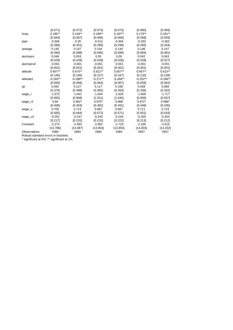
[0.071] [0.072] [0.073] [0.073] [0.080] [0.083]hosp 0.185** 0.194** 0.189** 0.187** 0.179** 0.181**

[0.064] [0.067] [0.066] [0.069] [0.059] [0.059]pipe -0.306 -0.35 -0.313 -0.304 -0.333 -0.362

[0.288] [0.301] [0.289] [0.299] [0.260] [0.264]sewage 0.145 0.147 0.144 0.144 0.146 0.147

[0.090] [0.088] [0.090] [0.090] [0.084] [0.081]alumxpro 0.049 0.053 0.05 0.05 0.042 0.043

[0.028] [0.028] [0.028] [0.028] [0.028] [0.027]alumxpro2 -0.001 -0.001 -0.001 -0.001 -0.001 -0.001

[0.001] [0.001] [0.001] [0.001] [0.001] [0.001]altitude 0.607** 0.675** 0.621** 0.607** 0.567** 0.610**

[0.146] [0.166] [0.157] [0.167] [0.132] [0.139]altitude2 -0.265** -0.288** -0.271** -0.266** -0.252** -0.266**

[0.060] [0.066] [0.064] [0.067] [0.059] [0.062]iql 0.091 0.127 0.117 0.108 0.058 0.084

[0.370] [0.398] [0.382] [0.393] [0.336] [0.352]wage_r -1.573 -1.641 -1.644 -1.626 -1.658 -1.717

[0.992] [0.968] [1.021] [1.040] [0.956] [0.937]wage_r2 0.94 0.962* 0.975* 0.968 0.972* 0.996*

[0.469] [0.453] [0.482] [0.491] [0.448] [0.435]wage_u 0.705 0.713 0.687 0.687 0.711 0.723

[0.565] [0.564] [0.572] [0.571] [0.551] [0.543]wage_u2 -0.252 -0.247 -0.243 -0.244 -0.255 -0.254

[0.217] [0.220] [0.220] [0.222] [0.213] [0.212]Constant -2.274 -2.493 -2.802 -2.719 -2.166 -2.015

[13.786] [14.087] [13.954] [13.854] [14.003] [14.232]Observations 4384 4384 4384 4384 4557 4557Robust standard errors in brackets* significant at 5%; ** significant at 1%

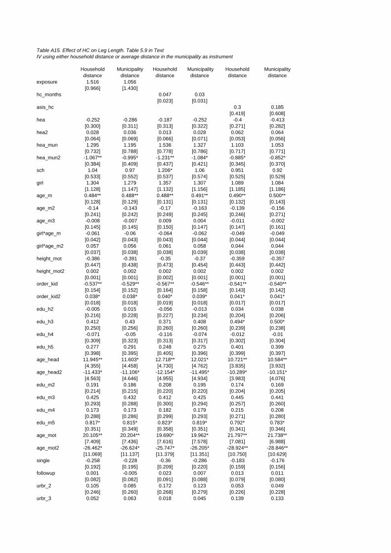
Table A15. Effect of HC on Leg Length. Table 5.9 in TextIV using either household distance or average distance in the municipality as instrument

Household distance

Municipality distance

Household distance

Municipality distance

Household distance

Municipality distance

exposure 1.516 1.056[0.966] [1.430]

hc_months 0.047 0.03[0.023] [0.031]

asis_hc 0.3 0.185[0.419] [0.608]

hea -0.252 -0.286 -0.187 -0.252 -0.4 -0.413[0.300] [0.311] [0.313] [0.322] [0.271] [0.282]

hea2 0.028 0.036 0.013 0.028 0.062 0.064[0.064] [0.069] [0.066] [0.071] [0.053] [0.056]

hea_mun 1.295 1.195 1.536 1.327 1.103 1.053[0.732] [0.788] [0.778] [0.786] [0.717] [0.771]

hea_mun2 -1.067** -0.995* -1.231** -1.084* -0.885* -0.852*[0.384] [0.409] [0.437] [0.421] [0.345] [0.370]

sch 1.04 0.97 1.206* 1.06 0.951 0.92[0.533] [0.552] [0.537] [0.574] [0.525] [0.529]

girl 1.304 1.279 1.357 1.307 1.089 1.084[1.128] [1.147] [1.132] [1.156] [1.185] [1.186]

age_m 0.484** 0.488** 0.488** 0.491** 0.490** 0.500**[0.128] [0.129] [0.131] [0.131] [0.132] [0.143]

age_m2 -0.14 -0.143 -0.17 -0.163 -0.139 -0.156[0.241] [0.242] [0.249] [0.245] [0.246] [0.271]

age_m3 -0.008 -0.007 0.009 0.004 -0.011 -0.002[0.145] [0.145] [0.150] [0.147] [0.147] [0.161]

girl*age_m -0.061 -0.06 -0.064 -0.062 -0.049 -0.049[0.042] [0.043] [0.043] [0.044] [0.044] [0.044]

girl*age_m2 0.057 0.056 0.061 0.058 0.044 0.044[0.037] [0.038] [0.038] [0.039] [0.038] [0.038]

height_mot -0.386 -0.391 -0.35 -0.37 -0.359 -0.357[0.447] [0.438] [0.473] [0.454] [0.443] [0.442]

height_mot2 0.002 0.002 0.002 0.002 0.002 0.002[0.001] [0.001] [0.002] [0.001] [0.001] [0.001]

order_kid -0.537** -0.529** -0.567** -0.546** -0.541** -0.540**[0.154] [0.152] [0.164] [0.158] [0.143] [0.142]

order_kid2 0.038* 0.038* 0.040* 0.039* 0.041* 0.041*[0.018] [0.018] [0.019] [0.018] [0.017] [0.017]

edu_h2 -0.005 0.015 -0.056 -0.013 0.034 0.038[0.216] [0.228] [0.227] [0.234] [0.204] [0.206]

edu_h3 0.412 0.43 0.371 0.408 0.494* 0.500*[0.250] [0.256] [0.260] [0.260] [0.239] [0.238]

edu_h4 -0.071 -0.05 -0.116 -0.074 -0.012 -0.01[0.309] [0.323] [0.313] [0.317] [0.302] [0.304]

edu_h5 0.277 0.291 0.248 0.275 0.401 0.399[0.398] [0.395] [0.405] [0.396] [0.399] [0.397]

age_head 11.945** 11.603* 12.718** 12.021* 10.721** 10.584**[4.355] [4.458] [4.730] [4.762] [3.835] [3.932]

age_head2 -11.433* -11.106* -12.154* -11.495* -10.289* -10.151*[4.563] [4.646] [4.955] [4.934] [3.983] [4.076]

edu_m2 0.191 0.186 0.208 0.195 0.174 0.169[0.214] [0.215] [0.220] [0.220] [0.204] [0.205]

edu_m3 0.425 0.432 0.412 0.425 0.445 0.441[0.293] [0.288] [0.300] [0.294] [0.257] [0.260]

edu_m4 0.173 0.173 0.182 0.179 0.215 0.208[0.288] [0.286] [0.299] [0.293] [0.271] [0.280]

edu_m5 0.817* 0.815* 0.823* 0.819* 0.792* 0.783*[0.351] [0.349] [0.358] [0.351] [0.341] [0.346]

age_mot 20.105** 20.204** 19.690* 19.962* 21.797** 21.738**[7.409] [7.436] [7.616] [7.578] [7.081] [6.988]

age_mot2 -26.462* -26.624* -25.747* -26.205* -28.924** -28.846**[11.069] [11.137] [11.379] [11.351] [10.750] [10.629]

single -0.258 -0.228 -0.36 -0.286 -0.183 -0.176[0.192] [0.195] [0.209] [0.220] [0.159] [0.156]

followup 0.001 -0.005 0.023 0.007 0.013 0.011[0.082] [0.082] [0.091] [0.088] [0.079] [0.080]

urbr_2 0.105 0.085 0.172 0.123 0.053 0.049[0.246] [0.260] [0.268] [0.279] [0.226] [0.228]

urbr_3 0.052 0.063 0.018 0.045 0.139 0.133

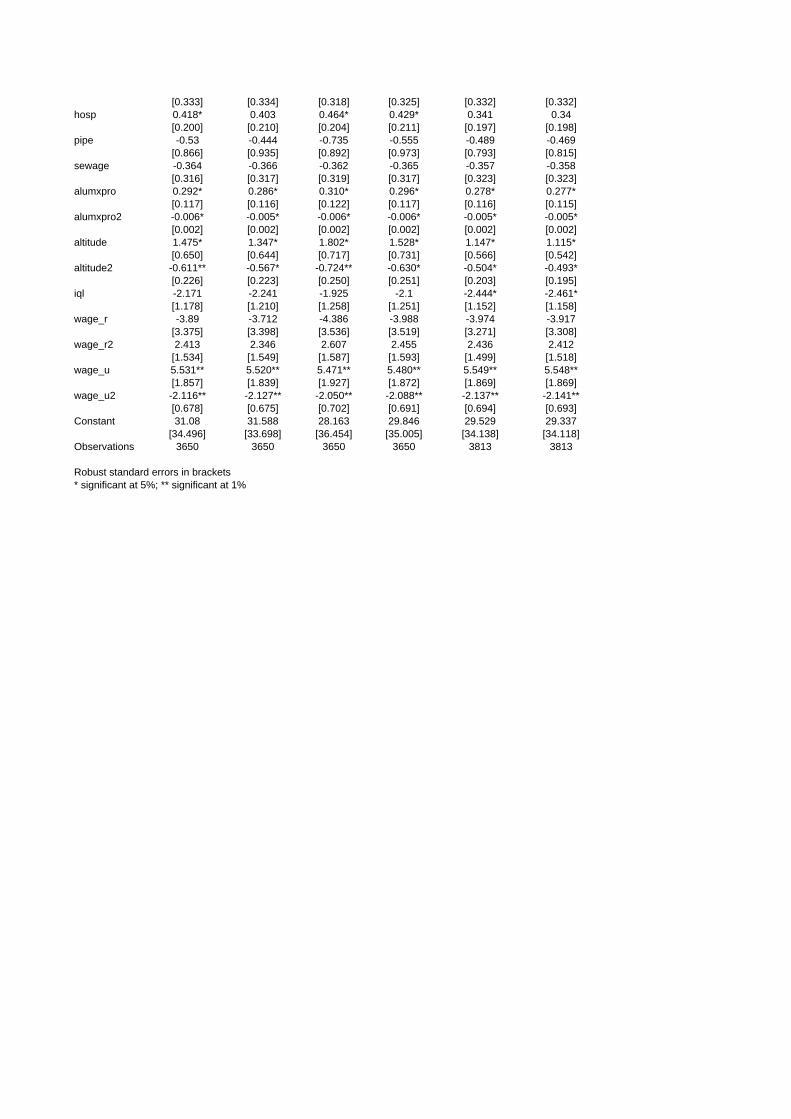
[0.333] [0.334] [0.318] [0.325] [0.332] [0.332]hosp 0.418* 0.403 0.464* 0.429* 0.341 0.34

[0.200] [0.210] [0.204] [0.211] [0.197] [0.198]pipe -0.53 -0.444 -0.735 -0.555 -0.489 -0.469

[0.866] [0.935] [0.892] [0.973] [0.793] [0.815]sewage -0.364 -0.366 -0.362 -0.365 -0.357 -0.358

[0.316] [0.317] [0.319] [0.317] [0.323] [0.323]alumxpro 0.292* 0.286* 0.310* 0.296* 0.278* 0.277*

[0.117] [0.116] [0.122] [0.117] [0.116] [0.115]alumxpro2 -0.006* -0.005* -0.006* -0.006* -0.005* -0.005*

[0.002] [0.002] [0.002] [0.002] [0.002] [0.002]altitude 1.475* 1.347* 1.802* 1.528* 1.147* 1.115*

[0.650] [0.644] [0.717] [0.731] [0.566] [0.542]altitude2 -0.611** -0.567* -0.724** -0.630* -0.504* -0.493*

[0.226] [0.223] [0.250] [0.251] [0.203] [0.195]iql -2.171 -2.241 -1.925 -2.1 -2.444* -2.461*

[1.178] [1.210] [1.258] [1.251] [1.152] [1.158]wage_r -3.89 -3.712 -4.386 -3.988 -3.974 -3.917

[3.375] [3.398] [3.536] [3.519] [3.271] [3.308]wage_r2 2.413 2.346 2.607 2.455 2.436 2.412

[1.534] [1.549] [1.587] [1.593] [1.499] [1.518]wage_u 5.531** 5.520** 5.471** 5.480** 5.549** 5.548**

[1.857] [1.839] [1.927] [1.872] [1.869] [1.869]wage_u2 -2.116** -2.127** -2.050** -2.088** -2.137** -2.141**

[0.678] [0.675] [0.702] [0.691] [0.694] [0.693]Constant 31.08 31.588 28.163 29.846 29.529 29.337

[34.496] [33.698] [36.454] [35.005] [34.138] [34.118]Observations 3650 3650 3650 3650 3813 3813

Robust standard errors in brackets* significant at 5%; ** significant at 1%

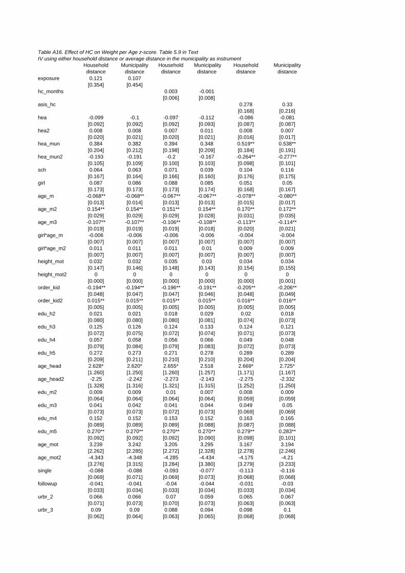
Table A16. Effect of HC on Weight per Age z-score. Table 5.9 in TextIV using either household distance or average distance in the municipality as instrument

Household distance

Municipality distance

Household distance

Municipality distance

Household distance

Municipality distance

exposure 0.121 0.107[0.354] [0.454]

hc_months 0.003 -0.001[0.006] [0.008]

asis_hc 0.278 0.33[0.168] [0.216]

hea -0.099 -0.1 -0.097 -0.112 -0.086 -0.081[0.092] [0.092] [0.092] [0.093] [0.087] [0.087]

hea2 0.008 0.008 0.007 0.011 0.008 0.007[0.020] [0.021] [0.020] [0.021] [0.016] [0.017]

hea_mun 0.384 0.382 0.394 0.348 0.519** 0.538**[0.204] [0.212] [0.198] [0.209] [0.184] [0.191]

hea_mun2 -0.193 -0.191 -0.2 -0.167 -0.264** -0.277**[0.105] [0.109] [0.100] [0.103] [0.098] [0.101]

sch 0.064 0.063 0.071 0.039 0.104 0.116[0.167] [0.164] [0.166] [0.160] [0.176] [0.175]

girl 0.087 0.086 0.088 0.085 0.051 0.05[0.173] [0.173] [0.173] [0.174] [0.168] [0.167]

age_m -0.068** -0.068** -0.067** -0.067** -0.078** -0.080**[0.013] [0.014] [0.013] [0.013] [0.015] [0.017]

age_m2 0.154** 0.154** 0.151** 0.154** 0.170** 0.172**[0.029] [0.029] [0.029] [0.028] [0.031] [0.035]

age_m3 -0.107** -0.107** -0.106** -0.108** -0.113** -0.114**[0.019] [0.019] [0.019] [0.018] [0.020] [0.021]

girl*age_m -0.006 -0.006 -0.006 -0.006 -0.004 -0.004[0.007] [0.007] [0.007] [0.007] [0.007] [0.007]

girl*age_m2 0.011 0.011 0.011 0.01 0.009 0.009[0.007] [0.007] [0.007] [0.007] [0.007] [0.007]

height_mot 0.032 0.032 0.035 0.03 0.034 0.034[0.147] [0.146] [0.148] [0.143] [0.154] [0.155]

height_mot2 0 0 0 0 0 0[0.000] [0.000] [0.000] [0.000] [0.000] [0.001]

order_kid -0.194** -0.194** -0.196** -0.191** -0.205** -0.206**[0.048] [0.047] [0.047] [0.046] [0.048] [0.049]

order_kid2 0.015** 0.015** 0.015** 0.015** 0.016** 0.016**[0.005] [0.005] [0.005] [0.005] [0.005] [0.005]

edu_h2 0.021 0.021 0.018 0.029 0.02 0.018[0.080] [0.080] [0.080] [0.081] [0.074] [0.073]

edu_h3 0.125 0.126 0.124 0.133 0.124 0.121[0.072] [0.075] [0.072] [0.074] [0.071] [0.073]

edu_h4 0.057 0.058 0.056 0.066 0.049 0.048[0.079] [0.084] [0.079] [0.083] [0.072] [0.073]

edu_h5 0.272 0.273 0.271 0.278 0.289 0.289[0.209] [0.211] [0.210] [0.210] [0.204] [0.204]

age_head 2.628* 2.620* 2.655* 2.518 2.669* 2.725*[1.260] [1.250] [1.260] [1.257] [1.171] [1.167]

age_head2 -2.25 -2.242 -2.273 -2.143 -2.275 -2.332[1.328] [1.316] [1.321] [1.315] [1.252] [1.250]

edu_m2 0.009 0.009 0.01 0.007 0.008 0.009[0.064] [0.064] [0.064] [0.064] [0.059] [0.059]

edu_m3 0.041 0.042 0.041 0.044 0.049 0.05[0.073] [0.073] [0.072] [0.073] [0.069] [0.069]

edu_m4 0.152 0.152 0.153 0.152 0.163 0.165[0.089] [0.089] [0.089] [0.088] [0.087] [0.088]

edu_m5 0.270** 0.270** 0.270** 0.270** 0.279** 0.283**[0.092] [0.092] [0.092] [0.090] [0.098] [0.101]

age_mot 3.239 3.242 3.205 3.295 3.167 3.194[2.262] [2.285] [2.272] [2.328] [2.278] [2.246]

age_mot2 -4.343 -4.348 -4.285 -4.434 -4.175 -4.21[3.276] [3.315] [3.284] [3.380] [3.279] [3.233]

single -0.088 -0.088 -0.093 -0.077 -0.113 -0.116[0.069] [0.071] [0.069] [0.073] [0.068] [0.068]

followup -0.041 -0.041 -0.04 -0.044 -0.031 -0.03[0.033] [0.034] [0.033] [0.034] [0.033] [0.034]

urbr_2 0.066 0.066 0.07 0.059 0.065 0.067[0.071] [0.073] [0.070] [0.073] [0.063] [0.063]

urbr_3 0.09 0.09 0.088 0.094 0.098 0.1[0.062] [0.064] [0.063] [0.065] [0.068] [0.068]

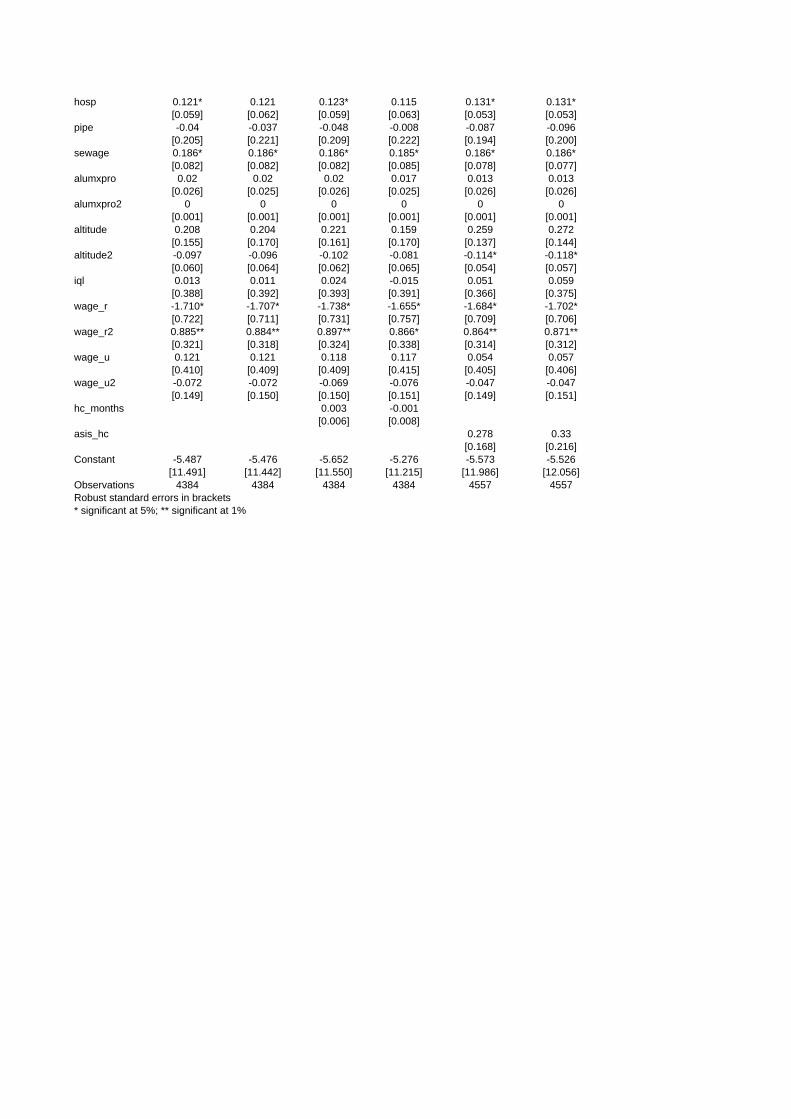
hosp 0.121* 0.121 0.123* 0.115 0.131* 0.131*[0.059] [0.062] [0.059] [0.063] [0.053] [0.053]

pipe -0.04 -0.037 -0.048 -0.008 -0.087 -0.096[0.205] [0.221] [0.209] [0.222] [0.194] [0.200]

sewage 0.186* 0.186* 0.186* 0.185* 0.186* 0.186*[0.082] [0.082] [0.082] [0.085] [0.078] [0.077]

alumxpro 0.02 0.02 0.02 0.017 0.013 0.013[0.026] [0.025] [0.026] [0.025] [0.026] [0.026]

alumxpro2 0 0 0 0 0 0[0.001] [0.001] [0.001] [0.001] [0.001] [0.001]

altitude 0.208 0.204 0.221 0.159 0.259 0.272[0.155] [0.170] [0.161] [0.170] [0.137] [0.144]

altitude2 -0.097 -0.096 -0.102 -0.081 -0.114* -0.118*[0.060] [0.064] [0.062] [0.065] [0.054] [0.057]

iql 0.013 0.011 0.024 -0.015 0.051 0.059[0.388] [0.392] [0.393] [0.391] [0.366] [0.375]

wage_r -1.710* -1.707* -1.738* -1.655* -1.684* -1.702*[0.722] [0.711] [0.731] [0.757] [0.709] [0.706]

wage_r2 0.885** 0.884** 0.897** 0.866* 0.864** 0.871**[0.321] [0.318] [0.324] [0.338] [0.314] [0.312]

wage_u 0.121 0.121 0.118 0.117 0.054 0.057[0.410] [0.409] [0.409] [0.415] [0.405] [0.406]

wage_u2 -0.072 -0.072 -0.069 -0.076 -0.047 -0.047[0.149] [0.150] [0.150] [0.151] [0.149] [0.151]

hc_months 0.003 -0.001[0.006] [0.008]

asis_hc 0.278 0.33[0.168] [0.216]

Constant -5.487 -5.476 -5.652 -5.276 -5.573 -5.526[11.491] [11.442] [11.550] [11.215] [11.986] [12.056]

Observations 4384 4384 4384 4384 4557 4557Robust standard errors in brackets* significant at 5%; ** significant at 1%

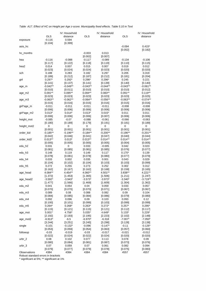
Table A17. Effect of HC on Height per Age z-score. Municipality fixed effects. Table 5.10 in Text

OLSIV: Household

distance OLSIV: Household

distance OLSIV: Household

distanceexposure -0.116 0.594

[0.104] [0.399]asis_hc -0.094 0.415*

[0.052] [0.182]hc_months -0.003 0.013

[0.002] [0.007]hea -0.116 -0.088 -0.117 -0.089 -0.134 -0.106

[0.117] [0.122] [0.118] [0.119] [0.110] [0.115]hea2 0.014 0.007 0.015 0.007 0.019 0.012

[0.023] [0.024] [0.024] [0.023] [0.020] [0.020]sch 0.188 0.283 0.182 0.297 0.205 0.319

[0.189] [0.212] [0.187] [0.212] [0.181] [0.204]girl 0.297* 0.292* 0.296* 0.296* 0.245 0.221

[0.141] [0.137] [0.141] [0.139] [0.140] [0.140]age_m -0.042** -0.049** -0.043** -0.044** -0.043** -0.061**

[0.010] [0.011] [0.010] [0.010] [0.010] [0.012]age_m2 0.091** 0.095** 0.094** 0.083** 0.091** 0.119**

[0.023] [0.023] [0.023] [0.023] [0.023] [0.025]age_m3 -0.063** -0.062** -0.064** -0.056** -0.063** -0.074**

[0.015] [0.016] [0.015] [0.016] [0.015] [0.016]girl*age_m -0.011 -0.011 -0.011 -0.011 -0.008 -0.008

[0.006] [0.006] [0.006] [0.006] [0.006] [0.006]girl*age_m2 0.013* 0.014* 0.013* 0.015* 0.011 0.011

[0.006] [0.006] [0.006] [0.007] [0.006] [0.006]height_mot -0.085 -0.07 -0.088 -0.061 -0.066 -0.063

[0.180] [0.189] [0.179] [0.191] [0.181] [0.189]height_mot2 0 0 0 0 0 0

[0.001] [0.001] [0.001] [0.001] [0.001] [0.001]order_kid -0.185** -0.196** -0.184** -0.200** -0.196** -0.201**

[0.042] [0.046] [0.041] [0.047] [0.040] [0.044]order_kid2 0.013** 0.013* 0.013** 0.014** 0.014** 0.014**

[0.005] [0.005] [0.005] [0.005] [0.004] [0.005]edu_h2 0.031 0 0.033 -0.005 0.042 0.023

[0.081] [0.085] [0.081] [0.085] [0.076] [0.077]edu_h3 0.148 0.119 0.149 0.117 0.170* 0.139

[0.078] [0.081] [0.078] [0.080] [0.077] [0.079]edu_h4 0.033 0.002 0.035 0.001 0.043 0.029

[0.104] [0.102] [0.104] [0.103] [0.103] [0.099]edu_h5 0.272 0.255 0.273 0.252 0.302 0.312

[0.162] [0.167] [0.162] [0.168] [0.159] [0.165]age_head 4.084** 4.454** 4.060** 4.501** 3.838** 4.221**

[1.372] [1.453] [1.365] [1.506] [1.211] [1.247]age_head2 -3.592* -3.943* -3.573* -3.973* -3.340* -3.719**

[1.477] [1.566] [1.469] [1.609] [1.304] [1.362]edu_m2 0.041 0.054 0.04 0.059 0.033 0.057

[0.070] [0.070] [0.070] [0.071] [0.067] [0.067]edu_m3 0.089 0.08 0.088 0.082 0.09 0.104

[0.084] [0.085] [0.084] [0.086] [0.079] [0.080]edu_m4 0.092 0.096 0.09 0.103 0.093 0.12

[0.100] [0.101] [0.099] [0.103] [0.099] [0.099]edu_m5 0.264* 0.268* 0.263* 0.272* 0.257* 0.295*

[0.115] [0.121] [0.115] [0.121] [0.112] [0.117]age_mot 5.001* 4.756* 5.035* 4.649* 5.133* 5.229*

[2.192] [2.193] [2.195] [2.223] [2.102] [2.148]age_mot2 -6.913* -6.5 -6.970* -6.318 -7.007* -7.050*

[3.244] [3.251] [3.245] [3.298] [3.128] [3.138]single -0.101 -0.132* -0.096 -0.147* -0.11 -0.126*

[0.053] [0.059] [0.054] [0.063] [0.057] [0.060]followup -0.03 -0.019 -0.03 -0.017 -0.021 -0.012

[0.022] [0.024] [0.022] [0.024] [0.020] [0.020]urbr_2 0.08 0.102 0.077 0.113 0.078 0.09

[0.080] [0.084] [0.081] [0.087] [0.073] [0.076]urbr_3 0.07 0.059 0.07 0.061 0.082 0.094

[0.079] [0.077] [0.079] [0.078] [0.075] [0.083]Observations 4384 4384 4384 4384 4557 4557Robust standard errors in brackets* significant at 5%; ** significant at 1%

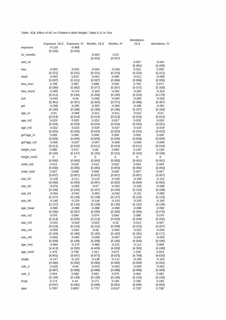
Table A18. Effect of HC on Children's Birth Weight. Table 5.11 in Text

Exposure. OLS Exposure. IV Months. OLS Months. IVAtendance.

OLS Atendance. IVexposure -0.119 -0.468

[0.135] [0.434]hc_months -0.004 -0.01

[0.002] [0.007]asis_hc 0.057 -0.041

[0.081] [0.205]hea -0.003 -0.042 -0.004 -0.028 0.015 0.005

[0.221] [0.231] [0.221] [0.215] [0.223] [0.221]hea2 -0.002 0.013 -0.001 0.009 -0.011 -0.008

[0.097] [0.101] [0.097] [0.096] [0.096] [0.095]hea_mun 0.708 0.587 0.689 0.593 0.745 0.671

[0.380] [0.362] [0.377] [0.357] [0.372] [0.339]hea_mun2 -0.355 -0.274 -0.343 -0.281 -0.362 -0.316

[0.211] [0.194] [0.209] [0.190] [0.210] [0.179]sch -0.046 -0.09 -0.056 -0.094 -0.005 -0.028

[0.361] [0.367] [0.363] [0.372] [0.396] [0.397]girl -0.298 -0.295 -0.302 -0.309 -0.285 -0.281

[0.190] [0.188] [0.189] [0.186] [0.187] [0.184]age_m -0.01 -0.008 -0.011 -0.011 -0.012 -0.01

[0.014] [0.014] [0.014] [0.013] [0.014] [0.014]age_m2 0.029 0.029 0.033 0.037 0.028 0.026

[0.034] [0.033] [0.034] [0.034] [0.032] [0.031]age_m3 -0.022 -0.023 -0.024 -0.027 -0.019 -0.019

[0.025] [0.025] [0.025] [0.025] [0.024] [0.023]girl*age_m 0.005 0.006 0.006 0.006 0.005 0.005

[0.009] [0.009] [0.009] [0.009] [0.009] [0.009]girl*age_m2 -0.006 -0.007 -0.007 -0.008 -0.006 -0.006

[0.011] [0.010] [0.011] [0.010] [0.011] [0.010]height_mot 0.086 0.071 0.08 0.063 0.146 0.139

[0.150] [0.147] [0.152] [0.151] [0.163] [0.160]height_mot2 0 0 0 0 0 0

[0.000] [0.000] [0.000] [0.000] [0.001] [0.001]order_kid 0.012 0.018 0.015 0.022 0.004 0.004

[0.056] [0.055] [0.056] [0.054] [0.056] [0.054]order_kid2 0.007 0.006 0.006 0.006 0.007 0.007

[0.007] [0.007] [0.007] [0.007] [0.007] [0.007]edu_h2 -0.128 -0.111 -0.123 -0.106 -0.158 -0.151

[0.096] [0.094] [0.097] [0.092] [0.094] [0.092]edu_h3 -0.076 -0.059 -0.07 -0.053 -0.109 -0.098

[0.106] [0.102] [0.107] [0.104] [0.115] [0.108]edu_h4 -0.054 -0.042 -0.053 -0.043 -0.101 -0.095

[0.127] [0.128] [0.128] [0.127] [0.126] [0.123]edu_h5 -0.148 -0.129 -0.146 -0.133 -0.203 -0.195

[0.137] [0.134] [0.138] [0.135] [0.142] [0.136]age_head -0.085 -0.088 -0.088 -0.096 -0.088 -0.082

[0.296] [0.287] [0.295] [0.285] [0.284] [0.276]edu_m2 0.076 0.064 0.074 0.064 0.088 0.076

[0.214] [0.205] [0.213] [0.203] [0.209] [0.202]edu_m3 -0.022 -0.018 -0.022 -0.02 0.013 0.007

[0.216] [0.210] [0.215] [0.208] [0.215] [0.207]edu_m4 -0.059 -0.062 -0.06 -0.065 -0.023 -0.034

[0.193] [0.185] [0.192] [0.183] [0.181] [0.171]edu_m5 -0.056 -0.065 -0.058 -0.067 -0.042 -0.053

[0.209] [0.199] [0.208] [0.196] [0.200] [0.190]age_mot -0.564 -0.174 -0.486 -0.151 -0.111 0.065

[4.413] [4.265] [4.405] [4.269] [4.336] [4.249]age_mot2 1.476 0.786 1.311 0.672 1.235 0.919

[6.901] [6.647] [6.873] [6.625] [6.768] [6.620]single -0.147 -0.125 -0.138 -0.112 -0.169 -0.163

[0.090] [0.092] [0.090] [0.090] [0.093] [0.091]urbr_2 -0.026 -0.04 -0.033 -0.052 -0.059 -0.062

[0.087] [0.088] [0.088] [0.088] [0.088] [0.089]urbr_3 0.044 0.069 0.051 0.075 0.064 0.062

[0.139] [0.139] [0.138] [0.136] [0.152] [0.150]hosp 0.174 0.16 0.171 0.159 0.185 0.183

[0.097] [0.092] [0.096] [0.091] [0.095] [0.092]pipe 0.765* 0.800* 0.775* 0.810* 0.729* 0.736*

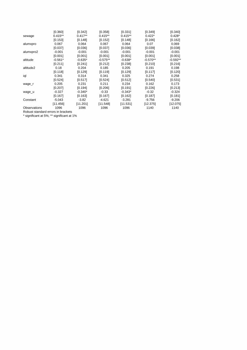
[0.360] [0.342] [0.358] [0.331] [0.349] [0.340]sewage 0.415** 0.417** 0.415** 0.415** 0.422* 0.428*

[0.153] [0.148] [0.152] [0.148] [0.166] [0.162]alumxpro 0.067 0.064 0.067 0.064 0.07 0.069

[0.037] [0.036] [0.037] [0.036] [0.039] [0.038]alumxpro2 -0.001 -0.001 -0.001 -0.001 -0.001 -0.001

[0.001] [0.001] [0.001] [0.001] [0.001] [0.001]altitude -0.561* -0.635* -0.575** -0.638* -0.570** -0.592**

[0.211] [0.241] [0.212] [0.238] [0.210] [0.216]altitude2 0.18 0.204 0.185 0.205 0.191 0.198

[0.118] [0.129] [0.119] [0.129] [0.117] [0.120]iql 0.341 0.314 0.341 0.325 0.274 0.258

[0.524] [0.517] [0.524] [0.512] [0.540] [0.531]wage_r 0.205 0.231 0.211 0.234 0.162 0.173

[0.207] [0.194] [0.206] [0.191] [0.226] [0.213]wage_u -0.327 -0.340* -0.33 -0.343* -0.32 -0.324

[0.167] [0.163] [0.167] [0.162] [0.187] [0.181]Constant -5.043 -3.82 -4.621 -3.281 -9.756 -9.206

[11.456] [11.201] [11.548] [11.531] [12.375] [12.075]Observations 1096 1096 1096 1096 1140 1140Robust standard errors in brackets* significant at 5%; ** significant at 1%

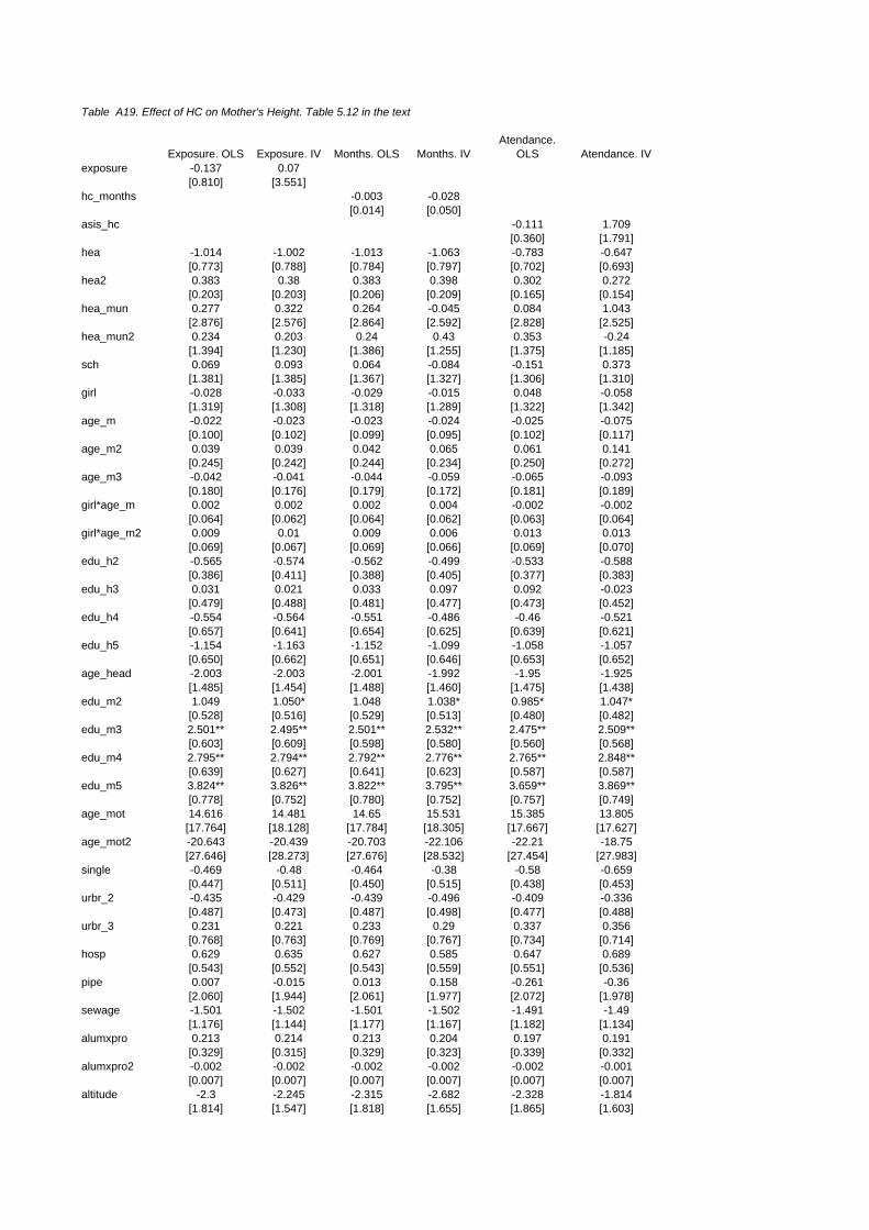
Table A19. Effect of HC on Mother's Height. Table 5.12 in the text

Exposure. OLS Exposure. IV Months. OLS Months. IVAtendance.

OLS Atendance. IVexposure -0.137 0.07

[0.810] [3.551]hc_months -0.003 -0.028

[0.014] [0.050]asis_hc -0.111 1.709

[0.360] [1.791]hea -1.014 -1.002 -1.013 -1.063 -0.783 -0.647

[0.773] [0.788] [0.784] [0.797] [0.702] [0.693]hea2 0.383 0.38 0.383 0.398 0.302 0.272

[0.203] [0.203] [0.206] [0.209] [0.165] [0.154]hea_mun 0.277 0.322 0.264 -0.045 0.084 1.043

[2.876] [2.576] [2.864] [2.592] [2.828] [2.525]hea_mun2 0.234 0.203 0.24 0.43 0.353 -0.24

[1.394] [1.230] [1.386] [1.255] [1.375] [1.185]sch 0.069 0.093 0.064 -0.084 -0.151 0.373

[1.381] [1.385] [1.367] [1.327] [1.306] [1.310]girl -0.028 -0.033 -0.029 -0.015 0.048 -0.058

[1.319] [1.308] [1.318] [1.289] [1.322] [1.342]age_m -0.022 -0.023 -0.023 -0.024 -0.025 -0.075

[0.100] [0.102] [0.099] [0.095] [0.102] [0.117]age_m2 0.039 0.039 0.042 0.065 0.061 0.141

[0.245] [0.242] [0.244] [0.234] [0.250] [0.272]age_m3 -0.042 -0.041 -0.044 -0.059 -0.065 -0.093

[0.180] [0.176] [0.179] [0.172] [0.181] [0.189]girl*age_m 0.002 0.002 0.002 0.004 -0.002 -0.002

[0.064] [0.062] [0.064] [0.062] [0.063] [0.064]girl*age_m2 0.009 0.01 0.009 0.006 0.013 0.013

[0.069] [0.067] [0.069] [0.066] [0.069] [0.070]edu_h2 -0.565 -0.574 -0.562 -0.499 -0.533 -0.588

[0.386] [0.411] [0.388] [0.405] [0.377] [0.383]edu_h3 0.031 0.021 0.033 0.097 0.092 -0.023

[0.479] [0.488] [0.481] [0.477] [0.473] [0.452]edu_h4 -0.554 -0.564 -0.551 -0.486 -0.46 -0.521

[0.657] [0.641] [0.654] [0.625] [0.639] [0.621]edu_h5 -1.154 -1.163 -1.152 -1.099 -1.058 -1.057

[0.650] [0.662] [0.651] [0.646] [0.653] [0.652]age_head -2.003 -2.003 -2.001 -1.992 -1.95 -1.925

[1.485] [1.454] [1.488] [1.460] [1.475] [1.438]edu_m2 1.049 1.050* 1.048 1.038* 0.985* 1.047*

[0.528] [0.516] [0.529] [0.513] [0.480] [0.482]edu_m3 2.501** 2.495** 2.501** 2.532** 2.475** 2.509**

[0.603] [0.609] [0.598] [0.580] [0.560] [0.568]edu_m4 2.795** 2.794** 2.792** 2.776** 2.765** 2.848**

[0.639] [0.627] [0.641] [0.623] [0.587] [0.587]edu_m5 3.824** 3.826** 3.822** 3.795** 3.659** 3.869**

[0.778] [0.752] [0.780] [0.752] [0.757] [0.749]age_mot 14.616 14.481 14.65 15.531 15.385 13.805

[17.764] [18.128] [17.784] [18.305] [17.667] [17.627]age_mot2 -20.643 -20.439 -20.703 -22.106 -22.21 -18.75

[27.646] [28.273] [27.676] [28.532] [27.454] [27.983]single -0.469 -0.48 -0.464 -0.38 -0.58 -0.659

[0.447] [0.511] [0.450] [0.515] [0.438] [0.453]urbr_2 -0.435 -0.429 -0.439 -0.496 -0.409 -0.336

[0.487] [0.473] [0.487] [0.498] [0.477] [0.488]urbr_3 0.231 0.221 0.233 0.29 0.337 0.356

[0.768] [0.763] [0.769] [0.767] [0.734] [0.714]hosp 0.629 0.635 0.627 0.585 0.647 0.689

[0.543] [0.552] [0.543] [0.559] [0.551] [0.536]pipe 0.007 -0.015 0.013 0.158 -0.261 -0.36

[2.060] [1.944] [2.061] [1.977] [2.072] [1.978]sewage -1.501 -1.502 -1.501 -1.502 -1.491 -1.49

[1.176] [1.144] [1.177] [1.167] [1.182] [1.134]alumxpro 0.213 0.214 0.213 0.204 0.197 0.191

[0.329] [0.315] [0.329] [0.323] [0.339] [0.332]alumxpro2 -0.002 -0.002 -0.002 -0.002 -0.002 -0.001

[0.007] [0.007] [0.007] [0.007] [0.007] [0.007]altitude -2.3 -2.245 -2.315 -2.682 -2.328 -1.814

[1.814] [1.547] [1.818] [1.655] [1.865] [1.603]

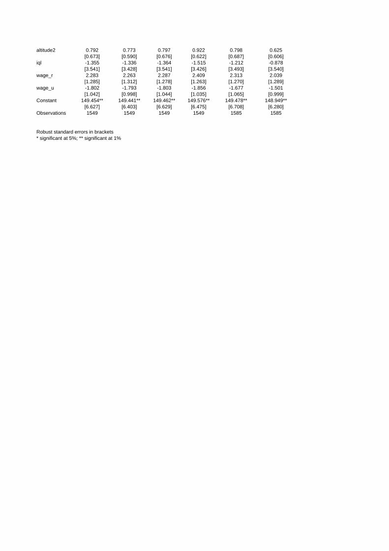
altitude2 0.792 0.773 0.797 0.922 0.798 0.625[0.673] [0.590] [0.676] [0.622] [0.687] [0.606]

iql -1.355 -1.336 -1.364 -1.515 -1.212 -0.878[3.541] [3.428] [3.541] [3.426] [3.493] [3.540]

wage_r 2.283 2.263 2.287 2.409 2.313 2.039[1.285] [1.312] [1.278] [1.263] [1.270] [1.289]

wage_u -1.802 -1.793 -1.803 -1.856 -1.677 -1.501[1.042] [0.998] [1.044] [1.035] [1.065] [0.999]

Constant 149.454** 149.441** 149.462** 149.576** 149.478** 148.949**[6.627] [6.403] [6.629] [6.475] [6.708] [6.280]

Observations 1549 1549 1549 1549 1585 1585

Robust standard errors in brackets* significant at 5%; ** significant at 1%

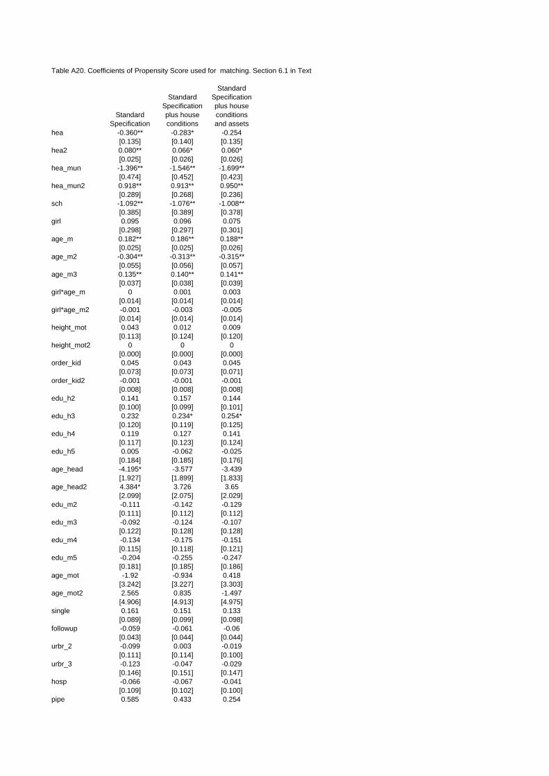
Table A20. Coefficients of Propensity Score used for matching. Section 6.1 in Text

Standard Specification

Standard Specification plus house conditions

Standard Specification plus house conditions and assets

hea -0.360** -0.283* -0.254[0.135] [0.140] [0.135]

hea2 0.080** 0.066* 0.060*[0.025] [0.026] [0.026]

hea_mun -1.396** -1.546** -1.699**[0.474] [0.452] [0.423]

hea_mun2 0.918** 0.913** 0.950**[0.289] [0.268] [0.236]

sch -1.092** -1.076** -1.008**[0.385] [0.389] [0.378]

girl 0.095 0.096 0.075[0.298] [0.297] [0.301]

age_m 0.182** 0.186** 0.188**[0.025] [0.025] [0.026]

age_m2 -0.304** -0.313** -0.315**[0.055] [0.056] [0.057]

age_m3 0.135** 0.140** 0.141**[0.037] [0.038] [0.039]

girl*age_m 0 0.001 0.003[0.014] [0.014] [0.014]

girl*age_m2 -0.001 -0.003 -0.005[0.014] [0.014] [0.014]

height_mot 0.043 0.012 0.009[0.113] [0.124] [0.120]

height_mot2 0 0 0[0.000] [0.000] [0.000]

order_kid 0.045 0.043 0.045[0.073] [0.073] [0.071]

order_kid2 -0.001 -0.001 -0.001[0.008] [0.008] [0.008]

edu_h2 0.141 0.157 0.144[0.100] [0.099] [0.101]

edu_h3 0.232 0.234* 0.254*[0.120] [0.119] [0.125]

edu_h4 0.119 0.127 0.141[0.117] [0.123] [0.124]

edu_h5 0.005 -0.062 -0.025[0.184] [0.185] [0.176]

age_head -4.195* -3.577 -3.439[1.927] [1.899] [1.833]

age_head2 4.384* 3.726 3.65[2.099] [2.075] [2.029]

edu_m2 -0.111 -0.142 -0.129[0.111] [0.112] [0.112]

edu_m3 -0.092 -0.124 -0.107[0.122] [0.128] [0.128]

edu_m4 -0.134 -0.175 -0.151[0.115] [0.118] [0.121]

edu_m5 -0.204 -0.255 -0.247[0.181] [0.185] [0.186]

age_mot -1.92 -0.934 0.418[3.242] [3.227] [3.303]

age_mot2 2.565 0.835 -1.497[4.906] [4.913] [4.975]

single 0.161 0.151 0.133[0.089] [0.099] [0.098]

followup -0.059 -0.061 -0.06[0.043] [0.044] [0.044]

urbr_2 -0.099 0.003 -0.019[0.111] [0.114] [0.100]

urbr_3 -0.123 -0.047 -0.029[0.146] [0.151] [0.147]

hosp -0.066 -0.067 -0.041[0.109] [0.102] [0.100]

pipe 0.585 0.433 0.254

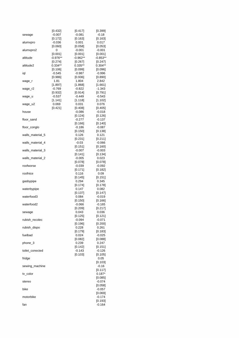
[0.432] [0.417] [0.399]sewage -0.007 -0.081 -0.18

[0.172] [0.163] [0.163]alumxpro -0.036 0.001 0.017

[0.060] [0.058] [0.053]alumxpro2 0 -0.001 -0.001

[0.001] [0.001] [0.001]altitude -0.976** -0.962** -0.853**

[0.274] [0.267] [0.247]altitude2 0.334** 0.335** 0.304**

[0.106] [0.099] [0.096]iql -0.545 -0.987 -0.996

[0.986] [0.936] [0.890]wage_r 1.81 1.804 2.842

[1.897] [1.868] [1.661]wage_r2 -0.769 -0.822 -1.343

[0.932] [0.914] [0.791]wage_u -0.537 -0.449 -0.543

[1.141] [1.118] [1.102]wage_u2 0.069 0.031 0.076

[0.421] [0.408] [0.405]house -0.086 -0.018

[0.124] [0.126]floor_sand -0.277 -0.137

[0.166] [0.140]floor_conglo -0.186 -0.087

[0.150] [0.138]walls_material_5 0.126 0.121

[0.231] [0.211]walls_material_4 -0.03 -0.066

[0.151] [0.160]walls_material_3 -0.007 -0.003

[0.141] [0.134]walls_material_2 -0.005 0.023

[0.078] [0.078]roofworse -0.039 -0.092

[0.171] [0.182]roofnice 0.116 0.09

[0.145] [0.151]gasbypipe 0.294 0.345

[0.174] [0.178]waterbypipe 0.147 0.082

[0.137] [0.147]waterfood3 0.084 -0.019

[0.150] [0.166]waterfood2 -0.066 -0.165

[0.209] [0.217]sewage 0.043 0.036

[0.125] [0.121]rubish_recolec -0.094 -0.071

[0.196] [0.200]rubish_dispo 0.228 0.261

[0.179] [0.183]fuelbad 0.024 -0.025

[0.082] [0.088]phone_3 0.239 0.247

[0.142] [0.151]toilet_conected -0.143 -0.126

[0.103] [0.105]fridge 0.05

[0.103]sewing_machine -0.16

[0.117]tv_color 0.187*

[0.085]stereo -0.074

[0.058]bike -0.057

[0.069]motorbike -0.174

[0.193]fan -0.164

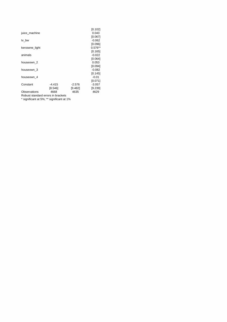
[0.102]juice_machine 0.043

[0.067]tv_bw -0.062

[0.096]kerosene_light 0.576**

[0.165]animals -0.022

[0.064]houseown_2 0.053

[0.094]houseown_3 -0.082

[0.145]houseown_4 -0.01

[0.071]Constant -4.415 -2.576 -3.057

[8.546] [9.482] [9.239]Observations 4668 4635 4629Robust standard errors in brackets* significant at 5%; ** significant at 1%

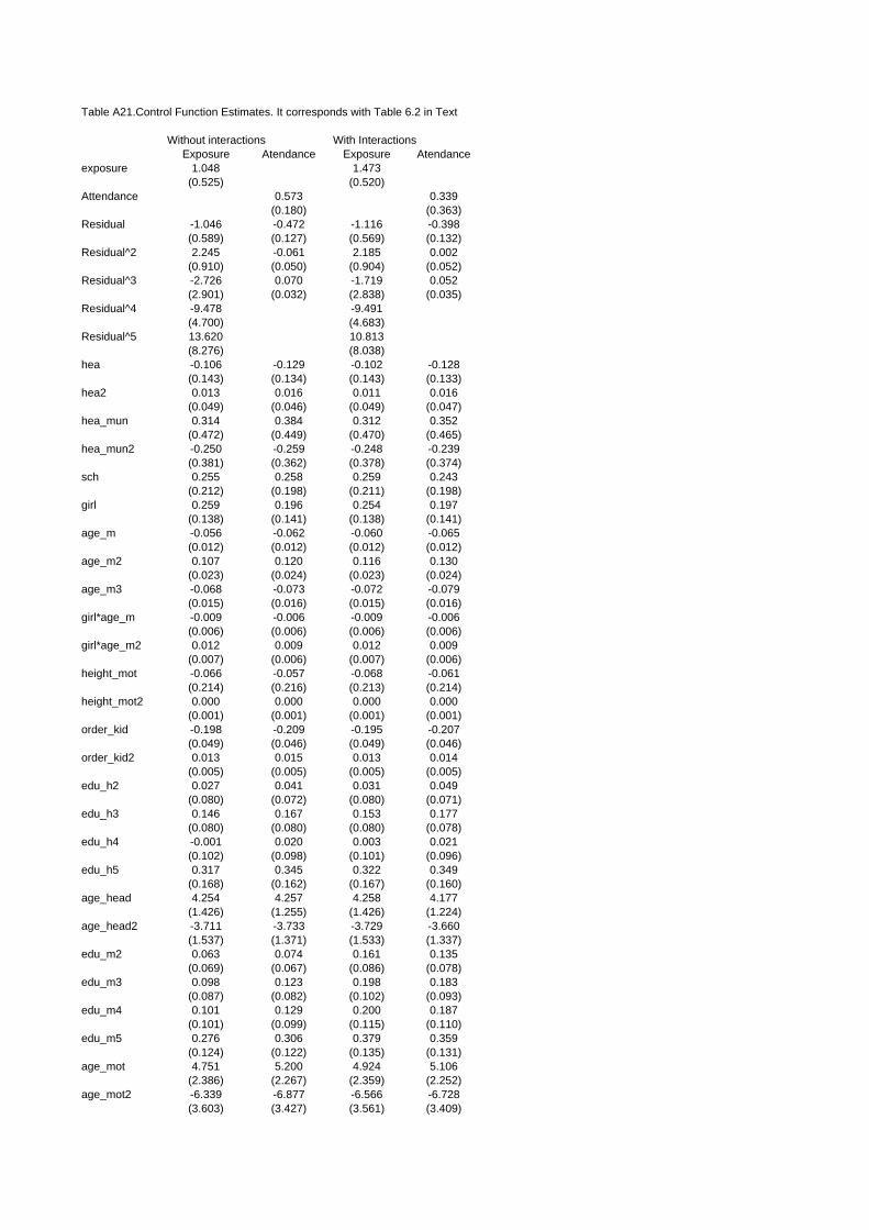
Table A21.Control Function Estimates. It corresponds with Table 6.2 in Text

Without interactions With InteractionsExposure Atendance Exposure Atendance

exposure 1.048 1.473(0.525) (0.520)

Attendance 0.573 0.339(0.180) (0.363)

Residual -1.046 -0.472 -1.116 -0.398(0.589) (0.127) (0.569) (0.132)

Residual^2 2.245 -0.061 2.185 0.002(0.910) (0.050) (0.904) (0.052)

Residual^3 -2.726 0.070 -1.719 0.052(2.901) (0.032) (2.838) (0.035)

Residual^4 -9.478 -9.491(4.700) (4.683)

Residual^5 13.620 10.813(8.276) (8.038)

hea -0.106 -0.129 -0.102 -0.128(0.143) (0.134) (0.143) (0.133)

hea2 0.013 0.016 0.011 0.016(0.049) (0.046) (0.049) (0.047)

hea_mun 0.314 0.384 0.312 0.352(0.472) (0.449) (0.470) (0.465)

hea_mun2 -0.250 -0.259 -0.248 -0.239(0.381) (0.362) (0.378) (0.374)

sch 0.255 0.258 0.259 0.243(0.212) (0.198) (0.211) (0.198)

girl 0.259 0.196 0.254 0.197(0.138) (0.141) (0.138) (0.141)

age_m -0.056 -0.062 -0.060 -0.065(0.012) (0.012) (0.012) (0.012)

age_m2 0.107 0.120 0.116 0.130(0.023) (0.024) (0.023) (0.024)

age_m3 -0.068 -0.073 -0.072 -0.079(0.015) (0.016) (0.015) (0.016)

girl*age_m -0.009 -0.006 -0.009 -0.006(0.006) (0.006) (0.006) (0.006)

girl*age_m2 0.012 0.009 0.012 0.009(0.007) (0.006) (0.007) (0.006)

height_mot -0.066 -0.057 -0.068 -0.061(0.214) (0.216) (0.213) (0.214)

height_mot2 0.000 0.000 0.000 0.000(0.001) (0.001) (0.001) (0.001)

order_kid -0.198 -0.209 -0.195 -0.207(0.049) (0.046) (0.049) (0.046)

order_kid2 0.013 0.015 0.013 0.014(0.005) (0.005) (0.005) (0.005)

edu_h2 0.027 0.041 0.031 0.049(0.080) (0.072) (0.080) (0.071)

edu_h3 0.146 0.167 0.153 0.177(0.080) (0.080) (0.080) (0.078)

edu_h4 -0.001 0.020 0.003 0.021(0.102) (0.098) (0.101) (0.096)

edu_h5 0.317 0.345 0.322 0.349(0.168) (0.162) (0.167) (0.160)

age_head 4.254 4.257 4.258 4.177(1.426) (1.255) (1.426) (1.224)

age_head2 -3.711 -3.733 -3.729 -3.660(1.537) (1.371) (1.533) (1.337)

edu_m2 0.063 0.074 0.161 0.135(0.069) (0.067) (0.086) (0.078)

edu_m3 0.098 0.123 0.198 0.183(0.087) (0.082) (0.102) (0.093)

edu_m4 0.101 0.129 0.200 0.187(0.101) (0.099) (0.115) (0.110)

edu_m5 0.276 0.306 0.379 0.359(0.124) (0.122) (0.135) (0.131)

age_mot 4.751 5.200 4.924 5.106(2.386) (2.267) (2.359) (2.252)

age_mot2 -6.339 -6.877 -6.566 -6.728(3.603) (3.427) (3.561) (3.409)

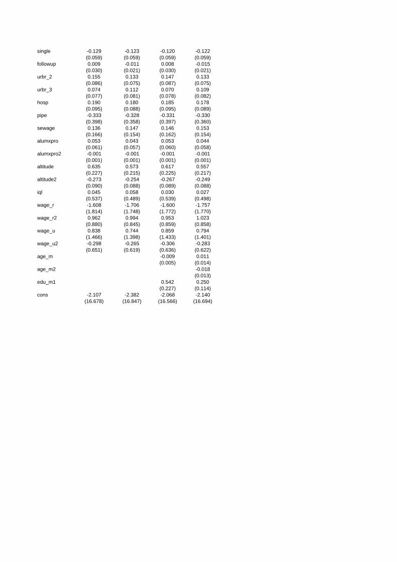
single -0.129 -0.123 -0.120 -0.122(0.059) (0.059) (0.059) (0.059)

followup 0.009 -0.011 0.008 -0.015(0.030) (0.021) (0.030) (0.021)

urbr_2 0.155 0.133 0.147 0.133(0.086) (0.075) (0.087) (0.075)

urbr_3 0.074 0.112 0.070 0.109(0.077) (0.081) (0.078) (0.082)

hosp 0.190 0.180 0.185 0.178(0.095) (0.088) (0.095) (0.089)

pipe -0.333 -0.328 -0.331 -0.330(0.398) (0.358) (0.397) (0.360)

sewage 0.136 0.147 0.146 0.153(0.166) (0.154) (0.162) (0.154)

alumxpro 0.053 0.043 0.053 0.044(0.061) (0.057) (0.060) (0.058)

alumxpro2 -0.001 -0.001 -0.001 -0.001(0.001) (0.001) (0.001) (0.001)

altitude 0.635 0.573 0.617 0.557(0.227) (0.215) (0.225) (0.217)

altitude2 -0.273 -0.254 -0.267 -0.249(0.090) (0.088) (0.089) (0.088)

iql 0.045 0.058 0.030 0.027(0.537) (0.489) (0.539) (0.498)

wage_r -1.608 -1.706 -1.600 -1.757(1.814) (1.748) (1.772) (1.770)

wage_r2 0.962 0.994 0.953 1.023(0.880) (0.845) (0.859) (0.858)

wage_u 0.838 0.744 0.859 0.794(1.466) (1.398) (1.433) (1.401)

wage_u2 -0.298 -0.265 -0.306 -0.283(0.651) (0.619) (0.636) (0.622)

age_m -0.009 0.011(0.005) (0.014)

age_m2 -0.018(0.013)

edu_m1 0.542 0.250(0.227) (0.114)

cons -2.107 -2.382 -2.068 -2.140(16.678) (16.847) (16.566) (16.694)

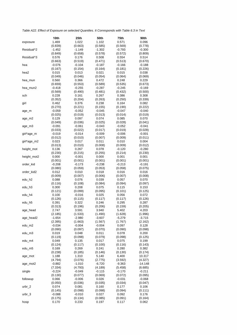
Table A22. Effect of Exposure on selected Quantiles. It Corresponds with Table 6.3 in Text

10th 25th 50th 75th 90th exposure 1.469 1.022 1.102 0.571 0.096

(0.839) (0.663) (0.585) (0.569) (0.778)Residual^2 -1.452 -1.149 -1.302 -0.793 -0.300

(0.849) (0.658) (0.578) (0.572) (0.809)Residual^3 0.576 0.176 0.508 0.554 0.514

(0.663) (0.519) (0.471) (0.513) (0.670)hea -0.076 -0.104 -0.187 -0.166 -0.188

(0.167) (0.154) (0.164) (0.181) (0.226)hea2 0.015 0.013 0.021 0.015 0.038

(0.049) (0.046) (0.054) (0.064) (0.069)hea_mun 0.560 0.366 0.472 0.248 0.229

(0.659) (0.553) (0.589) (0.535) (0.673)hea_mun2 -0.418 -0.255 -0.287 -0.245 -0.169

(0.569) (0.490) (0.481) (0.432) (0.500)sch 0.228 0.161 0.267 0.386 0.308

(0.352) (0.204) (0.263) (0.250) (0.339)girl 0.462 0.376 0.238 0.164 0.082

(0.270) (0.221) (0.155) (0.190) (0.222)age_m -0.059 -0.052 -0.045 -0.047 -0.040

(0.025) (0.019) (0.013) (0.014) (0.019)age_m2 0.129 0.097 0.074 0.085 0.070

(0.049) (0.036) (0.025) (0.028) (0.041)age_m3 -0.091 -0.061 -0.043 -0.052 -0.041

(0.033) (0.022) (0.017) (0.019) (0.028)girl*age_m -0.019 -0.014 -0.009 -0.006 -0.001

(0.012) (0.010) (0.007) (0.009) (0.011)girl*age_m2 0.023 0.017 0.011 0.010 0.004

(0.013) (0.010) (0.008) (0.009) (0.012)height_mot 0.136 0.267 0.078 -0.120 -0.280

(0.230) (0.215) (0.255) (0.214) (0.230)height_mot2 0.000 -0.001 0.000 0.001 0.001

(0.001) (0.001) (0.001) (0.001) (0.001)order_kid -0.208 -0.173 -0.238 -0.213 -0.191

(0.080) (0.059) (0.053) (0.058) (0.075)order_kid2 0.012 0.010 0.018 0.016 0.016

(0.009) (0.007) (0.006) (0.007) (0.008)edu_h2 0.088 0.076 0.039 0.057 0.070

(0.116) (0.108) (0.084) (0.094) (0.097)edu_h3 0.300 0.208 0.075 0.115 0.153

(0.121) (0.099) (0.095) (0.101) (0.125)edu_h4 0.100 -0.016 0.025 0.056 0.072

(0.126) (0.115) (0.117) (0.117) (0.126)edu_h5 0.391 0.322 0.246 0.295 0.287

(0.313) (0.196) (0.206) (0.159) (0.205)age_head 2.747 3.591 3.940 5.402 4.203

(2.185) (1.533) (1.490) (1.628) (1.996)age_head2 -1.654 -2.980 -3.607 -5.279 -3.715

(2.395) (1.663) (1.567) (1.767) (2.162)edu_m2 -0.034 -0.004 -0.004 0.097 0.128

(0.090) (0.097) (0.070) (0.090) (0.098)edu_m3 0.019 0.048 0.011 0.078 0.200

(0.119) (0.098) (0.079) (0.098) (0.125)edu_m4 0.049 0.135 0.017 0.075 0.199

(0.124) (0.117) (0.100) (0.116) (0.143)edu_m5 0.169 0.269 0.241 0.280 0.382

(0.238) (0.185) (0.146) (0.130) (0.174)age_mot 1.188 1.310 5.140 6.400 10.317

(4.794) (3.076) (2.775) (3.592) (4.327)age_mot2 -0.882 -1.010 -6.720 -9.363 -14.148

(7.334) (4.793) (4.189) (5.458) (6.685)single -0.224 -0.049 -0.115 -0.170 -0.211

(0.130) (0.077) (0.069) (0.072) (0.095)followup 0.066 -0.006 0.026 -0.031 -0.068

(0.050) (0.036) (0.035) (0.034) (0.047)urbr_2 0.074 0.081 0.160 0.177 0.106

(0.145) (0.098) (0.098) (0.094) (0.111)urbr_3 -0.088 -0.010 0.027 0.092 0.176

(0.175) (0.134) (0.085) (0.091) (0.164)hosp 0.170 0.233 0.197 0.117 0.062

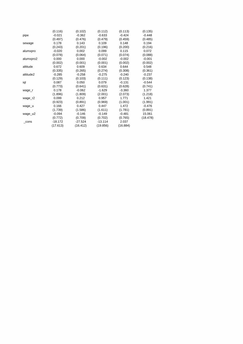
(0.116) (0.102) (0.112) (0.113) (0.135)pipe -0.021 -0.362 -0.633 -0.424 -0.448

(0.497) (0.476) (0.479) (0.459) (0.485)sewage 0.178 0.143 0.109 0.148 0.194

(0.243) (0.201) (0.196) (0.200) (0.216)alumxpro -0.020 0.002 0.099 0.115 0.072

(0.078) (0.064) (0.071) (0.074) (0.088)alumxpro2 0.000 0.000 -0.002 -0.002 -0.001

(0.002) (0.001) (0.001) (0.002) (0.002)altitude 0.672 0.609 0.634 0.644 0.548

(0.335) (0.265) (0.274) (0.308) (0.361)altitude2 -0.285 -0.258 -0.275 -0.240 -0.237

(0.129) (0.103) (0.111) (0.123) (0.138)iql 0.087 0.050 0.079 -0.131 -0.544

(0.773) (0.641) (0.631) (0.628) (0.741)wage_r 0.178 -0.062 -1.629 -3.360 1.377

(1.896) (1.809) (2.001) (2.073) (1.218)wage_r2 0.099 0.212 0.957 1.771 1.421

(0.923) (0.891) (0.969) (1.001) (1.991)wage_u 0.166 0.427 0.447 1.472 -0.476

(1.739) (1.586) (1.611) (1.781) (0.891)wage_u2 -0.094 -0.146 -0.149 -0.481 15.061

(0.772) (0.709) (0.702) (0.765) (18.478) _cons -18.172 -27.524 -13.114 2.037

(17.613) (16.412) (19.856) (16.884)

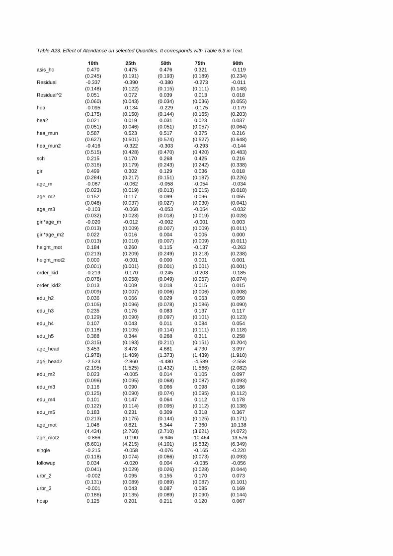
Table A23. Effect of Atendance on selected Quantiles. It corresponds with Table 6.3 in Text.

10th 25th 50th 75th 90th asis_hc 0.470 0.475 0.476 0.321 -0.119

(0.245) (0.191) (0.193) (0.189) (0.234)Residual -0.337 -0.390 -0.380 -0.273 -0.011

(0.148) (0.122) (0.115) (0.111) (0.148)Residual^2 0.051 0.072 0.039 0.013 0.018

(0.060) (0.043) (0.034) (0.036) (0.055)hea -0.095 -0.134 -0.229 -0.175 -0.179

(0.175) (0.150) (0.144) (0.165) (0.203)hea2 0.021 0.019 0.031 0.023 0.037

(0.051) (0.046) (0.051) (0.057) (0.064)hea_mun 0.587 0.523 0.517 0.375 0.216

(0.627) (0.501) (0.574) (0.527) (0.648)hea_mun2 -0.416 -0.322 -0.303 -0.293 -0.144

(0.515) (0.428) (0.470) (0.420) (0.483)sch 0.215 0.170 0.268 0.425 0.216

(0.316) (0.179) (0.243) (0.242) (0.338)girl 0.499 0.302 0.129 0.036 0.018

(0.284) (0.217) (0.151) (0.187) (0.226)age_m -0.067 -0.062 -0.058 -0.054 -0.034

(0.023) (0.019) (0.013) (0.015) (0.018)age_m2 0.152 0.117 0.099 0.096 0.055

(0.048) (0.037) (0.027) (0.030) (0.041)age_m3 -0.103 -0.068 -0.053 -0.054 -0.032

(0.032) (0.023) (0.018) (0.019) (0.028)girl*age_m -0.020 -0.012 -0.002 -0.001 0.003

(0.013) (0.009) (0.007) (0.009) (0.011)girl*age_m2 0.022 0.016 0.004 0.005 0.000

(0.013) (0.010) (0.007) (0.009) (0.011)height_mot 0.184 0.260 0.115 -0.137 -0.263

(0.213) (0.209) (0.249) (0.218) (0.238)height_mot2 0.000 -0.001 0.000 0.001 0.001

(0.001) (0.001) (0.001) (0.001) (0.001)order_kid -0.219 -0.170 -0.245 -0.203 -0.185

(0.076) (0.058) (0.049) (0.057) (0.074)order_kid2 0.013 0.009 0.018 0.015 0.015

(0.009) (0.007) (0.006) (0.006) (0.008)edu_h2 0.036 0.066 0.029 0.063 0.050

(0.105) (0.096) (0.078) (0.086) (0.090)edu_h3 0.235 0.176 0.083 0.137 0.117

(0.129) (0.090) (0.097) (0.101) (0.123)edu_h4 0.107 0.043 0.011 0.084 0.054

(0.118) (0.105) (0.114) (0.111) (0.118)edu_h5 0.388 0.344 0.268 0.311 0.258

(0.315) (0.193) (0.211) (0.151) (0.204)age_head 3.453 3.478 4.681 4.730 3.097

(1.978) (1.409) (1.373) (1.439) (1.910)age_head2 -2.523 -2.860 -4.480 -4.589 -2.558

(2.195) (1.525) (1.432) (1.566) (2.082)edu_m2 0.023 -0.005 0.014 0.105 0.097

(0.096) (0.095) (0.068) (0.087) (0.093)edu_m3 0.116 0.090 0.066 0.098 0.186

(0.125) (0.090) (0.074) (0.095) (0.112)edu_m4 0.101 0.147 0.064 0.112 0.178

(0.122) (0.114) (0.095) (0.112) (0.138)edu_m5 0.183 0.231 0.309 0.318 0.367

(0.213) (0.175) (0.144) (0.125) (0.171)age_mot 1.046 0.821 5.344 7.360 10.138

(4.434) (2.760) (2.710) (3.621) (4.072)age_mot2 -0.866 -0.190 -6.946 -10.464 -13.576

(6.601) (4.215) (4.101) (5.532) (6.349)single -0.215 -0.058 -0.076 -0.165 -0.220

(0.118) (0.074) (0.066) (0.073) (0.093)followup 0.034 -0.020 0.004 -0.035 -0.056

(0.041) (0.029) (0.026) (0.028) (0.044)urbr_2 -0.002 0.095 0.155 0.170 0.073

(0.131) (0.089) (0.089) (0.087) (0.101)urbr_3 -0.001 0.043 0.087 0.085 0.169

(0.186) (0.135) (0.089) (0.090) (0.144)hosp 0.125 0.201 0.211 0.120 0.067

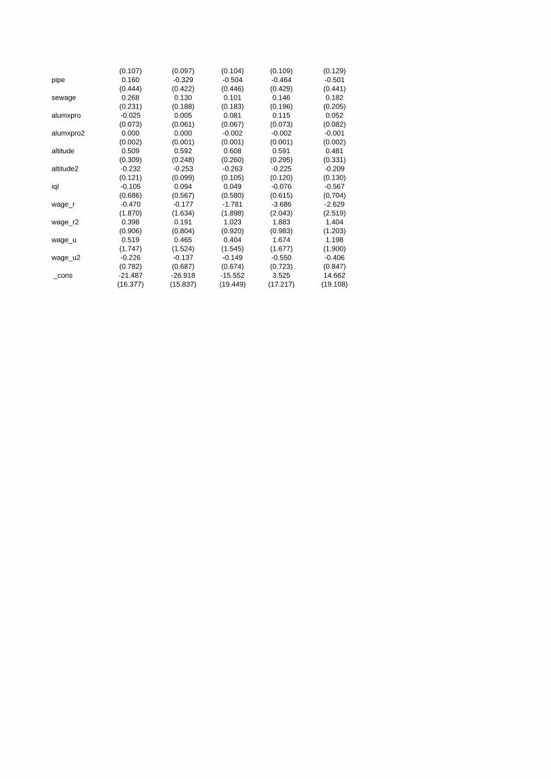
(0.107) (0.097) (0.104) (0.109) (0.129)pipe 0.160 -0.329 -0.504 -0.464 -0.501

(0.444) (0.422) (0.446) (0.429) (0.441)sewage 0.268 0.130 0.101 0.146 0.182

(0.231) (0.188) (0.183) (0.196) (0.205)alumxpro -0.025 0.005 0.081 0.115 0.052

(0.073) (0.061) (0.067) (0.073) (0.082)alumxpro2 0.000 0.000 -0.002 -0.002 -0.001

(0.002) (0.001) (0.001) (0.001) (0.002)altitude 0.509 0.592 0.608 0.591 0.481

(0.309) (0.248) (0.260) (0.295) (0.331)altitude2 -0.232 -0.253 -0.263 -0.225 -0.209

(0.121) (0.099) (0.105) (0.120) (0.130)iql -0.105 0.094 0.049 -0.076 -0.567

(0.686) (0.567) (0.580) (0.615) (0.704)wage_r -0.470 -0.177 -1.781 -3.686 -2.629

(1.870) (1.634) (1.898) (2.043) (2.519)wage_r2 0.398 0.191 1.023 1.883 1.404

(0.906) (0.804) (0.920) (0.983) (1.203)wage_u 0.519 0.465 0.404 1.674 1.198

(1.747) (1.524) (1.545) (1.677) (1.900)wage_u2 -0.226 -0.137 -0.149 -0.550 -0.406

(0.782) (0.687) (0.674) (0.723) (0.847) _cons -21.487 -26.918 -15.552 3.525 14.662

(16.377) (15.837) (19.449) (17.217) (19.108)