Orbital Mechanics and AnalyticModeling of Meteorological Satellite Orbits

Applications to the Satellite Navigation Problem

byEric A. Smith

Department of Atmospheric ScienceColorado State University

Fort Collins, Colorado

ORBITAL MECHANICS AND ANALYTIC MODELING OF

METEOROLOGICAL SATELLITE ORBITS

Applications to the Satellite Navigation Problem

by

Eric A. Smith

Department of Atmospheric ScienceColorado State University

Fort Collins, Colorado 80523February, 1980

Atmospheric Science Paper No. 321

ABSTRACT

An analysis is carried out which considers the relationship of

orbit mechanics to the satellite navigation problem, in particular,

meteorological satellites. A preliminary discussion is provided which

characterizes the distinction between "classical navigation" and

"satellite navigation" which is a process of determining the space

time coordinates of data fields provided by sensing instruments on

meteorological satellites. Since it is the latter process under con­

sideration, the investigation is orientated toward practical appli­

cations of orbit mechanics to aid the development of analytic solu­

tions of satellite orbits.

Using the invariant two body Keplerian orbit as the basis of

discussion, an analytic approach used to model the orbital char­

acteristics of near earth satellites is given. First the basic con­

cepts involved with satellite navigation and orbit mechanics are

defined. In addition, the various measures of time and coordinate

geometry are reviewed. The two body problem is then examined be­

ginning with the fundamental governing equations, i.e. the inverse

square force field law. After a discussion of the mathematical and

physical nature of this equation, the Classical Orbital Elements used

to define an elliptic orbit are described. The mathematical analysis

of a procedure used to calculate celestial position vectors of a

satellite is then outlined. It is shown that a transformation of

Kepler's time equation (for an elliptic orbit) to an expansion in

powers of eccentricity removes the need for numerical approximation.

ii

The Keplertan solution is then extended to a perturbed solution,

which considers first order. time derivatives of the elements defining

the orbital plane. Using a formulation called the gravitational per­

turbation function, the form of a time variant perturbed two body orbit

is examined. Various characteristics of a perturbed orbit are analyzed

including definitions of the three conventional orbital periods, the

nature of a sun-synchronous satellite, and the velocity of a non­

circular orbit.

Finally, a discussion of the orbital revisit problem is provided

to highlight the need to develop efficient, relatively exact, analytic

solutions of meteorological satellite orbits. As an example, the

architectural design of a satellite system to measure the global radia­

tion budget without deficiencies in the space time sampling procedure

is shown to be a simulation problem based on "computer flown" satel­

lites. A set of computer models are provided in the appendiceso

iii

Chapter

1.0

2.0

TABLE OF CONTENTS

INTRODUCTION •

BASIC CONCEPTS

2.1 Orbit mechanics and navigation•••2 0 2 Satellite navigation modeling •2.3 Satellite orientation •••2.4 Applications of a satellite navigation model o •

1

4

4678

TIME

3013.23.3

o • 0 • • • • • 0

Basic systems of time 0

The annual cycle and zodiac 0

Sidereal time • • 0 • •

10

1017:l1

4.0 GEOMETRICAL CONSIDERATIONS • • 0 • 23

4.1 Definitions of latitude •••••••• 234.2 Cartesian - spherical coordinate transformations. 284.3 Satellite - solar geometry. • • ••• 0 0 • 0 29

5.0 THE TWO BODY PROBLEM • • • • 0 • • 34

5.15.25.35.45055065075085095.10

The inverse square force field law. 0 • • • •

Coordinate systems and coordinates. • 0 0 • •

Selection of units. • • 0 • •

Velocity and period 0 • • 0 • • •

Elliptic orbits 0 • • • • • •

The Gaussian constant •Modified time variable. 0

Classical Orbital Elements ••Calculation of celestial pointing vector•••• 0 •

Rotation to terrestrial coordinates

34404446505355565977

PERTURBATION THEORY•• 0 0 0 81

6.1 Concept of gravitational potential. • 816.2 Perturbative forces and the time dependence of

orbital elements••••• 0 • • • • • • • • 866.3 Longitudinal drift of a geosynchronous satellite. 0 986.4 Calculations required for a perturbed drift 0 0 •• 996.5 Equator crossing period ••••• 0 0 • 0 •• 0 •• 1016.6 Required inclination for a sun synchronous orbit. 0 105607 Velocity of a satellite in an elliptic orbito •• 0 106

iv

Chapter

THE ORBITAL REVISIT PROBLEM. • • • • ~ • 0 0 • 0 • • 109

7.1 Sun-synchronous orbits•••7.2 Multiple satellite system 0

. . . . . . ~

• • • 0 • • • •

109113

o •8.0

9.0

CONCLUSIONS 0 • 0 •

ACKNOWLEDGEMENTS •

• Cl • C C

. . . . .o • 0

o 0 . . • • 0

. . .o • • •

116

117

10.0 REFERENCES • • • • . . . . . . . 118

APPENDIX A--EXAMPLES OF NESS, NASA, ESA, AND NASDAORBITAL ELEMENT TRANSMISSIONSo • • • • 120

APPENDIX B--COMPUTER SOLUTION FOR AN EARTH SATELLITEORBIT (PERTURBED TWO BODY) • • • • • • • • • 133

APPENDIX C--COMPUTER SOLUTION FOR FINDING A SYNODICPERIOD • • • • 0 • • • • • • • • • • . . 141

APPENDIX D--COMPUTER SOLUTION FOR A SOLAR ORBIT(PERTURBED TWO BODY) • • • • • • • 0 o. 144

APPENDIX E--COMPUTER SOLUTIONS FOR A SOLAR ORBIT(APPROXIMATE AND NON-LINEAR REGRESSION). 150

APPENDIX F--LIBRARY ROUTINES FOR ORBITAL SOFTWARE. 154

APPENDIX G--COMPUTER ROUTINE FOR DETERMINING THEINCLINATION REQUIRED FOR A SUN-SYNCHRONOUSORBIT. • 0 • • • • • 0 0 • 0 • • 0 • • 0 • • 160

v

1.0 INTRODUCTION

The topic of this investigation is orbital mechanics and its

relationship to the satellite navigation problem. Since the term

"satellite navigation" denotes a variety of concepts, it is important

to refine a definition for purposes of this study. We say, in general,

that satellite navigation is a process of identifying the space and

time coordinates of satellite data products (in this case meteorologi­

cal satellites). Note that this characterization departs somewhat from

the classical usage of navigation which implies the definition and

maneuvering of the position of ships, aircraft, satellites, etc. A

more exact definition is given in Chapter 2. A fundamental component

of any satellite navigation system is a model of the satellite's orbit­

al properties. This investigation is primarily concerned with the

mathematical and physical nature of near earth meteorological satellite

orbits and thus meteorological satellite navigation requirements. The

study also considers the basic nature of coordinate systems and the

various measures of time.

There are two very general orbital application areas insofar as

meteorological satellites are concerned. The first and more traditional

application of orbital analysis is the process of tracking the position

and motion of satellites, by the space agencies, so as to provide ephem­

eris and antenna pointing information to ground readout stations and

operations command facilities. Considering that in this process, the

actual characteristics of an orbital plane are defined, this can be

referred to as a navigation process. However, for our purposes, we

shall consider this process as an "orbital tracking" problem.

1

2

The second application is the analytic treatment of orbital motion

in a model designed for processing the meteorological data, generated

by spacecraft instrumentation. In this case, there are very different

computational and operational restraints than in the case of orbit

tracking. Primarily we are concerned with developing efficient and

quick computational routines that retain a relatively high degree of

orbital position accuracy, but are not bogged down with the multiplicity

of external forces that orbit tracking models must consider.

The practical outcome of the study is a set of orbital computer

models, which are adaptable in a very general fashion, to a variety of

analytic near-earth satellite navigation systems. The usability of

these models is insured because they are based on the conventional or­

bital elements available from the primary meteorological satellite

agencies, i.e. the National Environmental Satellite Service (NESS), the

National Aeronautical Space Administration (NASA), the European Space

Agency (ESA), and the National Space Development Agency (NASDA) ~f

Japan. The reader may refer to Appendix A for an explanation.

Meteorological satellites, whether they are of the experimental or

operational type, are classified as either geosynchronous (~ 24 hour

period) or polar low orbiter (~ 100 minute period) by the above agencies.

The low orbiters may be placed in either sun-synchronous or non-sun­

synchronous orbit. All of these satellites are in nearly circular orbit,

and in general, are at altitudes at which atmospheric drag is not a

significant factor over the prediction time scale under consideration

(~ 1-2 weeks). This investigation will be addressed to these types of

orbits.

3

Chapter 2.0 considers some basic concepts which are crucial to an

understanding of the satellite navigation problem. Chapter 3.0 provides

a set of definitions and an explanation of the various measures of time.

A discussion of station coordinates (latitude) is given in Chapter 4.0

along with some fundamental geometric definitions. Chapter 5.0 repre­

sents the major portion of the analysis, that is, a discussion of the

two body orbit problem and a method to calculate orbital position vec­

tors given a set of "Classical Orbital Elements". Chapter 6.0 considers

the time varying properties of an orbit and goes on to look at the

resultant effects of the aspherical gravitational potential of the earth

on the orbital characteristics of a satellite. The topic of the orbital

revisit problem is considered in Chapter 7.0. Finally, appendices are

included which provide a set of computer models which can be used to

calculate orbital position vectors and the various orbital periods

which are discussed in the chapter on perturbation theory.

A principle reference used in this analysis is the very fine com­

pendium on Orbit Mechanics by Pedro Ramon Escoba1 (1965), hereafter EB.

This work stands alone as an aid to solving orbital mechanics problems

faced by satellite workers and scientists. Other very helpful ref­

erences used in this study were The Handbook on Practical Navigation by

Bowditch (1962) and a translation of a Russian text on orbit determina­

tion by Dubyago (1961). The latter work provides a very interesting

historical sketch of the development of orbital mechanics and man's

understanding of the motion of celestial bodies.

2.0 BASIC CONCEPTS

2.1 Orbit Mechanics and Satellite Navigation

The following definitions are essential to an understanding of the

ensuing analysis:

Orbital Mechanics: A branch of celestial mechanics concerned with

orbital motions of celestial bodies or artificial spacecraft.

Celestial Mechanics: The calculation of motions of celestial bodies

under the action of their mutual gravitational attractions.

Astrodynamics: The practical application of celestial mechanics,

astroballistics, propulsion theory, and allied fields to the problem of

planning and directing the trajectories of space vehicles.

Navigation (General): The process of directing the movement of a

craft so that it will reach its intended destination: subprocesses are

position fixing, dead reckoning, pilotage, and homing.

Navigation (Satellite): The process of determining a set of unique

transformations between the coordinates of satellite data points in a

satellite frame of reference and their associated terrestrial or plane­

tary coordinates. (This definition should be contrasted with "Satellite

Image Alignment", which is a non-analytic, mostly subjective process in

which the two or more images to be aligned often have different aspect

ratio characteristics.)

The major areas of Orbital Mechanics are:

1. Satellite Orbit Injection

a. Thrust (Ballistic, Propulsion) forces

be Drag forces

c. Lift forces

4

5

2. Determination of Orbital Elements

a. Position vector, velocity vector, and initial time

+ +(r, r, to)

b. Two position vectors and times (~l' tl

, ~2' t2

)

c. Three pairs of azimuth-elevation angles and times

[(~l' HI' t l ), (~Z' HZ' t 2), (~3' H3, t 3)]

d. Slant-range, range-rate, and time observations.[(dl , dl , t l ), (dZ' d2, t z)···]

e. Mixed observations (angles, ranges, range-rates, times)

3. Orbital Properties and Tracks

a. Orbital elements

b. Velocities and periods

c. Position vectors

d. Direct and retrograde orbits

e. Equator crossing data

f. Orbital revisit frequencies

4. Orbital Analytics (Keplermanship)

a. Nodal passages

b. Satellite rise and set times

c. Line of sight periods and eclipses

d. Orbital architecture

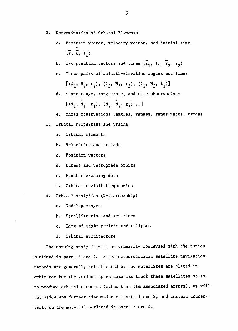
The ensuing analysis will be primarily concerned with the topics

outlined in parts 3 and 4. Since meteorological satellite navigation

methods are generally not affected by how satellites are placed in

orbit nor how the various space agencies track these satellites so as

to produce orbital elements (other than the associated errors), we will

put aside any further discussion of parts I and 2, and instead concen-

trate on the material outlined in parts 3 and 4.

6

2.2 Satellite Navigation Modeling

Satellite navigation modeling can be considered to be a five

part problem:

1. The time dependent determination of the spacecraft orbital

position in an inertial coordinate system.

2. The time dependent determination of the spacecraft orien­

tation (attitude) in an inertial coordinate systemo

30 The specification or determination (time dependent) of the

optical paths of the imaging or sounding instrument with respect to

the spacecraft.

4. The integration of the above static and dynamic aspects of the

spacecraft into a model which can provide measurement pointing vectors

in the inertial frame of reference.

5. The transformation of the inertial pointing vectors to pointing

vectors in the preferred (non-inertial) coordinate system.

The first requirement of an analytic navigation technique is a

model which can solve for satellite position at any specified time. In

fact, the determination of spacecraft orientation is absolutely depen­

dent on knowledge of satellite position if ground based or star based

attitude determination techniques are applied. A discussion of this

topic can be found in Smith and Phillips (1972) and is presently being

extended by Phillips (1979). With the knowledge of spacecraft position

and orientation, the dynamics of the actual on-board instrumentation can

then be considered. Finally, upon integration of these three dynamic as­

pects of an orbiting satellite into an appropriate model, pointing vec­

tors can be obtained which fix the relationship between an instrument

field-of-viewand a terrestrial coordinate (latitude, longitude, height).

7

2.3 Satellite Orientation

It is important to distinguish between the effect of varying

satellite position and varying satellite orientation on the apparent

earth scene. First of all it is instructive to define the various terms

associated with satellite orientation:

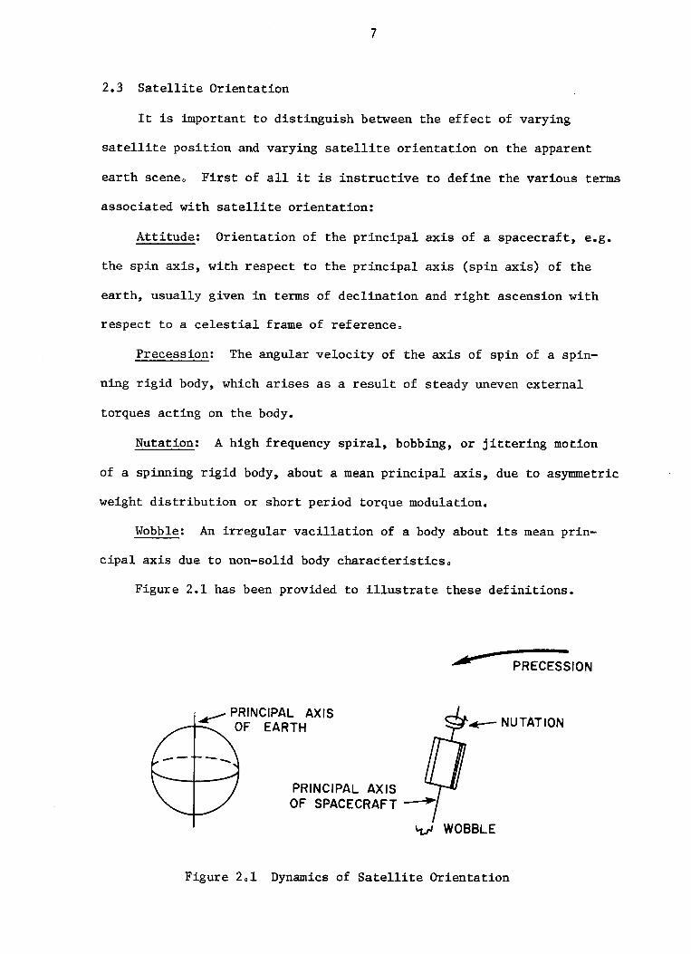
Attitude: Orientation of the principal axis of a spacecraft, e.g.

the spin axis, with respect to the principal axis (spin axis) of the

earth, usually given in terms of declination and right ascension with

respect to a celestial frame of reference.

Precession: The angular velocity of the axis of spin of a spin-

ning rigid body, which arises as a result of steady uneven external

torques acting on the body.

Nutation: A high frequency spiral, bobbing, or jittering motion

of a spinning rigid body, about a mean principal axis, due to asymmetric

weight distribution or short period torque modulation.

Wobble: An irregular vacillation of a body about its mean prin-

cipal axis due to non-solid body characteristics.

Figure 2.1 has been provided to illustrate these definitions.

PRECESSION

..- NUTATION.~ PRINCIPAL AXIS

OF EARTH

PRINCIPAL AXISOF SPACECRAFT ---.

"V WOBBLE

Figure 2.1 Dynamics of Satellite Orientation

8

Variation in the orientation of a meteorological satellite can

lead to both translations and rotations of earth fields with respect

to a fixed satellite field-of-view. These apparent motions are super­

imposed on real motions due to variation in the orbital position. A

requirement of any satellite navigation model is the inclusion of pro­

cedures to separate the apparent motions from the real motions which

are essentially independent processes. Therefore, this investigation

will be devoted to the determination of orbital position as these cal­

culations generally preface the determination of the remaining navi­

gational parameters.

2.4 Applications of a Satellite Navigation Model

Finally, an important question concerning satellite navigation is:

"What does a navigation model provide?" Essentially, it provides the

following three capabilities:

1. The capability of placing grid and/or geographic-topographic

annotation information in or on the datao This process should be called

a "Gridding" processo

2. A means to specify the terrestrial or planetary coordinate of

a given data point coordinate, or conversely, to specify the data point

coordinate corresponding to a given terrestrial or planetary coordinate.

This process should be called a "Navigational Interrogation" process.

3. A framework for transforming the raw satellite imagery into

alternate cartographic (map) projections. The actual process of re­

organizing the raw data into a new projection should be called a "Map­

ping" process.

9

Note the actual navigation process only involves specifying,

calculating, or determining the appropriate parameters inherent to the

navigation model and utilizing them to calculate coordinate transfor-

mat ions 0

3.0 TIME

3.1 Basic Systems of Time

Any navigational process, by its very nature, involves various

systems of time. Therefore, we need the following definitions:

Mean Solar Time (MST): Time that has the mean solar second as its

unit and is based on the mean sun's motion. One mean solar second is

1/86,400 of a mean solar day. One solar day is 24 hours of mean solar

timeo

Greenwich Mean Time (GMT): Mean solar time at the meridian of

Greenwich, England 0 Also referred to as Universal Time (UTO), Zulu

Time, Z-Time, or Greenwich Civil Time:

GMI' = MST + n

where n is the number of time zones to the west of the Greenwich meri-

dian as shown in Figure 3.1. There are also higher order systems of

Universal Time (UTI, UT2) which are corrected for variations in the

earth's rotational rate due to secular, irregular, periodic seasonal and

periodic tidal terms and polar motion due to solar and lunar gravita-

tiona1 effects on the earth's equatorial bulge. These corrections are

not significant for the time periods we are considering.

-180 -90

GREENWICHMERIDIAN

o +90 +180

~ r" ~~ J' 1.~ --;;

\ lr'~(K:~~P, r'

"""....."i\ )\..~~ .. ~

~ I"- A

\ "' \ J~/"~ i'

\) l( r-.. D

f I'" ~~'t

EO.

12 II 109 8 76 5 4 3 2 1 0-1-2-3-4-5-6-7-8-9-10-11-12

TIME ZONES

Figure 3.1 Time Zones

10

11

Ephemeris Time (ET): A uniform measure of time defined by laws

of dynamics and determined in principle from the orbital motions of the

planets, particularly of the earth. One ephemeris second (ISU:1960) is

1/31556925.9747 of a tropical year defined by the mean motion of the sun

in longitude at the epoch 1900, January 0, 12 hours (12:00 GlIT, Dec. 31,

1899). An ephemeris day is 86,400 ephemeris seconds. The earth's rota-

tion suffers periodic and secular variations in rotation so that ephem-

eris time is defined by:

ET = GMT + 8t (3.2)

where 8t is an annual increment tabulated in the American Ephemeris and

Nautical Almanac. For instance, using values from the American

Ephemeris and Nautical Almanac (1978), Table 3.1 is generated:

Table 3.1: Ephemeris Time Correction Increments

Year ~t

1956.5 31.521957.5 31.921958.5 32.451959.5 32.911960.5 33.391961.5 33.801962.5 34.231963.5 34.731964.5 35.401965.5 36.14

Note that 8t can not be calculated in advance. It is determined from

observed and predicted positions of the moon.

It is also worth noting that the change in the time increment

from year to year is fairly insignificant. The result of this

\

12

characteristic of ephemeris time, is that short term orbital predictions

(~ 5 years) can effectively ignore ephemeris corrections. Although this

may simplify operational satellite orbit prediction, incremental cor-

rection must be included when considering long term orbital calculations

such as historical earth-sun configurations. Table 3.2 represents a

listing of incremental corrections from the American Nautical and

Ephemeris Almanac (1978).

Atomic Time (AT): A measure of time based on the oscillations of

the U.S. Cesium Frequency Standard (National Bureau of Standards,

Boulder, Colorado). The standard is based on the U.S. Nava10bser-

vatory's suggested value of 9,192,631,770 oscillations per second of

the cesium atom - isotope 133. The reference epoch has been defined

h m sas January 1, 1958 0 0 0 GMT. The standard time scale to which U.S.

orbital tracking stations are synchronized is the Universal Time

Coordinated (UTC) system. This system is derived from an atomic time

scale. Prior to 1972 the UTC system operated at a frequency offset

from the AT system. Since January 1, 1972 the UTC system is derived

from a rubidium atomic frequency standard. The new measurements used

to convert to UTC come from various global stations and are thus re-

ferred to as Station Time (ST).

Tropical Year: Period of one revolution of the earth measured

between two vernal equinoxes. Equal to 365.24219879 mean solar days

or 365 days, 5 hours, 48 minutes, 46 seconds or 31,556,925.9747 ephem-

eris seconds. Also referred to as an Astronomical Year, Equinoctial

Year, Natural Year or Solar Year.

Anoma1istic Year: Period of one revolution of the earth measured

between perhe1ion to perhe1ion (see Figure 3.2). Equal to 365.259641204

13

Table 3.2: Ephemeris Time Correction Table (From the 1978American Ephemeris and Nautical Almanac)

.-Date <1T(A) <1UTl Date <1T(A) <1UTl Date <1T(A) <1UTl(0' UT) (0- UT) (0" UT)

1956 s s 1964 s s 1972 s sJan. 1 +31.34 -0.08 Apr. 1 +35.22 -0.05 Jan. 1 +42.22 -0.04Jan. 4 31.34 - .08 July 1 35.40 - .11 Apr. 1 42.52 - .34Jan. 4 31.34 - .02 Aug. 31 35.47 - .11 .June30 42.82 - .64Apr. 1 31.43 - .04 Sept. 1 35.47 - .01 July 1 42.82 + .36July 1 31.52 - .07 Oct. 1 35.52 - .02 Oct. 1 43.07 + .11Oct. 1 31.56 - .01 Dec. 31 35.73 - .11 Dec. 31 43.37 - .19

1957 1965 1973Jan. 1 +31.67 -0.04 Jan. 1 +35.73 -0.01 Jan. 1 +43.37 +0.81Apr. 1 31.79 - .06 Feb.28 35.86 - .06 Apr. 1 43.67 + .51July 1 31.92 - .07 Mar. 1 35.86 + .04 July 1 43.96 + .22Oct. 1 32.00 - .02 Apr. 1 35.94 .00 Oct. 1 44.19 - .01

Jllne30 36.14 - .08 Dec. 31 44.48 - .301958 July 1 36.14 + .02

Jan. 1 +32.17 -0.04 Aug. 31 36.24 - .01 1974Apr. 1 32.32 - .05 Sept. 1 36.24 + .09 Jan. 1 +44.48 +0.70July 1 32.45 - .06 Oct. 1 36.31 + .06 Apr. 1 44.73 + .45Oct. 1 32.52 - .01 July 1 44.99 +, .19

1966 Oct. 1 45.20 - .021959 Jan. 1 +36.54 -0.05 Dec. 31 45.47 - .29

Jan. 1 +32.67 -0.03 Apr. 1 36.76 - .03Apr. 1 32.80 - .03 July 1 36.99 - .02 1975July 1 32.91 - .06 Oct. 1 37.18 + .02 Jan. 1 +45.47 +0.71Oct. 1 33.00 .00 Apr. 1 45.73 + .45

1967 July 1 45.98 + .201960 Jan. 1 +37.43 +0.01 Oct. 1 46.18 .00

Jan. 1 +33.15 -0.01 Apr. 1 37.65 + .02 Dec. 31 46.45 - .27Apr. 1 33.28 - .03 July 1 37.87 + .04July 1 33.39 - .02 Oct. 1 38.04 + .10 1976Oct. 1 33.45 + .03 Jan. 1 +46.45 +0.73

1968 Apr. 1 ( 46.7 ) ( + .5 )1961 Jan. 1 +38.29 +0.09 July 1 ( 47.0 ) ( + .2 )

Jan. 1 +33.58 +0.02 Jan. 31 38.37 + .09 Oct. 1 ( 47.2 ) ( .0 )Apr. 1 33.70 + .02 Feb. 1 38.37 - .01July 1 33.80 + .04 Apr. 1 38.52 .00 1977July 31 33.81 + .06 July 1 38.75 + .01 Jan. 1 (+47.4 )Aug. 1 33.81 + .01 Oct. 1 38.95 + .04 Apr. 1 ( 47.7 )Oct. 1 33.86 + .04 July 1 ( 47.9 )

1969 Oct. 1 ( 48.1 )1962 Jan. 1 +39.20 +0.03

Jan. 1 +33.99 +0.04 Apr. 1 39.45 + .02 1978Apr. 1 34.12 + .01 July 1 39.70 + .01 Jan. 1 (+48.4 )July 1 34.23 .00 Oct. 1 39.91 + .03 Apr. 1 ( 48.6 )Oct. 1 34.31 + .02 July 1 ( 48.8 )

1970 Oct. 1 ( 49.1 )1963 Jan. 1 +40.18 0.00

Jan. 1 +34.47 -0.03 Apr. 1 40.45 - .03 1979Apr. 1 34.58 - .05 July 1 40.70 - .05 Jan. 1 (+49.3 )July 1 34.73 - .09 Oct. 1 40.89 - .01Oct. 1 34.83 - .09Oct. 31 34.90 - .12 1971Nov. 1 34.90 - .02 Jan. 1 +41.16 -0.04

Apr. 1 41.41 - .051964 July 1 41.68 - .08

Jan. 1 +35.03 -0.08 Oct. 1 41.92 - - .09Mar. 31 +35.22 -0.15 Dec.31 +42.22 -0.15

The quantity ~T(A)=32~18+TAI-UTI provides a first approximation to ~T=ET-UT,the reduction from Universal to Ephemeris Time. TAI is the scale of International Atomic Timeformally introduced on 1972 January 1, but extrapolated to previous dates; UTI is the observedUniversal Time, corrected for polar motion. The correction ~UTI = UTl- UTC is given for usein connection with broadcast time signals, which are now UTC in most countries. Coded values of~UTI are now given in the primary time signal emissions, and may be as much as ± 0"8. Dis­continuities in UTC can occur at Db UT on the first day of a month (exception: 1956 Jan. 4,discontinuity at 19b UT). Special entries are given for the two dates bracketing any discontinuitygreater than 0~02. Values within parentheses are either provisional (two decimals) or extrapolated(one decimal). Additional information is given in the e'Cplanation concerning time scales (page527) and concerning the use of ~T with ephemerides (pages 539-541).

14

Table 3.2 Continued

CORRECTIONS

The American Ephemeris, 1970-1978The corrections tabulated below should be added to AE +1800 and As +1800 in the

Ephemeris for Physical Observations of Jupiter for the years 1970-1978. Thesecorrections should also be subtracted from the Longitude of Central Meridian (Sys­tem I and System II).

1970 +0.031971 +0.021972 +0.021973 +0.011974 0.001975 -0.011976 -0.021977 -0.031978 -0.03

The American Ephemeris, 1972-1980All the negative values of the Astrometric Declination of the four principal minor

planets, Ceres, Pallas, Juno, Vesta, for the years 1972-1980 require a correction of-O~l.

For example, on page 281 of this volume:1978 Aug. 16 jor -31°15'52'~4 read -31°15'52~5

The American Ephemeris, 1972-1977

The mean motion for the Earth in the table of mean elements at the top of page216 is referred to a moving equinox while the mean motions for Mercury, Venus andMars are referred to a fixed equinox. For consistency, the Earth's mean motionshould also have been referred to a fixed equinox; in which case its value shouldhave been 0.985609.

CIVIL CALENDAR

New Year's Day Sun. Jan. 1 Labor Day. Mon. Sept. 4Lincoln's Birthday Sun. Feb. 12 Columbus Day Mon. Oct. 9Washington's Birthday Mon. Feb. 20 Veterans Day. Sat. Nov. 11Memorial Day Mon. May 29 General Election Day Tue. Nov. 7Independence Day Tue. July 4 Thanksgiving Day Thu. Nov. 23

15

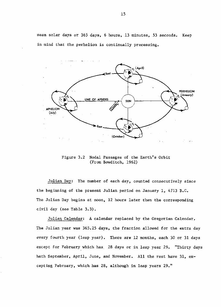
mean solar days or 365 days, 6 hou~s, 13 minutes, 53 seconds. Keep

in mind that the perhelion is continually precessing.

East -1lt-'"'1

LINE OF APSIDES

Figure 3.2 Nodal Passages of the Earth's Orbit(From Bowditch, 1962)

Julian Day: The number of each day, counted consecutively since

the beginning of the present Julian period on January 1, 4713 B.C.

The Julian Day begins at noon, 12 hours later then the corresponding

civil day (see Table 3.3).

Julian Calendar: A calendar replaced by the Gregorian Calendar.

The Julian year was 365.25 days, the fraction allowed for the extra day

every fourth year (leap year). There are 12 months, each 30 or 31 days

except for February which has. 28 days or in leap year 29. "Thirty days

hath September, April, June, and November. All the rest have 31, ex-

cepting February, which has 28, although in leap years 29."

16

Table 3.3: Julian Day Number (From EB, 1965)

Days Elapsed at Grccnwich Noon, A.D. 1950-2000

" ~KJAr-:. 0 HB. 0 MAR. 0 APR. a MAY 0 JUNE 0 JULY 0 At:G. 0 SEP. 0 OCT. 0 NOV. a mc. 0

,',50 243 3282 3313 3341 3372 3402 3433 3463 3494 3525 3555 3586 36161'1.' I 3647 3678 3706 3737 3767 3798 3828 3859 3890 3920 3951 39811'i5:! 4012 4043 4072 4103 4133 4164 4194 ·m5 4256 4286 4317 43471'1).' 4378 4409 4437 4468 4498 4529 4559 4590 4621 4651 4682 47121'154 4743 4774 4802 4833 4863 4894 4924 4955 4986 5016 5047 50771'1'5 243 5108 5139 5167 5198 5228 5259 5289 5320 5351 5381 5412 54421'156 5473 5504 5533 5564 5594 5625 5655 5686 5717 5747 5778 58081'157 5839 5870 5898 5929 5959 5990 6020 (\051 6082 6112 6143 6173l'1511 6204 6235 6263 6294 6324 6355 6385 6416 6447 6477 6508 65381'J5~ 6569 6600 6628 6659 6689 6720 6750 6781 6812 6842 6873 6903I')(,() 243 6934 6965 6994 7025 7055 7086 7116 7147 7178 7208 7239 72691<Ii>l 7300 7331 7359 7390 7420 7451 7481 7512 7543 7573 7604 76341'/(,2 7665 7696 7724 7755 7785 7816 7846 7877 7908 7938 7969 79991%3 8030 8061 8089 8120 8150 8181 8211 8242 8273 8303 8334 83641964 8395 8426 8455 8486 8516 8547 8577 8608 8639 8669 8700 873019M 243 8761 8792 8820 8851 8881 8912 8942 8973 9004 9034 9065 90951'166 9126 9157 9185 9216 9246 9277 9307 9338 9369 9399 9430 94601'.167 9491 9522 9550 9581 9611 9642 9672 9703 9734 9764 9795 9825I 'IllS 9856 9887 9916 9947 9977 ·0008 ·0038 ·0069 ·0100 ·0130 ·0161 ·01911~(,9 244 0222 0253 0281 0312 0342 0373 0403 0434 0465 0495 0526 05561'170 244 0587 0618 0646 0677 0707 0738 0768 0799 0830 0860 0891 0921l'iil 0952 0983 1011 1042 1072 1103 1133 1164 1195 1225 1256 12861'/71 1317 1348 1377 1408 ]438 1469 ]499 1530 ]561 1591 1622 16521973 1683 1714 1742 1773 1803 1834 1864 1895 1926 1956 1987 20171974 2048 2079 2107 2138 2168 2199 2229 2260 2291 2321 2352 23821975 244 2413 2444 2472 2503 2533 2564 2594 2625 2656 2686 2717 27471976 2778 2809 2838 2869 2899 2930 2960 2991 3022 3052 3083 3113In7 3144 3175 3203 3234 3264 3295 3325 3356 3387 3417 3448 34781978 3509 3540 3568 3599 3629 3660 3690 3721 3752 3782 3813 3843)1)79 3874 3905 3933 3964 3994 4025 4055 4086 4117 4147 4178 4208IQSO 244 4239 4270 4299 4330 4360 4391 4421 4452 4483 4513 4544 4574191\1 4605 4636 4664 4695 4725 4756 4786 4817 4848 4878 4909 49391982 4970 5001 5029 5060 5090 5121 5151 5182 5213 5243 5274 5304loJ!!3 5335 5366 5394 5425 5455 5486 5516 5547 5578 5608 5639 56691984 5700 5731 5760 579i 5M21 5852 5882 5913 5944 5974 6005 60351985 244 6066 6097 6125 6156 6186 6217 6247 6278 6309 6339 6370 64001'186 6431 6462 6490 6521 6551 6582 6612 6643 6674 6704 6735 6765IlJll7 6796 6827 6855 6886 6916 6947 6977 7008 7039 7069 7100 71301'188 7161 7192 7221 7252 7282 7313 7343 7374 7405 7435 7466 7496198IJ 7527 7558 7586 7617 7647 7678 7708 7739 7770 7800 7831 786111190 244 7892 7923 7951 7982 8012 8043 8073 8104 8135 8165 8196 82261'i91 8257 8288 8316 8347 8377 8408 8438 8469 8500 8530 8561 85911'i92 8622 8653 8682 8713 8743 8774 8804 8835 8866 8896 8927 89571993 8988 9019 9047 9078 9108 9139 9169 9200 9231 9261 9292 9322/994 9353 9384 9412 9443 9473 9504 9534 9565 9596 9626 9657 96871995 244 9718 9749 9777 9808 9838 9869 9899 9930 9961 9991 ·0022 ·00521996 245 0083 0114 0143 0174 0204 0235 0265 0296 0327 0357 0388 041819'/7 0449 0480 0508 0539 0569 0600 0630 0661 0692 0722 0753 07831998 0814 0845 0873 0904 0934 0965 0995 1026 1057 1087 1118 1148I'm 1179 1210 1238 1269 1299 1330 1360 1391 1422 1452 1483 1513:!OOO 254 ]544 ]575 ]604 1635 1665 1696 1726 1757 ]788 18]8 1849 1879

Gregorian Calendar: The calendar used for civil purposes through­

out the world, replacing the Julian calendar and closely adjusted to

the tropical year.

17

Note that it is common practice among satellite data users to refer

to the Julian day or date of a data set in terms of the day number of

the corresponding year (1-365 or 1-366). This is not inconsistent with

the classical definition since the initial day of the sequence is arbi­

trary.

3.2 The Annual Cycle and Zodiac

We must also consider the definition of sidereal time, but before

doing so, a brief discussion of the annual cycle and the zodiac is in

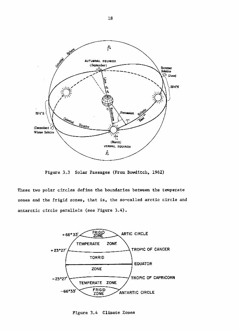
order. As the earth progresses through its annual cycle, there are four

solar passages which are used to distinguish the seasons and divide the

earth into its so called climate zones. There are two equator crossing

(equinoxes) and two maximum excursion passages (solstices) of the sun

with respect to the earth (see Figure 3.3). These are:

1 0 March or Spring Equinox

2. June or Summer Solstice

3. September or Autumnal Equinox

4. December or Winter Solstice

It is commonplace to refer to the summer and winter solstice latitudes

as the tropic of cancer and the tropic of capricorn, respectively.

To an observer on the earth the sun appears to achieve a maximum

latitudinal excursion of +230 27' or -230 27' at the solstices. The zone

between these two parallels is often referred to as the torrid zone.

The apparent motion of the sun, of course, is due to the inclination of

the earth's orbit about the sun. The apparent track of the sun is along

a plane which is called the ecliptic. When the sun reaches a solstice

position, the opposite hemisphere is having its winter in which the

limits of the circumpolar sun are approximately 230 27' from the pole.

18

R..

">/1 ~,....

rr,(March)

VERNAL EQUINOX

P,

Figure 303 Solar Passages (From Bowditch, 1962)

These two polar circles define the boundaries between the temperate

zones and the frigid zones, that is, the so-called arctic circle and

antarctic circle parallels (see Figure 304).

ZONE

ZONE

TORRID

TEMPERATE

\.-----------/ TROPIC OF CAPRICORN

I----------.....-j EQUATOR

+230271r- --~TROPICOF CANCER

Figure 3 0 4 Climate Zones

19

The names used to describe the boundaries of the torrid zone were

given some 2000 years ago when the sun was entering the constellations

Cancer and Capricorn at the time of the solstices. By the same token

the spring and autumnal equinoxes were taking place at the time the

sun was entering the constellations Aires and Libra. Thus, it is appro­

priate to refer to the solstices and the equinoxes as zodiacal passages.

What is the zodiac?

Figure 3.5 The Zodiac (From Bowditch, 1962)

Strictly, the zodiac is the circular band of sky extending 80

on

each side of the ecliptic (see Figure 3.5). The navigational planets

and the moon are within these limits. The zodiac is divided into 12

sections of 300 each, each section being given the name and symbol

20

(sign) of the constellation within it. The sun remains in each section

for approximately one month. Due to the precession of the equinoxes,

the sun no longer enters the aforementioned constellations at the sea­

sonal passages. However, astronomers still list the sun as entering

these constellations; this is their principal astronomical significance.

The pseudo-science of astrology assigns additional significance, not

recognized by all scientists to the position of the sun and planets

among the zodiacal signs (see Bowditch, 1962).

Since the precession of the equinoxes plays an important role in

celestial position fixing, we shall define it:

Precession of the Equinoxes: A slow conical motion of the earth's

axis (like the spinning of a top) about the vertical to the plane of

the. ecliptic, having a period of about 26,000 years (25,781 years)

caused by the perturbative attractions of the sun, moon, and other

planets on the equatorial protuberence (bulge) of the earth. It results

in a gradual westward motion of the equinoxes (50.27 arc-seconds per

year). Because of the precession, the zodiacal configuration with re­

spect to the sun at its seasonal passages, has shifted approximately

one section or constellation westward.

At the time of the definition of the zodiac, the sun was entering

the constellation Aires at the time of the Spring Equinox. This solar

position is of major importance to the sidereal reference system of

time. The celestial meridian corresponding to the sun position at the

time of a spring or vernal (from the Greek for spring) equinox defines

the reference meridian for sidereal time. The expression "vernal equi­

nox" and associated expressions, are applied to both "times" and

"points" of occurrence of various phenomena. The vernal equinox is

21

also called the "first point of Aries" (y) or the "rams horns", although

strictly speaking we should now call it the "first point of Pisces" due

to the precession of the equinoxes.

3.3 Sidereal Time

We can now provide a set of definitions which describe the sidereal

time system:

Sidereal Time: Time that is based on the position of the stars.

A sidereal period is the length of time required for one revolution of

a celestial body about its primary axis, with respect to the stars.

Thus, a sidereal year is one revolution of the earth around the sun

with respect to the fixed celestial reference.

Now there are 365.24219879 mean solar days in a tropical year. Due

to the earth's revolution about the sun and the respective orientation

of the sun and a fixed celestial reference (star reckoning), a sidereal

day is actually shorter in time than a solar day. In fact, it is easy

to show that there is exactly one more sidereal day in an annual period

(vernal equinox to vernal equinox) than there are mean solar days (see

Figure 3.6). Thus:

1 mean solar time unit 1.002737909 sidereal time units

= 366.24219879/365.24219879

Therefore, a sidereal day is 3'56" shorter than a solar dayo

Sidereal Year: A sidereal year (ioe. the period of revolution of

the earth relative to the stars) is 365.2563662 mean solar days (365

days, 6 hours, 9 minutes, 10 seconds) due to the precession of the

equinoxes (50027" per year).

3600 0'50.27"365.2563662 = 3600 • 365.24219879

CELESTIAL TRANSIT OCCURS3'56.6" PRIOR TO A SOLAR

TRANSIT

22

~_ ...-/" .........

/ ",/ \ EARTH

/ )... (Day n+ I)

I ---r

\\

\.'-.... /'

.......~-_/

---

FIXED CELESTIALREFERENCE

•

Figure 3 0 6 Difference between a solar and sidereal year(Not exact scale).

Hour Angles: Angular distance west of a celestial meridian or

ohour circle of a body (e.g. the sun) measured through 360 (see Figure

3.7)0 There are three conventionally defined hour angles:

10 Local Hour Angle (LHA): Angular distance west of the Local

celestial meridian.

2. Greenwich Hour Angle (GHA): Angular distance west of the

Greenwich celestial meridian o

3. Sidereal Hour Angle (SHA): Angular distance west of the Vernal

Equinox celestial meridian (Y)o

(GREENWICH) G

(MOON)

<l

o(OBSERVER)

T (FIRST POINTOF AIRES)

(SUN)

o

Figure 3.7 Hour Angles

4.0 GEOMETRICAL CONSIDERATIONS

4.1 Definitions of Latitude (Station Coordinates)

Since the earth is not a perfect sphere, there are a selection of

coordinates to choose from. Most systems are based on the assumption

that the earth can be represented by an oblate spheriod; that is, a

geometrical shape in which sections parallel to the equator are perfect

circles and meridians are ellipses (see Figure 401).

NORTH

QUADRANT OF ELLIPSE

OF REVOLUTION

Figure 4.1 Model of the earth (From EB, 1965)

We define an oblate spheroid in terms of two radial axes (a, b) where:

a - semi-major axis

b - semi-minor axis

We can now define the flattening (f) parameter which is related to

the eccentricity of the ellipsoid of revolution. We also define the

eccentricity (e), a parameter which will be considered in the discus-

sion of orbital calculations and conic sections. The flattening (f) and

23

24

eccentricity (e) are given by:

f (a-b)!a

= 0 for a perfect sphere

(4.1)

Also:

= 0 for a spheroid or a circular orbit

e =V2f - f2

f = 1 -V1 - e 2

(4.2)

(4.3)

Note that in the limit as b + 0 then e + 0 and f + O. Values of these

parameters for the earth are given by:

a = 6378.214 kInb = 6356.829 km.e = 8.1820157.10-2

f = 3.35289.10-3

Note that:

b = a· (1-f)

We can also define a mean earth radius (c) by a weighted average:

c = (2a + b)/3

= 6371.086 kIn

(4.4)

(4.5)

(4.6)

Using our adopted model of the geometric shape, we can define the

twa conventional measures of latitude. Following the approach given

in Chapter 2 of EB and using Figure 4.2 as a guide we first consider

geocentric latitude:

Geocentric Latitude: The acute angle (~) wrt the equatorial plane

determined by a line connecting the geometric center of the ellipsoid

and a point on its surface.

25

NORTHZ

CROSS SECTIONOF ELLIPSE

OBSERVER

MERIDIAN

+---- a ---+

Figure 4.2 Ellipsoid of revolution defining geocentriclatitude (Based on a figure from EB, 1965)

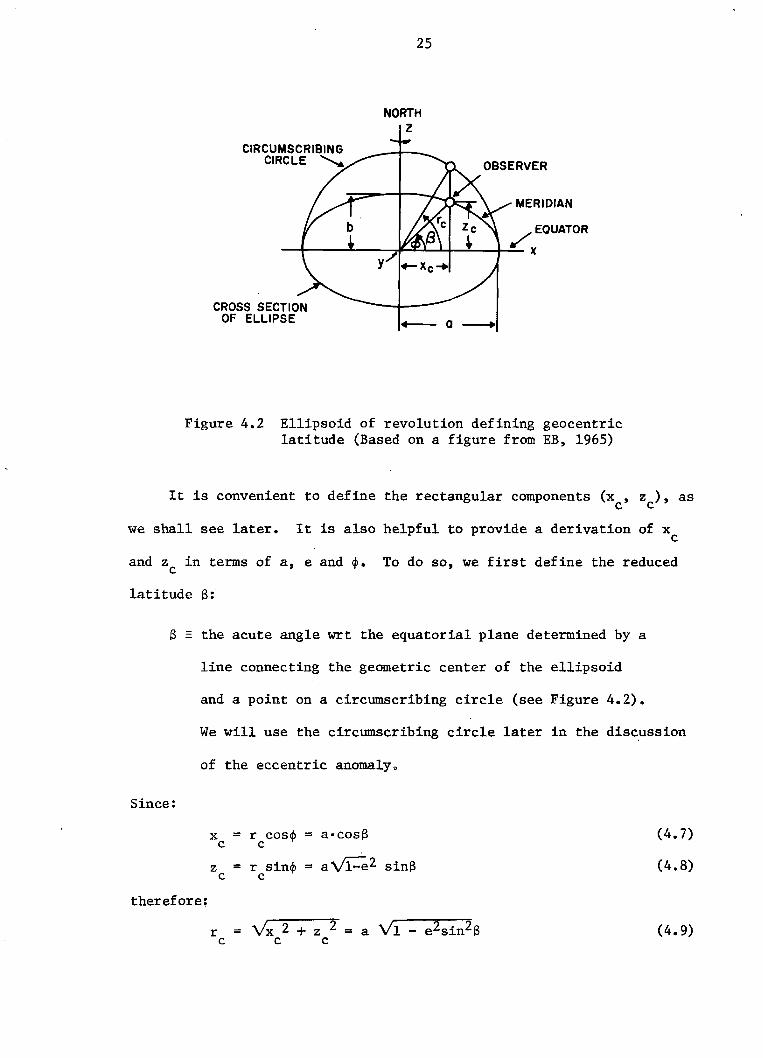
It is convenient to define the rectangular components (x , z ), asc c

we shall see later. It is also helpful to provide a derivation of xc

and Zc in terms of a, e and~. To do so, we first define the reduced

latitude 13:

13 = the acute angle wrt the equatorial plane determined by a

line connecting the geometric center of the ellipsoid

and a point on a circumscribing circle (see Figure 4.2).

We will use the circumscribing circle later in the discussion

of the eccentric anomaly.

Since:

x ::: r cos~ ::: a·cosSc c

Z ::: r sin4> ::: a~2 sinac c

therefore;

r ::: v'x 2 + z 2 ::: a Vi - e2sin2Sc c c

(4.7)

(4.8)

(4.9)

and:

26

sincPz

c= -=r c

VI - e2 sinS

vi - e2 sin2S(4010)

cos$ = _X_c = _...:;.co.=..s::...J·~::-.. _

r c vl""": e2sin2s(4011)

We square (4.10) and (4.11) and after multiplying by \/1 - e2

(1 - e2)sin2S

1 - e2sin2S(4.12)

now add (4.12) and (4.13) and after some manipulation:

VI _ eZsin2S = VI - e2

VI - e2cos2cP

We now combine (4.10) and (4.14) to solve for sinS:

(4.13)

(4.14)

sinS sinep (4.15)

similarly for (4.11) and (4.14):

Combining (4.16) and (4.7) with (4.15) and (4.8):

x = a VI - e2 cosepc VI - e2cos2cP

z = a VI - e2 sioepc VI - e2cos2cP

Next, we define geodetic latitude, again following EB:

(4.16)

(4.17)

(4.18)

27

Geodetic Latitude: The acute ($') wrt the equatorial plane

determined by a line normal to the tangent place of a point on the

surface of the ellipsoid and intersecting the equatorial plane. Geo-

detic latitude is often referred to as geographic latitude (see Figure

4.3).

Recalling Eqns. (4.7) and (4.8):

x = a cosSc(4.7)

z = ac(4.8)

we can now differentiate:

Now note:

(4.19)

(4.20)

ds(4.21)

and finally:

-dx i Qc s nl-'sinep' = -- = --;::==~===

ds \/1 _ e2cos2S

dzc \/1 - e2 cosScosep' = -- = -:;===::;:=~

ds \/1 - e2cos2S

(4.22)

(4.23)

Finally, using Equations (4.10, 4011) and (4.22, 4023), it is

easy to show that:

(4.24)

This provides a convenient transformation between the station coordinate

systems.

28

NORTHZ

CIRCUMSCRIBINGCIRCLE ""*

/CROSS SECTION

OF ELLIPSE

OBSERVER

EQUATOR

4-- a ----+

Figure 4.3 Ellipsoid of revolution defining geodeticlatitude (Based on a figure from EB, 1965)

A third definition of latitude is often used, particularly in the

process of surveying, that is astronomical latitude:

Astronomical Latitude: The acute angle (<1>") wrt the equatorial

plane formed by the intersection of a gravity ray with the equatorial

plane. This latitude is a function of the local gravitational field

(direction of a plumb-bob), and is thus affected by local terrain.

Tabulation of station errors is required to convert to geodetic lati-

tude. Note that most maps are in either geodetic or astronomical

latitude whereas navigational analysis will usually use a geocentric

system.

4.2 Cartesian - Spherical Coordinate Transformations

It is necessary to define transformations between a spherical

frame of reference and a cartesian frame of reference. For satellite

navigation purposes, two systems are convenient:

29

1. Declination-Right Ascension-Radial System (o,p,r) where we

have chosen declination to be defined in the same sense as

co-latitude:

x = r·sin(o) ocos(p)

y = r·sin(o) .sin(p)

z r.cos(o)

0 -l[ i,x2 + y2 + z2]= cos z/

p = tan-ley/x]

",x2 + y2 +r z2

2. Latitude-Longitude-Radial System (~,A,r):

x = r·cos(~)·COS(A)

y = rocos(~)·sin(A)

z = rosin(c/»

(4.25)

(4.26)

(4.27)

(4028)

r =

4.3 Satellite - Solar Geometry

A standard requirement for satellite data analysis is the defini-

tion of the angular configuration of a satellite and the sun with

respect to a terrestrial position (~,A,r)o In order to specify the

three usual angles (zenith, nadir, azimuth), we first define the fol-

lowing polar coordinates:

30

( ~ A r) satellite position'I's' s' S -

(ep,A,r) _ reference point

Converting these three positions to their terrestrial position vectors:

v -E>

-+V -s

solar vector in earth coordinates (from 4.27)

satellite vector in earth coordinates (from 4027)

-+V _ reference point in earth coordinates (from 4.27)p

We can define the solar and satellite zenith (0 ,0 ), nadir (n ,n ),e s E> s

and azimuth (~ ,~ ) angles and relative zenith (0 ) and azimuth (~ )E> S r r

angles:

Solar zenith _ 0 = cos-l[V o(V - V)]E> P E> P

Solar nadir = cos-l[-v • (V - V)]- ne e p ~

Satellite zenith ~....1(· -+ -+ ]- = cos V o(V - V )s p s P

-1 -+ -+ -+Satellite nadir - ns cos . [-V • (V .... V ) ]s p s

-1 -+ -+ -+Relative zenith - 0 = cos [(V - V ). (V - V ) ]r (9 p s p

Figure 4.4 illustrates the zenith and nadir angle defini-

tions.

(4.30)

(4.31)

In order to define the azimuth angles we first define a pointing

-+ -+vector (V

90) which is subtented 900 from Vp in the same hemisphere as

-+V and in the plane defined by the center of the earth, the north pole,p

:u

LOCAL VERTICAL

CENTER OF EARTH

SATELLITE

¢

Figure 4.4 Definition of zenith and nadir angles.

32

-+and the endpoint of V. Let:

p

-+ -+ -+ -+ -+S = (V - V )/ IIV - V \I~ @ p ~ p

Furthermore, we define:

(4.32)

-+ -+ -+X = V

90/ IIv

9011

El-+ -+ -+Z = V / II V II (4.33)

(!) p p-+ -+ -+y = X X Z

<;) (9 (!)

-l[ -+ -+ -+ -+ ]~l = cos (Z X S X Z )oXe (!) Q El

The solar zenith is then given by:

for ~2 2. 90

(4.34)

The satellite azimuth (~ ) is defined in the same way. Finally, wes

have the relative azimuth:

~ = MOn( I~ - ~ I, 180)r (;) s

See Figure 4.5 for an illustration o

(4.35)

33

//

//

/

~

Figure 405 Definition of azimuth angles.

5. 0 TIlE TWO BODY PROBLEM

5.1 The Inverse Square Force Field Law

We continue the analysis by considering the two body problem, ig-

noring all of the perturbative influences (i.e., thrust, drag, lift,

radiation pressure, proton bombardment or solar wind, assymetrical elec-

tromagnetic forces, auxilIary bodies and any aspherical gravitational po-

tential of either body), that is we consider only the mutual attractions

of a body A with a body B and the resultant motions. Furthermore, we

assume that the motion under consideration is that of a satellite or

planetary body B (secondary body of mass m2) with respect to a central

body A (primary body of mass ml)o

For closed solutions we will utilize the inverse square force field

law:

2 -+K llr

--3-r

(5.1)

First, we determine the origin of the above equation. Essentially,

Equation 501 embodies the laws of Kepler and Newton. To review:

Kepler's Laws (Empirical-aided by astronomical observations)

I. Within the domain of the solar system all planets describeelliptical paths with the sun at one focus.

II. The radius vector from the sun to a planet generates equalareas in equal times.

III. The squares of the periods of revolution of the planetsabout the sun are proportional to the cubes of their meandistances from the sun.

Newton's Laws of Motion

I. Every body will continue in its state of rest or of uniformmotion in a straight line except insofar as it is compelledto change that state by an impressed force.

34

35

II. Rate of change of momentum (mv) is proportional to theimpressed force and takes place in the line in which theforce acts o

F = ma = m(dv/dt)

III. Action and reaction are equal and oppositeo

Newton's Law of Universal Gravitation

Any two bodies in the universe attract one another with a force(FlZ) which is directly proportional to the product of theirmasses (ml,mz) and inversely proportional to the square of thedistance (rlZ) between them:

Z= Gmlm/rlZ

2 2K m/4l2

where:

G - Universal Gravitational Constant

-8 2-Z6.373 • 10 dyne·em .gm

m1 - larger mass (e.g. the earth)

mZ - smaller mass (e.g. a satellite)

(5.Z)

We can derive the inverse square force field law from Newton's

second law and his law of universal gravitationo Adopting the notation

in Chapter Z of EB, the Universal Law of Gravitation states:

(5.3)

Now consider an arbitrary inertial reference frame shown in Figure 501.

The force in the x direction FIx is:

(5.4)

36

therefore:

FIxGml m2 x 2 - xl

(5.5)= 2 r 12r 12

and finally:

FIx =Gm

lm

2(x2 - xl) (506)

3r12

- force on body 1

yB

y2 t---------(J m2

Figure 5.1 Arbitrary inertial coordinate referenceframe

Newton's second law states that the unbalanced force on a body in

the x direction is given by:

F =Ix

(5.7)

therefore:(5.8)

37

Now repeating the analysis for the y and z components we find:

-+ -+( r - r )2'1

3r 12

(5.9)

or:

(5.10)

Now transform to a relative inertial coordinate system as shown in

Figure 5.2. From above:

(5.11)

where:

(5.12)

Now considering only the x component:

(5.13)

we note that:

(5.14)

which is the desired expression for the acceleration of body 2 with

respect to body 1.

From our arbitrary inertial analysis:

(5.15)

2d x

2m --=

2 dt2(5.16)

38

y

B

A lJ-----.........----- X

Figure 5.2 Relative inertial coordinate reference frame.

Now since r12

= r Z1 ' and cancelling masses, then:

and subtracting the two equations yields:

(5.17)

(5.18)

Z 2 2d x2 d Xl d xlZdtZ - dtZ = -d-t-==Z= = - GmZ

(5.19)

, (xZ -Xl)= -G(m

l+ m

2) -=3:=-----­

r 1Z'(5.20)

39

Now repeating the analyses for the y and z components we find:

- Gm1 (5.21)

and finally:

d2-;.+ 2 -;dt2 = r = -K 1l~3

where:

- normalized mass sum

(5.22)

We generally apply (5.22) to a system where the primary mass (ml ) is

much greater than the secondary mass (m2), yielding II approximately 1 0 0.

Often in the study of orbital mechanics, an n-body system arises

in which the desired origin of the coordinate system is the mass center

or barycenter; that is, motion is relative to the barycenter and not

any single central body (see Figure 5.3). We refer to such a reference

system as a Barycentric Coordinate System (see a review in Chapter 2

of EB). The utility of this frame of reference arises in the event

that the trajectory of a space vehicle would undergo less disturbed

motion if referred to a barycenter. Since we are primarily concerned

with near earth satellites we will forego an examination of the bary-

centric coordinate system. It is useful to examine the governing equa-

tion, however:

n

GL mi ;i2

i=li#2

(5.23)

40

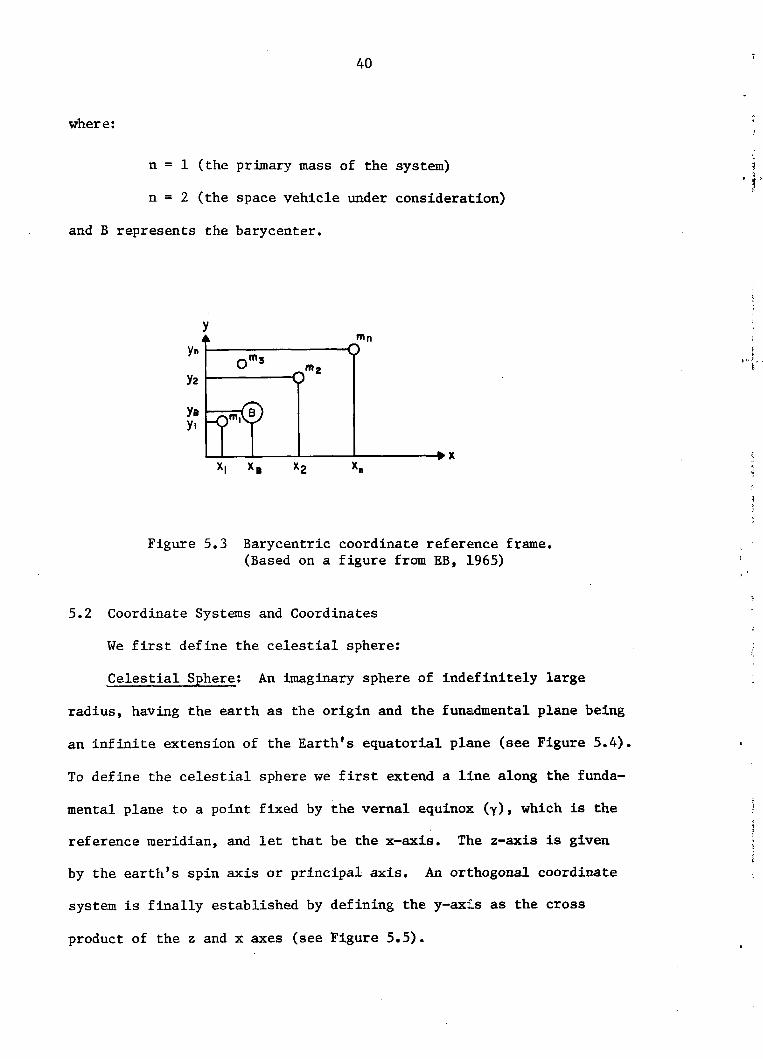
where:

n 1 (the primary mass of the system)

n = 2 (the space vehicle under consideration)

and B represents the barycenter.

l·t·

ymn

yn i.<io

m2 •yz

Y.y.

XxI x. x2 xn

Figure 5.3 Barycentric coordinate reference frame.(Based on a figure from EB, 1965)

5.2 Coordinate Systems and Coordinates

We first define the celestial sphere:

Celestial Sphere: An imaginary sphere of indefinitely large

radius, having the earth as the origin and the funadmental plane being

an infinite extension of the Earth's equatorial plane (see Figure 5.4).

To define the celestial sphere we first extend a line along the funda-

mental plane to a point fixed by the vernal equinox (y), which is the

reference meridian, and let that be the x-axis. The z-axis is given

by the earth's spin axis or principal axis. An orthogonal coordinate

system is finally established by defining the y-axis as the cross

product of the z and x axes (see Figure 5.5).

I:

41

Figure 5.4 The celestial sphere (From Bowditch, 1962)

42

z...- PRINCIPAL AXIS

.k-¥I---+------,-I--- Y

~ FUNDAMENTAL PLANE

-r X MERIDIAN

~igure 5 0 5 The right ascension - declinationinertial coordinate system.

This celestial reference frame is often termed a right ascension-

declination inertial coordinate system, in which declination (0) is

analogous to latitude (~) (or as the case may be - colatitude), and

right ascension (p) is analogous to longitude (A) or hour angle (RA)Q

Note that we refer to the equatorial plane as the fundamental plane,

the z-axis as the principal axis, the the vernal equinox as the ref-

erence meridian. Also note that the celestial coordinate system is

not truly an inertial system since it utilizes the terrestrial spin

axis as the principal axis. Since the earth's spin axis precesses

(giving rise to the westward precession of the equinoxes) we are left

with a non-inertial reference frame if we consider very long time

periods. There is also a lunar influence on the earth's spin axis

which causes a nutation having a periodicity of approximately 18.5

43

years. Superimposed on these motions is the so-called Chandler Wobble,

which has a period of approximately 14 months and is due to the non­

solid nature of the earth itself. For our purposes, the non-inertial

variation in the terrestrial spin axis is ignored.

It should be noted that we can define our coordinate system in any

way we choose, however, simplicity and convenience are the watchwords.

In designing coordinate systems for the various orbiting bodies or ve­

hicles contained in the solar system, the same basic principles that

are used for the earth centered (geocentric) celestial coordinate system

are applied. Examples of various coordinate systems adopted for orbital

analysis are referred to as follows (see EB):

Reference Body

Earth

Sun

Moon

Mars

Satellite

Coordinate System

Geocentric

Heliocentric

Selenographic

Arcocentric

Orbit Plane

It should also be pointed out that there are a choice of coordi­

nates to be used once the coordinate system is defined. Again, the

choice is arbitrary, however, the chosen coordinate parameters should

have a natural relationship between the observer and the observed de­

pending on whether measurement, calculation, or description is the

nature of the problem on hand. Again, there are a variety of choices:

1. Declination (0) - right ascension (p) - radial distance (r)

2. Declination (0) - hour angle (HA) - radial distance (r)

44

3. Latitude (~) - longitude (A) - height (h)

4. Elevation (H) - azimuth (~) - slant range (d)

50 Zenith (0) - azimuth (~) - altitude (h)

60 Cartesian (x,y,z)

The solution of the governing equation (5.22) given in an earth-

relative celestial coordinate system will yield three constants after

the first integration (of the three component equations), and three

constants after the second. Since (5.22) is an acceleration form of a

linear, second order, ordinary differential equation, the first set of

constants are initial velocity terms (i,y,~) and the second set of

constants are initial position terms (x ,y ,z). Thus, if we are given000

a position vector and a velocity vector at an epoch time t (six orbitalo

elements and an epoch), we have a means to solve the governing equation.

Usually, this set of initial elements is not available since obser-

vations of the secondary body B are made from a rotating primary body

A (that is a coordinate system that is different from that in which the

analysis will be performed). That is why elevation-azimuth angle ob-

servations or range-range rate signals must first be transformed to a

set of convenient orbital elements in the preferred coordinate system.

Since this problem comes under the more general problem of orbital de-

termination we will not consider it any further.

5.3 Selection of Units

Simplicity and computational efficiency can be achieved with the

proper selection of units, based on the particular orbital problem.

The proper choice of physical units for length, mass, and time is pri-

marily determined by the dimensionality of the primary body A. We

45

shall discuss two systems of units; the Heliocentric (solar origin)

and Geocentric (terrestrial origin) systems.

1. Heliocentric Units

Length: Astronomical Unit (A.U.)

The mean distance between the sun and a fictitious

planet, subjected to no perturbations, whose mass

and sidereal period are the values adopted by Gauss

in his determination of Ke

(we will discuss Ke

later) 0

1 A.U. = 1.496 0 108km (~ 93,000,000 miles) per A.U.

Mass: Mass of Sun (m0) .

m = 1.9888822 • 1033 gm per solar mass (s.mo)i

Now if we use our previous definition:

(5.24)

where:

m9 - mass of sun

m =mass of planetp

K2 = Gme~ = (me + mp)/mQ

we can define normalized mass factors for the nine planets.

Note that the mass of a planet in the heliocentric system

would also include the mass of its moons. Table 5.1 pro-

vides normalized mass factors for the nine p1anetso

Mass:

46

Table 5.1: Solar System Normalized Mass Factors

Planet Normalized Mass Factor (ll)

Mercury 1.0000001

Venus 1.0000024

Earth-Moon 1.0000030

Mars 1.0000003

Jupiter 1.0009547

Saturn 1.0002857

Uranus 1.0000438

Neptune 1.0000512

Pluto 1.0000028

2. Geocentric Units

Length: Earth equatorial radius (e.r.)

1 e.r. = 6378.214 km (= 3960 miles) per e.r.

Mass of earth (m )e

me = 5.9733726 • 1027 gm per earth mass (e..m.)

Note the mass of the moon (m ):m

m = 7.3473218 • 1025 gm per moon mass (m )m m

must be considered as part of the planetary mass when con-

sidering the earth orbit in a heliocentric system, but is

ignored when considering a satellite in a geocentric system.

5.4 Velocity and Period

We need to define the velocity and period of an orbiting body.

Consider first the circular orbit of a satellite at height h (mass ms )

above the earth (radius R). Therefore, the geocentric radius r ise.

47

given by:

and:r = R + he

+m r = - ms s K2 +/ 3].lr r

(5.25)

(5026)

+ 2However, the magnitude of msr is a centrifugal force -ms·V /r where V

is the circular velocity at orbital altitude. Therefore in scalar form:

V2 m • K2 • ].1

m _= ~s_~ _s r 2

r(5.27)

(5.28)

(5.29)

(5.30)

Therefore V is the required orbit velocity for a circular orbit at

height h.

Since the circular orbital track would be a distance of 2n(R + h),e

for a single revolution, the orbital period (P) would be 2n·(R + h)/V,e

or:

P2n.(R +h)3/2

e(5.31)

Note that as the height of a satellite increases, the velocity required

to maintain it in circular orbit decreases. See Figure 5.6 for an

illustration. Note, however,' from a propulsion point of view, more

energy is expended in lifting :a satellite against gravity to reach a

higher orbit, than is ~ained in the reduction or the forward speed re-

quired for orbit injection.

48

.....(I)a::;:)

40::t:

oo

3~LLIQ.

...J

~iiia::o

ALTITUDE OF ORBIT (N.MI.)100 200 300 1100 1000 2000

,=:±:::~TT...:.=r::.....:::r=--,,,,,,:,:::::r-T15...... 8-i'o~ 7......:E 6::.::>- 5~

o 4

9LLI> ORBITAL PERIOD...J 2.~

ena::o

Figure 506 Velocity and period of a satellite incircular orbit as a function of altitude(From Widger, 1966)

If we solve P = 2TI.(R + h)3/2/(K~1/2) for h using a period P ofe

24 hours, we have solved for the required height of a geosynchronous

satellite; that is, an orbital configuration in which the period is

that of a single rotation of the earth. The required height for a

geosynchronous satellite in a circular orbit is thus approximately

35,863km (42241.214 km from geocentric origin).

Now since we know the orbital period P, we can determine the ground

speed (Vgs) of a circular orbit, ioeo, the velocity at radius ReO

Since the path of one revolution is 2TI • R , thene

(5032)

and applying equation (5029):

(5.33)Re

= (R + h) • Ve

Vgs

49

Table 5.2 tabulates various orbital characteristics as a function

of satellite altitude.

Table 5.2: Orbital Characteristics as a Function of Altitude ­R = 6370 km or 3435 N. miles (From Widger, 1966).

e

GrounciVelocity Westward

Orbit Orbit Orbital (Non-Rotating Orbital Displace.Altitude Altitude R,,+ h' R,,+ h C~~Reh ) RC~)

Velocity Earth) Period Per OrbitKm N. Mile. Km N. Miles kmhlr knot. kmlhr knots hours min. Deg.Long.

150 81 6520 3516 1.024 .9770 28111 15245 27464 14894 1.458 87.48 21.87185 100 6555 3535 1.029 .9717 28080 15203 27285 14773 1.468 88.08 22.02200 lOB 6570 3543 1.031 .9695 28004 15188 27150 14725 1.476 88.56 22..14250 135 6620 3570 1.039 .9622 27901 15130 26H46 1<1558 1.492 89.52 22.38278 150 6648 3585 1.044 .9582 27839 1~u99 26675 1~468 1.502 90.12 22.53300 162 6670 3597 1.047 .9550 27795 15074 26544 14396 I. 509 90.54 22.b4350 189 6720 3624 1.055 '.9478 27690 15017 26245 14233 I. 526 91.56 22.89371 200 6741 3635 1.058 .9450 27649 14994 26128 14169 I. 533 91. 98 23.00400 216 6770 3651 1.063 .9408 27589 14962 25956 14076 I. 543 92.58 23.15450 243 6820 3678 I. 071 .9339 27488 14905 25671 13920 1.560 93.60 23.40463 250 6833 3bH5 I.on .9H2 27462 14893 251>00 13M83 I. 565 93.90 23.48500 270 6870 3705 1.079 .9271 27386 14851 25390 13768 1.578 94.68 23.67550 297 6920 3732 1.086 .9204 27287 14798 25115 13620 1.595 95.70 23.93556 300 6926 3735 I. 087 .9197 27277 14793 250H7 I ~605 1.597 95.82 23.96600 324 6970 3759 1.094 .9138 27189 14745 24845 1.i474 I. 612 96.72 24.18649 350 7019 3785 1.102 .9075 27095 14694 24589 U335 1.629 97.74 24.44650 351 7020 3786 1.102 .9073 27092 14692 24581 13330 1.629 97.74 24.44700 378 7070 3813 1.110 .9009 26995 14640 24320 13189 1.647 98.82 24.71741 400 7111 3835 1.116 .8957 26919 14597 24111 13075 1.661 99.66 24.92750 405 7120 3840 1.118 .8945 26902 14588 24064 13049 1.664 99.84 24.96800 432 7170 3H67 l.1l6 .8883 26807 145.>6 B8D 12912 I. bl:i2 iuO.92 2~.l3

834 450 7214 3885 1.131 .8842 26725 14503 23630 12824 I. 697 101. H2 25.46850 459 7220 3894 1.134 .8821 26715 14487 23565 12779 1.699 101. 94 25.'49900 486 7270 3921 1.141 .8761 26624 14436 23325 12647 1.717 103.02 25.76927 500 7297 3935 1.146 .8729 26575 14411 23197 12579 1.727 103.62 25.91950 513 7320 3948 1.149 .8701 26531 14388 23oB5 12519 I. 735 104.10 26.03

1000 540 7370 3975 1.157 .8642 26441 14338 22850 12391 I. 753 105.18 26.301019 550 7389 3985 1.160 .8620 26408 14320, 22764 12344 1.760 105.60 26.401050 567 7420 4002 1.165 .8583 26352 14290 22618 12265 I. 771 106.26 26.571100 594 7470 4029 1.173 .8526 26264 14243 22393 12144 1.788 107.26 26.821112 600 7482 4()j5 1.175 .8513 26243 14232 22341 12116 1.793 107.58 26.901150 (,21 7520 4056 1.181 .8469 26179 14194 ,22171 12021 1.806 108.36 27.091200 648 7570 4083 1.189 .8413 26089 14147 21949 11902 I. 825 109.50 27.381205 650 7575 4085 1.189 .8409 26083 14145 2193'3 11895 I. 826 109.56 27.391250 674 7620 4109 I. 196 .8360 26005 14103 21740 11790 1.842 110.52 27.631297 700 7667 4135 1.204 .8307 25925 14059· 21536 11679 1.860 111.bO 27.901300 701 7670 4136 1.204 .8305 25919 14057 21526 11674 1.861 111.66 27.921350 728 7720 4163 1.212 .8251 25834 14011 21316 11560 1.879 112.H 28.191390 750 7760 4185 I. 218 .8208 25769 13974 21151 11470 1.894 113.64 28.411400 755 7770 4190 1.220 .8198 25752 13966 21111 11449 1.897 113.82 28.461450 782 7820 4117 1.228 .8146 25670 13921 20911 11340 1.915 114.90 28. 731483, 800 7853 4235 1.233 .8111 25615 13891 20776 11267 I. 928 115.68 28.921500 809 7870 4244 1,236 .8094 25589 13876 20712 11231 1.934 116.04 29.011550 836 7920 4271 1.243 .8043 25508 13833 20516 11126 1.952 ' 117.12 29.281575 850 7945 4285 1.247 .8016 25468 13810 20415 11070 1.961 117.66 29.421600 S63 7970 4298 1, 251 .7992 25428 13789 20322 11020 1.971 118.26 29.571650 890 8020 ' 4325 I. 259 .7942 25349 13747 20132 10918 I. 989 119.34 29.841668 900 8038 4335 , 1, 262 .7924 25321 13730 20064 10880 1.996 119.76 29.941700 917 8070 4352 1.267 .7893 25267 13703 19943 10816 2.008 120.48 30.121750 944 8120 4379 1, 275 .7844 25191 13662 19760 10716 2.027 121.62 30.4\1761 950 8131 4385 1.277 .7834 25175 13651 197Z2 10694 2.031 121.86 30.471800 971 8170 4406 1.283 .7796 25113 13619 19578 10617 2.046 122.76 30.691850 998 8220 4433 \, 291 .7749 25039 13578 19403 10522 2.064 123.84 30.961853 1000 ' 8223 4435 1.291 .7745 25033 13574 19388 10513 2.066 Il3.96 30.99

35815 19326 42185 22761 6.622 .1510 11052 5992 24.000 1440.00

50

5.5 Elliptic Orbits

In the consideration of elliptic orbits governed by our principle

equation, the radius r, of the second body from the primary body, can

be given by:

r = p/(l + e·cosv) (5.34)

which is simply the equation describing conic sections (see Figure 5.7),

where:

e - eccentricity

v - true anomaly

p - semi-parameter of conic

= ed

DIRECTRIX

I YI LM1---

I QIII

--,--f-L-"'f,::-------- x

IIIII.... d ....

If a point P moves so that its distance from a fixed point(called the focus) divided by its distance from a fixed line(called the directrix) is a constant e (called the eccentricity),then the curve described by P is called a conic (so-calledbecause such curves can be obtained by intersecting a planeand a cone at different angles). If the focus is chosen atorigin 0 the equation of a conic in polar coordinates (r,v) is,if OQ - p and LM • d:

r- P a ed1 + ecosv 1 + ecosv

Figure 5.7 Conic sections (Based on a figure from Spiega1, 1968).

Thus we see that if p * 0, then:

o < e < 1

e = 1

1 < e < 00

the conic is an ellipse

the conic is a parabola

the conic is a hyperbola

51

In the following discussions the term semi-major axis (a) will be

used. It is defined as half the maximum diameter of the conic. Note

that (see Dubyago, 1961):

a = 0 for parabolic motion

o < a < 00 for elliptic or circular motion

-00 < a < 0 for hyperbolic motion

2For an ellipse, a and p are related through e by p=ed=a(l-e )0

As an aside, it is interesting to note that for any arbitrary

position of a vehicle, within the influence of the terrestrial gravi-

tational field, there is a given escape velocity (Vesc)' The magnitude.-+

of the initial velocity vector r determines the type of path, that is:

-+elliptic if II r II < Vesc.

-+parabolic if II r II = Vesc

-+hyperbolic if II r II > V

eSC

The escape velocity from a celestial body is given by:

V = (2 R)1/2esC g

where:

g - gravitational constant of body

R - radius of body

(5035)

For the earth and moon, the escape velocities of a missile launched

from the surface are:

Body Vesc

Earth 11 km 0-1

~ sec

Moon 2.5 km-1

~ . sec

S2

Contrast the above to the velocity of an air parcel at the earth's

surface (no wind):

v = nR = 7.292 • 10-S • 6371 kmpar e

= 0046 km • -1sec

-1• sec

(S.36)

where n is the earth's angular velocity and R is the earth radius.e

The equation for an ellipse, in polar coordinates with the origin

at a focus, is given by:

r = a(l - e2)/(1 + e.cosv) = p/(l + e·cosv) (5037)

Noting that p ¢ 0, 0 < e < 1, and 0 < a < 00 for the planets, consti-

tutes a proof of Kepler's First Law.

A proof of Kepler's Second Law requires an integration of the area

+swept out by the radius vector r. This results in the definition of

the orbital period P in the relative inertial coordinate system which

we have established. The period is then given by:

which corresponds to equation (S.31). A proof of equation (5.38) is

given in Chapter 3 of EB.

This is the appropriate form in a relative inertial coordinate

system. Note that for circular orbits:

v = K i~/a (5.39)

which corresponds to equation (5.30). For elliptic orbits V is not

constant. We will derive the velocity for elliptic orbits in Chapter

6.

53

Now since the period P of a body is:

P = .-E..... a 3/ 2 (5.40)K{li

we can square both sides to get Kepler's Third Law:

The squares of the periods of revo­lution of the planets about the Sunare proportional to the cubes oftheir mean distances from the Sun.

(5.41)

It is interesting that Kepler derived his laws empirically, involving

many years of laborious data reduction. His 3rd law did not include

the mass factor ~ since the accuracy in his data simply did not allow

the detection of the secondary mass effect (see EB).

5.6 The Gaussian Constant

We can now define the Gaussian constant K0, noting that:

and choosing a heliocentric system of characteristic units.

(5042)

It is

a simple matter to compute the numerical value of K2 or the Gaussian

constant:

(5.43)

thus:

'(5.44)

Now since the period of the Earth is 365.256365741 mean solar days

(celestial period), and if the semi-major axis of the earth's orbit is

./- 3/2 -1taken to be 1 A.U. and ,~ = 1.0000015, then K@ = 0.017202099 A.lJ. ·day.

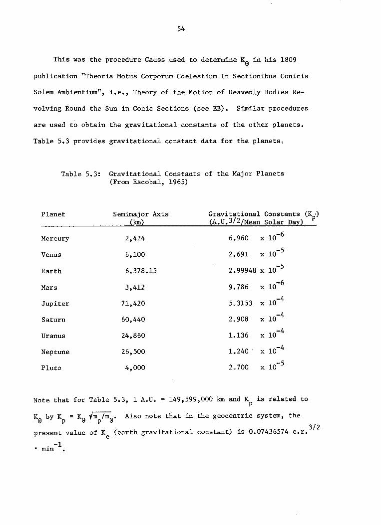
54

This was the procedure Gauss used to determine Ke in his 1809

publication "Theoria Motus Corporum Coe1estium In Sectionibus Conicis

Solem Ambientium", i.e., Theory of the Motion of Heavenly Bodies Re-

vo1ving Round the Sun in Conic Sections (see EB). Similar procedures

are used to obtain the gravitational constants of the other planets.

Table 5.3 provides gravitational constant data for the planets.

Table 5.3: Gravitational Constants of the Major Planets(From Escoba1, 1965)

Planet Semimaj or Axis Gravitational Constants (Kp)(km) (A.U. 3/2 /Mean Solar Day)

Mercury 2,424 6.960 x 10-6

Venus 6,100 2.691 x 10-5

Earth 6,378.15 2.99948 x 10-5

Mars 3,412 9.786 x 10-6

Jupiter 71,420 5.3153 x 10-4

Saturn 60,440 2.908 x 10-4

Uranus 24,860 1.136 x 10-4

Neptune 26,500 1.240 x 10-4

Pluto 4,000 2.700 x 10-5

Note that for Table 5.3, 1 A.U. = 149,599,000 km and K is related top

Kn by K = Kn vm Imn. Also note that in the geocentric system, the\!I p \!I P \!I

present value of K (earth gravitational constant) is 0.07436574 e.r.3/2

e. -1• m~n •

55

5.7 Modified Time Variable

It is often convenient in the treatment of orbital problems to

transform the time dimension to the so-called modified time variable

(.). The transformation involves a gravitational constant (e.g., Keor K ) and an epoch time t 0 In Heliocentric units:e 0

whereas in Geocentric units:

T = K (t-t )e 0

The advantage of using this quantity can be seen if we recast

the governing equation in terms of T. Since:

(5046)

then:

d2-:; 2 -+ 3-- - - K llr/rdt2 -

(5.48)

transforms to:

d 2-;

dT 2 =

-+ 3- llr/r (5.49)

and K2 does not appear.

Use of characteristic units, leads to a new unit of velocity

(V), the circular satellite unit velocity (see Chapter 3 of EB):csu

V = K~rEcsu ., a

In the Heliocentric System:

vcsu = Ke ~ 1 ~oU. = 0.017202099 A.U. 3/ 2

day ~ 1 ~.U.

(5.50)

(5.51)

56

vcsu= 0.017202099 A.D. • 1.496 • 1011 m • 1 day

day A.D. 86400 sec (5.52)

= 29,785 m/sec

In the Geocentric System:

V K /11

0.07436574 3/2/1

1= = e.r.csu e e.r. e.r.min

V 0.07436574 e.r. . 6.378214 0 106 m 1 mincsumin e.r o 60 sec

= 7,905 m/sec

(5053)

(5.54)

5 0 8 Classical Orbital Elements

Let us first establish an elliptic frame of reference in which

we consider coordinates along x , y axes in a plane containing thew w

orbit (see Figure 508).

Yw

APOFOCUS PERIFOCUS

- ......::.r---"""-------< r-.........,..n-----l...--f,/::....-t_ Xw

Figure 5.8 Elliptic frame of reference(Based on a figure from EB, 1965)

57

We have already defined:

e - eccentricity

= Ya2 - b2/a

a - semi-major axis

b - semi-minor axis

p - semi-parameter of conic

= a(1-e2)

\) - true anomaly

In addition, the positions where dr/dl' are zero are called apsis

(plural for apse). Elliptical orbits possess two points where the

above condition is satisfied, i.e., the minimum radius position

(perifocus) and the maximum radius position (apofocus). In discussing

the sun in its ecliptic, we refer to the apsis as perihelion and ap-

helion (see Figure 5.9).

EARTH

PERIHELION ~

yAPHELION

ORBITALTRACK -----...,

Figure 5.9 Perihelion and aphelion of earth in solar orbit(Not exact scale)

58

A complete set of orbital elements sufficient to describe an orbit

are the "Classical Orbital Elements". They are as follows:

1. Epoch Time (to): Julian day and GMT time for which thefollowing elements are definedo

2. Semi-major Axis (a): Half the distance between the two apsisof perifocus and apofocus.

3. Eccentricity (e): Degree of ellipticity of the orbit.

4. Inclination (i): Angle between the orbit plane and theequatorial plane of the primary body.

50 Mean Anomaly (MQ): Angle in orbital plane with respect tothe center of a mean circular orbit, having a period equi­valent to the anoma1istic period, from perifocus to thesatellite position (anoma1istic period is discussed inChapter 6)0

6. Right Ascension of Ascending Node (Qo): Angle in orbitalplane between vernal equinox (reference meridian) andnorthward equator crossing.

7. Argument of Perigee (wo): Angle in orbit plane fromascending node to perifocus.

The above set of elements satisfies the requirement of defining six

constants and an epoch time noted in Section 5.2. Note that if the

epoch time were to correspond to perifocus, the mean anomaly would be

zero and thus would be an unnecessary parameter. This is generally not

the case with either NASA, NESS, ESA, or JMS orbital element trans-

missions. Of the 7 parameters, the three angular quantities (M , Q , w )000

are subscripted similar to t indicating that they are time dependento

quantities. The time dependence of a two body orbit will be discussed

in Chapter 6. The European Space Agency has used true anomaly rather than

mean anomaly in their orbital transmissions for the Meteosat and GOES-1

satellites. This presents no difficulty as will be seen in the following

section. Appendix A provides examples of orbital parameter trans-

missions for various U.S., European, and Japanese satellites.

59

5.9 Calculation of Celestial Pointing Vector

First we recall the essential angles:

i-Orbital inclination

no - Right ascension of ascending node (note that Uo isdefined as the right ascension of descending node)

Wo :: Argument of perigee

Following the approach given in Chapter 3 of EB, the angles i, no' Wo

(the "Classical Orientation Angles") are used to define the orbit

plane in celestial space, defined by an orthogonal (I,J, K) coordinate

system (as shown in Figure 5.10).

+z

T

~ORBIT PLANE

Figure 5.10 The Classical Orientation Angles and theOrthogonal I, J, K Coordinate System(Based on a figure from EB, 1965)

Note that:

O<i<1T

o < n < 21T- 0

o < w < 21T- 0

60

From Figure 5.10 it is convenient to define retrograde and direct

orbits:

1. Retrograde: Orbits whose motion is in the direction of y to x.

2. Direct or Prograde: Orbits whose motion is in the direction of

x to y.

Compare the above with the classic definition of a retrograde orbit:

Motion in an orbit opposite to the usual orbitaldirection of celestial bodies within a given system;i.eo, a satellite motion, in a direction opposite tothe motion of the primary body.

Since the use of angles is cumbersome, we transform to a set of

orthogonal vectors (P, Q, W) in a cartesian reference frame (see

Figure 5.11):

P is a vector pointing toward perifocus

Q is in the orbit plane and advanced 900 from P

W is the normal to the orbit plane

+xT

~igure 5.11 The P, Q, W orthogonal reference frame(Based on a figure from EB, 1965)

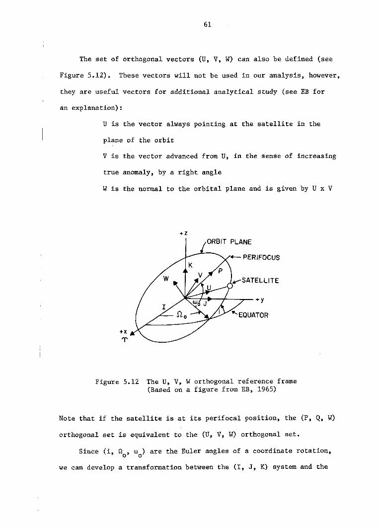
61

The set of orthogonal vectors (U, V, W) can also be defined (see

Figure 5.12). These vectors will not be used in our analysis, however,

they are useful vectors for additional analytical study (see EB for

an explanation):

U is the vector always pointing at the satellite in the

plane of the orbit

V is the vector advanced from U, in the sense of increasing

true anomaly, by a right angle

W is the normal to the orbital plane and is given by U x V

+z

+X1"'

Figure 5.12 The U, V, W orthogonal reference frame(Based on a figure from EB, 1965)

Note that if the satellite is at its perifocal position, the (P, Q, W)

orthogonal set is equivalent to the (U, V, W) orthogonal set.

Since (i, n , w ) are the Euler angles of a coordinate rotation,o 0

we can develop a transformation between the (I, J, K) system and the

62

(P Q W) t The direction cosines of this transformation are" sys em.

thus:

P cos Wo · cos Qo - sin Wo . sin Qo . cos ix

(5.55)p cos W · sin Q + sin W . cos Q . cos i

Y 0 0 0 0

P sin W sin iz 0

Q = -sin W . cos Q - cos W . sin Q . cos ix 0 0 0 0

(5.56)Qy -sin W . sin Q + cos W . cos Q - cos i

0 0 0 0

Qz cos W · sin i0

W sin Q . sin ix 0

W -cos Q . sin iy 0

W cos iz

Therefore we have:

(5.58)

where (P, Q, W) is wrt the orbit plane frame of reference and (I, J, K)

is wrt the celestial frame of referenceo Note that the (P, Q, W)

system utilizes (x ,y , z ) coordinates (see Figure 5.10) whereas theW W W

(I, J, K) system utilizes (x, y, z) coordinates (see Figure 5011).

Now if (P, Q, W) are mutually orthogonal and we define the trans-

formation matrix B, where:

63

P P Px Y z

then:

B =

w w wx y z

(5.59)

and since:

-1B

therefore:

where:

so that:

x = xP +yQ + z Ww x w X (;) X

Y = xwP + YwQ + zwWy y .y

z = xP +yQ + z Ww z w z (j) z

(5.60)

(5.61)

(5062)

(5.63)

(5.64)

Now since the satellite always remains in the P,Q orbital plane, then

z . is always zero. Therefore:w

64

x = x P + y Qw x w x

y = x P + YwQy (5065)w y

z = x P + YwQzw z

implying that if we can determine (x , Y ), we can solve for a celestialw w

position vector. Note that if we remain in the orbital plane coordinate

system as long as possible, we will have an easier time than working

in a 3-dimensional systemo

In order to determine orbit plane coordinates we need to derive

Kepler's Equation which relates geometry or position in the orbit plane

to time. We will restrict the analysis to an elliptical formulation,

ignoring the parabolic and hyperbolic formulations. We first need a

new definition, i.eo, the eccentric anomaly (see Figure 5.13).

Eccentric Anomaly (E): The angle measured in the orbital plane

from the P axis to a line through the origin and another point de-

fined by the projection of the moving vehicle in the Yw direction upon

a circumscribing circleo Note that this angle is analogous to the

angle S (reduced latitude) which was defined in Chapter 4 during the

discussion of station coordinates.

QPROJECTION OF SATELLITE

JPOSITION ON CIRCUMSCRIBINGCIRCLE

.... CIRCUMSCRIBING CIRCLE

SATELLITE

-+----!'--=-~.F_J_+J_+_. P

Figure 5.13 Definition of eccentric anomalyBased on a figure from EB, 1965)

6S

Recalling the definition of true anomaly (also shown in Figure So13):

True Anomaly (v): Angle in the orbital plane with respect to a

focus of the ellipse from the perifocal position to the satellite

position.

and with the aid of the previous figure:

x r cos vw

Y = r sin vw

x a·cosE - a.ew

Now since:

r = p/(l + eocosv)

then:

r = p/(l + e·x Ir)w

or:

(S.67)

(5.68)

(5.69)

p = r +

But we know:

e·xw

(5.70)

2p = a(l - e )

therefore from equation (S.67):

x = a(cosE - e)w

we have:

r + e.a(cosE - e) = a(l - e2)

r = a(l - e2 - ecosE + e2)

r = a(l - ecosE)

Now since:

222r x + yw w

(5.71)

(5.72)

(5073)

(5.74)

(507S)

(S.76)

66

by manipulation:

y = a(sinE • V1-e2)LU

(5.77)

and thus equations (5.72) and (5.77) give us orbital plane coordinates

in terms of Classical Orbital Elements and the eccentric anomaly.

We can now develop the relationship between E and \I. Noting that:

a(cosE - e) = rcosv

= a(l e 2)• cosv1 + ecosv

and with suitable manipulation:

cosE - ecosv = ";l"";;"';;;-=-e-c-o"';;'sE

Also:

asinE f1-e2 = rsinv

= a(l - e2)~-.=..._=--,- sin\)1 + ecos\l

(5.78)

(5.79)

Now using equation (5.79) to define cosv and with suitable manipulation:

sinv = sinE {};;21 - ecosE

(5.80)

Equations (5.79) and (5.80) thus provide a transform pair between E

and \I. If we invert the expressions, we have a transform pair between

v and E. It is easy to show that:

cosE =

sinE =

COS\) + e1 + ecosv

f l-e2 • sin\l1 + ecos'V

(5.81)

67

Now we will go through a brief derivation of Kepler's equation.

First we note:

.xw - - a E sinE

(5.82)0 EVl-e2 cosEYw = a

Next we require some identities that are basic properties of orbits.

From equation (5.49):

d~..+ -...l!..+-= r = 3 rdT r

therefore:

+ + =H.+ +r x r = 3 r x r = 0

r

Now since:

.. .d + + + + + +dT (r x r) = r x r + r x r

therefore:

o

d + -todT (r x r) = 0

and:

~ x t = h =a vector constant.

+ + + 2(r x r) • h = h = a scalar constant

A proof in Chapter 3 of EB shows that:

r = h2

J}J1 + eCOS\l

and therefore:

2 2 + +) (+ +r)~p = ~·a(l - e ) = h = (r x r • r·

(5~83)

(5.84)

(5085)

(5.86)

(5.87)

(5.88)

(5.89)

(5.90)

68

Now expanding the right hand side of equation (5090):

i j k i j k

2 0\loa(l - e ) = x Yw x Yw0w w

0 .0

0x Yw x Yw 0w w

(5.91)

results in the following:

definitions of0 .

From the x , Yw' x , Ywit is easy to show that:w w

{; = .3/2 (1 - e cosE)E

a

(5.92)

(5.93)

Now if we integrate equation (5.87) from T' =

i T JETa~2 dT' = (1 - e cosE)dE'

o 0

we find:

o to T' = T:

(5094)

(5095)

We now recall the definition of the modified time variable:

(5096)

where we understand that from the integration limits, the initial time

t corresponds to the point on the orbit where E = 00 We shall callo

this time T, the time of perifocal passage. Substituting for T, such

that E =Et

, we have Kepler's equation:

~3/2 K(t - T) = E - e sinEa

(5.97)

69

N 11 '~K/a3/2 how we ca f~ t e mean motion n, where:

n=...!L K3/2a(5098)

and it is now apparent that we have a formulation for the mean anomaly

(M) :

M = n(t- T)

Note that M is one of the Classic Orbit Elements:

Mean Anomaly (M): Angle in orbital plane with respect to the

center of a mean circular orbit, having a period equivalent to the

anoma1istic period, from perifocus to the satellite position. We

shall defer our discussion of anoma1istic period until we discuss

perturbation theory in Chapter 60

We now see what the mean motion has to do with the period. Re-

calling equation (5.40):

(50100)

Therefore the mean motion constant (n) and the period (P) are simply

reciprocal quantities:

21Tn =-P

(5.101)

21TP =­

n

It is important to note why the recovery of an accurate value of

the semi-major axis (a) from raw orbit tracking data is so important.

S · h . did' 1 . 1 t 3/2 .1nce t e per10 s 1rect y proport10na 0 a , any error 1n

70

recovering the semi-major axis translates to a cumulative error in

position due to an incorrect period. Figure 5.14 provides a graph for

both a low orbiting satellite and a geosynchronous satellite indicating

the period error corresponding to errors in specifying the semi-major axis.

24 240 CJ)::>0Z

0::: 20 200 ~-;w GEOSYNCHRONOUS~ :I: .-

t:- u E-men 16 160 Zca::Q)~o0'S

c: 0-~.- 12 120

wO:::oE C)~...J-

zc ZO:::-0 8 80 -wa::- o:::t:00::: omo:::w a:: 0:::o:::Q.. 4 40 0:::0W w

I 2 3 4 5 6 7 8 9 10% ERROR IN SPECIFYING SEMI- MAJOR AXIS

Figure 5.14 Error in determining satellite period correspondingto error in recovering the semi-major axis

From equations (5.97) and (5.99) we have a relationship between

M and E:

M = E - e sinE (5.102)

however, we want E in terms of M. Since equation (5.102) is a trans-

cendenta1 equation we can transform it. First equation 5.102 is

differentiated:

dM = (1 - e cosE)dE (5.103)

71

Next we rearrange and integrate from the position of perigee at which

E = M = 0, to an arbitrary position in the orbit corresponding too 0

(5.104)

We can now express the term under the integral of equation 5.104 as a

Fourier expansion:

(5.105)

where 21/, is the period of the function and:

·_f2tIa - = -:- (1

m J/"o

.1j2R.b = - (1m 9,

o

-1 (m1TM)- e cosE) cos T dM

-1 (m1TM)- e cosE) sin -9,- ell'! (5.106a)

12.Q,

1 -1a = - (1 - e cosE) dMo R,

o

Now substituting for dM from equation (5.103) and noting that 29, = 21T:

121T

a =1. dE = 2o 1T

o (5.106b)21T

a = 1 (cOS(m!M)dEm :I

o

and all b = 0 since we are integrating an even function. Now usingm

72

our definition of M from equation (5.10Z):

Now using an integral representation property of Bessel functions (see

Abramowitz and Stegun, 197Z):

a = Z J (me)m m

(5.107)

where J is a Bessel function of the first kind of order m and argu­m

ment me:

Jm(me) =2:k=O

2k+m fk+m(_l)k (mze) lX> (_l)k (~)

k! (k+m)! =2: k!r(k+m+1)k=O

(5.108)

We can now rewrite equation (5.105) as:

and integrating, we can finally express the eccentric anomaly E,

explicitly in terms of M and e with a Fourier-Bessel series:

(5.109)

E 1:. J (me) sin(mM)m m

where E and M represent the eccentric and mean anomaly at an arbitrary

time t.

The above expression remains cumbersome for computer ca1culationso

However, the series term can be expanded in powers of e. Noting that

e < 1.0, we can truncate at some power of e, say 5:

73

+ 000

9 3 81 5J 3(3· e) = 16 e - 256 e + •••

625 5J 5(5. e ) = 768 e + 000

Now if we collect terms in similar powers of e:

E = M+ ~ • ~ 0 sin(M)1 2

2 e2+ - 0 - 0 sin(2M)

2 2

(50111)

2 9+ - • - 0

3 163 2 1 3

e • sin (3M) - I 0 16 0 e • sin(M) (5.112)

224.21 4+ 4 0 3 • e • s~n(4M) - 2 0 6 • e • sin(2M)

Simplifying:

2 625 5+ 5 0 768 • e 0 sin(5M)

215+ - • --- • e • sin(M)1 384

2 81--. - 0

3 256 e50 sin (3M)

E = M+ sin(M) 0 e + sin(2M) 0 e2 + 1 [3 • sin(3M) - sin(M)]e32 8

+ ~ [2 0 sin(4M) - sin(2M)] 4Q e (5.113)

+ 3~4 [125 • sin(5M) - 81 • sin(3M) + 2 • sin(M)] • e5

74

We now note that all the coefficients of the expansion are less than

one, thus insuring that the truncation in powers of e only ignores

increasingly smaller terms. Now we can apply the trigonometric multiple

angle relationships:

sin (2M)

sin(3M)

sin(4M)

sin(5M)

2sin(M)cos(M)

3sin(M) - 4sin3(M)

4sin(M)cos(M) - 8sin3(M)cos(M)

5sin(M) - 20sin3(M) + l6sin5 (M)

(50114)

Substituting and simplifying we arrive at our final equation for E in

explicit terms; an expression which involves only a single sin and cos

calculation insofar as computational requirements are concerned:

E = M+ sin(M) 0 e + sin(M)cos(M)e2

+ [sin(M) - (3/2)sin3(M)]e3

+ [sin(M)cos(M) - (8/3)sin3(M)cos(M)]e4

+ [sin(M) - (17/3)sin3 (M) + (125/24)sin5(M)]e5

(50115)

Note that if we consider only the first power term (for example, in

the event e is very small), then:

E ~ M+ eosin(M) (5.116)

To illustrate the error in ignoring the higher order terms we

examine the eccentric anomaly of the sun with respect to the earth

under various orders of expansion. Table 5.4 provides the resultso

Appendix D provides a computer solution for an apparent solar orbit

which considers the above expansion.

75

Table 5.4 Eccentric Anomaly of Sun wrt Earth Under VariousOrders. of Expansion (Eccentricity of solar orbitis .081820157)

Mean Anomaly Eccentric Anomaly

1 2 3 4 5e e e e e

0 0.000000 00000000 00000000 0.000000 0.00000015 15.021177 150022850 150022978 150022987 15.02298830 30.040910 300043809 300043980 300043987 30.04398645 450057856 450061203 45.061300 45.061292 45006129160 60.070858 600073757 60.073698 60.073678 60007367775 750079032 75 0080706 750080494 750080478 75.08047990 90.081820 900081820 90.081546 900081546 90.081548

105 105.079032 105 0077359 1050077147 105.077164 1050077165120 120.070858 1200067960 120.067900 1200067920 120.067919135 135.057856 135.054508 135.054605 135.054613 1350054611150 150.040910 150.038011 150.038182 1500038176 150.038176165 165.021177 1650019503 165.019631 1650019621 1650019622180 1800000000 180.000000 1800000000 1800000000 1800000000

The stage is now set for the calculation of a celestial pointing

vector. We first transform the epoch from t to the time of perifocalo

passage (T). Since:

M = net - T)o 0

therefore:

T = t - M /no 0

Thus we can now solve for M at any arbitrary time t:

M = net - T)

and then solve for E:

E = M + e sin(M) + ..•

We now solve for x and y and note that z is always 0:w w w

(50117)

(5.118)

(5.119)

(50120)

76

x = a(cosE - e)w

yw = a(sinE . -Il-e2)

z 0w

Now transform to a celestial pointing vector:

(50121)

(50122)

where BT is the transpose of the celestial frame-orbital plane trans-

formation matrix. This completes the desired solution.

It is useful to summarize the relationships bet~een M, v, and E:

M = E - e·sinE.

E = H + e' sinM + '.0

(5.123)

cos v (cosE - e)/(l - e cosE)(5.124)

sin v \/1 - e2'sinE/(1 - e cosE)

cosE = (cosv + e)/(l + e cosv)

sinE \/1 - e2.sinv/(1 + e cosv)

(5.125)

Now recall that ESA uses True Anomaly (v ) rather than Mean Anomalyo

(M ) in their orbital element transmissions. Thus before we can applyo

equation (50118), we first transform v to an initial eccentric anomalyo

E :o

E = cos-l[(cos v + e)/(l + e cos v )]000

The initial mean anomaly can now be solved:

M = E + eosinEa a a

(5.126)

(50127)

77

5.10 Rotation to Terrestrial Coordinates

Finally, we transform to our rotating frame of reference (i.e.,

the earth). This is accomplished by noting that the observer's meri-

dian is rotating with an angular velocity equal to p, that is the

sidereal rate of change. Thus the observer's right ascension can be

given by:

p = p + pet - t )o e

in which we have defined:

P ;::: SIlAo

(5.128)

(5.129)

where Pd is the daily period (24 hours), t e is a sidereal epoch, and

SIlA is the sidereal hour angle at the epoch t. We can choose SHA = 0,e

i.e. a time when the Greenwich meridian is in conjunction with the

vernal equinox. To do so, the "Universal and Sidereal Time" table

from the American Ephemeris and Nautical Almanac can be used. Table

5.5 provides an example from the 1978 version for January, in which

can be seen that on January 1, at 17 16 00 GMT the vernal equinox

and the Greenwich meridian are aligned. S simply converts solar mean

time to sidereal time, where:

S = 366.25/365.25 (5.130)

Thus, by rotating the (x, y, z) vector through an angle p, we finally

achieve our desired earth reference vector (x , y , z ):e e e

xe ;::: cos(p)·x + sin(p).y

y = -sin(p)·x + cos(p)·ye

z = ze

(5.131)

78

Now, using the transformation between cartesian and spherical coor-

dinates, we can solve for the sub-satellite point (~sp' Asp) in geo­

centric coordinates and the satellite height (h). First, we solve for

latitude and longitude (~,A) and the radius coordinate (r) in a spher-

ical reference frame:

-l[ I 2 2 2]~ = sin z I Yx + Y + ze e e e

A = tan-ley Ix ]e e (5.132)

r = Ix 2 + 2+ z 2e Ye e

Finally we transform to geocentric coordinates (~ ,A ) and heightsp sp

(h) :

A = Asp (5.133)

where R is the earth radius at latitude ~ and e is the eccentricitye sp

of the earth itself.

Computer codes adopted to the above methodology are given in

Appendices Band D. Appendix B considers an earth-satellite config-

uration whereas Appendix D considers an earth-sun configuration.

Appendix C consists of a numerical routine used to determine an earth

satellite equator crossing period which will be discussed in Chapter

6. Appendix E gives two approximate solutions for determining solar

position; these routines can be compared to the solution given in

Appendix D. Appendix F represents a set of library routines applicable

79

to the aforementioned orbital codes, and finally Appendix G provides a

solution for determining the required inclination for a sun-synchronous

orbit (this problem is discussed in Chapter 6).

80

Table 505: Universal and Sidereal Time Table for January, 1978(From the American Ephemeris and Nautical Almanac,1978)

Date Julian G. SIDEREAL TIME Equation of G.S.D. UNIVERSAL TIMEDate (G.H.A. of the Equinox) Equinoxes (Greenwich Transit of the Equinox)

OhU.T. Apparent Mean at Oh V.T. Oh G.S.T. Date Apparent Mean

244 h m , , , 245 d h m , ,Jan. 0 3508. 5 637 13'506 13.280 +0·226 0200·0 Jan. ° 17 1<) 55 ·662 55.886

I 35°9'5 64 110 .°59 ol).835 ·223 0201·0 I [7 15 5()'756 59· l)762 35 1°'5 64506.611 06'391 ·220 0202·0 2 17 12 °3.849 °4.0673 35 11· 5 649°3. 164 02'946 .218 0203.0 3 1708 °7'94 1 08.1574 35 12 '5 6 52 59'718 59·5°1 .21 7 020 4.0 4 17°4 [2'°3 1 12.248

5 35 13.5 656 56.275 56'°57 +0·218 0205.0 5 17 00 16. II8 16'3396 35 14'5 700 52.835 52.612 ·222 0206,0 6 16 56 20·203 2°'4297 35 15'5 7°449'397 49. 167 ·229 0207. 0 7 16 52 24. 285 24'5208 35 16'5 7 08 454>0 45 '723 .238 0208·0 8 1648 28'367 28.6to

9 35 17. 5 7 12 42.524 42.278 .246 020 9.0 9 16 44 32'45 I 32'7°1

10 35 18 '5 7 1639.086 38.834 +0.25 2 0210·0 10 16 40 36.537 36'791II 35 19' 5 7 20 35.644 35'389 .255 0211·0 II 16 364°.626 40.88212 352°'5 724 32. 200 31'944 .256 0212·0 12 [6 3244'718 44'97213 352I·5 72828'753 28'500 ·254 021 3.0 13 16 2848.812 49.06314 3522 .5 73225'3°5 25'°55 .25° 0214.0 14 16 24 52'9°6 53. 153

15 35 23'5 7 36 21.857 2[ .610 +0·247 0215.0 15 16 20 57·000 57'24416 3524'5 740 18'409 18·166 .244 0216.0 16 16 17 01'093 01'33417 35 25'5 744 14'963 14 '7 21 '242 021 7. 0 171613°5.183 °5'42518 3526'5 748 II'5 19 11.276 '242 0218,0 18 16 09 °9.273 09' 51519 35 27'5 7 5208.076 07.832 ·244 0219.0 19 16 os 13'361 13.606

20 3528 '5 7 5604.634 °4'387 +0·247 0220·0 20 1601 17'448 17.69721 35 29' 5 80001.193 °°'943 ·25° 0221·0 21 15 5721'535 21 '78722 353°'5 803 57'752 57'498 ·254 0222·0 22 15 53 25·622 25.87823 353 1'5 807 54'310 54'°53 .257 0223.0 23 15 49 29'710 29'96824 3532.5 8 II 50.868 50.609 .260 0224.0 24 15 45 33'799 34'°59

25 3533' 5 8 15 47'424 47. 164 +0·260 0225.0 25 15 41 37.890 38.14926 3534·5 8 1943'979 43'719 ·259 0226.0 26 153741'983 42.24°27 3535'5 8 234°'531 4°·275 .256 0227.0 27 15 3346,077 46'33028 3536.5 827 37.082 36.830 .252 0228.0 2815295°.172 5°'42129 3537·5 831 33.633 33'385 ·247 0229.0 29 15 25 54. 268 54' 5II

3 0 3538.5 8 35 30' 183 29'94 1 +0·243 023 0 •0 30 15 21 58'362 58.6023 1 3539'5 839 26 '735 26'496 .239 023 1 •0 31151802'456 02.692

Feb. I 354°'5 843 23.289 23'°52 .237 023 2 •0 Feb. I 15 14 06'546 06'7832 354 1.5 847 19.845 19.607 .238 0233.0 2 15 10 10.635 10.8733 3542'5 851 16'4°3 16·162 .24 1 00234.0 3 IS 06 14.721 14'964

4 3543'5 8 55 12'964 12'718 +°'246 0235.0 4 150218.806 19'°55S 3544'5 859°9'524 °9·273 .25 1 023 6 •0 5 14 58 22.891 23. 1456 3545·5 9°3 06.084 05.828 .256 0237.0 6 14 54 26'979 27.2367 3546'5 9 07 02.642 02'384 .258 0238 •0 7 14 5°31.069 31'3268 3547· 5 9 10 59. 197 58'939 ·257 0239.0 8 144635.162 35-4 17

9 3548'5 91455'748 55'495 +0·254 024 0 •0 9 14 42 39·257 39'5°710 3549'5 9 18 52.298 52'°5° .248 024 1 •0 10 14 38 43' 354 43'598II 355°'5 9 22 48.847 48.605 '242 024 2 •0 II 14 3447'45° 47.68812 355 1'5 9 26 45'397 45. 161 .236 0243.0 12 14 30 5I· 546 51'77913 3552'5 93°4 1 '948 41'716 .232 0244.0 13 14 26 55.640 55.869

14 3553·5 934 38'500 38.271 +0·229 0245.0 14 14 22 59'733 59'960IS 3554'5 938 35.°54 34.827 +0·227 024 6 •0 15 14 19 03.824 °4'°5°

6.0 PERTURBATION THEORY

6.1 Concept of Gravitational Potential

We will now consider the deviation of an orbit from the ideal, two

body, inverse square-force field law 0 In order to do so, we must dis­

tinguish the concepts of empirically correcting orbit calculations due

to a non-perfect two body system, and the actual prediction of orbit

positions based on a physical model which accounts for forces that per­

turb a body from perfect two body motion~ The first technique has

received a good deal of study under the general heading of "Differential

Correction". A discussion of this topic is given in Chapter 9 of EB,

by Dubyago (1961), and by Capellari et ale (1976)0 The method consists

of bringing a predicted orbit position into agreement with a set of

actual orbit measurements in such a way so as to adjust a set of con­

stant orbital elements to satisfy a new local time period. Thus the

methodology does not necessarily consider the physical reasons why an

orbit is perturbed.

The general area of "Perturbation Theory" consists of developing

a set of reasonable, time dependent quantities which arise due to

various perturbation forces, which in turn lead to time dependent ex­

pressions for the orbital elements themselves. This theory, although

not necessarily adaptable to analytic techniques, has a physical basis

in facto Since the satellite navigation problem is not really compatible

with the required procedures used in Differential Correction techniques,

we shall address the following discussion to perturbation techniques.

We first need to consider the governing equation in terms of the

concept of potential. Following the approach of Kozai (1959) and

EB and using a spherical coordinate system defined by the earth's

81

82

equatorial plane, we define a potential (V):

2v+~

r

where:

(6.1)

-+and (x, y, z) are the cartesian components of a radius vector r ex-

tended from the earth center to an arbitrary satellite position. Taking

partial derivatives with respect to x, y and z yields:

ov =_ llK2 or

ox 2 oxr

ov llK2 or

= --2oy oyr

ov JlK2 or= --2 5Zoz r

and since:

or x or = y.. or z-=- -=-ox r oy r oz r

then:

(6.4)

2d x OVdt2 = ~

or simply:

2d z oVdt2 = ~ (6.5)

(6.6)

Equation 6.6 thus states that the acceleration of a body is due to the

gradient of what we shall call a potential V.

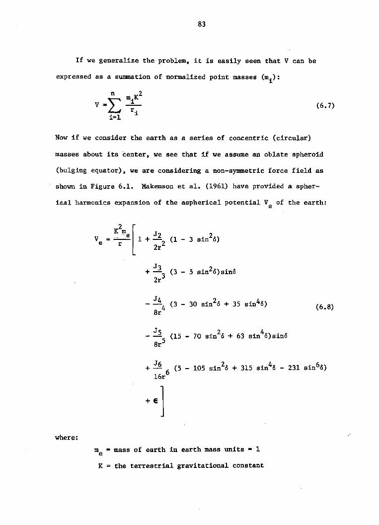
83

If we generalize the problem, it is easily seen that V can be

expressed as a summation of normalized point masses (mi ):

n

V=L:i=l

(6.7)

Now if we consider the earth as a series of concentric (circular)

masses about its center, we see that i£ we assume an oblate spheroid

(bulging equator), we are considering a non-symmetric force field as

shown in Figure 6.1. Makemson et ale (1961) have provided a spher-

i~al harmonics expansion of the aspherical potential Ve of the earth:

_J5 2 4(15 - 70 sin 0 + 63 sin o)sino8r5

(6.8)

where:

m = mass of earth in earth mass units = 1e

K = the terrestrial gravitational constant

84

-1sin (z/r)

r = distance from the earth center to a spacecraft in e.r.

units

and the Ji's are the spherical harmonic coefficients of the earth's

gravitational potential. Equation (6.8) has been normalized such that

J 1 = 1. The term E simply expresses the error due to ignoring higher

order terms. The lower order coefficients have been tabulated by

Makemson et a1. (1961) and are given in Table 601.

Table 601: Harmonic Coefficients of the Earth'sGravitational Potential

J2 +1082.28 10-6

J3

-2.30 • 10-6

J4 -2.12 10-6

J S -0.20 • 10-6

J 6 +1.00 • 10-6

Equation (6.8) is actually a simplification of the gravitational

potential of the earth. When considering the departures from symmetry,

there are two kinds of spherical harmonics: zonal harmonics (departures

due to the ellipticity of the meridians), and tessera1 harmonics (depar-

tures due to the ellipticity in latitudinal cross sections). Only

zonal harmonics are considered in the above expansion. This is a stan-

dard model adopted in general perturbation techniques (see Escoba1 (1968)

for a discussion of higher order models).

Since we can express the governing equation as:

(6.9)

85

~ASYMMETRICAL SHELL

~ig~re 6.1 Depiction of the earth as a sequence ofconcentric mass shells

86

by differentiating equation (6.8) with respect to x, y, z and using

eq~ation (6.4) we have the equations of motion of a satellite with re-

spect to an oblate spheroidal central body (expressed to order J3):

d2 oVx e

dtZ = ox

Z-K m x [ 3 J Z 2--3-:;;eo- 1 + "2 2' (1 - 5 sin 0)

r r

+ 1 J 3 (3 _ 7sin2o)sino + 0.0]'Z 3

r

Zd2 OVe -K mey [ 3 J 2 Z~ = - =- 1 + - - (l - 5 sin 0)dtZ fly r3 Z r2

5 J32 1+ 2~ (3 - 7sin o)sino + •• 0r

(6.10)

This lays the foundation for considering the motion of a satellite with

respect to an oblate spheriodal central body and under the influence

of additional perturbative effects.

6.2 Perturbative Forces and the Time Dependence of Orbital Elements

A satellite, under the influence of a perfect inverse square force

field law, would have a set of constant orbital elements:

[a, e, i, M , n , w ]000

87

devoid of any time dependence. However, due to perturbative forces, the

orbital elements are acted upon leading to shifts or osci11ationso

There are a number of effects which can be considered as perturbative

forces:

1. Aspherica1 gravitational potential

2. Auxi11ary bodies (e.g. sun, moon, planets)

3. Atmospheric drag

40 Atmospheric lift

5. Thrust

6. Radiation Pressure (shortwave and 10ngwave radiation)

7. Galactic particle bombardment, e.g. protons (i.e. solar wind)

8. Electromagnetic field asymmetry

The most important of these effects on earth satellites is due to the

first factor; the aspherica1 gravitational potential of the earth itself.

Atmospheric drag becomes significant for the lower orbit satellites

(heights less than 850 km).

The aim of general perturbation theory is to develop closed ex-

pressions for the time dependence of the orbital elements. It has been

shown that perturbations possess different characteristics (see Chapter

10 of EB and Dubyago (1961) for a review):

10 Secular variations

2. Long term periodic variations

30 Short term periodic variations

In working with meteorological satellite orbits, we are primarily con-

cerned with non-oscillatory secular perturbations which cause ever

increasing or decreasing changes of particular orbital elements away

from their values at an epoch t as shown in Figure 6.2 0o

~zw~W--IW

--I

f!CDa::oLLoW:::>--I:s

88

SECULAR VARIATIONLONG PERIOD VARIATION

~-- SHORT PERIOD VARIATION

t

Figure 6.2 Three principle types of orbital perturbations

The aspherica1 gravitational potential of the earth primarily ef-

fects M, n, and w (where we understand that M, n, and w without sub-

scripts are no longer constant). The other elements (a, e, i) undergo

minor periodic variations about their mean values due to the aspherica1

gravitational potential, but in terms of meteorological satellite or-

bits, are not considered significant. In general, long period varia-

tions are caused by the continuous variance of w whereas short period

variations are caused by linear combinations of variations in M and w.

The general form of the equation of motion in a relative inertial

coordinate system is given by:

(6.11)

where subscript 1 indicates the earth, subscript 2 indicates the sate1-

lite, the summation over m represents accelerations due to all auxil1ary

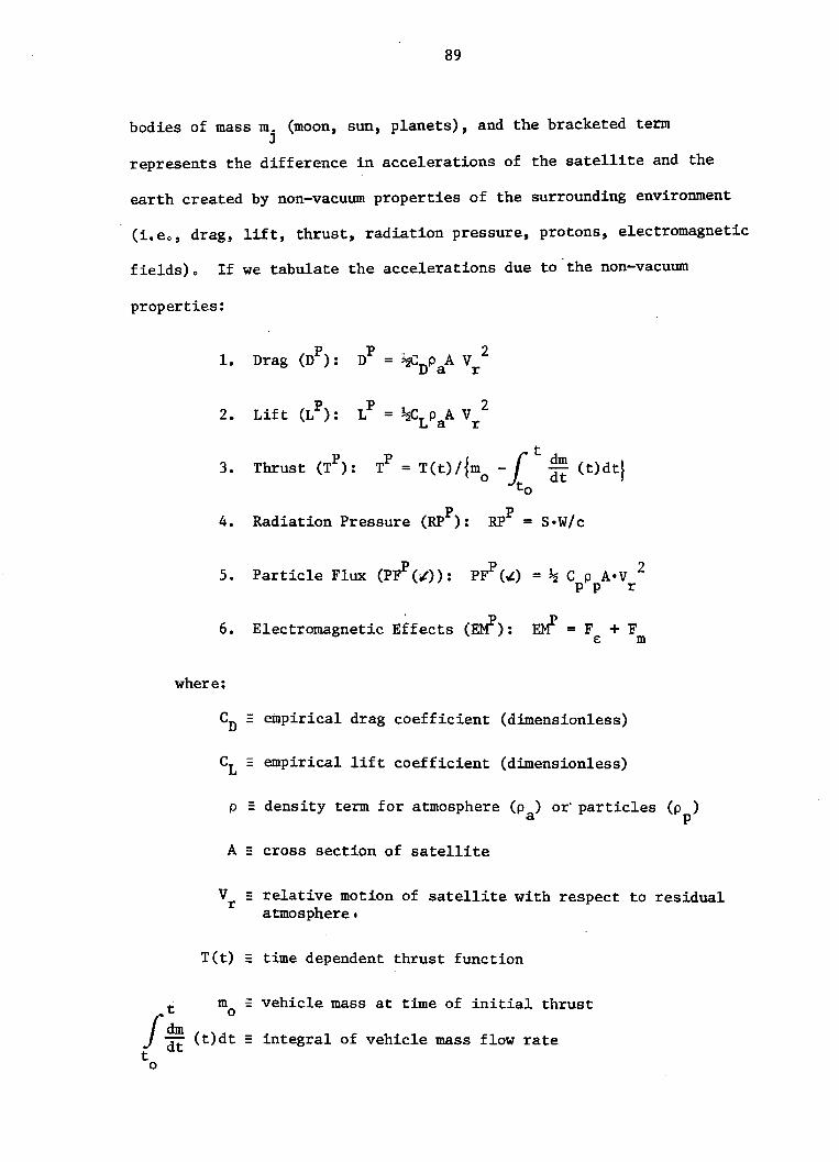
89

bodies of mass m. (moon, sun, planets), and the bracketed termJ

represents the difference in accelerations of the satellite and the

earth created by non-vacuum properties of the surrounding environment

(i.eo, drag, lift, thrust, radiation pressure, protons, electromagnetic

fields) 0 If we tabulate the accelerations due to the non-vacuum

properties:

2. Lift (LP): L

P = ~LPaA vr2

3. Thrust (TP): T

P= T(t)/{mo -J(t ~~ (t)dt}

o

4. Radiation Pressure (RPP): RPP = s.w/c

5. Particle Flux (P~(~»: PFP(~) = ~ C p A.V 2p p r

6. Electromagnetic Effects (EMt):

where:

~ = F + FE m

integral of vehicle mass flow rate

Cn - empirical drag coefficient (dimensionless)

CL - empirical lift coefficient (dimensionless)

p =density term for atmosphere (Pa) or' particles (p )p

A _ cross section of satellite

Vr - relative motion of satellite with respect to residualatmosphere.

T(t) _ time dependent thrust function

t mo - vehicle mass at time of initial thrust

~~ (t)dt _t

o

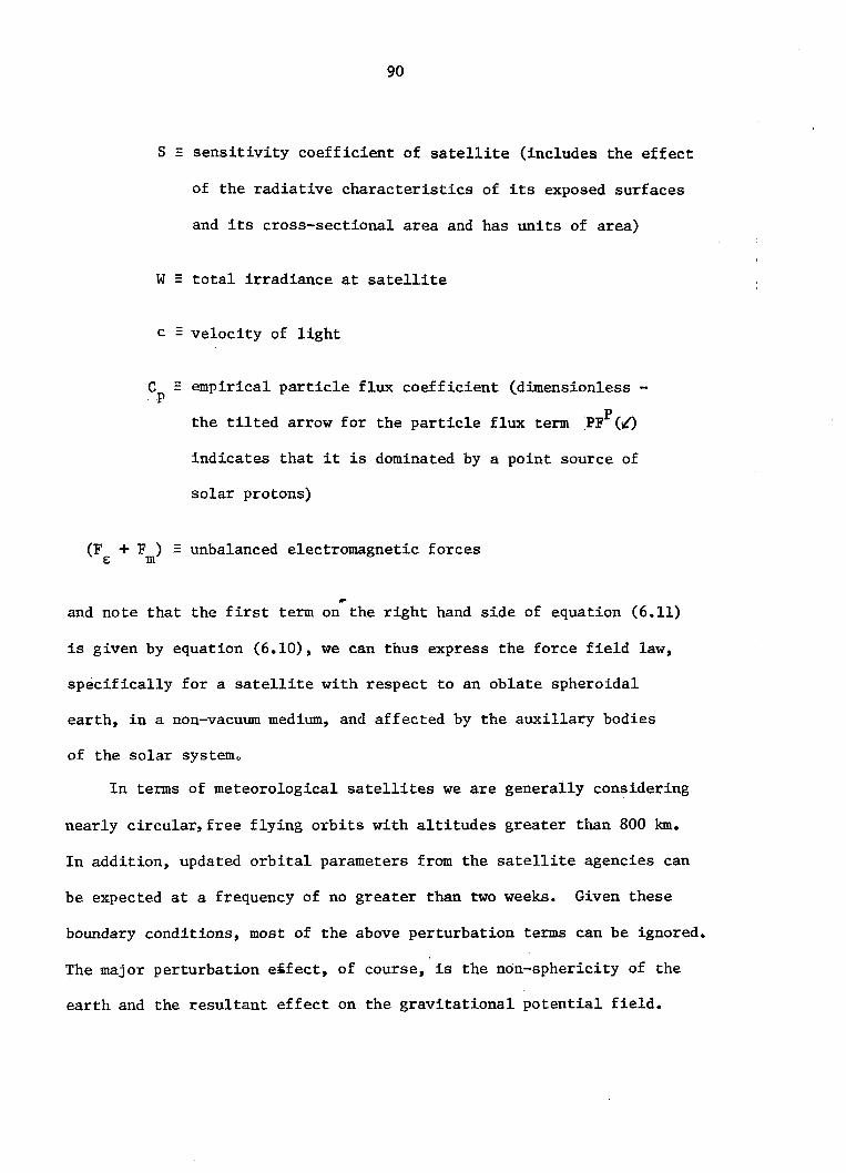
90

S _ sensitivity coefficient of satellite (includes the effect

of the radiative characteristics of its exposed surfaces

and its cross-sectional area and has units of area)

W - total irradiance at satellite

c - velocity of light

Cp - empirical particle flux coefficient (dimensionless ­

the tilted arrow for the particle flux term :PFP(i)

indicates that it is dominated by a point source of

solar protons)

(F + F ) - unbalanced electromagnetic forces~ m

r

and note that the first term on the right hand side of equation (6.11)

is given by equation (6.10), we can thus express the force field law,

specifically for a satellite with respect to an oblate spheroidal

earth, in a non-vacuum medium, and affected by the auxilIary bodies

of the solar systemo

In terms of meteorological satellites we are generally considering

nearly circular, free flying orbits with altitudes greater than 800 km.

In addition, updated orbital parameters from the satellite agencies can

be expected at a frequency of no greater than two weeks. Given these

boundary conditions, most of the above perturbation terms can be ignored.

The major perturbation eifect, of course, is the non-sphericity of the

earth and the resultant effect on the gravitational potential field.

91

The minor tenns insofar as meteorological satellites are concerned, are

the lunar effect, atmospheric drag, and solar radiation pressure. In

general the minor terms need not be included in orbit propagations that

take place over a one to two week period, if we consider the allowable

error bars associated with satellite navigation requirements. That is

to say, ignoring the effect of the minor perturbations does not lead

to position or ephemeris errors significantly greater than the resolu-

tion of the data fields under analysis.

It is ;f;mportant to note that the space agencies responsible for

tracking satellites often include the minor terms in retrieving orbital

elements. This is due to the fact that generalized orbit retrieval

packages have been developed for the extensive variety of operational

and experimental satellites, and missiles rather than retrieval pac-

kages individually tailored to specific types of satellites o The

primary difficulty with treating the minor terms in a satellite navi-

gation model is that the required mathematics does not lend itself to

streamlined analytic calculations, a principle requirement for pro-

cessing the vast amounts of data produced by most meteorological satel-

lite instruments. This is the principle reason for retaining only

the major perturbation effect (asymmetric gravitational potential)

which can be handled in a direct analytic fashion.

Following EB, if we consider the potential of an aspherical earth

(V ) with respect to the potential of a perfectly spherical earthe

(Vp)' where:

V = K2(m + m )/rpes (6012)

Klme [J2 2 J 3 2 JVe = -r-"- 1+ 2r2 (1-3 sin IS) + 2r3 (3-5 sin o)sino+ ••.•. (6.13)

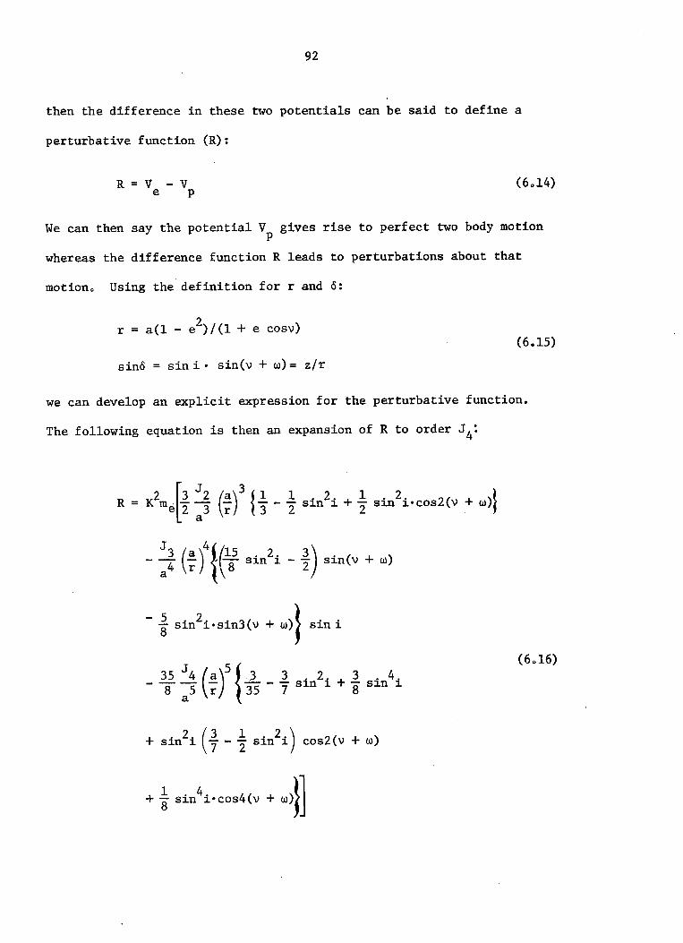
92

then the difference in these two potentials can be said to define a

perturbative function (R):

R = V - Ve p

We can then say the potential V gives rise to perfect two body motionp

whereas the difference function R leads to perturbations about that

motion o Using the definition for rand 0:

2r = a(l - e )/(1 + e cosv)

(6.15)

sino = sin i· sin(v + w) = z/r

we can develop an explicit expression for the perturbative function.

The following equation is then an expansion of R to order J 4:

J 4t~ )3 a 15. 2. 3 .- a4 (r) '"8" Sln 1. -"2 s1.n(v + w)

- 5 . 2. . 3( + )} . i8 S1.n 1.°S1.n V w S1.n

J ( )5{35 4 a 3 3 2 3. 4.-"8" a 5 r 35 - '7 sin i + 8 Sln 1.

+ . 2. (3 1 . 2i ) 2( + )S1.n 1. '7 - "2 S1.n cos V w

(6 0 16)

+ 1 . 4. 4(8 S1.n 1. °cos V

93

Brouwer and Clemence (1961) and Sterne (1960) have provided the

analysis necessary to relate time derivatives of the orbital elements to

derivatives in R. These expressions as given by EB are as follows:

da 2 oRdt = na oM

de 2 ~2 oR(l-e ) oRdt =. - OW2 oM 2na e na e

di cosi oR-=dt 2 V12 .. owna -e s~n~

dM (l-e2) oR 2 oR-= n - 8e ---dt 2 na oana e(6.17)

dn 1dt = 24 ~2

na Vl-e

oR. i oi

s~n

dw-=dt

cosi oR + 'Vi=';2 oR2 ... C--;;l2 . . oi 2 oena Vl-eLs~n~ na e

It is now possible to partition the resultant derivatives into secular

components, long period oscillatory components, and short period oscil-

latory components.

If we ignore the oscillatory components (in a, e, and i) we can

then develop secular perturbation expressions for any selected order

of the graVitational potential expansion. It is this process, for

satellite applications, which eliminates the time dependence in a, e,

and i while including it in M, n, and wo Next note that the time

dependence of an arbitrary orbital element (X) can be expressed as

a Taylor series expansion:

94

• " 2X = X + X(t - t ) + X(t - t ) /2! + ••.o 0 Q

(6.18)

where Xo is the initial value at an epoch to' and X, X, ... , are time

derivatives. Now, if we ignore all but first order time derivatives

and consider only the first order variations of the aspherica1 gravi-

tationa1 potential (due to J 2), we can express the time dependence of

M, Q, and w in simple finite difference form with adequate accuracy:

M= M + M(t - t )o 0

(6.19)

w w + ~(t - t )o 0

where M=n is defined as the Anoma1istic Mean Motion and n, ware the

first derivatives of Q and w. These expressions, derived in Chapter 10

of EB, are given by:

. (3 J 2"[ 5 2J)w = 2"""2 2 - 2" sin i np

(6.20)

(6.21)

(6022)

which are all functions of a, e, and io It is important to note that

as long as the latter 3 parameters remain nearly constant with time, it

is not necessary to apply implicit numerical techniques to the solutions

of equations (6.20), (6.21), and (6.22). However, a principal effect

of atmospheric drag on low orbit satellites is to modify the values

of a, e and i as a function of the eccentric anomaly. This is due to

the fact that the essential effect of drag is to de-energize a satellite

95

orbit and thus reduce the dimension (semi-major axis) of the orbit

ellipse. In addition, if the initial orbit is highly non-circular, the

variation in the drag effect due to the elliptic path leads to modi­

fication of the orbit inclination. If a low-flying satellite (small

period or high eccentricity) were being considered, time dependent ex­

pressions for the semi-major axis, eccentricity, and inclination should

be included. EBprovides a set of expressions for drag induced deri­

vatives of a, e, and i in Chapter 10 of his text, however, to include

these expressions in an orbital solution would require a multiple step

iterative approach to the calculation of the six derivative quantities.

According to Fuchs (1980), with respect to the satellite navigation

problem, drag induced perturbations need not be considered for meteoro­

logical satellites until orbital altitudes start falling below 850 km.

With equation (6.20) we can define the Anomalistic Period (P):

P = 2n/n (perifocus to varying perifocus)

Contrast this with the non-perturbative or mean period P:

P = 2n/n (perifocus to non-varying perifocus)

(6.23)

(6.24)

96

Expanding to second order variations in potential results in terms

of J 2 and J 4, where the Anoma1istic Mean Motion n is given by: (see EB):

= [ 3 ~2n = n 1 + 2' J 2 p2 (1 3 . 2.)- 2' Sl.n J.

(6.25)

+ [105 + 144~2 + 25(l-e2)] 4 i\cos 'J.;

and the Anoma1istic Period (P) and the Mean Anomaly (M) are given by:

(6.26)M = M + n(t - t )o 0

.. .The first derivative terms M, Q, and ware given by:

( 5 5 2 .. ,r- 2) . 2 }]- 3 - 24 e - 3 V1-e sJ.n i

(6.27)

(6.28)

9.7

2+~

2_ 2~2 _ (43 _e

2_ 3~2)24 48

\ . 2.}] 45 J 2 2S1.n 1. - 36 p4 e

4. 35 J 4n cos 1. - '8""4 n

p (6.29)

·[12 93 . 2i + 21 i 4. +- - - S1.n - s n 1.7 14 4 \

2 {27e 14

189 . 2. + 81- -zs S1.n 1. 16

Note that the sign of the expression for dn/dt (see Equation (6.21»

indicates·why orbits must retrograde to achieve a sun synchronous

configuration (eastward precession of ascending node). Since dn/dt

must be positive and the expression is of the form -[positive constant]

·cosi, then the cosine of i must be negative. This requires i > 90.

It is worth comparing the first derivative terms (M, n, ~) for

the first and second order expansions for both short period polar or-

biting satellites and longer period geosynchronous satellites. Using

typical orbital data we can generate Table 6.2 from the computer routine

given in Appendix B.

98

Table 6.2: Comparison of First Derivative Terms for First andSecond Order Expansions (deg/day)

First Order Second OrderPolar Geosynchronous Polar Geosynchronous

n 49850237053 3570564532 4985.237053 35705645320M 4982.408922 3570577648 49820410662 357.5776480n .990040 -0013117 .993605 -00131150

-2.666695 0026234w -2.664593 .026237

6.3 Longitudinal Drift of a Geosynchronous Satellite

We can now show that a geosynchronous satellite has a n term,

even if the inclination and eccentricity are zero. Setting i = 0 and

using a first order expansion:

• dn ( 3 3 2 ) [ 3 {:;02] (6.30)n =- = -Z

p2 n 1+"2J2dt

Now since n = K/a3/ 2 and p = a(l - e2), and if we set e=O, and letting:

J2

= 1082.28 0 10-6

K = 0007436574 e.r0 3/ 2/min

a = 6.6229 e.ro

then:

o -1= -0.01332 day westward drift

(6.31)

This gives rise to the so-called figure 8 orbit track of a geosynchronous

satellite as shown in Figure 6.30

99

ORBITAL TRACK/

---~~~--+-t+---:= ­EQUATOR

Figure 6.3 Figure 8 orbital track of a geosynchronous satellite

604 Calculations Required for a Perturbed Orbit

To calculate an orbital position vector t now that Mt 0t ware no

longer constant requires 2 more steps than the analysis given in

Chapter 5. Recalling that prior to orbit calculations we determined

the time of perifocal passage (T):

(6.32)

we must now update nand w to time T since they are no longer constant

parameters; we shall call these new initial terms wT and nT:

= w + weTwT 0

n = n + ~(TT 0

(6.33)

Finally t instead of cd.nsidering the transformation matrix B (see

Equation 5.59) as constant t we must calculate wand n at the specified

time t:

w = wT + wet - T)

(6.34)

100

and then use these values to calculate the direction cosines for the

transformation matrix B:

P (t), P (t), P (t)x Y z

B = Qx(t), Qy(t), Qz(t)

W (t), W (t), W (t)x y z

(6.35)

where:

P (t) = cosw . cosn - sinw . sinn 0 cosix

P (t) = cosw 0 sinn + sinw . cosn . cosiy

P (t) = sinw siniz

Qx(t) = -sinw 0 cosn - cosw . sinn cosi

Qy(t) = -sinw 0 sinn + cosw 0 cosn . cosi

Q (t) = cosw . siniz

W (t) = sinn 0 sinix

W (t) -cosn . siniy

W (t) = cosiz

(6.36)

This requirement slightly alters the run-time on a computer as shown in

Table 6.3.

101

Table 6.3: Difference in Computational Time Between Non-Perturbedand Perturbed Orbit Calculations (times are given inrelative units (RU) for a CDC-7600: 1 RU = .25 milli­seconds of CPU time)

No. of Vector Calculations

1

10

50

100

6.5 Equator Crossing Period

Non-Perturbed

LOO

9.20

44.00

88.00

Perturbed

L08

10.00

50.00

100.00

There is another satellite period to be considered assuming varying

orbital elements. This is the so-called synodic, nodal, or equator

crossing period, which is very useful to operational tracking stations.

The equator crossing period is most easily defined if we first let:

+v 360 .. wT

v = 180 - wT

(6.37)

and use the relationships between E and v:

cos E

sin E

cosv + e1 + e cosv

1_e2 sinv1 + e cosv

(6.38)

yielding two solutions E+ and E-. d f ·, + dBy e 1n1ng v an v according to

Equation (6.37) we have placed the satellite at its equatorial crossing

nodes. + -We can now solve for M and M :

+ + ... + -M ,- = E' ... e sinE ' (6.39)

102

and since M = n(t - T), we can solve for the times of equator crossings:

(6.40)M-

t = -+ Teqcs n:

where + indicates a northward excursion and - indicates a southwardN

excursion. Finally, the equator crossing period (P ) is given by;

N + _P = 2 • It - t Ieqcs eqcs (6.41)

The difficulty with the above approach is that over a half period,

w is varying, so that application of Equation (6.37) is only approximate.

A rather simple solution to this problem is a numerical iterative

approach in which two adjacent equator crossing nodes are found to a

specified degree of accuracy. Appendix C provides a listing of a

routine which will isolate a pair of equator crossings for a perturbed

orbit. By applying the computer codes given in Appendices Band C,

Table 6.4 is generated. This table compares the differences between

the mean period, anomalistic period, and synodic period for both opera-

tional polar orbiter and geosynchronous satellites. Typical orbit data

have been used in the calculations.

Table 6.4: Comparison of Three Satellite Periods (minutes)

Mean

Anomalistic (first order)

Synodic

Polar

103.987

104.046

104.102

Geosynchronous

1440.108

1440.055

1339.935

103

Finally, to illustrate the application of a perturbed model,

Figures 604 and 6.5 are providedo These figures portray typical orbital

paths of both a geosynchronous satellite (GOES-3) and a polar orbiting

satellite (TIROS-N).

15:00 -APOGEE 12:00(42179.53km)

18:00 i/ASCENDING NODE

~DESCENDING NODE 21006:00

PERIGEE0:00 ~ (42155.14km

24:00 3:00 -

f I I

2"N

EQ

PERIODS

P=1436.225 min

p= 1436.172 min

15= 1436.064min

ORBITAL ELEMENTS

t =JUL 15, 1978 Oh 42m406 GMT

a =42167.339 km Mo =307.0778 °

e =0.0002892 .0.0 =276.0909°

i = 1.0017° wo =305.3629°

GOES-3;1 ORBIT - JUL 15,1978( • TIMES GIVEN IN GMT)

Figure 6.4 Typical orbital path of a geosynchronoussatellite (GOES-3)

104

PERIODS ORBITAL ELEMENTS

P=101.946 min

p=102.006min

P=102.063min

to= DEC 31,1979 19h 19m 248

a =7228.960 km Mo = 12.2181°

e =0.0013493 no =329.4173°i =98.9782° Wo =96.7544°

80° Nr"'il;::-u-,--.-r-r-'--'--"l)T1...--r.-r,...--r"'T::I;;;;;;;IIl~"~~""""'~IIlI:I""-r-t-11

60

20

20 ~DESCENDING~NODE 3: 30

EQ t-----tF-----tr-----+--~-----+--F--_F_-------"'i~~~--~

ASCENDING-'NODE./

C-0 .J

40

60

40

TIROS-N:2.5 ORBITS-DEC 31,1979

( • TIMES GIVEN IN GMT)

Figure 6.5 Typical orbital path of a polar orbitingsatellite (TIROS-N)

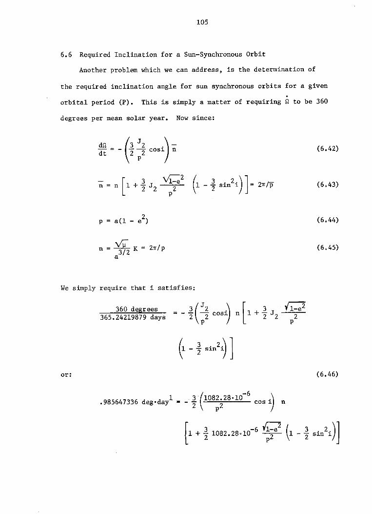
105

6.6 Required Inclination for a Sun-Synchronous Orbit

Another problem which we can address, is the determination of

the required inclination angle for sun synchronous orbits for a given.

orbital period (P). This is simply a matter of requiring Q to be 360

degrees per mean solar year. Now since:

dQ-=dt (

J ). 3 2 -

- 2' p2 cosi n (6.42)

2p = a(1 - e )

n =~ K = 2n/p3/2a

(6043)

(6044)

(6045)

We simply require that i satisfies:

or:

360 d~grees

365.24219879 days

(6.46)

1.985647336 deg·day 3(1082.28.10-6

.)= - - cos 1. n2 p2

(3 -6 Q ( 3 2 )]1 + 2' 1082.28 010 ~ 1 - I sin i

106

Note that a is assumed to be in cannonica1 units:

a(e.ro) = a(km)/R (km)e

This equation is easily solved numerically. Since the right hand

side of equation (6.46) is monotonically increasing as i goes from 900

to 1800, we can use a Newton's method approach in the interval (900 ~

i ~ 1800) to isolate, to a specified tolerance, a solution matching the

left hand side. By applying this procedure, Table 6.5 has been generated

which gives the required satellite height and inclination for a sun

synchronous orbit, given the satellite period. A circular orbit (e=:O)

is assumed. A listing of a computer routine is given in Appendix G.

Table 605: Required Orbital Inclination for a Sun SynchronousSatellite Given a Satellite Period (e=O)

Period (minutes)

90

100

110

120

Height (km)

758.44

1226062

1680.80

Inclination (DElg)

96.5893

98.4366

100.5585

102.9718

6.7 Velocity of a Satellite in a Secularly Perturbed Elliptic Orbit:

A final problem we might want to solve is the determination of the

velocity V of a satellite in an elliptic orbit at time t. Since we

know:

x = a(cosE - e)w (6047)

YUl = a 11 - e2 sinE

107

and thus:

.x = -a E sinE

w

Yw = a EY1 - e2 casE

and since V is simply:

then:

Note immediately that for a circular orbit where e=O:

.= a E

and since if e=O then E=M, thus:

.V = aM

(6048)

(6049)

(6050)

(6.51)

(6.52)

~2

2p

(6.53)

.and i.f we ignore the perturbation term then M = n, and we have a velocity

exprE~ssion for a circular, non-perturbed orbit:

(6.54)V = an

Now note that since:(6.55)

then:

108

v = a0 K = K~3/2 a

a(6.56)

which is similar to Equation 5.30, an expression that is independent of

time.

In the case e = 0, we consider the perturbative effects:

·£1 2 2 2V = a E~sin E + (1 - e )·cos E

using:

E = M + e"sinM

E= M(l + e·cosM)(6.58)

where:

and:

M = n(t - T)

n =

p = a(l - e2)

J2

= 1082.28 • 10-6

(6059)

(6.60)

Thus we have solved for V as a function of time, knowing only the orbital

elements.

7.0 THE ORBITAL REVISIT PROBLEM

7.1 Sun Synchronous Orbits

Does a satellite pass over the same point on each orbit if it is

sun synchronous? It would, only if the equator crossing separation

ois an integer factor of 360. For example:

1. Assume a 60 minute period. After 1 orbit period, the earth

would rotate 150 underneath the satellite. This would continue 24 times

until the satellite was back to exactly the same point that it started.

2. Assume a 120 minute period. In this instance, there would be

a 30° equator crossing separation. Therefore since 360/30 = 12 is

an exact integer, the satellite would return to the same point.

Tables 7.1 and 7.2 are useful.

Table 7.1: Orbit Crossing Separations up to 900

Integer NumberPeriod Longitudinal Separation of Orbits---20 min x 150/60 min = 50 which divides 3600

72 times

40 min " 100

" 36 times

60 min " 150" 24 times

80 min " 200" 18 times

120 min " 300 " 12 times

160 min " 400" 9 times

180 min " 450 " 8 times

240 min " 600" 6 times

360 min " 900

" 4 times

109

110

Table 7.2: Complete Table for Orbit Crossing Separa.tionswith 1 to 6 Hour Periods.

Integer NumberPeriod Longitudinal Separation of Orbits

60.0 min x 15°/60 min 15.00 which divides 360° 24 times

62.60870 min " 15065217° " 23 times

65.45455 min " 16.34364° " 22 times

68.57143 min " 17.14286° " 21 times

72.0 min " 18.0° " 20 times

75.78947 min " 18.94737° " 19 times

80.0 min " 20.0° " 18 times

84.70588 min " 21.17647° " 17 times

90.0 min " 22.5° " 16 times

96.0 min " 24.0° " 15 times

102.85714 min " 25.71429° " 14 times

110.76923 min " 27.69231° " 13 times

120.0 min " 30.0° " 12 times

130.90909 min " 32.72727° " 11 times

144.0 min " 36.0° " 10 times

160.0 min " 40.0° " 9 times

180.0 min " 45.0° " 8 times

205.71429 min " 51.42857° " 7 times

240.0 min " 60.0° " 6 times

288.0 min " 72.0° " 5 times

360.0 min " 90.0° " 4 times

111

3. Now consider a period which results in a longitudinal separation

which does not divide 3600 an integer number of times, such as 100 min­

utes. Then 100 x 0.25 = 25 degree longitudinal crossing, which divides

3600 exactly 14.4 t~es. If we let the first crossing occur at 00

longitude (Greenwich Meridian), Table 7.3 gives the equatorial cros-

sing sequence.

Table 7'.3: Equator Crossings for a Non-Integer Separation Factor

CYCLE I

Orbit Number

o

1

2

3

Equatorial Crossing Longitude

0°

250 W

500 W

750W

13 3250W (350E)

14 3500W (IOoE)

15 150W

16 400W

CYCLE 2

27 3150W (450E)

28 3400W (20oE)

29 50W

CYCLE 3

42 3300W (JOoE)

43 3550W (50E)

44 200W

CYCLE 4

57 3450W (150E)

58 lo°W

CYCLE 5

72 0°

112

Note that it takes 5 complete orbital cycles or 72 orbital periods

until the pattern repeats. It is easy to see why this gets more com­

plicated if the period is something like 101.358 minutes. Basically, to

determine how many cycles are required to repeat the sequence, the

smallest integer (I) must be found such that:

I x P(period) = another integer

Thus, in order to find I:

1. Calculate the orbits per cycle (N):

N = 360/(0.25P) where the period(P) is in minutes.

2. Now N is given by:

N = nl n2n3n

4•••

Take the decimal portion and divide it by a power of 10

corresponding to the number of places in the decimal portion

at a preferred decimal accuracy.

3. Simplify that fraction to its least common denominator (LCD).

4. The LCD is the smallest integer I. Example:

Assume an orbit of 110 minutes. How many cycles and orbits

must pass before the orbit pattern repeats itself?

N = 360/(0.25 • 110) = 13.09090909 •• 0

Let us make our calculation accurate to 4 decimal places,

thus:

N = 13.0909

Take the decimal portion 0909 and divide it by 10,000,

yielding 909/10,000. Since any power of ten (109

) can be

given as the multiples of its prime factors, i.e.,

109 = 59 • 29, then the numerator 909 would have to be

113

divisible by 5 or 2 to have a lower least common denominator.

Thus, in this case, 10,000 is the LCD because 909 is not

divisible by 2 or 5. Therefore, it would take 10,000 cycles

or 130,909 orbits for the orbit pattern to repeat itself to

within 4 decimal place accuracyo

Also note that even though the orbit pattern of a sun-synchronous

satellite does not repeat every cycle, this does not make it any less

sun-synchronous. It simply pseudo-randomizes the equator crossings.

Actually, there is a predictable phase pattern to the equator crossing

changes although ,it can be considered as a randomizing process.

7.2 Multiple Satellite System: Mixed Sun-Synchronous and Non-Sun­Synchronous Orbits

In order to achieve uniform spatial and temporal sampling, future

satellite systems will include various sun-synchronous and non-sun-

synchronous satellites. The basic problem is to design an orbit con-

figuration which will yield an optimal revisit frequency over all parts

of the globe. Since the topic of diurnal variability has become such

an important consideration in radiation budget studies, future satellite

systems cannot afford to provide only twice a day coverage of the globe.

The most successful technique which has been used to design the orbit

architecture for a multiple satellite system is the computer simulation

of multiple satellite orbits. By "flying satellites" in a computer,

the revisit frequencies for a global spatial grid can be computed for

a variety of orbital parameters. Campbell and Vonder Haar (1978) used

this approach for the specification of the optimal orbit inclination

for a system of polar-orbiting satellites designed to measure the

earth's radiation budget. Circular orbits were used in their analysis.

114

It should be recognized that when considering polar orbiting

satellites, an analysis of the revisit problem must include not only

the orbital period but also the scanning pattern of the satellite in­

strument. As the satellite height increases, the period increases and

thus the longitudinal separation of equator crossings increases. A

fixed nadir viewing instrument would miss global strips (swaths) to

the east and west of the orbital track as the satellite height is in­

creased. If a satellite instrument is designed to scan across the

orbital track, the longitudinal separation can be increased up to the

point at which the atmospheric path length would have to be considered.

Essentially, the solution of the orbital revisit problem should

be an attempt to sample the three dimensional volume: latitude, longi­

tude and local time. Polar orbiters with inclinations near 900 would

sample all latitudes and longitudes in a time period of approximately

one month. However, only a very narrow local time interval would be

sampled because of the slow precession rates. Satellites with lower

inclination orbits such as 300, would precess rapidly (about 50 per

day) for an 800 Km altitude orbit, sampling 12 hours in a month. Com­

puter simulations indicate that a set of satellites at 800 and 500,

and 800 , 600 , and 500 inclinations would provide nearly optimum sampling

for two and three low orbit satellite systems, respectively (see

Campbell and Vonder Haar, 1978). The geosynchronous satellites are

examples of satellite platforms which provide fixed spatial and angular

sampling but can provide high temporal sampling.

Another factor which must be included in the analysis is the quan­

tity which is being measured. For observations of emitted flux, obser­

vations at any time of day generally provide good results. However,

115

when considering albedo measurements, observations at night are useless

and observations near sunrise or sunset (local times 600 and 1800) are

very difficult to analyze because of the high solar grazing angles.

Any variation of the observed field must also be considered in the

orbital design. For radiation budget purposes, a set of 80°, 500 and

sun-synchronous satellites is better than an 800 _600 _500 set. The

sun-synchronous orbit should be located at some local time between 900

and 1500 so as to provide uniform quality albedo estimates. The

drifting orbiters are able to measure the diurnal variations. There

are, of course, additional requirements for which orbits at other times

of the day might be more useful. For example, in order to observe the

earth's surface, an orbit at 8:00 am local time might be best since

there are generally fewer clouds to obscure the ground.

8.0 CONCLUSIONS

This investigation has been directed toward the study of the orbit

properties of near earth meteorological satellites, and in particular,

the application of the results to the satellite navigation problem.

Beginning with some basic definitions of time and coordinate systems,

the basic foundation for the solution of the two body Keplerian orbit

was outlined. This solution was adapted to the conventional orbital

element parameters available from the meteorological satellite agencies

so as to develop computer models for calculating orbital position vec­

tors as a function of time. This is a fundamental requirement for any

analytic satellite navigation model.

The invariant two body solution was then extended to a perturbed

solution in which the time variant nature of an orbit was considered.

Using a formulation called the perturbation function, derived from a

harmonic expansion of the earth's gravitational potential, a set of

closed form time derivatives of particular orbital elements were

examined. From these definitions, it was possible to examine various

orbital characteristics of near earth satellites.

Next, a discussion of the orbit revisit problem was provided as

a means to highlight the significance of exact computer solutions to

the orbital properties of meteorological sate~lites. Finally, a set

of computer codes for calculating orbital position vectors and various

orbital period quantities is provided in the appendices. The input to

these routines is based on the "Classical Orbital Elements" available

from the operational satellite agencies. A brief description of the

source of these elements is provided in Appendix Ao

116

900 ACKNOWLEDGEMENTS

I would first like to express my gratitude to Dr o Dennis Phillips

who was a colleague of mine at the University of Wisconsin's Space

Science and Engineering Center, during the period 1966-1974. His in­

sight and planning spearheaded the development of the first successful

geosynchronous satellite navigation model which we ultimately completed

in 1972. It was from my discussion with Dr. Phillips and his guidance

in transforming the mathematical descriptions of satellite orbit pro­

perties into workable computer code, that I first developed an appre­

ciation for analytic navigation techniqueso I must also acknowledge

Mr. Jim Ellickson of the National Environmental Satellite Service and

Dr. Art Fuchs of the NASA Goddard Space Flight Center for their helpful

discussions in preparing Appendix Ao I ~m indebted to Professor Thomas

Vonder Haar for his generous assistance in planning the manuscript and

Mr. Garrett Campbell for valuable discussions on the orbital revisit

problem. Finally, I express my warmest regards to Laurie Parkinson for

her excellent care and patience in preparing the manuscript and Mark

Howes for his very fine drafting assistance.

The research was supported by the National Science Foundation

under Grants ATM-7807l48 and ATM-7820375 and the Office of Naval Re­

search under Contract NOOOl4-79-C-0793. Computing support and ser­

vices were provided by the National Center of Atmospheric Research

which is supported by the National Science Foundation.

117

1000 REFERENCES

Abramowitz, M., and I. A. Stegun, 1972: Handbook of MathematicalFunctions 0 Dover Publications, Inc., New York, 1046 pp.

American Ephemeris and Nautical Almanac, 1978: Issued by the NauticalAlmanac Office, U.S. Naval Observatory and Her Majesty's NauticalAlmanac Office, Royal Greenwich Observatory, u.S. GovernmentPrinting Office, Washington, D.C., 573 pp.

Bowditch, Nathaniel, 1962: American Practical Navigator - An Epitomieof Navigation. UoS. Navy Hydrographic Office, HoO. Pub o No.9,u.s. Government Printing Office, 1524 pp.

Brouwer, D., and G. Mo Clemence, -1961: Methods of Celestial Mechanics.Academic Press, New York, 598 pp.

Campbell, G. G., and T. H. Vonder Haar, 1978: Optimum Satellite Orbitsfor Accurate Measurement of the Earth's Radiation Budget, Summary.Atmospheric Science Paper No. 289, Department of AtmosphericScience, Colorado State University, Fort Collins, CO, 61 pp.

Cappellari, J. 0., C. E. Velez, and A. J. Fuchs, 1976: MathematicalTheory of the Goddard Trajectory Determination System. TechnicalReport X-582-76-77, Goddard Space Flight Center, Greenbelt, MD,599 pp.

Ellickson, J., (1980): Personal Communication.

Escobal, P. R., 1965: Methods of Orbit Determination. John Wiley andSons, Inc., New York/London/Sydney, 463 ppo

Escobal, P. R., 1968: Methods of Astrodynamics. John Wiley and Sons,Inc., New York/London/Sydney, 342 pp.

Fuchs, Ao J., (1980): Personal Communication.

Kozai, Y., 1959: The Motion of a Close Earth Satelliteo TheAstronomical Journal, 64, 9.

Makemson, ~1. We, R. L. Me Baker, and G. B. Westrom, 1961: Analysisand Standardization of the Astrodynamic Constants. Journal ofthe Astronautical Sciences, 8, 1, pp. 1-13.

McGraw-Hill, 1974: Dictionary of Scientific and Technical Terms.McGraw-Hill Book Co., New York/St. Louis/San Francisco, 1634 pp.

Phillips, D. R., 1979: Incorporation of Star Measurements for theDetermination of Orbit and Attitude Parameters of a GeosynchronousSatellite. Presented at the 4th Annual Flight Mechanics/EstimationTheory Symposium, Oct. 15-18, NASA Goddard Space Flight Center,Greenbelt, MD.

118

119

Smith, E. Ao, and D. R. Phillips, 1972: Automated Cloud TrackingUsing Precisely Aligned Digital ATS Pictureso IEEE Trans. onComp., C-2l, pp. 715-729.

Spiegel, M. Ro, 1968: Mathematical Handbook of Formulas and Tables.McGraw-Hill Book Coo, New York/Sto Louis/San Francisco/Toronto/Sydney, 271 pp.

Sterne, T. E., 1960: An Introduction to Celestial Mechanics.Interscience Publishers, New York, 206 pp.

Widger, W. Ko, 1966: Orbits, Altitudes, Viewing Geometry, Coverage,and Resolution Pertinent to Satellite Observations of the Earthand Its Atmosphereo Technical Report: Contract No. N-6l339-66­C-003l, U.S. Naval Training Device Center, Port Washington, NY,ppo 489-5370

120

APPENDIX A

EXAMPLES OF NESS, NASA, ESA, AND NASDA ORBITAL ELEMENT TRANSMISSIONS

121

APPENDIX A

EXAMPLES OF NESS, NASA, ESA, AND NASDA ORBtTAL ELEMENT TRANSMISSIONS

Classical Orbital Elements for meteorological satellites are, in

general, provided by the operational satellite agencies, i.e., NESS,

NASA, ESA, and NASDA. Although actual satellite tracking data may be

provided by other agencies such as the North American Air Defense Com-

mand (NORAD), the reduction of this data to the conventional elements

is under the management of the operational space agencies. Before

providing examples of orbital element transmissions for various satel-

lites from these agencies, a brief explanation of the format is re-

quired.

1.

3.

4.

5.

6.

7.

As discussed in Chapters 5 and 6, the standard elements include:

Epoch Time (to)

Semi-major Axis (a)

Eccentricity (e)

Inclination (i)

Mean Anomaly or True Anomaly (M or "I)o 0

Right Ascension of Ascending Node (no)

Argument of Perigee (w )o

In the discussion of Chapters 5 and 6, these elements were referred to

as "Classical Orbital Elements" although in actuality, the space agen-

cies refer to the above set of elements by other names. The three

basic categories of orbital elements that appear on standard orbital

transmission documents are as follows:

1. Keplerian Elements

2 Q Osculating Elements

3. Brouwer Mean Elements

122

There are no differences in the definitions of the classical

elements insofar as the above categories are concerned, however, there

are differences in the time varying properties of orbital elements with

respect to the three categories. Referring to the Orbital Elements

as Keplerian, implies that pure unperturbed two body motion is under

consideration. Referring to the Classical Elements as Brouwer Mean

Elements implies that time derivatives are involved with respect to

various elements and that the elements themselves are based on Brouwer

theory (see Brouwer and Clemence, 1961) or Brouwer-Lyddane theory

(see Cappel1ari et al., 1976). Keplerian or Brouwer Mean elements are

the standard products of the operational space agencies. The model

developed in Chapters 5 and 6 incorporates the basic physics considered

in Brouwer or Brouwer-Lyddane theory but uses a different formulation,

see Kozai (1959) or EB (1965).

Referring to a set of elements as Osculating Elements can lead to

some confusion. We say, in general, that an orbit osculates (kisses)

an instantaneous position and velocity vector. In this sense, various

sets of elements compatible with the various orders of perturbation

theory could propogate an orbit which kisses or osculates a pre~defined

position-velocity constraint which is known to define an orbit. When

the space agencies label a set of orbital elements as osculating, they

are indicating that the elements used in a Keplerian theory will os­

culate a position-velocity constraint which could have been based on

two-body theory or perhaps a perturbation theory applied to raw trac­

king data used to generate the ephemeris constraint. Therefore os­

culating elements can be considered as Keplerian elements, although the

elements themselves may represent a fit to ephemeris data based on any

number of perturbation models.

123

The above points ~ay seem academic in terms of reducing tracking

station data to a set of orbital elements, however, the distinction is

very important. It is instructive to discuss this statement by example.

We will consider the approaches used by NESS and NASA in their genera­

tion of orbital elements for TIROS-N, GOES, and Nimbus-7 satellites.

TIROS-N, which is a NESS operated polar orbiting satellite, is radar

tracked by NORAD. In addition, NORAD reduces approximately a week of

tracking data to a set of orbital elements which are compatible with

the NORAD perturbation model (the model itself is classified). Pertur­

bation factors included in this model include zonal and meridional

asymmetries in the earth's gravitational potential, lunar forces, at­

mospheric drag, and solar radiation pressure. The retrieved orbit ele­

ments are then used to propogate approximately 3 weeks of ephemeris

data which are transmitted to NESS, who in turn, retrieves either

Keplerian Elements or Brouwer Mean Elements based on unperturbed two

body theory or Brouwer-Lyddane theory. The orbit retrieval package is

based on sub-systems of the NASA Goddard Trajectory Determination Sys­

tem (GTDS) which is a large computer package designed for a vast array

of NASA orbital problems, and is developed and maintained by the NASA

Goddard Space Flight Center. Therefore, NESS can provide either un­

perturbed or perturbed model elements, but it must be recognized that

these elements represent fits to model produced ephemeris data, not

raw tracking data (see Ellickson, 1980).

The retrieval of GOES-East and GOES-West orbital elements takes

place at both NESS and NASA. . The NESS produced elements are based on

approximately one week of tri-lateration (3 station) ranging data

generated by the 5 NOAA operated tracking stations (Wallops Island, VA;

124

Seattle, WA; Honolulu, HI; Santiago, Chile; Ascension Island). The

type of model used to fit the ranging data is based on unperturbed

two-body motion, so by definition, the NESS produced orbital elements

for GOES are Kepleriano NASA, on the other hand, bases its orbit re­

trievals on range and range-rate data available from its own global

network of tracking stations. Unlike NESS, NASA uses the GTDS per­

turbation model to retrieve orbital elements which ,are then used to

propogate an ephemeris stream. These model data are finally fit by a

Keplerian model to produce a set of elements which osculate a position­

velocity vector pair which best characterizes a two body orbit. NASA

then transmits these elements under the heading of Osculating Elements,

although it is understood that they are Keplerian Elementso NASA

uses a very similar procedure for producing Nimbus-7 orbital elements,

however, the elements derived from the model ephemeris stream are

Brouwer Mean Elements based on Brouwer-Lyddane theory.

The following ten cases are examples of various orbital trans­

mission documents from four operational space agencies (NASA, NESS, ESA,

JMS) for the following seven different satellites:

1. GOES-2 (Eastern Geosynchronous)

20 GOES-3 (Western Geosynchronous)

3. GOES-l (Indian Ocean Geosynchronous, also called GOES-A)

4. METEOSAT (European Geosynchronous)

5. GMS (Japanese Geosynchronous)

6. TIROS-N (NESS Polar Orbiter)

7. NIMBUS-G (NASA Polar Orbiter)

125

CASE 1: GOES-2: NASA Transmission

T~X022••• 8 710-828-9716

[,E GI.r~i!·: 04002/08182FM ~ISSION AND rATA OFEFATICNS NASA GSFC GREENBELT MOTO GSr-:;·j/i.JAVSPflSllP. I:i\HLGPnJ VAGSPI~/t\OFt.I;· cec CEEYEt;t:E: t·nK CDtTLEX CO/COFSO t.Tn: CHltF At,ALYSTGSFM/~ILHEL~ F STEPNWAPTE BEPLIN W GE~MANY ATTN ZI~KER

Lsm·;/F.AE FAPNE'C'F'Gl:GS ENGLAi';O ATTN KH;G-HELE SPACE rEPTGSTS/JCE JOHt:S COlCE:. 933IVILLINGHAI'! CODE 572/PETRl'ZZO CODE 581GSTS/~APSH ceCE 490CPOe/H GKCPCHAI<GST5/Vt-'llJ OF '.'ISCOl')SIN COLLECT TI,X 9l0-286-277lGTOS/SOCC/MCINTOSH/SHA?TSGSRI':/Plt\,'CtlS!'.I~: 1LLSTCNE HILL HESTFORD r-1A ATTN SRI ['!';AP.AtJGSRt:;R1}~·JIi'!'.~./~mITE SI'.:·:r:s MISSILE RAl~GE l:r1 ATTN MEYEF.SGsprl/f.l.FcrL EM,SCOI·l .~F3 EEl:fORD I'::A ATn: StTYA/Hl!SSEYGSRM/Fl:~TGPA/SEL EOULDER CO ATTN SCHOEDEP/NBS BCULDER CO ATTN W HANSONGSTS/CONPUT

THE FOLLOVI~G APE THE OSCULATING ORBITAL ELEMENTSFO~ SATELLITE 1977 ~BA GOE5-2CONPUTED ANI:: IS SUEI; EY THE GOI;r:ARO SPACE FL I GHT CEI~TER.

DEGREESCEGf\EE.SCEGREES!:EG. PER J:AYl:EGREESCEG. PER CAYNINVTESI.ILONETERS .Y. I LOr:ETERSKI·;. PER HF.Xl-1. PER HP..DEGP.EES

OF DATE. KILOt':ETEP.S}<ILC:1EiERSKILOllETEFSKi'!. PEr SEC.Kr1. PEP. SEC.KM. PER SEC.

EPOCH 79 Y 02 M 23 D 00 H 00 M O.COOSEI:I-I·!.<JOP. AXIS 42432.7798ECCENTRICITY .006227I~CLINATION 0.0271MEAN ANOMALY 309.9886ARGUMENT CF PErIGEE 3~1.~S53

MOTION I PLUS 0.0262R.A. OF ASCEND. NCDE 148.3225

NOTION MINUS 0.0131r.NOXALISTIC· PE'f~IOO 1449.81255HElGET OF PERIGEE 35790.~3

HEIGHT OF APOGEE 3631g.85VELOCIT~ AT PEPIGEE 11103.VELOCITY AT A?OGEE 10965.GEOC •. LAT. OF PEFIGEE MINUS 0.013INERTIAL COOP.DINA7ES PEFERF~CE TP.~E

X 1~996.5485

Y 39513.8631Z -19.6313X DOT ~2.8821

y DOT 1.0761ZOOT 0.0003

0~/0819Z ~AR G~WW

S UT.HILOr1ETEf:S

126

Case 2; GOES-2; NESS Transmission

1~XC19 ••• 710-c28-9716

rE GrOS 007C1/1630ZFT SOCC/t-lCINTOSHTO m:ocGPHYGPOB/M PPOKCPCHAKGSR~l/m:PPI':OA/NOP.{.D CDC CHEYENNE MTN COU?LEX CO/DOFO CHIEF ANALYSTGSRM/EV~TCrA/J SCHPOE&EP, SEL EOULDEP/~ HANSON, NESGSRN/Pl'~':OI': SA/I·: ILLSTOr;E HILL ~:ESTFORD MA ATTN sr~I DHAFANGSRM/RUEOFFA/AFGL HANSCOM AFB MA LYS/S MEYERS, SUA/POBINSONGSTS/B PICEAPCSON t,;ILLINGHA~l CODE 572GSTS/R MARSH CODE.490GSTS/PHIL FEASE CODE 933GS7S/UNIV OF ~ISC SPACE SCI AND ENGRNG CENTER TWX 910~286-2771

GSTS/COLO 5T UNIV DE?T OF ATl-IOS?HERIC SCIENCE n.~ 910-930-9008CSU LIEFARIES

/SUS DU?EI

PREDICTED POST MANEUVER

ORBITAL ELEMENTS FOR GOES-2

EPOCH 79Y 02M 28DAT 04H 28MIN 24SEC UT

SEMI-~AJOR AXIS (KM) 42164.189

FCCEt~TRICITY 0.000156

INCLINATION (eEC) 0.059

R. A. OF A5C. NODE (DEG) 144.047

AEGUMENT OF PERIGEE (eEC) 138.064

~EAN ANOMALY (DEG)

LONGITUDE (DEG WEST)

202.303

100.0

127

Case 3: GOES-3; NASA Transmission

T~YCC~••• 7IC-f2e-9716

rE G'J.aj,'\t 03'1IOnC56ZF~ I.I5SIO~ A~D CATA O?EFATIC~S ~ASA GS~~ GfEEhEELT NDTO G5F~/~AUSPASUF CAELGFEN VAGSR~:/I~CPAi) COC n;EYENl,2 I·;T!'; Cm·;PLEy. CO/COfSO ATTI' CUEf Al,ALYSTGSPI:ll:"ILhEL,I: F STEPI"",A?T::: EEFL 11; ~~ GEFI:Al.Y 'ATTN Z IU.E.F.LS~~/~AE FA?~EOPOUGH ENGLA~D ATT~ KING-BELt SPACE t~?T

GSTS/F. ~:AFSHCODE 490/E FIl.LINGliA'{ cotE 572/5 EICliAEI:SOl-./. CODE 572GSTS/C. PETP~ZZO COLE 581/J. JCH~S CCCE 933 ." i .GSTS/UKIV OF ~ISCCNSIN COLLECT TWX 910-266-~771

GPO"/!':. ?POr:OPCHAK -;.GTOS/SOCC/MCINTOSH .GSn:/Rt'I,10~:SA/!':ILL5TONE PoILL WESTfOF.t· l'lA ATn; 5RII:;HAFANGSR1·:/::U"JHTA/v'E I Tt: SAI,DS '1': I S5 I LEo F.AI.JGE· Nt-; ATTN !·.EYEP.S .GSF?-,/AfGL HA!\SCOI':B !'.FE PEL:fORC hASS ATTN,SUjVROEH.~SON.. LY IEYERSGSRi':/FU1,:GTPA/l:.'OULDER co ATTl\,.SEL/SCHROEDER.NES/HANSON '.GSF.li/Pt'.'..'JHTA)TnlTE SAl.J['S I:ISSLE PP.tJGE/XPD ATTN CLAP 26Ar,sGS'!"5/C011Pl'T •

CEGRE2SDEGREE5CEG?..EESI:;EG.PEP.:t'AY·[,EGF.EES .LEG! FER DAYMINUTES .....l·:IN. PEP" DAYKILOl-'ETERS '!{ILOEETERS· ,la·'., P:t:F. HP..!'.r.:. FER tip. •I:EGFEES

35792.5535925.32.

. 11077.11042.

0.301PLPS

n-;E fOLl-OVnG' AP.E TilE' OSCCLATlI:G OF:::rTtlL ELEl·;EhTSFOF SATELLITE 1978 62A GCES-3COMPUTED ~~C I~SUED EY THE GCDrA~C SFACE f~IG~T CE~TE2.

EPOCW 78 '1', 07 t1 <l9 D 18 }i 20 1'; O. coo 5 CT. .SEU -~AJOFAXIS 4223701 C1 I 1-: I LC!·;ETEf.S

. IECCEI\TRICITY' .001572U:CLIl\ATIO!', -" 1.0121LEAN ANOlM1.Y··· . " 352.7205A?Gt:r:ENT CF PERIGEE' ".,:. 162.67(l5

r:.OTICt\· : PLllS- 0.0267F..A. OF ASCn-:r::. NOCE. '," 275. 94S.t.l

:~CTIOr-.: :r:uJUs 0.0133A!,O!:ALISTIC PEF:IOD' 1439.78823FERIOD DOTEEIGHT Of F'EEIGE'EHElGET OF A?CGEE\'£LCC11Y AT PEF.IGEEVELOCITY AT APOGEEGEOC. LAT. OF ~ERIGEE

IC/2056Z JUL G~~~

Case 4: GOES-3: NESS Transmission

ORBITAL ELEMENTS FOR GOES 3 .SATID 7806201EPOCH 78'1' 07M 150 AT OOHR 42MIN 40SEC utSEMI-MAJOR AXIS- 42167.339 KMECCENTRICITY 0.Q002892INCLINATION 1.00173 DEGR. A. OF ASC. NODE 276.0909 DEGARGUMENT OF PERIGEE 305.3629 DEGMEAN ANOMALY 307.0778 DEGLONGITUDE 134.6859 OEG VATTITUDE - SPIN VECTOR

R. A. - 14.383 DEGDECLIN- -88.707 DEG

SPIN PERIOD/RATE- 0.60000 SEC / 100.0000 RPM

17/1817Z JUL 78 GTOS .

128

Case 5: GOES-I: NASA Transmi$sion

TWXOOS ••• 710-S28-9716

DE GWWW 021"E30/1611 ZFM MISSION AND DATA OPERATIONS NASA G5FC GREENBELT MDTO GSRM/NAVSPASUR DAHLGREN VAGSPM/NORAD COC CHEYENNE MTN COMPLEX CO/DOFSO ATTN CHIEF A~ALYST

GSRM/WILHELM F STERN\:ARTE BERLIN 11.' GERMANY ATTN ZINMER 'GSBM/AFGL HANSCOMB AFB BEDFORD MASS ATTN SUA/ROBINSON.LYS/S. MEYERSGSflM/RtHJTGPA/NBS BOULDER CO ATTN HANSONLsn~/RAE FARNEOROUGH ENGLAND ATTN KING-HELE SPACE DEPTGPOB/PROKOPCHAKGSTS/BRYANT CODE 581/WIRTH CODE 4901\:ILLINGHAM CODE 572GSTS/UNIV OF WISCONSIN COLLECT TWX NR. 910-286-2771GTOS/SOCC/L RANNEGSRM/RUWOMSA/MILLSTONE HILL WESTFORD MA ATTN SRIDHARAN'GSP.M/RUIrIJHTA/B. MEYERS WHITE SANDS MISSILE RANGE. N. MEXGSRM/RUWJHTA/OLAP 26ADS WHITE SANDS MISSILE RANGE NM/XPDGSTS/JOE JOHNS CODE 933LESR/PALLASCHICE. K. AUBECKGSTS/COMPUT

DEGREESDEGREESDEGREESDEG. PER DAYDEGREESDEG. PER DAY1'1INUTESl'HN. PER DAYKILOMETERSKILOI-iETE~S

KH. PER HR.KM. PER HR.DEG'REE:S

35700.89135769.967

11085.11066.0.037

THE FOLLOWING ARE THE OSCULATING ORBITAL ELEMENTSFOR SATELLITE 1975 100A GOES-A COMPUTED ANCOMPUTED AND ISS~ED BY THE GODDARD SPACE FLIGHT CENTER.

S UT.KILOMETERS

EPOCH 78 Y 10 M 27 DOH 0 M 0.0SEMI-MAJOR AXIS 42113.5688ECCENTRICITY .000820INCLINATION 001.106MEAN ANO~lALY 81.6045ARG. OF PERI FOCUS 20.7101

HOTION PLUS 0.0269R.A. OF ASCEND. NODE 274.7950

MOTION MINUS 0.0135ANOMALISTIC PERIOD 1433.42979PERIOD DOT 'HT. OF PERI FOCUSHT. OF APOFOCUSVEL. AT PERI FOCUSVEL. AT APOFOCUSGEOC. LAT OF PERI FOCUS PLUS

30/1611Z OCT GWWW

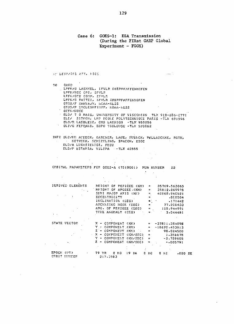
129

Case 6: GOES-1: ESA Transmission(During the FrRst GARP GlobalExperiment - FGGE)

t:" LESP/ors A:T" !-.scc

TO GAQDLPFN/G LAE~~EL. [¥VLR CEEPPFAFFENHOFENLPFN/NOC OPS. DfVL~

LPF1UOP.E CO:!P. Df\/LRLPFN/G FATTEI, [',f11LR OEERPFI>.FFE1;IiOFENGTOS/F l'iAlil.'AJY, toOAA-m:::ssGTOS/P EYCLESHEI~EP,'~OAA-~ESS

GCFN/lJOCCDLD! T 0 HAIG. UNIVERSITY OF ~ISCONSIN TLX 9'0-2~6-2771

eLCI SITEON. LMP ECOLE PGLYTECHNIQCE PARIS -TLX 691596DLD/R LASBLEIZ. CMS LA~NION -TL~ 950256DLD/G FEF!1.AND, EOPO TOULOUSE -TLX 520862

INFO DLD/l'it·; Al'PECI{, GAR[I~ER, LAUE, llua.CJ-i, Pf.LLf.SCHKE, ROTH,NETWORK, SCHErULI~G. SPACON,' ESOC

~LD/A LVKASIEWICZ, RECUOLD/P ESTARIA, VILSPA -TLX 42555

ORBITAL PAPA~ETEPS FOF GCES-A (7510001) RUN NUMBER 22

DERIVED ELEl':ENTS

STATE VECTOR

HEIGHT OF PEFIGEE (KM)HFIGHT OF APCGEE.(KM)snn MflJOP AXIS (X1'l)ECCEl;TRICI,YINCLINATION (rEG)ASCEKDING NODE (DEG)ARG. OF PERIGEE (rEG)TPoUE AlI;Ol~AL Y (DEG)

X - CCMPONE~T (Kl':)Y - COMPONE~T ,(KM)

Z - CO~PONENT (KM)X - COI'~PONEN'!' (j~M/SEC>'

Y - COMPO~ENT (KM/SEC)Z - COMPONENT (KlllSEC)

=

=

35769.56306535812.06997842168.960521

.OC0504

.17144277.228633

125.94 l !9913.044481

-37811.3841898-18620.453813

98.0245001.358878

-2.759605-.005791

EPOCH (PT)CPBIT ~:l'~:rEF'

79 YR 2 ~o 19 DA217.3583

o HO o ~a .000 SE

130

Cas·e 7:METEOSAT: ESA Transmission

NR23 RR ESOC DARMSTADT AllEXMAGNE APR 18/15'4Z

HI LESR/ORB All. ESOC

TO GAQDlPFN/G lAEMMEl. DFVlR DBERPFAFFEHHOFENlPFN/NOC OPS. DFVlRLPFN/ORB COMP. DFVlRGSTS/G MARECHEK, CODE 572.3 GSFCGSTS/R SClAFFORD, COOE 861.2 GSFCGCEN/lIOCCGTOS/NOAAGOPS/OPERATIONS CENTRE BRANCH CODE 512 GSFC

INFO DLD/MM BERLIN, KUMMER. MUENCH, PAlLASCHKE, ROBSON, ROTH,SOOP, WALES, NETWORK, SCHEDULING, ESOC

DLD/A LUKASIEWICZ, REDUDLD/MR P SIBTON, LHD ECOLE POLYTECHNIQUE TLX 691596

ORBITAL PARAMETERS FOR HETEOSAT RUN NUtiBER 33

DERIVED ELEMENTS HEIGHT OF PERIGEE (KH) K 3576B.439692HEIGHT OF APOGEE (KH) K 358Q6.748998SEMI MAJOR AXIS (KM) K ~ 42165.738345ECCENTRICITY .QnU454INCLINATiON (DEG) .191114ASCENDING NODE (DEG) 189.B54~27ARG. OF PERIGEE (DEG) 253.674435TRUE ANOMALY (DEG) 12~.281Q37

• _38585.968653• _ln26.&22147

33.927\1941.239819

_2.812761.~&9952

X- COMPONENT (KH)Y_ COMPONENT (KH)Z _ COMPONENT (KH)X_ COMPONENT (KM/SEC) •Y_ COMPONENT (KM/SEC) •Z _ COMPONENT (KH/SEC) •

STATE VECTOR

EPOCH (UT> 78 YR 4 HO 17- DA &HO QHIORBIT NUMBER 145.U38a

la/15~5Z APR 78 lESR

Case 8: GMS:

131

NASDA produced elements transcribedonto GMS data tapes and decoded bythe McIDAS system at the Universityof Wisconsin's Space Science andEngineering Center.

1\ L S 5 h C I D A S

ETIn=O?3HC=

7C12Z~

::f

1276337nI1'iE= 0l":EHA=- 283=85

:3 I,lT~ 1378SFMH'A= 421E:f03?ERE1i.=- eSf?4

~CCEN=

.'l.SNCDE=-10f

1S?1l4

Case 9: TIROS-N: NESS Transmission

TlIlOS-Il IIAVlCATlON SYSTEM POLAa SPACECIlAFT EPHEKIlUS ACCISS IlOUTINE INlTIALIZATlON WOIlT AT JAN 02. 1910 VEIl 3.0 PAGE 1

IPOCH OF CI/1UU!NT CYCLE IS 79/12/31 19 19 23.664 SPACECllAFT 10 IS •••••• DEFAULT NUl1BEIl OF INTEIlPOLATION POINTS IS 10

STANT TIME OF DATA GlADES END TIME OF DATA GlADES INTEIlVAL OF DATA LENGTH OF DATA

GlADES DATE DAY SECONDS GIlADES DATE DAY SECONDS

COURSE 3/10/80 80. 70 3600.

MEDIllH 1/ 5/80 80. 5. 600.

FINE 12/30/79 79.364

KEPLEIlIAN

O. FINE 1/11/80 80. 11

MEDIllH 3/17/80 80. 77

COAllSE 6/14/80 80.166

ELEMENTS AT CURRENT CYCLE'. EPOCH

INERTIAL TOO

o.

o.

o.

100 SECONDS

10 MINUTES

1 HOURS

BROUWER MEAN

12 CYCLES

72 CYCLES

96 CYCLES

SEKl-MA.lOR AXIS 7221.8962554074 SEIlI-MAJOR AXIS 7228.9597759711

ECCENTRICITY 0.0012051329

X -2568.2800593576

Y 280.5696240752 ECCENTRICITY 0.0013492807

INCUNATION 98.9826322459 Z 6737.4203664218 INCLINATION 98.9782134269

RT AlC OF AlC.NODE 329.4207821364

ARC OF PEUGEE 63.5514823988

!lEAN ANOMALY ;5.3887663021

XDOT -5.3608748958

YDOT 3.9020314858

ZOOT -2.3898005021

RT AlC OF AlC NODE 329.4172856807

ARG OF PERIGEE 96.7543541300

!lEAN ANOMALY 12.2180973526

0002 PSCEAR - FOR INTERPOLATION PURPOSES 10 POINTS WILL BE USED INSTEAD OF THE INPUT VALUE 0

TIME. BROUWER ELEIlENTS 800102. O.

7228.96 0.001349 98.98 329.42 96.75 12.22

ORBITAL PEUOD IN SECONDS 6123.89

lJt.btd:.l:..::iL.I:.c::,<t,E::'LlE..Gnl:.l:.:>l..;iGo t'i::.n ).;/-H

Ld:..Gn t.l:.::'In:,Go r En IJAi."1 l.-J UH,:> .,{1 LJ.'.I j::'! ~K.::i

" I LJ ,'II-,1 it\.:>",'1. rE.:t rl.n;{,"l. r'En'rin.Lil:~Gl\l:.I:.::'

132

Cas,e 10: NnmVS...G: NASA TX'anS11\ission

'I?l:>!-I (, ::,r C1." .... UI"' ••• 71\J-j2,'i~:J'lll)

DE G.... " u8~·l-.

u,://ullJl'; ,i'''~I'''.::>lJ\i H.\iu ).;hlA J,...tIH·dIJ,\i'" ,\iA::';':' {i':'r'C G"l:.E\li;.cl.1 ·11..~ J G ::",'1 / .\il; v ",j-A:'ua DA:iL (;nt.,'1 'v A

LI:.::i,,/l;r'i::' L ...~H0'11 i'nA"CE AI'I.\l h. Lfl':'bLl:.l~nLl:J. G~~Ul

G:>t."!/~·JI';AlJ (;JC C:'irii:.\i,H..\/jL'J C'J"ir-Ll:..... GJ/lJJF~J An:~ C.-Hr;.' A~f1Li':'.

G::'tt:"-/ •• lLrH,L''1 I- :>'il~.n:~',.AI',ll:. bl:,j\LL~ •• GJ:.I\.1kll{ H'IL'ol lol'i1I:hL::iw/)/I1.1\h. r-AJ,llbJil,)JGri !:.IIGLA'oli,. AiH r(UG-riI:Ll:. ::'/"'A(;1:. IJE/"'I,G:'I~/i;" Trti)~A:::' v.H lJr,I\ rlAAr: lJl:r'1 AI....jfJ:>t'dl:.'1U; "'Cl1:.IICI:.':'CJL'JnADJ ::il U,1l1\i ell 'L.r. ':I10-,:/3u-,:/OUdG'::'1 ~/ll. ..,,1 Gril CJ DE ':118(·:::>1 :::'/(;J·~j-{j'1

Inr. jO';,jLLJd,-lG H:tl:. lri!:. i:'NJUwEr. i'1h.A,'ol Jl\c1 'IAoL l:.Ll:.r'1E..IlI:>FOh "'AiELL1ll:. 1':/7d ':IdA ~l~~US-G

(;O'~/"'UTI:JJ A:IlD I ::,:>uEL 01 'hil:. GJDIJAn1J :>r'I;Cl:.' FLI (,...n Cl:.HEl1..irJClt B (,11 M U3 lJ UU rt 00 (VI O.uuU::i ~i.,SI::'1I-:1AJOh At;: 1 ~ 7~25. IUS? '(1l.J,'1EH,l\':'ECCj"lllh1CI U, .UUUd<431 ,\I CLI:IlAllJ.Il' ':I'). ~':Iu5

'''l l:.A:1I H.,IlJ',1AL l' 1:d':l. ;: 7 Ol::!AhfiU:-n.\ll JF' r'Eh1 GEE.. ~~':I. U<4Uo

,J'I(ITIH l'JLIIU;:; c~\60p

1-..1-1 • .JI-' .A:>Cl:..IlIJ. ,IIJ'l;i:. <:1>1.3325-"I')'IlJ,~ k-LiJ'::' Ud1Uo

-A'IIi);VjAL1:>'dC t-FhlJlJ lu3.':Ib734rlEIGrtl OF r'~l1.1GEE ~<40.7~

ri~lGril JF Ar'JGi~ ':I~3. 14vlLJC1l( At k-E~lGEE.. ~6~7Y.

v~LOCllt HI A~JGEE ~653<4.

G~JC. LAT. )F i'EtdGI:.E 'lj1.'IILi~ 4d.183

I. - 56<48. 0572 ,{ I LJ:'.i l:.'Il:.n.:>( -1.,0714. :>6::Kl ,Ut..Ji'.il:.1 r..I\':'t. -218. ':11 ~';/ "lL.J ;:EH.h::'A D.J'l -u. ':123':1 4'\.~ • ... l:.iI ::'I:,C.t j;) 'I u. 17':1~ r\ 't'i. rI:.h ':'i:,C.~ 1;,) 'I 7.2715 h'''v'i • r' E,,, ",.1;.(;.

133

APPENDIX B

COMPUTER SOLUTION FOR AN EARTH SATELLITE ORBIT

(PERTURBED TWO BODY)

134

APPENDIX B

COMPUTER SOLUTION FOR AN EARTH SATELLITE ORBIT(PERTURBED TWO BODY)

SU~MUUTl~~ ~~-r~OS(IYKOAi,SArTl~,ICOOK,XSAl,YSAT,ZSAT,SAlLAT,SAILON*,SATH(;l) -

DI::1'1::1<1"1'-.t. 1\ 5.:.tr.LLl'l'r. PliSITllIi-j VECrnk ACCIJIWli~G TU A KEPLF.IUMJ URBIT

ERIC A. ~MlT'"iD~~AKTMl::Hl G~ AT~OSPH~klC SCISNCiCOLU~ADLI STATE U~IVERSlri/~UUlHiLLS CAMPUSFUM! CULLI~S, CULURADO ~u~23TEL 3()j-4~I-tl~33

KI::F£,;IH~NCI:..s.

BUWDITCH,HArHANl~L,1962.

A~~RIC~N ~KACTICA~ ~AVIGAI0~ - AN l::~ITOMll:: OF ~AVIGArION.U• .':i. r~AV 'f HilJRtlGKAPMIC LJFf} Cr:, H. O. ~LJii. NO.9.U~lrED SfAr~s GOVgRNMl::Nl PRIHIING UfFIC~,1524 PP.

l::SCOJJA1.I, ~H)R'J f<A,~tJN, 196:>.MEfHUUS u~ URbIT OEll::HMlNATIuH.JOH~ wlL~i A~D SONS,INC.,NEW YORK/LONDO~/S'fDN~Y,463 PP.

II~PU'1' PARA,~I::1'F.;RS

IIMQAY = YEAR ( 'fIDDD IN JULIAN DAY )SATtlM = TI~E ( ~OURS IN GMf )ICUUM ; U FU~ TERREstRIAL CUORDINATES

= 1 FOR C~L~SlIAL CuOHDINAT~S

OUTPUT ~A~4M~lE~S

KMKI'IKM

VECTORVECTORVECTOR

Of SATELLITE POSITIONuf SATELLITE ?USIT10NOf S4fELLITE POSITrONLAliTUDE ( DEGR~~S )LDI,G1'fuDr~ ( Dt;',';Ki'~~:S )i1t:1GHl ( 1\1'1 )

CONTROL

IOSA'l =

IMDR'I =;

IOSEC =:::=

IEOATF.: ;

=IEJHll:: ==SEMIi-1A =

=DECCElIo =

=ORjjINC =:::OANCIl'lLJ ==

XSAT = XYSAI = 'fZSA'f = ZSAl'LATSA!I..ILJN =SAl'"i(;'f =~AtIrUD£ IS GJV[N IN TERMS OF SPHERICAL COORDINAtESus~ rH~ fOLLQWING T"ANSFOHMATIUN TO CUNVENT TO GEUCENTRIC LATITUDE

S=RDPDG*SATLATSATLAI=AC0S(CUS(S)/SURT(1.O-(g.SIN(S))**2))/RDPDG

HEAL J2,~4,I~C,MMC,MANOML

KEYS AND 8ROU~ER MEAN ORBITAL ELEMENTS

SAl'[LLI'l'E TYPESET POSITLVE ~OR INITIALIZING NEW SATELLITE TYPESET ~EGA'l'IVF fOR H~TAINING uLD SATELLItE TYP~ WITH NEW ORRIT PAR~S

IUSAT IS TH~N S~T PUSIIIVEU FU~ OKaIl ANUMALY GIVEN AS _EAN A~OMALY ( l::.G. NASA )1 fOK OR~]T ANOMALY bIVE~ AS TkU~ ANOMALY (~.G. ~SA)u FOR ZERLI uRDER SECULAR pgRTUkBATION THEORYI fOK FIRST ORDER SECULAR PERTURBATION THEORY2 fOR SECOND UROER SECULAR PERTUR~ATION ThEORY

EPOCH lJATE ( ~YMMDD IN CALE~DER FURM )UATg FUR ~hICrl FULLO~I~G o~alTAL PARAMETlRS ARE VALID~PUCH TIME ( hH~MSS I~ GMt )lIMe FOR W~ICH FDLLONING 0R~ITAL PARA~E'l'~HS ARE VALID~EMI-~AJOM AXIS ( KM )HALF lHE U)StA~CE BEfWEEN TWO APSES OF A~O-FUCUS AND PERI-FOCUSr:CCEIHRICITY OF t:ARTii ORilIT ( UNITLESS )U~~M8E OF ELLIPTICITY OF OKeITUM~IT INCLINATION ( O!Gk~~S )ANGL~ BETWE~N IHE URdiT AND EQUATORIAL PLANESUH~IT ANOMALY AI E~uCH TIME ( DEGR~Eti )A~GL~ I~ UkBITAL PLANE bSfWl::EN ~ERI-FOCUS AND SATELLITE POSITIONGIV~N AS EIThER A ~~AN ANU~ALY OK A TRUE ANu~ALY

cCCCCCCCCCCCCCCCCCCCCCCCCCCCCCCCCCCCCCCCCC

CCCCCCCCCCCCCCCCCCCCCCCCC

Pt-:!{IGr

AS,WUr.

Pb<Iu{, ::::::

APt::kUU ::::::

EPC:kOLJ ::::::

cCCCCCCCCCCCCCC

CCCCCCCCCCCCCCCCCCCCCCCCCCCCCCCCCCCCCCCCCCCCCCCC

135

"1«,Li/"t.,'IJ' I;'r' r'r:kl\,~:r. "r EYOCH THIi'. ( lJ~.l;r<r.~S )AI;~Lt: T,~ u"i'j1'l r'LA'~r. HWh ~~Ce.r)lllNr. 1,L1ur: n, t'2~I-r'UCUS"1,;,,,n ASC~:I',;"IO~, lJl" {,Scr:.~uI"l, 1'.1'11'1-: AT r:I-'UCrI TIM. ( Dl::GREES )A"(,Lr, 11. ':UdAl UKIAl. Pl. i\I'; t. br.TNEr," VEr'""L t:IWIi.UX (r'IUi.CIPI,E AXIS)A/o,j"j '\)ll'lfHw"ku t,IJUAlL,r{ CKIISSIN(,~'t:Rlll[) ( "Ij "LJ'l't.S )SfATI-:fVif',in 1.11-' !\t:PI,EfJb 'I HIRD LAWTHIS PAKA~~lfR IS LALCdLHTt:U IN SAfPUS,Ald"~ALlSIIC "U~II'li ( NINUH.S )fl,',"; rltT"'t:H.: 'l'HI' Pi.SSA(;;'; H'{I~' Iji.r' e>ERI-FuClJS Tlj HiE Ni:XlI HiS PI'''Io,~'',liK Is CAI,CULA1't::iJ Ii' Sll,TPljSi.UiJ/\ L f'tY IllU ( "II i"JL';S )J'lMt: 1:lf':'l'wC::I-;,' TtlI-; PAbSAGr: FRI)~1 UN;': ~:QUAfUR CHussrr,,; Til THE NEx'rIrtlS PA~4~~1'~R IS CALCULATED IN iuCROS

COMMUI~/UHhCUM/IUSAT,]hORr,lUS~C,]~lJAl~,I~fI~~,SE~IMA,OECCEN,ORbI~C*, U/<I',U",L, t't:.,nu~:, {,S"I'.JVf':, t>f_RIllD, AJ>r~r<'Ii.J, t:.Pt::KU[)

Dt:r'i'HTIUi.S

MEAN ANGMkLY(M) • ANGLe. IN URRITAL PLANE WIT~ k~SPEcr TO THE CENTt::ROr' A "1 "_A 1\1 CIRCULAR LJt<i:lIT(HAVING A J>l=:RIOD El~UIVALENTTu IMt:. ANOMALl~IIC P~HIOD)FRUM PERI-FOCUS fO fHESAT~LLITE ~uSlrION.

TRur. J',I'UNALY(I'1) ,llrJ(;I,~. Hi UktHTA1, F'1,A'~~ ... 1 fH RU:iPECl' TO A r"OClIS OFlHf rLLIPfiC F~uM P~HI-FOCUS TO lHE SATELLITEPu.slllJN.

ECCt:.NTklC A~OMALi(E) • ANGLt:: IN URhI1AL PLANE WIIH RESPECT TU tHE CE~rERuf A ClkCL~ Cl~CUKSCRIBING TH~ ELLIPSE OF MOTIONfHUM P~HIfOCLJS tu THE SAIELLlr~ POSITION.

ORdlfAL CU~SrA~rS

PI = VJdolh OF PISIlLYH ::: 1·.Ui,in~H UF IlI'.Y;:; IN SULilH YEi<fi ( [JilYS )&IuYH = NU~b~R OF ~AY~ IN SIO~Ht::AL Yt::Ak ( UAYSRF~ ::: t<.i,lIIA'lCJkIA!.J ,,;/10:< l'H RADIUS l K", )GRACUN = l~~H~SfRIAL GRAVITATIONAL CIINSTANT ( KE=SQRT(G*ME*6U**2/R~**3 )

ftHER~ ~~ ::: rERR~SrkIAL GRAV CON ( O.u743b574 EM**.5*ER**1.5/MIN )G = UN]V~H5AL GkAV CONSTANt ( b.h73E-8 DYN~*CM**2*GM**-~ )~S = MASS Of EARTH ( ~.973~72b~27 GM PER EM )R~ = kAOl~S Of ~A~lH ( b.3/b~14~8 C~ P~R ER )

r ::: fLA'I''l'i-:r.ll,lG lIf fht: EAkJ'rJ ( F=(A-;n/ll , f=1-S0kT(1-E**2)E = ~CCENT~ICIrY UF tHE ~AkrH ( E:::S~kT(A**2-B**~)/A , l::=SQRrl2*F-F**2)

~ht::Ht: F = FLATTENING UF EARTH ( 3.35~6YE-3 )E = eCC~NTRICITY Uf EAk'l'~ ( 8.1820157~-2 )A = SEMI-~AJLlH EARTH AXIS - EQUATORIAL ( b37B.214 KMh = st<:;.l I -~, I I~CJK EAK'l'rj .A XIS - PPLA R ( 6356.8 29 K~i

= A*(l-f)C ::: :~ r.: II I~ b· At-! 'J' H HA lJ III S ( b37 1 • l! bb KM )

= (2'1-A+b)/3J2 = S~CUNO HARMONIC COEf Ur ~ARtrlS ASPHE~ICAL GRAVITATIONAL potENTIALJ4 = F8UHTH HARMONIC cut::r U~ SARTriS ASPH~HICAL GRAVITATiONAL POTENTIALIRfOAY = YYDOD ~riEII CEL~STIAL COUk SYS COINCIDES WITH ~ARrH COO~ SYS

I.~. TRANSIT OF FiRST ruiNT UF AIRES ~lrH GHE~~wlCH MERIDIANlRFH~S = HHMMSS WriEN CELESTIAL COOH SYS COINCIO~S WITH EARTH CUOR SYS

I.E. THA~SIt UF FIRST ~UIN1 OF AI~ES wl1H GRE~NWICH MERIDIANCHRII,;G ::: Ct::l,".:Sf IAT, HUIJR ANGLE - Zt-;"U AT THANSIT TIME ( LJEGHEES )PH!::.'It:f.l = f'EKICN UF JHr i-'R~,CI:.SION OF l'tlE Vt<:IWAL t-:(WINDX l it:ARS )U~CLIf' = UbLIQUiTY lW THE ECLIPTIC ( Di:.GRi:.ES )NU,H l' = I~AXHilJ~ ,JU,4tlER OF ll'ERATIf)!~S ALLUWED FOR CALC ECCENTRIC ANOMALYEPSILN = CUNV~HG~~C~ CRITERION USt:D f0R CALC ~CCE~TRIC AND~ALYLY~DAr = PR~VIOUS VALU~ Of IiKDAK1,[)SA'l' = ~REV IflUS Vi\L~l:. UF' IUSAl

DAIA Pl/j.lql~Y26~35ijY7YI

DAfA SULKk,SIDYR/3b~.~4~lYH7Y,366.24~lYR7Y/DA1A ~~/oj7ti.2141

Oil. fA Gi{hCfJilll l!. 07 436~ 74 IDATA f/j.j~28YE-31

136

DA1~ ~/~.lH201S7~-i/DAtA JL,J4/~lUHL.)~~-h,-~.li~-6/UA~A J~~UAY,I~~~~S/7~001,17JD~O/

llA1A lI1KIIN(;/O.0/DAr A P r\ r. vEU/ 2:; hi • I, /UAiA ubCLIP/23.4S/D,II.A I,U~II'I,~:P::;i"'J/I.(),1.0E-H/DAtA LY~UAY,LUSAT/-l,-l/

D i\ 1'11. 11<1 1/ U/CC I~lrlALIZt CU~STA~rs

C

CCC

CCC

CCC

1

IF(INJ1.NE.U)GQ 10IiHT=lkOt?lJ\;=t? 1 /1 tlU. 0T\~uPi=2.U*t?1So liS Ili =:, 1l.J if< / SilL i KRHMS=fTiM~(IRF~MS)

CIiIl:::KlJt"U(;*C "'i< A:H~

ROTA1'ION RATE Of TH~ V~HNAL ~~UINOX IN T~RMS Of SIDEREAL TIME

v~~=rWUPI.SULSID/(PR~V~U'SULYK*1440.0)

TEKk~SI~lI\L ~OfATiON HAYE IN r~RMS OF SlDiR~AL TIME

ROI=rwUi"1*SuLSIU/1440.D

TEST TU b~E If DAY UR SATELLITE HAS CHANGED NECfSSITlTING PARM UPDATE

If(IlRDAi.~W.LYRnAi.AND.IOSAT.EQ.LOSAr.AND.IOSAT.GT.O)GO TO YIOSA1=lAI1SI10SAf)I~YKDAY=IY!WAYLU.:iA'l'=lCJ:::>A'l'

cC COWV~MT ~PUC~ to JULIAN DAY-TiMECC IEPDAY = YEAR-DAY Uf ~PUCH ( tYDDD I~ JULIAN DAY )C Iif't1MS = 110UK-MIwn:-sr:::CUI~D Of EPOCH ( HH~iMSS IN (;I'ITC

IE2nAY=~ueU~ll,IEDATE)

I ~t>H 1~5= ll:.t J::4 E

IflIMOR'l'.EQ.O)MAHOML=OANOMLIF(I~ORr.NE.O)CTA=COS(RDPuG*OANOML)If(IMUHT.Ni.O)EA~U"L=ACOSl(CTA+OEeCEw)/(1.0+0fCCEN*CTA»If(lMU~T.N8.U)~A~O~L=(EANUML-OECCEN'SIN(EANO~L))/kDPUGMAIWI'iL=AMUD (,'IAI~U,'Il~,3blJ. 0)IFlMA~uML.lI'l'.U.uJ~ANOML=3~O.O+MANOML

DEfIi~~: E~CCENt'RICI'fY FACTOR AI~D ORBITAl, SEMI-PARAM':'TER

EFACIH=S~HT(1.0-U~CCEN**2)OSPAKM=lSi~IM~/~E)*EFACTK**2

CALCULAT~ INCLINATIUN SI~ AND COS TERMS

I NC=Kut',J(;*L1Rtll HeSI=SlrJ(JI~C)CI=CUS(lI~C)

CCC

CCC

CC DEfIN~ M~AN ANOMALYCC EXPLICIT RELATIO~SHIPS 8EfW~EN V,E, AND M ARE GIVEN BY TH~ F[JLLOWINGCC eus(v)=(cnSlE)-I)/(l-I.COSlE))C SlNlV)=s~~r(1-I**2)*SIN(E)/(1-I*CUS(E))C CUA(~)=(CU:::>(V)+I)/ll+l*COS(V»)C SJ~(E)=S~MT(1-1*'2)*SIM(V)/ll+I*COSlV)C M=~-I*SI~(~) .C

cccccccccc

137

eALCJI,AT~ UR91tAL Pl~lOu

P~:K [IJI)='l .'/UP I I M"IeeALC'IL4T"; lI;;ll'1ALISTIC :'1".1<,'. :'lulll1r~ Cll"STilIH AND iJEhlVITlVI::S r.lAS~:DurJ c,::.lt:.L l't..Li lIeD~H Of :>r:CU I,;; 1< t't-:hTU khA rIUI, THt-:t,lk Y

IF(lLJ,,";C.r~\J.O)GO TO 2IFlluSt::C.,,;U.l)GO TO 3GO 'fLJ 4

ee Zl::Hu iJi\ l)r~ke

2 A;·\".c=/""cDPr:R:IJ. UDI\::'~!=O. UGU Tu 5

ec FIKST UHU~H

eJ A~MC=M~C.(1.0+l1.~*J2*EFArrR/USPA~~*.2).(1.0-1.5*SI**2))

DP~K=+(1.5.JL*(2.U-2.j*Sl.'L)/nSPA~~**2)*A~NC/RUPUGDASi" =-ll . ~ 'iC,J) ¥ C.L IllSI' Ilk "1 ..... ,: J:;;I< ,~I~CI Kllf'lJGGu l'U :>

cC CALCULAT~ ~NO~ALISTJe Pl~IOD

c5 APl::KUi,:T wUPl I A~MC

CC DET~H~lW"; tIMS OF P~kI-FOCAL PASSAGECC IPFOAY = \~AR-OIIY U~ PEkIFOCUS ( {YOUD IN JULIAN DAY IC IP~HMS = HUUK-~I~UT";-S~COND Of P~klFUCUS ( HHMMSS IN GMTC

JY~AK=lNl~rV(IiPUAY,100U)

JUAY=~OU(llP0AY,lUOO)~HMS:flIh~(l€PHMS)

l'HIIo:=I'.I1~IS-f< !Ji-'DG'i'i'\I<"UMLI l6 o. U*AI'oi"lC)If(TIM~.~~.u.O)lS=+lIf(11M~.Lr.u.O)JS=-1

Il'=ADS(TIM~)/74.U+l.O

1DA1=1s*n'IF'lluili.(;T.OJII)Ai=ILiAI-1PHM.s=~lM~-IDAY.~4.0

IFlIDA~.~Y.O)GU TO bJLJAY=<JuAi+ID4YIFlJLiAY.Ll.1IGO TO DJTUf=~UMiH(J{~AH)

138

7

B

1 r'l u U" 'i • ~! • J l",l r) GU 'l U 7GU 10 "J Y~~;\" =,J Yt:. II K-lJOt. r=.vui" ~ K (.1 'it:4t<) +JI'A 'iGO 1'0 bJYt.""=JY,,,AR+lJ ,) .. y =,1u ,1\ Y- J T l) Tl'-'l'UA Y=1UV'J'f'J Yr~AH+J IfAYl~~~MS=lll~~(~rl~S)PHNS=~11M~(I~FY~~)

A[lvLJ~T ~1o.~IGEE: A"il) ASCt::l~l)JN(; ,jUDI': TU rI!~i::: ur l:'t:kl-F"uCAL PASSAGE

DI~Tl~=TlMUIF(IV~UAY,EHMS,IPFDAy,~HMS)~EKt'fP=~t:l< 1(,<::+llt'r:K*I>IrT JillP~KPf~=AMUU(~~~PFP,360.0)

I F ( L" c.: r' t'r t' • i,r • U • ;j ) Pt:: k t> r I:'=36 Li • V+t> F.: HPI" t>A5,<" n-= A6 i' UJJt:+ ,)/\ S~*II H r 1J-lAS"Pi'l-'=A "1011 (AS,4\:- 1"1:', .3 ;'\1. u)IF(ASNr'~t'.LT.U.U)AS~I:'FP=360.V+ASNPFI:'

KEX=lCC CALCULAl~ DELTA-flMl ( fRuM rIME Of P£Rl-fOCUS 10 ~p~CIFleD TIME)C

9 DIflIM=11~DIF(IPfOAY,PH~S,lY~DAy,SATlI~)IFlIuS~C.~U.O.A~D.K~Y.EU.U)G~ TO 10Kt;l=V

ccc

CC CALCULAT~ TIME OEPENDiNT VALUES OF p~RrGEE AND ASCEJUING NUDEC

PER=R0PDG'(~EHPFP+DI:'ER'UlfTIM)AS~=MD~D~*(ASN~FI:'.DAS.'UIfTIM)

CC CALCULAT~ PEHIGE~ AND ASCt~UING NUDE SIN AND CUS T~HMS

CSP=SIN(Pt.K)Ctl=COS(i"t."l)SA=SlNlA~N)

CA=CUS (A;:'I')cC CALCULAT~ fHE (P,U,W) OHTHOGONAL OkIENT~rION V~CTORS

cC P I:'Ul~fS TUWARD tlEHI-fOCUSC Q IS IN IHi URRIT ~LA~~ ADVANCED fROM P BY A HIGHT A~GLE IN THE DIRECTIONC Of INCk~ASING rRU~ ANUMALYC W CU~PLE1~S A HIGHT HANDED COOHDINAT~ SY~TEM

CPX=+C~*CA-S~*SA*CIPY=TC?'S~TS~*CA'CIPZ=+SP'I'SIUX=-bP*CA-CP*SA~CI

QY=-SP*SA+C~*CA*CIllZ=+CP*Sl

C WX=+SA*SIC wY=-C,,*51C wZ=+ClCC U~rINE ~t.AN ANOMALY(M) Af S~~CIFIED TIMEC

10 MANOML=A~OU(AMMC*OIfTIM,TW0PI)CC CALCULATi:: ECCE,rHRIC MOi<iI\I.Y(O AT SPI:-CIFIED TIMECC l'H~ bflLUl'JON IS GIVE;lJ BY A SIMPLIflED NUMERICAL (NEWrOrJS) METHUDC AN ~~r'LICIT RELAflUNSrllP INVULVES A ~ES6EL fUNCTIUN Uf THE FIRST KIND J(N)CC E = ~+~*SUM(~=1,INfI0ITi)(J(N)(N*I).SlN(N*M»C

139

~~All:...I!'ilj=I:lk ·~lli·ilJ+ilt:.:CCt.i.. *':'l;1 (~;I.iL ,»)1 f l I' t,:, lU\ ,,j c', L. -".: I L.ll) • L r • tY:::> 1 L", ) I,; ,', T U 1 I

11 EUI.,li::<.""LF,f,CC EX~k~~Slu~ ~0k ~AG~ITUD~ UF S~T~LLITF HAUIUS V~CTOH ( R )CC " :;: H~;*()SPAK"~/(J..O+ut:cct:r~*(:(lS(~;A!'lPIL))

Cc C;r:i~r_t<"ll:. i\ iJDSJ r i'Ii'J V~~C I'CJR 1'1 iTh kr:St-'i'~C1 111 'l'rlt: F dellS A:W 11'1 THE; OkBI1'ALc Pl,k'H.. ,,(,1't'; 1'11"T '1'i"r: Z CtJUKIJll'IAT~: J:, ,n Li~YlldTlUN ZUW.C

12 XU,'\.:.liJl.=St.I'1 T"~A* (C' IS (t-.AI"lJroIl.J) -Ut-:Ccr:i")YUM~liA:;:S~HJ~A.(SJ~(t-,ANOHL)*i~HCrH)

c ZO,'I::;l,ll=lJCC 'l'HI\~ISrUkNA'l'l L)I, l'!,l A O;Lf,STlI'.L PiJl~I'fII"G Vl-:CTllk bY UTILIZATION nr' THEC TKi\;,Sr-uSr: fir' trie, ("',",1>1) U1H'11L1Gil',AL THA"~:'~'(JRNATIU~' ',lATRIX. Nu'H': THATC Trll': J.HIKlJ '1lh~ ClJ"JTAli'lNG VI IS i'CiT kr.I"/II],,iD dt-:CI\U.:iL L.U-IEGA IS ZbW.C

XSA1=XUM~GA*PX+YU~~GA*UXYs;\r=XUMt.~A4~Y+YU~iG~*Qi

ZSA'l'=XU~I:.~A*~Z+YUM~~A*QZIF(ICl!Ll~.t'r:.'J)GI'1 TLl 13

cC DEr[~~lNt. T~~~SF(I~M~TION MATRIX FUR kLJ1ATiUN TO rERR~STRIAl.J COURDINArESC

DI r 'I' Jr., ='I' Hi II J ~. ( I q FDA Y , k rl '\j S , I YHDAY, .". AT '1 L~)RJ\S=CriA+lJ H"n ~1'1- (~IH-Vt.lJ)RAS=Ai<,OiJ l HAS, 'i'W r It' 1):;Hl\=SJI~(KkS)

Ct'\A=CU:> (ri/;S)XS=XSATYS=¥SAI

C ZS=ZSATCC RorArlU~ iLl TERREST~IAL ~OINTING V~CTUk

CXSAJ=+CHA*XS+SkA~YS

YSAT=-SkH*XS+CHA*YSC ZSA1=+lSCC CONV~Hr lU SPHERICAL CUUKuINAIESC

13 SS=XSA .~SAf+YSAT*YSAlS II 1'L, ATid' AI_ .1 ( ZSAT, S'", K'I (51 S ) ) / k l) I'DGSA1Lu~ AfAN2(YSAT,XSA1)/K0P0GSATHGT SWKt(SS+ZSAT~ZSAT)

kEl'Urii\jt-:i;l)

140

APPENDIX C

COMPUTER SOLUTION FOR FINDING A SYNODIC PERIOD

CCCCCCCCCCCCCCCCC

1

2

3

4

:;

100

101

141

APPENDIX C

COMPUTER SOLUTION FOR FINDING A SYNODIC PERIOD

SLJbHUUTl N~~ r:'JCt{US (Ill.:,:, J UKt'>l T ,IGD .. 'i ,GH1S)

1-~!U)lklC!\L lJr~Tr:R",Ilji\IIU", Ufo SuLlIITl)k CKIISSHH;::; ANlI 1;!1fJAL ,",Ep.lun

l-:klC A • .:>hlTrl,1.)".1:' AK 1,',1::,,'1' Uf A'l't1US~''''r~~ 1 C SC 1 r..1~CE.CuLlIr<AIJLJ ::-'TATr~ Ui'JJ 'Iu<i») lY IfUIJ'J'HILL,S CC,i'II-'USr'UI\'f CULL) Ni', CULIJKp,Ou t<O!:>23TEL 303- .. '11-Cl~33

lJl/f'U'l PAkAHI-:n:RS

NUM = NUMh~R uF UkK11S fUR wHICH TU CALCULATE EGU,TDH CkOSSIN~ PA~AM~TEH5II' NUI~ IS 51-.'1 11.1 ZiRU IHI i::\,IllAlUr< CH')SSI"G HlfURi·\ATIU1, I:> PRINTt:1>

IOt<iHT = UHIHT NIlI·ilkk UF INITIAl, C;UrJSS t:.\,lUATUR CIWSSll,G1GlJAY = l:I:.Ak-OAY UF lldTIAL <;UESS ( ¥YJ)DD )GHI~S = Gi~'l' 'i'l,.jl'; Ilf 1I'dTlAL ~UE;:;S ( HIILJkS )

C01~M u,~ I 11K t',CuA/I USA l' , H'IUkl' ,HjSc.C, H;UIU.:, H,T ll~ F.;, SE:IH ~i A, UI-:CCF:N , UHtH IlC*, OAi~ LJ~:L, f"t.k 1 Gf::, A51'IUiJE, P r.K I UiJ, APEkIJIJ, tl-'t kljU

DATA C1<11/0.000011It>ASS=1IYIWAY=IGDAYSA'fT H!=GI1~jS

Nt~C;=O

XINC=O.U:.!CALL SATPUS(IYRDAY,SA1TIM,O,XSAT,YSAI,ZSAT,SATLAT,SATLON,SAT~GT)IflA6S(SATL~1').LT.CRIT)G01U Srr'(SATLA'l'.G'l'.O.O)GO I'll 3N!';C;=lIUDAx=lYRI)AYX0'1' I M=SA '1'1' I ~j

SAITIM=SMITJM+XINCIf(SATTIM.GK.:.!4.0)IYRUA)=IYRDAY+1IP(SATIIM.G~.24.U)6A11I~=SAlrlM-24.0Gil 'J'U 11f(h~G.~~.0)GO TO 4SATTIM=:;Alrl~-XlNCIf(SAT1'IM.LT.O.C)JYRDAY=lYRDAY-IIF(SMTlIM.LT.O.O)SATTIM=SAlTIM+24.0GO ')'0 1XI,~C=XINC/I0.0

IYklIAY=lUIlAYSAITli'1=Xu'11MGfl l'u 2IFll!-'ASS.~~.2)GO TU 6IPASS=2l~DA x=1 YHllAYt:H~iS=SA'1'l'l MIYt<L)AY=lt:.OI\YSA'l"1' I ~i=~~i1i'1SSAITIM=SATTI~+APEROil/bO.OH'lSATl'HI. G... '24.0) I !kIJO Y=1 YkDAY+ 1If(SAITIM.G~.~4.U)SkTI1~=SAT11"-24.0N.:C;=OXINC=u.02GO Tu 1IFuAx=IYRDAYI-'H,01S='sAl''rlMEPUilJiJ='l'HJVIF(Ie:t>AY ,£JlMS,H'UAY ,FHMS)IF(NUM.Ll.I)REIURNWklT~(b,l0U)~ERIUO,AP~ROD,E~~~UDFO~MAr('O ~EkIOD = -,fI5.b,I,* ANOMALISTIC P~RIOD = *,F

*15.b,I,* NIJDAL PEkiOD = *,f'IS.b,/)wRITi(b,lU1)FO~MAT( * UR8IT DAlE YYDuD HHMMSS LATITUDE LUNGITUDE SAT

*H~:lGh!,"',1)ul-;LT=El:'t.kUD/o\J.OII)Ki:l=J.u~:oIT

lYRLlAY=li:.UAY

7

102tl

142

143

APPENDIX D

COMPUTER SOLUTION FOR A SOLAR ORBIT

(PERTURBED TWO BODY)

ccCcCcccccccccccccccccccccccccccccccccccccccccccccccccccccccc

144

APPENDIX D

COMPUTER SOLUTION FOR A SOLAR ORBIT (PERTURBED TWO BODY)

SLJ tlkLill'fl Nt"_ ~1)J,AjJ 3 (11 f' l' 1\ 'i ,SIlLT 1 M, 1 C:UI.IK, XSLJ i-J, YSUI., ZSLJ I'l, :>UI~LAT , ::;UI~ I,UN*, SLii~ HVl')

CiJr·'1PUll:. ::il./II PUSll'IfJI, VECl'()!' I<CCO"'iil/'JG TI) 4 KfPld,:i<I4i, ();<i:llT

E;l{lC A. :::'MITrlOE~AKTMl~l UF ATMOSPHlklC SC]~NC~

COLURADO Sl' .. f~: I.ilnV~kSniIFuIJTc<lL'JS C.4eIIJUSfUNt CULLl~~. COLURI<DU dU~2)TEL j03-'t~1-ij~j3

kt:;FEr<I-,I.Ct:.S.

EHlwl) I1'Ci1, NA1'H AIv Ir:L" 190?A'~t::KlCAN PK.I\CTIC4L i;t,vJGIlTO" - AN i:.l-ITLtrHE OF NAVIGATIOI'.U.:::'. NA~l HYDwOGRAf'HIC UfFIC~,H.O. PLiK. NO.9.UNIT~D StATES GUV~k~ME;NT PNINTING UrrICE,15~4 PP.

~~C~eAL,pt:.DHO R~MO~,196~.M!:.IHUD::i uf DRbil U~l~kMI~~TIUN.JUH~ ~lL~Y A~D SU~S,l~C.,NEW YORK/LUNUUN/SYU~~Y,'b3PP.

TH~ AM~RICAN ~PHg~~~lS AND NAUTICAL ALMANAC,1~78.IS::iU~D bi THE NAUTICAL ALMANAC U.FIC~

UNITEO STATES NAVAL OBSEkVAT~R~ANI)

HER MAJESTYS ~AUTICAL ALMANAC OfFIC~

ROYAL Gk£~NwICH O~SERVATUH~U.S. GOVERNMENT PRIhTING OFfICE, WASHINGTON DC,573 ~P.

INPUT PAkAMr~'rERS

IYk~AY = YEAN ( YYDUD IN JULIAN DAY )SOLTIM = TIME ( ~OURS IN G~T )lCUOk = U rUR t~~RESIHIAL CUOKDINAT~S

= 1 fOR C~LESllAL COOkul~ATES

OUTPut PARAMETERS

XSU~ = X COMPU~ENT UF SUN POSITION Vl:.CfOR ( KM )YSUN = Y COMPONENT (W SUN P~SITIO!'1 VE..C'lOk ( KJ'I )ZSUN = Z CO~PO~ENT OF SUN POSITION VEClOR ( KM )SUiVLAT = :-,UN LATITULl!:. ( DEG~t::ES )SlINLLlN = :>UN LOj'IGI1'U!)!:. ( D£GR.-.;ES )SUNHGl = SUN rlEIGHT ( KM )

L4TfIUUE IS GIV~N IN TERMS OF SPHERICAL COORDINATESUS~ tHE rOLLJWING TkANSFO~MATIUN TO CONVENT TO G~UCENTRIC LATIlUDE

/:i=RDPDG*SA'fLATSArLAT=ACfJS(ClJS(S)/SQ~I (1.0-(F.:*SIiHS» **2») /RDPDG

HEAL M~C,MANUML,INC

BROUwER M!:.AN ORBITAL ELEMENTS

lEY DAY = ~paCH DAY ( YYDOD IN JULIAN DAY )IEPH~S = E?UCH TIME ( HHM~SS IN GMT )SE~IMA = SE~I-MftJOR AXIS ( KM )U~CCEN = £CC~NTRrCIT1 Of SOLAR DHBIT ( UNITLESSURbI~C = OH~IT INCLINATION ( DEGkEES )

'PErlH~L = AHG0KENT or PEkIHELIU~ AT EPOCH TIME ( Ut::GkEES )ASNouE = RIGHT ASC~~SlU~ OF ASC£wUING NODE AT EPOCH TIME ( DEGREES)

DATA J£YUAY,IEPHMS/7B001,~30UOO/DATA S~~1~~/14q59613~.21

DATA U~CC~~/a.Olb7511DATA OH~1~C/23.4~2/DAlA PEMh~L/2Yl.2211

IJAJA ASIWlJl::/O.O/

CCCCCCCCCCCCCCCCCCCCCCCCCCCCCCCCC

CCCCCCCCCCCCCC

cCC

145

UH~lrAL CUNsrA~1S

PI = VALuE Ur t>lSUI,VI< = NU~r:lJ:;K lIf U",'/S Ii. SLlLhk Yi-:Af' ( DAiS)SIUYk = ~u~&~P UF 0A~~ 1~ ~lUEREAL i~AR ( OAYSRS = A:iT KCJI~ u''Il C ':If, U,.,j"j ( 1\ ;'1 )GR~CUN = GAUS8IA~ G~AVI]A"jIUNAL CONSTANT ( KS=S0KT(G.MS*8h4DO**2/RS**3 )

.H~~~ ~S = G~J~~IAN G~AV CU~ ( 0.uI7~U~U~9 SM.*.5*AU •• 1.~/UAY )G = J~I~~KSAL GHAV COwbtANl ( D.b7jJ:;-8 D~N~.CM**2.GM**-l )"'5 = 1"",56 (Ji" SJIJ ( 1.'::I"!:lll8:.1:l!~.33 Gr~ PER SM )HS = ~SfHU~OMICAL UNIT ( 1.496~13 eM PJ::k AU )

NUT~. MEA~ EAHfn-S~N DIS1ANCE IS 1.00UUU003*AUS~~l-MAJUk AXIS 15 O.9Y99741~6*AU

SQNTMU = S~COND HUlli hASS COHKECIION f~CTCR ( SQHTMU=8QKT(I+(~E+MM)/MSw>ir~RE S,HHMU = MASS CORRECTION ~'ACTUR ( 1.00UOOI5.:.! SI~**.5 )

~~ = MASS OF ~AHlh ( ~.Y7j37L6£27 GM )'M = MASS O~ ~UGN (7.347321b£2~ GM )~S = ~ASS OF SUN (1.g~~h8:.12~33 GM )

f = fLATf~~ING U~ THE E~HTH ( f=(A-K)/A , f=I-S~kT(I-E**2)E = ~CCE~tHICIIY Of THE EARTH ( l=SQ~T(A ••2-S*.~)/A , E=suRT(2*f-f**2)

~htR~ r = FLA11~NING Of EARTH ( ~.3~2b9E-3 )~ = ~CC~NTRICITY U~ EARTH ( b.18201~7~-2 )A = SEM1-~AJO~ EAkTH AXIS - ~UUAI0~IAL ( 637B.214 KM~ = SE~r-~INOR ~AklM AXIS - PuLAR ( &3S6.&29 KN

= A*(1-~')C = M~Aw SAHTh RADIUS ( 6371.086 KM )

= l2*A+t»/3IRfDAJ = YYOOD ~HEN CELESTIAL CO(J~ SYS COINCIDES WITh EARTH COOR SYS

I.E. TRANSIT or rINST POINT ur AIR~S WITH GREENWICH MERIDIANIR~IIMS'= HHMMSS WHeN CELESTIAL COOk SYS COINCIDES wITH EARTH COOk SYS

I.E. TRANSIT Uf FINS1 POINT UF AIRES WI~H GREENWICH ~ERIDIANCHRANG = CELESTIAL HOUR ANGLg - ZlMO AT TKANSIT T]ME ( DEGREES)UAtA PR~VEQ/257Hl.U/OBCLIP = O~LI~UITY Uf ThE ECLI~TIC ( D~GkEES )KKi = U fOR CO~PUTING ~CC~NlkIC A~UMALY WITH ITlkATIVE METHOD

SI~PLIflEU ~~wT(JNS M~rrloD= 1 fOR COM~UTI~G ECClNTHIC ANOMALY WITH EXPLICIT METHOD

r tjIJRIU(-l:IESS"L St:HI~S= ~ fON ClI~PUTING EccrNT~IC ANOMALY WIT~ 2ND UkDE~ ~XPANSIUN Of

fUUHIER-~~SS8L S~kI~S= ~ ~UK CllMPUTING lCC~NTRIC ANOMALY WITH ~RD ORDER EXPANSION OFfUUkIER-~~SSEL ~CHI£S

= '* FOH Co'·1?11TING ECCt.i'J'l'HIC ANOI~ALi WITH 4TH UNDER EXPANSION UFfUUHIER-d~SSEL S~HIES

NUNI! = MAXI~UM NUAUER Of IT~RATIU~S ALLOWED fOR CALC, ECCENTRIC ANOMALYEPSILN = CONVERGENCE CRItEkION USED fUR CALC ~CCE~TRIC ANUMALY

DAlA Pl/j.1415Y2653~a979/DA£A 5ULiP,SIDIR/~D5.i~i19879,366.2421Yb79/DAtA HS/14YbOOono.u/DAlA GHACON/O.OI720~09Y/DATA SQHT~U/l.0000015i/DAtA F/3.35289E-3/ .D~lA £/8.1820157£-21UAfA IKfuAY,IRFHMS/78001,171bUO/DArA CHHANG/O.O/DATA PKl~~Q/25791.~/DATA (IJjCLIPI7.3.451DAT~ KE;Yl2IDAfA NUMIT,EPsrL~/20,I.vE-H/DA1'A IWIl/u/

INIflALIZ~ CUNSTANTS

IF(lln'f.NE.u)GO roINiT=1RDt'U(;=t-']/lilO.OTWUPI=2.u"'~ISOLS I D=Sl PY H1 sor. Yii

ccccccccccCcccc

cccccC

1

CCC

CCC

2

3CCC

4

5

146

EH~S=~llM£(l~P~M~)

R~MS=f(1~~(I~~~~5)Cli ~=IWt'I)(;"'C~>{A 'JG

ROfATIUN hAT~ UF TH~ VERNAL ~YUINUX l~ TEM~S UF SIDE~~AL TIME

VE (,l ='1' vi uP I *Sij IJ S III I ( 1-' k Ii: VI:. LI *SuL YP, *144 U • II )

n:KI<I:.SlkLA1, kUl'AT1lJi. "<ATE. l,~ TERNS (iF SIDF.:HEAL TII~I:.

RU (='1'''a.l1-' l·*S"LS I i: I 1 'l!';o. (I

DEfINE ~CC~~rNIClrY FACTUR

EFAClri=SwHT(l.U-U~CC~~**~)

ME~N MurluN CONSTANT

~NC=S~Kl~U*GRACOh/1440.0*(1<5/5E~]~A)**1.~

CALCULAr~ THE (P,g,~) O~THO~ONAL OHIENtATIO~ VECrOHS

I NC=i<D"DG*Ol<iHNCPEk=i<Dt'U",lFPfflHELAS'" =Klii>L'<,;* AS~lI)DES I =S Ifl ( 1,K)CI =CU:; (I I~C)sv=s 1I~ (P t.i<)CP=ClJS(P~I()S~=SIN(A;'N)

CA=COS(ASN)"X=+Ct'*CA-SP~SA*CIPY=+CP*SA+SP*CA*CIPZ=+sP*SiYX=-S~*CA-CP*SA*CIQY=-SP*SA+CP*CA*CIQZ=+CP*SIWX=+SA*5lwi=-CA"'SIWZ=+Cl

DEfINe. MEAN A~O~ALY[M) AT SPECIFIED TIME

DlfTlM=rlMnlF(I£YDAY,~HkS,IYkDAy,SULTIM)

MANUML=AMUU(MMC*UIFTI~,TWOPI)

CALCULAT~ ~CCENTRIC ANUMALY(~) AT SPECI~IED TIME

IF(KEY.Gt..l.AND.KKY.LE.4)GlJ TG 3

IT~HATIV~ M~r~on - SIMPLIFIED ~EwTONS METHOD

EOL Ll =MAl'Wi'l 1,DO 'i. N:;I,i~UI~ITEA~UML=K~NOML+OECCEN*SIW(EOLD)H'(A8S(~:ANOfl\L-EOLf» .LT.Et'SIl.l\i)GO TO 9EULl,=Ii:Al'llJioiLGO 'fLJ ~GO TU(4,c.1,8),KEY

EX~LICIT METHOD - fUUHIEk-8~SSEL SERIES

t:AI~O/o\L=I'IAi~OML

EOLU=I::ANui'lLDO S !'J=l,NlIMI'fX=iHO~_CCI'~N

'i =N '" _I A/II Ui'lL1i.4NOMl.J=I:.AiHJML+2*8ESI'"1\( f\I , X, EP&ILr-J) *5 1 i~ ( Y) INIF[AbS(~A~OML-gOLO).LT.~PSILN)GOTO YEOLO=I::ANUML

147

GO Tu ~

cC 2Nu ukU~H EX~ANSJ0N

Cb SM=SlN(MA~UML)

C:~ =CUS (i'l AIHI i~ L)EANUML=NA~UML+SM*0iCCE~+S~.C~~OiCCEN·OECCENGO TLJ 9

cC 4TH UHU~rt EX~ANSION

CB SM=SI~(MANOML)

CM=C0S ("\ArWMI,)SMCM=S~I"'CI~S3N=,s,·; ;j.SI·i"Si~

E1=Dc.CCc.N~£=O~CCl'~IHF:lF.3=OI:.CCr;I~H:;/

E4=Ul:.CO.IHf<:3EA~UML=MANOML+SM*£1+SMCM*i~+(SM-l.5*S3M)*E3+(SMCM-g*S3M*CM/3)*E4

CC GENERAtE A PUSITInN VECTUk WITH RES~ECT TO THE fOCUS AND IN TH~ ORBITALC PLAN~. hUTE THAT THE Z CUUHJINATE IS BY DEfINITIUN ZEHO.C

9 XO~EGA=SEMIMA*(COS(~ANO~L)-UECCEN)YOI~EGA=St:.MHIA* (SB (r:.A~JUi·iL)*t::F'ACTR)

C ZUI'iEGA=OCC TRANSfORMATION TO A C~LESTIAL POINTING VECTOR 8Y UTILIZATIUN Of THEC' THANSPUSE OF THE (P,W,W) ORTHOGONAL THANSFORMATION MATRIX. NOTE THATC TH~ ThIHu HU~ CU~lQINING w IS NOT R~QUIRED 8~CAUSE ZOMEGA IS ZERO.C

XSU i~=XUi'lt:GA"'P X+YI'lt~t:GA*QX

YSUN=XUM~GA*PY+YJM~GA*UYZSU~=XUM~GA*P~+YO~EGA*QZIf(ICOOH.NE.O)GU TO 10

CC DETEdMIN~ rRANSf~RMATION MATRIX fOri ROTATION TO TERRESTRIAL COORDINATgSC

DJFTI~=lIMUIf(IRFDAy,RHMS,IYRDAy,SOL1IM)RAS=CrlA+~l~r{_*(Rut-V~Q)

KAS=AMUu(RAS,TWO~I)SRA=::;I ,H HilS)CHII=COS(HAS)XS=XSUNYS=YSUrJ

C ZS=ZSUi,CC H01AfrUN TO TERRgSTRIAL POINTING VECTORC

XSUN=+CRA"'XS+SRA*ISYSUN=-SRA*XS+CHA*YS

C ZSU[~=+ZS

CC CONV~Rr TU SPH~RICAL COOkDINATESC

10 SS=X::;UII"'XSUiH-Y::;U:.*Y:;\JI'SUNLAl=AIANi(ZSUN,SQH~(SS))/HUPDG

SUi~Lut,=AI'AN 2 (Y SU'~ , XSUH) IRDPUGSUNH~T=SUHT(SS+ZSUrJ*ZSUN)

148

Kl=;l'UKi"EiJuF'U •• C 11 em tiF £Ie (,n

CC CALCllj,ATe.S fJ FACTON} ALC

N~-AC=lI.- (i~. Lf::.Ii) ><I-:l'UKI'JDlJ 1 I=l,!~

1 NF'i<C=NfAC*1N'":'1Ut{Nt:1~ DF'lJl~Cl1UN H[Sfl\(rJ,X ,l:-f'S)

CC CALCuLATf::S H~SS~L fUNCTIUN UF FIRS1 KIND Of ORDER ~ USING ANGUM~NTC x TO A ~~~CISIQ~ rUL~N~NCE uf EPSC

R~;AL NIH';l::K~AC=~*.~/(~.U**M*~fAC(N))t1ES~'t\=i'AC

XS\.i=x*xTWI.=i*NISI~= (+1)I!J1=UNUl''':,:N= 1i)~~NUM=1

1 1:I0LD=.;!::SFJ<ISN=( -1 ) '" I:; i~I!H=INT+:lNUMEH=N Ur'l E;1{ '" XSQDENOM=Ul::NU~*INT*(TWN+INT)t1ESfK=8ESFK+ISN*FAC*fllUMER/DENOMIf(AHS(b~SFK-~OLU).GE.EPS)GO TO 1R!:;'l'UHJJ~rw

149

APPENDIX E

COMPUTER SOLUTIONS FOR A SOLAR ORBIT

(APPROXIMATE AND NON-LINEAR REGRESSION)

XSUN = X COMPOiJE"T uF SUN PUSiT IUN VEr.'l'fJH KMYSUJi = ~. COi'lPOI~i';ln 0F SUN POSITION Vr~C1OR K!'1ZSUN = Z Cor.~PUN~:I~T (JF SUN POSll'IUI~ VECIGI< KMSUNLAT = SUN LATlTUvE ( DEGI<EE:S )SUNLUN = SUi, LUl'GITUUI:.. ( DEGREES )SUi,HGT = SUN HEIGHT ( Ki~ )

150

APPENDIX E

COMPUTER SOLUTIONS FOR A SOLAR ORBIT(APPROXIMATE AND NON-LINEAR REGRESSION)

SlIbRUUT II,;:; S.JLAH 1 (I, ;{UII Y, SOLT 1 M, lC!JOR, iCSiJlIi, YSUIl, ZSUU, SUNLA T ,SUNLOH*, SU"4r1t;!')

CC CU"IPUlc; ;;'U" POSIlIU;, Vt:Cl'OH ACCQHIJJNl,., Tu t::~Ii'IKICAL r'OHiHILAt:CC ERIC A. ~MIlHC D~PAHT~~~T Of AT~USPH~kIC SCIt:NC~

C COLOkAuu STI\.rr~ IJ,n Iit.i'lSITY IF UUTHILLS CA~IPUSC FORT CULLINS, COLnHADO ~0523C T~L jOj-4~1-dS33

CC INPUT PARAMETERSCC IYKDAY = Yt:A~ ( ¥YUDU IN JULIAN DAY JC SOLTIM = TI~~ ( ~UU~S IN G~f )C ICQuR = u FUR T~HR~STRIAL CUORDINATESC = 1 FUR Cc;LESIIAL COORUIWAT~S ( NuT AVAILABLE)CC OUfPiJT PARAMETERSCCCCCCCC

DAl. PI/3.1415926~1DA1A AVE"~r/14g600000.01RDPOG=I:'I/180.0IYEAk=I~TDIV(IrRDAY,1000)

IOAY=~UU(IYROAY{lUOO)TOT=NUr,HI< (IYEA~ JDAY=lUAY-IT50LTIM/24.0TH~11=l*I:'I*DAYITOTTHET2=2*THET1THt:.T 3=3*'l'Hl':TlCl=CUSl1'tt1'.:Tl)Sl=SIN(TIH::Tl)C2=CU,s(THE1'2)S2=Sli\l(Tiii£T2)C3=Cu,s(TrI£1'3)S3=Sli. ('l'uET3)SUN~EC=U.UUh918-0.39Y~12*Cl+O.0702~7*Sl-0.006758*C2+0.000907*52* -O.uvLo~7*C3+0.00148*S3DISCU~=1.UUUl1+0.034221*Cl+0.0012H*Sl+0.U00719*C2+0.000077*S2SuwLAr=Su~D~C/RDPDGSUNLO~=-1~*(50LTIM-l?.0)SUNHGT=AV~HGT/SnHT(DISCUR)XLAr=kD~U~*SUNLATXLON=~DI:'UG*SUNLONXSUN=SUNHGT*CDS(XLAT)*CUS(XLON)YSUN=SUNHGT*COS(XLAT)*SIN(XLON)ZSUN=SUNHGT*SIN(XLAT)R~:l'UKI~

ENO

151

OUTPUT t'At<AMI:.TEkS

XSuN = X COr,IPiJi'lEln' OF SUN POSITION VECTOR KMYSUN = y CO!'!POI;H'AT OF Slli~ PiJ:>l'fION V~:C'l'OR KMZSUN = Z Cl)~.P(J'~i':,n OF SUN Pf)SITION Vl:;CTOR Ki'ISUNLAT = SllN LA1'l'J'dJt: ( Di::GKt:.t.:S )SUIH-UN = SUN LONG1TUDI:~ ( Dt:GKt:ES )SU1~I1GT = SLJI~ t'ld<;HT ( KM )

R~:AL LP

ORBI1AL CUNSTA~TS

PI = V/l.LUE OF' PISULYH = NUMBER ~F D~YS IN SOLAH YEAH ( DAYS )SloYM = ~U~dER OF DAYS 10 SIU~REAL YEAk ( OArs )IR~DA~ = ~~DDD ~HEN C~L~srIA~ COOk SYS COINCID~S WITH EAkTH COO~ SYS

I.E. T~ANSII ur FIRST POINT OF AIkES WITH G~E~NWICH M~kIDIANJRFHMS = hHMMSS WHEN CELESTIAL COOH SYS COl~CIDi::S WITH t.:ARTH COOk SYS

1.~. TRA~SlT UF Fl~bT POI~l OF AIMES WITH GRE~NWICH ME~IDIANCHRANG = C~LESTIAL YUUR 4HG~i:: - ~EkO AT TRANSIt TIME ( UEG~Ets )PREliEQ = ~~WIOD OF fH~ DkECiSl0N OF tHE VERNAL EQUINOA ( YEAMS )O~";LH) = IjI'H,llliJITY lW THE: ECIJIPTIC ( Dt:<;kS"S )(ll:.YuAY, iii-H','S) = E;PllCH '1'1 M~. rlASE r'OR REGRio;SSION(CU-C~,~1-t:7) = HEG~~~SIUN CU~STANTS

SUbHUUl1~E SULAM~(lYRI!A),SU~TIM,ICOUk,XSUN,YSUN,ZSU~,SUNL~l,SU~LON*,SUlllhVl')

CUi'li,>lJTt, ~UIJ PUSITluJ 1i~~C1IJK ACCLHWl·,I(; 10 lJCJi~-LINE:A~ REGkESSIUN

EtUC A. s":IfHDE~AKTNE:~T Of AT~US~H~KIC SCI~NCECOLUr<JlUU STAT!:. llNlVE-;';Sl'n/futJ'l'tlILLS CAI~~US~O~r CUL~iNS, COLOkADO bu~2lTEL lOj-,*~1-l:l~33

MODl~ICAIluN UF ~ H0UJINE: SUPPLIED MY !H~ NATIUNAL ENVIRO~ME:NTALSA1E:LLll~ SI:.~VICi ( N!:.SS )

INt'Ul' t'At<AME'1'E:RS

J¥tWAY = YEAR ( YY;)I)[) IN JUIJIAN DAY)SO~TIM = TI~E ( HOU~S I~ G~T )ICUOK = u FOR TEKk~S1RIAL CUUHDINATES

= 1 FO~ CF:LES'I'1 AL CnORLllNATES

cccccccccccccccccccccccccccccccccccccccccccc

DAl'ADUADATADATADIITADArADA'.L'ADAl'ADAl'ADATADATAD.4I'ADII1'ADArADAtADATADATADATADATA[)AIADATADUADA!'A

PI/3.141591.6535a~791SULit{, 51 iJ{R/3b~.H:.I19!l19, 360.2421%791Ik}J/l.{,IRrH~S/7HUOl,1716001ChkilN(;/O.OIPKt~vi:.\l/257~1.O/Di:l(;~lP/23.4~/

I~YDAYLIgPH~~/~8~61,OICl/U.l/ti64~784YOY4UOOE3/

C2/U.9056473449S~uU07EOIC3/u.~26Y5b9~212~~403E-121C4/U.:.I5443h6103435000EjlC5/U.9b5600262~UD:.IUjlgUI

C~/U.l1/437403YH~Y~7Y~-J~1C7/~.22~941164u5v4500E3/C~/u.51.~5jb~b5jHIHo60E-ll

CY/O.15574b62~2bb2.15E-lll~I/U.33502DOOOOOUUUOOE-lli:.l/u.234447805Y~22770E21El/u.35b45296220i44AY£-6/~./u.255H3j333l333333~-21~5/U.1533B88~~"Bri6bBb£-l/~6/0.14~hOOOOOu0UOOOOE91t7/U.7274120UOOOUOOOOi-2/

CCC

CCC

CCC

1

CCC

152

l) A1 A 1 i~ J l'/ () ICC IIHTlMLI~r: CLJi'ISl'A:JT':'C

IF(INIT.NE.U)GU TOINIT=!RDt'U\"=i:'I/ll:lo.0Tlo/UP1=l.O*PISOLSID=SllJ'iRISDLYREHMS=fTJM~(l€f'HMS)RHMb=~[IM~(I~fri~S)

CHA=~Gt'u\"*CHRANG

RO'fA'£IOli kA'fE Of TtH. Vr;IWAL EQUINIlX IN TI:.IH~S LJr SIUr:RI::AL TIME

VEQ=lftUPI*SOLSIn/(Pk~VEa.SOLY~*1440.0)

T~rlRESIRIAL ROrA'fl~N KATE IN TI:.RMS 0~ SIDEREAL TIM~

RQ1=TWUPl*SOLSIU/1440.0

CALCULATE TI~r.: ()IFF~AENCE IN UAIS

DIn' n,=T l/'iDIF (I EYllA Y, t:HlIo\S, I YRUA Y, SOl,'!'! M)D=DIFTlMIl440.0

CALCULAr~ H~GH~SSION

D5\,l=u*ULP=Cl+C~¥D+C3*D~Q

ALP=C,*+C:>*D-Cb*DSQOM~GA=C7-C8*[)+C9*DSULP=RU~UG'AMOU(LP,3bU.O)ALP=KI)P[)(;*A~'OD (A II?, ~ 00.0)ONr.:GA=KDPUG*_MOn(OM~GA,l60.D)XSUL=LP+El*SIN(ALP)XEPS=kuPUG*(E2-E3*O+E4*COS(OMEGA)+E5*COS(2*LP))RSUN=~0*10.0**(-E7*CUS(ALP)J

CC COMPUTE A CEL~STIAL POSITluN VEctORc

XSUN=kSUN*CUS(XSOL)YSUN=HSUN*SIN(XSOLJ*COS(XEPS)ZSUN=HSU~*SlN(XSOL)~bl~(XEPS)

IF(ICUUk.NE.O)GO TO 2CC OE'l't:K~III~E TkANSF'()RMATION MAl'K.LX ~ Uil RUTATION TO TERRESTRIAL COOIlDINA'rESc

DIfTl~=TlMOlf(IRYDAY,RHMS,IYRDAY,SOLTIM)HAS=CHA·UlflIM*(~nt-V~Q)R"AS=AJ.10IJ (t<AS, TWOPl)SRA=SINlKAS)CHf.=CUS (i<AS)XS=XSUNYS=YSUI~

C ZS=ZSUNCC ROTATIUN TO tERREST~lAL POINTING VECTORC

XSUN=+CRA*XS+SHA*YSYSUN=-SHA*XS+CRA*YS

C ZSUN=+ZSCC CONVERT to S~HERICAL COORDINATESC

2 SS=XSUIHXSlJN+YSUIHYSUNSUNLAr=ATAN~(ZSlJN,SYRl(SS)/kJPDGSUNLUN=AtAN~(YSUN,XSUN)/kDPDG

SUNH~r=b~RT(SS+ZSUN~ZSUN)REl'UHNE!w

153

APPENDIX F

LIBRARY ROurINES FOR ORBITAL SOFTWARE

154

APPENDIX F

LIBRARY ROUTINES FOR ORBIT SOFTWARE

fUNC'1'lO,l n,AI/U(~;)

CC PACKC;O I i.'1'f::Gr:R ( ,..; l\.;r~ DUll Mi4 $., ) LA'l nUDl!:-Llit.G nUDE 'I'D FLUATING PUINTCC INPUT PAHA~fr~~s

CC M = PACK~U l~TSGi~ ( SIGN DOD M~ SS ) LATITUDE-LONGITUDEC

CCCCCCC

CCCCCCCCCC

1

2

1

2

IF(M.LT.O)GO TU 1N=MX=I.UGU 'l'lJ :lN=-MX=-l.OFL~LU=fLOAT(lNrDIVl~.10000»)+FLOAr(MUOllNTDIVlN.I00),1OO»/60.0+FL~OAllMU[)lN.10U»/3bUU.Uf[,ALu=X~fLALUHETUt<NENlJFllNcnuN F'l'IME;lt'l)

PACKC;D INTEGER l SIGN Hh M~ SS ) TIM~ TO FLOATING PUINT

INPU1' PARA!~C;rERS

M = PACKED INTEGE~ l SIGN HH MM ~s ) TIME

IFlM.LI.U)GO TO 1i~=M

X=l.vGO TO 2N=-MX=-l.UFrlMC;=fLOATlI~rD1Vli'.lOOuO»+fLOATlMUO(INTDlV(~,100),lOU»/bO.O+FL*OArlMUU(~.lOu»/j6uu.OrT Ij~t;;=X 'H'TI!~ i::Ri'~TUHN

E"UFUNCTIUN GCI~ClXLATl,XLuNl.XLAT2,XLON2)

GREAT CIKCL~ ARC DISTANCE IN KILOMgrEH~

HJr'Uf r'AkA"Il::n:RS

XLA'l'1 = LATITIlDE Of fIRST PUll\I! ( DEbRE~:S )XLUNI = ~U~~ITUD£ UF fINST ~UINt ( D~~kE~S )XLAT2 = LPTIrUDE Of SECOND ~~INT ( D~GK~ES )XLUN~ = LONGITUDE Of SECOND PUINT l DEGREES )

D~TA Pl/3.14159265/DATA XK~~UG/ll1.12/I)ATA X,~11~i2. 0/HDl-'U-';=PI/lbO.OCOSLAr=cuS(kDPUG*XLATAV(XLATl,XL~T2»YLAl=XLAfSb(XLAT2,XLATl)YLUN=XLONSblXLON2,XLON1)X=XKMPUG*xLArY=XKMPDG*¥LON*COSLATGCIPC=SQKT(X*X+Y~Y)IflGCIKC.LT.XMI~)AETUHNYLarl=RD~U~~XLArlYLMTL=RU~UG*XLAT2YLUN=HUi'DG*'l'LONGClkC=XK~\POG*ACOSlSlN(YLATl)*~IN(YLAT2)+COS(YLATl)*COS(YLAT2)** CUS(YLO~)/RDPDGR~lUt<N

ENDFu~crIuN GEUGAT(!UIR,XLAT)

CC GEUU~11C-G~UC~Nr~IC LAT1IUDE CU~VKRSION

155

I;\)Pi.J'J: t?AI~A,·,t::r~~KS

x = FL~AIl~G PUl~r LATIIUDE Oil LO~GlrJD~

IP(X.Ll.U.UJGO TO 1y=x1=1GO TU 'l.y=-x1=-1d=jbUU.U"'Y"'O.~ILALU=lUuUO*INr01V(J,]bOU)+lOO*~OU(INTDIV(J,6u),bO)+MOD(J,60)I LALU=I*1 LAl,iJREi'U,HJE:r~uFU~CTJUN I~rDIV(I,J)

[NfEGiK ulVIDE WlfHuUT l<OUNDUfr P~O~LE~S

INIJUT t'Al<AMEl'EKS

J = i'HlMl::l<ATORJ = Llt:I~Ufoll LIIIATOR

DATA CUN/l.0~-111

K=lIF'(l*J .LT .0) 1\=-1X=IAtl,s(J)INfUIV=lAHS(I)/X+CUIII1 N'i'D 1V=K:" HlTlJI VRETUr<I~

ENuF'U~CTl~N IkUUND(X)

HUUfhlS A n,LlATII~G PUlN'!' NUj~~ER

1 Nt'ur PAHAME:n:RS

x = fLUATING PUINT NUMBER TO CONV~l<T

InX)l,'l.,]IRuUI~D=X-U.~HE'£Ukl~IRlJlJl~IJ=UHE'!'Ul<I~

IROIJI~LJ=X+u.~

1

'J.

1

2

CCCCCCC

cCCCCCCC

CCCCCCC

1

2

3

cC Ihl:-'d I' I'AKM\~:f~~ilS

C 'C 101K = 1 rOt{ G!::fli>U' j C 'W GE;UCi:;t,I'IHCC = 'l. HlK Gt::LJCt:::;'J'Klr. '1'0 lit:l\ul::'l'lCC XLA'J' = L;.'l'lTUO~: ( L'·;Gid,:t::S )C

OArA ~l/j.\41j9/.6'1

DAfA R~,"l:-'/Oi7~.j~~,bJ~h.Y)21a'1101l< • L'f • 1 • f)H • t iII K • G'l.l ) r< ~'l II tI'~I< 1H'IH;=t-' 1111:< u. uF'= (Ht::-KP) II< r~

[o'AC=(l.0-n**2YLl<f=KUP ut;* J\ LI< 'I'GU'IU(l,l),IUlKG£uLA~=ArAN(fA~(YLAr)*FAC)/RDPDGl<~_l'lll< r-.GEuLAI=AIA~(rAN(YLAT)IPAC)/kPPDG

l<i'.lUt<NE'WFUHCfIUN ILALO(X)

FLUAIING PUl~T L,rIIUuE-LONGIfUDE TO PACKED I~r~G~K ( SIGN DUD M~ 55 )

1

'l.

cCCCCCCC

100

cCCCCCCCC

1

2

156

PU'lIHiJE.I~ i.JF'LJ"CI1LJi~ 1 r r.,l!~(X)

1V(X.Lf.U.O)Ga tJ 1i=A1=1GO TLl }.y=-x1=-1J=.:lbuo.o"'Y+'J.5ITIME=lovu0"'rNrUIVCJ,jbOO)+IOU*~UI)CI~rDiV(J,6u),bU)+MOD(J,60)I'l'll',~=l"'l'1'hlr::R~;rUl<N

ENOSUtlROU11N~ JULO~YCIYkDAY.ltIT)

CO~VER'l' JULIA~ DAY TO ALPHA rl~A0I~G

HH"U'l' IJAkAM,,;tt:RS

lYRDAY = Y~AK-OA~ C YYOUD )ITIT = 2u C~AKAcr~K TITLE

Dlr~~NSILli'l Il'lT(l),I"UI~'l'HS(2,12) ,DATA MONlhS/2HJA,lHN ,2rlFE,~H8 .2rlMA,2HR ,2HAP,2HH ,2HMA t 2HY ,2HJU

*,2rlN ,:.!HJU,Li1L ,?HAu,:.IHG ,:.IrlSC:,7.HP ,lHOC,2HT ,:.IHI'ju,.WV ,;lHul::,2HC IIDAl~=MUCLJ~C2,IY~UAY)IY=I~IUIVlIYrt0AY,lUUO)

JDAY=~OUlIYH0AY,I0UO)IM=MUO(IWTDIV(lUATE,lOO),lOO)ID=MOoClUAfE.IUO)ENCOu~(20,luJ,ITrT)MON'l'HS(1,lM),MONTHSC2,IM),IO,Ii,JDAYfORMAT(2Al,Il,4H, lY,12,lH(,I.:l,4H) )RETURNE:I~0

FUNCTION MnCJNCIDIR,lUATE)

CONV~KSION ~ETWE~I~ YI~MDD C YEAR-MONTH-DAY ) AND YYDOD ( YEAH-JULIAN DAY )

INt'UI' PAHAMt:'f~RS

IOIR = 1 fOR YYMMDD TLl YYDnD=l ~U" YiDOD Tu YiMMDOIDA'!'!:. = iJA'fC:

DIMENSION ~UM(12)U~TA NUM/~1,S9,90,120~~~~(1~~,212,243,273,304,334,3b51IrCIDIK.Ll.1.U~.IDIH~br.l)H~1URNGU TLJCl,l),lDIKIY=INTOIW(IUAfE,tuuOO)IM=i~U[)lIi~TDIif (lIlATE, 1(0), IOU)ID=MUD(IDAT~,IUU)IF(Ii4.LT.l) II~=l

IFCIM.Gt.ll)IM=12LI::AP=~100llY,4)ITUT=OlrC(IM-l).N~.O)I'l'UT=NUM(IM-l)IF OJiAt'. ~ll. o. AND. IN • GT. 2) I'fO'r=nOT+1IJu=I1'lJTtlDMDCUN=10UO*lY+IJDHEl'UWI'IY=INTUIVCID4TE,lOOO)IJU=MOU(lDA'l'E,1000)

CCCCCCCC

cccccCC

3

4

23

4

157

l.r:At>='·:ULl II Y,'1)~IAA=jo:>

I F' ltd:. Al-' • r.:lJ • I) ) '.j II X=3 fl hI r- Lid II • ld • ! ) ! J () =1IFl10U.~1.MAX)rJU=MAA

!'fU'l'=ODO 3 1 =1 , l:i.IFll.~w.1)N~.Y=~UN(I)J Ft 1 • r. to:. ! ) " U [~Y =I~ iJ I" (J ) - NUM( 1-1 )Ir" LI. ~. il t"' • t:. ,J • 0 • A i~ Ll. 1 • t: Ii • l. ) Nl.l A :i =", UA)' +1ITLlJ=ll'L'J.+NiJA'lIrlIJD.bl'.lIOT)GO ru 3HI=!ID~lJD-ll'DT+NDAY!~0CLJ,~=1 OUU 0 >1'1 i +1 uU:;: HI+I DGtJ Tu 4 ..CLJj~fI[\;Ui::

MD":l1l,=! lJulJO'f IY +1 '.J0:1' 12+31Kr-:1UK1~Eill)FUNCTION NU~()Y(IrVl,IYD2)

tI"IE LJlfrr,HE'';Ct:: IN DAYS ( SiCLlI'L) inrHiS flHST )

INt'lI1' I:'ArtA,\ito:n:RS

11'01 = flkST YEAR-DnY ( YYDDr )IY0~ = S~CUND YEAH-DAY ( YYUULJ )

IYl=lNtUIV(IYDl,1000)IDl=MOD(lYDl,IOOJ)IY~=lNl'DIV(IYD2,1000)IUL=MOLl(lYD2,lOOO)1=1Ifllxl.GT.IY2)I=-1IFllxl.~u.IY2.A~D.IDl.GT.ID~)I=-1IF(I.LT.u)GO TO 1JYl=l:i1J01=l!)!,11'.1=11':£Jlli=.1DiGO TU ;<JY 1=lY2JfJ1=1l'iJU=1I1JDi=IJJ1iIIur·,Dx=oIf(JXl.Gi.JY2)GQ TO 4NU~D:i=NUALlY+~UMrR(J:il)-JUl+1

0'i!=0Yl+1Jfll=1GU Tu 3NUM~Y=NU~DY+JD2-JOlNLIM LJ 'x =1 'I< UUl~!) YflU' Uti tvt:NLIFlI:~ClIUN NUMYH (IH_Ak)

NUMbgt< Of DAYS IN A Yt:AK

INPUT ?At<AMETERS

IYI::AR = 'It.AH

NLll'iYH=3b:>Li::A~=I':OI) (J. YEAH, 4)IF (l,l:.AY .':;lJ. 0) NUMfR=3b6RETUKNENDFUNCTION TIMDIF(IYDl,IIME1,I'lD2.TIME2)

158

ccccccccc

ccccccccC

CCCCCCCCCCCCC

1J.

3

4

CCCCC

T 1 ;""HF'=14'-lu. 0* "IU,H)'( (1 YiJ 1 ,Ii III.) +60.0* (1'1111=;;.-"[' I'·IEI)Ri:.ltJt<Nr:rH)fUNCTIUN XLAfAV(XLA11,XLAT2)

AV~~AG~S l~U LATlrUn~ VALUESL~rltu0~ HUNS FRO~ +YO.u NU~tH TO -90.0 &UUIH

INPUT PAKl\J'o'd::l'ERS

XLAT1 = ~lRSf LAfITUDEXi-AT;' = »e:COrw LATll'tJuE:

XLATAV=(XL.Tl+XLAT2)/~.O

RETURN!i;NuFU'~Cl' ION ALA fStl (XLAT 1, XI,AT 2)

SU~rMACrS TWO LArITUD~ VALUESLA1ITUO£ RO~S FRUM +9U.0 NOHTH TO -90.0 SOUTH

INPUT PAKAM~'l'ERS

XLATl = j'IINIJErWXLAT2 = SUbT~A~~~0

XLATS~=XLATI-XLAT2R~;! URN£IH)~'UNC'1'IUN XLON AV(IDI R, XLll!H , Xl.ON2)

AV~RAGES TWO LONGITuDE VALUESLUNGITuD~ RU~S FRO~ +l~O.O EAST TO -180.0 w~sr

I NPUr PARA~it:TE:RS

IDlf< = 1 TU CO~PUTE AVE:HAG~ LONGITUDE ASSUMI~G SHORTEST VECTUR bETWEgN TWO/o",ERIDBNS= I. Tu co~pur~ AVE~AG~ L0NGITUU~ ASSUMING VECTOR EXT~N0ING FRUM XLUNItU XLON2 IN TrlE wEST TO EAST DIRECtION

XLONl = ilNSr LONGITUDEXLU~1. = SiCO~U LUNG1TUDi

If(I01R.Lf.l.uR.IDIR.GT.2)HETURNGO 'l'U(l,4),IDINIF(A"S(XLONI-XLO~2).GT.180.0)GUTO 3XLUNAV=(XLU~1+XLONA)/2.0kU'UtH,XLUi\AV= (XLUiJ 1+XLUl'l2+300. 0) II.. I)Ir(XLO~AV.G'l'.lYO.O)XLUNAV=XLUHAV-3tiO.O

RF~'!'UKI~IFlXLON1.GT.XLO~2)GO TO 3G'J TO 2EIWfUNCfiUN XLO~S8(XLUNI,XLON2)

SU"THACTS TWO LO~~ITUDE VALO~SLUNGITtJU~ HUNS F~OM +lHU.O EAST TO -l~U.O WEST

INr'UI t'ARAI~ETERS

159

cC XI,LJI~ 1 = "IHllJr:i~[)

C Xl,u".t = ;jUhl'r{/\!"ir~ JiJC

XLLJNSH=XLU~l-XLGNLIfl4oS(XLUNSn).Gr.lou.O)GO tu 1HEl'UHNIf(XLO'~So.GT.t1.())GLI TO 2XLUNS~=~LUNS1+3~U.UHEluKI-

;. Xi.,Q"Sn=XLl.JiJS~)-3h.,).(l

f{r:lllKI't::NI)

160

APPENDIX G

COMPUTER ROUTINE FOR DETERMINING THE INCLINATION

REQUIRED FOR A SUN-SYNCHRONOUS ORBIT

161

APPENDIX G

COMPUTER ROUTINE FOR DETERMINING THE INCLINATION REQUIREDFOR A SUN-SYNCHRONOUS ORBIT

PNlH.;kAi" sur.s i,eN~~AL ~~.M~C.J2.L~SP.. IA ... 1/.3.141:>'1;1,:>1n~TA ~~/bJ7R.~111UA1'" ~~/u.D74jo~/41

DATA JJJI0M1.2k~.-bl/JAIl'. t.I'J/DAl~ hU·.PI~IT!P1Nll•• ~U.V.IU.O/OAf A ~AX.CRJr/:>~o,l.Y~-:>1

\O~.l'!l:.(b.llJO)100 f~N~A1(.1 P~K1UU HtiGHT l~CLJNAIIUN*,II)

'1 .. UP1=4!*PI~IJPIJl;=i'J/180.0

~XI-'=:.!.o/3.0LHS=3hO.u/36~.4!4;19dJ~I"=PII,j'J-PINTulJ J l=l,IlUM~=PH>J!>T

A=(K~:*"'/'foVUPJ).*/!;)(P11="~,"'A-ktt>'''C=Jo(J.O/P·I44U[,i'=A* (1. O-t:'Hl)r.t=oXU.Cl=\jOX]NC:.1=1l:l0"=,,.1If(h.GT.MAX)GU TU 2AINC=(~I~Cl+Xl~C2)/2.okH=~I1S(XINC,J).~P,~~C,f)

IF(AbS(HH-LriS).Ll.CNIT)~O TU 2l~(NN.GE.LHS)~JNC:.!=)(l~CJf(R~.Ll.LHS)KlhCl=)(INC

GO TO 12 ~HITt(b.l01)i',M.XJ~C101 FUk~AI(lX.fl0.:.!.2A.~IU.4,2X,Fl~.b).i COI.rI~I.J~:

M'Nl'l'f(b,I02)102 F'Oki"AT{1hl)

STOPt::NDFUNCTION kHS(XINC,J2,Si'.MMC,gjRE;AL J2.Io1MCDATA ROPUGIO.017453~~jl

).)=kDPDG*J\lNCIHiS:-I. 5* (J2.COS (Xl) I 51>'*2) *Itlfllc.;* (1.0+ (1. 5*J2*Sl)WI( 1. O-En2) /SP**A!)

* *(1.O-1.5*SIN(Xj)**L»kE.1UIH<I:.ND

r BIBLIOGRAPHIC DATA 11• H.cporr );0. 12•I ~HEET ' CSU-ATSP-32l 14. T H Ie .inc! Subr ide

Orbital Mechanics and Ana~yticModeling of MeteorologicalSatellite Orbits - Appli~ations to the SatelliteNa~igationProblem

t. .-\ ur hor(s)

Eric A. Smith

3. Recipient's Accession /1:0.

5. Report Date

February, 19806.

8. Performing Organizarion Repr.No. 321

!~. Periorming Organization Name and Addtess·,

Department of Atmospheric ScienceColorado State UniversityFort Collins, Colorado 80523

,j 2. Sponsoring Organization Name and ,Address

National Science FoundationWashington, D.D. 20550

15. Supplememary Nores

Office of Naval ResearchDepartment of the NavyWashington, D.C.

10. Ptoject/Task/Work Unir 1\0.

11. Conrract/Grant No.NSFATM-7807148NSF ATM-7829375ONR N00014- 9-C-0793

13. Type of Report &: PeriodCovered

14.

16. Absrracts

An analysis is carried out which considers the relationship of orbit mechanics to the satellite navigationproblem, in particular, meteorological satellites. A preliminary discussion is provided which characterizes thedistinction between "classical navigation" and "satellite navigation" which is a process of determining thespace time coordinates of data fields provided by sensing instruments on meteorological satellites. Since it isthe latter process under consideration, the investigation is orientated toward practical applicationa of orbitmechanics to aid the development of analytic solutions of satellite orbits.

Using the invariant two body Keplerian orbit as the basis of discussion, an analytic approach used to modelthe orbital characteristics of near earth aatellites is given. First the basic concepts involved with'satellitenavigation and orbit mechanics are defined. In addition, the various measures of time and coordinate geometryare reviewed. The two body problem is then examined beginning with the fundamental governing equations, ie.e theinverse square force field law. After a discussion of the mathematical and physical nature of this equation, theClassical Orbital Elements used to define an elliptic orbit are described. The mathematical analysis of a pro­cedure used to calculate celestial position vectors of a satellite is then outlined. It is'shown that'a trans­fo~tion of Kepler's time equation (for an elliptic orbit) to an expansion in powers of ecdentricity removes theneed for numerical approximation.

The Keplerian solution is then extended to a perturbed solution, which conaiders firat order time derivativesof the elements defining the orbital plane. Using a formulation called the graVitational perturbation function,the form of a time variant perturbed two body orbit is examined. Various chsractertstics of a perturbed orbitare analyzed including definitions of the three conventional orbital periods, the nature of a sun-synchronoussatellite, and the velocity of a,~on-circular orbit.

Finally, a discussion of the orbital revisit problem is provided to highlight the need to develop efficient,relatively exact, analytic solutions of meteorological satellite orbits. As an example, the architectural de­sign of a satellite system to measure'the global radiation budget without deficiencies in the space time samplingprocedure is shown to be a simulation problem based on "computer flown" satellites. A set of computer lIIO(\elsare provided in the appendices.

It7. Key Words and Document Analysis

Orbital MechanicsSatellite NavigationMeteorological Satellite OrbitsAnalytic Orbit Models

17c. COSATI Fi,dd/Group

18. Availabiliry Sratement

FCRM NTIS-3, tR:£v. S~7'-1

19. Security Class (ThisReport)

"UNCl.'.SSIFIEn20. Secumy Class (This

PageUNC;LASSIFIED

THIS FORM MAY BE REPRODUCED'

21. No. oi PaGes

22. Price