orca lab ii basic setupscienide2.uwaterloo.ca/.../orca_lab_ii_basic_setup.pdf · cp file1 file2...
TRANSCRIPT

The Basic Computational Environment 1
1 Introduction – The Basic Computational Environment This chapter provides you with some basic introduction to your 'Computational Work
desk'. It is structured into three parts. The first one consists of some quick tutorial how
to login into your machine. The second part deals with basic steps in a UNIX-‐like
environment and introduces the 'SHELL', the UNIX command line. In the third part two
of the most used editors are presented in order to enable the user to manipulate text
files at will.
1.1 Login Into Your Computer Before you can login it is essential that you haven been provided with a username and a
password. Usually these are provided by your chemistry department or your system
administrator.
The first thing you will see is the 'login-‐screen', asking you to type in your username.
Figure 1: a typical login screen
The screen might look somewhat different, but it should be similar to the one shown
above. Once you typed in your username and pressed the <RETURN> key, the system
will ask you for your password, which you are expected to type, again followed by
<RETURN>. (The pressing of the <RETURN> key after typing in some commands or
other things is assumed from now on.) Having succeeded in providing the correct
password you are provided with your graphical desktop. All your actions will take place
in this environment. The next thing to do is to open a window containing a command-‐
line, which is usally called a 'shell'. This is nothing else than a window where you can
type in your commands. Click unto the icon on the left bottom (or top) and search for a
program called 'Konsole' or 'Terminal'. Having done so, your screen will look similar to
the one in the figure below:

The Basic Computational Environment 2
Figure 2: The graphical desktop with a shell window
The following part deals with commands you can enter into this command window and
how to find your way around in a UNIX system.
1.2 The UNIX Command Line Although most computer use graphical displays and fancy graphical user interfaces
nowadays, UNIX is traditionally rooted in text based environments without any graphics,
that is, you tell the computer what to do only by typing in commands without further use
of a mouse or by clicking onto menu bars. In this it is not so different from very old
personal computers running MS-‐DOS in times when no Windows was around.
One essential feature of the shell is the administration and organisation of the files
within your home directory. Typing in the command 'pwd' the computer will tell you
where in the directory hierarchy you are at the moment, e. g. /home/frankw. Unix
directories are sperated by the slash '/' character. So /home/frankw means, the
directory 'frankw' in the 'home' directory which itself is located at the root of all
directories on this computer, called root, or '/'. When you just opened you command
window, you usually end up in your 'HOME' directory, the directory which is your own
private data space. Here you can copy files, create further directories, execute programs
and all other things usually done with a computer. When you get lost in all the
directories, 'pwd' (print working directory; you see most UNIX commands are
abbreviations or acronyms....) will tell you where you are now and a simple 'cd' (change
directory) will bring you back to the top of your HOME directory.
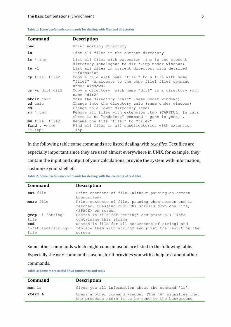
Some useful commands dealing with files and directories are listed in Table 1.
The Basic Computational Environment 3
Table 1: Some useful unix commands for dealing with files and directories
Command Description pwd Print working directory
ls List all files in the current directory
ls *.inp List all files with extension .inp in the present directory (analogous to dir *.inp under windows)
ls -l List all files in current directory with detailed information
cp file1 file2 Copy a file with name “file1” to a file with name “file2” (analogous to the copy file1 file2 command under windows)
cp -r dir1 dir2 Copy a directory with name “dir1” to a directory with name “dir2”
mkdir calc Make the directory “calc” (same under windows) cd calc Change into the directory calc (same under windows) cd .. Change to a lower directory level rm *.tmp Remove all files with extension .tmp (CAREFUL: in unix
there is no “undelete” command – gone is gone!). mv file1 file2 Rename the file “file1” to “file2” find . -name "*.inp"
Find all files in all subdirectories with extension .inp
In the following table some commands are listed dealing with text files. Text files are
especially important since they are used almost everywhere in UNIX, for example, they
contain the input and output of your calculations, provide the system with information,
customize your shell etc. Table 2: Some useful unix commands for dealing with the contents of text files
Command Description cat file Print contents of file (without pausing on screen
boundaries) more file Print contents of file, pausing when screen end is
reached. Pressing <RETURN> scrolls down one line, <SPACE> on screen
grep -i "string" file
Search in file for "string" and print all lines containing this string
sed "s/string1/string2" file
Search in file for all occurences of string1 and replace them with string2 and print the result on the screen
Some other commands which might come in useful are listed in the following table.
Especially the man command is useful, for it provides you with a help text about other
commands. Table 3: Some more useful linux commands and tools
Command Description man ls Gives you all information about the command 'ls'.
xterm & Opens another command window. (The ‘&’ signifies that the processs xterm is to be send to the background
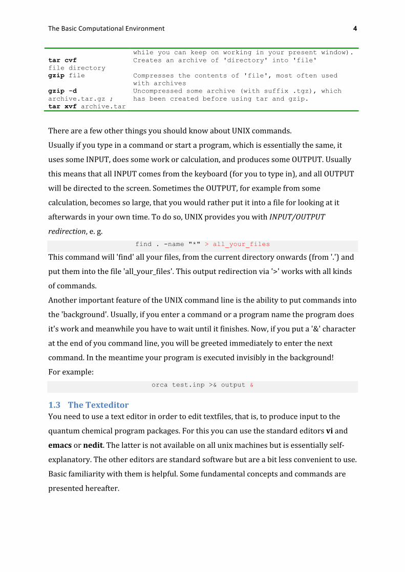
The Basic Computational Environment 4
while you can keep on working in your present window). tar cvf file directory
Creates an archive of 'directory' into 'file'
gzip file Compresses the contents of 'file', most often used with archives
gzip -d archive.tar.gz ; tar xvf archive.tar
Uncompressed some archive (with suffix .tgz), which has been created before using tar and gzip.
There are a few other things you should know about UNIX commands.
Usually if you type in a command or start a program, which is essentially the same, it
uses some INPUT, does some work or calculation, and produces some OUTPUT. Usually
this means that all INPUT comes from the keyboard (for you to type in), and all OUTPUT
will be directed to the screen. Sometimes the OUTPUT, for example from some
calculation, becomes so large, that you would rather put it into a file for looking at it
afterwards in your own time. To do so, UNIX provides you with INPUT/OUTPUT
redirection, e. g. find . -name "*" > all_your_files
This command will 'find' all your files, from the current directory onwards (from '.') and
put them into the file 'all_your_files'. This output redirection via '>' works with all kinds
of commands.
Another important feature of the UNIX command line is the ability to put commands into
the 'background'. Usually, if you enter a command or a program name the program does
it's work and meanwhile you have to wait until it finishes. Now, if you put a '&' character
at the end of you command line, you will be greeted immediately to enter the next
command. In the meantime your program is executed invisibly in the background!
For example: orca test.inp >& output &
1.3 The Texteditor You need to use a text editor in order to edit textfiles, that is, to produce input to the
quantum chemical program packages. For this you can use the standard editors vi and
emacs or nedit. The latter is not available on all unix machines but is essentially self-‐
explanatory. The other editors are standard software but are a bit less convenient to use.
Basic familiarity with them is helpful. Some fundamental concepts and commands are
presented hereafter.

The Basic Computational Environment 5
1.3.1 The VI Editor One of the most widely used editors on UNIX systems is the vi editor. Although it lacks
the look and feel of today's editors, it has the advantages of being available on all UNIX
systems and being very quick to use (and in extended versions also very powerful).
You can load a file into vi just by typing: vi filename
If the file did not exist before it will be created. One feature that is somwhat difficult to
grasp at the beginning is that editing in vi takes place in two different modes: A
command mode and an insert or edit mode. Vi starts in command mode. You can always
get back into command mode by pressing <ESC>. In this mode you can move the cursor
around on the screen and position it where you want to modify your text. For moving
around you can use the CURSOR keys or the keys h, j, k, l. Having positioned the cursor,
press i for insert mode. Now you can enter your text. Pressing <ESC> enters command-‐
mode again. In the following table are the most common keys accessible in command
mode. Table 4: usage of the vi editor
Command Description h, j, k, l Movement (left, down, up, right)
i, I Insert text before cursor position (before first character of the line)
a, A Append text after cursor position (at the end of current line)
o, O Open new line below the current line (or above current line)
X Delete charcter under cursor
Dd Delete whole line D Delete line from cursor position to the end of line
r, R Replace character under cursor (replace from cursor on onwards until leaving by <ESC>)
:wq Save file and exit vi :wfile Save current contents in 'file'. :q! Exit without saving changes
1.3.2 The EMACS Editor Another powerful editor under UNIX is the EMACS editor. You can start it by simply
calling: emacs filename
or
xemacs filename
The file will be opened in a different window, displaying the file's content. In this buffer
you can move around either by using the cursor keys or by scrolling and placing the

The Basic Computational Environment 6
cursor via mouse click. Editing is done in the usual way, text is inserted before the cursor
and you can delete it by pressing the delete key repeatedly. Many functions in emacs are
accessible through the menu bar, but using key combinations is more flexible and faster.
This is just a small subset of those Table 5: Useful key-‐combinations for the emacs editor.
Command Description <CTRL>-x <CTRL>-s Save file and exit emacs <CTRL>-x <CTRL>-c Exit emacs <CTRL>-u Undo <CTRL>-k Delete line from cursor on to the end of line
(pressing <CTRL>-k repleatedly deletes lines) <CTRL>-<space> Mark beginnig of a selected region <CTRL>-w Cut region <CTRL>-y Paste region <CTRL>-x r k Cut marked rectangle <ALT>-x transient-mark-mode
Enable highlighting of selected region
If things get rough: <ALT>-x doctor
...

Quick Start into The Program Packages 7
2 Introduction – Quick Start into the Program Packages and Analysis
Tools
2.1 Calling the ORCA Program In order to run the ORCA program you need to create an input file (e.g. myinp.inp) and
then call: orca myinp.inp >myinp.out &
You can look at the progress of the calculation using tail –f myinp.out
A general form of the input file is:
(NOTE: the multiplicity is defined as 2S+1 where S is the total spin of the state under
investigation; for our purposes Mult=Number of unpaired electrons+1).
An example is:
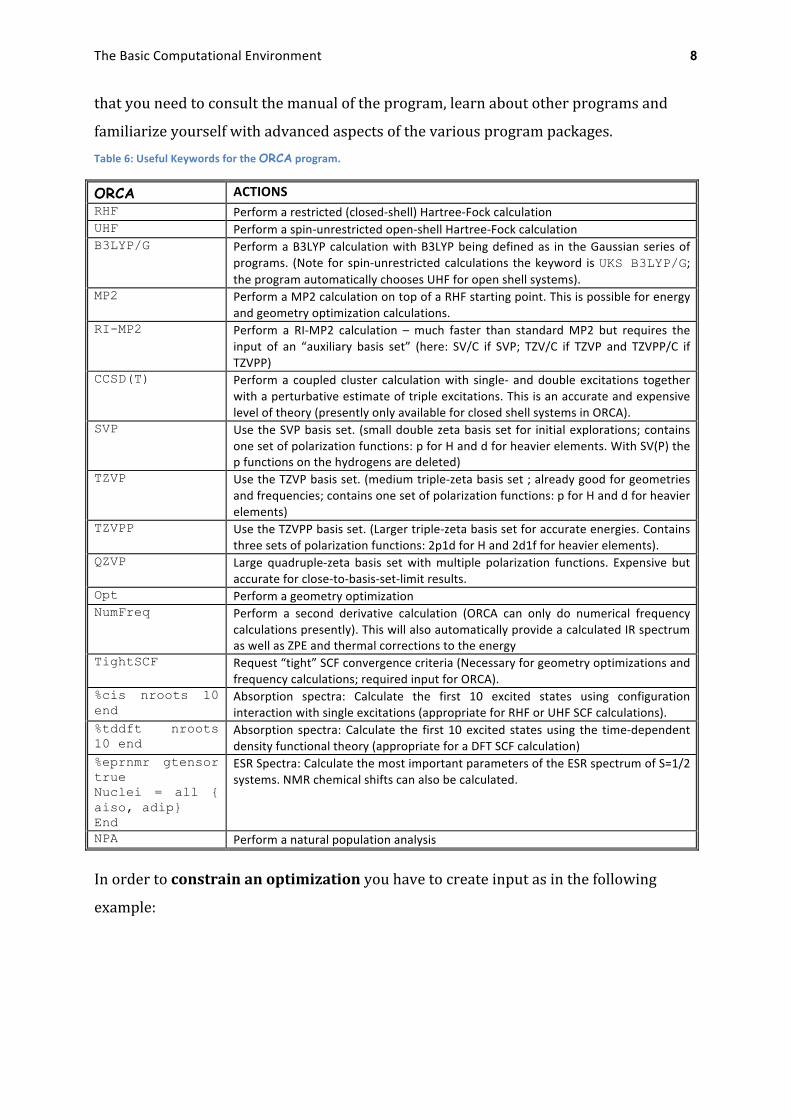
2.2 Keywords for ORCA Below is a summary of keywords that will be used within this course. The program has,
of course, many more options – however, in this course you will essentially only need
those listed below. If you go on to do research in theoretical chemistry it is very likely
# comment lines (anywhere in input) ! Method BasisSet Additional-Keywords #Possible input blocks start with ‘%’ # for example: %scf maxiter 150 end * xyz Charge, Multiplicity Cartesian coordinates * or: * int Charge, Multiplicity Z-Matrix *
# Check H2CO optimization ! B3LYP SVP Opt TightSCF * xyz 0 1 C 0.000000 0.000000 0.000000 O 1.200000 0.000000 0.000000 H -0.550000 0.952628 0.000000 H -0.550000 -0.952628 -0.000000 *
The Basic Computational Environment 8
that you need to consult the manual of the program, learn about other programs and
familiarize yourself with advanced aspects of the various program packages. Table 6: Useful Keywords for the ORCA program.
ORCA ACTIONS RHF Perform a restricted (closed-‐shell) Hartree-‐Fock calculation UHF Perform a spin-‐unrestricted open-‐shell Hartree-‐Fock calculation B3LYP/G Perform a B3LYP calculation with B3LYP being defined as in the Gaussian series of
programs. (Note for spin-‐unrestricted calculations the keyword is UKS B3LYP/G; the program automatically chooses UHF for open shell systems).
MP2 Perform a MP2 calculation on top of a RHF starting point. This is possible for energy and geometry optimization calculations.
RI-MP2 Perform a RI-‐MP2 calculation – much faster than standard MP2 but requires the input of an “auxiliary basis set” (here: SV/C if SVP; TZV/C if TZVP and TZVPP/C if TZVPP)
CCSD(T) Perform a coupled cluster calculation with single-‐ and double excitations together with a perturbative estimate of triple excitations. This is an accurate and expensive level of theory (presently only available for closed shell systems in ORCA).
SVP Use the SVP basis set. (small double zeta basis set for initial explorations; contains one set of polarization functions: p for H and d for heavier elements. With SV(P) the p functions on the hydrogens are deleted)
TZVP Use the TZVP basis set. (medium triple-‐zeta basis set ; already good for geometries and frequencies; contains one set of polarization functions: p for H and d for heavier elements)
TZVPP Use the TZVPP basis set. (Larger triple-‐zeta basis set for accurate energies. Contains three sets of polarization functions: 2p1d for H and 2d1f for heavier elements).
QZVP Large quadruple-‐zeta basis set with multiple polarization functions. Expensive but accurate for close-‐to-‐basis-‐set-‐limit results.
Opt Perform a geometry optimization NumFreq Perform a second derivative calculation (ORCA can only do numerical frequency
calculations presently). This will also automatically provide a calculated IR spectrum as well as ZPE and thermal corrections to the energy
TightSCF Request “tight” SCF convergence criteria (Necessary for geometry optimizations and frequency calculations; required input for ORCA).
%cis nroots 10 end
Absorption spectra: Calculate the first 10 excited states using configuration interaction with single excitations (appropriate for RHF or UHF SCF calculations).
%tddft nroots 10 end
Absorption spectra: Calculate the first 10 excited states using the time-‐dependent density functional theory (appropriate for a DFT SCF calculation)
%eprnmr gtensor true Nuclei = all { aiso, adip} End
ESR Spectra: Calculate the most important parameters of the ESR spectrum of S=1/2 systems. NMR chemical shifts can also be calculated.
NPA Perform a natural population analysis
In order to constrain an optimization you have to create input as in the following
example:

The Basic Computational Environment 9
NOTE:
• “value” in the constraint input is optional. If you do not give a value, the present
value in the structure is constrained. For cartesian constraints you can’t give a
value, but always the initial position is constrained.
• It is recommended to use a value not too far away from your initial structure.
• It is possible to constrain whole sets of coordinates:
Relaxed surface scans can be performed as in the following example:
In the example above the value of the bond length between C and O will be changed in
12 equidistant steps from 1.35 down to 1.10 Angströms and at each point a constrained
geometry optimization will be carried out.
! RKS B3LYP/G SV(P) TightSCF Opt %geom Constraints { B 0 1 1.25 C } { A 2 0 3 120.0 C } end end * int 0 1 C 0 0 0 0.0000 0.000 0.00 O 1 0 0 1.2500 0.000 0.00 H 1 2 0 1.1075 122.016 0.00 H 1 2 3 1.1075 122.016 180.00 *
Constraining bond distances : { B N1 N2 value C } Constraining bond angles : { A N1 N2 N1 value C } Constraining dihedral angles : { D N1 N2 N3 N4 value C } Constraining cartesian coordinates : { C N1 C }
! RKS B3LYP/G SV(P) TightSCF Opt %geom Scan B 0 1 = 1.35, 1.10, 12 # C-O distance that will be scanned end end * int 0 1 C 0 0 0 0.0000 0.000 0.00 O 1 0 0 1.3500 0.000 0.00 H 1 2 0 1.1075 122.016 0.00 H 1 2 3 1.1075 122.016 180.00 *
The Basic Computational Environment 10
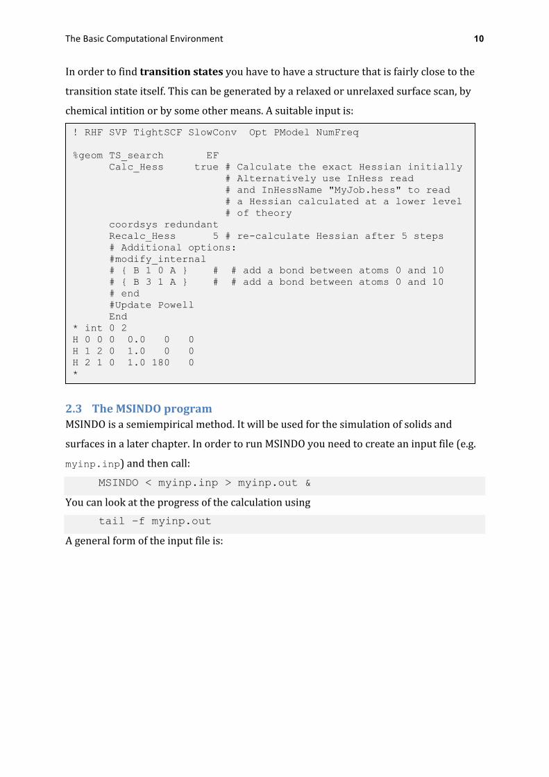
In order to find transition states you have to have a structure that is fairly close to the
transition state itself. This can be generated by a relaxed or unrelaxed surface scan, by
chemical intition or by some other means. A suitable input is:
2.3 The MSINDO program MSINDO is a semiempirical method. It will be used for the simulation of solids and
surfaces in a later chapter. In order to run MSINDO you need to create an input file (e.g.
myinp.inp) and then call:
MSINDO < myinp.inp > myinp.out &
You can look at the progress of the calculation using tail –f myinp.out
A general form of the input file is:
! RHF SVP TightSCF SlowConv Opt PModel NumFreq %geom TS_search EF Calc_Hess true # Calculate the exact Hessian initially # Alternatively use InHess read # and InHessName "MyJob.hess" to read # a Hessian calculated at a lower level # of theory coordsys redundant Recalc_Hess 5 # re-calculate Hessian after 5 steps # Additional options: #modify_internal # { B 1 0 A } # # add a bond between atoms 0 and 10 # { B 3 1 A } # # add a bond between atoms 0 and 10 # end #Update Powell End * int 0 2 H 0 0 0 0.0 0 0 H 1 2 0 1.0 0 0 H 2 1 0 1.0 180 0 *

The Basic Computational Environment 11
Due to the approximative nature of the semiempirical method, MSINDO results are in
general different from ORC or other ab initio/DFT programs. The parameterization
includes the most common bonding situations of elements H, Li -‐ F, Na -‐ Cl, K – Br.
2.4 The Molecular Editing and Visualization Program Molden Molden is a convenient visualization program for displaying molecular structures
(including animation for geometry optimizations and vibrations), electronic properties
(orbitals, electron densities) http://www.cmbi.ru.nl/molden/molden.html.
ORCA cube files can also be displayed in the <Dens. Mode>. For outputs of geometry
optimizations the starting structure is displayed. Structural changes are visualized by
<Movie>. Animations of vibrations are possible in the <Norm. Mode>. MSINDO
generates Molden inputs if the keyword
is given. This will produce a file named by the chemical formula, e.g. OCH2.molden for
the above example. The command molden OCH2.molden
PRINTOPTS=MOLDENMOS
# 1st line: Title (must include the string :NEW) CH2O :NEW # Section 1: keywords RHF or UHF MULTIP=… # closed or open shell OPT ANALY # opt. of internal coordinates CARTOPT ANALY # opt. of Cartesian coordinates # using analytical 1st derivatives NVIB=4 FULL # vibrations/heat of formation PRINTOPTS=MOLDEN # output for MOLDEN :END # end of section 1 # Section 2: atomic coordinates # Cartesian coordinates (CARTES in section 1): # Atomic number or symbol x y z (one per line) C 0.000000 0.000000 0.000000 O 1.200000 0.000000 0.000000 H -0.550000 0.952628 0.000000 H -0.550000 -0.952628 -0.000000 # Or Z-Matrix: 1 O 1 2 C RCO 1 2 3 H RCH AOCH 3 1 2 4 H RCH AOCH DHOCH :END # end of section 2 # Section 3: variables (if used in section 2) RCO = 1.20 RCH = 1.10 # Angstrom AOCH = 120 # Degrees DHOCH = 180 :END # end of section 3 END # End of input

The Basic Computational Environment 12
will give the output shown below. With the <ZMAT Editor > it is possible to generate
structure definitions of simple molecules or to modify the actual Z Matrix.
Figure 3: Screenshot of the MolDen program showing the molecular structure window as well as the progress of SCF and geometry convergence and the Z-‐matrix (=structure) editor
2.5 The Visualization Program Molekel You can use the ORCA program to produce so-‐called Cube files, which contain the
information that is necessary in order to visualize molecular orbitals with either the
Molden or Molekel programs.
In order to use orca you have to invoke a small auxiliary program called orca_plot.
You have to start it with the name of a so-‐called gbw-‐file. The GBW file is a file that is
automatically made during the execution of ORCA. It contains in binary form a summary
of the calculation. For example, if you ran myjob.inp the program will produce
myjob.gbw which contains the geometry, the basis set used and the wavefunction that
was computed. Call: orca_plot myjob.gbw -i
This will give you a small “stone-‐age” menu which you can use to produce the desired
graphical information. First choose “5” to choose an output format. Select “7” to choose
“Gaussian Cube”. Then select “2” and choose the number of the MO that you want to plot.
Remember that ORCA starts counting with zero and refer to the output file to figure out
which MO you want to see. Finally choose “10” in order to produce the plot. This will
lead to a file called myjob.moXa.cube where X is the number of the MO that you
selected for plotting. After you have made all cube files that you wanted, start the

The Basic Computational Environment 13
Molekel program and proceed as described below. Since the cube-‐files are ASCII files
you can also transfer them between platforms.
You can now start Molekel and load (via a right mouse click) the XYZ file (or also
directly the .cube file). Then go to the surface menu, select “Gaussian-‐cube” format and
load the surface. For orbitals click the “both signs” button and select a countour value in
the “cutoff” field. The click “create surface”. The colour schemes etc. can be adjusted at
will – try it! It’s easy and produces nice pictures. Create files via the “snapshot” feature of
Molekel. Other programs can certainly also deal with Gaussian-‐Cube files.
Figure 4: The π and π*-‐MOs of CO as visualized by Molekel.
2.6 The Data Analysis Program XMGrace For a survey over all features of xmgrace, the reader is referred to the excellent manual
provided under http:www.grace.com
2.6.1 Plotting a Graph with XMGrace Getting data Before anything can be plotted, the data must be generated. To prepare the data so that
it can be read in directly by xmgrace, one should store it in a plain text file, containing
only numbers. Decimal numbers must be written with points. To actually start xmgrace,
type
$: xmgrace datafile
while datafile is the name of the file containing the prepared data.

The Basic Computational Environment 14
Figure 5: The “Getting Data” window of Xmgrace
By default, the first column is read in as the x values, while the second represents the y values. Getting even more data To load a new dataset (in short: “set” into the actual graph, select “Data -‐> Import... -‐>
ASCII” from the menu bar. Be sure to eliminate the last entry of the filter (*.dat) if you
can't see the desired file (1).
To start a completely new graph, select “File -‐> New” from the menu bar.
Getting more complicated data Data that contains more than two rows can be read in via “Data -‐> Import... -‐> ASCII”.
Selecting “Load as -‐> Block data” (2) will provide a new window where you can select
which row of data should be used for the x and the y axis.
2.6.2 Polishing the Graph: Menu Plot Graph appearance... Here one can alter the appearance of the legend, the title, the frames of the graph as well
as the legend box. It is common to select “2” for the width of all lines, in this case the
frames.
The image cannot be displayed. Your computer may not have enough memory to open the image, or the image may have been corrupted. Restart your computer, and then open the file again. If the red x still appears, you may have to delete the image and then insert it again.

The Basic Computational Environment 15
Figure 6: The “Set Appearance” window of Xmgrace
The same menu can be opened by double clicking with the left mouse button outside the
graph.
Set appearance... Here one can change the design of every single set (of data). The first part “Select set”
(1) allows to choose the set to edit. Because we normally have discrete values, we prefer
a representation of every single point over lines. This is done by going to tab “Main”,
select “Symbol properties -‐> Type: Diamonds” (for example) (2) and select “Line
properties -‐> Type: None” (3). Here you can also fill in the name of the data set for the
legend (4). The command “\s” makes all following letters to be written as a subscript,
“\N” returns to normal format. Hit “Apply” (5) to not loose this changes while going to
the next tab, “Symbols”.
Here, set the “Symbol outline -‐> width” to “2” and “Symbol fill -‐> Pattern” to the filled
black square. All other tabs are not important at the moment.
The same menu can be opened by double clicking with the left mouse button directly on
one data point (or one line).
Axis properties Here the range of the axis, the appearance of the axis bars and the title of the axis are set.
The image cannot be displayed. Your computer may not have enough memory to open the image, or the image may have been corrupted. Restart your computer, and then open the file again. If the red x still appears, you may have to delete the image and then insert it again.

The Basic Computational Environment 16
“Edit” determines which axis is to be edited. Make sure that you edit the right axis, and
that “Apply to” at the bottom is set to “Current axis” before hitting apply. Note that most
of the alterations have to be done twice.
The tab “Main” is mostly to modify the axis label. If “Symbol” must be used as the
language, open in the main menu “Window -‐> Font tool”, select “Symbol” as the
language, and click on the desired letter. The appearing string can directly be plugged
into the axis label.
To get a consistent graph, go to tab “Tick marks” and set all line width to “2” as well as
“Placement -‐> Draw on:” to “Normal side”.
The same menu can be opened by double clicking with the left mouse button directly on
one axis.
2.6.3 Evaluating the data: Fitting Procedures The most frequently used methods to search for trends in experimental or
computational data are regression analysis and the non-‐linear curve fitting.
A. Regression analysis To do a linear regression analysis, select “Data -‐> Transformation -‐> Regression ...” . This
will lead to a new window, where you can choose which data set should be analyzed, and
with which method. Furthermore, selecting “Restrictions -‐> Region ..” you can choose
which subset of data points should be used for the regression.
To define a region, go to “Edit -‐> Regions ...-‐> Define” in the main menu. Select the region
type and click “Define”. Then use the left mouse button (one click per corner/end) to
define the geometrical structure you have selected.
Back to the linear regression, click “Accept”. Now a new data set is created, which can be
treated like any data set before. Also, all information of the fitting procedure are printed
in a new window. There, go to File -‐> Save to save these results.
The Basic Computational Environment 17
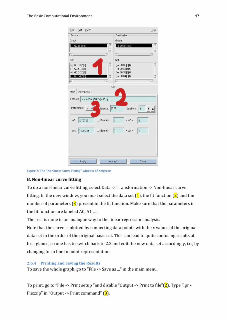
Figure 7: The “Nonlinear Curve Fitting” window of Xmgrace
B. Non-‐linear curve fitting
To do a non-‐linear curve fitting, select Data -‐> Transformation -‐> Non-‐linear curve
fitting. In the new window, you must select the data set (1), the fit function (2) and the
number of parameters (3) present in the fit function. Make sure that the parameters in
the fit function are labeled A0, A1 ... .
The rest is done in an analogue way to the linear regression analysis.
Note that the curve is plotted by connecting data points with the x values of the original
data set in the order of the original basis set. This can lead to quite confusing results at
first glance, so one has to switch back to 2.2 and edit the new data set accordingly, i.e., by
changing form line to point representation.
2.6.4 Printing and Saving the Results To save the whole graph, go to “File -‐> Save as ...“ in the main menu.
To print, go to “File -‐> Print setup “and disable “Output -‐> Print to file”(2). Type “lpr -‐
Plexzip” in “Output -‐> Print command” (3).
The image cannot be displayed. Your computer may not have enough memory to open the image, or the image may have been corrupted. Restart your computer, and then open the file again. If the red x still appears, you may have to delete the image and then insert it again.

The Basic Computational Environment 18
Select “File -‐> Print” back in the main menu.
To save this graph as an eps file, go to the print setup and enable “Output -‐> print to
file”(2).
Select “Device Setup -‐> Device -‐> EPS”(1).
Alter “Output -‐> File name -‐> ....eps”(4).
Select “File -‐> Print” back in the main menu.
Figure 8: The “Printing and Saving the Results” window of Xmgrace
The image cannot be displayed. Your computer may not have enough memory to open the image, or the image may have been corrupted. Restart your computer, and then open the file again. If the red x still appears, you may have to delete the image and then insert it again.

The Basic Computational Environment 19

The Basic Computational Environment 20