ordinary kriging - midland valley ordinary kriging interpolation between data points is a useful...
TRANSCRIPT

www.mve.com
Ordinary Kriging
Interpolation between data points is a useful tool for constructing and visualizing 3D
surfaces (e.g. Figure 1). In Move you can create surfaces using interpolation techniques,
such as inverse distance weight, spline algorithms and ordinary kriging. Here we will
focus on the use of ordinary kriging for modelling geological contacts, such as horizons
and faults. However, the algorithm can also be used to interpolate attributes, such as
ore grade or Total Organic Carbon (TOC), via the Variogram Modelling tab in the
Vertex Attribute Analyser.
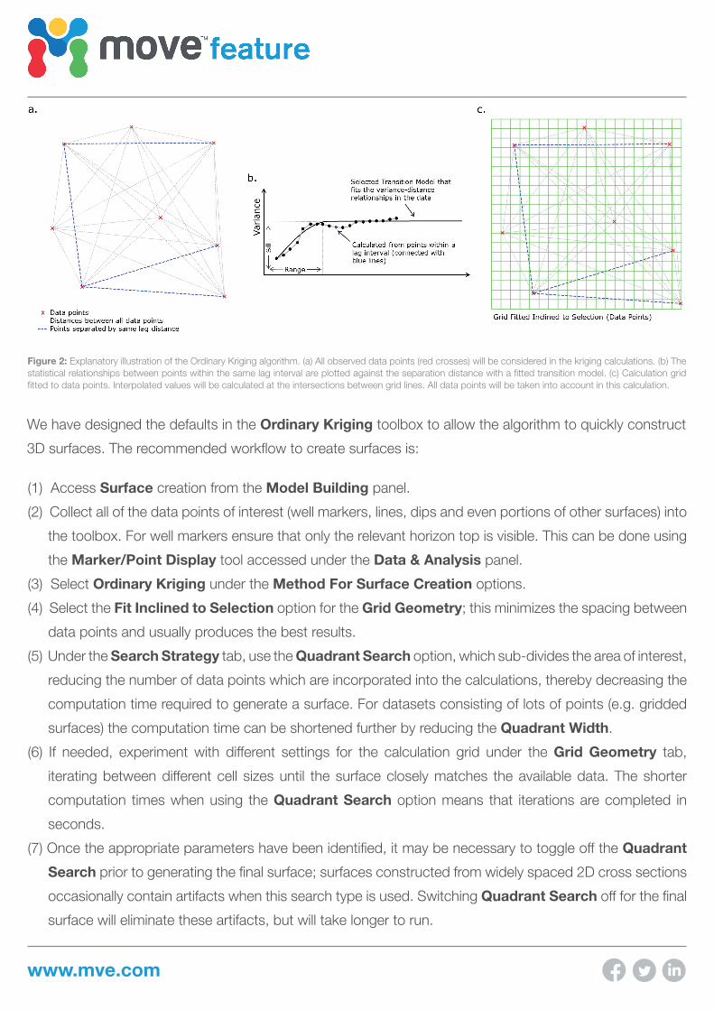
The ordinary kriging algorithm calculates the statistical relationship (variance) between similarly spaced data
points (Figure 2); data points are deemed to be similarly spaced if they lie within the same lag interval,
defined by the maximum lag distance, number of lags and a tolerance. A mathematical function (referred to
as the transition model) is then fitted to the graph (the variogram) showing the separation distance of data
points against variance. This function is used to establish the weighting that observed data points will give
during the calculation. The algorithm then computes values at the defined calculation points on a grid by
performing a regression through all of the observed data points, weighted by the distance away from the
calculation point.
Modules Used:
Figure 1: Surface constructed from a series of interpreted sections and well markers using the Ordinary Kriging workflow in the Create Surface toolbox.
www.mve.com
(1) Access Surface creation from the Model Building panel.
(2) Collect all of the data points of interest (well markers, lines, dips and even portions of other surfaces) into
the toolbox. For well markers ensure that only the relevant horizon top is visible. This can be done using
the Marker/Point Display tool accessed under the Data & Analysis panel.
(3) Select Ordinary Kriging under the Method For Surface Creation options.
(4) Select the Fit Inclined to Selection option for the Grid Geometry; this minimizes the spacing between
data points and usually produces the best results.
(5) Under the Search Strategy tab, use the Quadrant Search option, which sub-divides the area of interest,
reducing the number of data points which are incorporated into the calculations, thereby decreasing the
computation time required to generate a surface. For datasets consisting of lots of points (e.g. gridded
surfaces) the computation time can be shortened further by reducing the Quadrant Width.
(6) If needed, experiment with different settings for the calculation grid under the Grid Geometry tab,
iterating between different cell sizes until the surface closely matches the available data. The shorter
computation times when using the Quadrant Search option means that iterations are completed in
seconds.
(7) Once the appropriate parameters have been identified, it may be necessary to toggle off the Quadrant
Search prior to generating the final surface; surfaces constructed from widely spaced 2D cross sections
occasionally contain artifacts when this search type is used. Switching Quadrant Search off for the final
surface will eliminate these artifacts, but will take longer to run.
Figure 2: Explanatory illustration of the Ordinary Kriging algorithm. (a) All observed data points (red crosses) will be considered in the kriging calculations. (b) The statistical relationships between points within the same lag interval are plotted against the separation distance with a fitted transition model. (c) Calculation grid fitted to data points. Interpolated values will be calculated at the intersections between grid lines. All data points will be taken into account in this calculation.
We have designed the defaults in the Ordinary Kriging toolbox to allow the algorithm to quickly construct
3D surfaces. The recommended workflow to create surfaces is:
www.mve.com
The toolbox can also be used for generating surfaces using an enhanced ordinary kriging workflow. Directional
variogram modelling can be used to investigate the statistical relationship (variance) of observed data points
in a particular direction. This analysis could indicate that points have a greater statistical correlation in a
particular direction, meaning that the observed data set contains an anisotropy which ought to be considered
during the kriging procedure by attaching greater weighting to points located parallel to the anisotropy.
Failing to account for these anisotropies often leads to artifacts on the kriged surfaces.
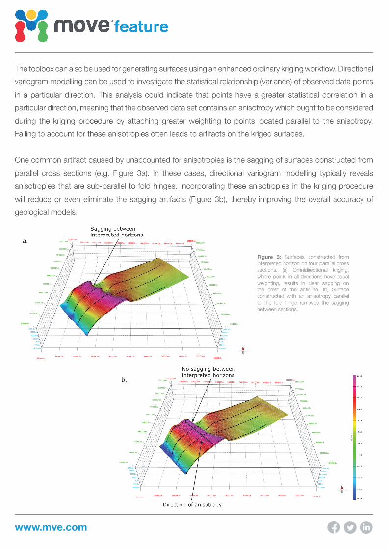
One common artifact caused by unaccounted for anisotropies is the sagging of surfaces constructed from
parallel cross sections (e.g. Figure 3a). In these cases, directional variogram modelling typically reveals
anisotropies that are sub-parallel to fold hinges. Incorporating these anisotropies in the kriging procedure
will reduce or even eliminate the sagging artifacts (Figure 3b), thereby improving the overall accuracy of
geological models.
Figure 3: Surfaces constructed from interpreted horizon on four parallel cross sections. (a) Omnidirectional kriging, where points in all directions have equal weighting, results in clear sagging on the crest of the anticline. (b) Surface constructed with an anisotropy parallel to the fold hinge removes the sagging between sections.