oregon pers financial modelingg:\wp\retire\2011\opersu\board mtgs\0328 financial modeling.ppt. 1....

$: Oregon PERS Financial ModelingG:\WP\Retire\2011\Opersu\Board mtgs\0328 Financial Modeling.ppt. 1. Introduction Mercer conducts actuarial valuations of the PERS program annually –$
www.mercer.com

Oregon PERS Financial Modeling Contribution Projections and Impact of Side Accounts

March 28, 2011

Matt Larrabee, FSAScott Preppernau, FSA

1G:\WP\Retire\2011\Opersu\Board mtgs\0328 Financial Modeling.pptMercer

Introduction

Mercer conducts actuarial valuations of the PERS program annually– Valuations are used to develop recommended contribution rates

and assess system funded status– Valuation calculations are based on outcomes if all actuarial

assumptions are met

A key assumption is annual investment return, currently at 8%

Of course, assumptions are never met precisely and in some years actual experience will vary widely from assumption

Given this, periodically Mercer conducts financial modeling studies– In these studies, contribution rates and funded status levels are

calculated under a variety of possible investment return scenarios– While the scenarios shown are not all inclusive, the study results

convey the system’s sensitivity to investment results


Overview of Employer Rate Setting

Actuarial valuations are conducted annually each year-end– Rates are set biennially based on “odd year” actuarial valuations– “Even year” valuations are strictly advisory

The rates determined by the actuarial valuation are adopted by the Board and go into effect 18 months subsequent to the valuation date

Valuation Date Employer Contribution Rates

12/31/2009 July 2011 – June 2013

12/31/2011 July 2013 – June 2015



Two types of employer contribution rates calculated in each valuation

Base Rate– A base rate is calculated for each employer or employer rate pool,

and base rates vary from employer to employer and pool to pool– The base rate has two components:

Normal cost rate – economic value of benefits earned during the current year

UAL (unfunded actuarial liability) rate – projected cost to eliminate funding shortfalls for benefits already earned over a period of time approved by the PERS Board and assuming actuarial assumptions are met

– The change in base rate from period to period is restricted by the “rate collar” mechanism



Two types of employer contribution rates calculated in each valuation

Net Rate– Employers pay the net rate– For employers without a side account, the net rate is the same as

the base rate– For side account employers, the net rate is lower than the base rate

In the valuation, the employer’s side account asset and payroll levels are used to develop a “side account rate offset”

The rate offset level is calculated to provide a steady level of contribution rate relief until the end of 2027 if assumptions are met

– Side account employers pay their calculated net rate

The difference between an employer’s base rate and its net rate is funded by a transfer from the employer’s side account to general PERS assets at the calculated rate offset level


Overview of Employer Rate Setting Structure of Employer Pension Contribution Rates

Employer pension contribution rates have two key components: Normal Cost and UAL

Rates shown here and throughout the rest of this presentation are calculated on a systemwide basis

– Rates for any single employer will vary from the systemwide rate

IAP and retiree healthcare rates, as well as any repayment on pension obligation bonds (POBs) are charged in addition to the pension rate

Employer Contribution Rates* July 2011 – June 2013

Payroll Tier 1/Tier 2 OPSRP GS OPSRP P&F Combined

Normal Cost 8.6% 6.1% 8.8% 7.8%

T1/T2 UAL 7.7% 7.7% 7.7% 7.7%

OPSRP UAL 0.1% 0.1% 0.1% 0.1%

Base Rate* 16.4% 13.9% 16.6% 15.6%

Average Adjustment** (5.5%) (5.5%) (5.5%) (5.5%)

Net Rate* 10.8% 8.4% 11.1% 10.1%

* Base and net rates excluding retiree healthcare component** Adjustments are for side accounts and Pre-SLGRP liabilities and are shown on a system-wide basis


Overview of Employer Rate Setting The Rate Collar

From one biennium to the next, employer base rate changes for Tier 1/Tier 2 and OPSRP are restricted to stay inside of a “rate collar”– The rate collar is defined as the greater of:

20% of the base rate currently in effect, or

3% of payroll

If the plan’s funded status goes above 120% or below 80%, the width of the rate collar increases on a graded schedule such that above 130% or below 70% the size of the collar is doubled

The rate collar will limit base rates for the 2011-2013 contribution period– The 12/31/2009 valuation established 2011-2013 employer rates– Without the collar, the average system-wide base rate of 15.6% would

have been approximately 19.6%– This deferred increase means the rates for the 2013-2015 biennium are

expected to rise if assumptions are met during 2010 and 2011

Baseline Financial Modeling


Baseline Financial Modeling Overview of Modeling

Basis for modeling is most recently available year-end asset and liability information– 12/31/2009 liabilities and assumptions for Tier 1/Tier 2/OSPRP

Modeling assumes 8% annual investment return assumption remains in place for duration of modeling period

– Does not include retiree healthcare or IAP contributions– 12/31/2010 assets based on preliminary board crediting decisions– Investment policy as selected by Oregon Investment Council (OIC)

In the 12/31/2009 valuation, the Contingency Reserve and Tier 1 Rate Guarantee Reserve were each excluded from valuation assets– The Tier 1 Rate Guarantee Reserve (RGR) is currently negative

Excluding a negative reserve increases valuation assets

If the RGR remains negative for 5 years, action must be taken to address the deficit, per statute

– Our model treats a negative reserve as part of the unfunded actuarial liability (UAL)


Baseline Financial Modeling Introduction

We used a stochastic model to create 1,000 trials of projected future experience for the system– Uses Mercer Investment Consulting’s capital market assumptions – Detail on model and market assumptions included in the appendix

The model outputs key system measures such as contribution rates and funded status, with results displayed graphically in percentiles

50%25%

90%

Percentile Ranking Likelihood of Occurrence

95th90th75th

50th

25th10th5th

80%

15%

15%

25%

5%

5%5%

5%

$ or %

Darkening shades of green indicate progressively more favorable

outcomes. Red is used in the same way to show progressively more

unfavorable results. The graphics are supplemented with numerical tables.


Baseline Financial Modeling Combined (Tier 1/Tier 2, OPSRP) Base* Contribution Rate

toptoptop

top

toptoptop

Biennium 2011 - 2013 2013 - 2015 2015 - 2017 2017 - 2019 2019 - 2021 2021 - 2023 2023 - 2025 2025 - 2027 2027 - 2029

th 5th 15.6% 21.6% 29.9% 38.1% 41.3% 42.4% 43.8% 44.3% 46.2%10th 15.6% 21.6% 28.9% 34.4% 35.3% 37.0% 38.1% 39.6% 40.4%25th 15.6% 21.0% 25.6% 27.0% 28.5% 30.0% 30.3% 31.2% 30.7%50th 15.6% 18.7% 20.5% 20.7% 21.8% 21.3% 20.6% 20.4% 20.5%75th 15.6% 17.4% 16.0% 15.8% 14.9% 14.2% 13.3% 12.3% 11.0%90th 15.6% 14.2% 13.2% 11.9% 10.2% 8.7% 6.6% 4.7% 2.7%95th 15.6% 12.3% 11.3% 9.6% 7.8% 4.5% 1.8% 0.9% 0.5%

5th - 95th 0.0% 9.3% 18.6% 28.5% 33.5% 37.9% 41.9% 43.5% 45.8%

0%

5%

10%

15%

20%

25%

30%

35%

40%

45%

50%

*Base rates do not reflect the effects of side account rate offsets and Pre-SLGRP liabilities, and do not include contribution rates for the IAP or retiree healthcare programs, or debt service on pension obligation bonds. The Tier 1

Rate Guarantee Reserve is not excluded from assets for years where the reserve is negative.

In over 75 percent of scenarios, base rates increase at 2013. The 50th

percentile increase is 3.1% of payroll. The rate collar prevents rates in worst

scenarios from rising above 21.6%.

For 2015 and beyond, over half of all scenarios have base rates in excess of 20% of payroll, but significant volatility exists


Baseline Financial Modeling Combined (Tier 1/Tier 2, OPSRP) Funded Status (Excluding Side Accounts)

toptoptop

top

toptoptop

2010 2011 2012 2013 2014 2015 2016 2017 2018 2019 2020 2021 2022 2023 2024 2025 2026 2027 2028 20295th 95th 79% 94% 100% 104% 106% 110% 114% 119% 123% 127% 129% 133% 134% 138% 142% 145% 152% 156% 159% 162%

90th 79% 90% 96% 98% 100% 103% 105% 109% 111% 115% 118% 120% 122% 124% 130% 132% 137% 139% 143% 147%75th 79% 84% 86% 88% 90% 91% 92% 94% 95% 97% 98% 102% 103% 106% 107% 109% 112% 116% 120% 123%50th 79% 79% 78% 78% 78% 78% 78% 78% 79% 82% 83% 85% 87% 87% 88% 90% 93% 95% 97% 99%25th 79% 72% 69% 67% 66% 65% 65% 65% 66% 66% 68% 68% 69% 69% 71% 73% 73% 75% 78% 81%10th 79% 66% 60% 56% 54% 52% 53% 53% 54% 54% 54% 55% 56% 57% 58% 59% 60% 60% 64% 63%5th 79% 62% 53% 49% 45% 46% 46% 45% 46% 46% 48% 48% 49% 50% 50% 50% 52% 49% 52% 55%

95th - 5th 0% 32% 48% 55% 61% 65% 69% 74% 77% 81% 82% 86% 85% 88% 92% 95% 100% 107% 107% 106%

PY Ending 12/31

0%

20%

40%

60%

80%

100%

120%

140%

160%

180%

The large Tier 1/Tier 2 shortfall created by the 2008 market downturn is scheduled to be amortized over 20

years if assumptions are met. At the 50th percentile, the amortization pattern is that funded status stabilizes over the first ten years and then improves over the second

ten years.

Investment sensitivity is high enough that by the 2013 rate-setting valuation, funded status is greater than 100% in more than 5% of

scenarios and less than 50% in more than 5% of scenarios


Baseline Financial Modeling Combined (Tier 1/Tier 2, OPSRP) Net* Contribution Rate

toptoptop

top

toptoptop

Biennium 2011 - 2013 2013 - 2015 2015 - 2017 2017 - 2019 2019 - 2021 2021 - 2023 2023 - 2025 2025 - 2027 2027 - 2029


5th - 95th 0.0% 11.8% 22.4% 32.9% 37.6% 38.1% 39.6% 41.0% 45.4%

0%

5%

10%

15%

20%

25%

30%

35%

40%

45%

50%

*Net rates do reflect the effects of side account rate offsets and Pre-SLGRP liabilities, but do not include contribution rates for the IAP or retiree healthcare programs, or debt service on pension obligation bonds. The Tier 1 Rate Guarantee

Reserve is not excluded from assets for years where the reserve is negative.

Net rates exhibit even higher volatility than base rates. This is because investment return scenarios that increase base rates

tend to simultaneously decrease side account rate offset levels.

Net rates increase at 2027-2029 with the expiration of side

account rate offsets, but this increase coincides with the

expiration of debt payments on pension obligation bonds


Baseline Financial Modeling Biennium to Biennium Change to Contribution Rates

toptoptop

top

toptoptop

Biennium

Base Net Base Net Base Net Base Net Base Net Base Net Base Net Base Net Base Netth 5th 3.5% 5.1% 6.0% 7.1% 8.4% 9.6% 10.2% 11.3% 9.4% 11.1% 10.0% 11.7% 10.1% 11.6% 10.3% 12.6% 10.0% 15.1%

10th 3.5% 5.1% 6.0% 6.7% 8.1% 9.0% 8.8% 9.9% 7.7% 9.2% 7.9% 9.3% 8.1% 9.3% 8.1% 9.2% 7.2% 12.6%25th 3.5% 5.1% 5.4% 5.7% 6.7% 7.3% 5.8% 6.5% 4.7% 5.6% 4.0% 4.7% 3.7% 4.5% 3.9% 4.4% 4.0% 8.0%50th 3.5% 5.1% 3.1% 3.0% 2.3% 2.4% 1.4% 1.5% 0.2% 0.1% (0.2%) 0.0% (0.8%) 0.0% (0.4%) 0.0% (0.4%) 1.2%75th 3.5% 5.1% 1.8% 1.3% (1.6%) (2.2%) (3.8%) (4.2%) (4.5%) (4.9%) (5.0%) (5.2%) (5.3%) (5.5%) (5.1%) (4.9%) (5.0%) (2.3%)90th 3.5% 5.1% (1.4%) (2.5%) (4.6%) (5.9%) (5.6%) (7.0%) (6.5%) (7.8%) (7.3%) (8.5%) (7.6%) (9.0%) (7.9%) (9.1%) (8.3%) (7.2%)95th 3.5% 5.1% (3.3%) (4.7%) (5.0%) (6.7%) (6.3%) (7.8%) (7.6%) (9.1%) (8.4%) (10.0%) (9.3%) (10.9%) (9.5%) (11.0%) (10.1%) (9.7%)

5th - 95th 0.0% 0.0% 9.3% 11.8% 13.3% 16.3% 16.5% 19.2% 17.0% 20.3% 18.4% 21.7% 19.4% 22.5% 19.8% 23.7% 20.1% 24.8%

2025 - 2027to

2027 - 2029

2021 - 2023to

2023 - 2025

2023 - 2025to

2025 - 2027

2017 - 2019to

2019 - 2021

2019 - 2021to

2021 - 2023

2013 - 2015to

2015 - 2017

2015 - 2017to

2017 - 2019

2009 - 2011to

2011 - 2013

2011 - 2013to

2013 - 2015

(15%)

(10%)

(5%)

0%

5%

10%

15%

This chart compares period-to-period changes in base and net rates. Change levels tend to be similar around

the 50th percentile, which are for investment returns close to assumption In scenarios with both good and

poor deviation from assumption, net rate changes exhibit higher volatility.

About 1/3rd of PERS payroll is for employers without side accounts, for whom base rates and net rates are identical.

This means that employers with side accounts will have somewhat higher volatility than that displayed in this

“system-wide average” chart.


Baseline Financial Modeling Tier 1 Rate Guarantee Reserve

toptoptop

top

toptoptop

($millions)2010 2011 2012 2013 2014 2015 2016 2017 2018 2019 2020 2021 2022 2023 2024 2025 2026 2027 2028 2029

5th 95th (208) 1,305 1,989 2,302 2,467 2,748 2,811 3,213 3,471 3,854 3,981 4,095 4,433 4,669 5,317 5,451 5,852 6,680 7,424 7,68190th (208) 914 1,542 1,673 1,750 1,881 2,038 2,406 2,518 2,639 2,674 2,808 3,120 3,457 3,515 3,756 4,158 4,569 4,995 5,35275th (208) 236 490 560 726 742 791 760 814 951 939 1,016 991 1,117 1,103 1,153 1,250 1,385 1,485 1,56150th (208) (250) (364) (384) (497) (494) (639) (726) (833) (832) (850) (865) (896) (969) (1,044) (1,165) (1,273) (1,371) (1,488) (1,599)25th (208) (854) (1,113) (1,385) (1,554) (1,680) (1,824) (1,959) (2,068) (2,218) (2,389) (2,534) (2,686) (2,939) (3,200) (3,482) (3,827) (4,141) (4,569) (4,944)10th (208) (1,405) (1,968) (2,331) (2,617) (2,840) (3,109) (3,277) (3,462) (3,730) (4,049) (4,334) (4,729) (5,130) (5,584) (6,049) (6,734) (7,185) (7,859) (8,738)5th (208) (1,757) (2,559) (2,965) (3,327) (3,439) (3,629) (3,819) (4,066) (4,429) (4,772) (5,200) (5,692) (6,272) (6,855) (7,596) (8,474) (9,181) (10,309) (10,762)

95th - 5th 0 3,062 4,548 5,267 5,793 6,187 6,440 7,032 7,536 8,283 8,753 9,295 10,124 10,941 12,173 13,047 14,326 15,861 17,733 18,443

PY Ending 12/31

(12,000)

(10,000)

(8,000)

(6,000)

(4,000)

(2,000)

0

2,000

4,000

6,000

8,000

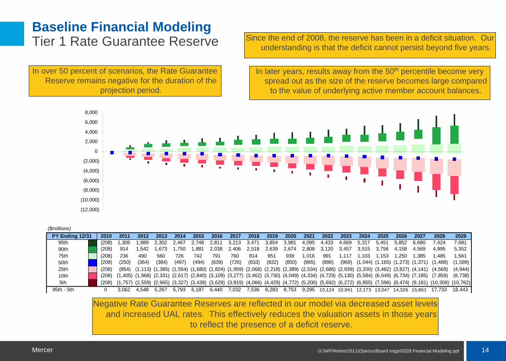
Since the end of 2008, the reserve has been in a deficit situation. Our understanding is that the deficit cannot persist beyond five years.

Negative Rate Guarantee Reserves are reflected in our model via decreased asset levels and increased UAL rates. This effectively reduces the valuation assets in those years

to reflect the presence of a deficit reserve.

In over 50 percent of scenarios, the Rate Guarantee Reserve remains negative for the duration of the

projection period.

In later years, results away from the 50th percentile become very spread out as the size of the reserve becomes large compared

to the value of underlying active member account balances.


Baseline Financial Modeling Observations

Base rate and net rates for 2013-2015, which will be based on 12/31/2011 valuation results, increase in over 75 percent of scenarios, despite good 2010 investment results – At the 50th percentile, the increase is just over 3% of payroll– Increases are due to the rate collar spreading the base rate impact

of 2008 investment losses over more than one rate-setting period

The spread in projected outcomes is greater for the net rates than for base rates, due to the additional volatility of side accounts

At the 50th percentile, projected funded status does not begin to increase significantly until about ten years out

For scenarios that deviate from assumption, system volatility is increasing as the system continues to mature– For the 12/31/2013 rate-setting valuation, more than 5% of

scenarios show funded status (excluding side accounts) greater than 100% and more than 5% of scenarios show funded status (excluding side accounts) under 50%

Modeling Hypothetical Side Account Including Debt Service Costs


Modeling Hypothetical Side Account Including Debt Service Costs Introduction

In our baseline financial modeling, net rates are lower than base rates due to the effect of side account rate offsets– The baseline modeling does not display the cost of debt service on

pension obligation bonds (POBs) used to establish side accounts

POB debt payment schedules vary from employer to employer and are not collected as part of our valuation process

In addition, since approximately 1/3rd of system payroll is for employers without side accounts the net rate volatility for side account employers is understated when it is blended at a system-wide level with the base/net rate volatility of non-side account employers

To address these two issues and give side account employers a better understanding of the potential cost/benefit trade-offs and underlying volatility associated with side accounts, we extended our analysis by modeling a hypothetical single system-wide side account


Modeling Hypothetical Side Account Including Debt Service Costs Structure of Hypothetical Side Account and POB

To address the two issues noted on slide 17 and make the analysis as useful as possible, the hypothetical side account was established in the following manner:– The level of the side account was “scaled up” so that at a system-

wide level the side account exposure would parallel the current exposure of the average employer that presently has a side account

It produces an $8.3 billion hypothetical side account at 12/31/2010- For comparison, actual system side accounts at 12/31/2010

were $5.6 billion– The side account level so modeled will allow system-wide results to

be more consistent with expectations for current side account employers


Modeling Hypothetical Side Account Including Debt Service Costs Structure of Hypothetical Side Account and POB

To address the two issues noted on slide 17 and make the analysis as useful as possible, the hypothetical side account was established in the following manner:– A pension obligation bond (POB) debt service payment schedule

was created for the hypothetical side account and incorporated into the employer cost model

The schedule was made assuming a borrowing rate of 5.75% per year and payments as a level percentage of payroll from POB issue date to 2027 assuming 3.75% annual payroll growth- While actual side account schedules and borrowing rates

vary from employer to employer, we feel the hypothetical schedule provides an approximate guide to total cost dynamics for a side account employer

– By incorporating POB debt service into the modeling, the overall cost of the side account/POB combination can be shown


Modeling Hypothetical Side Account Including Debt Service Costs Decision-Making Process Regarding Establishment of Side Accounts

The decision to issue a POB and establish a side account is an investment decision made individually by sponsoring employers, and one that includes significant risk– These decisions are made based on each employer’s governance

structure and in consultation with the employer’s own advisors– By modeling such a situation, we are not counseling for or against

the establishment of side accounts in general or any POB structure in particular

– Our sole intent is to illustrate dynamics of choices that many employers have already made or may make in the future to help employers understand the possible outcomes of establishing a side account, based on the underlying assumptions in our financial model


Modeling Hypothetical Side Account Including Debt Service Costs Combined (Tier 1/Tier 2, OPSRP) Net* Contribution Rate

toptoptop

top

toptoptop

Biennium 2011 - 2013 2013 - 2015 2015 - 2017 2017 - 2019 2019 - 2021 2021 - 2023 2023 - 2025 2025 - 2027 2027 - 2029


5th - 95th 0.0% 13.0% 23.9% 32.8% 35.6% 36.6% 38.1% 39.2% 45.3%

0%

5%

10%

15%

20%

25%

30%

35%

40%

45%

50%

At the scaled up level of the

hypothetical side account, a higher

portion of the base rate is paid by side account

rate offsets, which reduces the net

rate shown. The 50th percentile net

rates top out at 13.6% of payroll during the POB

repayment period.

Rate volatility is significant in “deviation from assumption” scenarios. In over 10% of scenarios 2015-2017 net rates are less than 3% of payroll. Alternatively 2015-2017 net rates are

greater than 22% of payroll in over 10% of scenarios.

* Net rate excluding retiree healthcare component


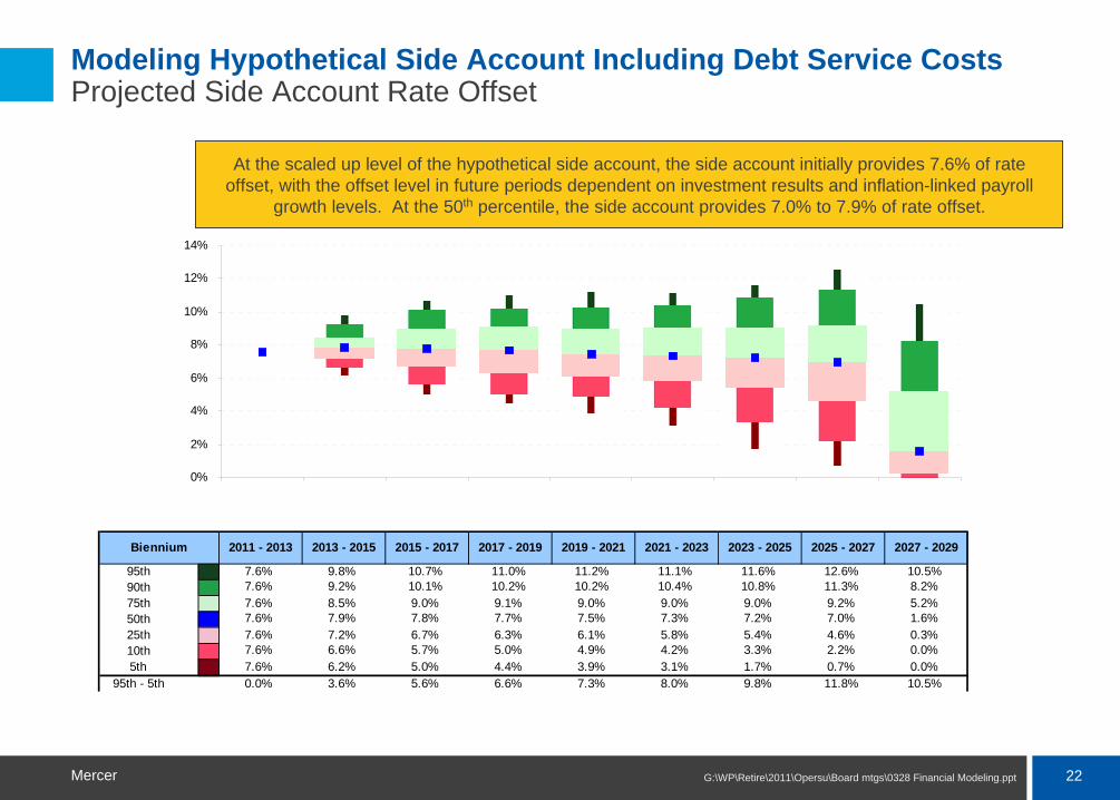
Modeling Hypothetical Side Account Including Debt Service Costs Projected Side Account Rate Offset

toptoptop

top

toptoptop

Biennium 2011 - 2013 2013 - 2015 2015 - 2017 2017 - 2019 2019 - 2021 2021 - 2023 2023 - 2025 2025 - 2027 2027 - 2029

5th 95th 7.6% 9.8% 10.7% 11.0% 11.2% 11.1% 11.6% 12.6% 10.5%90th 7.6% 9.2% 10.1% 10.2% 10.2% 10.4% 10.8% 11.3% 8.2%75th 7.6% 8.5% 9.0% 9.1% 9.0% 9.0% 9.0% 9.2% 5.2%50th 7.6% 7.9% 7.8% 7.7% 7.5% 7.3% 7.2% 7.0% 1.6%25th 7.6% 7.2% 6.7% 6.3% 6.1% 5.8% 5.4% 4.6% 0.3%10th 7.6% 6.6% 5.7% 5.0% 4.9% 4.2% 3.3% 2.2% 0.0%5th 7.6% 6.2% 5.0% 4.4% 3.9% 3.1% 1.7% 0.7% 0.0%

95th - 5th 0.0% 3.6% 5.6% 6.6% 7.3% 8.0% 9.8% 11.8% 10.5%

0%

2%

4%

6%

8%

10%

12%

14%

At the scaled up level of the hypothetical side account, the side account initially provides 7.6% of rate offset, with the offset level in future periods dependent on investment results and inflation-linked payroll

growth levels. At the 50th percentile, the side account provides 7.0% to 7.9% of rate offset.


Modeling Hypothetical Side Account Including Debt Service Costs Projected Pension Obligation Bond (POB) Repayment

toptoptop

top

toptoptop

Biennium 2011 - 2013 2013 - 2015 2015 - 2017 2017 - 2019 2019 - 2021 2021 - 2023 2023 - 2025 2025 - 2027 2027 - 2029

5th 95th 7.1% 7.5% 8.0% 8.3% 8.7% 9.0% 9.1% 9.3% 0.0%90th 7.0% 7.4% 7.8% 8.1% 8.3% 8.5% 8.7% 8.8% 0.0%75th 7.0% 7.2% 7.4% 7.6% 7.6% 7.7% 7.7% 7.6% 0.0%50th 6.9% 6.9% 7.0% 7.0% 6.9% 6.8% 6.7% 6.7% 0.0%25th 6.8% 6.7% 6.5% 6.3% 6.2% 6.0% 5.9% 5.7% 0.0%10th 6.7% 6.4% 6.1% 5.9% 5.6% 5.3% 5.1% 5.0% 0.0%5th 6.6% 6.2% 5.8% 5.4% 5.2% 4.9% 4.7% 4.5% 0.0%

95th - 5th 0.4% 1.3% 2.1% 2.9% 3.5% 4.1% 4.4% 4.8% 0.0%

0%

2%

4%

6%

8%

10%

The POB repayment schedule is established as annual fixed-dollar amounts. In future periods, the repayment level as a percentage of payroll depends on inflation-linked payroll growth levels. At the 50th

percentile, the repayment is 6.7% to 7.0% of annual pay.


Modeling Hypothetical Side Account Including Debt Service Costs Net* Rate + Pension Obligation Bond Repayment

toptoptop

top

toptoptop

Biennium 2011 - 2013 2013 - 2015 2015 - 2017 2017 - 2019 2019 - 2021 2021 - 2023 2023 - 2025 2025 - 2027 2027 - 2029


5th - 95th 0.4% 13.0% 23.5% 33.3% 37.0% 38.4% 40.3% 42.1% 45.3%

0%

5%

10%

15%

20%

25%

30%

35%

40%

45%

50%

Combining the net rate with the POB repayment schedule is an estimate of overall cost for employers with POBs

* Net rate excluding retiree healthcare component


Modeling Hypothetical Side Account Including Debt Service Costs Compare Base* Rate vs. Net* Rate + Pension Obligation Bond Repayment

toptoptop

top

toptoptop

Biennium

Base Net+POB Base Net+

POB Base Net+POB Base Net+



POB Base Net+POB

th 5th 15.6% 14.7% 21.6% 22.0% 29.9% 31.1% 38.1% 40.4% 41.3% 43.7% 42.4% 44.4% 43.8% 46.1% 44.3% 47.4% 46.2% 45.3%10th 15.6% 14.6% 21.6% 21.6% 28.9% 29.7% 34.4% 35.7% 35.3% 36.8% 37.0% 38.2% 38.2% 40.1% 39.6% 42.2% 40.4% 38.5%25th 15.6% 14.6% 21.0% 20.3% 25.6% 25.5% 27.0% 26.9% 28.5% 28.6% 30.0% 30.3% 30.3% 30.4% 31.2% 31.6% 30.7% 28.0%50th 15.6% 14.5% 18.7% 17.3% 20.5% 18.9% 20.7% 19.4% 21.8% 20.4% 21.3% 19.7% 20.6% 18.6% 20.3% 18.3% 20.4% 17.1%75th 15.6% 14.4% 17.4% 15.4% 16.0% 13.4% 15.8% 12.8% 14.9% 11.8% 14.2% 10.8% 13.3% 9.1% 12.3% 8.2% 11.0% 2.1%90th 15.6% 14.3% 14.2% 11.3% 13.2% 9.2% 11.9% 8.1% 10.2% 7.3% 8.7% 6.9% 6.6% 6.5% 4.7% 6.0% 2.7% 0.0%95th 15.6% 14.2% 12.3% 9.1% 11.3% 7.6% 9.6% 7.2% 7.8% 6.6% 4.5% 6.0% 1.8% 5.8% 0.9% 5.3% 0.5% 0.0%

5th - 95th 0.0% 0.4% 9.3% 13.0% 18.6% 23.5% 28.5% 33.3% 33.5% 37.0% 37.9% 38.4% 41.9% 40.3% 43.5% 42.1% 45.7% 45.3%

2011 - 2013 2013 - 2015 2015 - 2017 2017 - 2019 2027 - 20292019 - 2021 2021 - 2023 2023 - 2025 2025 - 2027

0%

5%

10%

15%

20%

25%

30%

35%

40%

45%

50%

This slide compares the “net rate plus POB” cost for the hypothetical bond to the “base rate” cost of no

side account and no POB

At the 50th and 75th percentiles, establishing a side account is forecast

to save money as assumptions are met or exceeded

In the 5th and 10th percentiles, where assumptions are not met,

establishing a side account is more expensive as side account

assets lose value

For most scenarios,

and especially

poor outlier scenarios,

the effect of the side

account is to increase rate

volatility

* Base rates and net rates excluding retiree healthcare component


Modeling Hypothetical Side Account Including Debt Service Costs Win/Lose Chart: Base Rate – (Net Rate + Pension Obligation Bond Repayment)

toptoptop

top

toptoptop

Biennium 2011 - 2013 2013 - 2015 2015 - 2017 2017 - 2019 2019 - 2021 2021 - 2023 2023 - 2025 2025 - 2027

5th 95th 1.3% 3.2% 4.0% 4.2% 4.4% 4.5% 4.8% 5.3%90th 1.3% 2.8% 3.6% 3.7% 3.8% 3.9% 4.2% 4.5%75th 1.2% 2.0% 2.5% 2.7% 2.7% 2.7% 2.9% 3.0%50th 1.1% 1.4% 1.4% 1.3% 1.1% 0.9% 1.0% 0.7%25th 1.0% 0.7% 0.2% (0.3%) (0.4%) (0.9%) (1.1%) (1.6%)10th 1.0% (0.0%) (1.1%) (1.9%) (2.1%) (2.7%) (3.4%) (4.5%)5th 0.9% (0.5%) (2.1%) (2.9%) (3.4%) (4.0%) (5.4%) (7.0%)

95th - 5th 0.4% 3.7% 6.1% 7.1% 7.8% 8.5% 10.2% 12.3%

(10%)

(5%)

0%

5%

10%

15%

For each contribution period modeled, this slide indicates the difference

between the “no side account” and “side account” costs

In the majority of scenarios, the net rate plus POB cost is less

than the base rate

The asymmetrical risk profile (downside risk is greater than upside reward) is due to very good scenarios with base rates low enough that the

maximum rate offset is limited

Net Rate +POB payments lower than Base Rates


Modeling Hypothetical Side Account Including Debt Service Costs Observations

Despite establishing a fixed schedule to pay a variable cost, creating a side account does not appear to trade “variable for fixed”– Instead, due to bond proceeds being invested in the trust, rate

volatility increases when a side account is created

In the majority of scenarios modeled, overall costs decrease when a side account is established– Lower cost scenarios occur when investments meet or exceed

assumption

In scenarios where investment results are the most poor, costs increase as an outcome of establishing a side account

Payment schedules or borrowing terms that differ significantly from the hypothetical POB could significantly affect analysis– For example, a “back loaded” debt payment schedule may lead to

early savings followed by likely higher costs in later years

Effect of Early-Year Returns on Cost Analysis


Effect of Early Year Returns on Cost Analysis Introduction

The prior section indicated that in over 50% of the scenarios the “side account plus pension obligation bond (POB)” approach had lower costs than the “pay the base rate” approach– This is unsurprising given the hypothetical POB’s cost structure and

the model’s expected investment return level on side accounts

The hypothetical POB’s fixed rate interest cost is 5.75% per year

The side account’s 50th percentile geometric average annualized investment return is 8.1% for 2011 to 2027

It would seem that if: – The side account’s average investment return over the POB’s debt

payment period exceeds– The POB’s interest rate, then– The “side account plus POB” approach will have lower costsThis is not always the case, however


Effect of Early Year Returns on Cost Analysis Hypothetical Bond Model

One reason for this is that early year side account investment returns carry greater weight than later year returns

– Even if the side account’s average investment return exceeds the bond’s cost rate over the debt payment period, the “side account plus POB” approach can be more costly if early returns are poor

To illustrate this phenomenon, we modeled the effect on the hypothetical bond from the prior section of side accounts underperforming compared to assumption during the initial three years of the bond (2011-2013)

– We used asset returns approximately equal to those experienced by the PERS regular account for the period 2008-2010

The cumulative three year return of -2.5% during that period is between a 10th and 25th percentile event in our financial model


Effect of Early Year Returns on Cost Analysis Assumed Regular Account Asset Returns – Geometric Average

toptoptop

top

toptoptop

2011 2012 2013 2014 2015 2016 2017 2018 2019 2020 2021 2022 2023 2024 2025 2026 2027 2028 20295th 95th (27.2%) (6.9%) (0.8%) 7.2% 9.4% 10.8% 11.0% 11.4% 11.4% 11.3% 10.8% 10.9% 11.0% 10.9% 10.8% 11.0% 10.8% 10.8% 10.7%

90th (27.2%) (6.9%) (0.8%) 5.9% 7.9% 9.0% 9.7% 9.8% 9.7% 9.9% 9.7% 9.7% 9.8% 9.8% 9.8% 9.9% 9.8% 9.8% 9.7%75th (27.2%) (6.9%) (0.8%) 3.8% 5.6% 6.4% 7.0% 7.5% 7.6% 7.7% 7.9% 8.0% 7.9% 7.9% 8.0% 8.1% 8.3% 8.3% 8.4%50th (27.2%) (6.9%) (0.8%) 1.6% 3.0% 3.5% 4.2% 4.8% 5.1% 5.4% 5.7% 6.0% 6.1% 6.2% 6.4% 6.6% 6.8% 6.9% 6.9%25th (27.2%) (6.9%) (0.8%) (1.2%) (0.2%) 0.7% 1.6% 1.9% 2.7% 3.3% 3.7% 4.0% 4.3% 4.6% 4.7% 4.9% 5.0% 5.3% 5.4%10th (27.2%) (6.9%) (0.8%) (3.9%) (2.7%) (2.2%) (1.2%) (0.1%) 0.6% 1.2% 1.7% 2.4% 2.7% 3.1% 3.2% 3.4% 3.6% 3.9% 4.2%5th (27.2%) (6.9%) (0.8%) (5.6%) (4.9%) (4.2%) (2.9%) (1.7%) (0.8%) (0.1%) 0.5% 1.1% 1.5% 2.0% 2.4% 2.8% 2.6% 3.0% 3.2%

95th - 5th 0.0% 0.0% 0.0% 12.8% 14.3% 15.0% 13.9% 13.1% 12.3% 11.4% 10.2% 9.8% 9.5% 8.9% 8.3% 8.2% 8.2% 7.8% 7.6%

For PYE 12/31

(30%)(25%)(20%)(15%)(10%)(5%)0%5%

10%15%20%25%30%35%

With the initial three years of side account returns set to parallel 2008-2010 returns, the average annualized investment return for the 2011-2027 debt repayment period is 6.8% at the 50th percentile, which is in excess of the 5.75% bond interest rate

The initial three years have a cumulative return of -2.5% and an

average annualized return of -0.8%


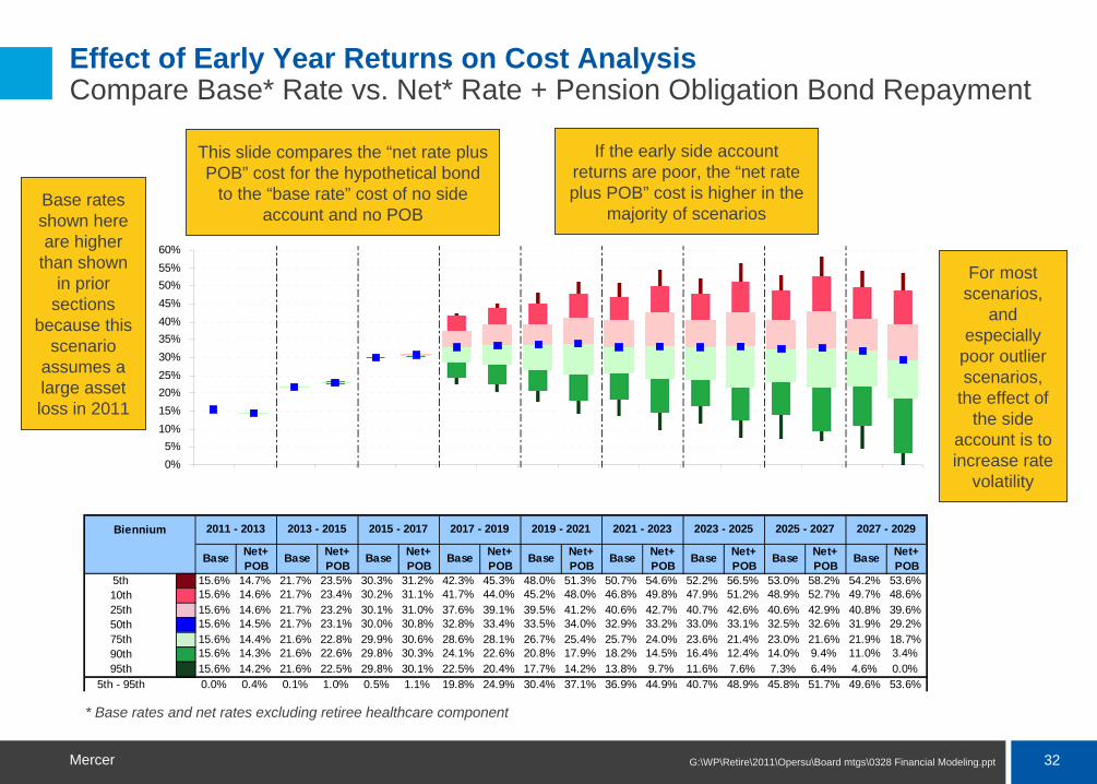
Effect of Early Year Returns on Cost Analysis Compare Base* Rate vs. Net* Rate + Pension Obligation Bond Repayment

This slide compares the “net rate plus POB” cost for the hypothetical bond

to the “base rate” cost of no side account and no POB

If the early side account returns are poor, the “net rate plus POB” cost is higher in the

majority of scenarios

For most scenarios,

and especially

poor outlier scenarios,

the effect of the side

account is to increase rate

volatility

* Base rates and net rates excluding retiree healthcare component

toptoptop

top

toptoptop

Biennium

Base Net+POB

Base Net+POB

Base Net+POB

Base Net+POB

Base Net+POB

Base Net+POB

Base Net+POB

Base Net+POB

Base Net+POB

th 5th 15.6% 14.7% 21.7% 23.5% 30.3% 31.2% 42.3% 45.3% 48.0% 51.3% 50.7% 54.6% 52.2% 56.5% 53.0% 58.2% 54.2% 53.6%10th 15.6% 14.6% 21.7% 23.4% 30.2% 31.1% 41.7% 44.0% 45.2% 48.0% 46.8% 49.8% 47.9% 51.2% 48.9% 52.7% 49.7% 48.6%25th 15.6% 14.6% 21.7% 23.2% 30.1% 31.0% 37.6% 39.1% 39.5% 41.2% 40.6% 42.7% 40.7% 42.6% 40.6% 42.9% 40.8% 39.6%50th 15.6% 14.5% 21.7% 23.1% 30.0% 30.8% 32.8% 33.4% 33.5% 34.0% 32.9% 33.2% 33.0% 33.1% 32.5% 32.6% 31.9% 29.2%75th 15.6% 14.4% 21.6% 22.8% 29.9% 30.6% 28.6% 28.1% 26.7% 25.4% 25.7% 24.0% 23.6% 21.4% 23.0% 21.6% 21.9% 18.7%90th 15.6% 14.3% 21.6% 22.6% 29.8% 30.3% 24.1% 22.6% 20.8% 17.9% 18.2% 14.5% 16.4% 12.4% 14.0% 9.4% 11.0% 3.4%95th 15.6% 14.2% 21.6% 22.5% 29.8% 30.1% 22.5% 20.4% 17.7% 14.2% 13.8% 9.7% 11.6% 7.6% 7.3% 6.4% 4.6% 0.0%

5th - 95th 0.0% 0.4% 0.1% 1.0% 0.5% 1.1% 19.8% 24.9% 30.4% 37.1% 36.9% 44.9% 40.7% 48.9% 45.8% 51.7% 49.6% 53.6%

2011 - 2013 2013 - 2015 2015 - 2017 2017 - 2019 2027 - 20292019 - 2021 2021 - 2023 2023 - 2025 2025 - 2027

0%5%

10%15%20%25%30%35%40%45%50%55%60%

Base rates shown here are higher

than shown in prior

sections because this

scenario assumes a large asset loss in 2011


toptoptop

top

toptoptop

Biennium 2011 - 2013 2013 - 2015 2015 - 2017 2017 - 2019 2019 - 2021 2021 - 2023 2023 - 2025 2025 - 2027

5th 95th 1.3% (0.8%) (0.1%) 2.1% 3.9% 4.0% 4.5% 4.7%90th 1.3% (0.9%) (0.3%) 1.4% 2.8% 3.2% 3.6% 3.5%75th 1.2% (1.1%) (0.5%) 0.5% 1.2% 1.6% 1.6% 1.5%50th 1.1% (1.4%) (0.8%) (0.5%) (0.4%) (0.3%) (0.4%) (0.5%)25th 1.0% (1.6%) (1.0%) (1.4%) (1.8%) (2.0%) (2.1%) (2.6%)10th 1.0% (1.8%) (1.2%) (2.4%) (2.9%) (3.2%) (3.7%) (4.4%)5th 0.9% (1.8%) (1.3%) (3.0%) (3.6%) (4.3%) (4.7%) (5.9%)

95th - 5th 0.4% 1.1% 1.2% 5.1% 7.5% 8.3% 9.2% 10.5%

(10%)

(5%)

0%

5%

10%

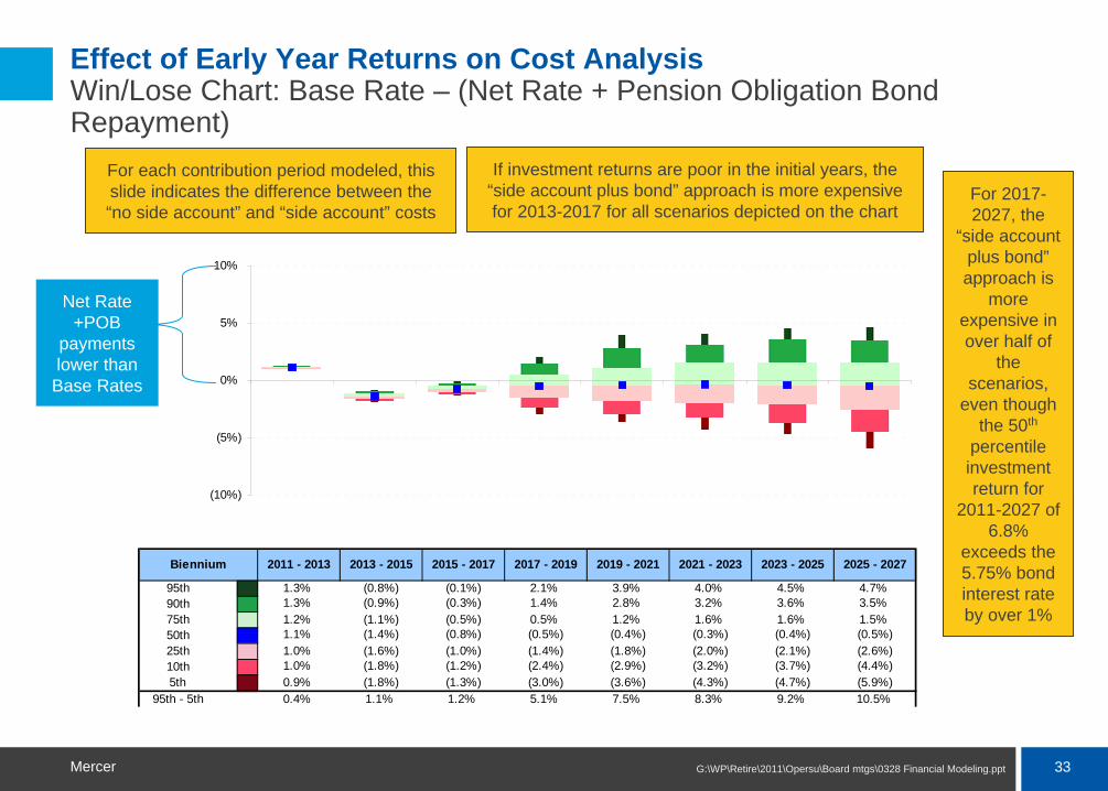
Effect of Early Year Returns on Cost Analysis Win/Lose Chart: Base Rate – (Net Rate + Pension Obligation Bond Repayment)

For each contribution period modeled, this slide indicates the difference between the “no side account” and “side account” costs

If investment returns are poor in the initial years, the “side account plus bond” approach is more expensive for 2013-2017 for all scenarios depicted on the chart

Net Rate +POB

payments lower than

Base Rates

For 2017- 2027, the

“side account plus bond” approach is

more expensive in over half of

the scenarios,

even though the 50th

percentile investment return for

2011-2027 of 6.8%

exceeds the 5.75% bond interest rate by over 1%


Effect of Early Year Returns on Cost Analysis Observations

Even if side account investment earnings average in excess of the bond interest rate, it is possible for the side account approach to be more expensive

– This can occur if early year investment returns are poor

– Because the side account is depleted steadily over time via rate offset transfers, strong later year returns may not be able to restore the side account approach to a net cost savings position

The early year returns of side accounts determine the long-term win/lose profile of a side account

– In essence, if market conditions deviate significantly from the assumption in early years the long-term win/lose prospects may become firmly established


Wrap-Up/Forward Looking Calendar

Questions or comments on today’s presentation?

Upcoming actuarial calendar

– May Board meeting

Review of economic assumptions and actuarial methods

– July Board meeting

Review of demographic assumptions

Board approval of all assumptions and methods

– September Board meeting

Presentation of summary 12/31/2010 actuarial valuation results

Appendix


Mercer has prepared this report exclusively for the Oregon PERS Board; Mercer is not responsible for reliance upon this report by any other party. The only purposes of this report are to present Mercer’s actuarial estimates of the system’s contributions rates and funded status under a limited set of assumptions. This report may not be used for any other purpose; Mercer is not responsible for the consequences of any unauthorized use.

Decisions about benefit changes, granting new benefits, investment policy, funding policy, benefit security and/or benefit- related issues should not be made on the basis of this report, but only after careful consideration of alternative economic, financial, demographic and societal factors, including financial scenarios that assume future sustained investment losses.

The Oregon Investment Council (OIC) is solely responsible for selecting the plan’s investment policies, asset allocations and individual investments of the Oregon PERS program. Mercer’s actuaries have not provided any investment advice to Oregon PERS or OIC.

A valuation report is only a snapshot of a Plan’s estimated financial condition at a particular point in time; it does not predict the Plan’s future financial condition or its ability to pay benefits in the future and does not provide any guarantee of future financial soundness of the Plan. Over time, a plan’s total cost will depend on a number of factors, including the amount of benefits the plan pays, the number of people paid benefits, the period of time over which benefits are paid, plan expenses and the amount earned on any assets invested to pay benefits. These amounts and other variables are uncertain and unknowable at the valuation date

Because modeling all aspects of a situation is not possible or practical, we may use summary information, estimates, or simplifications of calculations to facilitate the modeling of future events in an efficient and cost-effective manner. We may also exclude factors or data that are immaterial in our judgment. Use of such simplifying techniques does not, in our judgment, affect the reasonableness of valuation results for the plan.

To prepare the valuation report, actuarial assumptions, as described in the actuarial valuation report as of December 31, 2009, for Oregon PERS are used in a forward looking financial and demographic model to select a single scenario from a wide range of possibilities; the results based on that single scenario are included in the valuation. The future is uncertain and the plan’s actual experience will differ from those assumptions; these differences may be significant or material because these results are very sensitive to the assumptions made and, in some cases, to the interaction between the assumptions.

Appendix Important Notices


Different assumptions or scenarios within the range of possibilities may also be reasonable and results based on those assumptions would be different. As a result of the uncertainty inherent in a forward looking projection over a very long period of time, no one projection is uniquely “correct” and many alternative projections of the future could also be regarded as reasonable. Two different actuaries could, quite reasonably, arrive at different results based on the same data and different views of the future. A "sensitivity analysis" shows the degree to which results would be different if you substitute alternative assumptions within the range of possibilities for those utilized in this report. This report displays a limited-scope sensitivity analysis of alternate possible economic scenarios only, as detailed in this report. At Oregon PERS request, Mercer is available to perform additional sensitivity analyses.

Actuarial assumptions may also be changed from one valuation to the next because of changes in mandated requirements, plan experience, changes in expectations about the future and other factors. A change in assumptions is not an indication that prior assumptions were unreasonable when made.

The calculation of actuarial liabilities for valuation purposes is based on a current estimate of future benefit payments. The calculation includes a computation of the "present value" of those estimated future benefit payments using an assumed discount rate; the higher the discount rate assumption, the lower the estimated liability will be. For purposes of estimating the liabilities (future and accrued) in this report, Oregon PERS selected an assumption based on the expected long term rate of return on plan investments. Using a lower discount rate assumption, such as a rate based on long-term bond yields, could substantially increase the estimated present value of future and accrued liabilities.

Because valuations are a snapshot in time and are based on estimates and assumptions that are not precise and will differ from actual experience, contribution calculations are inherently imprecise. There is no uniquely “correct” level of contributions for the coming plan year.

Valuations do not affect the ultimate cost of the Plan. Plan funding occurs over time. Contributions not made this year, for whatever reason, including errors, remain the responsibility of the Plan sponsor and can be made in later years. If the contribution levels over a period of years are lower or higher than necessary, it is normal and expected practice for adjustments to be made to future contribution levels to take account of this with a view to funding the plan over time.




Data, computer coding and mathematical errors are possible in the preparation of a valuation involving complex computer programming and thousands of calculations and data inputs. Errors in a valuation discovered after its preparation may be corrected by amendment to the valuation or in a subsequent year’s valuation.

To prepare this report, Mercer has used and relied on member and financial data submitted by the Oregon Public Employees Retirement System as summarized in the December 31, 2009 actuarial valuation report and on investment return information as published by Oregon PERS and Oregon Investment Council (OIC). Oregon PERS is responsible for ensuring that such participant data provides an accurate description of all persons who are participants under the terms of the plan or otherwise entitled to benefits as of December 31, 2009, that is sufficiently comprehensive and accurate for the purposes of this report. Although Mercer has reviewed the data in accordance with Actuarial Standards of Practice No. 23, Mercer has not verified or audited any of the data or information provided.

Mercer has also used and relied on the plan provisions described in Oregon Revised Statutes Sections 238 and 238A and legislative amendments supplied by Oregon PERS. A summary of the plan provisions valued is presented in our report. Oregon PERS is solely responsible for the accuracy, validity and comprehensiveness of this information. If the data or plan provisions supplied are not accurate and complete the valuation results may differ significantly from the results that would be obtained with accurate and complete information; this may require a later revision of this report. Moreover, plan documents may be susceptible to different interpretations, each of which could be reasonable, and that the different interpretations could lead to different valuation results.

Assumptions used are based on the last experience study, as adopted by the Board on July 16, 2009. The Board is responsible for selecting the plan’s funding policy, actuarial valuation methods, asset valuation methods and assumptions. This valuation is based on assumptions, plan provisions, methods and other parameters so prescribed and as summarized in this report. Oregon PERS is solely responsible for communicating to Mercer any changes required thereto.



Professional Qualifications

We are available to answer any questions on the material in this report or to provide explanations or further details as appropriate. The undersigned credentialed actuaries meet the Qualification Standards of the American Academy of Actuaries to render the actuarial opinion contained in this report. We are not aware of any direct or material indirect financial interest or relationship, including investments or other services that could create a conflict of interest, that would impair the objectivity of our work. We are available to answer any questions on the material contained in the report, or to provide explanations or further details as may be appropriate.

The information contained in this document is not intended by Mercer to be used, and it cannot be used, for the purpose of avoiding penalties under the Internal Revenue Code that may be imposed on the taxpayer.

Matthew R. Larrabee, FSA, EA, MAAA Enrolled Actuary No. 08-6154

Date Scott D. Preppernau, FSA, EA, MAAA Enrolled Actuary No. 08-7360

Date

Mercer (US), Inc.111 SW Columbia Street, Suite 500Portland, OR 97201-5839503 273 5900

March 28, 2011 March 28, 2011


Appendix Actuarial Basis

DataWe have based our projection of the liabilities on the data, methods, assumptions and plan provisions described in the December 31, 2009, Actuarial Valuation (“2009 Valuation Report”) for the Oregon Public Employees Retirement System.

Assets as of December 31, 2010, were based on values provided by Oregon PERS reflecting the Board’s preliminary earnings crediting decisions for 2010.

We have assumed that the active participant data reflected in the valuation of the Plan remains stable over the projection period (i.e. – participants leaving employment are replaced by new hires in such a way that the total counts, average age, and average service remain stable from year to year). No new members are assumed to be eligible for Tier 1 and Tier 2 benefits; all new entrants are assumed to become members under the OPSRP benefit formula.

Methods / PoliciesLiabilities are based on the Projected Unit Credit method and are rolled forward according to the following rules:

Normal cost: Normal cost increases with assumed wage growth adjusted for wage experience, demographic experience and asset return experience (if applicable). Demographic experience follows assumptions described in the Valuation Report.

Accrued liability: Liabilities increase with normal cost and decrease with benefit payments. Results are adjusted for wage, demographic and asset experience (if applicable).

Contribution Rates: The projected contribution rates are calculated on each odd valuation date in accordance with methodologies described in the Valuation Report. Rates are applied 18 months after the determination date.

Expenses: OPSRP administration expenses are assumed to be equal to $6.6M and are added to the OPSRP normal cost.

Actuarial Value of Assets: Equal to Market Value of Assets excluding Contingency and Tier 1 Rate Guarantee Reserves, when such reserves are individually greater than zero


Appendix Actuarial BasisInvestment Policy General Accounts were assumed to be invested as follows: 46% Global Equity; 11% Real Estate; 16% Private Equity; 27% Fixed Income, in accordance with the Oregon Investment Council “Statement of Investment Objectives and Policy Framework for the Oregon Public Employees Retirement Fund” dated December 1, 2010.

Variable Accounts were assumed to be invested in 100% Global Equity.

AssumptionsIn general, all assumptions are as described in the Valuation Report.

The major assumptions used in our projections are shown below. They are aggregate average assumptions that apply to the whole population and were held constant throughout the projection period. The economic experience adjustments were allowed to vary in future years given the conditions defined in each economic scenario.

– Valuation interest rate — 8.00%– General Accounts Growth — 8.00%– Variable Account Growth — 8.50%– Wage growth assumption — 3.75%– Wage growth experience — inflation + 1.25%– Demographic experience — reflects decrement assumptions as described in the Valuation Report.– Actual Investment earnings are based on Mercer’s Capital Market Outlook reflecting actual market experience through January 1,

2011.

Reserve ProjectionsContingency Reserve as of 12/31/2010 was estimated to be $734.4M. No future increases or decreases from this reserve were assumed.

Tier 1 Rate Guarantee Reserve (“T1RGR”) was estimated to be $-207.8M as of 12/31/2010. The reserve was assumed to grow with returns in excess of 8% on Tier 1 Member Accounts plus T1RGR. When aggregate returns were below 8%, applicable amounts from the T1RGR were transferred to the Tier 1 Member Accounts to maintain the 8% target growth on the member accounts. The T1RGR reserve was allowed to go negative, but the reserve is not excluded from valuation assets when it is negative.


Appendix Actuarial Basis

AssumptionsAssumptions for valuation calculations are as described in the 2009 Valuation Report.

ProvisionsProvisions valued are as detailed in the 2009 Valuation Report.

Arken and Robinson LitigationWe have made no adjustment to these valuation results to reflect any interpretation of Judge Kantor’s rulings in the Arken and Robinson cases.


Appendix Assumed Regular Account Asset Returns – Geometric Average

toptoptop

top

toptoptop

2011 2012 2013 2014 2015 2016 2017 2018 2019 2020 2021 2022 2023 2024 2025 2026 2027 2028 20295th 95th 30.0% 22.8% 18.7% 16.5% 15.3% 14.3% 14.2% 13.8% 13.5% 13.0% 12.6% 12.2% 12.1% 12.0% 11.8% 11.8% 11.7% 11.5% 11.3%

90th 24.4% 19.9% 16.4% 14.4% 13.6% 13.0% 12.8% 12.3% 12.1% 11.7% 11.5% 11.3% 11.3% 11.2% 11.0% 10.9% 10.8% 10.8% 10.7%75th 14.5% 12.9% 11.8% 11.3% 10.9% 10.6% 10.4% 10.1% 9.9% 9.8% 9.9% 9.8% 9.7% 9.7% 9.5% 9.5% 9.6% 9.5% 9.5%50th 7.5% 7.4% 7.5% 7.3% 7.5% 7.4% 7.5% 7.6% 7.8% 8.0% 8.1% 8.2% 8.1% 8.0% 8.0% 8.1% 8.1% 8.2% 8.2%25th (1.2%) 1.4% 2.7% 3.5% 4.3% 4.6% 5.0% 5.3% 5.6% 5.9% 6.0% 6.1% 6.1% 6.4% 6.6% 6.6% 6.7% 6.8% 6.7%10th (9.2%) (5.0%) (2.7%) (1.1%) 0.3% 1.5% 2.3% 3.0% 3.5% 3.9% 4.1% 4.4% 4.7% 4.9% 5.0% 5.2% 5.1% 5.5% 5.5%5th (14.3%) (10.0%) (6.3%) (4.7%) (2.4%) (0.7%) 0.3% 1.5% 2.0% 2.7% 2.9% 3.4% 3.6% 3.9% 3.9% 4.2% 4.2% 4.6% 4.6%

95th - 5th 44.3% 32.8% 25.0% 21.2% 17.6% 15.0% 13.9% 12.3% 11.5% 10.2% 9.7% 8.8% 8.5% 8.1% 7.9% 7.7% 7.5% 6.9% 6.7%

For PYE 12/31

(15%)

(10%)

(5%)

0%

5%

10%

15%

20%

25%

30%

35%


Appendix Baseline Projected Side Account Balance

toptoptop

top

toptoptop

($millions)2010 2011 2012 2013 2014 2015 2016 2017 2018 2019 2020 2021 2022 2023 2024 2025 2026 2027 2028 2029

5t 95th 5,580 6,740 7,292 7,532 7,588 7,784 7,726 7,823 7,930 7,927 7,623 7,272 7,097 6,743 6,353 6,347 6,356 6,820 6,927 6,85690th 5,580 6,423 6,949 7,037 7,055 7,071 7,054 7,128 6,953 6,766 6,493 6,176 5,773 5,205 4,744 4,214 3,513 3,032 2,492 2,18675th 5,580 5,876 6,073 6,114 6,202 6,112 6,019 5,876 5,661 5,421 5,069 4,868 4,349 3,852 3,242 2,573 1,751 802 97 950th 5,580 5,483 5,384 5,334 5,199 5,083 4,889 4,647 4,475 4,313 4,083 3,746 3,324 2,879 2,332 1,685 999 216 13 025th 5,580 4,995 4,764 4,502 4,363 4,141 3,959 3,760 3,525 3,306 3,058 2,739 2,366 1,969 1,525 1,029 435 29 0 010th 5,580 4,549 4,056 3,746 3,472 3,215 3,125 2,922 2,804 2,551 2,282 2,032 1,726 1,385 1,024 551 124 0 0 05th 5,580 4,266 3,584 3,242 2,849 2,737 2,599 2,361 2,296 2,112 1,895 1,583 1,306 1,048 721 347 39 0 0 0

95th - 5th 0 2,474 3,708 4,290 4,739 5,047 5,126 5,462 5,634 5,815 5,728 5,689 5,791 5,694 5,632 5,999 6,317 6,820 6,927 6,856Variable 122

PY Ending 12/31

0

1,000

2,000

3,000

4,000

5,000

6,000

7,000

8,000

9,000


Appendix Baseline Combined (Tier 1/Tier 2, OPSRP) Funded Status (Including Side Accounts)

toptoptop

top

toptoptop

2010 2011 2012 2013 2014 2015 2016 2017 2018 2019 2020 2021 2022 2023 2024 2025 2026 2027 2028 20295th 95th 88% 105% 112% 115% 117% 121% 125% 130% 133% 137% 139% 142% 144% 145% 148% 151% 157% 159% 163% 166%

90th 88% 101% 108% 109% 111% 113% 115% 119% 120% 123% 126% 127% 129% 130% 135% 136% 140% 142% 146% 148%75th 88% 93% 96% 97% 100% 100% 101% 102% 103% 104% 104% 108% 109% 110% 111% 112% 114% 118% 122% 123%50th 88% 88% 87% 86% 86% 86% 85% 85% 85% 87% 89% 89% 91% 91% 91% 92% 94% 95% 97% 100%25th 88% 80% 77% 74% 73% 71% 71% 70% 71% 71% 72% 72% 72% 72% 73% 75% 74% 76% 78% 81%10th 88% 73% 66% 62% 59% 57% 58% 58% 58% 58% 57% 57% 59% 59% 59% 59% 61% 61% 64% 63%5th 88% 69% 59% 54% 49% 50% 50% 49% 50% 49% 51% 49% 51% 52% 51% 51% 53% 49% 52% 56%

95th - 5th 0% 36% 53% 61% 68% 71% 76% 81% 84% 88% 88% 92% 92% 94% 97% 100% 104% 110% 110% 111%Variable 172

PY Ending 12/31

0%

20%

40%

60%

80%

100%

120%

140%

160%

180%


Appendix Stochastic Modeling

Stochastic (Monte Carlo) Modeling

– In order to understand the range of outcomes, we employ an economic model of capital markets in which we focus on the three fundamental factors – growth, inflation, and interest rates – that drive capital markets.

– Thus, if interest rates rise due to inflation, we utilize the same rise in inflation and interest rates in order to calculate returns on bonds and to determine if the discount rate is reasonable.

– Stochastic modeling is used to help assign probabilities to the various market environments.

– Our capital market assumptions represent general future expectations and significant volatility around those expectations.


Appendix Capital Market Assumptions

Mercer’s Methodology:– Mercer’s stochastic model is based on a 7 state regime-switching Monte

Carle simulation. – This technique generates 1,000 economic trials with each trial producing

projected results for each year over the selected planning horizon. – Each state or regime has a defined set of means, volatilities, reversion

coefficients and correlation assumptions.– We define a probability transition matrix for achieving each regime given

the past state-of-the-world. – We adjust the Base Case state (described on next slide) so that the

median results across all trials produce inflation and growth that correspond to our long run projections. Essentially, this becomes a recentering state because in the other six states there are more negative than positive states. Properly speaking, this state should be labeled “Optimistic Normal”, since we generally have to lower inflation, raise growth, and lower credit spreads to more optimistic conditions (but not quite as high as Ideal Growth).


Appendix Capital Market Assumptions

Mercer’s Methodology (continued):– We define the seven possible states (or regimes) of the world as:

Base Case: Inflation, growth, and equity returns hover around their long term expected values. (Inflation is 2.8%, growth is 3.1%, and equity returns are in the low 8.0% range.) Bond yields adjust from their current conditions to their long run values over a period of three to five years. This path of interest rates then determines bond returns.

- Since the Treasury curve in the US is quite steep with very low short rates, this Base Case scenario has low bond returns initially and then returns in the 5.0% to 5.5% range once the adjustment of interest rates is finished.

Recession: This is a “classical recession”, not a severe credit crunch or depression. In the recession scenario, inflation is quite low, but not negative, while growth dips below zero. Treasury yields decline sharply, but T-Bills do not approach zero. Credit spreads widen and the equity returns are low because of a decline in earnings and drop in the P/E level.

Stagflation: Inflation rises to around 6.0% and growth stalls to 1.0% (but is not necessarily negative). The Treasury yield curve flattens at about 7.0% to 7.5%. Equity returns are weak, because the P/E level drops. Credit spreads widen, but not to recession levels.

Inflationary growth: Inflation rises to 6.0% and economic growth is very strong at 4.5%. Treasury yields rise to the 8.0% level. The P/E level of the market rises slightly, producing returns consistently in the 10% range.

Ideal Growth: Inflation falls to 0.5%, economic growth booms at 6%. Treasury yields stay near our long run projected curve, producing very high real yields. P/E level soars, producing equity returns in the teens. If this regime persists for a few years, equity returns drop back down to the 8.0% level, which means that real returns are still quite high, in the 7.5% range.

High Inflation: Inflation rises to 10%, economic growth is below average at 2.5%. Treasury yields rise to 10% to 11%, credit spreads widen slightly. Equity returns are depressed as the P/E level falls.

Credit Crunch/Depression: This is modeled after the events of 2008. Inflation and economic growth are both negative (around -1.5% to -2.0%). Credit spreads soar, treasury yields decline sharply and T-Bill yields approach zero. The P/E level of the market declines sharply.


Appendix Capital Market Assumptions - Base Case State Modeling Parameters

Based on Mercer’s December 2010 Capital Market Outlook

Correlation Matrix

Count 1 2 3 4 51 Global All Cap Unhedged 10.00% 8.33% 19.40% 1.00 0.09 0.62 0.40 0.652 Fixed Income-Aggregate 4.70% 4.53% 6.00% 0.09 1.00 0.50 0.25 0.203 Fixed Income-High Yield 6.40% 5.89% 10.50% 0.62 0.50 1.00 0.35 0.404 Real Estate-Core 8.20% 7.11% 15.49% 0.40 0.25 0.35 1.00 0.505 Private Equity-Total 13.40% 9.17% 31.86% 0.65 0.20 0.40 0.50 1.00

Annual Standard Deviation

Asset Class NameArithmetic Expected

Annual Return

Geometric Annual Return

Equivalent


Step 1. Generate

Inflation

Economic growth

Step 2. Generate

Nominal yield curve

Real yield curve

Equity yields, dividend yields

Corporate bond spreads

Step 3. Determine changein exchange rates

Step 4. Compute

Bond returns

Equity returns

Step 5. Determine Int’l returns

Inflation

Economic & Earnings Growth

Corporate Bond Defaults

Nominal Yields

Real Yields

Corporate Bonds Spreads

Equity Yields

Dividend Yields

Bond Returns

Equity Returns

Wage Growth

Inflation

Bond Returns

Equity Returns

Wage Growth

Exchange Rate

International Returns

Nominal Yields

Real Yields

Corporate Bonds Spreads

Equity Yields

Dividend Yields

United States Europe

Regional Correlation

Economic & Earnings Growth

Corporate Bond Defaults

Appendix Investment Strategy - Capital Market Simulator


1998 2000 2002 2004 2006 2008 2010 2012 2014 2016 2018

1998 2000 2002 2004 2006 2008 2010 2012 2014 2016 2018

1998 2000 2002 2004 2006 2008 2010 2012 2014 2016 2018

inferior

bad

goodsuperior

Lines between regions95th Percentile75th Percentile50th Percentile (Median)25th Percentile 5th Percentile

Results are calculated for one path of the stochastic model

This is repeated 1000 times

Each year is percentiled

The percentiles group each years’ results into regions

The good and bad regions represent 25% variance from median results, or together what would be expected half of the time

The superior and inferior regions add another 20% of upside and downside variance

All the regions combined show 90% of simulated results

AppendixModeling Parameters and Assumptions Simulation Framework – Unfunded Liabilities Illustrated


The line chart is potentially confusing because it might appear that the 75th percentile (for example) is generated by the same simulated path over time.

In fact, any given simulated path could vary between regions over time

In any year, we can represent the key percentile values with “candlesticks”, which remove the implied connection between percentiles over time.

AppendixPresenting Results - Stochastic percentiles

1998 2000 2002 2004 2006 2008 2010 2012 2014 2016 2018

inferior

bad

goodsuperior

Lines between regions95th Percentile75th Percentile50th Percentile (Median)25th Percentile

5th Percentile

1998 2000 2002 2004 2006 2008 2010 2012 2014 2016 2018

inferior

bad

goodsuperior

Lines between regions95th Percentile75th Percentile50th Percentile (Median)25th Percentile

5th Percentile

1998 2000 2002 2004 2006 2008 2010 2012 2014 2016 2018

95% Percentile

75% Percentile50% Percentile25% Percentile

5% Percentile

50% Percentile

www.mercer.com

oregon pers financial modelingg:\wp\retire\2011\opersu\board mtgs\0328 financial modeling.ppt. 1....

Documents