oregon state bank analysis -...

Oregon State Bank Analysis ‐ Revised Center for State Innovation – December 2010

In the wake of the financial market collapse of 2009, banks sharply curtailed their lending. Bank lending in 2009 declined more sharply than in any year since 1942, according to FDIC data.1 This drop‐off was particularly pronounced for the largest Wall Street banks; in Oregon, for instance, Bank of America SBA loans dropped from 555 in 2007 to 19 in 2009. Overall, lending through the Small Business Administration’s flagship 7(a) program in Oregon declined 35% between 2007 and 2009. This, in turn, has been one driver of current massive and continued unemployment. The reduction in lending has led policymakers to consider a number of reforms designed to increase bank lending, particularly to small businesses which have been the hardest hit by tightening credit standards. One such measure that has drawn increasing interest is the creation of a state bank modeled after the Bank of North Dakota (BND), currently the only such state bank in the country, to increase liquidity and spur lending and development in a given state. This paper offers some predictions about the effect of a proposed Oregon State Bank (OSB) on the state banking industry, job creation and small businesses, and the state budget. While the sample size of one makes it difficult to accurately predict a public bank’s effect on any given state, we have used FDIC bank data and some conservative assumptions to estimate the effects of a BND‐like bank in Oregon. Highlights include:

Estimated Effect on OR Small Business Loans and Jobs From an 8.2% Increase in Average Loans due to State Bank

Increased Amount of Small Business Loans $328,669,550

Small Business Jobs Created or Retained 5,391

• Job Creation/Retention. We estimate that a state bank could help create or retain 6,900‐8,800 additional small business jobs in Oregon, and that about 5,400 jobs would have been supported due to increased loan activity through bank participation loans from a state bank at full lending capacity.

• New Lending. BND helped to sustain a loan to asset ratio for North Dakota banks – a key measure of direct economic impact – by mitigating the effects of the recession on lending, resulting in reductions of 33%‐45% less than comparable states. In Oregon, this would have resulted in roughly 6.75 to 8.60 percentage points greater loan to asset ratios during the current economic downturn. We also estimate that a state bank in Oregon could generate roughly 8.2% or about $1.3B in new lending activity due to bank participation loans.

• New Revenue. An Oregon State Bank could generate dividends for the state starting in year 2, and a bank capitalized at $100M—and conservatively run—could pay total accumulated dividends to the state’s General Fund or Rainy Day Fund of $69M after 10 years, $234M after 20 years, $611M after 30 years, and $1.3B after 40 years.

• Return on Equity. An Oregon State Bank would have a positive Return on Equity (ROE) of real profits to the state within 3 years with prudent banking practices.

• Other Economic Impacts. The actual effect of a state bank on the state economy and job market would likely be greater than the above estimates, since this analysis does not look at non‐small business lending, nor does it try to account for the indirect and induced economic impacts of increased lending.

1 “Lending Falls at Epic Pace,” Wall Street Journal, 2/24/10

Center for State Innovation – Revised Oregon State Bank Analysis – December 2010 2

I. Introduction This analysis takes a look at the effect a state bank might have on the state banking industry by helping to provide liquidity and stability, using lending rates as a rough proxy for this effect. Part II compares lending rates in North Dakota small and medium sized banks with the equivalent banks in the comparable states (based on geography, population size and density) of Montana, South Dakota, and Wyoming and finds that loan to asset ratios in North Dakota have averaged over 7 percentage points greater than these states over the period 2005‐2009 (so, including years both pre‐ and post‐financial collapse). During the current recession (which started in the 4th quarter of 2007), with the help of BND, North Dakota banks have had the least reduction in loan to asset ratios, compared to neighboring states. This, along with other supporting data, suggests that the Bank of North Dakota has helped to raise and sustain the lending market in North Dakota. We also estimate increased lending due to a state bank based on the amount of participation loans undertaken by the BND. Part III attempts to provide a rough measurement of the effects of this increase in lending rates on state job creation/retention. We estimate that for every 1 percentage point increase (or sustained) loan to asset ratio in the lending market for small and medium sized banks in Oregon, about 1,000 small business jobs in Oregon are created or retained. Parts IV & V look at bank ROA and other financials for four likely sources of bank start‐up capital: (1) General Fund Revenue, (2) General Obligation Bond w/20yr maturity payment, (3) General Obligation Bond w/sinking fund, and (4) Bank Stock IPO. It estimates the returns to both the state bank and to the state itself. State Banks, Generally It seems first useful to start with some general description of state banks for those who are new to the idea. A state bank is in essence a simple concept—simply put, it is a bank capitalized by state money, that would serve as the repository for state deposits, and would be publicly governed and return a negotiated portion of bank profits to the state. Apart from that, it would operate much as any private bank, though deposits would be guaranteed by the state rather than the FDIC. Currently, only one state has a public state bank—the Bank of North Dakota. The Bank of North Dakota was formed in 1919 in response to the farm crisis and tightening of credit after the First World War In North Dakota, all state funds (state tax collections and fees, and for all funds of state institutions) are deposited with the Bank of North Dakota. This does not include pension funds or other trusts managed by the state; rather the deposits are the state’s cash – revenue that the state collects before it is spent on payroll, contracts, procurement, etc. Non‐state deposits (10‐20% of total in the case of the BND) could be accepted from other sources, from private citizens (who account for less than 2% of total deposits for BND) to the U.S. government. The Bank of North Dakota is governed by the state Industrial Commission, made up of the Governor, Attorney General and Commissioner of Agriculture. A seven‐member Advisory Board, appointed by the Governor, reviews the Bank's operations and makes recommendations to the Industrial Commission relating to the Bank's management, services, policies and procedures The Bank of North Dakota and, we assume, any state bank, would have a limited portfolio; in that way it is somewhat different than most private banks. One primary activity of the BND is participation lending, participating in loans originated by local banks and credit unions, either by increasing the total size of the loan, buying down the interest rate, or providing loan guarantees. It also performs other banker’s bank functions, including check clearing, bond accounting


safekeeping, and providing fed funds lines with excess liquidity. The bank is a participant in the secondary market for residential loans, and also a direct lender for student loans for North Dakotans, thereby decreasing rates, though new student loan origination will decrease markedly due to the recent federal reforms of the student loan market.2 Finally, the bank can make capital available to local banks via direct bank stock lending, as well as by purchasing loans from their portfolios. The BND also has a couple of specific lending programs that make low‐interest loans available to, for instance, agricultural start‐ups and new small businesses. In this way, it leverages the income earned through more lucrative market‐driven activities to subsidize economic development activities that may carry somewhat higher risks or where borrowers have difficulty accessing capital. Finally, a state bank typically returns a portion of its profits to the state General Fund or Rainy Day Fund. In the case of the BND, the size of this “state dividend,” explained in more detail below, is set by negotiation between the Legislature and the bank’s Governing Board. The amount has varied from year to year (from as little as 0 in some years to up to $50 million in others), but over the past 10 years has averaged $29.4 million (about 72% of bank profits) and totaled almost $300 million.

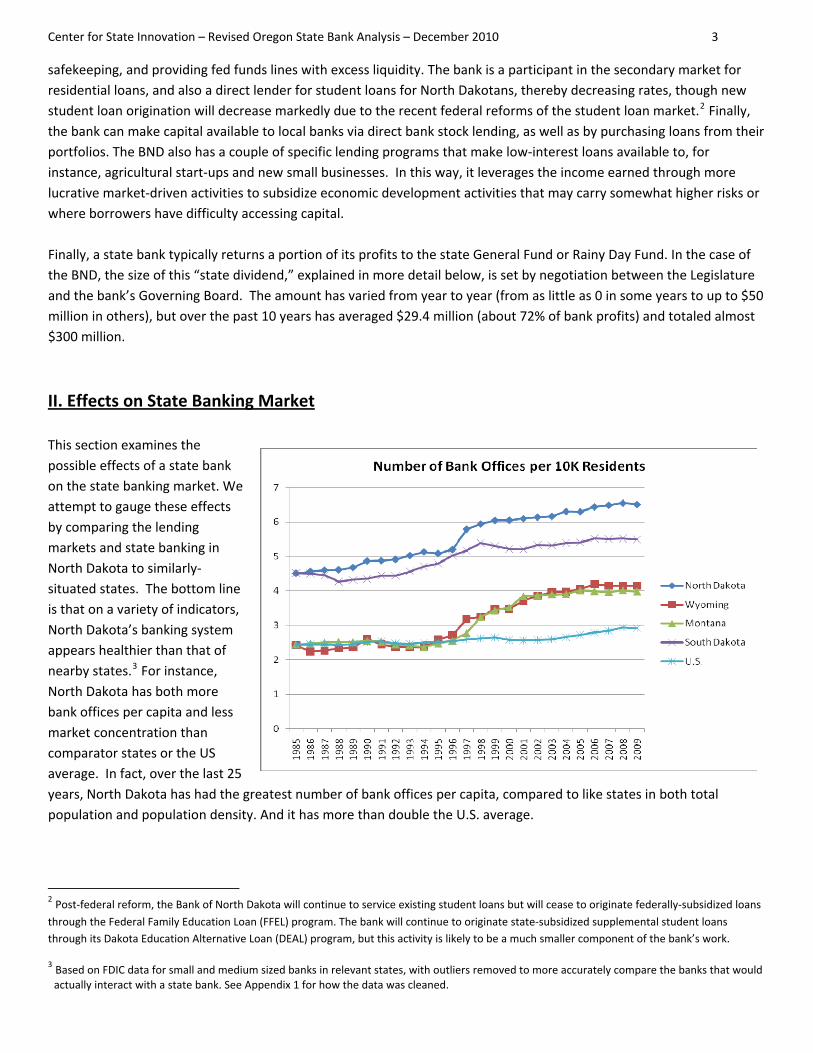
II. Effects on State Banking Market This section examines the possible effects of a state bank on the state banking market. We attempt to gauge these effects by comparing the lending markets and state banking in North Dakota to similarly‐situated states. The bottom line is that on a variety of indicators, North Dakota’s banking system appears healthier than that of nearby states.3 For instance, North Dakota has both more bank offices per capita and less market concentration than comparator states or the US average. In fact, over the last 25 years, North Dakota has had the greatest number of bank offices per capita, compared to like states in both total population and population density. And it has more than double the U.S. average.

2 Post‐federal reform, the Bank of North Dakota will continue to service existing student loans but will cease to originate federally‐subsidized loans

through the Federal Family Education Loan (FFEL) program. The bank will continue to originate state‐subsidized supplemental student loans through its Dakota Education Alternative Loan (DEAL) program, but this activity is likely to be a much smaller component of the bank’s work.

3 Based on FDIC data for small and medium sized banks in relevant states, with outliers removed to more accurately compare the banks that would actually interact with a state bank. See Appendix 1 for how the data was cleaned.


Similarly, for the last 14 years, North Dakota has had the lowest Herfindahl‐Hirschmann Index4 (HHI)—a measure of market concentration used by the Federal Reserve—and in 2009 it was more than 300 points (or 47%) less than its closest comparator, Montana. While none of the bank markets outside of South Dakota would be considered moderately concentrated, the notably low concentration (and therfore greater competitiveness) of the North Dakota bank market may be indicative of the influence of the state bank. The extra leveraging ability that

the state bank provides through participation loans, the increase in municipal deposits from letters of credit, and the other supports that a state bank can provide as a banker’s bank are all critical in helping to strengthen small and/or young banks. These indicators would seem to suggest that BND has been effective in broadening and strengthening the banking market, leading to robust competition.

Removing South Dakota—which has had a surge in bank concentration over the past 5 years or so—from the chart to the right provides a better look at the difference between North Dakota and its comparator states. Bank Branching Laws North Dakota was a late adopter of bank branching laws; the state did not deregulate statewide branching through mergers & acquisitions (M&A), interstate banking, and statewide de novo5 branching until the 1980’s and 90’s, well after most states. While this history may have played some role in driving the current large number of bank offices and

4 The Herfindahl‐Hirschman Index is a commonly accepted measure of market concentration. It is calculated by squaring the market share of each firm competing in the market and then summing the resulting numbers. The HHI takes into account the relative size and distribution of the firms in a market and approaches zero when a market consists of a large number of firms of relatively equal size. The HHI increases both as the number of firms in the market decreases and as the disparity in size between those firms increases.

Markets in which the HHI is between 1000 and 1800 points are considered to be moderately concentrated and those in which the HHI is in excess of 1800 points are considered to be concentrated. Transactions that increase the HHI by more than 100 points in concentrated markets presumptively raise antitrust concerns under the Horizontal Merger Guidelines issued by the U.S. Department of Justice and the Federal Trade Commission. See Merger Guidelines § 1.51.

5 De novo banks are state chartered banks in operation for 5 years or less.


low market concentration—particularly vis‐à‐vis South Dakota, which abolished bank branching restrictions quite early—it would not seem to explain North Dakota’s variation from the other comparator states, most of whom were similarly late deregulators.

Year Statewide Branching Permitted in ND & Comparator States

States

Statewide Branching through

M&As Interstate Banking Statewide De Novo

Branching North Dakota 1987 1991 1996 Montana 1990 1993 1997 South Dakota 1960* 1988 1960* Wyoming 1988 1987 1999 Average of States that Deregulated After 1960 1986 1987 1990

* For states that deregulated before 1960 the dates is listed as 1960.

Source: Demyanyk, Ostergaard, and Sorensen. (December 2007). U.S. Banking Deregulation, Small Businesses, and Interstate Insurance of Personal Income. The Journal of Finance, Vol. LXII, No. 6.

For instance, as can be seen from the table above, Montana deregulated its branching laws after North Dakota. In fact, North Dakota is largely in line with the national average of states that deregulated after 1960. Lending Rates Over the last five years, small and medium sized banks in North Dakota had higher loan to asset ratios (4.4 to 12.4 percentage points greater) and more loans per capita (14% to 121% greater) than similarly situated states. To provide some sense of the economic and employment effects of a state bank, we attempted to quantify the effect of a state bank on the lending rates of small and medium sized banks in its state. We’ve compared the 5‐year average lending rates of North Dakota banks with assets<$10B versus the same category of banks (see Appendix 1 for how data was cleaned) in states that are roughly comparable in location, total population, and population density (Montana, South Dakota, and Wyoming in this case). Obviously, this is an imperfect way to parse out the specific effects a state bank has on a state’s banking community, but should provide at least some gauge of its effect. As can be seen from the loan activity charts (see Appendix 2 for data), North Dakota banks in the aggregate had significantly higher average loan to average asset and average loan per capita rates than the comparator states.


The previous chart shows the spread between North Dakota and its comparator states, with the average loans to average asset ratios from small and medium sized banks in North Dakota, over the last five years, at 4.42 percentage points greater than its closest comparator (Montana), 7.16 percentage points greater than the average of the like states,

and 6.57 percentage points greater than the U.S. average.

North Dakota also outperforms comparator states and the U.S. in loan activity per capita (see chart to the left), as its average loans per capita over 5‐years is 14% greater than its closest comparator (South Dakota), 35% greater than Montana, and a whopping 121% greater than Wyoming and 175% greater than the U.S. average.

While it is hard to attach a specific figure to the effect, the above lending figures provide some support for the claim that a state bank helps to grow and stabilize the loan market in its state.6 This presumably results from the added liquidity and high rate of participation loans helping to increase or retain loans. Loan Strength Over the last five years, small and medium sized banks in North Dakota had 26% to 44% less assets put into non‐accrual status (typically when payment in full of the principal is not expected to happen and the account is 90+ days past due) and 34% to 45% less C&I loans put into non‐accrual status than the comparator states. Another effect that a state bank should have on the state banking market is to help make loans more secure. One way to measure the security of loans is to look at the number of loans moved into non‐accrual status. In theory, a state bank that provides participation loans should spread the risk and reduce the number of loans that a bank would have to put into non‐accrual. The “non‐accrual” charts look at non‐accruing assets over average assets in small and medium sized banks in North Dakota and comparator states. We find that North Dakota banks on average have a lower percentage of non‐accruing assets, 26% less than its closest comparator (Wyoming) and 54% less than the U.S. average. This is again, we believe, indirect evidence of the effectiveness of a state bank in supporting the state lending market.

6 It should be noted that this is a comparison of small and medium sized banks to other small and medium sized banks. Mega banks (banks with

assets>$100B) have far worse loan to deposit ratios and have reduced lending even more since the economic downturn.


As most of the participation loans that a state bank would take part in would be commercial and industrial (C&I) loans, we’ve also looked at non‐accruing C&I loans as a percentage of total C&I loans (see chart to the left). By this measure, North Dakota clearly had the safest C&I loans in 2009. Over the last 5 years, North Dakota had 34% fewer non‐accruing loans than its closest comparators, Montana and South Dakota. And compared to Wyoming, North Dakota averaged 45% less. In 2009, the numbers are even greater, as North Dakota’s ratio was about half of the comparator states and U.S. average.

It’s the Economy, Stupid (or is it?) It is, of course, difficult to separate the health of the lending market in a state from the overall economic health of the state. Over the past two years, North Dakota has been one of the states least impacted by the recession and it is difficult, if not impossible, to know to what extent that is due to the presence of the BND as opposed to other factors. However, attempting to tease apart the economy‐lending linkage slightly, we find that the health of North Dakota’s lending market has been largely independent of other major components of the state’s economic health (here, the housing markets and oil and gas industries). This provides circumstantial evidence, at least, that the BND has played an important role in supporting the state’s lending market. To begin with, North Dakota’s per capita real GDP and personal income (reasonable indicators of overall state economic health) have tracked—and for the most part, been lower than—those of its closest neighbors, particularly Wyoming.

Center for State Innovation – Revised Oregon State Bank Analysis – December 2010 8 Center for State Innovation – Revised Oregon State Bank Analysis – December 2010 8

There is a slight uptick in these indicators in 2006, when an oil and gas boom in the western part of the state helped strengthen the state’s economy (as the charts below show, production of oil and natural gas increased dramatically starting in 2006 and 2007). The strength of North Dakota’s extractive industries—generally less affected by recession—could well be one piece of the explanation of the state’s general economic health and the health of its lending market in particular.

However, neither the generally lower per capita GDP and personal income nor the oil and gas boom in 2006 appears to have had much effect on lending rates at small and medium sized banks in North Dakota, which remained higher than the comparators throughout. In 2006, average loan to asset ratios in North Dakota did rise by 1.5 percentage points compared to 2005, but even in 2005 (before the oil boom) they were already noticeably greater (7.5 percentage points) than the average of the neighboring states. By the end of 2007, when the oil boom was in full swing, the difference in loan to asset ratios between North Dakota and the average of its bordering states was actually down to 6.8 percentage points, not a significant difference from pre‐boom (about 70 basis points) and in the opposite direction one would expect if they were being driven by the oil and gas boom. From 2005 to 2007, the difference between the loan to asset ratios of small and medium sized banks in North Dakota and the U.S. average fell from 7.5 to 6.6 percentage points. It


seems likely that larger, mostly out of state, banks were the big loan generators for the oil and gas exploration companies as they ramped up operations in the state; thus the effect on smaller, in‐state banks (the BND’s target audience) was minimal. Moreover, it should also be noted that most of the comparator states also had large, albeit generally more gradual, increases in natural gas production during the same period.

In short, neither the small upswing in overall economic indicators like per capita GDP and per capita personal income (still generally lower than those of its neighbors), nor the boom in crude oil and natural gas production, seems to have greatly affected the loan to asset data for in‐state small‐ and medium‐sized banks.


It is also true that North Dakota was less affected by the real estate market crash than other parts of the country.

However, while the above chart shows that the North Dakota housing market had a softer rise and fall than its neighboring states, it is also clear that the state was not unaffected by the housing bubble.7 North Dakota housing prices do appear to have rebounded more quickly in the first quarter of 2010 than those of its neighbors but, as noted above, bank lending rates have remained relatively higher—and relatively constant—throughout the past five years, not tracking the real estate crash or the state housing market’s price swings. Where the North Dakota loan markets have really shined is in response to the economic downturn of 2009. In fact, the loan to asset ratios of North Dakota banks versus similar state banks rose to 4.92 to 13.19 percentage points greater than the comparators in 2009. The average growth in housing prices from the first quarter of 2009 to the second quarter of 2010 for North Dakota was about 2 to 5.5 percentage points higher than its comparator states. These figures suggest that neither the state’s strong extractive industries nor its somewhat more stable real estate market fully explains that strength. Estimating the Effect of State Bank on Lending Rates Part 2 We estimate that a fully functioning state bank in Oregon in 2010 could have helped to sustain direct lending by between 6.75 and 8.60 percentage points in the third quarter of 2010. While data to calculate the precise effect of the BND on lending in North Dakota does not exist, nor does the sample size of one allow us to confidently project the effect of a state bank on lending in other states, one relatively straightforward (and rough) way to estimate this effect is to compare the change in loan to asset ratios of banks in North Dakota to those in similar states from pre‐recession to current quarterly data. The assumption here is that a state bank would have helped to stabilize the lending market in its

7 The Bank of North Dakota is a big player in the residential mortgage secondary market (about $500M for a state with a total population of about

650K in 2009, 300K housing units and 200K homes owned in 2008). It is possible that the state bank, which generally followed an atypically prudent loan investment strategy with regard to real estate (i.e. avoiding credit default swaps and high risk mortgage loans), may have had some leveling effect on prices.


state during an economic downturn. Here we examine the drops in loan to asset ratios of small and medium sized banks in North Dakota to its comparator states from the 3rd quarter of 2007 to the most recent FDIC data, 3rd quarter 2010 (the recession officially began in the 4th quarter of 2007). We find that over the last 12 quarters (3 years) North Dakota banks on average reduced their loan to asset ratios by 4%, compared to about 9% for comparator states. And not all of the state averages show a decrease immediately following the beginning of the recession. When looking at the high‐points, we see that the comparator states’ LTA’s dropped from 9 to 12 percent during the recession (see chart to the right). This means that North Dakota’s reduction in LTA’s was about 33%‐45% of the reduction seen across the comparator states. How might this translate to Oregon? Theoretically, had an Oregon state bank mitigated the effects of the recession on the state’s lending market in the same way it appears that BND did in North Dakota, the state’s average loan to asset ratios would have fallen to 73.67% to 75.52% (from about 79% in Q3 of 2007 or 80% at its high in Q3 of 2008), rather than to their current level of 66.93% in Q3 of 2010. In other words, loan to asset ratios would have been 6.75 to 8.60 percentage points higher, with resulting increases in the absolute amount of lending (see right chart). Another way to gauge the increase in lending due to a state bank is by estimating the absolute increase in loan activity due to new participation loans from a state bank. In North Dakota, total net loans in the third quarter of 2010 for small and medium banks8 were about $13.45B. In the same period, the Bank of North Dakota had participation loans of about $1.16B. BND estimates that their loans generally cover about 50% of the overall loan amount; thus, roughly $2.32B in loans was issued with the help of BND. This amount is an 18.87% increase over the $12.29B in net non‐participation loans for the banks in North Dakota (subtracting out the $1.16B for their share of the participation loans). To estimate the proportion of loans that would be in some sense “new loans” – that is, loans that would not have been made without the participation of state money and would not have been made by another bank—and the amount that would be made to in‐state lenders, we extrapolate data drawn from a recent survey of community banks and bankers in New Mexico.9 That survey found that:

8 Umpqua Bank’s assets went above $10B in 2010 (average assets: $10.6B and average earning assets: $9.2B in Q3 of 2010), it but was included in

the quarterly data to preserve consistency, as it has been in the Oregon small & medium‐sized bank dataset for the previous 15 years.

9 Popp, Anthony V. & Widner, Benjamin. (March 12, 2009). New Mexico’s Public Funds Investment Policies: Impact on Financial Institutions and the State Economy. Arrowhead Center, New Mexico State University. As far as we know, this is the only publicly‐available data of its type.


• 57% of new loans were non‐replaceable (i.e., does not replace money that would have been used for loans by these banks even absent the state’s money)

• 82% of new loans would not have been made by other banks, and

• 93% of new loans were likely to be made to in‐state borrowers/businesses Discounting by these factors, an 18.87% overall increase in lending would result in about 8.2% “new” lending activity in the state, a not insignificant increase. While we stress that these estimates are just that—estimates, and rough ones at that—we believe that they provide some sense of the scale of new lending that one might attribute to participation loans due to a state bank.

A Note on Direct Bank Stock Lending

Another way that a state bank makes capital available to private state banks is through direct bank stock purchases and lending. BND has estimated that they have a total bank stock portfolio of $150‐$160M. This portfolio is from their bank stock and trust preferred securities financing loan programs. These “loans” are typically for bank M&A, capital refinancing, or capital expansion. Loans that expand private banks’ capital would presumably result in increased lending by those banks. If we assume that on average banks leverage the expansion capital at a 10% leverage ratio, then BND’s $150M of direct bank stock lending could potentially create up to $1.5B in additional lending. To estimate how much of this would be new lending (that is, lending that the private banks would otherwise not have done), one would need to discount for other sources of bank stock loans available to the small and medium sized banks in the state as well as other factors. In any event, the economic impact of direct bank stock lending from a state bank on the overall loan activity of the state is both positive and potentially very significant.

III. Small Business Jobs Created or Retained This section looks at how an increase in lending would affect small businesses, an engine of economic growth and job creation. Bottom line, we estimate that Oregon would have created or retained about 6,900‐8,800 more small business jobs with the help of the additional lending generated by a state bank. Via a slightly different method, we estimate that state bank at full loan capacity would have resulted in 5,400 additional small business jobs created or retained in Oregon during the 3rd quarter of 2010 due to participation loan activity.10 We arrive at these figures by looking at how the estimated increase in lending activity—and thus, the capital available to small businesses to expand or begin operations—due to the presence of a state bank would impact job creation by

10 To be clear, this is the number of additional jobs that a hypothetical Oregon with a fully‐functioning state bank with a full loan portfolio (so,

post‐start‐up period) would have compared to the current Oregon due to increased loan activity. Thus, it is not a per year increase, in the sense of 10,000 additional jobs being created in year 1 of state bank, then another 10,000 in years 2, 3, etc. On the other hand, this estimate does not represent a one‐time economic boost like, say, a large construction project in which several hundred jobs are created for the duration of the project but then disappear. The additional job creation and economic activity, etc. would be a sustained increase over the baseline, sans state bank, economy. This, of course, necessarily implies some number of new jobs created or retained each year. Our method of estimating job creation does not allow us to break out the per year number; to know that, we would need other data such as the rate of turnover in the state bank’s loan portfolio.


small businesses in the state. We use Small Business Administration (SBA) data to derive an estimate of one job created or retained per $31,801 in small business C&I loans or $121,374 in small business real estate loans.11

Small Business Loan to Job Conversion Estimates SBA 7(a) Loans (2/2009‐5/2010)

Approved (Total SBA 7(a) Loans) $15,838,836,235

Jobs Created or Retained (Reported by SBA) 592,928

Estimated Jobs Created or Retained (discounted by 16%*) 498,060

Loan AMT/1 Job Created or Retained $31,801

SBA 504 Loans (2/2009‐5/2010)

Approved (SBA Backed Portion) $5,614,730,000

Total Loan Amt (40% SBA Portion + 50% Bank Portion, but not 10% Downpayment) $12,633,142,500

Jobs Created or Retained (Reported by SBA) 104,084

Loan AMT/1 Job Created or Retained $121,374

*SBA7(a) job numbers discounted by 16% to account for overestimates highlighted by the SBA OIG in Review of Controls Over Job Creation and Retention Statistics Reported by SBA under the American Recovery and Reinvestment Act of 2009 ‐ ROM‐10‐04.

Using that conversion factor, we estimate that for every 1 percentage point increase (or not decrease) in loans to assets for the small and medium banking market in Oregon, a little over 1,000 jobs are created or retained. Thus, if we take our estimate that by September of 2010, a state bank in Oregon could have helped to sustain a loan to asset ratio of roughly 6.75 to 8.60 percentage points greater than present, that difference in lending would translate into 6,900‐8,800 additional small business jobs created or retained by the support of a fully functional Oregon state bank (see the calculator to the right to test the affect of various assumptions regarding increased

lending).12

Total Average Assets in Oregon Small & Medium Sized Banks in Q3 2010 $ 24,252,389,000 Percent Higher Loan to Asset Ratio Projected due to a State Bank 1%

Increased Amount of Total Loans $ 242,523,890 Increased Amount of Small Business Real Estate Loans $ 40,259,010 Increased Amount of Small Business C&I Loans $ 21,853,113 Increased Amount of Small Business Jobs due to Real Estate Loans 332 Increased Amount of Small Business Jobs due to C&I Loans 687 Estimated Total Effect on Small Business Jobs due to a State Bank 1,019

Oregon Small Business Jobs Calculator ‐ Jobs Created or Retained Per Percentage Point Increase

in Loan to Asset Ratio

Alternatively, using the increase in new lending activity due to participation loans, which we estimated earlier at 8.2%, we find that if the total average net loans in September of 2010 by Oregon small and medium sized banks had been 8.2% greater due to participation loans from an Oregon state bank, around 5,400 additional small business jobs would have been created or retained (see following table).

11 SBA 7(a) loans are roughly analogous to private Commercial & Industrial (C&I) Loans. SBA 504 Loans are effectively small business Real Estate

Loans. 12 As this analysis does not take into account non‐small business lending, nor does it try to factor in the indirect and induced economic benefits to

increased small business lending, it seems likely that the actual effect on jobs in the state would be even greater.


Oregon Small Business Jobs Created or Retained From an 8.2% Increase in Average Loans

Total Average Net Loans in Oregon Small & Medium Sized Banks in September 2010 $15,650,339,500

Percent Higher Average Loans due to a State Bank 8.2%

Increased Amount of Total Loans $1,283,327,839

Increased Amount of Small Business Real Estate Loans $213,032,658

Increased Amount of Small Business C&I Loans $115,636,892

Increased Amount of Small Business Jobs due to Real Estate Loans 1,755

Increased Amount of Small Business Jobs due to C&I Loans 3,636

Estimated Total Effect on Small Business Jobs due to a State Bank 5,391

A significant open question, and one that has been debated extensively over the course of the recession—and current fledgling recovery—is whether there is sufficient demand on the part of small businesses such that the increased access to funds generated by a state bank would actually result in additional lending. The brief look we have taken at North Dakota and the BND over the course of this paper seems to suggest that, at least in that state, there has been demand for the increased liquidity the BND provides. At least, it seems clear that the BND has had little or no difficultly assembling and maintaining its loan portfolio. In addition, we believe that there is at least anecdotal evidence that there is demand for small business loans that is currently going unmet (see, e.g., “Slump in small‐business lending vexes Oregon”, Bloomberg Businessweek, 6/29/10; “Lending Falls at Epic Pace,” Wall Street Journal, 2/24/10; “Bernanke: $40B in small biz loans disappears”, CNN Money, 7/12/10; “Small business loans lacking”, Milwaukee Journal Sentinel, 7/19/10; “Small business owners await Congress to loosen credit”, Pittsburgh Post‐Gazette, 8/5/10). One reason for this may be that many U.S banks are under pressure from regulators to reduce risk, and one of the main ways that banks have done so is by reducing the amount of higher risk assets on their books, including certain small business loans. This is done by tightening credit standards and increasing the cost of debt for small businesses; this cost is currently at the highest point since the Fed began tracking it (see chart to the right). Moreover, Federal Reserve data shows a strong inverse relationship between bank loan spread and tightening underwriting standards on the one hand and demand for new loans on the other (see following chart). Note that changes to demand happen right after the bank polices occur, as loan demand reacts to the change in banking policies. This suggests that the decrease in demand for loans is being driven at least in part by tightened credit rather than simply suppressed economic activity.


Whether banks are increasing the cost of small business loans due to risk‐averse bank regulators or because of internal business decisions, a state bank (which would also operate outside of FDIC regulation) that contributes to lower loan to value ratios for commercial bank loans via participation lending will reduce risk and should lead to a reduction in the spread and an increase in total lending. And, assuming that the demand is there, this should bring increased small business lending and ultimately the creation of new small business jobs.

IV. Returns to the Bank There is evidence that a state bank would help to strengthen the lending market in its state and thereby increase the amount of jobs created or retained due to that economic activity. We now assess the cost of this economic engine – both to the state bank and to the state itself. We find that with prudent banking practices, Oregon could expect an average Return on Assets (ROA) for a state bank of around 1.4% until all start‐up debt obligations are expired, after which the ROA would be closer to 2%. Estimating Bank ROA We first estimate the Return on Assets (ROA) of an Oregon State Bank. ROA is equal to Net Income/Average Assets. We calculate Net Income for a state bank by the following formula: Net Income = Total Interest Income13 – Total Interest Expense + Total Noninterest Income – Total Noninterest Expense – Provision for Loan Loss.14 A state bank modeled

13 In order to better estimate the effects that policymakers and bank officials can have on the overall return, we broke down Total Interest into

Note that net income is usually calculated as Bank Net Income = Total Interest Income – Total Interest Expense + Total Noninterest Income +

s

Interest Income from Loans and Interest Income from Non‐Loan Assets.

14

Securities Gains (Losses) + Extraordinary Gains – Total Noninterest Income – Provision for Loan Loss – Applicable Income Taxes. But because recent FDIC data (2005‐2009) indicates that securities gains/losses are extremely small for medium and small sized banks (that is, those with assets less than $10B) in Oregon, a mean of ‐$18,000, and relatively small for BND (.01% of assets) we have not included securities gains/lossein the following calculation. BND also had zero extraordinary gains over the last 5 years and does not pay income taxes, thus those variables are irrelevant to the calculation.


after BND would have a large percentage of its loan portfolio made up of bank participation loans and much of its expenses based on the average market rates. This would presumably result in its financial performance being closely connected tothe health and performance of small and medium sized banks in its state. Thus, for the purposes of this analy

BANK ROA EXAMPLE So, for example, if Loans are 75% of Assets,

in liabilitie for every $1 Income = (Assets*

+ (Asse .38%)

Net Income = Assets*2.06%

and Equity Leveraged $10 in assets and $9 s (Liabilities = Assets – Equity)in equity, then Net

75%*6.65% + Assets*25%*2.17%)‐ (Assets*90%*2.67%)

ts*0‐ (Assets* 3.5%*28.86%) ‐ (Assets*75%*0.59%)

OR

And since ROA = Net Income/Assets, ROA = 2.06%

sis, we

Bank/Oregon Small and Medium Banks. The results of that calculation, using these ratios and primarily 15‐year averages of average YTD FDIC data, are summarized in the above table (see Appendix

e varia e de

e Bank

n

may be partially explained by the fact that a tate bank would be tax‐exempt and would almost certainly have very low

which averaged 1.87% over e past 5 years (figures in Appendix 3B). Once the cost of capitalization from a general obligation (GO) bond is factored

assume a more‐or‐less direct correspondence between the performance of a state bank and the banks in its state, and we extrapolate relevant data by assuming a proportional relationship: Bank of North Dakota/North Dakota Small and Medium Banks = Oregon State

3A for how th bles wer rived).

We then apply the net income percentage estimates for an Oregon Stat(see above) to medium and small Oregon banks (assets < $10B), which we assume are the primary market for a bank that effectively expands the leveraging power of private banks.15 Using a reasonable range of assumptions, that is a leverage ratio between 7% (BND’s leverage ratio) 10%and a loan to assets ratio of 65% to 75%, we estimate an ROA for an Oregostate bank of around 1.7‐2.1% (see box to the right for sample calculation of upper ROA end).16 This range is higher than the average post‐tax ROA for small banks (about 1.2%) but thatsnoninterest expenses (see Appendix 3A). And this estimate is very much in line with the ROA generated by the Bank of North Dakota,thin, the bank’s effective ROA actually falls closer to the industry average (see chart below).

Inc % of Loans)

Income (as % Assets)

(as %Liabilities)

Inc % of Assets)

(as % of Net + Nonint. Inc.)

Loan (as % of Loans)

Based on 15‐yr Averages (1995 through 2009)

Interest ome (as

Interestof Non‐Loan

Interest Expense of

Noninterestome (as

Noninterest Expense Int. Inc.

Provision for Losses

North Dakota Small & Medium Banks

7.58% 4.34% 2.99% 1.01% 62.24% 0.42%

Bank of North Dakota 6.40% 2.96% 3.18% 0.44% 28.09% 0.24%

Ratio of BND vs NorthDakota Banks

0.8451 0.6823 1.0615 0.4318 0.4514 0.5704

Oregon Small & Medium Banks

7.87% 3.18% 2.51% 0.89% 63.95% 1.03%

Oregon State Bank 28.86% 0.59%

Estimates 6.65% 2.17% 2.67% 0.38%

15 The basic calculation is: Estimated Net Income for OR State Bank = Total Interest Income (Loans*6.58%+ Assets that are Not Loans*2.52%)

– Total Interest Expense (Liabilities*3.42%) + Total Noninterest Income (Assets*0.38%) – Total Noninterest Expense [(Net Int. Inc.+Nonint. Inc.)* 27.46%] – Provision for Loan Loss (Loans*0.45%)

16 The calculation finds, as one would expect, the higher loan to asset ratio, the greater the return (as loans have both a higher risk and return). But it also shows that a smaller leverage ratio (smaller capital to assets or inversely greater assets to capital) returns a smaller ROA and greater ROE. This is because as assets grow, the denominator (assets) grows faster than the numerator (net income) in the ROA calculation.


Some argue that while a staprohibitive and result in a truecapital for the bank in theform of payment on a GObond in bank net income (though the state would technically be the entity responsible for repayithe debt), we still estimate that after taking into account bond payments ona 20‐year bond with a 5% coupon rate and sinking fund with a 3.65% interesrate, the bank would han ROA that would

te bank could become profitable over time, creating the bank in the first place would be cost loss to the state. We find this not to be the case. Even including the cost of start‐up

ng

t ave

grow om 1.23 in year 5 to

is by no r

e

d

bank

very well appreciate over time. Pension or ther state investment money could also provide bank startup capital, either by investing pension funds in bank stock or y using them in lieu of general funds through some dedicated fund.

fr1.62% in year 20. Funding Scenarios While we believe that a GO bond with a sinking fund is themost likely source of capitalfor a state bank, thismeans the only option. Fostarters, there is no requirement that we araware of that there be a sinking fund; the bond principal could be paid off in one lump sum when the bonmatures. The state could also use general funds forstart‐up capital. While there are obvious political difficulties attendant on this option, it also reaps the greatest returns as the bank is effectively created with no debt obligations. Another option is to raise capital through the sale of bank stock, much like a private bank would. Somestart‐up funds from the state would also be required in order for the state to earn dividend payments; however, this would also mean that the state would hold shares in the bank which could

A Note on Leverage Ratios The leverage ratio (capital/assets) is one of the biggest decisions a bank makes. The larger the leverage ratio, the less assets there are for every dollar of capital – which is less risky, but also less profitable. This is because at the end of the day, a bank makes a return off of its profit generatingassets (like commercial loans), not its core capital. So, all else equal, the more you leverage capital (asmaller leverage ratio), the more assets you have and the more profits you make. But with more rewards comes more risk, and a bank’s capital is a critical cushion when assets default. The chart below shows a state bank’s ROE for the four likely capital sou

rces by leverage ratios of 5‐10% (other variables are held constant). The General Fund and Bank Stock scenarios yield the same ROE’s as neither scenario incurs a debt service cost to the bank itself.

ob


State Dividend ExampleA $100M general obligation (GO) bond issuance, with a 5% coupon rate, 20year term & 3.65% IR on a sinking fund; bank policies that result in a 10% leverage ratio and 75% loan to asset ratio (graduated increase from 15% to 75% over 5 years); and state dividend of 70% of prof

‐

its per year would result in the following accumula to Oregoted dividends n:

Year 5 $17,240,824 Year 25 $394,124,336

Year 10 $69,077,449 Year 30 $610,938,092

Year 15 $139,051,491 Year 35 $903,614,071

Year 20 $233,509,158 Year 40 $1,298,696,147

Dividends would be sent to the state starting in year 2. The state ROE (state dividends as a percent of state bank equity) is positive starting in year 2, and would be about 8.6% in year 5, 9.6% in year 10, 10.5% in year 15 and would

at about 14.4% in years 21 and on (after bond maturity).

with a $200M GO bond you would

multi

remain

Profit projections include the cost of debt and are per $100M in GO bonds(thus, if the state capitalized the bank

ply the projections above by 2).

V. Returns to the State

costs of a revenue positive economic development tool.

Another Note on Funding Sources As discussed above, the source of the state bank’s start‐up capital is a critical early decision, and has a great effect on the amount returned to the state. Looking at the below chart, we see that the funding scenarios that rely on state funds (e.g. the general fund and bank stock) return the greatest dividends, as the bank is effectively free from debt service obligations. The bank stock scenario is really only lower than the general fund scenario as it requires 25% less state funds and therefore gets 25% less state dividends. The bond scenarios show that requiring a sinking fund will keep the accumulated dividends the lowest during the first 25 years of operation. It should also be noted that even after the bonds mature in year 20, the general fund and bank stock scenarios accelerate at a quicker rate, as they have built up more capital to compound returned earnings off of.

While we have found that a state bank in Oregon could stabilize the banking market,would likely contribute to jobcreation, and would be financially self‐sustaining, policymakers and the public will presumably want some estimate of the bottom‐line costs and returns to state taxpayers. We find that after a relatively short start‐up phase(3‐5 years), the state could notonly be getting an annual dividend, but that even after taking into account the opportunity cost of capital, lost tax revenue and other state bank, it is stilla State Dividends One of the virtues of a state bank is that, while it should primarily be seen as a tool for stabilizing and increasing state lending by providing liquidity to private banks (and as a potential source of leveraged economic development funds), itcan also return a portion of its profits to the state. In the case of the Bank of North Dakota, the amount returned the state’s General Fund or, in the case of the Oregon State Bank, Rainy Day Fund is determined by the Industrial Commission (which is composed of the Governor, the Attorney General, and the Agriculture Commissioner and governs

the bank’s operations) and bank leadership in negotiation with the state legislature. Thus, in flush times the state can choose to plow all bank profits back into the bank, while drawing on them (within reason) in times of fiscal need. For instance, from 2004‐2009 the negotiated return from the bank to North Dakota was $30 million per year; in 2001 the BND returned $50 million to the state; while in 2000 the bank did not return any profits to the state. Since the return to the state—or state dividend as we call it here—is set by bank and the legislature on a yearly or biannual basis, any projection regarding return to the state is obviously completely contingent. And, of course, returning a greater percentage of the profits to the state in the short


term hurts bank profitability in the long‐term and the converse. That said, under most scenarios, the bank’s return to the state would be positive starting in year 2, and would ramp up quickly thereafter, such that if the bank returned an average of 70% of profits (the average return to the state from the BND over the past decade was 72%), by year 5 the bank would have cumulatively returned over $17 million to the state per $100 million in start‐up capital and by year 10, almost $70 million (see the State Dividend Example box on previous page). The below yearly state dividend charts illustrate both of these points (both charts assume a GO bond with a sinking fund). For instance, by year 5 (when the bank had fully assembled its loan portfolio) a state bank could return anywhere

from less than $1.4M to over $10.6M per year to the state Rainy Day Fund depending on whether the state chose to take very little (10%) or almost all (90%) of the state bank’s profits. However, by year 40, if the bank consistently returned most profits to the state, the year‐by‐year return would be only about $33M compared to the $600M in dividends if the state let the bank keep and accrue most of its profits (see Appendix 4 for the data behind these charts).


In the chart years 1‐20, we see that the higher the dividend rate, the greater the state’s yearly dividend in the early years (the first 11 years). But as the state bank’s capital grows more slowly with a high state dividend, the lower dividend rate numbers start to return a higher profit such that even with the lower rate going back to the state the absolute amount of state dividend becomes greater. The crossover for many of the dividend rates happens in years 12‐18. The trend continues in years 21‐40, but with more steady growth rates.17 These are clearly very long timeframes to be planning out for, and to some extent the above charts are simply meant to show the general effect of the dividend rate on the amount returned to the state. However, like any bank, a public state bank would take some time to start‐up operations, to assemble its loan portfolio, and to mature its operations, and it is over the (relatively) long haul that such a bank would both maximize its efficacy and return the most to the state. The Bank of North Dakota has been in operation for over 90 years, progressively increasing both the magnitude of its operations and its return to the state.

Real Profits to the State The state dividends described above are the amount of money that would go back into a state Rainy Day Fund, and thus clearly important from both a budgetary and political perspective, but this is not a perfect measure of financial return. A more complete accounting would encompass the overall profits of the state bank (since it is an entity of the state in its entirety after all) along with the estimated loss in interest income due to moving state deposits from demand deposit accounts with higher yields (estimated to be about 0.25% or 25 basis points greater) and lost income tax revenues from moving the deposits into a nontaxable financial institution, as well as the cost of start‐up debt service as described above. 18 With those amounts included, actual net profit to the state would be about $10 million per $100 million in start‐up capital (assuming the leverage ratio, etc. outlined above) and net state ROE would be around 9.96%. Since this analysis is meant to inform policymakers, we have set‐up a fiscal impact calculator that allows one to set capital, leverage ratio, loan to asset ratio, state dividends, bond coupon rate, bond term, and bond sinking fund interest rate (based on capitalization from a bond with a sinking fund; see Appendix 3C for conversion ratios). This calculator is not an accurate tool for projecting out multiple years, but it does demonstrate how decisions by policymakers and bank officials regarding bank set‐up and operations can affect the returns to the bank and the state itself (double click on the previous table to input values). For example, you can see that by changing the leverage ratio from 10% to 9%, all else equal, the actual state ROE would rise to over 11.7%.

Capital $ 100,000,000 Leverage Ratio 10%Loans to Assets 75%State Dividend 32%

Bond Coupon Rate 5.00%Bond Term (in Years) 20Bond Sinking Fund IR 3.65%

Interest Income $ 55,340,095 Interest Expense $ (23,996,014)Nonint. Income $ 3,835,233 Nonint. Expense $ (10,154,010)Provision for Loan Loss $ (4,411,182)Net Income (Before Bond Payments) $ 20,614,122 Bank ROA (Before Bond Payments) 2.06%Bank ROE (Before Bond Payments) 20.61%

Bond Interest Payment (5,000,000)$ Bond Sinking Fund Payment (3,359,329)$ Net Income (After Bond Payments) $ 12,254,794 Bank ROA (After Bond Payments) 1.23%Bank ROE (After Bond Payments) 12.25%

State Dividend $ 3,921,534 State Dividend ROE 3.92%

Loss in Interest Income $ (1,674,772)Loss of Income Tax Revenue $ (617,960)Actual Profits to State $ 9,962,063 Actual State ROE 9.96%

State Bank Fiscal Impact Calculator

17 We have not adjusted for inflation and would expect flatter curves but the same underlying points with inflation factored in.

18 This does not take into account potential savings from reduced fiscal agent fees, which would offset some of this cost.


The chart below shows actual net profits to the state over a 25‐year period based on the four start‐up capital scenarios (and discounting the profits back to the state by 3% per year to account for inflation). As mentioned earlier, we assume a 5‐year start‐up period, over which the loan to asset ratio gradually ramps up to account for the fact that it will take

time to generate the participation loans this analysis is based on. To simplify the applicability of the estimates to other capital amounts, the profits are projected per $100M initial start‐up capital. The below chart of real profits highlights three important points: 1) the loan to asset ratio greatly affects profits during the start‐up phase, 2) the year 20 maturity has opposite effects on the two bond scenarios, and 3) the general fund scenario is the most “profitable” to the state, even after taking into account the opportunity cost of the funds. It should be noted that while the general fund scenario returns the greatest real profits to the state, it does not come without some drawbacks, namely that 1) the funds are all from state coffers (unlike the bond scenarios) and 2) while the state gets the dividends it does not have stock shares that can appreciate over time like the bank stock scenario. Ramping Up Capital Given that it will take some time for the bank to ramp up its lending, some have suggested a phased capitalization period as well. This could be done, for instance, by issuing four bonds during the first four years of operation: rather

than a $100M bond in year 1, the state would issue $25M in year 1 and another $25M in years 2, 3, & 4. This scenario returns a slightly higher state dividend and real profit per year (see above chart). Enacting four bonds, e.g., as opposed


to one arguably presents more of a political hurdle, but does result in a greater return due to the higher loan to asset ratio over the early years of the bank. Multiple Bank Stock Scenario Also, take the example of a state bank created in Oregon from a total of $300M in bank stock issuances (which could be, in part, capitalized through state pension funds), with capital investment ramped up gradually ($75M in capital per year for the first 4 years), 75% state ownership, and assuming 75% LTA for years 5 and on and an average 70% state dividend.

State Dividend Example A $225M state investment from pension funds; bank policies that result in ramped up capital; a 10% leverage ratio; up to 75% loan to asset ratio; and state dividend of 70% per year would result in the following accumulated dividends to Oregon:

Year 5 $105,941,909 Year 25 $1,570,030,576

Year 10 $326,705,836 Year 30 $2,303,072,985

Year 15 $624,714,135 Year 35 $3,292,603,858

Year 20 $1,026,994,287 Year 40 $4,628,367,431

In this scenario, accumulated state dividends would cover the initial state investment of $225 (75% of $300M) in less than 8 years. Even real state profits, which grow more slowly than state dividends, would also pay back the initial start‐up capital in year 8. Real annual state profits show that even after accounting for inflation, there is a strong return to the state. In fact, the $225M state investment returns real profits of about $42M in year 5, $50M in year 10, $58M in year 15, and $68M in year 20. So by year 20, the state would be getting a real yearly return of over 30% on the initial investment by the state. And presumably the $225M in bank stock that was purchased in years 1‐4 could have appreciated, especially if dividends remain relatively large and stable (see State Dividend Example).


VI. Conclusion This analysis is a first—and admittedly simplified in many respects—effort to estimate the effect of an Oregon State Bank on the state’s fiscal health, banking industry, and small businesses. While we were forced to make a number of assumptions, in each case we have endeavored make those as conservative as possible. With more time and the application of more powerful analytical tools, a more comprehensive analysis of the economic impact of a state bank is certainly possible. This first step does, however, strongly suggest that a state bank would have a positive effect on state revenue and could effectively strengthen the banking industry and create and sustain jobs through a revenue positive investment in a state bank. Questions for Further Consideration Some of the decisions that policymakers will have to make when designing a state bank:

1) Start‐up Capital: As mentioned in our analysis, there are many pros and cons to the sources of start‐up capital that go beyond the return on equity to the state. Will the most profitable scenarios be politically feasible? Are there other effects to the state from increasing its portfolio of GO bonds? Could the bonds or stock sale be designed in a way that promotes the health of the state pension funds as well? Will the start‐up phase see a ramping up of loan to assets or capital itself?

2) Deposits: Where will the deposits come from? Will they only be from the state itself? What amount of state deposits will be put into the bank and under what schedule (similar to the capital ramp up decisions)? How can in‐state small and medium sized banks best utilize the depository services and letters of credit this banker’s bank would provide?

3) Loans: What limitations will be put on loans and other economic development tools for the bank? Are only

participation loans going to be allowed? Will the bank be allowed to purchase real estate loans from the secondary market, like BND does? Will there be provisions for loans targeted toward specific economic development purposes, such as agricultural start‐ups or venture capital investments (again, similar to BND), or even clean energy or infrastructure projects that fit with the goals of the state? How can in‐state small and medium sized banks best utilize the participation loans and correspondent lending services?

4) State Dividend: This is another subject that we have looked at in the analysis, and while we find that higher

dividends make the quickest return to the state, lower dividends grow the state bank’s capital and eventually result in higher profits in out years. Policymakers will have to answer the question, is it better to get a return right away or build up a pool of funds that can be leveraged to help future generations? The Bank of North Dakota has been around for over 90 years, how best can a state bank in Oregon be designed in a way that your great‐grandchild can benefit from its positive economic impact in the 22nd Century?


APPENDICES Appendix 1 – Cleaning the Data In order to more accurately compare the banks that we believe a state bank would work with, we started isolating outlier banks based on their loan to deposit ratios (LTD). We found that there were bank trusts with 0 LTD’s and credit card processing facilities with well over 400% LTD. We also removed retail store credit card banks as well as banks that are part of a megabank holding company; the financial institutions that we removed from the analysis are listed below:

Financial Institution State

Big Bank Holding Company

Average Loan to Deposits

Years Removed

Davidson Trust Co.* Montana No 0% 2001‐2009 U.S. Bank National Association MT (fka First Bank Montana, National Association) Montana U.S. BANCORP 86% 1995‐2001 Wells Fargo Bank Montana, National Association (fka Norwest Bank Montana, National Association) Montana

WELLS FARGO & COMPANY 67% 1995‐2002

Frontier Trust Company, FSB North Dakota No 0% 2000‐2006 U.S. Bank National Association ND* (fka First Bank National Association ND; fka First Bank, Federal Savings Bank) North Dakota U.S. BANCORP 4774% 1995‐2009 Wells Fargo Bank North Dakota, National Association (fka Norwest Bank North Dakota, National Association) North Dakota


Bank of America Oregon Oregon

BANK OF AMERICA

CORPORATION 122% 1995

Bank of America Oregon, National Association Oregon

BANK OF AMERICA

CORPORATION 1496782% 2000‐2005

Bank of America, Federal Savings Bank Oregon

BANK OF AMERICA

CORPORATION 368% 1995

First Consumers National Bank Oregon No 381% 1995‐2004 U.S. Bank National Association OR (fka First State Bank of Oregon) Oregon U.S. BANCORP 91% 1997‐2000 Axsys National Bank (fka Fingerhut National Bank) South Dakota No 8.45% 1996‐2003 Citibank USA, National Association (fka Hurley State Bank) South Dakota

CITIGROUP INC. 268% 1995‐2005


Department Stores National Bank* South Dakota CITIGROUP

INC. 31% 2005‐2009

First Bank of South Dakota (National Association) South Dakota U.S. BANCORP 232% 1995‐1997

Green Tree Retail Services Bank South Dakota No 12192% 1996‐2002 Target National Bank* (fka Retailers National Bank) South Dakota No 1469% 1995‐2009 Wells Fargo Bank South Dakota, National Association (fka Norwest Bank South Dakota, National Association) South Dakota


Wells Fargo Financial Bank (fka Dial Bank) South Dakota


Wells Fargo Bank Wyoming, National Association (fka Norwest Bank Wyoming, National Association) Wyoming


*2010 data removed in quarterly analysis but not reflected in LTD averages here. NA=Not Available. For the U.S. Averages, we eliminated all banks with LTD’s of less than 0.5% (those that round down to 0%) and those with LTD’s of greater than 200%.


Appendix 2 ‐ Average Loan to Asset Ratios and Loans Per Capita for North Dakota and Like States

Average Loan to Asset Ratios for ND and Like States

12/31/05 12/31/06 12/31/07 12/31/08 12/31/09

North Dakota 73.61% 75.12% 75.58% 75.00% 74.33%

Montana 68.07% 70.25% 71.37% 72.43% 69.41%

South Dakota 69.10% 71.19% 72.41% 69.51% 68.13%

Wyoming 61.89% 62.44% 63.84% 62.30% 61.14%

U.S. Average 66.11% 67.85% 68.94% 69.72% 68.17%

Average Loans Per Capita for ND and Like States

12/31/05 12/31/06 12/31/07 12/31/08 12/31/09

North Dakota $14,135 $15,792 $17,299 $18,960 $20,074

Montana $10,975 $12,197 $12,647 $13,670 $14,608

South Dakota $12,217 $13,393 $16,158 $16,983 $16,887

Wyoming $7,089 $7,970 $8,839 $7,434 $7,716

U.S. Average $5,871 $6,143 $6,297 $6,599 $6,467

Average Loan to Assets by Quarter 20

07Q3

2007Q4

2008Q1

2008Q2

2008Q3

2008Q4

2009Q1

2009Q2

2009Q3

2009Q4

2010Q1

2010Q2

2010Q3

North Dakota

75.88% 75.58% 73.79% 74.51% 75.04% 75.00% 74.27% 74.76% 74.81% 74.33% 72.11% 72.78% 72.82%

Montana 71.35% 71.37% 71.49% 72.20% 72.59% 72.43% 71.29% 71.31% 70.41% 69.41% 65.00% 65.03% 64.59%

South Dakota

72.56% 72.41% 70.86% 70.19% 69.98% 69.51% 68.21% 68.29% 68.33% 68.13% 66.49% 66.27% 66.11%

Wyoming 63.58% 63.84% 64.53% 65.67% 65.06% 62.30% 61.92% 62.20% 61.78% 61.14% 58.70% 58.49% 57.74%

Oregon 79.27% 79.19% 79.52% 79.75% 79.83% 79.60% 77.78% 76.92% 75.51% 74.27% 68.76% 68.33% 66.93%

27

Appendix 3(A, B, &C) – Calculations & Variables Appendix 3A – How Revenue Variables Were Derived

1. Total Interest Income: Interest Income as a percentage of average net loans, in order to take into account the greater return on loans and allow for policymakers to adjust the loan to asset ratio accordingly. BND Loan and Non‐Loan Averages are derived from averaging net loans; all others from averaging average YTD loans.

2. Total Interest Expense: Interest Expenses as a percentage of average liabilities, in order to take into account a more nuanced effect of the leverage ratio . . . a smaller leverage ratio not only increases assets compared to capital but also liabilities compared to assets (a 10% leverage ratio results in $9 liabilities for every $10 in assets or 9/10 or 90% liabilities to assets, but a 5% leverage ratio would result in 19/20 in liabilities over assets or 95%).

3. Total Noninterest Income: Total noninterest income as a percentage of average total assets. 4. Total Noninterest Expense: We extrapolate the total noninterest expense by utilizing the standard efficiency

ratio, which is noninterest expense/(net interest income + noninterest income). BND has a very low efficiency ratio (which is very good) due in large part to not needing branches and not needing to spend a lot of money on marketing their services. As the state bank and a banker’s bank, they avoid much of the overhead seen in private banks. We would expect the same efficiency advantages for a state bank in Oregon.

5. Provision for Loan Loss: This loan loss is as a percentage of average loans, and acts as a small counterbalance to the higher rate of return, by factoring in a cost to the higher risk of having a larger loan to asset ratio.

6. Interest Cost of General Obligation Bond: The other likely funding mechanism for the bank’s start‐up capital is a General Obligation Bond. For this bond issuance we assume a 20‐year maturity and a 5% coupon rate.

7. Sinking Fund for General Obligation Bond: The largest pension fund that the Oregon office of State Treasurer manages is the Oregon Public Employee Retirement Fund (OPERF), which accounts for roughly 70% of the treasury’s overall portfolio. OPERF’s 5 year return on its’ regular account was 3.65% as of 12/31/2008. We use this figure to estimate an annual compounded return of 3.65% on the bond sinking fund. For simplicity, we assume the bond will be retired at its maturity and will not have the principle paid down beforehand.

8. Bank Assets: Based on capital and leverage ratio (Capital/Leverage Ratio). 9. Return on Assets (ROA): Based on leverage ratio and loans/assets (see above for details). 10. State Dividend: The percentage of bank profits returned to the state. 11. Loan to Asset Ratio: Over the last 5 years, the Bank of North Dakota had an average of about 77% loan to assets.

In order to take into account a start‐up phase, we assume the following loan to assets: 15% in year 1, 30% in year 2, 45% in year 3, 60% in year 4, 75% in years 5‐40.

12. Loss of Interest Income: We assume a slightly lower rate of return for deposits in the state bank. We use 0.25% or 25 basis points less interest earned by depositing in state bank vs. commercial banks as a rule of thumb, see Hearings on OR SB 3162 [cite to record].

13. Loss of Tax Revenue: The state bank is not taxed, so this would be a loss of corporate income taxes on revenue from in‐state private banks (and some out‐of‐state banks with offices inside Oregon) derived from state deposits. Here we estimate the tax losses based on the allocation of state deposits (57.68% to in‐state banks), the average percentage of liabilities that are deposits (about 74%), the average 15 years of pretax income (13.41% of deposits) for in‐state banks and an estimate of pretax income from loans for out‐of‐state banks, and the corporate income tax rate for financial firms (estimated at 7.5% of taxable income).

14. State Deposits: For BND’s 15‐yr average, deposits make up 74.43% of liabilities. For the Oregon model, we assume that all deposits will be state deposits.

28

Appendix 3B – BND ROA for the Past 4 years

Bank of North Dakota ROA 12/31/2006 12/31/2007 12/31/2008 12/31/2009 MEAN Return on Average Assets (Annualized)

1.99% 2.04% 1.86% 1.57% 1.87%

Appendix 3C – Conversions used to calculate fiscal impact on state

Assets = Capital/Leverage Ratio Liabilities = Assets ‐ Capital or [(Capital/Leverage Ratio) ‐ Capital] Loans = Loan/Assets*Assets or [(Loan/Assets)*(Capital/Leverage Ratio)] Non‐Loan Assets = {Capital/Leverage Ratio ‐ [(Loan/Assets)*(Capital/Leverage Ratio)]} State Deposits = Liabilities*0.83245329 or [(Capital/Leverage Ratio) ‐ Capital]*0.83245329

29

Appendix 4 – Yearly State Dividends based on Dividend Rate ‐ Data Table

Years 1‐20 Yearly State Dividends ‐ Bond Issue with Sinking Fund Scenario

($100M in Start‐up Capital, 10% Leverage Ratio, Rising Loan to Asset Ratio up to 75%, & 20‐yr Bond w/5% Coupon Rate + 3.65% Sinking Fund IR)

State Dividend Year 1 Year 2 Year 3 Year 4 Year 5 Year 6 Year 7 Year 8 Year 9 Year 10

90% $‐ $230,987 $3,626,518 $7,080,604 $10,634,180 $10,853,394 $11,077,127 $11,305,473 $11,538,525 $11,776,382

80% $‐ $205,322 $3,226,203 $6,351,269 $9,655,505 $10,053,585 $10,468,077 $10,899,657 $11,349,031 $11,816,931

70% $‐ $179,657 $2,825,230 $5,607,662 $8,628,276 $9,161,869 $9,728,461 $10,330,092 $10,968,929 $11,647,274

60% $‐ $153,992 $2,423,599 $4,849,748 $7,551,566 $8,174,241 $8,848,261 $9,577,857 $10,367,614 $11,222,491

50% $‐ $128,326 $2,021,310 $4,077,496 $6,424,446 $7,086,617 $7,817,039 $8,622,746 $9,511,498 $10,491,854

40% $‐ $102,661 $1,618,363 $3,290,872 $5,245,984 $5,894,832 $6,623,933 $7,443,212 $8,363,824 $9,398,302

30% $‐ $76,996 $1,214,759 $2,489,844 $4,015,247 $4,594,643 $5,257,644 $6,016,316 $6,884,464 $7,877,884

20% $‐ $51,331 $810,497 $1,674,378 $2,731,298 $3,181,724 $3,706,432 $4,317,670 $5,029,710 $5,859,175

10% $‐ $25,665 $405,577 $844,441 $1,393,196 $1,651,672 $1,958,102 $2,321,382 $2,752,062 $3,262,644


90% $12,019,141 $12,266,905 $12,519,777 $12,777,861 $13,041,265 $13,310,100 $13,584,476 $13,864,508 $14,150,312 $14,442,009

80% $12,304,123 $12,811,400 $13,339,592 $13,889,560 $14,462,202 $15,058,453 $15,679,287 $16,325,716 $16,998,797 $17,699,627

70% $12,367,569 $13,132,408 $13,944,548 $14,806,912 $15,722,606 $16,694,929 $17,727,383 $18,823,686 $19,987,788 $21,223,880

60% $12,147,858 $13,149,528 $14,233,791 $15,407,460 $16,677,905 $18,053,106 $19,541,702 $21,153,042 $22,897,248 $24,785,275

50% $11,573,256 $12,766,118 $14,081,930 $15,533,363 $17,134,396 $18,900,449 $20,848,529 $22,997,400 $25,367,756 $27,982,426

40% $10,560,728 $11,866,929 $13,334,687 $14,983,984 $16,837,274 $18,919,788 $21,259,877 $23,889,399 $26,844,153 $30,164,365

30% $9,014,654 $10,315,458 $11,803,967 $13,507,266 $15,456,349 $17,686,683 $20,238,851 $23,159,294 $26,501,153 $30,325,240

20% $6,825,429 $7,951,031 $9,262,259 $10,789,725 $12,569,091 $14,641,897 $17,056,536 $19,869,380 $23,146,099 $26,963,191

10% $3,867,953 $4,585,563 $5,436,309 $6,444,892 $7,640,594 $9,058,131 $10,738,660 $12,730,972 $15,092,913 $17,893,057

30

Appendix 4 (Continued) – Yearly State Dividends based on Dividend Rate ‐ Data Table

Years 21‐40 Yearly State Dividends ‐ Bond Issue with Sinking Fund Scenario

($100M in Start‐up Capital, 10% Leverage Ratio, Rising Loan to Asset Ratio up to 75%, & 20‐yr Bond w/5% Coupon Rate + 3.2% Sinking Fund IR)


90% $22,263,114 $22,722,048 $23,190,443 $23,668,494 $24,156,399 $24,654,362 $25,162,590 $25,681,295 $26,210,692 $26,751,003

80% $25,116,815 $26,152,337 $27,230,552 $28,353,220 $29,522,173 $30,739,321 $32,006,649 $33,326,227 $34,700,209 $36,130,837

70% $28,387,945 $30,143,523 $32,007,669 $33,987,099 $36,088,942 $38,320,768 $40,690,615 $43,207,019 $45,879,043 $48,716,312

60% $31,844,579 $34,470,371 $37,312,677 $40,389,349 $43,719,713 $47,324,687 $51,226,914 $55,450,906 $60,023,193 $64,972,495

50% $35,046,257 $38,658,496 $42,643,050 $47,038,296 $51,886,562 $57,234,541 $63,133,740 $69,640,974 $76,818,911 $84,736,684

40% $37,238,968 $41,844,860 $47,020,430 $52,836,139 $59,371,163 $66,714,470 $74,966,031 $84,238,185 $94,657,162 $106,364,808

30% $37,208,936 $42,578,142 $48,722,120 $55,752,666 $63,797,712 $73,003,649 $83,537,992 $95,592,428 $109,386,306 $125,170,625

20% $33,081,637 $38,537,229 $44,892,518 $52,295,877 $60,920,145 $70,966,668 $82,669,993 $96,303,347 $112,185,019 $130,685,785

10% $22,048,637 $26,139,256 $30,988,797 $36,738,058 $43,553,964 $51,634,404 $61,213,986 $72,570,839 $86,034,697 $101,996,464


90% $27,302,451 $27,865,267 $28,439,685 $29,025,945 $29,624,289 $30,234,968 $30,858,235 $31,494,350 $32,143,579 $32,806,190

80% $37,620,448 $39,171,473 $40,786,444 $42,467,998 $44,218,879 $46,041,946 $47,940,174 $49,916,664 $51,974,640 $54,117,463

70% $51,729,044 $54,928,090 $58,324,973 $61,931,928 $65,761,945 $69,828,819 $74,147,198 $78,732,637 $83,601,649 $88,771,773

60% $70,329,898 $76,129,055 $82,406,390 $89,201,331 $96,556,560 $104,518,275 $113,136,485 $122,465,322 $132,563,383 $143,494,094

50% $93,470,545 $103,104,612 $113,731,667 $125,454,060 $138,384,686 $152,648,081 $168,381,612 $185,736,807 $204,880,814 $225,998,005

40% $119,520,511 $134,303,374 $150,914,651 $169,580,489 $190,555,007 $214,123,752 $240,607,592 $270,367,077 $303,807,358 $341,383,690

30% $143,232,603 $163,900,904 $187,551,617 $214,615,101 $245,583,815 $281,021,278 $321,572,327 $367,974,846 $421,073,196 $481,833,576

20% $152,237,567 $177,343,518 $206,589,766 $240,659,099 $280,346,908 $326,579,752 $380,436,992 $443,175,989 $516,261,461 $601,399,677

10% $120,919,573 $143,353,431 $169,949,377 $201,479,592 $238,859,517 $283,174,431 $335,710,962 $397,994,444 $471,833,199 $559,371,045

oregon state bank analysis -...

Documents