PhenoRipper

1

PhenoRipper Documentation

PhenoRipper Installation Windows We provide 32 bits and 64 bits installers. Choose the one that corresponds to your operating system, double click on it and follow the installer instructions. The installer will install both the MCR (MATLAB Compiler Runtime) and PhenoRipper.

Mac OSX We provide a Mac OSX compiled version of PhenoRipper. Due to MATLAB restrictions, the compiled code will only work on Mac OSX versions ≥ 10.6.

First, install the MCR by double clicking on the file MCRInstaller.zip. It will unzip the into the folder MCRInstaller. Double click on the file InstallForMacOSX.

By default, it will install the MCR in the folder /Applications/MATALB/MATLAB_Compiler_Runtime/v716

PhenoRipper

2

Then copy the PhenoRipper folder into your Applications directory.

GNU/Linux Installation on GNU/Linux is not available yet, but it will be supported soon (by 6/12).

Start PhenoRipper Windows To start PhenoRipper, double click on the PhenoRipper icon

Figure 1 - Start PhenoRipper

and wait to see the main interface.

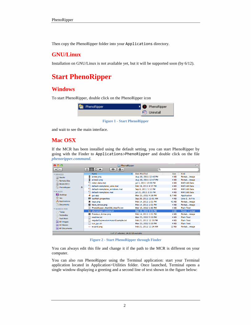
Mac OSX If the MCR has been installed using the default setting, you can start PhenoRipper by going with the Finder to Applications>PhenoRipper and double click on the file phenoripper.command.

Figure 2 - Start PhenoRipper through Finder

You can always edit this file and change it if the path to the MCR is different on your computer.

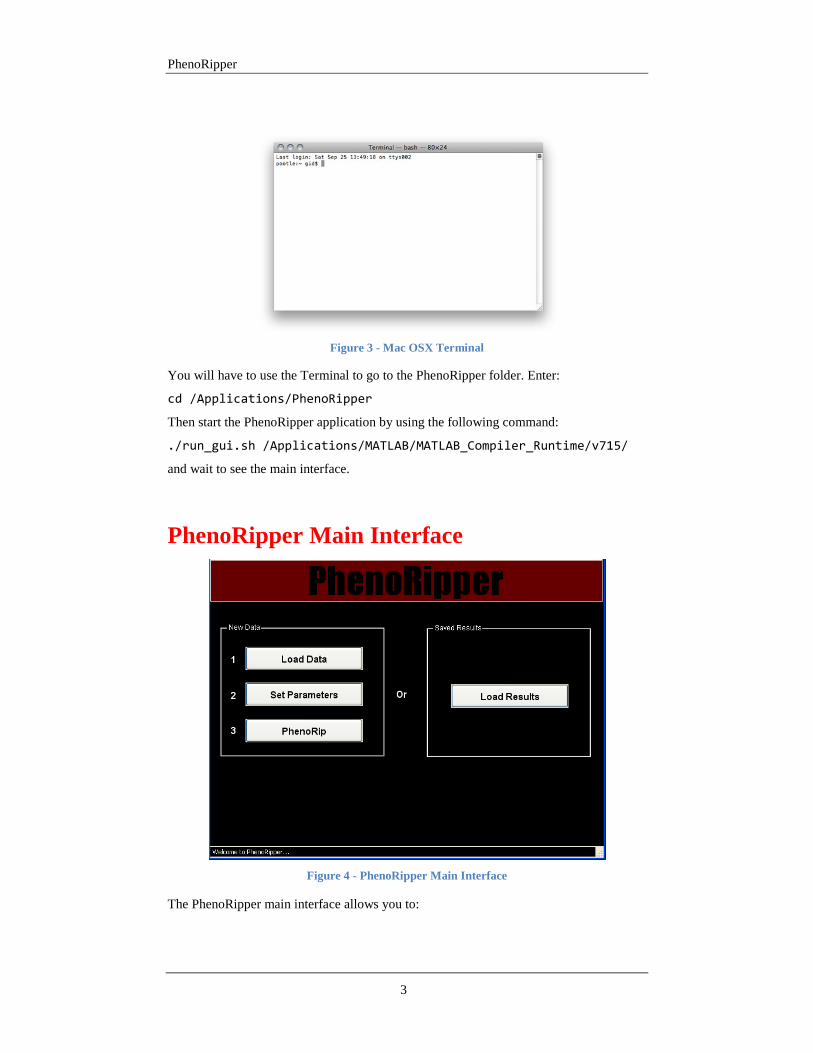
You can also run PhenoRipper using the Terminal application: start your Terminal application located in Application>Utilities folder. Once launched, Terminal opens a single window displaying a greeting and a second line of text shown in the figure below:

PhenoRipper

3

Figure 3 - Mac OSX Terminal

You will have to use the Terminal to go to the PhenoRipper folder. Enter:

cd /Applications/PhenoRipper

Then start the PhenoRipper application by using the following command:

./run_gui.sh /Applications/MATLAB/MATLAB_Compiler_Runtime/v715/

and wait to see the main interface.

PhenoRipper Main Interface

Figure 4 - PhenoRipper Main Interface

The PhenoRipper main interface allows you to:

PhenoRipper

4

• Load data • Load previously “PhenoRipped” results

Let’s first see how to load new data into PhenoRipper

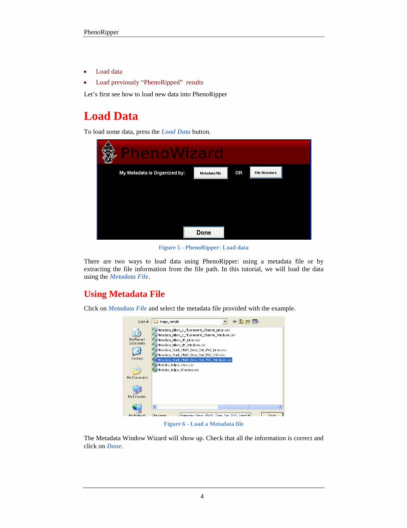
Load Data To load some data, press the Load Data button.

Figure 5 - PhenoRipper: Load data

There are two ways to load data using PhenoRipper: using a metadata file or by extracting the file information from the file path. In this tutorial, we will load the data using the Metadata File.

Using Metadata File Click on Metadata File and select the metadata file provided with the example.

Figure 6 - Load a Metadata file

The Metadata Window Wizard will show up. Check that all the information is correct and click on Done.

PhenoRipper

5

Figure 7 - View the Metadata content

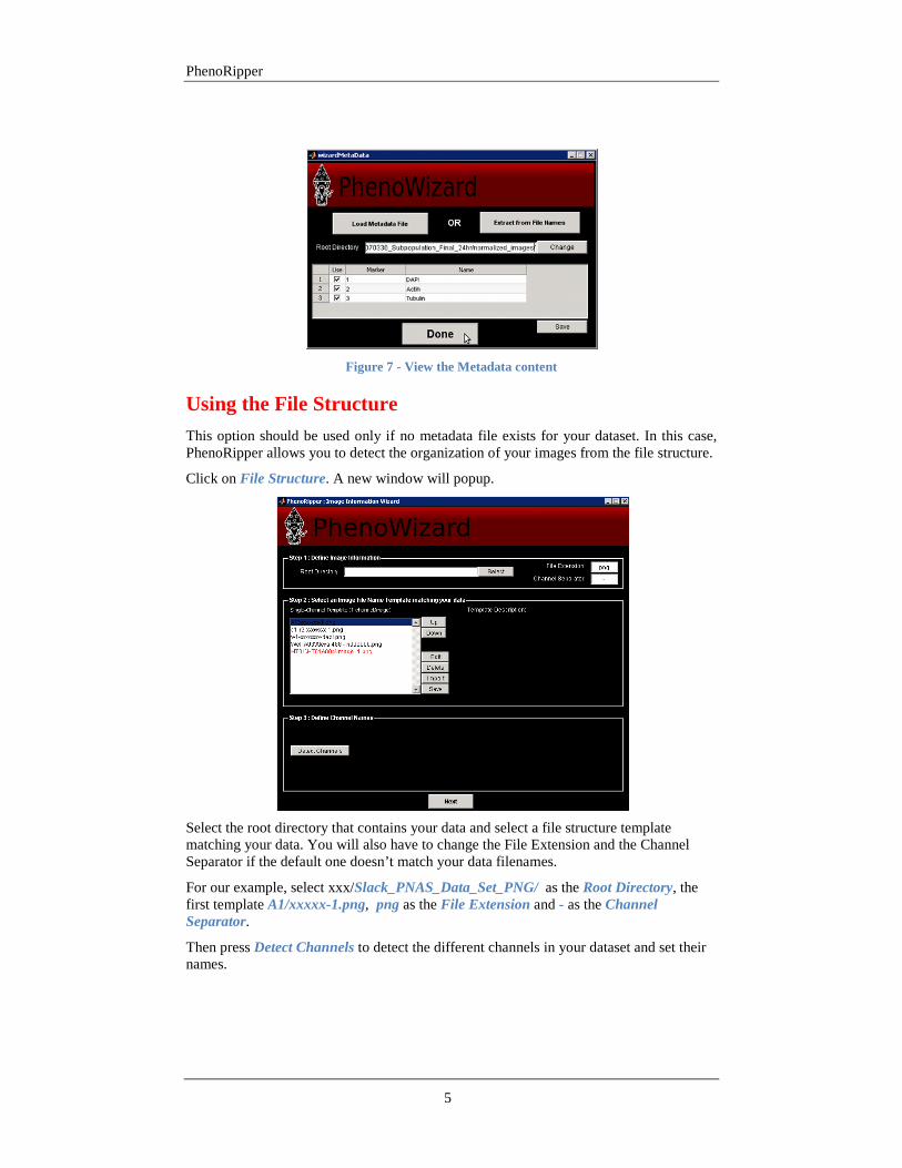
Using the File Structure This option should be used only if no metadata file exists for your dataset. In this case, PhenoRipper allows you to detect the organization of your images from the file structure.

Click on File Structure. A new window will popup.

Select the root directory that contains your data and select a file structure template matching your data. You will also have to change the File Extension and the Channel Separator if the default one doesn’t match your data filenames.

For our example, select xxx/Slack_PNAS_Data_Set_PNG/ as the Root Directory, the first template A1/xxxxx-1.png, png as the File Extension and - as the Channel Separator.

Then press Detect Channels to detect the different channels in your dataset and set their names.

PhenoRipper

6

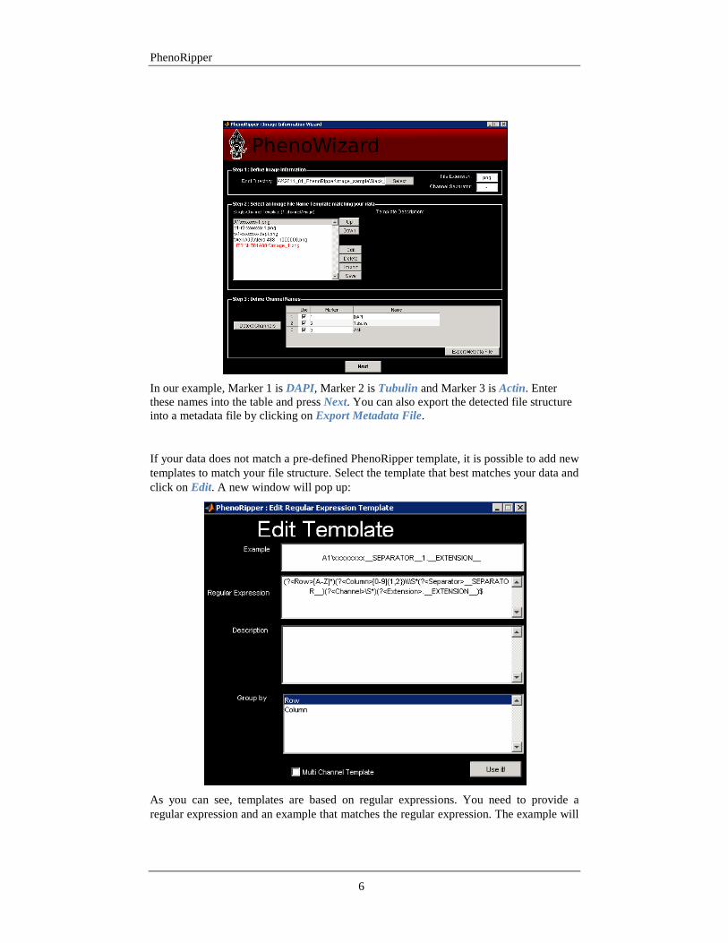
In our example, Marker 1 is DAPI, Marker 2 is Tubulin and Marker 3 is Actin. Enter these names into the table and press Next. You can also export the detected file structure into a metadata file by clicking on Export Metadata File.

If your data does not match a pre-defined PhenoRipper template, it is possible to add new templates to match your file structure. Select the template that best matches your data and click on Edit. A new window will pop up:

As you can see, templates are based on regular expressions. You need to provide a regular expression and an example that matches the regular expression. The example will

PhenoRipper

7

be used as the name for your new template on the template list. Click on Use it! to use it right away. This will close the Edit Template window and take you back to the PhenoWizard. Here you should click on Save if you want to add this new template to your default template list.

If you are familiar with regular expressions, you will notice that we use two unusual expressions, __SEPARATOR__ and __EXTENSION__. These expressions refer to the Separator and File Extension specified in the PhenoWizard and allow reuse of a template even if these parameters have been modified.

To test your regular expressions, you can use regexphelper, a tool available in the MATLAB file exchange at the following URL http://www.mathworks.com/matlabcentral/fileexchange/15215-regexphelper.

Learn Image Phenotypes You now have to choose a strategy for sampling a representative subset of the data. We will choose a grouping so all images in a group are expected to be similar (like replicate experimental conditions, same wells, similar perturbations).

In our example, we could group by Drug or Drug class. Here, we guess that different drugs in a drug class could have different effects, so we will choose to group by Drug.

Figure 8 - Learn Image Phenotypes

You should now see the Load Data Successfully dialog. Note: you have to wait for the computer to finish analyzing your file structure -the more images you have, the longer you have to wait. You will then be taken back to the main interface where you can move to the next step.

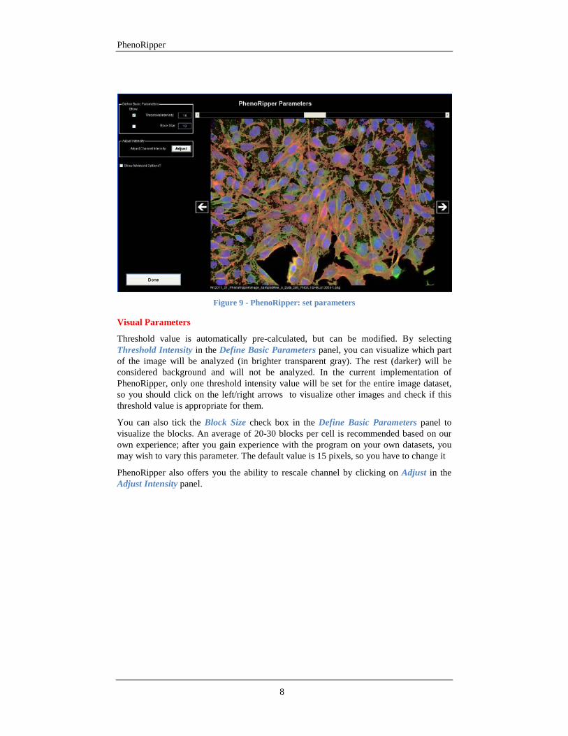
Set Parameters Click on Set Parameters to set the PhenoRipper parameters.

PhenoRipper

8

Figure 9 - PhenoRipper: set parameters

Visual Parameters

Threshold value is automatically pre-calculated, but can be modified. By selecting Threshold Intensity in the Define Basic Parameters panel, you can visualize which part of the image will be analyzed (in brighter transparent gray). The rest (darker) will be considered background and will not be analyzed. In the current implementation of PhenoRipper, only one threshold intensity value will be set for the entire image dataset, so you should click on the left/right arrows to visualize other images and check if this threshold value is appropriate for them.

You can also tick the Block Size check box in the Define Basic Parameters panel to visualize the blocks. An average of 20-30 blocks per cell is recommended based on our own experience; after you gain experience with the program on your own datasets, you may wish to vary this parameter. The default value is 15 pixels, so you have to change it

PhenoRipper also offers you the ability to rescale channel by clicking on Adjust in the Adjust Intensity panel.

PhenoRipper

9

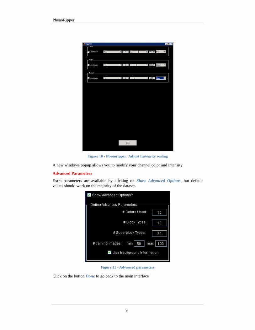
Figure 10 - Phenoripper: Adjust Instensity scaling

A new windows popup allows you to modify your channel color and intensity.

Advanced Parameters

Extra parameters are available by clicking on Show Advanced Options, but default values should work on the majority of the dataset.

Figure 11 - Advanced parameters

Click on the button Done to go back to the main interface

PhenoRipper

10

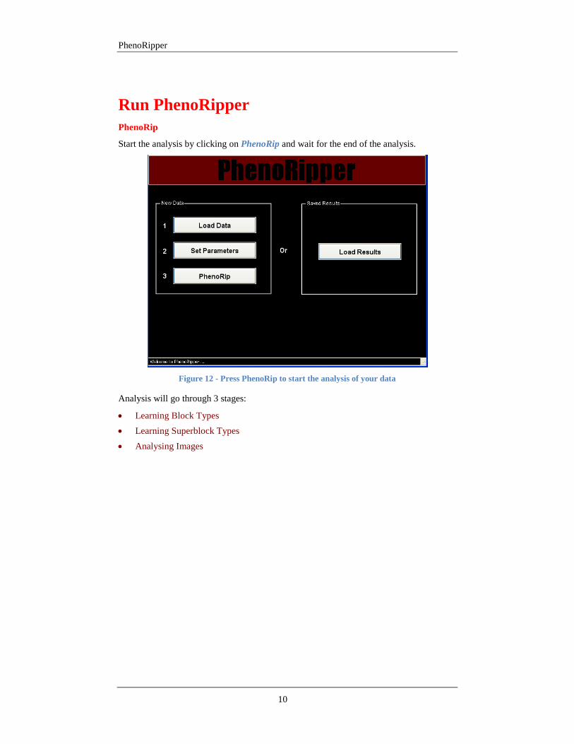
Run PhenoRipper PhenoRip

Start the analysis by clicking on PhenoRip and wait for the end of the analysis.

Figure 12 - Press PhenoRip to start the analysis of your data

Analysis will go through 3 stages:

• Learning Block Types • Learning Superblock Types • Analysing Images

PhenoRipper

11

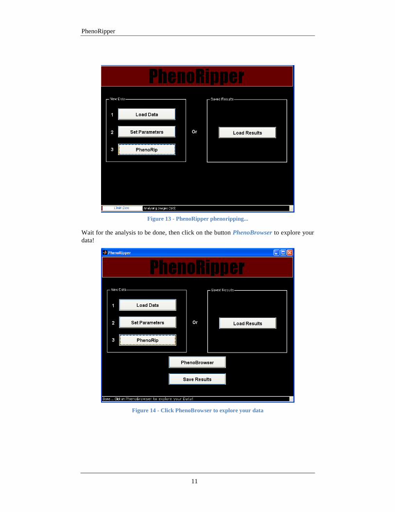
Figure 13 - PhenoRipper phenoripping...

Wait for the analysis to be done, then click on the button PhenoBrowser to explore your data!

Figure 14 - Click PhenoBrowser to explore your data

PhenoRipper

12

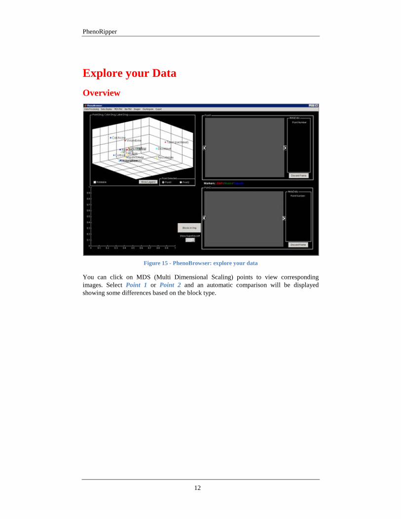
Explore your Data Overview

Figure 15 - PhenoBrowser: explore your data

You can click on MDS (Multi Dimensional Scaling) points to view corresponding images. Select Point 1 or Point 2 and an automatic comparison will be displayed showing some differences based on the block type.

PhenoRipper

13

Figure 16 - Select some point on the MDS to visualize the data

To rotate the MDS plot, click on Rotatable and drag and drop on the plot. Once you are satisfied with the position, you will need to un-select the Rotatable check box to be able to click on points and visualize the corresponding image.

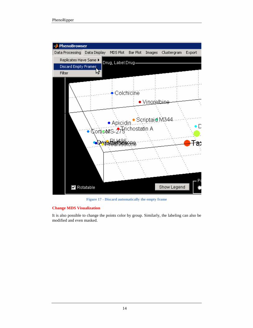
Adjust visualization Discard Frame

You can remove automatically empty frames by selecting the option shown below.

PhenoRipper

14

Figure 17 - Discard automatically the empty frame

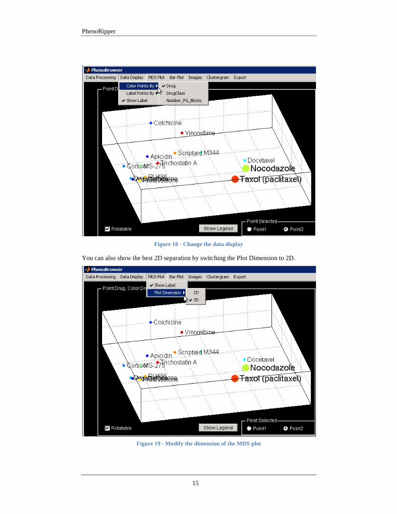
Change MDS Visualization

It is also possible to change the points color by group. Similarly, the labeling can also be modified and even masked.

PhenoRipper

15

Figure 18 - Change the data display

You can also show the best 2D separation by switching the Plot Dimension to 2D.

Figure 19 - Modify the dimension of the MDS plot

PhenoRipper

16

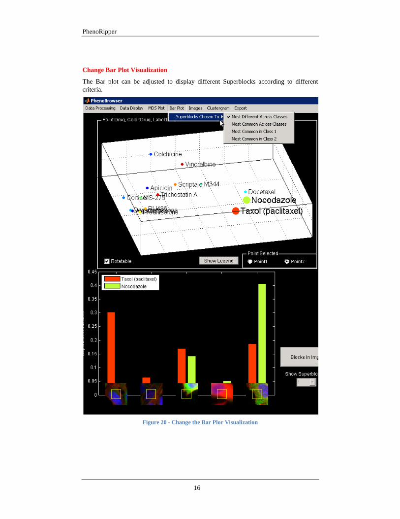
Change Bar Plot Visualization

The Bar plot can be adjusted to display different Superblocks according to different criteria.

Figure 20 - Change the Bar Plor Visualization

PhenoRipper

17

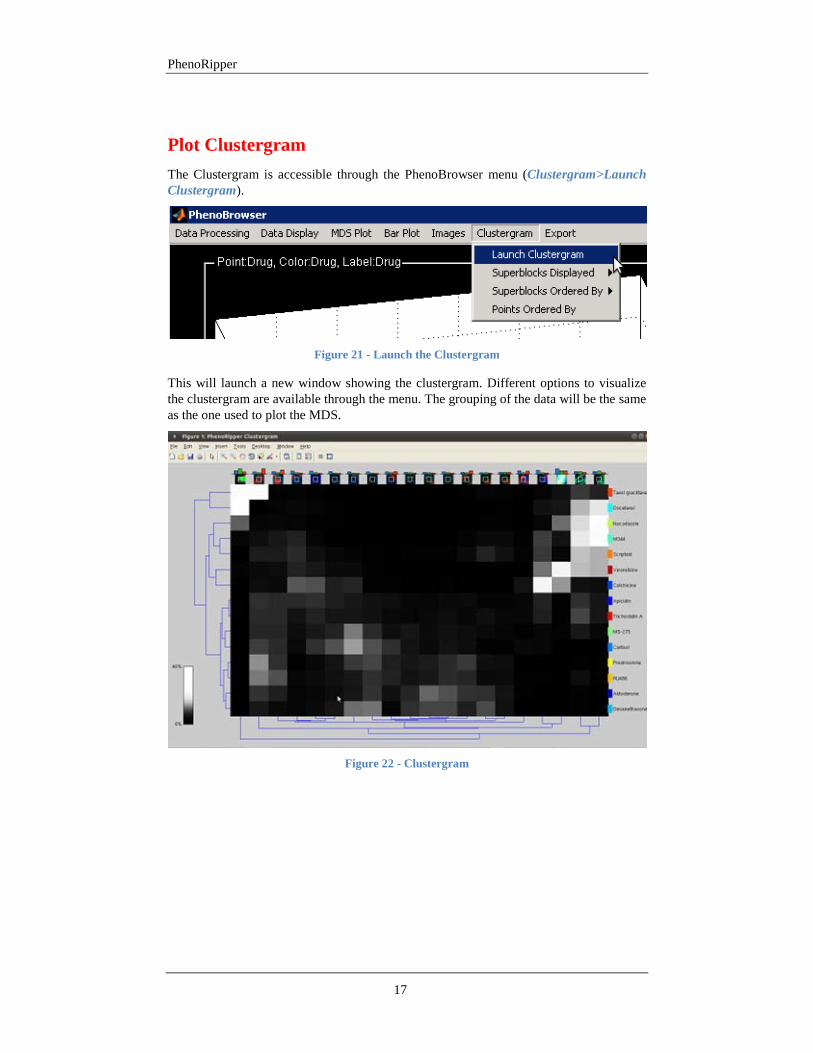
Plot Clustergram The Clustergram is accessible through the PhenoBrowser menu (Clustergram>Launch Clustergram).

Figure 21 - Launch the Clustergram

This will launch a new window showing the clustergram. Different options to visualize the clustergram are available through the menu. The grouping of the data will be the same as the one used to plot the MDS.

Figure 22 - Clustergram