orfeo toolbox workshop at foss4g europe 2015

IntroductionAbout the data and software

Preparing the dataImage Classification

Getting back to OpenStreetMapConclusion

Land cover mapping with high resolution satellite images usingOrfeo Toolbox, QGIS and OSM

Workshop - W04

Julien Michel (CNES), Jordi Inglada (CNES/CESBIO), Manuel Grizonnet (CNES)

July 14th 2015 - FOSS4GE, Como, Italy

http://creativecommons.org/licenses/by-sa/3.0/

http://www.orfeo-toolbox.org




Disclaimer

I We come from the remote sensing world, not the GIS one,

I What we propose in this workshop works, we tested it!

I But ... It may look over-complicated to the GIS ninjas in the audience

I There are for sure many smarter ways for the GIS processing we will do

I Not to mention better GIS data sources or more adapted tools!

I Keep in mind: The workshop focuses on the concept, not the tools (except forOrfeo ToolBox)






About land cover mapping and supervised classification

I Land cover maps are produced using supervised classification

I A supervised classifier is trained to assign class labels to input features

I Reference data is used for training and validation

Data Preparation

Supervised Learning

Map Production

Reference DataSample Selection

sample ratioTraining Samples

Validation Samples

Input ImagesFeature Extraction

Radiances, NDVI, NDWI

TrainingSVM, RF

ClassificationModel

Classification Land Cover Map ValidationOA, FScore






Can we use OpenStreetMap as reference data?

I Reference data has to:I represent the land cover classes of interestI be spatially coherent with the input imagesI contain few errors

I OSM pros:I available everywhereI rich nomenclatureI good geometric quality

I OSM cons:I may be out of date in many placesI polygons of one class may contain objects of other classesI May have improper classes for land-cover mapping (e.g. land use)






Outline of the workshop

In this workshop we will do the following

1. Extract relevant data from OpenStreetMap to perform supervised imageclassification

2. Experiment several classification set-ups and assess their performances

3. Use the final classification map to highlight OpenStreetMap shapes that mayneed an update

Using the following software

I Gdal for vectorial data manipulation

I Orfeo ToolBox for image processing and classification

I QGis for visualisation

And data

I SPOT4 (Take5) time series over Ardeche, France as a proxy for future Sentinel-2data,

I Offline OpenStreetMap export from geofrabrick.de






DataSoftware

Outline

About the data and softwareDataSoftware

Preparing the dataImage preprocessingOpenStreetMap preprocessing

Image ClassificationEstimation of image statisticsTraining of the classification algorithmClassifying the imageNoise cleaning

Getting back to OpenStreetMapAccuracy assesmentWhere do OSM and Land Cover differs






DataSoftware

SPOT4 (Take5) data and upcoming Sentinel-2 data

Sentinel-2

I 2 satellites ESA mission, firstlaunch june 2015

I Will observe all continental landsevery 5 days

I 13 spectral bands and spatialresolution of 10 to 60 meters

I Application friendly licence

SPOT4 (Take5)

I CNES short term experiment forSPOT4 end of life

I Simulate temporal revisit of futureSentinel-2 mission

I on 42 sites of 60x60 squared km.around the Earth

I With a spatial resolution of 20meters and 4 spectral bands

SPOT4 (Take5) data will be used in this workshop as a proxy of future Sentinel-2 data.






DataSoftware

Images overview (SPOT4 (Take5) Ardeche site, France)






DataSoftware

OpenStreetMap data (exports from geofabrick.de)

Land use, natural and waterways layers






DataSoftware

The Orfeo ToolBox

What is the Orfeo ToolBox?

I An image processing library dedicated to remote sensing,

I An open-source software under the CeCILL-v2 licence (French equivalent toGPL),

I Funded by CNES in the frame of the Orfeo program (and beyond),

I Written in C++ on top of ITK (free medical image processing library),

I Based on many other image processing and remote sensing open-source softwaresuch as Gdal, OSSIM or OpenCV

I Designed to process large data volumes seamlessly thanks to piece-wiseprocessing and multi-threading

www.orfeo-toolbox.org



www.itk.org




DataSoftware

How to use the Orfeo ToolBox

Write your own codeFlexible, full API available, requires C++ knowledge

Use OTB applicationsHigh level functions (e.g. segmentation), command-line, graphical interface, or Pythonwriting availabe. Can be extended (write your own app). Also available in Qgisprocessing framework.

Use Monteverdi2Data visualization and access to all applications in an integrated software






DataSoftware

Other software used in this workshop

Do we really need to introduce them ?!?

We will be using the OSgeoLive 8.5 (Orfeo ToolBox 4.2.1, Gdal 1.11.0, Qgis 2.4.0)USB stick provided by FOSS4GE organization. . . Time to insert it into your computer!



http://gdal.org/

http://qgis.org/en/site/




Image preprocessingOpenStreetMap preprocessing

Outline











Objectives of this section

1. Pre-process image to get it ready for visualisation and classification

2. Learn some basics of command-line OTB processing







A first glimpse at the image

The image is located here :

I Folder:raw_data/spot4t5/SPOT4_HRVIR1_XS_20130607_N2A_CArdecheD0000B0000/

I Image file:SPOT4_HRVIR1_XS_20130607_N2A_ORTHO_SURF_CORR_PENTE_CArdecheD0000B0000.TIF

In the following slides, it will be refered to as im.tif.

1. Open the image in Qgis

2. In layer properties:2.1 Set the no data value to -10 000 in the transparency tab,2.2 In the style tab, change color composition to r=b3,g=b2,b=b1,2.3 Reload statistics in the Style tab.

What do you see ?







Natural colors synthesis

SPOT4 images have the following spectral bands: Green (b1), Red (b2), NearInfra-Red (b3), Short Wavelength Infra-Red (b4)To get familiar with Orfeo ToolBox processing, and to ease data visualisation, we willbuild a synthetic green and blue channel with the following formula:

b = 0.7 ∗ green + 0.24 ∗ red − 0.14 ∗ swir (1)

We are going to use the BandMath application, as well as the ConcatenateImagesapplication.Caution: this synthetic image is only for visualisation, not for processing!







Natural colors synthetis (Solution)

Extract red band:

$ otbcli_BandMath -il im.tif -out red.tif int16 -exp "im1b2"

Extract green band:

$ otbcli_BandMath -il im.tif -out green.tif int16 -exp "im1b1"

Compute synthetic blue band:

$ otbcli_BandMath -il im.tif -out blue.tif int16 -exp "im1b1==-10000?-10000:0.7*im1b1+0.24*im1b2-0.14*im1b3"

Concatenate all bands:

$ otbcli_ConcatenateImages -il red.tif green.tif blue.tif -out rgb.tif int16

Open resulting image in qgis, and set the rendering option likewise.







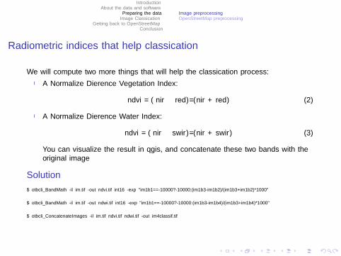
Radiometric indices that help classification

We will compute two more things that will help the classification process:

I A Normalize Difference Vegetation Index:

ndvi = (nir − red)/(nir + red) (2)

I A Normalize Difference Water Index:

ndvi = (nir − swir)/(nir + swir) (3)

You can visualize the result in qgis, and concatenate these two bands with theoriginal image

Solution

$ otbcli_BandMath -il im.tif -out ndvi.tif int16 -exp "im1b1==-10000?-10000:(im1b3-im1b2)/(im1b3+im1b2)*1000"

$ otbcli_BandMath -il im.tif -out ndwi.tif int16 -exp "im1b1==-10000?-10000:(im1b3-im1b4)/(im1b3+im1b4)*1000"

$ otbcli_ConcatenateImages -il im.tif ndvi.tif ndwi.tif -out im4classif.tif








1. Turn OSM data into a vector layer suitable for classifier training:1.1 Filter and join features to get a limited number of well-defined classes (in the sense of

classification)1.2 Build a single layer with polygon feature bearing an integer class attribute

2. Learn how training polygons should be and which features of OSM are suitable







Pre-processing OpenStreetMap data

The data are located in the raw data/osm/ folder.For each region, open the following files on top of the image in Qgis:

I landuse.hsp

I natural.hsp

I waterways.hsp

To get OpenStreetMap data ready for classification, we will do the following:

1. Extract geometries that actually cover our image (area of interest)

2. Reproject all geometries in the image SRS

3. Filter OSM classes to build a set of 3 classes suitable for supervised classification

4. Process waterways to turn polylines into polygons with buffers

5. Separate our set of polygons between a training set and a validation set







Extracting geometries that cover our image

Extracting image footprint

1. Use the ImageEnvelope application

2. Output a shapefile or sqlite file

3. Control results in Qgis

4. For a more accurate result, draw the envelope by hand in Qgis

Clip OSM layers to ROI and reproject to image SRS

1. For each region and each layer

2. Use ogr2ogr

3. Use the -clipsrc option to filter by image footprint

4. Use the -t srs option to define the output SRS using the raw data/l93.wkt file

5. Use the -append option to merge both regions for each layer







Extracting geometries that cover our image (solution)

Extract image enveloppe:

$ otbcli_ImageEnvelope -in SPOT4_HRVIR1_XS_20130607_rgb.tif -proj "EPSG:32631" -out env.shp

Clipping, reprojecting and merging land use layers:

$ ogr2ogr -append -t_srs raw_data/l93.wkt -clipsrc env.shp landuse_l93.shp raw_data/osm/auvergne/landuse.shp

$ ogr2ogr -append -t_srs raw_data/l93.wkt -clipsrc env.shp landuse_l93.shp raw_data/osm/rhone-alpes/landuse.shp

Clipping, reprojecting and merging natural layers:

$ ogr2ogr -append -t_srs raw_data/l93.wkt -clipsrc env.shp natural_l93.shp raw_data/osm/auvergne/natural.shp

$ ogr2ogr -append -t_srs raw_data/l93.wkt -clipsrc env.shp natural_l93.shp raw_data/osm/rhone-alpes/natural.shp

Clipping, reprojecting and merging waterways layers:

$ ogr2ogr -append -t_srs raw_data/l93.wkt -clipsrc env.shp waterways_l93.shp raw_data/osm/auvergne/waterways.shp

$ ogr2ogr -append -t_srs raw_data/l93.wkt -clipsrc env.shp waterways_l93.shp raw_data/osm/rhone-alpes/waterways.shp

Open the three new layers in Qgis.







Build consistent classes for supervised classification

The idea

I Select and join OSM features from landuse and natural layers

I That form simple landcover classes (e.g. water or vegetation)

I Which are big enough wrt. to image resolution (20m)

I You can walk the layers and have a look at OSM spec here1

Our Proposal

I Water:I basin, pond, reservoir, salt pond, water larger than 1000 squared meters from land use

layerI water larger than 1000 squared meters from natural layerI main rivers (Loire, Rhone) from waterways layer, buffered with 25 meters

I Vegetation: forest from natural layer

I Built-up: residential, commercial, cemetery, construction, industrial, recreational,harbour, allotments, yard, brownfield, from land use layer

1https://wiki.openstreetmap.org/wiki/Map_Features



https://wiki.openstreetmap.org/wiki/Map_Features





Building the water class

1. Extract the two large rivers covering the image:$ ogr2ogr -append -sql "select * from waterways_l93 where name in ("La Loire", "Le Rhone")" large_rivers.shp waterways_l93.shp

2. In Qgis, use the vector/geoprocessing/buffer tool to build a 25m buffer around,and save it to water.shp.

3. Append selected features from land use layer:$ ogr2ogr -append -sql "select * from landuse_l93 where type in \

(\"basin\",\"pond\",\"reservoir\",\"salt_pond\",\"water\") \

and OGR_GEOM_AREA > 10000" water.shp landuse_l93.shp

4. Append selected features from natural layer:$ ogr2ogr -append -sql "select * from natural_l93 where type in \

(\"water\") and OGR_GEOM_AREA > 1000" water.shp natural_l93.shp







Building the vegetation and built-up classes

Vegetation classExtract selected features from natural layer:

$ ogr2ogr -append -sql "select * from natural_l93 where type in \

(\"forest\")" forest.shp natural_l93.shp

Built-up classExtract selected features from land use layer:

$ ogr2ogr -append -sql "select * from landuse_l93 where type in \

(\"residential\",\"commercial\",\"cemetery\",\"construction\",\

\"industrial\", \"recreational\",\"harbour\", \

\"allotments\",\"brownfield\")" builtup.shp landuse_l93.shp







Final steps (1/2): add class label, exclude overlaps

Add class labels

I Goal: create a new integer field with a unique id for each of the 3 classes

I Can be done in Qgis attribute table manager

I Or With the VectorDataSetField application in OTB

Exclude overlaps

I Overlapping polygons of different classes confuses training and evaluation

I We will therefore ignore those areas

I To do so, we will use the Vector/Geoprocessing tools/Differentiate tool in Qgis

I Twice for each layer, e.g. Builtup vs. water then vs. forest . . .







Final steps (2/2): build separate sets for training and validation, merge

Build separate sets for training (250 polygons of each class) andvalidation (the remaining)

$ ogr2ogr -append -dialect SQLITE -sql "select * from forest order by osm_id limit 250" training.shp forest.shp

$ ogr2ogr -append -dialect SQLITE -sql "select * from water order by osm_id limit 250" training.shp water.shp

$ ogr2ogr -append -dialect SQLITE -sql "select * from builtup order by osm_id limit 250" training.shp builtup.shp

$ ogr2ogr -append -dialect SQLITE -sql "select * from forest order by osm_id limit 250,1000000" validation.shp forest.shp

$ ogr2ogr -append -dialect SQLITE -sql "select * from water order by osm_id limit 250,1000000" validation.shp water.shp

$ ogr2ogr -append -dialect SQLITE -sql "select * from builtup order by osm_id limit 250,100000" validation.shp builtup.shp

Also merge everything in a single layer

$ ogr2ogr -append all.shp water.shp

$ ogr2ogr -append all.shp forest.shp

$ ogr2ogr -append all.shp builtup.shp






Estimation of image statisticsTraining of the classification algorithmClassifying the imageNoise cleaning

Outline












1. Learn the steps of supervised classification processing with Orfeo ToolBox

2. Perform the classification based on the OSM pre-processed data







Step 1: Estimation of image statistics

I Some machine learning algorithm require the input features to have similar ranges

I Also, the SVM algorithm will converge faster if this range is [−1, 1]

I We will therefore center and reduce all image bands prior to classification

I For this, we need to estimate the mean and variance of each band

I Which is what this step is about

For this we will use the EstimateImagesStatistics application. Do not forget to setthe background value (-10 000)!







Step 1: Estimation of image statistics (solution)

$ otbcli_ComputeImagesStatistics -il im4classif.tif -out stats.xml -bv -10000

Look at the stats.xml file. Does it look correct?







Step 2: Training the classification algorithm

I We will be using the TrainImagesClassifier application

I The application should receive the image, the training layer and the xml stats file,

I We will use the libsvm implementation, with a RBF kernel,

I We will select at most 1000 random samples per class (2000 for validation),

I You also need to set the name of the class field in the training layer.







Step 2: Training the classification algorithm (solution)

$ otbcli_TrainImagesClassifier -io.il im4classif.tif -io.vd training.shp -io.out model.svm \

-classifier libsvm -classifier.libsvm.k rbf -sample.mt 1000 -sample.mv 2000 \

-sample.vfn "class" -io.imstat stats.xml

2015 Jun 15 13:56:21 : Application.logger (INFO) Confusion matrix (rows = reference labels, columns = produced labels):

[1] [2] [3]

[ 1] 1668 278 73

[ 2] 46 1773 146

[ 3] 52 208 1772

2015 Jun 15 13:56:21 : Application.logger (INFO) Precision of class [1] vs all: 0.944507

2015 Jun 15 13:56:21 : Application.logger (INFO) Recall of class [1] vs all: 0.826152

2015 Jun 15 13:56:21 : Application.logger (INFO) F-score of class [1] vs all: 0.881374







2015 Jun 15 13:56:21 : Application.logger (INFO) Global performance, Kappa index: 0.799899







Step 3: Classifying the image

I Now that we trained a classifier with a satisfactory level of performance, letsclassify the image,

I We will use the ImageClassifier application,

I It should receive the input image, the model and the stats files,

I We will also build a mask of no data pixels, so that they will be ignored duringclassification (use the BandMath app for this)







Step 3: Classifying the image (solution)

$ otbcli_BandMath -il im4classif.tif -out mask.tif uint8 -exp "im1b1>-10000?255:0"

$ otbcli_ImageClassifier -in im4classif.tif -mask mask.tif -model model.svm -imstat stats.xml -out classif.tif uint8

Open the resulting land cover map in Qgis. Set the rendering to color each class witha discriminative color. Does the classification map look correct?







Step 4: Classification noise cleaning

I Classification maps often suffer from salt and pepper noise (isolated pixels withclass different from neighborhood)

I We can filter that with the ClassificationMapRegularization application

I It will perform a majority voting of classified pixels in a fixed neighborhood(radius = 2 for instance)







Step 4: Classification noise cleaning

$ otbcli_ClassificationMapRegularization -io.in classif.tif -io.out classif_reg.tif -ip.radius 2

Load the cleaned map into QGis as well.






Accuracy assesmentWhere do OSM and Land Cover differs

Outline











Getting a better idea of our land cover accuracy

I What is our final accuracy after regularization (e.g. denoising)?

I What is our final accuracy wrt. our validation layer?

I We will find out with the ComputeConfusionMatrix application

I Which can cross-compare our land-cover map with our validation layer







Accuracy assesment (solution)

$ otbcli_ComputeConfusionMatrix -in classif_reg.tif -ref vector -ref.vector.in validation.shp \

-ref.vector.field "class" -nodatalabel 0 -out conf.txt

2015 Jun 15 17:36:11 : Application.logger (INFO) Confusion matrix (rows = reference labels, columns = produced labels):

[ 1] [ 2] [ 3]

[ 1] 24532 4491 1258

[ 2] 8903 1761939 141961

[ 3] 2830 36018 573860










2015 Jun 15 17:36:11 : Application.logger (INFO) Precision of the different classes: [0.676465, 0.977526, 0.800274]

2015 Jun 15 17:36:11 : Application.logger (INFO) Recall of the different classes: [0.810145, 0.921129, 0.936596]

2015 Jun 15 17:36:11 : Application.logger (INFO) F-score of the different classes: [0.737295, 0.94849, 0.863086]

2015 Jun 15 17:36:11 : Application.logger (INFO) Kappa index: 0.811052

2015 Jun 15 17:36:11 : Application.logger (INFO) Overall accuracy index: 0.923522







Where do OSM and Land Cover differs?

Now that we have a rough idea of the level of agreement between our land cover mapand the OSM layer, it would be useful to see where the differences are.

I We can use the Rasterization application to make a raster out of our layer

I And then use the BandMath to make a raster of the disagreements betweenlandcover and OSM

I Write the proper expression so that the raster is null or bears the land cover classif it differs from OSM







Where do OSM and Land Cover differ? (Solution)

Rasterize our layer

$ otbcli_Rasterization -in all.shp -out all.tif -im im4classif.tif \

-mode attribute -mode.attribute.field "class" -background 0

Compute the difference map

$ otbcli_BandMath -il classif_reg.tif all.tif -out errors.tif \

-exp "im2b1>0?(im1b1!=im2b1?im1b1:0):0"

Display the difference map in Qgis, and superimpose the original OSM layers. Findevidence of:

I Forest areas that are endangered by urban growth,

I Parks and other green areas in residential neighborhood that are not referenced inOSM,

I Water bodies that are not referenced as well.






Conclusion

Time for a talkAccording to what you did in this workshop, do you think OpenStreetMap can be usedfor S2 land-cover applications? And vice-versa?

To go further

I How well does the trained model generalize to other dates / areas?

I Can we add new classes for a more detailed map?

I Can we set-up automatic alerts on some features (e.g. forest polygons that donot seem to contain a lot of forest) ?






Thank you for attending this workshop! Any questions?



orfeo toolbox workshop at foss4g europe 2015

Software

data image classication

software data software

relevant data

supervised image classication

features reference data

classication qgis

classication algorithm

classication setups