organic waste recycling - oapen
TRANSCRIPT

1.0996.14 x 9.21 6.14 x 9.21
This book covers the principles and practices of technologies for the control
of pollution originating from organic wastes (e.g. human faeces and urine,
wastewater, solid wastes, animal manure and agro-industrial wastes) and the
recycling of these organic wastes into valuable products such as fertilizer,
biofuels, algal and fish protein and irrigated crops.
Each recycling technology is described with respect to:
• Objectives
• Benefits and limitations
• Environmental requirements
• Design criteria of the process
• Use of the recycled products
• Pubic health aspects
This new edition, an update of the previous book, is a response to the
emerging environmental problems caused by rapid population growth and
industrialization. It describes the current technology and management options
for organic waste recycling which are environmentally friendly, effective in
pollution control and yield valuable by-products. Every chapter has been revised
to include successful case studies, new references, design examples and
exercises. New sections added to the 3rd edition include: Millennium
development goals, waste minimization and cleaner production, methanol and
ethanol production, chitin and chitosan production, constructed wetlands,
management and institutional development.
This is a textbook for environmental science, engineering and management
students who are interested in the current environmental problems and seeking
solutions to the emerging issues. It should be a valuable reference book for
policy makers, planners and consultants working in the environmental fields.
www.iwapublishing.com
ISBN 184339121X ISBN 13: 9781843391210
Organic W
aste Recycling
Chongrak Polprasert
Technology and Managem
ent 3rd Edition
Organic Waste Recycling Technology and Management
3rd Edition
Chongrak Polprasert

Organic Waste RecyclingTechnology and Management


Organic Waste Recycling Technology and Management
Third Edition
Chongrak Polprasert Environmental Engineering and Management Field
Asian Institute of Technology
Bangkok
Thailand

Published by IWA Publishing, Alliance House, 12 Caxton Street, London SW1H 0QS, UK
Telephone: +44 (0) 20 7654 5500; Fax: +44 (0) 20 7654 5555; Email: [email protected]
Web: www.iwapublishing.com
First published 2007
© 2007 IWA Publishing
Printed by Lightning Source Cover design by www.designforpublishing.co.uk
Apart from any fair dealing for the purposes of research or private study, or criticism or review,
as permitted under the UK Copyright, Designs and Patents Act (1998), no part of this publication
may be reproduced, stored or transmitted in any form or by any means, without the prior
permission in writing of the publisher, or, in the case of photographic reproduction, in accordance
with the terms of licences issued by the Copyright Licensing Agency in the UK, or in accordance
with the terms of licenses issued by the appropriate reproduction rights organization outside the
UK. Enquiries concerning reproduction outside the terms stated here should be sent to IWA
Publishing at the address printed above.
The publisher makes no representation, express or implied, with regard to the accuracy of the
information contained in this book and cannot accept any legal responsibility or liability for
errors or omissions that may be made.
Disclaimer
The information provided and the opinions given in this publication are not necessarily those of
IWA and should not be acted upon without independent consideration and professional advice.
IWA and the Author will not accept responsibility for any loss or damage suffered by any person
acting or refraining from acting upon any material contained in this publication.
British Library Cataloguing in Publication Data
A CIP catalogue record for this book is available from the British Library
Library of Congress Cataloging- in-Publication Data
A catalog record for this book is available from the Library of Congress
ISBN: 184339121X
ISBN13: 9781843391210

Contents
Preface ix
Abbreviations and symbols xi
Atomic weight and number of elements xvi
Conversion factor for SI units xix
1 Introduction 1
1.1 Problems and need for waste recycling 1
1.2 Objectives and scope of organic waste recycling 6
1.3 Integrated and alternative technologies 9
1.4 Feasibility and social acceptance of waste recycling 17
1.5 References 19
1.6 Exercises 20
2 Characteristics of organic wastes 21
2.1 Human wastes 22
2.2 Animal wastes 28

iv Contents
2.3 Agro-industrial wastewaters 30
2.4 Pollution caused by human wastes and other wastewaters 54
2.5 Diseases associated with human and animal wastes 57
2.6 Cleaner production (CP) 72
2.7 References 83
2.8 Exercises 86
3 Composting 88
3.1 Objectives, benefits, and limitations of composting 89
3.2 Biochemical reactions 92
3.3 Biological succession 95
3.4 Environmental requirements 97
3.5 Composting maturity 109
3.6 Composting systems and design criteria 111
3.7 Public health aspects of composting 129
3.8 Utilization of composted products 134
3.9 References 140
3.10 Exercises 142
4 Biofuel production 145
4.1 Objectives, benefits, and limitations of biogas technology 147
4.2 Biochemical reactions and microbiology of anaerobic digestion 150
4.3 Environmental requirements for anaerobic digestion 158
4.4 Modes of operation and types of biogas digesters 162
4.5 Biogas production 185
4.6 End uses of biogas and digested slurry 199
4.7 Ethanol production 207
4.8 References 213
4.9 Exercises 215
5 Algae production 219
5.1 Objectives, benefits, and limitations 222
5.2 Algal production and high-rate algal ponds 225
5.3 Algal harvesting technologies 244
5.4 Utilization of waste-grown algae 251
5.5 Public health aspects and public acceptance 255
5.6 References 257
5.7 Exercises 259
6 Fish production 262
6.1 Objectives, benefits, and limitations 263

Contents v
6.2 Herbivores, carnivores, and omnivores 267
6.3 Biological food chains in waste-fed ponds 269
6.4 Biochemical reactions in waste-fed ponds 272
6.5 Environmental requirements and design criteria 274
6.6 Utilization of waste-grown fish 293
6.7 Public health aspects and public acceptance 295
6.8 Chitin and chitosan production 299
6.9 References 302
6.10 Exercises 305
7 Aquatic weeds and their utilization 308
7.1 Objectives, benefits, and limitations 309
7.2 Major types and functions 310
7.3 Weed composition 313
7.4 Productivity and problems caused by aquatic weeds 316
7.5 Harvesting, processing and uses 321
7.6 Food potential 330
7.7 Wastewater treatment using aquatic weeds 338
7.8 Health hazards relating to aquatic weeds 375
7.9 References 376
7.10 Exercises 379
8 Land treatment of wastewater 383
8.1 Objectives, benefits, and limitations 383
8.2 Wastewater renovation processes 384
8.3 Wastewater renovation mechanisms 399
8.4 System design and operation 407
8.5 Land treatment – design equations 418
8.6 System monitoring 430
8.7 Public health aspects and public acceptance 436
8.8 References 440
8.9 Exercises 441
9 Land treatment of sludge 445
9.1 Objectives, benefits, and limitations 446
9.2 Sludge transport and application procedures 450
9.3 System design and sludge application rates 454
9.4 Toxic compounds vs. crop growth 469
9.5 Microbiological aspects of sludge application on land 470
9.6 References 472

vi Contents
9.7 Exercises 473
10 Management of organic waste recycling program 476
10.1 Planning for waste recycling programs 476
10.2 Guidelines for technology and site selection 483
10.3 Institutional arrangements 486
10.4 Regulatory aspects 488
10.5 Monitoring and control of facility performance 501
10.6 Case studies of waste recycling management program 503
10.7 References 507
10.8 Exercises 508
Index 509

Preface
As the world population is projected to increase from the current number of 6
billions to 9 billions in the year 2050, the amount of organic wastes generated
from human, animal and agricultural activities would also increase, causing
more pollution problems to the environment. The Millennium Development
Goals call for actions on environmental protection, sustainable development and
poverty alleviation. Despite a lot of efforts from the national and international
agencies, waste treatment alone will not be able to respond effectively to the
challenges.
The book presents new concept and strategy of waste management which
combines technologies of waste treatment and recycling and emphasizing the
benefits to be gained from use of the recycled products. These technologies such
as composting, fermentation, algal photosynthesis, and natural treatment
systems are cost-effective, bring economic returns and are applicable to most
countries, in particular those located in the tropical areas. They are considered as
sustainable technologies which, if properly applied, should be an effective tool
in responding to the Millennium Development Goals.
In the third edition, I have included up-to-date information on organic waste
recycling technologies and more case studies of successful organic waste

x Preface
recycling programs implemented in several countries. New sections on: cleaner
production is added in chapter 2, ethanol production in chapter 4, chitin and
chitosan production in chapter 6, and constructed wetlands in chapter 7. Chapter
10 has been revised to cover management aspects of organic waste recycling
programs including the planning, institutional development and regulatory
standards. More examples and exercises are given in each chapter to help the
readers understand the technical principles and their application.
This book is intended to be used as a text for students majoring in
environmental sciences and engineering and for graduate students conducting
research in the related fields. Many universities worldwide have developed new
curricula on environment and sustainable development or are offering
specialized courses on sustainable waste management, all relating to the subject
contents of this book. Environmental professionals and policy makers should
find this book a useful reference source for planning, design and operation of
organic waste recycling programs.
In the preparation of the third edition, I am grateful to my graduate students
at the Asian Institute of Technology, Bangkok, Thailand and the UNESCO-IHE
Institute for Water Education, Delft, the Netherlands, for the constructive
suggestions on the book contents and feedbacks on the use of the book in
teaching and application of these organic waste recycling technologies in their
home countries. The book reviewers, Professor Dr. Hubert Gijzen, Director and
Representative of UNESCO office, Jakarta, Indonesia and Dr. Rao Surampalli,
Engineer Director of U.S. Environmental Protection Agency, Kansas, U.S.A.
and adjunct Professor of Environmental Engineering at the University of
Nebraska, U.S.A., gave useful and constructive suggestions on the content of
the revised book. I am thankful to Professor Dr. Shigeo Fujii who invited me to
spend a sabbatical leave at the Reseach Center for Environmental Quality
Management, Kyoto University, Japan, which allowed me to finalize the book
revision. My student assistants, Warounsak Liamleam and Robert Dongol, did
an excellent job in assisting me in the overall revision of the book.
I would like to express my sincere appreciation to the Aeon Group
Environment Foundation, Japan, for the generous support of the endowed
professorial chair which has enabled me to complete the revision of this book.
Grateful acknowledgement is expressed to Alan Click of IWA Publishing,
London, for his professional support in the publication of the third edition. The
inspiration and encouragement I always receive from Nantana, Jim and Jeed
made this project possible.
Chongrak Polprasert
Bangkok, Thailand
January 2007

Abbreviations and symbols
AFP advanced facultative ponds
AIT Asian Institute of Technology, Bangkok, Thailand
AIWPS advanced integrated wastewater pond system
AMP advanced maturation ponds
APU aquatic processing unit
ASP advanced settling ponds
atm atmosphere (pressure)
AU animal unit
BARC Beltsville aerated rapid composting
BOD5 5-day biochemical oxygen demand
BODL ultimate biochemical oxygen demand
BTU British thermal unit
C carbon
C/N carbon/nitrogen ratio
C2H5OH ethanol
cal calorie

xii Abbreviations and symbols
CEC cation exchange capacity
CH3OH methanol
CH4 methane gas
Cl chloride
cm centimeter
CO carbon monoxide
CO2 carbon dioxide
COD chemical oxygen demand
CP cleaner production
d days
d dispersion number
DAF dissolved air flotation
DDT dichloro-diphenyl-trichloro-ethane, (ClC6H4)2CHCCl3
DO dissolved oxygen
DOd dissolved oxygen at dawn
e or exp exponential
EC electrical conductivity
FAO United Nations Food and Agriculture Organization
FCR food conversion ratio
FFB fresh fruit bunches (referring to palm oil wastewater)
ft foot
FWS free water surface (constructed wetlands)
g gram
gal gallon
gcal calorie
gmole molecular weight in grams of any particulat compound
H hydrogen
h unit heat of algae
H2 hydrogen gas
H2S hydrogen sulfide gas
ha hectare
hp horsepower
hr hour
HRAP high-rate algal pond
HRT hydraulic retention time
in inch
IRCWD International Reference Centre for Waste Disposal,
Switzerland
ISO International standards organization
K potassium
kcal kilocalorie
Abbreviations and symbols xiii
kg kilogram
kJ kilojoule
km kilometer
KVIC Khadi and Village Industries Commission (India)
kWh kilowatt-hour
L liter
LAS linear alkylbenzene sulfonates
lb pound
LDP limiting design parameter
LPG liquefied petroleum gas
m meter
meq milli-equivalent (referring to concentration of an ion)
mg milligram
mgad million gallons per acre per day
mgd million gallons per day
min minute
mL milliliter
mM milliMolar
mm millimeter
MPN most probable number
mV millivolt
MWh megawatt-hour
N nitrogen
NAS U.S. National Academy of Sciences
NH3 un-ionized ammonia
NH3-N ammonia N
NH4+-N ammonium N
nm nanometer = 10-9 m
NO2- nitrite
NO3- nitrate
NOx nitrogen oxides in various oxidation states
O oxygen
OF overland flow process (referring to land treatment)
Org-N organic nitrogen
P phosphorus
PCBs polychlorinated biphenyls
PFU plaque forming unit
Pa algal productivity
PO43- phosphate
ppm part per million

xiv Abbreviations and symbols
psi pound per square inch
psi pound per square inch (referring to pressure)
PVC polyvinyl chloride
RCRA Resource Conservation and Recovery Act of the U.S.A.
RI rapid infiltration process (referring to land treatment)
RMP red mud plastic
rpm revolution per minute
s or sec second
S sulfur
SAR sodium adsorption ratio
SD stocking density (of fish or aquatic weeds)
SF subsurface flow (constructed wetlands)
SI international system
SOx sulfur oxides in various oxidation states
SR slow rate (irrigation) process (referring to land treatment)
SS suspended solids
TKN total Kjeldahl nitrogen = organic N + NH4+-N + NH3-N
TLW total live weight of animal
TN total nitrogen
TOC total organic carbon
ton metric tonne = 1000 kg
TP total phosphorus
TS total solids
TSS total suspended solids
TVS total volatile solids
TWW total wet weight
U.N. United Nations
U.S. DA United States Department of Agriculture
U.S. EPA United States Environmental Protection Agency
UASB upflow anaerobic sludge blanket digester
UMER unit mass emission rate (referring to tapioca starch
wastewater)
UNEP United Nations Environment Program
UNESCO United Nations Eduction, Science and Culture Organization
UV ultraviolet
VIP ventilated improved pit
VSS volatile suspended solids
W Watt
WHO World Health Organization
WHP water hyacinth ponds
wk week

Abbreviations and symbols xv
WSP waste stabilization ponds
yr year
z pond depth or distance down slope (in case of OF)
γ porosity of media
C mean cell residence time
g microgram = 10-6 gram
m micrometer
°C degree centigrade (temperature)
°F degree Fahrenheit (temperature)
% percent

Atomic weight and number of
elements
Element Symbol Atomic number Atomic weight
Aluminum Al 13 26.97
Antimony Sb 51 121.76
Argon A 18 39.944
Arsenic As 33 74.91
Barium Ba 56 137.36
Beryllium Be 4 9.02
Bismuth Bi 83 209.00
Boron B 5 10.82
Bromine Br 35 79.916
Cadmium Cd 48 112.41
Calcium Ca 20 40.08

Atomic weight and number of elements xvii
Element Symbol Atomic number Atomic weight
Carbon C 6 12.01
Cerium Ce 58 140.13
Cesium Cs 55 132.91
Chlorine Cl 17 35.457
Chromium Cr 24 52.01
Cobalt Co 27 58.94
Copper Cu 29 63.57
Dysprosium Dy 66 162.46
Erbium Er 68 167.2
Europium Eu 63 152.0
Fluorine F 9 19.00
Gadolinium Cd 64 156.9
Gallium Ga 31 69.72
Germanium Ce 32 72.60
Gold Au 79 197.2
Hafnium Hf 72 178.6
Helium He 2 4.003
Holmium Ho 67 164.94
Hydrogen H 1 1.0081
Indium In 49 114.76
lodine I 53 126.92
Iridium Ir 77 193.1
Iron Fe 26 55.84
Krypton Kr 36 83.7
Lanthanum La 57 138.92
Lead Pb 82 207.21
Lithium Li 3 6.940
Lutecium Lu 71 175.00
Magnesium Mg 12 24.32
Manganese Mn 25 54.93
Mercury Hg 80 200.61
Molybdenum Mo 42 95.95
Neodymium Nd 60 144.27
Neon Ne 10 20.183
Nickel Ni 28 58.69
Niobium Nb 41 92.91
Nitrogen N 7 14.008
Osmium Os 76 190.2
Oxygen O 8 16.000

xviii Atomic weight and number of elements
Element Symbol Atomic number Atomic weight
Palladium Pd 46 106.7
Phosphorus P 15 30.98
Platinum Pt 78 195.23
Potassium K 19 39.096
Praseodymium Pr 59 140.92
Protactinium Pa 91 231
Radium Ra 88 226.05
Radon Rn 86 222
Rhenium Re 75 186.31
Rhodium Rh 45 102.91
Rubidium Rb 37 85.48
Ruthenium Ru 44 101.7
Samarium Sm 62 150.43
Scandium Sc 21 45.10
Selenium Se 34 78.96
Silicon Si 14 28.06
Silver Ag 47 107.880
Sodium Na 11 22.997
Strontium Sr 38 87.63
Sulfur S 16 32.06
Tantalum Ta 73 180.88
Tellurium Te 52 127.61
Terbium Tb 65 159.2
Thallium Tl 81 204.39
Thorium Th 90 232.1
Thulium Tm 69 169.4
Tin Sn 50 118.70
Titanium Ti 22 47.90
Tungsten W 74 183.92
Uranium U 92 238.07
Vanadium V 23 50.95
Xenon Xe 54 131.3
Ytterbium Yb 70 173.04
Yttrium Y 39 88.92
Zinc Zn 30 65.38
Zirconium Zr 40 91.22
Source: www.petrik.com

Conversion factors for SI units
Measurement Unit Multiplier SI unit
Area in2
ft2
yd2
acre
acre
6.452
0.0929
0.836
0.4047
4047
cm2
m2
m2
ha
m2
Flow ft3/s
gal/min
gal/d
mgd
ft3/m
0.02832
0.0631
4.4x10⁻⁵
0.044
43.81
0.4720
m3/s
L/s
L/s
m3/s
L/s
L/s
Heat Btu
Btu
Btu
hp
1.055
2.928 × 10⁻⁴
0.2520
745.7
kJ
kWh
kcal
watt

xx Conversion factors for SI units
Measurement Unit Multiplier SI unit
Heat hp 10.70 kcal/min
Length in
in
ft
ft
yd
mile
2.54
25.40
30.48
0.3048
0.914
1.605
cm
mm
cm
m
m
km
Load/Pressure lb/ft2
atmosphere
lb/in2
4.881
10,333
703
kg/m2
kg/m2
kg/m2
Mass lb 0.4536 kg
Temperature °F (°F - 32)/1.8 °C

© 2007 IWA Publishing. Organic Waste Recycling: Technology and Management. Authored by
Chongrak Polprasert. ISBN: 9781843391210. Published by IWA Publishing, London, UK.
1
Introduction
1.1 PROBLEMS AND NEED FOR WASTE RECYCLING
A significant challenge confronting engineers and scientists in developing countries
is the search for appropriate solutions to the collection, treatment, and disposal or
reuse of domestic waste. Technologies of waste collection and treatment that have
been taught to civil engineering students and practiced by professional engineers
for decades are, respectively, the water-borne sewerage and conventional waste
treatment systems such as activated sludge and trickling filter processes. However,
the above systems do not appear to be applicable or effective in solving the
sanitation and water pollution problems in developing countries. Supporting
evidence for the above statement is the result of a World Health Organization
report (WHO 2000) which showed that in the year 2000 some 1.1 billion people
(about 18% of the world population) did not have access to improved water supply,
and 2.4 billions (about 40% of the world population) were without access to any
sort of improved sanitation facility. For both the water supply and sanitation
services, the vast majority of those without access are in Asia (as shown in Table

2 Organic Waste Recycling: Technology and Management
1.1). Although the percentages of population served with adequate water supply
and sanitation increased during the past decade, due to rapid population and urban
growth, these percentages for the urban areas are not expected to increase much in
the next decade, while a lot of improvement is needed for the rural areas.
Table 1.1 Water supply and sanitation coverage (adapted from United Nations 2005)
Percentage covered in year Regions
1990 2002
Developing
Urban water 93 92 Rural water 59 70 Total water 71 79 Urban sanitation 68 73 Rural sanitation 16 31 Total sanitation 34 49 Global
Urban water 95 95 Rural water 63 72 Total water 77 83 Urban sanitation 79 81 Rural sanitation 25 37 Total sanitation 49 58
Sanitation conditions in both urban and rural areas need to be much improved as
large percentages of the population still and will lack these facilities (Table 1.1).
There are approximately 3.6 million deaths and 5.7 billion episodes of morbidity
per year related to poor quality of water supply and unhygienic sanitation (WHO
2000). One of the U.N. Millenium Development Goals is to have water and
sanitation for all by the year 2025, with the interim target of halving the proportion
of people living in extreme poverty or those without adequate water supply and
sanitation by 2015. To meet the 2025 target, with continued population growth
(Figure 1.1), some 2.9 billion people will need to be provided with improved water
supply and about 4.2 billion people will need improved sanitation.
Polprasert and Edwards (1981) cited several reasons for the failure to provide
sewerage to the population of the cities of the developing countries. The
construction of sewerage systems implies large civil engineering projects with high
investment costs. These projects are ill-suited to incremental implementation in
densely built-up cities and usually involve long planning periods, which can take
up to a decade to implement. In the mean time, the problem has once more
outstripped the solution.

Introduction 3
Conventional waste treatment is rarely linked to waste reuse, such as irrigation,
fertilization, or aquaculture. Thus it does not generate either income or
employment, both high priorities in developing countries.
Most obviously, sewers are simply too expensive. The cost of sewers and
sewage treatment is high by the standards of the richest countries in the world. Not
only are many of the cities in the developing countries larger, but an unprecedented
number of people must be provided with hygienic sanitation in an extremely short
time. The developed countries had the luxury of almost a century to build their
sanitation systems, the developing countries must do it in a decade, on a larger
scale, often with water shortages, in extremely densely populated cities, and
sometimes with a lower level of technological development than existed in Europe
and North America at the turn of the century. And this must be done at a cost that is
affordable today.
Bangkok city, the capital of Thailand, is a typical case study to show the
difficulty of implementing sewerage scheme in a newly industrialized country. In
Bangkok, excreta disposal is generally by septic tank or cesspool; other
wastewaters from kitchens, laundries, bathrooms, etc. (grey water) are discharged
directly into nearby storm drains or canals. Because the Bangkok subsoil is
impermeable clay, overflows from septic tanks and cesspools normally find their
ways into the canals and storm drains, resulting in serious water pollution and
health hazard to the people. A master plan of sewerage, drainage and flood
protection for Bangkok city was completed in 1968; the required facilities to serve
approximately 1.5 million people would cost about US$110 million. By the year
2000, the entire program would serve about 6 million people at a cost in excess of
US$500 million. The proportions of cost by facility were: sewerage 35 percent,
drainage 27 percent, and flood protection 38 percent (Lawler and Cullivan 1972).
Since the year 2006, seven central wastewater treatment plants, which employ
primary and secondary treatment processes, are in operation and costing about US$
500 million in construction. They are able to treat 40 % of the total wastewater
volume or about 1 million cubic meters per day. The remaining wastewater, raw or
partially treated, is being discharged into nearby storm drains or water bodies.
Besides the sanitation problem, man's energy needs have also grown
exponentially, corresponding with human population growth and technological
advancements (Figures 1.1 and 1.2). Although the energy needs are being met by
the discovery of fossil fuel deposits, these deposits are limited in quantity and their
associated costs of exploration and production to make them commercially
available are high. Figure 1.2 shows the world fuel energy consumption to increase
almost linearly since 1970 and is projected to be more than double in the year 2025.
The worldwide energy crisis in the 1970s and very high oil prices in the 2000s are
examples to remind us of the need for resources conservation and the need to
develop alternative energy sources, e.g. through waste recycling.

4 Organic Waste Recycling: Technology and Management
Another concern for rapid population growth is the pressure exerted on our fixed
arable land area on earth. Table 1.2 projects the ratio of arable land area over world
population in the year 2063 to be half of that in the year 2000. There is an obvious
need to either control population growth or produce more foods for human needs.
Figure 1.1 World population increases with human advances in science and technology
(United Nations, 2005)
Table 1.2 Population growth and arable land
Year Estimated population
billion
Arable land ha/capita
2000 6 1 2020 10 0.6 2063 22 0.3 2100 ? 0.1-0.2
Note: Earth total surface is 51 billion ha. Only 6 billion ha is arable land suitable for crop production
(adapted from Oswald 1995)

Introduction 5
Figure 1.2 Energy consumption increases and changes in use pattern with human
advances in science and technology (Energy Information Administration 2004)
Organic wastes such as human excreta, wastewater and animal wastes, contain
energy which may be recovered by physical, chemical, and biological techniques,
and combinations of these. Incineration and pyrolysis of sewage sludge are
examples of physical and chemical methods of energy recovery from municipal
and agricultural solid wastes; however, these methods involve very high investment
and operation costs, which are not yet economically viable. The treatment and
recycling of organic wastes can be most effectively accomplished by biological
processes, employing the activities of microorganisms such as bacteria, algae,
fungi, and other higher life forms. The by-products of these biological processes
include compost fertilizer, biofuels, and protein biomass. Because the growth of
organisms (or the efficiency of organic waste treatment/recycling) is temperature-
dependent, areas having hot climates should be most favorable for implementation
of the waste recycling schemes. However, waste recycling is applicable to
temperate-zone areas also, with successful results from several projects (from
which many design criteria were derived) presented in this book.
It is therefore evident that technologies of waste management which are simple,
practical, and economical for use should be developed, and they should both
safeguard public health and reduce environmental pollution. With the current
energy crisis and since one of the greatest assets in tropical areas - where most
developing countries are located - is the production of natural resources, the
BTU (× 1015
)
250
150
200
1970 1980 1990 2001 2010 2025
100
50
0
Renewables
Natural Gas
Oil
Projections History
Coal
Nuclear

6 Organic Waste Recycling: Technology and Management
concept of waste recycling rather than simply waste treatment has received wide
attention. A combination of waste treatment and recycling such as through biogas
(methane) production, composting, or aquaculture, besides increasing energy or
food production, will, if carried out properly, reduce pollution and disease transfer
(Rybczynski et al. 1978). Waste recycling also brings about a financial return on
the biogas, compost, and algae or fish which may be an incentive for the local
people to be interested in the collection and handling of wastes in a sanitary
manner.
The technologies to be discussed in this book apply mainly to human waste
(i.e. excreta, sludge, nightsoil, or wastewater), animal wastes and agro-industrial
wastewaters whose characteristics are organic in nature.
1.2 OBJECTIVES AND SCOPE OF ORGANIC WASTE
RECYCLING
The objectives of organic waste recycling are to treat the wastes and to reclaim
valuable substances present in the wastes for possible reuses. These valuable
substances include carbon (C), nitrogen (N), phosphorus (P), and other trace
elements present in the wastes. The characteristics and significance of these
substances are described in Chapter 2.
The possible methods of organic waste recycling are as follows:
1.2.1 Agricultural reuses
Organic wastes can be applied to crops as fertilizers or soil conditioners. However,
direct application of raw wastes containing organic forms of nutrients may not
yield good results because crops normally take up the inorganic forms of nutrients
such as nitrate (NO3-) and phosphate (PO4
3-). Bacterial activities can be utilized to
break down the complex organic compounds into simple organic and finally
inorganic compounds. The technologies of composting and aerobic or anaerobic
digestion are examples in which organic wastes are stabilized and converted into
products suitable for reuse in agriculture. The use of untreated wastes is undesirable
from a public health point of view because of the occupational hazard to those
working on the land being fertilized, and the risk that contaminated products of the
reuse system may subsequently infect man or other animals contacting or eating the
products.
Wastewater that has been treated (e.g. by sedimentation and/or biological
stabilization) can be applied to crops or grasslands through sprinkling or soil
infiltration. The application of sludge to crops and forest lands has been
practiced in many parts of the world.

Introduction 7
1.2.2 Biofuels production
Organic wastes can be biochemically converted into biofuels such as biogas and
ethanol which can be used for heating or as fuel for combustion engines and co-
generators for electricity and heat generation.
Biogas, a by-product of anaerobic decomposition of organic matter, has been
considered as an alternative source of energy. The process of anaerobic
decomposition takes place in the absence of oxygen. The biogas consists mainly of
methane (about 65 percent), carbon dioxide (about 30 percent), and trace amounts
of ammonia, hydrogen sulfide, and other gases. The energy of biogas originates
mainly from methane (CH4) whose calorific value is 1,012 BTU/ft3 (or 9,005
kcal/m3) at 15.5 °C and 1 atmospheric pressure or 211 kcal/g molecular weight,
equivalent to 13 kcal/g. The approximate calorific value of biogas is 500-700
BTU/ft3 (4,450-6,230 kcal/m3).
For small-scale biogas digesters (1-5 m3 in size) situated at individual
households or farm lands, the biogas produced is used basically for household
cooking, heating and lighting. In large wastewater treatment plants, the biogas
produced from anaerobic digestion of sludge is frequently used as fuel for boiler
and internal combustion engines. Hot water from heating boilers may be used for
digester heating and/or building heating. The combustion engines, fuelled by the
biogas, can be used for wastewater pumping, and have other miscellaneous uses in
the treatment plants or in the vicinity.
The slurry or effluent from biogas digesters, though still polluted, is rich in
nutrients and is a valuable fertilizer. The normal practice is to dry the slurry, and
subsequently spread it on land. It can be used as fertilizer to fish ponds, although
little work has been conducted to date. There are potential health problems with
biogas digesters in the handling and reuse of the slurry. It should be treated further;
such as through prolonged drying or composting prior to being reused.
Ethanol or ethyl alcohol (C2H5OH) can be produced from three main types of
organic materials such as: sugarcane and molasses (containing sugar); cassava,
corn and potato (containing carbohydrates) and wood or agricultural residues
(containing cellulose). Except those containing sugar, these organic materials need
to be converted firstly into sugar, then fermented by yeast into ethanol, and finally
distilled to remove water and other fermentation products from ethanol. The
calorific value of ethanol is 7.13 kcal/g or 29.26 kJoule/g.
1.2.3 Aquacultural reuses
Three main types of aquacultural reuses of organic wastes in hot climates involve
the production of micro-algae (single-cell protein), aquatic macrophytes, and fish.
Micro-algal production normally utilizes wastewater in high-rate photosynthetic

8 Organic Waste Recycling: Technology and Management
ponds. Although the algal cells produced during wastewater treatment contain
about 50 percent protein, their small size, generally less than 10 m has caused
some difficulties for the available harvesting techniques which as yet are not
economically viable. Aquatic macrophytes such as duckweeds, water lettuce or
water hyacinth grow well in polluted waters and, after harvesting, can be used as
animals feed supplements or in producing compost fertilizer.
There are basically three techniques for reusing organic wastes in fish culture:
by fertilization of fish ponds with human or animal manure; by rearing fish in
effluent-fertilized fish ponds; or by rearing fish directly in waste stabilization
ponds. Fish farming is considered to have a great potential for developing countries
because fish can be easily harvested and have a high market value. However, to
safeguard public health in those countries where fish are raised on wastes, it is
essential to have good hygiene in all stages of fish handling and processing, and to
ensure that fish are consumed only after being well cooked.
Chitin and chitosan are non-toxic, biodegradable polymers of high molecular
weight and of same chemical structure. They are a nitrogenous polysaccharide
which can be isolated from shells of crustaceans, such as shrimps and crabs. Chitin
is a linear chain of acetyl glucosamine groups which is insoluble in water. Chitosin
is obtained by removing acetyl group (CH3-CO) from chitin molecules (a process
called deacetylation). Chitosan has cationic characteristics, is soluble in most
diluted acids and is able to form gel, granule, fiber and surface coating.
Chitin and chitosan have many useful applications in the environmental, food,
cosmetic and pharmaceutical fields. They have been used in wastewater treatment
and as food additives, disinfectants and soil conditioners. Chitin and chitosan are
being used as components in the manufacturing of several cosmetic and medicinal
products.
Since crustacean shells, abundant in nature, are usually disposed of as waste
materials from households and food industries, converting them into valuable
products, such as chitin and chitosan, should help to protect the environment and
bringing financial incentives to the people. More details of chitin and chitosan
production and their application are given in Chapter 6.
1.2.4 Indirect reuse of wastewater
The discharge of wastewater into rivers or streams can result in the self-purification
process in which the microbial activities (mainly those of bacteria) decompose and
stabilize the organic compounds present in the wastewater. Therefore, at a station
downstream and far enough from the point of wastewater discharge, the river water
can be reused in irrigation or as a source of water supply for communities located
downstream. Figure 1.3 depicts typical patterns of dissolved oxygen (DO) sag
along distance of flow of a stream receiving organic waste discharge. Type 1

Introduction 9
pollution occurs when the organic waste load is mild and little DO is utilized by the
bacteria in waste decomposition. At higher organic waste load (type 2 pollution),
more oxygen is utilized by the bacteria, causing a greater DO sag and consequently
a longer recovery time or distance of flow before the DO could reach the normal
level again. Type 3 pollution has an over-loading of organic waste into the stream,
resulting in the occurrence of anaerobic condition (zero DO concentration). This is
detrimental to the aquatic organisms; the recovery time for DO will be much longer
than those of the types 1 & 2 pollution. Although DO is an indicator of stream
recovery from pollution discharge, other parameters such as the concentrations of
pathogens and toxic compounds should be taken into account in the reuse of the
stream water.
Figure 1.3 DO sag profile in polluted stream
Similarly, raw or partially treated wastewater can be injected into wells
upstream and, through the processes of filtration, straining, and some microbial
activities; good quality water can be deducted from wells downstream. The subject
of groundwater recharge is presented in Chapter 8.
1.3 INTEGRATED AND ALTERNATIVE TECHNOLOGIES
Depending on local conditions, the above-mentioned technologies can be
implemented individually or in combination with each other. For optimum use of
resources, the integration of various waste recycling technologies in which the
wastes of one process serve as raw material for another should be considered. In
these integrated systems, animal, human and agricultural wastes are all used to
Type 3 pollution
Saturated DO concentration
DO
co
nce
ntr
ati
on
Org
an
ic w
aste
dis
ch
arg
e
Type 1 pollution
Distance of flow
Type 2 pollution
Waste decomposition
zone DO recovery zone
0

10 Organic Waste Recycling: Technology and Management
produce food, fuel and fertilizers. The conversion processes are combined and
balanced to minimize external energy inputs and maximize self-sufficiency. The
advantages of the integrated system include (NAS 1981):
• Increased resource utilization,
• Maximized yields,
• Expanded harvest time based on diversified products,
• Marketable surplus, and
• Enhanced self-sufficiency.
Figure 1.4 Some integrated systems of organic waste recycling program
Some of the possible integrated systems of organic waste recycling are shown in
Figure 1.4. In scheme (a), organic waste such as excreta, animal manure or sewage
sludge is the raw material for the composting process; the composted product then
serves as fertilizers for crops or as soil conditioner for infertile soil. Instead of
composting, scheme (b) has the organic waste converted into biogas, and the
digested slurry serves as fertilizer or feed for crops or fish ponds, respectively.
Schemes (c)-(f) generally utilize organic waste in liquid form and the biomass
Organic waste
Biogas digester
High-rate algal pond
Composting
Biogas
Duckweed ponds
Irrigated land Wastewater
Organic waste
Organic waste
Organic waste
Organic waste Humans
Wastestabilization /
fish ponds
Shrimp
ponds Fish
Crops
Algae
Duckweeds
Slurry
Fish ponds
Crops
Soil
conditioner
Crops
Irrigation
Fish ponds
Animals
Humans
(a)
(b)
(c)
(d)
(e)
(f)
Introduction 11
yields such as weeds, algae, crops and fish can be used as food or feed for other
higher life forms, including human beings, while treated wastewater is discharged
to irrigated land. The integrated systems that combine several aspects of waste
recycling at small- and large-scale operations have been tested and/or commercially
implemented in both developing and developed countries.
An alternative concept, that has high application potential for unsewered areas,
is decentralised wastewater management. This concept implies the collection,
treatment and disposal or reuse of wastewater from individual, or clusters of
homes, at or near the point of waste generation (for example, a decentralized
system may employ composting toilets to treat feces and other organic solid
wastes, while the wastewater liquids (from bathroom and washing) can be treated
by constructed wetlands). The composted products are used as organic fertilizers,
which effluent of the constructed wetlands can be used for irrigation of crops and
lawns. Some examples of the above systems that have been in successful operation
on a commercial scale are described below.
1.3.1 Kamol Kij Co. Rice Mill Complex and Kirikan Farm,
Thailand (Ullah 1979)
The Rice Mill Complex (area 18 ha) and Kirikan Farm (area 81 ha), owned by the
same company, are located in Pathumthani Province, about 30 km north of
Bangkok. Figure 1.5 shows the recycling of by-products or wastes generated from
the rice milling units which produce about 500 tons per day of parboiled and
polished rice from purchased paddy. Rice husks are burned to produce the energy
needed for parboiling, paddy drying and oil extraction. The husk ash is mixed with
clay to make bricks, and the white ash from the kiln, containing about 95 percent
silica, is sold for use in making insulators and abrasives.
Fine bran from the rice mill is passed to the oil extraction plant to produce crude
vegetable oil about 20 percent in concentration; this crude oil is sold to a vegetable
oil refinery factory to produce edible vegetable oil. The defatted rice bran is used as
animal feed at Kirikan Farm.
The Kirikan Farm, one of the biggest integrated farms in Thailand, maintains
livestock, fish and crops, as shown in Figure 1.6. There are approximately 7,000
ducks, 6,500 chickens and 5,000 pigs being raised there, using feed from the rice
mill defatted bran and other feed components. The farm could sell about 430,000
duck eggs and 1.2 million chicken eggs in a year.

12 Organic Waste Recycling: Technology and Management
Figure 1.5 Kamol Kij Co. Rice Mill complex, Thailand
The chicken pens are located above the pigsties so that the waste food and
chicken droppings are consumed by the pigs. The manure from pigs, chickens and
ducks is fed to fish ponds. Part of the pig manure is used as influent to the biogas
digester to produce biogas for use in the farm. The fish ponds are cultured with
Pangasius, Tilapia and Clarias and good fish yields are reported. The crops
cultivated on the farm are sugar cane, potatoes, beans, bananas, mangoes and some
vegetables. These crops are fertilized with the fish pond water and the biogas
digester slurry.
1.3.2 Maya Farms, the Philippines
The 24-ha Maya Farms complex maintains 15,000 pigs and markets nearly twice
that number annually (NAS 1981). The biogas plants have been established
primarily to control the pollution from its integrated piggery farms, meat
processing and canning operations. There are various kinds of biogas digesters, but
the large-scale, plug-flow digesters are part of the waste recycling system. About
7.5 tons of pig manure is fed daily into the three biogas digesters; the size of each
digester is 500 m3 and each produces approximately 400 m3 of biogas per day. The
biogas replaces liquefied petroleum gas (LPG) for cooking and other heating
Rice mill
Parboiled
paddy
Rice Market
Oil extraction plant
Kiln
Rice bran
Rice husks
De-fatted bran
Bricks
White ash (Silica)
Bran oil
Ash
Agricultural (Kirikan) farm
Paddy
Introduction 13
operations in the canning plant. It also replaces steam for heating the scalding tank
in the slaughterhouse and the cooking tank in the meat processing plant; and
replaces the electric heaters in the drying rooms. The farms use biogas to run the
gas refrigerators and electric generators, and converted gas engines to replace the
electric motors for deep-well pumping (Maramba 1978).
Figure 1.6 Flow diagram of Kirikan Farm, Thailand
Digested slurry from the above biogas digesters is conditioned in a series of
waste stabilization ponds and used as a partial ration (10 percent) in the pig feed.
Treatment of the sludge supernatant (liquid portion) is through a combination of
planktonic algae (Chlorella) and fish (Tilapia) ponds (Diaz and Golueke 1979).
Feed Mill
Chicken farm
Duck farm Piggery
Fish ponds
Agricultural farm
Biogas digester
Cooking
dead pigs
Maize
Manure
Gas
MarketPigs
EggsMarket
Chickens
Feed
Defatted bran,
small broken rice
From rice mill Defatted Soya bean, fish meal, etc.
Feed
Feed
Eggs
Market
Ducks
Market
Wastes Wastes
Market
MarketMarket
Vegetable Fruits
Paddy
Fish
Effluent

14 Organic Waste Recycling: Technology and Management
1.3.3 Werribee Farm, Australia
The Werribee Farm was established at the inception of the Melbourne Sewerage
System and has been in operation since 1897. It is situated in an agricultural
area 33 km from Melbourne and has a frontage of 21 km to Port Phillip Bay. Of
the Melbourne sewage flow received at the Farm, 70 percent is municipal waste
with the remainder coming from trade and industrial wastes. Table 1.3 shows
the infrastructure and facilities for sewage treatment, and data of livestock being
raised at the Farm.
Figure 1.7 Sewage purification and waste recycling-Werribee Farm, Australia (Barnes 1978)
Figure 1.7 shows the sewage purification and waste recycling schemes in
operation at Werribee Farm, consisting of three treatment processes, namely
waste stabilization ponds (or lagooning), land filtration (or irrigation) and grass
filtration (or overland flow). Sewage is primarily treated by a series of waste
stabilization ponds. Sewage irrigation through land filtration and cattle grazing
DOMESTIC and INDUSTRIAL
SEWAGE FROM MELBOURNE
BROOKLYN PUMPING
STATION
MAIN OUTFALL SEWER
TO FARM
Livestock
Intermittent irrigation and
grazing
GRASS FILTRATION PASTURES
SUMMER WINTER
PORT PHILLIP BAY
SYSTEMDRAINAGE
Overland
flow
Facultative
and aerobic
Anaerobic
unit
Continuous irrigation
Waste
sta
biliz
atio
n p
on
ds

Introduction 15
of grass are conducted in the summer period. The annual gross return from the
sale of livestock is of the order of Australian $1 million. Grass filtration of
sewage is employed during the winter season. A description of methods of land
treatment of wastewater is given in Chapter 8. The final effluent from the Farm
is discharged into the sea at Port Phillip Bay without causing any serious
environmental impact to the marine ecosystem. The Werribee Farm treatment
complex supports an abundance of wildlife, including over 250 species of birds
and several species of fauna and flora (Bremner and Chiffings 1991).
Table 1.3 Facts about the Board of Works Farm - Werribee, Austrialia (Bremner & Chiffings 1991)
Area 10,850 ha
Road construction 231 km
Fencing erected App. 2,024 km
Channels constructed 853 km
Drains constructed 666 km
Annual rainfall 530 mm
Annual evaporation 1350 mm
Average daily flow 470,000 m3/day
Sewage BOD5 510 mg/L
Sewage SS 450 mg/L
Area used for purification of sewage
Land filtration 3,830 ha
Grass filtration 1,520 ha
Lagoon treatment 1,500 ha
Livestock
Cattle on farm 12,000
Cattle bred on farm during year 4500
Sheep on farm 25,000-70,000
BOD5 = 5-day biochemical oxygen demand
SS = Suspended solids
The Werribee Farm occupies almost 11,000 ha of land and treats an average of
500 million litres of sewage and industrial waste daily. Under the upgrading plan,
the land and grass filtration treatment processes were phased out in 2005 and all
sewage is being treated in lagoons which cover about 1,820 ha of land. Biogas is
being collected from the first 3 covered anaerobic lagoons to generate electricity for

16 Organic Waste Recycling: Technology and Management
uses in the treatment operation. Treated effluent form the maturation ponds is used
to irrigate padlocks, previously used for land and grass filtration. These padlocks
are used for cattle and sheep grazing.
1.3.4 Decentralized sanitation in western Africa
A research project on the use of composted organic wastes from urban households
for phytosanitary purposes in the peri-urban agriculture in Western Africa was
reported by Streiffeler (2001). In Senegal, the organic materials, separated from
household’s solid wastes, were composted for 2-3 months before uses in
agriculture. Temperature rises in the compost heap were up to 70ºC, sufficient to
kill any pathogenic organisms present in the waste materials. The compost extracts
were applied to plants that were most susceptible to diseases, such as tomato and
cassava, and the preliminary results obtained showed some reduced rates of plants
succumbing to diseases. The project outcomes suggested the benefits of using
organic compost as fertilizers and for controlling of plants diseases.
1.3.5 Cogeneration at Rayong Municipality, Thailand
(http://www.cogen3.net)
The Rayong municipality has a population of about 60,000 in the year 2006 and is
located 180 km east of Bangkok city. With financial support from the central
government, it has built a solid waste treatment facility for waste stabilization,
electricity generation and production of soil conditioner. As shown in Figure 1.8,
the facility costing US$ 4.3 million includes an anaerobic digestion tank, a biogas
storage dome and a biogas fired co-generator. It is designed to handle at full
capacity 25,550 tons of municipal solid wastes annually (or 70 tons per day), with
the projected biogas production of 2.2 million cubic meters per year, electricity
generation of 5,100 MWh and production from the digested solids wastes of 5,600
tons per year of soil conditioners containing 35 % moisture content. Financial gains
from the sales of mainly electricity and soil conditioners are expected to pay the
invested cost in 10 years.

Introduction 17
Figure 1.8 Solid waste treatment facility of Rayong municipality, Thailand.
(http://www.cogen3.net)
1.4 FEASIBILITY AND SOCIAL ACCEPTANCE OF
WASTE RECYCLING
The feasibility of a waste recycling scheme depends not only on technical and
economic aspects, but also on social, cultural, public health and institutional
considerations. Although waste recycling has been in practice successfully in many
countries (both developed and developing), as cited in examples in section 1.3, a
large number of people still lack understanding and neglect the benefits to be
gained from these waste recycling schemes. Waste recycling should not aim at only
producing food or energy. In considering the cost-effectiveness of a waste
recycling scheme, unquantifiable benefits to be gained from pollution control and
public health improvement should be taken into account. Because human excreta
and animal manure can contain several pathogenic microorganisms, the recycling
of these organic wastes has to be undertaken with great care; the public health
aspects of each waste recycling technology are discussed in the following chapters.
Biogas-fired cogenerator
Anaerobic digestion tank
Biogas storage tank

18 Organic Waste Recycling: Technology and Management
Institutional support and cooperation from various governmental agencies in the
promotion, training and maintenance/monitoring of waste recycling programs are
also essential for success.
Since the success of any program depends greatly on public acceptance, the
communities and people concerned should be made aware of the waste recycling
programs to be implemented, their processes, and advantages and drawbacks. A
public opinion survey was conducted in 10 communities in Southern California,
USA, (Stone 1976) to assess the social acceptability of water reuse. For lower
contact uses (such as in irrigating parks/golf courses, factory cooling, toilet
flushing, and scenic lakes), public attitudes are largely accepting; besides, treatment
costs are generally low due to the requirement for a lesser degree of treatment, and
adverse impacts on public health are minimized. In contrast, the reuse of
wastewater for body contact uses (such as in boating/fishing, beaches, bathing, and
laundry) produced more neutral or negative attitudes, while those for human
consumptive reuses (such as in food canning, cooking, and drinking) were not
acceptable to the people surveyed.
A recent report by Metcalf et al. (2006) indicated that in Florida U.S.A.,
irrigation with reclaimed water has become common and demand for the reclaimed
water is highest during the dry season. The advanced wastewater treatment plant of
Tampa, Florida, currently produces 190,000 - 227,000 m3/day of reclaimed water
and the flow rate is expected to increase to 265,000 m3/day within the next 20
years. The use of the reclaimed water for irrigation and stream augmentation is
expected to offset about 98,400 m3/day of potable water. Another 30,300 m3/day of
the reclaimed water will also be available for natural systems restoration and
aquifer recharge.
The assessment of public acceptance for wastewater reuse has not been
undertaken or is rarely, if at all, conducted in developing countries. Because several
countries such as China, India, and Indonesia have been recycling either human or
animal wastes for centuries, and due to their socio-economic constraints, the social
acceptability for wastewater reuses should be more positive than those in
developed countries. A recent study in southern Thailand by Schouw (2003) found
the recycling of human waste nutrients through composting toilets and irrigation of
septic effluents to be socially acceptable. The uses of composting toilet for excreta
treatment and waste stabilization ponds for the treatment of sullage (wastewater
from kitchens, bathrooms and washing) were considered to be the most
environmentally feasible.

Introduction 19
1.5 REFERENCES
Barnes, F. B. (1978) Land treatment and irrigation of wastewaters. Paper presented at Pre-conference short course, International Conference on Water Pollution Control
in Developing Countries, 17 pp., Asian Institute of Technology, Bangkok. Bremner, A. J. and Chiffings, A. W. (1991) The Werribee treatment complex—an
environmental perspective. J. Australian Water and Wastewater Assn., 19, 22-4. Diaz, L. F. and Golueke, C. G. (1979) How Maya Farms recycle wastes in the Philippines.
Compost Sci./Land Util. 20, 32-3. Energy Information Administration (2004) International Energy Outlook.
http://www.eia.doe.gov/oiaf/ieo/index.html. Lawler, J. C. and Cullivan, D. E. (1972) Sewerage, drainage, flood protection—Bangkok,
Thailand. J. Water Pollut. Control Fed. 44, 840-6. Maramba, F. D., Sr (1978) Biogas and Waste Recycling—the Philippine Experience. Regal
Printing Co., Manila. Metcalf, R., Bennett, M., Baird, B., Houmis, N., and Hagen, D. (2006) Reuse it all. Water
Environment and Technology, 18, 38-43. NAS (1981) Food, Fuel and Fertilizer from Organic Wastes. National Academy Press,
Washington, D.C. Oswald, W. J. (1995) Ponds in the twenty-first century. Water Sci. and Tech. 31, 1-8. Polprasert, C. and Edwards, P. (1981) Low-cost waste recycling in the tropics. Biocycle, J.
Waste Recycling 22, 30-5. Rybczynski, W., Polprasert, C., and McGarry, M. G. (1978) Low-Cost Technology Options
for Sanitation, IDRC-102e, International Development Research Centre, Ottawa, Canada. (republished by the World Bank, Washington, D.C., 1982).
Schouw,N.L. (2003) Recycling Plant Nutrients in Waste in Southern Thainland. Ph.D Thesis. Environmental and Resources, Technical University of Denmark.
Stone, R. (1976) Water reclamation-technology and public acceptance. J. Env. Eng. Div.—ASCE, 102, 581-94.
Streiffeler, F. (2001) Potential of urban and per-urban agriculture in Africa by the valorization of domestic waste in DESAR, in Decentralized Sanitation and Reuse-
concepts, systems and implementation, editors P. Lens, G.Zeeman abd G. Lettinga, IWA Publishing, London, pp 429-445.
Taiganides, E. P. (1978) Energy and useful by-product recovery from animal wastes. In Water Pollution Control in Developing Countries (eds. E. A. R. Ouano, B. N. Lohani and N. C. Thanh), pp. 315-23, Asian Institute of Technology, Bangkok.
Ullah, M. W (1979) A case study of an integrated rice mill farm complex. M. Eng. thesis no. AE 79-8, Asian Institute of Technology, Bangkok.
United Nations (2005) Monitoring Progress towards the achievements of Millennium
Development Goals. http://unstats.un.org/unsd WHO (2000) Global Water Supply and Sanitation Assessment 2000 report, World Health
Organization, Geneva

20 Organic Waste Recycling: Technology and Management
1.6 EXERCISES
1.1 List the major types of organic wastes available in your own country and
give examples of organic waste recycling practices being undertaken there.
1.2 Based on the data given in Table 1.1, give reasons why the percent
coverage of urban and rural sanitation in the year 2000 is not much higher
than in the year 1990. Suggest measures to increase these coverage
percentages.
1.3 Find out the current practices of agricultural fertilization in your country
with respect to the use of chemical fertilizer. How can you convince the
farmers to use more organic waste fertilizer?
1.4 Conduct a survey, through interviews or questionnaire, about the public
acceptance of the following methods of organic waste recycling:
composting, biogas, production, algal production, fish production and crop
irrigation. Based on the survey results, rank the public preference of these
waste recycling methods and discuss the results.
1.5 You are to visit an agro-based industry or farm and investigate the present
methods of waste treatment/recycling being undertaken there. Determine
the potential or improvements that can be made at the industry or farm on
the waste management aspects.
1.6 From the website of the Millenium Development Goals
(www.un.org/millenium goals), find out: (a) which Goals and Actions are
most relevant to the situations of your country and (b) measures being
implemented in your country to achieve these goals.

© 2007 IWA Publishing. Organic Waste Recycling: Technology and Management. Authored by
Chongrak Polprasert. ISBN: 9781843391210. Published by IWA Publishing, London, UK.
2
Characteristics of organic wastes
Almost all kinds of organic wastes can be recycled into valuable products
according to the technologies outlined in Chapter 1. In designing facilities for the
handling, treatment, and disposal/reuse of these wastes, knowledge of their nature
and characteristics is essential for proper sizing and selecting of a suitable
technology. This chapter will describe characteristics of organic wastes generated
from human, animal and some agro-industrial activities. Pollution caused by these
organic wastes, and possible diseases associated with the handling and recycling of
both human and animal wastes are described. A section on cleaner production is
presented to emphasize the current trend of waste management. The analysis of
physical, chemical and biological characteristics of the organic wastes can be done
following the procedures outlined in "Standard Methods for the Examination of
Water and Wastewater (APHA, AWWA, WEF 2005) and Official Methods of
Analysis of the Association of Official Analytical Chemists (AOAC 2000); while
the significance of these characteristics for waste treatment and recycling can be
found in Chemistry for Environmental Engineering and Science (Sawyer et al.

22 Organic waste recycling: technology and management
2003) and Wastewater Engineering: Treatment, Disposal and Reuse (Metcalf and
Eddy Inc. 2003).
2.1 HUMAN WASTES
Excreta is a combination of feces and urine, normally of human origin. When
diluted with flushing water or other grey water (such as from washing, bathing and
cleansing activities), it becomes domestic sewage or wastewater. Another type of
human wastes, called solid wastes, refers to the solid or semi-solid forms of wastes
that are discarded as useless or unwanted. It includes food wastes, rubbish, ashes
and residues, etc.; in this case, the food wastes which are mostly organic are
suitable to be recycled.
The quantity and composition of human excreta, wastewater and solid wastes
vary widely from location to location depending upon, for example, food diet,
socio-economic factors, weather and water availability. Therefore, generalized data
from the literature may not be readily applicable to a specific case and, wherever
possible, field investigation at the actual site is recommended prior to the start of
facility design.
2.1.1 Human excreta
Literature surveys by Feachem et al. (1983) found the quantity of feces production
in some European and North American cities to be between 100 to 200 g (wet
weight) per capita daily, while those in developing countries are between 130-520
g (wet weight) per capita daily. Most adults produce between 1 to 1.3 kg urine
depending on how much they drink and the local climate. The water content of
feces varies with the fecal quantity generated, being between 70-85%. The
composition of human feces and urine is shown in Table 2.1. The solid matter of
feces is mostly organic, but its carbon/nitrogen (C/N) ratio is only 6-10 which is
lower than the optimum C/N ratio of 20-30 required for effective biological
treatment. If such processes as composting and/or anaerobic digestion are to be
employed for excreta treatment, other organic matters high in C content are needed
to be added to raise the C/N ratio. Garbage (food wastes), rice straw, water
hyacinth, and leaves are some easily available C compounds used to mix with
excreta. A person normally produces from 25 to 30 g of BOD5 daily through
excreta excretion.
In areas where sewerage systems are not available, excreta is commonly treated
by on-site methods such as septic tanks, cesspools, or pit latrines. Periodically
(about once in every 1-5 years), septage or the sludge produced in septic tanks and
cesspools needs to be removed so that it does not overflow from the tanks to clog
the soakage pits (Figure 2.1) or the drainage trenches (soakage pit and/or drainage

Characteristics of organic wastes 23
trench is a unit where septic tank/cesspool overflow flows into and from where it
seeps into the surrounding soil where the soil microorganisms will biodegrade its
organic content). The most satisfactory method of septage removal is to use a
vacuum tanker (size about 3-10 m3) equipped with a pump and a flexible suction
hose (Figure 2.1). If vacuum tankers are not available, the septage has to be
manually collected by shovel and buckets; in this case the laborer who does the
septage emptying can be subjected to disease contamination from the septage, and
the practice is considered to be unaesthetic and unhygienic.
Table 2.1 Composition of human feces and urinea
Feces Urine
Quanity (wet) per person per day 100-400 g 1 - 1.31 kg Quanity (dry solids) per person per day 30 - 60 g 50 -70 g Moisture content 70 -85 % 93 - 96 %
Approximate composition (percent dry weight) Organic matter 88 - 97 65 - 85 Nitrogen (N) 5.0- 7.0 15 – 19 Phosphorus (as P2O5) 3.0 - 5.4 2.5 - 5.0 Potassium (as K2O) 1.0 - 2.5 3.0 - 4.5 Carbon (C) 44 - 55 11.0 - 17.0 Calcium (as CaO) 4.5 4.5 -6.0 C/N ratio ~ 6 -10 1 BOD5 content per person per day 15 - 20 g 10 g a Adapted from Gotaas (1996) and Feachem et al. (1983)
Figure 2.1 Vacuum tanker removing septage
Septage is characterized by high solid and organic contents, large quantity of
grit and grease, great capacity to foam upon agitation, and poor settling and
Vent
Hose
Soakage pit
Toilet
House
Vacuum tanker
Vault or septic tank

24 Organic waste recycling: technology and management
dewatering characteristics. A highly offensive odor is often associated with brown
to black septage. The composition of septage is highly variable from one location
to another. This variation is due to several factors including: the number of people
utilizing the septic tank and their cooking and water use habits, tank size and
design, climatic conditions, septage pumping frequency, and the use of tributary
appliances such as kitchen waste grinders and washing machines.
Table 2.2 summarizes the septage characteristics in the U.S.A. and
Europe/Canada as reported in the literature. The last column of this table shows the
suggested design values of the septage characteristics for use as guidelines in the
design and operation of septage handling and treatment facilities. Characteristics of
some septage in Asia are shown in Table 2.3.
Brandes (1978) reported that longer detention time of septage in the tanks
contributed to better decomposition of organic materials and, consequently, to
lower amounts of septage pumped out per year. He found the septage accumulation
rate for the residents of Ontario, Canada, which is applicable for septage disposal
and treatment planning, to be approximately 200 L per capita yearly. Septage
accumulation rates under Japanese conditions were estimated to be 1-1.1 L per
capita daily (or 365-400 L per capita yearly) (Pradt 1971). However, field
investigations at the actual site are strongly recommended prior to the inception of
detailed planning and design of septage treatment facilities. Because of its
concentrated characteristics, septage needs to be properly collected and treated
prior to disposal. On the other hand, its concentrated form would be advantageous
for reclaiming the valuable nutrients contained in it.
Human excreta that is deposited in pit latrines normally stay there under
anaerobic conditions for 1-3 years prior to being dug out for possible reuse as a soil
conditioner or fertilizer. The rather long period of anaerobic decomposition in pit
latrines will cause the excreta to be well stabilized and most pathogens inactivated.
2.1.2 Wastewater
Urban cities in developed countries and many cities in developing countries have
sewerage systems to carry wastewater from households and buildings to central
treatment plants. This wastewater is a combination of excreta, flushing water and
other grey water or sullage, and is much diluted depending on the per capita water
uses. According to White (1977), the volume of water used ranges from a daily
mean consumption per person of a few L to about 25 L for rural consumers without
tap connections or standpipes. The consumption is 15-90 L for those with a single
tap in the household, and 30-300 L for those with multiple taps in the house.

Characteristics of organic wastes 25
Su
gg
este
d
des
ign
val
ue
40
,00
0
10
,00
0
7,0
00
15
,00
0
70
0
25
0
8,0
00
6.0
150
- -
EP
A m
ean
38
80
0
8,7
20
5,0
00
42
,85
0
68
0
25
0
9,0
90
6.9
15
7 - -
Var
ian
ce
61
9
13
36
88
17
32 - - - - -
Max
imu
m
12
3,8
60
52
,37
0
25
00
0
11
48
70
25
70
64
0 - 9 - - -
Min
imu
m
20
0
40
00
70
0
13
00
15
0
20 - 5.3 - - -
Eu
rop
e/C
anad
a
Av
erag
e
33
,80
0
29
90
0
83
40
28
97
5
10
70
15
5 - - - - -
Var
ian
ce
11
5
54
2
17
9
46
9
16
38
11
2
8 2 - -
Max
imu
m
13
0,4
75
51
50
0
78
60
0
70
30
00
10
60
76
0
23
37
0
12
.6
20
0
10
9
10
8
Min
imu
m
1,1
30
95
44
0
15
00
66
20
21
0
1.5
11
0
10
7
10
6
Un
ited
Sta
tes
Av
erag
e
34
,10
0
90
30
64
80
31
90
0
55
0
21
0
56
00
- - - -
Par
amet
ers
TS
VS
S
BO
D5
CO
D
TK
N
To
tal
P
Gre
ase
pH
LA
Sc
To
tal
coli
form
s
Fec
al c
oli
form
s
Tab
le 2
.2 P
hy
sica
l an
d c
hem
ical
ch
arac
teri
stic
s o
f se
pta
ge,
as
fou
nd
in
th
e li
tera
ture
, w
ith
su
gg
este
d d
esig
n v
alues
a,b (
adap
ted f
rom
U.S
. E
PA
19
94
)
a Val
ues
ex
pre
ssed
as
mg
/L, ex
cep
t fo
r p
H, w
hic
h i
s u
nit
less
an
d t
ota
l an
d f
ecal
co
lifo
rms
wh
ich
are
no
./1
00
mL
b T
he
dat
a p
rese
nte
d i
n t
his
tab
le w
ere
com
pli
ed f
rom
man
y s
ou
rces
. T
he
inco
nsi
sten
cy o
f in
div
idu
al d
ate
sets
res
ult
s in
so
me
skew
ing
of
the
dat
a
and
dis
crep
anci
es w
hen
in
div
idu
al p
aram
eter
s ar
e co
mp
ared
. T
his
is
tak
en i
nto
acc
ou
nt
in o
ffer
ing
su
gg
este
d d
esig
n v
alu
e c L
AS
= l
inea
r al
ky
lben
zen
e su
lfo
nat
e, u
sed
in
mak
ing
det
erg
ents

26 Organic waste recycling: technology and management
Table 2.3 Characteristics of septage in Asiaa
Japanb Bangkok, Thailandc
pH 7-9 7-8
TS 25,000-32,000 5,000-25,400
TVS 3,300-19,300
TSS 18,000-24,000 3,700-24,100
VSS 3,500-7,500 -
BOD5 4,000-12,000 800-4,000
COD 8,000-15,000 5,000-32,000
NH3-N - 250-340
Total P 800-1,200 -
Total coliforms, no/100mL 106-107 106-108
Fecal coliforms, no/100mL - 105-107
Bacteriophages, no/100 mL - 103-104
Grit (%) 0.2-0.5 - a Values expressed as mg/L, except for pH and those specified b Date from Magara et al. (1980) c Data from Arifin (1982) and Liu (1986)
It should be noted that households with per capita water consumption less than
100 L per day may produce wastewater containing very high solids content which
could possibly cause sewer blockage. The strength of a wastewater depends mainly
on the degree of water dilution which can be categorized as strong, medium, or
weak as shown in Table 2.4. These wastewater characteristics can vary widely with
local conditions, hour of the day, day of the week, seasons, and types of sewers
(either separate or combined sewers where storm water is included). It is seen from
Table 2.4 that domestic wastewaters generally contain sufficient amounts of
nutrients (based on BOD5: N: P ratio) suitable for biological waste treatment and
recycling, where microbial activities are employed.
In sewerless areas where septic tanks or cesspools are employed for wastewater
treatment, the hydraulic retention time (HRT) designed for these units are only
about 1-3 days to remove the settleable solids and retain the scum. Because of short
HRT, the effluent from a septic tank or septic tank overflow is still obnoxious
liquor, containing high concentrations of organic matter, nutrients, and enteric
microorganisms. The septic tank effluent is normally treated through a subsurface
soil absorption system or soakage pits (as shown in Figure 2.1) (Polprasert and
Rajput 1982). Where land is not available for the treatment of septic tank effluent,
the effluent can be transported, via small-bore sewers, to a central wastewater

Characteristics of organic wastes 27
treatment/recycling plant (small-bore sewers have diameters smaller than
conventional sewers and carrying only liquid effluents from septic tanks or aqua
privies). The characteristics of septic tank effluent are more or less similar to those
of the wastewater (Table 2.4), but contain less solid content.
Table 2.4 Typical characteristics of domestic wastewater (all values are expressed in mg/L)
Concentration
Parameters Strong Medium Weak
BOD5 400 200 100
COD 800 400 250
Org.-N 25 15 8
NH3 50 25 12
Total-N 70 40 20
Total-P 15 8 4
Total solids 1200 720 350
Suspended solids 400 200 100
Data adapted from Metcalf and Eddy Inc.(2003)
2.1.3 Solid wastes
Solid wastes generated from human activities include those from residential,
commercial, street sweepings, institutional and industrial categories. Table 2.5 is a
comparative analysis of solid waste characteristics of some developing and
developed countries. The percentages of food wastes (organic matter) were 60 -70
for the developing countries (Thailand and Egypt) which were a few folds higher
than those of the developed countries (U.K. and U.S.A.). On the other hand, paper
and cardboard were found to be higher in the solid wastes of the developed
countries. The quantity of solid waste generation is generally correlated with the
per capita income and affluence, i.e. the higher the income the greater the amount
of solid wastes generated. The global range of solid waste generation is 0.2-3 kg
per capita daily (Pickford 1977). Solid waste generation rates of less than 0.4 kg per
capita daily can be applied to some cities of developing countries and a range of 1.0
– 1.5 kg per capita daily for major cities and tourism areas. Generation rates greater
than 2 kg per capita daily are applicable to several cities in the U.S.A. (Cook and
Kalbermatten 1982; and Pickford 1977).
Since the food waste portion of the solid wastes is suitable for recycling (e.g.
through composting and anaerobic digestion), it should be ideally stored and
collected separately for this purpose. However, for convenient and practical

28 Organic waste recycling: technology and management
reasons, food waste is normally collected together with other kinds of wastes to be
processed and treated at a solid waste treatment plant. If composting is to be
employed as a means to stabilize and produce fertilizer from the solid wastes,
several methods of solid waste processing have to be utilized to separate out the
food waste. These processing methods include mechanical size reduction and
component separation, the details of which can be found in the book Integrated
Solid Wastes Management (Tchobanoglous et al. 1993) and Handbook of Solid
Waste Management (Wilson 1977). The subject of composting is described in
Chapter 3 of this book.
Table 2.5 Comparative solid wastes analysisa
Thailand b Egypt c U.K d U.S.A e
Food wastes (organic) 63.6 70 17.6 9
Paper and card board 8.2 10 36.9 40
Metals 2.1 4 8.9 9.5
Glass 3.5 2 9.1 8
Textiles 1.4 2 2.4 2
Plastics and rubber 17.3 1 1.1 7.5
Miscellaneous, incombustible 3.2 10 21.9 4
Miscellaneous, combustible 0.7 1 3.1 20
Bulk density, kg/L 0.28 - 0.16 0.18
a unit in % wet weight b http://www.mnre.go.th c Cook and Kalbermatten (1982) d Department of Environment (1971) e Tchobanoglous et al. (1993)
2.2 ANIMAL WASTES
The amount and composition of animal wastes (feces and urine) excreted per unit
of time also vary widely. They depend on various factors such as the total live
weight of the animal (TLW), animal species, animal size and age, feed and water
intake, climate, and management practices, etc. For design of facilities for animal
waste collection and treatment, measurements and samples should be taken at the
farm site or (if the farm is not built) at similar sites. For planning purpose,
Taiganides (1978) suggests that the general guideline values given in Table 2.6
may be used. Young animals excrete more waste per unit of TLW than mature
animals. The quantities of wastewater or wastes to be handled would, in general, be
larger than those given in Table 2.6, due to the addition of dilution water,
washwater, moisture absorbing materials and litter, etc.

Characteristics of organic wastes 29
Table 2.7 shows the approximate weights of animals, the quantity of waste
produced and their BOD5 values. The annual production of nutrients from animal
wastes is given in Table 2.8. During storage of animal wastes, a considerable
portion of N which exists in the form of ammonia (NH3) is lost through NH3
volatilization.
Table 2.6 Bioengineering parameters of animal wastes (Taiganides 1978)
Parameters Symbol Units Porkpigs
Laying hens
Feedlotbeef
Feedlot sheep
Dairy cattle
Wet waste TWW %TLW/day 5.1 6.6 4.6 3.6 9.4
Total solids TS %TWW 13.5 25.3 17.2 29.7 9.3
%TLW/day 0.69 1.68 0.7 1.07 0.89
Volatile solids
TVS %TS %TLW/day
82.40.57
72.81.22
82.80.65
84.70.91
80.30.72
Biochemicaloxygen demand
BOD5 %TS %TVS%TLW/day
31.838.60.22
21.429.40.36
16.219.60.13
8.810.40.09
20.425.40.18
COD/BOD5
ratio COD/BOD5 ratio 3.3 4.3 5.7 12.8 7.2
Total nitrogen
N %TS %TLW/day
5.60.039
5.90.099
7.80.055
4.00.043
4.00.043
Phosphate P2O5 %TS 2.5 4.6 1.2 1.4 1.1
%TLW/day 0.017 0.077 0.008 0.015 0.010
Potash K2O %TS 1.4 2.1 1.8 2.9 1.7
%TLW/day 0.01 0.035 0.013 0.031 0.015
TLW = Total live weight of animal
For systems handling animal wastes as solids (>30%TS), N losses will range
from 20% in deep lagoons to 55% for open feedlots. For animal waste liquid
handling systems (<12%TS), N loses can range from about 25 % in anaerobic
lagoons to 80 % for aerated systems (Taiganides 1978). P and K are physically
and chemically less mobile than N. However, when applied to land the actual
amounts of nutrients available to crops can be much less than those shown in
Table 2.8 because of nutrient loss through soil leaching and the inability of
crops to utilize the nutrients effectively, etc.

30 Organic waste recycling: technology and management
2.3 AGRO-INDUSTRIAL WASTEWATERS
This section will describe six types of agro-industries namely tapioca, palm oil,
sugar cane, brewery, slaughter house, and fruit and vegetables. The general
processes of the above industries and the quantity and characteristics of waste
generation are presented. The processing diagrams of each agro-industry will
include the sources of waste generation which should be useful for the
environmental engineers and scientists to understand the waste characteristics and
to investigate means to reduce waste generation at the industries.
Table 2.7 Waste production by various animals (Adapted from Lohani and Rajagopal 1981)
Animal
Averageweight of animal (kg)
Total wastea
(kg/head per day)
BOD5
(kg/head per day b)
Beef cattle 360 18-27 0.45-0.68
Dairy cattle (milk cows, replacement heifers, breeding stock)
590 44 0.9
Swine 45 - -
Chickens: Broilers - 0.05 0.0044
Laying hens - 0.06 0.0044
Sheep and lambs - 7.0 0.16
Turkeys 7 0.41 0.023
Ducks 1.6 - 0.017
Horses c (pleasure, farm racing) - 37 0.36 a Total excreta including feces and urine. b All units for waste and BOD5 production are in kg/head/day except for those for chickens (broilers and
laying hens) in kg/kg of bird/day as indicated. c Manure for broilers and horses is mixed with bedding material or litter.
2.3.1 Tapioca industry
Tapioca, also known as cassava or manioc, is grown in most tropical areas of the
world. The root of the plant contains approximately 20 percent starch in a cellulose
matrix. Tapioca starch is in particular demand for sizing paper or fibres and is also
used in food industry.

Characteristics of organic wastes 31
Tapioca products include pellets, chips and flour. The production of pellets
has been increasing steadily, due to increase in demands of pellets as animal
feeds from European countries (Unkulvasapaul 1975).
Production of pellets and chips are not water-using processes and hence are
not causes of pollution. On the other hand, the production of tapioca flour
requires large quantities of water and the resulting wastewaters are highly
polluting. About 5 to 10 m3 of water is used to process one ton of input root, or
about 30 to 50 m3 of water is used per ton of starch produced. The wastewaters
produced are organic in nature and highly variable in quantity and quality. They
are characterized by high BOD5 and SS values, with low pH and few nutrients
(Jesuitas 1966).
Tapioca processing
The main products of tapioca roots are pellets, chips and flour. Most of these (about
90% by weight) are marketed / exported in the form of pellets.
The manufacture of tapioca products is seasonal: plants begin processing in
June and thereon production increases steadily to a peak production period
between September and January, then production falls off gradually and comes
to a halt in April. A few larger plants operate throughout the year.
Chip and pellet production
Chips are manufactured by chopping the tapioca roots and then spreading them out
on large concrete pads for drying. They are either transported directly to market or
are pelletized before shipping overseas.
Table 2.8 Nutrient content of raw livestock wastes in kg per 500 kg live animal weight per day, and as influent wastewater to a treatment system (mg/L)a
Raw waste characteristics
BOD5 TN TP TK
(kg) (mg/L) (kg) (mg/L) (kg) (mg/L) (kg) (mg/L)
Cattle 0.9 18,800 0.24 4,800 0.03 500 0.16 3,200 Beef 0.8 25,400 0.17 5,400 0.05 1,450 0.11 3,300 Pig 1.6 27,300 0.26 4,600 0.09 1,600 0.15 2,550 Poultry 1.7 43,600 0.42 11,100 0.15 4,000 0.15 4,000 aAdapted from Sukias and Tanner (2005)
Pellets are produced by pressing chips into a cylindrical shape under high
pressure and raised temperature; a small quantity of waste pulp from the starch
plant is also added for adhesive purposes. Sometimes, an even smaller quantity of
rice bran is added to improve the nutritional value of the pellets.

32 Organic waste recycling: technology and management
Flour production
Tapioca starch is produced in two grades by two types of processes. The final
quality of starch is, however, similar.
First grade tapioca processes
A typical flow diagram of the first-grade starch plant is illustrated in Figure 2.2.
Roots, transported to the plant, should be processed within 24 hours to avoid
degradation of the starch. The sand on the roots is first removed by dry rasping
in a revolving drum and the peel is then removed by mechanical tumbling in a
wash basin, from which the root washwater is derived. The roots are then
mechanically crushed, releasing the starch granules from their surrounding
cellulose matrix. Most of the cellulose material is removed by centrifugal means
in a jet extractor and then by continuous centrifugation. The cellulose material
or pulp is sold as poultry feed, provided it is fresh; or dewatered, dried and sold
as animal feed. After primary centrifugation, the starch milk is sieved through a
series of three sieves decreasing in pore size to assist in separating the starch
from the small amount of pulp remaining. The recovered pulp is recycled to the
jet extractor and the processed starch milk is led to a second centrifuge, from
which wastewater is derived and by which a more concentrated starch is
produced. After dewatering to a paste-like substance in a basket centrifuge, the
product is spray dried and packed.
As shown in Figure 2.2, there are three main sources of wastewaters, namely
that from the root washer, centrifuge 1 and centrifuge 2. These wastewaters are
normally combined and treated prior for discharge or reuse. The wastewaters from
centrifuge 1 and centrifuge 2 are sometimes called separator wastewater.
Second grade tapioca process
Second-grade tapioca plants are labour intensive, employing simple processes
with little mechanization, and are mostly small private-enterprise operations. A
typical process flow diagram is shown in Figure 2.3. The roots are washed in a
wooden tank with revolving paddles; sand and clay particles as well as some
peel are removed at this step. The washed roots are conveyed to the rasper,
followed by filtration through nylon mesh supported by a large cylindrical
drum. The starch is sprayed through and the pulp is slowly drawn off and
collected for dewatering. The starch milk is then released into large concrete
settling basins. After 24 hours settlement, the supernatant is removed by
decantation. The surface of the starch cake on the bottom is washed; the starch
is then resuspended and pumped to a second sedimentation basin. After 24 hours
the supernatant is decanted and the surface is then washed again. The starch is
then removed in large cakey chunks and spread on a heated concrete pad to dry.

Characteristics of organic wastes 33
After drying, the starch is packed. The supernatant and surface washwaters from
the first and second settling basins are discharged or directed to a third settling
basin. In the case where a third settling basin is available, the supernatant and
the surface washwaters are allowed to settle for 24 hours before the supernatant
is decanted and discharged. The bottom sediment is dredged about once every
two months; the sediment is resuspended two times again as mentioned above,
and the starch thus recovered is sold as a lower-grade starch.
Tapioca starch wastewater characteristics
The combined wastewater from tapioca starch production is composed mainly of
root washwater and either the starch supernatant decanted from sedimentation
basins or the separator wastewater, depending upon whether a second-grade or
first-grade starch factory is being considered. First-grade and second-grade
factories in Thailand commonly process in the order of 200 and 30 tons of tapioca
root per day, respectively, and release wastewaters with unit mass emission rates
(UMER values) as shown in Table 2.9. Designations A, B, C and D refer to
wastewater sources shown in Figures 2.2 and 2.3.
The characteristics of tapioca starch wastewaters are summarized in Table 2.10.
Root washwater contains high settleable solids, mainly sand and clay particles from
the raw roots. The combined waste is acidic in nature, its pH ranging from 3.8 to
5.2, resulting from the addition of sulphuric acid in the extraction process and also
from the release of some prussic acid by the tapioca root.
Tapioca starch wastewaters are highly organic but have relatively low nitrogen
and phosphorus concentrations. The ratio of soluble BOD5 to soluble COD in the
settled separator waste is 0.6 - 0.8, indicating that the waste is biologically
degradable. It is likely that biological treatment methods will be most economical
for this organic waste.
The high BOD5 and COD concentrations suggest that anaerobic biological
processes, as the first-stage treatment, will be effective for organic reduction, and
the biofuel by-products, such as CH4 gas are useful for energy generation. The
treated effluent, still high in organic and nutrient contents, can be further stabilized
through agricultural or aquaculture reuse, as stated in section 1.2.

34 Organic waste recycling: technology and management
Figure 2.2 First-grade tapioca processing (Thanh 1984)
Roots
Root washer and
peeling
Root rasp
Jet extractor
Centrifuge 1
Sieve 1
Sieve 2
Sieve 3
Centrifuge 2
Basket centrifuge 3
Spray drying
Packaging
Dry sand removal Peelings, sand
Water spray
Water spray
Animal feed
Wastewater B
Pulp
Water
Fertilizer
Root wash, Wastewater A
Water
Water spray
Pulp
Pulp
Pulp
Supernatant
Wastewater C
Combined
wastewater
Characteristics of organic wastes 35
Figure 2.3 Second-grade tapioca processing (Thanh 1984)
Resuspension
2nd
Sedimentation
Decanting
Starch surface washing
Roots
Root washer and peeling
Root rasp
Cylindrical sieving Dewatering
drying
1st
Batch sedimentation
Decanting
Starch surface washing
Sedimentation
decantation
Drying on heated concrete slab
Packaging
Dry sand removal
Surfacewash water
Animal food
Supernatant B
Pulp
Water Root wash, Wastewater A
Spray water
Mixingwater
Supernatant
Combined
wastewater
Fertilizer
Surfacewash water
Surface
water
Wastewater C
Wastewater D
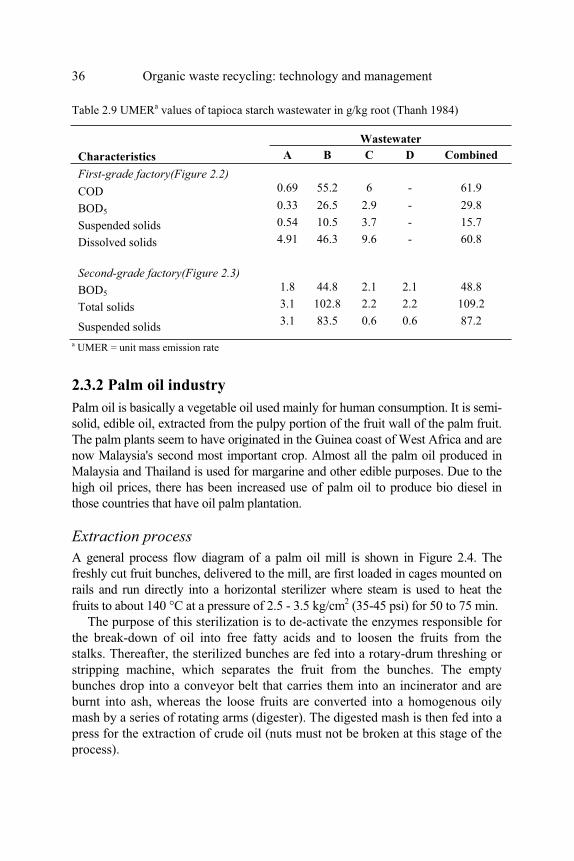
36 Organic waste recycling: technology and management
Table 2.9 UMERa values of tapioca starch wastewater in g/kg root (Thanh 1984)
Wastewater
Characteristics A B C D Combined
First-grade factory(Figure 2.2)
COD 0.69 55.2 6 - 61.9
BOD5 0.33 26.5 2.9 - 29.8
Suspended solids 0.54 10.5 3.7 - 15.7
Dissolved solids 4.91 46.3 9.6 - 60.8
Second-grade factory(Figure 2.3)
BOD5 1.8 44.8 2.1 2.1 48.8
Total solids 3.1 102.8 2.2 2.2 109.2
Suspended solids 3.1 83.5 0.6 0.6 87.2
a UMER = unit mass emission rate
2.3.2 Palm oil industry
Palm oil is basically a vegetable oil used mainly for human consumption. It is semi-
solid, edible oil, extracted from the pulpy portion of the fruit wall of the palm fruit.
The palm plants seem to have originated in the Guinea coast of West Africa and are
now Malaysia's second most important crop. Almost all the palm oil produced in
Malaysia and Thailand is used for margarine and other edible purposes. Due to the
high oil prices, there has been increased use of palm oil to produce bio diesel in
those countries that have oil palm plantation.
Extraction process
A general process flow diagram of a palm oil mill is shown in Figure 2.4. The
freshly cut fruit bunches, delivered to the mill, are first loaded in cages mounted on
rails and run directly into a horizontal sterilizer where steam is used to heat the
fruits to about 140 °C at a pressure of 2.5 - 3.5 kg/cm2 (35-45 psi) for 50 to 75 min.
The purpose of this sterilization is to de-activate the enzymes responsible for
the break-down of oil into free fatty acids and to loosen the fruits from the
stalks. Thereafter, the sterilized bunches are fed into a rotary-drum threshing or
stripping machine, which separates the fruit from the bunches. The empty
bunches drop into a conveyor belt that carries them into an incinerator and are
burnt into ash, whereas the loose fruits are converted into a homogenous oily
mash by a series of rotating arms (digester). The digested mash is then fed into a
press for the extraction of crude oil (nuts must not be broken at this stage of the
process).

Characteristics of organic wastes 37
Pla
nt
B
Co
mb
ined
55
50
-740
0
13
30
0-1
95
00
19
70
-385
0
0 86
-115
0 3.8
-5.2
0 13
5-1
010
Was
h w
ater
20
0-1
700
20
00
-485
0
40
0-6
100
0-1
.1
14
-18
1.2
-1.3
4.2
-7.1
0.6
-5.3
20
-220
Fir
st-g
rad
e st
arch
was
tew
ater
Pla
nt
A
Sep
arat
or
was
tew
ater
30
00
-400
0
31
00
-139
00
14
80
-840
0
0-4
.7
19
-39
5.6
-8.5
3.4
-4.2
0 67
0-8
60
Mea
n
4,1
50
75
80
85
0
16
70
6.6
3.4
1 -
Su
per
nat
ant
Ran
ge
17
20
-682
0
47
00
-100
00
47
0-1
710
1.2
-35
.0
4-1
09
0-1
0.5
2.6
-4.0
0
-2.7
-
Mea
n
11
90
27
00
18
80
1.9
32
3.6
4.2
2.7
-
Sec
on
d-g
rad
e st
arch
was
tew
ater
Was
hw
ater
Ran
ge
30
0-2
490
610
-61
10
29
0-4
240
0-7
.8
0-6
7
0-6
.0
3-4
.6
0-4
.9
-
Ch
arac
teri
stic
s,
mg
/L (
exce
pt
as
ind
icat
ed)
BO
D5
CO
D
Su
spen
ded
so
lid
s
NH
3-N
Org
-N
Ph
osp
ho
rus
pH
DO
Aci
dit
y
Tab
le 2
.10
Ch
arac
teri
stic
s of
tapio
ca s
tarc
h w
aste
wat
er (
Aft
er T
ho
ng
kas
ame
1968 a
nd U
nku
lvas
apau
l 19
75
)
38 Organic waste recycling: technology and management
Nuts and fresh fiber are then separated to recover the nuts which are
subsequently cracked to produce kernels for sale. The pressed fiber and some of
the shells are usually burnt as fuel in the steam-raising boiler.
The extracted crude oil, consisting of a mixture of oil, water and some fine
solid materials, is passed through a vibrating screen to remove the solid matters.
Hot water is often added in this operation. A clarification tank is used to
separate the oil by gravity and the oily sludge settles at the bottom. The clarified
oil is further purified in a vacuum dryer prior to being pumped to a storage tank.
The oil sludge, after straining and desanding, is centrifuged to recover the oil
which is returned to the clarifier. The sludge is discharged into an oil trap, where
further oil is recovered by heating the sludge with steam prior to discharge of
the sludge to a waste treatment facility.
With respect to Figure 2.4, the sources of wastewater and sludge generated
during palm oil milling are given below.
1. Sterilizer's condensates, cleansing of the sterilizers and floor washing at the
sterilizer station.
2. Floor washing and desanding of the press station.
3. Steam condensates
4. Steam condensates
5. Hydrocyclones discharge
6. Steam condensates
7. Turbines cooling water and steam condensates
8. Boilers blowdown
9. Overflow and backwash water of the water softening plant
10. Floor washing of the oil room
11.
12. Wastewaters discharged from various units in the oil room
13.
14. Overflow from the vacuum dryers
15. Oil trap discharge
A general mass balance of various products generated from a palm oil mill plant
is shown in Figure 2.5. It is seen that of the 100 tons fresh fruit bunches (FFB)
processed, about 21 tons of palm oil and 6 tons of palm kernel will be produced.
Other miscellaneous by-products can be used as animal feed, fertilizer, and boiler
fuel.

Characteristics of organic wastes 39
Figure 2.4 General process diagram of a palm oil mill
15
Sterilizer
Kernels silos
Kernels
Hydrocyclones
Nut crackers
Nut bins
Nuts
Depericarping
Presser
Digester
Thresher Incinerators
Weighing machine bagging
1
2
3
4
5
6
7
8
9
10
Empty Bunches
Fresh fruit bunches
Shell
Fiber
Crude Oil
Ash
Shell bunker
Water softening
plant
Boiler
Engine room
Sh
ell
Purifiers
Centrifuge
Desander
Strainer
Oil clarification room
To port
installation
Dryers
Bulk storage
tanks
11
12
13
14
Oil Trap
Process
Wastewater
Water
Recla
imed
oil
Cla
rifi
ed
oil

40 Organic waste recycling: technology and management
Figure 2.5 Product mass balance of a typical palm oil mill (Muttamara et al. 1987)
Palm oil mill wastewater characteristics
Thanh et al. (1980) conducted a study on wastewater characteristics of 4 palm oil
mills in Malaysia and Thailand. The data of wastewater flows per ton of FFB
processed were classified into 50, 70, 80 and 90 percentiles. Table 2.11 shows the
percentiles of wastewater flows in m3 per ton of FFB measured at some sampling
From 100-ton FFB products
obtained are:
Pure oil 21 tons
Palm kernel 6 tons
Bunch ash 0.5 tons
Fresh fruit bunch
100%
Dry fibre fuel
12%
Crude oil
43%
Nuts
13%
Pericarp
14%
Bunch ash
0.5%
Empty bunch
20%
Fruits
70%
Evaporation
10%
Water
evaporation
20%
Pure oil
21%
Shell
6%
Moisture
1%
Kernel
6%
Solids 2%
(Animal
feed/fertilizer)
Water
evaporation
2%

Characteristics of organic wastes 41
stations of the palm oil mills. The characteristics of these wastewaters at 50
percentile values are given in Table 2.12.
Table 2.11 Probability of wastewater flows per ton of FFB processed at different measuring stations of palm oil mills (Thanh et al. 1980)
Flow in m3/ton FFB (m3/hour)
Palm oil mill
Measuring station (see Figure 2.4)
50Percentile*
70Percentile*
80Percentile*
90Percentile*
Plant A (Malaysia)
1. Oil clarification room
1.04(22.0) 1.14(24.8) 1.21(26.5) 1.31(29.0)
2. Boiler house and hydrocyclones
0.49(10.5) 0.57(12.5) 0.62(13.8) 0.70(16.0)
3. Sterilizer building and press station
0.76(15.8) 0.84(17.5) 0.89(18.8) 0.96(20.6)
4. Combined flow (1+2+3)
2.32(47.0) 2.50 (49.8) 2.60 (51.5) 2.75(54.0)
Plant B (Malaysia)
1. Oil clarification room
1.25(15.5) 1.50 (18.0) 1.68 (19.5) 1.94(22.0)
2. Boiler house, sterilizer building and hydrocyclones
1.90(21.0) 2.21(23.7) 2.43(25.7) 2.80(28.5)
3. Combined flow (1+2)
3.23(37.0) 3.72(42.0) 4.10(46.0) 4.60(51.0)
Plant C (Malaysia)
1. Sterilizer building
0.11(2.2) 0.15(2.7) 0.17(3.1) 0.22(3.8)
2. Oil clarification room
1.30(22.5) 1.60(27.0) 1.83(31.0) 2.21(36.0)
3. Boiler house 0.52(8.7) 0.61(10.2) 0.67(11.2) 0.76(13.0) 4. Hydrocyclones 0.27(4.7) 0.34(5.9) 0.38(5.8) 0.45(6.5) 5. Combined flow
(1+2+3)2.25(36.0) 2.60(41.5) 2.85(45.0) .25(50.0)
Plant D (Thailand)
1. Oil clarification room
0.89(6.1) 1.01(8.0) 1.09(9.2) 1.11(11.8)
2. Sterilizer building and oil clarification room
1.09(8.9) 1.21(10.5) 1.29(12.0) 1.39(13.0)
3. Miscellaneous sources
0.64(4.9) 0.80(5.9) 0.87(6.5) 1.00(7.8)
4. Combined flow (1+2+3)
1.73(13.8) 2.01(16.4) 2.16(18.5) 2.39(20.8)
*If a 50 percentile flow is used in the design of wastewater treatment facility, it means that 50% of
the time the flow of that particular waste stream will be equal or less than the stated figures.

42 Organic waste recycling: technology and management
It appears from the above data that wastewaters from the oil clarification
room and sterilizer building are the most concentrated, containing high
concentrations of COD, BOD, solids and oil & grease. Palm oil mill
wastewaters generally have pH below 5 while their temperature can range from
30 to 70°C. The C/N ratios are higher than the optimum value of 30/1,
suggesting that some N needs to be added to the wastewater before being treated
by biological means.
The main solid wastes produced from palm oil milling are nuts, fibres and
shells. The nuts are processed to make kernels, and fibres and shells are used as
boiler fuel as explained earlier. Palm oil can be used for cooking and heating.
The production of bio diesel using palm oil as a raw material is done in some
countries, but depending on local situations, detailed cost-benefit analysis of this
practice needs to be carried out to avoid the impacts as stated in section 4.7.1.
2.3.3 Sugar cane industry
Raw sugar cane manufacturing process
A flow diagram of the sugar cane manufacturing process is shown in Figure 2.6.
The first step in raw sugar processing is juice extraction carried out by crushing the
cane between a series of rollers under pressure. To aid in the extraction of the juice,
sprays of water or thin juice are directed on the blanket of bagasse (fibrous part of
the cane) as it emerges from each mill unit to leach out sugar. The final bagasse
from the last roller contains the unextracted sugar, the woody fiber, and 40-50%
water. This is used as fuel or as material for wallboard and paper manufacture.
The extracted juice is acidic, turbid, and dark green in color. It is treated with
chemicals, such as lime, sulfur dioxide, carbon dioxide and phosphate, and
heated for clarification. This treatment has the effect of precipitating suspended
solids and some impurities and color removal, which are allowed to settle, and
the clear juice is then filtered through vacuum filters. The filter press juice
returns to the clarification process or goes directly to clarified juice. The press
cake is discarded or returned to the fields as fertilizer.

Characteristics of organic wastes 43
Tem
per
atu
re
(ºC
)
46-7
7
30-6
5
32-7
7
32-7
5
36-5
3
30-5
1
30-5
1
45-4
9
31-3
3
pH
4.0
-4.3
4.7
-5.9
4.3
-4.7
4.3
-4.7
3.9
-4.8
4.9
-6.6
4.1
-6.3
4.5
-4.9
5.6
-7.1
Oil
an
d
gre
ase
18500
800
1100
9600
11500
-
8200
86000
180
To
tal
N 490
14
.5
60
265
450
39
230
720
15
To
tal
P
285
20
.5
42
163
230
28
135
330
73
SS
28000
850
1250
10000
20000
680
7500
31000
360
TS
45000
1300
6000
23000
31000
2180
15500
47500
840
BO
Da /
CO
D
0.4
7
0.5
6
0.5
3
0.4
9
0.3
7
0.5
7
0.5
5
0.4
6
0.6
1
BO
Da
30000
1050
5500
14000
16800
1600
10000
28500
460
CO
D
64000
1860
10300
28500
4500
2800
18300
61000
750
Mea
suri
ng
sta
tion
Oil
cla
rifi
cati
on r
oo
m
Bo
iler
ho
use
an
d
hy
dro
cycl
ones
Ste
rili
zer
bu
ildin
g a
nd
pre
ss
stat
ion
Co
mb
ined
flo
w
Oil
cla
rifi
cati
on r
oo
m
Bo
iler
ho
use
, st
eril
izer
bu
ild
ing
an
d h
ydro
cycl
ones
Co
mb
ined
flo
w (
(1+
2)
Ste
rili
zer
bu
ildin
g a
nd
clar
ific
atio
n r
oom
Mis
cell
aneo
us
sou
rces
Pal
m o
il m
ill
Pla
nt
A (
Mal
aysi
a)
Pla
nt
B (
Mal
aysi
a)
Pla
nt
D (
Th
aila
nd
)
Tab
le 2
.12 F
ifty
per
cen
tile
val
ues
of
pal
m o
il w
aste
wat
er c
har
acte
rist
ics
at d
iffe
ren
t sa
mp
lin
g s
tati
on
s (a
ll v
alu
es a
re i
n m
g/L
,
exce
pt
pH
wh
ich i
s d
imen
sio
nle
ss a
nd
tem
per
atu
re i
s in
ºC
) (T
han
h e
t al.
19
80
)
a Fo
r p
lan
t in
Mal
aysi
a, B
OD
was
mea
sure
d a
t 3
0ºC
fo
r 3 d
ays.
Fo
r p
lants
in T
hai
lan
d,
BO
D w
as m
easu
red
at
20
ºC f
or
5 d
ays

44 Organic waste recycling: technology and management
The clarified juice contains approximately 88% water. Two-thirds of this
water is evaporated in vacuum multiple-effect evaporators. Crystallization takes
place in a single-effect vacuum pan where the syrup is evaporated until saturated
with sugar. It is at this point that the sugar first appears as fine crystals, which
are then built up to the size required for the final product. The mixture of
crystals and syrup is then concentrated to a dense mass (massecuite) and the
contents of the pan are discharged into a mixer or crystallizer.
The massecuite from the mixer or crystallizer is drawn into revolving
machines called centrifugals. The sugar crystals are retained and the mother
liquor, molasses, passes through. The final molasses or blackstrap is a heavy
viscous material containing approximately one-third reducing sugars, and the
remainder ash, organic non-sugars, and water. It may be used as cattle feed or as
a raw material for distilleries, to produce ethanol.
Sugar industry wastewater effluents
The sugar industry uses large amounts of water, mainly for cane washing,
condensing of vapor, boiler feed water, and other miscellaneous uses. Sources of
wastewater and sludge generation during the manufacturing of sugar are given in
Figure 2.6. There are air emissions from the sugar manufacturing process which
include a variety of pollutants such as particulates, SOx, NOx, CO, and
hydrocarbons; these pollutants have to be removed to the required air emission
standards set by the appropriate regulatory agency.
Table 2.13 Wastewater characteristics of Crescent Sugar Mills, Pakistan (Qureshi 1977)
Characteristics Range Fifty percentile Ninety percentile
pH 6.7-10.0 8.15 9.11
Alkalinity 260-490 370 494
Total solids 4,520-10,790 6,500 10,300
Fixed solids 1,850-6,150 4,000 6,100
Volatile solids 1,825-4,600 2,700 4,500
COD 607-3,680 2,030 3,500
Nitrogen 15-50 33 -
Phosphorus 6.7-11.25 9.25 -
All values are in mg/L, except pH
The characteristics of wastewater from a sugar mill in Pakistan are given in
Table 2.13. Its pH varied from 6.7 to 10 and the COD range was 600 - 3,700 mg/L.
The wastewater contained rather high solid concentrations in which the ranges of
total solids and volatile solids were 4520 - 10790 and 1820 - 4600 mg/L,
respectively. Wastewater data from a sugar mill in U.S.A. are also given in Table

Characteristics of organic wastes 45
2.14, which indicate relatively low N contents, similar to the characteristics of
tapioca and palm oil wastewaters (Tables 2.10 and 2.11).
Figure 2.6 Diagrammatic flow sheet of the process of raw sugar manufacture (adapted
from Meade and Chen 1977)
2.3.4 Brewing industry
The brewing process
The principal stages in brewing are mashing, boiling and fermentation with
subsequent packaging into bottles and casks followed by cooling, clarification
and pasteurization.
Sugar cane
Juice extraction
Clarification and
color removal
Sedimentation
Evaporation
Crystallization
Separation (Centrifugation)
Raw sugar
Blackstrap
molasses
Condenser water
Filter cake
(fertilizer)
Filtration
Spillage
Scums, leakage
and spillage
Cane wash
water
Condenser water
Water for
washing cane
Maceration
water
Steam for
heating
Steam
Steam

46 Organic waste recycling: technology and management
Table 2.14 Wastewater characteristics of a sugar mill plant in U.S.A. (Oswald et al. 1973)
Parameter Units Value
Total nitrogen (N) mg/L 16.4
Chlorides mg/L 400a
Sulfate mg/L 210
Alkalinity (CaCO3) mg/L 538.0b
Phosphate (P) mg/L 3.4
Potassium mg/L 88.0c
BOD5 (unfiltered) mg/L 930
COD (unfiltered) mg/L 1600
Suspended solids mg/L 1015
Dissolved solids mg/L 2209
Total solids mg/L 3224
Sugar mg/L 1.25
Dissolved oxygen mg/L 0
pH - 7.1 a Based on specific conductivity, b By difference, c Single values
Figure 2.7 Brewing process
Malting
Racking
Fermentation
Cooling
Brewing
Mashing
Grinder & Mixing Washing
Bottling or Kegging
Filtration / Carbonation

Characteristics of organic wastes 47
During mashing, the mixture of finely ground malt and hot water undergoes
enzymatic changes whereby the starch is converted into sugar and dextrins and
the protein into amino acids and polypeptides. The soluble product from
mashing is known as sweet wort and this is subsequently boiled with hops in a
metal vessel. Boiling destroys the enzymes and, at the same time, extracts resins
from the hops to give bittering effect. The wort then goes to a cooling process in
the cool-ship, yeast is added and during the resultant fermentation, the sugars
present are converted into alcohol and CO2. The nitrogenous material and
phosphates in the wort are also utilised by the yeast for growth and
fermentation. The beer is stored in lager tanks for some period and filtered and
pasteurized before being bottled or canned. A schematic diagram of this brewing
process is given in Figure 2.7.
Sources of wastewaters and characteristics
The sources of wastewaters that contain very high amounts of suspended and
dissolved solids are: washing from cool ships, lager tanks and fermentation
tanks. These wastewaters contain excessive amounts of beer, malt and yeast
which possess a very high COD, sometimes as high as 20,000 mg/L, amounting
to about 10% of the total waste discharged. Brewery wastewaters normally have
an amber color and a rich grainy smell of malt.
Brewery wastewaters have been found to be highly contaminated with soluble
organics, low in nutrients and pH, and they have a high temperature (Table 2.15).
The COD content can vary from as much as 24,000 mg/L to as little as 6,000 mg/L.
The ratio of BOD5: COD varies between 0.2 and 0.9.
2.3.5 Slaughterhouse industry
This section will describe waste generation from the abattoirs, meat processing
plants and poultry processing plants.
Abattoirs (Griffiths 1981)
Lairage / stockyard
Lair refers to animals’ lying-place or cages whose wastes comprise mainly of
dung and urine - contaminated straw. Straw is separated by a conventional trap
and the effluent is fairly weak due to frequent washing down. This effluent is
not usually kept separate unless fat is to be recovered from other effluents.
Table 2.16 shows the analysis of wastes from one Chicago stockyard.
Another study of these same wastes showed a volume of 623,000 gallons (165
m3) per day for a 27 acre (11 ha) section of the yard and an average BOD5 of
100 mg/L (U.S.PHS 1943).

48 Organic waste recycling: technology and management
Table 2.15 Characteristics of brewery wastewater (Tantideeravit 1975)
BOD5 (mg/L) 1800
COD (mg/L) 3100
Total solids (mg/L) 1750
Suspended solids (mg/L) 800
pH 7.5
Alkalinity (mg/L as CaCO3) 160
Table 2.16 Characteristics of stockyard wastewater (U.S.PHS 1943)
Total suspended solids (mg/L) 170
Volatile suspended solids (mg/L) 13
Organic nitrogen (mg/L) 11
Ammonia nitrogen (mg/L) 8
BOD5 (mg/L) 60
Slaughter: bleeding and carcass separation
Figure 2.8 is a schematic diagram of a slaughter house operation. After killing, the
carcasses are bled, the hide is stripped, the abdominal mass is removed and the
carcass is split into smaller pieces. At some stage washing takes place which gives
rise to dirt, dung, grit, etc., in the effluent.
Blood is normally kept separate to reduce the polluting load in the effluent
and because it can be a valuable by-product. The abdominal mass is removed and
sorted for collection by the pharmaceutical and by-products industries.
The paunch (stomach) is removed, and it is important to keep the contents
out of the normal effluent stream (to simplify subsequent treatment). The
contents, partly digested food, are handled separately; they are best kept as dry
as possible and disposed of on land as fertilizer.
The cutting down of the carcass involves blood, bone dust, tissue and fat
contaminating the wash water, some of which can be caught in traps, but this is
the main pollutant which has to be dealt with.
Meat processing (Griffiths 1981)
Meat processing plants are completely different from abattoirs. There is no
paunching, no blood, no gut; but there is a lot more meat and fat wastes plus all
sorts of additives, e.g. pastry, soya, sauces, spices, preservatives, colorings, etc.

Characteristics of organic wastes 49
Figure 2.8 Fundamental processes in a slaughterhouse (Nemerow 1971) (© 1971,
Addison-Wesley Publishing Co., Reading, Mass)
The major problem is the flow of the effluent stream not being constant. Little
water is used whilst production is under way, but when a batch is complete a lot of
water is used to wash down. The additives vary and so does production. In order to
treat the effluents properly it is necessary in each case to study and to understand
the variations in the process and the waste characteristics.
Live animals Killing
Hide removal Hog dehairing
Evisceration
Blood
Hides
Boning, cutting and grinding
Inedible rendering
Edible rendering
Paunch removal
Sausage
Pollution By-products
Tripe
Lards and edible
tallows
Inedible tallows, greases and tankage
Fresh meat
Scraps

50 Organic waste recycling: technology and management
Poultry processing (Griffiths 1981)
Due to the large demand for fowls, poultry processing is now a high volume
operation which has developed from its original farmhouse background. The
basic procedures for poultry processing are shown in Figure 2.9.
Figure 2.9 Major steps in poultry processing (Nemerow 1971) (© 1971, Addison Wesley
Publishing Co., Reading, Mass)
The birds are hung by the feet on a conveyor. They are then killed and bled. The
blood is taken away and, if recovered, used for human or pet foods (it is of less
value than beef blood).
The next stage is feather plucking. This is done by a series of flaps and flails in a
tunnel, under a hot-water spray. There are two ways of disposing of the feathers.
Killing
station
Shipment
Inside washOutside
wash
Chilling
tanks
Weighing and
packaging
Eviscerating table or trough
Scalding tanks
PickerSingerWasher
Bleeding area
(tunnel or enclosed area)
Uploading of live
poultry

Characteristics of organic wastes 51
It can be taken away by water in a flume or taken away by a conveyor. The feathers
can be reused as a material for mattresses.
Next the heads, feet and innards are removed. The removal of innards is done by
hand and they are disposed of by a wet or dry viscera line. In a dry line the innards
are removed and taken to a disposal skip by conveyor or by vacuum. In a wet line
they are taken by a water flume to be separated later.
The final stages are washing by a fixed amount of water per fowl, then spin
chilling and freezing or washing (with the addition of chlorine for disinfection),
drying and vacuum sealing.
The following are the possible causes of pollution in the poultry processing
effluent:
1. Blood - if not recovered; this has a high BOD5.
2. Feather water and flume: if a wet flume is used, this can have a high
proportion of dissolved or emulsified fats.
3. Wet viscera: requires screening to remove the solid matters.
4. Wash and spin chiller discharge: note that chlorine is introduced in the
wash water.
Characteristics of slaughter house and meat-packing wastes
Effluents from slaughter houses and meat-packing houses are usually heavily
polluted with solids, floatable matter (fat), blood, manure and a large variety of
proteinaceous compounds. The composition depends very much on the type of
production and facilities. The main wastes originate from lairage, killing, hide
removal or dehairing, paunch handling, rendering, trimming, processing and
clean-up operations. The BOD5 and solids concentrations in the plant effluent
depend on in-plant control of water use, by-products recovery, waste separation
at the source and plant management.
When considering effluent disposal, the first consideration is water
consumption. The range of wastewater production from abattoirs is 5-15 m3/ton
live weight. For the poultry industry a typical discharge lies between 10 and 55
L per bird (Brolls and Broughton 1981).
In terms of BOD5, typical loads from abattoirs and meat processing are 6-12
kg/ton live weight at UK abattoirs, usually at a concentration of 1,000 - 3,000
mg/L. From poultry packing, the effluent is normally about half the strength of
the abattoir wastewater, with a BOD5 content of 13-23 kg/1,000 birds (Brolls
and Broughton 1981)
Some characteristics of slaughter house wastewaters, as reported by Brolls and
Broughton (1981), are given in Table 2.17, while those of meat-packing wastes are
given in Table 2.18. Table 2.19 shows the wastewater characteristics of a poultry
processing plant in Thailand.

52 Organic waste recycling: technology and management
Table 2.17 Characteristics of slaughterhouse wastewater (Brolls and Broughton 1981)
Item Lower range Upper range
BOD5 (mg/L) 360 - 1,880 900 - 2,600
Suspended solids (mg/L) 489 - 1,450 600 - 1,800
Organic N (mg/L) 36 - 510 -
Grease (mg/L) 88 - 440 200 - 800
Chlorides (mg/L) as Cl 190 - 5,690 -
pH 6.5 - 8.4 6.1
COD (mg/L) - 2,000 - 4,900
Flow (L/1000 kg live wt.) 1,690 - 7,920
Table 2.18 Characteristics of meat packing wastewatera
(Brolls and Broughton 1981)
Item Average Range
BOD5 (mg/L) 1,240 600 - 2,720
COD (mg/L) 2,940 960 - 8,290
Organic N (mg/L) 85 22 - 240
Grease (mg/L) 1,010 250 - 3,000
Suspended solids (mg/L) 1,850 300 - 4,200
Volatile suspended solids (mg/L) 92 80 - 97 a Composite samples from 16 plants
Table 2.19 Characteristics of poultry processing wastewater (Visittavanich 1987)
Parameters Mean Range
COD (mg/L) 2110 1260 - 3260
BOD5 (mg/L) 1010 520 - 1740
TKN (mg/L) 150 90 - 200
TS (mg/L) 1940 1290 - 2640
Total P (mg/L) 14 12 - 17
pH 7.1 6.7 - 7.7

Characteristics of organic wastes 53
2.3.6 Fruit and vegetable industry
Processing operations and waste generation
Unit operation
The processing steps for five typical commodities are outlined in Figure 2.10 for
peaches (to exemplify fruits), peas and corn (common vegetables), beets (peeled
root crops), and tomato products (pulped commodities). The principal steps
where water (or steam) is used and where solid and dissolved residuals are
generated are indicated.
The containers of fruits or vegetables are dumped into the first stage washer or
flume or onto belts. The products are conveyed by flumes, pipes, belts, elevators, or
other conveyors between processing steps. Fluming water, generally reused, and
small flows of water to belts, graders, and other equipment for lubrication and
sanitation are not noted in the flow diagrams.
Type of waste generated
Operation Peas Corn
Tomato
products Solid Soluble Soil
Dry dump × ×
Water dump ×
Air cleaner × ×
Trash eliminator
Husker ×
Sorting/trimming × × ×
Washer × × ×
Grader/sizer ×
Cutter ×
Peeler/rinse (×)
Blancher/rinse × (×)
Pulper/finisher (×)
Slicer/dicer
Evaporator (×) b
a Operational or alternative operations in (). b Relatively clean water
Figure 2.10 Use of water and generation of wastes in typical unit operations of fruit and
vegetable processing (U.S. EPA 1971)
Water

54 Organic waste recycling: technology and management
Waste generation by unit operations
Much of the total waste flows from many commodities, especially from citrus,
come from relatively clean water used in cooling, condensing, and
concentrating. The segregation of this water for reuse is practised to some extent
and should become almost universal. Other large waste flows are from washing
tomatoes, peeling potatoes, peeling peaches, washing potatoes, cutting corn,
cutting and pitting peaches, washing corn, and blanching corn. Large quantities
of BOD5 are generated in those processes. Citrus by-products recovery also
generates very large amounts of BOD5 and SS. Other large sources of SS are
peeling potatoes, cutting corn, and washing tomatoes.
Peeling: Table 2.20 shows a summary of estimated pollution loads in the
effluent from peeling fruits and vegetables reported by various investigators.
Peel wastes comprise a high percentage of the total pollution loads in the
effluent of fruit and vegetable plants.
Blanching: Table 2.21 shows examples of losses from vegetables during
blanching expressed in BOD5, COD, and SS. The volume of effluent from
blanchers is generally relatively small, but the concentrations of suspended and
total solids can be high. These wastewaters contain a high organic content (in terms
of BOD5 and COD) which can be treated or recycled by biological processes.
2.4 POLLUTION CAUSED BY HUMAN WASTES AND
OTHER WASTEWATERS
Because human, animal and agricultural wastes are organic in nature, when
being discharged into a stream or lake, they will serve as food for heterotrophic
bacteria. Bacterial reactions will decompose the organic compounds to simple,
inorganic end-products with the production of energy for cell synthesis as
shown in Equations 2.1 and 2.2 (Metcalf and Eddy Inc. 2003):
Oxidation or dissimilatory process
(COHNS) + O2 + aerobic bacteria CO2 + NH3 + other end products
+ energy (2.1)
Synthesis or assimilatory process
(COHNS) + O2 + aerobic bacteria + energy C5H7O2N
(new bacterial cells) (2.2)

Characteristics of organic wastes 55
Table 2.20 Characteristics of wastewater from peeling fruits and vegetables a (U.S.EPA 1971)
BOD5 SS
Product kg/ton
% of plant
waste stream Rate
Beets (blancher/peeler) 88 84 100 kg/hr
Peaches (rinse after peeling) 40 5 kg/ton
Peaches 27(COD) 5 kg/ton
Peaches 4-6 2.5-4 kg/ton
Potatoes (peeler) 9 41 kg/ton
Potatoes 17-36 34-49 kg/ton
Potatoes (peeler chips) 1 2 kg/ton
Potatoes (peeler/ dehydration) 9 41 kg/ton
Potatoes 15
Potatoes (lye peel) 84 89
Potatoes (dry caustic peel) 12 80
Potatoes (lye peel) 171
Potatoes (infra red peel) 119
Potatoes (steam peel) 118
Potatoes (infra red peel) 91
Peach/tomato (flume after peel) 1 383 mg/L
Peach/tomato (rinse after peel) 19 1230 mg/L
Peach/tomato (rinse after peel) 20
Tomato (lye peel) 39
Tomato (lye peel) 35 a Kilograms of BOD5 or suspended solids per ton of raw product, or per hour of operation
Under anaerobic conditions (i.e. in the absence of oxygen), anaerobic
bacteria will decompose the organic matter as follows:
(COHNS) + anaerobic bacteria CO2 + H2S + NH3 + CH4 + other
end products + energy (2.3)

56 Organic waste recycling: technology and management
Table 2.21 Pollution loads in effluents from water blanching of vegetablesa (U.S.EPA 1971)
VegetableEffluent
flow (L/hr)
BOD5
(kg/ton)
COD
(kg/ton)
SS
(kg/ton)
Beets (and peelers) 3,013 88(85)b 147(83) 109(55) Carrots (and peelers) 1,937 44(65) 90(67) 153(64) Corn 523 11.2(16) 14(18) 3(12) Peas 294 3,500 ppm
in effluent
Potatoes 580 24 26 21 Potatoes (and peelers) 2,118 84(89) 127(86) 82(37) a BOD5, COD, and SS in kg per ton of raw product except as noted b Percent of total effluent pollution load in ().
(COHNS) + anaerobic bacteria + energy C5H7O2N
(new bacterial cells) (2.4)
Note: C5H7O2N is a common chemical formula used to represent bacterial
cells.
In the absence of organic matter, the bacteria will undergo endogenous
respiration or self-oxidation, using its own cell tissue as substrate:
C5H7O2N + 5O2 5CO2 + NH3 +2H2O + energy (2.5)
The compounds CO2 and NH3 are nutrients for algae. With sufficient
sunlight, algal photosynthesis will occur (Oswald and Gotaas 1955):
NH3 + 7.62CO2 + 2.53H2O C7.62 H8.06 O2.53 N+ 7.62 O2
(new algal cells) (2.6)
Another equation to incorporate P compound in the algal photosynthesis is
(Oswald 1988):
106CO2 + 236H2O + 16NH4+ + HPO4
2- C106H181O45N16P + 118O2 +
171H2O + 14H+ (2.7)
In a natural water course receiving low organic loading, the oxygen produced in
Equation 2.6 can be used by the bacteria in Equations 2.1 and 2.2, and the cycle is
repeated. This cycle, called ‘algal-bacterial symbiosis’, is a natural phenomenon
occurring in a water body that receives a low organic loading, and these algal-
bacterial reactions are in a state of dynamic equilibrium. Parts of the algal and
Sunlight
Algae
Sunlight
Algae

Characteristics of organic wastes 57
bacterial cells serve as food for protozoa and some small fishes, which are further
consumed by big fishes and finally by man.
The discharge of untreated wastes into a receiving water body will create a
biologically unbalanced condition. At high organic loading, the bacteria will
require more oxygen for their oxidation and synthesis (Equations 2.1 and 2.2),
resulting in the depletion of oxygen in the water body which is detrimental to all
aquatic life (Figure 1.3). Although algal photosynthesis produces some oxygen
(Equation 2.6), during night time when there is no sunlight algae respire or use
oxygen, causing a further depletion of oxygen in the water. Eventually, the water
will become anaerobic (without oxygen), dark in color, and only anaerobic
microorganisms and certain types of worms can live. Besides this organic
pollution, the water body would become very unaesthetic to the nearby inhabitants
and would lower the environmental quality of its surrounding areas.
However, knowledge of the pollution effects as cited above has, in turn, been
used for the design of technologies and facilities for waste treatment and recycling.
For example, the reactions of Equations 2.1 and 2.2 are basically used in the design
and operation of aerobic waste treatment facilities such as activated sludge,
trickling filtration, and composting. The algal-bacterial symbiosis is the basis for
the design of facultative waste stabilization ponds and high-rate algal ponds (for the
production of algal protein biomass). Equation 2.3 is the reaction where biogas
(CH4 and CO2) is produced; application of this basic information to waste recycling
is given in Chapters 3 to 9.
2.5 DISEASES ASSOCIATED WITH HUMAN AND
ANIMAL WASTES
There are various kinds of enteric microorganisms present in human excreta and
animal manure, some of which are pathogenic and some are not. They can be
classified into such major groups as bacteria, viruses, protozoa and helminths.
Some of the important enteric pathogens commonly found in human excreta and
wastewater, the diseases they cause, modes of transmission and geographical
distribution are listed in Table 2.22 Feachem et al. (1983) estimated the possible
outputs of some pathogens in the feces and wastewater of a tropical community as
shown in Table 2.23.

58 Organic waste recycling: technology and management
Co
nce
ntr
atio
n
per
lit
er i
n t
ow
n
sew
ageb
5,0
00
7,0
00
1,0
00
4,5
00
60
0
32 1
To
tal
excr
eted
dai
ly b
y t
ow
n
2.5
× 1
01
1
3.5
× 1
01
1
5 ×
10
10
2.2
5 ×
10
11
3 ×
10
10
1.6
× 1
09
5 ×
10
7
To
tal
excr
eted
dai
ly
per
in
fect
ed p
erso
nc
10
8
10
8
10
8
15
× 1
06
10
6
8 ×
10
4
4 ×
10
3
Av
erag
e n
um
ber
of
org
anis
ms
per
gra
m
of
fece
sb
10
6
10
6
10
6
15
× 1
04
10
4f
80
0f
40
f
Pre
val
ence
of
infe
ctio
n
in c
ou
ntr
y (
per
cen
tag
e)a
5 7 1 30
60
40
25
Pat
hog
en
Vir
use
s
E
nte
rov
iru
sesd
Bac
teri
a
S
alm
on
ella
sp
p.
V
ibri
o c
ho
lera
e
Pro
tozo
a
E
nta
mo
eba
his
toly
tica
Hel
min
ths
A
sca
ris
lum
bri
coid
es
H
oo
kw
orm
sg
S
chis
toso
ma
man
son
i
Tab
le 2
.22
Po
ssib
le o
utp
ut
of
sele
cted
pat
ho
gen
s in
the
fece
s an
d s
ewag
e o
f a
tro
pic
al c
om
mu
nit
y o
f 5
0,0
00 i
n a
dev
elo
pin
g
cou
ntr
y

Characteristics of organic wastes 59
Co
nce
ntr
atio
n
per
lit
er i
n t
ow
n
sew
ageb 1
0
12
0
To
tal
excr
eted
dai
ly b
y t
ow
n
5 ×
10
8
6 ×
10
9
To
tal
excr
eted
dai
ly
per
in
fect
ed p
erso
nc
10
4
2 ×
10
5
Av
erag
e n
um
ber
of
org
anis
ms
per
gra
m
of
fece
sb
10
4
2 ×
10
3f
Pre
val
ence
of
infe
ctio
n
in c
ou
ntr
y (
per
cen
tag
e)a
1 60
Pat
hog
en
T
aen
ia s
agin
ata
T
rich
uri
s tr
ich
iura
Tab
le 2
.22
Po
ssib
le o
utp
ut
of
sele
cted
pat
ho
gen
s in
the
fece
s an
d s
ewag
e o
f a
tro
pic
al c
om
mu
nit
y o
f 5
0,0
00 i
n a
dev
elo
pin
g
cou
ntr
y(c
on
tin
ued
)
a Th
e p
rev
alen
ces
giv
en i
n t
his
colu
mn
ref
er t
o i
nfe
ctio
n a
nd n
ot
to m
orb
idit
y
b I
t m
ust
be
reco
gn
ized
that
th
e pat
ho
gen
s li
sted
hav
e d
iffe
ren
t ab
ilit
ies
to s
urv
ive
ou
tsid
e th
e h
ost
, an
d t
hat
th
e co
nce
ntr
atio
n
of
som
e o
f th
em w
ill
rapid
ly d
ecli
ne
afte
r th
e fe
ces
hav
e bee
n p
asse
d.
The
conce
ntr
atio
ns
of
pat
ho
gen
s p
er l
iter
in
the
sew
age
of
the
tow
n w
ere
calc
ula
ted
by
ass
um
ing
th
at 1
00
lit
ers
of
sew
age
are
pro
du
ced
dai
ly p
er c
apit
a, a
md
th
at 9
0 p
erce
nt
of
the
pat
ho
gen
s d
o n
ot
ente
r th
e se
wer
s o
r ar
e in
acti
vat
ed i
n t
he
firs
t fe
w m
inu
tes
afte
r ex
cret
ion
c T
o c
alcu
late
th
is f
igu
re i
t is
nec
essa
ry t
o e
stim
ate
a m
ean
fec
al w
eig
ht
for
tho
se p
eop
le i
nfe
cted
. T
his
mu
st n
eces
sari
ly b
e th
e
rou
gh
est
of
esti
mat
es b
ecau
se o
f th
e ag
e-sp
ecif
ic f
ecal
wei
gh
ts a
nd
th
e ag
e d
istr
ibu
tio
n o
f in
fect
ed p
eop
le i
n t
he
com
mu
nit
y.
It w
as a
ssu
med
th
at p
eop
le o
ver
15
yea
rs o
ld e
xcr
ete
15
0 g
dai
ly,
and
th
at p
eople
un
der
15
ex
cret
e, o
n a
ver
age
75
g d
aily
. It
was
als
o a
ssu
med
th
at t
wo
-th
ird
s o
f al
l in
fect
ed p
eop
le a
re u
nder
15
. T
his
giv
es a
mea
n f
ecal
wei
gh
t fo
r in
fect
ed i
nd
ivid
ual
s
of
10
0 g
d I
ncl
udes
po
lio
-, e
cho
-, a
nd c
ox
sack
iev
iru
ses
e In
clu
des
en
tero
tox
igen
ic,
ente
roin
vas
ive,
an
d e
nte
rop
ath
ogen
ic E
.co
li
f Th
e d
istr
ibuti
on
of
egg
ou
tput
fro
m p
eop
le i
nfe
cted
by
thes
e h
elm
inth
es i
s ex
trem
ely
sk
ewed
; a
few
peo
ple
ex
cret
e v
ery
hig
h
egg
co
nce
ntr
atio
ns
gA
ncy
lost
om
a d
uoden
ale
an
d N
ecato
r am
eric
anus
Fro
m F
each
em e
t a
l. 1
98
3;
repro
du
ced
wit
h p
erm
issi
on
of
the
Worl
d B
ank

60 Organic waste recycling: technology and management
Geo
gra
ph
ical
dis
trib
uti
on
Asi
a, A
fric
a, s
om
e
par
ts o
f E
uro
pe
Wo
rld
wid
e
Wo
rld
wid
e
Wo
rld
wid
e
Wo
rld
wid
e
Wo
rld
wid
e
Wo
rld
wid
e
Tra
nsm
issi
on
a
Per
son
p
erso
n
Per
son
(o
r an
imal
s)
per
son
Per
son
p
erso
n
Per
son
p
erso
n
Per
son
p
erso
n
Per
son
p
erso
n
Per
son
p
erso
n
Dis
ease
Ch
ole
ra
Ty
ph
oid
fev
er
Bac
teri
al d
yse
nte
ry
Dia
rrh
ea
Po
lio
my
elit
is
Var
iou
s, i
ncl
ud
ing
sev
ere
resp
irat
ory
dis
ease
,
fev
ers,
ras
hes
, p
aral
ysi
s, a
sep
tic
men
ing
itis
, m
yo
card
itis
Var
iou
s, s
imil
ar t
o c
ox
sack
iev
irus
Pat
hog
en
Bac
teri
a
Vib
rio c
ho
lera
e
Sa
lmon
ella
typ
hi
Sh
igel
la d
ysen
teri
ae
and
oth
er s
pec
ies
Pat
hog
enic
Esc
her
ich
ia c
oli
Vir
us
Po
lio
vir
us
Co
xsa
ckie
vir
us
(so
me
stra
ins)
Ech
ovir
us
Tab
le 2
.23
Ente
ric
pat
ho
gen
s in
hum
an e
xcr
eta
and
was
tew
ater
(G
aud
y a
nd G
aud
y 1
98
0;
Fea
chem
et
al.
19
83
)

Characteristics of organic wastes 61
Geo
gra
ph
ical
dis
trib
uti
on
Wo
rld
wid
e
Wo
rld
wid
e
Wo
rld
wid
e
Wo
rld
wid
e
Wo
rld
wid
e
Wo
rld
wid
e
Mai
nly
in
war
m,
wet
clim
ates
Afr
ica,
Asi
a, S
ou
th
Am
eric
a
Tra
nsm
issi
on
a
Per
son
p
erso
n
Per
son
p
erso
n
Per
son
(o
r an
imal
s)
per
son
Per
son
p
erso
n
Per
son
(an
imal
s)
per
son
Per
son
s
oil
p
erso
n
Per
son
s
oil
p
erso
n
Per
son
a
qu
atic
sn
ail
per
son
Dis
ease
Res
pir
ato
ry a
nd
gas
tro
inte
stin
al i
nfe
ctio
ns
Infe
ctio
us
hep
atit
is (
liv
er m
alfu
nct
ion
), a
lso
may
aff
ect
kid
ney
s an
d s
ple
en
Dia
rrh
ea (
inte
stin
al p
aras
ite)
Am
oeb
ic d
yse
nte
ry,
infe
ctio
n o
f o
ther
org
ans
Dy
sen
tery
, in
test
inal
ulc
ers
Asc
aria
sis
(ro
un
dw
orm
)
Ho
ok
wo
rm
Sch
isto
som
iasi
s or
bil
har
zias
is
Pat
hog
en
Ad
enov
iru
s
Hep
atit
is
Pro
tozo
a
Gia
rdia
la
mb
lia
En
tam
oeb
a h
isto
lyti
ca
Ba
lan
tid
ium
co
li
Hel
min
ths
Asc
ari
s lu
mb
rico
ides
An
cylo
sto
ma
du
od
enale
Sch
isto
som
a
Tab
le 2
.23
Ente
ric
pat
ho
gen
s in
hum
an e
xcr
eta
and
was
tew
ater
(G
aud
y a
nd G
aud
y 1
98
0;
Fea
chem
et
al.
19
83
) (c
onti
nu
ed)

62 Organic waste recycling: technology and management
Geo
gra
ph
ical
dis
trib
uti
on
So
uth
east
Asi
a
Wo
rld
wid
e
Wo
rld
wid
e
Wo
rld
wid
e
Tra
nsm
issi
on
a
Per
son
(o
r an
imal
) a
qu
atic
snai
l f
ish
per
son
Per
son
c
ow
p
erso
n
Per
son
p
ig (
or
per
son
)
per
son
Per
son
s
oil
p
erso
n
Dis
ease
Liv
er f
luk
e
Bee
f ta
pew
orm
Po
rk t
apew
orm
Wh
ipw
orm
Pat
hog
en
Clo
no
rch
is s
inen
sis
Ta
enia
sag
ina
ta
Ta
enia
so
liu
m
Tri
chu
ris
tric
hiu
ra
Tab
le 2
.23
Ente
ric
pat
ho
gen
s in
hum
an e
xcr
eta
and
was
tew
ater
(G
aud
y a
nd G
aud
y 1
98
0;
Fea
chem
et
al.
19
83
) (c
onti
nu
ed)
a Tra
nsm
issi
on
mo
de
is g
ener
ally
th
rou
gh
th
e fe
cal-
ora
l ro
ute
, i.
e. t
he
excr
eted
dis
ease
may
be
ing
este
d b
y o
ther
per
son
s o
r
the
excr
eted
dis
ease
go
th
rou
gh s
om
e d
evel
opm
ent
stag
es i
n t
he
env
iro
nm
ent
(wat
er,
soil
, o
r an
imal
s) a
nd
in
fect
oth
er
per
son
s. S
om
e v
iru
s d
isea
ses
may
be
tran
smit
ted
by
th
e o
ral-
ora
l ro
ute
, e.
g.
thro
ug
h t
hro
at s
ecre
tio
n.
Fo
r so
me
hel
min
tic
infe
ctio
ns
such
as
Ancy
lost
om
aan
dSch
itoso
ma
, th
e in
fect
ive
larv
ae w
ill
pen
etra
te t
he
skin
of
a p
erso
n d
irec
tly

Characteristics of organic wastes 63
Pro
bab
le v
ecto
r o
r m
ean
s
of
spre
ad
Var
iou
s C
ule
x
mo
squ
ito
es
Var
iou
s m
osq
uit
oes
Var
iou
s m
osq
uit
oes
Var
iou
s m
osq
uit
oes
Var
iou
s m
osq
uit
oes
Occ
up
atio
nal
ex
po
sure
Co
nta
ct e
xp
osu
re
Geo
gra
ph
ical
dis
trib
uti
on
Eas
tern
Asi
a an
d E
ast
Ind
ies
No
rth
Am
eric
a
So
uth
and
cen
tral
Afr
ica
So
uth
Afr
ica
So
uth
Afr
ica
Eu
rop
e an
d N
ort
h A
mer
ica
Wo
rld
wid
e, e
spec
iall
y
wh
ere
smal
l p
ox e
xis
ts
Pri
nci
pal
an
imal
s
affe
cted
Bir
d, h
ors
es,
catt
le, p
igs
Bir
ds,
fo
wl
Sh
eep
, g
oat
s, c
attl
e,
rela
ted
wil
d a
nim
als
Sh
eep
Sh
eep
Sh
eep
, g
oat
s
Cat
tle,
ho
rses
Cau
sati
ve
org
anis
m
Vir
us
Vir
us
Vir
us
Vir
us
Vir
us
Vir
us
Vir
us
Dis
ease
1.
Vir
us
dis
ease
s
A
rth
ropo
d-b
orn
e in
fect
ion
s:
J
apan
ese
B e
nce
ph
alit
is
S
t. L
ou
is e
nce
ph
alit
is
S
ou
th A
fric
an d
isea
se
R
ift
Val
ley f
ever
W
esse
lsb
ron f
ever
M
idd
leb
urg
dis
ease
C
on
tag
iuo
s ec
thy
ma
C
ow
pox
Tab
le 2
.24
Epid
emio
logic
al a
spec
ts o
f so
me
of
the
zoo
no
ses

64 Organic waste recycling: technology and management
Pro
bab
le v
ecto
r o
r m
ean
s o
f
spre
ad
Occ
up
atio
nal
ex
po
sure
Co
nta
ct a
nd
occ
up
atio
nal
exp
osu
re
Co
nta
ct e
xp
osu
re (
hu
man
s ar
e
qu
ite
resi
stan
t)
Co
nta
ct e
xp
osu
re
Vir
us
con
tam
inat
es f
ood
and
env
iron
men
t
Mai
nly
air
bo
rne,
alt
hou
gh
mil
k m
ay b
e a
veh
icle
and
occ
asio
nal
ly t
ick
s
Occ
up
atio
nal
ex
po
sure
,
ing
esti
on
of
con
tam
inat
ed
mea
t
Occ
up
atio
nal
ex
po
sure
Ing
esti
on
of
con
tam
inat
ed
mil
k p
rodu
cts
and o
ther
foo
ds
Geo
gra
ph
ical
dis
trib
uti
on
Wo
rld
wid
e
Wo
rld
wid
e
Eu
rop
e, A
sia,
Afr
ica,
and
So
uth
Am
eric
a
Asi
a an
d E
uro
pe
Wo
rld
wid
e
Wo
rld
wid
e
Wo
rld
wid
e
Wo
rld
wid
e
Pri
nci
pal
an
imal
s
affe
cted
Cat
tle
Bir
ds,
rel
ated
vir
us
foun
d
in c
attl
e an
d c
ats
Cat
tle,
pig
s, r
elat
ed
spec
ies
Pig
s ro
den
ts
Ro
den
s p
igs,
do
gs
Sh
eep
, ca
ttle
, g
oat
s,
fow
l, w
ild
bir
ds,
mam
mal
s
Cat
tle,
sh
eep
, g
oat
s
Cat
tle,
sh
eep
, g
oat
s, p
igs
Cau
sati
ve
org
anis
m
Vir
us
Vir
us
Vir
us
Vir
us
Vir
us
Co
xiel
la
bu
rnet
ii
Ba
cill
us
an
thra
cis
Bru
cell
a
ab
ort
us
Br.
su
is
Br.
mel
iten
sis
Dis
ease
P
seud
o-c
ow
pox
P
sitt
aco
sis-
orn
ith
osi
s
F
oo
t an
d m
ou
th d
isea
se
I
nfl
uen
za a
nd
p
arai
nfl
uen
za
L
ym
pho
cyti
c
c
ho
rio
men
ing
itis
2.
Ric
kett
sia
l d
isea
ses
Q
fev
er
3.
Ba
cter
ial
dis
ease
s
A
nth
rax
B
ruce
llo
sis
Tab
le 2
.24
Epid
emio
logic
al a
spec
ts o
f so
me
of
the
zoo
no
ses
(co
nti
nu
ed)

Characteristics of organic wastes 65
Pro
bab
le v
ecto
r o
r m
ean
s o
f
spre
ad
Occ
asio
nal
ly a
irbo
rne
Ing
esti
on
Ing
esti
on
Un
kno
wn
Ex
po
sure
and
in
ges
tion
Ex
po
sure
and
in
ges
tion
Ing
esti
on
, ai
rbo
rne
and c
onta
ct
Ing
esti
on
and
con
tact
Geo
gra
ph
ical
dis
trib
uti
on
Wo
rld
wid
e
Wo
rld
wid
e
Wo
rld
wid
e
Asi
a an
d N
ort
h A
mer
ica
Wo
rld
wid
e
Wo
rld
wid
e
Wo
rld
wid
e
Pri
nci
pal
an
imal
s
affe
cted
Cat
tle,
pig
s, f
ow
l
Cat
tle,
pig
s, f
ow
l
Ro
den
ts, sh
eep
, ca
ttle
,
pig
s
Ro
den
ts, sh
eep
Mam
mal
s, b
ird
s
Cat
tle,
pig
s, f
ow
l
Cat
tle,
pig
s
Cau
sati
ve
org
anis
m
Var
iou
s b
acte
ria
and
thei
r to
xin
s in
clud
ing
Sa
lmon
ella
,
Sta
ph
ylo
cocc
us,
and
Clo
stri
dia
Esc
her
ich
ia s
pp
.
Ari
zon
a g
roup
Lis
teri
a
mo
no
cyto
gen
es
Pse
ud
om
ona
s
pse
udo
ma
llei
Pa
steu
rell
a
mu
lto
cid
a
Sa
mon
ella
sp
p.
Sta
ph
ylo
cocc
us
spp
.
Dis
ease
B
acte
rial
fo
od
p
ois
on
ing
C
oli
bac
illo
sis
L
iste
rio
sis
M
elio
ido
sis
P
aste
ure
llo
sis
S
alm
on
ello
sis
S
taph
ylo
cocc
us
Tab
le 2
.24
Epid
emio
logic
al a
spec
ts o
f so
me
of
the
zoo
no
ses
(co
nti
nu
ed)

66 Organic waste recycling: technology and management
Pro
bab
le v
ecto
r o
r m
ean
s o
f
spre
ad
In
ges
tio
n a
nd
co
nta
ct
Ing
esti
on
, in
hal
atio
n a
nd
occ
up
atio
nal
exp
osu
re
Un
kno
wn
Geo
gra
ph
ical
dis
trib
uti
on
Wo
rld
wid
e
Wo
rld
wid
e
Eu
rop
e ,
Nort
h a
nd
Sou
th
Am
eric
a
Pri
nci
pal
an
imal
s
affe
cted
Cat
tle,
fo
wl
Cat
tle
Mo
nk
eys
Fo
wl
Cat
tle,
sh
eep
Cau
sati
ve
org
anis
m
Str
epto
cocc
us
spp.
Myc
ob
act
eriu
m
tub
ercu
losi
s
var
. bo
vis
var
. ho
min
is
var
. a
viu
m
Vib
rio f
etu
s
Dis
ease
S
trep
toco
ccu
s
T
ub
ercu
losi
s
V
ibri
osi
s
Tab
le 2
.24
Epid
emio
logic
al a
spec
ts o
f so
me
of
the
zoo
no
ses
(co
nti
nu
ed)
Fro
m S
teel
e (1
99
6);
rep
rod
uce
d b
y p
erm
issi
on
of
the
Fo
od
an
d A
gri
cult
ure
Org
aniz
atio
n o
f th
e U
nit
ed N
atio
ns

Characteristics of organic wastes 67
It is obvious from these tables that human wastes (excreta and wastewater) are a
source of health hazards to the public and are the beginning of the transmission
route of many diseases. The engineering profession responsible for the
collection, transport, treatment and disposal/reuse of these wastes must be aware
of the potential infectivity and transmission of these diseases, so as to be able to
ensure that these pathogens do not pose an actual threat to human health. Details
of these diseases, their modes of transmission and die-offs can be found in
"Sanitation and Disease" by Feachem et al. (1983).
Animals and their manure can also be sources of disease transmission to
human beings. The term "zoonoses" is defined as those diseases and infections
which are naturally transmitted between man and other vertebrate animals.
There are two groups of zoonoses. In the first group, animals act as hosts
alternative to man, for example the protozoon Balantidium (Table 2.22). In this
case both human excreta and animal manure have to be properly controlled to
avoid transmission of the disease. Taenia (Table 2.22) is an example of the
second group of zoonoses in which the animals (either cow or pig) are the
intermediate step in the disease transmission. Inactivation of Taenia ova in the
feces or consumption of well-cooked beef or pork will prevent the transmission
of Taeniasis. Therefore the control of either human excreta or animal manure
would be sufficient in controlling the spread of the second group of zoonoses.
Some of the zoonoses relating to viral, rickettsial and bacterial diseases are
given in Table 2.24, while those relating to protozoan and helminthic infections
are shown in Table 2.25.
Table 2.25 Partial list of parasitic zoonoses
Disease in humans Causative organism Vertebrate animals principally involved
1. Protozoa infections
Amoebiasis Entamoeba histolytica Nonhuman primates, dogs
Babesiosis Babesia divergens Cattle Babesia microti Voles, mice
Balantiduasis Balantidium coli Swine, rats, nonhuman primates
Giadiasis Giardia spp. Beavers Sarcoporidiosis intestinal Sarcocystis miesheriana
(syn. S. suihominis; =
Isospora hominis proparte)
Pigs
Sarcocytis hominis (syn. S.
bovihominis; = Isospora
hominis proparte)
Cattle
Toxoplasmosisa Toxoplasma gondii Cats, mammals, birds

68 Organic waste recycling: technology and management
Table 2.25 Partial list of parasitic zoonoses (continued)
Disease in humans Causative organism Vertebrate animals principally involved
Trypanosomiasisa
African Trypanosoma rhodesiense Game animals, cattle America Trypanosoma cruzi Dogs, cats, pigs, other
small mammals 2. Helminthic infections
Trematode infections: Amphistomiasis Gastrodiscoides hominis Swine Cercarial dermatitis Schistosomatids Birds, mammals Clonorchiasisa Clonorchis sinensis Dogs, cats, swine, wild
mammals, fish Dicrocoeliasis Dicrocoelium dendriticum Ruminants
Dicrocoelium hospes RuminantsFascioliasis Fasciola hepatica Ruminants
Fasciola gigantica RuminantsFasciolopsiasisa Fasciolopsis buski Swine, dogs Heterophyasis and other heterophids
Heterophyes heterophyes Cats, dogs, fish
Metagonimiasis Metagonimum yokogawi Cats, dogs, fish Opisthorchiasisa Opisthorchis felineus Cats, dogs
Opisthorchis viverrini and occasionally other Opisthorchis species
Cats, wildlife, fish
Schistosomiasis Schistosoma japonicuma Wild and domestic mammals
Schistosoma haematobium RodentsSchistosoma mansoni Baboons, rodents Schistosoma mekongi Dogs, monkeys Schistosoma mattheej and occasionally other schistosomes
Cattle, sheep, antelopes
Cestode infections: Coenuriasis Taenia multiceps Sheep, ruminants, pigs Diphyllobothriasisa Diphyllobothrium latum Fish, carnivores Taeniasisa Taenia saginata Cattle Taeniasis-cysticercosisa
Taenia solium Swine
Nematode infections: Ancylostomiasis Ancylostoma ceylanicum and
other Ancylostoma species Dogs
Ascariasis Ascaris suum Swine Capillariasis Intestinal Capillaria philippinensis FishDioctophymiasis Dioctophyme renale Fish, dogs Gongylonemiasis Gongylonema species Ruminants, rats

Characteristics of organic wastes 69
Table 2.25 Partial list of parasitic zoonoses (continued)
Disease in humans Causative organism Vertebrate animals principally involved
Mammomonogamiasis Mammomonogamum
laryngeus
Ruminants
Strongyloidiasis Strongyloides stercoralis Dogs, monkeys Strongyloides fuelleborni Dogs, monkeys
Thelaziasis Thelazia species Dogs, ruminants Trichinellosisa Trichinella spiralis and other
Trichinella species Swine, rodents, wild carnivores, marine mammals
Trichostrongyliasis Trichostrongylus
colubriformus and other Trichostrongylus species
Ruminants
From WHO (1970); reproduced by permission of the World Health Organization, Geneva. This list
is not comprehensive and is confined to those diseases in which the animal link in the chain of
infection to humans is considered to be important, although not alwaus essential. a Diseases or causative organisms of particular importance over large areas
The detection and identification of pathogenic microorganisms are generally
difficult, time-consuming and expensive. For routine analyses or monitoring,
fecal indicator microorganisms are the preferred microbes analyzed. An ideal
indicator should be non-pathogenic, easily detected and counted, present where
fecal pathogens are present but in higher numbers, and a member of the normal
flora of the intestinal tract of healthy persons.
Some of the common fecal indicators for bacteria are fecal coliforms, fecal
streptococci, Clostridium perfringens, and Pseudomonas aeroginosa.
Bacteriophages or coliphages which use bacteria as their host cells have been
employed as indicators for enteric viruses. It should be noted that at present,
definite relationships between the die-offs of the indicator microorganisms and
those of the pathogenic microorganisms are not well established. For example, in a
sludge composting unit, the absence of fecal coliforms does not necessarily mean
that other enteric bacteria will be dead. Therefore, appropriate indicator
microorganisms should be selected for a specific case or a treatment/reuse method
being employed. Because they are the most hardy and resistant of all helminth
pathogens, viable Ascaris ova have been recommended to be the best pathogen
indicator for non-effluent wastes (such as nightsoil, the contents of pit latrines, and
septage Feachem et al. 1983). Liquid or effluent wastes are normally treated by
waste stabilization ponds and/or other conventional waste treatment processes
including sedimentation. Under satisfactory operation most helminth ova would be
removed by sedimentation, while bacteria and viruses are still carried over with the
effluents. In this case the use of indicators for either fecal bacteria or viruses would
be appropriate. Methods to enumerate common fecal indicators for bacteria and

70 Organic waste recycling: technology and management
viruses can be found in Standard Methods (APHA, AWWA, WEF 2005). The
detection of helminth ova can be conducted according to the procedures outlined in
Mara and Cairncross (1989).
Table 2.26 Relative health risks from use of untreated excreta and wastewater in agriculture and aquaculture (IRCWD 1985)
Class of pathogen Relative excess frequency of infection
or disease
1. Intestinal nematodes: Ascaris, Trichuris, Ancylostoma, Necator
High
2. Bacterial infections: bacterial diarrheas (e.g. cholera), typhoid.
Lower
3. Viral infections: Viral diarrheas, hepatitis A
Least
4. Trematode and cestode schistosomiasis, clonorchiasis, taeniasis
From high to nil, depending upon the particular excreta use practice and local circumstances
In the design and operation of a waste treatment/recycling system, the
engineer/scientist in charge has to ensure that the public health risks are kept to a
minimum. Each country or state/province normally develops its own standards of
microbiological quality to be used in the disposal or reuses of wastewater and
sludge.
A report published by the International Reference Centre for Wastes Disposal
(IRCWD 1985) proposed the relative health risks from the use of human excreta
and wastewater as shown in Table 2.26. The microbiological quality guidelines for
wastewater reuse in agricultural irrigation are recommended as given in Table 2.27,
while those for aquacultural use of wastewater and excreta are given in Table 2.28.
Because of their relatively high health risks, almost complete removal of the ova of
intestinal nematodes is emphasized. The guidelines for restricted irrigation aim to
protect the health of agricultural workers who are at high risks from nematode
infection, while those for unrestricted irrigation are to protect the health of the
consumers of the crops. Fecal coliform concentrations of 1000 and 10000
(geometric mean) no. per 100 mL or less are recommended for wastewater to be
used in unrestricted irrigation and aquaculture respectively. Because of the high
risks of helminthic disease transmission through aquacultural practices, all
helminth eggs present in the organic wastes must be rendered non-viable or
removed prior to reuses. In areas where there is a high prevalence or an outbreak of
a particular disease, attention should be given to the detection of the infectious
agent present in the waste to be recycled, or the waste recycling practice is
terminated until the disease is under control.

Characteristics of organic wastes 71
Table 2.27 Tentative microbiological quality guidelines for treated wastewater reuse in agricultural irrigationa (IRCWD 1985).
Reuse process
Intestinal nematodesb
(arithmetic mean no. of viable eggs per litre)
Fecal coliforms (geometric mean no. per 100 ml)
Restricted irrigationc
Irrigation of trees, industrial crops, fodder crops, fruit treesd
and pasturee
1 Not applicablec
Unrestricted irrigation
Irrigation of edible crops sports fields, and public parkf
1 1000g
a In specific cases, local epidemiological, socio-cultural, and hydrogeological factors should be taken
into account, and these guidelines modified accordingly. b Ascaris, Trichuris and hookworms. c A minimum degree of treatment equivalent to at least a 1-day anaerobic pond followed by a 5-day
facultative pond or its equivalent is required in all cases. d Irrigation should cease two weeks before fruit is picked, and no fruit should be picked off the
ground. e Irrigation should cease two weeks before animals are allowed to graze. f Local epidemiological factors may require a more stringent standard for public lawns, especially
hotel lawns in tourist areas. g When edible crops are always consumed well-cooked, this recommendation may be less stringent.
Since the organic wastes described in sections 2.1, 2.2 and 2.3 would normally
contain low concentrations of heavy metals, the health risks with respect to heavy
metal contamination resulting from the practice of organic waste recycling should
not be of a great concern.
However, there is a possibility of accumulation of heavy metals (even though at
trace concentrations) in the biological food chain and in soils receiving wastewater
and sludge for a long period of time. This long-term accumulation of heavy metals
can lead to a problem of bio-magnification where organisms in the upper part of the
food chain (e.g. animals or human beings) that feed on the contaminated crops
could have heavy metal concentrations several times greater than those present in
the soil or crops.
Information about standards or guidelines of heavy metal concentrations in
wastewater and sludge to be reused in agriculture or aquaculture are available for
most developed countries in North America and Europe; this information will be
referred to in Chapters 8 and 9 (Land Treatment of Wastewater and Sludge,
respectively).

72 Organic waste recycling: technology and management
Table 2.28 Tentative microbiological quality criteria for the aquacultural use of wastewater and excreta (Mara and Caincross 1989)
Reuse process Viable trematode eggsa
(arithemetic mean number per liter or kg)
Fecal coliforms (geometric mean number per 100 mL or per 100 g)b
Fish culture 0 < 104
Aquatic macrophyte culture
0 < 104
a Clonorchis, Fasciolopsis, and Schistosoma. Consideration should be given to this guideline only in
endemic area b This guideline assumes that there is a one log10 unit reduction in fecal coliforms occurring in the
pond, so that in-pond concentrations are <1,000 per 100 mL. If consideration of pond temperature
and retention time indicates that a higher reduction can be achieved, the guideline may be relaxed
accordingly.
2.6 CLEANER PRODUCTION (CP)
The rapid population growth (Figure 1.1) will place more demand on the
agricultural and agro-industrial sectors (sections 2.2 and 2.3) to produce more
food for human consumption. Accordingly, the extent of agricultural and agro-
industrial practices in this decade will have to expand and becoming more
intensive, resulting in more generation of organic wastes which need to be
properly handled. This section will describe the principles of cleaner production
and their application to achieve waste minimization, pollution control and cost
saving.
Cleaner production (CP) is the continuous application of an integrated
preventive environmental strategy to processes, products and services to increase
overall efficiency. CP can be applied to the processes used in any industry, to
products themselves and to various services to the society. For example, for an
agro-industrial process, CP results from one or a combination of conserving raw
materials, water and energy; eliminating toxic and hazardous raw materials and
reducing the quantity and toxicity of all emissions and wastes at sources during the
production process. For an agro-industrial product, CP aims to reduce the
environmental, health and safety impacts of the products over its entire life cycles,
from raw material extraction, through manufacturing and use, to the ultimate
disposal of the product. For services, CP implies incorporating environmental
concerns into designing and delivering services (UNEP 2001).

Characteristics of organic wastes 73
Table 2.29 shows a comparison between conventional and cleaner production
for an industry. It is apparent from this table that industries that practice CP could
achieve the following benefits:
• Improved products and processes
• Saving on raw materials and energy, and production costs
• Increased competitiveness through the use of new and improved
technologies
• Reducing needs for more environmental regulations
• Reducing risks from on and off site treatment, storage and disposal of
toxic and other kinds of wastes
• Improved health and safety of employees
• Improved staff morale, leading to better productivity
• Improving the industry’s public image, and
• Reducing the cost of end-of-pipe solutions
Table 2.29 Comparison between conventional and cleaner production (UNEP 2001)
Consideringpoint
Conventional production Cleaner production
Process design not designed for waste prevention
designed for minimum waste or zero waste
Plant lay-out design
not designed designed to minimize motion in work
Selection of raw materials
use cheapest raw materials
use raw materials less effect on environments
By product no use of by products, considering in term of waste
use of by-product
Product less concern on environments
concern impact to environments at the end of their life
Treatment end-of-pipe pollution technology
pollution control technology
However, there are some limitations to the CP approach and operation as
listed in Table 2.30. For a CP program to be successful, these limitations, which
can vary from industry to industry, have to be understood and resolved by the
management and concerned personnel. The four principle steps in the planning
and implementation of a CP program as shown in Figure 2.11 are briefly
described below:

74 Organic waste recycling: technology and management
Table 2.30 Limitations for cleaner production (UNEP 2001)
Types of constraints
Sub categories
High cost of external capital for investments in industry.
Lack of funding mechanisms (lending schemes etc) appropriate for cleaner production investments.Perception that investments in cleaner production present a high financial risk due to the innovative nature of cleaner production
Financial
Cleaner production not properly valued by credit providers in their evaluation procedures for lending, equity participation. Cleaner production investments are not sufficiently cost effective (compared with other investment opportunities), given present resources prices Immaturity of the company's internal cost calculation and cost allocation practices
Economic
Immaturity of the company's internal capital budgeting and capital allocation procedures Insufficient focus on cleaner production in environmental, technology, trade and industry development and strategies.
Policy-related
Immaturity of the environmental policy framework (including lack of enforcement, etc.) Lack of leadership for environmental affairs Perceived management risk related to cleaner production (e.g. no incentives for managers to put their efforts into implementation of cleaner production) Immaturity of the environmental management function in the company's operations. (General) immaturity of the organization structure of the company and its management and information systems.
Organizational
Limited experience with employee involvement and project work
Absence of a sound operational basis (with well established production practices, maintenance schemes etc.) Complexity of cleaner production (e.g. need to undertake comprehensive assessment to engineering small wares for process instrumentation) Limited accessibility of equipments supportive to cleaner production (e.g. high quality engineering small wares for process instrumentation)
Technical
Limited accessibility of reliable technical information tailored to the company's needs and assimilative capacities. Indifference: perception regarding the own role in contributing to environmental improvement Narrow interpretation or misunderstanding of the cleaner production concept
Conceptual
(General) resistance to change

Characteristics of organic wastes 75
Figure 2.11 Four principle steps of cleaner production
2.6.1 Planning and organization
Planning and organization starts once one or a few persons in the company
become interested in cleaner production. A CP assessment can be initiated after
a conscious decision has been made by the management to take action.
Experiences from a growing number of companies show that the following
elements are important for the successful start of a CP program:
Management committee: Plant management has to set the stage for CP
activities in order to ensure collaboration and participation. Management
committee may be reflected in environmental policy statements; however, the
actual behaviour of the management is at least equally important as written
Recognised need for cleaner prodution
Continuation of the cleaner
production program
4. Implementation and
continuation
3. Feasibility analysis
2. Assessment
1. Planning and organization
Project result assessment

76 Organic waste recycling: technology and management
statements. A CP project team has to be set up to initiate, co-ordinate and
supervise the CP activities.
Employee involvement: Management should set the stage, but whether or not
good CP opportunities are found is largely dependent on the collaboration of
employees. Employees, in particular those involved in the daily operations and
maintenance on the shop-floor usually have good understanding of why wastes and
emissions are generated, and are often able to come up with solutions.
Cost awareness: Proper cost information can convince management, as well as
employees, that producing cleaner can save or make money. Unfortunately, many
companies, in particular small and medium sized enterprises, do not know how
much money is wasted. Typically, only costs charged by external waste contractors
are taken into consideration. Actual waste costs can be significantly more.
2.6.2 Assessment
During the assessment phase the material balance is studied, and appropriate
measures are proposed to reduce or prevent loss of materials. The ideas for
options may come from literature search, personal knowledge, discussion with
suppliers, examples in other companies and specialized data bases.
Brainstorming is an indispensable tool to ensure creative intellectual
environment to think of all possibilities.
A key assessment objective is to reduce waste generation at the source or
source reduction which involves such options as: good operating practices,
technology changes and input material changes. A brief description of source
reduction and the related options are given below.
Source reduction refers to any practices which reduce the amount of any
pollutant or contaminant entering any waste stream of otherwise released into
the environment prior to recycling, treatment or disposal (Holmes et al. 1993).
By avoiding the generation of wastes, source reduction eliminates the
problems associated with the handling and disposal of wastes. A wide variety of
facilities can adopt procedures to minimize the quantity of waste generated.
Many source reduction options involve a change in procedural and
organizational activities, rather than a change in technology. For this reason,
these options tend to affect the managerial aspect of production and usually do
not demand large capital and time investments.
Figure 2.12 shows the various options of source reduction which can be
categorized as good operating practices, changes in technology, input materials
or products.

Characteristics of organic wastes 77
Figure 2.12 Source reduction (U.S. EPA 1988)
Good operating practices
Good operating practices are procedural, administrative or institutional measures
that an industry can use to minimize waste. Good operating practices apply to the
human aspects of manufacturing operations which can often be implemented with
little cost and, therefore, have a high return on investment. Good operating
practices include the following (U.S. EPA 1998):
• waste minimization programs;
• management and personnel practices, including employee training,
incentives and bonuses, and other program that encourage employees to
conscientiously strive to reduce waste;
Source reduction
Source control Production changes
- Product substitution
- Product conservation
- Change in product
composition
Input material changes
- Material purification
- Material substitution
Technology Changes
- Process changes
- Equipment, piping, or
layout changes
- Additional automation
- Changes in operational
setting
Good operating practices
- Procedural measures
- Loss prevention
- Management practices
- Waste stream
segregation
- Material handling
improvements
- Production scheduling

78 Organic waste recycling: technology and management
• materials handling and inventory practices, including programs to reduce
loss of input materials due to mishandling, expired shelf life of time
sensitive materials;
• loss prevention by avoiding leaks from equipment and spills;
• waste segregation;
• cost accounting practices, including programs to allocate waste treatment
and disposal costs directly to the departments or groups that generate
waste, rather than charging these costs to general factory overhead
accounts; and
• Production scheduling.
Example 2.1
A sausage industry plans to assess the production of its grinding machine (refer
to Figure 2.8) by using cleaner production method. Determine the percent loss
and percent waste generated from the grinding machine. For input materials,
raw meat is 10,000 kg/hr, ingredient is 2,000 kg/hr and water consumption is 3
m3/ hr. For outputs, ground meat is 8,500 kg/hr and wastewater generated is
5m3/hr. The densities of water and wastewater are 1,000 kg/m3 and 1,200 kg/m3,
respectively.
Solution
1. For the inputs:
Raw meat 10,000 kg/hr
Ingredients 2,000 kg/hr
Water consumption 3×1,000= 3,000 kg/hr
Total inputs 15,000 kg/hr
2. For the outputs:
Ground meat 8,500 kg/hr
Wastewater generated 5×1,200= 6,000 kg/hr
Total output 14,500 kg/hr
3. Percent loss and waste generated
(15,000 - 14,500) Percent loss =
15,000 × 100 = 3.30%
6,000 Percent waste generated =
15,000 × 100 = 40.00%

Characteristics of organic wastes 79
2.6.3 Feasibility analysis
The feasibility analysis has to prove whether each or a combination of the above
options are technically and economically feasible and whether they contribute to
the environmental improvement. The technically non-feasible options and the
options without significant environmental benefits can be eliminated. All
remaining options can, in principle, be implemented. Example 2.2 compares
financial feasibility of two CP options
Example 2.2
The sausage industry from Example 2.1 needs to reduce the quantity of waste
generated by considering two alternatives. For the first alternative, a recovering
machine will be set up to recover the small pieces of meat contained in the
wastewater back to the grinding process. The density of the wastewater will then
be reduced to 1,050 kg/m3. For the second alternative, the old grinding machine
will be replaced by a new one, so the wastewater generated will be reduced to
4m3/hr (density is 1200 m3/kg) and ground meat output will be 9,250 kg/hr. The
investment costs of the recovering machine and the new grinding machine are
$100 and $150, respectively. The two machines are assumed to have the same
lifetime and the wastewater treatment costs are the same.
Solution
A. For the first alternative which employs a recovering machine
Wastewater generated 5 × 1,050 = 5,250 kg/hr
Small pieces of meat recovered 6,000- 5,250 = 750 kg/hr
Total ground meat 8,500 + 750 = 9,250 kg/hr
Production quanity per investment cost 9,250/100 = 92.5 kg/hr/$
B. For the second alternative which employs a new grinding machine
Wastewater generated 4 × 1,200 = 4,800 kg/hr
Ground meat 9,250 kg/hr
Production quanity per investment cost 9,250/150 = 61.67 kg/hr/$

80 Organic waste recycling: technology and management
The first alternative which employs a recovering machine gives higher
production quantity per cost than the second alternative. Therefore based on the
financial feasibility, the recovering machine should be selected.
Technology changes
Technology changes are oriented toward process and equipment modifications
to reduce waste, primarily in a production setting. Technology changes include
the following:
1. changes in the production process;
2. equipment, layout, or piping changes;
3. use of automation; and
4. changes in process operating conditions, such as flow rate,
temperatures, pressures, and residence times.
Example: Technology changes
The U.S. DA-Magnuson Infrared Antipollution Peeling Process uses infrared
energy at 900°C (1,650°F) to condition the surfaces of potatoes treated with
strong sodium hydroxide solutions (refer to Figures 2.2 and 2.3). The peel can
then be removed mechanically by soft rubber scrubbing rolls rather than by
water as is done in conventional caustic peeling. A final spray rinse using low
volumes of water removes residual peel fragments and excess sodium
hydroxide. Direct comparison of this process with conventional peeling has
demonstrated that the strength of the waste discharged has been reduced by 40
percent (Jones 1973).
Input material changes
Input material changes accomplish waste minimization by reducing or
eliminating the pollutant materials that enter the production process. Also,
changes in input material can be made to avoid the generation of pollutant
wastes within the production processes. Input material changes include: (i)
material purification; and (ii) material substitution.
Product changes
Product changes are performed by the manufacturer of a product with the intent
of reducing waste resulting from a product’s use. Product changes include:
1. product substitution;
2. product conservation; and
3. changes in product composition.

Characteristics of organic wastes 81
2.6.4 Implementation and continuation
To achieve the CP result, the following tasks should be undertaken:
Prepare cleaner production plan: the CP measures are organized according
to the expected dates of implementation. Additionally, the person or department
with the prime responsibility for the implementation should be identified.
Implement feasible cleaner production measures: The effort needed to
implement various cleaner production measures can differ substantially. Simple CP
measures (like good housekeeping) can be easily implemented. However, focus
should be on complex CP measures, which require a substantial investment (high
cost option) and detailed preparation such as planning for equipment installation
and funding requirements. The installation of equipment requires supervision in
order to safeguard optimal use of the new facilities.
Monitor cleaner production progress: Simple indicators should be used to
monitor CP progress and to keep the management as well as other interested parties
frequently informed. The choice of the measurement method is crucial. It can be
based on the changes in waste (and/or emission) quantities, changes in resource
consumption (including energy) or changes in profitability. The evaluation of the
monitoring data should include changes in the production output and/or changes in
the product mix.
Sustain cleaner production: The ongoing application of the cleaner production
concept may require structural changes in the organization and management system
of the company. The key areas are: integration into the technical development of
the company, proper accountability of waste generation, and employee
involvement. Integration into the technical development could include preventive
maintenance schedules, integration of environmental criteria (such as energy and
resource consumption) in the selection of new equipment, or integration of CP into
long term research and development plans. Employee involvement can be achieved
by staff education, creation of regular opportunities for two way internal
communication and employee reward programs.
The following case studies demonstrate CP activities done at some industries in
Thailand, Australia, and U.K.
Case study A: Frozen shrimp industry, Thailand
A frozen shrimp factory in Thailand, having over 4,000 workers and staffs,
operates eight hours a day, six days a week. The main products are frozen
shrimp and cuttlefish. Ninety percent of the factory products are exported:
twenty percent to United States, ten percent to Europe and sixty percent to Asia.

82 Organic waste recycling: technology and management
Recently, the frozen shrimp production was found to consume 2,400 tons of
shrimp, 980,000 kWh of energy and 78,000 m3 of water per year. The average
annual production was 1,500 tons of frozen shrimp. By adopting available CP
technology, such as heat exchanger, insulation and equipment modification,
water consumption in the cleaning process was reduced to 55,380 m3 per year or
a 30% reduction, and energy consumption was reduced up to nearly 50%. Good
house keeping practices were taken for all parts of the production process
(Yolthantham 2002)
Case study B: Birkdale Nursery, Australia
Brikdale Nursery has a reputation of being one of Australia’s leading
ornamental horticultural businesses. It was one of the first nurseries to achieve
ISO certification (ISO 9002: 1994) and was an active participant in the EPA’a
Cleaner Production Partnerships Program.
Increased water charges along with an expansion of the nursery meant that
Brikdale Nursery faced a hefty water bill. The CP assessment made
recommendations to combat excessive water consumption by using alternative
water sources and reuse techniques. Brikdale Nursery has two main sources of
water: town water (at a cost of about 0.7 $/kL) and dam water (leased on
adjacent land for $10,000 per year). The assessment identified two areas where
Brikdale Nursery could reduce water use: collection of run-off water for re-use
and efficient use of water in the plant propagating area. For the first method, the
site has been re-designed to collect run-off for re-use on site. Run-off is
collected, screened, disinfected with chlorine and then re-used to water plants in
the later stages of development. Approximately 35 to 45 percent of the total
water used on the site is now recycled. Water re-use and the use of dam water as
an alternative has cut the treated town water bill by a staggering $2,000 per
week. For the efficient water use, the plant propagation takes place in an
enclosed building monitored for temperature and humidity. This is the only area
that uses treated town water, as the young plants have a high level of sensitivity.
To reduce water use, overhead fine mist sprinklers and capillary watering
systems are now used. The sprinklers are triggered to operate only when the
humidity drops below the desired level. Capillary watering, via mats, delivers
the required amount of water directly to plant roots. A small amount of
additional overhead watering is needed to remove salt from the top of the soil
(www.env.gld.gov.au).

Characteristics of organic wastes 83
Case study C: Waste minimization in the food and drink industry,
East Anglia, U.K.
Waste minimization in the food and drink industry leads to many improvements
such as energy efficiency, reduction of raw material use, reduction in water
consumption and increasing reuse and recycling on site. Such improvements in
environmental performance result in the profitability of business.
The East Anglia, U.K., waste minimization in the food and drink industry
project demonstrated that waste reduction of 12 % of raw materials can be
achieved through good operating practices and this has made a significant
contribution to the company profitability by improving yields per unit output
and by reducing costs associated with waste disposal. Potentials for further
improvements through improving dialogue between producers, retailers and
consumers are being studied (Hyde et al. 2001)
2.6.5 Waste recycling
A material is “recycled” if it is used, reused, or reclaimed. Recycling through
use and/or reuse involves returning waste material either to the original process
as a substitute for an input material, or to another process as an input material.
Recycling through reclamation is the processing of a waste for recovery of a
valuable material or for regeneration. Recycling techniques may be performed
on site or at an off-site facility designed to recycle the waste. Recycling of
wastes can provide a very cost-effective waste management alternative. This
option can help eliminate waste disposal costs, reduce raw material costs, and
provide income from salable waste. The technologies described in Chapter 3-9
are mainly for waste recycling purposes.
2.7 REFERENCES
AOAC (2000) Official Methods of the Association of Official Analytical Chemists, 17th Edition, Association of Official Analytical Chemists, Arlington, VA.
APHA, AWWA, WEF (2005) Standard Methods for the Examination of Water and
Wastewater, 21th edition, American Public Health Association, Washington, D.C. Arifin, B. (1982) Design criteria development of septage recycling ponds, Master's thesis
no. EV-82-24, Asian Institute of Technology, Bangkok. Brandes, M. (1978) "Accumulation rate and characteristics of septic tank sludge and
septage", J. Water Pollut. Control Fed., 50, 936-943. Brolls, E.K. and Broughton, M. (1981) "The treatment of effluents arising from the
animal by-products industry", in Food Industry Wastes: Disposal and Recovery,
(Eds. A. Herzka and R.G. Booth) pp. 184-203, Applied Science Publishers, London. Cook, D.B. and Kalbermatten, J.M. (1982) "Prospects for resource recovery from urban
solid wastes in developing countries", in Proceedings Regional Seminar on Solid

84 Organic waste recycling: technology and management
Waste Management, (Ed. G. Tharun) pp. 267-273, Asian Institute of Technology, Bangkok.
Department of Environment (1971) Refuse Disposal; Report of the working party on refuse disposal, London: HMSO, U.K.
Feachem, R.G., Bradley, D.J., Garelick, H. and Mara, D.D. (1983) Sanitation and
Disease - Health Aspects of Excreta and Wastewater Management, Wiley, Chichester.
Gaudy, A. and Gaudy, E. (1980) Microbiology for Environmental Scientists and
Engineers, McGraw-Hill, Inc., New York. Gotaas, H.B. (1956) Composting: Sanitary Disposal and Reclamation of Organic
Wastes, WHO Monograph Series No.31, World Health Organization, Geneva. Griffiths, A. (1981) "Meat and animal by-products: processes and effluents", in Food
Industry Wastes: Disposal and Recovery, (Eds. A. Herzka and R.G. Booth) pp. 171-183, Applied Science Publishers, London.
Hyde, K., Smith, A. Smith, M. and Henningsson, S. (2001) The challenge of waste minimization in the food and drink industry: a demonstration project in East Anglia, UK, Journal of Cleaner Production, 9, 57-64.
IRCWD (1985) "The Engelberg report: Health aspects of wastewater and excreta use in agriculture and aquaculture", IRCWD News, 23, 11-18.
Jesuitas, E.P. (1966) "An investigation of tapioca wastes", AIT Thesis, No. 136, Asian Institute of Technology, Bangkok.
Jones, H.R. (1973) Waste Disposal Control in the Fruit and Vegetable Industry, Noyes Data Coporation, Park Ridge, New Jersey.
Liu, C.L. (1986) Anaerobic lagoon treatment of septage, Master's thesis no. EV-86-15,
Asian Institute of Technology, Bangkok. Lohani, B.N. and Boonthanon, S. (1985) "Comparative Study of the Properties of
Bangkok Solid Waste and Compost", Research report no. 183, Asian Institute of Technology, Bangkok.
Lohani, B.N. and Rajagopal, K. (1981) "Human and Animal Waste Management Strategies in Developing Countries, Environmental Sanitation Review", No.4/5,
Environmental Sanitation Information Center, Asian Institute of Technology, Bangkok.
Lovan, C.R. and Foree, E.G. (1971) "The anaerobic filter for the treatment of brewery press liquor waste", Proc. Industrial Waste Conference, Purdue University, pp. 1074-1086, W. Lafayette.
Magara, Y., Sugito, D. and Yagome, K. (1980) "Design and performance of night soil treatment plants", J. Water Pollut. Control Fed., 52, 914-922.
Mara, D.D. and Cairncross, A.M. (1988) Guidelines for the Safe Use of Wastewater and
Excreta in Agriculture and Aquaculture: Measures for Public Health Protection,
World Health Organization, Geneva. Meade, G.P. and Chen, J.C.P. (1977) Cane Sugar Handbook, 10th edition, Wiley-
Interscience, New York. Metcalf and Eddy, Inc. (2003) Wastewater Engineering, Treatment, Disposal, Reuse, 4th
Edition, McGraw-Hill, New York. Muttamara, S., Vigneswaran, S. and Shin, H.S. (1987) Palm Oil Mill Effluent
Management in Thailand: A Preliminary Study, Final report submitted to UNDP/FAO, Asian Institute of Technology, Bangkok

Characteristics of organic wastes 85
Nemerow, N.L. (1971) Liquid Wastes of Industry-Theories, Practices and Treatment,
Addison-Wesley, Massachusetts. Oswald, W.J. and Gotaas, H.B. (1955) "Photosynthesis in sewage treatment",
Transactins-Amer.Soc. Civil Engineer, 122, 73-97. Oswald, W.J. Tsugita, R.A., Golueke, C.G. and Cooper, R.C. (1973) "Anaerobic -
Aerobic Ponds for Beet Sugar Waste Treatment", EPA-R2-73-025, Environmental Protection Agency, Washington, D.C.
Pickford, J. (1977) "Solid waste in hot climates", in Water, Wastes and Health in Hot
Climates (Eds. R. Feachem, M. McGarry and D. Mara), pp. 320-344, Wiley, Chichester.
Polprasert, C. and Rajput, V.S. (1982) "Septic Tanks and Septic Systems, Environmental
Sanitation Review, No. 7/8, Environmental Sanitation Information Center, Asian Institute of Technology, Bangkok.
Pradt, L.A. (1971) "Some recent developments in night soil treatment", Water Research,
5, 507-521. Qureshi, M.S. (1977) A study of cane sugar waste treatment. AIT thesis no. 1092, Asian
Institute of Technology, Bangkok Sawyer, C.N. McCarty, P.L., and Parkin, G.F. (2003) Chemistry for Environmental
Engineering and Science, 5th edition, McGraw-Hill, New York. Steele, J.H. (1966) "Animal Disease and Human Health", Freedom from Hunger
Campaign Basic Study No.3, Food and Agricultural Organization of United Nations, Rome.
Sukias, J. and Tanner, C. (2005) Ponds for livestock wastes. In Pond Treatment
Technology, A. Shilton, editor, IWA Publishing, London. Taiganides, E.P. (1978) "Energy and useful by-product recovery from animal wastes", in
Water Pollution Control in Developing Countries (Eds. E.A.R. Ouano, B.N. Lohani and N.C. Thanh), pp. 315-323, Asian Institute of Technology, Bangkok.
Tantideeravit, T. (1975) "Evaluation and treatment of brewery wastewaters", AIT thesis
no. 835, Asian Institute of Technology, Bangkok. Tchobanoglous, G., Theisen, H. and Eliassen, R. (1993) Integrated Solid Wastes
Management, McGraw-Hill, New York. Thanh, N.C. (1984) "Pollution control and management of agro-industrial wastes".
Proceedings: UNEP/ESCAP/FAO Workshop on Agricultural and Agro-Industrial
Residue Utilization in the Asian and Pacific Region, pp. 93-164, Pattaya, Thailand. Thanh, N.C., Muttamara, S. and Lohani, B.N. (1980) "Palm Oil Wastewater Treatment
Study in Malaysia and Thailand", IDRC Final Report, No.114, Asian Institute of Technology, Bangkok.
Thanikaivalen, P., Rao, J.R., Nir, B.U. and Ramasami, T. (2003) Approach toward zero discharge tanning: role of concentration on the development of eco-friendly liming-reliming processes, Journal of Cleaner Production, 11, 79-90.
Thongkasame, C. (1968) "Anaerobic treatment of tapioca starch waste", AIT thesis no.
288, Asian Institute of Technology, Bangkok. U.S. EPA (1971) Liquid Wastes from Canning and Freezing Fruits and Vegetables,
Program no. 12060 EDK, U.S. Environmental Protection Agency, Washington, D.C. U.S. EPA (1988) Waste Management Opportunity Assessment Manual, EPA-625-7-
88/033, U.S. Environmental Protection Agency, Cincinnati, OH.

86 Organic waste recycling: technology and management
U.S. EPA (1994) Handbook - Septage Treatment and Disposal, EPA - 625/R-94/002, Environmental Protection Agency, Washington D.C.
UNEP (2001) Cleaner Production-Key Elements, [email protected], United Nations Environment Programme.
Unkulvasapaul, Y. (1975) "Evaluation and treatment of wastes from the tapioca starch industry", AIT thesis no. 836, Asian Institute of Technology, Bangkok.
U.S. PHS (1943). Industrial Waste Guide to the Meat Industry, US Public Health Service, Washington, D.C.
Visittavanich, D. (1987) "The Physicochemical Treatment of Poultry Processing Wastewater with Regionally Available Chemicals, AIT thesis no. EV-87-21, Asian Institute of Technology, Bangkok.
White, A.U. (1977) "Patterns of domestic water use in low-income communities", in Water, Wastes and Health in Hot Climates, (Eds. R.G. Feachem, M.G. McGarry and D.D. Mara), pp. 96-112, Wiley, London.
Wilson, D.G., editor (1977) Handbook of Solid Waste Management, Van Nostrand Reinhold, New York.
World Health Organization (1979) "Parasitic Zoonoses", Report of a WHO Expert Committee with the participation of FAO: Technical Report Series 637, World Health Organization, Geneva.
Yolthantham, T. (2002) Cleaner production in a frozen shrimp factory in Thailand, AIT
thesis no. EV-02-4, Asian Institute of Technology.
2.8 EXERCISES
2.1 You are to visit an agro-based industry or an animal farm and determine the
waste quantity and characteristics. Compare the results obtained with the
data presented in Chapter 2.
2.2 From the data given in Table 2.1, derive the following information for your
hometown:
a) Daily generation of human excreta both in wet weight and in volume,
assuming a density of 1.05 kg/L.
b) Daily production of total solids from the excreta.
c) Daily production of total nitrogen from the excreta.
d) Daily production of BOD5 from the excreta.
e) C/N ratio of the excreta.
2.3 A chicken farm has 5000 laying hens in stock, each with an average live
weight (LW) of 1.5 kg. Use the data in Table 2.6 to estimate the following:
a) Daily production of chicken wastes in wet weight.
b) Daily production of total solids from the chicken farm.
c) Daily production of volatile solids.
d) Daily production of total nitrogen.

Characteristics of organic wastes 87
2.4 Based on the microbiological guidelines given in Tables 2.27 and 2.28, you
are to survey a waste recycling project (either in agriculture or aquaculture)
and collect the wastewater for analysis of fecal coliform and nematode egg
contents.
From the results obtained, discuss the possible health impacts of this waste
recycling practice.
2.5 Discuss the extent of waste minimization that is being implemented in your
country at the national and local (city) levels.
2.6 You are to visit an agro-industrial factory in your area and with permission
of the factory management, observe the factory operation with respect to the
“Cleaner Production” principles. List some improvement measures the
factory can do towards the cleaner production goals and the benefits to be
gained from these improvements measures.
2.7 Find out the common waterborne diseases occurring in your country,
determine the causes of the disease transmission and recommend measures
to prevent the disease transmission.
2.8 Find out the water quality standards for agricultural and aquacultural reuses
in your country and compare with those given in Table 2.27 and 2.28. If not
available, discuss whether Table 2.27 and 2.28 can be applied for use in your
country.
© 2007 IWA Publishing. Organic Waste Recycling: Technology and Management. Authored by
Chongrak Polprasert. ISBN: 9781843391210. Published by IWA Publishing, London, UK.
3
Composting
Haug (1980) defined composting as the biological decomposition and
stabilization of organic substrates under conditions which allow development of
thermophilic temperatures as a result of biologically produced heat, with a final
product sufficiently stable for storage and application to land without adverse
environmental effects. Another definition refers composting to a controlled
aerobic process carried out by successive microbial populations combining both
mesophilic and thermophilic activities, leading to the production of carbon
dioxide, water, minerals, and stabilized organic matter (Pereira-Neta, 1987).
Generally, composting is applied to solid and semi-solid organic wastes such as
nightsoil, sludge, animal manures, agricultural residues, and municipal refuse,
whose solid contents are usually higher than 5 %.
Aerobic composting is the decomposition of organic wastes in the presence
of oxygen (air); the end-products of biological metabolism are carbon dioxide
(CO2), NH3, water and heat (similar to Equation 2.1). Anaerobic composting is
the decomposition of organic wastes in the absence of oxygen; the end-products
are methane (CH4), CO2, NH3 and trace amounts of other gases, and other low-

Composting 89
molecular-weight organic acids (Equation 2.3). NH3 is further oxidized to
become nitrate (NO3-) by the nitrifying bacteria during the maturation or curing
phase. Because it can release more heat energy resulting in a rapid
decomposition rate, aerobic composting has been a preferred technology for
stabilizing large quantities of organic wastes. Anaerobic composting is a slow
process and can produce obnoxious odors originating from the intermediate
metabolites such as mercaptans and sulfides. Depending on the methods of
operation, anaerobic composting can produce temperatures near to or at
thermophilic levels. Because of its simplicity, anaerobic composting has found
some applications in many rural areas of developing countries in the
stabilization of wastes generated from households and farms.
It should be noted that, in contrast to wastewater treatment, the terms
"aerobic" and "anaerobic" for composting have relative meanings. They simply
indicate what conditions are predominant in the process. Since the compost
materials are heterogeneous and bulky in character, in a compost heap, there
always exist "anaerobic" composting, which are few in "aerobic" composting
but abundant in "anaerobic" composting; and vice versa. Some composting
processes, such as composting pits being practiced in rural China, are aerobic at
first and become anaerobic during the later stages of composting period.
Using technology as the key, composting can be classified into 'mechanical'
and 'non-mechanical' processes, or 'on-site' and 'off-site' processes. Composting
can also be divided with respect to the modes of operation, i.e. batch operation
and continuous or semi-continuous operation. These technologies and
operational classifications of composting processes will be described in section
3.6. When temperature is the basis, composting can be divided into 'mesophilic'
composting (whose temperatures in the compost heap are between 25-40°C) and
'thermophilic' composting (whose temperatures are between 50-65°C).
3.1 OBJECTIVES, BENEFITS AND LIMITATIONS OF
COMPOSTING
The main purposes and advantages of composting are classified as follows:
• Waste stabilization. The biological reactions occurring during composting will convert the putrescible forms of organic wastes into stable, mainly inorganic forms which would cause little pollution effects if discharged onto land or into a water course.
• Pathogen inactivation. The waste heat biologically produced during
composting can reach a temperature of about 60 °C which is sufficient to inactivate most pathogenic bacteria, viruses and helminthic ova, provided that this temperature is maintained for at least 1 day. Therefore, the composted products can be safely disposed of on land or used as

90 Organic waste recycling: technology and management
fertilizers/soil-conditioners. Figure 3.1 shows the influence of time and temperature on die-off of selected pathogens in nightsoil and sludge. The higher the temperature the shorter the time required for pathogen die-off.
• Nutrient and land reclamation. The nutrients (N, P, K) present in the wastes are usually in complex organic forms, which are difficult for the crops to uptake. After composting, these nutrients would be in inorganic forms such as NO3
- and PO4-3 suitable for crop uptake. The application of
composed products as fertilizer to land reduces loss of nutrients through leaching because the inorganic nutrients are mainly in the insoluble forms which are less likely to leach than the soluble forms of the uncomposted wastes. In addition, the soil tilth is improved, thereby permitting better root growth and consequent accessibility to the nutrients (Golueke 1982). The application of compost to unproductive soils would eventually improve the soil quality and the otherwise useless lands can be reclaimed.
• Sludge drying. Human excreta, animal manure and sludge contain about 80-95% water which makes the costs of sludge collection, transportation and disposal expensive. Sludge drying through composting is an alternative in which the waste heat biologically produced will evaporate the water contained in the sludge.
A major drawback of composting concerns the unreliability of the process in
providing the expected nutrient concentrations and pathogen die-offs. Because
the characteristics of organic wastes can vary greatly from batch to batch, with
time, climates, and modes of operation, the properties of the composted products
would also vary accordingly. The heterogeneous nature of materials in the
compost piles usually causes uneven temperature distribution (except in well-
operated compost reactors - see section 3.6), resulting in incomplete inactivation
of pathogens present in the composted materials. Other limitations of
composting relate to socio-economic factors. For example, the handling of
nightsoil during composting can be unappealing, unaesthetic and obnoxious in
odor. Most farmers still prefer to use chemical fertilizers because they are
relatively not too expensive and, in short term, produce reliable results on crop
yields.

Composting 91
Figure 3.1 Influent of time and temperature on selected pathogens in night soil and
sludge (Feachem et al. 1983; reproduced by permission of the World Bank). Note: The
time represents conservative upper boundaries for pathogen death that is, estimates of
time-temperature combinations required for pathogen inactivation. A treatment process
with time-temperature effect falling within the “safety zone” should be lethal to all
excreted pathogens (with the possible exception of hepatitis A virus – not included in the
enteric viruses in the figure – at short retention time). Indicated time-temperature
requirements are at least: 1 h at 62°C, 1 day at 50°C and 1 week at 46°C
Safety zone
Vibrio cholerae
Entamoeba histolytica
Ascaris salmonella
Taenia
Shigella
Enteric viruses
Te
mp
era
ture
(°C
)
Time (h)

92 Organic waste recycling: technology and management
3.2 BIOCHEMICAL REACTIONS
Organic wastes suitable for composting vary from the highly heterogeneous
materials present in municipal refuse and sludge to virtually homogeneous
wastes from food processing plants. The courses of biochemically breaking
down these wastes are very complex, encountering several intermediates and
pathways. For examples, the breaking down of proteins includes the following
pathways:
Proteins peptides amino acids ammonium compounds bacterial
protoplasm and atmospheric nitrogen or ammonia.
For carbohydrates:
Carbohydrates simple sugars organic acids CO2 and bacterial
protoplasm.
The precise details of the biochemical changes taking place during the
complex processes of composting are still lacking. The phases which can be
distinguished in the composting processes according to temperature patterns are
(Figure 3.2):
• Latent phase, which corresponds to the time necessary for the microorganisms to acclimatize and colonize in the new environment in the compost heap.
• Growth phase, which is characterized by the rise of biologically produced temperature to mesophilic level.
• Thermophilic phase, in which the temperature rises to the highest level. This is the phase where waste stabilization and pathogen destruction are most effective. This biochemical reaction can be represented by Equations 2.1 and 2.3 for the cases of aerobic and anaerobic composting, respectively.
• Maturation phase, where the temperature decreases to mesophilic and, consequently, ambient levels. A secondary fermentation takes place which is slow and favors humification, that is, the transformation of some complex organics to humic colloids closely associated with minerals (iron, calcium, nitrogen, etc.) and finally, to humus. Nitrification reactions in which ammonia, a by-product from waste stabilization as shown in Equations 2.1 and 2.3 in the form of ammonium ion, is biologically oxidized to become nitrite (NO2
- ) and finally nitrate (NO3-) also occur, as
follows:

Composting 93
Figure 3.2 Patterns of temperature and microbial growth in compost piles
NH4 + 2
3O2 NO2
- + 2H+ + H2O (3.1)
NO2- +
2
1 O2 NO3
- (3.2)
Combining Equations 3.1 and 3.2, the overall oxidation reaction for
nitrification is: NH4
+ + 2O2 NO3- + 2H+ + H2O (3.3)
Since NH4+ is also synthesized into cell tissue, a representative reaction for
cell synthesis is: NH4
+ + 4 CO2 + HCO3- + H2O C5H7O2N + 5O2 (3.4)
Nitrosomonas
Nitrobactor
bacteria
bacteria
Time (h)
Tem
pera
ture
(°C
)
Late
nt
Me
so
ph
ilic
gro
wth
B
acte
ria Bacteria, fungi,
actinomycetes
Thermophilic
Second and third
level consumers
Mesophilic Ambient (Maturation)

94 Organic waste recycling: technology and management
The overall nitrification reaction, combining Equations 3.3 and 3.4 is:
22 NH4- +37O2 + 4CO2 +HCO3
- 21NO3- +C5H7O5N + 20H2O + 42 H+ (3.5)
The nitrifying bacteria responsible for nitrification consist of two main
groups i.e. the Nitrosomonas which converts NH4+ to NO2
- and the Nitrobactor
which converts NO2- to NO3
-. The nitrifying bacteria have a relatively slow
growth rate and are inactive at temperatures greater than 40°C (Alexander
1961), hence they will become active normally after the reactions of organic
waste decomposition (the growth phase and thermophilic phase) are complete.
Since NO3- is the form of N which is readily available for crop uptake, the
maturation phase thus becomes an essential step in composting to produce good-
quality compost for use as fertilizer/soil conditioner.
At this stage, the organisms classified as second- and third-level consumers
(Figure 3.3), such as protozoa and beetles, will grow and will feed on the first-
level consumers (e.g. bacteria, fungi, actinomycetes).
The composted products after maturation can be used as fertilizers or soil
conditioners to crops. In this way, the nutrients returned as compost are in the form
of microbial protoplasm and/or organic compounds that break down slowly. Other
nutrients present in the compost such as nitrates are readily available to crops.
In the aerobic composting systems, the degradation of organic matter depends
on the presence of oxygen. Oxygen serves two functions in the metabolic reactions:
as the terminal electron acceptor in aerobic respiration; and, as a substrate required
for the operation of the class of enzymes called oxygenase (Finstein et al. 1980).
Organic matter generally degrades more rapidly and more completely if oxygen
is plentiful. This can be explained by the presence of the large amount of free
energy produced for microbial growth where the prominent electron acceptor is
oxygen. Oxygen can be incorporated into molecules devoid of this element with the
function of the widely distributed, non-substrate specific and inducible enzymes '
oxygenases'. This is often the first necessary step in the metabolic sequences
leading to the degradations of molecules resistant to biological attack. Classes of
organic microcontaminants acted upon by oxygenase include saturated alkanes,
aromatic hydrocarbons, and halogenated hydrocarbons; while anaerobic
environment lack this mechanism (Finstein et al. 1980). In anaerobic composting,
the free energy (heat) produced is much less than that of aerobic composting and
thus the longer time required for organic decomposition and pathogens
inactivation.
The kinetics of composting systems is a subject of vital interest to the design
engineer who must determine the type and size of composting plants and the
detention time required to achieve a certain degree of organic stabilization and

Composting 95
pathogen inactivation. Haug (1980) conceptually described the various rate-
controlling phenomena occurring during aerobic composting which include:
• Release of extracellular hydrolytic enzymes by the cell and transport of
the enzymes to the surface of the substrate;
• Hydrolysis of substrate molecules into lower molecular weight, soluble
fractions;
• Diffusion transport of solubilized substrate molecules to the cell;
• Diffusion transport of substrate into the microbial cell, floc or mycelia;
• Bulk transport of oxygen (usually in air) through the voids between
particles;
• Transport of oxygen across the gas-liquid interface and the unmixed
regions which lie on either side of such an interface;
• Diffusion transport of oxygen through the liquid region;
• Diffusion transport of oxygen into the microbial cell, floc or mycelia;
and
• Aerobic oxidation of the substrate by biochemical reaction within the
organism.
In practice, the design of a composting plant is based on such criteria as: type
and quantity of materials to be composted, time required for waste stabilization
and pathogen inactivation, degree of compost maturity, type of composting
process to be employed, and area and location of the composting plant. Data
from laboratory and pilot-scale investigation together with knowledge of past
experiences greatly help in designing an efficient composting plant.
3.3 BIOLOGICAL SUCCESSION
Composting is a biological process in which organic wastes are converted into
stabilized humus by the activity of complex organisms which are naturally
present in the wastes. These include microorganisms such as bacteria, fungi and
protozoa and may also involve invertebrates such as nematodes, earthworms,
mites, and various other organisms (Figure 3.3).
The organic wastes are firstly decomposed by the first level consumers such
as bacteria, fungi (molds), and actinomycetes. Waste stabilization is
accomplished mainly through the bacterial reactions. Mesophilic bacteria are the
first to appear. Thereafter, as the temperature rises, thermophilic bacteria appear
which inhabit all parts of the compost heap. Thermophilic fungi usually grow
after 5-10 days of composting. If the temperature becomes too high, i.e., greater
than 65-70°C, the fungi, actinomycetes and most bacteria are inactive, and only
spore-forming bacteria can develop. In the final stages, as the temperature

96 Organic waste recycling: technology and management
declines, members of the actinomycetes become the dominant group which may
give the heap surface a white or grey appearance.
Figure 3.3 Food web of the compost pile (Dindal 1978; reproduced by permission of the
JG Press)
Thermophilic bacteria mostly Bacillus spp. (Strom 1985), play a major role in the decomposition of proteins and other carbohydrate compounds. In spite of being confined primarily to the outer layers of the compost piles and becoming active only during the latter part of the composting period, fungi and actinomycetes play an important role in decomposing cellulose, lignins and other more resistant materials, which are attacked after the readily decomposed materials have been utilized. The common species of actinomycetes are reported to be Streptomyces
and Thermoactinomyces, while Aspergillus is the common fungus species (Strom 1985).
After these stages, the first level consumers become the food for second level consumers such as mites, beetles, nematodes, protozoa and rotifers. Third level consumers such as centipedes, rove beetles and ants prey on the second level consumers. A schematic diagram showing the growth patterns of different level consumers with composting time and temperature is presented in Figure 3.2.

Composting 97
In order for the composting process to function effectively, a suitable number of organisms must be present which are capable of attacking the types of wastes to be stabilized. These organisms are naturally present in the wastes, such as nightsoil, animal manure, and wastewater sludges; hence, compost seeding is usually not necessary. Although packages of compost inoculum are commercially available, controlled scientific tests showed no increased benefits over natural sources of organisms (Dindal 1978). However, some types of agricultural wastes such as rice straw, leaves, and aquatic weeds which do not readily have these organisms may require the seeding of nightsoil or sludge at the starting period.
3.4 ENVIRONMENTAL REQUIREMENTS
The effectiveness of a composting process is dependent upon the groups of
organisms that inhabit and stabilize the organic wastes. Any process failure may
be due to some unbalanced chemical and physical conditions in the compost
piles which are unfavorable for microbial growth. The major environmental
parameters needed to be properly controlled in the operation of composting
processes are as follows:
3.4.1 Nutrient balance
The most important nutrient parameter is the carbon/ nitrogen or C/N ratio.
Phosphorus (P) is next in importance, and sulfur (S), calcium (Ca) and trace
quantities of several other elements, all play a part in cell metabolism.
Alexander (1961) reported that between 20-40% of C substrate in the organic
wastes (compost feed) is eventually assimilated into new microbial cells in
composting, the remainder being converted to CO2 in the energy-producing
processes. However, these cells contain approximately 50% C and 5% N on a
dry weight basis or the C/N ratio is about 10/1. If 30 % of C substrate is
converted into microbial cells, to make a balanced substrate proportion of cell
growth, the initial C/N ratio of the compost feed should be adjusted to 30/1.
Accordingly, the requirement of N in the composting feed is 2 - 4% of initial C,
i.e. a C/N ratio range of about 20/l - 40/1 should be considered optimum for
biological processes.
The C/N ratios of various wastes are shown in Table 3.1. Except for horse
manure and potato tops, the C/N ratios of other wastes should be adjusted to the
optimum value of 25/1 prior to being composted. In practice, accurate
calculation and adjustment of optimum C/N ratio are made difficult by the
following factors (Gray et al. 1971).

98 Organic waste recycling: technology and management
Table 3.1 C/N ratio of various wastes
Materials Nitrogen
(percent of dry weight)
C/N ratio
Nightsoil 5.5 - 6.5 6 to 10
Urine 15 - 18 0.8
Blood 10 to 14 3
Animal tankage - 3
Cow manure 1.7 18
Poultry manure 6.3 15
Sheep manure 3.8 -
Pig manure 3.8 -
Horse manure 2.3 25
Raw sewage sludge 4 to 7 11
Digested sewage sludge 2 to 4
Activated sludge 5 6
Grass clippings 3 to 6 12 to 15
Nonlegume vegetable waste 2.5 to 4 11 to 12
Mixed grasses 2.4 19
Potato tops 1.5 25
Straw, wheat 0.3 to 0.5 128 to 150
Straw, oats 1.1 48
Saw dust 0.1 200 to 500
From Golueke (1972); reproduced by permission of the JG Press
• Some of the C substrate such as cellulose and lignin are highly resistant to biological break-down, and are only decomposed over a long period of time.
• Some of the nutrients such as keratin-type proteins are in the accessibly difficult form and is not easily available during much of the composing process.
• Some nitrogen fixation can take place through the bacteria Azotobactersp. especially in the presence of adequate phosphatic material.
• Analysis of C concentration may be difficult and the following relationship providing an accuracy of within 2-10% is proposed (Gotaas 1956):
100 - % ash % C = (3.6) 1.8

Composting 99
Percent ash in Equation 3.6 refers to materials remaining after being burnt at
550°C for 1 hour. For some types of wastes that contain a large portion of
plastics (which do disappear at 550°C), the use of Equation 3.6 will give a high
value of % C which is largely non-biodegradable.
Based on the above reasons, the initial C/N ratios of between 20/1 to 40/1
should serve adequately as an optimum range for composting.
If the initial C/N ratio of materials to be composted is greater than the
optimum value (such as sawdust and wheat straw), the microorganisms will
have growth limitations due to the lack of N. They will have to go through many
life cycles, oxidizing the excessive C until a final C/N ratio of about 10/1 is
reached in the composted products. Therefore, an extra composting time is
needed and a smaller quantity of final humus is obtained. The relationship
between aerobic composting time and C/N ratio observed during studies at the
University of california, USA, is as follows (reported in Haug 1980):
Initial C/N ratio = 20/1,
Composting time about 12 days
Initial C/N ratio = 20/1-50/1,
Composting time about 14 days
Initial C/N ratio = 78/1,
Composting time about 21 days
With lower than optimum initial C/N ratio (such as the cases of nightsoil and
sludge), N will probably be lost as NH3 gas, especially under conditions of high
temperatures and pH and forced aeration, hence a loss of the valuable nutrient to
atmosphere.
An example showing a method of calculation of appropriate mixing ratio of
some raw materials to be composted is given below.
Example 3.1
Sludge from a septic tank has the following characteristics:
C/N ratio = 15/l (dry weight basis)
Total solids = 10%
Volatile solids = 90% of total solids
Specific gravity = 1.1
Determine the quantity of rice straw needed to be mixed with this septic tank
sludge to raise the C/N ratio of the mixture to 30/l, suitable for composting. Rice
straw has a C/N ratio of 80/l, moisture content 50%, bulk density = 100
kg/m3and N = 0.2 % of dry weight.

100 Organic waste recycling: technology and management
For the sludge that has 90 % volatile solids, the percent ash is 10, Equation
3.6 gives:
100-10 % C = = 50% of total solids
1.8
Let x be kg dry weight of rice straw needed to be mixed with 1 kg dry weight
of septic tank sludge (or total solids)
For 1 kg dry weight of septic tank sludge, C content = 1(0.5) kg,
N content = 1(0.5) (1/15) kg.
For x kg dry weight of rice straw, N content = x (0.2/100) kg,
C content = x(0.2/100)(80/l) kg.
Therefore C/N of the mixture is,
1(0.5) + x (0.2/100) (80/l) 30 =
1(0.5) (1/15) + x (0.2/100) 1
x = 5 kg 5
Volume of rice straw required = = 100 L 0.5(100 kg/1000L)
1
1 kg dry weight of septic tank sludge = = 9.09 L 0.1(1.1)
Therefore, 9.09 L septic tank sludge requires 100 L of rice straw to be mixed
to raise the C/N ratio to 30/l.
3.4.2 Particle size and structural support of compost pile
The particle size of composting materials should be as small as possible so as to
allow for efficient aeration (in case of aerobic composting) and to be easily
decomposed by the bacteria, fungi and actinomycetes. Therefore municipal solid
wastes and agricultural residues, such as aquatic weeds and straws, should be
shredded into small pieces prior to being composted. Nightsoil, sludge, and
animal manure usually contain fine solid particles suitable for microbial
decomposition. However, other materials such as organic amendments and/or

Composting 101
bulking materials are needed to be added to these wastes to raise the C/N ratio,
provide structural support for the compost pile, and create void spaces in case of
aerobic composting. Organic amendments are materials added to the composting
feed to increase the quantity of degradable organic C, reduce bulk weight, and
increase air voids of the compost mixture; examples of these materials are
sawdust, rice straw, peat, rice hulls, and domestic refuse. Bulking materials can
be either organic or inorganic of sufficient size which, when added to sludge,
will provide structural support and maintain air space in the compost mixture.
Dried water hyacinth (Eicchornia crassipes) and rice straw, shredded into small
pieces (2-3 cm long), and were found to be suitable as both organic amendments
and bulking materials for the composting of nightsoil (Polprasert et al. 1980).
3.4.3 Moisture control
An optimum moisture content of the compost mixture is important for microbial
decomposition of the organic waste. Since water is essential for nutrient
solubilization and cell protoplasm, moisture content below 20% can severely
inhibit the biological process. Too-high moisture content will cause leaching of
nutrients and pathogens from the compost pile. In aerobic composting, too much
water will block air passage, causing the compost pile to become anaerobic. A
moisture content of between 50-70% (average 60%) is most suitable for
composting and should be maintained during the periods of active bacterial
reactions, i.e. mesophilic and thermophilic growth (Figure 3.2).
Since nightsoil, sludge, and animal manure usually have moisture contents
higher than the optimum value of 60% (see Chapter 2), the addition of organic
amendments and bulking materials will help reduce the moisture content to a
certain degree. On the other hand, most agricultural residues have moisture
contents lower than 60% and some water have to be added during the
composting period of these wastes. For batch operation of composting, the
moisture content of the compost mixture can be controlled by adding water to
the compost piles one or two times daily. The moisture content should be
controlled at the optimum range until the thermophilic period is completed
which is evidenced from the decline of temperature in the compost pile and the
occurrence of the second- and third-level consumers (Figure 3.3).
For a composting system which is continuously operated, the control of
moisture content of compost mixture can be achieved through the recycle of
composted product, as schematically shown in Figure 3.4 (Haug 1979).

102 Organic waste recycling: technology and management
Assuming organic amendments or bulking materials have been added to the
compost feed already, a mass balance on total wet solids is written as:
Xc + Xr = Xm (3.7)
For dry solids:
ScXc + SrXr = Sm Xm (3.8)
ScXc + Sr Xr = Sm (Xc + Xr) (3.9)
Where:
Xc = total wet weight of compost feed produced per day Xp = total wet weight of compost product produced per day
Xr = total wet weight of compost product recycled per day Xm = total wet weight of mixed material entering the compost per
day
Figure 3.4 Schematic mass balance diagram for sludge composting showing inputs of
compost feed and compost recycle, and compost product (adapted from Haung 1979;
reproduced by permission of the Water Pollution Control Federation USA)
Sc = fractional solids content of compost feed
Sr = fractional solids content of compost product and compost
recyclesSm = fraction solids content of mixture before composting
Vc = volatile solids content of compost feed, fraction of dry solids
Composting process
Exhaust gases
Mixture
Xm, Sm
Compost product Xp, Sr
Air
Compost recycle Xr, Sc
Wet organic substrate
Xc, Sc
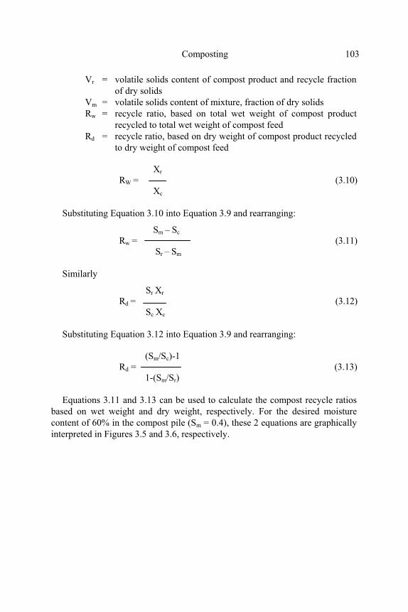
Composting 103
Vr = volatile solids content of compost product and recycle fraction
of dry solids
Vm = volatile solids content of mixture, fraction of dry solids
Rw = recycle ratio, based on total wet weight of compost product
recycled to total wet weight of compost feed
Rd = recycle ratio, based on dry weight of compost product recycled
to dry weight of compost feed
Xr
RW = (3.10) Xc
Substituting Equation 3.10 into Equation 3.9 and rearranging:
Sm – Sc
Rw = (3.11) Sr – Sm
Similarly
Sr Xr
Rd = (3.12) Sc Xc
Substituting Equation 3.12 into Equation 3.9 and rearranging: (Sm/Sc)-1 Rd = (3.13) 1-(Sm/Sr)
Equations 3.11 and 3.13 can be used to calculate the compost recycle ratios
based on wet weight and dry weight, respectively. For the desired moisture
content of 60% in the compost pile (Sm = 0.4), these 2 equations are graphically
interpreted in Figures 3.5 and 3.6, respectively.

104 Organic waste recycling: technology and management
Figure 3.5 Effect of compost feed solids content on the wet weight recycle ratio needed
to achieve a 40% mixture solids content (Haug 1979; reproduced by permission of the
Water Pollution Control Federation USA)
Example 3.2
From the data of Example 3.1, suppose the moisture content of the composted
product is 20%. Determine the quantity of the composted product needed to be
recycled to achieve 40% mixture solids content.
From Example 3.1, moisture content of the mixture between septic tank
sludge and rice straw is:
Compost feed solids, percent (Sc)
Sr = Fractional solids content of compost recycle
Re
cy
cle
ra
tio
, R
w, b
ased
on
to
tal
wet
weig
ht

Composting 105
Figure 3.6 Effect of compost feed solids content on the dry-weight recycle ratio needed
to achieve a 40 percent mixture solids content (Haug 1979; reproduced by permission of
the Water Pollution Control Federation USA)

106 Organic waste recycling: technology and management
(1/0.1)(90) + (5/0.5) (50) 14 = (100) = 70% (1/0.1) + (5/0.5) 20
Or the compost feed solids are = 30%.
From Equation 3.13,
(Sm/Sc-1) (0.4/0.3) - 1 Rd = = = 0.67
(1-Sm/Sr) 1 – (0.4/0.8)
From Equation 3.11,
Sm - Sc 0.4 - 0.3 Rw = = = 0.25
Sr - Sm 0.8-0.4
Also from Figure 3.6, at Sr = 0.8 and the compost feed solids of 30%, the
value of Rd = 0.7; and from Figure 3.5, Rw = 0.25.
Therefore, for composting 6 kg dry weight of the mixture of septic tank
sludge and rice straw, the quantity of compost recycle is
6 x 0.67 = 4 kg dry weight or 20 x 0.25 = 5 kg wet weight, in order to
achieve a 40% solids content of the compost mixture.
3.4.4 Aeration requirements
Aerobic composting needs proper aeration to provide sufficient oxygen for the
aerobic microbes to stabilize the organic wastes. This is accomplished through
some non-mechanical means such as periodic turning of the compost piles,
insertion of perforated bamboo poles into the compost piles, or dropping of
compost heaps from floor to floor. A more effective, mechanical way is the
forced-air aeration in which air is pumped through perforated pipes and orifices
into the compost heaps.
Because non-mechanical aeration cannot supply sufficient oxygen to the
microorganisms, aerobic conditions prevail only at the outer surface of the
compost heaps, while facultative or anaerobic conditions exist inside. The
composting rate is accordingly slow and requiring a longer composting period.

Composting 107
When mechanical aeration is to be employed, the quantity or rate of air flow
has to be properly controlled. Too much aeration is wasteful and can cause a
loss of heat from the compost piles, while too little aeration would lead to the
occurrence of anaerobic conditions inside the compost piles.
A simple method to determine aeration requirements is based on the
stoichiometric reaction of waste oxidation. A knowledge of the chemical
compositions of the wastes to be composted or oxidized (Table 3.2) is useful for
the calculation. Since compost feed is a combination of various organic
compounds, for practical purposes, the formulae C10H19O3N and C5H7O2N have
been used to represent its chemical composition. The stoichiometric equations
for complete oxidation of these compounds are as follows:
C10 H19 O3 N + 12.5 O2 10 CO2 + 8 H2O + NH3 (3.14)
C5 H7 O2 N + 5O2 5 CO2 + 2 H2 O + NH3 (3.15)
Table 3.2 General chemical composition of various organic materials (Haug 1980)
Waste component Typical chemical composition
Carbohydrates (C6H10O5)x
Protein C16H24O5N4
Fat and oil C50H90O6
Sludge
Primary C22H39O10N
Combined C10H19O3N
Refuse (total organic fraction) C64H104O37N
C99H148O59N
Wood C295H420O186N
Grass C23H38O17N
Garbage C16H27O8N
Bacteria C5H7O2N
Fungi C10H17O6N

108 Organic waste recycling: technology and management
Parts of NH3 generated from the above reactions will be lost through
volatilization if pH of the compost piles is above 7. The remaining NH3 will be
nitrified to become NO3- during the maturation or curing of the composted
products. Example 3.3 shows a method to determine aeration requirements
based on the stoichiometric equations.
Example 3.3
Suppose Equation 3.14 represents the reaction occurring during aerobic
composting of septic tank sludge. Calculate the amount of air required to
completely oxidize this sludge.
C10H19O3N + 12.5O2 10CO2 + 8H2O + NH3 (3.14) (201) (400)
1g of C10 H19 O3 N requires O2 = 2 g
Assume septic tank sludge contains 75% volatile solids of which 50% is
biodegradable (as represented by C10H19O3N):
Therefore, the amount of O2 required per 1 g of septic tank sludge is
2(0.75)(0.5) = 0.75 g.
Since air contains 23% O2 (by weight), the amount of air required is
0.75/0.23 = 3.26 g.
The specific weight of air is 1.20 g/L at 25 °C and 1 atmospheric pressure.
The volume of air required to oxidize 1 g (dry weight) of septic tank sludge is
3.26/1.20 = 2.72 L.
Note: This is a theoretical method of calculating aeration requirement. In
practice, the amount of air supply should be adjusted according to the biological
reactions taking place, e.g. thermophilic reactions will require oxygen several
times higher than those of mesophilic and maturation reactions (see Figure 3.2).
Additional amount of air needs to be supplied to compensate for loss to
atmosphere, which can be up to 95-99 percent.
3.4.5 Temperature and pH
The biologically produced heat generated within a composting mass is
important for two main reasons:
• To maximize decomposition rate; and
• To produce a material which is microbiologically ‘safe’ for use

Composting 109
It is generally known that compost temperatures greater than 60-65 °C, above
thermophilic range, will significantly reduce the rate of biodegradation in
compost piles. A recent work using compost samples from a full scale
composting plant showed the optimal temperature for composting, as measured
by microbial activity (incorporation of [14C] acetate) was consistently below
55°C (McKinley et al. 1985). On the other hand, most pathogenic
microorganisms are inactivated effectively at temperatures above 50°C (Figure
3.1). So the key concern is to control temperatures in the compost piles in such a
way as to optimize both the breakdown of organic material and pathogen
inactivation (approximately 55°C). Temperature can be controlled by the
adjustment of aeration and moisture content and the utilization of screened
compost as insulation cover of the compost piles. Temperature patterns in compost piles influence the types and species of
microorganisms' growth. Mesophilic temperature (25-45°C) is developed first in
composting, followed by thermophilic temperature (50-65°C). After this phase, most organic substrates will have been stabilized, resulting in the decline of temperature to mesophilic and eventually to ambient level (Figure 3.2). In many
cases, the thermophilic temperature can even reach 55-65°C and last for a few days, causing an effective inactivation of the pathogens.
Aerobic composting normally proceeds at a neutral pH and rarely encounters
extreme pH drop or rise. A slight pH drop may occur during the first few days
of anaerobic composting due to the production of volatile fatty acids. After this
period, the pH becomes neutral again when these acids have been converted to
methane and carbon dioxide by the reactions of methane-forming bacteria.
3.5 COMPOSTING MATURITY
There are many criteria to judge the maturity or completion of a composting
process. In general, a composted product should contain a low organic content
that will not undergo further fermentation when discharged on land, and the
pathogens inactivated. Some of the approaches to measure the degree of
compost stabilization are (Haug 1980):
• Temperature decline at the end of batch composting
• Decrease in organic content of the compost as measured by the
volatile solid (VS) content, chemical oxygen demand (COD),
percent carbon content, and C/N ratio
• Presence of particular constituents such as nitrate, and the absence
of others such as ammonia
• Lack of attraction of insects or development of insect larvae in the
final product
• Absence of obnoxious odour

110 Organic waste recycling: technology and management
• Presence of white or grey colour due to the growth of
actinomycetes.
In cases where the composted products are to be applied to crops and public
health aspects are of concern, the time required for pathogen die-offs during
composting is another important criterion to be considered (see Figure 3.1).
More information about pathogen die-off during composting and the public
health risks are discussed in section 3.7. Because compost materials usually contain some biologically resistant
compounds, a complete stabilization during composting may not be achieved. The time required for a satisfactory degree of composting would depend on the environmental factors in and around the compost heap as were described in section 3.4. Under suitable conditions, aerobic composting normally takes about 10-30 days, while anaerobic composting can last from 45 to 100 days. The maturing or curing time of compost may be approximately the same as those required for organic stabilization. Some manufacturers have produced mechanical composting reactors which claim to yield satisfactory compost within a short period, e.g. 24 hours. However, these reactors are both expensive and difficult to operate, and the composted materials will usually need an additional time for curing or nitrification.
It should be noted that in batch composting, the temperature pattern and
biological succession developed in the compost piles are similar to those shown
in Figures 3.2 and 3.3, respectively. Because both the stages of waste
stabilization and consequently curing occur during batch composting, the
composted product is suitable to be used in agriculture or horticulture.
The continuous composting process is normally aerobic and has a semi-
continuous plug-flow passage of composting materials through a reactor
structure, and temperatures of the reactor contents are continuously in the
thermophilic range. Depending on the specific design, the material is
translocated through the structure as part of the tumbling action in a large
revolving drum, by the action of augers force through the mass, or by gravity.
These approaches may provide the gas exchange by forcing air through the
mass. Residence time in the reactor is 1-10 days with 5 days being typical. The
material displaced from the continuous stage is biologically stabilized (i.e. the
reaction of Equation 2.1 is achieved, but mostly not nitrified (i.e. reaction of
Equation 3.5 is not achieved). It should be processed further in the curing stage
to allow for nitrification to occur and to make the composted products suitable
for agricultural reuse. Composting may be employed for the purpose of sludge
dewatering or drying. In this case, there is no need for the nitrification reactions
to take place and the composted products from continuous reactors can be
disposed off in sanitary landfills or reused in non- agricultural activities.

Composting 111
An experienced compost operator can, most of the time, recognize the
maturity of a composted product. However, it is advisable that the quality of the
composted products be regularly checked for the nutrient contents and presence
of any pathogenic microorganisms. Chemical fertilizers can be added to a
composted product to make it suitable for applying to a particular crop,
according to its nutrient requirement (see Table 8.7).
Details about the composting systems of both batch and continuous operation
are given in section 3.6.
3.6 COMPOSTING SYSTEMS AND DESIGN CRITERIA
In this section the composting systems will be described as the on-site and off-
site processes. On-site systems are the ones that compost organic wastes at the
places of generation, e.g., at home or in the toilets; the composting process is
usually not controlled and occur naturally. Off-site systems involve the
collection and transportation of organic wastes to be composted at central
treatment plants; the composting process is usually controlled either manually or
mechanically. Nowadays, there are many manufacturers producing various
composting units for the treatment of nightsoil, sludge, or municipal refuse;
some of these units will be described herein.
3.6.1 On-site composting
Aerobic composting toilets
These types of composting toilets, often referred to as the ‘multrum’, were
originally invented by Lindstrom and put into commercial production about 20
years ago (Rybczynski et al. 1978). The multrum (Figure 3.7) consists of a
water-tight container with a sloping bottom. Human excreta (without flushing
water) is introduced at the upper end of the container, and mixed with organic
kitchen and garden wastes, introduced lower down, to increase the C/N ratio.
Air ducts and a vent pipe are provided to promote aeration. The composted
material moves toward the lower end and from where it is periodically removed.
The decomposition period is long, up to 4 years, and the container is quite large
(3 x 1 x 1 m: length x width x height). The air ducts also help to evaporate the
humidity and eliminate odors, while the sloping bottom permits continuous use
of a single container by separating the fresh and the decomposed materials.
Another modification of the multrum is the biopit composting toilet (Figure 3.8)
which incorporates a gravel soakage pit to treat and dispose of the liquid waste
present in the excreta.

112 Organic waste recycling: technology and management
Figure 3.7 The Clivus Multrum (Rybczyski et al. 1978; reproduced by permission of the
International Development Research Centre, Canada)
Anaerobic composting
Pit latrines (or holes in the ground) are the simplest form of anaerobic
composting toilets. The excreta deposited into the pit is decomposed
anaerobically. When the pit is about two-thirds full, it is filled up with dirt and
left there for approximately 2-3 years. After this period, the excreta would be
well stabilized and the pathogens inactivated, rendering it for satisfactory use as
soil conditioner. To avoid the occurrence of obnoxious odor, ventilated
improved pit (VIP) latrines were developed (Figure 3.9) which have yielded
encouraging results in many places such as Zimbabwe (Morgan and Mara 1982)
and Botswana (Nostrand and Wilson 1983).

Composting 113
Figure 3.8 The Biopit composting toilet (Rybczynski et al. 1978; reproduced by
permission of the International Development Research Centre, Canada)
Another version of anaerobic composting is the Vietnamese toilet (Figure
3.10) which was claimed to be the key component of a rural sanitation program
for disease prevention and increased food production. It has two watertight tanks
serving by turns as receptacles for defecation and composting. A hole is made
on the face of each for feces deposition. Kitchen ash is added after each use to
reduce odor and increase the C/N ratios. Urine is channelled in a groove into a
separate vessel; this method reduces moisture content but does not decrease C/N
ratio of feces in the toilet, which is favourable for the composting reactions.
Apertures are made in the back wall for the collection of the composted
products. The toilets are constructed above ground so as not to be submerged by
rainwater.
1. Gravel seepage pit
2. Triple layered filter
3. Air duct
4. Toilet chute
5. Access hatch
1
2
3
45
6

114 Organic waste recycling: technology and management
Figure 3.9 Schematic diagram of a ventilated improved pit latrine (Morgan and Mara
1982; reproduced by permission of the World Bank)
When the tank is about two-thirds full, it is filled to the brim with dried
powdered earth and kept under anaerobic conditions for a few-year period.
During this time, another tank is used for defecation, and the cycle is repeated.
The anaerobically composted products were reported to be rich in nutrients and
hygienically safe for reuse as fertilizers (McMichael 1976).
Odours Flies
Screen
Vent pipe
Air currents
Flies
PIT
Pit cellar
Pit contents

Composting 115
Figure 3.10 The Vietnamese composting toilet (Rybczynski et al. 1978; reproduced by
permission of the International Development Research Centre, Canada)
3.6.2 Off-site composting
Because of large quantities of organic wastes to be decomposed, off-site
composting should employ aerobic reactions to shorten the composting period
and reduce the size of composting plants. Some of the aerobic composting
systems currently in operation are:
Chinese ground-surface aerobic composting pile
As shown in Figure 3.11, the compost feed (a mixture of human or animal
manure and vegetable matters) is piled up into a heap of approximately 2 x 2 x
0.5 m (length x width x height). The compost heap is inserted with perforated
bamboo poles to facilitate natural aeration and provide a kind of structural
support, and no turning of the compost pile is required. To control excessive
heat loss, the compost pile is covered with rice straw or a plaster of mud (Figure
3.12). The poles can be removed after 1 or 2 days when the mud has hardened or

116 Organic waste recycling: technology and management
the compost pile is structurally stable, but they can remain there for a longer
period. An experiment conducted at the Asian Institute of Technology (AIT),
Bangkok, Thailand, found the time required for compost stabilization to be
about 60 days (Polprasert et al. 1980), and the composted product was suitable
for use as soil conditioner. In China, more than 90% kill of Ascaris ova in the
compost was achieved (McGarry and Stainforth 1978).
Figure 3.11 Chinese composting pile (McGarry and Stainforth 1978; reproduced by
permission of the International Development Research Centre, Canada)
Windrow composting
This system involves periodic turning of the compost piles, manually about once
a week, or mechanically once (or more) daily. The purpose of pile turning is to
provide aeration and mix the compost materials, hence, a faster decomposition
rate than that of the Chinese ground-surface aerobic composting. The
approximate size of each pile is 15 x 3 x 1.5 m (length x width x height), but
other sizes, subject to convenience, have been employed. The period required
for compost stabilization varies according to the frequency of pile turning, being
20 - 40 days, and temperatures over 65°C in the center of the compost pile can
be reached.
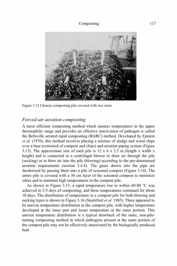
Composting 117
Figure 3.12 Chinese composting pile covered with rice straw
Forced-air aeration composting
A more efficient composting method which ensures temperatures in the upper
thermophilic range and provides an effective inactivation of pathogen is called
the Beltsville aerated rapid composting (BARC) method. Developed by Epstein
et al. (1976), this method involves placing a mixture of sludge and wood chips
over a base (consisted of compost and chips) and aeration piping system (Figure
3.13). The approximate size of each pile is 12 x 6 x 2.5 m (length x width x
height) and is connected to a centrifugal blower to draw air through the pile
(sucking) or to blow air into the pile (blowing) according to the pre-determined
aeration requirements (section 3.4.4). The gases drawn into the pipe are
deodorized by passing them into a pile of screened compost (Figure 3.14). The
entire pile is covered with a 30 cm layer of the screened compost to minimize
odors and to maintain high temperatures in the compost pile.
As shown in Figure 3.15, a rapid temperature rise to within 60-80 °C was
achieved in 3-5 days of composting, and these temperatures continued for about
10 days. The distribution of temperature in a compost pile for both blowing and
sucking types is shown in Figure 3.16 (Stentiford et al. 1985). There appeared to
be uneven temperature distribution in the compost pile, with higher temperature
developed at the inner part and lesser temperature at the outer portion. This
uneven temperature distribution is a typical drawback of the static, non-pile-
turning composting method in which pathogens present at the outer portion of
the compost pile may not be effectively inactivated by the biologically produced
heat.

118 Organic waste recycling: technology and management
Figure 3.13 Schematic diagram of an aerated pile indicating location of aeration pipe.
Loop is perforated for air distribution system (units in millimetres) (Shuval et al. 1981;
reproduced by permission of the World Bank)
However, satisfactory reductions of indicator bacteria and viruses have been
reported for the BARC system, and the system is essentially unaffected by low
ambient temperatures and/or rainfall. It does not require pile turning (which is
rather labor intensive), and should be applicable for nightsoil composting in hot
climates (Shuval et al. 1981).
Odor filter
compost
sawdust
Section a-a
SchematicSection b-b Section c-c
Odor filter
Plan
As needed
Blower
Aeration pipe is perforated for even air distribution
Finished compost
bed

Composting 119
Figure 3.14 Configuration of aerated piles showing construction of pile and the
arrangement of aeration pipe - the BARC system (Shuval et al. 1981; reproduced by
permission of the World Bank)
The area required for the BARC system and conventional windrow system
has been estimated to be 1 hectare (ha) per 10-12 dry tons per day of sewage
sludge. This area estimate includes: (1) area for mixing the sludge or nightsoil
with bulking materials, (2) area required for composting, (3) area required for
storage and curing piles and long-term storage before marketing, (4) area
required for screening of the final compost and separation and recycling of
wood chips, (5) area required for lagooning or waste stabilization ponds to treat
leachate and drainage from the composting area, and (6) area required for
administration, work-shops, parking of vehicles, and storage of spare parts
(Shuval et al. 1981).
A. COMPOSTING WITH FORCED AERATION
B. EXTENDED AERATED PILE

120 Organic waste recycling: technology and management
Figure 3.15 Temperature during sludge composting by the BARC system (Shuval et al.
1981)
Benedict et al. (1986) reported that with the operation capacity of 450 wet
tons/day of sludge, the area required for conventional windrow composting of
the Los Angeles, USA, and facility was about 20 ha. However, this total area
included those used for storages of bulking agents, finished compost and
equipment, and for research area; so the operating area for composting was
about 15 ha or 0.03 ha for composting of 1 ton/day of wet sludge.
The DANO System
A schematic diagram of a typical DANO plant manufactured for solid waste
composting is shown in Figure 3.17. It includes storage hoppers, rotary screens
and magnetic separators to separate out non-compostable materials. Materials to
be composted are fed into the "DANO bio-stabilizer", a cylindrical chamber,
tilted slightly from the horizontal, usually about 3 - 4 m in diameter and varying
from 25 to 30 m in length according to the quantity of the feeding materials. The
cylinder rotates at up to 1 revolution per minute (rpm) and air is supplied by
fans at a low pressure, through longitudinal ducts, each having several injector
nozzles. The above conditions enhance effective aerobic decomposition of the
organic matters in the cylinder in which temperatures of 60°C and over are
developed inside. The steam and waste gases are exhausted through extractor
Rainfall events
Temperature
Max.
Mean
Min.
Te
mp
era
ture
(°C
)
Days
Rainfall (cm)

Composting 121
fans. The composting period required for this type of compost reactor ranges
from 2.5 to 5 days.
Figure 3.16 Typical temperature cross-section distributions in a pile with (a) positive
pressure (blowing) aeration; and (b) negative pressure (sucking) aeration (from Stentiford
et al. 1985; by permission of the Institute of Water Pollution Control, U.K.)
The DANO system, developed in Denmark, is presently being employed for
solid waste composting in several countries throughout the world. Although
very efficient in composting, the DANO system involves high capital and
operation costs, and requiring skillful manpower to maintain the system. Figure
Perforated pipe in duct
Perforated pipes in ducts
Insulating compost cover
< 45ºC
45 - 55ºC
55 - 65ºC
> 65ºC
KEY
(a)
(b)

122 Organic waste recycling: technology and management
3.18 is a DANO composting plant treating part of Bangkok city, Thailand, solid
wastes, while a smaller unit made for composting solid wastes generated from a
community of 1,000 people in central Thailand is shown in Figure 3.19.
Figure 3.17 Typical DANO plant (after Flintoff and Millard 1969)
Figure 3.18 A DANO composting plant in Bangkok
“Dano” Bio-stabilizer
Vibrating
screens
Rejects
Air (pumped in through ducts)
Water or sludge added in amount necessary to raise total moisture
content to 50% Rejects
Cinder
extractor
Elevating
conveyor
Picking
beltMagnetic
separator
HopperRotary screen

Composting 123
Figure 3.19 Aerobic composting unit for a small community, Thailand
From Obeng and Wright (1987) and Haug (1980), composting systems can
be classified into non-reactor and reactor (Tables 3.3 and 3.4, respectively).
Based on the information given in Table 3.3, it appears that for the non-reactor
composting systems (with proper C/N ratio and provided with some types of
aeration, natural or forced-air), the time required for the first phase composting
(Figure 3.2) is at least 3-4 weeks, followed by about 4 weeks of maturation or
curing. The reactor composting systems (operating under aerobic conditions,
Table 3.4) should require about 4 weeks. These composting systems, when
properly operated according to the environmental requirements listed in section
3.4, should result in a temperature increase in the compost mixture up to 50oC or
more which is essential in inactivating the pathogens.

124 Organic waste recycling: technology and management
Gen
eral
des
crip
tion
Raw
sew
age
slu
dg
e (2
2%
so
lid
s) i
s m
ixed
wit
h w
oo
d c
hip
s, a
nd
then
tra
nsf
erre
d t
o a
co
mp
ost
ing p
ad c
on
sist
ing
of
woo
d c
hip
s
spre
ad o
ver
per
fora
ted p
ipin
g.
Air
is
dra
wn
th
rou
gh
th
e p
ipe
into
a
com
po
st f
ilte
r. T
he
pil
e is
mai
nta
ined
fo
r 21
day
s fo
llo
wed
by
Th
e n
igh
tso
il i
s m
ixed
wit
h p
aper
an
d w
ood
ch
ips
on
a c
on
cret
e
pad
and
th
en t
ran
sfer
red
to
th
e co
mp
ost
ing
pad
, w
hic
h i
s a
bed
of
wo
od c
hip
s co
ver
ing
a p
erfo
rate
d p
ipe.
Air
is
dra
wn t
hro
ug
h t
he
pip
e in
to a
co
mp
ost
fil
ter.
Th
e p
ile
is m
ain
tain
ed f
or
21
day
s at
Ex
per
imen
t. N
igh
tso
il,
wat
er h
yac
inth
, an
d (
in s
om
e ca
ses)
ric
e
stra
w w
ere
mix
ed a
nd
co
mpo
sted
in
pil
es f
or
2-3
mo
nth
s.
Aer
atio
n t
hro
ugh
per
fora
ted
bam
bo
o p
ole
s. T
emp
erat
ure
s o
f 43
-
64
°C w
ere
mai
nta
ined
fo
r at
lea
st 8
da y
s in
th
e co
ole
st p
arts
of
the
Tre
nch
in
gro
un
d,
2-3
ft
dee
p. M
ater
ial
pla
ced
in a
lter
nat
e la
yer
s
of
refu
se, n
igh
tso
il,
eart
h, st
raw
, et
c. N
o g
rind
ing
. T
urn
ed b
y h
and
as o
ften
as
po
ssib
le.
Det
enti
on
tim
e o
f 1
20
-18
0 d
ays.
Use
d
exte
nsi
vel
y i
n I
nd
ia
Th
e sl
ud
ge
(30%
so
lid
s) a
nd
saw
du
st a
re m
ixed
at
wei
ght
rati
os
4:1
. T
he
win
dro
ws
are
turn
ed f
or
3 m
onth
s an
d t
hen
sold
as
a
pro
du
ct “
Gro
w R
ich
”. T
he
max
imu
m t
emp
erat
ure
ach
iev
ed i
s
74
°C
Raw
mat
eria
l
Sew
age
slu
dg
e an
d w
ood
chip
s
Nig
hts
oil
, p
aper
, w
ood
ch
ips
Wat
er h
yac
inth
, n
igh
tsoil
,
rice
str
aw
Ref
use
, n
igh
tso
il,
eart
h,
stra
w,
etc.
Sew
age
slu
dg
e an
d s
awdu
st
Co
mp
ost
ing
sy
stem
Aer
ated
sta
tic
pil
e
Ban
gal
ore
(In
do
re)
Win
dro
w
Tab
le 3
.3 N
on
-rea
cto
r co
mp
ost
ing
sy
stem
s

Composting 125
Gen
eral
des
crip
tion
Dig
este
d s
ewag
e sl
udg
e is
mix
ed w
ith
woo
d c
hip
s (1
:3 v
olu
me
rati
o)
in w
ind
row
s 1
.8 m
hig
h a
nd 2
.1 m
wid
e. T
he
win
dro
ws
are
turn
ed
dai
ly f
or
at l
east
2 w
eek
s, t
hen
they
are
sp
read
ou
t, d
ried
, an
d c
ure
d
for
30
day
s. T
he
woo
d c
hip
s ar
e sc
reen
ed o
ut
for
reu
se
Th
e sl
ud
ge
(25%
so
lid
s) m
ixed
wit
h b
ark
(1
:3)
and
co
mp
ost
ed i
n
win
dro
ws
for
at l
east
21
day
s. I
n g
ener
al,
tem
per
atu
res
of
50
-75
°C a
re
mai
nta
ined
fo
r at
lea
st h
alf
of
this
tim
e
(Fu
ll-s
cale
ex
per
imen
tal
pla
nt)
Th
e se
wag
e sl
ud
ge
(25
-30%
soli
ds)
was
mix
ed w
ith
str
aw (
1:1
volu
me)
an
d c
om
po
sted
in
win
dro
ws,
w
hic
h w
ere
turn
ed e
igh
t ti
mes
fo
r 3
mon
ths.
At
the
end
of
this
tim
e
the
com
po
st w
as r
ead
y f
or
use
. T
emp
erat
ure
s o
f 55
-60
°C w
ere
Ex
per
imen
t. D
iges
ted
slu
dg
e w
as m
ixed
wit
h s
traw
at
a ra
tio
of
1:
1.2
5 i
n w
ind
row
s fo
r 6
wee
ks
du
rin
g w
hic
h t
emp
erat
ure
of
65
-70
°Cw
ere
ach
iev
ed.
Raw
mat
eria
l
Sew
age
slu
dg
e an
d w
ood
chip
s
Raw
dew
ater
ed s
ewag
e
slu
dg
e an
d b
ark
Raw
dew
ater
ed s
ewag
e
slu
dg
e an
d s
traw
Dig
este
d s
lud
ge
and
str
aw
Co
mp
ost
ing
sy
stem
Tab
le 3
.3 N
on
-rea
cto
r co
mp
ost
ing
sy
stem
s (c
on
tin
ued
)

126 Organic waste recycling: technology and management
Gen
eral
des
crip
tion
Dis
per
sed
flo
w r
ota
ting
dru
m,
slig
htl
y i
ncl
ined
fro
m t
he
ho
rizo
nta
l, 9
-12
ft i
n d
iam
eter
, u
p t
o 1
50
ft
lon
g. D
rum
kep
t ab
ou
t h
alf
full
of
reu
se.
Dru
m r
ota
tio
n o
f 0.1
-1.0
rp
m, 1
-5 d
ays
dig
esti
on
fo
llo
wed
by
win
dro
win
g.
No g
rin
din
g.
Fo
rced
aer
atio
n i
nto
dru
m.
Tem
per
atu
res
of
60
°C o
r ov
er a
re r
each
ed
Rea
cto
r is
of
the
tow
er t
yp
e w
ith
a s
pec
ial
extr
acti
on
an
d a
git
atio
n
mec
han
ism
at
the
bott
om
. T
he
reac
tor
is b
atch
-op
erat
ed.
On
ce t
he
reac
tor
is l
oad
ed w
ith t
he
mix
ture
of
the
slud
ge
and
ag
itat
ion
and
ass
ure
un
ifo
rm e
xp
osu
re t
o t
emp
erat
ure
. R
esid
ence
tim
e is
4-6
day
s.
Cir
cula
r ta
nk.
Ver
tica
l sc
rew
s, m
ou
nte
d o
n t
wo
ro
tati
ng
rad
ial
arm
s,
kee
p g
roun
d m
ater
ial
agit
ated
. F
orc
ed a
erat
ion
th
rou
gh
tan
k b
ott
om
an
d
ho
les
in s
crew
s. C
on
tinu
ou
s fl
ow
ty
pe.
Dew
ater
ed s
ewag
e sl
udg
e is
mix
ed w
ith s
hre
dd
ed p
aper
and
fed
into
a r
eact
or.
Th
e re
ten
tion
tim
e is
5-7
da y
s an
d t
emp
erat
ure
is
ov
er 6
0°C
are
rea
ched
Th
e se
wag
e sl
udg
e an
d r
ecy
cled
co
mp
ost
are
mix
ed a
nd
gro
un
d a
nd f
ed
into
th
e fe
rmen
ter,
wh
ere
the
mix
ture
is
aera
ted
an
d t
urn
ed. T
he
rete
nti
on t
ime
is 1
0 d
ays
and
tem
per
atu
res
of
up
to
75
°C a
re a
ttai
ned
.
Th
e co
mp
ost
is
then
gra
ded
and
bag
ged
Cel
ls-i
n-s
erie
s ty
pe.
Un
gro
un
d r
efu
se p
lace
d i
n r
ota
tin
g d
rum
, 11
ft
dia
met
er,
11
0 f
t lo
ng
, sl
igh
tly i
ncl
ined
fro
m h
ori
zonta
l. T
hre
e
com
par
tmen
ts i
n d
rum
. R
efu
se t
ran
sfer
red
to
nex
t co
mp
artm
ent
ever
y 1
-
2 d
ays
for
tota
l d
iges
tio
n t
ime
of
3-6
day
s. S
cree
ned
ou
tpu
t cu
red
in
pil
es
Raw
mat
eria
l
Mu
nic
ipal
so
lid
was
tes,
slu
dg
e
Dew
ater
ed s
lud
ge
and
recy
cled
co
mp
ost
Sew
age
slu
dg
e an
d s
hre
dd
ed
pap
er,
mun
icip
al r
efu
se
Dew
ater
ed s
ewag
e sl
ud
ge
and
rec
ycl
ed c
om
po
st
Mu
nic
ipal
ref
use
, sl
udg
e
Co
mp
ost
ing
sy
stem
Dan
o
Eu
ram
ca (
Ro
edig
er,
Fer
men
-tec
hn
ik)
Fai
rfie
ld d
iges
ter
reac
tor
Fo
rced
aer
atio
n
thro
ugh
fer
men
ter
Geo
chem
ical
-Ew
eso
n
Tab
le 3
.4 R
eact
or
com
po
stin
g s
yst
ems

Composting 127
Gen
eral
des
crip
tion
Rea
cto
r is
of
the
com
ple
te-m
ix, ro
tati
ng
dru
m t
yp
e. T
he
slud
ge
and
recy
cled
co
mp
ost
are
add
ed t
o a
slo
wly
ro
tati
ng
dru
m (
wh
ich
is
stop
ped
at n
igh
t). T
he
rete
nti
on
tim
e is
24 h
fo
llo
wed
by
a 2
-wee
k m
atu
rati
on
per
iod i
n a
win
dro
w. T
emp
erat
ure
s o
f 60
-75
°C a
re a
ttai
ned
Rea
cto
r co
nsi
sts
of
cyli
nd
rica
l to
wer
wit
h n
o i
nte
rio
r fl
oo
rs o
r o
ther
mec
han
ism
s. F
eed
is
intr
odu
ced
at
the
top
an
d f
low
s do
wn
war
d a
s
pro
du
ct i
s re
mov
ed b
y m
ech
anic
al s
crap
er f
rom
th
e b
ott
om
. O
xy
gen
is
sup
pli
ed b
y f
orc
ed a
erat
ion f
rom
th
e b
ott
om
. R
esid
ence
tim
es o
f 3
-14
day
s. T
emp
erat
ure
s o
f 60
-85
°C a
re a
chie
ved
. T
hen
th
e ra
w c
om
po
st i
s
mat
ure
d f
or
6-8
wee
ks
in a
win
dro
w
Rec
tan
gu
lar
tank
s, 2
0 f
t w
ide,
10 f
t d
eep
, 2
00
-40
0 f
t lo
ng
. R
efu
se i
s
gro
und
. R
esid
ence
tim
e o
f ab
ou
t 7
day
s. “
Ag
ilo
ader
” m
ov
es o
n r
ails
m
ou
nte
d o
n b
in w
alls
an
d p
rov
ides
per
iodic
ag
itat
ion
by t
urn
ing
Fiv
e 9
-ft
wid
e st
eel
con
vey
or
bel
ts a
re a
rran
ged
to p
ass
mat
eria
l fr
om
bel
t to
bel
t. E
ach
bel
t is
an i
nsu
late
d c
ell.
Air
pas
ses
up
war
d t
hro
ugh
dig
este
r. D
eten
tio
n t
ime
of
6-8
day
s.
Dew
ater
ed d
iges
ted
sew
age
slu
dge
was
mix
ed w
ith
bar
k (
1:3
) an
d
com
po
sted
in
lar
ge
bas
ket
s th
at c
ou
ld b
e ea
sily
sta
cked
. T
emp
erat
ure
s o
f
up
to
75
°C w
ere
atta
ined
. T
he
rete
nti
on
tim
e in
th
e b
ask
ets
was
9-1
2
wee
ks
foll
ow
ed b
y 3
-4 w
eek
s m
atu
rati
on
in p
iles
Raw
mat
eria
l
Sew
age
slu
dg
e an
d r
ecy
cled
com
po
st
Slu
dg
e, m
ush
roo
m w
aste
s,
po
ult
ry w
aste
s, o
rgan
ic
bu
lkin
g a
gen
ts
Mu
nic
ipal
ref
use
, an
imal
man
ure
, sl
ud
ge
Mu
nic
ipal
ref
use
Dig
este
d s
ewag
e sl
udg
e an
d
bar
k
Co
mp
ost
ing
sy
stem
HK
S
Kn
eer
(Lat
er v
ersi
on
kn
ow
n a
s B
AV
)
Met
row
aste
Nat
uri
zer
(In
tern
atio
nal
)
Op
en b
ask
ets
Tab
le 3
.4 R
eact
or
com
po
stin
g s
yst
ems
(co
nti
nu
ed)

128 Organic waste recycling: technology and management
Gen
eral
des
crip
tion
Rea
cto
r co
nsi
sts
of
a v
erti
cal
tow
er w
ith
10
flo
ors
on
e ab
ov
e th
e o
ther
. E
ach
flo
or
con
tain
s a
hy
dra
uli
call
y o
per
ated
val
ve
whic
h a
llo
ws
mat
eria
l to
be
dis
char
ged
to
th
e n
ext
flo
or.
Oxyg
en i
s in
tro
du
ced
by
fo
rce
aera
tion
.
Dew
ater
ed s
lud
ge,
rec
ycl
ed c
om
po
st a
nd g
roun
d b
ark
mix
ed i
n p
rop
ort
ion
s o
f
2:
2:
1 v
olu
me.
Co
mp
ost
ing m
ixtu
re i
s ab
ou
t 1
m d
eep o
n e
ach
flo
or.
Res
iden
ce t
ime
is a
bo
ut
3 d
ays
on e
ach
, g
ivin
g a
to
tal
reac
tor
tim
e o
f 30
day
s
Tw
o c
ells
co
nsi
stin
g o
f th
ree
ho
rizo
nta
l d
eck
s. H
ori
zon
tal
rib
bo
n s
crew
s
exte
nd
ing
th
e le
ng
th o
f ea
ch d
eck r
ecir
cula
te g
rou
nd
ref
use
fro
m d
eck
to
dec
k.
Air
in
tro
du
ced
in b
ott
om
of
cell
s. T
hre
e d
ays
com
po
stin
g f
oll
ow
ed b
y c
uri
ng
for
7 d
ays
in a
bin
.
Rea
cto
r is
a c
on
cret
e to
wer
cal
led a
“H
yg
ien
sato
r” w
hic
h i
s d
ivid
ed i
nto
fou
r
sep
arat
e v
erti
cal
com
par
tmen
ts.
Res
iden
ce t
ime
of
4-1
5 d
ays
dep
end
ing
on
feed
an
d t
emp
erat
ure
of
70
-80
°C a
re a
chie
ved
. A
ir i
s p
ull
ed o
ut
of
top
of
reac
tor.
Scr
ew e
xtr
acto
r re
mo
ves
an
d a
git
ates
mat
eria
l fr
om
bo
tto
m o
f re
acto
r.
Ex
trac
ted
mat
eria
l is
rec
ycl
ed t
hre
e to
fiv
e ti
mes
du
rin
g c
om
po
st p
erio
d t
o
avo
id c
om
pac
tion
at
bo
tto
m.
Cu
rin
g p
erio
d o
f 2
-4 m
on
ths.
Th
e d
iges
ted
sew
age
slu
dg
e is
mix
ed w
ith
ric
e hu
lls
and
fin
ish
ed c
om
po
st
(1:1
:1 v
olu
me)
an
d f
ed i
nto
a t
roug
h w
her
e it
is
com
po
sted
fo
r 2
wee
ks
by
forc
ed a
erat
ion
an
d t
urn
ing
. T
his
is
foll
ow
ed 1
-2 m
on
ths
of
mat
ura
tio
n.
Tem
per
atu
res
reac
h u
p t
o 7
0°C
.
Raw
mat
eria
l
Dew
ater
ed s
lud
ge,
rec
ycl
ed
com
po
st a
nd
gro
und
bar
k
Mu
nic
ipal
ref
use
Mu
nic
ipal
ref
use
, se
wag
e
slu
dg
e, b
ark,
saw
du
st
Sew
age
slu
dg
e an
d r
ice
hu
lls
and
rec
ycl
ed c
om
po
st
Co
mp
ost
ing
sy
stem
Sch
orr
“B
ioce
ll”
Sy
stem
T.A
. C
ran
e
Tri
ga
Tro
ug
h f
erm
ente
r
Tab
le 3
.4 R
eact
or
com
po
stin
g s
yst
ems
(co
nti
nu
ed)

Composting 129
3.7 PUBLIC HEALTH ASPECTS OF COMPOSTING
The composting of human or animal wastes involves the following disease risks:
• From the pathogens normally present in the raw wastes (called
primary pathogens), and
• From fungi and actinomycetes that grow during composting (called
secondary pathogens).
The primary pathogens such as bacteria, viruses, protozoa and helminthes
can initiate an infection in healthy individuals, while secondary pathogens
usually infect people with debilitated immune systems, such as those weakened
by primary infections or respiratory diseases (U.S. EPA 1981). Examples of
primary and secondary pathogens are listed in Table 3.5; more examples of
these pathogens can be found in Chapter 2.
3.7.1 Die-offs of primary pathogens
Time and temperature are the two most important parameters responsible for
pathogen die-offs during composting. It should be noted that a complete
inactivation of pathogens in a compost pile is rarely achieved. This is due to
many reasons such as:
• The heterogeneous character of the compost materials, which may
form clumps with the pathogens and protect them from being fully
exposed to thermophilic temperatures.
• The uneven temperature distribution in the compost piles. Unless
completely mixed continuously, the outer surfaces of a compost
heap normally have a lower temperature than the inside, causing a
lower efficiency of pathogen kill (see Figure 3.16).
• Partial inactivation of pathogens. Many pathogens such as spore-
forming bacteria, cysts and helminthes ova are only partially
inactivated during composting. They can re-grow and become
infective again if exposed to a favorable environment such as under
moistened conditions in crop fields.
A number of researchers (Kawata et al. 1977; and Cooper and Golueke 1979)
reported several orders of magnitude reduction of bacteria (total coliforms, fecal
coliforms and fecal streptococci) and viruses (poliovirus and coliphages) during
composting. Better inactivation rates were observed with the BARC system in
which these bacteria including Salmonella were non-detectable after 10 days of
composting (Figure 3.20) and for F2 bacteriophages about 15-20 days (Figure
3.21). The thermal death points of some common pathogens and parasites are

130 Organic waste recycling: technology and management
shown in Table 3.6, while the relationships between time and temperature that
cause pathogen inactivation as shown in Figure 3.1 are useful information to
determine the required composting period.
The microbiological quality guidelines shown in Table 2.27 and 2.28 should
be strictly observed when the composted products are to be used as fertilizers in
agricultural or aquacultural activities, respectively.
Table 3.5 Examples of pathogens found in, or generated during, composting of sewage slidge, together with human diseases associated with these pathogens (U.S. EPA 1981)
Group Example Disease
Primary pathogens
Bacteria Salmonella enteritidis Salmonellosis (food poisoning)
Protozoa Entamoeba histolytica Amoebic dysentery (bloody diarrhea)
Helminths Ascaris lumbricoides Ascariasis (worm infecting the intestine)
Viruses Hepatitis virus Infectious hepatitis (jaundice)
Secondary pathogens
Fungi Aspergillus fumigatus Aspergillosis (growth in lungs and other organs)
Actinomycetes Micromonospora spp. Farmer's lung (allergic responses in lung tissue)
3.7.2 Health risks from secondary pathogens
The contact or inhalation of air, containing a high density of spores of secondary pathogens can cause health hazards to the compost workers and users. An epidemiological study was conducted on compost workers at 9 sludge composting plants in USA to evaluate the associated potential health hazard (Clark et al. 1984). The results summarized in Table 3.7 indicate a higher health risk for the compost workers than for the control groups not involved in compost activities, nose and throat cultures positive for Aspergillus fumigatus were more common for these compost workers than for others. Since Aspergillus fumigatus can cause serious infections to lungs and other human organs, proper care must be taken to avoid the uptake of these spores.
The growth of Aspergillus fumigatus in composting may be controllable
through moisture control management practice (Finstein et al. 1980) because
fungi tend to thrive in material that is slightly too dry for profuse bacterial
growth (Millner et al. 1977). However, routine monitoring for the presence of

Composting 131
this type of fungus in compost piles should be carried out, and the compost
workers must be informed of the potential infection from Aspergillus fumigatus.
Figure 3.20 Destruction of Salmonellae, fecal coliforms, and total coliforms during
composting by the BARC system (U.S. EPA 1985)
Total coliforms
Salmonellae
Fecalcoliforms
Su
rviv
al
– L
og
cell
s/g
Days

132 Organic waste recycling: technology and management
Figure 3.21 Destruction of F2 bacteria virus during composting by the BARC system
(U.S. EPA 1985)
Blanket
Sampling locations
Aeration pipes
Pile
base
Days
Su
rviv
al
– L
og
PF
U/g

Composting 133
Table 3.6 Thermal death points of some common pathogens and parasites
Organisms Thermal death point
Salmonella typhosa No growth beyond 46°C; death within 30 minutes at
55°C to 60°C
Salmonella spp. Death within 1 hour at 55°C; death within 15 minutes
to 20 minutes at 60°C
Shigella spp. Death within one hour at 55 °C
Escherichia coli. Most die within one hour at 55°C, and within 15 to 20
minutes at 60°C
Entamoeba histolytica cysts Thermal death point is 68°C
Taenia saginata Death within 5 minutes at 71°C
Trichinella spiralis larvae Infectivity reduced as a result of one hour exposure at
50°C; thermal death point is 62-72°C
Necater americanus Death within 50 minutes at 45°C
Brucella abortus or suis Death within 3 minutes at 61°CMicrococcus pyogenes var.
aureus
Death within 10 minutes at 50°C
Streptococcus pyogenes Death within 10 minutes at 54°C
Mycobacterium tuberculosis
var.hominis Death within 15 to 20 mins at 66°C, or momentary
heating at 67°C
Corynebacterium diptheriae Death within 45 minutes at 55°C
Table 3.7 Epidemiological effects to compost workers (Clark et al. 1984)
Excess of nasal, ear and skin infections (by physical exams) in compost and intermediate-exposed workers
Symptoms of burning eyes and skin irritation higher in compost and intermediate-exposed workers
Fungal colonies greater in cultures from compost workers
Legionella infections not associated with compost exposure but were higher among all workers exposure categories in Philadelphia-Camden area than in Washington, D.C., area
Evidence of higher white blood cell counts and hemolytic complement in compost workers
Higher antibody levels to compost-endotoxin in compost workers

134 Organic waste recycling: technology and management
Although such epidemiological study for compost workers in developing
countries has not been reported, the health risks originating from the secondary
pathogens should be similar or even greater than those reported in U.S.A.
Therefore, skin contact with the composted materials should be avoided and
proper measures, such as wearing gloves, boots and masks, are undertaken to
prevent the inhalation of the spores of secondary pathogens, especially during
turning of compost piles. The composting processes without pile turning, such
as the BARC (Figure 3.14) and the Chinese (Figure 3.12) composting system,
should pose less health hazards to the compost workers than those with pile
turning.
3.8 UTILIZATION OF COMPOSTED PRODUCTS
Compost has been used as: a) fertilizer, b) soil conditioner, c) feed for fish in
aquaculture, d) landfill material, e) horticultural medium on parkland,
ornamental and recreational areas and in highway right-of-ways.
Screening, grinding, or combination of similar processes should be done to
remove plastics, glass, and other materials from the compost that might be
objectionable in its use. For some uses such as land filling and land reclamation,
compost needs not be finished or processed further. For general
agriculture/aquaculture, a coarse grind is satisfactory, whereas for horticulture
and luxury gardening, the compost product must be finer. Compost to be used as
fertilizer or soil conditioner is usually mixed with chemical fertilizers to make
its nutrient contents suitable for crop growth. A schematic diagram of compost
fertilizer production process is given in Figure 3.22.
3.8.1 Utilization as fertilizer and soil conditioner
Compost can improve overall soil fertility through the addition of organic matter
and plant nutrients, and modify the soil pH. The long-term effect on soil fertility
is also important. The result is that soil erosion can be reduced, the water
retention capacity raised, the soil structure improved, and subsequently,
vegetation can be established quickly.
The utilization of composted municipal wastes as fertilizers and soil
conditioners will depend on three principal factors:
• Socio-economic considerations,
• Product quality, and
• Soil and plant responses

Composting 135
Socio-economic considerations
Socio-economic factors relate to health regulations, state laws regarding the sale of fertilizers or soil conditions, public acceptance, and marketing and distribution.
The distribution and utilization of composts produced from sewage sludge or
refuse may need regulations that will require stabilization, pathogen reduction,
and chemical analysis. The general public is more attuned to acceptance of
composted sludges or refuses than unstabilized and potentially malodorous
materials. If the application of chemical fertilizer is cheap, subsidized or
practiced for long time, then the farmers will be reluctant to use compost
products as fertilizer. The extent of utilization of composts will depend on the
type of market and its proximity to the processing facility. Transportation costs
and distance to markets will affect product value and its potential use.
Figure 3.22 Flow chart of compost fertilizer production process
Product quality
The compost quality is greatly dependent on the chemical and physical
characteristics of the raw materials, and on the processing system used to
produce it. N, P and K are essential plant micronutrients (the higher the content
Composted material Coarse screening
Marketing
Waste materials
Curing
Grinding
Chemical fertilizers Compost mixture
Packaging of composted product

136 Organic waste recycling: technology and management
of these elements, the greater the fertilizer value of the compost). Most of the N
in the compost in an organic form and must be mineralized (such as through
curing) to inorganic ammonium or nitrate before it is available to plants.
Composted organic wastes function as slow-release N fertilizers when applied to
soil. The K content of sludge compost is usually low (0.5%) because it is water
soluble and remains in the effluent after wastewater treatment. However, in
refuse compost the level of K may exceed 1 percent. The N, P and K values of
compost do not only depend on the type of materials composted but also the
initial C/N ratio of those materials.
Table 3.8 shows the composition of compost produced from municipal refuse
of Bangkok city, Thailand. The percentages of N, P, K contents were 2.58, 1.67,
and 0.58, respectively, which are several times lower than those present in
chemical fertilizers. This compost thus needs to be mixed with chemical
fertilizers prior to being used as fertilizer.
Table 3.8 Composition of compost produced from municipal refuse
Items % of composition
(based on dry solids)
Total-N 2.58
Total-P (P2O5) 1.67
Total-K (K2O) 0.58
Magnesium (Mg) 0.49
Calcium (Ca) 6.20
Sulfur (S) 0.37
Iron (Fe) 4.39
Manganese (Mn) 0.16
Copper (Cu) 0.09
Zinc (Zn) 0.30
Baron (B) 0.051
Molybdinum (Mo) 0.001
Chlorine (Cl) 0.66
Moisture Content 23.86 pH 7.2 (dimensionless)
Source: The office of Bangkok municipal fertilizer (personal communication)
An experiment was carried out at AIT by composting night soil, water
hyacinth and leaves (compositions are shown in Table 3.9) with different initial
C/N ratios (Table 3.10). The method of composting employed was similar to
that shown in Figures 3.11 and 3.12. The percent N, P and K of the composted

Composting 137
products were found to be highest when C/N ratio of the mixture was 20 (Table
3.11) (Polprasert 1984). It is apparent the magnitude of increase in N, P and K
percentages in the composted products was related to the initial characteristics
of the composting materials and the percent loss of volatile solids after
composting.
Organic chemicals such as pesticides, PCB's and heavy metals may be
present in some wastes in sufficiently high concentrations to make the compost
undesirable for land application.
Soil and plant response
Composts can be considered as fertilizers rich in organic matter. The organic
matter is an excellent soil conditioner because it has been stabilized,
decomposes slowly and thus remains effective over a longer period of time.
Composts improve soils' physical properties as evidenced by increased water
content and water retention; enhanced aggregation; increased soil aeration, soil
permeability, and water infiltration; and decreased surface crusting. The greatest
improvement in soil physical properties occurs in sandy and clayed soils.
Table 3.9 Nutrient contents of nightsoil, water hyacinth and leaves (dry weight basis)
Raw materials Carbon (C ) (%)
Nitrogen (N) (%)
Phosphorus (P) (%)
C/N Ratio
Nightsoil 54.1 3.6 0.9 15.2
Water hyacinth 45 2.9 0.5 15.8
Leaves 49.9 0.8 0.2 60.8
From Polprasert (1984); reproduced by permission of Pergamon Books Ltd
Table 3.10 Percentage of raw materials required in preparing compost piles (dry weight basis)
Initial C/N ratio
Raw materials 20 30 40
Nightsoil, (%) 14.4 10.9 7.3
Water hyacinth, (%) 57.4 25.4 10.9
Leaves, (%) 28.2 63.7 81.8
Water hyacinth: Nightsoil ratio 80:20 70:30 60:40
From Polprasert (1984); reproduced by permission of Pergamon Books Ltd

138 Organic waste recycling: technology and management
There are two principle objectives in applying sludge compost as a source of
N for crops: to supplement the amount of potentially available N, and to ensure
that the level of N applied as compost does not greatly exceed that necessary for
attainable crop yields. Based on the N requirements of different crops (Table
8.7), the application rates will be different and the rates should be able to
produce maximum growth and yield.
Table 3.11 Average nutrient contents (dry weight basis) of compost piles at the starting period and during the 30-60 days of composting
Initial C/N ratio
20 30 40
NutrientsStartingperiod
30-60 days ofcomposting
Startingperiod
30-60 days ofcomposting
Startingperiod
30-60 days ofcomposting
% N 2 2.2 1.3 1.9 1.3 1.9
% P 0.3 0.6 0.2 0.4 0.3 0.3
% K 1 1 0.6 0.6 0.6 0.6
From Polprasert (1984); reproduced by permission of Pergamon Books Ltd.
Table 3.12 Fish Yields from compost fed ponds (Edwards et al. 1983)
Experiment number
Pondnumber
Compost feeding rate, kg COD/(ha-yr)
Fish yield, kg /pond per 6 months
Extrapolated fish yield, kg/(ha-yr)
1 50 a 26.5 2,840
2 0 7.6 820
3 50 b 51.9 5,570
1
4 0 8.15 875
1 25 b 15.7 1,510
2 100 b 32.2 3,090
3 0 6.6 630
2
4 50 b 30.2 2,900
1 25 b 36.1 3,530
2 50 b 35.9 3,500
3 100 b 57.7 5,640
3
4 0 11.2 1,100 a Compost whose initial C/N ratio was 30 b Compost whose initial C/N ratio was 20

Composting 139
3.8.2 Utilization as feed for fish
In waste recycling through aquaculture, herbivorous fish species (e.g. Tilapia)
feeding on phytoplankton are commonly used. The addition of compost to fish
ponds could increase the growth of phytoplankton, and will increase the fish
growth and yield.
A preliminary experiment was carried out at AIT on Tilapia ponds fed with
the composts whose characteristics are given in Table 3.11. The fish ponds were
earthen, each having a working dimension of 20 x 10 x 1 m3, length x width x
depth. Three experimental runs, each lasting 6 months were carried out on 4 fish
ponds. In experiment 1, ponds 2 and 4 served as control without compost
feeding. Although the compost feeding rate for ponds 1 and 3 was 50 kg
COD/(ha-day), the compost materials fed were obtained from the compost piles
where initial C/N ratios were 30/1 and 20/1, respectively. Consequently,
because of the higher nutrients content of the compost pile with the initial C/N
ratio of 20/1 (Table 3.11), the fish yield in pond 3 was almost double of that in
pond 1, while ponds 2 and 4 without compost feeding had fish yields several
times lower than those of the other two ponds (Table 3.12). Based on these
results, the compost materials used in experiments 2 and 3 were obtained from
the compost piles with the initial C/N ratio of 20/1.
The data from Table 3.12 showed that the compost of nightsoil mixed with
water hyacinth and vegetable leaves added to fish ponds increase the fish yield
considerably and the amount of fish yields were almost proportional to the rate
of compost feeding. Also these experimental results strongly indicated the
technical feasibility of using composted nightsoil as feed for Tilapia growth.
More details of the waste fish ponds are given in chapter 6.
The public health hazard resulting from this practice is considered to be
much lower than the direct feeding of septic tank sludge or nightsoil to fish
ponds. This is because most of the enteric microorganisms had been inactivated
by heat during composting, and the remaining in the compost, when applying to
fish ponds, would be diluted and, eventually, subject to natural die-off.
However, in areas where certain helminthic diseases are endemic, care should
be taken to control the transmission of these helminths, whose life cycle include
pond fauna such as snails and/or fish as their intermediate hosts.

140 Organic waste recycling: technology and management
3.9 REFERENCES
Alexander, M. (1961) Introduction to Soil Microbiology, Wiley, New York. Benedict, A.H., Epstein, E., English, J.N. (1986) "Municipal sludge composting
technology evaluation", J.Water Pollut. Control Fed., 58, 279-289. Clark, C.S., Bjornson, H.S., Schwartz-Fulton, J., Holland, J.W. and Gartside, P.S. (1984)
"Biological health risks associated with the composting of wastewater treatment plant sludge", J.Water Pollut. Control Fed., 56, 1269-1276.
Cooper, R.C. and Golueke, C.G. (1979) "Survival of enteric bacteria and viruses in compost and its leachate", Compost Science/Land Utilization, 20, 29-35.
Dindal, D. (1978) "Soil organisms and stabilizing wastes", Compost Science/Land
Utilization, 19, 8-11. Edwards, P., Polprasert, C., Pacharaprakiti, C., Rajput, V.S. and Suthirawut, S. (1983)
"Compost as fish food, a practical application of detritivory for cultivation of Tilapia", Aquaculture, 32, 409-413.
Epstein, E., Wilson, G.B., Burge, W.D., Mullen, D.C. and Enkiri, N.K. (1976) "A forced aeration system for composting wastewater sludge", J.Water Pollut.Control Fed.,
48, 688-694. Feachem, R.G., Bradley, D.J., Garelick, H. and Mara, D.D. (1983) Sanitation and
Disease: Health Aspects of Excreta and Wastewater Management, Wiley, Chichester.
Finstein, M.S., Morris, M.L. and Strom, P.F. (1980) "Microbial ecosystem responsible for anaerobic digestion and composting", J.Water Pollut. Control Fed., 52, 2675-2685.
Flintoff, F. and Millard, R. (1969) Public Cleansing, Maclaren and Sons, London. Golueke, C.G. (1972) Composting: A Study of the Process and Its Principles, Rodale
Press, Emmaus. Golueke, C.G. (1982) "Composting: A Review of Rationale, Principles and Public
Health", in Composting: Theory and Practice for City, Industry and Farm, The JG Press, Emmaus.
Gotaas, H.B. (1956) Composting: Sanitary Disposal and Reclamation of Organic
Wastes, World Health Organization Monograph Series No. 31, Geneva. Gray, K.R., Sherman, K. and Biddlestone, A.J. (1971) "A Review of Composting - Part
1", Process Biochemistry, 6, 32-36. Haug, R.T. (1979) "Engineering principles of sludge composting", J. Water Pollut.
Control Fed., 51, 2189-2206. Haug, R.T. (1980) Compost Engineering: Principles and Practice, Ann Arbor Science,
Michigan. Kawata, K., Cramer, W.W. and Burge, W.D. (1977) "Composting destroys pathogens in
sewage solids" Water and Sewage Works, 124, 76-79. McGarry, M.G. and Stainforth, J. (1978) Compost, Fertilizer, and Biogas Production
from Human and Farm Wastes in the People's Republic of China, IDRC-T58e, International Development Research Centre, Ottawa.
McKinley, V.L., Vestal, J.R. and Eralp, A.E. (1985) Microbial activity in composting, Biocycle, 26, 47-50.

Composting 141
McMichael, J.K. (1976) Health in the Third World --- Studies from Vietnam, Spokesman Books, London.
Millner, P.D., Marsh, P.B., Snowden, R.B. and Parr, J.F. (1977) "Occurrence of Aspergillus fumigatus during composting of sludge", Applied & Environmental
Microbiology, 34, 765-772. Morgan, P.R. and Mara, D.D. (1982) Ventilated Improved Pit Latrines: Recent
Developments in Zimbabwe, World Bank Technical Paper No. 3, Washington, D.C. Nostrand, J.V. and Wilson, J.G. (1983) "The Ventilated Improved Double-Pit Latrine: A
Construction Manual for Botswana", TAG Technical Note No. 3, World Bank, Washington, D.C.
Obeng, L. A., and Wright.,F.W. (1987) The Co-cmposting of Domestic Solid and Human wastes. World Bank Technical Paper Number 57. The World Bank, Washington, D.C.
Pereira-Neta, J.T. (1987) "On the treatment of municipal refuse and sewage sludge using
aerated static pile composting - A low cost technology approach", Ph.D. dissertation, Leeds University, U.K.
Polprasert, C. (1984) "Utilization of composted night soil in fish production", Conservation & Recycling, 7, 199-206.
Polprasert, C., Wangsuphachart, S. and Muttamara, S. (1980) "Composting nightsoil and water hyacinth in the tropics", Compost Science/Land Utilization, 21, 25-27.
Rybczynski, W., Polprasert, C. and McGarry, M.G. (1978) Low-Cost Technology
Options for Sanitation", IDRC-102e, International Development Research Centre, Ottawa.
Shuval, H.I., Gunnerson, C.G. and Julius, D.S. (1981) Nightsoil Composting, World Bank, Washington, D.C.
Stentiford, E.I., Taylor, P.L., Leton, T.G. and Mara, D.D. (1985) "Forced aeration composting of domestic refuse and sewage sludge", Water Pollution Control, 84,23-32.
Strom, P.F. (1985) "Identification of thermophilic bacteria in solid-waste composting", Applied and Environmental Microbiology, 50, 906-913.
U.S. EPA (1981) Composting Processes to Stabilize and Disinfect Municipal Sewage
Sludge, U.S. Environmental Protection Agency Report No. 430/9-81-011, Cincinnati.
U.S. EPA (1985) Composting of Municipal Wastewater Sludges, U.S. Environmental Protection Agency Report No. EPA/625/4-85/014, Cincinnati.

142 Organic waste recycling: technology and management
3.10 EXERCISES
3.1 You are to conduct a batch composting experiment at home using raw
materials generated in your home. Prepare a report describing the
composition and characteristics of the organic wastes used as raw
materials, types of composting (aerobic, anaerobic, aeration or pile
turning, etc), temperature profiles, composting period, and changes
(physical, chemical, biological characteristics) observed in the compost
materials.
3.2 You are to conduct a survey of fertilizer usage in your country. Then
estimate the amount of compost fertilizer that can be produced from the
organic wastes, and calculate economic savings that could be achieved
from usage of the compost fertilizer.
3.3 You are to conduct a public opinion survey to assess social
acceptability of the usage of compost fertilizer in your community. The
survey is to be done through questionnaire in which you (or a group of
colleagues) need to set up suitable questions. The main aim of the
survey is to find out means to increase public acceptability of the
compost fertilizer.
3.4 A farm in Cambodia has 10 beef cattle. The cattle manure is to be
composted together with rice straw, and the composted product used as
fertilizer. The composting is carried out one batch each month. From
the data in Tables 2.7 and 3.1, estimate the quantity of rice straw
needed to mix with the cattle manure to obtain a C/N ratio of 25/1.
Other data necessary for the estimation are as follows:
Manure:
Total solids = 10%
Rice straw:
C/N ratio = 80/1
Moisture content = 30%
Bulk density = 150 kg/m3
N content = 0.2% of dry weight
3.5 In Exercise 3.4, calculate the initial moisture content of the manure-
straw mixture. What would you suggest if the moisture content is
greater than 70%?

Composting 143
3.6 A sludge contains 70% of volatile portion (dry weight basis) and 60%
of this volatile portion is biodegradable. The chemical composition of
the volatile portion is C10H19O2N. Calculate the weight and volume of
air required to oxidize 1 kg of the sludge. Assume that the nitrogen is
first converted to ammonia (NH3) and then to nitrate (NO3-). Air
contains 23% O2 by weight with a specific weight of 1.2 kg/m3 at 25°C
and 1 atmospheric pressure.
3.7 Compare the advantages and disadvantages of aerobic composting and
anaerobic composting?
3.8 What measures should be taken in using the composted products as soil
conditioner or fertilizer in order to minimize the health risk?
3.9 The Bangkok city, Thailand, produces 200 tons (wet weight) of septage
daily. This septage, whose C/N ratio is 15/1, contains 10% total solid
(TS), volatile solids (VS) are 90% of TS, and the bulk density is 1.1 kg
(wet weight)/L.
Sawdust is to be mixed with the above septage to adjust the mixture
C/N ratio to be 30/1 before composting. Characteristics of saw dust are
C/N ratio = 70/1, moisture content = 40%, N content = 0.1% (of dry
weight), and the bulk density is 0.1 kg (wet weight)/L
a) Determine the amount of saw dust, in m3/day, needed to be mixed
with the Bangkok septage to adjust the C/N ratio to be 30/1, and the
corresponding moisture content of the mixture.
b) Suppose windrow composting is to be employed to compost the
mixture in (a) and the composting periods for first-stage composting
and maturation are 5 and 10 days, respectively.
Determine the dimension (length × width × depth) of the windrow
composting pile(s). Also suggest suitable operation procedures to
achieve optimum composting efficiency. (Note: 1 ton = 1000 kg)
3.10 A municipality in Vietnam plans to employ a continuous compost
reactor to stabilize its garbage and to produce compost fertilizer for use
in public parks. The garbage characteristics are as follows:
Total wet weight (TWW) = 2,000 kg/day
Bulk density = 1.2 kg/L

144 Organic waste recycling: technology and management
Total solids (TS) content = 20% of TWW
Organic compound (as C10H19O2N) = 50% of TS
Fecal coliforms = 106 no./100 g
Bacteriophages = 104 no./100 g
For continuous compost reactor:
Detention time = 1 day
Temperature inside reactor = 45°C
TS of composted product = 50%
You are to determine the follows:
a) Size and dimensions of this continuous compost reactor suitable for
treating this garbage. Draw schematic diagram of this continuous
compost reactor.
b) The amount of composted product (in kg/day) that needs to be recycled
to maintain the optimum TS content of the compost mixture of 40% at
the inlet of the continuous compost reactor. Assuming that bulk density
of the composted product and the compost mixture is also 1.2 kg/L.
(See Figure 3.5)
c) The amount of air needed to be applied to this continuous compost
reactor to compost the garbage. Assume that the following equation is
applicable.
C10H19O3N + 12.5O2 10CO2 + 8H2O + NH3
Note: Air contains 20% O2 by weight and specific weight of air is 1.2 g/L at
25°C and 1 atmosphere.
d) Based on the public health and scientific point of view, discuss whether
the composted product of this continuous compost reactor is suitable
for use as fertilizer give the reasons (See Figure 3.1)

© 2007 IWA Publishing. Organic Waste Recycling: Technology and Management. Authored by
Chongrak Polprasert. ISBN: 9781843391210. Published by IWA Publishing, London, UK.
4
Biofuels Production
With increasing population growth (Figure 1.1) and energy consumption (Figure
1.2), there have been a lot of interests worldwide to develop alternative sources
of energy to supplement the heavy demands on natural oil and gases. Biogas
(also called 'marsh gas'), a by-product of anaerobic decomposition of organic
matters (Equation 2.3), has been considered as an alternative source of energy.
The biogas can be used at small family units for cooking, heating and lighting,
and at larger institutions for heating or power generation. Another potential
source of renewable energy is ethanol, a liquid form of biofuel, which can be
produced from fermentation of organic wastes such as sugarcanes, molasses,
cassava and corn etc. Besides its current use as fuel, ethanol is also widely used
in the chemical, pharmaceutical and cosmetic industries.
The common raw materials used for biogas generation are often defined as
'waste materials', e.g. human excreta, animal manure, sewage sludge, and
vegetable crop residues, all of which are rich in nutrients suitable for the growth
of anaerobic bacteria. Although some of the above materials can be used
directly as fuels and fertilizers, they could be used for biogas production, as
146 Organic waste recycling: technology and management
illustrated in Figure 4.1, to gain some additional heat value (from the biogas)
while the other benefits are still retained. Depending on the composition of the
raw materials, organic loading applied to the digestor and time and temperature
of anaerobic decomposition, some variations in the composition of biogas can
be noticed, but approximately it conforms to the following:
Methane (CH4) 55-65 %
Carbon dioxide (CO2) 35-45 %
Nitrogen (N2) 0.3 %
Hydrogen (H2) 0-1 %
Hydrogen sulphide (H2 S) 0-1 %
Of the different gases produced, CH4 is the desirable gas, because it has a
high calorific value (≈ 9000 kcal/m3, equivalent to 13 kcal/g or 211 kcal/gmole
at standard temperature and pressure.); the approximate heat value of the biogas
is 4,500-6,300 kcal/m3, depending on the contents of other gases besides CH4.
The three main types of biomass raw materials suitable for ethanol
production are: (a) sugar containing materials (such as sugarcanes, molasses and
sweet sorghum etc); (b) starch- containing materials (such as cassava, corn and
potato etc); and (c) cellulose materials (such as wood and agricultural residues
etc). Among the above, because the sugar content is already in the fermentable,
simple sugar form, the sugar containing materials can be readily fermented to
produce ethanol. For the other two raw materials (the starch and cellulosic
materials), the carbohydrates have to be biochemically converted into sugars
first before being fermented by yeasts into ethanol. Finally, the fermented
ethanol needs to be separated from water and other fermentation products by
distillation prior to application. The calorific value of ethanol is 7.13 kcal/g or
328 kcal/gmole. Description of the biogas and ethanol production technology is
given below.

Biofuels production 147
4.1 OBJECTIVES, BENEFITS AND LIMITATIONS OF
BIOGAS TECHNOLOGY
The main purposes and benefits of biogas technology are classified as follows:
Original uses:
Addition of methane generation:
Figure 4.1 Impact of anaerobic fermentation on use of organic wastes (NAS 1977)
Animal wastes Crop residues
Burned as fuel
Heat
Applied directly to the land as fertilizer
Ploughed under to increase soil organic matter and return nutrients to soil
Animal wastes
Night soil
Crop residues
Domestic wastes
Methane
generator
Original nitrogen and other nutrients returned to soil as fertilizer; sludge improves soil structure and increases organic matter
Electrical energy
Heat and light
Mechanical energy
FuelSludge
residue

148 Organic waste recycling: technology and management
4.1.1 Production of an energy source
The production of an energy resource (biogas) from anaerobic digestion of
organic wastes is the most tangible benefit of biogas technology. Practicing
biogas production in rural areas can have several advantages such as relieving
demand on electricity, coal, oil and firewood, and those associated with
administrative/distribution network. Organic matters required for biogas
production are abundant and easily available. Decreasing the demand for
firewood spares the forest and furthers afforestation efforts.
4.1.2 Waste stabilization
The biological reactions occurring during anaerobic digestion in the biogas
digester reduce the organic content of waste materials by 30 - 60% and produce
a stabilized sludge which can be used as a fertilizer or soil conditioner.
4.1.3 Nutrient reclamation
The nutrients (N, P and K) present in the wastes are usually in complex organic
forms that are difficult for the crops to uptake. After digestion, at least 50% of
the nitrogen present is as dissolved ammonia which can be nitrified to become
nitrate when applied to crops (Equation 3.5) or is readily available to crops.
Thus digestion increases the availability of nitrogen in organic wastes above its
usual range of about 30-60%. The phosphate and potash contents are not
decreased and their availability of around 50% and 80%, respectively, are not
changed during digestion. Anaerobic digestion does not lose or destroy any of
the nutrients from domestic and farm wastes, but makes them more available to
plants. In addition to being used as a fertilizer, the biogas digester slurry also
acts as a soil-conditioner and helps in improving the physical properties of the
soil. The application of digester slurry to unproductive soils would eventually
improve the soil quality, or the useless lands can be reclaimed.
4.1.4 Pathogen inactivation
During the digestion process, the waste is kept without oxygen for a long period
of time (15-50 days), at about 35°C. These conditions are sufficient to inactivate
some of the pathogenic bacteria, viruses, protozoa and helminth ova.
However, biogas technology has some drawbacks. When compared with
other alternatives, such as composting, biogas production can be construed as
the only major advantage of this technology. Other advantages, e.g. waste
stabilization and pathogen inactivation, are fulfilled better by composting (a
comparative analysis between biogas technology and composting is summarized

Biofuels production 149
in Table 4.1). Other limitations include high capital cost, seasonal variations in
gas production, operation and maintenance problems.
Because pathogen inactivation in anaerobic digesters is generally incomplete
and the digested slurry is in liquid form, special care has to be taken in the
handling and reuse of the digested slurry. Perhaps, this is a reason for the
negative attitude towards the use of human nightsoil for biogas production.
Table 4.2 summarizes some of the advantages and disadvantages of the use
of biogas technology as a method of processing biodegradable organic wastes.
Table 4.1 Comparative analysis of biogas technology and composting (Adapted from Tam and Thanh 1982)
Operating conditions Composting (aerobic/anaerobic)
Biogas technology
Materials added to nightsoil or animal manure for C/N ratio and moisture adjustments.
Vegetation
Water + vegetation
Temperatures 50 - 70°C Ambient
Period of operation 6-8 weeks (including maturation and curing)
4-8 weeks
Nitrogen loss Low to high Low to medium
Space required Same Same
Modes of operation Range from traditional to complicated
Complicated
Odor Problem for open system Less problem due to closed system
End products Composted material Digested slurry (and CH4
gas)
Weight Reduced due to water loss Increased in density due to biomass production
Water content 40 - 50 % 88 - 92 %
Humus content Abundant Less than composted products
Pathogen destruction Good Moderate
Transport Easier (solid matter) More difficult (liquid matter)
Further handling Not necessary Drying usually needed
Storage Easy, little loss of nitrogen
Difficult. With possible loss of nitrogen

150 Organic waste recycling: technology and management
Table 4.2 Advantages and disadvantages of biogas technology (NAS 1977)
Advantages Disadvantages
Produces large amount of methane gas. Methane can be stored at ambient temperature.
Produces free-flowing, thick, liquid sludge.
Sludges are almost odorless, odor not disagreeable.
Sludge has good fertilizer value and can be used as a soil conditioner.
Reduces organic content of waste materials by 30-50 percent and produces a stabilized sludge for ultimate disposal.
Weed seeds are destroyed and pathogens are either destroyed or greatly reduced in number.
Rodents and flies are not attracted to the end product of the process.
Access of pests and vermin to wastes is limited.
Provides a sanitary way for disposal of human and animal wastes.
Helps conserve scarce local energy resources such as wood.
Possibility of explosion. High capital cost. (However, if operated
and maintained properly, the system may pay for itself.)
May develop a volume of waste material much larger than the original material, since water is added to substrate. (this may not be a disadvantage in the rural areas of developing countries where farm fields are located close to the village, thus permitting the liquid sludge to be applied directly to the land, serving both for irrigation and as fertilizer.)
Liquid sludge presents a potential water pollution problem if handled incorrectly.
Maintenance and control are required. Certain chemicals in the waste, if
excessive, have the potential to interfere with digester performance. (However, these chemicals are encountered only in sludges from industrial wastewaters and therefore are not likely to be a problem in a rural village system.)
Proper operating conditions must be maintained in the digester for maximum gas production.
Most efficient use of methane as a fuel requires removal of impurities such as CO2 and H2S, particularly when the gas is to be used in internal-combustion engines.
4.2 BIOCHEMICAL REACTIONS AND MICROBIOLOGY
OF ANAEROBIC DIGESTION
The anaerobic digestion of organic material is, chemically, a very complicated
process involving hundreds of possible intermediate compounds and reactions,
each of which is catalyzed by specific enzymes or catalysts. However, the
overall chemical reaction is often simplified to:

Biofuels production 151
Anaerobic
Organic matter CH4 + CO2 + H2 + NH3 + H2S (4.1)
digestion
In general, anaerobic digestion is considered to occur in the following stages:
1) Liquefaction or polymer breakdown
2) Acid formation, and
3) Methane formation
Figure 4.2 shows the main intermediate compounds formed during anaerobic
decomposition of protein, carbohydrate, and fat. Descriptions of reactions
occurring in each of the three stages are as follows:
Figure 4.2 Anaerobic digestion of organic compound
Stage 1: Liquefaction
Many organic wastes consist of complex organic polymers such as proteins,
fats, carbohydrates, cellulose, lignin, etc., some of which are in the form of
insoluble solids. In this stage, these organic polymers are broken down by
extracellular enzymes produced by the hydrolytic bacteria, and dissolved in the
water. The simple, soluble, organic components (or monomers) which are
formed are easily available to the acid producing bacteria. It is difficult to
distinguish this stage from what is known as stage 2 (acid-formation stage), for
Organic matter
Acetate Volatile fatty
acidsSimplesugars
Carbohydrate
Hydrogen Carbon dioxide
Long chain fatty acids
Fat and oil
Methane formation Acid formation Liquefaction
Carbon dioxide Methane
Amino acids
Ammonia
Bacterial cells
(Acid-formers and
methane formers)
Protein

152 Organic waste recycling: technology and management
some molecules will be absorbed without further breakdown and can be
degraded internally.
As shown in Figure 4.2, the hydrolysis reactions occurring in this stage will
convert protein into amino acids, carbohydrate into simple sugars and fat into
long-chain fatty acids. However the liquefaction of cellulose and other complex
compounds to simple monomers can be the rate-limiting step in anaerobic
digestion, since this bacterial action is much slower in stage 1 than in either
stage 2 or 3 (NAS 1977). Hydrolysis rate is dependent on substrate and bacterial
concentrations as well as on the environmental factors such as pH and
temperature.
Stage 2: Acid formation
The monomeric components released by the hydrolytic breakdown that occurs
during the stage-1 bacterial actions are further converted to acetic acid (acetates)
and H2/CO2 by the acetogenic bacteria in this stage. Volatile fatty acids are
produced as the end products of bacterial metabolism of protein, fat and
carbohydrate; in which acetic, propionic, and lactic acids are the major products.
Carbon dioxide and hydrogen gas are also liberated during the carbohydrate
catabolism. Methanol and other simple alcohols are other possible by-products
of carbohydrate breakdown. The proportion of these different substrates
produced depends on the flora present as well as on the environmental
conditions.
Stage 3: Methane formation
The products of stage 2 are finally converted to CH4 and other end products by a
group of bacteria called methanogens. Methanogenic bacteria are obligate
anaerobes whose growth rate is generally slower than those bacteria in stages 1
and 2.
The methanogenic bacteria utilize acetic acid, methanol, or carbon dioxide
and hydrogen gas to produce methane. Acetic acid or acetate is the single most
important substrate for methane formation, with approximately 70% of the
methane produced being from acetic acid. The remaining methane comes from
carbon dioxide and hydrogen. A few other substrates can also be utilized, such
as formic acid, but these are not important, since they are not usually present in
anaerobic fermentation. The methanogenic bacteria are also dependent on the
stage-1 and -2 bacteria to provide nutrients in a utilizable form. For example,
organic nitrogen compounds must be reduced to ammonia to ensure efficient
nitrogen utilization by the methanogenic bacteria.
The reactions of methane formation in stage 3 are most important in
anaerobic digestion. Besides producing CH4 gas, the methanogens also regulate

Biofuels production 153
and neutralize the pH of the digester slurry by converting the volatile fatty acids
into CH4 and other gases. The conversion of H2 into CH4 by the methanogens
helps reduce the partial pressure of H2 in the digester slurry which is beneficial
to the activity of the acetogenic bacteria. If the methanogenic bacteria fail to
function effectively there will be little or no CH4 production from that digester
and waste stabilization is not achieved because the organic compounds will be
converted to only volatile fatty acids, which can cause further pollution if
discharged into a water course or on land. Since the methanogenic bacteria are
obligate anaerobes, their growth is inhibited even by small amounts of oxygen
and it is essential that a highly reducing environment be maintained to promote
their growth. The methane bacteria are also sensitive to other environmental
factors which are discussed in detail in section 4.3.
The current understanding of the microbiology of anaerobic digestion is
illustrated in Figure 4.3. There are four main groups of bacteria involved in the
process namely (Brown and Tata 1985):
1) Acid-forming (hydrolytic and fermentative) bacteria,
2) Acetogenic (acetate and H2-producing) bacteria,
3) Acetoclastic (methane-forming) bacteria, and
4) Hydrogen-utilizing methane bacteria
Acid-forming and acetogenic bacteria are collectively called non-
methanogenic bacteria in which the major bacterial species are given in Table
4.3. The acetoclastic and hydrogen-utilizing methane bacteria are collectively
called methanogenic bacteria as shown in Table 4.4.
The acid-forming bacteria are involved in the hydrolysis and break down of
complex organic compounds into simple products such as CO2, H2 and other
volatile fatty acids via two main pathways (Gunnerson and Stuckey 1986):
Substrate CO2 + H2 + acetate (4.2)
Substrate propionate + butyrate + ethanol (4.3)
The products from Equation 4.2 can be utilized directly by the acetoclastic
bacteria (Equation 4.4) and the hydrogen-utilizing methane bacteria (Equation
4.5) to produce CH4.
CH3COO- + H2O CH4 + H CO3
- + energy (4.4)
(acetate)
4H2 + H CO3- + H+ CH4 + CO2 + energy (4.5)

154 Organic waste recycling: technology and management
McInerney and Bryant (1981) reported that the reaction in Equation 4.2 will
predominate in a digester having a low H2 partial pressure. At high H2 partial
pressure Equation 4.3 will be favoured with the formation of volatile fatty acids
having more than two carbon atoms (e.g. propionate and butyrate) and ethanol.
These products are converted further to methanogenic substrate such as acetate,
H2 and CO2 by the acetogenic bacteria through the acetogenic dehydrogenation
reaction. Some acetogenic bacteria can also convert H2 and CO2 to acetate
through the acetogenic hydrogenation (Figure 4.3).
Brown and Tata (1985) reported that the acetoclastic bacteria have a longer
generation time than the acid-forming bacteria (i.e. 2-3 days vs. 2-3 hours at
35°C, under optimum conditions). Thus, anaerobic digesters should not receive
too high organic loadings as the acid forming bacteria will produce volatile fatty
acids faster than the rate at which the acetoclastic bacteria can utilize them.
It is currently known that the growth of acetogenic bacteria is sensitive to the
H2 partial pressure in the anaerobic digestion system (McInerney and Bryant
1981). If the H2 partial pressure is above 0.0001 atmospheres, the Equation 4.3
reaction will be formed and the production of acetate will be minimized. Since
about 70% of CH4 is formed by the reaction in Equation 4.4 (as previously
stated), the rate of biogas production will be decreased. Note: partial pressure of
a gas is the percent by volume of that gas in the mixture. The H2 partial pressure
of 0.0001 is equivalent to 0.01% or about 100 ppm.
It appears that the reaction in Equation 4.5 is important to the anaerobic
digestion process because it removes H2 gas from the system and helps maintain
the low H2 partial pressure. Mosey (1982) suggested that it may be more useful
to monitor the H2 partial pressure in a digester with a simple electronic
instrument, to control the anaerobic digestion process. However, a
malfunctioned digester might also be caused by other environmental factors
such as pH decrease and overloading, etc.; these factors are described in section
4.3.

Biofuels production 155
Figure 4.3 Biomethanation of organic wastes (Brown and Tata 1985)
II Acetogenic bacteria
Organic wastes
(Carbohydrates, proteins, fats)
Organic acids, alcohols and other neutral compounds
Acetogenic dehydrogenation
Acetate
Acetegenic hydrogenation
Reductive methane formation
Acetate decarboxylation
Methane + Carbon dioxide
Methane + Carbon dioxide
Hydrogen + Carbon dioxide
Hydrolysis and fermentation
I Acid-forming bacteria
III Acetoclastic
bacteria
IV Hydrogen-utilizing
methane bacteria

156 Organic waste recycling: technology and management
Table 4.3 Non-methanogenic bacteria
Bacterium Substrate Product
1. Cellulose-splitting
Acetivibrio cellulolyticus Bacteroides fibrisolvens
B. succinogenes
Clostridium cellulovorans
Cl. dissolvens
Cl. omelianskii
Cl. papyrosolvens
Cl. populeti
Cl. thermocellum
Neocallimastix frontalis
Ruminococcus flavefaciens
Cellulose Smaller compounds of low molecular weight, e.g. formate, acetate, succinate, lactate, H2, CO2, ethanol
2. Semi-cellulose-splitting
Bacteroides fibrisolvens
B. ruminicola
Semi-cellulose Xylose, arabinose, galactose, mannose, formate, butyrate, lactate, H2, CO2, propionate, acetate, succinate
3. Starch-splittingBacterium butylicum
Bacteroides spp.
Clostridium acetobutylicum Lactobacillus spp.
Starch Acetobutanol, butyrate, acetate, H2, glucose, maltose, oligosaccharides
4. Protein-splitting
Bacteroides amylophilus
B. ruminicola
Clostridium spp.
Protein Amino acids, organic acids, NH3, H2S
5. Fat-splitting Alcaligenes spp.
Bacillus spp.
Micrococcus spp.
Pseudomonas spp.
Streptomyces spp.
Fat and oil Long-chain fatty acids
6. Acetogenic Species of the
Enterbacteriaceae and
Bacillaceace families
e.g. alcohol, butyric acid, aromatic acids, long-chain fatty acids
Acetate, H2, CO2
Sources: United Nations (1984); Smith et al. (1988); ESCAP (1975)

Biofuels production 157
Table 4.4 Type species of methanogenic bacteria (Ferguson and Mah 1987)
Bacterium Substrate
Methanobacterium alcaliphilum WeN4 H2-CO2
Methanobacterium bryantii M.O.H. H2-CO2
Methanobacterium formicicum DSM 863 H2-CO2, formate
Methanobacterium thermoautotrophicum H H2-CO2
Methanobacterium uliginosum P2St H2-CO2
Methanobacterium wolfei DSM 2970 H2-CO2
Methanobrevibacter arboriphilicus DH1 H2-CO2
Methanobrevibacter ruminantium M1 H2-CO2, formate
Methanobrevibacter smithii PS H2-CO2, formate
Methanococcoides methylutens TMA-10 Methanol, trimethylaminea
Methanococcus halophilus INMI Z-7982 Methanol, trimethylaminea
Methanococcus jannaschii JAL-1 H2-CO2
Methanococcus maripaludis JJ H2-CO2, formate
Methanococcus thermolithotrophicus DSM 2095 H2-CO2, formate
Methanococcus vannielii DSM 1224 H2-CO2, formate
Methanococcus voltae PS H2-CO2, formate
Methaongenium aggregans MSt H2-CO2, formate
Methanogenium bourgense MS2 H2-CO2, formate
Methanogenium cariaci JR1 H2-CO2, formate
Methanogenium marisnigri JR1 H2-CO2, formate
Methanogenium thermophilicum CR1 H2-CO2, formate
Methanolobus tindarius Tindari 3 Methanol, trimethylaminea
Methanomicrobium mibile BP H2-CO2, formate
Methanomicrobium paynteri G-2000 H2-CO2
Methanoplanus limicola DSM 2279 H2-CO2, formate
Methanosarcina acetivorans C2A H2-CO2, methanol, trimethylaminea,acetate
Methanosarcina barkeri MS H2-CO2, methanol, trimethylaminea,acetate
Methanosarcina mazei S-6 Methanol, trimethylaminea, acetate
Methanosarcina thermophila TM-1 Methanol, trimethylaminea, acetate
Methanosphaera stadmanae MCB-3 Methanol plus H2b
Methanospirillum hungatei JF1 H2-CO2, formate

158 Organic waste recycling: technology and management
Table 4.4 Type species of methanogenic bacteria (Ferguson and Mah 1987) (continued)
Bacterium Substrate
Methanothermus fervidus DSM 2088 H2-CO2
Methanothrix concilii GP6 Acetate
Methanothrix soehngenii Opfikon Acetate
a May also use mono- and dimethylamine b Requires the combination of methanol and H2
4.3 ENVIRONMENTAL REQUIREMENTS FOR
ANAEROBIC DIGESTION
Anaerobic reactions in a digester can start quickly with the presence of a good
inoculum or seed, such as digested sludge. During start-up or acclimation, the
seed material should be added to the influent feed material in sufficient quantity,
e.g. at least 50%. The seed volume can then be progressively reduced while
increasing the proportion of the influent feed over a three- or four-week period.
At the end of this period, the influent feed can be fed alone to the digester to
support the growth of anaerobic bacteria. Solid content of the feed material
should be about 5-10%, the remaining being water.
Like any other biological processes, anaerobic digestion is a multi-parameter
controlled process, each individual parameter having overall control over the
process either through their own effect on the system or interaction with other
parameters. These parameters are described below:
4.3.1 Temperature
Temperature and its daily and seasonal variation have a pronounced effect on
the rate of gas production. Generally two ranges of temperature are considered
in methane production. These are mesophilic (25 - 40°C) and thermophilic (50 -
65°C) similar to those described in Chapter 3. The rate of methane production
increases as the temperature increases, but there is a distinct break in the rise at
around 45°C, as this temperature favours neither the mesophilic nor the
thermophilic bacteria (Figure 4.4). However, no definite relation other than
increasing rate of gas production (within certain limits) can be established.
Below 10°C the gas production reduces drastically; therefore, operation below
this level is not recommended due to limited amount of gas production (among
other technical problems). Above 30 - 35°C, operation of the digester requires
substantial amount of energy input for digester heating and this in turn will
make the operation economically impractical. This suggests that mesophilic

Biofuels production 159
range provides the optimal operational range of temperature, although pathogen
inactivation will be less than those to be achieved in the thermophilic range
(Figure 3.1).
During winter period, heating of biogas digesters may be necessary so that
growth of anaerobic bacteria, especially the methanogens, will be possible. The
heating of a digester can be accomplished by heating the influent feeding
materials (e.g. with the biogas produced) and feeding it to the digester, or by the
recirculation of hot water through coils of pipe installed inside the digester.
Other means to heat a digester include (Brown and Tata 1985):
• housing the digester in an enclosure lined with a thick transparent
plastic film; the heat within the enclosure can be 5 - 10°C higher
than the ambient temperature.
• designing the digester in such a way that water can be held on the
roof of the digester and heated by solar radiation.
• insulating the digester with suitable materials available locally or by
placing compostable material like leaves in an annular space built
around the digester.
Figure 4.4 Effect of temperature on gas production (Price and Chermisinoff 1981)
4.3.2 pH and alkalinity
Operational range of pH in anaerobic digesters should be between 6.6 and 7.6,
with the optimum range being 7 to 7.2. Although acid-forming bacteria can
tolerate a pH as low as 5.5, the methanogenic bacteria are inhibited at such low
pH values. The pH of a digester may drop to below 6.6 if there is an excessive
Gas p
rod
ucti
on
(vo
lum
e / t
ime)
Temperature (°C)

160 Organic waste recycling: technology and management
accumulation of volatile fatty acids. Such an accumulation may occur when the
organic loading rates are excessively high and/or when toxic materials are
present in the digester, all producing inhibitory effects to the methanogenic
bacteria.
Appropriate measures should be taken promptly when there is a lowering of
pH in an anaerobic digester due to accumulation of volatile fatty acids or
increase in H2 partial pressure, and the rate of CH4 production decreases. In
general, the feeding of the digester should be stopped to allow the methanogens
to utilize the accumulated volatile fatty acids and H2 at their pace. When the
optimal gas production rates are re-established, the normal loading of the
digester can be resumed. In addition, the pH of the digester needs to be adjusted
to neutrality by the addition of lime or other basic materials. If the alkalinity of
the digester slurry is maintained within the range of 2,500 to 5,000 mg/L, a good
buffering capacity is normally obtained in the digester.
4.3.3 Nutrient concentration
Most of the information available in this area has been obtained from studies of
rumen bacteria. Energy for growth of most rumen bacteria is obtained through
anaerobic fermentation of carbohydrates. Nitrogen is utilized for cell structure.
To guarantee the normal biogas production, it is important to mix the raw
materials in accordance with a proper C/N ratio. Bacteria use up carbon 25 - 30
times faster than they use nitrogen. Therefore, at this ratio of C/N (25-30/l) the
digester is expected to operate at the optimal level of gas production, similar to
that required for composting (Chapter 3). Importance of other elements such as
P, Na, K and Ca in the gas production is also indicated. However, C/N ratio is
considered the essential factor.
The C/N ratios of various organic wastes are given in Table 3.1. Since human
nightsoil, animal manures and sewage sludge have C/N ratios lower than the
optimum values; they may be mixed with other agricultural residues that have
high C/N ratios. Examples of these residues are wheat straw, rice straw, water
hyacinth and duckweeds, all of which are usually biodegradable, and can be
made more so by physical size reduction (e.g. shredding) or by precomposting.
However, problems can arise with these agricultural residues as they float to the
top and forming a hard layer of scum on the slurry surface inside the digester
(Polprasert et al. 1982)
When combination of organic wastes is considered for anaerobic digestion,
Table 3.1 should be referred to select the proper combination and appropriate
C/N ratio according to the method shown in Example 3.1.
Biofuels production 161
4.3.4 Loadings
This term can be expressed as organic loading {kg COD or volatile solids
(VS)/m3-day} and hydraulic loading or retention time (HRT). A too-high
organic loading will normally result in excessive volatile fatty acid production
in the digester (sour condition) with a consequent decrease in pH, and adversely
affecting the methanogenic bacteria. A too-low organic loading will not provide
sufficient quantity of biogas for other uses and will make the digester size
unnecessarily too large. Because organic materials feeding to anaerobic
digesters are in semi-solid form, organic loading to a digester can be
conveniently interpreted in terms of VS.
Section 4.4 describes the two main types of anaerobic digesters i.e. the
dispersed-growth digesters (those employing dispersed-growth bacteria) and the
attached-growth digesters (those employing attached-growth bacteria).
Optimum organic loadings to dispersed-growth digesters have been reported to
be 1-4 kg VS/(m3-day) and 1-6 kg COD/(m3-day); for attached-growth
digesters, they are 1-15 and 5-30 kg COD/(m3-day) for anaerobic filters and up-
flow sludge blanket digesters, respectively (Barnet et al. 1978 and Brown and
Tata 1985).
HRT has an equally significant effect on digester performance. Too short an
HRT will not allow sufficient time for anaerobic bacteria, especially the
methane-forming bacteria, to metabolize the wastes. Too long an HRT could
result in excessive accumulation of digested materials in the digester, and
construction of the digester too large in size. Similar to the organic loadings, an
optimum HRT depends on the characteristics of influent feed materials and
environmental conditions in the digesters. For dispersed-growth digesters, the
optimum HRT falls within the range of 10-60 days; while for the attached-
growth digesters, they are 1-10 and 0.5-6 days for anaerobic filters and up-flow
sludge blanket digesters, respectively (Brown and Tata 1985).
It appears from the above information that the attached-growth digesters can
be operated at higher organic loadings or shorter HRT than the dispersed-growth
digesters. This advantage is attributed to the nature of attached-growth bacteria
that attach to the media and/or stay in the digester for a long period of time.
They are thus present in the digesters in high concentrations, not easily washed
out/overflowed in the digester slurry, and are well acclimated to the incoming
wastes. To increase the process performance or achieve higher loading rates, the
dispersed growth digesters can have part of their slurry recycled back to the
digesters in order to retain more active biomass and increase the solids retention
time.

162 Organic waste recycling: technology and management
4.3.5 Presence of toxic compounds
For anaerobic digestion of organic wastes such as human excreta, animal
manure and other agricultural residues, accumulation of volatile fatty acids, H2
and undissociated ammonia are commonly associated with digester failure. The
presence of molecular oxygen is also inhibitory to the methanogenic bacteria.
A list of common inhibitors to anaerobic digestion is given in Table 4.5.
Inhibition caused by excess concentrations of certain ions can be
counterbalanced by some other ions (antagonistic ions), while it can also be
exacerbated by others (synergistic ions). Organic wastes containing those
inhibitors as listed in Table 4.5 should be pre-treated or diluted so that the
inhibitors' concentrations are below the inhibiting concentrations prior to being
fed to anaerobic digesters
4.3.6 Mixing
Mixing of digester slurry is important to provide better contact between the
anaerobic bacteria and the incoming organic wastes, so that biogas production is
enhanced. It reduces the settling of solids or accumulation of digested solids at
the bottom of the digester and helps to prevent/break-up scum formation at the
slurry surface. For small-scale digesters, mixing of the digester's slurry can be
accomplished manually as described in section 4.4. In large-scale digesters,
mixing can be done mechanically by stirring and recirculation of the gas and/or
the digested slurry.
4.4 MODES OF OPERATION AND TYPES OF BIOGAS
DIGESTERS
There are different types of anaerobic digesters for experimental purposes, pilot
plant investigations and actual field use. Their design, materials, system
performance, price, etc. naturally vary a great deal. Operationally, it is required
that air is excluded from the content of the digester, and sufficient volume is
provided within the digester for the biological reactions to take place. Major
modes of digester operation can be classified into three groups as follows:

Biofuels production 163
Table 4.5 Inhibitors of biomethanation (U.S. EPA 1979)
Parameters Inhibiting concentration (mg/L)
Volatile acids >2,000 (as acetic acid)a
Ammonia nitrogen 1,500 - 3,000 (at pH>7.6)
>200;Sulfide (soluble)b
>3,000 toxic 2,500 - 4,500; Calcium 8,000 strongly inhibitory 1,000 - 1,500; Magnesium3,000 strongly inhibitory 2,500 - 4,500; Potassium 12,000 strongly inhibitory 3,500 - 5,500; Sodium8,000 strongly inhibitory
Copper 0.5 (soluble metal)
Cadmium 150c
Iron 1,710c
Chromium+6 3
Chromium+3 500
Nickeld 2
a Within the pH range of 6.6 to 7.4 and with adequate buffering capacity, volatile acids
concentrations of 6,000 to 8,000 mg/L may be tolerated. b Off-gas concentration of 6% is toxic. c Millimoles of metal per kg of dry solids. d Nickel promotes methane formation at low concentrations. It is required by methanogens.
4.4.1 Modes of operation
Batch operation
In this mode of operation the digester is filled completely with organic matter
and seed inoculum, sealed, and the process of decomposition is allowed to
proceed for a long period of time until gas production decreases to a low rate
(duration of process varies based on regional variation of temperature, type of
substrate, etc.), it is unloaded, leaving 10-20% as seed, then reloaded and
operation continues. In this type of operation the gas production is expected to
be unsteady and the production rate varying from high to low, and digestion
failures due to shock load is not uncommon. This mode of operation, however,
is suitable for handling large quantities of organic matter at distant intervals. It
may need separate gas holders if a steady supply of gas is desired.

164 Organic waste recycling: technology and management
Semi-continuous operation
This involves feeding of the digester on a more regular basis. Feeding is done
usually once or twice a day. The digested organic matter is also removed on the
same time interval basis. This type of operation is suitable when there is a
steady flow of organic matter. The digester volume will have to be large enough
to serve both as a reactor and a gas storage tank. Total gas production per unit
organic weight of organic matter loaded is usually high. Most of the operational
biogas plants in the field are of this type.
Continuous operation
In this mode of operation the feeding and removal of organic matter take place
at all times. The amount of material to be digested is kept constant in the
digester by overflow or pumping. It has been used in treatment of liquid wastes
or organic wastes with low solid concentrations. Continuous operation relies
heavily on external energy inputs for pumping and mixing, and therefore has
limited application in the areas where energy resources are of limited supply.
It should be noted, however, that seed inoculum is added at the beginning of
the process of anaerobic digestion (start-up) and actual operation starts as soon
as the microbial population establishes itself, and gas production plus
percentage of methane gas in total gas production stabilize. In field
implementation of anaerobic digestion, the animal manure itself acts as seed
inoculum and the process may reach its stability within 20-30 days of operation
(depending upon temperature, digester size and type of substrate).
4.4.2 Types of digesters
Various designs of biogas digesters for actual field operation range from a
simple design to a sophisticated one. It is generally known that, the increased
level of sophistication in design would result in a higher demand on manpower
with appropriate skills, which is normally in short supply. Furthermore, more
advanced designs increase the cost associated with construction and operation,
with small apparent increase in the level of gas production.
Double-stage digesters (i.e. first-stage for acid formation and second-stage
for CH4 formation) are mostly designed for experimental purposes to provide
more insight into, and an understanding of, the complex nature of the anaerobic
process. Single-stage digesters, on the other hand, are of more practical nature.
In general, types of digesters can be divided into two main groups, i.e. those
utilizing the dispersed-growth bacteria and those utilizing the attached-growth
bacteria. Because most digesters are operated as flow-through without sludge
recycle, the dispersed bacteria overflow in the digester slurry, making the HRT

Biofuels production 165
equal to the mean cell residence time ( c) in the digester. To provide longer c in
the digesters, attached-growth bacteria have been employed in which the
anaerobic bacteria, attached to artificial media or settled as blanket in the
digesters, decompose the organic wastes. Descriptions of the dispersed-growth
digesters and attached-growth digesters are given below.
Dispersed-growth digesters
Combined digester and gas holder - fixed dome (Chinese design)
In this type of digester (Figure 4.5) the gas storage volume is directly above the
digesting contents of the reactor. The volume of the digester equals the volume
of slurry and gas combined. The small-capacity digesters of this type (6-12 m3)
are suitable for single family or a group of families. The larger sizes (50 m3) are
designed for community gas requirements. The roof, walls and bottom of the
reactors are constructed either of bricks (in-situ) or precast concrete. The inlet
opening and displacement tank are of lime clay. Both the top and the bottom are
hemispherical, and are joined together by straight sides. If the digester is
constructed from bricks the inside surface is sealed by many thin layers of
mortar to make it water and gas tight.
Figure 4.5 Fixed-dome digester
This digester is totally buried underground to ensure uniform temperature
distribution, to save space, and to make use of soil support. The inlet pipe is
straight and ends at mid level in the digester. The outlet is also at the same level,
and consists of a fairly large storage tank. A manhole is provided at the top to
gain access to digester during cleaning times. When digester is in operation, this
manhole is covered and sealed with clay.
The gas produced during digestion is stored under the dome and displaces
some of the digester contents into the effluent chamber; this condition creates
INLET GAS OUTLET
REMOVABLE MANHOLE COVER SEALED WITH CLAY LOOSE COVER
DISPLACEMENT TANK
SLURRY
GAS 1000 mm
OUTLET PIPE

166 Organic waste recycling: technology and management
gas pressure in the dome of between 1 and 1.5 m of water. The high pressure
exerted on the construction is partially balanced by the weight of soil which
covers the digester's top.
This type of digester is common in developing countries. Approximately
seven millions of this type is in use in China. Most of the operational parameters
of this digester are semi-continuous, although some digesters are operated as
batch operation. Figure 4.6 shows fixed-dome digesters in a rural village in
Thailand.
Figure 4.6 Fixed-dome digesters treating piggery wastewater, central Thailand
Typical feed to these digesters is usually a mixture of animal manure,
nightsoil, water hyacinth and agricultural residues, depending on their
availability and C/N ratios. The rate of gas production is reported to be 0.15 -
0.2m3/day per m3 of digester capacity, but in tropical areas it can be as much as
0.3-0.4m3/day per m3 of digester capacity.
Mixing of the digester contents is accomplished through feeding of the
influent materials and withdrawal of effluent slurry. An improvement on mixing
efficiency of the digester contents is shown in Figure 4.7. In this digester design,
mixing is accomplished by pulling the plastic rope back and forth at the inlet
and outlet, causing the plastic blades to agitate the slurry to provide better
contact between the organic matter and the anaerobic bacteria. This method of
mixing prevents both blocking of the inlet and outlet pipes and accumulation of
the digested residues in the digestion chamber.

Biofuels production 167
Figure 4.7 Low-cost biogas digester (note a unique mixing device)
Table 4.6 Characteristics of raw materials used to prepare influent mixing
Material Total organiccarbon(%)
Total Kjeldahl nitrogen (%)
Total phos-phorus(%)
Total volatilesolids(%)
Carbon/nitrogen ratio
Moisturecontent (%)
Nightsoil 47.6 4.5 0.7 85.6 10.7 82.3 Rice straw 42.7 0.9 0.1 77.3 50.3 14.1 Water hyacinth 37.8 1.4 0.4 68.0 27.0 43.7
Inlet Outlet
Outlet pipe
Mixing device
Water pressure
tank
Gasvent
Fermentation tank
Gas storage tank

168 Organic waste recycling: technology and management
pH
7.4
7.4
7.4
To
tal
Kje
ldah
l
nit
rog
en
(mg
/L)
89
0
90
0
88
0
Ch
emic
al
ox
yg
en
dem
and
(g/L
)
46
48
.7
49
.6
To
tal
vo
lati
le
soli
ds
(g/L
)
36
.1
37
.7
37
.2
Infl
uen
t m
ixtu
re
To
tal
soli
ds
(g/L
)
46
.9
49
.0
48
.1
Wet
wei
gh
t
bas
is
3.1
: 3
.2:
4.3
- 3.0
: 9
.5:
11.5
5.5
: 3
.8:
1.3
- 8.3
: 1
.4:
2.1
6.1
: 2
.2:
1.3
- 5.6
: 3
.1:
1.3
Ap
pro
xim
ate
pro
po
rtio
n o
f
raw
mat
eria
ls (
nig
hts
oil
/ ri
ce
stra
w/
wat
er h
yac
inth
)
Dry
wei
gh
t
bas
is
1.0
: 5
.6:
3.0
- 1.0
: 8
.0:
8.0
1.0
: 3
.4:
1.0
- 1.0
: 0
.9:
1.0
1.0
: 2
.0:
1.0
- 1.0
: 2
.8:
1.0
To
tal
soli
ds
to w
ater
rat
io
8:
92
8:
92
8:
92
Car
bo
n t
o
nit
rog
en
rati
o (
C/N
rati
o)
25
25
25
Hy
dra
uli
c
rete
nti
on
tim
e (d
ays)
30
50
70
In a study conducted at the Asian Institute of Technology (AIT), Bangkok,
Thailand, four pilot small-scale digesters (size = 3.5 m3) were fed with
Tab
le 4
.7 P
rop
ort
ion
s o
f ra
w m
ater
ials
use
d t
o o
bta
in t
he
des
ired
C/N
rat
io o
f 2
5,
and
ch
arac
teri
stic
s o
f in
fluen
t m
ixtu
re

Biofuels production 169
heterogenous substrate comprising of nightsoil, chopped and sun-dried water
hyacinth and rice straw (Polprasert et al. 1982). These digesters were operated
under ambient conditions (mean temperature = 30°C). The characteristics of
these feeding materials are given in Table 4.6; the proportions of these materials
mixed to obtain the desired C/N ratio of 25 are shown in Table 4.7. Among the
three hydraulic retention times (HRT) studied, biogas production was highest
from the digesters operated at an HRT of 30 days (Figure 4.8). A comparison
using volumetric methane production rate per unit volume of digester (Table
4.8) showed the digesters operated at the 30-day HRT to give the highest value
of 0.33 m3/(m3-day); this parameter is important for operational design because
it relates the size (or capital cost) of digester to gas production.
Polprasert et al. (1982) reported that there was floating scum formed in the
digesters fed with a mixture of nightsoil, water hyacinth and rice straw, causing
operational problems with mixing and feeding/withdrawal of slurry. Table 4.9
shows the characteristics of the digested slurry which still contained high
concentrations of organic matters (based on total volatile solids and chemical
oxygen demand) and nitrogen, and thus need to be treated further prior to
disposal. On the other hand, this slurry is suitable to be reused as fertilizer or
soil conditioner (Figure 4.1).
Table 4.8 Summary of biogas production from the pilot-scale digesters
Hydraulic
retention
time (days)
Organic
loading
rates (kg
TVS/m3-
day)
Number of
digesters
Total biogas
production
rate (m3/kg
TVS-day)
Volumetric
biogas
production
rate (m3/m3-
day)
Methane
production
rate (m3/kg
TVS-day)
Volumetric
methane
production
rate
(m3/m3-
day)
30 1.20 4 0.28 0.33 0.18 0.22
50 0.75 4 0.32 0.24 0.21 0.16
70 0.53 3 0.25 0.13 0.16 0.09
Table 4.9 Characteristics of effluents from biogas digesters
TS Reduction TVS Reduction Nonfiltered COD TKN Reduction HRT
(days)
Number
of digesters g/L (%) g/L (%) g/L (%) mg/L (%) pH
30 4 24.7 47 19.1 47.3 24.8 46.7 707.5 20.5 7.4
50 4 18.4 62 13.7 62.7 17.7 63.4 635.8 29.1 7.3
70 3 16.5 68 11.2 70.0 14.9 69.3 619.5 31.4 7.2

170 Organic waste recycling: technology and management
Figure 4.8 Mean daily biogas production at hydraulic retention times of 30, 50, and 70
days from pilot small-scale digesters. Each point is the mean of four digesters.
Floating gas holder digester (Indian design)
This type of digester, designed by the Khadi and Village Industries Commission
(KVIC), India, consists of a cylindrical well, most commonly made from bricks,
although chicken wire mesh reinforced concrete has been used. Pressure in the
digester remains constant because the gas produced is trapped under a floating
cover on the surface of the digester which rises and falls on a central guide
(Figure 4.9 a & b). The cover is usually constructed of mild steel, although, due
to corrosion problems, other materials such as ferrocement, bamboocement,
different kinds of plastic and fiberglass have been used. A major cause for the
loss of heat from this kind of digester is its cover. The digester may be buried
under the ground to prevent heat loss, leaving the gas holder more or less above
the ground
This digester is fed semi-continuously through a straight inlet pipe, and
displaces an equal amount of slurry through an outlet pipe. When ratios of
height to diameter are high, a central partition wall is built inside the digester to
prevent short circuiting of the substrate.
This design is extensively used in India and fed with cattle dung only. If
agricultural residues are being used or mixed with animal wastes, the residues
should be chopped to small pieces to prevent blockage. This design is simple to
build and maintain, and does not require an experienced builder. It is used
throughout the world and both it and the Chinese-type fixed-dome digesters are
the most common types of digester used for treating organic wastes.
Table 4.10 briefly compares the various aspects of the Chinese and Indian-
type biogas digester systems.
30 days
50 days
70 days
Operation period (days)
Bio
gas p
rod
ucti
on
(m
3 d
ay
-1)

Biofuels production 171
Plug-flow digester (Horizontal displacement digesters)
This type of digester consists of a long trench cut into the ground and lined
either with concrete or an impermeable membrane. The digester is covered with
either a flexible cover anchored to the ground which acts as a gas holder, or with
a concrete or galvanized iron top. In the latter type a gas storage tank is
required. The main difficulty in plug-flow digestion is to ensure true plug-flow
conditions, and to achieve this, the length has to be considerably greater than the
width and depth (Figure 4.10). The digester is fed semi-continuously through
the inlet which locates at one end of the digester. This type of digester has
limited use in developing countries and only a few of them are operating in
Mexico. It can sustain relatively high loading rates of organic matter with less
frequent failure due to shock loads.
(a)
Mixing pit
Ground
Gas holder Gas pipe
Outlet tank
level
Outlet pipe
Guide pipe Inlet pipe
Slurry
Partition wall
(a)

172 Organic waste recycling: technology and management
(b)
Figure 4.9 (a) Schematic of floating gas holder digester. (b) A floating gas holder
digester (GATE 2006)
Table 4.10 Comparison between Chinese and Indian designs of biogas digesters (Tam and Thanh 1982)
Chinese design Indian design
Construction material
Several different materials Usually locally available
Masonry May be brought from outside village
Construction Closed, underground masonry or concrete pit with adjacent inlet and outlet Requires skill to build dome, careful lining to prevent gas leaks Usually self-help
Simply above-ground tank
Easy to build but hard to install when drum cannot be made or easily carried Self-help possible, but gas holder has to be produced in workshop
Gas storage In dome combined with digestion chamber
Manometer indicates gas volume
For use throughout digester lifespan with occasional liningsKeeping it gastight is a problem; needs efficient lining
In floating metal drum
Height of drum indicates gas volumeDrum needs regular painting to prevent corrosion
No problem in keeping gastight

Biofuels production 173
Gas pressure High: up to 1000 mm water column Varying according to gas use Automatic release of excessive gas through manometer
Low: 70-150 mm water column
Steady, due to floating drum Automatic release of excessive gas through drum
Efficiency Low, due to gas escape through large inlets and outlets: 0.15-0.30 m3 gas produced per m3 digester per day Stable through seasons, due to good insulation of underground construction
Higher, gas escape insignificant: 0.30-0.60 m3 gas produced per m3 digester per day
Subjected to seasonal variations, loss heat through metal drum
Feeding materials
Mostly mixtures of animal wastes, human excreta, household refuse, agricultural residues
Virtually semi-continuous loading
Operation Mostly semi-continuous loading, can be batch operationEffluent removal by pump or bucketLabor-intensive for batch loading, emptying pit and removing effluent
Virtually semi-continuous loading
Effluent removal by gravity flow Virtually no attention beyond mix and feeding influent
Maintenance cost
Wall lining Low, because no metal part
Drum painting High due to metal drum
Figure 4.10 Plug-flow digester
INLET PIT FLEXIBLE MEMBRANE
GAS
SLURRY
GAS OUTLET
OUTLET PIT
SECTION
COMPACTED BACKFILL AND
INSULATION

174 Organic waste recycling: technology and management
Similar to the plug-flow digester is the 'bag digester' which is commonly used
in Taiwan and Korea. The early digesters of this type were made of neoprene
coated nylon, which was expensive. The present ones are made from red mud
plastic (RMP) which is residue of aluminum refineries. There are bag digesters
made of PVC in Central America. This is a very light weight digester, easy to
install and durable (estimated at 20 years). The Chinese have also started
producing this kind of digester. A rapid expansion in the use of bag digesters is
expected in China, due to its simplicity, durability, and low cost - US$8/m3 of
digester volume (Figure 4.11). This digester is fed semi-continuously. The inlet
and outlet to the digester are at opposite ends. The biogas is accumulated at the
top of the digester and collected through the gas pipes. The digester is easily
installed by excavating a shallow trench slightly deeper than the radius of the
digester. This digester is designed to receive mostly swine manure, but other
agricultural residues can be added. The reported values of gas production is very
much temperature dependent. For swine manure these values are 0.14 m3/day
per m3 of digester capacity at 8°C to 0.7 m3 /day per m3 of digester capacity at
32°C (Hao 1981). A higher gas production rate of 1.53m3/day per m3 of digester
volume was reported by Yang and Nagano (1985) for the RMP digester
operating with slurry recycle at the ratio of 0.25 of the influent flow rate.
Anaerobic lagoons covered with plastic sheets can be considered as plug flow
digesters. Biogas is stored in the plastic sheets and pumped to the heating
facilities. Besides energy recovery through biogas production, covered
anaerobic lagoons help to minimize the release of green house gases, such as
CH4 and CO2, to the atmosphere.
Figure 4.11 Bag digester
INLET
GAS
OUTLET
GAS PIPE
d
LEVELED
SURFACE
LAYER OF ABOUT 70mm COMPACTED
BACKFILL
150mm approx.
SLURRY

Biofuels production 175
Figure 4.12 Fixed-dome digester with separate gas holder
Separate gas holder digester
This kind of system could be any of the digesters so far explained. The
difference is that a separate tank is added for the purpose of gas collection
(Figure 4.12). In addition, the gas holding tank can be used as a common
reservoir for a few digesters and therefore the system as a whole can serve larger
communities or industrial plants. The chief advantage of this kind of system is
that it provides a continuous supply of biogas (even in the case of batch system),
furthermore, the gas pressure can be regulated and therefore, appliances and
engines may be designed and used at their optimum working conditions.
Table 4.11 Design criteria and performance data of dispersed growth biogas digesters
Temperature inside digester (°C)pHAlkalinity (mg CaCO3/L)C/N ratio Loading rate (kg VS/m3-day) (kg COD/m3-day) Feed solid content (%) HRT (days) Gas production (m3/day per m3 of digester capacity) Fixed-dome digester Floating gas holder digester Volume for gas storage (% of 1-day gas production)Seeding material at start-up
25-40 (optimum 35, mesophilic) 6.6-7.6 (optimum 7.0-7.2) 2500-500025-30
1-41-65-1010-60 (no sludge recycle)
0.15-0.40 (part of digester for gas storage) 0.30-0.6050-100>50% of influent feed
Gas pipe
Water
Floater
Inlet
Gas
Slurry
Loose
cover
Bamboo cement
gas holder
Displacement
tank
Removable manhole cover
sealed with clay

176 Organic waste recycling: technology and management
Table 4.11 Design criteria and performance data of dispersed growth biogas digesters (Continued)
Air tightness Water tightness COD removal (%) VS removal (%) N reduction (%)
EssentialStrongly required 30-7040-7020-35
Conventional digesters
This type of digester is used in conventional sewage treatment plants to treat
sludge. The gas produced is used to augment the energy demand of the
treatment plant or to heat the digester. Figure 4.13 shows a typical design of
cylindrical shape digester. Major components of the digester are for mixing and
recirculation of the digester contents, elimination of scum, gas collection and
digested sludge withdrawal. The operation of the above digesters requires
skilled labor and regular monitoring. Variation of designs is in shape and in
mixing method. Elimination of scum is easier in a dome-shaped digester
because of the low surface area at the top portion of the digester, even though its
construction requires special techniques. The size of these conventional
digesters ranges from 250 m3 to 12,000 m3 or more.
(a)

Biofuels production 177
(b)
Figure 4.13 (a) Schematic diagram of anaerobic digester at Huay Kwang, Bangkok,
Thailand. (b) Anaerobic digester at Nongkham, Bangkok, Thailand.
Besides the above types of digesters, there are numerous modifications of
biogas digesters made to suit particular needs and local conditions. Schematic
drawings of these modifications can be found in the book "Biomethanation" by
Brown and Tata (1985). A summary of design criteria and performance data of
dispersed-growth biogas digesters is given in Table 4.11.
Attached-growth digesters
Anaerobic filter (Young and McCarty 1969)
This is essentially a filter column packed with stationary media such as rocks,
gravels or different types of proprietary plastic materials (Figure 4.14). Columns
with media having a larger specific surface area (surface area per unit volume of
the medium) will have more fixed-film bacteria attached to the media and some
entrapped within the void spaces of the media. In general, the packing media to
be installed in anaerobic filters should have a high specific surface area (surface
area to volume ratio) to provide a large surface for the growth of attached
biofilms, while maintaining a sufficient void volume to prevent the reactor from
plugging either from particulate solids entering with influent waste stream or
bacterial floc growing within the reactor (Vigneswaran et al. 1986). Commercial
media available for use in anaerobic filters include loose fill media such as Pall
rings and modular block media formed from corrugated plastic sheets, in which
the channels in modular media may be tubular or crossflow (Figure 4.15). The
specific surface area of media used in full scale anaerobic filters averages
approximately 100 m2/m3. Table 4.12 lists size, specific surface area and

178 Organic waste recycling: technology and management
porosity of some packing media used for anaerobic filters. The waste flows
upward or downward through the anaerobic filter column, contacting the media
on which anaerobic bacteria grow and are retained. Because the bacteria are
retained on the media and not easily washed off in the effluent, the mean cell
residence times ( c) on the order of 100 days can be achieved with short HRT
(Metcalf and Eddy Inc. 2003). Table 4.13 shows the advantages and
disadvantages of anaerobic filter process, while Table 4.14 reports operating and
performance data of some full-scale anaerobic filters in U.S.A. and Canada.
Depending on the flow regime, the enrichment of the acid- and methane-
forming bacteria takes place at different zones in the filter. For an up-flow
column, there will be enhancement of the acid formers and methane formers at
the bottom and top regions, respectively.
Figure 4.14 Up-flow anaerobic filter
Influent feed
Liquid effluent
Gas trap
Packing media
Packing support
Biogas

Biofuels production 179
Figure 4.15 Packing media for anaerobic filters: (a) pall ring; (b) crossflow media; (c)
tubular media
Table 4.12 Packing media for anaerobic filters (Henze and Harremoes 1983)
Material Characteristics Specific surface area (m2/m3)
Empty bed porosity
Quartz stone Granite stone Lime stone GravelOyster shells Active carbon Red clay blocs Corrugated blocs PVCGranite chips Pall rings Norton plastic rings Rachig rings Polypropylene spheres
20-40 mm dia. 25-38 mm dia.20-40 mm dia. 6-38 mm dia. 60-100 mm dia. 1.5 mm dia. 28.28 mm pore size
25 mm dia. 12-25 mm 90.90 mm 90 mm 10.16 mm 90 mm dia.
15798-132
10211445-4989
0.420.530.490.40.820.600.70.95
0.400.950.950.76-0.78>0.95

180 Organic waste recycling: technology and management
Table 4.13 Characteristics of anaerobic filter process
Advantages Disadvantages
High organic removal capacity Short HRT Good adaptation to different wastewater Application to dilute and high strength
wastewater No mechanical mixing required Intensive against load fluctuations Low area demand
Difficult to start up Risk for clogging Restricted to wastewater with low TSS High TSS and NH4-N contents in the
effluent May require periodic biomass removal Limited access to reactor interior for
monitoring and inspection of biomass accumulation
High costs for packing media and support systems
Because of the physical configuration of the filter, only soluble waste or
wastes with low solid contents including domestic wastewater should be treated
to avoid frequent clogging of the filter.
Up-flow anaerobic sludge blanket (UASB) reactor
This type of reactor, developed by Lettinga et al. (1983) in the Netherlands, is
suitable for the treatment of high-strength organic waste that is low in solid
content (e.g. the agro-industrial wastes mentioned in Chapter 2) with or without
sludge recycle. The digester has three distinct zones: a) a densely packed sludge
layer at the bottom, b) a sludge blanket at the middle, and c) a liquid layer at the
top (Figure 4.16).
Wastewater to be treated enters at the bottom of the reactor and passes
upward through the sludge blanket composed of biologically formed granules.
Treatment occurs as the wastewater comes in contact with the granules. The
gases produced under anaerobic conditions (principally CH4 and CO2) cause
internal sludge circulation, which helps in the formation and maintenance of the
biological granules. Some gas bubbles, produced within the sludge blanket,
become attached to the biological granules and bring them to the top of the
reactor. The granules that reach the surface hit the bottom of the inverted pan-
like gas/solids separator (degassing baffles), which causes the attached gas
bubbles to be released. The degassed granules typically settle to the sludge
blanket zone, thus creating a long mean cell residence time ( c) and a high solid
concentration in the system. About 80 - 90 percent of the decomposition of the
organic matter takes place in the sludge blanket zone; this occupies about 30
percent of the total volume of the reactor. To keep the sludge blanket in

Biofuels production 181
suspension, upflow velocities in the range of 0.6-0.9 m/hr have been used
(Metcalf and Eddy Inc. 2003).
Table 4.15 summarizes the advantages and disadvantages of the UASB
process, while the design and performance data of some UASB reactors in the
U.S. and Netherlands are given in Table 4.16. To minimize the overflow of
granules in the effluent, the design guidelines of the gas-solids separator device
for UASB reactors, listed in Table 4.17, should be followed.
It should be noted from Table 4.16 that the volumetric gas production rates
from the UASB reactors, ranging from 3.7 to 7.5 m3/m3 of reactor volume, are
over 10 times higher than those of the conventional biogas digesters (see Table
4.8). This is probably due to three reasons: a) the UASB reactors were fed with
wastes which contain high concentrations of soluble COD and are readily
biodegradable; b) better mixing and less shorting-circuiting in the UASB
reactors; and c) due to the internal sludge circulation in the UASB reactors,
more active microorganisms in the form of granules are available for anaerobic
biodegradation. However, it is much more expensive to build a UASB reactor
than a conventional biogas digester.
Besides the anaerobic filter and UASB reactor, other anaerobic fixed-film
reactors have been developed such as the fluidized and expanded bed reactors.
Since the fixed-film bacteria stay in the reactor longer or have longer c than the
dispersed bacteria, they are able to withstand shockloading or receive higher
organic loadings better than the dispersed bacteria. Application of anaerobic
fixed-film reactors in waste treatment and biogas production is current growing.

182 Organic waste recycling: technology and management
Rea
cto
r d
ata
Up
flo
w,
V =
760
m3,
D =
9 m
,
H =
6 m
, M
= 1
2-5
0 s
ton
e
Up
flo
w,
V =
6,4
00
m3,
D =
26
m,
H =
12
.2 m
, M
= 9
0 m
m
pal
l ri
ng
Do
wn
flo
w, V
= 1
2,5
00 m
3,
D
= 3
6 m
, H
= 1
2 m
, M
= t
ubu
lar
mo
du
les
Up
flo
w,
V =
2,8
00
m3,
D =
18
.3 m
, H
= 1
1 m
, M
= t
ubu
lar
mo
du
les
Up
flo
w,
V =
3,6
00
m3,
D =
33
m,
H =
4 +
m,
M =
cro
ssfl
ow
m
od
ule
s
Per
cen
t re
mo
val
70
-80
CO
D
75
-85
CO
D
65
-75
CO
D
70
-80
BO
D
90
-96
BO
D
89
CO
D
97
BO
D
HR
T
44
hr
24
-36
hr
12
-14
day
s
30
-40
day
s
48
-72
hr
Tem
p.
(°C
)
32
37
38
37
35
CO
D l
oad
ing
(k
g/m
3-
day
)
4.4
8-1
2
6-7
0.2
-0.7
1.2
-2.5
Fee
d C
OD
or
BO
D
(mg
/L)
8,0
00
CO
D
6,5
00
BO
D
12
,000
CO
D
85
,000
CO
D
40
,000
BO
D
11
,000
CO
D
8,6
50
BO
D
4,0
00
CO
D
2,5
00
BO
D
Ty
pe
of
was
te
(maj
or
con
stit
uen
t)
Wh
eat
star
ch
(Car
bo
hy
dra
tes)
Ch
emic
al
pro
cess
ing
(alc
oh
ols
)
Ru
m d
isti
ller
y
(car
bo
hyd
rate
)
Lan
dfi
ll l
each
ate
(org
anic
aci
ds)
Fo
od
can
nin
g
(car
bo
hyd
rate
)
Tab
le 4
.14
Op
erat
ing
an
d p
erfo
rman
ce d
ata
of
som
e fu
ll-s
cale
an
aero
bic
in
th
e U
.S.A
. an
d C
anad
a (a
dap
ted
fro
m Y
oung
and
Yan
g 1
991
)
a V =
rea
cto
r v
olu
me,
D =
rea
cto
r d
iam
eter
, H
= r
eact
or
hei
gh
t, M
= m
edia

Biofuels production 183
Table 4.15 Characteristics of the UASB process (adapted from Weiland and Rozzi 1991)
Advantages Disadvantages
High organic removal capacity Short HRT Low energy demand No need of packing media Long experience in practice
Granulation process difficult to control Granulation depends on wastewater properties Start-up eventually needs granular sludge Sensitive to organic and hydraulic shock loads Restricted to nearly solid free wastewater Ca2+ and NH4
+ inhibit granular formation Re-start can result in granular flotation
Figure 4.16 Upflow anaerobic sludge blanket digester
4.4.3 Trouble-shooting
All biogas digesters will have problems sooner or later with their structure
components and in the operation and maintenance. Tables 4.18 and 4.19 deal
with problems associated with the dispersed-growth digesters, their causes and
remedies; while Table 4.20 deals with those of the attached-growth digesters,
i.e. anaerobic filters and UASB.
Liquid inlet
Settler/gas
separator
Liquid
Sludge blanket
Liquid outlet
Gas outlet

184 Organic waste recycling: technology and management
% CH
4
75
77
NA
a
82
Gas
pro
du
ctio
n
Gas
pro
d.
(m3/h
)
35
,300
7,8
00
NA
a
20
0
CO
D
rem
ov
al
(%)
80
85
90
75
CO
D
load
ing
(kg
/m3-
day
)
16
.34
11
.05
16
.02
12
.02
Fee
d
CO
D
(mg
/L)
2,5
00
22
,000
5,3
30
2,4
00 Oper
atin
g d
ata
HR
T
(hr)
4.9
47
8 4.8
Cap
acit
y
96
1.4
m3/h
r
37
.85
m3/h
r
10
97
7 k
g
CO
D/d
ay
15
56
8 k
g
CO
D/d
ay
Lo
cati
on
LaC
ross
e, W
isc
Car
ibo
u,
Mai
ne
ZN
SF
, N
eth
er.
CS
M B
red
a,
Net
her
.
Rea
ctor
des
crip
tion
Ty
pe
of
was
te
Bre
wer
y
Po
tato
sta
rch
Alc
oh
ol
Su
gar
bee
t
Tab
le 4
.16
Des
ign
and
per
form
ance
dat
a o
f U
AS
B r
eact
ors
in t
he
U.S
. an
d N
eth
erla
nd
s (a
dap
ted f
rom
Bil
jeti
na
198
7)
a NA
= n
ot
avai
lab
le

Biofuels production 185
Table 4.17 Guidelines for the design of the gas-solids separator device for UASB reactor
(Lettinga and Hulshoff Pol 1992)
1. The slope of the settler bottom, i.e., the inclined wall of the gas collector, should be
between 45-60°.2. The surface area of the apertures between the gas collectors should not be smaller than
15-20% of the total reactor surface area. 3. The height of the gas collector should be between 1.5-2 m at reactor heights of 5-7 m. 4. A liquid gas interface should be maintained in the gas collector in order to facilitate
the release and collection of gas bubbles and to combat scum layer formation. 5. The overlap of the baffles installed beneath the apertures should be 10-20 cm in order
to avoid upward flowing gas bubbles entering the settler compartment. 6. Generally scum layer baffles should be installed in front of the effluent weirs. 7. The diameter of the gas exhaust pipes should be sufficient to guarantee the easy
removal of the biogas from the gas collection cap, particularly also in the case where foaming occurs.
8. In the upper part of the gas cap anti-form spray nozzles should be installed in the case where the treatment of the wastewater is accompanied by heavy foaming.
4.5 BIOGAS PRODUCTION
Rate of biogas yield per unit weight of organic wastes can vary widely
depending on the characteristics of influent feed and environmental conditions
in the digesters as stated in section 4.3. Data of biogas production from various
types of wastes can be obtained from literature or can be theoretically estimated
from chemical stoichiometry and kinetic reactions. This information is given
below.
A compilation of data of biogas yield from various organic waste materials is
presented in Table 4.21. The range of biogas production is 0.20-1.11 m3/kg of
dry solids, with CH4 content being 57-69%. Theoretically, CH4 production can
be determined according to the method outlined in Metcalf and Eddy Inc.
(2003):
During anaerobic digestion biodegradable organic matter (BODL) is covered
to mainly:
• CH4, CO2, NH3, H2 and trace quantities of other gases, and
• Biological cells.

186 Organic waste recycling: technology and management
Rem
edy
Ou
tlet
par
t o
f th
e p
lan
t sh
ould
be
pac
ked
in
lay
ers
of
soil
of
30 c
m
thic
kn
ess
each
, w
ith
su
ffic
ien
t w
ater
,
afte
r th
e co
nst
ruct
ion
of
the
dig
este
r
is c
om
ple
ted
. T
his
wo
uld
in
crea
se t
he
life
of
the
stru
ctu
re a
nd
als
o r
educe
seep
age
loss
to
so
me
exte
nt.
Pre
ssu
re i
s n
eutr
aliz
ed w
hen
th
e pla
nt
is f
ull
. S
o w
her
e th
e w
ater
tab
le i
s h
igh
the
pla
nt
sho
uld
alw
ays
rem
ain
full
.
a) S
cum
sh
ou
ld n
ot
be
allo
wed
to
dry
and
sho
uld
be
forc
ed d
ow
n w
ith
a r
od
2-3
tim
es a
wee
k.
b)
Gu
ide
pip
e sh
ou
ld b
e re
wel
ded
an
d
riv
ette
d a
nd
gu
idef
ram
e, e
tc.,
sh
ou
ld
be
chec
ked
bef
ore
in
stal
ling
it
in t
he
dig
este
r.
Po
ssib
le c
ause
Lac
k o
f co
nso
lid
atio
n o
f so
il o
n
the
ou
tsid
e o
f th
e d
iges
ter
wal
l,
resu
ltin
g i
n c
avit
ies
in s
oil
surr
oun
din
g t
he
mas
on
ry w
all,
and
lea
din
g t
o t
he
dev
elop
men
t
of
crac
ks
in t
he
dig
este
r w
all.
a) F
ault
y c
om
pac
tion
of
the
bo
tto
m.
b)
Hyd
rau
lic
pre
ssu
re o
f g
rou
nd
wat
er.
a) G
as h
old
er a
t th
e to
p b
eco
mes
jam
med
in
th
e d
iges
ter
du
e to
dry
ing
of
the
scu
m i
n b
etw
een
the
gas
ho
lder
an
d d
iges
ter
and
rest
rict
ing
mov
emen
t o
f th
e
ho
lder
.
b)
Gu
ide
fram
e g
ets
loo
sen
ed
fro
m i
ts s
up
po
rt a
nd
th
e ho
lder
can
no
t m
ov
e fr
eely
.
Pro
ble
m
1.
Cra
ckin
g o
f th
e
dig
este
r w
all
du
e to
hy
dra
uli
c pre
ssu
re f
rom
insi
de
or
fro
m o
uts
ide
in h
ori
zon
tal
gas
pla
nts
.
2.
Ris
ing
of
the
dig
este
r
flo
or
wit
h t
he
rise
of
gro
und
wat
er t
able
.
3.
Bu
rsti
ng
of
the
dig
este
r w
ith e
xce
ssiv
e
gas
pre
ssu
re.
Dig
este
r
Tab
le 4
.18
Pro
ble
ms
wit
h t
he
dig
este
r, g
as h
old
er,
and
pip
es (
adap
ted
fro
m T
ata
Ener
gy
Res
earc
h I
nst
itu
te 1
98
2)

Biofuels production 187
Rem
edy
Pai
nti
ng
of
the
gas
ho
lder
wit
h
bla
ck p
ain
t o
r ev
en c
oal
tar
eac
h
yea
r. A
lter
nat
e m
ater
ials
lik
e
PV
C,
ferr
oce
men
t, g
alv
aniz
ed
iro
n, fi
ber
gla
ss,
etc.
may
be
use
d
for
man
ufa
ctu
rin
g t
he
ho
lder
.
1.
Sh
ou
ld b
e w
ash
ed o
r fl
ush
ed
reg
ula
rly w
ith
cle
an w
ater
or
sho
uld
be
clea
ned
wit
h a
po
le
mo
vin
g u
p a
nd
do
wn
.
2.
Rep
lace
men
t (a
s it
is
mo
stly
bey
on
d r
epai
r).
Co
nd
ensa
te s
hou
ld b
e blo
wn o
ut
2-3
tim
es a
wee
k.
Th
e pip
e m
ay
be
kep
t at
a s
lop
e to
eas
e b
low
ing
off
.
Po
ssib
le c
ause
Gas
ho
lder
s, c
om
mon
ly m
ade
of
mil
d s
teel
, re
mai
n i
n c
onta
ct
wit
h d
iges
ter
slu
rry
and
wit
h t
he
gas
co
nta
inin
g m
eth
ane
and
oth
er g
ases
, in
clud
ing
H2S
wh
ich
is h
igh
ly c
orr
osi
ve.
1.
Acc
um
ula
tio
n o
f fe
ed o
r
scu
m.
2.
Ru
stin
g
Pre
sen
ce o
f w
ater
vap
ors
in
th
e
gas
.
Pro
ble
m
1.
Co
rro
sion
of
the
gas
ho
lder
.
1.
Clo
gg
ing
of
the
inle
t/ou
tlet
pip
es.
2.
Bre
akdo
wn
of
cen
tral
gu
ide
pip
e.
1.
Coll
ecti
on
of
con
den
sate
.
Gas
ho
lder
Inle
t an
d o
utl
et
and
cen
tral
gu
ide
pip
es
Gas
pip
e
carr
yin
g g
as t
o
the
uti
liti
es
Tab
le 4
.18
Pro
ble
ms
wit
h t
he
dig
este
r, g
as h
old
er,
and
pip
es (
adap
ted
fro
m T
ata
Ener
gy
Res
earc
h I
nst
itu
te 1
98
2)
(conti
nu
ed)

188 Organic waste recycling: technology and management
Rem
edy
a) S
eed
wit
h s
lurr
y f
rom
a w
ork
ing
dig
este
r b
efo
re
add
ing
th
e n
ew s
lurr
y t
o t
he
dig
este
r; r
ota
te t
he
gas
ho
lder
dai
ly.
b)
In c
old
wea
ther
it
tak
es a
bo
ut
3 w
eek
s to
fil
l th
e g
as
ho
lder
fo
r th
e fi
rst
tim
e.
c) N
o s
lurr
y s
ho
uld
be
fed
in
un
til
suff
icie
nt
amou
nt
of
bu
rnab
le g
as h
as b
een
pro
du
ced
.
d)
Abo
ut
0.2
5 L
of
wat
er s
hou
ld b
e p
ou
red
in
to t
he
dip
per
pip
e an
d t
he
exce
ss r
emo
ved
.
e) S
hou
ld b
e lo
cate
d a
nd
rep
aire
d.
a) C
lose
th
e ta
ps.
b)
Po
ur
wat
er i
nto
wat
er o
utl
et d
evic
e to
rem
ov
e ex
cess
wat
er.
c) L
eak
s sh
ould
be
loca
ted
an
d r
epai
red
Cau
se
a) V
ery
few
bac
teri
a
b)
Lac
k o
f ac
clim
atio
n t
ime.
c) F
eed
ing o
f sl
urr
y w
hil
e w
aiti
ng
for
gas
ho
lder
to f
ill.
d)
No
wat
er i
n w
ater
ou
tlet
dev
ice.
e) L
eak
in
gas
hold
er o
r g
as p
ipe.
a) C
on
den
sate
or
wat
er o
utl
et t
ap
op
en (
if f
itte
d)
or
gas
tap
fo
r b
urn
er
op
en o
r g
as c
ock
fo
r la
mp
op
en.
b)
No
wat
er i
n w
ater
ou
tlet
dev
ice
or
syp
ho
n.
c) M
ajo
r le
ak i
n t
he
pip
e-w
ork
.
Pro
ble
m
1.
Gas
ho
lder
(o
f fl
oat
ing
ty
pe)
do
es n
ot
rise
or
bag
(o
f fl
exib
le b
ag
typ
e) d
oes
no
t in
flat
e o
r p
ress
ure
(of
fix
ed d
om
e ty
pe)
do
es n
ot
rise
at t
he
star
t o
f th
e o
per
atio
n.
2.
Gas
ho
lder
or
bag
(o
r p
ress
ure
in f
ixed
do
me
typ
e p
lan
t) g
oes
do
wn v
ery q
uic
kly
on
ce m
ain
gas
val
ve
is o
pen
ed.
Tab
le 4
.19
Pro
ble
ms
wit
h t
he
op
erat
ion
of
the
bio
gas
pla
nt
(ad
apte
d f
rom
Tat
a E
ner
gy
Res
earc
h I
nst
itu
te 1
982
)

Biofuels production 189
Rem
edy
a) T
emp
erat
ure
may
be
rais
ed b
y, e.
g.,
so
lar
hea
tin
g,
hea
tin
g w
ith
bio
gas
, an
d c
om
po
stin
g a
roun
d t
he
dig
este
r w
all.
b)
Rem
ov
e th
e sc
um
lay
er b
y a
git
atin
g t
he
dru
m d
aily
and
see
ing t
o i
t th
at n
o s
traw
or
gra
ss,
etc.
get
in
to t
he
pla
nt.
c) C
orr
ect
amo
un
t o
f sl
urr
y s
hou
ld b
e ad
ded
dai
ly.
d)
Slu
rry m
ixtu
re s
ho
uld
no
t b
e al
tere
d t
oo
mu
ch a
t a
tim
e.
e) D
aily
fee
d w
ith d
ung
and
wat
er o
nly
, to
be
conti
nu
ed.
f) L
eak
sh
ou
ld b
e lo
cate
d a
nd
rep
aire
d.
g)
Slu
rry t
o b
e m
ade
of
the
rig
ht
con
sist
ency
.
Gas
jet
to
be
clea
ned
wit
h s
pli
t b
amb
oo
or
nee
dle
.
Cau
se
a) T
emp
erat
ure
to
o l
ow
.
b)
Thic
k s
cum
on
to
p o
f sl
urr
y.
c) T
oo
mu
ch s
lurr
y p
ut
in d
aily
.
d)
Slu
rry m
ixtu
re s
udd
enly
ch
anged
a lo
t.
e) C
hem
ical
s, o
il,
soap
or
det
erg
ent
pu
t in
to s
lurr
y.
f) G
as l
eak
.
g)
Slu
rry m
ixtu
re t
oo
th
ick
or
too
thin
.
Gas
jet
is
blo
cked
.
Pro
ble
m
3.
Gas
ho
lder
or
bag
or
pre
ssu
re
(in
fix
ed d
om
e d
iges
ter)
ris
es v
ery
slo
wly
.
4.
To
o l
ittl
e g
as a
lth
ou
gh
pre
ssu
re
is c
orr
ect.
Tab
le 4
.19
Pro
ble
ms
wit
h t
he
op
erat
ion
of
the
bio
gas
pla
nt
(ad
apte
d f
rom
Tat
a E
ner
gy
Res
earc
h I
nst
itu
te 1
982
) (c
on
tin
ued
)

190 Organic waste recycling: technology and management
Rem
edy
a) O
pen
th
e v
alv
e.
b)
Cle
an t
he
tap
.
c) R
emo
ve
the
con
den
sate
.
a) F
irst
gas
sho
uld
no
t b
e bu
rned
as
air
may
be
mix
ed
wit
h i
t an
d c
ou
ld e
xp
lod
e. A
lso,
freq
uen
tly
th
e fi
rst
gas
pro
du
ced
in
win
ter
has
a h
igh
per
cen
tag
e o
f C
O2.
b)
Air
sho
uld
be
allo
wed
to
esc
ape
un
til
ther
e is
a
def
init
e sm
ell
of
gas
.
Cau
se
a) M
ain
val
ve
is c
lose
d.
b)
Gas
tap
is
blo
cked
.
c) B
urn
er o
r p
ipe
is c
om
ple
tely
blo
cked
by
con
den
sate
.
a) W
rong
kin
d o
f g
as.
b)
Air
in
th
e g
as p
ipe.
a) P
rese
nce
of
und
iges
ted
veg
etab
le
mat
ter
(e.g
. st
raw
, w
ater
hy
acin
th o
r
coar
se d
ung
su
ch a
s el
eph
ant
du
ng
),
anim
al b
eddin
g (
e.g
. st
raw
, sa
wdu
st),
anim
al c
loth
ing (
e.g
. p
ig h
air,
chic
ken
fea
ther
s) a
nd
no
t p
rop
erly
bro
ken
du
ng
.
b)
Slu
rry n
ot
pro
per
ly m
ixed
.
c) M
ixin
g t
he
slu
rry
to
dis
per
se t
he
flo
atin
g m
ater
ial.
Pro
ble
m
5.
No g
as a
t th
e bu
rner
.
6.
Fir
st g
as p
rodu
ced
wil
l no
t b
urn
.
7.
Fo
rmat
ion o
f sc
um
.
Tab
le 4
.19
Pro
ble
ms
wit
h t
he
op
erat
ion
of
the
bio
gas
pla
nt
(ad
apte
d f
rom
Tat
a E
ner
gy
Res
earc
h I
nst
itu
te 1
982
) (c
on
tin
ued
)

Biofuels production 191
Rem
edy
a) R
edu
ce f
eed
ing r
ate.
b)
Sta
bil
ize
tem
per
atu
re.
c) R
emo
ve
scu
m.
Hav
e p
atie
nce
. N
ever
pu
t ac
id i
nto
th
e d
iges
ter.
a) D
ilu
tion
or
low
lo
adin
g m
akes
am
mo
nia
to
xic
ity
les
s
crit
ical
.
b)
Sti
rrin
g, d
iluti
on
or
low
lo
adin
g r
edu
ces
vis
cosi
ty.
c) A
s d
iscu
ssed
ear
lier
in
Pro
ble
ms
8 a
nd
9.
d)
Rai
se t
he
tem
per
atu
re b
y h
eati
ng
.
e) D
o n
ot
chan
ge
the
slu
rry m
ixtu
re o
f a
wo
rkin
g
dig
este
r.
Cau
se
a) A
dd
ing
raw
mat
eria
l to
o f
ast.
b)
Wid
e te
mp
erat
ure
flu
ctu
atio
n.
c) B
uil
d-u
p o
f sc
um
.
Init
ial
raw
mat
eria
l to
o a
lkal
ine.
a) I
ncr
ease
in
to
xic
ity
wit
h r
eten
tio
n
tim
e.
b)
Incr
ease
in
soli
d c
on
ten
t.
c) p
H t
oo
aci
dic
or
too
alk
alin
e.
d)
Lo
w t
emp
erat
ure
.
e) A
dd
itio
n o
f si
gn
ific
ant
qu
anti
ty o
f
dif
fere
nt
typ
es o
f fe
ed m
ater
ial
to a
wo
rkin
g d
iges
ter,
fo
r ex
amp
le,
add
itio
n o
f an
eq
ual
mas
s o
f v
eget
able
mat
ter
to t
he
dig
este
r
uti
lizi
ng
pig
was
te.
Pro
ble
m
8.
pH
too
aci
dic
(p
H <
6)
9.
pH
too
alk
alin
e (p
H >
7)
10
. S
low
rat
e o
f g
as p
rod
uct
ion o
r
no
gas
pro
du
ctio
n.
Tab
le 4
.19
Pro
ble
ms
wit
h t
he
op
erat
ion
of
the
bio
gas
pla
nt
(ad
apte
d f
rom
Tat
a E
ner
gy
Res
earc
h I
nst
itu
te 1
982
) (c
on
tin
ued
)

192 Organic waste recycling: technology and management
Rem
edy
Ino
cula
tio
n w
ith t
he
rig
ht
mic
rob
ial
cult
ure
.
Lo
w i
nit
ial
load
ing
du
rin
g s
tart
-up
(ap
pro
x.
0.1
kg
CO
D/k
g V
SS
/day
)
Bac
kw
ash
ing
to
rem
ov
e ex
cess
so
lid b
uil
d-u
p
in t
he
vo
ids
Rem
ov
e th
e so
lid
s fr
om
pac
kin
g b
y d
rain
ing
and
bac
kw
ash
ing t
he
med
ia
Am
ou
nt
of
seed
slu
dg
e: 1
0-1
5 k
g V
SS
/m3.
Init
ial
org
anic
lo
ad:
0.0
5-0
.1 k
g C
OD
/kg
V
SS
/day
. N
o i
ncr
ease
of
the
org
anic
lo
ad
un
less
all
VF
A's
are
mo
re t
han
80%
deg
rad
ed.
Per
mit
th
e w
ash
-ou
t o
f po
orl
y s
ettl
ing s
lud
ge.
Ret
ain
th
e h
eav
y p
art
of
slud
ge.
Kee
p t
he
gas
-liq
uid
in
terf
ace
wel
l st
irre
d t
o
allo
w e
ntr
app
ed g
as t
o r
ead
ily
esc
ape.
Cau
se
Imp
rop
er s
eed
ing
or
imp
rop
er
init
ial
load
ing
Gas
bu
bb
les
adh
ere
to
flo
cs/b
ed p
arti
cles
an
d c
ause
thes
e to
ris
e in
th
e re
acto
r
Clo
gg
ing
du
e to
to
o m
uch
soli
ds
reta
ined
in
th
e fi
lter
Imp
rop
er s
eed
ing
or
imp
rop
er
init
ial
slu
dg
e lo
adin
g
Inef
fect
ive
sep
arat
ion
of
the
entr
app
ed o
r at
tach
ed g
as
fro
m t
he
slu
dg
e fl
ocs
at
the
gas
-liq
uid
in
terf
ace
Pro
ble
m
Sta
rt-u
p d
iffi
cult
y
Ch
ann
elli
ng a
nd s
ho
rt
circ
uit
ing
Hig
h l
evel
s o
f S
S i
n
reac
tor
effl
uen
t
Sta
rt-u
p d
iffi
cult
y
Bu
oyin
g s
lud
ge
pu
shed
thro
ugh
th
e ap
ertu
re a
nd
ov
erfl
ow
wit
h t
he
liq
uid
effl
uen
t
An
aero
bic
fil
ter
UA
SB
Tab
le 4
.20
Pro
ble
ms
wit
h a
nae
rob
ic f
ilte
rs a
nd
UA
SB
rea
cto
rs (
Let
tin
gs
et a
l. 1
98
3;
Vig
nes
war
an e
t a
l. 1
986
; H
enze
and
Har
rem
oes
19
83
)

Biofuels production 193
Fer
men
tati
on
tim
e (d
ays)
- - - - 10
10
30
10
-15
9 10
-15
10
CH
4 c
on
ten
t in
gas
(%
)
- - - - 58
57
60
58
69
58
-60
61
(°C
)
- - 11
.1-3
1.1
15
.5-1
7.3
34
.6
34
.6
37
.3
32
.6
50
.6
32
.6
34
.6
Tem
per
atu
re
(°F
)
- - 52
-88
60
-63
95
95
99
90
.5
12
3
90
.5
91
m3/k
g
0.3
3
0.3
1
0.2
3-0
.50
0.2
0-0
.29
0.8
6b
1.1
1
0.3
1c
0.4
6-0
.54
f
0.5
6c
0.6
9-0
.76
0.4
9
Bio
gas
pro
du
ctio
n p
er u
nit
wei
gh
t o
f d
ry s
oli
ds
ft3/l
b
5.3
5 3.6
-8.0
3.1
-4.7
13
.7b
17
.7
5.0
c
7.3
-8.6
f
8.9
c
11
.1-1
2.2
7.9
Raw
mat
eria
ls
Co
w d
ung
Cat
tle
man
ure
Cat
tle
man
ure
(In
dia
)
Cat
tle
man
ure
(G
erm
any
)
Bee
f m
anu
re
Bee
f m
anu
re
Ch
ick
en m
anu
re
Po
ult
ry m
anu
re
Po
ult
ry m
anu
re
Pig
man
ure
d,e
Pig
man
ure
d,e
Tab
le 4
.21
Yie
ld o
f bio
gas
fro
m v
ario
us
was
te m
ater
ials
a

194 Organic waste recycling: technology and management
Fer
men
tati
on
tim
e (d
ays)
20
29
14
11
-20
21
CH
4 c
on
ten
t in
gas
(%
)
64
- - - -
(°C
)
- - - 45
-50
20
-26
.2
Tem
per
atu
re
(°F
)
- - - 11
3-1
12
68
-79
m3/k
g
0.3
7-0
.61
0.5
0.5
0.3
2
0.3
8
Bio
gas
pro
du
ctio
n p
er u
nit
wei
gh
t o
f d
ry s
oli
ds
ft3/l
b
5.9
-9.7
8 8 5.1
6
Raw
mat
eria
ls
Sh
eep
man
ure
d
Fo
rag
e le
aves
Su
gar
bee
t le
aves
Alg
ae
Nig
hts
oil
Tab
le 4
.21
Yie
ld o
f b
iog
as f
rom
var
iou
s w
aste
mat
eria
lsa(c
on
tinu
ed)
a Co
mp
iled
by N
AS
(19
77
)
b B
ased
on
to
tal
soli
ds
c Bas
ed o
n v
ola
tile
so
lid
s fe
d
d I
ncl
ud
es b
oth
fec
es a
nd
uri
ne
e An
imal
s o
n g
row
ing
an
d f
inis
hin
g r
atio
ns
f Bas
ed o
n v
ola
tile
so
lid
s d
estr
oyed
. O
n t
he
bas
is o
f co
nv
ersi
on
eff
icie
nci
es,
thes
e re
sult
s m
ay b
e ex
pre
ssed
as
4.0
-4.7
ft3
/lb
dry
so
lid
s ad
ded
or
0.2
6-0
.30
m3/k
g
No
te:
So
me
of
the
repo
rted
val
ues
are
hig
her
th
an t
he
theo
reti
cal
val
ue
of
0.3
5 m
3 C
H4/k
g C
OD
giv
en i
n E
qu
atio
n 4
.10 a
nd
care
mu
st b
e ta
ken
in
app
lyin
g t
hes
e d
ata
in p
ract
ices

Biofuels production 195
Organic matter used for CH4 production
= Organic matter stabilized - Organic matter used for cell production (4.6)
= (BODL stabilized – BODL for cell production) (4.7)
A relationship between BODL and CH4 production is considered as follows:
C6 H12 O6 3 CH4 + 3 CO2 (4.8)
3 CH4 + 6 O2 3 CO2 + 6 H2 O (4.9)
180 kg glucose produces 48 kg CH4
180 kg glucose is equivalent to 192 kg BODL
i.e. 1 kg BODL produces
= (48/180)x(180/192) kg CH4
= 0.25 kg CH4
= 0.25 kg x (103 mol/16 kg)
x (22.4 L/1 mol) x (1 m3/103 L)
= 0.35 m3 CH4 at STP (standard temperature & pressure)
Volume of CH4 produced, m3/day
= 0.35 (BODL stabilized – BODL for cell production) (4.10)
To solve Equation 4.10, the terms "BODL stabilized" and "BODL for cell
production" need to be determined.
BODL stabilized = EQSo (103 g/kg)-1 kg/day (4.11)
Where: E = Efficiency of waste stabilization, fraction
Q = Influent flow rate, m3/day, and
So = Ultimate influent BOD, g/m3
From Equation 2.5,
kg O2 = 160
kg Cells 113

196 Organic waste recycling: technology and management
in which, BODL = 1.42 Px (4.12)
Where: Px = net mass of cells produced
From Monod equation and considering mass balance in a digester without cell
recycle, the term “Px” in kg/day can be expressed as follows:
Px = QYESo × 10-3 (4.13)
1 + kd c
Where: Y = yield coefficient of anaerobic bacteria (normally = 0.10), and
kd = decay coefficient of anaerobic bacteria (normally = 0.02-0.04
day-1)
c = mean cell residence time, days
Substituting Equations 4.11, 4.12 and 4.13 into Equation 4.10, the following is
obtained:
Volume of CH4 produced, m3/day
= 0.35 E Q So (10-3) (1- (1.42 Y/ (1+ kd c )) (4.14)
If the kinetic coefficients Y and kd for cell production and the efficiency of
waste stabilization (E) in a digester are known, then CH4 production can be
predicted from Equation 4.14. Experimental method to determine values of the
kinetic coefficients for a particular type or mixture of influent feed is outlined in
Metcalf and Eddy Inc. (2003), or these values can be obtained from literature.
It should be noted that Equation 4.14 is applicable to only dispersed-growth
digesters without sludge recycle. Although kinetic models for methane production
and waste stabilization for attached-growth digesters have been developed, their
application to field-scale digesters is not yet widely adopted.
An example showing the application of Equation 4.14 is given in Example 4.1.
Example 4.2 is a simplified method to design a biogas digester using data obtained
from the literature.
Example 4.1
A tapioca industry produces wastewater with the characteristics as shown
below.
Flow rate = 100 m3/day
COD = 20,000 mg/L
N = 400 mg/L

Biofuels production 197
Determine the quantity of CH4 that can be produced from a dispersed-growth
digester treating this tapioca wastewater and the digester size. Assume that at
the c value of 10 days, there is a waste stabilization efficiency of 65% and the
values of Y and kd were experimentally found to be experimentally found to be
0.05 and 0.02 day-1, respectively.
Solution
From Equation 4.14,
CH4 produced = 0.35(0.65) (100) (20,000) (10-3
) {1- 1.42 (0.05)}
1+0.02(10)
= 423.1 m3/day
Note: if COD represents total C in the wastewater, the ratio of COD/N = 50/1
which is more than the optimum value of 25/1. This tapioca wastewater needed to
add with some nitrogenous compounds (such as urea) to adjust the C/N ratio prior
to feeding to the digester.
Volume of this digester is = 100 m3/day x 10 days
= 1000 m3
Construct 2 conventional digesters, each with a working volume of 500 m3
Example 4.2
A family of five persons needs about 10 m3 of methane for family uses daily.
Determine the size of biogas digester required and other operating procedures
necessary to maximize the gas production. Raw materials available are nightsoil
and rice straw.
Characteristics of raw materials:
Nightsoil Rice straw
Organic Carbon (C), % total solids 48 43
Kjeldahl Nitrogen (N), % total solids 4.5 0.9
Volatile Solids (TVS), % total solids 86 77
% Moisture 82 14
Let the dry weights of nightsoil and rice straw required to be fed to the
digester be m1 and m2 kg/day, respectively. An optimal condition for anaerobic
digestion should have a C/N = 25/1 in the influent feed:

198 Organic waste recycling: technology and management
0.48 m1 +0.43 m2 = 25
0.045 m1 + 0.009 m2
m2/m1 = 0.645/0.205 = 3.15 (4.15)
From Table 4.21, choose a methane production rate
= 0.3 m3/kg TVS added.
TVS required/day = 10/0.3 ≈ 33.33 kg, or 0.86 m1 + 0.77 m2 = 33.33 (4.16)
From Equations 4.15 and 4.16
m1 = 10.16 kg/day
m2 = 32 kg/day
Wet weight of nightsoil required = 10.16/0.18 = 56.44 kg/day
Wet weight of rice straw required = 32/0.86 = 37.22 kg/day
Volatile solids added/day
Volume of digester =
Volatile solids loading
The normal range of volatile solids loading
= 1-4 kg VS/(m3-day)(Barnett et al. 1978)
Choose a volatile solids loading rate = 2 kg VS/(m3-day)
The volume of digester required = 33.33/2 ≈ 17 m3
To provide additional space for gas storage, the digester volume should be
approximately 22-25 m3.
The normal hydraulic retention time = 10-60 days (Barnett et
al. 1978 and section 4.3)
Choose a hydraulic retention time = 30 days
Waste volume to be added/day = 17/30 = 0.57 m3/day = 570 L/day
Assume bulk densities of 1.1 and 0.1 kg/L for nightsoil and rice straw,
respectively.
Volume of raw wastes to be added each day:
= (56.44/1.1) + (37.22/0.1)
= 423.5 L
Volume of dilution water required to be added to the influent mixture:

Biofuels production 199
= 570-423.5
= 146.5 L/day
The design and operation of a biogas digester can follow those outlined in the
above example. In practice, the process of digester size selection may be as
follows. First, gas plant size is determined. This requires an estimate of the daily
requirements of biogas (see Table 4.22), coupled with the availability of the
organic materials which is given in Chapter 2. In calculating the required
volume for digester, the amount of dilution water needed and additional space
for gas storage should be considered.
4.6 END USES OF BIOGAS AND DIGESTED SLURRY
4.6.1 Biogas
Based on the heat value of the biogas (4,500-6,300 k-cal/m3
), Hesse (1982)
estimated that on complete combustion one m3 of biogas is sufficient to:
• run a 1 horsepower (hp) engine for 2 hours
• provide 1.25 kWatt-hour of electricity
• provide heat for cooking three meals a day for five people
• provide 6 hours of light equivalent to a 60-Watt bulb
• run a refrigerator of 1-m3 capacity for 1 hour
• run an incubator of 1-m3 capacity for 0.5 hour.
Therefore 1 m3 of biogas is equivalent to 0.4 kg of diesel oil, 0.6 kg petrol or
0.8 kg of coal. Quantities of biogas required for specific application are
presented in Table 4.22. Figure 4.17 shows examples of stoves and lamps that
use biogas as fuel for their operation.
In China and India a large number of rural households are being served by
biogas (Barnett et al. 1978). About 95% of all the biogas plants in Asia are of
family-size type and therefore the principal uses of their output are cooking and
lighting. The remaining 5% of biogas plants are being used for other purposes
like refrigeration, electricity generation, and running irrigation pumps. For these
purposes it becomes necessary to compress and store the gas in containers made
of a variety of materials such as PVC, rubber and polyethylene which are
commercially available as shown in Figure 4.18.

200 Organic waste recycling: technology and management
a) Earthen stove with mixing groove
b) Biogas lamps
Figure 4.17 (a) Biogas stove and (b) lamp (after McGarry and Stainforth 1978;
reproduced by permission of the International Development Research Centre, Canada
Biogas spurt holes
Biogas air inlet
Biogas air inlet
Biogas-airmixing groove
Air inlet
Biogas inlet
Mantle
Air inlet
Biogas and air mixing chamber
Air inlet
Biogas inlet
Mantle
Lampglass
Standing biogas lamp Hanging biogas lamp
Earthen foot
Rootstockof lotus

Biofuels production 201
Engines are designed to run either on pure methane gas or digester gas.
Either type of gas is a suitable fuel for petrol and diesel engines. Diesel engines
to run on dual fuel (biogas/diesel oil) or diesel fuel only are now manufactured
in India. Kerosene- and gas-operated engines can also be modified to use biogas.
Stationary engines located near a large-size biogas plant can be an economical
and practical proposition. It is more efficient to use biogas to generate electricity
rather than direct lighting. However, high cost of engine and generator might be
prohibitive for the farmers or biogas owner. Figure 4.19 is a co -generator run on
biogas produced from digestion of solid wastes. The produced electricity is used in
the plant and also sold to the electricity authority, while the produced heat is used
to dry the digested sludge to make it suitable for land application.
The biogas from digestion of animal manure and vegetable matter normally
do not contain sufficient quantity of H2S to require purification before use. For
cooking and lighting, the biogas does not need to be purified. However, if the
gas is to be stored or transported, then H2S should be removed to prevent
corrosion of storage bags. CO2 should also be removed as there is no advantage
in compressing it. Biogas purification is not normally practiced for small-scale
digesters. For large-scale or institutional digesters, there might be economic
reasons favoring biogas purification. Some practical methods of biogas
purification are described below.
CO2 removal
Since CO2 is fairly soluble in water, water scrubbing is perhaps the simplest
method of CO2 removal from biogas. However, this method requires a large
quantity of water for scrubbing CO2, as can be estimated from Table 4.23.
Assuming that a biogas has 35 % CO2 content and CO2 density is 1.84 kg/m3 at
1 atmospheric pressure and at 20 °C, the amount of water required is 429 L to
scrub 1 m3 of this biogas.
CO2, being an acid gas, can be absorbed in alkaline solution. The three
common alkaline reagents are NaOH, Ca(OH)2 and KOH. Two consecutive
alkaline reactions of CO2 removal in NaOH solution are:
2 NaOH + CO2 Na2 CO3 + H2O (4.17)
Na2 CO3 + CO2 + H2O 2 NaHCO3↓ (4.18)

202 Organic waste recycling: technology and management
Figure 4.18 Biogas storage tank made of polyethylene, Rayong Municipality, Thailand
(www.cogen3.net)
Figure 4.19 Co-generator run on biogas (www.cogen3.net)

Biofuels production 203
Table 4.22 Quantities of biogas required for a specific applicationa
Quantity of gas required
Use Specification ft3/hr m3/hr
Cooking 2" burner 11.5 0.33 4" burner 16.5 0.47 6" burner 22.5 0.64 2"-4" burner 8-16 0.23-0.45 per person/day 12-15 0.34-0.42 Gas lighting per lamp of 100 4.5 0.13 candle power per mantle 2.5-3.0 0.07 2 mantle lamp 5 0.14 3 mantle lamp 6 0.17 Gasoline or diesel engineb
converted to biogas, per hp
16-18 0.45-0.51
Refrigerator per ft3 capacity 1.0-1.2 0.028-0.034 Incubator per ft3 capacity 0.4-0.7 0.013-0.020 Gasoline 1 liter 47-66c 1.33-1.87c
Diesel fuel 1 liter 53-73c 1.50-2.07c
Boiling water 1 liter 3.9d 0.11d
a Compiled by NAS (1977) b Based on 25 percent efficiency c Absolute volume of biogas needed to provide energy equivalent of 1 L of fuel d Absolute volume of biogas needed to boil off 1 L of water
Table 4.23 Approximate solubilitya of CO2 in waterb
Pressure Temperature oF (0C)
Atm kg/cm2 32 (0) 59 (10) 68 (20) 86 (30) 104 (40)
1 1.03 0.40 0.25 0.15 0.10 0.10 10 10.3 3.15 2.15 1.30 0.90 0.75 50 51.7 7.70 6.95 9.00 4.80 3.90 100 103 8.00 7.20 6.60 6.00 5.40 200 207 - 7.95 7.20 6.55 6.05 a Solubility is expressed as kg CO2 per 100 kg H2Ob Adapted from Nonhebel (1964)
NaHCO3 is the precipitate form which can be removed from the solution.
Lime or Ca(OH)2 is readily available in most areas and is low-cost. The
reaction of CO2 removal in lime solution is
Ca(OH)2 + CO2 CaCO3↓ + H2 O (4.19)

204 Organic waste recycling: technology and management
CaCO3 is the precipitate needed to be removed from the solution. Based on
the stoichiometry in Equation 4.19, a mixture of 1 kg burnt lime in 1 m3 of water
is sufficient to remove about 300 L of CO2 or 860 L of biogas (assuming a CO2
content of 35 %).
The availability of KOH is not as extensive as Ca(OH)2 and its application in
CO2 scrubbing is also limited.
Hesse (1982) showed a model of lime scrubber for biogas (Figure 4.20)
which was developed by Ram Bux Singh in India. A stirring paddle creates
agitation which aids in the diffusion of gas molecules into the alkaline solution
and extending the contact time between the liquid and the gas.
Figure 4.20 Model of CO2 and H2S scrubber in alkaline water
Example 4.3
Suppose the quantity of CO2 present in biogas produced by a small digester is 3
m3/ day. Compare the amount of water and Ca(OH)2 needed to completely
remove this CO2 from the biogas.
For CO2 density of 1.89 kg/m3 at 20o C and 1 atmosphere pressure, the
weight of CO2 is 1.89 × 3 = 5.52 kg/day
For water scrubbing, based on Table 4.23, at 20o C the solubility of CO2 is
0.15 kg/100 kg of water.
Therefore the amount of water needed for CO2 scrubbing is 5.52 (100)/0.15
= 3,680 kg/day.
Precipitates
Water-sealed stirring paddle
Alkaline water
Biogas out Biogas in

Biofuels production 205
For Ca(OH)2 or lime scrubbing, based on stiochiometric reactions of
Equation 4.19, the amount of Ca(OH)2 needed for CO2 scrubing is 74(5.52)/44 =
9.28 kg/day or the amount of CaO needed is 7.02 kg/day.
H2 S removal
Na2CO3 formed in Equation 4.17 can also be used to remove H2S from the
biogas, provided the contact time is sufficiently long for the reaction (Equation
4.20) to occur in the scrubber:
H2S + Na2CO3 NaHS + NaHCO3↓ (4.20)
A simpler and more economical method of H2S removal, when other
constituents need not be removed, is to pass the biogas over iron fillings or
ferrix oxide (Fe2O3) mixed with wood shavings (NAS 1977). This method called
'dry gas scrubber' can have a model as shown in Figure 4.21 (This model was
developed by Ram Bux Singh as reported by Hesse 1982). The reaction
occurring during H2S scrubbing is:
Fe2O3 + 3 H2S Fe2S3 + 3 H2O (4.21)
The Fe2O3 can be regenerated by exposing or heating Fe2S3 in air (or oxygen)
according to the following reaction:
2Fe2S3 + 3 O2 2Fe2O3 + 3 S2 (4.22)
Other processes of biogas purification are available (Nonhebel 1972), but
they are technically sophisticated and expensive which are not applicable to the
biogas systems as described in this chapter.
4.6.2 Methanol Production
CH4 produced from anaerobic digestion can be catalytically reacted with steam
and CO2 to yield H2 and CO, as shown in Equation 4.23.
3CH4 + 2H2O +CO2 8H2 +4CO (4.23)
The gas mixture of H2 and CO (called syngas) is then compressed and
converted to methnol (CH3OH) according Equation 4.24.
8H2 + 4CO 4CH3OH (4.24)

206 Organic waste recycling: technology and management
Methanol, a liquid fuel, has a calorific value of 5.34 kcal/g or 171
kcal/gmole. It is a poisonous liquid, but has wide applications as fuels, solvents
and anti-freeze agents. The use of methanol as an automotive fuel has the
following advantages such as: reduced emission of hydrocarbons, particulate
matters and toxic compounds, increased fire safety (because methanol is less
flammable than gasoline) and reduced dependence on imported oils. More than
10,000 methanol passenger cars and buses are currently in use and the number is
expected to increase in the years to come.
Figure 4.21 Model of dry gas scrubber for H2S removal
4.6.3 Digested Slurry
Although there is a considerable degree of reductions of organic, solid and
nitrogenous matters in anaerobic digesters, digester slurry still contains high
concentrations of the above matters (see Table 4.9) which should be treated
further prior to disposal. The digester slurry also contains various types of
pathogens (as stated in section 4.1), requiring great care in the handling and
disposal. On the other hand, high nutrient contents in the slurry make it suitable
to be reused such as compost fertilizer (Chapter 3) and in application to fish
ponds (Chapter 6) or on land (Chapter 9).
Biogas in
Wire net support
Ferric oxide or iron filings

Biofuels production 207
4.7 ETHANOL PRODUCTION
4.7.1 Objectives, benefits and limitations
This section describes the principles of ethanol (C2H5OH) production by
fermentation of organic wastes and other biomass, such as molasses, sugarcane,
cassava and corn. Ethanol is a liquid fuel which, due to the increasingly high oil
price, is being produced in several countries for use as an alternative source of
energy. Since these organic materials contain high BOD concentrations,
fermenting them to produce liquid fuel would yield economic return and help
reducing pollution problems that could occur if they are improperly disposed off
to the water or land environment.
Table 4.24 compares ethanol yields from the four types of biomas raw
materials. Molasses and corn give relatively high ethanol yields of 280 and 310
L/ton, respectively; while, based on land area, sugarcane gives the highest
ethanol yield of 3,500 – 4,000 L/(ha-yr). Figure 4.20 describes the basic ethanol
production process which indicates that for starch-containing biomass (such as
cassava and corn), the carbohydrates need to be biochemically converted into
simple sugars (C6H12O6) first by alpha-amylase and gluco-amylase enzymes.
Through the reactions of yeast Saccharomyces cerevisae, sugars are then
biochemically converted to ethanol. Theoretically, 1 g of C6H12O6 can produce
about 0.5 g of C2H5OH (Figure 4.23).
It can be seen from Table 4.24 and Figure 4.23 that, based on economic and
technical aspects, sugarcane is among the most attractive biomass materials to
be used for ethanol production. Not only that sugar is easily converted by yeast
to become ethanol, the sugar manufacturing process also produces bagasse as a
by-product (section 2.3.3), which can be burnt to generate heat and steam
needed for the ethanol fermentation and distillation processes. Molasses
produced from the sugar manufacturing process (Figure 2.6) and contained
mostly C6H12O6 can also be easily converted, through the yeast reaction, to
become C2H5OH.
Table 4.24 Ethanol yields from selected biomass raw materials (adapted from NRC 1983)
Biomass raw materials
Ethanol Yield (L/ton)
Raw materials yield tons/(ha-yr)
Ethanol yield L/(ha-yr)
Sugarcane 70-90 50-90 3,500-8,000a
Molasses 280 NA NA Cassava 180 12-60a 2,000-5,000a
Corn 370 6 2,220
NA = Not applicable a potential yields with improved cultivation technology

208 Organic waste recycling: technology and management
Figure 4.23 Ethanol production process
Some limitations of ethanol production from biomass raw materials include:
• Competition for land to be used for food crops and energy crops. As
several economically developing countries are not self sufficient in
food production, too much cultivation of these biomass raw
materials for ethanol production may lead to reduced land area
available for cultivation of food crops for human and animal
consumption.
• Land degradation and loss of soil fertility. Because they are high
yield crops, if without proper soil management, land areas used for
growing these biomass raw materials may lose soil fertility in a
short period of time.
4.7.2 Ethanol production process
The production of ethanol from biomass raw materials normally involves;
storage and preparation of the raw materials, fermentation, distillation and
drying and ethanol storage. A brief description of the above process is given
below.
Carbohydrates
Dextrins
Simple sugars (C6H12O6)
C2H5OH
Alpha- amylase enzyme
(Long chain water soluble sugars)
Yeast (Saccharomyces cerevisae)
Gluco-amylase enzyme

Biofuels production 209
Storage and preparation of raw materials
Because most crops (as shown in Table 4.24) are normally harvested once a
year, to provide for year-round operation of ethanol fermentation plants, the
harvested raw materials have to be properly stored to avoid loss of
carbohydrates through spoilage, sprouting or (in temperate climate) freezing.
This is generally done by storing the raw materials in rooms equipped with
proper ventilation or drying to reduce the moisture content. For sugarcane, it is
advisable to extract the juice syrups from the crops by crushing or pressing and
concentrate them to about 20-24% sugar content to avoid microbial growth.
Except the sugarcane juice or molasses which contain readily fermentable
sugar compounds (C2H12O6), the starch-containing materials such as cassava
and corns contain large amount of simple sugars bound up in complex
molecules of carbohydrates, not easily fermentable. To break down these
complex carbohydrates molecules, cassava or corns have to be milled or grinded
and water is added to form slurry containing about 65% water content. The
slurry is then heated to 65 – 93oC (150-200oF) and an enzyme alpha-amylase is
added to convert the starch to become long chain water soluble sugars called
dextrins (C6H10O5). These dextrins are further converted to simple sugars
(C6H12O6) by an enzyme gluco-amylase at temperature of 60oC (135-140oF).
Fermentation
Ethanol fermentation is a complex process accomplished biochemically by
yeast, Saccharomyces cerevisae, according to the following simplified equation:
C6H12O6 2C2H5OH + 2 CO2 + heat (4.23)
Simple sugar ethanol
Theorectially, from Equation 4.23, 1 g of C6H12O6 produces about 0.5 g of
C2H5OH, but actual C2H5OH yield at fermentation is less because about 5% of
sugar is used by the yeast to produce new cells and other by-products such as
glycerols, acetic acid and lactic acid etc.
For the ethanol fermentation or the yeast reaction to proceed at an optimum
rate, the following environmental conditions as summarized in Table 4.25
should be maintained in the fermenter:
• Sugar concentration should be controlled at 20 %. Too high sugar
concentrations can inhibit the growth of yeast cells in the initial
stage of fermentation, or they can result in too high ethanol
concentration more than 10 % in the fermenter which are also toxic
to the yeast cells.

210 Organic waste recycling: technology and management
• Nutrient requirements, such as N, P, K, essential for yeast growth,
have to be provided.
• The optimum temperatures for Saccharomyces cerevisae are 27-
35oC. Fermentation rates will decrease at temperatures above 35oc
and will stop at temperature above 43oC. Temperatures below 27oC
will also decrease the fermentation rates. In general, the
fermentation period is 2-3 days to produce an ethanol concentration
of 8-10%.
• Contamination of the fermenters with other microorganisms (such
as bacteria) should be avoided because bacteria will also utilize
sugar for their growth, resulting in less ethanol production.
• Since Saccharomyces cerevisae grow best at pH range 4-6, this pH
level (about 5) should be maintained in the fermenters.
Table 4.25 Environmental conditions for ethanol fermentation
Design parameters Optimum values
Sugar concentration 20% Temperature 27-35°CFermentation period 2-3 days pH range 4-6
Distillation and drying
In general, the fermented ethanol will contain about 10 % ethanol and 90 %
water and other by-products. Distillation process is usually employed to produce
about 96% pure ethanol which is the highest ethanol solution that can be
recovered by simple distillation (called azeotropic condition where the relative
volatilities of ethanol and water are the same). The 96% pure ethanol solution
can be used in various applications such as fuel in engines and disinfectants, etc.
Ethanol drying is done to further remove the remaining 4% water content
before its use as a blend with gasoline or as fuel for engines and automobiles.
Three proven methods of ethanol drying include: azeotropic distillation (in
which some compounds such as benzene are added to change the relative
volatilities of the ethanol/water mixture); adsorption of water by the reactions of
dessicants, such as CaO; and molecular sieving of the water molecules by some
zeolites.
Figure 4.24 is a schematic diagram showing the process of ethanol
production from cassava. In addition to ethanol, other valuable by-products are
also produced which are applicable for agricultural and aquacultural reuses.

Biofuels production 211
Figure 4.24 Ethanol production from cassava
Because ethanol distillation and drying require capital investment and are
energy intensive, more research in these areas should be undertaken to reduce
the cost of ethanol production and make it economically feasible for wider
applications.
1. Cassava
5. Distillation process
5. Mixture fermented with yeast to change sugars to ethanol
4. Enzyme added to change carbohydrates to sugars
3. Finely ground cassava
2. Skins peeled off and cassava washed with clean
water
Composting
Fertilizer
Ethanol
Ethanol 99.5% Waste liquid
Sludge
Animal foods
Anaerobic digestion
Fertilizer
Biogas Energy

212 Organic waste recycling: technology and management
Due to the high oil prices, world ethanol production has been increasing as
shown in Table 4.26, with Brazil and U.S.A. being the largest producers.
Millions of car that can use gasoline and ethanol interchangeably have been sold
in Brazil, U.S.A., and elsewhere. These cars can use up to 85% ethanol,
compared with 10% ethanol blend with gasoline for normal cars. Case studies of
ethanol production programs in Brazil and U.S.A. are given below:
4.7.3 Case Studies of ethanol production
U.S.A. (Renewable Fuel Association 2006)
In the year 2005, ethanol production in the U.S.A. was 16.14 million m3. The
major raw material was corns which are grown mainly in the mid-west states.
Due to the high oil prices, the rates of ethanol production has been on the
increasing trend, from 0.66 million m3 in 1980 to 16.14 million m3 in 2005,
equivalent to a gross output of US$ 32.2 billion against the investment costs for
corns and other grains and operation-related activities of US$ 5.1 billion. It is
expected that in the year 2012 ethanol production in the U.S.A. will result in:
reduced crude oil imports of 2 billion barrels, creating 234,840 new jobs in the
ethanol production industry and increased household income by US$ 43 billion.
Table 4.26 World ethanol productiona (Renewable Fuel Association 2006)
Countries 2004 2005
Brazil 15.10 16.00 U.S.A. 13.38 16.14 China 3.65 3.80 India 1.75 1.70 France 0.83 0.91 Russia 0.75 0.75 South Africa 0.42 0.39 UK 0.40 0.35 Thailand 0.28 0.30 Others 4.21 5.65 Total 40.76 45.99
a Millions of m3
Brazil (Wikipedia 2006)
Ethanol production in Brazil in 2005 was 16 million m3, about the same as those
in U.S.A., but sugarcane is the major raw material used in ethanol fermentation.
Land used in sugarcane plantation is 45,000 km2 and annual sugarcane
production is 344 million tons. Half of the harvested sugarcane is used for sugar
production, while the other half is used for ethanol production. From 1978 to
Biofuels production 213
2005, ethanol production in Brazil was found to increase about 3-4% annually.
Presently, the use of ethanol as fuel by Brazillian cars - as pure ethanol and in
gasohol – replaces gasoline at the rate of about 27,000 m3 per day or about 40%
of the fuel needed for the vehicles running on gasoline alone. Ethanol uses have
resulted in improved air quality in big cities due to better combustion efficiency
and also in improved water quality because ethanol (which is easier to be
biodegraded) replaces some toxic compounds of the gasoline. However, there
are reports of negative environmental impacts results from extensive ethanol
production from sugarcane. These include: reduced areas of food-growing
fields, social-economic effect on the poor farmers who have to give up food-
crop lands for biofuel production.
4.8 REFERENCES
Barnett, A., Pyle, L. and Subramanian, S.K. (1978) Biogas Technology in the Third
World : A Multidisciplinary Review, IDRC-103e, International Development Research Centre, Ottawa.
Biljetina, R. (1987) Commercialization and economics. In Anaerobic Digestion of
Biomass (eds D. P. Chynoweth and R. Isaacson), pp. 231-255. Elsevier Applied Science, London.
Brown, N.L. and Tata, P.B.S. (1985) "Biomethanation", ENSIC Review no. 17/18,
Environmental Sanitation Information Center, Asian Institute of Technology, Bangkok.
COGEN 2004 Environmentally Friendly Conversion of Municipality Wastes into Useful Energy., www.cogen3.com
ESCAP (1975) Report of the Preparatory Mission on Bio-gas Technology and
Utilization. RAS/74/041/A/01/01, United Nations Economic and Social Commission for Asia and Pacific, Bangkok.
Ferguson, T., and Mah, R. (1987) Methanogenic bacteria. In Anaerobic Digestion of
Biomass (eds D. P. Chynoweth and R. Isaacson), pp. 49-63. Elsevier Applied Science, London.
GATE (2006) Biogas-Digester Types. www5.gtz.de/gate/techinfo/biogas/appldev/design/Gnanadipathy, A., and Polprasert, C. (1992) Anaerobic treatment processes for high-
strength organic wastewaters. Proceedings of the National Seminar on Conventional
and Advanced Treatment Techniques for Wastewater Treatment. 7-8 February 1992, Bangkok, Thailand.
Gunnerson, C.G. and Stuckey, D.C. (1986) Anaerobic Degestion: Principles and
Practices for Biogas Systems, UNDP project management report no.5, the World Bank, Washington, D.C.
Hao, P.L.C. (1981) "The application of red mud plastic pig manure fermenters in Taiwan", in Proceedings of the Regional Workshop on Rural Development
Technology, pp. 489-504, Seoul. Henze, M., and Harremoes, P. (1983) Anaerobic treatment of wastewater in fixed film
reactors—a literature review. Water Sci. Technol., 15, 1-101.

214 Organic waste recycling: technology and management
Hesse, P.R. (1982) Storage and Transport of Biogas, Project field document no.23, Food and Agriculture Organization of the United Nations, Rome.
Lettinga, G. L. and Hulshoff Pol, L. W. (1992) UASB process design for various types of wastewaters. In Design of Anaerobic Processes for the Treatment of Industrial and
Municipal Wastes (eds J. F. Malina, Jr. and F. G. Pohland), pp. 119-145. Technomic Publishing Co., Inc., Lancaster, Pennsylvania.
Lettinga, G., Hobma, S.W., Hulshoff Pol, L.W.P., de Zeeuw, W., de Jong, P. and Roersma, R. (1983). "Design operation and economy of anaerobic treatment", Water
Sci. Technol.,15, 177 - 195. Lettinga, G., Van Velsen, A. F. M., Homba, S. W., De Zeeuw, W., and Klapwijk, A.
(1980) Use of the upflow sludge blanket (USB) reactor concept for biological wastewater treatment, especially for anaerobic treatment. Biotech. Bioeng., 22, 699-734.
McGarry, M.G. and Stainforth, J. (1978) Compost, Fertilizer, and Biogas Production
From Human and Farm Wastes in The People's Republic of China, IDRC - TS8e, International Development Research Centre, Ottawa.
McInerney, M.J. and Bryant, M.P. (1981) "Review of methane Fermantation fundamentals", in Fuel Gas Production from Biomass, Vol.1, (Ed.D.L. Wise), pp.19-46, CRC Press, Boca Raton, FL.
Metcalf and Eddy Inc., (2003) Wastewater Engineering: Treatment, Disposal, Reuse,Fourth Edition, McGraw Hill Book Co., New York.
Mosey, F.E. (1982) "New developments in the anaerobic treatment of industrial wastes", Water Pollution Contral, 81, 540-552.
NAS (1977) Methane Generation from Human, Animal, and Agricultural Wastes, U.S. National Academy of Sciences, Washington, D.C.
Nonhebel, G. (1972) Gas Purification Processes, Butterworth, London. NRC (1983) Alcohol Fuel-Option for Developing Countries, National Research Council,
Washington D.C. Polprasert, C., Edwards, P., Pacharaprakiti, C., Rajput, V.S. and Suthirawut, S. (1982)
Recycling Rural and Urban Nightsoil in Thailand, AIT Research Report no. 143, Asian Institute of Technology, Bangkok.
Price, E.C. and Cheremisinoff, P.N. (1981) Biogas Production and Utilization, Ann Arbor Science Publishers Inc., Ann Arbor
Renewable Fuel Association (2006) From Niche to Nation: Ethanol Industry Outlook
2006. U.S.A. Smith, P. H., Bordeaux, F. M., Wilkie, A., Yang, J., Boone, D., Mah, R. A., Chynoweth,
D., and Jerger, D. (1988) Microbial aspects of biogas production. In Methane from
Biomass: A Systems Approach (eds W. H. Smith and J. R. Frank). Elsevier Applied Science, London.
Tam, D.M. and Thanh, N.C. (1982) Biogas Technology in Devoloping countries : An Overview of Perspectives, ENSIC Review No.9, Environmental Sanitation Information Center, Asian Institute of Technology, Bangkok.
Tata Energy Research Institute (1982) Biogas Handbook, Pilot Edition. Documentation Centre, Bombay, India.
United Nations (1984) Updated Guidebook on Biogas Development. Energy Resources Development Series no. 27, United Nations, New York.

Biofuels production 215
U.S. EPA (1979). Design Manual for Sludge Treatment and Disposal, EPA 625/1-79-011, U.S. Environmental Protection Agency, Washington, D.C.
Vigneswaran, S., Balasuriya, B. L. N., and Viraraghavan, T. (1986) Anaerobic
Wastewater Treatment—Attached Growth and Sludge Blanket Process.
Environmental Sanitation Review No. 19/20, Environmental Sanitation Information Center, Asian Institute of Technology, Bangkok.
Weiland, P., and Rozzi, A. (1991) The start-up, operation and monitoring of high-rate anaerobic treatment systems: Discusser's report. Water Sci. Tech., 24, 257-77.
Wikipedia (2006) Ethanol Fuel in Brazil. en.wikipedia.org/wiki/Ethanol_fuel_in_Brazil. Yang, P. Y., and Nagano, S. Y. (1985) Red mud plastic swine manure anaerobic reactor
with sludge recycles in Hawaii. Trans. Amer. Soc. Agric. Eng., 28, 1284-8. Young, J.C., and Yang, B. S. (1991) Design considerations of full scale anaerobic filters.
J. Water Pollut. Control Fed., 61, 1576-87. Young, J.C. and McCarty, P.L. (1969) "The anaerobic filter for waste treatment",J.Water
Pollut. Control Fed., 41, R160-R173.
4.9 EXERCISES
4.1 a) You are to visit a biogas digester located at a farm or at a wastewater
treatment facility, and find out the organic loading rate, HRT, and biogas
(CH4) production rate. Compare these data with those given in Table 4.11 or
4.14. Discuss the results.
b) Also check with the biogas digester operator about the common problems
of the digester and the remedial measures employed to solve these problems.
4.2 A farm has 100 cattle, each producing 40 L manure/day with 12.5% total
solids (125 kg TS/m3), volatile solids (VS) is 75%TS and a C/N ratio of 15.
The manure is to be used for biogas production together with rice straw,
which has a C/N ratio of 80, moisture content of 50%, VS is 80%TS,
bulking density of 0.5 kg/L and N content of 0.9% dry weight. How much
rice straw is needed to be mixed with the cattle manure to reach a C/N ratio
of 25? At the VS loading of 2 kg/m3-day and an HRT of 40 days, determine
the volume of the biogas digester and the volume of dilution water required
to mix with the manure.
4.3 A biogas digester produces 5 m3 of biogas per day, which contains 35% of
CO2 by volume. The density of CO2 is 1.80 kg/m3 at 25°C and 1 atmosphere
pressure. Determine the daily requirement for quicklime (containing 95%
CaO) to remove the CO2.
4.4 A 1000-pig farm plans to purchase 8-m3 PVC bag digesters to produce
biogas using pig wastes in its own stock. Each pig weighs 80 kg. The

216 Organic waste recycling: technology and management
loading rate of the bag digester and HRT recommended by the producer are,
respectively, 1.5 kg VS/m3-day and 30 days for pig wastes diluted with
water. Other data are available in Table 2.7. Determine the number of bag
digesters that should be installed to treat the pig wastes and the amount of
biogas to be produced if the biogas production rate is 0.3 m3/kg VS added. If
the density of the pig wastes is 1.1 kg/L, what is the volume of dilution
water required?
4.5 Differentiate the hydraulic patterns and treatment mechanisms occurring in
an anaerobic filter and an upflow sludge blanket reactor.
4.6 A farmer in a rural area in northern Thailand plans to use cattle manure to
produce about 5 m3/day of biogas for domestic use.
a) Determine the size of the biogas digester, the amount of cattle manure
to be added to the biogas digester and the amount of water dilution (if
necessary), in order to produce the required amount of biogas.
b) If the biogas contains 30% CO2 (by volume), determine the amount of
Ca(OH)2 needed to completely remove CO2 from the biogas. How
much sludge is produced from this CO2 removal operation and how
should this sludge be handled by the farmer?
Given: Ca(OH)2 + CO2 CaCO3 + H2O
c) If the farmer wants to produce ethanol from his cattle manure, based on
theoretical knowledge given in section 4.7, explain how it can be done.
Draw schematic diagram.
d) If you are to advise this farmer on the production of biofuel from cattle
manure, would you advise that he produce biogas or ethanol? Give
reasons.
The following information are given:
For cattle manure:
VS content = 300 kg/m3 of manure (wet weight)
For biogas digester:
Organic loading rate = 3 kg VS/(m3-day)
Hydraulic retention time = 30 days
Biogas production = 0.3 m3/kg VS added

Biofuels production 217
For biogas purification
Density of CO2 = 1.5 kg/m3 at 1 atmosphere and ambient temperature
4.7 A cattle farm in rural Thailand needs 10 m3 of CH4 gas daily for cooking
and heating purposes. The farmer plans to construct a biogas digester using
cattle manure as the raw material.
a) Determine the size of the biogas digester to be built, the amount of
cattle manure to be fed daily to the biogas digester and the amount of
water dilution (if necessary), in order to produce the required CH4 gas.
Draw a schematic diagram of this biogas digester.
The following information are given:
For biogas digester design and operation:
Organic loading rate = 3 kg VS/(m3-day)
Hydraulic retention time = 20 days
CH4 production = 0.2 m3/kg VS added
For cattle manure:
Total solids (TS) content = 10%
Volatile solids (VS) content = 90% of TS
Bulk density = 1.1 kg/L
b) Suppose CO2 production from this biogas digester is 3 m3/day. To
increase the heating value of the biogas, the farmer plans to use water
scrubbing to remove CO2.
You are to determine the amount of water needed to completely remove this
CO2 gas and the size of the water scrubber, if the scrubbing water is to be
replaced once a week. Draw a schematic diagram of this water scrubber and
suggest method to handle the effluent from the water scrubber.
The following information are given:
Water temperature = 20°C
Solubility of CO2 in water = as given in Table 4.23
Density of CO2 = 1.8 kg/m3 at 20°C and 1
atmospheric pressure
Density of H2O = 1 kg/L at 20°C and 1
atmospheric pressure

218 Organic waste recycling: technology and management
c) If Ca(OH)2 is to be used for CO2 removal, determine the daily amount
of Ca(OH)2 required and the daily amount of precipitates to be
produced. How to handle or reuse the precipitates?
4.8 With the high oil prices, you are to explore the agricultural raw materials
being grown in your country which are suitable for ethanol production.
Based on the available data, estimate the gross ethanol production and the
economic gains to be achieved from the ethanol production.
4.9 You are to evaluate alternative energy sources that can be produced in your
country and recommend measures to increase the production of these
alternatives. Your recommendation should be based on technical capability
and socio-economic conditions of your country.

© 2007 IWA Publishing. Organic Waste Recycling: Technology and Management. Authored by
Chongrak Polprasert. ISBN: 9781843391210. Published by IWA Publishing, London, UK.
5
Algal production
Algae are diverse group of microorganisms that can perform photosynthesis.
They range in size from microscopic unicellular forms smaller than some
bacteria to multicellular forms such as seaweeds that may become many meters
in length. Unicellular algae are collectively called phytoplankton or single cell
protein (e.g. green algae, blue-green algae) and these are main interest in the
waste treatment and recycling processes because they are tolerant to change in
environmental conditions.
Botanists generally classify algae on the basis of (1) their reproductive
structures, (2) the kind of products synthesized and stored in the cells, and (3)
the nature of the pigments in the chromatophores. There are seven phyla of
algae as shown in Table 5.1, and examples of some planktonic algae are given in
Figure 5.1.
In most algal species the cell wall is thin and rigid. Cell walls of diatoms are
impregnated with silica, making them rather thick and very rigid. Walls of blue-
green algae contain cellulose and are semi-rigid. The motile algae such as the
euglena have flexible cell walls. The cell walls of most algae are surrounded by
a flexible, gelatinous outer matrix secreted through the cell wall. As the cells

220 Organic waste recycling: technology and management
age, the outer matrix often becomes pigmented and stratified, developing into a
semi-rigid surface membrane.
Of the seven phyla shown in Table 5.1, the largest division of algae is the
Chlorophyta or green algae. The photosynthetic ability of algae enables them to
utilize sunlight energy to synthesize cellular (organic) material in the presence
of appropriate nutrients. Thus the algae (and also the bacteria) are the major
primary producers of organic matter in aquatic environment.
Figure 5.1. Examples of planktonic algae. Diatoms: (a) Asterionella; (b) Skeletonema.
Dinoflagellates: (c) Ceratium and (d) Peridinium. Green Algae: (e) Chlamydomonas; (f)
Scenedesmus. Blue-green algae: (g) Aphanizomenon and (h) Anabaena. Chrysophytes: (i)
Dinobyron and (j) Synura. Euglenoids: (k) Euglena.

Algal production 221
Table 5.1 Summary of the major phyla of algae (adapted from Mitchell 1974)
Phylum Common name and species
Pigmentation Other characteristics
Cynophyta Blue green algae; Spirulina,
Oscillatoria,
Anabaena
Blue-green; phycocyanin, phycoerythrin chlorophyll a and b
Multicellular or unicellular but usually microscopic; some forms become unicellular in turbulent media; usually with gelatinous sheath
Euglenophyta Euglenoids; Euglena Grass green Unicellular motile; lacking cell wall
Chlorophyta Green algae; Chlorella,
Oocystis,
Scenedesmus
Grass green Chlorophyll aand b
Unicellular or multicellular; a few microscopic; cell wall of cellulose and pectins
Chrysophyta Yellow green or golden brown algae (diatoms); Diatoma,
Navicula,
Asterionella
Yellow green to golden brown; xanthophylls and carotenes may mask the chlorophyll. Chlorophyll aand c
Microscopic, mostly unicellular; includes the large group of diatoms which have a cell wall containing silica
Pyrrophyta Some are dinoflagellates;Peridinium,
Massarita
Yello green to dark;xanthophylls predominant.Chlorophyll aand c
Unicellular motile; cellulose cell wall
Phaeophyta Brown algae; Fucus Olive green to dark brown;fucoxanthin and otherxanthophylls predominantChlorophyll aand c
Principally multicellular and marine (sea weeds) cellulose and pectin cell wall
Rhodophyta Red algae; Polysiphonia
Red; phycocyanin, phycoerythrin. Chlorophyll a
Some unicellular, mostly multi cellular; marine-cellulose and pectin cell wall

222 Organic waste recycling: technology and management
5.1 OBJECTIVES, BENEFITS AND LIMITATIONS
With respect to algal mass culture in wastewater, efforts have been directed
towards single cell protein production for potential human and animal
consumption. The desirable properties of algal single cell protein are:
• High growth rate
• Resistance to environmental fluctuations
• High nutritive value
• High protein content
• Ability to grow in wastewater
The production of algal biomass from wastewater has the following
objectives and benefits:
5.1.1 Wastewater treatment and nutrient recycling
The biological reactions occurring in the algal ponds reduce the organic content
and nutrients of the wastewater by bacterial decomposition, and convert them
into algal biomass by algal photosynthesis. Algal cells have high protein value,
and subsequent harvesting of algae for human and animal consumption will be
the financial incentive to wastewater treatment. The average production of algae
is reported as 70 tons/(ha-yr) or 35 tons/(ha-yr) algal protein; comparing with
the productivity of conventional crops, wheat 3.0 (360 kg protein), rice 5.0 (600
kg protein) and potato 40 (800 kg protein) tons/(ha-yr) (Becker 1981).
Almost all the organic wastes such as municipal wastewater, agricultural and
animal wastes can be treated by the algal systems, resulting in considerable algal
biomass yields.
5.1.2 Bioconversion of solar energy
Solar energy is the primary source of energy for all life. This energy is utilized
by phytoplankton during photosynthesis and synthesis of new cell occurs. Algae
are phytoplankton and they are the primary producers in the food chain with
high productivity. Therefore algal production will be the efficient method of
conversion of solar energy.
5.1.3 Pathogen destruction
Wastewater usually contains pathogens that are harmful to human. Therefore
pathogen destruction with waste stabilization is advantageous in waste recycling
process. Some magnitude of pathogen destruction occurs in algal ponds due to

Algal production 223
adverse environment prevailing in the pond. Adverse environment to pathogens
is caused by:
• Diurnal variation of pH due to photosynthesis,
• Algal toxins excreted by algae cells, and
• Most importantly, solar radiation (UV light)
At present, the main attractiveness of algal mass cultures is that they have
great versatility to be integrated into multi-use systems for simultaneously
solving several environmental problems. Figure 5.2 shows possible applications
of the algal mass cultures, the details of which are described in section 5.4.
Since algal mass culture systems must be large and exposed to the outdoor
environment, it greatly magnifies the bioengineering problems involved.
Specific problems relating to culture mixing, nutrient availability and addition,
species control, algal separation and harvesting have been of major concern, as
outlined below.
Harvesting
Algae are very small in size (ranging from 1 to several m), difficult to harvest
and requiring skilful operation. The existing technologies of algal harvesting are
normally complex and expensive, and will be discussed in section 5.3.
The economical method of harvesting of algal cells from algal pond is still
under research.
Algae composition
Except Spirulina, algae have thick cell wall, which makes the untreated algae
indigestible to non-ruminants. Therefore before feeding to animals, algae cells
have to be ruptured by:
• Chemical alteration of cell wall by acid treatment, or
• Mechanical or thermal treatment for cell wall destruction.
Another factor limiting the consumption of waste-grown algae is nucleic acid
present in algae cells (4-6%), which may be harmful to human bodies (Becker
1981).
To produce algal biomass for animal or human consumption, the blue-green
algae, Spirulina (Figure 5.3), is the desirable species to be cultured because its
cell wall is more digestible by non-ruminants and its filamentous cells are easier
to be harvested. Mass culture of pure species of Spirulina requires certain
environmental conditions (e.g. pH and nutrients) conducive to its growth
without contamination from other microbes. Algal ponds or high-rate ponds
treating wastewater will contain several algal and bacterial species essential for

224 Organic waste recycling: technology and management
wastewater treatment. (The term 'high-rate' is commonly used for algal ponds
because algal growth rate in these ponds is several times greater than that
occurring in conventional waste stabilization ponds whose objective is mainly
waste treatment. Details of the high-rate ponds are given in section 5.2.) The
waste-grown algae thus need to be processed further prior to being employed as
human or animal feed. These algae can be used for other purposes as shown in
Figure 5.2 and section 5.4.
CO2 + NO3- + PO4
3- + H2O {CH2ONP} + O2
Figure 5.2 Possible applications of algal mass cultures (from Goldman 1979a;
reproduced by permission of Pergamon Books Ltd)
Photosynthetic reaction
Solar
energy Algal biomass
O2
Production
Water
Fertilizers
Extracted commercial chemicals
Animal protein
supplement
Human protein
supplement
Aquaculture
Treated
wastewater
Solar energy
Nutrients wastes
chemicals
Methane energy
Commercial chemicals
N2 Fixation
CO2
Algal growth
Anaerobic
digestion
Algal separation

Algal production 225
Figure 5.3 Spirulina “jeejibai”, showing tapering of end turns, (magnification × 600)
Contamination of toxic materials and pathogens
Possible contamination of algae with toxic substances (heavy metals, pesticides)
and pathogens, which are common in wastewater, will reduce the potential value
of the algal production.
5.2 ALGAL PRODUCTION AND HIGH-RATE ALGAL
POND
There are three possible algal cultivation and processing systems, depending on
the raw material used and the utilization of the obtained biomass (Becker 1981):
• System in which selected algal strain is grown using fresh water,
mineral nutrients and additional carbon sources. The algae produced
in such systems are utilized mainly as human food.
• System in which sewage or industrial wastewater is used as culture
medium without addition of minerals and external carbon. In such
system algal population consists of several species in the presence
of high amount of bacteria. The main purpose of this system is
wastewater treatment and biomass produced as feed for animals or
as substrate for energy production.
• System where cultivation of algae in an enclosed system (fermenter)
under sunlight or artificial light, with cells being grown in a
completely autotrophic medium.

226 Organic waste recycling: technology and management
System (b) is related with our objectives of waste treatment, recovery and
recycling and will be the main concern in this chapter.
The basic reactions occurring in an algal pond can be represented by
Equations 2.1, 2.2 and 2.6 or the “algal-bacterial symbiosis” previously cited in
section 2.4. These reactions are schematically shown in Figure 5.4. Organic
matter entering the system as wastewater or sludge is aerobically decomposed
by bacteria, using oxygen produced by algal photosynthesis. The algae, utilizing
solar energy and nutrients (or by-products) from the bacterial oxidation, perform
photosynthesis and synthesizing new algal biomass. It is apparent from Figure
5.4 that the excess biomass of algae and bacteria produced during the algal-
bacterial symbiosis needs to be regularly removed from the system to maintain a
constant biomass and efficient performance of the system.
Figure 5.4 The cycle of oxygen and algal production in sewage treatment by photo-
synthesis (from Oswald and Gotaas 1955; reproduced by permission of the American
Society of Civil Engineers)
5.2.1 High-rate algal pond (HRAP) systems
The HRAP conventionally takes the form of a continuous channel equipped
with an aerator-mixer to re-circulate the contents of the pond. It is characterized
by large area/volume ratios, and shallow depths in the range of 0.2-0.6 m to
allow sunlight to penetrate the whole pond depth. To minimize short-circuiting,
baffles are normally installed in the pond to make the length/width ratio of the
channel greater than 2/1. A diagram and photograph of HRAP are shown in
DISSOLVEDOXYGEN
EXCESSALGAE
SOLAR ENGERY
ORGANIC WASTE
EXCESSBACTERIA
BACTERIAL
OXIDATION ALGAL
PHOTOSYNTHESIS
CO2 + H2O + NH4+
CHOROPHYLL

Algal production 227
Figures 5.5 and 5.6. Depending on the mode of operation, sewage can be fed to
the HRAP continuously or intermittently, i.e. 12 hours per day during sunlight
period. HRAP is not sensitive to daily fluctuations in loading rate. Effluent
overflow from HRAP, containing high algal suspension, normally goes into an
algal separation unit. The effluent obtained, after the algae have been separated,
is expected to have BOD5 of 20 mg/L and DO of 0.5 mg/L. The effluent may be
used for various purposes such as irrigation, industrial cooling, or recreational
purposes. Because of these advantages, HRAP has in recent years received
increasing attention as a means of both treating wastewater and producing algal
biomass.
Factors affecting the performance of HRAP and algal production include
available carbon and nutrient sources, temperature, light intensity, mixing or
agitation, pond depth, and hydraulic retention time (HRT). It is generally known
that light intensity is the important factor for photosynthesis and therefore algal
production. Temperature influences the biodegradation rate of the organic
matter, and consequently the HRT to be designed for HRAP.
In the context of photosynthesis, illuminance and irradiance are the two terms
commonly used to express light intensity. Illuminance, or luminous intensity, is
defined as luminous flux per unit area and bears a photometric unit of lux
(lumen/m2) or foot-candle (1 ft-candle = 10.764 lux), which can be measured by
a lux meter or foot-candle meter. Irradiance, or radiant intensity, is defined as
quantity of energy that is received on a unit area of surface over time and bears a
radiometric energy unit of calorie per area per time, for example, gcal/cm2-day
(also called Langley/day), which can be measured by an actinometer or a
pyranometer. Table 5.2 gives conversion factors for the most commonly used
units of irradiance. It should be noted that illuminance and irradiance may not be
directly correlated or convertible, depending on several factors such as location
on the earth, latitude, season, and other meteorological effects. Some reported
energy equivalents of illuminance and irradiance in the visible range of daylight
(400-700 nm wavelengths) are shown in Table 5.3, where only ft-candle and
gcal/cm2-day are used for the convenience of comparison.
Only solar radiation of wavelengths between 400 nm and 700 nm is available
for photosynthesis by green plants and algae, coinciding with the range of
wavelengths visible to the human eye. The daily amount of solar energy that
reaches the earth and water surface depends on astronomical, geographical, and
meteorological factors. The maximum illuminance measured on the earth
surface is about 20,000 ft-candle while the total solar irradiance (TSI) is about
1370 W/m2. As the earth surface absorbs about 70 % of TSI and the visible light
intensity within the wavelengths of 400-700 nm is about 40 % of TSI, the
maximum light intensity available for algal photosynthesis is approximately 385

228 Organic waste recycling: technology and management
W/m2, or about 790 gcal/cm2-day. Nowadays, information of illuminance and
irradiance can be obtained from meteorological data of the local weather bureau.
Figure 5.5 High-rate algal pond: (a) schematic plan, (b) schematic cross-section
Some illuminance and irradiance data of Bangkok city, Thailand are given in
Table 5.4.
OUTFLOW
SEWAGE INFLOW
AERATOR AND MIXER
BAFFLES
TO ALGAE SEPARATION UNIT
(a)
(b)
AERATOR / MIXER
SLUDGE

Algal production 229
Figure 5.6 High-rate algal pond at Royal Chitrlada Palace, Bangkok, Thailand
Table 5.2 Conversion factors for the most commonly used units of irradiance
Units gcal/(cm2- day) watt/m2
(or joule/(m2-sec))Btu/(ft2-hr)
gcal/(cm2-day) watt/m2 (or joule/(m2-sec))Btu/(ft2-hr)
12.066.51
0.48513.155
0.1540.3171
The engineering factors that can be controlled in the design and operation of
HRAP are described below.
Nutrients
Algae utilize ammonia as the principal source of nitrogen with which to build
their proteinaceous cell material by photosynthetic reaction (Equation 2.6). At
moderately long HRT of 3 days or 4 days when temperature and light are
optimum, almost all the ammonia nitrogen appears in the form of algal cell
material (Oswald and Gotaas 1955). The nitrogen content of a waste material
places an upper limit on the concentration of algal cells to be developed from it.

230 Organic waste recycling: technology and management
Since about 80% of nitrogen is the waste is recovered in the algal cells (Ca) and
algal cells contain approximately 8% nitrogen (N), a relationship of Ca = 10 N
has been proposed. This relationship suggests that a wastewater containing 20
mg/L of N will yield an algal concentration of about 200 mg/L in HRAP, and
that N in domestic sewage might become a limiting factor for algal growth if Ca
exceeds 200 mg/L. To maintain efficient performance of HRAP in waste
stabilization and algal biomass production, the excess algal biomass has to be
regularly removed or harvested as previously mentioned.
Table 5.3 Reported energy equivalents of illuminance and irradiance in the visible range of daylight (400-700 nm wavelengths)
Energy equivalents Reference
1 ft-candle = 0.0206 gcal/(cm2-day) 1 ft-candle = 0.0936 gcal/(cm2-day) 1 ft-candle = 0.0913 gcal/(cm2-day) 1 ft-candle = 0.0933 gcal/(cm2-day) (daylight, full sun) 1 ft-candle = 0.1119 gcal/(cm2-day) (blue sky light) 1 ft-candle = 0.072 gcal/(cm2-day)
Kreith and Kreider (1978) Wetzel and Likens (1979) Golterman (1975) Coombs and Hall (1982) Coombs and Hall (1982) Bickford and Dunn (1972)
Table 5.4 Illuminance and irradiance data for Bangkok, Thailand (25th February 2006)
Time of day Temperature (oC)
Illuminance(ft-candle)
Irradiance a
(gcal/(cm2-day))
7:00 am 21 360 80
12:00 pm 37 6450 1370
5:00 pm 36 870 230 a the visible light intensities are about 40% of these measured values
Phosphorus (P), important to algal growth, is not expected to become a
limiting factor because of increased use of detergents in the home and
industries. Other nutrients, such as magnesium (Mg) and potassium (K), should
be presented in domestic sewage in sufficient quantities to support the growth of
algae in HRAP. The percent contents of P, Mg, and K in algal cells are 1.5, 1,
and 0.5, respectively (Oswald and Gotaas 1955).
Depth
Pond depth should be selected on the basis of the availability of light to algae.
Oswald and Gotaas (1955) suggested that it might be approximated by Beers-
Lambert law:

Algal production 231
Iz
= exp (Ca. .z) (5.1)
Ii
Where,
Ii = the measured light intensity at the pond surface, varying from 0 to
20,000 ft-candle
Iz = the measured light intensity at depth z, ft-candle
= the specific absorption coefficient, ranging from 1x10⁻³ to 2x10⁻³
Ca = the concentration of algae, mg/L
z = pond depth, cm
For practical design it should be assumed that all available light is absorbed;
therefore, at the pond bottom the transmitted light, Iz, should be relatively small.
If Iz is taken as equal to 1, Equation 5.1 can be written as:
z =1n Ii (5.2)
Ca.
Equation 5.1 defines the effective depth for photosynthetic oxygen
production in as much as there is no visible light and, hence, no algal growth
below depth z.
To determine z for an HRAP, the values of Ii, Ca and have to be selected. Ii
values can be obtained from meteorological data of that particular area which
will vary as seasons, climate and latitude, normally from a few hundred ft-
candles to more than 10,000 ft-candles. Ca concentrations in HRAP are between
200 and 300 mg/L. The value of depends on the algal species and their
pigmentation, which practically may be taken as 1.5x10⁻³.
It appears from Equation 5.2 that Ca is the only controllable parameter, which
determines optimum pond depth for an HRAP. Theoretically, the depth for
maximum algal growth should be in the range of from 4.5 to 5 in. (about 12.5
cm). Oswald (1963) carried out laboratory and pilot-scale experiments and
found the optimum depth to range from 8 to 10 in. (20 to 25 cm). However from
a practical point of view, the depth should be greater than 20 cm (i.e. 40-50 cm)
to allow for the sludge layer and for maintaining the needed HRT (Moraine et
al. 1979).

232 Organic waste recycling: technology and management
Example 5.1
A municipality in Southeast Asia produces wastewater with the following
characteristics:
Flow rate = 2000 m3/day
BOD5 = 100 g/m3
NH3-N = 20 g/m3
If this wastewater is to be applied to an HRAP to produce algae density (Ca)
of 200 g/m3, determine the following:
a) suitable dimensions (depth x width x length) of the HRAP and the
algal productivity to be obtained, assuming the optimum HRT is 5
days, Ii is 10,000 ft-candle and = 10-3.
b) if it is desired to double the algal productivity from this wastewater,
what measures can be done to achieve this objective?
a) From Equation 5.2,
z = ln (10,000)/(200 × 10-3) = 46.05 cm
Volume of HRAP = 2000 × 5 = 10,000 m3
Surface area of HRAP = 10,000/0.46 = 21,739 m2
To allow for sludge layer and freeboard, the recommended dimensions
(depth × width × length) are 0.8 × 100 × 200 m3.
Note: To provide plug-flow and mixing conditions, baffles need to be placed
in the HRAP similar to that shown in Figure 5.5.
The algal productivity is 2000 × 200 = 400 kg/day
b) To double the algal productivity, Ca has to be 400 g/m3 and the value of z
determined from Equation 5.2 is 23 cm. With the same wastewater flow rate of
2,000 m3/day, the land area of the HRAP is double of (a), or the HRAP
dimensions (depth × width × length) are 0.4 × 100 × 400 m3.
Note: to provide sufficient nutrients for algal growth, NH4-N concentration in
the wastewater needs to be increased to 40 g/m3.
Hydraulic retention time (HRT)
The optimum HRT for HRAP should be such that most nutrients are converted
into algal cells. From theoretical analysis, Oswald and Gotaas (1955) derived
the following relationship:

Algal production 233
Ca .h.z
HRT = (5.3)
1000 F.Io.Tc
or
Lt .h.z
HRT = (5.4)
1000 F.Io.Tc p
Where:
HRT = days
h = unit heat of combustion of the algae, kcal/g of algae (for sewage-
grown algae = 6 kcal/g)
F = efficiency of light energy conversion to chemical energy,
usually = 0.1
Io = the amount of visible solar energy penetrating a smooth water
surface, varying from 0 to 800 gcal/(cm2-day)
Tc = temperature coefficient, values given in Table 5.2
Lt = ultimate BOD or COD of influent wastewater, mg/L
p = ratio of weight of O2 produced and weight of algal cells synthesized,
calculated from Equation 2.6 to be 1.58
The term Ca and z are as defined previously. Equation 5.4 indicates that HRT
varies inversely with Io. Therefore a strong Io may be associated with a reduced
HRT. Oswald et al. (1953) indicated that while other factors being constant, the
most favorable environment for algal growth in continuous cultures is obtained
at relatively short HRT. Under these conditions, algal growth is maintained in
logarithmic phase and cells are large and fat, rich in chlorophyll, low in
carbohydrate and produce protoplasm rapidly. For biological reasons the HRT
should be larger than 1.8 days which is a minimum time span for generation of
the algae in HRAP (Oron and Shelef 1982). Oswald et al. (1953) reported that
the algal fraction of the SS in effluent increases with increasing HRT, and at
HRT greater than 4 days, practically all of the VSS consist of algal cells.
Moraine et al. (1979) reported that algae constituted about 30-90% of the VSS
in an HRAP in Israel, and 65% being typical. They also found longer HRT to
favor higher algal fraction in the HRAP water.
The maximum value for HRT of HRAP should not exceed 8 days, since
under these conditions the pond will be under-loaded (lack of nutrients), causing
a decrease in algae concentration. Therefore, for the maximization of the net
production in HRAP, the choice of the optimum value of HRT/z (subject to
environmental and biological conditions) is of utmost importance. From a

234 Organic waste recycling: technology and management
practical point of view, HRT/z at a range of 6 to 12 day/m seems to be
appropriate for all operational purposes (Oron and Shelef 1982).
BOD loading
BOD loading of HRAP should have an influence on algal yield because a too-
high BOD loading can result in anaerobiosis and interference with the algal-
bacterial symbiosis. Hsu (1970) did an experiment on HRAP in Thailand using
diluted-fresh Bangkok night soil as raw material to find out the optimum design
parameters of HRAP. He concluded that, for tropical region like Bangkok, the
optimum pond depth, HRT and BOD5 loading should be 0.35 m, 1.5 days, and
300 lbs/(acre-day) (336 kg/(ha-day)), respectively. Under these conditions,
BOD5 removal efficiency was about 95%, the effluent BOD5 was below 10
mg/L, and the algal yield was around 350 lbs/(acre-day) (390 kg/(ha-day)). An
experiment on a 200-m2 HRAP by Edwards and Sinchumpasak (1981) using
weak sewage (mean BOD5 = 45 mg/L) resulted in the mean algal concentration
of 94 mg/L or the mean algal yield of 157 kg/(ha-day); the organic load and
HRT applied to this pond were 75 kg BOD5/(ha-day) and 3 days, respectively.
Table 5.5 Temperature coefficients for chlorella grown in pilot-plant (Oswald and Gotaas 1955)
Mean temperature, in degrees
Centigrade Fahrenheit Photosynthetic temperature coefficient, Tc
0 32 - 5 41 0.26 10 50 0.49 15 59 0.87 20 68 1.00 25 77 0.91 30 86 0.82 35 95 0.69 40 104 -
Mixing and recirculation
Mixing of HRAP content is essential to prevent algal sedimentation and provide
interactions between the benthic deposits and free oxygen containing
supernatant. Mixing keeps the nutrients in active contact with the algal cell
surface, leading to a stimulation of metabolic activities and a more effective
utilization of incident light (Persoone et al. 1980). In large-scale HRAP, mixing
can prevent thermal stratification and the development of anaerobic condition at
the pond bottom, and avoid photo-inhibition through a decrease of the duration

Algal production 235
of stay in over-exposed layer where irradiance might be too high for the algal
cells (Soeder and Stengel 1974).
On the other hand, mixing results in the suspension of sediments and reduces
light penetration. Too much mixing is also not economic for HRAP operation.
Moraine et al. (1979) found the intensified mixing to adversely affect the algal
population stability and suggests a flow velocity of algal suspension in HRAP to
be 5 cm/sec. Because the surface water in HRAPs is fairly homogeneous due to
paddle wheel mixing, Green and Oswald (1995) suggested that the mixing linear
velocity should be maintained near 15 cm/sec due to the following reasons:
• There are two distinct biological portions in a high-rate algal pond,
an oxidative bacterial floc portion and the photosynthetic algal
portion. At the flow velocity of 15 cm/sec, the algal portion is
suspended but the bacterial portion, being stickier and hence heavier
and more flocculent, stays near the bottom where its optimal pH is
about 7.0 and it is protected from the higher pH surface water.
Being near the bottom, the bacterial floc does not interfere with the
penetration of light into the algal portion, permitting photosynthesis
to proceed.
• Maintaining a velocity of 15 cm/sec requires only 1/8 as much
energy as a velocity of 30 cm/sec and only 1/64 the energy of a
velocity of 60 cm/sec
• Delicate algal flocs that tend to form are not disrupted at 15 cm/sec
and hence are more settleable when transferred to the settling pond.
Based on the information given above, design criteria for HRAPs are given in
Table 5.5. Since the algal-bacteria symbiotic activities are greatly dependent on
temperature, under tropical conditions, low HRTs and/or high organic loading
rates can be employed for HRAP design and operation.
The principal advantages of pond recirculation are the maintenance of active
algal and bacterial cells in the HRAP system and aeration of the influent
wastewater. Most HRAP have configuration similar to that shown in Figure 5.5
in which recirculation is normally practiced in pond operation.
Although the major factors affecting HRAP performance are light intensity
and temperature, the engineering parameters, which can be manipulated to
produce optimum HRT in year-round operation, are pond dimensions, namely
area and depth (Azov and Shelef 1982). Based on their HRAP research in Israel,
they have proposed three modes of pond operation in which a comparison of
estimated pond dimensions and productivity based on a community of 50,000
people is given in Figure 5.7.

236 Organic waste recycling: technology and management
Table 5.6 Design criteria for high-rate algal ponds
Pond depth (z), m HRT, days HRT/z, day/m BOD loading, kg/(ha-day) Mixing linear velocity, cm/sec Channel length/width ratio
0.3-0.61.5-86-1275-3005-15> 2
1. Constant-HRT operation, which is appropriate for tropical climates
where seasonal variations in solar radiation and temperature are
minimal. This method requires the least area, but also produces the
least biomass.
2. Variable-HRT or -depth operation, which is recommended for
moderate climates and can be economically achieved by varying
pond depth at constant area using a variable-level overflow weir.
During summer period when temperature is high, the required HRT
and consequently pond depth should be less; and vice versa during
the winter period. Azov and Shelef (1982) stated that determining
the required changes in pond depth to produce optimal HRT is a
matter of 'trial and error', depending on operational experiences and
wastewater characteristics.
This method of pond operation has land area requirement 25%
greater than method 1, but the pond productivity is highest.
3. Variable-HRT operation using dual function ponds, which might be
of interest in agricultural locations, but it has double the land
requirement of method 1. The ponds are operated solely for
wastewater treatment during winter, while some can be converted
into fish-rearing ponds during summer.
A recent development on HRAPs by Green and Oswald (1995), called
“Advanced Integrated Wastewater Pond System” (AIWPS, Figure 5.8), was
found very effective in wastewater treatment and algal production. The system
consists of four units in series: a primary pond (advanced facultative pond, or
AFP) with internal fermentation pits, a secondary shallow continuously mixed
pond (high-rate algal pond, or HRAP), a tertiary settling pond (advanced settling
pond, or ASP), and a quaternary holding pond (advanced maturation pond, or
AMP), which can be used as aquaculture tanks.

Algal production 237
Figure 5.7. Three modes of HRAP operation.
Figure 5.8 Advance integrated wastewater ponding system (Pilot plant at the University
of California, Berkeley, Richmond Field Station, USA)
1
ANNUAL
BIOMASS
PRODUCTION
(tons)
DEPTH (m)
RETENTION TIME (days)
AREA (km2)
DUAL
FUNCTION
VARIABLE
DEPTH
CONSTANT
RETENTION TIME
32
3 2.5-5
0.45
3, 6
Algae
0.100 0.125 0.100 0.100
18001920
1840
680
1040
0.3-0.6 0.45
940

238 Organic waste recycling: technology and management
The AFPs are designed to retain the settleable solids in wastewater and to
foster their long-term fermentation to gaseous products such as methane, carbon
dioxide, and ammonia. The HRAPs are designed to produce algae and
photosynthetic oxygen in sufficient, but not excessive, amounts to permit
microbial oxidation of organic residuals. Algae in the HRAPs tend to raise the
water pH and a pH of 9.2 for 24 hours will provide an almost 100% kill of E.
coli and presumably most pathogenic bacteria (Oswald 1991). It is not
uncommon for HRAPs to reach pH levels of 9.5 or 10 during the day, so they
have a high disinfection rate. The ASPs are designed to settle and remove algal-
bacterial concentrates from the oxidized waste; and the AMPs are designed to
hold the treated wastewater for reuse in aquaculture or seasonal applications of
irrigation water for controlled discharges and further improve the disinfection.
Table 5.7 shows the performance of AIWPS. The algal biomass production
ranges from 80 to 220 kg (dry weight) / (ha-day).
Table 5.7 Performance of AIWPS (Oswald 1991)
(a) St Helena, California
Parameter Influent sewage
AFP HRAP ASP AMP % removal
HRT (days) BOD5 (mg/L) COD (mg/L) Total C (mg/L) Total N (mg/L) Total P (mg/L)
02204402104014
20201201401613
10970901312
56607068
-7305045
9793779064
(b) Hollister, California
Parameter Influent sewage
AFP HRAP ASP AMPa % removal
HRT (days) BOD (mg/L) TVS (mg/L) E. coli (MPN/ 100 mL)
0194604108
3243393106
107341105
77347104
----
964299.999
a Hollister's settling pond effluent is discharged to natural gravel percolation beds; there is no surface effluent
5.2.2 Estimation of algal production
A detailed literature review of photosynthetic algal yield was conducted by
Goldman (1979b). He summarized that at best conversion efficiencies of less
than 5% of total sunlight into algal biomass can be expected, leading to the
upper limit in yields of 30-40 g (dry weight)/ (m2-day). Although high
temperature leads to high algal yields, respiratory and other decay processes are

Algal production 239
also influenced by this parameter, making temperature to be not nearly as
important as sunlight in controlling algal productivity. To achieve maximum
algal yield in outdoor HRAP, consideration must be given also to the factors
that affect algal growth as described in section 5.2.1.
Some of the engineering models to predict algal productivity in outdoor mass
culture or HRAP are given below.
Goldman formula
Based on the simple energy balance in photosynthesis and considering the
characteristics of sunlight, Goldman (1979b) derived the following model in
which the effect of algal decay was excluded:
Pa = 0.28 Is [ln 0.45 I0/Is + 1] (5.5)
Where
Pa = algal productivity (dry weight), g/ (m2-day),
Is = saturation light intensity, gcal/ (cm2-day)
Io is as defined in Equation 5.4.
The values Is depends on temperature and is not the same for all cultures of
algal species, but rather is a function of the physiological make-up of the
particular cells in the culture. Goldman (1979b) stated that good values of Is for
different algal species from the literature generally are lacking. The data of Is
given in Table 5.7 only represent the general magnitude of Is for different types
of algae and demonstrate the effect of temperature on the Is values or the
photosynthetic efficiency factor. The range of Is values likely to be experienced
with outdoor HRAP is 29-86 gcal/ (cm2-day) (Goldman 1979b). The value of Io
depends on the latitude and local weather conditions such as cloudy or clear sky,
which can range from 0 to 800 gcal/(cm2-day).
The effects of Is and Io or Pa values, based on Equation 5.5, are graphically
shown in Figure 5.9. It is apparent from this figure that the algal productivity
can be almost double by culturing the algal species with an Is value of 86
gcal/(cm2-day) instead of an Is value of 29 gcal/(cm2-day) at the higher light
intensities (or higher Is values). However, Pa values do not linearly increase with
Io at higher Io values because of the light saturation effect on algal growth. The
large data compilation of maximum algal yields attained in outdoor HRAP
systems (Goldman 1979a) falls within the ranges shown in Figure 5.9.
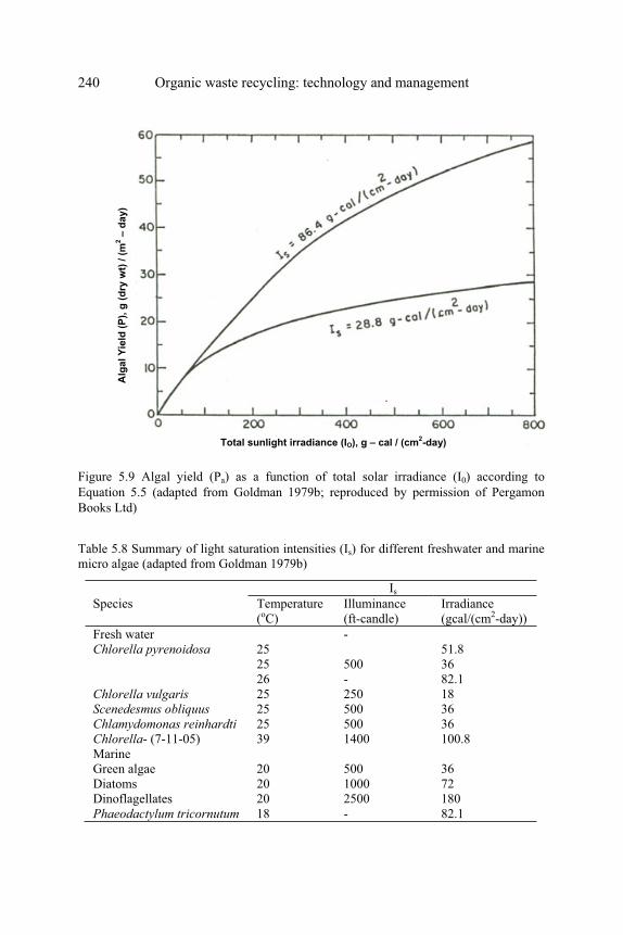
240 Organic waste recycling: technology and management
Figure 5.9 Algal yield (Pa) as a function of total solar irradiance (I0) according to
Equation 5.5 (adapted from Goldman 1979b; reproduced by permission of Pergamon
Books Ltd)
Table 5.8 Summary of light saturation intensities (Is) for different freshwater and marine micro algae (adapted from Goldman 1979b)
Is
Species Temperature (oC)
Illuminance(ft-candle)
Irradiance (gcal/(cm2-day))
Fresh water - Chlorella pyrenoidosa 25 51.8
25 500 36 26 - 82.1
Chlorella vulgaris 25 250 18 Scenedesmus obliquus 25 500 36 Chlamydomonas reinhardti 25 500 36 Chlorella- (7-11-05) 39 1400 100.8 Marine Green algae 20 500 36 Diatoms 20 1000 72 Dinoflagellates 20 2500 180 Phaeodactylum tricornutum 18 - 82.1
Total sunlight irradiance (IO), g – cal / (cm2-day)
Alg
al Y
ield
(P
), g
(d
ry w
t) / (
m2 –
da
y)

Algal production 241
Oron and Shelef formula
To account for the effects of environmental and operational conditions on algal
growth in HRAP, Oron and Shelef (1982) proposed the following empirical
formula.
Ca = a. (HRT/z)b .Io .Tr (5.6)
Where,
Ca = algal concentration, mg/L
T = ambient temperature, °C
a,b,ß,r = constants, dimensionless
Units of HRT, z and Io are days, m and gcal/(cm2-day), respectively.
The numerical values of these constants were determined from the data
collected from pilot- and field-scale HRAP operating in Israel. By applying the
nonlinear least-square method, the following equation was derived:
Ca = 0.001475(HRT/z) 1.71 Io0.70T1.30 (5.7)
The related algal productivity, Pa in g/(m2-day) may be given by:
Pa = Ca (z/HRT) = 0.001475(HRT/z) 0.71 Io0.70 T1.30 (5.8)
An experiment was carried out in Israel with domestic wastewater (average
BOD5 of 400 mg/L) and algae such as Micractiniumpusillum, M.quadriesetum
and Scenedesmus dimorphus in HRAP. Table 5.9 shows the predicted algal
concentrations using Equation 5.7 and measured algal concentrations during 6
seasons. The results of this experiment show the applicability of Equation 5.7
for the assessment of algal concentration in HRAP.
Some drawbacks of Equation 5.7 are that it is applicable to influent BOD5
ranging from 200 to 400 mg/L and to Israel conditions where these experiments
were carried out. However, the same approach can be applied to suit other local
conditions, but with different values of a, b, ß, r.
Theoretical estimation
Equation 2.6 implies that one mole of algal cell (molecular weight 154 g) is
synthesized with production of 7.62 mole O2. Therefore, as previously state in
Equation 5.4, 1 g of algal cell is equivalent to:

242 Organic waste recycling: technology and management
Table 5.9 Environmental and operational conditions and predicted algal concentration (dry weight) of the HRAP in Israel (Oron and Shelef 1982)
Solar radiation,
Io (gcal/(cm2-
day))
Ambient
temperature
(oC)
Effluent
depth
z, (m)
Retention
time,
HRT
(days)
Measured algal
concentration,
Ca (mg/L)
Predicted algal
concentration,
Caa (mg/L)
Spring 1977 576 14.6 0.45 4 176 173
Summer
1977
679 24.2 0.45 2.9 229 215
Fall 1977 393 21.4 0.4 3.4 210 201
Winter
1977/8
318 13.8 0.45 3.9 95 101
Spring 1978 538 18.9 0.35 2.9 240 204
Summer
1979
649 25.4 0.25 2 285 321
a Algal concentration was predicted from Equation 5.7
7.62 x 32
= 1.58g O2
154
or the factor
Weight of O2 produced
p = = 1.58
Weight of algal cell synthesized
The oxygen demand of a waste is met through photosynthetic oxygen
production; the ultimate biochemical oxygen demand, Lt in any time t, may be
substituted for oxygen produced, and algal concentration Ca may be substituted
for weight of algal cell synthesized. Therefore:
Lt
p = (5.9)
Ca
Lt z
and algal productivity Pa, in g/(m2-day) = . (5.10)
p HRT
Where the units of z, HRT and Lt are m, days and mg/L, respectively.
Oswald and Gotaas (1955) reported that under environmental conditions
suitable for photosynthetic oxygen production, the value of p is normally

Algal production 243
between 1.25 and 1.75. The deviation of value for p from theoretical value, 1.58,
was due to various reasons. In practice, all Lt cannot be oxidized even though
enough O2 is present; therefore low value for p is observed. Or a strong wind
blow can increase the surface re-aeration, increasing the value of O2 produced;
therefore high p value can be obtained.
Example 5.2
An agro-industry in Thailand is producing wastewater at a flow rate of 500
m3/day and its COD or Lt is 400 mg/L. Determine the size of HRAP to be used
to produce algae from this wastewater. The following information are given:
H = unit heat value of algae = 6 kcal/g
p = 1.5
F = efficiency of energy conversion = 0.1
Tc = temperature coefficient = 0.9
Io or Ii = visible solar energy irradiance = 400 gcal/(cm2-day) or 11100 ft-
candle, respectively
= specific light absorption coefficient = 1.5x10⁻³
From Equation 5.9, algal concentration in HRAP may be theoretically
estimated.
Ca = Lt/p = 400/1.5 = 266.7 mg/L
Pond depth can be estimated from Equation 5.2.
ln Ii ln 11,100
z = = = 23.3 cm
Ca 266.7(1.5x10⁻³)
Select a ‘z’ value of 25 cm.
HRT of the pond is estimated from Equation 5.3
Ca .h.z
HRT =
1000 F.Io.Tc.
266.7×6×25
HRT = = 1.11 days
1000×0.1×400×0.9

244 Organic waste recycling: technology and management
To satisfy the minimum time span for algal generation in HRAP and to avoid
cell washout from the system, select an HRT = 1.8 days.
Volume of HRAP = flow x HRT
= 500 × 1.8 = 900 m3
Surface area of HRAP = pond volume/depth
= 900/0.25 = 3600 m2
Choose 2 HRAP units, each with the following dimensions: length = 100 m,
width = 18 m with 6 channels (or the width of each channel flow is 3 m).
From the above results, the value of Ca could be re-calculated using Equation
5.7 and taking T = 30°C.
Ca = 0.001475(1.8/0.25)1.71 (400)0.70 (30)1.30
= 238 mg/L which is slightly lower than the theoretical value of 266.7
mg/L as determined from Equation 5.9.
The algal productivity is determined from Equation 5.10.
Pa = Ca (z/HRT) = 266.7 (0.25/1.8)
= 37 g/(m2-day)
The above Pa value is within the practical range predicted by Equation 5.5 as
shown in Figure 5.9.
5.3 ALGAL HARVESTING TECHNOLOGIES
The algal biomass cultured in outdoor HRAP is mainly in the microscopic
unicellular forms with concentrations in the pond water ranging from 200 to 400
mg/L. As shown in Figure 5.2, these algal cells need to be separated from the
pond water prior to being used further. The HRAP effluent to be discharged to a
watercourse may need to have algal cells removed so that the suspended solid
content of the pond effluent is within the regulatory standard for discharge.
Because of their microscopic sizes (generally less than 10 m), the separation or
harvesting of algal cells have been a major challenge and difficulty for
environmental engineers and scientists to develop an efficient harvesting
technology which is economically viable. Some of the technologies that have
been used to separate algal cells from effluents of conventional waste
stabilization ponds and HRAP systems are presented below.
5.3.1 Microstraining
Microstrainers or microscreens are low speed (upto 4 to 7 rpm) rotating drum
filters operating under gravity conditions. The filtering fabrics are normally
made of finely woven stainless steel and are fitted on the drum periphery. Mesh

Algal production 245
openings are normally in the range of 23 to 60 m, but microscreens with 1 m
mesh size made of polyester fabric has been developed (Harrelson and Cravens
1982). Wastewater enters the open end of the drum and flows outward through
the rotating fabric. The collected solids are continuously removed by high-
pressure jets (located outside at the top of the drum) into a trough within the
drum (Middlebrooks et al. 1974 and Metcalf and Eddy Inc. 2003).
Microstrainers are normally operated at hydraulic loading rates of 5-15 m3/(m2-
day), drum submergence 70-75% of height or 60-70% of filter area, and drum
diameters varying from 2.5-5 m depending on the design of screen. The full-
scale microstrainers with a 1 m mesh size installed at the Camden waste
stabilization ponds in South Carolina, U.S.A. (flow rate = 7200 m3/day) were
operated at hydraulic loadings between 60-120 m3/(m2-day).
Typical SS and algal removal achieved with microstrainers is about 50
percent, the range being 10 to 80 percent. Reed et al. (1988) suggested that
microstrainers with 1 m polyester screening media are capable of producing an
effluent with BOD5 and SS concentrations lower than 30 mg/L. However, the
service life of the screen was found to be about 1.5 years, which is considerably
less than the manufacturer's prediction of 5 years: this was probably due to
operational and maintenance problems associated with this type of screen. A
simple mesh screen with pore opening of 50 µm (Figure 5.10) can be used to
separate algal cells from HRAP effluent. Although low cost in investment, algal
cell removal with this method is about 50 %.
Figure 5.10 Mesh screen for separation of algal cells

246 Organic waste recycling: technology and management
Problems encountered with microstrainers having large mesh openings
include inadequate solids removal and inability to handle solids fluctuations.
These problems may be partially over-come by varying the speed of drum
rotation. In general, drum rotation should be at the slowest rate as possible, that
is, consistent with the throughput, and should provide an acceptable head
differential across the fabric. The controlled variability of drum rotational speed
is an important feature of the process, and the speed may be automatically
increased or decreased according to the differential head best suited to the
circumstances involved (Middlebrooks et al. 1974).
5.3.2 Paper precoated belt filtration
Because conventional microstrainer fabric (mesh sizes greater than 23 m) is
too coarse for the unicellular algae grown in HRAP and extremely fine fabric
media capable of effective separation of algal cells cannot be adequately
cleaned, a new harvesting process developed in Australia, utilizing a paper
precoated belt filter, seems to be able to overcome these difficulties (Dodd and
Anderson 1977). A schematic diagram of the paper precoated belt filtration
process is shown in Figure 5.11. The belt filter incorporates a coarse fabric belt
on which a precoat of paper fibres is deposited, as in a paper machine, forming a
continuously renewed filter medium. The paper precoat is continuously
reformed to provide a fresh filter medium having high trapping efficiency and
good throughput characteristics.
According to Figure 5.11, the algal water or influent is filtered by the
filtration drum. The filtered algal cells attached on the main belt are sandwiched
between the main and secondary fabric belts during application of vacuum and
water to separate the algae from the precoat. The paper precoat and the algal
cells are then removed from the belts by water showers (no. 14 and 15 in Figure
5.11) which are called first-stage and second-stage algal concentrates. These
algal concentrates are further washed to remove the algae, and the washed paper
fibers are recycled to form new paper precoat.
From their experiments, Dodd and Anderson (1977) found the average SS of
the first stage algal concentrate (no. 14 in Figure 5.11) to be 1.18 percent,
ranging from 0.81 to 1.49 percent. The average SS of the second stage algal
concentrate (no. 15 in Figure 5.11) was 0.43 percent. The second stage
concentrate appeared to have flocculent characteristics, which should be
beneficial in the thickening of the algal concentrate to reduce the cost of further
dewatering by centrifugation or filtration.

Algal production 247
Fig
ure
5.1
1 S
chem
atic
of
a p
reco
ated
bel
t fi
ltra
tio
n u
nit
(af
ter
Do
dd
an
d A
nd
erso
n 1
97
7;
rep
rod
uce
d b
y p
erm
issi
on
of
Per
gam
on
Bo
oks
Ltd
)

248 Organic waste recycling: technology and management
5.3.3 Flocculation and flotation
Flocculation is a process of floc formation through slow mixing so that the sizes
of flocculent materials are large and heavy enough to be settled in a
sedimentation tank. In water and wastewater treatment, flocculation is normally
preceded by coagulation in which coagulant materials such as alum, lime, ferric
chloride or polymers are added individually or in combination and rapidly
mixed to enhance floc formation. Flotation is a physical process in which solid
particles float to the water surface through some kinds of buoyant forces (such
as dissolved-air flotation or foam flotation), and the floated particles can be
skimmed off from the water surface, learning the clear liquid at the lower
portion of the flotation tank. The application of coagulation process preceding
flotation is expected to be beneficial to solids removal as the floated particles
will be larger in size, easier to entrap or absorb air bubbles and be buoyed up by
dissolved air so that they can be effectively skimmed off from the water body.
Coagulation-flocculation
Based on the above information it appears that higher efficiency of solids
removal by flocculation or flotation can be achieved with the aid of coagulation.
For the case of algal flocculation using alum as coagulant, the pH range between
6.0-6.8 (6.5 optimum) gave good algal removal efficiency (Golueke and Oswald
1965). The same result was also found by Batallones and McGarry (1970) when
they studied jar test by using a fast mixing speed of 100 rpm for 60 sec for
coagulation and a final slow mixing speed of 80 rpm for 3 min for flocculation.
They found the most efficient alum dose for algal flocculation to be between 75-
100 mg/L, while Golueke and Oswald (1965) found the alum dose to be 70
mg/L.
Besides alum, other polyelectrolytes or polymers can also be used as
coagulant aid materials. Only cationic polyelectrolytes should be used in algal
flocculation because the algal cells act like a negative charge. Batallones and
McGarry (1970) found the cost of harvesting by alum alone at algal
concentrations below 30 mg/L to be rather expensive and, to reduce the
chemical cost, suggested the use of alum in combination with some cationic
polyelectrolyte. They reported that if polyelectrolyte (Purifloc-C31) was used to
aid alum, the most economic doses were 40 mg/L of alum together with 2-4
mg/L of Purifloc-C31.
It is well known that the efficiency of coagulation-flocculation is dependent
on several environmental parameters such as pH, alkalinity, temperature, and
turbidity, etc. Therefore laboratory or pilot-scale experiments on individual
HRAP water should be conducted, wherever possible, to select the appropriate

Algal production 249
coagulant materials and other operating conditions for the coagulation-
flocculation process.
Figure 5.12 Schematic of a dissolved air flotation unit
Dissolved-air flotation (DAF)
Theoretically, there is a tendency for algal cells to float to the water surface due
to the release of supersaturated oxygen gas generated during the photosynthetic
period. To make the algal cells float more effectively DAF is normally
employed. In DAF systems, air dissolved in the water under a pressure of
several atmospheres, and the pressure is later released to the atmospheric level
in the flotation tank. For small-scale operation, part or all of the influent flow is
pressurized and is added with coagulant materials such as alum (Figure 5.12).
For large-scale operation and to improve the system performance, the clarified
effluent is normally recycled to mix with the influent feed prior to being
released into the flotation tank. In this case, the recycled effluent is pressurized
and semi-saturated with air, and is mixed with the unpressurized influent water.
DAF efficiency depends on various factors such as the air/solids ratio, dissolved
air pressure, flotation time, types and dose of coagulant aids, and pH of the
water. There are various types of DAF units produced by some manufacturers in
Europe and U.S.A. for full-scale application.
McGarry and Durrani (1970) conducted DAF experiments on HRAP water
and found that at the alum dosages of 125-145 mg/L, pH = 5-7, air pressure =
35-50 psi gage (2.4-3.4 atmospheric pressures), and flotation time = 6-10 min,
an algal concentration of 8% was obtained in the overflow effluent. Bare et al.
Pressurizedinfluent wastewater
Algal concentrate to be removed manually
or mechanically
Chemical
coagulant
Clarified
effluent
Baffle

250 Organic waste recycling: technology and management
(1975) studied algal removal using dissolved-air flotation process, with and
without coagulant aids. They found that at 25% recycle and 3 atmospheric
recycle pressure the algal removal was 35% in batch process without coagulants.
The percent removal increased to about 80 when ferric sulphate was used at 85
mg/L. The same result could be obtained when 75 mg/L of alum was used at the
same operating conditions.
Autoflocculation
Autoflocculation refers to the precipitation of algae and other particulate matters
in a pond when the pH rises to a highly alkaline level. This phenomenon is
related to the chemical make-up of the water, and, in particular, the presence of
calcium and magnesium carbonates (Middlebrooks et al. 1974). As the algae
remove CO2, the pH rises to a point at which precipitation of magnesium
hydroxides and calcium carbonate along with algae occurs, causing removal of
the particulate matters.
A recent study by Sukenik and Shelef (1984) found the proper concentrations
of calcium and orthophosphate ions in the medium to be important for
autoflocculation. To attain autoflocculation within the pH range of 8.5-9.0, the
culture medium (or HRAP water) should contain 0.1-0.2 mM orthophosphate
and between 1.0-2.5 mM calcium. Calcium phosphate precipitates are
considered as the flocculating agent, which reacts with the negatively charged
surface of the algae and promote aggregation and flocculation.
Removal of the precipitated algal cells require another non-agitated basin for
the cells to settle, or mechanical aeration has to cease for a few hours daily if
cell precipitation is to occur in the HRAP. Removal of the precipitated cells may
be conducted during nighttime or early morning when the photosynthetic
activity is non-existent and the algal cells do not tend to rise to the water
surface.
Autoflocculation appears to be a rather simple method of algal harvesting
because it does not require sophisticated mechanical equipments and operation.
However its efficiency in algal removal is generally less than the
aforementioned methods, and requiring a large area for construction of a settling
basin. In addition a very warm and cloudless day is required to attain the high
pH values (greater than 9) in HRAP water; this condition does not occur all year
round in most locations.
5.3.4 Biological harvesting
The unicellular algae grown in HRAP are food for herbivorous fish (fish feeding
on phytoplankton) and other macro-invertebrates. The culture of herbivorous
fish in algal pond water to graze on the algae is an attractive means to produce

Algal production 251
protein biomass in the fish tissue. However, fish cannot effectively graze all the
algal cells and will also discharge fish feces, causing the pond water to still
contain high algal contents and organic matters. Details about fish production in
wastewater can be found in Chapter 6.
5.3.5 Comparison of alternative algal harvesting methods
The literature on algal harvesting contains numerous studies and discussion of
various harvesting methods (Golueke and Oswald 1965; Middlebrooks et al.
1974; Parker and Uhte 1975; Benemann et al. 1980). Besides the 4 harvesting
methods listed above, there are other methods that can be used to separate algal
cells such as centrifugation, fine-weave belt filtration and sand filtration.
However there does not appear to be any method, which is clearly superior for a
"typical" application. Due to the very wide range of conditions and objectives
encountered, the selection of an algal harvesting technology and its application
should be approached as a distinct case, weighing the merits/drawbacks of each
method for the particular circumstances.
Factors to be considered in the selection of a harvesting method include
wastewater and HRAP effluent characteristics, treatment objectives (in terms of
harvested effluent quality for different water reuse applications or discharge
requirements), algal product quality, capital and operating costs, energy
requirements, level of operator skill required, and availability of equipments and
chemicals. The specific physical properties of algae also directly affect the
selection of a harvesting method, e.g. the motile euglenoids may resist
sedimentation or flotation because they can swim away from the process
effluent or the unicellular green algae will have sizes too small for the
conventional microstrainers. It is apparent that laboratory- or pilot-scale
experiments with that particular HRAP water should be conducted and the data
thoroughly analyzed prior to the selection of an algal harvesting method.
5.4 UTILIZATION OF WASTE-GROWN ALGAE
Besides the benefits in wastewater treatment gained from waste-grown algae,
these algae, depending on their characteristics, can be further used according to
the applications shown in Figure 5.2.

252 Organic waste recycling: technology and management
5.4.1 Algae as food and feed
Protein content of algae is about 50%, which is higher than soya bean, while
other vitamins and minerals are present in desirable proportions (Tables 5.10
and 5.11 show the chemical compositions of various algal species and soya
bean). However Waslien (1975) reported that there is an imbalance in the amino
acid composition of the algal protein, notably in the absence of sulfur-containing
amino acids, methionine and cystine, making the nutritional value of algae to be
considerably less than conventional foods such as eggs and milk. Another
problem with the algae is their high nucleic acid content which is about 4
percent or more (see Table 5.11, the values of RNA + DNA). These nucleic
acids, when being ingested in large quantity, can result in unacceptably high
level of uric acid (an illness) in human blood. In addition, except the Spirulina
sp., most of the waste-grown algae have thick cell walls, which are not well
digestible by human and non-ruminant animals (such as poultry). Therefore
these cell walls have to be ruptured such as by heat or acid treatment or some
mechanical means such as ball milling and crushing.
Table 5.10 Chemical composition of different algae compared with soya (% dry matter) (Becker 1981)
Component Scenedesmus Spirulina Chlorella Soya
Crude protein 50-55 55-65 40-55 35-40 Lipids 8-12 2-6 10-15 15-20 Carbohydrates 10-15 10-15 10-15 20-35 Crude fibre 5-12 1-4 5-10 3-5 Ash 8-12 5-12 5-10 4-5 Moisture 5-10 5-10 5-10 7-10
Table 5.11 Chemical composition of algae (g/100 g dry matter) (Becker 1981)
Component Spirulina Scenedesmus
Total nitrogen 11.0 8.3 Non-protein nitrogen 1.5 1.05 Protein-nitrogen 9.5 7.25 Available lysine (g/100 g protein)
2.96 3.66
Ribonucleic acid (RNA) 2.90 4.4 Deoxy-ribonucleic acid (DNA) 1.00 1.6 Calcium 0.75 0.85 Phosphorus 1.42 1.9
The thin-walled algae, such as Spirulina, thus appear to be a suitable algae
species that should be cultured for use as human food supplement. However, as

Algal production 253
pointed out by Goldman (1979a), it is rather impossible to control algal
speciation in outdoor cultures for sustained periods, except in unique chemical
environments that rarely exist in nature. Due to the rapid generation of algae,
certain species tend to dominate through natural selection regardless of which
algae is used as an inoculum. Invariably, the thick-walled and multicellular
freshwater species such as Chlorella, Scenedesmus and Micractinium tend to
become dominant over time (Goldman 1979b).
The direct use of algae for human food supplement may be unnecessary, if the
algae can be fed to the animals (pigs, poultry, and fish, etc.) and these animals are
used as food for human. Hintz et al. (1966) reported that the waste-grown algae
(Chlorella and Scenedesmus) were 73 percent digestible when fed to ruminant
animals such as cattle and sheep, and were only 54 percent digestible when fed to
pigs. The digestible energy content for the ruminants was 2.6 kcal per g algae.
These algae were found to supply adequate protein to supplement barley for pigs.
Alfafa-algae pellets, when fed to lambs, resulted in higher weight gains than alfafa
pellets alone.
Algae are basically not palatable to most of the livestocks, but this may be
overcome by pelletizing the processed algae with usual feed of particular animal,
such as steam barley in the case of cattle. In general, the waste-grown algae appear
to have potential as a livestock feed because of the high contents of protein and
other valuable substances (Tables 5.10 and 5.11).
Edwards et al. (1981a) reported the use of waste-grown algae as feed for
herbivorous fish (Tilapia). Extrapolated fish yields approaching 20 tons/(ha-year)
were obtained in the 4m3 concrete pond system based on 3 month growing periods
under ambient, tropical conditions. A linear relationship was established between
fish yields and means algal concentration in the fish ponds, in which an algal
concentration of 70 mg/L in the pond water was considered to be high enough to
produce good fish growth. Higher algal concentrations were not recommended
since it might lead to zero dissolved oxygen concentrations in the early morning
hours.
5.4.2 Algae for fertilizer
Algae may be used directly or indirectly as fertilizer in agriculture. In direct use,
algae is cultured in HRAP and then irrigated to crops. This method is simpler,
but requires more time because the algal cells need to be decomposed in the soil
first. In term of indirect use, algae is harvested and composted and then applied
to soil as fertilizer. The application of algal-laden water to crops should be
undertaken with due respect to public health considerations and guidelines as
proposed in Table 2.27.
254 Organic waste recycling: technology and management
Since algae are capable of fixing nitrogen from atmosphere, they have an
important role in agriculture. It was reported that rice field inoculated with the
nitrogen fixing algae Tolypothrix tenvis for four years produced 128% more
crop than uninoculated field. Furthermore, the plant from the inoculated field
contained 8.4 kg N/ha more than the uninoculated field. Also, using algae as
fertilizer will improve the soils' water holding capacity which is an advantage to
crop yield (Alexopulos and Bold 1967).
5.4.3 Algae for energy
The fuel characteristics of dry algae (average heat content of 6 kcal/g) are
similar to those of medium-grade bituminous coal, and suitable for using as
energy source (Benemann et al. 1980). Algae can be used together with other
organic amendments to produce biogas from anaerobic digestion.
5.4.4 Algae as source of chemicals
A significant amount of lipids is present in algal cells (Table 5.12), which can be
used for many industrial purposes such as manufacturing of surfactants, grease,
textiles, food additives, cosmetics and pharmaceuticals. The lipids of micro
algae often contain large amount of neutral lipids, mainly as glycerides, and this
might serve as a source of glycerol (Aaronson et al. 1980).
Micro algae may also serve as a source of steroids. The concentration of
steroids in algae is variable but significant amount may be found in some algae.
Algae may also contain upto 0.2% of dry weight as carotenoids (Paoletti et al.
1976). Some medicinal products have been isolated from algae (Volesky et al.
1970).
5.4.5 Algae as a future life support technology
As shown in Figure 1.1 and Table 1.2, the increase in population growth and
decrease in arable land will require technologies of food or protein production
which are cost-effective and use less land area. The HRAP technology as
described in this chapter should be able to respond effectively to this need and
the algal cells can be used at least as fish and other animal feeds. The current
progress in space exploration should eventually lead to a possibility that human
beings can stay in space, on the Moon or Mars for a longer period of time and
the algal technology that produces O2 and algal protein biomass is being
considered as a potential life-support technology.

Algal production 255
Table 5.12 Total lipids in algae harvested from high rate algal ponds in Israel (Aaronson et al. 1980)
Major species Total lipids (% of dry weight) Neutral lipids (% of dry weight)
Chlorella 22.6 10.9 Euglena 11.0 8.9 Micractinium 17.4 6.0 Oocystis 19.9 13.5 Scenedesmus 22.2 10.4
Reproduced by permission of Elsevier Science Publishers B.V.
5.5 PUBLIC HEALTH ASPECTS AND PUBLIC
ACCEPTANCE
5.5.1 Public health risks
Production of waste-grown algae involves some public health risks due to:
• Contamination of the pathogens normally presents in raw wastes,
and
• Accumulation of heavy metals and other toxic compounds in algae
cells.
As discussed in section 5.1, pathogen die-off in the algal ponds can take
place due to the ultra-violet light, algal toxins produced by algae cells,
competition with other micro organisms, inhibitory environments such as high
pH during photosynthesis, and sedimentation with sludge. However, a complete
removal of pathogens never exists in practice, because they may be protected by
self-shading of algae and clumping with sewage solids.
Edwards et al. (1981b) found the microorganism removal in their HRAP unit
located in Thailand to be about 1 order of magnitude. The ranges of bacterial
densities in the HRAP effluents were 1.0x10⁵ - 1.3x10¹⁰, 1.6x10⁵ - 2.4x10⁶, and
7.0x10⁴ - 9.2x10⁵ no./100 mL for the standard plate count bacteria, total
coliforms and fecal coliforms, respectively. According to Table 2.27, this HRAP
effluent is not suitable for unrestricted irrigation (e.g. irrigation of edible crops),
but may be used for restricted irrigation such as irrigation of trees and other
industrial crops.
Care should be taken on occupational risks to the people working with HRAP
units. The possibility of contamination to these people is high, particularly
during algal harvesting which may lead to the spreading of pathogens to other
people by carrying with body or clothes. The possibility of swallowing
pathogens during the working period cannot be ruled out. Therefore it is always

256 Organic waste recycling: technology and management
advisable to use protecting covers, such as masks, hand gloves, etc., when
working in algal pond system.
The possibility of algal contamination with toxic substances and heavy
metals has also another adverse effect on public health. Heavy metals and
pesticides may be concentrated in algae by the process of bioaccumulation,
inducing impact on other consumers in food chain through biomagnification (as
discussed in section 2.5). The concentration of toxic substances in algae is
expected to be higher than in wastewater discharged into the pond. Therefore, to
avoid such risks, the treatment of wastewater up to the allowable concentration
of heavy metals and other toxic substances should be done prior to the feeding
of this wastewater to HRAP. The waste-grown algae to be used for human or
animal feed should be regularly monitored for the presence and concentrations
of these substances.
5.5.2 Public acceptance
Unprocessed freshwater algae tend to have strong smell and taste similar to
those detected in natural waters that are undergoing eutrophication. Algal
texture is also slimy and uninviting, making the direct dietary use unlikely for
human and animals (except for herbivorous fish). Therefore the conversion of
algal biomass into dietically acceptable forms or palatable material (such as the
pelletization) is important, and some encouraging results on the use of pelletized
algae as animal feed have been reported (section 5.4).
Considering the results on the acceptability and the nutritive value of waste-
grown algae, the prospect of their direct use as human protein supplement is
relatively remote. Although the strain Spirulina seems to have potential to be
used as human or animal feed, the main problem is that, whereas species control
is relatively simple with terrestrial crops so that the best suited species are
grown, it is almost impossible to control algal speciation in outdoor HRAP
cultures (Goldman 1979a). The uses of HRAP and the waste-grown algae
appear to be limited to solving specific environmental problems such as
wastewater treatment and other applications shown in Figure 5.2. These
limitations include the upper limit in algal yield of 30-40 g/(m2-day), the
economics of algal harvesting and the algal cell characteristics, which are the
key factors in determining the application of HRAP to a particular situation.

Algal production 257
5.6 REFERENCES
Aaronson, S., Berner, T. and Dubinsky, Z. (1980) "Microalgae as a source of chemicals and natural products", in Algae Biomass, Production and Use, (Eds. G. Shelef and C.J. Soeder), pp. 575-601, Elsevier/North-Holland Biomedical Press, Amsterdam.
Alexopulos, C.J. and Bold, H.C. (1967) Algae and Fungi, The Macmillan Company, New York.
Azov, Y. and Shelef, G. (1982) 'Operation of high-rate oxidation ponds: theory and experiments', Water Research, 16, 1153-1160.
Bare, R.W.F., Jones, N.B. and Middlebrookes, E.J. (1975) "Algae removal using dissolved air flotation", J. Water Pollut. Control Fed., 47, 153-169.
Batallones, E.D. and McGarry, M.G. (1970). "Harvesting of algae through chemical flocculation and flotation", Research Program Report No.4, Asian Institute of Technology, Bangkok.
Becker, E.W. (1981) "Algae mass cultivation - production and utilization", Process
Biochemistry, 16, 10-14. Benemann, J., Koopman, B., Weissman, J. Eisenberg, D. and Goebel, R. (1980)
"Development of microalgae harvesting and highrate pond technologies in California", in Algae Biomass, Production and Use, (Eds. G. Shelef and C.J. Soeder), pp. 457-495, Elsevier/North-Holland Biomedical Press, Amsterdam.
Bickford, E. D., and Dunn, S. (1972) Lighting for Plant Growth. Kent State University Press, Ohio.
Coombs, J., and Hall, D. O. (eds) (1982) Techniques in Bioproductivity and
Photosynthesis. Pergamon Press, Oxford, U.K. Dodd, J.C. and Anderson, J.L. (1977) "An integrated high-rate pond algae harvesting
system", Progress Water Technology, 9, 713-726. Edwards, P. and Sinchumpasak, O. (1981) 'The harvest of microalgae from the effluent
of a sewage fed high rate stabilization pond by Tilapia nilotica. Part I: Description of the system and the study of the high rate pond', Aquaculture, 23, 83-105.
Edwards, P., Sinchumpasak, O., Labhsetwar, V.K. and Tabucanon, M. (1981) 'The harvest of microalgae from the effluent of a sewage fed high rate stabilization pond by Tilapia nilotica. Part 3: maize cultivation experiment, bacteriological studies, and economic assessment', Aquaculture, 23, 149-170.
Edwards, P., Sinchumpasak, O. and Tabucanon, M. (1981a) 'The harvest of microalgae from the effluent of a sewage fed high rate stabilization pond by Tilapia nilotica.Part 2: studies of the fish ponds', Aquaculture, 23, 107-147.
Goldman, J.C. (1979a) "Outdoor algal mass culture-I. Applications", Water Research,13, 1-19.
Goldman, J.C. (1979b) "Outdoor algal mass culture-II. Photosynthetic yield limitations", Water Research, 13, 119-136.
Golterman, H. L. (1975) Physiological Limnology. Elsevier Scientific Publishing Co., Amsterdam.
Golueke, C.G. and Oswald, W.J. (1965) "Harvesting and processing of sewage-grown plantonic algae", J. Water Pollut. Control Fed., 37, 471-498.
Green, F. B., and Oswald, W. J. (1995) Engineering strategies to enhance microalgal use in wastewater treatment. Water Sci. Technol., 31, 9-18.

258 Organic waste recycling: technology and management
Harrelson, M.E. and Cravens, J.B. (1982) "Use of microscreens to polish lagoon effluent", J. Water Pollut. Control Fed., 54, 36-42.
Hintz, H.F., Heitman, H., Jr., Weir, W.C., Torell, D.T. and Meyer, J.H. (1966) 'Nutritive value of algae grown on sewage', J. of Animal Science, 25, 675-681.
Hsu, S.C. (1970) "Factors Affecting Algal Yields from High-rate Oxidation Ponds Treating Sewage", Thesis No. 325, Asian Institute of Technology, Bangkok.
Kreith, F. and Kreider, J. F. (1978) Principles of Solar Engineering. Hemisphere Publishing Corp., Washington
McGarry, M.G. and Durrani (1970) "Flotation as a method of harvesting algae from ponds", Research Program Report No.5, Asian Institute of Technology, Bangkok.
Metcalf and Eddy, Inc. (2003) Wastewater Engineering, Treatment, Disposal and Reuse,4Th Edition, Tata McGraw-Hill, New York.
Middlebrooks, E.J., Porcella, D.B., Gearheart, R.A., Marshall, G.R., Reynolds, J.H. and Grenney, W.J. (1974) "Techniques for algae removal from waste stabilization ponds", J. Water Pollut. Control Fed., 46, 2676-2692.
Mitchell, R. (1974) Introduction to Environmental Microbiology, Prentice-Hall, Englewood Cliffs, N.J.
Moraine, R., Shelef, G., Meydan, A. and Levi, A. (1979) "Algal single cell protein from wastewater treatment and renovation process", Biotechnology and Bioengineering,
XXI, 1191-1207. Oron, G. and Shelef, G. (1982) "Maximizing algae yield in high-rate oxidation ponds", J.
Environmental Engineering Division, ASCE, 108, 730-738. Oswald, W.J. (1963) "High rate ponds in waste disposal", Development in Industrial
Microbiology, 4, 112-119. Oswald, W. J. (1991) Introduction to advanced integrated wastewater ponding systems.
Water Sci. Technol., 24, 1-7. Oswald, W.J. and Gotaas, H.B. (1955) "Photosynthesis in sewage treatment",
Transactions, American Society of Civil Engineers, 122, 73-105. Oswald, W.J., Gotaas, H.F., Ludwig, H.F. and Lynch, V. (1953) "Algae symbiosis in
oxidation ponds, III. photosynthetic oxygenation", Sewage Ind. Wastes, 25, 692-705.
Paoletti, C., Phushparaj, B., Florenzano, G., Capella, P. and Lercker, G. (1976) "Unsaponifiable matter of green and blue-green algal lipids as a factor of biochemical differentiation of their biomass: I. total unsaponifiable and hydrocarbon fraction", Lipids, 11, 258-265.
Parker, D.S. and Uhte, W.R. (1975) 'Discussion: Technique for algal removal from oxidation ponds', J. Water Pollut. Control Fed., 47, 2330-2332.
Persoone, G., Morales, J., Verlet, H. and De Pauw, N. (1980) "Air lift pumps and the effect of mixing on algal growth", in Algae Biomass, Production and Use, (Eds. G. Shelef and C.J. Soeder) pp. 505-522. Elsevier/North-Holland Biomedical Press, Amsterdam.
Reed, S.C., Middlebrooks, E.J. and Crites, R.W. (1988) Natural Systems for Waste
Management and Treatment, McGraw-Hill, New York. Soeder, C.J. and Stengel, F. (1974) "Physico-chemical factors affecting metabolism and
growth rate", in Algal Physiology and Biochemistry, (Ed. W.D.P. Stewart), pp 714-740, Blackwell Scientific Publ., London.

Algal production 259
Sukenik, A. and Shelef, G. (1984) 'Algal autoflocculation-verification and proposed mechanism', Biotechnology and Bioengineering, XXVI, 142-147.
Volesky, B., Zajic, J.E. and Knettig, E. (1970) "Algal Products", in Properties and
Products of Algae, (Ed. J.E. Zajic), pp. 49-82, Plenum Press, New York. Waslien, C.I. (1975) 'Unusual sources of proteins for man', Crit. Rev. Food Sci. and
Nutrition (CRC Press), 6, 77-151. Wetzel, R. G., Likens, G. E. (1979) Limnological Analysis. W. B. Saunders, Co.,
Philadelphia.
5.7 EXERCISES
5.1 There are three formulas presented in this book for estimating algal productivity
in high-rate algal ponds (HRAPs): the Goldman formula (Equation 5.5), the
Oron and Shelef formula (Equation 5.8) and theoretical estimation (Equation
5.10). Discuss the merits and shortcomings of these formulas.
5.2 You are to obtain the meteorological data (for the past 12 months) which are
important for algal production in high-rate algal ponds from the local weather
bureau. Using these data and those reported in Chapter 2, determine the amount
of algal cells that can be produced if all of your city's wastewater is to be used
as the influent feed. Use the three formulas in section 5.2.2 for the calculation
and discuss which of the three calculated results of algal production is most
applicable to your city.
5.3 You are to survey the algal harvesting equipments currently available in the
market in your country or elsewhere. Based on your inspection and information
obtained from the equipment manufacturers, describe the equipment that
appears most impressive with respect to: the harvesting technique employed,
efficiency of algal harvesting, costs of investment and operation and
maintenance.
5.4 If human beings are to live in space or on the moon for an extended period of
time, discuss the possibility of producing oxygen and algal single-cell protein
from the wastes we produce. Estimate the amount of oxygen and algal protein
that can be produced from a person's wastes using the data given in Chapter 2.
Also sketch the bioreactor(s) to be constructed in a space shuttle and/or the
moon to recycle the human wastes.
5.5 A food-processing factory produces 400 m3/day of wastewater with an average
COD concentration of 400 mg/L. The factory wants to construct its own high-
rate algal pond (HRAP) to produce algal single cell protein from this
wastewater. As a consulting engineer, you are asked to estimate the land area

260 Organic waste recycling: technology and management
required and the annual algal production including the income that can be
earned from the sale of the algal biomass. Submit the schematic drawings of the
HRAP. The following information is given:
HRT for HRAP = 2-5 days
Depth of HRAP = 0.2-0.4 m.
Average I0 = 400 gcal/ (cm2-day).
Mean temperature = 25°C
Light saturation intensity (Is) is to be estimated from Table 5.7.
Cost of algal harvesting = US$ 0.2/m3 of algal water
Algal density in HRAP = 300 mg/L
Price of algae = US$ 30/kg (dry weight)
5.6 A small community has a one-ha land available to treat its sewage with a COD
of 300 mg/L. It plans to build high rate algal ponds (HRAPs) on this piece of
land to treat the sewage. Determine the total treatment capacity of the HRAPs
and the optimum pond depth. Also estimate the daily algal and protein
production to be obtained from this piece of land. Additional information is
given below:
I0 or Ii = visible solar energy irradiance = 500 gcal/(cm2-day) or
13,900 ft-candle
= specific light absorption coefficient = 1.5x10⁻³
Tc = temperature coefficient = 0.8
F = efficiency of energy conversion = 0.1
p = 1.6
h = unit heat of algae = 6 kcal/g
5.7 A municipality in Vietnam produces wastewater with the following
characteristics:
Flow rate = 2000 m3/day
BOD5 = 100 g/m3
NH4-N = 20 g/m3
a) If this wastewater is to be treated in a high-rate algal pond (HRAP) to
produce algal density of 200 g/m3, determine the dimension (depth ×
width × length) of the HRAP to achieve this objective. Draw schematic
diagram of this HRAP.
The following information about HRAP are given in Equation 5.2.

Algal production 261
z = ln Ii
Ca.
Where,
z = depth of HRAP, cm
Ii = measured light intensity = 10,000 ft-candle
Ca = algae density, mg/L
= specific light absorption coefficient = 1x10⁻³
Hydraulic retention time of HRAP = 5 days
b) If we want to increase the algal productivity of this HRAP to be twice of
that given in (a), suggest methods to achieve this objective and the
required dimension of the HRAP. Also suggest methods to re-use the
produced algal cells that would be acceptable to the public.

© 2007 IWA Publishing. Organic Waste Recycling: Technology and Management. Authored by
Chongrak Polprasert. ISBN: 9781843391210. Published by IWA Publishing, London, UK.
6
Fish, chitin, and chitosan production
Among several waste recycling methods, the reuse of human and animal wastes
for the production of algae and fish has been extensively investigated. Although
the algal cells photosynthetically produced during sewage treatment contain
about 50% protein, their small sizes, generally less than 10 m, have caused
some difficulties for the available harvesting techniques, which as yet are not
economically viable (see Chapter 5). Apart from aesthetic reasons, one of the
drawbacks concerning the direct utilization of the waste-grown algae as an
animal feed, except Spirulina, has been the low digestibility of the algal cell
walls. Thus the culture of phytoplankton-feeding (herbivorous) fish in the same
pond to graze on the algae, or feeding the algal-laden water to herbivorous-fish
ponds is attractive, in order to produce the fish protein biomass which is easily
harvestable for animal (or human) feed.
There are basically three techniques for reusing organic wastes in
aquaculture: by fertilization of fish ponds with excreta, sludge or manure; by
rearing fish in effluent-fertilized fish ponds; and by rearing fish directly in waste
stabilization ponds (such as in maturation ponds). A World Bank report
(Edwards 1985) cited several Asian countries, especially China, where excreta

Fish, chitin, and chitosan production 263
or animal manure is fed to fish ponds for the purpose of fish production. Most
fish farmers also add supplementary feed such as agricultural by-products and
grains to the fish ponds.
The second and third techniques of waste reuse in aquaculture have been
practiced in both developing and developed countries. There are about 2,500 ha
of sewage-fertilized fish ponds in Calcutta, India; 270 ha in Hunan, China; 233
ha in Munich, Germany; 50-100 ha in Israel; and a smaller-scale operation in
Hungary. When properly operated, the productivity of fish ponds using
wastewater has been found to be higher than that of inorganically fertilized
ponds (Allen and Hepher 1976).
Some reported yields of fish raised in waste-fed ponds in various countries
are shown in Table 6.1.
Another type of aquacultural waste that has high reuse potentials is shrimp
biowaste. Shrimp production is being done in several tropical countries such as
Thailand, Vietnam, Indonesia, India, China and Honduras. Thailand is currently
one of the largest shrimp producers with an estimated shrimp production in
2006 of 450,000 tons, about 10% of the total world production. The shrimp
biowaste, which is mostly shrimp shells, comprises about 40% of the total
shrimp production. Since shrimp shells contain about 10-20% chitin, the
production of chitin and chitosan from shrimp shells, as earlier stated in section
1.2.3, would bring economic returns and reduce pollution load resulting from
the disposal of shrimp biowaste to landfills.
The cultivation of fish in waste-fed ponds and production of chitin and
chitosan will be described in this chapter.
6.1 OBJECTIVES, BENEFITS AND LIMITATIONS OF
FISH CULTIVATION IN WASTE-FED PONDS
The main objectives and benefits that can be gained from waste recycling
through fish production are as follows:
6.1.1 Waste stabilization and nutrient recycling
Waste treatment is the primary objective of any waste recycling scheme and the
inclusion of fish production recovers nutrients in the waste, such as N, P and K.
Addition of waste or its by-products such as biogas slurry and compost to fish
pond resulted in increased fish yields (Polprasert et al. 1982). Due to the
economic value of fish, part of the waste treatment costs can be recovered. This
financial return will be an incentive for safe disposal of waste, which will lead
to better public health conditions, particularly among the rural people where
malnutrition and excreta-related diseases are common.

264 Organic waste recycling: technology and management
Ref
eren
ces
Sch
roed
er (
1977)
Wohlf
arth
and
Sch
roed
er (
1979)
Mar
amba
(1978)
Dja
jadir
edja
and
Jangkar
u (
1978)
Thors
lund (
1971)
Tan
g (
1970)
Edw
ards
(1985)
Edw
ards
(1985)
Edw
ards
(1985)
Edw
ards
(1985)
Colt
et a
l (1
975)
Hen
der
son (
1983)
Edw
ards
et a
l (1
984)
Edw
ards
et a
l (1
988)
Rem
ark
s
Extr
apola
ted f
rom
exper
imen
ts
Extr
apola
tion
India
n C
arp
Com
mon C
arp
Poly
cult
ure
, C
hin
ese
carp
and c
om
mon c
arp
Chan
nel
cat
fish
Sil
ver
car
p, big
hea
d c
arp
Til
apia
(ex
trap
ola
tion)
Til
apia
(ex
trap
ola
tion)
Yie
ld
10,9
50 k
g/(
ha-
day
)
14,6
00 k
g/(
ha-
day
)
8,0
00 k
g/(
ha-
day
)
7,5
00 k
g/(
ha-
day
)
400-5
00 k
g/(
ha-
gro
win
g s
easo
n)
6,8
93-7
,786 k
g/(
ha-
yea
r)
958-1
,373 k
g/(
ha-
yea
r)
6,0
00-1
0,0
00 k
g/(
ha-
gro
win
g s
easo
n)
500 k
g/(
ha-
gro
win
g s
easo
n)
1,7
00 k
g/(
ha-
gro
win
g s
easo
n)
126-2
18 k
g/(
ha-
yea
r)
5000 k
g/(
ha-
yea
r)
5,0
00-6
,000 k
g/(
ha-
yea
r)
3,7
00 k
g/(
ha-
yea
r)
Ty
pes
of
was
te
Cat
tle
man
ure
Du
ck m
anu
re a
nd
was
te d
uck
fo
od
Bio
gas
slu
rry
Liv
e st
ock
was
te
Sugar
bee
t w
aste
Nig
hts
oil
Was
tew
ater
Was
tew
ater
Was
tew
ater
, l
oad
ing
s =
30
-77 k
g
BO
D5 /
(ha-
day
)
Was
tew
ater
Was
tew
ater
eff
luen
t, 3
7 %
Was
tew
ater
Sep
tag
e, l
oad
ing =
15
0
kg
/CO
D/(
ha-
day
)
Bio
gas
slu
rry
, lo
adin
g =
10
0 k
g
CO
D/(
ha-
day
)
Co
un
try
Isra
el
Ph
ilip
pin
es
Ind
on
esia
Po
lan
d
Tai
wan
Cal
cutt
a, I
ndia
Ch
ina
Mu
nic
h,
Ger
man
y
Hungar
y
U.S
.A
Asi
an I
nst
itute
of
Tec
hn
olo
gy
,
Th
aila
nd
Tab
le 6
.1 F
ish
yie
lds
in w
aste
-fed
po
nd
s

Fish, chitin, and chitosan production 265
6.1.2 Upgrading effluent from waste stabilization ponds
Algae in suspension increase the suspended solids content of most waste
stabilization pond effluents. (Waste stabilization ponds are a waste treatment
process encompassing reactions of the algal-bacteria symbiosis as described in
Chapters 2 and 5) Effluent discharge without the removal of algae might cause
algal blooms or increasing organic and nutrient loads to the receiving waters.
Introducing fish ponds in series with waste stabilization ponds or its rearing in
the waste stabilization ponds was found to reduce the algal and bacterial
concentrations to a considerable extent when herbivorous fish species (Tilapia
and silver carp) were used (Schroeder 1975). The layouts in Figure 6.1 could be
used for the above purpose. In this way, the death of fish in the fish ponds may
also indicate the presence of some toxic materials and/or low dissolved oxygen
(DO) levels in the effluent discharging into the receiving water.
Figure 6.1 Layouts to upgrade waste stabilization pond (WSP) effluents using fish
6.1.3 Better food conversion ratio
Fish are cold-blooded animals and, unlike other farm animals such as cattle or
poultry, do not have to spend a lot of energy for movement because friction is
less in water. Thus fish have a better food conversion ration than any other farm
animals. Table 6.2 compares the relative growth and feed utilization of farm
animals and fish during a period of rapid growth. Food conversion ratio (FCR)
is defined as:
(kg)gainedanimalofWet weight
(kg)givenfeedofDry weight=FCR
therefore, the lower the FCR, the better the food conversion efficiency.
Waste stabilization ponds Fish pond Upgraded effluent Influent Effluent
Waste stabilization ponds + Fish
Upgraded effluent Influent

266 Organic waste recycling: technology and management
6.1.4 Operational skill and maintenance
Fish culture does not require highly skilled manpower for its operation. Fish
harvesting is easier than algal harvesting. Fish processing is usually not required
for human consumption. For other uses such as animal feeds, drying is generally
sufficient.
However, fish production from wastes might have some or all of the
following limitations:
Land requirement and existence of a waste collection system
Land requirement for fish production is quite large as the organic loading to fish
ponds has to be low to avoid DO depletion at dawn. Land should be available at
low cost and closer to the source of waste and natural water courses (e.g. canals
or rivers). The transportation of waste should be safe, easy and cheap. If the
waste is available in a concentrated form such as septage, suitable sources of
water to make-up the evaporation and seepage losses should be available.
Table 6.2 Efficiency of feed utilization of various animal species per 1000 g of feed intake (adapted from Hastings and Dickie 1972)
Species Live weight gain (g)
Foodconversion ratio
Energy gain (kcal)
Proteingain (g)
ChicksPigsSheep Steers Channel catfish Brown trout
356292185163715576
2.83.45.46.11.41.7
7821492832748935608
10130222611875
Availability of suitable fish fry
Fish species suitable for stocking in waste-fed ponds should be available locally
at low price. If such facility for fish fry production is not available or its
production is not economically feasible locally, fish production is not possible.
Public health risks
Waste-grown fish have a potential to be contaminated with several kinds of
pathogens that may be present in the waste itself (Table 2.23). Fish growing in a
medium that has high concentrations of heavy metals or other toxic substances
may, through the processes of bioaccumulation and biomagnifications, contain
high concentrations of these substances in the fish tissue.

Fish, chitin, and chitosan production 267
Marketing and public acceptance
Unless the public is convinced that waste-grown fish are safe for consumption,
the fish production is bound to fail. In those areas where fish from sea or river
origins are available in sufficient quantity and cheap, marketing of waste-grown
fish will be difficult for human consumption. However, other methods of use
(i.e. as animal feed) or other recycling options have to be considered.
6.2 HERBIVORES, CARNIVORES AND OMNIVORES
Feeding is one of the most essential factors that strongly influence the growth
rate of fish. Moreover, similar to other animals, different fish species have their
own special feeding habits. Fish can be classified into three groups on the basis
of feeding habits. Their morphologies are also different accordingly, mainly in
the aspect of the specialized type of alimentary system. Thus, the functional
morphology of fish species can often indicate the type of food they eat and those
they are unable to eat. These three groups are characterized below:
6.2.1 Herbivorous fish
Herbivorous fish lack teeth, but possess fine gill rakers that can sieve
microscopic plant from the water; they also lack a true stomach (i.e. a highly
muscular, acid secreting) but possess a long, thin-walled intestine. They mainly
feed on plant including algae and higher plants. Typical examples are grass carp
(Ctenopharyngodon idella) (unlike other herbivores, its gut is very short), and
silver carp (Hypophthalmichthys molitrix) (Figure 6.2 a, b).
Under optimum conditions, small grass carp, less than 1.2 kg, may eat
several times their body weight of plant material daily (NAS 1976). Thus, in
addition to being as a source of protein, many herbivorous species, such as grass
carp and silver carp, are often grown in the weed-infested water for biological
control of phytoplankton blooms and some aquatic weeds.
6.2.2 Carnivorous fish
Carnivorous fish have teeth well developed to seize, hold and tear, and gill-
rakers modified to grasp, retain, rasp and crush prey. There is a true flask-like
stomach and a short intestine, elastic and thick walled. These fish mainly eat
zooplankton, insects, bacteria, trash fish and other animals. Snakehead
(Ophicephalus striatus) (Figure 6.2c) is mainly carnivorous, feeding on small
fish, crustacean, insects and worms. Usually carnivorous fish are preferred to
other fish by people for their high nutritive value and taste. But much higher
investment is needed for carnivores' feed and fertilizer than other fish.

268 Organic waste recycling: technology and management
Figure 6.2 Examples of herbivores, carnivores and omnivores
6.2.3 Omnivorous fish
Carnivorous fish have alimentary systems, which are more or less intermediate
between those of the extreme herbivores and carnivores, but there is a range of
types between the extremes. The alimentary canal is much longer, relative to
body length. Most fish belonging to these groups, that consume both animal and
plants, for example, the Chinese common carp (Cyprinus carpio) and Tilapia
(Oreochromis niloticus) (Figure 6.2d & e), have a wide range of diet.
The terms herbivores and carnivores have relative meaning. Usually they just
indicate the type of food predominantly consumed by the fish (actually most
fish are highly adaptable in their feeding habits and utilize the most readily
available foods (Lagler et al. 1962)). Relatively few kinds are being strict
herbivores or carnivores, and perhaps none of all feed solely on one organism.
Food habits may change as fish grow, accompanied by marked change in the
morphology of alimentary system in early life. Fish such as Bermuda angelfish
(Holacanthus bermudensis) may even change their diet with season. It may be
quite herbivorous in winter and spring and become predominantly carnivorous
in the summer and early fall.

Fish, chitin, and chitosan production 269
Therefore, feeding materials will vary with the different fish species and the
stages of development according to their feeding habits, so that fish can keep
growing at higher rate.
Fish to be reared in waste-fed ponds should have the following
characteristics:
• tolerant to low DO level which can occur during night time or at
dawn when photosynthetic oxygen production does not occur,
• herbivorous or omnivorous in nature to feed on the waste-grown
phytoplankton, and
• tolerant to diseases and other adverse environmental conditions.
Some species such as Tilapia (Figure 6.2 e), Chinese carp, and Indian carp
have been widely used in waste recycling practices. Organic wastes, including
septage, could provide sufficient nutrients to promote the growth of
phytoplankton and consequently of zooplankton which is natural food of these
fish (Polprasert et al. 1984). Among these species, Tilapia needs to be
particularly mentioned, for its being used widely in waste recycling in the
tropical and sub-tropical areas. It feeds directly on algae and other primary
aquatic vegetation (and on zooplankton as well). It grows rapidly and multiplies
abundantly. Furthermore, it has better tolerance to low DO level and resistance
to diseases (which often occur in fish ponds) than many other species such as
carp.
The culture of carnivores is also of interest in waste recycling if fish for
human consumption is desired. But they have to be raised in separate ponds fed
with pellets made from herbivores, omnivores, or trash fish (to allow the growth
of herbivores or omnivores), and to safeguard public health because the
carnivores will not be in direct contact with the organic wastes. Catfish,
snakehead and shrimp, which are of high market value, are the carnivores
commonly reared.
6.3 BIOLOGICAL FOOD CHAINS IN WASTE-FED PONDS
Food chain is the series of organisms existing in any natural community through
which energy is being transferred. Each link in such a chain feeds on and
obtains energy from the ones preceding it. In a pond ecosystem, there are
generally three major groups of organisms present in the food chain, similar to
the other marine and freshwater ecosystems. The three groups consist of: the
primary producers; the primary, secondary and tertiary consumers; and the
decomposer organisms (Figure 6.3).
At the beginning of the food chain, the primary producers (algae and aquatic
plants) represent the first trophic or energy level. They synthesize organic

270 Organic waste recycling: technology and management
materials (or cell biomass) through photosynthesis (e.g. Equation 2.6), utilizing
the nutrients present in the water and light energy. Next is the primary consumer
group, mainly zooplanktons and the herbivores, which consumes the primary
producers, then they are preys for secondary consumers such as small fish and
other plankton feeders. In this step, some fish consume benthic animals that
grow at the pond bottom. Some herbivorous fish such as silver carp consumes
phytoplankton directly and it can also take detritus. Tertiary consumers such as
snakehead predate small fish. Depending on the type of fish stocked, they feed
on phytoplankton or zooplankton and are primary consumers, secondary
consumers or tertiary consumers.
The waste material produced by fish and decaying biomass will settle to the
pond bottom and be decomposed by bacteria (the decomposers), resulting in the
release of nutrients such as CO2 and NH3 (Equation 2.1) required for the
primary production.
When comparing food chains in a normal fish pond and a waste-fed fish
pond, there are no wide differences between them. However, to allow the
herbivorous fish to grow effectively and maximizing the fish biomass
production, carnivorous fish (tertiary consumers) are not normally stocked in the
waste-fed fish ponds where herbivores are being reared. Additionally, in waste-
fed fish ponds, there are more nutrients for primary producers due to the
application of waste and its decomposition. Food chain depends on the primary
productivity of the pond, which in turn depends on the nutrients and light. The
subject of environmental requirements in waste-fed ponds will be discussed in
section 6.5.
Another important consideration related to food chain is the problems caused
by biomagnification and bioaccumulation. Biomagnification may be defined as
the accumulation of toxic materials such as pesticides or heavy metals in an
organism in any particular trophic level at a concentration greater than that in its
food or the preceding trophic level so that essentially animals at the top of food
chain accumulate the largest residues (see Figure 6.3). Bioaccumulation is the
phenomena where the toxic matter is in equilibrium at a higher concentration in
tissues than that of the surrounding aquatic environment. This depends on the
time of exposure, rate of uptake, metabolism within organism, rate of excretion,
potential for storage in tissues and the physiological state of organism.
Therefore the effect of both factors should be investigated especially when
industrial or agricultural wastes containing high concentrations of heavy metals
and/or toxic organic compounds are to be applied to fish ponds.

Fish, chitin, and chitosan production 271
Figure 6.3 Food chain and other relationships in waste-fed ponds
A well-known example of bioaccumulation and biomagnifications involves
the pesticide DDT, which is now banned in the United States (Campbell 1990).
DDT concentration in a long Island Sound food chain was magnified by a factor
of about 10 million, from just 0.000003 ppm as a pollutant in the seawater to a
concentration of 25 ppm in a fish-eating bird, the osprey (see Figure 6.4).
Organic waste
inputDecomposers: bacteria
CO2 and NH3
Light
O2
Benthic animals
Detritus: faeces and
decayed biomass
Primary producers: algae and aquatic plants (1st
trophic level)
Primary consumers, zooplankton and
herbivorous fish (2nd
trophic level)
Secondary consumers:plankton feeds and some fishes
(3rd
trophic level)
Tertiary consumers:
carnivorous fish (4th
trophic level)
Man

272 Organic waste recycling: technology and management
6.4 BIOCHEMICAL REACTIONS IN WASTE-FED PONDS
In a waste-fed fish pond that is functioning well, algae, bacteria and fish are
having symbiotic relationships. The oxygen and food for fish are to be produced
by the algae, while bacteria decompose the waste. Figure 6.5 depicts the
interactions among these organisms in a pond fed with wastewater or sludge.
Figure 6.4 Bioaccumulation and biomagnifications of DDT in a food chain (adapted from
Campbell 1990)
The biochemical reactions occurring in waste-fed fish ponds should be
similar to those of facultative waste stabilization ponds in which the organic
matter is decomposed by a combination of aerobic, facultative and anaerobic
bacteria. Three zones exist in the ponds: the first is an aerobic zone where
aerobic bacteria and algae exist in a symbiotic reaction, i.e. the oxygen supplied
partly by natural surface re-aeration and from algal photosynthesis (Equation
2.6) is used by the bacteria in the aerobic decomposition of the organic matter
(Equations 2.1 and 2.2); the nutrients and carbon dioxide released in this
decomposition are, in turn, used by the algae (Equation 2.7). The second is an
intermediate (facultative) zone which is partly aerobic and partly anaerobic, in
which waste stabilization is carried out by facultative bacteria; and the third, an
DDT in phytoplanktons
0.04 ppm
DDT in small fish
0.5 ppm
DDT in large fish
2 ppm
DDT in fish eating
birds 25 ppm
Trophic level
DDT in water
0.00003 ppm

Fish, chitin, and chitosan production 273
anaerobic bottom zone in which the accumulated solids are decomposed by
anaerobic bacteria. Fish normally live in the aerobic and facultative zones where
oxygen and food (algae) are present.
When organic wastes are discharged into a pond, the soluble and colloidal
compounds that remain in suspension will be decomposed by the aerobic and
facultative bacteria. The settleable solids will settle down to the pond bottom
and, together with other decayed biomass that settles there, forming a sludge
layer. Anaerobic reactions occurring in the sludge layer zone are similar to those
described in Chapter 4 in which there will be releases of soluble organic by-
products (such as amino acids and volatile fatty acids, etc.) and gaseous by-
products such as CH4 and CO2. Since the pond depth is usually about 1 m, these
soluble by-products will dissolve in the water due to wind-induced mixing and
fish movement, which will be further decomposed by the aerobic and facultative
bacteria present in the above pond layers.
Figure 6.5 A simplified view of septage-fed fish pond dynamics (adapted from Bhattrai
1985)
The above biochemical reactions normally result in diurnal changes in pH
and DO in the pond water as shown in Figure 6.6. The basic phenomena
involved are that during the dark periods, photosynthetic activity ceases to
function and the algal cells do not utilize the CO2 released by bacterial
decomposition of organic matter, resulting in the formation of carbonic acid
and, consequently, a decrease in pH. Biomass respiration and the absence of
photosynthesis during night time contribute to a drop in DO. With the onset of

274 Organic waste recycling: technology and management
the light period, the algae consume CO2 for photosynthesis with the production
of oxygen and more algal cells, this results in a gradual increase in pH and DO
(upto supersaturation level) in the pond water. In Figure 6.6, the DO at dawn did
not reach zero because the applied organic loading was not excessive. Since fish
are generally sensitive to low DO, organic loadings to be applied to fish ponds
should be properly controlled so that the DO level at dawn, the critical period,
does not become zero. Otherwise, some kinds of mechanical aeration need to be
provided to the fish ponds to avoid fish suffocation.
6.5 ENVIRONMENTAL REQUIREMENTS AND DESIGN
CRITERIA
6.5.1 Environmental requirements
To enhance the fish growth in waste-fed ponds, various environmental
parameters should be properly maintained or acquired, as follows:
Light
Light should be in sufficient intensity and with suitable duration during the
daytime. It is the main factor in algal photosynthesis, which results in the
production of fish feed (algal cells) and oxygen for fish respiration. Generally
this requirement is always met in tropical area where depth of fish ponds is
maintained at about 1 m to allow for light penetration to the whole pond depth.
Temperature
Fish metabolic rate is directly correlated with water temperature. Heut and
Timmermans (1971) reported that temperature has a considerable influence on
the principal and vital activities of fish, notably their breathing, growth and
reproduction. Increased temperature will lower the DO in the water (according
to Table 6.3) and also increase the metabolism of fish, which require more
oxygen. The temperature tolerance limit within each species with individuals of
different ages is the same, but the limit is different if they are acclimatized at
different temperatures. Unfavourable temperatures at either end of the tolerance
range produce a stress in which a prolonged exposure could result in lowered
resistance and greater susceptibility to disease. Temperature does affect
metabolism as well as food intake. Hickling (1971) reported that carp stop
feeding at about 10°C, and become torpid at about 5°C; trout cease to feed at
about 8°C.

Fish, chitin, and chitosan production 275
Figure 6.6 Semi-diurnal studies of the septage-fed pond system. Dissolved oxygen and
pH were measured at 3 hr interval from 6 a.m. to 6 p.m. on four occasions. Mean of 15
septage fed ponds with fish stocking densities of 3, 6, 9, 12, and 15 /m2 in triplicate
(Polprasert et al. 1985)
Dissolved oxygen (DO)
DO is an important factor in the growth of fish because all metabolic activities
of fish are dependent on the oxygen consumed during respiration. As shown in
Figure 6.6, DO in a waste-fed pond have diurnal variation. Factors affecting the
variation of DO include organic loading, algal concentration, type of fish, fish
stocking density, sludge accumulation, temperature and chloride concentration
(Table 6.3). Organic loading to a pond has influence on the bacterial activity in
waste stabilization and, consequently, the oxygen utilization (Equation 2.1).
Therefore, to design a waste-fed fish pond, organic loading and fish stocking
density have to be properly selected so that the lowest DO to occur in the pond
at dawn is within the tolerable range for fish.
Dissolved oxygen
pH

276 Organic waste recycling: technology and management
Table 6.3 Solubility of dissolved oxygen in water in equilibrium with dry air at 760 mm Hg and containing 20.9 percent oxygen (after Whipple and Whipple 1911)
Chloride concentration (mg/L) Temperature 0C 0 5000 10,000 15,000 20,000
0 14.6 13.8 13.0 12.1 11.3 1 14.2 13.4 12.6 11.8 11.0 2 13.8 13.1 12.3 11.5 10.8 3 13.5 12.7 12.0 11.2 10.5 4 13.1 12.4 11.7 11.0 10.3 5 12.8 12.1 11.4 10.7 10.0 6 12.5 11.8 11.1 10.5 9.8 7 12.2 11.5 10.9 10.2 9.6 8 11.9 11.2 10.6 10.0 9.4 9 11.6 11.0 10.4 9.8 9.2 10 11.3 10.7 10.1 9.6 9.0 11 11.1 10.5 9.9 9.4 8.8 12 10.8 10.3 9.7 9.2 8.6 13 10.6 10.1 9.5 9.0 8.6 14 10.4 9.9 9.3 8.8 8.3 15 10.2 9.7 9.1 8.6 8.1 16 10.0 9.5 9.0 8.5 8.0 17 9.7 9.3 8.8 8.3 7.8 18 9.5 9.1 8.6 8.2 7.7 19 9.4 8.9 8.5 8.0 7.6 20 9.2 8.7 8.3 7.9 7.4 21 9.0 8.6 8.1 7.7 7.3 22 8.8 8.4 8.0 7.6 7.1 23 8.7 8.3 7.9 7.4 7.0 24 8.5 8.1 7.7 7.3 6.9 25 8.4 8.0 7.6 7.2 6.7 26 8.2 7.8 7.4 7.0 6.6 27 8.1 7.7 7.3 6.9 6.5 28 7.9 7.5 7.1 6.8 6.4 29 7.8 7.4 7.0 6.6 6.3 30 7.6 7.3 6.9 6.5 6.1
Fish species have different rates of oxygen consumption, which vary with the
different stages of life. Young fish need more DO than adult fish. Among the
various species, Tilapias are the most resistant to low DO. Among carps,
common carp is more resistant than silver carp. Most of the data concerning the
tolerance to low DO were mainly derived from experiments conducted at
constant DO, thus have little relevance to waste-fed ponds where DO fluctuate
to a wide extent. Fish may be much more resistant to low DO for a short period
of time. Waste-fed fish ponds should be designed to have lowest DO levels of 1-

Fish, chitin, and chitosan production 277
2 mg/L at dawn, otherwise some kinds of mechanical aeration (e.g. surface
aerator) has to be provided during this critical period.
Experiments were conducted at the Asian Institute of Technology (AIT),
Bangkok, to observe the effects of adding septage at the loadings of 50, 150,
250 and 350 kg COD/(ha-day) to concrete ponds (the working dimensions of
each pond were 2x2x0.9 m3: length x width x depth). Septage loading to these
ponds was conducted once daily, and the data reported in Figure 6.7 are the
mean values obtained during steady-state conditions (based on relatively
constant COD concentrations in the pond water). The concentrations of algae
and NH3-N were found to increase with increasing septage loadings, while the
levels of DO at dawn decreased at high septage loadings, according to the
phenomena described in section 6.4. It appears from Figure 6.7 that, under this
ambient condition, septage loadings in the range of 50-150 kg COD/(ha-day)
should result in suitable DO levels at dawn for Tilapia growth.
Figure 6.7 Effects of septage loadings on pond characteristics (no fish culture) from
Polprasert et al. (1984); reproduced with permission of Pergamon Books Ltd
Alg
ae c
on
c.
mg
/ L
Pond loading, kg COD / (ha – day)
algae conc.
NH3 – N
pond surface DO
at 8.30 am

278 Organic waste recycling: technology and management
Sharma et al. (1987) investigated the variation with time of DO levels at
dawn and COD concentrations in the pond water fed with septage at various
organic loadings. Their experiments were conducted at AIT campus, Bangkok,
under ambient, tropical conditions. Because the pond system used was static and
non-flow-through, and septage loading was undertaken once a day, the total and
filtered COD concentrations of the pond water increased gradually with respect
to time (Figure 6.8 a and b). The increase in COD consequently resulted in a
decrease of DO at dawn as observed in Figure 6.8 c.
Figure 6.8 Variations of COD and DO in septage-fed ponds at various COD loadings
(Sharma et al. 1987; reproduced by permission of Elsevier Science Publishers, B.V)
300
(a) Variation of total COD (b) Variation of filtered COD
(c) Fluctuation of dissolved oxygen (DO) at dawn
To
tal
CO
D,
mg
/L
Fil
tere
d C
OD
, m
g/L
Dis
so
lve
d o
xy
ge
n,
mg
/L
Time, days Time, days
Time, days
(a) (b)
(c)

Fish, chitin, and chitosan production 279
A portion of the COD increase could be due to the anaerobic decomposition
of the settled septage (or sludge) occurring in the sludge layer, which released or
resulted in the solubility of some organic compounds to the pond water. These
organic compounds were further decomposed by the facultative bacteria and the
algal-bacterial symbiotic reactions taking place in the aerobic zone, hence a
decrease in the DO level. The filtered COD concentrations of the pond loaded at
75 kg COD/(ha-day) became relatively stable (or attaining steady-state
conditions) after about 40 days of operation (Figure 6.8 b), similar to that of the
DO level (Figure 6.8 c).
Ponds fed with wastewater or algal-laden water will have diurnal variation of
DO similar to the septage-fed ponds. However, there will be less sludge
accumulation at the bottom layer, and COD concentrations in the pond water
should fluctuate less than those in the ponds fed with sludge.
Ammonia concentration
Un-ionized ammonia (NH3) is toxic to fish, but the ammonium ion (NH4+) is
not. Many laboratory experiments of relatively short duration have demonstrated
that the acute lethal concentrations of NH3 for a variety of fish species lie in the
range 0.2-2.0 mg/L (Alabaster and Lloyd 1980). Un-ionized ammonia is more
toxic when DO concentration is low. However, this effect is probably nullified
in fish ponds since CO2 concentrations are usually high when DO levels are low
and the toxicity of NH3 decreases with increasing CO2 (Boyd 1979).
The relationship between NH3 and NH4+ is pH-dependent, as follows:
NH3 + H+ NH4+ (6.1)
Equation 6.1 indicates that NH3 formation is favored under high pH or
alkaline conditions as shown in Figure 6.8.
High concentrations of total ammonia (NH3 + NH4+ or NH3 -N) can occur
following phytoplankton die-offs, but abundant CO2 production associated with
such events depresses pH and the proportion of the total ammonia present as
NH3 (Equation 6.1). NH3 also increases the incidence of blue-sac disease in the
fry of freshwater fish when the eggs were cultured in water with high NH3
content (Wolf 1957). Considering some safety factor, the U.S. Committee on
Water Quality Criteria (1972) has recommended that no more than 0.02 mg/L
NH3 be permitted in receiving waters. Sawyer et al. (2003) concluded that
ammonia toxicity would not be a problem in receiving waters with pH below 8
and NH3-N concentrations less than 1 mg/L.

280 Organic waste recycling: technology and management
pH
Huet and Timmermans (1971) stated that the best water for fish cultivation is
that which is neutral or slightly alkaline, with a pH between 7.0 and 8.0.
Reproduction diminishes at pH value below 6.5 and growth rate becomes lower
at pH range of 4 to 6.5.
Figure 6.9 Effects of pH and ammonia nitrogen concentration (NH3+ NH4+)) on the
concentration of free ammonia in water (Sawyer et al. 2003: reproduced by permission of
McGraw-Hill Book Company)
Carbon dioxide
The presence of free CO2 may depress the affinity of fish blood for oxygen. Fish
can sense small differences in free CO2 concentration and apparently attempt to
avoid area with high CO2 levels. Nevertheless, 10 mg/L or more of CO2 may be
tolerable provided DO concentration is high. Water with less than 5 mg/L of
CO2 is preferable. The most detrimental effect of free CO2 results during the
period of critically low DO (Boyd 1979).
NH
3, m
g/L
, a
s N
pH

Fish, chitin, and chitosan production 281
Stocking density
In addition to the limitations imposed by the available oxygen, the density of
fish population can increase to the point of growth inhibition. Overcrowding can
result in a reduction in growth rate due to stress and competition for food,
oxygen and space, and in poor food utilization caused by wastage. It is generally
known that there is a limit to the density at which fish can be stocked in ponds,
for beyond a certain point, the advantage of growing a larger population of fish
is cancelled by the slower growth of the fish, in spite of an excess of food.
Figure 6.10 shows some experimental results of mean weight of fish being
cultured at different stocking densities (SD) in earthen ponds, but at a constant
organic loading of 150 kg COD/(ha-day). Each pond had a dimension of 20 × 10
× 1 m3 (length × width × depth). These data clearly show the effects of SD on
the mean fish weight. After 6 months of operation, the highest mean fish weight
of 118 g was observed in the pond having a SD of 1 fish/m2, while the lowest
mean fish weight of 27 g occurred in the pond with a SD of 20 fish/m2.
The data from Figure 6.10 were used in plotting Figure 6.11 to show the
effects of SD on the mean fish weight and total fish yield. It can be seen that
although a lower SD could give a higher individual fish weight, it resulted in a
lower total fish yield; the opposite took place in case of a high SD. This
information implies that fish to be used as human food should be reared at a low
SD to obtain table-size fish. Fish to be used as animal feed can be reared at a
high SD to maximize the total fish yield; these fish, small in size, may be used
directly or processed further prior to being used as animal feed.
Hydrogen sulfide (H2 S)
Un-ionized H2S, mainly from anaerobic decomposition of bottom sludge, is
extremely toxic to fish at concentrations that may occur in natural waters.
Results from various bioassay studies suggest that any detectable concentration
of H2 S should be considered detrimental to fish production (Boyd 1979).
Sulfide formation often occurs in anaerobic and facultative waste
stabilization ponds due to the reduction of sulfate (SO42-) under anaerobic
conditions:
Anaerobic
SO42-+ organic matter S2- + H2 O + CO2 (6.2)
bacteria
S2- + 2H+ H2S (6.3)

282 Organic waste recycling: technology and management
Figure 6.10 Mean individual fish weight (g) at monthly intervals in the septage-fed fish
pond system. Each point is a mean of three ponds. Organic loading = 150 kg COD/ (ha-
day). Stocking densities (SD) in number of fish/m2 (Edwards et al. 1984)
The relationships between H2S, HS- and S2- at various pH levels are shown in
Figure 6.12. At pH values of 8 and above, most of the reduced sulfur exists in
solution as HS- and S2- ions, and little amount of un-ionized H2S, the
malodorous gas, is present. However, the formation of un-ionized H2S is
significant at pH levels below 8, which can cause detrimental effects to fish
production and producing the malodorous problems.
It is interesting to note that, although an increase in water pH to above 8 can
avoid H2S formation, this pH condition would enhance the formation of the un-
ionized NH3 compounds (see Figure 6.9), which is toxic to fish. Therefore
organic loadings to fish ponds have to be properly controlled to avoid the
occurrence of anaerobic conditions and DO depletion. Sludge deposits should be
Time (months)
Mean
Fis
h W
eig
ht,
g

Fish, chitin, and chitosan production 283
periodically removed from the ponds so that anaerobic reactions at the bottom
layers are kept to a minimum.
Figure 6.11 Effects of fish stocking density on mean fish weight and total fish yield after
6 months of pond operation. Data obtained from Figure 6.10 and assuming no fish
mortality and no spawning
Heavy metals and pesticides
These compounds, either individually or in combination, can produce acute
toxicity to fish at concentrations as low as a few g/L, and the extent of toxic
effects depends on several factors such as water quality; species, age and size of
fishes; and antagonistic and synergistic reactions occurring in the pond water.
Long-term effects of these compounds may include decline in growth rate and
To
tal
fis
h y
ield
, k
g/2
00 m
2
Mean
Fis
h W
eig
ht,
g
Fish Stocking Density, Fish / m2

284 Organic waste recycling: technology and management
reproduction, and the enhancement of bioaccumulation and biomagnification in
the food chains as described in section 6.3.
Figure 6.12 Effect of pH on hydrogen sulfide-sulfide equilibrium (after Sawyer et al.
2003; reproduced by permission of McGraw- Hill Book Company)
6.5.2 Design criteria
Organic loading, DO and fish yield models
Almost all kinds of organic wastes can be fed to fish ponds. These wastes can be
in any of the following forms: raw sewage, effluents from wastewater treatment
plants or high-rate algal ponds, nightsoil and septage, biogas slurry, composted
products, animal manures, and agro-industrial wastewaters. Fish may be reared
directly in waste stabilization ponds. In any case, organic loadings to be applied
to waste-fed fish ponds should be in the range that anaerobic conditions do not
prevail in the ponds.
Data in Table 6.1 show that well-operated fish ponds fed with wastewater
had organic loadings in the range of 25-75 kg BOD5 /(ha-day), while those fed
with organic solids e.g. septage or biogas slurry had organic loadings from 50 to
150 kg COD/(ha-day). Data of fish yields vary widely depending on the modes
of pond operation, climates, fish species and stocking densities employed.
pH
H2S
HS- S
%

Fish, chitin, and chitosan production 285
However, these fish yield data were reported to be at least comparable to or
better than those ponds fed with conventional fish feed.
DO-at-dawn (DOd) model
Since the critical period of DO depletion in fish ponds occurs during night time
or the early morning period, a model to predict this critical DO (or DOd) would
be useful for fish pond operators. Boyd (1979) proposed a mass-balance
equation to estimate the amount of DO remaining at dawn.
DOd = DOdusk ± DOdf – DOf –DOin – DOp (6.4)
Where,
DOd = DO concentration at dawn, mg/L
DOdusk = DO concentration at dusk, mg/L
DOdf = gain or loss of oxygen due to diffusion, mg/L
DOf = DO used by fish, mg/L
DOm = DO consumed by sediment, mg/L
DOp = DO used by planktonic community, mg/L
To determine DOd from Equation 6.4, values of the parameters on the right
hand side have to be determined, either experimentally or obtained from
literature. Computer simulations programs have been developed by Boyd
(1979), which could model the dynamics or fluctuation of DOd in channel
catfish ponds satisfactorily.
From a practical point of view, DOd model should be a simple one to enable
fish pond operators to easily determine the occurrence of critical DO, so that
appropriate measures (such as mechanical aeration or temporary discontinuation
of organic waste feeding) can be undertaken. Bhattarai (1985) proposed an
empirical DOd model for waste-fed fish ponds as follows:
DOd = 10.745 exp {-(0.017 t + 0.002 Lc )} (6.5)
Where,
exp = exponential
t = time of septage loading, days
Lc = cumulative organic loading to fish ponds up to time t, kg COD (per
200 m3 pond volume).
Equation 6.5 was developed and validated with experimental data of Edwards
et al. (1984), as shown in Figure 6.13 for the experiments with a septage loading
of 100 kg COD/(ha-day). These experiments were conducted in Thailand with

286 Organic waste recycling: technology and management
earthern ponds, each with working dimensions of 20x10x1 m3: length x width x
depth. These ponds were daily fed with septage at organic loadings of 50, 100,
150, 200, 250 and 300 kg COD/(ha-day), and Tilapia stocking densities were
varied at 1, 3, 5, 10 and 20 fish/m2. The ponds were operated as “non-flow-
through” in which there was no effluent overflow, but canal water was
periodically added to make up for water losses due to evaporation and seepage.
It is apparent that Equation 6.5 is applicable to only the above experimental
conditions. Other types of fish pond conditions and operation will have different
coefficient values for Equation 6.5, but the effects of t and Lc on DOd might be
similar.
Figure 6.13 Cumulative load versus DOd for 100 kg COD/(ha-day) loaded septage ponds
The trend of DOd decline with time as shown in Figures 6.8 and 6.13 is
usually expected in fish ponds fed with organic wastes such as septage, sludge
or manure. This phenomenon is due to the pond hydraulics that are static and
Equation 6.5
DO
d(m
g/L
)
Time of pond operation, days
Cumulative Load, Lc (kg COD per 200m3pond volume)
Predicted data from Equation 6.5
Observed date from Edwards et al. (1984)

Fish, chitin, and chitosan production 287
without effluent overflow. All the loaded organic wastes stay in the ponds and
exert an oxygen demand which keeps on increasing due to the accumulation of
the residual organic compounds and solubilization of some organics from the
sediment layer (see Figures 6.8 a and b). After some period of pond operation,
the DOd level seemed to reach a plateau in which a further decline of DOd was
not observed much, an indication of a somewhat steady-steady condition with
respect to DOd dynamics in the waste-fed ponds.
For the flow-through ponds fed with wastewater, there is effluent flow that is
more or less equal to that of the influent flow. In this case there is less sediment
accumulation at the pond bottom and consequently less variation of the DOd
concentration with time of pond operation.
Tilapia growth model
An empirical model of Tilapia growth in septage-fed fish ponds was developed
by Bhattarai (1985) using the data of Edwards et al. (1984). The model
considered the effects of: a) fish stocking density (SD), as evidenced from
Figure 6.11; b) nitrogen loading, as nutrient source for algal growth (or Tilapia
food); and c) time of fish culture. The effect of initial fish weight was not
included because all the fish stocked had approximately the same initial weight
of about 2.7 g. The developed model, assuming a constant temperature of 30 °C
and neglecting spawning, is
Wt = 12.032 (t.N/SD)0.707 (6.6)
Where:
Wt = mean fish weight at time t, g
t = time of fish rearing, months
N = total Kjeldahl nitrogen (organic N + NH3-N + NH4-N) loading, kg/(ha-day)
SD = fish stocking density, no./m2
Equation 6.6 is valid when N, t and SD are greater than zero, and the term
(t.N/SD) can be interpreted as the applied weight of nitrogen per fish. Figure
6.14 shows a typical relationship between the observed and predicted fish
weight (using Equation 6.6) in which a good correlation is observed.
It should be pointed out that the development of Equations 6.5 and 6.6 and
their validations were undertaken by using different sets of experimental data.
However, it is apparent that, to ensure their applicability, these two equations
should be validated further with other field-scale data and with data of fish
ponds having different modes of operation, fish species and types of organic
waste input.

288 Organic waste recycling: technology and management
Figure 6.14 Observed versus predicted fish weight for septage-fed pond; SD = 1, 5; COD
loadings = 150 kg/(ha-day)
Fish culture and stocking density
Polyculture of fish (such as herbivores and carnivores) is not advisable in waste-
fed ponds because of public health considerations due to direct contact of all
these fish to the wastewater, even though it utilizes all part of the aquatic
environment. It is not practical to design a waste-fed pond to rear different
species of fish because their tolerance levels to low DO are different. Also the
carnivores might predate the herbivores, thus hampering the potential growth of
the herbivores.
Fish sex is an important factor when yield needs to be increased. Due to
genetic reasons, male tilapia generally grows faster than their female
counterparts (Guerrero, 1982). Monosex male culture of tilapias gives faster
growth and eliminated unnecessary reproduction, which can take place during
the culture period. Besides the increased yields, the produced male tilapias
would be of the same size, easier to be harvested and marketed. Monosex
tilapias can be obtained by:
r2 = 0.98
+ Data from Equation 6.6
Data from experiment 2 of
Edwards et al. (1984)
Pre
dic
ted
fis
h w
eig
ht
(g)
+
Observed mean fish weight (g) *

Fish, chitin, and chitosan production 289
• manual separation of the sexes, which can be difficult when small
fish fry is used;
• production of monosex broods through hybridization;
• sex reversal with the use of sex steroids (such as androgen,
methyltestosterone and ethynyltestosterone) in the diet of fish fry
during the period of gonadal differentiation (or the production of
male or female organs). The effectiveness of these steroids was
reported to be 93 – 100% (Nacario 1987).
Tilapia species is most suitable for waste-fed ponds due to its hardy
characteristics. Other herbivorous fish such as silver carp and bighead carp are
also promising species. Polyculture is recommended where benthic feeding fish
such as mud carp are stocked together with omnivorous fish like common carp.
Stocking density should be of primary concern in fish culture. As shown in
Figure 6.11 and Equation 6.6, high stocking density gives high yield per pond
volume, but with the smaller mean size of fish. To produce trash fish for animal
feed, stocking density of 10 or more fish/m2 is recommended and the period of
fish culture may be as short as 3 months. Ponds producing marketable-size fish,
for possible use as human food, should be stocked at a lower density such as 1-2
fish/m2 or even less, but the rearing period may be up to 1 year or longer.
However, several commercial fish farms are reportedly able to stock fish at
densities greater than 50 fish/m2 provided that pond water quality (listed in
section 6.5.1) and fish food are maintained at the levels favourable for fish
growth.
Water supply
Water supply should be sufficient in quantity and of good quality since ponds
fed with solid or semi-solid organic wastes e.g. animal manures or nightsoil,
need a certain amount of water to compensate for losses through evaporation
and seepage. Ponds fed with sewage or effluent of wastewater treatment plant
sometimes needs dilution water. The quality of water should be in the
permissible range for fish growth.
Pond size
Generally pond depth of 1-1.5 m is suitable for fish with the provision of free
board of 0.3 to 0.6 m. In rain-fed pond, if the organic input is in solid form,
deeper water level should be provided to compensate the water loss during dry
season. A polyculture fish pond is recommended to have 2-3 m depth with an
area of manageable size; normally the 1,000-4,000 m2 pond area is suitable in
the tropics. The width of ponds should not exceed 30 m to facilitate seining

290 Organic waste recycling: technology and management
operation. Separate water supply and drainage system should be provided in
each pond.
Pond arrangement
Various pond arrangements can be made to suit the local condition as well as
type of organic wastes available. Figure 6.15 shows some possible arrangements
of the ponds with appropriate measures such as depuration to safeguard the
public health (see sections 6.6 and 6.7). In some cases, it might be necessary to
drain the fish ponds during or after harvesting. Therefore additional pond area or
water storage space should be provided for the drained water to prevent
contamination of the fish pond water to the nearby water courses. Depending on
the water quality and local conditions, the fish pond water can be used for
irrigation. Fish ponds that have been drained should be sun-dried for 1-2 weeks
to inactivate any pathogens inhabiting at the pond bottom and side walls. The
bottom mud should be removed to maintain the working pond volume and
avoiding excessive accumulation of sludge at the pond bottom.
Based on the above information and the data from Edwards (1992), design
guidelines and performance data of waste-fed fish ponds are given in Table 6.4.
Table 6.4 Design guidelines and performance data of waste-fed fish ponds
Pond depth (m) Pond width (m) Pond area (m2)Minimum DO at dawn (mg/L) NH3 concentration of pond water (mg/L) pH of pond water Organic loading rate (kg BOD5/ha-day) (kg COD/ha-day) Fish stocking density (fish/m2)Recommended fish species Culture period (months) Fish yield (kg/(ha-yr))
1-1.5< 30 400-40001-2< 0.02 6.5-9 (optimum 7.0-8.0)
25-7550-1500.5-50Tilapia and carps 3-121000-10000
Removal efficiencies Suspended solids (%) BOD5 (%) Total nitrogen (%) Phosphorus (%)
70-8575-9070-8080-90

Fish, chitin, and chitosan production 291
Figure 6.15 Some arrangements of waste-fed ponds
Example 6.1
Design a septage-fed fish pond from the given septage characteristics.
Quantity 10 m3/day
BOD5 5,000 mg/L
COD 25,000 mg/L
Org-N 1,500 mg/L
NH3-N 500 mg/L
Total-P 300 mg/L
Total solids 4.5%
Volatile solids 70% of total solids
Biogas slurry
or sludge
(Option)
Depuration
Human
Fish feed or
livestock feed
Fish
Maturation fish
pond
Facultative fish
pond
Facultative
pond
Fish pond
Septage or
nightsoil
Sewage Composted
product
Fish pond
Fish
Human
292 Organic waste recycling: technology and management
Solution
From data presented in Table 6.4 and Figure 6.7,
Use organic loading rate = 50 kg COD/ (ha-day)
10 x 25,000
Area requirement = = 50,000 m2 = 5 ha
50 x 1,000
Select a fish pond size of 25.0 m (width) x 50.0 m (length) x 1.5 m (depth);
water depth = 1.0 m
50,000
Number of ponds = = 40 ponds
25 x 50
Each pond is separated from each other to facilitate harvesting and drying
operation.
Select Tilapia (Oreochromis niloticus) with a stocking density of 5 fish/m2.
The products will be sold as trash fish to produce animal feed. This will reduce
possible health hazard from direct consumption of these fish.
Number of fingerling (about 0.5-5 g) used = 1,250 x 5 = 6,250 fish/pond.
Select harvesting period of 3 months and 10 days of pond drying or 100 days
in total before subsequent operation.
Calculate fish yield from Equation 6.6:
Wt = 12.032 (t.N/SD)0.707
(500 + 1,500) 10
N = x = 4 kg/(ha-day) (6.6)
1,000 5
t = 3 months
SD = 5 fish/m2
Wt = 12.032(3x4/5)0.707 = 22.3 g/fish
Assume mortality rate = 20%
22.3
Estimated fish yield = 6,250 x 0.8 x
1,000
= 112 kg/pond per 100 days
365
Extrapolated fish yield = 112 x = 408.8 kg/(pond-year)
100
408.8
= = 3,270 kg/(ha-year)
0.125

Fish, chitin, and chitosan production 293
Estimated total fish yield = 5 ha x 3,270 kg/(ha-year) = 16,350 kg/year
Calculate DO at dawn (DOd) from Equation 6.5:
DOd = 10.745 exp [-(0.017t + 0.002 Lc)] (6.5)
t = 90 days
Lc = Cumulative COD loading in pond = 50 x 0.125 x 90 = 562.5 kg/
(1250 m3 pond volume)
= 90 kg/(200 m3 pond volume)
DOd = 10.745 exp [-(0.017x90 + 0.002x90)] = 1.94 mg/L
Tilapia should be able to survive at this DOd level of about 2 mg/L. Or
organic loading to this fish pond can be a little more than 50 kg COD/(ha-day)
because Tilapia can tolerate DO level of about 1 mg/L.
6.6 UTILIZATION OF WASTE-GROWN FISH
Waste-grown fish may be used as:
• A source of animal protein in human diet
• Fish meal or feed for other animals
6.6.1 Human consumption
The fish to be used for human consumption should be bigger in size, safe from
pathogens and helminths, and have nutrition equal to or higher that obtained
from other sources of fish. Size can be obtained by increasing the nitrogen
loading, lengthening the rearing period, and using a lower stocking density or
stocking with monosex male fish.
The following measures are believed to reduce the transfer of pathogens such
as: raising carnivorous fish for human consumption using the herbivorous fish
from waste-fed ponds as feed; pretreatment of waste input so that its
microbiological quality meets the standards for aquacultural reuse stated in
Table 2.28; depuration which is a natural process to remove some
microorganisms or toxic and malodorous compounds from the fish body by
putting contaminated fish in clean water for 1-2 weeks; and finally public
education to wash, to remove intestines and to cook the fish well before
consumption. Nutritional value of waste-grown fish has shown to be better than
those grown using other sources of feed. Most of the nutrition applied in the
form of waste is converted to protein rather than fat as reported by Moav et al.
(1977) and Wohlfarth and Schroeder (1979).
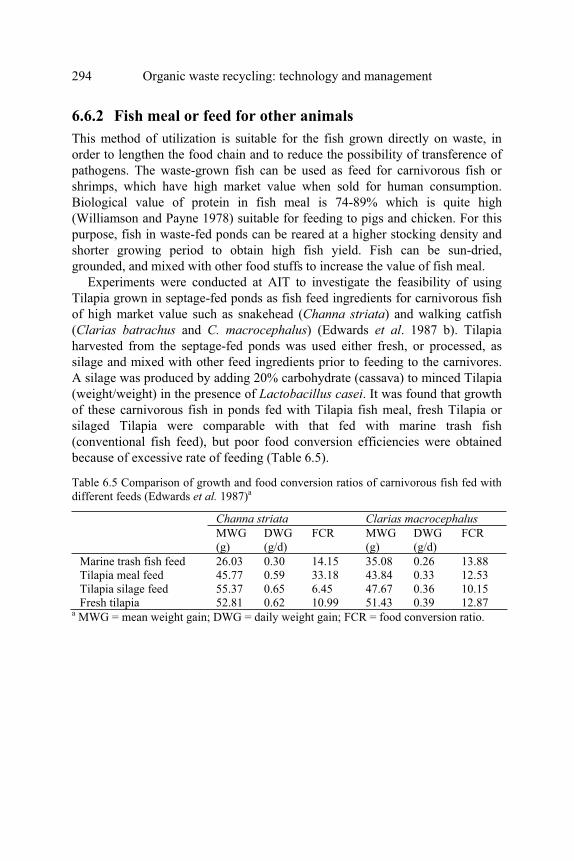
294 Organic waste recycling: technology and management
6.6.2 Fish meal or feed for other animals
This method of utilization is suitable for the fish grown directly on waste, in
order to lengthen the food chain and to reduce the possibility of transference of
pathogens. The waste-grown fish can be used as feed for carnivorous fish or
shrimps, which have high market value when sold for human consumption.
Biological value of protein in fish meal is 74-89% which is quite high
(Williamson and Payne 1978) suitable for feeding to pigs and chicken. For this
purpose, fish in waste-fed ponds can be reared at a higher stocking density and
shorter growing period to obtain high fish yield. Fish can be sun-dried,
grounded, and mixed with other food stuffs to increase the value of fish meal.
Experiments were conducted at AIT to investigate the feasibility of using
Tilapia grown in septage-fed ponds as fish feed ingredients for carnivorous fish
of high market value such as snakehead (Channa striata) and walking catfish
(Clarias batrachus and C. macrocephalus) (Edwards et al. 1987 b). Tilapia
harvested from the septage-fed ponds was used either fresh, or processed, as
silage and mixed with other feed ingredients prior to feeding to the carnivores.
A silage was produced by adding 20% carbohydrate (cassava) to minced Tilapia
(weight/weight) in the presence of Lactobacillus casei. It was found that growth
of these carnivorous fish in ponds fed with Tilapia fish meal, fresh Tilapia or
silaged Tilapia were comparable with that fed with marine trash fish
(conventional fish feed), but poor food conversion efficiencies were obtained
because of excessive rate of feeding (Table 6.5).
Table 6.5 Comparison of growth and food conversion ratios of carnivorous fish fed with different feeds (Edwards et al. 1987)a
Channa striata Clarias macrocephalus
MWG (g)
DWG(g/d)
FCR MWG (g)
DWG(g/d)
FCR
Marine trash fish feed Tilapia meal feed Tilapia silage feed Fresh tilapia
26.0345.7755.3752.81
0.300.590.650.62
14.1533.186.4510.99
35.0843.8447.6751.43
0.260.330.360.39
13.8812.5310.1512.87
a MWG = mean weight gain; DWG = daily weight gain; FCR = food conversion ratio.

Fish, chitin, and chitosan production 295
Data in Table 6.5 were obtained by using a feeding rate of 20% body
weight/day. In studies in which excellent FCRs of 2.5 or less were reported, a
feeding rate of less than 10% body weight/day was used (Edwards et al. 1987).
6.7 PUBLIC HEALTH ASPECTS AND PUBLIC
ACCEPTANCE
Since organic wastes such as sludge and animal manure can contain a large
number of pathogens, fish rearing in a waste-fed pond obviously have a risk of
becoming contaminated by these pathogens. In this regard, fish are considered
to be indicators of the sanitary condition of the fish pond water, in which the
microbial flora present in the fish body directly reflects the microbiological
condition of the water from which they are taken.
According to Feachem et al. (1983), three distinct health problems associated
with fish culture in ponds enriched with human and/or animal wastes are:
• The passive transference of pathogens by fish, which become
contaminated in polluted water.
• The transmission of certain helminths whose life cycles include fish
as an intermediate host, and
• The transmission of other helminths with a life cycle involving other
pond fauna such as snail hosts of schistosomes.
The first problem is a cause of concern worldwide, whereas the second and
third apply only in areas where the helminths concerned are endemic.
The passive transference of pathogens occurs because fish can carry these
pathogens, especially bacteria and viruses on their body surfaces or in their
intestines, which can later contaminate people who handle or eat these fish raw
or partially cooked. Pilot-scale experiments on waste-fed ponds were conducted
at the AIT using septage, composted nightsoil and biogas slurry as organic
wastes feeding into Tilapia ponds (Polprasert et al. 1982 and Edwards et al.
1984). Within the organic loadings upto 150 kg COD/(ha-day), the total
coliform and fecal coliform bacteria and the E.coli bacteriophages (a viral
indicator) were found to be absent in the various fish organ samples such as
blood, bile and meat. These microorganisms were found at high densities in the
fish intestines (up to 109/mL), as normally expected. The levels of total
coliforms and fecal coliforms in the fish pond water were 103-104 no./100 mL,
comparable to those in the control ponds without septage feeding.
Fish have been shown not to be susceptible to the same enteric bacterial
diseases of humans and animals (Allen and Hepher 1976; and Jansen 1970).
Therefore, several human bacterial pathogens, which have been shown to be

296 Organic waste recycling: technology and management
carried in and on fish (Jansen 1970), may be carried passively, infecting only the
gut surface, which can be cleaned by depuration. Studies of human pathogens in
salmonides reared in Arcata wastewater fish ponds, in California, showed
bacteria causing human infections only in the gut (Allen et al. 1976). Results
from kidney, liver and spleen samples indicated that none of the potential
pathogens were present in these fish organs under the fish culture conditions in
Arcata.
Cloete et al. (1983) reported that the skin, gills and intestines of the waste-
grown fish from a pond system treating cattle feedlot effluents contained large
numbers of bacteria, including potential pathogens. However, similar bacterial
numbers, including potential pathogens, were also associated with the skins,
gills and intestines of naturally grown fish. This suggests that the health risk
involved in the consumption of waste-grown fish might not be substantially
different to that of natural fish populations. In both cases, the tissues and blood
appeared to be sterile, which would contribute to a much reduced health risk.
From the above information, it appears that bacteria are normally present in
fish intestines. However, if bacteria are present in very high concentrations in
the fish pond water or the fish body, the natural immunological barrier of fish
could be overcome and the bacteria could invade the fish meat. Buras et al.
(1985) defined a "threshold concentration" as the number of bacteria which,
when inoculated into the fish, causes their appearance in the fish meat. From
their experiments with Tilapia and carp, a list of threshold concentrations is
given in Table 6.6. Depuration experiments were found to be effective when the
fish did not contain high concentrations of bacteria in their meat. With respect to
the microbiological quality of fish pond water, Buras et al. (1987)
experimentally found the 'critical concentration' of standard plate count bacteria
to be 5x10⁴ no./mL, in which bacterial concentrations higher than this critical
concentration were found to cause their appearance in the meat of the fish reared
in the ponds.
Hejkal et al. (1983) investigated the levels of bacteria and viruses in fish
reared in experimental wastewater-fish ponds in Arkansas, U.S.A. They found
that even when levels of bacteria exceeded 105/100g in the fish guts, very little
penetrated into the fish muscle tissue; the maximum of 25 fecal streptococci/100
g was found in the fish meat. They finally suggested that while the fish do not
accumulate bacteria in the muscle tissue, contamination of the muscle tissue
during processing is difficult to avoid. Buras et al. (1985) proposed that to
prevent serious public health problems, the threshold values in Table 6.6 should
be considered satisfactory criteria for the design and management of fish ponds
in which wastewater is used. In addition, since the experiments performed with
Polio 1 LSc viruses suggested a very low threshold concentration, and since

Fish, chitin, and chitosan production 297
viruses have a low infective dose, their presence in the fish pond water or
wastewater to be fed to the fish pond should be of a major concern.
The second public health problem is related to the helminths requiring fish as
intermediate hosts. The major and common types of these helminths associated
with waste-fed fish ponds include Clonorchis and Opisthorchis (Feachem et al.
1983). The excreted eggs of these helminths, once discharged into a pond, will
release miracidium (a larvae), which after ingested by specific species of
freshwater snails will develop and multiply into free-swimming cercarial larvae.
Within 1-2 days these cercaria have to find a fish as second intermediate host, in
which they penetrate under the fish scales and forming cysts in the connective
tissues. When the fish are eaten raw or partially cooked, the cysts enter the
human body and developing into worms in the digestive tract. Female worms
will lay eggs, which will come out with the feces. If this feces is discharged into
a pond, this transmission cycle of the helminths could start again.
The third public health problem concerns with schistosomiasis in which
specific species of freshwater snails serve as intermediate hosts for certain
Schistosome helminths. The schistosome eggs that are discharged into a pond
will release miracidium. After ingested by the snails, these miracidium will
develop and multiply into infective cercarial larvae that can penetrate directly
into human skin. Once entered human body, these cercaria will develop into
mature worms and the female worms will lay eggs that will come out with the
feces again, and the transmission cycle is repeated.
Table 6.6 Threshold concentrations of microorganisms inoculated to fish (adapted from Buras et al. 1985)
Threshold concentration, no/fish Micro organisms Tilapia aurea Cyprinus carpio
Bacteria E. coli 2.5x10⁶ 1.5x10⁶
Clostridium freundii 9.3x10³ - Streptococcus faecalis 1.9x10⁴ 4.0x10⁴
Streptococcus Montevideo 1.8x10⁴ 3.7x10⁴
Bacteriophages T2 Virus 4.0x10³ 4.6x10³
T4 Virus 2.0x10⁴ -
It appears that the cooking and eating habits of the people will have great
impact upon the people who handle and eat the waste-grown fish. Fish that are
well cooked will have all the pathogens that are on or in the fish body killed.
However, disease transmission during fish harvesting, cleansing, and
preparation prior to cooking can occur, depending upon the types of the diseases
present. In areas where there are endemics or outbreaks of diseases related to

298 Organic waste recycling: technology and management
fish ponds, organic wastes to be applied to fish ponds have to be properly
treated to ensure destruction of these pathogens, or feeding of organic wastes to
fish ponds should be discontinued temporarily. Fish to be used as animal feed
will normally have to be processed further e.g. through drying, silaging and/or
pelletization which will result in die-off of most pathogens.
Another major problem relating to the consumption of fish raised on wastes
is the public acceptability of the fish. As far as taste and texture is concerned,
personel observations by various workers indicate that fish grown in well-
treated domestic wastes are equal to or even superior in taste or odor to non-
wastewater cultivated fish (Allen and Hepher 1976). Fish grown in manure-fed
ponds have a different taste and texture since they are much leaner, with only
6% fat, which is excellent compared to fish raised on high protein feed pellets
with 15% fat, and fish rose on grain with 20% fat (Wohlfarth and Schroeder
1979).
Probably the most critical prerequisite before we can obtain public
acceptance of waste-grown fish is the public health concerns. All legitimate
public health concerns must be adequately assessed and resolved and adequate
public health safeguards provided. Perhaps a way to overcome this public health
problem is to treat the waste prior to use in fish culture to meet the WHO
standard for aquacultural reuse (Table 2.28). Lime treatment of sludge can
inactivate a large number of bacteria and viruses, but not helminthic ova. Waste
stabilization ponds in series or sedimentation basins with a detention time of at
least ten days can settle out most of the helminthic ova, but care has to be taken
with the second and third types of helminthic problems, described earlier. An
increased destruction of pathogens would also take place if the waste were
treated by a biogas or composting system before adding to the fish pond since
both processes, especially the latter, lead to an increased temperature which kills
pathogens. An additional step could involve depuration, the maintenance of the
fish in clean water for a week or two, which may eliminate any disease
organisms that survived the earlier treatments. The final step would be to have
good hygiene in all stages of fish handling and processing, and to ensure that the
fish intestines are removed and the meat thoroughly washed and cooked before
consumption. Another strategy could involve feeding the waste-grown fish to
other animals that can be consumed by humans, so that the fish raised on waste
are not consumed directly by humans. Both strategies would reduce the
possibility of disease transfer.
Public need will probably determine the degree of public acceptance of
waste-grown fish in a particular area. Table 6.1 shows that the practice of fish
production in waste-fed ponds, although at a small extent, has been undertaken
in both developed and developing countries. The social, economic and political
considerations that influence human behaviour are very complicated. However,

Fish, chitin, and chitosan production 299
openness, candour, public education and public involvement appear to be the
keys to public acceptance. In spite of the many problems, the future for waste-
fish recycling systems seems promising This is due to the ever increasing
demands for both waste disposal and food production in today's rapidly
expanding populations.
6.8 CHITIN AND CHITOSAN PRODUCTION
The conventional process of chitin production from shrimp shells consists of (a)
alkaline treatment of deproteination by using 4% NaOH at 30oC for 24 hours
and (b) acid treatment or decalcification by using 4% HCl at 30oC for 24 hours.
Chitin is polysaccharides polymers made up of a linear chain of N-
acethylglucosamine groups as shown in Figure 6.16.
Figure 6.16 Chemical structures of chitin and chitosan
Chitosan is obtained by a process called deacethylation, which treats the
chitin compounds in 50% NaOH solution for 24 hours at 30oC or ambient
temperatures. The deacethylation reaction remove acethyl groups (CH3-CO)
from the chitin molecules and makes the product, chitosan (see Figure 6.16),
cationic in characteristic and soluble in most dilute acids. A schematic diagram
of chitin and chitosan production from shrimp shells is shown in Figure 6.17.
To produce chitin from 100 kg of fresh shrimp shells, about 250 L of 4%
NaOH and 250 L of 4% HCl would be required for the deproteination and
decalcification, respectively; while about 80 L of 50% NaOH is needed for the
deacethylation. Chitin content in shrimp shells is in the range of 10-20%.
Chitin Chitosan
CH2OH CH2OH
NHCOCH3 NHCOCH3
OH OH
O O
O
CH2OH CH2OH
NH2 NH2
OH OH
O O
O

300 Organic waste recycling: technology and management
The application of chitin and chitosan in the various fields is shown in Figure
6.18, while those of chitin in the industrial and medical fields are listed in Table 6.7.
Due to its characteristics chitosan, when dissolved in dilute acids, becomes a
cationic polymer that can be effectively used in flocculation, film forming, or
immobilization of various biological reagents including enzymes. It can act as a
moisturizing agent in cosmetics or used in wound healing and controlled release
of drugs in animal or human bodies.
Figure 6.17 Production of Chitin and Chitosan
Decalcification: 4% HCl, 24 hrs,
ambient temp (300C)
Deacethylation: 50% NaOH,
24 hrs, ambient temperature Chitin
Check ash content
Fresh shrimp
Deproteination: 4% NaOH, 24 hrs,
ambient temp (300C)
Check protein content
Chitosan

Fish, chitin, and chitosan production 301
Table 6.7 Applications of chitin in its original or modified form
It appears that the production of chitin and chitosan from shrimp or
crustacean shells will yield several benefits to human and the environment.
Further research in this aspect is needed to develop more cost-effective
production methods, which should enhance the properties of chitin and chitosan
and broaden their uses and applications.
Chitin form Properties used Applications References
Micro crystalline chitin
Phosphorylation Aroma in diet foods Austin et al. (1981)
Micro crystalline chitin
Growth of bifido bacteria
Feed preparation using whey with high lactose content.
Austin et al. (1981)
Crossed linked chitin with glutaraldhehyde
Adsorptionnatural flocculants
Removal of cupric ions
Koyama and Taniguchi (1986)
Pure form chitin Solid support Immobilization of enzymes papian, phosphate, trypsin, lactase
Brzeski (1987)
Dissolved chitin Membrane formation
Osmosis, ultrafiltration, reverse osmosis, desalinization.
Brzeski (1987)
Chitin flakes Conditioning agent
Activated sludge, trap pollutants, insecticides, pesticides
Brzeski (1987)
Partially deacethylated chitin (PDC)
Antistatic and soil repellent
Textiles, reduce shrinking
Brzeski (1987)
Chitin flake, sponge and ointment (polyethylene glycol)
Anti fungal agent, activate cell growth
Wound healing on different parts of body
Hirota et al. (1995) Sathirakul et al.
(1995)

302 Organic waste recycling: technology and management
Figure 6.17 Application of chitin and chitosan
Figure 6.18 Application of Chitin and Chitosan
6.9 REFERENCES
Alabaster, J.S. and Lloyd, R. (1980) Water Quality Criteria for Freshwater Fish,
Butterworths, London. Allen, G.H., Bush, A. and Mortan, W. (1976) "Preliminary bacteriological experiences
with wastewater - fertilized marine fish ponds, Humboldt Bay, California", Proceedings of FAO Technical Conference on Aquaculture, Japan.
Allen, G.H. and Hepher, B. (1976) "Recycling of waste through aquaculture and constraints to wider application", Proceedings of FAO Technical Conference on
Aquaculture, Japan. Austin, F., Buckle, K. A. (1991) Enlisting of prawn heads. ASEAN Food Journal. 6: 58-
63Bhattarai, K.K. (1985) Septage Recycling in Waste Stabilization Ponds, Doctoral
dissertation, Asian Institute of Technology, Bangkok. Boyd, C.E. (1979) Water Quality in Warmwaters Fish Ponds, Craftmaster Printers,
Alabama. Brine, C.J. and Austin, P.R. (1981) Chitin variability with species and method of
preparation. Comp. Biochem. Physiology, 69 B, 283
Food
Membrane
technology
Applications of
chitin and
chitosan
Medical
Paper
technology
Textiles
Cosmetics
Waste
water
treatment

Fish, chitin, and chitosan production 303
Brzeski, M. M. (1987) Chitin and chitosan – putting waste to good use. Infofish
International. 5/87: 31-33 Buras, N., Duck, L. and Niv, S. (1985) "Reactions of fish to microorganisms in
wastewater", Applied and Environmental Microbiology, 50, 989-995. Buras, N., Duck, L., Niv, S., Hepher, B. and Sandbank, E. (1987) "Microbiological
aspects of fish grown in treated wastewater", Water Research, 21, 1-10. Campbell, N. A. (1990) Biology, 2nd edition. The Benjamin/Cummings Publishing Co.,
Inc., Redwood City, California. Cloete, T.E., Toanien, D.F. and Pieterse, A.J.H. (1983) "The bacteriological quality of
water and fish of a pond system for the treatment of cattle feed effluent", Agricultural Wastes, 9, 1-15.
Colt, J., Tchobanoglous and Wang, B. (1975) The Requirement and Maintenance of
Environmental Quality in the Intensive Culture of Channel Catfish, Dept. of Civil Eng., University of California, Davis.
Djajadiredja, R. and Jangkaru, Z. (1978) Small Scale Fish/Crop/Livestock/Home Industry
Integration, a Preliminary Study in West Java, Indonesia, Inland Fisheries Research Institute, Bogor, Indonesia.
Edwards, P. (1980) "A review of recycling organic wastes into fish, with emphasis on the tropics", Aquaculture, 21, 261-279.
Edwards, P. (1985) "Aquaculture; a component of low cost sanitation technology", UNDP Project Management Report #3, World Bank, Washington, D.C.
Edwards, P. (1992) Reuse of human wastes in aquaculture—a technical review. Water
and Sanitation Report No. 2, UNDP-World Bank Water and Sanitation Program, The World Bank, Washington, D.C.
Edwards, P., Pacharaprakiti, C., Kaewpaitoon, K., Rajput, V.S., Ruamthaveesub, P., Suthirawut, S., Yomjinda, M. and Chao, C.C. (1984) "Reuse of cesspool slurry and cellulose agricultural residues for fish culture", AIT Research Report No. 166, Asian Institute of Technology, Bangkok.
Edwards, P., Polprasert, C., Rajput, V.S. and Pracharaprakiti, C. (1988) Integrated biogas technology in the tropics- 2. Use of slurry for fish culture. Waste Management and
Research, 6, 51-61.Edwards, P., Polprasert, C. and Wee, K.L. (1987 b) "Resource Recovery and Health
Aspects of Sanitation", AIT Research Report No. 205, Asian Institute of Technology, Bangkok.
Feachem, R.G., Bradley, D.J., Garelick, H., Mara, D.D. (1983) Sanitation and Disease -
Health Aspects of Excreta and Wastewater Management, Wiley, Chichester. Guerrero, R.D. III. (1982) Control of tilapis reproduction. In The Biology and Culture of
Tilapias (eds. R.S.V. Pullin and R. H. Lowe-McConnell), pp. 309 -315, International Center for Living Aquatic Resources Management, Manila
Hanstins, W. H., and Dicke, L. M. (1972) Feed formulation and evaluation. In Fish
Nutrition (ed. J. E. Halver). Academic Press, New York Hejkal, T., Gerba, C.P., Henderson, S. and Freeze, M. (1983) "Bacteriological,
virological and chemical evaluation of a wastewater - aquaculture system", Water
Research, 17, 1749-1755. Henderson, S. (1983) An Evaluation of Filter Feeding Fishes for Removing Excessive
Nutrients and Algae from Wastewater. EPA-600/52-83-019, Ada, Oklahoma. Hickling, C.F. (1971) Fish Culture, Revised Edition, Faber and Faber, London.

304 Organic waste recycling: technology and management
Hirato, Y., Tanioka, S., Tanigawa, T. and Ojima, R. (1995) Clinical applications of chitin and chitosan to human decubitus. In: Advance in Chitin Science, Vol I, Eds. Domard A., Jeuniaux C., Muzzarelli R.A.A., Roberts G.A..F, 407-413
Huet, M. and Timmermans, J.A. (1971) "Breeding and Cultivation of Fish", Fishing News (Book) Ltd., London.
Janssen, W.A. (1970) "Fish as potential vectors of human bacterial diseases of fishes and shellfishes", Special Publication of American Fish Society, 5, 284-290.
Koyama, Y. and Taniguchi, A. (1986) Journal of Applied Polymer Science. 31: 1951 Lagler, K.F., Bardach, J.E. and Miller, R.R. (1962) Ichthyology: The Study of Fishes,
Wiley, New York. Maramba, F.D. (1978) Biogas and Waste Recycling. The Philippines Experience, Maya
Farms Division, Liberty Flour Mills Inc., Manila, Philippines. Moav, R., Wohlfarth, G. and Schroeder, G.L. (1977) "Intensive polyculture of fish in
freshwater ponds, I - substitution of expensive feeds by liquid cow manure", Aquaculture, 10, 25-43.
Nacario, E.N. (1987) Sex reversal of Nile tilapia in cages in ponds. AIT master’s thesis No AE-87-35, Asian Institute of Technology, Bangkok
NAS (1976) Making Aquatic Weeds Useful: Some Perspectives for Developing
Countries, National Academy of Sciences, Washington, D.C. Polprasert, C., Dissanayake, M.G. and Thanh, N.C. (1983) "Bacterial die-off kinetics in
waste stabilization ponds", J. Water Pollut. Control Fed., 55, 285-296. Polprasert, C., Edwards, P., Pracharaprakiti, C., Rajput, V.S. and Suthirawat, S. (1982)
Recycling Rural and Urban Nightsoil in Thailand. AIT Research Report no. 143,
Asian Institute of Technology, Bangkok. Polprasert, C., Udom, S. and Choudry, K.H. (1984) "Septage disposal in waste recycling
ponds", Water Research, 18, 519-528. Sathirakul, K., How, N.C. Stevens, W.F. and Chandrakrachang, S. (1995) In: Advance in
Chitin Science, Vol I. Eds: Domard, A., Jeuniaux, C., Muzzarelli, R.A.A., Roberts, G.A.F. 490- 492
Sawyer, C.N. and McCarty, P.L. and Parkin, G.F (2003) Chemistry for Environmental
Engineering and Science, 4th edition, McGraw-Hill, New York. Schroeder, G.L. (1975) "Some effects of stocking fish in waste treatment ponds", Water
Research, 9, 591-593. Schroeder, G.L. (1977) "Agricultural wastes in fish farming - a commercial application
of the culture of single-celled organisms for protein production", Water Research,11, 419-420.
Sharma, H.P., Polprasert, C. and Bhattarai, K.K. (1987) "Physico-chemical characteristics of fish ponds fed with septage", Resources and Conservation, 13,207-215.
Tang, Y.A. (1970) "Evaluation of balance between fishes and available fish foods in multi-species fish culture ponds in Taiwan, Trans. Am. Fish. Soc., 99, 708-718.
Thorslund, A.E. (1971) Potential Uses of Wastewaters and Heated Effluents, European Inland Fisheries Advisory Commission Occasional Paper No. 5, FAO, Rome.
U.S. Committee on Water Quality Criteria (1972) Water Quality Criteria, Superintendent of Documents, Washington, D.C.
Whipple, G.C. and Whipple, M.C. (1911) "Solubility of oxygen in sea water", J. Am
Chem. Soc., 33, 362.

Fish, chitin, and chitosan production 305
Williamson, G. and Payne, W.J.A. (1978) Animal Husbandry in the Tropics, 3rd edition, Longman, London.
Wohlfarth, G.W. and Schroeder, G.L. (1979) "Use of manure in fish farming - a review", Agricultural Waste, 1, 279-299.
Wolf, K. (1957) "Blue-sac disease investigations, microbiology and laboratory induction", Progressive Fish Culturist, 19, 14-18.
6.10 EXERCISES
6.1 What are the health problems associated with fish farming in wastewater-
enriched pond? What would you suggest to solve these problems?
6.2 Calculate the ammonia concentration in a water sample at pH = 8 and NH3-
N + NH4-N = 10 mg/L. The following equilibria exist:
OH+NHOH+NH-+
423 →
C)25(at10x1.76=]NH[
]OH][NH[ 5-
3
-4 °=K b
C)25(at10=]OH][H[-14-+ °=K w
The U.S. Committee on Water Quality Criteria (1972) has recommended
that, to safeguard fish, no more than 0.02 mg/L NH3 be permitted in
receiving waters. Does the ammonia concentration in the above calculation
meet the Criteria? If not, suggest methods to make the water safe for the fish.
6.3 Compare the advantages and disadvantages of applying commercial fish
meal or cattle manure into fish ponds for the purpose of raising Tilapia for
use as animal feed.
6.4 You are to visit a commercial fish farm and obtain the following
information:
• fish species and stocking density
• type and amount of fish meal being fed to the fish ponds
• productivity of the fish ponds in unit of kg fish/(ha-yr)
From the above data, estimate the organic loading rate (in kg BOD or
COD/ha-day) and the percent fish mortality. Also suggest some
improvements, if any, to be made to increase the fish productivity in this
farm.

306 Organic waste recycling: technology and management
6.5
a) A small community produces septic tank sludge (septage) with the
following characteristics:
Quantity = 10 m3/day
COD = 20000 mg/L
Total Kjeldahl N = 1800 mg/L
This septage is to be used to feed to fish ponds to produce Tilapia with a mean
weight of about 30 g for use as animal feed. Three fish harvests are planned
annually, with 100 days for fish culture and 3 weeks for pond maintenance.
Suppose Tilapia can tolerate DO concentration at dawn of no lower than 1.5
mg/L. What should be the highest COD loading to be applied to the septage-fed
fish pond(s)? Also determine the total land area required, stocking density, the
number of fingerlings needed and the expected fish output for each cycle (120
days).
b) Suppose that for efficient fish harvesting, the pond water is to be drained
out, what should be done with this pond water and the pond sediment that
needs to be removed?
6.6 What are the fish species that the people in your country like to eat? Would
the people mind if the fish sold in the market are reared in waste-fed ponds?
Suggest methods to make the waste-grown fish more acceptable to the
people.
6.7 An agro-industrial factory produces wastewater with the following
characteristics
Flow rate = 10 m3/day
COD = 5,000 g/m3
NH3 + NH4+ = 10 g/m3
The factory plans to apply this wastewater to a fish pond to raise tilapia for use
as animal feed (mean individual fish weight = 30 g)
a) If, to maintain satisfactory D.O. levels at dawn, the organic loading rate
to be operated in the tilapia pond is 100 kg COD/(ha-day), determine
the required dimension (length × width × depth) of the tilapia pond,
appropriate fish stocking density and fish productivity in kg/year (if
this tilapia is to be harvested 2 times per year). Data on fish
productivity is given in Figure 6.11.

Fish, chitin, and chitosan production 307
b) To avoid fish toxicity, the NH3 concentration in the fish pond water
should be less than 1 mg/L. If due to the algal-bacteria symbiotic
reactions, the pH of the fish pond water becomes 9 at 3 pm., determine
whether there will be NH3 toxicity to fish or not. If so, suggest method
to alleviate this problem. Figure 6.9 shows the effects of pH on NH3 +
NH4+ concentrations.

© 2007 IWA Publishing. Organic Waste Recycling: Technology and Management. Authored by
Chongrak Polprasert. ISBN: 9781843391210. Published by IWA Publishing, London, UK.
7
Aquatic weeds and their utilization
Aquatic weeds are prolific plants growing in water bodies, which can create a
number of problems due to their extensive growth and with high productivity.
Since they exhibit spontaneous growth, they usually infest polluted waterways
or water bodies, reducing the potential uses of these watercourses. The problems
of aquatic weeds have been magnified in recent decades due to human's
intensive uses of the natural water bodies and pollution discharges into these
water bodies. Eradication of the aquatic weeds has proved impossible and even
reasonable control is difficult. However, turning these aquatic weeds into
productive uses such as in wastewater treatment, in making compost fertilizer,
and as human food or animal feed, etc., some of the problems created by aquatic
weeds may be minimized and yielding some incentives for the people to harvest
the aquatic weeds more regularly.

Aquatic weeds and their utilization 309
7.1 OBJECTIVES, BENEFITS, AND LIMITATIONS
7.1.1 Objectives
The main purposes of using aquatic weeds in waste recovery and recycling are
for waste stabilization and nutrient removal, and conversion of the harvested
weeds into productive uses. Aquatic weeds provide a medium for bacteria to be
attached and grow at their roots and stems, to stabilize the waste. The presence
of weeds in the aquatic medium and subsequent harvesting enable the nutrient
removal from the wastewater. Even though stabilization of waste is a slow
process in aquatic systems, the removal efficiency is high and can produce an
effluent superior or comparable to that of any other treatment systems. The
productive uses of aquatic weeds are given below.
7.1.2 Benefits
Aquatic weeds can be used, directly or after processing, as soil additives, mulch,
fertilizer, green manure, pulp and fibre for paper making, animal feed, and
human food, organic malts for biogas production and for composting. If
properly designed, the operation and maintenance of the aquatic weed system
does not require highly skilled manpower.
7.1.3 Limitations
Land requirement
Waste treatment with aquatic weeds requires large area of land at reasonably
low cost. This will become one of the major limitations in urban areas, but in
rural areas this will not be a problem.
Pathogen destruction
The reliability of an aquatic system with regard to pathogen destruction is low
because the inactivation mechanism is natural die-off during long detention
time, and some of the aquatic plants will provide suitable condition for the
survival of pathogenic microorganisms.
End uses
Most of the end use of aquatic weeds are for agricultural and livestock rearing
purposes. So the aquatic weed systems are suitable for rural areas.

310 Organic waste recycling: technology and management
However, interests in the beneficial uses of aquatic weeds are increasing
worldwide and the methods of aquatic weed utilization, as listed in sections 7.5
and 7.6, are being applied in several countries with positive results.
7.2 MAJOR TYPES AND FUNCTIONS
Aquatic weeds may be divided into several life forms, a somewhat arbitrary
separation since there are plants, which may change their life form depending on
their stage of growth or on the depth of water. The major types are: submerged,
floating and emergent weeds, as shown in Figures 7.1, 7.2 and 7.3, respectively.
The most common plants and their scientific names are given in Table 7.1.
7.2.1 Submerged type
Weeds that grow below the water surface are called submerged. Often they form
a dense wall of vegetation from the bottom of the water surface. Submerged
species can only grow where there is sufficient light and may be adversely
affected by the onset of factors such as turbidity and excessive populations of
planktonic algae, which decreases the penetration of light into the water. Thus
these species are not effective for effluent polishing.
7.2.2 Floating type
According to Reimer (1984), there are two subtypes of floating weeds, i.e.
floating unattached and floating attached. The roots of floating unattached plants
hang in the water and are not attached to the soil. The leaves and stems are
above the water thus receiving sunlight directly. The submerged roots and stems
serve as habitat for the bacteria responsible for waste stabilization, the aquatic
weeds that cause some of the most widespread and serious problems fall into
this type. As these plants are unattached, populations of the plants are seldom
permanent and, if space permits, are liable to be moved by wind and water
currents or, if confined in one place, initiate the accumulation of organic matter
which decreases the depth of water until it is sufficiently shallow for the
establishment of emergent swamp vegetation. Thus they are essentially primary
colonizers in aquatic ecosystems.
Floating attached plants have their leaves floating on the water surface, but
their roots are anchored in the sediment. The leaves are connected to the bottom
of petioles (e.g. water lilies, Figure 7.2 f and g), or by a combination of petioles
and stems.

Aquatic weeds and their utilization 311
7.2.3 Emergent Type
These are rooted weeds that extend above the water surface. Such attached
aquatic plants usually grow well in a stable hydrological regime and are less
likely to be a problem in situations where rapid or extensive fluctuations in
water level occur. Specialized communities of emergent species may develop on
a substratum of floating aquatic plants, especially where stands of the emergent
species are particularly stable.
There is frequently a pronounced zonation of different life forms to different
depths of water (Figure 7.4). The emergent type normally grows in shallow
water and the submerged type in deeper water in which light can still penetrate
to the bottom. The floating types are independent of soil and water depth.
Like any other plants, aquatic weeds require nutrients and light. The major
factors governing their growth are:
• Ambient temperature
• Light
• Nutrients and substrate in the water
• pH of water
• Dissolved gases present in the water
• Salinity of the water
• Toxic chemicals present in the water
• Substrate and turbulence
• Water current in rivers and lakes
• River floods
• Morphology of bodies of water
While the above-mentioned factors modify the composition of the plant
communities, they are in turn modified by the latter. This results in constant
interaction between the plants and the environment. Furthermore, the
environmental factors also interact with one another, resulting in a complex
relationship between the environmental factors and the aquatic weeds.

312 Organic waste recycling: technology and management
Table 7.1 Types and common names of aquatic weeds
Types Common name Botanical name
Submerged Hydrilla Water milfoil Blyxa
Hydrilla verticillata
Myriophyllum spicatum
Blyxa aubertii
Floating Water hyacinth Duckweeds Water lettuce Salvinia
Eichhornia crassipes
Wolfia arrhiga
Pistia stratiotes
Salvinia spp.
Emergent Cattails BulrushReed
Typha spp.
Scirpus spp.
Phragmites communis
Figure 7.1 Submerged aquatic weeds, hydrilla (Hydrilla verticillata)

Aquatic weeds and their utilization 313
7.3 WEED COMPOSITION
7.3.1 Water content
Aquatic weeds have high water content, in general ranging from 85-95%. It
varies from 90-95% for floating species, 84-95% for submerged species, and 76-
90% for emergent species. The differences amongst the various life forms can
be correlated to some extent with the amount of fiber present in the plant. Water
supports the weight of submerged aquatic plants, so they do not develop fibrous
stems. Floating plants and emergent plants require more skeletal strength in
their aerial parts and so have more fiber than most of the submerged plants.
The low level of dry matter has been the major deterrence to the commercial
use of harvested weeds. In order to obtain 1 ton of dry matter, 10 tons of aquatic
weeds must be harvested and processed. For water hyacinth, which usually
contains only 5% dry matter, 20 tons must be harvested and processed just to
obtain 1 ton of dry matter. By comparison, terrestrial forages contain 10-30%
solids, and therefore, are cheaper to harvest.
Figure 7.2 Floating aquatic weeds, water hyacinth (Eichhornia crassipies)

314 Organic waste recycling: technology and management
Figure 7.3 Emergent aquatic weeds, cattail
Figure 7.4 A diagrammatic representation of a lake showing zonation of aquatic weeds,
the photic zone, and thermal stratification (adapted from Mitchell 1974; ©UNESCO
1974; reproduced by permission of UNESCO)
Zonation
Emergentweeds
Zonation of aquatic
macrophytes
Floatingleaves and free floating
weeds
Submerged
weeds
Temperature
depth curves
Limit of photic zone
Epilimnion
Mesolimnion
Hypolimnion
Th
erm
oc
lin
e
Win
ter
Su
mm
er

Aquatic weeds and their utilization 315
7.3.2 Protein content
For most species of aquatic weeds about 80% of the total-N is in the form of
protein. Aquatic weeds contain 8-30% of crude protein (on a dry-matter basis) -
a range similar to that found in terrestrial crops. The considerable variations in
crude protein content are due to both seasonality and environment. The crude
protein content of Typha latifolia decreased from 10.5% in April to 3.2% in July
(Boyd 1970) and that of Justicia americana from 22.8% in May to 12.5% in
September (Boyd 1974). In addition, the crude protein content of Typha latifolia
from different sites varied from 4.0-11.9% (Boyd 1970), and that of water
hyacinth grown on a stabilization pond was 14.8% compared to 11.3% in
samples from a lake (Bagnall et al. 1974). This indicates that the crude protein
content increases as the nutrient content of the water in which the plant is grown
increases. According to Wolverton and McDonald (1976b), the crude protein of
water hyacinth leaves grown in wastewater lagoons average 32.9% dry weight,
which is comparable to the protein content of soyabean and cotton seed meal.
This value is more than two times the maximum crude protein content of water
hyacinth reported by Bagnall et al. (1974). Duckweeds have a crude protein
content over 30% and have a better spectrum of amino acids as regards to lysine
and methionine than the other plants (Oron et al. 1986).
Although the protein content of various aquatic weeds differs greatly, the
amino acid composition of the protein is relatively constant, nutritionally
balanced, and similar to many forage crops. But the levels of methionine and
lysine - generally considered as the limiting amino acids in plant proteins - are
lower than in terrestrial crops (Boyd 1970). Additional information on protein
content of aquatic weeds is given in section 7.6.2.
7.3.3 Mineral content
The ash content of aquatic weeds varies with location and season. Sand, silt, and
encrusted insoluble carbonates from the water account for much of the mineral
content. Although silt can be washed off the plants, in practice it represents part
of the chemical composition of the harvest. The amount of minerals varies from
15-25% of the harvest (dry weight), depending on the waterway's chemical
content and turbidity (Table 7.2).
The amounts of phosphorus, magnesium, sodium, sulfur, manganese, copper
and zinc in aquatic weeds growing in nature are similar to those in terrestrial
plants. However, aquatic plants are often richer in iron, calcium and potassium
than land forages, and some species are known to concentrate such minerals.
Elements can be exceptionally high in aquatic plants grown in sewage or

316 Organic waste recycling: technology and management
industrial and agricultural wastewaters. In fact, the low palatability of aquatic
weeds to livestock has been attributed to a high mineral content (see section
7.6).
7.3.4 Miscellaneous
Some aquatic plants have carotene and xanthophyll pigment concentrations that
equal or exceed those of terrestrial forages such as alfalfa. These pigments are
important ingredients in poultry rations.
Pesticides have been found in aquatic plant samples collected when the
waterway has been recently treated with herbicides or insecticides. Also, traces
of cyanide, oxalate, and nitrate have been found. However, no evidence of
toxicity to mice, sheep or cattle has yet been found in water hyacinth or hydrilla
samples.
7.4 PRODUCTIVITY AND PROBLEMS CAUSED BY
AQUATIC WEEDS
Aquatic weeds, especially rooted, emergent species and floating species are
some of the most productive freshwater ecosystems. Typical values for the net
production of different types of aquatic vegetation from fertile sites (recorded in
terms of unit weight per unit area of the earth's surface per unit time) are as
follows (Westlake 1963): lake phytoplankton 1-8, submerged weeds 3-18, and
emergent weeds 27-77 and floating weeds 35-90 tons of dry organic matter/(ha-
yr). At that time, the highest net productivity recorded was for sugar cane, 85
tons dry matter / (ha-yr).
The productivity of submerged weeds is usually low because the water
reflects and absorbs some of the incident light, coloured substances in the water
absorb light, and the diffusion of carbon dioxide in solution is slow compared to
its diffusion in air. The presence of phytoplankton in the water column also
reduces the light available for submerged plants, and, in eutrophic waters may
be dense enough to cause the elimination of aquatic weeds. On the other hand,
emergent weeds are particularly productive since they make the best use of all
three possible states, with their roots in sediments beneath water and with the
photosynthetic parts of the plant in the air. The surrounding mud around the
roots may be a good source of soluble nutrients, which can diffuse to the roots
via the pore water in the sediments. Light and carbon dioxide are more readily
available in the air than in water. Thus, they make the best of both aquatic and
terrestrial environments.

Aquatic weeds and their utilization 317
Table 7.2 Chemical composition of water hyacinth taken from several natural Florida, USA, locations (composition reported as percentage dry weight)
Origin Ash C N C/N ratio
P K Ca Mg Na
Lake Istokpoga (Sebring)
24.4 18.0 1.08 16.7 0.14 1.00 0.73 0.38 0.15
Lake Eden Canal (SR 532)
19.4 28.8 0.86 33.5 0.09 1.95 0.46 0.31 0.23
Lake Thonotosassa 23.0 23.0 1.17 19.7 0.33 3.35 1.49 0.29 0.21 Waverly Creek (SR 60)
25.0 33.1 2.26 14.6 0.56 3.10 1.58 0.50 0.37
Arbuckle Creek 23.4 34.9 1.90 18.4 0.23 3.35 1.06 0.49 0.28 Lake Tohopekaliga (Kissimmee)
21.7 34.0 1.69 20.1 0.60 4.70 1.56 0.71 0.53
Lake Monroe (Sanford)
20.4 32.5 2.86 11.4 0.59 5.55 1.73 0.54 0.83
Duda Canal No 1 (Bella Glade)
20.3 39.1 1.30 30.1 0.13 3.80 1.99 0.60 0.48
St. Johns River (Astor)
20.1 36.4 2.33 15.6 0.51 6.50 1.43 0.51 0.63
W. R. Grace landfill (Bartow)
19.0 36.4 1.86 19.6 0.59 2.72 1.99 0.56 1.54
Ponce de Leon Springs
18.5 37.5 1.74 21.5 0.33 5.40 2.34 0.50 0.47
Waverly Creek (SR 540)
18.5 38.1 1.76 21.6 0.32 4.85 1.45 0.55 0.67
Duda Canal No 2 (Bella Glade)
17.5 37.8 1.66 22.8 0.15 4.70 2.28 0.69 0.57
Lake Alive (North of Florida)
17.3 38.6 1.17 33 0.40 3.66 2.41 0.69 0.40
Lake Apopka (Monteverde I)
15.8 38.8 1.22 31.8 0.14 4.26 2.07 0.54 0.41
St. Johns River (Palatka)
15.8 38.0 1.82 20.9 0.16 3.44 1.83 0.73 0.86
Lake George 15.4 40.2 1.48 27.1 0.21 3.21 1.91 1.86 1.24 Lake Apopka (Monteverde I)
14.9 39.8 1.36 29.3 0.09 4.08 1.96 0.60 0.21
Lake East Tohopekaliga (St. Cloud)
14.7 37.2 1.08 34.5 0.23 2.90 1.19 0.51 0.53
Mean 19.2 34.9 1.61 23.3 0.31 3.81 1.66 0.56 0.56 Standard Deviation 3.2 5.9 0.50 7.0 0.18 1.30 0.53 0.14 0.36

318 Organic waste recycling: technology and management
Floating weeds are also equally or more productive than emergent plants as
they can be moved with winds and currents and their productivity far exceed the
biomass yields of many subtropical terrestrial, salt water, and freshwater plants
(Wolverton and McDonald 1978).
The growth rate for aquatic weeds can also be expressed as the specific
growth rate independent of biomass or the units in which biomass is measured
(dry weight). The values can be measured as fractional increase per day or
percent increase per day. In 1969, Bock calculated the daily incremental factor
using the following formula (Mitchell 1974):
t
t xNN .0= (7.1)
Where:
No = initial number of plants
Nt = final number of plants
t = time interval in days
x = daily incremental factor
However, the specific growth rates are generally high at low plant density
and decrease as the plant density increases.
Growth of aquatic weeds can also be reported in terms of doubling time, the
time taken for the material present to double itself (or Nt /No = 2). In 1974,
Gaudet while working with Salvinia minima and S. molesta under standardized
culture conditions calculated the doubling time using the following formula
(Mitchell 1974):
Doubling time = ln 2 (7.2)
(ln Nt – ln N0)/t
The notations are the same as used in Equation 7.1.
Under favorable conditions, the area doubling time for water hyacinth ranges
between 11-18 days, depending on the weather. Mitchell (1974) obtained
doubling times for S. molesta of 4.6-8.9 days in culture solutions in the
laboratory, compared to 8.6 days on Lake Kariba, Africa. Bagnall et al. (1974)
and Cornwell et al. (1977) both reported doubling times of 6.2 days for water
hyacinth grown on a stabilization pond receiving secondarily treated effluent.
The variation of doubling times reported in the literature is due to the effects of
weather, nutrients, growing season and plant density.
Knowledge of area doubling time is useful to determine the frequency of
plant harvesting and the amount of harvested plant biomass to be further

Aquatic weeds and their utilization 319
processed. Because plants grow and die relatively quickly under tropical
conditions, harvesting of these plants from the water body needs to be done
properly to prevent plant decay and impairment of the water quality. Application
of the area doubling time in plant harvesting is given in Examples 7.3 and 7.4
Due to their prolific growth, aquatic weeds can cause many problems, the
major ones being listed below:
• Water loss by evapo-transpiration,
• Clogging of irrigation pumps and hydroelectric schemes,
• Obstruction of water flow (Figure 7.5),
• Reduction of fish yields and prevention of fishing activities,
• Interference with navigation,
• Public health problems, as aquatic weeds can become the habitat for
several vectors,
• Retardation of growth of cultivated aquatic macrophyte crops, e.g.,
rice and water chestnut,
• Conversion of shallow inland waters to swamps.
The problem of aquatic weed infestation is global but is particularly severe in
the tropics and subtropics where elevated temperatures favor year round or long
growing seasons, respectively. The annual world cost of attempts to control
aquatic weeds is nearly US$2,000 million (Pirie 1978).
Currently the most serious problems associated with aquatic weeds are
caused by water hyacinth, which is now more or less ubiquitous in warm waters.
In the tropical and subtropical southeastern USA, there is a serious water
hyacinth problem. In Florida alone more than 40,000 ha are covered by the
plant, despite a continuous control program costing US$10-15 million annually.
Subsistence-level farmers in the wet lowlands of Bangladesh annually face
disaster when rafts of water hyacinth weighing up to 270 tons/ha are carried
over their rice paddies by floodwaters. The plants remain on the germinating
rice and kill it as the floods recede. In India, large irrigation projects have been
rendered useless by plants that block canals, reducing water flow significantly.
Water hyacinth came originally from South America where it causes few
problems since it is kept in check by periodic flooding and changes in water
level. The plants are flushed out as a water body enlarges due to seasonal
flooding and as the floods subside the aquatic plants are left stranded on dry
land above the receding water level (Mitchell 1976). The absence of natural
enemies in their new environments has often been implicated as a casual factor
in the rampant growth of water hyacinth and other aquatic weeds. Therefore, the
absence of periodic flooding in artificial lakes and irrigation schemes may be the
major contributing factor to the development of aquatic weed problem. This
problem is further exacerbated by eutrophication from human, animal and agro-

320 Organic waste recycling: technology and management
industrial wastes, and agricultural runoff (Figure 7.5). As new lakes and
irrigation schemes are developed, the newly submerged soil and vegetation
provides a rich source of nutrients favouring aquatic plant growth (Little 1968).
Another problematical aquatic weed is the fern Salvinia molesta. On Lake
Kariba, Africa, the largest man-made lake in the world, there was a steady
increase in the area of the lake colonized by the fern following the closure of the
dam in 1959, when 1,000 km2 or 2.5% of the lake's surface was covered. Since
1964 (two years after the dam was opened in 1962) the area covered has
fluctuated between 600 and 850 km2 and is limited mainly by wave action that
has increased as the lake has reached full size (Mitchell 1974). The same species
is a serious threat to rice cultivation throughout western Sri Lanka and covers
about 12,000 ha of swamp and paddy fields (Dissanayake 1976).
Figure 7.5 A drainage canal in Colombo, Sri Lanka, filled with water hyacinth,
Eichhornia crassipes

Aquatic weeds and their utilization 321
7.5 HARVESTING, PROCESSING AND USES
Harvesting aquatic weeds from the waterways and utilizing them to defray the
cost of removal is one of the most successful approaches to aquatic weed
management. It results in weed-free waterways while providing an extensive
vegetation resource. This is especially advantageous in developing countries
where forage and fertilizer are in short supply.
The removal and recycling of nutrients and other components is done by
harvesting, processing and utilizing the aquatic plants in which the nutrients are
collected. The whole process is shown by a simple schematic diagram given
below:
AQUATIC WEEDS HARVESTING PROCESSING PRODUCT USES
A complete network of the possible processes used to convert aquatic weeds
to a variety of products is shown in Figure 7.6. Harvesting and chopping are
precursors to all of the other processes and all of the products. The chopped
plants can be applied directly to land, composted to stabilize and reduce mass,
digested to produce methane, pulped to produce paper, or pressed to reduce
moisture content and produce a highly reactive protein-mineral-sugar juice. The
juice can be separated to recover a high quality food-feed protein-mineral
concentrate or digested to produce methane. The pressed fibers may be ensiled
with appropriate additives or dried to produce a granular feed component.
This section deals with all uses of harvested weeds, except the use of weeds
as food and feed, which is dealt separately in section 7.6 (Food Potential of
Aquatic Weeds).
7.5.1 Harvesting
Harvesting can be accomplished manually or mechanically, depending on the
amount of weeds to be harvested and the level of available local technology.
Large floating plants such as Eichhornia crassipes and Pistia stratiotes can
be lifted from the water by hand or with a hayfork. Smaller floating plants such
as Lemna or Azolla can best be removed with small mesh sieves or dip nets.
Submerged plants can be harvested by pulling rakes through the under-water
plants. Emergent and floating-leaved plants can be cut at the desired height with
knives, or in areas with loose bottom soil, pulled by hand. One man can harvest
1,500 kg or more of fresh weight of plants per day from moderately dense
stands of most species.

322 Organic waste recycling: technology and management
Figure 7.6 Different end products of harvested aquatic weeds (from Bagnell 1979;
reproduced from the permission of the American Society of Agricultural (Engineers)
Large-scale harvesting is done with the help of various mechanical devices
mounted on boats or barges. Harvesting can be carried out from a site at the
water's edge or with a self-propelled, floating harvester. Shoreside harvesting
requires that the plants float to the harvester. Rooted species must be uprooted
or mowed and then moved to the harvester by boat or by wind and current.
Plants can then be lifted from the water by hand, crane, mechanical conveyor, or
pump. On the other hand, mobile harvesters sever, lift, and carry plants to the
shore. Consisting of a large barge on which a belt conveyor and a suitable
cutting mechanism are mounted, these harvesters are mostly intended for
harvesting submerged plants. Nowadays, some harvesters have also been
designed to harvest floating plants or the mowed tops of submerged plants.
Harvesting frequency has to be chosen depending on the initial area of
coverage of the plants (or stocking density) and the area doubling time. For
example, if a plant is stocked to cover half of the pond area harvesting may be
done to remove half of the plants at every interval of doubling time. Plants such
as duckweeds which are easily piled up due to wind or could not compete with
Pulp
Wilt
Pellet
Mix
DryFiberPressChop Harvest
DrySeparateDigest
Paper
EnsileCompost
Dry feed SilageSoil amendment
Aquatic
weeds
Chemicals
Grain
Juice
Feed-foodMethane
Mix

Aquatic weeds and their utilization 323
algae for space and food have to be stocked at higher initial stocking density to
prevent algal blooms.
After the weeds have been harvested, their handling is another problem.
Because of their enormous water content (which results in very low bulk
density), the weeds are exceedingly difficult to handle and their transportation is
very expensive. Thus, choppers are often incorporated into harvesting
machinery designed for aquatic weeds. Chopping makes the plants much easier
to handle and reduces their bulk to less than a fourth of the original volume,
greatly simplifying transportation, processing, and storage.
The energy cost of combined harvesting / chopping amounts to about 0.34
kWh/ton and the economic cost to about US$0.14/ton of fresh plants (Bagnall
1979).
7.5.2 Dewatering
Because harvested or chopped aquatic weeds contain 80-95% water, they should
be dewatered prior to being used as animal feed or for other purposes. Although
sun drying can be employed, this must occur so rapidly that mold and decay do
not ruin it, and this practice is not possible all year round.
About half the moisture is on the surface and some is loosely contained in the
vascular system. This water can be removed relatively easily by lightly pressing
the plant. The squeezed out water contains only about 2% of the plant solids and
often can be returned directly to the waterway without causing pollution. Even
with half the water removed, aquatic vegetation is still much wetter than
terrestrial grass. In order to reduce the moisture further, heavier pressing is
required. This process can remove about 70% of the water content and yielding
a product that is comparable to terrestrial forage grasses in moisture content.
Depending on plant species, process design and operating conditions, the
water removed can carry with it 10-30 percent of the plant's solid matter, 15-
35% of the protein, and up to 50% of the ash (for the most part, silt and mineral
encrustations caught on the plants). Roller, belt, cone and screw presses are the
different types commercially available to dewater weeds, but they are usually in
heavy, durable designs that are unnecessarily complex and cumbersome for
pressing aquatic vegetation. Lightweight experimental screw presses (suitable
for developing countries) have been designed. For example, a small screw press
of a simple design has been constructed at the University of Florida, USA (NAS
1976). With its 23 cm bore, this press weighs between 200-250 kg. Complete
with a power plant, it can be carried by a truck, trailer or barge to remote
locations, and can press 4 tons of chopped water hyacinth per hour. Such presses
are compatible with a program of manual harvest and with the small-scale needs
for animal feed in rural areas in developing countries (in addition, these presses

324 Organic waste recycling: technology and management
can be manufactured locally). Estimates of aquatic weed pressing costs range
from US$5.0 to US$10.0/ton of dry matter (depending on machine cost,
machine use, production rate, amortization time and labour costs) (NAS 1976;
Bagnall 1979; Bagnall et al. 1974).
In some arid climates solar drying may be feasible, either by exposing a thin
layer of the plants to the sun or by more sophisticated solar collector-heat
transfer systems. In the U.S., a solar drying system for aquatic weeds was
constructed at the National Space Technology Laboratories. Depending on the
weather, it is capable of drying 15-17 tons of newly harvested water hyacinth in
36-120 hours (Figure 7.7). Drying of the aquatic weeds with conventional fuel-
heated air is economically impractical because of the high moisture content.
Figure 7.7 Solar energy being harnessed to dry aquatic weeds at the National Space
Technology Laboratories (NSTL) near Bay St. Louis, Mississippi (NAS 1976). Note: this
system is connected to a lagoon full of water hyacinth growing in sewage effluent.
Water hyancinth-filled
sewage treatment lagoon
NSTL vascular aquatic plant drying system
Greenhouse
Solar heat
collectors

Aquatic weeds and their utilization 325
7.5.3 Soil Additives
Mineral fertilizers are expensive for many farmers in developing countries, yet
there is a greater need now than ever to increase food production. As an
alternative, the 1974 World Food Conference and, more recently, the Food and
Agricultural Organization (FAO) of the United Nations have stressed the
urgency of reassessing organic fertilization. This includes the possible ways in
which aquatic weeds can be used as organic fertilizers, namely, as mulch and
organic fertilizer, ash, green manure, compost, or biogas slurry.
Mulch and organic fertilizer
Mulching involves the laying of plant material on the surface of the soil to
reduce evaporation and erosion, to smother weeds and for temperature control.
Both sand and clay soils need conditioning to make them productive. Working
plant material into the soil improves its texture, and also, by acting as manure,
improves the nutrient content. Several species of aquatic weeds that can be used
as manure are Pistia stratiotes, Hydrilla verticillata, Salvinia spp., Eichhornia
crassipes and Azolla (Frank 1976; Gopal and Sharma 1981; Gupta and Lamba
1976; Little 1968).
The high moisture content of aquatic weeds makes them suitable as mulch.
But the time and labour involved in harvesting and distributing even sun-dried
material would preclude such a use, except on a small scale adjacent to the
watercourse in which the aquatic weeds occur.
Ash
Although it has been suggested that the ash of water hyacinth can be used as a
plant fertilizer, some reasons showing that it is not feasible are:
• Burning of the plant to ash results in the loss of nitrogen and organic
matter, which reduces the fertilization potential of the plant.
• Burning of the plant requires previous drying which involves
additional labour and expenditure and is restricted to dry days of the
year, while growth and distribution of the weeds is most profuse in
wet months.
• Ash needs immediate bagging and storing in order to prevent it from
being washed away by rain or carried away by wind.
Thus, the cost of labour and energy required to obtain ash from aquatic
weeds seems to far exceed the value of the ash obtained as a fertilizer (Little
1968).

326 Organic waste recycling: technology and management
Green manure
Green manure, in a strict sense, is plant matter cultivated for its fertilizer value
to other crops. However, certain species of aquatic weeds that grow wild in rice
fields and are ploughed into paddy, e.g. Limnocharis flava and Sesbania
bispinnosa, are sometimes referred to as green manure. Thus, the distinction
between aquatic weeds, which grow wild and are used as manure and fertilizer,
and green manure which is cultivated, is not always maintained. Certain types of
aquatic weeds are cultivated as green manure or biofertilizers to add nitrogen to
the soil, and this practice is useful since it lessens dependence on commercial,
inorganic fertilizer.
The cultivation of the fern Azolla pinnata, with its symbiotic nitrogen fixing
blue-green algae was developed in Vietnam, where it is treated not as a weed
but as a valuable crop (Ngo 1984). Edwards (1980) cited a literature that
reported that the cultivation of the fern has recently spread to southern China
also. In both countries, Azolla is produced to fertilize areas of rice and other
crops. In northern Vietnam, just before or after rice transplanting, Azolla is
scattered in the fields at the rate of 4-5 tons/ha, and in January and February it
grows along with the rice. During this time, when the mean daily air
temperature is 16-17 °C, the paddy is young and available solar radiation and
nutrients allow Azolla to grow normally, with a result that it completely covers
the surface of the water. Towards the end of March, when the temperature rises
to 22-24°C, the paddy has grown up and shades most of the surface, resulting in
the death of Azolla and release of P and K and newly acquired nitrogen to the
paddy. The Azolla produces about 18 tons of fresh material/ha, and assimilates
more than 100 kg N/ha in the 3-4 months growing period. A negligible portion
of the fixed nitrogen is released when Azolla is growing and it becomes
available only on the death of the plant.
Before being applied to agricultural lands and fields, Azolla is produced in
small, special field where it receives appropriate fertilization and care. In these
fields the Azolla biomass can double every 3-5 days in good weather. A one-
hectare field fully covered with Azolla can produce 1-4 tons of fresh biomass
per day, which contains 2.6-2.8 kg of nitrogen (Ngo 1984). Within 3 months
green manure enough to fertilize 4,000 ha of rice fields can be produced from 1
ha of Azolla fields. Thus, if year round production of Azolla is maintained, one
ha of Azolla can save 5-7 tons of costly imported chemical fertilizer (ammonium
sulfate) per year. Ngo (1984) reported that increase in yield of rice by 30-50%,
of sweet potato by 50-100%, and of corn by 30%, have been achieved in fields
green manured with Azolla.
Because Azolla is cultivated as green manure in only limited areas of Asia,
there can be management problems in other areas. It grows in abundance in

Aquatic weeds and their utilization 327
Japan, India, China, Philippines and Thailand, and tropical strains that grow at
30-35 °C are also found. Because these tropical, local varieties are more heat
resistant than the one found in northern Vietnam, they could be developed to
become a high-yield and high N-content crop. However, experimentation is
needed to determine the full potential of Azolla in tropical areas.
Attempts have also been made to use free-living, filamentous, nitrogen-fixing
blue green algae to improve fertility of rice fields in Japan and India, but they
are still in an experimental stage.
Composting
One of the most promising methods to utilize aquatic weeds is to use them to
make compost. Composting requires about 60-70% moisture content (see
Chapter 3) and this can be achieved by a few days of wilting in the sun, a great
saving over the other drying methods in terms of cost and equipment. They also
generally contain adequate nutrients (C/N ratio is between 20 to 30, see Table
7.2), which favour the growth of microbes that produce compost. As previously
stated in Chapter 3, the nutrient contents of compost products are usually several
times less than inorganic fertilizers. However, when applied to land, about 25-
30% of inorganic fertilizer nutrients can leach to groundwater or are not
available to the crops. The compost nitrogen is in both organic (or cell biomass)
and inorganic forms and is released into the soil gradually, and is thus available
throughout the growing season.
Compost can be used as soil conditioner, and as organic fertilizer to raise
phytoplankton in fish ponds. The phytoplankton production was found to be
directly related to nutrient content of the composts and field trials of using
composted water hyacinth to fish ponds resulted in a considerable yield of
Tilapia (a herbivorous fish) as shown in Table 3.10 (Polprasert 1984).
Pulp, fiber, and paper
Aquatic weeds have found use in producing fibers and pulp for making paper. In
Romania Phragmites communis (the common reed) has been used to make
printing paper, cellophane, cardboard, and various synthetic fibers. Wood pulp
is mixed with the reed pulp to increase the tear strength and the density of paper.
In addition, the raw weed and pulp mill wastes yield a variety of other products
notably cemented reed blocks, compressed fiber board, furfural, alcohol, fuel,
insulation material and fertilizer (NAS 1976). For centuries common reed is
used to produce peasant crafts, thatching, fences and windbreaks. Its stems are
used in basketwork, as firewood, fishing rods, weaver's spool and as
mouthpieces for musical instruments.

328 Organic waste recycling: technology and management
Cattail is another weed that can be used as a source of pulp, paper and fiber.
Its leaves and stems are suitable for papermaking, and the paper obtained is
fairly strong but difficult to bleach. Bleaching is however not essential for the
production of wrapping paper which is in great demand nowadays. Cattail
leaves yield a soft fiber that can be used in mats, baskets, chair seats, and other
woven articles. Because they swell when wet, the leaves are good for caulking
cracks in houses, barrels, and boats. Studies in Mexico show that woven cattail
leaves coated with plastic resins have potential as place mats, building siding,
and roof tiles. The resulting product is as strong as fiberglass (NAS 1976).
At the University of Florida, U.S.A., attempts to make paper from water
hyacinth were carried out (Bagnall et al. 1974). Different pulping materials and
conditions were used, but it failed to produce suitable pulp. Reasons for the
failure were:
• Very low fiber yield
• Excessive shrinkage of the paper on drying, and subsequent
wrinkling
• Brittleness of the paper
• Poor tear properties
Because of the low yield, it was felt that the use of water hyacinth for pulp
would not be profitable even if it were delivered to the pulp plant at no cost.
However, dried water hyacinth petioles (leaf stalks) are woven into baskets
and purses in Philippines (NAS 1976). In Thailand, water hyacinth leaves are
used as a cigar wrapper and for preparing plastic molded materials like
furniture, electric insulation board, radio cabinets, and biodegradable pots for
flower plants, etc.
Biogas and power alcohol
Chopped water hyacinth alone without dewatering or mixed with animal manure
or human waste can be anaerobically digested to produce methane gas (see
Table 4.7). Nutrients such as P and K are provided in adequate proportions by
water hyacinth. Digestion takes about 10-60 days and requires skilled
supervision. Table 7.3 shows the production of several volatile fatty acids
during anaerobic digestion of a mixture of cattle dung and water hyacinth. The
highest biogas production and methane content were achieved during the
digestion period of 30-60 days. It is estimated that water hyacinth harvested
from 1 ha will produce approximately 70,000 m3 of biogas.
Each kg of water hyacinth (dry weight) yields about 370 L of biogas with an
average methane content of 61% and the fuel value was about 22,000 kJ/m3.
Temperature has a marked effect on biogas production. The biogas was

Aquatic weeds and their utilization 329
produced quickly and had higher methane content (69.2%) at 36°C than at 25°C
(59.9%). In the same study, Wolverton et al. (1975) noted that the rate of
methane production is higher in plants contaminated with nickel and cadmium
than in uncontaminated plants.
Table 7.3. Production of volatile fatty acids and methane from laboratory fermentation of cattle dung + water hyacinth (1:1 mixing ratio) (Gopal and Sharma 1981).
Duration
(days)
pH Temp. (°C) Volatile fatty acid Average
gas
production
(L/day)
Methane
(%)
1-4 7.0-
7.5
30 Acetic, propionic and
butyric acids
0.95 0
5-13 6.5 27-30 Acetic, propionic and
butyric acids and
ethanol on 7th day
1.22 3-8
14-28 6.5-7.0 26-29 Acetic, propionic,
butyric, isobutyric,
valeric and isovaleric
acids
0.81 10-60
29-49 7.0 27-28 Propionic acid
isovaleric acids
6.01 57-62
50-60 8.0 26-28 4.31 60-64
1-60 8.0-8.5 26-28 From cattle dung
alone, acetic,
propionic, acid and
butyric acids
3.81 50-60
The use of dried water hyacinth as fuel in Indian villages is common. Gopal
and Sharma (1981) reported that in 1931, Sen and Chatterjee were the first to
demonstrate the possibility of using water hyacinth for generation of power
alcohol and fuel gas. They described three methods of utilizing the plant. In one
of the methods the plant is saccharified by acid digestion and subsequent
fermentation, yielding 100 kg potassium chloride, 50 L ethanol and 200 kg
residual fibre of 8,100 kJ calorific value. In another method the plant is gasified
by air and steam to produce 1,150 m3 of gas (equivalent to 150 kJ/m3), 40-52 kg
ammonium sulphate and 100 kg potassium chloride. The gas obtained at 800 °C
comprises of 16.6% hydrogen, 4.8% methane, 4.1% carbon dioxide, 21.7%
carbon monoxide, and 52.8% nitrogen. The third method employs bacterial
fermentation, which produces 750 m3 gases with a calorific value of 22,750
kJ/m3. It comprises of 22% carbon dioxide, 52% methane and 25% hydrogen.

330 Organic waste recycling: technology and management
The slurry that is the by-product of biogas digestion can be used as organic
fertilizer for fish ponds and crops. Field experiments were conducted at the
Asian Institute of Technology, Bangkok, in which biogas slurry from four,
3.5m3 biogas digester units fed with water hyacinth and nightsoil, was added to
fish (Tilapia) ponds. Extrapolated yields of Tilapia were found to be 2800-3700
kg/(ha-year) and this scheme was considered to have potential for rural waste
recycling in developing countries (Polprasert et al. 1982 and Edwards et al.
1987)
These initial studies have generated great interest in biogas production and
the recovery of fuel from aquatic weeds, especially for rural areas in developing
countries. As many developing countries have an inexhaustible supply of
aquatic weeds, this potential energy source deserves further investigation before
being commercially exploited.
7.6 FOOD POTENTIAL
Since plants are a starting point of the food chains, they are naturally the source
of all food for animals and human. The major pathways involving the use of
aquatic weeds in food production are shown in Figure 7.8. The pathways
involving composting, mulching, green manuring, ash, and biogas digestion
were previously discussed in section 7.5. The discussion on the remaining
pathways is presented in this section.
7.6.1 Food for herbivorous fish
There are many species of herbivorous fish that feed on aquatic weeds (Edwards
1980; Mehta et al. 1976; NAS 1976), thus converting them to valuable food.
They basically fall into three categories:
• Grazers - if they eat stems and foliage.
• Mowers -if they devour the lower portions of aquatic plants and thus
cut them down.
• Algal feeders - if they consume algae.
Algal feeders are not considered as they consume single-cell-protein algae,
which is outside the scope of this Chapter.

Aquatic weeds and their utilization 331
Figure 7.8 A schematic diagram of the major pathways involving aquatic weeds in food
production (Edwards 1980) Note: Pathways which may have the greatest potential at
present are in a heavier solid line. The broken line indicates that the recycling of
livestock and human wastes could play an important role in food production (from
Edwards 1980; reproduced by permission of the International Centre for Living Aquatic
Resources Management).
Chinese grass carp
The most promising species for the consumption of aquatic weeds is the
Chinese grass carp or white amur, Ctenopharyngodon idella (Figure 6.2a). It is a
fast growing fish that feeds voraciously on many aquatic weeds and grows to
weigh as much as 32 kg in mass. It exhibits tolerance to a wide range of
temperatures, to low dissolved oxygen level, as well as to brackish water
(Mitchell 1974).Being a grazer, the grass carp feeds primarily upon submerged
plants, but also eats small floating plants such as duckweed. Submerged weeds
consumed by the fish include hydrilla, water milfoil, chara, Elodea canadensis,
Man
Plankton Slurry
FreshFreshDe-
hydratedFreshAsh
Mulch,manure
SilageFreshBiogas
digesterGreen
manure Composting
Aquatic weeds
Manatee, rodent, turtle
Herbivorous fish
LivestockLand crops
Plankton feeding
fish

332 Organic waste recycling: technology and management
Potamogeton spp., Ceratophyllum demursum, and most other submerged plants
(Mehta et al. 1976; NAS 1976). Overhanging terrestrial plants and bank grasses
are consumed when preferred plants are not available. Small fish, less than 1.2
kg, may eat several times their body weight of plant material daily, while large
fish consume their body mass daily (NAS 1976). Thus, rapid weed control is
achieved if more than 75 fish/ha are present. Stocking rates lower than 75
fish/ha reduce the rate of weed control, but result in larger, more valuable food
fish. Grass carp cultured for food yields 164 kg/ha in temperate zones and 1,500
kg/ha in tropical weed infested waters (NAS 1976).
The main difficulty with grass carp is that it is restricted to southern China
and does not reproduce in captivity. Recent studies, however, have shown that
spawning can be induced by injecting fish pituitary hormone, and in Arkansas,
USA, artificial spawning is routine. Another problem is that water hyacinth,
Salvinia, and other floating weeds that are prevalent in the tropics are not
preferred by the grass carp, and it is therefore not a satisfactory agent for
controlling them. Neither is it good for controlling tall, hard, emergent aquatic
weeds like cattails.
Other herbivorous fish
Besides the grass carp, there are several other species of fish which are used in
the dual role of a source of food and as weed-control agents (Edwards 1980;
Mitchell 1974; NAS 1976). Of the different species, Tilapia spp. is the most
commonly used. This tropical lowland fish is common in Africa and Asia, cheap
and easy to breed, grows rapidly, and is a voracious feeder of aquatic weeds.
Since its flesh is much valued as food, peasant farmers in Africa and Asia
culture them in small-scale subsistence and commercial enterprises. Several
species of Tilapia fish have been grown in different parts of the world,
especially Africa and Southeast Asia.
Two South American species, Metynnis roosevelti and Mylossoma
argenteum, both known as silver dollar, attack a variety of submerged weeds,
especially pondweeds. Dense growths of weed are rapidly removed at stocking
densities of 1,200 to 2,500 fish/ha. Little is known of their potential yield or
value as food, although they occur in large numbers and are sought and relished
by people along the Amazon River (NAS 1976).
In addition, a number of other species namely silver carp, tawes, common
carp, tambaqui, pirapitinga, American flagfish, and goldfish are being tested for
use as weed control agents.
Considerable research is required to identify techniques for their spawning,
culturing and managing; their value as food; and their sensitivity to adverse
water quality.

Aquatic weeds and their utilization 333
Crayfish
Crayfish or freshwater lobsters are an under-exploited food source. They are
produced commercially in some European countries, a few areas of U.S.A., and
a few tribes in New Guinea use them extensively as their major protein source.
Boiled in salt water, they are a delicacy and a gourmet's delight.
There are over 300 known species and a few are exclusively herbivorous.
Such varieties appear promising for aquatic weed control and utilization.
Orconectes causeyi, a species native to the western U.S.A., has been used
experimentally for weed control and was effective against pondweeds.
Orconectes nais has been shown to control aquatic weeds in Kansas, U.S.A.
Beyond that little is known about weed control by the herbivorous species of
crayfish (NAS 1976). In general, crayfish is thought of more in terms of an
available crop associated with aquatic weeds, not as a weed-control agent. Red
crayfish (Procambarus clarkii) is widely farmed in California and Louisiana in
flooded rice fields and lives mainly on aquatic weeds that grow among the rice.
The crayfish is too small to eat the rice seedlings at planting, and by the time the
crayfish mature, the rice plants are too tall and fibrous to be eaten.
Before crayfish are introduced into new areas, their effect on rice production
should be studied carefully. Imported crayfish have become a problem in Japan
and in Hawaii where rice paddy dikes have been weakened by their burrowing.
Some species of crayfish eat tender shoots of newly germinated rice and should
be avoided.
7.6.2 Livestock fodder
Aquatic weeds can be used as feed for livestock after suitable processing.
Excessive moisture content in fresh plants restricts the ability of animals to
obtain adequate nourishment. The palatability of feed processed from aquatic
weeds compares poorly with that of most other conventional feeds. A good feed
must contain adequate levels of protein, fat, carbohydrate, vitamins, and mineral
nutrients for satisfactory growth. The feed should have fairly low fiber content
so that most of the organic matter is highly digestible even to non-ruminant
animals.
The proximate compositions of some aquatic weeds which appear suitable as
feed are compared with that of alfafa hay, as given in Table 7.4. As can be seen,
the composition of dried samples of many species show that they were inferior
to alfafa hay for use as livestock feed, but some species were as suitable, or
better, than dried alfafa. On average, aquatic weeds contained less crude protein,
somewhat more ash and fat and slightly less cellulosic fiber than alfafa.
Submerged and floating plants usually have higher values for crude protein and

334 Organic waste recycling: technology and management
ash than emergent plants. However, the amino acid composition of protein in
aquatic weeds is similar to many forage crops (section 7.3b).
Figure 7.9 compares the crude protein content of fresh and dried aquatic
weeds to that of fresh and dried alfafa hay. Aquatic weeds compare favorably on
a dry mass basis, but not on a fresh mass basis.
Even though nutritional value of aquatic weeds compare favorably (when
dried) with alfafa, the cost of artificial drying, grinding, formulating with other
feed to improve palatability and pelleting makes the cost of feed from aquatic
weeds expensive (Frank 1976; NAS 1976). Nevertheless, water hyacinth can
support the growth of livestock, if it is partially dried and properly
supplemented, and if the animals are accustomed to it.
None of the feeding tests reported in the literature produced evidence of
toxins in aquatic weeds. Potentially toxic substances such as nitrates, cyanides,
oxalates, tannins and discoumarins are all present in aquatic weeds, but they also
occur in many terrestrial types of forage, so that in general aquatic plants are no
more hazardous to livestock than conventional forages (NAS 1976). Boyd
(1974), however, reported a concentration of tannins of 10% or more of the dry
weight in some species of aquatic weeds, which would greatly impair the
digestibility of their protein.
Silage
A promising technique to eliminate the expense of artificially drying aquatic
weeds is to convert them to silage (Frank 1976; NAS 1976). Ensiling aquatic
weeds could become very important in the humid tropics where it is difficult to
sun-dry plants to make hay. According to NAS (1976), water hyacinth silage
can be made with 85-90% moisture content since the fiber retains water well
and thus the material does not putrefy. But Bagnall et al. (1974) found that
chopped water hyacinth alone could not be made into silage since it putrefied
and that 50% or more of the water had to be pressed from the hyacinth before it
could be made into acceptable silage. The aquatic weeds could be wilted in the
shade for 48 hours, or chopped and pressed to remove some of the water. Also,
since silage is bulky, the silos should be located near the animals and supply of
plants.

Aquatic weeds and their utilization 335
Table 7.4 Proximate composition (% dry weight) of some aquatic plants and alfafa hay (Boyd 1974)
Species Ash Crude proteina Fatb Cellulosec
Eichhornia
crassipesd18.0 17.0 3.6 28.2
Pistia
stratiotesd
21.1 13.1 3.7 26.1
Nelumbo luteae 10.4 13.7 5.2 23.6 Nuphar
advenae
6.5 20.6 6.2 23.9
Nymphoides
aquaticaf7.6 9.3 3.3 37.4
Potamogeton
diversifoliusf22.7 17.3 2.8 30.9
Najas
guadalupensisf18.7 22.8 3.8 35.6
Ceratophyllum
demersum f20.6 21.7 6.0 27.9
Hydrilla
verticillataf27.1 18.0 3.5 32.1
Egeria densaf 22.1 20.5 3.3 29.2 Typha latifoliag 6.9 10.3 3.9 33.2 Justicia
americanag17.4 22.9 3.4 25.9
Sagittaria
latifoliag10.3 17.1 6.7 27.6
Alternanthera
philoxeroidesg13.9 15.6 2.7 21.3
Orontium
aquaticumg14.1 19.8 7.8 23.9
Alfaalfa hay 8.6 18.6 2.6 23.7 a Nitrogen x 6.25. b Ether-extractable material. c Cellulose values are slightly lower than values for crude fibre. d Floating species. e Floating-leaved species. f Submerged species. g Emergent species.
Note: -Each value is the average of 3-15 samples
-All samples represent plants, which were in lush, green stage of growth.

336 Organic waste recycling: technology and management
Figure 7.9 Comparison of the percentage crude protein of young alfalfa hay with the
crude protein content of eight aquatic weeds (Boyd 1974; © UNESCO 1974; reproduced
by permission of UNESCO)
To make silage, the aquatic weeds is chopped into small pieces and firmly
packed into a silo to produce oxygen-free conditions. Putrefaction is avoided
since material is preserved by organic acids such as lactic and acetic acids,
which are produced during anaerobic fermentation. The process takes about 20
days, after which the pH falls to about 4. Aquatic plants are often low in
fermentable carbohydrates so it is necessary to add sugar cane, molasses, rice
bran, wheat middlings, peanut hulls, cracked corn, dried citrus pulp, etc. to
avoid putrefaction. Silage made from water hyacinth alone is not acceptable to
livestock, but the quantity consumed by cattle increases as the level of added
carbohydrate is increased, although the addition of sugar cane molasses alone
does not improve acceptability. The most acceptable water hyacinth silages to

Aquatic weeds and their utilization 337
cattle contain 4% dried citrus pulp or cracked yellow dent corn (Bagnall et al.
1974).
Silage treated with formic acid as a preservative (about 2 L acid/ton pressed
water hyacinth) is usually superior to untreated silage as cattle feed. Studies
with other organic acid preservatives, e.g. acetic and propionic acids, have also
been successful.
Added carbohydrate also functions as an absorbent material that is necessary
because of the high water content of the weed. If highly absorbent additives
could be found, this may eliminate the need for preliminary dehydration (NAS
1976). In this respect, the use of chitin as an absorbent additive (section 6.8)
appears promising, but cost effectiveness of this application needs to be studied
on a case-by-case basis.
Human food
Aquatic plants can provide three types of food: foliage for use as a green
vegetable; grain or seeds that provide protein, starch or oil; and swollen fleshy
roots that provide carbohydrate, mainly starch. There are more than 40 species
of aquatic weeds that are edible.
Certain species having potential for more widespread use are Chinese water
chestnut (Eleocharis dulcis), water spinach (Ipomoea aquatica) (Figure 7.10),
water lilies and taro (Clocasia esculenta). Duckweeds, Spirodela and Lemna ,
which contain high protein content (over 30% of dry weight) warrant further
study. But before any waste recycling system is started, social acceptance and
possible public health hazards has to be investigated.
Figure 7.10 Water spinach, an aquatic plant that can be used for human consumption
338 Organic waste recycling: technology and management
7.6.3 Food for other aquatic and amphibious herbivores
The concept of harvesting aquatic weeds in situ can be extended to include other
herbivorous animals.
Ducks, geese, and swans
Ducks, geese, swans, and other waterfowl forage on vegetation, controlling weeds on the banks of waterways and often clearing aquatic weeds and algae from small lakes, ponds and canals. In Hawaii, USA, 65 Chinese white goslings were placed in a 1 ha pond, completely covered with dense paragrass (Brachiaria mutica) and cattail (Typha spp.) that annually grew 1.8 metres above the water. Despite the failure of mechanical and chemical controls to manage the weeds for several previous years, the geese cleared them out in 2.5 years. Also, in 1967, 100 mute swans were added to Nissia Lake near Agras in northern Greece. The lake was being used to produce hydroelectricity, but the turbine inlets were clogged with aquatic vegetation. When the swans were placed in the inlet area, they cleared it within a few weeks (NAS 1976).
These waterfowl can control aquatic weeds noticeably only in small bodies of water such as farm ponds and small lakes. In a larger waterway the number of waterfowl needed to solve the weed problem makes their use impractical. Nonetheless, waterfowl could be used to supplement other weed control efforts such as the use of herbivorous fish or mechanical harvesting.
In addition to being weed-control agents, ducks and geese produce nutritious
eggs and highly prized meat. Thus they provide an additional income to farmers
that raise them at little extra cost. But, if not carefully managed, ducks and geese
can become pests for some crops (especially grains) neighbouring their
waterway. Where sanitation is poor, salmonellosis sometimes decimates ducks,
geese, and swans, and this disease can be transmitted to humans. Due to the
outbreaks of avian influenza (bird flu) diseases in several countries worldwide
which affect the poultry and humans, the practice of using this type of animals
for weed control is not attractive and should be avoided.
Turtles, rodents and manatees can be used as weed control agents, but they
cannot be used for food as they are endangered species and are not usually
consumed by people.
7.7 WASTEWATER TREATMENT USING AQUATIC
WEEDS
Most aquatic treatment systems consist of one or more shallow ponds in which
aquatic weeds are grown to enhance the treatment potential. Typically, each

Aquatic weeds and their utilization 339
pond will be dominated by one species of plant, but in some cases a variety of
plants will be combined for a particular treatment objective.
The presence of aquatic weeds in place of suspended algae is the major
physical difference between aquatic treatment systems and waste stabilization
ponds. A waste stabilization pond is highly effective if the algal population
(often occurring as blooms of extremely high density) can be removed prior to
final discharge of the effluent. However, algal biomass is usually carried away
with the pond effluent resulting in an increase in the BOD and the production of
inferior quality effluent. Thus, waste stabilization ponds which sustain good
algal growth are often less effective in producing effluents having acceptable
levels of suspended solids or BOD. Some of these problems associated with
waste stabilization ponds can be overcome by the use of aquatic weeds.
Although the latter may have slower growth rates, they can be more readily
harvested, especially if they are free-floating, and therefore amenable to a
simple mechanized system of continuous harvesting. Moreover, the weed
growth tends to shade out the algae and prevents the erratic fluctuations in algal
population densities that are a frequent characteristic of algal ponds or waste
stabilization ponds.
Contrary to common opinion, the aquatic plants themselves bring about very
little actual treatment of the wastewater. Their function is to provide
components of the aquatic environment that improve the wastewater treatment
capability and/or reliability of that environment. Reported values of oxygen
transfer from leaves to the root surface of aquatic plants are 5-45 g O2/(cm2-
day), with an average being 20 g O2/(cm2-day) (WEF 2001). Some specific
functions of aquatic plants in aquatic treatment systems are presented in Table
7.5. These functions may be more clearly envisioned and understood by
considering them in light of the morphologies of aquatic plants, some of which
are shown in Figures 7.1, 7.2, 7.3 and 7.4.
Table 7.5 Functions of aquatic plants in aquatic treatment systems (Stowell et al. 1980)
Plant parts Function
Roots and / or stem Surfaces on which biofilm bacteria grow in the water column. Media for filtration and adsorption of solids
Stem and/or leaves at or above the water surface
1. Attenuate sunlight and thus can prevent the growth of suspended algae
1. Reduce the effect of wind on water 2. Reduce the transfer of gases between the
atmosphere and water 3. Transfer of oxygen from leaves to the root
surfaces

340 Organic waste recycling: technology and management
Aquatic treatment systems are analogous to many more common treatment
systems. The principal removal mechanisms are physical sedimentation and
bacterial metabolic activity, the same as is the case in conventional activated
sludge and trickling filter systems. Because the plants provide a support medium
for bacterial attachment and growth, aquatic treatment systems have thus been
equated with a slow-rate, horizontal trickling filter.
The fundamental difference between aquatic systems and more conventional
technology is the rate of treatment. In conventional systems wastewater is
treated rapidly in highly managed environments whereas in aquatic systems
treatment occurs at a relatively slow rate in essentially unmanaged natural
environments. The consequences of this difference are:
• Conventional systems require more construction and equipment but
less land than aquatic systems.
• Conventional processes are subject to greater operational control
and less environmental influence than aquatic process.
Assuming land is available, the comparative economics of conventional and
aquatic systems are contrasted in Table 7.6.
Table 7.6 Costs and energy requirements of conventional and aquatic treatment systems (Adapted from Stowell et al. 1981)
Treatment plant size
378.5m3/day (0.1m.g.d)
1892.5 m3/day (0.5 m.g.d)
3785 m3/day (1.0 m.g.d)
Item Conva Aquaticb Conv Aquatic Conv Aquatic
Capital cost, US$ ×10-6 0.71 0.37 1.23 0.55 1.60 0.90 O & M cost, US$/ year ×10-3
35 21 78 48 117 74
Energy, kJ/year×10-9 0.93 0.53 3.32 1.27 5.06 2.19 a Activated sludge + chlorination b Primary clarification + artificial wetlands + chlorination
m.g.d = million gallons per day
O & M = operation and maintenance
kJ = kilo-joules
Aquatic treatment systems should not be confused with other types of
systems that may involve the application of wastewater to wetlands for reasons
other than wastewater treatment:
• Aquaculture (growth of organisms having economic value).
• Environmental enhancement (creation of habitat for wildlife).
• Wetlands effluent disposal (non point source disposal of treated
wastewater).

Aquatic weeds and their utilization 341
The wetlands environment needed for each specific case can be quite varied,
and therefore, a system designed to treat wastewater will be different from that
designed for any other purpose.
7.7.1 Wastewater contaminant removal mechanisms
The general mechanisms involved in the removal of contaminants by aquatic
weeds are discussed below.
BOD5 removal
In aquatic systems, the BOD5 associated with settleable solids in a wastewater is
removed by sedimentation and anaerobic decay at the pond bottom. The
colloidal/soluble BOD5 remaining in solution is removed as a result of
metabolic activity by micro-organisms that are:
• suspended in the water column;
• attached to the sediments, and
• attached to the roots and stems of the aquatic plants.
The microbial activity at the roots and stems is the most significant for BOD5
removal. Reduction of colloidal/soluble BOD5 will be, at least in part,
depending on the design of the aquatic system. Direct uptake of BOD5 by
aquatic plants is not significant. Factors affecting the BOD5 removal rate and
efficiency of conventional trickling filters have similar effects on aquatic
systems.
The BOD5 of effluents from aquatic systems will be primarily the result of:
• Extra-cellular organic compounds produced by plants during the
growing season, and
• Organic compounds leached from decaying vegetation during
periods of vegetative die-off and dormancy.
These plant-related BOD5 loads are part of the colloidal/soluble BOD load
and should be considered as such in aquatic system design. The release of BOD5
by plants is species specific and affected by environmental factors. The BOD5
leakage from plants is presently not well quantified in literature, although
releases upto 25% of the photosynthetically produced organic matter have been
reported (Stowell et al. 1980).
If aquatic systems are not overloaded, effluent BOD5 concentrations are
primarily a function of the plant species grown, the growth phase of the plant,
and the wastewater temperature. In such systems, effluent BOD5 concentrations
of 3-10 mg/L during the growing seasons and 5-20 mg/L during periods of
dormancy can be expected. An example of the seasonality of aquatic systems

342 Organic waste recycling: technology and management
effluent BOD5 concentrations is presented in Figure 7.11. In this example, the
magnitude of the winter leakage of BOD is quite high (around 30 mg/L). If the
BOD5 loading rate is either reduced in winter in conjunction with climatically
induced reductions in bacterial metabolic rates and in bacterial support structure,
or low on a year-round basis so as to avoid overloading the system in winter,
then the effluent BOD5 in winter would be lower than the concentrations
reported in Figure 7.11.
Figure 7.11 An example of the seasonality of effluent BOD5 concentrations. Note:
Compiled by Stowell et al. (1980), using data from Wolverton and McDonald (1976a).
Reproduced by permission
TEMPERATURE (°C)
EF
FL
UE
NT
BO
D5 (
mg
/L)
ZONE DESCRIPTION
Late spring to fall: active bacterial metabolism and full plant structure for supporting bacteria; effluent BOD at
background concentrations.
Late fall to winter: diminishing bacterial activity caused by cooling temperatures: progressive loss of bacterial support
structure as plants die off.
Winter to spring: increasing bacterial activity, but continued loss of bacterial support
structure as plants again.
Spring: increasing bacterial activity and plant
structure (regrowth).
A
B
C
D
C
B
A
D
BACKGROUND BOD
CONCENTRATION (VARIABLE)

Aquatic weeds and their utilization 343
Solids removal
Aquatic systems have long hydraulic residence times, generally several days.
Consequently, virtually all settleable and floatable solids of wastewater origins
are removed.
Non-settling/colloidal solids are removed, at least partially, by a number of
mechanisms. Colloidal solids tend to be the foci for bacterial growth. Such
growth during the residence time of the water in the aquatic system will result in
the settling of some solids and the microbial decay of others. Colloidal solids
will also be removed as a result of collisions (inertial and brownian) with an
adsorption to other solids such as plants, pond bottom and suspended solids.
Ultimate removal of suspended solids will be by bacterial metabolism:
anaerobic decay of settled solids and aerobic decay of floating solids entangled
in the surfaces of vegetation. The annual build-up of stable residues from these
decay processes at the bottom of aquatic systems will be quite less, so that
frequent dredging of the pond bottom will not be necessary.
Solids in aquatic system effluents will be decayed or detrital to aquatic plant
matter and bacterial flocs. Effluent SS concentrations are a function of water
velocity and turbulence in the aquatic system, the type(s) of plant being grown,
and the time of the year. An important function of the plants in aquatic systems
is attentuation of sufficient light to prevent algae growth. The plants also help
reduce the effects of wind (e.g., water turbulence) on aquatic systems. Effluent
SS concentrations are normally less than 20 mg/L, typically, and often less than
10 mg/L, particularly during summer and fall.
Nitrogen removal
Nitrogen is removed from wastewater by a number of mechanisms:
• Uptake by plants and subsequent harvesting of them.
• Volatilization of ammonia.
• Bacterial nitrification/denitrification.
Of these, bacterial nitrification/denitrification has the greatest nitrogen
removal potential. To maintain significant populations of the slowly
reproducing nitrifying bacteria in an aquatic system, the aquatic plants provide
structure to which these organisms can attach. For bacterial nitrification to
occur, the DO concentration of the wastewater must be above 0.6-1.0 mg/L
(Metcalf and Eddy Inc. 2003). Thus, the depth of zone below the water surface
in which nitrification will occur is a function of BOD loading rate and oxygen
flux into the aquatic environment. In estimating the depth of this zone for the
purpose of providing sufficient support structure for the design nitrification rate,

344 Organic waste recycling: technology and management
the oxygen used in nitrification must be added to that used to metabolize
soluble/colloidal BOD. The rate of nitrification also depends on water
temperature, and is very slow at temperatures below 10 °C.
Denitrification is an anoxic metabolic pathway used by specific bacterial
genera in aquatic environments characterized as having little or no dissolved
oxygen, an adequate supply of carbon for cell synthesis and neutral pH. These
criteria are met readily in the bottom sediments and detrital layer of aquatic
systems thus leading to rapid denitrification. The rate of denitrification depends
on:
• the metabolic activity of the bacteria, i.e., environmental factors
such as organic carbon availability, pH, and wastewater
temperature;
• the effective surface area of the bottom sediments, and
• the potential for the produced N2 to escape to the atmosphere rather
than be fixed in the overlying water of vegetation.
Nitrogen uptake by plants and its subsequent removal by harvesting plants is
another mechanism of nitrogen removal. The N-uptake is quite high in plants
grown in primary sewage effluent, but is very low for plants cultured in
secondary sewage effluent. This is due to the following reasons:
• Low concentration of the inorganic N in the influent.
• Plant-available N in the secondary sewage effluent is present in
NO3- (nitrate) form compared with NH4
+ in the primary sewage
effluent. A significant portion of NO3- in the secondary sewage
effluent is lost through denitrification (Reddy and Sutton 1984).
Thus, harvesting plants, especially those grown in secondary sewage
effluents, remove little nitrogen directly. However, the indirect effects of plant
harvesting on oxygen transfer rates and the quantity of bacterial support
structure in the aerobic zone may affect the rates of bacterial nitrification and
denitrification significantly.
Phosphorus removal
Phosphorus removal mechanisms in aquatic systems are plant uptake and
several chemical adsorption and precipitation reactions (occurring primarily at
the sediment/water column interface).

Aquatic weeds and their utilization 345
In general, chemical adsorption and precipitation are more significant
mechanisms of removal (Whigham et al. 1980) because:
• the potential rates of phosphorus removal by these mechanisms are
greater than that achievable by plant uptake, and
• harvesting and disposal of plants is not a necessary part of removing
phosphorus by chemical means.
However, the removal of phosphorus by chemical reactions cannot be
predicted accurately because of the many competing and interacting reactions
occurring simultaneously in the water column, detrital layer and sediments. The
major factors determining how much and at what rate phosphorus will be stored
in an aquatic system as a result of chemical reactions are pH, redox potential,
and the concentrations of iron, aluminium, calcium, and clay minerals. For
example, at pH greater than 8, metal phosphates precipitate from solution.
While, at pH less than 6 and redox potential greater than 200 mv, phosphate
adsorbs strongly to ferric oxyhydroxides and similar compounds. Many other
phosphate retaining reactions occur to a greater or lesser extent depending on
the aquatic environment. General conclusions as to what aquatic environmental
conditions will maximize phosphorus removal have not been reached, and
phosphorus removals from various aquatic treatment research projects and
systems have not been consistent (Cornwell et al. 1977; Dinges 1979; Reddy
and Sutton 1984; Wolverton and McDonald 1976a).
Ultimate disposal of phosphorus from aquatic system is by:
• harvesting the plants;
• dredging the sediments, and
• desorbing/ re-solubilizing phosphorus stored in the sediments and
releasing it to the receiving water when it will have the least
environmental impact.
Selection of the method will depend on design considerations such as the
discharge permit, environmental factors, and the rate of sediment build-up as
compared to the rate of phosphorus accumulation.
Heavy metals removal
Heavy metals are removed from wastewater during aquatic treatment by:
• Plant uptakes;
• Precipitation as oxides, hydroxides, carbonates, phosphates, and sulfides, and
• Ion exchange with and adsorption to sedimented clay and organic compounds.
346 Organic waste recycling: technology and management
Although plants can concentrate some metals by over three orders of
magnitude above the concentration in water (O'Keefe et al. 1984; Wolverton
and McDonald 1976b), the potential of this removal mechanism is small
compared to that of the other removal mechanisms.
The principal means for removing heavy metals during aquatic treatment is
by controlling the aquatic environment to optimize the precipitation and ion
exchange/adsorption removal mechanisms. The rate of removal and storage
capacity associated with these mechanisms are functions of redox potential, pH,
the presence of clay minerals and insoluble/particulate organic matter, and the
concentrations of co-precipitating elements and related compounds, such as
sulfur, phosphorus, iron, aluminium, manganese and carbonate. Unfortunately,
wetlands environments are sufficiently complex to preclude accurate theoretical
determination of what environmental conditions will result in maximum
removal of heavy metals in a given situation. The results of field observations
and experiments in this area have not been conclusive.
To some extent heavy metals will be removed in every aquatic system. The
extent of removal is affected by aquatic system design and management as well
as wastewater quality (including pretreatment). Resolubilization of sediment-
stored heavy metals (intentionally for discharge or accidentally as a result of
process upset) can occur. Ultimate disposal of heavy metals from aquatic
systems will be by the methods discussed for phosphorus in the previous
section.
Refractory organic removal
In aquatic systems refractory organic compounds are removed from solution by
adsorption to intrasystem surfaces and are altered chemically by physical,
chemical, and biological decay processes. During the residence time of a
wastewater in an aquatic system, chemically unstable compounds will
disintegrate and the diverse bacterial populations, characteristic of aquatic
systems, will metabolize the more biologically degradable compounds.
Refractory organics more resistant to chemical and/or biological decay will be
removed, at least partially, by adsorption to the bottom sediments, detrital layer,
or "ooze" layer enveloping the submerged parts of plants (once adsorbed, decay
as a result of bacterial or botanical metabolism and/or physical/chemical
processes takes place).
Aquatic systems are reported to remove phenolic compounds, chlorinated
hydrocarbons, petroleum compounds, and other refractory organics (Dinges
1979; Seidal 1976). Quantification of the removal of specific refractory organic
compounds from a specific wastewater by means of aquatic treatment methods
will require detailed studies (Stowell et al. 1980).

Aquatic weeds and their utilization 347
Removal of bacteria and viruses
In aquatic systems concentrations of pathogenic organisms are reduced by
prolonged exposure (days) to physical, chemical, and biological factors hostile
to these organisms. Physical factors include sedimentation and exposure to ultra
violet (UV) radiation. Chemical factors include oxidation, reduction, and
exposure to toxic chemicals, some of which may be excreted by plants (Seidal
1976). Biological factors include attack by other organisms (particularly
bacteria) and natural die-off as a result of being away from a suitable host
organism for a long period of time.
However, the extent and reliability of reductions in pathogen concentrations
in aquatic systems is unknown. In most wastewater treatment situations some
form of disinfection e.g. chlorination, is necessary to satisfy public health and
water quality requirements.
Summary
The principal wastewater contaminant removal mechanisms operative in aquatic
treatment systems are summarized in Table 7.7. The effect of each mechanism
depends on the design and management of the aquatic system, the quality of the
influent wastewater, and climatic and environmental factors.
7.7.2 Aquatic system design concepts
Design concepts for aquatic treatment systems differ somewhat from those for
conventional systems because aquatic systems have larger surface areas, longer
hydraulic detention times, and aquatic plants. The aquatic environment or series
of environments necessary to achieve the desired level of wastewater treatment
must be envisioned. The plants, and equipment, to maintain this environment
must be selected. The effects of climatic and environmental factors on the
aquatic treatment processes must be anticipated and mitigating measures taken
as necessary. These concepts and others are part of the rational design of an
aquatic treatment system.
Aquatic processing unit (APU)
An APU is an assemblage of plants (and possibly animals) grouped together to
achieve specific wastewater treatment objectives. One or more APU's constitute
an aquatic system. In this regard APU's are similar to conventional processes
making up a conventional system but direct comparisons between APU's and
specific types of conventional processes cannot be made in general. However,
this does not preclude the use of APU's in conjunction with conventional

348 Organic waste recycling: technology and management
processes. The conceptual use of APU's to accomplish various treatment
objectives is illustrated in Figure 7.12.
Figure 7.12 Conceptual uses of APUs (aquatic processing units) for the treatment of
wastewater (Tchobanoglous et al. 1979)
The APU's in Figure 7.12 are arranged so that the application is from least to
most complex conceptually. In levels (a) and (b) of Figure 7.12, the APU's are
used for the removal of nutrients, refractory organics, and/or heavy metals. In
contrast to this relatively simple application, the complete treatment of
wastewater is envisioned in level (f).
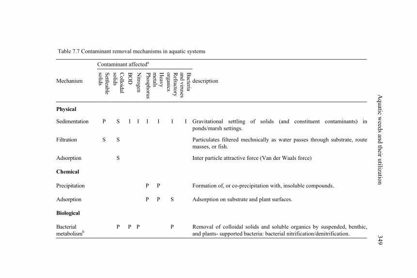
A
quatic w
eeds an
d th
eir utilizatio
n
349
description
Gravitational settling of solids (and constituent contaminants) in
ponds/marsh settings.
Particulates filtered mechnically as water passes through substrate, route
masses, or fish.
Inter particle attractive force (Van der Waals force)
Formation of, or co-precipitation with, insoluble compounds.
Adsorption on substrate and plant surfaces.
Removal of colloidal solids and soluble organics by suspended, benthic,
and plants- supported bacteria: bacterial nitrification/denitrification. B
acteria an
d v
iruses
I
Refracto
ry
org
anics
I
S
P
Heav
y
metals
I
P
P
Phosp
horu
s
I
P
P
Nitro
gen
I
P
BO
D
I
P
Collo
idal
solid
s
S
S
S
P
Contaminant affecteda
Settleab
le so
lids
P
S
Mechanism
Physical
Sedimentation
Filtration
Adsorption
Chemical
Precipitation
Adsorption
Biological
Bacterial
metabolismb
Table 7.7 Contaminant removal mechanisms in aquatic systems

35
0
Org
anic w
aste recyclin
g: tech
no
log
y an
d m
anag
emen
t
description
Uptake and metabolism of organics by plants; root excretion may be
toxic to organisms of enteric origin.
Under proper conditions significant quantities of these contaminants
will be taken up by plants.
Natural decay of organisms in an unfavourable environment.
Bacteria an
d
viru
ses
S
P
Refracto
ry
org
anics
S
S
Heav
y
metals
S
Ph
osp
ho
rus
S
Nitro
gen
S
BO
D
Co
lloid
al so
lids
Contaminant affecteda
Settleab
le so
lids Mechanism
Plant
metabolismb
Plant adsorption
Natural die off
Table 7.7 Contaminant removal mechanisms in aquatic systems (continued)
a P = primary effect, S = secondary effect, I = incidental effect (effect occurring incidental to removal of another contaminant)b The term metabolism includes both biosynthesis and catabolic reactions
From Tchobanoglous et al. 1979; reproduced by permission

Aquatic weeds and their utilization 351
Use of plants and animals in aquatic treatment
The fundamental purpose of plants, animals and the management of these
organisms in aquatic systems is to provide components to the aquatic
environments that improve the rate and/or reliability of one or more of the
contaminant removal mechanisms to be operative by design in the aquatic
treatment system. Plants play a more dominant role than animals in aquatic
systems because plants have a greater effect on the aquatic environment and are
more adaptable to harsh and/or fluctuating environment.
Aquatic animals are used, primarily, as biological controls of insect vectors
and as bioassay organisms for monitoring the treatment performance of an APU
or aquatic system. In certain situations animals can also play a role in plant
harvesting and suspended solids removal. In general, however, the direct uptake
and/or removal of wastewater contaminants by plants and animals are not
significant treatment mechanisms. An observation of interest is that some
molecular oxygen produced by the photosynthetic tissue of plants is translocated
to the roots and may keep root zone microorganisms metabolizing aerobically,
though the surrounding water is anoxic (Tchobanoglous et al. 1979).
7.7.3 Process design parameters
The different parameters currently being used in the design of aquatic systems
include organic loading rate, hydraulic loading rate, hydraulic application rate,
hydraulic detention time, and nitrogen loading rate. Depending on the treatment
objective the major design parameter will be different, for example, organic
loading rate is important for organic matter removal. Root depth of the plant is
important as it provides the bacterial support and the media for interaction
between wastewater and the bacterial mass. Even though there are many
potential aquatic plants that can be used for waste treatment they have not yet
been investigated to develop rational design criteria. Design criteria for water
hyacinth treatment systems are given below, while some data from the existing
systems are given in section 7.7.4.
Hydraulic retention time and process kinetics
Hydraulic retention time, typically expressed in days, is the most frequent
parameter used to design aquatic systems. The greatest benefit derived from the
use of hydraulic retention time is that a majority of performance data reported in
the literature are correlated to retention time. The use of hydraulic retention
time, however, has some serious drawbacks. Depending on system geometry,
systems with similar hydraulic retention times may be quite different
hydraulically. Also, accurate determination of hydraulic retention time is

352 Organic waste recycling: technology and management
difficult in aquatic treatment systems because of complex flow patterns and
volume displacement attributable to the plants. Generally, hydraulic retention
times reported in the literature are based on the assumption of their ideal
complete mix or plug flow hydraulics, neither of which are valid assumptions.
In addition, no attempt has been made to account for plant volume displacement
in the hydraulic retention times reported in the literature. Very little data are
available for hydraulic characterization of existing aquatic systems. In summary,
while hydraulic retention time has been used widely as an aquatic system design
parameter, little insight into how the hydraulic conditions affect the efficiency of
pollutant removal mechanisms can be derived from its usage.
Based on performance data of water hyacinth ponds used to treat domestic
wastewaters on San Diego, California, U.S.A. and elsewhere, it was suggested
that if the length/width ratios of the ponds are not great (probably less than 3/1),
a first order complete mix reaction may be applied (WEF 2001) as shown in
Equation 7.4.
tkC
C
t
e
+=
1
1
0
(7.4)
Where:
C0 = Influent BOD5 concentration, mg/L
Ce = Effluent BOD5 concentration, mg/L
kt = first order BOD5 removal rate constant at temperature T o C, day-1
T = Liquid temperature, 0C
k20 = first order BOD5 removal rate constant at 20o C, day-1
kT = k20 (1.06)T-20
t = hydraulic retention time, days
The estimated k20 value is 1.95 day-1
To describe the process kinetics of water hyacinth ponds in more details,
Polprasert and Khatiwada (1998) developed an integrated kinetic model which
encompasses the effects of both the suspended and biofilm bacteria and the
hydraulic dispersion number on the BOD5 removal efficiency. Based on a
dispersed flow model, an equation to predict BOD5 removal efficiency is shown
in Equation 7.5.
dada
d
e
eaea
ea
C
C2/
1
2/
1
2/1
1
011 )1()1(
2−− −−+
= (7.5)

Aquatic weeds and their utilization 353
Where:
Ce, Co, and t = as defined in Equation (7.4)
a1 = dtk ..41+ (7.6)
d = dispersion number, which is 0 at plug flow and infinite at complete
mix condition
k = kfs + kfb .as (7.7)
kfs = first-order rate constant for suspended bacteria, day-1
kfb = first-order rate constant for biofilm bacteria, day-1
as = specific surface area of water hyacinth ponds, m2/m3
as = 1/z + 2/w + 2/l + Rs/z (7.8)
z = pond depth, m
w = pond width, m
l = pond length, m
Rs = effective root surface area per unit pond area of surface area, m2/m3
For a pond with relatively large width and depth,
as = (1+Rs)/z (7.9)
To use Equation (7.5) is predicting BOD5 removal efficiency; the values of
the above parameters have to be determined experimentally or obtained from the
literature. Figure 7.13 determines the applicability of Equation (7.5) in
predicting the effluent BOD5 concentration of a water hyacinth pond treating a
domestic wastewater and showing the significance of the biofilm bacteria
attached on the root surfaces in BOD5 removal. To assist in the calculation, a
diagram based on Equation (7.5) and showing the relationship among BOD5
removal efficiency, k.t and d is given in Figure 7.14. Example 7.1 demonstrates
the application of Figure 7.14 in the design of a water hyacinth pond for
wastewater treatment.
Example 7.1
A water hyacinth pond is designed to treat a wastewater whose flow rate is 500
m3/day and BOD5 concentration is 200 g/m3. Determine the appropriate
dimensions of this pond so that at least 90% BOD5 removal is achieved. The
following information is given; d = 0.2, T = 20oC, z = 1.5 m, Rs = 1.18 m2/m3,
kfs = 0.07 day-1, kfb =0.048 day-1.
From Equation 7.9,
as = (1+1.18)/1.5 = 1.45 m2/m3

354 Organic waste recycling: technology and management
Figure 7.13 Predicted and observed effluent BOD5 concentration of the WHP (Polprasert
and Khatiwada 1998)
Figure 7.14 Design chart for BOD5 removal in water hyacinth ponds (Polprasert et al.
1998)
d=2
d=0.7
d=0.5
d=0.3 d=0.2d=0.15
d=0.1
d=0
d=1
k.t
d=1.5d=1.5
12108642
100
10
1
0k.t
d=2
d=0.7
d=0.5
d=0.3d=0.2d=0.15
d=0.1
d=0.005d=0
d=1
% B
OD
5 r
em
ov
al
BO
D5 (
mg
/L)
Day
Influent
Effluent, observed
Predicted effluent without biofilm consideration
Predicted effluent with biofilm
consideration
Aquatic weeds and their utilization 355
From Equation 7.7,
k = 0.07 + 1.45 (0.048) = 0.14 day-1
From Figure 7.15, for the 10% BOD5 remaining and d = 0.2, the value of k.t
is 4.
Therefore the value of t is 4/0.14 or 28.6 days.
Chose a “t” value of 30 days, the pond area is 500 × 30/1.5 = 10,000 m2. The
dimension of this water hyacinth pond is 200 × 50 × 1.5 m3 (length × width ×
depth). Note: a freeboard of about 0.5 m should be added to the depth of this
pond.
Check for BOD5 loading rate = 500 m3/d × 200 g/m3 × 1/10,000 m2
= 100 kg/(ha-day)
Note: the value of organic loading rate determined from this example is
within the range shown in Figure 7.15 and should result in about 90% BOD5
removal. If, due to evapotranspiration, the effluent flow rate value is much less
than 500 m3/day, average between the influent and effluent flow rate should be
used in calculating the pond dimensions.
Hydraulic loading rate
Hydraulic loading rate, expressed in units of m3 / (m2-day), is the volume of
wastewater applied per day per unit surface area of the aquatic system. Most
likely, the use of hydraulic loading rate stems from its popular use in land
application systems. Typically, aquatic systems are operated in a continuous
flow manner and as a result hydraulic loading or dosing rate is not a pertinent
design parameter.
Hydraulic application rate
Hydraulic application rate refers to the volumetric flow rate of wastewater
applied to the aquatic system per unit cross sectional area of the reactor
assuming the wastewater is applied uniformly to the system. The unit for this
parameter is m3 / (m2-day), which reduces to an expression of fluid velocity.
Hydraulic application rate has not been used widely, but offers a much better
unit of comparison for system performance data than the aforementioned
parameters for several reasons. One reason hydraulic application rate should be
a better design parameter is because hydraulic application rate is a gauge of the
fluid velocity that is thought to have a significant effect on removal mechanisms
operative in aquatic systems. In addition, hydraulic application rate can be
compared directly from system to system.

356 Organic waste recycling: technology and management
Organic loading rate
Organic loading rate, expressed as kg / (m2-day), is the mass of applied organic
material per unit surface area of the system per unit time. It is a function of flow
rate and concentration of organic matter. Theoretically, organic loading rates are
dictated by a balance between the applied carbon and available oxygen based on
the oxygen/carbon stoichiometry of bacterial conversion. In practice, organic
loading rates, based on experience, are dependent on effective distribution of
wastewater to the system. To avoid odour problems due to uneven organic
loading, the wastewater should be distributed evenly over the entire pond
system.
A relationship between average BOD5 loading and removal rates for aquatic
systems obtained from 24 different studies is shown in Figure 7.15. These data
suggest that aquatic systems using either emergent or floating plants could be
designed at BOD5 loading rates up to approximately 110 kg / (ha-day) with 80%
or more of the applied BOD5 being removed. It is apparent that a low effluent
BOD5 concentration from aquatic systems can be achieved with a reduced
BOD5 loading rate. BOD5 removal rates naturally decrease during the winter
period if the influent wastewater has a low temperature (Figure 7.11).
Nitrogen loading rate
Nitrogen loading rate, expressed as kg / (m2-day), is defined as the mass of
applied nitrogen to the system per unit surface area per unit time. If plants are
being harvested on a regular basis, the nitrogen requirement for new plant
reproduction can be matched with the system nitrogen loading rate. Early in the
development of aquatic systems, nitrogen removal by plant uptake and
subsequent harvesting was suggested as the principal removal mechanism. More
recently the potential for nitrogen removal through nitrification/denitrification
has been identified. If nitrification is the major step for total nitrogen removal,
then nitrogen loading rate is not a valid design parameter. System environmental
conditions favoring nitrification are different from those that would enhance
denitrification. As a result, a loading rate based on a lumping of the various
forms of influent nitrogen into a single unit is not fundamentally sound.
From their experimental study Weber and Tchobanoglous (1985) found
ammonium nitrogen removal rate in an aquatic (water hyacinth) system to be a
function of the hydraulic application rate and reactor length. The ammonium
nitrogen conversion rate was independent of the ammonium loading rate; and
hydraulic retention time was not recommended as a design parameter. As shown
in Figure 7.16, ammonium removal rates were observed to be inversely
proportional to the hydraulic application rates, while Figure 7.17 shows the

Aquatic weeds and their utilization 357
concentrations of ammonium nitrogen removal to be proportional to the reactor
length within the experimental conditions employed.
Figure 7.15 BOD removals as a function of BOD loading in aquatic systems (after
Stowell et al. 1981; reproduced by permission of the American Society of Civil
engineers)
Weber and Tchobanoglous (1986) developed an equation for ammonium
nitrogen removal in water hyacinth reactors as follows:
q
lkNr
.= (7.10)
Where,
Nr = ammonium nitrogen removal, mg/L
k = rate coefficient, mg/(L-day)
q = hydraulic application rate, m3/m2-day
l = reactor distance, m
BO
D5 r
em
oved
, kg
/ (
ha-d
ay)
BOD5 loading, kg / (ha-day)
Water hyacinth systems
Emergent plant systems
DATA FROM 24 DIFFERENT STUDIES

358 Organic waste recycling: technology and management
Based on the data shown in Figure 7.17, the values of k as a function of q are
given in Table 7.8.
Climatic influences
Surface area loading rates are much lower in aquatic systems than conventional systems, typically more than two orders of magnitude lower. A consequence of these lower loading rates is greater exposure to climatic factors such as temperature, rain, and wind. Any of these factors can disrupt treatment by altering the aquatic environment or damaging the plants. In general, the use of aquatic plants native to the climatic regime at the aquatic system site is encouraged but, in certain cases, this may not be desirable or possible.
Figure 7.16 NH4+- N removal as a function of hydraulic application rate
(corresponding loading rates for NH4+- N are as shown) (after Weber and
Tchobanoglous 1985; reproduced by permission of the Water Pollution Control Federation, USA)
Temperature
Wastewater in aquatic systems will be warm in summer and cool in winter
because of the large surface areas and long hydraulic residence times. A 10°C
rise or drop in temperature is generally known to double or halve the metabolic
Re
mo
val ra
te, k
g N
H4
+-N
/ (
ha-d
ay)
Hydraulic application rate, m3 / (m
2-day)
126 kg NH4+-N / (ha-day)
121 kg NH4+-N / (ha-day)
131 kg NH4+ -N / (ha-day)

Aquatic weeds and their utilization 359
rate of bacteria and plants. Temperature has a similar effect on the reproductive
rates of these organisms.
Figure 7.17 Ammonium nitrogen removal (Nr) as a function of reactor distance for three
hydraulic application rates (after Weber and Tchobanglous 1986; reproduced by the
permission of the Water Pollution Control Federation, USA)
Summer high temperatures may upset treatment by causing damage to some
plant species and/or by increasing bacterial metabolic activity, resulting in
altered balances between BOD5 reduction rates and oxygen flux from the
atmosphere. Another potential problem is that the water may become
sufficiently warm to result in violations of discharge permit requirements on
water temperature or other factors affected by water temperature such as un-
ionized ammonia concentration.
Winter low temperatures will reduce the metabolic rate of bacteria and may
kill many plant species. A plant kill may, but not necessarily, result in loss of
bacterial structure and/or leakage of plant-contained compounds. Research in
this area is necessary. As water temperatures approaching 0°C metabolic
activity virtually ceases, thus, wastewater treatment would result only from
physical/chemical mechanisms. This reduced level of treatment may be
inadequate in some situations. In these cases aquatic treatment would have to be
considered a seasonal treatment process. Wastewater storage or some other form
Reactor distance (l), m
Am
mo
niu
m n
itro
gen
rem
oval
(Nr)
, m
g/L
Hydraulic application rate
9.91 m3 / (m
2-day)
14.8 m3 / (m
2-day)
19.9 m3 / (m
2-day)

360 Organic waste recycling: technology and management
of treatment would be necessary during the periods when the aquatic system is
not functional.
Rain
Rain storms could overload aquatic systems hydraulically. Water inflow will
increase from I/I (inflow/infiltration) and direct rainfall into the APU's. Direct
rainfall alone from a typical storm could more than double the hydraulic load to
an aquatic system. The nature, magnitude, and duration of effects resulting from
hydraulic overloading are unknown. Probable effects of hydraulic overloading
would include wash-through of BOD5, re-suspension of sediment, and addition
of dissolved oxygen to APU's designed to be anaerobic.
Table 7.8 Calculated value of the rate coefficient, k as a function of hydraulic application rate (Weber and Tchobanoglous 1986)
Hydraulic application rates (m3/m2-day) k (mg/L-day)
9.91 11.9 14.8 9.47 19.9 8.77
Note: k =hydraulic application rate multiplied by the slopes from Figure 7.17
Wind
Wind can alter the aquatic environment directly or indirectly, the latter by
damaging the plants. Wind increases the rate of gas transfer between the
wastewater and atmosphere. Wind also increases water turbulence, which may
result in re-suspension of sediment. Plants broken or otherwise damaged by
wind may not function as intended, which would upset the wastewater treatment
process until the plants have recovered. Floating plants, particularly duckweeds,
are more sensitive to wind than rooted plants because the former tend to be
blown around and may result in open water surfaces which are vulnerable to the
direct effects of wind and other environmental factors. Though more sensitive to
winds, floating plants, by virtue of their mobility, are less likely to be physically
damaged by wind than rooted plants.
Environmental factors
Environmental impacts that could result from the presence of an aquatic
treatment system include odors, fog generation, increased vector-organism
population, and introduction of nuisance organisms to the local environment.
The potential for significant environmental impact from any of these or other
factors must be evaluated and mitigating measures taken as necessary.

Aquatic weeds and their utilization 361
The potential of the local environment to have significant impact on the
organisms in the aquatic system must also be evaluated. Of particular concern in
this regard are:
• local and/or migratory animals that may eat the APU plants, damage
APU levees by burrowing, or upset APU hydraulics by either
channelizing or blocking flow, and
• local plant diseases or plant-consuming insects.
As an example, water hyacinths could not be used for wastewater treatment
in an area where biological control of water hyacinths has been established.
Wastewater characteristics
Contaminant concentrations in domestic wastewaters should not be toxic to
aquatic plants in properly designed APU's. As the industrial fraction of the
wastewater increases, the chance of contaminants occurring in toxic
concentrations on a regular basis, or as shock loadings, increases. When an
appreciable portion of the wastewater is of industrial origins, small-scale pilot
studies should be conducted to evaluate the toxicity of the wastewater. If
toxicity from shock loadings occurs, mitigating measures such as flow
equalization/storage facilities will be necessary. If the wastewater is consistently
toxic, source control, pretreatment, or processes other than aquatic treatment
will be necessary.
Process reliability, upsets, and recovery
Little is known about the reliability of aquatic systems. The greater influence of
climatic and other environmental factors on aquatic processes should reduce
their reliability in comparison to conventional processes. However, the slower
rate of treatment, reduced reliance on equipment, and greater bacterial diversity
of aquatic processes should improve their reliability, comparatively. Currently
operating aquatic processes have not been as reliable as conventional processes;
but considering how little is known about the design, monitoring, and
management of aquatic processes, significant improvement in reliability should
be achievable.
Causes of aquatic process upsets and the nature, magnitude, and duration of
disruption of treatment have not been studied. Once rational aquatic treatment
design criteria have been established, most process upsets will result from:
• unusual climatic and environmental events insufficiently accounted
for in design, and
• improper APU management, such as lack of plant harvesting, etc.

362 Organic waste recycling: technology and management
The nature, magnitude, and duration of treatment process disruption will
depend, primarily, on the severity of the event causing the upset, which APU's
are affected, and the extent of damage/alteration to the aquatic environment.
Essentially nothing is known about the recovery times of aquatic processes
from various types and magnitudes of upsets. Recovery times are expected to be
longer in aquatic processes than conventional processes because environmental
conditions in the former are less conducive to rapid bacterial growth rates. If a
necessary function of the APU plants is damaged, the recovery time could be
several weeks or more if a new group of plants must be grown.
7.7.5 Review of existing aquatic treatment systems
There is a vast amount of literature available on aquatic treatment systems.
O'Brien (1981) summarized the design and performance characteristics of such
systems in the U.S., as shown in Tables 7.9 and 7.10. Most of these systems are
in the hotter parts of the U.S. and the climate there closely resembles the tropical
climates of developing countries. The wide differences in design parameters
shown in Table 7.9 are typical for an emerging technology. But sufficient
information is now available to suggest the criteria shown in Table 7.9 for the
design of water hyacinth systems intended to produce secondary or advanced
secondary effluents. Criteria similar to those given in Table 7.9 were also
recommended by Dinges (1979), who focused on the development of low
technology systems suitable for upgrading lagoon performance in small towns.
Suggestions by Dinges (1979) to supplement the design criteria in Table 7.9
include the use of:
• Perforated pipe to achieve uniform influent flow distribution;
• Filters around the effluent structure to prevent the escape of plants,
and
• Circular galvanized wire-mesh enclosures in ponds to improve
production of the fish used for controlling mosquitoes.
The data in Table 7.10 suggests that secondary waste treatment standards can
be met if intensive management techniques are practiced. Ultimate disposal of
the harvested plants as surface mulch, compost, animal feed, or for generation of
biogas (see sections 7.5 and 7.6) ensures that resource recovery is also practiced.
But, in most wastewater treatment installations, these processes will not be
sufficiently profitable to offset the cost of solids disposal (because performances
of natural treatment systems are site specific and dependent on climatic and
related factors, wherever possible, pilot-scale experiments should be done to
confirm the selected design criteria).

Aquatic weeds and their utilization 363
Tota
l
phosp
horu
s
0.4
5
0.8
9
0.8
5
- -
Nu
trie
nt
con
tent
of
pla
nts
, d
ry w
eig
ht,
(%)
Tota
l
Kje
dah
l
nit
rogen
2.7
3
3.5
6
3.7
5
- -
Hyac
inth
cover
(%)
10
0
100
100
100
100
Org
anic
load
ing r
ate
(kg/h
a-day
)
26
44
179
31
43
Hydra
uli
c
resi
den
ce
tim
e (d
ays)
54
~ 6
7a
6.8
22
5.3
Hydra
uli
c
load
ing
rate
,
(m3/h
a-day
)
240
260
a
3,5
70
700
1,8
60
Dep
th o
f
hyac
inth
ponds
(m)
1.2
2
1.7
3
1.8
3
1.5
1.0
Surf
ace
area
of
hyac
inth
ponds
(ha)
2 3.6
0.2
8
0.0
7
0.0
6
Types
of
pre
-
trea
tmen
t
None
None
Fac
ult
ativ
e
lagoons
One
aera
ted a
nd
one
facu
ltat
ive
lagoon
Pla
nt A
: ae
rati
on
bas
in, c
lari
fier
,
thre
e la
goons
in
seri
es
Lo
cati
on
Nat
ional
Spac
e
Tec
hnolo
gy L
ab:
Luce
dal
e, M
iss
Ora
nge
Gro
ve,
Mis
s.
Ced
er L
ake,
Mis
s
(
Du
ckw
eed)
Wil
liam
son
Cre
ek, T
ex.:
Phas
e I
Tab
le 7
.9 S
um
mar
y o
f d
esig
n a
nd p
erfo
rman
ce c
har
acte
rist
ics
of
aqu
atic
wee
d w
aste
wat
er t
reat
men
t sy
stem
s

364 Organic waste recycling: technology and management
Tota
l
phosp
horu
s
Nu
trie
nt
con
tent
of
pla
nts
, d
ry w
eig
ht,
(%)
Tota
l
Kje
dah
l
nit
rogen
Hyac
inth
cover
(%
)
100
100
Org
anic
load
ing r
ate
(kg/h
a-day
)
5.2
Hydra
uli
c
resi
den
ce
tim
e (d
ays)
~3
0.6
3
Hydra
uli
c
load
ing
rate
,
(m3/h
a-day
)
430
1220
Dep
th o
f
hyac
inth
ponds
(m)
1.2
3
1.4
Surf
ace
area
of
hyac
inth
ponds
(ha)
1.4
0.7
6
Types
of
pre
-
trea
tmen
t
Exce
ss a
ctiv
ated
sludge
lagoons
over
flow
to
hyac
inth
ponds
Tri
ckli
ng f
ilte
r
and a
ctiv
ated
sludge
wit
h
poli
shin
g p
ond
Lo
cati
on
Aust
in-
Horn
sby
Ben
d, T
ex.:
Un
iver
sity
of
Flo
rida,
Gai
nse
vil
le,F
la
Tab
le 7
.9 S
um
mar
y o
f d
esig
n a
nd p
erfo
rman
ce c
har
acte
rist
ics
of
aqu
atic
wee
d w
aste
wat
er t
reat
men
t sy
stem
s (c
on
tinu
ed)
aB
ased
on
eff
luen
t fl
ow
rat
e
Fro
m O
’Bri
en (
198
1);
rep
rod
uce
d b
yp
erm
issi
on o
f th
e A
mer
ican
So
ciet
y o
f C
ivil
En
gin
eers

Aquatic weeds and their utilization 365
Sam
pli
ng p
erio
d a
nd
co
mm
ents
May
19
74
-May
197
6
Jun
e 19
76
-Sep
tem
ber
197
7
Od
ors
at
nig
ht
Eff
luen
t
pH
val
ues
9.3
7.1
Dis
solv
ed
ox
yg
en,
(mg
/L)
6.9
2.3
0 2.0
0.5
Eff
.
2.1
1.6
TP
(m
g/L
)
Inf.
2.9
3.7
Eff
.
5.2
3.4
TN
(m
g/L
)
Inf.
9.8
12
.0
Eff
.
49
10
77
6 53
15
11
9
Su
spen
ded
soli
d(m
g/L
)
Inf.
70
97
14
0
12
5
49
49
18
8
40
Eff
.
17
7 57
23
37
14
18
12
BO
D5
(mg
/L)
Inf.
91
11
0
12
7
16
1
50
50
44
42
Lo
cati
on
Nat
ion
al S
pac
e T
ech
no
logy
Lab
:
B
efo
re h
yac
inth
s
A
fter
hy
acin
ths
Lu
ced
ale,
Mis
s.:
B
efo
re h
yac
inth
s
A
fter
hy
acin
ths
Ora
ng
e G
rov
e, M
iss.
:
W
ith
ou
t h
yac
inth
s
W
ith
hy
acin
ths
Ced
ar L
ake,
Mis
s.
(du
ckw
eed
)
Wil
liam
son
Cre
ek, T
ex.:
F
ull
-sca
le
Tab
le 7
.10
Su
mm
ary
of
infl
uen
t/ef
flu
ent
char
acte
rist
ics
of
aqu
atic
wee
d w
aste
wat
er t
reat
men
t sy
stem
s
a On
ly p
arti
al c
ov
er a
nd l
imit
ed p
reli
min
ary
dat
a b E
xp
erim
enta
l u
nit
s no
t fu
lly
op
erat
ion
al
Fro
m O
’Bri
en (
198
1);
rep
rod
uce
d b
y p
erm
issi
on o
f th
e A
mer
ican
So
ciet
y o
f C
ivil
En
gin
eers

366 Organic waste recycling: technology and management
Example 7.2Design a water hyacinth treatment system to treat the following wastewater.
Wastewater characteristics:
BOD5 = 200 mg/L
COD = 300 mg/L
Flow Rate = 100 m3/day
Choose organic loading = 25 kg BOD/ (ha-day) (From Table 7.9)
Area required = 100 x 200 x 10-3/ (25)
= 0.8 ha
If two basins are to be constructed,
Area of individual basin = 0.4 ha
Length: width = 4: 1
Width = (0.4 x 10⁴/4)0.5 = 31.6 m
Choose width = 32 m
Length = 125 m
Choose depth = 1.2 m (Root depth = 0.9 m; bottom layer = 0.3 m
Check with data in Table 7.9
Hydraulic loading rate = 100/(2 x 0.4)
= 125 m3/(ha-day)
Hydraulic retention time = 4000 x 1.2 x 2 / (100)
= 96 days
The design is acceptable.
Example 7.3
Estimate the yield of duckweeds from an aquatic treatment system treating
domestic sewage.
Area of ponds = 1 ha (or 104 m2)
Doubling time of duckweed = 10 days
Choose stocking density = 400 g/m2 (wet weight)
Note:
• Stocking density reported in the literature varies from 200 g/m2 to
700 g/m2
• Lower initial density may cause algal blooms that could suppress
the growth of duckweed.
• Harvesting interval has to be chosen such that the growth of
duckweed is not reduced due to overcrowding.

Aquatic weeds and their utilization 367
To compensate for other factors, choose the harvesting interval to be once
every 10 days, and to maintain continuous duckweed growth, only 50 % of the
total duckweeds or 50 % of the pond area are to be harvested.
Amount of duckweeds to be harvested each time = (400 x 104 g)/2
= 2 tons
Monthly harvest = 2 x 30 /(20)
= 6 tons wet mass
If duckweeds contain 95% water, dry mass = 6 x 0.05
Amount of duckweeds = 0.3 tons dry mass
The yield of duckweeds is 0.3 tons dry mass / (ha-month).
Example 7.4
Wastewater from a food-processing factory has the following characteristics:
Flow rate = 100 m3/day
COD = 300 mg/L
BOD5 = 200 mg/L
NH4+ - N = 10 mg/L
PO43- - P = 5 mg/L
The factory plans to convert this wastewater to produce protein biomass
using the existing pond system that has an area of 1.2 ha. The available
alternatives are to grow either water hyacinth or duckweeds. Determine a
suitable weed option that will give more financial return annually.
The following information are given:
Water hyacinth
Average stock density = 2 kg/m2
Area doubling time = 10 days
Protein content = 17% by weight (dry)
Harvesting is done by manually (no addition cost)
Market price of protein = 1 Baht/kg
Duckweeds
Average stock density = 0.7 kg/m2
Area doubling time = 15 days
Protein content = 20% by weight (dry)
Harvesting cost = 100 Baht/ton dry wt.
Market price of protein = 3 Baht/kg

368 Organic waste recycling: technology and management
Note: 1US$ = 40 Baht
a) Water hyacinth
Organic loading of the pond = ha
kg
L
mg
d
m
2.1
1
10
10200100
3
63
××× −
−
= 16.66 kg BOD5/(ha-day)
Hydraulic loading = haday
m
2.1
1100
3
× = 83.3 m3/(ha-day)
Note: these loading rates are within the ranges reported in Tale 7.9.
Because the doubling time is 10 days, the no. of water hyacinth harvesting is
36 times per year. The amount of water hyacinth harvested is half of the total
pond area.
Amount of water hyacinth harvested/year
= 36 x 2
1x 1.2 x 104 x 2.0 kg = 432x103 kg.
Assuming solid content = 5%
Total protein obtained = 0.05 x 0.17 x 432 x 103 kg = 3.672 kg.
Income from protein = 1.0 x 3672 = 3672 Baht
Annual income = 3672 Baht
b) Duckweeds
Because the doubling time is 15 days, the frequency of duckweed harvesting is
24 times per year. The amount of duckweeds harvested is half of the total pond
area.
Amount of duckweeds harvested per year = 2
1 x 24 x 0.7 x 1.2x104 kg
= 100.8x10³ kg
Solid content in duckweed = 20%
Total protein obtained = 0.2x0.2x100.8x103 = 4032 kg/year
Cost for harvesting = 100.8 x 103 x 000,1
1002.0 ×
Income from protein = 4032x3.0 Baht/year
= 12,096 Baht/year
Net income = (12,096 – 2,016) Baht/year
= 10,080 Baht/year

Aquatic weeds and their utilization 369
Based on data used in this example, duckweed culture will give more
financial return annually.
7.7.5 Emergent aquatic weeds and constructed wetlands
Wetland is an area that is inundated or saturated by surface or groundwater at a
frequency or duration sufficient to maintain saturated conditions and growth of
related vegetation. Emerged aquatic weeds, such as cattails (Typhas), bulrushes
(Scripus) and reeds (Phragmaites) are the major and typical component of the
wetland systems (Figure 7.3). Wetland is a natural system where complex
physical, biological and chemical reactions essential for wastewater treatment,
listed in Table 7.7, exist. To avoid interference with the natural ecosystems,
constructed wetland in which hydraulic regime is controlled have been used for
treatment of a variety of wastewaters (Hammer 1998; WPCF 1990). Constructed
wetlands can range from creation of a marsh land to intensive construction
involving earth moving, grading, impermeable barriers, or erection of tanks or
trenches (U.S. EPA 1988). Two types of constructed wetlands have been developed for wastewater
treatment, namely, free water surface (FWS) and subsurface flow (SF). An FWS system consists of parallel basins of channels with relatively impermeable bottom and soil and rock layers to support the emergent vegetation, and the water depth is maintained at 0.1 – 0.6 m above the soil surface. An SF system, also called ‘root zone’, or reed bed, consists of channels or trenches with impermeable bottom and soil and rock layers to support the emergent vegetation, but the water depth is maintained at or below the soil surface (Figure 7.18). To reduce the short-circuiting, the length to width ratios of constructed wetlands units should be more than 2:1 and bed slopes of 1 – 5 %. Although it might appear that SF constructed wetlands could be subjected to frequent clogging problems, performance data reported so far have shown them to function satisfactorily with a high degree of removal efficiencies (Reed and Brown 1992 and 1995). An SF constructed wetland can be operated in a vertical flow mode in which wastewater is applied uniformly over the wetland surface and the effluent is collected at the bed bottom. High percentages of BOD and nitrogen removal have been reported from this type of operation (WEF 2001).
Table 7.11 shows removal efficiencies of some constructed wetlands located in the USA, which, in general, are comparable with other constructed wetlands in operation worldwide. Although more than 80 percentage of N and P removal can be expected in constructed wetlands, not much information about the removal of faecal micro organisms is available (see section 7.1.3). Based on the performance data, a summary of wetland design consideration is given in Table 7.12, which should serve as guidelines in the design and operation of natural and constructed wetlands for wastewater treatment.

370 Organic waste recycling: technology and management
Table 7.11 Summary of BOD5 and SS removal from constructed wetlands (U.S. EPA 1988)
a Free Water Surface System b Subsurface Flow System
Owing to the complex reactions occurring in wetland beds, it is very difficult
to develop a comprehensive model that would adequately describe or predict the
treatment efficiency. Nevertheless, Reed and Brown (1995) recommended a
first-order reaction for BOD5 removal in constructed wetlands:
tke TeC
C .
0
−= (7.11)
Where,
Ce = Effluent BOD5 concentration, mg/L
Co = Influent BOD5 concentration, mg/L
kT = k20(1.06)T-20
T = liquid temperature, oC
k20 = 1.104 day-1, for SF constructed wetlands,
k20 = 0.687 day-1 for FWS constructed wetlands
t = hydraulic retention time in the wetland beds, days.
BOD5 mg/L SS mg/l % reduction Project Flow, m3/day
Wetlandtype Influent Effluent Influent Effluent BOD5 SS
Hydraulic surface loading rate,m3/(ha-day)
Listowel, Ontario
17 FWSa 56 10 111 8 82 93 -
Santee, CA SFb 118 30 57 5.5 75 90 - Sydney, Australia
240 SF 33 4.6 57 4.5 86 92 -
Arcata, CA 11,350 FWS 36 13 43 31 64 28 907 Emmitsburg, MD
132 SF 62 18 30 8.3 71 73 1,543
Gustine,CA
3785 FWS 150 24 140 19 84 86 412

Aquatic weeds and their utilization 371
Table 7.12 Summary of wetland design consideration (WPCF 1990). Reproduced by the permission of the Water Environment Federation
Constructed
Design consideration free water surface submerged bed Natural
Minimum size
requirement, ha/1000
m3/d
3 – 4 1.2 – 1.7 5- 10
Maximum water
depth, cm
50 Water level
below ground
surface
50; depends on native
vegetation
Bed depth, cm Not applicable 30 – 90 Not applicable
Minimum aspect ratio
(L/W)
2:1 Not applicable Prefer 2:1
Minimum Hydraulic
residence time, days
5 – 10 5 – 10 14
Maximum hydraulic
loading rate, cm/day
2.5 – 5 6 – 8 1 – 2
Minimum pre
treatment
Primary;
secondary is
optional
Primary Primary;
Secondary;
Nitrification,
TP Reduction
Configuration Multiple cells in
parallel and series
Multiple beds in
parallel
Multiple discharge
sites
Distribution Swale; perforated
pipe
Inlet zone (> 0.5
m wide) of large
gravel
Swale; perforated
pipes
Maximum loading,
kg/ha-day
BOD5 100 – 110 80 – 120 4
TN 60 60 3
Additional
consideration
Mosquito control
with mosquito fish;
remove vegetation
once each 1 to 5
years
Allow flooding
capability for
weed control.
Natural hydro period
should be > 50 %;
no vegetation harvest

372 Organic waste recycling: technology and management
Figure 7.18 Typical cross-section of SF constructed wetlands (U.S. EPA 1988)
It is apparent from the k20 values that the SF constructed wetlands are more
efficient in the removal of BOD5 than the FWS constructed wetlands. This
superior efficiency is obviously due to better contact between the liquid
wastewater and the micro-organisms (mainly bacteria) present in the SF wetland
beds responsible for BOD5 biodegradation, including the filtration and
adsorption mechanisms.
It is important to point out that the value of ‘t’ determined from the Equation
(7.11) is the time the liquid stays in the void spaces of the constructed wetland
beds. Determination of the total bed volume has to include the porosity
parameters ( ) as follows:
= Vv/Vt (7.12)
Vt = Q .t/ (7.13)
Where, Vv and Vt = void volume and total bed volume, respectively, m3.Q = wastewater flow rate, m3/day = porosity, unitless
The values of for some bed media are given in Table 7.13, which indicate
the larger the media diameter, the higher the values. Due to the level of free
water maintained in the FWS constructed wetlands (10 – 60 cm), their values
are in the range of 0.65 – 0.75 (WEF 2001).
Since the effect of evapotranspiration (section 7.4) can be significant during
the summer and windy periods, the effluent flow rate of a constructed wetland
may be much less than that of the influent flow rate. In this respect, the value of
Q used in the calculation of Vt (Equation 7.13) should be the average between
the influent and effluent flow rates. Depth of a constructed wetland should be
CATTAILS
SLOTTED PIPE FOR WASTEWATER DISTRIBUTION
INLET STONE
DISTRIBUTOR
SOIL OR GRAVEL
EFFLUENT OUTLET
HEIGHT VARIABLE
WATERTIGHT MEMBRANE RHIZOME NETWORK
SLOPE 1%

Aquatic weeds and their utilization 373
deep enough to support the growth of the emergent plant’s roots, i.e. about 1.0 –
1.5 m deep. The cross-sectional area of a SF constructed wetland is calculated as follows
(U.S. EPA 1988):
Ac = Q/(Ks.S) (7.14)
Where, Ac = cross sectional area of wetland bed perpendicular to the direction of flow (or depth × width), m2,Ks = hydraulic conductivity of the medium, m3/(m2-day), as given in Table 7.13 S = slope of the wetland bed (as a fraction or decimal)
To ensure the sufficient contact time for wastewater, the value of Ks.S or
Q/Ac should be less than 8.6 m/day.
Table 7.13 Typical media characteristics for SF wetlands (WEF 2001)
Media type D10 Effective size a, mm Porosity ( ) Ks,(m3/m2-day)
Coarse sand 2 0.28 – 0.32 100 – 1000 Gravely sand 8 0.30 – 0.35 500 – 5000 Fine gravel 16 0.35 – 0.38 1000 – 10000 Mediumgravel
32 0.36 – 0.40 10000 – 50 000
Coarse rock 128 0.38 – 0.35 50000 – 250 000 aD10 = effective size of the media at 10 % cumulative weight of total, or the size of the media such
that 10 % by weight are smaller.
Example 7.5
Compare the area requirements of FWS and SF constructed wetlands (planted
with cattails) to be used to treat a wastewater having the following
characteristics: average flow rate = 760 m3/day, influent BOD5 = 200 g/m3, and
water temperature = 20oC. To meet the discharge standard for reuse, the effluent
BOD5 concentration has to be 10 g/m3 or less. For FWS constructed wetland:
= 0.75 and bed depth is 0.7 m (cattail plants root is 0.5 and free water depth is
0.2 m)
For SF constructed wetland: = 0.3 and bed depth is 0.5m
Equation 7.11 is applicable to describe the BOD5 removal efficiency of
constructed wetlands.

374 Organic waste recycling: technology and management
Solution:
Based on Equation 7.11, determine ‘t’ values.
For FWS: 10/200 = e-0.678*t
tFWS = 4.4 days
For SF: 10/200 = e-1.104*t
tSF = 2.7 days
Surface area (A) = (t*Q)/(d* )
AFWS = (4.4*760) / (0.7*0.75) = 6370 m2
ASF = (2.7*760) / (0.5*0.3) = 13680m2
To check for hydraulic flow of SF, choose 2 SF units, each with a surface
area of 7,000 m2 or length × width of 100 × 70 m2. If depth of SF is 1 m, the Ac
value is 70 × 1 = 70m2.
The value of Q/Ac is 380/70 = 5.43 m/day, less than 8.6 m/day.
Note: AFWS and ASF are surface areas of FWS and SF constructed wetlands,
respectively. Although the SF constructed wetland has higher k value than the
FWS constructed wetland, due to the low porosity ( ) of the bed media, it
requires more land area than that of FWS constructed wetland.
Because of current interest in the utilization of constructed wetlands in
wastewater treatment/recycling, more comprehensive design models with
respect to BOD5, nutrient and faecal coliform removal that will encompass, not
only temperature but also other important parameters, should be developed.
Polprasert et. al. 1998 applied a dispersed flow model incorporating biofilm
activity (similar to Equation 7.5) to describe organic removal efficiency of a
FWS constructed wetlands with satisfactory results. They also found the biofilm
activity to be several times more significant in organic removal than the
suspended bacterial activity in the FWS constructed wetland bed.
From their surveys of more than 20 constructed wetlands sites in the USA,
Reed and Brown (1992) did not observe the need of annual harvesting of the
common emergent vegetation, but recommended that the vegetative detritus
present in the wetland beds be cleaned out on some extended schedule.
However, because vegetative plants obviously grow faster in the tropics than in
temperate climates, it would be useful to study the need and frequency of plant
harvesting for constructed wetlands located in tropical areas in accordance with
the area doubling time, as discussed in section 7.4. When subjected to frequent
harvesting, Sawaittayothin and Polprasert (2006) found N uptake by cattail
plants to be 80% of the total N input when they were cultured in a SF

Aquatic weeds and their utilization 375
constructed wetlands located in the tropics. The plant productivity was
accordingly high and beneficial for reuses.
7.8 HEALTH HAZARDS RELATING TO AQUATIC
WEEDS
The cultivation of aquatic weeds may cause health problems by:
• Contamination of the people who work in the aquatic pond
operation with pathogens in the water,
• Contamination of the plants with pathogens and toxic materials such
as heavy metals and pesticides, and
• Providing habitats (pond & plants) for various vectors.
Concerning the first and second health problems, the risk of contacting
pathogens by workers and contamination of plants with pathogens can be
minimized if the waste is adequately treated to eliminate pathogens before
applying to aquatic plants. This step is necessary as pathogen removal in an
aquatic system is not very effective. Direct fertilization of aquatic weed ponds
with nightsoil should be avoided as the risk is high and it reduces the
acceptability of the product.
The third health problem involves the possibility of disease transmission
through infection by metacercariae, (infective stage) which has its intermediate host
in the pond, such as snails (in case of Schistosomiasis) or attached to the plant
leaves and stems. According to Feachem et al. (1983), the parasitic fluke
Fasciolopsis buski is important in some parts of Asia. The worm has a life cycle
that moves from man (or pig or dog) to snail to water plant and then to man again.
Animals or people become infected by eating the encysted metacercariae on water
plants, such as seed pods of water caltrop, bulbs of water chestnut, and roots of
lotus, water bamboo, etc. In cases where those diseases associated with
intermediate hosts in the pond are endemic and their respective hosts are present in
that area, waste recycling using aquatic plants is not advisable.
Aquatic vegetation enhances the production of mosquito by protecting the
larvae from wave action, providing a habitat for breeding and interfering with
mosquito control procedures. The two major vectors are Anopheles that transmits
malaria, and Mansonia that carries filariasis and encephalitis.
The eggs of Mansonia are laid on the undersides of leaves of aquatic weeds
just above the surface of the water. The mosquito larvae inserts it’s respiratory
siphon into the air-containing tissues of the plant and need not come to the
surface of water for air. The air is obtained from the submerged portions of the
plant, especially from the roots. Different Mansonia species have a preference

376 Organic waste recycling: technology and management
for certain plants but water lettuce seems to be the most common host, followed
by water hyacinth then Azolla and duckweeds.
An effective way to prevent breeding of mosquito in the pond is to stock fish
that feed on mosquito larvae. Successful control was reported by culturing fish
S. Mossambicus in water spinach ponds and Gambusia affinis in water hyacinth
ponds (Edwards 1980; Wolverton et al. 1975).
Biological accumulation in aquatic weeds will occur when wastewater
containing pesticides and heavy metals are treated, thus reducing their potential
as food and as for agricultural purposes. Wastewaters containing toxic materials
should be pretreated to remove these specific contaminants or other alternatives
for treatment and recovery has to be considered.
7.9 REFERENCES
Bagnall, L.O., Furman, T.D.S., Hentges, J.F., Nolan, W.J. and Shirley, R.L. (1974) "Feed
and Fiber from Effluent-Grown Water Hyacinth". Environmental Protection Technology Series: EPA-660/2-74-041, Washington, D.C.
Bagnall, L.O. (1979) "Resource recovery from wastewater aquaculture". In Aquaculture
Systems for Wastewater Treatment - Seminar Proceedings and Engineering
Assessment, Report No. EPA 430/9-80-006, pp. 421-439, US Environmental Protection Agency, Washington, D.C.
Boyd, C.E. (1970) "Amino acid, protein, and caloric content of vascular macrophytes". Ecology, 51, 902-906.
Boyd, C.E. (1974) "Utilization of aquatic plants". In Aquatic Vegetation and Its Use and
Control. (Ed. D.S. Mitchell), pp. 107-115, UNESCO, Paris. Cooper, A. (1976) Nutrient Film Technique of Growing Crops, Grower Books, London. Cornwell, D.A., Zoltek, J., Jr., Patrinely, C.D., Furman, T.D.S. and Kim, J.I. (1977)
"Nutrient removal by water hyacinths". J. Water Pollut. Control Fed., 49, 57-65. Dassanayake, M.D. (1976) "Noxious aquatic vegetation control in Sri Lanka". In Aquatic
Weeds in South East Asia. (Eds. C.K. Varshney and J. Rzoska) pp. 59-61, Dr. W. Junk B.V., The Hague.
DeBusk, T.A., Williams, L.D. and Ryther, J.H. (1977) "Growth and yields of the freshwater weeds Eichhornia crassipes (water hyacinth), Lemna minor (duckweed), and Hydrilla verticillata". In Cultivation of Macroscopic Marine Algae and
Freshwater Aquatic Weeds. (Ed. J.H. Ryther) pp. 275-295, Contract No. E (11-1)-2948. US Department of Energy, Washington, D.C.
Dinges, R. (1979) "Development of water hyacinth wastewater treatment systems in Texas". In Agriculture Systems for Wastewater Treatment - Seminar Proceedings
and Engineering Assessment, Report No. EPA 430/9-80-006, pp. 193-226, US Environmental Protection Agency, Washington, D.C.
Edwards, P. (1980) "Food Potential of Aquatic Macrophytes". ICLARM Studies and Reviews No. 5, International Center for Living Aquatic Resources Management, Manila.

Aquatic weeds and their utilization 377
Edwards, P., Polprasert, C., Rajput, V.S. and Pacharaprakiti, C. (1987) "Integrated biogas technology in the tropics 2. Use of slurry for fish culture", Waste Management and
Research, 6, 51-61. Feachem, R.G., Bradley, D.J., Garelick, H. and Mara, D.D. (1983) "Sanitation and
Disease-Health Aspects of Excreta and Wastewater Management". Wiley, Chichester.
Frank, P.A. (1976) "Distribution and utilization-research on tropical and subtropical aquatic weeds in the United States". In Aquatic Weeds in South East Asia. (Eds. C.K. Varshney and J. Rzoska) pp. 353-359, Dr. W. Junk B.V., The Hague.
Gopal, B. and Sharma, K.P. (1981) Water Hyacinth - The Most Troublesome Weed of the
World". Hindasia Publishers, Delhi. Gupta, O.P. and Lamba, P.S. (1976) "Some aspects of utilization of aquatic weeds". In
Aquatic Weeds in South East Asia. (Eds. C.K. Varshney and J. Rzoska) pp. 361-367, Dr. W. Junk B.V., The Hague.
Jewell, W.J., Madras, J.J., Clarkson, W.W., Delancey-Pompe, H. and Kabrick, R.M. (1982) Wastewater Treatment with Plant in Nutrient Films, US EPA Report No. PB 83-247-494, Springfield, Virginia.
Little, E.C.S. (1968) "Handbook of Utilization of Aquatic Plants". A Compilation of the World's Publications, Food and Agriculture Organization, Rome.
Mehta, I., Sharma, R.K. and Tuank, A.P. (1976) "The aquatic weed problem in the Chambal irrigated area and its control by Grass Carp". In Aquatic Weeds in South
East Asia. (Eds. C.K. Varshney and J. Rzoska) pp. 307-314, Dr. W. Junk B.V., The Hague.
Metcalf and Eddy Inc. (2003) Wastewater Engineering: Treatment, Disposal, Reuse, 4th
Edition, McGraw-Hill, New York. Mitchell, D.S. (1974) "Aquatic Vegetation and Its Use and Control", UNESCO, Paris. Mitchell, D.S. (1976) "The growth and management of Eichhornia crassipes and
Salvinia spp. in their native environment and in alien situations". In Aquatic Weeds
in South East Asia. (Eds. C.K. Varshney and J. Rzoska) pp. 167-176, Dr. W. Junk B.V., The Hague.
NAS (1976) Making Aquatic Weeds Useful: Some Perspectives for Developing
Countries, National Academy of Sciences, Washington, D.C. Ngo, H.N. (1984) "Waste Recycling Through Bio-Fertilization". Enfo, Environmental
Sanitation Information Center, Asian Institute of Technology, Bangkok, 2, 11-13. O'Brien, W.J. (1981) "Use of aquatic macrophytes for wastewater treatment". J. Env.
Eng. Division-ASCE, 107, 681-698. O'Keefe, D.H., Hardy, J.K. and Rao, R.A. (1984) "Cadmium uptake by the water
hyacinth : Effects of solution factors". Environmental Pollution, 34, 133-147. Oron, G., Porath, D. and Wildschut, L.R. (1986) "Wastewater treatment and renovation
by different duckweed species". J. Env. Eng. - ASCE, 112, 247-263. Pirie, N.W. (1978) "Freshwater weeds are a resource". Appropriate Technology, 4, 15-
17.Polprasert, C., Edwards, P., Pacharaprakiti, C., Rajput, V.S. and Suthirawut, S. (1982)
"Recycling Rural and Urban Nightsoil in Thailand", AIT Research Report No. 143, Submitted to International Development Research Centre, Ottawa, Canada. Asian Institute of Technology, Bangkok, Thailand.

378 Organic waste recycling: technology and management
Polprasert, C., (1984) "Utilization of composted nightsoil in fish production", Conservation and Recycling, 7, 199-206.
Polprasert, C. and Khatiwada, N.R. (1998) An integrated model for water hyacinth ponds used for wastewater treatment, Water Research, 32, 179-185
Polprasert, C., Khatiwada, N.R. and Bhurtel, J. (1998) Design model for COD removal in constructed wetlands based on biofilm activity, J. Environmental Engineering
ASCE, 124, 834-843 Reddy, K.R. and Sutton, D.L. (1984) "Water hyacinths for water quality improvement
and biomass production". J. Environmental Quality, 13, 1-8. Sawaittayothin, V. and Polprasert, C. (2006) Nitrogen mass balance and microbial
analysis of constructed wetlands treating municipal landfill leachate, Bioresources
Technology, 97, (in press) Seidal, K. (1976) "Macrophytes and water purification". In Biological Control of Water
Pollution. (Eds. J. Tourbier and R.W. Pierson) pp. 109-121, University of Pennsylvania Press, Philadelphia.
Stowell, R., Ludwig, R., Colt, J. and Tchobanoglous, G. (1980) "Towards the Rational
Design of Aquatic Treatment Systems". Paper presented at the ASCE Convention, 14-18 April, Portland, Oregon. Department of Civil Engineering, University of California, Davis, California.
Stowell, R., Ludwig, R., Colt, J. and Tchobanoglous, G. (1981) "Concepts in aquatic treatment system design", J. Env. Eng. Division - ASCE, 107, 919-940.
Taylor, J.S. and Stewart, E.A. (1978) "Hyacinths". In Advances in Water and Wastewater
Treatment - Biological Nutrient Removal. (Eds. M.P. Wanielista and W.W. Eckenfelder, Jr.) pp. 143-180, Ann Arbour Science, Ann Arbour, Michigan.
Tchobanoglous, G., Stowell, R. and Ludwig, R. (1979) "The Use of Aquatic Plants and Animals for the Treatment of Wastewater : An Overview". In Aquaculture Systems
for Wastewater Treatment - Seminar Proceedings and Engineering Assessment,
Report No. 430/9-80-006. US Environmental Protection Agency, Washington, D.C., pp. 35-55.
U.S. EPA (1988) Design Manual-Constructed Wetlands and Aquatic Plant Systems for
Municipal Wastewater Treatment, EPA/625/1-88/022. US Environmental Protection Agency, Cinunnati, Ohio.
Weber, A.S. and Tchobanoglous, G. (1985) "Rational design parameters for ammonia conversion in water hyacinth treatment systems", J. Water Pollut. Control Fed., 57,316-323.
Weber, A.S. and Tchobanoglous, G. (1986) "Prediction of nitrification in water hyacinth treatment systems", J. Water Pollut. Control Fed., 58, 376-380.
WEF (2001) Natural System for Wastewater Treatment, Manual of practice 2nd edition, Water Environment Federation, Alexandria, VA,USA
Westlake, D.F. (1963) "Comparisons of plant productivity", Biological Review, 38, 385-425.
Whigham, D.F., Simpson, R.L. and Lee, K. (1980) "The Effect of Sewage Effluent on the
Structure and Function of a Freshwater Tidal Marsh Ecosystem". New Jersey Water Resources Research Institute, New Jersey.
Wolverton, B.C., McDonald, R.C. and Gordon, J. (1975) "Bio-conversion of Water
Hyacinth into Methane Gas : Part I : NASA Technical Memorandum, TM-X-72725. National Aeronautics and Space Administration, Washington, D.C.

Aquatic weeds and their utilization 379
Wolverton, B.C. and McDonald, R.C. (1975) "Water Hyacinths for Upgrading Sewage
Lagoons to Meet Advanced Wastewater Treatment Standards, Part I". NASA Technical Memorandum, TM-X-72729. National Aeronautics and Space Administration, Washington, D.C.
Wolverton, B.C. and McDonald, R.C. (1976a) "Water Hyacinths for Upgrading Sewage
Lagoons to Meet Advanced Wastewater Treatment Standards, Part II". NASA Technical Memorandum, TM-X-72730. National Aeronautics and Space Administration, Washington, D.C.
Wolverton, B.C. and McDonald, R.C. (1976b) "Water Hyacinths (Eichhornia crassipes)
for Removing Chemical and Photographic Pollutants from Laboratory
Wastewater". NASA Technical Memorandum, TM-X-72731. National Aeronautics and Space Administration, Washington, D.C.
Wolverton, B.C. and McDonald, R.C. (1978) "Water hyacinth (Eichhornia crassipes)productivity and harvesting studies", Economical Botany, 33, 1-10.
Wolverton, B.C. and McDonald, R.C. (1979) "The Water hyacinth: from prolific pest to potential provider", Ambio, 8, 2-9.
Yount, J.L. and Crossman, R.A., Jr. (1970) "Eutrophication control by plant harvesting", J. Water Pollut. Control Fed., 42, 173-183.
7.10 EXERCISES
7.1 From Equations 7.1 and 7.2, derive the following equation:
ln 2
Doubling time =
ln x
where x = daily incremental factor.
7.2 It is estimated that water hyacinths have a doubling time of 10 days in
natural freshwater. Determine how much time is needed for initially 10
water hyacinth plants to cover 0.4 ha of a natural freshwater surface The
average density of water hyacinths in water bodies is about 150 plants/m2.
7.3 Design a constructed wetland system to treat a raw wastewater with the
following characteristics:
Flow rate = 500 m3/day
BOD5 = 200 mg/L
COD = 300 mg/L
The effluent BOD5 concentration after treatment should be less than 10 mg/L.

380 Organic waste recycling: technology and management
Give reasons about the types of constructed wetlands you plan to choose, and
draw schematic diagram of the constructed wetlands including the hydraulic
profiles.
7.4 A rural household plans to build a 200 m2 fish pond to raise Tilapia. It
intends to grow duckweeds as fish feed. To produce a fish yield of 110
kg/pond/yr, a duckweed loading of 4 kg dry weight per pond per day is
needed. If the doubling time of duckweed is 10 days, determined the
required area of the duckweed pond. Assume an average duckweed density
of 8 kg (wet weight)/m2 and a moisture content of 94% for duckweeds.
7.5 You are to visit a floating aquatic weed pond and a constructed wetland unit
being used for wastewater treatment, and determine the first-order kT values,
as shown in Equations 7.4 and 7.11, respectively. Compare the results and
discuss whether the k values of these two systems should be the same or
different.
7.6 If you are to modify Equations 7.4 and 7.11 to encompass other parameters
responsible for wastewater treatment in constructed wetlands or floating
aquatic weed ponds, what are the parameters to be included and how are
these equation to be modified?
7.7 An international space station (ISS) has 10 astronauts and is producing total
wastewater with the following characteristics:
Flow rate = 1 m3/day
BOD5 = 200 g/m3
Fecal coliforms = 103 no./100 mL
Assuming that a floating-aquatic-plant system, employing water lettuce (Pistia
stratiotes), is to be used to treat this wastewater on the ISS at the organic
loading rate of 100 kg BOD5/(ha-day) and hydraulic retention time of 5 days.
a) Based on the data given in Figure 7.15, determine the dimension (length
× width × depth) required for the floating-aquatic-plant system to be built
on the ISS and the BOD5 concentration of the treated effluent. Draw a
schematic diagram of this wastewater treatment system to be installed in
the ISS and suggest a possible method to reuse this treated wastewater in
the ISS. Note: Assuming that sunlight is sufficient at the ISS for plant
growth, but there is no gravitational force.

Aquatic weeds and their utilization 381
b) Assuming an optimum density of the water lettuce is 20 kg (wet
weight)/m2, water content of the water lettuce is 90%, and the area
doubling time of water lettuce is 20 days. Determine the monthly
productivity of the water lettuce from this wastewater treatment system.
Can this harvested water lettuce from this wastewater treatment system
be consumed by the astronauts and why? The WHO microbiological
guidelines for wastewater reuse is given in Table 2.28.
7.8 A university campus in central Asia produces wastewater with the following
characteristics:
Flow rate = 3,000 m3/day
BOD5 = 150 g/m3
Fecal coliforms = 106 no./100 mL
Temperature = 25°C
It is required that the above wastewater be treated to attain the effluent BOD5
and fecal coliform standards of 20 g/m3 and 103 no./100 mL, respectively,
suitable for discharging to the nearby canal.
a) Determine the dimension (length × width × depth) of a subsurface flow
(SF) constructed wetlands that needs to be constructed to achieved the
above requirements of BOD5 and fecal coliform reduction. The following
information about SF constructed wetlands and cattail plants are :
Bed porosity = 0.3
Depth of cattail roots = 0.5 m
Evapotranspiration = 50% of influent wastewater
Removal of BOD5 and fecal coliforms in SF constructed wetlands follow
Equation 7.11
b) Suppose the same SF constructed wetland in (a) is converted to become
free-water-surface (FWS) constructed wetland by raising the effluent
outlet pipe to be 10 cm above the constructed wetland bed. The bed
porosity of the FWS constructed wetlands is 0.7, while the value of k25
for BOD5 and fecal coliform removal are 0.7 and 1.6 day-1, respectively,
for use in Equation 7.11

382 Organic waste recycling: technology and management
Determine whether the effluent BOD5 and fecal coliform
concentrations of the FWS construct wetlands will meet the
required standards or not and why?
7.9 A small municipality in Southeast Asia produces wastewater with the
following characteristics:
Flow rate = 100 m3/day
BOD5 = 200 g/m3
NH4-N = 20 g/m3
Fecal coliforms = 104 no./100 mL
The municipality plans to construct a water hyacinth-based pond to treat this
wastewater and reuse the treated wastewater for fish production.
a) Determine the dimension of the water hyacinth-based pond to treat this
wastewater that should produce an effluent having BOD5 and NH4-N
concentrations of less than 20 and 5 g/m3, respectively. Indicate whether
the treated wastewater is suitable to be applied to fish ponds.
b) If the area doubling time of the water hyacinth plants is 20 days and
density of the water hyacinth plants growing in this pond is 4 kg (wet
weight) per m2, determine: (1) the monthly quantity of water hyacinth
plants that needs to be harvested to maintain optimum pond performance
and (2) the annual productivity of the water hyacinth plants.
For BOD5 removal in water hyacinth-based ponds: recommended BOD5 loading
rate = 100 kg/(ha-day) and the BOD5 removal follows the data given in Figure
7.15.
For NH4-N removal in water hyacinth-based ponds: NH4-N removal follows
Equation 7.10.

© 2007 IWA Publishing. Organic Waste Recycling: Technology and Management. Authored by
Chongrak Polprasert. ISBN: 9781843391210. Published by IWA Publishing, London, UK.
8
Land treatment of wastewater
Land treatment is defined as the controlled application of wastes on to the land
surface to achieve a specified degree of treatment through natural physical,
chemical and biological processes within the plant-soil-water matrix.
Land treatment of wastewater has been practiced for long time and it has
received considerable attention nowadays as an alternative treatment to other
existing treatment processes. In developing countries, where land is plentiful,
land treatment is considered as a less expensive treatment method.
8.1 OBJECTIVES, BENEFITS, AND LIMITATIONS
In the past, the objective of land treatment was simply to dispose of the wastes,
but the current trend of this practice has included the utilization of nutrients in
the wastewater and sludge for crop production and tertiary (advanced) treatment
of wastewater or to recharge groundwater.
Wastewater disposal on land will be a viable treatment method only if the
protection of groundwater from possible degradation is held as a prime
objective. With the treatment of wastewater, other benefits such as economic

384 Organic waste reuse and recycling: technology and management
return from marketable agricultural crops, exchange of wastewater for irrigation
purposes in arid climates to achieve overall water conservation, and
development and preservation of open space and green belts can also be
obtained from land treatment process.
Land treatment systems are less energy intensive than conventional systems.
(Examples of conventional systems include activate sludge, trickling filters and
aerated lagoons, etc.) In land treatment, energy is needed for transportation and
application of wastewater to the land. But in conventional treatment systems
such as activated sludge, energy is needed for transportation of wastewater,
mixing and aeration of wastewater and sludge, return sludge, effluent
recirculation, and transportation of digested sludge.
Since less mechanical equipments are needed for land treatment process
when compared with other conventional treatment processes, the maintenance of
the land treatment system is easy and less expensive.
However, land area, soil condition and climate are the main limiting factors
of this treatment process. Large area of land is normally required for application
of wastewater; for some cities, these land treatment sites may be too expensive
or too far away from the wastewater sources. Soil condition is important for the
removal mechanisms of wastewater constituents, and a soil having too coarse or
too fine texture is not appropriate for land treatment. Climate conditions where
the magnitude of evaporation and evapotranspiration is greater than that of
precipitation are generally preferred for land treatment of wastewater and
sludge.
8.2 WASTEWATER RENOVATION PROCESSES
Depending on the rate of water movement and the flow path within the process,
the treatment of wastewater by land is classified as:
• Slow rate (or irrigation) process (SR),
• Rapid infiltration process (RI), and
• Overland flow process (OF)
Selection of process depends on the required objectives as well as the soil
condition of the land. Figure 8.1 gives the relationship between loading rate, and
soil type for the above three processes. A description of soil textural classes is
given in Table 8.1.
A comparison of design features for alternative land treatment processes is
shown in Table 8.2 and the expected quality of treated wastewater from land
treatment processes are given in Table 8.3. The site characteristics for the land
treatment processes are comparatively shown in Table 8.4. Excellent effluent
quality is usually obtained with land treatment systems (Table 8.3) because the

Land treatment of wastewater 385
BOD5 loadings applied (Table 8.2) are much lower than the BOD5 removal
capabilities. Design of a land treatment system is based generally on hydraulic
application rates and nitrogen loadings. However, BOD5 loading to a land
treatment site needs to be carefully evaluated so that anaerobic conditions do not
occur. The occurrence of anaerobic conditions is usually harmful to the root
system of crops and affecting the availability of nutrients to the crop; it may also
enhance mobility of toxic materials previously precipitated there.
Table 8.1 Soil texture classes and general terminology used in soil descriptions (U.S. EPA 1981)
General terms
Common names Texture Basic soil textural class names
Sandy Soil Coarse
Moderately coarse
Sandy Loamy sand Sandy loam Fine sandy loam
Loamy soils Medium
Moderately fine
Very fine sandy loam Loam Silt loam Silt Clay loam Sandy clay loam Silty clay loam
Clayey soils Fine Sandy clay Silty clay Clay
8.2.1 Slow rate process (SR)
SR is the controlled application of wastewater to a vegetated land at a rate of a few centimetres of liquid per week. The flow path depends on infiltration, and usually lateral flow within the treatment site. Treatment occurs by means of physical, chemical and biological processes at the surface as the wastewater flows through the plant-soil matrix. A portion of the flow may reach the groundwater, some is used by the vegetation, but off-site runoff of the applied wastewater is avoided by the proper system design. Typical hydraulic pathways for SR treatment are shown in Figure 8.2 (a) in which surface vegetation responsible for evapotranspiration and soil percolation is essential components in this treatment process. The percolated water can be collected through underdrains placed under the vegetation soil or from the recovery wells constructed within the vicinity.

386 Organic waste reuse and recycling: technology and management
Figure 8.1 Soil type vs liquid loading rates for different load application approaches
(U.S. EPA 1976)
The objectives of SR process are: treatment of the applied wastewater;
conservation of water through irrigating landscaped areas; and economic gain
from the use of wastewater and nutrients to produce marketable crops.
The principal limitations to the practice of SR are: the considerable land area
required, its relatively high operating cost, and the treatment site is usually long
distance away from the wastewater sources. As shown in Figure 8.1 and Table
8.1, wastewater application rates for SR are smaller than the other two land
treatment processes. The SR application rates vary from 2.5-10 cm/week
depending on the types of crops and soil. In some cases, certain wastewater
characteristics, such as high salt and boron concentrations, may preclude
irrigation of many crops, especially in the arid regions.
AV
ER
AG
E L
IQU
ID L
OA
DIN
G R
AT
E,
IN/W
K
Inch = 2.54cm
IRRIGATION
OVERLAND
FLOW
INFILTRATION
PERCOLATION

Land treatment of wastewater 387
Table 8.2 Comparison of typical design features for land treatment processes (U.S. EPA 1981)
Features Slow rate Rapidinfiltration
Overland flow
Application techniques
Annual loading rate, m Field area required, hab
Typical weekly loading rate, cm
Minimum preapplication treatment provided in the United States
Disposition of applied wastewater
Need for vegetation BOD5 loadingf kg/ (ha-year)
Sprinkler or surfacea
0.5 – 6 23 – 280 1.3 – 10
Primary sedimentationd
Evapotranspiration and percolation
Required 370-1,830
Usually surface
6 – 125 3 – 23 10 – 240
Primary sedimentatione
Mainly percolation
Optional8,000–46, 000
Sprinkler or surface 3 – 20 6.5 – 44 6 – 40c
Grit removal and comminutione
Surface runoff and evapotranspiration with some percolationRequired2,000–7,500
a Includes ridge-and-furrow and border strip. b Field area in hectares not including buffer area, roads, or ditches for 3,785 m3/day (1 mgd) flow. c Range includes raw wastewater to secondary effluent, higher rates for higher level of preapplication treatment. d With restricted public access; crops not for direct human consumption. e With restricted public access. f Range for municipal wastewater.
Adequately disinfected wastewater should pose no danger to health when it is
used for irrigation. Adequate disinfection, which can be very costly, requires
complete and rapid mixing and a specified contact time of the disinfectant in the
effluent. Any aerosolising of inadequately disinfected water produces possible
health risks to human, and these risks should be minimized. Before harvesting
of the irrigated crops, wastewater application must be stopped to allow for
drying of the soil and die-off of the pathogens that may be present on the crops.

388 Organic waste reuse and recycling: technology and management
Table 8.3 Expected quality of treated water from land treatment processesa (U.S. EPA 1981)
Slow rateb Rapid infiltrationc Overland flowd
Constituents Average
Upperrange
Average Upper range
Average Upper range
BOD5
Suspended solids Ammonium nitrogen as N Total nitrogen as N Total phosphorus as P Fecal coliforms, no/100 ml
< 2 <1<0.53e
<0.10
<5<5<2<8e
<0.3<10
520.510110
<10<5<2<20<5<200
1010<45f
4200
<15<20<8<10f
<6<2,000
Units in mg/L unless otherwise noted a Quality expected with loading rates as the mid to low end of the range shown in Table 8.2.b Percolation of primary of secondary effluent through 1.5 m (5 ft) of unsaturated soil. c Percolation of primary or secondary effluent through 4.5 m (15 ft) of unsaturated soil; phosphorus and fecal coliform removals increase with distance of wastewater flow. d. Treating comminuted, screened wastewater using a slope length of 30-36 m (100-120 ft). e Concentration depends on loading rate and crop. f Higher values expected when operating through a moderately cold winter or when using secondary effluent at high rates.
In general maximum cost effectiveness for both municipal and industrial
wastewater systems will be achieved by applying the maximum possible amount
of wastewater to the smallest possible land area. This will in turn limit the
choice of suitable vegetation and possibly the market value of the harvested
crop. Optimization of a system for wastewater treatment usually results in the
selection of perennial grasses because of the longer application season, higher
hydraulic loadings, and greater nitrogen uptake, compared to other agricultural
crops. Annual planting and cultivation can also be avoided with perennial
grasses.
Forest systems also offer the advantage of a longer application season and
higher hydraulic loadings than typical agricultural crops, but may be less
efficient than perennial grasses for nitrogen removal depending on the type of
tree, its stage of growth and the general site conditions.

Land treatment of wastewater 389
Methods of irrigation
Spray, ridge and furrow, and flood are the wastewater irrigation methods
commonly adopted in this process (Figure 8.2). Spray irrigation may be
accomplished by using a variety of systems from portable to solid-set sprinklers
(Figure 8.2c). Ridge and furrow irrigation consists of applying water by gravity
flow into furrows. The relatively flat land is groomed into alternating ridges and
furrows with crops grown on the ridges (Figure 8.2b). Flood irrigation is
accomplished by inundation of land with water. The type of irrigation system to
be used depends upon the soil drainability, the crop, the topography, process
objective and the economics. Table 8.5 gives the methods of surface irrigation
(flood and ridge and furrow) and their conditions of use applicable for
wastewater and other irrigation water.
Table 8.4 Comparison of site characteristics for land treatment processes (U.S. EPA 1981)
Slow rate Rapid infiltration Overland flow
Grade
Soilpermeability
Depth to groundwater
Climatic restrictions
Less than 20 % on cultivated land; less than 40 % on non-cultivated land Moderately slow to moderately rapid (clay loam to sand loam), > 0.15 cm/h 0.6 – 1 m (minimum)b
Storage often needed for cold weather and during heavy precipitation
Not critical; excessive grades require much earthwork
Rapids (sands, sandy loams), >5.0 cm/h
1 m during flood cycle;b 1.5 – 3 m during drying cycle None (possibly modify operation in cold weather)
Finish slopes 2- 8 %
Slow ( clays, silts and soil with impermeable barriers), < 0.5 cm/h
Not critical
Storage usually needed for cold weather
a Steeper grades might be feasible at reduced hydraulic loadings. b Under drains can be used to maintain this level at sites with high ground water table. c Impact on ground water should be considered for more permeable soils.

390 Organic waste reuse and recycling: technology and management
Figure 8.2 Slow-rate land treatments (U.S. EPA 1981)
a) Hydraulic pathway
b) Surface distribution
c) Sprinkler distribution
EVAPOTRANSPIRATION
APPLIED
WASTEWATER
PERCOLATION

Land treatment of wastewater 391
Rem
arks
Hig
h inst
alla
tion c
ost
s
Consi
der
ed lab
our
requir
ed f
or
irri
gat
ions
When
use
d f
or
close
-spac
ed
crops
a hig
h p
erce
nta
ge
of
land
is u
sed f
or
levee
s an
d
dis
trib
uti
on o
f w
ater
use
poss
ible
.
Low
er inst
alla
tion c
ost
s an
d l
ess
labour
requir
ed f
or
irri
gat
ion
than
sm
all bas
ins.
Subst
anti
al
levee
s nee
ded
.
Lit
tle
land g
radin
g r
equir
ed.
Chec
ks
can b
e co
nti
nuousl
y
flooded
(ri
ce),
wat
er p
onded
(orc
har
ds)
, or
inte
rmit
tentl
y
flooded
(pas
ture
s)
Soil
s
Suit
able
for
soil
s
of
hig
h o
r lo
w
inta
ke
rate
s;
should
not be
use
d o
n s
oil
s th
at
tend to p
uddle
Soil
s of
fine
textu
re w
ith low
inta
ke
rate
s
Soil
s of
med
ium
to h
eavy tex
ture
that
do n
ot
crac
k
on d
ryin
g
Wat
er q
uan
tity
Can
be
adap
ted to
stre
ams
of
var
ious
size
s
Lar
ge
flow
s of
wat
er
Flo
ws
gre
ater
than
1 f
t3 /s
Topogra
phy
Rel
ativ
ely f
lat la
nd;
area
wit
hin
eac
h b
asin
should
be
level
led.
Fla
t la
nd; m
ust
be
gra
ded
to u
nif
orm
pla
ne.
Irre
gula
r la
nd, sl
opes
less
than
2%
Suit
abil
itie
s an
d c
ondit
ions
of
use
Cro
ps
Gra
ins,
fie
ld c
rops,
orc
har
ds,
ric
e
Gra
ins,
fil
d c
rops,
rice
Orc
har
ds,
gra
ins,
rice
, fo
rage
crops
Irri
gat
ion m
ethods
Flo
odin
g
Sm
all re
ctan
gula
r
bas
ins
Lar
ge
rect
angula
r
bas
ins
Conto
ur
chec
k
Tab
le 8
.5 S
urf
ace
irri
gat
ion
met
ho
ds
and
con
dit
ion
s o
f u
se

392 Organic waste reuse and recycling: technology and management
Rem
arks
Ver
y c
aref
ul la
nd g
radin
g
nec
essa
ry
Min
imum
of
labour
requir
ed f
or
irri
gat
ion
Lit
tle
inte
rfer
ence
wit
h u
se o
f
farm
mac
hin
ery
Bes
t su
ited
fo
r cr
op
s th
at
can
no
t b
e fl
oo
ded
.
Hig
h i
rrig
atio
n e
ffic
ien
cy
po
ssib
le. W
ell
adap
ted
to
mec
han
ized
far
min
g.
Ro
den
t co
ntr
ol
is e
ssen
tial
.
Ero
sion
haz
ard
fro
m h
eavy
rain
s o
r w
ater
bre
akin
g o
ut
of
furr
ow
s. H
igh
lab
ou
r
req
uir
emen
ts f
or
irri
gat
ion.
Soil
s
Dee
p s
oil
s of
med
ium
to f
ine
textu
re
Can
be
use
d o
n
all
soil
s if
len
gth
of
furr
ow
s is
adju
sted
to
ty
pe
of
soil
.
So
ils
of
med
ium
to f
ine
tex
ture
that
do
no
t cr
ack
du
rin
g d
ryin
g
Wat
er q
uan
tity
Lar
ge
flow
s up to
20 f
t3/s
Flo
ws
up
to
12
ft3/s
Flo
ws
up
to
3 f
t3/s
Topogra
phy
Lan
d g
raded
to u
nif
orm
pla
ne
wit
h m
axim
um
slope
less
than
0.5
%
Un
ifo
rm s
lop
es n
ot
exce
edin
g 2
% f
or
cult
ivat
ed c
rop
s
Un
du
lati
ng
lan
d w
ith
slo
pes
up
to
8%
Suit
abil
itie
s an
d c
ondit
ions
of
use
Cro
ps
Gra
ins,
alf
alfa
,
orc
har
ds
Veg
etab
les,
ro
w
cro
ps,
orc
har
ds,
vin
eyar
ds
Veg
etab
les,
fie
ld
cro
ps,
orc
har
ds,
vin
eyar
ds
Irri
gat
ion m
ethods
Wid
e bord
ers
up to
100 f
t w
ide
Fu
rro
ws
Str
aig
ht
furr
ow
Gra
ded
co
nto
ur
furr
ow
s
Tab
le 8
.5 S
urf
ace
irri
gat
ion
met
ho
ds
and
con
dit
ion
s o
f u
se (
conti
nu
ed)

Land treatment of wastewater 393
Rem
arks
Hig
h w
ater
lo
sses
po
ssib
le
fro
m d
eep
per
cola
tion
or
surf
ace
run
off
. C
are
mu
st b
e
use
d i
n l
imit
ing
siz
e o
f fl
ow
in
co
rru
gat
ion
s to
red
uce
so
il
ero
sio
n. L
ittl
e la
nd g
rad
ing
req
uir
ed.
Sim
ilar
to
sm
all
rect
angu
lar
bas
ins,
ex
cep
t cr
op
s p
lan
ted
on
rid
ges
Th
is m
eth
od
is
use
d t
o s
low
the
flo
w o
f w
ater
in f
urr
ow
s to
in
crea
se w
ater
per
cola
tio
n
into
so
il
Soil
s
Bes
t o
n s
oil
s o
f
med
ium
to
fin
e te
xtu
re
Can
be
use
d w
ith
mo
re s
oil
ty
pes
Use
d o
n s
oil
s
wit
h l
ow
in
tak
e ra
tes
Wat
er q
uan
tity
Flo
ws
up
to
1 f
t3/s
Flo
ws
up
to
5 f
t3/s
Flo
ws
requ
ired
are
usu
ally
les
s th
an
for
stra
igh
t fu
rro
ws
Topogra
phy
Un
ifo
rm s
lop
es o
f u
p
to 1
0 %
Rel
ativ
ely
fla
t la
nd
Lan
d g
rad
ed t
o
un
ifo
rm s
lop
es o
f le
ss
than
1 %
Suit
abil
itie
s an
d c
ondit
ions
of
use
Cro
ps
Clo
sed
-sp
aced
cro
ps
such
as
gra
in, p
astu
re,
alfa
lfa
Veg
etab
les,
co
tton
,
mai
ze,
and
oth
er
row
cro
ps
Vin
eyar
ds,
bu
sh,
ber
ries
, o
rch
ard
s
Irri
gat
ion m
ethods
Co
rrug
atio
ns
Bas
in f
urr
ow
s
Zig
zag
fu
rro
ws
Tab
le 8
.5 S
urf
ace
irri
gat
ion
met
ho
ds
and
con
dit
ion
s o
f u
se (
conti
nu
ed)
1 f
t3/s
= 0
.028
m3/s
; 1
ft
= 0
.305
m F
rom
Boo
her
(1
97
4);
rep
rodu
ced
by
th
e p
erm
issi
on o
f th
e F
oo
d a
nd
Ag
ricu
ltu
re O
rgan
izat
ion
of
the
Un
ited
Nat
ion
s.

394 Organic waste reuse and recycling: technology and management
ReliabilityAs shown in Table 8.3, a high-quality effluent can be expected from SR process.
For a well-operated SR system, treatment efficiency is in the order of 99% for
BOD5, suspended solids, and fecal coliforms. As irrigation soils are loamy (see
Figure 8.1), considerable amounts of organic matter, heavy metals, phosphorus,
and microorganisms are retained in the soil by adsorption and other
mechanisms. It should be noted that plant uptake and/or adsorption of heavy
metals and pathogens are a potential problem in the reuse of these irrigated
plants. Nitrogen is up taken by plant growth and if the crop is harvested, the
removal rate can be in the order of 90%.
Site selection
Soils ranging from clay loams to sandy loams are suitable for irrigation (Figure
8.1). Soil depth should be at least 0.3 m of homogeneous material and
preferably 1.5 to 2 m throughout the site. The depth is needed for extensive root
development of some plants and for wastewater renovation. The minimum depth
to groundwater should be 0.6-1.0 m to avoid groundwater contamination (Table
8.4). If the site drainage is poor, control procedures such as under drains or
wells may be required. For crop irrigation, slopes should be limited to 20% or
less depending upon the type of farm equipment to be used. Forested hillsides
and non-cultivated land up to 40% in slope have been spray irrigated
successfully (Table 8.4).
8.2.2 Rapid infiltration process (RI)
RI is the controlled application of wastewater to earthen basins in rapidly
permeable soils (e.g. sandy loam, loamy sand and sand) at a high rate (Figure
8.1). Treatment is accomplished by biological, chemical and physical
interactions in the soil matrix with the near surface layer being the most active
zone. The design flow path requires infiltration, and typically lateral flow away
from the application site. A cyclic application is the typical mode of operation
with the flooding period followed by the drying period. This allows aerobic
restoration of the infiltration surface and drainage of the applied percolate. The
geo-hydrological aspects of the RI site are more critical than for other processes.
Proper subsurface conditions and the local groundwater system are essential for
design. Schematic views of the typical hydraulic pathways for RI process are
shown in Figure 8.3. A much greater portion of the applied wastewater
percolates to the groundwater than with slow rate land treatment. The percolated
water is collected for reuse by under drains or recovery wells (Figure 8.3 b & c).

Land treatment of wastewater 395
In some cases, the percolated water can move through underground aquifers into
surface streams nearby.
Figure 8.3 Rapid infiltrations (U.S.EPA 1981)
a) HYDRAULIC PATHWAY
b) RECOVERY OF RENOVATED WATER BY UNDERDRAINS
c) RECOVERY OF RENOVATED WATER BY WELLS
APPLIED
WASTEWATER
EVAPORATION
PERCOLATION
FLOODING BASINS
PERCOLATION
(UNSATURATED ZONE)
GROUNDWATER
UNDERDRAINS
PERCOLATION
(UNSATURATED ZONE)
RECOVERED
WATER
WELLS

396 Organic waste reuse and recycling: technology and management
The main objective of a rapid infiltration system is wastewater treatment, and
the system design and operating criteria are developed to achieve this goal.
However, there are other objectives with respect to the utilization or final
disposal of the treated water. They are:
• Groundwater recharge
• Recovery of treated water for subsequent reuse or discharge
• Recharge of surface streams
• Seasonal storage of treated water beneath the site with recovery and
agricultural reuse during the growing season.
The wastewater is applied to rapidly permeable soils by spreading in basins
or by sprinkling, and is treated as it travels through the soil matrix. Vegetation is
not usually used, but there are some exceptions.
Advantages of this process are: it is a treatment system with nearly complete
recovery of renovated water; and it is a method of repelling salt-water intrusion
into the aquifers. Where ground water quality is being degraded by salinity
intrusion, groundwater recharge can be used to reverse the hydraulic gradient
and protect the groundwater.
The limitations of this process are in connection with groundwater effects:
influent nitrogen may be converted to the nitrate form, which is leached to the
groundwater; if the zone becomes anaerobic or anoxic, conversion of sulphates
to hydrogen sulfide may be a problem; and phosphorus retention in the soil
matrix may be neither complete nor of long duration.
Reliability
Removal of constituents by the filtering and straining action of the soil is
effective. Suspended solids, fecal coliforms, and BOD5 are almost completely
removed in most cases. Nitrogen removal is generally about 50%, unless
specific operating procedures are established to maximize denitrification.
Phosphorus removals range from 70 to 95% depending on the physical and
chemical characteristics of the soil that influence retention of phosphorus.
Site selection
Acceptable soil types include sand, sandy loams, and loamy sand (Figure 8.1).
Very coarse sand and gravel is not ideal because it allows wastewater to pass too
rapidly through the upper few cm of soil where biological and chemical actions
take place. Other factors include percolation rate, depth, movement and quality
of groundwater, topography and underlying geological formations.

Land treatment of wastewater 397
8.2.3 Overland flow process (OF)
A schematic view of overland flow treatment including a pictorial view of a
typical OF sprinkler system is shown in Figure 8.4.
OF is a treatment method in which wastewater is applied over the upper
reaches of sloped terraces and allowed to flow across the vegetated surface to
runoff collection ditches. The objectives of OF process are: (1) to treat the
wastewater to a degree comparable to that of secondary or tertiary treatment and
(2) to produce forage grasses or preserving greenbelts and open space. OF is
subject to the same type of limitations as SR, but it can be applied to relatively
impermeable soil and a gently sloping terrain. The technique has considerable
potential for treatment of municipal wastewater. The effluent is of a quality
approaching that from tertiary treatment. In addition to a low construction cost,
the system produces little or no sludge, which is convenient for the system's
operation and maintenance.
Operating costs are considerably lower than the conventional and advanced
waste treatment because of the relative simplicity of operation. It has the
advantages of avoiding groundwater degradation, providing economic return
through the growth and sale of hay, and providing a high quality effluent
suitable for industrial or agricultural reuse. Sodium effects (discussed in section
8.3) on overland flow systems are less critical because the infiltration rates of
the soils are low.
Reliability
Overland flow systems at various places using wastewater have been monitored
to determining removal efficiencies. The expected ranges based on results at
these sites are BOD5 and SS removal of 95 to 99%, nitrogen removal of 70 to
90%, and phosphorus removal of 50 to 60% (see Table 8.3). Biological
oxidation, sedimentation, and grass filtration are the primary removal
mechanisms for organics and suspended solids. Nitrogen removal mechanisms
include crop uptake, biological uptake, denitrification, and fixation in soil.
Phosphorus is removed by adsorption and precipitation.
Site selection
Soils with limited drainability, such as clay and clay loams are suitable for OF
system (Figure 8.1). The land may have a slope between 2 to 8% and a very
smooth surface so that the wastewater will flow in a sheet over the ground
surface. Grass is planted to provide a habitat for the bacteria to stabilize the
wastewater and for further use as animal feeds. Because groundwater will not
likely to be affected, it is of little concern in site selection.

398 Organic waste reuse and recycling: technology and management
Figure 8.4 Overland flow (U.S.EPA 1981)
a) Hydraulic Pathway
b) Pictorial view of sprinkler application
EVAPOTRANSPIRATIONGRASS AND VEGETATIVE
LITTER
APPLIED
WASTEWATER
RUNOFF
COLLECTION
SLOPE 2 - 8%
PERCOLATION
SPRINKLER CIRCLES
RUNOFFCOLLECTION
DITCH

Land treatment of wastewater 399
8.2.4 Combined processes
Rapid infiltration can be used after overland flow to further reduce
concentrations of BOD5, suspended solids, and phosphorus. Because of the
increased reliability and overall treatment capability, the application rates for the
overland flow process could be higher than normal. This is shown schematically
in Figure 8.5 (a).
In another scheme, Figure 8.5 (b), the rapid infiltration process precedes slow
rate treatment. The recovered renovated water should meet even the most
restrictive requirements for use on food crops. The unsaturated zone can be used
for storage of renovated water to be withdrawn on a schedule consistent with
crop needs.
8.2.5 Groundwater recharge
Recharging underground aquifers with treated wastewater is one of the generally
accepted forms of water reuse. The water disappears from the site and is usually
diluted by other sources of water. Furthermore, a long time ordinarily elapses
before recharged water is extracted, so most microbial contaminants will die off.
Basically, there are two different methods for recharging an aquifer. Either
water may be allowed to enter the aquifer from the surface through spreading
beds or spray irrigation, or it may be pumped under pressure through to down
wells which will penetrate a deep aquifer.
Water applied to the soil surface will be filtered and biologically oxidised,
and many chemical constituents will be adsorbed or precipitated on the soil
particles. The treatment given by surface infiltration can be equivalent to, or
better than, conventional biological treatment followed by filtration and
disinfection.
8.3 WASTEWATER RENOVATION MECHANISMS
Any wastewater treatment system, including a land treatment system, is
designed to convert the wastewater into an acceptable effluent and to dispose of
the solids removed and produced in the system. The basic approach is to
determine the characteristics of the untreated waste and to utilize the capabilities
of various treatment processes to achieve the desired effluent quality.
The effectiveness of a land treatment system is related to the characteristics
of the soil and the resultant pollutant removal mechanisms. When wastewater is
applied to the soil, some constituents may pass through the soil to the
groundwater, some are utilized by growing plants, some are metabolized by the
soil micro-organisms, and others are retained within the soil. The design of a

400 Organic waste reuse and recycling: technology and management
wastewater land treatment system and the need for pre-application (or pre-
treatment) methods must relate the quantity and types of pollutants in the
wastewater to the pollutant removal mechanisms in the soil. These can be
categorized as physical, such as gravitational settling, filtration and dilution;
chemical, such as adsorption and precipitation; and biological, such as microbial
transformations and plant uptake. The need for pre-application can be determined
by evaluating the possibility of overloading the removal mechanisms.
(a) Overland flow followed by rapid filtration
(b) Rapid infiltration followed by slow rate treatment
Figure 8.5 Examples of combined systems (U.S.EPA 1981)
The waste management relationship that occurs with land treatment of
wastewater is shown in Figure 8.6.
8.3.1 Physical removal mechanisms
As wastewater moves through the soil pores, suspended solids are removed by
filtration. The depth at which removal occurs varies with the size of the
particles, soil texture, and rate of water movement. The higher the hydraulic
application rate and the coarser the soil, the greater the distance the particles will
move. However, at the wastewater application rates used with the slow rate
PREAPPLICATION
TREATMENTSTORAGE OVERLAND
FLOW
RAPID
INFILTRATION
OPTIONAL RECOVERY
WELLS
DISCHARGEOVERLAND
FLOW
PREAPPLICATION
TREATMENT
RAPID
INFILTRATION
RECOVERY
WELLS
SLOW RATE
TREATMENT

Land treatment of wastewater 401
process, large suspended solids are removed in the surface soil and smaller
particulates including bacteria are removed in the upper few centimeters of most
soils, except the very coarse soils.
Constituents in the applied wastewater can be diluted by rain and, for cold
climates, snowmelt. Chemical and biological transformations and removals in
the soil also can reduce concentrations of specific constituents. Where
evaporation losses are high, as in arid climates, increases in the concentration of
conservative constituents such as salts can occur.
Excessive suspended solids can clog the soil pores as well as the wastewater
distribution systems. Clogging of the soil will reduce the soil infiltration rate.
Natural decomposition of the organic solids during non-application of
wastewater or "resting" periods will allow the infiltration rate to recover.
The design hydraulic application rate for a land treatment system should be
less than the infiltration rate of the soil. At this application rate, soil clogging
due to suspended solids will not be a significant problem. Thus preapplication
methods for suspended solids removal should be limited to methods such as
screening or primary sedimentation that will avoid clogging of the irrigation
distribution equipment or avoid excessive wear of pumps and piping.
Figure 8.6 Waste management relationships that occur with land treatment (from Loehr
and Overcash 1985; reproduced by the permission of the American Society of Civil
Engineers)
Nutrient removal due to
vegetation
Biological treatment in
upper soil layers
Physical and chemical treatment throughout the
soil
Percolate contains very small
concentrations of BOD or COD
Nitrogen losses due to volatilization and
denitrification are
possible
Aeration and aerobic conditions due to
proper non-application
(resting) period
• Hydraulic retention time = long
• Solids retention time = infinite
• No sludge requiring further treatment and disposal

402 Organic waste reuse and recycling: technology and management
8.3.2 Chemical removal mechanisms
Chemical reactions in the soil affect the mobility of dissolved ions or
compounds with the result that some constituents are retained within the soil
profile for extended periods of time while the movement of others may only be
temporarily restricted. Liquid residence times for normal wastewater irrigation
rates are on the order of weeks, while some constituents may be retained in the
soil for a much longer period.
Adsorption and chemical precipitation are the most important chemical
reactions governing the movement of constituents in the irrigated wastewater
with cation exchange being the most important adsorption phenomenon. The
cation exchange capacity (CEC) of soils can range from 2 to 60 meq/100 g of
soil, with most soils having a CEC value between 10 and 30. The differences
occur because soils vary widely in their humus and clay content, the
components that have the highest CEC.
Typical soils have considerable capacity to adsorb many of the cations in
wastewater, including many of the metals, which may adversely affect the
health of human and animals eating the crops grown on the irrigated fields.
Cation exchange of ammonium nitrogen is a possible control mechanism for
nitrogen. However, the ammonium ion is biologically oxidized to nitrate in
aerobic soils. Nitrate is an anion and will move with the soil water.
Phosphate is the only anion appreciably retained in soil. The primary
mechanism is the formation of insoluble or slowly soluble precipitates.
In arid regions, wastewater irrigation rates may not be enough to avoid the
accumulation of sodium ions in the soil. Such accumulations can lead to a
degradation of soil structure and reduction in water percolation rates.
The relationship between the principal cations in wastewater (calcium,
magnesium, sodium, and potassium) is of importance. When the ratio of sodium
to the other cations, especially calcium and magnesium, becomes too high, the
sodium tends to replace the calcium and magnesium ions on clay particles. The
predominance of sodium ions on clay particles has the effect of dispersing the
soil particles and decreasing the soil permeability. To determine the sodium
hazard, the Sodium Adsorption Ratio (SAR) has been developed. It is defined as
follows:
( )[ ] 5.02/MgCa
NaSAR
+= (8.1)
Where Na, Ca, and Mg are concentrations of the respective ions in milli
equivalents per liter of water (meq/L).

Land treatment of wastewater 403
In chemistry, an equivalent weight of an ion is equal to its molecular weight
divided by absolute value of ion charge. For example the equivalent weight of
calcium is 40/2 or 20 g equivalent.
When industrial wastes are included in the wastewater to be irrigated,
adjustment of the pH and SAR may be needed. The wastewater to be applied
should have a pH within the range of 6.0 to 9.5 to avoid adverse effects to site
vegetation. Wastewaters with high SAR must be pre-treated to remove Na or
accompanied by special soil management procedures to compensate for the
effect of the sodium. The SAR of wastewaters used for irrigation should be no
more than 8 to 10; otherwise these wastewaters should not be used in irrigation.
Some pre-application methods that may be used to control the chemical
reactions in the soil could include:
• Pre-treatment controls, such as industrial source control or chemical
precipitation, if the amount of potentially toxic elements and
chemicals in the wastewater are likely to exceed the chemical
removal mechanisms in the soil.
• Adjustment of wastewater pH and SAR to acceptable levels.
The relationship of potential problems to concentrations of major inorganic
constituents in irrigation waters is shown in Table 8.6.
8.3.3 Biological removal mechanisms
The biological transformations that occur in the soil include organic matter
decomposition and nutrient assimilation by plants. These transformations occur
in the biologically active upper few centimeters of the soil, i.e., the rooting zone.
The numbers of bacteria are large ranging from one to three billions per g of
soil. The great diversity of native organisms enhances the capability of a soil to
degrade the variety of natural and man-made organic compounds in the applied
wastewater.
The presence or absence of oxygen in the soil has a significant effect on the
rate and end products of degradation. The oxygen status of the soil is a function
of soil porosity. Soil properties that allow for rapid infiltration and transmission
of the applied wastewater also yield good oxygen movement; low and
intermittent wastewater application rates used with SR system normally result in
aerobic conditions, rapid organic matter decomposition, and oxidized end
products.

404 Organic waste reuse and recycling: technology and management
Table 8.6 Relationship of potential problems to concentration of major inorganic constituents in irrigation waters for arid and semi-arid climates (Ayers and Westcot 1976)
Problem and related constituent No problem Increasing problem
Severeproblem
Salinitya
EC of irrigation water, mmhos/cm
Permeability
EC of irrigation water, mhos/cm SAR (sodium adsorption ratio)b
Specific ion toxicityc
From root absorption Sodium (evaluated by SAR) Chloride, meq/L Chloride, mg/L Boron, mg/L From foliar absorption (sprinklers)d
Sodium, meq/L Sodium, mg/L Chloride, meq/L Chloride, mg/L Miscellaneouse
HCO3-, meq/L
HCO3-, mg/L
<0.75
>0.5 <6.0
<3<4 <142<0.5
<3.0 <69<3.0 <106
<1.5 <90
0.75-3.0
<0.56.0-9.0
3.0-9.0 4.0 – 10 142-355 0.5-2.0
>3.0 >69>3.0 >106
1.5-8.5 90-250
>3.0
<0.2 >9.0
>9.0>10 >355 2.0-10.0
----
>8.5 >520
pH Normal range = 6.5-8.5
Note: Interpretations are based on possible effects of constituents on crops and/or soils. Suggested values are flexible and should be modified when warranted by local experience or special conditions of crop, soil, and method of irrigation. a Assuming water for crop plus water needed for leaching requirement will be applied. Crops vary in tolerance to salinity. Electrical conductivity (EC) mmhos/cm x 640 = approximate total dissolved solids (TDS) in mg/L or ppm. b
( )[ ] 5.02/MgCa
NaSAR
+=
where Na = sodium; Ca = calcium; Mg = magnesium, in all meq/L. c Most tree crops and woody ornamentals are sensitive to sodium and chloride (use values shown). Most annual crops are not sensitive. d Leaf areas wet by sprinklers (rotating heads) may show a leaf burn due to sodium or chloride absorption under low-humidity, high-evaporation conditions. (Evaporation increases ion concentration in water films on leaves between rotations of sprinkler heads.) e HCO3
- with overhead sprinkler irrigation may cause a white carbonate deposit to form on fruit and leaves.

Land treatment of wastewater 405
Oxygen at the soil surface must diffuse into the soil layer or waste-soil
matrix, depending on the nature of the wastewater application and soil-water
migration of liquid and waste organics (Figure 8.7). The transfer mechanism is
oxygen diffusion. Because soil pores are usually smaller and having solids
deposits, the diffusion of oxygen into soils may be the rate limiting step in
satisfying the waste oxygen demand and maintaining aerobic soil conditions.
The phenomena of transfer of photosynthetic oxygen from the crop's leaves to
the root zone, similar to that of aquatic weeds (see Chapter 7), is not yet well
understood.
As a result of organic matter decomposition, elements such as nitrogen,
phosphorus, and sulfur are converted from organic to inorganic forms. Many of
these mineralized constituents can be assimilated by plants. Crops are an
essential part of the SR and OF processes (see Table 8.2).
Figure 8.7 Schematic of oxygen transfer to stabilize organic compounds applied to land
The biological nitrification processes in the soil produce nitrate from
ammonia and organic nitrogen under aerobic conditions. However, nitrate
compounds can be reduced into nitrogen gas under anoxic conditions as a result
of denitrification.
It is possible to consider both gaseous nitrogen losses (volatilization and
denitrification) and nitrogen removal by plant uptake as control mechanisms for
the nitrogen in the applied wastewater.
Crop selection and management are important components of the wastewater
irrigation system. Plant uptake of nitrogen is in the range of 100 to 400 kg per
ha per growing season, depending upon specific crop and management
techniques. Data on nutrient (N, P, K) uptake rates for selected crops are given
in Table 8.7. It appears from this table that forage crops have ability to uptake
nutrients better than field crops.
Atmospheric oxygen diffusion into matrix
Photosynthetic oxygen transfer to matrix
ATMOSPHERE
OXYGEN
WASTE SOIL MATRIX

406 Organic waste reuse and recycling: technology and management
Table 8.7 Nutrient uptake rates for selected crops, kg/(ha-yr) (adapted from U.S. EPA 1981 and local agricultural offices of Asian countries)a
Nitrogen Phosphorus Potassium
Forage crops
Alfalfaa
Bromegrass Coastal bermudagrass Kentucy bluegrass QuackgrassReed Carnarygrass Rye grass Sweet clovera
Tall fescue Orchargrass
Field crops
Barley CornCottonGrain sorghum PotatoesSoya beans Wheat Rice Non sensitive to light Sensitive to light Mustard CabbageCarrotOnionTea OrangeCoffee
225-540 130-225 400-675 200-270 235-280 335-450 200-280175150 – 325 250 – 350
125175 – 200 75 – 110 135230250160
1106060210 – 240 180 – 190 120 – 170 120330110
22-3540-5535-454530-4540-4560-85203020 – 50
1520 – 30 15152010 – 20 15
40404035 – 40 20 – 30 20 – 30 4524020
175-225245225200275315270-325100300225 – 315
201104070245 – 325 30 – 55 20 - 45
404020300 – 345 325 – 445 120 – 140 N.A. 250125
a Legumes will also take nitrogen from the atmosphere. These are data for temperate climates where the growing season is usually once a year. For tropical areas where there are more than one growing season in a year, the unit of nutrient uptake rates can be changed to kg/(ha-growing season)
N.A. = not available
The nitrogen application rate should be determined from a nitrogen balance on
the system. The important processes involved in nitrogen removal from wastewater
applied to the land are ammonia volatilization, crop uptake and removal, soil
adsorption of ammonia, incorporation into the soil organic fraction, and
denitrification. With the slow rate process, nitrogen management is principally due
to crop uptake with some denitrification. The proper application rate will be that
which, when crop uptake and denitrification are considered, maintains the nitrogen

Land treatment of wastewater 407
concentration in the percolating water below allowable limits, generally less than
10 mg/L nitrate nitrogen or 45 mg/L nitrate to prevent methamoglobenemia, a
disease caused by drinking water that contains too high nitrate concentrations.
The factors that favor denitrification in the soil are: high organic matter, fine
textured soil, frequent wetting or high groundwater table, neutral to slightly
alkaline pH, vegetative cover, and warm temperature.
Denitrification losses of nitrogen can range up to 50% depending upon how
the land disposal site is managed. A conservative estimate would be to assume
denitrification and volatilization losses to be 20 to 30% of the applied nitrogen.
Consideration of plant uptake and these losses as the nitrogen control
mechanisms will reduce the risk of excessive nitrogen in the percolate
(Broadbent et al. 1977) as shown in example 8.2.
Pre-application approaches related to biological mechanisms could include
nitrogen removal prior to land application where the nitrogen application rate is
the limiting factor and the required land area is excessive. Such removal could
include nitrification followed by denitrification in preliminary wastewater
storage ponds.
8.4 SYSTEM DESIGN AND OPERATION
Three methods can be used to determine wastewater application rates in land
treatment systems: field measurements; comparison with application rates from
similar existing projects; and combination of the above two methods together
with previous experience and judgement. In view of the present state of the art
in land treatment technology, the third method is recommended, so as to
maximise the land treatment efficiency and minimise operation and maintenance
costs.
In SR or irrigation systems, application rates are determined by using the
water balance, the nitrogen balance, and measured or estimated percolation
rates. In rapid infiltration systems, field measurements are necessary, coupled
with a detailed knowledge of the subsurface hydrology and comparisons with
existing systems. In overland flow systems, application rates depend mostly on
required wastewater treatment and are currently determined by comparison with
existing treatment systems or by calculation from kinetic equations.

408 Organic waste reuse and recycling: technology and management
8.4.1 Irrigation or SR system
Wastewater application rate
Typical wastewater application rates for irrigation or slow rate systems range
from about 1.5 to 10 cm/week (Figure 8.1 and Table 8.2). The choice depends
on the climate, soil permeability, crop type and management practices, and
required quality of the treated water. Information on climate and soil
permeability can be obtained from meteorological data and site investigation,
respectively; this information is used in the water balance calculation as shown
in the next section on "Hydraulic loading rate". The required quality of the
treated water is usually evaluated by using the nitrogen balance. When crop
production is the priority, the irrigation requirements of the crop may limit the
application rate.
Example 8.1
For a clay-loam soil, which is irrigated periodically, the moisture content before
irrigation is 19% by weight. If the effective infiltrated irrigation water is 1,000
m3 per hectare, estimate the soil moisture content after irrigation. Assume that
the soil's bulk density is 1.35, and the depth to which the soil is wetted is 90 cm.
What should be the period of irrigation if the evapotranspiration rate is 250
mm/month?
Infiltrated water, I = 1,000 m3/10,000 m2 = 100 mm
The effect of irrigation on the soil moisture content can be estimated from the
following equation.
I = (P" - P') S.D/100 (8.2)
Where,
I = effective infiltrated irrigated water, mm
P" = final moisture content, % by wt.
P' = initial moisture content, % by wt.
S = soil's bulk density
D = depth of soil to the root zone to be wetted, mm
Hence,
100 mm = (P" - 19%) 1.35 x 900/100
Thus, P" = 27.3%
Therefore, soil moisture content after irrigation = 27.3%

Land treatment of wastewater 409
100 mm
Required irrigation period = = 12 days
250 mm/month
Select 5 days for irrigation period and 7 days for resting or drying period.
Wastewater application rate is 100 mm/5 days or 20 mm/day during the
irrigation period.
Hydraulic loading rate
In the water balance, the inputs are wastewater application and precipitation and
the outputs are evapotranspiration, percolation and runoff. The precipitation and
evapotranspiration values should be determined for a design year that is wetter
than the normal climatic condition. The percolation rate can be either estimated
from the soil permeability or measured in the field. Recommended field
measurement techniques for soil percolation rates are basin flooding or the
sprinkler infiltrometer, the details of which can be found in U.S. EPA (1981) or
other handbooks on groundwater and hydrology.
Using water balance, the following is obtained:
Lh + Pp = ET + W + R (8.3)
Where:
Lh = wastewater hydraulic loading rate, cm/year
Pp = design precipitation, cm/year
ET = evapotranspiration, cm/year
W = percolation, cm/year
R = net runoff, cm/year
For slow rate systems, the design is such that there is no surface runoff.
Therefore net runoff, R, is usually negligible in the calculation.
Nitrogen loading rate
Because of the ability of nitrate nitrogen to move with the percolating water,
nitrogen is often the limiting water quality parameter in SR and RI systems. In
slow rate systems, the input nitrogen is balanced against crop uptake,
denitrification, and the nitrogen that percolates through the root zone. The
climate can also influence the nitrogen balance. For example, in a humid
climate, the water from precipitation (in excess of evapotranspiration) can dilute
the percolating nitrogen concentration, as shown in Example 8.2 and Table 8.8
for a percolate containing a maximum of 10 mg/L nitrogen. Thus, under a

410 Organic waste reuse and recycling: technology and management
humid climate condition (as shown in Table 8.8), 36% more nitrogen can be
applied than in the arid climate.
The annual nitrogen balance is given by:
L'h = U + D + 0.1 W Cn (8.4)
Where,
L'h = wastewater nitrogen loading, kg/(ha-yr)
U = crop nitrogen uptake, kg/(ha-yr)
W = percolation rate, cm/yr
Cn = percolate nitrogen concentration, mg/L
D = denitrification rate, kg/(ha-yr)
The term 0.1 WCn on the right side of Equation 8.4 is the percolate N loading
or P'n whose unit is kg/(ha-yr).
Table 8.8 Comparison of nitrogen loadings in humid and arid climates (Olsen and Kemper 1968)
Parameter Humid climate Arid climate
Applied nitrogen, mg/L 25 25 Precipitation minus evapotranspiration, m/yr 0.5 -0.5 Crop uptake, kg/ha 336 336 Denitrification, % of applied N 20 20 Hydraulic loading, m/yr 4.0 2.9 Wastewater nitrogen loading, kg/ha-yr 980 720
Example 8.2
Determine the nitrogen balance for a designed percolate nitrogen concentration
(Cn) of 10 mg/L for the following conditions. Humid Arid
1. Applied N concentration, C'n, mg/L 25 25
2. Crop nitrogen uptake, U, kg/(ha-yr) 336 336
3. Denitrification, as % of applied N 20 20
4. Precipitation (Pp) – Evapo-transpiration (ET), cm/yr 50 -50
Assuming denitrification (D) is 20% of the wastewater nitrogen loading (L'n)
From Equation 8.3, the annual water balance is:
Lh + Pp = ET + W + R
or W = Lh + Pp - ET - O (assuming R is negligible)

Land treatment of wastewater 411
W = Lh + 50 (humid)
W = Lh - 50 (arid)
The amount of percolating water, W, resulting from the applied wastewater,
Lh, has a significant effect on the allowable nitrogen loading, L'n.
From Equation 8.4, the annual N balance is:
L'n = U + D + 0.1 W Cn
for humid L'n = 336 + .2 L'n + (0.1)(Lh + 50) 10
for arid L'n = 336 + .2 L'n + (0.1)(Lh - 50) 10
The relationship between the nitrogen loading and the hydraulic loading is :
L'n = 0.1 C'n Lh (SI units). Where, L'n = wastewater nitrogen loading, kg/(ha-yr);
C'n = applied nitrogen concentration, mg/L; Lh = wastewater hydraulic loading,
cm/yr.
L'n = 0.1 x 25 Lh = 2.5 Lh
or Lh = 0.4 L'n
For humid climate,
L'n = 336 + .2 L'n + 0.1(0.4L'n + 50)x10
= 965 kg/(ha-yr)
Lh = 965 x 0.4 = 386 cm/yr
For arid climate,
L'n = 336 + .2L'n + 0.1(0.4L'n - 50)x10
= 715 kg/(ha-yr)
Lh = 715 x 0.4 = 286 cm/yr
Summary of solutions Humid Arid
1. Wastewater N loading, (L'n), kg/(ha-yr) 965 715
2. Wastewater hydraulic loading, (Lh), cm/yr 386 286
3. Percolating water, (W), cm/yr 436 236
4. De-nitrification, (D), kg/(ha-yr) 193 143
5. Percolate N loading (P'n), kg/(ha-yr) 436 236
(P'n = 0.1 Cn W = L'n - U - D)

412 Organic waste reuse and recycling: technology and management
Application schedule
The application schedule for irrigation depends on the soil permeability, type of
crop, application technique, and the climate. Operator convenience should also
be considered. For permeable soils, the schedule should be to irrigate once a
week or more frequently. For less permeable soils using surface irrigation, the
application schedule should include a longer period of drying.
8.4.2 Rapid infiltration or RI system
Wastewater application rate
In rapid infiltration, evaporation and vegetation are relatively unimportant, but
the soil permeability is critical. It is therefore important to concentrate the
planning and design on determining the optimal infiltration rate to ensure that
the system will work hydraulically while providing the necessary wastewater
treatment. As given in Figure 8.1 and Table 8.2, typical application rates for RI
systems range from 10 to 250 cm/wk.
Hydraulic loading rate
Although the soil permeability can be related to the infiltration rate, as
previously described, it is recommended that the soil profile be evaluated and
that field measurements of infiltration rates be conducted. The preferred method
of determining the infiltration rate depends on the nature of the soil profile. If
the profile is generally homogeneous, a surface flooding basin 2 m or more in
diameter can be used. The basin is filled with clean water until the soil is
saturated, and then the rate of infiltration is measured. Clean water is generally
used unless the actual wastewater is available.
Treatment performance
In rapid infiltration systems, the required treatment performance is of primary
importance in determining the application rate. Lance and Gerba (1977) showed
that decreasing the application rate from the hydraulic limit could result in
increased removals of constituents, especially nitrogen. Because the chief
mechanism of nitrogen removal in rapid infiltration systems is denitrification,
the following requirements of biological denitrification must be met: adequate
detention time, anoxic conditions (or at least anaerobic micro-sites), and
adequate carbon to drive the reaction. The reduction in application rate increases
detention time and increases the potential for denitrification. The effect of
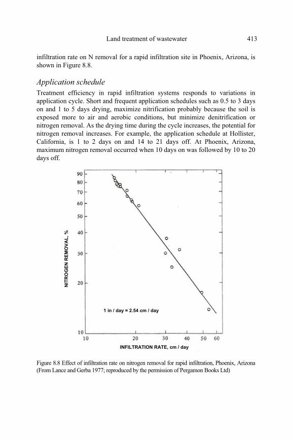
Land treatment of wastewater 413
infiltration rate on N removal for a rapid infiltration site in Phoenix, Arizona, is
shown in Figure 8.8.
Application schedule
Treatment efficiency in rapid infiltration systems responds to variations in
application cycle. Short and frequent application schedules such as 0.5 to 3 days
on and 1 to 5 days drying, maximize nitrification probably because the soil is
exposed more to air and aerobic conditions, but minimize denitrification or
nitrogen removal. As the drying time during the cycle increases, the potential for
nitrogen removal increases. For example, the application schedule at Hollister,
California, is 1 to 2 days on and 14 to 21 days off. At Phoenix, Arizona,
maximum nitrogen removal occurred when 10 days on was followed by 10 to 20
days off.
Figure 8.8 Effect of infiltration rate on nitrogen removal for rapid infiltration, Phoenix, Arizona
(From Lance and Gerba 1977; reproduced by the permission of Pergamon Books Ltd)
NIT
RO
GE
N R
EM
OV
AL
, %
INFILTRATION RATE, cm / day
1 in / day = 2.54 cm / day

414 Organic waste reuse and recycling: technology and management
Example 8.3
A sandy soil with an infiltration capacity of 90 cm/day will be used for
wastewater treatment and renovation through the rapid infiltration (RF) process.
Based on a laboratory study and Figure 8.1, the following wastewater
application modes were found suitable for the RI operation.
Average wastewater application rate = 30 m/yr
Application period = 4 days
Resting period = 10 days
Determine whether this RI operation will create flooding condition or not.
Wastewater cycle time = 4 +10 = 14 days
Number of cycle per year = 365/ 14 = 26
Wastewater application per cycle = 30/26 = 1.15 m/cycle
Wastewater application rate = (1.15 m/cycle)/ 4 days
= 0.29 m/day-cycle
= 29 cm/day-cycle
The wastewater application of 29 cm/day is less than the soil infiltration
capacity of 90 cm/day, so flooding will not occur.
Note: Suppose 1 ha land is used for this RI unit, the wastewater flow would
be 822 m3/day. Since the wastewater application rate of 29 cm/day is equivalent
to a wastewater flow rate of 2,900 m3/day, for the application period of 4 days, a
storage reservoir of 11,600m3 capacity should be built to store the wastewater
sufficient for the above RI operation.
8.4.3 Overland flow or OF system
Wastewater application rate
Overland flow is a form of a fixed-film biological reactor. The application rate
should therefore be predictable on the basis of the kinetics of treatment and the
required treatment levels. For example, high-quality effluent has been produced
in research projects using these application rates: raw wastewater, 10 cm/week;
primary effluent, 15 to 20 cm/week; and secondary effluent, 25 to 40 cm/week.
With all three application rates, the runoff contained less than 10 mg/L BOD5 on
the average. Slopes of the land were 2 to 4% and 36 m long (Tucker and Vivado
1980).

Land treatment of wastewater 415
Wastewater application rates for OF systems are usually determined from
comparisons with existing systems and research projects (see also Figure 8.1
and Table 8.2). For raw wastewater, 7.5 to 10 cm/week should be considered.
For primary effluent, 10 to 20 cm/week could be used, depending on the level of
overall treatment required. For secondary effluent, either from waste
stabilization ponds or conventional secondary treatment facilities (e.g. activated
sludge or trickling filters), the need is either for polishing (further reductions for
BOD5 and suspended solids) or for nutrient removal. For polishing, 20 to 40
cm/week could be considered. For nutrient removal, only 10 to 20 cm/week may
be possible because adequate detention time is necessary for denitrification.
Application schedule
Experience with existing systems suggests application schedules to be 6 to 8
hours on and 16 to 18 hours off over 5 to 6 days/week. At Melbourne, Australia,
however, the application has been continuous rather than intermittent. The
optimum cycle will depend on the climate and the BOD5 loading. Other
considerations include the harvesting of grass and the potential for propagation
of insects.
8.4.4 Other design considerations
There are many factors that determine the area required for a wastewater land
treatment system. These factors are related to the characteristics of the soil,
wastewater, climate, crop, pre-application treatment, and should be evaluated
using site-specific information.
In determining the required land area, the land area for each potentially
limiting parameter (such as hydraulic, nitrogen, toxic compounds and salt
loadings) should be evaluated. The parameter that requires the largest land area
to avoid environmental problems becomes the limiting parameter. When the
land area determined for the limiting parameter is used for the design of a land
treatment system, there is an additional degree of safety in terms of the
application rates of the other constituents or parameters of concern.
It should be possible to determine application rates for land treatment
systems on a case-by-case basis using data on soil infiltration rates, climate,
wastewater characteristics, and required treatment performance. Unfortunately,
neither the relationship between the infiltration rate and loading rate nor the
relationship between the loading rate and treatment performance have been
developed to the point where they can be used in design without requiring
comparisons with other land treatment systems.

416 Organic waste reuse and recycling: technology and management
Pre-application treatment
Pre-application treatment of wastewater to be used for land treatment is
necessary to:
• Inactivate the entero-pathogenic organisms to an acceptable levels
so that public health risks to the workers, grazing animals or human
beings who consume those irrigated crops are minimized (see
section 8.7),
• Minimize operational problems in distribution systems such as
clogging of the spray nozzles and distribution pipes, etc.,
• Lengthen the working life of land treatment sites as clogging of the
soil pores will be less when pre-treated wastewater is applied,
• Prevent nuisance conditions during wastewater storage prior to
being applied to land.
Screening, screening with comminution, aeration, ponding, and disinfection
are the common types of pre-treatment facilities used. In case of industrial
wastewaters containing some toxic compounds, other pre-application treatment
such as chemical precipitation and flocculation/sedimentation might be
necessary. Where concern is on nitrate contamination to groundwater aquifers,
pre-application treatment may include ammonia stripping, water hyacinth pond
treatment, or storage ponds having a long detention time, to reduce the nitrogen
content.
The level of pre-application treatment provided should be the minimum
necessary to achieve objectives stated above. Any additional treatment will, in
most cases, only increase cost and energy use.
Crop selection
Crop selection is an important factor in SR and OF processes. Presence of
suitable crops on the application area will reduce the erosion, provide support
media for microorganisms, remove the wastewater nutrients by plant uptake and
produce revenue where markets for these crops exist. Nutrient uptake capacity
(see Table 8.7), tolerance to high soil moisture conditions, consumptive use of
water and irrigation requirements and revenue potential should be considered
when selecting a crop for SR and OF systems. In SR system, presence of crop
will maintain or increase the soil infiltration rate. In OF system, a mixture of
grasses is generally preferred over a single species. Corn and paddy are also
suitable crops to be used but the public health aspects should be studied in detail
as the public consumes these crops.

Land treatment of wastewater 417
Storage
Storage of wastewater is required for any process of land treatment in order to
equalize the incoming flows, to maintain constant application rates, and in the
case of repairs or operational problem in the distribution system. Even though
SR and RI systems are capable of operating during adverse climatic conditions
storage may be required. In the case of OF system, storage is necessary to
accommodate the wastewater during rainy and winter seasons due to reduced
hydraulic loading or complete shut down, and also to accommodate stormwater
runoff. Generally 5-10 days of storage is sufficient to overcome the problems.
Distribution system
Distribution system design consists of two important components:
• selection of the type of distribution system, and
• detail design of system components.
Method of wastewater distribution varies with the type of land treatment
system. For SR system, either surface distribution system in which wastewater
is applied to the land at one end and allowed to spread over the field by gravity
(Figure 8.2 b) or sprinkler distribution system where the wastewater is spread
over the land by sprinklers (Figure 8.2 c) is suitable. In the case of RI system,
wastewater distribution is usually by surface spreading (Figure 8.3). This
method employs gravity flow from piping systems or ditches to flood the
application area. Wastewater distribution onto OF slopes can be achieved by
surface methods, low-pressure sprays and high-pressure impact sprinklers.
Choice of the appropriate system should be based on minimization of
operational difficulties such as uneven distribution onto the slope, and also the
operational cost of the system. If surface distribution method is adopted, the
land should be perfectly levelled to avoid ponding. Extreme care should be
taken when sprinkler system is used for the treatment area situated near
residential areas to avoid spreading of pathogens due to aerosols and wind
action.

418 Organic waste reuse and recycling: technology and management
8.5 LAND TREATMENT- DESIGN EQUATIONS
Mathematical models for the three land treatment processes have not been
extensively developed. This is due partly to the complex nature of land
treatment involving the physical, chemical and biological reactions. Efficiency
of a land treatment system also depends on climate and soil conditions at the
specific site. SR process is normally designed based on practical experiences.
Some empirical and rational models for the RI and OF processes have been
developed.
8.5.1 RI process
Treatment performance of RI systems with respect to nitrogen and phosphorus
removal is given below.
Nitrogen removal
Application rates up to 30 cm/day with 20 mg/L of ammonia will result in a
nitrified effluent. As wastewater temperatures drop, the rate of nitrification will
also decrease. For nitrification, the loading cycle should consist of short
application periods (1 day or so) and relatively long drying periods (5 to 10
days) to allow for aeration and the occurrence of aerobic conditions in the soil
favourable for the growth of nitrifying bacteria.
Nitrogen removal by denitrification requires both adequate organic carbon
and adequate detention time. Nitrogen removal can be expressed by the
following equation (Reed and Crites 1984).
TOC - 5
Nt= (8.5)
2
Where:
Nt = total nitrogen removal, mg/L
TOC = total organic carbon in the applied wastewater, mg/L
The 5 mg/L of residual TOC is typical for municipal wastewater passage
through about 5 ft (1.5 m) of soil. The coefficient 2 in the denominator is based
on experimental data where 2 g wastewater carbon was required to denitrify 1 g
of wastewater nitrogen.

Land treatment of wastewater 419
Nitrogen removal is also related to infiltration rate and an application rate of
15 cm/day is recommended as a maximum where 80% N removal is needed
with secondary effluent (Figure 8.8). When primary effluent is used, the
maximum application rate is recommended not to exceed 20 cm/day.
Phosphorus removal
There is no crop uptake in RI systems and the nature of the soils and high
hydraulic rates used require greater travel distances in the soil for effective P
removal.
An equation to predict phosphorus removal at RI sites has been developed
from data collected at number of operating systems (Reed and Crites 1984).
Px = Po .exp(-kt) (8.6)
Where:
Px = total P concentration at a distance x along the percolate flow path, mg/L
P0 = total P concentration in the applied wastewater, mg/L
k = instantaneous rate constant, 0.002/hr at neutral pH
t = detention time = x. /I, hr
x = distance along the flow path, in
= volumetric water content, usually 0.4
I = infiltration rate, in/hr
8.5.2 OF process
Based on a pilot study conducted by Smith and Schroeder (1985), it was found
that the removal of organic material from primary effluent is accomplished in
two stages as a function of slope length (z) and application rate (q).
In the first stage a rapid removal of organic matter takes place within the first
6 to 10 meters of slope length and in the second stage a slower rate of organic
removal takes place in the remainder of the slope.
From a practical design and operation standpoint only the second stage would
be the basis for design and operation.
The probable reason for the observation of the two distinct rates of organic
removal over the length of the overland flow slope is that settleable matter is
removed readily by sedimentation in the first few meters, leaving colloidal and
soluble organic material to be removed at a slower rate by adsorption and,
ultimately, bacterial assimilation over the remaining length of the slope.
The mathematical model was developed from the studies made on lands with
down-slope grade of 2% and cross-slope grade of 0.2% with a mixture of
420 Organic waste reuse and recycling: technology and management
perennial rye grass, annal rye grass, orchard grass, and tall fescue grass. The tall
fescue grass was predominant.
BOD5 and TOC removal
Removal of BOD5 and TOC from wastewater and primary effluent after the first
9 m of travel down the overland flow slope followed the first-order removal
model:
Cz/Co = A.exp(-K.z) (8.7)
Where:
z = distance down-slope, in m (z > 9 m)
Cz = organic concentration (BOD5 or TOC) at a distance (z) down-slope, mg/L
Co = initial organic concentration (BOD5 or TOC), mg/L
K = empirically determined overall rate constant
A = empirically determined coefficient
It has been shown that BOD5 concentrations in the runoff from overland flow
slopes approach a nonzero value in the range of 3 to 5 mg/L. Effluent BOD5 and
TOC concentrations approach average values of 5 mg/L and 7 mg/L, respectively,
after 64 m of down-slope travel. Hence the removal models were modified to
account for this as follows:
BOD5 removal model:
(C - 5)/Co = A.exp (-K.z) (8.8)
TOC removal model:
(C - 7)/Co = A'.exp (-K'.z) (8.9)
Where:
C = required effluent BOD5 or TOC concentrations at distance z
K and K' = empirical rate constants for BOD5 and TOC removal, respectively
A and A' = empirical coefficients for BOD5 and TOC removal, respectively
The overall rate constants K and K' in Equations 8.8 and 8.9 vary as a function
of application rate q, according to the following equation:
K or K' = k/qn (8.10)
Where, k and n are empirical coefficients and q is wastewater application rate
whose unit is m3/(hr-m of slope width).

Land treatment of wastewater 421
Then,
BOD5 model: (C - 5)/Co = A.exp (-k.z/qn) (8.11)
TOC model : (C - 7)/Co = A'.exp (-k’.z/qn) (8.12)
The values of coefficients k and n, obtained for q values ranging from 0.1 -
0.37 m3 / (hr-m) are summarized in Table 8.9.
A family of curves that describe BOD5 and TOC removal as functions of
slope length (up to 64 m) and application rates (0.1, 0.16, 0.25, and 0.37 m3/(hr-
m)) for raw wastewaters and primary effluent are shown in Figures 8.9 – 8.12
(application periods were up to 16 hr/day). Either application rate or slope
length may be used as the independent design variable. The variation of A and
A' with q was found to be inconsistent. Therefore, for design purposes, it would
be satisfactory to use directly the family of curves given in Figures 8.9 to 8.12.
When designing a system, the required or desired level of treatment is
known. Thus a value for (C - c)/Co, according to Equation 8.8 or Equation 8.9
can be established. If slope length is used as the independent variable then a
design value for slope length, z, is selected. The required value of application
rate, q, is then determined by entering the appropriate curve with the known
values of z and (C - c)/Co. Alternatively, if application rate q is the independent
design variable, then a value for q is selected and the required value of slope
length, z is taken from the curves. The independent design parameter used
depends on the individual case.
Table 8.9 Summary of coefficients for BOD5 and TOC removal models (Smith and Schroeder 1985)
Coefficient value
Applied wastewater k N
Primary effluent
BOD5
TOCScreened raw wastewater
BOD5
TOC
0.0430.038
0.0300.032
0.1360.170
0.4020.350
From Smith and Schroeder (1985); reproduced by the permission of the Water Pollution Control Federation, U.S.A.
A later study by Witherow and Bledsoe (1986) confirmed the removal of
BOD5, TOC, total suspended solids (TSS) and NH4-N to follow the models
given in Equation 8.11 and 8.12. By setting n at 0.5 and using field data from a
4-ha OF site in Oklahoma, U.S.A., the intercept constant A and rate constant k
of equation 8.13 for the four pollutants are given in Table 8.10.

422 Organic waste reuse and recycling: technology and management
Cz/Co = A.exp (-k.z/q0.5) (8.13)
The total area required for slopes must be determined to complete the system
design. Total area required may be computed by the following equation:
Area = (Q) (z)/(q) (pd) (8.14)
Where,
Area = total area of OF site, m2
Q = design daily flow, m3/day
z = slope length, m
q = application rate, m3/(hr-m)
Pd = daily application period, hr/day
Design values for Q, p and q should be selected to allow operating flexibility
during periods when parts of the system must be shut down for harvesting or
repairing.
Figure 8.9 BOD5 fraction remaining versus distance down-slope; application rate study
with screened raw wastewater (Smith and Schroeder 1985)
Distance down slope (m)
BO
D5 f
racti
on
rem
ain
ing
(C
-5/C
o)

Land treatment of wastewater 423
Figure 8.10 TOC fraction remaining versus distance down-slope; application rate study
with screened raw wastewater (Smith and Schroeder 1985)
Table 8.10 Intercepts (A) and rate constants (k) of Equation 8.13 (adapted from Witherow and Bledsoe 1986)
Pollutants A k (m/hr)
TSS 0.44-0.96 0.024-0.056 BOD5 0.58-0.88 0.030-0.046 TOC 0.57-0.88 0.016-0.039 NH4-N 0.99-1.12 0.016-0.054
Distance down slope (m)
TO
C f
racti
on
re
main
ing
(C
-7/C
o)

424 Organic waste reuse and recycling: technology and management
Figure 8.11 BOD5 fraction remaining versus distance down-slope; application rate study
with primary effluent (Smith and Schroeder 1985)
Design daily flow (Q)
It is preferable to provide equalization or off-line storage facilities to allow for
constant application rates and short-term storage during power outage or
extremely heavy precipitation. The design daily flow should be based on peak
seasonal average daily flow. For systems without such storage facilities the
design daily flow Q should be based on the average flow during selected period
depending on the flow conditions.
Distance down slope (m)
BO
D5 f
rac
tio
n r
em
ain
ing
(C
-5/C
o)

Land treatment of wastewater 425
Figure 8.12 TOC fraction remaining versus distance down-slope; application rate study
with primary effluent (from Smith and Schroeder 1985; reproduced by permission of the
Water Pollution Control Federation, USA)
Design application rate (q)
The design q value for an OF should generally match with the infiltration rate of
the soil or vegetated surface of the soil, to prevent excessive run-off and
impairment of effluent quality. The value of q in Equation 8.14 should be less
than the value used to determine z to provide a safety factor in process
performance and to allow operating flexibility by permitting a range of
application rates to be used. A factor of 1.5 is suggested for design. Thus, if a
design value for q of 0.37 m3/(hr-m) is used to determine z, then a design value
for q of 0.25 m3/(hr-m) should be used in Equation 8.13 to calculate the required
area.
Design application period (Pd)
Design application periods of 8-12 hr/day are recommended. For small systems
it may be more convenient or cost-effective to operate only during one working
Distance down slope (m)
TO
C f
racti
on
re
main
ing
(C
-7/C
o)

426 Organic waste reuse and recycling: technology and management
shift. In this case, the entire area would receive the design daily flow during 8-
hour application period. Storage facilities would be required to hold wastewater
during the 16 hr non-operating period.
Example 8.4
Determine the area required for land treatment of wastewater using the overland
flow method.
The following information is given: screened raw wastewater is to be used;
the flow (Q) is 3,000 m3/day; the influent BOD5 (Co) is 200 mg/L; and the
required effluent BOD5 (C) is 20 mg/L.
The necessary design calculations are as follows:
Compute the required removal ratio, (C - 5)/Co, from Equation 8.8:
(C - 5)/Co = (20 - 5)/200 = 0.07
Select an application rate, q, in valid range of the model:
q = 0.25 m3/ (hr-m)
Determine required value of slope length, z, using Figure 8.9:
z = 37 m
Select application period, Pd.
Pd = 8 hr/day
Compute q for area calculation
q = (0.25 m3/(hr-m)/1.5
q = 0.17 m3/(hr-m)
Compute required total area from Equation 8.14. Assume 7 days/wk
application frequency.
Area = (Q) (z)/ (q) (Pd)
Area = (3,000 m3/day) (37 m)/(0.17 m3/(hr-m))(8 hr/day)
= 81,620 m2 ≈ 8.2 ha
Comparison of current design based on hydraulic loading
Assume the hydraulic loading = 3 cm/day (Figure 8.1)
Land area required is given by:
Area = 3.65 Q/Lh (8.14)
Where,
Area = Wetted land area, ha;
Q = Design flow, m3/day; and
Lh = Hydraulic loading, cm/yr.

Land treatment of wastewater 427
Therefore,
Area = (3.65x3, 000 m3/day)/(3 cm/day x 365 days/year)
= 10 ha
From the required area values obtained using both design criteria, it can be
seen that the mathematical model presented based on application rate, slope
length and application period (Equation 8.14), gives an economical value of 8.2
ha compared to an area of 10 ha with a 3 cm/day hydraulic loading.
Example 8.5
A wastewater has the following characteristics.
Flow rate = 100 m3/day
BOD5 = 250 mg/L
Fecal coliforms = 6 x 10⁵ no./100 mL
Design precipitation = 1000 mm/year
Percolation = 400 mm/year
Evapo-transpiration = 1200 mm/year
a) If the soil type is clay loam, which type of land treatment could be
suitable?
b) Determine whether there will be run-off from this land treatment or
not, if so calculate the run-off in m3/day.
c) From the experimental results it was found that the wastewater
application cycle to this land should be 3 days of application and 11
days of resting. Application area of the site is 14 ha. Determine the
approximate wastewater application rate to be applied, which will
not produce run-off.
Solution:
a) As the soil type is clay loam, the suitable type of land treatment will be the
OF system (according to Figure 8.1).
b) From Figure 8.1:
Choose a liquid loading rate = 4 in/week
= 4 x 25.4 x 52 mm/year
= 5283 mm/year.
General mass balance equation for land treatment of wastewater is given in
equation 8.3:
Design precipitation + wastewater applied = percolation + evapotranspiration + runoff.
1000 + 5283 = 400 + 1200 + Runoff

428 Organic waste reuse and recycling: technology and management
Runoff = 4683 mm/year
Application rate = 4 x 2.54 cm/week
Assuming that the wastewater is applied continuously: 4 x 2.54 x 10-2
Liquid loading rate = m/day = 0.0145 m/day
7
100 m3/d
Area required = = 6889 m2
0.0145
Choose the land area required = 7000 m2
7 x 103 x 4.683
Total run off from site = m3/day = 89.8 m3/day
365
c) If there should not be any run off from the land, then from equation 8.3,
wastewater applied = 400 + 1200 - 1000 = 600 mm/year which is less than
the liquid loading rate in (b).
No. of days in one cycle = 14 days
No. of cycle in year = 26
600
Wastewater flow rate to be applied = mm/cycle
26
No. of days of application/cycle = 3 days
600
Application rate = mm/day = 7.7 mm/day during the 3 days
3x26
application period.
If the application area is 14 ha, wastewater flow rate to be applied during the
application period is 0.0077 × 14 × 104 =1078 m3/day which is greater than the
available flow rate of 100 m3/day.

Land treatment of wastewater 429
Example 8.6
A wastewater has the same characteristics as in Example 8.5. Design an OF
system to treat this wastewater so that the treated effluent contains BOD5 and
fecal coliforms less than 50 mg/L and 100 no./100 mL, respectively. The
application rate is 0.1 m3/(hr-m width).
The following information are given
C - 5 0.02 z
For BOD5 removal = 0.72 exp (- )
Co q0.5
N
For fecal coliform removal = exp ( - Kf.t)
No
Where:
N and No= effluent and influent fecal coliform concentration, no./100 mL
Kf = fecal coliform removal rate in OF, 0.2/min
t = time of wastewater flow in OF
1
v = R2/3S1/2
n
Where:
v = flow velocity of wastewater during OF treatment, m/sec
R = hydraulic radius of flow, m
S = slope of soil = 0.02
n = coefficient of roughness = 0.38
For BOD5 removal
50 - 5 0.02 z
( ) = 0.72 exp (- )
250 0.10.5
Slope length, z = 22 m for BOD5 removal

430 Organic waste reuse and recycling: technology and management
For fecal coliform removal Assuming that during wastewater application, the height of wastewater is 5 cm throughout the entire down slope distance
Wetted area Hydraulic radius, R = Wetted perimeter
Q 100 m3/day Width of the applied area = = = 41.7 m q 0.1 m3/hr-m
≈ 42 m
42 (0.05) R = = 0.05
42+2(0.05) 1 v = (0.05)2/3 (0.02)1/2 = 0.05 m/sec 0.38 100 Fecal coliform reduction = exp (-0.2 t) 6x10⁵
t = 43.5 min
Slope length for fecal coliform removal = 0.05x43.5x60 = 130.5 m
Choose slope length of the OF area of 130.5 m to provide the treated effluent
quality meeting the required BOD5 and fecal coliform concentrations. Width of
the applied area is 42 m.
8.6 SYSTEM MONITORING
Monitoring of land treatment systems involves the observation of significant
changes resulting from the application of wastewater. The monitoring data are
used to confirm environmental assessment and to determine if any corrective
action is necessary to protect the environment or maintain the renovation
capacity of the system. The components of the environment that need to be
observed include wastewater, groundwater, and soils upon which wastewater is
applied and, in some cases, vegetation growing in soils that are receiving
wastewater.

Land treatment of wastewater 431
Water quality
Monitoring of water quality for land application systems is generally more
involved than for conventional treatment systems because non-point discharges
of system effluent into the environment are involved. Monitoring of water
quality at several stages of a land treatment process may be needed for process
control. These stages may be at: the applied wastewater, the renovated water,
and the receiving waters - surface water or groundwater.
The water quality parameters and the frequency of analysis will vary from
site to site depending on the nature of the applied wastewater. The measured
parameters may include:
• Those adversely affect receiving water quality either as drinking
water supply or as irrigation water supply,
• Those required by regulatory agencies, and
• Those necessary for system control.
An example of a suggested water quality monitoring program for a large
scale SR system is presented in Table 8.11. Renovated water may be recovered
as runoff in an overland flow system, or as drainage from underdrains, or
groundwater from recovery wells in SR and RI systems.
Groundwater
In groundwater, travel time of constituents is slow and mixing is not as
significant as with surface water. Surface inputs near a sampling well will move
vertically and arrive at the well much sooner than inputs several hundred meters
away from the well. Thus, the groundwater sample represents contributions
from all parts of the surface area with each contribution arriving at the well at a
different time. A groundwater sample may reflect surface inputs, especially
inorganic constituents such as heavy metals, from several years before sampling
and have no association with the land application system. Consequently, it is
imperative to obtain adequate background quality data and to locate sampling
well so that response times are minimized.
If possible, existing background data should be obtained from wells in the
same aquifer both beyond and within the anticipated area of influence of the
land application system.
Wells with the longest history of data are preferable. Monitoring of
background wells should continue after the system is in operation to provide a
base for comparison.
In addition to quality, the depth to groundwater should be measured at the
sampling wells to determine if the hydraulic response of the aquifer is consistent
with what was anticipated. For SR systems, a rise in water table levels to the

432 Organic waste reuse and recycling: technology and management
root zone would necessitate corrective action such as reduced hydraulic loading
or adding under drainage. The appearance of seeps or perched groundwater
tables might also indicate the need for corrective action.
Soil
In some cases, application of wastewater to the land will result in changes in soil
properties. Results of soil sampling and testing will serve as the basis for
deciding whether the soil properties should be adjusted by the application of
chemical and organic amendments. Soil properties that are important to land
treatment of wastewater include: pH, exchangeable sodium percentage or SAR,
salinity, nutrient status, and heavy metals.
Soil pH below 5.5 or above 8.5 generally is harmful to most plants. Below
pH 6.5 the capacity of soils to retain metals is reduced significantly, the soil
with pH above 8.5 generally indicates high sodium content and possible
permeability problems.
The levels at which salinity becomes harmful to plant growth depend on the
type of crop. Salinity in the root zone is controlled by leaching soluble salts to
the subsoil or drainage system.
Crop tissue
Plant tissue analysis is probably more revealing than soil analysis with regard to
deficient or toxic levels of elements. All of the environmental factors that affect
the uptake of an element are integrated by the plant, thus eliminating much of
the complexity associated with interpretation of soil test results. If a regular
plant tissue monitoring program is established, deficiencies and toxicities can be
determined and corrective action can be taken.

Land treatment of wastewater 433
8.6.5 Case studies
The followings are successful case studies for the three-land treatment processes
operated at full-scale in the USA.
Table 8.11 Monitoring program for a large slow-rate system (U.S.EPA 1973)
Frequency analysis
Groundwater
Parameters
Appliedwater
Soil Plants
Onsitewells
Perimeter wells
Backgroundwells
Flow C - - - - - BOD5 of TOC W - - Q Q Q COD W - - Q Q Q Suspended solids W - - - - - Nitrogen, total W 2A A Q Q Q Nitrogen, nitrate - - - Q Q Q Phosphorus, total M 2A A Q Q Q Coliforms, total W - - Q Q Q pH D Q - Q Q Q Total dissolved solids
M - - Q Q Q
Alkalinity M - - Q Q Q SAR M Q - Q Q Q Static water level - -- - M M M
Legend: C = continuously 2A = Two samples per year D = Daily A = Annually Q = Quarterly M = Monthly W = Weekly SAR = Sodium absorption ratio Note: Wastewater applied and groundwater should be tested initially and periodically thereafter, as appropriate, for heavy metals, trace organics, or other constituents of environmental concern.
Slow rate process
The city of San Angelo in Texas, USA, owns and operates a wastewater
irrigation system with an area of 259 ha and a capacity of 1.9x10⁴ m3/day. The
surface soil is clay and clay loam. A hay crop is grown, which is baled and sold,
and an average of 500 cattle are grazed on the pasture land (Crites and Pound
1976). Primary treatment of the wastewater precedes surface irrigation, and
about 1 week of storage capacity is available when irrigation is not needed.
Operating and performance data of this system are shown in Table 8.12.

434 Organic waste reuse and recycling: technology and management
Rapid infiltration process
At Lake George, New York, a rapid filtration system has been in operation since
1933. The soil type is sand. Wastewater that has received secondary treatment
from trickling filters is spread at a rate of about 76 cm/week in the summer. In
the winter the application rate is reduced to 18 cm/week because of reduced
flows (the city's population fluctuates seasonally). Spreading of the wastewater
is continuous, and when ice forms on the surface it is not removed but merely
floated by the next wastewater application (Crites and Pound 1976). The
operating and performance data are shown in Table 8.13.
Table 8.12 Operating and performance data of an irrigation system in San Angelo, Texas (U.S. EPA 1981)
Annual wastewater loading rate, cm/yr
BOD in applied wastewater, mg/L BOD in percolate, mg/L BOD removal, %
Total N in applied wastewater, mg/L as N Total N in percolate, mg/L as N N removal, %
290
890.799
35.46.183
Table 8.13 Operating and performance data of a rapid infiltration system in Lake George, New York (U.S. EPA 1981)
Hydraulic loading rate, cm/week Summer loading rate, cm/week Winter loading rate, cm/week BOD:N ratio Flooding to drying time ratio
Average BOD loading rate, kg/(ha-day) BOD in applied wastewater, mg/L BOD in percolate water, mg/L BOD removal, %
Total N in applied wastewater, mg/L as N Total N in percolate, mg/L as N Removal of total N, %
Soluble phosphate in applied wastewater, mg/L as P Soluble phosphate in percolate, mg/L as P Removal of soluble phosphate, %
Fecal coliforms in applied wastewater, MPN/100 mL Fecal coliforms in percolate, MPN/100 mL
5876182:11:4
53601.298
11.5 (summer), 12.0 (winter) 7.70 (summer), 7.50 (winter) 33 (summer), 38 (winter)
2.1< 1 (summer), 0.014 (winter) > 52 (summer), 99 (winter)
359,00072 (summer), 0 (winter)

Land treatment of wastewater 435
Overland flow process
The Campbell Soup Company in Paris, Texas, USA, operates a complete line of
heat-processed soups as well as beans and spaghetti products. Its 364-ha
overland flow treatment site is planted with water tolerant grasses, such as reed
canary grass, perennial rye grass, bermuda grass, tall fescue, and native
vegetation (Loehr et al. 1979). The soils at the site are sandy loam, clay, and
clay loam. Study of the fate of the applied wastewater indicates that about 20%
percolates down through the soil, 10-30% is lost by evapo-transpiration, and the
remaining 60% returns to the surface stream as runoff (Loehr et al. 1979). A
sprayed effluent is allowed to flow down 45-60 m slopes ranging from 2 to 6
percent. Grasses are harvested two or three times a year as cash hay crops. The
purified water (or runoff) is discharged to the receiving stream via prepared
waterways. Table 8.14 shows the design, operation and performance data of this
system.
This overland flow system operates as well in winter as in other seasons.
Although the removal of phosphorus was about 42%, a later change in the
operating procedure, to provide a longer rest period between applications with
no change in the total wastewater volume, has increased phosphorus removal to
nearly 90% without affecting the BOD or nitrogen removals.
Table 8.14 Design, operation and performance data of overland flow process of the Campbell Soup System, Paris, Texas (Loehr et al. 1979; Hinrichs et al. 1980)
Length of slope SlopeSize of sprinkler nozzles Distance between sprinklers Operating pressure at sprinkler heads PretreatmentVolume of wastewater treated Number of months working in a year Wastewater application rate Wastewater application schedule
45-60 m 2-6%6.5 (50 L/min)-8 (80 L/min) mm 25 m 340-480 kPa Screen and degrease 22,700 m3/day 12 months/yr 5-7.6 (cm/wk) 6-8 hr/day on, 16-18 hr/day off
Mean concentration (mg/L) Removal (%) Parameter
Influent Effluent Concentration Mass (based on runoff)
TSS BODNP
26361617.47.6
1692.84.3
93.598.583.942.5
98.299.191.561.5

436 Organic waste reuse and recycling: technology and management
Chemical analyses of the soil indicate that while the concentration of sodium
salts is increasing, it has not reached a level injurious to plants and is not
expected to do so in the future. Similarly, nitrates percolating into the
groundwater reserve are not expected to build up to the point of concern.
8.7 PUBLIC HEALTH ASPECTS AND PUBLIC
ACCEPTANCE
Land treatment of wastewater provides many potential benefits but carries with
it the risk of contamination of human and animal food. Land treatment can
produce an equal or better quality of effluent than a conventional treatment
process, but the public is not aware of it. To be a successful method of
wastewater treatment and reuse, the public acceptance of land treatment as a
safe and suitable method is very important.
The major health concern is possible pollution by nitrogen, heavy metals,
toxic organic compounds and pathogens.
8.7.1 Nitrogen
Excess concentration of nitrate (greater than 10 mg/L, NO3-N) in drinking water
will be the major health concern for infants under 6 months of age. The major
pathway of concern in land treatment is conversion of the wastewater nitrogen
to nitrate and percolation to drinking water aquifers. All three land treatment
methods are quite efficient in nitrification of the wastewater nitrogen. Since OF
is a surface discharge system, it is only the SR and RI systems that are of
concern for groundwater impacts. Nitrogen is often the limiting factor for design
of SR system. Appropriate amount of nitrogen in the percolate can be achieved
by selecting proper crop and application rate. The very high loading rates
inherent in RI systems result in the greatest potential for nitrate contamination of
drinking water in the underground aquifers. The extent of nitrification and
nitrate contamination depend on temperature, carbon source, hydraulic loading
rate, loading period and physical properties of the soil. To overcome this
problem the treatment site can be located far away from drinking water sources,
or located above non-drinking water aquifers, or recover the percolate with
wells or underdrains for reuse elsewhere. An alternative that has been proposed
is to use a two step land treatment consisting of OF system followed by RI
system; in this way most of nitrogen could be recovered during the OF process
through biomass uptake, nitrification/denitrification, and volatilization.

Land treatment of wastewater 437
8.7.2 Heavy metals and other toxic organic compounds
The pathways of potential concern are movement of metals and other toxic
organic compounds to drinking water sources and translocation of these
compounds through the food chain to human. The plants grown on a land
treatment site can accumulate toxic compounds in their leaves, stems and fruits.
Removal of metals and toxic compounds is generally effective in all three land
treatment methods with that effectiveness retained for considerable period of
time. Since the problem of heavy metal and toxic compound pollution is more
serious with respect to sludge application to land, this matter will be discussed
more in Chapter 9.
8.7.3 Pathogens
The pathogens of concern in land treatment systems are bacteria, parasites and
viruses. The major pathways of concern are to the groundwater, internal or
external contamination of crops, translocation to grazing animals and human,
and off-site transmission via aerosols or runoff. There is no evidence available
indicating transmission of parasite diseases from application of wastewater in
land treatment systems, because the parasite cysts and eggs will normally settle
out during pre application treatment or in storage ponds. But there are chances
of human infection by parasite diseases if the land treatment area is accessible to
the public. It has been found that Ascaris ova will survive in soil for long period
and investigations on a site in France proved the presence of ascaris ova in soil.
Concerns, with respect to crop contamination, focus mainly on surface
contamination and then persistence of the pathogens until consumed by human
or animals or the internal infection of the plant via the roots. As shown in Figure
8.13, pathogen survival periods on leaves and fruit crops tend to be shorter than
the growth periods of most of these plants (Strauss 1986). In soil, however,
survival of viruses, Salmonellae bacteria, and Ascaris eggs may exceed the
growth period of crops (Figure 8.14). Viable pathogens are therefore more likely
found on root crops and soil than on leaf crops.
Human or animal infection can be reduced by taking preventive methods
such as prohibiting the consumption of raw vegetables grown on land treatment
sites, and allowing a period of two weeks or more after application of
wastewater before animals are allowed to graze. This will allow sunlight to kill
most of the fecal bacteria and viruses. As time and temperatures have significant
effects on pathogen die-off (Figure 3.1), prolonged storage of wastewater or
sludge to be applied to crops will help minimize the public health risks. Strauss
(1986) suggested storage periods for pathogen inactivation in excreta, as shown
in Table 8.12.

438 Organic waste reuse and recycling: technology and management
Runoff from a land treatment site might be a potential pathway for pathogens
transport; but this is not a problem in RI system. Groundwater contamination
has the highest potential for RI system due to the high hydraulic loading rate
and coarse texture of the receiving soils.
Table 8.15 Tentative recommendations for excreta storage periods in warm climates
Storage period Hygienic quality acheived
2 days Inactivation of Clonorchis and Opisthorchis eggs 1 month Complete inactivation of viruses, bacteria and protozoa
(except, possibly, Salmonella on moist, shaded soil); inactivation of schistosome eggs
4 months Inactivation of nematode (roundworm) eggs e.g. hookworm and whipworm (Trichuris); survival of a certain percentage (10-30%) of Ascaris eggs
12 months Complete inactivation of Ascaris eggs
From Strauss (1986); reproduced by the permission of IRCWD
Figure 8.13 Pathogen survival on crops vs. vegetable growth periods in warm climates
(from Strauss 1986; reproduced by permission of IRCWD, Switzerland)
1) Determined under widely varying conditions 2) Maturation period from transplanting or from sowing if not transplanted
1

Land treatment of wastewater 439
The potential for transport of pathogens by aerosols from land treatment sites
has been the most controversial issue in recent years. The main reason for this
controversial is due to the unawareness of the difference between aerosols and
sprinkler droplets. To avoid bacterial and virus transport through aerosols it is
preferable to locate the treatment site away and down wind from the residential
areas, when sprinklers are used for distribution of wastewater. Depending on the
wind speed and topography, pathogen-carried aerosols can travel several
hundred meters away from the land treatment site.
With respect to epidemiological study of land treatment of wastewater, it
appears from Table 2.26 that the relative health risks due to intestinal nematodes
are high, followed by bacterial and viral infections. The microbiological quality
guidelines (Table 2.27) suggest that the density of viable eggs of intestinal
nematodes (Ascaris, Trichuris and hookworms) be equal to or less than 1 per L
of wastewater to be used for both restricted and unrestricted irrigation. With
respect to fecal coliforms, their density should be less than 1000 no. per 100 mL
of wastewater to be used for unrestricted irrigation. A relaxed standard of fecal
coliform density is applied to wastewater to be used for restricted irrigation.
Figure 8.14 Pathogen survival in soil vs vegetable growth periods in warm climates
(from Strauss 1986; reproduced by the permission of IRCWS, Switzerland)
1) Determined under widely varying conditions 2) Maturation period from transplanting or from sowing if not transplanted
1

440 Organic waste reuse and recycling: technology and management
Land treatment of wastewater has been in practice in many parts of the world
for decades. Where land is available, this method of wastewater treatment is
generally attractive because it is low-cost, easy to operate and maintain, and can
yield some financial return from the sale of marketable crops. Similar to other
waste recycling options, the public, depending on their socio-economic
conditions, is likely to accept and support this method of wastewater treatment if
public health risks are kept to a minimum and the reuse is directed towards non-
body contact (see section 1.4). The current effort to improve design and
operation criteria for land treatment together with regulatory standards for
effluent discharge should make the method of wastewater treatment by land a
viable method compatible with other conventional methods.
8.8 REFERENCES
Ayers, R.S. and Westcot, D.W. (1976) Water Quality for Agriculture, FAO irrigation and drainage paper no. 29, Food and Agriculture Organization of the United Nations, Rome.
Booher, L.J. (1974) Surface Irrigation, Agricultural development paper no. 95, Food and Agriculture Organization of the United Nations, Rome.
Broadbent, F.E., Pal, D.A. and Aref, K. (1977) "Nitrification and Denitrification in Soil Receiving Wastewater", in Wastewater Renovation and Reuse, (Ed. F.M. D'Itri), pp. 321-348, Marcel Dekker Inc., New York.
Crites, R. W. and Pound, C. E. (1976) Land treatment of municipal wastewater. Environ.
Sci. Technol., 10, 548-51. Hinrichs, D. J., Faisst, J. A., Pivetti, D. A., and Schroeder, E. D. (1980) Assessment of
Current Information of Municipal Wastewater. EPA 430/9-80-002, U.S. Environmental Protection Agency, Washington, D.C.
Lance, J.C. and Gerba, C.P. (1977) "Nitrogen, phosphate and virus removal from sewage water during land filtration, Progress in Water Technology, 9, 157-166.
Loehr, R. C., Jewell, W. J., Novak, J. D., Clarkson, W. W., and Friedman, G. S. (1979) Land Application of Wastes, Vol. 1. Van Nostrand Reinhold Co., New York.
Loehr, R.C. and Overcash, M.R. (1985) "Land treatment of waste: concepts and general design", J. Env. Eng., ASCE, 111, 141-160.
Olsen, S.R. and Kemper, W.D. (1968) "Movements of nutrients to plant growth, Advances in Agron., 20, 91-149.
Reed, S.C. and Crites, R.W. (1984) Handbook of Land Treatment Systems for Industrial
and Municipal Wastes, Noyes Publications, New Jersey. Smith, R.G. and Schroeder, E.D. (1985) "Field studies of the overland flow process for
the treatment of raw and primary treated municipal wastewater", J. Water Pollut.
Control Fed., 57, 785-793. Strauss, M. (1986) Health Aspects of Nightsoil and Sludge Use in Agriculture and
Aquaculture. Part II - Pathogen Survival, International Reference Centre for Waste Disposal (IRCWD), Duebendorf, Switzerland.
Tucker, D.L. and Vivado, N.D. (1980) "Design of a overland flow system", J. Water
Pollut. Control Fed., 52, 559-567.

Land treatment of wastewater 441
U.S. EPA (1973) Wastewater Treatment and Reuse by Land Application Vol. I and II, EPA-660/2-73-006 a&b, Washington, D.C.
U.S. EPA (1976) Land Treatment of Municipal Wastewater Effluents. Design Factors-1,
EPA-625/4-76-010, U.S. Environmental Protection Agency, Washington, D.C. U.S. EPA (1981) Process Design Manual for Land Treatment of Municipal Wastewater,
EPA-625/1-81-013, U.S. Environmental Protection Agency, Cincinnati, Ohio. Witherow, J.L. and Bledsoe, B.E. (1986) "Design model for the overland flow process",
J. Water Pollut. Control Fed., 58, 381-386.
8.9 EXERCISES
8.1 Discuss the functions of vegetation in the land treatment process. Give
the criteria to be used in selecting a type of vegetation (or crop) for a land
treatment process.
8.2 a) You are to find out the indigenous types of soil and crops in your city.
Based on this information, suggest a suitable process of land treatment of
wastewater you would select for the city.
In practice, what are the other information needed for the selection of the
type of land treatment process?
b) If the city agrees to employ the land treatment process recommended
in a), you are to determine the following:
• Land area requirement for wastewater treatment
• Method of wastewater application
• Wastewater application rate (hydraulic and organic loading rates),
and the periods of wastewater application and resting
• expected characteristics of the treated wastewater
• harvesting frequency of the crop
• lay-out (or schematic diagram) of the land treatment system,
including the pre-treatment units.
8.3 Among the three processes of land treatment, i.e. slow-rate, rapid
infiltration and overland flow, discuss which process is most effective in
treating wastewaters containing the following constituents:
a) Nitrogen (in organic and ammonium forms)
b) Phosphorus
c) Heavy metals
d) Fecal coliform bacteria

442 Organic waste reuse and recycling: technology and management
e) Helminth ova
f) Toxic organic compounds (e.g. trichloroethylene)
8.4 A wastewater is generated at a flow rate of 1000 m3/day. An irrigation
(slow-rate) system is to be designed to treat this wastewater with an
application rate of 5 cm/week. What is the required land area if the
system is operated all year round? What is the required land area if the
system is designed for 40 weeks/yr?
A sprinkler system is chosen for application of the wastewater. The
sprinklers are spaced in a square grid pattern of 20 m x 20 m, and each
sprinkler discharges at a rate of 1.6 L/s. How many sprinklers are needed
for the year-round operation? What is the application rate in cm/h? How
many hours should the system be operated each week to achieve the
application rate of 5 cm/week?
8.5 A rapid infiltration system is designed for an application rate of 30 m/yr.
The system is run throughout the year by applying the wastewater every
Monday of a week followed by 6 days of resting. The wastewater
contains 50 mg/L of BOD5. What are the average BOD5 loading rates
annually, weekly and on Monday? Over the 7-day cycle, what is the
average BOD5 loading rate in kg/(ha-day)? What is the BOD5 loading on
Monday in kg/(ha-day)? If the wastewater flow is 2500 m3/day, with
respect to the above application cycle, calculate the land area required.
8.6 A design equation for the overland flow process is given in Equation
8.13:
a) Discuss the merits and drawbacks of this equation in predicting the
wastewater treatment efficiency;
b) Discuss whether equation 8.13 can be applied to predict fecal
coliform removal in the overland flow process;
c) Discuss whether equation 8.13 can be applied to predict wastewater
treatment efficiency for the slow-rate and rapid infiltration
processes.
8.7 The soil of a municipality located in Southeast Asia is found to have an
infiltration capacity of 50 cm/day. It is planned to employ the rapid
infiltration (RI) system to treat this municipal wastewater whose flow
rate is 2000 m3/day. If only 1 ha of land is available for construction of
the RI system, determine:

Land treatment of wastewater 443
a) the required volume of the wastewater storage pond,
b) whether flooding will occur from this wastewater application or not?
c) possible environmental impacts to be resulted from the RI application.
Note: the following RI application procedures is recommended
Wastewater application = 4 days
Resting period = 10 days
8.8. A municipality in Southeast Asia plans to use part of its wastewater to
irrigate a 1-ha land for growing corns. The following information are
given:
Applied N concentration = 30 mg/L
N uptake of corns = 200 kg/(ha-year)
Denitrification, as % of applied N loading = 20
Precipitation (Pp) – evapotranspiration (ET) = 30 cm/year
Runoff = 0
a) To prevent excessive N contamination of the groundwater, the percolate
N of this wastewater irrigation should be equal to or less than 10 mg/L.
Determine the amount of wastewater (in m3/year) that should be applied
to this 1-ha land to support corn growth.
b) If, due to a severe drought in a particular year, the Pp – ET is -30 cm/yr,
but the municipality still applies the same amount of wastewater as in a)
to this 1-ha land for corn growth. Determine the concentration of
percolate N in this particular year and the environmental impacts to be
resulted from this practice.
8.9 A municipality in Southeast Asia produces wastewater with the
following characteristics:
Flow rate = 2,000 m3/day
BOD5 = 100 g/m3
NH4-N = 20 g/m3
Fecal coliforms = 103 no./100 mL
a) You are to design an overland flow (OF) unit to treat this wastewater to
produce an effluent having BOD5 and NH4-N concentrations of less
than 20 and 5 g/m3, respectively. Give dimension (length × width) and

444 Organic waste reuse and recycling: technology and management
slope height and draw a schematic diagram of this OF unit or plots. The
design OF system is based on Equation 8.13.
b) If this municipality is located on a flat plain land, suggest measures to
make the OF site suitable for wastewater treatment and a method to
reuse of the OF effluent that would be both acceptable by the students
and microbiologically safe for them.
8.10 An agro-industry factory in northeast Thailand produces wastewater
with the following characteristics:
Flow rate = 20 m3/day
N concentration = 20 g/m3
a) The factory plans to use its wastewater to grow corns. Determine the
land area of the corn field that can be irrigated by this wastewater so
that the percolate N is equal to or less than 10 mg/L (to prevent
methamoglobinemia).
Note: N uptake of corns = 200 kg/(ha-year)
Denitrification = 20% of applied N loading
Precipitation (PP) – Evapotranspiration (ET) = -20 cm/yr
Runoff = 0
b) If, due to an unusual weather in the year 2004, the Pp-ET is equal to +
20 cm/yr, but the factory still applies all its wastewater to this same
land area of the cornfield. What would be the effects of this practice on
corn growth and groundwater N concentration? Give reasons.

© 2007 IWA Publishing. Organic Waste Recycling: Technology and Management. Authored by
Chongrak Polpresert. ISBN: 9781843391210. Published by IWA Publishing, London, UK.
9
Land treatment of sludge
Land treatment of sludge has become a method that is being increasingly
considered by many municipalities throughout the world. It offers the advantage
of recycling nutrients back to the land at low cost, and of reclaiming lands being
spoiled by strip mining, deforestation and too much application of inorganic
fertilizers. Sludge is normally stabilized by anaerobic digestion or other suitable
means before application on land. Such stabilization eliminates obnoxious
odours and fly problems. Yield of grain and forage crops are increased by the
nutrients and water supplied by irrigating with digested sludge. Organic matter
in digested sludge accumulates in and imparts favourable characteristics to soils
because of its normally high humus content. “Biosolid” is a term commonly
used to describe sludge solids that are suitable for beneficial land application or
digestion to produce compost and/or biofuels as described in Chapters 3 and 4,
respectively.
Sludge production in the U.S. in 2005 was estimated to 7.6 millions dry tons,
and this quantity is expected to increase to 8.3 millions dry tons by 2010 (U.S.
EPA 1999). Table 9.1 shows the various means of sludge disposal in which
smaller wastewater treatment plants tend to use land application more than do

446 Organic Waste Recycling: Technology and Management
large wastewater treatment plants. The total production of sewage sludge per
year in the 15 original European Union countries was estimated to be 10.7
million tons of dry matter in 2005 (www.mapa.es/app); this sludge is disposed
of as follows (Kofoed 1984):
• 29 % is used in agriculture
• 45 % is disposed of on controlled refuse dump
• 7 % is disposed of by incineration
• 19 % is discharged in the sea
Data on sludge production in developing countries are not readily available
because most cities do not have adequate sewerage systems for wastewater
transportation to central treatment plants. However, it can be estimated that each
person generates 25-40 kg dry matter of sludge per year or about 800 kg wet
sludge (95% water content) per year.
Table 9.1 Estimated distribution of municipal sludge in 1980 (U.S. EPA 1983)
Percent of total sludge
Disposal Practice U.S.A. European Community
Beneficial land application 36 32 Landfills 38 48 Incineration 16 13 Surface disposal 10 2 Sea disposal - 5
9.1 OBJECTIVES, BENEFITS AND LIMITATIONS
There are four major categories of sludge land application systems:
1. Agricultural utilization: Sludge is used as a source of fertilizer
nutrients and/or as a soil amendment.
2. Forest utilization: Sludge is used to enhance forest productivity.
3. Land reclamation: Sludge is used to reclaim disturbed land, such as
strip mined area for the purpose of re-vegetation, or to reclaim
seashore land.
4. Land disposal: Sludge is applied to soils, with or without vegetation,
for the primary purpose of sludge disposal. Crop production or
improvement of soil characteristics is of secondary importance.

Land treatment of sludge 447
The physical characteristics of various types of sludge are given in Table 9.2.
Well-digested sludge is inoffensive and quite suitable for land application. Other
types of sludge are mostly not well stabilized and have offensive odours.
Typical chemical compositions of raw and digested sludge are presented in
Table 9.3. Digested sludge usually contains less percentage of volatile solids
and protein than raw sludge, however the former types of sludge have high
contents of nutrients (N, P, and K). Table 9.4 gives the nutrient contents of
several sludge types in USA, which indicates the suitability of using this sludge
in agricultural production and land reclamation. Since many municipalities can
offer their sludge at practically no cost to the farmers, a significant cost saving is
effected both for the farmers and the municipality which produces the sludge.
However, the cost of sludge transportation from a treatment plant to a land
application site and proper application of sludge to land (see section 9.2) can be
expensive, in some cases.
Table 9.2 Physical characteristics of various types of sludge (Loehr and Jewell 1979)
Sludge Colour Other physical properties
Odour Digestibility (amenability to further biological stabilisation)
Primary sedimentationChemical precipitation (primary)
Activated sludge
Trickling filter humus
Digestedsludge
Septic tank sludge
Grey
Black, red surface if high in iron
Brown, dark if nearly septic
Brownish
Dark brown to black
Black
Slimy
Slimy, gelatinous,gives off considerable gasFlocculent
Flocculent
Containsvery large quantity of gas
Extremely offensiveOffensive
Inoffensive,earthy when fresh, putrefies rapidly Relatively inoffensive,decomposes slowly Inoffensive if thoroughly digested; like tar or loamy soilOffensive(H2S) unless very long storage time
Readily digested
Slower rate than primary sedimentation
Readily digested
Readily digested
Well stabilized
Mostly stabilized

448 Organic Waste Recycling: Technology and Management
Table 9.3 Chemical composition of raw and digested sludge (Loehr et al. 1979)
Raw primary sludgea Digested sludgebItem
Range Typical Range Typical
Total dry solids (TS), % Volatile solids (% of TS) Grease and fats (ether-
soluble, % of TS) Protein (% of TS) Nitrogen (% of TS) Phosphorus (P2O5, % of TS) Potash (K2O, % of TS) Cellulose (% of TS) Silica (SiO2, % of TS) pHAlkalinity (mg/L as CaCO3)
2.0 – 7.0 60 – 80
6.0 – 30.0
20 – 30 1.5 – 4.0 0.8 – 2.8 0 – 1.0 8.0 – 15 15 – 20 5.0 – 8.0
500 – 1,500
4.065-
252.51.60.4
10.0-
6.0600
6.0 – 12.0 30 – 60
5.0 – 20.0
15 – 20 1.6 – 6.0 1.5 – 4.0 0.0- 3.0
8.0 – 15.0 10.0 – 20.0 6.5 – 7.5 2,500 – 3,500
10.040.0
-
183.02.51.0
10.0-
7.03,000
a refer to sludge settled in primary sedimentation tanks b Mostly refers to anaerobically digested sludge
Sewage sludge when applied to soils provides a source of plant nutrients and
it is an effective soil amendment. Sludge applied to land provides major plant
nutrients such as N, P, K; micro-plant nutrients such as Cu, Fe and Zn; and
organic matter for improving the soil structure (e.g. better aeration and water
holding capacity). The effectiveness of sludge as a soil improving agent depends
upon the composition of the sludge, the characteristics of the soil to which it is
applied and the plant species to be grown.
Some of the limitations in using sludge as fertilizer include the fluctuation of
nutrient content. The nutrient content of municipal sludge varies considerably,
and N, P, and K levels are about one-fifth of those found in typical chemical
fertilizers. Much of the N and P in sludge are in organic combination that should
be mineralized before becoming available to plants. The rate of mineralization
for N and P in soil is dependent upon local conditions such as soil type,
temperature, soil pH, soil water and other soil chemical and physical
characteristics. Certain sludge can be quite inert and create problems in the
consideration of ultimate disposal techniques. In addition, sludge application on
land may create odor problems and potential health hazards due to the presence
of some toxic compounds and pathogens contained in the sludge itself.

Land treatment of sludge 449
Table 9.4 Concentration of organic carbon (C), total nitrogen (TN), phosphorus (P), ammonia (NH4
+), nitrate (NO3-), sulphur (S) and potassium (K) in sewage (U.S. EPA
1983)
Components Sludge typeb
Number of samples
Range Mediumc Mean
Organic C, %
Total N,%
NH4+- N,
mg/kg
NO3- - N,
mg/kg
Total P, %
Total S, %
K, %
AnaerobicAerobic
AnaerobicAerobic
AnaerobicAerobic
AnaerobicAerobic
AnaerobicAerobic
AnaerobicAerobic
AnaerobicAerobic
3110
8538
6733
358
8638
199
8637
18 – 39 27 – 37
0.5 – 17.6 0.5 – 7.6
120– 67,600 30 – 11,300
2 – 4,900 7 – 830
0.5 – 14.3 1.1 – 5.5
0.8 – 1.0 0.6 – 1.1
0.02 – 2.64 0.08 – 1.10
26.829.5
4.24.8
1,600400
79180
3.02.7
1.10.8
0.300.39
27.631.7
5.04.9
9,400950
520300
3.32.9
1.20.8
0.520.46
a Concentration and percentage composition are on a dried solids basis b Other includes lagooned, primary, tertiary and unspecified sludges. c Median concentration are reported to be better measures of ‘typical’ concentration than the arithmetic mean - Not reported.

450 Organic Waste Recycling: Technology and Management
9.2 SLUDGE TRANSPORT AND APPLICATION
PROCEDURES
The important elements of system design of land treatment of sludge are: modes
of sludge transport, sludge application procedures, and sludge application rates.
The first two elements will be described in this section while section 9.3 will
discuss the third element.
9.2.1 Mode of sludge transport
Table 9.5 shows the various methods to handle and transport sludge from a
source to land application/disposal site. Transportation may be accomplished by
pipeline (gravity flow or pressured), tank truck, barge, or conveyor rail. Sludge
characteristics (e.g. solid contents), sludge volume, elevation differences,
transport distance and land availability are important factors in selecting a
method of sludge transportation. As shown in Table 9.6, liquid sludge (1-10%
solid contents) is generally suitable for any modes of sludge transport, while
semi-solid or solid sludge, having high solid content (8-80%), should be
transported only by trucks or rail hopper cars.
Tank trucks are currently widely used to transport and apply sludge on land
because they afford flexibility in the selection of land application sites. Usually,
a storage facility for sludge is provided at the land application site.
Table 9.5 Sludge solids content and handling characteristics (Knezek and Miller 1976)
Type Solid contents (%) Handling methods
LiquidSemi- solid (‘wet’ solid)
Solid (‘dry’ solid)
1 – 10 8 – 30
25 – 80
Gravity flow, pump, tank support Conveyor, auger, truck transport (water tight box) Conveyor, bucket, truck transport
9.2.2 Sludge application procedures
Similar to the mode of sludge transport, the selection of sludge application
systems and equipments depends on: type of the sludge (liquid, semi-solid or
solid), quantity, a real application rate, frequency of application, topography of
the applied area, and time of the year. Table 9.7 gives the various sludge
application methods and the equipments required for the application. The
irrigation methods such as sprinkling, ridge and furrow (Figure 8.2) and
overland flow (Figure 8.4), are similar to those described in Chapter 8 "Land
Treatment of Wastewater". Sprinkling systems, applicable to only liquid sludge,

Land treatment of sludge 451
require less preparation and can be used with a wide variety of crops. Ridge-
and-furrow and overland flow are suitable to level land and sloped land,
respectively; they also minimize aerosol-related pathogens and aesthetic
problems.
Tank trucks, farm tank wagons and tractors are also effective in applying
sludge on crop lands in which sludge is pumped from roadway onto the field.
Commercial tank trucks with plow furrow cover are available where sludge is
discharged in furrow ahead of plow mounted on rear of the trucks.
Table 9.6 Transport modes for sludge (Knezek and Miller 1976)
Type Characteristics
Liquid sludge
Rail tank car
Barge
Pipeline
Vehicles Tank truck
Farm tank wagon and tractor Sem-solid or solid sludge
Rail hopper car
Truck
100 wet tons (24,000 gala) capacity; suspended solids will settle while transit.
Capacity determined by waterways; Chicago has used 1,200 wet tons (290,000 gal) barges.
Need minimum velocity of 1 f.p.s. (30 m/s) to keep solids in suspension; friction decreases as pipe diameter increases (to the fifth power); buried pipelines suitable for one-year use.
Capacity-up to maximum load allowed on road Can have gravity or pressurized discharge. Field
trafficability can be improved by using floatation tires. Capacity: 830 – 3,000 gal. Principal use would be for
field application
Need special unloading sites and equipment for field application
Commercial equipment available to unload and spread on ground need to level sludge piles if dump truck is used.
a 1 gallon = 3.785 L

452 Organic Waste Recycling: Technology and Management
To
po
gra
ph
ical
an
d s
easo
nal
su
itab
ilit
y
Can
be
use
d in
sl
opin
g la
nd;
can be
use
d yea
r-
round i
f th
e pip
e is
dra
ined
in w
inte
r; n
ot
suit
able
for
appli
cati
on
to
som
e cr
ops
duri
ng
gro
win
g
seas
on; odour
(aer
oso
l) n
uis
ance
may
occ
ur.
Bet
wee
n
0.5
an
d
1.5
%
sl
ope
dep
endin
g
on
per
centa
ge
soli
ds;
can
be
use
d f
rom
row
s of
crops.
Can
be
appli
ed f
rom
rid
ge
road
s.
Til
lable
lan
d;
not
usa
ble
wit
h r
ow
cro
ps
or
on s
oft
gro
und.
Til
lable
lan
d,
not
usa
ble
wit
h r
ow
cro
ps
or
on s
oft
gro
und.
Til
lable
lan
d; not usa
ble
on w
et o
r fr
oze
n g
round.
Til
lable
lan
d, n
ot usa
ble
on w
et o
r fr
oze
n g
round.
Ch
arac
teri
stic
s
Lar
ge
ori
fice
req
uir
ed o
n n
ozz
le; la
rge
pow
er a
nd
low
er lab
our
requir
emen
ts; w
ide
sele
ctio
n o
f
com
mer
cial
equip
men
t av
aila
ble
; sl
udge
must
be
flush
ed f
rom
pip
es w
hen
irr
igat
ion c
om
ple
ted
Lan
d p
repar
atio
n n
eeded
; lo
wer
pow
er r
equir
emen
ts
than
spra
y.
Use
d o
n s
lopin
g g
round w
ith v
eget
atio
n w
ith n
o
runoff
per
mit
ted: su
itab
le f
or
emer
gen
cy o
per
atio
n;
dif
ficu
lt to g
et u
nif
orm
aer
ial ap
pli
cati
on.
Cap
acit
y 5
00 to m
ore
than
2,0
00 g
al; la
rge
volu
me
truck
s w
ill re
quir
e fl
oat
atio
n tir
es;
can u
se w
ith
tem
pora
ry irr
igat
ion s
et u
p; w
ith p
um
p d
isch
arge
can
spra
y f
rom
road
way
s on t
o f
ield
.
Cap
acit
y 5
00 to 3
,000 g
al; la
rger
volu
me
wil
l re
quir
e
float
atio
n tir
es; ca
n u
se w
ith tem
pora
ry irr
igat
ion s
et-
up; w
ith p
um
p d
isch
arge
can s
pra
y f
rom
road
way
s on
to f
ield
.
Use
wit
h p
ipel
ines
or
tank t
ruck
wit
h p
ress
ure
dis
char
ge;
hose
connec
ted to m
anif
old
dis
char
ge
on
plo
w o
r dis
c.
500 g
al. C
om
mer
cial
equip
men
t av
aila
ble
; sl
udge
dis
char
ged
in f
urr
ow
ahea
d o
f plo
w m
ounte
d o
n r
ear
of
four
whee
l-dri
ve
truck
.
Met
ho
d
Irri
gati
on
Spra
y (
Spri
nkle
r)
Rid
ge-
and-
furr
ow
Over
land f
low
Tank
truck
Farm
tank
wagon a
nd t
ract
or
Fle
xible
irr
igati
on h
ose
wit
h
plo
w furr
ow
or
dis
c co
ver
Tank
truck
wit
h p
low
furr
ow
cove
r
Tab
le 9
.7 A
pp
lica
tio
n m
eth
od
s an
d e
qu
ipm
ents
fo
r li
quid
an
d s
om
e se
mi-
soli
d s
lud
ge

Land treatment of sludge 453
To
po
gra
ph
ical
an
d s
easo
nal
su
itab
ilit
y
Til
lable
lan
d, n
ot usa
ble
on w
et o
r fr
oze
n g
round.
Til
lable
lan
d, n
ot usa
ble
on w
et o
r fr
oze
n g
round.
Ch
arac
teri
stic
s
Slu
dge
dis
char
ged
into
furr
ow
s ah
ead o
f plo
w
mounte
d o
n tan
k tra
iler
- ap
pli
cati
on o
f 170 –
225
tons/
acre
; or
sludge
spre
ad i
n n
arro
w b
and o
n g
round
surf
ace
and im
med
iate
ly p
low
ed u
nder
- ap
pli
cati
on o
f
5-1
25 w
et tons/
acre
.
Slu
dge
dis
char
ged
into
chan
nel
open
ed b
y a
til
lable
tool
mounte
d o
n tan
k tra
iler
; ap
pli
cati
on r
ate
25 –
50
tons/
acre
; veh
icle
should
not tr
aver
se inje
cted
are
a fo
r
sever
al d
ays.
Met
ho
d
Plo
w furr
ow
cove
r
Subsu
rface
inje
ctio
n
Tab
le 9
.7 A
pp
lica
tio
n m
eth
od
s an
d e
qu
ipm
ents
for
liq
uid
an
d s
om
e se
mi-
soli
d s
lud
ge
(co
nti
nued
)
1 a
cre
= 0
.40
5 h
a
1 t
on/a
cre
= 2
,470 k
g/h
a
1 g
allo
n =
3.7
85
L
Fro
m K
nez
ek a
nd
Mil
ler
(19
78
)

454 Organic Waste Recycling: Technology and Management
9.3 SYSTEM DESIGN AND SLUDGE APPLICATION
RATES
The design of land treatment of wastewater and sludge is usually based on the
limiting design parameter (LDP). LDP is the design value in which other
constraints such as nutrient requirements or public health problems will be
overcome. For example, the annual sludge application rate on an agricultural
land may be determined by N or P requirement, and the useful life of the site
may be limited by cadmium (Cd) loading. Sludge should be applied to
agricultural land at a rate equal to the N uptake rate of the crop unless less
application rates are required because of cadmium limitations. The basis for N
loading criteria is to minimize nitrate leaching to groundwater. The annual limit
for Cd loading is to minimize crop uptake and the potential long-term, sub-
clinical adverse effects on human health. The lifetime limit of a land application
site is established on the basis of maximum cumulative loadings of heavy metals
such as lead (Pb), zinc (Zn), copper (Cu), and nickel (Ni) and Cd. These limits
are designed to allow for growth and use of food-chain crops at future dates.
Since the liquid content of sludge is typically low, the hydraulic capacity of
the site soils is seldom the LDP for design. An exception might be toxic and
hazardous waste sites where very permeable soils would permit too rapid
percolate movement.
A preliminary estimate of the land area required for screening purposes can
be determined for municipal sludge with Table 9.8. Estimates of soil treatment
area for industrial sludge should be based on the critical LDP such as metal
concentration, etc. Slope limitation for the land application of the sludge is
given in Table 9.9.
For the agricultural utilization of sludge, the design approach is based on the
utilization of sludge as a supplement or replacement for commercial fertilizers.
As a result the annual application is based on either the N or P needs of the crop
in a particular soil. In addition, both the annual and cumulative sludge loadings
must be consistent with regulatory limits on pathogens and metals. Table 9.10
summarizes the U.S. EPA limits on cumulative heavy metal loadings for
agricultural land as a function of soil cation exchange capacity (CEC). CEC has
been employed as an indicator of soil properties because it has been shown
experimentally that most metals in sludge-amended soils are not present as an
exchangeable cation, or these metals are not exchangeable with a neutral salt.
Therefore soil with a higher CEC value would minimize the plant availability of
sludge-borne metals more than soil with a lower CEC value (U.S. EPA 1983).

Land treatment of sludge 455
In general the CEC ranges of less than 5, 5-15, and more than 15 meq/100 g
correspond to sands, sandy loams, and silt loams, respectively.
Table 9.8 Estimated land area for municipal sludge application
Options Application period Reported range (dry tons/ha)
Typical rate (dry tons/ha)
Agricultural Forest
Site reclamation
AnnualOne application or at 3-5 year interval One application
0.4 – 12 1.6 – 40.5
1.2 – 81
28
20
From Reed and Crites (1984); reported by permission of Noyes Publications, from Handbook of Treatment Systems for Industrial and Municipal Wastes.
Table 9.9 Recommended slopes for sludge sites (U.S. EPA 1983)
Slope (%) Comment
0 – 3 3- 6 6 – 12 12- 15
IdealAcceptable for surface application of injection Applicable for injected liquid sludge Immediate incorporation of all sludge, and effective runoff control are necessary
Based on scientific risk-assessment evaluation aimed at limiting human and
ecological exposure to sludge contaminants, in relation to the current sewage
sludge and disposal regulations the U.S. EPA has implemented the new land
application limits for the 10 heavy metals, as shown in Table 9.11. These limits
do not mention about soil CEC, but the cumulative limits for Pb and Ni are
lower than those reported in Table 9.10 (at CEC greater than 15 meq/100g) and
Table 9.12 (for Pb), while the cumulative limits for other heavy metals (Cd, Cu,
and Zn) are higher. Table 9.11 classifies sludge quality as “ceiling concentration
limits” and higher quality pollutant concentration limits”. Sludge quality
classifications and application restrictions are defined as follows:
1. If a sludge meets the “high quality” metal concentration limits, it
can be land applied provided that the application rate does not
exceed annual pollutant loading rates as shown in Table 9.11.
2. If a sludge does not meet the “high quality” limits but does meet the
ceiling concentration limits, the sludge can be land applied provided
that the cumulative pollutant loading rates as defined in Table 9.11
are not exceeded (in addition to annual pollutant loading rates).
3. If a sludge does not meet ceiling concentration limits, it cannot be
land applied.

456 Organic Waste Recycling: Technology and Management
Table 9.10 Recommended cumulative limits for metals of major concern applied to agricultural cropland (U.S. EPA 1983)
Soil cation exchange capacity (meq/100 g)a,bMetal
< 5kg/ha
5 – 15 kg/ha > 15 kg/ha
PbZnCuNiCd
5602801401405
1,12056028028010
2,2401,12056056020
a Interpolation should be used to obtain values in the CEC range 5-15 b Soil must be maintained at pH 6.5 or above
Table 9.11 U.S. land application pollutant limits (Walsh 1995)a. Reproduced by permission of IWA Publishing
Pollutants Ceiling concentration limits (mg/kg)
Cumulative pollutant loading rates (kg/ha)
‘High quality’ pollutants concentration limits (mg/kg)
Annualpollutant loading rates (kg/ha-yr)
ArsenicCadmiumChromiumCopperLeadMercury Molybdenum NickelSeleniumZinc
75853,0004,30084057754201007,500
41393,0001,5003001718b
4201002,800
41391,2001,5003001718b
420362,800
2.01.915075150.850.90215.0140
a All weight are on a dry weight basis and ceiling concentration limits represent absolute values. ‘High quality’ pollutants loading rates represent monthly averages. b In February 1994, the U.S. EPA withdrew the molybdenum value of 18 mg/kg pending further review of scientific information supporting a higher concentration.
Table 9.13 shows the concentration limits of heavy metals in sewage sludge
used for land application in several Europe countries. These limits put stringent
standards on Cd, Hg, and As similar to those of Table 9.11.
Other guidelines for sludge application for fruits and vegetable production
are given in Table 9.12. It is required that soils at sludge application sites be
maintained at a soil pH of 6.5 or above. Information on fertilizer
recommendations for a particular crop in a specific location can be obtained
from agricultural experiment extension stations located in the province or country
(see Table 8.7). The design is then based on meeting either the N or P needs.

Land treatment of sludge 457
Optimum yields and crop production may then require supplemental fertilization
for the other nutrients (N, P and K) (Reed and Crites 1984).
Table 9.12 Summary of joint EPA/FDA/USDA guidelines for sludge application for fruit and vegetable production (U.S. EPA 1983)
Annual and cumulative Cd rates
Annual rate should not exceed 0.5 kg/ha. Cumulative Cd loadings should not
exceed 5, 10, or 20 kg/ha, depending on soil pH and CEC values of <5, 5 to 15,
and >15 meq/100 g, respectively.
Soil pH
Soil pH (plow zone - top 6 in) should be 6.5 or greater at time of each sludge
application.
PCB's
Sludges with PCB concentrations greater than 10 mg/kg should be incorporated
into the soil.
Pathogen reduction
Sludge should be treated by pathogen reduction process before soil application.
Waiting period of 12 to 18 months before a crop is grown may be required,
depending on prior sludge processing and disinfection.
Use of high-quality sludge
High-quality sludge should not contain more than 25 mg/kg Cd, 1,000 mg/kg Pb,
and 10 mg/kg PCB (dry weight basis).
Cumulative lead application rate
Cumulative Pb loading should not exceed 800 kg/ha.
Pathogenic organisms
A minimum requirement is that crops to be eaten raw should not be planted in
sludge-amended fields within 12 to 18 months after the last sludge application.
Further assurance of safe and wholesome food products can be achieved by
increasing the time interval to 36 months.
Physical contamination and filth
Sludge should be applied directly to soil and not directly to any human food crop.
Crops grown for human consumption on sludge-amended fields should be
processed with good food industry practices, especially for root crops and low-
growing fresh fruits and vegetables.
Soil monitoring
Soil monitoring should be performed on a regular basis, at least annually for pH.
Every few years, soil test should be run for Cd and Pb.
Choice of crop type
The growing of plants that do not accumulate heavy metals is encouraged. Note:FDA = U.S. Food and Drug Administration USDA = U.S. Department of Agriculture

458 Organic Waste Recycling: Technology and Management
In addition to Table 9.12, the U.S. EPA also classifies sludge quality based on indicator bacteria. The class A indicator standard is less than 1000 faecal coliforms per gram of dry solids and the class B indicator standard is less than 3 million faecal coliforms per gram of dry sludge solids (Walsh 1995). If a sludge contains about 1% solids, the class A standard is apparently similar to the WHO standard for unrestricted irrigation (Table 2.27), and there are no use restrictions placed on sludge that meet the class A requirements. Because the class B sludge poses greater health risks, the U.S.EPA imposes more use restrictions than those outlined in Table 9.12, e.g.
1. food crops that receive a sludge application cannot be harvested for
periods ranging from 14 – 38 months afterwards, depending on the
type of crop grown and the method of application
2. pasture lands that receive sludge cannot be grazed for 30 days
3. turflands are not allowed to be harvested within 12 months of
application, and
4. public lands that receive sludge application will have access
restricted for 30 days in low-exposure area and up to 1 year for high
exposure areas.
Table 9.13 Concentration limits of heavy metals in sewage sludge used for land application in some European countries (cited in Rulkens et al. 1989). Reproduced by permission of Chapman and Hall
Concentration Limit (mg/kg dry solids)
Zn Cu Pb Cr Ni Cd Hg As
NetherlandsFrance Germany Norway Sweden FinlandScotland
2,0003,0003,0003,00010,0005,00010,000
6001,0001,2001,5003,0003,0001,000
5008001,2003003001,200800
5001,0001,2002001,0001,000800
100200200100500500250
5402010153020
5102578257.5
10-----150
9.3.1 Sludge Application Rates
The application rates of sludge to cropland vary according to the nutrient
requirements of the crop, existing soil characteristics (e.g. drainage, nutrient
level, heavy metal content), climate, and the characteristics of the sludge. In all
cases, the application rate should be such that:
1. Crop production and quality are not decreased.
2. The soil does not build up excessive organic material or heavy
metals.

Land treatment of sludge 459
3. Nutrients and excessive salts do not leak into surface or subsurface
water supplies.
4. Crops are not contaminated with pathogens that will become health
risks to the farm operators and consumers.
Application rate based on heavy metal concentrations
It is apparent from Table 9.10 that sludge with significant metal concentrations
might have an annual application limited by Cd. According to this table, the
maximum lifetime application of cadmium is 5 kg/ha for soils with a cation
exchange capacity (CEC) less than 5 meq/100 g, 10 kg/ha for soils with a CEC
between 5 and 15 meq/100 g, and 20 kg/ha for soils with CEC exceeding 15
meq/100 g. A further restriction is that sludge containing Cd in excess of 25
mg/kg should not be applied to sites where tobacco, leafy vegetables or root
crops are grown. The state of California, U.S.A., additionally recommends that
the annual application of Cd from sludge should not exceed 0.5 kg/ha on land
use for production of crops grown for human consumption (Crites and Richard
1987).
Application rate based on nitrogen
Since much of the sludge nitrogen is in the organic form, as shown in Tables 9.3
and 9.4, it is not all readily available to the plants. Other forms of nitrogen in
sludge are ammonia nitrogen and very little nitrate. When applied on land, part
of organic nitrogen will be mineralized or biologically converted into ammonia
and/or nitrate to become available to the plants. Table 9.14 contains suggested
mineralization rates for organic nitrogen present in a few types of sludge. The
organic nitrogen not mineralized in the first year (or the first growing season)
will be mineralized in the subsequent years according to these mineralization
rates. Because of the high temperatures prevailing in the tropics,
Sripanomtanakorn and Polprasert (2002) found the percent N mineralization of
anaerobically digested sludge in the first growing season to be 27-42%, higher
than the 20% value shown in Table 9.14.
Under a high pH condition some ammonia nitrogen will be lost through
volatilization (Equation 6.1 and Figure 6.9). Ammonia nitrogen is readily
absorbed by soil but nitrate nitrogen is not. Nitrates that are not uptaken by the
plants and not biologically denitrified (or converted into gaseous nitrogen) may
be leached into groundwater.
The following example shows a method to calculate sludge application rate
in the first year based on nitrogen uptake rate of a crop and considering mass
balance of nitrogen in soil.

460 Organic Waste Recycling: Technology and Management
Table 9.14 Mineralization rates for organic N in wastewater sludge (U.S. EPA 1983)
Mineralization rate % Year of sludge application Raw sludge Anaerobically
digested sludge Composted sludge
FirstSecondThirdFourthFifthSixthSeventhEighthNinthTenth
4020105333333
201053333333
10533333333
Example 9.1
If corn is to be grown in a sandy loam soil, estimate the application rate of a
digested sludge which has the following nitrogen analysis: organic N = 20,000
mg/L, ammonia N = 1,500 mg/L, nitrite N = 5 mg/L, nitrate N = 50 mg/L. This
sludge contains 21,555 mg/L total N or 2.15% N by weight.
The annual nitrogen uptake rate for corn is about 224 kg/ha. Assume the
nitrogen mineralized during the first year is 20% of the organic nitrogen and that
the volatilized fraction is 50% of the ammonia nitrogen. Also assume that no N
flows into the groundwater, no denitrification occur, and initial available
nitrogen content of the soil is negligible.
The mass balance is:
N applied = N volatilized + N leached to groundwater + N used by plants +
N lost through denitrification. (9.1)
The amount of N applied is calculated as kg/ha. N is volatilized in the form
of ammonia nitrogen. Since 20% of the organic is mineralized (to ammonia), the
total available ammonia N is 1,500 + 0.2 (20,000) = 5,500 mg/L, and the
volatilized ammonia is 0.5 (5,500) = 2,750 mg/L (or about 0.275% N is lost
through volatilization). If the annual application rate of sludge is X kg/ha dry
weight, the total N volatilized is 2.75 x 10⁻³ (X) kg/ha.
The amount of N loss to groundwater and due to denitrification is zero. The
amount N used by the corn is 224 kg/(ha-year).
The total N applied is the product of dry solids application rate, X kg/ha
times the fraction of total nitrogen or 21.555 x 10⁻³ (X) kg/ha.

Land treatment of sludge 461
From the mass balance equation (Equation 9.1)
21.555 x 10⁻³ (X) = 2.75 x 10⁻³ (X) + 0 + 224 + 0
and X = 11,912 kg/ha
The amount of sludge to be applied to corn crop in the first year is 11,912
kg/ha (dry weight).
9.3.2 Sludge loading determination
The calculation for sludge loading on a nitrogen basis is a three-step procedure:
1. Determine the plant-available nitrogen (Np) in the sludge during the
application year:
Np = (1,000) [NO3 + Kv (NH4) + f1 (ON)] (9.2)
Where,
Np = plant-available nitrogen in sludge during application year, kg/dry
ton of sludge
NO3 = percent nitrate in sludge, as a decimal (e.g. 1000 mg/L = 0.1% =
0.001)
Kv = volatilization factor: 0.5 for surface applied liquid sludge, 1.0 for
incorporated (or injected) liquid sludge and dewatered digested
sludge applied in any manner
NH4 = percent ammonia nitrogen in sludge, as a decimal
f1 = mineralization factor for first year, as a decimal (Table 9.14)
ON = percent organic nitrogen in sludge, as a decimal
Equation 9.2 will determine the plant-available N in sludge in kg/ton. To
convert the concentrations of NO3, NH4 and ON into the same unit, the value of
each of these N constituents has to be in decimal term. For example, an NH4
concentration of 1000 mg/L is equivalent to 0.1%, or sludge 100 kg contains
NH4 0.1 kg. Therefore, sludge 1000 kg (or 1 ton) will contain NH4 = 1000.
(0.1/100). The term in bracket is the decimal value.
2. Determine the plant-available nitrogen (NPR) from mineralization of
the residual sludge in subsequent years:
NPR1 = 1,000 [f2 (ON)2 + f3 (ON)3 + ......] (9.3)
Where,
NPR1 = plant-available nitrogen from mineralization of the first-year
sludge in subsequent years, kg/dry ton of sludge
462 Organic Waste Recycling: Technology and Management
f = mineralization rate (Table 9.14), as a decimal. Subscripts refer
to the year of concern
ON = percent organic nitrogen remaining in the sludge in a particular
year, as a decimal. Subscripts refer to the year of concern.
A system with continuous annual applications will have to solve Equation 9.3
for each of the subsequent year, i.e.: NPR2, NPR3, NPR4 etc. The calculations will
converge on a relatively constant value after 5 to 6 years if the sludge
composition remains the same.
3. The annual sludge loading (SNy) based on nitrogen is determined
with:
Un
SNt = (9.4)
(NP + NPR1……)
Where:
SNt = annual sludge loading in year (t) of concern, dry ton/ha
Un = crop uptake of N kg/(ha-year)
NP, NPR1 = from Equations 9.2 and 9.3
In addition to the above three-step procedure, attention should be given to
possible loss of sludge or nutrients due to surface run-off. This sludge loss can
be significant in areas having high rainfall intensity and soil erosion. According
to Battele Memorial Institute (1987), the extent of sludge loss is dependent upon
rainfall intensity, soil erosivity, soil slope, type of crops being grown, and
erosion control practice implemented at the site. Under conditions where high
rainfall and steep slope prevail or when sludge application is conducting during
flooding and raining, the magnitude of sludge loss due to surface runoff should
be taken into consideration.
Example 9.2
Determine land area for application of anaerobically digested municipal sludge
with the following conditions:
a) Sludge production: 22 dry tons/day
b) Sludge characteristics: Pb = 500 ppm, Cd = 50 ppm, Ni = 100 ppm,
Cu = 500 ppm, Zn = 2,000 ppm, Total N = 2.5%, NH4 = 1.0%, NO3
= 0.

Land treatment of sludge 463
c) Sludge will be incorporated, so Kv = 1, CEC of 10 meq/100 g for
site soils. Corn is the intended crop, Un = 180 kg/(ha-yr).
d) The design can be based on N fertilization rates or heavy metal
loading rates.
Mineralization rates (Table 9.14) for digested sludge are:
Year f 1 0.20 2 0.10 3 0.05 4-10 0.03
Solution:
(1) Organic nitrogen (ON) = Total N – NH4
= 2.5 - 1 = 1.5% = 0.015
From Equation 9.2, available nitrogen in the first year:
Np = (1,000)[0 + 1(0.01) + 0.20(0.015)]
= 13 kg/ton of dry sludge
a. From the first-year sludge, the organic N remaining in second year:
ON2 = (0.015) - (0.20)(0.015)
= 0.012
b. From Equation 9.3, the amount of first-year sludge mineralized in second
year:
NPR2 = (1,000) (f2)(ON2) = (1,000)(0.1)(0.012)
= 1.2 kg/ton of dry sludge
c. From the first-year sludge, organic N remaining in third year:
ON3 = (0.012) - (0.1)(0.012) = 0.0108
Mineralization of the first-year sludge in third year:
NPR3 = (1,000)(f3) (ON3) = (0.05)(0.0108)(1,000)
= 0.54 kg/ton of dry sludge

464 Organic Waste Recycling: Technology and Management
d. In the fourth year:
ON4 = (0.0108) - (0.05)(0.0108) = 0.0103
NPR4 = (1,000)(f4)(ON4) = (1,000)(0.03)(0.0103)
= 0.309 kg/ton of dry sludge
e. The NPR for year 5 and beyond converges on a value of about 0.3 kg/ton of
dry sludge
(2) Repeat the calculations for sludge applied in years 2 through 5 and
tabulate results.
a. For all applications of sludge in each year.
Year after Application NPR kg/ton
2 1.2
3 0.55
4 0.31
5 0.3
b. The total available N for each year in kg/ton will therefore increase yearly
as shown in column 2 of Table 9.15. Since the crop uptake of N is fixed at 180
kg/(ha-year), the amount of sludge applied has to be decreased yearly according
to Equation. 9.4, as shown in column 3 in Table 9.15.
(3) Since Cd application rate to crop should not exceed 0.5 kg/(ha-year), for
this sludge containing 50 ppm Cd, the recommended loading is:
0.5kg 1 ton
. . = 10 tons/(ha-year)
ha-year 0.00005 (1000 kg)
This Cd-application is lower than the N-application rate. Thus the sludge
loading of 10 tons / (ha-year) is the LDP to be used in determining the land
requirement of sludge application.

Land treatment of sludge 465
Table 9.15 Total available N and sludge application rates for Example 9.2
Year Total Available N (kg/dry ton of sludge) Annual sludge
loading (Equation
9.4), SNt, dry ton
sludge/(ha-yr)
12345678910
13 = 13 13+1.2 = 14.2
13+1.2+0.55 = 14.75 13+1.2+0.55+0.3 = 15.05
13+1.2+0.55+0.3+0.3 = 15.35 13+1.2+0.55+0.3+0.3+0.3 = 15.65
13+1.2+0.55+0.3+0.3+0.3+0.3 = 15.95 13+1.2+0.55+0.3+0.3+0.3+0.3+0.3 = 16.25
13+1.2+0.55+0.3+0.3+0.3+0.3+0.3+0.3 = 16.55 3+1.2+0.55+0.3+0.3+0.3+0.3+0.3+0.3+0.3=16.85
13.8512.6812.2111.9611.7311.5011.2811.0810.8810.68
Note: If the Cd loading rate of 1.9 kg/(ha-year) as listed in Table 9.11 is used, the sludge loading rate would be 38 tons/(ha-year). However, to avoid excessive N loading to corn crops, the land area requirements should be calculated from the sludge loading rates given in Table 9.15
(4) In case where Cd is LDP, the land area requirement for the sludge
production rate of 22 tons/day is:
(22 tons/day) (365 days/year)
10 tons / (ha-year)
= 800 ha.
(5) At the sludge application rate of 10 tons/(ha-year), Cd content in sludge =
50 ppm, and soil CEC of 10 meq/100 g, the life period of sludge application that
will not allow Cd to exceed the cumulative limit as given in Table 9.10 is:
10 kg/ha ton 1
. . = 20 years
10 tons / (ha-year) 1000 kg (0.00005)
The design period of this land application site based on cumulative limit of
Cd loading is 20 years. The design period based on cumulative limits of other
heavy metals will be several times higher than that of Cd for this type of sludge.

466 Organic Waste Recycling: Technology and Management
9.3.3 Monitoring program
Since the design is normally based on limiting both N and Cd, monitoring for
these two parameters should not be necessary. Routine soil testing every 2 to 4
years for plant available P and K and to determine lime requirements for pH
maintenance at 6.5 is all that should be necessary.
The schedule for sludge applications will depend on the type of crop and on
the climate for the area. Sludge is not usually applied when the ground is
flooded or frozen to reduce risk of runoff contamination. Sludge can be applied
to the fields for row crops prior to planting and after harvest. Sludge application
to forage grasses is possible in all months of the year when the ground is not
flooded.
Periodic sludge analyses are needed to provide nutrient and heavy metal
concentrations so that rates of application can be determined to meet crop
nutrient needs, and total heavy metal loadings can be recorded from year to
year.
9.3.4 Case studies
The followings are two case studies of agricultural application of sludge in the
U.S.A and Canada.
Case study I: U.S.A
The city of Salem, Oregon, generates 121,120 m3/year of anaerobically digested
sludge containing 2.7 percent solids, and 90 – 95 percent of this sludge is
recycled to local farmland (U.S.EPA 1984). Typical sludge characteristics after
digestion are shown in Table 9.16. The sludge N levels are raised by the
addition of ammonia during the treatment processes because the raw sewage
contains a high percentage of food processing waste, which are deficient in
nutrients. The sludge is applied to about 1,200 ha of local agricultural land. At
virtually all application sites, the sludge is applied only once per year. Sludge
application rates are based on the N needs of the crop and the nutrient content of
the sludge. They vary from 2.2 to 6.3 dry tons/ha, averaging approximately 3.4
dry tons/ha.
The sludge is applied primarily to fields used to produce grains. Sludge-
amended sites are also used to produce seed crops, Christmas tree farms,
commercial nurseries, and filbert orchards. No sludge is applied to fruit and
vegetable crops. For poorly drained soils, sludge can be applied from April to
October. For well-drained soils, sludge can be applied anytime except during or
immediately after rainstorms. Schedules for application of sludge to soils with
intermediate drainage capacity fall between these two extremes. Cation

Land treatment of sludge 467
exchange capacity is used to limit cumulative metal loadings added by sludge
application. However, if soil pH is less than 6.5, as it is in most of the Salem
area, then cumulative Cd addition is limited to 4 kg/ha, regardless of soil cation
exchange capacity. As the sludge generated by Salem is very low in metals,
application sites generally have a life well over 25 years.
Table 9.16 Typical characteristics of digested sludge at Salem, Oregon (U.S.EPA 1984)a
Characteristics Concentration
pHTotal solids (%) Total Nitrogen (%) Ammonium Nitrogen (%) Phosphorus (%) Potassium (%) Zinc (%) Copper (mg/kg) Nickel (mg/kg) Cadmium (mg/kg) Lead (mg/kg) Chromium (mg/kg) Magnesium (mg/kg) Calcium (mg/kg) Sodium (mg/kg)
7.32.510.35.92.00.969804704372306020012,2003,000
a All constituents except pH are reported on a dry-weight.
Each sludge site is investigated by the Oregon Department of Environmental
Quality, which makes recommendations on a case-by-case basis. General
guidelines for sludge application sites are as follows:
1. Minimum distance to domestic wells = 61 m
2. Minimum distance to surface water = 15 m
3. Minimum rooting depth (effective depth of soils) = 0.61 m
4. Minimum depth to groundwater at time that sludge is applied = 1.22
m
5. Minimum distance of sludge application to public access areas
varies with the method of sludge application:
a. If the sludge is incorporated into soil = 0
b. If the sludge is not incorporated into soil = 30.5 m
c. If the sludge is pressure-sprayed (‘big gun’-type sprayer)
over the soil = 91 – 152 m
6. Sludge application is not approved close to residential
developments, schools, parks, and similar areas.

468 Organic Waste Recycling: Technology and Management
7. Minimum slope is largely left to the investigator’s discretion. Where
no surface waters are endangered slopes as high as 30 percent have
been approved. Generally, however, the maximum allowable slope
is 12 percent and, in cases where sensitive waters are nearby,
maximum slopes may be held at 7 percent or less.
In general, pasture and grassland receive sludge applications during the
winter months; agricultural land growing seasonal crops receives sludge during
the warmer months, before planting or after harvesting. When weather prevents
sludge application, the sludge is stored in lagoons at the treatment plant.
Sludge is usually applied by haul trucks. If the application soil is too wet or
otherwise unsuitable for direct truck access, then the sludge is sprayed on to the
application site.
Analyses of the sludge-amended soil showed virtually no change in soil
chemical and physical characteristics. Groundwater from wells on or within 150
m of sludge application sites was sampled and analyzed before and after
application. Results showed no significant changes in groundwater quality over
a period of 3 years and now only selected wells are sampled approximately
every 3 years. Crop tissue sampling and analysis during the initial years of the
sludge application showed no significant difference between crops grown in
sludge amended soils and control crops.
Case study II: Canada
The Halton region in Ontario Province operates seven municipal wastewater treatment plants treating over 220,000 m3/day of wastewater. The primarily treated sludge is stabilized in anaerobic digesters and the stabilized sludge, rich in N, P and organic matter, is produced at about 220,000 m3/year. The sludge is applied on farmland (growing field crops, e.g. wheat) by tractors equipped with the injectors for direct incorporation of sludge into the ground. Another mode of sludge application by pressure spread on the field surface is also employed. At the Halton Region, sludge application rate is based on NH3 and NO3
-
N loading which should not exceed 135 kg/ha during the 5-year period; this practice also results in about 220 kg/year of P applied on the farmland in 5 years, a cost-saving for N and P for the farmers.
According to the Ontario Ministry of Agriculture and Food (1993), the
application of this sludge on the farmland follows the provincial guidelines for
sewage sludge utilization on agricultural lands, and has proven to be safe.
Sludge is routinely analyzed for N, P, and heavy metal contents, and strict
control is maintained to prevent heavy metal overloading to the soils.

Land treatment of sludge 469
During wet weather, which could cause soil compaction and run-off
problems, the sludge is taken to a temporary storage site with a sludge storage
capacity of 63,000 m3.
9.4 TOXIC SUBSTANCES VS CROP GROWTH
Toxic substances in sludge can be categorized as heavy metals and toxic organic
compounds. The U.S.EPA had collected sludge samples from more than 200
representative wastewater treatment facilities and analyzed for more than 400
pollutants. They found that many toxic compounds traditionally subject to
regulations were either not present or were present at levels that would not pose
a health or environmental risk (Walsh 1995). Hence, only the heavy metal limits
(see Table 9.11) and faecal coliform standards, reported in section 9.3 are being
emphasized.
Some of the factors affecting plant uptake of heavy metals are as follows
(Bitton et al. 1980):
1. Levels of toxic elements in the wastewater or sludge and their
characteristics;
2. Species of plants grown, their age, condition, and rooting depth.
Some plants are known to be metal accumulators.
3. Background concentration of toxic elements in the soil and their
distribution;
4. Ability of soil chemical constituents to convert toxic elements to
non-available chemical compounds. This ability is in turn affected
by the nature of toxic element and the type of soil, for example:
a. pH of the soil solution
b. Organic and clay content and type of the soil
c. Phosphate level in the soil
d. Cation exchange capacity (CEC) of the soil
e. Adsorption and precipitation.
The above factors determine the deleterious effect of heavy metals and other
substances on plants and soils. In soils with high pH, most heavy metals occur
in precipitated, unavailable forms. Similarly, the phosphorus uptake by plants is
also retarded at high pH. Thus, calcareous solids are generally less amenable to
manifestations of heavy metal toxicity than are the neutral or acidic soils.
More serious consideration is being given at present to the fate of cadmium,
mercury, selenium, molybdenum, arsenic, copper, and zinc in the food chain.
The other heavy metals do not seem to accumulate in edible portions of crops
and are essentially phyto-toxins (some substances in trace amounts may, in fact,
be advantageous for crop growth). Zinc is more readily absorbed than most

470 Organic Waste Recycling: Technology and Management
other heavy metals. The presence of copper somewhat inhibits zinc transport
through the plant.
There is some uncertainty at the present time concerning safe levels of many
elements accumulating in plants. Little is known concerning the long-range
effects of toxic elements applied to agricultural lands through the continuous use
of wastewater and sludge. The guidelines given in Tables 9.10-9.13 have been
proposed to minimize the health impact resulting from the heavy metals present
in sludge. These guidelines should be followed wherever possible in the design
and operation of land treatment of sludge. At present, polychlorinated biphenyls
(PCBs) are the only group of toxic organic compounds addressed in the joint
U.S. EPA/FDA/U.S.DA guidelines for sludge application for fruit and vegetable
production (Table 9.12). Sludge containing more than 10 mg PCB/kg must be
soil incorporated, and sludges containing more than 50 PCB/kg may not be land
applied at any rate, not mixed with less contaminated sludges to lower the
mixture’s PCB content (O’Conner et al. 1990).
The principal problem arising from PCBs is direct ingestion by animals
grazing on forages treated with surface-applied sludge. Dairy cattle are most
susceptible to PCB contamination of forages, because PCBs in the diet are
readily partitioned into milk fat. Several studies have shown that essentially
PCBs do not adsorb onto the surface of root crops such as carrots, hence they
are not a major concern for this kind of crops (U.S. EPA 1983)
9.5 MICROBIOLOGICAL ASPECTS OF SLUDGE
APPLICATION ON LAND
With the practice of land disposal of sludge becoming more popular and
widespread, the survival of pathogenic organisms in the soil, water, and on
crops grown in sludge assumes increasing importance. Pathogens in soil are
destroyed by the natural environmental conditions that favor native soil
organisms. Some pathogens are entrapped and adsorbed at the soil surface and
undergoing rapid die-off in the soil matrix.
In general, microorganisms may survive in the soil for a period varying from
a few hours to several months, depending on the type of factors such as: (1) type
of organism; (2) temperature: lower temperature increases survival time; (3)
moisture: longevity is greater in moistened soils than in dry soils; (4) type of soil:
neutral pH, high-moisture-holding soils favor survival; (5) organic matter: the type
and amount of organic matter present may serve as a food or energy to sustain the
microorganisms; and (6) the presence of other micro-organisms can have an
antagonistic effect on the pathogens. Pathogens do not generally survive as long on
vegetation as they do in soil because they are exposed to adverse environmental

Land treatment of sludge 471
conditions like UV radiation, desiccation, and temperature extremes (see Figures
8.13 and 8.14).
There are various forces acting to retain or facilitate the movement of
microorganisms through soil. Filtration by the soil at the soil-water interface is the
primary means of retaining bacteria in the soil, or in some cases in an additional
biological mat formed in the top 0.5 cm of soil. Other mechanisms that retain
bacteria in the top few cm of fine soil are intergrain contacts, sedimentation and
adsorption by soil particles. The soils containing clay remove most microorganisms
through adsorption, while soils containing sand remove them through filtration at
the soil-water interface. The movement of microorganisms through soil relates
directly to the hydraulic infiltration rate and inversely to the size of soil particles
and the concentration of cations in the solute. Microorganisms will travel quickly
through fissured zones, such as limestone, to the groundwater.
The potential for pathogen transmission exists and can cause a public health
problem if land application is carried out improperly. The transmission can occur
through groundwater, surface runoff, aerosols formed during application and direct
contact with the sludge or raw crops from the application site, because bacteria,
viruses and parasites do not enter plant tissue, transmittal of pathogens via crops
grown on the land application site results from contamination of the plant surface.
If contaminated crops are consumed raw, disease transmission is possible;
however, disease transmission due to application of sludge onto farmland is rare.
Reported outbreaks of disease generally have been the result of application of
inadequately treated sludge to gardens or other crops which were eaten raw.
Pathogens in land-applied sludge usually will die rapidly depending on
temperature, moisture and exposure to sunlight. In general, pathogen survival is
shorter on plant surfaces than in the soil. To prevent disease transmission, sludge
should not be applied to land during a year when crops are to be grown that will be
eaten. Where humans have little physical contact, the presence of pathogens may
be of less concern. The soil can filter and inactivate bacteria and viruses. Sludge
application methods and rates should take advantage of the soil to reduce public
health concerns.
The microorganisms present in human/animal wastes and in sludge as described
in Chapter 2 can pose potential health risks when these wastes are applied on land
and agricultural crops. From a review of epidemiological effects of the use of
sludge on land, the transmissions of hookworm, Ascaris, Trichuris and
Schistosoma japonicum infections should be of major concern (Blum and Feachem
1985). The above helminths are present in ova form in sludge, hence their long
survival in soil or on crops and becoming high risks to human health (see Table
2.26). In general, the microbiological guidelines as given in Table 2.27 should be
followed to minimize this public health impact.

472 Organic Waste Recycling: Technology and Management
9.6 REFERENCES
Battelle Memorial Institute (1987) Manual for Sewage Sludge Application to Crop Lands
and Orchards. Report submitted to U.S. Environmental Protection Agency. Contract no.68-01-6986. Battelle's Environmental Program Office, Washington, D.C.
Bitton, G., Damron, B.L., Edds, G.T. and Davidson, J.M. (ed.) (1980) Sludge-Health
Risks of Land Application, Ann Arbor Science, Michigan. Blum, D. and Feachem, R.G. (1985) "Health aspects of nightsoil and sludge use in
agriculture and aquaculture: Part III. An Epidemiological Perspective",
International Reference Centre of Waste Disposal (IRCWD), Duebendorf, Switzerland.
Crites, R.W. and Richard, D. (1987) "Land application of sludge in San Diego", J. Water
Pollution Control Fed., 59, 774-780. EPA (1983) Process Design Manual--Land Application of Municipal Sludge, EPA-
625/1-83-016, Cincinnati, Ohio, USA. Knezek, B.D. and Miller, R.H. (1978) Application of Sludge and Wastewater on
Agricultural Land: A Planning and Education Guide, MCD-35, U.S. EnvironmentalProtection Agency, Washington, D.C.
Kofoed, A.D. (1984) "Optimum use of sludge in agriculture", in Utilization of Sewage
Sludge on Land: Rates of Application and Long-Term Effects of Metals (Eds. S. Berglund, R.D. Davis and P. L'Hermite), pp. 2-21, D. Reidel, Dordrecht.
Loehr, R.C., Jewell, W.J., Novak, J.D., Clarkson, W.W. and Friedman, G.S. (1979) Land
Application of Wastes, Vol. I, Van Nostrand- Reinhold, New York. O’Conner, G.A., Kiehl, D., Eiceman, G.A., and Ryan, J.A. (1990) Plant uptake of sludge
borne PCBs. J. Environ. Qual., 19, 113-118. Ontario Ministry of Agriculture and Food (1993) Halton sludge utilization program, a
brochure, Halton, Ontario, Canada. Reed, S.C. and Crites, R.W. (1984) Handbook of Land Treatment Systems for Industrial
and Municipal Wastes, Noyes Publications, New Jersey. Rulkens, W.H., Voornebure, F.V., and Joziasse, J. (1988). Removal of heavy metals from
sewage sludges, In Sewage Sludge Treatment and Use-New Developments,
Technological Aspects and Environmental Effects (eds, A.H. Dirkzwager and P. L’Hermite). Elsevire Applied Science, London and New York.
Sripanomtanakorn, S. and Polprasert, C., (2002) Plant available nitrogen from anaerobically digested sludge and septic tank sludge applied to crops grown in the tropis, Waste Management and Research, 20, 143-149.
U.S. EPA (1999) Biosolids Generation, Use and Disposal. Report no. EPA/530/R-99-009, U.S. Environmental Protection Agency, Washington, D.C.
U.S.EPA (1983) Process Design Manual for Land Application of Municipal Sludge.
EPA-625/1-83-016, United States Environmental Protection Agency, Cincinnati, Ohio.
U.S.EPA (1984) Use and Disposal of Municipal wastewater sludge. EPA 625/10-84-003, United States Environmental Protection Agency, Washing ton, D.C.
Walsh, M. J. (1995) Sludge handling and disposal – An American perspective. Water
Qual. Int., 2, 20 -3.

Land treatment of sludge 473
9.7 EXERCISES
9.1 Discuss the advantages and limitations of agricultural utilization of
sludge, and compare them with aquacultural utilization (or fish
production) of sludge.
9.2 Why is it important to maintain the soil pH at 6.5 or greater in sludge
application on land? What should be done if the land for sludge
application has a pH lower than 6.5?
9.3 Objectionable odour of the sludge could result in unfavourable public
relations and reduced acceptance of land application options. Therefore,
all sludge management systems must consider objectionable odour as a
potential problem. What measures should be taken to reduce the odour
problems during sludge application on land?
9.4 A piece of land received anaerobically digested sludge containing 3
percent organic N at a rate of 15 dry tons/ha in 2003. In 2004, a
composted sludge containing 2% organic N was applied to the same land
at a rate of 10 dry tons/ha. Determine the available N in the Year 2005
from the sludge applications in the year 2003 and 2004.
9.5 An analysis of a composted sludge reveals the following information:
Production 100 tons/day
Dry solids 15 %
Total N 3.5 %
NO3-N 0.1 %
NH4-N 1.6 %
P 1.2 %
K 0.3 %
Zn 2000 ppm
Cu 1000 ppm
Ni 100 ppm
Cd 2 ppm
Pb 500 ppm
Determine the land area needed for application of this sludge for a period
of ten years and the amount of additional chemical fertilizers required.
The sludge is to be incorporated into cotton fields with a CEC of 8
meq/100 g soil. Nutrient uptake rates of cotton are given in Table 8.7.

474 Organic Waste Recycling: Technology and Management
9.6 The Chiang Mai Municipality in northern Thailand produces septage (or
anaerobically digested sludge) with the following characteristics:
Total weight = 100 tons/day
Total solids (TS) = 15 tons/day
Organic N = 20,000 mg/kg of TS
Cd = 20 mg/kg TS
The septage is to be applied by incorporation into a land for growing
soya bean, whose N uptake rate is 250 kg/(ha-year). Assuming N loss via
volatilization and runoff is negligible.
a) If all the septage is to be used to grow soya bean, based on N
requirement alone, determine the land areas for growing soya bean
in years 1 and 2. Data on N mineralization rate is given in Table
9.14.
b) If the Cadmium application rate to the soya bean field should not
exceed 0.5 kg/(ha-year), determine the land areas, based on Cd limit
alone, for growing soya bean in years 1 and 2.
Compare the results of a) and b) and recommend to the Chiang Mai
Municipality the best option for applying septage to grow soya bean.
9.7 A cattle farm in southern China produces animal manure (raw sludge)
with the following characteristics;
Total weight = 2 tons/day
Total solids (TS) = 0.2 tons/day
Organic N = 20,000 mg/kg TS
Arsenic (As) = 10 mg/kg TS
1,000 kg = 1 ton
This animal manure is to be applied as fertilizer to grow sunflower crops
whose N uptake rate is 200 kg/(ha-year). Assume N losses via
volatilization and runoff is negligible.
a) If the farmer has only 1 ha of farm land to grow sunflower crops,
determine the amounts of animal manure the farmer should apply to
this farm land in years 1 and 2 to obtain maximum crop yields and
minimum impact on the environment. Data on N mineralization is
given in Table 9.14.

Land treatment of sludge 475
b) Table 9.11 shows the land application pollution limits of various
heavy metals, including As. Based on As limits alone, determine if
this animal manure is suitable to be used as fertilizer for sunflower
crops or not? If yes, determine the annual amount of animal manure
that can be applied on this 1-ha farmland and the life period of this
farmland that can be used for sunflower cultivation until the As
cumulative loading limit is reached.
9.8 Discuss the significance of CEC in sludge application an agricultural
land. You are to determine CEC of soil in your hometown and evaluate
the feasibility of applying municipal or agricultural sludge to agricultural
land in your hometown.
9.9 You are to conduct an opinion survey on social acceptance of agricultural
products fertilized with sludge from domestic, agricultural or industrial
sources and recommend measures to increase public acceptance.

© 2007 IWA Publishing. Organic Waste Recycling: Technology and Management. Authored by
Chongrak Polprasert. ISBN: 9781843391210. Published by IWA Publishing, London, UK.
10
Management of organic waste
recycling program
This chapter describes the management procedure for organic waste recycling
program. A waste management program should include as many alternatives as
possible to enable the decision making process to reach a cost-effect solution. A
sequential approach in the management of an organic waste recycling program
generally comprises of: planning, technology and site selection including cost
benefit analysis, institutional arrangement, compliance with regulatory
guidelines and standards, and monitoring and control of facility performance.
Each of these aspects and some case studies are presented below.
10.1 PLANNING FOR WASTE RECYCLING PROGRAMS
Waste recycling program has been practiced in many countries for decades, but
proper planning procedures and institutional set-up are yet to be developed. The
overall success of a waste-recycling program depends greatly on its planning and
implementation.

Management of organic waste recycling program 477
Planning for a waste-recycling program requires the following aspects for
consideration.
1. Raw materials: Wastes from households, industries and public institutions
are the ingredients of a waste recycling program and the outcome is the
useful products as well as other benefits, such as public health
improvement and pollution abatement. The program has to envisage the
limitation of the waste quality and quantity over the planning period.
2. Manpower: Various levels of skill are needed for the execution of the
program. Present and future requirements of manpower are to be
estimated, and future development of manpower planned.
3. Capital: A waste recycling program or project has to be financially viable.
It may be necessary to initially fund the programs by local authorities or
by international agencies. Later on, collection of fees for waste collection
and treatment and sale of the recycled products have to be implemented
which should be satisfactorily accepted by the public.
4. Technology: Collection, handling, processing and final disposal/reuse of
the waste and by-products need efficient methods so as to maximise the
benefits and minimise the environmental pollution.
5. Market study: all the resources and effort devoted to recover and recycle
the wastes will not be useful if there is not market for the recycled
products. Waste recycling technology and facilities must be able to
consistently meet the user’s quality, quantity and reliable delivery period,
when required.
6. Political will: This is an important aspect of a waste-recycling program.
Education of the people at all levels to promote public awareness and to
realise the importance of waste recycling has to be done continuously.
Uncertainties and myths have to be clarified, such as the aspects of public
health and environmental impacts due to waste recycling programs.
The above-mentioned aspects inter-relate and influence each other with respect
to a decision to proceed with a waste recycling program. In general, steps that
should be considered in the planning of waste recycling program (Figure 10.1) are:
1. Identification of objectives
2. Constraints
3. Data collection
4. Analysis of principal options
5. The decisions and process of review

478 Organic Waste Recycling: Technology and Management
Figure 10.1 Principal steps in the development of a waste-recycling program (Thanh et al. 1979)
10.1.1 Identification of objectives
The objectives should identify the purpose of the waste recycling program, that is
to be able to reclaim, reuse and at the same time to treat the waste to a certain
degree that it does not cause health hazard or environmental pollution. In
considering the cost effectiveness of a waste-recycling scheme, the benefits to be
1. Objectives
3. Preliminary data collection on
- waste resource
- waste collection
- waste disposal
- reclaimable materials
- operation and maintenance law
2. Identification of constraints
4. Identification of aspects requiring detailed investigation
5. Future data requirements
6. Analysis of options
Organizational
9. Implication 8. Process of continuous
review
7. Decisions
Technical Financial Legal

Management of organic waste recycling program 479
gained from pollution control and public health improvement should also be taken
into account.
The objectives should, in particular, include what the plan is to encompass in
terms of:
1. geographical area, where waste collection and treatment/recycling can be
planned on a regional basis to minimize expenditures and to yield
effective management of the system;
2. types of waste, so that appropriate waste recycling program can be
selected;
3. time period of the plan, which depends on local circumstances and needs
such as the waste quantity and characteristics and long-term needs of the
recycled products.
10.1.2 Constraints
There are a number of constraints that will tend to limit the available waste
recycling alternatives. By recognizing these at the outlet, a great deal of
unnecessary work can be avoided; their recognition will also be of assistance in the
eventual selection of appropriate recycling scheme. These constraints are:
1. Financial constraints, which may limit the use of capital-intensive high
technology for recycling the waste, unless the advantages or market for
the recycled products are promising. For example, it may not be
appropriate to employ a Dano composting unit (Figure 3.18) to produce
compost fertilizer where farmers still prefer to use chemical fertilizers
available cheaply. In addition, the production of virgin materials often
enjoys a wide range of subsidies and incentives that make them cheaper
then the recycled products.
2. Manpower constraints; the manpower constraint in the planning of waste
recycling program should be taken into account such as the need for
skilled technicians to operate some biogas digesters and high-rate algal
ponds.
3. Land use constraints; some waste recycling systems are not suitable for
urban and suburban areas due to shortage of land. Existing land uses will
provide the best guideline that is likely to prove more or less acceptable.
4. Environmental constraints; hydrogeological characteristics of the waste
recycling area must be considered so that the environment of the site and
nearby is not affected by this practice.
5. Public acceptance constraints; the recycled products from the waste
recycling processes should be acceptable to the public, otherwise the
recycling process is of no use. In general, people do not want to have
waste recycling sites located close to residential areas.

480 Organic Waste Recycling: Technology and Management
10.1.3 Data collection
Preliminary information requirement
The following information will be required for the planning of waste recycling
program:
1. population, housing, industries, or agricultural activities;
2. waste quantity, composition and source;
3. waste storage, collection and transportation;
4. treatment and disposal/reuse methods; existing methods, future capacities,
plant's life, local hydrogeology, land availability;
5. existing waste recycling system and benefits achieved, if any;
6. public acceptance of reclaimed products
7. management and law, organization, regulations and their enforcements.
Detailed investigation
In particular, there is often a shortage of information on the quantity and
composition of waste, and the amount of reclaimed products. Hence, detailed
surveying and estimating the quantity and composition of waste should be carried
out before planning a waste-recycling program.
Both waste quantity and composition are subject to daily and seasonal
fluctuation. Waste recycling facilities must be provided to cope with peak waste
load rather than the average, and seasonal variations in the quantities of available
materials may have impact upon the extent of resources recovery. In addition, data
on national average characteristics of the wastes can be significantly different from
local characteristics of the wastes of concern.
For the treatment and recovery of products (e.g. composting - material recovery;
anaerobic digestion - energy and materials; pond system - food production), the
waste composition is an important factor.
Where specific problems have been identified, a more detailed investigation on
waste composition and quantity will be required to provide sufficient data for the
options or decisions to be made. The detailed investigations should also take into
account the amount and value of reclaimed products as well as their public
acceptance. Long-term outlets for these reclaimed products should also be
considered.

Management of organic waste recycling program 481
10.1.4 Analysis and decisions
Where a number of options for waste recycling scheme are available, it is necessary
to evaluate each option for capital and operating costs, the benefits and associated
health and environmental impacts.
Alternative technological options and waste recycling plans are assessed against
a set of criteria which will normally encompasses economic, technical,
environmental and political objectives. Possible subdivisions of each category are
suggested in Table 10.1. The selection and definition of criteria are dynamics, with
feedback occurring from later stages of the planning process. For example, the
criteria may be revised or the emphasis given to a particular criterion may be
altered when practical implications rather than initial abstractions are considered.
With regard to cost and benefits, all elements in the systems should be costed for
comparisons on the options and for evaluation of improvements in performance.
Costs and benefits should be expressed in terms of cost and benefit per ton of waste
recycled in the system. The costs include capital and operating cost in terms of its
present value whereas the benefits should include not only in terms of financial
benefits but also its pollution control and public health impacts.
Table 10.1 Criteria for the assessment of waste recycling plans (Wilson 1981). Reproduced by permission of Oxford University Press
Economic
Capital costs Land costs Operating costs Revenues: Extent of market commitment Stability of markets Net recycling cost per ton of wastes Net present cost of the recycled products Sensitivity of costs to market or other fluctuations Uncertainty in cost estimates, i.e. financial risk
Technical
Adequacy of the technology: Feasibility Operating experience Adaptability to local conditions Reliability Interdependence of components (can the system be operated if one component fails?)

482 Organic Waste Recycling: Technology and Management
Table 10.1 Criteria for the assessment of waste recycling plans (Wilson 1981). Reproduced by permission of Oxford University Press (continued)
Safety Potential for future development Flexibility to cope with changes in: Waste quantities Waste composition Source separation of materials Dependence on outside systems: e.g. vulnerability
Environmental
Public health Water pollution Air pollution: Dust Noxious gases Odors Quality and quantity of residual wastes Noise Traffic Aesthetics
Political
Equity between communities or interest groups Flexibility in location of facilities Public acceptance Number of jobs created Employee acceptance
Use and conservation of resource
Products covered: Market potential Net effect on primary energy supply: Energy requirements Net effect on supply of materials: Raw materials usage Land usage: Volume reduction Land reduction Water requirement

Management of organic waste recycling program 483
10.2 GUIDELINES FOR TECHNOLOGY AND SITE
SELECTION
10.2.1 Definition of technology and its choice
Technology is often identified as knowledge about machine and processes,
extending to skill, knowledge and procedures for making, using and doing useful
things. It includes the nature and specification of what is produced as well as how it
is produced. A complete description of technology used in a country must include
the organization of productive units in terms of scale and ownership.
10.2.2 Limiting factors in the choice of technology
In general, people would select a technology that is suitable to its environment and
economical to operate. However, technology selection is not an easy job. There are
some factors that limit the choice of technology. The first factor is the incomplete
knowledge of the techniques and methods. Technology is generally developed in
industrialized countries. Although in some instances a certain technology can be
adapted to developing country environment, no country is willing to try it because
of the lack of knowledge of that technology. The absence of individuals or group
involved in using the technology in the community also hinders technology
selection. This is true when the individual or the community lacks the
entrepreneurial spirit to innovate or try new. Unless the technologies from other
countries are tried and tested, the choice of technology selection would be very
limited.
Guidelines for technology selection are proposed to possibly reduce the failures
in adopting technology from other countries. Although some techniques like the
use of excreta for composting are acceptable in some region, they may not be
socially acceptable in other countries. The following guidelines are recommended
for the technology selection in waste recycling and recovery, but should be
applicable to other categories of technology also:
1. The technology should be suited to the local environment economically
and culturally
2. The operation and maintenance should be easily undertaken by the local
manpower;
3. The technology should use, whenever possible, local materials and energy
sources. In such case that imported materials are recommended, it must be
affordable and easily obtainable;
4. The technology should be simple and easily understood by the local
people and have certain flexibility for possible changes;

484 Organic Waste Recycling: Technology and Management
5. The technology should be innovative in order to improve the human and
material conditions of the local people through the use of new
organizational types and new technological devices;
6. The technology whenever possible could be sited in existing high density
areas;
7. The technology should not directly or indirectly contribute to the pollution
and destruction of the existing ecology;
8. The technology should enhance the health and sanitation and upgrade the
economic well being of the community.
Site identification
An ideal site to be selected for organic waste recycling program should be the
one that supports the community livelihoods and is acceptable to the people. A
preliminary site screening should be conducted to obtain such important data as:
soil characteristics, depth to ground water, site grades, land use patterns at
present and in the future and haul distance of organic wastes from the
community to the potential site. To minimise health risks and gain better public
acceptance, the organic waste-recycling site should be located downwind and
away from the community centres.
Important information needed for site selection is the land area requirement,
which is usually dependent on the required degree of waste treatment and the
technology of organic waste recycling to be employed. The design criteria and
procedures outlined in Chapters 3-9 can be used in determining land area
requirements. For composting, no special site investigation is required but
impermeable barrier should be provided to protect groundwater contamination.
In general the area estimate for aquatic weeds and land treatment of wastewater
depends on the effluent quality required. The requirements for these systems
include: proximity to surface water for effluent discharge, impermeable soil or
liner, no steep slopes, out of flood plain or dike, no bed rock or ground water
within excavation depth. A suitable location must have favourable climate to
support growth of aquatic plants and other biological components. For
constructed wetlands, impermeable soil or liner is required to prevent the soil
and ground water contamination. The constructed wetlands should be built on
land having slopes 0-3% and not located in flood plain.
For slow rate land treatment systems, soil should be clay loams and sandy
loams. On the other hand, sandy loams and sands are required for rapid
infiltration systems. For an overland flow system, land with relatively
impermeable soils, such as clay and clay loams, is necessary. The slope of the
land should be in the range of 0-15%. The depth to ground water and bedrock is
not critical, but it should be kept at least 0.5-1m.

Management of organic waste recycling program 485
Apart from the purpose of wastewater or sludge management, local
knowledge, technical and cost requirements including regulatory standards
should be taken into account in the selection of a suitable site for the intended
organic waste-recycling program.
Site evaluation
Site evaluation involves field surveys to confirm the data obtained from the
preliminary site screening. The following aspects should be undertaken during
site evaluation:
1. Soil investigation: This includes determination of soil texture and
structure. Soil borings should be conducted to investigate the depth of
soil and groundwater table. In the design of land treatment of
wastewater, information on soil aggregation is necessary to make a
decision on an appropriate system.
2. Soil chemistry: The chemical properties of soil such as pH, cation
exchange capacity (CEC), and sodium absorption ratio (SAR) have
effects on the removal efficiency of pollutants such as heavy metals and
toxic organic compounds.
3. Soil infiltration and permeability: The ability of water to infiltrate and
percolate a soil is a critical factor in the design of constructed wetlands
and land treatment systems. Porosity, the ratio of void to the total
volume of soil, should be determined (as a decimal factor or percentage)
and incorporates in the design of concerned treatment/recycling systems.
4. Buffer zone: The concept of having buffer zone is based on aesthetic and
public acceptance. Organic waste recycling technologies may create an
obnoxious odor and the potential for aerosol transportation of pathogens
during the application of wastewater, both problems can be minimised
through the application of buffer zones.
Cost and benefit analysis
The cost of an organic waste-recycling program normally includes: investment
costs for land, facility construction, site preparation and associated requirement,
and operation and maintenance costs. Except for the land cost, the total
investment, operation, and maintenance costs of an organic waste recycling
system are generally lower than those of the conventional treatment systems. In
addition, the valuable by-products obtained from organic waste recycling such
as compost fertilizer, biofuels and protein biomass, etc., are financial benefits to
be gained from this practice. As mentioned earlier in Chapter 1, other intangible
benefits such as environmental protection and health improvement resulting
from organic waste recycling programs should be taken into account.

486 Organic Waste Recycling: Technology and Management
10.3 INSTITUTIONAL ARRANGEMENTS
A critical dimension in the success of waste recovery and recycling programs
concerns an institutional arrangement between the government agencies,
municipalities, private corporations, and non-government organizations. All these
institutions must join together and coordinate all activities in order to avoid
conflicts and duplication of works and duties. Institutional arrangements may be
considered for financing, administering and operating recovery and recycling
projects. In developing countries, without government guidance it seems unlikely
that other institutions can be expected to handle waste materials efficiently and
optimally. Some government control, guidance and incentive are necessary to
secure success in pursuing the program. A strategy or approach has to be
developed, either regional or grassroots, to lay the foundation of work. Private
corporations and non-governmental organizations including international agencies
and foundations should be approached for financial or technical support. The
municipality must cooperate with the government for the promotion and
implementation of planning programs. Cooperatives or districts should be
established to be directly involved in construction, operation and maintenance of
recycling facility if there are any.
The development and application of science and technology should be
conducive to waste recycling from the basis of comprehensive policy of these
agencies. Furthermore, policy that takes into account natural, economic and social
characteristics of each region or locality, if taken wisely, would secure more
cooperation in creating recycling policy.
To make steady progress in waste recycling policy to produce more satisfactory
result in this direction, all parties interested in recycling issues (such as government
agencies, municipality, non-profit corporation, entrepreneurs, and inhabitants),
should be aware of their respective roles and make continuous efforts befitting their
positions. Government agencies, among others, have the leading role to make the
program successful.
Close cooperation among interested parties (including government agencies,
municipality, non-profit agencies, entrepreneurs, and inhabitants) is indispensable
to enforce recycling policy that take into account either local or regional
characteristics. Each of the institution has to have a role. The following institutional
arrangement is suggested for the success of a recycling and reuse program.

Management of organic waste recycling program 487
10.3.1 Government agency
Its role is to:
1. Formulate policy, prepare guidelines, and undertake planning programs on
waste recovery and recycling.
2. Extend technical, financial and management support to all participants of
the program.
3. Promote and coordinate all activity related to waste recovery and recycling
to assure public acceptance of the program and to avoid duplication of
work.
4. Monitor success and failures of the program. Formulate alternate programs
to reduce losses (in terms of investment).
5. Undertake manpower development and training programs for people
involved in the program.
10.3.2 Municipality
Its role is to:
1. Assist the government agencies in the selection of the most appropriate
recovery and recycling programs that would be established in community.
2. Act as a link between government agencies and the community for the
continuous flow of information necessary to ensure success of recovery
and recycling program.
3. Initiate acceptance and participation of the people on the government
program through information dissemination.
4. Assume a leading role in the formation of cooperatives or a local district,
which would have a direct responsibility over the implementation of
recovery and recycling program in the community.
5. Assist the cooperative and district or individual in identifying problem
areas. Recommend remedial solutions to prevent failure of the program.
10.3.3 Private corporation
Its role is to:
1. Assist the government agency and municipality in waste recovery and
recycling program by extending financial and possibly technical support.
2. Embark on projects that would transform their wastes into useful
products, (this is possible for private corporations dealing with agro-based
industry where large quantity of agro-industrial wastes are produced, see
Chapter 2).

488 Organic Waste Recycling: Technology and Management
3. Undertake some research for the development of sound technology in
recovery and recycling program.
4. Participate in government programs by providing loans at low interest
rate to community or individual who need capital for construction of
equipment and facilities needed in recovery and recycling.
5. Assist in the promotion of the programs.
10.3.4 Non-government organization
Its role is to:
1. Assist government agencies and municipalities in waste recycling and
recovery programs by extending financial and technical assistance.
2. Finance projects that may have low profitability but would insure the
abatement of pollution and degradation of environment.
3. Assist in the promotion of pioneer or innovative technology in waste
recovery and recycling.
4. Assist the government in the manpower development and training as well
as the technology transfer.
5. Undertake research for the improvement of recycling technology.
10.4 REGULATORY ASPECT
Appropriate legislation establishes binding policies and standards, provides the
base for substantive and procedural regulations and creates institutions to
implement policies and enforce the rules. Legislation is a measure of the public
acceptance of the need for waste recycling and enhancement through
institutions; it is also a measure of how adequately waste recycling institutions
are entrusted with political clout and legal justifiability such that environment
regulations are better enforced. Waste recycling legislation and waste recycling
administration reinforce each other, and in the process become practically more
effective.
10.4.1 Legislation in developed countries
It is well known that developed countries, such as the U.S.A., Japan, and
Germany have paid much attention to environmental quality control for decades.
Environmental legislations in these countries are very stringent and have been
progressively developed for several years. Application of waste recycling
technology in pollution control has been widely practiced in these countries. For
example, Japan has achieved a waste-recycling rate of 55.4% (Environment
Agency 1993) and the U.S.A. was expected to achieve a waste-recycling rate of

Management of organic waste recycling program 489
50% in the year 2000 (Grogan 1993). Table 10.2 lists water quality standards set
by U.S. EPA, WHO and Japan, which together with Table 2.27 and 2.28, can be
used as guidelines for setting waste recycling objectives. Table 10.3 gives some
examples of measure that could be used to encourage resource recovery. Table
10.4 shows some measures employed in European Community countries for
promoting reclamation. Solid waste legislations including waste recycling goals
in some states of the U.S. A. are presented in Table 10.5.
10.4.2 Legislation in developing countries
One of the most difficult problems facing governments of developing countries
is how to set up appropriate legislation on environmental quality control.
Examples of such legislation include water quality standards, treated effluent
standards for industrial and domestic wastes, ambient air quality standards,
waste reuse and recycling regulation. Because setting of this legislation
influences the cost of development projects (both capital and operation and
maintenance costs), development of appropriate legislation requires knowledge
of the receiving environment, available technology, and affordability.
UNEP (1991) reported that deaths due to infectious and parasitic diseases are
six times more frequent in developing countries than in developed countries.
One possible cause of the diseases is the severe degradation of water quality,
which is due to less stringent water quality standards and ineffective
implementation. Experiences in implementing the water quality standards in
Japan reveal that actual effectiveness of a water pollution control system
depends not on values of the regulated parameters, but on the supporting
measure to implement the system itself.
In general, developed countries have rich experiences in waste recycling
legislation, the most cited example being the Resource Conservation and
Recovery Act (RCRA) of the U.S.A. On the contrary, most of the developing
countries do not have any laws concerning waste recycling. Recently, however,
waste recycling has been included in the national policies of some developing
countries, either in the promotion stage and or in the drafting of the legislation.
Therefore, investigation and evaluation of legislative instruments used in the
developed countries should be made prior to formulating the legislation.
Porteous (1977) proposed the following fiscal/regulatory measures, which
may be used, either singly or more likely jointly, for recycling programs:
1. resource depletion levy, which is a negative incentive applied to the
producers to prevent the rapid run-down of virgin materials
2. virgin material tax, e.g. an import levy on groundwood pulp to
encourage the use of a higher recycled paper content in newsprint.

490 Organic Waste Recycling: Technology and Management
3. recycled materials utilization incentives; these can be a straightforward
subsidy or tax allowance for the consumers of recycled as opposed to
virgin materials;
4. accelerate depreciation allowances; these would be made available to
the recycling industries on plant and buildings used wholly or partly for
reclamation and recycling;
5. price support, i.e. excess stocks of recycled materials are not allowed to
drive down the price, thus allowing recycling efforts to continue at
predetermined levels.
Other legislative instruments for regulating and promoting waste recycling
programs, as listed in Tables 10.3-10.5, which are applicable to developing
countries, are:
1. mandatory source separation
2. mandatory deposit-refund system
3. payment per unit of waste handled
4. advance disposal fees
5. disposal bans
6. tax credit
7. subsidies
8. market development initiatives
Each instrument has some advantages and constraints in implementations,
depending on areas, economic, people, waste characteristics, public
participation, and public awareness of each country. Some developed countries
like U.S.A. and Japan, whose gross national products are considerably high,
would have capacity of implementing monetary instruments, such as advance
disposal fees, payments per unit of waste handled, and subsidies. Furthermore,
people in these countries are willing to incorporate waste recycling program
because the public environmental awareness is somewhat high.
To utilize effectively these legislative instruments in developing countries,
the legislators should realize the realistic status of the country as well as crucial
roles of the institutes/agencies involved, as previously described in section 10.3.
Management of organic waste recycling program 491
EF
200
6.5
-8.5
RC
6.5
-8.5
FS
6.5
-8.5
RW
S
25-5
0
5-7
.5
6.5
-8.5
Jap
an
CW
S
25
7.5
WH
O
RW
S
300
1,5
00
AG
RC
FS 5.5
[20]
6.5
-9.0
RW
S
75
U.S
. E
PA
CW
S
1
500
5-9
150
b
250
Par
amet
er
(Av
erag
e m
axim
a, e
xce
pt
[ ]
=
min
ima)
(ND
= n
on
-det
ecta
ble
)
1.
Phys
ical
pa
ram
eter
s a
nd
so
lids
1
.1 T
emp
erat
ure
(°C
)
1
.2 C
olo
r (u
nit
s)
1
.3 T
urb
idit
y (
un
its)
1
.4 S
usp
ended
soli
ds
(mg/L
)
1
.5 T
ota
l dis
solv
ed s
oli
ds
(mg
/L)
1
.6 D
isso
lved
ox
yg
en (
mg/L
)
2.
Min
era
l w
ate
r q
ua
lity
para
met
ers
2
.1 B
uff
er c
apac
ity
/pH
/har
dnes
s
2.1
.1 A
lkal
init
y (
CaC
O3)
(
mg
/L)
2.1
.2 p
H
2.1
.3 H
ard
nes
s (C
aCO
3)
(
mg
/L)
2
.2 M
ajo
r ca
tio
n (
mg
/L)
2
.2.1
Cal
cium
(ca
)
2
.2.2
Mag
nes
ium
(M
g)
2
.2.3
So
diu
m (
Na)
Tab
le 1
0.2
Wat
er q
ual
ity
sta
nd
ard
s o
f U
.S. E
PA
, W
HO
, an
d J
apan
(L
oh
ani
and
Ev
ans
19
93
)

492 Organic Waste Recycling: Technology and Management
EF
RC
FS
RW
S
Jap
an
CW
S
WH
O
RW
S
45
50 5
AG
0.7
5
4-8
500
RC
0.0
25
-0.0
05
c
FS
225
1 80 5
RW
S
U.S
. E
PA
CW
S
250
250
45
0.3
0.0
5
Par
amet
er
(Av
erag
e m
axim
a, e
xce
pt
[ ]
=
min
ima)
(ND
= n
on-d
etec
table
)
2.3
Min
or
Cat
ion
(m
g/L
)
2.3
.1 S
ulf
ate
(SO
4)
2.3
.2 C
hlo
ride
(Cl)
2.3
.3 N
itra
te (
NO
3)
2.4
Iro
n a
nd m
ang
anes
e (m
g/L
)
2.4
.1 I
ron
(F
e, s
olu
ble
)
2
.4.2
Man
gan
ese
(Mn
,
solu
ble
)
3.
Nu
trie
nt/
eutr
op
hic
ati
on
para
met
ers
3.1
Nit
rogen
(m
g/L
as
N)
3.1
.1 N
itra
te (
NO
3)
3
.1.2
Nit
rite
(N
O2)
3
.1.3
Tota
l n
itro
gen
3.2
Ph
op
hat
e (m
g/L
as
P)
3.2
.1 T
ota
l p
ho
sph
ate
4.
Agri
cult
ura
l para
met
ers
4.1
Bo
ron (
mg
/L)
4.2
So
diu
m a
dso
rpti
on
rat
io
(SA
R)
4.3
Tota
l d
isso
lved
so
lid
s
(mg
/L)
Tab
le 1
0.2
Wat
er q
ual
ity
sta
nd
ards
of
U.S
. E
PA
, W
HO
, an
d J
apan
(L
oh
ani
and
Ev
ans
19
93
) (c
on
tin
ued
)

Management of organic waste recycling program 493
EF
12
100
0.5 2 3
100
RC
30
0,0
00
2
FS
1,0
00
-5,0
00
2.5
RW
S
50 1
Jap
an
CW
S
10
0.0
5
100
WH
O
RW
S
5,0
00
6 10 1 0 0.5 10
0.0
5
1.5 50
AG
R
C
1,0
00
126
ND
ND
FS
0.7
-2d
0.1
1d
0.0
06
-0.0
2d
1.8
d
RW
S
ND
ND
10
0.1
7
1 50
U.S
. E
PA
CW
S
1 0.5 1 10
0.0
5
0.1 1 50
Par
amet
er
(Av
erag
e m
axim
a, e
xce
pt
[ ]
= m
inim
a)
(ND
= n
on
-det
ecta
ble
)
5.
Aq
uati
c ec
olo
gy
5.1
Dis
solv
ed o
xy
gen
(m
g/L
)
6.
Rec
reati
on
/sw
imm
ing
6.1
Co
lifo
rms,
tota
l (n
o./
10
0
mL
)
7.
Poll
uti
on
pa
ram
eter
s
7.1
Coli
form
s, t
ota
l (n
o./
100
mL
)
7.2
Coli
form
s, E
.coli
(n
o./
10
0
mL
)
7.3
BO
D (
mg/L
)
7.4
CO
D (
mg/L
)
7.5
Oil
/gre
ase
(mg
/L)
7.6
Flo
atab
les
(mg
/L)
7.7
MB
AS
8.
Hea
vy m
eta
ls
8.1
Bar
ium
(m
g/L
)
8.2
Cad
miu
m (
mg/L
)
8.3
Ch
rom
ium
(V
I) (
mg
/L)
8.4
Ch
rom
ium
(to
tal)
(m
g/L
)
8.5
Co
pp
er (
mg/L
)
8.6
Lea
d (
µg/L
)
Tab
le 1
0.2
Wat
er q
ual
ity
sta
nd
ards
of
U.S
. E
PA
, W
HO
, an
d J
apan
(L
oh
ani
and
Ev
ans
19
93
) (c
on
tin
ued
)

494 Organic Waste Recycling: Technology and Management
EF 0.5 5 0.5 1 15 5
RC
FS
RW
S
Jap
an
CW
S
0.5
0.0
5
ND
WH
O
RW
S
0.0
1
0.0
5
0.0
5
0.2
1.5
0.0
02
AG
RC
FS 1.0
12
d
0.0
6-0
.16
d
0.0
35
1-1
.3
0.2
-0.6
0.1
9d
0.0
05
d
2.6
RW
S
0.1
3
0.2
U.S
. E
PA
CW
S
0.1
0.0
13
0.0
1
50
50
0.0
5
0.1
0.2
1.1
-2.4
0.3
Par
amet
er
(Av
erag
e m
axim
a, e
xce
pt
[ ]
= m
inim
a)
(ND
= n
on-d
etec
table
)
8
.7 M
ercu
ry (
µg/L
)
8.8
Nic
kel
(m
g/L
)
8.9
Sel
eniu
m (
mg
/L)
8.1
0 S
ilv
er (
µg/L
)
8.1
1Z
inc
(mg
/L)
9.
Oth
er t
oxi
cs
9.1
Am
monia
(N
H3)
(mg
/L)
9.2
Ars
enic
(m
g/L
)
9.3
Ch
lori
ne,
fre
e (m
g/L
)
9.4
Cy
anid
e (m
g/L
)
9.5
Flu
ori
de
(mg/L
)
9.6
Ph
eno
l (m
g/L
)
9.7
Su
lfid
e (H
2S
) (m
g/L
)
Tab
le 1
0.2
Wat
er q
ual
ity
sta
nd
ards
of
U.S
. E
PA
, W
HO
, an
d J
apan
(L
oh
ani
and
Ev
ans
19
93
) (c
on
tin
ued
)
a Raw
wat
er s
upp
ly s
uit
able
fo
r tr
eatm
ent
by
co
nv
enti
onal
rap
id s
and
fil
trat
ion t
o p
rod
uce
fin
ish
ed C
WS
b M
od
erat
e har
dn
ess
c 0.0
25
fo
r re
serv
oir
s, a
nd 0
.05 f
or
stea
ms
d 4
-day
av
erag
e, o
nce
ev
ery 3
yea
rs
CW
S =
co
mm
unit
y w
ater
su
pp
ly;
RW
S =
raw
wat
er s
up
ply
; R
C =
rec
reat
ion
(fr
esh/m
arin
e);
AG
= a
gri
cult
ure
; F
S =
fis
her
y;
EF
= e
fflu
ent;
MB
AS
= m
eth
yle
ne-
blu
e-ac
tive
sub
stan
ces

Management of organic waste recycling program 495
By
off
icia
l
pro
cure
men
t
Reg
ula
tio
ns
By
leg
isla
tio
n
Pro
hib
itio
n o
f unco
ntr
oll
ed
dis
char
ge
Req
uir
emen
t th
at w
aste
be
reco
ver
ed a
nd
/or
par
ticu
lar
reco
ver
y m
eth
ods
be
use
d.
Req
uir
emen
t th
at a
uth
ori
ties
and
oth
er o
rgan
izat
ion
s
coo
per
ate
in v
ario
us
way
s.
Req
uir
emen
t th
at a
cer
tain
lev
el o
f st
ock
s of
recl
aim
ed
mat
eria
l be
hel
d
Req
uir
emen
t th
at r
eco
ver
ed
mat
eria
ls b
e tr
eate
d i
n c
erta
in
way
s. R
equ
irem
ent
for
a
nec
essa
ry d
egre
e o
f
coo
per
atio
n b
etw
een
was
te
han
dle
rs/r
ecla
imer
s an
d
mat
eria
l u
sers
. R
equ
irem
ent
that
a c
erta
in l
evel
of
sto
cks
of
recl
aim
ed m
ater
ial
be
hel
d
Su
bsi
die
sa
Pu
bli
city
cam
pai
gn
on
the
nee
d f
or
recl
amat
ion
.
Pay
men
ts f
or
was
te
id
Fin
ance
for
dat
a ban
k f
or
info
rmat
ion
on r
eco
ver
y
met
hods.
Fin
anci
al
assi
stan
ce f
or
rese
arch
an
d
dev
elo
pm
ent
or
pil
ot
pla
nts
,
new
op
erat
ing p
lan
ts, et
c.
Pay
men
ts p
er u
nit
of
was
te
han
dle
d f
or
reco
ver
y i
n a
n
acce
pta
ble
man
ner
. F
inan
ce
Fis
cal
mea
sure
s
Tax
es
Tax
on w
aste
dis
char
ged
in
un
con
tro
lled
Tax
o
n
was
te
no
t re
cov
ered
Tax
on m
ater
ial
no
t su
bje
cted
to
furt
her
trea
tmen
t
Sta
ge
of
mat
eria
l
han
dli
ng i
nit
iall
y
affe
cted
Was
te d
isch
arg
e
Init
ial
reco
ver
y
Fu
rth
er t
reat
men
t
Tab
le 1
0.3
Exam
ple
s o
f m
easu
res
for
enco
ura
gin
g r
eso
urc
e re
cov
ery
(E
nvir
on
men
tal
Res
ou
rces
Ltd
19
78
)

496 Organic Waste Recycling: Technology and Management
By
off
icia
l
pro
cure
men
t
Set
tin
g o
f st
andar
ds
of
reco
ver
abil
ity a
nd
/or
recl
aim
ed m
ater
ial
con
tent
for
pro
du
cts
pu
rch
ased
Reg
ula
tio
ns
By
leg
isla
tio
n
Req
uir
emen
t th
at p
rod
uct
s
mee
t ce
rtai
n s
tand
ard
s o
f
reco
ver
abil
ity a
nd
/or
inco
rpo
rate
a c
erta
in
pro
po
rtio
n o
f re
clai
med
mat
eria
l. P
rohib
itio
n o
f
cert
ain
pro
du
cts
that
cre
ate
no
n-r
eco
ver
able
was
tes.
Req
uir
emen
t th
at a
cer
tain
lev
el o
f st
ock
s of
recl
aim
ed
mat
eria
l be
hel
d
Su
bsi
die
sa
Pu
bli
city
cam
pai
gn
an
d
dat
a b
ank f
or
info
rmat
ion
on
nat
ure
of
recl
aim
ed
mat
eria
ls a
nd p
rod
uct
s
mad
e fr
om
th
em.
Pay
men
ts i
n r
elat
ion
to
use
of
recl
aim
ed m
ater
ial
(e.g
. d
irec
t g
ran
ts,
assi
stan
ce w
ith n
ew
pla
nts
, et
c.).
Fin
ance
fo
r
sto
ckp
ilin
g o
f re
clai
med
mat
eria
l
Fis
cal
mea
sure
s
Tax
es
Pro
du
ctio
n c
har
ges
(tax
) o
n i
tem
s
con
trib
uti
ng
to
was
te o
r d
iffi
cult
to
reco
ver
. D
epo
sit
refu
nd
able
on r
etu
rn
for
recl
amat
ion. T
ax
on
vir
gin
mat
eria
ls
Sta
ge
of
mat
eria
l
han
dli
ng
init
iall
y a
ffec
ted
Pro
du
ctio
n a
nd
sale
Tab
le 1
0.3
Exam
ple
s o
f m
easu
res
for
enco
ura
gin
g r
eso
urc
e re
cov
ery
(E
nvir
on
men
tal
Res
ou
rces
Ltd
19
78
) (c
on
tinu
ed)
a In
clu
din
g r
elie
fs f
rom
exis
tin
g t
axes
Management of organic waste recycling program 497
Act
ion
Gover
nm
ent
inte
nds
to s
pec
ify m
inim
um
pro
port
ions
of
seco
ndar
y m
ater
ials
in
pro
du
cts
pro
cure
d f
or
pu
bli
c b
od
ies
Go
ver
nm
ent
inte
nd
s to
sp
ecif
y p
rop
ort
ion
s o
f se
con
dar
y m
ater
ials
in
pro
duct
s
pro
cure
d f
or
pu
bli
c b
od
ies
Fo
r ca
teg
ori
es o
f p
rod
uct
s def
ined
by
Go
ver
nm
ent,
it
is f
orb
idden
to
dis
crim
inat
e ag
ain
st t
he
pre
sen
ce o
f re
clai
med
mat
eria
ls i
n p
rod
uct
s, w
hic
h
sati
sfy
reg
ula
tio
ns
and
sta
nd
ard
s. L
aw e
nab
les
Go
ver
n t
o f
ix m
inim
um
pro
po
rtio
ns
of
seco
nd
ary
mat
eria
ls c
on
tain
ed i
n p
rod
uct
s
Qu
alit
y c
on
trol
and
sta
nd
ardiz
atio
n o
f se
con
dar
y m
ater
ials
un
der
in
ves
tig
atio
n
Inv
estm
ent
gra
nts
up
to
60%
of
con
stru
ctio
n c
ost
s av
aila
ble
to m
un
icip
alit
ies
for
was
te t
reat
men
t an
d r
eco
ver
y p
lants
Lim
ited
ad h
oc
rese
arch
an
d d
evel
op
men
t g
ran
ts f
or
pri
vat
e an
d p
ub
lic
sect
or
pro
ject
s
Nat
ion
al A
gen
cy c
an m
ake
avai
lab
le r
esea
rch
gra
nts
Gra
nts
av
aila
ble
fo
r in
no
vat
ive
inv
estm
ents
an
d r
esea
rch
an
d d
evel
op
men
t in
to
recl
amat
ion.
Gra
nts
av
aila
ble
fo
r p
lan
ts t
o r
ecla
im e
ner
gy f
rom
was
te
Co
un
try
Fra
nce
Ger
man
y
Fra
nce
Ger
man
y
Bel
giu
m
Den
mar
k
Fra
nce
Ger
man
y
Ty
pe
of
mea
sure
1.
Pro
cure
men
t p
oli
cies
2.
Sp
ecif
icat
ion
s to
enco
ura
ge
dem
and
fo
r
recl
aim
ed m
ater
ials
3.
Fin
anci
al a
ssis
tance
to
recl
amat
ion p
roje
cts
Tab
le 1
0.4
Gen
eral
mea
sure
s in
sel
ecte
d E
uro
pea
n c
ou
ntr
ies
for
pro
mo
tin
g r
ecla
mat
ion (
En
vir
onm
enta
l R
eso
urc
es L
td 1
97
8)

498 Organic Waste Recycling: Technology and Management
Act
ion
New
co
mp
any p
lan
ned
to h
and
le r
ecla
mat
ion
fro
m r
efu
se
Pro
vis
ion u
nder
tax
law
for
acce
lera
ted d
epre
ciat
ion i
n i
nves
tmen
ts o
f
imm
edia
te a
nd
ex
clu
siv
e b
enef
it t
o t
he
env
iro
nm
ent.
Go
ver
nm
ent
is
con
sid
erin
g r
egula
tio
ns
to m
ake
reco
ver
y f
rom
cer
tain
ty
pes
of
was
te
ob
lig
ato
ry
Un
der
pro
po
sed
law
, G
over
nm
ent
may
ord
er t
he
sep
arat
e co
llec
tion
of
do
mes
tic
was
tes
Law
of
Mar
ch 1
94
1 r
equ
ires
com
mu
nit
ies
wit
h o
ver
50
,00
0 p
opu
lati
on t
o
seg
reg
ate
refu
se (
no
t in
use
)
Pu
bli
c ed
uca
tio
n p
rog
ram
pla
nn
ed
Pu
bli
c ed
uca
tio
n p
rog
ram
on
was
te a
nd
rec
over
y p
lan
ned
Co
un
try
Bel
giu
m
Ger
man
y
Net
her
lan
ds
Ital
y
Fra
nce
Ger
man
y
Ty
pe
of
mea
sure
4.
Oth
er m
easu
res
to
assi
st w
ith s
epar
atio
n a
nd
use
of
recl
aim
ed m
ater
ial
5.
Publi
c ed
uca
tion
pro
gra
ms
Tab
le 1
0.4
Gen
eral
mea
sure
s in
sel
ecte
d E
uro
pea
n c
ou
ntr
ies
for
pro
mo
tin
g r
ecla
mat
ion
(E
nv
iro
nm
enta
l R
eso
urc
es L
td 1
97
8)
(co
nti
nued
)

Management of organic waste recycling program 499
Oth
er u
niq
ue
char
acte
rist
ics
Tax
cre
dit
on p
urc
has
ing
of
recy
clin
g
equ
ipm
ent.
New
spap
er p
ub
lish
ers
to
use
new
s w
ith 2
5%
rec
ycl
ed c
onte
nt
by
19
91
an
d 5
0%
by
20
00.
Co
mm
issi
on
to s
tud
y m
ark
et
op
po
rtu
nit
ies.
Pla
stic
co
din
g
Ad
dit
ion
al a
dvan
ce d
isp
osa
l fe
es i
f
recy
clin
g w
aste
tar
get
s n
ot
met
.
Pla
stic
s co
din
g. S
tate
ag
enci
es t
o u
se
com
po
st a
nd
rec
ov
ered
co
nst
ruct
ion
mat
eria
ls
Co
un
trie
s re
qu
ired
to f
orm
so
lid
was
te m
anag
emen
t dis
tric
ts. L
ow
-
inte
rest
loan
s fo
r re
cycl
ing
org
aniz
atio
ns.
Fundin
g
Ca
lifo
rnia
Sta
tew
ide
dis
po
sal
surc
har
ge.
Ad
van
ce d
isp
osa
l fe
e o
n t
ires
Flo
rid
a
Ad
van
ce d
isp
osa
l fe
es,
sale
s
tax
, b
usi
nes
s re
gis
trat
ion.
Oil
ov
erch
arge
mo
nie
s. S
oli
d
was
te m
anag
emen
t tr
ust
fu
nd
Ind
ian
a
Sta
tew
ide
dis
po
sal
surc
har
ge
Pro
du
ct a
nd d
ispo
sal
ban
s
None
Pro
du
ct b
an o
n
det
ach
able
pull
-rin
gs,
som
e n
on
bio
deg
rad
able
pla
stic
pac
kag
ing
.
Dis
posa
l ban
on t
ires
,
and
lea
d-a
cid b
atte
ries
Dis
po
sal
ban
on
des
ign
ated
rec
ycl
able
s
wil
l be
imp
lem
ente
d i
f
dee
med
nec
essa
ry
Co
mp
leti
on
dat
e
1995
2000
1994
1996
2001
WR
/Ra
go
al
25%
50%
30%
35%
50%
Dat
e
pas
sed
1989
1988
1990
Tab
le 1
0.5
So
lid w
aste
leg
isla
tion
by
som
e st
ates
of
U.S
.A.
(Gro
gan
19
93
)

500 Organic Waste Recycling: Technology and Management
Oth
er u
niq
ue
char
acte
rist
ics
30
% t
ax c
red
it o
n r
ecycl
ing
equ
ipm
ent
pu
rchas
es.
Cre
ates
Was
te
Man
agem
ent
Agen
cy.
Sta
te a
gen
cies
to p
urc
has
e re
cycl
ed p
aper
.
Co
mm
erci
al s
ecto
r to
rec
ycl
e
Co
un
ty s
oli
d w
aste
man
agem
ent
pla
ns
to i
ncl
ud
e W
R/R
ed
uca
tio
n
pro
gra
ms
and m
ark
et s
trat
egie
s.
Mar
ket
dev
elo
pm
ent
com
mit
tee
esta
bli
shed
Mu
nic
ipal
ity r
ecy
clin
g p
rog
ram
s
req
uir
ed.
Bu
sines
ses,
go
ger
nm
ent
off
ices
, hosp
ital
and s
chools
req
uir
ed t
o s
ou
rce
sep
arat
e.
Fu
nd
ing
fo
r m
ark
et r
esea
rch
an
d
dev
elo
pm
ent.
Low
in
tere
st l
oan
s
avai
lab
le t
o r
ecycl
ing c
om
pan
ies.
Fundin
g
Ma
ine
Dis
po
sal
surc
har
ge.
Ad
van
ce
dis
po
sal
fee
on s
pec
ial
was
tes
Wash
ingto
n
Ad
van
ce d
isp
osa
l fe
e o
n t
ires
.
Soli
d w
aste
coll
ecti
on t
ax.
County
dis
posa
l su
rchar
ge
Pen
nsy
lva
nia
Dis
po
sal
surc
har
ge
Pro
du
ct a
nd d
ispo
sal
ban
s
Pro
du
ct b
an o
n
mu
ltil
ayer
juic
e
conta
iner
s, p
lals
tic
cans,
6-p
ack
yo
kes
Dis
po
sal
ban
on l
ead
-
acid
bat
teri
es
None
Co
mp
leti
on
dat
e
1992
1994
1995
1997
WR
/Ra
go
al
25%
50%
50%
25%
Dat
e
pas
sed
1989
1989
1988
Tab
le 1
0.5
So
lid w
aste
leg
isla
tion
by
so
me
stat
es o
f U
.S.A
. (G
rogan
19
93
) (c
on
tinu
ed)
aW
R/R
= w
aste
reu
se a
nd r
ecy
clin
g

Management of organic waste recycling program 501
10.5 MONITORING AND CONTROL OF FACILITY
PERFORMANCE
One of the essential aspects of waste recycling program is monitoring of facility
performance. This is required for the analysis and evaluation of the chosen
technology in achieving its objective. One of the many reasons why some of the
objectives of a planned program are not attained are due to failures of the
concerned persons or agencies to monitor the project implementation and evaluate
operational problems which are generally dealt only at the critical stage. To avoid
such failures and prevent the problems from becoming a crisis it is obligatory for
all projects to formulate a monitoring program. A monitoring set-up for facility
performance depends on:
1. Objectives defined for monitoring;
2. Data evaluation, analysis and documentation;
3. Equipment monitoring efficiency; and
4. Organizational infrastructure
10.5.1 Objectives defined for monitoring
In view of the present socio-economic situations of most societies, the pragmatic
objectives of such monitoring system can be stated as:
1. Efficient control and regulation of the present system;
2. Emission analysis and evaluation;
3. Catering for the future needs; and
4. Analysis of public response for system interaction.
Effective control and regulation of the system
Monitoring is a present day scientific tool for efficient management of a system.
As in most systems, efficiency is evaluated on an economical scale, and making
sure that the system is working on the positive side. Based on the technology
selected, the monitoring process is regulated depending on the inflow of the
suitable wastes and demand of the recycled product. Examples for this are the
slow-rate (irrigation) system where certain crops are grown from wastewater
application (see Chapter 8) and fish production in waste-fed ponds (see Chapter
6), etc.

502 Organic Waste Recycling: Technology and Management
Emission analysis and evaluation
The purpose of monitoring in this context is to check the addition of pollutants
to the environment from waste recycling programs. Practically it can be better
explained by the analysis and evaluation of the recycled products such as
pathogen contents in the wastewater-irrigated crops or fish raised in waste-fed
ponds and nutrient balances in the composted products or digester slurry.
Catering for future needs
The present-day technologies are changing rapidly with time. Any system has to
be flexible to cope up with future changes, and this applies to the case of waste
recycling and recovery. One of the solutions therefore is to foresee the changing
trend and restructure the waste recycling system to take care of future demands.
The increased reuse of organic wastes may be cited as an example. In the past,
animal manure was applied direct on a agricultural land, but currently it is being
fed to anaerobic digesters to produce biogas and the digested slurry applied to
crop lands in an engineered manner.
Analysis of public response for system interaction
A system can exist and grow only when it is patronized by the people for whom it
has been established. In the context of developing countries, the waste recycling
system adopted should coincide with the social attitudes and must be compatible to
the people. A typical example is the gradually diminishing public defiance in Asian
countries for consuming crops fertilized with composted materials or wastewaters.
An efficient monitoring system must then have its feed back from end users and
should consider it with due concern.
10.5.2 Data evaluation, analysis, and documentation
Monitoring relies on statistical information generated from continuous study of the
various parameters of the waste recycling system and their thorough analysis. Some
common parameters used in waste recycling systems are BOD5, nutrients and
pathogen contents, etc. These parameters give information on the quality and
characteristics of the incoming waste and the output or recycled products. The
above data help to identify trends in performance and phenomena of the process
and, in many cases, to establish empirical formulae.
Documentation of data is equally important to keep relevant and reliable data for
future reference and decision-making. In all cases easy to handle and systematic
storage is a must since the long-term evaluation of the process is mostly based on
these data.

Management of organic waste recycling program 503
10.5.3 Equipment monitoring
A major part of waste recycling technology is the various items of equipment used in the
program. These can vary widely in nature according to use. Monitoring of these assets is
equally important since they can influence the system efficiency to a great extent. For
example, a leak in the gas holder tank of a digester can reduce its efficiency significantly.
10.5.4 Organizational infrastructure
The organization for monitoring depends largely on the extent and intensity of the
program. In most cases the program is not for a central based system, but for large-
scale people participation. For a centrally based recovery and recycling program,
reasonably well-qualified technicians (but less in number) are required. Where the
program is more public intensive and emphasis is placed on making it a social
habit, a large number of people who may not necessarily be with higher
qualification but with more dedication and commitment are required. In such cases
large-scale training and apprenticeship are more beneficial.
The financial aspects of these establishments depend on their size and
manpower involvement. In all cases the central organization should be
adequately furnished with basic requirements such as laboratory and training
units so that feedbacks from the field and the present knowledge can be better
blended to support the implementation of the waste recycling programs.
10.6 CASE STUDIES OF WASTE RECYCLING
MANAGEMENT PROGRAM
10.6.1 Biomass management by the Montreal Metropolitan
Community, Canada (Frigon and Guiot 2005)
The Quebec Waste Management Policy (1998-2008) is requesting the
municipalities within its province to prepare a waste management plan including
a global objective of 60% reduction of the solid wastes destined for sanitary
landfills. The Montreal municipality which has a population of 3.5 millions
produces about 5.8 million tons of solid wastes annually. Based on a study of
various management scenarios, it was found that anaerobic digestion of the solid
wastes was the most cost-effective solution resulting in a potential CH4 gas
generation of 17-140 Mm3 which can be used to produce electricity of 53,000-
440,000 MWh equivalent to a revenue of 17 million Canadian $ annually. This
solution would lead to a reduction of greenhouse gas emission of 62,000-
500,000 tons of CO2-equivalents annually.

504 Organic Waste Recycling: Technology and Management
This environmental policy initiated by the Quebec Province is considered an
effective tool for the municipalities to determine sustainable solutions to manage
their solid wastes with the beneficial results in pollution control, energy
recovery and reduction of greenhouse gas emission to the atmosphere.
10.6.2 Sanguan Wongse Industries Co., Ltd., Nakhorn
Ratchasima province, Thailand. (www.swi.co.th)
The Sanguan Wongse Industries Co., Ltd., located about 200 km northeast of Bangkok
city, Thailand, uses about 4,000 tons/day of fresh cassava roots to produce 1,000 tons/day
of starch and related products for local consumption and exports to several countries
worldwide. The tapioca production processes (see section 2.3.1) generate 9,600 m3/day
of wastewater having a COD concentration of 30,000 mg/L.
Figure 10.2 Anaerobic baffled reactors (ABR) covered with plastic sheets for wastewater
treatment and biogas production
As part of its efforts to meet the ISO 9002 standard for quality assurance and
the Thailand brand logo for high quality export certification of the Department of
Export Promotion of Thailand, the company has employed anaerobic baffled
reactors (ABR) to treat 60% of this wastewater volume (Figure 10.2). This reactor
is able to remove more than 90% of the COD input with CH4 gas production of
70,000 m3/day, equivalent to the CH4 production rate of 0.35 m3/kg COD (similar
to the theoretical value as given in section 4.5). The CH4 gas is fed to a co-
generator to produce boiler steam and electricity for uses in the starch production
processes, resulting in a cost saving of approximately 35,000 Baht (US$ 900) per
day. The remaining 40% of the wastewater together with the ABR effluent are
treated in a series of waste stabilization ponds. The pond effluent, which meets the
Thailand effluent standard (Table 10.6), is discharged to a nearby river.

Management of organic waste recycling program 505
Table 10.6 Thai industrial effluent standard (www.pcd.go.th)
Parameters Standard value Method for examination
1. pH value 5.5-9.0 pH meter 2. Total dissolved solids (TDS)
not more than 3,000 mg/L depending on receiving water or type of industry under consideration of PCCa but not exceed 5,000 mg/L
Dry evaporation 103-105 °C, 1 hour
3. Suspended solids (SS)
not more than 50 mg/L depending on receiving water or type of industry or wastewater treatment system under consideration of PCC but not exceed 150 mg/L
Glass fiber filter disc
4. Temperature not more than 40°C Thermometer during the sampling
5. Color and odor not objectionable Not specified 6. Sulphide as H2S not more than 1.0 mg/L Titration 7. Cyanide as HCN not more than 0.2 mg/L Distillation and
Pyridine barbituric acid method
8. Fat, oil & grease (FOG)
not more than 5.0 mg/l depending of receiving water or type of industry under consideration of PCC but not exceed 15.0 mg/L
Solvent extraction by weight
9. Formaldehyde not more than 1.0 mg/L Spectrophotometry 10.Phenols not more than 1.0 mg/L Distillation and 4-
aminoantipyrine method 11.Free chlorine not more than 1.0 mg/L lodometric 12.Pesticides not detectable Gas chromatography 13.Biochemical oxygen demand (BOD5)
not more than 20 mg/L depending on receiving water or type of industry under consideration of PCC but not exceed 60 mg/L
Azide modification at 20 °C , 5 days
14.Total Kjedahl nitrogen (TKN)
not more than 100 mg/L depending on receiving water or type of industry under consideration of PCC but not exceed 200 mg/L
Kjeldahl
15.Chemical oxygen demand (COD)
not more than 120 mg/L depending on receiving water of type of industry under consideration of PCC but not exceed 400 mg/L
Potassium dichromate digestion

506 Organic Waste Recycling: Technology and Management
Table 10.6 Thai industrial effluent standard (www.pcd.go.th) (continued)
Parameters Standard value Method for examination
16.Heavy metals 16.1. Zinc (Zn) not more than 5.0 mg/L Atomic absorption spectro-
photometry; Inductively coupled plasma (ICP)
16.2. Chromium (Hexavalent)
not more than 0.25 mg/L
16.3. Chromium (Trivalent)
not more than 0.75 mg/L
16.4. Copper (Cu) not more than 2.0 mg/L 16.5. Cadmium
(Cd)not more than 0.03 mg/L
16.6. Barium (Ba) not more than 1.0 mg/L 16.7. Lead (Pb) not more than 0.2 mg/L 16.8. Nickel (Ni) not more than 1.0 mg/L 16.9. Manganese
(Mn)not more than 5.0 mg/L
16.10. Arsenic (As) not more than 0.25 mg/L Atomic absorption spectrophotometry; Hydride generation, or plasma emission spectroscopy; Inductively coupled plasma : ICP
16.11. Selenium (Se)
not more than 0.02 mg/L
16.12. Mercury (Hg)
not more than 0.005 mg/L Atomic absorption cold vapour technique
a PCC = Pollution Control Committee, Thailand
This case study demonstrates the significance of ISO and the government
certification standards in encouraging the industry to collect, treat and recycle its
wastewater. The overall benefits are cost saving to the industry and protection of
the water and air environment.

Management of organic waste recycling program 507
10.7 REFERENCES
Congdon, R.J., editor (1977) Introduction to Appropriate Technology: Towards a Simple
Life Style, Rodale Press, Emmaus, Pa. Environment Agency (1993) Quantity of the Environment In Japan, 1992. Environmental
Agency of Government of Japan, Tokyo. Environmental Resources Ltd. (1987) The Economics of Recycling. Graham & Trotman
Ltd / London. Feachem, R., McGarry, M. and Mara, D., editors (1977) Water, Waste and Health in Hot
Climates, John Wiley & Sons, Chichester. Frigon, J.C. and Guiot S.R. (2005) Anaerobic digestion as a sustainable solution for
biosolids management by the Montreal Metropolitan Community. Wat. Sci. Tech.
52, 561-566. Grongan, P.L. (1993) Legislative evaluations. in the McGraw- Hill Recycling Handbook
(ed. H.F. Lund). McGraw- Hill, New York. Lohani, B.N., and Evans, J.W(1993) Appropriate Environmental Standards for
Developing Countries. Environmental Systems Reviews No. 35. Environmental Sanitation Information Center, Asian Institute of Technology.
Polprasert, C. and Edwards, P. (1981) "Low-cost waste recycling in the tropics", Bio-
Cycle, Journal of Waste Recycling, 22, 30-35. Porteous, A. (1977) Recycling Resources Refuse. Longman, London. Stewart, F. (1978) Technology and Under-Development, 2nd edition, McMillan Press
Ltd., London. Thanh, N.C. Lohani, B.N. and Tharun, G., editors, (1979) Waste Disposal and Resources
Recovery, Proceedings of the Seminar on Solid Waste Management, Bangkok, Thailand, September 25-30, 1978, Asian Institute of Technology, Bangkok.
U.N. (1980) Guidebook on Biogas Development. Energy Resource Development Series No 21. United Nations, New York.
UNEP (1991) Environmental Data Report, 3rd edition. United Nations Environment Program. Basil Blackwell, Oxford.
U.S. EPA (1971) Guidelines for Local Governments on Solid Waste Management, US Government Printing Office, US Public Health Service Publication No. 2084, Washington, D.C.
White, L.P. and Plaskett, L.G. (1981) Biomass as Fuel, Academic Press, London. Wilson, D.C (1981) Waste Management. Oxford University Press, New York.

508 Organic Waste Recycling: Technology and Management
10.8 EXERCISES
10.1 Find out the existing regulations and measures dealing with waste
recycling in your country and compare them with those in Tables 10.3-
10.5.
10.2 You are to develop a program of wastewater land treatment in your
country. Draw a strategic plan for implementation (e.g. similar to that
shown in Figure 10.1) so that this waste-recycling program will be
sustainable.
10.3 Find out the basis for development of regulatory standards for effluent
discharges in your country. How can these standards be applied for waste
recycling activities?
10.4 In your opinion, should organic waste recycling programs be carried out in
rural or urban areas of your country?
10.5 What are the present institutional set-ups for waste recycling programs in
your country? Give recommendations for improvement of these set-ups.

Index
Acetoclastic bacteria 153-155
Acetogenic bacteria 153-155
Acid formation 153-155
Actinomycetes 94-96
Advanced integrated wastewater
pond system 236-238
Aeration requirements, in
composting 106-108
Agricultural reuses 6
Agro-industrial waste water 30-54
Algal-bacterial symbiosis 57, 226
Algal classification 220-221
Algal composition 223
Algal photosynthesis 56
Algal production, from wastewater
219-244
objectives and benefits 223-224
limitations 223-224
Algal productivity 222, 238-244
Alternative technologies 9-16
Ammonia nitrogen, in waste-fed fish
ponds 279-280
Anaerobic filter 178-180
Animal feed, from waste-grown fish
294-295
Animal wastes, quantity and
characteristics 28-29
Aquacultural reuses 7-8
Aquatic processing units (APUs)
348-350
Aquatic weeds, composition 313-
316

510 Organic Waste Recycling: Technology and Management
mineral content 315-316
protein content 315
water content 313
Aquatic weeds, major types 310-
312
emergent 311-312
floating 310-312
submerged 310-312
Aquatic weeds, limitations 309-
310, 319-320
Aquatic weeds, objectives and
benefits 309
Aquatic weeds, productivity 316-
318
Aquatic weeds, wastewater
treatment 338-376
bacteria and viruses removal 374
BOD5 removal 341-342, 352-355
functions of aquatic plants 339
heavy metals removal 345-346
mechanisms of removal 341-347
nitrogen removal 343-344, 357-
360
phosphorus removal 344-345
refractory organic removal 346-
347
solids removal 343
Aquatic weeds, zonation in a water
body 314
Arable land 4
Aspergillus 130-134
Assessment criteria, for recycling
plans 481-482
Autoflocculation 250
Bacteria, in biogas production 153-
158
acetoclastic 153-155
acetogenic 153-155
acid forming 153-155
hydrogen-utilizing 153-155
methanogenic 153-155, 157
non-methanogenic bacteria 156
Bacterial reactions 54-56
Bag digester 175
Beltsville aerated rapid composting
(BARC) 117-120
Bio-accumulation 270-271
Biochemical reactions, in biogas
digesters 150-155
Biochemical reactions, in
composting 92-95
Biochemical reactions, in waste-fed
fish ponds 272-274
Biofuels 7, 145-213
Biogas composition 147
Biogas digesters 162-183
attached-growth 171-83
dispersed-growth 165-178
Biogas production 7, 146-198
limitations 148-150
objectives and benefits 146-148
Biogas purification 201-205
Biogas yields, from waste materials
193-196
Biological harvesting, of algae 250-
251
Biological succession, in composting
95-97
Bio-magnification 71, 270-271
Biomethanation 155
Biosolids 445
BOD loading, of HRAP 234-236
Brewing industry 45-47
Bulking materials, for composting
101
C/N ratio, for anaerobic digestion
160-161
C/N ratio, for composting 97-100
C/N ratio, of excreta 23

Index 511
Carbon dioxide (CO2), in waste-fed
fish ponds 280
Carnivorous fish 267-268
Cation exchange capacity (CEC)
454-458
Ceiling concentration limits, of
heavy metals 456-458
Cesspools 22
Chinese composting pile 115-116
Chitin 8, 299-302
Chitosan 8, 299-302
Cleaner production 72-83
Clonorchis, in waste-fed fish ponds
297
CO2 removal, from biogas 201-205
Coagulation-flocculation 248-249
Cogeneration 16-17, 202
Combined processes, wastewater
land treatment 399-400
Compost quality 135-138
Composting 88-90
definitions 88
limitations 89
objectives and benefits 89-90
Composting maturity 109-111
Composting systems 111-128
non-reactor type 124-125
reactor type 126-128
Composting toilets 111-115
Constraints, of waste recycling
programs 479-480
Constructed wetlands 369-375
free water surface (FWS) 369-
375
subsurface flow (SF) 369-375
Conventional biogas digester 176-
178
Criteria, for assessment of waste
recycling program 481-482
Cumulative pollutant loading rates,
of heavy metals 456
DANO composting system 120-
123
Data collection, for waste recycling
programs 480
Deacetylation 299-300
Decentralized waste system 11,16
Decreases, of organic wastes 57-72
Denitrification, in wastewater land
treatment 410-411
Depth, of HRAP 230-232, 236
Depuration, of waste-grown fish
298
Design guidelines, for aquatic
processing units 351-369
hydraulic application rate 355-
358
hydraulic retention time 351-355
nitrogen loading rate 356-358
organic loading rate 356
process reliability 361-362
Design guidelines, for biogas
digesters 196-199
Design guidelines, for composting
systems 97-109
Design guidelines, for constructed
wetlands 370-374
Design guidelines, for HRAP 236
Design guidelines, for sludge land
application 459-460
Design guidelines, for waste-fed fish
ponds 284-293
Design guidelines, for wastewater
land application 407-417
Dewatering, of aquatic weeds 323-
324
Dissolved air flotation 249-250

512 Organic Waste Recycling: Technology and Management
Dissolved oxygen (DO), in waste-
fed fish ponds 275-279
Distribution system, for wastewater
land treatment 389-393
Diurnal changes, in waste-fed fish
ponds 275
DO model, in fish ponds 285-287
DO sag profile 9
Doubling time, of aquatic weeds
318
Emergent aquatic weeds 311-312,
369-375
End-uses, of biogas 199-201
of digested slurry 206
Energy demand 2-5
Environmental requirements, for
anaerobic digestion 158-162
Environmental requirements, for
composting 97-109
Environmental requirements, for
HRAP 229-236
Environmental requirements, for
waste-fed fish ponds 274-284
Epidemiological aspects 63-68
Epidemiology, of composting 133
Ethanol production 7, 207-213
Ethyl alcohol 7
Evapotranspiration 319-372
Excreta, quantity and characteristics
22-24
Fecal indicator 69
First-order reaction, for constructed
wetlands 370-371
Fish production, in waste-fed fish
ponds 262-267
benefits and objectives 263-266
limitations 266-267
Fish sex 288-289
Fish stocking density 281-283
Fish yields, in waste-fed fish ponds
264
Fixed-dome (Chinese) digester
165-170
Floating aquatic weeds 310
Floating gas holder (Indian) digester
170-174
Food, from algae 252-253
Food chains, in waste-fed fish ponds
269-271
Food conversion ratio, of fish 265
Food potential, of aquatic weeds
330-338
Forced-air aeration composting
117-119
Fruit and vegetable industry 53-54
Grass filtration 14
Green manure, from aquatic weeds
326-327
Groundwater recharge 394-396
H2S removal, from biogas 205
Harvesting, in constructed wetlands
374-375
Harvesting, of algae 244-251
Harvesting, of aquatic weeds 321-
322
Health hazards, from aquatic weeds
375-376
Health risks 70
Heat value, of algae 233
Heat value, of biogas 146
Herbivorous fish 267-268
High-rate algal ponds (HRAP) 226-
243
Human food, from aquatic weeds
337
Human food, from waste-grown fish
293-294
Human wastes 22-28

Index 513
Hydraulic retention time (HRT)
of HRAP 232-233, 236
of biogas digesters 161
Hydrilla 312
Hydrogen partial pressure 154
Hydrogen sulfide (H2S), in waste-
fed fish ponds 281-283
Hydrogen-utilizing methane bacteria
153-155
Illuminance, in algal photosynthesis
227-230
Indicator microorganisms 69
Inhibition, of biomethanation 162
Input material changes, in waste
minimization 80
Institutional arrangements, for waste
recycling programs 486-488
government agency 487
municipality 487
non-government organization 488
private corporation 487-488
Integrated technologies, of organic
waste recycling 9-16
Irradiance, in algal photosynthesis
227-230
Irrigation methods 391-393
Irrigation process or slow rate 385-
394
Land treatment, of sludge 445-446
limitations 447
objectives and benefirs 446-447
Land treatment, of wastewater
limitations 386
objectives and benefits 383-384
Latrines, ventilated improved pit
(VIP) 114
Legislation, waste recycling 488-
490
Light intensity, in algal
photosynthesis 227-228
Limiting design parameter (LDP)
454-465
Liquefaction 151-152
Loadings, to biogas digester 161-
162
Management, of organic waste
recycling program 476-507
Mansonia mosquitoes, and aquatic
weeds 375
Maturation, in composting 92-97
Mechanisms, of wastewater land
treatment 399-407
biological removal 403-407
chemical removal 402-403
physical removal 400-401
Mesophilic temperatures, in biogas
digesters 158-159
Mesophilic temperatures, in
composting 108-109
Methane formation 152-155
Methenol production 205-206
Methanogenic bacteria 157-158
Microbiological criteria, for waste
reuse 70-72
Microbiology, of anaerobic digestion
153-159
Microstraining 244-246
Millennium Development Goals 2
Mineralization, of organic nitrogen
460
Moisture control, in composting
101-106
Monitoring, of sludge land
application 466
Monitoring, of waste recycling
programs 501-503

514 Organic Waste Recycling: Technology and Management
data evaluation, analysis, and
documentation 503
equipments 503
Monitoring, of wastewater land
application 430-432
crop tissue 432
groundwater 431-432
soil 432
water quality 431
Mulch, from aquatic weeds 325
Nitrate in groundwater 410-411
Nitrification, in composting 92-94
Nitrobactor bacteria 94
Nitrosomonas bacteria 94
Non-methanogenic bacteria 156
Nutrient uptake rates, for crops
406-407
Omnivorous fish 268-269
Operation, of HRAP 235-238
Operational modes, of biogas
digesters 163-164
Opisthorchis, in waste-fed fish
ponds 297
Organic amendments, in composting
101
Organic loading rates, in biogas
digesters 161
Organic wastes, characteristics 21-
54
Overland flow (OF) process 397-
398
design procedures 414-417, 419-
430
Oxygen release rates, from aquatic
weeds 339
Packing media, for anaerobic filters
197
Palm oil industry 36-42
Paper precoated belt filtration 246-
247
Pathogen die-off, due to temperature
91
Pathogen inactivation, in composting
129-131
Pathogens, in algal ponds 255-256
Pathogens, in anaerobic digestion
159
Pathogens, in human wastes 58-62
Pathogens, in sludge land application
470-472
Pathogens, in wastewater land
application 437-439
Pathogens, in waste-fed fish ponds
295-299
Planning, for waste recycling
program 476-482
Pollution effects, of organic wastes
54-57
Polychlorinated biphenyls (PCBs)
457
Population growth 4
Porosity 372
Primary pathogens, in composting
129-130
Product changes, in waste
minimization 80
Public acceptance, of composted
products 135
Public acceptance, of waste-grown
algae 256
Public acceptance, of waste-grown
fish 298-299
Public acceptance, of waste
recycling 17-18
Public acceptance, of wastewater
land application 18, 440
Public health aspects, of aquatic
weed systems 375-376

Index 515
Public health aspects, of composting
129-134
Public health aspects, of sludge land
application 469-472
Public health aspects, of waste-
grown algae 255-256
Public health aspects, of waste-
grown fish 295-299
Public health aspects, of wastewater
land application 436-439
Rapid infiltration (RI) process 394-
396
design procedures 412-414, 418-
419
Recycling of organic wastes 6-9
Reeds (Phragmites) 312
Regulatory aspects, of waste
recycling 488-501
Sanitation, coverage 1-2
Schistosomiasis, in waste-fed fish
ponds 297
Secondary pathogens, in composting
130-134
Septage, quantity and characteristics
22-24
Septic tanks 22-24
Sewerage systems 2-3
Sex reversal, of tilapia 288-289
Shrimp biowaste 263
Silage 334-337
Site selection 484-486
Slaughterhouse industry 47-52
Slow rate (SR) process or irrigation
385-394
design procedures 408-412
Sludge application rates 458-460
Sludge characteristics 447-449
Sludge land application procedures
451-455
Sludge loading to land, computation
461-465
Sludge production 446-446
Sludge transport 450-451
Small-bore sewers 27
Soakage pits 22
Social acceptance 17-18
Sodium adsorption ratio (SAR)
402-403
Soil texture 385
Solar energy, irradiance 227-229
Solid wastes, quantity and
characteristics 27-28
Source reduction 76-81
Spirulina algae 224-225
Stocking density, of fish 281-283
Submerged aquatic weeds 310
Sugar cane industry 42-45
Sullage 24
Tapioca industry 30-36
Technology changes, in waste
minimization 80
Technology selection 483-484
Temperature effects, on pathogen
die-off 91
Thermophilic temperatures, in
biogas digesters 158-159
Thermophilic temperatures, in
composting 108-109
Tilapia (Oreochromis nilotica) 267-
269
Tilapia growth model 287-288
Toxic substances, in algal ponds
256
Toxic substances, in biogas digesters
162

516 Organic Waste Recycling: Technology and Management
Toxic substances, in waste-fed fish
ponds 283-284
Toxic substances, of sludge land
application 469-470
Toxic substances, of wastewater
land application 437
Trouble-shooting, for biogas
digesters 183-192
Unit mass emission rate (UMER)
33, 36
Upflow anaerobic sludge blanket
(UASB) digester 180-185
Utilization, of aquatic weeds 325-
338
Utilization, of biogas 199-201
Utilization, of biogas slurry 206
Utilization, of composted products
134-139
Utilization, of waste-grown algae
251-256
Utilization, of waste-grown fish
293-295
Vacuum tanker, for septage removal
23
Waste minimization 76-78
Wastewater, quantity and
characteristics 24-27
Water hyacinth 319-320
Water quality standards 491-494,
506-507
Water spinach 337
Water supply, coverage 1-2
Wetlands, see constructed wetlands
Windrow composting 116
Zoonoses 63-69
epidemiology 63-69
parasitic 67-69

1.0996.14 x 9.21 6.14 x 9.21
This book covers the principles and practices of technologies for the control
of pollution originating from organic wastes (e.g. human faeces and urine,
wastewater, solid wastes, animal manure and agro-industrial wastes) and the
recycling of these organic wastes into valuable products such as fertilizer,
biofuels, algal and fish protein and irrigated crops.
Each recycling technology is described with respect to:
• Objectives
• Benefits and limitations
• Environmental requirements
• Design criteria of the process
• Use of the recycled products
• Pubic health aspects
This new edition, an update of the previous book, is a response to the
emerging environmental problems caused by rapid population growth and
industrialization. It describes the current technology and management options
for organic waste recycling which are environmentally friendly, effective in
pollution control and yield valuable by-products. Every chapter has been revised
to include successful case studies, new references, design examples and
exercises. New sections added to the 3rd edition include: Millennium
development goals, waste minimization and cleaner production, methanol and
ethanol production, chitin and chitosan production, constructed wetlands,
management and institutional development.
This is a textbook for environmental science, engineering and management
students who are interested in the current environmental problems and seeking
solutions to the emerging issues. It should be a valuable reference book for
policy makers, planners and consultants working in the environmental fields.
www.iwapublishing.com
ISBN 184339121X ISBN 13: 9781843391210
Organic W
aste Recycling
Chongrak Polprasert
Technology and Managem
ent 3rd Edition
Organic Waste Recycling Technology and Management
3rd Edition
Chongrak Polprasert