Organiza(on  and  technical  aspects  of  LMD  model  

developments  E.  Millour  (LMD)  

and  the  LMDZ  development  teams    

Japanese-­‐French  worshop  May  11th  2015,  Kobe  

 

Overview  of  LMDZ  •  LMDZ: the Global Circulation Model (GCM)

developed at LMD (and co-workers). •  Versions of the LMDZ code are used for modeling

the Earth (e.g. LMDZ5 used in the IPCC exercise) and planets (LMDZ-MARS, LMDZ-VENUS, etc.). We try (want!) to not reinvent the wheel each time… In practice, over the years, the codes were first

developed separately (Venus from LMDZ4 Earth code, Mars code from LMDZ3 code, Generic model from Mars model, etc.). We now strive for a more unified way of developing our codes.

•  Code designed and maintained to be used in serial

on « small » computers as well as in parallel (mixed MPI/OpenMP) on supercomputers.

Grids  in  LMDZ  

Separation between physics and dynamics: ●  “dynamics”: solving the GFD equations on the sphere; usually with the assumption of

a hydrostatic balance and thin layer approximation. Valid for most terrestrial planets. ●  “physics”: (planet-specific) local processes, local to individual atmospheric columns.

Horizontal  grids  in  LMDZ  

Grid dimensions specified when compiling LMDZ:

makelmdz_fcm -d iimxjjmxllm In the dynamics: ● Staggered grids, u, v and

scalars (temperature, tracers) are on different meshes

● Global lonxlat grids with redundant grid points

- at the poles - in longitude In the physics: ● Colocated variables ● No global lonxlat horizontal

grid, columns are labelled using a single index (from North Pole to South Pole)

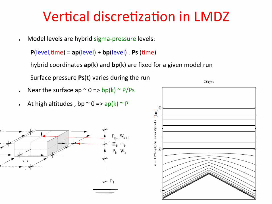
●  Model  levels  are  hybrid  sigma-­‐pressure  levels:  

P(level,(me)  =  ap(level)  +  bp(level)  .  Ps  ((me)  

hybrid  coordinates  ap(k)  and  bp(k)  are  fixed  for  a  given  model  run  

Surface  pressure  Ps(t)  varies  during  the  run  

●  Near  the  surface  ap  ~  0  =>  bp(k)  ~  P/Ps  

●  At  high  al(tudes  ,  bp  ~  0  =>  ap(k)  ~  P  

Ver(cal  discre(za(on  in  LMDZ  

LMDZ,  Z  for  Zoom  

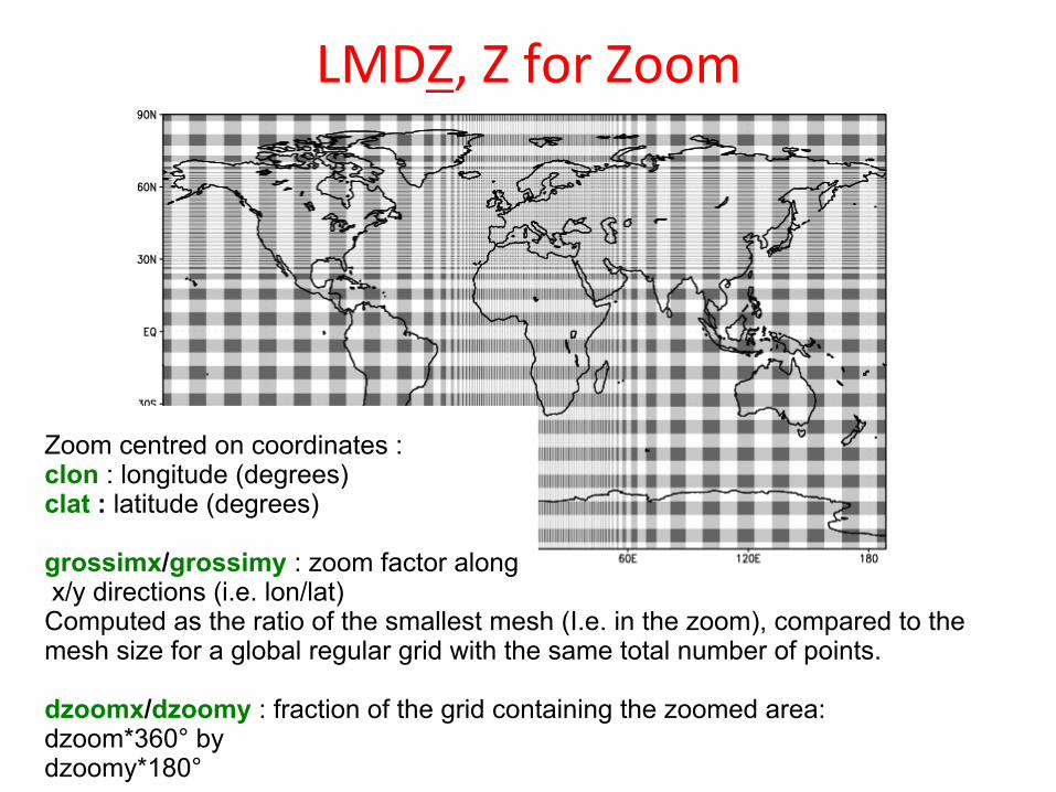
Zoom centred on coordinates : clon : longitude (degrees) clat : latitude (degrees) grossimx/grossimy : zoom factor along x/y directions (i.e. lon/lat) Computed as the ratio of the smallest mesh (I.e. in the zoom), compared to the mesh size for a global regular grid with the same total number of points. dzoomx/dzoomy : fraction of the grid containing the zoomed area: dzoom*360° by dzoomy*180°

Longitudinal  polar  filter  ●  A  lon-­‐lat  grid  implies  that  the  meshes  (ghten  drama(cally  as  the  pole  is  approached.  

●  CFL  condi(ons  there  would  dictate  using  an  extremely  small  (me  step  for  our  explicit  (leapfrog-­‐Matsuno)  (me  marching  scheme.  

● Longitudinal (Fourier) filtering, removing high spatial frequencies, is used to enforce that resolved features are at the level of those at ~60°

 Energy  spectra  and  lateral  dissipa(on  

●  In  order  to  fulfil  the  observed  energy  cascade  from  resolved  scales  to  unresolved  scales  in  GCMs,  a  dissipa(on  term  is  added:  

●  Observations (Nastrom & Gage 1985, Lindborg 1999) collected over length scales from a few to thousands of km display a characteristic energy cascade (from Skamarock, 2004).

Lateral dissipation in GCMs as a tool to pin the energy cascade

Controlling  dissipa(on  in  LMDZ  ●  Parameters  :  

tetagdiv:  dissipa(on  (me  scale  (s)  for  smallest  wavelength  for  u,v  (grad.div  component)  

tetagrot:  dissipa(on  (me  scale  (s)  for  smallest  wavelength  for  u,v  (grad.rot  component)  

tetatemp:  dissipa(on  (me  scale  (s)  for  smallest  wavelength  for  poten(al  temperature  (div.grad)  

op(mal  teta  values  depend  on  horizontal  resolu(on  

●  Moreover  there  is  a  mul(plica(ve  factor  for  the  dissipa(on  coefficient,  which  can  be  controlled  by  the  user.  

 

Some  spectra  (from  LMDZ/Saturn)  

●  In  addi(on  to  lateral  dissipa(on,  it  is  necessary  to  damp  ver(cally  propaga(ng  waves  (non-­‐physically  reflected  downward  from  model  top).  

●  The  sponge  layer  is  limited  to  topmost  layers  (usually  4)  and  added  during  the  dissipa(on  step.  

●  Sponge  modes  and  parameters:  

Type:  Can  act  on  zonal  wind,  meridional  wind  and/or  temperature.  Relaxa(on  can  be  towards  zero  or  mean  zonal  values.  

Intensity:  User-­‐provided  relaxa(on  characteris(c  (me  scale  (at  topmost  layer;  relaxa(on  intensity  decreases  along  successive  descending  layers).  

The  sponge  layer  

Parallelism in LMDZ

A few words on what is done

Hybrid MPI/OpenMP programming Different parallelization approaches in the dynamics and physics ➢  In the dynamics

Short time steps; many interactions between neighbouring meshes, and therefore numerous cases of data exchange and synchronizations. The subtler part of the parallelism in the code..

➢  In the physics

Longer time steps; no interaction between neighbouring columns of the atmosphere.

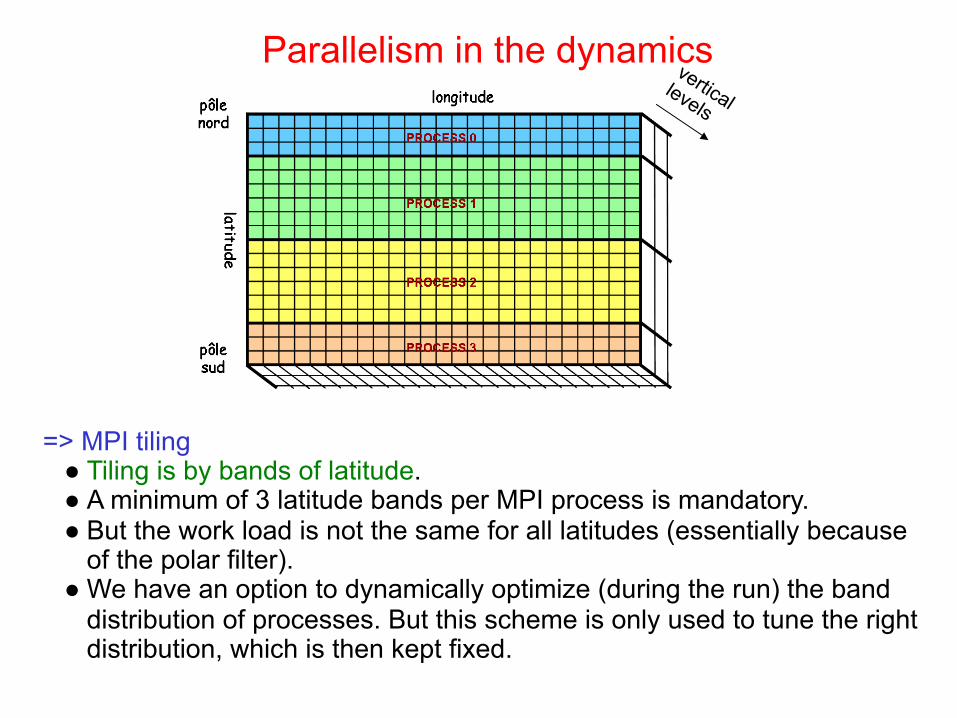
Parallelism in the dynamics => MPI tiling ● Tiling is by bands of latitude. ● A minimum of 3 latitude bands per MPI process is mandatory. ● But the work load is not the same for all latitudes (essentially because

of the polar filter). ● We have an option to dynamically optimize (during the run) the band

distribution of processes. But this scheme is only used to tune the right distribution, which is then kept fixed.

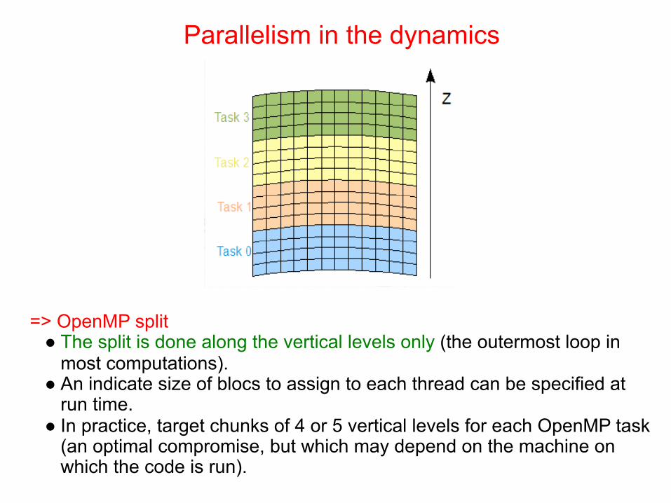
Parallelism in the dynamics => OpenMP split ● The split is done along the vertical levels only (the outermost loop in

most computations). ● An indicate size of blocs to assign to each thread can be specified at

run time. ●  In practice, target chunks of 4 or 5 vertical levels for each OpenMP task

(an optimal compromise, but which may depend on the machine on which the code is run).

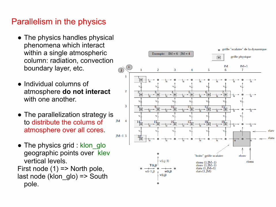
Parallelism in the physics ●  The physics handles physical

phenomena which interact within a single atmospheric column: radiation, convection boundary layer, etc.

●  Individual columns of

atmosphere do not interact with one another.

●  The parallelization strategy is

to distribute the colums of atmosphere over all cores.

●  The physics grid : klon_glo

geographic points over klev vertical levels.

First node (1) => North pole, last node (klon_glo) => South

pole.

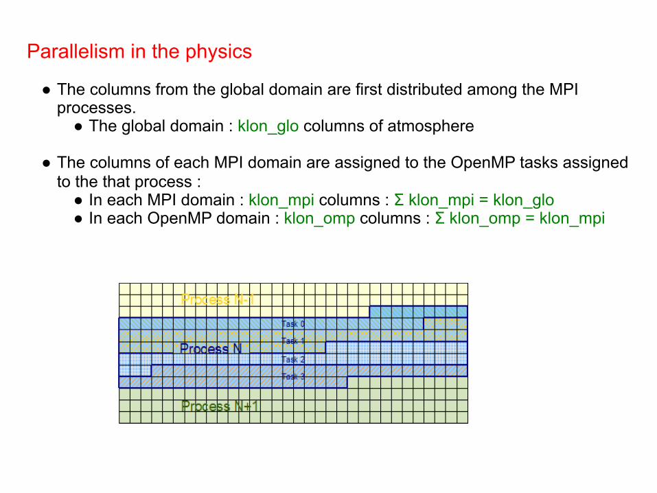
Parallelism in the physics ●  The columns from the global domain are first distributed among the MPI

processes. ●  The global domain : klon_glo columns of atmosphere

●  The columns of each MPI domain are assigned to the OpenMP tasks assigned to the that process : ●  In each MPI domain : klon_mpi columns : Σ klon_mpi = klon_glo ●  In each OpenMP domain : klon_omp columns : Σ klon_omp = klon_mpi

Code  organiza(on  and  management  

It’s all about making everyone’s life easier (i.e. being efficiently lazy): • Using the svn (subversion) tool to maintain codes and share updates. • Enforcing (as much as possible) the separation between dynamics and physics in models. • Sharing input/output library/routines across models and post-processing tools • Sharing dynamical cores between models (at code level, not just in principle).

Code  organiza(on  and  management  Illustrative example • Codes are in the same svn repository, in separate directories:

DOC, LMDZ.GENERIC, LMDZ.MARS, LMDZ.VENUS, LMDZ.TITAN, LMDZ.COMMON

• Source code is split in directories, e.g. for LMDZ.GENERIC:

dyn3d , dynlonlat_phylonlat, filtrez, grid, misc, phystd, Where the dynlonlat_phylonlat directory contains the interface

between dynamics and physics (1D dynamics in phy***)

• LMDZ.COMMON stores « only » dynamical cores: dyn3d, dyn3d_common, dyn3dpar, dynlonlat_phylonlat, filtrez,

grid, misc, phymars, phystd, phytitan, phyvenus Where phy*** are just links to LMDZ.*** directories

• Again, the idea is to set up an infrastructure that makes it easy to use a given physics package with a (i.e. any) given dynamical core.

Upcoming improvements

• A new dynamical core (Dynamico). • Revisiting the equations we solve (i.e. extention to deep atmospheres, going non-hydrostatic, …), and how we solve them. • Being able to run on multicore (>10000 cores) supercomputers.

=> All that, thanks to very hard work by T. Dubos (LMD), M. Tort (LMD), Y. Meurdesoif (LSCE), and co-workers.

LMD-Z lon-lat core

The pole problem : FFT filters around the pole for stability => global dependency (Williamson, 2007)

Moreover it is quite unnecessary to compute the physics on the small meshes in the polar regions.

?

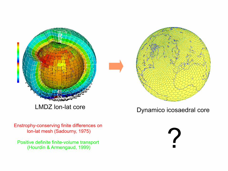
Enstrophy-conserving finite differences on lon-lat mesh (Sadourny, 1975)

Positive definite finite-volume transport

(Hourdin & Armengaud, 1999)

LMDZ lon-lat core Dynamico icosaedral core

The icosahedral grid

Subdividing the 20 faces yield a triangular or (almost) hexagonal mesh.

The icosahedral grid

The icosahedral grid is in fact structured! (important for computational efficiency)

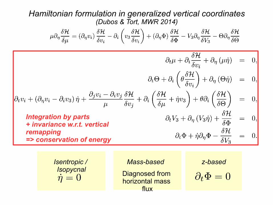
Hamiltonian formulation in generalized vertical coordinates (Dubos & Tort, MWR 2014)

Isentropic / Isopycnal

Mass-based z-based

Diagnosed from horizontal mass

flux

Integration by parts + invariance w.r.t. vertical remapping => conservation of energy

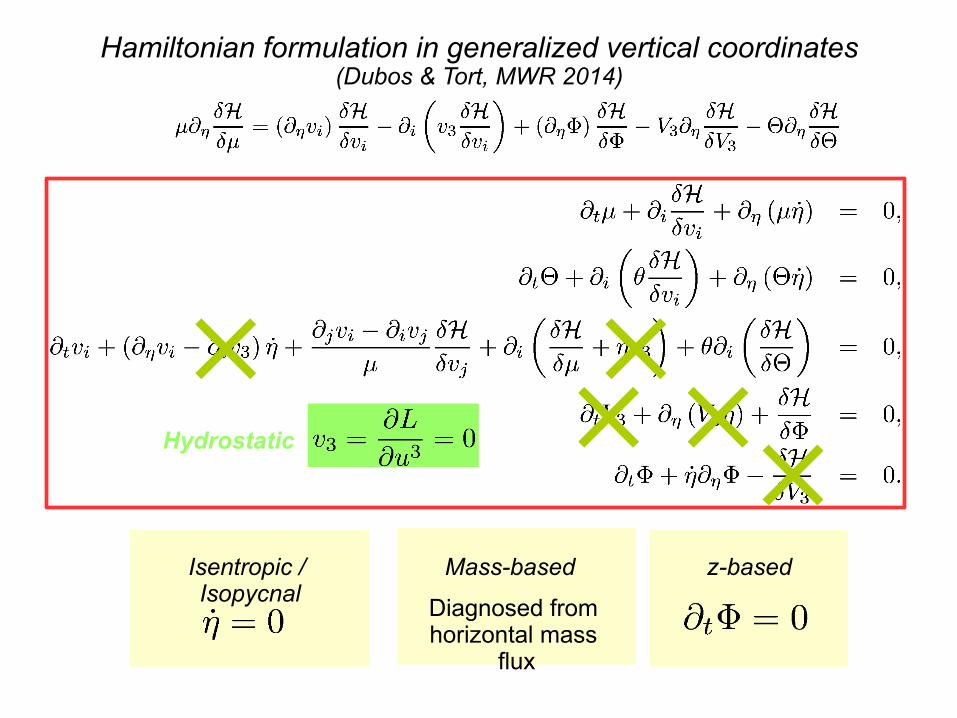
Hamiltonian formulation in generalized vertical coordinates (Dubos & Tort, MWR 2014)

Isentropic / Isopycnal

Mass-based z-based

Diagnosed from horizontal mass

flux

Hydrostatic

Eule

rian

coor

dina

tes

in p

lane

tary

fram

e

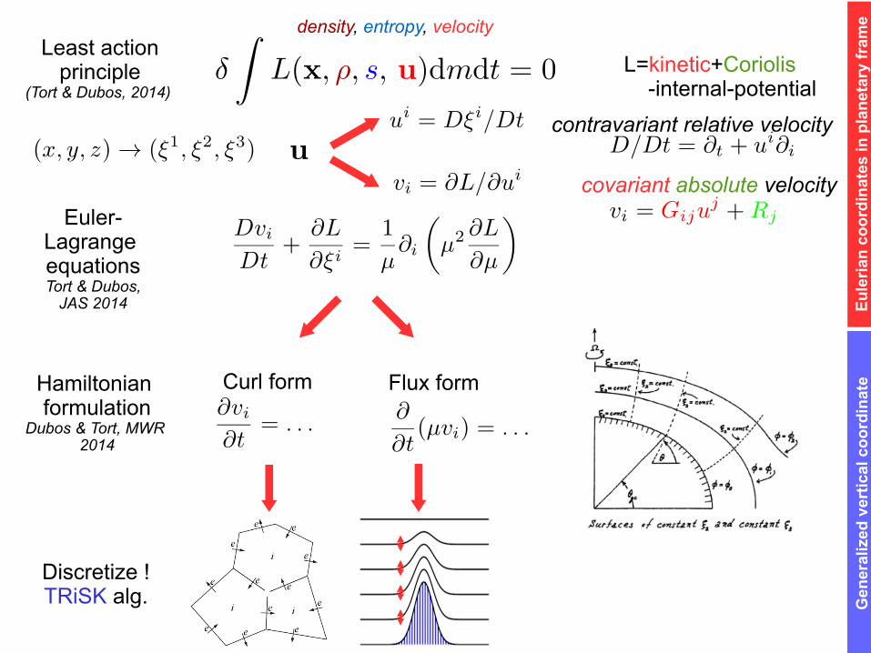
Euler-Lagrange equations Tort & Dubos,

JAS 2014

Curl form Flux form Hamiltonian formulation

Dubos & Tort, MWR 2014

Gen

eral

ized

ver

tical

coo

rdin

ate

Least action principle

(Tort & Dubos, 2014) L=kinetic+Coriolis -internal-potential

density, entropy, velocity

contravariant relative velocity

covariant absolute velocity

Discretize ! TRiSK alg.

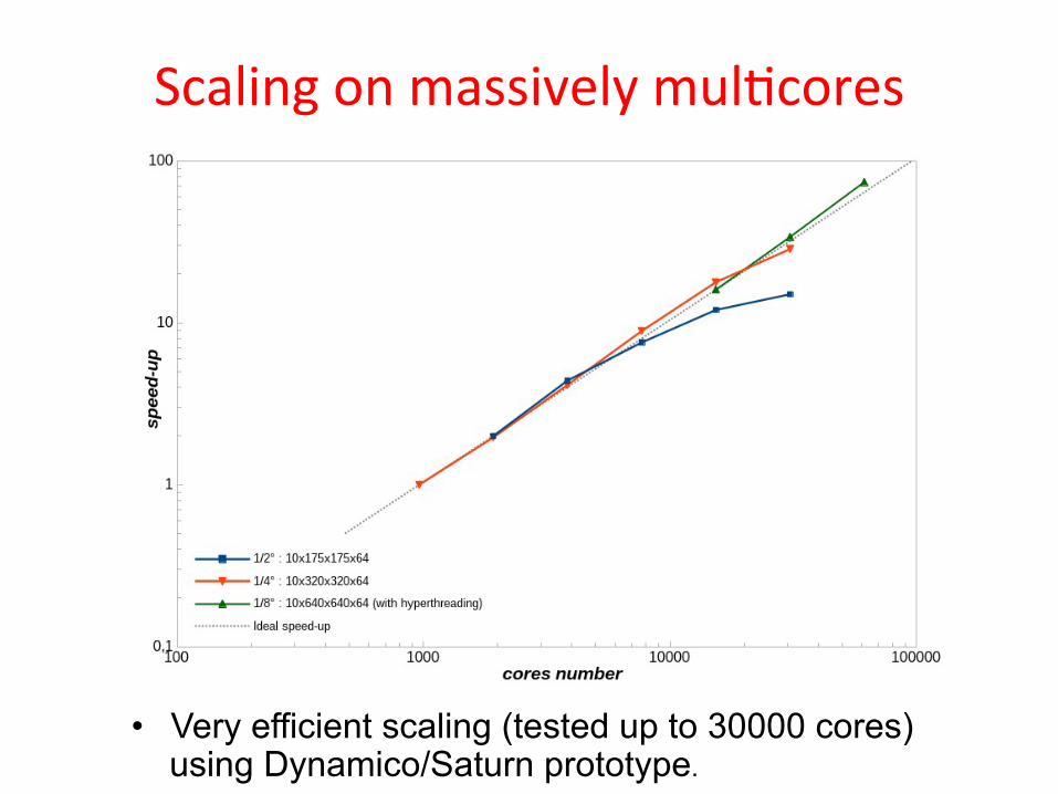
Scaling  on  massively  mul(cores  

•  Very efficient scaling (tested up to 30000 cores) using Dynamico/Saturn prototype.

Miscellaneous  concluding  thoughts  •  Still some work to do to finalize in practice the

physics/dynamics separation. But with the arrival of a new dynamical core (and also with enabling using WRF mesoscale dynamics), it is mandatory to do it fully and well.

•  Likewise there is a new inputs/outputs library

under development at IPSL, XIOS, which is very efficient even in multicore environments. We plan to integrate it shortly.

•  We already know that we need to work further

to unify our post processing tools. This is a target for the near future.

•  We also need to work on documentation...