original research open access integrated approach … · original research open access integrated...

Yu et al. International Journal of Energy and Environmental Engineering 2012, 3:25http://www.journal-ijeee.com/content/3/1/25

ORIGINAL RESEARCH Open Access

Integrated approach for the optimal selection ofenvironmentally friendly drilling systemsOk-Youn Yu1*, Zenon Medina-Cetina2, Seth D Guikema3, Jean-Louis Briaud2 and David Burnett2

Abstract

There is a pressing need in the energy industry to develop technologies capable of reducing the environmentalimpact during oil and gas drilling operations. However, these technologies have not been fully integrated into adecision-making system that can reflect a quantitative effort toward this goal. This paper introduces twoquantitative decision methods for the selection of environmentally friendly drilling systems. One is based on amulti-attribute utility approach and the other one is based on the analysis of interventions or causal approach. Toillustrate the applicability of the proposed methods and to contract their benefits and limitations, a case study ispresented using data collected from Green Lake at McFaddin, TX, USA.

Keywords: Comparative analysis, Environmentally friendly drilling, Decision-making, Multi-attribute utility, Systemselection, Intervention, Causal approach

BackgroundOne of the current goals of the oil and gas industry is tominimize the environmental impact during drillingoperations. This is because an effective management ofthe environmental impacts during drilling operation hasproven to lead to a greater access of reserves in environ-mentally sensitive areas, particularly those classified as‘off-limits’ [1-3]. As a consequence, a significant numberof Environmentally Friendly Drilling (EFD) technologiescontinue to emerge, but these have not been integratedinto a decision-making method capable of combiningthem to define an optimal drilling system for specificconditions on a given site. In practice, the major chal-lenge is to select the best combination of EFD technolo-gies based on a set of competing evaluation criteria. Inthis paper, a ‘system’ will be defined as a set of EFDtechnologies.From an engineering perspective, the civil infrastruc-

ture needed to complete a drilling operation maystrongly condition its success (e.g., access and mainten-ance of roads, power supply, water availability and man-agement of residuals, traffic and noise control). Thisinteraction is exacerbated when the drilling operations

* Correspondence: [email protected] State University, Boone, NC 28608, USAFull list of author information is available at the end of the article

© 2012 Yu et al. This is an Open Access article(http://creativecommons.org/licenses/by/2.0), wprovided the original work is properly cited.

expand on large areas, and at a rapid pace, threateningthe sustainability of the inherent civil infrastructure.A number of studies have introduced decision support

systems for the selection of drilling well locations [4-7].A few studies on the best practices on the use of EFDtechnologies are also available such as in the case of dril-ling waste discharge [8] and in the design of cementing[1]. However, to the best knowledge of the authors, thereare few precedents on a quantitative decision-makingmethod for the integral selection of standard drillingsystems.This work aims at introducing a decision-making

evaluation protocol to find the optimal EFD system for agiven drilling site and also discusses the sensitivity of theinherent input parameters with respect to the expectedoutcomes. A search algorithm is proposed as the basis ofa multi-attribute utility model combined with an ex-haustive enumeration of all available technology combi-nations. This work hypothesizes that optimal decision-making on EFD technology selection can be achieved byan integrated approach, which allows decision-makers tominimize the environmental impact, to maximize theexpected profits, to account for the influence of publicperception, and, most importantly, to guarantee theoperation's safety [9,10].To support this hypothesis, two competing methods

for the selection of EFD systems are presented in this

distributed under the terms of the Creative Commons Attribution Licensehich permits unrestricted use, distribution, and reproduction in any medium,

mailto:[email protected]

http://creativecommons.org/licenses/by/2.0

Yu et al. International Journal of Energy and Environmental Engineering 2012, 3:25 of 18http://www.journal-ijeee.com/content/3/1/25

paper. One follows a simple system selection approachwhere no formal consideration on the dependencies be-tween the system components was considered (non-causal approach). The other takes into account thesame drilling system components as in the previous ap-proach but, in addition, introduces the effect of the de-pendencies between events taking place during thedrilling operation (causal approach). As it is expected,the non-causal approach permits to reduce the compu-tation time for the selection of the optimal drilling sys-tem, becoming a very good reference for preliminaryanalyses. On the other hand, the causal approachrequires further knowledge on the dependencies takingplace during the decision-making process, which addscomputational effort to the optimal selection of EFDsystems. Since the decision-making process is inher-ently conditioned in a drilling sequence (i.e., reservoirassessment dictates the drilling technologies to use, thearea where the drilling is located dictates the technolo-gies used to reduce emission, etc.), a comparison be-tween both approaches seems convenient to addressthe relevance of interventions as the decision-makingfor the EFD system progresses. Irrespective of themethod used, results show consistent support to thehypothesis that an integrated approach for the selectionof EFD systems is needed to maximize the benefits ofall stakeholders participating in an oil and gas relateddrilling operation.To illustrate the benefits and limitations of the pro-

posed methods (non-causal and causal), a case study ispresented based on prescribed EFD system selectioncriteria for a drilling site located in Green Lake atMcFaddin, TX, USA. The aim is to help decision-makers select an optimal drilling system for the site byminimizing environmental impact, maximizing profit,and at the same time accounting for perceptions andsafety. In addition to showing the need for the use ofan integrated decision-making approach on this case,the differences between each approach are discussed.Results of this comparative analysis show the relevanceof introducing causal dependencies between systemcomponents during the search for the optimal selectionof EFD systems.

MethodsOptimal drilling system selectionThis section summarizes an optimal drilling system se-lection procedure for a given site [9]. The proposed sys-tem evaluation protocol defines a decision-makingprocess that ensures the selection of an optimal drillingsystem according to given criteria.The basis for an EFD system selection includes

four main subsystems (Access, Drill Site, Rig, andOperation) and 13 subsets, which have been

previously identified through standard EFD opera-tions (see Figure 1). Design of the decision modelshas been undertaken as part of a comprehensiveacademic-industry collaboration funded by the USDepartment of Energy (DOE) and the Research Part-nership to Secure Energy for America (RPSEA),which integrates the key drilling phases [2].Once the subsystems and subsets are defined, avail-

able technologies within each subset need to be fullycharacterized. A drilling technology selection exampleis also presented in Figure 1, where technologies,indicated within circles for each subset box, repre-sent one possible combination defining a drilling sys-tem. Further combinations of technologies arerequired to evaluate all possible systems and, conse-quently, to find the optimal drilling system for agiven site [11].For the proposed selection criteria, an attribute is

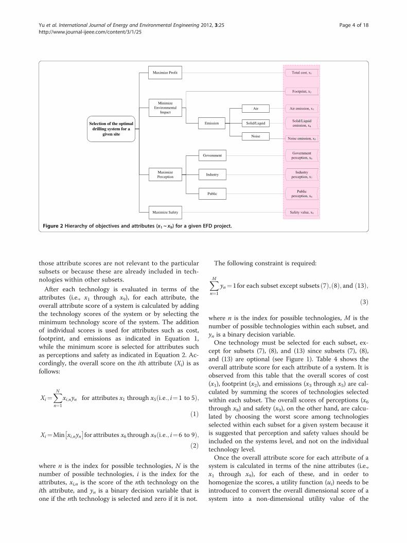
defined as one of the parameters considered in theevaluation of the system (e.g., cost, footprint, emis-sion, perceptions, and safety). Each attribute has anattribute scale used to score the technology on howwell it meets the objective for this attribute (e.g.,minimization of cost, footprint, and emissions andmaximization of positive perceptions and safety value).To evaluate available technologies against each attri-bute, it is required to introduce attribute scales thatexplicitly reflect their possible impacts on the systemselection process [12]. In this case, nine attributesand the corresponding scales are considered for theselection of the EFD system as shown in Figure 2.These attributes should describe accurately their cor-responding technologies. Notice that the proposedattributes are measurable (i.e., dollars, hectares, anddecibels) or constructed (i.e., perceptions and safetyvalues) [9].The attributes considered in this study are as follows:

� Total cost (x1) = the total expenditure in dollarsduring the drilling operation.

� Footprint (x2) = the total used land area in hectares.� Emissions of air pollutants (x3) = emissions of three

air contaminants (i.e., carbon monoxide (CO),nitrogen oxides (NOx), and particulate matter (PM)).The relative importance of these contaminants isCO (20%), NOx (40%), and PM (40%) as shown inTable 1. Table 1 shows an example of how tocalculate the air emission score for each technology:First, estimate the three contaminants' real value foreach technology in pounds per operating hour;second, in order to get an overall air emission scorefor each technology, transform each contaminant'sscore into a non-dimensional score (normalization)between 0 and 1 using the proportional scoring

(1) Transportation:

• Conventional diesel truck

• Low sulphur diesel truck w/noise suppressor

• Rolligon

(3) Site preparation:

• Gravel pad

• Composite mat

• Module + driven piles

(4) Rig type:

• Conventional old rig

• Rapid rig

• LOC250.

Environmentally Friendly Onshore Oil and Gas Drilling System

1. Access 2. Drill Site 3. Rig 4. Operation

(5) Conventional rig power:

• Internal combustion

• Gas turbine

• Lean-burn natural gas engine

(6) Fuel type:

• Diesel

• Low sulphur diesel

• Natural gas

(7) Unconventional rig power:

• Power from grid

• Wind turbine

• None

(8) Energy storage device:

• Flywheel

• Battery

• None

(10) Drilling fluid type:

• Oil-based mud

• Water-based mud

• Synthetic-based mud

•(11) Waste

management:

• Closed loop + container

• Open reserve pit

• Lined reserve pit

(12) Cuttings treatment:

• Bioremediation

• Cutting injection

• Evaporation and burial onsite

(9) Drilling :

• Conventional overbalanced

• Underbalanced

• Managed pressure

Notes:( ) : Subsets

: Available technologies

(2) Road construction:

• Board road

• Gravel road

• Composite mat

(13) Noise reductionfacility:

• Construct a building

• Construct a wall

• None

SUBSYSTEMS

•

Figure 1 Example of one possible EFD system selection (adapted from [9]).


approach, (x – Worst score) / (Best score – Worstscore); and third, calculate the overall air emissionscore of a technology as

Pkiui (where ki is a

weight factor for each air contaminant and uiis a non-dimensional score for each contaminant).

� Emissions of solid and liquid pollutants (x4) =?>thinsp;the ordinal scale as constructed inTable 2.

� Emissions of noise pollutants (x5) = the 8-h time-weighted average (TWA) sound level given indecibels.

� Perception of government, as regulator, (x6) = theordinal scale as constructed in Table 3.

� Perception of industry, as decision maker, (x7).� Perception of the general public (x8).

� Safety value (x9).� Notice that the ordinal scales of x7 through x9 are

similar to that of x6 [9].

To estimate the impact of available technologies withrespect to the proposed nine attributes (i.e., x1 throughx9), the decision method relies on experts' beliefs and onfactual computations generated from available infor-mation sources. For instance, ‘Composite mat (rent)’ ,a selected technology for subset (2) ‘Road construc-tion’ , is estimated in terms of the required attributesbased on the engineering calculations (cost, footprint,and emissions) and experts' beliefs (perceptions andsafety) as shown in Table 4. It is noted that attributescores are not evaluated for the empty cells because

Selection of the optimaldrilling system for a

given site

Maximize Profit

MinimizeEnvironmental

Impact

MaximizePerception

Emission

Government

Industry

Public

Air

Solid/Liquid

Maximize Safety

Noise

Figure 2 Hierarchy of objectives and attributes (x1 ~ x9) for a given EFD project.


those attribute scores are not relevant to the particularsubsets or because these are already included in tech-nologies within other subsets.

After each technology is evaluated in terms of theattributes (i.e., x1 through x9), for each attribute, theoverall attribute score of a system is calculated by addingthe technology scores of the system or by selecting theminimum technology score of the system. The additionof individual scores is used for attributes such as cost,footprint, and emissions as indicated in Equation 1,while the minimum score is selected for attributes suchas perceptions and safety as indicated in Equation 2. Ac-cordingly, the overall score on the ith attribute (Xi) is asfollows:

Xi¼XN

n¼1

xi;nyn for attributes x1 through x5 i:e:; i¼1 to 5ð Þ;

ð1Þ

Xi¼Min xi;nyn� �

for attributes x6 through x9 i:e:; i¼6 to 9ð Þ;ð2Þ

where n is the index for possible technologies, N is thenumber of possible technologies, i is the index for theattributes, xi,n is the score of the nth technology on theith attribute, and yn is a binary decision variable that isone if the nth technology is selected and zero if it is not.

The following constraint is required:

XM

n¼1

yn¼1for each subset except subsets 7ð Þ; 8ð Þ; and 13ð Þ;

ð3Þ

where n is the index for possible technologies, M is thenumber of possible technologies within each subset, andyn is a binary decision variable.One technology must be selected for each subset, ex-

cept for subsets (7), (8), and (13) since subsets (7), (8),and (13) are optional (see Figure 1). Table 4 shows theoverall attribute score for each attribute of a system. It isobserved from this table that the overall scores of cost(x1), footprint (x2), and emissions (x3 through x5) are cal-culated by summing the scores of technologies selectedwithin each subset. The overall scores of perceptions (x6through x8) and safety (x9), on the other hand, are calcu-lated by choosing the worst score among technologiesselected within each subset for a given system because itis suggested that perception and safety values should beincluded on the systems level, and not on the individualtechnology level.Once the overall attribute score for each attribute of a

system is calculated in terms of the nine attributes (i.e.,x1 through x9), for each of these, and in order tohomogenize the scores, a utility function (ui) needs to beintroduced to convert the overall dimensional score of asystem into a non-dimensional utility value of the

Table 1 Example of air emission score calculation

Technologies Unit 20% 40% 40% OverallscoreCO NOx PM

Gravel road: diesel truck + dust g/hp-h 15.5 4 0.1 0.566

lb/hp-h 0.03418 0.00882 0.00022

(lb/h)/unit 10.253 2.646 0.216

lb/operation 3,250.280 838.782 68.520

U-value 0.000 0.822 0.593

Composite mat: low-sulphur diesel truck with noise suppressor g/hp-h 15.5 0.2 0.01 0.976

lb/hp-h 0.03418 0.00044 0.00002

(lb/h)/unit 10.253 0.132 0.007

lb/operation 369.117 4.763 0.238

U-value 0.886 0.999 0.999

Internal combustion engine lb/MWh 6.2 21.8 0.78 0.118

(lb/h)/unit 6.200 21.800 0.780

(lb/h) × portion 6.200 21.800 0.780

lb/operation 1,339.200 4,708.800 168.480

U-value 0.588 0.000 0.000

Internal combustion engine with SCR and with noise suppressor (lb/MWh) 6.2 4.7 0.78 0.431

(lb/h)/unit 6.200 4.700 0.780

(lb/h) × portion 6.200 4.700 0.780

lb/operation 1,339.200 1,015.200 168.480

U-value 0.588 0.784 0.000

Lean-burn natural gas engines with noise suppressor lb/MWh 5 2.2 0.03 0.878

(lb/h)/unit 5.000 2.200 0.030

(lb/h) × portion 5.000 2.200 0.030

lb/operation 1,080.000 475.200 6.480

U-value 0.668 0.899 0.962

Power from grid lb/MWh 0 0 0 1.000

(lb/h)/unit 0.000 0.000 0.000

(lb/h) × portion 0.000 0.000 0.000

lb/operation 0.000 0.000 0.000

U-value 1.000 1.000 1.000

SCR, selective catalytic reduction.

Table 2 Proposed attribute scale for solid and liquid emissions

Waste managementtechnologies

Cuttings treatment Solid/liquid emissionscore

Closed loop Cuttings injection 1.00

- Bioremediation, composting, in situ vitrification, land spreading, plasma arc, microwavetechnology

0.75

Lined reserve pit Thermal desorption 0.50

- Chemical fixation and solidification 0.25

Open reserve pit Evaporation and burial on-site 0.00


Table 3 Proposed attribute scale for government perception

Scale Description Perceptionscore

Strong support All parties will encourage its use and are willing to appropriate funds for the cause 1.00

Moderate support There is interest from a majority. Its use will be encouraged, but funds will not be appropriated 0.75

Neutrality All parties are indifferent. There is no resistance, but there is also no help 0.50

Moderateopposition

Some resistance from the majority. Its use may be discouraged, but fines or restrictions will not beimposed

0.25

Strong opposition Strong resistance to its use from all parties. Restrictions or fines will be set up to eliminate this option 0.00


system, which ranges between 0 and 1. This allows thedecision-makers to make the overall attribute score foreach attribute uniform and comparable. AlthoughKeeney and Raiffa [12] introduced the distinction be-tween a value function and a utility function, the authorsbelieve that this is still largely a personal choice withinthe decision analysis community. Herein, it is called autility function since it is based on assessed preferenceparameters of a decision-maker and it represents theirutility. Also, there are different approaches to developsingle-attribute functions (i.e., linear and nonlinear). Theproportional scoring approach (i.e., linear approach) ismainly used in this paper because of the limited expert

Table 4 Example of a system matrix

40% 25%

Selected technologies in each subset Totalcost,x1, ($)

Footprix2, (ha

(1) Transportation: conventional diesel truck

(2) Road construction: composite mat (rent) 132,000 0.615

(3) Site preparation: composite mat (rent) 90,000 0.420

(4) Rig type: LOC250 (CWD) 182,000

(5) Rig power (conventional): internal combustionengine with SCR and with noise suppressor

73,369

(6) Fuel type: low-sulphur diesel 47,628

(7) Rig power (unconventional): electric power from grid(10%)

5,918 0.000

(8) Energy storage: flywheels 30,000 0.000

(9) Drilling technology: conventional overbalanceddrilling

170,000

(10) Fluid type: water-based muds 47,940

(11) Waste management: closed loop + containers +solid control equipmenta

30,000 0.000

(12) Cuttings management: cuttings injection 54,000

(13) Noise reduction facility: N/A

Overall attribute scores (P

or minimum value) 862,855 1.035

Single-attribute utility values (Ui) 0.883 0.764

∴ Multi-attribute utility value = 0.740; asolid control equipment includes shakers, posscentrifuge; CWD, casing-while-drilling; SCR, selective catalytic reduction; N/A, not appli

assessment. This can and should be revisited for futureapplications as needed based on interactions with EFDsubject matter experts, mainly due to changes in tech-nology. A general formula for the proportional scoringapproach is given by [11]:

ui Xið Þ ¼ Xi �Worst scoreBest score�Worst score

; ð4Þ

where Xi is the overall score on the ith attribute of asystem.Figure 3 shows an example of utility function curves

used in this study. As can be seen in Figure 3, the max-imum and minimum values of each attribute need to be

Weights (P

=100% ∴ O.K!)

5% 5% 5% 5% 5% 5% 5%

nt,)

Emissions (x3 ~ x5) Perceptions (x6 ~ x8) Safetyvalue(x9)

Air Solidandliquid

Noise(TWA)

Government Industry Public

0.250 1.000 0.250 0.750

0.964 82.870 1.000 0.500 1.000 1.000

0.976 79.945 0.750 0.750 0.750 1.000

0.977 77.458 1.000 0.500 1.000 1.000

0.574 90.259 0.750 0.750 0.750 0.750

0.750 0.750 1.000 0.750

1.000 0.000 0.500 1.000 1.000 1.000

0.500 1.000 1.000 0.750

115.385 1.000 0.500 0.500 0.500

1.000 1.000 1.000 1.000

1.000 1.000 0.500 1.000 0.750

1.000 1.000 0.500 1.000 0.750

4.490 2.000 445.917 0.250 0.500 0.250 0.500

0.757 1.000 0.655 0.250 0.500 0.250 0.500

ibly cone centrifuge, desander, desilter, cuttings dryer, and perhaps decantingcable.

0

0.2

0.4

0.6

0.8

1

0.7 0.9 1.1 1.3 1.5

X1 = Total Cost ($ M)

u1

0

0.2

0.4

0.6

0.8

1

350 400 450 500

X5 = Noise emission (TWA)

u5

Figure 3 Examples of single-attribute utility function curves.


computed in order to generate the utility functioncurves. For example, it is known that the range of thecost attribute (X1) values in Figure 3 is from $0.79 mil-lion to $1.42 million, where the minimum total costs arepreferred over the maximum ones. Thus, to remain con-sistent with the scaling rule where the utility functionsranged from 0 to 1, u1 ($0.79 million) = 1 and u1 ($1.42million) = 0 are defined. Simple linear curves are usedfor attributes x1 through x9 except x5. The noise attri-bute (x5) utility function discussed in Yu et al. [9] ismodified in this paper in order to better satisfy the noiselevel in normal working conditions, as described by theOccupational Safety and Health Administration [13]:

u5 X5ð Þ ¼ X5 �Worst score425�Worst score

� 0:9 for X5

> 425; ð5Þ

u5 X5ð Þ ¼ X5 � 425Best score� 425

� 0:1

þ 0:9 for X5≤425; ð6Þ

where X5 is the noise attribute score, an 8-h TWA soundlevel in decibels, and u5 is the noise attribute utilityvalue of the system.Once each single-attribute utility function ui(Xi) is

derived for its attribute measure, these individual utilityvalues are combined into a final utility value. If mutualpreferential and utility independence are satisfied in thisstudy, it is possible to define the multi-attribute utilityfunction with the additive form [12]:

U X1;X2; . . . ;X9ð Þ ¼ U u1 X1ð Þ; u2 X2ð Þ; . . . ; u9 X9ð Þf g¼ k1u1 X1ð Þ þ . . .þ k9u9 X9ð Þ ¼

X9

i¼1

kiui Xið Þ;

ð7Þwhere ui(Xi) is the expected utility of the ith attributescaled from 0 to 1, and ki is the weighting constant forthe ith attribute.

Since it is assumed that there is no interaction be-tween each attribute (no cause-effect dependency), all ofthe weights are positive and they must sum to one [14].The weight combination represents the trade-offs be-tween the utility of the different attributes, and in prac-tice, they are chosen by the stakeholders. One weightcombination example assigned to a system is shown inTable 4. It is suggested to examine the appropriatenessof any independence condition before adopting the addi-tive utility function to see if violations of the independ-ence condition are found [15]. In this study, forexample, it was verified that the trade-offs for attributesx1 (total cost) and x2 (footprint), keeping the levels ofthe other attributes (x3 through x9) fixed, do not dependon the particular values of these fixed levels and so onfor each pair of attributes.Since the exhaustive search optimization is a simple,

practical, and very robust method given the speed ofmodern computers [16], it is proposed to evaluate allpossible systems according to nine attributes, with therelative importance of the different attributes (i.e., weightcombination) defined by the stakeholders. Then, it fol-lows to find the ‘best’ available system that should beparticularly suitable for a specific site. Once all possiblesystems have been evaluated, the system containing thehighest overall utility score is the best system with givenweighting factors.After the optimization scheme has determined the best

system, it is suggested to conduct a sensitivity analysis toexamine the impact of possible changes in the attributescores, weight factors, and utility functions on the bestsystem. For example, the weight assigned to the cost at-tribute shown in Table 4 could be changed from the ini-tially assigned value of 0.40. Since the weighting factorsmust sum to one in this study, the weights assigned toother attributes are known once a weight assigned to thecost attribute is decided. Note that the final result needsnot be a single system but that a few ‘optimal’ systemsclose to the best score. This may provide some flexibility

Green LakeGreen LakeGreen Lake

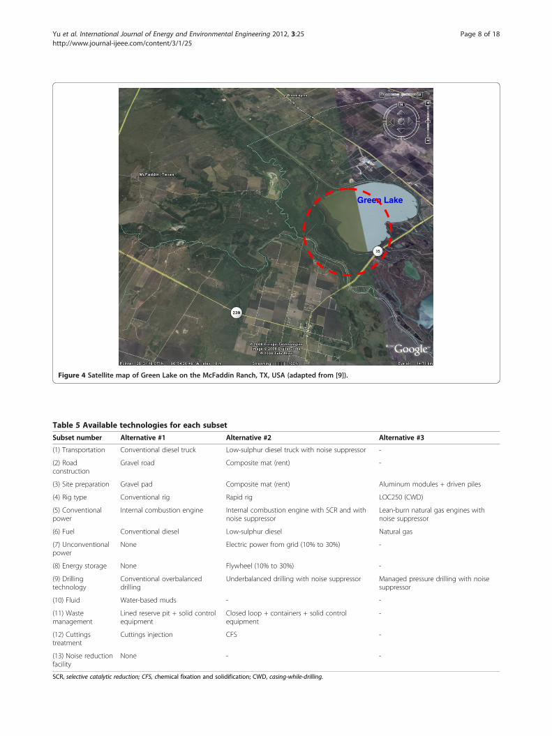
Figure 4 Satellite map of Green Lake on the McFaddin Ranch, TX, USA (adapted from [9]).

Table 5 Available technologies for each subset

Subset number Alternative #1 Alternative #2 Alternative #3

(1) Transportation Conventional diesel truck Low-sulphur diesel truck with noise suppressor -

(2) Roadconstruction

Gravel road Composite mat (rent) -

(3) Site preparation Gravel pad Composite mat (rent) Aluminum modules + driven piles

(4) Rig type Conventional rig Rapid rig LOC250 (CWD)

(5) Conventionalpower

Internal combustion engine Internal combustion engine with SCR and withnoise suppressor

Lean-burn natural gas engines withnoise suppressor

(6) Fuel Conventional diesel Low-sulphur diesel Natural gas

(7) Unconventionalpower

None Electric power from grid (10% to 30%) -

(8) Energy storage None Flywheel (10% to 30%) -

(9) Drillingtechnology

Conventional overbalanceddrilling

Underbalanced drilling with noise suppressor Managed pressure drilling with noisesuppressor

(10) Fluid Water-based muds - -

(11) Wastemanagement

Lined reserve pit + solid controlequipment

Closed loop + containers + solid controlequipment

-

(12) Cuttingstreatment

Cuttings injection CFS -

(13) Noise reductionfacility

None - -

SCR, selective catalytic reduction; CFS, chemical fixation and solidification; CWD, casing-while-drilling.



for the person in charge of the overall decision-makingabout the drilling process [15,17].

Results and discussionApplicationsTo illustrate the applicability of an integrated approachfor the selection of EFD systems, a case study was con-ducted at a site in Green Lake at McFaddin, TX, USA.This assumed that an independent operator was to drilla well on their lease in South Texas, located in an envir-onmentally sensitive wetland area. The lease extends tothe center of Green Lake on the McFaddin Ranch asshown in Figure 4. The formation target belongs to theupper Frio sand at a vertical depth of approximately8,500 ft [18]. The available technologies within each sub-set for this case study are shown in Table 5. This tableshows that some subsets (i.e., (3), (4), (5), and (9)) havethree available technologies while subset (10) has onlyone available technology. It is also noticed that subset(13) is not considered in this case study.

Non-causal approachAn exhaustive search optimization generates all possiblecombinations of technologies for a given site. The corre-sponding influence diagram for this approach is shownin Figure 5. Notice that the configuration of the influ-ence diagram for the non-causal system selection ap-proach denotes no influences between the system's maincomponents.The influence diagram is a compact way for describing

the dependencies among variables and decisions [19].Normally, an arc in an influence diagram denotes an in-fluence (i.e., the fact that the node at the tail of the arcinfluences the value of the node at the head of the arc).

Figure 5 Influence diagram considered in the non-causal approach.

These arcs are drawn as solid lines. Arcs coming intodecision nodes have different meanings. As decisionnodes are under the decision maker's control, these arcsdo not denote influences but rather temporal precedence(in the sense of flow of information). The outcomes ofall nodes at the tail of informational arcs will be knownbefore the decision will need to be made. In particular, ifthere are multiple decision nodes, they need to be allconnected by information arcs. This reflects the fact thatthe decisions are made in a sequence and the outcomeof each decision is known before the next decision ismade. Informational arcs are drawn as dashed lines [20].Figure 5 shows a drilling system comprised of 13 subsetsand the corresponding dependencies between them. In areal application, a non-causal system selection approachis not recommended as the best practice. However, thiscan help to assess preliminary responses of the systemselection due to its simple implementation and efficientcomputational effort. Moreover, it typically serves as thebasis for the development of more complex systemselections.Only three basic dependencies were considered in this

specific application as shown in Figure 6 (i.e., dependen-cies between subsets (5) and (7), between subsets (5)and (6), and between subsets (7) and (8)). For example,the number of possible fuel types for a conventionalpower generation engine varies by what kind of engine isselected and whether using an energy storage device ornot should be dependent on whether an unconventionalpower generation method is used or not. If it is decidednot to use an unconventional power generation method,an energy storage device is not considered as a possiblesubset in the ‘Rig’ subsystem. In this case study, therange of unconventional power usage is varied from 0%to 30% of total power usage (see Figure 6). The

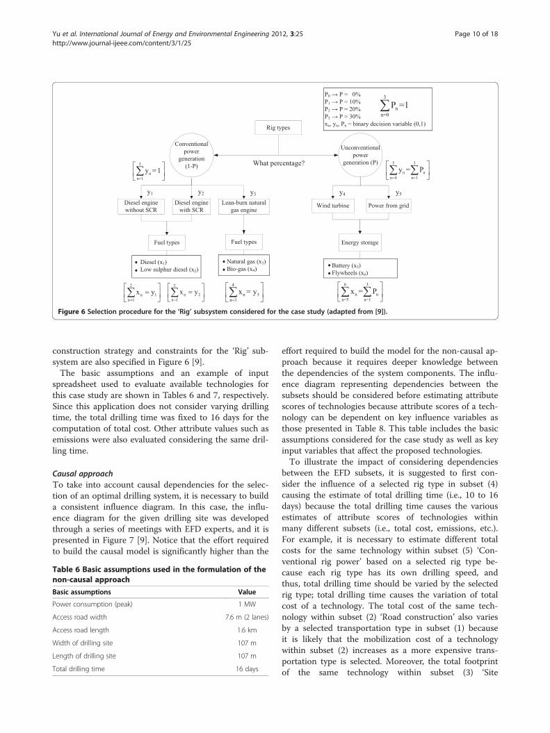
Figure 6 Selection procedure for the ‘Rig’ subsystem considered for the case study (adapted from [9]).


construction strategy and constraints for the ‘Rig’ sub-system are also specified in Figure 6 [9].The basic assumptions and an example of input

spreadsheet used to evaluate available technologies forthis case study are shown in Tables 6 and 7, respectively.Since this application does not consider varying drillingtime, the total drilling time was fixed to 16 days for thecomputation of total cost. Other attribute values such asemissions were also evaluated considering the same dril-ling time.

Causal approachTo take into account causal dependencies for the selec-tion of an optimal drilling system, it is necessary to builda consistent influence diagram. In this case, the influ-ence diagram for the given drilling site was developedthrough a series of meetings with EFD experts, and it ispresented in Figure 7 [9]. Notice that the effort requiredto build the causal model is significantly higher than the

Table 6 Basic assumptions used in the formulation of thenon-causal approach

Basic assumptions Value

Power consumption (peak) 1 MW

Access road width 7.6 m (2 lanes)

Access road length 1.6 km

Width of drilling site 107 m

Length of drilling site 107 m

Total drilling time 16 days

effort required to build the model for the non-causal ap-proach because it requires deeper knowledge betweenthe dependencies of the system components. The influ-ence diagram representing dependencies between thesubsets should be considered before estimating attributescores of technologies because attribute scores of a tech-nology can be dependent on key influence variables asthose presented in Table 8. This table includes the basicassumptions considered for the case study as well as keyinput variables that affect the proposed technologies.To illustrate the impact of considering dependencies

between the EFD subsets, it is suggested to first con-sider the influence of a selected rig type in subset (4)causing the estimate of total drilling time (i.e., 10 to 16days) because the total drilling time causes the variousestimates of attribute scores of technologies withinmany different subsets (i.e., total cost, emissions, etc.).For example, it is necessary to estimate different totalcosts for the same technology within subset (5) ‘Con-ventional rig power’ based on a selected rig type be-cause each rig type has its own drilling speed, andthus, total drilling time should be varied by the selectedrig type; total drilling time causes the variation of totalcost of a technology. The total cost of the same tech-nology within subset (2) ‘Road construction’ also variesby a selected transportation type in subset (1) becauseit is likely that the mobilization cost of a technologywithin subset (2) increases as a more expensive trans-portation type is selected. Moreover, the total footprintof the same technology within subset (3) ‘Site

Table 7 Example of input scores used in the non-causal approach

Subsets Technologies Buy($)

Resellvalue($)

Rent/day($)

Dailyrate($)

Totalcost ($)

Ecologicalfootprint

(ha)

Emissions Perceptions Safetyvalue

Air Solid andliquid

Noise(TWA)


1 Conventional diesel truck 20,000 0.000 0.250 1.000 0.250 0.750

Low-sulphur diesel truck with tier III engine andwith noise suppressor

28,000 0.000 1.000 0.500 1.000 0.750

2 Gravel roads 148,500 1.226 0.570 99.000 0.250 1.000 0.250 0.500

Composite mat 132,000 0.613 0.960 83.000 1.000 0.500 1.000 1.000

3 Gravel pad 137,000 1.133 0.600 98.000 0.250 1.000 0.250 0.500

Composite mat 120,000 0.567 0.970 82.000 0.750 0.750 0.750 1.000

Aluminum modules + driven piles 220,000 0.003 0.970 97.600 1.000 0.500 1.000 0.500

4 Conventional order vintage rig 200,000 0.970 79.000 0.500 1.000 0.500 0.500

Rapid rig 224,000 0.970 77.000 1.000 0.500 1.000 1.000

LOC250 (CWD) 240,000 0.980 77.500 1.000 0.500 1.000 1.000

5 Internal combustion engine 56,000 0.384 107.000 0.500 1.000 0.500 0.750

Internal combustion engine with SCR and withnoise suppressor

83,020 0.601 90.000 0.750 0.750 0.750 0.750

6 Conventional diesel 65,800 0.500 1.000 0.500 0.500

Low-sulphur diesel 69,160 0.750 0.750 1.000 0.750

7 Electronic power from grid 25,800.00 0.000 1.000 0.000 0.500 1.000 1.000 1.000

8 Flywheels 450,000 360,000 90,000 0.000 0.500 1.000 1.000 0.750

9 Conventional overbalanced drilling 204,000 117.000 1.000 0.500 0.500 0.500

Underbalanced drilling with noise suppressor 221,400 101.000 0.750 0.750 0.750 0.750

Managed pressure drilling with noise suppressor 232,200 99.000 0.750 0.750 1.000 1.000

10 Water-based muds 48,000 1.000 1.000 1.000 1.000

11 Lined reserve pit + solid control equipmenta 24,000 0.015 0.500 0.750 0.750 0.750 0.750

Closed loop + containers + solid controlequipmenta

36,000 0.000 1.000 1.000 0.500 1.000 0.750

12 Cuttings injection 54,000 1.000 1.000 0.500 1.000 0.750

CFS 61,710 0.250 0.750 0.750 1.000 0.500

13 N/AaSolid control equipment includes shakers, possibly cone centrifuge, desander, desilter, cuttings dryer, and perhaps decanting centrifuge; CWD, casing-while-drilling; SCR, selective catalytic reduction; CFS, chemical fixation andsolidification; N/A, not applicable.

Yuet

al.InternationalJournalofEnergy

andEnvironm

entalEngineering2012,3:25

Page11

of18

http://www.journal-ijeee.com

/content/3/1/25

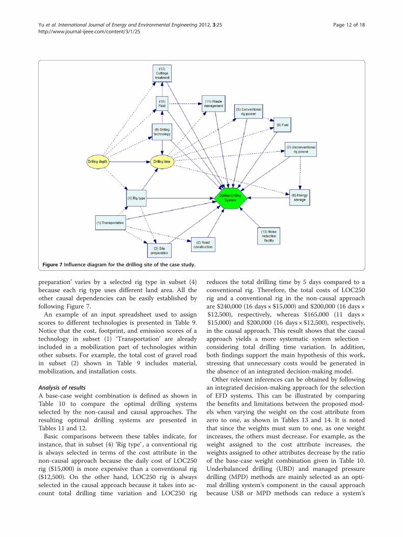
Figure 7 Influence diagram for the drilling site of the case study.


preparation’ varies by a selected rig type in subset (4)because each rig type uses different land area. All theother causal dependencies can be easily established byfollowing Figure 7.An example of an input spreadsheet used to assign

scores to different technologies is presented in Table 9.Notice that the cost, footprint, and emission scores of atechnology in subset (1) ‘Transportation’ are alreadyincluded in a mobilization part of technologies withinother subsets. For example, the total cost of gravel roadin subset (2) shown in Table 9 includes material,mobilization, and installation costs.

Analysis of resultsA base-case weight combination is defined as shown inTable 10 to compare the optimal drilling systemsselected by the non-causal and causal approaches. Theresulting optimal drilling systems are presented inTables 11 and 12.Basic comparisons between these tables indicate, for

instance, that in subset (4) ‘Rig type’ , a conventional rigis always selected in terms of the cost attribute in thenon-causal approach because the daily cost of LOC250rig ($15,000) is more expensive than a conventional rig($12,500). On the other hand, LOC250 rig is alwaysselected in the causal approach because it takes into ac-count total drilling time variation and LOC250 rig

reduces the total drilling time by 5 days compared to aconventional rig. Therefore, the total costs of LOC250rig and a conventional rig in the non-causal approachare $240,000 (16 days × $15,000) and $200,000 (16 days ×$12,500), respectively, whereas $165,000 (11 days ×$15,000) and $200,000 (16 days × $12,500), respectively,in the causal approach. This result shows that the causalapproach yields a more systematic system selection -considering total drilling time variation. In addition,both findings support the main hypothesis of this work,stressing that unnecessary costs would be generated inthe absence of an integrated decision-making model.Other relevant inferences can be obtained by following

an integrated decision-making approach for the selectionof EFD systems. This can be illustrated by comparingthe benefits and limitations between the proposed mod-els when varying the weight on the cost attribute fromzero to one, as shown in Tables 13 and 14. It is notedthat since the weights must sum to one, as one weightincreases, the others must decrease. For example, as theweight assigned to the cost attribute increases, theweights assigned to other attributes decrease by the ratioof the base-case weight combination given in Table 10.Underbalanced drilling (UBD) and managed pressuredrilling (MPD) methods are mainly selected as an opti-mal drilling system's component in the causal approachbecause USB or MPD methods can reduce a system's

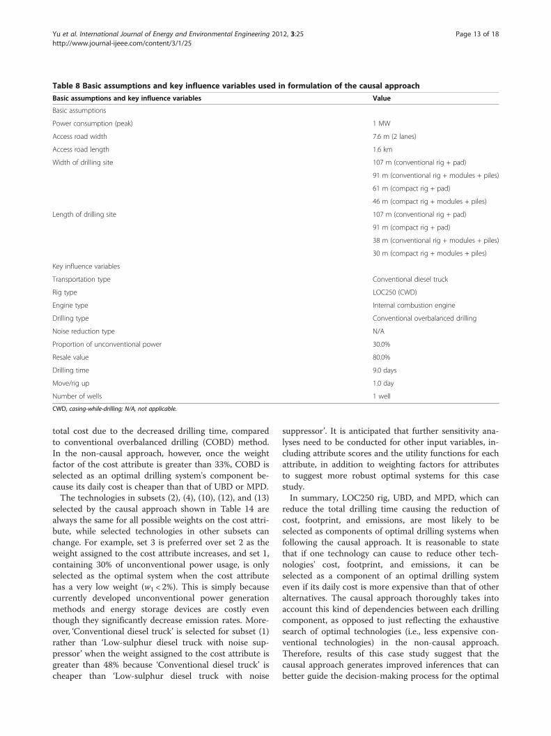
Table 8 Basic assumptions and key influence variables used in formulation of the causal approach

Basic assumptions and key influence variables Value

Basic assumptions

Power consumption (peak) 1 MW

Access road width 7.6 m (2 lanes)

Access road length 1.6 km

Width of drilling site 107 m (conventional rig + pad)

91 m (conventional rig + modules + piles)

61 m (compact rig + pad)

46 m (compact rig + modules + piles)

Length of drilling site 107 m (conventional rig + pad)

91 m (compact rig + pad)

38 m (conventional rig + modules + piles)

30 m (compact rig + modules + piles)

Key influence variables

Transportation type Conventional diesel truck

Rig type LOC250 (CWD)

Engine type Internal combustion engine

Drilling type Conventional overbalanced drilling

Noise reduction type N/A

Proportion of unconventional power 30.0%

Resale value 80.0%

Drilling time 9.0 days

Move/rig up 1.0 day

Number of wells 1 well

CWD, casing-while-drilling; N/A, not applicable.


total cost due to the decreased drilling time, comparedto conventional overbalanced drilling (COBD) method.In the non-causal approach, however, once the weightfactor of the cost attribute is greater than 33%, COBD isselected as an optimal drilling system's component be-cause its daily cost is cheaper than that of UBD or MPD.The technologies in subsets (2), (4), (10), (12), and (13)

selected by the causal approach shown in Table 14 arealways the same for all possible weights on the cost attri-bute, while selected technologies in other subsets canchange. For example, set 3 is preferred over set 2 as theweight assigned to the cost attribute increases, and set 1,containing 30% of unconventional power usage, is onlyselected as the optimal system when the cost attributehas a very low weight (w1 < 2%). This is simply becausecurrently developed unconventional power generationmethods and energy storage devices are costly eventhough they significantly decrease emission rates. More-over, ‘Conventional diesel truck’ is selected for subset (1)rather than ‘Low-sulphur diesel truck with noise sup-pressor’ when the weight assigned to the cost attribute isgreater than 48% because ‘Conventional diesel truck’ ischeaper than ‘Low-sulphur diesel truck with noise

suppressor’. It is anticipated that further sensitivity ana-lyses need to be conducted for other input variables, in-cluding attribute scores and the utility functions for eachattribute, in addition to weighting factors for attributesto suggest more robust optimal systems for this casestudy.In summary, LOC250 rig, UBD, and MPD, which can

reduce the total drilling time causing the reduction ofcost, footprint, and emissions, are most likely to beselected as components of optimal drilling systems whenfollowing the causal approach. It is reasonable to statethat if one technology can cause to reduce other tech-nologies' cost, footprint, and emissions, it can beselected as a component of an optimal drilling systemeven if its daily cost is more expensive than that of otheralternatives. The causal approach thoroughly takes intoaccount this kind of dependencies between each drillingcomponent, as opposed to just reflecting the exhaustivesearch of optimal technologies (i.e., less expensive con-ventional technologies) in the non-causal approach.Therefore, results of this case study suggest that thecausal approach generates improved inferences that canbetter guide the decision-making process for the optimal

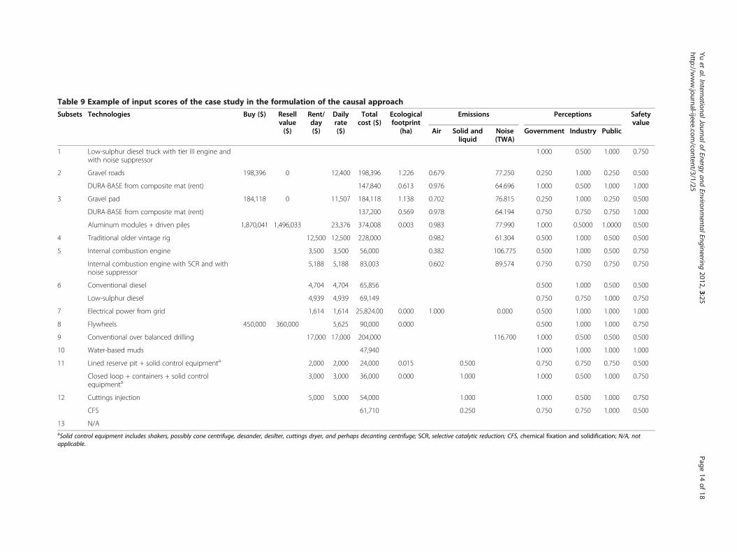
Table 9 Example of input scores of the case study in the formulation of the causal approach

Subsets Technologies Buy ($) Resellvalue($)

Rent/day($)

Dailyrate($)

Totalcost ($)

Ecologicalfootprint

(ha)

Emissions Perceptions Safetyvalue

Air Solid andliquid

Noise(TWA)


1 Low-sulphur diesel truck with tier III engine andwith noise suppressor

1.000 0.500 1.000 0.750

2 Gravel roads 198,396 0 12,400 198,396 1.226 0.679 77.250 0.250 1.000 0.250 0.500

DURA-BASE from composite mat (rent) 147,840 0.613 0.976 64.696 1.000 0.500 1.000 1.000

3 Gravel pad 184,118 0 11,507 184,118 1.138 0.702 76.815 0.250 1.000 0.250 0.500

DURA-BASE from composite mat (rent) 137,200 0.569 0.978 64.194 0.750 0.750 0.750 1.000

Aluminum modules + driven piles 1,870,041 1,496,033 23,376 374,008 0.003 0.983 77.990 1.000 0.5000 1.0000 0.500

4 Traditional older vintage rig 12,500 12,500 228,000 0.982 61.304 0.500 1.000 0.500 0.500

5 Internal combustion engine 3,500 3,500 56,000 0.382 106.775 0.500 1.000 0.500 0.750

Internal combustion engine with SCR and withnoise suppressor

5,188 5,188 83,003 0.602 89.574 0.750 0.750 0.750 0.750

6 Conventional diesel 4,704 4,704 65,856 0.500 1.000 0.500 0.500

Low-sulphur diesel 4,939 4,939 69,149 0.750 0.750 1.000 0.750

7 Electrical power from grid 1,614 1,614 25,824.00 0.000 1.000 0.000 0.500 1.000 1.000 1.000

8 Flywheels 450,000 360,000 5,625 90,000 0.000 0.500 1.000 1.000 0.750

9 Conventional over balanced drilling 17,000 17,000 204,000 116.700 1.000 0.500 0.500 0.500

10 Water-based muds 47,940 1.000 1.000 1.000 1.000

11 Lined reserve pit + solid control equipmenta 2,000 2,000 24,000 0.015 0.500 0.750 0.750 0.750 0.500

Closed loop + containers + solid controlequipmenta

3,000 3,000 36,000 0.000 1.000 1.000 0.500 1.000 0.750

12 Cuttings injection 5,000 5,000 54,000 1.000 1.000 0.500 1.000 0.750

CFS 61,710 0.250 0.750 0.750 1.000 0.500

13 N/AaSolid control equipment includes shakers, possibly cone centrifuge, desander, desilter, cuttings dryer, and perhaps decanting centrifuge; SCR, selective catalytic reduction; CFS, chemical fixation and solidification; N/A, notapplicable.

Yuet

al.InternationalJournalofEnergy

andEnvironm

entalEngineering2012,3:25

Page14

of18

http://www.journal-ijeee.com

/content/3/1/25

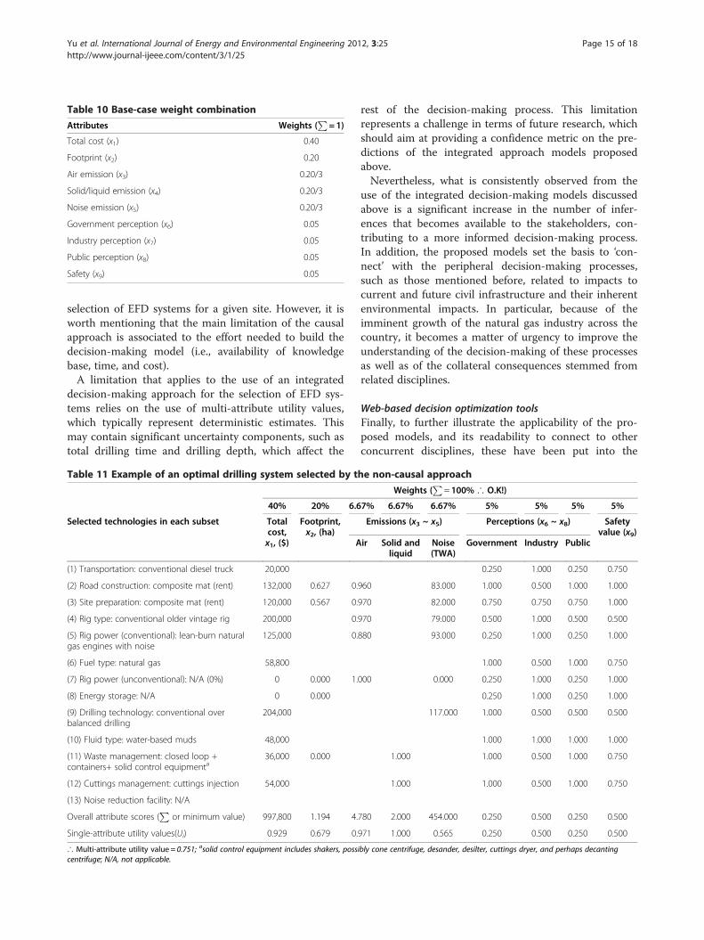
Table 10 Base-case weight combination

Attributes Weights (P

=1)

Total cost (x1) 0.40

Footprint (x2) 0.20

Air emission (x3) 0.20/3

Solid/liquid emission (x4) 0.20/3

Noise emission (x5) 0.20/3

Government perception (x6) 0.05

Industry perception (x7) 0.05

Public perception (x8) 0.05

Safety (x9) 0.05


selection of EFD systems for a given site. However, it isworth mentioning that the main limitation of the causalapproach is associated to the effort needed to build thedecision-making model (i.e., availability of knowledgebase, time, and cost).A limitation that applies to the use of an integrated

decision-making approach for the selection of EFD sys-tems relies on the use of multi-attribute utility values,which typically represent deterministic estimates. Thismay contain significant uncertainty components, such astotal drilling time and drilling depth, which affect the

Table 11 Example of an optimal drilling system selected by t

40% 20% 6.6


Footprint,x2, (ha)

A

(1) Transportation: conventional diesel truck 20,000

(2) Road construction: composite mat (rent) 132,000 0.627 0.

(3) Site preparation: composite mat (rent) 120,000 0.567 0.

(4) Rig type: conventional older vintage rig 200,000 0.

(5) Rig power (conventional): lean-burn naturalgas engines with noise

125,000 0.

(6) Fuel type: natural gas 58,800

(7) Rig power (unconventional): N/A (0%) 0 0.000 1.

(8) Energy storage: N/A 0 0.000

(9) Drilling technology: conventional overbalanced drilling

204,000

(10) Fluid type: water-based muds 48,000

(11) Waste management: closed loop +containers+ solid control equipmenta

36,000 0.000

(12) Cuttings management: cuttings injection 54,000

(13) Noise reduction facility: N/A


or minimum value) 997,800 1.194 4.

Single-attribute utility values(Ui) 0.929 0.679 0.

∴ Multi-attribute utility value = 0.751; asolid control equipment includes shakers, posscentrifuge; N/A, not applicable.

rest of the decision-making process. This limitationrepresents a challenge in terms of future research, whichshould aim at providing a confidence metric on the pre-dictions of the integrated approach models proposedabove.Nevertheless, what is consistently observed from the

use of the integrated decision-making models discussedabove is a significant increase in the number of infer-ences that becomes available to the stakeholders, con-tributing to a more informed decision-making process.In addition, the proposed models set the basis to ‘con-nect’ with the peripheral decision-making processes,such as those mentioned before, related to impacts tocurrent and future civil infrastructure and their inherentenvironmental impacts. In particular, because of theimminent growth of the natural gas industry across thecountry, it becomes a matter of urgency to improve theunderstanding of the decision-making of these processesas well as of the collateral consequences stemmed fromrelated disciplines.

Web-based decision optimization toolsFinally, to further illustrate the applicability of the pro-posed models, and its readability to connect to otherconcurrent disciplines, these have been put into the

he non-causal approach

Weights (P

= 100% ∴ O.K!)

7% 6.67% 6.67% 5% 5% 5% 5%

Emissions (x3 ~ x5) Perceptions (x6 ~ x8) Safetyvalue (x9)

ir Solid andliquid

Noise(TWA)


0.250 1.000 0.250 0.750

960 83.000 1.000 0.500 1.000 1.000

970 82.000 0.750 0.750 0.750 1.000

970 79.000 0.500 1.000 0.500 0.500

880 93.000 0.250 1.000 0.250 1.000

1.000 0.500 1.000 0.750

000 0.000 0.250 1.000 0.250 1.000

0.250 1.000 0.250 1.000

117.000 1.000 0.500 0.500 0.500

1.000 1.000 1.000 1.000

1.000 1.000 0.500 1.000 0.750

1.000 1.000 0.500 1.000 0.750

780 2.000 454.000 0.250 0.500 0.250 0.500

971 1.000 0.565 0.250 0.500 0.250 0.500

ibly cone centrifuge, desander, desilter, cuttings dryer, and perhaps decanting

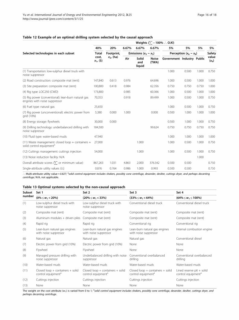
Table 12 Example of an optimal drilling system selected by the causal approach

Weights (P

= 100% ∴ O.K!)

40% 20% 6.67% 6.67% 6.67% 5% 5% 5% 5%


Footprint,x2, (ha)

Emissions (x3 ~ x5) Perception (x6 ~ x8) Safetyvalue(x9)

Air Solidandliquid

Noise(TWA)


(1) Transportation: low-sulphur diesel truck withnoise suppressor

1.000 0.500 1.000 0.750

(2) Road construction: composite mat (rent) 147,840 0.613 0.976 64.696 1.000 0.500 1.000 1.000

(3) Site preparation: composite mat (rent) 100,800 0.418 0.984 62.356 0.750 0.750 0.750 1.000

(4) Rig type: LOC250 (CWD) 173,800 0.985 60.366 1.000 0.500 1.000 1.000

(5) Rig power (conventional): lean-burn natural gasengines with noise suppressor

70,353 0.918 89.499 1.000 0.500 1.000 0.750

(6) Fuel type: natural gas 25,650 1.000 0.500 1.000 0.750

(7) Rig power (unconventional): electric power fromgrid (10%)

5,380 0.000 1.000 0.000 0.500 1.000 1.000 1.000

(8) Energy storage: flywheels 30,000 0.000 0.500 1.000 1.000 0.750

(9) Drilling technology: underbalanced drilling withnoise suppressor

184,500 99.624 0.750 0.750 0.750 0.750

(10) Fluid type: water-based muds 47,940 1.000 1.000 1.000 1.000

(11) Waste management: closed loop + containers +solid control equipmenta

27,000 1.000 1.000 0.500 1.000 0.750

(12) Cuttings management: cuttings injection 54,000 1.000 1.000 0.500 1.000 0.750

(13) Noise reduction facility: N/A 1.000


or minimum value) 867,263 1.031 4.863 2.000 376.542 0.500 0.500 0.750

Single-attribute utility values (Ui) 0.876 0.764 0.986 1.000 0.993 0.500 0.500 0.750

∴ Multi-attribute utility value = 0.827; asolid control equipment includes shakers, possibly cone centrifuge, desander, desilter, cuttings dryer, and perhaps decantingcentrifuge; N/A, not applicable.

Table 13 Optimal systems selected by the non-causal approach

Subsetnumber

Set 1 Set 2 Set 3 Set 4

(0%≤w1 < 20%) (20%≤w1 < 33%) (33%≤w1 < 64%) (64%≤w1≤ 100%)

(1) Low-sulphur diesel truck withnoise suppressor

Low-sulphur diesel truck withnoise suppressor

Conventional diesel truck Conventional diesel truck

(2) Composite mat (rent) Composite mat (rent) Composite mat (rent) Composite mat (rent)

(3) Aluminum modules + driven piles Composite mat (rent) Composite mat (rent) Composite mat (rent)

(4) Rapid rig Rapid rig Conventional rig Conventional rig

(5) Lean-burn natural gas engineswith noise suppressor

Lean-burn natural gas engineswith noise suppressor

Lean-burn natural gas engineswith noise suppressor

Internal combustion engine

(6) Natural gas Natural gas Natural gas Conventional diesel

(7) Electric power from grid (10%) Electric power from grid (10%) None None

(8) Flywheel Flywheel None None

(9) Managed pressure drilling withnoise suppressor

Underbalanced drilling with noisesuppressor



(10) Water-based muds Water-based muds Water-based muds Water-based muds

(11) Closed loop + containers + solidcontrol equipmenta

Closed loop + containers + solidcontrol equipmenta

Closed loop + containers + solidcontrol equipmenta

Lined reserve pit + solidcontrol equipmenta

(12) Cuttings injection Cuttings injection Cuttings injection Cuttings injection

(13) None None None None

The weight on the cost attribute (w1) is varied from 0 to 1; asolid control equipment includes shakers, possibly cone centrifuge, desander, desilter, cuttings dryer, andperhaps decanting centrifuge.


Table 14 Optimal systems selected by the causal approach

Subsetnumber

Set 1 Set 2 Set 3 Set 4 Set 5

(0%≤w1 < 2%) (2%≤w1 < 27%) (27%≤w1 < 48%) (48%≤w1 < 81%) (81%≤w1≤ 100%)

(1) Low-sulphur diesel truckwith noise suppressor

Low-sulphur diesel truckwith noise suppressor

Low-sulphur diesel truckwith noise suppressor

Conventional diesel truck Conventional diesel truck

(2) Composite mat (rent) Composite mat (rent) Composite mat (rent) Composite mat (rent) Composite mat (rent)

(3) Aluminummodules + driven piles

Aluminummodules + driven piles

Composite mat (rent) Composite mat (rent) Composite mat (rent)

(4) LOC250 (CWD) LOC250 (CWD) LOC250 (CWD) LOC250 (CWD) LOC250 (CWD)

(5) Lean-burn natural gasengines with noisesuppressor

Lean-burn natural gasengines with noisesuppressor



Internal combustionengine

(6) Natural gas Natural gas Natural gas Natural gas Conventional diesel

(7) Electric power from grid(30%)

Electric power from grid(10%)

Electric power from grid(10%)

None None

(8) Flywheel Flywheel Flywheel None None

(9) Managed pressure drillingwith noise suppressor

Managed pressure drillingwith noise suppressor

Underbalanced drillingwith noise suppressor



(10) Water-based muds Water-based muds Water-based muds Water-based muds Water-based muds

(11) Closed loop + containers+ solid controlequipmenta

Closed loop + containers+ solid controlequipmenta



Lined reserve pit + solidcontrol equipmenta

(12) Cuttings injection Cuttings injection Cuttings injection Cuttings injection Cuttings injection

(13) None None None None None

The weight on the cost attribute (w1) is varied from 0 to 1; asolid control equipment includes shakers, possibly cone centrifuge, desander, desilter, cuttings dryer, andperhaps decanting centrifuge; CWD, casing-while-drilling.


form of two web-based decision optimization tools(non-causal and causal), replicating the system selectionprocesses discussed above. These applications provide aquantitative basis for suggesting appropriate EFD sys-tems, which explicitly evaluate the proposed selectioncriteria and allow for using the best available evidence,including expert's belief, data, and models.The non-causal approach has been already used by

students enrolled in the ‘Drilling Engineering (PETE661)’class at Texas A&M University as an integrateddecision-making tool for their well site design [21]. Morerecently, the causal application was completed and usedfor the same course, allowing for the generation of simi-lar inferences and comparisons as discussed in this work.The key features of both applications are summarized inTable 15 and can be accessed at [22].

Table 15 Key features of the two web-based decision-making

Features

Providing a quantitative basis for selecting EFD drilling systems

Evaluating different EFD drilling technologies

Optimizing selection of EFD systems for given conditions

Introducing drilling time variation effects

Introducing causal dependencies between the system components

ConclusionsThis work makes the case for introducing an integrateddecision-making approach for the selection of optimalenvironmentally friendly drilling (EFD) systems to pro-vide a more logical and comprehensive approach thatmaximized the economic and environmental goals ofboth the landowner and the natural gas industry. Twodifferent drilling system selection approaches were dis-cussed based on a combination of the multi-attributeutility theory and the exhaustive search optimization,which are formulated as a non-causal and a causal ap-proach. The proposed models were implemented to acase study defined in an environmentally sensitive areain Green Lake at McFaddin, TX, USA.Results showed the relevance of using an integrated

decision-making approach for the selection of EFD

optimization tools

Non-causal Causal

Included Included

Included Included

Included Included

Not included Included

Not included Included


systems. This was corroborated by assessing each modeland by showing the type of inferences that can beretrieved from the definition of such a complex system.A comparison between the proposed models also helpedto address the need for the use of an integrateddecision-making approach because it was possible toreplicate the real trade-off between technology costs andreduction of the environmental impacts.The proposed decision-making methods aim at indi-

cating a critical shift from non-causal to causal systemselection, which the authors strongly believe can im-prove the finding of optimal components in such a com-plex system as of EFDs. By having access to suchdecision-making models, optimal scenarios can be sug-gested, contributing to a more informed decision-making process. This becomes significantly relevant inlight of an imminent growth of the natural gas industryand the potential consequences this may impose in con-current processes such as those related to civil infra-structure and its corresponding environmental impacts.

Competing interestsThe authors declare that they have no competing interests.

Authors’ contributionsOY carried out the optimization studies and drafted the manuscript. ZMCdrafted the manuscript. SG participated in the optimization study andanalyzed the results. JB and DB conceived of the study and participated inits design and coordination. All authors read and approved the finalmanuscript.

AcknowledgementsThe authors would like to thank the EFD subject matter experts for theirassistance with this research. They want to acknowledge in particular Ms.Carole Fleming, Dr. John Rogers, and Dr. Jerome Schubert. The informationcontained in this paper was provided in part from the research project ‘FieldTesting of Environmentally Friendly Drilling Systems’ sponsored by the USDOE, from the project ‘Environmentally Friendly Drilling Systems’ sponsoredby the RPSEA, and by the contribution of experts from oil and gascompanies. The authors want to thank all the sponsors and subject expertsfor their support.

Author details1Appalachian State University, Boone, NC 28608, USA. 2Texas A&M University,College Station, TX 77843, USA. 3Johns Hopkins University, Baltimore, MD21218, USA.

Received: 16 July 2012 Accepted: 27 August 2012Published: 3 October 2012

References1. Al-Yami, A, Schubert, J, Medina-Cetina, Z, Yu, O-Y: Drilling expert system for

the optimal design and execution of successful cementing practices. In:Proceedings of IADC/SPE Asia Pacific Drilling Technology Conference andExhibition, Ho Chi Minh City, 1–3 Nov 2010

2. Haut, R, Williams, T, Burnett, D, Theodori, G, Veil, J: The EnvironmentallyFriendly Drilling Systems Program Report. Houston Advanced ResearchCenter, The Woodlands (2010)

3. Rogers, JD, Knoll, B, Haut, R, McDole, B, Deskins, G: Assessments ofTechnologies for Environmentally Friendly Drilling Project: Land-BasedOperations. Texas A&M University Environmentally Friendly Drilling Report,Houston Advanced Research Center, The Woodlands (2006)

4. Herbert, M, Pedersen, J, Pedersen, T: A step change in collaborativedecision making - onshore drilling center as the New Work space. In:

Proceedings of SPE Annual Technical Conference and Exhibition,Denver, 5–8 Oct 2003

5. King, WW: Iterative drilling simulation process for enhanced economicdecision making. (22 Nov 2001). US Patent 6612382

6. Hui, Z, Deli, G: Screening the key techniques for oil & gas drilling inconsideration of safety. Nat. Gas Ind. 25(4), 77 (2005)

7. Simon, HA, Dantzig, GB, Hogarth, R, Plott, CR, Raiffa, H, Schelling, TC,Shepsle, KA, Thaler, R, Tversky, A, Winter, S: Decision making and problemsolving. Interfaces 17(5), 11–31 (1987)

8. Sadiq, R, Husain, T, Veitch, B, Bose, N: Risk-based decision-making for drillingwaste discharges using a fuzzy synthetic evaluation technique. Ocean Eng.31(16), 1929–1953 (2004)

9. Yu, O-Y, Guikema, S, Briaud, J-L, Burnett, D: Quantitative decision tools forsystem selection in environmentally friendly drilling. Civ. Eng. Environ. Syst.28(3), 185–208 (2011)

10. Yu, O-Y, Guikema, S, Briaud, J-L, Burnett, D: Sensitivity analysis for multi-attribute system selection problems in onshore environmentally friendlydrilling (EFD). Syst. Eng. 15(2), 153–171 (2012)

11. Clemen, RT, Reilly, T: Making Hard Decisions with Decision Tools. Duxbury,Pacific Grove (2001)

12. Keeney, RL, Raiffa, H: Decisions with Multiple Objectives: Preferences andValue Tradeoffs. Cambridge University Press, New York (1976)

13. Occupational Safety & Health Adminstration: Noise exposure computation.http://www.osha.gov/dts/osta/otm/noise/hcp/index.html. Accessed Feb2012

14. Hardaker, JB: Coping with Risk in Agriculture. CABI, Cambridge (2004)15. Keeney, RL: Value-Focused Thinking: A Path to Creative Decisionmaking.

Harvard University Press, Cambridge (1992)16. Cover, KS, Verbunt, JPA, de Munck, JC, van Dijk, BW: Fitting a single

equivalent current dipole model to MEG data with exhaustive searchoptimization is a simple, practical and very robust method given the speedof modern computers. Int. Congr. Ser. 1300, 121–124 (2007)

17. Guikema, S, Milke, M: Quantitative decision tools for conservationprogramme planning: practice, theory and potential. Environ. Conserv.26(03), 179–189 (1999)

18. Hovorka, SD, Doughty, C, Knox, PR, Green, CT, Pruess, K, Benson, SM:Evaluation of brine-bearing sands of the Frio formation, upper Texas GulfCoast for geological sequestration of CO2. In: Proceedings of First NationalConference on Carbon Sequestration, Washington, DC, 14–17 May 2001

19. Howard, RA, Matheson, JE: Influence diagrams. Decis. Anal. 2(3), 127–143(2005)

20. Decision Systems Laboratory: GeNIe Tutorial. http://genie.sis.pitt.edu/(2005–2007). Accessed Sept 2011

21. Burnett, D, Yu, O-Y, Schubert, J: Well design for environmentally friendlydrilling systems: using a graduate student drilling class team challenge toidentify options for reducing impacts. In: Proceedings of the SPE/IADCConference and Exhibition, Amsterdam, 17–19 March 2009

22. Medina-Cetina, Z, Yu, O-Y: Environmentally Friendly Drilling Systems.https://stochasticgeomechanics.civil.tamu.edu/efd/ (2009–2011).Accessed 18 Sept 2012

doi:10.1186/2251-6832-3-25Cite this article as: Yu et al.: Integrated approach for the optimalselection of environmentally friendly drilling systems. InternationalJournal of Energy and Environmental Engineering 2012 3:25.

Submit your manuscript to a journal and benefi t from:

7 Convenient online submission

7 Rigorous peer review

7 Immediate publication on acceptance

7 Open access: articles freely available online

7 High visibility within the fi eld

7 Retaining the copyright to your article

Submit your next manuscript at 7 springeropen.com

http://www.osha.gov/dts/osta/otm/noise/hcp/index.html

http://genie.sis.pitt.edu/

https://stochasticgeomechanics.civil.tamu.edu/efd/

original research open access integrated approach … · original research open access integrated...

Documents