orks with real-time ser - columbia universityhgs/papers/schu9305_reducing.pdf · orks with...
TRANSCRIPT
Reducing and Characterizing Packet Loss for High-Speed ComputerNetworks with Real-Time Services
A Dissertation Presented
by
Henning G. Schulzrinne
Submitted to the Graduate School of theUniversity of Massachusetts in partial ful�llment
of the requirements for the degree of
Doctor of Philosophy
May 1993
Department of Electrical and Computer Engineering

c Copyright Henning G. Schulzrinne 1993
All Rights Reserved

Reducing and Characterizing Packet Loss for High-Speed ComputerNetworks with Real-Time Services
A dissertation Presented
by
Henning G. Schulzrinne
Approved as to style and content by:
James F. Kurose, Chair of Committee
Donald F. Towsley, Member
Christos G. Cassandras, Member
Wei-Bo Gong, Member
Aura Ganz, Member
Lewis E. Franks, Acting Department HeadDepartment of Electrical and ComputerEngineering

To Carol, Nathan Paavo and my parents
iv

Acknowledgements
It is with great pleasure that I acknowledge the encouragement, insight and
valuable advice of Professor James F. Kurose and Professor Donald F. Towsley,
without whom this work would not have been possible. I feel very fortunate to
have had them as my advisors. The opportunities for travel and meeting fellow
researchers provided by them allowed me to broaden my professional horizon.
Appreciation is also due to Professor Christos Cassandras for help in charting the
course through the thesis process, his technical guidance and making workstations
available for some of the kernel and Nevot work. The editing e�orts of Professor
Weibo Gong and Aura Ganz are gladly acknowledged.
The work was supported �nancially in part by the O�ce of Naval Research under
contract N00014-87-K-304 and N00014-90-J-1293, the Defense Advanced Research
Projects Agency under contract NAG2-578, an NSF equipment grant, CERDCR
8500332 and a fellowship from the graduate school of the University of Massachusetts
at Amherst. DARTnet is funded by the Defense Advanced Research Projects
Agency.
I have enjoyed the priviledge of sharing spirited discussions with fellow graduate
students, in particular the members of our research group both during our research
group meetings and in one-on-one conversations.
Charles Lynn (Bolt, Beranek and Newman in Cambridge) helped with navigat-
ing the intricacies of the ST-II protocol implementation; Karen Seo (BBN) helped
to establish and foster the connection between our research group and BBN. Steve
Deering (Xerox Parc) elucidated IP multicast issues. Steve Casner (Information
Sciences Institute) and Allison Mankin (MITRE Corporation) supported this re-
search by making the loan of a video codec possible. I am also grateful to Steve
v

Casner, Van Jacobsen (LBL) and Eve Schooler (ISI) and for sharing their expertise
in audio conferencing. Lixia Zhang (Xerox Parc) quick answers to my questions
regarding her FIFO+ experiments were much appreciated, as well as the discussions
with David Clark (MIT) on resource control in networks. It has been a pleasure to
become part of the DARTnet research community through meetings and through
the regular teleconferences.
The friendship of the members of First Congregational Church has enriched my
stay in Amherst and have made Amherst a home to return to. Finally, I would like
to thank my wife Carol and my parents for their encouragement, understanding and
support.
vi

Abstract
Henning G. Schulzrinne
Reducing and Characterizing Packet Loss for High-Speed Computer
Networks with Real-Time Services
May 1993
B.S., Technische Hochschule Darmstadt
(Federal Republic of Germany)
M.S., University of Cincinnati
Ph.D., University of Massachusetts
Directed by: Professor James F. Kurose
Higher bandwidths in computer networks have made application with real-time
constraints, such as control, command, and interactive voice and video communica-
tion feasible. We describe two congestion control mechanisms that utilize properties
of real-time applications. First, many real-time applications, such as voice and
video, can tolerate some loss due to signal redundancy. We propose and analyze a
congestion control algorithm that aims to discard packets if they stand little chance
of reaching their destination in time as early on their path as possible. Dropping
late and almost-late packets improves the likelihood that other packets will make
their deadline.
Secondly, in real-time systems with �xed deadlines, no improvement in perfor-
mance is gained by arriving before the deadline. Thus, packets that are late and have
many hops to travel are given priority over those with time to spare and close to their
destination by introducing a hop-laxity priority measure. Simulation results show
marked improvements in loss performance. The implementation of the algorithm
vii

within a router kernel for the DARTnet test network is described in detail. Because
of its unforgiving real-time requirements, packet audio was used as one evaluation
tool; thus, we developed an application for audio conferencing. Measurements with
that tool show that traditional source models are seriously awed.
Real-time services are one example of tra�c whose perceived quality of service
depends not only on the loss rate but also on the correlation of losses. We investigate
the correlation of losses due to bu�er over ow and deadline violations in both
continuous and discrete-time queueing systems. We show that loss correlation does
not depend on value of the deadline forM=G=1 systems and is generally only weakly
in uenced by bu�er sizes. Per-stream loss correlation in systems with periodic and
Bernoulli on/o� sources are evaluated analytically. Numerical examples indicate
that loss correlation is of limited in uence as long as each stream contributes less
than about one-tenth of the overall network load.
viii

Table of Contents
Acknowledgements : : : : : : : : : : : : : : : : : : : : : : : : : : : : : : : : : : : : : : : : : v
Abstract : : : : : : : : : : : : : : : : : : : : : : : : : : : : : : : : : : : : : : : : : : : : : : : : : : vii
List Of Tables : : : : : : : : : : : : : : : : : : : : : : : : : : : : : : : : : : : : : : : : : : : : : xii
List Of Figures : : : : : : : : : : : : : : : : : : : : : : : : : : : : : : : : : : : : : : : : : : : : xiii
Chapter : : : : : : : : : : : : : : : : : : : : : : : : : : : : : : : : : : : : : : : : : : : : : : : : : : : xv
1. Introduction : : : : : : : : : : : : : : : : : : : : : : : : : : : : : : : : : : : : : : : : : : : : : 1
1.1 Organization : : : : : : : : : : : : : : : : : : : : : : : : : : : : : : : 31.2 Contributions : : : : : : : : : : : : : : : : : : : : : : : : : : : : : : 4
2. Congestion Control for Real-Time Traffic in High-Speed Net-works : : : : : : : : : : : : : : : : : : : : : : : : : : : : : : : : : : : : : : : : : : : : : : : : : : : 6
2.1 Introduction : : : : : : : : : : : : : : : : : : : : : : : : : : : : : : : 62.2 System Model and Notation : : : : : : : : : : : : : : : : : : : : : : 92.3 Packet Loss in Virtual Circuit : : : : : : : : : : : : : : : : : : : : : 11
2.4 FIFO-BS: Bounded System Time : : : : : : : : : : : : : : : : : : : : 12
2.5 FIFO-BW: Bounded Waiting Time : : : : : : : : : : : : : : : : : : : 14
2.6 Congestion Control and Robust Local Deadlines : : : : : : : : : : : 212.7 Summary and Future Work : : : : : : : : : : : : : : : : : : : : : : : 23
3. Scheduling under Real-Time Constraints: A Simulation Study : : 29
3.1 Introduction : : : : : : : : : : : : : : : : : : : : : : : : : : : : : : : 29
3.1.1 Performance Metrics : : : : : : : : : : : : : : : : : : : : : : : 30
3.1.2 A Taxonomy of Real-Time Scheduling Policies : : : : : : : : 32
3.1.3 Objectives for Scheduling Policies : : : : : : : : : : : : : : : 363.2 Scheduling and Discarding Policies : : : : : : : : : : : : : : : : : : : 393.3 Scheduling Policy Performance in a Symmetric Network : : : : : : : 433.4 Scheduling Policy Performance for a Tandem System : : : : : : : : : 493.5 Notes on Modeling Voice Sources : : : : : : : : : : : : : : : : : : : : 55
ix

4. Experiments in Traffic Scheduling : : : : : : : : : : : : : : : : : : : : : : : : : : 61
4.1 The Experimental Network : : : : : : : : : : : : : : : : : : : : : : : 624.2 Protocol and Operating System Support for Laxity-Based Scheduling 63
4.2.1 IP Implementation : : : : : : : : : : : : : : : : : : : : : : : : 64
4.2.1.1 Extensions to the Internet Protocol : : : : : : : : : 64
4.2.1.2 Hop Count Information : : : : : : : : : : : : : : : : 66
4.2.1.3 Timing and Deadline Information : : : : : : : : : : 68
4.2.1.4 Kernel Modi�cations : : : : : : : : : : : : : : : : : 71
4.2.1.5 Scheduling Overhead Considerations : : : : : : : : : 74
4.2.2 ST-II Implementation : : : : : : : : : : : : : : : : : : : : : : 764.3 Tra�c Sources : : : : : : : : : : : : : : : : : : : : : : : : : : : : : : 78
4.3.1 Lecture Audio and Video : : : : : : : : : : : : : : : : : : : : 79
4.3.2 Conversational Audio Source : : : : : : : : : : : : : : : : : : 804.4 The Network Voice Terminal : : : : : : : : : : : : : : : : : : : : : : 804.5 A Trace-Based Tra�c Generator : : : : : : : : : : : : : : : : : : : : 854.6 Experiments : : : : : : : : : : : : : : : : : : : : : : : : : : : : : : : 85
4.6.1 Simulation as Predictor of Network Performance : : : : : : : 874.7 DARTnet Experiment: First Topology : : : : : : : : : : : : : : : : : 90
4.7.1 DARTnet Experiment: Second Topology : : : : : : : : : : : 924.8 Conclusion and Future Work : : : : : : : : : : : : : : : : : : : : : : 93
4.8.1 Supporting Non-FIFO Scheduling in BSD Kernels : : : : : : 93
4.8.2 Simulation and Network Measurements : : : : : : : : : : : : 94
5. Distribution of the Loss Period for Queues with Single ArrivalStream : : : : : : : : : : : : : : : : : : : : : : : : : : : : : : : : : : : : : : : : : : : : : : : : : : 97
5.1 Introduction : : : : : : : : : : : : : : : : : : : : : : : : : : : : : : : 975.2 Clip Loss in Continuous Time (G=M=1) : : : : : : : : : : : : : : : : 100
5.2.1 Performance Measures : : : : : : : : : : : : : : : : : : : : : : 100
5.2.2 Distribution of the G=M=1 Initial Jump and Loss Period : : 104
5.2.3 Consecutive Customers Lost : : : : : : : : : : : : : : : : : : 109
5.2.4 Distribution of Noloss Period : : : : : : : : : : : : : : : : : : 110
5.2.5 Customers per Noloss Period : : : : : : : : : : : : : : : : : : 1145.3 Clip Loss in Discrete-time Systems : : : : : : : : : : : : : : : : : : : 115
5.3.1 The Busy and Idle Period : : : : : : : : : : : : : : : : : : : : 116
5.3.2 The Loss Period : : : : : : : : : : : : : : : : : : : : : : : : : 119
5.3.3 The Noloss Period : : : : : : : : : : : : : : : : : : : : : : : : 124
x

5.3.4 Numerical Examples : : : : : : : : : : : : : : : : : : : : : : : 1255.4 Bu�er Over ow in Single-Stream Discrete-Time Queues : : : : : : : 128
5.4.1 First-Come, First-Served : : : : : : : : : : : : : : : : : : : : 128
5.4.2 In uence of Service and Bu�er Policies : : : : : : : : : : : : 1315.5 Summary and Future Work : : : : : : : : : : : : : : : : : : : : : : : 136
6. Loss Correlation for Queues with Multiple Arrival Streams : : : 137
6.1 Introduction : : : : : : : : : : : : : : : : : : : : : : : : : : : : : : : 1376.2 Superposition of Periodic and Random Tra�c : : : : : : : : : : : : 138
6.2.1 Constant Period, Fixed Position: First and Last AdmittanceSystems : : : : : : : : : : : : : : : : : : : : : : : : : : : : : 141
6.2.2 Constant Period, Random Position : : : : : : : : : : : : : : : 143
6.2.2.1 FT Loss Probability and Waiting Time : : : : : : : 143
6.2.2.2 BT Loss Probability : : : : : : : : : : : : : : : : : 145
6.2.2.3 Conditional Loss Probability : : : : : : : : : : : : : 147
6.2.2.4 Numerical Examples : : : : : : : : : : : : : : : : : 150
6.2.2.5 Asymptotic Analysis in � : : : : : : : : : : : : : : : 154
6.2.3 Random Period, Random Position : : : : : : : : : : : : : : : 159
6.2.4 Future work : : : : : : : : : : : : : : : : : : : : : : : : : : : 1606.3 Bursty Tra�c Sources : : : : : : : : : : : : : : : : : : : : : : : : : : 160
6.3.1 The Interarrival Time Distribution in an IPP : : : : : : : : : 162
6.3.2 The N � IPP=D=c=K queue : : : : : : : : : : : : : : : : : : : 164
6.3.2.1 The Loss Probability : : : : : : : : : : : : : : : : : 166
6.3.3 The Conditional Loss Probability : : : : : : : : : : : : : : : 167
6.3.4 Numerical Examples : : : : : : : : : : : : : : : : : : : : : : : 1716.4 Summary and Conclusions : : : : : : : : : : : : : : : : : : : : : : : 175
7. Conclusion : : : : : : : : : : : : : : : : : : : : : : : : : : : : : : : : : : : : : : : : : : : : : : 176
Bibliography : : : : : : : : : : : : : : : : : : : : : : : : : : : : : : : : : : : : : : : : : : : : : : : 180
xi

List of Tables
3.1 Properties of scheduling disciplines : : : : : : : : : : : : : : : : : : : : : 42
3.2 Losses (in percent) for discarding based on local wait, M = 5, � = 0:8,d = 20; net-equilibrium tra�c model : : : : : : : : : : : : : : : : : : 44
3.3 Losses (in percent) for age-based discarding, M = 5, N = 50, � = 0:8,d = 20 : : : : : : : : : : : : : : : : : : : : : : : : : : : : : : : : : : : 45
3.4 Packet losses (in percent) for di�erent service and discarding policies;M = 5, N = 50, � = 0:8, d = 20 : : : : : : : : : : : : : : : : : : : : : 47
3.5 Packet losses (in percent) with discarding of expired packets; Poissonand geometric arrivals, N = 50, � = 0:8 : : : : : : : : : : : : : : : : : 48
3.6 Results for tandem network of Fig. 3.1 : : : : : : : : : : : : : : : : : : : 51
3.7 Comparison of queueing delays experienced by voice tra�c and equiva-lent two-state model : : : : : : : : : : : : : : : : : : : : : : : : : : : 59
4.1 DARTnet node locations (as of August, 1992) : : : : : : : : : : : : : : : 63
4.2 Comparison of queueing delays estimated by simulation and networkmeasurements : : : : : : : : : : : : : : : : : : : : : : : : : : : : : : : 90
4.3 End-to-end delay performance measured in DARTnet (topology of Fig. 4.6 91
4.4 End-to-end delay performance measured in DARTnet (topology of Fig. 3.1) 92
5.1 Expected initial jump and expected loss period for M=D=1 queue : : : : 108
5.2 Probability of loss, expected composite loss period and jump for Poissonbatches as a function of h for � = 0:8 : : : : : : : : : : : : : : : : : : 127
5.3 Expected loss run length (E[CC]) for D[G]=D=1=K system : : : : : : : : 131
5.4 Performance measures for geometric and Poisson arrivals, � = 1:5, K =4, 90% con�dence intervals : : : : : : : : : : : : : : : : : : : : : : : : 134
5.5 E�ect of random discarding for system with geometrically distributedbatch arrivals : : : : : : : : : : : : : : : : : : : : : : : : : : : : : : : 135
xii

List of Figures
2.1 Sample virtual circuit : : : : : : : : : : : : : : : : : : : : : : : : : : : : 7
2.2 Total and drop loss; analysis and simulation : : : : : : : : : : : : : : : : 17
2.3 Total packet loss vs. number of nodes, for optimal homogeneous dead-lines based on homogeneous or decreasing tra�c, � = 0:30 : : : : : : 19
2.4 Total packet loss vs. number of nodes, for optimal homogeneous dead-lines based on homogeneous or decreasing tra�c, � = 0:90 : : : : : : 20
2.5 Best achievable ratio of controlled (FIFO-BW) to uncontrolled (M/M/1)loss for homogeneous tra�c and deadlines; uncontrolled losses of 10�5,0:001, 0:01 and 0:05 : : : : : : : : : : : : : : : : : : : : : : : : : : : : 22
2.6 Comparison of overload performance of FIFO-BW to that of uncontrolledsystem; overload region : : : : : : : : : : : : : : : : : : : : : : : : : : 24
2.7 Comparison of goodput: tandem-M/M/1 vs. FIFO-BW with variouslocal deadlines, M = 5, � = 1 : : : : : : : : : : : : : : : : : : : : : : 25
3.1 The Tra�c Streams for Tandem Network : : : : : : : : : : : : : : : : : : 50
3.2 99.9-percentile values for the queueing delays (low-delay policies) : : : : 53
3.3 99.9-percentile values for the queueing delays (high-delay policies) : : : : 53
3.4 The interarrival time distribution for packet audio : : : : : : : : : : : : : 56
3.5 The silence duration distribution for packet audio : : : : : : : : : : : : : 56
4.1 The DARTnet topology, with link round-trip propagation delays : : : : : 64
4.2 The hop-laxity IP option : : : : : : : : : : : : : : : : : : : : : : : : : : : 66
4.3 Data ow in BSD kernel for IP : : : : : : : : : : : : : : : : : : : : : : : 72
4.4 Nevot Structure Overview : : : : : : : : : : : : : : : : : : : : : : : : : 84
4.5 Scheduling jitter for trace-based tra�c generator : : : : : : : : : : : : : 86
4.6 Tra�c Flows for DARTnet Experiment : : : : : : : : : : : : : : : : : : : 91
xiii

5.1 Virtual work sample path : : : : : : : : : : : : : : : : : : : : : : : : : : 102
5.2 Loss periods in discrete time (h = 3) : : : : : : : : : : : : : : : : : : : : 120
5.3 Expected composite loss period as a function of system load for h = 5 : : 126
5.4 Probability mass function of the composite loss period for � = 0:1 andh = 5 : : : : : : : : : : : : : : : : : : : : : : : : : : : : : : : : : : : : 127
6.1 Loss probability and conditional loss probability for Poisson or geomet-rically distributed background tra�c BT with �0 = 0:8 and periodictra�c FT with period � = 10, as a function of system size K : : : : 151
6.2 Loss probability and conditional loss probability for Poisson or geomet-rically distributed background tra�c BT with �0 = 0:8 and periodictra�c FT (random arrival), as a function of � ; system size K = 10 : 152
6.3 Loss probability and conditional loss probability for geometrically dis-tributed background tra�c BT with �0 = 0:8 and periodic tra�c FTwith period � = 10, as a function of system size K : : : : : : : : : : 153
6.4 Loss probability and conditional loss probability for geometrically dis-tributed background tra�c BT with �0 = 0:8 and periodic tra�cFT, as a function of � ; system size K = 10 : : : : : : : : : : : : : : 154
6.5 Loss probability and conditional loss probability for Poisson distributedbackground tra�c BT with �0 = 0:8 and periodic tra�c FT, as afunction of � ; system size K = 10 : : : : : : : : : : : : : : : : : : : : 155
6.6 Loss probability and conditional loss probability for geometrically dis-tributed background tra�c BT with total load of � = 0:8 and periodictra�c FT, as a function of � ; system size K = 10 : : : : : : : : : : : 156
6.7 Loss probabilities and expected run length for Poisson and geometricallydistributed background tra�c BT and periodic tra�c FT (randomarrival), as a function of BT intensity �0; system size K = 10, period� = 10 : : : : : : : : : : : : : : : : : : : : : : : : : : : : : : : : : : : 157
6.8 Probability that a loss run exceeds length x for given conditional lossprobability r : : : : : : : : : : : : : : : : : : : : : : : : : : : : : : : 158
6.9 Conditional and unconditional loss probability for N � IPP=D=c=K sys-tem, as a function of the bu�er size, K; N = 4, � = 0:8, = 0:7,! = 0:9 : : : : : : : : : : : : : : : : : : : : : : : : : : : : : : : : : : : 172
6.10 Conditional and unconditional loss probability for N � IPP=D=c=K sys-tem, for constant activity, � = 0:25, and load, � = 0:8, as a functionof the number of sources, N ; K = 1, � = 3:2=N : : : : : : : : : : : : 173
xiv

6.11 Conditional and unconditional loss probability for N � IPP=D=c=K sys-tem, for constant load (� = 0:8), cycle time (T0+T1 = 25) and bu�ersize (K = 1), as a function of � : : : : : : : : : : : : : : : : : : : : : 174
xv

C h a p t e r 1
Introduction
Computer networks are in a transition period, moving from relatively slow
communication links and data-oriented services to high-speed links supporting a
diverse set of services, including those such as video and voice with stringent real-
time constraints. These real-time services demand not only high bandwidth, but a
predictable quality of service not o�ered by current best-e�ort delivery networks.
Clearly, scaling bandwidths by a factor of thousand or more is bound to have
profound e�ects on all aspects of networking, but supporting the more diverse mix of
services raises issues that go beyond mere bandwidth and bandwidth-delay product
scaling.
Real-time services also shift the emphasis from throughput and delay as the
preeminent network performance metrics to packet loss caused by congestion. Tradi-
tional data services use retransmission schemes to hide network packet loss from the
application; packet loss is only re ected in the throughput and delay characteristics.
A 10% packet loss, for example, reduces throughput by a barely noticeable 10% if the
retransmission algorithm is implemented e�ciently, but could well make an audio
or video connection unusuable1. Similarly, a doubling of the end-to-end delay from
50 to 100 ms would be barely noticed for a �le transfer, but could lead to severe
talker echo in a voice conference.
For most high-speed connections2, packet losses are primarily due to bu�er
over ows in switching nodes and deadline violations rather than channel noise. The
1Due to delay constraints, retransmission is usually not possible with real-time services
2excluding, for example, packet radio or analog modems

2
problem of bu�er over ows is aggravated by bursty input tra�c and the large amount
of data \stored" by the transmission medium, which makes feedback controls di�cult
to implement.
This dissertation proposes and evaluates algorithms to reduce congestion-induced
losses in packet-switched networks carrying tra�c with real-time constraints. In
addition to the packet losses due to channel errors and queue over ows experienced
by all network services, real-time services also lose packets that violate their end-
to-end delay constraints. Two complementary heuristics for reducing loss caused
by deadline violation are presented and their performance is analyzed. The �rst
heuristic selectively discards packets within the network that either have, or are
likely to exceed, their delay bounds. Approximate analytical methods for tandem
queues are shown to provide good engineering estimates of the loss probabilities.
The network con�gurations, load and deadline regimen under which selective packet
dropping provides are identi�ed, showing realistic networks that can reduce such
packet loss by a factor of two. The second heuristic, called hop-laxity scheduling,
schedules packets for transmission on an outgoing link based on the ratio of the
time available to their deadline expiration and the number of hops needed to reach
the destination. This heuristic can be used to reduce deadline-violation losses (or,
equivalently, provide similar quality of service to packet ows traversing network
paths of di�erent length and cross tra�c loading). The heuristic is evaluated both
by simulation and by measuring the performance of an implementation within an
experimental transcontinental network using audio and video tra�c streams. A
number of tools for tra�c generation were also developed as part of this work and
are discussed in this thesis.
The dissertation also provides analytical methods that allow the characterization
of the structural properties of packet losses in queues subject to bu�er size limita-
tions or delay bounds. The loss properties are characterized here by measures of loss
correlation. Both queues serving single tra�c streams as well as queues multiplexing
3
a number of correlated sources are analyzed. In general, we �nd that loss correlation
is either independent of, or only very weakly correlated with, the bu�er size or delay
threshold. The in uence of other factors, such as tra�c burstiness, is quanti�ed.
1.1 Organization
The dissertation is organized as follows. First, we propose and analyze algorithms
that relieve congestion by selectively discarding packets (Chapter 2). As a comple-
mentary approach, a number of queue scheduling disciplines that strive to maximize
the amount of on-time arrivals are discussed in Chapter 3. Through simulations,
we �nd that hop-laxity scheduling appears particularly promising. Both for selec-
tive discarding and deadline-based scheduling, we emphasize end-to-end methods
rather than concentrating on a single queue. The implementation of the hop-laxity
scheduling algorithm within an experimental network is discussed in Chapter 4. We
discuss necessary protocol extensions for implementing hop-laxity scheduling within
the IP and ST-II Internet network layer framework. Also summarized are the kernel
modi�cations required to support this and other similar scheduling methods. We
also highlight the pertinent features of a voice conference application known as
Nevot, which we developed to provide realistic tra�c sources in our experimental
setting.
The structural properties of loss are addressed in Chapters 5 and 6, where we
analyze the time and correlation properties of packet loss in a large class of queueing
systems, both with a single and multiple arrival streams, where losses are caused by
either bu�er over ow or deadline violations.
Note that, due to the diversity of topics covered, each major chapter contains
its own literature review.

4
1.2 Contributions
The contributions of this thesis can be summarized as follows:
� development of a light-weight congestion control mechanism for real-
time services in networks with high delay-bandwidth product: The
mechanism attempts to reduce congestion by removing packets that are unlikely
to meet their end-to-end deadline. Approaches for choosing the parameters of
the algorithm are presented.
� end-to-end performance evaluation of a multi-hop queueing network
employing the proposed congestion control method: Using transform-
domain techniques, the end-to-end performance of the selective discarding
heuristic is studied. The approximate analysis is found to provide good con-
servative estimates of actual network performance and is suitable for numeric
parameter optimization.
� development of a link-level deadline-based scheduling policy for real-
time services that is aware of end-to-end performance requirements:
The policy is shown to reduce delay-induced losses for many network con�gu-
rations and equalizes the delay of ows traversing paths with di�erent number
of hops and network loading.
� implementation of the proposed scheduling policy in an operating
router: The scheduling policy was implemented in a standard BSD-based
operating system in the SPARCstation routers operating within the DARTnet
cross-country network testbed and its performance measured and compared to
FIFO queueing. Realistic tra�c sources based on actual voice and video confer-
ences, rather than statistical models, were used for the evaluation. Based on the
experiences with implementing non-FIFO disciplines with a BSD Unix kernel,

5
suggestions are o�ered on implementing a more general-purpose interface to
transmission scheduling.
� tool for audio conferencing: The work creating Nevot a tool for audio
conferencing, allowed us to explore issues in implementing real-time services in
non-real-time operating systems. The tool also serves as a tra�c generator for
the network, either directly or through its extensive tracing facility.
� trace-driven simulation and network tra�c generation tools: These
program provide tools to the experimenter to recreate a packet interarrival
time trace on an actual network, thus facilitating the comparison of simulation
with actual network performance and the reconstruction of fault scenarios.

C h a p t e r 2
Congestion Control for Real-Time Traffic inHigh-Speed Networks
2.1 Introduction
The higher bandwidths promised by broadband integrated services digital networks
(BISDN) have made applications with real-time constraints, such as control, com-
mand, and interactive voice and video communications, feasible. Many types of
real-time tra�c are characterized by \perishable", but redundant messages. In
other words, excessive delay renders them useless, but a certain degree of loss can
be tolerated without objectionable degradation in the grade of service. Real-time
packets are lost for several reasons. The packet may arrive at the receiver after the
end-to-end deadline has expired because it su�ered excessive waiting times in the
intermediate nodes (late loss). Also, queues may over ow or intermediate nodes
may shed load by dropping packet as an overload control measure (drop loss).
The tolerance for packet loss varies with the type of tra�c carried and the
measures the receiver is prepared to take to reconstruct lost packets. For speech
coded with PCM and adaptive DPCM, losses from 2 to 5% are tolerable without
interpolation, while odd-even interpolation raises the threshold of objectionable loss
to between 5% and 10% [1]. Compressed video is far less tolerant of lost packets.
A variable-rate DPCM coder operating at around 30 Mb/s [2] is designed for a loss
rate of below 10�11.
The goal of this chapter is to investigate controlling congestion for real-time
tra�c by judiciously discarding packets at the intermediate nodes. Packets that
stand little chance of making their end-to-end deadline should be discarded as early

7
in the virtual circuit as possible. Discarding applied with care has two bene�cial
e�ects. First, instantaneous congestion at the discarding node is relieved. This
type of congestion is caused by the statistical uctuations in the arrival process.
Secondly, downstream nodes are not burdened with tra�c that in all likelihood will
not meet its deadline at the receiving end, speeding up service for the remaining
packets. Reduced downstream load counteracts longer-term congestion, expressed
as high average load.
-
?
����
1 � P [J1]
�1
�1� -
�1 -
?
����
1 � P [J2]
�2
�2� -
�2 -
?
����
1 � P [J3]
�3
�3� -
�3�
� -d
��@@��@
@
?Yes
P [T jA]
�P [A]
�(1 � P [L])late?
Figure 2.1. Sample virtual circuit
Barring clairvoyance, we have four choices in discarding packets, depending on
our degree of caution and amount of available information (see Fig. 2.1 for notation):
1. discard randomly
2. discard a packet if the time spent at the node under consideration exceeds the
end-to-end deadline d
3. discard a packet whose time spent in the virtual circuit so far, including time
in current node, exceeds the end-to-end deadline d
4. discard a packet if the time to be spent in current node i exceeds a �xed local
deadline �i
The �rst scheme, random discarding, has been widely studied [3] [4] [5] [6],
and generally been found to be lacking as a congestion control mechanism. It, for

8
example, does not substantially improve the disproportionate probability that long
round-trip time tra�c is dropped [4]. We will further compare random dropping to
our schemes.
The next two schemes above are conservative in the sense that no packet will
ever be dropped voluntarily at the intermediate nodes that would not have been late
at the destination. The third approach risks the possibility of discarding packets
that would have made the end-to-end deadline. The parameter space investigated
will cover the �rst and third possibility, as the second requires \travel history" to
be carried with each packet.
We note that in a high-speed wide-area environment, control measures such
as ow-control windows, backpressure or choke packets [7] lose e�ectiveness since
the high delay-to-bandwidth ratio may render the feedback information obsolete
by the time it reaches the controlling agent. Because of this, local, distributed
control mechanisms are preferable to centralized algorithms. Also, not all real-time
sources can be readily rate-controlled (e.g., standard PCM voice). Even in high-
speed networks, window-based ow control with appropriate feedback may still be
suitable for avoiding congestion during �le transfers [8{14]. Resource allocation
may avoid congestion, but typically with the penalty of reduced carrying capacity if
streams do not utilize their allocated bandwidth. For a survey of resource allocation
policies, see [15].
After outlining the system model underlying this thesis in section 2.2 and the
general equations governing packet loss in section 2.3, we will in turn investigate two
queueing models for the proposed control mechanism, �rst-in{�rst-out with bounded
system time, referred to for brevity as FIFO-BS (section 2.4), and �rst-in{�rst-out
with bounded waiting time (FIFO-BW) in section 2.5.1 For each, the expressions for
the conditional distribution of the system or waiting time available in the literature
1In this thesis, system time is de�ned to include service, i.e., transmission, time. Waiting time
refers to the delay between arrival and start of service.

9
will be reviewed and extended where necessary. Expressions and numerical values
for the end-to-end delay distributions are presented and compared to simulation
results. Node rejection probability and the tail of the delay distribution establish
the end-to-end loss probability under the various congestion control schemes. A
simple scheme of using the same value for all local deadlines in the VC performs
will be shown to perform almost as well as the more di�cult scheme of selecting
optimal local deadlines for each node. We discuss implementing these policies in
high-speed networks and show that they compare favorably to random discarding
as a congestion countermeasure. We conclude this chapter with some alternative
approaches and future work in section 2.7.
2.2 System Model and Notation
This work is primarily concerned with packet voice tra�c. The approaches are also
applicable to other real-time tra�c, such as sensor data and control commands,
assuming that it shares a similar tolerance for loss and similar tra�c characteristics.
We study virtual circuits (VCs) with nodes labeled i = 1; 2; : : :M , typically
switching nodes in a wide-area network interconnected by high-bandwidth �ber
optic links. Packet losses caused by bit errors and other hardware faults are ignored
as the probability of their occurrence falls several orders of magnitude below that
of bu�er-related losses. Packet arrivals to all nodes are approximated by Poisson
processes with arrival rate �i. Modeling a superposition of SAD (speech activity
detection) voice sources as a Poisson source leads to overly optimistic estimates in
the case of a voice multiplexer [16]. However, for the case of voice trunks considered
here, the number of voice sources is possibly two orders of magnitude higher than
that found at the T1 rate (1.544 Mb/s) multiplexer studied by [17] and others. A 150
Mbit channel can support 4380 64 kB/s PCM sources of speech activity factor 0.42
with a utilization of 0.8. Thus, according to the arguments of [18], we can conclude
that for short time spans, the superposition process is adequately modeled by a

10
Poisson process. The discarding mechanism further limits the interaction period of
packets in the queue, improving the approximation [16].
Even assuming that the input tra�c to the �rst node is indeed modeled accu-
rately by a Poisson source, packet dropping at the intermediate nodes will make
the input stream to subsequent nodes non-Poisson. The analysis, however, ignores
this, based on the premise that the relatively small losses investigated should have
limited e�ects on the delay distribution. Simulation experiments will be used to
assess the validity of this assumption, which is also supported by [19,20].
The service time is assumed to be exponentially distributed with mean 1=�,
redrawn at each node (Kleinrock's independence assumption). Without loss of
generality, all times are scaled relative to the average service time, i.e., � = 1.
Since we are primarily interested in communication channels, we assume that the
packet transmission and waiting time is proportional to the number of bits in the
packet or queue, respectively. Also, the service time of each packet is assumed to
be known at the instant of arrival to a queue. (The results for FIFO-BW do not
change if the packet leaves the queue if it has not started service within the local
deadline; the service time of an individual packet does not enter into consideration.
For FIFO-BS, we have to assume that the service time is known on joining the
queue.)
We investigate a single virtual circuit in isolation, taking into account interfering
tra�c by reducing the service rate, as in [21]. The length of the virtual circuit
obviously depends on the system architecture, but examples in the literature [22]
suggest a range of four to eleven, with the values at the lower end appearing more
often. Following [23], most of the examples will have �ve nodes.
In summary, the above assumptions ensure independence of service and arrival
sample paths for each node. Nodes are linked only by the reduction in tra�c
a�orded by dropping certain packets. These assumptions are necessary for analytic
tractability, but as discussed above, will be validated through simulation.

11
A number of researchers have investigated the e�ect of packet dropping on a
single packet voice multiplexer (e.g., [24{26], and that of bit dropping on a virtual
circuit [19], but the performance of packet dropping in a VC seems to have been
considered only in the context of an ARQ-schemewith variable window size [27]. The
latter scheme requires acknowledgements, which are not typically used for real-time
tra�c, and uses feedback, with the concomitant delay problems. Most importantly,
packet dropping is performed without regard to the packet's time constraint.
In the following, probability density functions will be denoted by lower case
letters, with w and s standing for waiting and system time, respectively. The
respective uppercase letters represent the corresponding cumulative distribution
functions. An asterisk indicates the one-sided Laplace transform.
2.3 Packet Loss in Virtual Circuit
This section outlines some of the general relations governing packet loss in a virtual
circuit, independent of the particular queueing model used for the individual nodes.
A packet is considered lost if it is either discarded by any one of the M nodes it
traverses (because it missed the local deadline �i) or if the total system (FIFO-BS
case) or the waiting time (FIFO-BW) exceeds a set, �xed end-to-end deadline d (see
Fig. 2.1).
Components of Loss Probability
The arrival event A occurs if a packet reaches its destination, i.e., is not dropped
by any of the queue controllers along the VC. In a tandem-M=M=1 system, A occurs
with certainty. The complementary event will be referred to as D and its probability
as the drop loss. Ji represents the event that a packet joins queue i (given that it
has traversed nodes 1 through i� 1), while the event of a lost packet, regardless of
cause, will be labeled as L. The probability of an event is shown as P [�].

12
The probability that a packet is not dropped in any of the M (independent)
nodes is the destination arrival probability P [A] =QMi=1 P [Ji] In other words, P [A]
does not include the probability that a packet reaching the destination misses its
deadline. In computing P [Ji], the reduced tra�c due to packets dropped in nodes
0; 1; : : : ; i� 1 needs to be taken into account, where �i = �i�1P [Ji�1].
Thus, given that the end-to-end conditional cumulative distribution of system
time for non-discarded packets is S(djJ) = P [S � djJ ] , the total loss probabilityP [L], encompassing both drop loss and late loss, can be computed by the law of
total probabilities as
P [L] = (1 � S(djA))P [A] + (1 � P [A]) = 1� S(d)P [A]:
Here, the conditioning on J indicates that we only take packets that were not
dropped into consideration. The �rst part of the equation shows the contribution
of dropped and late packets to the total loss. In the case of voice, 1 � P [L] is the
fraction of packets that are actually played out at the receiver.
Since each link is assumed to be independent of all others, the conditional density
of the end-to-end system time, s(tjA), is derived from the convolution of the single-
node conditional densities, si(tjA). By the convolution property of the Laplace
transform we obtain,
s(tjJ) = s1(tjJ) � : : : � sM (tjJ) = L�1(
MYi=1
s�i (sjJ))
(2:1)
where L�1 represents the inverse Laplace transform.
2.4 FIFO-BS: Bounded System Time
In the �rst of the two congestion control policies considered, a packet joins queue i
(i = 1; : : : ;M) only if the virtual work, that is, the amount of time it would take
to empty the queue with no new arrivals, plus the service time of the arrival is less
than the local deadline, �i. In other words, the time spent in the queueing system,

13
including service, is bounded from above by �i. In this section, the results provided
in [28,29] will be simpli�ed to a form more amenable to computation. Some of the
tedious algebra has been relegated to a separate report [30].
Laplace Transform of the Pdf of the Virtual Waiting Time
The pdf of the waiting time, w(t), can be expressed as w(t) = Qh(t), where the
function h(t) is of no further interest for our purposes. The normalization factor Q
is de�ned as
Q = (1 � �)
"1 � �a+
1Xn=1
�n(bn � a)
(�)n
#�1; � 6= 1: (2:2)
where � = �=�, b � e��� , a � b1��e�(b�1). (x)n = x(x + 1)(x + 2) : : : (x + n � 1)
denotes Pochhammer's symbol.
The Laplace transform of the virtual waiting time is derived in [28]. The
transform expression can be immediately simpli�ed with the identity �(i+ 1) = i!,
yielding in our notation:
w�(s) = w�(�1)b1+s(1 + (1 + s)
1Xi=0
�i�(� � s � 1)
�(� � s+ i)
)
�Q(1 + s)1Xi=0
(�b)i�(� � s� 1)
�(� � s+ i): (2.3)
(Throughout this section, we are only concerned with the case � 6= 1.)
By making use of the identities �(�+ i) = �(�)(�)i and �(�� 1) = �(�)��1 , we can
avoid the evaluation of the gamma function with complex arguments:
w�(s) = Qabs(1 +
1 + s
�� s� 1
1Xi=0
�i
(�� s)i
)
+Q1 + s
�� s� 1
1Xi=0
(�b)i
(�� s)i:
Thus, the transform equation for the density of the system time of a single node
is
s�(s) =1
P [J ]
�
s+ �w�(s):
The technical report [30] also contains closed-form expressions for the cumulative
distribution functions of the waiting and system time of a single queue.

14
2.5 FIFO-BW: Bounded Waiting Time
Arriving customers join queue i if and only if the virtual work at queue i at the
arrival instant is below �i. In contrast to the FIFO-BS case discussed above, the
service time of the arriving customer does not enter into the admission decision,
thus eliminating the bias against long packets present in FIFO-BS. Here, the time a
packet spends waiting for service to begin is bounded by �i. Results for this system
are summarized in [31] (called FIFO-TO there). Among the policies for a single
queue studied in that paper, FIFO-BW performed best in the sense of maximizing
the throughput of packets meeting their deadlines, suggesting that it may be a good
candidate for a tandem system as well. As in the previous section, we will extend
the results for a single queue and then proceed to obtain closed-form expressions for
the densities and distributions of the waiting time of a tandem system. For brevity,
only results for � 6= 1 will be shown here.
A customer's conditional waiting time is distributed with density
w(tjJ) = ��e��t
�u(� � t)u(t) +
1 � �
��(t);
where u(t) is the unit step function and � = �e��� .
Recognizing u(� � t) = 1� u(t� � ), the waiting time in the Laplace domain is
derived:
w�(sjJ) = 1
�
���
s+ �
n1 � e�(s+�)�
o+ (1 � �)
�: (2:4)
Extending the results in [31], the nth moment can be written as
E[wn] =�
��n[n!� �(n + 1; �� )] =
n
�E[wn�1]� ��e���
�
where �(n; x) is the complementary incomplete Gamma function.
The IMSL routine DINLAP is able to invert Eq. (2.1) (with waiting time
replacing system time), using Eq. (2.4), with desired accuracy only for small M
and losses above 1%. Therefore, it was attempted to obtain tight bounds on the

15
tail of the waiting time distribution by using the moment generating function in the
Cherno� bound or higher moments in Bienaym�e's inequality [32]. Both produced
bounds too loose to judge the bene�ts of applying queue control via local deadlines.
An algebraic inversion of the Laplace-transform expression proved more fruitful.
This was possible because unlike the transform for the FIFO-BS case (Eq. (2.3)),
Eq. (2.4) is rational and thus amenable to closed-form expansion. As a general
strategy, the product of sums is expanded into a sum of products and each term in
the sum transformed separately.
The multiplicity of poles in the Laplace-domain convolution expression and the
potential for analytic and numerical simpli�cation make it expedient to distinguish
four cases when inverting the transform. The cases are classi�ed by the dependence
of the local deadline �i and the tra�c parameter �i = �i � �i on the node index:
1. homogeneous tra�c and local deadlines (�i = �j ; �i = �j 8 i; j)
2. homogeneous tra�c, but arbitrary local deadlines
3. strictly heterogeneous tra�c (�i 6= �j 8 i 6= j) and arbitrary local deadlines
4. arbitrary tra�c and deadlines, i.e., �i = �j is allowed
The closed-form expressions for calculating losses for these four cases appear in
the appendix.
Performance Evaluation: Numerical Examples and Validation
Having derived expressions for the cdf of the end-to-end system and waiting
times, we can now compare the performance of the suggested queue control mecha-
nisms. Because of space limitations, we will restrict our discussion to the FIFO-BW
case. In this section, the end-to-end deadline d is �xed so that the packet loss equals
a given value when no queue control is applied (\uncontrolled loss").

16
We �rst consider the case of homogeneous local deadlines, i.e., �i = �j = � . It
is clear that the optimal value of � has to fall between d=M and d since for values
of � less than or equal to d=M , all packets which are not dropped will make their
end-to-end deadline; For � � d, any packet dropped at an intermediate node would
be late on arrival at the destination.
Since relatively high load and loss should expose the de�ciency of ignoring the
non-Poisson nature of input streams, the �rst example uses the parameter setM = 5,
� = 1, �1 = 0:8 and d = 40:47, resulting in an uncontrolled loss of 5%. The
simulation maintains Kleinrock's independence assumption, but not the Poisson
nature of the interior arrival streams. The simulation was terminated once the
95%-con�dence interval halfwidths computed by spectral estimation [33] and the
regenerative method were both less than 10% of the point estimate. Depending on
� , a simulation run consisted of between one and �ve million packets. An initial
transient period estimated at 3000 packets was discarded.2
Fig. 2.2 compares analytical and simulation results for the �rst example, plotting
the total loss, composed of packets dropped in intermediate nodes and packets
missing their end-to-end deadline, as a function of the local deadline � . The
horizontal line at 5% loss indicates the asymptotic uncontrolled case with � = 1.
The graph shows that the analytical results overestimate end-to-end losses, with
simulation and analysis agreeing more closely as � increases towards in�nity and
the system approaches a tandem-M/M/1 queueing system. Fortunately, the opti-
mal nodal deadlines seem to fall in the same neighborhood for both analysis and
simulation. For this set of parameters, the FIFO-BW dropping mechanism reduces
total losses from 5% to 3.1% according to the analysis and to 2.4% according to
the simulation. From Fig. 2.2 we can also conclude that the drop losses incurred
by tight deadlines are not compensated for by the reduction in downstream tra�c.
2The estimate was based on the di�usion approximation of the G/G/1 queue, see [34] [35].

17
tota
l pac
ket l
oss
P[L
], %
node deadline τλ= 0.8, µ= 1.00, M = 5, d = 40.47
10−2
10−1
100
101
102
5 10 15 20 25 30 35 40 45
drop loss (analysis)• simulation
analysis
•
••
• • • • • • • •
Figure 2.2. Total and drop loss; analysis and simulation
Since the performance varies little in the region from � � 17 to � � 21, a looser
deadline in that range is preferable, providing a margin of safety to compensate for
errors in the estimation of the system parameters.
The dashed line traces late loss, showing that for very tight deadlines, almost
all packets that have not been dropped at intermediate nodes make their deadline.
Optimal Local Deadlines
While the experiments above used the same � for all nodes, it seems reasonable to
assume that the lower tra�c impacting downstream nodes could make heterogeneous
deadlines advantageous. To test this hypothesis, anM -dimensional simplex method
was used to �nd a set of �i's minimizing the overall loss, taking downstream tra�c

18
reductions into account. The optimal homogeneous � was used as a starting point to
minimize the probability of trapping the optimization in a local optimum. From the
examples reported in [30], it can be concluded that even for high loads (� = 0:9) and
short VCs such as M = 2, heterogeneous deadline yield less than 1% improvement
over using a homogeneous � .
Since the expressions for homogeneous tra�c and deadlines are algebraically
much simpler and numerically more stable, we examined the performance penalty
incurred by ignoring downstream tra�c reductions. Clearly, for homogeneous tra�c
only homogeneous deadlines can be optimal. As the examples in Fig. 2.3 and 2.4
demonstrate, the penalty increases with higher loads, higher uncontrolled losses and
longer virtual circuits. (In the �gures, the horizontal lines denote the asymptotic
losses for the uncontrolled system.)
Range of E�ectiveness
In the course of investigation it became clear that the proposed queue control
is advantageous only for a range of parameter values. The contour plot of Fig. 2.5,
containing lines of equal ratio of controlled to uncontrolled loss vs. length of VC,M ,
and tra�c intensity � for uncontrolled losses of 10�5, 10�3, 10�2 and 5�10�2, showsthat the ratio decreases (performance gains realized by queue control increase) with
increasing loads, shorter virtual circuits, higher uncontrolled losses and higher loads.
For example, at an uncontrolled loss of 5%, overall losses can drop to as little as
40% of the uncontrolled losses for a three-node circuit operating at a load of � = 0:9.
On the other hand, at uncontrolled losses of less than 10�3, even loads of � = 0:9
and the minimal circuit length of 2 does not push the controlled loss much below
75% of the uncontrolled loss. The parameter region of worthwhile gains agrees well
with the operating region of overload control for packet voice systems. However,
for the uncontrolled losses found in video applications, little gain can be expected.
It should be noted that the results shown in the graphs are conservative estimates

19
uncontrolled loss = 0.05
uncontrolled loss = 0.02
uncontrolled loss = 0.01
Figure 2.3. Total packet loss vs. number of nodes, for optimal homogeneousdeadlines based on homogeneous or decreasing tra�c, � = 0:30

20
uncontrolled loss = 0.05
uncontrolled loss = 0.02
uncontrolled loss = 0.01
Figure 2.4. Total packet loss vs. number of nodes, for optimal homogeneousdeadlines based on homogeneous or decreasing tra�c, � = 0:90

21
since they do not take into account the global tra�c reduction a�orded by having all
virtual circuits apply the control policy, especially signi�cant under loads of 0:8 and
above. Also, the simulation results discussed earlier show that actual performance
may be slightly better than the analysis predicts.
Investigations showed that the optimal local deadlines are relatively insensitive
to the number of nodes in the network and, to a lesser extent, the VC load. Also, no
obvious relationship seems to exists between drop loss and late loss at the optimal
operating point.
2.6 Congestion Control and Robust Local Dead-lines
In practical networks, it may not be feasible to measure tra�c accurately and adjust
the local deadlines accordingly, even with a table-lookup mechanism instead of on-
line optimization. However, a static control scenario such as the following would be
possible. At call setup, the end-to-end deadline (and, therefore, the playout bu�er
delay) is set so that the desired loss under non-overload conditions can be met.
The local deadlines are then established by table look-up based on the length of
the virtual circuit and a tradeo� between overload protection and additional loss
incurred under lighter loads. For each packet, the queue controller determines the
applicable � , measured in transmission units, from a look-up table and compares it
to the current number of transmission units queued, including those of the packet in
transmission. (Here we assume a �xed-rate channel.) These operations are readily
implementable in hardware at packet rate.
An example illustrates the approach. Suppose that a 5-node connection can
tolerate a loss of 1% without noticeable grade-of-service degradation. A call is
allowed into the network only if the average load does not exceed � = 0:8 at the time
of call setup. Correspondingly, the playout bu�er is set up for an end-to-end deadline
d = 52:7. The e�ect of several choices for � is shown in Fig. 2.6. We now describe

22
0.70.750.80.85
0.9 0.95 1
0.3
0.4
0.5
0.6
0.7
0.8
0.9
1e-05
0.6 0.7 0.8
0.9
0.001
0.450.50.550.6 0.65 0.7 0.75 0.8
0.85 0.9 0.95
2 4 6 8 10
0.3
0.4
0.5
0.6
0.7
0.8
0.9
0.01
0.35 0.4 0.45 0.5 0.55 0.6 0.650.70.75
0.8 0.85 0.9 0.95
2 4 6 8 10
0.05
nodes in virtual circuit
offe
red
load
Figure 2.5. Best achievable ratio of controlled (FIFO-BW) to uncontrolled (M/M/1)loss for homogeneous tra�c and deadlines; uncontrolled losses of 10�5, 0:001, 0:01and 0:05

23
the e�ect of several di�erent choice of � . In our �rst experiment, we pick a value
of � optimized for moderate overload, namely � = 0:9, yielding � = 18:3. Assume
that during the call the network load rises to that value of 0.9. If no queue control
were applied, the losses would reach an intolerable 32%. With the queue control,
� = 18:3, losses are reduced to 7%, which an interpolation method might be able to
cope with. However, this deadline is unduly restrictive for lower loads. For example,
at � = 0:8, losses are twice that of applying no control. Tightening the deadline to
� = 15 does not improve overload performance, but leads to further deterioration of
the grade of service at � = 0:8, pushing losses to 3.5%. A more conservative choice,
� = 23:3, ensures that losses at design load and below never exceed 1%, while still
limiting overload losses to 9.2%. If load should rise momentarily to � = 0:95, the
overload mechanism will cut losses from an uncontrolled 80% to 20%. As mentioned
at the end of section 2.5, actual network performance will most likely be better as
all VCs can be assumed to apply similar control mechanisms.
Figure 2.7 compares the goodput, de�ned as �(1�P [L]), of the uncontrolled andcontrolled system. Beyond a certain load, � = 0:83 in the example, the goodput for
the uncontrolled system actually decreases with increasing load. Optimal random
discarding as proposed in [5] can hold the goodput at the peak value even under
overload, as indicated by the horizontal line in the �gure. It throttles the input
tra�c to the point of optimal goodput by randomly discarding packets at the source.
Optimal random discarding requires, however, on-line tra�c or gradient estimation
(@P [D]=@�) to determine the fraction of packets to be discarded. Note also that if we
allow the deadline to be adjusted on-line according to the current tra�c, FIFO-BW
o�ers a higher goodput than optimal random discarding.
2.7 Summary and Future Work
In this chapter, we have presented an analytic model for evaluating the loss per-
formance of two queue control schemes, based on rejecting packets at intermediate

24
Figure 2.6. Comparison of overload performance of FIFO-BW to that of uncon-trolled system; overload region

25
Figure 2.7. Comparison of goodput: tandem-M/M/1 vs. FIFO-BW with variouslocal deadlines, M = 5, � = 1

26
nodes in a virtual circuit. It was shown that the fraction of lost packets could
be reduced substantially for suitable tra�c types and virtual circuit size. Even if
the exact load is not known, a static overload control mechanism can ameliorate
the e�ects of temporary overload situations. In related work [30], it is shown that
analysis technique and performance gains carry over to the case of �xed packet sizes.
It is anticipated that history-based discarding, which admits a packet only if
the time spent waiting upstream plus the virtual wait falls below a given threshold,
o�ers improved performance due to better information, albeit with higher processing
overhead.
In the next chapter, we will see how selective discarding can be complemented
e�ectively by laxity-based scheduling.
Appendix
In this appendix, closed-form expressions for the waiting-time density and distribu-
tion function for the FIFO-BW system will be presented. Homogeneous and het-
erogeneous tra�c leads to Mth order and �rst-order poles in the Laplace transform
expression, respectively, and thus requires separate treatment. A special case for
homogeneous tra�c simply reduces the number of terms in the expansion. Results
for the �rst three cases enumerated in section 2.5 will be presented; the fourth case
of arbitrary �i and �i is conceptually similar, but incurs another order-of-magnitude
increase in complexity not compensated for by increased insight.
For the �rst case of homogeneous tra�c and deadlines, the closed-form expres-
sion for the density can be derived from the Laplace transform as
L�1�1
�
��
s+ �(1� e�(s+�)� ) +
1 � �
�
�M
= L�18<: 1
�MX
k+l+m=M
�M
k; l;m
�e�l�� (��)k+l

27
�(1� �)m(�1)l e�l�s
(s+ �)k+l
)
For k + l > 0, the fraction containing terms in s can be readily inverted as
(t� l� )k+l�1
(k + l � 1)!e��(t�l�)u(t� l� )
For k + l = 0, that is, k = l = 0, the summand reduces to (1� �)m. The cdf can be
computed by integrating terms over the interval from l� to d � l� .
The second case allows for local deadlines that depend on the node index. The
Laplace transform can be rewritten as
MYi=1
1
�i
���
s+ �(1� e�(s+�)� ) + (1 � �)
�
=
"MYi=1
1
�i
#MXk=0
X~l:j~lj=M�k
���
s+ �+ (1 � �)
�k(�1)M�k
����
s + �
�M�k
exp
�(s+ �)
MXi=1
li�i
!
where the binary vector ~l has components li, restricted to the values zero or one. j~ljdenotes the number of ones in ~l.
Each term in the inner sum can be readily inverted for a given k as
(�1)M�ke���0
kXj=0
�kj
�(1 � �)k�j(��)j+M�kAk;j
where
Ak;j =(t� � 0)M+j�k�1
(M + j � k � 1)!e��(t��
0)u(t� � 0)
for j +M � k > 0 and Ak;j = �(t � � 0) for j = k �M . Here, � 0 =P
i li�i. The
number of terms depends on the value of � and t and is less than 2M (1 +M=2).
The third case allows for tra�c that depends on the node index; the condition
of strict heterogeneity in �i insures single poles. The PDF is expressed in the
time-domain as
wM(t) =2M�1Xk=1
"MYi=1
1
�i
# 24 MYj=1
r1�b(k)jj (�j�j)
b(k)j
35 �
28
Xj2b(k)
P2jb(k)j�1m=0 e��m��j(t��
0m)u(t� � 0m)Q
i2b(k)i6=j
�i � �j+
MYn=1
rn�(t):
b(k)i 2 f0; 1g stands for the ith digit of k written as a base-2 (binary) number. For
brevity, i 2 b(k) denotes all indices i such that b(k)i is 1. The computation of the
quantities �m and � 0m is based on the expansion of the product of the jlkj terms of theform 1� exp(�(s+ �i)�i). De�ne the mapping function h(k), whose ith component
h(k)i is the index of the ith one bit in b(k). Then,
� 0m =jb(k)jX
i=1;i2b(i)
�h(k)i
and
�m =jb(k)jX
i=1;i2b(i)
�h(k)i�h(k)i:
The distribution is readily computed by replacing the terms in the summation
over m by
1
�j
h1 � e��j(t��
0m)ie��mu(t� � 0m)
This case requires the evaluation of at most 2M � 3M�1 terms, with the exact
value depending on t. The large number of terms for high M (above �ve), di�ering
in absolute value by several orders of magnitude, forces use of quadruple precision
arithmetic and magnitude-sorted summation to control round-o� errors.

C h a p t e r 3
Scheduling under Real-Time Constraints: ASimulation Study
3.1 Introduction
We �rst motivate the performance metrics that may be used to evaluate scheduling
disciplines by providing some background on a class of real-time services with
adaptive constraints. We then provide a classi�cation system that categorizes
scheduling disciplines of interest to real-time services and highlight some additional
guidelines that may be used to choose between them. With this background,
section 3.2 summarizes a number of scheduling policies that suggest themselves
in a real-time environment.
Section 3.3 picks up from the previous chapter, where we had investigated FIFO
queues with discarding in some detail. Here, we turn our attention to a number of
other queue control and scheduling mechanisms for the slotted system covered in
that chapter, comparing them to the simple discarding mechanism described there.
Simulation experiments using a di�erent network with a more typical topology and
bursty tra�c will provide additional insights into the behavior of a wide range of
scheduling policies (Section 3.4. We will describe the theoretical and simulation
aspects in this chapter, while deferring implementation aspects to Chapter 4. At
that point, we can then also draw some conclusions as to the suitability of the policies
proposed. The chapter concludes in Section 3.5 by providing detailed statistical data
on the audio source used. We point out through the example that the commonly
assumed statistical descriptions of audio sources may not be accurate, either in
isolation or in aggregation.

30
3.1.1 Performance Metrics
Two basic measurements suggest themselves in evaluating the performance of
scheduling disciplines. First, we can specify a �xed deadline and determine the
fraction of packets that miss the deadline. This approach models most closely
the demands of \rigid" applications, i.e., those that cannot adapt their deadline
to changing network conditions and where the packet has to arrive absolutely,
positively on time. A control system would probably require �xed deadlines for both
measurement and control signals in order to guarantee stability and allow accurate
design of the system transfer function in advance. Applications in manufacturing
systems also fall into this category.
Beyond this \classical" performance objective, there is a large class of real-time
services that have slightly di�erent characteristics. Before discussing the second
metric appropriate to their needs, some background information appears called for.
In past chapters, we have categorized real-time applications according to their
loss tolerance, emphasizing that many applications can work quite well with a
rather substantial amount of packet loss. Although not required for the algo-
rithms, the implication was that the deadline itself was �xed by properties of
the application. In discussing scheduling policies for real-time system, however,
it is no longer appropriate to consider deadlines static for all applications. Many
emerging applications feature deadlines that stay constant over the short term, but
can be adjusted over longer time periods. Examples of such applications include
the well-known interactive audio, video and other continuous media applications as
well as distributed simulation. All these applications have in common that they
attempt to replicate the relative timing of elements as seen by the sender at the
receiver fairly strictly1; however, the absolute time di�erence of the sender and
receiver sequences is far less critical. All such reconstruction mechanisms are based
1for audio, to within a sample, i.e., several tens to a hundred microseconds
31
on providing the illusion of a channel with a �xed delay, �xed at least over a short
time span. The receiver must be provided with an indication by the sender at what
time the information was originally transmitted; the receiver then plays out the
information, that is, passes it in order to the next higher layer, at the origination
time plus some �xed delay. Choosing the �xed playout delay for a channel with
variable and unknown delays is a compromise between two competing objectives:
First, it is usually desirable to limit the playout delay, because the application is
interactive (as for voice and video) and/or because storing data that has arrived but
needs to be delayed is expensive. However, if the delay is too short, data may arrive
too late and thus miss its playout date. Thus, the playout delay needs to be chosen
conservatively so as to limit information loss to acceptable values.
Given these con icting objectives, it appears natural to try to choose the small-
est possible playout delay that satis�es the loss criterion. Thus, we need two mecha-
nisms: an estimator that predicts future delay distributions so that the playout delay
can be chosen appropriately and a mechanism that allows the time lines of sender
and receiver to shift slightly without violating the tight short-term synchronization
constraints. The �rst aspect is still an open problem; one simple approach will be
discussed in connection with Nevot, the network voice terminal, in Section 4.4.
Fortunately, the second mechanism is naturally accommodated for some media:
For these media, there are distinct blocks of signals that have very tight internal
constraints on reconstructing timing, but the spacing between these blocks itself
is more exible. Voice and music have talkspurts and pause-separated phrases,
while video has frames2. An adaptive application then adjusts the spacing between
these blocks to increase or decrease the playout delay. As long as the adaptation
is slight and does not a�ect synchronization with other media, the change will
remain unnoticed. (See also p. 82 for a discussion on playout as applied to voice
2life has weekends

32
transmission over variable-delay channels.) Finally, note that adaptation is required
even for �xed-delay channels as long as sender and receiver have clocks which are
not in phase lock. The same adjustment mechanism will compensate for clock drift,
without special e�orts.
See [36] for a more detailed discussion of the di�erence between rigid and
adaptive applications.
After this digression, we return to the point of justifying the second performance
metric, namely delay percentiles. A delay percentile provides the optimal playout
delay that an service could choose, given a perfect estimator. In other words, a
service desiring not to loose more than 0.1% of packets due to missed playout would
want to set its playout delay to the 99.9% percentile of the end-to-end delay.
It should be noted that the current metric does not take the actual delay
adaptation mechanism into account. A true end-to-end evaluation would also sim-
ulate the estimator and use some statistical measure of both loss and playout
delay as the overall �gure of merit. This metric would then capture the dynamic
characteristics of the queueing policy. For adaptive applications, a queueing policy
where packet delays would be strongly correlated would probably perform better
than one where delays are completely random, even though they both yield the same
delay percentile. Unfortunately, the overall performance would strongly depend on
the time constants of the estimator. The author is planning work in this area.
3.1.2 A Taxonomy of Real-Time Scheduling Policies
Before describing the details of the policies and their performance, it may be
helpful to provide a framework into which to place the scheduling policies. We
propose to distinguish four classes of service that can be provided by a network.
Note that these are not exhaustive of the desirable types of guarantee, merely of the
types of service for which known policies exist that implement them.

33
1. bounded delay jitter: the network admits only a certain number of ows
and can then guarantee that all packets of a ow experience queueing delays
between given upper and lower bounds. Barring the degenerate case of all lower
bounds being zero, the node has to implement a non-workconserving queueing
discipline, where packets are delayed even if the channel is idle. Hierarchical
round-robin [37], jitter-earliest-due-date [38, 39] and stop-and-go [40{45] are
examples of jitter-bounding policies.
2. guaranteed throughput: The network does not guarantee delay bounds, but
assures that each ow can obtain its guaranteed throughput regardless of the
behavior of other ows. In addition, such policies have to limit the time period
over which a ow can claim accumulated bandwidth credit, so as to avoid
unduly delaying other streams. Weighted fair queueing (WFQ) [36, 46{48],
virtual clock [49] and similar algorithms fall into this category. These scheduling
policies are generally work-conserving. As long as the tra�c obeys certain
restrictions (in particular, that it is shaped by a leaky bucket), the delay can
actually be upper-bounded. The bound is tight in the sense that some packets
actually experience the delay bound for certain tra�c patterns.
3. best-e�ort, \need-based": While making no guarantees about its perfor-
mance, the network tries to provide the performance best suited for the
particular type of tra�c carried. No upper bounds have been put forward
for this class of scheduling disciplines.
4. best-e�ort, \need-blind": The network makes no commitments about its
service characteristics, although some networks, by their physical properties,
can guarantee that packets will not be reordered, for example. Also, the
queue scheduler does not take the type of service or service requirements of
the packet into account. The current Internet clearly falls into this category, as

34
IP datagrams can take an arbitrary amount of time to reach the destination, if
they reach it at all. Resequencing is also surprisingly prevalent3. Under certain
limitations on the source tra�c and its peak rates, even for FIFO scheduling,
deterministic and probabilistic delay bounds can be computed [50].
Why would a real-time application request anything but the �rst class of service,
i.e., guaranteed jitter, except for reasons of cost? The �rst \social" reason is fairly
obvious, as a network guaranteeing jitter bounds has to set aside bandwidth based
on the application's peak needs to serve the jitter-controlled tra�c. Since many
real-time applications are bursty on long time scales (for example, silence periods
for audio and no-motion periods for conference video), only a small fraction of
the network bandwidth can be used, on average, for real-time services. It should
be noted, however, that the network may �ll the unused bandwidth reserved for
�rst class service with low-priority fourth-class service, as long as the maximum
packet size of these fourth class packets is factored into the service guarantee. If the
guaranteed tra�c class has a peak-to-mean ratio of, say, ten, a value representative
of uncontrolled video sources, close to 90% of the overall tra�c would have to
be data (non-guaranteed) tra�c. Smoothing of video tra�c [51] may reduce the
peak-to-mean ratio to a more tenable two to three.
There is another advantage to need-based service policies, namely that delay can
be shifted from one ow to another. These can take two forms: ows traversing short
paths with mostly uncongested nodes can assume some of the delay of long-haul
ows without noticeably degrading their own perceived quality of service. Thus,
need-based scheduling disciplines can help ensure uniform and distance-independent
quality of service4. Secondly, since adaptive applications cannot make use of low
delays available only for an occasional packet, low-delay packets with time to spare
3The author has experienced instances where the proportion of reordered packets reached 3%.
4This is something we have come to expect, for example, in the telephone network.
35
might as well be delayed to give better service to other ows more in need. For
services with rigid deadlines, the latter rationale becomes even stronger, as packets
arriving before the deadline do not improve the quality of service seen by the
application.
The adaptability of applications can also be taken as another example of the
end-to-end argument [52]. Since all packet-switched networks with statistical mul-
tiplexing introduce some amount of delay jitter, an application has to be prepared
to compensate for that. Given the low cost of memory, bounding the jitter from
below appears to be of secondary importance [53]. However, limiting the delay vari-
ability, particularly short term uctuations, improves the performance of adaptive
applications by yielding more accurate playout delay estimates.
Surprisingly, there are also \greedy" reasons why a real-time application may
opt for second or third class service. First, it may be able to obtain service when
�rst class bandwidth is not available due to network congestion or network provider
policies. But secondly, the guaranteed service provided by the �rst class service may
be worse than that provided by second or third class service. For �rst class service,
the channel may be idle even though a packet is ready to be transmitted. But,
on average, third class service may be better than second class service for adaptive
applications. We will see, using the example shown in [36], that the 99.9% queueing
delay percentiles for a particular second class service, namely WFQ, are signi�cantly
higher than for some of the third class services investigated here.
Clearly, all four classes of scheduling policies will have their place in an integrated-
services network, with decreasing cost from jitter-controlled to need-blind, best-
e�ort service. However, it should be emphasized that better service, higher network
utilization and call acceptance rates may result by not automatically assigning
real-time services to the jitter-controlled class, as seems to be the tendency in some
quarters. (See also [53] for a more elaborate argument why isochronous services do
not require an isochronous network.)

36
The remainder of this chapter will only be concerned with need-based (third class)
scheduling disciplines. The scheduling policies described here are designed for the
common case and do not address the issue of policing and fairness between streams.
Separate security mechanisms must be in place to keep individual users from ooding
the network. Policing can be handled with di�erent degrees of force: It may be
desirable to allow an individual (paying) customer to exceed committed resource
reservations as long as the network is underutilized, possibly with increased charges
for excess data5. Then, excess packets may be marked for preferred deletion either
by the customer, based on its knowledge of the relative importance of the data, or
the network [54]. Finally, a fuse-like mechanism may terminate the connection if
severe overload persists, as it may be due to faulty customer premise equipment.
Given these di�erent policing methods, it appears that there might be an advantage
to keeping scheduling and policing separate, as advocated here. Within the con-
text presented, a marking agent could, for example, transform excess packets from
deadline-scheduled to best-e�ort.
3.1.3 Objectives for Scheduling Policies
Beyond the basic performance expressed as deadline violation probability or per-
centile, other considerations should enter into evaluating the merits of the candidate
policies:
local information only: For general applicability, a scheduling policy should de-
pend only on local queue information, node state and information carried by the
packets themselves. Obtaining data from downstream queues will usually not
be feasible as the propagation delays make the information inaccurate. Also,
the every output queue would have to maintain information for every output
queue of the next hop. Worse, it would e�ectively have to duplicate the routing
5This is similar to how some electric utilities charge large customers.

37
performed by the next node to decide whom to tell about which downstream
queue occupancy.
bandwidth overhead: Almost all need-based policies have to carry additional
information needed by the service policy, thus increasing network utilization
particularly for the short packets that are often found with real-time applica-
tions (e.g., packet audio). For some policies, we can trade ow or connection
state with per-packet header overhead.
computational cost: The scheduling policies intervene either at enqueueing time
or dequeueing time. LIFO and FIFO do not need to inspect other packets
within the queue, for a total computational complexity of O(1).. Other algo-
rithms such as earliest-deadline-�rst, fair queueing or virtual clock maintain a
sorted list of packets, into which each newly arriving packet is entered. The
relative ordering of packets in the queue is time-invariant. With proper data
structures, such as a binary tree, the insertion complexity can be limited to
O(logN), where N is the queue length. Finally, in policies where the urgency
of packets changes as a non-linear function of time, the scheduling order can
only be determined at dequeue time. At that time, the urgency of each packet
in the queue has to be recomputed, with the packet having the highest urgency
selected for transmission. Policies of this kind incur computation of O(N) per
packet.
In order to avoid idling the communications channel, we cannot generally make
the dequeueing decision when the previous packet has completed transmission.
However, making the decision just after a packet has entered the server can lead
to packet transmissions which are suboptimal as the decision at that point may
di�er from the one taken at the dequeue instant. In general, the performance
penalty should be slight, but may make performance guarantees di�cult.

38
reordering: While deadline-based and FIFO policies maintain packet sequences
within the same stream, other policies such as LIFO may reorder packets.
The consequences of reordering depend on whether the application can process
packets out of order or needs to reorder packets internally. In the latter case,
any delay advantages of the early, but out of order packets are lost to the
application. Also, care has to be taken that delay measurements that form
the base for delay adaptation mechanisms only take into account in-sequence
packets. Furthermore, some audio/video transport protocols, for example NVP
[55] and PVP [56], have di�culties with reordered packets. It is conceivable
that a video application could display packets representing a pixel block within
a frame out-of-order, while audio applications clearly cannot do that.
robustness: \First, do no harm". The performance of the scheduling policy should
not degrade below FIFO even if the parameters (where applicable) are not set
exactly right. If the policy estimates local queue behavior, the e�ect of noisy
estimates needs to be determined, as changing loads and bursty tra�c will
likely make high-precision estimation di�cult.
Since the bandwidth and computational costs depend very much on the low
level details of the implementation, we ignore them in the simulation experiments
in this chapter, but these concerns will assume center stage in Chapter 4. We will
discuss how the scheduling policies fare in general under these considerations in the
next section.
Due to the relative complexity of the scheduling mechanisms and since we are
interested in end-to-end performance, only simulation results are available. Indepen-
dently, Kobza and Liu [57] simulated related laxity-based scheduling disciplines for
a three-node continuous-time system with deterministic service. In their study, the
laxity-based scheduler only operated in the �nal node of the virtual circuit. Here, we
attempt to cover a wide range of parameter values for a more realistic network model.
39
Also, the combined e�ect of scheduling and packet discarding will be investigated.
A subset of the simulations results also serve to validate the discrete-time results
obtained in the previous chapter.
3.2 Scheduling and Discarding Policies
In this section, we extend our focus from simple �rst-in, �rst-out service to a number
of service disciplines, the last two of which are based on laxity6:
�rst-in, �rst-out (FIFO): Packets are served in order of arrival.
last-in, �rst-out (LIFO): The most recent local arrival is served �rst. This
discipline was investigated since [58] indicated that for concave deadline dis-
tributions, LIFO yields the highest fraction of on-time packets among non-
preemptive, non-deadline dependent scheduling disciplines. Thus, performance
better than FIFO might be expected even for deterministic deadlines.
transit priority (TP): Packets that enter the network defer to those passing
through (so-called transit tra�c). Implemented as two queues, the complexity
for enqueueing and dequeueing is O(1). (For related considerations in a
non-real-time context, see [59] and [60].)
long-haul �rst (LHF): Packets are simply scheduled according to the number of
remaining hops.
FIFO+: This policy is proposed by Clark, Shenker and Zhang in [36]. Each node
estimates the average delay for all packets of a given class passing through
it7. Each packet carries a priority �eld that is initialized to zero as the packet
6Laxity is the time remaining until the packet's deadline expires, i.e., until its time in thenetwork exceeds the deadline
7for example, by using a �rst-order estimator
40
enters the network. As a packet departs from a node, the di�erence between
the queueing delay actually experienced at the node and the average queueing
delay for all packets of the class is added to the priority �eld. Thus, a positive
value in the priority �eld indicates that the packet has spent more than the class
average in the queues traversed so far. Conversely, a negative value indicates
that the packet has received better-than-average service. At any queue, the
accumulated delay di�erence is used as the priority measure in enqueueing the
arriving packet. If the system time (including service time) is used instead
of the waiting time, reordering of variable-length packets within a stream is
possible.
hop laxity (HL): Packets are served smallest-per-hop-laxity-�rst. More precisely,
the laxity measure determining the order of service at a packet's ith hop is
given by the ratio of laxity to hops remaining,
di =d +M � a
M � i+ 1
where a is the age of the packet, that is, the time between its creation and
the current time slot at the node. While waiting, the di value of a packet
decreases with a rate that depends on the number of nodes left to travel. At an
output link, the packet with the lowest value of di is always transmitted next.
Ties between packets with the same laxity are broken in favor of the earliest
arrival. A packet is eligible for consideration one slot after its arrival, re ecting
the processing delay. This local time-based priority captures the system time
remaining until extinction, scaled by the number of nodes that the packet still
has to traverse. Thus, packets tend to be \compensated" by a higher priority
for above-average delays su�ered at earlier nodes. This policy is identical to
the \Budgeted Residual-Life Dependent Discipline" (BURD) in [57].

41
minimum laxity (ML): The earliest-extinction-�rst \seniority" discipline is sim-
ilar to HL, but based solely on laxity, without regard to the number of hops
left to travel, i.e., di = d+M �a. Again, the packet with the lowest value of di
is transmitted. If all deadlines are the same, the policy of selecting the packet
with the largest accumulated queueing delay is equivalent to ML.
Variations on local earliest-deadline-�rst or minimum-laxity (ML) scheduling
are quite common [49] [61] [62] [63] [15], as ML is known to be an optimal
policy in many circumstances. Note, however, that our policy is meant to be
end-to-end, rather than hop-by-hop.
Some of the qualitative properties of these policies are tabulated in Tab. 3.1.
Note that all proposed policies are local in the sense that they depend only on
information contained within the packets themselves plus the local queue state.
They do not depend on the state of queues further down the virtual circuit, although
it could be imagined that the extension of the policies based on laxity and accumu-
lated queueing time could bene�t from estimates of future delay. Cognizant of the
di�culties due to propagation delays and the considerable overhead particularly for
datagram networks, these extensions are not pursued further here, but may prove
useful as a sort of bound for achievable performance.
The policies above are scheduling policies. Two discarding policies were studied.
In local-wait-based discarding, a packet is dropped if its waiting time at a given node
exceeds the threshold �i. For FIFO service, this case corresponds to the analysis
presented in the �rst part of this chapter, with �i replacing the system size limit K.
In age-based discarding, on the other hand, a packet is discarded at the ith hop of
its path of length M if its age, that is, the time between entering the system and
departing from the ith node in its path, exceeds �i. Among the many possible ways
to set the �i's within the network, we explored �i's of the general form
�i = ��i
M
��d;

42
Table 3.1. Properties of scheduling disciplines (parenthesized header cost can beavoided by maintaining router state)
reorders complexity header router estimationpolicy const. length var. length enqueue dequeue cost stateFIFO no no O(1) O(1) none none noLIFO yes yes O(1) O(1) none none noFIFO+ no no O(logN ) O(1) yes yes yesHL no yes O(1) O(N ) yes optional noML no no O(logN ) O(1) yes none noTP no no O(1) O(1) none none noLHF no no O(logN ) O(1) (yes) optional noWFQ no no O(logN ) O(1) none yes no
with control parameters � and �. As before, d denotes the end-to-end system time
deadline. The expression for �i is motivated by trying to distribute the permissible
travel time d overM nodes. For � = 1, the local deadline is proportional to an equal
allotment of travel time among all nodes. For � < 1, deadlines are looser for early
nodes, re ecting the higher uncertainty about the end-to-end waiting time (i.e., we
might expect that a packet early in its travel has better chances of \making up"
time along the remainder of the VC).
Note that the service and discarding policy are orthogonal. For FIFO, the
discarding decision can be made on entering the system as the waiting time within
the node is known at that point; for the other disciplines, a packet that is eventually
discarded will occupy bu�er space until it is discarded.
A packet is �rst scheduled according to the service discipline, regardless of
whether it will be discarded later on. When the packet does enter service, the
discarding policy is applied. If the packet is indeed deemed expendable, the next
packet enters service within this same time slot and the process is repeated. Actual
implementations might choose to discard packets while waiting to make better use
of �nite bu�er resources.

43
3.3 Scheduling Policy Performance in a Sym-metric Network
In this section, the simulation results for the various combinations of discarding
and scheduling policy will be presented and discussed. For results where explicit
con�dence intervals are shown, 106 packets contributed to the loss statistic. For
the other experiments, the simulation was terminated when all con�dence interval
halfwidths were within 20% of the point estimate. The con�dence level was set at
90%. The con�dence intervals were computed using the spectral method [33]. The
�rst 2000 observations were discarded as transient data in all experiments.
Unless noted otherwise, external arrival occur in Poisson-distributed batches so
that the total system load (including arrivals from other nodes) at each node without
discarding equals � = 0:8.
For the discrete-time simulations, we chose arbitrarily to let arrivals from other
nodes (internal arrivals) enter the queue before arrivals from outside the network
(external arrivals). Among internal arrivals, those coming from lower-numbered
queues acquire the outgoing link �rst. This ordering should be equivalent to random
service since the sequence of node numbers a packet traverses is random. Pilot
experiments we performed indicate that the ordering between internal and external
arrivals has virtually no e�ect.
In the analysis of the previous chapter, interfering tra�c was accounted for by
reducing the service rate. In a discrete-time simulation, interfering tra�c must be
generated explicitly as a straightforward implementation of a tandem queue with
deterministic servers would lead to zero waiting times at all but the �rst queue (the
so-called \pipelining" e�ect). We introduce interfering tra�c in such a way that it
contributes to our performance statistics. Speci�cally, we choose for each packet an
arbitrary, but loop-free random path of length M through the network of N nodes
for each packet. Since a node can receive packets from any other node, this model

44
is representative of a highly-interconnected network with homogeneous links and
uniform tra�c.
Table 3.2. Losses (in percent) for discarding based on local wait, M = 5, � = 0:8,d = 20; net-equilibrium tra�c model
� FIFO LIFO HL ML
N = 5 N = 50 N = 90 N = 50 N = 50 N = 50
4 4.66�0.09 9.35�0.11 9.66�0.15 32.2�0.14 33.000�0.267 16.000�0.094
5 2.55�0.08 6.24�0.13 6.48�0.14 28.1�0.15 27.500�0.249 12.700�0.106
6 1.55�0.07 4.24�0.13 4.47�0.13 24.9�0.15 22.900�0.249 10.100�0.105
7 1.28�0.09 3.11�0.11 3.28�0.13 22.3�0.17 18.080�0.231 8.110�0.114
8 1.39�0.12 2.58�0.13 2.78�0.15 20.2�0.15 15.200�0.202 6.460�0.094
9 1.56�0.13 2.47�0.16 2.68�0.18 18.4�0.16 12.000�0.158 5.110�0.110
10 1.73�0.16 2.58�0.15 2.78�0.20 16.8�0.16 9.140�0.110 4.040�0.082
11 1.84�0.17 2.80�0.18 3.02�0.23 15.6�0.14 6.570�0.103 3.140�0.100
12 1.90�0.18 3.02�0.18 3.23�0.27 14.6�0.15 4.410�0.789 2.430�0.079
13 1.94�0.18 3.31�0.23 3.45�0.29 13.7�0.14 2.650�0.064 1.840�0.080
14 1.96�0.18 3.40�0.25 3.61�0.36 13.0�0.12 1.410�0.042 1.380�0.067
15 1.96�0.18 3.51�0.23 3.77�0.36 12.4�0.15 0.605�0.029 1.020�0.061
16 1.97�0.18 3.66�0.23 3.89�0.40 12.0�0.13 0.211�0.026 0.740�0.056
17 1.97�0.18 3.66�0.25 3.98�0.42 11.6�0.12 0.094�0.020 0.532�0.049
18 1.97�0.18 3.76�0.28 4.01�0.39 11.4�0.14 0.059�0.017 0.387�0.047
19 1.97�0.18 3.80�0.29 4.09�0.40 11.2�0.14 0.047�0.019 0.305�0.042
20 1.97�0.18 3.78�0.28 4.05�0.43 11.1�0.17 0.050�0.023 0.296�0.050
21 1.97�0.18 3.79�0.28 4.05�0.45 11.3�0.15 0.069�0.030 0.459�0.087
50 1.97�0.18 3.81�0.28 4.14�0.47 12.7�0.14 0.129�0.061 0.905�0.160
In a �rst experiment, we showed that the analysis performed in the previous
section predicts the simulation results well. For deadlines that are looser than
optimal, all analytical results fall within the con�dence intervals, while for tighter
deadlines the analysis tends to overestimate the errors, but by no more than about
20% of the simulation estimate. The agreement between analysis and simulation
improves as N increases. In all cases, both arrive at the same estimate for the
optimal local deadline.
Let us now turn to the e�ect of scheduling and discarding on end-to-end loss,
using the results for our running example, tabulated in Table 3.2 and 3.3 for
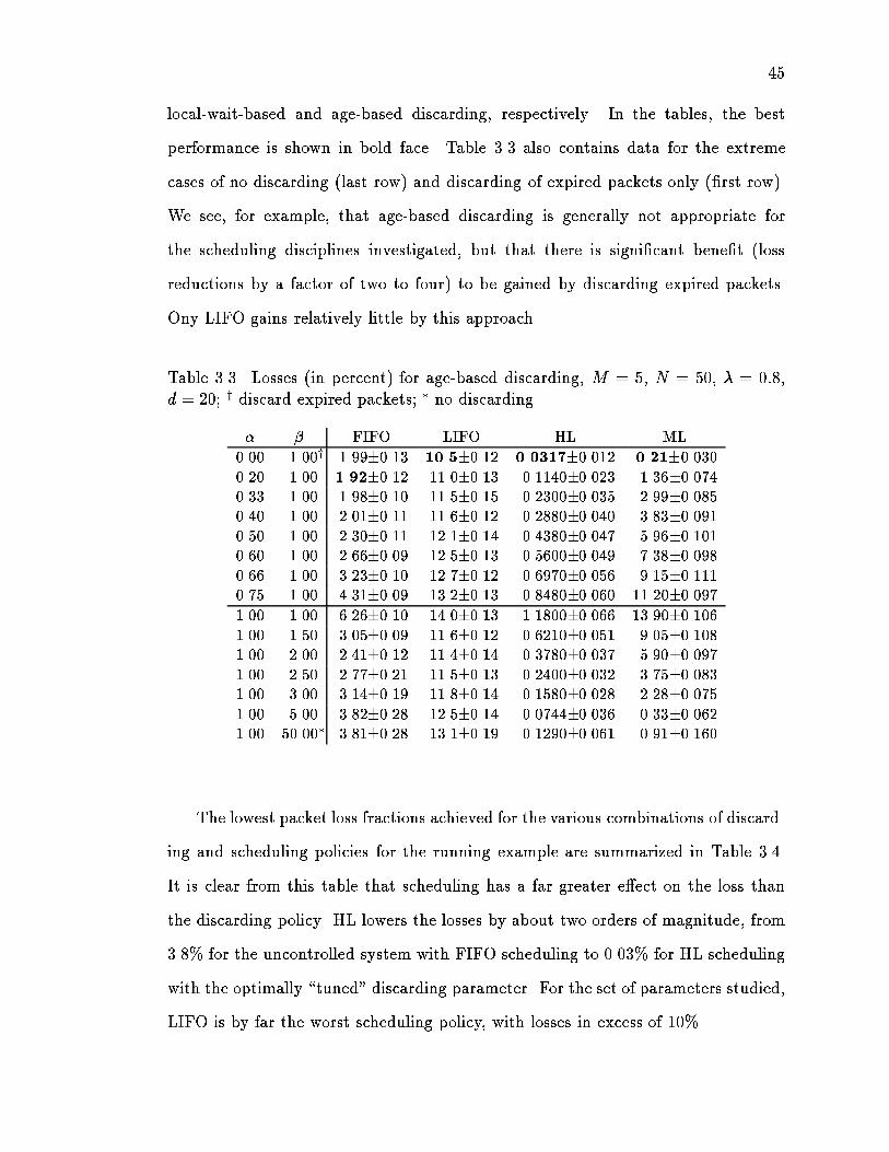
45
local-wait-based and age-based discarding, respectively. In the tables, the best
performance is shown in bold face. Table 3.3 also contains data for the extreme
cases of no discarding (last row) and discarding of expired packets only (�rst row).
We see, for example, that age-based discarding is generally not appropriate for
the scheduling disciplines investigated, but that there is signi�cant bene�t (loss
reductions by a factor of two to four) to be gained by discarding expired packets.
Ony LIFO gains relatively little by this approach.
Table 3.3. Losses (in percent) for age-based discarding, M = 5, N = 50, � = 0:8,d = 20; y discard expired packets; � no discarding
� � FIFO LIFO HL ML
0.00 1.00y 1.99�0.13 10.5�0.12 0.0317�0.012 0.21�0.030
0.20 1.00 1.92�0.12 11.0�0.13 0.1140�0.023 1.36�0.074
0.33 1.00 1.98�0.10 11.5�0.15 0.2300�0.035 2.99�0.085
0.40 1.00 2.01�0.11 11.6�0.12 0.2880�0.040 3.83�0.091
0.50 1.00 2.30�0.11 12.1�0.14 0.4380�0.047 5.96�0.101
0.60 1.00 2.66�0.09 12.5�0.13 0.5600�0.049 7.38�0.098
0.66 1.00 3.23�0.10 12.7�0.12 0.6970�0.056 9.15�0.111
0.75 1.00 4.31�0.09 13.2�0.13 0.8480�0.060 11.20�0.097
1.00 1.00 6.26�0.10 14.0�0.13 1.1800�0.066 13.90�0.106
1.00 1.50 3.05�0.09 11.6�0.12 0.6210�0.051 9.05�0.108
1.00 2.00 2.41�0.12 11.4�0.14 0.3780�0.037 5.90�0.097
1.00 2.50 2.77�0.21 11.5�0.13 0.2400�0.032 3.75�0.083
1.00 3.00 3.14�0.19 11.8�0.14 0.1580�0.028 2.28�0.075
1.00 5.00 3.82�0.28 12.5�0.14 0.0744�0.036 0.33�0.062
1.00 50.00� 3.81�0.28 13.1�0.19 0.1290�0.061 0.91�0.160
The lowest packet loss fractions achieved for the various combinations of discard-
ing and scheduling policies for the running example are summarized in Table 3.4.
It is clear from this table that scheduling has a far greater e�ect on the loss than
the discarding policy. HL lowers the losses by about two orders of magnitude, from
3.8% for the uncontrolled system with FIFO scheduling to 0.03% for HL scheduling
with the optimally \tuned" discarding parameter. For the set of parameters studied,
LIFO is by far the worst scheduling policy, with losses in excess of 10%.

46
On the other hand, it has been shown [58,64] that LIFO maximizes the goodput
of a single G=G=c queue among all work-conserving, non-preemptive scheduling
disciplines that do not take the service time or the laxity into account, as long
as the deadlines have a concave cumulative distribution function (equivalently, a
non-decreasing pdf). Thus, HL and ML would not fall into this category as they
obviously schedule based on laxity. Also, queues that discard packets would dis-
qualify as they are not work-conserving. Even for non-discarding FIFO and LIFO,
the result does not apply in our case since the system investigated has deterministic
deadlines. Kallmes et al. show [58] that for looser, constant deadlines FIFO may
indeed result in lower losses than LIFO.
The mean wait experienced at the ith hop of a packet (omitted here for reasons
of space) clearly shows the e�ect of the scheduling disciplines. This mean wait is
naturally identical for each hop in the case of FIFO and LIFO, it increases with i
(as the packet approaches its destination) for HL, while it decreases for ML.
The relative bene�ts of discarding packets, the in uence of the discarding policy
and the parameter �i depend on the scheduling discipline. Judicious discarding can
lower the losses by a factor of between 1.3 for LIFO, to 2 for FIFO and up to factors
of 4 and 3 for HL and ML, respectively. In all cases, moreover, age-based discarding
improves upon discarding based on local waiting times. This should be expected
since age-based discarding uses more information, re ecting the whole travel history,
than local-wait based discarding. The di�erence between the two discarding policies
is least pronounced for LIFO, with a factor of 1.05 improvement, while introducing
age-based discarding with the other scheduling disciplines lowers losses by a factor
of between 1.3 and 1.5 times compared to local-wait discarding. Since HL and ML
scheduling require laxity information for scheduling, age-based discarding seems to
recommend itself for these two policies, while for FIFO the choice is more of a
tradeo� between performance and simplicity of implementation.

47
Table 3.4. Packet losses (in percent) for di�erent service and discarding policies;M = 5, N = 50, � = 0:8, d = 20
Service policyDropping FIFO LIFO HL MLnone 3.81 13.1 0.129 0.905expired 1.99 10.5 0.032 0.210age 1.92 10.5 0.032 0.210local wait 2.47 11.1 0.047 0.296
For age-based discarding, discarding only expired packets seems to be the best
policy (at least for the cases studied here), even though marginal improvements
are sometimes possible for slightly tighter deadlines. (It is not clear why tighter
deadlines work better for N = 5.) Discarding expired packets is a no-risk policy
as it never discards packets that may make their deadline, requires no adjustment
of parameters and does not depend on model assumptions with regard to tra�c
statistics.
For local-wait based discarding, the optimal deadline for FIFO di�ers markedly
from that for the other scheduling disciplines. For FIFO, a deadline signi�cantly
below d (here, around 0:5d) recommends itself, while for the others, discarding
packets that have spend their entire allotment of d waiting at a single node performs
best or very close to best.
After this rather detailed investigation of the �ve-node VC, the question of the
performance of the policies studied under a wider range of parameters needs to be
addressed. We limit ourselves to discarding expired packets for the reasons noted
above as well as to keep the parameter space manageable. We maintain the node
load at � = 0:8 and the network size at N = 50, but vary the end-to-end deadline
d to obtain the loss performance under di�erent amounts of packet loss. Also,
both the case of geometrically and that of Poisson-distributed external arrivals were
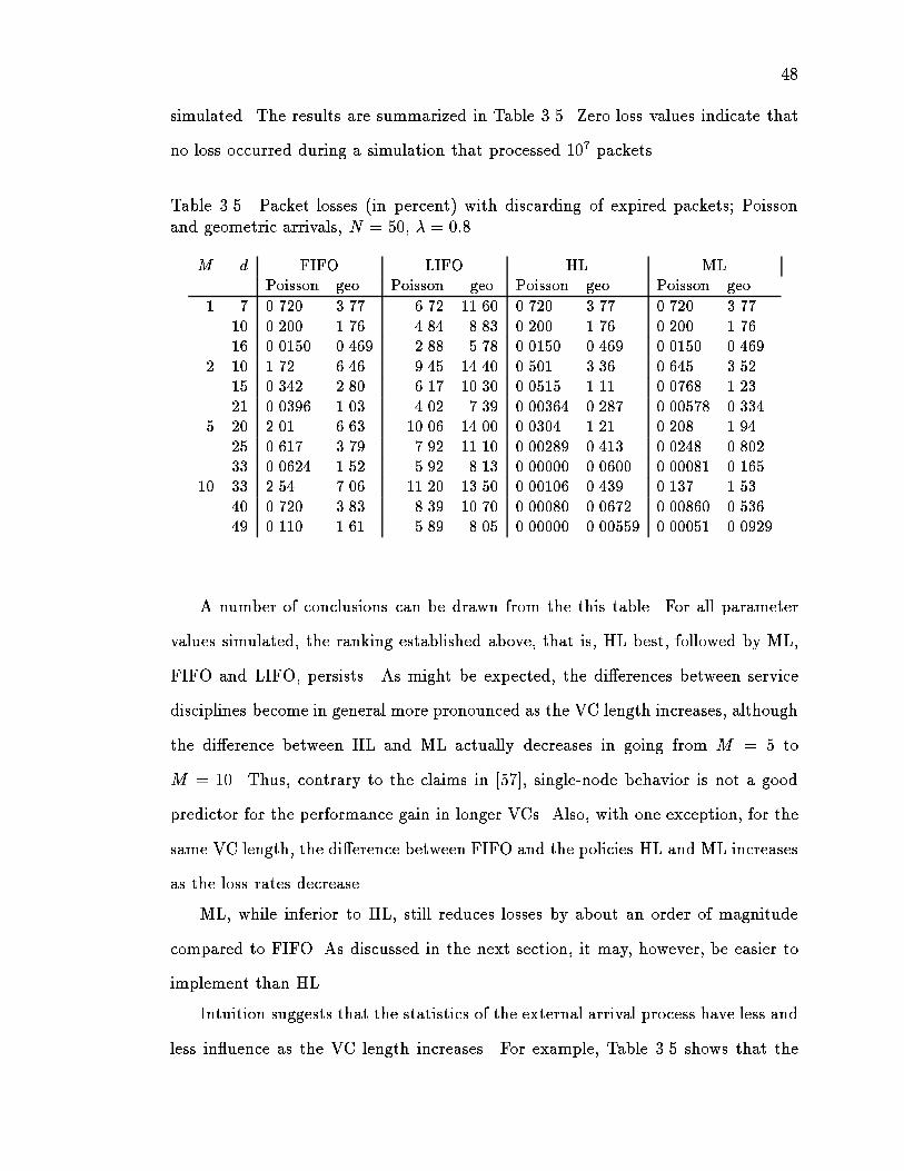
48
simulated. The results are summarized in Table 3.5. Zero loss values indicate that
no loss occurred during a simulation that processed 107 packets.
Table 3.5. Packet losses (in percent) with discarding of expired packets; Poissonand geometric arrivals, N = 50, � = 0:8
M d FIFO LIFO HL ML
Poisson geo. Poisson geo. Poisson geo. Poisson geo.
1 7 0.720 3.77 6.72 11.60 0.720 3.77 0.720 3.77
10 0.200 1.76 4.84 8.83 0.200 1.76 0.200 1.76
16 0.0150 0.469 2.88 5.78 0.0150 0.469 0.0150 0.469
2 10 1.72 6.46 9.45 14.40 0.501 3.36 0.645 3.52
15 0.342 2.80 6.17 10.30 0.0515 1.11 0.0768 1.23
21 0.0396 1.03 4.02 7.39 0.00364 0.287 0.00578 0.334
5 20 2.01 6.63 10.06 14.00 0.0304 1.21 0.208 1.94
25 0.617 3.79 7.92 11.10 0.00289 0.413 0.0248 0.802
33 0.0624 1.52 5.92 8.13 0.00000 0.0600 0.00081 0.165
10 33 2.54 7.06 11.20 13.50 0.00106 0.439 0.137 1.53
40 0.720 3.83 8.39 10.70 0.00080 0.0672 0.00860 0.536
49 0.110 1.61 5.89 8.05 0.00000 0.00559 0.00051 0.0929
A number of conclusions can be drawn from the this table. For all parameter
values simulated, the ranking established above, that is, HL best, followed by ML,
FIFO and LIFO, persists. As might be expected, the di�erences between service
disciplines become in general more pronounced as the VC length increases, although
the di�erence between HL and ML actually decreases in going from M = 5 to
M = 10. Thus, contrary to the claims in [57], single-node behavior is not a good
predictor for the performance gain in longer VCs. Also, with one exception, for the
same VC length, the di�erence between FIFO and the policies HL and ML increases
as the loss rates decrease.
ML, while inferior to HL, still reduces losses by about an order of magnitude
compared to FIFO. As discussed in the next section, it may, however, be easier to
implement than HL.
Intuition suggests that the statistics of the external arrival process have less and
less in uence as the VC length increases. For example, Table 3.5 shows that the

49
ratio of loss between geometric and Poisson arrivals decreases from about 5.2 to
roughly 2.8 as the VC length increases from 1 to 10 (for closest deadline and FIFO
service). However, for HL, no clear trend is discernible, with ratios of two orders of
magnitude even for the longest VC.8
3.4 Scheduling Policy Performance for a Tan-dem System
In the last section, we covered in detail a set of experiments where the network
was completely homogeneous. All packets traversed the same number of hops, all
queues were equally loaded. The fraction of packets exceeding a given �xed deadline
served as the �gure of merit. In this section, we widen the scope of scheduling policies
investigated and change the network con�guration, the �gure of merit and the tra�c
characteristics. The topology, ows and metrics duplicate that presented by Clark
et al. [36], allowing for ready comparison.9. The network con�guration is shown in
Fig. 3.1. 22 statistically identical ows, described below, traverse the network, all
owing in the same direction. Twelve of these streams are of length one hop, four
each of length two and three, and the remaining two streams reach touch all nodes
for a length of four hops. Each link is shared by ten of the streams. All ows belong
to the same class. Each node has a queue that can hold 200 packets.
While the last section was meant to re ect the characteristics of applications
with rigid deadlines, the experiments in this section are geared more towards appli-
cations with adaptive deadlines. Thus, instead of loss caused by exceeding a �xed
deadline, we measure average delay and the 99.9-percentile of the delay distribution.
8The results in Table 3.5 di�er slightly from those in Table 3.3 as they are derived from di�erentsimulation runs.
9Note, however, that the delays reported in the paper are slightly too high, apparently due toa problem with the random number generator used (Lixia Zhang, private communication).

50
1 2 3 4 5
12
34
56
78
910
11121314
1516
1718
19202122
Figure 3.1. The Tra�c Streams for Tandem Network
Two sources model the tra�c generated by bursty real-time applications. The
�rst source is a two-state Markov process. This source, with the same characteristics
as the one in [36], alternates between idle and active periods. The idle period is
exponentially distributed with a mean of 29.4 ms, while packets arrive with a �xed
rate of 170 packets/second during the active period. The �rst packet arrives 5.88 ms
after the beginning of the active period. The number of packets during an active
period is geometrically distributed with a mean of 5 packets. Thus, an average active
period last 29.4 ms, yielding an average packet rate of 85 packets/second. Note that
an active period may contain zero packets and that the minimum packet separation
is 5.88 ms. Each packet has a �xed length of 1000 bits. The source is �ltered with
a (r; b) token bucket regulator. Here, the average rate r is set to 85 packets/second,
the token bucket depth to 50 packets. The regulator discarded roughly 2% of the
generated packets, so that the original per-node load of 0.85 was reduced to about
0.83.
The second source is derived from a packet trace recorded during a 52 minute,
15 second transatlantic packet voice conversation across the Internet between Dr.
Towsley and a colleague in France held on August 17, 1992. The conversation was
recorded using the Nevot network voice terminal described later (Section 4.4).

51
Each packet of length 180 bytes (plus headers) represented 22.5 ms of 8-bit �-law
audio sampled at 8,000 Hz. Note that for experimental reasons, the packet length
was increased to 300 and 600 bytes, including headers. A total of 1643 talkspurts
and silence periods consisting of a total of 50468 audio packets were transmitted,
for an average rate of 16.1 packets per second or an audio rate of 23.1 kb/s at the
original packet size. The minimum interarrival time was measured at 0.7 ms, the
maximum at 19.8 seconds. The average interarrival time was 62.1 ms, with a 99.9
percent below 985 ms. Each silence period had an average duration of 1.23 seconds,
while each talkspurt consisted, on average, of 30.69 packets. To ensure approximate
statistical independence of ows, the traces were read with di�erent initial o�sets,
i.e., one ow would read the trace starting at the �rst packet, the next at packet
2000, and so on.
The last section in this chapter contains some observations on modeling voice
sources, pointing out the potential inadequacy of currently accepted voice models.
Table 3.6. Results for tandem network of Fig. 3.1; for Markovian (M) and voice (V)sources; results from [36] marked with \M (Clark)"
path length1 2 3 4
source policy mean 99.9% mean 99.9% mean 99.9% mean 99.9%M (Clark) WFQ 2.65 45.31 4.74 60.31 7.51 65.86 9.65 80.59
FIFO 2.54 30.49 4.73 41.22 7.97 52.36 10.33 58.13FIFO+ 2.71 33.59 4.69 38.15 7.76 43.30 10.11 45.25
M FIFO 2.60 27.65 4.99 36.15 7.28 45.25 9.84 54.45FIFO+ 3.23 35.55 4.98 36.35 6.44 36.05 7.76 35.65HL 30 4.87 30.85 4.94 32.75 4.99 35.25 4.03 39.35HL 50 5.29 39.85 4.93 38.45 4.83 35.75 3.35 30.75HL 100 5.50 59.25 4.92 56.06 4.82 53.15 3.10 27.25TP 4.47 59.85 4.54 59.35 5.05 57.55 4.26 31.15LHF 5.18 69.95 5.20 68.55 5.59 67.25 4.31 33.35ML 4.14 58.45 4.88 101.8 5.43 119.4 5.21 128.0LIFO 2.74 202.9 5.07 254.2 7.37 287.3 9.83 307.2
V FIFO 10.04 344.7 19.06 340.3 20.18 359.2 32.18 407.6HL 30 10.80 344.7 19.06 340.3 19.27 472.2 34.28 622.6HL 50 11.35 273.4 17.85 315.3 18.60 471.2 31.78 614.4HL 300 15.25 322.5 17.97 327.0 14.62 372.4 16.25 392.8

52
For this set of simulation experiments, the network link speed was assumed to
be 1 Mb/s. Together with packet sizes of 125 bytes, the per-packet transmission
time computes to 1 ms.
Discrete-event simulations covering 62 minutes of simulated time were run. The
�rst two minutes were discarded to reduce the e�ect of the initially empty system
on the performance measured. For the FIFO+ policy, a �rst-order recursive �lter
with a weighing constant of 0:001 estimated the mean queueing delay. (The weighing
constant was determined during pilot experiments; sensitivity experiments still need
to be completed.) For FIFO+, we could only achieve reasonable results coming close
to the values published [36] by combining it with transit priority.10
The queueing delays, i.e., not including transmission times or propagation de-
lays, of our simulations are displayed in Table 3.6. For HL, the laxity parameter
chosen is shown in parentheses. All delay values are shown in milliseconds. The
tra�c source is indicated by the letters 'M' and 'V', representing the Markovian
two-state source and the conversational voice source, respectively. The �rst three
rows show the values reported in the paper by Clark et al. [36]. The parameter
following the HL designation denotes the end-to-end deadline measured in millisec-
onds.
For easier comparison, the 99.9% percentiles for the delay are also graphed in
Fig. 3.2 and Fig. 3.3, using the data for the two-state source. The �rst graph shows
the scheduling policies with generally lower delay percentiles than FIFO, while the
second graph shows those with higher delays.
First, we note that, as expected for work-conserving disciplines, the average
waiting times are roughly equal, albeit distributed di�erently between long and
short paths for the di�erent policies. Of primary concern, however, is the delay
10It is conjectured that that may have to do with the fact that, at least for M/M/1, for all loadsa majority of packets are going to experience delays less than the average delay and are thus goingto be disadvantaged with respect to new arrivals. For M/M/1, the fraction of packets experiencingno more than average delay is always greater than 1� 1=e = 0:6321.

53
hops
99.9
per
cent
ile o
f qu
euei
ng d
elay
25
30
35
40
45
50
55
60
65
1 2 3 4
TPHLFIFO+FIFO
FIFO
FIFO+HL (30 ms)
HL (50 ms)
HL (100 ms)TP
Figure 3.2. 99.9-percentile values for the queueing delays (low-delay policies)
hops
99.9
per
cent
ile o
f qu
euei
ng d
elay
0
50
100
150
200
250
300
350
1 2 3 4
LIFOLHFMLFIFO
Figure 3.3. 99.9-percentile values for the queueing delays (high-delay policies)
54
percentile. Immediately, LIFO, LHF and, surprisingly, ML can be ruled out from
further consideration. Note that the delays for LIFO do not include any necessary
reordering delays.
The simple transit-priority (TP) policy shifts too much of the delay from the
long-haul paths to the short-haul paths. Note that this e�ect is probably partially
explained by the particular topology, as the 4-hop tra�c in this example never has
to yield to other tra�c, as at its entry point at node 1, all other tra�c is also
entering the network. The parametrized family of hop-laxity (HL) policies can be
tuned to keep the delay almost constant or even decreasing, independent of the path
length. Queueing delays decreasing with hop count may be desirable to compensate
for longer propagation delays. For long paths, the queueing delay is almost cut in
half. Unfortunately, the delay performance of HL as a function of path length seems
to strongly depend on the value of the laxity parameter.
With the caveat about the priority of packets entering the network noted earlier,
FIFO+ seems to perform reasonably well without as much concern about choosing
an appropriate laxity parameter.
FIFO+ and HL require roughly the same amount of computation, with a slight
advantage for FIFO+ as it only requires one comparison per packet while searching
through the queue for the next candidate. Also, it can perform its computation
when enqueueing packets, while that reduces performance for HL.
From the data, it is apparent that limiting delays appears to be inherently
di�cult, in particular since we can only try to compensate for past delays by
increased priorities, without knowledge about queue states seen at future nodes.
Thus, pending further investigation, we can tentatively state that for applica-
tions with �xed deadlines, where choosing the laxity value is not an issue, the HL
policy appears promising, while for the case where delay percentiles are used as the
performance metric, FIFO+ suggests itself. FIFO+ has the property that delays
are balanced rather than depending on a parameter choice of the end user. Thus, if

55
loading increases, all ows in a class share in the increased delay, while for HL, the
tendency to assign one's own tra�c lower laxity values would have to be balanced
by appropriate admission or charging policies.
HL o�ers a straightforward way to o�er di�erent classes of service to di�erent
real-time streams according to their urgency; this can only be indirectly achieved
through a strict scheduling priority mechanism in FIFO+.
From the above discussion, a number of areas for future research seem indicated.
For FIFO+ and the other policies, the performance under the uniform conditions
discussed in the last section needs to evaluated. Also, the sensitivity to load changes
and the estimation parameter requires further study. For the HL policy, a heuristic
for choosing the laxity parameter is called for. For all policies, the performance
in networks with bottlenecks, probably the more typical scenario11, needs careful
study. It is expected that the policies that try to compensate for queueing delays
su�ered at past nodes by increased priority down stream will not do as well, since
there is less chance for compensation once the bottleneck has been cleared.
3.5 Notes on Modeling Voice Sources
In this section, we closely analyze the conversational voice source introduced on
page 50, as it allows us (by negative example) to gauge the e�ectiveness of the
two-state voice source model commonly found in queueing analyses.
The traditional voice model of roughly exponentially distributed talkspurt and
silence periods dates back to the mid-sixties [65{67].
Fixed-rate voice codecs, which generate audio packets at �xed intervals during
talkspurts, are the dominant form of audio codecs in use, even though a number of
researchers have proposed variable-rate codecs suitable for packet voice networks
11The introduction of the 45 Mb/s backbone in the Internet, for example, typically introducestwo transitions from high-speed local networks to the slow speed access into the backbone and viceversa.

56
duration (sec)
1-cd
f
10−4
10−3
10−2
10−1
100
0 0.02 0.04 0.06 0.08 0.1 0.12 0.14 0.16
Figure 3.4. The interarrival time distribution for packet audio
duration (sec)
1-cd
f
10−4
10−3
10−2
10−1
100
0 2 4 6 8 10 12 14 16 18 20 22
silence (exp.)silence
Figure 3.5. The silence duration distribution for packet audio

57
[68{74]12. The \traditional" packet spacing (in uenced by the frame size used
by the linear predictive coder employed during the early low-bit-rate packet voice
experiments within the ARPANET) is 22.5 ms, equivalent to 180 bytes at 8,000
samples per second. However, the packet stream appearing on the network is not as
regularly spaced, as shown by the distributions in Fig. 3.4 and 3.5 computed from
the voice conversation described in Section 3.5. There are three e�ects that make
packet voice a very bursty source:
1. The terminal does not transmit packets deemed to contain silence or back-
ground noise. Silence suppression is particularly important for audio confer-
ences with a large number of participants13. It signi�cantly reduces the overall
network load if mixing is done by the end systems, as every conferee is active
only a small fraction of the time, but also prevents that the combined back-
ground noise from all conference locations is heard by each conferee. The latter
part assumes greater importance as the availability of audio and video capable
workstations moves teleconferences out of acoustically dampened teleconference
rooms into regular o�ces. Breaking up the audio stream into talkspurts also
allows easy playout delay adaptation and compensation for sampling clock drift
between sender and receiver.
Silences can be roughly divided into two categories. The �rst category with a
small mean duration is caused by brief pauses between words and sentences,
while much longer pauses re ect pauses while listening [65{67, 75{79]. Silence
suppression accounts for the long tails in the interarrival time distribution. In
a lecture with audience participation, the maximum silence period is bound to
be even longer.
12Also, any �xed-rate coder can be transformed into a variable-rate coder by entropy-encodingthe output symbols, for example by a Hu�man code.
13The DARTnet research community routinely conducts teleconferences with more than a dozenparticipants.

58
Fig. 3.5 shows by example that an exponential distribution with the same mean
does not �t the measured silence distribution well. The dotted line shows the
inverse distribution (1 � F (t)) of the silence period duration, which has far
shorter tails than the actual distribution.
2. The second reason accounts for variable interarrival times at the beginning
of talkspurts, where the silence suppression algorithm commonly used also
explains the extremely short interarrival times seen, down to 0.7 ms. Energy-
based silence detection typically misses the important onset of particularly
unvoiced speech, introducing audible clipping [80{83]. To reduce this so-called
front clipping, the packet voice terminal bu�ers a small number of voice packets
during silence periods and then transmits on the order of 40 ms of stored audio
before the �rst packet containing su�cient energy to be declared speech.
3. The third reason for non-uniform interarrival times a�ects every packet within
the talkspurt and has not been widely discussed. It is caused by the scheduling
delays introduced by a non-real-time operating system, where a variable amount
of time can elapse between the time a packet's worth of audio has been sampled
and the time the voice application actually submits a packet to the network.
As shown in Fig. 4.5, this can introduce a jitter of up to 3.5 milliseconds,
even if the system only serves the audio application and some routing and
clock synchronization daemons. Additional user processes could be expected
to drastically increase this jitter.
Fig. 3.4 shows the inverse distribution (1�F (t)) of the packet interarrival time.While most of the interarrival times are concentrated around the nominal value
of 22.5 ms (shown as a dotted line) and twice that (shown as a dashed line), the
interarrival times span the range from 0.7 ms to 171 ms, with times up to 100 ms
occurring with non-negligible probability. The extremely long interarrival times
are probably due to process lockouts caused by window resizing or movement.

59
Details on the implementation of a voice terminal within the Unix operating
system can be found in Section 4.4.
One experiment was performed to gauge whether the multiplexing of such voice
sources obeys the two-state models commonly used [84,85]. The source was modeled
by a two-state process characterized by an average burst size of 30.69 packets, a mean
silence duration of 1.23 seconds and an interpacket spacing of 22.5 ms during the
talkspurt. The voice sources were o�ered to the same �ve-node network topology
as in Fig. 3.1. To allow easy comparison with actual network experiments over
DARTnet, the network speed was set to 1.344 Mb/s and packets were scaled to
a �xed length of 600 bytes. The results shown in Table 3.7 demonstrate that the
two-state model signi�cantly underestimates both the average delay (by roughly a
factor of two) and the tail of the delay distribution. The agreement between the
models appears to improve slightly for long-haul ows, as their queueing delay is
in uenced less by the original source characteristics and more by the shaping applied
by the queues themselves.
Table 3.7. Comparison of queueing delays experienced by voice tra�c and equivalenttwo-state model
path length
1 2 3 4
tra�c mean 99.9% mean 99.9% mean 99.9% mean 99.9%
voice trace 10.0 345 19.1 340 20.2 359 32.2 407
two-state model 5.0 229 9.6 238 12.3 281 17.5 319
Based on this negative example, we claim that the traditional two-state Markov
model [16] where talkspurts with arrivals that are spaced at constant time intervals
alternate with exponentially distributed silence periods does not capture the com-
plexity of this tra�c generation process. Firm conclusions certainly require more
extensive traces. It should also be emphasized that the results will depend strongly
on the type of silence detector used, in particular, on whether the detector ignores

60
short inter-word pauses or not. A suitable statistical model, preferably one that
is analytically tractable, to capture these e�ects needs to be developed and tested.
Brochin and Thomas [86] present a three-state model that might make a good initial
candidate. (The paper [86] does not address how to �t the parameters to observed
data or how well the three-state model can indeed predict, say, queueing delays.)
The conversational and lecture audio sources (the latter will be covered in
Section 4.3) also point out the di�culty of policing audio with a token bucket (also
called a \leaky bucket") [87{91] unless the content of the tra�c carried is known in
advance. Since we usually cannot accurately predict how much of the time a speaker
will be active during a conference, we can only set the regulator to very near the
peak rate.14
The di�culty of policing mean rate even if the mean rate is assumed to be
known can be illustrated by the example as well. If the conversational voice source
is regulated to half the peak rate, i.e., assuming that each party participates equally
in the conversation, the regulator drops about 4% of the packets if the token reservoir
holds ten average talkspurts worth of tokens (here, 307 tokens). The two-state model
described later also shows a similar behavior if subjected to the regulator.
Finally, some indication of clock drift can also be derived from this example.
A comparison of sequence numbers with trace time stamps showed that over the
roughly one hour duration of the conversation, the sampling clock fell behind real
time by about 360 ms, thus indicating the need for both inter-media (lip-synch) syn-
chronization [92{100] and clock drift synchronization between sender and receiver.
14On the other hand, some may consider degraded quality for those dominating a conference afeature, not a problem.

C h a p t e r 4
Experiments in Traffic Scheduling
This chapter describes an implementation of hop-laxity scheduling within an
operational router. Hop laxity scheduling was described in Section 3.2 and evaluated
by simulation experiments in Section 3.4. Measurements performed on the kernel
implementation allow us to gauge the e�ect of protocol overhead and queue process-
ing costs on the overall algorithm performance, providing a more realistic picture
of the achievable performance gains. It also establishes how readily non-FIFO
disciplines can be integrated into a \standard" Unix-based operating system and
existing network protocols. Issues of set-up, largely unaddressed by simulation
experiments, are also discussed in some detail, as they drastically a�ect the usability
of the proposed scheduling mechanism.
In Section 4.1, we describe the experimental network used for the experiments.
The hop-laxity scheduling algorithm requires some additions to existing network
protocols, which are discussed for the examples of IP and ST-II in Section 4.2. That
section also describes some design trade-o�s, the initial distribution of algorithm
parameters and the changes to the kernel network modules that implement the
protocol. Section 4.3 then covers the tra�c sources used in the experiments, drawn
mainly from actual audio and video network applications, including a videotaped
lecture and a transatlantic packet voice conversation.
A network voice terminal written by the author served as one application used
to generate trace data. Some of its features and its design are summarized in
Section 4.4. Another set of tools, described brie y in Section 4.5, then used these
traces to regenerate network tra�c. The trace-based tra�c generator allows us

62
to reconstruct network tra�c, even when the voice or video codec is not available
at the remote site. Within some limitations, it also assures repeatability of the
performance measurements.
The actual experimental results are summarized and discussed in Section 4.6.
In the beginning of that section, we also illustrate the di�erence between the per-
formance predicted by simulation and that seen in an actual network and strive to
illuminate some of the potential causes for these di�erences.
4.1 The Experimental Network
All network experiments were performed within DARTnet, the DARPA-sponsored
research network [101] spanning the continental United States. This network does
not carry regular Internet tra�c and can be reserved for the exclusive use of indi-
vidual research groups. Sun SPARCstation 1+ workstations, currently running a
modi�ed SunOS BSD 4.3-based kernel, serve as routers, thus allowing modi�cation
of packet scheduling, instrumentation, implementation of new routing algorithms,
etc., while providing a high-level operating environment. 1
All nodes within DARTnet are connected by T1-lines running at 1.344 Mb/s2.
The logical topology of the network is shown in Fig. 4.1; the links are annotated
with the estimated per-link propagation delays measured in milliseconds. The node
locations are listed in Table 4.1. A POP designates a point of presence, i.e.,
telephone company provided equipment closet, where the router connects to the
physical transmission facility.
1The kernel was modi�ed to support IP multicasting [102{104] [105, p. 281f] and the ST-IIstream protocol. In addition, it incorporates network performance enhancements, such as largerpacket bu�ers and other algorithmic improvements, mostly for TCP, contributed by Van Jacobsen.He also wrote the device driver for the high-speed serial interface board, that we modi�ed for ourpacket transmission discipline.
2The speed has been reduced below the nominal rate of 1.536 Mb/s to accommodate thede�ciencies of the HSI/S serial interfaces.

63
Table 4.1. DARTnet node locations (as of August, 1992)
name institution geographic locationparc XEROX Parc Palo Alto, CAames NASA, Ames Sunnyvale/Mountain View, CAsri SRI Menlo Park, CAlbl Lawrence Berkeley Laboratory Berkeley, CAisi Institute for Information Sciences Marina del Ray, CAudel University of Delaware Newark, DEbbn Bolt, Beranek and Newman Cambridge, MAmit Massachusetts Institute of Technology Cambridge, MAdc unattended POP downtown Washington, D.C.la unattended POP downtown Los Angeles, CAsun Sun Microsystems Sunnyvale, CAbell Bell Communications Research (Bellcore) Morristown, NJdarpa Defense Advanced Research Projects Administration Reston, VA
The T1 lines are connected through CSU/DSUs3 that perform electrical signal
conversion to four-channel serial interface boards (called HSI/S) attached to the
SPARCstation system bus.
4.2 Protocol and Operating System Support forLaxity-Based Scheduling
The hop-laxity algorithm requires two pieces of information: the time remaining to
expiration (laxity) and the number of hops until reaching the destination host. The
laxity information must be carried with every packet, while the hop count remains
invariant throughout the life of a connection and can thus be part of the connection
state.
The scheduling mechanism was implemented under both the Internet Protocol
(IP) [106] and the experimental stream protocol called ST-II [107]. In this sec-
tion, we describe how the protocol data units were modi�ed for each protocol to
accommodate the new scheduling algorithm and how the kernel had to be adapted.
For both protocols, the basic protocol operation was una�ected. Applications that
3channel service unit/digital service unit

64
mit
bbn
dc
udel
isi
la
lbl
ames
sri
parc2.9
3.0
10.8
10.1
3.1
53.2
5.9
11.0
2.7
Figure 4.1. The DARTnet topology, with link round-trip propagation delays
do not wish to participate in the new scheduling algorithm or are unaware of its
existence are una�ected, although they receive lower-priority service. In general,
the kernel modi�cations were limited to a small number of routines within the BSD
networking code and the ST-II control message and data packet routines.
4.2.1 IP Implementation
4.2.1.1 Extensions to the Internet Protocol
The standard IP protocol does not support time stamp or hop count information, but
is extensible through options. Each IP datagram may carry zero or more options, up
to a total length of 44 bytes (that is, the maximum header length of 64 bytes minus
the �xed header length). There are a small number of prede�ned one-byte options,
while the remainder of the option types have a �xed self-describing structure shown
in Fig. 4.2. The �rst two bytes of an IP option consist of the option code octet and
65
the option length, measured in bytes. The option code octet is broken into three
parts. If the copy bit is set, the node has to copy the option into fragments if the IP
datagram has to be split into fragments when being forwarded. If the copy bit is zero,
the option is only copied into the �rst fragment. The 2-bit option class determines
whether the option is used for datagram and network control or debugging and
measurement. Finally, the 5-bit option number determines the interpretation of the
remaining option bytes according to a list of assigned well-known numbers. Given
the length �eld and copy bit, a node that does not understand a particular option
code can just copy the option into the outgoing packet without needing to know its
interpretation.4
Since none of the existing options convey the needed information, we de�ne a
new experimental IP option with a code of 1010, the lowest currently unused option
code within the datagram control class. The format of the option is shown in Fig. 4.2.
For this scheduling application, fragments should be treated as the original packet
and thus the copy bit is set.
The newly de�ned option encompasses a total of eight bytes. The option code
(value 8a16) and length (value 8), each one octet, are followed by a ag octet, which
modi�es the behavior of the scheduling algorithm. If the least signi�cant bit of the
ag octet is set, packets that have exceeded their laxity (i.e., when the laxity value
has become negative) are dropped. If that bit is zero, scheduling priority increases
with negative laxity. The second least signi�cant bit switches from hop-laxity to
a simple minimum laxity algorithm by not decrementing the remaining hop count
from its initial value of one.
4There is, however, a set of options de�ned in [106] that have to be handled appropriately byall IP agents.
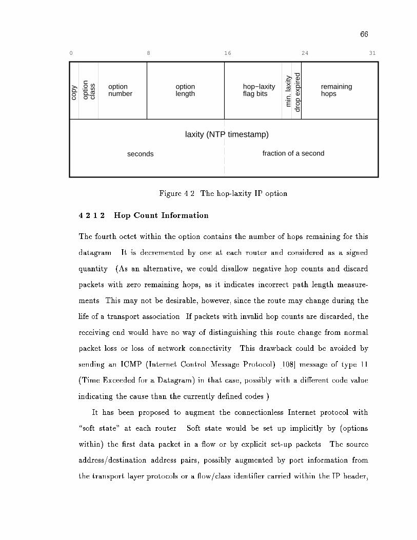
66
copy
optio
ncl
ass option
numberhop−laxityflag bits
optionlength
remaininghops
seconds fraction of a second
laxity (NTP timestamp)
0 8 16 24 31
min
. lax
itydr
op e
xpire
d
Figure 4.2. The hop-laxity IP option
4.2.1.2 Hop Count Information
The fourth octet within the option contains the number of hops remaining for this
datagram. It is decremented by one at each router and considered as a signed
quantity. (As an alternative, we could disallow negative hop counts and discard
packets with zero remaining hops, as it indicates incorrect path length measure-
ments. This may not be desirable, however, since the route may change during the
life of a transport association. If packets with invalid hop counts are discarded, the
receiving end would have no way of distinguishing this route change from normal
packet loss or loss of network connectivity. This drawback could be avoided by
sending an ICMP (Internet Control Message Protocol) [108] message of type 11
(Time Exceeded for a Datagram) in that case, possibly with a di�erent code value
indicating the cause than the currently de�ned codes.)
It has been proposed to augment the connectionless Internet protocol with
\soft state" at each router. Soft state would be set up implicitly by (options
within) the �rst data packet in a ow or by explicit set-up packets. The source
address/destination address pairs, possibly augmented by port information from
the transport layer protocols or a ow/class identi�er carried within the IP header,

67
would be used to map an incoming datagram to a soft state record. Alternatively,
the already de�ned stream identi�er option (option number 8), currently considered
obsolete, could be used to identify the ow, allowing ows to span several destination
addresses.
Unlike a true connection-oriented model, only scheduling information, not the
next hop, would be drawn from the soft state record. Thus, packets would continue
to ow, albeit without the bene�t of tra�c-class speci�c scheduling, even if the soft
state record got lost due to router failure and recovery. The use of soft state has been
suggested, for example, for maintaining resource allocations within routers [109].
Clearly, such a soft state record could also hold the remaining hop count.
In a connectionless protocol such as IP, the path length (hop count) can only
be approximately determined, since by de�nition, there is no guarantee that any
two packets travel the same route through the network. However, for most existing
networks, the hop count and even the route change infrequently. Thus, it appears
to be su�cient to initially establish the path length when setting up a transport
association and to then reevaluate the path length based on ICMPmessages received,
as described above, or the actual remaining hop count found in arriving messages.
In the latter case, the receiver would have to notify the sender of the change in path
length. Unfortunately, current networking implementations based on the Berkeley
(BSD) distribution lack a mechanism for a user process to be noti�ed about ICMP
messages or to inspect the IP options found in an arriving IP packet.
The initial path length can be determined in a number of ways. A simple,
though not completely foolproof method, implemented uses the ICMP echo request
(ICMP type 8 and 0) and the IP time-to-live (TTL) �eld. Each node along the path
decrements the TTL �eld by one5. Since ICMP apparently uses the maximum TTL
5The IP speci�cation [106] requires that a gateway decrements the TTL by the number ofseconds the packet has resided in that gateway, with a minimum decrement of one. Given currentnetwork speeds and implementations, the time-based rule appears to be rarely if ever used.

68
for outgoing IP packets, the TTL value of the incoming packet can be used to deduce
the number of intervening hops. Since the TTL value to be used for ICMP messages
is only required to be su�ciently large to reach the destination, this method may
not work reliably for all host implementations.
As an alternative, ICMP echo requests with the IP record route option can be
used. However, only 40 bytes are available for that option, allowing a maximum
of 10 hops, as each IP address takes up four bytes. Within DARTnet, this is not
a serious limitation, but paths across the Internet routinely require �fteen or more
hops.6
The scheme to determine path lengths described above can be extended to a
multicast network [102] by simply using the maximum computed hop count. A
suitable time period has to be de�ned during which ICMP echo responses are
accepted. Since nodes can join and leave the multicast group without the source
having any direct way of knowing about it, the maximum hop count has to be
periodically redetermined. Alternatively, destinations �nding that packets arrive
with negative hop counts could advise the source appropriately. It should be realized,
however, that in an IP multicast setting with dynamic group membership, any hop
count information has to remain approximate. The details of determining hop counts
within multicast groups are left to future research.
4.2.1.3 Timing and Deadline Information
Our hop-laxity algorithm requires information not only about the hop count, but
also about the time remaining to expiration. Depending on network properties
and desired scheduling algorithm properties, a number of alternatives as to the
information carried by the packet can be considered:
source time: The timestamp encodes the departure time of the packet from the
source. This time may not necessarily be the actual time the packet reaches
6The path from erlang.cs.umass.edu to cub.isi.edu spans 19 hops, for example.

69
the network interface, but could be a time meaningful to the application, for
example, the time a video or audio frame was generated. This requires that
the nodes maintain information about the permissible laxity and that laxity
remains the same for each packet within a stream.
deadline: The timestamp encodes the desired arrival time of the packet. Thus, if
higher level demultiplexing is desired, packets can easily be marked as more or
less urgent. With this encoding, the nodes need to keep no state information.
queueing delay: The timestamp contains the permissible sum of all queueing de-
lays. Each node then subtracts the actual queueing delay experienced. This
requires that each packet be accurately timestamped on arrival to the node
or, if generated locally, when it is passed down from the socket layer. (The
BBN ST-II implementation provides such functionality.) Hardware and soft-
ware interrupt latencies are not accounted for in this case. In this method,
only queueing delays, not propagation or transmission delays enter into the
scheduling decision. Also, the delays accrued by routers not participating in
the scheduling algorithm are not accounted for.
All but the last timestamp encoding require clocks to be synchronized to within a
few milliseconds. This is well within the current state-of-the art, as evidenced by
the sub-millisecond synchronization found within DARTnet [110].
Any timestamp that includes the transmission time may lead to packet reorder-
ing within the same stream if two packets with di�erent lengths follow each other
closely.
We chose to use the second approach, that is, carrying the deadline within the
packet, mainly because we wanted to eliminate any state information (here, laxity)
that a node would have to maintain, as it would force us to implement and design
a ow setup and look-up mechanism. Since the number of ows may be large,
this could also add non-trivial packet processing overhead. It also allows us to

70
compensate by scheduling for di�erent propagation delays, thus providing a quality
of service less a�ected by physical distance.
The deadline timestamp is carried within the �nal four bytes of the option,
encoded in network byte order (most signi�cant byte �rst or big endian). The
timestamp uses a shortened version of the network time protocol (NTP) [111, 112]
timestamp, extracting the middle 32 bits from the original 64 bits. The shortened
timestamp encodes the least signi�cant 16 bits of the number of seconds since zero
hours (Universal Time) January 1, 1990 plus a 16-bit binary fraction of a second,
resolving time to about 15.2 �s. The NTP timestamp format and its shortened
version have the advantage that addition and comparison are e�cient, requiring no
explicit carry, in contrast to the standard Unix time values represented as seconds
and microseconds. The conversion from the Unix system clock to NTP timestamp
is relatively simple:
ntp = ((tv.tv_sec + 2208988800) << 16) +
(((unsigned)tv.tv_usec * 0x10c6
+ (((unsigned)tv.tv_usec * 0xf7a) >> 12)) >> 16);
Here, tv holds a Unix time value, with tv.tv sec denoting the number of seconds
since January 1, 1970 and tv.tv usec denoting the number of microseconds within
the current second. The conversion is required once per call to the output dequeue
routine.
The shortened NTP timestamp wraps around roughly every 18 hours. Thus,
during a window of a few hundred milliseconds, packets would be stamped with a
deadline just above zero, while the transit hosts' shortened NTP clocks have not yet
reached the rollover point. During this window of vulnerability, packets would be
treated as if they had an extremely long laxity and scheduled appropriately. Since
the occurrence of this event is su�ciently rare and the consequences bearable, the
expense of adding explicit checks was judged to be unwarranted.

71
4.2.1.4 Kernel Modi�cations
Before describing the actual kernel implementation, we brie y outline the procedures
a data packet traverses before leaving the network interface. A general description
of the BSD networking code can be found in [113]. The data ow is also depicted
in Fig. 4.3.
As we will modify the data structures used to hold packet data, we brie y
describe the data structures used in BSD Unix. Network packets in the BSD
networking code are stored in so-called mbuf's. Mbuf's are linked blocks of memory
of 128 bytes each, which either directly contain packet data or point to larger (2048
byte) so-called \clusters". The �rst twelve bytes of each mbuf contain information
about the amount of packet data contained in the mbuf, an o�set into the mbuf
that indicates where packet data begins, the data type and a pointer that is used
to chain together all mbuf's within a chain. If headers are added to an mbuf, the
o�set is decremented and the length incremented. If not enough space is available,
another mbuf is chained to the front or back. Chains of mbufs can be linked with
another pointer �eld. This scheme allows dynamically growing data structures with
easy storage reclamation and no memory fragmentation.
For our purposes, we are only concerned with outputting an IP packet. (While
there is a queue that holds incoming packets from the device driver waiting to be
processed by the ipintr() software interrupt handler, it is expected to be short,
as IP input processing should not require large amounts of CPU time. IP input
processing mainly consists of parsing options and determining the outgoing interface.
Thus, it is probably ine�cient to add any form of scheduling to the IP input queue.)
A packet can reach the output routine, ip output() on two di�erent paths. If
it reaches the node from an external network, it is processed by the IP input routine
The actual implementation of the scheduling algorithm consists of two functions.
The �rst function, ip hl opt(), translates the IP option described above into a
data structure residing at the very beginning of the �rst packet. It is called at the

72
T1 lineHSI/S
ipintr()
hsis_output()
ip_output()
hsisintr()
ip_forward()
udp_output()socket
Figure 4.3. Data ow in BSD kernel for IP

73
beginning of ip output(). The �rst 16-bit word of the mbuf data area designates
the resource control family, so that multiple scheduling policies (e.g., virtual clock,
weighted fair queueing, FIFO+ and other mechanisms [114] [15] [46] [115] [36]) can
be supported.
The translation routine of that mbuf is then changed to MT DATASORTED, a newly
de�ned mbuf type. This translation takes place in the ip output routine; it requires
a linear through all IP options within the packet to determine if the scheduling option
is present. The code module also decrements the hops-to-go �eld.
Instead of transcribing the IP option in ip hl opt(), we could have the de-
queueing routine parse the IP options directly. This, however, has three severe
disadvantages. First, note that not every packet is \seen" by the output scheduler.
The packet is directly copied to the device bu�er if the device is idle when the device
driver is invoked. Thus, any hops-to-go adjustments need to take place outside
the dequeueing routine. Secondly, it is undesirable to embed knowledge about
the network layer header format into a device driver. By divorcing the IP layer
representation and the data structure seen by the driver dequeueing routine, several
network layer protocols (e.g., ST-II, OSI CLNP or X.25) could transparently use
the same queueing mechanism. Third, since each packet may have to be inspected
several times while residing in the queue, access to the scheduling information has
to be as fast as possible.
While the scheduling information is inserted into the �rst mbuf of a packet,
further link-level processing may prepend another mbuf to make room for link-level
headers. Thus, the dequeueing routine searches for an mbuf of type MT DATASORTED
within the �rst two mbufs. Packets that are not marked do not enter the priority
computation and are thus served with lower priority.
Within Berkeley Unix, the actual packet scheduling takes place when the device
driver completes an output operation and pulls the next packet o� the output queue.

74
4.2.1.5 Scheduling Overhead Considerations
The hop-laxity scheduling algorithm imposes a signi�cantly greater processing bur-
den at packet dequeueing time. However, for the serial interface used in the ex-
periments, channel utilization should not be a�ected, for the following reason. The
HSI/S device driver manages two �xed-size output bu�ers (of size 1500 bytes). While
one output bu�er is being output to the serial line by the on-chip DMA controller,
the other bu�er can be �lled with the next packet to be transmitted. Thus, line
output overlaps with dequeueing and copying from system memory to board bu�er.
For long queues of very short packets, however, it is possible that selecting the next
packet to be output may take longer than the packet transmission time, thus idling
the channel.
Measurements were made to estimate the cost of hop-laxity scheduling on the
DARTnet routers. The cost consists of the delay incurred each time the output
dequeue routine is invoked plus the sum of the processing times for each packet
in the queue. The �rst component consists of obtaining the current system time,
converting it into the shortened NTP timestamp, which takes a total of about 10
�s, and the linked list manipulation to extract the selected packet from the queue.
The latter cost would also have to be borne by a FIFO queue, except for some slight
penalty for potentially having to extract a packet from the middle of the queue.
The dominant cost for hop-laxity scheduling, however, is caused by having to
compute the scheduling priority of each packet in the queue, entailing a division
operation, and then determining the minimum priority value. For the SPARC
architecture, the cost of arithmetic operations di�ers from common perceptions.
The CPU chip lacks integer division and multiplication instructions, but does have
a fast oating point unit. The execution times of various arithmetic operations of
interest here are shown below. Note that these times encompass all necessary data
access, not just the arithmetic operation itself.

75
operation time (�s)r = c >> 2 0.37r = c / 4 5.64r = c * 4 6.28r = c / 4.0 3.65r = c * 4.0 1.39
The table shows that integer multiplication and division should be avoided in
favor of shifts and oating point multiplication. The scheduling code takes note
of that and also makes use of the fact that the divisor, i.e., the remaining hop
count, is typically a small number. It treats each hop count up to twelve separately,
evaluating divisions by 2, 4 and 8 by right shifts, other divisors by oating point
multiplications with a constant. As another minor performance improvement, the
timestamp conversion and minimum search is performed only if at least two packets
reside in the queue.
With these optimizations, each packet within the queue takes about 8 �s to
process during each call to the dequeueing routine. With long queues, this can clearly
be a signi�cant burden for the processor, particularly if it has to attend to a number
of busy interfaces. It should be noted, however, that typical implementations of
bandwidth management mechanisms such as fair queueing or virtual clock also
require searching on average half the queue for each output packet to determine
the proper insertion point. However, typically, no arithmetic beyond a simple
comparison is required.
As pointed out earlier, the dual-bu�ering scheme prevents the processing over-
head from reducing channel utilization under normal circumstances. If short packets
prevent a complete parallelization of copying and output, the scheduling operation
could be shifted to the input queue, by computing the priority value and using it
to insert the newly arriving packet at the appropriate location. The dequeueing
routine would then only have to pick o� the �rst element from the queue. Since the
laxity computation does not take the queueing delay at the node into consideration,
the algorithm performance is anticipated to deteriorate as compared to the current

76
implementation. As another alternative, instead of searching the whole queue for
the packet with the lowest priority value, the search could be limited to the �rst n
packets, under the assumption that the most urgent packets will most likely be found
there [116]. The impact of these implementation alternatives on both performance
and computational cost is left for further study.
4.2.2 ST-II Implementation
The ST-II implementation is very similar to the IP implementation described at
length above. Thus, we will focus only on those parts that di�er substantially. For
the experiments, we made use of the implementation of ST-II for SunOS written by
Charlie Lynn of Bolt, Beranek and Newman (BBN), Cambridge, Massachusetts.
ST-II is a connection-oriented internet protocol. The protocol description states
[107, p. 7]:
ST has been developed to support e�cient delivery of streams of pack-
ets to either single or multiple destinations in applications requiring guar-
anteed data rates and controlled delay characteristics. ST is an internet
protocol at the same layer as IP. ST di�ers from IP in that IP, as originally
envisioned, did not require routers (or intermediate systems) to maintain
state information describing the streams of packets owing through them.
ST incorporates the concept of streams across an internet. Every inter-
vening ST entity maintains state information for each stream that passes
through it. The stream state includes forwarding information, including
multicast support for e�ciency, and resource information, which allows
network or link bandwidth and queues to be assigned to a speci�c stream.
This pre-allocation of resources allows data packets to be forwarded with
low delay, low overhead, and a low probability of loss due to conges-
tion. The characteristics of a stream, such as the number and location

77
of the endpoints, and the bandwidth required, may be modi�ed during
the lifetime of the stream. This allows ST to give a real time application
the guaranteed and predictable communication characteristics it requires,
and is a good vehicle to support an application whose communications
requirements are relatively predictable.
As it is a common misunderstanding, it should be emphasized that ST-II provides
only the data structures, but not the mechanisms and policies that allocate resources
or guarantee a certain quality of service.
The major di�erence in scheduler implementation is caused by the fact that
ST-II is connection-oriented, while IP is connectionless. Therefore, the hop count
can be readily maintained as part of the connection state in ST-II. Within the
experimental implementation, the one-octet hop count was inserted into the ow
speci�cation just after the ow version. Since the ow speci�cation already speci�es
a limit on delay and timestamps are generated by the ST-II kernel modules at the
source rather than the application, the source timestamp option suggests itself, as
opposed to the deadline used for IP.
ST-II connections are established in two steps. First, the source propagates a
CONNECT message to all target nodes along the multicast tree, which then respond
with an ACCEPTmessage routed back along the tree to the source. Each intermediate
node increments the node count within the ow speci�cation included with the
CONNECT message. As in the unmodi�ed protocol, the transit nodes maintain the
ow speci�cation contained in the CONNECT message. The ACCEPT message contains
the resource speci�cation as modi�ed by the target. It is passed back through the
transit nodes, which now leave the hop count unmodi�ed. On receiving an ACCEPT
message from a target, each transit node computes the hop distance to the target
in the ACCEPT message by subtracting the hop count found in the CONNECT message
from that in the ACCEPT message. The maximum hop count is then updated as
appropriate.

78
The hop count and timestamp information are copied to the �rst mbuf of a
data packet's mbuf chain in the enforcement function, which is a scheduling-speci�c
function invoked just before the output routine. The enforcement function7 inserts
the deadline computed from the sum of origin timestamp and the permissible delay
into the �rst mbuf, in the same manner as for IP. The dequeueing function is
independent of the network protocol; it was described earlier in Section 4.2.1.4.
The implementation of hop-laxity scheduling within ST-II has two advantages.
First, the resulting data packet length is signi�cantly smaller. Equivalent transport
services within the IP stack require the UDP transport layer for port information.
IP plus UDP require a minimum of 28 header bytes, with the hop-laxity scheduling
option adding another eight bytes, for a total of 36 bytes of overhead. ST-II, on
the other hand, only has an eight-byte header, plus another eight bytes for the full
NTP timestamp, for a total of sixteen bytes. The second advantage concerns the
computation of the hop count. Since the source explicitly adds destinations to the
multicast tree, the hop counts at intermediate nodes are readily kept current.
The major disadvantage of using ST-II is the complexity of the implementation
{ about 17,000 lines of C code, as compared to the roughly 3,500 lines for IP with
multicast extensions, plus 400 lines for UDP. Applications using ST-II also tend
to be signi�cantly more complex than those using IP/UDP only. Currently, a full
implementation of ST-II is only available on SunOS. Before ST-II is widely accepted,
it will probably have to be signi�cantly streamlined and made easier to implement
[117]. Also, for some applications, the connection set-up delay may be signi�cant.
4.3 Tra�c Sources
For the network experiments we ran in order to obtain packet delay data in DARTnet
under the hop-laxity scheduling discipline, the tra�c was generated from traces
7The function is used for enforcing ow rates for other scheduling mechanisms.

79
based on real network transmissions rather than statistical models. Three sources
were used, representing two audio and one video streams.
4.3.1 Lecture Audio and Video
The sources designated 'lecture audio and video' were drawn the traces produced
by encoding parts of a video tape from a distinguished lecture given by Dave
Cheriton at the University of Massachusetts in 1989. The Bolter Vision video
encoder was used to compress the 30 frame/second full-color NTSC video data into
a bit stream with a data rate of 128 kb/s. The synchronous data provided by the
codec was packetized, stripped of �ller bytes and pre�xed with the PVP header [56]
by the pvp packet video processor program (written by Dave J.W. Walden at the
Information Sciences Institute) to arrive at packets averaging 457 bytes and ranging
in size from 16 to 534 bytes, with an e�ective data rate of 109,680 b/s. With UDP
and IP packet headers added, the data rate reached 116.6 kb/s. The hop-laxity IP
option added 1824 b/s. The frame rate was found to be 28.5 frames per second,
slightly lower than the nominal 30 frames per second. A total of 3411 seconds (about
56 minutes) of video was encoded.
The lecture audio was drawn from the same lecture. The audio data, �-law
coded 8-bits/sample PCM sampled at 8000 samples per second, was packetized
into blocks of 180 bytes representing 22.5 ms of sound each. Then, silent packets
were removed by a level-adaptive silence detection algorithm based on frame energy
estimates [118]. All audio processing was performed by Nevot, a network voice
application [119] described brie y below. A trace event was generated each time
a packet was submitted to the socket library. In this manner, network interface
interarrival times for 100,000 frames of audio data spanning 2413 (about 40 minutes)
seconds of real time were gathered. The interarrival time spanned the range from
0.71 ms to 1.86 seconds, with an average of 24.1 ms and a 99 percentile value of
65 ms. With IP and UDP overhead, the 61 kb/s audio rate measured for this test

80
signal creates a network load of 71.6 kb/s. The hop-laxity IP option adds another
2844 b/s. Even though audio and video data were generated at a �xed rate in the
codecs used here, the non-real-time nature of the Unix operating system introduces
several milliseconds of jitter due mostly to process scheduling delays.
4.3.2 Conversational Audio Source
A description of the conversational audio source can be found in Section 3.4.
Where indicated, seven of the conversational audio sources were multiplexed. Rather
than using several di�erent packet traces, independence of the sources was assured
by having the tra�c generators read the trace �les with an o�set of 4000 samples
each, i.e., the �rst generator would start reading at sample 0, the second at sample
4000, etc. To increase variability and model high-quality variable bit rate audio
coding, the packet length was made to vary uniformly around the mean value of 250
bytes, � 200 bytes. With headers, the multiplexed sources had an aggregate data
rate of 260.8 kb/s.
For future work, use of the variable-rate video source described in [120] is
planned.
4.4 The Network Voice Terminal
Throughout this dissertation, packet voice tra�c is repeatedly cited as an example
for real-time tra�c. Despite its relatively low bandwidth, as compared to video, for
example, its delay and continuity requirements are fairly strict.
Research in transmitting voice across a packet network dates back to the early
ARPAnet days. Cohen [121] refers to cross-continental packet voice experiments in
1974. According to [122], low-bit rate voice conferences very carried out in 1976.
The early '80s saw experiments of transmitting low-bitrate voice across mobile radio
[77, 123, 124] and satellite [125] packet channels. The �rst Internet packet voice
protocol was speci�ed formally in 1977 [126], and a packet video standard followed in
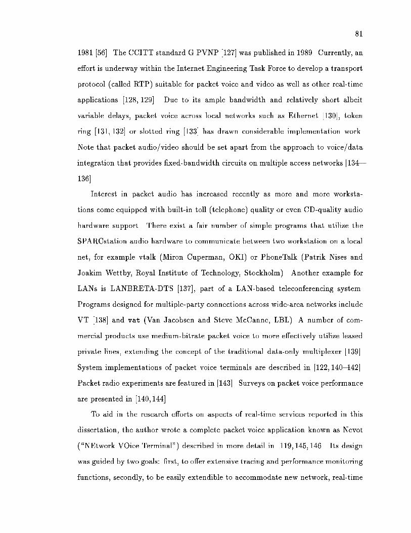
81
1981 [56]. The CCITT standard G.PVNP [127] was published in 1989. Currently, an
e�ort is underway within the Internet Engineering Task Force to develop a transport
protocol (called RTP) suitable for packet voice and video as well as other real-time
applications [128, 129]. Due to its ample bandwidth and relatively short albeit
variable delays, packet voice across local networks such as Ethernet [130], token
ring [131, 132] or slotted ring [133] has drawn considerable implementation work.
Note that packet audio/video should be set apart from the approach to voice/data
integration that provides �xed-bandwidth circuits on multiple access networks [134{
136].
Interest in packet audio has increased recently as more and more worksta-
tions come equipped with built-in toll (telephone) quality or even CD-quality audio
hardware support. There exist a fair number of simple programs that utilize the
SPARCstation audio hardware to communicate between two workstation on a local
net, for example vtalk (Miron Cuperman, OKI) or PhoneTalk (Patrik Nises and
Joakim Wettby, Royal Institute of Technology, Stockholm). Another example for
LANs is LANBRETA-DTS [137], part of a LAN-based teleconferencing system.
Programs designed for multiple-party connections across wide-area networks include
VT [138] and vat (Van Jacobsen and Steve McCanne, LBL). A number of com-
mercial products use medium-bitrate packet voice to more e�ectively utilize leased
private lines, extending the concept of the traditional data-only multiplexer [139].
System implementations of packet voice terminals are described in [122, 140{142].
Packet radio experiments are featured in [143]. Surveys on packet voice performance
are presented in [140,144].
To aid in the research e�orts on aspects of real-time services reported in this
dissertation, the author wrote a complete packet voice application known as Nevot
(\NEtwork VOice Terminal") described in more detail in [119, 145, 146]. Its design
was guided by two goals: �rst, to o�er extensive tracing and performance monitoring
functions, secondly, to be easily extendible to accommodate new network, real-time

82
and session control protocols, inter and intra-media synchronization algorithms,
�xed and variable rate audio encodings and user interfaces.
For this dissertation research and follow-on work, Nevot was used:
� as a tra�c source, both interactively and by providing trace data for network
tests and simulations
� as a quality-of-service measurement tool, allowing the measurement of packet
loss and end-to-end delay as actually perceived by the user, after delay adap-
tation and loss reconstruction
� as a test bed for improved delay adaptation, intra-media synchronization algo-
rithms and protocols for real-time services [128,129]
Nevot has also served as a demonstration tool for real-time applications across
both wide-area packet switched networks such as the Internet as well as corporate
private networks. It has demonstrated both the feasibility of implementing real-
time services within a non-real time operating system such as BSD Unix, and also
highlighted the shortcomings of current operating systems in supporting real-time
applications.
The main function of a packet voice terminal is the reconstruction of the syn-
chronous audio stream produced by the remote source, in the face of random and
nonstationary network and operating system delays. The audio device generates
samples at a �xed rate, typically 8,000 samples per second, which are then gathered
into packets of around 20 ms. (Currently, 180 samples representing 22.5 ms is most
commonly used; this value dates back to the frame size of the 2,400 bit/second LPC
vocoder used in early experiments.)
The packet voice receiver compensates for the delay variabilities introduced by
the sender, the network and the network receiver processing by adding a variable
delay between the arrival time and the time the audio data is submitted to the audio

83
output device. [147] [148] [149] [150]. In general, packets within a talkspurt have to
be played out consecutively, so that playout delay adaptation can only take place
at the beginning of a talkspurt. Since low end-to-end delays are highly desirable for
interactive voice communication, adaptive rather than worst-case playout delays are
typically used. Nevot models the variable delays as a Gaussian random variable
and adjusts the playout delay of the talkspurt beginnings as a constant factor times
the current delay variance estimate. (An additional delay bu�er on the order of 20
to 30 ms has to be added for workstations within the audio device to compensate
for operating system scheduling delays.)
Nevot is meant to serve four purposes:
� as a demonstration tool for Internet audio conferences,
� as a measurement tool to investigate tra�c patterns and losses in packet voice
applications across wide-area networks,
� as a demonstration implementation of real-time services in a distinctly non-
real-time operating system (Unix)
� as a tra�c source to validate and evaluate resource allocation protocols and
algorithms.
The modular software architecture of Nevot is shown in Fig. 4.4. Operational
experience showed that multiple concurrent conferences or conversations are desir-
able, for example for private side chats within a conference. Within a packet voice
setting, multiple conversations are much easier to support than with traditional
telephony. Audio mixing and multiple audio channels make it possible to listen in
on several conferences.
Since Nevot is expected to operate over a wide range of networks, from FDDI
to modem SLIP lines, it supports audio encodings spanning the range from 48 kHz
sample rate, 16 bits/sample CD quality through standard telephony toll-quality

84
64 kb/s PCM8, 32 and 24 kb/s ADPCM9 [151] to low-bit rate vocoder quality 4 kb/s
LPC. Support for variable rate encodings (e.g., by Hu�man-encoding the ADPCM
coe�cients) is planned. The variety of audio encodings used makes the use of
application-layer gateways necessary. Nevot implements a gateway by making use
of the multiple stream design, forwarding input for each stream, after transcoding,
to all other streams. Privacy of conversations and conferences is assured by DES
encryption.
NVP vat
UDP
TCP
ST−II
???
setupnetwork I/O
XView
Motif
curses
stdio
userinterface
services
G.711 G.721 G.723 DVI LPC
agcVUmeter
silencedetection
commandlineinter.
playout synchronization
vat
session
audio codecs
NEVOTkernel
.snd
AIFC
???
audiofiles
???
RTP
RTP
Figure 4.4. Nevot Structure Overview
8pulse code modulation
9adaptive di�erential pulse code modulation
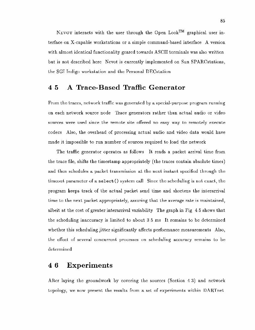
85
Nevot interacts with the user through the Open LookTM graphical user in-
terface on X-capable workstations or a simple command-based interface. A version
with almost identical functionality geared towards ASCII terminals was also written.
but is not described here. Nevot is currently implemented on Sun SPARCstations,
the SGI Indigo workstation and the Personal DECstation.
4.5 A Trace-Based Tra�c Generator
From the traces, network tra�c was generated by a special-purpose program running
on each network source node. Trace generators rather than actual audio or video
sources were used since the remote site o�ered no easy way to remotely execute
codecs. Also, the overhead of processing actual audio and video data would have
made it impossible to run number of sources required to load the network.
The tra�c generator operates as follows. It reads a packet arrival time from
the trace �le, shifts the timestamp appropriately (the traces contain absolute times)
and then schedules a packet transmission at the next instant speci�ed through the
timeout parameter of a select() system call. Since the scheduling is not exact, the
program keeps track of the actual packet send time and shortens the interarrival
time to the next packet appropriately, assuring that the average rate is maintained,
albeit at the cost of greater interarrival variability. The graph in Fig. 4.5 shows that
the scheduling inaccuracy is limited to about 3.5 ms. It remains to be determined
whether this scheduling jitter signi�cantly a�ects performance measurements. Also,
the e�ect of several concurrent processes on scheduling accuracy remains to be
determined.
4.6 Experiments
After laying the groundwork by covering the sources (Section 4.3) and network
topology, we now present the results from a set of experiments within DARTnet.

86
packet count
erro
r (s
ec)
−0.004
−0.0035
−0.003
−0.0025
−0.002
−0.0015
−0.001
−0.0005
0
0 50 100 150 200 250 300 350 400 450 500 550
Figure 4.5. Scheduling jitter for trace-based tra�c generator

87
First, in Section 4.6.1, we show that the accuracy of simulations in predicting actual
network performance, even with appropriate corrections, is limited. With that
caveat, we then summarize the results of network measurements providing insight
into the performance of the hop-laxity (HL) queueing policy as compared to the
standard FIFO policy. All DARTnet experiments described in this section ran the
IP version of the kernel described earlier in Section 4.2.1
4.6.1 Simulation as Predictor of Network Performance
To gain an understanding of how well simulations can predict actual network
performance, we mapped the topology used in Section 3.4 into DARTnet, with nodes
1 through 5 represented by DARTnet nodes parc, ames, la, dc and bbn, respectively.
For both simulation and network measurements, only streams arriving at node 5 (or
DARTnet node bbn, respectively) are taken into account.
In order to transmit an equal number of bits during the simulation and network
experiments, the header overhead incurred by the DARTnet protocol stack needs
to be taken into account. The HSI/S serial interface supports HDLC as its data
link layer. HDLC adds two bytes of framing and 2 bytes for a cyclic redundancy
check (CRC) to each frame. We ignore the overhead caused by bit-stu�ng since the
data portion of the packets used in the experiments is zero and thus not a�ected
by bit-stu�ng. The point-to-point protocol (PPP) serves as the media access layer
and adds four bytes, two of which are �xed-value HDLC address and control bytes.
IP, without options, and UDP add another 20 and 8 bytes of header, respectively,
for a grand total of 36 header bytes.
Another factor to be taken into account when comparing simulation and network
measurements is that most network interfaces cannot keep the channel busy con-
tinuously due to interrupt latencies, register set-up time and the like. By carefully
following a UDP packet train submitted at maximum rate as it progressed through
the network interface, we could estimate the latencies involved as well as the achiev-

88
able channel utilization. Since the latencies depend on other system activity and
the packet length, only rough estimates are possible. For 600 byte packets, the
time between packet transmissions was found to average about 3.67 ms, while pure
transmission time at a rate of 1.344 Mb/s would only require 3.571 ms. The idle
time of 98 �s per packet translates to a roughly 2.7% loss of channel capacity.
Throughout the simulation experiments reported in this subsection, we thus model
the channel as having a capacity of 1.308 Mb/s. The achievable ftp throughput
measured at 1.318 Mb/s (including IP and TCP headers), but with signi�cantly
longer (1500 byte) packets, lends some credence to this estimate.
At low load, i.e., without queueing, a packet would experience a latency of
approximately 460 to 600 �s, composed of the following components. The hardware
interrupt triggered by receiving a frame at the serial interface was measured to take
about 75 �s; then, 18 �s would elapse until the software interrupt posted by the
hardware interrupt was serviced. The software interrupt itself would add another
150 �s. 160 �s elapsed until the output handler was started, the time being occupied
by IP processing. The actual transmission then began about 160 �s later.
The delay measurements within DARTnet are by necessity end-to-end, including
all propagation and transmission delays. We used two methods to estimate these
�xed delays, both yielding results within 2 ms of each other. The �rst method used
a ping program with enhanced timing resolution to measure the round-trip delay
between sending ICMP echo request packets and receiving the corresponding ICMP
echo reply packet. Propagation delay was estimated at half the minimum round-
trip delay measured, ignoring the transmission time for the short (about 60 byte)
packets. The results of these measurements are una�ected by clock synchronization
and are shown in Fig. 4.1. The second method simply takes the minimum delays
measured during the experiment as an indication of the combined propagation and
transmission delays.

89
Table 4.2 compares the performance estimated by the simulation and actual
network measurements. Two sets of experiments were performed to gauge the
relative impact of low and high loads on how well simulation results predicted actual
network performance. In the �rst, labeled S1 and N1 in Table 4.2, the packets, with
headers, were sized at 300 bytes, while the experiment labeled S2 and N2 in that
table, consisted of packets of length 600 bytes. Note that the system load for the
low-load and high-load experiments is roughly the same. Except for additional time
needed to copy longer packets between kernel and user space, the overhead imposed
by tallying arriving packets and generating new arrivals is the same for both long
and short packets.
For both low and high network load, the simulation predicts the average queue-
ing delays within the current clock synchronization spread. However, the delay
percentiles are consistently underestimated by the simulation, for both low and high
loads. The di�erences between simulated and measured performance are seen to be
increasing with longer paths and higher load. Fortunately, for the high-load case,
the error is still only roughly 5 to 10%. Since per-packet penalty should decrease
with increasing packet size, the load-dependence of the error points to additional
queueing within the kernel. The only additional queue in the IP forwarding path is
that between the receive hardware interrupt and the software interrupt (see Fig. 4.3).
Thus, if the processing of the software interrupt is delayed due to other system
activity, packets could queue up there. Simply measuring the queue occupancy,
however, will not su�ce, as packets queued on input would probably been queued
on output even in the absence of input processing delays.
Another factor, probably of minor importance, is the background tra�c induced
by the multicast group management protocol IGMP and the clock synchronization
protocol ntp. Given that the system is operating in a high-load region (due to
the burstiness of the tra�c, the average utilization is only about 60%), even small

90
amounts of additional tra�c could have a disproportionate impact on queueing
delays.
Table 4.2. Comparison of queueing delays estimated by simulation (S) and networkmeasurements (N) for FIFO scheduling
path length1 2 3 4
tra�c mean 99.9% mean 99.9% mean 99.9% mean 99.9%S1 0.5 5.0 1.0 6.7 1.4 8.8 1.8 10.8N1 0.8 1.0 1.0 12.7 1.7 13.8 1.9 17.7S2 10.2 346 19.0 444 26.5 511 37.3 528N2 10.7 362 20.8 492 28.7 545 38.3 559
It should be noted that the measurements have not been compensated for the
clock o�set between bbn.dart.net and the various source nodes. From information
provided by the clock synchronization control program ntpq, the clock o�set can be
estimated at about �1 ms.
4.7 DARTnet Experiment: First Topology
This section discusses the �rst experiment comparing the measured network perfor-
mance of the hop-laxity (HL) and FIFO policies. The network ows are depicted in
Fig. 4.6. The thick arrows originating at node parc and terminating at node mit
indicate the ow of interest, while the thinner arrows represent cross tra�c. Each
ow consists of seven multiplexed conversational audio traces, as discussed earlier
in Section 4.3.2. The assignment of ows to links assures equal loading of each link
with the equivalent of 21 voice sources.
The ows were assigned a laxity of 500 ms. In the experiment labeled 'HL 5' in
Table 4.3, each packet started out with a hop count of �ve, regardless of the actual
number of hops the ow it belonged to was to traverse. This was meant to model a
larger network, where the interfering tra�c continues to other destinations beyond

91
mit
bbn
dc
udel
isi
la
lbl
ames
sri
parc
Figure 4.6. Tra�c Flows for DARTnet Experiment
Table 4.3. End-to-end delay performance measured in DARTnet (topology ofFig. 4.6
mean delay percentilesdelay 0.90 0.99 0.999
policy (ms) (ms) (ms) (ms)FIFO 60.5 80.1 162.5 243.0HL 5 77.0 125.9 312.0 423.4HL 55.5 64.8 99.9 133.5

92
the scope of the limited DARTnet topology. In the second experiment, the ows
were marked with their \true" hop count, i.e., all interfering ows had initial hop
counts of three and one, while the parc to mit ow started with a hop count of
�ve. As one would expect, the latter provides a more favorable treatment to the
long-distance ow, somewhat reducing its mean delay and signi�cantly reducing the
delay percentiles for all measurable and interesting percentile values. The 'HL 5'
experiment indicates that some ows may be considerably worse o� when hop laxity
scheduling is introduced.
4.7.1 DARTnet Experiment: Second Topology
In a second experiment, DARTnet was used to model the topology described in
[36], with the same ows and conversational voice tra�c as discussed in Section 4.6.1.
Here, all packets had a length of 600 bytes, including headers.
Table 4.4. End-to-end delay performance measured in DARTnet (topology ofFig. 3.1)
path length1 2 3 4
tra�c mean 99.9% mean 99.9% mean 99.9% mean 99.9%FIFO 18.6 370 57.6 529 73.5 590 87.1 608HL (200 ms) 26.3 515 59.9 632 59.9 632 81.4 661HL (400 ms) 26.4 500 56.9 584 65.9 553 74.7 599
The end-to-end delays (including transmission and propagation delays) of the
streams reaching the node bbn, are summarized in Table 4.4. 'HL (x)' refers to
hop-laxity scheduling with a laxity value of x. From the table, we conclude that the
performance between FIFO and HL does not di�er markedly, indicating that the
performance gains attributable to delay-sensitive scheduling are outweighed by the
additional processing costs and packet header overhead. It appears doubtful that
other laxity values would yield signi�cantly better results. It should be noted that

93
the goal of delay equalization has indeed been reached, by reducing the delay spread
between long-haul and short-haul ows from 238 for FIFO to 99 ms for HL.
A third set of experiments used several lecture voice and video streams multi-
plexed at each source, con�rming the basic results shown here. Further details are
relegated to a technical report in progress.
In summary, the network measurements generally con�rm the conclusions drawn
from the simulation experiments discussed in Section 3.4, but indicate that the
gains attributable to hop-laxity scheduling are further diminished by the additional
processing and packet header overhead. Further studies are needed before it could
be recommended to expend the computational e�ort needed to implement HL in
routers.
4.8 Conclusion and Future Work
The experiments performed so far have opened a range of possibilities for future
explorations. We start by summarizing in Section 4.8.1 how the BSD networking
code could be modi�ed to ease implementation of resource-control algorithms. This
complements the suggestions o�ered in [117]. Based on our experience, suggestions
on the appropriate use of simulations and network measurements are made in
Section 4.8.2.
4.8.1 Supporting Non-FIFO Scheduling in BSD Kernels
The networking code within Berkeley Software Distribution Unix (BSD) and
the commercial Unix systems derived from it (such as SunOS or DEC Ultrix) have
the exibility to incorporate new protocols at both the transport and network layer,
such as ST-II or OSI-based protocols, as well as the integration of new devices,
even without access to the operating system source code. However, the support
for alternate process scheduling and resource control is weak. Adding the hop-
laxity scheduler or resource-reservation methods requires modifying the network

94
kernel and device driver sources, which are often not available to the experimenter.
For example, the enqueueing and dequeueing routines within the device drivers are
actually macros, so that relinking cannot be used to replace them with modi�ed
versions.
The combination of di�erent scheduling methods is even more di�cult since
there is no standardized way of providing the necessary information to the schedul-
ing routines. It would, however, be relatively easy to add a fairly general facil-
ity that would allow easy experimentation with a variety of scheduling methods.
First, each network interface de�nition (contained in the ifnet structure de�ned in
net/if.h) should have function pointers to the enqueueing and dequeueing routines.
For the other layers, hooks should be added to the protosw structure (de�ned in
sys/protosw.h) to access an enforcement or translation function that would do the
mapping from protocol-speci�c scheduling information to the generic data structures
understood by the device-level schedulers.
Less readily solved is the question of how to encapsulate the necessary per-packet
and per-association \out-of-band" scheduling information. As described earlier, in
our implementation, we simply mark special mbufs as containing the scheduling
information within the �rst few bytes of their data area. This works reasonably well
as long as there is enough space so that no additional mbuf has to be prepended.
Alternatively, a new mbuf could always be used, but then all device drivers would
have to be aware that certain types of mbufs are not meant to be transmitted.
Keeping scheduling information within the same mbuf chain as the actual packet
data simpli�es argument passing and queueing, but may require searching a number
of mbufs for the desired type.
4.8.2 Simulation and Network Measurements
Clearly, any proposed protocol, queueing policy etc. must �nally prove itself in
real networks, with realistic tra�c and under the software and hardware constraints

95
of real routers and workstations. The experiments conducted on DARTnet highlight
some of the di�culties in conducting performance measurements in a real network:
Kernel programming is tedious. Changing the kernel, even if all sources are
available, is far more tedious and time consuming than programming a sim-
ulation. Debugging support for Unix kernels is rather limited, so that in
many cases the cause for failure has to be divined by deciphering optimized
assembly code. This is particularly true if the hardware used in the network
is not available locally, as was the case for the work reported here. We used a
tracing facility with timestamps to keep track of signi�cant events as a packet
crossed a router. As an example, adding time stamps recording progress along
the path traversed by a packet is trivial in a simulation program, requires
extensive programming e�ort and incurs nonnegligible delays when translated
to IP packet handling code.
Measurements a�ect the outcome. Any timing measurements delays packet
transmission and may reduce channel utilization. Packet receiver processing
may impose additional delays.
Clocks are not synchronized. Even though DARTnet runs a state-of-the-art
clock synchronization protocol, clock di�erences of several milliseconds, subject
to drift, cannot be ruled out, thus making accurate delay measurements
di�cult. (It is possible to get statistics about actual clock di�erences from
the clock daemon, but the e�ort is substantial.)
A channel is never idle. Even though DARTnet is dedicated to experiments,
there are a number of services that need to be running during many exper-
iments, such as clock synchronization and the multicast group management
protocol (IGMP). Fortunately, the background tra�c is usually insigni�cant.
96
Experiments are hard to reproduce. Since the tra�c is generated by a non-
real-time operating system, two experiments never produce the same packet
timing. The disturbances introduced by background tra�c can usually be
ignored.
Network measurements generally take longer to set up, run and evaluate
than equivalent system experiments. In our experience, the �ve-node network
mapped onto DARTnet could be simulated in signi�cantly less time than it
took for the actual network experiment, even though �ve processors were
contributing during the network experiment. Also, trace and statistics �les
have to be gathered after each experiment.
The topology is very restricted. Although topology constraints did not impact
our work signi�cantly, the current DARTnet topology has no alternate paths
to a destination, thus making routing experiments di�cult.
Thus, network measurement experiments should only be undertaken after exten-
sive simulation experiments. However, limited network experiments can be useful in
deriving information about computational overhead that can ow back into realistic
simulation experiments.
C h a p t e r 5
Distribution of the Loss Period for Queueswith Single Arrival Stream
5.1 Introduction
For soft real-time communication systems, the packet loss rate rather than the
average packet delay becomes the critical performance measure. Interactive voice,
video and distributed measurement and control are examples of such systems that
impose delay constraints, but also show a certain tolerance for lost packets. Most
previous studies of real-time systems only measure loss as a time-average fraction
of missing packets [5, 30, 58, 152{154]. In order to judge the \quality" of loss-prone
communication, however, it is important to know not just how many packets are
being lost, but also whether losses occur in clusters or randomly. The importance of
accounting for correlated losses has long been recognized in speci�ying acceptable
performance of data circuits. \An errored second is declared when one or more bits
in that second is found in error. [155]" This leads to the metric of the percentage of
error-free seconds (EFS).
Papers on the replacement of lost packets in packet voice communication systems
typically assume random, uncorrelated occurrence of packet loss [156, 157]; as we
will show, this assumption might be overly optimistic. The work by Shacham and
Kenney [158,159] provides another example. They observed that loss correlation in
a �nite-bu�er system could completely eliminate the advantage of three orders of
magnitude predicted for forward-error correction under the assumption of indepen-
dent (Bernoulli) losses.
98
The investigation of loss correlation has a long history in the context of bit errors
in data communication [160], but has only recently attracted stronger interest in the
area of packet networks.
A number of authors have quanti�ed the in uence of loss correlation for network
performance. For example, it has been shown [161{164] how the throughput of
go-back-N ARQ increases with positive loss correlation. Similar results for the
N -packet transfer time and go-back-1 and blast protocols are presented in [165]. All
papers1 assume a two-state Markovian error model with geometrically distributed
run lengths for losses and successes, which will be seen to be appropriate for some,
but not all queueing systems studied below. Thus, our results can be used in
conjunction with the work cited here to directly predict ARQ performance.
In some simulation studies, cell loss correlation has been investigated [166,167]
and methods for the compensation of correlated cell loss have been proposed [159,
168]. Biersack [169] uses simulation to evaluate the e�ect of burst losses on the
performance gains achievable by forward error correction.
In this chapter, we consider a single FCFS queue with in�nite bu�er in isolation
in which an arriving customer2 which reaches the server after waiting h or more
units of time is considered \lost" (even though it still receives service). Chapter 6
will tackle more complex arrival statistics.
We characterize the stochastic properties of the time-out loss period, the un-
interrupted interval of time during which the virtual work in the queue exceeds
the given threshold h. Given this time-based quantity, we also arrive at measures
of customer-based quantities such as the distribution of the number of consecutive
customers which each spends more than an allotted time waiting for service. We
show that the assumption that each customer is lost independently from the previous
1except for [163], which allows a more general Markovian error model
2The terms \customer" and \packet" will be used interchangeably.

99
one leads to a signi�cant underestimation of the duration of such loss periods. Using
elementary methods of probability, we also prove that for certain classes of queues
the duration of the loss period is independent of the value of the threshold. We
further show through numerical examples for other important types of queues that
the in uence of the threshold on this metric is minimal for interesting probabilities of
loss. Our numerical results also indicate that the expected number of consecutively
lost customers (for the same loss probability) varies by as much as 50% depending
on the batch arrival distribution used. We also derive measures of the time between
loss periods. Throughout the proposal, emphasis is placed on providing results that
can be readily numerically evaluated.
A number of authors have investigated related aspects of the problem. Kamitake
and Suda [170] consider a discrete-time queue in which tra�c is generated by a
changing number of active callers, with each active caller generating a packet in a
slot according to a Bernoulli process. They compute the steady state loss rate for a
given number of active callers and then consider the variation in the number of active
callers in computing the amount of uninterrupted time from when this loss rate �rst
exceeds a value � until it drops below another value �, with � < �. Our work di�ers
from [170] in that we directly characterize those periods of time in which arriving
customers are lost, rather than characterizing loss as being \quasi-stationary" during
periods of times during which the number of active sources remains constant.
Leland [171] mentions, but does not elaborate on measuring consecutive losses
per connection in an ATM simulation experiment. Woodru� and Kositpaiboon [172]
mention the desirability of specifying the probability and duration of periods of high
cell loss rates. By rate conservation methodology, Ferrandiz and Lazar [173{175]
develop a theoretical framework for studying loss correlation in queueing systems.
They investigate the distribution of gaps, that is, consecutive losses, due to blocking
and clipping (see below) in a multiclass G=G=m=B queueing system; we discuss
similarities and di�erences between our work and [173] in the following sections. In
100
general, our focus is more on deriving computable results, relying on well-known
Markov chain methods.
Van Doorn [176] and Meier-Hellstern [177,178] characterize the over ow process
from a �nite Markovian queueing system. As pointed out earlier, [159] underlines
the importance of taking loss correlations into account, but investigates their e�ect
on forward-error correction only through simulation. A large body of literature
analyzes the over ow process of blocked-calls-cleared systems, but the results do
not seem directly applicable to our problem. Norros and Virtamo [179] use the
average loss probability during congestion as an indicator of loss correlation. They
assume that the total rate has a Gaussian distribution and that congestion occurs
when the total instantaneous rate exceeds the channel capacity.
The chapter is organized as follows. After de�ning more precisely the systems
and measures of interest in the section below, continuous-time queues are investi-
gated in Section 5.2. In Section 5.3 we then apply similar methods to derive the
corresponding measures for a discrete-time queue of interest in packet switching.
We conclude by summarizing the work presented and pointing out some issues to be
investigated. Additional details and examples can be found in a companion technical
report [180].
5.2 Clip Loss in Continuous Time (G=M=1)
5.2.1 Performance Measures
This chapter focuses on a single-server queue, where customers are processed in
the order of arrival. Customers that spend more than a deterministic, �xed amount
of time h waiting for service are tagged as lost on leaving the queue, but are still
served. (Ferrandiz and Lazar [173] refer to this as clipping loss.) This de�nition of
loss is motivated by considerations of tra�c with soft real-time constraints, where
packets that are excessively delayed are worthless to the receiver. The loss as de�ned

101
here di�ers from that studied in our earlier work [152], where excessively delayed
customers depart before occupying the server.
A loss period (LP) is an uninterrupted interval during which all arriving cus-
tomers would experience a waiting time exceeding h. For in�nite queues with FCFS
service, the loss period equals the interval during which the virtual work in the
queue is greater than the threshold h. Loss periods and busy periods are related
in that a busy period is a special case of a loss period, with threshold value h = 0.
Also, both busy periods and loss periods start with the arrival of a customer. They
di�er, however, in that a busy period ends with a departure of a customer, while the
end of a loss period is not connected with a customer departure. A noloss period is
the interval between two loss periods. For h = 0, noloss periods correspond to idle
periods of the queue.
While the loss period is of independent interest, we are particularly concerned
with measuring the number of consecutively lost customers, called loss run for
brevity. Note that the number of customers arriving in a loss period is not identical
to the number of consecutively lost customers. In particular, the �rst customer
triggering a loss period, i.e., the customer that pushes the virtual work above h,
is itself not lost. Thus, loss periods consisting of a single arrival do not contribute
to customer loss. Note that there may also be several noloss periods interspersed
between two customer losses if each of the loss periods separating the noloss periods
consists of only the arrival triggering a loss period. Similar to loss runs, success runs
denote the number of consecutive customer without any loss.
Fig. 5.1 depicts a virtual work sample path and the measures de�ned above.
Time proceeds along the abscissa from left to right, while the ordinate shows the
virtual work at a given instant. In the �gure, arrivals that will be tagged as lost on
departure are marked with , the others with �. The extent of loss periods (LP)and busy periods (BP) are indicated by horizontal bars. Bold arrows represent
initial jumps, the amount of virtual work above h at the beginning of a loss period.

102
6@@@@
6@@
@@@
@@@@@@@@@@@@
@@@@@
@@
6@@@
-
� � � � � � �
h
tLPBP
Figure 5.1. Virtual work sample path
The height of the vertical jumps indicates the amount of work brought to the system
by an arriving customer. The un�nished work decreases at a unit rate as the server
processes jobs.
Let us brie y touch upon other measures of loss behavior for queueing systems.
For �nite queues with m deterministic servers and bulk arrivals, at least m of the
arriving packets are always served. For an individual source, the probability of
consecutive losses depends on its position within the bulk, which might be �xed,
uniformly distributed or a time-varying stochastic process, depending on the bu�er
management policy. This system was treated extensively by Li [181]. Li de�nes as
blocking those states where the bu�er is full prior to service completion.
We may also look at loss-correlation through a frequency-domain perspective.
As an example, the �rst-order autocorrelation coe�cient of intervals between losses
was measured experimentally for a �ve-stage virtual circuit model with bounded
waiting times. Using the von-Neumann statistic [182] as a robust estimator, it was
found that the intervals between losses were essentially uncorrelated. Autocorrela-
tion information might be useful in comparing di�erent bu�er management schemes
or service disciplines, but cannot readily be used to predict the performance of
packet reconstruction algorithms.

103
The stochastic properties of the loss period or consecutive customer losses can
be quanti�ed in the usual manner, for example through its distribution or its average
duration, either in terms of time or the number of customers a�ected. Details are
discussed in the next two sections for continuous and discrete-time queueing systems
of interest.
As a �rst model, we investigate a system with general (not necessarily i.i.d.)
arrival process of rate � and exponential service with rate �. (The service process
does not have to be independent of the arrival process.) The bu�er is in�nite, so
that only loss due to excessive delays in the queue occurs. All packets, regardless
of whether they exceed the waiting time threshold or not, are served. (A system
where late packets are dropped will be treated later.) The special case of Poisson
arrivals, i.e., the M=M=1 system, will be treated in detail since it yields closed-form
expressions for the measures of interest. The M=M=1=1 system was also investi-
gated by Ferrandiz and Lazar [173] as a special case of their G=G=m=B analysis.
Their analysis seems considerably more involved, does not readily yield numerical
results and does not make use of the simple connection to the busy period pointed
out here. Our model is applicable, if only in approximation, to systems with variable
packet sizes, for example the PARIS network [183] or a variation of the Knockout
switch [184].
Throughout this section, we will illustrate our calculations through a running
example consisting of anM=M=1 queue with arrival rate � = 0:8, service rate � = 1
(and thus a load of � = �=� = 0:8) and a clipping threshold of h = 3 so that
� = 1 � �e(���)h = 43:905% of all arrivals experience a delay of more than 3 (are
\lost"). The methods presented below apply equally well at lower loss probabilities;
we have chosen this (impractically) high loss to simplify simulation veri�cation of
our results through simulation.

104
5.2.2 Distribution of the G=M=1 Initial Jump and Loss Period
As pointed out above, a loss period commences when an arrival causes the virtual
work to cross the threshold h from below. In order to establish the distribution of
the loss period, the following lemma describes the distribution that governs the
initial jump, i.e., the virtual work immediately after the arrival of the �rst customer
in a loss period.
Lemma 1 For a G=M=1 queue, the initial jump has the same distribution as the
service time and does not depend on the threshold h.
Proof Let the random variable J represent the height of the initial jump and
fJ (j) its density. The density fJ (j) can be expressed through conditioning, where
we de�ne V as the virtual work just prior to the arrival of the customer whose new
work pushes the virtual work above h. A denotes the arriving (new) work.
fJ(j) =Z h
0P [V = vjV � h] � P [A = h+ j � vjA � h� v] dv (5:1)
The second conditional probability can be rewritten as
�e��(h+j�v)
e��(h�v)= �e��j;
which follows immediately from the memorylessness property of the exponential
distribution.
Now we can rewrite the jump density as
fJ (j) = �e��jZ h
0
P [v = y \ y � h]
P [v � h]dy
= �e��j1
P [v � h]
Z h
0P [v = y] dy
= �e��j1
P [v � h]P [V � h]
= �e��j :
This shows that the jump density is indeed exponentially distributed.

105
Given this property of the initial jump, the following theorem follows immedi-
ately:
Theorem 5.1 In a G=M=1 queueing system, a loss period is stochastically identical
to a busy period. The loss period distribution is independent of the threshold h. For
G=G=1 queues, a loss period is stochastically identical to a busy period with special
�rst service.
For the G=G=1 case, note that busy periods with special (or exceptional) �rst service
are covered by Wol� [185, p. 392-394].
The independence of the loss behavior from the threshold recalls a similar
observation made by Li [181] regarding the bu�er over ow process in a packet voice
system. There, the time spent in the overload state was found to be independent of
the bu�er size.
Let the random variable L denote the time duration of a loss period. Then, given
Theorem 5.1, busy and loss periods for the M=M=1 queue have the density [186, p.
215]
fL(y) =1
yp�e�(�+�)I1[2y
q��]
and mean
E[L] =1
�� �=
1
�
1
1 � �;
where I1(y) is the modi�ed Bessel function of the �rst kind of order one. The
cumulative distribution function is best computed by numerical integration, as there
are no suitable closed-form expression for the integral.
For non-G=M=1 queues, the computation of the initial jump can be di�cult. In
general, the relationship
fJ (j) =Z h
0
w(v)b(h+ j � v)
W (h)(1 �B(h� v))dv
holds, where b(x), w(x), B(x) and W (x) are the densities and distributions of
arriving work and the virtual work seen by the arrival, respectively.

106
However, some stochastic ordering results for busy periods with special �rst
service and loss periods may be of interest.
Lemma 2 The loss period for a G=GI=1 queue is stochastically longer than (shorter
than) a busy period if the initial jump is stochastically larger (smaller) than a service
duration.
Proof We prove the �rst, non-parenthesized part; the other proceeds similarly.
Let the random variables X and Y denote a regular service time and an initial
jump, respectively. From the coupling theorem (see [187, Proposition 8.2.2]), we
know that if Y �st X, then there exist random variables ~X and ~Y , with the same
distributions as X and Y , such that ~Y � ~X , i. e., P ( ~Y � ~X) = 1. Without
changing the duration of the loss period, we preempt the �rst customer after ~X and
then complete its remaining service time, ~Y � ~X, at the conclusion of the loss period.
Denote the sum of the service periods of the remaining customers in the busy or
loss period by S and the extension of the loss period caused by arrivals during the
~Y � ~X segment as E. Since
~X + S > a) ~X + S + (~Y � ~X) + E > a;
we write
P [ ~X + S + (~Y � ~X) + E > a] � P [ ~X + S > a];
from which the stochastic inequality for the coupled loss and busy periods follows.
Finally, we uncondition to make the result apply to any busy and loss period.
Alternatively, we can argue by using [187, Example 8.2(a)], where it is shown
that
f(Y1; : : : ; Yn) �st f(X1; : : : ;Xn)
for any increasing function f if Yi �st Xi and given that X1; : : : ;Xn and Y1; : : : ; Yn
are independent. Clearly, the length of the busy period is an increasing function
(the sum) of the service periods that constitute it.

107
Using this lemma, it is easy to show the following general relation between loss
periods and service times.
Theorem 5.2 If the service time has decreasing failure rate (DFR), the loss pe-
riod is stochastically longer than a busy period. Conversely, for service times with
increasing failure rate (IFR), the loss period is stochastically shorter than a busy
period.
Proof De�ne Xt as the additional life of X from t onward, given that X � t.
In [187, Proposition 8.1.3], it is shown that i� X is DFR, then Xt �st X and i� X
is IFR, then Xt �st X. This is true for any value of t.
Let the conditional random variable Xt denote the initial jump initiating a
random loss period, given that the amount of service time needed to reach from
the virtual work to h equals t. Let X 0 be the unconditional initial jump and X the
service time. We show the proposition for the IFR case; it follows for the DFR case
by reversing the relational operators.
If X is IFR, then Xt �st X, so that
P [Xt < X] � P [X < x]:
X 0 can be computed from Xt by removing the condition:
P [X 0 < x] =Z 1
0P [Xt < x] dFx(t)
Thus,
P [X 0 < x] =Z 1
0P [Xt < x] dFx(t) >
Z 1
0P [X < x] dFx(t) = P [X < x]:
In other words,
X 0 �st X;
from which Lemma 2 yields the proposition.
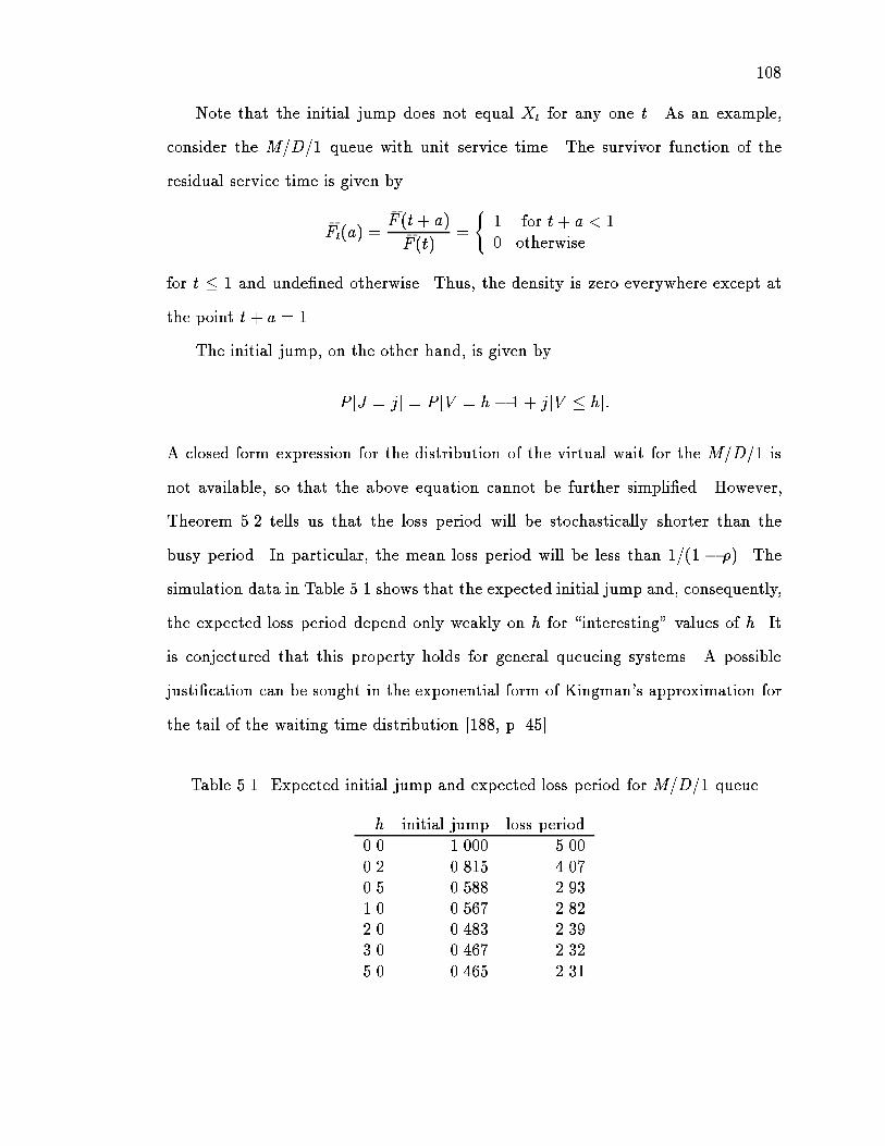
108
Note that the initial jump does not equal Xt for any one t. As an example,
consider the M=D=1 queue with unit service time. The survivor function of the
residual service time is given by
�Ft(a) =�F (t+ a)�F (t)
=
(1 for t+ a < 10 otherwise
for t � 1 and unde�ned otherwise. Thus, the density is zero everywhere except at
the point t+ a = 1.
The initial jump, on the other hand, is given by
P [J = j] = P [V = h� 1 + jjV � h]:
A closed-form expression for the distribution of the virtual wait for the M=D=1 is
not available, so that the above equation cannot be further simpli�ed. However,
Theorem 5.2 tells us that the loss period will be stochastically shorter than the
busy period. In particular, the mean loss period will be less than 1=(1 � �). The
simulation data in Table 5.1 shows that the expected initial jump and, consequently,
the expected loss period depend only weakly on h for \interesting" values of h. It
is conjectured that this property holds for general queueing systems. A possible
justi�cation can be sought in the exponential form of Kingman's approximation for
the tail of the waiting time distribution [188, p. 45].
Table 5.1. Expected initial jump and expected loss period for M=D=1 queue
h initial jump loss period0.0 1.000 5.000.2 0.815 4.070.5 0.588 2.931.0 0.567 2.822.0 0.483 2.393.0 0.467 2.325.0 0.465 2.31
109
5.2.3 Consecutive Customers Lost
While the duration of a loss period is distributed like the duration of a busy
period, we recall from Section 5.2.1 that the number of consecutive customers lost
does not have the same distribution as the number of customers in a busy period.
De�ning CC and CB as the number of consecutively lost customers and the number
of customers in a busy period, respectively, we have
P [CC = n] =P [CB = n + 1]
P [CB > 1]; n > 0
where P [CB > 1] is the probability that the busy period contains more than one
customer.
Let us apply these results to the M=M=1 queue. With P [CB = n] given by
[186, Eq. (5.157)]
P [CB = n] =1
n
�2n � 2n� 1
��n�1(1 + �)1�2n; n > 0
we compute
P [CB > 1] = 1� P [CB = 1] = 1� 1
1 + �=
�
1 + �:
Thus,
P [CC = n] =1
n+ 1
2n
n
!�n�1
(1 + �)2n; n > 0:
Note that this result di�ers markedly from the geometric distribution postulated by
Ferrandiz [173, Corollary 5.3].
Since the average number of customers per busy period is 1=(1 � �), we have
that for the M=M=1 queue the average number of consecutive customers lost is
E[CC] =1
P [CB > 1]
1
1� �� 1
!=
1 + �
1� �: (5:2)
This result di�ers markedly from that obtained under the assumption that losses
occur independently as Bernoulli events with the time-average loss probability �.

110
In that case, the conditional probability mass function (pmf), given one loss, for the
number of consecutive losses would be distributed geometrically as
P [CC = n] = �n�1(1� �)
with an average value of E[CC] = 1=(1 � �). For our running example, the
independence assumption leads one to conclude that a loss period consists of 1.78
customers on average, while our analysis above shows that the actual number for
this system is 9. Thus, customer losses are far more clustered than the assumption
of independent losses would suggest.
An additional characterization of loss periods is provided by the conditional
probability of packet loss given that the previous packet was lost, denoted here by r.
It is directly related to the average loss run length, E[CC], through [173, eq. (5.1)]
E[CC] =1
1 � r� 1 + r + r2 + : : : ;
r = 1 � 1
E[CC]:
For the M=M=1 case,
r =2�
1 + �:
The clustering of losses in a queueing system is naturally also re ected in this mea-
sure. For our M=M=1 example, the conditional loss probability equals 0:89, while
the assumption of independent losses would result in a conditional loss probability
r equal to the loss probability �, which evaluates to 0:44 for our running example.
5.2.4 Distribution of Noloss Period
The distribution of the time between loss periods is more di�cult to determine.
This interloss time comprises the interval between the time the virtual workW drops
below h from above and the �rst time instance it rises above this mark again, i.e.,
the event minft : W (t) = hjW (0) = hg. The sample path with respect to time t of

111
this stochastic process is continuous in time and right-continuous in state, with drift
of rate t and jumps of exponential height at Poisson intervals. The di�culty appears
since the process is \sticky" at the zero line, with dwell time corresponding to the
interarrival (or queue idle time) distribution. We are interested in the distribution
of the time to absorption of this process at the W = h barrier.
To make the problem tractable, we have assumed a Markovian arrival process;
otherwise the duration of the noloss period would depend on the time of the last
arrival during the preceding loss period. Thus, the computation of this section will
be limited to the M=G=1 model.
Aspects of this problem or approximations of it appear in a number of applied
stochastic models [189]. In collective risk theory [190] the insurance company starts
out with some �xed capital. This capital increases through premiums at a constant
rate and decreases (or increases) by claims occurring at Poisson instants. Of interest
is the time until the capital reaches zero, that is, the company is ruined. To model
noloss periods, the capital would represent the mirror image of the virtual work,
with an initial value of zero. However, the model does not allow for the fact that
the state cannot exceed h (idle system). Thus, it would tend to overestimate the
duration of the noloss period and be most suitable for heavy tra�c where the idle
period is short. It would give exact results, however, for t < h since the system
cannot have reached h by that time.
We select a model involving an approximation that is based on the so-called
Moran dam model [191, 192] [193, p. 336f] [194, p. 200]. In this model, the
water content of a dam or reservoir is represented by a continuous or discrete-state,
discrete-time homogeneous Markov process. For reasons of computability, we choose
a discrete-state representation, yielding a discrete-time Markov chain (DTMC).
Time is discretized in quantities of � , a fraction of the service time, and the Markov
chain tracks the virtual work Wn in the queue at epochs of integer multiples of
� . Thus, the Markov chain has k = h=� + 1 states with values from the set

112
f0; 1=�; 2=�; : : : ; hg. At the end of each discretization interval, at (n� )�, the virtual
work, if positive, decreases by one unit, re ecting the fact that the virtual work
decreases at unit rate. Arrivals bring in an amount of work Xn, again in multiples
of � , and occur just after the beginning of the discretization interval, at (n� )+. The
noloss period ends as soon as the virtual work reaches h or state k. We model this
by making state k an absorbing state and compute the duration of the noloss period
as the time to absorption into state k. Given this description of the DTMC, we can
write the state evolution recursively as
Wn+1 = min(k;Wn +Xn)�min(1;Wn +Xn):
Let us de�ne ak as the probability that k units of work of size � arrive. Also, denote
the complementary cumulative distribution function gj as
gj =1Xi=j
aj = 1�i�1Xi=0
aj:
The state transition matrix follows readily:
P =
2666666664
0 1 : : : k � 1 k
0 a0 + a1 a2 ak gk+11 a0 a1 ak�1 gk: : :k � 1 0 0 a1 g2k 0 0 0 1
3777777775
(5:3)
The last row stems from the fact that state k� 1 is absorbing. The state transition
probabilities are computed as
aj = P [�j � X � � (j + 1)]; (5:4)
where X is the amount of work arriving in a slot. We know that the accumulated
work from n arrivals in a G=M=c system is Erlang-n distributed with density
f(x) =�n(�nx)n�1
�(n)e��nx:

113
and cumulative distribution function F (x) = P (n; �x), where P (a; x) is the normal-
ized incomplete gamma function
P (a; x) , (a; x)
�(a)=
1
�(a)
Z x
0e�tta�1 dt:
The distribution of arriving work needed in evaluating Eq. (5.4) is, hence, given by
P [X < x] =1Xn=0
P [X < xjn arrivals]P [n arrivals]
= e��� +1Xn=1
P (n; �x)e���(�� )n
n!:
The distribution of the time to absorption can be computed in two basic ways.
First, since the probability of having been absorbed by the nth transition is simply
the probability that the DTMC is in state k after n steps, we can use the basic state
probability equation in its recursive or matrix-power form,
�(n) = �(n�1)P = �(0)Pn; (5:5)
where �(0) = (0; 0 : : : 0; 1; 0), i.e., k�1 is the initial state. The matrix power in Eq. 5.5can be evaluated as a special case of the general relationship for any functional f
of a matrix, given by f(P) = Vf(�)V�1, where V is the matrix of eigenvectors
of P and the function f is applied element-by-element to the diagonal matrix of
eigenvalues � [195, p. 8]. This eigenvalue approach may be more accurate for large
values of n.
The other alternative de�nes f (n)il as the probability that the system �rst enters
state l after n steps, given the initial state is i. To use the �rst-passage formulation,
the matrix P has to be returned to its recurrent form by replacing the last row with
(0; : : : ; 0; a0; g1). It is readily seen that this �rst-passage probability mass function
is recursively de�ned for all transition matrices as
f(1)il = Pil for i = 0; 1; : : : ; (5.6)
f(n)il =
Xj;j 6=l
Pijf(n�1)jl (5.7)
Sample calculations showed that state equations, matrix computations and
the approach using fil yield the same numerical result to within four signi�cant

114
�gures, indicating that roundo� errors are not a serious problem here. Also, the
computational e�ort is about the same.
The discretization error incurred by using a particular value of � can be esti-
mated by computing the expected duration of the noloss period. Since the fraction
of packets lost, �, is related to the expected loss period E[L] and the expected noloss
period E[N ] by3
� =E[L]
E[L] + E[N ]; (5:8)
the expected noloss period can be computed as
E[N ] = E[L]�1
�� 1
�:
Given the DTMC approximating the virtual work process, the expected noloss
period (equivalent to the time to absorption) can be computed as
E[N ] =
1
�0k�1� 1
!� (5:9)
where �0k�1 is the steady-state probability that the return process corresponding to
the DTMC is in state k� 1. The transition probability matrix of the return process
is derived from P de�ned in Eq. 5.3 by replacing the last row with all zeros, except
for a one in column k�1. This relationship is derived in [196, p. 112, Problem 3] for
the case of two absorbing states, but the result generalizes readily to any number of
absorbing states (see also [197, p. 103]).
For our example, the exact value of E[N ] is 6.388. For the discretization with
� = 0:1, Eq. (5.9) yields a value of 6.109, which improves to 6.237 and 6.327 for
� = 0:05 and � = 0:02, respectively.
5.2.5 Customers per Noloss Period
It appears di�cult to derive an expression for the distribution of the number
of customers in a noloss period. The expected value, however, is readily available
3Replacing � by the load, �, noloss and loss periods by idle and busy periods yields the well-known relation for busy cycles, again underlining the strong connection between loss and busyperiods.
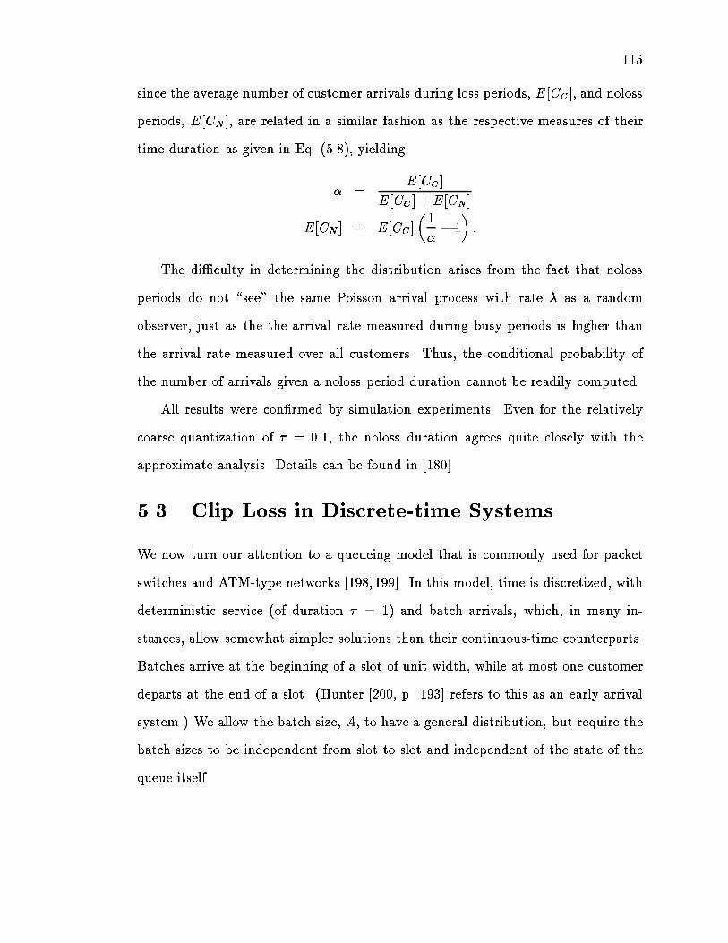
115
since the average number of customer arrivals during loss periods, E[CC], and noloss
periods, E[CN ], are related in a similar fashion as the respective measures of their
time duration as given in Eq. (5.8), yielding
� =E[CC]
E[CC] + E[CN ]
E[CN ] = E[CC]�1
�� 1
�:
The di�culty in determining the distribution arises from the fact that noloss
periods do not \see" the same Poisson arrival process with rate � as a random
observer, just as the the arrival rate measured during busy periods is higher than
the arrival rate measured over all customers. Thus, the conditional probability of
the number of arrivals given a noloss period duration cannot be readily computed.
All results were con�rmed by simulation experiments. Even for the relatively
coarse quantization of � = 0:1, the noloss duration agrees quite closely with the
approximate analysis. Details can be found in [180].
5.3 Clip Loss in Discrete-time Systems
We now turn our attention to a queueing model that is commonly used for packet
switches and ATM-type networks [198,199]. In this model, time is discretized, with
deterministic service (of duration � = 1) and batch arrivals, which, in many in-
stances, allow somewhat simpler solutions than their continuous-time counterparts.
Batches arrive at the beginning of a slot of unit width, while at most one customer
departs at the end of a slot. (Hunter [200, p. 193] refers to this as an early arrival
system.) We allow the batch size, A, to have a general distribution, but require the
batch sizes to be independent from slot to slot and independent of the state of the
queue itself.

116
We will say that batch sizes are geometrically distributed if their probability
mass function (pmf) is an = pqn, with q = 1 � p and an average batch size of
� = q=p. We will also cover the Poisson distribution with mean �,
an =e���n
n!for n 2 [0;1);
and the binomial distribution with mean � = �p,
an =
( ��
n
�pnq��n for n 2 [0; �]
0 otherwise:
While numeric solutions are possible for general batch size distributions, a queue
with geometric batch sizes, i.e., the system D[Geo]=D=1, will be shown to exhibit the
property that busy periods and loss periods are equal in distribution, analogous
to the result described in Section 5.2 for the continuous-time GI=M=1 system.
Also, restricting batch sizes to be geometrically distributed will yield closed-form
expressions for many distributions of interest. Due to the close relationship between
busy and loss periods, we will investigate busy periods in some detail in Section 5.3.1,
followed by derivations of the properties of loss and noloss periods in sections 5.3.2
and 5.3.3, respectively.
5.3.1 The Busy and Idle Period
In discrete-time systems, we de�ne the beginning of a busy period to be the time
that the �rst customer in a batch experiences no waiting, i.e., �nds the server free.
Note that, unlike in a continuous time system, two successive busy periods need not
have an intervening period of time during which the server is idle. This occurs if the
last customer in a busy period, departing in (n�; n), is immediately followed by one
or more new arrivals in (n; n+). Thus, the �rst customer in that batch enters service
immediately, starting a new busy period, while the server experiences no idle slot.
Later, we will discuss the composite busy period which encompasses time intervals
without server idling, consisting of one or more busy periods.

117
Let us return now to the busy period and compute its distribution. Because
each customer occupies the server for one slot, the busy period length is equal to
the number of customers served during the busy period in the discrete-time case.
For geometric batches4, we can compute the number of customers in a busy period
by making use of Tak�acs combinatorial arguments [201, p. 102f], [186, p. 225f]. Let
B be the number served in a busy period and ~An the number of arrivals during the
service times of customers 1 through n, where these customers may belong to one
or more busy periods.
The probability mass function of the number served in a busy period is given
by [186, Eq. (5.166)]
P [B = n] =1
nP [ ~An = n� 1]:
For the case of deterministic service and batch size distribution an, the proba-
bility on the right-hand side can be readily derived:
P [ ~An = n� 1] = P [n� 1 arrivals in n slots] = an�n�1:
Here, an�n denotes the n-fold convolution of an with itself. For the case of geometri-
cally distributed batches, the convolution becomes the negative binomial or Pascal
distribution with probability mass function
ar�n =
r + n � 1
n
!prqn:
Thus, the busy period for geometric batches is distributed according to
P [B = n] =1
qn
2n � 2
n� 1
!(qp)n (5.10)
4The ensuing development requires that the work arriving during the service of each customerbe i.i.d.. For batch arrivals, the arrivals that occur while the �rst customer is being serviced consistof the batch starting the busy period minus one. The distribution of this \shortened" batch hasthe same distribution as a regular batch only if batches are geometrically distributed. For otherbatch distributions, the following calculations can serve as an approximation.

118
=1
n
2n� 2
n� 1
!�n�1(1 + �)1�2n: (5.11)
The last transformation makes use of the fact that the system load � is related to
the batch distribution parameter p through p = 1=(1 + �). We recognize the last
expression as the distribution of the number of customers served in anM=M=1 busy
period [186, p. 218].
The z-transform of the number served in a busy period, B(z), follows from the
M=M=1-derivation [186, p. 218]:
B(z) =1 + �
2�
"1�
s1� 4�z
(1 + �)2
#=
1�p1� 4pqz
2q(5:12)
The expected number served (and arriving) in a busy period can be computed by
evaluating an in�nite series using Eq. (5.12) or directly copying the M=M=1 result:
E[B] =1Xn=1
nP [B = n] =pp
1 � 4pq=
1
1� �:
The idle period I for general batch sizes is geometrically distributed with density
P [I = n] = an0(1 � a0); n � 0. Recall that a0 is the probability of a batch having
zero members. Thus, the average idle period is given by a0=(1� a0). For geometric
batch sizes, a0 = p and thus an idle period last an average of 1=� slots.
In contrast to the continuous-time case, an idle period may have zero duration.
This occurs if a new batch arrives immediately after the last customer of a busy pe-
riod departs. We will call a period of continuous server occupancy spanning several
busy periods a composite busy period and identify random variables associated with
it by a tilde. A composite busy period consists of � busy periods with the geometric
probability P [� = k] = (1 � a0)k�1a0. In the z-transform domain, the number of
customers in the composite busy period, ~B, is determined as ~B(z) = �(B(z)), where
�(z) =pz
1� qz
is the probability generating function of the number of busy periods constituting a
composite busy period.

119
For geometric batches, ~B(z) can be expanded using Eq. (5.12):
~B(z) =p
q
1�p1� 4pqz
1 +p1 � 4pqz
=p
q
1� 2p1� 4pqz + 1� 4pqz
4pqz
=1
zq
"1 �p1� 4pqz
2q
#� p
q
The bracketed fraction is recognized as B(z) and thus ~B(z) can be inverted easily,
yielding
P [ ~B = n] =1
q
1
n+ 1
2n
n
!�n
(1 + �)2n+1
=1
n+ 1
(2n)!
(n!)2�n�1
(1 + �)2n(n � 1):
The expected number of customers in a composite busy period (and its expected
duration in slots) is seen to be
E[ ~B] = E[B] � E[�] = E[B]
a0;
in general or
E[ ~B] =1 + �
1 � �
for geometric batches.
5.3.2 The Loss Period
A loss period begins when one or more customers arriving in a batch see h or
more customers already in the system (in other words, if their wait is equal to or
greater than h.) Thus, a busy period is (again) a special case of a loss period with
h having the value zero. A loss period ends when there are h or fewer customers
left after a departure. Just as discussed above for the case of busy periods, a loss
period may be followed immediately by another loss period. This occurs if the
number of customers reaches h at some point n, i.e., the loss period ends, and a

120
batch arrives in (n; n+), starting a new loss period. An uninterrupted interval where
the number of customers in the system just prior to an arrival never drops below
h (or, equivalently, where the occupancy after the arrival instants remains above
h) will be referred to as a composite loss period. Clearly, it consists of an integral
number of loss periods.5 The random variables L and ~L represent the loss period
and composite loss period, respectively, while the random variable V represents the
occupancy on the slot boundary, equivalent to the work in the queue seen by an
arriving batch (virtual work). Because of the deterministic service time and the
slotted arrivals, duration and customer count properties are the same, i.e., a loss
period of l slots leads to l consecutive losses.
Fig. 5.2 depicts an example of a sample path showing a composite loss period
made up of two loss periods (LPs) for a threshold of h = 3.
h
- ta; b c; d; e; f g arrivals
LPCLP
Figure 5.2. Loss periods in discrete time (h = 3)
Just as in the continuous-time case, we are interested in determining the distri-
bution of the initial jump J , that is, the work load or, equivalently, the number of
5However, unlike in the M=M=1-case, we do not have to factor out the single-customer busyperiods.

121
customers that begins a loss period. Fig. 5.2, for example, shows two initial jumps,
one occurring at the arrival of batch fc : : : fg, with a height of two, and the second
at the arrival of fgg, with a height of one.
Lemma 3 The initial jump J into a loss period has the distribution
P [J = j] =
Pmin(h+j;�)a=j P [Vh = h+ j � a]P [A = a]Pmin(h;�)
a=1 P [Vh > h� a]P [A = a] + P [A > h];
where the distribution of the batch size random variable A is zero outside the range
[0; �]. The random variable Vh represents the occupancy seen by an arriving batch
when the occupancy is less than or equal to h. The conditional occupancy distribution
seen by an arriving batch is de�ned as
P [Vh = v] ,P [V = v]
P [V � h]:
Proof We sum the probabilities of all events leading to a jump of size j (given
that a jump occurred), noting that the random variables A and V are independent.
Thus, we have for jumps into loss periods,
P [J = j]
=X
v+a=h+j
P [Vh = v \A = ajA+ Vh > h]
=
Pv+a=h+w P [Vh = v \A = a \A+ Vh > h]
P [A+ Vh > h]
=
Pv+a=h+w P [Vh = v]P [A = a]Pv+a>h P [Vh = v]P [A = a]
=
Pmin(h+j;�)a=1 P [Vh = h+ j � a]P [A = a]Pmin(h;�)
a=1 P [Vh > h � a]P [A = a] + P [A > h]:
Among loss periods, we have to distinguish those that form the �rst loss period
in a composite loss period. While an arriving batch that starts a loss period may

122
see between 0 and h in the system, a batch that initiates a composite loss period,
i.e., the initial jump conditioned on the fact that the loss period is the �rst in a
composite loss period, can see at most h� 1 customers. Thus, the following lemma
provides a separate expression for the jump into a composite loss period, ~J .
Lemma 4 The initial jump into a composite loss period ~J has the distribution
P [ ~J = j] =
Pmin(h+j;�)a=j+1 P [Vh�1 = h+ j � a]P [A = a]Ph
a=2 P [Vh�1 > h� a]P [A = a] + P [A > h]:
The derivation of P [ ~J] proceeds as in the proof of the previous lemma.
Finally, initial jumps of all but the �rst loss period within a composite loss
period always start at h. Since the queue occupancy seen by an arriving batch and
the batch size itself are independent, the jump into these \interior" loss periods is
distributed like a regular non-zero batch.
In close parallel to the continuous-time case, the memorylessness property of
the geometric distribution makes the distribution of both types of initial jump a
shifted version of the batch distribution, independent of h. We formulate this more
precisely in lemma 5.
Lemma 5 For the D[Geo]=D=1 queue, the initial jump J and the initial jump into
composite loss periods ~J are distributed like non-zero batches, with pmf P [J = j] =
P [ ~J = j] = pqj�1 = �j�1=(� + 1)j .
The proof can be found in [180].
Given the characteristics of the initial jump, the length of a (composite) loss
period is stochastically identical to the length of a (composite) busy period with a
special �rst service given by the initial jump distribution. By the previous lemma,
loss periods in a system with geometric batch arrivals have the same distribution as
regular busy periods of the same system. Since the members of a batch that initiate
a loss period also experience delays of at least h, the number of customers lost in

123
a loss period and the number served in a busy period with the above-mentioned
special �rst service are stochastically identical as well.
For general batch-size distributions, the probabilities for loss periods of length
one can easily be written down exactly:
P [L = 1] = P [J = 1];
P [ ~L = 1] = P [J = 1]a0:
Closed-form expressions for measures of L and ~L for longer durations seem di�cult
to obtain, however. We therefore model the queue state during loss periods as
a discrete-time Markov chain with an absorbing state. Since the composite loss
period is of greater practical signi�cance, indicating the number of consecutively
lost customers, we will focus on this random variable for the remainder of this
section. The states of the chain indicate the amount of un�nished work above h just
after a batch has arrived. For computational reasons, we truncate the transition
matrix to K + 2 states and write
P =
26666666664
0 1 2 : : : K K + 10 1 0 0 : : : 0 01 a0 a1 a2 : : : aK 1 �PK
j=0 P1j
2 0 a0 a1 : : : aK�1 1 �PKj=0 P2j
...K + 1 0 0 0 : : : a0 1 � a0
37777777775:
The choice of K depends on the accuracy requirements and available computational
resources; it can be selected by increasing K by small increments until the solu-
tion does not change appreciably. Note that the zero state is absorbing since the
loss period ends when the amount of un�nished work above h reaches zero. We
therefore obtain the duration of a composite loss period by evaluating the chain's
absorption probabilities over time, given the initial state probabilities determined
by the distribution of the initial jump, also truncated to K + 2 values.6
6For the tail of the loss-period, this random walk with drift and one absorbing barrier may berepresented by the corresponding Brownian motion [202, p. 437].

124
Since the distribution of the composite loss probability typically has a very long
tail, computing its expected value through summation of the weighted probabilities
was found to be numerically inaccurate and computationally expensive. However,
an alternate approach exists [203, p. 425]. Let dj be the expected time to absorption
into state 0, starting at state j. By the law of total probability, we can write a system
of linear equations
dj =K+1Xk=1
Pjkdk + 1:
In matrix from, the linear system consists of the P matrix with its �rst row and
column removed. All results were derived using this approach.
5.3.3 The Noloss Period
The state evolution during a noloss period can also be modeled by a discrete-time
transient Markov chain with initial state h. Unlike the continuous-time case, this
model is exact. Since the number of possible states is limited to h + 1 (including
the absorbing state h + 1 representing a new loss period), no truncation error is
incurred.
We track the number of customers in the system just after arrivals, at n+. Since
we cannot easily accommodate zero �rst-passage times, we compute the conditional
probability mass function of the length of a noloss period given that it lasts at least
one slot. The pmf of the unconditional loss period is then simply the conditional
pmf scaled by a0. We denote the respective random variables by N 0 and N .
The transition probability matrix is similar to the one used to approximate
the noloss period for the continuous-time case, Eq. (5.3), but since there are no
departures when the system is empty, the �rst and second row are identical.

125
P =
2666666666664
0 1 : : : h� 1 h h + 10 a0 a1 ah�1 ah gh+11 a0 a1 ah�1 ah gh+1: : :h� 1 0 0 a1 a2 g3h 0 0 a0 a1 g2
h+ 1 0 0 0 0 1
3777777777775
where
gk =1Xj=k
aj = 1�k�1Xj=0
aj:
The expected length of the noloss period can be obtained as in the continuous-
time case by evaluating the steady-state probabilities of the return process. The
state transition matrix of the return process is derived from the matrix P by
replacing the last row (h+1) with zeros except for a one in column h (see Eq. (5.9)).
The expected number of consecutive successful customers can be computed as
discussed in Section 5.2.5.
5.3.4 Numerical Examples
For a �rst impression of the behavior of the loss period, we plot the mean value
of the composite loss period as a function of the system load � in Fig. 5.3. As
expected, the curves follow the characteristic pattern of loss probability and delay
curves for queueing systems, with a gradual rise up to a \knee" point, followed by
a region of high sensitivity to � for high loads. Exhibiting a pattern that will be
seen in the following curves as well, the geometric case is clearly separated from the
other distributions, which track each other closely in mean composite loss period.
We stated in Lemma 5 that the distribution of the initial jump and (composite)
loss period of the D[Geo]=D=1 queue are independent of the threshold h. It seems
therefore natural to investigate to what extent these quantities depend on h for other
batch distributions commonly used for modeling data communication systems. As
an example, consider the Poisson distribution and binomial distribution7 with an
7The value of � = 2 used here is the smallest non-trivial value. As � increases, the behaviorshould approach that of the Poisson distribution.

126
expe
cted
com
posi
te lo
ss p
erio
d
system load ρ0.1 0.2 0.3 0.4 0.5 0.6 0.7 0.8 0.9 1
0
10
20
30
40
Binomial (N=5)Binomial (N=10)PoissonGeometric
Figure 5.3. Expected composite loss period as a function of system load for h = 5
average batch size of � = 0:8. For values of h ranging from 3 on up (corresponding
to losses of about 30% and less), Table 5.2 shows that h plays no signi�cant role in
E[ ~J] and consequently E[ ~L]. (The same observation also holds for the distribution,
not shown here.) It other words, for loss probabilities of practical interest, the loss
period is basically independent of the threshold.
The distribution of the composite loss period is shown in Fig. 5.4. It is seen
here that the distributions di�er little for small composite loss periods, with most of
the di�erence in expectation caused by the divergence in the tail of the distribution.
The loss period for geometric batches tails o� signi�cantly faster than those for the
either the Poisson or the binomial distribution.

127
Table 5.2. Probability of loss, expected composite loss period and jump for Poissonbatches as a function of h for � = 0:8
Poisson Binomial (� = 2)
h � E[ ~J] E[ ~L] � E[ ~J] E[ ~L]0 1.0000 1.453 7.264 1.0000 1.25 6.251 0.6936 1.304 6.520 0.5556 1.00 5.002 0.4569 1.275 6.376 0.2469 1.00 5.003 0.2974 1.272 6.358 0.1097 1.00 5.004 0.1933 1.272 6.358 0.0488 1.00 5.005 0.1256 1.272 6.358 0.0217 1.00 5.006 0.0816 1.272 6.358 0.0096 1.00 5.007 0.0531 1.272 6.358 0.0043 1.00 5.008 0.0345 1.272 6.358 0.0019 1.00 5.0010 0.0146 1.272 6.358 0.0004 1.00 5.00
prob
abili
ty
slots0 5 10 15 20 25 30 35 40 45 50 55
10−4
10−3
10−2
10−1
100
Binomial (N=5)Binomial (N=10)PoissonGeometric
Figure 5.4. Probability mass function of the composite loss period for � = 0:1 andh = 5

128
5.4 Bu�er Over ow in Single-Stream Discrete-Time Queues
5.4.1 First-Come, First-Served
In this section, we will derive properties of the loss correlation for a class of
discrete-time queues with restricted bu�er size. As our queueing model, we consider
a FIFO single-server discrete-time queue where arrivals occur in i.i.d. batches of
general distribution with mean batch size �. Each arrival requires exactly one unit
of service. For short, we will refer to this system as D[G]=D=1=K [204]. Let K
denote the system size, that is, the bu�er capacity plus one. Arrivals that do not
�nd space are rejected, but once a customer enters the system, it will be served.
This bu�er policy will be referred to as rear dropping in section 5.4.2. Arbitrarily,
arrivals are �xed to occur at the beginning of a time slot and departures at the end,
creating, in Hunter's terminology [200], an early arrival system. This model is used
to represent the output queue of a fast packet switch, for example [205].
The waiting time and loss probability for this model have been analyzed by a
number of authors [30, 198, 204{208]. For Poisson-distributed batches, Birdsall et
al. [206, p. 392] compute the conditional probability of a run of exactly n slots in
which one or more arrivals are rejected given that an arrival was rejected in the
preceding slot. We will call this probability P [CR = n]. The quantity is seen to be
the product of the probability that two or more arrivals occur during the next n� 1
slots and the probability of zero or one arrivals occurs in the terminating interval,
P [CR = n] = e��(1 + �)h1� (1 + �)e��
in�1:
Birdsall et al. [206, Eq. (11)] also compute the probability that exactly d arrivals
are rejected in the next slot, provided that one or more was rejected in the previous
slot. Their result is related to a relation we will derive later (Eq. (5.15)).
We de�ne Qk to be the event that the �rst customer in an arriving batch sees
k customers already in the system and qk to be the probability of that event. For

129
general batch size probability mass function (pmf) ak, the qk's are described by the
following recursive equations [205]:
q1 =q0a0(1� a0 � a1)
qn =1
a0
"qn�1 �
nXk=1
akqn�k
#; 2 � n < K
q0 = 1 �K�1Xn=1
qn =
"1 +
K�1Xn=1
qn=q0
#�1
The probability that a packet joins the queue, P [J ], is given by
P [J ] =1� q0a0
�;
since 1 � q0a0 is the normalized throughput. Note that qn, n = 1; 2; : : :, depends
on the bu�er size only through the factor q0, i.e., qn=q0 is independent of the bu�er
size [200, p. 236].
For later use, let us compute the probability P [S] of the event S that one or
more losses occurs during a randomly selected time slot. By conditioning on the
system state k (which occurs with probability probability qk), we can write
P [S] =K�1Xk=0
qkP [SjQk] =K�1Xk=0
qk1X
j=K�k+1
aj =K�1Xk=0
qk
0@1� K�kX
j=0
aj
1A
Let the random variable CC be the number of consecutively lost customers. The
distribution of loss run lengths follows readily,
P [CC = n] =KXs=1
P [s spaces available j loss occurs in slot] � an+s;
=1
P [S]
KXs=1
qK�san+s (5.13)
as the number of arrivals in a slot is independent of the system state.
The expected number of consecutive losses can be computed from Eq. (5.13)
or directly by observing that loss runs are limited to a single slot since the �rst
customer in a batch will always be admitted. The expected loss run length is simply

130
the expected number of customers lost per slot, given that a loss did occur in that
slot. The expected number of customers lost in a slot is given by �(1 � P [J ]), so
that
E[CC] = E[losses per slot j loss occurs in slot] =�(1 � P [J ])
P [S]=
�� 1 + q0a0P [S]
:
(5:14)
Numerical computations show that in uence of K on the distribution of CC is very
small (see Table 5.3). The table also shows that E[CC] is roughly a linear function
of �.
Losses that occur when a batch arrives to a full system, i.e., a system with only
one available bu�er space, are independent of the system size and can thus be used
to approximate the distribution of CC quite accurately. For K = 1, n consecutive
losses occur if and only if n+1 packets arrive during the slot duration, conditioned
on the fact that two or more packets arrived. Thus,
P [CC = n] � P [CC = njK = 1] =an+1
1� a0 � a1(5.15)
E[CC] � 1
1� a0 � a1
1Xn=1
nan+1
=1
1� a0 � a1
"1Xn=2
nan �1Xn=2
an
#
=1
1� a0 � a1[� � a1 � (1� a0 � a1)]
=1
1� a0 � a1[�� 1 + a0]: (5.16)
As can be seen readily, the above agrees with Eq. (5.13) and Eq. (5.14) for K = 1.
Also, by the memorylessness property of the geometric distribution, Eq. (5.15)
and Eq. (5.16) hold exactly for geometrically distributed batches with parameter p
and evaluates to
P [CC = n] =p(1 � p)n+1
1 � p � p(1 � p)= p(1� p)n�1

131
E[CC] =1
p= 1 + �
(Regardless of what system occupancy an arriving batch sees, the packets left over
after the system is �lled are still geometrically distributed.)
Table 5.3. Expected loss run length (E[CC]) for D[G]=D=1=K system
ak K � = 0:5 � = 0:8 � = 1 � = 1:5Poisson 1 1.18100 1.30397 1.39221 1.63540
2 1.15707 1.27511 1.36201 1.605743 1.15707 1.27158 1.35911 1.604034 1.15226 1.27153 1.35910 1.604035 1.15238 1.27159 1.35914 1.604046 1.15242 1.27160 1.35914 1.604041 1.15242 1.27160 1.35914 1.60404
Geo any 1.5 1.8 2.0 2.5
5.4.2 In uence of Service and Bu�er Policies
It is natural to ask how the burstiness of losses is a�ected by di�erent scheduling
and bu�er management policies. As scheduling policies, FIFO (�rst-in, �rst-out) and
non-preemptive LIFO (last-in, �rst-out) are investigated. For either policy, we can
either discard arriving packets if the bu�er is full (rear discarding) or push out those
packets that have been in the bu�er the longest (front discarding). Note that this
dropping policy is independent of the service policy. From our viewpoint, LIFO
serves the packet at the rear of the queue. Obviously, only systems with K greater
than one show any di�erence in behavior.
The analysis of all but FIFO with rear discarding appears to be di�cult. Let
us brie y discuss the behavior of FIFO and LIFO, each either with front or rear
discarding.

132
FIFO with rear discarding: The �rst customer in an arriving batch always en-
ters the bu�er and will be served eventually. Thus, a loss run never crosses
batch boundaries.
FIFO with front discarding: Here, a batch can be completely lost if it partially
�lls the bu�er and gets pushed out by the next arriving batch. However, if a
batch was completely lost, the succeeding batch will have at least one of its
members transmitted since it must have \pushed through" until the head of
the bu�er.
LIFO with rear discarding: The �rst packet in a batch will always occupy the
one empty bu�er space and be served in the next slot. Again, loss runs are
interrupted by packet boundaries.
LIFO with front discarding: A run of losses can consist of at most than one less
than arrive in a single batch since the last customer in the batch will be served
during the next slot. A loss run never straddles batch boundaries.
For all four systems, indeed over all work-conserving disciplines, the queue length
distribution (and, thus, the loss probability) are the same [209{211]. The mean
waiting time results favoring front dropping agree with those of [211] for general
queueing systems. Clare and Rubin [210] show that the minimum mean waiting
time for non-lost packets is obtained using LCFS with front dropping (referred to
as preemptive bu�ering in [210]).
For all systems, a batch arrival causes the same number of lost packets. If there
are q packets in the bu�er (0 � q < K) and a arrive in a batch, [(q + a)�K]+ will
be lost.
For rear dropping, at least the �rst packet in the batch will always enter the
system, interrupting any loss run in progress. Thus, we have:
Lemma 6 The same packets (as identi�ed by their order of generation) will be
dropped for all work-conserving service policies and rear dropping.
133
Here, we visualize packets within the same batch generated sequentially in the
interval (t; t+ 0).
Lemma 7 The distributions of loss runs for FIFO with rear and front dropping are
the same.
Proof We number packets in the order of generation; packets within an arrival
batch are numbered arbitrarily, but such that packets that are served are served in
increasing sequence number.
We note �rst that the bu�er for front dropping always contains an uninterrupted
sequence of packets: Assume that the bu�er contains an uninterrupted sequence.
A service completion removes the �rst element of the sequence, without creating
an interruption. A batch arrival that is accepted completely will also not create
a sequence number gap within the bu�er. A batch that pushes out some of the
customers likewise will continue the sequence. Finally, a batch that pushes out all
customers certainly does not create a gap within the bu�er. Note that this property
does not hold for rear dropping, as the example of two successive batch arrivals with
over ows demonstrates.
As pointed out before, the loss runs for rear dropping are con�ned to a single
arriving batch and comprise [q+a�K]+ packets. For front dropping, the losses are
made up of packets already in the bu�er and possibly the �rst part of the arriving
batch. By the sequence property shown in the preceding paragraph, all these form
a single loss run (again of length [q + a�K]+), which is terminated by serving the
next customer. Thus, while the identity of packets dropped may di�er, the lengths
of the loss runs are indeed the same for both policies.
The issue is more complicated for front dropping and general service disciplines.
A number of simulation experiments were performed to investigate the behavior
of the four combinations of service and bu�er policies, with results collected in

134
Table 5.4. (The rows labeled \theory" correspond to the values for FIFO and rear
dropping, computed as in discussed in the previous section.) These experiments
suggest the following conjecture:
Conjecture 1 The distribution of loss runs is the same for all combinations of
FIFO, LIFO and rear and front dropping. The sample path of loss run lengths is
the same for all systems except for LIFO with front dropping.
Table 5.4. Performance measures for geometric and Poisson arrivals, � = 1:5,K = 4,90% con�dence intervals
arrivals service dropping E[W ] 1� P [J ] E[CC]geometric theory 1.985 0.3839 2.500
FIFO rear 1.984: : : 1.987 0.3833: : : 0.3840 2.496: : : 2.502front 1.349: : : 1.351 0.3833: : : 0.3840 2.496: : : 2.502
LIFO rear 1.984: : : 1.987 0.3833: : : 0.3840 2.496: : : 2.502front 0.867: : : 0.869 0.3833: : : 0.3840 2.495: : : 2.500
Poisson theory 2.417 0.341 1.604FIFO rear 2.416: : : 2.418 0.340: : : 0.341 1.602: : : 1.604
front 1.582: : : 1.584 0.340: : : 0.341 1.602: : : 1.604LIFO rear 2.416: : : 2.418 0.340: : : 0.341 1.602: : : 1.604
front 0.549: : : 0.553 0.340: : : 0.341 1.603: : : 1.604
Let us brie y outline a possible approach to a more formal analysis. We focus
on one batch and construct a discrete-time chain with the state
(i; j) = (left in bu�er; consecutive losses in batch) i 2 [1;K � 1]; j 2 [0;1)
The initial state, that is, the state immediately after the arrival of the batch
of interest, is determined by the batch size and the system state and should be
computable. The states (0; j) are absorbing.

135
The transition matrix is given by:
(i; j)! (i; j) = a1 8i; j;(i; j)! (i� 1; j) = a0 j > 0;(i; j)! (i� 1; j + 1) = a2 i; j > 0;(i; j)! (i� 2; j + 2) = a3 i > 1; j > 0;: : :(i; j)! (i� k; j + k) = ak+1 i > k; j > 0;(i; j)! (0; i+ j) =
P1k=i+1 ak i; j > 0;
(0; j)! (0; j) = 1
All other entries are zero.
The probability of j losses given initial state (i0; j0) is the probability distribution
of being absorbed in state (0; j).
Intuitively, random dropping, i.e., selecting a random packet from among those
already in the bu�er, should reduce the loss run lengths, particularly for large bu�ers.
However, this policy appears to be di�cult to implement for high-speed networks.
Simulation results for geometric arrivals support this result, as shown in Table 5.5
as a front or rear dropping would result in an average loss run length of 2:5 for
� = 1:5 and 1:8 for � = 0:8.
Table 5.5. E�ect of random discarding for system with geometrically distributedbatch arrivals
� = 1:5 � = 0:8K E[W ] 1� P [J ] E[CC] E[W ] 1� P [J ] E[CC]3 0.913 0.4148 2.304 0.750 0.1731 1.6694 1.509 0.3833 2.175 1.120 0.1213 1.5736 2.842 0.3534 2.008 1.771 0.0659 1.4518 4.304 0.3415 1.915 2.300 0.0386 1.38210 5.851 0.3365 1.849 2.721 0.0234 1.32815 9.884 0.3331 1.755 3.399 0.0071 1.238
It should be noted that average run lengths exceed a value of two only for
extremely heavy load. Thus, on average, reconstruction algorithms that can cope
with two lost packets in a row should be su�cient. Also observe that the loss

136
correlation has a noticeable dependence on the bu�er size K, although the change
in E[CC] is far less dramatic than that in the loss probability, 1 � P [J ].
5.5 Summary and Future Work
In the preceding sections, we have developed probabilistic measures for the behavior
of losses in single-server queues commonly used in analyzing high-speed networks
and fast packet switches. These measures should be useful in the design and test
of packet recovery systems, which face a much harder task than predicted by the
optimistic assumption of independent losses.
We found that for certain important queues, the distribution of the loss period
is independent of the threshold value used, while for all discrete-time batch distribu-
tions investigated the threshold value has very little in uence on the loss period. It
remains to be seen whether there exists a certain value of h above which the initial
jump (and, hence, the loss period) changes no further with increases in h.
For G=M=1 and D[Geo]=D=1 queues, a busy period can be regarded as a special
case of a loss period. Thus, computation of the distribution of busy periods is
of particular interest in studying loss phenomena. Our computation of the busy
period using combinatorial arguments applied strictly only to geometric batches,
but it might provide a readily computable approximation for other distributions.
We also found in section 5.4, somewhat surprisingly, that for a discrete-time
queue with general batch arrivals, LIFO and FIFO combined with di�erent discard-
ing policies exhibit the same loss correlation.
C h a p t e r 6
Loss Correlation for Queues with MultipleArrival Streams
6.1 Introduction
As was emphasized already in the introduction to the previous chapter, loss prob-
ability and loss correlation supersede average waiting time and throughput as the
performance measures determining quality of service for many real-time applica-
tions. Bursty tra�c, as generated for example by multimedia applications, has
made concerns about loss correlation more urgent.
This chapter generalizes the work described in the previous chapter, extending
it to derive the loss correlation seen by packets of a selected stream in queues with
several arrival streams. The goal of this work is to provide insights as to the structure
and magnitude of loss correlation, so that the protocol and system architecture
designer can judge when loss correlation will signi�cantly e�ect system performance.
The designer can judge whether either ameliorating measures are called for (in the
case of real-time sequence reconstruction) or the bene�ts of loss correlation (in the
case of retransmission algorithms) can be reaped.
Throughout this chapter, our interest in broadband ISDN and ATM-like systems
motivates a discrete-time perspective, with packet losses caused by bu�er over ow1
We denote the event that packet n is lost as L(n). Loss correlation is measured here
by the conditional loss probability, the conditional probability that a packet from a
stream is lost given that its immediate predecessor was also lost. The conditional
1It appears to be generally accepted that bu�er over ow will be the dominant loss mode inwide-area high speed networks.

138
loss probability will be denoted as P [L(n)jL(n� 1)]. The expected loss run length
E[CL], that is, the average number of consecutively lost packets from a stream, is
related to the conditional loss probability by
E[CL] =1
1 � P [L(n)jL(n� 1)]:
The chapter is divided into two major sections. First, in section 6.2, we focus
on a system where a foreground stream with random or deterministic interarrival
time competes with a batched background stream for bu�er space. We allow general
batch arrivals for the background stream and general, but i.i.d., interarrival times
for the foreground stream. This model allows us to judge the dependence of the loss
correlation as a function of the contribution of the foreground stream, the burstiness
of the background stream, the bu�er size and the space priority order of the streams.
We �nd �rst that the bu�er size has no appreciable in uence for all but the smallest
bu�ers. Also, it appears that as long as the contribution of the foreground stream
to the total tra�c is su�ciently small, the losses of that stream can be considered
independent.
Then, in section 6.3, we address the issue of the in uence of tra�c correlation or
burstiness on the loss correlation. Here, the input tra�c consists of a superposition
of identical sources, so that the total input tra�c may be correlated. Since they
are commonly used to model voice and video tra�c, we choose the superposition of
interrupted Poisson processes in the N � IPP=D=c=K queue. We �nd that bu�er size
plays almost no role in the value of the loss correlation, while the burstiness a�ects
both loss probability and conditional loss probability in a similar way.
6.2 Superposition of Periodic and Random Traf-�c
Up to this point, we have assumed that the stream analyzed is the only one arriving
at a queue. Clearly, this is not realistic in many network situations. As a simple

139
�rst model closer to actual network tra�c, we again consider a discrete-time system
similar to the one studied in [212]: single, �rst-come, �rst-serve queue with batch
arrivals at every time slot and unit service time. The stream of interest is modeled as
periodic, superimposed on background tra�c with general, but i.i.d., batch arrivals.
The background tra�c is envisioned as the superposition of a large number of
sources. For brevity, the two streams are abbreviated as \foreground tra�c" (FT,
stream 1) and \background tra�c" (BT, stream 0). If the foreground tra�c is
periodic, it is also referred to in the literature as constant bit-rate (CBR) [213]
or continuous bit-stream oriented (CBO) [214, 215] tra�c. This tra�c model is
motivated by voice and video applications, where the source of interests emits
packets periodically during a talk spurt, a video scan line or even a whole image2.
To gain insight into the loss behavior, we require transient rather than steady-state
results.
A number of authors have investigated the issue of superimposing di�erent tra�c
streams. Kaplan [216] develops steady-state waiting time results in the transform
domain for a continuous-time system with a single deterministic server with in�nite
bu�er used by a primary, deterministic (periodic) stream and a secondary or back-
ground stream with Poisson characteristics. A more general continuous-time model
is treated in [217], where the primary stream can have any random interarrival
and service distribution and the secondary stream is a sequence of deterministic
arrivals whose interarrival times are not necessarily identical. The steady-state
distribution of the virtual waiting time for the in�nite-bu�er case is described by
an integral equation. For a secondary stream with random arrivals, consult [218].
A number of authors [219{221] analyze the superposition of independent periodic
arrival streams at a single server with in�nite waiting space. Bhargava et al. analyze
the same system using the ballot theorem [215]. In general, the queue length survivor
2e.g., video sources with compression on whole image and/or smoothing bu�er
140
function for in�nite queues can be used to approximate the cell loss probability for
�nite queues for su�ciently low (order of 10�9) loss probabilities [221].
Closely related to the issue of superimposed heterogeneous tra�c streams is that
of over ow problems, covered extensively in the literature. While many over ow
models, motivated by call set up in the switched telephone network, assume loss
systems, i.e., no bu�er, (among others, [222, 223]), a number of authors consider
delay systems. For example, Matsumoto and Watanabe [224] derive approximations
for the individual and combined mean waiting time and over ow probability in a
�nite system with two over ow streams, modeled as interrupted Poisson processes
(IPPs), and one Poisson stream, which is a special case of the more general model
of a MMPP=M=c=c+ k queue analyzed by Meier-Hellstern [178]. In most cases, the
distribution of the number of busy servers in an in�nite-server system accepting the
over ow input is evaluated. In [225], the Laplace transform of the inter-over ow
time matrix probability density function is provided. In [226], the related model of
alternating voice and data input to a �nite bu�er is treated.
Kuczura [227] treats in�nite queues (in continuous time) with one Poisson and
one renewal input, in particular the GI + M=M=1 and GI + M=M=1 systems.
In the context of discrete-time single-server queues with in�nite bu�er, correlated
inputs and unity service time, Gopinath and Morrison [228] include an example of
a two-class model with di�erent arrival statistics.
Superimposed tra�c streams of the same statistical description are found in the
analysis of packet voice multiplexers [229], usually in the form of approximations
[17,84].
In the following sections, we set out to analyze in some detail three imple-
mentations of the model described at the beginning of this section, increasing in
generality as we progress through the section. The �rst two models assume a
constant, deterministic interarrival time for the foreground tra�c. The �rst model
(Section 6.2.1) assumes that the foreground tra�c arrives at periodic intervals. It

141
always either attempts to enter the queue before all background tra�c arriving dur-
ing the same slot (�rst-admittance system) or attempts to enter after all background
tra�c has competed for bu�er space (last-admittance system). These policies provide
bounds when the system practices source discrimination, i.e., has sources compete
for bu�er space in a speci�c order as is often the case in packet switches. The more
general model of section 6.2.2 allows these two admittance policies, but also the
more interesting case where the foreground packet is positioned randomly among
the cells from the background stream. Finally, the third model in section 6.2.3
straightforwardly extends the analysis to the case where the interarrival time of the
foreground stream is a random variable.
6.2.1 Constant Period, Fixed Position: First and Last Admittance Systems
For simpli�ed analysis and to obtain best or worst-case results, we �rst assume
that the cells that are part of the periodic stream arrive as either the �rst (early
arrival) or last cell (late arrival) during a slot. The case when the FT cell always
arrives �rst is of no particular interest as it will always get admitted. To evaluate
performance for the pessimistic late-arrival assumption, we embed a discrete-time
Markov chain at the (imagined) instant just after the arrival of the background
tra�c and just before the arrival of the cell from the periodic stream.
We �rst consider the simple D[X]=D=1=K system with batch size pmf ak and
transition matrix Q embedded after the arrivals, with states labeled 0 through K.
Q =
2666666666664
a0 a1 a2 : : : aK�1 1�PK�1j=0 q0j
a0 a1 a2 : : : aK�1 1�PK�1j=0 q1j
0 a0 a1 : : : aK�2 1�PK�1j=0 q2j
0 0 a0 : : : aK�3 1�PK�1j=0 q3j
: : :0 0 0 : : : a1 1�PK�1
j=0 qK�1;j0 0 0 a0 1 �PK�1
j=0 qKj
3777777777775
Given this transition matrix for the background tra�c only, the transition matrix
for the combined system, embedded just before arrivals of the periodic tra�c with

142
period � , is computed by taking the � th power of Q and de�ning hi;j as element i; j
of that matrix.
~Q =
26666664
h10 h11 h12 : : : h1;K�1 1 �PK�1j=0 ~q0j
h20 h21 h22 : : : h2;K�1 1 �PK�1j=0 ~q1j
: : :hK;0 hK;1 hK;2 : : : hK;K�1 1�PK�1
j=0 ~qK�1;jhK;0 hK;1 hK;2 : : : hK;K�1 1�PK�1
j=0 ~qK�1;j
37777775:
Note that the last two rows are identical since the customer from the periodic stream
will not be admitted if the system is already in state K prior to its arrival.
After the usual computations, we arrive at the vector of steady-state probabil-
ities as seen by a periodic arrival, = ( 0; : : : K). Then, the loss probability of
periodic arrivals is simply K and the expected waiting time for admitted customers
is
E[W1] =
PK�1k=0 k k1� K
:
Finally, ~qK;K is the conditional loss probability (given that the previous customer
was lost). The expected number of consecutively lost periodic customers is a function
of the conditional loss probability and given by the properties of the geometric
distribution as
E[CC] =1
1� ~qK;K:
As an example, consider a system under overload, with a geometrically dis-
tributed batch size of mean 0.7, a period � of 3 (for a combined average load of
1.033) and a system size of 3. The periodic tra�c experiences a loss of 15.74%
and an average wait of 0.875. The conditional loss probability is 20.03%, with an
average number of 1.25 consecutively lost customers (loss run length). If losses were
independent, the average loss run length would be 1.187. Thus, even under heavy
load and a periodic stream that contributes a signi�cant fraction of the total tra�c,
the loss run lengths in that system are very close to one. The calculations were
con�rmed by simulations.

143
6.2.2 Constant Period, Random Position
In this variation, called the random-arrival system, the periodic cell is randomly
interspersed with the background tra�c. Again, a periodic arrival occurs every �
slots. We will refer to a sequence of � slots commencing with a slot with a periodic
arrival as a cycle. The �rst slot in a cycle bears the index zero.
6.2.2.1 FT Loss Probability and Waiting Time
The probability that k BT cells enter the queue before the FT cell is given by
bk =1Xj=k
ajj + 1
for k = 0; 1; 2; : : : ; (6:1)
since the cell has an equal chance to be at any position of the total batch arriving
to the queue. The expected number of cells entering the queue prior to the FT cell
can be computed by rearranging the order of summation as
E[B] =1Xk=1
kbk =1Xk=1
k1Xj=k
aj+1j
=1Xj=1
ajj + 1
jXk=1
k =1Xj=1
ajj(j + 1)
2(j + 1)
=1
2
1Xj=1
jaj =1
2E[A];
as intuition suggests. Here, E[A] denotes the average batch size. By virtue of its
random position, the FT cell is (in distribution) followed by as many BT cells as
precede it. However, these two quantities are not independent within a single slot.
Through the remainder of this section, we will see that the results for the late-
arrival system follow from those of the random-arrival system by simply replacing
bk by ak.
As a preliminary step in the transient analysis, we write down the Markov chain
for the background tra�c only, embedded just before the �rst arrival in a batch.
Here, the state space encompasses states 0 through K � 1.
P =
26666664
a0 + a1 a2 a3 : : : aK�1 1�PK�2j=0 p0j
a0 a1 a2 : : : aK�2 1�PK�2j=0 p1j
0 a0 a1 : : : aK�3 1�PK�2j=0 p2j
: : :0 0 0 : : : a0 1 �PK�2
j=0 pK�1;j
37777775
(6:2)

144
Similar to the case of �xed position arrivals, we now embed a Markov chain with
state transition probability matrix ~P(j) just prior to the �rst arrival in the jth slot
of a cycle. This �rst arrival could be from either the periodic or the background
stream. Since we embed the chain just after a departure, the state space reaches up
to K � 1, not K. The matrix ~P(j) is given by
~P(j) =
(P��jP0Pj�1 for 0 < j � �P0P(��1) for j = 0:
(6:3)
Here, P0 is the transition matrix computed with the shifted batch size distribution
that takes account of the single foreground arrival: a0, a0j = aj+1; j = 1; : : : ;K,
a00 = 0.
The steady state probabilities seen by the �rst customer in the jth slot of a
cycle are derived from ~P and are denoted by the vector ~�(j) = (~�(j)0 ; : : : ; ~�
(j)K�1).
De�ne the random variable B as the number of customers that arrive before the
selected customer in the batch (i.e., the customer position). The random variable
S describes the state seen by an arrival from the periodic stream, i.e, where j = 0.
The steady-state probability of loss for periodic arrivals is given by the convolution
of position and state distributions,
P [L1] = P [B + S � K] =KXk=1
~�(0)K�kP [B � k] =
KXk=1
~�(0)K�k
0@1� k�1X
j=0
bj
1A
= 1�KXk=1
~�(0)K�k
k�1Xj=0
bj; (6.4)
since position B and state S are independent. Alternatively, given the above
measures, the distribution of the state seen by a periodic arrival is given by
�k =kX
j=0
~�(0)j bk�j:
Then, the loss probability P [L1] for periodic tra�c is seen to be equal to �K. P [L1]
and �k for the last-admittance system can be computed by replacing bk by ak. The
�rst-admittance system has b0 = 1; bk = 0 for k > 0, so that �k = ~�(0)k .

145
An arriving periodic customer has to wait for those already in the queue at
the beginning of the slot and those customers within the same batch that enter the
queue ahead of the periodic customer. Since these two components are independent,
the distribution of the waiting time, P [W = k], for the periodic tra�c is given by
the convolution
P [W = k] =1
1 � P [L1]
kXj=0
~�(0)j bk�j =�k
1� P [L1]for k = 0; : : : ;K � 1:
Again, the last-admittance and �rst-admittance quantities are computed by replac-
ing bk as described above.
6.2.2.2 BT Loss Probability
The loss probability for BT cells, P [L0], is computed indirectly through the channel
utilization. The channel idle probability, without regard to tra�c type, is computed
as
P [idle] =a0�
��1Xj=1
~�(j)0
since the slot steady-state probabilities seen by an arriving batch di�er for each slot
within a cycle of length � . The term for j equal to zero is omitted since the FT
arrival assures that the channel is never idle. From the idle probability, the loss
probability for the combined stream, called P [L], follows from ow-conservation as
P [L] =1 � P [idle]
�0 + 1=�:
Background tra�c constitutes a fraction of
�0�0 + 1=�
=1
1 + 1=(�0� );
while foreground tra�c contributes
1=�
�0 + 1=�=
1
1 + �0�:

146
Given these fractions, the total loss probability can be expressed as the weighted
sum of the stream loss probabilities, P [L0] and P [L1], as
P [L] =P [L0]
1 + 1=(�0� )+
P [L1]
1 + �0�:
Then, the loss probability for the background tra�c can be solved for:
P [L0] = (1 + 1=�� )
"P [L]� P [L1]
1 + ��
#(6:5)
The same results for the BT loss probability P [L0] can also be obtained by
direct methods, similar to those used to compute P [L1]. First, we need to compute
the probability mass function of the number of cells that arrive in the batch prior
to a randomly selected customer. Since arrivals occur in batches, we are dealing
with a random incidence problem. For all but slot zero in a cycle, we have that the
distribution of the batch size that a random customer �nds itself in is given by
~an =nan�0
Thus, the probability that a random customer �nds k other customers ahead of it
in its batch, �k, is found by observing that a random customer is equally likely to
occupy any position within the arriving batch. For all but the �rst slot (index j)
within a cycle, we have
�(j)k =
1Xi=k+1
~aii=
1
�0
1Xi=k+1
ai; 0 < j < � � 1
Similarly, for slot zero in a cycle, the BT cell is equally likely to occupy positions 1
through n+ 1 given that the batch it arrived in had size n. Thus,
�(0)k =
1
�0
1Xj=k
jajj + 1
The loss probability for BT cells, P [L0], is then given by a relation analogous to
Eq. (6.4), except that we average over all � slots in a cycle:
P [L0] =1
�
��1Xj=0
1 �
KXk=1
~�(j)k
k�1Xi=0
�(j)i
!= 1� 1
�
��1Xj=0
(KXk=1
~�(j)k
k�1Xi=0
�(j)i
)(6:6)

147
Both methods of computing the BT loss, Eq. (6.5) and Eq. (6.6) require approxi-
mately the same computational e�ort that increases linearly in � , assuming matrix
powers are computed through eigenvalue methods.
It is tempting to embed a Markov chain just before FT arrivals as it would
yield both the unconditional and conditional loss probability for FT packets. This,
however, is di�cult for random FT arrivals since the number of BT arrivals after the
FT arrival depends on the number that have arrived before (in the same slot). The
system state seen by the FT arrival in turn depends on the number of BT arrivals
that precede the FT arrival.
6.2.2.3 Conditional Loss Probability
In order to compute the conditional loss probability, we note that the state at the
next slot after a FT loss is always K�1. Also, all BT cells arriving within the same
slot and following a FT cell that is lost are also lost and can thus be ignored. Thus,
the dependence of the number of arrivals after the FT cell on the state is no longer
a problem. Then, the conditional loss probability is given by
P [L1(n)jL1(n� 1)] =hP��1B
iK�1;K
;
where L1(n) indicates the event that FT arrival n is lost (n is the packet sequence
number within the FT stream.) P denotes the transition matrix de�ned in Eq. (6.2),
but padded to K rows and columns by zero elements. The K byK transition matrix
B describes the state transition caused by the arrivals preceding the FT cell in the
same slot. For randomly placed FT cells, the elements bk are computed according
to Eq. (6.1).
B =
26666664
b0 b1 b2 : : : 1�PK�1j=0 bj
0 b0 b1 : : : 1�PK�2j=0 bj
0 0 b0 : : : 1�PK�3j=0 bj
: : :0 0 0 : : : 1
37777775

148
For late-arrival FT, the matrix B contains the batch probabilities:
B =
26666664
a0 a1 a2 : : : 1 �PK�1j=0 aj
0 a0 a1 : : : 1 �PK�2j=0 aj
0 0 a0 : : : 1 �PK�3j=0 aj
: : :0 0 0 : : : 1
37777775
After having evaluated the conditional loss probability algebraically, we brie y
highlight two structural properties. For this queue, the independence of loss cor-
relation and bu�er size observed earlier [212] holds exactly for certain (common)
combinations of � and K.
Theorem 6.1 The conditional loss probability for FT packets is independent of K
for values of K � � .
Intuitively, this result holds since for � � K, the bu�er that was full on a FT arrival
will not empty until the next FT arrival slot, if at all. In other words, there will be
a departure at every slot until the next FT arrival after a FT arrival has been lost.
The probability that the next FT arrival again sees K in the system depends only
on the arrival probabilities, not on the system size. We prove the result formally by
sample path arguments.
Proof We track the number of available spaces rather than the system occupancy.
After a FT loss, there will be zero available slots. Thus, the conditional loss
probability can be viewed as the probability of reaching state zero at the next FT
arrival given that the (lost) FT arrival left state zero behind. At the end of each
slot, the number of available spaces increases by one. Here, we make use of the fact
that the condition � � K guarantees a departure. At the beginning of each slot,
it decreases by the number of BT arrivals, but not below zero. This behavior is
completely independent of the system size.
Theorem 6.2 (i) The conditional loss probability is greater than or equal to the
unconditional loss probability. (ii) The conditional loss probability decreases mono-
tonically in K.

149
Proof The following argument shows part (i). For any customer, the probability
that it is lost depends only on the state after the arrivals of the previous slot (\state")
and the number of arrivals that precede the arrival during the same slot (\arrivals").
The latter quantity is by system de�nition independent of the state of the queue.
Clearly, the loss probability for the next customer increases with increasing state3.
For the loss probability, we consider a random customer. The state lies somewhere
between 0 and K. In contrast, for the conditional loss probability, we only consider
those customers that follow a lost customer of the same stream. Their state is known
to be K. Since, in particular, some non-zero number of random customers will see
states of less than K, their loss probability will be lower than those seeing K as
state.
Part (ii) follows from a sample-path argument. Consider two systems that are
distinguished only by their bu�er size: one has a bu�er of K slots, the other K +1.
Since we are interested in the conditional loss probability, we assume that a loss has
occurred in both systems. The arrival process in the following slots is independent
of the loss event. Consider the state just after a batch arrival. As long as the K +1
system occupancy stays above zero, the state of the K + 1 system is simply that
of the K plus one. In that case, the probability that the next FT arrival �nds the
system full is the same for both systems. (This is the argument used in the proof
of theorem 6.1.)
On the other hand, if theK+1 system reaches zero, we know that the K system
will also be at zero since it must have been at zero at the previous slot already. (The
occupancy can only decrease by at most one in this single-server system). Thus,
from that point on the two systems share the same occupancy. The next FT arrival
will only be lost if the occupancy reaches K or K+1, respectively. Since the arrivals
are the same, the probability of that event for the smaller system is larger.
3Formal proof by sample path arguments.

150
6.2.2.4 Numerical Examples
To gain a better understanding of the dependence of conditional and unconditional
loss probabilities on system structure and parameters, we graph and discuss a num-
ber of numerical examples below. All graphs display unconditional and conditional
loss probabilities for FT packets as well as the unconditional loss probability for
the BT stream. (The conditional loss probability for BT is less interesting since we
assumed that the BT stream is the aggregate of several streams.)
In Fig. 6.1, the loss behavior for a BT stream consisting of either geometrically
and Poisson distributed batches (mean batch size of 0:8) is shown as a function of
the system size K. The FT period is held constant at � = 10. We see that the
unconditional loss probabilities for the BT and FT stream di�er, at least for larger
values of K, by a roughly constant factor. That factor is larger for geometric than
for Poisson arrivals, as the burstiness of the latter is smaller (and thus closer to
that of the periodic tra�c). In comparing unconditional loss probabilities across
BT batch distributions, we note that the Poisson arrivals are associated with loss
probabilities that decrease much more rapidly with increasing system size, again
re ecting the lower burstiness. As expected, the conditional loss probability mono-
tonically decreases as K increases, but is independent of K for K � � , as predicted
by Theorem 6.1 and shows very little dependence for values of K � �=2. (This
behavior seems to be valid across the range of K and � , judging from sampling
experiments not shown here.) For interesting loss probabilities, the conditional
loss probability is several orders of magnitude larger than the unconditional loss
probability, but the average number of consecutively lost packets is still very close
to 1 (1.049 for geometric arrivals and the given set of parameters).
Plotting loss against FT period � , as in Fig. 6.2, yields similar conclusions. In
addition, we note that the conditional loss probability approaches the unconditional
loss probability from above as � increases, re ecting the fact that as the FT arrivals

151
are spaced further and further apart, the congestion experienced by one arrival
is dissipated by the time of the next FT arrival. The asymptotic behavior as �
approaches in�nity will be discussed shortly, in Section 6.2.2.5. In the �gure, the
asymptotic loss probability is marked with a dot. It is worth noting that a single
64 KBit/second voice connection on a 150 MBit/second data link corresponds to a
value of � of approximately 2300. At that value, losses are virtually uncorrelated
(according to our de�nition of loss correlation.)
prob
abili
ty
system size K0 5 10 15 20 25 30 35
10−5
10−4
10−3
10−2
10−1
100
FT cond. loss prob.
BT loss prob.
FT loss prob.
Poi Poi
Poi
Geo
Geo
Geo
Figure 6.1. Loss probability and conditional loss probability for Poisson or geomet-rically distributed background tra�c BT with �0 = 0:8 and periodic tra�c FT withperiod � = 10, as a function of system size K
Rather than comparing batch size distributions, Fig. 6.3, Fig. 6.4, and Fig. 6.5
illustrate the connection between loss and the bu�er admission policy for FT cells.
Placing the FT arrivals randomly among the BT arrivals yields a conditional and

152
prob
abili
ty
FT period τ100 101 102 103
0
0.1
0.2
0.3
0.4
0.5
0.6
0.7
FT cond. loss prob.BT loss prob.FT loss prob.
Geo Geo Geo •
Figure 6.2. Loss probability and conditional loss probability for Poisson or geo-metrically distributed background tra�c BT with �0 = 0:8 and periodic tra�c FT(random arrival), as a function of � ; system size K = 10
unconditional probability that is better by factor of about �ve than that for the
late-admittance system. The factor stays rather constant for all but the smallest
values of K. Except for values of � of less than, say, ten, the BT loss probability is
largely una�ected by the treatment of FT arrivals. Beyond a certain value of � , the
overall system load and therefore the FT loss probability change relatively little.
In Fig. 6.6, the FT period � is varied while the overall system load remains
constant at � = 0:8. As the contribution of periodic tra�c diminishes and random
tra�c increases, the increased overall burstiness leads to increased loss probability.
At the same time, the increased spacing of FT arrivals has the conditional loss
probability approach the unconditional one as losses become independent. Again,

153
prob
abili
ty
system size K0 5 10 15 20 25 30 35
10−4
10−3
10−2
10−1
100
FT cond. loss prob.
BT loss prob.
FT loss prob. random
random
random
last last
last
Figure 6.3. Loss probability and conditional loss probability for geometricallydistributed background tra�c BT with �0 = 0:8 and periodic tra�c FT with period� = 10, as a function of system size K
the spacing by a constant factor of roughly �ve in both conditional and unconditional
loss is observed between the two FT arrival patterns.
Almost all queueing systems show a roughly exponential rise in loss probability
as the system load approaches one. This behavior is also found in Fig. 6.7 for
the loss probabilities of both tra�c types as the background tra�c is varied from
� = 0:2 to 0:9. The bu�er size and FT period are held constant at K = 10 and
� = 10, respectively.4 The attening of the loss curve seen here is also common to
all �nite-bu�er systems. The more interesting observation in our context, however,
is that the expected loss run length varies relatively little, staying close to the value
4Thus, the expected run length would remain the same for all values of K greater or equal to10.

154
prob
abili
ty
FT period τ100 101 102 103
10−2
10−1
100
FT cond. loss prob.
BT loss prob.
FT loss prob.
random
random
random
last
first
last
last
Figure 6.4. Loss probability and conditional loss probability for geometricallydistributed background tra�c BT with �0 = 0:8 and periodic tra�c FT, as afunction of � ; system size K = 10
of one associated with random loss. Note the vastly di�erent scales of the left and
right ordinate in Fig. 6.7. While the loss probability ranges over eleven orders of
magnitude, the mean loss run length changes by less than ten percent.
Finally, Fig. 6.8 provides a graphic illustration of the e�ect of the conditional
loss probability r on the distribution of loss run lengths. Since the loss run lengths
are geometrically distributed, the tail of the run length distribution decays rapidly
even for values of r signi�cantly larger than \typical" loss probabilities.
6.2.2.5 Asymptotic Analysis in �
It is instructive to take a closer look at the case when � approaches in�nity. We
will show in this section that all three performance measures (loss of FT and BT,

155
prob
abili
ty
FT period τ100 101 102 103
10−3
10−2
10−1
100
FT cond. loss prob.
BT loss prob.
FT loss prob.
random
random
random
last last
first
last
Figure 6.5. Loss probability and conditional loss probability for Poisson distributedbackground tra�c BT with �0 = 0:8 and periodic tra�c FT, as a function of � ;system size K = 10
conditional loss of FT) converge to the same value for Poisson BT, while FT and BT
loss probabilities for geometric BT converge to di�erent values. The convergence
of the unconditional and conditional loss probability for all batch distributions was
pointed out earlier and is to be expected since the state seen by one FT arrival is
less and less correlated to that seen by the next FT arrival as the spacing between
FT arrivals increases.
The unconditional loss probabilities for both types of tra�c as � approaches
in�nity is computed intuitively by ignoring the FT arrivals. The loss probability
can easily be derived formally. We de�ne
bj =1Xi=j
aii+ 1
;

156
prob
abili
ty
FT period τ0 5 10 15 20 25 30 35
10−4
10−3
10−2
10−1
100
FT cond. loss prob.
BT loss prob.
FT loss prob.
random
random
random last last last
Figure 6.6. Loss probability and conditional loss probability for geometricallydistributed background tra�c BT with total load of � = 0:8 and periodic tra�cFT, as a function of � ; system size K = 10
�j =1X
i=j+1
ai�:
Also, ~�k is de�ned as the steady-state distribution computed from ~P . Using standard
arguments [230, p. 45], we take the limit of Eq. (6.6):
lim�!1
P [L0] = 1�KXk=1
8<: lim�!1
1
�
��1Xj=0
~�(j)k
k�1Xi=0
�(j)i
9=;
= 1�KXk=1
(lim�!1
~�(�)k
k�1Xi=0
�(�)i
)
= 1�KXk=1
(~�k
k�1Xi=0
�i:
)

157
expe
cted
run
leng
th
prob
abili
ty
BT traffic λ0
1
1.02
1.04
1.06
1.08
1.1
10−12
10−11
10−10
10−9
10−8
10−7
10−6
10−5
10−4
10−3
10−2
10−1
0.2 0.4 0.6 0.8 1
FT run length
BT loss prob.
FT loss prob.
Poi Poi
Poi
geo geo
geo
Figure 6.7. Loss probabilities and expected run length for Poisson and geometricallydistributed background tra�c BT and periodic tra�c FT (random arrival), as afunction of BT intensity �0; system size K = 10, period � = 10
Here, ~�(j)k is the steady state distribution for the jth slot, which can be computed as
one row of [P (j)]1. Taking the limit for the state transition matrix used to compute
~�, we obtain, limj!1~P (j) = P 0P 0P1 = P 0P1 = P1. The last step follows since P 0
is stochastic and all rows are equal to the steady-state state distribution in matrix
P1.
Hence, every slot has the same transition matrix and state distribution. The
derivation for the limit of P [L1] proceeds similarly. Therefore, the loss probabilities
for background and foreground tra�c are given by, respectively,
P [L0] = 1 �KXk=1
~�K�kk�1Xi=0
�i; (6.7)
P [L1] = 1 �KXk=1
~�K�kk�1Xi=0
bi: (6.8)

158
x
P[lo
ss r
un >
x]
10−9
10−8
10−7
10−6
10−5
10−4
10−3
10−2
10−1
100
0 5 10 15 20 25 30 35
r=0.7r=0.5r=0.2r=0.1r=0.05r=0.02r=0.01
Figure 6.8. Probability that a loss run exceeds length x for given conditional lossprobability r
(6.9)
The two loss probabilities are equal if and only if bk equals �k. For the geometric
distribution with parameters p and q, due to its memorylessness property, �j equals
aj, so thatk�1Xj=0
�j = qk�1:
No closed-form expression appears to exist for the corresponding sum of bj. Clearly,
�j is not equal to bj for the geometric distribution. For the Poisson distribution,
however, we see that �j and bj, and therefore the loss probabilities, are indeed the
same:
bj =1Xi=j
e���i
(i+ 1)i!= e��
1Xi=j
�i
(i+ 1)!;

159
�j =1
�
1Xi=j+1
e���i
i!= e��
1Xi=j
�i
(i+ 1)!:
6.2.3 Random Period, Random Position
Previously, the foreground source was assumed to transmit at periodic intervals
of constant duration � . We now relax this restriction and allow the interarrival time
of the foreground stream, � , to be a random variable. By simple conditioning, the
results for the conditional loss probability in the previous section can be extended
to cover this case. If � can assume only values strictly greater than zero, that is,
the foreground cells do not arrive in batches, we can write
P [L1(n)jL1(n� 1)] =1Xk=1
P [L1(n)jL1(n� 1); � ]P [� = k]:
The evaluation of this sum is made easier by the fact that the conditional loss
probability approaches the unconditional loss probability as � gets large.
If batch arrivals are permitted for the foreground stream5, renewal-type e�ects
need to be taken into account and the conditional loss probability is written as
P [L1(n)jL1(n � 1)] = P [� � = 0] +1Xk=1
P [L1(n)jL1(n� 1); � ]P [� � = k]: (6:10)
Here, � � denotes the interarrival time random variable as seen by a random fore-
ground arrival, which is related to the interarrival distribution seen by a random
observer by [231]
P [� � = k] =kP [� = k]
E[� ]:
The �rst term in the sum of Eq. (6.10) is due to the fact that once an arrival is lost
within a slot, all subsequent arrivals within the same slot will also be lost.
5In most applications, batch arrivals from the foreground stream seem unlikely unless its peakrate exceeds the channel rate or a fast link feeds a switch with a slow outgoing link. The Knockoutswitch [199], for example, allows at most one packet from each input to reach the concentrator.Depending on the switch hardware to be modeled, the FT cells can either be treated as arrivingconsecutively or randomly distributed within the total arrivals in a slot.

160
Computation of the unconditional loss probability is more di�cult, requiring
a two-dimensional Markov chain, except for the case where the interarrival distri-
bution translates into a distribution of the number of FT packets per slot that
is identical and independent from slot to slot. This is satis�ed for the geometric
interarrival distribution with support [1;1], where each slot sees zero or one FT
arrivals according to a Bernoulli process.
6.2.4 Future work
A number of extensions to the model treated in this section suggest themselves.
First, a stream could receive preferential treatment if it has su�ered a loss at its
last arrival, reducing the average loss run length to very close to one. However,
implementation costs may not make this practical except in the case when the
number of streams is very small (which is where the issue of long loss runs is of
interest in any event).
In the analysis, it was assumed that the foreground stream contributes at most
one packet per slot, which is a reasonable assumption as long as the outgoing link
speed is at least as large as the access link speeds. The e�ect of batch foreground
tra�c on loss correlation could be investigated within the same analytical frame-
work.
6.3 Bursty Tra�c Sources
There appears to be general agreement that traditional, Poissonian tra�c models
do not capture the bursty arrival process that characterizes many proposed sources
of BISDN tra�c, for example packet voice, still and compressed full motion video.
Since the exact behavior of these sources is ill understood and may depend strongly
on the source material, several generic bursty-source models have been proposed
and analyzed. These models di�er not only in their generality, but also seem to
be appropriate for di�erent parts of the network. Note that altogether di�erent

161
tra�c models are appropriate when aggregating sources. (Examples include Markov
modulated Poisson processes or batch-arrival processes.) We will emphasize discrete-
time models for individual sources.
The �rst model, commonly referred to as an on/o� source, features periodic
arrivals during a burst and no arrivals during the silence periods separating bursts.
For analytical tractability, it is often assumed that the burst and silence duration are
exponentially (continuous time) or geometrically (discrete-time) distributed. The
model was probably �rst used for packet voice sources with speech activity detection.
Examples can be found in [17,89,181,232{234]. For packet video, Maglaris et al. [235]
model each source as the superposition of a number of on/o� minisources. For their
picturephone source, about ten identical minisources provided su�cient accuracy.
Li also investigated the loss behavior for a voice source model [181] related to the
N �IPP=D=c=K queue studied here. However, he considered the temporal properties
of the aggregate loss rate for all sources, not the behavior of individual sources. Li
also arrives at the conclusion that the bu�er size does not materially a�ect the loss
behavior once an overload period sets in.
Multiplexers and other packet switch queues introduce delay jitter, thus, packet
arrivals within a burst even of a on/o� source will no longer be strictly periodic
within the network. The interrupted Poisson process (IPP) source model attempts to
capture this. In continuous time [236,237], the on/o� time periods are exponentially
distributed and independent of each other. A �xed-rate Poisson source emits packets
during the on periods. In discrete-time [238,239], the on/o� periods are taken to be
geometrically distributed. A packet arrives at each slot during the on period with
probability �. The designation as a discrete-time IPP appears misleading since the
source does not generate a Poisson-distributed number of cells in a time interval
during on periods. Interrupted Bernoulli process (IBP) seems more descriptive.
When the peak rate of sources or input channels exceeds the output rate, a batch
arrival model is more appropriate. We can generalize the IPP model by allowing

162
batch arrivals at each time slot during the on period. No performance evaluations
using this model are known to the authors.
For the aggregate stream, a number of simplifying models can be used. The
most popular in continuous time is probably the Markov-modulated Poisson process
(MMPP), typically with two states. A simpler model aggregates all arrivals into
batches, where batch arrivals occur as Bernoulli events with a given probability in
a slot [238]. Thus, batches are separated by a geometrically distributed number of
slots.
In this section, we limit our discussion to the IPP model. Possible extensions
are discussed at the end of the section. In the subsequent discussion we will
neglect source discrimination e�ects and assume random admittance, as de�ned
in Section 6.2.
We begin in section 6.3.1 by reviewing some fundamental results for a single
interrupted Poisson process (IPP) and then use these in section 6.3.2 �rst to describe
the queue arrival process as a superposition of IPPs, proceed to �nd the loss
probability and �nally, the conditional loss probability. Numerical examples in
section 6.3.4 illustrate the in uence of bu�er size and burstiness on loss correlation.
6.3.1 The Interarrival Time Distribution in an IPP
An interrupted Poisson process (IPP) is de�ned as follows:
De�nition 1 A discrete-time interrupted Poisson process (IPP) alternates between
active (on) and silence (o�) periods. At each slot, the state moves from active to
silent with probability 1� and from silence to active with probability 1�!. Thus,
silence and activity durations are geometrically distributed. In the active state, a
packet is generated independently from slot to slot with probability �.
We assume that a state transition takes place just prior to the end of a time slot
and that a packet is generated at the beginning of a slot with probability � if the

163
new state is the active state. Below, the silence and active states will be indicated
by subscripts zero and one, where necessary.
For ease of reference, we reproduce the results for the interarrival (distance)
random variable D presented by Murata et al. [238]. The average dwell times, Ti,
for the o� and on state, respectively, are given by T0 = 1=(1�!) and T1 = 1=(1� ),or, conversely, ! = 1� 1=T0 and = 1� 1=T1. We also de�ne the activity factor �,
� =T1
T0 + T1=
1 � !
2� ! � :
The z-transform of the interarrival times is computed [238, Appendix B] by
recursively writing down the probability that no arrival occurred in k slots since the
last arrival, given that the system is in burst or silence state after k steps. These
probabilities are denoted by p1(k) and p0(k), respectively. The recursive equations
are
p1(0) = 1;
p0(1) = (1� )p1(0);
p1(1) = p1(0);
p0(k) = !p0(k � 1) + (1� �)(1 � )p1(k � 1); k = 2; 3; : : : ;
p1(k) = (1� !)p0(k � 1) + (1� �) p1(k � 1); k = 2; 3; : : :
Arrivals occur with probability � if the system is in burst state, so that the z-
transform of D, denoted by �IPP can be derived as
�IPP(z) = E[zD] = �P1(z) =�[(1� � !)z2 + z]
1� ( (1� �) + !)z � (1� �)(1 � � !)z2:
Inversion of AIPP yields the probability density function of the interarrival time,
�IPP(k):
�IPP(k) = d(1 � r1)rk�11 + (1 � d)(1� r2)r
k�12 (6:11)
where
r1;2 =1
2
� (1 � �) + ! �
q( (1 � �) + !)2 + 4(1 � �)(1 � � !)
�

164
d =1 � � � r2r1 � r2
By di�erentiating the z-transform, or by taking the ratio of the burst over the
total cycle time, we obtain the average interarrival time
E[�] =@�IPP(z)
@z
�����z=1
=1=(1 � ) + 1=(1 � !)
�=(1 � )=
1
�+
1�
�(1 � !)
and its inverse, the arrival rate
� =� � 1=(1 � )
1=(1 � ) + 1=(1 � !)= �
1� !
2 � � !:
The �rst moment can also be expressed in the quantities r1;2 and d:
E[�] =d
1 � r1+
1 � d
1 � r2
With the aid of the relation [240, p. 72]
1Xk=1
k2xk�1 =x+ 1
(1 � x)3;
we obtain the second moment from the probability density function,
E[�2] = d1 + r1
(1� r1)2+ (1� d)
1 + r2(1 � r2)2
:
The autocorrelation function of this process was derived by Gihr [241]. Other
metrics, and methods of matching this process to an observed random process,
are provided by Gilbert [160].
6.3.2 The N � IPP=D=c=K queue
We analyze the N �IPP=D=c=K queue operating in discrete time. N IPP sources,
as described above, feed into the queue, which has K bu�er positions, not including
the customer being served. There are c identical servers. Each customer requires
a service time of one time slot. All customers arrive at the beginning of a slot,
while the departure, if any, occurs at the end of the slot (so-called early arrival
system [200]).

165
We work towards the goal of computing the conditional loss probability6 in sev-
eral steps. First, immediately below, we characterize the aggregate arrival process.
Then, we write down the transition matrix, which also yields the (unconditional)
loss probability. Through a number of intermediate quantities, we �nally arrive at
the desired conditional loss probability.
To set the stage, we review the behavior of the aggregate arrival process. The
superposition of N i.i.d. IPPs is described in [239]. The transition probability that
j sources are active in the current slot, given that i were active in the previous slot
can be computed by [239, Eq. (3)]
Si;j =iX
m=0
��im
� m(1� )i�m
� ��N � ij �m
�(1 � !)j�m!N�i�(j�m)
�
for i; j 2 [0; N ]; 0 � j �m � N � i
The �rst bracketed term is the probability that i�m sources go o�, while m sources
stay on; the second bracketed term is the probability of j�m sources turning on and
N � i� (j�m) staying o�. The steady-state distribution vector s of the number of
active sources is, as usual, computed as s = sS, where S is the transition probability
matrix with elements Si;j. We can, however, write it down immediately:
si =�Ni
��i(1 � �)N�i:
The mean and variance of the number of active sources are N� and N�(1��). The
correlation coe�cient r is given by [233] r = ! + � 1.
Because of batch-e�ects, the activity distribution vector seen by a random
arrival, s0, is a scaled version of the vector s [185, p. 69]:
s0i =isiE[i]
6As usual, we mean the conditional probability that customer n is lost given that customern� 1 from the same source was also lost.

166
Given that i sources are active, the number of packets generated during a slot
is binomially distributed with pmf
ai;k =�ik
��k(1� �)i�k for k = 0; 1; : : : ; i
and zero otherwise. The distribution of batch sizes seen by a random observer is
given by
ak =NXi=1
ak;isi;
while the distribution of batch sizes seen by a random arrival is given by a0k =
kak=E[A], where E[A] is the expected batch size as seen by a random observer.
Naturally, it equals �.
6.3.2.1 The Loss Probability
As a �rst performance metric, we derive the customer loss probability of this queue-
ing system through the state transition matrix. The state of the system is described
by the tuple (k; i), i.e., k cells in the system (waiting and in service), with i sources
active and N � i silent. For brevity, k and i will be referred to as the occupancy
and activity, respectively. The state is tracked on slot boundaries, with state
transitions occurring on the boundary and batch arrivals immediately afterwards.
As in all �nite-capacity, early-arrival systems with deterministic service time and
batch arrivals, the �rst cell in a batch always enters the system. At most a single
cell departs immediately prior to the slot boundary.
The (N;K) � (N;K) transition matrix is given by
P(i;q);(j;r) = Si;jai;r�q+1 for 0 � q � K; 0 < r < KP(i;q);(j;K) = Si;j
P1m=K�q+c ai;m for 0 < q � K
P(i;q);(j;0) = Si;jPc�q
m=0 ai;mP(i;q);(j;r) = 0 otherwise
where we de�ne ai;k = 0 for k < 0 and k > i. We denote the corresponding
steady-state distribution as p with elements pi;k.

167
The probability that a customer is lost, P [L], is most readily computed by
conservation-of- ow arguments as the ratio of channel occupancy, called � here, to
arrival rate:
1 � P [L] =�
�=
1�PNi=0 pi;0ai;0�
for c = 1:
For general values of c, the mean channel occupancy is given by
� =NXi=1
24c�1Xk=1
iXj=0
pi;k�jai;j + ciX
j=0
pi;k�jiX
m=j
ai;m
35
6.3.3 The Conditional Loss Probability
The conditional loss probability is computed by tracing the state of the system
from the time some random customer, called the test customer, is lost to the time
when the next customer from that same source, the so-called test source, arrives.
The computation is only possible because arrivals from a single source are i.i.d.,
even though the aggregate arrival process is correlated.
The computation proceeds in four major steps. First, we compute the activity
seen by the test customer. Then, we compute the activity without the test source
at the next slot boundary immediately following the loss. At both instants, the
occupancy is known to be K +1 or K, respectively, since at least one loss occurred.
Then, we condition on the interarrival time A of the test source. For each value of
the interarrival time, we compute the state, i.e., occupancy and activity, at the slot
beginning of the slot containing the next arrival from the test source. Finally, we
arrive at the loss probability of the next arrival from the test source by computing
the number of customers from other sources that arrive in that slot.
Even though not directly needed for the �nal result, the conditional probability
that one or more customers are lost during a slot given that M = i sources are
active is given by
P [jM = i] ==KXk=0
pi;ksi
iXj=K�k+2
ai;j:
Here, we designate the over ow event, i.e., one or more customers are lost, by .

168
Through Bayes' rule, the conditional probability that i sources are active given
that one or more losses occurred during a slot can be computed given that the
converse probability is available:
P [M = ij] = siP [jM = i]PNi=1 P [jM = i]si
:
Recall that L de�nes the loss event for a customer. For the �rst step, we need
the probability P [M = ijL] that a lost customer sees i active sources (including
itself), which is most readily derived by Bayes' rule,
P [M = i� 1jL] = s0iP [LjM = i]PNi=1 P [LjM = i]s0i
;
where
P [LjM = i] =KXk=0
pi;ksi
i�1Xj=K�k+1
bi;j;
and s0i is the activity seen by a random arrival, with s0i = isi=E[s].
P [LjM = i] depends in turn on the number of arrivals that precede a randomly
chosen customer in the same slot, conditioned on the number of active sources i in
a slot. Since a customer is equally likely to occupy every position within the batch,
we have that
bi;k =
( Pij=k
ai�1;j
j+1 ; for k < i;
0; otherwise:
For convenience, we de�ne b0;0 = b1;0 = 1.
Naturally, P [LjM = i] is related to the loss probability:
P [L] =NXi=1
P [LjM = i]s0i;
The initial state vector q0 seen by the test customer is written as
q0(i; k) =
(P [M = i� 1jL]; for k = K0; otherwise.
Note that here and in the following steps, we condition on the interarrival time so
that the test source is known to be inactive up to the last slot of that interarrival
time.

169
The transition matrix ~P0 from the loss of the test customer to the next slot has
to re ect the fact that the test source is inactive. Any arrivals that occur after the
test customer are lost and do not a�ect the system state. Thus,
~P0(i;k);(j;l) =
(~Si;j; for k = l0; otherwise.
Here, ~S and ~P are the source activity and queue state transition matrices for N � 1
sources, respectively.
In the slot where the test source emits the next customer, the activity increases
deterministically by one. Also, the arrivals before the customer from the test source
increase the queue occupancy. Note that the occupancy ranges now from 0 to K+1.
This (N;K + 1)� (N;K + 1) transition matrix is therefore written down as
~P1(i; k); (j; l) =
8>>><>>>:
PNj=l�k bi+1;j for k � l � K + 1; 0 � i < N; j = i+ 1
1 for 0 � k � K; i = j = N1 for 0 � i < N; j = i+ 1; k = l = K + 10 otherwise.
Given all these intermediate quantities, we then uncondition on the interarrival
distribution P [D = n] and obtain the state distribution vector seen by the next
arrival from the test source as
q =1Xn=1
q0 ~P0~P n�1 ~P1P [A = n]: (6:12)
The conditional loss probability is thenPN
i=0 qi;k. Note that the interarrival time
distribution, Eq. (6.11), is monotonically decreasing in k, simplifying the truncation
of the sum when numerically evaluating Eq. (6.12).
The computation cost is dominated by the matrix multiplication to compute ~P n
and the matrix product. Since the computation time is proportional to (N � K)3,
and, to make matters worse, larger N tend to increase the number of terms that
need to be evaluated in Eq. (6.12), a direct computation is only feasible for relatively
small systems. On the other hand, as pointed out in more detail below, the loss
correlation depends very little on K, so that K = 1 or even K = 0 can be used.

170
Also, non-random behavior is most pronounced when a small number of sources is
superimposed. It remains to be determined whether bounding the conditional loss
probability is possible, for example by assuming that the number of active sources
remains constant in the interarrival interval. Choosing the distribution as seen by a
lost customer should provide an upper bound, while choosing the distribution seen
by an average arrival should bound the conditional loss probability from below. As
a closer approximation, we could treat the number of active sources as a birth-death
process, as is commonly done for voice multiplexers [232,233], and then use numerical
methods for sparse and block matrices. This approximation would probably improve
in accuracy with larger N and longer state holding times.
While the discussion has focused on the N � IPP=D=c=K system, a number of
extensions are immediately apparent. We discuss them brie y in their rough order
of complexity. As for the example in Section 6.2, di�erent ordering of sources in
competing for bu�er space (priority discarding) can be modeled by appropriately
modifying bi;j. Sources with more than two states are also readily handled at the
expense of a larger state space. Note that as long as the loss probability for the
individual source can be determined, only the aggregate batch arrival process of the
remaining background sources enters into the calculation.
The case of an on/o� source with periodic arrivals during the active periods can
be approximately treated within this framework as well by making some simplifying
assumptions. First, the interarrival time of the test source can be modeled as
a constant since most of the consecutive losses will take place within the active
period of the source. Then, the superposition of the remaining sources should have
roughly the same impact on the test source as the superposition of the sources with
Bernoulli arrivals, at least for large N . These assumptions remain to be validated
by analysis. Also, the case of several heterogeneous sources and of sources with two
di�erent Bernoulli arrival processes (MMBP) rather than on/o� sources deserve
closer scrutiny (see [242,243] for a loss probability analysis).

171
In the Gilbert channel model [160], the system alternates between two states
in a manner identical to the IPP source. In one state, every packet is lost, in the
other, no losses occur. While the loss runs are indeed geometrically distributed,
simulations indicate that the success runs (the sequences of customers from a single
source without loss) are not. It remains to be investigated whether the model can
be applied nevertheless. Naturally, the mean of the success runs can be computed
from the loss probability and the loss run length (see [212]).
6.3.4 Numerical Examples
Compared to earlier systems, the large number of queueing system parameters
(�, , !, N , K, c) covers a wide range of systems, but also makes it di�cult to
generalize from numerical examples.
The systems studied earlier had the property that the conditional loss probabil-
ity depended only weakly, if at all, on the system size K. This property carries over
into this queueing system, as indicated by Fig. 6.9, and other examples not shown
here. The e�ect of K will be small, by the argument of Theorem 6.1, as long as
most of the probability mass of the interarrival time is concentrated in the �rst K
slots.
The in uence of the channel bandwidth is indicated by Fig. 6.10, where the ratio
of the source on/o� durations and the system load are kept constant, but the number
of sources, N , is raised, with �, and ! scaled correspondingly. Thus, the source
correlation coe�cient r increases with N . This leads to a somewhat unexpected
result: The conditional loss probability decreases with increasing N , indicating that
the e�ect of burstiness is more than compensated for by the \thinning" during active
periods.
As a �nal parameter study, we investigate the e�ect of di�erent source behavior,
again maintaining the same average load by adjusting � and �. We also keep
the sum of active and silent time constant. Thus, for high values of �, a source

172
cond
ition
al lo
ss p
roba
bilit
y
loss
pro
babi
lity
buffer size K0 1 2 3 4 5 6 7 8 9 10 11
0
0.05
0.1
0.15
0.2
0.25
0.3
0.28
0.29
0.3
0.31
0.32
0.33
0.34
0.35
cond. loss prob.
loss prob.
Figure 6.9. Conditional and unconditional loss probability for N � IPP=D=c=Ksystem, as a function of the bu�er size, K; N = 4, � = 0:8, = 0:7, ! = 0:9
emits a short burst of densely packed packets, followed by a long silence. A lower
value of �, conversely leads to a smoother tra�c process. Fig. 6.11 shows that the
loss probability is far more a�ected by the change in tra�c burstiness than is the
conditional loss probability.
To provide a real-life example, the loss correlation in a DS1 voice multiplexer was
determined. The DS-1/T1 channel o�ers a user capacity of 1.536 Mb/s. Following
He�es and Lucantoni [17], each source encodes speech in 64 kb/s and generates
a 128-byte packet every 16 ms. Talk spurts and silence periods are geometrically
distributed with means 352 ms and 650 ms, respectively, for an activity factor of 35%.
When active, this source produces a packet every 24 slots. The channel processes
1324.2 packets per second. These system characteristics translate, at a load of 0.8,
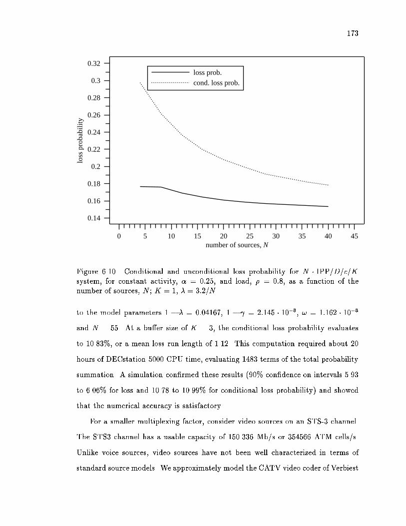
173
loss
pro
babi
lity
number of sources, N0 5 10 15 20 25 30 35 40 45
0.14
0.16
0.18
0.2
0.22
0.24
0.26
0.28
0.3
0.32
cond. loss prob.
loss prob.
Figure 6.10. Conditional and unconditional loss probability for N � IPP=D=c=Ksystem, for constant activity, � = 0:25, and load, � = 0:8, as a function of thenumber of sources, N ; K = 1, � = 3:2=N
to the model parameters 1 � � = 0:04167, 1 � = 2:145 � 10�3, ! = 1:162 � 10�3
and N = 55. At a bu�er size of K = 3, the conditional loss probability evaluates
to 10.83%, or a mean loss run length of 1.12. This computation required about 20
hours of DECstation 5000 CPU time, evaluating 1483 terms of the total probability
summation. A simulation con�rmed these results (90% con�dence on intervals 5.93
to 6.06% for loss and 10.78 to 10.99% for conditional loss probability) and showed
that the numerical accuracy is satisfactory.
For a smaller multiplexing factor, consider video sources on an STS-3 channel.
The STS3 channel has a usable capacity of 150.336 Mb/s or 354566 ATM cells/s.
Unlike voice sources, video sources have not been well characterized in terms of
standard source models. We approximately model the CATV video coder of Verbiest
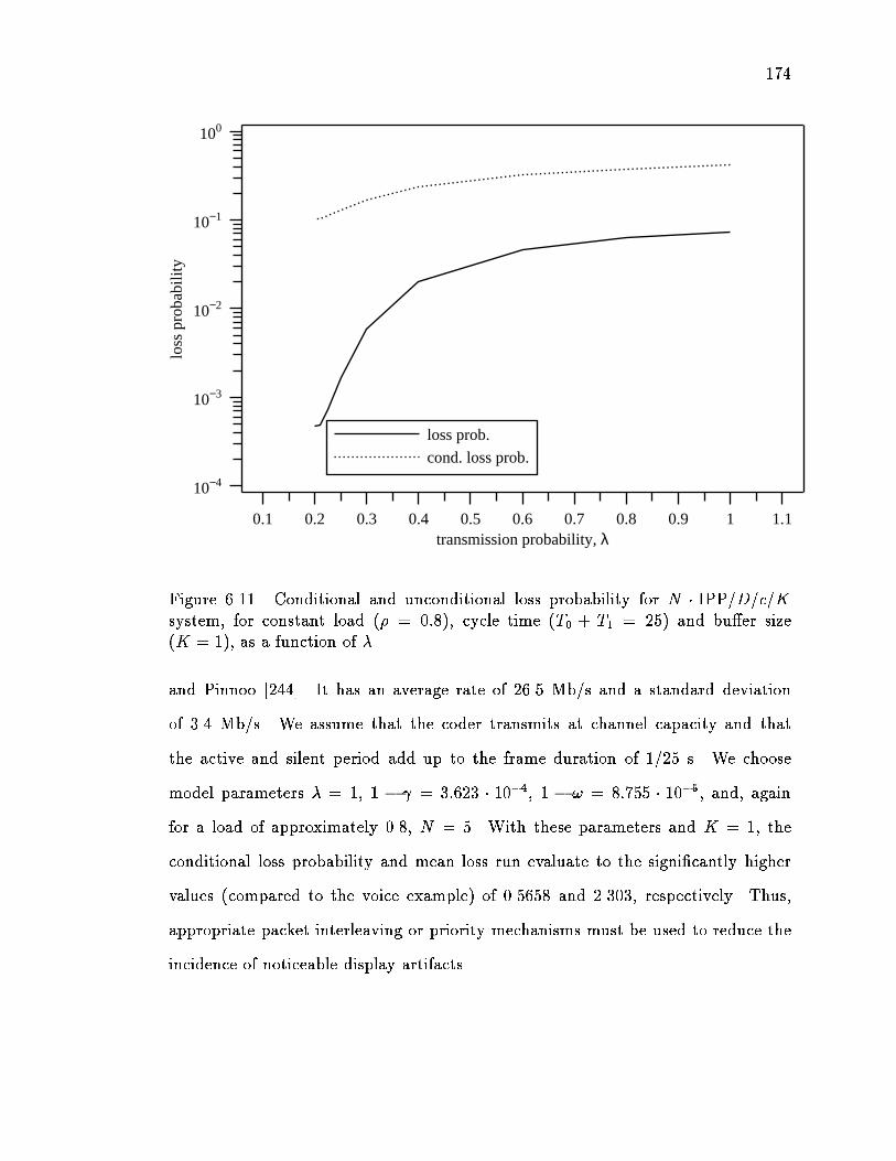
174
loss
pro
babi
lity
transmission probability, λ0.1 0.2 0.3 0.4 0.5 0.6 0.7 0.8 0.9 1 1.1
10−4
10−3
10−2
10−1
100
cond. loss prob.
loss prob.
Figure 6.11. Conditional and unconditional loss probability for N � IPP=D=c=Ksystem, for constant load (� = 0:8), cycle time (T0 + T1 = 25) and bu�er size(K = 1), as a function of �
and Pinnoo [244]. It has an average rate of 26.5 Mb/s and a standard deviation
of 3.4 Mb/s. We assume that the coder transmits at channel capacity and that
the active and silent period add up to the frame duration of 1/25 s. We choose
model parameters � = 1, 1 � = 3:623 � 10�4, 1 � ! = 8:755 � 10�5, and, againfor a load of approximately 0.8, N = 5. With these parameters and K = 1, the
conditional loss probability and mean loss run evaluate to the signi�cantly higher
values (compared to the voice example) of 0.5658 and 2.303, respectively. Thus,
appropriate packet interleaving or priority mechanisms must be used to reduce the
incidence of noticeable display artifacts.

175
6.4 Summary and Conclusions
In this chapter, we have attempted to provide both methodologies and tra�c en-
gineering insight. The tools provided should allow the computation of the loss
correlation for a wide variety of sources of practical interest in high-speed network-
ing. Also, for a range of systems, it was shown qualitatively that the bu�er size
or waiting time limit has virtually no in uence on the loss correlation. For the
periodic arrival case, we saw that as long as individual sources do not contribute
more than, say, 10% of the total bandwidth, the average loss run lengths are not
signi�cantly larger than one, even though the conditional loss probability can be
orders of magnitude higher than the time-averaged loss probability. As expected,
the tra�c burstiness and the number of multiplexed sources play signi�cant roles in
the loss correlation for the IPP system.
Throughout this chapter, we have used the conditional loss probability, or,
equivalently, the average loss run length as an indicator of loss correlation. Another
useful indicator could be the number of lost packets among a random sequence
of packets with a given length. Also, the distribution of success runs deserves
closer investigation. Particularly for queues with correlated inputs, Approximation
methods need to be investigated that allow systems with large state spaces to be
treated.

C h a p t e r 7
Conclusion
We conclude this dissertation by summarizing the main points again, while
outlining areas for future research. We highlight some of the dualities of real-time
and data tra�c, re ect on the methods of research used and stress the need to do
end-to-end analysis.
High-bandwidth wide area network provide the foundation for a range of new
services, many of which are characterized by end-to-end real-time constraints. Mul-
timedia conferencing, for example, o�ers the promise of collaboration and social
interaction unhindered by physical distance. Current packet networks, even if
they have su�cient physical-layer capacity to carry these services, lack the control
mechanisms to provide adequate quality of service to make them truly feasible.
Through a combination of queueing theoretical analysis, simulations and actual
implementations, this dissertation has endeavored to �ll in some of the missing pieces
in an architecture for networks integrating real-time and non-real-time services. Our
guiding concern was to provide end-to-end results rather than results characterizing
individual system components.
Our research was motivated by the observation that many interesting applica-
tions envisioned for future high-speed integrated services networks would be charac-
terized by rather di�erent properties than the data transfer applications in common
use today, namely loss tolerance and delay sensitivity. Our selective discarding
algorithm makes use of that property by trading direct packet loss for reduced delay
distribution tails.
Despite their di�erences, it has been realized in recent years that there exist
interesting dualisms between real-time services and bulk data services. For example,

177
it could be argued that window-based ow control for data transfer applications
makes a similar tradeo� as our controlled-loss algorithm, but in terms of throughput.
By limiting throughput voluntarily and in a controlled manner, they prevent the
uncontrolled and presumably larger loss of throughput caused by queue over ows
at intermediate and end systems.
Another dual between real-time and data applications can be noted in relation
to propagation delays. For data transfer applications, window-based ow control
and appropriate selective retransmission mechanisms aim to make the throughput
largely independent of the propagation delay within the network. Similarly, the
proposed hop-laxity scheduling algorithm can help to compensate to some extent
for longer propagation delays and larger hop counts in a real-time connection.
More recently, the dichotomy of tra�c characteristics between controllable data
tra�c and basically unchangeable real-time sources has been reexamined. Originally,
the perception was that, for example, audio and video tra�c characteristic are
determined by the content, with few possibilities for controlling its tra�c charac-
teristics. On the other hand, data tra�c could be slowed down as necessary to
relieve network congestion. Rate control appears to be a promising approach for
data and real-time sources, in particular video [51]. Rate control for multimedia,
however, takes the form of actually in uencing the data that is carried in the
network, rather than just pacing its entry into the network. The interest in rate
control is an example of increased interaction between the network and the data
source. Adaptive applications, made possible by sophisticated end systems such as
workstations replacing \dumb" terminals and telephones, that adjust to the current
network congestion are an example of fruitful interaction between the network and
the receiver. This approach contrasts somewhat with the more adversarial approach
implied by such terms as tra�c contracts and policing1. These interactions between
1This does not imply that either are unnecessary.

178
the end systems and the network provide a new facet of meaning to the term
\intelligent network" and appear to be a promising area of further research.
Data applications and real-time applications such as audio and video also share
the property that packet losses can severely impact their performance. For real-
time applications, propagation delays make retransmission often infeasible so that
lost packets can translate directly into audible and visible impairments. For that
reasons, many of these applications can recover from isolated packet losses, using
forward error correction or data interpolation. However, the performance of these
concealment techniques depend to a large measure on the temporal structure of
packet loss, not just its rate. This dissertation has made contributions to more
accurately predict the performance as seen by an application by allowing a detailed
description of the packet loss behavior in time. The evaluation of scheduling policies
should be extended to provide performance results after delay adaptation has taken
place. Unfortunately, these results will likely involve a complex tradeo� between
average delay seen by the application and loss due to deadline misses. Developing
simple models that accurately predict end-to-end performance promises to be chal-
lenging. The large number of states needed to describe realistic tra�c models for a
single queue implies that more qualitative or approximate analyses are called for to
understand loss correlation in multi-queue systems.
The use of multi-process workstations also challenges the assumptions underly-
ing many tra�c models for voice and video, as evidenced by the tra�c data gathered
in the course of experiments. Clearly, additional e�orts must be made in modeling
even supposedly well-understood tra�c classes such as packet voice, in particular
when source and network interact.
As our understanding of networks grow, we have learned that looking at single
nodes in isolation provides at best an incomplete picture of network performance.
In recent years, characterizing end-to-end network behavior has begun to attract
179
research interest, but much remains unknown particularly when sources, network
nodes and receivers interact as described above.
A more complete understanding of emerging packet networks requires a range
of approaches. Through the use of analysis, simulation and actual network imple-
mentation and measurements, the relative bene�ts and predictive power of all three
methods and their combinations (such as trace driven simulation and statistical
packet generation in real networks) could be evaluated in this dissertation. The
high cost of running controlled experiments on real networks, both in terms of pro-
viding physical lines spanning a continent as well as the di�culty debugging \live"
operating systems and of observing performance without changing the measurement
results, suggests that guidelines that allow to relate simulation experiments to actual
network performance are urgently needed. Also, con�gurable network emulators
might provide a way station between simulation and integration into testbeds and
operational networks.

Bibliography
[1] Jayant, Nuggehally S., \E�ects of packet losses on waveform-coded speech,"in Proceedings of the Fifth International Conference on Computer Communi-cations, (Atlanta, Georgia), pp. 275{280, IEEE, Oct. 1980.
[2] Verbiest, Willem, Pinnoo, Luc, and Voeten, Bart, \The impact of the ATMconcept on video coding," IEEE Journal on Selected Areas in Communica-tions, vol. JSAC-6, pp. 1623{1632, Dec. 1988.
[3] Williamson, Carey L. and Cheriton, David R., \Loss-load curves: supportfor rate-based congestion control in high-speed datagram networks," in Sig-comm '91 Conference: Communications Architectures and Protocols, (Z�urich,Switzerland), pp. 17{28, ACM, Sept. 1991.
[4] Mankin, Allison, \Random drop congestion control," in SIGCOMM Sympo-sium on Communications Architectures and Protocols, (Philadelphia, Pennsyl-vania), pp. 1{7, ACM, Sept. 1990. in Computer Communication Review, Vol.20, No. 4.
[5] Cassandras, Christos G., Kallmes, Michelle Hruby, and Towsley, Don, \Opti-mal routing and ow control in networks with real-time tra�c," in Proceedingsof the Conference on Computer Communications (IEEE Infocom), (Ottawa,Canada), pp. 784{791, IEEE, Apr. 1989.
[6] Hashem, Eman Salaheddin, \Analysis of random drop for gateway congestioncontrol," Technical report MIT/LCS/TR-465, MIT Laboratory for ComputerScience, Cambridge, Massachusetts, Nov. 1989.
[7] Ramakrishnan, K. K. and Jain, Raj, \A binary feedback scheme for congestionavoidance in computer networks with a connectionless network layer," in Pro-ceedings of the 1988 SIGCOMM Symposium on Communications Architecturesand Protocols, (Stanford, California), pp. 303{313, ACM, Aug. 1988.
[8] Mitra, Debasis and Mitrani, Isi, \Asymptotic optimality of the go-back-nprotocol in high speed data networks with small bu�ers," in Proceedings ofthe Fourth International Conference on Data Communication Systems andTheir Performance, (Barcelona), June 1990.
[9] Mitra, Debasis, \Optimal design of windows for high speed data networks," inProceedings of the Conference on Computer Communications (IEEE Infocom),(San Francisco, California), pp. 1156{1163, IEEE, June 1990.
[10] Mitra, Debasis, Mitrani, Isi, Ramakrishnan, K. G., Seery, J. B., and Weiss,Alan, \A uni�ed set of proposals for control and design of high speed datanetworks," in International Teletra�c Congress, Seventh Specialist Seminar,(Morristown, New Jersey), pp. 12.4.1{12.4.8, ITC, Oct. 1990.
181
[11] Mitra, Debasis and Seery, Judith B., \Dynamic adaptive windows for highspeed data networks with multiple paths and propagation delays," in Proceed-ings of the Conference on Computer Communications (IEEE Infocom), (BalHarbour, Florida), pp. 39{48 (2B.1), IEEE, Apr. 1991.
[12] Fendick, Kerry W., Mitra, Debasis, Mitrani, Isi, Rodrigues, Manoel A., Seery,Judith B., and Weiss, Alan, \An approach to high-performance, high-speeddata networks," IEEE Communications Magazine, vol. 29, pp. 74{82, Oct.1991.
[13] Elwalid, Anwar I. and Mitra, Debasis, \Analysis and design of rate-basedcongestion control of high speed networks, I: stochastic uid models, accessregulation," Queueing Systems, vol. 9, pp. 29{64, Oct. 1991.
[14] Mitra, Debasis, Mitrani, I., Ramakrishnan, K. G., Seery, J. B., and Weiss,Alan, \A uni�ed set of proposals for control and design of high-speed datanetworks," Queueing Systems, vol. 9, pp. 215{234, Oct. 1991.
[15] Zhang, Hui and Keshav, Srinivasan, \Comparison of rate-based service dis-ciplines," in Sigcomm '91 Symposium { Communications Architectures andProtocols, (Z�urich, Switzerland), pp. 113{121, ACM, Sept. 1991.
[16] Sriram, Kotikalapudi and Whitt, Ward, \Characterizing superposition arrivalprocesses in packet multiplexers for voice and data," in Proceedings of the Con-ference on Global Communications (GLOBECOM), (New Orleans, Louisiana),pp. 778{784 (25.4), IEEE, Dec. 1985.
[17] He�es, Harry and Lucantoni, David M., \A Markov modulated characteri-zation of packetized voice and data tra�c and related statistical multiplexerperformance," IEEE Journal on Selected Areas in Communications, vol. SAC-4, pp. 856{867, Sept. 1986.
[18] Sriram, K. and Lucantoni, David M., \Tra�c smoothing e�ects of bit droppingin a packet voice multiplexer," in Proceedings of the Conference on ComputerCommunications (IEEE Infocom), (New Orleans), pp. 759{769, IEEE, Mar.1988.
[19] Dravida, S. and Sriram, K., \End-to-end performance models for variable bitrate voice over tandem links in packet networks," in Proceedings of the Con-ference on Computer Communications (IEEE Infocom), (Ottawa, Canada),pp. 1089{1097, IEEE, Apr. 1989.
[20] Li, San-qi and Mark, Jon W., \Simulation study of a network of voice/dataintegrated TDMs," IEEE Transactions on Communications, vol. COM-36,pp. 126{132, Jan. 1988.
[21] Bhargava, Amit, Kurose, James F., Towsley, Don, and van Lamport, Guy,\Performance comparison of error control schemes in high speed computer

182
communication networks," in Proceedings of the Conference on ComputerCommunications (IEEE Infocom), (New Orleans), IEEE, Apr. 1988.
[22] Takahashi, Kenzo, Yokoi, Tadahiro, and Yamamoto, Yutaka, \Communi-cations quality analysis for ATM networks," in Conference Record of theInternational Conference on Communications (ICC), (Boston), pp. 423{427(13.6), IEEE, June 1989.
[23] De Prycker, Martin, \Impact of data communication on ATM," in ConferenceRecord of the International Conference on Communications (ICC), (Boston),pp. 705{712 (22.4), IEEE, June 1989.
[24] Yin, Nanying, Li, San-qi, and Stern, Thomas E., \Congestion control forpacket voice by selective packet discarding," in Proceedings of the Conferenceon Global Communications (GLOBECOM), (Tokyo), pp. 1782{1786, IEEE,Nov. 1987.
[25] Yuan, Chin and Silvester, John A., \Queueing analysis of delay constrainedvoice tra�c in a packet switching system," IEEE Journal on Selected Areasin Communications, vol. SAC-7, pp. 729{738, June 1989.
[26] Kim, Byung K. and Towsley, Don, \Dynamic ow control protocols forpacket-switching multiplexers serving real-time multipacket messages," IEEETransactions on Communications, vol. COM-34, pp. 348{356, Apr. 1986.
[27] Luan, Daniel T. and Lucantoni, David M., \Throughput analysis of a window-based ow control subject to bandwidth management," in Proceedings of theConference on Computer Communications (IEEE Infocom), (New Orleans),pp. 411{417, IEEE, Mar. 1988.
[28] Cohen, J. W., \Single server queues with restricted accessibility," Journal ofEngineering Mathematics, vol. 3, pp. 265{284, Oct. 1969.
[29] Gavish, Bezalel and Schweitzer, Paul J., \The Markovian queue with boundedwaiting time," Management Science, vol. 23, pp. 1349{1357, Aug. 1977.
[30] Schulzrinne, Henning, Kurose, James F., and Towsley, Don, \Congestioncontrol for real-time tra�c in high-speed networks," Technical Report TR89-92, Department of Computer and Information Science, University of Mas-sachusetts, Amherst, Massachusetts, 1989.
[31] Doshi, Bharat T. and He�es, Harry, \Overload performance of several pro-cessor queueing disciplines for the M/M/1 queue," IEEE Transactions onCommunications, vol. COM-34, pp. 538{546, June 1986.
[32] Papoulis, Athanasios, Probability, Random Variables, and Stochastic Pro-cesses. New York, New York: McGraw-Hill Book Company, 2nd ed., 1984.

183
[33] Heidelberger, Philip and Welch, Peter D., \A spectral method for con�denceinterval generation and run length control in simulations," CommunicationsACM, vol. 24, pp. 233{245, Apr. 1981.
[34] Kobayashi, Hisashi, \Application of the di�usion approximation to queueingnetworks II: Nonequilibrium distributions and applications to computer mod-eling," J. ACM, vol. 21, pp. 459{469, July 1974.
[35] Kobayashi, Hisashi, Modeling and Analysis: An Introduction to System Per-formance Evaluation Methodology. Reading, Massachusetts: Addison-Wesley,1981.
[36] Clark, David D., Shenker, Scott, and Zhang, Lixia, \Supporting real-timeapplications in an integrated services packet network: architecture and mech-anism," in SIGCOMM Symposium on Communications Architectures andProtocols, (Baltimore, Maryland), pp. 14{26, ACM, Aug. 1992.
[37] Kalmanek, C. R., Kanakia, H., and Keshav, Srinivasan, \Rate controlledservers for very high-speed networks," in Proceedings of the Conference onGlobal Communications (GLOBECOM), (San Diego, California), pp. 12{20(300.3), IEEE, Dec. 1990.
[38] Ferrari, Domenico and Verma, Dinesh C., \Scheme for real-time channelestablishment in wide-area networks," IEEE Journal on Selected Areas inCommunications, vol. 8, pp. 368{379, Apr. 1990.
[39] Ferrari, Domenico, Verma, Dinesh Chandra, and Zhang, Hui, \Guaranteeingdelay jitter bounds in packet-switching networks," tech. rep., TENET Group,CS Division of the University of California and the International ComputerSciences Institute, Berkeley, California, 1991.
[40] Golestani, S. Jamaloddin, \A stop-and-go queueing framework for congestionmanagement," in Sigcomm '90: Communication Architectures and Protocols,(Philadelphia, Pennsylvania), pp. 8{18, ACM, Sept. 1990.
[41] Golestani, S. Jamaloddin, \Congestion-free communication in broadbandpacket networks," in Conference Record of the International Conference onCommunications (ICC), (Atlanta, Georgia), pp. 489{494, IEEE, Apr. 1990.
[42] Golestani, S. Jamaloddin, \Congestion-free transmission of real-time tra�c inpacket networks," in Proceedings of the Conference on Computer Communica-tions (IEEE Infocom), (San Francisco, California), pp. 527{536, IEEE, June1990.
[43] Golestani, S. Jamaloddin, \Congestion-free communication in high-speedpacket networks," IEEE Transactions on Communications, vol. 39, pp. 1802{1812, Dec. 1991.

184
[44] Golestani, S. Jamaloddin, \Duration-limited statistical multiplexing of delaysensitive tra�c in packet networks," in Proceedings of the Conference on Com-puter Communications (IEEE Infocom), (Bal Harbour, Florida), pp. 323{332(4A.4), IEEE, Apr. 1991.
[45] Golestani, S. Jamaloddin, \A framing strategy for congestion management,"IEEE Journal on Selected Areas in Communications, vol. 9, pp. 1064{1077,Sept. 1991.
[46] Demers, Alan, Keshav, Srinivasan, and Shenker, Scott, \Analysis and simu-lation of a fair queueing algorithm," in Proceedings of Sigcomm'89: Commu-nication Architectures and Protocols, (Austin, Texas), pp. 1{12, ACM, Sept.1989.
[47] Parekh, Abhay K. and Gallager, Robert G., \A generalized processor shar-ing approach to ow control in integrated services networks: the multiplenode code," manuscript, Massachusetts Institute of Technology, Cambridge,Massachusetts, Summer 1992. submitted to ACM/IEEE Transactions onNetworking.
[48] Parekh, Abhay K. and Gallager, Robert G., \A generalized processor sharingapproach to ow control in integrated services networks { the multiple nodecase," in Proceedings of the Conference on Computer Communications (IEEEInfocom), vol. 2, (San Francisco, California), pp. 521{530 (5a.1), IEEE,March/April 1993.
[49] Zhang, Lixia, \VirtualClock: A new tra�c control algorithm for packet switch-ing networks," in SIGCOMM Symposium on Communications Architecturesand Protocols, (Philadelphia, Pennsylvania), pp. 19{29, ACM, Sept. 1990.
[50] Kurose, Jim, \On computing per-session performance bounds in high-speedmulti-hop computer networks," in Sigmetrics 1992, (New Port, Rhode Island),pp. 128{139, ACM, June 1992.
[51] Reibman, Amy R. and Berger, Arthur W., \On VBR video teleconferencingover ATM networks," in Proceedings of the Conference on Global Communi-cations (GLOBECOM), (Orlando, Florida), pp. 314{319 (10.03), IEEE, Dec.1992.
[52] Saltzer, J. H., Reed, D. P., and Clark, D. D., \End-to-end arguments in systemdesign," ACM Trans. Computer Systems, vol. 2, pp. 277{288, Nov. 1984.
[53] Partridge, Craig, \Isochronous applications do not require jitter-controllednetworks," NetworkWorking Group Request for Comment RFC 1257, SwedishInstitute of Computer Science (SICS), Kista, Sweden, Sept. 1991.
[54] Bala, Krishna, Cidon, Israel, and Sohraby, Khosrow, \Congestion controlfor high speed packet switched networks," in Proceedings of the Conference

185
on Computer Communications (IEEE Infocom), (San Francisco, California),pp. 520{526, IEEE, June 1990.
[55] Cohen, Danny, \A network voice protocol: NVP-II," technical report, Univer-sity of Southern California/ISI, Marina del Ray, California, Apr. 1981.
[56] Cole, Randy, \PVP - a packet video protocol," W-Note 28, InformationSciences Institute, University of Southern California, Los Angeles, California,Aug. 1981.
[57] Kobza, John and Liu, Steve, \A head-of-line approximation to delay-dependent scheduling in integrated packet-switched networks," in Proceedingsof the Conference on Computer Communications (IEEE Infocom), (Ottawa,Canada), pp. 1106{1113, IEEE, Apr. 1989.
[58] Kallmes, Michelle Hruby, Towsley, Don, and Cassandras, Christos G., \Op-timality of the last-in-�rst-out (LIFO) service discipline in queueing systemswith real-time constraints," in Proceedings of the 28th Conference on Decisionand Control (CDC), (Tampa, Florida), pp. 1073{1074, IEEE, 1989.
[59] van As, Harmen R., \Congestion control in packet switching networks by a dy-namic foreground-background storage strategy," in Performance of Computer-Communication Systems (Proceedings of the IFIP WG 7.3/TC 6 SecondInternational Symposium on the Performance of Computer-CommunicationSystems) (Bux, Werner and Rudin, Harry, eds.), (Z�urich, Switzerland),pp. 433{448, IFIP, North-Holland, Mar. 1984.
[60] Kamoun, Farouk, \A drop and throttle control policy for computer networks,"IEEE Transactions on Communications, vol. COM-29, pp. 444{452, Apr.1981.
[61] Chen, Thomas M., Walrand, Jean, and Messerschmitt, David G., \Dynamicpriority protocols for packet voice," IEEE Journal on Selected Areas in Com-munications, vol. SAC-7, pp. 632{643, June 1989.
[62] Lim, Youngho and Kobza, John, \Analysis of a delay-dependent priority disci-pline in a multi-class tra�c switching node," in Proceedings of the Conferenceon Computer Communications (IEEE Infocom), (New Orleans, Louisiana),pp. 889{898, IEEE, Mar. 1988.
[63] Peha, Jon M. and Tobagi, Fouad A., \Evaluating scheduling algorithms fortra�c with heterogeneous performance objectives," in Proceedings of the Con-ference on Global Communications (GLOBECOM), (San Diego, California),pp. 21{27, IEEE, Dec. 1990.
[64] Doshi, Bharat T. and Lipper, E. H., \Comparison of service disciplines ina queueing system with delay dependent customer behavior," in AppliedProbability { Computer Science: The Interface (Disney, R. L. and Ott, T. J.,eds.), vol. 2, Cambridge, Massachusetts: Birkhauser, 1982.

186
[65] Brady, Paul T., \A technique for investigating on-o� patterns of speech," BellSystem Technical Journal, vol. 44, pp. 1 { 22, Jan. 1965.
[66] Brady, Paul T., \A model for generating on-o� speech patterns in two-wayconversation," Bell System Technical Journal, vol. 48, pp. 2445{2472, Sept.1969.
[67] Brady, Paul T., \A statistical analysis of on-o� patterns in 16 conversations,"Bell System Technical Journal, vol. 47, pp. 73{91, Jan. 1968.
[68] Karanam, V. R., Sriram, K., and Bowker, Duane O., \Performance evalua-tion of variable-bit-rate voice in packet-switched networks," AT&T TechnicalJournal, pp. 57{71, September/October 1988.
[69] Nakada, Hiroshi and Sato, Ken-Ichi, \Variable rate speech coding for asyn-chronous transfer mode," IEEE Transactions on Communications, vol. 38,pp. 277{284, Mar. 1990.
[70] Huggins, A. W. F., Viswanathan, R., and Makhoul, J., \Speech-quality testingof some variable-frame-rate (VFR) linear-predictive (LPC) vocoders," Journalof the Acoustical Society of America, vol. 62, pp. 430{434, Aug. 1977.
[71] Steele, Raymond and Benjamin, Frank, \Variable-length packetization of �-law PCM speech," AT&T Technical Journal, vol. 64, pp. 1271{1292, July{August 1985.
[72] Steele, Raymond and Fortune, Peter, \An adaptive packetization strategy forA-law PCM speech," in Conference Record of the International Conference onCommunications (ICC), (Chicago, Illinois), pp. 941{945 (29.6), IEEE, June1985.
[73] Kondo, Kazuhiro and Ohno, Masashi, \Variable rate embedded ADPCMcoding scheme for packet speech on ATM networks," in Proceedings of theConference on Global Communications (GLOBECOM), (San Diego, Califor-nia), pp. 523{527 (405.3), IEEE, Dec. 1990.
[74] Magill, D. T., \Adaptive speech compression for packet communication sys-tems," in Conference record of the IEEE National Telecommunications Con-ference, (??), pp. 29D{1 { 29D{5, ?? 1973.
[75] Sherman, D. N., \Storage and delay estimates for asynchronous multiplexingof data in speech," IEEE Transactions on Communications, vol. COM-19,pp. 551{555, Aug. 1971.
[76] Yatsuzuka, Yohtaro, \Highly sensitive speech detector and high-speed voice-band data discriminator in DSI-ADPCM systems," IEEE Transactions onCommunications, vol. COM-30, pp. 739{750, Apr. 1982.

187
[77] Mahmoud, Samy A., Chan, Wai-Yip, Riordon, J. Spruce, and Aidarous,Salah E., \An integrated voice/data system for VHF/UHF mobile radio,"IEEE Journal on Selected Areas in Communications, vol. SAC-1, pp. 1098{1111, Dec. 1983.
[78] Haccoun, David, Cohen, Paul, and Hai-Hoc, Hoang, \An experimental inves-tigation of the active-idle pattern of speech over land mobile radio telephonechannels," IEEE Transactions on Vehicular Technology, vol. VT-32, pp. 260{268, Nov. 1983.
[79] Gruber, John G., \A comparison of measured and calculated speech temporalparameters relevant to speech activity detection," IEEE Transactions onCommunications, vol. COM-30, pp. 728{738, Apr. 1982.
[80] Gruber, John G. and Strawczynski, Leo, \Subjective e�ects of variable delayand speech clipping in dynamically managed voice systems," IEEE Transac-tions on Communications, vol. COM-33, pp. 801{808, Aug. 1985.
[81] Campanella, S. Joseph, \Digital speech interpolation techniques," in Con-ference record of the IEEE National Telecommunications Conference, vol. 1,(Birmingham, Alabama), pp. 14.1.1 { 14.1.5, IEEE, Dec. 1978.
[82] Rieser, J. H., Suyderhood, H. G., and Yatsuzuka, Y., \Design considerationsfor digital speech interpolation," in Conference Record of the InternationalConference on Communications (ICC), (Denver, Colorado), pp. 49.4.1 {49.4.7, IEEE, June 1981.
[83] Ashmend, Rais and Fatehchand, Richard, \E�ect of sample duration on thearticulation of sounds in normal and clipped speech," The Journal of theAcoustical Society of America, vol. 31, pp. 1022{1029, July 1959.
[84] Nagarajan, Ramesh, Kurose, James F., and Towsley, Don, \Approximationtechniques for computing packet loss in �nite-bu�ered voice multiplexers," inProceedings of the Conference on Computer Communications (IEEE Infocom),(San Francisco, California), pp. 947{955, IEEE, June 1990.
[85] Nagarajan, Ramesh, Kurose, James F., and Towsley, Don, \Approximationtechniques for computing packet loss in �nite-bu�ered voice multiplexers,"IEEE Journal on Selected Areas in Communications, vol. 9, pp. 368{377, Apr.1991.
[86] Brochin, Frank M. and Thomas, John B., \Voice transmission in packetswitching networks: a model for queueing analysis," in 26th Annual AllertonConference on Communication, Control and Computing, (Monticello, Illinois),pp. 1001{1004, Sept. 1988.
[87] Berger, Arthur W., \Overload control using rate control throttle: Selectingtoken bank capacity for robustness to arrival rates," in Proceedings of the

188
IEEE Conference on Decision and Control, (Tampa, Florida), pp. 2527{2529,IEEE, Dec. 1989.
[88] Ahmadi, Hamid, Gu�erin, Roch, and Sohraby, Khoshrow, \Analysis of leakybucket access control mechanism with batch arrival process," in Proceedingsof the Conference on Global Communications (GLOBECOM), (San Diego,California), pp. 344{349, IEEE, Dec. 1990.
[89] Butto�, Milena, Cavallero, Elisa, and Tonietti, Alberto, \E�ectiveness of the\leaky bucket" policing mechanism in ATM networks," IEEE Journal onSelected Areas in Communications, vol. 9, pp. 335{342, Apr. 1991.
[90] Cooper, C. Anthony and Park, Kun I., \Toward a broadband congestioncontrol strategy," IEEE Network, vol. 4, pp. 18{23, May 1990.
[91] Rathgeb, Erwin P., \Modeling and performance comparison of policing mech-anisms for ATM networks," IEEE Journal on Selected Areas in Communica-tions, vol. 9, pp. 325{334, Apr. 1991.
[92] Escobar, Julio, Deutsch, Debra, and Partridge, Craig, \Flow synchroniza-tion protocol," in Proceedings of the Conference on Global Communications(GLOBECOM), (Orlando, Florida), pp. 1381{1387 (40.04), IEEE, Dec. 1992.
[93] Little, T. D. C., Ghafoor, A., Chen, C. Y. R., Chang, C.S., and Berra, P. B.,\Multimedia synchronization," The Quarterly Bulletin of the IEEE ComputerSociety Technical Committe on Data Engineering, vol. 14, pp. 26{35, Sept.1991.
[94] Anderson, David P. and Homsy, George, \A continuous media I/O server andits synchronization mechanism," IEEE Computer, vol. 24, pp. 51{57, Oct.1991.
[95] Auzimoor, P., Hazard, L., Horn, F., Lacroix, D., and Stefani, J. B., \Ananalysis of multimedia restitution and its architectural impact," in FirstInternational Workshop on Network and Operating System Support for DigitalAudio and Video, (Berkeley, California), 1990. TR-90-062.
[96] Yavatkar, Raj, \Issues of coordination and temporal synchronization in multi-media communication (extended abstract)," ACM Computer CommunicationReview, vol. 22, pp. 77{78, Mar. 1992.
[97] Li, Li, Karmouch, A., and Georganas, N. D., \Real-time synchronizationcontrol in multimedia distributed systems," ACM Computer CommunicationReview, vol. 22, pp. 79{87, Mar. 1992.
[98] Little, T. D. C., \Protocols for bandwidth-constrained multimedia tra�c,"ACM Computer Communication Review, vol. 22, pp. 47{48, Mar. 1992.
189
[99] Steinmetz, Ralf and Meyer, Thomas, \Multimedia synchronization techniques:experiences based on di�erent system structures," ACM Computer Communi-cation Review, vol. 22, pp. 90{91, Mar. 1992.
[100] Campbell, Andrew, Coulson, Geo�, Garc�ia, Francisco, and Hutchison, David,\A continuous media transport and orchestration service," in SIGCOMM Sym-posium on Communications Architectures and Protocols (Sidhu, Deepinder P.,ed.), (Baltimore, Maryland), pp. 99{110, ACM, Aug. 1992. in ComputerCommunication Review 22 (4), Oct. 1992.
[101] DARPA/ISI, DARTnet planning and review workshop, (Marina del Ray, Cal-ifornia), Dec. 1991.
[102] Deering, Stephen E. and Cheriton, David R., \Multicast routing in datagraminternetworks and extended LANs," ACM Trans. Computer Systems, vol. 8,pp. 85{110, May 1990.
[103] Deering, Steve, \Host extensions for IP multicasting," Network WorkingGroup Request for Comments RFC 1054, Stanford University, May 1988.
[104] Deering, Steve, \Host extensions for IP multicasting," Network WorkingGroup Request for Comments RFC 1112, Stanford University, Aug. 1989.
[105] Comer, Douglas E., Internetworking with TCP/IP, vol. 1. Englewood Cli�s,New Jersey: Prentice Hall, 1991.
[106] Postel, Jon, \Internet protocol," Network Working Group Request for Com-ments RFC 791, Information Sciences Institute, Sept. 1981.
[107] Topolcic, Claudio, Casner, Stephen, Lynn, Charles, Jr., Park, Philippe, andSchroder, Kenneth, \Experimental internet stream protocol, version 2 (ST-II)," NetworkWorking Group Request for Comments RFC 1190, BBN Systemsand Technologies, Oct. 1990.
[108] Postel, John, \Internet control message protocol," Network Working GroupRequest for Comments RFC 792, ISI, Sept. 1981.
[109] Zhang, Lixia, Deering, Steve, Estrin, Deborah, Shenker, Scott, and Zappala,Daniel, \Rsvp: a new Resource ReSerVation Protocol." preliminary draft(anon. ftp), Mar. 1993.
[110] Mills, David L., \Network time protocol (version 3) { speci�cation, implemen-tation and analysis," Network Working Group Request for Comments RFC1305, University of Delaware, Mar. 1992.
[111] Mills, David L., \Network time protocol (version 2) | speci�cation andimplementation," Network Working Group Request for Comments RFC 1119,University of Delaware, Sept. 1989.

190
[112] Mills, David L., \Internet time synchronization: the network time protocol,"IEEE Transactions on Communications, vol. 39, pp. 1482{1493, Oct. 1991.
[113] Le�er, Samuel J., McKusick, Marshall Kirk, Karels, Michael J., and Quarter-man, John S., The Design and Implementation of the 4.3BSD UNIX OperatingSystem. Reading, Massachusetts: Addison-Wesley, 1988.
[114] Zhang, Lixia, A New Architecture for Packet Switched Network Protocols. PhDthesis, Massachusetts Institute of Technology, Cambridge, Massachusetts, July1989.
[115] Weinrib, Abel and Wu, L. T., \Virtual clocks and leaky buckets: ow controlprotocols for high-speed networks," in Proceedings of the IFIP Working GroupWG 6.1 and WG 6.4 Second International Workshop on Protocols for High-Speed Networks (Johnson, Marjory J., ed.), pp. 3{15, IFIP, 1991.
[116] Goli, Praveen, Kurose, James F., and Towsley, Donald F., \Approximate min-imum laxity scheduling algorithms for real-time systems," Technical ReportTR 90-88, Department of Computer and Information Sciences, University ofMassachusetts, Amherst, Massachusetts, Jan. 1990.
[117] Partridge, Craig and Pink, Stephen, \An implementation of the revised Inter-net Stream Protocol (ST-2)," in Second International Workshop on Networkand Operating System Support for Digital Audio and Video, (Heidelberg,Germany), ACM Sigcomm, Nov. 1991.
[118] Merritt, Ian H., \Providing telephone line access to a packet voice network,"Research Report ISI/RR-83-107, Information Sciences Institute (ISI), Marinadel Ray, California, Feb. 1983.
[119] Schulzrinne, Henning, \Voice communication across the internet: A networkvoice terminal," Technical Report TR 92-50, Dept. of Computer Science,University of Massachusetts, Amherst, Massachusetts, July 1992.
[120] Garrett, Mark W. and Vetterli, Martin, \Congestion control strategies forpacket video," in Fourth International Workshop on Packet Video, (Kyoto,Japan), Aug. 1991.
[121] Cohen, D., \On packet speech communication," in Proceedings of the FifthInternational Conference on Computer Communications, (Atlanta, Georgia),pp. 271{274, IEEE, Oct. 1980.
[122] Forgie, James W., \Voice conferencing in packet networks," in ConferenceRecord of the International Conference on Communications (ICC), (Seatle,Washington), pp. 21.3.1{21.3.4, IEEE, June 1980.
[123] Shacham, Nachum, Craighill, Earl J., and Poggio, Andrew A., \Speech trans-port in packet-radio networks with mobile nodes," IEEE Journal on SelectedAreas in Communications, vol. SAC-1, pp. 1084{1097, Dec. 1983.
191
[124] Chan, Wai Yip, \A speech detector for mobile radio," Master's thesis, CarletonUniversity, Ottawa, Ontario, Canada, Sept. 1982.
[125] Falk, Gilbert, Gro�, Stephen J., Milliken, Walter C., Nodine, Marian, Blu-menthal, Steven, and Edmond, Winston, \Integration of voice and data inthe wideband packet satellite network," IEEE Journal on Selected Areas inCommunications, vol. SAC-1, pp. 1076{1083, Dec. 1983.
[126] Cohen, Danny, \Speci�cation for the network voice protocol (NVP)," NetworkWorking Group Request for Comment RFC 741, ISI, Jan. 1976.
[127] CCITT, \Draft recommendation G.PVNP: Packetized voice networking pro-tocol," 1989. Appendix 2 to Annex 1 of Question 24/XV (COM XV-1-E).
[128] Schulzrinne, Henning, \Issues in designing a transport protocol for audio andvideo conferences and other multiparticipant real-time applications." Internetdraft (work-in-progress) draft-ietf-avt-issues-*.txt, Dec. 1992.
[129] Schulzrinne, Henning, \A transport protocol for real-time applications." In-ternet draft (work-in-progress) draft-ietf-avt-rtp-*.txt, Dec. 1992.
[130] Donofrio, Edward J., \The experimental communication system for voice/dataon the Ethernet," in Proceedings of the Conference on Global Communications(GLOBECOM), vol. 2, (New Orleans, Louisiana), pp. 848{851 (28.2), IEEE,Dec. 1985.
[131] Friedman, Eluzor and Ziegler, Chaim, \Real-time voice communications overa token-passing ring local area network," in SIGCOMM Symposium on Com-munications Architectures and Protocols, (Stowe, Vermont), pp. 52{57, ACM,Aug. 1986.
[132] Friedman, Eluzor and Ziegler, Chaim, \Packet voice communications overPC-based local area networks," IEEE Journal on Selected Areas in Commu-nications, vol. 7, pp. 211{218, Feb. 1989.
[133] Ades, Stephen, Want, Roy, and Calnan, Roger, \Protocols for real timevoice communication on a packet local network," in Conference Record ofthe International Conference on Communications (ICC), (Toronto, Canada),pp. 525{530 (17.1), IEEE, June 1986.
[134] Brandsma, J. R., Bruekers, A. A. M. L., and Kessels, J. L. W., \PHILAN: a�ber-optic ring for voice and data," IEEE Communications Magazine, vol. 24,pp. 16{22, Dec. 1986.
[135] Casey, L. M., Dittburner, R. C., and Gamage, N. D., \FXNET: a backbonering for voice and data," IEEE Communications Magazine, vol. 24, pp. 23{28,Dec. 1986.

192
[136] Limb, John O. and Flamm, Lois E., \A distributed local area network packetprotocol for combined voice and data transmission," IEEE Journal on SelectedAreas in Communications, vol. SAC-1, pp. 926{934, Nov. 1983.
[137] Soares, L. F. G., Martins, S. L., Bastos, T. L. P., Ribeiro, N. R., and Cordeiro,R. C. S., \LAN based real time audio-data system," in Conference on O�ceAutomation Systems, vol. 11, (Cambridge, Massachusetts), pp. 152{157, ACM,Apr. 1990.
[138] Schooler, Eve M. and Casner, Stephen L., \A packet-switched multimediaconferencing system," SIGOIS (ACM Special Interest Group on O�ce Infor-mation Systems) Bulletin, vol. 10, pp. 12{22, Jan. 1989.
[139] Corley, L. T., \Bellsouth trial of wideband packet technology," in ConferenceRecord of the International Conference on Communications (ICC), vol. 3,(Atlanta, Georgia), pp. 1000{1002 (324.2), IEEE, Apr. 1990.
[140] Barberis, Guilio, Calabrese, Mario, Lambarelli, Livio, and Ro�nella, Daniele,\Coded speech in packet-switched networks: Models and experiments," IEEEJournal on Selected Areas in Communications, vol. SAC-1, pp. 1028{1038,Dec. 1983.
[141] Kapaun, A. A., Leung, W.-H. F., Luderer, G. W. R., Morgan, M. J.,and Vaidya, A. K., \Wideband packet access for workstations: integratedvoice/data/image services on the Unix PC," in Proceedings of the Confer-ence on Global Communications (GLOBECOM), vol. 3, (Houston, Texas),pp. 1439{1441 (40.6), IEEE, Dec. 1986.
[142] Bowker, D. O. and Dvorak, C. A., \Speech transmission quality of widebandpacket technology," in Proceedings of the Conference on Global Communica-tions (GLOBECOM), vol. 3, (Tokyo, Japan), pp. 1887 { 1889 (47.7), IEEE,Nov. 1987.
[143] Spilling, Paal and Craighill, Earl, \Digital voice communications in the packetradio network," in Conference Record of the International Conference onCommunications (ICC), (Seattle, Washington), pp. 21.4.1{21.4.7, IEEE, June1980.
[144] Muise, R. W., Schonfeld, T. J., and Zimmerman III, G. H., \Experimentsin wideband packet technology," in Proceedings of the International Seminar,(Z�urich), pp. 135{139, North-Holland/IEEE, Mar. 1986.
[145] Steinberg, Daniel and Rua, Monica, \Desktop audio at Sun Microsystems," inAmerican Voice Input/Output Society Conference, (Minneapolis, Minnesota),AVIOS, Sept. 1992.
[146] Casner, Stephen and Deering, Stephen, \First IETF Internet audiocast," ACMComputer Communication Review, vol. 22, pp. 92{97, July 1992.

193
[147] Montgomery, Warren A., \Techniques for packet voice synchronization," IEEEJournal on Selected Areas in Communications, vol. SAC-1, pp. 1022{1028,Dec. 1983.
[148] Suda, Tatsuya, Miyahara, Hideo, and Hasegawa, Toshiharu, \Performanceevaluation of a packetized voice system | simulation study," IEEE Transac-tions on Communications, vol. COM-34, pp. 97{102, Jan. 1984.
[149] Gopal, Prabandham M., Wong, J. W., and Majithia, J. C., \Analysis ofplayout strategies for voice transmission using packet switching techniques,"Performance Evaluation, vol. 4, pp. 11{18, Feb. 1984.
[150] Ma, Joong and Gopal, Inder, \A blind voice packet synchronization strategy,"Research Report RC 13893, IBM, T. J. Watson Research Center, YorktownHeights, New York, July 1988.
[151] Jayant, Nuggehally S. and Noll, Peter, Digital Coding of Waveforms. Engle-wood Cli�s, New Jersey: Prentice Hall, 1984.
[152] Schulzrinne, Henning, Kurose, James F., and Towsley, Don, \Congestioncontrol for real-time tra�c in high-speed networks," in Proceedings of theConference on Computer Communications (IEEE Infocom), (San Francisco,California), pp. 543{550, June 1990.
[153] Berger, Arthur W., \Overload control in star networks: Comparison of percentblocking throttle and LIFO queue discipline." Working paper from AT&T BellLaboratories, 1989.
[154] Forys, L. J., \Performance analysis of a new overload strategy," in Proceedingsof the Tenth International Teletra�c Congress (ITC-10), (Montreal), p. 5.24,IAC, North Holland, June 1983.
[155] Gruber, John G. and Le, Nguyen H., \Performance requirements for integratedvoice/data networks," IEEE Journal on Selected Areas in Communications,vol. SAC-1, pp. 981{1005, Dec. 1983.
[156] Jayant, Nuggehally S., \E�ects of packet losses in waveform-coded speech,"in International Conference on Computers and Communications, (Atlanta,Georgia), pp. 275{280, IEEE, Oct. 1980.
[157] DaSilva, Luiz A., Petr, David W., and Frost, Victor S., \A class-orientedreplacement technique for lost speech packets," in Proceedings of the Con-ference on Computer Communications (IEEE Infocom), (Ottawa, Canada),pp. 1098{1105, IEEE, Apr. 1989.
[158] Shacham, Nachum, \Packet resequencing under reliable transport protocols,"in Hawaii International Conference on System Sciences, vol. 3, (Kailua-Kona,Hawaii), pp. 716{723, Jan. 1989.

194
[159] Shacham, Nachum and McKenney, Paul, \Packet recovery in high-speed net-works using coding and bu�er management," in Proceedings of the Conferenceon Computer Communications (IEEE Infocom), (San Francisco, California),pp. 124{131, IEEE, June 1990.
[160] Gilbert, Edgar N., \Capacity of a burst-noise channel," Bell System TechnicalJournal, vol. 39, pp. 1253{1265, Sept. 1960.
[161] Kaul, A. K., \Performance of high-level data link control in satellite commu-nications," COMSAT Technical Review, vol. 8, pp. 41{88, Spring 1978.
[162] Fujiwara, F. C., Kasahara, M., Yamashita, K., and Namekawa, T., \Evalu-ations of error-control techniques in both independent and dependent-errorchannels," IEEE Transactions on Communications, vol. COM-26, pp. 785{793, June 1978.
[163] Towsley, Don, \A statistical analysis of ARQ protocols operating in a non-independent error environment," IEEE Transactions on Communications,vol. COM-29, pp. 971{981, July 1981.
[164] Leung, C. H. C, Kikumoto, Y., and Sorensen, S. A., \The throughput e�ciencyof the go-back-n ARQ scheme under Markov and related error structures,"IEEE Transactions on Communications, vol. 36, pp. 231{234, Feb. 1988.
[165] Pieris, Gerard R. and Sasaki, Galen H., \The performance of simple errorcontrol protocols under correlated packet losses," in Proceedings of the Confer-ence on Computer Communications (IEEE Infocom), (Bal Harbour, Florida),pp. 764{772 (7C.1), IEEE, Apr. 1991.
[166] Ohta, Hiroshi and Kitami, Tokuhiro, \Simulation study of the cell discardprocess and the e�ect of cell loss compensation in ATM networks," TheTransactions of the IEICE, vol. E73, pp. 1704{1711, Oct. 1990.
[167] Lazar, Aurel A., Paci�ci, Giovanni, and White, John S., \Real-time tra�cmeasurements on MAGNET II," IEEE Journal on Selected Areas in Commu-nications, vol. 8, pp. 467{483, Apr. 1990.
[168] Kitami, Tokuhiro and Tokizawa, Ikuo, \Cell loss compensation schemes in anasynchronous broadband ISDN," in Proceedings of the Conference on Com-puter Communications (IEEE Infocom), (San Francisco, California), pp. 116{123, IEEE, June 1990.
[169] Biersack, Ernst W., \Performance evaluation of forward error correction inATM networks," in SIGCOMM Symposium on Communications Architecturesand Protocols (Sidhu, Deepinder P., ed.), (Baltimore, Maryland), pp. 248{257,ACM, Aug. 1992. in Computer Communication Review 22 (4), Oct. 1992.

195
[170] Kamitake, Takashi and Suda, Tatsuya, \Evaluation of an admission controlscheme for an ATM network considering uctuations in cell loss rate," inProceedings of the Conference on Global Communications (GLOBECOM),(Dallas, Texas), pp. 1774{1780, IEEE, Nov. 1989.
[171] Leland, Will E., \Window-based congestion management in broadband ATMnetworks: the performance of three access-control policies," in Proceedings ofthe Conference on Global Communications (GLOBECOM), (Dallas, Texas),pp. 1794{1800, IEEE, Nov. 1989.
[172] Woodru�, Gillian M. and Kositpaiboon, Rungroj, \Multimedia tra�c man-agement principles for guaranteed ATM network performance," IEEE Journalon Selected Areas in Communications, vol. 8, pp. 437{446, Apr. 1990.
[173] Ferrandiz, Josep M. and Lazar, Aurel A., \Consecutive packet loss in real-timepacket tra�c," in Proceedings of the Fourth International Conference on DataCommunication Systems, (Barcelona), pp. 306{324, IFIP TC6, June 1990.
[174] Ferrandiz, Josep M. and Lazar, Aurel A., \A study of loss in N=GI=1 queueingsystems." Department of Electrical Engineering and Center for Telecommuni-cations Research, Columbia University, New York, New York, Jan. 1990.
[175] Ferrandiz, Josep M. and Lazar, Aurel A., \Rate conservation for stationaryprocesses," Journal of Applied Probability, vol. 28, pp. 146{158, Mar. 1991.
[176] van Doorn, Erik A., \On the over ow process from a �nite Markovian queue,"Performance Evaluation, vol. 4, pp. 233{240, Nov. 1984.
[177] Meier-Hellstern, Kathleen S., \Parcel over ows in queues with multiple in-puts," in Proceedings of the 12th International Teletra�c Congress (ITC)(Bonatti, Mario, ed.), (Torino, Italy), pp. 1359{1366, North-Holland, June1988.
[178] Meier-Hellstern, Kathleen S., \The analysis of a queue arising in over owmodels," IEEE Transactions on Communications, vol. 37, pp. 367{372, Apr.1989.
[179] Norros, I. and Virtamo, J. T., \Who loses cells in the case of burst scalecongestion?," in Teletra�c and Datatra�c in a Period of Change (Jensen,Arne and Iversen, V. B., eds.), (Copenhagen, Denmark), pp. 829{834, North-Holland, June 1991.
[180] Schulzrinne, Henning, Kurose, James F., and Towsley, Don, \Distribution ofthe loss period for some queues in continuous and discrete time," Technical Re-port TR 91-03, Department of Computer and Information Science, Universityof Massachusetts, Amherst, Massachusetts, 1991.
[181] Li, San-qi, \Study of information loss in packet voice systems," IEEE Trans-actions on Communications, vol. 37, pp. 1192{1202, Nov. 1989.

196
[182] Kleijnen, Jack P. C., Statistical Tools for Simulation Practitioners. New York,New York: Marcel Dekker, 1987.
[183] Cidon, Israel and Gopal, Inder S., \PARIS: An approach to integrated high-speed private networks," International Journal of Digital and Analog CabledNetworks, vol. 1, pp. 77{85, April{June 1988.
[184] Eng, K. Y., Hluchyj, M. G., and Yeh, Y. S., \A knockout switch for variable-length packets," in Conference Record of the International Conference onCommunications (ICC), (Seattle, Washington), pp. 794{799, IEEE, June 1987.
[185] Wol�, Ronald W., Stochastic Modeling and the Theory of Queues. EnglewoodCli�s, New Jersey: Prentice Hall, 1989.
[186] Kleinrock, Leonard, Queueing Systems | Theory, vol. 1. New York, NewYork: Wiley-Interscience, 1975.
[187] Ross, Sheldon M., Stochastic Processes. New York, New York: John Wileyand Sons, 1983.
[188] Kleinrock, Leonard, Queueing Systems | Computer Applications, vol. 2. NewYork, New York: Wiley-Interscience, 1976.
[189] Prabhu, Narahari Umanath, Stochastic Storage Processes | Queues, Insur-ance Risk, and Dams, vol. 15 of Applications of Mathematics. New York, NewYork: Springer-Verlag, 1980.
[190] Kemperman, J. H. B., The Passage Problem for a Stationary Markov Chain.Chicago: University of Chicago Press, 1961.
[191] Moran, P. A. P., \A probability theory of a dam with a continuous release,"The Quarterly Journal of Mathematics { Oxford Second Series, vol. 7, pp. 130{137, June 1956.
[192] Moran, P. A. P., The Theory of Storage. Methuen's Monographs on AppliedProbability and Statistics, London/New York, New York: Methuen/Wiley,1959.
[193] Saaty, Thomas L., Elements of Queueing Theory. New York, New York: DoverPublications (originally published by McGraw-Hill), 1983/1961.
[194] Prabhu, Narahari Umanath, Queues and Inventories | A Study of TheirBasic Stochastic Processes. New York, New York: John Wiley, 1965.
[195] Tak�acs, Lajos, Stochastic Processes | Problems and Solutions. London/NewYork, New York: Methuen/Wiley, 1960.
[196] Karlin, Samuel and Taylor, Howard M., A First Course in Stochastic Pro-cesses. San Diego, California: Academic Press, 2nd ed., 1975.

197
[197] Bhat, U. Narayan, Elements of Applied Stochastic Processes. New York, NewYork: John Wiley, 2nd ed., 1984.
[198] Karol, Mark J., Hluchyj, Michael G., and Morgan, Samuel P., \Input versusoutput queueing on a space-division packet switch," IEEE Transactions onCommunications, vol. COM-35, pp. 1347{1356, Dec. 1987.
[199] Yeh, Yu-Shuan, Hluchyj, Michael G., and Acampora, Anthony S., \Theknockout switch: A simple, modular architecture for high-performance packetswitching," IEEE Journal on Selected Areas in Communications, vol. SAC-5,pp. 1274{1282, Oct. 1987.
[200] Hunter, Je�rey J., Mathematical Techniques of Applied Probability { DiscreteTime Models: Techniques and Applications, vol. 2. New York, New York:Academic Press, 1983.
[201] Tak�acs, Lajos, Combinatorial Methods in the Theory of Stochastic Processes.New York, New York: John Wiley, 1967.
[202] Moran, P. A. P., An Introduction to Probability Theory. Oxford, Great Britain:Clarendon Press, 1968.
[203] Feller, William, An Introduction to Probability Theory and Its Applications,vol. 1. New York, New York: John Wiley and Sons, third ed., 1968.
[204] Dor, Neville M., \Guide to the length of bu�er storage required for random(Poisson) input and constant output rates," IEEE Transactions on ElectronicComputers, vol. EC-16, pp. 683{684, Oct. 1967.
[205] Hluchyj, Michael G. and Karol, Mark J., \Queueing in high-performancepacket switching," IEEE Journal on Selected Areas in Communications,vol. SAC-6, pp. 1587{1597, Dec. 1988.
[206] Birdsall, T. G., Ristenbatt, M. P., and Weinstein, S. B., \Analysis of asyn-chronous time multiplexing of speech sources," IRE Transactions on Commu-nication Systems, vol. CS-10, pp. 390{397, Dec. 1962.
[207] Tran-Gia, Phuoc and Ahmadi, Hamid, \Analysis of a discrete-timeG[X]=D=1�S queueing system with applications in packet-switching systems," in Proceed-ings of the Conference on Computer Communications (IEEE Infocom), (NewOrleans), pp. 861{870 (9A.1), IEEE, Mar. 1988.
[208] Lin, Arthur Y. M. and Silvester, John A., \Queueing analysis of an ATMswitch with multichannel transmission groups," Tech. Rep. CRI 89-25, Com-puter Engineering Division, Electrical Engineering-Systems Department, Uni-versity of Southern California, Los Angeles, California, 1989.

198
[209] Clare, Loren P. and Rubin, Izhak, \On the design of prioritized multiplexingsystems," in Conference Record of the International Conference on Commu-nications (ICC), (Boston, Massachusetts), pp. 1344{1348 (E5.3), IEEE, June1983.
[210] Clare, Loren P. and Rubin, Izhak, \Preemptive bu�ering disciplines fortime-critical sensor communications," in Conference Record of the Interna-tional Conference on Communications (ICC), (Toronto, Canada), pp. 904{909,IEEE, June 1986.
[211] Yin, Nanying and Hluchyj, Michael G., \Implication of dropping packets fromthe front of a queue," in International Teletra�c Congress, Seventh SpecialistSeminar, (Morristown, New Jersey), p. 10.4, ITC, Oct. 1990.
[212] Schulzrinne, Henning and Kurose, James F., \Distribution of the loss periodfor some queues in continuous and discrete time," in Proceedings of theConference on Computer Communications (IEEE Infocom), (Bal Harbour,Florida), pp. 1446{1455 (12C.1), Apr. 1991.
[213] Study Group XVIII, CCITT (International Telegraph and Telephone Consul-tative Committee), \Study group XVIII - report R 34," June 1990.
[214] Joos, P. and Verbiest, W., \A statistical bandwidth allocation and usage moni-toring algorithm for ATM networks," in Conference Record of the InternationalConference on Communications (ICC), (Boston), pp. 415{422 (13.5), IEEE,June 1989.
[215] Bhargava, Amit, Humblet, Pierre, and Hluchyj, Michael G., \Queueing anal-ysis of continuous bit-stream transport in packet networks," in Proceedings ofthe Conference on Global Communications (GLOBECOM), (Dallas, Texax),pp. 903{907, IEEE, Nov. 1989.
[216] Kaplan, Michael, \The queue D=D=1 with a Poisson background," in Con-ference Record of the International Conference on Communications (ICC),(Toronto, Canada), pp. 36.5.1{36.5.4, IEEE, June 1978.
[217] Sahin, Izzet and Bhat, U. Narayan, \A stochastic system with scheduledsecondary inputs," Operations Research, vol. 19, pp. 436{446, March-April1971.
[218] Sahin, Izzet, \Equilibrium behavior of a stochastic system with secondaryinput," Journal of Applied Probability, vol. 8, pp. 252{260, June 1971.
[219] Eckberg, Adrian E., Jr., \The single server queue with periodic arrival processand deterministic service times," IEEE Transactions on Communications,vol. COM-27, pp. 556{562, Mar. 1979.

199
[220] Karol, Mark J. and Hluchyj, Michael G., \Using a packet switch for circuit-switched tra�c: A queueing system with periodic input," in ConferenceRecord of the International Conference on Communications (ICC), (Seattle,Washington), pp. 1677{1682 (48.3), IEEE, June 1987.
[221] Virtamo, J. T. and Roberts, J. W., \Evaluating bu�er requirements in an ATMmultiplexer," in Proceedings of the Conference on Global Communications(GLOBECOM), (Dallas, Texas), pp. 1473{1477, IEEE, Nov. 1989.
[222] Fredericks, A. A., \Congestion in blocking systems | a simple approximationtechnique," Bell System Technical Journal, vol. 59, pp. 805{827, July{August1980.
[223] Kuczura, Anatol, \Loss systems with mixed renewal and Poisson inputs,"Operations Research, vol. 21, pp. 787{795, May-June 1973.
[224] Matsumoto, Jun and Watanabe, Yu, \Individual tra�c characteristics ofqueueing systems with multiple Poisson and over ow inputs," IEEE Trans-actions on Communications, vol. COM-33, pp. 1{9, Jan. 1985.
[225] Machihara, Fumiaki, \On the over ow processes from the PH1+PH2=M=S=Kqueue with two independent ph-renewal inputs," Performance Evaluation,vol. 8, pp. 243{253, Aug. 1988.
[226] Kekre, Hemant B., Saxena, C. L., and Khalid, Mohd, \Bu�er behavior formixed arrivals and single server with random interruptions," IEEE Transac-tions on Communications, vol. COM-28, pp. 59{64, Jan. 1980.
[227] Kuczura, Anatol, \Queues with mixed renewal and Poisson inputs," BellSystem Technical Journal, vol. 51, pp. 1305{1326, July{August 1972.
[228] Gopinath, B. and Morrison, J. A., \Discrete-time single server queues withcorrelated inputs," Bell System Technical Journal, vol. 56, pp. 1743{1768,Nov. 1977.
[229] Chang, Cheng-Shang, Chao, XiuLi, and Pinedo, Michael, \Integration ofdiscrete-time correlated Markov processes in a TDM system," Probability inthe Engineering and Informational Sciences, vol. 4, pp. 29{56, Jan. 1990.
[230] Parzynski, William R. and Zipse, Philip W., Introduction to MathematicalAnalysis. New York, New York: McGraw-Hill, 1982.
[231] Burke, P. J., \Delays in single-server queues with batch input," OperationsResearch, vol. 23, pp. 830{833, July{August 1975.
[232] Sriram, Kotikalapudi, Varshney, Pramod K., and Shanthikumar, J. George,\Discrete-time analysis of integrated voice/data multiplexers with and withoutspeech activity detection," IEEE Journal on Selected Areas in Communica-tions, vol. SAC-1, pp. 1124{1132, Dec. 1983.

200
[233] Li, San-qi and Mark, Jon W., \Performance of voice/data integration ona TDM system," IEEE Transactions on Communications, vol. COM-33,pp. 1265{1273, Dec. 1985.
[234] Li, San-qi and El Zarki, Magda, \Dynamic bandwidth allocation on a slottedring with integrated services," IEEE Transactions on Communications, vol. 36,pp. 826{833, July 1988.
[235] Maglaris, Basil, Anastassiou, Dimitris, Sen, Prodip, Karlsson, Gunnar, andRobbins, John D., \Performance models of statistical multiplexing in packetvideo communications," IEEE Transactions on Communications, vol. 36,pp. 834{844, July 1988.
[236] Kuczura, Anatol, \The interrupted Poisson process as an over ow process,"Bell System Technical Journal, vol. 52, pp. 437{448, Mar. 1973.
[237] Rath, John H. and Sheng, Diane, \Approximations for over ow from queueswith a �nite waiting room," Operations Research, vol. 27, pp. 1208{1216,November{December 1979.
[238] Murata, Masayaki, Oie, Yuji, Suda, Tatsuya, and Miyahara, Hideo, \Analysisof a discrete-time single-server queue with bursty inputs for tra�c control inATM networks," IEEE Journal on Selected Areas in Communications, vol. 8,pp. 447{458, Apr. 1990.
[239] Ohba, Yoshihiro, Murata, Masayuki, and Miyahara, Hideo, \Analysis ofinterdeparture processes for bursty tra�c in ATM networks," IEEE Journalon Selected Areas in Communications, vol. 9, pp. 468{476, Apr. 1991.
[240] Mangulis, V., Handbook of Series for Scientists and Engineers. New York:Academic Press, 1965.
[241] Gihr, O. and Tran-Gia, Phuoc, \A layered description of ATM cell tra�cstreams and correlation analysis," in Proceedings of the Conference on Com-puter Communications (IEEE Infocom), (Bal Harbour, Florida), pp. 137{144(2D.4), IEEE, Apr. 1991.
[242] Bae, Jaime Jungok, Suda, Tatsuya, and Simha, Rahul, \Analysis of individualpacket loss in a �nite bu�er queue with heterogeneous Markov modulated ar-rival processes: a study of tra�c burstiness and priority packet discarding.," inProceedings of the Conference on Computer Communications (IEEE Infocom),vol. 1, (Florence, Italy), pp. 219{230 (2C.1), IEEE, May 1992.
[243] Bae, Jaime Jungok, Suda, Tatsuya, and Simha, Rahul, \Heterogeneous arrivalstreams, burstiness and packet discarding: A study of individual packet loss,"Technical Report 91-58, Dept. of Computer and Information Science at theUniversity of California, Irvine, Irvine, California, July 1991.

201
[244] Verbiest, Willem and Pinnoo, Luc, \A variable bit rate codec for asynchronoustransfer mode networks," IEEE Journal on Selected Areas in Communications,vol. 7, pp. 761{770, June 1989.