orthogonal zig-zag: an algorithm for vectorizing...

ELSEVIER

Advances in Engineering Softwore 28 (1997) I l-24 0 1997 Elsevier Science Limited

PII:SO965-9978(96)00035-X Printed in Great Britain. All rights reserved

0965-9978/97/$17.00

Orthogonal Zig-Zag: an algorithm for vectorizing engineering drawings compared with Hough

Transform

Dov Dori Information Systems Engineering, Faculty of Industrial Engineering and Management, Technion, Israel Institute of Technology,

Haifa 32000, Israel

(Received 1 December 1994; revised version received 15 December 1995; accepted 24 July 1996)

Vectorization is the process of extracting bars (straight line segments) from a binary image. It is the first processing step in a system for understanding engineering drawings. This work presents the Orthogonal Zig-Zag (OZZ) algorithm as an efficient vectorization method, shows its suitability to vectorization of engineering drawings and compares it to the Hough Transform (HT). The underlying idea of OZZ is inspired by a light beam conducted by an optic fiber: a one-pixel-wide ‘ray’ travels through a black pixel area designating a bar, as if it were a conducting pipe. The ray’s trajectory is parallel to the drawing axes, and its course zig-zags orthogonally, changing direction by 90” each time a white area is encountered. Accumulated statistics about the two sets of black run-lengths gathered along the way provide data for deciding about the presence of a bar, its endpoints and its width, and enable skipping junctions. Using the object-process analysis methodology, the paper provides an overview of the OZZ algorithm by explicitly showing the algorithm’s procedures and the corresponding processes they support. The performance of OZZ is demonstrated on a sample of engineering drawings and compared to HT. The work shows theoretically and empirically that the sparse-pixel approach of OZZ results in about twenty-fold reduction in both space and time complexity compared to HT, while the recognition quality is about 40% higher. 0 1997 Elsevier Science Limited. All rights reserved.

Key words: vectorization, understanding engineering drawings, Hough Trans- form, line extraction, document analysis, CAD/CAM.

1 INTRODUCT:[ON

An engineering drawing is a graphic product definition. Its proper, high-level interpretation is based on some domain-specific Iknowledge, possessed by the human expert spectator. In the domain of mechanical engineering, a drawing consists of several orthogonal views of the geometry of a product with optional cross-sections. It is also enhanced by annotation, primarily dimensioning and tolerancing. The annotation method is based on a detailed drafting standard, such as IS0 or ANSI. The standard establishes conventions for stating requirements and constraints on the part or assembly defined graphically in the drawing.

The significant recent progress made in scanning and high-volume secondary storage technology has made electronic archiving of paper drawings an economically viable option. ‘Electronic drawings’, stored as scanned

11

raster files on magneto-optical gigabyte jukeboxes are becoming increasingly prevalent. This evolving storage technology underscores the absence of an automatic or close-to-automatic capability of intelligent processing of these electronic drawings.

Drawings in both paper and electronic media are contrasted with Computer Aided Design (CAD) repre- sentations, in that the latter attach semantic meaning to graphic entities, enabling them to be redesigned or serve as a basis for Computer Aided Manufacturing (CAM). Drawings, on the other hand, regardless of media, have no such inherent semantics. To be converted to CAD, they must be correctly understood and interpreted, either by a human or a machine. Beside being error-prone, the cost of converting paper drawings into a CAD database by trained humans is prohibitively high for most drawings. Hence, the motivation for such processing is that as a result of being ‘understood’ by an

12 D. Dori

automated system, masses of electronically stored drawings can be incorporated into a CAD database.

Several works have coped with the problem of convertin

4 format.‘- mechanical engineering drawings into a CAD These works emphasize analysis at advanced

levels beyond vectorization, using existing methods for the early vision task of primitive recognition.

Bars are the most prominent constituent in most engineering drawings. They appear in the raster image as elongated rectangles of black pixels, usually with noisy edges. Vectorization, or recognition of bar8 (straight line segments) in engineering drawings is a preliminary stage for higher level inte

‘g retation. It is the main problem

in low-level processing. The task calls for massive processing of vohuninou8 scanned raster flies. This is a heavy undertaking if each pixel is to be addressed at least once, as required by Hough Transform or thinning-based methods. Nevertheless, many vectorization algorithms are designed to operate on a skeleton of pixels. This implies that some thinning algorithm must be applied to the raster image before vectorization can take place.

Since thinning is normally a multi-pass process that examines every pixel at least once, it is by nature a computationally intensive process. To do the segmentation, further processing is needed. Most segmentation algorithms get a skeleton as an input, and find a subset of the skeleton’s pixels. This subset is defined such that the polygonal approximation to the path formed by comrect- ing each pair of consecutive pixels is not farther than E from any of the skeleton’s pixels. The de&&ion of 6 differs from one segmentation algorithm to another, leading to different segmentations of the same skeleton. Renmann & Witkam” propose a stripe algorithm, in which a segment is continued until a pixel is found to lie in a distance larger than a parameter d from the centerline of the stripe. Sklnasky & Guzman” deflne a uniform Euclidean norm 6 and keep adding pixels to the string approximated by the curve as long as the maximal distance does not exceed e. Dunham’* also defines e and finds the minimal number of segments that approximate a recursive function. Yuan & Suen

@ven skeleton using a devise an algorithm for

detecting straight lines from chain codes based on a qua&ration scheme. Around pixels, a passing area is constructed so that a line formed by these pixels must pass through this area if it is straight. Since this algorithm assumes a Freeman’s chain code as its input, it tacitly assumes that the lines are originally one pixel wide, such that encoding them by Freeman’s chain code is possible. In real engineering drawings, however, lines are usually more than one pixel wide. This is due to the relatively high resolution needed for the various recognition tasks.

Many existing vector&&on methods initially apply either morphological operations14 on the input raster file or some variant of the Hough transform. The system for interpretation of line drawings,15 for example, employs the thinning algorithm specified in Harris et a1.,16 as a nrst step in line extraction, and a Hot&based method for

locating text strings. Other vectorization technique8’7 involve a combination of thinning with non-thinning methods or run length codes.” Line tracking after thinning is employed by Fahn et al.,” while Nagasamy & Langrana*’ carry out line tracking after preprocessing and thinning. Other techniques avoid thinning by doing window following,21 meshes,** using gray level data,23 or analysis of strokes parallel to the line direction.24 The majority of these operations is computationally intensive, because each pixel in the image must be inspected at least once.

In Hough Transform,25 which also addresses each pixel, extra memory and processing are needed to handle the multi-dimensional accumulator array and to determine the edges and widths of the detected lines. Width is an important parameter in engineering drawings, because drafting standards require that geometry lines be thicker than annotation ones, hence it may provide an important criterion for separating the geometry from the annotation in the drawing.

The rest of the paper is organized as follows: a detailed presentation of the OZZ algorithm is provided in Section 2. Section 3 introduces the Hough Transform with emphasis on the implementation used for the comparison. Section 4 concludes the paper with a theoretical and empirical comparison between OZZ and Hough Transform as two vectorization methods.

2 BAR DETECI’ION: THE ORTHOGONAL ZIGZAG (OZZ) ALGORITHM

Figure 1 is an object-process diagram (OPD)26 describing the bar detection step of the lexical phase of the Machine Drawing Understanding System (MDUS).27728 A preliminary version of the algorithm appears in Dori & Chai.2g The input to the system is a binary raster file (in Sun Raster Format) obtained through scanning of the original drawing, usually at 300 DPI (12 pixels/mm).

The underlying idea of OZZ is inspired by a light beam conducted by an optic fiber: a one-pixel-wide ‘ray’ travels through a rectangular black pixel area designating a bar, as if it were a conducting pipe. The ray’s trajectory is always parallel to one of the drawing axes. The course of the ray zig-zags orthogonally, changing direction by 90” each time a white area is encountered. Accumulated statistics about the two sets of black run-lengths gathered along the way provide data for deciding about the presence of a bar, its endpoints and its width, and enable skipping junctions. The Bar Detection process and Orthogonal Zig-Zag Algorithm object are described in the object-process diagram of Fig. 1. The Sparse Screening Procedure is the instrument of the Sparse Screening process, the OZZ Procedure is the instrument of both the Orthogonal Zig- Zagging and Parallel Probing, the Merging Procedure is the instrument of the Bar Merging process, and the

Orthogonal Zig-Zag 13

spurs -El

gcrming Procedure

Offhogonal ‘%2

A/pMthm

Fig. 1. An object-process diagram describing the Bar Detection process and the Orthogonal Zig-Zag Algorithm object as its instrument. Objects are denoted by boxes and processes by

ellipses.

Corner Correction Procedure is the instrument of the Corner Correction process. The result of the last process, Corner Correction, is the result of the entire Bar Detection process, i.e. the object Bar List. In the subsequent sub-sections, a more detailed description of these main OZZ procedures is provided.

2.1 The Sparse Screening procedure

To be considered a bar, a rectangle of black pixels should meet maximum width and minimal length requirements. Normally, the percentage of black pixels in a machine drawing is no more than 5%. If lines in a drawing can be classified by width into two major groups, then thin lines are likely to be part of the annotation, with width of at least 0.25mm (3 pixels for 300DPI resolution). The thick lines, about double the width, represent the geometry. Suppose the minimal bar length is at least 0.1 = 2.5mm (30 pixels). To recognize a bar, we need to detect at least two points along its medial axis. Screening the Raster Drawing horizontally, then vertically, the worst case is that this shortest, 30pixel long bar is oriented at f45”. To

encounter the 30-pixel long bar at least twice, we should screen the raster tie every 3O/(q2) = 10th row and column of the image. Hence, for 300 DPI scanned raster drawings we need to inspect just about 20% (two sides of a square of 10 x 10 pixels) of the white pixels.

Generalizing this result, let s be the screenskip parameter, i.e. the number of rows/columns skipped between two consecutive passes (10 in our case). Let r be the scanning resolution of the drawing, let m be the length of the shortest line we wish to detect, and let p be the proportion of pixels that need to be screened. With this notation, s = mr/(2J2), and p = 2s/S2 = 2/s = 4,/2/mr. Hence, p is inversely proportional to the resolution. For example, in 600 DPI scans we would need to inspect just about 10% of the white pixels.

2.2 Slanted Bar Detection: the Orthogonal Zig-Zagging procedure

When a black pixel is detected during screening, it is suspected to belong to a bar. That bar may be either parallel to one of the axes or slanted in some angle. Because of the nature of mechanical design and manufacturing, it is a very common situation that bars in engineering drawings are parallel to either one of the drawing axes. The bar’s inclination affects the choice of the detection procedure to be applied. The decision as to whether the currently detected bar is parallel or slanted is based on the length of the first or second black run encountered after meeting the first black pixel. If this length is below a certain parameter, the potential bar is considered to be slanted, otherwise, it is parallel. Let us consider first the general case, in which the bar is slanted.

As described in Fig. 2, the screening is first done horizontally, skipping a fixed number of rows, equal to the screenskip parameter, between one screening cycle and the next, until a black pixel is encountered for the first time. The screening then goes on in the same direction through the black-pixel area. A parameter that determines the maximal bar width puts a limit on the number of black pixels that are traversed before running along black pixels is aborted. This limit is just above ,/2 times the maximal expected bar width, ensuring that bars steeper than f45” (such as the one in Fig. 4) are handled during the horizontal screen, while the rest are detected during the vertical screen. As long as this limit is not reached, tracing through the black area progresses, until a sequence of a predetermined number, called fudge, or longer, of white pixels is encountered again. Fudge accounts for possible ‘white holes’ or short gaps within the bar due to noise. At this point, the length of the black run and its midpoint are recorded. The procedure than ‘peeks’ in both positive and negative directions of the axis perpendicular to the screening direction. It determines the direction (left or right) of the 90” turn that would leave the screening within the area of black pixels.

14 D. Dori

r

-________________________ ____---__-_---__------------------

/

w 1.FhtWWll line does not 4. changa enoounter eny direction in 90

blaok plxd. 2&TZ”

2. Second scam line enoounters a \ blaok obtel hem.

until a

different

,’

d

through black area till white x encountered again.

6. Do the same to the other direction.

Fig. 2. The basic Othogonal Zig-Zag (OZZ) move.

While this orthogonal zig-zagging (OZZ) routine is repeated periodically, statistics are being gathered as to the running average of the length of black runs parallel to the horizontal and vertical axes. As explained later, these two averages are used to verify that the zig-zagging is done inside the same bar and does not change course into another bar connected to the one currently being traversed. When it is no longer possible to proceed zig-zagging in this manner, we assume that the edge of the bar has been reached, and the same OZZ routine starts again from the first black pixel encountered towards the opposite direction, as shown in Fig. 4. This is the basic step of the OZZ procedure.

When the whole bar is detected, its pixels are ‘painted’ (marked in another bit-plane), such that subsequent screenings will traverse through it as if it were white pixels, thereby avoiding unnecessary multiple detections. The midpoint of each horizontal and vertical run is inserted into a linked list data structure, which is later used to reconstruct the bar.

The run midpoints near the bar edges frequently tend to be inaccurate due to artifacts stemming from joining with other lines or arrowheads. Therefore, to determine the bar’s slope, if the list is long enough, OZZ backtracks a predetermined number of midpoints from each end of the linked list.

2.3 Parallel Bar Detection: the Parallel Bar Probing pCt!dllR

In case the potential bar is parallel to either one of the drawing axes, the OZZ procedure described above is not adequate, because the black run is in a direction parallel to one of the zig-zagging directions, yielding one or few very long runs in that direction and none or few in the perpendicular direction. Such bars must therefore be treated differently, and are detected by the Parallel Bar Probing procedure. This procedure is a modified version of OZZ, where instead of the orthogonal zig-zag cycle, the trace is done along the bar’s medial axis. As shown in Fig. 3, each screenskip pixels, the procedure probes in both directions perpendicular to the parallel axis to make sure that the bar is still within the width tolerance. The midpoints from which the width probing is started are calculated and inserted into a linked list - a data structure, similar to that obtained for a slanted bar. Due to the calculation of the midpoints, even if the bar is slightly slanted, this procedure still gives an accurate set of midpoints, which follow closely the real medial axis of this slightly slanted bar.

2.4 Overcoming Bar Crossings and T-junctions

A common artifact with thinning as a fist step in vectorization is the distortion of the original idealized skeleton around crosses and T-junctions. This problem has an adverse effect on the quality of vectorization in skeleton-based methods, and usually requires a special post processing corrective treatment. Since OZZ involves no thinning, this problem is avoided. OZZ has a checking mechanism to identify the presence of junctions and continue zig-zagging along the currently detected bar in spite of their potentially misleading effect. The mechanism is based on keeping track on the

4. Repeat Ill the other 1 .Inltiai screen

meets the bar here

2. Find width then go to middle

3. Scream tc the end, probing the width every rcreeflakip pixels to make sure width I8 cwtant I

Fig. 3. Detection of a bar parallel to one of the drawing axes by the Parallel Bar Probing procedure.


1.Awwnllne en- II black

__________________---------

5.Ratmaltothe expected run

6. Continue as

4.Aveiticairunis significantly longer than the average.

Fig. 4. Overcoming a junction or a crossing.

cumulative avera.ge of the alternating horizontal and vertical runs.

As demonstrated in Fig. 4, if one of these runs is significantly diRerent from the cumulative running average obtained so far during the detection of the current bar, 022: tries to validate the assumption that a junction of some kind has been encountered. ‘Signifi- cance’ here means exceeding the cumulative running average run length by more than a tolerance parameter that allows for variations due to noise. The procedure tests this hypothesis by backing up along the significantly long run until the expected length - the cumulative running average length - has been restored. The tracing then attempts to continue in the (left or right) perpendicular direction, as it did in the previous zig- zags. If the lengths of the next pair of horizontal and vertical runs are within the tolerances of the cumulative running averages, the assumption that a junction or crossing has been encountered is validated, and the orthogonal zig-zagging continues. If not, the procedure assumes that a bar end has been reached.

2.5 Almost-collinear bar separation

Having performed the OZZ tracing to both edges of the potential bar under consideration, the procedure is expected to yield a linked list of at least two midpoints that should lie along the medial axis of the potential bar. If the list contains only one such point, the small ‘blob’ of pixels encountered is considered noise and discarded. A significant change in the detected width causes the parallel probing process to cease, and a bar edge is

3. Retreat enough run mIdpoInts to forcethelinetopass

tobenotked;OZZ

Fig. 5. Correcting merger of two bars that are almost collinear: original ‘retreat and check’ procedure.

determined as the exact location where the change in width occurs. This prevents collinear bars of different widths, such as a witness leading to a geometry bar, from being considered the same bar. To prevent long, redundant probing, if the perpendicular width check happens to spill into the area of another bar, perpendicular to the one originally being probed, the width check is terminated when it exceeds the maximum width parameter.

Two bars in the original drawing may have the same width and touch each other, while making an obtuse angle close to 180”, as shown in Fig. 5. In this case, the difference. in run lengths between the two bars may be small enough to lie within the tolerance limits that allow for variations due to noise. T&is may cause two such bars to be erroneously merged by the OZZ procedure and detected as one long bar. To overcome this problem, we introduce the following condition.

The connectivity condition The ratio of the number of black pixels in a one-pixel- wide bar, connecting the potential bar endpoints, to the total number of pixels in that bar, must be at least a predetermined fraction (typically 0.8-0.9). As can be seen in Fig. 5, this condition increases the probability that the detected bar is indeed one bar rather than two or more almost collinear bars.

If the connectivity condition is not met, OZZ is probably trying to merge two bars that are not quite collinear. To solve this erroneous bar merging problem, OZZ performs the following ‘retreat-and-check’ procedure. It keeps one extreme run midpoint fixed, retreats one run midpoint from the other end of the linked list,

16 D. Dori

1. Retreat-and-chedc from both wtremee of the mldpdnt li6t until the connactlvlty condition Is met. Results am the dashed

2. Switch endpoints: consider each new endpoint as a point

a on the other line. Results are \the solid lines

3. Flnd the lnter6ecUon of the two lines with switched edges and set it as the endpoint of both bars

Fig. 6. Correcting merger of two bars that are almost collinear: improved ‘retreat and check’ procedure.

and checks the connectivity condition again (see Fig. 5). This iteration continues until the connectivity condition is met. A possible result of this process is that the angle between the two detected bars is slightly closer to 180” than the original. This can be corrected by performing the ‘retreat-and-check’ procedure from both extremes of the midpoint linked list. Then, as described in Fig. 6, the two new inner endpoints are switched, and new endpoints to the two resulting bars are set as the intersection of the bars with the switched endpoints. The result of this improved ‘retreat-and-check’ procedure yields more accurate segmentation than the original, simpler one.

2.6 Exact bar endpoint determination

Having found a properly connected preliminary pair of bar endpoints, we find a more accurate pair. As shown in Fig. 7, this is done by moving from each endpoint away from the middle of the bar, while checking the

2. Check bar width while movlng

3. Exact endpolnts are set just before width chanslw abrum

Fig. 7. Finding the exact bar endpoints.

width at each pixel, until either the end (white area) is encountered, or the current width exceeds the running average bar width by more than the width tolerance.

2.7 Merging multiple bar detection

With the above processes performed, we now have a list of bars in vector form (each with its endpoints and width) that should represent the bars in the Raster Drawing. Due to such artifacts as noise and lines crossing each other, several partially overlapping segments are frequently found instead of a single bar. Alternatively, rather than detecting a whole bar in one zig-zagging sequence, only a portion of it is found, while the rest is recovered in one or more subsequent iterations. Such redundant bars need to be merged and combined into a longer bar.

In order for two bars to be merged, they must meet a series of three merging tests for each pair of bars. This set of tests is repeated until no more merging can be done.

The tirst merging test is the ‘width-and-angle’ test. It checks if the two bars’ widths are within a width- tolerance parameter and if the angle between them is closer to 180” than the angle-match parameter.

The second merging test is the ‘intersection of enclosing rectangles’ test. It checks whether the two bars that are candidates for merging are within the neighborhood of each other. This is done by taking the smallest enclosing rectangle of each bar, adding a margin of the widths of both lines, and checking whether these two rectangles intersect. If they do not, there is no point in going on to the next test.

The third merging test is the ‘endpoint-coherence’ test. It checks for coherence of each bar’s endpoints with the other bar. A bar endpoint is said to be coherent with another bar if it is both within the other bar’s smallest enclosing rectangle and its distance from the other bar is less than the average of the two bars’ widths + fudge. Two bars that pass the endpoint-coherence test overlap either fully (one bar is contained within the other, as its two endpoints lie along the other bar) or partially (exactly one endpoint of each bar lies along the other bar). Both overlap types justify bar merging.

The three merging tests are administered in an order of increasing computational complexity, such that if the first or second fails, the check is aborted at a relatively low cost.

2.8 The Comer Cometion procedure

When two bars intersect and form a corner, they terminate prematurely, leaving a black rectangle in the expected corner, as seen in the left part of Fig. 8. This occurs because when the OZZ tracing within one bar reaches a comer, the orientation of the other bar causes the width to exceed the width tolerance parameter, as shown in Fig. 7. To remedy this, the comer correction


Fig. 8. Two touching lines before (left) and after corner correction.

procedure, depicted in Fig. 8, is performed by changing the respective endpoints of both bars to the theoretical intersection point.

To avoid corner correction where it is not justified, a comer-correction check, consisting of the following series of three comer-correction tests, must be passed. To save unnecessary, costly computations, like the three merging tests, these tests are also administered in an increasing order of computational complexity.

The first comer correction test is the bar-parallelism test. It checks if the two bars are not parallel to each other, in which case no corner correction is needed. The second test is the endpoint-distance test. It checks whether the distance between the endpoints closest to the theoretical intersection of the two bars is less than a certain parameter, related to the bar width. The third, bar-connectivity test, checks whether in the raster file (describing the Raster Drawing), there is a continuum of black pixels that makes the two bars one connected component.

3 THE HOUGH[ TRANSFORM

Hough Transform” is used in line recognition by transforming spatially extended patterns in binary image data into spatially compact features in a parameter space. This means that a difficult global detection problem in the image space is transformed into a more easily solved local peak detection problem in the

Exampk of an original line in a drawing Sample liaes in the tmsfom space. a b

Fig. 9. Demonstration of the Hough Transform principle.

parameter space. One way the HT can be used to detect lines is to parameterize it according to its slope and intercept. Straight lines are defined in eqn (1).

y=mx+c (1) Thus, every line in the (x,y) plane corresponds to a

point in the (m, c) plane. Every point on the (x,y) plane cati have an infinite number of possible lines that pass through it. A sample line with m = 0.4 and c = 4 is shown in Fig. 9(a), and a sample of the corresponding lines in the transform plane are shown in Fig. 9(b). The gradients and intercepts of these lines form on the (m, c) plane a line described by eqn (2).

c= -xm+y (2)

The (m, c) plane is divided into rectangular ‘bins’ which accumulate for each black pixel in the (x,y) plane; all the pixels lying along the line in eqn (2). When the line of eqn (2) is drawn for each black pixel, the cells through which it passes are incremented.

After accounting for all the pixels in the image space, lines are detected as peaks in the transform space. Since peaks are expected to be formed in the (m, c) plane for points whose m and c belong to broken or noisy lines in the original image, HT can be used to detect lines in noisy images. The same HT principle is also used to detect other shapes, like circles, ovals, etc.30-33

3.1 Implementation considerations

For a practical implementation of the HT, one must convert the transform space into a finite accumulator array,34 while taking care of the singularity point of m as the line approaches 90”. To overcome this singularity problem, we divide the plane into two halves, each taking care of one set of orientations. The first and second halves handle lines whose slopes are in the range of -45” to 45” (the horizontal range) and 45”-135” (the vertical range), respectively. This is obtained by inter- changing the x and y axes for lines whose slope is in the vertical half, and keeping separate records of two accumulator arrays.

The size of the original picture is xSize by ySize. Due to the multiples of 45”, the parameter m is bounded within the interval of I-1,1] in each range. The smallest difference in slope that can be represented by the pixel array is the angle between a 45” line (slope = 1) that crosses the entire width, and a line that starts at the same point, but ends one pixel below. The difference in slope between the two lines is given in eqn (3).

mDiv = 1 - (xSize - l)/xSize = l/xSize (3)

However, this fine division of the slope parameter takes up too much memory for processing drawings of any reasonable size. To make a coarser division, we introduce the slope resolution parameter, mRez, defined as the number of pixels along the short side of a right

18 D. Dori

YA ,........................., : i

M -Jtiez . . : xSize :

: :.........................:

/ x

Fig. 10. Calculating the resolution of the slope parameter m.

triangle, whose long side is x&e (see Fig. 10). In the experiments described below, the parameter mRez was taken as 10. The increment of the slope parameter, mDiv, is expressed in eqn (4).

mDiv = mRez/xSize (4)

To determine the number of divisions for the intercept parameter c, we note that every line that can possibly pass through the xSize by ySize rectangle should be representable, for each range. Consider first the horizontal range. The two extreme possibilities for c occur in the line passing through (xSize, 0) with a slope of 1, and the one that passes through @Size, ySize) with a slope of -1. The intercepts in these two extreme cases are -xSize and ySize + xSize, respectively (see Fig. 11). Thus, the range is [-xSize, ySize + xSize]. Similarly, for the other orientation, the range is [-ySize, xSize+ ysize].

The resolution of the intercept parameter c is taken to be 1, i.e. the resolution of the pixel array in pixel coordinates. Thus, for the horizontal range, the number of divisions of the intercept parameter c is expressed in ew (5).

cTota1 = ( ySize + xSize) - (-xSize)

= ySize + 2xSize (5)

Calculating the number of divisions of the slope

y = ysize + xsizef

Highest extreme

z

45” line

Fig. 11. The calculation of the range of the parameter c.

Fig. 12. The calculation of the range of the parameter m.

parameter m for the range [-1, l] is shown in Fig. 12 and expressed in eqn (6).

mTota1 = 2xSizelmRez (6) Multiplying eqns (5) and (6), we get the size of the

transform plane accumulator for the horizontal range in ew (7).

acch = cTota1 mTota1 = 2xSize

x ( ySize + 2xSize)lmRez (7)

The total space for both ranges is expressed in eqn (8).

acc,ll = [ (2xSize) ( ySize + 2xSize)

+ (2ySize)(xSize + 2ySize)]/mRez

= 4(xSize* + xSize ySize + ySize*)/mRez

= 4[(xSize + ySize)* - xSize ySize]/mRez (8)

To detect lines in the original drawing, one should look for peaks in the accumulator array (clusters of points in the transform plane). However, due to noise and aliasing, there are generally many local peaks that are not actual lines. Moreover, since there are many geometric (zero-width) lines passing through an actual bar with non-zero width, the transform reports many lines for each bar in the drawing. We report only those peaks that are higher than a pre-defined threshold.

HT implementations may yield better results if preceded by some kind of thinning in order to get sharper peaks in the (m,c) plane. This preprocessing step, however, is pixel-oriented and therefore prohibitively time demanding. For this reason we elected to avoid any kind of thinning and take care of spurious result by a post processing step described below.

3.2 Post processing

Since bars, rather than infinite lines, are sought, we need to determine the bar’s two endpoints along the line. In addition, we wish to report the bars’ width, since, as noted, this parameter is very instrumental in subsequent


phases of the drawing understanding process. When a line with given m and c is reported by the existence of a peak in the (m, c) plane that passes the threshold, we follow the line in the original image, keeping track of its width and endpomts. Small extraneous streaks caused by image noise or crossing a line with a different slope are eliminated. Multiple lines resulting from a single bar are unified using the same merging algorithm used in OZZ, as described in Section 2.7. Finally, line slope refinement is done during endpoint tracing by small corrections of the line center each time the width is checked. This enables the representation of lines that are originally not representable in their exact inclination due to the coarseness of mRez.

4 COMPARISOIU BETWEEN HOUGH TRANSFORM AND OZZ

In this section, O.ZZ and HT are compared from both theoretical and pcactical aspects. In the theoretical part, the complexity of the two approaches concerning both space and computational effort is compared. In the practical part, we show actual results of drawings vectorized by both methods and compare the number of bars detected as well as the execution time.

4.1 Space complexity analysis

The amount of space (in byte units) needed for Hough Transform is the sum of the space needed to store the data and the transform:

spaceHT = data-spacen-r + transform-spaceur (9)

The space needed to store the data is simply the number of pixels in the binary image:

data-spacenT = xSize ySize/(8 bits/byte) (10)

The amount of transform space needed is the size of the accumulator, expressed in eqn (8), where each bin is expressed as an integer:

transform-spacenr = acc,[[ ’ size-of (integer) (11)

Assuming that an integer occupies 4 bytes, eqn (11) is rewritten in eqn (l&2).

transfotmspaceur = 16( (xSize + ySize)* - xSize ySize] /mRez (12)

Substituting eqn (12) and (8) in eqn (9) we get:

spaceHT = xSize ySize/8 + 16[(xSize + ySize)* - xSize ySize] /mRez (13)

Since xSize and ySize are of the same order of

magnitude, we take each one as n. Also, as noted, mRez = 10. Substituting these values, we get:

spaceHT =O(n*/S + 16[(2n)* - n*]/lO)

= 4.8125 O(n*) (14)

The space needed for OZZ consists of the two following quantities.

(1) Two bit planes, each one having the size of the picture. One bit plane is for the original raster file and the other for the ‘colored’, detected bars, to avoid multiple detections. This quantity is 2xSize ySize/8 = xSize ySize/4, or , since we take xSize = ySize = n, this is equal to n*/4.

(2) An array large enough to contain the longest possible list of intermediate points obtained from the zig-zagging process. To find this quantity, we note that the worst case is a one-pixel-wide line at 45”, where OZZ needs to zig-zag at every pixel. In this situation, two sets of coordinates need to be recorded for each pixel. Hence, this quantity is 2.2. min(xSize, ySize). Since we take xSize = ySize = n, and the size of integer as 4 bytes, we get 4. min(xSize, ySize) +ize-of (integer) = 16~

Adding these two quantities we get the total OZZ space:

spaceozz = n2/4 + 16n = 0.25 O(n*) (15) The ratio between the space complexities of HT and

OZZ is:

spaceHT/spaceozz =4.8125 O(n*)/0.25 O(n*)

= 19.25 (16)

We see that even though the space complexity of both HT and OZZ are quadratic, there is a linear factor of almost 20 in favor of OZZ. As shown below, a similar factor in favor of OZZ has been found also in the experimental results for the time performance.

4.2 Experimental results

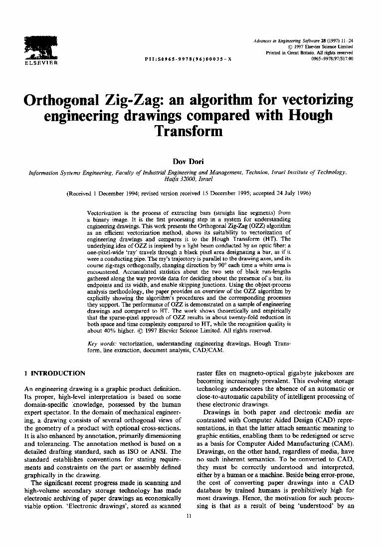
Six drawings were used as test-cases for the comparison. In Figs 13-18, each one of these drawings is shown in three versions: on the left hand side is the original drawing, scanned at 100 or 200 dpi, in the middle is the OZZ result, and on the right hand side, the HT result. The drawings were selected such that they would represent various complexity and noise levels.

Table 1 gives their names, sizes, the time it took each one of the two vectorization methods to process each drawing, and the ratio of execution times for each drawing. As the table shows, the time ratio values range from 10.4 to 57.2, with a mean of 21.8. This result, which pertains to the time complexity, is very close to

20 D. Dori

Fig. 13. Base: side view.

the theoretical result of 19.25 that was obtained from the theoretical computation of the space complexity ratios of the two methods. Although this is probably a coincidence, it does indicate the order of magnitude of execution time ratio that should be expected.

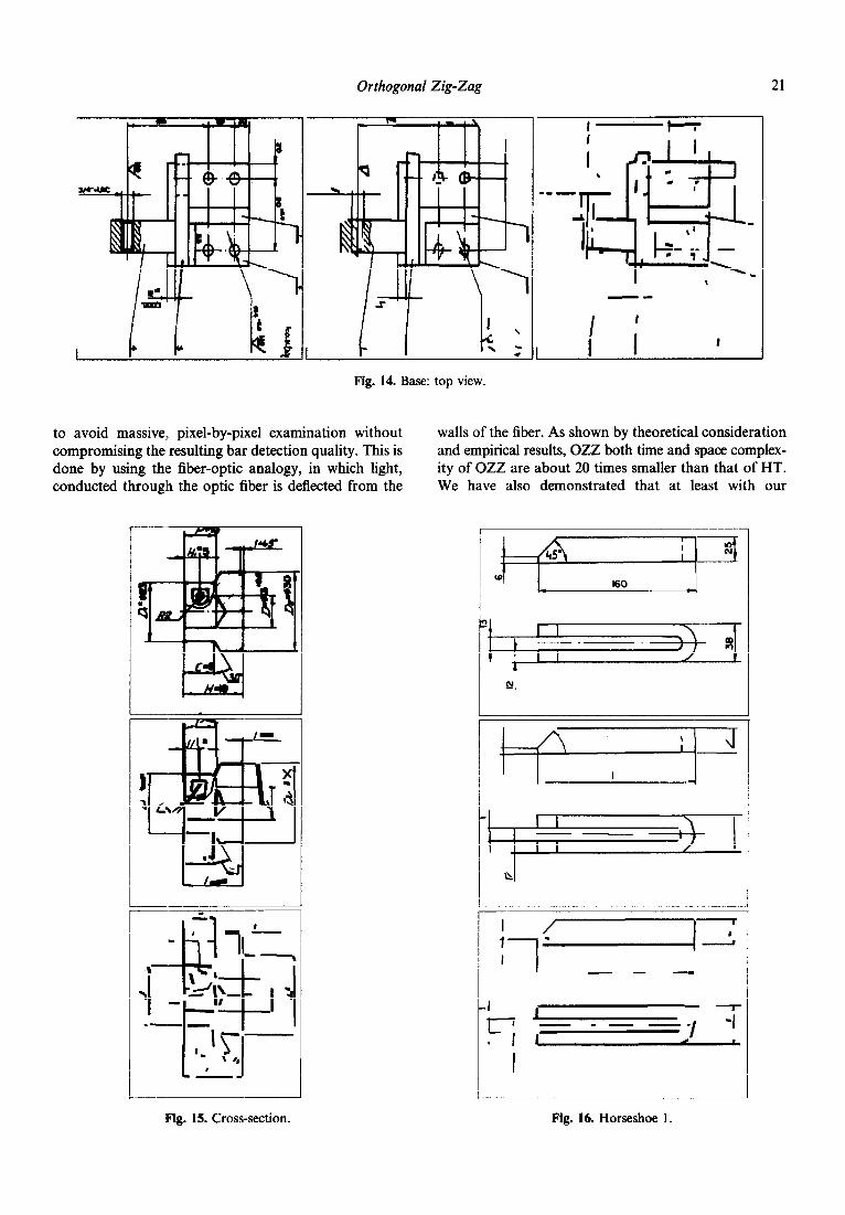
‘Cross-section’ is an exceptionally noisy and relatively complex drawing, because it was deliberately scanned from a semi-original transparent brown photocopy with poor contrast. It therefore gave ‘hard time’ to both methods, but, as can be seen in Table 1, whereas it took a time in the order of 2 min for OZZ, it took almost 2 h for HT, almost 60 times longer.

Examining Table 1, a direct relation can be observed between the image size and the performance time ratio. In other words, one can hypothesize that the performance time ratio of HT over that of OZZ deteriorates (grows) as the image size grows. To test this hypothesis, a plot of the performance time ratio as a function of the image size is drawn in Fig. 19. The resulting graph indeed supports the hypothesis. A linear fit equation is written at the top of the plot, with R2 = 0.62. Surpris- ingly high is the value R2 = 0.97 of the cubic fit, whose equation is also given below the linear fit equation. Whether this is a coincidence or not needs to be investigated.

Visual inspection of the six triplets of drawings in Figs 15-20 shows that the quality of bar detection by OZZ is better than that of HT. One simple quantitative measure that supports the conclusion that OZZ performs better than HT is the number of bars detected by each one of the methods. Table 2 presents the number of bars detected and the average time needed to detect a bar in each one of the two methods, as well as the corresponding ratios. The detected bars’ ratio averages 1.4, i.e. OZZ detects about 40% more bars on the average. This ratio does not seem to depend on the image size. The only drawing in which this ratio is less than 1 (0.92) is Horseshoe 1 (Fig. 16). Examining this drawing we see that this is a result of the fact that HT erroneously broke complete bars into a number of segments.

The ratio between the average time needed to detect a bar in HT vs OZZ does depend on the image size: the bigger the image, the more time it takes HT to detect a line, while for OZZ this times does not seem to be affected by the image size. To see this, Fig. 22 shows two graphs. The one on the left shows the average number of seconds per line for OZZ and the one on the right, for HT. The corresponding linear fits are written above each graph. The slope of the fitted line for HT is 0.40 with $ = 0.61 as opposed to a slope of 0*0012 with R2 = 0.074 for OZZ. These results strongly support the observation that the time performance of HT decreases as the image size grows, while the time performance of OZZ is barely affected by the image size.

5 CONCLUSIONS

A fast vectorization algorithm for extracting bars from line drawings, orthogonal Zig-Zag (OZZ) has been developed, implemented, tested and compared with Hough Transform. The underlying principle of the approach is


Fig. 14. Base: top view.

to avoid massive! pixel-by-pixel examination without compromising the resulting bar detection quality. This is done by using the fiber-optic analogy, in which light, conducted through the optic fiber is deflected from the

walls of the fiber. As shown by theoretical consideration and empirical results, OZZ both time and space complexity of OZZ are about 20 times smaller than that of HT. We have also demonstrated that at least with our

I I ‘- - - I

Fig. 15. Cross-section. Fig. 16. Horseshoe 1.

D. Dori

I ’

1 :i d

I

a

, s I

Fig. 17. Horseshoe 2.

Fig. 18. Small straight.

-I- - /-

IL ’ -- I 1

L

Table 1. Comparison of elapsed time of HT vs OZZ for six drawings

J

Drawing name

Base side view Base top view Cross-section Horseshoe 1 Horseshoe 2 Small straight

Size in pixels Time (HT) Time (OZZ)

653 x 516 = 337K 0:08:57 0:00:46 69Ox604=418K 0:17:17 0:01:02 692 x 752 = 520K 1:38:07 0:01:43 821 x 565 = 464K 0:12:54 o:ooA8 677 x 606 = 410K 0:09:34 0:00:55 851 x 502 = 427K 0:16:44 0:00:53

Time ratio HT/OZZ

11.7 16.7 57.2 16.1 10.4 18.9


Linear fit:

Y' - 77 + 0.23x; Fe! - 0.62 cubic fil: Y- - 204s + 15.5x - 0.038xw + o.omo2Jc4; Iv2 - 0.07

400 500 Image Size (K pixels)

Fig. 19. The ratio between the time performance of HT and OZZ as a function of the image size.

y = 0.37 + 0.0012x; RA2 = 0.074

1.4-

8

8 0.6 - 8 0.’ 11 7

300 400 500 600 300 400 500 600 Image Size (K pixels) Image Size (K pixels)

y = - 144 + 0.40x; R"2 = 0.61

loo- -7

I

Fig. u). A comparison between time per detected bar in OZZ (left) and HT and their relation to the image size.

Drawing mme

Base side view Base top view Cross-section Horseshoe 1 Horseshoe 2 Small straight

Bars detected

HT OZZ

48 69 78 109 66 115 50 46 28 42 55 65

Bars ozz/ barsHT

144 140 l-74 O-92 l-50 1.18

s=lbar HT OZZ -/b= ml

set/bar OZZ

7-8 O-67 11.6 9-5 o-57 16.7

89.2 090 99-1 15-5 1.04 14-9 20.5 I.31 15.7 18.3 O-81 22.5

D. Dori

implementation of HT, for the application of extracting bars from engineering drawings, the quality of the results provided by OZZ is better than the bar detection quality obtained from HT.

REFERENCES

1.

2.

3.

4.

5.

6.

7.

8.

9.

10.

11.

12.

13.

14.

15.

16.

King, A. K. An expert system facilitates understanding the paper engineering drawings, Proc. IASTED Int. Symp. Expert Systems Theory and Their Applications, Los Angeles, California, ACTA Press, Anaheim, Calgary, Zurich, pp. 169-72, 1988. Joseph, S. H. 8c Pridmore, T. P. Knowledge directed interpretation of mechanical engineering drawings, IEEE Trans. PAMI, August 1989. Dori, D. A syntactic/geometric approach to recognition of dimensions in engineering machine drawings, Computed Vision, Graphics and Image Processing, 1989, 41, 1-21. Antoine, D., Collin, S. & Tombre, C. Analysis of technical documents: the REDRAW system. Pre-Proc. IAPR Work- shop on Syntactic & Structural Pattern Recognition, pp. l-20, Murray Hill, NJ, 1990. Collin, S. & Comet, D. Analysis of dimensions in mechanical engineering drawings, Proc. Machine Vision Applications, pp. 105-108, 1990. Tombre, K. & Vaxiviere, P. Structure, syntax and semantics in technical document recognition, Proc. First Int. Conf. Document Analysis and Recognition, IEEE Computer Society, Saint Malo, France, 1991. Collin, S. & Vaxiviere, P. Recognition and use of dimensioning in digitized industrial drawings, Proc. First Int. Conf. Document Analysis and Recognition, IEEE Computer Society, Saint Malo, France, 1991. Dori, D. & Tombre, K. From engineering drawings to 3-D CAD models - Are we ready now? Computer Aided Design, 1995, 27(4), 517-29. Arcelli, C. & San&i di Baja, G. Quenching points in distance labeled pictures, Proc. 7th Int. Conf. on Pattern Recognition, Montreal, pp. 344-46, 1984. Reumann, K. & Witkam, A. P. M. Optimizing curve segmentation in computer graphics, International Computer Symposium, pp. 467-72. Sklansky & Gonzalez, Fast polygonal approximation of digital curves, Pattern Recognition, 1980, 12, 327-31. Dunham, J. G. Optimum uniform piecewise linear approximation of planar curves, IEEE Trans. Pattern Analysis and Machine Intelligence, 1986, 8, 1. Yuan, J. 8z Suen, C. Y. Generalized chain codes based on straight line detection. In Advances in Structural and Syntactic Pattern Recognition, ed. Bunke, H. World Scientitic, Series in Machine Perception Singapore, 1992. Haralick, R. M. Computer and Robot Vision, Addison Wesley, 1991. Kasturi, R., Bow, S. T., El-Masri, W., Shah, J., Gattiker, J. R. & Mokate, U. B. A system for interpretation of line drawings, IEEE Trans. Pattern Analysis and Machine Intelligence, 1990, 12(10), 978-91. Harris, J. F., Kittler, J., Llewellyn, B. & Preston, G. A modular system for interpreting binary pixel representation of line-structured data. In Pattern Recognition: Theory

and Applications, D. Reide, Dordrecht, The Netherlands, pp. 311-351, 1982.

17. Fukada, Y. Primary algorithm for the understanding of logic circuit diagrams, Proc. 6th ICPR, Munich, pp. 706- 9, 1982.

18. Furuta, M., Kase, N. & Emori, S. Segmentation and recognition of symbols for handwritten piping and instrument diagram, Proc. 7th ICPR, Montreal, pp. 612- 14, 1984.

19. Fahn, C. S., Wang, J. F. & Lee, Y. J. A topology-based component extractor for understanding electronic circuit diagrams, Computer Vision, Graphics and Image Processing, 1988,44, 119-38.

20. Nagasamy, V. t Langrana, N. A. Engineering drawing processing and vectorization system, Computer Vision, Graphics and Image Processing, 1990, 49, 379-97.

21. Sato, T. L Tojo, A. Recognition and understanding of hand-drawn diagrams, Proc. 6th ICPR, Munich, pp. 674-77, 1982.

22. Lin, X., Shimotsuji, S., Minoh, M. & Sakai, T. Efficient diagram understanding with characteristic pattern detection, Computer Vision, Graphics and Image Processing, 1985,30,84-106.

23. Takaji, M., Konishi, T. & Yamada, M. Automatic digitizing and processing method for the printed circuit pattern drawings, Proc. 6th ICPR, Munich, 1982.

24. Csink, L. On the recognition of elements appearing in a certain diagram, Proc. 2nd Hungarian AI Conf., Budapest, 1991.

25. Hough, P. V. C. A method and means for recognizing complex patterns, USA Patent 3,096,654, 1962.

26. Dot-i, D. Object-process analysis: maintaining the balance between system structure and behaviour, I. Logic and Computation, 1995, 5(2), 227-49.

27. Dori, D., Liang, Y., Dowell, J. & Chai, I. Sparse pixel recognition of primitives in engineering drawings, Machine Vision and Applications, 1993, 6, 69-82.

28. Dori, D. Representing pattern recognition-embedded systems through object-process diagrams: the case of the machine drawing understanding system. Pattern Recognition Letters, 1995, 16(4), 377-84.

29. Dori, D. & Chai, I. Orthogonal Zig-Zag: an efficient method for extracting bars in engineering drawings. In Visual Form, ed. Arcelli, C., Cordella, L. P. & Sanniti di baja, G. Plenum, New York, pp. 127-36, 1992.

30. Kimme, C., Ballard, D. H. & Sklansky, J. Finding circles by an array of accumulators, CACM, 1975, 18, 120-22.

31. Conker, R. S. A dual-plane variation of the Hough Transform for detecting non-concentric circles of different radii, Computer Vision, Graphics and Image Processing, 1988,43, 115-32.

32. Hunt, D. J. & Nolte, L. W. Performance of the Hough Transform and its relationship to statistical signal detection theory, Computed Vision, Graphics and Image Processing, 1988,43, 221-38.

33. Illingworth, J. t Kit&r, J. The adaptive Hough Transform, IEEE Trans. Pattern Analysis and Machine Intelligence, 1987, PAMI-9(5), 690-97.

34. O’Gorman, L. & Sanderson, A. C. The converging squares algorithm: an efficient method for locating peaks in multidimensions, IEEE Trans. Pattern Analysis and Machine Intelligence, 1984, T-PAMI, 280-88.

orthogonal zig-zag: an algorithm for vectorizing...

Documents