6.1

Tishk International UniversityScience FacultyIT Department

Operating Systems

3rd Grade - Fall Semester 2021-2022

Lecture 4: CPU Scheduling

Instructor: Alaa Ghazi

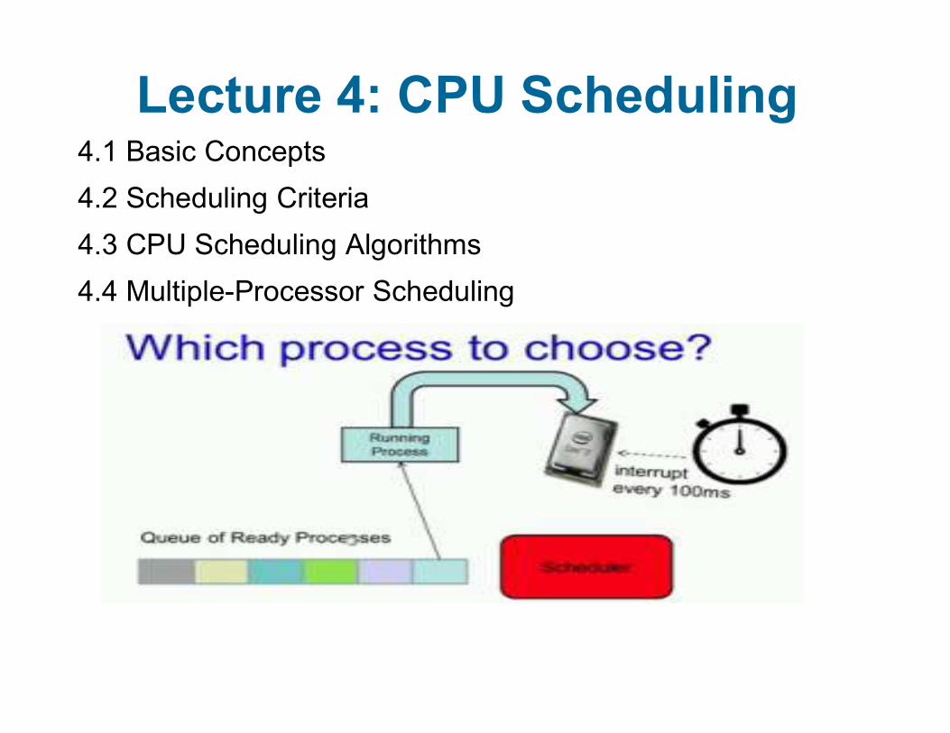
Lecture 4: CPU Scheduling4.1 Basic Concepts

4.2 Scheduling Criteria

4.3 CPU Scheduling Algorithms

4.4 Multiple-Processor Scheduling

6.3

4.1 Basic Concepts

CPU scheduling allows one process to use the CPU while the execution of another process is on hold.

Maximum CPU utilization obtained with multitasking

Each process will pass into cycles of CPU execution and I/O wait, CPU burst followed by I/O burst and so on.

CPU burst distribution is of main concern to the CPU scheduling.

6.4

CPU burst vs I/O burst

The important role of an OS is the act ofmanaging and scheduling these activities tomaximize the use of the resources and minimizewait and idle time.

Process execution repeats the CPU burst andI/O burst cycle.

When a process begins an I/O burst, anotherprocess can use the CPU for a CPU burst

6.5

CPU burst vs. I/O burst –Diagram(not required in the exam)

6.6

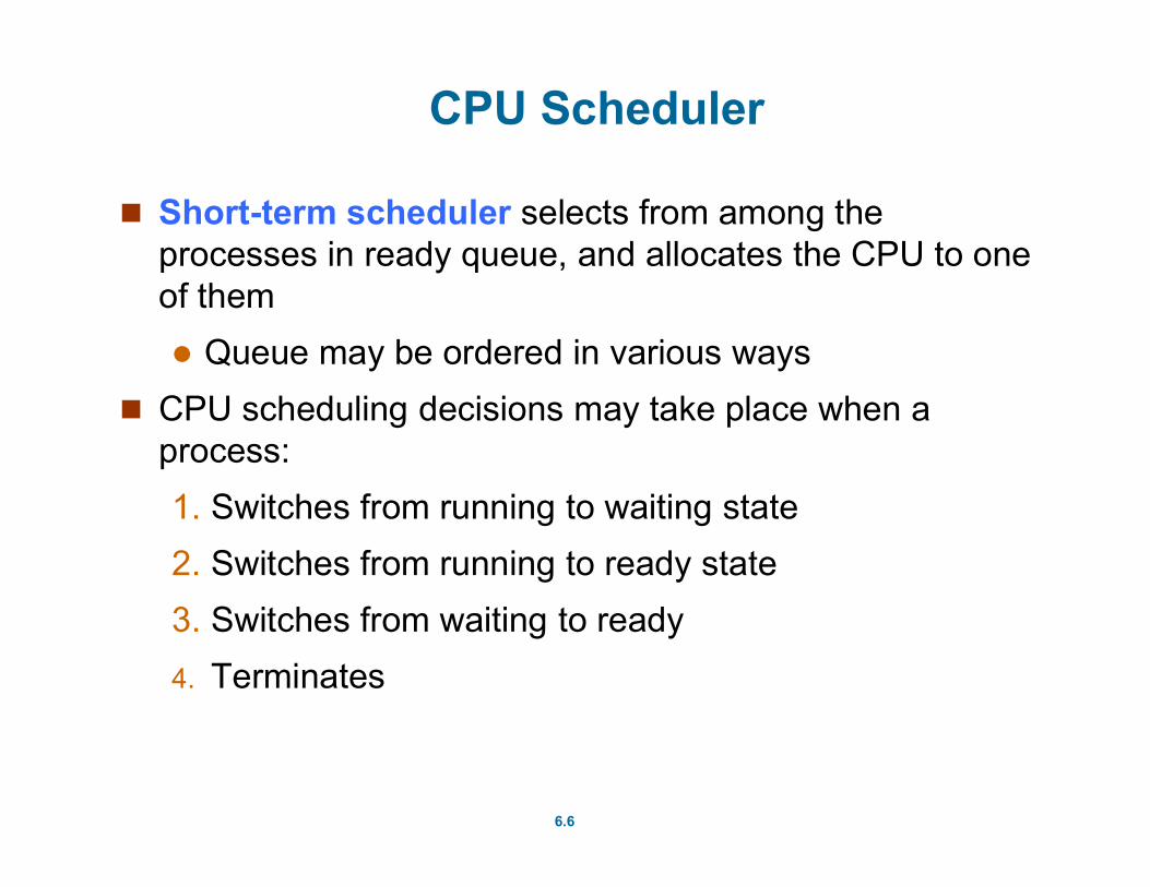
CPU Scheduler

Short-term scheduler selects from among the processes in ready queue, and allocates the CPU to one of them

Queue may be ordered in various ways

CPU scheduling decisions may take place when a process:

1. Switches from running to waiting state

2. Switches from running to ready state

3. Switches from waiting to ready

4. Terminates

6.7

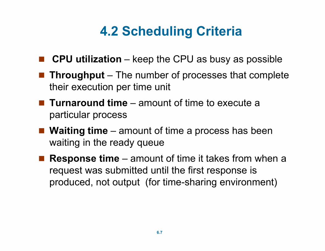
4.2 Scheduling Criteria

CPU utilization – keep the CPU as busy as possible

Throughput – The number of processes that complete their execution per time unit

Turnaround time – amount of time to execute a particular process

Waiting time – amount of time a process has been waiting in the ready queue

Response time – amount of time it takes from when a request was submitted until the first response is produced, not output (for time-sharing environment)

6.8

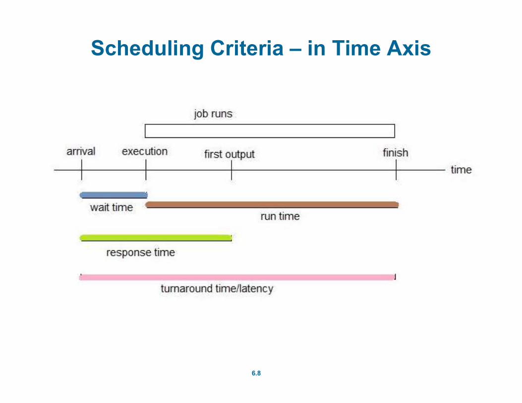
Scheduling Criteria – in Time Axis

6.9

Scheduling Algorithm Optimization Criteria

Max CPU utilization

Max throughput

Min turnaround time

Min waiting time

Min response time

6.10

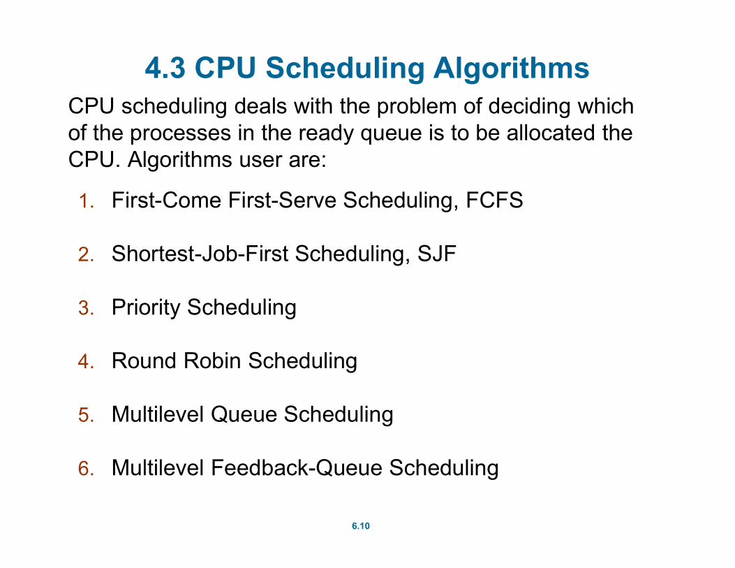
4.3 CPU Scheduling AlgorithmsCPU scheduling deals with the problem of deciding which of the processes in the ready queue is to be allocated the CPU. Algorithms user are:

1. First-Come First-Serve Scheduling, FCFS

2. Shortest-Job-First Scheduling, SJF

3. Priority Scheduling

4. Round Robin Scheduling

5. Multilevel Queue Scheduling

6. Multilevel Feedback-Queue Scheduling

6.11

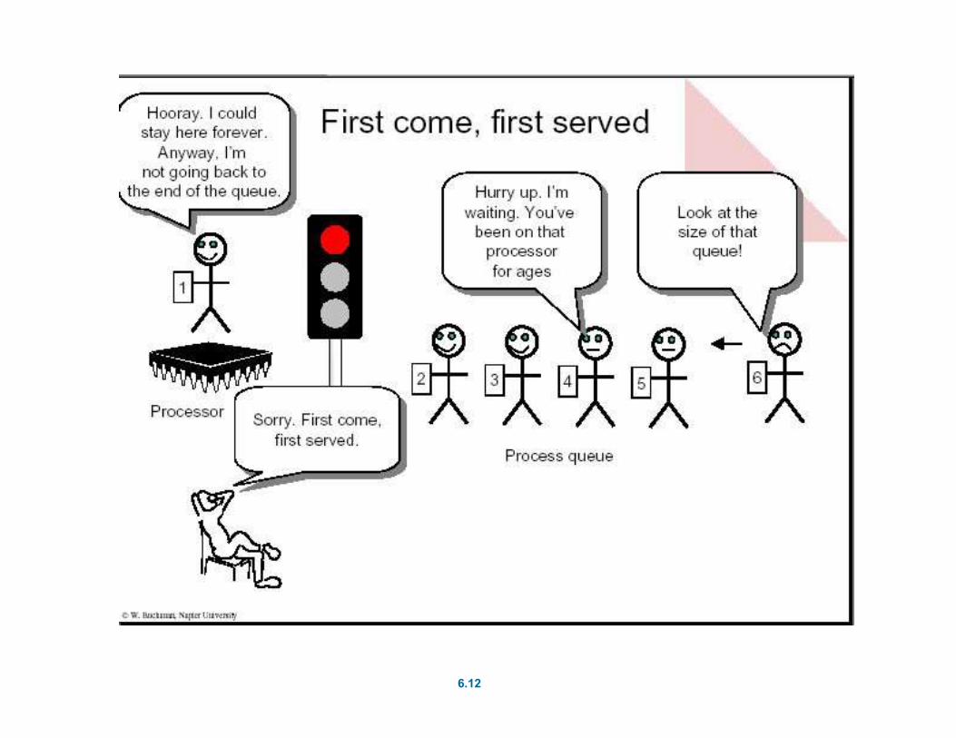
First- Come, First-Served (FCFS) Scheduling

FCFS is very simple - like customers waiting in line at the bank or the post office.

However, FCFS can yield some very long average wait times, particularly if the first process to get there takes a long time. For example, consider the following Example

6.12

6.13

First- Come, First-Served (FCFS) Scheduling

Process Burst Time

P1 24

P2 3

P3 3

Suppose that the processes arrive in the order: P1 , P2 , P3 The Gantt Chart for the schedule is:

Waiting time for P1 = 0; P2 = 24; P3 = 27

Average waiting time: (0 + 24 + 27)/3 = 17

P P P1 2 3

0 24 3027

6.14

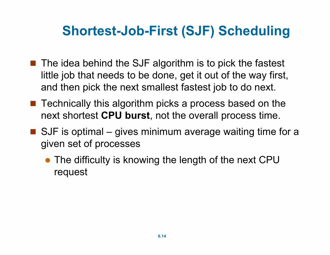
Shortest-Job-First (SJF) Scheduling

The idea behind the SJF algorithm is to pick the fastest little job that needs to be done, get it out of the way first, and then pick the next smallest fastest job to do next.

Technically this algorithm picks a process based on the next shortest CPU burst, not the overall process time.

SJF is optimal – gives minimum average waiting time for a given set of processes

The difficulty is knowing the length of the next CPU request

6.15

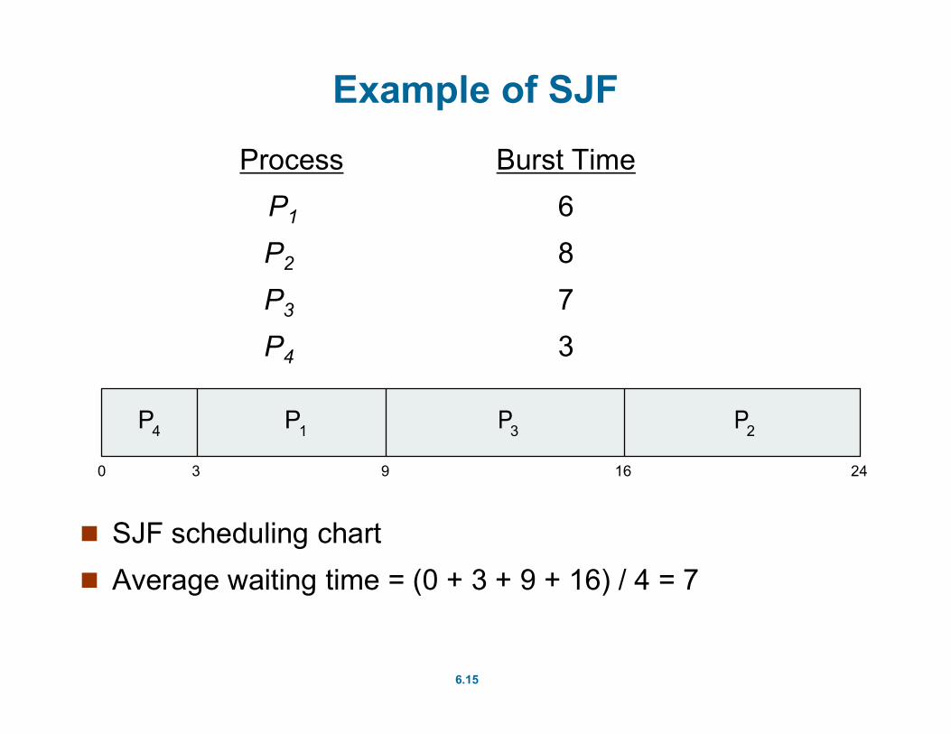
Example of SJF

ProcessArrTime Burst Time

P1 0.0 6

P2 2.0 8

P3 4.0 7

P4 5.0 3

SJF scheduling chart

Average waiting time = (0 + 3 + 9 + 16) / 4 = 7

P3

0 3 24

P4 P1

169

P2

6.16

Priority Scheduling

A priority number (integer) is associated with each process

The CPU is allocated to the process with the highest priority (smallest integer highest priority)

Priorities can be assigned either internally or externally. Internal priorities are assigned by the OS using criteria such as average burst time, ratio of CPU to I/O activity, system resource use, and other factors available to the kernel. External priorities are assigned by users, based on the importance of the job.

6.17

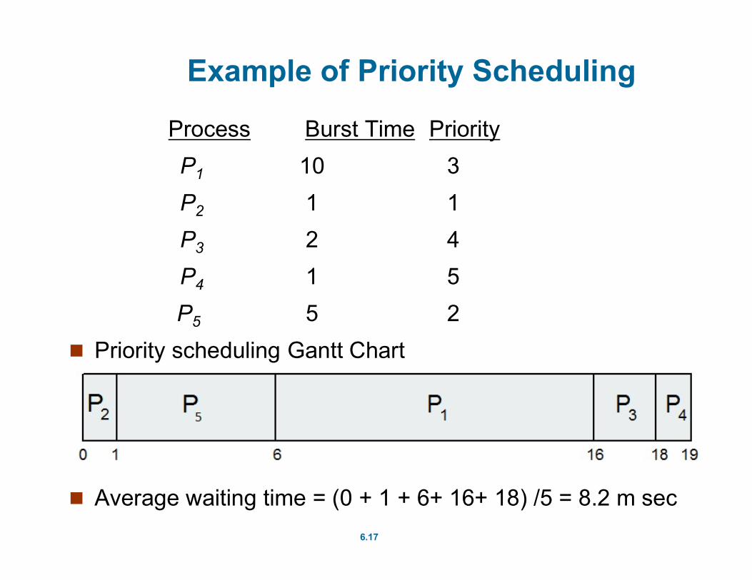
Example of Priority Scheduling

ProcessAarri Burst TimeTPriority

P1 10 3

P2 1 1

P3 2 4

P4 1 5

P5 5 2

Priority scheduling Gantt Chart

Average waiting time = (0 + 1 + 6+ 16+ 18) /5 = 8.2 m sec

6.18

Priority Scheduling - Problem

Priority scheduling can suffer from a major problem known as indefinite blocking, or starvation, in which a low-priority task can wait forever because there are always some other jobs around that have higher priority.

Solution Aging – as time progresses increase the priority of the process

6.19

Round Robin (RR)

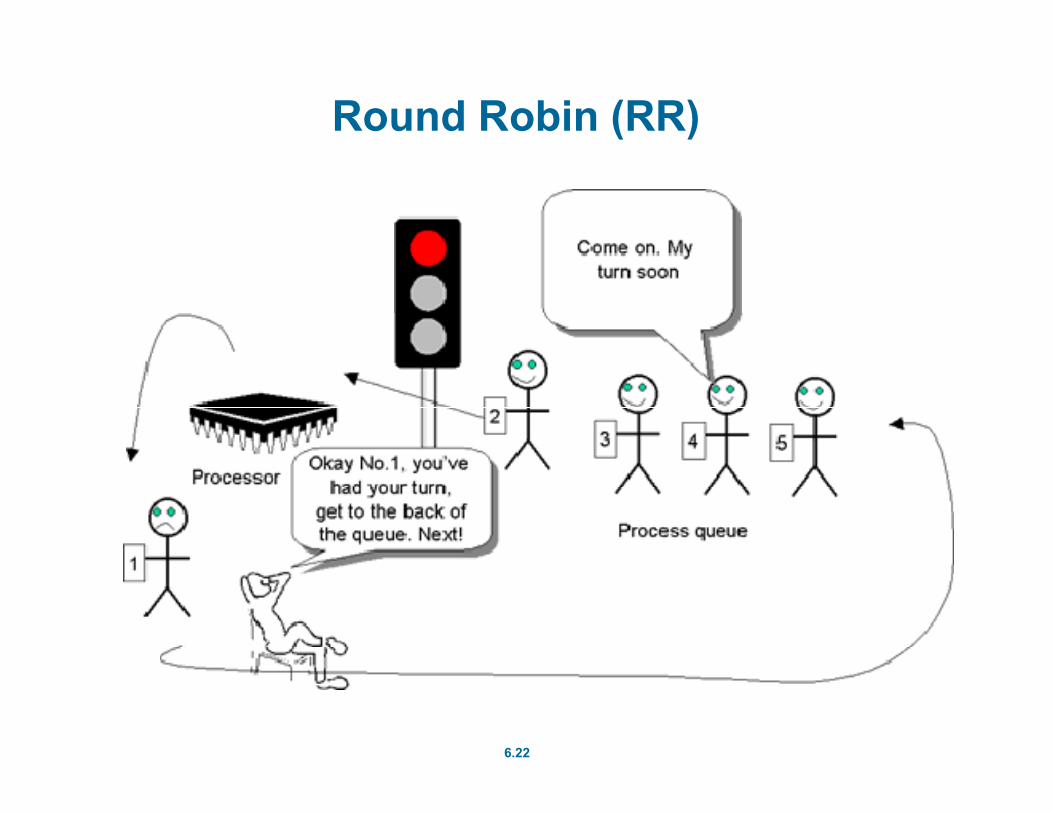
Round robin scheduling is similar to FCFS scheduling, except that CPU bursts are assigned with limits called time quantum.

When a process is given the CPU, a timer is set for a time quantum.

If the process finishes its burst before the time quantum timer expires, then it is swapped out of the CPU just like the normal FCFS algorithm.

If the timer goes off first, then the process is swapped out of the CPU and moved to the back end of the ready queue.

6.20

Round Robin (RR)

The ready queue is maintained as a circular queue, sowhen all processes have had a turn, then the schedulergives the first process another turn, and so on.

RR scheduling can give the effect of all processes sharingthe CPU equally, although the average wait time can belonger than with other scheduling algorithms.

6.21

Advantages and Drawbacks of Round Robin (RR)

The advantages of the round robin scheduling algorithmare: The algorithm is fair because each process gets a fair chance to

run on the CPU.

The average wait time is low especially when the burst times varyand the response time is very good.

The drawbacks of the round robin scheduling algorithm areas follows; there is an increase number of context switching that occurs with

considerable over heads.

the average wait time is high especially when the burst times haveequal lengths.

6.22

Round Robin (RR)

6.23

Example of RR with Time Quantum = 4

Process Burst Time

P1 24

P2 3

P3 3

The waiting time chart is:

In this example the average wait time is 5.66 ms.

Typically, higher average turnaround than SJF, but better response

P P P1 1 1

0 18 3026144 7 10 22

P2 P3 P1 P1 P1

6.24

Example of RR with Time Quantum = 3

6.25

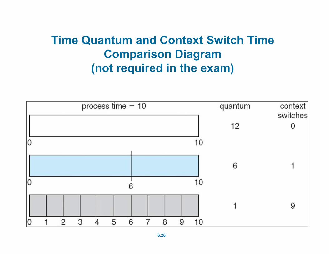
Time Quantum Value

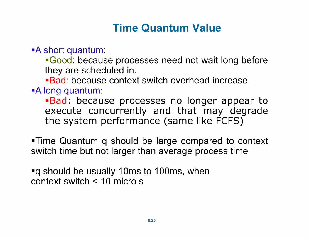
A short quantum:Good: because processes need not wait long beforethey are scheduled in.Bad: because context switch overhead increase

A long quantum:Bad: because processes no longer appear toexecute concurrently and that may degradethe system performance (same like FCFS)

Time Quantum q should be large compared to contextswitch time but not larger than average process time

q should be usually 10ms to 100ms, whencontext switch < 10 micro s

6.26

Time Quantum and Context Switch Time Comparison Diagram

(not required in the exam)

6.27

Multilevel Queue

When processes can be readily categorized, then multipleseparate queues can be established, each implementingwhatever scheduling algorithm is most appropriate for thattype of job, and/or with different parametric adjustments.

Note that under this algorithm jobs cannot switch fromqueue to queue - Once they are assigned a queue, that istheir queue until they finish.

Each queue has its own scheduling algorithm for example:

foreground – RR

background – FCFS

6.28

Multilevel Queue

Scheduling must be done between the queues:

Fixed priority scheduling; (i.e., serve all from foreground then from background). Possibility of starvation.

Time slice – each queue gets a certain amount of CPU time which it can schedule amongst its processes; i.e.,

80% to foreground in RR

20% to background in FCFS

6.29

Multilevel Queue Scheduling

6.30

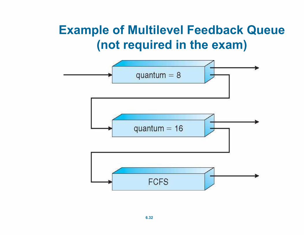
Multilevel Feedback Queue

Multilevel feedback queue scheduling is similar to theordinary multilevel queue scheduling described above,but the difference is jobs may be moved from onequeue to another for a variety of reasons:

If the characteristics of a job change between CPU-intensive and I/O intensive, then it switchs a job fromone queue to another.

Aging: a job that has waited for a long time can getbumped up into a higher priority queue.

6.31

Multilevel Feedback Queue

Multilevel feedback queue scheduling is the most flexible,because it can be tuned for any situation. But it is alsothe most complex to implement because of all theadjustable parameters. Some of the parameters whichdefine one of these systems include:

The number of queues.

The scheduling algorithm for each queue.

The methods used to transfer processes from onequeue to another.

The method used to determine which queue a processenters initially.

6.32

Example of Multilevel Feedback Queue(not required in the exam)

6.33

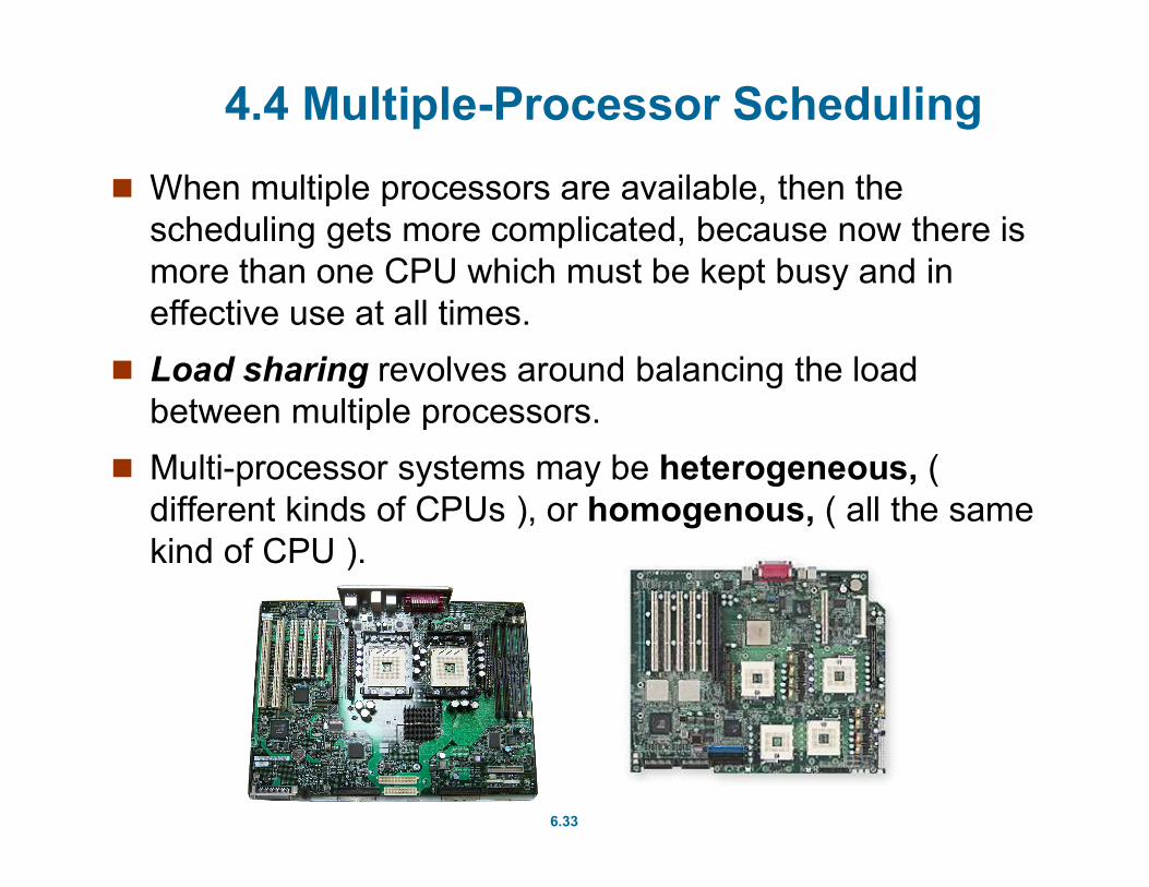
4.4 Multiple-Processor Scheduling

When multiple processors are available, then the scheduling gets more complicated, because now there is more than one CPU which must be kept busy and in effective use at all times.

Load sharing revolves around balancing the load between multiple processors.

Multi-processor systems may be heterogeneous, ( different kinds of CPUs ), or homogenous, ( all the same kind of CPU ).

6.34

Approaches to Multiple-CPU Scheduling

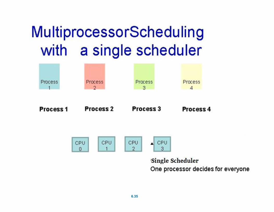
Asymmetric multiprocessing – here a single scheduler is running only one CPU accesses the system data structures, and decides for every CPU.

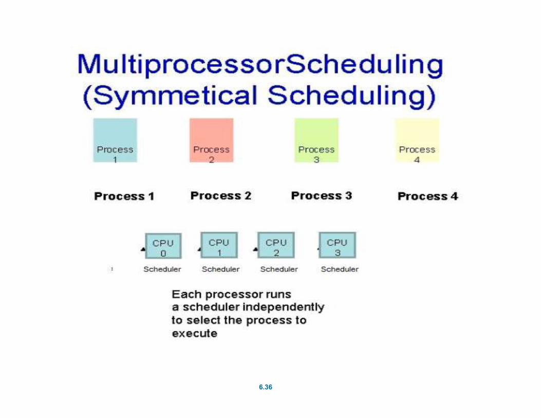
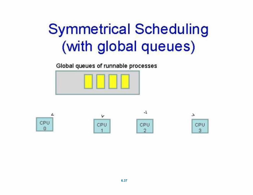
Symmetric multiprocessing (SMP) – the most common approach, when each CPU is self-scheduling, with two versions: Global Queues: all processes in common ready queue, or

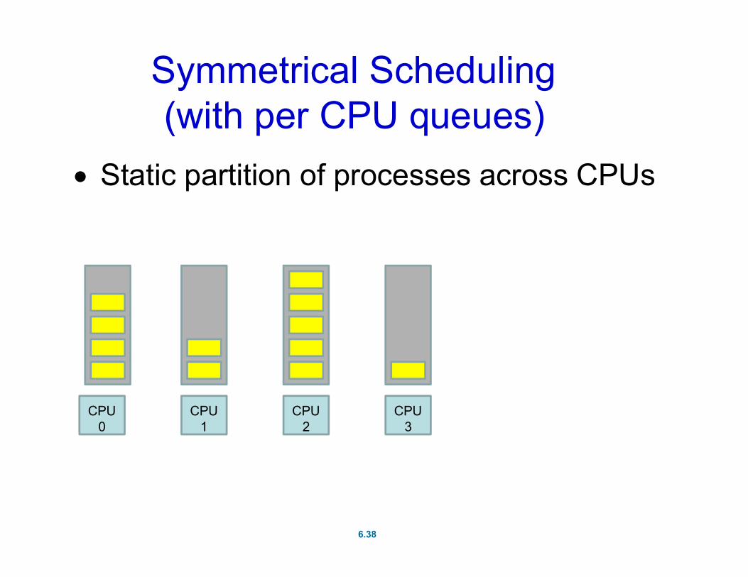
Per CPU Queues: each has its own private queue of ready processes

6.35

6.36

6.37

6.38

Symmetrical Scheduling (with per CPU queues)

CPU 0

CPU 1

CPU 2

CPU 3

Static partition of processes across CPUs

6.39

Process Affinity

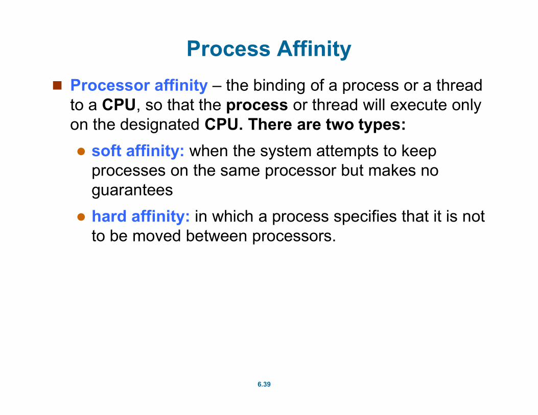
Processor affinity – the binding of a process or a thread to a CPU, so that the process or thread will execute only on the designated CPU. There are two types:

soft affinity: when the system attempts to keep processes on the same processor but makes no guarantees

hard affinity: in which a process specifies that it is not to be moved between processors.

6.40

Multiple-Processor Scheduling – Load Balancing

Load balancing attempts to keep workload evenly distributed, so that one CPU won't be sitting idle while another is overloaded. This is done using Process Migration.

Load Balancing Techniques:

Push Migration is where the operating system checks the load on each CPU periodically. If there’s an imbalance, some processes will be moved from one CPU onto another.

Pull Migration is when idle CPU pull a waiting task from busy CPU.