oscillator design with genesys

Oscillator Design with Genesys

with techniques from the book

by Randy Rhea

I'll Cover

• A unified design process for different active devices,

resonators and simulation technologies applicable from low

frequency to microwaves

• How Genesys aids the design process

• What the book offers

• Example Genesys workspaces

Slide 2

Randy Rhea Susina LLC

[email protected] Sept 16, 2010

Step 1

Perform a linear analysis

• This is the design foundation

– determines design margins

– reveals tuning characteristics

– estimates phase noise

– fast exploration of topologies

• Provides intuitive grasp of the design process

• Does not provide level, harmonic or transient data

Slide 3



Two Linear Analysis Methods

• One-Port Reflection

AMPLIFIERRESONATOR

LOOP_INPUT LOOP_OUTPUT

OSCILLATOR_OUTPUT

• Open-Loop Cascade

RESONATOR DEVICE

REFLECTION_PORT OSCILLATOR_OUTPUT



The Open-Loop Cascade

Slide 5

Initial 40 MHz Colpitts with a FET device and an L-C resonator

50ΩOscOut

.01μF

C4

LoopOutLoopIn

270nH

L1

0.011A

CP1

J310

5V

180pF

C3

180Ω

R2

27ΩR1

74.7pF

C1

180pF

C2



Oscillator Starting Conditions

Slide 6



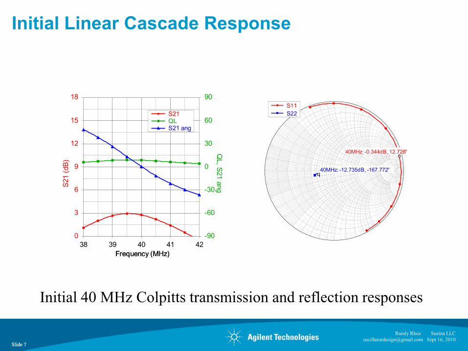
The open-loop response criterion that insure the oscillator will start are

• The oscillation frequency is the transmission phase zero-crossing, f0

• The initial linear gain at f0 must be greater than 0 dB

• The phase slope at f0 must be negative

Additional objectives are

• The phase slope should be as steep as possible

• The maximum phase slope occurs at f0

• The gain margin at f0 is moderate, for example 3 to 8 dB

• The amplifier is stable

• The maximum gain margin occurs at f0

• S11 and S22 are small

Initial Linear Cascade Response

Slide 7

Initial 40 MHz Colpitts transmission and reflection responses

Frequency (MHz)

S21 (

dB

)

0

3

6

9

12

15

18

QL, S

21 a

ng

-90

-60

-30

0

30

60

90

Frequency (MHz)

38 39 40 41 42

S21QLS21 ang

0

0.1

0

.2

0.3

0

.4

0.5

0

.6

0

.7

0.8

0

.9

1.0

1.2

1

.4

1.6

1.8

2.0

3.0

4.0

5.0

1

0

20

0.1

0.2

0.3

0.4

0.5

0.6

0.7

0.8 0

.9 1.0

1.2

1.4

1. 6

1. 8

2.0

3.0

4.0

5 .0

10

20

50

0. 2

0.4

0. 6

0.8

1.0

0.2

0.4

0.6

0.8

1.0

0 .1

0.2

0.3

0.4

0.5

0. 6

0.7

0.8

0.9

1.0 1

.2

1.4

1.6

1.8

2.0

3.0

4.0

5.0

10

20

50

0.2

0.4

0.6

0.8

1.0

0.2

0 .4

0.6

0.8

1 .0

S11

S22

40MHz: -12.735dB, -167.772°

40MHz: -0.344dB, 12.728°



Randall/Hoch Correction

1212212211

1221

21 SSSSS

SSG

Slide 8

G is the true open-loop complex gain with the loop self-

terminated.

[1] M. Randall and T. Hoch, "General Oscillator Characterization Using Linear Open-

Loop S-Parameters," IEEE Trans. MTT, Vol. 49, June 2001, pp 1094-1100



Optimizing the Open-Loop Response



Optimized Cascade Design

Slide 10

Optimized Colpitts transmission and reflection responses

50ΩOscOut

.01μF

C4

LoopOutLoopIn

330nH

L1

0.011A

CP1

J310

5V

180pF

C3

180Ω

R2

120ΩR1

48pF

C1

390pF

C2

Frequency (MHz)

S21, S

tart

Opt:

S21 (dB

)

0

3

6

9

12

15

18

QL

, S21

ang

, Sta

rtOpt:Q

L, S

tartO

pt:S

21 a

ng-90

-60

-30

0

30

60

90

Frequency (MHz)

38 39 40 41 42

S21QLS21 angStartOpt:S21StartOpt:QLStartOpt:S21 ang

0

0.1

0

.2

0.3

0

.4

0.5

0

.6

0

.7

0.8

0

.9

1.0

1.2

1

.4

1.6

1.8

2.0

3.0

4.0

5.0

1

0

20

0.1

0.2

0.3

0.4

0.5

0.6

0.7

0.8 0

.9 1.0

1.2

1.4

1. 6

1. 8

2.0

3.0

4.0

5 .0

10

20

50

0. 2

0.4

0. 6

0.8

1.0

0.2

0.4

0.6

0.8

1.0

0 .1

0.2

0.3

0.4

0.5

0. 6

0.7

0.8

0.9

1.0 1

.2

1.4

1.6

1.8

2.0

3.0

4.0

5.0

10

20

50

0.2

0.4

0.6

0.8

1.0

0.2

0 .4

0.6

0.8

1 .0

S11

S22

StartOpt:S11

StartOpt:S22

40MHz: -12.735dB, -167.772°

40MHz: -0.344dB, 12.728°

40MHz: -17.841dB, 39.881°



Alechno Technique

Slide 11



[1] S. Alechno, "The Virtual Ground in Oscillator Analysis – A Practical Example",

Applied Microwave & Wireless, July 1999, pp.44-53

Back when…….

• A random combination of a device and resonator may not satisfy the starting criterion

• Historically, successful combinations were named for the discoverer and became standards

• Copying designs was (and is!) common, often resulting in nonoptimum performance

• Modern linear, nonlinear and transient simulation is a better method that improves designs

Slide 12



Unified Approach

• These techniques are general

• All resonator or device types are treated in a like manner

• In Genesys, the same schematic is used for linear, nonlinear,

transient and noise simulation

• Ideal or real models are treated in a like manner

Slide 13



Step 2

Perform a harmonic-balance simulation

• This determines the output level and harmonics

• Predicts noise more accurately

• Predicts the frequency more accurately

Requires nonlinear device models

• Numerous models are provided with Genesys

• Genesys imports Spice models

• Devices can also be characterized by

X-parameters

Slide 14



330 MHz Colpitts & Spectrum

Slide 15

330 MHz Colpitts simulated through the 7th harmonic

0.02ACP1

BFT92

Port_2

Port_3

9V

20pFC1

Port_136pFC2

2700Ω

R1

4700Ω

R2

47pFC3

270pF

Csimulation

150ΩR3

FB

27Ω

10pF

C4

120

16.16nHL1

1 2 3

Open_Loop

50Ω

Output1.155V

330.028MHz

OSCPORT

Frequency (MHz)

Po

ut (

dB

m)

-50

-40

-30

-20

-10

0

10

Frequency (MHz)

0 330 660 990 1320 1650 1980 2310

Pout

330.0

28 M

Hz

8.321 dBm

1*330.028



Nonlinear Noise Analysis

Slide 16



Nonlinear Noise Analysis Plot

Slide 17

4 most significant noise contributors of the 330 MHz Colpitts bipolar oscillator

Frequency (MHz)

Q1 B

ase, O

utp

ut Therm

al, Q

1 C

olle

cto

r, F

B (dB

)

-190

-180

-170

-160

-150

-140

-130

-120

-110

-100

-90

-80

-70

Frequency (MHz)

100e-6 1e-3 0.01 0.1 1 10 100

Q1 Base

Output Thermal

Q1 Collector

FB



Step 3

Perform a time-step transient analysis

• This determines the starting characteristics

• This helps discover transient spurious modes

• Can be used as a substitute to HB to find output level and harmonics if

nonlinear noise estimates are not required

Uses the same models as HB simulation

Slide 18



1

50Ω

Output

1 2 3

Data_Linear1

Output Waveform

Slide 19

330 MHz Colpitts transient starting waveform

Time (ns)

VP

OR

T (

V)

-2

-1.6

-1.2

-0.8

-0.4

0

0.4

0.8

1.2

1.6

2

Time (ns)

0 20 40 60 80 100 120 140 160 180 200



0.02ACP1

BFT92

Port_2

Port_3

9V

20pFC1

Port_136pFC2

2700Ω

R1

4700Ω

R2

47pFC3

270pF

Csimulation

150ΩR3

FB

27Ω

10pF

C4

120

16.16nHL1

Genesys Oscillator Analysis

Slide 20



Genesys is

• An integrated linear, nonlinear, transient, noise simulation

environment with schematic and layout tools

• A process for creating new oscillator designs or repairing under

performing designs

• A learning tool that provides intuitive insight into all aspects of

oscillator behavior

Slide 21



Oscillator Topics Not Covered in this Webinar

• Genesys oscillator synthesis

• Integrated layout tools

• Electromagnetic simulation of the layout

• Instrument control for data acquisition

• System simulation

Slide 22



Why Did I Write the Book?

• My previous books only covered nonlinear

and transient theory qualitatively

• I gained knowledge while teaching an

oscillator design course to over a thousand

engineers

• Both oscillator and simulation technologies

have advanced significantly in the last decade

• I needed something to do

Slide 23



What's in the Book ?

• Detailed descriptions of linear, nonlinear, transient and noise

techniques for practical oscillator design

• 350 illustrations

• 200 applicable equations

• 60 example oscillators covering bipolar,

FET, and MMIC devices with R-C, L-C,

ceramic, crystal, SAW and distributed

resonators

• Confirmation data for a dozen

prototype oscillators

Slide 24



Genesys Workspaces

140 Genesys workspaces were used to create the illustrations in the book. Genesys is a powerful documentation tool.

• Agilent EEsof EDA has established a website for downloading 73 of the more important workspaces

• These workspaces may be used with either full or trial Genesys licenses

Slide 25



The Available Workspaces

• The workspace template.wsx may be used to start a design. Simply add your schematic to the workspace

• There are 13 utility and tutorial workspaces for amplifier and resonator design

• There are 27 workspaces for general purpose oscillators

• There are 13 workspaces of VCOs and distributed resonator oscillators

• There are 20 workspaces with ceramic, crystal and SAW oscillators

Slide 26



Summary

• Genesys is an integrated tool, ideally suited for a unified

approach to oscillator design

• Discrete Oscillator Design covers practical oscillator design for

a wide variety of oscillator types

• Example Genesys workspaces from the book are available

from Agilent EEsof

Slide 27



For More Info: Just Google “Agilent Genesys”

Email Randy Rhea at [email protected]

• for questions about this presentation• for questions about the book• for a Microsoft Excel spreadsheet of equations in the book• for an errata sheet for the book, as published

About Genesys:• Genesys product page http://www.agilent.com/find/eesof-genesys• USA Genesys Specialist, Rick Carter [email protected]

To download the workspaces:• Go to http://www.agilent.com/find/eesof-genesys-osc-workspaces

To obtain a free trial Genesys license:• Go to http://www.agilent.com/find/eesof-genesys-evaluation

Slide 28



“This is a list of questions posed after my Agilent webinar presentation: Oscillator Design with Genesys. I must say, responding to these questions

brought back many memories for me, and it was a lot of fun”,

Randy Rhea 16 Sept 2010

1. QUESTIONS REGARDING THE OPEN-LOOP MATCH

1) S11 and s22 would not be always low at any impedance......

2) Do the termination resistances need to be at least conjugates of each other in addition to being 50 Ohms?

3) Low s11 and s22: is 50 ohm needed? what impedance level? is it relative , i.e. both should be at same (or conjugate) impedance?

4) I did not catch completely your remark about the conditions (for s11, s22, ...?), which must be fulfilled that the open-loop analysis will yield

realistic values. We tried several times to make an open-loop analysis of a Colpitts crystal oscillator by opening the loop between emitter and the

capacitive divider, but never got zero phase or other reasonable results.

My point is, that opening the loop - is loading the emitter output with a different impedance than it is with the closed loop and - is feeding the

"Input" (capacitive divider) with a different source impedance than it is the case with the closed loop. Can you please explain again.

5) I agree that targeting 50 ohms for the port impedances makes it convenient to make measurements using a network analyzer. However, it

seems to me that that will not necessarily result in the correct prediction of tank Q -- if the tank shunt resistance is much larger than 50 ohms, for

example, connecting a 50 ohm measurement device (or simulation port) across that tank will distort the value of the Q. I haven't had a chance to

absorb the implications of the Randall-Hock equation, so it's not clear whether that corrects for the error due the artificial loading introduced by the

open loop measurement system.

ANSWERS: I will answer these five match questions as a group. The issue of match in the open loop cascade has always generated a lot of

questions, and skepticism, in my oscillator classes. I’ll try to explain it in steps.

Point 1: While the idea of an amplifier matched to 50 ohms is easy to accept, it may be difficult to accept that a resonator consisting of only

reactors can have a resistive input impedance. Consider a simple series resonator cascaded with a 50 ohm amplifier. At resonance, the reactance

of the series inductor and series capacitor cancel, and the impedance seen looking into the resonator is the 50 ohms of the amplifier. The cascade

input is matched to 50 ohms! So to obtain a matched open loop it is only necessary to have a matched amplifier.

Point 2: Consider slide 10 of the presentation. This is a simple, but typical, FET Colpitts oscillator. Even though a FETs input impedance is high,

notice that after optimization, the cascade input return loss is 12.7 dB. The Colpitts resonator matched 50 ohms to the gate. In this case, the

source impedance is naturally well matched to 50 ohms with a 17.8 dB return loss.

Point 3: Why 50 ohms? First of all, don’t become hung up on this idea. From the simulator’s standpoint, you can chose any equal and resistive

termination impedance: 1 ohm, 50 ohms, 1Mohm. You simply choose the resistance that best matches the source and then use the capacitive tap

to match the gate to that resistance. It is often 100 to 200 ohms for a low-frequency FET. As you go up in frequency, it tends lower in impedance.

The same process is used regardless of the device, or type of resonator, ei, whether it is a Pierce, Colpitts, Clapp or whatever. You’ll be surprised

how often the selected impedance can be close to 50 ohms, and that is convenient for confirmation on the bench. 50 ohms is merely convenient,

not required.

Point 4: Don’t worry about matching to 20 dB return loss. It is wasted effort. In an oscillator, there is no advantage to knowing the gain margin to

fractions of a dB. The simulation will be reasonably accurate with 12 dB return losses. For the simple, uncorrected S-parameters to be an accurate

simulation, with a reasonably small S12, only EITHER S11 or S22 needs to be small. To understand this statement, test it against the

Randall/Hoch equation.

Point 5: If you are having trouble getting a reasonable match, at any chosen reference impedance, be sure to assess stability. CB, CC, CG and

CD amplifiers, typically used with Colpitts oscillators, are notoriously unstable. That is why these configurations are used in negative resistance

and negative conductance oscillators. A sure sign of instability is either or both of the loop port impedances plotting outside the circumference of

the Smith chart somewhere in the frequency range. If this is the case, before beginning the analysis, stabilize the device with resistance in series

with the base or the emitter. Be sure to assess how this degrades the noise figure. This resistance not only makes the simulation go better, it

reduces potential spurious modes in the oscillator.

Point 6: This point addresses the questions of the simulator loading the resonator. Consider again slide 10 in the presentation. After optimization,

both ports are well matched. That means the source is near 50 ohms. The simulator termination was set to 50 ohms. Therefore, when the loop is

closed, the source will terminate the tap with the same impedance that the simulator did!

Final Point: If the cascade does not optimize to a reasonable match, or if the gain margin is small and you need a more accurate simulation, or if

you are just skeptical, then use the Randall/Hoch correction. Their G is the true open-loop gain with the cascade self-terminating. G is exact. You

may measure the initial loop S-parameters with ANY reference impedance, and you may even open the loop at ANY node, and the result for G is

identical, including the phase slope of G, which defines the loaded Q. Computing and displaying G in Genesys is a snap.

2. QUESTION: To optimize at a given frequency it is possible to put the same value for maximum and minimum. I used it in ADS and maybe this

could be useful for Genesys too?

ANSWER: The attendee is remarking about the fact that the frequency range set in the optimization goals displayed in slide 9 was 39.9 to 40.1

MHz rather than 40 MHz. This is simply an old habit of mine, because digital computers use floating-point math when computing frequency points

in a sweep. If the step point for 40 MHz computed as 39.99999999999999 there would be no data point at 40 MHz. For 15 years, I haven’t tested

if this old habit to see if its still necessary.

3.. QUESTION: How is the loaded Q simulated? Also, can you elaborate on the sharp phase slope required? Isn’t the idea to keep the phase as

close to 0 deg as possible across freq, considering temp changes and component tolerances?

ANSWER: The loaded Q computed by Genesys is derived from the slope of the forward transmission phase. Loaded Q is also defined as the

center frequency divided by the 3 dB down amplitude bandwidth of a single resonator. However, with oscillators, we are primarily concerned with

the phase. Also, the phase definition is somewhat more consistent with multiple resonators.

Well yes, the objective is to keep the phase zero crossing at the desired frequency under all conditions. In fact, if we were perfectly successful in

doing so, there would be absolutely no long term (drift) or short term (noise) frequency deviation.

In practice, the absolute value of the transmission phase can change with temperature, noise, supply and load changes. Examine the response of

the transmission phase. Now imagine the entire curve shifts up or down in phase. If the slope is shallow, a large shift occurs in the zero crossing

frequency. Now image the slope is infinitely steep. In that case, the frequency shift resulting from a phase shift is zero! Wouldn’t that be nice?!

That is why a steep phase slope (which is high loaded Q) is so important.

4. QUESTION: one attendee reported that “manor” on slide 13 should be spelled “manner”.

ANSWER: Thank you for the errata. I also noticed after the presentation that Hock in the title of slide 8 should be spelled Hoch. These have been

corrected in the final download slides.

5. QUESTION: kayan? a time domain simulator used within genesis?

ANSWER: Yes. In English it is spelled Cayenne. It is a hot spice named after the city in French Guiana. This is obviously a name play on the

popular simulator family SPICE, originally from UC Berkeley. Cayenne is not a derivative of SPICE, but like SPICE, it is a time-step simulator.

Cayenne uses the same nonlinear models that both the Genesys linear and HARBEC harmonic balance simulators use. Genesys can import

SPICE models.

6. QUESTION: What input do you use to simulate the time-to-steady-state behavior?

ANSWER: That is a great question because it points out a strength of time-step simulation. With a real oscillator, when not powered, all voltages

rest at zero. When power is applied, the rising supply voltage begins to charge the bias and resonator circuitry. A time-step simulator emulates this

process with small time-step changes propagating through the circuit. If you draw your schematic and apply a power supply turn-on step, Cayenne

accurately simulates the actual starting process. No “artificial” starting techniques are needed. You also have the option in Cayenne to begin at

time zero at the quiescent, steady state bias conditions. You do not use this option when simulating starting.

7. The next two questions are related and are answered as a group.

QUESTIONS:

1) Up to what frequencies will Genesys simulate to?

2) During simulation, how accurate is just laying the copper (coplanar WG) on the schematic compare vs running the EM simulation?

ANSWER: The short answer is up to any frequency where the components are described with electrical models. In practice, the answer to this

question is very complex. The difficulty is with the models. Genesys includes all well published models for lumped and distributed passive

components, and these same models are used in all commercial simulators on the market. The answer also depends on the details. For example,

the basic model for an inductor with a 1 cm diameter may fail at 100 MHz, while the same model for a 0.1 mm diameter inductor may work well

through 10 GHz. To successfully use any simulator, and Genesys is no different, the engineer must be willing to study components (and a

simulator helps here also) before building a circuit. Nevertheless, up to about 500 MHz, except for some filters, standard simulation techniques

should suffice.

Above 500 MHz, the successful engineer will spend as much time characterizing components as he does simulating his circuits. Above about 2

GHz (again depending on the specific circuit), electromagnetic simulation (EM) should be added to the toolbox.

Another factor influencing whether EM simulation is required is the distributed process used. For example, there are well-engineered circuit-theory

models for numerous microstrip objects. On the other hand, the models available for coplanar objects are more limited. There may be no models

for less common, special layer configurations. In this case, EM simulation is mandatory.

8. The next two questions are related and are answered as a group

QUESTIONS:

1) What is the highest frequency accuracy of the nonlinear models? Are they compatible with ADS?

2) Are active device libraries provided? (transistors, varactors, etc.)

ANSWERS: The nonlinear active device models are provided by the manufacturers. In most cases, the manufacturers SPICE models were

imported by Agilent and converted to Genesys compatible models for distribution. In general, the models are usable over the frequency range for

which the devices are intended for use. The user may import SPICE models as well. Genesys has supported Verilog A models for several

releases, and the most recent release supports X-parameters. Genesys can use ADS nonlinear models. Manufacturers with nonlinear models in

Genesys include Agilent, Fairchild, NEC, On Semi and Phillips.

There is a varactor model built into Genesys that uses the parameters Co, gamma, package parasitics and unloaded Q. In the book, I illustrate

how to fit manufacturers C-V data to these parameters using the Skyworks Solutions SMV series of varactors as an example. As far as I know, no

manufacturers varactor models are bundled with Genesys. SPICE models for varactors are available from some manufacturers and these may be

imported into Genesys.

9. The next three questions are related and are answered as a group.

QUESTION:

1) Does the presenter have recommendations for designing for good phase noise besides have a good resonator Q?

2) Can you describe criteria for selecting active device used in oscillators for optimized phase noise?

3) How important for lowest phase noise is it to provide a good noise match in the open loop cascade? Can the simulator output an estimate of

the noise figure for inclusion in the Leeson equation?

ANSWER: State of the art in oscillator design often involves phase noise. Scores of manufacturers of crystal and microwave oscillators have years

of in-the-trenches experience in achieving the ultimate in phase noise. It is hard to describe how minute a perturbation can cause noise at –170 dB

or more below the carrier. In my first year as an engineer, I battled phase noise in a magnetron for days until I discovered it was the fan-bearing

noise of a spectrum analyzer on the bench vibrating the magnetron. Ten years later, I battled a phase noise issue until I discovered that a

florescent light was modulating an IC through its black plastic package. I have only a few paragraphs, but I’ll describe some key points. The book

devotes Chapter 4 to the topic, and even then, it certainly isn’t comprehensive.

Yes, the most important parameter is the loaded Q, because phase noise improves with the square of loaded Q. It is important to recognize the

difference between loaded and unloaded Q. Unless the loaded Q is very high, improving the component (unloaded Q) will have little effect on

performance.

Next in importance is the oscillator power level. Since the noise is a fixed level, increasing the carrier level improves noise in relation to the carrier,

in dBc. Higher power resulting in lower noise might seem counterintuitive, and it often generates as much skepticism as the open loop cascade

match issue. However, increasing oscillator output power improves phase noise, almost linearly, and there are several measured data examples in

the book. In most active devices, increasing the current and power level degrades the noise figure to a degree, but not nearly as rapidly as it

improves the phase noise. Unfortunately, increased output power requires increased device current, which is often not acceptable for battery-

powered applications. Amplifying the signal after the intrinsic oscillation process is of no benefit because it amplifies both the noise and the carrier.

Also, operation above a few milliwatts may crack a quartz crystal, so higher power in not an option in crystal oscillators.

Third in importance is device selection. While improving the noise figure makes common sense, today the difference in the noise figure of a state

of the art device and an inexpensive one is 1 or 2 dB. One thing that is important about device selection is flicker noise. Bipolar and FET devices

typically have low flicker noise and it doesn’t matter which is chosen. However, GaAs devices have horrible flicker noise below 1 MHz. While this

is not an issue in high frequency amplifiers, it is terrible for oscillators, because this low frequency noise becomes upconverted around the carrier.

Yes, to both parts of the final question: it is a good idea to worry about the impedance presented to the amplifier with regard to the effect on noise

figure, and the noise figure of an amplifier predicted by Genesys is available for use Leeson’s equation. However, keep in mind, a 1 or 2 dB

improvement in noise figure may be minor in relation to focusing the design on higher loaded Q and power level.

10. The next two questions are related and I will answer them as a group.

QUESTION:

1) A more generic question. We have focused mainly on Colpitts oscillator. When the main concern is phase-noise, how can it be minimized and

how this topology compares to Pierce and Clapp, in terms of phase-noise ? Does Genesis calculates phase-noise in detail ? Its calculation is

based on Leeson's equation or others ? Thank you very much.

2) QUESTION: I read that phase noise of a colpitts oscillator is lower than that of a negative gm oscillator (both oscillators are differential). Is that a

general statement?

ANSWER: David Leeson, Founder of California Microwave, wrote a classic paper in 1966, predicting the phase noise of oscillators. He assumed

oscillator noise is “primarily” a linear effect. Later, other authors modified his equation to add flicker noise. Leeson’s equation has received

considerable criticism in recent years, and in fact, nonlinear behavior does add some noise, and the “modified” equation is a rather poor predictor

of flicker effects. Nevertheless, I feel some of this criticism is unwarranted. Leeson’s equation is a straightforward guide on how to improve

oscillator phase noise that has driven oscillator design improvements for decades. Its usefulness is more limited when designers are forced to use

devices that have high flicker noise.

An alternative theory, described by Lee and Hajimiri, and others, also assumes oscillator noise is linear, but that it is Linear Time Variant (LTV). It

is a good tool for minimizing flicker noise. The difficulty with LTV noise theory is that it requires finding the Impulse Sensitivity Function (ISF),

which generally requires the same complex simulation technologies that compute phase noise anyway. LTVs usefulness as a simple phase noise

predictor is therefore compromised.

Genesys uses a fundamental approach to computing and propagating noise throughout the oscillator circuit. It does not rely on any theory that

attempts to reduce noise prediction to analytical equations. It relies on the quality of the manufacturers (or users) model.

With that background, I’ll address the topology questions. I used the Colpitts topology in the presentation because it is popular, and I had a limited

amount time. The book discusses 14 named topologies, and many more that aren’t named. Leeson’s equation, which predicts phase noise fairly

well, does not have a parameter for the “topology”! I am very skeptical of claims that this or that topology has a better phase noise. The devil is in

the details. If the same loaded Q, output power, and in-circuit noise figure are achieved, a Clapp, Colpitts, Pierce, Seiler, Gumm and Butler will

have the same noise performance. The topology choice is dictated by practical issues. For example, depending on the inductor technology used,

lower or higher inductance may be more realizable. To satisfy the initial oscillator criteria with good Q, the Colpitts requires lower inductance and

the Clapp requires higher inductance. The Colpitts tunes OK over a moderate bandwidth, but the Vacker maintains the desired open-loop

characteristics over a wide tuning range. Using a unified approach and searching for the topology that best satisfies the goals and practical

constraints faced by the designer, frees him from the confines of a “named” design.

11. QUESTION: Does Genesis provide an option for computing the noise impulse function of an oscillator circuit for predicting phase noise?

ANSWER: The noise impulse function is what I referred to previously as the Impulse Sensitivity Function (ISF).

Genesys harmonic balance simulator, Harbec, can directly simulate phase noise of an oscillator based on the nonlinear characteristics of the

active device.

12. QUESTION: I have a question about wideband design and low noise. I'm interested in converting my existing distributed design to use a

coupled resonator. I can see that the Q can be doubled in theory and lumped simulations when coupling two identical resonators together but how

when simulating distributed coupled resonators (coupled lines for instance) in Momentum the Q is not improved. How do you go about simulating

this with Genesys, ADS etc.?

ANSWER: For a single pole resonator, the loaded Q, group delay and 3 dB amplitude bandwidth are related by simple equations given in the

book. Higher loaded Q is achieved with narrower bandwidth, which is achieved by more extreme reactor values, or better, by resonator coupling.

For a given unloaded Q, increasing the loaded Q unfortunately increases the resonator insertion loss. This is what limits loaded Q (resonator

voltage overdriving a varactor may also limit the loaded Q). Too much loaded Q and the active device can’t overcome the resonator loss.

It is true, that given a maximum acceptable loss, say 10 dB, that multiple resonators can achieve a steeper phase slope for a given component

(unloaded) Q. Two resonators don’t double the loaded Q for a given loss, its more like a factor of 1.4. With three resonators, its around 1.5. This is

easily explored using a linear simulator. This should improve oscillator phase noise performance. Whether it does, and what the “shape” of the

phase noise curve is with respect to offset frequency, needs further investigation. I would be interested to hear about what you learn regarding

this.

13. QUESTION: From phase noise perspective, what do you think of using DC supply voltage regulators?

When the supply voltage changes, the bias and phase shift of the amplifier will change. If the supply voltage change is noise, then noise is

modulated into the oscillator. This is easily quantifiable and predictable and equations are given in the book. Higher loaded Q reduces this problem

as well.

Therefore, it is important to have a well-regulated supply to the oscillator. You can test if supply noise is an issue by temporarily replacing the

supply with a battery. Chemical batteries have extremely low noise voltage.

The noise properties of IC voltage regulators vary widely. Once, while observing oscillator phase noise during a spectrum analyzer sweep, I

noticed that the phase noise erratically stepped up or down by 10 dB, over a period of a few minutes. A can of spray coolant quickly isolated the

problem to a small, plastic voltage regulator. Since then, I tend to use simple RC filtering for low power oscillators that don’t draw much current, or

discrete voltage regulators in higher power oscillators. If I were to use an IC voltage regulator, I would at least use a high quality regulator with

controlled and specified noise performance.

14. QUESTION: Any examples available where parametric amplifier stage is used in place of discrete?

ANSWER: In 1972, while a student at Arizona State, I constructed an earth station to listen to Apollo 16 and 17 astronauts Young, Mattingly and

Duke, and Cernan, Evans and Schmitt, from their command modules on the way to, and in orbit around, the moon. Not all conversations made the

public news broadcasts, which made for interesting listening. This was before the common availability of low-noise transistors at 2.4 GHz, so I

used a parametric amplifier. I’ve never tried using a paramp in an oscillator, but there is no fundamental reason why Genesys could not be used

for such a design. I would probably start by eliminating the circulator and using negative-resistance analysis at the common port. Except for

narrow tuning oscillators, it might be necessary to tune both the resonator and the pump frequency.

15. QUESTION: Does Genesys simulate subharmonic oscillations?

ANSWER: Yes, Genesys will simulate subharmonic, or parametric modes. Parametric modes are caused by the same phenomena used in

parametric amplifiers. In oscillators, these spurious modes are caused by excessive open-loop gain, negative resistance, or negative conductance.

Negative conductance oscillators are particularly susceptible to this problem, if the conductance is not moderated. An example and how to control

the problem is described in the book.

16. QUESTION: FET is stable at first, when it starts oscillate would it go to unstable region?

ANSWER: This is the first time I recall being asked this excellent question. The answer is yes, for both FETs and bipolars. This is one reason why

excessive loop gain, negative resistance or negative conductance is undesirable. When driven too nonlinear, the device could change from stable

to unstable, leading to spurious oscillation modes. Beginning with a stabile amplifier and using moderate gain allows for some device change while

maintaining stability.

17. QUESTION: Will or are there any oscillators using dielectric resonators (DRO's)?

ANSWER: The book includes a brief description of DRO oscillators and one of the downloadable workspaces illustrates how to simulate them

using Genesys.

18. QUESTION: What kind of EM simulator comes with Genesys? Full 3D for DROs? Was surprised by availability of HB on Genesys

ANSWER: The EM simulator that integrates with Genesys is Agilent’s Momentum GXF. It is a 3D planar electromagnetic simulator suited for

single layer or complex multilayer circuits or antennas. It uses an extremely memory and speed efficient NlogN solver that supports multicore

CPUs.

A separate Agilent software, EMPro, is a full 3D electromagnetic simulator that includes both Finite Element Method (FEM) and Finite Difference

Time Domain Techniques (FTDT) routines under a single UI. EMPro can be used standalone or integrated into the Advanced Design System

(ADS) environment. EMPro can exchange data with Genesys and can be used for DRO simulation, including the housing around it.

In the 1980s, Eagleware had only linear simulation and synthesis tools. Some engineers discounted Eagleware because of this. Those days are

long gone. Genesys has included HB and EM simulators for over a decade, transient and system simulation for a number of years, and has

continuously added synthesis capabilities. In fact, Eagleware was the first company to introduce seamless cosimulation in HB and EM products.

19. QUESTION: How do crystal characteristics define the oscillation frequency? Does it have to do with the difference in frequency between the

series and parallel resonances? Is this the region where a steep phase characteristic is present? Is this also the region where a negative

resistance is presented to the transistor?

ANSWER: One beauty of the unified approach is that the same analysis techniques are used for all oscillators. The technique is the one described

for the LC oscillators in the presentation. A resonator with a crystal is cascaded with an amplifier and design begins with the open loop analysis.

With some crystal resonator and amplifier cascades, the phase zero crossing will occur near the crystal series resonant frequency. With other

cascades, the zero crossing occurs closer to the parallel resonant frequency of the resonator. The goals are always the same as those listed in

slide 6 of the presentation.

The crystal is a passive device. It does not present a negative resistance. The active device creates the gain, or negative-resistance, needed for

oscillation.

20. QUESTION: What's the best and correct way to measure the crystal quality?

ANSWER: Crystal unloaded Q at resonance is the ratio of the motional inductance (or motional capacitance) divided by the motional (series)

resistance. The resistance of an AT or SC cut crystal can be relatively high, for example 500 ohms at 1 MHz dropping down to 15 ohms at 20

MHz. Crystal unloaded Q is very high, not because of low resistance, but because of phenomenal motional inductance. Inexpensive quartz crystal

offer unloaded Qs of 50,000 and unloaded Qs of a million are available. A good oscillator design will have loaded Qs approximately 40-60% of

these unloaded values. The high Q leads to phenomenal close to the carrier phase noise, but the low power limitation degrades noise far from the

carrier. The result is “flattened” phase noise versus offset frequency for crystal oscillators.

All crystal parameters are easily computed using formula in the book, the measured low-frequency capacitance, and the transmission amplitude

response taken with a vector or scaler network analyzer. Good resolution is required in the network analyzer, but any Agilent analyzer will work

fine.

21. QUESTION: If an oscillator is successfully designed with a Xtal (Crystal) for the resonator source, would replacing the Xtal with a TCXO (for

temp stabilty) cause a maor change to resonator performance?

ANSWER: I presume when the attendee is referring to a Temperature Compensated Xtal Oscillator (TCXO), in this question he is referring to the

temperature compensating circuitry added to his crystal oscillator. Again, this is a beauty of the unified approach. The designer merely adds the

compensating circuitry, whether it is varactors, temperature compensated capacitors or thermistors, in the simulator schematic, and studies the

influence on the open loop response.

The advantage of crystal-controlled resonators is the extreme stability and unloaded Q of the quartz. Anytime circuitry is added that assumes

partial control of the open loop characteristics, then to that extent, performance may be compromised. However, TC has been used in crystal

oscillators for decades, and the technique is successful when properly designed.

22. QUESTION: How about overtone crystal oscillators?

The resonant frequency of AT and SC cut crystals is controlled by the thickness of the quartz slice (blank). As the blank is made thinner to

increase the frequency, the blank becomes physically fragile. The practical upper frequency limit of this fundamental mode is 20 to 30 MHz. A

crystal oscillator can be designed for higher frequency by exciting the crystal on an odd overtone of the fundamental frequency. They are called

overtones rather than harmonics because no fundamental frequency component is generated during oscillation.

Again, the unified design technique is the same. Added circuitry insures that the phase zero crossing occurs at, and only at, the desired overtone.

This usually requires one or two more reactors in the circuit. Overtones through the 11th are feasible, providing operation to about 200 MHz.

Overtone circuits are slightly more complex, but overtone operation provides even higher unloaded Q

23. QUESTION: Can you tell us about the new crystals that have fundamental mode up to 100MHz so you can use an overtone at several

hundred MHz?

A difficulty with overtone oscillators is that the ability to tune or modulate an overtone mode oscillator degrades with the square of the overtone. By

chemically lapping the center section of a blank to make it thin, while retaining a thicker, outer supporting ring for durability, practical quartz

resonators can be manufactured for fundamental mode operation up to a few hundred megahertz. These are referred to as inverted mesa crystals

because of the cross-sectional shape of the blank. Besides offering improved tuning and modulation capabilities, by using overtones, crystal

operation to several hundred megahertz is feasible.

24. QUESTION: To do a VCO, can you simply assume that one of the capacitors in the feedback divider is variable? What else do you need to

consider?

ANSWER: Yes, any reactor in the resonator can be variable and tune the oscillator. With a Colpitts, the “lower” capacitor is generally much larger

than the “upper” capacitor. The capacitance presented to the resonator is approximately the series combination of these two capacitors.

Therefore, for a given percentage change in value, the “upper” capacitor provides a wider tuning range. The lower capacitor is typically used to

initially adjust the coupling, or match and it is not changed for tuning. When the inductor is tuned, it is a permeability-tuned oscillator.

Topology does influence the tuning range. The Clapp oscillator has an additional capacitor in series with the inductor, and it is a good choice for

tuning. The Vacker uses a rather complex resonator, but it maintains constant phase shift and impedance over a wide tuning range. For wide

tuning range, it is also important to consider the active device. For example, a CE transistor amplifier has a 180-degree phase shift (inverting) only

up to a small fraction of Ft. As the frequency is tuned, the varying amplifier phase will cause the phase zero crossing to drift off the maximum

phase slope. A similar issue with negative resistance devices is maintaining a constant negative resistance across the tuning range.

Another issue that must be considered is the resonator RF voltage impressed across a varactor. If it is too high, the varactor may go into forward

conduction. While I often advise engineers to not be overly concerned about nonlinear effects in the active device, the resonator becoming

nonlinear is a disaster of major proportion. High Q and high power, both good for phase noise performance, are what leads to high varactor

voltage. The necessary compromises are discussed in detail in the book.

25. QUESTION: Does your book contain examples of oscillators where the output is connected directly to a small antenna or other uncontrolled

impedance?

ANSWER: Great point, and I should have written specifically about this, but didn’t.

However, I can think of only two new issues added by this requirement. First is the impedance of the antenna and how this is presented to the

oscillator. The book covers output coupling to a load in detail, much more so than my first and second oscillator books. The open loop has three

ports. Two for the two-port cascade analysis that are later connected, and one for the load. You would simply add the impedance of your antenna

as the output load on port three.

The second issue is load pulling. If the antenna impedance changes, such as would happen when a hand-held antenna is moved about, these

impedance changes coupled back to the oscillator could change the oscillation frequency, and even the amplitude. Load pulling and how to

simulate it is well covered in the book. Interestingly, this is yet another characteristic improved with increased loaded Q.

26. QUESTION: How do I obtain a copy of the presentation slides and a copy of the book?

ANSWER: The presentation slides and the workspaces used in the book may be downloaded from

http://www.agilent.com/find/eesof-genesys-osc-workspaces.

The book Discrete Oscillator Design is published by Artech House

or at discounted price from Amazon

27. QUESTION: Is it possible to simulate differential oscillators and get NVA measurements of differential items?

ANSWER: Yes, it is possible to simulate differential oscillators in Genesys by first connecting baluns before and after the single ended osc-port to

convert it to a differential osc-port. Differential measurements can be made on 4 port vector network analyzers such as the Agilent’s PNA and ENA

series of vector network analyzers.

28. QUESTION: Will these tools also become available in ADS?

ANSWER: The techniques described in the presentation are equally applicable to ADS. ADS has capable linear and nonlinear harmonic balance,

transient and circuit envelope simulators for oscillator designs. Genesys capabilities (minus its circuit & EM simulators) are integrated into ADS as

the W2362 RF architect and Synthesis element. Genesys workspace schematic can be imported into ADS and both ADS and Genesys use the

same simulation models to ensure simulation consistency.

29. QUESTION: How much does Genesys cost?

ANSWER: From under $5K to $29K USD, depending on which performance bundle is chosen.

For more information and to download the latest Genesys brochure, Google “Agilent Genesys Config” or visit eesof-genesys-config-guide to see

prices and get instant quotes.

http://www.agilent.com/find/eesof-genesys-osc-workspaces

http://www.artechhouse.com/Detail.aspx?strIsbn=978-1-60807-047-3

http://www.amazon.com/Discrete-Oscillator-Design-Nonlinear-Transient/dp/1608070476/ref=sr_1_1?ie=UTF8&s=books&qid=1274389326&sr=8-1

http://www.agilent.com/find/pna

http://www.home.agilent.com/agilent/product.jspx?nid=-536902639.0.00&lc=eng&cc=US#_512

http://www.agilent.com/find/eesof-genesys-config-guide

For more information aboutAgilent EEsof EDA, visit:

www.agilent.com/find/eesof

For more information on Agilent Technologies’products, applications or services, pleasecontact your local Agilent office. Thecomplete list is available at:

www.agilent.com/find/contactus

Contact Agilent at:

AmericasCanada (877) 894-4414Brazil (11) 4197 3500Mexico 01800 5064 800United States (800) 829-4444

Asia PacificAustralia 1 800 629 485China 800 810 0189Hong Kong 800 938 693India 1 800 112 929Japan 0120 (421) 345Korea 080 769 0800Malaysia 1 800 888 848Singapore 1 800 375 8100Taiwan 0800 047 866Thailand 1 800 226 008

Europe & Middle East

Austria 01 36027 71571Belgium 32 (0) 2 404 93 40Denmark 45 70 13 1515Finland 358 (0) 10 855 2100France 0825 010 700*

*0.125 €/minuteGermany 07031 464 6333Ireland 1890 924 204Israel 972-3-9288-504/544Italy 39 02 92 60 8484Netherlands 31 (0) 20 547 2111Spain 34 (91) 631 3300Sweden 0200-88 22 55Switzerland 0800 80 53 53United Kingdom 44 (0) 118 9276201Other European Countries:www.agilent.com/find/contactus

Product specifications and descriptions in this document subject to change without notice.

© Agilent Technologies, Inc. 2010Printed in USA, October 14, 20105990-6728EN

www.agilent.comwww.agilent.com/find/eesof-genesys

http://www.agilent.com/find/eesof�

http://www.agilent.com/find/contactus�

http://www.agilent.com/find/contactus�

http://www.agilent.com/�

http://www.agilent.com/find/eesof-genesys�



oscillator design with genesys

Documents