THE FADING OF RADIO ECHOES FROM THE IONOsm:ml

by

John Herbert Chapman

A thesis submitted in partial :f'u1tilment ot

the reouirements for the degree of' Doctor ot

Phi1osophy in the Faculty of' Gradœte Studies

and Research

Eaton Electronics Research Laboratory

McG111 University, Mon treal

August 1951

TABLE OF CONTDTTS Page

s~ ....................................................... 1

••••••••••••••••••••••••••••••••••••••••••••••• ii

I INTRODUCTION •••••••••••···•••••••••••••••••••••••·•••••••••• l

II RECENT FADING THEORY •••••••••••••••••••••••••••••••••••••• 4

2.1 Diffraction from Ion Clouds ••••••••••••••••••••••••••• 4

2.2 Hecbanism of Scatteri.ng from an Irregularity in Ionization •••••••••••••••••••••••••••••••••••••••••••• 9

III EXPERIMENTAL TECHNIQUES ••••••••••••••••••••••••••••••••••• 11

J.l Exper.i.JIIBntal Apparatus •••••••••••••••••••••••••••••••• 11

3.2 Methods of Analysis ••••••••••••••••••••••••••••••••••• 19

3.3 Errors of Wind Measurements ••••••••••••••••••••••••••• 21

3.4 Recording Programs •••••••••••••••••••••••••••••••••••• 24

IV WIND MEASUREMENTS •••••••••••••••••••••••••••••••••••••••••• 26

4.1 Mean Drift Velocity ••••••••••••••••••••••••••••••••••• 26

4.2 Diurnal Wind Variations ••••••••••••••••••••••••••••••• 26

4.3 Variation of Wini Velocity with Height • • • • • • • • • • • • • • • • 27

v ANALISIS OF PERIODIC WIND VARIATIONS ••••••••••••••••••••••• 39

5.1 Har.monic Analysis ••••••••••••••••••••••••••••••••••••• 39

5.2 Solar Harmonies, Region E ••••••••••••••••••••••••••••• 39

5.3 Lunar Harmonies, Region E •••••••••••••••••••••••••••••

5.4 S'UliiiD8.l7 of Periodic Variations in Wind Velocity at llO km.. 47

VI SOLAR AND LUNAR TIDES IN TIŒ ATMOSPHERE •••••••••••••••••••

6.1 Theory of Tid.al Oscillations •• •· •••••••••••••••• •·.... 48

6.2 Winds from Sinusoïdal Pressure Variations ••••••••••••• 51

6.3 Estiua te of Pressure Oscillations Causing Winds • • • • • • • 52

VII

VIII

WINDS AND IOOOSPHERIC S'l'ORMS •••••••••••••••••••••••••

Page

55

7.1 Ionospberic Storm Indices •• • • • •• • • • • • • •• • • • • • • • • • 55

7.2 Region E Observations •••••••••••••••••••••••••••• 56

7.3 Region F Observations •••••••••••••••••••••••••••• 58

7.4 Discussion of Storm Winà.S ••••••••••••••••••••••••

CONCLUSIONS •••••••••••••••••••••••••••••••••••••••••

58

61

APPENDII I •••••••••••••••••••••••••••••••••••••••••••••• 62

APPENDIX II ••••••••••••••••••••••••••••••••••••••••••••• 64

APPENDII III

APPENDIX IV

••••••••••••••••••••••••••••••••••••••••••••

•••••••••••••••••••••••••••••••••••••••••••••

77

81

~~ERENCES •••••••••••••••••••••••l•••••••••••••••••••••• 83

i

SUMMARY

The fading of a single echo retlected trom the ionosphere has

been investilated experimentally by periodic sampling ot amplitude

variations at spaced receivers, tor one year. Regular time displace­

ments in the fading records have been measured and analysed and have

been tound to be consistent with assumed horizontal motion of irregular­

ities in the ionosphere.

Variations consistent with solar and lunar atmospheric tides have

been located in the E region through the semi-diurnal winds at this

level. The wind magnitude is of the order predicted by the theory of

Taylor and Pekeris.

It has been shown that the dritt velocity in the F layer increases

with an increase of the K-index ot magnetic activity, indicating a

strong geo-magnetic control in this layer. A similar ettect is not

observed in the E region until the K-index exceeds tour. The wind

systems in the E and F regions appear to arise from different causes.

The tading ot radio echoes is to a large extent governed by winds in

the retlecting layer.

The claim of original work is based on certain aspects of the

experimental arrangements, on the discovery of the atmospheric tides

at the llO km. level, and on the demonstration ot an increase in wind

velocity in the ionosphere during a storm.

ii

AOKNOWI.EDGMENTS

The author wishes to acknowledge the assistance of the Defence

Research Telecommunications Establishment, Radio Physics Laboratory,

Ottawa, who made the eQuipment for this research available for use

at McGill University. The problem was suggested by Mr. J .w. Co::z: and

supported by :Mr. F.T. Devies, Superintendent of the D.R.T.E. To these

gentlemen and to Dr. T.w. Straker who has helped guide the project,

the author is very grateful.

Thanks are also due to the Executive of the City of Montreal for

permission to use the city reservoir as a recording site, and to all

the graduate students of the Eaton Electronics Research Laboratory tor

their aid at various times. The assistance ot the Research Council ot

Ontario in providing a Scholarship, and the National Research Counoil

in gran ting a Fellowship to the au thor is greatly appreeiated. Finally,

thanks are also due to Protessor G.A. Woonton, Director ot this Labor­

atory, w1 thout who se encouragement and guidance the researeh eould not

have been made.

1

I DrmODUCTION

The phenomenon of fading of radio wa.ves has been the subject of

inquiry for the past ouarter century. It has become elear that the

phenomenon is oaused by the interference of waves Whieh have travelled

from the transmit ter to the recei ver by paths of different length. Experi­

menta have progressed from the stufy of such multiple paths to the study

of the fine structure of the ionosphere using the fading of a singly

refleeted echo as a research tool.

The earliest use of fading as a tool for probing the ionosphere was

the Appleton "fret'lueney change 11 method of measuring the height of the

ionosphere by the interference of the ground and sk:y waves. (1) The

discovery of the presence of a number of ionized layera in the upper

atmosphere and the development of the magneto-ionie theory of radio wave

propagation in this region have sinee elucidated the causes of multiple

path transmission.

In 1933, Ratcliffe and Pawsey (2) observed that a wave refleeted

but once from the ionosphere was subject to fading. They eoncluded that

the effeet was due to interference between wavelets scattered from

irregularities in ionization in the reflecting region. This conclusion

has since been eontirmed by the measurements of Eekersley (3}, Mitra (4),

MeNieol (5} and others. Pawsey (6) also observed that fading at t'WO

receivers diaplaced about a wavelength apart on the ground was similar

in form but appeared to be shifted in time. He suggested that this was

evidence of a horizontal motion of irregularities in the ionosphere since

the velocity calculated on that assumption was of the same order as that

observed by Stormer (7) on the drift of noetiluscent clouds at 80 km. and

by Trowbriàge (8) on the drift of long-enduring meteor trails. Furbher

2

observations with spaced receivers by Krautkramer (9), Mitra (10), and

the present author (11, 12) have tended to confirm Pawsey•s suggestion

of ionospheric drift.

Recent theory on the subject has made clear the probable mechanism

of the phenomenon of fading. Ratcliffe (1.3) has sb.own how the random

motion of irregW.ari ti es in the ionosphere scatters the radio wave and

changes the freauency by a Doppler effect to produce fading of the received

signal. Booker (14) has deaëribed how irregW.arities ot ionization cause

the scattering postW.ated by Ratcliffe. The overall affect of a large

number of irregularities or ion clouds is to produce a diffraction pattern

on the ground, mich Booker, Ratcliff'e and Shinn (15) have related to the

statistical properties ot irregularities at the level of reflection. The

way in which the twc affects, random change of the diffraction pattern and

the drift of the pattern on the ground are combined in the fading recorda,

has been described by Briggs, Phillips and Shinn. (16)

The period of the fading observed in these experimenta and which appeers

to be explained by these theories is of the order of a few seconds. Another

type of fading is observed with a period of the order of 10 minutes. This

slow fading has been described by Ross (17) as due to "tilt 11 of the ionosphere.

A theory of the propagation of cellular waves in the ionosphere developed by

Martyn (18) and apparently in agreement with observations byMunro (19)

may of'fer an explanation of slow fading.

The investigation reported in this thesis has as its purpose the search

for winds in the upper atmosphere by observation of fading at spaced receivers.

The relation of those winds to terrestrial magnetic phenomene and to world­

wide atmospheric tides has been studied. An apparent increase of wind

velocity during disturbed magnetic conditions has been round and also a

variation consistent with solar and lunar tides expected at ionospheric

levels. ~is agreement with phenomena not direetly connected with

fading is confirmatory evidence of the essential truth of the theories

of fading mentioned above.

4

II RECENT FADING 'llŒORY

2.1 Diffraction from Ion Clouds

In this chapter, the recent mathematical theory of fading developed

around the postulate of scattering from irregularities in the ionosphere

is diseussed briefly. Wbile not essential to the study of winds this

discussion shows that a logical explanation of the phenomenon of fading

has been developed.

Ratcliftess Theorz of Fading.

Ratclifte (13) considered the following tacts about the fading of a

radio echo singly re~lected from the ionosphere.

1. The speed of fading is roughly proportional to freouency.

2. The speed ot fading is inversely proportional to the distance of

the transmitter.

3. At vertical incidence, the fading shows dissimilari ty at points

separated by one wavelength.

To explain these observations, Ratcliffe made the following assumptions:

1. The downcoming wave is returned to the reeei ver by a process of

scattering from irregularities distributed in a horizontal plane.

2. Each seattering centre scatters the same power.

3· The centres are in continuel random motion with velocities dis-

tributed according to a Gaussian law.

4. The phases of contributions from different centres are randomly

distributed since the centres are at random distances.

From these assumptions, Retcliffe showed that the treauency f 0 , of a

wavelet scattered by a centre moving with a velocity v in the line of

sight would undergo Doppler frenueney shift to a new freouency t gi ven by,

f "" f 0 (1 + 2 y). c

(1)

5

He recognized that the combination of many auch wavelets is eauivalent to

passing "white 11 noise through a Gaussian filter, and ahowed that the prob-

ability P (R) of f'inding an amplitude R between R and R + dR is given by:

P (R) = R exp (- R2

) (2) ., 21f

wb.ere Y= total power in the wave.

This expression was f'irst developed by Rayleigh (20) in connection with the

combination of' a large number of' sound waves of' random amplitude and phase.

For this reason, this type of' fading is usually called Rayleigh fading. The

expression has been cheeked experimentally and has been extended f'or the

case in which a steady, specularly ref'lected signal is also present. (4, 5)

Diffraction from the Ionosphere

The theory of' scattering from irregularities in the ionosphere has

been extended to include diffraction patterns f'ormed by an ionosphere

containing a large number of irregulari ties in the horizontal plane. Booker,

Rateliffe and Shinn (15) have studied the statistical properties of the

Fresnel diffraction pattern and have related it to the statistical properties

of' the dif'fracting screen. They have shown tb. at the sc ale of the irregular-

ities in the diffraction pattern is of the same order as the aize of the

irregularities in the ionosphere. Radio measurements place the aize of

the irregularities at about 200 metres. (21)

It is shown that the ionosphere may behave like a 1completaly rougl:l 1

diffracter to wavelengths longer th an 200 metres, in which case the ground

pattern is unoorrelated at points separated by half a wavelength. It is

also shown t.hat the diffraction pattern oould be produced b,r an ionosphere

in which the irregul.arities were in random motion, or in which the irregular-

i ties had a steady horizontal drift. The two f'orms of fading are indis-

tinguishable at one observation point on the ground and both mechanisms

6

are presumed to operate at once.

Separation of Random Fading and Drift Fading

The separation of the two types of fading from observations at spaced

receivers has been eonsidered by Briggs, Ehillips and Shinn. (16) First

consider the uniform drift of a diffraction pattern over the ground from

an unchanging ionosphere. In Fig. 1, let A, 0 and B be points of observation

at the corners of a ri.ght-angled triangle. The diffraction pattern is

shown by contours of constant amplitude R, dritting with a veloci ty V in

the direction indicated. On the average these contours are circles, and

the pattern changes at an angle ~ wi th OB. Now a detail which passes 0

can never recur in exactly the same form at B (unless ~ is zero} but a

somewhat similar variation is obta.ined a.t B, w:Lth a t:l.me lag correspond.ing

to the time taken tor the pattern to traverse the projection of OB on the

line of motion of tb. e pattern. AB a resul t of the measuremnt s a.t 0 and B

then, an apparent veloeity V'x is observed, defined as the length OB

di vided by the observed ti me lag. It can be seen that

v• =v x -cos~

(3)

It will be noted tl:l.at this apparent velocity along OB is greater than the

true velocity V of the pattern.

It iB found. however that the veloci ty Vx at which an observer would

have to move along OB in order to reduce the apeed of fading as observed

by him to a minimum is gi ven by

Vx =V cos ~

The difference between V'x and Vx increases as ~ increases.

(4)

Similar expressions can be found for the two velocities in the OA

direction.

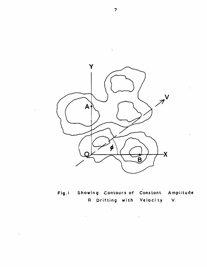
Fig.l

7

Showing Contours of

R Ori1ting wi th

Constant Amplitude

Vcloci ty V.

8

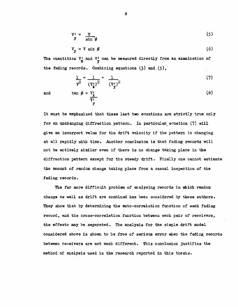
v• = v (5) Y sin ~

vy = v sin r6 (6}

The auantities V1 and V' can be measured directly from an exam.ination ot x y

the fading records. Combining equations (3) and (5 ) ,

and tan f6 = v• ...!... v•

y

(7)

(8)

lt must be emphasized that these last two eauations are strictly true only

tor an unchenging diffraction pattern. ln particular> eauation (7) will

give an incorrect value tor the drift velocity if the pattern is changing

at all rapidly w1 th time. Another conclusion ie that fading recorde will

not be entirely similar even if there is no change ta.king place in the

diffraction pattern except tor the steady drift. Finelly one cannot estimate

the am.ount of random change taking place from a casuel inspection of the

fading records.

The far :more difticult problem of analysing records in Y.ilich random

change as well as drift are combined has been considered by these authors.

They show that by determining the auto-correlation tunction of each fading

record, and the cross-correlation tunction between each pair of receivers,

the etfects may be separated. The analysis tor the simple drift model

considered above is show.n to be free of serious error When the fading records

between receivers are not much different. This conclusion justifies the

method of analysis used in the reaearch reported in this thesis.

9

2.2 The Mechanism of Scattering from an Irregularity in Ionization

The Booker Theorz

The proeess by which sn irregularity in ionization seatters a radio

wave has been investigated by Booker in a paper read to the Conference on

Ionospheric Propagation at the Pennsylvania State College in July 1950·

The theory is adapted from a paper by Booker and Gordon (14) on tropospheric

scattering. Booker shows that the power scattered at an angle e to the

angle of inci denee and sn angle )( w1 th the direction of the incident field

is cr (9, X) gi ven by

( 2u l) 3 sin2 X

= ~ · (AN\ 2

~(1 +( ~1 sin ~)'J2 TJ cr(&, X) (9)

per unit solid angle, per unit incident power density, and per unit

macroscopic element of volume.

where 2 (~) = mean sQuare fraetional deviation of the electron densi ty

from the average

= wa.velength in the medium

= ~ (fm is the critical penetration frequency) rn

= scala of turbulence, a m.easure or the radius of a 11blob 11 •

Booker's development or this expression is given in Appendix I. It is not

otherwise available in the literature.

For scattering at vertical incidence, X is nearly 90° and sin2X:::::.L

If !:t'!Il:_ >> 1, (blobs large compared to )..} the power scattered backward is À. 4

proportional to ).. • If kJI.!. <.< 1 (blobs small eompared to )..) , the power )..

scattered f'orward or backward is constant, independant of )... This type of'

scattering from (relatively) small clouds of ions is believed to be

10

responsible for the spread echoes from the F region at night, and the

high freouency echoes from sporadic E. Booker 1s theory is a significant

advance in the study of small scale effects in the ionosphere.

ll

III EXPERDJENTAL TECHNIQUES

3.1 Experimental Apparatus

A vertical-incidence ionosphere sounding eauipment for the study

of fading is essentially a radar-type installation with the addition of

extra receivers which are spaced on the ground to sample at different

points, the echo returned from the ionosphere.

Radio-freouency pulses are radiated upward by a delta antenna. The

entenna is supported on the roof of the Eaton Laboratory by a 60-foot steel

mast shown in Fig. 2. One of the sauare receiving loops can also be seen

on the upper platform of the roof. Two more of the reoei ving loops can be

seen in Fig. 3 on the top of the city reservoir adjacent to the Eeton

Laboratory. The cables going from the receivers in the Laboratory to the

loops are suspended over the roadway and lie on the top of the reservoir.

The central recording station is shown in Fig. 4. In the left-hand

rack are two transmitters (one spare), a mainsdistribution panel and the

power supplies. To the right, the second rack oontains the monitor cathode

ray tube, chassie for generating the gate pulse for selecting a particular

echo and for tuning the pre-amplifiera at the base of the receiving antennas,

and a receiver, (no. 4). Next is the recorder with motor-driven camera,

and finally, three recei vers (nos • 1, 2 and 3) • Another view of the

recorder wi th the camera removed to show the two cathode ray tubes and the

two lenses of the camera is shown in Fig. 5.

In Fig. 6 are shown the layout of the recei ving antennas, and the

method of presentation of fading records. The recei ving-antennas are at

the corners o:r a right-angled triangle, of lOO .metres to the si de. This

distance was found to g1 ve the greatest number of usef'ul records, being

long enough to show a convenient time shift between records, yet not so

long tb.at the records were appreciably di ssimilar. The antennes are aligned

Fig . 2 Singlf D(llta Anttnna ùn tht Eoton

Laborotory w i th N o Rf c e iv in g Loo p in Situ.

Fi9.3 Anttnnos 3 and 4 in Position on lhc

City Rtstrvoir

14

Fig. 4 The Central Recording Station, showing in order from the left,

the Transmitters and Power Supplies, the monitor C.R.T. and Control

Chassie, the Recorder, and three Receivers.

15

Fig. 5 The Recorder with Camera removed.

_R~c. 1

Rec. 2

Rec. 3

16

Ant. 1

lOO m.

A nt. 2 lOO m. A nt. 3

Antenne Ar rang~ ment

Double B~am C.R.T. s

Photographie Recorder

One Second Time Markers

-------

Moving Paper

Fig.6 Receiving Antennes and Recorder

"0 c

.c u

L..

.c

u.

0 ~

0 (\')

"' -E

"0 u L. 0 0 u ~ a:

-0

.,J

L..

0 n.

~

>

18

·,

1 '

1 )

l J 1 ' 1 \

1 : 1 .

1 )

1 ) 1 1 1 ·.

1 )

l 1 ) 1 / 1

1' ~ t 1' \ 1 (

1 ) 1 J

r i ) 1

1 ) 1 .

1 · , 1 ,

f ) 1) 1 \ 1 1 1 )

i J 1\ 1 )

1 )

!l 1 ( 1\ ~/

l> If ,. J? 1 •

0' c ·-

E ~

0 ,.... N

c 0 ·-

u.

,..., 0

~ L.

0 u w Œ

-0

~

L. 0 a.

CD . 0'

u.

u 0

w >

c

E L.

0 ~

en u ·-

"' 0 c 0 -c 0

l9

vertically in the north-south plane, for reasons which will be made

clear later. The signals picked up by the antennas are carried on cables

to the three recei vers, where they are ampli fied and detected. A:t'ter

passing through a selective gate, they are impressed on the deflector

plates of two double beam cathode ray tubes. The iiiiBges on the C.R.T.

faces are focussed on moving photographie paper as show.n. The centre

record is seen to be inverted with respect to the other two. This is a

consequanc~ of the use of double beam cathode ray tubes, in which similar

voltAges on the two Y-pl~tes produce opposite directions of deflection.

Some typicel records are shown in Figs. 7 and 8.

3.2 Methods of Analysis

In Chapter II i t was shown that two factors, random variation and

drift of the diffraction pattern are contained in each record. The method

of separating these effects by the calculation of auto- and cross correlation

coefficients is mainly of theoretical interest due to the labour involved.

A more practical but still laborious procedure is to calculate the difference

function A to determine the time shift between records.

A= JR(t) - R(t +1")1 (10)

where R( t) and R( t + T) are the amplitudes of the signal

at time t and t + T , the average being carried out

over t, for different values of ~ •

In Fig. 9 are shown several of the results of calculations from one

record. The process involves measuring the amplitude of the signal at one

second intervals for several minutes of record depending on the fading

speed, then finding the m.ean value of the differences taken ·wi thout regard

'0 c.. 0 u CiiJ a::

20

0

N 1

VI

-o c 0 v CiiJ

"' ~

Il

<J

c 0

..,J

v c ::J u..

c 0 ..,J

0

w 1.. 1..

0 v 11'1 VI

0 1..

u 0\

0

u..

21

to sign, between the :fading curves from two recei vers. The procedure is

repeated a:tter shifting one curve one second with respect to the other,

and so on. This process takes at least :tour hours for each record. Never­

theless 1 t was done to check the measurements by a more rapid method liln

enougn cases to ensure that no serious error was being made.

The more rapid first used by Mi tra and Krautkramer forma the basis

for the analysis in this thesis. The positions of the maxima and minima

in the fading curves from the three recei vers are m.arked on the record.

The average time shift between corresponding maxima and minima is :tound

:tor tv.JO fading curves. A second determination :tor the two recei vers in

a line at right angles to the f'irst two is made. The two ti me shi:tts so

determined are used to calculate the apparent drift velocities. Enuations

(7) and (8) are then used to :tind the drift velocity on the ground.

Neither of the last two methods gives a measure of the random fading,

which could cause a serious error in the end result. The thoory shows that

the error is unlikely to be large i:t the fading curves between reoei vers

are very similar. Renee records Which have been analysed have been selected

on this basis and a subjective weight allotted depending on the correlation

between the fading curves from the separate receivers.

3 ·3 Errors in Wind Measurements

Errors in wind measurements can be divided into tv.JO groups, first

those involving analysis of records, end second those caused by polarization

fading e:tfects. The fundamantal measuremnt obtained from the records is

o:t time, the time lag of corresponding ma.zima and minima. The measurements

are made with a 1/50 inch scale marked on a plastic ruler. Ten divisions

ne arly correspond to one second (1.0.3 seo a. actually). The di visions can

be apli t, g1. ving a maximum accuracy of .:t. 1/20 sec. Subtracti on of the ti me

22

readings g1 ves an error in the result o:f :t. 1/10 second.

In the case ot very short ti me shifts, that is records of high

velocity winds, this is the limiting factor. The measuremmts of wind

magnitude and direction are at beat good to only 20%, w1 th an upper limi t

(of resolution) of about 1000 metres per second on the ground.

A check on this method of estimating time differences was made a

number of times by calculation of 4 function' v.hich are statistically far

more reliable. Some resulta of the check are shown in the ibllowing table.

Record Method of Number Measurement

355 A

Time 1ag

Â

Time 1ag

Time Differences, seconds

Rec. 1-2 Rec. 2-3

0.58

o.u -0.45

-0.32

0.17

0.16

-0.57

-0.65

Wlnd Magnitude, m/s

88

120

70

70

Wind Direction

The tw methode give comparative resulta, though the 6analysis is much

more time consuming.

The other known sources of errer are due to the peculiar polarizatiun

of the echoes returned from the ionosphere. The two magneto-ionie modes

are elliptieally polarized in opposite senses. The orientation of the

ellipse at the ground apparently changes (rotates) w1 th a period of the

order of the observed fading (22). The resu1t is to give an apparent time

displa.ce.n:ent of the fading at tw antennes at the same po si tien on the

ground, but oriented in different vertical planes. Some records showing

a spurious "drittn in this manner have been published by Mitra (10) who

first pointed out its harmful affects. The errer introduced by as little

as 30° difference in the vertical planes of two antennes is sur ficient to

2.3

disguise all affects due to a real drift. What at first was believed to

be evidence of non-unifo~ drift velocity with increased antenna epacing

was e:v:entually traced to this affect. A fourth antenne, placed at the

centre of the hypotenuse of the triangle of antennes gives a ready check

of the constancy of the apparent drift and enables doubtful records to be

discarded. The relative significance of fading in a linear antenna due

to this cause has not yet been tully investigated.

A further cause of error is what may be called "polarization" fading.

This is fading due to the interference between the two magneto ionie com­

ponents. Since the components travel different paths, and the path lengths

are probably changing steadily, the relative phase of the two eomponents

changes eyclically, produeing an almost sinusoidal fading pattern. This

can often be detected as a ripple on the random fading caused by the

scattering process, and records which showed this characteristic were dis­

carded.

'There are severa! 1:1ays of reducing the influence of polarization fading.

One of the magneto-ionie modes can be selected with the movable gate, if

the modes are separated in height by choosing a freouency near the cri tical

penetration freouency. This invol vas opera ting in a narrow frequency band,

which may be occupied by other transmissions, or the echoes may be "spread11

in height so much as to be useless. There is no signiti canee to an "ampli­

tude" Vlben a score or more soattered echoes from apparent heights differing

by tans of kilometres are combined in the echo.

Polarization fading can be neglected during the daytime, if the operating

freauency is lesa than 75% of the critical penetration freouenoy of the layer.

This useful method of avoiding polarization fading occurs because the extra­

ordinary mode is highly absorbed at freouencies of three megacycles and

below.

A third method of avoiding polarization fading has been described in

Appendix II. If a nearly circularly polarized wave is propa.gated, ot that

sense which at the time is most favourable tor retlection, the unwa.nted

mode is so weak as to be insignifica.nt. The ordina.ry (left-handed) mode

is usua.J.ly transmitted, as in general it is the most favoured mode e:xcept

close to the criticsl freauency.

The use of a tourth recei ver and an tanna as mentioned above, of a

transmitting antenne. to fa.vour one magneto-ionie component, and an experienced

observer to analyse the records,can be relied on to avoid serious errors

due to pola.rization affects from attect1ng the measurements.

3 .4 Recording PJ:ograms

Sb.ortly atter the reeording was begun, it was learned that an agreement

had been made between a group at the National Bureau of Standards in Wash­

ington and the Cavendish group, to measure winds on three deys each month.

The resulte were to be com;pared tor evidence of world-wide wind systems in

the upper atmosphere. It was theretore decided to record as much as possible

on these 11 internationsl days", and to make the data available tor eompa.rison

with the other two groups. Further, if records were taken on deys sel.ected

by an arbitrary system, the tendancy for a subjective selection of recording

daye muld be overcome.

This wlicy was followed from August 1960. Records were taken until

October in Ottawa, and from December in Montreal. No records were taken

during November as the eauipment was in the process of erection. Data were

obtained on other daye as well, vmen conditions in the ionosphere were

disturbed during the international daye.

In all, 1154 recorda of an average length of four minutes, were

obtained. About 500 wind determinations were made, evenly di vided between

E and F regions. A smaller percentage of uaeful recorda waa obtained

during the winter months. Midday absorption at lower freauenciea and

spread echoes at nigb.t caused poor records. Other factors \'il.ich made

recorda useless for wind determinations were fading wb.ich was too slow,

too rapid, or too shallow, interference from other transmissions, and

low signal-to-noise ratio. Of these, only the last can be affected by

improvements in eauipment or technioue.

26

IV WIND ME.ASURI!lŒNTS

4.1 Mean Drift Velocity

The re sul ts of measurement s of dri tt of the diffraction pattern on

the ground interpreted as due to wind in the ionosphere are gi ven in this

chapter. The wind velocities shown are half the magnitude of the drift

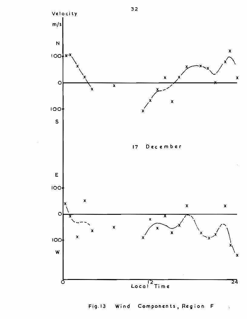
velocity on the ground. In Figs. 10, 11, 12, 13 are shown a few of the

observationsc.of winds on typical quiet deys. Two plots, one for each vect~r

component, represent one wind determination. A casual inspection of the

observations from the E region shows a trend for a wind vector increasing

towards the north during the afternoon, and having a minimum eastward about

noon. This trend will be discussed in more detail later.

The histograms of Figs. 14, 15 show freauency of occurrence against

wind velocity in metres par second for the E and F regions respectively.

The mode or most freauent velocity is 80 metres par second for the E region

and lOO metres par second for the F. These figures are not tru1y indicative

of a difference in wind velocity between the two regions because the

observations were not complementary. The tendency has been to record on

E region echoes only during the daytime. Most of the daytime F observations

were made because E echoes were not obtainable. Also, E region observations

are, with the exception of a few E sporadic echoes, entirely restricted to

day1ight hours.

4.2 Diurnal Wind Variations

Observations tak:en over a few deys served to show tb.at a regular

variation of the wind vectors occurred in the E region. To learn the

nature of this variation, the wind components were grouped into intervals

of one hour, centred on the hour, and the weighted hour1y averages obtained

as shown in Fig. 16. About 250 observations tak:en over a period of

27

thirteen months are incorporated in the data. The hourly means fall on a

smooth curve, of nearly 12 hour period , and about 40 metres per second

amplitude. The mean values obtained before 0600 and atter 1700 hours are

unreliable because of the paucity of observations obtainable on the E region

outside of' the day1ight hours. The two curves in Fig. 16 are believed to

represent the true diurnal wind variations in the E region. The cause of

the predominately semi-diurnal variation is discussed later.

No such variation is f'ound in the F region observations. There may be

a tendenoy for winds to blow east in the daytime and west at night, possibly

reversing in the winter months. The data are not complete enough to deter­

mine this trend more defini tel y. The hourly mean values of the wind oom­

ponents for the wbole period of' observation are more or 1ess randomly dis­

tributed about the datum line and do not show the smooth variation of the

E region hourly eans.

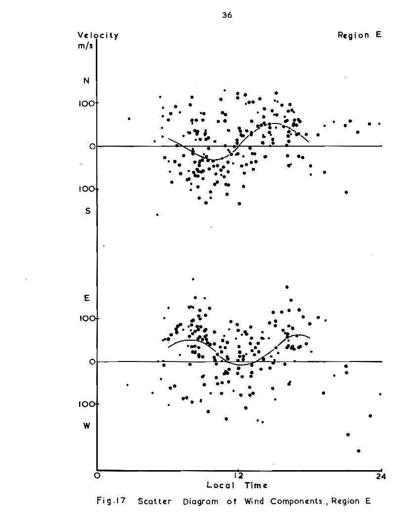
All the data for the E region are shown on the scatter diagram of

Fig. 17, and for the F region in Fig. 18. The observations considered

lesa reliable are shown by dots of a smal1er aize. For convenience, the

smooth curve of Fig. 16 is shown on the scatter diagram for the E region.

The observations are seen to faU in a random manner about this curve.

4.3 Variation of Wind Velocity with Height

Meek has reported (23) radio observations at Baker Lake (66° N, 94°W)

of moving clouds in the ionosphere which aP.Pear to drift over the ionosphere

station with velocities of the same order as those found from fading

observations. However he has noticed tbat the velocity increases from

about llO m/s at lOO km. height to 330 m/s at 300 km. Baker Lake is

within the auroral zone, and a comparison of resulta of wind measurements

from a station outside the auroral zone is of interest.

28

The wind velocity plotted against height for the fading measurements

is show.n in Fig. 19. A similar affect to that observed by Meek, if

present, is certainly much smaller and less noticeable.

Velocity

m/s

N

100

29

•

0~-----------------,~----------------------------

100

s

E

100

100

w

0

•

10 July

•

12 Local Tim~

• •

F i 9. 1 0 W i n d Co m p o n ~ n t s , R~ g i o n E

24

Veloc.ity

m/s

N

100

30

• •

0~--------------------------------~~------------

100

s

E

100

100

w

0

14 August

12 Local Time

•

•

•

Fig.ll Wind Components,Region E

Vt:locity

m/s

N

100

0

100

s

E

100

0

100

w

• •

•

•

•

31

• • •

_... ./ •

•

21 March

•

• ./. •

0 12 24 Local Ti mc

Fig.l2 Wind Compont:nts, Rt:gion E

32 Vcloci ty

m/s

N

x 100 x .. x

\ x \

x 0 x

x

100

x 1

x

x

s

17 Dccczmbcr

E

100

x )( x x \

0 / ' , __ ......... x 1 \ ' ~x / .... )( \ 1 \ x x ......, _..,x

100 )( x x

w x\

x

1 Lo ca 1 Ti m cz

Fig.l3 Wind Componcznts, Region F

UJ

c 0 0'1 ... a:

..... 0 .... w .0

E ::;, z

33

.,. c 0 ~

a > .... "'

0 .,. N 0

.0 0

>-.., ·-u 0 w >'

0 0

c 0

0\ till

a:

UJ

.n tl ... v 0

tl

> '0 c

3:

-0

E 0 ._ 0\ 0 ... tA

::r:

u..

u..

c: 0 at .. a:

""' c - 0 0 .... &.. 0 w >

.&J &.. .. E "' ::::. .0 zo

0 N

34

0

c: 0

u..

c:

u v 0 0

.... 0

E 0 L. at 0

:r .l.i1

u..

Velocity mjs

N

50

0

50

s

E

50

0

50

w

0

x

x

35

x

~x ' x 1 \ " x

x x ...._/ x

/ /x

x

x-x "x

x

12 Local Timc

Region E

x

x

x

x

x x

24

Fig.l6 Hourly Averages of Wind Componcnts, Region E

V~locity

m/s

N

100

0

100

s

E

10

10

w

0

Fig .17

•

•

• • • • • • • • • •

• • •• • •

•

• •• •

•

Scatt~r

..

36

• • • • .. .. , .. • •

•

• • • • • • •

•

• •

tl A • • • •• • •

• • • •

• • • • • ••• •• • • • • • ... . ... .,....,-· ,, \ ..... . .. ' :~" 1 • : •

• • •

•

• • • • • ..

• • •

12

• • • .. • •

• •

• • • •

• •

1

• •

Loc a 1 Tim t:

Regi on E

• • • • • • • •

•

•

• •

•

• •

•

• •

24

Diagram of Wind Compont:nts, R~gion E

Vtllocity m/s

N •

•

•• 10

s

E

• 10 •

• • •

100 • • w •

0

• • • •

•

•

• • •

• • • •

•

• •

• • • •

• • • • • •

• •• • •• •

••• • • •

• •

•

• •

•

•

•

• • • •

•

•

• • • •

•

• • •

• • • •

• •

•

• •

•

•

•

•

• • •• ••

• • •

• • •••

•

• • • • •

•

•

•

•

•

• •

37

•

• •

•

• • •

• • •

• •

•

•

• •

•

• • • •

• •

• • • ••

•

Local

•

• •

• •

•

• • • • •

• •

• •

•

• •

•

• .. •

• • • • • •

• •

• • • • • •

Timtl

• •

• • • • •

• • • • • •

Rtlgion F

• • •

• • • • • • • ••• • • 1. • •• 1 . .,. . -.. ;

•.#. • ••

• •

• • •

\ i•• • •

••

•

., • • • • :.. . •

••

• • • •

•• ••

•

•

•

•

•

• • • • • • •• • • • • • • • • • • fllj, •

• • • • • • • 1 • • • • • ..., • ' • • • .. . . ·., ••• • • • • • • •• •• • •• • ,. • •

• • •• • • • • • • • •

4

Fig. 18 Scotttl r Dio gram of Wind Compontlnts, Rtlgion F

38

Apparent Height km • •

400

300

200

•

100 •

• • •

• • • • • • •••

• • • • ,. ••••••• ..

• • ... . •• • • • • •• .. • • • • •

••• ... . ., .... ' • • •• • • • . ' •lw. • • • • • • • .. • .... •• • .,. -· •• ... • .... .. •

•• • .. ... •c•• (··: • • • .. ••• • • .. •

•• • • • • • • • • • • •

• . .. . . ., . . -~ . . . \1 • • ._. • • "r: •

• • • ' .. i. "J • &. • • • • • • •• • , • • • • s· .. • •.. '' r '• 'i- :(. ' •• • .. • • .,., • .... 4WM..J• .,....... •• • .. "-.1 • •

• .. ·-·- .. • .. ••

•

• •

• • •

•

• • • •

•• •

•

•

.. •• •

•

•

-•

1

•

•

• •

• •

•

• • •

•• •

• • •

•

• • • •

• •

•

Q._----------------~----------------+---------~--1 00 ve ! 0 c i l y 200 m 1 s

Fig. 19 Height ogoinst Wind V«locity

39

V .AN.ALYSIS OF PERIODIC WIND VARIATIONS

5.1 Harmonie An~lysis

Winds in the upper atmosphere are produced by differences in air

pressure, which may be due to a variety of causes. The purely gravitational

forces of the sun and moon causes pressure differences vmich have periods

of half a solAr and lunar day; these forces cause the predominately semi-

diurnal tides on the oceans. SolAr heating causes a variation which is

mainly diurnal because it affects one side of the earth at a time. UltrA-

violet and corpuscular radiations from the sun cause variations which may

have diurnal period but VAry greatly from day to day. In this chapter

harmonie analysis will be applied to the wind data to find and test the

significance of periodic varir-~tions. Non-periGdic effects will be considered

in later chapters.

The harmonie analysis of discontinuous data like the wind components

of region E is the process of fitting the data to a curve of the form:

Bu cos nt + bn sin nt

or alternately,

en sin (nt + E)

J 2 2 where en = an + bn

E = tan-1 an

bn

(n=l,2, •••••• )

The harmonie amplitudes are calculated from the mean value of the wind

vector at each hour by evaluating a and b according to the formulee in n n

Appendix III •

).2 Sol~r Harmonies, Region E

Because the data for the E region winds are not complete for 24 hours,

the diurnal (n = 1) component cannet be deterndned although it is undoubtedly

40

present. Before investigating the higher harmonies (n = 2, 3 ••• ), it

is necessary to determine Whether or not the hourly means are significant.

To give an estimate of the scatter due to all causes other than the solar

variation (the error), the scuare of the st~ndard devi8tion or the variance,

is calculated. (See APpendix III).

= << (yp - yp)2 Variance of hourly meens - (( _ _ n - 12

where Yp is an observation at hour p (p = 0, 1, 2 ••••• 23)

Yp is mean of all observations in interval p ! 1/2 hour

n is the total number of observations.

Then the variance of the hourly means Yp from the general mean y is

calculated. If the deviation of the hourly means is of the same order as

the error, then there is no effect dependent on solar hour.

Variance of Yp from y= Z np (Yp - y} 2

n' - 1 where y =Il,, the mean of all observations irrespective of hour,

n ~ is the number of observations at hour p,

n' is the number of hourly means.

The results of the detailed calculations shown in the appendix are

given below.

North wind component

Vl'lriance of Yp from ~

Variance of Tp from y

30.56

13879

East wind component

3332

12366

Whether this difference in variance is significant is found from a cal-

culation of the Z transformation gi ven in the appendix. It is found that

the probability of obtaining this difference by chance is lesa than one in

a thousand, for beth wind components. From this it is concluded that a

significant affect dependent on solar hour is present in the E region data.

41

The hourly means can then be used for a calculation of the harmonie

components. The resulta are shown below for

12 hour wind harmonies (m/s)

North ward 33·9 sin (2t - 10°)

E~stward 22.7 sin (2t 87°)

8 hour wind harmonies (m/s)

Northward 13.2 sin (3t - 107°)

Eastward 27.7 sin (3t + 75°)

n = 2 and n = 3.

(11)

(12)

(13)

(14)

The formulae used for finding the harmonie components are applicable

to any form of discontinuous data, hence the resulta may not be significant.

By determining the coefficients of correlation between the harmonie eom­

ponents and the data, the signifieance of the harmonies ean be found. This

has been done for the semi-diurnal wind eomponents. The probability that

harmonies of this amplitude could oceur by chance in the data is lesa than

one in ten thousand. The semi-diurnal harmonie variations are signifieant.

It is still possible that the harmonies are a result of persistance of

strong transient effects. To investigate this possibility the data are

di vided up into periods of roughly 50 observations each. The four periods

e:x:tend over a year. If the harmonies eomputed from each group are mutually

compati ble, then the affects are undoubtedly IB rsistent. The harmoni c dials

of Fig. 21 have been devised for displaying this type of data. (See

.A;ppendi:x: III}. The vectors from the origin give the time and amplitude of

the first maxima of the harmoni cs. The solid line shows the meen vector for

all the points on the dial. The circle centred on the end of this vector

is the probable error circle, such that of an infinite number of points in

a Gaussian distribution, one half would lie inside this circle. If a

similar circle were drawn passing through the origin, one in seven points

42

would lie outside it in the case of the northward component, and one in 112

for the east ward compone nt. In spi te of the sma.ll number of groups, the

tests show the harmonies are significant.

The harmonie dial gives a more reliable estimate of the probable error

than do es the standard deviation of the mean. If the errors were normally

distributed, the measure of reliaùility of the mean would be found by

dividing the standard deviation by the square root of the nun1ber of observ­

ations. This is not a valid procedure unless a further test is made to

ensure that the errors are normal. The number of independant observations

may be reduced by conservation. The ouality of conservation in geo-physics

is the tendency for one observation to be followed by another not much

different. Conservation randers a simple calculation of the standard

deviation invalid.

5·3 Lunar Harmonica, Region E

The previous section has established the significance of the solar

variation of the E region winds. The best estimate of this variation is

the s;nooth curve through the hourly mean values shown in Fig. 16. If en

affect dependent upon lunar time is present, it is included in the deviations

of the individual observations Bbout this curve. If the ordinAtes represented

by the hourly values of this curve are subtracted from the indi vidual

observations, the residue will contain the lun~ affect and errors of

measurement but no sol::~.r affect. If the data is then related to lunar time,

where the time of upper transit at Greenwich is considered lunar noon, the

seme methods of search for harmonie components mey be applied as before.

This has been done (Fig. 21); the detailed statistics are glven in

the appendi:x:. The final calculations of variance are gi ven below.

Variance or Yp rrom'P

Variance or Yp rrom y

43

North w.ind com:ponent,

2753

5879

East wind com:ponent

2809

5909

The dirrerence in variance could occur by chance less than one time in

twenty. From vtlich it is concluded tb.at an errect relating to lunar time

is present.

The semi-diurnal variation is known to be dominant in the case of the

lunar gravi tational rorce. To test the rit or a single semi-di urnal wave,

the variance of 'Yp from the corresponding ordinAte or the harmonie. YP,

has been calculated. It is found that the dirference between this variance

and the error (vA.rümce of Yp from "Yp) is not significant. Hence fitting

or other harmonies is not justified. This el so allov;s all the data to be

related to 12 lunar hours, thereby increasing the reliability of the hourly

means.

The semi-diurnal harmonie w.ind com:ponents are found to be:

North ward

Eastward

23 • 7 sin ( 2 "t" + 68° )

20 • 5 sin ( 2 "Y - 41° )

(15)

(16)

A correction has been made to change from Greenvdch lunar time to local

lunar time. The correlation coerficients have been calculated and the

probability that the se harmonies could occur by chance i s less than one

in tan thou sand.

The harmonie dial test has been a:pplied to the data in the same four

periods as the solar test. The resulte are slwwn in Fig. 22. The harmonies

are significant, the :probability of a point falling outside a circle centred

on the mean amplitude vector and :passing through the origin being one in

12 and one in 8 for the north and east wind components respecti vely.

44

6 North Componttnt

12

• 6

East Componcznt

Fig.20 Harmonie Diois Showing Solor Sttmi-diurnal

Winds in Rczg ion E

Velocity m/$

N

25

s

E

25

25

w

•

45

Region E

•

• •

•

6 12 Greenwich Lunor Time~:

Fig.21 Hourly Me~:ons of Wind Components and Lunor

Semi-diurnol Harmonies

•

•

46 1.2

6

1.2

6

North Componcnt

East Compon~tnt

Fig.22 Harmonie. Diois Showing Lunar Semi-

d i ur n o 1 W i n d s i n Re g i o n E

47

5 .4 Su.Inn'l.Ary of Peri a di c Varia ti ons in Wind. Velo city l"t llO km.

Sola.r and lunar semi-diurnal variations have been found in the region

E wind components, but not in those from Region F. The variations are

significant as regards ta tests applied ta the two w:i.nd components

separAtely. The probabili ty that the se harmonies would appear in bath

wind companents by chance is much less than that of their appearnace in

one companent. There CF\Il be no doubt the variations are significant.

The northward and eastward semi-diurnal wind components have been deter-

mined at a height of 110 km. as fallows.

North ward wind ~m/s) Eastward vJind (m/s)

Sol ar 33·9 sin (2t - 10°) 22.7 sin (2t - 87°) (11,12)

Lunar 23.7 sin (2-r' + 68°) 20.5 sin (21"- 41°) (15,16)

Other harmonies are present in the solar veriation, but probably not

in the lunar variation.

VI SOLAR MTD LUN.AR TIDES IN THE A'I"M:OSl?HERE

6.1 Theory of Tidal Oscillations

The theory of tidal oscillations of the earth 1s atmosphere was

developed to explain the small daily variation of atrrospheric pressure

which has been known to physicists for the past two centuries. Harmonie

analysis of the variation yields large components of 24 and 12 hour period

and lesser ones of 8 and 6 hour period. Of these, the 12 hour component

shows the greatest regulari ty of phase and ampli tude over the earth. This

led Lord Kelvin to suggest that the atmosphere had a free period of

oscillation of about 12 hours. Thermal (diurnal) ,Qnd gravitational (semi­

diurnal) action by the sun excite all modes and the near-resonance amplifies

the semi-diurnal oscillation to the extent that it exceeds in ampli tude

the diurnal variation. The mathemtttical theory has been developed by

Laplace, Lamb, Taylor, and Pekeris. A short account is given by1.dtra (24a),

and a more complete discussion by Wilkes. (25)

The atmosphere is e0uivalent to an ocean of air about 10 km. deep

surrounding the earth. Energy introduced into this system causes a forced

oscillation of the sarne period as the disturbing force. The co incidence

of a free period of the ocean and the 12 hour period of the solar perturbing

force is responsible for the relatively large semi-diurnal atmospheric

pressure variation. Laborious calculations are reouired to find a solution

for the pressure variation with height, and the se have been made by Wilkes

for severa! modela of the atmosphere differing in the assumptions made about

the temperature above lOO km. In Fig. 23 is sho'WD. the result of calculations

on a madel which assumes a gradually increasing temperature above the E

region. Of particular interest is the phase change of 180 degrees at 30 km.

and the progressive phase change occurring at 100 km. An eoua.lly acceptable

Hczight km

120 lu nor

1

1

1 1

sol or

sot , 1

40f // ----~

01

- .....

1 1

1 1

Rez la ti v ct

1

' 1 1

1

.o4 l Pl A m p 1 f t u d ct • 1 ° 91o p

0

Hctight km

120 lunar __ -1

1 1

BOf 1

40t ,.----------""' 1 1

1 1 1

1 1 1

""' /

o· . . . tsoo • . 36oo Pho.scz

F i 9 . 2 3 Th ct Am p 1 i tu d ct a nd Pho scz of S cz rn i-d i u r n a 1 Prczssurcz

variation os 0 Fun c.t ion of Hct i ght ( Aftczr Wi 1 kczs)

~ '10

50

modal with the assumption of a cold region between the E and F layera

gives a different set of curves, rOPinly with regard to the phase of the

pressure oscillation.

The pressure variation at the ground will cause winds of about 40

centimetres per second amplitude. The wind system has been calculated by

McNish (24b), who shows winds blowing from two regions, one almost under

the sun and one on the opposite si de of the earth, and into tv.o regions in

the same eouatorial plane but 90 degrees distant in latitude. The theory

indicates tbat similar winds should blow at ionospheric levels, probably

of different phase, and certainly of much greater magnitude (about 200

times).

It is believed that these winds in the ionosphere blowing ionized gas

across the earth 1 s ma.gnetic field cause a system of currents to flow in a

horizontal plane. The currents produce the ouiet day solar and lunar mag­

netic variations. The predominately semi-diurnal periodicity of the winds

accounts for the large semi-diurnal harmonies in the ouiet day magnetic

variations. The semi-di urnal solar and lunar magne tic varia ti ons are both

about 10 gammas in amplitude, indicating the winds 1nay be about eaual in

magnitude. The conductivi ty of the E region is kno'Wll to be of the correct

order of magnitude for the reouisi te currents to flow, if the vdnds are

of the order predicted by the theory of atmospheric oscillations. The

phase of the pressure variation causing the vùnds at the leval of current

flow has been calculated to be out of phase ;.'li th the pressure variation

at the ground. The leval at which the currents actually are located will

be found from a measurenent of the amplitude and phase of the pressure

variation at some height Vllhich oombined wi th the known conducti vi ty at

that height, gives the correct current system. This accounts for the

51

great interest which has been shawn in the subject of pressure variations

at different heights due to soler and lunar ti des.

For comparison wi th pressure variations estimated from wind measurements

at llO km. the oolar and lunar semi-diurnal pressure variations at the

ground are;

Sol ar

Lunar

0.362 sin {2t + 161°) nw. of mercury,

0.0088 sin (2~+ 114°) mm. of mercury

(17)

(18)

The solar variation was calculated from Wilkes empirical formula (25) for

45.5° N. lAtitude, 75° W. longitude, Vilhich is a point roughlymidway between

Ottawa and }lon treal. The 1 unar va ri a ti on was measured at Greenwich. Lo cel

tirr~ is given in both cases.

6.2 Winds from Sinusoidal Pressure Variations

The northward and eastward vrl.nd components re sul ting from a semi-diurnal

pressure variation are shown in Appendix IV to be:

Northward

Eastward

where 9

P'

Po

t'

w

À

is

- 350

-70 2

~2 + 3 cos 9)

sin3e

the co-latitude

cos (2(~· +~)+à)

~sin (2(~ 1 +À) + h) Po

is amplitude of pressure variation

is the mean static air press ure

is Greenwich time

is the angular velocity of the earth

is east longitude

(19)

(20)

52

The northward wind is seen to be in phase ouadrature 1eading the

eastward wind. In Chapter V the semi-diurnal v.d.nd components were found

to be:

Northward wind m/s Eastward wind m/s

So1ar 33·9 sin (2t-10°) 22.7 sin (2t-87°) (11 ,12)

Lunar 23·7 sin (2"r+68°) 20.5 sin (21" -41°} (15,16)

The winds observed experimentally are seen to be in the correct phase

relationship, wi thin the error of rneasurerr.ent.

The ratio of the amplitudes of the northwRrd to eastward wind components

should be 1.01. The observed ratios are 1.49 in the solar case and 1.15

in the lunar case, again agreeing vdthin the 1imits of error.

This agreement in phase and amplitude is the basis for the belief that

the winds are caused by semi-diurnal so1ar and lun?.r pressure variations.

6.3 Estimate of Pressure Oscillations causing Winds

The relative pressure variation at llO lan. can be estimated from the

winds using eauations (19} and (20}. After adjustment of the phase and

amplitude to fit the ex,pected theoretica1 relationships for the two wind

components in each of the soler and lunar cases, the relative pressure

va ri at ions are fo und to be,

Sol Ar :E.!. = 0.040 sin (2t + 87°) (21)

Po

Lunar :E.!. = o.o31 sin (21" + 149°} (22)

Po

A number of assumptions of doubtful va1idity were made in the develop-

ment of eauations (19) and (20) from waich these resulta were derived. The

semi-diurnal pressure oscillation was assumed to vary .ith latitude in the

same mannar at llO lan. as at the ground. \i.e. as sin3e) The assumption

that vertical motion could be neglected was undoubtedly faulty. A value of

53

6.8 has been assumed for the scala height at llO km. in arder that the

data might be compared wi th Wilkes r theoretical calculation of the pressure

oscillation, and this value is not definitely established by experiment.

As a result, the estimate of relative pressure variation can be relied on

only to the arder of magnitude. The errors mentioned above affect the

~nplitude of the oscillation but leave the phase unchanged.

By comparison, Appleton and Weekes (32) have estimated the relative

pressure variation at llO km. from the lunar variation of height of the E

region, and find the value 0.081 sin (?1"+ 112°), though the interpretation

of their resulta in this mannar is open to some doubt. Their resulta can

be reeonciled with tho se from wind measurements w1 thin the limi ts of error.

By comparison with the seiui-diurnal barometric variations on the ground,

it is seen that the pressure variation at llO km. is 84 times as great in

the solar case and 2700 in the lunar case. From the theoretical calculations

of Fig. 23, the amplification i s 250 in the sol ar ca se and 60 in the lunar.

Also from Fig. 23, the phase angle at llO km. is expected to be 81°

for the soler and 4° for the lunar vari a.tion. This compares favourably

0 wi th 87 for the experimental sola.r case, but unfavourably wi th 149° in

the lunar case.

In conclusion it is interesting to note that Wilkes stated (25} 11In

view of the fact that the ionization in the E region is directly dependent

on radiation from the sun, it is not possible by radio means ta determine

the sol ar oscillation in the E region • 11 In fact an estimate of the solar

oscillation has been made from radio observations and found ta be in

egreemen t vii th that predic ted by the ory. The agreement wi th theory in

the lunar case is not good, but the lunar variation can be reconciled wi th

an experimental determination by Appleton and Weekes. Recently Phillips

54

indicated agreement wi th the solar wind determinations, by reporting a

semi-diurnal variation of 20 + 10 m/s in the E region winds with a maximum

eastward about 0600 hours. (26)

In neither the solar nor the lunar pressure variations was the phase

observed to be in opposition to th at on the ground. For this rea son i t

is difficult to see how the currents responsible for the ouiet day magnetic

variations can be located in the E regi on. The F~uthor suggests tha t the

current system is not confined to the horizontal plane but is closed

vertically. The reason for this view is the much higher conducti vit y along

the lines of magnetic force, aiding a vertical flow of current.

55

VII WINDS AND IONOSP.HERIC STORïYiS

7.1 Ionospheric Storm Indices

The first observations of fading at spaced receivers in May 1950

indicated a movement of the order of 300 metres per second. This occurred

during a period of iono~heric disturbance, as measured by depression of

the noon cri ti cal penetration freauency of the F 2

layer, at the Can~.dian

ionospheric stations. To test the correlation between wind velocity and

ionospheric storminess, a continuous index of storminess was required.

There is at present no generally accepted index, due to lack of knowledge

of wnat constitutes a storm and the freQuent lack of radio echoes during

a storm.

There are two nuantities which have been used as indices of storminess.

The firat is the North Atlantic Q.uality Figure, a subjective estimate by

commercial radio operators of the cuality of' transmission between Europe

and North America. It is considered unsatisfactory on the grouuds tha t it

is subjective, is influenced by such things as the fre0uency of transmission,

and does not bear a functional relationship with a measurable geo-physical

ouantity.

The second index is the K-index of magnetic ac ti vit y. It doe s not

suffer from the 1ast three objections, rut on the other hand, it is not

directly related to the ionosphere. Rather it is a measure of magnetic

storminess, which is knovm. to be connected wi th ionospheric storminess due

to the high frequency of simul taneous occurrence of the tv.Q forma of di a­

turban ce. The connection between the two indices i s indic ated by a coefficient

of cor rel a ti on of 0. 7 between quali ty of transmission and magne tic ac ti vi ty.

(McNish and Johnston, 27)

The K-indices are published monthly by the Dominion Observatory for

the station at Agincourt, neer Toronto. The distance of this observa tory

from the si te of the wind measureiœnts is snall compared to the extent of

ionospheric and rnagn.etic disturbances, which justifies the use of the data

for statistical purposes. The index has values from 0 to 9 and indic at es

the maximum range of the most active magnetic element over a three hour

period. The range of variation in gam.ma.s is shawn baside the appropriate

K value on the ordinates of the next two figures.

7.2 Region E ObservAtions

lviost of the observations of fading were made on the normal E layer which

ocours during the daylight hours. Soma observations were mAde on the E

sporadic layer itlich occurs a few lan. below the normal E, generally duri ng

disturbed periods. The E sporadic records showed very rapid fading, about

120 maxima per minute compared to the usual fi ve to 10, and winds in excess

of 300 metres per second. About 4 per cent of the E region records were

obtained from observations of E sporadic during disturbed periods (K index

five or more). Lesa confidence can be placed in mean 'W.ind velocities deter-

mined from such a small number of measurenents than in those from the mass

of meesure.ments obtained when the K-index was four or less.

In Fig. 24 are shawn the data reduced from all the E region observations,

on logarith.mic axes. The abscissa is wind veloci ty and the ordinate is K­

inde:x:. The mean value of the wind veloci ty for all measurernent s at a given

K-inde:x: is shawn with horizontal bars inàicating the standard deviation of

the mean.

s

85t \

Î4 1

4~ f

!3 1

24~

57

1\>egion E " '"" •< «-• "·•·<'--«~--~-----•w••-· -·-·--<'_"_"''-·---~-··l

1 !

1--4---c

4

t--A

Fig.24 M~an Wind V<Ziocity Agoinst K-lnd<Zx, R<Zgion E

58

The mean wind velocity is sensibly independant of K-index until the

K exceeds four. For K-index fi ve or greater, the mean wind veloci ty is

three times higp.er, though as has been pain ted out, less reliance can be

placed on these observations. These facts have been considered in the

investigation into harmonie variations discussed previously, by the

rejection of E region measurements taken when the K-index exceeded four.

7 ·3 Region F Observations

Unlike region E, the F layers (200 to 600 km.) reflect radio waves

day and night. Good wind measure.rœnts are more difficult to obtain from

the F region because the echoes are often sprea.d in height, particularly

during the night.

In Fig. 25 are shawn the data for the F region correspondi ng to the

previous figure for the E region.

The trend towards increased w:ind veloci ty 11d th increasing K-index is

evident. The data are not considered suffi cie nt to justify the fit ting of

curve. A high po si ti ve carrela tian between wind veloci ty and magne tic or

ionospheric stonuiness clearly is present. This correlation is assumed to

explain why no regular daily variation was found for the F region winds.

7.4 Discussion of Storm Winds

If the wind measurements are valid, it has been shovm. that the w:ind

velocity in the F region is directly related to the state of storminess in

that region. Miner disturbances èb not affect the E region though the re

is reason to believe that severe disturbances do. A posai ble e:x:planation

of this phenomenon is that the disturbing agency a1ters the ionosphere from

Rbove, the depth of penetration being proportional to the severity of the

disturbance. This suggestion is compatible with the common assl.Ullption that

r K

60<>! 8

400+

\7 24of

i6 \ t

14 si 15

as.; 1

Î4 1

4Bt l !3 ;

1 24-+

1 j2

i

59

Region F --·~~· ·-····_..~---··-~~·---·-·····-· .. -·- .. --··"-... --..... -,.,.,,' ·"·--... l

1

...._._X___,

12i ~-----------+--------------------------------------4

10 ao 90 roo ISO Vclocity m/s

200

Fig.25 Meon Wind Velocity Agoinst K-lndext Region F

60

ultra-violet and corpusculF~r radiations from the sun are the disturbing

l"lgency.

The success of the use of the m.agnetic K-indax as a measure of

storminess in the ionosphere indicates a causual relationship exista

between iono~haric winds and magnatic ac ti vit y. Logically such connection

might lie in the electric cuiTents which auch winds muld induce in the

ionized layera.

61

VIII CONCLUSIONS

The fading of radio echoes has been observed at spaced receivers.

A diffraction pattern on the ground was seen to drift in a regular manner

such that its velocity could be determined. The drift veloci ty of the

pattern formed from E region reflections varied regularly when observed

for some days. From the nearly semi-diurnal period of the variation, and

the quadrature of phase between the northward and eastward wi.nd components,

it has been assumed that the wind variation is caused by a corresponding

pressure variation at the level of reflection. The pressure variation is

predicted by the theory of tidal oscillations of the earth 1s Btmosphere.

Variations corresponding to both solar and lunar tides have been detected.

This apparently establishes the premise that the dr.ifting diffraction

pattern is due to a bodily transport of the air mass and ion cl.ouds in a

horizontal plane. The movement of the ion clouds is supposed to be the

major cause of fading of a singly reflected radio vmve.

The tidal v.tinds have not been observed in the F region. The wind

velocity in this region has been observed to increase during magnetic and

ionospheric storms. A corresponding increase in w.ind velocity in the E

region occurred only during severe storms.

62

APPEl\TDIX I

THE BOOK.ER SCATTERING IJHEORY FOR 'JlΠIONOSPHERE

The expression given by Booker and Gordon (14} for the power scattered

by a tropospheric irregularity at an angle 9 to the angle of incidence and

and angle X wi th the direction of the incident electric field is:

. 3

(~J) cr(El,"X) = (23)

per unit solid angle, per incident power density and per unit macroscopic

elenent of volume.

where E~~)~ is the mean square fractional deviation of the dielectric

constant from the average,

À is the mean wavelength in the ruadi um

J is the scale of turbulence, defined auch that at a distance l, the

auto-correlation function of the dielectric constant has declined

to 1 • e I:ooker extends this to the ionosphere as follov!S:

The dielectric constant in the ionosphere is 2

f = E0 -Ne

~2 = E (1 - ~}

o w2

where N = number of free electrons /cu. metre

e = electronic c:targe

~ = dielectric constant of free space

m = electronic mass

w = free space radial frecuency

2 ~=~

€m 0

(24)

This expression negl.ects oollision and the earth 1 s magnetic field.

Renee,

(25)

Enuation (2.4) can be. put in the form

2 2 ~o} = 1 -(ùtr)

).. w (26)

which, substituted in (10) gives

- 4 2

(~)':.(U (~) WN

= ( ~ ) 4 ( â:) 2 ( ~Nt 0

(27)

Final1y from eouati<?n (1}, the expression for scattered power cr is obtained,

(m:r sin2

'l(

Cï( G, ~) = ------~--=--}. [1 + ( ~ .( sin ; )

2 t (%1 sin

2)t

= -------~-------------

Two wave1engths are invo1ved, the incident wavelength À in the medium

and a wavel.ength ~ wbich is a constant depending on the ele etron den sity.

Booker used this for.mula (6) to explain scattering from E sporadic clouds.

64

APPE.NDIX II

EXPERilviE1"TAL Al?P.ARATUS

1. Receiving system

Antenna

An unbalanced unshielded loop, consisting of two turns of multi-strand

copper antenna wire, eight feet in area was constructed. It wes calculated

that the loop had an inductance of 17 ~enries and tuned from 1.7 to 5.4 mc/s

with a 50-500 ~d. condenser. If necessary to tune above 5·4 mc/s one turn

could be shorted to increase the tuning range. Identical loops were built

for the four channels.

Pre-l'lmplifiers

Each of the four identical pre-amplifiera contained a cathode-follovver

for matching the loop to the line, a small power supply, and a variable

condenser for tuning the loop. The oondenser was rotated by means of a

selsyn motor controlled from the central recording station. The circuit is

shown in Fig. 26.

Ca bles

The signal from each antanna ~~s carried to the appropriata receiver by

73 ohm co-axial cable (RG 22U). The A.C. mains voltage and selsyn stator

voltages were carried from the distribution panel to each pre-amplifier by

five-core rubber covered cable. The master control selsyn was switched to

one pre-amplifier at a time for tuning.

Receivers

Four R.C .A. (Canada) type CR91A colllii'ercial recei vers, modified in the

laboratory for pulse reception, were used. A video amplifier was added to

each receiver following the second detecter.

300V.

68 K

An t. 1 1 50·500,.-.P fd.

'--------t~~;f~~~ r·~" f'" T J RF. Cable

S-Core Cobl e

Sc:Jsyn

Power Suppl y

30H

, + 300 V. D.C. 1

2)Afd.

Qi l·Fi lied llO V. A.C.

Fig. 26 Diogrom of Pre·ompli fier

(

c.

2. Transmitting system

Transmit ter

66

The circuit diagram of the transmit ter and modtùator is shown in Fig.

27. The mod ulat or is a bo ot-strap cathode fo llower dri ven by an arti:ficial

transmission line. The oscilla tor is screen-modtùated, and sel:f-biased

into class C operation. This portion of the circuit was developed by the

author :for this application. To increase the nominal power output to

15 kw. peak, an aperiodic push-pull amplifier built at the Radio Physics

Laboratory was added.

Tl

Ov from unit 6

:-J\\[A

Ci5

• d 1 j Trlgger pulsf''

V4

fr o m u nit 7 ·"--

'>

~ R7

"\, ;~ ....

~""B

R

f"

ANTfNNA V2 ~---/.- C3

C2 (-----

j :i, 1 \~--i-- --.. -- ::;: -c·< -500 L2 -

C4 t, ... ~. ~ C6 l1 C7 1 j!u;c •2600( \. ~~· f---t ,- :' ~. C5 2 1

' = 1 +IOOOv

ji + · .... L~:--_ cel J :/ \ --~--TT v C9 V3 ~ T/ Cl

bond switch. L .... =--------'----1

1-----,---~ + 3000 v

Cl4

ANTfNNA

"tIl -1\,/\/'l't LG l7

~ iL 1 l'~__....__- :

~ , -i 1 B_~·· l • A .- t ' Cl7 1 '

R9 Cl6 RIO 1

l .t. ,_l '

" ~ '" ~z t

V5

~

+1000 Power Input plugs

Rl4 /------ c.---" ""

/ . ~ -.J

/ +2600v • ··\ ( .~·- iJ 1 ,. •''i) Rl5 1 \~,0~ \?:Ov 10ogv

a. c. -----

LB L9 LlO lit Ll2 L13

y~~l' 23 C24

Z ~--_1_.----'----L ___ __L __

i- -27.5v from unit 7

Fig. 27 Moduletor and 15 kw. Transmitter.

68

Circuit Components of the Tr,.nsmitter and J:.;odulator Fig. 27

Resistances Condensera

Rl 4.7 K cl 50 !-4.1.

R2 lOO w c2 50 !-4.1.

~ 11 (1.) c3 .1 j.l.

R4 4.7 K c4 12 - 500 tJ.l.l.

R5 100 w c, .1 j.i.

R6 47 (1.) c6 lOO !-4.1.

R7 lOO K c7 lOO j.l.j.i.

Ra lOO K c8 100 j.i.j.l.

R9 100 K c9 50 j.i.j.l.

RlO 1 K clO 50 j.l.j.i.

Rll 500 K cll .1 j.i.

R12 27 K c12 .1 j.i.

R13 4·5 K c13 .002 j.i.

R14 330 K c14 .002 J..l.

~5 330 K c15 .01 1J.

R16 20 K c16 .01 j.l.

R17 2.7 K cl7 .1 j.l.

~8 6.8 K c18 1 j.l.

C19 to C24 .004 j.l.

Tubes

v1 3E29 Inductances

v2, v3 715C 18 to 113 2.5 mh

v4 6x5

v5 2050

v6 3E29

69

Transmitting Antenna

A modification of the delta antenna, described by Oones, Oottony and

watts was used. (28) The modification involves using severa! conductors,

in this case tw::>, for each element of the antenne, to maintain the

impedance more nearly constant over the freouency range from 2 to 20 mc/s.

The conductors are kept apart by spacers, as shawn in Fig. 2.

The base of the del ta was 90 feet long, the height 60 feet. A term-

inating resistance of 800 ohms was placed at the peak of the del ta, at the

top of the mast.

Because of the necessi ty for reducing the unwanted mode of magneto-

ionie propagation, an antenne to radiate circularly-polarized waves was

devised. It consisted of tv;o identical delta antennes, placed at right

angles to each other and suspended from the same mast. They were fed by

netvrorks which advanced the phase 45 degrees in one case, and retarded it

45 degrees in the ether. The two antennes were th us 90 degrees apart in

phase, and radiated a nearly circularly-polarized •vave.

The networks were L-section filters designed to give a two to one

match in impedance as well as the required phase change. One fil ter

operated at each cor1nnonly used f'reouency, with acceptable perfornance over

a 10 percent range of frequency. The elements of the filters are given

in the following table. L-Section Filters

l!'reouency Mc/s

Series Arms

Phase Advance Phase Delay !J.h. 14Lfd.

19 210

16 180

12 130

9.6 105

8.0 90

Parallel Arm

Phase Advance Phase Delay !J.h. 1-J.lJ.fd.

76 52

64 44

4B 33

38 27

32 22

70

The only way tests could be made on the se netv~rks was to observe

the behaviour of responses from the ionosphere. For E region responses

lesa th an 75% of the critical penetration frequency and less than 3 mc/s,

the extra-ordinary ray (right-handed circularly polarized) is attenuated

many db below the ordinary. With one arrangement (2.5 mes net"WOrk) the

mode of propagation favouring the ordinary wave produced an echo 28 db

l:".bove that f:wouring the extra-ordinary wave. It is considered th at

this is a .meesure of the ability of the antenna to reject the unwanted mode.

The other network produced rejection 10 db or greater.

The high freauency networks could only be tested vnen ordi nary and

extra-ordinary echoes were produced separately on the trace. The resulta

of one test are seen in Fig. 28. It CRn be seen that one mode is favoured

in each case. Complete rejection of one component is not to be expected,

since the echoes are elliptically, not circularly, polarized. Some

coupling into the unwanted mode is bound to occur.

......,

{a) (b)

F i g 2 8 M o n i l o r C . R . T . T r a c (Z , 2 7 S (Z p t . 2 1 4 5 h r !> , F1 L a y (Z r , 4 . 0 m c / s .

(a) RiQht -Hand Circuler Polarizal ion 1 F1 .. at 300km. F1° at 350 km, Equal Ampli t udes.

(b) L eft-Hand Circuler Polarizalion 1 F.,_• Suppr(ZH<zd,F1° Gr<zater Amplitu d <z

3. Recording system

Gate Circuits

72

The circuit diagram of the gate cb.assis i s shawn in Fig. 29. The

beginning of the gate pulse is determined by the position of the 'delay'

control, vbich allows the 6.AL5 diode to conduct when the negative-going time­

base saw-tooth wave on its cathode drops below the potential of the plate.

The flip-flop is triggered by this signal, and produces a sauare-wave gate

whose time dur at ion can be controlled. The gate pulse is cancelled once

each second by the output from the one-second oscillator, and is impressed

on the gri ds of the two cati.ode ray tubes of the recorder. The gate action

is produced by brightening the C.R.T.s only when the desired echo appears.

The gate also is impressed on the roonitor C.R.T. so that it rœy be set to

coincide with the echo, as shown in Fig. 30.

R_~Q_order

The recoràer wes produced by A.C. Cossor and Co. of England. Two

double-bearn cathode ray tubes provide four recording chennels. A motor

driven cruner~?t draws 70 mm. wide photo-graphie paper (Kodak Linegrapb. 697)

across the tube faces at a speed set by a chain of gears. The lowest speed

ev ai la ble was ten cm. per second and this >vas reduc ed by a further chain of

ge ars f1 xed externally, as shawn. in Fig. 4. The film s.peed used fbr al most

all the records was one foot per minute, W:lich experience has shown. to be

the most satisfactory speed.

D.C. resto ring diodes were built into the circuits of all four

deflection plates to meintain a constant dBtum line for the signal.

73

:V.10ni tor

Fi,g;. 31 sbows a schematic àiagram of the monitor circuit. The trigger

functions for the time-base, calibrating oscillator, transmitter and gate

8re provided by a multivibrator Which can be lockad to the mains if desired.

The calibrator is a 3000 c/s second oscillator for setting the range marks

on the tirœ -base.

•300 2.1 K + 1!50v fiN j

,-..... SAW-TOOTHI] _\

IIID •\ ·~100

liME ,._ '1 ' l BASE, 6 "l ' ...... , • TO ' l ~---fi.' + RECORDER SLIDING FLIP-FLOP MIXER

CWE SECOND OSCILLATOR SQUARift

Fig. 29 Diagram of the Gate Circuit.

-.,J .+:--

' '

Fig.30 Monitor Troc~ Showing Multipl~

Rtfltctions. Tht Got~ is ovtr the E

Echo at 130 km H~ ight.

7

300V--~----------r---~------.---r-~~

Tx Sync

loooy. ~250K

60c/s Lock

Multivibrotor Cali brator

300V--------~~--------------------~

10~/

6AC7

1 M Gate Sync o j

'----+SOV

":"

.1,....

Time Bose

T.B.

.Il"

'470K

F i g. 3 1 5 i m p 1 i f i e d Sc h e m a t i c o f M on i to r C i r c u i t

...J 0

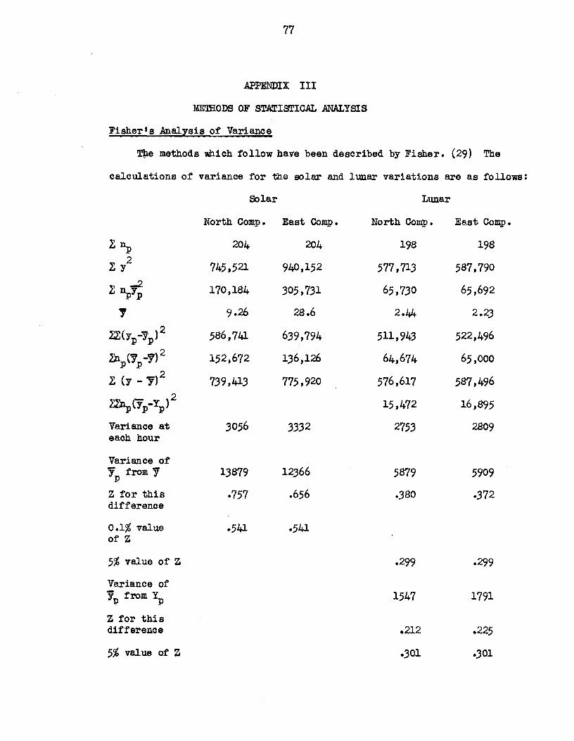
77

APPENDIX III

METHODS OF STATISI'ICAL ANALYSIS

Fisher • s Analzsis of Variance

~e methode Whioh fo1low have been described by Fisher. (29) The

oalculations of variance for the so1ar and 1unar variations are as follows:

So1ar Luna.r

North Comp. East Comp. North Comp. East Com.p.

z~ 204 204 198 198

Ey 2 745,521 940,152 577,713 587,790

-2 ~~Yp 170,184 305,731 65 t 730 65,692 , 9·26 28.6 2.44 2.23

X,Z(yp-lp) 2 586,741 639,794 511,943 522,496

Zn (y _,,2 p p 152,672 136,126 64,674 65,000

z (y- y)2 739,413 775,920 576,617 587,496

~Cfp-Yp) 2

15,472 16,895

Variance at 3056 3332 2753 2809 each hour

Variance of yp from Y 13879 12366 5879 5909

Z for this ·757 .656 .380 ·372 difference

0.1% value ·541 ·541 of Z

5% value of Z .299 .299

Variance of y'P from YP 1547 1791

Z for this difference .212 .225

5% value of Z ·301 ·301

78

The Z transformation is caleulated to find the significance of a

ditterœce in variance from the following formulae,

1 1

Variance of Tp from y Z =- og

2 e . h Var~ance at eac hour

l 1

Variance at each hour Z=2 og •

e Variance of Tp from Yp

The probability at obtaining a value of Z by chance 0.1% or 5% of the time

is determined from Fisher's Table V for the appropriate values of n.

Coefficient of Correlation

The coefficient of correlation is caleulated from the formula given

by Chapman and Bartels (30a).

r = __!!_ ff'{

where r = coefficient of correlation

A = amplitude af harmonie caleulated by ba.rmonic aoalysis

~ = standard deviation of tile data considered as a normally

distributed population, i.e. ~'Y- z)2

1: n - 1 p

The probabili ty ot obtaining this correlation by chance is cal.culated from

the Z transformation. (29).

z =!log 1 + r 2 e 1 - r

In this case Z is nearly norma.lly distributed and it s standard deviation a. z

is 1 , n being the sample num.ber. The ratio of Z to its standard

ln- 3 deviation is computed and the probability ot obtaining it by chance is

found from a. table of the probability integral, (or Fisher's Table II or IV).

79

The calcula ti ons are shown below.

Sol ar Lunar

North Comp. East Comp. North Comp. East Comp.

~ 60.4 62.0 5!i-·3 54.6

A 33·9 22.7 23.7 20.5

r ·397 .259 ·309 .268

z .420 .268 ·318 .275

1 14.2 14.2 14.0 14.0 (l

z

z 5·90 3.81 4·44 3·84 (l

z From F1eher 1s Table II, the probability of obtaining a value of~= 3·74

az by chance is one in ten thousand. The experimental values all exceed this

value, hence the probability of' obtaining tilem by chance is lesa th an one in

ten tho us and.

Harmomic Disl .est

The harmonie dial test has been developed by Bartels (31, 30b). If

tbere is a cloud of N points on the dial, the centroid lX0

, Y0 ) is given by

b x=~ o N

a y=~

o N

where Sn and bn are the Fourier harmonie amplitudes calculated from the

f'ollow1ng formulas. (30c) 2 .,.

a = - X Ya- cos ntr -n r r-1

2 r b = - Z y., sin ntr n r ...._,

wb.ere Yr are the values of' the f'unction to be fitted, at interval.s r= 1,2, •• r

and n gives the order of the halmonic. The affect of smoothing due to taking

hourly means can be allowed for by an appropriate correction. (30d). The

80

points on the di al are found by plot ting ~ upward and bn to the right. The

mean amplitude is (:X:0

2 + y0

2}1/ 2•

The probable error circle is drawn about (Xc, Y0 ) with radius R.Jc

given by: 2 2] 1/2

[

z(bn -Xc) + (~ - Yo) R_g = 0.833

N

In the case of a perfect Gaussian distribution there would be as many points

inside the circle as outside it.

Let the ratio of the mean amplitude to the probable error radius be K. Ji.:o

Then (1/2) ~· -- representa the probabil1 ty that a point will fall outside the

circle with centre (X0

, Y0

) passing through the origin. The experimental

data are gi ven below.

Soler Lunar

North Comp. East Oomp. North Oomp. East Oomp.

xo +33·5 +5.2 -22.0 -3.8

Yo -3·8 -21.2 -13·5 +19.;

~ 20.2 8.4 13.7 11.6

:s:2 2.76 6.8 3·54 2.93 K2

(1/2) 1/7 1/112 1/12 1/S

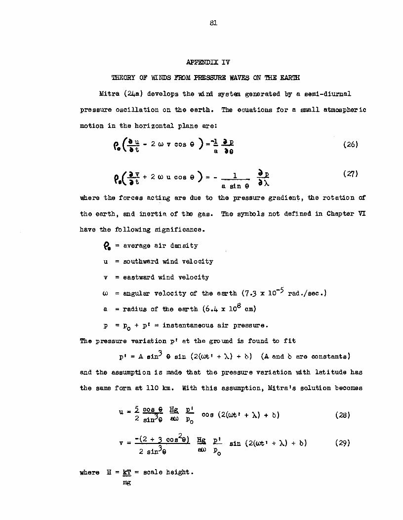
81

.APP.ENDIX IV

IJHEORY OF WINDS FB)M PRESSURE WAVES ON 'l'HE EAR'lH

Mitra (24a) develops the wl.Di systEIIl generated by a semi-diurnal

pressure oscillation on the earth. The eauations :tor a small atmospherie

motion in the horizontal plane are:

e (• u - 2 w v cos e ) = "':! .u 0 at a ae (26)

~.( :~ + 2 wu cos 9) = - 1 a sin 9

(27)

wb.ere the :torees acting are due to the pressure gradient, the rotation o:t

the earth, and inertia o:t the gas. The symbole not de:tined in Chapter VI

have the :tollowing significance.

~. = average air density

u = southward wind velocity

v = eastward wind velocity

w = angular velocity o:t the earth (7.3 x lo-5 rad./see.)

a = radius of the earth (6.4 x 108 cm)

p = p0 + p' = instantaneous air pressure.

The pressure variation p' at the ground is f'ound to f'it

p • = A sin3 9 ain (2(wt r + )..) + b) (A and b are constants)

and the assumption is made that the pressure variation wl.th latitude has

the same f'orm at llO lan. With this assum.ption, Mitra's solution becomes

u = 2. cos 9 ~ :e!. cos (2(wtl + )..) + b) 2 s1n39 ._, P0

where H =kT= ecale height. mg

(28)

(29)

82

The scale height is takEil to be 6.8 km at a height o:f llO km, atter

Wilkes. (25). Hence in m/s,

u = 350 cos3Q 1!!.. cos (2(wt 1 + }.) + b) (30) sin Q Po

2 v= -70 ( 2 + 3 cos 9) 1!!.. sin (2(wt 1 + }.) + b). (31)

sin3Q Po

83

BIBLIOGRAPHY

1. Appleton, E.V. and Barnett, M.A.F. "On tdre1ess interference phenomena between ground. waves and waves deviated by the upper atmosphere" Pree. Roy. Soc. A. ll3, p. 450, (1927)

2. Ratcllft'e, J.A. and Pawsey, J.L. 11A study of intensity variations of downeoming wire1ess waves" Proe. Camb. Phys. Soc. ~ P• 301, (1933).

3. Eckersly, T.L. "Analysis of the ef'fect of seattering in radio trans­mission" Jour. Inst. E.E. (London), ~ p. 548, (1940).

4. Mitra, S.N. "Statistieal analysis of the fading o! a single downcoming wave from the ionosphere11 , Proe. Inst. E.E. (London), III, !z!i, p. 505 (1949)

5. MeNicol, 11Fading of radio waves of medium and high frequencies", Proc. Inst. E.E. (Lord on), III !z!i, P• 511 (1949)

6. Pawsey, T.L. "Purther investigations of' the amplitude variations of down­coming wire1ess waves", Pree. Camb. Pbys. Soe. Jl, p. 125 (19.35).

7. Stormer 1 c. "Iainescent night e1oud.s over Norway in 19.33 and 1934n, Nature, ~ p. 103 (1935).

8. Trowbridge, Astroph1Sical Joumal g&, P• 95 (1907)

9. Krautkramer "Uber wallierungserscheinungen -.on feldstarkeschwankungen bei ionosphKrenechos" Deutsche Luf'tt'ahrtforsChung, Forschungsbericht Nr. ~761 Universitat Kônn, (194.3}

10. Mi tra, S.N. "A radio method of measuring ld.nds in the ionosphere", Proc. Inst. E.E. (London), III, ~ p. 441, (1949)

11. Chapman, J.H. "The fading of radio echoes from the ionos phere11 , Radio Physics La.boratory Report No. 4, Defence Research Board, Canada, (1950)

12. Chapma.n., J.H. "The fading o1: radio echoes from the ionosphere", Paper No. 92 read to the Royal Society of Canada, Section III, June 1951.

13. Ra.tc1iffe, J .A. "Diffraction from the ionosphere and the fading of radio waves", Nature 162, p. 9 (1948)

14. Booker, H.G., Gordon, W.E., "A theory of radio scatter.ing in the tropospherert, Proc. I.R.E. ~ p. 401, (1940}

15. Boolœr, H.G., Ratoliffe, J.A., Shinn, D.H., "Diffraction t'rom an irregula.r sere en wi th applications to ionospbe rie prob lems tt, Phil. Trans. R.S. (Lond.} ~ P• 579, (1950)

16. Briggs, B.H., Phillips, G.J. and Shinn, D.H. "Deductions from. spaced receiver observations of the fading of radio si gnals •, Pro c. Pby8. Soc.

(Lond.) 6.3B, 106, (1950}.

84

17. Boss, w. "Direction of arrival of ionospheric radio waves", Nature 166, P• 1011, (1950)

Boss, w. 11La.teral dev.i.ation of radio waves renected at the ionosphere", D.S.I.R., Radio Research Special Report No. 19, London, H.M. Stationar;y Office, (1949)

18. Martyn, D.F., "Cellular atmospheric waves in the ionosphere and troposphere 11

Proc. Roy. Soc. A 201, P. 216, (1950)

19. Hanro, G.H. "Travelling disturbances in the ionœphere", Proc. Roy. Soc • A 202, P• 208 (1950)

20. Rayleigh, Lord, "'l'he Theor;y of Sound", -vol. I, P• 35, Dover, N.I., (1945)

21. Briggs, B.H., Phillips, G.J. "A study of horizontal irregulari ti es of the ionosphere", Proc. Pb.ys. Soc., ~ p. 907, (1950)

22. Eckersley, T.L., Fa:r:mer, F.T. "Short period fluctuations in the cb.aracter­istics of wireless echoes from the ionosphereu, Proc. Royl Soc. A 184, p. 196, (1945) .

23. Meek:, J. "Sporadic ionisation at high latitudes", Jour. Geophys. Res., 2!:z., P• 339, (1949)

24,&. Mitra~ S.K. "The Upper Atmosphere", The Royal biatic Society of Ben gal, (1948, J p. 30

24b. ibid, p. 350

25. Wilkes, M.v. "Oscillations of the Earth 1s Atmospbere11 , Cambridge University Press, (1949) ·

26 • .Anon. "Winds and turbulence in the upper atmosphere", Nature, 167, p. 626, (1951)

27. McNish, A.G. and Johnston, H.F. "Correlation ot ma.gnetie activity with disturbances of radio transm:i.8sion11 , Terr. Mag. Atmos. Elect., ·s-.2., p. 417, (1938)

28. Cones, H.N., Cottony, H.V., and Watts, J.M. "A 600 ohm multiple w:tre delta antenna", U.S. Dept. of Comm.., Nat. Bur. of Standards, Report CRPL-5-6, Washington, (1950)

29. Fisher, R.A. "Statistical. Methods for Research Worlœrs", paras. 35,39,40, 41, 44, Oliver and Boyd, London. (1936)

30a Chapman, S., and Ba:rtels, J., 1*Geomagnetism11 , II, Oxiford U:niv. Press, London (1940), p. 558

30b ibid., P• 670 30c ibid., p. 557 30d ibid., p. 563

31. Bartels, J. "Statistical :methods for research on diurnal variations", Terr. Mag. Atmos. Elect., îZ1 P• 2911 (1932)

32. Appleton, E. V., and Weelœs, K. "On 1unar tid es in the upper atmosphere" 1 Proc. Roy. Soc. A, 171, (1939)